CISM International Centre for Mechanical Sciences 558 Courses and Lectures Peter Hagedorn Gottfried Spelsberg-Korspeter Editors Active and Passive Vibration Control of Structures International Centre for Mechanical Sciences

Welcome message from author
This document is posted to help you gain knowledge. Please leave a comment to let me know what you think about it! Share it to your friends and learn new things together.
Transcript

CISM International Centre for Mechanical Sciences 558Courses and Lectures
Peter HagedornGottfried Spelsberg-Korspeter Editors
Active and Passive Vibration Control of Structures
International Centrefor Mechanical Sciences

Series Editors:
The RectorsFriedrich Pfeiffer - Munich
Franz G. Rammerstorfer - ViennaElisabeth Guazzelli - Marseille
The Secretary GeneralBernhard Schre er - Padua
Executive EditorPaolo Sera ni - Udine
CISM Courses and Lectures
The series presents lecture notes, monographs, edited works andproceedings in the eld of Mechanics, Engineering, Computer Science
and Applied Mathematics.Purpose of the series is to make known in the international scienti cand technical community results obtained in some of the activities
organized by CISM, the International Centre for Mechanical Sciences.

International Centre for Mechanical Sciences
Courses and Lectures Vol. 558
For further volumes:www.springer.com/series/76

Peter Hagedorn · Gottfried Spelsberg-KorspeterEditors
Active and Passive Vibration Control of Structures

Editors
Peter HagedornTU Darmstadt, Darmstadt, Germany
Gottfried Spelsberg-KorspeterTU Darmstadt, Darmstadt, Germany
ISSN 0254-1971 ISBN 978-3-7091-1820-7 ISBN 978-3-7091-1821-4 (eBook)DOI 10.1007/ 978-3-7091-1821-4Springer Wien Heidelberg New York Dordrecht London
© CISM, Udine 2014
This work is subject to copyright. All rights are reserved by the Publisher, whether the whole or part of the material is concerned, speci cally the rights of translation, reprinting, reuse of illustrations, recitation, broadcasting, reproduction on micro lms or in any other physical way, and transmission or information storage and retrieval, electronic adaptation, computer software, or by similar or dissimilar methodology now known or hereafter developed. Ex-empted from this legal reservation are brief excerpts in connection with reviews or scholarly analysis or material supplied speci cally for the purpose of being entered and executed on a computer system, for exclusive use by the purchaser of the work. Duplication of this pub-lication or parts thereof is permitted only under the provisions of the Copyright Law of the Publisher’s location, in its current version, and permission for use must always be obtained from Springer. Permissions for use may be obtained through RightsLink at the Copyright Clearance Center. Violations are liable to prosecution under the respective Copyright Law.
The use of general descriptive names, registered names, trademarks, service marks, etc. in this publication does not imply, even in the absence of a speci c statement, that such names are exempt from the relevant protective laws and regulations and therefore free for general use.
While the advice and information in this book are believed to be true and accurate at the date of publication, neither the authors nor the editors nor the publisher can ac-cept any legal responsibility for any errors or omissions that may be made. The publish-er makes no warranty, express or implied, with respect to the material contained herein.
All contributions have been typeset by the authorsPrinted in Italy
Printed on acid-free paper
Springer is part of Springer Science+Business Media (www.springer.com)

PREFACE
Active and passive vibration control of structures form a topic ofvery actual interest in many different fields of engineering, for ex-ample in the automotive industry, in aerospace engineering (e.g. inlarge telescopes) and also in civil engineering. The material presentedin this book tries to fill gaps between structural mechanics, vibrationsand modern control theory. It also establishes links between the dif-ferent applications in structural control. In vibration control it is stillcommon practice to a large extent to regard the design of mechanicalstructures and their damping and control as different topics, whichoften are treated sequentially, with the design of the structure to becarried out first, followed later by designing the active and passivevibration control. Similarly, in the standard curricula at most uni-versities, the mechanical modelling and the design of structures aswell as their control are treated as separate subjects. This book in-tends to fill some of the gaps between these different issues. Theintention is to give a solid foundation of the mechanical modellingand the vibration control for discrete and continuous structures, withan emphasis on the interfaces of the different disciplines.
This book was written accompanying the CISM Course no. 418entitled ‘Active and Passive Vibration Control of Structures’ held inUdine from May 27 to 31, 2013. Therefore it is directed to youngresearchers, to doctoral students and also to engineers working infields related to structures, vibrations and control.
A thorough introduction into the relevant theory both of the me-chanical modelling as well as of the vibration control theory are pre-sented and the most important design goals are discussed. Variousstrategies for modelling complex mechanical structures are given andan introduction to active, passive and semi-active strategies for vi-bration control are discussed. In a number of examples from differentareas it is shown that a comprehensive approach, in which both themechanical design problem and the development of suitable controlsare considered simultaneously, can present substantial advantages.
The organization of the book is as follows.Chapter I, by Peter Hagedorn (Technische Universitat Darm-
stadt, Germany), treats equations of motion for discrete and con-

tinuous mechanical systems laying the foundation for the creation ofcontrol models.
Chapter II, by Gottfried Spelsberg-Korspeter (TechnischeUniversitat Darmstadt, Germany), gives an introduction to varia-tional principles in mechanics and control relating to mechanical mod-elling and the development of control strategies.
Chapter III, by Andre Preumont, David Alaluf and Renaud
Bastaits (Universite Libre de Bruxelles, Belgium), treat hybrid massdampers for mitigating the dynamic response of buildings.
Chapter IV, by Andre Preumont and Bilal Mokrani (Uni-versite Libre de Bruxelles, Belgium), discuss the theory of electromag-netic and piezoelectric transducers and presents some applications instructural control.
Chapter V, by Robert Skelton (University of California SanDiego, United States), focuses on structure and design of control sys-tems with an emphasis on the advantages of using matrix inequalities.
Chapter VI, by Adnan Akay (Bilkent University, Turkey) andAntonio Carcaterra (University of Rome, Italy), address thephysics and modelling of structural damping which is extremely im-portant in almost every structural control problem.
Chapter VII, by Rainer Nordmann (Technische UniversitatDarmstadt, Germany), deals with active magnetic bearings, whichcan be used for control purposes in rotating machinery.
Summarizing, the material presented in this book will offer a uni-fied view on active and passive control and the mechanical modellingof structures presented from the point of view of experienced research-ers with quite different perspectives.
The authors want to express their gratitude for the support of theCISM organization, in particular to Professor Friedrich Pfeiffer forchairing the course in Udine, and to Carla Toros for her tremendoussupport in organizing it.
The authors sincerely thank Manuel Eckstein, who carried themain burden of editing the manuscripts and coordinating the differ-ent chapters, as well to Eduard Heffel, Matthias Heymanns, HenningSpiegelberg and Andreas Wagner.
Peter HagedornGottfried Spelsberg-Korspeter

CONTENTS
Mechanical Systems: Equations of Motion and Stability
by P. Hagedorn . . . . . . . . . . . . . . . . . . . . . . . . . . . . . . . . . . . . . . . . . . 1
Variational Principles in Mechanics and Control
by G. Spelsberg-Korspeter . . . . . . . . . . . . . . . . . . . . . . . . . . . . . . . . 133
Hybrid Mass Damper: A Tutorial Example
by A. Preumont, D. Alaluf and R. Bastaits . . . . . . . . . . . . . . 179
Electromagnetic and Piezoelectric Transducers
by A. Preumont and B. Mokrani . . . . . . . . . . . . . . . . . . . . . . . . . 213
LMIs in Control Optimization
by R.E. Skelton . . . . . . . . . . . . . . . . . . . . . . . . . . . . . . . . . . . . . . . . . . 249
Damping Mechanisms
by A. Akay and A. Carcaterra . . . . . . . . . . . . . . . . . . . . . . . . . . . 259
Vibration Control and Failure Diagnosis in Rotating
Machinery by means of Active Magnetic Bearings
by R. Nordmann . . . . . . . . . . . . . . . . . . . . . . . . . . . . . . . . . . . . . . . . . 301

Mechanical Systems:Equations of Motion and Stability
Peter Hagedorn
TU Darmstadt, Darmstadt, Germany
Abstract The Chapter ‘Mechanical Systems: Equations of Motionand Stability’ corresponds to the material presented in five lecturesgiven at the CISM Course no. 418. The first parts deal with theform of the equations of motion of mechanical systems, in particu-lar the linearized equations and the influence and importance of thedifferent terms (inertia terms, damping, gyroscopic terms, restoringterms and circulatory terms as well as with their physical origin).This is done both for discrete systems, and the corresponding mate-rial is part of the recent book Hagedorn & Hochlenert, Technische
Schwingungslehre, Verlag Harri Deutsch, Frankfurt, 2012, as well asfor continuous systems, the material being adapted from Hagedorn
& DasGupta, Vibrations and Waves in Continuous Mechanical Sys-
tems, Wiley, Chichester, 2007. Almost all the material is presentedin typical elementary vibration courses, but here certain aspectswill be highlighted, which are not always stressed in basic vibra-tion courses. The third part deals with Liapounov stability, thematerial is from the author’s earlier book Hagedorn, Non-Linear
Oscillations, 2nd edition, Oxford Science Publications, 1988. Thematerial of these five lectures is used in the other lectures of thecourse.
The author prepared most of the material in 2012 and 2013,while staying at the University of Canterbury in Christchurch, NewZealand. The author thanks the Department of Mechanical Engi-neering of the UC for providing the infrastructure and assistance.
P. Hagedorn, G. Spelsberg-Korspeter (Eds.), Active and Passive Vibration Control of Struc-tures, CISM International Centre for Mechanical Sciences DOI 10.1007/ 978-3-7091-1821-4_1 © CISM Udine 2014

2 P. Hagedorn
1 Equations of Motion of Discrete Mechanical
Systems
In this lecture we will shortly recapitulate the form of the equations ofmotion of discrete mechanical systems (which may of course be an approx-imation of continuous systems). We will highlight certain aspects which,although elementary, are not always stressed in basic vibration courses.
For a holonomic system of n degrees of freedom and generalized coordi-nates
q = (q1, q2, · · · , qn)T (1)
the equations of motion can be obtained from the Lagrange equations ofthe second type, based on the Lagrangian
L = T − U, (2)
where T is the kinetic energy and U the potential energy function (whichwe assume may also depend on the time t). Lagrange’s equations thenread
∂
∂t
∂L
qs− ∂L
∂qs= Qs, (3)
where the Qs are the generalized forces not represented by the potential U .For a large class of systems these equations can be written as
Mq +Gq +Kq = f(q, q, t). (4)
The term f(q, q, t) contains for example the damping and other nonconser-vative terms, as well as for example control forces. The linearized equations(linearized about an equilibrium of the unforced autonomous system) canthen be written as
Mq + (D +G)q + (K +N)q = f(t). (5)
This linearized form of the equations of motion is usually employed to de-velop appropriate active or passive vibration control. The control strategiesbased on these linear models may then later be tested for the nonlinearmodel.
In many cases, setting up the equations of motion using Lagrange’sequations is not a practical approach and other methods may be more effi-cient. The form of the equations will however be the same as above. Unless

Mechanical Systems: Equations of Motion and Stability 3
stated otherwise, we will assume the following properties for the matrices:
Mass matrix: M = MT, M > 0 (symmetric, positive definite)
Damping matrix: D = DT, D ≥ 0 (symmetric, positive semidef.)
Stiffness matrix: K = KT, K ≥ 0 (symmetric, positive semidef.)
Gyroscopic matrix: G = −GT, (skew symmetric)
Circulatory matrix: N = −NT, (skew symmetric)
In this lecture and in the next one, we will discuss in some more detailthe significance of the different matrices for the behavior of the mechanicalsystems.
We will first consider the free vibrations, i.e. the case f(t) = 0:
Mq + (D +G)q + (K +N)q = 0. (6)
1.1 The Eigenvalue Problem
Since (5) is a system of ode’s with constant coefficients, the exponentialansatz
q(t) = reλt (7)
is successful, leading to[λ2M + λ(D +G) +K +N
]reλt = 0. (8)
In order for (8) to be valid for all times, the condition[λ2M + λ(D +G) +K +N
]r = 0 (9)
must be fulfilled. Equation (9) is the eigenvalue problem, and the soughtvalues of λ and r are respectively the eigenvalues and the eigenvectors.
The eigenvalue problem is a linear homogeneous algebraic system in theunknown vector r. A necessary condition for the existence of non-trivialsolutions in r, is that the determinant of the coefficient matrix vanishes,and this leads to the characteristic equation
det(λ2M + λ(D +G) +K +N
)= 0. (10)

4 P. Hagedorn
The left-hand side is a polynomial of degree 2n in λ and can be written as
a2nλ2n + . . .+ a2λ
2 + a1λ+ a0 = 0. (11)
The 2n solutions λi (i = 1, 2, . . . , 2n) are real or appear in complex conju-gate pairs, since all the coefficients ak are real. For each eigenvalue λi thecorresponding nontrivial eigenvector ri can then be calculated from[
λ2iM + λi(D +G) +K +N]ri = 0, i = 1, . . . , 2n. (12)
We will not deal with the case of multiple eigenvalues with multiplicitylarger than the number of independent eigenvectors; the case of ‘semi-simple’multiple eigenvalues will however play an important role in a later lecture.Obviously the eigenvectors resulting from (12) can at most be determinedup to a multiplicative (complex) factor, since we found the eigenvalues bysetting the determinant of the coefficient matrix equal to zero and the rowsand columns of the coefficient matrix are therefore linearly dependent.
Only in very particular cases, matrix eigenvalue problems can be solvedanalytically. As a rule, eigenvalues and eigenvectors will be numericallycalculated using appropriate numerical tools. For example MATLAB im-mediately calculates the eigenvalues and eigenvectors with the commandpolyeig(K+N,D+G,M), if the corresponding numerical values are attributedto the matrices M, D, G, K and N.
Normalization of Eigenvectors It is often important to normalize theeigenvectors, if only for example to compare numerical or experimental re-sults. From (12) it is obvious that a complex eigenvalue will in general implya complex eigenvector ri, and that a real eigenvector can be found for eachreal eigenvalue. Real eigenvectors can be normalized e.g. according to
rTi ri = 1 or rTi Mri = 1 (13a)
with respect to their magnitude or with respect to the mass matrix. Let˜ri
be a non-normalized eigenvector, then the corresponding normalized eigen-vector ri is
ri = ˜ri√˜rTi ˜
rior ri = ˜
ri√˜rTi M˜
ri. (13b)
This eigenvector is still not uniquely determined, as is obvious that the realeigenvector ri=−ri also fulfills the normalization. This is more involved forcomplex eigenvectors, whose absolute value can be normalized in analogyto (13a) with
r∗i ri = 1 or r∗iMri = 1. (13c)

Mechanical Systems: Equations of Motion and Stability 5
Here r∗i is the complex conjugate transposed vector to ri. Since the normal-ization of complex eigenvalues is less commonly discussed in the literature,we will describe it in more detail. The normalization (13c) is here also ful-filled by the complex eigenvector ri=e
jβiri for an arbitrary βi, i.e. eachcomponent of ri can still be rotated in the complex plane by an equal butarbitrary angle βi. The components of the real eigenvectors can in the samefashion be rotated by the angle π, remaining real, or by an arbitrary angle,so that the eigenvectors become complex.
In order to obtain uniquely determined eigenvectors, so that the resultsof different computations can be compared with each other, it is convenientto fix the angle βi conveniently. This can be done by choosing βi so thata complex eigenvector is reduced to a real form, if this is possible. As anexample, consider the eigenvector
r = a+ jb (14)
with real part a and imaginary part b, as well as its representation rotatedby an angle β
r = ejβ(a+ jb) = (a cosβ − b sinβ) + j(a sinβ + b cosβ)
= a+ jb. (15)
The angle β will now be chosen in such a way that the real part of r becomes‘as large as possible’. We formulate this requirement by
maxβ
aTa = maxβ
(a cosβ − b sinβ)T(a cosβ − b sinβ)
= maxβ
aTa cos2 β − 2aTb cosβ sinβ + bTb sin2 β
= maxβ
[cosβ sinβ
][ aTa −aTb−aTb bTb
][cosβsinβ
], (16)
i.e. by the maximization of a positive definite quadratic form with the cor-responding eigenvalue problem in μ[
aTa− μ −aTb−aTb bTb− μ
][cosβsinβ
]=
[00
]. (17)
The two eigenvalues for (17) are
μ1,2 =aTa+ bTb
2±
√(aTa− bTb)
2
4−(aTb)2. (18)
6 P. Hagedorn
Substituting the larger of the two eigenvalues μ2 in (17) leads to the twoequations
(bTb− aTa+
√(bTb− aTa)
2 − 4(aTb)2)
cosβ + 2aTb sinβ = 0, (19a)
2aTb cosβ +
(aTa− bTb+
√(aTa− bTb)
2 − 4(aTb)2)
sinβ = 0 (19b)
for the determination of cosβ and sinβ. The two equations are of courselinearly dependent, but one should be careful in selecting one of the equa-tions. For aTb=0 and aTa=bTb both equations are identically fulfilled,independently of the value of β. In this case we choose β=0. For aTb=0and aTa>bTb both coefficients of the first equation vanish and the secondequation gives sinβ=0. For aTb=0 and aTa<bTb the first equation givescosβ=0, and both coefficients of the second equation vanish. For aTb �=0either the first or the second equation can be used. Summarizing, one has
tanβ =
⎧⎪⎪⎪⎪⎪⎪⎪⎨⎪⎪⎪⎪⎪⎪⎪⎩
0 for aTb = 0, aTa ≥ bTb
±∞ for aTb = 0, aTa < bTb
aTa− bTb
2aTb−
√(aTa− bTb)2
4(aTb)2− 1 for aTb �= 0
.
(20)
In case one desires to maximize the real part with respect to the massmatrix, according to max aTMa, the matrix M is introduced in the scalarproducts. A normalization of the eigenvectors with β according to (20)subject to (13c), will therefore always result in a real representation of theeigenvector, if this is at all possible. In order to make the normalizationcompletely unique, since (20) still permits a factor −1, one may for exampleprescribe that the first non vanishing component of a be positive.
For many applications, the normalization according to (13) is completelysufficient. Yet, for the comparison of different numerical results the deter-mination of β will in some cases be necessary and a completely uniquenormalization of the eigenvectors may be in order.
General Solution for Free Vibrations For distinct eigenvalues (λi�=λk)(12) gives 2n linear independent solutions of the form ri e
λit. With complexintegration constants, adding the individual solutions leads to the general

Mechanical Systems: Equations of Motion and Stability 7
solution of (6) in the form
q(t) =2n∑i=1
˜Ki ri e
λit. (21)
The integration constants˜Ki (i = 1, . . . , 2n) can be determined from the
initial conditions
q(0) = q0, q(0) = q0. (22)
For real initial conditions, q(t) will then also be real.It may however be convenient to directly write (21) in real form. In
doing this we assume first that the eigenvalues are all complex. From (12)one recognizes that for each pair of complex conjugate eigenvalues there isa pair of complex conjugate eigenvectors, so that
λi,n+i = −δi ± jωdi, ri,n+i = ai ± jbi (23)
holds. Next, we choose the integration constants in complex conjugate pairs
˜Ki=
˜K∗
n+i and write them as
˜Ki =
1
2Ki e
jγi ,˜Kn+i =
1
2Ki e
−jγi (24)
with the new integration constants Ki and γi. With this substitution, (21)assumes the real form
q(t) =
n∑i=1
1
2Ki (ai + jbi) e
−δit+j(ωdit+γi) +1
2Ki (ai − jbi) e
−δit−j(ωdit+γi)
=n∑
i=1
Ki e−δit[ai
(ej(ωdit+γi) + e−j(ωdit+γi)
)+ jbi
(ej(ωdit+γi) − e−j(ωdit+γi)
)]=
n∑i=1
Ki e−δit[ai cos(ωdit+ γi)− bi sin(ωdit+ γi)
]. (25a)
If the system does not have 2n complex eigenvalues, but only 2s complexeigenvalues λi,s+i (i=1, . . . , s) and 2(n−s) real eigenvalues λi(i=2s+1, . . . , 2n) with the corresponding real eigenvector, one has
q(t)=
s∑i=1
Ki e−δit[ai cos(ωdit+γi)−bi sin(ωdit+γi)
]+
2n∑i=2s+1
Ki ri eλit. (25b)

8 P. Hagedorn
The behavior of the different particular solutions corresponding to the dif-ferent eigenvalues strongly depends in particular on the real parts of theeigenvalues, as is well known. They determine the stability of the solutionsand of the system. An important aspect of (25) is that the eigensolutions ingeneral (when all the γ are different from zero) are such that their differentcoordinates vanish at different times. This is quite different in the particularcase which we examine next.
1.2 M-K-Systems
An important particular case is that in which the matrices D, G and N
vanish. The equations of motion are then of the form
Mq +Kq = 0. (26)
We will recapitulate their main properties and then later examine the wayin which the other terms in the equations of motion influence the solutions.
Properties of the Eigenvalues For M -K-systems the characteristicequation (10) simplifies to
det(λ2M +K) = 0. (27)
This is a polynomial of degree n in λ2. The roots λ2i (i = 1, . . . , n) notnecessarily are single. If they are, then for each λ2i there is exactly onenontrivial possibly complex eigenvector ri, satisfying
(λ2iM +K)ri = 0. (28)
Multiplying (28) from the left with the vector r∗i leads to
λ2i r∗iMri + r∗iKri = 0. (29)
In doing this we have in a way ‘projected’ the eigenvalue problem (28) onr∗i , which of course leads to a loss of information. It would not be correct toassume that all the solutions of (29) also fulfill (28). The inverse is howevertrue.
Since M and K were assumed symmetric, the expressions r∗iMri andr∗iKri are real for arbitrary vectors ri. For a positive definite matrix onehas r∗iMri>0 and (29) can be transformed into
λ2i = − r∗iKri
r∗iMri. (30)

Mechanical Systems: Equations of Motion and Stability 9
If also K is positive definite, we can conclude that λ2 is a negative realnumber. Since we obtained this result from the ‘projected’ equation (29),at this point we only can be sure that one of the two solutions of (30) willalso fulfill (28). We do however know that the eigenvalues appear in complexconjugate pairs
λi = λ∗n+i , i = 1, . . . , n, (31)
so that in fact both solutions of (30) fulfill (28). The 2n eigenvalus
λi,n+i = ±j√
r∗iKri
r∗iMri, i = 1, . . . , n (32)
of any M -K-system (26) are therefore purely imaginary (if K is positivedefinite). This according to (28) implies that the eigenvectors can be chosenreal, where ri is the eigenvector associated to λi and λ∗i . If the stiffnessmatrix is not positive definite but only positive semidefinite (rTiKri≥0),then there are pairs of zero eigenvaluse λi=λn+i=0; with positive definitestiffness matrix (rTiKri>0) all the eigenvalues are complex conjugate instrict sense.
Orthogonality Relations of Eigenvectors If (λi, ri) and (λk, rk) aretwo eigenpairs, i.e. pairs of eigenvalues with the corresponding eigenvectors,then (29) impies
λ2iMri +Kri = 0, (33a)
λ2kMrk +Krk = 0. (33b)
Multiplying (33a), respectively (33b) from the left with rTk , respectivelywith rTi , leads to
λ2i rT
kMri + rTkKri = 0, (34a)
λ2k rT
i Mrk + rTi Krk = 0. (34b)
Due to the symmetry of M and K we have rTkMri=rTiMrk and rTkKri=rTiKrk, so that the the difference of (34a) and (34b) gives
(λ2i − λ2k) rT
i Mrk = 0. (35)
This finally leads to
rTi Mrk = 0 for λ2i �= λ2k. (36a)

10 P. Hagedorn
The eigenvectors associated to different eigenvalues (λ2i �=λ2k) are orthogonalwith respect to the mass matrix. Similary one also has
rTi Krk = 0 for λ2i �= λ2k, (36b)
i.e. the eigenvectors are also orthogonal with respect to the stiffness matrix.In general the eigenvectors will however not be orthogonal in the usual sense,i.e. with respect to the identity matrix!
For multiple eigenvalues, i.e. for λ2i =λ2k, (35) does not imply the orthog-
onality of the corresponding eigenvectors. However, if the matrices M andK are symmetric, as we always assume according to our definition (5), itcan be shown that to each pair of eigenvalues of multiplicity m, exactly mlinearly independent eigenvectors exist, which are all orthogonal to the re-maining n−m eigenvectors. Each linear combination of these eigenvectors isagain an eigenvector λ2i . Using for example the Gram-Schmidt orthogonal-isation procedure, one can now construct an orthogonal basis (orthogonalwith respect to M) forming a basis of the subspace of Rn spanned by them eigenvectors. Doing that for all eigenvectors pertaining to multiple eigen-values, again results in n eigenvectors mutually orthogonal with respect toM and K.
The orthogonality of the eigenvectors has the consequence that r1, r2, . . .,rn is a basis of Rn. In fact, consider
e1r1 + e2r2 + . . .+ enrn = 0, (37)
i.e. a linear combination of the eigenvectors giving the zero vector, than,multiplication with rTi M from the left leads to
ei rT
i Mri = 0, (38)
i.e.
ei = 0, i = 1, . . . , n (39)
and this is the condition for linear independence. Since the eigenvectorsform a basis of Rn, any vector a of Rn has a unique representation in formof
a = a1r1 + a2r2 + . . .+ anrn. (40)
Multiplying from the left with rTi M and using orthogonality of the eigen-vectors leads to
rTi Ma = ai rT
i Mri, (41)
Mechanical Systems: Equations of Motion and Stability 11
so that the coefficients ai are obviously given by
ai =rTi Ma
rTi Mri=
rTi Ka
rTi Kri, i = 1, . . . , n. (42)
Modal Coordinates The eigenvectors can be assembled column wise inthe so called modal matrix
R =[r1 r2 · · · rn
](43)
of dimension n×n. With the coordinate transformation
q = Rp (44)
the equations of motion of a M -K-system (26) can be written in the form
MRp+KRp = 0 (45)
in the modal coordinates p. Multiplication with RT from the left gives
RTMRp+RTKRp = 0. (46)
Due to the orthogonality of the eigenvectors with respect to M and K thematrices
M = RTMR =
⎡⎢⎢⎢⎣m1 0
m2
. . .0 mn
⎤⎥⎥⎥⎦ , K = RTKR =
⎡⎢⎢⎢⎣k1 0
k2. . .
0 kn
⎤⎥⎥⎥⎦
are diagonal. The diagonal elements
mi = rTiMri, (47a)
ki = rTiKri (47b)
are called modal mass and modal stiffness. Both quantities of course dependon the normalization of the eigenvectors and moreover depend on an arbi-trary common factor (since (46) can be multiplied by an arbitrary factors).The quotient
ωi =
√kimi
=
√rTiKri
rTiMri= Imλi, i = 1, . . . , n (48)

12 P. Hagedorn
is however independent of the normalization, so that the equations of motion(46) can be written as
pi + ω2i pi = 0, i = 1, . . . , n. (49)
The term ωi is called the i-th circular eigenfrequency of the system, andin the case of semidefinte stiffness matrix there will also be zero circulareigenfrequenciss. In general the eigenfrequencies are ordered as
0 ≤ ω1 ≤ ω2 ≤ . . . ≤ ωn (50)
according to their magnitude.The zero eigenfrequencies can be understood intuitively with the aid of
the equations of motion of the M -K-system. The corresponding eigenvec-tors fulfill the condition Kri=0. They therefore correspond to motions inwhich there are no restoring forces (or restoring torques). It follows fromthe equations of motion that also no ‘inertia forces’ are present. Such mo-tions are called rigid body displacements and the corresponding systemsare called unconstrained or flying. The property of a system to be uncon-strained or flying is therefore equivalent to a positive semidefinite stiffnessmatrix.
General Solution If the system has m zero circular eigenfrequencies(ωi=0 for i=1, . . . ,m) then the solution of (49) is
pi(t) = Ai +Bit , i = 1, . . . ,m (51a)
pi(t) = Ci cosωit+ Si sinωit i = m+ 1, . . . , n, (51b)
where (51b) can of course also be written as
pi(t) = pi cos(ωit+ γi) i = m+ 1, . . . , n. (51c)
The general solution of the equations of motion of an M -K-system canthen of course be written in the form
q(t) = Rp(t) =n∑
i=1
pi(t) ri. (52)
The integration constants Ai, Bi and Ci, Si respectively pi, γi are determinedfrom the initial conditions and the transformations (44) as[
A1 · · · Am Cm+1 · · · Cn
]T= R−1q(0), (53a)[
B1 · · · Bm ω1S1 · · · ωnSn
]T= R−1q(0). (53b)

Mechanical Systems: Equations of Motion and Stability 13
The different integration constants are of course related via
pi =√C2
i + S2i , tan γi = −
Si
Ci, (53c)
Ci = pi cos γi, Si = pi sin γi. (53d)
Energy Integral Multiplying the equations of motion (26) from the leftby qT gives
qTMq + qTKq = 0, (54)
which can also be written as
d
dt
(1
2qTMq +
1
2qTKq
)= 0. (55)
The expression
1
2qTMq +
1
2qTKq = h (56)
with h=const. is therefore a first integral of the equations of motion (26).The system is conservative, since the sum of the kinetic and the potentialenergy is conserved (T+U=const.).
Rayleigh’s Quotient and Rayleigh’s Theorem For an M -K-systemwith n degrees of freedom we define Rayleigh’s quotient1
R(u) =uTKu
uTMu, (57)
where u ∈ Rn is an arbitrary non-zero vector. Obviously the value of
Rayleigh’s quotient does not depend on the normalization of the vector u.It is therefore sufficient to consider vectors u on the ‘sphere’ uTu=1 or onuTMu=1.
Rayleigh’s principle says that for the smallest eigenfrequency of a M -K-system
ω21 = min
uTu=1R(u) = min
uTMu=1R(u) (58)
1Named after the physicist John William Strutt, 3rd Baron Rayleigh, *1842 inLangford (Essex), †1919 in Witham (Essex).

14 P. Hagedorn
holds. This is very easy to prove. Since the eigenvectors ri (i=1, . . . , n) ofan M -K-system form a basis of Rn, any vector u can be written as
u = u1r1 + u2r2 + . . .+ unrn, (59)
where we assume that the eigenvectors are normalized via
rTiMri = 1. (60a)
Then also
rTiKri = ω2i (60b)
holds. Substituting (59) in (57) gives
R(u) =u21 r
T
1Kr1 + u22 rT
2Kr2 + . . .+ u2n rT
nKrn
u21 rT
1Mr1 + u22 rT
2Mr2 + . . .+ u2n rTnMrn
(61)
and with (60) we get
R(u) =u21 ω
21 + u22 ω
22 + . . .+ u2n ω
2n
u21 + u22 + . . .+ u2n
= ω21
u21 + u22 (ω22/ω
21) + . . .+ u2n (ω
2n/ω
21)
u21 + u22 + . . .+ u2n. (62)
Since by definition ω2i /ω
21 ≥ 1 for i = 2, . . . , n, the numerator in (62) will
always be larger or equal than the denominator. For u1=1 numerator anddenominator assume the same value and R(u) assumes its minimum. Thisproves (58).
As a consequence, inserting an arbitrary vector in the right hand sideof (57) always results in an upper bound for the square of the first circulareigenfrequency of the M -K-system. In many cases the form of the firsteigenmode, i.e. the first eigenvector can be intuitively estimated, and thenRayleigh’s quotient gives an upper bound for ω2
1 , which often is very closeto the exact value.
Finding the first eigenvector and the first eigenfrequency of a M -K-system is transformed into a minimization problem via Rayleigh’s princi-ple (58)2. Sometimes this is referred to as a variational problem. Similarly,
2The existence of at least one minimum of R(u) and at least one vector u leading tothis minimum is guaranteed by the WEIERSTRASS theorem on extrema of continousfunctions in closed domains. Named after the mathematician Karl Theodor WilhelmWEIERSTRASS, *1985 in Ostenfelde/Münsterland, †1897 in Berlin

Mechanical Systems: Equations of Motion and Stability 15
the second eigenfrequency can be characterized by minimal properties: Ob-viously
ω22 = min
uTMr1=0R(u) (63)
holds, i.e. ω22 is the minimum of R(u) over all the vectors orthogonal to the
first eigenvector r1 (with respect to M), which of course have the represen-tation
u = u2r2 + u3r3 + . . .+ unrn. (64)
Generalizing, this leads to a recursive characterization of the eigenfrequen-cies and eigenvectors of a M -K-system. The k-th eigenfrequency and thek-th eigenvector of a M -K-system are given by the minimum of Rayleigh’squotient
ω2k = min
uTMr1=0...
uTMrk−1=0
R(u), (65)
where the minimization is carried out with respect to all vectors orthog-onal to the first k−1 eigenvectors with respect to M . The validity ofthe recursive characterization immediately follows from (62), where nowu1=u2= . . .=uk−1=0 and the factor ω2
1 is substituted by ω2k.
The extremal properties of eigenvalues are particularly useful in thestudy of systems with additional constraints. If we introduce the additional(holonomic) constraint
b1q1 + b2q2 + . . .+ bnqn = 0 (66)
with b1, b2, . . . , bn for the M -K-system under consideration, then the equi-librium at q=0 remains unchanged, but the number of degrees of freedomis reduced from n to n−1. It is possible to use (66) to express one of the ngeneralized coordinates through the remaining n−1 coordinates. The origi-nal M -K-system is now reduced to a n−1 degree of freedom system witheigenfrequencies ωi and eigenvectors ri. This leads to a Rayleigh quotientdepending only on n−1 variables. It is however also possible to use theoriginal Rayleigh quotient (57) and only change the range of definition ofu∈Rn. It this manner it can be shown that the lowest eigenfrequency ωi ofthe system with the additional constraint (66) lies between the first and thesecond eigenvalue of the original system, i.e. ω1≤ ω1≤ω2. This statementis known as Rayleigh’s theorem.

16 P. Hagedorn
These ideas can be generalized and the original system can be subjectedto not only one, but h constraints of the type (66). Also in this more generalcase it can be shown that
ωk ≤ ωk+h (67)
holds. The (k+h)-th circular eigenfrequency ωk+h of the original systemis therefore an upper bound for the k-th eigenfrequency ωk of the systemsubjected to h additional constraints.
A simple example will be given during the lecture.
1.3 M-D-K-Systems
An important special case of (6) are the M -D-K-systems correspondingto equations of motion of the form
Mq +Dq +Kq = 0. (68)
They describe free damped linear vibrations and we assume the positivedefiniteness of M and the positive semidefiniteness of D and K.
Properties of the Eigenvalues The characteristic equation of (10) forthe M -D-K-systems simplifies to
det(λ2M + λD +K) = 0. (69)
Contrary to what was the case for M -K-systems in (27), the characteristicequation now also contains odd powers of λ. We therefore have to deal witha polynomial of degree 2n in λ, whose 2n roots, the eigenvalues of the M -D-K-system λi (i = 1, . . . , 2n) are real and/or occur in complex conjugatepairs. Let us first again assume that the eigenvalues are simple, so that foreach eigenvalue λi there is exactly one nontrivial eigenvector ri, fulfilling
(λ2iM + λiD +K)ri = 0. (70)
Multiplying from the left by the vector r∗i , the complex conjugate transposedto r, leads to
λ2i r∗iMri + λi r
∗iDri + r∗iKri = 0. (71)
From M=MT>0 follows that r∗iMri is real and for ri �=0 positive, andfrom D=DT≥0, K=KT≥0 follows that also r∗iDri, r
∗iKri are real and
non-negative. Solving (71) for λi gives
λi = −1
2
r∗iDri
r∗iMri±
√(1
2
r∗iDri
r∗iMri
)2− r∗iKri
r∗iMri. (72)

Mechanical Systems: Equations of Motion and Stability 17
Here again we have to observe that this information is obtained from the pro-jected systems of equations and that in general we cannot be sure that bothsigns in front of the root will actually represent solutions of (70). Certainlyhowever all the eigenvalues have a non-positive real part. In many cases inmechanical systems the damping will be ‘small’, which can be representedby
r∗iDri < 2√(r∗iMri)(r∗iKri) , i = 1, . . . , n. (73)
This condition is comparable to the case of undercritical damping in onedegree of freedom systems. We therefore write (72) as
λi,n+i = −1
2
r∗iDri
r∗iMri± j
√r∗iKri
r∗iMri−(1
2
r∗iDri
r∗iMri
)2, i = 1, . . . , n (74)
with a positive radicand and where under this condition
λi = λ∗n+i (75)
form a complex conjugate pair. Therefore both λi and λn+i are eigenval-ues of the M -D-K-system. The corresponding eigenvectors ri=r∗n+i arecomplex conjugate and due to the symmetry of M , D and K also
r∗iMri= r∗n+iMrn+i, r∗iDri= r∗n+iDrn+i, r∗iKri= r∗n+iKrn+i (76)
holds.
General Solution, Eigenforms and Eigensolutions It clearly followsfrom (70) that an eigenvector associated to a complex eigenvalue in generalcan not be chosen as real. With the already known abbreviations
δi = −Reλi =1
2
r∗iDri
r∗iMri(77a)
ωdi = Imλi =
√r∗iKri
r∗iMri−(1
2
r∗iDri
r∗iMri
)2(77b)
and
ri = ai + jbi , (77c)
the general solution in real form according to (25) can be written as
q(t) =
n∑i=1
Ki e−δit[ai cos(ωdit+ γi)− bi sin(ωdit+ γi)
], (78)

18 P. Hagedorn
where the integration constants Ki, γi are determined by the initial condi-tions. The M -D-K-system therefore has n eigensolutions of the type
qi(t) = Kie−δit[ai cos(ωdit+ γi)− bi sin(ωdit+ γi)
], i = 1, . . . , n. (79)
With the argument
εik = arg rik = arg(aik + jbik) (80)
of the k-th component of the i-th eigenvector ri, the i-th eigensolution canalso be written as
qi(t) = Kie−δit
⎡⎢⎢⎢⎣|ri1| cos(ωdit+ γi − εi1)|ri2| cos(ωdit+ γi − εi2)
...|rin| cos(ωdit+ γi − εin)
⎤⎥⎥⎥⎦ . (81)
Each component of such a solution obviously is a ‘damped harmonic oscilla-tion’ with ‘circular eigenfrequency’ ωdi. The essential difference to the caseof the undamped M -K-systems is that the ‘amplitude’ decreases exponen-tially with e−δit and that each component has a different phase angle εik.Therefore the elements of qi(t) do not simultaneously reach their zero posi-tion of their local maxima. If we observe an oscillation corresponding to aneigensolution of a M -D -K-system, in general we see a periodic change ofthe form of the oscillations and a ‘periodic’ change of the coordinates withexponential decay.
Complete and Pervasive Damping In engineering applications it is ingeneral important to know to which extent oscillations are damped. From(77) we recognize that a positive semidefinite damping matrix implies δi≥0,i=1, . . . , n. Similarly, it is clear that with complete damping, i.e. a positivedefinite damping matrix, the stronger inequality δi>0, i=1, . . . , n holds, sothat all the eigensolutions and therefore all the motions of the system aredamped. The condition of a positive definite damping matrix is howevernot necessary for δi>0, i=1, . . . , n, but only sufficient. This is the case forexample in the M -D-K-system of Figure 1 and the equations of motion
⎡⎣m 0 00 m 00 0 m
⎤⎦⎡⎣q1q2q3
⎤⎦+
⎡⎣d 0 00 0 00 0 0
⎤⎦⎡⎣q1q2q3
⎤⎦+
⎡⎣2k −k 0−k 2k −k0 −k 2k
⎤⎦⎡⎣q1q2q3
⎤⎦=⎡⎣000
⎤⎦ . (82)

Mechanical Systems: Equations of Motion and Stability 19
k
d
k k k
m m m
q1 q2 q3
Figure 1: Pervasively but not completely damped M -D-K-system
Although D here is only positive semidefinite, there certainly exists noundamped solution, for which obviously q1(t)≡0 would have to hold. Fromthe first equation of motion
mq1 + dq1 + 2kq1 − kq2 = 0 (83)
we conclude that q1(t)≡0 implies q2(t)≡0 and therefore the second equationof motion
mq2 − kq1 + 2kq2 − kq3 = 0 (84)
would also imply q3(t)≡0, so that the only undamped ‘motion’ is the trivialsolution q1 = q2 = q3 = 0. Therefore, in this example we have δ1,2,3 > 0,although the damping matrix is only semidefinite.
If the damping matrix is such that all δi > 0, then we say that thedamping is ‘pervasive’. The term indicates that the damping pervades allthe eigensolutions. If this is not the case, there is at least one eigenvectorrk satisfying
Drk = 0. (85a)
Since the corresponding eigensolutions describes an undamped motion, rkcan be chosen real and the eigenpair (λk, rk) of the M -D-K-system fulfils
(λ2kM +K)rk = 0, (85b)
i.e. it is an eigenpair of the undamped system, which is recognized imme-diately by inserting (85a) into (70). With known eigenvalue λk, (85) formsa homogeneous system of 2n linear equations for the determination of then unknown components of the eigenvector rk. Nontrivial solutions exist ifand only if the condition
rank[λ2kM +K, D
]< n (86)

20 P. Hagedorn
is fulfilled. Obviously one has rank(λ2kM+K) < n, since λk is an eigen-value of the undamped system, since decay in rank should however not becompensated by ‘adding’ the matrix D. If on the other hand
rank[λ2iM +K, D
]= n, i = 1, . . . , n (87)
holds for each eigenvalue of the undamped problem, then (85) admits nonontrivial solutions, i.e. there are no undamped motions and the dampingis pervasive. For positive definite damping matrices already rankD=nholds, so that (87) is automatically fulfilled, independently of M and K. Ifhowever D is only semidefinite, it will depend on the matrices M and K ifthe damping is pervasive or not.
The condition (87) is analogous to the criteria on controllability in con-trol theory. The question of pervasiveness of damping can be considered inthe following way: Is the undamped system controllable via forces acting inthe way of damping forces in the damped system? If the answer is positive,then the damped system is pervasively damped. The rank condition (87) ishowever not really very practical and in some practical problems, as in ourexample above, the pervasiveness of damping can be examined directly atthe equations of motion, or with other controllability criteria known fromcontrol theory.
Modal Damping While in the undamped case, that is for M -K-systems,the (real) eigenvectors define a coordinate transformation (44) uncouplingthe system into n uncouples differential equations, there is no such (real)transformation for all other systems, in particularly also not for M -D-K-systems.
Following the steps (33) to (36) in an analogous way for M -D-K-systems, it becomes clear that the eigenvectors in general, i.e. for an ar-bitrary damping matrix D, will no longer be orthogonal with respect to M
and K. Obviously however we can define a linear coordinate transformation
q = Tz (88)
reducing the equations of motion (68) of an M -D-K-System to
MT z +DT z +KT z = 0. (89)
Multiplication from the left with T T leads to
T TMT z + T TDT z + T TKT z = 0. (90)
In (90) the new mass matrix T TMT , the new damping matrix T TDT andthe new stiffness matrix T TKT are again symmetric.

Mechanical Systems: Equations of Motion and Stability 21
We now examine for which matrices D there is a transformation matrixleading to the simultaneous diagonalization of the new mass, damping andstiffness matrices in (90). To this end we again examine the eigenvalueproblem (
λ2M + λD +K)r = 0 (91)
of a M -D-K-system, which can also be written as(λ2 + λM−1D +M−1K
)r = 0 (92)
and after multiplication by M−1K from the left as(λ2(M−1K) + λ(M−1K)(M−1D) + (M−1K)2
)r = 0. (93)
If M−1K and M−1D commute, i.e. if
(M−1K)(M−1D) = (M−1D)(M−1K) (94)
holds, (λ2E + λM−1D +M−1K
)M−1K r = 0 (95)
follows, and therefore also(λ2M + λD +K
)M−1K r = 0. (96)
Therefore, if (λ, r) is an eigenpair of the M -D-K-system, the commutivityof M−1K and M−1D implies that also (λ,M−1Kr) is an eigenpair. Ifthe corresponding eigenvector has multiplicity one, both vectors differ onlybe a scalar factor
M−1K r = μ r. (97)
But this also implies
(−μM +K)r = 0. (98)
If r is an eigenvector of the M -D-K-system, then it follows from the com-mutativity condition (94) that r also is an eigenvector of the M -K-systemand can therefore be chosen real. This holds for all eigenvectors. If we mul-tiply (91) from the left with a different eigenvector, the orthogonality of the

22 P. Hagedorn
eigenvectors with respect to M and K (36), we see that the commutativityalso implies orthogonality with respect to D.
We thus have proved that the commutativity according to (94) is a suf-ficient condition for the diagonalization and uncoupling of the system. Itcan be shown without much difficulty that it also is a necessary condition.Also the case of multiple eigenvalues, which has so far been excluded, canbe dealt with in similar manner.
If the commutativity condition (94) is fulfilled, a M -D-K-system hasthe same real eigenvectors as the M -K-system and the equations of motioncan be uncoupled using the modal matrix R and the coordinat transforma-tion q=Rp. This is the case of modal damping. With the modal masses,dampings and stiffnesses
mi = rTiMri, di = rTiDri, ki = rTiKri, (99)
the uncoupled equations of motion assume the form
mipi + dipi + kipi = 0, i = 1, . . . , n, (100)
which, using (48) and the modal damping ratio
ϑi =di
2√kimi
(101)
can also be written as
pi + 2ϑiωi pi + ω2i pi = 0, i = 1, . . . , n. (102)
Assuming modal damping, there are exactly n linearly independent pa-rameters di, or ϑi, i=1, . . . , n for the description of the damping of a systemwith n degrees of freedom with given mass and stiffness matrix. The ques-tion arises, how D can be expressed as a function of n parameters, so thaton one side the commutativity condition (94) is fulfilled, and on the otherhand n arbitrary modal damping rations ϑi can be represented. It can beshown that both requirements are fulfilled if D is represented as a Caughey
sum3
D =
n∑s=1
αs M(M−1K
)s−1. (103)
3Named after the Scottish engineer and physicist Thomas K. Caughey, *1927 inRutherglen, Scottland,†2004 in Pasadena, CA, USA.

Mechanical Systems: Equations of Motion and Stability 23
It is clear that (103) satisfies the commutativity condition, since each termin the sum satisfies (94). Therefore
D = RTDR =
n∑s=1
αs RTM(M−1K
)s−1R (104)
is a diagonal matrix. If the eigenvectors are normalized via rTi ri=1,i=1, . . . , n, then RTR=E and (104) implies
D =
n∑s=1
αs RTMR RT
(M−1R RTK
)s−1R
=
n∑s=1
αs RTMR
(RTM−1R RTKR
)s−1
=
n∑s=1
αs M(M−1K
)s−1(105)
and finally
M−1D =n∑
s=1
αs
(M−1K
)s−1, (106)
where the diagonal elements can also be written in the form of a linearsystem of algebraic equations⎡
⎢⎢⎢⎣d1/m1
d2/m2
...
dn/mn
⎤⎥⎥⎥⎦ =
⎡⎢⎢⎢⎣ω01 ω2
1 · · · ω2n−21
ω02 ω2
2 · · · ω2n−22
......
. . ....
ω0n ω2
n · · · ω2n−2n
⎤⎥⎥⎥⎦⎡⎢⎢⎢⎣α1
α2
...αn
⎤⎥⎥⎥⎦ . (107)
It can be shown that this algebraic system can always be solved for the co-efficients αs provided ω2
i �=ω2k, i �=k 4. For arbitrarily given di and therefore
also modal damping ratios ϑi, a representation by the αs is always possi-ble. The Caughey sum (103) is therefore the most general form of modaldamping.
4The coefficient matrix is a Vandermonde-Matrix, named after the French musi-cian, mathematician and chemist Alexandre-Théophile Vandermonde, *1735 in Paris,†1796 in Paris.

24 P. Hagedorn
� A Special Case
In many engineering applications not only is the damping small, but alsothe damping terms are not well known and not easy to measure. Thereforein systems with many degrees of freedom rather arbitrary assumptions areoften made on the matrix D. Since the uncoupling in the real domain israther convenient, frequently it is assumed that the damping is modal andthat
D = α1M + α2K (108)
is valid, i.e. the Caughey sum is truncated after the second term. Thisis a special case which sometimes is referred to as convenience hypothesis(in German: Bequemlichkeitshypothese). The part proportional to the massmatrix α1M is often called external damping and the part α2K is calledinner or material damping.
If the damping matrix is unknown, in general one will first solve theeigenvalue problem of the undamped system, which leads to the principalcoordinates and the ωi, i= 1, . . . , n, and next in (102) direct assumptionson the values of the individual damping rations ϑi are made. For example,in vibrations studies of civil engineering structures, such as the vibrationsexcited by earthquakes in nuclear power stations, one sometimes assumesϑi = 0.05, for all i. In steel constructions on the other hand, values ofϑi=0.002 may be reasonable. This corresponds to an amplification of theamplitudes in the forced oscillations by the factor 300 approximately, inresonance. One should note that these damping ratios contain the totalstructural damping, which in reality is nonlinear, i.e. also the energy dissi-pation in the hinges and connections, as well as the energy losses throughthe foundations, and not only the losses due to nonelastic material behav-ior (material damping). This material damping is often taken into accountby considering a complex modulus of elasticity or a loss factor. These arematerial parameters; the resulting modal damping ratios will also dependon other system parameters. In most structures the effect of the materialdamping strictu senso is in general much smaller than those caused by otherloss mechanisms. In artificially damped systems, for example in a vehiclesuspension, the damping matrix may be relatively well known. The con-venience hypothesis as a rule is not fulfilled in these cases. The followingprocedure is then common: First, the eigenvectors ri, i=1, . . . , n and themodal matrix R are determined for the undamped system. The dampedsystem is then transformed to the modal coordinates of the undamped sys-tem. If now the nondiagonal terms in the matrix RTDR are neglected, thenagain an uncoupled system of the type (102) is obtained. These equations

Mechanical Systems: Equations of Motion and Stability 25
in many cases lead to a very good approximation to the exact solution of theoriginal undamped system, in particular if the terms on the main diagonalof RTDR are substantially larger than the off diagonal terms. This shouldat least give good starting values for a possible iterative determination ofthe complex eigenvectors.
1.4 M-G-K-Systems
Gyroscopic terms represented by the skew-symmetric matrix G occur forexample in conservative systems if the equations of motion are formulatedin a rotating coordinate system, or as a consequence of the elimination ofcyclic coordinates. In gyroscopic systems the kinetic energy contains termslinear in the generalized velocities. The equations of motion of the freevibrations of such a system are represented by
Mq +Gq +Kq = 0, (109)
where the gyroscopic matrix is skew-symmetric, that is, G=−GT, and, inparticular all elements on the main diagonal of this matrix vanish.
Properties of the Eigenvalues The characteristic equation (10) now issimplified to
det(λ2M + λG+K) = 0. (110)
The determinant of a matrix is equal to the one of its transposed, so thatfor all values of λ
det(λ2M + λG+K) = det(λ2M − λG+K). (111)
This means one has
det(λ2M + λG+K) = det((−λ)2M + (−λ)G+K), (112)
which is only possible if exclusively even powers of λ occur, so that, if λ isan eigenvalue, so is −λ. This is different from the damped systems, alreadyexamined, in which we had the symmetric matrix D instead of G, and inwhich the eigenvalues (λ, λ∗) occurred in complex conjugate pairs; now wehave quadruples (±λ,±λ∗) of eigenvalues! We now project the eigenvalueproblem
(λ2iM + λiG+K)ri = 0 (113)

26 P. Hagedorn
on r∗i and get
λ2i r∗iMri + λi r
∗iGri + r∗iKri = 0. (114)
The positive symmetric mass mass matrix and the semidefinite stiffness ma-trix imply r∗iMri>0 and r∗iKri≥0. Moreover, r∗iGri is purely imaginary,since G is skew-symmetric. Therefore
λi = −1
2
r∗iGri
r∗iMri±
√(1
2
r∗iGri
r∗iMri
)2− r∗iKri
r∗iMri
= j
⎛⎝1
2
jr∗iGri
r∗iMri±
√(1
2
jr∗iGri
r∗iMri
)2+
r∗iKri
r∗iMri
⎞⎠ (115)
is purely imaginary, since jr∗iGri is real and the radicand is non-negative.Note that in general only one of the signs in (115) will give a solution of(113), since (115) does not represent a complex conjugate pair, contrary towhat happened in (32) for the M -K-system and in (74) in the M -D-K-system.
Since the eigenvalues are purely imaginary, of course −λ and λ∗ areidentical, so that the eigenvalues and the eigenvectors
λi = λ∗n+i, rTi = r∗n+i (116)
again occur in complex conjugate pairs.
General Solution, Eigenforms and Eigensolutions From (113) it isobvious that the eigenvector associated to a complex eigenvalue can in gen-eral not be made real. We order the eigenvalues so that
ωi = Imλi, i = 1, . . . , n (117)
form an positively increasing sequence and set
ri = ai + jbi, i = 1, . . . , n. (118)
According to (25) this leads to the general solution in real form
q(t) =n∑
i=1
Ki
[ai cos(ωit+ γi)− bi sin(ωit+ γi)
], (119)
where the integration constants Ki, γi are determined by the initial condi-tions. The M -G-K-system therefore has eigensolutions of the form
qi(t) = Ki
[ai cos(ωit+ γi)− bi sin(ωit+ γi)
], i = 1, . . . , n. (120)

Mechanical Systems: Equations of Motion and Stability 27
With the argument
εik = arg rik = arg(aik + jbik) (121)
of the k-th component of the i-th eigenvector ri, the i-th eigensolution canalso be written as
qi(t) = Ki
⎡⎢⎢⎢⎣|ri1| cos(ωit+ γi − εi1)|ri2| cos(ωit+ γi − εi2)
...|rin| cos(ωit+ γi − εin)
⎤⎥⎥⎥⎦ . (122)
Therefore, each component of this eigensolution is a harmonic oscillationwith circular eigenfrequency ωi. However, exactly as in the M -D-K-systems,each component in general has a different phase angle εik. The elementsof qi(t) therefore do not reach their maxima or their zero position simulta-neously. Observing the eigensolutions of a M -G-K-system, in general onesees a periodic change of the vibration form and a periodic change of thecoordinate values.
Gyroscopic Stabilization Up to now we have always assumed that thestiffness matrix is at least positive semidefinite. For the time being werelax this assumption in discussing the eigenvalues of M -G-K-systems incomparison to those of underlying M -K-system (32). In the undampedM -K-systems, an indefinite stiffness matrix K with at least one nega-tive eigenvalue (no minimum of the potential energy!) leads to at leasttwo eigenvalues of the M -K-system with non-vanishing real part (i.e. onewith positive and one with negative real part). In M -G-K-systems thiscan be different, as can be seen from (115). Also for r∗iKri<0 with(jr∗iGri)
2>−4r∗iMri r∗iKri the radicand is positive and the eigenvalues
may possibly be purely imaginary. This is the case of gyroscopic stabiliza-tion. Note that even very small damping, as it is present in almost allengineering systems, may destroy the gyroscopic stabilization. This led toproblems with one of the first artificial satellites, which was stabilized gyro-scopically, since the damping was neglected in the calculations (the satellitelost its stability in attitude and started tumbling).

28 P. Hagedorn
��
n1 ��
n2
��
n3
��
b1
��
b2
��
b3
g
q1
q2
Ω
m, r
Figure 2: Rolling Penny
� The Rolling Penny
As an example for gyroscopic stabilization consider the rolling penny repre-sented in Figure 2. The linearized quations of motion are
mr2[34 00 5
4
][q1q2
]+mr2
[0 3
2Ω− 3
2Ω 0
][q1q2
]+
[0 00 −mgr
][q1q2
]=
[00
]. (123)
Obviously the system has a positive definite mass matrix, a negative semidef-inite stiffness matrix and is gyroscopic.
We first treat the case Ω = 0. The two equations of motion are thenuncoupled and the system has the eigenvalues
λ1 = 0, λ2 = 0, λ3 =
√4
5
g
r, λ4 = −
√4
5
g
r(124)
and therefore an unstable trivial solution. This result is also intuitivelyclear. The two zero eigenvalues λ1,2 are associated to the (unconstrained)rotation about the vertical axis, and λ3,4 are related to the falling penny.
In the case Ω �= 0, i.e. for small motions about the vertical rollingpenny, the behavior can be different. The ansatz q(t) = reλt leads to thecharacteristic equation
λ4 +
(12
5Ω2 − 4
5
g
r
)λ2 = 0 (125)

Mechanical Systems: Equations of Motion and Stability 29
with the eigenvalues
λ1 = 0, λ2 = 0, λ3,4 = ±j√
12
5Ω2 − 4
5
g
r. (126)
For Ω2 > g/3r all eigenvalues have vanishing real parts. The penny nolonger tips over, but performs oscillations about the rolling motion. Atypical example is the coin rolling on a table. Due to dissipative effects inthe contact between coin and table, omega decreases, and finally the coinends up tipping over. But also with constant rotational speed, dissipativeeffects may destroy the gyroscopic stabilization, as we shall see in the nextparagraph.
Gyroscopic Systems with Damping In the previous paragraph wementioned that a system with an indefinite stiffness matrix may be stabi-lized by gyroscopic forces, and we noted that damping may hinder such astabilization. For a better understanding the Thomson-tait theorem5 ishelpful:
The eigenvalues of a M -D-G-K-system with positive definitedamping matrix have negative real parts iff the stiffness matrixis positive definite.
The Thomson-tait theorem can be generalized for positive semidefinitedamping matrices, provided the damping is pervasive 6 in the sense of (87).With (115) it can then be said that with a positive definite stiffness matrixin the undamped or pervasively damped case the sign of the real parts ofthe eigenvalues is not affected by the gyroscopic matrix G.
The Thomson-tait theorem being a necessary (and sufficient) condi-tion, the problem of gyroscopic stabilization in real systems becomes obvi-ous. If a system with indefinite stiffness matrix is gyroscopically stabilized,pervasive damping as defined by (87) will lead to instability, i.e. to eigen-values with positive real part. This phenomenon is sometimes known asdestabilization due to damping or also as a damping paradoxon.
� The Rolling Penny with Damping
The damping paradoxon can be illustrated on the gyroscopically stabilizedwheel dealt with in the previous paragraph. Without examining the details
5Named after the Irish physicist William Thomson, 1. Baron Kelvin, *1824 inBelfast,†1907 in Netherhall and the Scottish physicist Peter Guthrie Tait, *1831 inDalkeith, †1901 in Edinburgh.
6In this context, pervasive damping means that the damping matrix fulfills therank condition (87) and not necessarily all the eigenvalues of the M -D-K-Systems havenegative real parts.

30 P. Hagedorn
of the physics, we add the damping matrix
D =
[d 00 0
](127)
to the system (123) and obtain the equations of motion
mr2[34 00 5
4
][q1q2
]+
[d 3
2mr2Ω
− 32mr
2Ω 0
][q1q2
]+
[0 00 −mgr
][q1q2
]=
[00
]. (128)
The characteristic equation now assumes the form
λ4 +4
3
d
mr2λ3 +
(12
5Ω2 − 4
5
g
r
)λ2 − 16
15
dg
mr3λ = 0. (129)
According to the Hurwitz criterion 7, there is at least one root with positivereal part, since the coefficient of λ is negative and the coefficient of λ3 doesnot vanish. The trivial solution of (128) is therefore unstable. This exampleshows that damping may in some cases have a negative effect on stability.
The Energy Integral As in the M -K-systems, also for M -G-K-systemsa first integral can easily be derived. Multiplying the equations of motion(109) from the left with qT gives
qTMq + qTGq + qTKq = 0. (130)
Since qTGq=0, it follows that the power of the gyroscopic forces vanishes.As in (56) we therefore have here
1
2qTMq +
1
2qTKq = h (131)
as a first integral of (109). Due to this first integral, also the eigenvaluesof M -G-K-systems have certain extremality properties, which are how-ever more complicated than in M -K-systems and we therefore will notdwell on them. Also the orthogonality conditions of the eigenvectors of M -K-systems are no longer valid for M -G-K-systems, at least not in theiroriginally very simple form.
7Named after the German mathematician Adolf Hurwitz, *1859 in Hildesheim,†1919 in Zürich.

Mechanical Systems: Equations of Motion and Stability 31
1.5 M-K-N-Systems
In the previous paragraphs it was shown that the eigenvalues of M -D-G-K-systems with a positive definite stiffness matrix have a non-positivereal part. For the undamped case the energy integrals (56) and (131) werederived. We now examine the case of generalized forces given by the prod-uct of a skew-symmetric matrix N=−NT with the vector of generalizedcoordinates q. Forces of this type are called circulatory forces and are non-conservative, i.e. their work depends not only on the end points but also onthe path in the configuration space. Systems leading to equations of motionwith a circulatory matrix N are for example systems with frictional contactwith a rotor rotating with fixed angular speed, as in disk brakes, etc. In thiscase the associated energy source is given by the rotor. In other systems itmay be given by fluid flow and fluid-structure interaction.
In the present paragraph we restrict our attention to the free vibrationsof undamped and non-gyroscopic systems with equations of motion of thetype
Mq + (K +N)q = 0. (132)
Properties of the Eigenvalues The characteristic equation (10) for M -K-N -systems assume the form
det(λ2M +K +N) = 0, (133)
i.e. a polynomial of degree n in λ2. Since only even powers of λ are present,the eigenvalues occur in pairs, λ and −λ. Also, the coefficients of the poly-nomial are all real, so that, as in M -G-K-systems, the eigenvalues willform quadruples (±λ,±λ∗). If the eigenvalues are simple, than for eachnontrivial λ2i there is exactly one eigenvector ri fulfilling
(λ2iM +K +N)ri = 0. (134)
Multiplication with r∗i from the left and projection of the equations on r∗igives
λ2i r∗iMri + r∗iKri + r∗iNri = 0 (135)
and with a positive mass matrix leads to
λ2i = −r∗iKri + r∗iNri
r∗iMri. (136)

32 P. Hagedorn
For positive semidefinite K one has r∗iKri≥ 0 and this expression is real.The product r∗iNri is purely imaginary since N=−NT. We therefore write(136) in the form
λ2i = − r∗iKri
r∗iMri+ j
(jr∗iNri
r∗iMri
), (137)
where the first summand as well as the expression in brackets is real. Hereof course we have to examine which of the solutions of the projected sys-tem also fulfill (134). For r∗iNri �=0, λ2i is complex, so that the quadruple(±λ,±λ∗) contains solutions which are point symmetric about the originin the complex plane. Therefore all the solutions of (137) are also solu-tions of (134) and (133). For r∗iNri = 0, (137) leads to a pair of purelyimaginary solutions. Two of the elements of the quadruple (±λ,±λ∗) aretherefore identical but each one fulfills both (134) and (133). For the furtherdiscussion of the eigenvalues and the resulting eigenmotions we distinguishbetween the following cases:
r∗iNri=0: The corresponding eigenvalues are purely imaginary. The cor-responding eigenmotions are harmonic oscillations with the imaginarypart of the eigenvalue being the circular frequency. Zero eigenfrequen-cies can only occur with non-positive definite stiffness matrix.
r∗iNri �=0: The eigenvalues occur in quadruples (±λ,±λ∗) with not van-ishing real and imaginary (for K>0) parts. The quadruple thereforecontains a complex conjugate eigenpair with positive real part, so thatfor t→∞ the corresponding eigensolutions grows beyond all bounds.The trivial solution of the equations of motion is therefore unstableand self-excited vibrations are present.
From (134) it is clear that eigenvectors associated to r∗iNri=0, i.e. topurely imaginary eigenvalues, can be chosen real, while real eigenvectorsare not possible for r∗iNri �= 0 in general. In any case the eigenvectorsassociated to the eigenvalue pair ±λ can be chosen to be identical, if wecontinue to assume that all eigenvalues are simple. The eigenmotions canbe written in real form (25b).
� A M-K-N-System with Two Degrees of Freedom
In order to illustrate the basic ideas, we consider the double pendulum withfollower force as shown in Figure 3 on the right. The equations of motion

Mechanical Systems: Equations of Motion and Stability 33
k
k
P
P2(m)
P1(2m)
q1
q2
l
l
k
k
P
P2(m)
P1(2m)
q1
q2
l
l
Figure 3: Double pendulum with conservative loads (left) and with followerforce (right)
linearized about the trivial equilibrium position read[6ml2 2ml2
2ml2 ml2
][q1q2
]+
[k P l0 k
][q1q2
]=
[00
]. (138)
For the following discussion we introduce the abbreviations
p =Pl
k, τ = t
√k
ml2(139)
and make the equations non-dimensional. We decompose the matrix of thecoordinate proportional forces into a symmetric and a skew-symmetric part(stiffness matrix and circulatory matrix), so that the equations of motionassume the form[
6 22 1
][q′′1q′′2
]+
([1 p/2p/2 1
]+
[0 p/2
−p/2 0
])[q1q2
]=
[00
], (140)
where the apostrophe indicates derivatives with respect to the nondimen-sional time. The follower force here appears both in the stiffness matrix aswell as in the circulatory matrix. The eigenvalue problem(
λ2[6 23 1
]+
[1 p0 1
])[r1r2
]=
[00
](141)

34 P. Hagedorn
has the characteristic equation
det
[6λ2 + 1 2λ2 + p2λ2 λ2 + 1
]=2λ4 + (7− 2p)λ2 + 1 = 0. (142)
The solution of this second order equation in λ2 gives
λ21=−7 + 4p+
√(7− 2p)2 − 8
4, λ22=
−7 + 4p−√
(7− 2p)2 − 8
4. (143)
Figure 4(left) shows the eigenvalues depending on the parameter: The eigen-values are imaginary for 0<p<7/2−
√2, as can be seen from a short analysis
of (143). With increasing p, they move pairwise towards each other, reach-ing a critical value at p=pCF=7/2−
√2 (the index F denotes the follower
force and the C stands for ‘critical’), where there are double eigenvalues,since the radicand in (143) vanishes. For p>pCF the radicand in negative,λ21,2 becomes complex and the eigenvalues appear in quadruples with non-vanishing real parts: one pair with positive and one pair with negative realpart. This means that for p>pCF the trivial solution of (140) is unstable.There will be exponentially growing solutions. If p is sufficiently close topCF, the system will oscillate with slowly increasing amplitude and with a‘circular frequency’ approximately given by
ω = | Imλ1,2,3,4| =√
7− 2pCF
4=
14√2. (144)
For p=pCF the system begins to flutter, and we also say that it becomesunstable through flutter8.
We now compare these results with those obtained if a vertical load Pacts at the upper particle, such as the weight, instead of the follower force(see left part of Figure 4). Such a force is conservative and can be derivedfrom a potential. The equations of motion are now of the form[
6ml2 2ml2
2ml2 ml2
][q1q2
]+
[k − 2Pl −Pl−Pl k − Pl
][q1q2
]=
[00
]. (145)
The non-dimensionalization with (139) leads to[6 22 1
][q′′1q′′2
]+
[1− 2p −p−p 1− p
][q1q2
]=
[00
](146)
8The stability of the trivial solution with p<pCF should really be examined witha nonlinear theory, since here we have weak stability and a critical case in the senceof Liapounov stability theory. Named after the Russian mathematician and physicistAlexander Michailowitsch Liapounov, *1875 in Jaroslawl, †1918 in Odessa.

Mechanical Systems: Equations of Motion and Stability 35
and therefore to the characteristic equation
det
[6λ2 + 1− 2p 2λ2 − p
2λ2 − p λ2 + 1− p
]=2λ4+(7− 4p)λ2 + p2 − 3p+ 1=0. (147)
The solution of this quadratic equation in λ2 gives
λ21=−7 + 2p+
√8p2 − 32p+41
4, λ22=
−7 + 2p−√
8p2 − 32p+41
4. (148)
Figure 4(right) shows the eigenvalues depending on the parameter p. Forp=0 the eigenvalues are imaginary and of course coincide with the one’s ofthe system subject to the follower force. It turns out that for p=pCK (theindex K indicates conservative loading) the first of the two solutions (148)vanishes, i.e. at the critical load one pair of eigenvalues is equal to zero.Therefore also the corresponding circular frequency is equal to zero. Theeigenvalue with the smaller magnitude therefore reaches the origin of thecomplex plane for p=pCK and for p>pCK assumes a real part different fromzero. The stability boundaries therefore are essentially different from theone’s with follower forces: Flutter, which marked the transition to instabil-ity, is now no longer present and in the present case we refer to instabilitythrough divergence. For a larger value of p, which can easily be calculatedfor the second solution of (148), also the second pair of eigenvalues reachesthe real axis and also the second eigenmode becomes unstable.
This concludes the example, but the following is of general importance:While with conservative loading a structure always looses stability throughdivergence, and the stability boundary can always be computed from thestiffness matrix alone, without even looking at the equations of motion, inthe case of circulatory forces flutter is possible, and the stability in generalhas to be decided on the basis of the equations of motion9.
It is true that the follower force as assumed in this example does notreally occur in engineering problems. It was chosen for a very clear andsimple clarification of the basic problems which may occur with circulatoryforces. Circulatory forces however appear in many engineering problems andcan be responsible e.g. for the flutter of an aircraft wing or the self-excitedvibrations leading to brake squeal.
1.6 M-G-K-N-Systems
If in addition to the circulatory forces also gyroscopic forces are presentin a system, we have the case of a M -G-K-N -system. These systems are
9It can easily be checked in the example that for p=pCK the stiffness matrix has azero eigenvalue and is positive semi-definite, for p>pCK it is indefinite.

36 P. Hagedorn
ω=1/ 4√2
Reλ ��−ω 0 ω
Imλ
��
−ω
0
ω
p=0
p=0
p=0
p=0
pCF
pCF
4,9 4,9
Reλ ��0
Imλ
��
0
p=0
p=0
pCK
Figure 4: Eigenvalues of the double pendulum with follower force (left,solution of (143)) and with conservative load (right, first solution of (148))
rather common in engineering applications and therefore merit our attention.Here we examine the free vibrations of a system with equations of motionof the type
Mq +Gq + (K +N)q = 0, (149)
where we make the usual assumption on the matrices.
Properties of the Eigenvalues The characteristic equation now as-sumes the form
det(λ2M + λG+K +N) = 0. (150)
This polynomial of degree 2n in λ can be written as
a2nλ2n + a2n−1λ
2n−1 + . . .+ a2λ2 + a1λ+ a0 = 0. (151)
From the properties of determinants we know that a2nλ2n is equal to the
product of the principal diagonal’s elements of the matrix(λ2M+λG+K+N). The term a2n is therefore different from zero for apositive mass matrix. Since the principal diagonal of G is formed exclu-sively by zeros (G=−GT), the coefficient a2n−1 vanishes, so that the firsteventually non-vanishing coefficient is a2n−2. Therefore, according the Hur-
witz criterion not all the eigenvalues of a M -G-K-N -system have negative

Mechanical Systems: Equations of Motion and Stability 37
real parts, i.e. there are purely imaginary eigenvalues and/or eigenvalueswith positive real parts. Furthermore it can be stated that at least oneeigenvalue with positive real part will occur, if not all the coefficients of theodd powers in λ disappear in (151). These conditions a2i−1=0 (i=1, . . . , n)have the consequence that in general M -G-K-N -systems have at least oneeigenvalue with positive real part and that the trivial solution is unstable.
We again clarify this with an example of a two-degree of freedom M -G-K-N -system. Without loss of generality a positive definite mass matrixcan be assumed as diagonal. The equations of motion therefore read[
m1 00 m2
][q1q2
]+
[0 g−g 0
][q1q2
]+
([k1 k3k3 k2
]+
[0 n−n 0
])[q1q2
]=
[00
], (152)
where n is not to be confused with the number of degrees of freedom. Incan be seen that the characteristic equation
m1m2λ4 + (g2 +m1k2 +m2k1)λ
2 + 2gnλ+ (n2 + k1k2 − k23) = 0 (153)
has in fact no term in λ3, so that according to the Hurwitz criterion not alleigenvalues can have negative real parts. Eigenvalues with zero real partsare possible only for ng=0, namely only if exclusively even powers of λare present. This however means that the gyroscopic matrix G and/or thecirculatory matrix N have to vanish, so that we would no longer have aM -G-K-N -system.
Systems with G and N matrices are very common in applications. Wellknown examples are the vibrations of a rotor in hydrodynamic bearingsand the squealing disk brake, already mentioned before. The interaction ofcirculatory forces with the gyroscopic effects in the undamped case alwaysleads to self-excited vibrations, except in some special cases. The trivialsolution can then only be stabilized by damping.
1.7 M-D-G-K-N-Systems
In the general case, the free vibrations of a linear mechanical system aredescribed by equations of motion of the type
Mq + (D +G)q + (K +N)q = 0, (154)
where D and K are not necessarily positive (semi-)definite. Simple state-ments on the eigenvalues and eigenvectors can then no longer be made onthe basis of the matrices, as was the case in particular situations examinedabove. It is then necessary to solve the eigenvalue problem numerically inorder to get information on the system’s stability.

38 P. Hagedorn
2 Equations of Motion of Continuous Mechanical
Systems
2.1 Equation of Motion of Beams
In this section we discuss the equations of elastic beams, which are asimple paradigm of more complex elastic structures. We study a beamtheory which considers only the effect of bending moment on the dynamicsof the beam. Thus, it is required that the shear forces be small so that theshear deformation of the beam is negligible. Another way of stating thisassumption is to say that the beam is almost infinitely stiff in shear. Theeffect of shear deformation on the transverse dynamics of a beam will beconsidered separately later in this chapter.
h
ρ(x, t)
Neutralfiber
Figure 5: Schematic representation of a beam under planar deflection
The Newtonian Formulation Consider a straight beam undergoing aplanar deflection in uni-axial bending as represented schematically in Fig. 5.The simplest of all beam theories starts with the assumption that planarcross-sections of the undeformed beam remain planar even after the beamundergoes a deformation, as illustrated in the figure. From elementary the-ory of elasticity (see, for example, Timoshenko and Goodier (1970)), it isknown that when the beam is deflected, certain hypothetical longitudinallines or fibers are elongated, while others are compressed. There, however,exist fibers which are neither elongated nor compressed, but are merely de-flected. Such a fiber is called the neutral fiber, and is shown in Fig. 5. It

Mechanical Systems: Equations of Motion and Stability 39
is assumed that cross-sections orthogonal to the neutral fiber before defor-mation are are also orthogonal to the neutral fiber in the deformed beam.These assumptions are referred to as the Euler-Bernoulli hypotheses10.The Euler-Bernoulli hypotheses hold good as long as the ratio of theheight of the beam h to the radius of curvature ρ(x, t) of the neutral fiberafter deformation is much smaller than unity. In terms of the forces, theassumptions remain meaningful for small bending moment gradient (i.e.,for small shear) along the length of the beam. With this assumption, and
w(x, t)
M
V
z
θ
dθ
M + dM
V + dV
Undeformed neutral fibre
Figure 6: Infinitesimal element of a deflected beam
referring to Fig. 6, the strain-displacement relation at any height z mea-sured from the plane of the neutral fibers can be written from the theory of
10Named after Jacob Bernoulli, a Swiss mathematician, *1654/55 in Basel, Switzer-land, †1705 in Basel, Switzerland; Leonhard Euler, a Swiss mathematician and physicist,*1707 in Basel, Switzerland, †1783 in Saint Petersburg, Russia, and Daniel Bernoulli,again a Swiss mathematician and physicist, *1700 in Groningen, Netherlands, †1782 inBasel, Switzerland.

40 P. Hagedorn
elasticity as
εx(x, z, t) =(ρ(x, t)− z) dθ − ρ(x, t) dθ
ρ(x, t) dθ= − z
ρ(x, t)
= − zw,xx(x, t)
[1 + w2,x(x, t)]
3/2
≈ −zw,xx(x, t) (assuming w,x � 1), (155)
where w(x, t) is the transverse deflection field. Next, the constitutive rela-tion for a linearly elastic material can be written from Hooke’s11 law as
σx(x, z, t) = Eεx(x, z, t) = −Ezw,xx(x, t), (156)
where E is Young’s modulus12. The bending moment at any section canthen be written as
M(x, t) = −∫ h/2
−h/2
zσx(x, z, t) dA
=
∫ h/2
−h/2
Ew,xx(x, t)z2 dA
= EI(x)w,xx(x, t), (157)
where I(x) is the second moment of area of cross-section of the beam aboutthe neutral axis. The neutral axis is the line of intersection of the planeof the neutral fibers, and the plane of the cross-section of the beam. Now,the equation of translational dynamics of an infinitesimal element can bewritten as
(ρA(x) dx)w,tt = p(x, t)dx+ (V + dV ) cos(θ + dθ)− V cos θ,
or ρAw,tt = p(x, t) + V,x, (158)
where p(x, t) is the external transverse force density, V is the shear force atany cross-section, and it is assumed that cos θ ≈ 1. The rotational dynamics
11Named after Robert Hooke, an English natural philosopher, physicist and chemist,*1635 on Isle of Wight, England, †1705 in London, England
12Named after Thomas Young, a British scientist, *1773 in Somerset, England,†1829 in London, England; developed by Leonhard Euler in 1727

Mechanical Systems: Equations of Motion and Stability 41
of the infinitesimal element is represented by
(ρI(x) dx)θ,tt = (M + dM)−M + (V + dV )dx
2+ V
dx
2,
or ρI(x)θ,tt =M,x + V. (159)
Using the relation tan θ = w,x, one can write
θ,t =w,xt
(1 + w2,x)
≈ w,xt, (160)
and θ,tt =w,xtt
(1 + w2,x)−
2w,xw2,xt
(1 + w2,x)
2≈ w,xtt, (161)
where all non-linear terms have been dropped. Using (157) and (161) in(159), and subsequently eliminating V between (159) and (158) yields onsimplification
ρAw,tt + [EIw,xx],xx − [ρIw,xtt],x = p(x, t). (162)
This equation of motion is known as the Rayleigh beam equation. Theterm (EIw,xx),xx is usually referred to as the flexure term, where EI iscalled the flexural stiffness, and (ρIw,xtt),x is known as the rotary inertiaterm. When the rotary inertia term is neglected, we obtain
ρAw,tt + [EIw,xx],xx = p(x, t), (163)
which is referred to as the Euler-Bernoulli beam model. It is observedthat the equations of motion (162) or (163) are fourth order partial differ-ential equations in space, and second order in time. Thus, we require fourboundary conditions, and two initial conditions. The boundary conditionsare discussed in a later section.
The Variational Formulation The variational method provides an al-ternate convenient approach for obtaining the equation of motion and theboundary conditions for beams. The total kinetic energy T due to transla-tion and rotation of an infinitesimal beam element can be written as
T =1
2
∫ l
0
[ρAw2
,t + ρIθ2,t]dx
=1
2
∫ l
0
[ρAw2
,t + ρIw2,xt
]dx (using (160)). (164)

42 P. Hagedorn
The potential energy V can be written from the theory of elasticity as
V =1
2
∫ l
0
∫A
σxεx dAdx
=1
2
∫ l
0
∫A
Ew2,xxz
2 dAdx (using (155) and (156))
=1
2
∫ l
0
EIw2,xx dx. (165)
The Lagrangian is given by L = T − V, and the variational formulationyields
δ
∫ t2
t1
L dt = 0,
or δ
∫ t2
t1
1
2
∫ l
0
[ρAw2
,t + ρIw2,xt − EIw2
,xx
]dxdt = 0. (166)
Following the procedure discussed in the appendix of Hagedorn and DasGupta(2007), we have from (166)∫ t2
t1
∫ l
0
[ρAw,t δw,t + ρIw,xt δw,xt − EIw,xx δw,xx] dxdt = 0,
or −∫ t2
t1
EIw,xx δw,x
∣∣l0dt−
∫ t2
t1
[(EIw,xx),x − ρIw,xtt] δw∣∣l0dt
+
∫ t2
t1
∫ l
0
[−ρAw,tt + (ρIw,xtt),x − (EIw,xx),xx] δw dxdt = 0,
(167)
where, we have used the fact that the variation of the field variable and itsspatial derivatives at the initial and final times is zero, i.e., δw|ti = δw,x|ti ≡0 for i = 0, 1. The condition (167) must holds for arbitrary variations δw.This yields, from the last integral in (167), the equation of motion
ρAw,tt + [EIw,xx],xx − [ρIw,xtt],x = 0. (168)
Similarly, boundary conditions are obtained from the first and second inte-grals in (167). For example, one possible set of boundary conditions is given

Mechanical Systems: Equations of Motion and Stability 43
(a)
z, w
x
l
Rigid link
(b)
a
z, w
x
l
Inextensible string
Figure 7: Special boundary conditions for beams
by
EIw,xx(0, t) ≡ 0 or w,x(0, t) ≡ 0, (169)
and EIw,xx(l, t) ≡ 0 or w,x(l, t) ≡ 0, (170)
and [(EIw,xx),x − ρIw,xtt](0, t) ≡ 0 or w(0, t) ≡ 0, (171)
and [(EIw,xx),x − ρIw,xtt](l, t) ≡ 0 or w(l, t) ≡ 0. (172)
The first condition in (169) and (170) implies zero moment at the ends,while the first condition in (171) and (170) implies zero shear force. Thesecond equation in each of the above conditions is a geometric boundarycondition which implies either a zero displacement, or a zero slope.
Other kinds of boundary conditions are also possible, involving a linearcombination of the boundary terms in (167). For example, for the beamshown in Fig. 7(a), the geometric boundary conditions are given by w(0, t) ≡0, w(l, t) ≡ 0, and w,x(0, t) = w,x(l, t). In this case, the difference of the

44 P. Hagedorn
boundary term evaluated at x = l and x = 0 under the first integral in(167) must vanish. This leads to the fourth (natural) boundary conditionsEIw,xx(0, t) = EIw,xx(l, t) (since δw,x(0, t) = δw,x(l, t)). In Fig. 7(b), theboundary condition are w(0, t) ≡ 0, EIw,xx(l, t) ≡ 0, and aw,x(0, t) =w(l, t). The natural boundary condition in this case also can be obtainedeasily from the boundary terms in (167).
(a) Simply supported beam
(b) Cantilever beam
(c) Beam with a sliding boundary
Figure 8: Various boundary conditions for a beam
Various Boundary Conditions for a Beam Some of the above bound-ary conditions are realized in various combinations in beams depending onthe support, as illustrated in Fig. 8. The simplest support conditions can beeither pinned, clamped, free, or sliding, as illustrated in Fig. 8. When theend is pinned without friction, there is zero transverse displacement (geomet-ric boundary condition), and zero moment (dynamic boundary condition)at that end. Thus, we have in Fig. 8(a)
w(0, t) ≡ 0, w(l, t) ≡ 0, EIw,xx(0, t) ≡ 0, and EIw,xx(l, t) ≡ 0. (173)
At a clamped end, as shown in Fig. 8(b), the displacement and slope of thebeam are zero (both are geometric boundary conditions). Therefore, we

Mechanical Systems: Equations of Motion and Stability 45
have
w(0, t) ≡ 0, and w,x(0, t) ≡ 0. (174)
At a free boundary, it is evident that the moment and the shear force vanish(both dynamic boundary conditions). Hence, one can write
EIw,xx(l, t) ≡ 0, and ρIw,xtt(l, t)− [EIw,xx(l, t)],x ≡ 0. (175)
A sliding boundary is characterized by zero slope and zero shear. Thus,the mathematical conditions for the right boundary of the beam shown inFig. 8(c) are
w,x(l, t) ≡ 0, and EIw,xxx(l, t) ≡ 0. (176)
When there are external forces over the beam, or at the boundaries,appropriate forcing terms can be added to, respectively, (168), or in themoment and shear boundary conditions.
z, w
x
ρ,A,EI
d kS
kM
a
l
Figure 9: Cantilever beam with discrete damping and stiffened free-end
For example, consider a uniform cantilever beam with discrete dampingand a stiffened free-end, as shown in Fig. 9. The equation of motion, andthe boundary conditions can be written as
ρAw,tt + [EIw,xx],xx − [ρIw,xtt],x + d δ(x− a)w,t = 0,
w(0, t) = 0, w,x(0, t) = 0, EIw,xx(l, t) = −kMw,x(l, t),
and EIw,xxx(l, t)− ρIw,xtt(l, t) = −kSw(l, t).

46 P. Hagedorn
Taut String and Tensioned Beam Before proceeding further, let uscompare a taut string and a tensioned beam. Consider a uniform beamunder axial tension. One can easily show that the equation of motion ofthis beam is obtained as
ρAw,tt − Tw,xx + EIw,xxxx − ρIw,ttxx = 0, (177)
where T is the tension in the beam. Consider a non-dimensionalizationscheme
w =w
rg, x =
x
l, and t =
tc
l=t
l
√T
ρA,
where rg :=√I/A is the radius of gyration of the cross-section about the
neutral axis of the beam. Using these non-dimensionalized variables, (177)can be written as
w,tt − w,xx +EI
T l2w,xxxx −
I
Al2w,ttxx = 0. (178)
Thus, the non-dimensional quantity EI/T l2 decides the relative importanceof the flexure term w,xxxx, while I/Al2 reflects the relative importance ofthe rotary inertia term w,ttxx. One can also write these non-dimensionalnumbers as
EI
T l2=
EI/ρA
T l2/ρA=
1
T/EA
1
l2A/I=
1
εx
1
s2r, and
I
Al2=
1
s2r, (179)
where εx is the longitudinal strain in the x-axis direction due to pre-tension,and sr := l/rg is defined as the slenderness ratio. Then, one can rewrite(178) as
w,tt − w,xx +1
εx
1
s2rw,xxxx −
1
s2rw,ttxx = 0. (180)
It is clear from (179) that when the beam is very slender (i.e., sr � 1), thethird and fourth terms in (180) become insignificant. In that case, the beamcan be treated as a string with no flexural stiffness, and no rotary inertia.Further, since εx � 1, it follows that the rotary inertia term is relativelysmall significant compared to the flexure term. However, as we shall seelater, the rotary inertia term gains in importance with increasing curvatureof the beam. In the case of a moderate slenderness ratio, due to the factthat εx � 1 (i.e., T � EA), we have 1/εxs
2r � 1, and the flexure term
becomes the most important term in the dynamics. In that case, we maydrop the second term in (180), and consider the simple beam equation (162),or (163). It may be further noticed that the third term in (180) becomes

Mechanical Systems: Equations of Motion and Stability 47
important for large curvatures of the continuum, which typically occursat the support points. In such cases, one may use a mixed string-beammodel in which the bulk of the continuum is modeled as a string, while nearthe support points, a beam model is used. Such analysis can be found inAnderson and Hagedorn (1995).
2.2 Free Vibration Problem
The free vibration problem is essentially the determination of the eigen-frequencies and the corresponding eigenfunctions of the system. Hence, webegin here with the modal analysis of the beam models derived above. Thesolution of the initial value problem can be formulated using the eigenfunc-tions obtained from the modal analysis.
Modal Analysis
� The Eigenvalue Problem
Consider a Rayleigh beam described by the equation of motion
ρAw,tt + (EIw,xx),xx − (ρIw,xtt),x = 0. (181)
Assume a modal solution of (181) in the form
w(x, t) =W (x)eiωt, (182)
where ω is the circular eigenfrequency, and W (x) is the eigenfunction. Theactual real solution is obtained by taking the real part, or the imaginarypart of the complex expression in (182). Substituting the modal solution inthe field equation (181) yields on rearrangement the eigenvalue problem fora Rayleigh beam as
− ω2[ρAW − (ρIW ′)′] + (EIW ′′)′′ = 0. (183)
One may consider (183) as a general eigenvalue problem of the form
− ω2M[W ] +K[W ] = 0, (184)
where
M[·] =[ρA− d
dx
(ρI
d
dx
)][·], and K[·] = d2
dx2
(EI
d2
dx2
)[·]. (185)
In the case of an Euler-Bernoulli beam described by
ρAw,tt + (EIw,xx),xx = 0, (186)

48 P. Hagedorn
substituting the solution form (182) leads to the eigenvalue problem
− ω2ρAW + (EIW ′′)′′ = 0. (187)
It is evident that (187) is a special case of (184) with
M[·] = ρA[·], and K[·] = d2
dx
(EI
d2
dx2
)[·].
The general solution of (184) (and hence (187)) cannot be obtained in closedform for arbitrary EI(x) and/or ρA(x). Therefore, we will solve the eigen-value problem for uniform beams only. Before proceeding further to solvethe eigenvalue problem, let us first discuss the orthogonality property ofeigenfunctions of (184).
� Orthogonality Relations
Consider the eigenvalue problem of the Rayleigh beam described by (184).For two different modes j and k, one can write (184) as
−ω2jM[Wj ] +K[Wj ] = 0, (188)
and −ω2kM[Wk] +K[Wk] = 0, (189)
where M[·] and K[·] are given by (185). Multiplying (188) by Wk, (188)by Wj , subtracting one equation from the other, and integrating the resultover the length of the beam gives
[((EIW ′′j )
′ − ω2jρIW
′j)Wk − ((EIW ′′
k )′ − ω2
jρIW′k)Wj ]
∣∣l0+
[EIW ′′kW
′j − EIW ′′
j W′k]∣∣l0+ (ω2
j − ω2k)
∫ l
0
[ρAWk − (ρIW ′k)
′]Wj dx = 0.
(190)
Using the boundary conditions defined by (169)-(172), it can be easilychecked that the boundary terms in (190) disappear. Hence, we immedi-ately obtain the orthogonality relation from (190) as∫ l
0
[ρAWk − (ρIW ′k)
′]Wj dx = 0, j �= k, (191)
or
∫ l
0
M[Wk]Wj dx = 0, j �= k. (192)

Mechanical Systems: Equations of Motion and Stability 49
In the case of an Euler-Bernoulli beam, (191) simplifies further to∫ l
0
ρAWkWj dx = 0, j �= k. (193)
One may normalize the eigenfunctions with respect to an inner product suchthat ∫ l
0
M[Wk]Wj dx = δjk, (194)
where δjk represents the Kronecker delta function. The eigenfunctions sonormalized form an orthonormal basis. As a consequence of this orthonor-mality, from (184) and (192), one can easily write∫ l
0
K[Wk]Wjdx = ω2kδjk.
� Modal Analysis of Uniform Beams
Consider the eigenvalue problem of a uniform Rayleigh beam describedby
− ω2[ρAW − ρIW ′′] + EIW ′′′′ = 0. (195)
Substituting in (195) a solution of the form
W (x) = Beβx, (196)
where B and β are constants, one can write
EIβ4 − ω2ρIβ2 − ω2ρA = 0
⇒ β2 =1
2EI
[ω2ρI ±
√ω4ρ2I2 + 4ω2EIρA
]. (197)
It is easily observed that the bracketed term in (197) will take both, apositive, and a negative value. Therefore, β has four solutions give as β =±β1, ±iβ2, where
β1 =1√2EI
[ω2ρI +
√ω4ρ2I2 + 4ω2EIρA
]1/2, (198)
and β2 =1√2EI
[− ω2ρI +
√ω4ρ2I2 + 4ω2EIρA
]1/2. (199)

50 P. Hagedorn
Thus, the general (complex) solution of (183) is obtained as
W (x) = A1eβ1x +A2e
−β1x +A3eiβ2x +A4e
−iβ2x, (200)
where Ai, i = 1, . . . , 4 are (complex) constants. Alternatively, the solutionmay also be expressed in the real form as
W (x) = B1 coshβ1x+B2 sinhβ1x+B3 cosβ2x+B4 sinβ2x, (201)
where Bi, i = 1, . . . , 4 are real constants to be obtained from the boundaryconditions.
Next, we consider the case of a uniform Euler-Bernoulli beam. Sub-stituting the solution (196) in the eigenvalue problem
− ω2ρAW + EIW ′′′′ = 0, (202)
where ρA and EI are constants, we obtain
−ρAω2 + EIβ4 = 0
⇒ β2 =
√ω2ρA
EI. (203)
Therefore, we have the four solutions β = ±β,±iβ, where
β = (ω2ρA/EI)1/4. (204)
Now, one can write the general (complex) solution (for ω �= 0) of the eigen-value problem (187) as
W (x) = A1eβx +A2e
−βx +A3eiβx +A4e
−iβx, (205)
where Ai, i = 1, . . . , 4 are (complex) constants, or in the real form as
W (x) = B1 coshβx+B2 sinhβx+B3 cosβx+B4 sinβx, (206)
where Bi, i = 1, . . . , 4 are real constants of integration which are determinedby the boundary conditions of the problem.
In the following, we consider beams with some typical support condi-tions, and determine their eigenfrequencies and eigenfunctions.
(a) Uniform Simply-Supported Beam
Consider a simply-supported (pinned-pinned) uniform Rayleigh beam. The

Mechanical Systems: Equations of Motion and Stability 51
boundary conditions for the corresponding eigenvalue problem (184) aregiven by
W (0) = 0, W ′′(0) = 0, W (l) = 0, and W ′′(l) = 0. (207)
Using the first two conditions from (207) in (201) yield B1 = B3 = 0. Thelast two boundary conditions in (207) yield
B2 sinhβ1l +B4 sinβ2l = 0, (208)
and B2 sinhβ1l −B4 sinβ2l = 0. (209)
For non-trivial solutions of (B2, B4) from (208)-(209), one must have
sinhβ1l sinβ2l = 0
⇒ sinβ2l = 0 (since sinhβ1l �= 0 for any β1l �= 0), (210)
which is the characteristic equation for the problem. The solutions of thecharacteristic equation are obtained as
β2 =nπ
l, n = 1, 2, . . . ,∞. (211)
Substituting this expression of β2 in (199), and solving for ω yield the cir-cular natural frequencies of a simply-supported uniform Rayleigh beamas
ωRn =
n2π2
l21[
1 + n2π2I
l2A
]1/2√EI
ρA, n = 1, 2, . . . ,∞. (212)
Taking n� 1 such that 1+n2π2I/l2A ≈ n2π2I/l2A, one obtains from (212)the approximation ωR
n ≈ (nπ/l)√E/ρ. As can be easily checked, these are
the circular eigenfrequencies of longitudinal vibrations of a fixed-fixed bar.The final step of modal analysis is to determine the eigenfunctions. From
(208) and (209), and the characteristic equation (210) one can easily con-clude that B2 = 0. Substituting this in (201), along with B1 = B3 = 0 and(211), the eigenfunctions of a simply-supported uniform Rayleigh beamcan be written as
Wn(x) = B sinnπx
l, n = 1, 2, . . . ,∞, (213)

52 P. Hagedorn
where B is an arbitrary constant. These eigenfunctions are clearly orthogo-nal, and can be normalized to make them orthonormal.
In the case of a simply-supported uniform Euler-Bernoulli beam, wehave the same expression for βn given by (211), as one can easily check.Therefore, the circular natural frequencies of an Euler-Bernoulli beamare obtained by substituting the expression of β from (211) in (204), andsolving for ωn. This yields
ωEBn =
n2π2
l2
√EI
ρA, n = 1, 2, . . . ,∞. (214)
It may be observed by comparing (212) and (214) that, in the case of avery slender beam (i.e., sr = l2A/I � 1), the natural frequencies of thelower modes given by the Rayleigh beam model tend to be the same asthose of those obtained from the Euler-Bernoulli beam model (since1+n2π2I/l2A ≈ 1). Thus, for lower modes of very slender beams, the effectof rotary inertia is insignificant. It can be checked that the eigenfunctionsfor the simply-supported uniform Rayleigh and Euler-Bernoulli beamsare the same.
1 2 3 4 5
5
10
15
20
25
Mode, n
ωnl/cL
Euler-Bernoulli
Rayleigh
Figure 10: Comparison of natural frequencies of a simply-supportedRayleigh beam and an Euler-Bernoulli beam for a fixed slendernessratio sr = 10
The two non-dimensional natural frequencies ωRn l/cL, and ωEB
n l/cL, wherecL =
√E/ρ, are compared for first few modes in Fig. 10. It is observed that
for lower modes, the two frequencies tend to match. However, divergence isobserved at higher modes. This is primarily due to the effect of rotary iner-tia in the Rayleigh beam. It is easy to conclude from the eigenfunctions

Mechanical Systems: Equations of Motion and Stability 53
(213) that, for higher modes, the curvature of the beam increases, therebyincreasing the influence of rotary inertia on the dynamics of the beam.
5 10 15 20
0.2
0.4
0.6
0.8
1
sr
ωRn /ω
EBn
n = 1
n = 2
n = 3
Figure 11: Variation of ωRn /ω
EBn with slenderness ratio sr for the first three
natural frequencies
The ratio ωRn /ω
EBn as a function of the slenderness ratio sr is plotted in
Fig. 11 for the first three modes. At low slenderness ratios, the frequencyratio is widely different for different modes. However, as the beam getsslender, the two frequencies tend to agree as can be observed from the fig-ure. Further, for the lower modes, the effect of rotary inertia becomes morepronounced at low slenderness ratios.
(b) Uniform Cantilever Beam
Here we consider a uniform Euler-Bernoulli cantilever beam for whichthe boundary conditions are given by
W (0) = 0, W ′(0) = 0, W ′′(l) = 0, and W ′′′(l) = 0. (215)
Substituting the solution form (206) in these boundary conditions yields
B1 +B3 = 0, (216)
B2 +B4 = 0, (217)
B1 coshβl +B2 sinhβl −B3 cosβl −B4 sinβl = 0, (218)
and B1 sinhβl +B2 coshβl +B3 sinβl −B4 cosβl = 0. (219)

54 P. Hagedorn
For a non-trivial solution of the (B1, . . . , B4), we must have
1 0 1 00 1 0 1
coshβl sinhβl − cosβl − sinβlsinhβl coshβl sinβl − cosβl
= 0
⇒ cosβl coshβl + 1 = 0, (220)
which is the characteristic equation of a cantilever Euler-Bernoulli beam.
Π 2 Π 3 Π 4 Π
�1
1
2
3
z
cosh z
−1/ cosh z cos z
Figure 12: Graphical representation of the solutions of the characteristicequation of a cantilever beam
The solutions of the characteristic equation (220) are visualized graph-ically by circles in Fig. 12. It can be observed that the function 1/ cosh zconverges to zero rapidly, and the characteristic equation (220) essentiallyreduces to cosβl = 0 for higher modes. The analytical solution can beexpressed in the form
βn = ωn
√ρA
EI=
(2n− 1
2π + en
)1
l(221)
⇒ ωn =
(2n− 1
2π + en
)21
l2
√EI
ρA, n = 1, 2, . . . ,∞, (222)
where en are small correction terms, and obtained as e1 = 0.3042, e2 =−0.018, e3 = 0.001, . . .. The corrections in the higer modes tend to zerorapidly, and can be neglected.

Mechanical Systems: Equations of Motion and Stability 55
For values of β given by (221), a non-trivial solution of (B1, . . . , B4)can be determined from (216)-(219) by considering any three of the fourequations. For example, using (216) and (217) we can eliminate B3 and B4
from (218) to obtain
B1 = − sinhβnl + sinβnl
coshβnl + cosβnlB2 := αnB2. (223)
Therefore, taking B2 = 1, one possible solution is given by
B1 = αn, B2 = 1, B3 = −αn, and B4 = −1, (224)
which yields the nth eigenfunctions as
Wn(x) = sinhβnx− sinβnx−[sinhβnl + sinβnl
coshβnl + cosβnl
](coshβnx− cosβnx).
(225)
1
�1
1
1
�1
1
1
�1
1
x/l
x/l
x/l
W1(x)
W2(x)
W3(x)
Figure 13: First three eigenfunctions of a cantilever beam
The first three eigenfunctions are shown in Fig. 13. These eigenfunctionssatisfy the orthogonality condition (193) as can be checked.

56 P. Hagedorn
(c) Uniform Free-Free Beam
Consider a free-free Euler-Bernoulli beam. The boundary conditions inthis case are zero moment and shear force at both ends of the beam. Thisimplies
W ′′(0) = 0, W ′′′(0) = 0, W ′′(l) = 0, and W ′′′(l) = 0. (226)
Using these boundary conditions in the shape function (206), we have
B1 −B3 = 0, (227)
B2 −B4 = 0, (228)
B1 coshβl +B2 sinhβl −B3 cosβl −B4 sinβl = 0, (229)
and B1 sinhβl +B2 coshβl +B3 sinβl −B4 cosβl = 0. (230)
A non-trivial solution of the Bi is obtained if and only if
1 0 −1 00 1 0 −1
coshβl sinhβl − cosβl − sinβlsinhβl coshβl sinβl − cosβl
= 0
⇒ cosβl coshβl − 1 = 0. (231)
The geometric visualization of the solution of the characteristic equation(231) is done by circles in Fig. 14. It can be observed that βl = 0 is a solutionto (231). However, for β = 0, (205) is no longer the form of solution to thedifferential equation. This case, therefore, has to be considered separately.For higer modes, since cosh z is an exponentially divergent function, thecharacteristic equation can be approximated by cosβl = 0. The solution of(231) can be represented in the form
βn = ωn
√ρA
EI=
(2n+ 1
2π + en
)1
l(232)
⇒ ωn =
(2n+ 1
2π + en
)21
l2
√EI
ρA, n = 1, 2, . . . ,∞, (233)

Mechanical Systems: Equations of Motion and Stability 57
Π 2 Π 3 Π 4 Π
�1
1
2
3
z
cosh z
−1/ cosh zcos z
Figure 14: Graphical representation of the solutions of the characteristicequation of a free-free beam
where en are small correction terms. For example, e1 = 0.01766, e2 =−0.00078, . . .. The correction for higher modes are negligibly small, andcan be dropped for all practical purposes.
The eigenfunctions for the non-zero eigenfrequencies can be determinedfrom (227)-(230). It can be easily checked that solving for B1 from (227)-(229) yields
B1 =− sinhβnl + sinβnl
coshβnl − cosβnlB2 := αnB2. (234)
Therefore, taking B2 = 1, a possible solution is given by
B1 = αn, B2 = 1, B3 = αn, and B4 = 1, (235)
which yields the nth eigenfunctions as
Wn(x) = sinhβnx+ sinβnx+
[− sinhβnl + sinβnl
coshβnl − cosβnl
](coshβnx+ cosβnx).
(236)The first three eigenfunctions of the free-free beam are shown in Fig. 15.
Once again it can be checked that these eigenfunctions are orthogonal.For the case β = 0 (i.e., ωn = 0), (187) implies that
W ′′′′ = 0
⇒ W (x) = B1 +B2x+B3x2 +B4x
3. (237)
This solution corresponds to the rigid-body motion, and consists of transla-tion and rotation of the beam. Using (226), we can easily obtain B3 = 0,

58 P. Hagedorn
1
�1
1
1
�1
1
1
�1
1
x/l
x/l
x/l
W1(x)
W2(x)
W3(x)
Figure 15: First three eigenfunctions of a free-free beam
and B4 = 0. Then, the solution for the rigid-body motion for small timecan be written as
w0(x, t) = (K + Lt) +
[x
l− 1
2
](G+Ht), (238)
where K, L, G, and H are appropriate constants to be determined from theinitial conditions. The complete solution of the free-free beam can now bewritten as
w(x, t) = (K+Lt)+
[x
l− 1
2
](G+Ht)+
∞∑n=1
(Cn cosωnt+Sn sinωnt)Wn(x),
(239)where Wn(x) are given by (236).
� Approximate Methods
In the case of an arbitrary geometry of the beam, or in the presence ofdiscrete elements, the exact modal analysis becomes at least difficult, andusually even impossible. In such situations, the approximate methods suchas the Ritz and the Galerkin methods are useful.

Mechanical Systems: Equations of Motion and Stability 59
In the both methods, we approximate the solutions of the variationalproblem (166) in the form
w(x, t) =
N∑j=1
pj(t)ψj(x) = ΨTp, (240)
where pj(t) are the modal coordinates, and the ψj(x) are suitably chosenshape-functions. In the Ritz method, for convergence, the shape-functionsmust satisfy all the geometric boundary conditions of the problem, and bedifferentiable at least up to the highest order of space derivative in the La-grangian (admissible functions). Substituting (240) in (166), and followingthe procedure detailed in Hagedorn and DasGupta (2007), we obtain thediscretized equations of motion as
Mp + Kp = 0, (241)
where
M =
∫ l
0
[ρAΨΨT + ρIΨ(Ψ ′)T ] dx, and K =
∫ l
0
EIΨ ′′(Ψ ′′)T dx. (242)
The approximate eigenfrequencies and eigenfunctions can now be obtained.In the case of the Galerkin method, for convergence, ψj(x) must satisfy
all the boundary conditions of the problem, and must be differentiable atleast up to the highest derivative in the equation of motion (comparisonfunctions). Substituting the solution form in the equation of motion, weobtain the discretized equations of motion (241). However, the definitionsin this case are
M =
∫ l
0
[ρAΨΨT − Ψ(ρI(Ψ ′)T )′] dx, and K =
∫ l
0
Ψ [(EIΨ ′′)T ]′′ dx.
(243)
The Initial Value Problem The initial value problem for a beam isspecified in terms of the initial position and velocity conditions as w(x, 0) =w0(x) and w,t(x, 0) = v0(x). The solution of this problem can be conve-niently represented as
w(x, t) =
∞∑j=1
(Cj cosωjt+ Sj sinωjt)Wj(x), (244)
whereWj(x) are the eigenfunctions of the beam, and Cj and Sj are unknownconstants which are to be determined from the initial conditions.

60 P. Hagedorn
l/2l/2
xF ρ,A,EI
z, w
Figure 16: Beam with an initial constant point force
Consider a simply-supported beam of uniform cross-section with a con-centrated force at the center, as shown in Fig. 16. If the force is suddenlyremoved, we have an initial value problem with an initial deflected shapew0(x), and zero initial velocity. The initial value problem can then be de-fined as
EIw,xxxx(x, t) + ρAw,tt = 0, w(0, t) ≡ 0, and w(l, t) ≡ 0, (245)
with the initial conditions w(x, 0) = w0(x), and w,t(x, 0) = v0(x) ≡ 0. Theinitial deflected shape can be determined from the statics boundary valueproblem
EIw,xxxx(x, 0) = −Fδ(x− l/2), w(0, 0) = 0, and w(l, 0) = 0. (246)
From the solution of the eigenvalue problem of a simply-supported beam,it is already known that the eigenfunctions are given by Wn(x) = sinnπx/l.Therefore, the solution of the initial value problem (245) can be sought usingthe expansion
w(x, t) =
∞∑n=1
(Cn cosωnt+ Sn sinωnt) sinnπx
l, (247)
where Cn and Sn are unknown constants to be determined from the initialconditions
w(x, 0) = w0(x) =
∞∑n=1
Cn sinnπx
l, and w,t(x, 0) = v0(x) ≡ 0.
(248)The initial shape w0(x) should satisfy (246). Therefore, substituting thefirst condition from (248) in (246), and taking the inner product of both

Mechanical Systems: Equations of Motion and Stability 61
sides with sinmπx/l yields on simplification
Cm =
⎧⎪⎨⎪⎩
2Fl3
m4π4EI(−1)(m−1)/2, m = 1, 3, 5, . . . ,∞
0, m = 2, 4, 6, . . . ,∞.
Using the initial condition on the velocity w,t(x, 0) ≡ 0 one can easily obtain
Sm = 0, m = 1, 2, . . . ,∞.
Thus, the solution of the initial value problem is of the form
w(x, t) =∞∑
n=1,3,5...
2Fl3
n4π4EI(−1)(n−1)/2 cosωnt sin
nπx
l.
2.3 Forced Vibration Analysis
The general forced vibration problem for an Euler-Bernoulli beamcan be represented as
ρAw,tt + (EIw,xx),xx = q(x, t), (249)
where q(x, t) is a general forcing function. In the following, we will discusssome solution methods for (249).
Eigenfunction Expansion Method The solution of (249) can be writ-ten as
w(x, t) = wH(x, t) + wP (x, t), (250)
where wH(x, t), and wP (x, t) are, respectively, the general solution to thehomogeneous problem (i.e., q(x, t) = 0), and a particular solution to theinhomogeneous problem. The homogeneous solution is already discussed inthe previous section, and is of the form (244). Consider a particular solutionin the form of the eigenfunction expansion
wP (x, t) =
∞∑j=1
pj(t)Wj(x), (251)

62 P. Hagedorn
where Wj(x) are the eigenfunctions, and pj(t) are the corresponding modalcoordinates. Using (251) in (250), and substituting (250) in (249) yields
∞∑j=1
ρApjWj + (EIW ′′j )
′′pj = q(x, t),
or
∞∑j=1
ρA[pj + ω2j pj ]Wj = q(x, t), (using (202)). (252)
Taking the inner product with Wk(x) on both sides, and using the orthonor-mality condition (194), we get
pk + ω2kpk = fk(t), k = 1, 2, . . . ,∞. (253)
where
fk(t) =
∫ l
0
q(x, t)Wk(x) dx.
Thus, (253) represents the modal dynamics of the forced Euler-Bernoulli
beam. These equations can be solved using standard techniques such asGreen’s function method, or the Laplace transform method, as illustratedin Hagedorn and DasGupta (2007). The complete solution is then obtainedfrom (250) as
w(x, t) =
∞∑j=1
(Cj cosωjt+ Sj sinωjt)Wj(x) +
∞∑j=1
pj(t)Wj(x), (254)
where Cj and Sj are the constants of integration to be determined from theinitial conditions.
l
vt
x
F v ρ,A,EIz, w
Figure 17: Beam with a traveling constant point force
Consider the case of a traveling force on a uniform Euler-Bernoulli
beam, as shown in Fig. 17. In this case, q(x, t) = Fδ(x− vt), where v is the

Mechanical Systems: Equations of Motion and Stability 63
speed of travel of the constant force of magnitude F . Therefore, from (253),we have the equations of modal dynamics as
pk + ω2kpk =
F
ρAsin
kπvt
l, 0 ≤ t ≤ l/c, k = 1, 2, . . . ,∞. (255)
The solution of pk is then obtained as
pk =2Fl3
π4EI
1
k2(k2 − ρAl2v2/π2EI), k = 1, 2, . . . ,∞. (256)
Using the initial conditions w(x, 0) ≡ 0 and w,t(x, 0) ≡ 0 one obtains thecomplete solution for 0 ≤ t ≤ l/c as
w(x, t) =2Fl3
π4EI
∞∑j=1
1
j2(j2 − ρAl2v2/π2EI)(sin
jπvt
l− jπv
lωjsinωjt) sin
jπx
l.
(257)The shape of the beam at certain selected time instants are shown in Fig. 18for v/l = ω1/4π, and in Fig. 19 for v/l = ω1π/4.
1
�1
1
�1
1
�1
1
�1
t = 0.2l/v
t = 0.4l/v
t = 0.6l/v
t = 0.8l/v
x/l
x/l
x/l
x/l
EIπ4
2Fl3w
Figure 18: Response of a beam with constant force with v/l = ω1/4π

64 P. Hagedorn
1
�1
1
�1
1
�1
1
�1
t = 0.2l/v
t = 0.4l/v
t = 0.6l/v
t = 0.8l/v
x/l
x/l
x/l
x/l
EIπ4
2Fl3w
Figure 19: Response of a beam with constant force with v/l = ω1π/4
Approximate Methods The approximate methods of Ritz and Galer-
kin can also be used for studying the forced motion of beams. Expressingthe solution of (249) as (240), the discretized equations of motion are ob-tained in the form
Mp+Kp = f(t),
where M and K are as defined in (242) (for the Ritz method), or (243) (forGalerkin’s method), and
f(t) =
∫ l
0
Ψ (x)q(x, t) dx, (258)
where Ψ(x) is the vector of admissible functions (for Ritz method), orcomparison functions (for Galerkin method).
2.4 Non-homogeneous Boundary Conditions
As discussed before, in the presence of non-homogeneous boundary con-ditions, we cannot use the expansion theorem for studying the dynamicsof a continuous system. Moreover, generating the comparison functions for

Mechanical Systems: Equations of Motion and Stability 65
the Galerkin method also becomes difficult. Here, we use the approachdiscussed in Section 2.7 to convert a non-homogeneous boundary conditionto a homogeneous one, along with an appropriate forcing in the equation ofmotion.
lx
M(t)ρ,A,EI
z, w
Figure 20: Beam with non-homogeneous boundary condition
Consider a simply-supported Euler-Bernoulli beam with a specifiedtime-varying moment M(t) at one end, as shown in Fig. 20. The equationof motion and the boundary conditions are given by
ρAw,tt + EIw,xxxx = 0, (259)
w(0, t) ≡ 0, w,xx(0, t) =M(t)
EI, w(l, t) ≡ 0, and w,xx(l, t) ≡ 0.
(260)
Let us rewrite the field variable w(x, t) as
w(x, t) = u(x, t) + η(x)M(t)
EI, (261)
where u(x, t) is a new field variable, and η(x) is an unknown function. Sub-stituting (261) in the equation of motion (259) yields
ρAu,tt + EIu,xxxx = −η(x)M(t)
EI− η′′′′(x)
M(t)
EI. (262)
Next, substituting (261) in the boundary conditions (260), one obtains
u(0, t) + η(0)M(t)
EI= 0, u,xx(0, t) + η′′(0)
M(t)
EI=M(t)
EI,
u(l, t) + η(l)M(t)
EI= 0, u,xx(0, t) + η′′(l)
M(t)
EI= 0.

66 P. Hagedorn
We assume homogeneous boundary conditions for (262), i.e., u(0, t) ≡ 0,u,xx(0, t) ≡ 0, u(l, t) ≡ 0, and u,xx(l, t) ≡ 0. Then, it is evident from theabove that the function η(x) must satisfy the conditions
η(0) = 0, η′′(0) = 1, η(l) = 0, and η′′(l) = 0. (263)
Let us assume η(x) = a0 + a1x+ a2x+ a3x3. Substituting this form of η(x)
in (263), one can easily obtain
η(x) =lx
6
(−x
2
l2+ 3
x
l− 2
).
This determines the right hand side of the transformed equation of motion(262) which now represents a simply-supported beam with forcing, and hashomogeneous boundary conditions. The transformed problem can be solvedeasily for u(x, t), and the solution of the original problem (259)-(260) isthen obtained from (261). It must be mentioned that η(x) is not a uniquefunction. However, the solution of the original problem can be correctlydetermined by the above procedure.
2.5 An example of a hybrid system
A continuous system may interact with discrete elements as discussedin previous sections. For such hybrid systems, the modal analysis can beperformed by analysing the system in parts along with appropriate matchingconditions and boundary conditions for each of the parts. Often in thesesystems, the boundary conditions themselves involve ordinary differentialequations, as will be evident in this section.
x
u(x, t)y(t)
M
K
l
ρ,A,E
Figure 21: A hybrid system formed by a continuous sub-system and lumpedelements
Let us consider the modal analysis of longitudinal vibrations of a barwith a mass-spring system at the right boundary, as shown in Fig. 21. This

Mechanical Systems: Equations of Motion and Stability 67
system can be described by one field variable u(x, t) and one discrete variabley(t). The equations of motion are
u,tt − c2u,xx = 0, (264)
and My +Ky = Ku(l, t), (265)
and the boundary conditions are given by
u(0, t) ≡ 0, and EAu,x(l, t) ≡ K(y − u(l, t)). (266)
As it is evident, the second boundary condition in (266) involves the ordinarydifferential equation (265).
Assume a modal solution of the form{u(x, t)y(t)
}=
{U(x)Y
}eiωt. (267)
It may be noted that the modal vector for this problem is given by (U(x), Y )T.Substituting this solution in the equations of motion (264)-(265) and sim-plifying, we obtain the eigenvalue problem
U ′′ +ω2
c2U = 0, (268)
and (−Mω2 +K)Y = KU(l), (269)
with the associated boundary conditions given by (266) as
U(0) = 0, (270)
and EAU ′(l) = K[Y − U(l)] =KMω2
K −Mω2U(l) , (271)
using (269). Note here that the boundary condition (271) also involves thecircular frequency ω. Assuming a solution of (268) in the form
U(x) = C cosωx
c+ S sin
ωx
c(272)
we have from the boundary conditions (270)-(271)⎡⎢⎢⎢⎢⎢⎢⎢⎢⎣
1 0(KMω2
K −Mω2cos
ωl
c+
(KMω2
K −Mω2sin
ωl
c−
EAω
csin
ωl
c
)EAω
ccos
ωl
c
)
⎤⎥⎥⎥⎥⎥⎥⎥⎥⎦{
CS
}= 0. (273)

68 P. Hagedorn
The non-triviality of the solution of (C, S) implies that the determinant ofthe matrix in (273) must vanish, which yields the characteristic equation
tanωl
c− EA(K −Mω2)
cωMK= 0.
This transcendental equation yields infinitely many circular eigenfrequen-cies ωk, k = 1, 2, . . . ,∞. Substituting these eigenfrequencies in (273), oneobtains (Ck, Sk) = (0, 1), and correspondingly
Uk(x) = sinωkx
c,
so that, using (269), the eigenvectors are obtained as
⎧⎨⎩
Uk(x)
Yk
⎫⎬⎭ =
⎧⎪⎪⎪⎨⎪⎪⎪⎩
sinωkx
c
K sin(ωkl/c)
−Mω2k +K
⎫⎪⎪⎪⎬⎪⎪⎪⎭ , k = 1, 2, . . . ,∞.
It is to be noted that these vectors are formed by the displacement fieldUk(x) in the rod, and the discrete coordinate Yk. They are a not vectorsin two dimensional Euclidean space, but rather in an (∞+ 1) dimensionalspace. Since these infinitely many eigenvectors are all linearly independent,one can conveniently express the solution of (264)-(265) using the expansiontheorem as {
u(x, t)y(t)
}=
∞∑k=1
pk(t)
{Uk(x)Yk
},
where pk(t) is the modal coordinate corresponding to mode k.The orthogonality relation for the above eigenvectors are obtained from
the procedure discussed in Hagedorn and DasGupta (2007) as follows. Con-sider the modes j and k which satisfy the following equations
U ′′j +
ω2j
c2Uj = 0, Yj =
KUj(l)
−Mω2j +K
, (274)
U ′′k +
ω2k
c2Uk = 0, Yk =
KUk(l)
−Mω2k +K
, (275)
along with appropriate boundary and matching conditions. Multiply thefirst equation in (274) by Uk and the first equation in (275) by Uj , and

Mechanical Systems: Equations of Motion and Stability 69
subtract the second product from the first and integrate over the length ofthe beam to obtain
∫ l
0
(UkU
′′j +
ω2j
c2UkUj
)dx−
∫ l
0
(UjU
′′k +
ω2k
c2UjUk
)dx = 0,
⇒∫ l
0
(UkU
′′j − UjU
′′k +
ω2j − ω2
k
c2UjUk
)dx = 0. (276)
Integrating by parts the first term in (276) twice, and using the boundaryand matching conditions from (270)-(271) yield on simplification
(ω2j − ω2
k)
[M
EA
(KUj(l)
K −Mω2j
)(KUk(l)
K −Mω2k
)+
1
c2
∫ l
0
UjUk dx
]= 0
⇒ MYjYk + ρA
∫ l
0
UjUk dx = 0, for j �= k,
where we have used (274) and (275). These are the orthogonality relationsfor the system.
2.6 Continuous Systems with Damping
All vibratory systems experience resistance to motion, commonly re-ferred to as damping. Damping forces may arise from external interactionsof the system (external damping), or from within the system (internal damp-ing). Damping from aerodynamic drag due to viscosity is the most commonexample of external damping, while internal damping occurs due to internalfriction between the molecular layers as a result of differential straining. Inthese damping mechanisms, mechanical energy is converted irreversibly intothermal energy which flows out of the system.
Three damping models, namely viscous damping, Coulomb damping(or dry friction), and structural damping (or hysteretic damping) are usu-ally used for engineering purposes. The viscous damping model, which isthe most commonly used model, relates the damping forces with the timerate of change of the field variable, or its spatial derivatives. We will usethis model only in our discussions below.

70 P. Hagedorn
Systems with Distributed Damping Consider the longitudinal oscil-lations of a uniform fixed-free bar. We assume that the internal dampingin the material is such that the stresses are a linear function of both, thestrain, and the strain rate. Thus, we have
σx(x, t) = Eεx(x, t) + dIεx,t(x, t) = Eu,x(x, t) + dIu,xt(x, t), (277)
where dI > 0 is the coefficient of internal damping in the material. We alsoassume a distributed external damping force of the usual form −dEu,t(x, t),where dE > 0 is the coefficient of external damping. Then, proceedingsimilarly to what was done previously, one obtains the equation of motionof the longitudinal dynamics of a bar with internal and external dampingas
ρAu,tt − EAu,xx − dIAu,xxt + dEu,t = 0. (278)
The boundary conditions are not affected by these damping terms. One candefine a damping operator
D[·] =(−dIA
d2
dx2+ dE
)[·], (279)
and represent (278) in a compact form as
ρAu,tt +D[u,t] +K[u] = 0, (280)
where K[·] = −EA[·],xx.Multiplying both sides of (278) by u,t and integrating over the domain
of the bar yields∫ l
0
(ρAu,tu,tt − u,tEAu,xx − u,tdIAu,xxt + dEu2,t) dx = 0,
⇒[u,tEAu,x + u,tdIAu,xt
]l0+
∫ l
0
[(1
2ρAu2,t
),t
+ u,xtEAu,x + dIAu2,xt + dEu
2,t
]dx = 0. (281)
Using the fixed-free boundary conditions, one can rewrite (281) as
d
dt
∫ l
0
(1
2ρAu2,t +
1
2EAu2,x
)dx = −
∫ l
0
(dIAu2,xt + dEu
2,t) dx. (282)
The integral on the left hand side in (282) can be easily recognized to bethe total mechanical energy of the bar. Since the right hand side is always

Mechanical Systems: Equations of Motion and Stability 71
negative, (282) implies that the time rate of change of mechanical energy ofthe bar is always negative, i.e., mechanical energy monotonically decreaseswith time.
Consider now a system represented by
μ(x)u,tt +D[u,t] +K[u] = 0. (283)
We explore the possibility of a solution of (283) in the form
u(x, t) =∞∑k=1
pk(t)Uk(x), (284)
where the eigenfunctions Uk(x) are taken to be the same as for the un-damped case, i.e., they are solutions of the self-adjoint eigenvalue problem
− λμ(x)U +K[U ] = 0, (285)
with appropriate boundary conditions. We will assume that the eigenfunc-tions are orthonormal with respect to μ(x), i.e., 〈μ(x)Uj , Uk〉 = δjk. Sub-stituting (284) in (283) and taking inner product with Uj(x) yields
pj +∞∑k=1
djkpk + λjpj = 0, j = 1, 2, . . . ,∞ (286)
wheredjk = 〈μ(x)(−dIAUk,xx + dEUk), Uj〉. (287)
It is evident that, in general, the damping matrix D = [djk] will not bediagonal. Therefore, all the modes of the system are coupled through D,and (286) cannot be solved exactly in closed form.
Consider the special situation when
D[Uk(x)] = dkμ(x)Uk(x), (288)
where dk are constants. Then, it can be easily checked that the resultingdamping matrix D is diagonal. It can be observed that (288) representsan eigenvalue problem for the damping operator similar to (285). It thenfollows that if the operators D[·] and K[·] have the same eigenfunctions, theresulting damping matrix D is diagonal. We can determine the condition forthe two operators to have the same eigenfunctions as follows. From (288),one can write
K[μ−1(x)D[Uk(x)]] = K[dkUk(x)]
= dkλkUk(x) (using (285)). (289)

72 P. Hagedorn
Similarly, from (285), it follows that
D[μ−1(x)K[Uk(x)]] = D[λkUk(x)]
= λkdkUk(x) (using (288)). (290)
From (289) and (290), we can conclude that when K[·] and D[·] have thesame eigenfunctions they satisfy
K[μ−1(x)D[Uk]]−D[μ−1(x)K[Uk]] = 0, k = 1, 2, . . . ,∞
⇒ (K[μ−1(x)D]−D[μ−1(x)K])[·] = 0, (291)
i.e., the two operators commute with respect to μ−1(x). The converse ofthis result can also be easily established. Let the two operators commute,i.e., (291) is satisfied. From (285), one can easily obtain
−λD[U ] +D[μ−1(x)K[U ]] = 0
⇒ −λD[U ] +K[μ−1(x)D[U ]] = 0 (using (291),
or −λμ(x)V +K[V ] = 0, (292)
whereV = μ−1(x)D[U ]. (293)
It is evident that if V satisfies (292), in view of (285) it must be true thatV = βU for some constant factor β. Hence, from (293) we have
D[U ] = βμ(x)U,
i.e., U must also be an eigenfunction of the damping operator D[·]. There-fore, (291) is the necessary and sufficient condition for K[·] and D[·] to havethe same eigenfunctions, and hence for the damping matrix D to be diag-onal. It is not difficult to show that the condition (291) implies that theoperator K[μ−1(x)D[·]] is self-adjoint.
One clear advantage obtained if D[·] satisfies (291) is that the discretizedequations of motion are completely decoupled when the solution of thedamped system is expanded in terms of the eigenfunctions of the undampedsystem. This decoupling allows us to solve the discretized equations in aneasy manner. One special choice of the damping operator for which thecommutation holds is
D[·] = βμ(x) + γK[·], (294)

Mechanical Systems: Equations of Motion and Stability 73
where β and γ are arbitrary constants. Such a damping is usually known asclassical damping or proportional damping. The condition (294) is satisfiedin the case of the damped bar described by (278). Therefore, the differentialequation for the jth modal coordinate of the bar is given by
pj + dj pj + λjpj = 0. (295)
which can be easily solved for pj(t). Finally, the complete solution of thelongitudinal vibration of the bar is obtained from (284).
Systems with Discrete Damping In many practical situations, a con-tinuous system may interact with discrete damping elements. For example,certain support points of a structure may provide substantially higher damp-ing to the structure than its internal damping. In that case, the dampingcan be considered to be due to discrete dampers at such support points.Discrete damper elements are also routinely attached to structures for vi-bration control. Here we consider two specific cases, and discuss the effectsof discrete damping.
d
lx
u(x, t) ρ,A,E
Figure 22: A uniform bar with boundary damping
Consider a uniform bar fixed at one end, and having an external damperat the other end, as shown in Fig. 22. The equation of motion can be writtenas
u,tt − c2u,xx = 0, (296)
while the boundary conditions are
u(0, t) = 0, and EAu,x(l, t) = −du,t(l, t). (297)
Assuming a solution form
u(x, t) = U(x)est, (298)

74 P. Hagedorn
we obtain the eigenvalue problem
U ′′ − s2
c2U = 0, (299)
with U(0) = 0, and U ′(l) = − sd
EAU(l). (300)
Consider the general solution of (299) in the form
U(x) = Besx/c + Ce−sx/c, (301)
where B and C are constants of integration. Substituting this solution inthe boundary conditions (300) yields on simplification⎡
⎣ 1 1
eγ(1 + a) −e−γ(1− a)
⎤⎦{ B
C
}= 0, (302)
where γ = sl/c, and a = cd/EA. The condition of non-triviality of thesolution of (302) yields the characteristic equation as
e2γ =a− 1
a+ 1, (303)
which can be solved for γ, and hence, the eigenvalues s of the system fora �= 1. When a = 1, which occurs for the special value of boundary dampingd = EA/c, it is observed from (303) that no eigenvalue exists. In this case,there is no solution of the assumed form (298).
When a �= 1, one can rewrite (303) using the definition γ := α+ iβ as
e2(α+iβ) =a− 1
a+ 1,
⇒ α =1
2ln
∣∣∣∣a− 1
a+ 1
∣∣∣∣ ,and βk =
{(2k − 1)π/2, 0 ≤ a < 1kπ, a > 1
k = 1, 2, . . . ,∞.
It can be easily checked that, when d = 0, this gives the eigenvalues ofa fixed-free bar, while d→∞ yields the eigenvalues of a fixed-fixed bar. Itis surprising to note that all the modes have the same decay rate since αdoes not depend on k. Further, the transition in the imaginary part of theeigenvalues is discrete as a crosses unity. The locus of an eigenvalue with aas the parameter is depicted in Fig. 23.

Mechanical Systems: Equations of Motion and Stability 75
Figure 23: Locus of an eigenvalue with a as a parameter for a bar withboundary damping
d
a
l
x
z, w
ρ,A, T
Figure 24: A string with discrete damping
Consider next the case of a taut string with a discrete external damper,as shown in Fig. 24. The equation of motion of the system can be writtenas
ρAw,tt + dw,tδ(x− xd)− Tw,xx = 0, (304)
where xd is the location of the damper. Let us expand the solution in termsof the eigenfunctions of an undamped string as
w(x, t) =∞∑k=1
pk(t) sinkπx
l. (305)
Substituting this solution in (304) and taking the inner product withsin jπx/l yields the jth modal coordinate equation as
pj +
∞∑k=1
(d
ρAsin
kπxdl
sinjπxdl
)pk +
T
ρApj = 0. (306)

76 P. Hagedorn
It may be observed here that the damping matrix is positive semi-definitewith rank one. Further, it couples all the modes of the undamped system.When xd is chosen such that jxd/l is never an integer for any j, it can beshown that all the modes are damped. In other words, the total mechanicalenergy of the string decreases monotonically in time. In this case, thedamping is called pervasive. Such a damper location is most desirable whenwe want to damp any arbitrary string motion. In the case, where jxd/l is aninteger for some j, the damping is not pervasive, and certain modes remainundamped since one of the nodes of such modes is at xd. For example, ifxd = l/3, the 3rd, 6th, . . . modes will remain undamped.
2.7 An example of non-homogeneous Boundary Conditions
In all the preceding discussions, the boundary conditions were assumedto be homogeneous. However, there are situations where they are not. Non-homogeneity in boundary conditions occur when either a motion or a forceis prescribed at a boundary.
l
xh(t)
z, w ρ,A, T
Figure 25: A string with a specified boundary motion
Consider a sliding-fixed string with a specified motion at the left bound-ary, as shown in Fig. 25. The equation of motion and boundary conditionscan be represented as
w,tt − c2w,xx = 0, (307)
w(0, t) = h(t), and w(l, t) ≡ 0, (308)
where h(t) is an arbitrary function of time. For such non-homogeneousboundary conditions, the solution cannot be directly expanded in a series ofeigenfunctions of a problem with homogeneous boundary conditions. How-ever, the methods of integral transforms (such as Laplace transforms) maystill be applicable. Alternatively, one may also convert a problem with non-homogeneous boundary conditions to an equivalent problem with homoge-

Mechanical Systems: Equations of Motion and Stability 77
neous boundary conditions and an appropriate forcing in the equation ofmotion to take care of the boundary non-homogeneity. Once this is done,the modal expansion method becomes applicable. In the following, we shallpursue this method.
For the problem (307)-(308), let
w(x, t) = u(x, t) + h(t)η(x), (309)
where u(x, t) and η(x) are unknown functions. Substituting this form in theboundary conditions (308), we have
w(0, t) = u(0, t)+h(t)η(0) = h(t), and w(l, t) = u(l, t)+h(t)η(l) = 0.
If we letu(0, t) ≡ 0 and u(l, t) ≡ 0, (310)
then η(x) must be chosen such that η(0) = 1, and η(l) = 0. The simplestchoice is then η(x) = 1− x/l. Therefore, from (309),
w(x, t) = u(x, t) + h(t)(1− x
l
).
Substituting this in (307), one can write the equation of motion of the stringusing the field variable u(x, t) as
u,tt − c2u,xx = −(1− x
l
)h(t),
along with the homogeneous boundary conditions (310). This transformedproblem can be easily identified as a fixed-fixed string with distributed forc-ing, and can be solved using the modal expansion method.

78 P. Hagedorn
3 Liapounov Stability Theory
3.1 The Concept of Liapounov Stability
The concept of the stability of an equilibrium is somewhat familiar fromelementary mechanics. It is known, for example, that in a system whosemechanical energy is conserved - that is, in a ‘conservative system’ - anequilibrium position corresponding to a minimum of the potential energy isa stable equilibrium position. This is schematically represented in Figure 26,where the ‘frictionless’ motion of a particle under the influence of gravityon a given curve y(x) in the vertical xy-plane is depicted.
��
g
x
y
m
A
B
C
stable
unstable
Figure 26: The concept of stability of an equilibrium position
Equilibrium positions are located at all points where the curve has ahorizontal tangent, that is where dy/dx is equal to zero. The point A (arelative minimum of the potential energy) corresponds to a stable equilib-rium position; the points B (a relative maximum of the potential energy)and C (a point of inflection with horizontal tangent) correspond to unstableequilibrium positions. These considerations intuitively make good sense inspite of the fact that no definition of stability (and of instability) has beengiven yet.
The theorem implying the stability of an equilibrium for a minimumof the potential energy may already be found in Lagrange’s Mecaniqueanalytique (1788); a rigorous proof was given later by Dirichlet. The sta-bility definition on which the theorem was based was quite similar to themodern definition as it will shortly be given here. In fact, the Lagrange-
Dirichlet stability theorem is often used as the definition of stability inelastomechanics: There, an equilibrium position is called stable when itcorresponds to a relative minimum of the potential energy; otherwise, it iscalled unstable. This approach is unsatisfactory for several reasons whichwill be discussed in more detail later. Dirichlet’s proof of the instabilitytheorem then provided the inspiration for the Russian engineerA. M. Liapounov to develop his stability theory (especially his ‘direct

Mechanical Systems: Equations of Motion and Stability 79
method’) towards the end of the 19th century. Today, the stability con-cept which he introduced plays an important role in the theory of ordinarydifferential equations. In the following, this concept will be used unlessspecifically stated otherwise.
In order to give a clear presentation of general results, it is advisableto use matrix notation and to write all differential equations as first-ordersystems in the form
x = f (x, t) (311)
where xT= (x1, x2, . . . , xn), fT= (f1, f2, . . . , fn). It is assumed that condi-
tions sufficient to guarantee the existence and uniqueness of the solutions of(311) on their domain of definition are satisfied for t ∈ [t0,∞)13. A solutionof (311) thus is uniquely determined by its initial conditions; one generallydenotes this by x = x (x0, t0; t) with x (x0, t0; t0) = x0.
Consider now a specific solution x (a, t0; t). Then x (a, t0; t) is said tobe stable, if the difference |x (x0, t0; t)− x (a, t0; t)| remains smaller thanan arbitrarily given small ε, for all time, as long as x0 is chosen sufficientlyclose to a. More precisely: x (a, t0; t) is stable, if for every (arbitrarilysmall) ε > 0 there exists a δ(ε) > 0 such that14
|x0 − a| < δ(ε) =⇒ |x (x0, t0; t)− x (a, t0; t)| < ε, ∀t ≥ t0. (312)
The solution x (x0, t0; t) thus remains in an arbitrarily thin ‘tube’ aboutx (a, t0; t) in the ‘augmented state space’ (Rn+1 corresponding to x1, x2, . . ., xn, t) for all time, as long as x0 is chosen sufficiently close to a (Figure 27).In this notation the vertical bars, for example, may refer to the Euclideannorm |x| =
√(x21 + x22 + · · ·+ x2n) or to any other norm, such as |x| =
|x1|+ |x2|+ · · ·+ |xn| (in finite-dimensional spaces all norms are equivalentin the sense that ‘smallness’ with respect to any of them implies ‘smallness’with respect to all others). Within this definition it thus makes no sense touse terms such as ‘stable system’ or ‘stable differential equation’, since oneand the same differential equation may have stable as well as unstable solu-tions (linear differential equations are an exception). A solution x (a, t0; t)of (311) is called unstable whenever it is not stable; in the case of instability,there always exists some ε > 0, and some x0 in an arbitrarily small neigh-borhood of a such that x (x0, t0; t) will leave the ε-tube for some t > t0 (bynow it is apparent that stability is nothing more than uniformly continuousdependence on the initial conditions).
13t ∈ [t1, t2) corresponds to t1 ≤ t < t2.14a =⇒ b means that the statement a implies the statement b; ∀t ≥ means ‘for all
values of t greater than or equal to t0’.

80 P. Hagedorn
��
x1��
x2
��
t
δ(ε)
x10a1 x20a2
ε
x(a,0; t)x(x0, 0; t)
Figure 27: The Liapounov stability definition
As an example, consider a brief investigation of the stability of varioussolutions of the governing differential equation for the mathematical pendu-lum
x+ ω20 sinx = 0 (313)
which may also be written in the form
x1 = ω0x2,
x2 = −ω0 sinx1.(314)
A brief scrutiny of the phase diagram, Figure 28, indicates that x ≡ 0 (thelower equilibrium position of the pendulum) is a stable solution. For thisexample, the function δ(ε) may be constructed in accordance with Figure 28.For a given ε > 0 a phase trajectory contained entirely within the circle|ε| = ε is chosen; a possible choice for δ then is the radius of any circlecontained entirely within this phase trajectory.
The instability of the solution xT ≡ (π, 0) is equally obvious: in everyarbitrarily small neighborhood of this point in the phase plane, there alwaysexist initial conditions leading to solutions which may ‘move far away fromthis point’. Now, what about the stability of any of the periodic solutions

Mechanical Systems: Equations of Motion and Stability 81
x1
x2
π
δε
-π
Figure 28: Stability of the static equilibriumof the pendulum
which correspond to the closed phase trajectories? All of the periodic solu-tions of (314) are unstable! This is apparent from Figure 29. Consider, forexample, the stability of the solution which passes through the point A fort = 0. A small change in the initial conditions from A to B, obviously inthe nonlinear system produces a slight change not only in the amplitude ofoscillation but also in the period of oscillation.
The point on the phase trajectory which passes through B moves aroundmore slowly, that is, for some time t > 0 it will happen that the points ofthe two motions occupy positions which are diametrically opposed to oneanother with respect to 0; then the distance between these two points is|CD|. It is not possible to make this distance arbitrarily small by choosingB sufficiently close to A! From this, one concludes instability. For similarreasons, the motion of an artificial satellite about the earth is unstable sincethe square of the time of revolution is proportional to the third power ofthe length of the semi-major axis, in accordance with Kepler’s third law.A small change in the initial conditions may result in only a small changein the time of revolution; however, every change in the time of revolution,no matter how small, means that the ‘disturbed’ and ‘undisturbed’ motionwill eventually be a large distance from one another in a sufficiently largetime interval. In contrast hereto, all of the solutions of the linearized system(314),
x1 = ω0x2,
x2 = −ω0x1,(315)

82 P. Hagedorn
x1
x2
A B
C
D
Figure 29: The stability of the periodic solu-tions of (314)
are stable.Thus, in spite of the fact that the new (disturbed) phase trajectory cor-
responding to a small change in the initial conditions remained everywhereclose to the original phase trajectory (Figure 29) it turned out that the peri-odic solutions of (314) were unstable. This phenomenon is present in manyof the applications from mathematical physics. Thus, although a motionmay be unstable in the Liapounov sense, it is useful to further distinguishthat case for which the phase trajectories remain close to each other. Thisis the purpose of the concept of a stable trajectory or of orbital stability:
The solution x (a, t0; t) has a stable trajectory (or is orbitally stable) iffor every (arbitrarily small) ε > 0 there exist a δ(ε) > 0 a function t1(t)such that
|x0 − a| < δ =⇒ |x (x0, t0; t)− x (a, t0; t1)| < ε,∀t ≥ t0. (316)
Expressed differently, the ‘ε-tube’ about x (a, t0; t) is now introduced in thephase space (in R as implied by x1, x2, . . . , xn) not in the augmented statespace as before. If for every ε > 0 there exists a δ-sphere about a such thatall solutions which begin in this sphere at t = t0, never leave this tube, then
Mechanical Systems: Equations of Motion and Stability 83
x (a, t0; t) is orbitally stable15. Obviously, the periodic oscillations of thependulum are orbitally stable.
A solution x (a, t0; t) is attractive if there exists an ε > 0 such that
|x0 − a| < ε =⇒ limt→∞
|x (x0, t0; t)− x (a, t0; t1)| = 0. (317)
A solution which is both stable and attractive is called asymptotically stable.It may very well be that a solution x (a, t0; t) is attractive without beingstable (see Hahn 1967, p. 191 ff).
For the investigation of the stability of x (a, t0; t), it is often useful tointroduce the coordinate transformation
y = x− x (a, t0; t) . (318)
The differential equation (311) then takes on the form
y = x− x (a, t0; t) = f(x)− f (a, t0; t) =
= f (y + x (a, t0; t))− f (x (a, t0; t)) ,(319)
that is,
y = g(y, t) (320)
since x (a, t0; t) is assumed known. The solution x (a, t0; t) of (311) nowcorresponds to the trivial solution y = 0 of (320) and the stability of thissolution corresponds exactly to that of x (a, t0; t).
As an example, consider again the stability of a periodic solution x∗(t) =x (a, t0; t) of (314). With y = x− x∗ (314) becomes
y1 = ω0y2,
y2 = −ω0 (x∗1 + y1) + ω0 sinx
∗1;
(321)
the system (321), however, is no longer autonomous but contains the timet explicitly! For the investigation of the motions in a neighborhood of thetrivial solution y = 0 of (320), it is often useful to develop the right-handside in a Taylor series with respect to y, where the coefficients correspondingto the solution x∗ are periodic in t. The periodic pendulum oscillations from(321) then become
y1 = ω0y2,
y2 = −ω0y1 cosx∗1 +
ω0
2y21 sinx
∗1 + . . . .
(322)
15In analytical mechanics, there also are other definitions of ‘orbital’ stability whichturn out to be useful.

84 P. Hagedorn
Another example which will be used a number of times concerns the freerotation of a rigid body supported by a frictionless ball-joint at its center ofgravity. Let A, B, and C be the three principal moments of inertia and let p,q, and r be the projections of the angular velocity ω onto the correspondingprincipal axes; then the Euler equations yield the system
Ap = (B − C)qr,
Bq = (C −A)rp,
Cr = (A−B)pq
(323)
with the particular solutions p = ω, q = r = 0; p = 0, q = ω, r = 0;p = q = 0, r = ω, where ω is an arbitrary constant in each case. Each ofthese solutions corresponds to the rotation of the rigid body about one ofthe three principal axes with angular velocity ω. To investigate the stabilityof the first solution, it is useful to introduce the transformation y1 = p−w,y2 = q, y3 = r, and to write (323) in the form
Ay1 =B − C
Ay2y3,
By2 =C −A
B(y1 + ω) y3,
Cy3 =A−B
C(y1 + ω) y2.
(324)
The trivial solution y1 = 0, y2 = 0, y3 = 0 of (324) then corresponds to thesolution p = w, q = r = 0 of (323).
The transformation which was carried out in both examples alwaysmakes it possible to reduce the concept of the stability of a motion to atreatment of the special case of the stability of an equilibrium position (orof a ‘critical point’). Although the definition of the stability of a motionnaturally includes that of the stability of an equilibrium position, the latterwill be repeated here. Assume that the differential equation
y = g (y, t) (325)
has the trivial solution y = 0, that is g(0, t) ≡ 0.This trivial solution is stable if for every ε > 0 there exists a δ(ε) > 0
such that
|y0| < δ(ε) =⇒ |y (y0, t0; t)| < ε, ∀t ≥ t0. (326)
Figure 27 now is replaced by Figure 30.Other than the Liapounov stability definition there are a number of
sometimes related concepts which - as was seen in the case of orbital stability

Mechanical Systems: Equations of Motion and Stability 85
y2
y1
δ(ε) y0
t
ε
y ≡ 0
y(y0,0; t)
Figure 30: The stability of the trivial solution of (325)
- often play a significant role in applications. For example, an importantquestion concerns the influence of additional ‘small’ terms on the right-handside of (311) on the behavior of the solutions. The Liapounov definitionallows only for disturbances in the initial conditions without producing anychange in the differential equation itself. Although extensive investigationsthereof are available, nothing more about this topic will be discussed here(see Hahn 1952, for example).
In applications, it is sometimes a disadvantage that Liapounov theorydeals with infinitesimal disturbances. Thus, it may happen that a solutionis L-unstable (‘unstable in the sense of Liapounov’) but that it may beconsidered to be ‘stable’ for all practical purposes. In this context, considerthe differential equation
x = x(a2 − x2
), (327)
where a is a constant. It has the trivial solution x = 0 and two furthercritical points x = a and x = −a. All other solutions x(x0, t0; t) are given

86 P. Hagedorn
by
a2 (t− t0) = ln
{x
x0
√(a2 − x20a2 − x2
)}(328)
(Figure 31). The solution x = 0 is unstable whereas the solutions x =+|a|, x = −|a| are stable (even asymptotically stable). If a is a very smallnumber, however, then x = 0 may still be called practically stable for certainapplications.
t
x = + |a|
x = − |a|
x
Figure 31: The stability of the solutions of (327)
Outside of the fact that a solution is stable, it thus is also importantto know how far the ‘disturbed’ solutions will separate from the motionbeing investigated. Naturally, one may similarly have practical instabilitysimultaneous with Liapounov stability. In Figure 32, the example of aparticle is again used to illustrate this possibility. Just what constitutespractical stability or practical instability in an actual situation naturallydepends on the orders of magnitude involved in the technical or physicalproblem under investigation.
The stability behavior of any given solution of (311) may be determinedwithout difficulty, if the general solution is known. However, for non-linear

Mechanical Systems: Equations of Motion and Stability 87
m
m
�g
Figure 32: The concept of practical stability. left: L-unstable, eventually‘practically stable’; right: L-stable, eventually ‘practically unstable’.
differential equations this is almost never the case; with few exceptions,one generally knows only certain particular, usually stationary or periodicsolutions whose stability then is of interest16. It thus becomes necessaryto search for means to clarify the stability behavior without solving thedifferential equations. Generally, the transformation (318) is introducedand one then has available at least two different methods for attacking theproblem, both of which were developed by Liapounov. The right-handside of eqn (320) may be developed in a Taylor series with respect to y,
y = A(t)y + n(y, t), (329)
where n(y, t) stands for all terms of higher than first order, that is, for allof the non-linear terms in eqn (320). Since a general solution of (329) isusually not available, one is led to try to deduce results from the linearizeddifferential equation
y = A(t)y. (330)
It is a good deal easier to investigate the stability of the trivial solutionof (330) rather than the stability of the solutions y = 0 of (320) since thetheory of linear differential equations is more complete. Liapounov was thefirst to obtain conditions subject to which the stability results obtained for(330) are also valid for eqn (320); this result is also called the method of firstapproximation. More generally, Liapounov’s first method consists of the
16Such stationary or periodic solutions often provide the basis for extensive inves-tigations about the general character of the solutions. As noted by Poincaré, they arethus of great importance: ‘Ce qui nous rend ces solutions périodiques si précieuses, c’estqu’elles sont, pour ainsi dire, la seule brèche par où nous puissons essayer de pénétrerdans une place jusqu’ici réputée inabordable.’

88 P. Hagedorn
direct investigation of the solutions of (329). Usually, such a solution mustbe sought in series form. Another approach is given by what is now calledLiapounov’s second or direct method. It is based on a direct estimate ofthe solutions of eqn (320). Consider the example:
y1 = −y2 + ay31 ,
y2 = y1 + ay32 ,(331)
where a is a constant. The stability of the trivial solution y = 0 maybe investigated, even though the general solution of equations (331) is not
immediately available. Toward this purpose, the time derivative of 12 |y(t)|
2
for an (unknown) solution y(t) of (331) is computed. The result is
1
2
d
dt
(y21(t) + y22(t)
)= y1(t)y1(t) + y2(t)y2(t)
= y1(t){−y2(t) + ay31(t)
}+ y2(t)
{y1(t) + ay32(t)
}= a(y41(t) + y42(t)
). (332)
For a > 0 the norm of all of the (non-trivial) solutions grows beyond allbounds so that the solution y = 0 is unstable; for a < 0, however, it isasymptotically stable. For a = 0, y = 0 is stable but not asymptoticallystable (this is also called weakly stable).
If one considers the linearized problem
y1 = −y2,y2 = y1
(333)
with the general solution
y1(t) = y10 cos t− y20 sin t,
y2(t) = y10 sin t+ y20 cos t,(334)
then it is apparent that the corresponding trivial solution is always weaklystable (eqns (333) are those of the linear oscillator). Thus, the linearizedequations here yield no valid information concerning the stability of thenon-linear system. In many other cases, however, the deductions for thelinear system are equally valid for the complete non-linear system.
3.2 The Direct Method of Liapounov
The direct method may be used to investigate the stability of the trivialsolution of
x = f(x, t) (335)

Mechanical Systems: Equations of Motion and Stability 89
without knowing the general solution or even an approximation thereof.For this purpose, one needs functions V (x, t) : Rn+1 → R, V (x, t) ∈ C1 (inother words: V is a mapping from the (n + 1)-dimensional real Euclideanspace into the reals; V has continuous first partial derivatives with respect toall of its variables), with the property V (0, t) ≡ 0, defined in a neighborhoodof the point x = 0 in phase space for all t ≥ t0.
First, time-independent functions of this type will be considered. Inthe following, some properties of V (x) will be used frequently and it isconvenient to list the corresponding definitions.
The function V (x) is positive definite iff there exists an h > 0 such thatV (x) > 0 for 0 < |x| ≤ h.
The function V (x) is positive semi-definite iff there exists an h > 0 suchthat V (x) ≥ 0 for 0 < |x| ≤ h (in every arbitrarily small neighborhood ofx = 0 there may be points such that V = 0).
Negative definiteness is analogously defined.The function V (x) is indefinite iff it is neither definite nor semi-definite.
In that case, every arbitrarily small neighborhood of x = 0 contains pointsfor which V takes on positive values, as well as points for which V takes onnegative values.
Consider some examples for n = 3:
V (x) = x21 + x22 + x43 positive definite (h is arbitrary);
V (x) = x21 + 2x1x2 + 3x22 + x23 positive definite (h is arbitrary);
V (x) = x21 + x22 + x23 − x33 positive definite (for sufficiently small h);
V (x) = x21 + x22 + 2x1x2 + x23 positive semi-definite;
V (x) = x21 + x22 positive semi-definite;
V (x) = x1 indefinite; and
V (x) = x21 + x22 − x43 indefinite.
To check the definiteness or indefiniteness of a function, one would like tohave as general criteria as possible. Unfortunately, criteria exist for onlyfairly simple functions V (x).
If one has
V (λx) = λmV (x) (336)

90 P. Hagedorn
for arbitrary λ and x, then V (x) is called a ‘form of order m’. It is imme-diately clear that a form is definite or indefinite on all of Rn as long as thesame is valid in only a neighborhood of x = 0. Furthermore, a form withodd order certainly is always indefinite, whereas a form of even order maybe definite, indefinite, or semi-definite. A simple criterion exists only forquadratic forms which are, of course, given by
V (x) =1
2xTAx, AT = A = (aij) . (337)
Here, a theorem due to Sylvester applies: A necessary and sufficientcondition for the positive definiteness of the form (337) is
a11 > 0,
∣∣∣∣ a11 a12a21 a22
∣∣∣∣ > 0, . . . ,
∣∣∣∣∣∣∣∣∣a11 a12 . . . a1na21 a22 . . . a2n...
...an1 an2 . . . ann
∣∣∣∣∣∣∣∣∣> 0.
This theorem is proven in Bellman (1969), for example.Now, let V (x) be a positive definite (indefinite) form of order m. Then
it is easy to prove the following theorem:There exists a number a > 0, depending only on V (x), such that
V (x) +W (x) (338)
is also positive definite (indefinite), where W (x) is an arbitrary functionR
n → R, which satisfies the inequality
|W (x)| < a|x|min 0 < |x| ≤ h (339)
and for which W (0) = 0.The proof will be given only for the definite case. For this purpose,
introduce U = V +W and note that
U(x) = |x|mV(
x
|x|
)≥ a|x|m +W (x) (340)
where a = min|x|=1 V (x); from condition (339) it then follows that U =V +W is also definite.
This theorem has the immediate corollary: If V (x) is a definite (indefi-nite) form, then the same is true for
U(x) = V (x) +W (x)

Mechanical Systems: Equations of Motion and Stability 91
provided W (x) is a form of the same order with sufficiently small coeffi-cients. Finally, consider an arbitrary function V (x) which has a Taylorseries expansion about x = 0. Write this expansion as the sum
V (x) = Vm(x) + V ∗(x) (341)
where Vm(x) is a form of order m representing the non-vanishing terms oflowest order in the expansion of V , whereas all of the terms of higher orderare contained in V ∗(x). Then one may consider V ∗(x) itself as an mth orderform whose coefficients are themselves continuous functions of x vanishingfor x = 0 . From this then follows the theorem:
If Vm is definite (indefinite), then V = Vm + V ∗ is also definite (indefi-nite).
The definiteness or indefiniteness of V thus depends on the terms oflowest order in the expansion of V , if these do not consist of a semi-definiteform.
Consider some examples for n = 2:
V (x) = x21 + x22 + x1x22 + x32 positive definite;
V (x) = x21 − x22 + x1x22 + x32 indefinite;
V (x) = x21 positive semi-definite;
V (x) = x21 − 2x1x22 indefinite;
V (x) = x21 − 2x1x22 + x42 + x41 =
(x1 − x22
)2+ x41 positive definite;
V (x) = x21 − 2x1x22 + x42 + x41 + x1x
52 indefinite.
On the parabola x1 = x22 the last of the functions V (x) above takes onvalues which are given by V = x72 + x82 and it changes sign on this curve atthe origin of coordinates. It thus is apparent that the addition of terms ofhigher order may eliminate the definiteness or indefiniteness of a functionV (x), if V (x) is not a form.
The theorem about the definiteness of V = Vm + V ∗ still is valid evenif one does not assume that V ∗ begins with the terms of order m + 1, butinstead demands that there exist numbers a > 0, α > 0 such that
|V (x)| < a|x|m+α
holds in a neighborhood |x| ≤ h of x = 0.
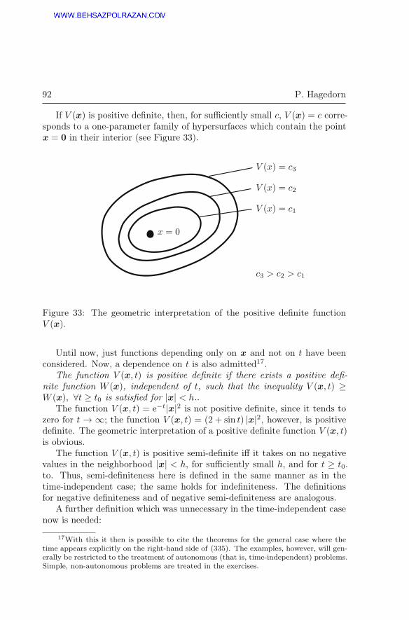
92 P. Hagedorn
If V (x) is positive definite, then, for sufficiently small c, V (x) = c corre-sponds to a one-parameter family of hypersurfaces which contain the pointx = 0 in their interior (see Figure 33).
x = 0
V (x) = c3
V (x) = c2
V (x) = c1
c3 > c2 > c1
Figure 33: The geometric interpretation of the positive definite functionV (x).
Until now, just functions depending only on x and not on t have beenconsidered. Now, a dependence on t is also admitted17.
The function V (x, t) is positive definite if there exists a positive defi-nite function W (x), independent of t, such that the inequality V (x, t) ≥W (x), ∀t ≥ t0 is satisfied for |x| < h..
The function V (x, t) = e−t|x|2 is not positive definite, since it tends tozero for t → ∞; the function V (x, t) = (2 + sin t) |x|2, however, is positivedefinite. The geometric interpretation of a positive definite function V (x, t)is obvious.
The function V (x, t) is positive semi-definite iff it takes on no negativevalues in the neighborhood |x| < h, for sufficiently small h, and for t ≥ t0.to. Thus, semi-definiteness here is defined in the same manner as in thetime-independent case; the same holds for indefiniteness. The definitionsfor negative definiteness and of negative semi-definiteness are analogous.
A further definition which was unnecessary in the time-independent casenow is needed:
17With this it then is possible to cite the theorems for the general case where thetime appears explicitly on the right-hand side of (335). The examples, however, will gen-erally be restricted to the treatment of autonomous (that is, time-independent) problems.Simple, non-autonomous problems are treated in the exercises.

Mechanical Systems: Equations of Motion and Stability 93
The function V (x, t) is uniformly small if there exists a positive definitefunction W (x) such that the inequality |V (x, t)| ≤W (x), ∀t ≥ t0 is satisfiedfor |x| ≤ h.
Thus, the function V (x, t) = |x| sin t is uniformly small; the functionV (x, t) = sin {t (x1 + · · ·+ xn)}, however, is not.
These functions, previously discussed, may now be used to formulate theLiapounov stability and instability theorems for the stability of the trivialsolution of (335).
First stability theorem. If there is a positive definite function V (x, t)such that
V (x, t) =∂V
∂t+ gradV · f(x, t)
is negative semi-definite or vanishes identically, then the trivial solution of(335) is stable.
Second stability theorem. If there is a positive definite and uniformlysmall function V (x, t) for (335) such that V (x, t) is negative definite, thenthe trivial solution of (335) is asymptotically stable.
Liapounov’s instability theorem. If there is a uniformly smallfunction V (x, t) for (335) such that V (x, t) is positive definite, whereasV (x, t) may take on positive values for arbitrarily small x and arbitrarilylarge t > t0, then the trivial solution is unstable.
All three of these theorems can be proven by simple geometric means(for example, see Malkin (1959)). In particular, in the autonomous casethe second theorem is based on the fact that the trivial solution certainlyis asymptotically stable if all of the solution trajectories x(t) penetrate thetrajectories V (x) = c of Figure 33 from outside to inside. Functions whichsatisfy the theorems above are called Liapounov functions.
� Some applications
(1) Lagrange’s theorem concerning the stability of equilibrium. Considera conservative holonomic mechanical system with kinetic energy T (q, q) =12 q
TA(q)q and with potential energy U(q) and assume that the system hasan equilibrium position for q = 0. With the Lagrangian L = T − U theequations of motion follow from Lagrange’s equations
d
dt
∂L
∂qi− ∂L
∂qi= 0, i = 1, 2, . . . , n (342)
and may always be written in the normal form
q = f(q, q) (343)

94 P. Hagedorn
since A(q) is assumed to be a symmetric positive definite matrix for all q.The system (343) may now be written as a first-order system. Prior thereto,it is advantageous to introduce different coordinates. Instead of the columnmatrix q of the generalized velocities, the generalized momenta
p =∂T
∂q= A(q)q (344)
are introduced. The kinetic energy is expressed in terms of p rather thanq and the Hamiltonian H(q,p) is defined as the sum of the kinetic and ofthe potential energy:
H(q,p) =1
2pTA−1(q)p+ U(q). (345)
The equations of motion now are given by
q =∂H
∂p,
p =∂H
∂q.
(346)
Obviously, the function H(q,p) is positive definite if the potential energy,given to within an arbitrary additive constant, is set equal to zero for q = 0
and if it has a minimum there. Furthermore, one has
H =
(∂H
∂q
)T
q +
(∂H
∂p
)T
p = 0 (347)
along the solutions of eqns (346) so that H(q,p) is a first integral of thesystem (346). The function H satisfies all of the hypotheses of the firststability theorem of Liapounov and from this it follows that the staticequilibrium position (q,p) = (0,0) is stable. In stability theory this resultis known as the Lagrange-Dirichlet Theorem.
Consider briefly two extensions of this theorem: the case of dissipativesystems and the case of conservative systems with gyroscopic forces. If thesystem is dissipative, eqns (342) are replaced by
d
dt
∂L
∂qi− ∂L
∂qi= Qi(q, q), i = 1, 2, . . . , n (348)
where one hasn∑
i=1
Qi(q, q)qi ≤ 0. In fact, ifn∑
i=1
Qi(q, q)qi is negative definite
with respect to q, then one has complete dissipation (complete damping). All

Mechanical Systems: Equations of Motion and Stability 95
motions of the system then experience damping (complete dissipation im-plies the pervasive damping as defined previously, not every system with per-vasive damping, however, has complete dissipation!). If one again choosesV = T + U , then it is apparent that the second stability theorem is notapplicable, since V is negative definite only with respect to q but not withrespect to q, q. However, asymptotic stability of the equilibrium positionstill follows from Krasovskii’s theorem (Krasovskii (1963), page 82).
Other than terms quadratic in q the Lagrangian occasionally also con-tains terms which are linear in q. The corresponding terms in the equationsof motion (342) are called gyroscopic terms. These always occur, for exam-ple, when a cyclic coordinate is being eliminated. It may easily be checkedthat even then a minimum of the potential energy still provides a sufficientcondition for stability - in the case of complete dissipation, even for asymp-totic stability.
In elastomechanics the Lagrange-Dirichlet stability theorem oftenis used as the definition of stability. There, an equilibrium position is stableiff the corresponding potential energy takes on a relative minimum, and it isunstable otherwise. This approach is unsatisfactory for various reasons. Onthe one hand, the concept of stability is best visualized in terms of motion:an equilibrium position is called stable iff all motions whose initial condi-tions are sufficiently close to the equilibrium position occur in a sufficientlysmall given neighborhood of the equilibrium (for this purpose, some conceptof distance must be introduced). On the other hand, however, the stabilityof equilibrium positions for non-conservative systems for which it may noteven be possible to define a potential energy, and that of periodic and othermotions is to be investigated also.
The main reason for this approach in elastomechanics is due to the con-siderable difficulties which may be encountered in the use of a Liapounov
stability theory extended to include applications involving partial differen-tial equations.
(2) The instability of equilibrium for a maximum of U(q). Consider againthe system described by eqns (346) and choose
V = pTq (349)
as a Liapounov function. Write
A−1(q) = A−1(0) + b(q), (350)
where B(0) = 0 and B(q) is continuous. From (345), (349) and (350) one

96 P. Hagedorn
then obtains
V = pTA−1(0)p+ pT
(bij(q)−
1
2
n∑k=1
qk∂bij∂qk
)p− qT
∂U
∂q. (351)
The coefficients of the second quadratic form in p tend to zero as |q| → 0,so that V is at least positive definite with respect to p, since A−1(0) is apositive definite matrix. U(q) now is written in the form
U(q) = Um(q) + Um+1(q) + . . . , (352)
where Uk stands for the kth-order terms in the power series expansion of U .Since q = 0 is to be an equilibrium position, one has ∂U
∂q and m ≤ 2 follows.
By using Euler’s theorem concerning homogeneous functions, (351) maybe replaced by
V=pTA-1(0)p+pT
(bij(q)−
1
2
n∑k=1
qk∂bij∂qk
)p−mUm−(m+1)Um+1−. . . . (353)
If Um is negative definite with respect to q, then V is positive definitein p, q whereas V = pTq takes on positive and negative values in everyarbitrarily small neighborhood of (q,p) = (0,0). This fulfills the hypothesesof the instability theorem; it has been shown that the equilibrium positionis unstable if Um is negative definite, that is, if U(q) has a maximum, andif the existence of this maximum follows from the terms of lowest order inthe series expansion U = Um + Um+1 + . . . .
Liapounov already proved this theorem. For an engineer, this theoremis extremely unsatisfactory since he believes that he knows from observationthat the equilibrium position is unstable not only for a maximum of thepotential energy but generally and without additional restrictions wheneverthere is no minimum. Furthermore, this Liapounov theorem may not evenbe used to show the instability of q1 = 0, q2 = 0, for
U = −q21 − q42 ,
since U2 = −q21 is not negative definite but only negative semi-definite. Thehypothesis ‘Um negative definite’ may not be omitted in the present theorem,even though this is occasionally done without comment (for example, seeLaSalle and Lefschetz (1967) and Hahn (1952)).18
18Even for a system with 2T = p21+p2
2, U = −
(q1 − q2
2
)2− 3
32q42, n = 2, the function
V = pTq is not a Liapounov function. In fact, one has qT
(∂U∂q
)= −2
(q1 − 3
2q22
)2+ 1
8q42,
and this expression is indefinite, even though U has a maximum for q = 0 (the expressionis positive for 7
4q22> q1 > 5
4q22
and negative for q1 < 5
4q22
and q1 > 7
4q22). Thus V is also
indefinite.

Mechanical Systems: Equations of Motion and Stability 97
Since the turn of the century, numerous mathematicians have concernedthemselves with the question of the stability of an equilibrium position of aconservative system in the absence of a minimum of U(q). Painlevé (1897)gave an example and showed that it is quite possible to have stability evenin the absence of a minimum of U(q)! A general proof of instability fora maximum of U(q) without any additional hypotheses on Um(q) was notavailable until given by Hagedorn (1971) (including a further, more detailedbibliography). In many practical applications, the stability problem is sim-plified considerably because of the often present dissipation of mechanicalenergy: then it is a great deal easier to prove instability!
(3) Stability of the rotational motion of a rocket. For nearly-level flight-trajectories of a projectile, it may be assumed that the center of gravityexperiences approximately linear and uniform motion. The same is approx-imately valid (at least during short time intervals) for the power-off motionof a rocket. Let β be the angle between the rocket axis and its projectiononto the vertical plane of flight and let α be the angle between this pro-jection and the velocity vector. The equations of motion then are givenby
Aβ +Aα2 sinβ cosβ − Cnα cosβ = eR sinβ cosα ,
Aα cosβ − 2Aαβ sinβ + Cnβ = eR sinα ,(354)
where C is the moment of inertia with respect to the longitudinal axis ofsymmetry and n is the constant projection of the angular velocity in thedirection of this axis. The moment of inertia with respect to an arbitrarydiameter through the center of gravity is given by A and e denotes thedistance between the center of gravity and the center of pressure (the pointof action of the resultant R of the air resistance). For small angles α, βthe resistance R may be taken to be constant. These equations of motionare derived, for example, in Gantmacher (1970), pages 186 ff, and theyare discussed in Luré (1968), pages 238 ff. The equations (354) have theparticular solution α = β = 0, α = β = 0. The stability of this trivialsolution is to be investigated.
From the theorems of mechanics, two first integrals of motion are imme-diate: the energy integral
F1
(α, α, β, β
)=
1
2A(β2 + α2 cos2 β
)+ eR(cosα cosβ − 1) (355)
and the angular momentum integral
F2
(α, α, β, β
)=A(β sinα−α cosβ sinβ cosα
)+Cn(cosα cosβ − 1). (356)

98 P. Hagedorn
gR v
α
β
e
S
Figure 34: Stability of a rocket.
It is easy to convince oneself that F1 and F2 actually are first integrals of(354), that is, that one has F1 = 0 and F2 = 0 for all of the solutions of(354). For F1 , for example, one has
F1 =∂F1
∂αα+
∂F1
∂αα+
∂F1
∂ββ +
∂F1
∂ββ
= −eRα sinα cosβ + cosβ(eR sinα− Cnβ + 2Aαβ sinβ
)α−
−Aα2β cosβ sinβ − eRβ cosα sinβ + β (eR sinβ cosα
−Aα2 sinβ cosβ + Cnα cosβ)≡ 0.
Unfortunately, neither of these first integrals F1 and F2 is definite. Consider,thus, a new integral
V = F1 − λF2, (357)
where lambda is a constant which is to be chosen in has m such a way thatV becomes positive definite. One has
V =1
2
{Aα2 + (Cnλ− eR)β2 + 2Aλαβ
}+
+1
2
{Aβ2 + (Cnλ− eR)α2 − 2Aλβα
}+ . . . , (358)
where only the terms of second order in the expansion of V with respectto α, α, β, β have been indicated. All additional terms are at least fourth

Mechanical Systems: Equations of Motion and Stability 99
order. Clearly, V2 is positive definite precisely when the two quadratic forms
Ax2 + (Cnλ− eR)x22 ± 2Aλx1x2
are positive definite. However, V then is also positive definite and the trivialsolution is stable. From Sylvester’s theorem one obtains
A > 0,
∣∣∣∣ A ±Aλ±Aλ Cnλ− eR
∣∣∣∣ > 0 (359)
as necessary and sufficient conditions for the positive definiteness of V2, thatis,
A > 0, A(Cnλ− eR)−A2λ2 > 0
or
A > 0, Cnλ− eR−Aλ2 > 0. (360)
The first condition in (360) is always fulfilled. In order to be able to satisfythe second condition for at least one real value of λ, the two roots λ1, λ2must be real and distinct from one another; this is the case only if one has
C2n2 − 4AeR > 0. (361)
Whenever (361) holds, one may always choose λ in such a way that V2 andhence V is definite with the consequent stability of the trivial solution. Theinequality (361) provides a lower bound on n for which the stability of thetrivial solution is assured. Later, it will be shown that the trivial solutionis unstable for smaller values of n.
Note also that the trivial solution here is stable in spite of the factthat the potential energy, represented by the second term in (355), has amaximum for α = β = 0. This is possible only because the equations ofmotion (354) contain terms which are linear in the generalized velocities.Under certain circumstances, such so called gyroscopic terms may serve tostabilize the equilibrium position of a conservative mechanical system evenfor a maximum of the potential energy.
(4) Free rotation of a rigid body about a fixed point. Consider againEuler’s equations (323) for the rotation of a rigid body. From mechanicsit is known that both energy and angular momentum are conserved. Thefirst integrals thus are known to be
T =1
2
(Ap2 +Bq2 + Cr2
),
L = Api+Bqj + Crk,(362)

100 P. Hagedorn
where i, j, k are the unit vectors in the directions of the principal axes ofinertia (for example, di/dt = ω × i = rj − qk). Naturally, the magnitudeof the angular momentum is also a first integral, as is its square
L2 = A2p2 +B2q2 + C2r2. (363)
Eqns (324) now are used to investigate the stability of the particular solutionp = ω, q = 0, r = 0. In terms of these new coordinates the expressions (362)and (363) result in the two first integrals
F1(y1, y2, y3) = Ay21 +By22 + Cy23 + 2Aωy1,
F2(y1, y2, y3) = A2y21 +B2y22 + C2y23 + 2A2ωy1.(364)
With 2Aωy1 = F1 −Ay21 −By22 − Cy23 it follows that
F3(y1, y2, y3) = A2y21 +B2y22 + C2y23 −A2y21 −ABy22 −ACy23
= B(B −A)y22 + C(C −A)y23 (365)
is a first integral and, naturally, that
F3(y1, y2, y3) = F 21 ± F3
={Ay21 +By22 + Cy232Aωy1
}2±±{B(B −A)y22 + C(CA)y
23
}(366)
also is. However, the function F corresponding to the upper sign is positivedefinite for A < B,C; it is positive definite with the lower sign for A > B,C.Thus, the rotations about the axes corresponding to the least and to thelargest principal moments of inertia are stable!
3.3 Supplementary Remarks Concerning the Direct Method ofLiapounov
The Liapounov theorems considered in the previous section providesufficient conditions for stability and instability. They contain no hint asto how a function V (x, t) may be found in a particular case. In problemsfrom mechanics or, more generally, for differential equations which describethe behavior of a physical system, it is often possible to deduce a suitableLiapounov function by using general physical principles. Thus, one oftenmakes use of energy expressions, various first integrals, or the entropy incertain cases. It can be proven (see Krasovskii (1963), for example) thatfor every differential equation with the trivial solution x = 0 there indeedexists a Liapounov function which satisfies the hypotheses of at least one

Mechanical Systems: Equations of Motion and Stability 101
of the three Liapounov theorems. In many cases, however, it just cannotbe found. There are a multitude of procedures which have been proposedfor the systematic construction of these functions (without solving the dif-ferential equation), but they are either too complicated or are suited onlyfor special classes of differential equations. For this reason, much effort hasgone into adjusting the Liapounov theorems in such a way that they maybe more easily used and, consequently, there are a large number of relatedstability theorems. One of the most important is the following theorem dueto Chetayev; a proof may be found in Malkin (1959), for example. For thisinstability theorem, the function V (x, t) need not be defined in a completeneighborhood of x = 0 but only in a ‘cone’ whose apex is located at x = 0.For instability it suffices to establish the existence of a single solution whichmoves away from x = 0. In the case of Chetayev’s theorem, this solutiondevelops with the ‘cone’. The theorem here is cited only for the autonomouscase
Consider the differential equation
x = f(x), f(0) = 0 (367)
and assume that there is a function V (x) such that1. in every arbitrarily small neighborhood of x = 0 there exists a region
in which V > 0 holds and on whose boundary one has V = 0, and2. at all points of the region defined by V > 0 the derivative V takes on
positive values,then, the solution x = 0 of (367) is unstable. There is one essential dis-advantage to the Liapounov theorems which have been considered. Forexample, if one tries to prove the asymptotic stability of the trivial solutionof
x+ cx+ ω20x = 0 (368)
by using the energy expression E = 12
(x2 + ω2
0x2), then it turns out that
this is not possible. In fact, one has
E = xx+ ω20xx = −cx2 (369)
and it follows that E is only negative semi-definite in x, x. Since E(x, x) ispositive-definite, Theorem 1 guarantees stability but Theorem 2, concern-ing asymptotic stability, is not applicable. Although (369) may be solvedexplicitly by analytical methods and one may of course also prove asymp-totic stability by using some other function, it would clearly be desirableto change Theorem 2 in such a way that asymptotic stability may also be

102 P. Hagedorn
deduced by using the energy expression. One might expect that this newtheorem then may also be used with more success for other more compli-cated differential equations. Such a generalization of the second Liapounov
theorem will be given shortly; another generalization will be taken up in theprocess . Namely, it is evident from the geometric significance of the directmethod that not only may the functions V (x, t) be used to investigate sta-bility, but one may also determine the ‘domain of attraction’ of x = 0 inthe asymptotically stable case. The term ‘domain of attraction’ here is usedto designate the region of those initial conditions x0 which lead to motionsx(x0, t0; t) such that x(x0, t0; t)→ 0 for t→∞.
The following discussion will be restricted to the autonomous differentialeqn (367) and to functions V (x) which are independent of t. The set
G = {x0|x (x0, t0; t) ∈ G, ∀t ≥ t0}
(in words: G is the set of all points x0, such that if x is located in G thenx(x0, t0; t) is also in G for all t ≥ t0) is called an invariant set of (367).This term now is used to formulate La Salle’s theorem:Let V (x) ∈ C1,
Ωl = {x|V (x) < l} , Ωlbounded,
V (x) > 0 for 0 �= x ∈ Ωl,
V (x) ≤ 0 for x ∈ Ωl,
L ={x ∈ Ωl|V (x) = 0
},
and let M be the largest invariant set in L. Then, every solution x(t) in Ωl
tends to M for t→∞ (For a proof, see LaSalle and Lefschetz (1967)).This theorem may be used not only to investigate the stability of the
trivial solution of (367) but also to investigate the stability of limit cycles.For the determination of the domain of attraction of x = 0 it is advanta-geous to write La Salle’s theorem in a somewhat less general form, such asmay be found, for example, in Krasovskii (1963).
Krasovskii’s theorem: Let V (x) ∈ C1, V (0) = 0,
Ωl = {x|V (x) ≤ l} ,V (x) > 0 for 0 �= x ∈ Ωl,
V (x) ≤ 0 for x ∈ Ωl.
If there is no solution x∗(t) of (367), other than the trivial solution, forwhich V (x∗(t)) ≡ 0 and which lies completely in Ωl, then every solutionx(x0, t0; t), x0 ∈ Ωl tends to x = 0 and x = 0 is asymptotically stable.

Mechanical Systems: Equations of Motion and Stability 103
This theorem now is used on (368) with V (x) = E(x, x); here, Ωl isthe interior of the ellipse 1
2
(x2 + ω2
0x2)= l. V vanishes on the x-axis, that
is, for x = 0. Other than the trivial solution, there is no further solutionx∗(t) for which V = −cx2 vanishes identically. Thus, the trivial solutionalso is asymptotically stable and for arbitrarily large l the ellipse is locatedin the domain of attraction of x = 0 which here consists of the whole phasespace.19
A second, less trivial example, which will also be discussed later in con-nection with self-excited oscillations, will now be treated. Consider thedifferential equation
x+ ε(x2 − 1
)x+ x = 0 (370)
with ε < 0 (for the case ε > 0 the equation is known as the Van der Polequation).The trivial solution is asymptotically stable and its domain of attraction is
Limit cycle
x
x
1 2
Figure 35: Phase diagram for (370) with ε < 0.
to be estimated. The corresponding phase diagram is sketched in Figure 35.It contains an isolated (unstable) periodic solution-a so-called limit cycle.
19The asymptotic stability of the equilibrium position may be proven for (348) inthe completely damped case in the same manner as long as the equilibrium position isan ‘isolated’ one.

104 P. Hagedorn
Since (370) cannot be solved analytically, an estimate of the domain ofattraction actually is of some importance here. The Liapounov functionis chosen to be
V (x, x) =1
2
(x2 + x2
)(371)
with the result
V (x, x) = xx+ xx = −ε(x2 − 1
)x2. (372)
For x2 < 1 the function V (x, x) is negative semi-definite since ε < 0 was as-sumed. In order to enforce x2 < 1, l = 1
2 is chosen, so that Ωl is the interiorof the circle x2 + x2 = 1. Since there are no non-trivial solutions in Ωl forwhich V vanishes identically, x = 0, x = 0 is asymptotically stable and theregion x2 + x2 ≤ 1 is located totally within the domain of attraction of thetrivial solution, independent of the value of |ε|. This result may be consider-ably improved upon by introducing a ‘suitable’ coordinate transformationprior to the application of the theorem. This will be dealt with later in thecase of self-excited oscillations (see Hagedorn and DasGupta (2007)).
3.4 Stability by the First Approximation (Autonomous Case)
A discussion of the ‘method of the first approximation’ will be given next.The method is used to obtain results concerning the stability of the trivialsolution of
x = Ax+ h(x, t) (373)
by making use of the linearized differential equation
x = Ax. (374)
Here, A is a constant real-valued matrix and there exist numbers β > 1, α ≥0, such that
|h(x, t)| ≤ α|x|β (375)
holds in a neighborhood of x = 0.In order to proceed in the indicated manner, the stability of the linear
system (374) must be investigated first and it must then be determinedwhen these results are also valid for the non-linear system (374).
The manner of obtaining a solution of (374) is known from the theoryof linear differential equations or, equivalently, from the theory of linear

Mechanical Systems: Equations of Motion and Stability 105
oscillations. The substitution x = aeλt in equation (374) results in thecharacteristic equation
det(A− λE) = 0 (376)
from which one may then calculate the eigenvalues of A. For the casen = 2, it is easy to draw the phase trajectories corresponding to the variouscombinations of eigenvalues. The following cases arise (Figure 36):
• (a) λ1, λ2 real, λ1 > 0, λ2 > 0, ‘unstable node’;• (b) λ1, λ2 real, λ1 > 0, λ2 < 0, ‘saddle point’;• (c) λ1, λ2 real, λ1 < 0, λ2 < 0, ‘stable node’;• (d) λ1, λ2 imaginary (λ1 = −iλ2, since A is real-valued), ‘centre’;• (e) λ1, λ2 complex (conjugates, since A is real), negative real part,
‘stable focus’;• (f) λ1, λ2 complex, positive real parts, ‘unstable focus’.
In addition, there may of course be vanishing and multiple eigenvalues; ineach of these cases the general solution may be stated without difficulty.
It is known from linear algebra (for example, see Pontryagin (1965) orGantmacher (1958)) that for arbitrary real matrices A there always existsa coordinate transformation
y = Sx (377)
which may be complex in general, such that
y = Sx = SAx = SAS−1y (378)
and such that (374) may always be transformed to the form
y = Jy, (379)
where only the main diagonal and adjacent diagonal are non-zero in theJordan normal form J = SAS−1. Here, the matrix J consists of ‘elemen-tary blocks’ whose main diagonal consists of one and the same eigenvalue,say λi, while all of the elements of the right-adjacent diagonal are unity;all of the remaining elements of the matrix are zero. Thus, an ‘elementaryblock’ has the form ⎛
⎜⎜⎜⎜⎜⎜⎝
λi 1 0 . . . 00 λi 1 . . . 0
0 0 λi...
......
... 10 0 0 . . . λi
⎞⎟⎟⎟⎟⎟⎟⎠ . (380)

106 P. Hagedorn
x1
x2
(a) Unstable node
x1
x2
(b) Saddle point
x1
x2
(c) Stable node
x1
x2
(d) Center
x1
x2
(e) Stable focus
x1
x2
(f) Unstable focus
Figure 36: Phase trajectories of an autonomous linear system with n = 2.

Mechanical Systems: Equations of Motion and Stability 107
Corresponding to every eigenvalue λi there exists at least one elementaryblock. For each distinct eigenvalue there always exists exactly one block of1 × 1 form so that the adjacent diagonal vanishes. Such blocks may alsooccur for multiple eigenvalues. If all eigenvalues are distinct, then J reducesto the main diagonal form
J =
⎛⎜⎜⎜⎜⎝
λ1 0 . . . 0
0 λ2 . . ....
... 00 0 . . . λn
⎞⎟⎟⎟⎟⎠ . (381)
A more typical structure of J , however, is given by
J =
⎛⎜⎜⎜⎜⎜⎜⎜⎜⎜⎜⎜⎜⎜⎜⎜⎝
. . .
⎞⎟⎟⎟⎟⎟⎟⎟⎟⎟⎟⎟⎟⎟⎟⎟⎠
, (382)
where the squares represent elementary blocks of the type (380). The trans-formation S thus decouples the system (374) into as many single systems ofdifferential equations as there exist elementary blocks. Consider, therefore,a system of order m of the form
z =
⎛⎜⎜⎜⎜⎜⎜⎝
λ 1 0 . . . 00 λ 1 . . . 0
0 0 λ...
......
... 10 0 0 . . . λ
⎞⎟⎟⎟⎟⎟⎟⎠ z. (383)
Define a corresponding function
V (x) = −(γ − ε)[z1z1 + (γ − ε)2z2z2 + · · ·+ (γ − ε)2(m−1)zmzm
], (384)
where λ = γ + iδ (γ, δ real, i = unit imaginary), ε and γ are different realconstants, and where z denotes the complex conjugate of z. From (383) and

108 P. Hagedorn
(384) one obtains
V (z) = 2
(γ − 1
γ − ε
)V −
[2z1z1 + 2(γ − ε)2z2z2 + · · ·+
+ 2(γ − ε)2(m−1)zmzm + (γ − ε) (z1z2 + z1z2)+
+ (γ − ε)3 (z2z3 + z2z3) + · · ·++ (γ − ε)2m−3 (zm−1zm + zm−1zm)
]. (385)
It may easily be established that the expression in brackets is always positivedefinite by investigating the matrix⎛
⎜⎜⎜⎜⎜⎜⎜⎜⎝
2 1 0 . . . 01 2 1 . . . .0 1 2 . . . .... .... 2 10 . . . . . . 1 2
⎞⎟⎟⎟⎟⎟⎟⎟⎟⎠. (386)
of the corresponding quadratic form in the new variables (γ − ε)kzk+1. Ifγ < 0, then ε may be chosen to satisfy ε > γ − ( 1γ ), resulting in a positive
definite V and a negative definite V . If one now adds the functions V (z)defined for each block, one obtains a function V (y). If all λi have a negativereal part, then V (y) also is positive definite and V (y) is negative definite.The functions V and V remain definite even when (377) is used to replacey by the real variable x . It follows that the trivial solution is asymptoti-cally stable. Instability may be proven in a similar manner if at least oneeigenvalue has a positive real part.
In summary, the following statements are valid in connection with (374):• all EV (eigenvalues) have negative real part ⇒ asymptotic stability;• at least one EV has positive real part ⇒ instability;• there do not exist any EV with positive real part, but there are EV
with vanishing real part of such a type that only ‘singleton blocks’ corre-spond to them in the Jacobi normal form⇒ stability (non-asymptotic);
• there do not exist any EV with positive real part, but there are EVwith vanishing real part of such a type that not only ‘singleton blocks’correspond to them ⇒ instability.
Confidence in the last two assertions may easily be gained by means ofthe following two examples. Consider the differential equation
x+ ω2x = 0. (387)

Mechanical Systems: Equations of Motion and Stability 109
If this is viewed as a first-order system, then
J =
(iω 00 iω
)(388)
is the Jordan normal form of A and it follows from the previous commentsthat the equilibrium position is stable-but not asymptotically stable. Here,this may be verified by means of the available general solution. However, aconsideration of the system
x1 = x2,
x2 = 0(389)
with
J =
(0 10 0
), (390)
indicates that a ‘2x2 block’ corresponds to the multiple eigenvalue ‘zero’,and instability follows. Again this is easily verified by using the generalsolution
x1 = x10 + x20t,
x2 = x20.(391)
Thus, a necessary and sufficient condition for the asymptotic stability of(374) is given by the requirement that all of the roots of (376) have negativereal parts. Generally, it is not a simple manner to determine all of the rootsof (376). One thus makes use of criteria which provide assertions about thereal parts of the roots of the characteristic equation
a0λn + a1λ
n−1 + a2λn−2 + · · ·+ an−1λ+ an = 0, a0 > 0 (392)
without having to resort to an actual solution of the equation. The mostimportant of these criteria is a theorem due to Hurwitz.
Use the coefficients of (392) to construct the minors
Δ1 = a1, Δ2 =
∣∣∣∣ a1 a0a3 a2
∣∣∣∣ , Δ3 =
∣∣∣∣∣∣a1 a0 0a3 a2 a1a5 a4 a3
∣∣∣∣∣∣ ,
Δn =
∣∣∣∣∣∣∣∣∣a1 a0 0 0 . . . 0a3 a2 a1 a0 . . . 0...
...0 0 0 . . . an
∣∣∣∣∣∣∣∣∣= anΔn−1;
(393)
then a necessary and sufficient condition assuring that all of the roots of(392) have negative real parts is given by
Δ1 > 0, Δ2 > 0, . . . ,Δn−1 > 0, an > 0 (394)

110 P. Hagedorn
(For a proof, see Chetayev (1961), for example).An application of Hurwitz’s theorem to the quadratic equation
a0x2 + a1x+ a2 = 0, a0 > 0 (395)
yields
a1 > 0,
∣∣∣∣ a1 a00 a2
∣∣∣∣ = a1a2 > 0, (396)
which may be replaced by the conditions a0 > 0, a1 > 0, a2 > 0.For the cubic equation
a0x3 + a1x
2 + a2x+ a3 = 0, a0 > 0 (397)
one obtains
a1 > 0,
∣∣∣∣ a1 a0a3 a2
∣∣∣∣ = a1a2 − a3a0 > 0, a3 > 0, (398)
and for the quartic equation
a0x4 + a1x
3 + a2x2 + a3x+ a4 = 0, a0 > 0 (399)
the criterion yields the conditions
a1 > 0,
∣∣∣∣ a1 a0a3 a2
∣∣∣∣ > 0,
∣∣∣∣∣∣a1 a0 0a3 a2 a10 a4 a3
∣∣∣∣∣∣ > 0, a4 > 0 (400)
or, equivalently,
a1 > 0, a1a2 − a0a3 > 0,
a3 (a1a2 − a0a3)− a4a21 > 0, a4 > 0.
(401)
Some additional simplification is possible; namely, the third and the fourthof these conditions imply
a3 (a1a2 − a0a3) > a4a21 > 0
so that the second condition may be replaced by a3 > 0. Thus, the condi-tions (401) may also be written in the form
a1 > 0, a3 > 0,
a3 (a1a2 − a0a3) > 0, a4 > 0.(402)

Mechanical Systems: Equations of Motion and Stability 111
For larger systems, the computation of the determinants Δi, i = 1, 2, . . ., n in (394) is rather tedious. Hence, it becomes desirable to replace theconditions (394) by others which may be more easily evaluated. This isthe case, for example, in the criterion of Liénard-Chipart, wherein theconditions (394) are replaced by
a1 > 0, a2 > 0, . . . , an > 0,
Δn−1 > 0, Δn−3 > 0, . . . .(403)
These also are necessary and sufficient conditions so that (403) is equivalentto (394) (for example, see Gantmacher (1970)). For the example (399), onethus immediately obtains (402) in place of (401).
It will now be investigated in what manner the stability behavior of (373)is determined by that of the linearized differential equation (374). If all ofthe real parts of the EV of A are negative, then an approach analogousto the one described in (384) may be used to construct a quadratic formwhich is itself positive definite and whose derivative is negative definite onthe solutions of (374). This quadratic form then may also be used as aLiapounov function for (373). If one computes its time derivatives onthe solutions of (373), then V is given by the negative definite quadraticform of the linear case with additional ‘small terms of higher order’, sinceh(x, t) satisfies the inequality (375); thus, V also is negative definite onthe solutions of (373)! Also, it follows that the trivial solution of the non-linear equation (373) also is asymptotically stable if all of the EV of A havenegative real parts! It may even be shown that one may choose an arbitrarynegative definite quadratic form W = xTCx in this case, so that V =W (x)on the solutions of (374), where the corresponding function V (x) = xTBx
always exists and is positive definite. Because of
V = xTBx+ xTBx = xTATBx+ xTBAx = xTCx (404)
the three matrices then are always related by the ‘Liapounov’ equation
ATB +BA = C. (405)
This means that the matrix equation (405) has a positive definite solutionB for every negative definite C as long as all of the EV of A have negativereal parts (for example, see Hahn (1967)).
In a similar manner, one may construct a Liapounov function for (374)if at least one of the EV of A has a positive real part, and then use thisfunction to prove the instability of the trivial solution of (373). A summaryof these results is given by the statements:

112 P. Hagedorn
• if all of the EV of A have negative real parts, then the trivial solutionof (373) is asymptotically stable;
• if at least one EV of A has a positive real part, then the trivial solutionof (373) is unstable.
These statements are valid independent of the higher order terms; h(x, t)need only satisfy the inequality (375). The linear part of (373) then is alsosaid to exhibit a dominant stability behavior. However, one may also show:
• if A has no EV with positive real part but at least one EV with van-ishing real part, then the higher order terms in (373) may always bechosen in such a manner that one obtains either stability or instability,just as desired.
In this case, the question of stability may not be decided on the basis ofthe linearized equation, but the effect of the non-linear terms must be takeninto account; this is called the critical case. The solution of the stabilityproblem in the critical case is often quite difficult and may be accomplishedonly in the special cases where one is able to find a Liapounov function.Systematic investigations of various types of critical cases may be found inMalkin (1959) for example.
Now, some examples appropriate to these stability and linearization the-orems.(1) Rotation of a rigid body about a fixed point. Consider once again theforce free and moment free motion of a rigid body about a point (Exam-ple (4) in section 3.2). The equations of motion for ‘disturbances’ of therotation with angular speed ω about an axis with corresponding moment ofinertia A were given in section 3.1 as:
y1 =B − C
Ay2y3,
y2 =C −A
B(y1 + ω) y3,
y3 =A−B
C(y1 + ω) y2;
(406)
with corresponding linearized differential equations
y1 = 0,
y2 =C −A
Bωy3,
y3 =A−B
Cωy2
(407)

Mechanical Systems: Equations of Motion and Stability 113
and with characteristic equation
∣∣∣∣∣∣∣∣−λ 0 0
0 −λ C −A
Bω
0A−B
Cω −λ
∣∣∣∣∣∣∣∣ = 0. (408)
It has a root λ1 = 0 along with
λ2,3 = ±ω√
(A−B)(C −A)
BC. (409)
For the case A > B,C or for A < B,C, λ2 and λ3 are imaginary andall three EV have zero real parts: the case is a critical case, that is, thelinearized differential equations yield no information concerning the stabilityof rotation about the principal axes corresponding to the largest and thesmallest principal moment of inertia. In this case, stability has alreadybeen shown previously (Example (4) of section 3.2) by means of a suitableLiapounov function.
However, if B > A > C or C > A > B, then λ2 and λ3 are real.Then there exists one EV with positive real part and it follows that thetrivial solution of (407) as well as that of the non-linear (324) are unstable.Thus, rotations about the principal axis corresponding to the intermediateprincipal moment of inertia are unstable!
(2) The heavy symmetric top. The stability of rotation of a heavy sym-metric top about its vertical axis of symmetry will now be investigated.First, the equations of motion are established. The usual manner of defin-ing the Euler angles is illustrated in Figure 37; the Oxyz axis system isfixed in space. It is assumed that the axi-symmetric top rests in a friction-less ball-joint at 0 and that the ζ-axis coincides with the axis of symmetrypassing through 0 and through the center of gravity S, with C as the cor-responding moment of inertia. In order to avoid any indeterminacy of theangles Φ and Ψ for the vertical position of the axis of the top, the positivey-direction is taken to be the same as that of the gravitational acceleration(the coordinates of the upright top are then given by Φ = 0, Θ = π
2 , Ψarbitrary).
The potential energy thus may be written as
U = mgl sinΘ cosΦ (410)
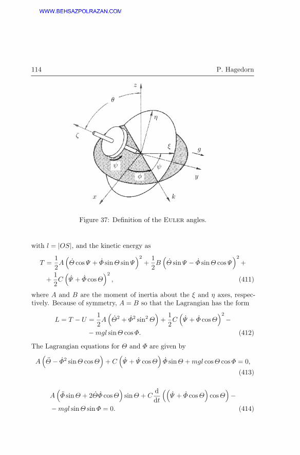
114 P. Hagedorn
x
y
k
z
ξ
ψ
φ
ψ
ζ
θ
g
η
Figure 37: Definition of the Euler angles.
with l = |OS|, and the kinetic energy as
T =1
2A(Θ cosΨ + Φ sinΘ sinΨ
)2+
1
2B(Θ sinΨ − Φ sinΘ cosΨ
)2+
+1
2C(Ψ + Φ cosΘ
)2, (411)
where A and B are the moment of inertia about the ξ and η axes, respec-tively. Because of symmetry, A = B so that the Lagrangian has the form
L = T − U =1
2A(Θ2 + Φ2 sin2Θ
)+
1
2C(Ψ + Φ cosΘ
)2−
−mgl sinΘ cosΦ. (412)
The Lagrangian equations for Θ and Φ are given by
A(Θ − Φ2 sinΘ cosΘ
)+ C(Ψ + Ψ cosΘ
)Φ sinΘ +mgl cosΘ cosΦ = 0,
(413)
A(Φ sinΘ + 2ΘΦ cosΘ
)sinΘ + C
d
dt
((Ψ + Φ cosΘ
)cosΘ
)−
−mgl sinΘ sinΦ = 0. (414)

Mechanical Systems: Equations of Motion and Stability 115
The angle Ψ is a cyclic coordinate from which it follows that
∂L
∂Ψ= C
(Ψ + Φ cosΘ
)= nC (415)
is constant; that is, the ‘eigenrotation’ n (the component of the angularvelocity in the direction of the axis of symmetry) is also constant. ForsinΘ �= 0, eqns (413) and (414) then take on the form
A(Θ − Φ2 cosΘ sinΘ
)+ CnΦ sinΘ +mgl cosΘ cosΦ = 0,
A(Φ sinΘ + 2ΘΦ cosΘ
)− CnΘ −mgl sinΦ = 0
(416)
with the particular solution Θ = 12π, Φ = 0, corresponding to the rotation
of the upright top about its axis of symmetry. Experience indicates thatthis axis position is stable as long as n is sufficiently large.
UseΘ =
π
2+ Θ,
Φ = Φ(417)
and linearize (416) with respect to the ‘disturbances’ Θ and Φ. This resultsin
A ¨Θ + Cn ˙Φ−mglΘ = 0,
A ¨Φ− Cn ˙Θ −mglΦ = 0(418)
with characteristic equation∣∣∣∣ Aλ2 −mgl Cnλ−Cnλ Aλ2 −mgl
∣∣∣∣ = 0 (419)
or, equivalently,
A2λ4 +(−2Amgl + C2n2
)λ2 + (mgl)2 = 0 (420)
(it is superfluous here to write (418) as a first-order system). A necessaryand sufficient condition to assure that there exist no roots with positive realpart is given by
C2n2 > 4Amgl. (421)
If this condition is violated, then the rotation of the upright top is unstable;if the condition is satisfied, then one has the critical case and the non-linearterms must be taken into consideration in order to draw any final conclusionsabout stability. It can be shown that the rotation about the upright axis ofsymmetry of the top is indeed stable as long as (421) is satisfied.

116 P. Hagedorn
3.5 Stability by the First Approximation (Periodic Case)
In the previous section it was assumed that linearization resulted in alinear differential equation with constant coefficients. It will now be assumedthat
x = A(t)x+ h(x, t) (422)
holds, where h(x, t) is assumed small in the sense indicated in condition(375). Again, the linearized differential equation
x = A(t)x (423)
is investigated first and any implications concerning the stability of thetrivial solution of (422) are treated subsequently.
The square matrix F (t) which satisfies the differential equation
F (t) = A(t)F (t) (424)
subject to the initial condition F (t0) = E (the unit matrix) is called thefundamental matrix of the system (423). The specific solution determinedby the initial condition x(t0) = x0 then is given by x(t) = F (t)x0. Theexistence of the fundamental matrix of (423) follows from known existencetheorems (e.g., see Pontryagin (1965)).
For a constant A the form of the fundamental matrix of (423) is easilydeduced, since the ith column of F (t) is given by the solution vector x(t)corresponding to the initial conditions x1 = x2 = . . . xi−1 = xi+1 · · · = xn =0, xi = 1. With t0 = 0 one often writes
F (t) = eAt =
(E +At+
1
2!A2t2 +
1
3!A3t3 + . . .
); (425)
convergence may easily be proven for arbitrary values of t.Next, the periodic case is discussed, where A(t) is periodic with pe-
riod T so that one has A(t + 1) = A(t), ∀t ≥ 0. Periodic differentialequations of this type were investigated by Floquet. Liapounov latershowed that corresponding to every periodic matrix A(t) there always ex-ists a non-singular continuous matrix P (t) with the same period T and withP (t0) = P (t0 + T ) = E, such that the transformation
y = P (t)x (426)
transforms the differential eqn (423) into the form
y = By (427)

Mechanical Systems: Equations of Motion and Stability 117
where B =(P (t) + P (t)A(t)
)P−1(t) is a constant matrix independent of t.
The solutions of (427), however, have already been discussed in section 3.4.If the fundamental matrix of (427) for t0 = 0 is written as eBt, then thefundamental matrix of (423) may be written as
F (t) = P−1(t)eBt (428)
in view of the transformation (426). It follows that the solutions of (423)are products of periodic functions with eBt and stability is determined bythe eigenvalues of B. Unfortunately, it is generally not possible to obtainthe matrix P (t) explicitly. If it were, one could compute B and then usethe Hurwitz criterion on B, for example. In stability investigations ofthe linear periodic differential eqn (423), it thus is common to obtain anapproximation to
F (t) = P−1(T )eBT = eBT (429)
by numerical or analytical means. In view of
x(T ) = eBTx(0) (430)
and because of the continuity of P (t), one has:• the trivial solution of (423) is asymptotically stable iff all of the EV
of the matrix eBT have a magnitude less than one;• if an EV of the matrix eBT with magnitude greater than one exists,
then the trivial solution of (423) is unstable;• if the matrix eBT has no EV with magnitude greater than one but has
one or more EV with magnitude one, then the trivial solution of (423)may be stable or unstable, depending on the structure of the Jordan
normal form corresponding to eBT .Note than an EV of the matrix eBT with magnitude larger than one
corresponds to an EV with positive real part for the matrix B (for example,see Knobloch and Kappel (1974)). The eigenvalues of the matrix B areoften designated as the characteristic exponents of the system (423).
Thus, if one wished to solve the stability problem of the linear system,one would first determine an approximate solution of the matrix equation(423) on the interval [0, T ] with initial conditions F (0) = E. Thereafter,one computes the EV of eBT = F (T ) and checks their magnitudes. Usually,this procedure would be applied in a form which is tailored to the particulartype of differential eqn (423) under investigation (for example, see Malkin(1959)).
Ultimately, one may prove linearization theorems which correspond ex-actly to those for systems with constant coefficients:

118 P. Hagedorn
• if all of the EV of eBT have magnitudes smaller than one, then thetrivial solution of (422) is asymptotically stable, independent of theform of the higher order terms;
• if eBT has at least one EV of magnitude greater than one, then thetrivial solution of (422) is unstable, independent of the form of thehigher order terms;
• if eBT has no EV of magnitude greater than one but has at least oneEV of magnitude equal to one, then the non-linear terms h(x, t) mayalways be chosen in such a way that one obtains either stability orinstability of the trivial solution in (422), just as desired.
Because of the complicated calculations involved in the analytical de-termination of the fundamental matrix by means of perturbation or othermethods, only a few simple examples will be considered here:
(1) The Hill and the Mathieu differential equations. One of the mostimportant ordinary differential equations with periodic coefficients is Hill’sdifferential equation
x+ g(t)x = 0, (431)
where g(t) is a periodic function with period T . For example, such a dif-ferential equation describes the oscillations of a spring-mass-system withperiodically changing spring stiffness, the small (linear) oscillations of apendulum with periodically excited support, the transverse oscillations of abeam with pulsating axial load, as well as the oscillations of a loudspeakersignal coil. The most important special case arises when g(t) has the form
g(t) = ω20(1 + ε cosΩt) (432)
in which case (431) becomes the Mathieu differential equation
x+ ω20(1 + ε cosΩt)x = 0. (433)
Here, parametrically excited oscillations as described by (431) with ε � 1will be treated. This terminology is founded on the fact that one does nothave a periodic excitation independent of x as is usual in the treatment offorced oscillations, that is, a term of the type P sinΩt ‘on the right-handside’, but much rather that the system parameters such as the mass or thestiffness themselves are periodic functions of the time. Properly, this typeof problem belongs in the realm of linear oscillations.
The stability of the trivial solution x(t) ≡ 0 of (431) and (433) is to beinvestigated. Consider, for the moment, the more general eqn (431) andwrite it in the form
x1 = x2,
x2 = −g(t)x1(434)

Mechanical Systems: Equations of Motion and Stability 119
in which one now needs to compute the eigenvalues of the matrix F = eBT
(see (429)). One has
F (T ) =
(x1(T ) ¯x1(T )x2(T ) ¯x2(T )
), (435)
where x(t) and ¯x(t) are the solutions of (434) corresponding to the initialconditions x1(0) = 1, x2(0) = 0, and ¯x1(0) = 0, ¯x2(0) = 1. The solutionsmay be determined approximately by numerical or analytical means. Thecharacteristic equation is obtained in the form∣∣∣∣ x1(T )− ρ ¯x1(T )
x2(T ) ¯x2(T )− ρ
∣∣∣∣ = 0, (436)
which may also be written as
ρ2 − 2aρ+ 1 = 0 (437)
with a = 12 (x1(T ) + ¯x2(T )).
20 The product of the two roots of (437) isalways equal to one so that either both roots have magnitude one or onehas magnitude greater than one and the other a magnitude less than one.From ρ = a ±
√(a2 − 1) it follows that for a2 < 1 both roots are complex
with magnitude one, whereas the roots are real, one with magnitude largerand one with magnitude smaller than one, for a2 > 1. For the limiting casea a2 = 1, one has the double root ρ = a; that is, either ρ = 1 or ρ = −1 asroots of multiplicity 2. From the theorems cited, it now is apparent that thetrivial solution of (431) is unstable for a2 > 1 and is stable (weakly stable)for a2 < 1. The result for a2 > 1 remains valid even when ‘small’ non-linearterms are added in (431).
Thus, stability results for (431) may be obtained in the following manner:the solutions x(t) and ¯x(t) on the interval [0, T ] are determined first; there-after, with a = 1
2 (x1(T ) + ¯x2(T )) instability may be deduced for a2 > 1and stability for a2 < 1.
The stability of solutions of the Mathieu differential equation (433)obviously depends on the values of the parameters ω0, Ω, and ε. Theintroduction of the dimensionless time τ , with Ωt = 2τ , in (433) results in
x′′ + (δ + η cos 2τ)x = 0 , (438)
20If F (r) is the fundamental matrix of x = A(t)x, then the Wronskian determinantis given by
Δ(t) = detF (t) = Δ(t0)exp
[∫ t1
t0
n∑i=1
aiidt
],
and it then follows from (434) that the ρ-independent term in (437) is equal to unity.

120 P. Hagedorn
where x′′ = d2xdτ2 , δ =
(2ω0
Ω
)2, η = ε
(2ω0
Ω
)2so that the stability of the trivial
solution depends only on δ and η or, equivalently, on Ωω0
and ε. In the
parameter plane of δ, η or Ωω0
, ε, respectively, there exist regions in which(438) is unstable and others in which (438) is stable (because of linearity,one may speak of the stability of a differential equation, since all of thesolutions exhibit the same stability behavior).
Approximate solutions for x(τ) and ¯x(τ) in the form x(τ) = x0(τ) +ηx1(τ) + η2x2(τ) + . . . may be obtained in the by now familiar manner;this is relatively easy, since only solutions on the interval [0, π] are to beapproximated so that the secular terms here do not introduce the difficultieswhich are encountered for approximations which are to be valid for ‘seculartimes’ (large values of τ) also.
The stability investigation is simplified still further if one realizes thatthe stability21 and instability regions in the δ, η-plane are separated bycurves whose corresponding parameter values result in periodic solutions.Thus, the boundaries of the stability regions in the parameter plane maybe obtained by determining those parameters δ, η which result in periodicsolutions. This will be done by using perturbation methods based on Lind-
stedt’s procedure. The treatment will be limited to small values of δ andη. With
δ = n2 + ηδ1 + η2δ2 + . . . ,
x(τ) = x0 + ηx1 + η2x2 + . . .(439)
equation (438) may be used to deduce
x′′0 + n2x0 = 0,
x′′1 + n2x1 = − (δ1 + cos 2τ)x0,
x′′2 + n2x2 = − (δ1 + cos 2τ)x1 − δ2x0, . . . .
(440)
It can be shown that periodic solutions are possible only for n = 1, 2, . . .(with the assumption of another value for n it becomes apparent after acomputation of the first approximation that the resulting solution cannotbe periodic). Periodic solutions with initial conditions x(0) = 1, x′(0) = 0,and x(0) = 0, x′(0) = 1 are to be determined, and a convenient way tosatisfy these conditions is to impose them on x0 in the calculations of the
21More precisely: those regions in the parameter plane whose points correspond toparameter values for which the trivial solution of (433) is stable.

Mechanical Systems: Equations of Motion and Stability 121
first approximation. Consequently, one has
x0 = cosnτ (441a)
or, respectively,
x0 =1
nsinnτ. (441b)
The first approximations corresponding to n = 0, 1, 2 are now computed.For n = 0 with x0 ≡ 1 the expression (441a)-(a) results in
x′′1 = −δ1 − cos 2τ ; (442)
for periodic solutions, one must choose δ1 = 0 so that
x1 =1
4cos 2τ + C. (443)
This yields
x′′2 = −δ2 −1
8− C cos 2τ − 1
8cos 4τ, (444)
and δ2 = − 18 is chosen. Based on (439), one now has
δ = −1
8η2 +O
(η3). (445)
For n = 0, the expression (441b) must be replaced by x0 ≡ 0, and itis impossible to construct a non-trivial periodic solution from this initialformulation!
For n = 1, the procedure is begun with x0(τ) = cos τ which results in
x′′1 + x1 = −(δ1 +
1
2
)cos τ − 1
2cos 3τ, (446)
with δ1 = − 12 and x1(τ) =
116 (cos 3τ − cos τ) as a consequence. From
x′′2 + x2 = −(
1
32+ δ2
)cos τ +
1
16cos 3τ − 1
32cos 5τ (447)
one then concludes δ2 = − 132 and obtains
δ = 1− 1
2η − 1
32η2 +O
(η3). (448)

122 P. Hagedorn
If the process had been begun with x0(τ) = sin τ , the result would havebeen
δ = 1 +1
2η − 1
32η2 +O
(η3). (449)
For n = 2, the same approach yields the two equations
δ = 4 +5
48η2 +O
(η3)
(450)
and
δ = 4− 1
48η2 +O
(η3). (451)
A sketch of the curves δ(η) in terms of the variables Ωω0
and ε in accordancewith (448) through (451) yields the wedge-shaped, shaded regions emanatingfrom the Ω
ω0-axis as shown in Figure 38; although not calculated above,
the curves for n = 3, 4 have also been included. Parameter combinations
24
23 1 2 Ω
ω0
ε0ε0
ε
n = 1 n = 2 n = 3 n = 4
Figure 38: The instability regions of the Mathieu differential equation.
corresponding to points on these curves result in periodic solutions. For theshaded regions in between, one has a2 > 1 resulting in an unstable trivialsolution. For parameter combinations which are located outside the shadedregions, the trivial solution is stable. The instability regions emanate fromthe points Ω
ω0= 2
n and they accumulate at Ωω0
= 0. If one, futhermore,includes linear damping, (433) must be replaced by
x+ βx+ ω20(1 + ε cosΩt)x = 0. (452)

Mechanical Systems: Equations of Motion and Stability 123
The instability regions then are bounded by the dashed lines in Figure 38.For sufficiently small values of the excitation (small values of ε), the trivialsolution always remains asymptotically stable and corresponding to everyinstability region there exists a ‘threshold’ ε = ε0 which must be exceededbefore instability can occur. The linear differential eqn (452) has a domi-nant stability behavior so that non-linear terms can no longer eliminate thestability or instability of the trivial solution.(2) The Mathieu differential equation with additional non-linear terms.Consider again the Mathieu differential equation with additional linearand non-linear damping terms as well as a non-linear restoring force so thatthe equation now has the form
x+ ω20(1 + ε cosΩt)x+ βx+ δx2 sgn x+ αx3 = 0. (453)
With α, β and δ small and of the same order of magnitude as ε, eqn (453)may also be written as
x+ ω20(1 + ε cosΩt)x+ ε
(ex+Dx2 sgn x+ fx3
)= 0. (454)
From Figure 38 it is apparent that the first-order instability region, ema-nating from Ω
ω0= 2 for the undamped case, is the most important region
in any applications; thus, only this region will be investigated here. Themethod of slowly changing phase and amplitude will be used and specialconsideration will be given to the non-trivial stationary solutions and theirstability.
The time is transformed with the substitution Ωt = τ ; the derivativewith respect to the transformed time is designated by a prime with x = Ωx′.The stability of the solutions in a neighborhood of the critical frequencyΩ1 = 2ω0 is of particular interest, and it is thus convenient to use Ω =Ω1(1− λ) where λ is a small factor of the order of magnitude of ε. The useof the abbreviations K = ω0
Ω1, A = f
ω2
0
, and E = eω0
along with the omission
of terms which are small and of second order in equation (454) result in
x′′ +K2(1 + 2λ)x+ ε(K2x cos τ + EKx′+
+ Dx′2 sgnx′ +AK2x3)= 0. (455)
With the transformations
x = a(τ) sin {Kτ + Ψ(τ)} ,x′ = Ka(τ) cos {Kτ + Ψ(τ)} ,
(456)

124 P. Hagedorn
where a(τ) > 0, eqn (455) may be written as
a′ = −λKa sin 2q + εKa
{−1
2sin 2q cos τ − E cos2 q−
−Da cos3 q sgn(cos q)−Aa2 sin3 q cos q},
Ψ ′ = 2λK sin2 q + εK{sin2 q cos τ + E sin q cos q+
+Da sin q cos2 q sgn(cos q) +Aa2 sin4 q},
(457)
where q = Kτ + Ψ(τ).It is now assumed that a(τ) and Ψ(τ) are ‘slowly’ varying and that the
right-hand sides of (457) may thus be replaced by their temporal means.The result of a choice of K = ω0
Ω1= 1
2 for the first-order instability regionthen results in
a′ = − ε8a sin 2Ψ − 2ε
3πDa2 − ε
4Ea,
Ψ ′ = − ε8cos 2Ψ +
λ
2+
3ε
16Aa2.
(458)
Naturally, this system has the trivial solution a ≡ 0; but, in addition, thereare also other stationary non-trivial solutions given by a = a0 = const.,Ψ = Ψ0 = const. The non-trivial stationary solutions are investigated first.
The elimination of Ψ0 from eqns (458) easily yields the expression forthe deviation λ of the frequency Ω from the nominal value Ω1 in terms ofthe stationary amplitude a0:
λ = −3ε
8Aa20 ± ε
√1
16− E2
4− 16
9π2D2a20 −
4
3πDEa0. (459)
Real values for λ are obtained when the expression under the radical is non-negative; two cases are to be distinguished . If D = 0, that is, no quadraticdamping is present, then one obtains real values for λ as long as E ≤ 1
2 ; a0may take on arbitrary values in this case. For D > 0 there exist non-trivialstationary solutions for all those values of a0 which satisfy the inequality
a0 ≤3π
16D(1− 2E)
(see Figure 39).From (459) it is furthermore apparent that the values of λ become inde-
pendent of the constants A and D for a0 → 0.Next, the stability of the stationary solutions just treated will be consid-
ered. Toward this purpose, a and Ψ in (458) are replaced by a = a0+ a andΨ = Ψ0 + Ψ , where a and Ψ represent the deviations from the stationary

Mechanical Systems: Equations of Motion and Stability 125
a0
1.00
0.50
1.95 2.00 2.05 2.10 Ωω0
D = 0.5
E = 0
D = 1
E = 0
D = 0.5
E = 0.3
a0
1.00
0.50
1.95 2.00 2.05 2.10 Ωω0
A = 0, D = 0.5, E = 0
A = 1
D = 0
E = 0.3
A = 1
D = 0
E = 0.5
Figure 39: Instability regions of the Mathieu-equation with linear andwith quadratic damping and with cubic restoring term. Left with A=1 andε = 0.1, right with ε = 0.1.
solution. Their substitution in (458) and the subsequent linearization of theequation with respect to a and Ψ results in
a′ = ε
{−1
8sin 2Ψ0 −
4
3
D
πa0 −
E
4
}a− ε
{a04
cos 2Ψ0
}Ψ,
Ψ ′ = ε3A
8a0a+ ε
{1
4sin 2Ψ0
}Ψ.
(460)
These equations may be used to investigate the stability of the stationarysolutions a0, Ψ0 of (458) by means of the method of the first approximation.An application of the Hurwitz criterion then yields the stability conditions
ε
[2D
πa0 +
E
2
]> 0, (461)
Aλ
ε> − 64
27π2D2 − 8
9π
DE
a0− 3
8A2a20. (462)
The inequality (461) is always satisfied as long as ε �= 0 and D and E arenot simultaneously zero. When the values of λ resulting from (459) are

126 P. Hagedorn
substituted in (462), one obtains the condition
±A√
1
16− E2
4− 16
9π2D2a20 −
4
3πDEa0 > −
64
27π2D2 − 8DE
9π a0. (463)
For the upper sign, this inequality is always satisfied, that is, the correspond-ing branch of the resonance curve a0(λ) is always stable; it corresponds tothe left (increasing) part of the resonance curve in Figure 39. Generally, thecondition (463) is also satisfied for the lower sign for certain values of a0;the stability boundary is however difficult to obtain explicitly. Eventually,one arrives at the following stability results:
• For D = 0, 0 < E < 12 , ε > 0 the right-hand part of the resonance
curve in Figure 39 is always unstable.
• For A = 0, all of the resonance curve is stable, as long as D > 0 andε > 0 are valid.
• For E = 0, the right-hand part of the resonance curve is stable for alla0 which satisfy the inequality
a0 >3π
4D
√1
16− 4096D4
729π4A2. (464)
It follows that all of the right-hand part of the resonance curve is stable for
E = 0 as long as D2 > A 27π2
256 the case.The resonance curves corresponding to several values of A, D, E and ε
have been depicted in Figure 39. From the figure as well as from (459), it isapparent that the quadratic damping has no influence on the width of theinterval which is cut out of the Ω
ω0-axis by the resonance curve. The width of
this interval clearly depends only on E. An essential difference between theresonance curves corresponding to the case of quadratic damping and thatwith only linear damping lies in the fact that with increasing values for Dand decreasing values for A, the right-hand part of the curve also becomesstable. This is true up to a limiting value of a0 where the curve has avertical tangent perpendicular to the Ω
ω0-axis; this may easily be deduced
from (459) together with (463). A further difference consists of the fact thatthe resonance curves according to the first approximation now are closed,something which was not the case for linear damping.
Finally, the stability of the trivial solution will be investigated. Withthe substitution
a sinΨ = y and a cosΨ = z

Mechanical Systems: Equations of Motion and Stability 127
equations (458) result in
y′ = − ε4Ey +
(− ε8+λ
2
)z − 2ε
3πDy√y2 + z2+
+3ε
16Az(y2 + z2
),
z′ =
(− ε8− λ
2
)y − ε
4Ez − 2ε
3πDz√y2 + z2 − 3ε
16Ay(y2 + z2
).
(465)
The Hurwitz-criterion may now be used to investigate the stability of thezero position by means of the first method of Liapounov, where only thelinear part of eqns (465) need be considered. This results in the conditions
E > 0 and λ2 > ε2
16
(1− 4E2
). It follows that the null position is always
stable as long as E > 12 and that for 0 < E < 1
2 the null position is stablefor
λ >ε
4
√1− 4E2 and λ < − ε
4
√1− 4E2
and is unstable for
ε
4
√1− 4E2 > λ > − ε
4
√1− 4E2
(see Figure 40).
ε
2 Ωω0
Boundary of the instabilityregion for linear damping
For exclusivelyquadratic damping
Figure 40: Boundaries of the instability region of first order.
Only the linear damping enters into this result, that is, for E > 0quadratic damping has no influence on the width of the instability regionof first order.

128 P. Hagedorn
The case E = 0 still needs to be investigated. The linearization of (465)with E = 0 yields
y′ =
(− ε8+λ
2
)z,
z′ =
(− ε8− λ
2
)y.
(466)
The instability of the trivial solution for − ε4 < λ < ε
4 follows immediately.For λ > ε
4 and λ < − ε4 no conclusions based on (466) can be drawn,
since the trivial solution of (466) is only stable but not asymptotically sta-ble. This corresponds to the critical case, and stability therefore must beinvestigated by means of Liapounov’s second method or the direct methodof Liapounov.
For D > 0 the Liapounov function V = 12y
2 + 12Bz
2 may be employedsuccessfully, where B is chosen so as to assure a vanishing of the second-order terms in V ′. The use of (465) then yields
V ′ = −2D
3πε(y2 +Bz2
)√y2 + z2 +
3A
16εyz(y2 + z2
)(1−B) (467)
with B =− ε
8+λ
2
ε
8+λ
2
> 0. For D > 0 there always exists a neighbourhood of
the point y = z = 0 in which (467) is negative definite. It follows thatin this case the null position is stable for λ > ε
4 and for λ < − ε4 , that is,
quadratic damping does not influence the stability of the null position evenwhen E = 0.
3.6 Stability by the First Approximation (Aperiodic Case)
In sections 3.4 and 3.5, it was shown that the asymptotic stability of thelinear autonomous or periodic system implied the asymptotic stability of thetrivial solution of the complete non-linear system. That this is no longerthe case when the coefficients of the linear system are arbitrary functionsof time is shown by the following counter-example.
Consider the linear system
x1 = −bx1,x2 = (sin(ln t) + cos(ln t)− 2b)x2
(468)
for 0 < t0 ≤ t. It consists of two uncoupled differential equations with thesolution
x1(t) = x10e−b(t−t0),
x2(t) = x20e−(t0 sin(ln t0)−2bt0)e(t sin(ln t)−2bt).
(469)

Mechanical Systems: Equations of Motion and Stability 129
As long as b > 12 the trivial solution of (468) is obviously asymptotically
stable.If one now adds a non-linear term in (468) in such a way that one obtains
x1 = −bx1,x2 = (sin(ln t) + cos(ln t)− 2b)x2 + x21
(470)
then the general solution has the form
x1(t) = x10e−b(t−t0),
x2(t) = et sin(ln t)−2b(t−t0) ·(x20e
−t0 sin(ln t0)+
+ x210
t∫t0
e−t1 sin(ln t1)dt1
),
(471)
a result which may easily be checked. The trivial solution of (470) however,is unstable, since
et sin(ln t)−2bt
t∫t0
e−t1 sin(ln t1)dt1
is unbounded as t→∞. For tn = e(2n+1
2 )π, n an integer, with tne−π > t0,
one has:
tn∫t0
e−t sin(ln t)dt >
tne−
2π
3∫tne−π
e−t sin(ln t)dt =
e(2n−1
6 )π∫e(2n−
1
2 )π
e−t sin(ln t)dt >
e(2n−1
6 )π∫e(2n−
1
2 )π
e−t sin(−π
6 )dt >
tne−
2π
3∫tne−π
e−tne−π sin(−π
6 )dt =
= e1
2tne
−π{e−
2π
3 − e−π}tn.

130 P. Hagedorn
For t = tn there thus follows:
etn sin(ln tn)−2btn
tn∫t0
e−t sin(ln t)dt > etn sin(ln tn)−2btn ·
·{e−
2π
3 − e−π}tne
1
2tne
−π
=
={e−
2π
3 − e−π}tne
tn(sin(ln tn)−2b+ e
−π
2
)
and this expression grows beyond all bounds as n→∞, as long as one has1 + 1
2e−π > 2b!
For 12 < b < 1
2 + 14e
−π one thus has the non-linear system (470) withunstable trivial solution and such that its linearized system is one with anasymptotically stable equilibrium position! It follows that the linearizationtheorems, as derived for autonomous and periodic systems, may not be gen-eralized to the case with arbitrary time dependence without some additionalassumptions!
However, even for systems of linear equations with arbitrary time depen-dent coefficients, one may define parameters which correspond to the realparts of the characteristic exponents defined in section 3.5, although withreversed sign: they are the characteristic numbers of Liapounov. Thesecharacteristic numbers may be used to describe the growth behavior of afunction f(t). The characteristic number z of a function f(t) is definedin the following manner: the number z is that number for which the twoconditions
limt→∞
|f(t)|e(z+ε)t = +∞, ∀ε > 0
limt→∞
f(t)e(z−ε)t = 0, ∀ε > 0(472)
are satisfied.22 It can be shown that (472) determines the characteristicnumber of a function f(t) uniquely and that z may also be calculated bymeans of the expression
z = − limt→∞
ln |f(t)|t
. (473)
This definition may now be used to define the characteristic numbers of thesolutions and consequently the characteristic numbers of a linear systemand to obtain a number of stability results (see Malkin (1959)).
As it turns out, one can obtain stronger linearization results for asymp-totic stability than for instability. As indicated by Krasovskii (1963), this
22lim means ‘lim sup’

Mechanical Systems: Equations of Motion and Stability 131
is due to the fact that uniform asymptotic stability is a structural propertywhereas instability is not.
A brief discussion of the concept of uniform stability follows. In the sta-bility definition (312), δ generally does not only depend on ε but also on t0. Ifit is possible to obtain a function δ(ε) such that the inequality (312) is satis-fied for all t0, the solution x (a, t0; t) is said to be uniformly stable. The solu-tion x (a, t0; t) then is said to be uniformly asymptotically stable if x (a, t0; t)is uniformly stable and if one has limt→∞ |x (x0, t0; t)− (a, t0; t)| = 0 uni-formly for all t0 and for every x0, |x| < δ.
With this in mind, one may formulate the following linearization theo-rem, proven in Halanay (1966):
If the trivial solution of
x = A(t)x
is uniformly asymptotically stable, if A(t) is bounded and if |h(y, t)| < c|y|(c is a sufficiently small positive constant which may depend on A(t)), thenthe trivial solution of
x = A(t)x+ h(x, t)
is also uniformly asymptotically stable.In the counter-example (equations (468) - (471)) at the beginning of this
section, the conditions for uniform asymptotic stability were not satisfied.There are numerous additional theorems concerning linearization and struc-tural properties to be found in the literature. However, this interesting andby no means exhausted area will be pursued no further here.
Bibliography
K. Anderson and P. Hagedorn. On the Energy Dissipation in Space Dampersin Bundeled Conductors of Overhead Transmission Lines. J. of Soundand Vibration, 180(4):539–556, 1995.
R. Bellman. Stability theory of differential equations. Dover, New York,1969.
N. G. Chetayev. The stability of motion. Pergamon Press, New York, 1961.F. Gantmacher. Matrizenrechnung [Matrix algebra]. VEB Deutscher Verlag
der Wissenschaften, Berlin, 1958.F. Gantmacher. Lectures in analytical mechanics. MIR Publishers, Moscow,
1970.P. Hagedorn. Die Umkehrung der Stabilitätssätze von Lagrange-Dirichlet
und Routh [Converse theorems for the stability theorems of Lagrange-Dirichlet and Routh]. Arch. rational Mech. Anal., 42:281–316, 1971.

132 P. Hagedorn
P. Hagedorn and A. DasGupta. Vibrations and Waves in Continuous Me-chanical Systems. 2007.
W. Hahn. Theorie und Anwendung der direkten Methode von Ljapunow[Theory and application of Liapounov’s direct method]. Springer, Berlin,1952.
W. Hahn. Stability of motions. Springer, Berlin, 1967.A. Halanay. Differential equations, stability, oscillations, time lags. Aca-
demic Press, New York, 1966.H.W. Knobloch and F. Kappel. Gewöhnliche Differentialgleichungen [Ordi-
nary differential equations]. Teubner, Stuttgart, 1974.N.N. Krasovskii. Stability of motion. Stanford University Press, Stanford,
California, 1963.J. LaSalle and S. Lefschetz. Die Stabilitätstheorie von Ljapunow [Liapounow
stability theory]. Bibliographisches Institut, Mannheim, 1967.L. Luré. Mecanique analytique [Analytical mechanics]. Libraire Universi-
taire, Louvain, 1968.J.G. Malkin. Theorie der Stabilität einer Bewegung [Theory of the stability
of motion]. Akademie-Verlag, Berlin, 1959.P. Painlevé. Sur la réciproque de la théorème de Lagrange [On the converse
of Lagrange’s theorem]. Comptes Rendus, 25:1021–4, 1897.L.S. Pontryagin. Gewöhnliche Differentialgleichungen [Ordinary differential
equations]. VEB Deutscher Verlag der Wissenschaften, Berlin, 1965.S.P. Timoshenko and J.N. Goodier. Theory of Elasticity, volume 3e. McGrw-
Hill Book Co., Singapore, 1970.

Variational Principles in Mechanics andControl
Gottfried Spelsberg-Korspeter
TU Darmstadt, Darmstadt, Germany
Abstract The chapter ’Variational principles in mechanics and con-trol’ summarizes the material presented in six lectures in the CISMcourse no. 418. The first part considers the derivation of equationsof motion for discrete and continuous systems. Founding on thebasics of the calculus of variations the relation of the principle ofvirtual work to Lagrange’s equations and Hamilton’s principle isdiscussed. The concepts are useful for an efficient modeling of con-trol systems. In the second part variational methods are used tointroduce basics of optimal control and control system design.
1 Introduction
One of the major tasks in mastering structural control problems is to findefficient models for the systems under investigation. For mechanical systemsthis means that appropriate degrees of freedom have to be defined in orderto keep the models managable and efficient. As a consequence we have toestablish appropriate methods to set up equations of motion for discrete andcontinuous systems and combinations of those. Once appropriate modelshave been derived they can in many cases be linearized and brought intothe standard form
x = Ax+Bu (1)
on which a good part of linear control theory is based. For the analysis ofequations of motion and corresponding control problems it is not enoughjust to study the equations of motion. Often further reasoning is neededfor example energetic considerations or the investigation and optimization ofobjective functions which are functionals of the degrees of freedom. The linkbetween the analysis of functionals and the governing differential equationsfor structural control problems are variational principles. Using the conceptof calculus of variations the relations between energy functionals and the
P. Hagedorn, G. Spelsberg-Korspeter (Eds.), Active and Passive Vibration Control of Struc-tures, CISM International Centre for Mechanical Sciences DOI 10.1007/ 978-3-7091-1821-4_2 © CISM Udine 2014

134 G. Spelsberg-Korspeter
equations of motion are established. The extension of the mathematicalreasoning to control problems is the basis of the theory of optimal control.
A profound understanding of the equations is necessary to gain insightinto the mechanical properties of a structure and is essential in order toset up appropriate controls. Often deep insight can already be gained fromthe linearized equations of motion of which the behavior is governed byeigenvalues and eigenvectors. Therefore, after establishing methods for theset up of equations of motion, we will investigate structural properties ofthe eigenvalue problems corresponding to the linearized equations of motionand their dependence on design parameters. The insights gained will be veryhelpful for example in passive control approaches for stabilizing rotors whichwill be studied as a technical example.
2 Contributing and non contributing forces in the
principle of virtual work
The basic principle for deriving equations of motion for mechanical systemsis Newton’s law. If kinematical constraints such as a rigid body assumptionare utilized in addition the balance equations for the moment of momentumhave to be used. In order to take into account the kinematic relationshipsbetween the different bodies constraints have to be fulfilled. For obtainingthe equations of motion in the form of ordinary differential equations theconstraint forces have to be eliminated, which can be quite tedious.
2.1 Introductory example
As an example let us consider a beam hoist shown in figure 1 consistingof two particles. In order to apply Newton’s law each of the particles hasto be considered separately. The corresponding equations of motion read
mP x1 = Z1 + Z3 sinϕ,
mP x2 = mpg + Z2 + Z3 cosϕ,
mQx3 = −Z3 sinϕ,
mQx4 = −Z3 cosϕ+mQg,
where
cosϕ =L+ x4 − x2√
(L+ x4 − x2)2 + (x3 − x1)2,
sinϕ =x3 − x1√
(L+ x4 − x2)2 + (x3 − x1)2.

Variational Principles in Mechanics and Control 135
��
n1��
n3
s(t) P,mP
Q,mQ
L gϕ
Z1
Z2
Z3
Z3
mQg
mP g
Figure 1. beam hoist
Since x1, x2, x3 and x4 are not independent we have consider the kinematicalconstraints
N0��
pP − s(t)��
n1 = 0, (2a)∣∣∣N0��
pP − N0��
p Q∣∣∣− L = 0. (2b)
In (2) we use the notation of Kane Kane and A. (1985), where N0��
pP is theposition vector from the origin N0 to the point P . Equations (2) finallyyield seven equations with the 7 unknowns x1, x2, x3, x4, Z1, Z2, Z3 whichclearly is not comfortable to deal with.
The first step to simplify the setup of equations of motion is the intro-duction of generalized coordinates. By definition generalized coordinatesare independent quantities which represent the configuration of the systemand therefore automatically fulfill the holonomic constraints of a system.
For the beam hoist considered here the angle ϕ is an intuitive choice forthe generalized coordinate which in the following will be denoted by q. Inorder to set up the equations of motion we need the accelerations of points

136 G. Spelsberg-Korspeter
P and Q which read
N0��
pP = s��
n1, (3a)
N ��
vP = s��
n1, (3b)
N ��
aP = s��
n1, (3c)
N0��
pQ = (s+ L sin q)��
n1 + L cos q��
n3, (3d)
N ��
vQ = (s+ Lq cos q)��
n1 − Lq sin q��
n3, (3e)
N ��
aQ = (s+ Lq sin q − Lq2 sin q)��
n1 + (−Lq sin q − Lq2 cos q)��
n3. (3f)
In (3) according to Kane’s notation Kane and A. (1985) position vectorsare indicated by
��
p, velocities by��
v and accelerations by��
a. For velocity andacceleration vectors the first superscript always indicates which respect towhich frame the time derivatives have been taken and the second superscriptindicates the point. For example N ��
aQ is the acceleration of particle Q withrespect to the Newtonian frame N . From Newton’s law we obtain theequations of motion in vector form
mPN ��
aP = (Z1 + Z3 sin q)��
n1 + (Z3 cos q + Z2mP g)��
n3, (4a)
mQN ��
aQ = −Z3 sin q��
n1 + (mQg − Z3 cos q)��
n3, (4b)
which yield four scalar equations
mP s = Z1 + Z3 sin q, (5a)
0 = Z3 cos q + Z2, (5b)
mQ(s+ Lq sin q − Lq2 sin q) = −Z3 sin q, (5c)
−mQ(−Lq sin q − Lq2 cos q) = −mQg + Z3 cos q, (5d)
from which the constraint forces have to be eliminated. In this case theequation of motion can be simply obtained by adding (5c) multiplied bycos q and (5d) multiplied by sin q
mQ(s cos q + Lq) = −mQg sin q. (6)
However especially for larger systems a formulation without constraint forcesis much more efficient and will now be introduced through the principle ofvirtual work.

Variational Principles in Mechanics and Control 137
2.2 Partial velocities
The velocity of a particle in a holonomic system with n degrees of free-dom is given by
N ��
vP =Nd
dtN0
��
pP =n∑
s=1
N∂N0��
pP
∂qsqs +
N∂N0��
pP
∂t(7)
and is always linear in the generalized velocities qs. In a shorter form (7)can be written as
N ��
vP =
n∑r=1
N ��
vPr qr +N ��
vP0 ,
where N ��
vPr = N ��
vPr (q1, . . . , qn, t) is called the rth partial velocity of P in Nand N ��
vP0 = N ��
vP0 (q1, . . . , qn, t) is a remaining term that only depends on thegeneralized coordinates and time. For the beam hoist example we obtainfrom (3b)
N ��
vP1 =��
0,
N ��
vP0 = s��
n1,
and from (3e)
N ��
v Q1 = L cos q
��
n1 − L sin q��
n3,
N ��
v Q0 = s
��
n1.
Visualizing the partial velocities in figure 2 we observe that��
Z3 is orthogonalto N ��
v Q1 and therefore the virtual work
��
Z3 · N ��
v Q1 = 0 of
��
Z3 vanishes. The
same is true for the virtual work of��
Z1 and��
Z2 since N ��
vP1 = 0. As we shallshow in the next section this observation is not specific for the particularexample but quite general for forces ensuring constraints. Therefore wecan make use of this fact and formulate the equations of motion withoutconstraint forces.
Consider a system with K particles and n degrees of freedom. Newton’s

138 G. Spelsberg-Korspeter
N ��
v Q1
Q
mQg
Z3
Figure 2. Virtual velocities of the beam hoist
law directly yields K equations in vector form
m1N ��
aP1 =∑k
��
F 1k +∑k
��
Z1k,
...
miN ��
aPi =∑k
��
F ik +∑k
��
Zik,
...
mKN ��
aPK =∑k
��
FKk +∑k
��
ZKk,
where��
Zjk are constraint forces and��
Fjk are all other forces. Every particle
Pi has n partial (virtual) velocities N ��
vPi
r , r = 1, . . . , n. Multiplicationof the ith equation with N ��
vPi
r and addition yields
(−m1N ��
aP1 +∑k
��
F 1k +∑k
��
Z1k) · N ��
vP1
r
...
+ (−miN ��
aPi +∑k
��
F ik +∑k
��
Zik) · N ��
vPi
r
...
+ (−mKN ��
aPK +∑k
��
FKk +∑k
��
ZKk) · N ��
vPK
r = 0.

Variational Principles in Mechanics and Control 139
This generates n scalar equations of the form
K∑i=1
(−miN ��
aPi · N ��
vPi
r +∑k
��
F ik · N ��
vPi
r ) = 0 r = 1, · · · , n, (8)
which do not contain constraint forces since their virtual work vanishes.Forces with vanishing virtual work are also called non-contributing forcesbecause they do not occur in the equations of motion. The equations ofmotion can therefore be set up by considering kinematics and contributingforces only without using free body diagrams containing constraint forces.This is also referred to as the principle of virtual work. For the example ofthe beam hoist we have
0=−mP (N ��
aP · N ��
vP1 )+mP g(��
n3 · N ��
vP1 )−mQ(N ��
aQ · N ��
vQ1 )+mP g(��
n3 · N ��
vQ1 ),
which using (3) directly yields
−mQ(s cos q + qL)−mQgL sin q = 0. (9)
In order to make efficient use of the principle of virtual work it remains tobe specified how to identify contributing and non contributing forces.
2.3 Constraints leading to ideal constraint forces
In this section we will consider four very general cases of kinematicalconstraints in which only ideal constraint forces namely non contributingforces arise.Particles rigidly connected through massless jointsProbably the most common constraint is the enforcement of a prescribeddistance between particles. It can be seen for example as the basis for theconcept of rigid bodies which can be thought of a set of rigidly constrainedparticles. The velocities of two particles Pi, and Pj on a rigid body are notindependent but given by the relation
N ��
vPj = N ��
vPi + N ��
ωB × Pi��
pPj ,N ��
vPi = N ��
vPj + N ��
ωB × Pj��
pPi .
Using that actio equals reactio the contribution of the forces acting betweenthe particles on the virtual work can therefore be written as
��
F ij · N ��
vPi
r +��
F ji · N ��
vPj
r =��
F ij · (N ��
vPi
r − N ��
vPj
r ) =��
F ij · (N ��
ωBr × Pi
��
pPj ).
In case of��
F ij‖Pi��
pPj the contribution of the constraint forces to the virtualwork is zero. However, it is easy to think of cases where the contact forces

140 G. Spelsberg-Korspeter
Q
B
Pi
Pj
Q ��
pPi
Q ��
pPj
��
Fij��
Fji
Figure 3. Two particles on a rigid body
do not lie on the lines between the particles. On the other hand, at leasttheoretically, there are many ways of physically ensuring the constraint ofkeeping the distance between particles constant. One possibility is to usea statically determined truss in which the nodes are defined as masslessparticles. Since the dynamical behavior of the structure cannot depend onthe way the constraint is enforced, the virtual work of all constraint forcesvanishes by the same argument.Velocity of a particle prescribed as a function of timeFor the next case consider a particle of which the position is prescribed asa function of time. Then
N ��
vPi = N ��
vPi(t) = N ��
vPi
0
and all partial velocities vanish. Therefore the virtual work of the forceswhich enforce the constraint vanishes.Particle sliding on a frictionless rigid surfaceFor the next case consider a particle P which is sliding on a rigid bodywithout penetrating it. Then the velocity of P is given by
N ��
vP = N ��
vQ + B ��
vP ,
where Q is the contact point on the rigid body and B ��
vP is the relativevelocity between the particle P and the surface of the rigid body. Since nopenetration occurs the velocity of the particle P is orthogonal to the normal

Variational Principles in Mechanics and Control 141
P
BQ
��
N
P
Figure 4. Particles sliding on a rigid body without penetration
vector of the surface��
n, i.e.
N ��
vP · ��
n = 0
and hence
B ��
vP =∑
B ��
vPr qr +B ��
vP0
multiplied by��
n yields∑(B ��
vPr ·��
n)qr +
(B ��
vP0 ·��
n)= 0.
Since the generalized velocities qr are independent by definition it follows(B ��
vPr ·��
n)= 0, r = 1, . . . , n(
B ��
vP0 ·��
n)= 0.
Therefore the virtual work of the contact force which is directed along��
nvanishes.

142 G. Spelsberg-Korspeter
B′
B
��
n1��
n2
��
n3
B′
B��
R′
��
R
Figure 5. Two bodies rolling on each other without slip
Two rigid bodies rolling on each otherFinally consider the case of a rigid body B′ rolling on another body Bwithout sliding. Mathematically this means that the velocity of the contactpoint P ′ on B′ equals the velocity of the contact point P on B, i.e.
N ��
vP = N ��
vP′
,
and therefore the virtual velocity of the contact forces read
��
R · N ��
vPr +��
R′· N ��
vP′
r = (��
R−��
R′) · N ��
vPr = 0
due to actio equals reactio��
R =��
R′.Equations of motion for a system of particlesSummarizing we have seen that for a system of particles the equations ofmotion read
−K∑i=1
mi(N ��
aPi · N ��
vPi
r ) +
K∑i=1
(��
F i · N ��
vPi
r ) = 0, (10)
which means that the only input for the equations of motion is� kinematics,� mass and mass distribution,� contributing forces and the velocities of the points where they act.The equations of motion can therefore be obtained without considering con-straint forces. It is therefore possible to set up the equations of motioncompletely analytically without considering any kind of free body diagram.The principle of virtual work was developed by Lagrange, therefore the equa-tions (10) are often referred to Lagrange’s equations of first kind. In thefollowing we will show that there is a strong relation between the equationsof motion and energy relations.

Variational Principles in Mechanics and Control 143
2.4 Relation of the principle of virtual work to Lagrange’s equa-tions of second kind
Consider the product of the acceleration and the virtual velocity of aparticle in (10) which can be expressed as
��
a · ��
vr =d
dt(
��
vr · ��
v)− d��
vrdt· ��
v
=d
dt(∂
��
v
∂qr· ��
v)− d��
vrdt
=d
dt
1
2
∂��
v2
∂qr− 1
2
∂��
v2
∂qr. (11)
The calculation makes use of the fact that
∂��
v
∂qr=
∂
∂qr(
n∑s=1
��
vsqs +��
vo)
=
n∑s=1
(∂
��
vs∂qr
qs +��
vs∂qs∂qr
) +∂
��
vo∂qr
,
which considering that ∂qs∂qr
= 0 and
∂��
vs∂qr
=∂
∂qr(∂
��
p
∂qs) =
∂
∂qs(∂
��
p
∂qr) =
∂��
vr∂qs
,
∂��
vr∂t
=∂
∂t(∂
��
p
∂qr) =
∂
∂qr(∂
��
p
∂t) =
∂��
vo∂qr
yields
∂��
v
∂qr=
n∑s=1
∂��
vr∂qs
qs +∂
��
vr∂t
=d
��
vrdt
.
Using (11) for a system of k particles with the kinetic energy
T =1
2
k∑i=1
mi(N ��
vPi)2,
we have
k∑i=1
−mNi
��
aPi
i ·N ��
vPi
r = −( ddt
∂T
∂qr− ∂T
∂qr)

144 G. Spelsberg-Korspeter
which means that the equations of motion can be written as
d
dt
∂T
∂qr− ∂T
∂qr=∑
��
FPi · ∂
O ��
pPi
∂qr. (12)
We now divide the contributing forces��
FPi
into forces which come from apotential and nonconservative forces
��
FPi
=��
P i︸︷︷︸conservative
+��
N i︸︷︷︸non conservative
.
For the conservative forces we have
��
P i = −∇U = −( ∂U∂xi
��
ex +∂U
∂yi
��
ey +∂U
∂zi
��
ez),
where U =∑Ui = U(q1, . . . , qn, t) is the sum of all potentials depending
on the generalized coordinates. Using
xi =O ��
pPi · ��
ex , yi =O ��
pPi · ��
ey , zi =O ��
pPi · ��
ez
for the virtual work of the potential forces we obtain
k∑i=1
��
P i ·∂O
��
pPi
∂qr= −
k∑i=1
(∂Ui
∂xi
∂xi∂qr
+∂Ui
∂yi
∂yi∂qr
+∂Ui
∂zi
∂zi∂qr
) (13)
= −k∑
i=1
∂Ui
∂qr= − ∂U
∂qr. (14)
From (12) and (13) it follows by defining the Lagrange function as
L = T − U,
that the equations of motion can be written as
d
dt
∂L
∂qr− ∂L
∂qr= Qr, Qr =
k∑i=1
��
N i ·∂O
��
pPi
∂qr(15)
which are the well known Lagrange equations of second kind. All non-potential forces have to be taken into account through the generalized forcesQr.
In the derivation of Lagrange’s equations of second kind we have estab-lished the connection between equations of motion and energy expressions

Variational Principles in Mechanics and Control 145
x
y
a b
ya
yb
Figure 6. Different trajectories from a to b
starting from Newton’s law. In the following we will see that Lagrange’sequations can also be derived form the energy expressions using the conceptof the calculus of variations, which is also very important in control theoryas we will see. In the following paragraph we will establish the basics.
3 Introduction to calculus of variations and
Hamilton’s principle
As a first step towards the introduction of the calculus of variations we needto introduce the the meaning of a functional.
Definition. The Integral
J [y] =
b∫a
F (x, y, y′) dx
is called a functional. A functional is a function of functions defined on aninterval.
One can now search for functions y(x) extremizing J [y] assuming thaty(a) = ya, y(b) = yb are prescribed. A necessary condition for an extremumof J [y] is that y makes J [y] stationary. This implies that the first variationdefined as
δJ [y] =d
dεJ [y + εη]
∣∣∣∣ε=0
= 0, ε ∈ R

146 G. Spelsberg-Korspeter
x
y
A
B
s
Figure 7. Path from A to B
has to vanish for arbitrary test functions η(x) which are required to be twicecontinuously differentiable on the interval [a, b] and vanish at the boundariesi.e.
η(x) ∈ C2[a, b],
η(a) = 0, η(b) = 0.
In the following we name the test functions as
η(x) = δy(x).
As an example consider the somehow trivial problem of finding the shortestway between two points in a flat plane. Whereas the result is intuitive themathematical formulation of this exercise reads
min
B∫A
ds, ds =√
dx2 + dy2,ds
dx=
√1 + y′2.
A necessary condition for an optimum is that the first variation of the func-

Variational Principles in Mechanics and Control 147
tional vanishes, i.e.
δ
xb∫xa
√1 + y′2 dx = 0, (16a)
d
dε
xb∫xa
√1 + (y′ + εδy′)2 dx
∣∣∣∣ε=0
= 0, (16b)
xb∫xa
y′√1 + y′2
δy′ dx = 0. (16c)
In order to be able to draw conclusions from (16c) we use integration byparts to obtain
−xb∫
xa
(y′√
1 + y′2
)′
δy dx+y′√
1 + y′2δy
∣∣∣∣xb
xa
= 0.
Since δy(xa) = δy(xb) = 0 and since δy(x) is arbitrary (from main theoremof variational calculus) it follows
(y′√
1 + y′2
)′
= 0,
which is a simple ordinary differential equation that can be integrated ana-lytically. For the result it follows that
y(x) = b+ cx
where b, c are constants determined by y(xa) = ya and y(xa) = ya.We now consider the more general case of a functional
δJ [y] = δ
b∫a
F (x, y, y′) dx = 0
depending on an unknown function y(x) and its first derivative satisfyingthe boundary conditions δy(a) = δy(b) = 0. Carrying out the variationssimilar to the previous example it follows taking into account the boundary

148 G. Spelsberg-Korspeter
conditions
0 = δJ [y] =d
dε
b∫a
F (x, y + εδy, y′ + εδy′) dx
∣∣∣∣ε=0
,
b∫a
∂F
∂yδy +
∂F
∂y′δy′ dx = 0,
b∫a
∂F
∂yδy − d
dx
∂F
∂y′δy dx = 0.
From the main theorem of variational calculus we conclude
d
dx
∂F
∂y′− ∂F
∂y= 0 (17)
which is known as the Euler equation. We observe that the structure of (17)is very similar to (15). We use this observation to state Hamilton’s principleMeirovitch (2001); Hagedorn (1989). For a conservative mechanical systemwith the Lagrange function
L = T − U = L(q1, ..., qn, q1, ..., qn, t)
the equations of motion can be derived from
δ
t2∫t1
Ldt = 0
δqi(t1) = 0, δqi(t2) = 0.
Indeed an easy calculation yields
t2∫t1
(− d
dt
∂L
∂q1+∂L
∂q1
)δq1 + ...+
(− d
dt
∂L
∂qn+
∂L
∂qn
)δqn dt = 0,
⇒ d
dt
∂L
∂qi− ∂L
∂qi= 0,
which shows that Lagrange’s equations are the Euler equations for Hamil-ton’s principle. Of course non potential forces can be considered through

Variational Principles in Mechanics and Control 149
their virtual work as previously derived for Lagrange’s equations.
4 Continuous systems
In the last section we have studied different methods in order to set up theequations of motion for discrete systems with a finite number of degrees offreedom which we regarded as a set of possibly connected particles. Themajor benefit we found from variational methods namely the principle ofvirtual work and Hamilton’s principle was that we did not have to eliminateconstraint forces from the equations of motion. In this section we will seethat continuous systems can be treated in a very similar way. The majordifference to the discrete systems where the degrees of freedom are scalar val-ued functions of time is that for continuous systems the degrees of freedomare functions of space and time. The continuous distribution of material pa-rameters also leads to the challenge that stiffness, mass and other materialparameters cannot be separated as for discrete systems. However it is stillpossible to simplify equations of motion through kinematical assumptionswhich means that many of the nice properties of the variational approachesform the last section can also be used in the continuous case. In order toshow this we start by shortly reviewing the basic equations of the theoryof elasticity and then turn to the introduction of simplified structural mod-els like rods, beams, plates shells, etc.. As a reference for this chapter thebook Washizu (1974) is recommended where detailed derivations of differentstructural models can be found.
4.1 Kinematics of deformation
In order to analyse continuous systems the first step is to describe theirdeformation mathematically. The three dimensional elastic body is thoughtof as a collection of infinitesimal parallelipipeds (c.f. figure 8) which deformunder external forcing. There are two most common ways to analyse thedeformation. In fluid problems the usual approach is to take an Eulerianpoint of view i.e. to turn the view to a control volume fixed in space and toinvestigate what happens at each particular point fixed in space. It is clearthat this means that at the particular point different material points passby. The common description for structural problems is to give each materialpoint a coordinate and to describe what happens to the particular materialpoint. This point of view is associated with Lagrange. The deformationof the body is expressed in terms of material coordinates x1, x2, x3 whichdetermine the position of material points of the body in the undeformedconfiguration. The position vector of a material point in the undeformed

150 G. Spelsberg-Korspeter
��
e1, x1
��
e2, x2
��
e3, x3
��
r
��
r 0
��uQ
Q0
P0
P
���
��
e1 dx1
dx2
dx3
��
E1 dx1 ��
E2 dx2
Figure 8. Kinematics of an infinitesimal parallelipiped
configuration is denoted by��
r0 and the position of a point in the deformedconfiguration is denoted by
��
r (c.f. figure 8). These position vectors in anatural way define coordinates associated to the boundaries of the infinites-imal parallelipiped under consideration. A lattice of the parallelipiped thatwas parallel to a vector
��
e1 of the global coordinate system is stretched anddirected in a different direction
��
E1 in the deformed configuration (c.f. figure8), where
��
ei =d
��
r0dxi
,��
Ei =d
��
r
dxi.
It follows that the position vector of a material point in the deformedconfiguration is given by
��
r =��
r0 +��
u,
where��
u is the displacement of the point. In order to measure how theparalelliped deforms we consider a vector on its diagonal given by
d��
r0 = dx1��
e1 + dx2��
e2 + dx3��
e3 = dxi��
ei.
The square of the length of the vector is therefore given by
d��
r0 · d ��
r0 = δij dxi dxj ,

Variational Principles in Mechanics and Control 151
where δij is the well known Kronecker delta. In the deformed configurationthe vector
��
r0 deforms to
d��
r =��
E1 dx1 +��
E2 dx2 +��
E3 dx3
and the length of the deformed vector is calculated as
d��
r · d ��
r = Eij dxi dxj , Eij =��
Ei ·��
Ej .
A measure for the deformation of the parallelipiped is therefore given by
( d��
r · d ��
r)− ( d��
r0 · d ��
r0) = (Eij − δij) dxi dxj ,
which motivates the definition of the Green-Lagrange strain tensor as
eij =1
2(Eij − δij) = eji.
From��
r =��
r0 +��
u it follows that
eij =1
2
[(∂
��
r0∂xi︸︷︷︸
��
ei
+∂
��
u
∂xi
)(∂
��
r0∂xj︸︷︷︸
��
ej
+∂
��
u
∂xj
)− δij
].
Substituting
��
u = u1��
e1 + u2��
e2 + u3��
e3
it follows
eij =1
2(ui,j + uj,i + uk,iuk,j), ui,j =
∂ui∂xj
, (18)
which is the common expression of the Green-Lagrange strain tensor, defin-ing the strain in terms of the displacement field. For small deformations(18) can be linearized as
εij =1
2(ui,j + uj,i). (19)
Based on the description of strain one can define constitutive laws for dif-ferent materials. Before we do so we however turn to the analysis of stress.
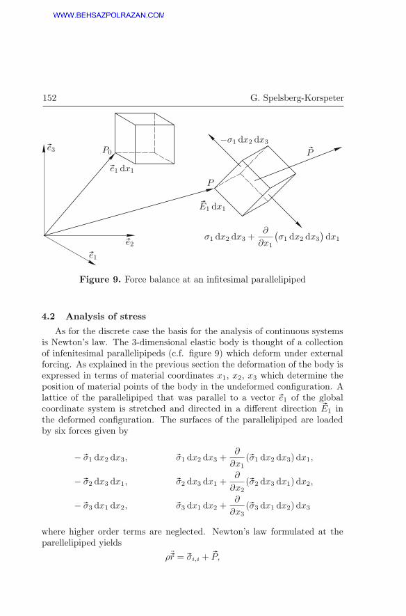
152 G. Spelsberg-Korspeter
��
e1
��
e2
��
e3 P0
P
��
e1 dx1
��
E1 dx1
−σ1 dx2 dx3
σ1 dx2 dx3 +∂
∂x1
(σ1 dx2 dx3
)dx1
��
P
Figure 9. Force balance at an infitesimal parallelipiped
4.2 Analysis of stress
As for the discrete case the basis for the analysis of continuous systemsis Newton’s law. The 3-dimensional elastic body is thought of a collectionof infenitesimal parallelipipeds (c.f. figure 9) which deform under externalforcing. As explained in the previous section the deformation of the body isexpressed in terms of material coordinates x1, x2, x3 which determine theposition of material points of the body in the undeformed configuration. Alattice of the parallelipiped that was parallel to a vector
��
e1 of the globalcoordinate system is stretched and directed in a different direction
��
E1 inthe deformed configuration. The surfaces of the parallelipiped are loadedby six forces given by
− ��
σ1 dx2 dx3,��
σ1 dx2 dx3 +∂
∂x1(
��
σ1 dx2 dx3) dx1,
− ��
σ2 dx3 dx1,��
σ2 dx3 dx1 +∂
∂x2(
��
σ2 dx3 dx1) dx2,
− ��
σ3 dx1 dx2,��
σ3 dx1 dx2 +∂
∂x3(
��
σ3 dx1 dx2) dx3
where higher order terms are neglected. Newton’s law formulated at theparellelipiped yields
�
r =��
σi,i +��
P,

Variational Principles in Mechanics and Control 153
where��
P denotes the volume forces and
��
σi = σij��
Ej ,
using index notation and σij are the components of the stress vector indirection of the lattice vectors. A momentum balance on the parallelipipedyields
��
0 =��
σ1 dx2 dx3 ×��
E1 dx1 +��
σ2 dx3 dx1 ×��
E2 dx2 +��
σ3 dx1 dx2 ×��
E3 dx3,
where terms higher order are neglected. Since
��
0 =��
σi ×��
Ei = σij��
Ej ��
Ei
= (σ21 − σ12)(��
E1 ��
E2) + (σ32 − σ23)(��
E2 ��
E3) + (σ13 − σ31)(��
E3 ��
E1)
it follows
σij = σji,
which implies that the stress tensor is symmetric.
4.3 Stress strain relations
Having introduced the stress and strain tensor the only thing missingto be able to formulate equations of motion for continuous systems areconstitutive material laws, i.e. relations between stress and strain. Theproperties of the materials to be studied enter to the governing equationsthrough the stress strain relations
σij = σij(e11, · · · , e33), (20)
which indicate how stresses are related to the deformation of the material.Although we assume in (20) that the stresses depend only on the strains itis very well possible that they also depend on other quantities such as thetime derivatives of the strains, etc. The easiest and most common materiallaw is Hooke’s law
σij = cijkl ekl (21)
which assumes a linear dependence between stresses and strains. For isotropicmaterial it can be shown that the cijkl depend only on two independent pa-rameters Becker and Gross (2002); Timoshenko and Goodier (1951). In theengineering literature the independent parameters are usually the modulus

154 G. Spelsberg-Korspeter
of elasticity E and the Poisson ratio ν. Using E and ν as parameters thestress strain relations for isotropic linear elastic material are written as
Ee11 = σ11 − ν(σ22 + σ33), (22a)
Ee22 = σ22 − ν(σ11 + σ33), (22b)
Ee33 = σ33 − ν(σ11 + σ22), (22c)
and
e12 =1 + ν
Eσ12 =
1
2Gσ12, (22d)
e23 = =1
2Gσ23, (22e)
e13 = =1
2Gσ13, (22f)
where the shear modulus is defined as
G =E
2(1 + ν). (23)
In more compact form the equations can be written as
σij =E
1− 2νeδij + 2G(eij − eδij),
e =1
3(e11 + e22 + e33), G =
E
2(1 + ν),
or
eij =1− 2ν
Eσδij +
1
2G(σij − σδij), (24a)
σ =1
3(σ11 + σ22 + σ33). (24b)
4.4 Basic equations of the theory of elasticity
We have now stated all ingredients to set up the basic equations of thetheory of elasticity. A force balance at the parallelipiped yields
− ρ¨��
r +��
σi,i +��
P = 0, (25)
where��
σi,i =∂
∂xi
��
σi =∂
∂xiσij
��
r,j

Variational Principles in Mechanics and Control 155
and��
r,j =��
Ej =∂
��
r
∂xj.
Substituting the stress strain relations and the Green Langrange strain ten-sor
eij =1
2(ui,j + uj,i + uk,iuk,j)
into (25) one obtains a system of partial differential equations, which withappropriate boundary conditions form the basic equations of elasticity. Inmost cases they need to be solved with numerical methods which can bevery challenging.
Since the solution of problems from 3D elasticity takes a lot of com-putation time it is in many cases very helpful to introduce simplifying as-sumptions. These are usually of kinematical nature and are used to derivesimplified models. Important examples are rods, beams, plates shells, etc..In order to be able to derive these models one needs to find ways to dealwith constraint forces. As in the discrete case the appropriate way to dothis will be variational principles which allow a formulation of the equationsof motion without constraint forces.
4.5 The principle of virtual work for continuous systems
Consider a body sketched in figure 10 which is subjected to distributedexternal volume forces
��
P in the interior and surface forces��
FE on the freeboundaries S1. Assume that there are geometric boundary conditions forthe displacement on the surface S2 of the body. In the interior of the body, aspreviously discussed, the equations of motion formulated on an infinitesimalparallelipiped read
− ρ¨��
r +��
σi,i +��
P =��
0. (26)
On the boundary S1 external and internal forces have to be in equilibriumyielding
��
F =��
FE = 0 on S1. (27)
As for discrete systems we can define a variation of the degrees of freedom,which in the continuous case are vector valued functions, that can for exam-ple be defined as
��
r = u(x1, x2, x3, t)��
e1+ v(x1, x2, x3, t)��
e2+w(x1, x2, x3, t)��
e3.The variation then reads
�
r =d
dε[(u+ εηu)
��
e1 + (v + εηv)��
e2 + (w + εηw)��
e3]
∣∣∣∣ε=0
=��
0, ε ∈ R
(28)

156 G. Spelsberg-Korspeter
��
P
S1
S2
����
��
FE
Figure 10. Body under forcing
where ηu, ηv, ηw are arbitrary twice continuously differentiable functions de-pending on x1, x2, x3 and t which satisfy the geometric boundary conditions.We now take the scalar product of the governing equations for the interior ofthe continuum (26) and the governing equations for the boundary (27) withδ
��
r and integrate over the volume of the continuum. Since the equations arehomogeneous we can add them to obtain
−∫∫∫V
(−ρ¨��r + ��
σi,i +��
P ) · δ ��
r dV +
∫∫S1
(��
F −��
FE) · δ ��
r dS = 0. (29)
Using the theorem of Gauß we can write the second term as
−∫∫∫V
��
σi,i · δ ��
r dV =
∫∫∫V
��
σi · δ ��
r,i dV −∫∫
S1+S2
��
F · δ ��
r dS. (30)
Since �
r vanishes on the geometric boundary conditions S2 we can write(29) as ∫∫∫
V
[ρ¨
��
r · δ ��
r +��
σi · δr,i −��
P · δ ��
r]dV −
∫∫S1
��
FE · δ ��
r dS = 0. (31)
Taking into account the definition of��
σi and��
r,i we can write
��
σiδ��
r,i = σijr,jδ��
r,i −1
2σijδEij = σijδeij (32)
since δEij = 0. It follows∫∫∫V
[ρ¨
��
r · δ ��
r + σijδeij
]dV −
∫∫∫V
��
P · δ ��
r dV −∫∫
S1
��
FE · δ ��
r dS = 0. (33)

Variational Principles in Mechanics and Control 157
As in the discrete case the virtual work of all ideal constraint forces vanishes.The derivations in section 2.3 stay valid for the continuous case as well ifone considers infinitely many partial velocities. This is valid because inan appropriate function space any test function η(
��
x, t) from (28) can beexpressed by an possibly infinite linear combination of base functions of thespace, the weight factors serving as the degrees of freedom. Hence we obtain∫∫∫
V
[ρ
(d2
dt2��
r
)· δ ��
r + σijδeij
]dV =
∑��
F · δ ��
r, (34)
where we introduce the notation∑ ��
F · δ ��
r for the virtual work of all con-tributing forces. As in the discrete case there is a strong relation betweenthe principle of virtual work and the energy expression of a body. If weassume that the variations δ
��
r vanish at two arbitrary fixed points in time,we can integrate by parts and write
t2∫t1
∫∫∫V
�
r · δ ��
r dV dt = −t2∫
t1
∫∫∫V
ρ ˙��
r · δ ˙��r dV dt = −δt2∫
t1
∫∫∫V
1
2ρ ˙
��
r2dV dt,
(35)
which is the variation of the kinetic energy. Additionally we can introducethe specific potential energy as
uel =
e∫0
σij(eij) deij , (36)
which yields
U =
∫∫∫V
uel dV. (37)
For linear elastic material we therefore have
δU = δ
∫∫∫V
1
2cijklekleij dV =
∫∫∫V
σijδeij dV. (38)
and hence (34) assuming linear elastic material can be written as
−δt2∫
t1
T − U dt =
t2∫t1
∑��
F · δ ��
r dt, (39)

158 G. Spelsberg-Korspeter
x
k
q
M
L
Figure 11. Rod with concentrated spring and concentrated mass
which is the formulation of Hamilton’s principle for the continuous case.Having established Hamilton’s principle for 3D elastic bodies specializedmodels can be derived by introducing kinematical constraints. Similarlyalso combinations of discrete and continuous systems can be analysed wherethe discrete systems can be thought of constrained elastic systems. In thefollowing sections we will treat simple intuitive examples.
4.6 Derivation of structural models from 3D elasticity
As probably the simplest example of a continuous structural model inthis section we discuss the elastic rod and the assumptions made in thederivation of the model. Consider a slender body and assume that we areonly interested in longitudinal vibrations. If such a structure is only loadedin axial direction it is reasonable to introduce simplifying assumptions whichare in fact kinematical constraints on the elastic body. For the model ofa rod we assume that the crossections stay planar and can only move inx-direction along the length axis of the rod, i.e.
u(x, y, z) = u(x), v(x, y, z) = 0, w(x, y, z) = 0.
To show that we can treat discrete and continuous models in the same waywe attach a spring and a point mass at the end of the rod as is shown infigure 4.6. Introducing the kinematic constraint the kinetic energy of therod then simplifies to
T =1
2
l∫0
ρAu2 dx+1
2Mq2, (40)
where the kinetic energy of the particle at the end is taken care of in thesecond term with a separate degree of freedom q. Due to the kinematical

Variational Principles in Mechanics and Control 159
assumption the expression for the specific potential energy simplifies to
u =
ε∫0
σ dε =1
2Eε2 (41)
since σ = Eε, where ε = u′. Therefore the total potential energy of the rodcan be written as
U =1
2
l∫0
EAu′2dx+
1
2k (q − u(l, t))
2, (42)
where the second term is due to the kinetic energy stored in the spring. Theequations of motion can now be derived using Hamilton’s principle
δ
t2∫t1
Ldt = 0, L = T − U, (43)
where in addition to the energy expressions the geometric boundary condi-tions
u(0, t) = 0, (44a)
δu(0, t) = 0, (44b)
and
δu(x, t1) = 0, (44c)
δu(x, t2) = 0, (44d)
have to be considered. As in the discrete case we have to carry out thevariations on the Lagrange function yielding
δ
t2∫t1
⎡⎣ l∫
0
1
2ρAu2 − 1
2EAu′
2dx+
1
2Mu2 − 1
2(q − u(l, t))2
⎤⎦ dt = 0,
(45a)
t2∫t1
⎡⎣ l∫
0
ρAuδu− EAu′δu′ dx+Mqδq − k(q − u(l, t))(δq − δu(l, t))
⎤⎦ dt = 0.
(45b)

160 G. Spelsberg-Korspeter
In order to be able to apply the main theorem of variational calculus wehave to use integration by parts with respect to x and t, yielding
t2∫t1
⎡⎣ l∫0
(−ρAu+EAu′′)δu dx−(Mq + k(q−u(l, t)))δq+k(q−u(l, t))δu(l, t) dt
⎤⎦
+
l∫0
ρAuδu dx
∣∣∣∣t2t1
−t2∫
t1
EAu′δu dt
∣∣∣∣l0
+Mqδq
∣∣∣∣t2t1
=0.
Since the variations δu(x, t) and δq are arbitrary, each term of the sum hasto vanish independently. Using the fact that variations vanish at t1 and t2and that they satisfy the geometric boundary conditions, i.e.
δu(x, t1) = 0, δu(x, t2) = 0, δq(t1) = 0, δq(t2) = 0, δu(0, t) = 0,
we conclude
ρAu− (EAu′)′ = 0, (46a)
Mq + k(q − u(l, t) = 0, (46b)
EAu′ = k(q − u(l, t)), (46c)
which together with the geometric boundary condition
u(0, t) = 0 (46d)
defines a linear boundary value problem in x and t that can be solveduniquely.
4.7 Discussion of properties of continuous systems
There are many interesting properties and insights that can directly bederived from (39). For example it can be seen that the energy expressionsonly contain first order derivatives whereas the derived boundary value prob-lems in fact have boundary conditions of higher order because of the use ofintegration by parts or Gauß’s theorem respectively. Boundary conditionsoccurring in (39) are referred to as geometric boundary conditions, the ad-ditional boundary conditions arising in the process of integration by partsare called natural boundary conditions. In order to solve a physical prob-lem one can either directly solve the variational problem or try to solve thecorresponding boundary value problem. Since functions occurring in thevariational problem have to fulfill less continuity and differentiability con-ditions the variational problem is often referred to as a weak formulation

Variational Principles in Mechanics and Control 161
yielding so called weak solutions. Solutions of the boundary value prob-lem are referred to as exact solutions. Whereas quite general existence anduniqueness theorems for weak solutions exist this is not the case for exactsolutions. From the symmetry of the energy expressions for the conservativecase one can derive orthogonality of eigenfunctions and max-min-propertiesfor the eigenvalues which can be directly formulated for the continuous case.For the sake of brevity we however directly turn to the discretization of theequations of motion which will allow the use of the corresponding theoremsfor the discretized case.
4.8 Approximation Methods
Whereas for discrete systems we had to deal with ordinary differentialequations and a finite number of degrees of freedom meaning that mathe-matically the underlying space was R
n, for continuous systems the spacesto be considered are function spaces, which for example have to be validfor the formulation of boundary conditions. In appropriate function spaces(separable Hilbert spaces) functions can be expressed as linear combinationsof other functions
f(x) =
∞∑i=1
αiWi(x)
if Wi, i = 1, ...,∞ span the space, where the sum is infinite. A truncatedseries is an approximation for f . A common example for an approximationof functions in a function space is the Fourier series given by
f(t) =a02
+∞∑k=1
ak cos kωt+ bk sin kωt,
which is defined for periodic functions f(t) on the function space L2. Theidea of expanding functions in terms of other functions is also the basisfor the Ritz and the Galerkin method. However the underlying spaces aremore complicated since boundary conditions have to be considered which isnot possible in L2. For many problems the appropriate spaces are Sobolevspaces however we do not go into details here. In order to approximate afunction w(x, t) depending on space and time we write
w(x, t) =
N∑i=1
Wi(x)qi(t) (47)
where Wi(x) are given linearly independent shape functions. If the functionsWi(x) span the space and we take enough shape functions the truncated se-ries in (47) will be a reasonably good approximation for w(x, t), provided

162 G. Spelsberg-Korspeter
Figure 12. Elastic rod
the qi(t) are calculated appropriately. Approximation methods differ in theform the shape functions are chosen and in the way the qi(t) are determined.Ritz methodThe idea behind the Ritz method is to substitute (47) into the energy expres-sion in Hamilton’s principle and to carry out the variations with respect tothe qi(t). This means that the solution of the variational problem is limitedto a subspace spanned by the shape functions Wi(x) which have to satisfythe geometric boundary conditions. Consider the example of the elastic rodshown in figure 12 for which as before the energy expressions read
T =1
2
l∫0
ρA(x)u2 dx,
U =1
2
l∫0
EA(x)u′2dx.
Substitution of
u(x, t) ≈ u(x, t) =
N∑i=1
Ui(x)qi(t)
where Ui(0) = 0 and Ui(x) are linearly independent yields the followingequations in Hamilton’s principle
δ
t2∫t1
⎡⎣ l∫
0
1
2ρA
(N∑i=1
Uiqi
)(N∑i=1
Uj qj
)dx−
l∫0
EA
(N∑i=1
U ′iqi
)(N∑i=1
U ′jqj
)dx
⎤⎦dt=0
(48)with boundary conditions
qi(t1) = qi(t2) = 0.

Variational Principles in Mechanics and Control 163
Carrying out the variations or quicker by application of Lagrange’s equationsit follows
N∑i=1
L∫0
ρAUiUj dx qi +
N∑i=1
L∫0
EAU ′iU
′j dx qi = 0, for j = 1, ..., N,
which in matrix form can be written as
Mq +Kq = 0
with
mij =
L∫0
ρAUiUj dx,
kij =
L∫0
EAU ′iU
′j dx.
Galerkin methodIn the Galerkin method we directly substitute the ansatz (47) into theboundary value problem (b.v.p.). For the example considered in figure 12we obtain
ρA
N∑i=1
Ui(x)qi(t)−[EA
N∑i=1
U ′i(x)qi(t)
]′= e(x, t),
which yields an error e(x, t). Note that in contrast to the Ritz method theshape functions have to satisfy all boundary conditions
Ui(0) = 0, (geometric b.c.)
U ′i(L) = 0 (natural b.c.).
In order to minimize the error e(x, t) we require that the projection on theshape functions vanishes, i.e.
L∫0
(ρA∑
Uiqi −[EA∑
U ′iqi
]′)U1 dx = 0,
...
L∫0
(ρA∑
Uiqi −[EA∑
U ′iqi
]′)UN dx = 0.

164 G. Spelsberg-Korspeter
In matrix notation the equations read
Mq +Kq = 0, (49)
where
mij =
L∫0
ρAUiUj dx, (50a)
kij = −L∫
0
[EAU ′i ]′Uj dx. (50b)
Since all boundary conditions have to be satisfied one can use integrationby parts on the stiffness matrix which shows that the matrices are formallyidentical to those obtained by the Ritz method. The Ritz method how-ever converges also if the geometric boundary conditions are not satisfied,whereas the Galerkin method with matrices of the form (50) does not.DiscussionIt can be clearly seen that for both Ritz and Galerkin method the matricesM and K are positive definite, which will generally be the case if conser-vative problems of linear elasticity are considered. This means that all niceproperties of discrete systems like the orthogonality of eigenvectors and themax-min-properties of the eigenvalues carry over also to the continuous case.This can be seen on the one hand from the convergence of the approxima-tion methods but can also be derived directly for the continuous problemsHagedorn (1989).
5 Aspects of design and optimization for active an
passive control systems
In the last chapters we have focused on the question how to derive efficientmechanical models for control structures. We have seen that both for dis-crete and continuous systems the mechanical models can be represented byordinary differential equations of the form
x = f(x,u, t), (51)
which are written here in first order form. For many practical applicationsthe linearized equations
x = Ax+Bu, (52)

Variational Principles in Mechanics and Control 165
which are in many cases autonomous, dominate the system’s behavior. Avery common task in control theory is of course to bring a system from aninitial state x0 to a final state xf using the possible controls u. The firstquestion is therefore always, whether this is possible, namely whether thesystems is controllable, meaning it can be brought from x0 to xf in arbitraryfinite time. This can be checked by the Kalman criterion according to whichthe system is controllable if and only if the controllability matrix has fullrank Unbehauen (2000), i.e.
rank{[B |AB | . . . |An−1B
]} = n. (53)
Usually it is helpful to transform the system matrix A to Jordan normalform, i.e. by writing
x = Qy,
where Q consists of the eigenvectors of A and the corresponding vectorsfrom the Jordan chains, in case multiple eigenvalues with degenerate eigen-spaces occur. With J = Q−1AQ the transformed equations read
y = Jy +Q−1Bu. (54)
From (54) it is for example easy to see that the system cannot be controllableif (54) contains any decoupled equations not influenced by the controls ui.As we stated above controllability means the system can be brought from x0
to xf in arbitrary finite time. For practical problems this is however usuallynot enough. First of all, due to the limitations of the actuators the controlsare also limited. Second, in many cases one wants to optimize the controlssuch that for example energy consumption is low or other requirements aremet. In addition to the need for the optimization of controls the systemneeds to be designed in order to be robust against disturbances. In the nextsection we address the question how this can be achieved in an active or apassive manner. Afterwards we will show how variational approaches canbe used to optimize controls.
5.1 Structural design and optimization of control systems
As mentioned above it is usually not enough to calculate an appropriatecontrol to bring a system from one state to another. In addition to design-ing an appropriate control u one has to make sure that the correspondingsolution of the system stays approxmimately valid also under small distur-bances which mathematically formulated means that the solution is stable.Having found a control u∗ which can be the result of an optimization we
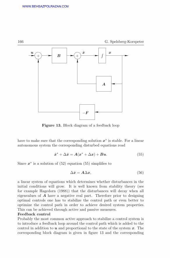
166 G. Spelsberg-Korspeter
+ +∫
A
−F
Bu x x
Figure 13. Block diagram of a feedback loop
have to make sure that the corresponding solution x∗ is stable. For a linearautonomous system the corresponding disturbed equations read
x∗ +Δx = A(x∗ +Δx) +Bu. (55)
Since x∗ is a solution of (52) equation (55) simplifies to
Δx = AΔx, (56)
a linear system of equations which determines whether disturbances in theinitial conditions will grow. It is well known from stability theory (seefor example Hagedorn (1988)) that the disturbances will decay when alleigenvalues of A have a negative real part. Therefore prior to designingoptimal controls one has to stabilize the control path or even better tooptimize the control path in order to achieve desired system properties.This can be achieved through active and passive measures.Feedback controlProbably the most common active approach to stabilize a control system isto introduce a feedback loop around the control path which is added to thecontrol in addition to u and proportional to the state of the system x. Thecorresponding block diagram is given in figure 13 and the corresponding

Variational Principles in Mechanics and Control 167
equations are given by
x = (A−BF )x+Bu, (57)
where F denotes the feedback matrix. If the system (52) is controllable theeigenvalues of the closed loop system namely the eigenvalues of the matrix(A − BF ) can be placed arbitrarily Föllinger (1994); Unbehauen (2000).However it is not easy to see what placement of the eigenvalues is favorable.Therefore, in section 5.2 we will use an objective function in order to designan optimal linear control system Unbehauen (2000).
In practice it is often not possible to measure all states of the system suchthat the procedure described is not directly applicable. The feedback con-trol methods have however been extended for much more general systemsby developing observers for the states which are not observable Föllinger(1994); Unbehauen (2000).Passive structural optimizationWe have seen in the context of (55) that in order to successfully apply con-trols to a system it is desireable to have a stable control path which for linearconstant coefficient systems means that all eigenvalues have a negative realpart. Of course it is usually beneficial to achieve this passively withoutthe need of a controller. For mechanical systems the common approach toachieve this is to introduce damping. In the linear case for systems withsymmetric positive definite mass and stiffness matrices this is always helpfulalthough it might not be easy to implement. One needs to insure that damp-ing is pervasive, a task that can be analysed in close analogy to the conceptof controllability Müller (1977); Hagedorn and Otterbein (1987). If the sys-tem under investigation is not conservative the question of how to stabilize itbecomes more involved. In this case most of the time one needs to deal withasymmetric parts in the velocity proportional matrix and or in the stiffnessmatrix. For representative examples we refer to Hagedorn and Hochlenert(1987) and to section 5.3 where we study possibilities to passively stabilizea rotor in frictional contact by changing the stiffness characteristics.
5.2 Variational approaches in control theory
In section 3 we have seen how the equations of motion of a systemcan be derived from making a functional stationary using the calculus ofvariations. The same mathematical technique is also very useful in controltheory. Generally we study systems of the form
x = f(x,u, t), (58)
where x is the vector of the states of the system and u is the vector of thecontrols. Note that in many cases the states are limited mathematically

168 G. Spelsberg-Korspeter
stated by u ∈ U , where U is the set of admissible controls. The system (58)can for example be a mechanical system written as first order differentialequations where the controls are external forces. The general problem inoptimal control is to bring a system from an initial state x0 to a desiredfinal state xf . This is possible in many different ways, provided the systemis controllable. In order to evaluate the different controls a cost functionalis implemented as
I =
∫ tf
t0
L(x,u, t)dt, (59)
which is to be minimized. Note that if we set L(x,u, t) = 1 the cost func-tional minimizes the time to bring the system from the initial to the finalstate. Mathematically the optimization problem to be solved is
Min I =
∫ tf
t0
L(x,u, t)dt,
s.t.
x = f(x,u, t).
In order to get rid of the boundary conditions the cost functional can beaugmented by the constraints using Lagrangian multipliers ψ(t) which arealso called adjoint variables. The augmented cost functional then reads
I =
∫ tf
t0
L(x,u, t)−ψT (f(x,u, t)− x)dt. (61)
If the controls u(t) are sufficiently smooth and unbounded the functional(69a) can be optimized using the calculus of variations with
x = x∗ + εδx, (62a)
u = u∗ + εδu, (62b)
ψ = ψ∗ + εδψ, (62c)
where the optimal trajectories are marked by ∗ and the variations vanishfor the boundaries t0 and tf . Note that the variation of ψ ensures that theequations of motion have to be fulfilled and therefore no extra constraintsare needed.
As a minimal example consider a particle which is moved on a line by acontrol force. At time t0 = 0 the particle is at rest at the position x(0) = 1and is to be transferred to the origin arriving there at tf = 1. The objective

Variational Principles in Mechanics and Control 169
is not to use high control forces which can be achieved by minimizing thesquare of the force. Mathematically the optimization problem reads
Min1
2
∫ 1
0
u2dt,
s.t.
x = u,
x(0) = 1, x(1) = 0, x(0) = 0, x(1) = 0.
In order to obtain a description compatible with (61) we write the equationof motion as a first order system[
x1x2
]=
[0 10 0
] [x1x2
]+
[01
]u (63)
and obtain for the augmented cost functional
I =
∫ 1
0
1
2u2 + ψ1(x1 − x2) + ψ2(x2 − u)dt.
A necessary condition for an optimum is that the variation δI vanishesyielding∫ 1
0
uδu+ δψ1(x1 − x2)+ψ1(δx1 − δx2)+δψ2(x2 − u)+ψ2(δx2 − δu)dt = 0.
(64)
Using integration by parts it follows∫ 1
0
(u− ψ2)δu+(x1 − x2)δψ1−ψ1δx1+(x2 − u)δψ2−(ψ2 + ψ1)δx2dt = 0.
(65)
Finally, from the main theorem of the variational calculus we obtain
u = ψ2
and
x1 = x2, (66a)
x2 = ψ2, (66b)
ψ1 = 0, (66c)
ψ2 = −ψ1. (66d)

170 G. Spelsberg-Korspeter
Due to their simple structure the equations (66) can be integrated analyti-cally yielding
x1 = −1
6k1t
3 +1
2k2t
2 + k3t+ k4, (67a)
x2 = −1
2k1t
2 + k2t+ k3, (67b)
ψ1 = k1, (67c)
ψ2 = −k1t+ k2. (67d)
Adjusting (67) to the boundary conditions yields
k1 = 12, k2 = 6, k3 = 0, k4 = 1,
and the optimal control reads
u = −12t+ 6. (68)
It can be easily verified that the solution actually yields a minimum.In the general case (61) is often written in the form
I = −∫ tf
t0
H(x,ψ,u, t)−ψT xdt, (69a)
defining the Hamilton function
H = −L(x,u, t) +ψTf(x,u, t). (69b)
The variation of (69a) yields
δI=−∫ tf
t0
(∂H
∂x
)T
δx+
(∂H
∂ψ
)T
δψ+
(∂H
∂u
)T
δu−xT δψ−ψT δx dt = 0.
(70)
Using integration by parts on the term with δx and the main theorem ofvariational calculus we obtain
x =∂H
∂ψ, (71a)
ψ = −∂H∂x
, (71b)
∂H
∂u= 0, (71c)

Variational Principles in Mechanics and Control 171
which are necessary conditions for an optimum. The equations (71) con-sist of a boundary value problem of the so called canonical Hamilton equa-tions in x and ψ given by (71a) and (71b) with the boundary conditionsx(t0) = x0 and x(tf ) = xf and a set of algebraic equations (71c) fromwhich the optimal controls can be calculated. Note that equations (71) im-ply that dH
dt = ∂H∂t and that H is therefore constant in the autonomous case.
Of course, after solving equations (71) it has to be checked whether a min-imum of the cost functional I has been found. In many cases however theequations (71) yield a unique solution with guaranties an optimum providedthe problem was well posed.
As an example consider the optimal linear control problem for the system
x = A(t)x+B(t)u, (72)
which is to be brought from x(t0) = x0 to x(tf ) = xf by a control u whichminimizes the quadratic cost functional∫ tf
t0
L(x,u, t)dt =1
2
∫ tf
t0
[xTQ(t)x+ uTR(t)u]dt. (73)
The possibly time dependent matrices Q(t) and R(t) are assumed to besymmetric positive definite and are weighting the minimization of the statesand controls of the system. The necessary conditions for an optimum (71)can be calculated as
x =∂H
∂ψ= A(t)x+B(t)u, (74a)
ψ = −∂H∂x
= Q(t)x−AT (t)ψ, (74b)
0 =∂H
∂u= R(t)u+BT (t)ψ. (74c)
From (74) we obtain
u = R−1(t)BT (t)ψ(t) (75)
and (x
ψ
)=
[A(t) B(t)R−1BT (t)Q(t) −AT (t)
](x
ψ
). (76)
For the solution of (76) we make the ansatz
ψ = −P (t)x, (77)
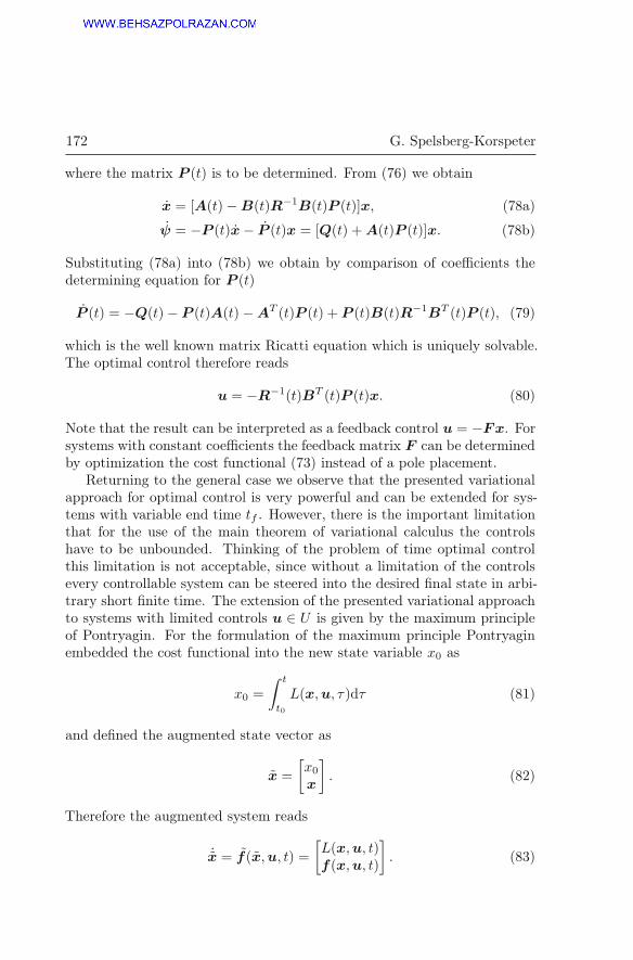
172 G. Spelsberg-Korspeter
where the matrix P (t) is to be determined. From (76) we obtain
x = [A(t)−B(t)R−1B(t)P (t)]x, (78a)
ψ = −P (t)x− P (t)x = [Q(t) +A(t)P (t)]x. (78b)
Substituting (78a) into (78b) we obtain by comparison of coefficients thedetermining equation for P (t)
P (t) = −Q(t)− P (t)A(t)−AT (t)P (t) + P (t)B(t)R−1BT (t)P (t), (79)
which is the well known matrix Ricatti equation which is uniquely solvable.The optimal control therefore reads
u = −R−1(t)BT (t)P (t)x. (80)
Note that the result can be interpreted as a feedback control u = −Fx. Forsystems with constant coefficients the feedback matrix F can be determinedby optimization the cost functional (73) instead of a pole placement.
Returning to the general case we observe that the presented variationalapproach for optimal control is very powerful and can be extended for sys-tems with variable end time tf . However, there is the important limitationthat for the use of the main theorem of variational calculus the controlshave to be unbounded. Thinking of the problem of time optimal controlthis limitation is not acceptable, since without a limitation of the controlsevery controllable system can be steered into the desired final state in arbi-trary short finite time. The extension of the presented variational approachto systems with limited controls u ∈ U is given by the maximum principleof Pontryagin. For the formulation of the maximum principle Pontryaginembedded the cost functional into the new state variable x0 as
x0 =
∫ t
t0
L(x,u, τ)dτ (81)
and defined the augmented state vector as
x =
[x0x
]. (82)
Therefore the augmented system reads
˙x = f(x,u, t) =
[L(x,u, t)f(x,u, t)
]. (83)

Variational Principles in Mechanics and Control 173
If one defines the augmented Hamilton function as
H(x, ψ,u, t) = ψT f(x,u, t), ψ =
[ψ0
ψ
](84)
and requires that for an optimal control the canonical Hamilton equations
˙x =∂H
∂ψ, (85a)
˙ψ = −∂H
∂x, (85b)
are fullfilled, one can state Pontryagin’s maximum principle as: A necessarycondition for the existence of an optimal control u∗ ∈ U and the correspond-ing solution x∗ is the existence of a solution ψ∗ �= 0 of (85) for which holds� for all t in t0 ≤ t ≤ tf the Hamiltonian takes its absolute maximum with
respect to u ∈ U i.e.
H(x∗, ψ∗,u∗, t) = maxu∈UH(x, ψ,u, t), (86)
� ψ0 does not get positive, i.e.
ψ0(t) ≤ 0. (87)
Note that equations (85) certify that the optimal control solution actuallysatisfies the system’s equations of motion. Therefore, in the case of un-bounded controls they imply that (69a) is made stationary. The calculus ofvariations is therefore a special case of the Pontryagin maximum principlewhich also holds for piecewise discontinuous controls. The extension to dis-continuous controls is the reason why (86) replaces the condition (71c) thathas previously been used.
As an important example where controls need to be assumed boundedwe consider a problem of time optimal control. Assume the very simplesystem (63) from the previous example is to be steered into the origin inminimal time using a control from u ∈ {−1, 1}. The Hamilton function inthis case reads
H = ψ0 + ψ1x2 + ψ2u. (88)
From (86) it follows
u =
{1 ψ2 > 0−1 ψ2 < 0
. (89)
174 G. Spelsberg-Korspeter
Equations (85) yield
x1 =∂H
∂ψ1= x2, (90a)
x2 =∂H
∂ψ2= u, (90b)
ψ1 = − ∂H∂x1
= 0, (90c)
ψ2 = − ∂H∂x2
= −ψ1. (90d)
The equations (90) can be easily integrated resulting in
x1 =1
2ut2 + c3t+ c4, (91a)
x2 = ut+ c3, (91b)
ψ1 = c1, (91c)
ψ2 = c2 − c1t, (91d)
and the optimal control reads u = sign(c2 − c1t). Using (91a) and (91a) wecan eliminate the time and obtain the system trajectories
x1 = ±1
2x22 + c5, (92)
which are parabolas depending on the sign of the control u and on theconstant c5 that is a function of c3, c4 and u. Using them the optimaltrajectories can be obtained by calculating the switching curve on the phaseplane Pontryagin and Mishchenko (1962); Ludyk (1995).
In the example we observe that the optimal control always takes itsextreme values in the set of admissible controls U . This is a general prop-erty of the controls for time optimal problems. Especially for linear systemstheorems for existence and uniqueness as well as the number of switching oc-casions have been derived. For details refer to Pontryagin and Mishchenko(1962); Ludyk (1995) and the references therein.
5.3 Example of passive structural design against self-excited vi-brations
In this section we consider an example of a system tending to self-excitedvibrations which are unwanted. In order to stabilize the system we will notintroduce damping but show that also with an appropriate design of the

Variational Principles in Mechanics and Control 175
μ
Ω
k, N0 k, N0
k, N0
k, N0
c1
c2
�n1
�n2
Figure 14. Rotor in frictional contact
stiffness properties the problem can be attacked. For a rather wide class ofsystems it is helpful to avoid symmetries either in the structure itself or inthe bedding. In order to motivate the ideas we consider a simple examplefrom rotor dynamics. Consider the Laval rotor shown in figure 14 which isbedded on two springs with stiffness c1 and c2 respectively and assumed toturn with constant angular velocity Ω. The rotor is in contact with frictionpads which are pressed onto it’s surface by prestressed springs (prestressN0, stiffness k). Between the pads and the rotor friction occurs which we

176 G. Spelsberg-Korspeter
model by Coulomb’s law with friction constant μ. Using
q1 = N0pP · �n1 (93a)
q2 = N0pP · �n2 (93b)
as degrees of freedom the equations of motion read[1 00 1
](q1q2
)+
[ω21 n−n ω2
2
](q1q2
)=
(00
), (94)
where ω21 = c1+2k
M , ω22 = c2+2k
M and n = 2μkM . The eigenvalues of the system
can readily be calculated as
λ1,2 =
√−1
2
(ω21 + ω2
2 ±√
(ω21 − ω2
2)2 − 4n2
). (95)
By inspection of (95) it can directly be seen that when
4n2 > (ω21 − ω2
2)2 (96)
the inner square root yields a complex number. Since the square root of acomplex number is point symmetry with respect to the origin of the complexplane this means that one of the eigenvalue λ1,2 has a positive real part andthe system is unstable. The analysis shows that if we split the eigenvalues ω1
and ω2 of the corresponding conservative system, it is stabilized. A splittingof eigenvalues can for example be achieved by changing the geometry of themountings of the bearings.
The observed effect can be shown to hold for a much more general classof problems given by equations of the type
Mq +ΔD(t)q + (K +ΔK(t))q = 0, (97a)
ΔD(t) = ΔD(t+ T ), ΔK(t) = ΔK(t+ T ), (97b)
using analytic perturbation theory for eigenvalues Seyranian and Mailybaev(2003). The matrices M , K are constant, symmetric and positive definiteand ΔD(t), ΔK(t) are time periodic but have arbitrary structure. Notethat the constant coefficient case studied in the previous example can beseen as a special case of the periodic setting. In fact if we had attachedthe pads to the rotor we would have obtained time periodic coefficients. Inapplications the perturbation matrices ΔD(t) and ΔK(t) often arise dueto contact forces as we saw in the previous example. In many cases theseforces are small compared to elastic restoring terms and can therefore betreated as perturbations.

Variational Principles in Mechanics and Control 177
As motivated by the example system from figure 14 systems of the type(97a) can be stabilized by separating the eigenvalues of the uperturbed con-servative M , K system. From a constructive point of view this is mucheasier than to introduce damping since it can be achieved by a change ofgeometry. Intuitively it is clear that multiple eigenvalues naturally arisedue to symmetries of the structure which means that symmetries have tobe destroyed in order to make the system robust against instability phe-nomena. In rotor dynamics this is not so easy since usually one wants therotor to be balanced. However the approach of designing asymmetric ro-tors to avoid self-excited vibrations has been successfully been performedin the past. For deeper insights into the underlying mechanisms we refer toSpelsberg-Korspeter (2013) and the references therein.
6 Concluding remarks
In this chapter we discussed the role of variational principles in the deriva-tion of mechanical control systems. The major goal was to show the con-nection between different methods for deriving the model equations and toemphasize the importance of structural models which significantly reducethe degrees of freedom of control models. We then showed that variationaltechniques are also useful in the theory of optimal control and discussedstrategies for active and passive stabilization of control systems. The chap-ter does not aim for completeness but tries indicate linkages between dif-ferent topics which are most often treated more or less independently inuniversity curricula.
Bibliography
W. Becker and D. Gross. Mechanik elastischer Körper und Strukturen.Springer, 2002.
O. Föllinger. Regelungstechnik. 1994.P. Hagedorn. Non-Linear Oscillations. Calendron Press Oxford, 1988.P. Hagedorn. Technische Schwingunslehre, volume 2. Springer-Verlag, 1989.
Lineare Schwingungen kontinuierlicher mechanischer Systeme.P. Hagedorn and D. Hochlenert. Technische Schwingunslehre. Harry
Deutsch, 1987.P. Hagedorn and S. Otterbein. Technische Schwingunslehre. Springer-
Verlag, 1987.T. R. Kane and Levinson D. A. Dynamics: Theory and Applications.
McGraw-Hill, New York, 1985.G. Ludyk. Theoretische Regelungstechnik 2: Zustandsrekonstruktion, opti-
male und nichtlineare Regelsysteme. Springer Verlag, Berlin, 1995.

178 G. Spelsberg-Korspeter
L. Meirovitch. Fundamentals of Vibration. McGraw-Hill, 2001.P. C. Müller. Stabilität und Matrizen. Springer, 1977.L. S. Pontryagin and E. F. Mishchenko. The Mathematical Theory of Opti-
mal Processes. John Wiley & Sons, 1962.A. P. Seyranian and A. A. Mailybaev. Multiparameter Stability Theory with
Mechanical Applications. World Scientific, 2003.G. Spelsberg-Korspeter. Robust structural design against self-excited vibra-
tions. Springer, 2013.S. Timoshenko and J. N. Goodier. Theory of Elasticity. McGraw-Hill, 1951.H. Unbehauen. Regelungstechnik. Vieweg Verlag, 2000.K. Washizu. Variational Methods in Elasticity and Plasticity. Pergamon
Press, 1974.

Hybrid Mass Damper: A Tutorial Example
Andre Preumont, David Alaluf and Renaud Bastaits
ULB, Brussels, Belgium
Abstract This chapter compares three different ways of mitigatingthe dynamic response of buildings: Dynamic Vibration Absorber(DVA), Active Mass Damper (AMD) and Hybrid Mass Damper(HMD). The methodology is illustrated with a shear frame exam-ple subjected to a random seismic input. Two different ways ofimplementing the HMD are considered, one called passive startingfrom a mistuned DVA, and one called active starting from a tunedDVA and using a control system with two feedback loops. It isshown that a well designed HMD may produce performances com-parable to that of an AMD while significantly reducing the actuatorforce and stroke requirements. Besides, the active implementationis immune to control system breakdown, because the HMD is re-duced to a properly tuned DVA with optimum performances for apassive system.
1 Introduction
1.1 Dynamic Vibration Absorber
The celebrated Dynamic Vibration Absorber (DVA) was invented byFrahm in 1909; it is based on simple idea of transferring the kinetic en-ergy of the vibrating structure to a properly tuned and specially designedsingle d.o.f. oscillator, where it is dissipated. The underlying theory wasdeveloped by Ormondroyd and Den Hartog in 1928. Depending on the ap-plication, it can also be called Tuned Mass Damper (TMD). Because it issimple and robust, the DVA has been used very successfully in many appli-cations, including the mitigation of the wind response of tall building andthe vibration alleviation in helicopters. Note, however, that in helicopterapplications, the disturbance f is harmonic at a constant frequency ω0, andthe DVA parameters are adjusted to produce a sharp transmission zero atω0 in the Frequency Response Function (FRF) between the disturbance andthe structural response; this usually implies a lightly damped DVA. On thecontrary, when the structure is subjected to a wide band disturbance (as inthe case of a tall buildings subjected to wind gusts or an earthquake), the
P. Hagedorn, G. Spelsberg-Korspeter (Eds.), Active and Passive Vibration Control of Struc-tures, CISM International Centre for Mechanical Sciences DOI 10.1007/ 978-3-7091-1821-4_3 © CISM Udine 2014

180 A. Preumont, D. Alaluf and R. Bastaits
DVA parameters are tuned in such a way that the structural response isminimized (in some sense); the DVA parameters appropriate for mitigatingthe response to wind gusts or to earthquake ground motion are essentiallythe same, except that the seismic excitation of strong earthquakes usuallyleads to much larger structural responses than that of wind gusts, and thisrequests DVAs with larger strokes. Figure 1 shows the DVA mounted at thetop of the Taipei 101 building in Taiwan. This building has a height of 509m and has 101 floors. The absorber consists of a pendulum with a mass of730 tons suspended with four cables extending over 4 floors.
Figure 1. Dynamic Vibration Absorber of the Taipei 101 building. The DVA consistsof a pendulum with a mass of 730 tons suspended with 4 cables extending over 4 floors.
1.2 Active Mass Damper and Hybrid Mass Damper
This study considers only the case of a wide band disturbance and com-pares various ways of enhancing the performance of a DVA, all based on the

Hybrid Mass Damper: A Tutorial Example 181
(a)
k1
m1
k
c 1
ca a
ma
Structure
�1
DVA
�a � �1
(b)
k1
m1
c 1
f
maInertial actuator
�a �1��AMD:
�a �1�HMD:
ma = �m1
Figure 2. (a) Dynamic Vibration Absorber (DVA): ωa � ω1. (b) Active Mass Damper(AMD) [ωa � ω1] and Hybrid Mass Damper (HMD) [ωa < ω1].
use of an inertial actuator with different tuning (Fig.2). A DVA is a passivespring and damper device whose natural frequency is close to the targetedmode ωa � ω1. The Active Mass Damper (AMD) includes a force actuatoracting in parallel with the spring and damper, between the inertial mass andthe supporting structure; the device (called a proof-mass actuator) is usu-ally tuned on a frequency significantly lower than the modes to be damped,so that it behaves as a perfect force actuator for the whole frequency rangeof interest (from ω1 and above). The Hybrid Mass Damper (HMD) is basedon the same principle as the AMD, except that the frequency ωa is tunedcloser to ω1, in an attempt to combine the properties of passive and activedevices, to achieve one or several of the following features: (1) improvedperformances; (2) improved robustness with respect to structural changes;(3) improved reliability (e.g. immunity with respect to power failure); (3)reduced construction and maintenance costs. Various examples of HMDused in civil engineering are described in [Seto, Spencer].
In this note, two different ways of implementing the HMD are consid-ered; the first one is based on a passive mistuning of the device beforeapplying active control (velocity feedback); this approach is simple, but hasthe drawback of reduced reliability in case of control system failure. Thesecond approach starts from a regularly tuned DVA and involves two controllayers : the first layer (P+D controller) produces the effect of the passivemistuning of the previous method and the second layer superimposes theactive control with velocity feedback. The various approaches are comparedon the simple example of shear frame.
This note is organized as follows: Section 2 recalls the equations govern-ing the seismic response of a building, describes the shear frame example

182 A. Preumont, D. Alaluf and R. Bastaits
used to illustrate the various methods and analyzes its random response toa stationary seismic input. Section 3 recaps the design rules of the DVA andits extension to multiple d.o.f. systems; the shear frame example is used forillustration. Section 4 is devoted to the active control with an AMD; theactuator and sensor are briefly discussed and the system response is formu-lated in state space. Section 5 discusses the HMD where a DVA is modifiedto operate as an AMD; the effect on performance and control requirementsis analyzed. Finally section 6 discusses how the mistuning of the HMD maybe achieved actively with a dual loop controller; it is demonstrated that thisoffers a better immunity with respect to control system failure.
2 Seismic response
2.1 Basic equations
The seismic excitation is usually specified by the support acceleration,x0. The seismic response of a building excited by a single-axis supportexcitation is governed by the following equations [e.g. Preumont, 2012,Ch.7]:
The global displacements may be decomposed into the rigid body motiondue to the support input motion x0 and the motion relative to the support;the total displacement is given by
x = x01+ y (1)
where 1 is the unit rigid body mode and y is the motion relative to thesupport. With these notations, the dynamic equation is
M y+ Cy+Ky = −M1x0 (2)
If y is decomposed into the modes of the structure fixed at its base, y =Φz, where the column of Φ are the modes φi of the structure clampedat the support, and if a modal damping is assumed, such that ΦTCΦ =diag(2ξiμiωi), the modal components zi satisfy a set of decoupled equations
μizi + 2ξiμiωizi + μiω2i zi = −φT
i M1x0 (3)
where Γi = −φTi M1 is known as the modal participation factor of mode
i. The absolute acceleration within the structure is related to the groundacceleration by (in the frequency domain)
X(ω) = [1−n∑
i=1
ω2Γi
μi(ω2i − ω2 + 2jξiωωi)
φi] X0(ω) (4)

Hybrid Mass Damper: A Tutorial Example 183
The reaction force is related to the ground acceleration by
F0 = 1TMX = [mT +
n∑i=1
Γ2i
μi(
ω2
ω2i + 2jξiωiω − ω2
)]X0 (5)
wheremT is the total mass of the system. Γ2i /μi is called the effective modal
mass of mode i ; it represents the part of the total mass which is associatedwith mode i for this particular type of excitation (defined by the vector 1).
2.2 n-storey shear frame
The structure analyzed in this comparison consists of a n-storey shearframe (Fig.3) made of identical floors of mass m and lateral stiffness k (inthe numerical example, n = 10).
mode 1 mode 2 mode 3
i
(b)(a)
Figure 3. (a) Model of a building with n identical floors; the floor is considered as arigid slab of mass m and the columns are massless and clamped at both ends; the lateralstiffness of one floor is k. (b) Mode shapes.
Owing to the simple geometry, there are analytical expressions for thenatural frequencies:
ωr = 2
√k
msin[
(2r − 1)
(2n+ 1)
π
2] (r = 1, 2, ..., n) (6)
where r is the order of the mode and n is the number of floors in the shearframe. The corresponding mode shape is
φr(i) = C sin[i(2r − 1)
(2n+ 1)π] (7)

184 A. Preumont, D. Alaluf and R. Bastaits
(i refers to the floor; r is the order of the mode). The first few mode shapesare illustrated in Fig.3. This structure is assumed to be excited by thehorizontal acceleration of the ground, x0. For this particular system, themodal participation factors are
Γr = −φTr M1 = −m
n∑i=1
φr(i) (8)
The generalized mass is
μr = φTr Mφr = m
n∑i=1
φ2r(i) (9)
The effective modal mass of mode r is
Γ2r
μr= m
[∑n
i=1 φr(i)]2∑n
i=1 φ2r(i)
(10)
Note that∑n
r=1 Γ2r/μr = n.m = mT , the total mass of the system.
1
1 2 3 4 5 6 7 8 9 10r
��r
1
1
1 2 3 4 5 6 7 8 9 10 l
�r2
�r(X
1mT
)l
r 1=
(a)
(b)
Figure 4. (a) Evolution of the modal participation factor |Γr/Γ1| with the order r of
the mode. (b) Cumulated effective modal mass 1
mT
∑lr=1
Γ2r/μr. The amplitude of the
steps correspond to the effective modal mass of individual modes.
Figure 4 shows the evolution of the modal participation factor |Γr/Γ1|and of the cumulated effective modal mass (normalized to the total mass);the modal participation factor and the effective modal mass decrease rapidlywith the order of the mode.

Hybrid Mass Damper: A Tutorial Example 185
2.3 Seismic excitation
In earthquake engineering, it is frequently assumed that the ground ac-celeration at one point can be modeled by the absolute acceleration responseof a linear oscillator excited by a white noise. The natural frequency ωg andthe damping ratio ξg are selected to fit the local ground conditions. Thisleads to the following (two-sided, defined on−∞ < ω <∞) Power SpectralDensity (PSD):
Φg(ω) = Φ0
1 + 4ξ2g(ω2/ω2
g)
(1− ω2/ω2g)
2 + 4ξ2g(ω2/ω2
g)(11)
It is often referred to as the Kanai-Tajimi spectrum. In the numerical ex-ample discussed later, the numerical constants are chosen in such a waythat the RMS ground acceleration is σg = 1 m/s2, the central frequency isωg = 12.56 rad/sec (2 Hz), and ξg = 0.1. This leads to the intensity
Φ0 =σ2g
πωg(1
2ξg+ 2ξg)
= 4.87× 10⁻³ [(m/s
2)2
(rad/s)=
m2
s3rad] (12)
The one-sided1 PSD of the ground acceleration, Φg(ω) = 2Φg(ω) is repre-sented in Fig.5.a. This model tends to produce unrealistic displacementsand velocities at low frequency, which interfere with the active control basedon the measurement of the absolute velocity; this issue may be solved bypassing the foregoing excitation in a second order high-pass filter of cornerfrequency and damping (ωf , ξf ); the FRF of the filter is.
Hf (ω) = −ω2
ω2f − ω2 + 2jξfωfω
(13)
leading to
Φ∗g(ω) = Φg(ω).|Hf (ω)|2 (14)
Typical values used in what follows are: ωf = 1.57 rad/sec (0.25 Hz), ξf = 1.We will use this form later when necessary, when the active control is addedto the system. The modified input PSD Φ∗
g(ω) is represented in dotted linesin Fig.5.a.
1One-sided PSD consider only positive frequencies.

186 A. Preumont, D. Alaluf and R. Bastaits
2.4 Seismic response of a n-storey building
Consider a shear frame with 10 identical floors, with m = 105 kg andk = 16×107 N/m.2 The damping is assumed uniform in all modes, ξi = 0.01.We evaluate the statistics of the random response of this building to theground acceleration defined in the previous section; in particular, we areinterested in the absolute acceleration xk of the various floors of the buildingand the support reaction f0 which is also the shear force in the column ofthe first floor of the building (excessive shear force in the first floor is afrequent failure mode of civil structures during strong earthquakes).
The transmissibility between the ground acceleration and the absoluteacceleration of floor k follows from Equ.(4):
Xk(ω) = [1−n∑
i=1
ω2Γi
μi(ω2i − ω2 + 2jξiωωi)
φi(k)] X0(ω) = T ak (ω)X0(ω) (15)
where φi(k) is the amplitude of mode i at floor k and Γi are the modalparticipation factors defined earlier. It follows that the one-sided PSD ofthe absolute acceleration of floor k is given by
Φxk(ω) = |T a
k (ω)|2.Φg(ω) (16)
Figure 5.b shows the one-sided PSD of the acceleration of floor 1 and floor10. Figure 5.c shows the cumulative RMS value of the floor acceleration,again of floor 1 and floor 10, defined by
σxk(ω) = [
∫ ∞
ω
Φxk(ν) dν]1/2 (17)
This diagram is very interesting, because the value for ω = 0 is the RMS ac-celeration, and the amplitude of the various steps at the natural frequenciesindicate how the corresponding mode contributes to the global response. Itis clear from this diagram that the top acceleration is dominated by thefirst mode. Figure 6 shows the evolution of the RMS absolute accelerationwithin the building; the figure illustrates how the ground acceleration is am-plified within the structure; one sees that higher floors experience a largeracceleration than the lower one. This is a general observation, and this iswhy precision equipments a rarely placed on the upper floors, to minimizetheir sensitivity to vibrations coming from the environment (traffic, etc...).
2these values are consistent with the empirical formula T1 = 2π/ω1 = 0.1n relating the
first natural period of vibration of buildings with the number n of stories [Newmark
and Rosenblueth, p.421]

Hybrid Mass Damper: A Tutorial Example 187
10 10 100 1 2
1
2
3
0
10 10 100 1 2
10-6
10-4
10-2
100
10-6
10-4
10-2
100
10 10 100 1 2
10-6
10-4
10-2
100
10 10 100 1 2
10-6
10-4
10-2
100
10 10 100 1 2
1
2
3
0
� �g
�
�
�
�
�
��� �x1
��� �x10
��� �x10
��� �x1
f0� �
��� �f0
=0.01
=0.02
mT
m2
T
(a)
(b)
(c)
(d)
(e)
Figure 5. Seismic response of a 10 storey shear frame. (a) One-sided PSD of theground acceleration; the PSD modified according to Equ.(13) is shown in dotted lines.(b) One-sided PSD of the acceleration of floor 1 and floor 10. (c) Cumulative RMSacceleration of floor 1 and floor 10. (d) One-sided PSD of the non-dimensional reactionforce f0/σgmT (ξ = 0.01). (e) Cumulative RMS value of the non-dimensional reactionforce, for ξ = 0.01 and ξ = 0.02.

188 A. Preumont, D. Alaluf and R. Bastaits
r1 2 3 4 5 6 7 8 9 100
1
2
3
4�xr�g
10x
2x1x
rx
m
k
Floor
Figure 6. Seismic response of a 10 storey shear frame. Amplification of the RMS flooracceleration σxk
/σg within the building.
The transmissibility between the ground acceleration and the supportreaction f0 (also called dynamic mass) is given by Equ.(5)
F0(ω)
X0(ω)= mT +
n∑i=1
Γ2i
μi(
ω2
ω2i + 2jξiωiω − ω2
) = T0(ω) (18)
where mT is the total mass of the structure and Γ2i /μi is the effective modal
mass of mode i. It follows that
Φf0(ω) = |T0(ω)|2.Φg(ω) (19)
The one-sided PSD of the non-dimensional reaction force f0/σgmT is rep-resented in Fig.5.d and the cumulative RMS value is represented in Fig.5.e,for two values of the damping ratio (ξ = 0.01 and ξ = 0.02). Once again,the amplitude of the various steps indicate how the corresponding modecontributes to the global response (the reaction force is dominated by thefirst mode) and the comparison between the two curves illustrates the ef-fect of the damping (From the random vibration theory, the contribution of
mode i to the RMS value is known to vary according to ξ−1/2i ). The value
at ω = 0,σf0σgmT
ratio between the RMS reaction force and the inertia forces associated withthe RMS ground acceleration, is a measure of the dynamic amplification ofthe shear force in the column of the first floor. One sees that a significantreduction of the shear force may be achieved by increasing the damping

Hybrid Mass Damper: A Tutorial Example 189
of the first mode; various solutions to achieve this, passive and active, areinvestigated in what follows.
3 Dynamic Vibration Absorber (DVA)
This section recaps the design of a DVA to reduce the structural responseto a wide band excitation. The results for a single d.o.f. oscillator areextended to multiple d.o.f. structures. Because of the presence of the DVA,the complete system does not satisfy the assumption of modal damping andthe problem is formulated in structural coordinates.
3.1 Equal peak design
Consider the single d.o.f. oscillator of mass m1, excited by a wide bandexternal force f (Fig.7.a). The DVA consists of a secondary single d.o.f.system, attached to the initial system, with properties such that the re-sponse of the primary system to the load f is reduced; the mass of the DVAis usually much smaller than that of the primary system, (m2 � m1). It isusual to introduce the following parameters:
ω1 =
√k1m1
, ω2 =
√k2m2
(20)
ξ1 =c1
2m1ω1, ξ2 =
c22m2ω2
(21)
Mass ratio: μ =m2
m1, Frequency ratio: ν =
ω2
ω1(22)
Typically, the mass ratio is μ � 1 to 3%, to limit the weight penalty asso-ciated with the DVA; the frequency ratio ν and the damping ratio ξ2 of the
(b)
k1
m1
k2
m2
x2
f
c 1
c 2
x1
(a)
k1
m1f
c 1
x1
Figure 7. (a) Single d.o.f. oscillator excited by an external force f . (b) Same systemequipped with a DVA.

190 A. Preumont, D. Alaluf and R. Bastaits
DVA are the design parameters which are adjusted to optimize the perfor-mances of the absorber. The optimum values depend on the optimizationcriteria; in all cases, ν is in general close to 1.
The most popular design method is known as “equal peak design”; it isdue to Den Hartog. The optimum is achieved when the frequency ratio is
ν =ω2
ω1=
1
1 + μ(23)
and the damping ratio of the DVA is
ξ2 =
√3μ
8(1 + μ)(24)
Figure 8 illustrates this design for various values of the mass ratio μ. Asμ increases, the frequency difference between the two peaks increases andtheir amplitude is reduced. The maximum amplification (quality factor) ofthe equal peak design depends only on the mass ratio μ
Hmax = Q =
√2 + μ
μ�√
2
μ(25)
Recall that, for a single d.o.f. system, the quality factor and the dampingratio are related by Q = 1/2ξ. Therefore, for a mass ratio μ, the maximumamplification will be that of a single d.o.f. with an equivalent damping ratioξe =
√μ/8; for μ = 0.01, ξe � 0.032; for μ = 0.02, ξe � 0.05, etc...
There are other ways of choosing the absorber parameters: ν and ξ2 maybe selected to minimize the MS response E[x21] of the primary structure toa white noise excitation [Crandall & Mark], or to maximize the stabilitymargin of the poles of the system. Different types of excitations and differentoptimization criteria will lead to slightly different values of ν and ξ2; acomprehensive discussion is done in [Warburton] and [Asami et al.] wherethe “optimal” values are tabulated for a large variety of situations. It turnsout, however, that, for small values of μ, the optimum is reasonably flat, andthat the DVA operates reasonably well even if the parameters differ fromtheir optimum values; the present study illustrates this fact by using theoptimal parameters obtained assuming an external force (f applied on m1)for a problem involving a seismic excitation. The relatively low sensitivityof the DVA performance to the tuning of its parameters explains why theDVAs are used extensively.
In order to apply DVAs to target one mode of a multiple d.o.f. system,say mode k, one needs to estimate what mass should be considered as m1
(the mass of the primary system) in the foregoing design procedure. If

Hybrid Mass Damper: A Tutorial Example 191
no DVA
� 0.05
� 0.02
� 0.01
0.8 0.9 1 1.1 1.2 1.3
1
10
100
��1
�FX1k1
0.7
Figure 8. DVA with equal peak design, dynamic amplification near resonance forvarious values of the mass ratio μ. Larger values of μ lead to more distant peaks, withlower amplitudes. The maximum amplification is Q �
√2/μ.
one assumes that the modes are well separated and that, in the vicinity ofωk, the system response is dominated by mode k, one can show that theequivalent mass to take into account in the design is
m1 =μk
φ2k(d)
(26)
where μk is the generalized mass of mode k and φk(d) is the modal amplitudeof mode k projected on the d.o.f. where the DVA is attached. Alternatively,the equivalent mass m1 is the generalized mass of mode k when the modalamplitude of mode k is normalized according to φk(d) = 1 at the d.o.f.where the DVA is attached. Once the mass m1 has been determined, thedesign of the DVA proceeds as for a single d.o.f. system. Observe fromthe previous equation that a larger modal amplitude will tend to decreasem1, that is to increase the mass ratio for a given mass m2 of the DVA.Thus, in order to maximize its efficacy, the DVA should be located wherethe targeted mode has large modal amplitudes.
3.2 n-storey shear frame with a DVA at the top
Consider the shear frame with 10 identical floors (Fig.9); in Fig.5.e, itwas observed that the shear force at the base, f0, is dominated by the

192 A. Preumont, D. Alaluf and R. Bastaits
response of the first mode. The collapse of buildings during earthquakesis often associated with the maximum shear force exceeding the buildingresistance; in this section, we examine the use of a DVA (tuned on mode1) to reduce the amplitude of the shear (reaction) force; all the data usedhere are identical to those used in the foregoing sections. We proceed in3 steps: (i) construction of a model including the DVA, (ii) design of theDVA (determination of the constants ka and ca), and (iii) calculation of therandom response of the structure with DVA to the random seismic input.
f0
x0
x10
x11
k
m
ca
ka
ma
DVA
Figure 9. 10-storey shear frame equipped with a DVA at the top. The mass ratio isdefined as ε = ma/mT = ma/10m. f0 is the shear force at the base; the stroke of theDVA is Δ = x11 − x10.
Model construction The structure is represented in Fig.9; we assumethat the mass of the DVA is only a small fraction of the total mass ofthe building, ma = εmT with ε = 0.01. The (11 × 11) mass and stiffnessmatrices of the global system can easily be constructed by inspection ofFig.9; m and k being the mass and stiffness of one floor, one finds
M =
[mI10 00 ma
](27)

Hybrid Mass Damper: A Tutorial Example 193
K =
⎡⎢⎢⎢⎢⎢⎢⎣
2k −k 0 . . . 0 0−k 2k −k 0 0 00 . . . . . . 00 . . . −k 2k −k 00 . . . 0 −k k + ka −ka0 . . . 0 0 −ka ka
⎤⎥⎥⎥⎥⎥⎥⎦ (28)
(the geometric stiffness due to the gravity load is ignored). The construc-tion of the damping matrix is more difficult, because the system consists ofa shear frame where a uniform modal damping ξ is assumed and a discretedamper (the DVA) connecting x10 and x11; the global system does not sat-isfy the assumption of modal damping. The (10 × 10) damping matrix C∗
of the shear frame alone can be reconstructed as follows: because of the uni-form mass distribution within the frame, M∗ = mI10 and the orthogonalitycondition reads
ΦTM∗Φ = m ΦTΦ = diag(μi)
Thus, the mode shapes are orthogonal:
ΦTΦ = diag(μi
m)
It follows that
C∗ = Φ diag(2m2ξiωi
μi) ΦT (29)
satisfies the assumption of modal damping, because ΦTC∗Φ = diag(2ξiωiμi).The global (11× 11) damping matrix of the system reads
C =
⎡⎣ C∗ 0
C∗10,10 + ca −ca
0 −ca ca
⎤⎦ (30)
where C∗10,10 is the component (10,10) of the matrix C∗ and ca the damper
constant of the DVA. In a more general case where the mode shapes arenot orthogonal, a full damping matrix may be constructed by making useof the Rayleigh damping assumption.
Design of the DVA The DVA is designed to operate on mode 1; it isplaced at the top, where the amplitude of mode 1 is maximum. Once themass ma of the DVA has been chosen, ma = εmT (with ε = 0.01 in thiscase), the equivalent mass of mode 1 is calculated from Equ.(26); combiningwith (9), one finds
m1 =μ1
φ21(n)
=m∑n
i=1 φ21(i)
φ21(n)
(31)

194 A. Preumont, D. Alaluf and R. Bastaits
In this formula, n is the index of the upper floor (n = 10 in this case).3
Next, the mass ratio is calculated, μ = ma
m1, and the optimum parameters
of the absorber, ka and ca, are obtained from Equ.(23) and (24)
ωa =
√kama
=ω1
1 + μ; ξa =
ca2maωa
=
√3μ
8(1 + μ)(32)
The parameters of the DVA, ma, ka and ca have all been determined; how-ever, for practical applications, an important design parameter remains tobe determined: the stroke, which depends on the seismic input; it will resultfrom the calculation of the random response of the structure with DVA tothe random seismic input.
Random response of the structure with DVA The random responseof the structure cannot be analyzed in modal coordinates, because the com-plete structure does not satisfy the assumption of modal damping, and ow-ing to the small size of the model, it is convenient to perform the analysisin global coordinates. The relative displacement response satisfies Equ.(2)where M , K and C are given above and 1 = (1, 1, . . . , 1)T is the unit rigidbody mode (all translational d.o.f. along the axis of excitation are equalto 1 and the rotational d.o.f. are equal to 0). Thus, the FRF between therelative displacement vector and the ground acceleration is
Y = −(K + jωC − ω2M)−1M1X0 (33)
The absolute accelerations of the various floors are
x = 1x0 + y (34)
leading to the FRF
X = [1+ ω2(K + jωC − ω2M)−1M1]X0 = Hx(ω) X0 (35)
Similarly, the reaction force is given by f0 = 1TM x, leading to the FRF
F0 = [mT + ω21TM(K + jωC − ω2M)−1M1]X0 = Hf0(ω) X0 (36)
after using mT = 1TM1.
3Since the DVA is placed on the upper floor where the amplitude φ1(n) is maximum,
m1 is significantly smaller than mT , which makes the mass ratio μ significantly larger
than ε; μ = 1.89ε in this case. According to (25), the equivalent damping is ξe �√μ/8 = 0.048, which is quite substantial.

Hybrid Mass Damper: A Tutorial Example 195
10 10 100 1 2
10-6
10-4
10-2
100
�
(a)
10 10 100 1 2
1
2
3
0�
(b)
10 10 100 1 2
0.1
�
�� �
(d)
10 10 100 1 2
10-8
10-6
10-4
�
��� ��
(c)
��� �f0
m2
T
f0� �
mT
with DVA
without DVA
without DVA
with DVA
10-2
10-10
0.2
0.3
Figure 10. Seismic response of a 10-storey shear frame equipped with a DVA atthe top (ε = 0.01). (a) One-sided response PSD of the non-dimensional reaction forcef0/σgmT with and without DVA. (b) Cumulative RMS value of the non-dimensionalreaction force, with and without DVA. (c) One-sided PSD of the relative displacement ofthe DVA, Δ = x11−x10. (d) Cumulative RMS value of the relative displacement, σΔ(ω)[m].

196 A. Preumont, D. Alaluf and R. Bastaits
0 0.5 1 2 3 4
f0�
f0� *
[m]
� [%]
0
0.2
0.4
0.6
0.8
1
��
f0�
0
0.2
0.4
0.6
0.8
1
��
Figure 11. 10-storey shear frame equipped with a DVA at the top. Influence of thefraction of mass ε = ma/mT on the reduction of the reaction force (σ∗
f0refers to the
response without DVA) and on the RMS relative displacement σΔ.
The displacement of the DVA relative to the upper floor, Δ = y11 − y10is an important design parameter; it may be obtained by defining a vectorbT = (0, . . . , 0,−1, 1) such that Δ = bTy; the FRF between the complexamplitudes of Δ and x0 is given by
Δ = −bT (K + jωC − ω2M)−1M1X0 = HΔ(ω) X0 (37)
The power spectral density of the relative displacement Δ is
ΦΔ(ω) = |HΔ(ω)|2 Φx0(ω) (38)
and similarly for all the response quantities. Figure 10 shows the influenceof the DVA on the structural response. Figure 10.a shows the impact ofthe DVA on the resonance peak of the first mode in the reaction force f0.The reduction of the RMS of the shear force is illustrated in Fig.10.b. Therelative response of the DVA with respect to the top floor is illustrated inFig.10.c and d. Finally, Fig.11 illustrates the influence of the mass of theDVA on the attenuation of the RMS reaction force σf0 and on the strokeσΔ. For every value of the mass fraction ε, the parameters are those of the
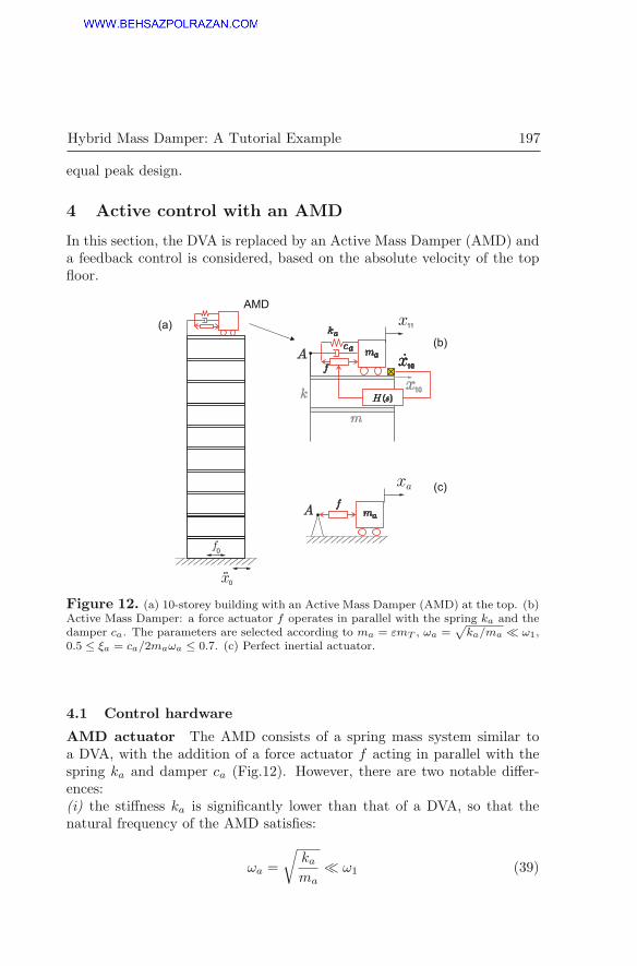
Hybrid Mass Damper: A Tutorial Example 197
equal peak design.
4 Active control with an AMD
In this section, the DVA is replaced by an Active Mass Damper (AMD) anda feedback control is considered, based on the absolute velocity of the topfloor.
f0
x0
x10
x11
k
m
ca
ka
ma
AMD
fx
10
H ( )s
A
xa
ma
fA
(a)
(b)
(c)
Figure 12. (a) 10-storey building with an Active Mass Damper (AMD) at the top. (b)Active Mass Damper: a force actuator f operates in parallel with the spring ka and thedamper ca. The parameters are selected according to ma = εmT , ωa =
√ka/ma � ω1,
0.5 ≤ ξa = ca/2maωa ≤ 0.7. (c) Perfect inertial actuator.
4.1 Control hardware
AMD actuator The AMD consists of a spring mass system similar toa DVA, with the addition of a force actuator f acting in parallel with thespring ka and damper ca (Fig.12). However, there are two notable differ-ences:(i) the stiffness ka is significantly lower than that of a DVA, so that thenatural frequency of the AMD satisfies:
ωa =
√kama
� ω1 (39)

198 A. Preumont, D. Alaluf and R. Bastaits
(ii) the damper ca is selected to introduce a significant damping in theactuator system:
0.5 ≤ ξa =ca
2maωa≤ 0.7 (40)
With these characteristics, the inertial actuator behaves as a near-perfectforce actuator in the frequency band containing the flexible modes of thestructure. To understand this, consider first a perfect inertial actuatorconsisting of a force actuator acting on a mass ma; if it is attached to a fixedpoint A (Fig.12.c), expressing the equilibrium of the massless actuator, theforce applied to A is f = −maxa (positive in traction). Next, if an AMD isconnected to a fixed point A, it is governed by the equation
maxa + caxa + kaxa = −f
(with again f being positive in traction). Thus, the transfer function be-tween f and xa is (s is the Laplace variable)
xa =−f
mas2 + cas+ ka;
the force F applied to point A is F = −maxa and the transfer functionbetween the actuator force f and the force F transmitted to the structureis that of a second order high-pass filter:
F
f=
s2
s2 + 2ξaωas+ ω2a
(41)
where ξa and ωa are defined according to Equ.(39) and (40). Thus, whenA is fixed, the AMD behaves as a perfect force generator for frequenciesω � ωa.
Geophone In addition to an actuator, the feedback loop needs a sensor; inthis study, we assume that the structure is equipped with a sensor measuringthe horizontal velocity of the top floor, x10; this can be obtained eitherwith a geophone, or by integrating the output signal of an accelerometer(although accelerometers do not work well at low frequency).
A geophone (Fig.13) is a spring mass system connected with a voicecoil transducer; the relationship between the output voltage and the floorvelocity is that of a high-pass filter
e
x0=
−s2Ts2 + 2ξgωgs+ ω2
g
(42)

Hybrid Mass Damper: A Tutorial Example 199
where e is the output voltage, x0 is the input velocity, T is the voice coilconstant (in volt.sec/m) and ωg and ξg are the frequency and the dampingconstant of the device. In the subsequent development, we will assumethat the corner frequency of the geophone, ωg is smaller than the cornerfrequency of the actuator, ωa, so that the velocity sensor may be regardedas perfect.
Note that, although both the velocity sensor and the AMD are attachedto the same floor, the control system is not collocated, because the systemoutput x10 is the top floor absolute velocity while the system input f consistsof a pair of opposing forces acting respectively on the top floor and on theinertial mass ma. However, if the inertial actuator parameters are chosenas explained before, it behaves closely to a perfect force actuator f appliedto the top floor (collocated), and the open-loop FRF, G = x10/f , exhibitsalternating poles and zeros (Fig.14).
4.2 System modeling
As compared to the system considered in the foregoing section on DVA,the only difference is the presence of a force f acting between the top floorx10 and the inertial mass x11. The governing equation is
M y+ Cy+Ky = −M1x0 + baf (43)
where ba = (0, . . . , 0, 1,−1)T is the influence vector of the control force(f assumed positive in traction). The matrices M , C and K have been
x0
e
Figure 13. Geophone based on a voice coil transducer of constitutive equations f =−T i and e = T (x − x0) (T is the transducer constant). The input is the motion x0 ofthe support and the output is the voltage e of the voice coil. Since the electrical circuitis open, i = 0.

200 A. Preumont, D. Alaluf and R. Bastaits
-180
-160
-140
-120
-100
-80
100
101
102
-90
0
90
180
270
Open-loop
�
G( )�
( )��
Figure 14. 10-storey building with an Active Mass Damper (AMD) at the top. Open-loop FRF G = v/f between the force f in the actuator and the velocity of the top floor(amplitude in dB and phase). The FRF exhibits alternating poles and zeros above ω1.
constructed before. Introducing the state vector
z = (yT , yT )T (44)
it can be rewritten in state variable form (as a system of first order differ-ential equations)
z = Az+ bf + ex0 (45)
where A is the system matrix
A =
[0 I
−M−1K −M−1C
], b = { 0
M−1ba}, e = { 0
−1 } (46)
(the size of the control input vector b and disturbance input vector e istwice the number of d.o.f., 22 in this case).
The sensor output is the velocity of the top floor,
v = x10 = x0 + bTs y (47)
where the vector bs = (0, . . . , 1, 0)T defines the sensor location (note thatbs �= ba, because the control force is acting also on ma). This equation isrewritten in state space form
v = cT z+ x0 (48)

Hybrid Mass Damper: A Tutorial Example 201
with the output vector cT = (0T ,bTs ). In addition to the system equation
(45) and the output equation (48), the feedback control law relates thecontrol input to the sensor output; in this case a direct velocity feedback isused:
f = −gv (49)
g is the control gain.
4.3 System response
The open-loop transfer function of the system is the relationship betweenthe control input f and the sensor output v without feedback control andwithout disturbance; it is readily obtained from Equ.(45) and (48):
G(s) = cT (sI −A)−1b (50)
The open-loop FRF G(jω) is obtained by substituting s = jω. It is rep-resented in Fig.14. The FRF exhibits alternating poles and zeros for allflexible modes (ω1 and above), typical of collocated control systems. The
-0.6 -0.4 -0.2 0
-1
0
1
2
3
4
5
6
Im( )s
Re( )s0
5
10
15
20
25
30
35
40
45
50
0-1-2-3-4-5-6-7
Im( )s
Re( )s
Closed-looppoles for 3 gains
( ) = 0.05, 0.1, 0.15
Detail near the origin
= 0.05
= 0.1
Figure 15. 10-storey building with an Active Mass Damper (AMD) at the top andvelocity feedback. Evolution of the closed-loop poles for increasing values of the controlgain g (root locus).

202 A. Preumont, D. Alaluf and R. Bastaits
closed-loop system equation is obtained by combining Equ.(45), (48) and(49); one finds easily
z = (A− gbcT )z− gbx0 + ex0 (51)
The eigenvalues of the closed-loop system matrix A− gbcT are the closed-loop poles. Their evolution for increasing values of the gain g is representedin the root locus of Fig.15. The transmissibility (in the frequency domain)between the the ground acceleration x0 and the state z is
Z(jω) = [jωI − (A− gbcT )]−1(−gbjω
+ e)X0(jω) (52)
The shear force at the base due to a seismic excitation can be expressedeither as a function of the absolute accelerations:
f0 = 1TM x (53)
or as a function of the relative displacements and velocities:
f0 = −1T (Ky+ Cy) = −1T (K,C)z (54)
(which is simpler in this case). The closed-loop transmissibility betweenthe ground acceleration x0 and f0 is readily obtained by combining withthe previous equation. Figure 16.a shows the PSD of the shear force f0resulting from the steady state response to a seismic acceleration with amodified Kanai-Tajimi profile Φ∗
g(ω), for various control gains, respectivelyg1 leading to a damping ratio of ξ = 0.05 in the first mode, g2 leading toξ = 0.1 and g3 to ξ = 0.15. The corresponding values of the closed-looppoles are indicated in Fig.15. An important observation is that the AMDdamps all the modes, unlike the DVA. The cumulative RMS value of thenon-dimensional shear force is shown in Fig.16.b, for the same values of thegain, and the cumulative RMS control force f is represented in Fig.16.c;this figure shows that the control effort increases rapidly with the gain, andso does the stroke of the actuator which may become unacceptable for largevalues of the gain. Note that the control effort and the stroke will eventuallyfix the size of the actuator. We now examine how the control effort may bereduced with a Hybrid Mass Damper.
5 Hybrid Mass Damper
The DVA is a purely passive device, tuned on the targeted mode (in thiscase mode 1) and it leaves the other modes unchanged. The AMD is fully

Hybrid Mass Damper: A Tutorial Example 203
0
0
5
2
4
1
2
3
10
15
x 104
�� �
��� �f0
m2
T
f0� �
mT
f� �
0
101 102100 �
�101 102100
�101 102100
�101 102100
10-8
10-4
100 g =0
g1
g =0
g3
g2
g1
g3
g2
g1
N
m
(b)
(c)
(a)
(d)
Figure 16. 10-storey building with an Active Mass Damper (AMD) at the top(ε = 0.01) and velocity feedback. (a) PSD of the shear force f0 due to the seismicacceleration with a modified Kanai-Tajimi profile Φ∗
g(ω), for various values of the controlgain, g1, g2, g3, leading respectively to a closed-loop damping ξ1 of 5%, 10% and 15 %in the first mode. (b) Cumulative RMS value of the non-dimensional reaction force. (c)Cumulative RMS value of the control force. (d) Cumulative RMS value of the stroke Δof the actuator.

204 A. Preumont, D. Alaluf and R. Bastaits
Figure 17. (a) Detail of the root locus of the AMD near the origin (ωa � ω1). (b)Same root locus when the actuator is tuned as a DVA [ωa = ω1/(1+μ)]; the branch of theroot locus starting from the pole of lower frequency points towards the imaginary axis,reducing the damping ratio. (c) Root locus after reducing the stiffness and increasing thedamping of the actuator, so that all the closed-loop poles have appropriate locations.
active and operates on all the controllable modes; it requires an absolutevelocity (or acceleration) sensor and an actuator of appropriate size andstroke, with a corner frequency satisfying the condition (39). The hybridcontroller is attempting to get the best of the two worlds by modifying aDVA to use it as an AMD (with the same absolute velocity feedback), withthe objectives of increasing the performance and/or decreasing the controleffort of the actuator. The idea is explained in Fig.17.4 Figure 17.a showsthe detail of the root locus of an AMD near the origin, and in particularthe trajectory of the actuator poles; Fig.17.b shows the root locus for anabsolute velocity feedback when the actuator is tuned as a DVA with theequal peak design; one observes that the control increases the damping ofthe structure pole (with a larger frequency) by moving it to the left, whilethe actuator pole is moved to the right (it can even become unstable if the
4All the root locus plots are symmetrical with respect to the real axis; only the upper
half is shown.

Hybrid Mass Damper: A Tutorial Example 205
�
���
� �
��� �
���
�
-1 0 1
-5
0
5
10
15
20
25
30
(a) Initial system
-1 0 1
-5
0
5
10
15
20
25
30
(b) DVA
-1 0 1
-5
0
5
10
15
20
25
30
(c) Hybrid
-1 0 1
-5
0
5
10
15
20
25
30
(d) AMD
�
���
� �
��� �
���
�
�
���
� �
��� �
���
�
�
���
� �
��� �
���
�
Figure 18. Position of the poles (×) and zeros (◦) in the complex plane. (a) Initialsystem with uniform damping of ξi = 0.01. (b) DVA (ε = ma/mT = 0.01) with ωa andca corresponding to the equal peak design; the pair of poles have a damping ratio close toξ � 0.05. (c) Root locus of the HMD starting from the location obtained for ω′
a = 0.74ωa
and c′a = 1.2ca. The red • indicates the position of the closed loop poles for g = 2.7 105,corresponding to the double peaked curve of Fig.19.a. (d) Root locus of the AMD as afunction of the control gain g. For g2 = 5.5 105, the pole of the first structural mode(indicated by the red •) has a damping ratio ξ1 � 0.1.
gain is large enough). The actuator of the HMD is tuned slightly differentlyfrom the DVA, by reducing the stiffness ka and increasing the dampingconstant ca of the actuator, so that the position of the poles after applyingthe feedback gain is where one wants them to be (Fig.17.c). This part ofthe design requires some trial and error, but may be done very quickly oncethe effect of the parameters ka and ca has been understood. In this study,the original system was assumed to have a structural damping of ξi = 0.01uniformly in all modes (Fig.18.a); the DVA with equal peak design led to

206 A. Preumont, D. Alaluf and R. Bastaits
0
1
2
3
0
5
10
15
x 104
0
1
2
3
101 102100 �
101 102100 �
101 102100 �
101 102100 �
� �
��� �f0
m2
T
f0� �
mT
f� �
10-8
10-4
100
N
m
No control
Active control
Hybrid control
No control
Active control
Hybrid control
Active control
Hybrid control
�
(b)
(c)
(a)
(d)
Figure 19. Comparison of the HMD with the AMD. (a) PSD of the shear force f0due to the seismic acceleration with modified Kanai-Tajimi profile. (b) Cumulative RMSvalue of the non-dimensional reaction force. (c) Cumulative RMS value of the controlforce. (d) Cumulative RMS value of the stroke Δ of the actuator. The position of thepoles are indicated in Fig.18.c and d.

Hybrid Mass Damper: A Tutorial Example 207
a pair of poles with about ξi = 0.05 (Fig.18.b); the HMD was designed (i)to bring the peak in the FRF corresponding to the first mode to the samelevel as that obtained with an AMD when ξ1 = 0.1 (this corresponds tothe gain g2 in Fig.16) and (ii) to achieve equal peak design for the two lowfrequency peaks in the FRF (Fig.19.a); this is achieved for ω′
a = 0.74ωa andc′a = 1.2ca where ωa and ca are given by Equ.(32).
Figure 19.a compares the PSD of the shear force f0 due to the seismicacceleration with modified Kanai-Tajimi profile for the AMD and HMDwith the poles being represented in Fig.18.c and d. Figure 19.b comparesthe cumulative RMS value of the non-dimensional reaction force; Figure 19.ccompares the cumulative RMS value of the control force and Fig.19.d thatof the actuator stroke. One sees that the performance of the HMD (non-dimensional reaction force) is only slightly worse than that of the AMD,but the actuator force is significantly reduced, by more than 50%, and thestroke even more, by 75%. Note also that the authority of the HMD onthe higher modes is slightly reduced as compared to the AMD, because thecontrol gain is reduced, but this is without consequence on this problemwhich is dominated by the first mode.
6 Dual loop Hybrid Mass Damper
The HMD performs better than the DVA, and has substantially less controlforce and stroke requirements than the AMD. However, in case of controlsystem failure, the HMD degenerates into a mistuned DVA with degradedperformances; this motivates to investigate the possibility to tune activelythe HMD from the DVA with equal peak parameters ωa and ca to the
ma
f
x10g
� = x11 x10 P D
Figure 20. Conceptual design of the dual loop HMD. The control system consists oftwo loops, one P+D controller acting on a sensor measuring the relative displacement ofthe actuator, Δ = x11 − x10, and a proportional controller on the absolute velocity x10.

208 A. Preumont, D. Alaluf and R. Bastaits
modified parameters ω′a = 0.74ωa and c′a = 1.2ca, by means of an additional
sensor (e.g. linear encoder) measuring the relative displacement between theinertial mass and the upper floor, Δ = x11 − x10 and a proportional plusderivative (P+D) compensator acting on the same actuator. The completecontrol system is represented in Fig.20. The purpose of the P+D loop isto bring the pair of poles of the DVA from the position in Fig.18.b to thepoles × for g = 0 in Fig.18.c. This is achieved with an appropriate negativestiffness and a positive damping.
A;B;C;Dx0
0fx10
P+D
-g+
+
f
�
Figure 21. Block diagram for the analysis of the dual loop HMD in MATLAB.
6.1 System modeling
In order to analyze this more complex control configuration in MATLAB,it is simpler to cast the equation in state space form as represented inFig.21. Because the absolute ground velocity x0 appears explicitly in outputequation (48), it is necessary to include it in the state vector. The extendedstate vector is now
z = (yT , yT , x0)T (55)
The input vector includes the control force f and the disturbance appliedto the system
u = (f, x0)T (56)
With these notations, the system equation in state variable form reads
z = Az+Bu (57)
where
A =
⎡⎣ 0 I 0−M−1K −M−1C 0
0 0 0
⎤⎦ , B =
⎡⎣ 0 0M−1ba −1
0 1
⎤⎦ (58)

Hybrid Mass Damper: A Tutorial Example 209
The output equation reads
y = (x10,Δ)T = Cz (59)
with
C =
[0T bT
s 1
−bTa 0T 0
](60)
where bs has been defined in Equ.(47) and ba in Equ.(43) (the relativedisplacement sensor is collocated with the force actuator).
6.2 System response
In the dual loop implementation of the HMD, the initial system is aDVA with equal peak design parameters, ωa, ca; the poles location of thesystem is that of Fig.18.b. The P+D loop modifies the system in such a waythat the poles are moved to the initial position × of Fig.18.c, from wherethey are moved further to the • by the second loop (with gain g). Sincethe closed loop poles are placed at the same location as in the previoussection, the overall performance is identical; the PSD of the shear force isthat displayed in Fig.19.a and the cumulative RMS of the shear force is thatof Fig.19.b. However, the control force f is different, because there is anadditional contribution coming from the P+D loop. This is shown in Fig.22;one sees that the P+D loop is responsible for an increment Δf in the RMScontrol force; this is the price to pay for changing actively the tuning of thesystem. Note that the actuator stroke is identical in both cases and is thatshown in Fig.19.d.
x 104
f� �
N
�101 102100
9
7
5
3
1
Active hybrid
Passive hybrid
�f
Figure 22. Cumulative RMS value of the control force f of the HMD; comparison ofthe passive hybrid (initial system tuned on ω′
a, c′
a) and the active hybrid (initial systemtuned on ωa, ca and P+D loop). The P+D loop is responsible for an increment Δf inthe RMS control force.

210 A. Preumont, D. Alaluf and R. Bastaits
Degraded mode
0
1
2
3
101 102100 �
f0� �
mTNo control
DVA
0
0.1
0.2
Degraded mode
DVA
� �
��� �f0
m2
T
10-8
10-4
100
101 102100 �
101 102100 �
m
Degraded mode
DVA
�
(b)
(c)
(a)
Figure 23. HMD when the control is disabled; comparison of the passive HMD (thecurve is referred to as “degraded mode”) with the active HMD (which degenerates intoan equal peak DVA). (a) PSD of the shear force f0 due to the seismic accelerationwith modified Kanai-Tajimi profile. (b) Cumulative RMS value of the non-dimensionalreaction force; the cumulative RMS response of the initial system is also included forcomparison. (c) Cumulative RMS value of the stroke Δ of the actuator.
6.3 HMD in degraded mode
Active systems are more sensitive than passive ones to reliability issues;their normal operation may be prevented by sensor failure, or cut off ofexternal power. It is therefore interesting to investigate the behavior of thesystem in case of control system breakdown. When the control system isswitched off, the single loop HMD (called here passive HMD) is reducedto a DVA with imperfect tuning (ω′
a, c′a), while the dual loop HMD (ac-

Hybrid Mass Damper: A Tutorial Example 211
tive HMD) is reduced to a DVA with equal peak design (ωa, ca). Thedegraded responses of the two systems are compared in Fig.23; one noticesthat the passive HMD is still better than the initial system, but the activeone degrades into the DVA with equal peak design, leading to much betterperformances (at the expense, however, of a larger control effort when inactive operation).
7 Conclusions
Using a multistory shear frame subjected to a seismic excitation, this studyhas compared three different ways of mitigating the dynamic response ofbuildings: Dynamic Vibration Absorber (DVA), Active Mass Damper (AMD)and Hybrid Mass Damper (HMD). It has been shown that a well designedHMD may produce performances comparable to that of an AMD while sig-nificantly reducing the actuator force and stroke requirements. Besides, ifa dual loop design is used, the system is immune to control system break-down, because the HMD is reduced to a properly tuned DVA with optimumperformances for a passive system.
Bibliography
[1] T. Asami, O. Nishihara and A. M. Baz. Analytical solutions to H∞ andH2 optimization of dynamic vibration absorbers attached to dampedlinear systems, ASME Journal of Vibration and Acoustics, Vol.124, 284-295, April 2002.
[2] S. H. Crandall and W. D. Mark. Random Vibration in Mechanical Sys-tems, Academic Press, 1963.
[3] J. P. Den Hartog Mechanical Vibrations, 4th Edition, Dover, 1985.[4] N. M. Newmark and E. Rosenblueth. Fundamental of Earthquake Engi-
neering, Prentice Hall, 1971.[5] J. Ormondroyd and J. P. Den Hartog. The theory of the damped vibra-
tion absorber, Trans. ASME, J. of Applied Mechanics, 50:7, 1928.[6] A. Preumont. Twelve Lectures on Structural Dynamics, Springer, 2013.[7] A. Preumont. Vibration Control of Active Structures, An Introduction,
3rd Edition, Springer, 2011.[8] A. Preumont and K. Seto. Active Control of Structures, Wiley, 2008.[9] B. F. Jr. Spencer and M. k. Sain. Controlling Buildings: A new Fron-
tier in Feedback, Special Issue of IEEE Control Systems Magazine onemerging Technology, Vol .17, No 6, pp.19-35, Dec. 1997.
[10] G. B. Warburton. Optimum absorber parameters for various combi-nations of response and excitation parameters, Earthquake Engineeringand Structural Dynamics, Vol.10, 381-401, 1982.

Electromagnetic and Piezoelectric
Transducers
Andre Preumont and Bilal Mokrani
ULB, Brussels, Belgium
Abstract This chapter analyzes the two most popular classes oftransducers used in active vibration control: the electromagnetictransducer known as voice coil, and the piezoelectric transducer.The first part of the chapter discusses the theory of the transduc-ers and the second part discusses some applications in structuralcontrol.
1 Introduction
Transducers are critical in active structures technology; they can play therole of actuator, sensor, or simply energy converter, depending on the appli-cation and the electrical connections. In many applications, the actuatorsare the most critical part of the system; however, the sensors become veryimportant in precision engineering where sub-micron amplitudes must bedetected. This chapter begins with a description of the voice coil transducerand its application to the proof-mass actuator and the geophone (absolutevelocity sensor). The remaining of the chapter is devoted to the piezo-electric materials and the constitutive equations of a discrete piezoelectrictransducer.
2 Voice coil transducer
A voice coil transducer is an energy transformer which converts electricalpower into mechanical power and vice versa. The system consists of a per-manent magnet (Fig.1) which produces a uniform magnetic flux density Bnormal to the gap, and a coil which is free to move axially within the gap.Let v be the velocity of the coil, f the external force acting to maintain thecoil in equilibrium against the electromagnetic forces, e the voltage differ-ence across the coil and i the current into the coil. In this ideal transducer,we neglect the electrical resistance and the self inductance of the coil, aswell as its mass and damping (if necessary, these can be handled by adding
P. Hagedorn, G. Spelsberg-Korspeter (Eds.), Active and Passive Vibration Control of Struc-tures, CISM International Centre for Mechanical Sciences DOI 10.1007/ 978-3-7091-1821-4_4 © CISM Udine 2014

214 A. Preumont and B. Mokrani
(b)
Figure 1. Voice-coil transducer: (a) Physical principle. (b) Symbolic rep-resentation.
R and L to the electrical circuit of the coil, or a mass and damper to itsmechanical model). The voice coil actuator is one of the most popular actu-ators in mechatronics (e.g. it is used in electromagnetic loudspeakers), butit is also used as sensor in geophones.
The first constitutive equation of the voice coil transducer follows fromFaraday’s law : A coil of n turns moving at the velocity v with respect to themagnetic flux density B generates an electromotive force (voltage) e givenby
e = 2πnrBv = Tv (1)
where
T = 2πnrB (2)
is the transducer constant, equal to the product of the length of the coilexposed to the magnetic flux, 2πnr, and the magnetic flux density B. Thesecond equation follows from the Lorentz force law: The external force frequired to balance the total force of the magnetic field on n turns of theconductor is
f = −i 2πnrB = −T i (3)
where i is the current intensity in the coil and T is again the transducerconstant (2). Equation (1) and (3) are the constitutive equations of the

Electromagnetic and Piezoelectric Transducers 215
voice coil transducer. Notice that the transducer constant T appearing inFaraday’s law (1), expressed in volt.sec/m, is the same as that appearingin the Lorentz force (3), expressed in N/Amp.
The total power delivered to the moving-coil transducer is equal to thesum of the electric power, ei, and the mechanical power, fv. Combiningwith (1) and (3), one gets
ei+ fv = Tvi− T iv = 0 (4)
Thus, at any time, there is an equilibrium between the electrical powerabsorbed by the device and the mechanical power delivered (and vice versa).The moving-coil transducer cannot store energy, and behaves as a perfectelectromechanical converter. In practice, however, the transfer is neverperfect due to eddy currents, flux leakage and magnetic hysteresis, leadingto slightly different values of T in (1) and (3).
Let us now examine various applications of the voice coil transducer.
2.1 Proof-mass actuator
A proof-mass actuator (Fig.2) is an inertial actuator which is used invarious applications of vibration control. A reaction mass m is connectedto the support structure by a spring k, a damper c and a force actuatorf which can be either magnetic or hydraulic. In the electromagnetic ac-tuator discussed here, the force actuator consists of a voice coil transducerof constant T excited by a current generator i; the spring is achieved withmembranes which also guide the linear motion of the moving mass. Thesystem is readily modelled as in Fig.2.a. Combining the equation of a singled.o.f. oscillator with the Lorentz force law (3), one finds
mx+ cx+ kx = T i (5)
or, in the Laplace domain,
x =T i
ms2 + cs+ k(6)
(s is the Laplace variable). The total force applied to the support is equaland opposite to the force applied to the proof-mass, −mx, or in Laplaceform:
F = −ms2x =−ms2T i
ms2 + cs+ k(7)
It follows that the transfer function between the total force F and thecurrent i applied to the coil is

216 A. Preumont and B. Mokrani
Permanentmagnet
Coil
Membranes
Magneticcircuit
Support
Movingmass
Figure 2. Proof-mass actuator (a) model assuming a current generator;(b) conceptual design of an electrodynamic actuator based on a voice coiltransducer. The mass is guided by the membranes.
F
i=
−s2Ts2 + 2ξpωps+ ω2
p
(8)
where T is the transducer constant (in N/Amp), ωp = (k/m)1/2 is thenatural frequency of the spring-mass system and ξp is the damping ratio,which in practice is fairly high, typically 20 % or more [the negative sign in(8) is irrelevant.] The Bode plots of (8) are shown in Fig.3; one sees that thesystem behaves like a high-pass filter with a high frequency asymptote equalto the transducer constant T ; above some critical frequency ωc � 2ωp, theproof-mass actuator can be regarded as an ideal force generator. It has noauthority over the rigid body modes (at zero frequency) and the operation atlow frequency requires a large stroke, which is technically difficult. Mediumto high frequency actuators (40 Hz and more) are relatively easy to obtainwith low cost components (loudspeaker technology).
If the current source is replaced by a voltage source (Fig.4), the modelingis slightly more complicated and combines the mechanical equation (5) andan electrical equation which is readily derived from Faraday’s law:
T x+ Ldi
dt+Ri = E(t) (9)

Electromagnetic and Piezoelectric Transducers 217
180
T!p !c
!
iF
Phase
!
Figure 3. Bode plot F/i of an electrodynamic proof-mass actuator (ampli-tude and phase).
where L is the inductance R is the resistance of the electrical circuit andE(t) is the external voltage source applied to the transducer.
Figure 4. Model of a proof-mass actuator with a voltage source.
2.2 Geophone
The geophone is a transducer which behaves like an absolute velocitysensor above some cut-off frequency which depends on its mechanical con-

218 A. Preumont and B. Mokrani
struction. The system of Fig.2.a is readily transformed into a geophone byusing the voltage e as the sensor output (Fig.5). If x0 is the displacementof the support and if the voice coil is open (i = 0), the governing equationsare
mx+ c(x− x0) + k(x− x0) = 0
T (x− x0) = e
combining these equations, one readily finds that
x− x0 =−ms2x0
ms2 + cs+ k
e = Ts(x− x0) =−s2T
s2 + (c/m)s+ k/msx0
e
x0=
−s2Ts2 + 2ξpωps+ ω2
p
(10)
Thus, there is a perfect duality between a proof-mass actuator and thegeophone. The same device may be used either as actuator or sensor, de-pending on the electrical boundary conditions. The proof-mass actuatoruses a current source while the geophone is connected to an infinite resistor.Above the corner frequency, the gain of the geophone is equal to the trans-ducer constant T . Designing geophones with very low corner frequency isin general difficult, especially if their orientation with respect to the gravity
x0
e
Figure 5. Model of a geophone based on a voice coil transducer.

Electromagnetic and Piezoelectric Transducers 219
vector is variable; active geophones where the corner frequency is loweredelectronically may constitute a good alternative option.
3 General electromechanical transducer
3.1 Constitutive equations
The constitutive behavior of a wide class of electromechanical transduc-ers can be modeled as in Fig.6, where the central box represents the conver-sion mechanism between electrical energy and mechanical energy, and viceversa. In Laplace form, the constitutive equations read
Tme
Teme
Zei Zm v = xç
f
Figure 6. Electrical analog representation of an electromechanical trans-ducer.
e = Zei+ Temv (11)
f = Tmei+ Zmv (12)
where e is the Laplace transform of the input voltage across the electricalterminals, i the input current, f the force applied to the mechanical termi-nals, and v the velocity of the mechanical part. Ze is the blocked electricalimpedance, measured for v = 0; Tem is the transduction coefficient repre-senting the electromotive force (voltage) appearing in the electrical circuitper unit velocity in the mechanical part (in volt.sec/m). Tme is the trans-duction coefficient representing the force acting on the mechanical terminalsto balance the electromagnetic force induced per unit current input on theelectrical side (in N/Amp), and Zm is the mechanical impedance, measuredwhen the electrical side is open (i = 0).
To illustrate this representation, consider the proof-mass actuator withthe voltage source of Fig.4; the electrical equation reads
E(t) = Ri+ Ldi
dt+ Tv
or in Laplace formE = (Ls+R)i+ Tv

220 A. Preumont and B. Mokrani
If F is the external force applied to the mechanical terminal (positive in thepositive direction of v), the mechanical equation reads
F (t) = mx+ cx+ kx− T i
or in Laplace form (using the velocity as mechanical variable)
F = (ms+ c+ k/s)v − T i
Thus, the constitutive equations may be written in the form (11) and (12)with
Ze = Ls+R, Zm = ms+ c+ k/s, Tem = T, Tme = −T
In absence of external force (f = 0), v can be resolved from Equ.(12)and substituted into Equ.(11), leading to
e = (Ze −TemTme
Zm)i
−TemTme/Zm is called the motional impedance. The total driving pointelectrical impedance is the sum of the blocked and the motional impedances.
3.2 Self-sensing
Equation (11) shows that the voltage drop across the electrical terminalsof any electromechanical transducer is the sum of a contribution propor-tional to the current applied and a contribution proportional to the velocityof the mechanical terminals. Thus, if Zei can be measured and subtractedfrom e, a signal proportional to the velocity is obtained. This suggeststhe bridge structure of Fig.7. The bridge equations are as follows: for thebranch containing the transducer,
e = ZeI + Temv + ZbI
I =1
Ze + Zb(e− Temv)
V4 = ZbI =Zb
Ze + Zb(e− Temv)
For the other branch,e = kZei+ kZbi
V2 = kZbi =Zb
Ze + Zbe

Electromagnetic and Piezoelectric Transducers 221
Transducer
Figure 7. Bridge circuit for self-sensing actuation.
and the bridge output
V4 − V2 = (−Zb TemZe + Zb
) v (13)
is indeed a linear function of the velocity v of the mechanical terminals.Note, however, that −Zb Tem/(Ze+Zb) acts as a filter; the bridge impedanceZb must be adapted to the transducer impedance Ze to avoid amplitude dis-tortion and phase shift between the output voltage V4 − V2 and the trans-ducer velocity in the frequency band of interest.
4 Smart materials
Piezoelectric materials belong to the so-called smart materials, or multi-functional materials, which have the ability to respond significantly to stim-uli of different physical natures. Figure 8 lists various effects that are ob-served in materials in response to various inputs: mechanical, electrical,magnetic, thermal, light. The coupling between the physical fields of differ-ent types is expressed by the non-diagonal cells in the figure; if its magnitudeis sufficient, the coupling can be used to build discrete or distributed trans-ducers of various types, which can be used as sensors, actuators, or evenintegrated in structures with various degrees of tailoring and complexity(e.g. as fibers), to make them controllable or responsive to their environ-ment (e.g. for shape morphing, precision shape control, damage detection,
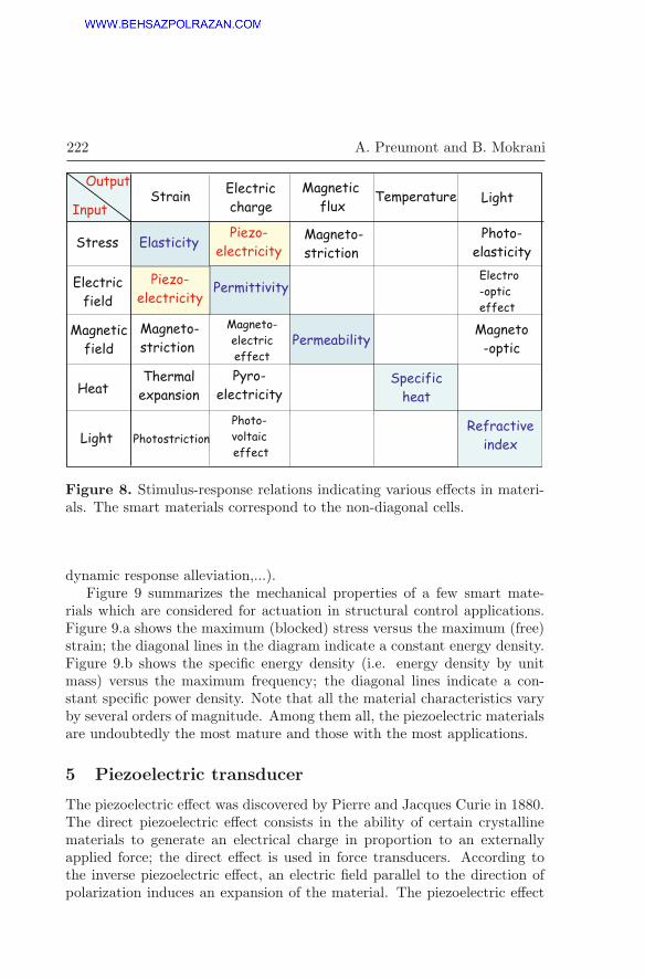
222 A. Preumont and B. Mokrani
Input
OutputStrain
Electric
charge
Magnetic
fluxTemperature Light
Stress
Electric
field
Elasticity
Heat
Light
Permittivity
Piezo-
electricity
Piezo-
electricity
Magneto-
striction
Magneto-
strictionMagnetic
field
Thermal
expansion
Photostriction
Magneto-
electric
effect
Pyro-
electricity
Photo-
voltaic
effect
Permeability
Specific
heat
Refractive
index
Magneto
-optic
Electro
-optic
effect
Photo-
elasticity
Figure 8. Stimulus-response relations indicating various effects in materi-als. The smart materials correspond to the non-diagonal cells.
dynamic response alleviation,...).Figure 9 summarizes the mechanical properties of a few smart mate-
rials which are considered for actuation in structural control applications.Figure 9.a shows the maximum (blocked) stress versus the maximum (free)strain; the diagonal lines in the diagram indicate a constant energy density.Figure 9.b shows the specific energy density (i.e. energy density by unitmass) versus the maximum frequency; the diagonal lines indicate a con-stant specific power density. Note that all the material characteristics varyby several orders of magnitude. Among them all, the piezoelectric materialsare undoubtedly the most mature and those with the most applications.
5 Piezoelectric transducer
The piezoelectric effect was discovered by Pierre and Jacques Curie in 1880.The direct piezoelectric effect consists in the ability of certain crystallinematerials to generate an electrical charge in proportion to an externallyapplied force; the direct effect is used in force transducers. According tothe inverse piezoelectric effect, an electric field parallel to the direction ofpolarization induces an expansion of the material. The piezoelectric effect

Electromagnetic and Piezoelectric Transducers 223
Strain (%)
Frequency (Hz)
10à2
10à1
100
101
102
103
100
101
102
103
104
105
Str
ess
(MPa
)S
peci
fic
Ene
rgy
Dens
ity
(J/k
g)
101
100
102
103 10
4 105 10
6
10à2
10à1
101
100 10
210
3
10 J/m³
10² J/m³
10³ J/m³
10J/m³
4
10J/m³
5
10J/m³
6
10J/m³
8
10J/m³
9Energy Density
Single Crystal
PZT
PZT
Electrostrictive
polymer
PVDFElectrostatic
device
Voice Coil
Magneto-
strictive
Nanotube
Dielectric
Elastomer
(Silicon)
Dielectric
Elastomer
(Acryl)
Ionic
Polymer
Metal
Composite
Responsive
Gels
Thermal
Shape Memory
Polymer
Conducting Polymer
Shape Memory Alloy
PZTSingle Crystal
PZT
Electrostrictive polymer
Electrostatic
device
Voice Coil
Magneto-
strictiveNanotube
Dielectric
Elastomer
(Silicon)
Dielectric
Elastomer
(Acryl)
Ionic
Polymer
Metal
CompositeResponsive
Gels
Thermal
Shape Memory
Polymer
Conducting Polymer
Shape Memory Alloy
Muscle
PVDF
10 W/kg (Muscle)
DC-Motor
10³ W/kg
10W
/kg
5
10W
/kg
7
Specific Power Density
10W
/kg
9
Figure 9. (a) Maximum stress vs. maximum strain of various smart ma-terial actuators. (b) Specific energy density vs. maximum frequency (bycourtesy of R.Petricevic, Neue Materialen Wurzburg).

224 A. Preumont and B. Mokrani
is anisotropic; it can be exhibited only by materials whose crystal structurehas no center of symmetry; this is the case for some ceramics below a cer-tain temperature called the Curie temperature; in this phase, the crystalhas built-in electric dipoles, but the dipoles are randomly orientated andthe net electric dipole on a macroscopic scale is zero. During the polingprocess, when the crystal is cooled in the presence of a high electric field,the dipoles tend to align, leading to an electric dipole on a macroscopicscale. After cooling and removing of the poling field, the dipoles cannotreturn to their original position; they remain aligned along the poling di-rection and the material body becomes permanently piezoelectric, with theability to convert mechanical energy to electrical energy and vice versa; thisproperty will be lost if the temperature exceeds the Curie temperature orif the transducer is subjected to an excessive electric field in the directionopposed to the poling field.
The most popular piezoelectric materials are Lead-Zirconate-Titanate(PZT) which is a ceramic, and Polyvinylidene fluoride (PVDF) which is apolymer. In addition to the piezoelectric effect, piezoelectric materials ex-hibit a pyroelectric effect, according to which electric charges are generatedwhen the material is subjected to temperature; this effect is used to produceheat detectors; it will not be discussed here.
In this section, we consider a transducer made of a one-dimensionalpiezoelectric material of constitutive equations (we use the notations of theIEEE Standard on Piezoelectricity)
D = εTE + d33T (14)
S = d33E + sET (15)
where D is the electric displacement (charge per unit area, expressed inCoulomb/m2), E the electric field (V/m), T the stress (N/m2) and S thestrain. εT is the dielectric constant (permittivity) under constant stress,sE is the compliance when the electric field is constant (inverse of theYoung’s modulus) and d33 is the piezoelectric constant, expressed in m/Vor Coulomb/Newton; the reason for the subscript 33 is that, by convention,index 3 is always aligned to the poling direction of the material, and weassume that the electric field is parallel to the poling direction. Note thatthe same constant d33 appears in (14) and (15).
In the absence of an external force, a transducer subjected to a voltagewith the same polarity as that during poling produces an elongation, and avoltage opposed to that during poling makes it shrink (inverse piezoelectric

Electromagnetic and Piezoelectric Transducers 225
effect). In (15), this amounts to a positive d33. Conversely (direct piezo-electric effect), if we consider a transducer with open electrodes (D = 0),
according to (14), E = −(d33/εT )T , which means that a traction stress willproduce a voltage with polarity opposed to that during poling, and a com-pressive stress will produce a voltage with the same polarity as that duringpoling.
5.1 Constitutive relations of a discrete transducer
Equations (14) and (15) can be written in a matrix form{DS
}=
[εT d33d33 sE
]{ET
}(16)
where (E, T ) are the independent variables and (D, S) are the dependentvariables. If (E, S) are taken as the independent variables, they can berewritten
D =d33sE
S + εT(1− d33
2
sEεT
)E
T =1
sES − d33
sEE
or {DT
}=
[εT (1− k2) e33−e33 cE
]{ES
}(17)
where cE = 1/sE is the Young’s modulus under E = 0 (short circuited elec-trodes), in N/m2 (Pa); e33 = d33/s
E , the product of d33 by the Youngmodulus, is the constant relating the electric displacement to the strain forshort-circuited electrodes (in Coulomb/m2), and also that relating the com-pressive stress to the electric field when the transducer is blocked (S = 0).
k2 =d33
2
sEεT=
e332
cEεT(18)
k is called the Electromechanical coupling factor of the material; it measuresthe efficiency of the conversion of mechanical energy into electrical energy,and vice versa, as discussed below. From (17), we note that εT (1− k2) isthe dielectric constant under zero strain.
If one assumes that all the electrical and mechanical quantities are uni-formly distributed in a linear transducer formed by a stack of n disks ofthickness t and cross section A (Fig.9), the global constitutive equations of

226 A. Preumont and B. Mokrani
+_
Cross section:Thickness:
# of disks in the stack:
Electric charge:
Capacitance:
At
nl = nt
Q = nAD
Electrode
Free piezoelectric expansion:Voltage driven:
Charge driven:
î = d33nV
î = d33nCQ
t
E = V=t
C = n2"A=l
Figure 10. Piezoelectric linear transducer.
the transducer are obtained by integrating Equ.(16) or (17) over the volumeof the transducer; one finds{
QΔ
}=
[C nd33nd33 1/Ka
]{Vf
}(19)
or {Qf
}=
[C(1− k2) nd33Ka
−nd33Ka Ka
]{VΔ
}(20)
where Q = nAD is the total electric charge on the electrodes of the trans-ducer, Δ = Sl is the total extension (l = nt is the length of the trans-ducer), f = AT is the total force and V the voltage applied between theelectrodes of the transducer, resulting in an electric field E = V/t = nV/l.C = εTAn2/l is the capacitance of the transducer with no external load(f = 0), Ka = A/sEl is the stiffness with short-circuited electrodes (V = 0).Note that the electromechanical coupling factor can be written alternatively
k2 =d33
2
sEεT=n2d33
2Ka
C(21)
Equation (19) can be inverted{Vf
}=
Ka
C(1− k2)
[1/Ka −nd33−nd33 C
]{QΔ
}(22)

Electromagnetic and Piezoelectric Transducers 227
from which we can see that the stiffness with open electrodes (Q = 0) isKa/(1−k2) and the capacitance for a fixed geometry (Δ = 0) is C(1− k2).Note that typical values of k are in the range 0.3− 0.7; for large k, thestiffness changes significantly with the electrical boundary conditions, andsimilarly the capacitance depends on the mechanical boundary conditions.
Next, let us write the total stored electromechanical energy and coenergyfunctions.1 Consider the discrete piezoelectric transducer of Fig.11; the
Figure 11. Discrete Piezoelectric transducer.
total power delivered to the transducer is the sum of the electric power, V iand the mechanical power, fΔ. The net work on the transducer is
dW = V idt+ fΔdt = V dQ+ fdΔ (23)
For a conservative element, this work is converted into stored energy, dWe,and the total stored energy, We(Δ, Q) can be obtained by integrating (23)from the reference state to the state (Δ, Q).2 Upon differentiatingWe(Δ, Q),
dWe(Δ, Q) =∂We
∂ΔdΔ+
∂We
∂QdQ (24)
and, comparing with (23), we recover the constitutive equations
f =∂We
∂ΔV =
∂We
∂Q(25)
1Energy and coenergy functions are needed in connection with energy formulations such
as Hamilton principle, Lagrange equations or finite elements.2Since the system is conservative, the integration can be done along any path leading
from (0, 0) to (Δ, Q).

228 A. Preumont and B. Mokrani
Substituting f and V from (22) into (23), one gets
dWe = V dQ+ fdΔ
=QdQ
C(1− k2)− nd33Ka
C(1− k2)(Δ dQ+QdΔ) +
Ka
1− k2Δ dΔ
which is the total differential of
We(Δ, Q) =Q2
2C(1− k2)− nd33Ka
C(1− k2)QΔ+
Ka
1− k2Δ2
2(26)
This is the analytical expression of the stored electromechanical energy forthe discrete piezoelectric transducer. The partial derivatives (25) allow torecover the constitutive equations (22). The first term on the right handside of (26) is the electrical energy stored in the capacitance C(1− k2)(corresponding to a fixed geometry, � = 0); the third term is the elasticstrain energy stored in a spring of stiffness Ka/(1 − k2) (corresponding toopen electrodes, Q = 0); the second term is the piezoelectric energy.
The electromechanical energy function uses Δ and Q as independentstate variables. A coenergy function using Δ and V as independent variablescan be defined by the Legendre transformation
W ∗e (Δ, V ) = V Q−We(Δ, Q) (27)
The total differential of the coenergy is
dW ∗e = QdV + V dQ− ∂We
∂ΔdΔ− ∂We
∂QdQ
dW ∗e = QdV − f dΔ (28)
where Equ.(25) have been used. It follows that
Q =∂W ∗
e
∂Vand f = −∂W
∗e
∂Δ(29)
Introducing the constitutive equations (20) into (28),
dW ∗e =[C(1− k2)V + nd33KaΔ
]dV + (nd33KaV −KaΔ) dΔ
= C(1− k2)V dV + nd33Ka (ΔdV + V dΔ)−KaΔ dΔ
which is the total differential of
W ∗e (Δ, V ) = C(1− k2)
V 2
2+ nd33KaVΔ−Ka
Δ2
2(30)

Electromagnetic and Piezoelectric Transducers 229
This is the analytical form of the coenergy function for the discrete piezoelec-tric transducer. The first term on the right hand side of (30) is recognizedas the electrical coenergy in the capacitance C(1− k2) (corresponding toa fixed geometry, Δ = 0); the third is the strain energy stored in a springof stiffness Ka (corresponding to short-circuited electrodes, V = 0). Thesecond term of (30) is the piezoelectric coenergy; using the fact that theuniform electric field is E = nV/l and the uniform strain is S = Δ/l, it canbe rewritten ∫
Ω
Se33E dΩ (31)
where the integral extends to the volume Ω of the transducer.The analytical form (26) of the electromechanical energy, together with
the constitutive equations (25) can be regarded as an alternative defini-tion of a discrete piezoelectric transducer, and similarly for the analyticalexpression of the coenergy (30) and the constitutive equations (29).
5.2 Interpretation of k2
Consider a piezoelectric transducer subjected to the following mechanicalcycle: first, it is loaded with a force F with short-circuited electrodes; theresulting extension is
Δ1 =F
Ka
where Ka = A/(sE l) is the stiffness with short-circuited electrodes. Theenergy stored in the system is
W1 =
∫ Δ1
0
f dx =FΔ1
2=
F 2
2Ka
At this point, the electrodes are open and the transducer is unloaded ac-cording to a path of slope Ka/(1− k2), corresponding to the new electricalboundary conditions,
Δ2 =F (1− k2)
Ka
The energy recovered in this way is
W2 =
∫ Δ2
0
f dx =FΔ2
2=F 2(1− k2)
2Ka
leaving W1−W2 stored in the transducer. The ratio between the remainingstored energy and the initial stored energy is
W1 −W2
W1= k2

230 A. Preumont and B. Mokrani
Similarly, consider the following electrical cycle: first, a voltage V isapplied to the transducer which is mechanically unconstrained (f = 0).The electric charges appearing on the electrodes are
Q1 = CV
where C = εTAn2/l is the unconstrained capacitance, and the energy storedin the transducer is
W1 =
∫ Q1
0
v dq =V Q1
2=CV 2
2
At this point, the transducer is blocked mechanically [changing its capac-itance from C to C(1 − k2)] and electrically unloaded from V to 0. Theelectrical charges are removed according to
Q2 = C(1− k2)V
The energy recovered in this way is
W2 =
∫ Q2
0
v dq =C(1− k2)V 2
2
leaving W1 −W2 stored in the transducer. Here again, the ratio betweenthe remaining stored energy and the initial stored energy is
W1 −W2
W1= k2
Although the foregoing relationships provide a clear physical interpretationof the electromechanical coupling factor, they do not bring a practical wayof measuring k2; the experimental determination of k2 is often based onimpedance (or admittance) measurements.
5.3 Admittance of the piezoelectric transducer
Consider the system of Fig.12, where the piezoelectric transducer is as-sumed massless and is connected to a massM . The force acting on the massis the negative of that acting on the transducer, f = −Mx; using (20),{
Q−Mx
}=
[C(1− k2) nd33Ka
−nd33Ka Ka
]{Vx
}(32)
From the second equation, one gets (in Laplace form)
x =nd33Ka
Ms2 +KaV

Electromagnetic and Piezoelectric Transducers 231
(a)
Transducer
dB
(b)
Figure 12. (a) Elementary dynamical model of the piezoelectric transducer.(b) Typical admittance FRF of the transducer, in the vicinity of its naturalfrequency.
and, substituting in the first one and using (21), one finds
Q
V= C(1− k2)
[Ms2 +Ka/(1− k2)
Ms2 +Ka
](33)
It follows that the admittance reads:
I
V=sQ
V= sC(1− k2)
s2 + z2
s2 + p2(34)
where the poles and zeros are respectively
p2 =Ka
Mand z2 =
Ka/(1− k2)
M(35)
p is the natural frequency with short-circuited electrodes (V = 0) and zis the natural frequency with open electrodes (I = 0). From the previousequation one sees that
z2 − p2
z2= k2 (36)
This relationship constitutes a practical way of determining the electrome-chanical coupling factor: An impedance meter is used to measure the Fre-quency Response Function (FRF) of the admittance (or the impedance), on

232 A. Preumont and B. Mokrani
which the position of the poles p and zeros z are identified and introducedin Equ.(36).
6 Vibration isolation with voice coil transducers
6.1 Viscous damping isolator
Consider the spring mass system of Fig.13. A voice coil connects themassM to the moving support and a resistor R is connected to the electricalterminals of the voice coil. The governing equations are
Voice coil
Figure 13. Voice coil used as viscous damper.
Mx+ k(x− x0) = T i
e = −Ri = Tv = T (x− x0)
where the constitutive equations of the voice coil [Equ.(1) and (3)] havebeen used. Upon eliminating i between these equations, one finds
Mx+T 2
R(x− x0) + k(x− x0) = 0 (37)
Thus, when a resistor connects the electrical terminals of the voice coil,it behaves as a viscous damper of damping coefficient c = T 2/R; a lowerresistance R will increase the damping (the minimum value of R is thatof the coil itself). From the foregoing equation, the transmissibility of theisolator is readily obtained:
X
X0=
1 + 2jξω/ωn
1 + 2jξω/ωn − ω2/ω2n
(38)
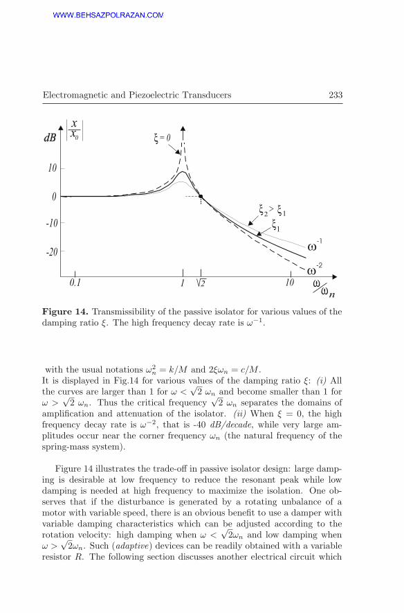
Electromagnetic and Piezoelectric Transducers 233
0
xx
0 = 0
1
2 1>
101 2
n
10
-10
0.1
-20
dB
�-2
�-1
Figure 14. Transmissibility of the passive isolator for various values of thedamping ratio ξ. The high frequency decay rate is ω−1.
with the usual notations ω2n = k/M and 2ξωn = c/M .
It is displayed in Fig.14 for various values of the damping ratio ξ: (i) Allthe curves are larger than 1 for ω <
√2 ωn and become smaller than 1 for
ω >√2 ωn. Thus the critical frequency
√2 ωn separates the domains of
amplification and attenuation of the isolator. (ii) When ξ = 0, the highfrequency decay rate is ω−2, that is -40 dB/decade, while very large am-plitudes occur near the corner frequency ωn (the natural frequency of thespring-mass system).
Figure 14 illustrates the trade-off in passive isolator design: large damp-ing is desirable at low frequency to reduce the resonant peak while lowdamping is needed at high frequency to maximize the isolation. One ob-serves that if the disturbance is generated by a rotating unbalance of amotor with variable speed, there is an obvious benefit to use a damper withvariable damping characteristics which can be adjusted according to therotation velocity: high damping when ω <
√2ωn and low damping when
ω >√2ωn. Such (adaptive) devices can be readily obtained with a variable
resistor R. The following section discusses another electrical circuit which

234 A. Preumont and B. Mokrani
improves the high frequency decay rate of the isolator.
6.2 Relaxation isolator
Voice coil
Figure 15. (a) Relaxation isolator. (b) Electromagnetic realization.
In the relaxation isolator, the viscous damper c is replaced by a Maxwellunit consisting of a damper c and a spring k1 in series (Fig.15.a). Thegoverning equations are
Mx+ k(x− x0) + c(x− x1) = 0 (39)
c(x− x1) = k1(x1 − x0) (40)
or, in matrix form using the Laplace variable s,[Ms2 + cs+ k −cs
−cs k1 + cs
]{xx1
}=
{kk1
}x0 (41)
Upon inverting this system of equations, the transmissibility is obtained inLaplace form:
x
x0=
(k1 + cs)k + k1cs
(Ms2 + cs+ k)(k1 + cs)− c2s2=
(k1 + cs)k + k1cs
(Ms2 + k)(k1 + cs) + k1cs(42)
One sees that the asymptotic decay3 rate for large frequencies is in s−2,that is -40 dB/decade. Physically, this corresponds to the fact that, at high
3the asymptotic decay rate is governed by the largest power of s of the numerator and
the denominator.

Electromagnetic and Piezoelectric Transducers 235
1 10-40
-20
0
!=!n
xx0dB
c = 0 c!1
copt
A
Figure 16. Transmissibility of the relaxation oscillator for fixed values ofk and k1 and various values of c. The first peak corresponds to ω = ωn =(k/M)1/2; the second one corresponds to ω = Ωn = [(k + k1)/M ]1/2. Allthe curves cross each other at A and have an asymptotic decay rate of -40dB/decade. The curve corresponding to copt is nearly maximum at A.
frequency, the viscous damper tends to be blocked, and the system behaveslike an undamped isolator with two springs acting in parallel. Figure 16compares the transmissibility curves for given values of k and k1 and variousvalues of c. For c = 0, the relaxation isolator behaves like an undampedisolator of natural frequency ωn = (k/M)1/2. Likewise, for c → ∞, itbehaves like an undamped isolator of frequency Ωn = [(k + k1)/M ]1/2. Inbetween, the poles of the system are solution of the characteristic equation
(Ms2 + k)(k1 + cs) + k1cs = (Ms2 + k)k1 + cs(Ms2 + k + k1) = 0
which can be rewritten in root locus form
1 +k1c
s2 + ω2n
s(s2 +Ω2n)
= 0 (43)
It is represented in Fig.17 when c varies from 0 to ∞; it can be shown that

236 A. Preumont and B. Mokrani
Figure 17. Root locus of the solutions of Equ.(43) as c goes from zero to
infinity. The maximum damping is achieved for k1/c = Ω3/2n ω
−1/2n .
the maximum damping ratio is achieved for
k1c
=Ω
3/2n
ω1/2n
(44)
and the corresponding damper constant is
copt =k1Ωn
(ωn
Ωn)1/2 =
k1Ωn
(1 +k1k)−1/4 =
k1ωn
(1 +k1k)−3/4 (45)
The transmissibility corresponding to copt is also represented in Fig.16; it isnearly maximum at A.
Electromagnetic realization The principle of the relaxation isolator issimple and it can be realized with viscoelastic materials. However, it maybe difficult to integrate in the system, and also viscoelastic materials arenotorious for their thermal sensitivity. In some circumstances, especiallywhen thermal stability is critical, it may be more convenient to achieve thesame effect through a voice coil transducer whose electrical terminals areconnected to an inductor L and a resistor R (Fig.15.b). The governingequations of the system are in this case
Mx+ k(x− x0)− T i = 0 (46)

Electromagnetic and Piezoelectric Transducers 237
Ldi
dt+ T (x− x0) +Ri = 0 (47)
where T is the transducer constant. In matrix form, using the Laplacevariable, [
Ms2 + k −TTs Ls+R
]{xi
}=
{kTs
}x0 (48)
It follows that the transmissibility reads
x
x0=
(Ls+R)k + T 2s
(Ms2 + k)(Ls+R) + T 2s(49)
Comparing with Equ.(42), one sees that the electromechanical isolator be-haves exactly like a relaxation isolator provided that
Ls+R
T 2=cs+ k1k1c
(50)
or
k1 =T 2
Lc =
T 2
R(51)
These are the two relationships between the three parameters T , L and Rso that the transmissibility of the electromechanical system of Fig.15.b isthe same as that of Fig.15.a.
7 Controlling structures with piezo transducers
Consider a structure with a single discrete piezoelectric transducer (Fig.18);the transducer is governed by Equ.(20):{
Qf
}=
[C(1− k2) nd33Ka
−nd33Ka Ka
]{VbTx
}(52)
where Δ = bTx is the relative displacement at the extremities of the trans-ducer. The dynamics of the structure is governed by
Mx+K∗x = −bf (53)
where K∗ is the stiffness matrix of the structure without the transducer andb is the influence vector of the transducer in the global coordinate system ofthe structure. The non-zero components of b are the direction cosines of theactive bar. The minus sign on the right hand side of the previous equationcomes from the fact that the force acting on the structure is opposed tothat acting on the transducer. Note that the same vector b appears in both

238 A. Preumont and B. Mokrani
I
VPiezoelectricTransducer
Structure� = b x
T
f
M K, *
Figure 18. Structure with a piezoelectric transducer. b is the influencevector of the transducer in the global coordinate system of the structure.
equations because the relative displacement is measured along the directionof f . Substituting f from the constitutive equation into the second equation,one finds
Mx+ (K∗ + bbTKa)x = bKand33V
or
Mx+Kx = bKaδ (54)
where K = K∗ + bbTKa is the global stiffness matrix of the structureincluding the piezoelectric transducer in short-circuited conditions (whichcontributes for bbTKa); δ = nd33V is the free expansion of the transducerinduced by a voltage V ; Kaδ is the equivalent piezoelectric loading: theeffect of the piezoelectric transducer on the structure consists of a pair ofself-equilibrating forces applied axially to the ends of the transducer; as forthermal loads, their magnitude is equal to the product of the stiffness of thetransducer (in short-circuited conditions) by the unconstrained piezoelectricexpansion; this is known as the thermal analogy.
Let φi be the normal modes, solutions of the eigenvalue problem
(K − ω2iM)φi = 0 (55)
They satisfy the usual orthogonality conditions
φTi Mφj = μiδij (56)
φTi Kφj = μiω
2i δij (57)

Electromagnetic and Piezoelectric Transducers 239
where ωi is the natural frequency when the transducer is short-circuited. Ifthe global displacements are expanded into modal coordinates,
x =∑i
ziφi (58)
where zi are the modal amplitudes, Equ.(54) is easily transformed into
μi(zi + ω2i zi) = φT
i bKaδ (59)
Upon taking the Laplace transform, one easily gets
x =
n∑i=1
φiφTi
μi(ω2i + s2)
bKaδ (60)
and the transducer extension
Δ = bTx =
n∑i=1
Ka(bTφi)
2
μiω2i (1 + s2/ω2
i )δ (61)
From Equ.(57), μiω2i /2 is clearly the strain energy in the structure when it
vibrates according to mode i, and Ka(bTφi)
2/2 represents the strain energyin the transducer when the structure vibrates according to mode i. Thus,the ratio
νi =Ka(b
Tφi)2
μiω2i
(62)
is readily interpreted as the fraction of modal strain energy in the transducerfor mode i. With this notation, the previous equation is rewritten
Δ = bTx =
n∑i=1
νi(1 + s2/ω2
i )δ (63)
which relates the actual displacement of the transducer with the free ex-pansion due to the voltage V .
7.1 Force feedback open-loop transfer function
A frequent control configuration is that of an active strut where thepiezoelectric actuator is coupled with a collocated force sensor. From thesecond constitutive equation (52), the open-loop transfer function betweenthe free expansion δ = nd33V of the transducer (proportional to the appliedvoltage) and the output force f in the active strut is readily obtained:
f = −Kaδ +KaΔ

240 A. Preumont and B. Mokrani
Figure 19. (a) Open-loop FRF of the active strut mounted in the structure(undamped). (b) Admittance of the transducer mounted in the structure;the poles are the natural frequencies with short-circuited electrodes ωi andthe zeros are the natural frequencies with open electrodes Ωi.
orf
δ= Ka[
n∑i=1
νi(1 + s2/ω2
i )− 1] (64)
All the residues being positive, there will be alternating poles and zerosalong the imaginary axis. Note the presence of a feedthrough in the transferfunction. Figure 19.a shows the open-loop FRF in the undamped case; asexpected the poles at ±jωi are interlaced with the zeros at ±zi. The transferfunction can be truncated after m modes, assuming that the modes above

Electromagnetic and Piezoelectric Transducers 241
a certain order m have no dynamic amplification:
f
δ= Ka[
m∑i=1
νi(1 + s2/ω2
i )+
n∑i=m+1
νi − 1] (65)
Collocated force feedback can be used very efficiently for active damping ofstructures, using Integral Force Feedback (IFF) and its variants; this topicis discussed extensively in [Preumont, 2011].
7.2 Admittance function
According to the first constitutive equation (52),
Q = C(1− k2)V + nd33KabTx
Using (63),
Q = C(1− k2)V + n2d233Ka
n∑i=1
νi(1 + s2/ω2
i )V (66)
and, taking into account the definition (21) of the electromechanical cou-pling factor, one finds the dynamic capacitance
Q
V= C(1− k2)[1 +
k2
1− k2
n∑i=1
νi(1 + s2/ω2
i )] (67)
The admittance is related to the dynamic capacitance by I/V = sQ/V :
I
V=sQ
V= sC(1− k2)[1 +
n∑i=1
K2i
(1 + s2/ω2i )] (68)
where
K2i =
k2νi1− k2
(69)
is the effective electromechanical coupling factor for mode i.4 The corre-sponding FRF is represented in Fig.19.b. The zeros of the admittance (orthe dynamic capacitance) function correspond to the natural frequenciesΩi with open electrodes (ωi is the natural frequency with short-circuitedelectrodes) and
K2i �
Ω2i − ω2
i
ω2i
(70)
4Note that k2 is a material property while νi depends on the mode shape, the size and
the location of the transducer inside the structure.

242 A. Preumont and B. Mokrani
I
VPZTTransducer
Structure
( )a
I
V
I
V R
I
V
R
L
(c)
(b)
(d)
PZT patch
R-shunt
RL-shunt
Figure 20. Structure with a piezoelectric transducer (a) in d33 mode (b)in d31 mode (c) R shunt (d) RL shunt.
The admittance of the transducer integrated in the structure may be written
I
V= sCstat.
∏ni=1(1 + s2/Ω2
i )∏nj=1(1 + s2/ω2
j )(71)
where Cstat is the static capacitance of the transducer when integrated inthe structure; it lies between C and C(1 − k2) depending on the restraintoffered by the structure.
7.3 Passive damping with a piezoelectric transducer
It is possible to achieve passive damping by integrating piezoelectrictransducers at proper locations in a structure and shunting them on pas-sive electrical networks. The theory is explained here with the simple caseof a discrete transducer, but more complicated configurations are possible(Fig.20).

Electromagnetic and Piezoelectric Transducers 243
Resistive shunting Using the same positive signs for V and I as for thestructure (Fig.20.c), the voltage drop in the resistor is V = −RI; therefore,the admittance of the shunt is −1/R. The characteristic equation of thesystem is obtained by expressing the equality between the admittance ofthe structure and that of the passive shunt:
− 1
R= sC(1− k2)[1 +
n∑i=1
K2i
1 + s2/ω2i
] (72)
or
− 1
sRC(1− k2)= 1 +
n∑i=1
K2i ω
2i
s2 + ω2i
(73)
In the vicinity of ±jωi, the sum is dominated by the contribution of modei and the other terms can be neglected; defining γ = [RC(1 − k2)]−1, theequation may be simplified as
−γs= 1 +
K2i ω
2i
s2 + ω2i
which, using Equ.(70), can be rewritten
1 + γs2 + ω2
i
s(s2 +Ω2i )
= 0 (74)
This form of the characteristic equation is identical to Equ.(43) that wemet earlier in this chapter. The root locus is represented in Fig.21; theparameter γ acts as the feedback gain in classical root locus plots. Forγ = 0 (R = ∞), the poles are purely imaginary, ±jΩi, corresponding tothe natural frequency of the system with open electrodes; the system isundamped. As the resistance decreases (γ increases), the poles move to theleft and some damping appears in the system; it can be shown that themaximum damping is achieved for γ = Ωi
√Ωi/ωi � Ωi and is
ξmaxi =
Ωi − ωi
2ωi� Ω2
i − ω2i
4ω2i
=K2
i
4(75)
Inductive shunting Since the electrical behavior of a piezoelectric trans-ducer is essentially that of a capacitor, the idea with the RL shunt is toproduce a RLC circuit which will be tuned on the natural frequency of thetargeted mode and will act as a dynamic vibration absorber. We proceedin the same way as in the previous section, but with a RL-shunt (Fig.20.d);the admittance of the shunt is now I/V = −1/(R+Ls). The characteristic

244 A. Preumont and B. Mokrani
Figure 21. Resistive shunt. Evolution of the poles of the system as γ =[RC(1− k2)]−1 goes from 0 to ∞ (the diagram is symmetrical with respectto the real axis, only the upper half is shown).
equation is obtained by expressing the equality between the admittance ofthe structure and that of the passive shunt:
− 1
R+ Ls= sC(1− k2)[1 +
n∑i=1
K2i
1 + s2/ω2i
] (76)
or
− 1
(R+ Ls)sC(1− k2)= 1 +
n∑i=1
K2i ω
2i
s2 + ω2i
(77)
Once again, in the vicinity of ±jωi, the sum is dominated by the contribu-tion of mode i and the equation is simplified as
− 1
(R+ Ls)sC(1− k2)= 1 +
K2i ω
2i
s2 + ω2i
(78)
Defining the electrical frequency
ω2e =
1
LC(1− k2)(79)
and the electrical damping
2ξeωe =R
L(80)

Electromagnetic and Piezoelectric Transducers 245
Equ.(78) is rewritten
− ω2e
2ξeωes+ s2= 1 +
K2i ω
2i
s2 + ω2i
=s2 +Ω2
i
s2 + ω2i
(81)
ors4 + 2ξeωes
3 + (Ω2i + ω2
e)s2 + 2Ω2
i ξeωes+ ω2i ω
2e = 0 (82)
This can be rewritten in a root locus form
1 + 2ξeωes(s2 +Ω2
i )
s4 + (Ω2i + ω2
e)s2 + ω2
i ω2e
= 0 (83)
In this formulation, 2ξeωe = R/L plays the role of the gain in a classicalroot locus. Note that, for large R, the poles tend to ±jΩi, as expected. ForR = 0 (i.e. ξe = 0), they are the solutions p1 and p2 of the characteristicequation s4+(Ω2
i +ω2e)s
2+ω2i ω
2e = 0 which accounts for the classical double
peak of resonant dampers, with p1 above jΩi and p2 below jωi. Figure 22shows the root locus for a fixed value of ωi/Ωi and various values of theelectrical tuning, expressed by the ratio
αe =ωeωi
Ω2i
(84)
The locus consists of two loops, starting respectively from p1 and p2; one ofthem goes to jΩi and the other goes to the real axis, near −Ωi. If αe > 1(Fig.22.a), the upper loop starting from p1 goes to the real axis, and thatstarting from p2 goes to jΩi, and the upper pole is always more heavilydamped than the lower one (note that, if ωe →∞, p1 →∞ and p2 → jωi;the lower branch of the root locus becomes that of the resistive shunting).The opposite situation occurs if αe < 1 (Fig.22.b): the upper loop goesfrom p1 to jΩi and the lower one goes from p2 to the real axis; the lowerpole is always more heavily damped. If αe = 1 (Fig.22.c), the two poles arealways equally damped until the two branches touch each other in Q. Thisdouble root is achieved for
αe =ωeωi
Ω2i
= 1 , ξ2e = 1− ω2i
Ω2i
� K2i (85)
This can be regarded as the optimum tuning of the inductive shunting. Thecorresponding eigenvalues satisfy
s2 +Ω2i +Ωi(
Ω2i
ω2i
− 1)1/2s = 0 (86)

246 A. Preumont and B. Mokrani
ëe > 1
(a) p1
p2Resistive
shunting
ëe < 1
(b) p1
p2
ëe = 1
(c)
p1
p2
Optimal
Damping
(d)
jÒi
à Òi
Q Q
à Òi
à Òià Òi
Re(s)
Im(s)
jÒi
jÒi
jÒi
j!i j!i
j!i
Figure 22. Root locus plot for inductive shunting (only the upper half isshown). The optimum damping at Q is achieved for αe = 1 and ξe = Ki;the maximum modal damping is ξi � Ki/2.
For various values of ωi/Ωi (or Ki), the optimum poles at Q move alonga circle of radius Ωi (Fig.22.d). The corresponding damping ratio can beobtained easily by identifying the previous equation with the classical formof the damped oscillator, s2 + 2ξiΩis+Ω2
i = 0, leading to
ξi =1
2(Ω2
i
ω2i
− 1)1/2 =Ki
2=
1
2(k2νi1− k2
)1/2 (87)
This value is significantly higher than that achieved with purely resistiveshunting [it is exactly the square-root of (75)]. Note, however, that it ismuch more sensitive to the tuning of the electrical parameters on the tar-

Electromagnetic and Piezoelectric Transducers 247
0.1 1 100
0.2 0.5 2 5!0i=!iFrequency ratio
Resistive
shunting0.05
0.1
0.15
0.2
0.25
0.3
Inductive
shunting
øi
p2 p1
Figure 23. Evolution of the damping ratio of the inductive and resistiveshunting with the de-tuning of the structural mode. ωi is the naturalfrequency for which the shunt has been optimized, ω′
i is the actual value(k = 0.5, νi = 0.3).
geted modes. This is illustrated in Fig.23, which displays the evolutionof the damping ratio ξi when the actual natural frequency ω′
i moves awayfrom the nominal frequency ωi for which the shunt has been optimized (thedamping ratio associated with p1 and p2 is plotted in dotted lines; the ratioω′i/Ω
′i is kept constant in all cases). One sees that the performance of the
inductive shunting drops rapidly below that of the resistive shunting whenthe de-tuning increases. Note that, for low frequency modes, the optimuminductance value can be very large; such large inductors can be synthesizedelectronically. The multimodal passive damping via resonant shunt has beeninvestigated by [Hollkamp, 1994].
Bibliography
[1] W. G. Cady. Piezoelectricity: an Introduction to the Theory and Ap-plications of Electromechanical Phenomena in Crystals, , McGrawHill,1946.
[2] S. H. Crandall. D. C. Karnopp, E. F. Jr. Kurtz, D. C. Pridmore-BrownDynamics of Mechanical and Electromechanical Systems, McGraw-Hill,N-Y, 1968.

248 A. Preumont and B. Mokrani
[3] E. De Boer. Theory of Motional Feedback, IRE Transactions on Audio,15-21, Jan.-Feb., 1961.
[4] J. Holterman and P. Groen. An Introduction to Piezoelectric Materialsand Components, Stichting Applied Piezo, 2012.
[5] J. J. Hollkamp. Multimodal passive vibration suppression with piezo-electric materials and resonant shunts, J. Intell. Material Syst. Struc-tures, Vol.5, Jan. 1994.
[6] F. v. Hunt. Electroacoustics: The Analysis of Transduction, and itsHistorical Background, Harvard Monographs in Applied Science, No 5,1954. Reprinted, Acoustical Society of America, 1982.
[7] IEEE Standard on Piezoelectricity. (ANSI/IEEE Std 176-1987).[8] J. van Randeraat. & SETTERINGTON, R.E. (Edts) Philips Applica-
tion Book on Piezoelectric Ceramics, Mullard Limited, London, 1974.[9] Physik Intrumente catalogue, Products for Micropositioning (PI
GmbH).[10] J. Pratt and A. Flatau. Development and analysis of self-sensing mag-
netostrictive actuator design, SPIE Smart Materials and StructuresConference, Vol.1917, 1993.
[11] A. Preumont. Vibration Control of Active Structures, An Introduction,Third Edition, Springer, 2011.
[12] A. Preumont.Mechatronics, Dynamics of Electromechanical and Piezo-electric Systems, Springer, 2006.
[13] C. A. Rosen. Ceramic transformers and filters, Proc. Electronic Com-ponent Symposium, p.205-211, 1956.
[14] K. Uchino. Ferroelectric Devices, Marcel Dekker, 2000.[15] H. H. Woodson and J. R. Melcher. Electromechanical Dynamics, Part
I: Discrete Systems, Wiley, 1968.

LMIs in Control Optimization
Robert E. Skelton
University of California, San Diego, CA, U.S.
1 Early Optimization History
Hamilton invented state space models of nonlinear dynamic systems withhis generalized momenta work in the 1800s, but, at that time, the lack ofcomputational tools prevented broad acceptance of the first order form ofdynamic equations. With the rapid development of computers in the 1960s,State Space models evoked a formal control theory for minimizing a scalarfunction of control and state, propelled by the calculus of variations andPontryagin’s maximal principle.
In the case of linear dynamic models, these methods led to the popu-larization of Linear Quadratic Gaussian (LQG) optimal control, which hadglobally optimal solutions, Skelton (1988). Since guarantees about the firsttwo moments of the stochastic process (the mean and the covariance) can bemade, regardless of the distribution of the random variables involved, LQGbecame just an acronym for the solution of quadratic functionals of controland state variables, even when the stochastic processes were not Gaussian,The label LQG was often used even for deterministic problems, where anintegral operator, rather than an expectation operator, was minimized, withgiven initial conditions or impulse excitations. These were formally calledLQR (Linear Quadratic Regulator) problems. Later the book Skelton (1988)gave the formal conditions under which the LQG and the LQR answers werenumerically identical, and this version was called the Deterministic LQG.
It was always recognized that the quadratic form of the state and controlin the LQG problem was an artificial goal. The real control goals usuallyinvolved pre-specified performance bounds on each of the errors and boundson each channel of control. This leads to Matrix inequalities rather thanscalar minimizations. While it was known early that any stabilizing linearcontroller could be obtained by some choice of weights in an LQG optimiza-tion problem, It was not known until the1980s what particular choice ofweights in an LQG problem would yield a solution to the matrix inequal-ity problem. A globally convergent algorithm by Zhu and Skelton (1992);
P. Hagedorn, G. Spelsberg-Korspeter (Eds.), Active and Passive Vibration Control of Struc-tures, CISM International Centre for Mechanical Sciences DOI 10.1007/ 978-3-7091-1821-4_5 © CISM Udine 2014
250 R.E. Skelton
Zhu et al. (1997) shows how to find such LQG weights when the matrix in-equality problem has a solution. Since then, linear control problems can bestated simply in terms of norm bounds on each input or each output of thesystem (L2 bounds , L-infinity bounds, or variance bounds and covariancebounds). These problems are convex for state feedback or full order con-trollers (the focus of this elementary introduction), and will be solved usingLinear Matrix Inequalities in this paper. However the earliest approach tothese problems were iterative LQG solutions (to find the correct weights touse in the quadratic penalty of the state), Zhu and Skelton (1992); Zhu et al.(1997).
2 Matrix Inequalities
Let Q be any square matrix. The Matrix Inequality "Q > 0" is just ashort-hand notation to represent a certain scalar inequality. That is, thematrix notation "Q > 0" means "the scalar xTQx is positive for all valuesof x, except x = 0". Obviously this is a property of Q, not x, hencethe abbreviated matrix notation Q > 0. This is called a Linear MatrixInequality (LMI), since the matrix unknownQ appears linearly in the matrixinequality Q > 0 . Note also that any square matrix, Q, can be written asthe sum of a symmetric matrix Qy = 1
2 (Q + QT ), and a skew-symmetricmatrix Qk = 1
2 (Q − QT ), but xTQkx = 0, so only the symmetric part ofthe matrix Q affects the scalar xTQx. We assume hereafter without loss ofgenerality that Q is symmetric. The notation "Q ≥ 0" means "the scalarxTQx cannot be negative for any x".
Liapunov proved that x(t) converges to zero if, along the nonzero trajec-tory of a dynamic system, (e.g. the system x = Ax), two scalars have theproperty, x(t)TQx(t) > 0 and d/dt((xT (t)Qx(t)) < 0. This proves that thefollowing statements are all equivalent:
1. For any initial condition x(0) of the system x = Ax, x(t) will convergeto zero as time approaches infinity
2. All eigenvalues of A lie in the open left-half plane.
3. There exists a matrix Q with these two properties: Q > 0, QA +ATQ < 0.
4. The set of all quadratic Liapunov functions that can be used to provethe stability or instability the null solution of x = Ax is xTQx, whereQ is any square matrix with the two properties of item 3, above.
For the linear system example x = Ax+Bu, y = Cx, the "Observability
Gramian" is the infinite integral Q =∫eA
T tCTCeAtdt which is affected onlyby the observable modes of the system. Furthermore Q > 0 if and only if

LMIs in Control Optimization 251
(A,C) is an observable pair, and Q is bounded only if the observable modesare asymptotically stable. If Q exists then the solution of QA + ATQ +CTC = 0 is Q > 0 if and only if the matrix pair (A,C) is observable.
Likewise the "Controllability Gramian" X =∫eAtBBT eA
T tdt > 0 ifand only if the pair (A,B) is controllable. If X exists it satisfies XAT +AX + BBT = 0, and X > 0 if and only if (A,B) is a controllable pair.Note also that (A,B) is controllable for any A if BBT > 0, and (A,C) isobservable for any A if CTC > 0. Hence the existence of Q > 0 or X > 0satisfying either (QA+ATQ < 0) or (AX +XAT < 0) is equivalent to thestatement that "all eigenvalues of A lie in the open left half plane".
It should be clear now that the set of all stabilizing state feedback con-trollers, u = Gx, is parametrized by the inequalities Q > 0, Q(A + BG) +(A + BG)TQ < 0. The difficulty here is the appearance of the product ofthe two unknowns Q and G.
Here we borrow some tricks from linear algebraic equations, where anyLinear Matrix Equality (LME), ΓGΛ = Θ has a solution G if and onlyif ΓΓ+ΘΛ+Λ = Θ. Notation M+ denotes the Moore-Penrose inverse ofmatrix M . If these existence conditions are satisfied, then all solutionsare parametrized by G = Γ+ΘΛ+ + Z − Γ+ΓZΛΛ+. The point is that inLMEs there are two separate questions and answers. The first question thatis answered is "Does there exist a solution?". The second question is "Whatis the set of all solutions?". LMI approaches will employ the same two stepsby formulating the necessary and sufficient conditions for the existence ofthe LMI solution, and then parametrize all solutions. The earliest book onLMI control methods was Boyd et al. (1994), but the notation used hereinis taken from Skelton et al. (1998).
3 Relation to Linear Algebraic Equations
Linear Matrix Equalities have been completely solved many years ago, andthe theory gives i) the necessary and sufficient conditions for the existenceof a solution, and then ii) the set of all solutions. The LME (Linear MatrixEquality) is supported by the following facts;
There exists a solution G to the LME
AGB = C (1)
if and only if, matrices A,B,C have the following property:
AA+CB+B = C. (2)
If the existence condition (2) is satisfied, then all solutions of (1) are given

252 R.E. Skelton
by
G = A+CB+ + Z −A+AZBB+, (3)
where Z is an arbitrary matrix, and the matrix A+ is the Moore Penroseinverse, which is the unique matrix which satisfies AA+A = A.
Much of the mystery of the above equations is removed by writing themin terms of the Singular Value Decomposition (SVD) of the matrices A andB. For any real matrix M the SVD is defined
M = UΣV T =[U1 U2
] [Σ 00 0
] [V T1
V T2
]. (4)
with these special properties of the SVD components,
Σ > 0, Σ = diagonal (5)
UTU = I = UUT (6)
V TV = I = V V T (7)
UT2 M = 0 (8)
MV2 = 0 (9)
M+ = U1Σ−1V T
1 , (10)
we call UT2 the basis for the left nullspace of M (the entire nullspace is
KUT2 for arbitrary K). Likewise, we call V2 the basis for the right nullspace
of M . Using these properties of the SVD of matrices A,B, one can write(2) and (3) as
UTA2C = 0, CVB2 = 0 (11)
G = VA1(Σ−1A UT
A1CVB1Σ−1B )UT
B1 + VA2Z1UTB1 + VAZ2U
TB2, (12)
where Z1, Z2 are arbitrary matrices. Note that the existence conditionsrequire the matrix C to lie in the left nullspace of A and in the right nullspaceof B.
4 Control Design Using LMIs
Let the system be described by the state equations⎡⎣xpyz
⎤⎦ =
⎡⎣Ap Dp Bp
Cp Dy By
Mp Dz 0
⎤⎦⎡⎣xpwu
⎤⎦ , [
uxc
]=
[Dc Cc
Bc Ac
] [zxc
]= G
[zxc
], (13)

LMIs in Control Optimization 253
where z is the measurement vector, y is the output to be controlled, uis the control vector, xp is the plant state vector, xc is the state of thecontroller, and w is the external disturbance (we will often treat w as zero-mean white noise in these discussions). We seek to choose the control matrixG to satisfy given upper bounds, E[yyT ] ≤ Y , where E represents the steadystate expectation operator in the stochastic case (when w is white noise),and in the deterministic case E represents the infinite integral of the matrix[yyT ]. The math we do here is the same, with appropriate interpretations ofcertain matrices. For a rigorous equivalence of deterministic and stochasticinterpretations see Skelton (1988)Defining
x =
[xpxc
],
[Acl Bcl
Ccl Dcl
]=
[A DC F
]+
[BH
]G[M E
](14)
A =
[Ap 00 0
], B =
[Bp 00 I
],M =
[Mp
0 I
], D =
[Dp
0
], E =
[Dz
0
](15)
C =[Cp 0
], H =
[By 0
], F = Dy, (16)
one can write the closed loop system dynamics in the form[xy
]=
[Acl Bcl
Ccl Dcl
] [xw
]. (17)
We shall often be interested in the set of all controllers that can satisfyvarious performance bounds, such as, E[yyT ] ≤ Y , E[uuT ] ≤ U .
4.1 State Feedback Stabilization
For only stability requirements our problem reduces to the case whereCp = Mp = I, Cc = 0, and Y has no specified bound. In this case thenecessary and sufficient condition for stability of the closed loop system is
(Ap +BpG)X +X(Ap +BpG)T < 0. (18)
This is satisfied if and only if there exists an arbitrarily small positivesemidefinite matrix that can be added to the left-hand side of this inequality.So lets add the matrix 1
γ2XGTGX, for a large enough γ, to get
(Ap +BpG)X +X(Ap +BpG)T +1
γ2XGTGX < 0. (19)
By completing the square, write this as,

254 R.E. Skelton
(1
γXGT + γBp)(
1
γXGT + γBp)
T < γ2BpBTp −ApX −XAT
p =: Φ. (20)
Now we will use corollary 2.3.6 in Skelton et al. (1998) which proves thatthe following Quadratic Matrix Inequality
(1
γXGT + γBp)(
1
γXGT + γBp)
T < Φ, (21)
has a solution G if and only if Φ > 0, in which case, all such G are given by
G = −γ2BTp X
−1 + γLΦ1/2X−1, LLT = I. (22)
Defining P = γ2X−1, Q = γ2X−1ΦX−1, we have
G = −BTp P + LQ1/2 (23)
PAp +ATp P − PBpB
Tp P +Q = 0. (24)
Since Y was not bounded in this stabilization problem, the existence ofX > 0 already satisfies, for Cp = I, CpXC
Tp = X = γ2P−1 < Y .
5 Information Architecture in Estimation and
Control Problems
In the typical "control problem" that occupies most research literature, thesensors and actuators have already been selected. Yet the selection of sen-sors and actuators and their locations greatly affect the ability of the controlsystem to do its job efficiently. Perhaps in one location a high precision sen-sor is needed, and in another location high precision is not needed, and highprecision there would be a waste of resources. These decisions are influencedby the control dynamics which are yet to be designed. How do we knowwhere to spend money to improve the system?
Lets consider the problem of selecting the control law jointly with theselection of the precision (inverse of the noise intensity) of each actua-tor/sensor, subject to the constraint of specified upper bounds on the co-variance of output error and control signals, and specified upper bounds onthe sensor/actuator cost. (We assume the price of these devices are propor-tional to their precision). Traditionally, with full order controllers, and prespecified sensor/actuator instruments (with specified precisions), this is awell-known solved convex problem and can be converted to an LMI prob-lem. If we enlarge the domain of the optimization to include sensor/actuator

LMIs in Control Optimization 255
precisions it is not obvious whether the problem is convex or not. The fol-lowing shows that this problem of including the sensor/actuator precisionswithin the control design problem is indeed convex and therefore completelysolved. The proof is provided in Li et al. (2010).
Consider the linear system (1)-(5). There exists a dynamic controller Gthat satisfies the constraints
E[uuT ≤ U, E[yyT ] ≤ Y, trPW−1 ≤ Ω (25)
if and only if there exists Matrices L,F,Q,X,Z,W−1 such that
trPW−1 ≤ Ω (26)⎡⎣ Y CX C(CX)T X ICT I Z
⎤⎦ > 0,
⎡⎣ U L 0LT X I0 I Z
⎤⎦ > 0,
[Φ11 ΦT
21
Φ21 −W−1
]< 0
(27)
Φ21 =
[D 0ZD F
], φ =
[AX +BL A
Q ZA+ FM
], Φ11 = φ+ φT . (28)
Furthermore, the solution of the problem (13) is given belowAssume a solution for (L,F,Q,X,Z,W) is found from (14)-(16). Then the
problem (13) is solved by the controller
G =
[0 I
V −1l −V −1
l ZB
] [Q− ZAX F
L 0
] [0 V −1
r
I −MXV −1r
], (29)
where Vl and Vr are left and right factors of the matrix I − Y X (whichcan be found from the singular value decomposition I − Y X = UΣV T =(UΣ1/2)(Σ1/2V T ) = VlVr).
To emphasize the theme of this article, to relate optimization to LMIs,we note that three optimization problems present themselves in the aboveproblem with three constraints: control effort U , output performance Y , andinstrument costs Ω. To solve optimization problems, one can fix any two ofthese pre-specified upper bounds and iteratively reduce the level set valueof the third "constraint" until feasibility is lost. This process minimizes theresource expressed by the third constraint, while enforcing the other twoconstraints.
As an example, if cost is not a concern, one can always set large limitsfor Ω and discover the best assignment of sensor/actuator precisions forthe specified performance requirements. These precisions produced by thealgorithm are the values W−1
ii , produced from the solution (14)-(16), wherethe observed rankings W−1
ii > W−1jj > W−1
kk > ..... indicate which sensors

256 R.E. Skelton
or actuators are most critical to the required performance goals (U, Y, Ω).If any precision W−1
n n is essentially zero, compared to other required preci-sions, then the math is asserting that the information from this sensor (n)is not important for the control objectives specified, or the control signalsthrough this actuator channel (n) is ineffective in controlling the system tothese specifications. This information leads us to a technique for choosingthe best sensor actuators and their location.
The previous discussion provides a solution to the precisions required ofeach sensor and each actuator in the system. Our final application of thistheory locates sensors and actuators in a large scale system, by discardingthe least effective ones. Suppose we solve any of the above feasibility prob-lems, by starting with as many sensors and actuators as is possible for thesystem (without regard to cost). For example in a flexible structure controlproblem we might not know whether to place a rate sensor or a displacementsensors at a given location, so we add both. We might not know whether touse torque or force actuators, so we add both. We fill up the system withall the possibilities we might want to consider, and let the above precisionrankings (available after the LMI problem is solved) reveal how much pre-cision is needed at each location and at each sensor/actuator. If there is alarge gap in the precisions required (say W−1
11 > W−122 > W−1
33 >> .....W−1nn ),
then delete the sensor/actuator n and repeat the LMI problem with one lesssensor or actuator. Continue deleting sensors/actuators in this manner un-til feasibility of the problem is lost. Then this algorithm, stopping at theprevious iteration, has selected the best distribution of sensors/actuatorsfor solving the specific problem (Ω, U, Y ). In my opinion this is the mostimportant contribution of the algorithm, to enlarge the set of solved linearcontrol problems, from solutions of linear controllers with sensors/actuatorspre-specified, to solutions which specify the sensor/actuator requirementsjointly with the control solution.
6 Many Control Problems Reduce to the Same LMI
Let the left and right null spaces of B be defined by UTBB = 0, UT
BUB >0, BVB = 0, , V T
B VB > 0. For any given matrices Θ,Φ,Q, the bookSkelton et al. (1998) provides all G which solve
ΘGΦ+ (ΘGΦ)T +Q < 0, (30)
and there exists such a matrix G if and only if the following two conditionshold
UTΘQUΘ < 0, or ΘΘT > 0, V T
Φ QVΦ < 0, or ΦTΦ > 0. (31)

LMIs in Control Optimization 257
The significance of this theorem is that 17 different control problems (usingeither state feedback or full order dynamic controllers) all reduce to thissame mathematical problem. That is, by defining the appropriate Θ,Φ,Q avery large number of different control problems (including the set of all sta-bilizing controllers, covariance control, H-infinity control, L-infinity control,LQG control, H2 control), can be reduced to the same matrix inequality(18).
7 Conclusions
LMI techniques provide more powerful tools for designing controllers or es-timators for linear systems then minimizing a scalar functional for optimiza-tion. LMI techniques extend the range of solvable system design problemsbeyond just control design. By integrating information architecture and con-trol design, one can decide what precision is required of all sensor/actuatorsto satisfy the closed loop performance constraints. A most amazing fact isthat most of the common linear control design problems all reduce to theexact same LMI problem (18).
Bibliography
S. Boyd, L. El Ghaoui, E. Feron, and V. Balakrishnan. Linear MatrixInequalities in System and Control Theory. SIAM, 1994.
F. Li, R. Skelton, and M. C. de Oliveira. Integrating information architec-ture and control or estimation. SICE Journal of Control, Measurement,and System Integration, Springer, 1:120–128, 2010.
R. Skelton. Dynamic Systems Control. John Wiley and Sons, 1988.R. Skelton, T. Iwasaki, and K. M. Grigoriadis. A Unified Algebraic Approach
to Control Design. Taylor and Francis, 1998.G. Zhu and R. Skelton. A two-riccati, feasible algorithm for guaranteeing
output l constraints. Journal of Dynamic Systems, Measurement andControl, 114:329–338, 1992.
G. Zhu, M.A. Rotea, and R. Skelton. A convergent algorithm for the outputcovariance constraint control problem. SIAM Journal on Control andOptimization, 35:341–61, 1997.

Damping Mechanisms
Adnan Akay* and Antonio Carcaterra†
* Bilkent University, Mechanical Engineering Department, Ankara, Turkey‡ University of Rome, La Sapienza, Department of Mechanics and Aeronautics,
Via Eudossiana, 18, 00184, Rome, Italy.
1 Linear Response and Damping
Introduction
The term damping is used to describe the means by which oscillationamplitudes are reduced through irreversible removal of vibratory energy ina mechanical system or a component. Dissipation, on the other hand, refersto the mechanism by which irreversible energy transfer, from vibratory tothermal, takes place. In this sense, damping is a macro-scale manifestationof atomic-scale dissipation.
High damping is desirable to attain low vibration and noise levels whereaslow damping is desirable for increased sensitivity in sensors and certain pre-cision instrumentation.
Damping is most obvious at resonance where the stiffness and inertiaforces become equal. As a result, damping is a key factor in predictingvibration response of structures.
As we will see in the following sections, there are numerous paths todamping and in a complex structure several means of damping may takeplace simultaneously at different locations throughout the structure. Ac-cordingly, in determining the response of a vibrating structure, the totaleffect of all types of damping that may be distributed throughout a struc-ture must be taken into account.
Measurements of damping normally indicate the total damping a sys-tem experiences. It is difficult to isolate a component or a subsystem ora material within a system and measure its damping. In describing thevarious damping mechanisms, we will examine each through its effect on asingle-degree-of-freedom (sdof) oscillator.
In this section, we will review the response of a simple oscillator andexamine the role of damping on it and review the basic methods of mea-surement criteria for damping properties of structures. However, we will
P. Hagedorn, G. Spelsberg-Korspeter (Eds.), Active and Passive Vibration Control of Struc-tures, CISM International Centre for Mechanical Sciences DOI 10.1007/ 978-3-7091-1821-4_6 © CISM Udine 2014

260 A. Akay and A. Carcaterra
not consider here the role of damping in dynamic behaviors such as chaos,stability, etc.
Dissipation of vibratory energy takes place in both fluid and solid me-dia, initiated by a number of possible macro activities. Accordingly, wewill consider damping methods to reflect the media in which dissipationtakes place when addressing damping methods in the next section. Modelsof fundamental dissipation mechanisms that describe energy transfer fromordered energy to disordered or thermalized energy are briefly summarizedin the last section.
1.1 Simple Harmonic Oscillator
We employ the simple harmonic oscillator as the platform to describedamping models and measures through its linear response.
Initial Value Problem Equation of motion for free vibrations of an un-damped sdof oscillator with mass M and stiffness K can be expressed as
Mη +Kη = 0
or in a simplified formη + ω2
0η = 0
where ω0 =√K/M is the natural frequency of the oscillator. General
solution for displacement η can be expressed as
η = A cos(ω0t− φ).
Expressing the initial conditions at t = 0 as η(0) = η0 and η(0) = η0, wecan write
η0 = A cos(φ) η0 = ω0A sin(φ)
and the vibration amplitude in terms of the initial conditions becomes
A =√η20 + (η0/ω0)2.
Free Damped Motion When damping is proportional to oscillator veloc-ity, represented by a constant of proportionality C, the equation of motionbecomes:
Mη + Cη +Kη = 0
with a corresponding solution for free vibrations:
η(t) = A e−γt cos(ωdt− φ)

Damping Mechanisms 261
where ωd = ω0
√1− ζ2 =
√ω20 − γ2 is the damped natural frequency and
γ = C/2M is the decay constant and is related to the damping ratio ζ =γ/ω0 = C/Cc, which is the ratio of damping constant to its critical valueCc = 2
√KM .
For underdamped cases, ζ < 1, response to initial conditions can bewritten as
η(t) = e−ζω0t
[η0 + ζω0η0
ωdsinωdt+ η0 cosωdt
].
When γ > ω0, or ζ > 1, ωd becomes complex and oscillations are notpossible and the system is referred as overdamped.
Between these two cases, when γ = ω0 or ζ = 1, the oscillator is consid-ered critically damped.
Forced Motion Response η of a sdof oscillator to a force F (t) can bedescribed with:
Mη + Cη +Kη = F (t). (1)
Fourier transforming the motion equation (1) according to
η(ω) =
∫ ∞
−∞
η(t)e−jωtdt
we obtain response equation in the frequency domain:
[−Mω2 − jωC +K] η(ω) = F (ω).
� Harmonic Excitation Response of a simple oscillator to harmonicexcitation F0e
jωt can be expressed in terms of receptance (or compliance)frequency response function (FRF), H(ω), of the oscillator
η(ω) = H(ω)F0e−jωt
whereH(ω) =
{K[1− (ω/ω0)
2 − j(2ζω/ω0)]}−1
.
Frequency response function is the Fourier transform of the impulse responsefunction and is generally a complex quantity:
H(ω) = |H(ω)| ejΦ
where
tanΦ =ωC
K − ω2M=
2ζ(ω/ω0)
1− (ω/ω0)2.

262 A. Akay and A. Carcaterra
Instead of displacement FRF, if we use the velocity FRF, we can write
η = −jωH(ω)F0e−jωt = Y (ω)F0e
−jωt
where the mobility relates to the impedance expression as Y (ω) = 1/Z(ω).The relationship between mobility and receptance is
Y (ω) = −jωH(ω) = ω|H(ω)|ejθ
where θ = Φ− π/2, since exp(−jπ/2) = −j.Similarly acceleration and excitation force are related through acceler-
ance (or inertance) A(ω) = (−jω)2η/F and
A(ω) = −jωY (ω) = ω|Y (ω)|e−jα = −ω2H(ω)
and α = θ − π/2 = Φ− π.
�Impulse or Step Excitation Impulse response of an undamped simpleoscillator can be considered as equivalent to response to an initial velocityand described as:
h(t) =1
Mω0sinωot, t > 0
and when damping is present:
h(t) =1
Mωde−ζωdt sinωdt, t > 0.
�Arbitrary Excitation Response η(t) of a system to an arbitrary exci-tation can be obtained through a convolution integral of the input F (t) andthe impulse response h(t) of the linear system:
η(t) =
∫ ∞
−∞
F (τ)h(t− τ)dτ =
∫ ∞
−∞
F (t− τ)h(τ)dτ. (2)
However, for the system to be causal, its impulse response also must becausal:
h(t) = 0 for t < 0.
The causality condition states that response must follow the excitationand not anticipate or precede it. Invoking causality, the limits of the con-volution expression given in (2) can be modified as:
η(t) =
∫ t
0
F (τ)h(t− τ)dτ =
∫ t
0
F (t− τ)h(τ)dτ.

Damping Mechanisms 263
1.2 Causality
The most significant consequence of causality emerges from the Fouriertransform of a causal impulse response function. Causal functions exhibit astrong linkage between the real and imaginary parts of their Fourier trans-forms, expressed in terms of Hilbert transform pairs or Kramer-Kronig re-lations.
The spectrum of h(t), namely the frequency response function H(ω)
H(ω) =
∫ ∞
−∞
h(t)e−jωtdt
must reflect in its spectrum the causal properties of h(t). Accordingly, itsinverse transform must have the following properties (Pierce, 2008):
1
2π
∫ ∞
−∞
H(ω) ejωtdt =
{0 if t < 0
h(t) if t > 0. (3)
The frequency response function H(ω) that satisfies the causality con-dition in Eq. (3), can be obtained by Fourier transforming the h(t) by ex-pressing its causal property with a unit step, or Heaviside’s, function U(t),
H(ω) = F{h(t)} = F{h(t)U(t)}
which can be expressed as a convolution of the Fourier Transforms of h andU
H(ω) = F [h(t)] ∗ F [U(t)]
where the Fourier transform of the unit step function is
F [U(t)] =∫ ∞
−∞
U(t)e−jωtdt =
[πδ(ω)− j
{1
ω
}].
It is understood that the second term in the brackets is interpreted as adistribution and when combined with a function its Cauchy principle value(p.v.) is taken. Substituting in the convolution equation above
H(ω) =1
2π
∫ ∞
−∞
H(ω′)
[πδ(ω − ω′)−
{j
ω − ω′
}]dω′
H(ω) =1
2H(ω)− j
2πp.v.
∫ ∞
−∞
{H(ω′)
ω − ω′
}dω′

264 A. Akay and A. Carcaterra
H(ω) = − jπ
p.v.
∫ ∞
−∞
{H(ω′)
ω − ω′
}dω′
switching ω and ω′ produces Hilbert transform of H(ω):
H(ω) =j
πp.v.
∫ ∞
−∞
{H(ω′)
ω′ − ω
}dω′.
Separating the real and imaginary parts of H(ω) yields:
HR(ω) = −1
πp.v.
∫ ∞
−∞
HI(ω′)
ω′ − ωdω′ (4)
HI(ω) =1
πp.v.
∫ ∞
−∞
HR(ω′)
ω′ − ωω′. (5)
These relations between the real and imaginary parts of the frequencyresponse function represent and assure the causality of the impulse response.They also show that when the real part of a causal function is known, theimaginary part can be obtained and vice versa.
Since in vibrations we deal with positive frequencies, the integral in theHilbert transform pair (4) and (5) can be re-expressed so long as H hasthe property H(−ω) = H∗(ω) that allows us to make the substitutionsHR(−ω) = HR(ω) and HI(−ω) = −HI(ω) in the following derivations:
HR(ω) = −1
πp.v.
∫ 0
−∞
HI(ω′)
ω′ − ωdω′ − 1
πp.v.
∫ ∞
0
HI(ω′)
ω′ − ωdω′
HR(ω) =1
πp.v.
∫ ∞
0
HI(−ω′)
ω′ + ωdω′ − 1
πp.v.
∫ ∞
0
HI(ω′)
ω′ − ωdω′
HR(ω) = −1
πp.v.
∫ ∞
0
HI(ω′)
(1
ω′ + ω+
1
ω′ − ω
)dω′
HR(ω) = −2
πp.v.
∫ ∞
0
HI(ω′)
(ω′
ω′2 − ω2
)dω′. (6)
Similarly,
HI(ω) =2
πp.v.
∫ ∞
0
HR(ω′)
(ω
ω′2 − ω2
)dω′. (7)
The last two equations (6) and (7) are known as the Kramers-Kronigrelations that are used to describe causal impulse response functions (viz.,Waters et al., 2005).

Damping Mechanisms 265
1.3 Damping Measurement Criteria
Since damping can only be measured indirectly by observing the responseof a system, we review below the different means by which damping can becharacterized. This section also introduces the terms commonly used inassociation with damping in vibrating systems. For example, in elasticsystems, a measure of damping during time-dependent or cyclic motion isdefined as the dissipated part �W of total elastic energy stored, W , duringone cycle. Their ratio is called the specific damping ratio
Ψ =�WW
and the corresponding loss factor is defined as
χ =Ψ
2π=
1
2π
�WW
.
As described later, loss factor is related to the Q-value as:
χ =1
Q.
Logarithmic Decrement Logarithmic decrement method is used in con-junction with decaying free vibration response of an oscillator taking advan-tage of the exponential nature of the response envelope as described in thetransient or complementary solution expressions above:
η(t) = Ae−γt cos(ωdt− α).
Again, the quantity γ = C/2M is the decay constant and its inverse isthe decay time, τ . Hence, the amplitude variation depends on time expo-nentially, exp(−t/τ).
The relative change of the amplitude in one period is called the logarith-mic decrement, δ, which describes the rate of decay
δ = γTd = γ2π/ωd = (πC/ω0M)(ω0/ωd).
Logarithmic decrement is also related to the damping ratio or dampingfactor ζ:
δ =2πζ√1− ζ2
and for very small values of ζ << 1
δ ≈ 2πζ.

266 A. Akay and A. Carcaterra
Logarithmic decrement is determined by measuring the response at twomaxima on its envelope that are apart by one or more periods:
δ =1
nlnη(0)
η(n)
where n is the number of periods between the measurement positions withamplitudes η(0), η(n) measured at times t = t0, tn, respectively.
η(t)
η(0)
η(n) t
Figure 1. Logarithmic decay of amplitude of damped vibrations of a sdofoscillator.
Quality Factor Damping values can be directly obtained from the fre-quency response functions. Normalizing the displacement amplitude of aharmonically forced oscillator with the static displacement ηst gives:∣∣∣∣η(ω)ηst
∣∣∣∣ = 1√[1− (ω/ω0)2]2 + 4ζ2(ω/ω0)2
where ηst = F0/K.From the response measurements, the maximum amplitude is measured
at approximately ω ≈ ω0 [|η(ω)|ηst
]max
≈ 1
2ζ= Q
resulting in the Q-value. Quality Factor of the system, which is inverselyrelated to the damping factor ζ, can now be directly measured from theFRF.
Damping Mechanisms 267
Using Q-value to determine amplitude is useful when damping is low andthe resonant amplitudes are high. In frequency response plots, bandwidthof the resonance at half-power points provide another measurement method.
Frequency Response & Half-Power At half power points in an FRF,we can write
Q√2=
1
{[1− (ω/ω0)2]2 + 4ζ2(ω/ω0)2}1/2=
1
2√2ζ.
Expanding the denominator
(ω/ω0)4 − (ω/ω0)
2(2− 4ζ2) + (1− 8ζ2) = 0
produces the roots:
(ω1/ω0)2 = 1− 2ζ2 − 2ζ
√1 + ζ2
(ω2/ω0)2 = 1− 2ζ2 + 2ζ
√1 + ζ2.
For small values of damping ratios, such that ζ < 0.05
(ω1/ω0)2 ≈ 1− 2ζ
(ω2/ω0)2 ≈ 1 + 2ζ.
Subtracting these equations
ω22 − ω2
1 = 4ζω20
(ω2 − ω1)2ω0 = 4ζω20 .
Then the damping ratio follows as
ζ =�ω2ω0
where �ω = ω2 − ω1 is the bandwidth at half-power points. Effect ofdamping on displacement amplitude is illustrated in Fig. (2) with transferfunctions for different damping values.
There are numerous other approaches to measure and quantify dampingin materials and mechanical systems such as using Nyquist plots and Bodeplots that can be found in the literature (viz., Mead, 1998; Nashif et al.,1985).

268 A. Akay and A. Carcaterra
Figure 2. Frequency response function of a SDOF oscillator for differentdamping values.

Damping Mechanisms 269
2 Damping in Structures
Vibratory energy is dissipated in structures through numerous dampingmechanisms. Several such damping mechanisms may take place simultane-ously in a complex a mechanical system, or even in a simple component.The total damping that characterizes a system is a combination of energydissipation effected by different mechanisms throughout the structure.
Damping mechanisms addressed here can be considered largely in threecategories according to their fundamental mode of energy dissipation:
• dissipation within a solid,
• dissipation within or to a fluid medium, and
• dissipation at the interfaces between solids or between a solid and afluid.
Some of the damping mechanisms described below are common to almostall systems and yet others are more specific to operating conditions andeven length scales involved, particularly in cases of design and manufactureof MEMS and nano-scale devices.
2.1 Dissipation within Solids:
Material or Internal Damping
Internal or material damping refers to inherent energy dissipation dur-ing cyclic motion or deformation of a material. The kinetic energy is ir-reversibly converted to thermal energy through one or more mechanisms.These mechanisms are associated with the internal structure of the materialand have different length scales, such as those associated with dislocations,grain boundaries, or atomic motion. Internal damping also refers to thosedissipations that arise from thermal, electronic and magnetic fields in thematerials. As such, effectiveness of internal damping mechanisms range overdifferent temperatures and frequencies.
Internal damping properties of materials can be enhanced by changingthe molecular structure of the materials, or by, using alloys and viscoelasticmaterials. For example, carbon in cast iron is known to increase its dampingproperties. In the case of composites, however, macroscopic modification ofthe material structure provides for increased damping properties. Variousfiber enhancements and foam-type structures are other examples.
In engineering, internal damping is generally characterized by a singlevalue and, where appropriate, with frequency and temperature dependence.Internal damping is, in fact, an aggregate of energy dissipation due to nu-merous microscopic sources and mechanisms in a material.
This section attempts to delineate and explain some of these fundamen-tal mechanisms of energy dissipation in types of solids that are of interest

270 A. Akay and A. Carcaterra
in structural vibrations, namely anelastic and viscoelastic materials. Weexclude here nonlinear elasticity and plasticity and consider linear elasticityto explain the anelastic properties.
Ideal (linear) elasticity assumes an instantaneous relationship betweenstress and strain with a unique equilibrium value and a perfectly reversibledeformation, i.e., with a complete recovery. On the other hand, anelasticityexhibits the same properties of recoverability and linearity but without theinstantaneous response. In an anelastic material, a unique equilibrium valueof strain corresponds to every stress (and vice versa), but the equilibriumis reached after a finite time rather than instantaneously. In viscoelasticity,in addition to time dependence, the initial equilibrium is not completelyrecoverable.
Anelastic solids, also described as thermodynamic solids, reach a ther-modynamic equilibrium in response to a change in applied external forces.Through self-adjustment the solid reaches the new equilibrium through aprocess called as anelastic relaxation, which takes place a over period ofrelaxation time. For instance, when a constant stress is applied, anelasticrelaxation manifests itself as a time-dependent (or frequency-dependent)equilibriation of strain and vice versa. This external manifestation of anelas-ticity reflects the thermodynamic equilibriation of internal variables in thesolid. In this manner, for each stress level, a strain relaxation developsin conjunction with a new internal equilibrium of the solid. In anelasticsolids the stress and strain relationship has different moduli correspondingto the initial and new equilibria and such a change in the modulus requiresa transport process, for example, of atomic migration, dislocation displace-ments, grain boundary sliding, and phase transformations as well as thermalrelaxation all of which lead to anelastic behavior.
Thermodynamic damping is the most fundamental internal dampingmechanism as it can develop without the presence of material inhomo-geneities. In the presence of material inhomogeneities, other peaks withrespective Lorentz distributions appear. Among these, Zener peaks re-fer to dislocation relaxation, Bordoni peaks describe grain boundary re-laxation, and Snoek peaks refer to defect pair reorientation. Presence ofmultiple such relaxation times may lead to multiple or broadened Debyepeaks (Lifshitz and Roukes, 2000).
A three-parameter solid is used commonly to describe thermoelasticdamping or thermoelastic relaxation of materials, which is referred as Zenermodel or standard linear solid. The Zener model consists of either a Maxwellmodel (spring and damping elements in series) parallel to another springor a Voigt element (spring and damping elements in series) in series withanother spring. Such models are found to effectively represent anelastic

Damping Mechanisms 271
material behavior.In what follows, we summarize the derivation of relaxation relations
with Zener’s anelastic solid model based on the thermodynamic model men-tioned above. The resulting expressions describe dissipation due to inho-mogeneities in a material, representing thermoelastic damping.
The thermoelastic damping expression has the form of a Lorentz dis-tribution, with a maximum sometimes called the Debye peak, magnitudeof which is the relaxation strength and the peak frequency corresponds tothe inverse of relaxation. Different anelastic relaxations have different fre-quencies and temperature dependence. When multiple peaks develop, theireffects are superposed.
2.2 Zener’s Anelasticity Model
A homogeneous material subject to homogeneous stress undergoes ther-mal relaxation through heat exchange with its environment. However, ifthe stress or strain field is inhomogeneous, the resulting temperature gra-dients can lead to thermal relaxation through internal flow or ‘‘thermalcurrents’’ to reach new equilibrium from one part of the material to another(Nowick and Berry, 1972). Such coupling between stress fields and thermalfields in a solid gives rise to thermoelastic damping. Thermoelastic couplingis quantified by thermal expansion coefficient, α, as the coupling constant.Thermal expansion, change in strain due to change in externally appliedtemperature and the converse, and thermoelastic effect that describes smallchanges in temperature due to isentropic changes in dilatational stress areexamples of thermoelastic coupling.
Thermoelastic effect can be considered by combining strain induced bytemperature change with that obtained under pure elastic conditions, byconsidering strain to depend only on stress, σ, and temperature, T ,
ε =σ
ER+ α�T (8)
where ER is the relaxed or isothermal modulus, α represents the linearthermal expansion coefficient, and �T is the deviation from standard tem-perature (Zener, 1948).
The variation in temperature,�T , is caused by either diffusion or changein strain. Temperature change caused by diffusion (or equalization or re-laxation) of thermal fluctuations, can be approximated by
(d
dt�T)
diffusion
= −1
τ�T (9)

272 A. Akay and A. Carcaterra
where τ is the relaxation time. Relaxation time may have different valuesdepending on the stress and strain restrictions imposed. For example, τεrepresents the relaxation time for stress relaxation and temperature relax-ation under constant strain. Analogously, a relaxation time τσ is definedfor strain relaxation and temperature relaxation under constant stress. Justas an increase in temperature leads to an increase in length, an adiabaticincrease in length leads to a decrease the temperature:(
d
dt�T)
adiabatic
= −γε (10)
with γ = (∂T/∂ε)adiabatic. Combining the two mechanisms of temperaturechange in (9) and (10), we have:
d
dt�T = −1
τ ε�T − γε. (11)
Isolating �T from the coupled equation (8) and substituting it and itsderivative in equation (11) above eliminates �T and leaves us with thestress-strain relationship:
ER ε+ EU τε ε = σ + τε σ (12)
where the unrelaxed modulus is
EU = (1 + αγ)ER.
Rewriting Eq. (12) leads to an expression:
σ + τεσ = ER(ε+ τσ ε) (13)
which describes the deviation from an elastic (Hook) solid into an anelastic,or standard, solid described by Zener (1948).
The relationship between τσ and τε can be obtained by integrating bothsides of (13) over a very small time δt, which yields∫ δt
0
(σ + τεσ)dt = ER
∫ δt
0
(ε+ τσ ε)dt. (14)
The first term on each side of (14) vanishes as δt→ 0 leaving
τε�σ = ER τσ�ε.
In this case, the relation between the changes in stress and strain take placeover such a short time that there is no time for relaxation to take effect and

Damping Mechanisms 273
the relationship between them, an adiabatic process, is through an unrelaxedelastic modulus, EU as
�σ = EU �εand
τστε
=EU
ER. (15)
Deviation of the ratio in (15) from unity indicates relaxation of stress orstrain.
Assuming ε = ε = 0, equation (13) becomes:
σ + τεσ = 0
with the solutionσ(t) = σ0e
−t/τε
where σ0 = σ(0). When an initial strain ε0 is suddenly applied at t = 0,the relaxation of stress follows
σ(t) = ERε0 + (σ0 − ERε0)e−t/τε .
After the relaxation is completed, the relationship is simply σ(t) = ERε0and, hence, the modulus is the relaxed elastic modulus. Analogously, for asuddenly applied stress σ0, the corresponding strain time history becomes(Beltzer, 1988)
ε(t) =1
ERσ0 +
(ε0 −
1
ERσ0
)e−t/τσ .
Substituting harmonic excitation and response expressions
σ(t) = σ0e−jωt and ε(t) = ε0e
−j(ωt−φ)
in the anelastic solid expression (13) yields:
σ0 =1− jωτσ1− jωτε
ER ε0 = Eε0. (16)
The angle by which strain lags behind stress is a measure of internal friction:
tanφ = Q−1 =�{E}�{E} =
ω(τε − τσ)
1 + (ωτε)(ωτσ)
which can be simplified as a Lorentzian distribution:
tanφ =ER − EU
E
ωτ
1 + (ωτ)2(17)

274 A. Akay and A. Carcaterra
with the geometric means: τ =√τστε and E =
√EREU . The first part of
the internal loss expression (17) represents the relative difference in relaxedand unrelaxed elastic moduli and the second part represents its frequencydependence. The relative difference of the moduli is defined as the relaxationstrength
�E =ER − EU
E.
The loss in Eq.(17) has a maximum value at ωτ = 1:
(tanφ)max = Q−1max =
1
2�E .
The magnitude of the complex modulus E in (16), the ratio of stress tostrain, is expressed as:
|E| = 1 + ω2τ2σ1 + ω2τστε
ER = EU −EU − ER
1 + ω2τ2
for which approximate values are expressed for low and high frequencies as(Beltzer, 1988):
EU − |E| =EU − ER
(ωτ)2
tanφ =EU − ER
E (ωτ)
⎫⎪⎪⎬⎪⎪⎭ ωτ � 1
|E| − ER = (EU − ER) (ωτ)2
tanφ =EU − ER
E(ωτ)
⎫⎬⎭ ωτ � 1
which can be further simplified as:
|E| ={EU ωτ � 1
ER ωτ � 1.
2.3 Thermoelastic Damping
It is known that a homogeneous material under homogeneous stress canundergo thermal relaxation only by heat exchange with its surroundingssince there is no other heat flux path. However, if the stress field changesperiodically, as it does during vibration, it gives rise to periodic changes intemperature, even if the material is homogeneous, resulting in temperaturegradients. Heat flux due to temperature gradients lead to increase in entropy

Damping Mechanisms 275
indicating an increase of internal energy by reducing mechanical energy(Zener, 1940).
Thermoelastic damping that develops during vibration of a homogeneoussystem has been calculated for transverse and longitudinal waves by com-puting the values for relaxation strength and relaxation time. An exampleof thermoelastic damping is given for a beam of thickness h that vibratesin flexure at a frequency f (Zener, 1937, 1938)
Q−1(f, T ) = �Tf · f0f2 + f2
0
which has the same functional form as a Lorentz distribution and a Debyepeak as a function of frequency given by:
f0 =πkT
2h2ρCp
where ρ is the density and Cp is the specific heat capacity under constantpressure or stress and the relaxation strength is defined as
�T = α2EUT
ρCp.
The relaxation time, in terms of the Debye peak frequency, f0, is
τT = 1/2πf0 = h2/π2Dth
with the thermal diffusivity Dth = kT /ρCp and kT is the thermal conduc-tivity. These relations are used in various forms to determine thermoelasticdamping in mechanical systems, particularly in micro- and nano-mechanicalsystems where it can have a significant influence.
2.4 Viscoelastic Damping
The basic relations between stress and strain no longer hold through asimple proportionality of a modulus for linear viscoelastic materials under atime-dependent stress and strain. Compared with a completely recoverablebehavior of an anelastic solid, viscous and viscoplastic properties describenonrecoverable behavior and viscoelasticity falls in between and may haveboth recoverable and nonrecoverable parts. Such a partially recoverablebehavior can be modeled using a four-parameter model that consists ofa Voigt model in series with a spring and a damping element, which iscommonly used to describe viscoelastic behavior. Origin of such models
276 A. Akay and A. Carcaterra
may be explained through a partial differential equation of arbitrary order(Nowick and Berry, 1972).
a0σ+a1∂σ
∂t+a2
∂2σ
∂t2+ · · ·+an
∂nσ
∂tn· · · = b0ε+b1
∂ε
∂t+b2
∂2ε
∂t2+ · · ·+bn
∂nε
∂tn· · ·
This differential stress-strain equation can be used to express most of thecomplex relationships for a viscoelastic material.
For example, by keeping only a0 and b0, it describes an elastic solid:
σ = Eε
or, keeping a0 and b1 and setting other coefficients to zero produces New-ton’s law of viscosity with the coefficient of viscosity η0:
σ = η0
(∂
∂t
)ε.
The Voigt model that is commonly used to describe viscoelastic solids hasa spring and a dashpot with a0, b0, b1
σ =
[E + η0
(∂
∂t
)]ε = Eε+ η0 ε.
The anelastic solid described earlier has an additional spring term thatmakes it a Voigt model in series with a spring:
σ + τε σ = ER ε+ EU τε ε.
where the relaxation time τε and the relaxed and unrelaxed elastic moduliER and EU are those described earlier.
2.5 Friction Damping
Miscroslip vs. Sliding Friction or contact damping refers to conversionof the kinetic energy associated with the relative motion of two surfaces incontact to thermal energy. Contact stresses generate inhomogeneous stress-strain fields on and near the surfaces leading to temperature gradients and,thus, transport of thermal energy from the contact areas.
Contacts that generate friction damping can be characterized by therelative motion between the surfaces: microslip and sliding. When contactis between nominally conforming surfaces that do not have a relative rigid-body motion, contact behavior is sometimes described as micromotion ormicroslip, and may not reach slip or sliding conditions. Friction remains

Damping Mechanisms 277
more or less in the “static” range and is associated with the tangentialstiffness of the contact zone. Examples of microslip can be found in boltedor riveted joints, braided wire ropes, and inserted gas turbine blades.
When the contacting surfaces have a relative whole-body motion as inthe case of brakes, damper rings in gears, and Lanchester dampers, fullslip can develop between the surfaces. In such cases, friction damping hasa preferred range of normal contact force within which it becomes mosteffective. Below such an optimum normal force, excess relative motion at theinterface develops without significant energy dissipation. Above it, excesspressure inhibits the relative sliding motion for friction to act as an effectivedamper (Akay, 2002).
The simplest case to illustrate the effects of friction on vibration is anoscillator with a friction damper as represented in the following equation ofmotion (Den Hartog, 2013):
mx+ kx = F0 cosωt− μNsgn(x).
Action of a friction damper on a simple oscillator is analogous to the fluiddamper where the drag force acts against the direction of motion of theoscillator. There is rich literature on the dynamic response of systems inthe presence of sliding friction including on the damping effects of friction(viz., Dowell and Schwartz, 1983b,a; Dowell, 1986, 1983).
Focusing on microslip or quasi-static contact damping, knowledge offriction characteristics is necessary to predict its damping effects, much likeany other dynamic problem that involves friction. However, this knowledgeis normally obtained through measurements, since we do not yet have anacceptable model of friction that is based on first principles.
Friction damping that develops during microslip, by necessity, is asso-ciated with the tangential stiffness between the contacting surfaces. Thetangential forces that develop not only resist relative motion but effectivelychange the boundary conditions and the resonant frequencies in the struc-ture and thus lead to nonlinearities in the response.
Considering a simple oscillator with friction force resisting its motion,its motion can be described by:
mx+ cx+ kx = f0 cosωt− fμ(t)
where the nonlinear friction force is approximated by a spring and a viscousdamper acting in the direction of motion
fμ(t) ≈ kex+ cex
where ke and ce represent the effective values of stiffness and damping,respectively, and are found from measurements (Filippi et al., 2004).

278 A. Akay and A. Carcaterra
Granular Damping Granular damping, or particle damping, in vibra-tions refers to absorption of waves or oscillations through the use of a col-lection of particles or granular materials. Granular materials are known toprovide effective means of dissipation of vibratory energy largely throughinelastic collisions and friction among the granules.
Physical properties of individual granular materials very much differfrom their ensemble properties in terms of elasticity and dissipation. Thecollective behavior is governed not only by the physical properties of indi-vidual grains but also through their interactions with each other and themanner by which the ensemble is contained. These parameters include fric-tion between the particles, filling factor or packing force, shape of the devicein which they are contained and frequency and amplitude of the vibrationsto which they are subjected. Based on these factors, the collective behav-ior of granular particles may be a plug-like solid, a fluid, or a gas, eachphase having different dissipation characteristics. Elastic particles, such asball bearings, absorb vibration energy effectively only when exposed to avibration field collectively, similar to the so-called beanbag absorbers. Al-though each ball bearing may rebound upon impact on an elastic solid,when collected in a flexible container such as a bag, they behave inelasti-cally, due to friction among the particles and due to diffusion of their energy(Jaeger et al., 1996).
Packing force of granular materials in a rigid container determines theirdensity and, thus, directly affects their collective behavior. Very high pack-ing forces can severely limit relative motion among the grains and thusreduce damping effectiveness.
2.6 Damping in Fluid Media
Radiation Damping Radiation damping describes a broad range of damp-ing effects such as those associated with gravitational fields, quantum me-chanics and optics, but we focus here on radiation damping effects on en-gineering structures. Radiation damping is a term also used in connectionwith civil engineering piles and footings to describe soil-structure interac-tion.
Radiation damping of a structure refers to energy lost from a vibratingsurface through sound radiation. As a simple demonstration, we consider asdof oscillator in a waveguide with the usual properties K,M excited by aharmonic force F0e
iωt such that 2πc/ω > D, where c is the speed of soundand D is the diameter of the duct, so that radiation can be assumed to bea plane wave. Since the pressure acts on the mass against its surface, theforces arising from radiation have opposite signs and add together to form

Damping Mechanisms 279
the total acoustic radiation force and can be expressed as
Fa = 2π(D2/4)ρc η
where ρ is the density of the fluid medium in the duct, and η representsthe displacement of the oscillator. The equation of motion for the oscillatorthen becomes
Md2η
dt2+ (πD2/2)ρc
dη
dt+Kη = F0e
iωt.
The harmonic solution yields a compliance expression:∣∣∣ ηF
∣∣∣ = 1√(K −Mω2)2 + (πD2ρcω/2)2
.
We note here that radiation damping is frequency dependent, which be-comes significant in cases of radiation damping that involves higher-ordersystems, such as plates and beams that have their own modal and criticalfrequencies.
The rather straightforward approach and the expression described abovetakes a more complicated form in the case of more complex structures. Sinceradiation damping results from loss of energy radiated into the adjacentmedium, its prediction requires modeling vibrations of the structure cou-pled with the medium. In media such as air, radiation damping from heavymachinery may be negligible whereas in water or soil, it is more significant.The fluid-structure coupling determines both the frequencies and magni-tude of damping due to radiation. Although approximate expressions areavailable, more complete expressions for damping require solution of thecoupled equations.
By defining a damping factor for radiation damping as the ratio of acous-tic energy radiated to the maximum kinetic energy stored per cycle of vi-bration in such a structure, an approximate value can be given for the firstmode of a rectangular plate with fixed edges as (Mangiarotty, 2005; Mead,1998):
δac = 1.155X10⁻⁵ ρ0ρm
√E
ρm
(N +
1
N
)where N = a/b is the ratio of its length to width and ρm and E are thematerial elastic properties and ρ0 is the density of the fluid medium. For asimply-supported panel a similar result is given as:
δac = 1.155X10⁻⁵ ρ0ρm
√E
ρm
(N2 +
2
3+
1
N2
)1/2
.

280 A. Akay and A. Carcaterra
We note that acoustic damping factor of a given material in these expres-sions depends on the density of the medium and the ratio of its length towidth of the plate.
Fluid Damping - Drag Different from radiation damping, fluid dampingrefers to energy lost through drag forces on a solid body moving in a fluid.The fundamental mechanisms may involve vortex shedding, but not always.
Drag force FD is proportional to the square of the relative velocity and,thus, is dominant at high relative velocities and may be negligible at lowvelocities. Drag force is also proportional to the density of the fluid mediumand to the cross-sectional area of the body facing the flow:
FD = −cDS(1
2ρv2).
The drag coefficient cD depends on the shape of the body and usually foundempirically. Because drag force acts against the relative motion, it is usuallyaccompanied by a sign switching function that depends on the direction ofvelocity v. For a unidirectional motion, drag force is:
FD = −cDS(1
2ρv2)sgn(v).
The corresponding equation of motion for a simple oscillator becomes:
mx+1
2cDρS x
2 sgn(x) + kx = 0.
Analogous to the dry friction problems, the above equation can be ex-pressed to obtain the phase plane for (x, x) by a first-order differential equa-tion for x2:
dx2
dx+
1
2
cDρS
mx2 sgn(x) = −2 k
mx.
Examples of its solution can be found elsewhere (Kneubuhl, 1997).
Damping Mechanisms 281
Squeeze-Film or Fluid-Film Damping
�Air-Film Dampers It is known that when two plates are brought inclose contact with each other (for example, through spot-welding), the vi-brational damping rate and the attenuation of radiated sound from theplates are markedly enhanced. This method of vibration damping and noisereduction can be used effectively in several applications where standard vis-coelastic layer damping cannot be used, such as in hostile chemical environ-ments and/or at high temperatures. For example, vibrations of combustionchambers can be reduced by applying patches of metal plates at strategiclocations on the chambers. Other applications include damping of vibra-tions in centrifugal separators and circular saw blades. In the latter case,damping can be obtained by means of the thin air layer between the bladeand a rigid block placed in close proximity of the blade (Meins, 1963; Allen,1977). They are particularly useful to reduce vibration of moving devices,such rotating shafts.
The principle of operation is based on the motion of fluid in a narrow gapbetween a moving vibrating surface and a fixed one. As the moving surfacesoscillate toward and away from the fixed surface, pressure in the fluid layerperiodically increases and decreases, squeezing the fluid out and pulling itback in, respectively. When the layer thickness is small, fluid motion islargely normal to the oscillation direction and parallel to the surfaces. Theenergy required to pump the fluid either through its edges or from a regionof compression to a region of rarefaction under a vibrating plate is suppliedby the motion of the plate and results in the damping of its motion.
The flow impedance per unit length of a thin film of fluid with densityρl can be expressed as (Morse, 1986; Ingard and Akay, 1987)
Z = R+ jX = −jωρl/(1− F )
withF (x) = x(1 + j) tanh[(1− j)/2x]
where x = dν/D is the ratio of viscous boundary layer and fluid layerthickness. Approximate expressions of F are given as:
F (x) ≈{(1 + j)x x << 1
1 + (j/6x2)− (1/30x4) x >> 1
with these values the flow impedance becomes:
Z =
{ρlω [(dν/D)− j] dν/D << 1
ρlω[12μ/D2 − j(1.2ω)
]dν/D >> 1

282 A. Akay and A. Carcaterra
where μ is the viscosity of the fluid.At very low frequencies, where traditional damping techniques are not
as effective, flow resistance per unit length becomes R = 12μ/D2 and thecorresponding damping factor for bending vibrations of a plate takes theform:
δ ∼ (λ/D)(λμ/D2)(1/ω0m)
where λ represents the bending wavelength of the plate with mass m perunit length vibrating at frequency ω0.
Q-value of the plate due to fluid layer damping is obtained as
Q = ω0mD3/μλ2.
Further damping can develop from acoustic streaming that develops ina squeeze film between two flat surfaces. Beyond a certain oscillation fre-quency and amplitude combination, in addition to the periodic flow in andout of the layer edges, continuous streams develop changing the flow patternin the layer (Akay and Xu, 1998).
2.7 Other Fluid Damping Mechanisms
It is worth mentioning other fluid damping mechanisms details of whichcan be found in literature.
�Couette Flow Damping Similar to squeeze film damping but the sur-faces move parallel to each other developing a unidirectional flow. Its effectson MEMS devices continue to be of interest.
�Damping in Porous Materials: Biot Damping Named after M.A. Biot who developed the theory of mechanics for porous media, Biotdamping describes dissipative effects of a material with fluid-filled pores(Biot and Tolstoy, 1992). Damping in porous materials results from a com-bination of the damping in the solid porous structure, the fluid that sat-urates it, and the relative motion at the interface of the two (Goransson,2006). The skeleton of the porous solid carries the stress waves as the acous-tic pressure waves propagate through the fluid medium. The configurationand properties of the porous material and the fluid pressure influence theenergy balance between the two media and thus the resulting dissipation.Biot damping is particularly significant in sound transmission and soil con-solidation problems in geophysics.

Damping Mechanisms 283
�Aerodynamic & Hydrodynamic Damping Aerodynamic dampingis commonly used in connection with wind effects on structures such asbuildings, airplanes, and cables. The forces generated by wind may attenu-ate vibrations but more commonly induce vibrations and instability. Whenthe wind forces cause instability, they are described as negative dampingforces. In aerodynamics, terms pitch-, yaw-, and roll-damping refer to mo-ments due to differential forces rather than dissipation of energy.
Similarly, hydrodynamic damping used in describing motion of marinevessels, typically consist of any combination of radiation damping into thefluid medium, viscous damping and its contributions to turbulent bound-ary layer, the so-called wave drift damping that describes added resis-tance due to waves in sea, and damping that results from vortex shedding(Kareem and Gurley, 1996).
�Damping with Magnetorheological & Ferro Fluids Effective vis-cous and stiffness properties of a fluid, such as oil, can be adjusted as desiredwhen mixed with ferrous particles and subjected to magnetic field. Magne-torheological (MR) fluids refer to liquids with micron-size particles unlikeferro fluids (FF) which contain nano-sized particles. The ability to con-trol their physical characteristics allows their use as lubricants, seals anddampers, for example.
Damping Materials and Devices Choice of damping treatment is gov-erned by the amount of vibration energy to be dissipated and by the oper-ating conditions under which a damping treatment is used. Environmentalconditions with hazardous chemicals or extreme temperatures may prohibituse of some of the treatments.
The basic mechanisms of dissipation are utilized in many different formsas mentioned above. In addition, use of tuned dampers, impact dampers,pendulum dampers also dissipate energy largely through momentum ex-change between moving parts and the dissipation mechanisms within them.One can consider sloshing fluids in the same category.

284 A. Akay and A. Carcaterra
3 Dissipation Mechanisms
Dissipation refers to conversion of kinetic energy associated with motion,oscillations or waves to heat, which is described as the thermalized oscil-lations of molecules of the medium in which the propagation takes place.Whether in a solid or a fluid, the conversion process leads to an increasein the kinetic energy of the molecules in the medium. In this sense, dis-sipation describes the conversion of ordered kinetic energy at macroscopicscale to disordered kinetic energy at the molecular scale. As described inthe previous section, damping models contain empirical constants that de-scribe dissipation through, for example, viscosity, coefficient of friction, ormaterial losses in solids.
Modeling dissipation based on first principles, requires knowledge of theheat capacity of the medium, which describes the increase in its internalenergy per unit temperature. The various damping mechanisms describedearlier involve some form of external excitation that leads to an increase ininternal energy of the medium. Since internal energy is proportional to theaverage kinetic energy of its molecules, understanding the dynamic responseof molecules and accurate prediction of their behavior constitutes a key tomodeling dissipation.
Dissipation is fundamentally a nonlinear process during which energytransfer takes place irreversibly (viz., Celik and Akay, 2000). The first-principles based quantitative models that can accurately predict dissipationawait further advances in molecular dynamics simulations. However, quali-tative relationships exist for thermal energy at the molecular scale in termsof average kinetic energy of molecules. Simulation studies that considersolids as a set of oscillators in a lattice have been continuing since the intro-duction of the FPU problem (Fermi, Pasta, and Ulam, 1955; Ford, 1992).Simulations invariably assume that the vibrations of molecules are in ther-mal equilibrium, or “thermalized,” such that all states of the molecules haveequal probability of having equal energy. As a result, investigations of ther-malization process look for conditions leading to energy equipartitioning.Chaotic response of, say, molecules in a lattice describing a solid, is consid-ered by some as the indicator of thermalization. Later the KAM theoremexplained the role of nonlinearities in such models indicating that not allnonlinearities lead to thermalization of their oscillations (Kolmogorov, 1979;Arnol’d, 1963; Moser, 1962; Salamon, 1986).
Notwithstanding the nonlinearity of a dissipation process at molecularlevel, linear dissipative media have long been modeled with a set of indepen-dent linear oscillators. In most of these approaches, a dissipative propertyemerges from the collective behavior of an ensemble of independent linear

Damping Mechanisms 285
oscillators. Such models have been developed to describe, for example, Lan-dau damping, dissipation in Langevin equation, and virtual damping dueto phase diffusion.
A final point to note about these models is that the linear oscillatorsdescribing a dissipative environment must have a continuous distributionand, by implication, the number of oscillators is very large, reaching infinity.Models based on such requirements fall short of describing conditions wherethe oscillator numbers are not necessarily very large. Special cases when afinite number of linear oscillators can be used to describe dissipation of amedium with near irreversibility is also described later in this section.
3.1 Linear Modeling of Dissipative Systems
In its most fundamental form, classical or quantum dissipation can beconsidered as an interaction of a particle with its environment. An approach,first introduced by Feynman and Vernon (1963), is to model the environmentas a continuous set of non-interacting, linear independent oscillators intowhich energy flows from the particle of interest. Presumption of infinitenumber of linear oscillators in the environment permits irreversible energyflow into it, which then acts as an energy sink as briefly summarized below.
Motion for a harmonically bound particle of massM and spring constantK, with N oscillators attached to it bilinearly, can be described by a set ofcoupled equations:
Mx(t) +Kx(t) =∑n
mω2n(x− qn) + F (t) (18)
qn(t) + ω2nqn(t) = ω2
nx(t) n = 1.2.3 . . . N (19)
where F (t) is an external force and the summation terms represent the forceby the oscillators, each with displacement qn(t), describing the environment.The force by the oscillators consists of a dissipative, or systematic, part anda fluctuating, or random, part described below.
To determine the force exerted by the oscillators on the bound particle,response of each oscillator is expressed as:
qn(t) = −∫ t
0
cosωn(t−τ) x(τ) dτ+qn(t0) cosωn(t′−t0)+
qn(t0)
ωnsinωn(t
′−t0)
where qn(t0) and qn(t0) are values of qn(t) and qn(t) at t′ = t0. Substituting
for qn(t) from above in equation (18), with t = t′ − t0:

286 A. Akay and A. Carcaterra
Mx(t)+
(MΩ2
0 +N∑
n=1
mω2n
)x(t) +
∫ t
0
N∑n=1
mω2n cosωn(t− τ)x(τ)dτ
=N∑
n=1
mω2n
[qn(0) cosωnt+
qn(0)
ωnsinωnt
]+ F (t).
(20)
We now set
Γ′(t) =
N∑n=1
mω2n cos(ωnτ), Π
′(t) =
N∑n=1
mω2n
[qn(0) cosωnt+
qn(0)
ωnsinωnt
](21)
and the system frequency
Ω2 = Ω20 +
N∑n=1
m
Mω2n
where the prime indicates the discrete summations for Γ and Π. With thesenotations the equation of motion (22) takes the form:
Mx(t) +MΩ2(t) +
∫ t
0
Γ′(τ)x(t− τ)dτ = Π′(t) + F (t). (22)
Coupled equations of motion for an unforced (F = 0) particle of massM with attached oscillators that are initially quiescent has the form:
Mx(t) +MΩ2x(t) +
∫ t
0
Γ′(τ)x(t− τ)dτ = 0
qn(t) + ω2nqn(t) = ω2
nx(t) n = 1.2.3 . . . N.
The solution of these equations show recurrence: energy is exchanged be-tween the particle and the attached oscillators. However, when the attachedoscillators are distributed continuously with a particular frequency distri-bution, energy is irreversibly absorbed by the attached particles even in theabsence of a dissipation source in the classical sense.
Feynman and Vernon (1963) showed how a continuous distribution ofoscillators describe loss using a perfectly linear, undamped set of oscillators.A simple demonstration of their approach is made using the distributionintroduced by Caldeira and Leggett (1983) for the oscillators as G(ω) =2Mγ0/πmω
2 in making the summation Γ′ an integral Γ:

Damping Mechanisms 287
∑n
→∫ ∞
0
G(ω) dω.
Expression Γ(τ) can be written and evaluated as
Γ(τ) =
∫ ∞
0
G(ω)mω2 cos(ωτ)dω = 2Mγ0 δ(τ)
where the constant γ0 is analogous to a velocity-dependent damping con-stant that introduces the familiar viscous damping into the equation ofmotion:
x(t) + γ0x(t) + Ω2x(t) = 0.
As shown later in this section, in cases where the summation can notbe substituted by an integral, special frequency distributions are shownto closely imitate the dissipative behavior of a continuously distributed,i.e., infinite number of oscillators (Carcaterra and Akay, 2004, 2007, 2011;Carcaterra et al., 2006; Koc et al., 2005; Akay et al., 2005).
�Dynamics of an Ensemble of Oscillators It is instructive to examinethe behavior of the attached oscillators independently of the particle towhich they are attached.
Consider an ensemble of simple oscillators each with a slightly differ-ent frequency, ω. If the entire set of oscillators start with the same initialconditions, their motions become out of phase with time and the averagedisplacement of the ensemble decays, displaying a process known as deco-herence (Ng, 2006, 2010; Carcaterra and Akay, 2004).
Motion of an oscillator in the ensemble with a displacement y and angularfrequency ω is described by
y + ω2y = 0
with the general solution
y(t) = y0 cosωt+ y0sinωt
ω
where y0 and y0 represent the initial values of y and y, respectively.If all the oscillators start with the same initial conditions, the average
displacement of the ensemble in time becomes
< y(t) >= y0H(t)
∫ρ(ω) cosωt dω, y0 = 0

288 A. Akay and A. Carcaterra
alternatively, the average velocity is
< y(t) >= y0H(t)
∫ρ(ω) cosωt dω, y0 = 0
where H represents the Heaviside step function, ρ(ω) is the distribution ofthe oscillation frequency in the ensemble, with the constraint∫ ∞
−∞
ρ(ω) dω = 1.
The impulse response of the ensemble is always real and vanishes fort < 0.
G(t) = H(t)
∫ρ(ω) cosωt dω, y0 = 0.
For ensemble frequencies having a Lorentz distribution with half-width-at-half-maximum �ω, we have
ρ(ω) =1
π
�ω(ω − ω)2 + (�ω)2
where ω is the mean angular frequency of the ensemble. For this distribu-tion, the impulse response is
G(t) = H(t)�ej(ω+j�ω)t = H(t)e−(�ω)t cos ωt
which shows that the average displacement of the oscillators decay witha relaxation time τ−1 ≈ �ω. The process described above is also calledkinematic decoherence (Ng, 2006, 2010).
Phase Damping Instead of frequency distribution, if all oscillators areassumed to have the same frequency but each with a time-dependent phase,their collective response again exhibits dissipation. Since the response decaydoes not involve any dissipation in a real sense, sometimes phase dampingis also called virtual damping when used in the context of phase noise inelectronics (Ham and Hajimiri, 2003). Describing, as before, the responseof a single oscillator as:
y(t) = y0 cos[ω0t+ φ(t)]
where y0, ω0 and φ(t) are initial displacement, oscillation frequency and thephase variation, respectively.
Assuming that the phase distribution φ(t) can be characterized as aWiener process, that is a zero-mean Gaussian random process, it can beshown that: < φ2(t) >= 2Dt where D is the diffusion constant.

Damping Mechanisms 289
For a Gaussian distribution of φ(t) for all oscillators at any given time,t:
< cosφ >= e−<φ2>/2 < sinφ >= 0
and, therefore, the average response
< y(t) >= y0 e−φ2(t)/2 cosω0t
and the autocorrelation
< y(t)y(t+ τ) >=1
2y20 e
−Dt cosω0τ
show the decaying behavior of the collective response.The corresponding power spectral density of the oscillators is a Lorentzian
distribution.
Sy,y(f) = y20D
(ω − ω0)2 +D2
where the diffusion constant D represents the damping rate.While the concept of virtual damping is used in connection with phase
noise in electronics, as seen above it has a direct bearing on dissipationmodels in vibrations.
Forced Oscillations - Landau Damping When the object, to whichthe oscillators are attached, is subjected to a harmonic force, response ofeach oscillator is described by:
y + ω2y = F0 cosΩt
with the general solution
y(t) = y0 cosωt+ y0sinωt
ω+
F0
ω2 − Ω2[cosΩt− cosωt].
Considering only the forced response, displacement of the center-of-mass ofan ensemble with a distribution ρ(ω) can be expressed as:
< y(t) >= F0
∫ ∞
−∞
cosΩt− cosωt
ω2 − Ω2ρ(ω) dω. (23)
For distribution ρ(ω) that is narrow and centered at ω and withoutother peaks, when the ensemble is driven at a frequency close to the meanfrequency, Ω ≈ ω, using the expansion ω = Ω + (ω − Ω), < y(t) > can beexpressed as (Ng, 2006):

290 A. Akay and A. Carcaterra
< y(t) >=F0
2ω
[cosΩt
∫ ∞
−∞
1− cos(ω − Ω)t
ω − Ωρ(ω)dω
+sinΩt
∫ ∞
−∞
sin(ω − Ω)t
ω − Ωρ(ω)dω
].
The ensemble response has a fast oscillating component at frequency Ωand a slow-oscillating component ω − Ω that acts like an envelope.
Noting that �ω is a measure of the width of the frequency distribu-tion ρ(ω), all transients vanish in the asymptotic behavior of the ensembleaverage displacement for t� 1/�ω leaving:
< y(t) >=F0
2ω
[cosΩt p.v.
∫ ∞
−∞
ρ(ω)
ω − Ωdω + πρ(Ω) sinΩt
].
For a narrow frequency distribution ρ(ω) centered around ω, the assem-bly average given in Eq. (23) can be approximated as (Ng, 2006, 2010)
< y(t) >=F0 sin ωt
ω
∫ ∞
−∞
sin 12 (ω − Ω)t
ω − Ω.
Considering the amplitude, A, of an oscillator with frequency ω as
A(ω) =F0
ω
sin 12 (ω − Ω)t
ω − Ω
all oscillators with frequency ω are excited at t = 0 and reach a maximumat t ≈ π/(ω − Ω) and vanish again at t ≈ 2π/(ω − Ω). Such absorptionand return of energy to the ensemble is a familiar display of recurrence.For frequencies ω closer to Ω, amplitude is larger and the return time islonger. For oscillators with ω = Ω, amplitude grows linearly with time andthe absorption continues indefinitely. This process of vanishing amplitudegrowth except for a few oscillators near Ω is called the Landau Damping(Ng, 2006).
3.2 Energy Sinks
Energy sink is a concept based on the linear models of dissipation de-scribed above but adapted for use with a finite number of oscillators. Asdescribed above, linear oscillators when attached to a primary structurecan irreversibly absorb its vibration energy provided their frequencies fol-low certain frequency distributions continuously. Since it is not practical inengineering applications to attach oscillators with a continuous frequency

Damping Mechanisms 291
distribution or, equivalently, to use an infinite number of them, the modelsare adapted for a finite set of oscillators (Carcaterra and Akay, 2004, 2007,2011; Carcaterra et al., 2006; Koc et al., 2005; Akay et al., 2005).
The energy sinks described here rely on the use of a set of undamped,linear oscillators with a particular frequency distribution that enables it torapidly absorb vibration energy from a structure and retain nearly all of it.
3.3 Dissipation in Finite Systems
Returning to the equation of motion (20) of an harmonically excitedparticle with a set of linear oscillators attached to it:
Mx(t) +MΩ2x(t) +
∫ t
0
Γ(τ)x(t− τ)dτ = F (t)
qn(t) + ω2nqn(t) = ω2
nx(t) n = 1.2.3 . . .
where we have assumed quiescent initial conditions, qn(t0) = 0, qn(t0) = 0,for the attached oscillators. The kernel of the dissipative term is
Γ(τ) =∑n
mnω2n cos(ωnτ).
In general, harmonic series such as Γ(τ) have properties similar to thoseof almost-periodic-functions and exhibit recurrence (Bohr, 1947), precludingthe use of independent linear oscillators to model irreversible absorption ofvibratory energy, except for early times of observation (Carcaterra and Akay,2004).
However, it has been reported that when the attached oscillators followparticular frequency distributions, they very closely mimic the dissipationcharacteristics of an infinite number of oscillators, reducing and nearly elim-inating the effects of recurrence (Carcaterra and Akay, 2004, 2007, 2011;Carcaterra et al., 2006; Koc et al., 2005; Akay et al., 2005).
�Example The prototypical system under consideration consists of arigid primary structure with a substructure comprised of a set of linearoscillators of equal mass mn attached to it, as described in Fig. 3. Thesystem does not possess any mechanism to dissipate energy in the classicalsense, thus stiffness alone characterizes the connections between the sub-structure and the primary structure. The total mass, m (m =
∑mn), of
the attachments is assumed to be fraction of the primary mass, M , say,m/M ≤ 0.1. Under these conditions, the significance of the stiffness orfrequency distribution is demonstrated for two different cases.

292 A. Akay and A. Carcaterra
Figure 3. Schematic description of a SDOF structure with a set of linearoscillators attached to it.
For example, Figure 4 shows a typical impulse response of the primarystructure with the attached set having a linear frequency distribution asshown in Fig. 4 (a). The oscillators have a constant frequency differencebetween the neighboring frequencies. As expected of linear oscillators witha linear frequency distribution, the response shows a recurrence (b); andas shown in Fig. 4(c), energy periodically returns to the primary struc-ture when the number of oscillators is finite, in this case N = 100. Thereturn time corresponds to the constant frequency difference t∗ = 2π/Δω(Koc et al., 2005).
Figure 4. Response of a SDOF structure with attached linear oscillatorsas shown in Fig.(3): (a) Attached oscillators have a linear frequency distri-bution, (b) displacement response of the structure with periodic increases,(c) energy of the structure displaying recurrence.
It has been shown that there exist optimum frequency distributionsfor such finite sets that increase the period of recurrence, effectively ab-sorbing vibratory energy in a nearly irreversible manner (Koc et al., 2005;Carcaterra and Akay, 2004).

Damping Mechanisms 293
In the example shown in Figure 5, for the particular frequency distri-bution shown in (a), recurrence nearly disappears in the response. A com-parison of the energy of the primary oscillator in Figure 5 (c) with that inFigure 4 (c) also shows the reduction in the energy of the structure as a re-sult of the frequency distribution of the attached oscillators. Experimentalverifications of such systems have also been reported (Akay et al., 2005).
Figure 5. Response of the SDOF structure as in Fig.(3): (a) Frequencydistribution among the attached oscillators, (b) displacement response ofthe structure is no longer periodic, (c) energy of the structure has beenabsorbed by the oscillators.
Compared with the conventional methods of vibration reduction, theconcept of energy sinks presents a unique and viable alternative for caseswhere the classical vibration absorption or damping techniques have limitedapplicability, particularly at low frequencies and under transient conditions.Energy sinks described here consist of a set of oscillators that collectivelyabsorb and retain energy when attached to a vibrating structure. An energysink admits flow of energy from a transiently excited structure and retainsit in the collective phase space of the oscillators.
3.4 Damping and Dissipation in an Ideal Gas
Damped motion of a piston in a cylinder presents another example ofdissipation at the molecular level where the piston energy is irreversiblyconverted to thermal energy in a gas. Piston motion is similar to that of aparticle motion in a thermal environment discussed earlier where its dissi-pation is modeled with independent linear oscillators. In this case, however,dissipation modeling is nonlinear and arises from individual impacts of par-ticles on the piston.
Considering a prototypical system illustrated in Fig. 6 in which a piston

294 A. Akay and A. Carcaterra
P with a cross-sectional surface area S moves freely without wall friction. Itmoves along the cylinder axis x at speed VP , separating the two reservoirsof the piston, each maintained at temperatures such that TH > TC .
Gas is modeled as a set of freely moving particles with a velocity distri-bution, rather than as attached oscillators. Pressures in volumes H and Cthat act on the piston in opposite directions are calculated by summing theimpulses from particles impinging on the two surfaces of the piston.
Considering first the pressure in the H reservoir, a single gas particlehas speed components vHx and v′Hx along x, before and after its impact onthe piston surface, respectively, and are related through the piston velocity:
v′Hx = −vHx + 2VP .
Note that this relationship is valid for cases where the particle mass mis very small compared with the mass M of the piston. The momentumvariation of a particle associated with the impact is 2m(VP − vHx). Theforce exerted on the piston surface H is then calculated as a sum of thex-components of the pulses:
FH(VP , t) = 2m∑i
(vHxi− VP ) δ(t− tiH) (24)
where FH depends both on time t and the piston speed VP . This forceevolves through a sequence of random impulses δ(t − tiH) of random am-plitude and random time delay. Analogous to the Fluctuation-Dissipation
Figure 6. Piston in a cylinder.
Theorem, we separate the mean and fluctuating parts of FH in Eq. (24).Designating by n(vHx) dvHx the number of particles per unit volume of gasthat have the speed component vHx, the number dN of particles that hitthe piston surface within the time interval dt can be expressed as:
dN =1
2(vHx − VP ) n(vHx) S dvHx dt

Damping Mechanisms 295
the factor 1/2 comes from the consideration of particles traveling in only onedirection along x. Then, the force produced on the piston by dN numberof impinging particles in the reservoir H becomes:
dFH(vHx) = mS (vHx − VP )2 n(vHx) dvHx.
Introduction of a velocity distribution fHx(vHx) = n(vHx)/N results in thecorresponding average total force expression:
FH = mNS
∫ ∞
0
(VP − vHx)2 fHx dvHx (25)
where N is the number of particles per unit volume. For piston velocitiesthat are small compared with the particle velocity in the gas, we can assumethe standard Maxwell distribution for fHx. The influence of piston motioncan be evaluated by modifying the Maxwell distribution to include a driftvelocity VGH = −VP /2 equivalent to the velocity of the center of mass ofthe gas in reservoir H, with respect to the piston reference frame:
fHx =
√m
2πkTHe− m
2kTH(vHx−VGH)2
. (26)
The distribution in (26) is a valid approximation for small drift velocities
compared to the gas particle velocity, VGH �√v2Hx, where the upper bar
represents the average value calculated with the standard Maxwell distri-bution, in the absence of any drift effects (VP = 0). Integrating equation(25) using (26) produces an average force on the piston facing reservoir H:
FH(VP ) = mNS
[v2Hx − 3VP vHx +
9
8V 2P
]
and similarly for its opposite side facing C:
FC(VP ) = mNS
[v2Cx + 3VP vCx +
9
8V 2P
].
These expressions differ only in the sign of the linear piston velocity terms.Independent of its direction piston motion induces damping. When bothreservoirs are at the same temperature, equivalently when the piston isunder pressure equilibrium, the average net force on the piston reduces to:
F (VP ) = FH(VP )− FC(VP ) = −6mNSVP vx (27)

296 A. Akay and A. Carcaterra
which reveals the viscous nature of the average damping force. The instan-taneous net force on the piston follows from equation (24):
F (VP , t) = 2m
[∑i
(vxi + VP ) δ(t− tiH)−∑i
(vxi − VP ) δ(t− tiC)
].
(28)The force (28) on the piston can be expressed as a combination of its averagevalue and a fluctuating part:
F (VP , t) = F (VP ) + f(t) (29)
where the mean value of force F (VP ) from Eq. (27) represents the dampingforce and f(t) represents the fluctuating force that evolves due to impulsesfrom the particles in the gas.
An explicit expression for the fluctuation can be obtained simply byconsidering the case for a stationary piston, and setting VP = 0, in Eq. (29):
F (0, t) = F (0) + f(t)
resulting in the expression for fluctuation:
f(t) = 2m∑i
vxiδ(t− ti).
Finally the general expression for the interaction force between the pistonand the gas can be expressed as:
F (VP , t) ≈ −6mNSVP vx + 2m∑i
vxiδ(t− ti).
This shows how the interaction with the particles in the reservoirs gen-erates a viscous damping, with damping coefficients CD = 6mNSvx, and arandom force on the right-hand side. Moreover, it appears the two terms arenot independent, since they appear to be both driven by the speed vx of theparticles in the gas. This fact again manifests the fluctuation-dissipationduality. Finally, note how the damping coefficient depends on the averagespeed vx of the particles contained in the reservoirs, that it is proportionalto the root of the temperature of the gas since T ∝ v2x ∝ v2x and thereforeCD ∝
√T .

Damping Mechanisms 297
Acknowledgement
Adnan Akay would like to express his gratitude to the Alexander vonHumboldt Foundation for supporting this work through a Research Award.
Bibliography
A. Akay. Acoustics of friction. The Journal of the Acoustical Society ofAmerica, 111(4):1525–1548, 2002.
A. Akay and Zh. Xu. Experiments on acoustic streaming in a fluid layerbetween vibrating surfaces and amplitude-dependent damping of vibra-tions. The Journal of the Acoustical Society of America, 103(2):865–871,1998.
A. Akay, Zh. Xu, A. Carcaterra, and I. M. Koc. Experiments on vibrationabsorption using energy sinks. The Journal of the Acoustical Society ofAmerica, 118(5):3043–3049, 2005.
C. H. Allen. Vibration damper for circular saws. In INTER-NOISE andNOISE-CON Congress and Conference Proceedings, volume 1977, pages569–572. Institute of Noise Control Engineering, 1977.
V. I. Arnol’d. Small denominators and problems of stability of motion inclassical and celestial mechanics. Russian Mathematical Surveys, 18(6):85–191, 1963.
A. I. Beltzer. Acoustics of solids. Springer, 1988.M. A. Biot and I. Tolstoy. Acoustics, elasticity, and thermodynamics of
porous media: twenty-one papers. Acoustical Society of Amer, 1992.H. A. Bohr. Almost periodic functions. American Mathematical Soc., 1947.A. O. Caldeira and A. J. Leggett. Path integral approach to quantum
brownian motion. Physica A: Statistical Mechanics and its Applications,121(3):587–616, 1983.
A. Carcaterra and A. Akay. Transient energy exchange between a primarystructure and a set of oscillators: Return time and apparent damping.The Journal of the Acoustical Society of America, 115(2):683–696, 2004.
A. Carcaterra and A. Akay. Theoretical foundations of apparent-dampingphenomena and nearly irreversible energy exchange in linear conservativesystems. The Journal of the Acoustical Society of America, 121(4):1971–1982, 2007.
A. Carcaterra and A. Akay. Dissipation in a finite-size bath. Physical ReviewE, 84(1):011121, 2011.
A. Carcaterra, A. Akay, and I.M. Koc. Near-irreversibility in a conservativelinear structure with singularity points in its modal density. The Journalof the Acoustical Society of America, 119(4):2141–2149, 2006.

298 A. Akay and A. Carcaterra
C. E. Celik and A. Akay. Dissipation in solids: Thermal oscillations ofatoms. The Journal of the Acoustical Society of America, 108(1):184–191, 2000.
J. P. Den Hartog. Mechanical vibrations. Courier Dover Publications, 2013.E. H. Dowell. The behavior of a linear, damped modal system with a
non-linear spring-mass-dry friction damper system attached. Journal ofSound and Vibration, 89(1):65–84, 1983.
E. H. Dowell. Damping in beams and plates due to slipping at the supportboundaries. Journal of Sound and Vibration, 105(2):243–253, 1986.
E. H. Dowell and H. B. Schwartz. Forced response of a cantilever beam witha dry friction damper attached, part ii: Experiment. Journal of Soundand Vibration, 91(2):269–291, 1983a.
E.H. Dowell and H.B. Schwartz. Forced response of a cantilever beam witha dry friction damper attached, part i: Theory. Journal of Sound andVibration, 91(2):255–267, 1983b.
E. Fermi, J. Pasta, and S. Ulam. Studies of nonlinear problems. Technicalreport, I, Los Alamos Scientific Laboratory Report No. LA-1940, 1955.
R. P. Feynman and F. L. Vernon Jr. The theory of a general quantumsystem interacting with a linear dissipative system. Annals of physics,24:118–173, 1963.
S. Filippi, M. M. Gola, and A. Akay. Measurement of tangential contacthysteresis during microslip. Journal of tribology, 126(3):482–489, 2004.
J. Ford. The fermi-pasta-ulam problem: paradox turns discovery. PhysicsReports, 213(5):271–310, 1992.
P. Goransson. Acoustic and vibrational damping in porous solids. Philo-sophical Transactions of the Royal Society A: Mathematical, Physicaland Engineering Sciences, 364(1838):89–108, 2006.
D. Ham and A. Hajimiri. Virtual damping and einstein relation in oscilla-tors. Solid-State Circuits, IEEE Journal of, 38(3):407–418, 2003.
K. U. Ingard and A. Akay. On the vibration damping of a plate by means of aviscous fluid layer. Journal of Vibration, Acoustics Stress and Reliabilityin Design, 109(2):178–184, 1987.
H. M. Jaeger, S. R. Nagel, and R. P. Behringer. Granular solids, liquids,and gases. Reviews of Modern Physics, 68(4):1259–1273, 1996.
A. Kareem and K. Gurley. Damping in structures: its evaluation and treat-ment of uncertainty. Journal of Wind Engineering and Industrial Aero-dynamics, 59(2):131–157, 1996.
F. K. Kneubuhl. Oscillations and waves. Springer, 1997.I. M. Koc, A. Carcaterra, Zh. Xu, and A. Akay. Energy sinks: vibration
absorption by an optimal set of undamped oscillators. The Journal ofthe Acoustical Society of America, 118(5):3031–3042, 2005.

Damping Mechanisms 299
A. N. Kolmogorov. Preservation of conditionally periodic movements withsmall change in the hamilton function. In Stochastic Behavior in Clas-sical and Quantum Hamiltonian Systems, pages 51–56. Springer, 1979.
R. Lifshitz and M. L. Roukes. Thermoelastic damping in micro-and nanome-chanical systems. Physical review B, 61(8):5600, 2000.
R. A. Mangiarotty. Acoustic radiation damping of vibrating structures. TheJournal of the Acoustical Society of America, 35(3):369–377, 2005.
D. J. Mead. Passive vibration control. Wiley Chichester, 1998.W. Meins. Gerauschuntersuchungen an Kreissagemaschinen. PhD thesis,
TH Braunschweig, 1963.P. M. Morse. Theoretical acoustics. Princeton University Press, 1986.J. Moser. On Invariant Curves of Area-preserving Mappings of an Annu-
lus... Vandenhoeck; ruprecht, 1962.A. D. Nashif, D. I. G. Jones, and J. P. Henderson. Vibration Damping.
Wiley New York et al., 1985.K.-Y. Ng. Physics of intensity dependent beam instabilities. World Scientific,
2006.K.-Y. Ng. Landau damping. Technical report, Fermi National Accelerator
Laboratory (FNAL), Batavia, IL, 2010.A. S. Nowick and B. S. Berry. Anelastic relaxation in crystalline solids.
Academic Press, 1972.A. D. Pierce. Causality and mathematical models in vibration and acoustics,
a realistic perspective. In Proceedings of Meetings on Acoustics, volume 5,page 065001. Acoustical Society of America, 2008.
D. Salamon. The kolmogorov-arnold-moser theorem. Zurich preprint, 1986.K.R. Waters, J. Mobley, and J.G. Miller. Causality-imposed (kramers-
kronig) relationships between attenuation and dispersion. Ultrasonics,Ferroelectrics and Frequency Control, IEEE Transactions on, 52(5):822–823, 2005.
C. Zener. Internal friction in solids. i. theory of internal friction in reeds.Physical review, 52(3):230, 1937.
C. Zener. Internal friction in solids ii. general theory of thermoelastic inter-nal friction. Physical Review, 53(1):90, 1938.
C. Zener. Internal friction in solids. Proceedings of the Physical Society, 52(1):152, 1940.
C. Zener. Elasticity and anelasticity of metals. University of Chicago press,1948.

Vibration Control and Failure Diagnosis inRotating Machinery by means of Active
Magnetic Bearings
R. Nordmann
TU Darmstadt, Darmstadt, Germany
Abstract Mechatronic components are getting more and more com-mon in mechanical systems. As an example Active Magnetic Bear-ings (AMB) are often used in Rotating Machinery. Besides theirfunction of an oil-, contact- and frictionless levitation of the rotor,they are best suited to be used as an exciter and measurementinstrument to extract more information from the system under ob-servation. In this paper it is shown, how Active Magnetic Bearingscan be used for identification, diagnosis and optimization purposes.
1 Introduction
In the field of rotating machinery the number of applications using mecha-tronic components is increasing. In comparison to conventional systems suchmechatronic products, consisting of mechanical, electrical and electronicalcomponents have the ability to pick up changes in their environment bysensors and react to the system or process by means of actuators after anappropriate information processing, carried out in a microprocessor (Aenis(2002)).Nowadays, rotors running with active magnetic bearings or with othermechatronic bearings or components already offer a variety of advantages.Some of them are the tuning possibilities for stiffness and damping, the ab-sence of friction and wear, the high running speeds, the vibration isolation,the active vibration damping and possible unbalance compensation. How-ever there is much more potential in such systems with respect to a smartbehaviour. In rotating machinery with mechatronic components, consistingof built in control, sensors, microprocessors, actuators and last but not leastintegrated software, different novel features like identification, diagnosis andcorrection can be realized. In this way it is possible to design new machineswith higher performance, higher reliability and longer lifetime.This paper particularly describes rotating machines with mechatronic com-ponents and concentrates on the mentioned smart features of identification,
P. Hagedorn, G. Spelsberg-Korspeter (Eds.), Active and Passive Vibration Control of Struc-tures, CISM International Centre for Mechanical Sciences DOI 10.1007/ 978-3-7091-1821-4_7 © CISM Udine 2014

302 R. Nordmann
process diagnosis and correction and process optimization as well. After ashort introduction to Mechatronics, technical applications of rotating sys-tems with mechatronic components will be presented.
Figure 1. Block diagram of a Mechatronic system
2 What is Mechatronics
Mechatronics is a multidisciplinary area of engineering including mechan-ical and electrical engineering together with information technology. Inmechatronic systems signals are measured by sensors and processed in em-bedded microcontrollers. Actuator forces and/or moments then act on theprocess, controlled by the microprocessor functions. In Figure 1 the blockdiagram shows the different components of a mechatronic system (micro-processor, actuator, process and sensor) and their connections for the flowof energy and information. However, a diagram like this can also be appliedfor classical mechanical-electrical control systems. In comparison modernmechatronic systems have much more potential. They are characterized bytwo types of integration: the hardware integration and the integration offunctions. The hardware integration or integration of components resultsfrom designing the mechatronic system as an overall system embedding thesensors, actuators and microcontrollers into the mechanical process. Thisspatial integration may be limited to the process and sensor or the processand actuator. The microcomputers can be integrated with the actuator, theprocess or sensor, or be arranged at several places.Integration by information processing (software integration) is mostly basedon advanced control functions. Besides a basic feed forward and feedbackcontrol, an additional influence may take place through the process knowl-edge and corresponding on-line information processing. This includes thesolution of tasks like supervision with fault diagnosis, identification, correc-tion and process optimization. In this paper applications of such integratedfunctions will be presented especially for rotating machinery.

Vibration Control and Failure Diagnosis in Rotating Machinery 303
3 Rotating Machinery: Configuration and Technical
Applications
In various technical areas rotating machinery systems are in operation, liketurbines, pumps, compressors, motors and generators etc.
Figure 2. Configuration of Mechanical Components in Rotating Machinery
An example of a steam turbine rotor is shown in figure 2 with its mainmechanical components. The rotating shaft with the blading system (en-ergy transfer from thermal to mechanical) is supported in oil film bearings.The rotating parts are arranged in the turbine housing and sealed to theenvironment by means of labyrinths. Users expect, that their machinesare running safe and reliable and have a high efficiency and availability aswell. In order to satisfy these requirements mechanical problems especiallyvibrations have to be considered very careful. Particularly the dynamic be-haviour of the rotating components and their different interactions with thestator are of great importance for the durability and lifetime of a machine.Therefore the machine designer already starts in an early stage of the de-velopment to investigate and to predict the machines dynamic behaviourand the corresponding internal forces and stresses, respectively Ω. Figure 3shows as another example a blower system consisting of the rotating shaft,supported in two roller bearings. The impeller in the center of the shaft de-livers a specified gas flow for the process in the plant. In order to investigate

304 R. Nordmann
the vibration problem of forced vibrations including the resonance problema relatively simple model can be used with a flexible shaft, rigid bearingsand the impeller with its inertia characteristics.
Model
angular velocity Ω
shaft
impeller
bearing
Realsystem: Blower
Figure 3. Blower system with model
The natural frequency f (Hz) of the first bending of the rotor system caneasily be calculated by
f =1
2πω =
1
2π
√c
m. (1)
With this natural frequency f or the circular natural frequency ω = 2πfthe critical angular of velocity is known. c is the shaft stiffness in N/m andm is the mass of the impeller in kg.Due to the fact, that the center of rotation is not equal to the center of grav-ity a mass eccentricity e has to be considered. This leads to an excitationby unbalance forces, with the rotational angular of velocity. The resultingforced unbalance vibration
x(Ω)
e=
mΩ2√(c−mΩ2)2 + (dΩ)2
(2)
is shown in figure 4.The diagram shows the relative amplitude of vibration x (related to the
mass eccentricity) versus the running speed (related to the natural frequency

Vibration Control and Failure Diagnosis in Rotating Machinery 305
0.5
0.2
0.1
D =
1
2
3
4
x(Ω)
e
1 2 3 Ω/ω
resonance,critical speed
x(t) = x sin (Ωt− ε)
Figure 4. Run up curve for blower
ω). The different curves belong to different damping values. It can clearlybe seen, that the resonance effect occurs (critical speed), when the rotationalfrequency is equal to the natural frequency (Ω = ω). Damping (passive oractive) helps to decrease the vibrations in the resonance. The example offigure 3 is relatively easy to solve. More general rotordynamic tools forcomputer simulations are available nowadays, usually based on the FiniteElement method. These routines allow to include all important compo-nents like shafts, impellers, bearings, seals etc. and take into considerationthe corresponding effects like inertia, damping, stiffness, gyroscopics, unbal-ance and fluid structure interaction forces. They predict modal parameterslike natural frequencies, damping values, mode shapes and unbalance andtransient vibrations as well. While these powerful tools itself usually workwithout difficulties, problems more often occur in finding the correct inputdata. Particularly not all of the physical parameters are available fromtheoretical derivations. This is especially true for the rotordynamic coef-ficients, describing various fluid structure interactions. In such cases therequired data have to be taken from former experience or have to be de-termined experimentally via identification procedures. The identification ofthe dynamic characteristics of a rotating system by means of mechatroniccomponents (Active Magnetic Bearings) offers further possibilities besides

306 R. Nordmann
identification. The developed procedures are an important base for failuredetection and failure diagnosis during operation. By using the actuatorsas elements to introduce static and dynamic forces into the system processoptimization and correction can also be performed. This will be shown inthe next section.
4 Use of Mechatronic Components in Rotating
Machinery
Identification techniques have already been used in different applications inorder to find rotordynamic coefficients (stiffness, damping, inertia) e.g. inbearings and seals. One of the main problems to work with identificationtechniques in rotordynamics is the excitation of a rotating structure duringoperation. On the one side it is not easy to have access to the rotor and onthe other side the force measurement is difficult, especially when a machineis running with full power and speed and the signal to noise ratio is bad.In some recent investigations Active Magnetic Bearings (AMB’s) have beenused in order to solve this difficult task. These new techniques seem to bevery promising, because AMB’s do not only support the rotor, but act asexcitation and force measurement equipment as well. In cases, where activemagnetic bearings arc designed as bearing elements for turbomachinery sys-tems, it seems helpful to use them also as excitation and force measurementtool. In such applications identification of the dynamic behaviour of therotating machinery system would be possible during normal operation.
4.1 Principle of active magnetic bearings
Unlike conventional bearing systems, a rotor in magnetic bearings iscarried by a magnetic field. This means, that sensors and controllers arenecessary to stabilize the unstable suspense state of the rotor. Therefore,essential dynamic characteristics like stiffness and damping properties ofthe whole system can be influenced by the controller (DSP-Board). For thefollowing applications the rotor can be moved on almost arbitrarily chosentrajectories independently of the rotation, e.g. harmonic motions in oneplane, forward or backward whirls. Additionally, an imbalance compensa-tion can be performed. A magnetic bearing system consists of four basiccomponents: magnetic actuator, controller, power amplifier, and shaft po-sition sensor. To keep the rotor in the bearing center, the position sensorsignal is used as input for a control circuit to adequately adjust the coilcurrents. The bearing configuration is composed of four horseshoe- shapedmagnets (8 magnetic poles) and is operated in the so-called differential driv-

Vibration Control and Failure Diagnosis in Rotating Machinery 307
ing mode, where one magnet is driven with the sum of bias current andcontrol current, and the other one with the difference (Figure 5).
Figure 5. Principle of an Magnetic Bearing
4.2 Failure diagnosis of a centrifugal pump
Today, monitoring systems are normally not an integral component ofturbomachines. With these failure detection systems, the relative and/orabsolute motions of the rotor are measured as output signals. After sig-nal processing, certain features (threshold values, orbits, frequency spectraetc.) are created from the measured data. With the deviations of thesefeatures from a faultless initial state, the diagnosis attempts to recognizepossible faults. The difficulty with these procedures is that the causes ofthe modifications of the output signals can not be detected clearly. Thereason might either be a change of the process or a modification of thesystem itself. An improvement of the existing diagnostic techniques canbe achieved by using AMBs. They are well suited to operate contactlessas actuator and sensor elements in rotating machinery. Consequently, fre-quency response functions (stiffness or compliance frequency responses) canbe determined from the measured input and output signals, of which thephysical parameters or modal parameters (natural frequencies, eigenmodes,modal damping) of the system can be identified. A magnetically suspendedcentrifugal pump is used to validate and to demonstrate the performance of

308 R. Nordmann
the developed model based diagnosis methods.Figure 6 shows the single stage pump with the pipe system and the drivingmotor. Two radial and axial magnetic bearings support the pump shaftand serve in addition as actuators and sensors for the determination of thefrequency response functions (compliance functions).
Magnetic Bearing
Pressure Line
Flow Meter
Shut-off Value
Centrifugal Pump
Figure 6. Centrifugal Pump with Magnetic Bearings
As an example, figure 7 represents a measured frequency response func-tion (reference) without any failure. If a failure occurs, e.g. dry run of thepump system, the frequency response function will change its behaviour,e.g. to the curve Dry Run (measured). Due to the dry run the fluid struc-ture interactions in narrow seals are no longer working and this changes thepump dynamic behaviour completely (stiffness and damping coefficients ofthe fluid). From the frequency response change it can be concluded that thefailure dry run has occurred. The task is to find out, when a fault occursand to determine the faults type, location and extend. A model of the pumpsystem can help to solve this problem (model based diagnosis).In figure 7 the simulation for the dry run system leads to another curve,
which fits very well to the measurements of the faulty rotor. The correspond-ing pump parameters for this simulation belong to the dry run situation.

Vibration Control and Failure Diagnosis in Rotating Machinery 309
Frequency (Hz)
Am
plitu
de
(m/N
)
Figure 7. Frequency Response functions for the centrifugal pump
4.3 Diagnosis and process optimization of a high speed grindingprocess
Internal grinding is applied on products such as outer rings of ball bear-ings or injection parts of combustion engines. The requirements for thisprocess are very high and contradictory. On the one hand, very high shapeand size accuracies as well as surface quality of the work-pieces are de-
Figure 8. Grinding Spindle with Magnetic Bearings

310 R. Nordmann
manded. On the other hand short process cycles are wanted due to themass production. The mean measures which can be taken to meet theserequirements are the improvement of the bearing system, the process mon-itoring and diagnosis as well as the process correction with regard of theprocess optimization. High speed grinding spindles in AMBs are best suitedin order to carry out these measures( figure 8).
Regarding the magnetic bearing system, they allow high rotational speedsup to 180.000 rpm leading to a decreasing normal process force. The notexisting mechanical friction within the bearings permits a long bearing life.Furthermore a high static spindle stiffness can be reached by an appropriatecontroller design. Using the measured displacement signals and the givencontrol currents supplied to the AMB system the AMB-forces are obtainedand out of it the normal, tangential and axial process forces respectively.The normal process force is the essential quantity for the process diagnosissince it permits a direct conclusion to the process state (figure 9).
0
5
10
15
0 5 10t (s)
FN
(N)
Figure 9. Process diagnosis with normal grinding force
Based on the measured and calculated quantities the diagnosis algo-rithms are carried out to evaluate the process state, for instants with re-gard of chatter or a broken grinding wheel. Out of the diagnosis procedureor directly out of the signals correction procedures take place in order tooptimize the grinding process. In this phase the AMBs are used as actua-tors to move the spindle to a required position. One correction procedureis shown in figure 10. Due to its flexible property the work- tool is bent

Vibration Control and Failure Diagnosis in Rotating Machinery 311
during grinding leading to an undesirable conical bore shape. By tilting thespindle within the bearing this effect does not take place. The describedconcept is developed and tested on a AMB high speed grinding spindle testrig. Another process optimization is possible by oscillation of the spindlein axial direction with a frequency of about 30 Hz and small amplitudes ofabout 20μm. This motion, generated by the axial magnetic bearing, leadsto an improvement of the workpiece surface.
Figure 10. Static tool bending compensation
5 Conclusions
The use of mechatronic components in rotating machinery may contributeto a better performance of this type of machines. As an example Active Mag-netic Bearings can also be used as sensor, actuator and exciter. Accuratemeasurements of forces and displacements and the generation of axial andradial shaft motions are possible. In this way AMBs offer new applicationsin turbomachinery, e.g. improved identification, diagnosis and optimizationtechniques. This technology supports the development of new products inthe field of rotating systems.
Bibliography
M. Aenis. Einsatz aktiver Magnetlager zur modellbasierten Fehlerdiagnosein einer Kreiselpumpe. Dissertation, TU Darmstadt, 2002.
Related Documents