San Jose State University San Jose State University SJSU ScholarWorks SJSU ScholarWorks Master's Theses Master's Theses and Graduate Research Spring 2010 Acoustic Intensity Measurement System: Application in Localized Acoustic Intensity Measurement System: Application in Localized Drug Delivery Drug Delivery Natalie Phipps San Jose State University Follow this and additional works at: https://scholarworks.sjsu.edu/etd_theses Recommended Citation Recommended Citation Phipps, Natalie, "Acoustic Intensity Measurement System: Application in Localized Drug Delivery" (2010). Master's Theses. 3784. DOI: https://doi.org/10.31979/etd.g9sp-chpd https://scholarworks.sjsu.edu/etd_theses/3784 This Thesis is brought to you for free and open access by the Master's Theses and Graduate Research at SJSU ScholarWorks. It has been accepted for inclusion in Master's Theses by an authorized administrator of SJSU ScholarWorks. For more information, please contact [email protected].

Welcome message from author
This document is posted to help you gain knowledge. Please leave a comment to let me know what you think about it! Share it to your friends and learn new things together.
Transcript

San Jose State University San Jose State University
SJSU ScholarWorks SJSU ScholarWorks
Master's Theses Master's Theses and Graduate Research
Spring 2010
Acoustic Intensity Measurement System: Application in Localized Acoustic Intensity Measurement System: Application in Localized
Drug Delivery Drug Delivery
Natalie Phipps San Jose State University
Follow this and additional works at: https://scholarworks.sjsu.edu/etd_theses
Recommended Citation Recommended Citation Phipps, Natalie, "Acoustic Intensity Measurement System: Application in Localized Drug Delivery" (2010). Master's Theses. 3784. DOI: https://doi.org/10.31979/etd.g9sp-chpd https://scholarworks.sjsu.edu/etd_theses/3784
This Thesis is brought to you for free and open access by the Master's Theses and Graduate Research at SJSU ScholarWorks. It has been accepted for inclusion in Master's Theses by an authorized administrator of SJSU ScholarWorks. For more information, please contact [email protected].

ACOUSTIC INTENSITY MEASUREMENT SYSTEM: APPLICATION IN
LOCALIZED DRUG DELIVERY
A Thesis
Presented to
The Faculty of the Department of Electrical Engineering
San Jose State University
In Partial Fulfillment
of the Requirements for the Degree
Masters of Science
by
Natalie Phipps
May 2010

© 2010
Natalie Phipps
ALL RIGHTS RESERVED

The Designated Thesis Committee Approves the Thesis Titled
ACOUSTIC INTENSITY MEASUREMENT SYSTEM: APPLICATION IN
LOCALIZED DRUG DELIVERY
by
Natalie Phipps
APPROVED FOR THE DEPARTMENT OF ELECTRICAL ENGINEERING
SAN JOSE STATE UNIVERSITY
May 2010
Dr. Mallika Keralapura Department of Electrical Engineering
Dr. David Parent Department of Electrical Engineering
Dr. Maryam Mobed-Miremadi Department of General Engineering

ABSTRACT
ACOUSTIC INTENSITY MEASUREMENT SYSTEM: APPLICATION IN
LOCALIZED DRUG DELIVERY
by Natalie Phipps
Ultrasound is used for many applications in diagnostics and therapy. New
developments are being made specifically for the use of therapeutic ultrasound for
enhancement of localized drug delivery. The long term goal of this study is to find
ultrasound pulsing sequences that will allow for controlled mass diffusion from hydrogel
drug reservoirs. Developing this new method requires the calibration and
characterization of therapy transducers using power and acoustic intensity
measurements. Mechanical index, spatial peak pulse average intensity, and spatial
temporal pulse average intensity calculations were made using hydrophone
measurements set-up in a tank measurement system. These were compared to safety
limits defined by the Food and Drug Administration. With these calculated safety values,
preliminary tissue mimicking phantom measurements were made to verify the possible
efficacy of the new method. The membrane of the microcapsule bulged under continuous
sonication from the transducer. Further investigation is needed to identify the
mechanisms responsible for this effect.

v
ACKNOWLEDGEMENTS
I would like to thank my MSEE thesis advisor Dr. Mallika Keralapura for her
many hours of guidance on this thesis. Also, my committee members Dr. Dave Parent
and Dr. Maryam Mobed-Miremadi have been very helpful and accommodating. I
appreciate Craig Stauffer, the head machinist at SJSU, for always doing excellent work
and being willing to help.
I would like to thank my family for all of the support that they have provided me
during the research process and the writing of this thesis. My father came in to the lab
with me on the weekends when it took a little extra encouragement. My brother searched
through microscope videos frame by frame. My mom stayed up with me trying to figure
out where the extra spaces were in my paper. My grandma fed me when I just was not up
for cooking. Finally my husband, a civil engineer, helped edit a paper with words like
interstitial, poly-lysine, and liposomes.

vi
TABLE OF CONTENTS
1. INTRODUCTION .......................................................................................................... 1
1.1 Breast Cancer ............................................................................................................ 2
1.1.1 Current Treatments ............................................................................................. 2
1.1.2 Basics of the Tumor Microenvironment ............................................................. 3
1.2 Ultrasound ................................................................................................................. 4
1.2.1 Diagnostic versus Therapeutic Ultrasound ......................................................... 6
1.2.2 Ultrasound in Drug Delivery .............................................................................. 6
1.3 Long Term Goals and Scope of Thesis ..................................................................... 7
2. LITERATURE REVIEW ............................................................................................... 8
2.1 Basics of Enhanced Drug Delivery ........................................................................... 8
2.2 A Brief History of Ultrasound in Medicine .............................................................. 9
2.3 Ultrasound Mechanisms and Transducer Characterization ..................................... 10
2.4 Applications and Challenges of Ultrasound in Cancer Treatments ........................ 11
3. METHODS ................................................................................................................... 14
3.1 Electrical Input Power Measurement ...................................................................... 14
3.1.1 Fundamental Concepts for Electrical Input Power Measurement .................... 15
3.1.1.1 Data sampling ............................................................................................ 15
3.1.1.2 Windowing ................................................................................................. 16
3.1.1.3 Power with discrete Fourier transform ...................................................... 17
3.1.2 Experimental Setup for Electrical Input Power Measurement ......................... 17
3.1.3 Measurements and Summary............................................................................ 19
vii
3.2 Acoustic Intensity Measurement System for a Therapy Transducer ...................... 19
3.2.1 Fundamental Concepts for Acoustic Intensity Measurement ........................... 19
3.2.1.1 Ultrasound harmonics ................................................................................ 20
3.2.1.2 Center frequency ........................................................................................ 21
3.2.1.3 Pulse repetition frequency.......................................................................... 21
3.2.1.4 Hydrophone voltage, acoustic pressure, and focal area ............................. 22
3.2.1.5 Pulse intensity integral and pulse duration ................................................ 23
3.2.1.6 Intensity values (Ispta and Isppa) ................................................................... 25
3.2.1.7 Mechanical index ....................................................................................... 25
3.2.2 Accepted Values of Safety Parameters ............................................................. 26
3.2.3 Experimental Setup for Acoustic Intensity Measurement System ................... 27
3.2.3.1 Software controller..................................................................................... 27
3.2.3.2 Transducer.................................................................................................. 31
3.2.3.3 Hydrophone and preamplifier .................................................................... 31
3.2.3.4 Three-axis motion controller...................................................................... 31
3.2.3.5 Water tank .................................................................................................. 32
3.2.4 Measurements Taken and Summary................................................................. 33
3.3 Preliminary Experiments with Tissue Mimicking Phantom ................................... 34
3.3.1 Material Development for Phantom Testing .................................................... 34
3.3.1.1 Ultrasound phantoms ................................................................................. 35
3.3.1.2 Acoustically sensitive microcapsules ........................................................ 35
3.3.2 Transport Methods for Phantom Testing .......................................................... 36

viii
3.3.2.1 Acoustic radiation force ............................................................................. 37
3.3.2.2 Acoustic cavitation..................................................................................... 37
3.3.3 Experimental Setup for Phantom Testing ......................................................... 38
3.3.4 Measurements Performed and Summary .......................................................... 38
4. RESULTS ..................................................................................................................... 40
4.1 Electrical Input Power Measurement ...................................................................... 40
4.1.1 Burst Count versus Output Power .................................................................... 40
4.1.2 Input Voltage versus Power Output .................................................................. 43
4.2 Acoustic Intensity Measurement System for a Therapy Transducer ...................... 46
4.2.1 Fundamental Concepts for Acoustic Intensity Measurement ........................... 47
4.2.1.1 Ultrasound harmonics ................................................................................ 47
4.2.1.2 Center frequency ........................................................................................ 48
4.2.1.3 Pulse repetition frequency.......................................................................... 48
4.2.1.4 Hydrophone voltage, acoustic pressure, and focal area ............................. 49
4.2.1.5 Pulse intensity integral and pulse duration ................................................ 52
4.2.1.6 Intensity values (Ispta and Isppa) ................................................................... 53
4.2.1.7 Mechanical index ....................................................................................... 56
4.2.2 Summary of Implications ................................................................................. 56
4.3 Preliminary Experiments with Tissue Mimicking Phantom ................................... 58
5. CONCLUSIONS AND FUTURE WORK ................................................................... 64
REFERENCES ................................................................................................................. 67

ix
LIST OF FIGURES
Fig. 1. Initial phases of interdisciplinary drug delivery study ............................................ 1
Fig. 2. Longitudinal ultrasound waves ................................................................................ 5
Fig. 3. Time representation of a pulsing scheme .............................................................. 15
Fig. 4. Setup for electrical input power measurement system .......................................... 18
Fig. 5. Lateral and axial beam definition of a single element transducer ......................... 20
Fig. 6. Tank setup for acoustic measuring system ............................................................ 28
Fig. 7. Acoustic measuring system setup .......................................................................... 28
Fig. 8. Overview of the Labview controller in acoustic measuring system ...................... 30
Fig. 9. Phantom testing setup on transmission light microscope ...................................... 39
Fig. 10. Time domain output of power amplifier over different burst counts .................. 40
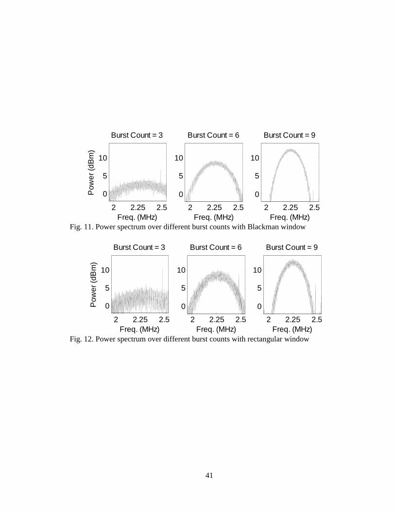
Fig. 11. Power spectrum over different burst counts with Blackman window ................. 41
Fig. 12. Power spectrum over different burst counts with rectangular window ............... 41
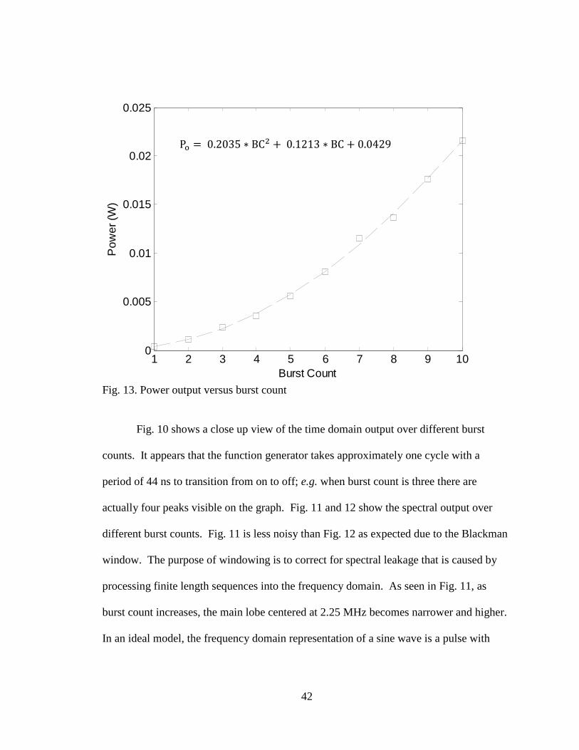
Fig. 13. Power output versus burst count .......................................................................... 42
Fig. 14. Time domain output of power amplifier over different input voltages ............... 44
Fig. 15. Power measurement over different voltages with Blackman window ................ 45
Fig. 16. Power measurement over different voltages with rectangular window .............. 45
Fig. 17. Power output versus voltage input from waveform generator ............................ 46
Fig. 18. Linear spectrum of received hydrophone voltage to show harmonics ................ 47
Fig. 19. Spectral amplitude calculation of center frequency ............................................ 48
Fig. 20. Hydrophone voltage with calculated pulse repetition frequency ........................ 49
Fig. 21. Hydrophone voltage output with peak rarefaction pressure ................................ 50

x
Fig. 22. Lateral contour of the transducer. ........................................................................ 51
Fig. 23. Axial contour of the transducer ........................................................................... 52
Fig. 24. Pulse intensity integral and calculated pulse duration ......................................... 53
Fig. 25. Intensity curve with Ispta and Isppa ......................................................................... 54
Fig. 26. Axial and lateral contours with peak Ispta ............................................................ 55
Fig. 27. Microcapsule image taken from transmission light video microscope ............... 60
Fig. 28. Microcapsule membrane under sonication at different times .............................. 61
Fig. 29. Microcapsule image taken from transmission light video microscope ............... 62
Fig. 30. Microcapsule membrane under sonication at different times .............................. 63

xi
LIST OF TABLES
TABLE 1. Summary of Ultrasound Properties ................................................................... 5
TABLE 2. Equipment Specifications for RF Power Measurement .................................. 18
TABLE 3. Units for Measured Parameters ....................................................................... 26
TABLE 4. Suggested FDA Acoustic Output Exposure Levels - Diagnostic ................... 26
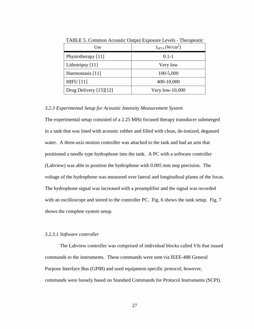
TABLE 5. Common Acoustic Output Exposure Levels - Therapeutic ............................ 27
TABLE 6. Electrical Input Power from Power Amplifier (mW) ..................................... 57
TABLE 7. Acoustic Power (mW) for 50 mV Input from Waveform Generator .............. 58
TABLE 8. Peak MI, Isppa, Ispta for 50 mV Input from Waveform Generator .................... 58

1
1. INTRODUCTION
The process of getting new medical devices or procedures into clinical practice is lengthy
and multi-phased. A procedure or device can only be used in clinical trials after
equipment calibration, tissue mimicking construct (phantom) tests, in-vitro tests, and in-
vivo tests. The purpose of these development phases is to ensure the safety and efficacy
of the new device or procedure. As detailed in the highlighted portions of Fig. 1, this
thesis will discuss ultrasound pulse sequence development, material development, and
preliminary phantom experiments for a new ultrasound based drug delivery method.
Fig. 1. Initial phases of interdisciplinary drug delivery study

2
Material development includes formulating phantoms and drug reservoirs
(microcapsules). Ultrasound pulse sequence development includes measuring electrical
input power applied to the therapy transducer and acoustic intensity emitted from the
therapy transducer. Optical measurements will include observing changes in phantoms
and microcapsules that are undergoing ultrasound sonication with a transmission light
video microscope.
1.1 Breast Cancer
The American Cancer Society estimates that 40,170 women died in the United States due
to breast cancer in 2009 [1], making it the second most common cause of cancer death in
women [2]. Between 1991 and 2006, the death rate among women has steadily declined
from 32.7 to 23.4 deaths per 100,000 [1]; this is a relative change of 28.3%. While this
trend can be partially attributed to a successful campaign for breast cancer screening, new
strategies are still needed for prevention, detection, and treatment to reduce overall
mortality rates.
1.1.1 Current Treatments
Current treatment methods for breast cancer include surgery, systemic therapies, and
localized therapies. Often large tumors are surgically removed and then therapies are
used to treat the residual cancer cells [3]. Some of these therapy methods include:
radiation therapy, chemotherapy, hormone therapy, and monoclonal antibody therapy [1].
In systemic chemotherapy drugs are injected intravenously to kill rapidly dividing cancer

3
cells. During the journey to the cancer cells, these drugs may bind to other rapidly
dividing cells or become metabolized [4]. This causes healthy bone marrow, hair, skin,
and intestinal cells to be destroyed. Some common side effects include nausea, hair loss,
mouth sores and throat sores [5]. A trade-off has to be made in chemotherapy treatment
between delivering an effective drug dose and preventing toxicity.
Targeting the cancer cells locally with optimal quantities of drug can mitigate the
side effects seen in systemic chemotherapy. For example, a method of local drug
delivery is with using thermosensitive liposomes that encapsulate anti-cancer agents [6].
These constructs undergo permeability changes when exposed to heat sources such as
microwaves and infrared lasers [6]. Changes in the membrane permeability allow the
release of the drug payload with lower systemic toxicity. Unfortunately, these constructs
rely on the chaotic tumor vasculature for transport and are too small (nanometers in
diameter) to supply an effective dose of drug over the entire cancer cell lifecycle.
1.1.2 Basics of the Tumor Microenvironment
Systemic chemotherapy is unable to reach all cells in a cancerous tumor because the
tumor microenvironment contains leaky vasculature, lack of functional lymphatics, and
lower vasculature density [3]. Blood flow in the tumor varies widely among the four
different regions of a tumor: necrotic tissue region, semi-necrotic tissue region, stabilized
microcirculation region and rapid cell growth region [4]. These necrotic masses form
because of nutrient deprivation in their respective regions. Other methods of treatment

4
must be performed in coordination with chemotherapy because of the tumor’s vascular
arrangement.
1.2 Ultrasound
Ultrasound describes a subset of mechanical waves in the frequency range of 0.02–2,000
MHz [7], which is above the audible frequency range for humans [8]. Clinical ultrasound
operates in the range of 1–15 MHz [7]. While ultrasound waves can propagate in four
different operating modes [7], only longitudinal waves are relevant in tissue imaging and
therapy. Table 1 summarizes the properties of ultrasound.
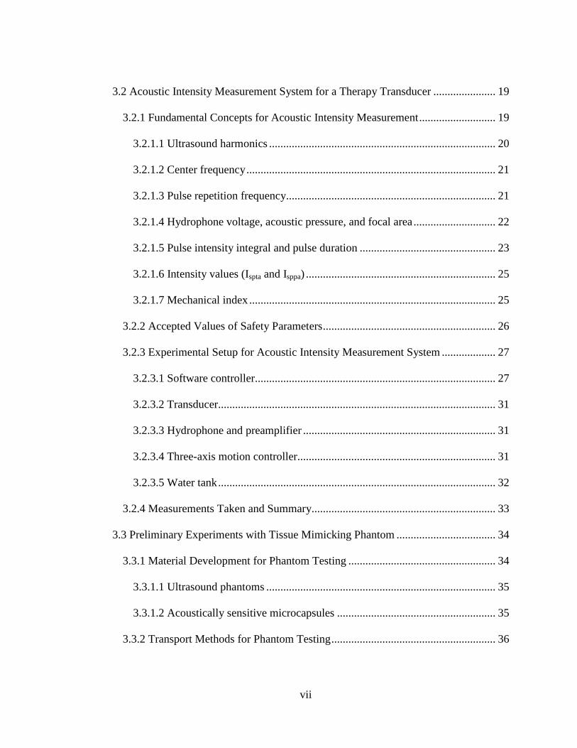
Longitudinal waves occur when the particles of a medium vibrate about their
resting location in the direction parallel to wave propagation. The wave contains zones
of alternating compression and rarefaction. Compression occurs when the particles of the
medium vibrate opposite to the direction of wave propagation. This creates a region in
the medium that is denser with sound pressure waves than at ambient pressure.
Rarefaction occurs when the particles vibrate in the direction of wave propagation. This
creates a region in the medium that is less dense with sound pressure waves than at
ambient pressure [9]. Fig. 2 shows that the wavelength, λ, represents one full cycle of
compression and rarefaction. Wavelength is related to f, the frequency, and c, the
velocity of wave propagation, which ranges from 1,450–1,600 m/s depending on the
tissue type [10]. The equation for calculating wavelength is
5
λ c . (1)
As ultrasound waves propagate through a medium, beam intensity is reduced by
reflection, scattering and absorption. The energy from the beam is absorbed by particles
of the medium that become heated. The rate of energy absorption or tissue attenuation
varies from 0.3–0.8 dB/cm/MHz depending on the tissue type [7]. This highlights that
attenuation is a function of distance traveled and wave frequency.
TABLE 1. Summary of Ultrasound Properties Property Type Value
Frequency Range
0.02–2,000 MHz, most common from 1–15 MHz for medical devices [7]
Velocity in Soft Tissue
1,450–1,600 m/s, depending on the tissue type [7]
Source Device
Transducer, piezoelectric elements convert between electrical and mechanical energy [7]
Wave Type
Mechanical, requires a medium to propagate [9]
Operating Modes
Longitudinal, transverse, surface, and plate [9]
Fig. 2. Longitudinal ultrasound waves

6
1.2.1 Diagnostic versus Therapeutic Ultrasound
Diagnostic and therapeutic ultrasound applications have different electrical input
waveforms characteristics, which results in different acoustic intensity outputs.
Diagnostic ultrasound has a maximum pulse duration of 1 µs [7], while therapeutic
ultrasound can operate with continuous wave for several minutes. Acoustic intensity is
the energy flow per second per unit of cross sectional area [9] and is an indicator of
possible bio-effects. Lower temporal average acoustic intensity waves are used in
diagnostic ultrasound (0.017–0.720 W/cm2) [10], while higher acoustic intensity waves
are used in therapy ultrasound (0.1–10,000 W/cm2) [11]. The applications of ultrasound
therapy range from physiotherapy to high intensity focused ultrasound in thermal ablation
of prostate cancer cells [3]. High ultrasound intensities can result in primarily three
mechanisms for causing bio-effects: heat generation, acoustic cavitation and acoustic
radiation force [3].
1.2.2 Ultrasound in Drug Delivery
Bio-effect mechanisms caused by high intensity ultrasound have generated interest
among those who are researching new methods for localized therapy. If these
mechanisms can be safely and effectively employed to alter tissue or drug agent
permeability, it could result in an increased absorption or delivery level of anti-cancer
agents in tumors.

7
1.3 Long Term Goals and Scope of Thesis
The long term goal in this multi-phased study (see Fig. 1) is to find a combination of drug
reservoir characteristics and a transducer pulse sequence that will allow time controlled
drug elution with the primary consideration to patient safety.
The scope of this thesis is to build a system that will calibrate and characterize an
acoustic transducer that will be used for mass transport from a microcapsule construct. In
particular it will include transducer power measurements, acoustic beam characterization,
and preliminary phantom testing under a microscope.

8
2. LITERATURE REVIEW
In the following discussion the development and challenges of ultrasound in different
drug delivery methods will be discussed. This literature review is broken into five
sections: basics of enhanced drug delivery, a brief history of ultrasound in medicine,
ultrasound mechanisms and transducer characterization, and applications and challenges
of ultrasound in cancer treatments.
2.1 Basics of Enhanced Drug Delivery
Enhanced drug delivery methods are developed in order to change biological properties
of tissue or drug vehicle [4]. The purpose of changing biological properties of tissue is to
reduce transport barriers that prevent drug uptake. Some current technologies used to
reduce these barriers are hyperthermia, radiofrequency ablation, electroporation,
magnetic fields, and acoustic cavitation with ultrasound [12]. An example of
hyperthermia would be the Krol et al. study that incubated ex-vivo cells at temperatures
from 37–41° C. This resulted in the reducing of the number of viable cells and increasing
the available fraction of drug [3]. Drug vehicles are used to position the drug in the
vicinity of the cancerous region so that drug will primarily diffuse into the cancerous
region. An example of changing properties of the delivery vehicle is liposomes that
release drug when exposed to heat [6]. Ultrasound is a more recent method for enhancing
drug delivery. It is an attractive approach to drug enhancement because it is non-
invasive, inexpensive, and can access deep tissues.
9
In any drug delivery approach it is important to understand the method by which
the chemical is delivered to the cancerous body. In order for chemotherapy to be
effective, the correct therapeutic agent and dose must be chosen to treat the region [4]. In
a blood born treatment, the drug must cross from blood vessel, through the vessel wall,
and into the interstitium (space between cells) [4]. Along this path the drug binds
randomly to healthy cells or becomes metabolized [4]. Heterogeneous movement of
molecules in the tumor is determined by the blood flow rate and the number, length,
diameter, and geometric arrangement of blood vessels [4]. Systemic chemotherapy is not
sufficient for delivering drug to cancerous cells in this environment.
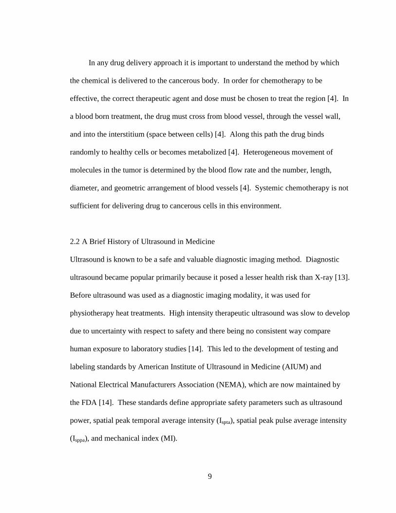
2.2 A Brief History of Ultrasound in Medicine
Ultrasound is known to be a safe and valuable diagnostic imaging method. Diagnostic
ultrasound became popular primarily because it posed a lesser health risk than X-ray [13].
Before ultrasound was used as a diagnostic imaging modality, it was used for
physiotherapy heat treatments. High intensity therapeutic ultrasound was slow to develop
due to uncertainty with respect to safety and there being no consistent way compare
human exposure to laboratory studies [14]. This led to the development of testing and
labeling standards by American Institute of Ultrasound in Medicine (AIUM) and
National Electrical Manufacturers Association (NEMA), which are now maintained by
the FDA [14]. These standards define appropriate safety parameters such as ultrasound
power, spatial peak temporal average intensity (Ispta), spatial peak pulse average intensity
(Isppa), and mechanical index (MI).
10
Many ultrasound therapies have been developed since these standards were
established. Treatments developed included lithotripsy for the treatment of kidney stones
and thrombolysis for the treatment of blood clots [14]. Therapeutic ultrasound
specifically for drug delivery is currently used in sonophoresis, a technique of sonicating
skin to enhance transdermal drug diffusion [12]. Extensive research is being done to
apply this method to drug delivery to solid tumors [15]. These will be discussed in detail
in section 2.4.
2.3 Ultrasound Mechanisms and Transducer Characterization
There are three well known risks to high intensity focused ultrasound: hyperthermia,
acoustic radiation force and acoustic cavitation. Hyperthermia is when the rise in
temperature causes proteins to denaturize and necrose [12]. Acoustic radiation force
occurs when momentum is transferred from the emitting wave to the tissue to elicit tissue
motion [3]. These effects have not been well studied with respect to temporary or
permanent tissue responses [14]. Acoustic cavitation occurs when oscillating pressure
changes due to the ultrasound wave causes oscillating bubbles to form in liquid media
like blood vessels or cysts, leading to the disruption of cells, blood vessels and tissue
structures [12]. The presence of these mechanisms is determined by spatial and temporal
acoustic power and intensity characteristics of the ultrasound transducer pulse sequence.
The highest level of acoustic intensity for diagnostic imaging is 0.72 W/cm2 [10] and
ranges from 100–10,000 W/cm2 for therapy applications [11]. In order to effectively and

11
safely use a transducer, the location and area of the highest focal intensity must be
known.
Transducers are normally characterized with an acoustic radiation force balance or
an acoustic raster scan system. A radiation force balance works by operating the
transducer directly over a target, e.g. cone, rubber, brush, and oil filled bag [11]. The
change in vertical position of the target due to the radiating force of the beam is sensed
by mechanical (weighing balance) or magnetic (electromagnetic coil) means and
converted into a force [8]. An acoustic raster scan system translates an acoustically
sensitive device called a hydrophone to different positions within the transducer beam.
These measurements are then converted from electrical power to acoustic power by the
hydrophone sensitivity constant at that frequency. The advantage of this system over the
acoustic radiation force balance system is that the entire beam can be spatially
characterized.
2.4 Applications and Challenges of Ultrasound in Cancer Treatments
Applications of high intensity focused ultrasound include thermal ablation of cancer cells
and localized mediated drug delivery. Thermal ablation uses high intensity focused
ultrasound (HIFU) and is currently in clinical use for certain types of cancers like prostate
cancer [12]. Thermal ablation is performed by exposing tissue to several minutes of high
power ultrasound. The focused beam allows tissue in the near and far field of the beam
to remain unharmed, while directly targeting the cancerous tissue at the focus [12]. This
12
procedure can be difficult to perform because cancerous tissues are often very close to
healthy tissues and appropriate monitoring mechanisms need to be in place.
Ultrasound mediated drug delivery is another application of ultrasound in cancer
treatments. A pulsing scheme set with a low duty cycle allows the tissue to cool by
diffusion and convection during the off part of the cycle [3]. This still enables the high
peak pulse to cause cavitational effects needed to create temporary holes in the
membrane. Cavitation is difficult to induce since there is a lack of dissolved gasses in the
blood stream [12]. When cavitation does occur, the timing and effect is hard to monitor
or control.
One solution is to add small gas bubbles or ultrasound contrast agents (UCAs) into
the blood stream to provide a nucleus in which a cavitational bubble can oscillate. This
allows cavitation to occur at lower acoustic intensities resulting in fewer complications
due to the heating of healthy tissue. These UCAs cannot diffuse through the vessel wall
because they are protected by a lipid or protein outer layer. Direct applications of this
effect are seen in sonoporation where direct and transient opening of the cell can be
modulated for gene delivery [12]. This solution was also found to create very strong and
damaging reactions to tissue cells when the UCA are destroyed.
The long term goal of this research is to encapsulate drug and UCAs into reservoirs
(microcapsules) in order to protect healthy cells from complications of acoustic
cavitation. This would contain the destructive nature of the UCA while keeping the
membrane of the microcapsule intact up to the acoustic threshold. Microcapsules are
made from polymer based shells and range from micrometers to a few millimeters. It has

13
been previously noted that microencapsulation allows better biodistribution of the drug
and has shown promising results with thermosensitive liposomes [6]. Even with the
successes of thermosensitive liposomes, new methods still need to be developed to
enhance localized mediated drug delivery.
14
3. METHODS
3.1 Electrical Input Power Measurement
Traditional diagnostic transducers are powered with high voltage (100 V) spikes to
generate short pulses for imaging. For therapeutics, the input voltage applied can range
from short pulses to continuous wave. A continuous wave is normally used for radiation
force, whereas short pulses are used to engage cavitational effects. Being able to
modulate the input voltage in terms of the voltage, duty cycle and overall power is
important for generating useful pulses for drug delivery design. A simple function
generator combined with an RF power amplifier can be used to power the transducer.
Calibration tests as well as electrical power measurements were performed.
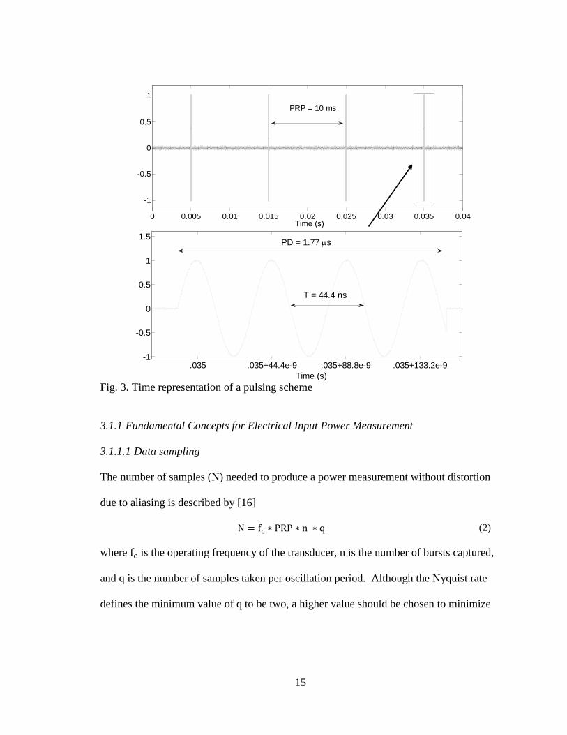
The power spectrum of a pulsed waveform is difficult to measure accurately when
the signal has a pulse repetition period (PRP) in tens of milliseconds, a pulse duration
(PD) in microseconds, and a period (T) in tens of nanoseconds (see Fig. 3). This is
because testing parameters, e.g. sweep time and sample rate, will drastically change the
measured or calculated power.
For power measurements, the data was sampled in the time domain with an
oscilloscope at 50 MHz for the length of the pulse repetition period (10 ms) and
processed in the time and frequency domains to calculate power. This method provided
more processing options when compared to measuring with a spectrum analyzer.
15
Fig. 3. Time representation of a pulsing scheme
3.1.1 Fundamental Concepts for Electrical Input Power Measurement
3.1.1.1 Data sampling
The number of samples (N) needed to produce a power measurement without distortion
due to aliasing is described by [16]
N f PRP n q (2)
where f is the operating frequency of the transducer, n is the number of bursts captured,
and q is the number of samples taken per oscillation period. Although the Nyquist rate
defines the minimum value of q to be two, a higher value should be chosen to minimize
0 0.005 0.01 0.015 0.02 0.025 0.03 0.035 0.04
-1
-0.5
0
0.5
1
PRP = 10 ms
Time (s)
.035 .035+44.4e-9 .035+88.8e-9 .035+133.2e-9-1
-0.5
0
0.5
1
1.5PD = 1.77 µs
T = 44.4 ns
Time (s)
16
distortion. If the value of q is too high, it will be difficult to store and process the data in
order to calculate power values.
3.1.1.2 Windowing
Windowing is a finite impulse response (FIR) filtering method that involves modifying
sampled data to produce a desired Fourier magnitude response. This is done by
truncating or tapering samples in the time domain. It is described by the equation [16]
xn xn wn (3)
where n is the index value, x(n) is the sampled data, w(n) is the applied window and
xn is the filtered data. The purpose of windowing is to correct for frequency spectral
leakage defined as power that is concentrated at frequencies other than the original signal
spectrum due to biases in finite length data processing methods. These spectral leaks
appear as side lobes on the spectrum. A rectangular window truncates the samples,
which results in high side lobe levels and a narrow main lobe at the center frequency.
Most other windows, e.g. Blackman window, gradually taper the samples to zero in the
window period, which results in low side lobe levels and a wide main lobe at the center
frequency. With any window chosen, there is a trade-off between narrow main lobe
around the center frequency (for high frequency resolution) and low side lobes (for less
spectral leakage). The equation for a rectangular window [16] is
wn 1 (4)
where n is an index value. The equation for Blackman window [16] is
17
wn 0.42 0.50 cos 2πnN 1 0.08 cos 4πn
N 1 (5)
where n is an index value and N is the total number of samples.
3.1.1.3 Power with discrete Fourier transform
Once the appropriate window filter is applied to the time domain data, the discrete
Fourier transform (DFT) is used to convert the data from time domain, xn, to
frequency domain, Xf by [16]
Xf " xne$%&π'()(*+ . (6)
Power is relative to the maximum value of the DFT squared by [16]
Pf |Xf&| R⁄ (7)
where X(f) is the value of frequency domain representation of the input voltage, and R is
the value of system loading. Since the relative peaks in the power spectrum are easier to
view in log scale, (7) is converted into dBm by
Pf./0 10 log3Pf/10$56. (8)
3.1.2 Experimental Setup for Electrical Input Power Measurement
Electrical input power measurements are necessary because it can be used to control the
acoustic output of the transducer. This is done by generating an electrical pulse with the
combination of waveform generator and RF power amplifier. The output voltage of the
power amplifier was attenuated with a 10x probe to ensure that the signal did not exceed
the voltage rating of the oscilloscope (5Vrms with 50 Ω load setting). The oscilloscope
samples the waveform and sends the data via IEEE-488 General Purpose Interface Bus
18
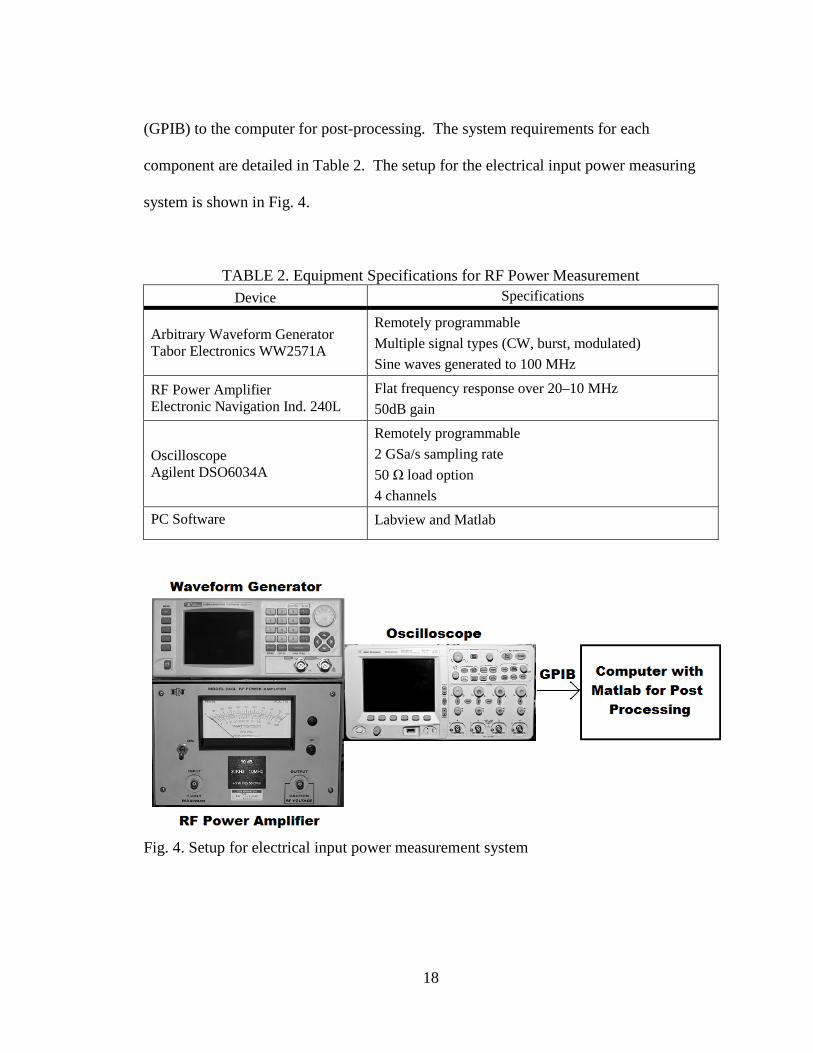
(GPIB) to the computer for post-processing. The system requirements for each
component are detailed in Table 2. The setup for the electrical input power measuring
system is shown in Fig. 4.
TABLE 2. Equipment Specifications for RF Power Measurement Device Specifications
Arbitrary Waveform Generator Tabor Electronics WW2571A
Remotely programmable
Multiple signal types (CW, burst, modulated)
Sine waves generated to 100 MHz
RF Power Amplifier Electronic Navigation Ind. 240L
Flat frequency response over 20–10 MHz
50dB gain
Oscilloscope Agilent DSO6034A
Remotely programmable
2 GSa/s sampling rate
50 Ω load option
4 channels
PC Software Labview and Matlab
Fig. 4. Setup for electrical input power measurement system

19
3.1.3 Measurements and Summary
Data sets were acquired over a pulse repetition period of 10 ms for 1–10 burst counts
(sine wave frequency: 2.25 MHz, duty cycle range: 0.0044–0.044%) at 50 mV input from
the function generator. Other data sets were acquired by varying the input voltage
between 20 mV and 100 mV keeping the burst counts constant at five. With (6)–(8)
power values were calculated.
This calibration study allowed verification of the RF power amplifier device
performance over a range of input voltages and burst counts. If transducer device
efficiencies are available, correlation of electrical input power to expected acoustic power
can be easily made. These correlation measurements can be used as a guide to choosing
a pulsing scheme relevant to drug delivery applications.
3.2 Acoustic Intensity Measurement System for a Therapy Transducer
The intent of ultrasound in therapy is to cause bio-effects that will improve the health of
the patient. The pressure and intensity of the ultrasound beam was measured spatially
with a hydrophone and compared with accepted mechanical and thermal parameters
defined by the Food and Drug Administration (FDA).
3.2.1 Fundamental Concepts for Acoustic Intensity Measurement
A single element focused transducer was measured in the axial and lateral planes that
contain the focus. The transducer converts electrical input power into mechanical
vibrations or acoustic energy by the piezoelectric effect. The piezoelectric effect is seen

20
in the transducer when the crystalline elements deform proportional to the strength and
polarity of the applied electric field causing mechanical stress on a medium [17]. Any
piezoelectric material can create and sense mechanical waves because the effect is
reversible.
In Fig. 5, the axial beam is the acoustic variation in the y-z plane and the lateral
beam is the acoustic variation in the x-z plane. Focal width, focal depth, ultrasound
harmonics, mechanical index, spatial peak pulse average intensity and spatial temporal
average intensity were calculated with this data. Definitions of these terms will be
discussed next. Table 3 at the end of the section gives a summary of all units used in
these terms, unless locally described.
Fig. 5. Lateral and axial beam definition of a single element transducer
3.2.1.1 Ultrasound harmonics
The transducer emits primary harmonics at center frequency fc along with contaminating
harmonics at multiples of the center frequency (2fc, 3fc, etc.) in the acoustic pulse [18].
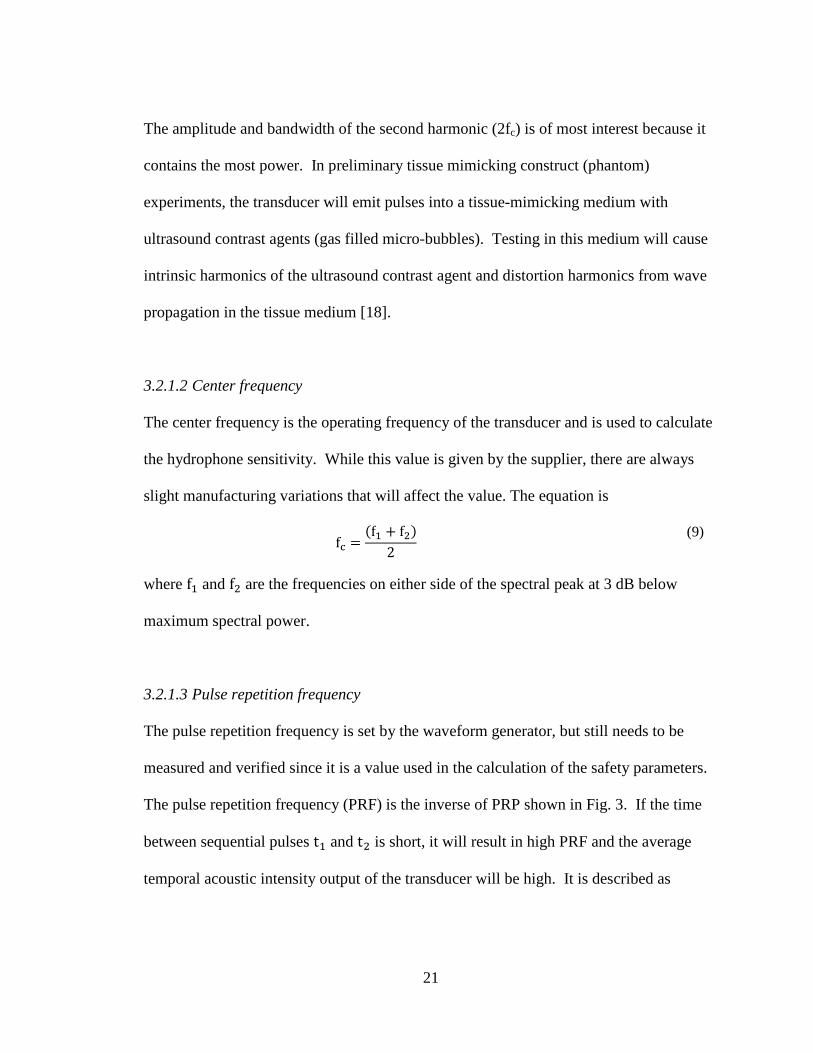
21
The amplitude and bandwidth of the second harmonic (2fc) is of most interest because it
contains the most power. In preliminary tissue mimicking construct (phantom)
experiments, the transducer will emit pulses into a tissue-mimicking medium with
ultrasound contrast agents (gas filled micro-bubbles). Testing in this medium will cause
intrinsic harmonics of the ultrasound contrast agent and distortion harmonics from wave
propagation in the tissue medium [18].
3.2.1.2 Center frequency
The center frequency is the operating frequency of the transducer and is used to calculate
the hydrophone sensitivity. While this value is given by the supplier, there are always
slight manufacturing variations that will affect the value. The equation is
f f+ f&2
(9)
where f+ and f& are the frequencies on either side of the spectral peak at 3 dB below
maximum spectral power.
3.2.1.3 Pulse repetition frequency
The pulse repetition frequency is set by the waveform generator, but still needs to be
measured and verified since it is a value used in the calculation of the safety parameters.
The pulse repetition frequency (PRF) is the inverse of PRP shown in Fig. 3. If the time
between sequential pulses t+ and t& is short, it will result in high PRF and the average
temporal acoustic intensity output of the transducer will be high. It is described as

22
PRF 1t& t+
(10)
where t1 is the time of the first burst cycle and t2 is time at which the next burst cycle
occurs.
3.2.1.4 Hydrophone voltage, acoustic pressure, and focal area
A hydrophone is a device that can measure mechanical pressure waves in liquids. Like
transducers, hydrophones convert acoustic pressure waves into voltage waves by the
piezoelectric effect. Unlike transducers, hydrophones are able to sense acoustic
excitation over a broad range of frequencies and at high spatial resolution. Hydrophones
are very expensive and sensitive instruments that must be handled with great caution and
care. The quality of the instrument degrades with any contact from a hard surface or
even prolonged exposure to water.
The sensitivity curves of the hydrophone and preamplifier must be used to convert
the voltage output of the hydrophone into acoustic pressure. These curves are normally
provided by the manufacturer. Voltage can be converted into acoustic pressure by [19]
M:f G<f Mf C>C> C<
(11)
where G<(f) and C<are the preamplifier gain and capacitance, and Mf and C> are the
hydrophone EOC sensitivity and capacitance.
After the voltage output of the hydrophone has been converted into acoustic
pressure, compression and rarefaction pressure values can be measured. Peak
rarefactional pressures are achieved when the region in a medium is the least

23
concentrated with sound pressure waves because particle oscillations are opposite the
direction of propagation (see Fig. 2). It is also the value used to plot the axial and lateral
planes of the transducer in order to calculate focal depth and focal width respectively. It
is defined as the absolute value of the most negative pressure from the hydrophone output
described by [10]
p@ |min vt|M:f
(12)
where v(t) is the voltage seen by the hydrophone and M:f is the hydrophone sensitivity
conversion factor at the center frequency.
3.2.1.5 Pulse intensity integral and pulse duration
Intensity is the power per unit area. It is defined as [10]
PII E v&F&F+ tdt
ρc M:&f (13)
where v(t) is the hydrophone voltage, Ml is the hydrophone sensitivity at the center
frequency, t1 and t2 represents the time duration of interest, and ρc is the specific acoustic
impedance.
Specific acoustic impedance is the level of resistance experienced by the
propagating wave. It is a value used to calculate all of the safety parameters. For a
longitudinal wave, the impedance is described by [10]

24
ρc ρ I Y1 σρ1 σ1 2σL
+/&
(14)
where ρ is the material density, c is the velocity of sound, Y is Young’s modulus, and σ is
Poisson’s ratio [9]. Young’s modulus is a measure of stiffness in an elastic material and
Poisson’s ratio is the ratio of transverse strain over axial strain.
At room temperature, the density and longitudinal velocities of water are
1000 kg/m5 and 1480 m/s respectively [9]. This results in ρc 1.48 MPa · s/m at
293 K. This value will be rounded to 1.50 MPa · s/m for simplicity and used in later
calculation.
A conversion factor to account for tissue calculations and attenuation is applied to
the PII with the equation [10]
PII.P@<FP. PII e$Q.++R S 'T U (15)
where the factor 0.115 is the conversion between decibels (log base 10) to Neper (natural
log), α is tissue attenuation, and z is the distance from the transducer to depth of interest.
The accepted value for tissue attenuation is 0.3 dB/cm/MHz.
The pulse duration is the amount of time that the ultrasound pulse is considered
on. It is calculated from the pulse intensity integral. The equation is [10]
PD 1.25 t& t+ (16)
where t+is the time when the amplitude is 10% below peak PII and t& is 90% below peak
PII.

25
3.2.1.6 Intensity values (Ispta and Isppa)
Spatial peak temporal average intensity (IWXF< is the maximum intensity occurring over
the pulse repetition period. It indicates the thermal deposition by ultrasound [10]. Spatial
peak pulse average intensity (IWXX< is the maximum intensity in the beam averaged over
the pulse duration [10]. The formulas used to calculate these values are as follows [10]:
IWXF< PII.P@<FP. PRF (17)
IWXX< PII.P@<FP.PD
(18)
where PIIderated is the derated pulse intensity integral, PRF is the pulse repetition
frequency and PD is the pulse duration.
3.2.1.7 Mechanical index
The mechanical index is a measure of the probable negative bio-effects experienced from
the applied ultrasound wave. All devices currently approved by the FDA must have a
mechanical index lower than 1.9 [10]. This index can be computed as [10]
MI p@,.P@<FP.Yf
(19)
where pr,derated is the derated peak rarefactional pressure at the location of the maximum
peak intensity integral and fc is the center frequency in megahertz.

26
TABLE 3. Units for Measured Parameters Value (units)
fc, f1, f2 (MHz) pr (MPa) α (dB/cm/MHz)
t, t1, t2 (seconds) v (volts) z (cm)
PRF (Hz) ρc (MPa · s / m) PD (seconds)
M l , Mc (V / Pa) Y (Pa) Ispta (W / cm2)
Ga (unitless) σ (unitless) Isppa (W / cm2)
Ch, Ca (pF) PII, PIIderated (µJ / cm2) MI (unitless)
3.2.2 Accepted Values of Safety Parameters
Table 4 describes some of the index levels allowed for safe use in diagnostic ultrasound.
Therapeutic ultrasound does not have maximum levels that are determined by the FDA.
The purpose of the maximum levels seen in Table 4 is to prevent bio-effects in the
corresponding tissue. The therapies in Table 5 are specifically trying to create bio-effects
for therapy purposes. These are not values that are regulated by the FDA but rather
suggested values accepted by the industry to gauge acoustic intensity. Both guidelines
will be used to determine safe levels of exposure.
TABLE 4. Suggested FDA Acoustic Output Exposure Levels - Diagnostic
Use ISPTA (W/cm2) ISPPA (W/cm2) MI (unitless)
Peripheral Vessel [10] 0.720 190 1.9
Cardiac [10] 0.430 190 1.9
Fetal Imaging & Other [10]
0.094 190 1.9
Ophthalmic [10] 0.017 28 0.23
27
TABLE 5. Common Acoustic Output Exposure Levels - Therapeutic Use ISPTA (W/cm2)
Physiotherapy [11] 0.1-1
Lithotripsy [11] Very low
Haemostasis [11] 100-5,000
HIFU [11] 400-10,000
Drug Delivery [15][12] Very low-10,000
3.2.3 Experimental Setup for Acoustic Intensity Measurement System
The experimental setup consisted of a 2.25 MHz focused therapy transducer submerged
in a tank that was lined with acoustic rubber and filled with clean, de-ionized, degassed
water. A three-axis motion controller was attached to the tank and had an arm that
positioned a needle type hydrophone into the tank. A PC with a software controller
(Labview) was able to position the hydrophone with 0.005 mm step precision. The
voltage of the hydrophone was measured over lateral and longitudinal planes of the focus.
The hydrophone signal was increased with a preamplifier and the signal was recorded
with an oscilloscope and stored to the controller PC. Fig. 6 shows the tank setup. Fig. 7
shows the complete system setup.
3.2.3.1 Software controller
The Labview controller was comprised of individual blocks called VIs that issued
commands to the instruments. These commands were sent via IEEE-488 General
Purpose Interface Bus (GPIB) and used equipment-specific protocol; however,
commands were loosely based on Standard Commands for Protocol Instruments (SCPI).

28
The waveform generator, oscilloscope, and three-axis motion controller all had its own
controller VI that was integrated into one top-level controller VI. Basic VIs were
Fig. 6. Tank setup for acoustic measuring system
Fig. 7. Acoustic measuring system setup
29
supplied by the manufacturers of the equipment, but modifications and coordination was
necessary to implement a properly functioning scanning system.
The waveform generator VI from the manufacturer was designed to output
continuous wave standard waveforms such as sine, square wave, ramp, etc. A custom VI
was created since this application required pulsed waveforms of varying duty cycles.
This custom VI allowed the user to generate a pulsed waveform with a defined duty cycle
and to select the appropriate voltage output.
The oscilloscope VI from the manufacturer was designed to capture a waveform
of 1000 samples after the device had undergone an auto-scale. The sampling rate was
insufficient for this application since a large number of samples were needed to capture
high frequency bursts at a low frequency pulse repetition frequency (see Fig. 3). The
only way to capture the needed number of samples was to capture the maximum number
of samples allowed by the device (two million samples when the time duration was
0.01 s). Then this data set was decimated to 50,000 samples for 8 µs of data, a sample
number determined by (2) to balance the problems of under-sampling and unmanageable
data processing times.
The default VI for the three-axis motion controller contained all of the commands
that the device could perform. The commands that were not necessary for this
application were removed. The user was left with the option of opening the port,
inputting instrument commands for motion, and closing the port. A Matlab program was
written in order to generate commands to move the instrument automatically. The user
could customize length of the sides of the scanning plane, time delay between

30
movements, and number of movements within that scanning area. The scanning area was
9 mm x 9 mm for the axial scan and 1.4 mm x 1.4 mm for the lateral scan. This was
selected after course scanning was performed to determine the approximate beam area.
The top level VI used included the waveform generator, oscilloscope and three-
axis motion controller. Fig. 8 shows how the Labview controller was integrated into the
experimental setup.
Fig. 8. Overview of the Labview controller in acoustic measuring system
The VI performed the following commands: (a) send configuration data to the
waveform generator and powered on the voltage output, (b) send relative position data
changes to the motion controller, and (c) request electrical voltage data from the
31
oscilloscope. To scan the transducer voltage over many different positions, (b) and (c)
were repeated until the entire requested area was scanned.
3.2.3.2 Transducer
The transducer used in this experiment is a 2.25 MHz immersion high power therapy
transducer with a cylindrical focus at 1.25 in. (3.175 cm) (Valpey Fisher Inc. IL0208HP-
SF=1.25). An immersion transducer emits ultrasound wave only in liquids and solids
since air is not a good enough conductor of sound. The exact choice of frequency is
arbitrary for now but future studies need to be done to choose the right frequency for the
drug delivery application.
3.2.3.3 Hydrophone and preamplifier
The trade-off in choosing a hydrophone is between sensitivity (large active element) and
spatial resolution (narrow acceptance angle). The hydrophone and preamplifier chosen
for this experiment are the HNP-0400 and the AH-2010 (20 dB gain) from Onda Corp.
This needle type hydrophone has a nominal sensitivity of 50 nV/Pa over the 1–20 MHz
frequency range and an acceptance angle of 60° both of which are best for these
measurements.
3.2.3.4 Three-axis motion controller
A three-axis motion controller is used to move the hydrophone over the axial and lateral
plane of the transducer in the water tank. This instrument is made by Velmex Inc. and is

32
controlled with custom Labview program that was built especially for this purpose. A
custom arm was also built in order to lower the hydrophone into the tank for
measurements. The range of motion can be adjusted on this device by moving the safety
stops but within a maximum limit of a 125 in.3 (2048 cm3). The transducer beam width
for this focused transducer is in the order of a few millimeters, which makes the 5 µm
step precision of this instrument essential.
3.2.3.5 Water tank
A custom tank was designed and made in the SJSU machine shop. The dimensions of the
tank are 9 in. x 12 in. (22.9 cm x 30.5 cm), which allowed for full range of motion by the
three-axis motion controller without the risk of hitting the hydrophone against the tank
wall. This tank has a threaded hole in the side to allow the transducer to be screwed into
the side while remaining water tight. The tank is fixed with clamps to maintain a
consistent position throughout the tests. It allows the tank to be removed for cleaning.
The tank is lined with a quarter inch acoustic rubber (McMaster Carr Corp.) to prevent
any acoustic reflections.
The effectiveness of the measurement is greatly impacted by the quality of the
testing medium. Any impurities in the water can become reflected and change the power
measurement greatly. The water was degassed by boiling distilled or DI water for 20
minutes and was stored in air tight containers in the refrigerator. This creates a vacuum
in the container until the water is used. The water was brought to 20° C, so that the speed

33
of sound was consistent over experiments on different days. Guidelines for making
degassed water were taken from [20].
3.2.4 Measurements Taken and Summary
In each experiment it was necessary to perform a manual search of the transducer focus.
Since the focal length is just a few millimeters, there is no automated way to line up the
transducer using entirely mechanical means. These experiments were run with a burst
cycle of five and a peak-to-peak input voltage from the arbitrary waveform generator at
50 mV. This generated 5 mW electrical power input to the transducer (see Fig. 13 and
Fig. 17).
To measure the lateral plane (see Fig. 5), the hydrophone was translated over nine
points in the x direction and nine points in the z direction (total 81 points) with 0.2 mm
step precision in each direction. The hydrophone voltage was captured and stored onto
the controller PC.
To measure the axial plane (see Fig. 5), the hydrophone was translated over the 20
points with 1.0 mm step precision in the y direction and 12 points with 0.5 mm step
precision in the z direction (total 240 points). The hydrophone voltage was captured and
stored onto the controller PC.
With this data, measurements of critical safety metrics like Ispta, Isppa and MI were
calculated and the lateral plane was plotted to view the focal width. With this data,
measurements of the axial plane were plotted to view the focal depth. With this system
any relevant pulsing scheme in drug delivery can be tested to determine if it is in

34
accordance with FDA safety levels or within the range of other therapeutic methods.
This acoustic system will also provide information about the beam profile so that an
investigator can determine if the chosen transducer is appropriate for the therapeutic task
at hand.
3.3 Preliminary Experiments with Tissue Mimicking Phantom
The effect of an ultrasound pulse from the transducer was tested with acoustically
sensitive microcapsules suspended in tissue mimicking constructs (phantoms). The
materials and methods for this experiment were developed between the Electrical
Engineering and General Engineering Departments. This collaborative effort will
continue in future development of this drug delivery method. The effect of the
ultrasound pulse on the microcapsules and phantoms were observed using a transmission
light video microscope where images were analyzed frame by frame to record any
changes.
3.3.1 Material Development for Phantom Testing
The materials in this experiment were essential for determining an appropriate pulsing
scheme. Without a consistent, stable material there can be no repeatability in the results
when finding an appropriate pulsing scheme.

35
3.3.1.1 Ultrasound phantoms
Phantoms are tissue mimicking constructs that are used to develop new devices, calibrate
equipment, and train medical professionals. The phantom must be spatially, thermally
and temporally uniform to provide useful results in therapy development. Phantoms can
be formulated to mimic magnetic, electrical, optical, thermal and mechanical properties
of a particular type of tissue for one or more imaging modalities. This experiment
required an optically clear phantom so that changes in the microcapsules under sonication
could be seen under a microscope.
The constructs for initial phantom testing were made with a mixture of 10%
transparent gelatin and DI water in a petri dish mold (3 mm height by 30 mm in
diameter). The gelatin solution was heated until it became clear at approximately 60° C.
Mold release was sprayed in the petri dish prior to pouring the gelatin mixture so that the
phantom could be removed and placed in a custom stand-off designed for the experiment.
Then the acoustically sensitive microcapsules were separated from their solution and
carefully placed in the bottom of the petri dish. Heat was applied to the petri dish using
steam to prevent the gelatin from solidifying before the bottom of the dish could be
evenly coated with 3 mm of gelatin. Finally, the phantom was covered with plastic to
prevent dehydration and placed in a refrigerator to solidify.
3.3.1.2 Acoustically sensitive microcapsules
The following microcapsule method was formulated by Dr. Maryam Mobed-Miremadi
who specializes in microencapsulation and has published several papers on this topic.
36
An acoustically sensitive microcapsule (ASM) is a shell that is sensitive to acoustic
pressure and coats and protects material in its interior. ASMs of different sizes (100–
2000 µm) were loaded with a mixture of drug-like substance (blue dextran) and
ultrasound contrast agents (UCAs 1–10µm that carry gas). This experiment used
commercially available UCAs (Targesons) that were purchased.
The microcapsule membrane is made of Alginate Poly-lysine Alginate, a common
encapsulation material [21]. The microcapsule was made by suspending the blue dextran
at a specific concentration in medium-to-high viscosity sodium-alginate that is atomized
into calcium chloride solution [21]. This is done in an atomizer chamber with coaxial air
flow. The size of the droplets was controlled by the flow-rate of the coaxial air, the flow-
rate of the sodium-alginate suspension and the radial dimensions of the atomizer. The
gelled droplets were coated with poly-lysine during an adsorption step resulting in a
hydrogel membrane. Finally, sodium-alginate within the capsule is liquefied and
incubated with sodium citrate. On average each microcapsule contained 10–15
Targesons. Newer methods are being developed to increase the density of Targesons in
the capsules to engage acoustic effects at potentially lower intensities.
3.3.2 Transport Methods for Phantom Testing
Transport methods are ultrasonic pulsing schemes that will move Targesons to the edge
of the microcapsule to potentially facilitate the controlled release of drug substance from
the microcapsule.

37
3.3.2.1 Acoustic radiation force
Acoustic radiation force (ARF) is a force applied to a medium by a sound wave [22]. It
is produced due to four physical effects: density changes of propagating waves, spatial
variation of energy density in standing acoustic waves, reflection from inclusions or other
interfaces, and spatial variation in propagation velocity [22]. An application of ARF is its
use in elasticity imaging (displacement of tissue in coordination with ultrasonic imaging
to observe mechanical properties) [23]. Other applications include monitoring therapy,
molecular imaging, and acoustical tweezers [22]. ARF was used in this experiment to
displace ultrasound contrast agents with each microcapsule in the solid medium to push
against the membrane of the microcapsule material.
3.3.2.2 Acoustic cavitation
Acoustic cavitation is the occurrence of vapor cavities inside a liquid when its pressure
has been lowered below vapor pressure [24]. In a medical ultrasound application, it
refers to bubbles induced in tissue by ultrasonic pressure [14]. When high acoustic
rarefactional pressure is applied, small cavities are compressed and begin to pulse [25].
Two types of cavitation effects can occur: stable and transient. Stable cavitation is when
a bubble forms and grows over multiple cycles of the acoustic intensity. Its effects can
cause surface wave activity and microstreaming (currents opposite in direction of the
main current motion) [26]. Transient cavitation is when the bubble forms and grows
within less than one cycle of the acoustic intensity. The effect of these transient bubbles
can cause high pressures and temperatures that can erode solids, initiate chemical

38
reactions and produce luminescence [26]. The long term goal of this study is to
determine if these transient bubbles will allow diffusion of drug through a membrane.
3.3.3 Experimental Setup for Phantom Testing
The experiment consists of an arbitrary waveform generator and power amplifier driving
a transducer to image microcapsules under sonication using a transmission light
microscope. These microcapsules were suspended in the phantom to simulate a very
simplistic tissue environment. Fig. 9 shows the experimental setup with a Nikon Epiphot
200, an inverted transmission light video microscope. In order to capture any effects of
the ultrasound on the material, the optical and acoustical focus was aligned. This was
done by positioning the light of the microscope in the center of the transducer face. The
video software of the microscope allowed images to be captured at 7–8 frames per
second. Both a stand-off and support clamp stand was used to stabilize and position the
transducer over the microcapsules. In the future, a more robust system for aligning the
acoustic focus of the transducer and optical focus of the microscope shall be developed.
The 3 mm phantom sample was submerged in 31.75 mm of DI water and the transducer
was placed above.
3.3.4 Measurements Performed and Summary
For the preliminary experiments, a continuous wave pulse (fc = 2.25 MHz with input
voltage 65 mV peak-to-peak) was used to sonicate the material. The above measurement

39
setup is the first step toward visualizing a potentially important drug delivery scheme
using a combination of ultrasound contrast agents and drug substance in microcapsules.
Fig. 9. Phantom testing setup on transmission light microscope
This experiment allowed for basic visualization of the effect of ultrasound on
microcapsules. However, the current limitations of the microscope and the stand-off do
not allow clear visualization of the ultrasound contrast agents, easy alignment of the
acoustic and optical focus, or high speed video for capturing stable or transient acoustic
cavitational effects. A more robust experimental setup will be built in the future along
with the use of a biological microscope and high speed camera.

40
4. RESULTS
4.1 Electrical Input Power Measurement
This calibration study showed RF power amplifier device performance over a range of
input voltages and duty cycles (burst counts). From these measurements, device
efficiency can be calculated if acoustic power is measured and electrical input power can
be correlated to expected acoustic power. These correlation measurements can be used as
a guide when choosing any pulsing scheme relevant to drug delivery applications.
4.1.1 Burst Count versus Output Power
Figures 10–13 show the effect of varying the burst count from 1–10 on output power.
This range of burst counts was chosen because it produces an acoustic pressure under 2
MPa, which is the maximum pressure that the hydrophone can be exposed to
continuously without damage. The expected results from this experiment also correspond
to the maximum Food and Drug Administration (FDA) data limits (see Table 4).
Fig. 10. Time domain output of power amplifier over different burst counts
0 1 2 3 4 5 6
-5
0
5
Burst Count = 3
Time (µs)
Vol
tage
(V)
0 1 2 3 4 5 6
-5
0
5
Burst Count = 6
Time (µs)0 1 2 3 4 5 6
-5
0
5
Burst Count = 9
Time (µs)
41
Fig. 11. Power spectrum over different burst counts with Blackman window
Fig. 12. Power spectrum over different burst counts with rectangular window
2 2.25 2.5
0
5
10
Burst Count = 3
Freq. (MHz)
Pow
er (d
Bm
)
2 2.25 2.5
0
5
10
Burst Count = 6
Freq. (MHz)2 2.25 2.5
0
5
10
Burst Count = 9
Freq. (MHz)
2 2.25 2.5
0
5
10
Burst Count = 3
Freq. (MHz)
Pow
er (d
Bm
)
2 2.25 2.5
0
5
10
Burst Count = 6
Freq. (MHz)2 2.25 2.5
0
5
10
Burst Count = 9
Freq. (MHz)
42
Fig. 13. Power output versus burst count
Fig. 10 shows a close up view of the time domain output over different burst
counts. It appears that the function generator takes approximately one cycle with a
period of 44 ns to transition from on to off; e.g. when burst count is three there are
actually four peaks visible on the graph. Fig. 11 and 12 show the spectral output over
different burst counts. Fig. 11 is less noisy than Fig. 12 as expected due to the Blackman
window. The purpose of windowing is to correct for spectral leakage that is caused by
processing finite length sequences into the frequency domain. As seen in Fig. 11, as
burst count increases, the main lobe centered at 2.25 MHz becomes narrower and higher.
In an ideal model, the frequency domain representation of a sine wave is a pulse with
1 2 3 4 5 6 7 8 9 100
0.005
0.01
0.015
0.02
0.025
Burst Count
Pow
er (W
)
PZ 0.2035 BC& 0.1213 BC 0.0429

43
infinite amplitude at the center frequency. In Fig. 13, the power output was converted
from decibels to watts by a variation of (8). The power output increases with the burst
count when input voltage is 50 mV varies in a quadratic manner by the equation
PZ 0.2035 BC& 0.1213 BC 0.0429.
(20)
These observations show that a Blackman window is a good windowing method and
the system behaves approximately according to (7) over 1–10 burst counts. If the
efficiency of the transducer were known, this equation could be used to directly calculate
the acoustic power output of the transducer. Efficiency is important because low
efficiency devices generate a lot of heat, potentially damaging the device and posing a
safety risk to the patient.
4.1.2 Input Voltage versus Power Output
Figures 14-17 show the effect of varying the input voltage from 20–100 mV on output
power. The lowest voltage that can be produced by the function generator is 20 mV. The
samples were clipped because limitations of the 10x probe for any input voltage above
100 mV.
As seen in the burst count experiment, the time domain output shown in Fig. 14
shows a 44 µs delay between transitioning the burst from on to off mode. Fig. 15 and
Fig. 16 show the spectral power output of the power amplifier over different input
voltages from the waveform generator. Fig. 15 is less noisy than Fig. 16 due to the
Blackman window. In Fig. 16 the power output was converted from decibels to watts by

44
a variation of (8). The power output increases with the voltage input (V) when burst
count is five by the equation
PZ 0.2248 V%& 0.3107 V% 0.8750. (21)
If the efficiency of the transducer were known, (20) and (21) could be adapted to
directly calculate the acoustic power output of the transducer. Again, efficiency is
important because low efficiency devices generate a lot of heat, potentially damaging the
device and posing a risk to the patient.
The implications from these two measurements is that the power amplifier behaves
according to (7) over a range of input voltages and burst counts. This will allow the
electrical power output of the power amplifier to be extrapolated over different input
voltages and burst count scenarios required during pulse sequence design for drug
delivery without direct measurement or calculation. With acoustic power measurements
that can be obtained using a radiation force balance, the transducer device efficiency can
be calculated over time to assess device damage due to heating with continuous use.
Heating can also cause a shortened device lifespan and quality degradation over time.
Fig. 14. Time domain output of power amplifier over different input voltages
0 1 2 3 4 5
-10
0
10
Vi = 40mV
Time (µs)
Vol
tage
(V)
0 1 2 3 4 5
-10
0
10
Vi = 70mV
Time (µs)0 1 2 3 4 5
-10
0
10
Vi = 100mV
Time (µs)

45
Fig. 15. Power measurement over different voltages with Blackman window
Fig. 16. Power measurement over different voltages with rectangular window
2 2.25 2.5
0
5
10
Vi = 40mV
Freq. (MHz)
Pow
er (d
Bm
)
2 2.25 2.5
0
5
10
Vi = 70mV
Freq. (MHz)2 2.25 2.5
0
5
10
Vi = 100mV
Freq. (MHz)
2 2.25 2.5
0
5
10
Vi = 40mV
Freq. (MHz)
Pow
er (d
Bm
)
2 2.25 2.5
0
5
10
Vi = 70mV
Freq. (MHz)2 2.25 2.5
0
5
10
Vi = 100mV
Freq. (MHz)

46
Fig. 17. Power output versus voltage input from waveform generator
4.2 Acoustic Intensity Measurement System for a Therapy Transducer
Acoustic intensity measurements are needed to evaluate the efficacy of relevant pulse
sequences and compare their characteristics to accepted safety parameters. Also these
measurements are required to measure the efficiency of the device and to line up the
acoustic and optical focus for phantom experiments.
20 30 40 50 60 70 80 90 1000
0.005
0.01
0.015
0.02
0.025
Vi (mV)
Pow
er (W
)
PZ 0.2248 V%& 0.3107 V% 0.8750

47
4.2.1 Fundamental Concepts for Acoustic Intensity Measurement
4.2.1.1 Ultrasound harmonics
Linear spectral amplitude is plotted to see any contaminating harmonics created by the
transducer. Fig. 18 shows the harmonics from the received hydrophone voltage. The
first harmonic is at 2.25 MHz. The transducer distortion at the second harmonic (2fc =
4.5 MHz) is a peak value of 70 µ with a bandwidth of 500 kHz. The third harmonic (3fc
= 6.75 MHz) is 35 µ and the bandwidth is indistinguishable. The third harmonic should
be at 9 MHz but is dominated by noise. Low powered harmonics are expected due to
irregularities in the transducer and by the ultrasound pulse propagating through water.
Fig. 18. Linear spectrum of received hydrophone voltage to show harmonics
0 2 4 6 8 10
10-4
10-3
Frequency (MHz)
Line
ar S
pect
ral A
mpl
itude
Second harmonic ↓ Third harmonic
↓
←First harmonic

48
4.2.1.2 Center frequency
The center frequency is needed in choose the correct sensitivity parameter in order to
convert the hydrophone voltage to into pressure. In Fig. 19, f1 is 2.1552 MHz and f2 is
2.5220 MHz. The center frequency of the transducer is at 2.3386 MHz. This is a 3.9%
difference from the manufacturer declared frequency value of 2.25 MHz.
Fig. 19. Spectral amplitude calculation of center frequency
4.2.1.3 Pulse repetition frequency
The pulse repetition frequency is parameter that can be controlled by the waveform
generator but still needs to be measured and verified. This value will be used in the
calculation of spatial peak temporal average intensity. The pulse repetition frequency
1.8 2 2.2 2.4 2.6-60
-59
-58
-57
-56
-55
-54
-53
-52
-51
-50
Frequency (MHz)
Spe
ctra
l Am
plitu
de (d
B)
f+ ↓
Spectral peak ↓
f '`a'b& 2.3386 MHz
f& ↓

49
(PRF) was found by taking samples over four burst periods. The PRF was found to be
100.3 Hz from Fig. 20. This is a 0.3% error from the expected value of 100 Hz.
Fig. 20. Hydrophone voltage with calculated pulse repetition frequency
4.2.1.4 Hydrophone voltage, acoustic pressure, and focal area
The hydrophone converts transducer spatial pressures into voltage. Acoustic pressure is
the hydrophone voltage multiplied by the manufacturer’s sensitivity value as in (11). Fig.
21 shows the output from the hydrophone in voltage on the left axis and pressure in
megapascal , calculated using the sensitivity factor from the hydrophone, on the right
axis. The peak rarefactional pressure is 0.5530 MPa shown at the most negative peak of
the waveform at 71.4 µs.
-5 0 5 10 15 20 25 30 35-50
-40
-30
-20
-10
0
10
20
30
40
50
Time (ms)
Hyd
roph
one
Vol
tage
(mV
)
PRF +Fb$F`
100.3 MHz
↓ t+
↓ t&

50
Fig. 21. Hydrophone voltage output with peak rarefaction pressure
The transducer focal width and depth are measured from the peak rarefactional
pressure (see Fig. 21) plotted over the lateral and axial planes. The transducer focal
width can be measured using Fig. 22. The peak rarefactional pressure at the focus is
found to be 0.5530 MPa with an input voltage of 50 mV and burst count of five. The
focal width is shown as 1.1 mm, where width is measured at 6 dB below peak value. The
focal width is important as it guides the size of the drug reservoirs used for the drug
delivery study. It is also used to align the acoustic and optical focus in the tissue
mimicking construct (phantom) experimentation. Without proper alignment, no bio-
effects can be seen. The transducer focal depth can be measured using Fig. 23 at 7 mm.
68 69 70 71 72 73 74 75 76-0.4
-0.3
-0.2
-0.1
0
0.1
0.2
0.3
Hyd
roph
one
Vol
tage
(V)
68 69 70 71 72 73 74 75 76-0.8
-0.6
-0.4
-0.2
0
0.2
0.4
0.6
Aco
ustic
Pre
ssur
e (M
Pa)
Time (µs)
←Peak rarefaction pressure
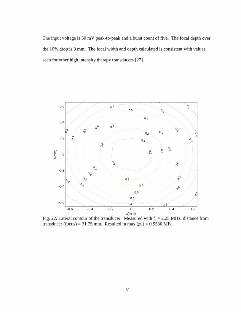
51
The input voltage is 50 mV peak-to-peak and a burst count of five. The focal depth over
the 10% drop is 3 mm. The focal width and depth calculated is consistent with values
seen for other high intensity therapy transducers [27].
Fig. 22. Lateral contour of the transducer. Measured with fc = 2.25 MHz, distance from transducer (focus) = 31.75 mm. Resulted in max (fg) = 0.5530 MPa.
0.2
0.2
0.3
0.3
0.3 0.3
0.3
0.3
0.4
0.4
0.4
0.4
0.4
0.40.4
0.5
0.5
0.5
0.5
0.5
0.5
0.6
0.6
0.6
0.6
0.6
0.7
0.7
0.7
0.7
0.70.8
0.8
0.8
0.8
0.9
0.9
0.9
x(mm)
z(m
m)
-0.6 -0.4 -0.2 0 0.2 0.4 0.6
-0.6
-0.4
-0.2
0
0.2
0.4
0.6
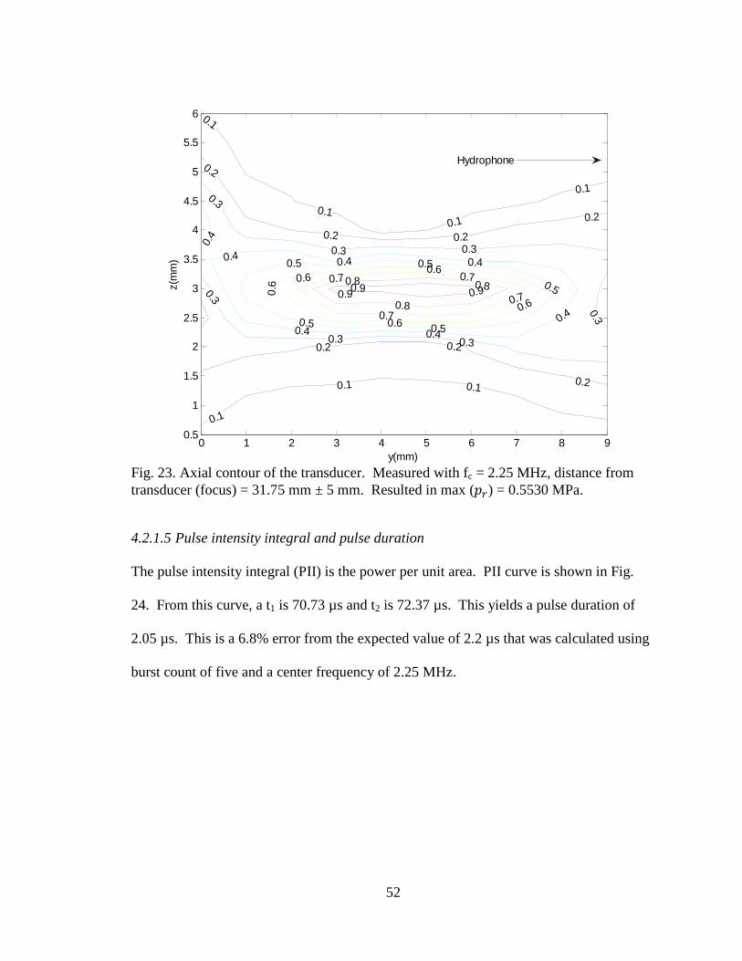
52
Fig. 23. Axial contour of the transducer. Measured with fc = 2.25 MHz, distance from transducer (focus) = 31.75 mm ± 5 mm. Resulted in max (fg) = 0.5530 MPa.
4.2.1.5 Pulse intensity integral and pulse duration
The pulse intensity integral (PII) is the power per unit area. PII curve is shown in Fig.
24. From this curve, a t1 is 70.73 µs and t2 is 72.37 µs. This yields a pulse duration of
2.05 µs. This is a 6.8% error from the expected value of 2.2 µs that was calculated using
burst count of five and a center frequency of 2.25 MHz.
0.1
0.10.1
0.1
0.1
0.1 0.1
0.2
0.2 0.2
0.2
0.2 0.2
0.2
0.3
0.3 0.3
0.3
0.3 0.3
0.3
0.4
0.4 0.4
0.4
0.40.4
0.40.5 0.5
0.5
0.50.5
0.60.6
0.6
0.6
0.6
0.7
0.7
0.7 0.70.8 0.8
0.8
0.9 0.90.9
y(mm)
z(m
m)
0 1 2 3 4 5 6 7 8 90.5
1
1.5
2
2.5
3
3.5
4
4.5
5
5.5
6
Hydrophone

53
Fig. 24. Pulse intensity integral and calculated pulse duration
4.2.1.6 Intensity values (Ispta and Isppa)
Spatial peak temporal average intensity (IWXF< is the maximum intensity occurring over
the pulse repetition period. Spatial peak pulse average intensity (IWXX< is the maximum
intensity in the beam averaged over the pulse duration [10]. The IWXF< and IWXX< values
were calculated with (17) and (18) respectively. Fig. 25 shows the Ispta on the left axis
and the Isppa on the right axis.
70 70.5 71 71.5 72 72.5 73 73.5 74
0
2
4
6
8
10
12
14
16
18
20
PII
( µJ/
cm2 )
Time ( µs )
PD 1.25 t& t+ 2.05 μs
t+↓
t&↓

54
Fig. 25. Intensity curve with Ispta and Isppa
Fig. 26 shows peak Ispta over axial and lateral dimensions (see Fig. 5). With these
plots, an estimation of acoustic power can be made by multiplying the maximum Ispta
with the 6 dB beam area. The maximum Ispta is found to be 1.15 mW/cm2. The focal
depth and width is as 4.0 mm and 0.8 mm respectively.
68 69 70 71 72 73 74 75 760
0.2
0.4
0.6
0.8
1
1.2x 10
-3
Spa
tial P
eak
Tem
pora
l Ave
rage
Inte
nsity
(W/c
m2)
68 69 70 71 72 73 74 75 760
1
2
3
4
5
Spa
tial P
eak
Pul
se A
vera
ge In
tens
ity (W
/cm2 )
Time (µs)
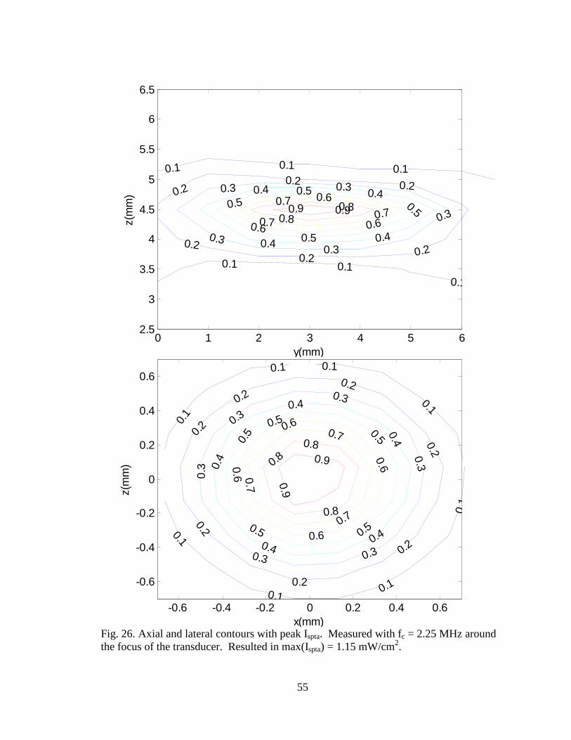
55
Fig. 26. Axial and lateral contours with peak Ispta. Measured with fc = 2.25 MHz around the focus of the transducer. Resulted in max(Ispta) = 1.15 mW/cm2.
0.1 0.1 0.1
0.1 0.10.1
0.20.2 0.2
0.20.2
0.2
0.3 0.3
0.3
0.30.3
0.4 0.4
0.40.4
0.50.5
0.5
0.5 0.6
0.60.6
0.70.7
0.70.8
0.80.90.9
y(mm)
z(m
m)
0 1 2 3 4 5 62.5
3
3.5
4
4.5
5
5.5
6
6.5
0.1
0.1
0.1
0.1
0.1
0.10.1
0.10.2
0.2
0.2
0.2
0.2
0.2
0.20.3
0.3
0.3
0.30.3
0.3
0.4
0.4
0.40.4
0.4
0.5
0.5
0.50.5
0.5
0.6
0.6
0.6
0.6
0.7
0.7
0.7
0.8
0.8
0.8 0.9
0.9
x(mm)
z(m
m)
-0.6 -0.4 -0.2 0 0.2 0.4 0.6
-0.6
-0.4
-0.2
0
0.2
0.4
0.6

56
4.2.1.7 Mechanical index
The mechanical index (MI) is a unitless value that is a measure of possible bio-effects.
The peak rarefaction pressure is seen in Fig. 21 and is used to calculate MI with (19).
The value is found to be 0.39, which is well below the limit of 1.9 limit defined by the
FDA (see Table 4).
4.2.2 Summary of Implications
Using the acoustic intensity measuring system, axial and lateral contour plots were
measured for a given therapeutic transducer. From the pulse intensity integral, the
following values were calculated from the focus for Ispta, Isppa, and MI respectively:
0.0059 W/cm2, 28.8 W/cm2, 0.39. Using Table 4, these levels are below the values for
Isppa, Ispta, and MI for diagnostic applications. This method can be used to test these
safety parameters for any transducer or pulsing scheme that proves to be useful in a drug
delivery scenario.
Tables 6-8 give a summary of the data acquired with electrical input power
measurements and acoustic intensity measurements. Table 6 shows how electrical input
power is related to input voltage and burst count over a range of values. Only values for
50 mV input voltage over 1–10 burst counts along with 20–100 mV input voltage at 5
burst counts were measured. All other values were estimated using Fig. 13 and Fig. 17.
Table 7 relates electrical input power to acoustic power assuming transducer efficiency of
90% as reported by the manufacturer and common with single element transducers [14].
Table 8 relates electrical power to peak values of the safety parameters MI, Isppa, Ispta

57
calculated at the focus. Only data for 5 burst counts at 50 mV was measured. Powers
and intensities for other burst counts was calculated based on (20) by changing the time
over which the integration was performed to the specific burst count number. The
purpose of these tables is to provide a reference for power and intensities measurements
for a given pulsing scheme. Further measurements need to be done at other input voltages
over various burst counts to obtain a comprehensive list for lookup during experimental
studies.
TABLE 6. Electrical Input Power from Power Amplifier (mW)
Input Voltage from Waveform Generator (mV)
Bur
st C
ount
20 30 40 50 60 70 80 90 100 1 0.2 0.3 0.3 0.4 0.5 0.7 0.9 1.0 1.1 2 0.7 0.8 0.9 1.1 1.3 1.5 1.8 2.1 2.3 3 0.9 1.6 2.0 2.4 3.5 5.4 7.2 8.9 10.5 4 1.1 2.0 3.5 3.5 5.4 8.1 10.5 14.2 15.5 5 1.2 2.2 4.1 5.6 8.9 10.9 12.7 17.6 22.6 6 1.8 4.4 7.2 8.1 10.5 12.5 18.5 20.6 25.0 7 2.0 5.5 10.5 11.5 12.5 15.4 19.4 22.6 28.5 8 2.7 6.6 12.5 13.6 18.4 21.0 26.7 27.4 30.6 9 3.9 8.6 15.4 17.6 22.5 22.3 28.4 31.5 35.6 10 5.4 10.5 19.2 21.6 25.4 28.4 32.5 35.4 40.1
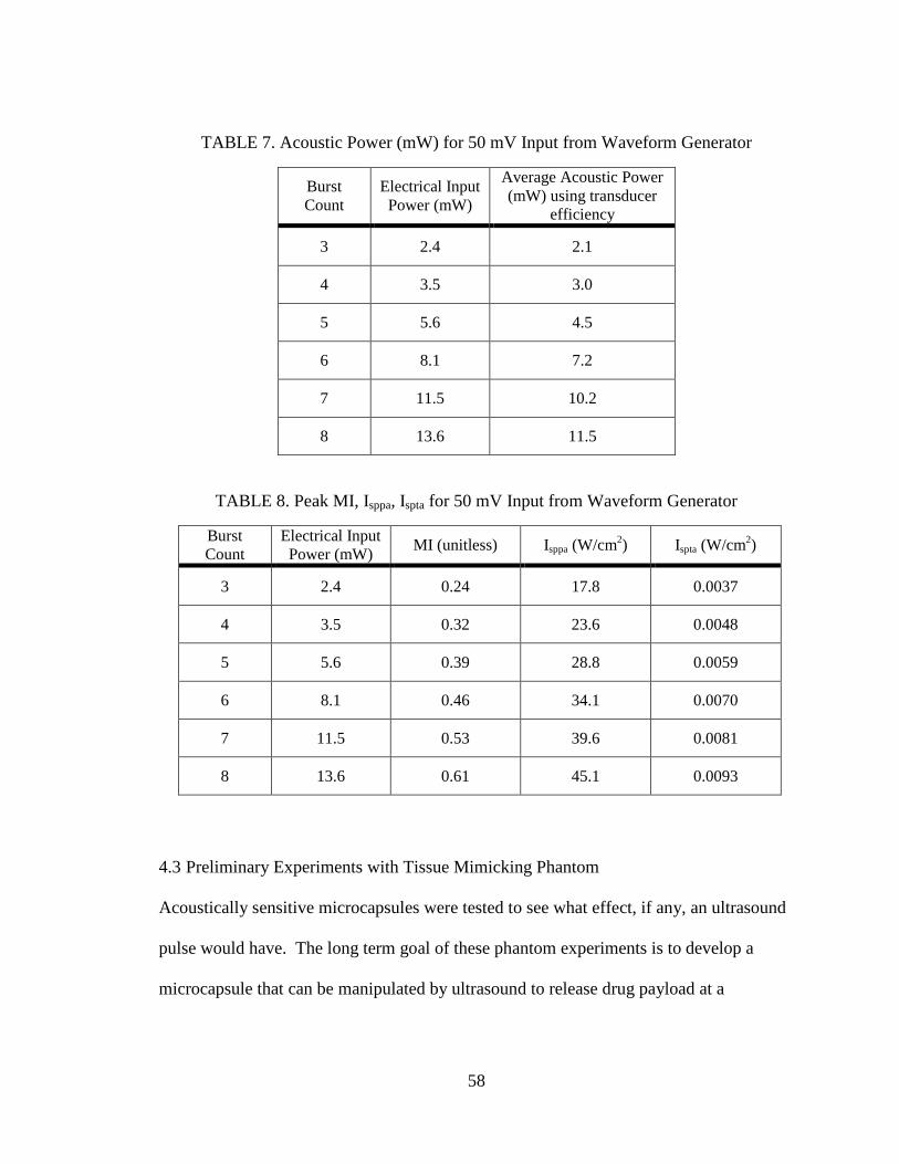
58
TABLE 7. Acoustic Power (mW) for 50 mV Input from Waveform Generator
Burst Count
Electrical Input Power (mW)
Average Acoustic Power (mW) using transducer
efficiency
3 2.4 2.1
4 3.5 3.0
5 5.6 4.5
6 8.1 7.2
7 11.5 10.2
8 13.6 11.5
TABLE 8. Peak MI, Isppa, Ispta for 50 mV Input from Waveform Generator
Burst Count
Electrical Input Power (mW)
MI (unitless) Isppa (W/cm2) Ispta (W/cm2)
3 2.4 0.24 17.8 0.0037
4 3.5 0.32 23.6 0.0048
5 5.6 0.39 28.8 0.0059
6 8.1 0.46 34.1 0.0070
7 11.5 0.53 39.6 0.0081
8 13.6 0.61 45.1 0.0093
4.3 Preliminary Experiments with Tissue Mimicking Phantom
Acoustically sensitive microcapsules were tested to see what effect, if any, an ultrasound
pulse would have. The long term goal of these phantom experiments is to develop a
microcapsule that can be manipulated by ultrasound to release drug payload at a

59
controlled rate. Microcapsules and tissue mimicking phantoms were tested under
sonication by an ultrasound pulse from a 2.25 MHz transducer and the effects were
recorded.
Two different sets of results are shown from two different dates. The same batch
of microcapsules was used in the phantom sample on both days. Fig. 27 shows a
microcapsule with surrounding gelatin. The Targesons do not appear to be visible in this
image. This is important because any effects by acoustic radiation force cannot be seen.
In Fig. 28, three different time periods are shown at the top left hand corner of this
microcapsule. The membrane of the capsule appeared to bubble after about a minute of
exposure to continuous wave 60 mV peak-to-peak input from the waveform generator.
For a continuous wave, this produces 0.57 W electrical input power into the transducer
from the arbitrary waveform generator and power amplifier. Acoustic power is 0.51 W
assuming a 90% efficiency, Ispta is 6.65 W/cm2, and MI is 0.31.
In Fig. 29 the Targesons do not appear to be visible in this image. This is important
because any effects by acoustic radiation force cannot be seen. At t = 45 s, the membrane
of the capsule appears to bulge suddenly. This bulging continued until t = 60 s when
there appeared to be a break in the membrane.
Fig. 30 shows a microcapsule that was sonicated for one minute at 65 mV input
peak-to-peak from the waveform generator. For a continuous wave, this produces 0.67
W input electrical power. Assuming 90% transducer efficiency, it produces an acoustic
power of 0.60 W, a Ispta of 8.58 W/cm2 and a mechanical index of 0.33. Four different
time periods are shown of the top right corner of this microcapsule. The oval mark on the

60
right side of the capsule gradually shrunk over one minute of sonication. Without being
able to view Targesons, it is difficult to determine what ultrasound mechanism may have
caused these changes (see section 3.3.2).
Fig. 27. Microcapsule image taken from transmission light video microscope
More than likely, the prolonged exposure to high intensity continuous wave caused
hyperthermia. These results are likely due to heat exposure because these effects were
not seen until a prolonged period. After running this experiment, neither the phantom,
the DI water, microcapsules, nor the plastic at the bottom of the stand-off were warm to
the touch.
Microcapsule
Gelatin
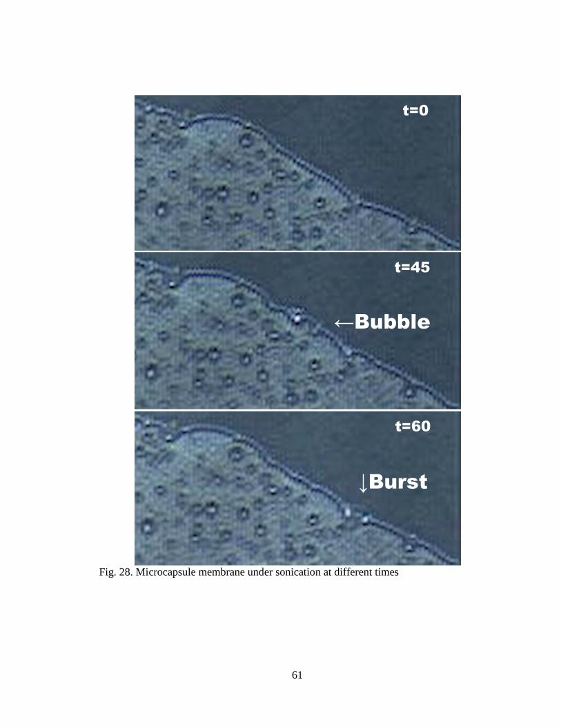
61
Fig. 28. Microcapsule membrane under sonication at different times
t=0
t=45
t=60
←Bubble
↓Burst
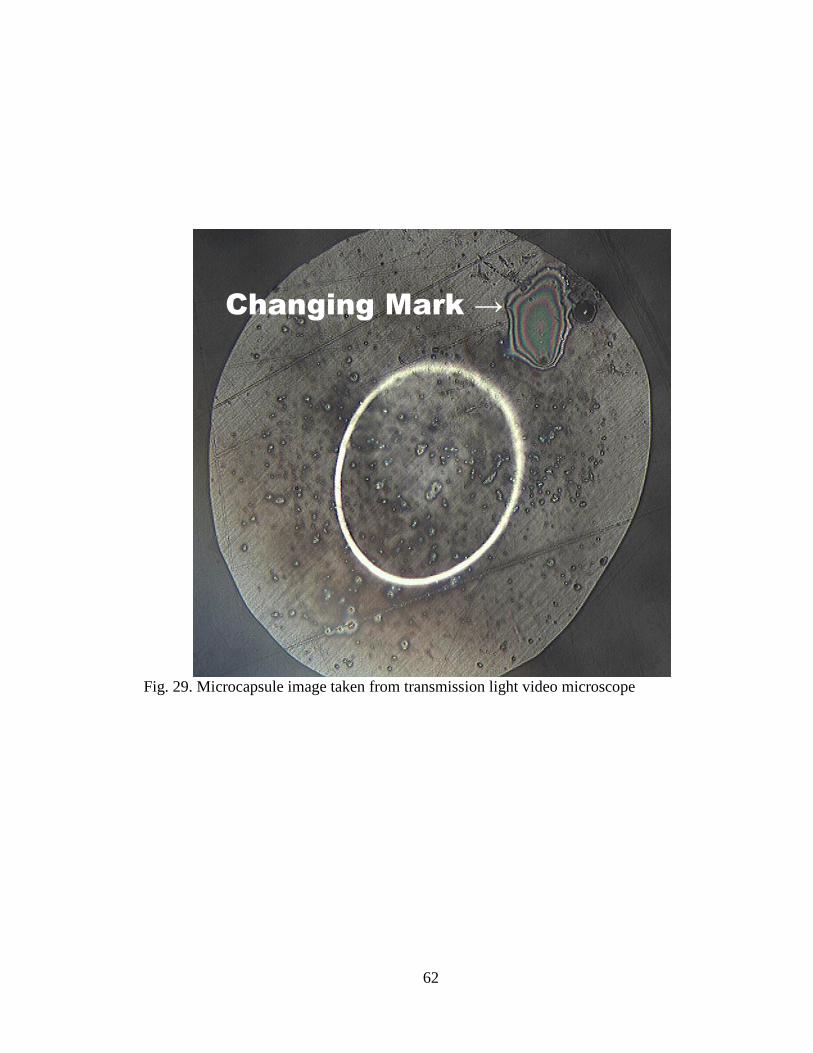
62
Fig. 29. Microcapsule image taken from transmission light video microscope
Changing Mark →
t=0 t=8

63
Fig. 30. Microcapsule membrane under sonication at different times
t=60
t=0
t=8
t=48
64
5. CONCLUSIONS AND FUTURE WORK
Multiple steps were performed to aid in the development of mass transport of drug for
cancer therapy. The electrical input power and acoustic intensity measurements provided
power and intensity information when the preliminary phantom measurement was
performed.
The RF power measurement revealed that the combination of arbitrary waveform
generator and RF power amplifier produced calibrated results corresponding to (7), the
equation relating voltage and power. The Blackman window was ideal for calculating the
power spectrum. Two different power equations, (20) and (21), were found based on
varying the burst count and varying the input voltage. These equations can be used to
calculate the electrical power input to the transducer for varying pulsing schemes in
Table 6, efficiency calculations seen in Table 7, and safety parameter measurements seen
in Table 8.
The acoustic pressure and intensity of the therapy transducer revealed contours
and values that allowed safety parameters to be calculated. A powered second harmonic
was seen at 70 µ and was expected due to irregularities in the transducer and by the
ultrasound pulse propagating though water. Measurements of center frequency, pulse
repetition frequency, and hydrophone sensitivity allowed calculations of the pulse
intensity integral. From the pulse intensity integral, the following peak values were
calculated at the focus for Ispta, Isppa, and MI respectively: 0.0059 W/cm2, 28.76 W/cm2,
0.39 for a 50 mV peak-to-peak input from the waveform generator. Using Table 4 to
compare accepted diagnostic levels, the calculated levels in this experiment are below the

65
values for Isppa, Ispta and MI. So the system serves as a vehicle tool to measure key
indices for different relevant pulsing schemes to ensure safety.
The optical measurements revealed that prolonged exposure to continuous wave
ultrasound produces visible changes in the membrane of the microcapsule. The
Targesons were not visible in the microscope images especially when combined with
gelatin. In the first experiment, the membrane appeared to bubble and burst at t=45 s and
t=60 s. In the second experiment, a mark on the microcapsule appeared to gradually
shrink over a period of one minute. These effects are possibly due to heat exposure since
they were only seen after a long ultrasound exposure.
There are many improvements that can be made in the future for these
experiments. The electrical input power measurement should be expanded to test the
efficiency of the transducer device. A radiation force balance can measure the actual
output power emitted from the transducer. The peak input power measurement in this
thesis will be compared to the radiation force balance measurements.
The acoustic measurements will be expanded to include many different pulsing
schemes as the effect of the transducer beam is seen on the microcapsules. As the lab
receives more funds, more therapy transducers and will be purchased and tested using the
same hydrophone scanning method.
The optical experimental materials and setup needs to be improved in order to
produce repeatable results. The phantom swells under exposure to water, which degrades
the quality of the microscopic image. The image gets increasingly worse over the
experimental session. Genipin can be put in the phantom material to prevent swelling.

66
Additionally, the phantom will include a coagulant so that it mimics the thermal
properties of tissue when heated above 55° C.
The stand-off and support clamp stand are not sufficient to use in positioning the
transducer over the phantom and microcapsule. In future experiments the phantom and
microcapsule will be simultaneously sonicated and imaged. This will require a new
apparatus to be designed and then built by the machinist at SJSU. The apparatus will
include two threaded sockets for the imaging and therapy transducer that are angled at
45° to the microscope plate.
A biological microscope with a depth of field of 35 mm and a high speed camera
is required to see clear effects of the ultrasound on the microcapsules. These experiments
used a metallurgical microscope which only has a depth of field of 3 mm. This makes
focusing on a microcapsule very difficult.
Work in the area of high intensity ultrasound for use in drug delivery methods
will continue within the Electrical and General Engineering departments. As seen in Fig.
1, there are multiple stages just in the development of the transport method. If this
experimental process yields positive results, further calibration and device development
will be needed.
67
REFERENCES
[1] American Cancer Society. (2009, Jun.). Breast Cancer. [Online]. Available: http://www.cancer.org/downloads/PRO/BreastCancer.pdf
[2] Centers for Disease Control and Prevention. (2010, Mar.). Breast Cancer Statistics. [Online]. Available: http://www.cdc.gov/cancer/breast/statistics/
[3] V. Frenkel, "Ultrasound mediated delivery of drugs and genes to solid tumors," Advanced Drug Delivery Reviews, vol. 60, pp. 1193-1208, 2008.
[4] R. K. Jain, "Delivery of molecular and cellular medicine to solid tumors," Advanced Drug Delivery Reviews, vol. 46, pp. 146-168, 2001.
[5] American Cancer Society. (2009, Apr.). Chemo: What It Is, How It Works. [Online]. Available: http://www.cancer.org/docroot/ETO/content/ETO_1_2X_ Chemotherapy_What_It_Is_How_It_Helps.asp
[6] S. Dromi, et al., "Pulsed-high intensity focused ultrasound and low temperature–sensitive liposomes for enhanced targeted drug delivery and antitumor effect," Clin Cancer Res., vol. 13, no. 9, pp. 2722-2727, May 2007.
[7] N. Hangiandreou, "AAPM/RSNA physics tutorial for residents: topics in US," RadioGraphics, vol. 23, pp. 1019-1033, 2003.
[8] M. Helguera. (2008). An Introduction to Ultrasound. [Online]. Available: http://www.cis.rit.edu/research/ultrasound/ultrasoundintro/ultraintro.html
[9] B. Raj, V. Rajendran, and P. Palanichamy, Science and Technology of Ultrasonics. Pangbourne, U.K.: Alpha Science International Ltd., 2007, pp. 4-26.
[10] Center for Devices and Radiological Health. “Information for manufacturers seeking marketing clearance of diagnostic ultrasound systems and transducers,” Rockville, MD, Sept. 2008.
[11] A. Shaw and G. t. Haar, "Requirements for measurement standards in high intensity focused ultrasound (HIFU) fields," Institute of Cancer Research, Teddington, NPL Report DQL AC 015, 2006.
[12] B. E. O’Neill and K. C. P. Li, "Augmentation of targeted delivery with pulsed high intensity focused ultrasound," International Journal of Hyperthermia, vol. 24, no. 4, pp. 506-520, Mar. 2008.

68
[13] Ng, Ka-yun and Liu, Yang., "Therapeutic ultrasound: its application in drug delivery." Medical Research Reviews, vol. 22, no. 2, pp. 204-223, Mar. 2002.
[14] O’Brien, William D., "Ultrasound–biophysics mechanism." Progress in Biophysics and Molecular Biology, vol. 93, pp. 212–255, Aug. 2006.
[15] Ferrara, Katherine W., "Driving delivery vehicles with ultrasound." Advanced Drug Delivery Reviews, vol. 60, pp. 1097-1102, Mar. 2008.
[16] A. V. Oppenheim, A. S. Willsky, and S. H. Nawab, Signals and Systems. 2nd ed., Beijing: Pearson Education Inc., 1997, pp. 2-19.
[17] NDT Resource Center., (2010, Mar.). Piezoelectric Transducers. [Online]. Available: http://www.ndt-ed.org/EducationResources/CommunityCollege /Ultrasonics/EquipmentTrans/piezotransducers.htm
[18] Verbeek, Xander, et al., "Measurement of the contrast agent intrinsic and native harmonic." Annals of Biomedical Engineering, vol. 27, pp. 670-681, Jul. 1999.
[19] Onda Corp., (2007, Oct.). Converting from EOC Sensitivity to Amplifier-loaded Sensitivity. [Online]. Available: http://www.ondacorp.com/images/List_HydroCalibrations.pdf
[20] D. Roveti. (2004, Mar.) Guidelines to Ultrasound Power Measurement. [Online]. http://www.24x7mag.com/issues/articles/2004-03_04.asp
[21] E. Sasaki, F. Karayuma, T. Matsuyama and H. Yamamoto “Preparation of microcapsules by electrostatic atomization.” Electrostatics, vol. 66, pp. 312-318, May 2006.
[22] Sarvazyan, Armen., "Diversity of biomedical applications of acoustic radiation force." Ultrasonics, vol. 50, pp. 230-234, Oct. 2009.
[23] M. L. Palmeri, S. A. McAleavey, G. E. Trahey, and K. R. Nightingale, "Ultrasonic tracking of acoustic radiation force-induced displacements in homogeneous media." IEEE Trans. Ultrason., Ferroelectr., Freq. Control, vol. 52, no. 7, pp. 1300-1313, Jul. 2007.
[24] R. S.Gupta, Hydrology and Hydraulic Systems. 2nd ed. Prospect Heights: Waveland Press, Inc., 2001, pp. 620-621.

69
[25] C. Coussios, et al., "Role of acoustic cavitation in the delivery and monitoring of cancer treatment by high-intensity focused ultrasound (HIFU)." International Journal of Hyperthermia, vol. 23, no. 2, pp. 105-120, Mar. 2007.
[26] J. L. Laborde, et al., "Acoustic bubble cavitation at low frequencies." Ultrasonics, vol. 36, pp. 589-594, 1998.
[27] L. Hallez, et al., "Characterization of HIFU transducers designed for sonochemistry application: cavitation distribution and quantification." Ultrasonics, vol. 50, pp. 310–317, Sept. 2010.
[28] P. Dayton, et al., "Optical and acoustical observations of the effects of ultrasound on contrast agents." IEEE Trans. Ultrason., Ferroelectr., Freq. Control, vol. 46, no. 1, pp. 220-232, Jan. 1999.
Related Documents