Acoustic Emission Study of Micro- and Macro-fracture of Large Rock Specimens Xiang-chu YIN 1,2, Huai-zhong YU 1, Ke-yin PENG 2, Victor Kukshenko 3, Zhaoyong.

Acoustic Emission Study of Micro- and Macro-fracture of Large Rock Specimens

Xiang-chu YIN1,2, Huai-zhong YU1, Ke-yin PENG2,Victor Kukshenko3, Zhaoyong XU5, Qi LI4, Meng-fen XIA1,6, Min LI1, and Surguei Elizarov 7

1, State Key Laboratory of Nonlinear Mechanics, CAS2, Center for Analysis and Prediction, China Seismological Bureau 3, Ioffe Physical Technique Institute, Russian Academy of Sciences4, Ibaraki University, Japan5, Yunnan Province Seismological Bureau, CSB6, Peking University, China7, Interunis Ltd, Moscow, Russia

Introduction

There are striking resemblances between AE

(acoustic emissions) and earthquakes.

Consequently to study the AE during the process

of micro- and macro-fracture in rock will help us

to understand the nature of earthquake.

.

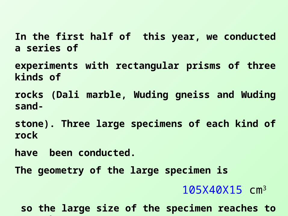
In the first half of this year, we conducted a series of

experiments with rectangular prisms of three kinds of

rocks (Dali marble, Wuding gneiss and Wuding sand-

stone). Three large specimens of each kind of rock

have been conducted.

The geometry of the large specimen is

105X40X15 cm3

so the large size of the specimen reaches to more than

1 meter

z

q

400

1050

xy

f

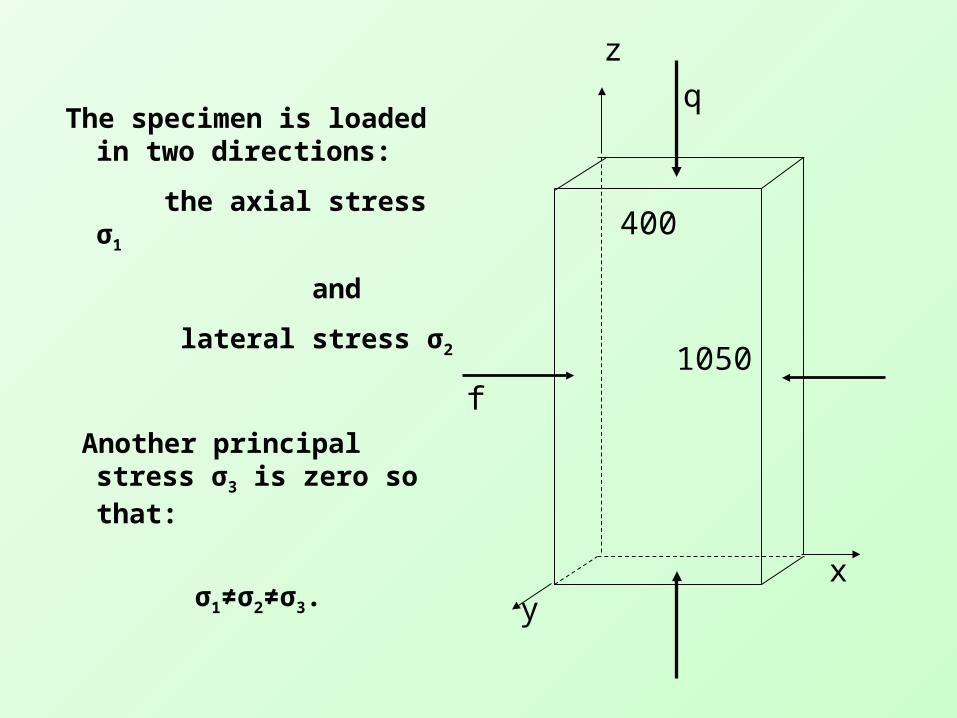
The specimen is loaded in two directions:

the axial stress σ1

and

lateral stress σ2

Another principal stress σ3 is zero so that:

σ1≠σ2≠σ3.

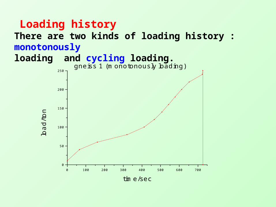
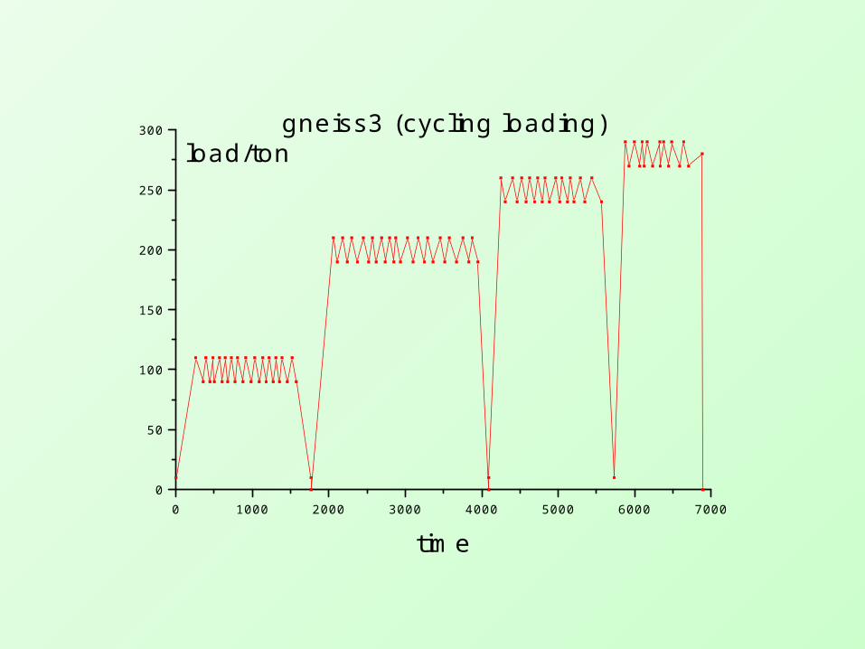
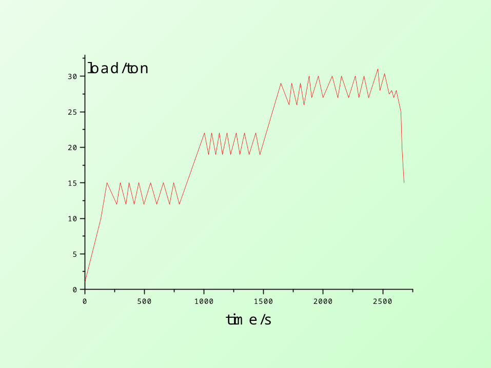
Loading history There are two kinds of loading history : monotonously loading and cycling loading.

0 100 200 300 400 500 600 7000

50

100

150

200

250gneiss 1 (monotonously loading)

load

/ton

time/sec

0 1000 2000 3000 4000 5000 6000 70000

50

100

150

200

250

300 gneiss3 (cycling loading) load/ton

time

0 500 1000 1500 2000 25000

5

10

15

20

25

30load/ton

time/s

Experiment results

At first I present the results of cycling loading. The

AE signals are recorded continuously with 《 A-line

32D---AE system》made by A.F Ioffe Physical

Technical Institute, Russian Academy of Sciences

and Interunis Ltd.

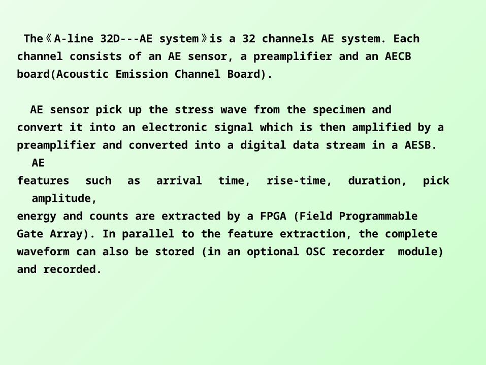
The 《 A-line 32D---AE system 》 is a 32 channels AE system.

Each

channel consists of an AE sensor, a preamplifier and an AECB

board(Acoustic Emission Channel Board).

AE sensor pick up the stress wave from the specimen and

convert it into an electronic signal which is then amplified by a

preamplifier and converted into a digital data stream in a AESB. AE

features such as arrival time, rise-time, duration, pick amplitude,

energy and counts are extracted by a FPGA (Field Programmable

Gate Array). In parallel to the feature extraction, the complete

waveform can also be stored (in an optional OSC recorder

module)

and recorded.

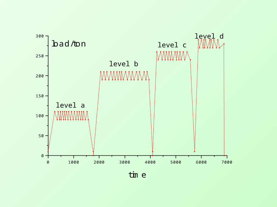
0 1000 2000 3000 4000 5000 6000 70000

50

100

150

200

250

300

load/ton

time

level a

level b

level clevel d

0 200 400 600 800 1000 1200 1400 1600 18000

200

400

600

800events per sec

time/s

0 200 400 600 800 1000 1200 1400 1600 1800

0.00E+000

1.00E+009

2.00E+009

3.00E+009

4.00E+009

5.00E+009

energy per sec

time/s

0 200 400 600 800 1000 1200 1400 16000

20

40

60

80

100

120

loading

time0 200 400 600 800 1000 1200 1400 1600

0

20

40

60

80

100

120

loading

time

Gneiss 3(a)

0 200 400 600 800 1000 1200 1400 16000

200

400

600

800

1000

events per sec

time/s

0 200 400 600 800 1000 1200 1400 1600

0.00E+000

1.00E+009

2.00E+009

3.00E+009

4.00E+009

5.00E+009

6.00E+009

energy per sec

time/s

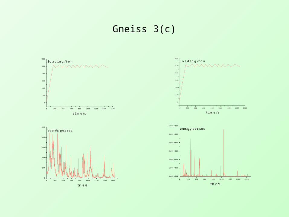
0 200 400 600 800 1000 1200 1400 1600

0

50

100

150

200

250

300

l oadi ng/t on

t i me/s

0 200 400 600 800 1000 1200 1400 1600

0

50

100

150

200

250

300

l oadi ng/t on

t i me/s

Gneiss 3(c)

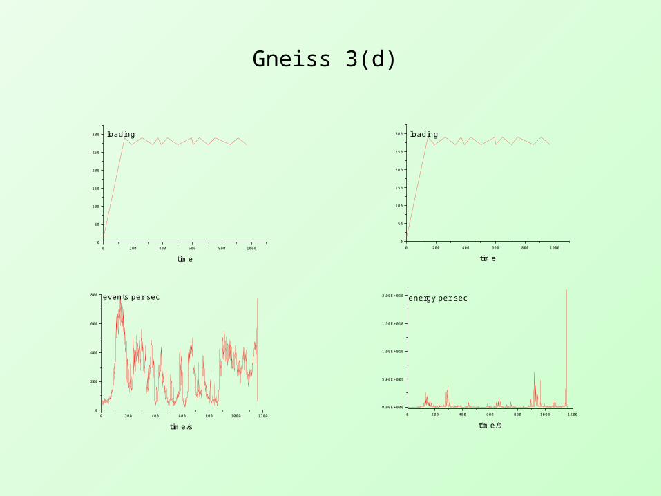
0 200 400 600 800 1000 12000

200

400

600

800 events per sec

time/s

0 200 400 600 800 1000 1200

0.00E+000

5.00E+009

1.00E+010

1.50E+010

2.00E+010 energy per sec

time/s

0 200 400 600 800 10000

50

100

150

200

250

300 loading

time

0 200 400 600 800 10000

50

100

150

200

250

300 loading

time

Gneiss 3(d)

0 1000 2000 3000 4000 5000 6000 70000

50

100

150

200

250

300

load/ton

time0 1000 2000 3000 4000 5000 6000 7000

0

50

100

150

200

250

300

load/ton

time

0 1000 2000 3000 4000 5000 6000 70000

200

400

600

800

1000

1200

events per second

time/s0 1000 2000 3000 4000 5000 6000 7000

0.00E+000

2.00E+010

energy

time/s

Gneiss 3

0 1000 2000 3000 4000 5000 6000 70000

50

100

150

200

250

300

load/ton

time0 1000 2000 3000 4000 5000 6000 7000

0

50

100

150

200

250

300

load/ton

time

0 1000 2000 3000 4000 5000 6000 70000

1000000

2000000

3000000

4000000

5000000

6000000

duration

time/s

0 1000 2000 3000 4000 5000 6000 70000

10000

20000

30000

40000

50000

60000

70000 amplitude

time/s

Gneiss 3

0 500 1000 1500 2000 25000

5

10

15

20

25

30load/ton

time/s0 500 1000 1500 2000 2500

0

5

10

15

20

25

30load/ton

time/s

0 500 1000 1500 2000 25000.00E+000

2.00E+010

4.00E+010

energy per sec

time/s0 500 1000 1500 2000 2500

0

500

1000

1500

2000 events per sec

time/s

Small gneiss 2

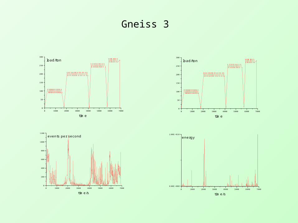
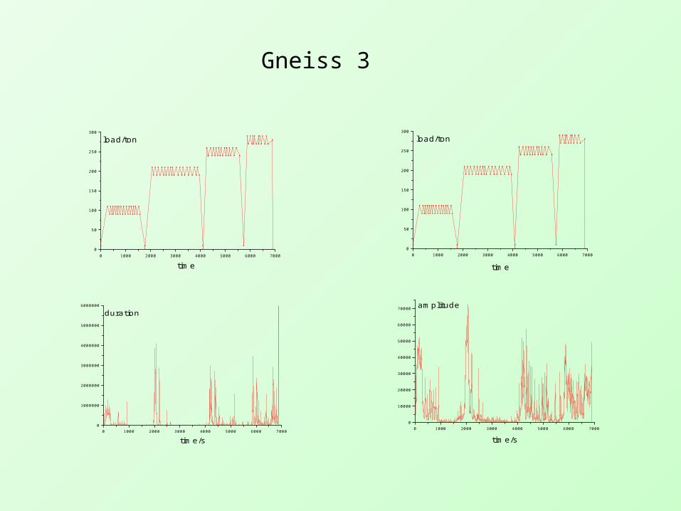
From these figures we can see the validity of Kaiser effect for rock is seriously questioned. In our cycling expe-riments, all the loading peaks are the same, but for the second and ensuing cycles their AE activity are still active,even though the activity decrease gradually with the cycle number.

Every peak of load correspond a peak of AE. The peak of AE lags behind the corresponding peak of load about a minute in order.

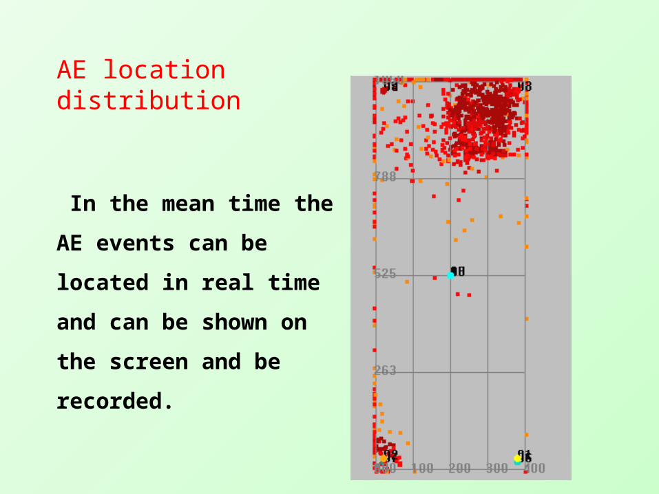
AE location distribution

In the mean time the AE

events can be located in

real time

and can be shown on the

screen and be recorded.

• LURR

• The Load-Unload Response Ratio (LURR) is defined

as

(1)

• where X+ and X- are the response rates during loadin

g and unloading according to some measure.

X

XY

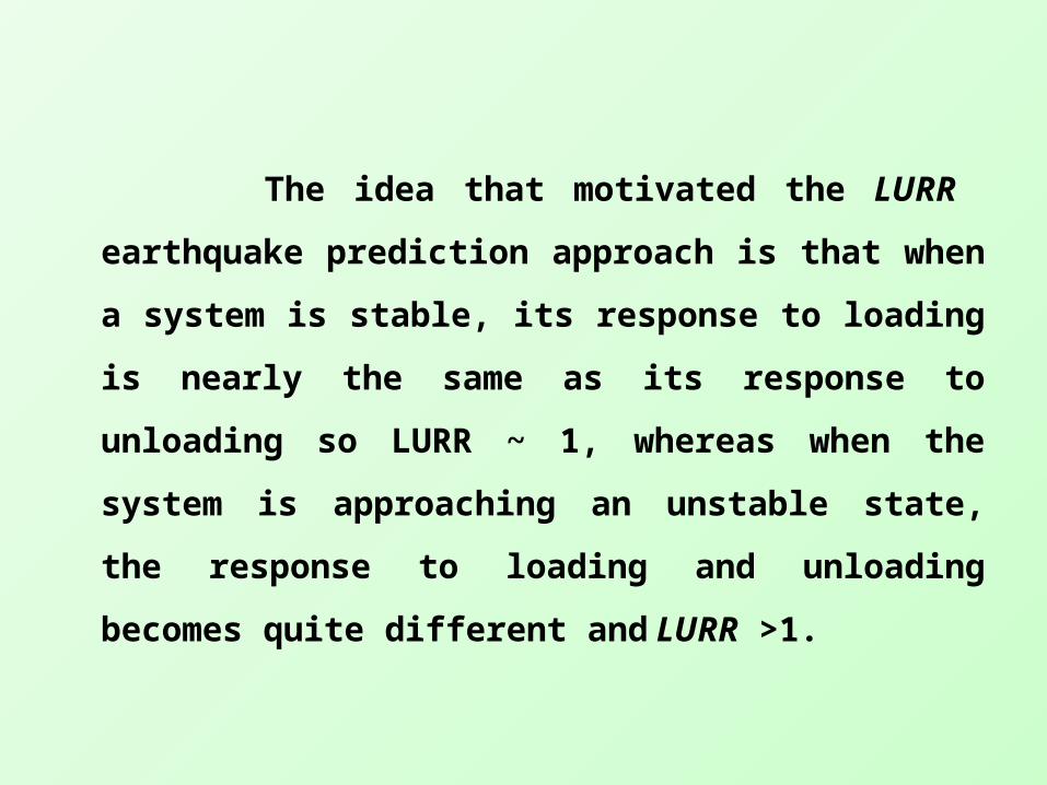
The idea that motivated the LURR earthquake

prediction approach is that when a system is stable,

its response to loading is nearly the same as its

response to unloading so LURR ~ 1, whereas when

the system is approaching an unstable state, the

response to loading and unloading becomes quite

different and LURR >1.

High LURR values (larger than unity) indicate that a r

egion is prepared for a large earthquake. In previous ye

ars, a series of successful intermediate-term prediction

s have been made for strong earthquakes in China and

other countries using the LURR (YIN and YIN, 1991; YIN, 199

3; YIN et al., 1994; YIN et al., 1995; YIN et al., 1996; YIN et al., 2000).

Usually the released seismic energy is adopted as the

“response” and then the LURR is defined as:

where E denotes seismic energy, the sign “+” means loading and

“–” means unloading, m=0 or 1/3 or1/2 or 2/3 or 1. When m=1, Em i

s exactly the energy itself; m=1/2, Em denotes the Benioff strain; m

=1/3, 2/3, Em represents the linear scale and area scale of the focal

zone respectively; m=0, Y is equal to N+/N–, and N+ and N– denote

the number of earthquake occurred during the loading and unloadi

ng duration respectively.

N

i

m

i

N

i

m

i

m

E

EY

1

1

( 2 )

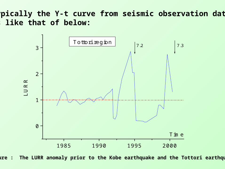
Typically the Y-t curve from seismic observation data is like that of below:

1985 1990 1995 2000

0

1

2

3 7.37.2

LU

RR

Time

Tottori region

Figure : The LURR anomaly prior to the Kobe earthquake and the Tottori earthquake.

The LURR reaches to a high value several months prior to the occurrence of the upcoming large earthquake, in the eve of the large earthquake the LURR decrease to a low level and then the large event occurs.

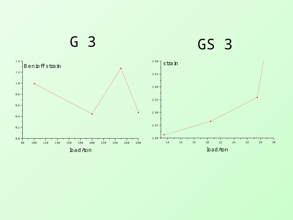
The results of LURR in this experiment are shown below. Figure * is the result for G3 (large specimen) and the Figure** is that one for specimen GS2 (small one). Both of them have the common feature that prior to the final fracture of the specimen the LURR reach to a high value , then the LURR decrease and followed by the occurrence of macrofracture. The experimental results coincide with the seismological observation very well. It seems that both the macrofracture and the earthquake have the CP (Critical Point) behavior

80 100 120 140 160 180 200 220 240 260 2800.0

0.2

0.4

0.6

0.8

1.0

1.2

1.4

Benioff strain

load/ton14 16 18 20 22 24 26 28 30

2.20

2.25

2.30

2.35

2.40

2.45

2.50 strain

load/ton

G 3 GS 3

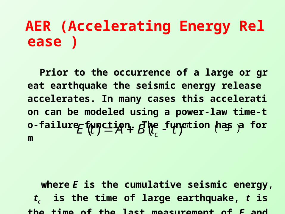
AER (Accelerating Energy Release )

Prior to the occurrence of a large or great earthquake the seismic energy release accelerates. In many cases this acceleration can be modeled using a power-law time-to-failure function. The function has a form

where E is the cumulative seismic energy, tc is the ti

me of large earthquake, t is the time of the last measurement of E and A, B and m are constants.

mc ttBAtE )()( ( 3 )

0 100 200 300 400 500 600 700 800

0.00E+000

1.00E+011

2.00E+011

3.00E+011

4.00E+011

5.00E+011

6.00E+011

7.00E+011

gneiss 2

a = 6.3996 * 1011

b = -1.1058 * 1011

m = 0.27122

en

erg

y

time/s

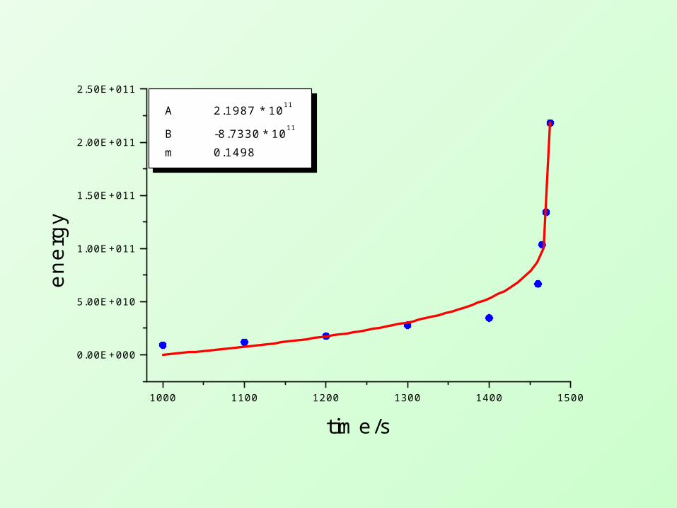
1000 1100 1200 1300 1400 1500

0.00E+000

5.00E+010

1.00E+011

1.50E+011

2.00E+011

2.50E+011

A 2.1987 * 1011

B -8.7330 * 1011

m 0.1498

ener

gy

time/s

0 200 400 600 800 1000 1200 1400 1600 1800

0.00E+000

2.00E+011

4.00E+011

6.00E+011

8.00E+011

1.00E+012sandstone 2

A 9.2822 * 1011

B -3.6316 * 1011

M 0.13848

ene

rgy

time/s

• In our experiment we focused our attention on the tempo-spacial distribution and evolution of meso-damage. We’ll analyze them in terms of the Statistical Meso-Damage Mechanics later.