Acoustic Emission Monitoring of Carbon Fibre Reinforced ...

sensors

Article

Acoustic Emission Monitoring of Carbon Fibre ReinforcedComposites with Embedded Sensors for In-SituDamage Identification

Arnaud Huijer 1,* , Christos Kassapoglou 2 and Lotfollah Pahlavan 1

�����������������

Citation: Huijer, A.; Kassapoglou, C.;

Pahlavan, L. Acoustic Emission

Monitoring of Carbon Fibre

Reinforced Composites with

Embedded Sensors for In-Situ

Damage Identification. Sensors 2021,

21, 6926. https://doi.org/10.3390/

s21206926

Academic Editor: Iren E. Kuznetsova

Received: 30 August 2021

Accepted: 12 October 2021

Published: 19 October 2021

Publisher’s Note: MDPI stays neutral

with regard to jurisdictional claims in

published maps and institutional affil-

iations.

Copyright: © 2021 by the authors.

Licensee MDPI, Basel, Switzerland.

This article is an open access article

distributed under the terms and

conditions of the Creative Commons

Attribution (CC BY) license (https://

creativecommons.org/licenses/by/

4.0/).

1 Department of Maritime and Transport Technology, Delft University of Technology,2628 CD Delft, The Netherlands; [email protected]

2 Department of Aerospace Structures and Materials, Delft University of Technology,2628 CD Delft, The Netherlands; [email protected]

* Correspondence: [email protected]

Abstract: Piezoelectric sensors can be embedded in carbon fibre-reinforced plastics (CFRP) forcontinuous measurement of acoustic emissions (AE) without the sensor being exposed or disruptinghydro- or aerodynamics. Insights into the sensitivity of the embedded sensor are essential foraccurate identification of AE sources. Embedded sensors are considered to evoke additional modesof degradation into the composite laminate, accompanied by additional AE. Hence, to monitorCFRPs with embedded sensors, identification of this type of AE is of interest. This study (i) assessesexperimentally the performance of embedded sensors for AE measurements, and (ii) investigates AEthat emanates from embedded sensor-related degradation. CFRP specimens have been manufacturedwith and without embedded sensors and tested under four-point bending. AE signals have beenrecorded by the embedded sensor and two reference surface-bonded sensors. Sensitivity of theembedded sensor has been assessed by comparing centroid frequencies of AE measured usingtwo sizes of embedded sensors. For identification of embedded sensor-induced AE, a hierarchicalclustering approach has been implemented based on waveform similarity. It has been confirmedthat both types of embedded sensors (7 mm and 20 mm diameter) can measure AE during specimendegradation and final failure. The 7 mm sensor showed higher sensitivity in the 350–450 kHzfrequency range. The 20 mm sensor and the reference surface-bounded sensors predominatelyfeatured high sensitivity in ranges of 200–300 kHz and 150–350 kHz, respectively. The clusteringprocedure revealed a type of AE that seems unique to the region of the embedded sensor when undercombined in-plane tension and out-of-plane shear stress.

Keywords: structural health monitoring; acoustic emissions; piezoelectric wafer active sensor;embedded sensors; carbon fibre reinforced plastic; waveform similarity

1. Introduction

The layered nature of fibre-reinforced plastic (FRP) materials allows the incorporationof sensors, such as piezoelectric wafer active sensors (PWAS) [1] or fibre-Bragg gratings(FBGs) [2]. Placing sensors within the structure gives the possibility of monitoring thestructure continuously without adversely affecting the hydro- or aerodynamics nor havingthe sensors exposed to harsh environments [3]. From the 1980’s [4] to present, a multitudeof applications for embedded PWAS were proposed and investigated, ranging from strainmeasurement [5,6], energy harvesting [7], vibration control [8], and excitation and mea-surement of guided waves [9–12], measurement of electromechanical impedance [13] andacoustic emissions (AE) [14,15]. The latter is the focus of the present paper for applicationto structural health monitoring (SHM).

Functioning of the embedded PWAS can be assessed through static capacitance mea-surements [16,17], impedance measurement [17] and Hsu-Nielsen tests [14]. The measure-

Sensors 2021, 21, 6926. https://doi.org/10.3390/s21206926 https://www.mdpi.com/journal/sensors

Sensors 2021, 21, 6926 2 of 19

ment of AE, when using piezoelectric sensors, is influenced by the spectral characteristicsof the sensor [18]. This influence may skew interpretations on whether certain damagemechanisms are occurring, or on the frequency content that a certain damage mechanismmay emit. For embedded PWAS, various models to simulate sensor behaviour exist [19–21].Nonetheless experimental assessment of the performance and sensitivity of the sensors forAE measurement has not been sufficiently researched and needs further development.

Embedding PWAS in a composite structure may also influence structural integrity andpossibly, damage mechanisms [10,12,16,22,23]. Ghezzo et al. [24,25] compared specimenswith and without an embedded device. AE in GFRP specimens loaded under tensionwith embedded devices were observed to have higher peak frequencies (up to 350 kHz)compared to baseline specimens (up to 180 kHz, depending on lay-up). Such signalswere attributed to debonding and matrix cracking at the embedded device location. Xiaoet al. [26] noted significant effects in AE energy and cumulative energy between CFRP spec-imens with and without embedded devices when loaded under tension. Early high-energysignals from the specimens with the embedded device were ascribed to CFRP-device in-terface delamination. This interface delamination is mentioned to cause further AE to beof relatively low energy, as compared to the energy of AE captured in baseline specimens.At the failure stage, lack of differences in the AE energy between specimens with andwithout embedded devices is associated with mutually occurring failure modes, such asfibre-breakage. The studies mentioned present case-specific results and it is uncertain towhat extent the conclusions are applicable in situations with different loading conditionsor different embedded devices. Further a method for clustering of AE signals in speci-mens with and without embedded sensors can provide a rigorous basis for assessment ofobservations, however to date it does not seem to have been reported.

Classification methods have been employed to relate AE to damage mechanisms inbaseline FRPs [27]. Typically these methods rely on seeking similarities in certain keyfeatures of the AE, such as signal rise time, energy, amplitude, counts and duration in thecase of Masmoudi et al. [14] and rise angle and average frequency in the case of Friedrichet al. [28]. In other research, in conjunction with assessment of aforementioned key features,the full waveforms are used [29]. For characterisation of damage in reinforced concretestructures, Kurz [30] and van Steen et al. [31,32] proposed clustering via similarity matrices.In such an approach, all waveforms are compared to each other using cross-correlation.Highly correlated waveforms are then clustered together. This method is well establishedin seismics to identify specific seismic emissions [33] and is expected to be greatly useful inother fields as well.

This research is aimed at providing insight into (i) qualitative assessment of theresponse of embedded piezoelectric sensors to damage-induced AE in CFRPs, and (ii)identification of clusters of AE that can be related to the possible damage induced bysensor embedment. To be able to assess these, CFRP beam specimens are manufactured byprepreg materials in three categories: no PWAS, smaller PWAS embedded, and larger PWASembedded. Experimental sensitivity assessment of the embedded sensor mainly revolvesaround mirroring the response of the small PWAS to that of the large PWAS during four-point bending of CFRP specimens up to failure. Concurrently, surface-mounted sensorsmonitored the AE behaviour in all specimens. A clustering method based on waveformsimilarity is employed to discern AE that can be related to a damage mechanism related tothe embedment of PWAS.

The manufacture of the specimens, the experimental procedure, and the clusteringmethod are explained in Section 2. Results are presented in Section 3, including obser-vations related to the characterisation of the PWAS and findings from the AE waveformclustering. Further discussions and conclusions are presented in Section 4.

Sensors 2021, 21, 6926 3 of 19

2. Materials and Methods2.1. Experimental Procedure2.1.1. Manufacturing of Specimens

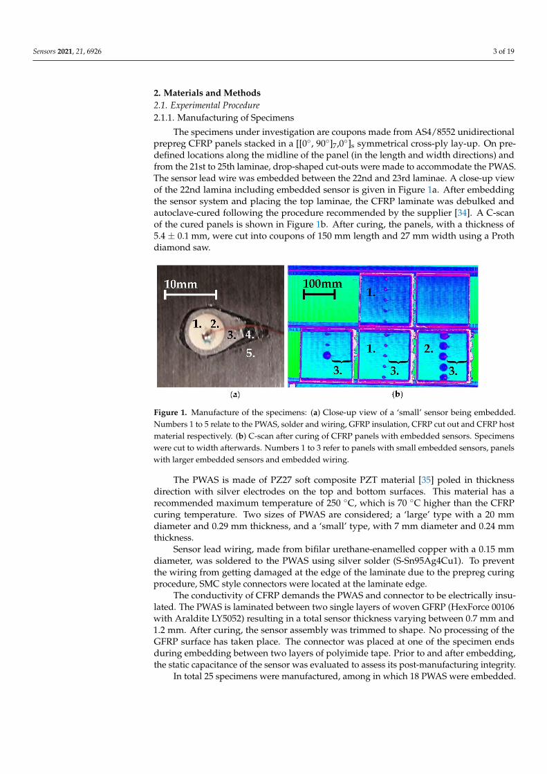
The specimens under investigation are coupons made from AS4/8552 unidirectionalprepreg CFRP panels stacked in a [[0◦, 90◦]7,0◦]s symmetrical cross-ply lay-up. On pre-defined locations along the midline of the panel (in the length and width directions) andfrom the 21st to 25th laminae, drop-shaped cut-outs were made to accommodate the PWAS.The sensor lead wire was embedded between the 22nd and 23rd laminae. A close-up viewof the 22nd lamina including embedded sensor is given in Figure 1a. After embeddingthe sensor system and placing the top laminae, the CFRP laminate was debulked andautoclave-cured following the procedure recommended by the supplier [34]. A C-scanof the cured panels is shown in Figure 1b. After curing, the panels, with a thickness of5.4 ± 0.1 mm, were cut into coupons of 150 mm length and 27 mm width using a Prothdiamond saw.

Sensors 2021, 21, 6926  3  of  19  

2. Materials and Methods 

2.1. Experimental Procedure 

2.1.1. Manufacturing of Specimens 

The specimens under investigation are coupons made from AS4/8552 unidirectional 

prepreg CFRP panels stacked in a [[0°, 90°]7,0°]s symmetrical cross‐ply lay‐up. On prede‐

fined  locations along  the midline of the panel (in the  length and width directions) and 

from  the  21st  to  25th  laminae, drop‐shaped  cut‐outs were made  to  accommodate  the 

PWAS. The sensor lead wire was embedded between the 22nd and 23rd laminae. A close‐

up view of the 22nd lamina including embedded sensor is given in Figure 1a. After em‐

bedding the sensor system and placing the top laminae, the CFRP laminate was debulked 

and autoclave‐cured  following  the procedure recommended by  the supplier  [34]. A C‐

scan of the cured panels is shown in Figure 1b. After curing, the panels, with a thickness 

of 5.4 ± 0.1 mm, were cut into coupons of 150 mm length and 27 mm width using a Proth 

diamond saw. 

Figure 1. Manufacture of  the specimens:  (a) Close‐up view of a  ‘small’ sensor being embedded. 

Numbers 1 to 5 relate to the PWAS, solder and wiring, GFRP insulation, CFRP cut out and CFRP 

host material respectively. (b) C‐scan after curing of CFRP panels with embedded sensors. Speci‐

mens were cut to width afterwards. Numbers 1 to 3 refer to panels with small embedded sensors, 

panels with larger embedded sensors and embedded wiring. 

The PWAS is made of PZ27 soft composite PZT material [35] poled in thickness di‐

rection with silver electrodes on the top and bottom surfaces. This material has a recom‐

mended maximum temperature of 250 °C, which is 70 °C higher than the CFRP curing 

temperature. Two sizes of PWAS are considered; a ‘large’ type with a 20 mm diameter 

and 0.29 mm thickness, and a ‘small’ type, with 7 mm diameter and 0.24 mm thickness. 

Sensor  lead wiring, made  from bifilar urethane‐enamelled copper with a 0.15 mm 

diameter, was soldered to the PWAS using silver solder (S‐Sn95Ag4Cu1). To prevent the 

wiring from getting damaged at the edge of the laminate due to the prepreg curing pro‐

cedure, SMC style connectors were located at the laminate edge. 

The conductivity of CFRP demands the PWAS and connector to be electrically insu‐

lated. The PWAS is laminated between two single layers of woven GFRP (HexForce 00106 

with Araldite LY5052) resulting in a total sensor thickness varying between 0.7 mm and 

1.2 mm. After curing, the sensor assembly was trimmed to shape. No processing of the 

GFRP surface has taken place. The connector was placed at one of the specimen ends dur‐

ing embedding between two layers of polyimide tape. Prior to and after embedding, the 

static capacitance of the sensor was evaluated to assess its post‐manufacturing integrity. 

In total 25 specimens were manufactured, among in which 18 PWAS were embedded. 

Figure 1. Manufacture of the specimens: (a) Close-up view of a ‘small’ sensor being embedded.Numbers 1 to 5 relate to the PWAS, solder and wiring, GFRP insulation, CFRP cut out and CFRP hostmaterial respectively. (b) C-scan after curing of CFRP panels with embedded sensors. Specimenswere cut to width afterwards. Numbers 1 to 3 refer to panels with small embedded sensors, panelswith larger embedded sensors and embedded wiring.

The PWAS is made of PZ27 soft composite PZT material [35] poled in thicknessdirection with silver electrodes on the top and bottom surfaces. This material has arecommended maximum temperature of 250 ◦C, which is 70 ◦C higher than the CFRPcuring temperature. Two sizes of PWAS are considered; a ‘large’ type with a 20 mmdiameter and 0.29 mm thickness, and a ‘small’ type, with 7 mm diameter and 0.24 mmthickness.

Sensor lead wiring, made from bifilar urethane-enamelled copper with a 0.15 mmdiameter, was soldered to the PWAS using silver solder (S-Sn95Ag4Cu1). To preventthe wiring from getting damaged at the edge of the laminate due to the prepreg curingprocedure, SMC style connectors were located at the laminate edge.

The conductivity of CFRP demands the PWAS and connector to be electrically insu-lated. The PWAS is laminated between two single layers of woven GFRP (HexForce 00106with Araldite LY5052) resulting in a total sensor thickness varying between 0.7 mm and1.2 mm. After curing, the sensor assembly was trimmed to shape. No processing of theGFRP surface has taken place. The connector was placed at one of the specimen endsduring embedding between two layers of polyimide tape. Prior to and after embedding,the static capacitance of the sensor was evaluated to assess its post-manufacturing integrity.

In total 25 specimens were manufactured, among in which 18 PWAS were embedded.

Sensors 2021, 21, 6926 4 of 19

2.1.2. Measurement Procedure

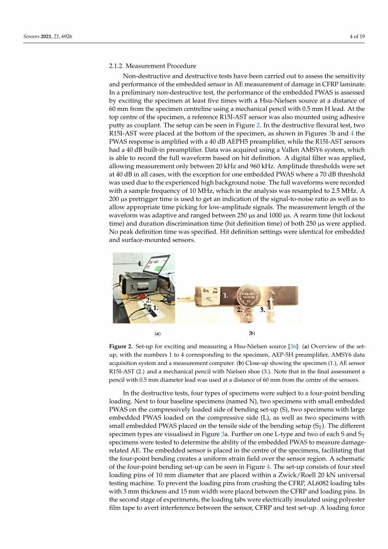
Non-destructive and destructive tests have been carried out to assess the sensitivityand performance of the embedded sensor in AE measurement of damage in CFRP laminate.In a preliminary non-destructive test, the performance of the embedded PWAS is assessedby exciting the specimen at least five times with a Hsu-Nielsen source at a distance of60 mm from the specimen centreline using a mechanical pencil with 0.5 mm H lead. At thetop centre of the specimen, a reference R15I-AST sensor was also mounted using adhesiveputty as couplant. The setup can be seen in Figure 2. In the destructive flexural test, twoR15I-AST were placed at the bottom of the specimen, as shown in Figures 3b and 4 thePWAS response is amplified with a 40 dB AEPH5 preamplifier, while the R15I-AST sensorshad a 40 dB built-in preamplifier. Data was acquired using a Vallen AMSY6 system, whichis able to record the full waveform based on hit definition. A digital filter was applied,allowing measurement only between 20 kHz and 960 kHz. Amplitude thresholds were setat 40 dB in all cases, with the exception for one embedded PWAS where a 70 dB thresholdwas used due to the experienced high background noise. The full waveforms were recordedwith a sample frequency of 10 MHz, which in the analysis was resampled to 2.5 MHz. A200 µs pretrigger time is used to get an indication of the signal-to-noise ratio as well as toallow appropriate time picking for low-amplitude signals. The measurement length of thewaveform was adaptive and ranged between 250 µs and 1000 µs. A rearm time (hit lockouttime) and duration discrimination time (hit definition time) of both 250 µs were applied.No peak definition time was specified. Hit definition settings were identical for embeddedand surface-mounted sensors.

Sensors 2021, 21, 6926  4  of  19  

2.1.2. Measurement Procedure 

Non‐destructive and destructive tests have been carried out to assess the sensitivity 

and performance of the embedded sensor in AE measurement of damage in CFRP lami‐

nate. In a preliminary non‐destructive test, the performance of the embedded PWAS  is 

assessed by exciting the specimen at least five times with a Hsu‐Nielsen source at a dis‐

tance of 60 mm from the specimen centreline using a mechanical pencil with 0.5 mm H 

lead. At the top centre of the specimen, a reference R15I‐AST sensor was also mounted 

using adhesive putty as couplant. The setup can be seen in Figure 2. In the destructive 

flexural test, two R15I‐AST were placed at the bottom of the specimen, as shown in Figures 

3b and 4 the PWAS response  is amplified with a 40 dB AEPH5 preamplifier, while the 

R15I‐AST sensors had a 40 dB built‐in preamplifier. Data was acquired using a Vallen 

AMSY6 system, which is able to record the full waveform based on hit definition. A digital 

filter was applied, allowing measurement only between 20 kHz and 960 kHz. Amplitude 

thresholds were set at 40 dB  in all cases, with  the exception  for one embedded PWAS 

where a 70 dB threshold was used due to the experienced high background noise. The full 

waveforms were recorded with a sample frequency of 10 MHz, which in the analysis was 

resampled to 2.5 MHz. A 200  μs pretrigger time is used to get an indication of the signal‐

to‐noise ratio as well as to allow appropriate time picking for low‐amplitude signals. The 

measurement length of the waveform was adaptive and ranged between 250  μs and 1000 μs. A rearm time (hit lockout time) and duration discrimination time (hit definition time) 

of both 250  μs were applied. No peak definition time was specified. Hit definition settings 

were identical for embedded and surface‐mounted sensors. 

Figure 2. Set‐up for exciting and measuring a Hsu‐Nielsen source [36]: (a) Overview of the set‐up, 

with the numbers 1 to 4 corresponding to the specimen, AEP‐5H preamplifier, AMSY6 data acqui‐

sition system and a measurement computer.  (b) Close‐up showing  the specimen  (1.), AE sensor 

R15I‐AST (2.) and a mechanical pencil with Nielsen shoe (3.). Note that in the final assessment a 

pencil with 0.5 mm diameter lead was used at a distance of 60 mm from the centre of the sensors. 

In the destructive tests, four types of specimens were subject to a four‐point bending 

loading. Next to four baseline specimens (named N), two specimens with small embedded 

PWAS on the compressively loaded side of bending set‐up (S), two specimens with large 

embedded PWAS loaded on the compressive side (L), as well as two specimens with small 

embedded PWAS placed on the tensile side of the bending setup (ST). The different spec‐

imen types are visualised in Figure 3a. Further on one L‐type and two of each S and ST 

specimens were tested to determine the ability of the embedded PWAS to measure dam‐

age‐related AE. The embedded sensor is placed in the centre of the specimens, facilitating 

that the four‐point bending creates a uniform strain field over the sensor region. A sche‐

matic of the four‐point bending set‐up can be seen in Figure 4. The set‐up consists of four 

steel loading pins of 10 mm diameter that are placed within a Zwick/Roell 20 kN universal 

testing machine. To prevent the loading pins from crushing the CFRP, AL6082 loading 

tabs with 3 mm thickness and 15 mm width were placed between the CFRP and loading 

pins. In the second stage of experiments, the loading tabs were electrically insulated using 

Figure 2. Set-up for exciting and measuring a Hsu-Nielsen source [36]: (a) Overview of the set-up, with the numbers 1 to 4 corresponding to the specimen, AEP-5H preamplifier, AMSY6 dataacquisition system and a measurement computer. (b) Close-up showing the specimen (1.), AE sensorR15I-AST (2.) and a mechanical pencil with Nielsen shoe (3.). Note that in the final assessment apencil with 0.5 mm diameter lead was used at a distance of 60 mm from the centre of the sensors.

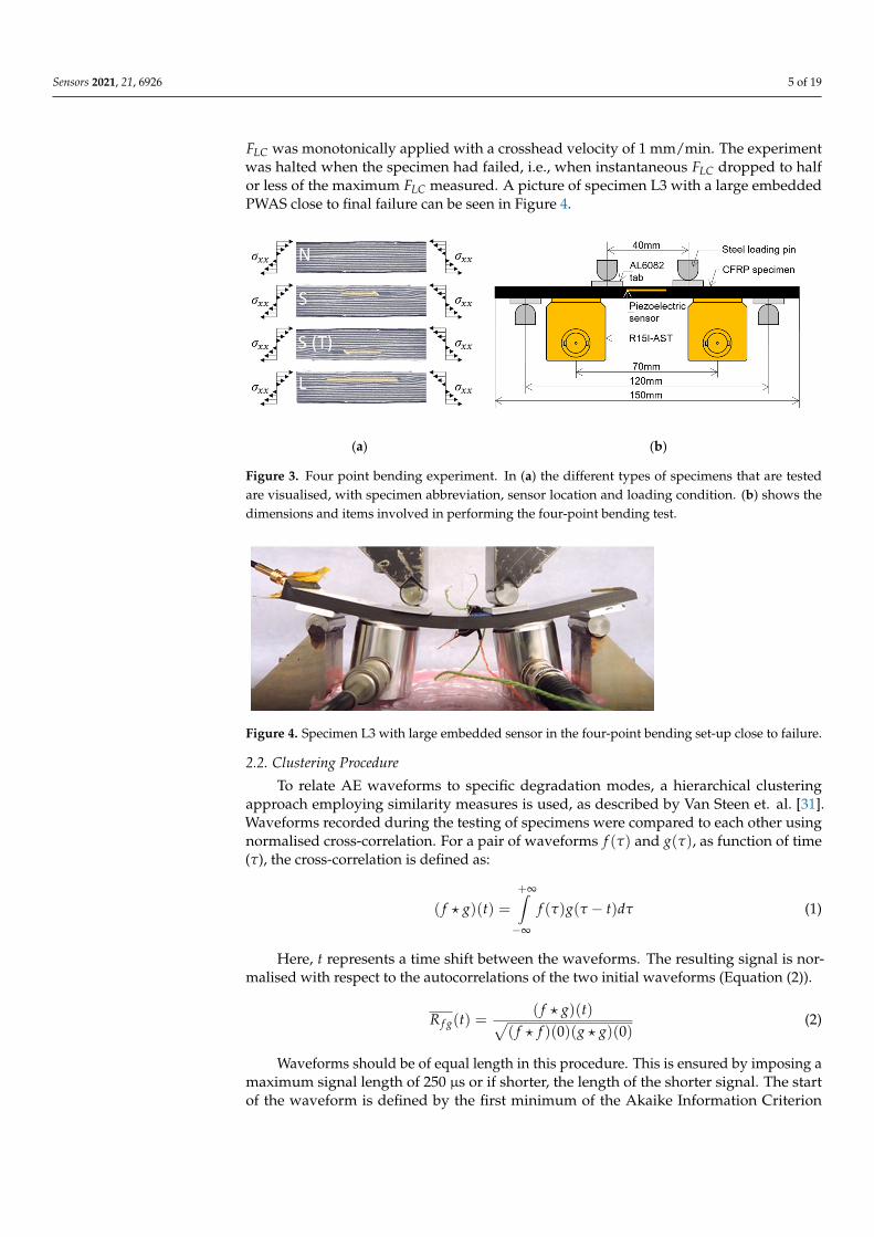
In the destructive tests, four types of specimens were subject to a four-point bendingloading. Next to four baseline specimens (named N), two specimens with small embeddedPWAS on the compressively loaded side of bending set-up (S), two specimens with largeembedded PWAS loaded on the compressive side (L), as well as two specimens withsmall embedded PWAS placed on the tensile side of the bending setup (ST). The differentspecimen types are visualised in Figure 3a. Further on one L-type and two of each S and STspecimens were tested to determine the ability of the embedded PWAS to measure damage-related AE. The embedded sensor is placed in the centre of the specimens, facilitating thatthe four-point bending creates a uniform strain field over the sensor region. A schematicof the four-point bending set-up can be seen in Figure 4. The set-up consists of four steelloading pins of 10 mm diameter that are placed within a Zwick/Roell 20 kN universaltesting machine. To prevent the loading pins from crushing the CFRP, AL6082 loading tabswith 3 mm thickness and 15 mm width were placed between the CFRP and loading pins. Inthe second stage of experiments, the loading tabs were electrically insulated using polyesterfilm tape to avert interference between the sensor, CFRP and test set-up. A loading force

Sensors 2021, 21, 6926 5 of 19

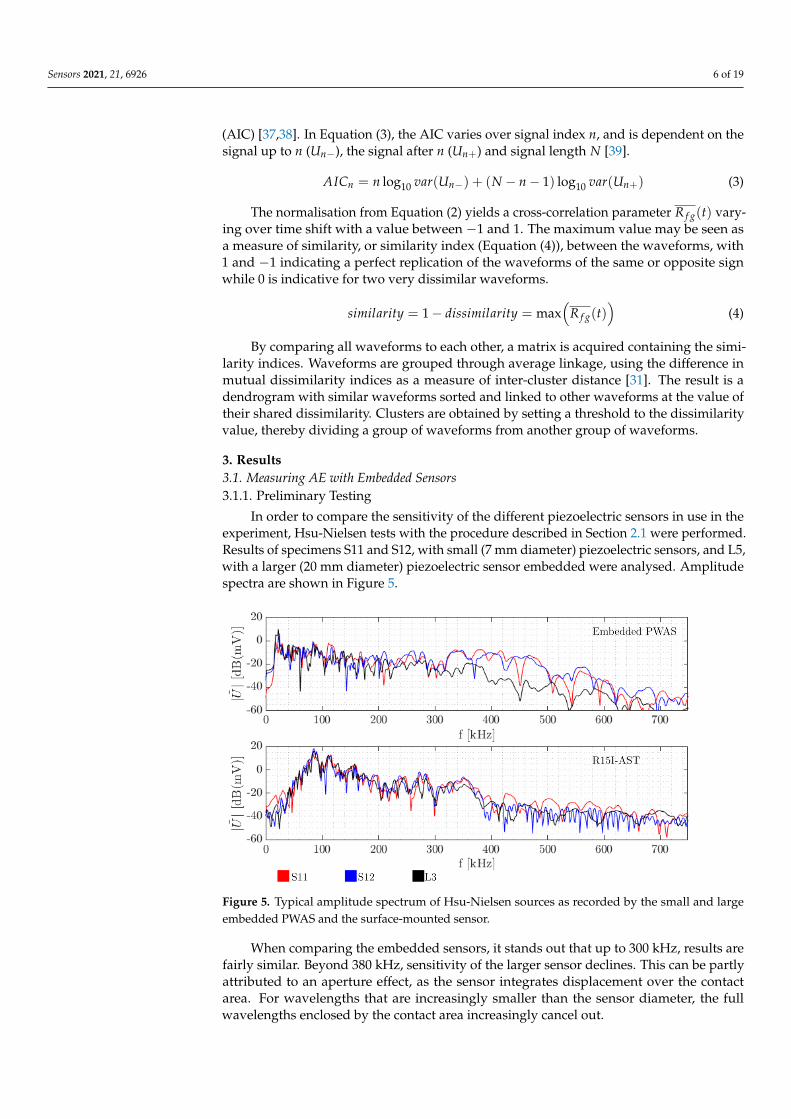
FLC was monotonically applied with a crosshead velocity of 1 mm/min. The experimentwas halted when the specimen had failed, i.e., when instantaneous FLC dropped to halfor less of the maximum FLC measured. A picture of specimen L3 with a large embeddedPWAS close to final failure can be seen in Figure 4.

Sensors 2021, 21, 6926  5  of  19  

polyester film tape to avert interference between the sensor, CFRP and test set‐up. A load‐

ing force  𝐹  was monotonically applied with a crosshead velocity of 1 mm/min. The ex‐

periment was halted when the specimen had failed, i.e., when instantaneous  𝐹   dropped 

to half or less of the maximum  𝐹  measured. A picture of specimen L3 with a large em‐

bedded PWAS close to final failure can be seen in Figure 4. 

(a)  (b) 

Figure 3. Four point bending experiment. In (a) the different types of specimens that are tested are 

visualised, with specimen abbreviation, sensor  location and  loading condition.  (b) shows  the di‐

mensions and items involved in performing the four‐point bending test. 

Figure 4. Specimen L3 with large embedded sensor in the four‐point bending set‐up close to failure. 

2.2. Clustering Procedure 

To relate AE waveforms to specific degradation modes, a hierarchical clustering ap‐

proach  employing  similarity measures  is used,  as described by Van  Steen  et.  al.  [31]. 

Waveforms recorded during the testing of specimens were compared to each other using 

normalised cross‐correlation. For a pair of waveforms  𝑓 𝜏   and  𝑔 𝜏 , as function of time 

(𝜏), the cross‐correlation is defined as: 

𝑓 ⋆ 𝑔 𝑡 𝑓 𝜏 𝑔 𝜏 𝑡 𝑑𝜏  (1)

Here,  𝑡  represents a time shift between the waveforms. The resulting signal is nor‐

malised with respect to the autocorrelations of the two initial waveforms (Equation (2)). 

𝑅 𝑡𝑓 ⋆ 𝑔 𝑡

𝑓 ⋆ 𝑓 0 𝑔 ⋆ 𝑔 0   (2)

Waveforms should be of equal length in this procedure. This is ensured by imposing 

a maximum signal length of 250  μs or if shorter, the length of the shorter signal. The start of  the waveform  is defined by  the  first minimum of  the Akaike  Information Criterion 

(AIC) [37,38]. In Equation (3), the AIC varies over signal index  𝑛, and is dependent on the signal up to  𝑛  (𝑈 ), the signal after  𝑛  (𝑈 ) and signal length 𝑁  [39]. 

Figure 3. Four point bending experiment. In (a) the different types of specimens that are testedare visualised, with specimen abbreviation, sensor location and loading condition. (b) shows thedimensions and items involved in performing the four-point bending test.

Sensors 2021, 21, 6926  5  of  19  

polyester film tape to avert interference between the sensor, CFRP and test set‐up. A load‐

ing force  𝐹  was monotonically applied with a crosshead velocity of 1 mm/min. The ex‐

periment was halted when the specimen had failed, i.e., when instantaneous  𝐹   dropped 

to half or less of the maximum  𝐹  measured. A picture of specimen L3 with a large em‐

bedded PWAS close to final failure can be seen in Figure 4. 

(a)  (b) 

Figure 3. Four point bending experiment. In (a) the different types of specimens that are tested are 

visualised, with specimen abbreviation, sensor  location and  loading condition.  (b) shows  the di‐

mensions and items involved in performing the four‐point bending test. 

Figure 4. Specimen L3 with large embedded sensor in the four‐point bending set‐up close to failure. 

2.2. Clustering Procedure 

To relate AE waveforms to specific degradation modes, a hierarchical clustering ap‐

proach  employing  similarity measures  is used,  as described by Van  Steen  et.  al.  [31]. 

Waveforms recorded during the testing of specimens were compared to each other using 

normalised cross‐correlation. For a pair of waveforms  𝑓 𝜏   and  𝑔 𝜏 , as function of time 

(𝜏), the cross‐correlation is defined as: 

𝑓 ⋆ 𝑔 𝑡 𝑓 𝜏 𝑔 𝜏 𝑡 𝑑𝜏  (1)

Here,  𝑡  represents a time shift between the waveforms. The resulting signal is nor‐

malised with respect to the autocorrelations of the two initial waveforms (Equation (2)). 

𝑅 𝑡𝑓 ⋆ 𝑔 𝑡

𝑓 ⋆ 𝑓 0 𝑔 ⋆ 𝑔 0   (2)

Waveforms should be of equal length in this procedure. This is ensured by imposing 

a maximum signal length of 250  μs or if shorter, the length of the shorter signal. The start of  the waveform  is defined by  the  first minimum of  the Akaike  Information Criterion 

(AIC) [37,38]. In Equation (3), the AIC varies over signal index  𝑛, and is dependent on the signal up to  𝑛  (𝑈 ), the signal after  𝑛  (𝑈 ) and signal length 𝑁  [39]. 

Figure 4. Specimen L3 with large embedded sensor in the four-point bending set-up close to failure.

2.2. Clustering Procedure

To relate AE waveforms to specific degradation modes, a hierarchical clusteringapproach employing similarity measures is used, as described by Van Steen et. al. [31].Waveforms recorded during the testing of specimens were compared to each other usingnormalised cross-correlation. For a pair of waveforms f (τ) and g(τ), as function of time(τ), the cross-correlation is defined as:

( f ? g)(t) =+∞∫

−∞

f (τ)g(τ − t)dτ (1)

Here, t represents a time shift between the waveforms. The resulting signal is nor-malised with respect to the autocorrelations of the two initial waveforms (Equation (2)).

R f g(t) =( f ? g)(t)√

( f ? f )(0)(g ? g)(0)(2)

Waveforms should be of equal length in this procedure. This is ensured by imposing amaximum signal length of 250 µs or if shorter, the length of the shorter signal. The startof the waveform is defined by the first minimum of the Akaike Information Criterion

Sensors 2021, 21, 6926 6 of 19

(AIC) [37,38]. In Equation (3), the AIC varies over signal index n, and is dependent on thesignal up to n (Un−), the signal after n (Un+) and signal length N [39].

AICn = n log10 var(Un−) + (N − n − 1) log10 var(Un+) (3)

The normalisation from Equation (2) yields a cross-correlation parameter R f g(t) vary-ing over time shift with a value between −1 and 1. The maximum value may be seen asa measure of similarity, or similarity index (Equation (4)), between the waveforms, with1 and −1 indicating a perfect replication of the waveforms of the same or opposite signwhile 0 is indicative for two very dissimilar waveforms.

similarity = 1 − dissimilarity = max(

R f g(t))

(4)

By comparing all waveforms to each other, a matrix is acquired containing the simi-larity indices. Waveforms are grouped through average linkage, using the difference inmutual dissimilarity indices as a measure of inter-cluster distance [31]. The result is adendrogram with similar waveforms sorted and linked to other waveforms at the value oftheir shared dissimilarity. Clusters are obtained by setting a threshold to the dissimilarityvalue, thereby dividing a group of waveforms from another group of waveforms.

3. Results3.1. Measuring AE with Embedded Sensors3.1.1. Preliminary Testing

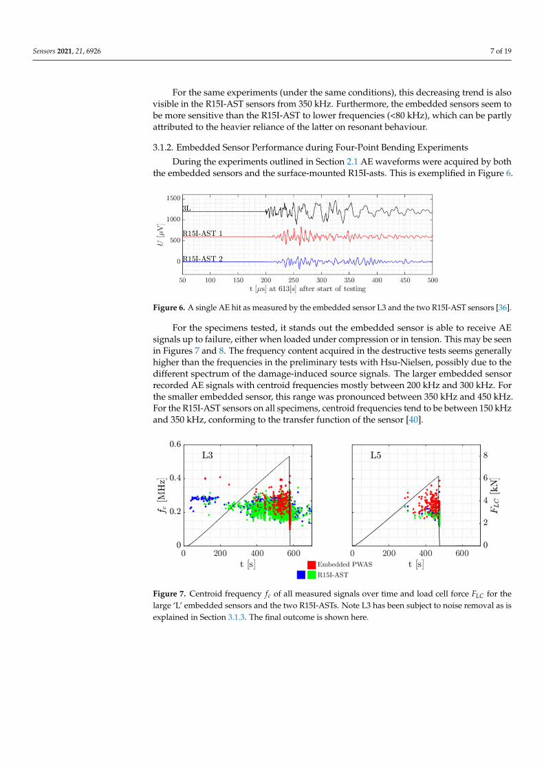
In order to compare the sensitivity of the different piezoelectric sensors in use in theexperiment, Hsu-Nielsen tests with the procedure described in Section 2.1 were performed.Results of specimens S11 and S12, with small (7 mm diameter) piezoelectric sensors, and L5,with a larger (20 mm diameter) piezoelectric sensor embedded were analysed. Amplitudespectra are shown in Figure 5.

Sensors 2021, 21, 6926  6  of  19  

𝐴𝐼𝐶 𝑛 log 𝑣𝑎𝑟 𝑈 𝑁 𝑛 1 log 𝑣𝑎𝑟 𝑈   (3)

The  normalisation  from  Equation  (2)  yields  a  cross‐correlation  parameter  𝑅 𝑡  varying over time shift with a value between −1 and 1. The maximum value may be seen 

as a measure of similarity, or similarity index (Equation (4)), between the waveforms, with 

1 and −1 indicating a perfect replication of the waveforms of the same or opposite sign 

while 0 is indicative for two very dissimilar waveforms. 

𝑠𝑖𝑚𝑖𝑙𝑎𝑟𝑖𝑡𝑦 1 𝑑𝑖𝑠𝑠𝑖𝑚𝑖𝑙𝑎𝑟𝑖𝑡𝑦 max 𝑅 𝑡   (4)

By comparing all waveforms to each other, a matrix is acquired containing the simi‐

larity indices. Waveforms are grouped through average linkage, using the difference in 

mutual dissimilarity indices as a measure of inter‐cluster distance [31]. The result is a den‐

drogram with similar waveforms sorted and linked to other waveforms at the value of 

their shared dissimilarity. Clusters are obtained by setting a threshold to the dissimilarity 

value, thereby dividing a group of waveforms from another group of waveforms. 

3. Results 

3.1. Measuring AE with Embedded Sensors 

3.1.1. Preliminary Testing 

In order to compare the sensitivity of the different piezoelectric sensors in use in the 

experiment, Hsu‐Nielsen  tests with  the  procedure  described  in  Section  2.1 were  per‐

formed. Results of specimens S11 and S12, with small (7 mm diameter) piezoelectric sen‐

sors, and L5, with a larger (20 mm diameter) piezoelectric sensor embedded were ana‐

lysed. Amplitude spectra are shown in Figure 5. 

Figure 5. Typical amplitude spectrum of Hsu‐Nielsen sources as recorded by the small and large 

embedded PWAS and the surface‐mounted sensor. 

When comparing the embedded sensors, it stands out that up to 300 kHz, results are 

fairly similar. Beyond 380 kHz, sensitivity of the larger sensor declines. This can be partly 

attributed  to an aperture effect, as  the sensor  integrates displacement over  the contact 

area. For wavelengths  that  are  increasingly  smaller  than  the  sensor diameter,  the  full 

wavelengths enclosed by the contact area increasingly cancel out. 

For the same experiments (under the same conditions), this decreasing trend is also 

visible in the R15I‐AST sensors from 350 kHz. Furthermore, the embedded sensors seem 

to be more sensitive than the R15I‐AST to lower frequencies (<80 kHz), which can be partly 

attributed to the heavier reliance of the latter on resonant behaviour. 

Figure 5. Typical amplitude spectrum of Hsu-Nielsen sources as recorded by the small and largeembedded PWAS and the surface-mounted sensor.

When comparing the embedded sensors, it stands out that up to 300 kHz, results arefairly similar. Beyond 380 kHz, sensitivity of the larger sensor declines. This can be partlyattributed to an aperture effect, as the sensor integrates displacement over the contactarea. For wavelengths that are increasingly smaller than the sensor diameter, the fullwavelengths enclosed by the contact area increasingly cancel out.

Sensors 2021, 21, 6926 7 of 19

For the same experiments (under the same conditions), this decreasing trend is alsovisible in the R15I-AST sensors from 350 kHz. Furthermore, the embedded sensors seem tobe more sensitive than the R15I-AST to lower frequencies (<80 kHz), which can be partlyattributed to the heavier reliance of the latter on resonant behaviour.

3.1.2. Embedded Sensor Performance during Four-Point Bending Experiments

During the experiments outlined in Section 2.1 AE waveforms were acquired by boththe embedded sensors and the surface-mounted R15I-asts. This is exemplified in Figure 6.

Sensors 2021, 21, 6926  7  of  19  

3.1.2. Embedded Sensor Performance during Four‐Point Bending Experiments 

During the experiments outlined in Section 2.1 AE waveforms were acquired by both 

the embedded sensors and the surface‐mounted R15I‐asts. This is exemplified in Figure 6. 

Figure 6. A single AE hit as measured by the embedded sensor L3 and the two R15I‐AST sensors 

[36]. 

For  the specimens  tested,  it stands out  the embedded sensor  is able  to receive AE 

signals up to failure, either when loaded under compression or in tension. This may be 

seen  in Figures 7 and 8. The  frequency content acquired  in  the destructive  tests seems 

generally higher than the frequencies in the preliminary tests with Hsu‐Nielsen, possibly 

due to the different spectrum of the damage‐induced source signals. The larger embedded 

sensor recorded AE signals with centroid frequencies mostly between 200 kHz and 300 

kHz. For the smaller embedded sensor, this range was pronounced between 350 kHz and 

450 kHz. For the R15I‐AST sensors on all specimens, centroid frequencies tend to be be‐

tween 150 kHz and 350 kHz, conforming to the transfer function of the sensor [40]. 

Figure 7. Centroid frequency  𝑓   of all measured signals over time and load cell force  𝐹   for 

the large ‘L’ embedded sensors and the two R15I‐ASTs. Note L3 has been subject to noise re‐

moval as is explained in Section 3.1.3. The final outcome is shown here. 

Figure 8. Centroid frequency  𝑓   of all measured signals over time and load cell force  𝐹   for the 

small ‘S’ and ‘ST’ embedded sensors and the two R15I‐ASTs. 

Figure 6. A single AE hit as measured by the embedded sensor L3 and the two R15I-AST sensors [36].

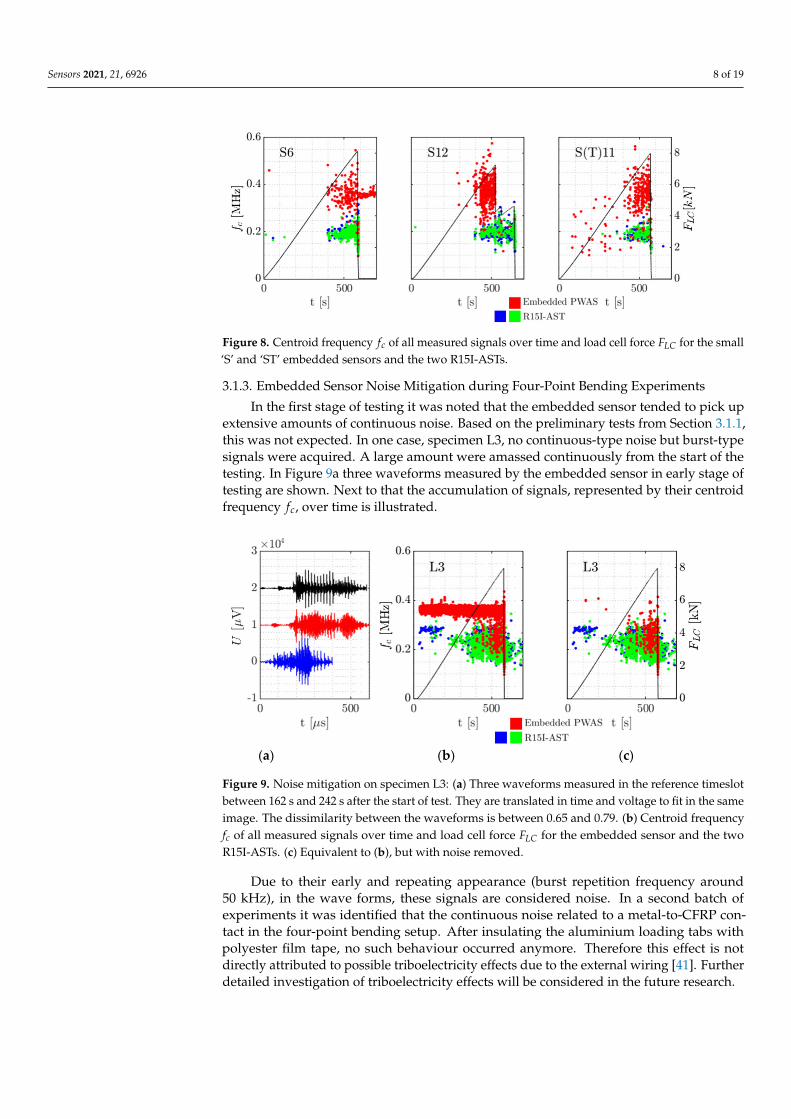
For the specimens tested, it stands out the embedded sensor is able to receive AEsignals up to failure, either when loaded under compression or in tension. This may be seenin Figures 7 and 8. The frequency content acquired in the destructive tests seems generallyhigher than the frequencies in the preliminary tests with Hsu-Nielsen, possibly due to thedifferent spectrum of the damage-induced source signals. The larger embedded sensorrecorded AE signals with centroid frequencies mostly between 200 kHz and 300 kHz. Forthe smaller embedded sensor, this range was pronounced between 350 kHz and 450 kHz.For the R15I-AST sensors on all specimens, centroid frequencies tend to be between 150 kHzand 350 kHz, conforming to the transfer function of the sensor [40].

Sensors 2021, 21, 6926  7  of  19  

3.1.2. Embedded Sensor Performance during Four‐Point Bending Experiments 

During the experiments outlined in Section 2.1 AE waveforms were acquired by both 

the embedded sensors and the surface‐mounted R15I‐asts. This is exemplified in Figure 6. 

Figure 6. A single AE hit as measured by the embedded sensor L3 and the two R15I‐AST sensors 

[36]. 

For  the specimens  tested,  it stands out  the embedded sensor  is able  to receive AE 

signals up to failure, either when loaded under compression or in tension. This may be 

seen  in Figures 7 and 8. The  frequency content acquired  in  the destructive  tests seems 

generally higher than the frequencies in the preliminary tests with Hsu‐Nielsen, possibly 

due to the different spectrum of the damage‐induced source signals. The larger embedded 

sensor recorded AE signals with centroid frequencies mostly between 200 kHz and 300 

kHz. For the smaller embedded sensor, this range was pronounced between 350 kHz and 

450 kHz. For the R15I‐AST sensors on all specimens, centroid frequencies tend to be be‐

tween 150 kHz and 350 kHz, conforming to the transfer function of the sensor [40]. 

Figure 7. Centroid frequency  𝑓   of all measured signals over time and load cell force  𝐹   for 

the large ‘L’ embedded sensors and the two R15I‐ASTs. Note L3 has been subject to noise re‐

moval as is explained in Section 3.1.3. The final outcome is shown here. 

Figure 8. Centroid frequency  𝑓   of all measured signals over time and load cell force  𝐹   for the 

small ‘S’ and ‘ST’ embedded sensors and the two R15I‐ASTs. 

Figure 7. Centroid frequency fc of all measured signals over time and load cell force FLC for thelarge ‘L’ embedded sensors and the two R15I-ASTs. Note L3 has been subject to noise removal as isexplained in Section 3.1.3. The final outcome is shown here.

Sensors 2021, 21, 6926 8 of 19

Sensors 2021, 21, 6926  7  of  19  

3.1.2. Embedded Sensor Performance during Four‐Point Bending Experiments 

During the experiments outlined in Section 2.1 AE waveforms were acquired by both 

the embedded sensors and the surface‐mounted R15I‐asts. This is exemplified in Figure 6. 

Figure 6. A single AE hit as measured by the embedded sensor L3 and the two R15I‐AST sensors 

[36]. 

For  the specimens  tested,  it stands out  the embedded sensor  is able  to receive AE 

signals up to failure, either when loaded under compression or in tension. This may be 

seen  in Figures 7 and 8. The  frequency content acquired  in  the destructive  tests seems 

generally higher than the frequencies in the preliminary tests with Hsu‐Nielsen, possibly 

due to the different spectrum of the damage‐induced source signals. The larger embedded 

sensor recorded AE signals with centroid frequencies mostly between 200 kHz and 300 

kHz. For the smaller embedded sensor, this range was pronounced between 350 kHz and 

450 kHz. For the R15I‐AST sensors on all specimens, centroid frequencies tend to be be‐

tween 150 kHz and 350 kHz, conforming to the transfer function of the sensor [40]. 

Figure 7. Centroid frequency  𝑓   of all measured signals over time and load cell force  𝐹   for 

the large ‘L’ embedded sensors and the two R15I‐ASTs. Note L3 has been subject to noise re‐

moval as is explained in Section 3.1.3. The final outcome is shown here. 

Figure 8. Centroid frequency  𝑓   of all measured signals over time and load cell force  𝐹   for the 

small ‘S’ and ‘ST’ embedded sensors and the two R15I‐ASTs. Figure 8. Centroid frequency fc of all measured signals over time and load cell force FLC for the small‘S’ and ‘ST’ embedded sensors and the two R15I-ASTs.

3.1.3. Embedded Sensor Noise Mitigation during Four-Point Bending Experiments

In the first stage of testing it was noted that the embedded sensor tended to pick upextensive amounts of continuous noise. Based on the preliminary tests from Section 3.1.1,this was not expected. In one case, specimen L3, no continuous-type noise but burst-typesignals were acquired. A large amount were amassed continuously from the start of thetesting. In Figure 9a three waveforms measured by the embedded sensor in early stage oftesting are shown. Next to that the accumulation of signals, represented by their centroidfrequency fc, over time is illustrated.

Sensors 2021, 21, 6926  8  of  19  

3.1.3. Embedded Sensor Noise Mitigation during Four‐Point Bending Experiments 

In the first stage of testing it was noted that the embedded sensor tended to pick up 

extensive amounts of continuous noise. Based on the preliminary tests from Section 3.1.1, 

this was not expected. In one case, specimen L3, no continuous‐type noise but burst‐type 

signals were acquired. A large amount were amassed continuously from the start of the 

testing. In Figure 9a three waveforms measured by the embedded sensor in early stage of 

testing are shown. Next to that the accumulation of signals, represented by their centroid 

frequency  𝑓 , over time is illustrated. 

 (a)  (b)  (c) 

Figure 9. Noise mitigation on specimen L3: (a) Three waveforms measured in the reference timeslot 

between 162 s and 242 s after the start of test. They are translated in time and voltage to fit in the 

same image. The dissimilarity between the waveforms is between 0.65 and 0.79. (b) Centroid fre‐

quency  𝑓   of all measured signals over time and load cell force  𝐹   for the embedded sensor and 

the two R15I‐ASTs. (c) Equivalent to (b), but with noise removed. 

Due to their early and repeating appearance (burst repetition frequency around 50 

kHz), in the wave forms, these signals are considered noise. In a second batch of experi‐

ments it was identified that the continuous noise related to a metal‐to‐CFRP contact in the 

four‐point bending setup. After insulating the aluminium loading tabs with polyester film 

tape, no such behaviour occurred anymore. Therefore this effect is not directly attributed 

to possible triboelectricity effects due to the external wiring [41]. Further detailed investi‐

gation of triboelectricity effects will be considered in the future research. 

Measures were taken to prevent the noise from interfering with the analysis. In as‐

sessing the performance and features of the embedded AE sensor, a waveform similarity 

approach as described in Section 2.2 is utilised to distinguish signals of interest from noise. 

For specimen L3, a total of 598 waveforms measured by  the embedded sensor be‐

tween 162 s and 242 s after the start of loading were used as a reference and compared to 

all 3939 waveforms from the embedded sensor. The resulting similarity matrix with the 

waveforms in chronological order is shown in Figure 10. 

Figure 10. Similarity matrix with reference ‘noise’ waveforms correlated with the rest of data. 

Note the faint diagonal line between  𝑗  = 800 to  𝑗  = 1300, indicating autocorrelation. 

Figure 9. Noise mitigation on specimen L3: (a) Three waveforms measured in the reference timeslotbetween 162 s and 242 s after the start of test. They are translated in time and voltage to fit in the sameimage. The dissimilarity between the waveforms is between 0.65 and 0.79. (b) Centroid frequencyfc of all measured signals over time and load cell force FLC for the embedded sensor and the twoR15I-ASTs. (c) Equivalent to (b), but with noise removed.

Due to their early and repeating appearance (burst repetition frequency around50 kHz), in the wave forms, these signals are considered noise. In a second batch ofexperiments it was identified that the continuous noise related to a metal-to-CFRP con-tact in the four-point bending setup. After insulating the aluminium loading tabs withpolyester film tape, no such behaviour occurred anymore. Therefore this effect is notdirectly attributed to possible triboelectricity effects due to the external wiring [41]. Furtherdetailed investigation of triboelectricity effects will be considered in the future research.

Sensors 2021, 21, 6926 9 of 19

Measures were taken to prevent the noise from interfering with the analysis. Inassessing the performance and features of the embedded AE sensor, a waveform similarityapproach as described in Section 2.2 is utilised to distinguish signals of interest from noise.

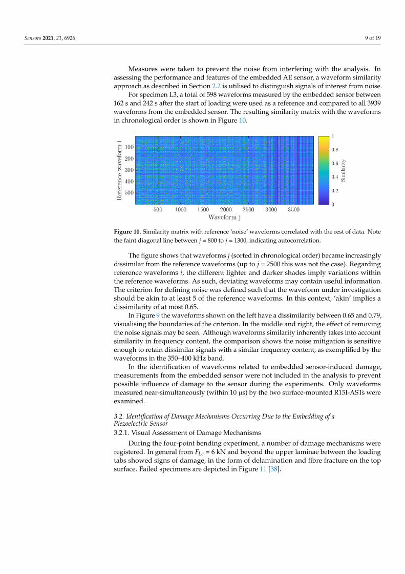
For specimen L3, a total of 598 waveforms measured by the embedded sensor between162 s and 242 s after the start of loading were used as a reference and compared to all 3939waveforms from the embedded sensor. The resulting similarity matrix with the waveformsin chronological order is shown in Figure 10.

Sensors 2021, 21, 6926  8  of  19  

3.1.3. Embedded Sensor Noise Mitigation during Four‐Point Bending Experiments 

In the first stage of testing it was noted that the embedded sensor tended to pick up 

extensive amounts of continuous noise. Based on the preliminary tests from Section 3.1.1, 

this was not expected. In one case, specimen L3, no continuous‐type noise but burst‐type 

signals were acquired. A large amount were amassed continuously from the start of the 

testing. In Figure 9a three waveforms measured by the embedded sensor in early stage of 

testing are shown. Next to that the accumulation of signals, represented by their centroid 

frequency  𝑓 , over time is illustrated. 

 (a)  (b)  (c) 

Figure 9. Noise mitigation on specimen L3: (a) Three waveforms measured in the reference timeslot 

between 162 s and 242 s after the start of test. They are translated in time and voltage to fit in the 

same image. The dissimilarity between the waveforms is between 0.65 and 0.79. (b) Centroid fre‐

quency  𝑓   of all measured signals over time and load cell force  𝐹   for the embedded sensor and 

the two R15I‐ASTs. (c) Equivalent to (b), but with noise removed. 

Due to their early and repeating appearance (burst repetition frequency around 50 

kHz), in the wave forms, these signals are considered noise. In a second batch of experi‐

ments it was identified that the continuous noise related to a metal‐to‐CFRP contact in the 

four‐point bending setup. After insulating the aluminium loading tabs with polyester film 

tape, no such behaviour occurred anymore. Therefore this effect is not directly attributed 

to possible triboelectricity effects due to the external wiring [41]. Further detailed investi‐

gation of triboelectricity effects will be considered in the future research. 

Measures were taken to prevent the noise from interfering with the analysis. In as‐

sessing the performance and features of the embedded AE sensor, a waveform similarity 

approach as described in Section 2.2 is utilised to distinguish signals of interest from noise. 

For specimen L3, a total of 598 waveforms measured by  the embedded sensor be‐

tween 162 s and 242 s after the start of loading were used as a reference and compared to 

all 3939 waveforms from the embedded sensor. The resulting similarity matrix with the 

waveforms in chronological order is shown in Figure 10. 

Figure 10. Similarity matrix with reference ‘noise’ waveforms correlated with the rest of data. 

Note the faint diagonal line between  𝑗  = 800 to  𝑗  = 1300, indicating autocorrelation. Figure 10. Similarity matrix with reference ‘noise’ waveforms correlated with the rest of data. Notethe faint diagonal line between j = 800 to j = 1300, indicating autocorrelation.

The figure shows that waveforms j (sorted in chronological order) became increasinglydissimilar from the reference waveforms (up to j = 2500 this was not the case). Regardingreference waveforms i, the different lighter and darker shades imply variations withinthe reference waveforms. As such, deviating waveforms may contain useful information.The criterion for defining noise was defined such that the waveform under investigationshould be akin to at least 5 of the reference waveforms. In this context, ‘akin’ implies adissimilarity of at most 0.65.

In Figure 9 the waveforms shown on the left have a dissimilarity between 0.65 and 0.79,visualising the boundaries of the criterion. In the middle and right, the effect of removingthe noise signals may be seen. Although waveforms similarity inherently takes into accountsimilarity in frequency content, the comparison shows the noise mitigation is sensitiveenough to retain dissimilar signals with a similar frequency content, as exemplified by thewaveforms in the 350–400 kHz band.

In the identification of waveforms related to embedded sensor-induced damage,measurements from the embedded sensor were not included in the analysis to preventpossible influence of damage to the sensor during the experiments. Only waveformsmeasured near-simultaneously (within 10 µs) by the two surface-mounted R15I-ASTs wereexamined.

3.2. Identification of Damage Mechanisms Occurring Due to the Embedding of aPiezoelectric Sensor3.2.1. Visual Assessment of Damage Mechanisms

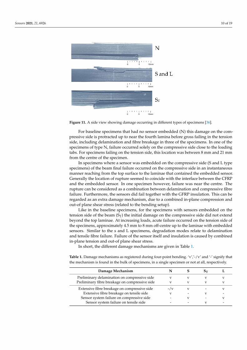
During the four-point bending experiment, a number of damage mechanisms wereregistered. In general from FLc = 6 kN and beyond the upper laminae between the loadingtabs showed signs of damage, in the form of delamination and fibre fracture on the topsurface. Failed specimens are depicted in Figure 11 [38].

Sensors 2021, 21, 6926 10 of 19

Sensors 2021, 21, 6926  9  of  19  

The figure shows that waveforms  𝑗  (sorted in chronological order) became increas‐

ingly dissimilar from the reference waveforms (up to  𝑗  = 2500 this was not the case). Re‐

garding reference waveforms  𝑖, the different lighter and darker shades imply variations 

within the reference waveforms. As such, deviating waveforms may contain useful infor‐

mation. The criterion for defining noise was defined such that the waveform under inves‐

tigation should be akin to at least 5 of the reference waveforms. In this context, ‘akin’ im‐

plies a dissimilarity of at most 0.65. 

In Figure 9 the waveforms shown on the left have a dissimilarity between 0.65 and 

0.79, visualising the boundaries of the criterion. In the middle and right, the effect of re‐

moving the noise signals may be seen. Although waveforms similarity inherently takes 

into account similarity in frequency content, the comparison shows the noise mitigation 

is sensitive enough to retain dissimilar signals with a similar frequency content, as exem‐

plified by the waveforms in the 350–400 kHz band. 

In  the  identification  of waveforms  related  to  embedded  sensor‐induced damage, 

measurements from the embedded sensor were not included  in the analysis to prevent 

possible  influence  of  damage  to  the  sensor during  the  experiments. Only waveforms 

measured near‐simultaneously  (within  10  μs) by  the  two  surface‐mounted R15I‐ASTs 

were examined. 

3.2. Identification of Damage Mechanisms Occurring Due to the Embedding of a Piezoelectric Sensor 

3.2.1. Visual Assessment of Damage Mechanisms 

During the four‐point bending experiment, a number of damage mechanisms were 

registered. In general from  𝐹   = 6 kN and beyond the upper laminae between the loading 

tabs showed signs of damage, in the form of delamination and fibre fracture on the top 

surface. Failed specimens are depicted in Figure 11 [38]. 

Figure 11. A side view showing damage occurring in different types of specimens [36]. 

For baseline specimens that had no sensor embedded (N) this damage on the com‐

pressive side is protracted up to near the fourth lamina before gross failing in the tension 

side, including delamination and fibre breakage in three of the specimens. In one of the 

specimens of type N, failure occurred solely on the compressive side close to the loading 

tabs. For specimens failing on the tension side, this location was between 8 mm and 21 

mm from the centre of the specimen. 

In specimens where a sensor was embedded on the compressive side (S and L type 

specimens) of the beam final failure occurred on the compressive side in an instantaneous 

manner reaching from the top surface to the laminae that contained the embedded sensor. 

Generally the location of rupture seemed to coincide with the interface between the CFRP 

and the embedded sensor. In one specimen however, failure was near the centre. The rup‐

ture can be considered as a combination between delamination and compressive fibre fail‐

Figure 11. A side view showing damage occurring in different types of specimens [36].

For baseline specimens that had no sensor embedded (N) this damage on the com-pressive side is protracted up to near the fourth lamina before gross failing in the tensionside, including delamination and fibre breakage in three of the specimens. In one of thespecimens of type N, failure occurred solely on the compressive side close to the loadingtabs. For specimens failing on the tension side, this location was between 8 mm and 21 mmfrom the centre of the specimen.

In specimens where a sensor was embedded on the compressive side (S and L typespecimens) of the beam final failure occurred on the compressive side in an instantaneousmanner reaching from the top surface to the laminae that contained the embedded sensor.Generally the location of rupture seemed to coincide with the interface between the CFRPand the embedded sensor. In one specimen however, failure was near the centre. Therupture can be considered as a combination between delamination and compressive fibrefailure. Furthermore, the sensors did fail together with the GFRP insulation. This can beregarded as an extra damage mechanism, due to a combined in-plane compression andout-of plane shear stress (related to the bending setup).

Like in the baseline specimens, for the specimens with sensors embedded on thetension side of the beam (ST) the initial damage on the compressive side did not extendbeyond the top laminae. At increasing loads, acute failure occurred on the tension side ofthe specimens, approximately 4.5 mm to 8 mm off-centre up to the laminae with embeddedsensors. Similar to the s and L specimens, degradation modes relate to delaminationand tensile fibre failure. Failure of the sensor itself and insulation is caused by combinedin-plane tension and out-of plane shear stress.

In short, the different damage mechanisms are given in Table 1.

Table 1. Damage mechanisms as registered during four-point bending. ‘v’,’-/v’ and ‘-’ signify thatthe mechanism is found in the bulk of specimens, in a single specimen or not at all, respectively.

Damage Mechanism N S ST L

Preliminary delamination on compressive side v v v vPreliminary fibre breakage on compressive side v v v v

Extensive fibre breakage on compressive side -/v v - vExtensive fibre breakage on tensile side v - v -

Sensor system failure on compressive side - v - vSensor system failure on tensile side - - v -

Sensors 2021, 21, 6926 11 of 19

3.2.2. Assessment of Energy and Cumulative Energy

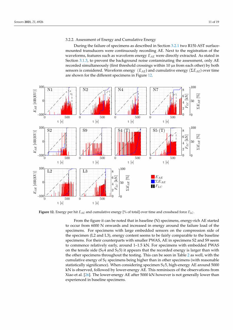
During the failure of specimens as described in Section 3.2.1 two R15I-AST surface-mounted transducers were continuously recording AE. Next to the registration of thewaveforms, features such as waveform energy EAE were directly extracted. As stated inSection 3.1.3, to prevent the background noise contaminating the assessment, only AErecorded simultaneously (first threshold crossings within 10 µs from each other) by bothsensors is considered. Waveform energy (EAE) and cumulative energy (ΣEAE) over timeare shown for the different specimens in Figure 12.

Sensors 2021, 21, 6926  11  of  19  

Figure 12. Energy per hit  𝐸   and cumulative energy [% of total] over time and crosshead force  𝐹 . 

From the figure it can be noted that in baseline (N) specimens, energy‐rich AE started 

to occur  from 6000 N onwards and  increased  in energy around  the  failure  load of  the 

specimens. For specimens with large embedded sensors on the compression side of the 

specimen (L2 and L3), energy content seems to be fairly comparable to the baseline spec‐

imens. For  their counterparts with smaller PWAS, AE  in specimens S2 and S9 seem  to 

commence relatively early, around 1–1.5 kN. For specimens with embedded PWAS on the 

tensile side (ST4 and ST5) it appears that the recorded energy is larger than with the other 

specimens throughout the testing. This can be seen in Table 2 as well, with the cumulative 

energy of ST specimens being higher than in other specimens (with reasonable statistically 

significance). When  considering  specimen ST5, high‐energy AE around 5000 kN  is ob‐

served, followed by lower‐energy AE. This reminisces of the observations from Xiao et al. 

[26]. The lower‐energy AE after 5000 kN however is not generally lower than experienced 

in baseline specimens. 

Table 2. Cumulative energy  Σ𝐸 . 

   N  S  ST    L   

Σ𝐸   [ 10 EU]  4.0 × 102  1.3 × 104  1.1 × 106  3.1 × 102 

9.0 × 102  1.2 × 102  2.5 × 104  8.1 × 101 

3.5 × 102       

7.0 × 102          

3.2.3. Identification of Damage Mechanisms Using Waveform Similarity 

Building further on the measurement of AE as explained in Section 2.1, effort is made 

to identify AE that is characteristic to failure related to the embedding of a piezoelectric 

sensor. Interpretation relies on the comparison between clusters of AE measured in the 

sensor‐less baseline specimens, and those from the specimens with sensors embedded. 

Using the method described in Section 2.2, a similarity matrix is constructed, contain‐

ing similarity information of AE waveforms captured during the loading and failure of all 

Figure 12. Energy per hit EAE and cumulative energy [% of total] over time and crosshead force FLC.

From the figure it can be noted that in baseline (N) specimens, energy-rich AE startedto occur from 6000 N onwards and increased in energy around the failure load of thespecimens. For specimens with large embedded sensors on the compression side ofthe specimen (L2 and L3), energy content seems to be fairly comparable to the baselinespecimens. For their counterparts with smaller PWAS, AE in specimens S2 and S9 seemto commence relatively early, around 1–1.5 kN. For specimens with embedded PWASon the tensile side (ST4 and ST5) it appears that the recorded energy is larger than withthe other specimens throughout the testing. This can be seen in Table 2 as well, with thecumulative energy of ST specimens being higher than in other specimens (with reasonablestatistically significance). When considering specimen ST5, high-energy AE around 5000kN is observed, followed by lower-energy AE. This reminisces of the observations fromXiao et al. [26]. The lower-energy AE after 5000 kN however is not generally lower thanexperienced in baseline specimens.

Sensors 2021, 21, 6926 12 of 19

Table 2. Cumulative energy ΣEAE.

N S ST L

ΣEAE [×106EU]

4.0 × 102 1.3 × 104 1.1 × 106 3.1 × 102

9.0 × 102 1.2 × 102 2.5 × 104 8.1 × 101

3.5 × 102

7.0 × 102

3.2.3. Identification of Damage Mechanisms Using Waveform Similarity

Building further on the measurement of AE as explained in Section 2.1, effort is madeto identify AE that is characteristic to failure related to the embedding of a piezoelectricsensor. Interpretation relies on the comparison between clusters of AE measured in thesensor-less baseline specimens, and those from the specimens with sensors embedded.

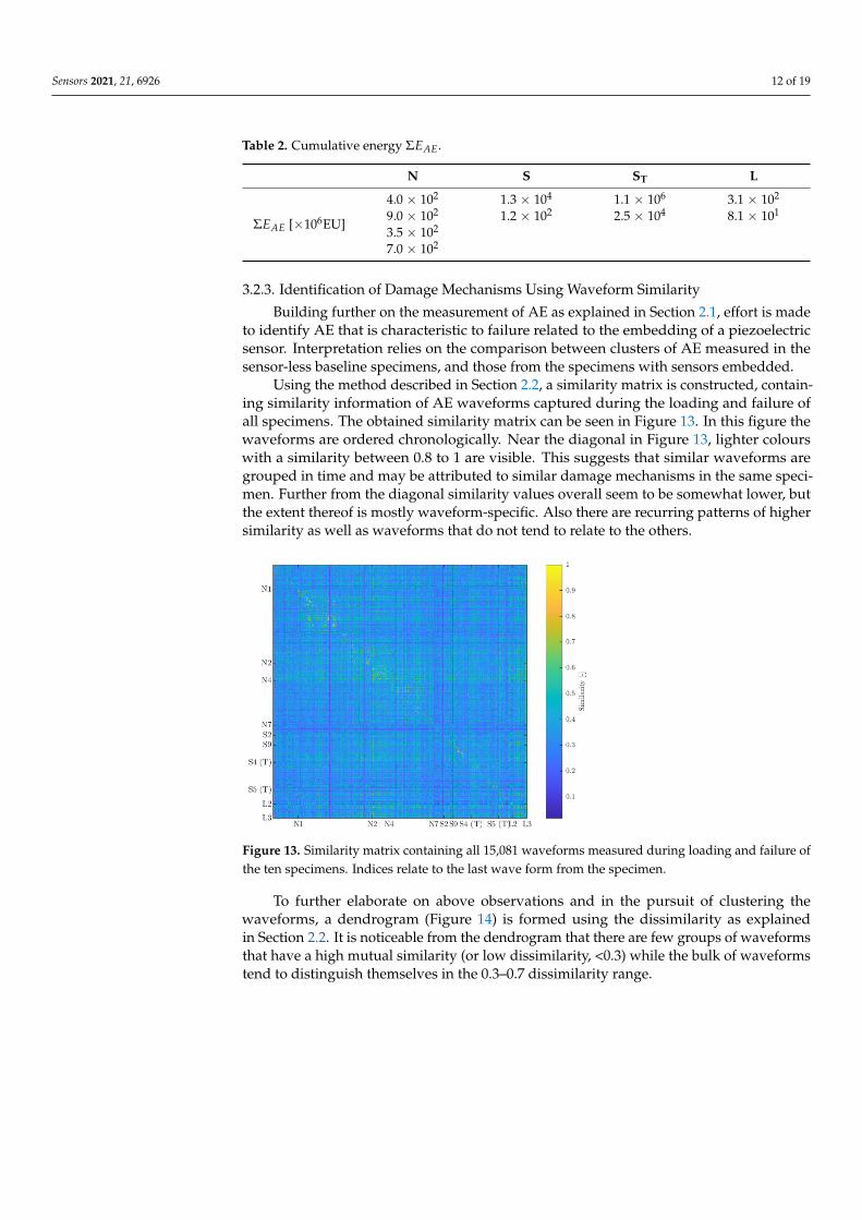
Using the method described in Section 2.2, a similarity matrix is constructed, contain-ing similarity information of AE waveforms captured during the loading and failure ofall specimens. The obtained similarity matrix can be seen in Figure 13. In this figure thewaveforms are ordered chronologically. Near the diagonal in Figure 13, lighter colourswith a similarity between 0.8 to 1 are visible. This suggests that similar waveforms aregrouped in time and may be attributed to similar damage mechanisms in the same speci-men. Further from the diagonal similarity values overall seem to be somewhat lower, butthe extent thereof is mostly waveform-specific. Also there are recurring patterns of highersimilarity as well as waveforms that do not tend to relate to the others.

Sensors 2021, 21, 6926  12  of  19  

specimens. The obtained similarity matrix can be seen in Figure 13. In this figure the wave‐

forms are ordered chronologically. Near the diagonal in Figure 13, lighter colours with a 

similarity between 0.8 to 1 are visible. This suggests that similar waveforms are grouped 

in time and may be attributed to similar damage mechanisms in the same specimen. Fur‐

ther from the diagonal similarity values overall seem to be somewhat lower, but the extent 

thereof is mostly waveform‐specific. Also there are recurring patterns of higher similarity 

as well as waveforms that do not tend to relate to the others. 

Figure 13. Similarity matrix containing all 15081 waveforms measured during  loading and 

failure of the ten specimens. Indices relate to the last wave form from the specimen. 

To further elaborate on above observations and in the pursuit of clustering the wave‐

forms, a dendrogram (Figure 14) is formed using the dissimilarity as explained in Section 

2.2. It is noticeable from the dendrogram that there are few groups of waveforms that have 

a high mutual similarity (or low dissimilarity, <0.3) while the bulk of waveforms tend to 

distinguish themselves in the 0.3–0.7 dissimilarity range. 

Figure 14. Dendrogram linking the data from the similarity matrix in Figure 13. The dashed 

lines represent the thresholds considered in the definition of clusters. Note that along the hor‐

izontal axis the waveforms are no longer ordered sequentially. 

Figure 13. Similarity matrix containing all 15,081 waveforms measured during loading and failure ofthe ten specimens. Indices relate to the last wave form from the specimen.

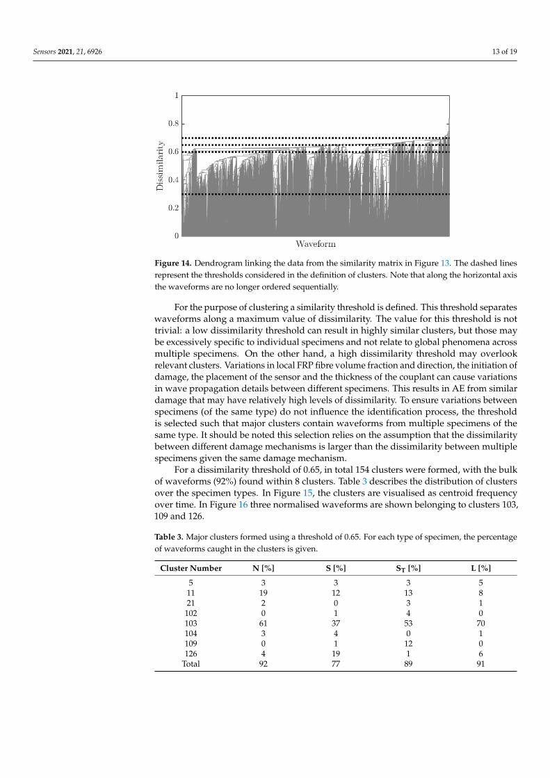
To further elaborate on above observations and in the pursuit of clustering thewaveforms, a dendrogram (Figure 14) is formed using the dissimilarity as explainedin Section 2.2. It is noticeable from the dendrogram that there are few groups of waveformsthat have a high mutual similarity (or low dissimilarity, <0.3) while the bulk of waveformstend to distinguish themselves in the 0.3–0.7 dissimilarity range.

Sensors 2021, 21, 6926 13 of 19

Sensors 2021, 21, 6926  12  of  19  

specimens. The obtained similarity matrix can be seen in Figure 13. In this figure the wave‐

forms are ordered chronologically. Near the diagonal in Figure 13, lighter colours with a 

similarity between 0.8 to 1 are visible. This suggests that similar waveforms are grouped 

in time and may be attributed to similar damage mechanisms in the same specimen. Fur‐

ther from the diagonal similarity values overall seem to be somewhat lower, but the extent 

thereof is mostly waveform‐specific. Also there are recurring patterns of higher similarity 

as well as waveforms that do not tend to relate to the others. 

Figure 13. Similarity matrix containing all 15081 waveforms measured during  loading and 

failure of the ten specimens. Indices relate to the last wave form from the specimen. 

To further elaborate on above observations and in the pursuit of clustering the wave‐

forms, a dendrogram (Figure 14) is formed using the dissimilarity as explained in Section 

2.2. It is noticeable from the dendrogram that there are few groups of waveforms that have 

a high mutual similarity (or low dissimilarity, <0.3) while the bulk of waveforms tend to 

distinguish themselves in the 0.3–0.7 dissimilarity range. 

Figure 14. Dendrogram linking the data from the similarity matrix in Figure 13. The dashed 

lines represent the thresholds considered in the definition of clusters. Note that along the hor‐

izontal axis the waveforms are no longer ordered sequentially. 

Figure 14. Dendrogram linking the data from the similarity matrix in Figure 13. The dashed linesrepresent the thresholds considered in the definition of clusters. Note that along the horizontal axisthe waveforms are no longer ordered sequentially.

For the purpose of clustering a similarity threshold is defined. This threshold separateswaveforms along a maximum value of dissimilarity. The value for this threshold is nottrivial: a low dissimilarity threshold can result in highly similar clusters, but those maybe excessively specific to individual specimens and not relate to global phenomena acrossmultiple specimens. On the other hand, a high dissimilarity threshold may overlookrelevant clusters. Variations in local FRP fibre volume fraction and direction, the initiation ofdamage, the placement of the sensor and the thickness of the couplant can cause variationsin wave propagation details between different specimens. This results in AE from similardamage that may have relatively high levels of dissimilarity. To ensure variations betweenspecimens (of the same type) do not influence the identification process, the thresholdis selected such that major clusters contain waveforms from multiple specimens of thesame type. It should be noted this selection relies on the assumption that the dissimilaritybetween different damage mechanisms is larger than the dissimilarity between multiplespecimens given the same damage mechanism.

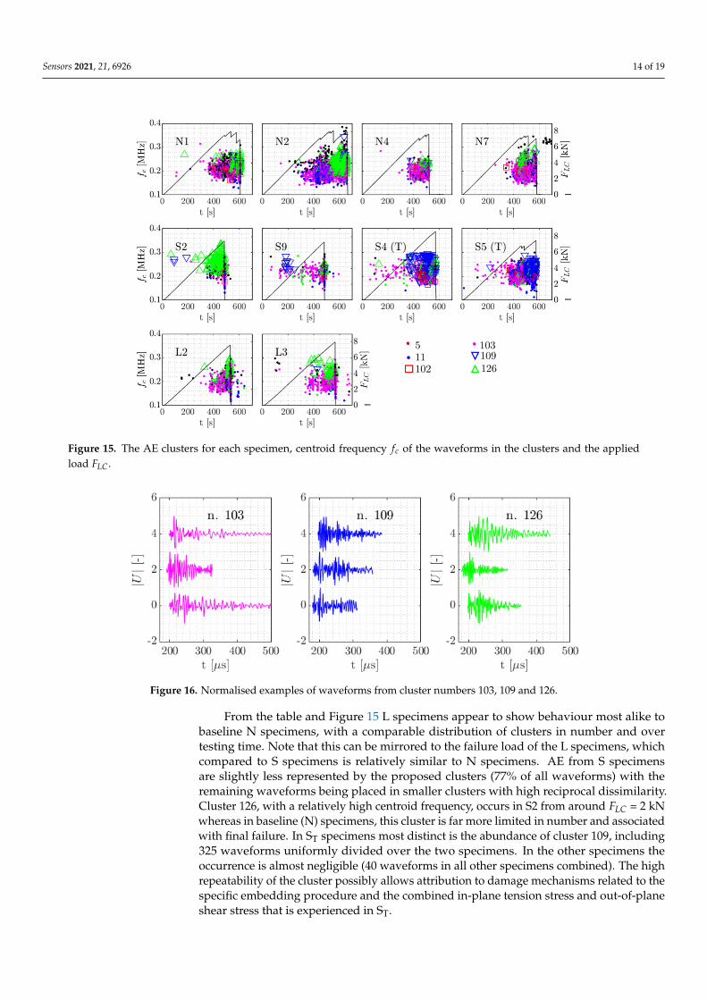
For a dissimilarity threshold of 0.65, in total 154 clusters were formed, with the bulkof waveforms (92%) found within 8 clusters. Table 3 describes the distribution of clustersover the specimen types. In Figure 15, the clusters are visualised as centroid frequencyover time. In Figure 16 three normalised waveforms are shown belonging to clusters 103,109 and 126.

Table 3. Major clusters formed using a threshold of 0.65. For each type of specimen, the percentageof waveforms caught in the clusters is given.

Cluster Number N [%] S [%] ST [%] L [%]

5 3 3 3 511 19 12 13 821 2 0 3 1

102 0 1 4 0103 61 37 53 70104 3 4 0 1109 0 1 12 0126 4 19 1 6

Total 92 77 89 91

Sensors 2021, 21, 6926 14 of 19

1

Figure 15. The AE clusters for each specimen, centroid frequency fc of the waveforms in the clusters and the appliedload FLC.

Sensors 2021, 21, 6926  14  of  19  

Figure 15. The AE clusters for each specimen, centroid frequency  𝑓   of the waveforms in the 

clusters and the applied load  𝐹 . 

Figure 16. Normalised examples of waveforms from cluster numbers 103, 109 and 126. 

From the table and Figure 15 L specimens appear to show behaviour most alike to 

baseline N specimens, with a comparable distribution of clusters in number and over test‐

ing time. Note that this can be mirrored to the failure load of the L specimens, which com‐

pared  to  S  specimens  is  relatively  similar  to N  specimens. AE  from  S  specimens  are 

slightly less represented by the proposed clusters (77% of all waveforms) with the remain‐

ing waveforms being placed in smaller clusters with high reciprocal dissimilarity. Cluster 

126, with  a  relatively  high  centroid  frequency,  occurs  in  S2  from  around  𝐹   =2  kN 

whereas in baseline (N) specimens, this cluster is far more limited in number and associ‐

ated with final failure. In ST specimens most distinct is the abundance of cluster 109, in‐

cluding 325 waveforms uniformly divided over the two specimens. In the other specimens 

the occurrence is almost negligible (40 waveforms in all other specimens combined). The 

high repeatability of the cluster possibly allows attribution to damage mechanisms related 

to the specific embedding procedure and the combined in‐plane tension stress and out‐

of‐plane shear stress that is experienced in ST. 

Figure 16. Normalised examples of waveforms from cluster numbers 103, 109 and 126.

From the table and Figure 15 L specimens appear to show behaviour most alike tobaseline N specimens, with a comparable distribution of clusters in number and overtesting time. Note that this can be mirrored to the failure load of the L specimens, whichcompared to S specimens is relatively similar to N specimens. AE from S specimensare slightly less represented by the proposed clusters (77% of all waveforms) with theremaining waveforms being placed in smaller clusters with high reciprocal dissimilarity.Cluster 126, with a relatively high centroid frequency, occurs in S2 from around FLC = 2 kNwhereas in baseline (N) specimens, this cluster is far more limited in number and associatedwith final failure. In ST specimens most distinct is the abundance of cluster 109, including325 waveforms uniformly divided over the two specimens. In the other specimens theoccurrence is almost negligible (40 waveforms in all other specimens combined). The highrepeatability of the cluster possibly allows attribution to damage mechanisms related to thespecific embedding procedure and the combined in-plane tension stress and out-of-planeshear stress that is experienced in ST.

Sensors 2021, 21, 6926 15 of 19

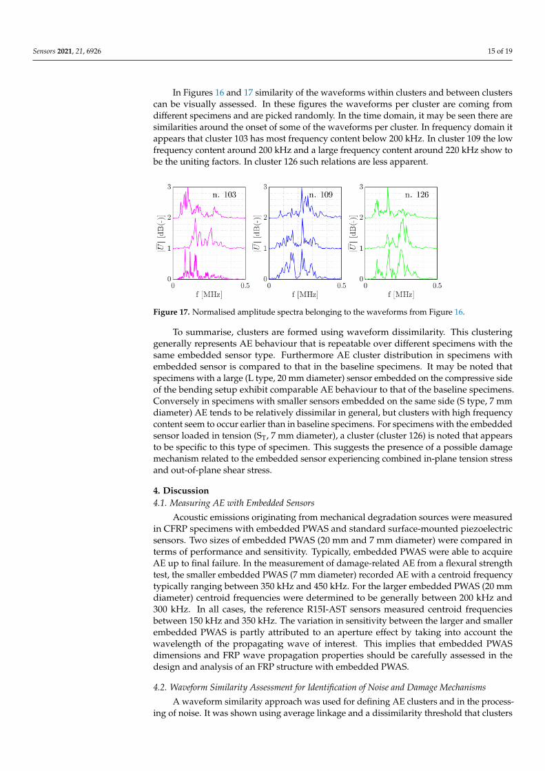
In Figures 16 and 17 similarity of the waveforms within clusters and between clusterscan be visually assessed. In these figures the waveforms per cluster are coming fromdifferent specimens and are picked randomly. In the time domain, it may be seen there aresimilarities around the onset of some of the waveforms per cluster. In frequency domain itappears that cluster 103 has most frequency content below 200 kHz. In cluster 109 the lowfrequency content around 200 kHz and a large frequency content around 220 kHz show tobe the uniting factors. In cluster 126 such relations are less apparent.

Sensors 2021, 21, 6926  15  of  19  

In Figures 16 and 17 similarity of the waveforms within clusters and between clusters 

can be visually assessed. In these figures the waveforms per cluster are coming from dif‐

ferent specimens and are picked randomly. In the time domain, it may be seen there are 

similarities around the onset of some of the waveforms per cluster. In frequency domain 

it appears that cluster 103 has most frequency content below 200 kHz. In cluster 109 the 

low  frequency content around 200 kHz and a  large frequency content around 220 kHz 

show to be the uniting factors. In cluster 126 such relations are less apparent. 

Figure 17. Normalised amplitude spectra belonging to the waveforms from Figure 16. 

To  summarise,  clusters  are  formed using waveform dissimilarity. This  clustering 

generally represents AE behaviour that  is repeatable over different specimens with the 

same embedded sensor type. Furthermore AE cluster distribution in specimens with em‐

bedded sensor is compared to that in the baseline specimens. It may be noted that speci‐

mens with a large (L type, 20 mm diameter) sensor embedded on the compressive side of 

the bending setup exhibit comparable AE behaviour  to  that of  the baseline specimens. 

Conversely in specimens with smaller sensors embedded on the same side (S type, 7 mm 

diameter) AE tends to be relatively dissimilar in general, but clusters with high frequency 

content seem to occur earlier than in baseline specimens. For specimens with the embed‐

ded sensor loaded in tension (ST, 7 mm diameter), a cluster (cluster 126) is noted that ap‐

pears to be specific to this type of specimen. This suggests the presence of a possible dam‐

age mechanism related to the embedded sensor experiencing combined in‐plane tension 

stress and out‐of‐plane shear stress. 

4. Discussion 

4.1. Measuring AE with Embedded Sensors 

Acoustic emissions originating from mechanical degradation sources were measured 

in CFRP specimens with embedded PWAS and standard surface‐mounted piezoelectric 

sensors. Two sizes of embedded PWAS (20 mm and 7 mm diameter) were compared in 

terms of performance and sensitivity. Typically, embedded PWAS were able to acquire 

AE up to final failure. In the measurement of damage‐related AE from a flexural strength 

test,  the  smaller  embedded PWAS  (7 mm diameter)  recorded AE with a  centroid  fre‐

quency typically ranging between 350 kHz and 450 kHz. For the larger embedded PWAS 

(20 mm diameter) centroid frequencies were determined to be generally between 200 kHz 

and 300 kHz. In all cases, the reference R15I‐AST sensors measured centroid frequencies 

between 150 kHz and 350 kHz. The variation in sensitivity between the larger and smaller 

embedded PWAS  is partly  attributed  to  an  aperture  effect by  taking  into  account  the 

wavelength of the propagating wave of interest. This implies that embedded PWAS di‐

mensions and FRP wave propagation properties should be carefully assessed in the de‐

sign and analysis of an FRP structure with embedded PWAS. 

Figure 17. Normalised amplitude spectra belonging to the waveforms from Figure 16.

To summarise, clusters are formed using waveform dissimilarity. This clusteringgenerally represents AE behaviour that is repeatable over different specimens with thesame embedded sensor type. Furthermore AE cluster distribution in specimens withembedded sensor is compared to that in the baseline specimens. It may be noted thatspecimens with a large (L type, 20 mm diameter) sensor embedded on the compressive sideof the bending setup exhibit comparable AE behaviour to that of the baseline specimens.Conversely in specimens with smaller sensors embedded on the same side (S type, 7 mmdiameter) AE tends to be relatively dissimilar in general, but clusters with high frequencycontent seem to occur earlier than in baseline specimens. For specimens with the embeddedsensor loaded in tension (ST, 7 mm diameter), a cluster (cluster 126) is noted that appearsto be specific to this type of specimen. This suggests the presence of a possible damagemechanism related to the embedded sensor experiencing combined in-plane tension stressand out-of-plane shear stress.

4. Discussion4.1. Measuring AE with Embedded Sensors

Acoustic emissions originating from mechanical degradation sources were measuredin CFRP specimens with embedded PWAS and standard surface-mounted piezoelectricsensors. Two sizes of embedded PWAS (20 mm and 7 mm diameter) were compared interms of performance and sensitivity. Typically, embedded PWAS were able to acquireAE up to final failure. In the measurement of damage-related AE from a flexural strengthtest, the smaller embedded PWAS (7 mm diameter) recorded AE with a centroid frequencytypically ranging between 350 kHz and 450 kHz. For the larger embedded PWAS (20 mmdiameter) centroid frequencies were determined to be generally between 200 kHz and300 kHz. In all cases, the reference R15I-AST sensors measured centroid frequenciesbetween 150 kHz and 350 kHz. The variation in sensitivity between the larger and smallerembedded PWAS is partly attributed to an aperture effect by taking into account thewavelength of the propagating wave of interest. This implies that embedded PWASdimensions and FRP wave propagation properties should be carefully assessed in thedesign and analysis of an FRP structure with embedded PWAS.

4.2. Waveform Similarity Assessment for Identification of Noise and Damage Mechanisms

A waveform similarity approach was used for defining AE clusters and in the process-ing of noise. It was shown using average linkage and a dissimilarity threshold that clusters

Sensors 2021, 21, 6926 16 of 19

of AE can be formed that are overarching different specimens while being specific enoughto accentuate the effects found in different specimen types. This confirms the assertion thatthe dissimilarity of AE between different types of specimens is larger than the dissimilaritybetween multiple same-type specimens. As is seen in Figures 14, 16 and 17 differences indissimilarity within clusters are relatively large while between the clusters the differencesin dissimilarity are relatively low. This indicates that for a small difference in dissimilaritythreshold, large differences in the formation of clusters are obtained. Cluster 109, thatis assigned to be specific to specimens with embedded PWAS on the tensile side of thebending test, is considered of note due to its occurrence being almost exclusive to this typeof specimens as well as its distribution being comparable over the two specimens of thistype.

4.3. Identification of Damage Mechanisms Occurring Due to the Embedding of aPiezoelectric Sensor

From the combination of waveform similarity and AE energy assessment it may beconcluded that the AE behaviour of the two specimens with embedded PWAS on the tensileside of the bending load are distinctly different from the baseline and other specimens.The identified AE phenomena are envisioned to be associated to a tensile cohesion-relatedfailure, since the strength of the GFRP-resin-CFRP interface is subject to large uncertainty.Tensile fracture of the PWAS is not expected as a likely source given the low stiffness ofGFRP and resin insulation, as confirmed by the embedded PWAS in specimen ST11 thatrecorded up to gross failure. Given the inaccessibility of the location of damage for detailedinspection during the test, further validation related to the degradation mode is needed.

Between baseline specimens and specimens with embedded PWAS on the compressiveside under the bending load, no clear relation in terms of AE can be established. Althoughvisually the damage mechanisms in these specimens are different compared to baselinespecimens, this did not translate to sufficiently consistent trends in AE.

4.4. Outlook and Future Research

From a wider perspective, the ability to relate AE to embedded PWAS-affiliatedand non-affiliated degradation mechanisms allows for the monitoring of a structure withembedded PWAS with respect to the health of the structure. Further, the monitoring forembedded PWAS-induced degradation facilitates the development of design criteria forstructures with embedded PWAS. In this regard, the observation that AE from PWAS-induced damage is distinguishable from other sources, prior to specimen gross failureand depending on loading direction, is of value. It is considered that this work will alsopave the way for more widespread use of embedded PWAS, such as in larger-scale FRPstructures with embedded arrays or distributed configurations.

This research can be seen as a preliminary step towards assessing the influence ofembedded PWAS size and location on their measurement capabilities and on the structuralintegrity of the host structure. As such, it is acknowledged that the topics and outcomespresented in this research can be elaborated upon, by means of extended experiments andnumerical simulations. Measuring different wave modes with different wave lengths andthe effect on the sensitivity of embedded PWAS deserves further research. Evaluation withrespect to the sensitivity of the embedded PWAS is envisioned on different host materials,such as GFRP and sandwich structures. The clustering method used may be comparedto other clustering procedures that are used typically in the classification of FRP damagemechanisms. In this context, the respective qualities of the formed clusters may be assessed.Moreover, it is recognised that increasing the population size of the specimens will helpdrawing more accurate and definite conclusions on the formation of AE clusters relatedto embedded PWAS-induced damage. Also, this will allow specimens in the destructivetesting to be stopped prematurely so that they can be inspected microscopically for theinitiation of damage mechanisms. The premature inspection will facilitate attributingclusters to damage mechanisms. In a further stage, a database of clusters of waveforms withidentified damage mechanisms may be used to quantify the nature and extent of damage

Sensors 2021, 21, 6926 17 of 19

in similar structures. The features of AE signals from identified damage mechanisms canalso be used to develop possible damage indices to better estimate the remaining loadbearing capacity or remaining lifetime.

5. Conclusions

Using data from destructive four-point bending tests performed on thick CFRP spec-imens with embedded PWAS the performance of the PWAS in terms of endurance andspectral sensitivity for AE measurement was investigated. Furthermore, a waveform sim-ilarity assessment method was employed to identify clusters of AE signals that relate toembedded PWAS-induced failure mechanisms. It was found that:

(1) The size of the embedded PWAS has an effect on the frequency content of the measure-ment of AE signals; Damage-related AE signals in CFRP specimens were measuredwith a centroid frequency between 350 kHz and 450 kHz by the 7 mm diameterembedded PWAS, while for the 20 mm embedded PWAS the range was between 200kHz and 300 kHz. For comparison, no change in frequency content in the AE signalswas measured by a reference surface-mounted sensor for the different specimens.

(2) Damage mechanisms in the CFRP laminates due to embedded PWAS when placedin the tension side in the bending experiment exhibited AE that were reasonablydistinguishable from other sources of AE. This was confirmed when assessing wave-form similarity and AE energy in specimens with and without embedded sensors.When loaded under compression, no major additional degradation AE due to theembedment process was identified.

Author Contributions: Conceptualization, A.H., L.P. and C.K.; methodology, A.H. and L.P.; software,A.H.; formal analysis, A.H.; investigation, A.H.; resources, L.P. and C.K.; writing—original draftpreparation, A.H.; writing—review and editing, L.P. and C.K.; visualisation, A.H.; supervision, L.P.and C.K.; project administration, L.P.; funding acquisition, L.P. All authors have read and agreed tothe published version of the manuscript.

Funding: This research was funded by The Netherlands Organization for Scientific Research (NWO),project number 18463. The APC was funded by TU Delft.

Institutional Review Board Statement: Not applicable.

Informed Consent Statement: Not applicable.

Data Availability Statement: The data presented in this study are available upon request from thecorresponding author.

Acknowledgments: The authors are grateful to Andre Vaders for his valuable prior support andcontribution. Further the authors are grateful to Bart Scheeren for his support regarding the waveformsimilarity processing.

Conflicts of Interest: The authors declare no conflict of interest. The funders had no role in the designof the study; in the collection, analyses, or interpretation of data; in the writing of the manuscript, orin the decision to publish the results.

References1. Ruan, J.; Michael Ho, S.C.; Patil, D.; Li, M.; Song, G. Wind turbine blade damage detection using an active sensing approach.

Smart Mater. Struct. 2014, 23. [CrossRef]2. Guo, Z.-S.; Zhang, J.; Hu, H.; Guo, X. Structural health monitoring of composite wind blades by fiber bragg grating. Int. Conf.

Smart Mater. Nanotechnol. Eng. 2007, 6423, 64230I. [CrossRef]3. Yang, B.; Xuan, F.-Z.; Jin, P.; Hu, C.; Xiao, B.; Li, D.; Xiang, Y.; Lei, H. Damage Localization in Composite Laminates by Building in

PZT Wafer Transducers: A Comparative Study with Surface-Bonded PZT Strategy. Adv. Eng. Mater. 2018, 21, 1801040. [CrossRef]4. Crawley, E.F.; De Luis, J. Use of piezoelectric actuators as elements of intelligent structures. AIAA J. 1987, 25, 1373–1385. [CrossRef]5. Tuloup, C.; Harizi, W.; Aboura, Z.; Meyer, Y. Structural health monitoring of polymer-matrix composite using embedded

piezoelectric ceramic transducers during several four-points bending tests. Smart Mater. Struct. 2020, 29. [CrossRef]6. Shin, S.; Zamorano, B.; Elvin, N. Comparison of the electromechanical properties of embedded and surface-mounted piezoelectric

transducers. J. Intell. Mater. Syst. Struct. 2016, 27, 2837–2850. [CrossRef]

Sensors 2021, 21, 6926 18 of 19

7. Erturk, A.; Inman, D.J. Piezoelectric Energy Harvesting; Wiley: Hoboken, NJ, USA, 2011; ISBN 9781119991359.8. Tzou, H.S.; Tseng, C.I. Distributed piezoelectric sensor/actuator design for dynamic measurement/control of distributed

parameter systems: A piezoelectric finite element approach. J. Sound Vib. 1990, 138, 17–34. [CrossRef]9. Paget, C. Active Health Monitoring of Aerospace Composite Structures by Embedded Piezoceramic Transducers; Institutionen för

flygteknik: Stockholm, Sweden, 2001.10. Andreades, C.; Mahmoodi, P.; Ciampa, F. Characterisation of smart CFRP composites with embedded PZT transducers for

nonlinear ultrasonic applications. Compos. Struct. 2018, 206, 456–466. [CrossRef]11. Tang, H.Y.; Winkelmann, C.; Lestari, W.; La Saponara, V. Composite structural health monitoring through use of embedded PZT

sensors. J. Intell. Mater. Syst. Struct. 2011, 22, 739–755. [CrossRef]12. Feng, T.; Bekas, D.; Aliabadi, M.H.F. Active Health Monitoring of Thick Composite Structures by Embedded and Surface-Mounted

Piezo Diagnostic Layer. Sensors 2020, 20, 3410. [CrossRef]13. Ferri Aliabadi, M.H.; Khodaei, Z.S. Structural Health Monitoring for Advanced Composite Structures; World Scientific: Singapore,

2017; ISBN 9781786343932.14. Masmoudi, S.; El Mahi, A.; Turki, S.; El Guerjouma, R. Structural Health Monitoring of Smart Composite Material by Acoustic

Emission. In Proceedings of the Acoustics 2012, Nantes, France, 23−27 April 2012.15. Dziendzikowski, M.; Niedbala, P.; Kurnyta, A.; Kowalczyk, K.; Dragan, K. Structural health monitoring of a composite panel

based on PZT sensors and a transfer impedance framework. Sensors 2018, 18, 1521. [CrossRef]16. Lampani, L.; Sarasini, F.; Tirillò, J.; Gaudenzi, P. Analysis of damage in composite laminates with embedded piezoelectric patches

subjected to bending action. Compos. Struct. 2018, 202, 935–942. [CrossRef]17. Dziendzikowski, M.; Kurnyta, A.; Dragan, K.; Klysz, S.; Leski, A. In situ Barely Visible Impact Damage detection and localization

for composite structures using surface mounted and embedded PZT transducers: A comparative study. Mech. Syst. Signal Process.2016, 78, 91–106. [CrossRef]

18. Sause, M.G.R. In Situ Monitoring of Fiber-Reinforced Composites Theory, Basic Concepts, Methods, and Applications; Springer:Berlin/Heidelberg, Germany, 2016; ISBN 9783319309538.

19. Kim, H.S.; Ghoshal, A.; Chattopadhyay, A.; Prosser, W.H. Development of embedded sensor models in composite laminates forstructural health monitoring. J. Reinf. Plast. Compos. 2004, 23, 1207–1240. [CrossRef]

20. Zappino, E.; Carrera, E. Advanced modeling of embedded piezo-electric transducers for the health-monitoring of layeredstructures. Int. J. Smart Nano Mater. 2020, 11, 325–342. [CrossRef]

21. Nanda, N. Spectral finite element method for wave propagation analysis in smart composite beams containing delamination.Aircr. Eng. Aerosp. Technol. 2020, 92, 440–451. [CrossRef]

22. Shukla, D.R.; Vizzini, A.J. Interlacing for improved performance of laminates with embedded devices. Smart Mater. Struct. 1996,5, 225–229. [CrossRef]

23. Lin, M.; Chang, F.-K. The manufacture of composite structures with a built-in network of piezoceramics. Compos. Sci. Technol.2002, 62, 919–939. [CrossRef]

24. Ghezzo, F.; Starr, A.F.; Smith, D.R. Integration of networks of sensors and electronics for structural health monitoring of compositematerials. Adv. Civ. Eng. 2010, 2010. [CrossRef]

25. Huang, Y.; Ghezzo, F.; Nemat-Nasser, S. Onset of resin micro-cracks in unidirectional glass fiber laminates with integrated SHMsensors: Numerical analysis. Struct. Heal. Monit. 2009, 8, 493–507. [CrossRef]

26. Xiao, Y.; Qiao, W.; Fukuda, H.; Hatta, H. The effect of embedded devices on structural integrity of composite laminates. Compos.Struct. 2016, 153, 21–29. [CrossRef]

27. Li, L.; Lomov, S.V.; Yan, X.; Carvelli, V. Cluster analysis of acoustic emission signals for 2D and 3D woven glass/epoxy composites.Compos. Struct. 2014, 116, 286–299. [CrossRef]

28. Friedrich, L.; Colpo, A.; Maggi, A.; Becker, T.; Lacidogna, G.; Iturrioz, I. Damage process in glass fiber reinforced polymerspecimens using acoustic emission technique with low frequency acquisition. Compos. Struct. 2021, 256, 113105. [CrossRef]

29. Saeedifar, M.; Zarouchas, D. Damage characterization of laminated composites using acoustic emission: A review. Compos. Part BEng. 2020, 195, 108039. [CrossRef]

30. Kurz, J.H.; Finck, F.; Grosse, C.U.; Reinhardt, H. Similarity matrices as a new feature for acoustic emission analysis of concrete. InProceedings of the 26th European Conference on Acoustic Emission Testing 2004, Berlin, Germany, 15–17 September 2004.

31. Van Steen, C.; Pahlavan, L.; Wevers, M.; Verstrynge, E. Localisation and characterisation of corrosion damage in reinforcedconcrete by means of acoustic emission and X-ray computed tomography. Constr. Build. Mater. 2019, 197, 21–29. [CrossRef]

32. van Steen, C. Clustering of acoustic emission signals for fracture monitoring during accelerated corrosion of reinforced concreteprisms. Mater. Sci. 2019. [CrossRef]

33. Trugman, D.T.; Ross, Z.E.; Johnson, P.A. Imaging Stress and Faulting Complexity Through Earthquake Waveform Similarity.Geophys. Res. Lett. 2020, 47, 1–8. [CrossRef]

34. Hexcel Composites Product data HexPly 8552. Hexcel 2000, 1, 1–6.35. Meggit Data for Modelling. Available online: https://www.meggittferroperm.com/resources/data-for-modelling/ (accessed on

10 April 2019).

Sensors 2021, 21, 6926 19 of 19

36. Huijer, A. Load And Damage Measurements on Fibre-Reinforced Composites with Embedded Piezoelectric Sensors. Master’sThesis, Delft University of Technology, Delft, The Netherlands, 2019.

37. Akaike, H. Markovian representation of stochastic processes and its application to the analysis of autoregressive moving averageprocesses. Ann. Inst. Stat. Math. 1974, 26, 363–387. [CrossRef]

38. Bai, F.; Gagar, D.; Foote, P.; Zhao, Y. Comparison of alternatives to amplitude thresholding for onset detection of acoustic emissionsignals. Mech. Syst. Signal Process. 2017, 84, 717–730. [CrossRef]

39. Scheeren, B. On the Development of a Volumetric Acoustic Emission Fatigue Crack Monitoring System; Delft University of Technology:Delft, The Netherlands, 2017.

40. MISTRAS R15I-AST Sensor. Available online: http://www.physicalacoustics.com/content/literature/sensors/Model_R15I-AST.pdf (accessed on 6 October 2021).

41. Perls, T.A. Electrical noise from instrument cables subjected to shock and vibration. J. Appl. Phys. 1952, 23, 674–680. [CrossRef]