ACompoundPoissonConvergenceTheoremforSumsof · PDF fileACompoundPoissonConvergenceTheoremforSumsof m-DependentVariables ... For exponentially weighted Wasserstein norm, we have the

arX

iv:1

402.

0183

v1 [

mat

h.ST

] 2

Feb

201

4

A Compound Poisson Convergence Theorem for Sums of

m-Dependent Variables

V. Cekanavicius and P. Vellaisamy

Department of Mathematics and Informatics, Vilnius University,

Naugarduko 24, Vilnius 03225, Lithuania.

E-mail: [email protected]

and

Department of Mathematics, Indian Institute of Technology Bombay,

Powai, Mumbai- 400076, India.

E-mail: [email protected]

Abstract

We prove the Simons-Johnson theorem for the sums Sn of m-dependent random variables,

with exponential weights and limiting compound Poisson distribution CP(s, λ). More precisely,

we give sufficient conditions for∑

∞

k=0ehk|P (Sn = k)−CP(s, λ){k}| → 0 and provide an estimate

on the rate of convergence. It is shown that the Simons-Johnson theorem holds for weighted

Wasserstein norm as well. The results are then illustrated for N(n; k1, k2) and k-runs statistics.

Key words: Poisson distribution, compound Poisson distribution, m-dependent variables, Wasser-

stein norm, rate of convergence.

MSC 2000 Subject Classification: 60F05; 60F15.

1

1 Introduction

Simons and Johnson (1971) established an interesting result that the convergence of the binomial

distribution to the limiting Poisson law can be much stronger than in total variation. Indeed, they

proved that if Sn = X1 +X2 + · · ·+Xn has binomial distribution with parameters n, p = λ/n and

g(x) satisfies∑∞

0 g(k)Pois(λ){k} <∞, then

∞∑

k=0

g(k)|P (Sn = k)− Pois(λ){k}| → 0, n→ ∞, (1)

where here and henceforth Pois(λ) denotes Poisson distribution with mean λ. The above result

was then extended to the case of independent and nonidentically distributed indicator variables by

Chen (1974); see also Barbour et al. (1995) and Borisov and Ruzankin (2002) for a comprehensive

study in this direction. That similar results hold for convolutions on measurable Abelian group

was proved in Chen (1975), see also Chen and Roos (1995). Dasgupta (1992) showed that to some

extent, the binomial distribution in (1) can be replaced by a negative binomial distribution. Wang

(1991) later extended Simons and Johnson’s result in (1) to the case of nonnegative integer valued

random variables and compound Poisson limit, under the condition that P (Xi = k)/P (Xi > 0)

does not depend on i and n.

All the above-mentioned works deal with sums of independent random variables only. More-

over, the essential step in the proofs lies in establishing an upper bound for the ratio P (Sn =

k)/Pois(λ){k} or making similar assumptions on the measures involved. The case of dependent

random variables is notably less investigated. In Cekanavicius (2002), the result in (1) was proved

for the Markov binomial distribution with g(k) = ehk. The possibility to switch from dependent

random variables to independent ones was considered in Ruzankin (2010). However, results from

Ruzankin (2010) are of the intermediate type, since their estimates usually contain expectations of

the unbounded functionals of the approximated random variables X1, · · · ,Xn, which still need to

be estimated.

In this paper, we prove the Simons-Johnson theorem with exponential weights and for the sums

of m-dependent random variables and limiting compound Poisson distribution. The main result

contains also estimates on the rate of convergence. A sequence of random variables {Xk}k≥1 is

2

called m-dependent if, for 1 < s < t < ∞, t− s > m, the sigma-algebras generated by X1, . . . ,Xs

and Xt,Xt+1, . . . are independent. Though the main result is proved for 1-dependent random

variables, it is clear, by grouping consecutive summands, that one can reduce the sum of m-

dependent variables to the sum of 1-dependent ones. We exemplify this possibility by considering

(k1, k2)-events and k-runs.

We consider henceforth the sum Sn = X1 + X2 + · · · + Xn of nonidentically distributed 1-

dependent random variables concentrated on nonnegative integers. We denote distribution and

characteristic function of Sn by Fn(x) and Fn(it), respectively. Note that we include imaginary unit

in the argument of Fn, a notation traditionally preferred over Fn(t) when conjugate distributions

are applied. We define j-th factorial moment of Xk by νj(k) = EXk(Xk − 1) · · · (Xk − j + 1),

k = 1, 2, . . . , n; j = 1, 2, . . . . Let

Γ1 = ESn =

n∑

k=1

ν1(k), Γ2 =1

2(VarSn − ESn) =

1

2

n∑

k=1

(ν2(k)− ν21(k)

)+

n∑

k=2

Cov(Xk−1,Xk).

Formally,

Fn(it) = exp{Γ1(eit − 1) + Γ2(e

it − 1)2 + . . . }. (2)

It is clear that Poisson limit occurs only if Γ1 → λ, Γ2 → 0, and other factorial cumulants also tend

to zero. Similar arguments apply for compound Poisson limit as well.

Next, we introduce compound Poisson distribution CP(s, λ) = CP(s, λ1, . . . , λs), where s > 1 is

an integer. Let Ni be independent Poisson random variables with parameters λi > 0, i = 1, 2, . . . , s.

Then CP(s, λ) is defined as the distribution of N1+2N2+3N3+· · ·+sNs with characteristic function

CP(s, λ)(it) = exp{ s∑

m=1

λm(eitm − 1)}= exp

{ s∑

j=1

(eit − 1)js∑

m=j

(m

j

)λm

}. (3)

Note also that

N1 + 2N2 + · · · + sNsL= Y1 + Y2 + · · ·+ YN ,

where the Yj are independent random variables with P (Y1 = j) = λj/(∑s

i=1 λi), for 1 ≤ j ≤ s and

N ∼ Pois(∑s

i=1 λi). It is clear that when s = 1, CP(1, λ) = Pois(λ), the distribution of N in this

case.

3

Let M be a signed measure concentrated on nonnegative integers. The total variation norm

of M is denoted by ‖M‖ =∑∞

m=0 |M{m}|. Properties of the norm are discussed in detail in

Shiryaev (1995), pp. 359–362. The total variation norm is arguably the most popular metric used

for estimation of the accuracy of approximation of discrete random variables. The Wasserstein (or

Kantorovich) norm is defined as ‖M‖W =∑∞

m=0

∣∣∣∑m

k=0M{k}∣∣∣. For other expressions of ‖M‖ and

‖M‖W one can consult appendix A1 in Barbour et al. (1992).

2 The Main Results

Henceforth, we assume that all random variables are uniformly bounded from above, that is, Xi 6

C0, 1 6 i 6 n. Here, C0 > 1 is some absolute constant. First, we formulate sufficient conditions for

compound Poisson limit with exponential weights.

Theorem 2.1 Let Xi be nonidentically distributed 1-dependent random variables concentrated on

nonnegative integers, Xi 6 C0, 1 6 i 6 n. Let Fn(x) denote the distribution of Sn = X1 +X2 +

· · · +Xn and let CP(s, λ) be defined by (3). Let s > 1 be an integer, λj > 0, 1 6 j 6 s, and h > 0

be fixed numbers. If, as n→ ∞,

max16j6n

ν1(j) → 0, (4)

1

m!

n∑

j=1

νm(j) →s∑

l=m

(l

m

)λl, m = 1, 2, . . . , s; (5)

n∑

j=1

νs+1(j) → 0, (6)

n∑

j=2

|Cov(Xj−1,Xj)| → 0, (7)

then∞∑

k=0

ehk|Fn{k} − CP(s, λ){k}| → 0. (8)

Remark 2.1 (i) Assumption C0 > 1 is not restrictive. Indeed, Xi < 1 is equivalent to the trivial

case Xi ≡ 0, since we assume that Xi is concentrated on integers.

(ii) Technical assumption that all random variables are uniformly bounded significantly simplifies

all proofs. Probably it can be replaced by some more general uniform smallness conditions for the

4

tails of distributions.

(iii) Conditions for convergence to compound Poisson distribution can be formulated in various

terms. In Theorem 2.1 we used factorial cumulants. Observe that such approach allows natural

comparison of the characteristic functions due to the exponential structure of CP(s, λ)(it).

(iv) Assumptions (4)–(7) are sufficient for convergence, but not necessary. For example, con-

sider the case s = 2 and compare (2) and (3). The convergence then implies Γ1 → λ1 + 2λ2 and

Γ2 → λ2. If we assume, in addition (4), then the last condition is equivalent to

1

2

n∑

j=1

ν2(j) +

n∑

j=2

Cov(Xj−1,Xj) → λ2,

and is more general than the assumptions∑n

1 ν2(j)/2 → λ2 and (7).

Observe that we can treat (1) as a weighted total variation norm with increasing weights.

A natural question that arises is the following: is it possible to extend this result to stronger

norms? If we consider the Wasserstein norm, then the answer is affirmative, see Lemma 4.8 below.

Let Fn(k) = Fn{[0, k]} and CP(s, λ)(k) = CP(s, λ){[0, k]} denote the corresponding distribution

functions. For exponentially weighted Wasserstein norm, we have the following inequality:

∞∑

k=0

ehk|Fn(k)− CP(s, λ)(k)| 6 1

eh − 1

∞∑

k=0

ehk|Fn{k} − CP(s, λ){k}|, (9)

provided the left-hand side is finite and h > 0. We see that, though Wasserstein norm (which

corresponds to the case h = 0) is stronger than the total variation norm, the weighted Wasserstein

norm is bounded from above by the correspondingly weighted total variation norm. Consequently,

from (9) and Theorem 2.1, the following corollary immediately follows.

Corollary 2.1 Let λ1 > 0, . . . , λs > 0, and s > 1 be an integer. Assume conditions (4)–(7) are

satisfied. Then, for fixed h > 0,

∞∑

k=0

ehk|Fn(k)− CP(s, λ)(k)| → 0. (10)

5

Indeed, Theorem 2.1 follows from more general Theorem 2.2 given below. Assuming maxj ν1(j) to

be small, but not necessarily converging to zero, we obtain estimates of remainder terms. Let

a = a(h,C0) = ehC0(2 + h)√C0, ψ = exp

{max

(4a2Γ1,

s∑

m=1

λm(ehm + 1))}, (11)

K1 = ψ√π + 1(eh + 1)s(s+ 1 + 4a2Γ1), K2 = ψ

√π + 1(s+ 1 + 4a2Γ1)

ehC0(eh + 1)s+1

(s+ 1)!,

K3 = 16ψa4√π + 1(5 + 6a2Γ1), K4 = 4ψa3

√π + 1(1.1 + a2Γ1).

Let us denote henceforth ν(n)1 = max16j6n ν1(j), for simplicity. We are ready to state the main

result of this paper.

Theorem 2.2 Let s > 1 be an integer, h > 0, λj > 0, 1 6 j 6 s, and let a2ν(n)1 6 1/100. Then,

∞∑

k=0

ehk|Fn{k} − CP(s, λ){k}| 6 K1

s∑

m=1

∣∣∣ 1

m!

n∑

j=1

νm(j) −s∑

l=m

(l

m

)λl

∣∣∣

+K2

n∑

j=1

νs+1(j) +K3

n∑

j=1

ν21 (j) +K4

n∑

j=2

|Cov(Xj−1,Xj)|. (12)

We next illustrate the results for the cases s = 1 and s = 2, which are of particular interest. Note

here the corresponding limiting distributions are as follows:

Pois(λ)(it) = exp{λ(eit − 1)}, CP(2, λ)(it) = exp{λ1(eit − 1) + λ2(e2it − 1)}.

The following corollary is immediate from (12).

Corollary 2.2 Let a2ν(n)1 6 1/100. Assume h > 0, λ, λ1 and λ2 are positive reals. Then,

(i)

∞∑

k=0

ehk|Fn{k} − Pois(λ){k}|

6 C1(h, λ) exp{4a2Γ1}{|Γ1 − λ|+

n∑

j=1

ν2(j) +

n∑

j=1

ν21(j) +

n∑

j=2

|Cov(Xj−1,Xj)|},(13)

(ii)

n∑

k=1

ehk|Fn{k} − CP(2, λ){k}|

6 C2(h, λ1, λ2) exp{4a2Γ1}{|Γ1 − λ1 − 2λ2|+

∣∣∣n∑

j=1

ν2(j) − 2λ2

∣∣∣+n∑

j=1

ν3(j)

+

n∑

j=1

ν21(j) +

n∑

j=2

|Cov(Xj−1,Xj)|}. (14)

6

Note here the constants C1 and C2 depend on h, λ, λ1 and λ2 only.

Remark 2.2 (i) Applying (9), we can obtain the estimate for exponentially weighted Wasserstein

norm, similar to Theorem 2.2.

(ii) Let us consider the sum of independent Bernoulli variables, W = ξ1 + · · · + ξn, where

P (ξi = 1) = 1 − P (ξi = 0) = pi. Assume that, for some fixed λ > 0, the parameter pi satisfies

∑nk=1 pi = λ and

∑nk=1 p

2i → 0, as n→ ∞. Then, putting h = 0 in (13), we obtain an estimate for

total variation metric as

∞∑

k=0

|P (W = k)− Pois(λ){k}| 6 C3

n∑

j=1

p2j ,

if n is sufficiently large. Observe that this estimate is of the right order.

We next show that Simons-Johnson result holds for convergence associated with (k1, k2)-events and

k-runs, which have applications in statistics. For example, the number of k-runs have been used to

develop certain nonparametric tests for randomness. See O’Brien and Dyck (1985) for more details.

3 Some Examples

In examples below, we assume λ, λ1, λ2 and h > 0 are some absolute constants.

1. Number of (k1, k2) events. Consider a sequence of independent Bernoulli trials with the

same success probability p. We say that (k1, k2)-event has occurred if k1 consecutive failures are

followed by k2 consecutive successes. Such sequences can be meaningful in biology (see Huang and

Tsai (1991), p. 126), or in agriculture, since sequences of rainy and dry days have impact on the

yield of raisins (see Dafnis et al. (2010), p. 1698).

More formally, let ηi be independent Bernoulli Be(p) (0 < p < 1) variables and Zj = (1 −

ηj−m+1) · · · (1 − ηj−k2)ηj−k2+1 · · · ηj−1ηj , j = m,m + 1, . . . , n, where m = k1 + k2 and k1 > 0 and

k2 > 0 are fixed integers. Then, N(n; k1, k2) = Zm+Zm+1+ · · ·+Zn denotes the number of (k1, k2)

events in n Bernoulli trials. We denote the distribution of N(n; k1, k2) by H. It is well known that

N(n; k1, k2) has limiting Poisson distribution, see Huang and Tsai (1991) and Vellaisamy (2004).

Note also that Z1, Z2, . . . are m-dependent. Consequently, the results of previous section cannot

7

be applied directly. However, one can group the summands in the following natural way:

N(n; k1, k2) = (Zm + Zm+1 + · · ·+ Z2m−1) + (Z2m + Z2m+1 + · · · + Z3m−1) + . . .

= X1 +X2 + . . . .

Here, each Xj , with probable exception of the last one, contains m summands. Let K and δ be the

integer and fractional parts of (n−m+ 1)/m, respectively, so that

K =

⌊n−m+ 1

m

⌋,

n−m+ 1

m= K + δ, 0 6 δ < 1,

and a(p) = (1 − p)k1pk2 . Then, considering the structure of new variables Xj we see that, for

j = 1, . . . ,K

Xj =

1, with probability ma(p),

0, with probability 1−ma(p),

XK+1 =

1, with probability δma(p),

0, with probability 1− δma(p).

Consequently, ν2(j) = ν2(K +1) = 0, ν1(j) = ma(p), ν1(K +1) = δa(p), Γ1 = (n−m+1)a(p) and

we obtain, checking for nonzero products,

E(X1X2) = a2(p)(m+(m−1)+(m−2)+· · ·+1) =a(p)2m(m+ 1)

2, E(XKXK+1) =

δm(δm + 1)a2(p)

2.

Therefore,

Cov(Xj−1,Xj) = −m(m− 1)a2(p)

2, Cov(XK ,XK+1) =

a2(p)δm(δm + 1− 2m)

2,

for j = 1, 2, . . . ,K. Consequently, if (n−m+ 1)a(p) → λ, then

∞∑

j=0

ehj |H{j} − Pois(λ){j}| → 0.

8

Indeed, we have a(p) = o(1) and

K+1∑

j=2

|Cov(Xj−1,Xj)| 6Km(m− 1)a2(p) + a2(p)δm(2m − 1− δm)

2

6 (Km+ δm)a2(p)m = (n−m+ 1)a2(p) → 0,K+1∑

j=1

ν21(j) 6 a(p)Γ1 → 0

Using (13) of Corollary 2.2, we see that (8) holds with CP(1, λ).

2. Statistic of k-runs. Let ηi, 1 ≤ i ≤ n + k − 1, be independent Bernoulli Be(p) (0 < p < 1)

variables and let Zj = ηjηj+1 · · · ηj+k−1. Then S = Z1 + Z2 + · · · + Zn is called k-runs statistic.

Runs statistics are important in reliability theory (m consecutive k out of n failure system) and

quality control (see, for discussion, Wang and Xia (2008)). Approximations of 2 or k-runs statistic

(including the case of different probabilities pi) by various distributions have been considered in

numerous papers, see Rollin (2005) and Wang and Xia (2008) and the references therein. As in the

previous example, we switch from k-dependent case to 1-dependent one by grouping k consecutive

summands as X1 = Z1 + · · · + Zk, X2 = Zk+1 + · · · + Z2k and so on. Note that such a grouping

is not unique. For example, it is possible to group (k-1) consecutive summands. Let K denote

the integer part of (n/k), where k is fixed. Next, we apply Corollary 2.2. It is obvious that

Γ1 = npk, ν2(K + 1) = o(1), and E(XKXK+1) = o(1) as n → ∞. For j = 2, . . . ,K, we have

E(Xj−1Xj) 6 C(k)pk+1 and ν2(j) 6 C(k)pk+1. Indeed, in both the cases, at least two of Zi’s must

be equal to unity. Next, note that

K∑

j=2

|Cov(Xj−1,Xj)| 6K∑

j=2

E(Xj−1Xj) +

K∑

j=2

ν1(j − 1)ν1(j) 6 C(k)npk+1.

Consequently, if npk → λ, then (8) holds for Fn = L(S) with limiting Pois(λ) distribution.

3. Convergence to CP(2, λ). By slightly modifying 2-runs, we construct an example of 1-

dependent summands with limiting compound Poisson distribution. Let ηi ∼ Be(p), (0 < p < 1,

i = 1, . . . , n + 1) and ξj ∼ Be(p), (0 < p < 1, j = 1, . . . , n) be two sequences of independent

Bernoulli variables (any ξj and ηi are also independent). Let X1 = η1η2 + 2ξ1(1 − η1η2), X2 =

η2η3 + 2ξ2(1 − η2η3), X3 = η3η4 + 2ξ3(1 − η3η4) and so on. Let S = X1 + · · · +Xn. It is obvious

9

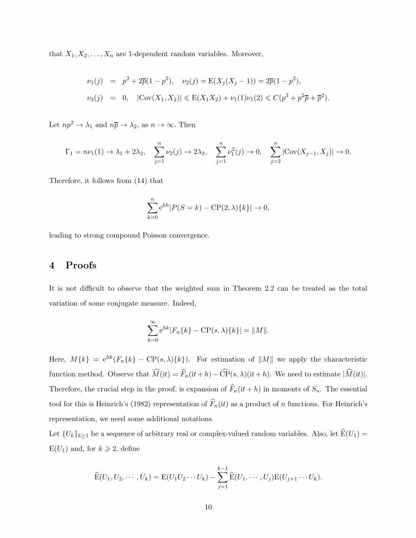
that X1,X2, . . . ,Xn are 1-dependent random variables. Moreover,

ν1(j) = p2 + 2p(1− p2), ν2(j) = E(Xj(Xj − 1)) = 2p(1− p2),

ν3(j) = 0, |Cov(X1,X2)| 6 E(X1X2) + ν1(1)ν1(2) 6 C(p3 + p2p+ p2).

Let np2 → λ1 and np→ λ2, as n→ ∞. Then

Γ1 = nν1(1) → λ1 + 2λ2,n∑

j=1

ν2(j) → 2λ2,n∑

j=1

ν21(j) → 0,n∑

j=2

|Cov(Xj−1,Xj)| → 0.

Therefore, it follows from (14) that

n∑

k=0

ekh|P (S = k)− CP(2, λ){k}| → 0,

leading to strong compound Poisson convergence.

4 Proofs

It is not difficult to observe that the weighted sum in Theorem 2.2 can be treated as the total

variation of some conjugate measure. Indeed,

∞∑

k=0

ehk|Fn{k} −CP(s, λ){k}| = ‖M‖.

Here, M{k} = ehk(Fn{k} − CP(s, λ){k}). For estimation of ‖M‖ we apply the characteristic

function method. Observe that M(it) = Fn(it+h)− CP(s, λ)(it+h). We need to estimate |M (it)|.

Therefore, the crucial step in the proof, is expansion of Fn(it+ h) in moments of Sn. The essential

tool for this is Heinrich’s (1982) representation of Fn(it) as a product of n functions. For Heinrich’s

representation, we need some additional notations.

Let {Uk}k≥1 be a sequence of arbitrary real or complex-valued random variables. Also, let E(U1) =

E(U1) and, for k > 2, define

E(U1, U2, · · · , Uk) = E(U1U2 · · ·Uk)−k−1∑

j=1

E(U1, · · · , Uj)E(Uj+1 · · ·Uk).

10

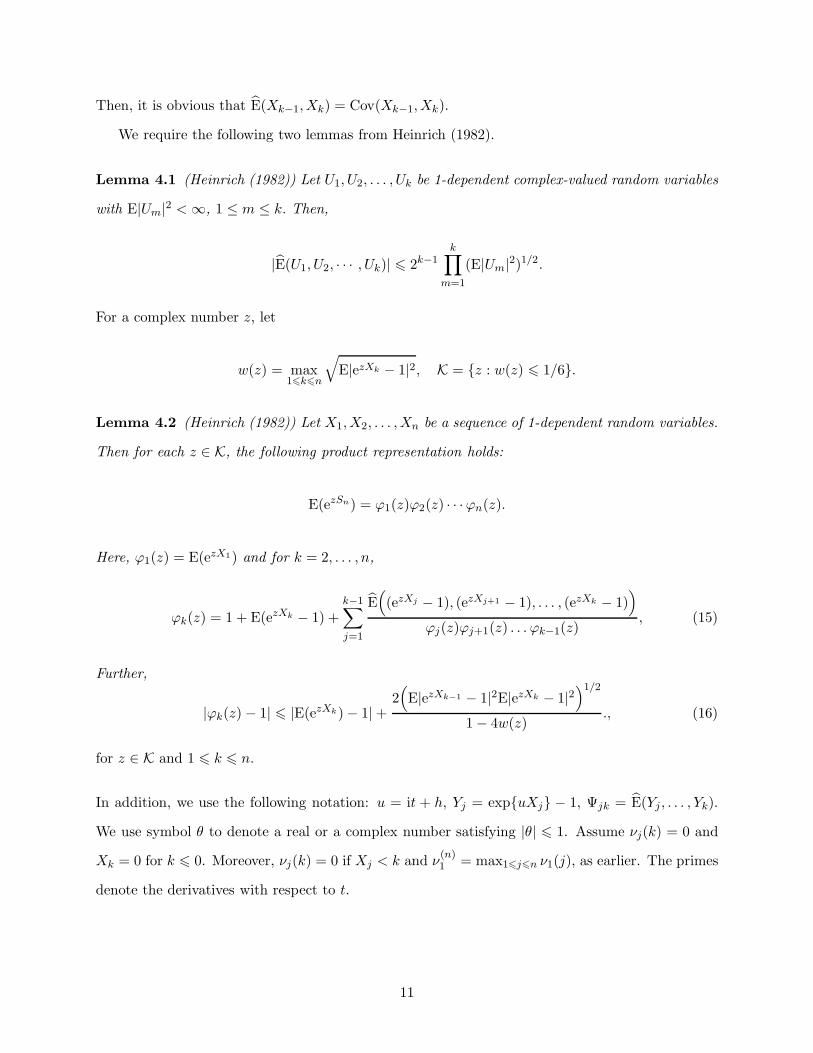
Then, it is obvious that E(Xk−1,Xk) = Cov(Xk−1,Xk).

We require the following two lemmas from Heinrich (1982).

Lemma 4.1 (Heinrich (1982)) Let U1, U2, . . . , Uk be 1-dependent complex-valued random variables

with E|Um|2 <∞, 1 ≤ m ≤ k. Then,

|E(U1, U2, · · · , Uk)| 6 2k−1k∏

m=1

(E|Um|2)1/2.

For a complex number z, let

w(z) = max16k6n

√E|ezXk − 1|2, K = {z : w(z) 6 1/6}.

Lemma 4.2 (Heinrich (1982)) Let X1,X2, . . . ,Xn be a sequence of 1-dependent random variables.

Then for each z ∈ K, the following product representation holds:

E(ezSn) = ϕ1(z)ϕ2(z) · · ·ϕn(z).

Here, ϕ1(z) = E(ezX1) and for k = 2, . . . , n,

ϕk(z) = 1 + E(ezXk − 1) +k−1∑

j=1

E((ezXj − 1), (ezXj+1 − 1), . . . , (ezXk − 1)

)

ϕj(z)ϕj+1(z) . . . ϕk−1(z), (15)

Further,

|ϕk(z)− 1| 6 |E(ezXk)− 1|+2(E|ezXk−1 − 1|2E|ezXk − 1|2

)1/2

1− 4w(z)., (16)

for z ∈ K and 1 6 k 6 n.

In addition, we use the following notation: u = it + h, Yj = exp{uXj} − 1, Ψjk = E(Yj , . . . , Yk).

We use symbol θ to denote a real or a complex number satisfying |θ| 6 1. Assume νj(k) = 0 and

Xk = 0 for k 6 0. Moreover, νj(k) = 0 if Xj < k and ν(n)1 = max16j6n ν1(j), as earlier. The primes

denote the derivatives with respect to t.

11

Lemma 4.3 The following relations hold for all t, k = 1, . . . , n, and an integer s > 1:

|Yk| 6 ehC0(2 + h)Xk, |Yk|2 6 a2Xk, E|Yk| 6 aν1(k), E|Yk|2 6 a2ν1(k), (17)

|Y ′k| 6 ehC0Xk, |Y ′

k|2 6 e2hC0C0Xk, E|Y ′k| 6

a

2ν1(k), E|Y ′

k|2 6a2

4ν1(k), (18)

EYk =s∑

m=1

νm(k)

m!(eu − 1)m + θehC0(eh + 1)s+1 νs+1(k)

(s+ 1)!, (19)

EY ′k = i

s∑

m=1

νm(k)

(m− 1)!eu(eu − 1)m−1 + θehC0(eh + 1)s

νs+1(k)

s!. (20)

Proof. Since | exp{it(Xk − j)}| = 1, we have

|Yk| 6 ehXk |eitXk − 1|+ ehXk − 1 6 ehXk

(|eit(Xk−1)|+ |eit(Xk−2)|+ · · ·+ 1

)|eit − 1|

+hXkehXk 6 ehC0Xk(|eit|+ 1) + hXke

hC0

6 ehC0(2 + h)Xk.

Other relations of (17) now follow. The proof of (18) is obvious. For the proof of (19), we apply

Bergstrom (1951) identity

αN =

s∑

m=0

(N

m

)βN−m(α− β)m +

N∑

m=s+1

(m− 1

s

)αN−m(α− β)s+1βm−s−1, (21)

which holds for any numbers α, β and s = 0, 1, 2, . . . , N . Let(jk

)= 0, for k > j. Then, (21) holds

for all s = 0, 1, . . . . We apply (21) with N = Xk, α = eu and β = 1. Then,

Yk =s∑

m=1

(Xk

m

)(eu − 1)m +

Xk∑

m=s+1

(m− 1

s

)eu(Xk−m)(eu − 1)s+1. (22)

Using the resultsN∑

m=s+1

(m− 1

s

)=

(N

s+ 1

), |eu| = eh,

we obtainXk∑

m=s+1

(m− 1

s

)|eu(Xj−m)| 6 ehC0

(Xj

s+ 1

).

The proof of (19) now follows by finding the mean of Yk in (22) and using the definition of νj(k).

12

For the proof of (20), we once again apply (21) to obtain

Y ′k = iXke

uXk = iXkeueu(Xk−1)

= iXkeu

{ s−1∑

m=0

(Xk − 1

m

)(eu − 1)m + (eu − 1)s

Xk−1∑

m=s

(m− 1

s− 1

)eu(Xk−1−m)

}.

The rest of the proof is the same as that of (19) and, therefore, omitted. �

Lemma 4.4 Let a2ν(n)1 6 0.01. Then, for k = 4, . . . , n and j = 1, . . . , k − 3,

|Ψjk| 6 250a4(1

5

)k−j 3∑

l=0

ν21(k − l), |Ψ′jk| 6 125a4(k − j + 1)

(1

5

)k−j 3∑

l=0

ν21(k − l)

and for k = 2, . . . , n; j = 1, . . . , k − 1,

|Ψjk| 6 5a2(1

5

)k−j

[ν1(k − 1) + ν1(k)],

|Ψ′jk| 6 (2.5)a2(k − j + 1)

(1

5

)k−j

[ν1(k − 1) + ν1(k)].

Proof. From Lemma 4.1 and (17), we have

|Ψjk| 6 2k−jk∏

l=j

√a2ν1(l) 6 2k−j(0.1)k−j−3a4

√ν1(k)ν1(k − 1)ν1(k − 2)ν1(k − 3)

and the estimates for Ψjk follow.

Similarly,

|Ψ′jk| 6

k∑

i=j

|E(Yj, . . . , Y ′i , . . . , Yk)| 6

k∑

i=j

2k−j√

E|Y ′i |2

k∏

l 6=i

√E|Yl|2

6 2k−j−1(k − j + 1)

k∏

i=j

√a2ν1(i)

and hence, the remaining two estimates follow. �

13

Lemma 4.5 Let a2ν(n)1 6 0.01 and s > 1 be an integer. Then, for k = 1, 2, . . . , n and t ∈ R,

|ϕk(u)− 1| 6a2

6[10ν1(k − 1) + 13ν1(k)], |ϕk(u)− 1| 6 1

25,

1

|ϕk(u)|6

10

9, (23)

ϕk(u) = 1 +

s∑

m=1

νm(k)

m!(eu − 1)m + θ

{ehC0(eh + 1)s+1νs+1(k)

(s+ 1)!

+(3.53)a43∑

l=0

ν21(k − l) + (1.8)a3[ν21(k − 1) + ν21(k)]

+(1.8)a3|Cov(Xk−1,Xk)|}, (24)

|ϕ′k(u)| 6 2a2[ν1(k − 1) + ν1(k)], |ϕ′

k(u)| 6 0.04, (25)

ϕ′k(u) = i

s∑

m=1

νm(k)

(m− 1)!(eu − 1)m−1eu + θ

{ehC0(eh + 1)sνs+1(k)

s!

+(8.2)a43∑

l=0

ν21(k − l) + 2.6a3[ν21(k − 1) + ν21(k)]

+(2.6)a3|Cov(Xk−1,Xk)|}. (26)

Proof. Further on, we assume that k > 4. For smaller values of k, all the proofs indeed become

shorter. For brevity, we omit the argument u, whenever possible. First note that for all t ∈ R,

u ∈ K. Indeed,

w(u) = maxj

√E|Yj |2 6 max

j

√a2ν1(j) 6

1

10.

Consequently, by (16) and (17)

|ϕk − 1| 6 E|Yk|+2(E|Yk−1|2E|Yk|2

)1/2

1− 4w(u)

6 aν1(k) +10

3(a4ν1(k − 1)ν1(k))

1/2

6a2ν1(k)

2+

5a2

3[ν1(k − 1) + ν1(k)]

=a2

6[10ν1(k − 1) + 13ν1(k)].

14

Using the assumption and noting that 1/|ϕk | 6 1/(1 − |ϕk − 1|), we obtain (23). By (15)

ϕk = 1 + EYk +Ψk−1,k

ϕk−1+

Ψk−2,k

ϕk−2ϕk−1+

k−3∑

j=1

Ψj,k

ϕj · · ·ϕk−1. (27)

Using Lemma 4.4, it follows that

k−3∑

j=1

|Ψjk|ϕj . . . ϕk−1

6 250a43∑

l=0

ν21(k − l)

k−3∑

j=1

(10

9

)k−j(1

5

)k−j

6 (3.53)a43∑

l=0

ν21(k − l). (28)

Similarly, we have from (17)

|E(Yk−1, Yk)| 6 E|Yk−1, Yk|+ E|Yk−1|E|Yk| 6 a2EXk−1Xk + a2ν1(k − 1)ν1(k)

= a2Cov(Xk−1,Xk) + a22ν1(k − 1)ν1(k)

6 a2|Cov(Xk−1,Xk)|+ a2[ν21(k − 1) + ν21(k)].

Due to the trivial estimate a > 2,

|Ψk−1,k||ϕk−1|

65a3

9

(|Cov(Xk−1,Xk)|+ [ν21(k − 1) + ν21(k)]

). (29)

By assumption, ν(n)1 6 1/400 and

|E(Yk−2, Yk−1, Yk)| 6 [ehC0(2 + h)]3(E(Xk−2Xk−1Xk) + ν1(k − 2)E(Xk−1Xk)

+E(Xk−2Xk−1)ν1(k) + ν1(k − 2)ν1(k − 1)ν1(k))

6 [ehC0(2 + h)]3(E(Xk−1Xk)(C0 + 1/400) + ν1(k − 1)ν1(k)(C0 + 1/400)

)

6401a3

400(E(Xk−1Xk) + ν1(k − 1)ν1(k))

6401a3

400(|Cov(Xk−1,Xk)|+ [ν21(k − 1) + ν21(k)]).

Therefore,

|Ψk−2,k||ϕk−2ϕk−1|

6

(10

9

)2 401a3

400

(|Cov(Xk−1,Xk)|+ [ν21(k − 1) + ν21(k)]

). (30)

15

The proof of (24) now follows by combining the last estimate with (28), (29), (27) and (19).

We prove (25) by induction. We have

ϕ′k = EY ′

k +

k−1∑

j=1

Ψ′jk

ϕj · · ·ϕk−

k−1∑

j=1

Ψjk

ϕj · · ·ϕk

k−1∑

m=j

ϕ′m

ϕm.

Applying Lemma 4.4 and using (17) and (18), we then get

|ϕ′k| 6

a2

4ν1(k) +

5

2a2[ν1(k − 1) + ν1(k)]

k−1∑

j=1

(2

9

)k−j

(k − j + 1)

+5a2[ν1(k − 1) + ν1(k)]10

9(0.04)

k−1∑

j=1

(k − j)

(2

9

)k−j

6 a2[ν1(k − 1) + ν1(k)]

(1

4+

80

49+

4

49

)

6 2a2[ν1(k − 1) + ν1(k)].

The proof of (26) is similar to the proof of (24). We have

|ϕ′k − EY ′

k| 6

k−3∑

j=1

(10

9

)k−j

|Ψ′jk|+

k−3∑

j=1

(10

9

)k−j

|Ψjk|(k − j)

(2

45

)

+

k−1∑

j=k−2

(10

9

)k−j

|Ψ′jk|+

k−1∑

j=k−2

|Ψjk||ϕj · · ·ϕk−1|

(k − j)

(2

45

). (31)

Applying Lemma 4.4, we prove that

k−3∑

j=1

(10

9

)k−j

|Ψ′jk|+

k−3∑

j=1

(10

9

)k−j

|Ψjk|(k − j)

(2

45

)6 (8.2)a4

3∑

l=0

ν21(k − l). (32)

From (29) and (30), it follows that

k−1∑

j=k−2

|Ψjk||ϕj · · ·ϕk−1|

(k − j)

(2

45

)6 (0.135)a3(|Cov(Xk−1,Xk)|+ [ν21 (k − 1) + ν21(k)]). (33)

Taking into account (17) and (18), we obtain

|E(Y ′k−1, Yk)| 6 E|Y ′

k−1Yk|+ E|Y ′k−1|E|Yk| 6 e2hC0(2 + h)E(Xk−1Xk) +

a2

2ν1(k − 1)ν1(k)

16

and10|Ψ′

k−1,k|9

610a2

9

(|Cov(Xk−1,Xk)|+ [ν1(k − 1) + ν1(k)]

). (34)

Similarly, (10

9

)2

|Ψ′k−2,k| 6 (1.86)a3(|Cov(Xk−1,Xk)|+ [ν1(k − 1) + ν1(k)]).

Combining the last estimate with (31)-(34) and (20), we complete the proof of (26). �

Let now

A(u) =

n∑

k=1

lnϕk(u) =

n∑

k=1

∞∑

j=1

(−1)j+1(ϕk(u)− 1)j

j. (35)

Lemma 4.6 Let a2ν(n)1 6 1/100. Then for all t ∈ R,

|A| 6 4a2Γ1, |A′| 6 4a2Γ1, (36)

A =

s∑

m=1

(eu − 1)m

m!

n∑

k=1

νm(k) + θ

{ehC0(eh + 1)s+1

(s+ 1)!

n∑

k=1

νs+1(k)

+24a4n∑

k=1

ν21(k) + (1.8)a3n∑

k=2

|Cov(Xk−1,Xk)|}, (37)

A′ = i

s∑

m=1

νm(k)

(m− 1)!(eu − 1)m−1eu + θ

{ehC0(eh + 1)s

s!

n∑

k=1

νs+1(k)

+(51.4)a4n∑

k=1

ν21(k) + (2.6)a3n∑

k=2

|Cov(Xk−1,Xk)|}. (38)

Proof. Using the first estimate in (23), we have |ϕk − 1| 6 0.04. Therefore,

|A| 6n∑

k=1

|ϕk − 1|∞∑

j=1

(0.04)j−16

( 1

0.96

) n∑

k=1

a2[10ν1(k − 1) + 13ν1(k)]

66 4a2Γ1.

Similarly,

|A′| 6n∑

k=1

|ϕ′k|

|ϕk|6

10

9

n∑

k=1

|ϕ′k| 6

20a2

9

n∑

k=1

[ν1(k − 1) + ν1(k)] 6 4a2Γ1.

From Lemma 4.5, it follows

|ϕk − 1|2 6 a4

36

(10ν1(k − 1) + 13ν1(k)

)26a4

36

(230ν21 (k − 1) + 299ν21 (k)

)

17

andn∑

k=1

∞∑

j=2

|ϕk − 1|j−2

j6

1

2

n∑

k=1

|ϕk − 1|2∞∑

j=2

(0.04)j−26 (7.66)a4

n∑

k=1

ν21(k).

Consequently,

A =

n∑

k=1

(ϕk − 1) + (7.66)θa4n∑

k=1

ν21 (k)

and (37) follows from Lemma 4.5 and the rough estimate a3 6 a4/2, since a > 2.

For the proof of (38), note that

A′ =n∑

k=1

ϕ′k +

n∑

k=1

ϕ′k

ϕk(1− ϕk)

and applying a slightly sharper estimate than in Lemma 4.5, namely 1/|ϕ| 6 25/24, we obtain

n∑

k=1

|ϕ′k|

|ϕk||1− ϕk| 6

25a4

72

n∑

k=1

[ν1(k − 1) + ν1(k)][10ν1(k − 1) + 13ν1(k)] 6 16a4n∑

k=1

ν21(k).

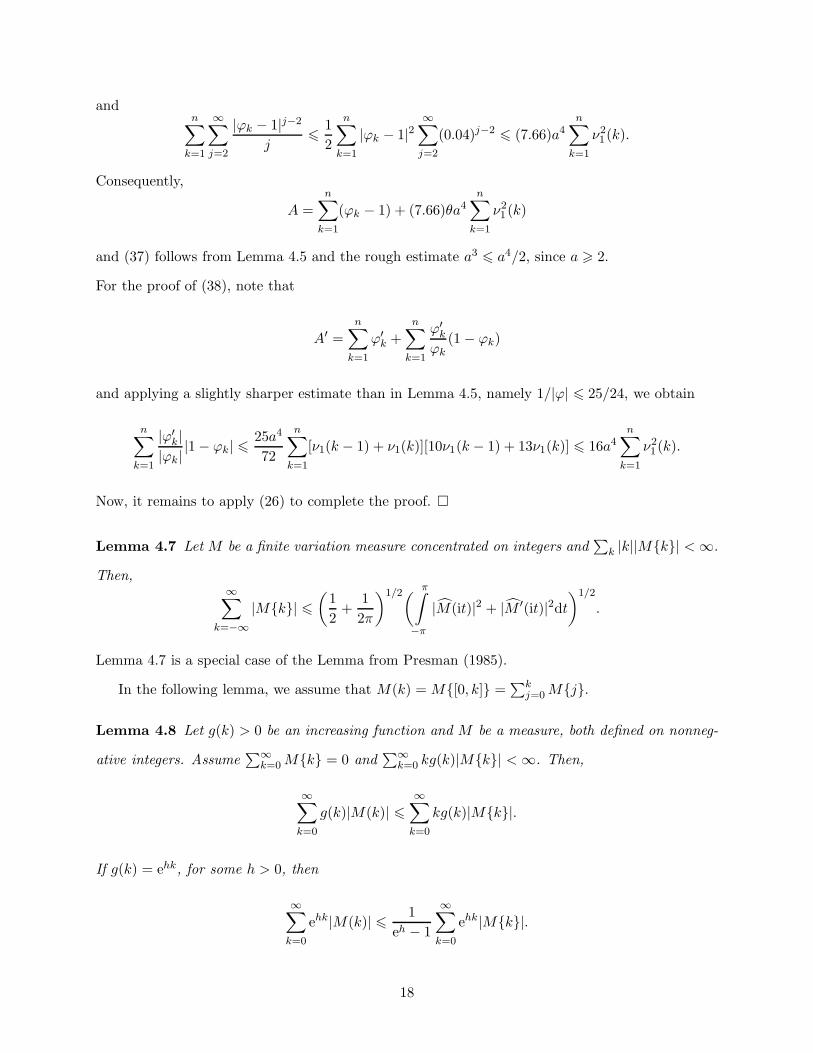
Now, it remains to apply (26) to complete the proof. �

Lemma 4.7 Let M be a finite variation measure concentrated on integers and∑

k |k||M{k}| <∞.

Then,∞∑

k=−∞

|M{k}| 6(1

2+

1

2π

)1/2( π∫

−π

|M(it)|2 + |M ′(it)|2dt)1/2

.

Lemma 4.7 is a special case of the Lemma from Presman (1985).

In the following lemma, we assume that M(k) =M{[0, k]} =∑k

j=0M{j}.

Lemma 4.8 Let g(k) > 0 be an increasing function and M be a measure, both defined on nonneg-

ative integers. Assume∑∞

k=0M{k} = 0 and∑∞

k=0 kg(k)|M{k}| <∞. Then,

∞∑

k=0

g(k)|M(k)| 6∞∑

k=0

kg(k)|M{k}|.

If g(k) = ehk, for some h > 0, then

∞∑

k=0

ehk|M(k)| 6 1

eh − 1

∞∑

k=0

ehk|M{k}|.

18

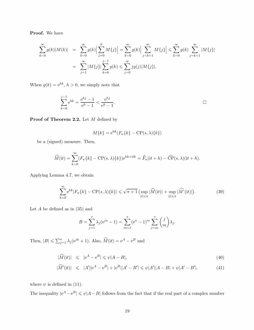
Proof. We have

∞∑

k=0

g(k)|M(k)| =

∞∑

k=0

g(k)∣∣∣

k∑

j=0

M{j}∣∣∣ =

∞∑

k=0

g(k)∣∣∣

∞∑

j=k+1

M{j}∣∣∣ 6

∞∑

k=0

g(k)

∞∑

j=k+1

|M{j}|

=

∞∑

j=1

|M{j}|j−1∑

k=0

g(k) 6

∞∑

j=0

jg(j)|M{j}|.

When g(k) = ehk, h > 0, we simply note that

j−1∑

k=0

ehk =ehj − 1

eh − 1<

ehj

eh − 1. �

Proof of Theorem 2.2. Let M defined by

M{k} = ehk(Fn{k} − CP(s, λ){k})

be a (signed) measure. Then,

M (it) =

∞∑

k=0

(Fn{k} − CP(s, λ){k})ehk+itk = Fn(it+ h)− CP(s, λ)(it + h).

Applying Lemma 4.7, we obtain

∞∑

k=0

ehk|Fn{k} − CP(s, λ){k}| 6√π + 1

(sup|t|6π

|M (it)|+ sup|t|6π

|M ′

(it)|). (39)

Let A be defined as in (35) and

B =

s∑

j=1

λj(eju − 1) =

s∑

m=1

(eu − 1)ms∑

j=m

(j

m

)λj.

Then, |B| 6 ∑sj=1 λj(e

jh + 1). Also, M(it) = eA − eB and

|M (it)| 6 |eA − eB | 6 ψ|A−B|, (40)

|M ′(it)| 6 |A′||eA − eB |+ |eB ||A′ −B′| 6 ψ|A′||A−B|+ ψ|A′ −B′|, (41)

where ψ is defined in (11).

The inequality |eA− eB | 6 ψ|A−B| follows from the fact that if the real part of a complex number

19

Rez 6 0, then

|ez − 1| 6∣∣∣∫ 1

0zeτzdτ

∣∣∣ 6 |z|∫ 1

0exp{τRez}dτ 6 |z|.

Indeed, if Re(A−B) < 0, then

|eA − eB | = |eB ||eA−B − 1| 6 |eB ||A−B| 6 ψ|A −B|.

If Re(B −A) 6 0, then

|eA − eB | = |eA||1− eB−A| 6 |eA||A−B| 6 ψ|A−B|.

The proof is now completed by combining (40), (41) with (39) and using Lemma 4.6. �

Acknowledgment

The authors wish to thank the referees for helpful comments which helped to improve the paper.

References

[1] Barbour, A. D., Chen, L. H. Y. and Choi, K. P. (1995). Poisson approximation for unbounded

functions I: Independent summands. Statist. Sinica 5, 749-766.

[2] Barbour, A.D., Holst, L. and Janson, S. (1992). Poisson Approximation. Clarendon Press,

Oxford.

[3] Bergstrom, H. (1951). On asymptotic expansion of probability functions. Skand. Aktuar., 1,

1-34.

[4] Dafnis, S.D., Antzoulakos, D.L. and Philippou, A.N. (2010). Distributions related to (k1; k2)

events. J. of Statistical Planning and Inference, 140, 16911700.

[5] O’Brien, P. C. and Dyck, P. J. (1985). A runs test based on run lengths. Biometrics, 41,

237-244.

[6] Borisov, I. S. and Ruzankin, P. S. (2002). Poisson approximation for expectations of unbounded

functions of independent random variables. Ann. Probab. 30, 1657-1680.

20

[7] Cekanavicius, V. (2002). On the convergence of Markov binomial to Poisson distribution.

Statist. Probab. Lett. 58, 83-91.

[8] Chen, L. H. Y. (1974). On the convergence of Poisson binomial to Poisson distributions. Ann.

Probab., 2, 178-180.

[9] Chen, L. H. Y. (1975). An approximation theorem for convolutions of probability measures.

Ann. Probab., 3, 992-999 .

[10] Chen, L. H. Y. and Roos, M. (1995). Compound Poisson approximation for unbounded func-

tions on a group with application to large deviations. Probab. Theory Related Fields, 103,

515-528.

[11] Dasgupta, R. (1992). Nonuniform rates of convergence to the Poisson distribution. Sankhya,

Ser. A., 54, 460-463.

[12] Heinrich, L. (1982). A method for the derivation of limit theorems for sums of m-dependent

random variables. Z. Wahrscheinlichkeitstheorie verw. Gebiete, 60, 501–515.

[13] Huang, W. T. and Tsai, C.S. (1991). On a modified binomial distribution of order k. Statist.

Probab. Lett., 11, 125-131.

[14] Presman, E. L.(1986). Approximation in variation of the distribution of a sum of independent

Bernoulli variables with a Poisson law. Theory Probab. Appl., 30(2), 417-422.

[15] Rollin, A. (2005). Approximation of sums of conditionally independent variables by the trans-

lated Poisson distribution. Bernoulli, 11, 1115-1128.

[16] Ruzankin P. S. (2010). Approximation for expectations of unbounded functions of dependent

integer-valued random variables. J. Appl. Probab., 47, 594-600.

[17] Shiryaev A. N. (1995). Probability (Graduate Texts in Mathematics. Springer Mathematics,

vol. 95, 2nd edn, Springer, Berlin.

[18] Simons, G. and Johnson, N. L. (1971). On the convergence of binomial to Poisson distributions.

Ann. Math. Statist., 42, 1735-1736.

21

[19] Vellaisamy, P. (2004). Poisson approximation for (k1, k2) events via the Stein-Chen method.

J. Appl. Probab., 41, 1081-1092.

[20] Wang, Y. H. (1991). A compound Poisson convergence theorem. Ann. Probab., 19, 452-455.

[21] Wang, X. and Xia, A. (2008). On negative binomial approximation to k-runs. J. Appl. Probab.,

45, 456-471.

22