acmgis 2008

Similarity-Based Prediction of Travel Times for Vehicles

Traveling on Known Routes

Christian S. Jensen and Dalia Tiesyte

Aalborg University, Denmark

ACMGIS, November 6-8, 2008

Bus Arrival Time Prediction• Modern collective transport infrastructures

encompass online, geo-positioned buses, a central server, and online variable displays

inform the users of the anticipated arrival times of buses

reward/penalize bus companies based on their compliance with service agreements

• Accurate arrival time prediction is of essence important for the companies that deliver the software to the bus

companies currently deployed techniques are typically do not offer the desired

accuracy motivated by the availability of large collections of historical data,

we propose a data-driven approach to arrival time prediction

3

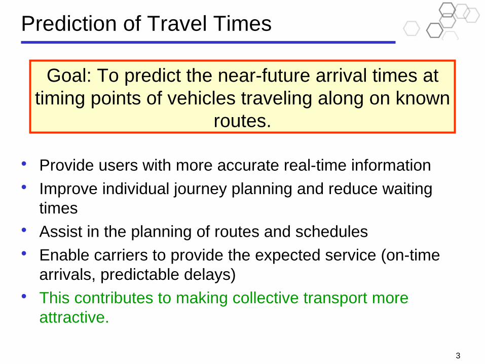
Prediction of Travel Times

• Provide users with more accurate real-time information• Improve individual journey planning and reduce waiting

times• Assist in the planning of routes and schedules• Enable carriers to provide the expected service (on-time

arrivals, predictable delays)• This contributes to making collective transport more

attractive.

Goal: To predict the near-future arrival times at timing points of vehicles traveling along on known

routes.

Proposed Approach

IWCTS, Dublin, 21 April 2008Summer School, Agder, July 1, 2008 4

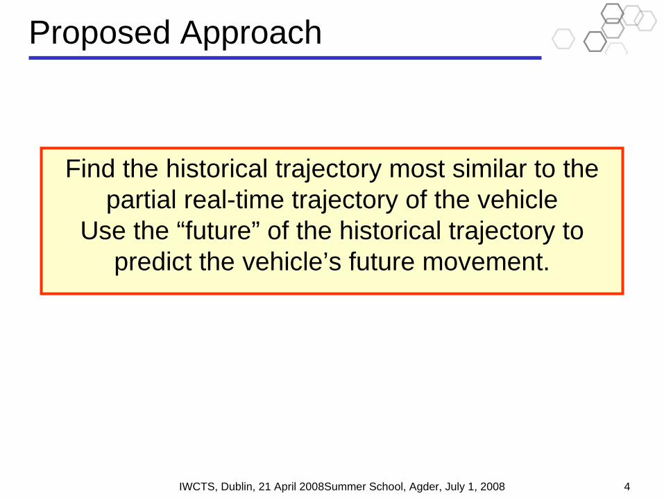
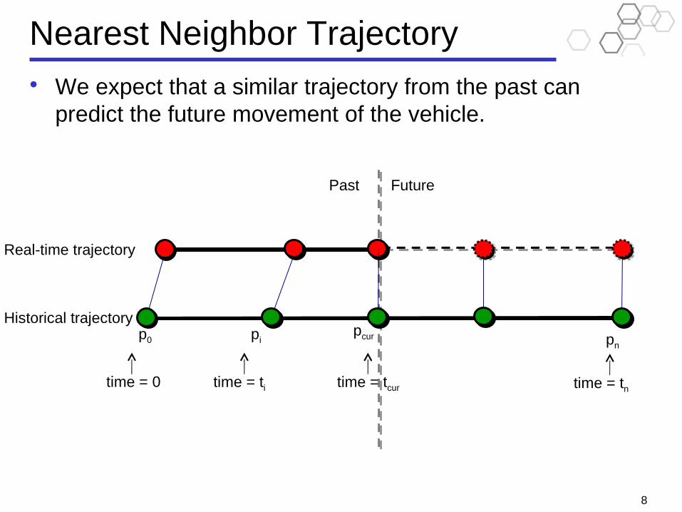
Find the historical trajectory most similar to the partial real-time trajectory of the vehicle

Use the “future” of the historical trajectory to predict the vehicle’s future movement.

5

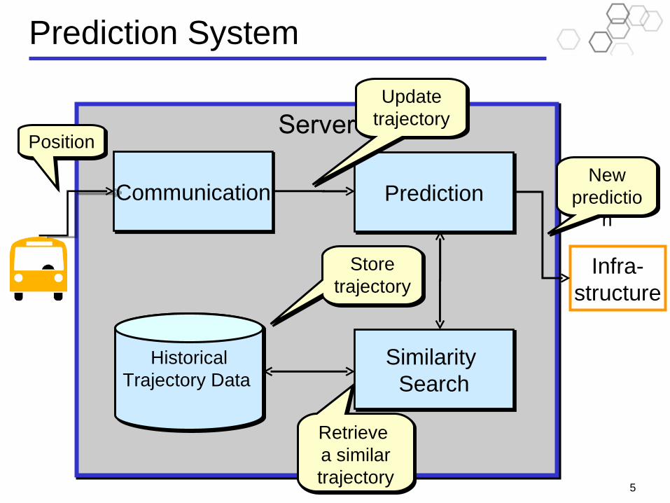
Prediction System

Server

Communication

Infra-structure

HistoricalTrajectory Data

Storetrajectory

Retrieve a similartrajectory

New predictio

n

Position

Prediction

Similarity Search

Update trajectory

6

Outline• Problem statement

Data representation Nearest neighbor trajectories

• Similarity measures for trajectories of vehicles• Similarity search• Results• Conclusion

7

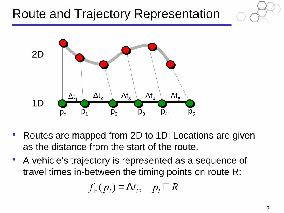
Route and Trajectory Representation

• Routes are mapped from 2D to 1D: Locations are given as the distance from the start of the route.

• A vehicle’s trajectory is represented as a sequence of travel times in-between the timing points on route R:

Rptpf iii ∈∆= ,)(tr

2D

1D ∆t1

∆t2 ∆t3 ∆t4 ∆t5

p0 p1 p2 p3 p4 p5

FuturePast

8

Nearest Neighbor Trajectory• We expect that a similar trajectory from the past can

predict the future movement of the vehicle.

pn

time = 0 time = tcurtime = ti time = tn

p0 pipcur

Real-time trajectory

Historical trajectory

9

Problem Statement• Travel-time prediction by similar historical trajectories

Define a similarity (distance) measure d that enables the selection of the most similar historical trajectory (NNT), which would serve as an accurate predictor of the vehicle’s future movement.

• Efficient similar historical trajectory retrieval. Retrieve the trajectory from the database that minimizes d

between a historical and the (partial) real-time trajectory. Enable variable-length queries. Incrementally update the NNT as new points arrive in the real-time

trajectory. Do this efficiently!

10

Outline• Problem statement

Data representation Nearest neighbor trajectories

• Similarity measures for trajectories of vehicles• Similarity search• Results• Conclusion

11

Similarity Measures–Requirements • Fundamental assumption: similar past implies similar

future.• A distance, or similarity, measure is needed for finding a

historical trajectory to predict the future movement.• Requirements for similarity/distance measures

support comparison of fixed-length trajectories support sub-trajectories is a metric amenable to efficient, scalable computation enable prioritization of either long- or short-term prediction

12

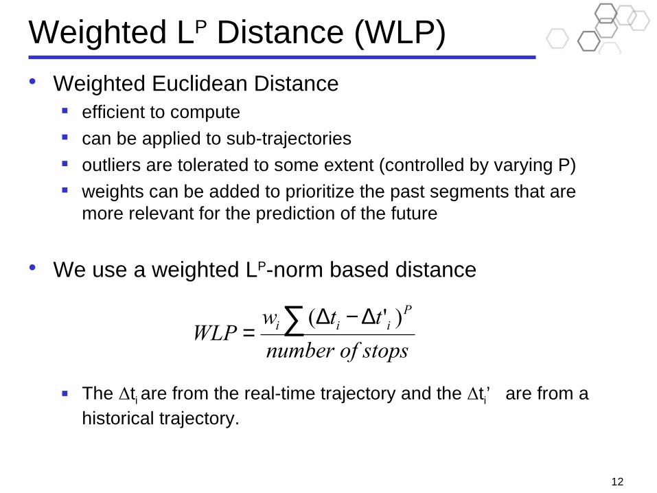
Weighted LP Distance (WLP)• Weighted Euclidean Distance

efficient to compute can be applied to sub-trajectories outliers are tolerated to some extent (controlled by varying P) weights can be added to prioritize the past segments that are

more relevant for the prediction of the future

• We use a weighted LP-norm based distance

The Δti are from the real-time trajectory and the Δti’ are from a historical trajectory.

stopsnumber of

ttwWLP

Piii∑ ∆−∆

=)'(

13

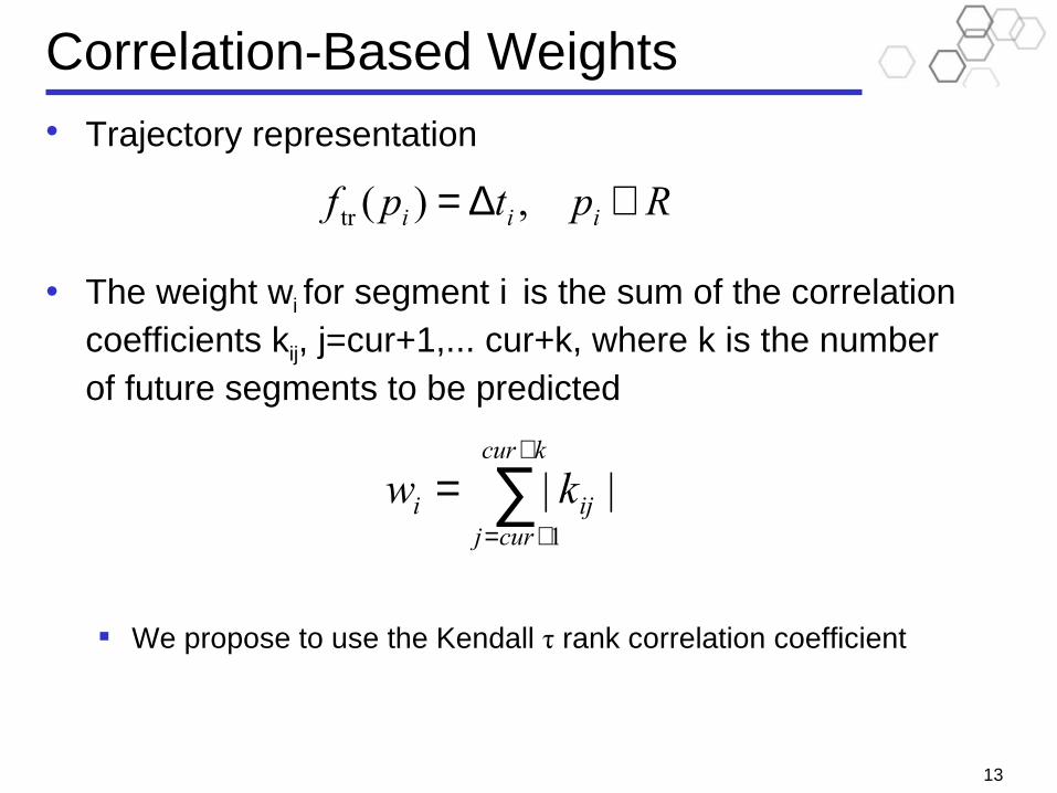
Correlation-Based Weights• Trajectory representation

• The weight wi for segment i is the sum of the correlation coefficients kij, j=cur+1,... cur+k, where k is the number of future segments to be predicted

We propose to use the Kendall τ rank correlation coefficient

Rptpf iii ∈∆= ,)(tr

∑+

+=

=kcur

curjiji kw

1

||

14

Outline• Problem statement

Data representation Nearest neighbor trajectories

• Similarity measures for trajectories of vehicles• Similarity search• Results• Conclusion

15

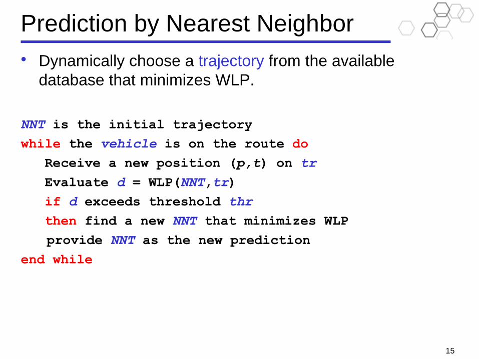
Prediction by Nearest Neighbor• Dynamically choose a trajectory from the available

database that minimizes WLP.

NNT is the initial trajectory

while the vehicle is on the route do

Receive a new position (p,t) on tr

Evaluate d = WLP(NNT,tr)

if d exceeds threshold thr

then find a new NNT that minimizes WLP

provide NNT as the new prediction

end while

16

List-Based Indexing• Assumptions

A trajectory is a sequence (Δt1, …, Δtn), where Δti represents the travel time for the ith segment of the route.

Each trajectory is of length n. (In most cases) there does exist a trajectory in the database that is

similar to the current real-time trajectory (i.e., trajectories are non-random).

• Requirements The index must be able to answer queries of varying length. The search should be incremental. Perfect precision is required (the most similar trajectory must be

found).

17

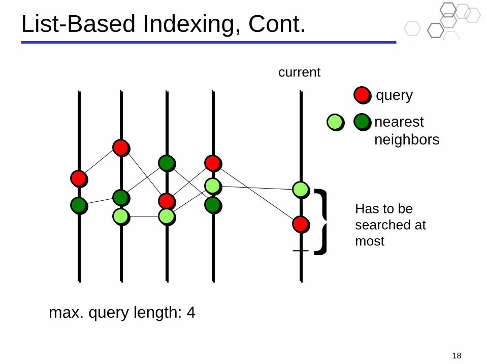
List-Based Indexing, Cont.• Data structure

A sorted list for each timing point on the route, and an entry in each list for each trajectory.

Random access is possible (a sequential-access algorithm exists as well).• Non-incremental algorithm

Perform binary search in each corresponding list and locate the points that are closest to the query points.

Access each list simultaneously (next closest point) and calculate the distances to the accessed trajectories.

Track the current NNT (i.e., the NNT seen so far): the trajectory that is within the minimum distance from the query trajectory.

Calculate bound: the distance in-between the query trajectory and the set of the most recently accessed entries in each list. This is the minimum possible distance to the query so far.

Stop when the bound exceeds the distance to the current NNT.• Incremental algorithm

When a new point arrives, re-use the bound calculated in the previous iteration.

18

Has to be searched at most

List-Based Indexing, Cont.

query

nearest neighbors

max. query length: 4

current

}

19

Outline• Problem statement

Data representation Nearest neighbor trajectories

• Similarity measures for trajectories of vehicles• Similarity search• Results• Conclusion

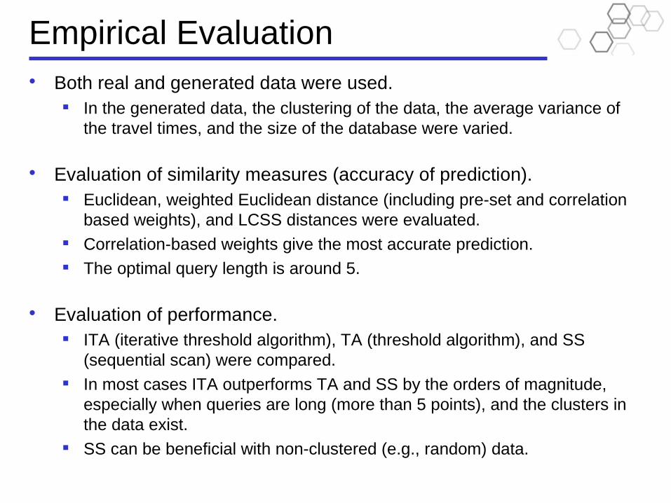
Empirical Evaluation• Both real and generated data were used.

In the generated data, the clustering of the data, the average variance of the travel times, and the size of the database were varied.

• Evaluation of similarity measures (accuracy of prediction). Euclidean, weighted Euclidean distance (including pre-set and correlation

based weights), and LCSS distances were evaluated. Correlation-based weights give the most accurate prediction. The optimal query length is around 5.

• Evaluation of performance. ITA (iterative threshold algorithm), TA (threshold algorithm), and SS

(sequential scan) were compared. In most cases ITA outperforms TA and SS by the orders of magnitude,

especially when queries are long (more than 5 points), and the clusters in the data exist.

SS can be beneficial with non-clustered (e.g., random) data.

21

Conclusions• Fundamental assumption: A similar past trajectory can

predict the future trajectory of a vehicle.• We have proposed

to use a weighted LP norm-based distance (WLP) as a trajectory similarity measure (more measures are discussed in the paper)

to index the trajectories with a sorted list-based index and to access them using an Iterative Threshold Algorithm (ITA)

• Experimental results suggest that the correlation-based WLP together with ITA yields vehicle travel time prediction that is satisfactorily accurate and efficient.

22

Future Work• Currently

Dynamic choice of the nearest neighbor trajectory (NNT) that minimizes the distance to the real-time trajectory.

• Proposed extension Dynamic choice of the prediction algorithm (including NNT) that

minimizes the real-time trajectory prediction error.

Thank you for your attention.

24

Related Work• Existing approaches to travel time prediction

Autoregressive models/Kalman filtering

[Shalaby and Farhan 2001, Cathey and Dailey 2003, Dailey et al. 2004, Mishalani 2008]

Machine learning:

Artificial Neural Networks

[Chien et al. 2002, Park et al. 2004, Hee and Rilett 2004]

Support Vector Machines [Bin et al. 2006]

Historical speed/time patterns

[Predic et al. 2007, Sun et al. 2007].

25

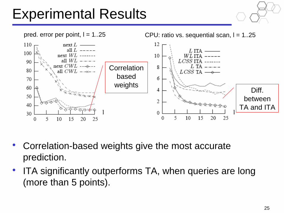
Experimental Results

• Correlation-based weights give the most accurate prediction.

• ITA significantly outperforms TA, when queries are long (more than 5 points).

pred. error per point, l = 1..25 CPU: ratio vs. sequential scan, l = 1..25

l l

Diff. between

TA and ITA

Correlation based

weights