Acidic Deposition Impacts on Natural Resources in ...

National Park Service U.S. Department of the Interior Northeast Region Philadelphia, Pennsylvania

Acidic Deposition Impacts on Natural Resources in Shenandoah National Park Technical Report NPS/NER/NRTR—2006/066

ON THE COVER Staunton River watershed, in the central section of Shenandoah National Park. Staunton River is one of the watersheds included in the long-term watershed research and monitoring program maintained by the Shenandoah Watershed Study. Photograph by: Rick Webb, Projects Coordinator, Shenandoah Watershed Study.

Acidic Deposition Impacts on Natural Resources in Shenandoah National Park Technical Report NPS/NER/NRTR—2006/066 Bernard J. Cosby, James R. Webb, James N. Galloway, and Frank A. Deviney Department of Environmental Sciences University of Virginia Clark Hall P.O. Box 400123 Charlottesville, VA 22904-4123 November 2006 U.S. Department of the Interior National Park Service Northeast Region Philadelphia, Pennsylvania

ii

The Northeast Region of the National Park Service (NPS) comprises national parks and related areas in 13 New England and Mid-Atlantic states. The diversity of parks and their resources are reflected in their designations as national parks, seashores, historic sites, recreation areas, military parks, memorials, and rivers and trails. Biological, physical, and social science research results, natural resource inventory and monitoring data, scientific literature reviews, bibliographies, and proceedings of technical workshops and conferences related to these park units are disseminated through the NPS/NER Technical Report (NRTR) and Natural Resources Report (NRR) series. The reports are a continuation of series with previous acronyms of NPS/PHSO, NPS/MAR, NPS/BSO-RNR, and NPS/NERBOST. Individual parks may also disseminate information through their own report series. Natural Resources Reports are the designated medium for information on technologies and resource management methods; "how to" resource management papers; proceedings of resource management workshops or conferences; and natural resource program descriptions and resource action plans. Technical Reports are the designated medium for initially disseminating data and results of biological, physical, and social science research that addresses natural resource management issues; natural resource inventories and monitoring activities; scientific literature reviews; bibliographies; and peer-reviewed proceedings of technical workshops, conferences, or symposia. Mention of trade names or commercial products does not constitute endorsement or recommendation for use by the National Park Service. This report was accomplished under Cooperative Agreement 4000-7-9002 with assistance from the NPS. The statements, findings, conclusions, recommendations, and data in this report are solely those of the author(s), and do not necessarily reflect the views of the U.S. Department of the Interior, National Park Service. Print copies of reports in these series, produced in limited quantity and only available as long as the supply lasts, or preferably, file copies on CD, may be obtained by sending a request to the address on the back cover. Print copies also may be requested from the NPS Technical Information Center (TIC), Denver Service Center, PO Box 25287, Denver, CO 80225-0287. A copy charge may be involved. To order from TIC, refer to document D-302. This report may also be available as a downloadable portable document format file from the Internet at http://www.nps.gov/nero/science/. Please cite this publication as: Cosby, B. J., J. R. Webb, J. N. Galloway, and F. A. Deviney. November 2006. Acidic Deposition Impacts on

Natural Resources in Shenandoah National Park. Technical Report NPS/NER/NRTR—2006/066. National Park Service. Philadelphia, PA.

NPS D-302 November 2006

iii

Acknowledgments

We wish to thank the National Park Service (NPS) staff who assisted in many aspects of this effort. John Karish assisted with cooperative agreement management and was the major impetus in developing and implementing the project. Dan Hurlbert coordinated GIS data for Shenandoah National Park and assisted in the mapping activities. Shane Spitzer prepared the tabular summary of the park’s past and present deposition monitoring, and assisted with Shenandoah-relevant publications distribution and tracking. Alan Williams assisted with natural resource data base queries and data summaries. Jim Atkinson provided I&M data for the fisheries response analyses. Constructive comments and criticisms were provided on an earlier draft of this report by Gordon Olson, of Shenandoah National Park

Bryan Bloomer (of the USEPA) assisted with development of emissions control scenarios for model projections of future change. Kai Snyder, Erin Gilbert, Deian Moore, and Jayne Charles (of E&S Environmental Chemistry) assisted with data analyses, graphics, and map construction.

At the University of Virginia (UVa), Art Bulger and Joe Krawzcel provided extensive help and insight into the fisheries responses. Danny Welsch collected and assisted in the analysis of the soils data and tree core data. Susie Maben contributed substantially to the analysis of stream water chemistry.

Special thanks are due to Grace Lipscomb, Grants Administrator for the UVa Department of Environmental Sciences, for her endless patience and invaluable expertise in managing the administrative and fiscal aspects of the project.

v

Relationship of this project to other research in Shenandoah National Park

Much of the material presented in this report has also been presented in:

Assessment of Air Quality and Related Values in Shenandoah National Park (Technical Report NPS/NERCHAL/NRTR-03/090) by T. J. Sullivan, B. J. Cosby, A. J. Bulger, J. R. Webb, J. A. Laurence, E. H. Lee, W. E. Hogsett, R. L. Dennis, K. Savig, H. Wayne, M. Scruggs, J. Ray, D. Miller, C. Gordon and J. S. Kern.

The above report (the “AQRV Report”), was a project completion report for a National Park Service (NPS) funded project (the “AQRV Project”) examining all aspects of air quality and related values within Shenandoah National Park (SHEN). The project described here (“Acid Impacts Project”; “Acid Impacts Report”) was also an NPS funded project, but had a specific focus on the impacts of acid deposition (only) on SHEN resources.

The AQRV Project was funded and completed first. However, the period of the Acid Impacts Project overlapped by more than a year with the period of the AQRV Project. As a result, many of the results of the Acid Impacts Project were available for inclusion in the AQRV Report. This was clearly a desirable circumstance for the AQRV Project because the included material made the AQRV Report more comprehensive and robust with respect to the sections devoted to acid deposition effects. Similarly, the material developed in the AQRV Project concerning the emissions, source areas, and deposition of acid pollutants complemented this Acid Impacts Project by providing a comprehensive and robust background for the evaluation of acid impacts on SHEN resources.

Therefore, there is an extensive overlap of the material presented in this Acid Impacts Report and in the AQRV Report. Rather than re-organize or re-write material, the same text was used in both reports where appropriate, or was modified as each report required.

The material in this Acid Impacts Report that derives in large part from the AQRV Project consists of Chapter 3 (Environmental Setting of SHEN) and Chapter 4 (Acidic Deposition in SHEN). These chapters are borrowed more or less literally from the AQRV Report and provide useful and necessary information that is relevant to the Acid Impacts Project.

The remainder of the material presented in this Acid Impacts Report was primarily a direct output of the Acid Impacts Project. Similarities (literal or otherwise) between this material and material in the AQRV Report result from the fact that the AQRV Report was published first. Given that the AQRV Report came out before this Acid Impacts Project was completed, an acknowledgement of this sort about shared textual material does not appear in the AQRV Report.

vii

Index to Chapters

Page

Chapter 1: An Overview of the Effects of Acidic Deposition in Shenandoah National Park and an Introduction to the Study .................................................... 1-1

1.1 Overview of the Effects of Acidic Deposition in Shenandoah National Park ..................................................................................................................... 1-1

1.2 Study Objectives and Structure of the Report ............................................................. 1-2

1.3 Acid Deposition and Shenandoah National Park......................................................... 1-3

1.4 Stream Water Acidification in Shenandoah National Park.......................................... 1-4

1.4.1 Shenandoah National Park: Current Stream Water Composition ............................................................................................................. 1-5

1.4.2 Shenandoah National Park: Changes in Stream Water Composition ............................................................................................................. 1-9

1.4.3 Shenandoah National Park: Acidification Effects on Fish ............................ 1-11

Chapter 2: An Assessment of Areas of Concern in Shenandoah National Park with Respect to Adverse Effects of Acidic Deposition ................................................... 2-15

2.1 Assessment Mapping Approach ............................................................................... 2-15

2.2 Categories of Concern for Assessment Mapping ...................................................... 2-16

2.2.1 Surface Waters .............................................................................................. 2-16

2.2.2 Soils ............................................................................................................... 2-17

2.3 Landscape Mapping .................................................................................................. 2-18

2.4 Acidification Response Modeling ............................................................................. 2-20

2.5 Historical Deposition Effects and Areas of Concern ................................................ 2-21

2.6 Future Forecast Scenarios ......................................................................................... 2-21

2.7 Future Deposition Effects and Areas of Concern ..................................................... 2-30

2.8 Conclusions ............................................................................................................... 2-35

viii

Chapter 3: The Environmental Setting of Shenandoah National Park .................................... 3-37

3.1 Background ............................................................................................................... 3-37

3.2 Climate ...................................................................................................................... 3-43

3.3 Scenery ...................................................................................................................... 3-44

3.4 Surface Waters .......................................................................................................... 3-44

3.5 Geology ..................................................................................................................... 3-45

3.6 Soils ........................................................................................................................... 3-47

3.7 Vegetation ................................................................................................................. 3-49

3.8 Wildlife ..................................................................................................................... 3-54

3.9 Disturbance ............................................................................................................... 3-54

Chapter 4: Acidic Deposition in Shenandoah National Park ................................................... 4-57

4.1 Sources of Acidic Deposition Arriving at Shenandoah National Park ................................................................................................................................. 4-57

4.1.1 Patterns of Atmospheric Transport ............................................................... 4-59

4.1.1.1 Source Areas ........................................................................................ 4-59

4.1.1.2 Airsheds ............................................................................................... 4-61

4.1.1.3 Top Five Air Pollutant Source Sub-regions for Shenandoah National Park ............................................................................... 4-67

4.1.1.4 Relative Contributions by State ........................................................... 4-69

4.2 Atmospheric Deposition in Shenandoah National Park ............................................ 4-71

4.2.1 Atmospheric Deposition Monitoring Efforts in Shenandoah National Park ..................................................................................... 4-72

4.2.2 Historical Deposition of S and N at Shenandoah National Park ........................................................................................................................ 4-74

4.2.3 Ambient Atmospheric Deposition at Shenandoah National Park .......................................................................................................... 4-74

4.2.4 Trends in Atmospheric Deposition at Shenandoah National Park .......................................................................................................... 4-84

ix

Chapter 5: Current Status of Water and Soil Acidification in Shenandoah National Park ........................................................................................................................... 5-87

5.1 Current Status of Stream Water Chemistry ............................................................... 5-89

5.2 Relationships Between Geology and Stream Water Chemistry ................................ 5-95

5.3 Relationships Between Soils and Stream Water Chemistry ..................................... 5-98

5.4 Regional Context ....................................................................................................... 5-99

Chapter 6: Current Trends in Water Acidification in Shenandoah National Park ........................................................................................................................................ 6-103

6.1 Trend Analyses: Statistical Methods, Data, and General Results ........................... 6-103

6.2 Trends in Acid Neutralizing Capacity (ANC) ........................................................ 6-109

6.3 Sulfate Trends ......................................................................................................... 6-109

6.4 Trends in Base Cation Concentrations .................................................................... 6-115

6.5 Summary of Trends in Stream Water Chemistry in Shenandoah National Park ................................................................................................................. 6-115

Chapter 7: Simulation of Soil and Water Acidification Responses in Shenandoah National Park ..................................................................................................... 7-117

7.1 Description of Sites Selected for Modeling ............................................................ 7-117

7.2 Future Deposition Scenarios Used for Simulations ................................................ 7-118

7.3 Modeling Results .................................................................................................... 7-119

Chapter 8: Stream and Soil Acidification and the Responses of Aquatic and Forest Resources in Shenandoah National Park .............................................................. 8-131

8.1 Overview of Stream Acidification Effects .............................................................. 8-131

8.1.1 Aquatic Macroinvertebrates ........................................................................ 8-131

8.1.2 Fish ............................................................................................................. 8-132

8.2 Effects of Stream Acidification in Shenandoah National Park ............................... 8-133

8.2.1 Acidification Effects on Aquatic Invertebrates in Shenandoah National Park .................................................................................... 8-133

x

8.2.1.1 Previous Studies of Invertebrates in Streams in Shenandoah National Park and Related Areas .............................................. 8-134

8.2.1.2 Stream Water ANC Relationships for Aquatic Invertebrates in Shenandoah National Park Streams ..................................... 8-136

8.2.2 Acidification Effects on Fish in Shenandoah National Park ...................................................................................................................... 8-142

8.2.2.1 Previous Studies of Fish in Streams in Shenandoah National Park and Related Areas ................................................................... 8-144

8.2.2.2 New Studies of Fish in Streams in Shenandoah National Park from this Project ..................................................................... 8-144

8.2.2.3 Stream Water ANC Relationships for Fish in Shenandoah National Park Streams ............................................................... 8-145

8.3 Overview of Soil Acidification Effects ................................................................... 8-147

8.3.1 Soil Base Cation Status ............................................................................... 8-147

8.3.2 Forest and Surface Water Responses .......................................................... 8-149

8.4 Effects of Soil Acidification on Ecosystem Responses in Shenandoah National Park ............................................................................................ 8-150

8.4.1 Soil Acidification Effects on Streams in Shenandoah National Park ......................................................................................................... 8-150

8.4.2 Soil Acidification Effects on Forests in Shenandoah National Park ........................................................................................................ 8-150

8.4.3 Soil Base Saturation % Categories for Soil Acidification Responses ............................................................................................................. 8-153

References .............................................................................................................................. 9-155

xi

Figures

Page

Figure 1.1. A view of headwater catchments in the Valley and Ridge Physiographic Province in western Virginia. ............................................................................. 1-4

Figure 1.2 Primary study watersheds in Shenendoah National Park; shown in relation to the distribution of major bedrock. ............................................................. 1-5

Figure 1.3. Median percent base saturation for soils associated with Shenandoah National Park’s three bedrock types. The base saturation of soils derived from siliceous and felsic bedrock is too low for effective buffering of acidic deposition. ................................................................................................... 1-7

Figure 1.4. Relationship between ANC and runoff for stream water samples collected at intensively studied sites in Shenandoah National Park. ........................................................................................................................................... 1-8

Figure 1.5. Loss of ANC and increase in dissolved aluminum in Paine Run in response to a sharp increase in streamflow. ................................................................... 1-8

Figure 1.6. Comparison of estimated natural and current median sulfate concentrations among streams associated with major bedrock types in Shenandoah National Park. ........................................................................................................ 1-9

Figure 1.7. Estimated historic loss of ANC in Shenandoah National Park stream waters classified by watershed bedrock type. .............................................................. 1-10

Figure 1.8. Relationship between number of fish species and minimum ANC recorded in Shenandoah National Park streams. ............................................................ 1-13

Figure 2.1. Left panel: Map of Shenandoah National Park showing the location of the 14 SWAS study watersheds and the dominate bedrock geology in the park. Right panel: Map of Shenandoah National Park showing the 231 watersheds used to extrapolate from the SWAS study sites to the park landscape. ....................................................................................................... 2-19

Figure 2.2. Landscape maps showing areas of concern for adverse effects from acidic deposition on surface water conditions in Shenandoah National Park. The figure compares maps generated from model simulated data (left) and observed data (right) for the 14 SWAS study sites extrapolated to the 231 mapping watersheds. Surface water conditions are based on simulated or observed stream water ANC (ueq/L). .................................................. 2-22

xii

Figures (continued)

Page

Figure 2.3. Landscape maps showing areas of concern for adverse effects from acidic deposition on soil conditions in Shenandoah National Park. The figure compares maps generated from model simulated data (left) and observed data (right) for the 14 SWAS study sites extrapolated to the 231 mapping watersheds. Soil conditions are based on simulated or observed soil base saturation (%). ........................................................................................................... 2-23

Figure 2.4. Landscape maps showing areas of concern for adverse effects from acidic deposition on surface water conditions in Shenandoah National Park. The figure compares maps generated for three historical periods: pre-industrial conditions (left), conditions in 1980 at the peak of acidic deposition in Shenandoah National Park (middle), and current conditions (right) Surface water conditions are based on simulated values of ANC (ueq/L). ....................................................................................................................... 2-24

Figure 2.5. Landscape maps showing areas of concern for adverse effects from acidic deposition on soil conditions in Shenandoah National Park. The figure compares maps generated for three historical periods: pre-industrial conditions (left), conditions in 1980 at the peak of acidic deposition in Shenandoah National Park (middle), and current conditions (right). Soil conditions are based on simulated values of soil base saturation (%). .......................................................................................................................... 2-25

Figure 2.6a. MAGIC model projections of stream water ANC (upper five panels) and of soil base saturation (lower five panels) for constant deposition at 1990 levels and for four emissions control scenarios. Plots are presented for the five study watersheds on basaltic bedrock. ............................................ 2-27

Figure 2.6b. MAGIC model projections of stream water ANC (upper four panels) and of soil base saturation (lower four panels) for constant deposition at 1990 levels and for four emissions control scenarios. Plots are presented for the five study watersheds on granitic bedrock. ............................................ 2-28

Figure 2.6c. MAGIC model projections of stream water ANC (upper five panels) and of soil base saturation (lower five panels) for constant deposition at 1990 levels and for four emissions control scenarios. Plots are presented for the five study watersheds on siliciclastic bedrock. ...................................... 2-29

xiii

Figures (continued)

Page

Figure 2.7. Landscape maps showing areas of concern for adverse effects from acidic deposition on stream conditions in Shenandoah National Park. The figure compares maps generated for three scenarios of future deposition in the year 2020. The three scenarios of deposition are described in the text. The map of current stream conditions (year 2000) is presented at far left. Stream conditions are based on simulated values of stream ANC (ueq/L). ............................................................................................................... 2-31

Figure 2.8. Landscape maps showing areas of concern for adverse effects from acidic deposition on stream conditions in Shenandoah National Park. The figure compares maps generated for three scenarios of future deposition in the year 2100. The three scenarios of deposition are described in the text. The map of current stream conditions (year 2000) is presented at far left. Stream conditions are based on simulated values of stream ANC (ueq/L). ............................................................................................................... 2-32

Figure 2.9. Landscape maps showing areas of concern for adverse effects from acidic deposition on soil conditions in Shenandoah National Park. The figure compares maps generated for three scenarios of future deposition in the year 2020. The three scenarios of deposition are described in the text. The map of current soil conditions (year 2000) is presented at far left. Soil conditions are based on simulated values of soil base saturation (%). .................................................................................................................. 2-33

Figure 2.10. Landscape maps showing areas of concern for adverse effects from acidic deposition on soil conditions in Shenandoah National Park. The figure compares maps generated for three scenarios of future deposition in the year 2100. The three scenarios of deposition are described in the text. The map of current soil conditions (year 2000) is presented at far left. Soil conditions are based on simulated values of soil base saturation (%). .................................................................................................................. 2-34

Figure 3.1. Shenandoah National Park and division into three management districts. Also shown are the locations of federally designated wilderness areas and air quality monitoring stations. The air quality stations at Dickey Ridge and Sawmill Run are no longer active. ................................ 3-38

Figure 3.2a. Location of roads, trails, streams, and scenic historical overlooks within park boundaries in the North District. .......................................................... 3-39

Figure 3.2b. Location of roads, trails, streams, and scenic historical overlooks within park boundaries in the Central District. ....................................................... 3-40

xiv

Figures (continued)

Page

Figure 3.2c. Location of roads, trails, streams, and scenic historical overlooks within park boundaries in the South District. .......................................................... 3-41

Figure 3.3. Lithologic and geological sensitivity maps of Shenandoah National Park. Geologic sensitivity classes are arranged in the legend from most (siliciclastic) to least (carbonate) sensitive to acidification. ................................... 3-46

Figure 3.4. Soils types in Shenandoah National Park. All soil types in the legend are present within the park, but several are present only in very small areas. ............................................................................................................................... 3-48

Figure 3.5a. Major forest types in the North District of Shenandoah National Park. .......................................................................................................................... 3-51

Figure 3.5b. Major forest types in the Central District of Shenandoah National Park. .......................................................................................................................... 3-52

Figure 3.5c. Major forest types in the South District of Shenandoah National Park. .......................................................................................................................... 3-53

Figure 4.1. New source permit reviews during the period January 1987 to June 2002. ................................................................................................................................ 4-58

Figure 4.2. Range of influence of (a) sulfur deposition, (b) oxidized nitrogen deposition, (c) reduced nitrogen deposition, and (d) sulfate air concentrations expressed as the percent contribution from Subregion 20, a 160x160 km square centered at the joining of the state boundaries of WV, KY, and OH in the Ohio River Valley. .................................................................................... 4-60

Figure 4.3. Major airsheds for Shenandoah National Park for (a) oxidized nitrogen deposition, (b) sulfur deposition, (c) sulfate air concentrations. ............................... 4-62

Figure 4.4. Geographic subdivision of Shenandoah National Park major airsheds: (a) oxidized nitrogen deposition, (b) sulfur deposition, and (c) sulfate air concentrations. ........................................................................................................ 4-65

Figure 4.5. Top 5 source regions contributing air pollution in Shenandoah National Park: (a) oxidized nitrogen deposition, (b) sulfur deposition, and (c) sulfate air concentrations. ................................................................................................... 4-68

Figure 4.6. First-ranked state percent contribution contours for (a) oxidized nitrogen deposition (VA), (b) sulfur deposition (WV), and (c) sulfate air concentration (OH). ................................................................................................ 4-70

xv

Figures (continued)

Page

Figure 4.7. Annual wet deposition of sulfate throughout the eastern United States during 2001. Note that sulfur deposition expressed as kg S/ha/yr (units routinely used elsewhere in this report) is approximately 33% of sulfate deposition expressed kg SO4/ha/yr (as shown on this NADP map). ............................................................................................................................ 4-76

Figure 4.8. Annual wet deposition of nitrate throughout the eastern United States during 2001. Note that nitrogen deposition expressed as kg N/ha/yr (units routinely used elsewhere in this report) is approximately 23% of nitrate deposition expressed kg NO3/ha/yr (as shown on this NADP map). ........................... 4-77

Figure 4.9. Annual wet deposition of total nitrogen (NH4+ plus NO3

-) throughout the eastern United States during 2001 (kg N/ha/yr). ............................................. 4-78

Figure 4.10. Wet sulfur deposition (left panels) and wet inorganic nitrogen deposition (right panels) for the period of record at three monitoring sites in Shenandoah National Park. ....................................................................... 4-85

Figure 4.11. Wet ammonium deposition (left panels) and wet nitrate deposition (right panels) for the period of record at three monitoring sites in Shenandoah National Park. .................................................................................................. 4-86

Figure 5.1. Primary study watersheds in Shenandoah National Park shown in relation to the distribution of major bedrock types in the park. ........................................... 5-87

Figure 5.2. Median percent base saturation for soils associated with Shenandoah National Park’s three bedrock types. The base saturation of soils derived from siliciclastic and granitic bedrock is too low for effective buffering of acidic deposition in many watersheds. .............................................................. 5-100

Figure 5.3. Median spring ANC of streams in SWAS watersheds during the period 1988 to 1999 versus median base saturation of watershed soils. .......................... 5-101

Figure 6.1. Trends in solute concentrations for the 14 SWAS streams in Shenandoah National Park (ueq/L/yr). The trends are the slopes of simple linear regressions on all quarterly data for 14 years (1988 to 2001; n=56). For each solute, the trends have been sorted from lowest to highest to display the range of estimated trends in a given solute across the 14 streams. .................................................................................................................................. 6-105

xvi

Figures (continued)

Page

Figure 6.2. Median values of annual and seasonal trends (in ueq/L) in stream water ANC concentrations among VTSSS and SWAS watersheds: 1988–2001. The median values are from distributions of ANC trends determined for streams within classes defined by physiography or lithology. The annual trends are based on simple linear regressions on all quarterly data for 14 years (n=56). Seasonal trends are based on individual quarterly values for 14 years (n=14). .................................................................... 6-110

Figure 6.3. Median values of annual and seasonal trends in stream water SO4

2- concentrations (in ueq/L) among VTSSS and SWAS watersheds: 1988–2001. The median values are from distributions of ANC trends determined for streams within classes defined by physiography or lithology. The annual trends are based on simple linear regressions on all quarterly data for 14 years (n=56). Seasonal trends are based on individual quarterly values for 14 years (n=14). .................................................................... 6-111

Figure 6.4. Median values of annual and seasonal trends in stream water SBC concentrations (in ueq/L) among VTSSS and SWAS watersheds: 1988–2001. The median values are from distributions of ANC trends determined for streams within classes defined by physiography or lithology. The annual trends are based on simple linear regressions on all quarterly data for 14 years (n=56). Seasonal trends are based on individual quarterly values for 14 years (n=14). .................................................................... 6-112

Figure 6.5. The life stages of brook trout when the species shows the greatest sensitivity to acidification. ........................................................................................ 6-113

Figure 6.6. Trends in stream water SO42- concentrations in relation to

median SO42- concentrations for VTSSS and SWAS streams. .............................................. 6-114

Figure 7.1. MAGIC model simulations of historical stream water concentrations of SO4, NO3, sum of base cations (SBC = Ca+Mg+Na+K), and ANC (Calk =SBC-SO4-NO3) for modeled sites on the three bedrock types in Shenandoah National Park – Siliciclastic (upper left), Basaltic (upper right), and Granitic (lower right). ............................................................................... 7-120

Figure 7.2. MAGIC model simulations of future stream water concentrations of SO4 under the scenario of constant deposition and the four emissions control scenarios (described in the text) for modeled sites on the three bedrock types in Shenandoah National Park – Siliciclastic (upper left), Basaltic (upper right), and Granitic (lower right). ............................................. 7-122

xvii

Figures (continued)

Page

Figure 7.3. MAGIC model simulations of future stream water concentrations of NO3 under the scenario of constant deposition and the four emissions control scenarios (described in the text) for modeled sites on the three bedrock types in Shenandoah National Park – Siliciclastic (upper left), Basaltic (upper right), and Granitic (lower right). ............................................. 7-123

Figure 7.4. MAGIC model simulations of future stream water concentrations of sum of base cations (SBC=Ca+Mg+Na+K) under the scenario of constant deposition and the four emissions control scenarios (described in the text) for modeled sites on the three bedrock types in Shenandoah National Park – Siliciclastic (upper left), Basaltic (upper right), and Granitic (lower right). .......................................................................................... 7-124

Figure 7.5. MAGIC model simulations of future stream water concentrations of charge balance ANC (Calk=SBC-SO4-NO3) under the scenario of constant deposition and the four emissions control scenarios (described in the text) for modeled sites on the three bedrock types in Shenandoah National Park – Siliciclastic (upper left), Basaltic (upper right), and Granitic (lower right). .......................................................................................... 7-125

Figure 8.1. Average number of families in a sample of a given order of aquatic insects for each of the 14 SWAS study streams in Shenandoah National Park versus the mean (left) or minimum (right) ANC of each stream. The stream ANC values are based on quarterly samples from 1988 to 2001. Invertebrate samples are contemporaneous. .................................................. 8-138

Figure 8.2. Average number of individuals in a sample of a given order of aquatic insects for each of the 14 SWAS study streams in Shenandoah National Park versus the mean (left) or minimum (right) ANC of each stream. The stream ANC values are based on quarterly samples from 1988 to 2001. ......................................................................................................................... 8-139

Figure 8.3. Shannon-Weaver diversity index for each of the 14 SWAS study streams in Shenandoah National Park versus the mean (left) or minimum (right) ANC of each stream. The diversity index was calculated for Orders (upper panels) and for Families (lower panels). The stream ANC values are based on quarterly samples from 1988 to 2001. Invertebrate samples are contemporaneous. .......................................................................... 8-140

xviii

Figures (continued)

Page

Figure 8.4. Shannon-Weaver eveness index for each of the 14 SWAS study streams in Shenandoah National Park versus the mean (left) or minimum (right) ANC of each stream. The evenness index was calculated for Orders (upper panels) and for Families (lower panels). The stream ANC values are based on quarterly samples from 1988 to 2001. Iinvertebrate samples are contemporaneous. ......................................................................... 8-141

Figure 8.5. Number of fish species (species richness) in each of 13 SWAS study streams in Shenandoah National Park versus the mean (left) or minimum (right) ANC of each stream. The stream ANC values are based on quarterly samples from 1988 to 2001. The fish species richness samples are contemporaneous. ............................................................................................... 8-147

Figure 8.6. A: Pre-Industrial Period: The base-cation supply in the soil is stable; losses to surface water are replaced by release from bedrock. Base cations taken up by vegetation are recycled. B: Post-Industrial Period: Sulfate (SO4

2-) moving through the soil leaches base cations. Acidity is buffered at the expense of the base-cation supply. In time, base-poor soils are dominated by the acidic cations H+ and Aln+. .................................................................. 8-148

Figure 8.7. Average ANC (left panel; ueq/L) and average Ca+Mg concentrations (right panel; ueq/L) in the 14 SWAS study streams in Shenandoah National Park versus the average base saturation (%) of the soils in each watershed. The stream ANC and Ca+Mg values are based on quarterly samples from 1988 to 2001. The soils were sampled in 2001. Between 4 and 6 soil pits were sampled in each watershed. ................................................. 8-151

Figure 8.8. Average Ca concentration (left panel; eq/gm) and average Mg concentration (right panel; eq/gm) in the wood of red oak trees in the 14 SWAS study streams in Shenandoah National Park versus the average base saturation (%) of the soils in each watershed. The soils were sampled in 2001. Between 4 and 6 soil pits were sampled in each watershed. The wood was sampled for the 10 year period 1980–1990. An average of 6 red oak trees (range 2–9) were sampled in each watershed. ........................................................ 8-152

xix

Tables

Page

Table 1.1. Range and distribution of stream water concentrations associated with major Shenandoah National Park bedrock classes: Spring 1992 Synoptic Survey (Galloway et al. 1999). .......................................................................... 1-6

Table 2.1. The site IDs, geological classes (dominate bedrock) and watershed areas for the 14 SWAS study sites in Shenandoah National Park. The number of mapping watersheds (231 total) associated with each of the study watersheds is given in the last column (see discussion in text). ................................................................................................................................................... 2-20

Table 3.1. Interquartile distribution of pH, cation exchange capacity (CEC), and percent base saturation for soil samplesa collected in Shenandoah National Park study watersheds during the 2000 soil survey. ............................. 3-50

Table 4.1. Characteristics of major airsheds that contribute air pollution to Shenandoah National Park. ...................................................................................................... 4-63

Table 4.2. 1990 emissions for the states nominally covered by Shenandoah National Park airsheds. ........................................................................................ 4-64

Table 4.3. Contributions from geographic subdivisions of Shenandoah National Park major airsheds and efficiency for causing pollution in the park. ......................................................................................................................................... 4-66

Table 4.4. Percent of the pollution in Shenandoah National Park explained by accumulating geographic subdivisions of the major airsheds. ........................... 4-67

Table 4.5. Percent of the pollution in Shenandoah National Park explained by state emissions, expressed as the individual state (adjusted) contributions to deposition and atmospheric concentrations (with sulfur nonlinearity adjustment). ......................................................................................................... 4-69

Table 4.6. Monitoring activities at Shenandoah National Park relevant to acidic deposition. ..................................................................................................................... 4-73

Table 4.7. Estimates of historical deposition in Shenandoah National Park of sulfur and oxidized nitrogen at five year intervals, normalized to 1990 and expressed as a percentage of the 1990 values. .................................................................. 4-74

Table 4.8. Precipitation volume and measured concentrations of major ions in precipitation at monitoring sites within Shenandoah National Park. ........................... 4-79

xx

Tables (continued)

Page

Table 4.9. Measured wet deposition fluxes at monitoring sites within Shenandoah National Park. ...................................................................................................... 4-81

Table 4.10. Estimated dry deposition fluxes at Big Meadows, based on data and calculations from CASTNet. ..................................................................................... 4-83

Table 5.1a. Interquartile distributions of ANC, sulfate (SO4), and sum of base cations (SBC = Ca+Mg+Na+K) for Shenandoah National Park study streams during the period 1988 to 2001 for ALL quarterly samples. ...................................... 5-90

Table 5.1b. Interquartile distributions of ANC, sulfate (SO4), and sum of base cations (SBC = Ca+Mg+Na+K) for Shenandoah National Park study streams during the period 1988 to 2001 for WINTER quarterly samples (sampled in the last week of January). ..................................................................................... 5-91

Table 5.1c. Interquartile distributions of ANC, sulfate(SO4), and sum of base cations (SBC = Ca+Mg+Na+K) for Shenandoah National Park study streams during the period 1988 to 2001 for SPRING quarterly samples (sampled in the last week of April). ......................................................................................... 5-92

Table 5.1d. Interquartile distributions of ANC, sulfate (SO4), and sum of base cations (SBC = Ca+Mg+Na+K) for Shenandoah National Park study streams during the period 1988 to 2001 for SUMMER quarterly samples (sampled in the last week of July). ........................................................................................... 5-93

Table 5.1e. Interquartile distributions of ANC, sulfate (SO4), and sum of base cations (SBC = Ca+Mg+Na+K) for Shenandoah National Park study streams during the period 1988 to 2001 for FALL quarterly samples (sampled in the last week of October). .................................................................................... 5-94

Table 5.2. Bedrock distribution in Shenandoah National Park and SWAS watersheds. ............................................................................................................................... 5-95

Table 5.3. Range and distribution of stream water concentrations within Shenandoah National Park associated with major bedrock classes: Spring 1992 Synoptic Survey. ............................................................................................................. 5-97

Table 5.4. Interquartile distribution of pH, cation exchange capacity (CEC), and percent base saturation for soil samples collected in Shenandoah National Park study watersheds during the 2000 soil survey. ............................. 5-98

xxi

Tables (continued)

Page

Table 5.5. Interquartile distributions for each bedrock class of pH, cation exchange capacity (CEC), and percent base saturation for all soil pits excavated during the 2000 soil survey. .................................................................................. 5-101

Table 6.1. Median trends in solute concentrations within geographically or lithologically defined classes for the 14-year period 1988–2001 (water years). The median trends were derived from the slopes of simple linear regressions on all quarterly data for annual trends (n=56), or on individual quarterly values for seasonal trends (n=14). .......................................................................... 6-106

Table 7.1. Annual deposition of sulfur and nitrogen projected by the Enhanced Regional Acid Deposition Model for the four scenarios. ..................................... 7-119

Table 7.2. ANC (ueq/L) in streams within Shenandoah National Park derived from MAGIC simulations for the past (in response to historical deposition), the present, and for selected years in the future (in response to simulated constant deposition at 1990 levels and the four emissions control scenarios). .................................................................................................................. 7-126

Table 7.3. pH in streams within Shenandoah National Park derived from MAGIC simulations for the past (in response to historical emissions), the present, and for selected years in the future (in response to simulated constant deposition at 1990 levels and the four emissions control scenarios). .............................................................................................................................. 7-128

Table 8.1. Minimum, average, and maximum ANC values in the 14 SWAS study streams during the period 1988 to 2001 for all quarterly samples. The data cover 14 water years except for VT75 (11 years). .................................. 8-136

Table 8.2. Critical pH thresholds for fish species of Shenandoah National Park. ....................................................................................................................................... 8-143

Table 8.3. Stream water acid neutralizing capacity (average ANC, ueq/L) categories for brook trout response. ....................................................................................... 8-146

Table 8.4. Minimum, average, and maximum soil base saturation (BS) values in the 14 SWAS Watersheds. These data are for vertically aggregated soil samples. Between 4 and 6 soil pits were sampled in each watershed. .............................................................................................................................. 8-151

xxiii

Appendixes

Page

Appendix A. Enlarged Assessment Maps from Figures in Chapter 2 ................................. A-169

Appendix B. Details of the Acid Deposition Effects Modeling using MAGIC .................................................................................................................................. B-197

xxv

Executive Summary

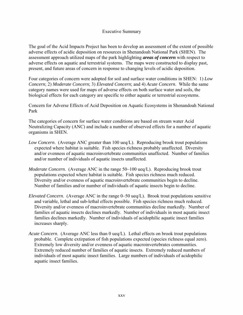
The goal of the Acid Impacts Project has been to develop an assessment of the extent of possible adverse effects of acidic deposition on resources in Shenandoah National Park (SHEN). The assessment approach utilized maps of the park highlighting areas of concern with respect to adverse effects on aquatic and terrestrial systems. The maps were constructed to display past, present, and future areas of concern in response to changing levels of acidic deposition.

Four categories of concern were adopted for soil and surface water conditions in SHEN: 1) Low Concern; 2) Moderate Concern; 3) Elevated Concern; and 4) Acute Concern. While the same category names were used for maps of adverse effects on both surface water and soils, the biological effects for each category are specific to either aquatic or terrestrial ecosystems.

Concern for Adverse Effects of Acid Deposition on Aquatic Ecosystems in Shenandoah National Park

The categories of concern for surface water conditions are based on stream water Acid Neutralizing Capacity (ANC) and include a number of observed effects for a number of aquatic organisms in SHEN.

Low Concern. (Average ANC greater than 100 ueq/L). Reproducing brook trout populations expected where habitat is suitable. Fish species richness probably unaffected. Diversity and/or evenness of aquatic macroinvertebrate communities unaffected. Number of families and/or number of individuals of aquatic insects unaffected.

Moderate Concern. (Average ANC in the range 50–100 ueq/L). Reproducing brook trout populations expected where habitat is suitable. Fish species richness much reduced. Diversity and/or evenness of aquatic macroinvertebrate communities begin to decline. Number of families and/or number of individuals of aquatic insects begin to decline.

Elevated Concern. (Average ANC in the range 0–50 ueq/L). Brook trout populations sensitive and variable, lethal and sub-lethal effects possible. Fish species richness much reduced. Diversity and/or evenness of macroinvertebrate communities decline markedly. Number of families of aquatic insects declines markedly. Number of individuals in most aquatic insect families declines markedly. Number of individuals of acidophilic aquatic insect families increases sharply.

Acute Concern. (Average ANC less than 0 ueq/L). Lethal effects on brook trout populations probable. Complete extirpation of fish populations expected (species richness equal zero). Extremely low diversity and/or evenness of aquatic macroinvertebrates communities. Extremely reduced number of families of aquatic insects. Extremely reduced numbers of individuals of most aquatic insect families. Large numbers of individuals of acidophilic aquatic insect families.

xxvi

Concern for Adverse Effects of Acid Deposition on Terrestrial Ecosystems in Shenandoah National Park

The categories of concern for soils are somewhat problematic in that direct observations of adverse effects of acidification are lacking in SHEN for terrestrial organisms. Nonetheless, there exist strong correlations between soil base saturation (BS) and measures of base cation availability for both forests and streams in SHEN. Because the relationships for effects of soil acidification are weaker than for surface waters, the expected effects for each category are less specific than for surface waters, but nonetheless represent best current knowledge.

Low Concern. (Average soil BS greater than 20%). No effects. Base cation availability for forests and surface waters not affected.

Moderate Concern. (Average soil BS in the range 10–20%). Moderate effects probable. Base cation availability for forests reduced and forest growth probably slowed. Base cation availability for surface waters reduced and moderate effects on aquatic biota expected (lowered stream water ANC).

Elevated Concern. (Average soil BS in the range 5–10%). Moderate effects certain and severe effects probable. Base cation availability for forests greatly reduced with resultant risk of mortality from various stresses (particularly if the base saturation was previously above 10% during the life of the tree). Base cation availability for surface waters greatly reduced producing sharp declines in stream water ANC (particularly during storm events) and resultant moderate to severe effects on stream water biota.

Acute Concern. (Average soil BS less than 5%). Severe effects certain. High risk of forest mortality from various stresses including direct acidification effects on roots and seedlings. Surface water ANC’s are likely to be in the range of severe biological effects (certainly episodically and perhaps chronically).

Conclusions

Although baseline, pre-industrial resource conditions are not well known in Shenandoah National Park, the analysis here suggests that ranges of both soil and stream conditions that would occur in SHEN in the absence of acid deposition impacts would not include any areas of “acute concern” or “elevated concern”. However, the historical mapping exercise also suggests that large areas of SHEN, especially in the southern district, may have always been of “moderate concern” reflecting the inherent sensitivity of the siliciclastic bedrock that dominates the southern district.

Simulation and mapping of watershed responses to historical changes in acidic deposition (from pre-industrial to current) suggest that large areas of SHEN have suffered deterioration of both soil and stream conditions. The changes in soil condition have been relatively modest up to the present time, with small areas in the southern district of SHEN moving from “moderate concern” (the historical baseline) to “elevated concern” as a result of leaching of base cations from the soils in these areas. Deterioration in stream conditions has been more severe than for soil conditions, with large areas in the southern district and some smaller areas in the central and northern districts moving from “moderate concern” to “elevated concern”. Neither soil nor

xxvii

stream conditions have shown any improvement from 1980 to the present in response to the decline in acidic deposition over the last 25 years.

Simulation and mapping of watershed responses to predicted future changes in acidic deposition (from current through several decades into the future) relied upon a comparative approach. Several scenarios of possible future acid deposition were developed for this report following U.S. Environmental Protection Agency (EPA) methods for preparation of emissions inventory inputs into air quality modeling for policy analysis and rule making purposes. These alternate scenarios were based on existing emission control regulations and several proposed alternatives.

With respect to future soil conditions, the assessment suggests that the responses of soil conditions to changes in acid deposition are relatively slow. In the short term (by year 2020), neither improvement nor further deterioration is likely to be observed in soil condition regardless of the future deposition scenario considered. However, by the year 2100 it becomes clear that constant deposition at 1990 levels would produce worsening soil conditions in SHEN with the development of areas of “acute concern” in the southern district. Perhaps more importantly, while the two scenarios of reduced future deposition did not produce worsening soil conditions, neither did they indicate any improvement in soil condition even in the long term. It is possible that emission control activities (and therefore emissions reductions) currently being considered in the policy arena would all be insufficient to reverse the soil acidification that has occurred in SHEN and start soil conditions on a path to recovery to pre-industrial conditions.

With respect to future stream conditions, the assessment suggests that the responses of stream conditions are relatively more rapid than those of soils. In the short term (by year 2020), while constant deposition at 1990 levels would likely produce further deterioration in stream condition, the two scenarios of future deposition reductions do nothing to reverse the deterioration of stream condition that has occurred in SHEN. In the long term (by year 2100), the effects of the two deposition reduction scenarios begin to diverge. The moderate deposition reduction scenario still produces no improvement in stream conditions relative to current conditions. The largest deposition reduction scenario, by contrast, produces modest improvements in stream conditions by 2100. It is important to note, however, that even the relatively large deposition reductions of this scenario do not result in a return of stream conditions in SHEN to the pre-industrial state. It is unlikely that the pre-industrial state for streams in SHEN can be reached until deposition reductions sufficient to stop the soil acidification (discussed above) in SHEN are achieved.

1-1

Chapter 1: An Overview of the Effects of Acidic Deposition in Shenandoah National Park and an Introduction to the Study

1.1 Overview of the Effects of Acidic Deposition in Shenandoah National Park

The Shenandoah Watershed Study has been investigating acid deposition and its effects on Shenandoah National Park (SHEN) since 1979. Some of the notable findings are:

The Shenandoah National Park and the central Appalachian Mountain region, defined as the mountainous area of Virginia, West Virginia, Pennsylvania, and Maryland, is exposed to among the highest acidic deposition loads in the United States.

Implementation of the 1990 Clean Air Act Amendments has achieved, and should achieve more, reduction in acidic deposition levels, especially reductions in the sulfur component. However, acidic deposition levels will remain high because anthropogenic emissions of sulfur will continue to greatly exceed natural background emission levels.

Sulfate concentrations in mountain streams in the Shenandoah National Park and the central Appalachian Mountains have increased dramatically as a consequence of acidic deposition, and sulfate concentrations in many streams will increase further as sulfur retention capacity in watershed soils is exhausted. Sulfate has become the dominant solute in many streams–a major change in the chemical environment.

The increase in sulfate concentrations in mountain streams in the Shenandoah National Park and western Virginia has had a dramatic effect on acid-base status and aquatic fauna. The evident elevation of sulfate concentrations in stream water, the presently low acid neutralizing capacity (ANC) in stream water, and the base-poor status of watershed soil and bedrock, provides strong evidence of historic acidification (loss of ANC) in a substantial portion of these streams.

The close correlation between ANC and fish diversity in Shenandoah National Park indicates that acidification-related species losses have occurred and that more losses will occur if acidification continues.

Despite recent declines in acidic deposition and encouraging evidence for initial recovery of some streams in the Shenandoah National Park and in the central Appalachian region, the degree of recovery has been minor in relation to historic acidification, and many streams continue to acidify.

The eventual magnitude of potential recovery will be limited by both the magnitude of reductions in sulfur deposition and the magnitude of cumulative long-term damage due to base-depletion in watershed soils.

These findings led us to propose the project “Acidic Deposition Impacts on Natural Resources in Shenandoah National Park: Loss of Fish Biodiversity and Forest Nutrients”. This report presents the results of that study.

1-2

1.2 Study Objectives and Structure of the Report

The goal of this project was to provide an assessment of the effects of acid deposition on aquatic and terrestrial resources within SHEN. Two specific objectives of the project relate directly to that assessment:

Objective 1: provide estimates of current and predictions of future responses of SHEN soil and stream resources (chemical and biological) to acidic deposition on a landscape basis within SHEN;

Objective 2: estimate the past acid-base status of streams and soils within SHEN (and therefore past forest and fish health) on a landscape basis;

Two additional objectives provided new information needed for the assessment:

Objective 3: determine the current base cation status of SHEN soils;

Objective 4: establish the sensitivity of additional fish species within SHEN streams;

Chapters 1 and 2 address Objectives 1 and 2. The remainder of this chapter (1) provides an summary of current knowledge concerning acidic deposition and its effects in SHEN. Chapter 2 provides the assessment in terms of maps and tables defining areas of current and future concern within SHEN for adverse effects of acid deposition on aquatic and forest resources.

The remaining chapters provide supporting information used in the assessment (and the results for Objectives 3 and 4).

Chapter 3 describes the environmental setting of SHEN and presents an overview of the landscape characteristics related to acidification responses within SHEN.

Chapter 4 describes atmospheric acidic deposition into SHEN—the cause of the problem and the reason for the assessment.

Chapter 5 presents an assessment of the current status of water and soil acidification in SHEN (related to Objective 1; the soil status is based on results from Objective 4). Chapter 6 presents an assessment of the current trends in water acidification in SHEN (related to Objective 1).

Chapter 7 presents reconstructed past and projected future trends in soil and water acidification (related to Objectives 1 and 2). This chapter uses the MAGIC model to estimate past and future water and soil chemistry (necessary for the past and future resource maps in Chapter 2).

Chapter 8 presents relationships between aquatic resources and water quality in SHEN that are used to construct the aquatic resource maps in Chapter 2. Chapter 8 also discusses the relationship between forest resources and soil quality in SHEN that are used to construct the terrestrial resource maps in Chapter 2. The inferential models for aquatic and terrestrial resources effects are explained, including the definitions of what is “low concern,” “concern,” and “acute concern” for each resource to be mapped.

1-3

1.3 Acid Deposition and Shenandoah National Park

Acidic deposition, or “acid rain” in popular terminology, is an insidious form of pollution. Its origins can be hundreds of miles upwind from its ultimate consequences. Its effects are commonly manifest in highly valued landscapes that are otherwise protected from human impact. Its effects are commonly subtle, a gradual cumulative loss of environmental quality that occurs on time scales of decades and presents few noticeable effects in the short-term. But in the long-term, the effects of acidic deposition can be dramatic, substantial, and essentially irreversible. Such is the case in the central Appalachian Mountain region where acidic deposition derived from multiple distant sources affects the remnant wild lands that have been set aside as National Forests, National Parks, and statutory Wilderness.

Although implementation of the 1990 Clean Air Act Amendments (CAAA) is likely to reduce the impact of acidic deposition on surface water resources in many regions of the United States, certain areas, including the central Appalachian region, remain at risk (USEPA 1995). It has been shown, based on the acid-base chemistry of surface waters, that the central Appalachian region is one of the two areas of the United States most affected by acidic deposition (Baker et al. 1991). As summarized by Herlihy et al. (1993), streams in the central Appalachian region are especially susceptible to acidification due to elevated rates of acidic deposition, the delayed-response properties of regional soils, and the presence of watersheds with base-poor bedrock. Church et al. (1992) concluded that further acidification of central Appalachian region streams can be expected as a consequence of continuing acidic deposition. More recently, Bulger et al. (2000) predicted that future losses of native brook trout (Salvelinus fontinalis) populations in the streams of western Virginia will be substantial unless acidic deposition reductions are much greater than the 1990 CAAA will provide.

Despite these sobering assessments, concern about acidic deposition impacts on aquatic systems in the central Appalachian region came relatively late. Earlier concerns about the problem in the United States tended to focus on the Adirondacks region in New York, where the linkage between acidic deposition and loss of fish populations in lakes was recognized by the 1970s (Driscoll et al. 1991). Although acidic and acidifying streams were previously known to exist at various locations in the central Appalachians, the extent of the problem, as well as the degree of association with acidic deposition, was not well established until surveys of regional stream water quality were conducted in the 1980s (Lynch and Dise 1985; Kaufmann et al. 1988; Webb et al. 1989). Concern about acidic deposition effects on aquatic systems reached particular prominence with the completion of the Southern Appalachian Assessment Aquatic Technical Report, an effort undertaken by resource agencies that served both to establish the vulnerability of the region’s brook trout habitat and document its recreational and aesthetic value (SAMAB 1996).

Much of the attention currently given to the acidic deposition problem is focused on prospects for recovery of acidified aquatic systems following the reductions in acid-forming emissions mandated by the 1990 CAAA. Despite recent declines in acidic deposition and some encouraging evidence for initial recovery in other parts of the country, recovery in the central Appalachian region in general, and the Shenandoah National park in particular, has been limited and impairment of surface waters due to acidic deposition continues (Stoddard et al. 2003; Webb et al. 2004).

1-4

1.4 Stream Water Acidification in Shenandoah National Park

The presence of acidic and low-ANC streams associated with forested mountain watersheds in Shenandoah National Park and the central Appalachian region has been well documented (Webb et al. 1989; Baker et al. 1990a; Herlihy et al. 1993). The following section describes findings from research and monitoring efforts conducted on a number of streams in Shenandoah National Park.

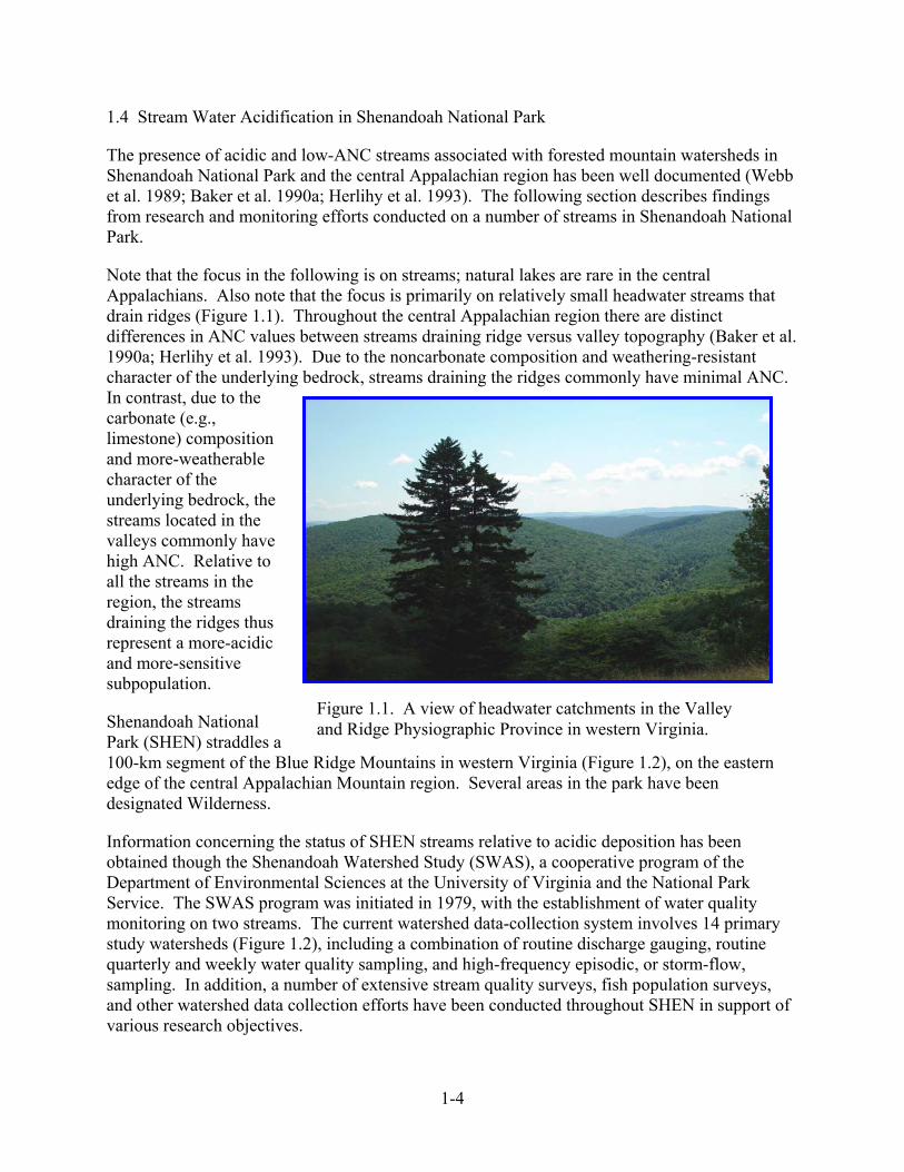
Note that the focus in the following is on streams; natural lakes are rare in the central Appalachians. Also note that the focus is primarily on relatively small headwater streams that drain ridges (Figure 1.1). Throughout the central Appalachian region there are distinct differences in ANC values between streams draining ridge versus valley topography (Baker et al. 1990a; Herlihy et al. 1993). Due to the noncarbonate composition and weathering-resistant character of the underlying bedrock, streams draining the ridges commonly have minimal ANC. In contrast, due to the carbonate (e.g., limestone) composition and more-weatherable character of the underlying bedrock, the streams located in the valleys commonly have high ANC. Relative to all the streams in the region, the streams draining the ridges thus represent a more-acidic and more-sensitive subpopulation.

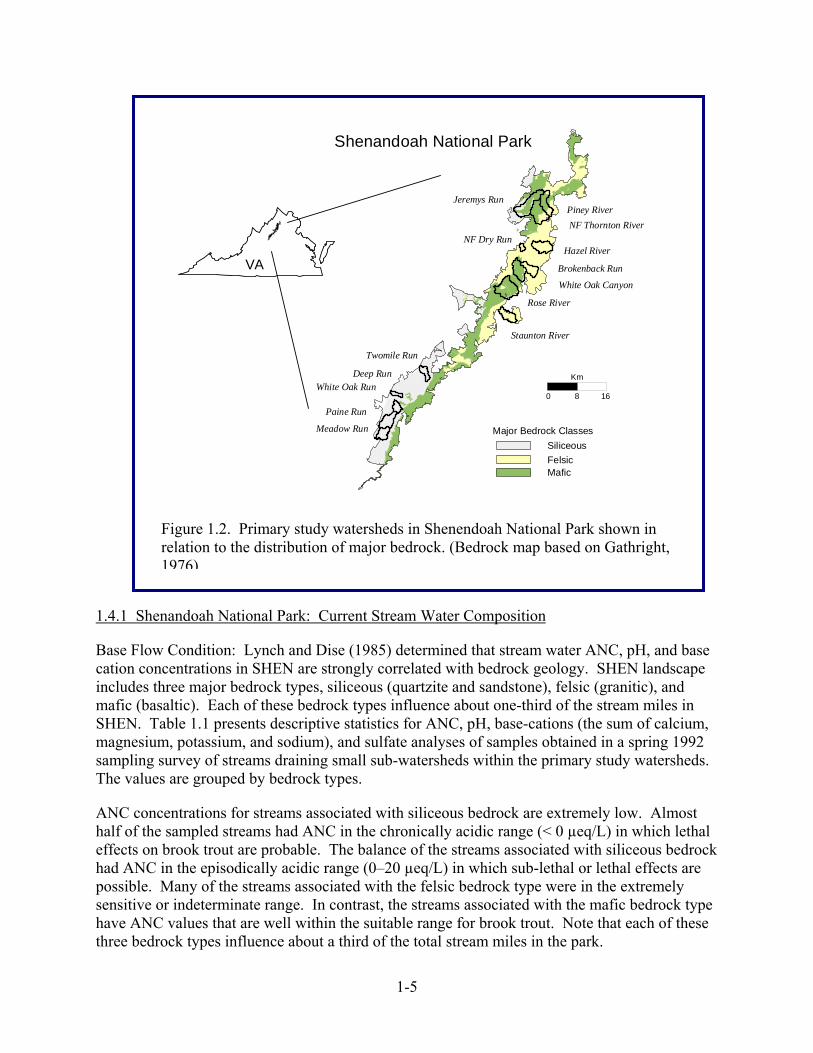
Shenandoah National Park (SHEN) straddles a 100-km segment of the Blue Ridge Mountains in western Virginia (Figure 1.2), on the eastern edge of the central Appalachian Mountain region. Several areas in the park have been designated Wilderness.

Information concerning the status of SHEN streams relative to acidic deposition has been obtained though the Shenandoah Watershed Study (SWAS), a cooperative program of the Department of Environmental Sciences at the University of Virginia and the National Park Service. The SWAS program was initiated in 1979, with the establishment of water quality monitoring on two streams. The current watershed data-collection system involves 14 primary study watersheds (Figure 1.2), including a combination of routine discharge gauging, routine quarterly and weekly water quality sampling, and high-frequency episodic, or storm-flow, sampling. In addition, a number of extensive stream quality surveys, fish population surveys, and other watershed data collection efforts have been conducted throughout SHEN in support of various research objectives.

Figure 1.1. A view of headwater catchments in the Valley and Ridge Physiographic Province in western Virginia.

1-5

1.4.1 Shenandoah National Park: Current Stream Water Composition

Base Flow Condition: Lynch and Dise (1985) determined that stream water ANC, pH, and base cation concentrations in SHEN are strongly correlated with bedrock geology. SHEN landscape includes three major bedrock types, siliceous (quartzite and sandstone), felsic (granitic), and mafic (basaltic). Each of these bedrock types influence about one-third of the stream miles in SHEN. Table 1.1 presents descriptive statistics for ANC, pH, base-cations (the sum of calcium, magnesium, potassium, and sodium), and sulfate analyses of samples obtained in a spring 1992 sampling survey of streams draining small sub-watersheds within the primary study watersheds. The values are grouped by bedrock types.

ANC concentrations for streams associated with siliceous bedrock are extremely low. Almost half of the sampled streams had ANC in the chronically acidic range (< 0 µeq/L) in which lethal effects on brook trout are probable. The balance of the streams associated with siliceous bedrock had ANC in the episodically acidic range (0–20 µeq/L) in which sub-lethal or lethal effects are possible. Many of the streams associated with the felsic bedrock type were in the extremely sensitive or indeterminate range. In contrast, the streams associated with the mafic bedrock type have ANC values that are well within the suitable range for brook trout. Note that each of these three bedrock types influence about a third of the total stream miles in the park.

Km

1680White Oak Run

Paine Run

Meadow Run

Rose River

White Oak Canyon

Piney RiverNF Thornton River

Jeremys Run

NF Dry Run

Staunton River

Brokenback Run

Hazel River

Major Bedrock Classes

VA

Twomile Run

Shenandoah National Park

Deep Run

SiliceousFelsicMafic

Figure 1.6: Primary study watersheds in Shenandoah National Park shown in relation to the distribution of major bedrock. (Bedrock map based on Gathright, 1976.)

Figure 1.2. Primary study watersheds in Shenendoah National Park shown in relation to the distribution of major bedrock. (Bedrock map based on Gathright, 1976).

1-6

Table 1.1. Range and distribution of stream water concentrations associated with major Shenandoah National Park bedrock classes: Spring 1992 Synoptic Survey (Galloway et al. 1999).

N Minimum 25% Median 75% Maximum ANC (μeq/L)

Siliceous 62 -18.1 -1.0 1.2 3.7 12.8 Felsic 46 22.0 47.2 58.7 67.0 130.4 Mafic 14 33.7 97.0 142.9 179.0 226.7

pH Siliceous 62 4.8 5.4 5.6 5.7 6.0 Felsic 46 6.0 6.7 6.8 6.8 7.1 Mafic 14 6.6 6.9 7.1 7.2 7.3

Sum of Base Cations (μeq/L) Siliceous 62 92.1 138.1 168.2 190.4 272.1 Felsic 46 89.5 136.7 147.7 161.3 243.5 Mafic 14 138.0 232.0 369.5 381.1 450.9

Sulfate (μeq/L) Siliceous 62 67.2 88.5 97.2 104.8 177.8 Felsic 46 13.4 30.1 36.6 42.1 96.3 Mafic 14 12.3 36.2 62.2 97.9 164.3

Note: 25% and 75% refer to the 25th and 75th percentile values. 50 percent of all the values are within the interquartile range, as bounded by the 25th and 75th percentile values. Sum of base cations is the sum of the concentrations of calcium, magnesium, sodium, and potassium. The pH values for the streams in the 1992 survey display a similar relationship with bedrock, with the most-acidic streams associated with siliceous bedrock and the least-acidic streams associated with mafic bedrock. All of the streams associated with siliceous bedrock are in the pH range (<6.0) identified by Baker and Christensen (1991) as too acidic for acid-sensitive fish species

The distribution of base-cation concentrations for streams in the 1992 survey indicates that soils in much of SHEN have extremely limited base-cation supplies (Figure 1.3). The base-cation concentrations for SHEN’s mountain streams are generally less than 25 percent of the median base-cation concentration value for the general population of all regional streams sampled in the 1986 National Stream Survey (Kaufmann et al. 1988; Sale et al. 1988). The availability of base-cations in watershed soils is a primary determinant of stream response to acidic deposition. A common measure of base availability in soils is percent base saturation, which is the base-cation fraction of total exchangeable acid and base cations. Percent base-saturation values in the range of 10−20 percent have been cited as threshold values for leaching of aluminum to soil and surface waters (Reuss and Johnson 1986; Binkley et al. 1989; Cronan and Schofield 1990). Median base saturation is less than 10 percent for SHEN soils associated with siliceous bedrock and less than 15 percent for SHEN soils associated with felsic bedrock (Figure 1.3). The present low base-cation availability in SHEN soils can be attributed to low base-cation content of the parent bedrock and depletion by decades of accelerated leaching by acidic deposition.

1-7

Sulfate is the major strong-acid anion present in most SHEN streams. Nitrate concentrations are generally negligible, except in association with forest defoliation by the gypsy moth (Webb et al. 1995). Sulfate concentrations in the streams sampled in the 1992 survey are consistent with the interpretation by Galloway et al. (1983), Elwood (1991), and others that a substantial proportion of atmospherically deposited sulfur is retained in the soils of the southeastern United States. Based on comparison with estimates of total sulfur deposition, sulfur retention in the forested mountain watersheds of western Virginia, including those in SHEN, has been variously estimated to range from 45–65 percent of sulfur deposition (Webb et al. 1989; Cosby et al. 1991). The evident differences in sulfate concentrations between streams associated with the different bedrock types is probably not due to differences in deposition amounts, as sulfur deposition is relatively uniform throughout SHEN (Galloway et al. 1999). Instead, the differences probably reflect variation in the sulfur retention properties of soils associated with the different bedrock types.

Given the absence of significant sulfur-bearing minerals in SHEN (Gathright 1976; Webb 1988), it is clear that most of the sulfate in SHEN streams is derived from the atmosphere. It is also clear that without the delaying effect of sulfur retention in watershed soils, many more SHEN streams would now be acidic.

High Flow Condition: Figure 1.4 displays the general relationship between flow level and ANC for three intensively studied streams representing the major bedrock types in SHEN. The most acidic conditions in SHEN streams occur during higher streams flows, with the most extreme conditions occurring in conjunction with storm or snowmelt runoff. The response of all three streams is similar in that most of the lower ANC values occur in the upper range of flows levels. However, consistent with observations by Eshleman (1988), the minimum ANC values that occur in response to high flow are related to base-flow ANC values. Paine Run (siliceous bedrock) has a mean weekly ANC value of about 6 µeq/L and often has high-flow ANC values that are less than 0 µeq/L. Staunton River (felsic bedrock) has a mean weekly ANC value of about 82 µeq/L and has only a few high-flow ANC values less than 50 µeq/L. Piney River (mafic bedrock) has a mean weekly ANC value of 217 µeq/L and no values as low as 50 µeq/L.

Siliceous Felsic Mafic0%

10%

20%

30%

40%

50%

60%

Bas

e S

atur

atio

n

Figure 1.7: Median percent base saturation for soils associated with SNP’s three bedrock types. Brackets delimit interquartile ranges. The base saturation of soils derived from siliceous and felsic bedrock is too low for effective buffering of acidic deposition.

(The data were obtained for mineral-horizon soil samples collected in the summer of 2000 at 80 geologically distributed sites in SNP; Welsch et al., 2001.)

Base Saturation of SNP Soils

Figure 1.3. Median percent base saturation for soils associated with Shenandoah National Park’s three bedrock types. Brackets delimit interquartile ranges. The base saturation of soils derived from siliceous and felsic bedrock is too low for effective buffering of acidic deposition. (The data were obtained for mineral-horizon soil samples collected in the summer of 2000 at 80 geologically distributed sites in Shenandoah National Park; Welsch et al. 2001.)

Base Saturation of SHEN Soils

1-8

Previous studies have shown that mobilization of dissolved aluminum during episodic acidification is a primary cause of fish mortality in streams that have low ANC under base-flow conditions (Wigington et al. 1993). Streams with higher ANC during base flow are less likely to become sufficiently acidic during episodic acidification to bring aluminum into solution. Figure 1.5 provides an example of changes in ANC and dissolved aluminum that occurred in Paine Run during a high-flow episode in the fall of 1992. Under base-flow conditions ANC is above 0 µeq/L and aluminum concentration is less than 20 µg/L. Stream flow levels increased dramatically around the 23rd of November, resulting in depression of ANC to less than 0 µeq/L and an increase in aluminum concentration to about 100 µg/L, well above the threshold for adverse effects on aquatic biota.

Episodic acidification in SHEN streams can be attributed to a number of causes, including dilution of base cations and increased concentrations of sulfuric, nitric, and organic acids (Eshleman et al. 1995; Hyer et al. 1995). Some of these causes are not related to acidic deposition. Base-cation dilution and release of organic acids during high-flow conditions are natural processes. The contribution of nitric acid, indicated by increased nitrate concentrations, is evidently (at least for SHEN streams) related to forest defoliation

Episodic Acidification:

Paine Run, November 1992

NOV. 2010 30

50

150

250

350Discharge (cfs)

-5

0

5

10

15ANC (µeq/L)

25

50

75

100

125Al (µg/L)

Figure 1.9: Loss of ANC and increase in dissolved aluminum in Paine Run in response to a sharp increase in stream flow.

Figure 1.5Figure 1.5. Loss of ANC and increase in dissolved aluminim in Paine Run in response to a sharp increase in stormflow.

0.0050.010 0.100 1.0002.00025

50

75

100

125

150

AN

C (µ

eq/L

)

Staunton River (felsic bedrock class)

0.001 0.010 0.100 1.000 3.00050

100

150

200

250

300

350

400

AN

C (µ

eq/L

)

Piney River (mafic bedrock class)

Runoff (mm/hr)

Figure 1.8: Relationship between ANC and runoff for stream water samples collected at intensively studied sites in Shenandoah National Park.

(The data represent samples collected during the 1992-1997 period.)

0.001 0.010 0.100 1.000 10.000-10

0

10

20

AN

C (µ

eq/L

)

Paine Run (siliceous bedrock class)

Figure 1.4Figure 1.4. Relationship between ANC and runoff for stream water samples collective at intensively studied sites in Shenandoah National Park. (The data represents samples collected during the 1992-1997 period.)

1-9

by the gypsy moth (Webb et al. 1995; Eshleman et al. 1998). However, significant contributions of sulfuric acid, indicated by increased sulfate concentrations, should be interpreted as an impact of atmospheric deposition (Eshleman and Hyer 1999). Moreover, the potential for biologically significant episodic acidification is determined by base-flow ANC, which for many SHEN streams is closely related to acidic deposition.

1.4.2 Shenandoah National Park: Changes in Stream Water Composition

Although SHEN has the longest continuous record of stream water composition in a national park and among the longest anywhere in the United States, the record only goes back to 1979. Given that stream water acidification has been occurring for many decades, the empirical record is only partial at best. Nonetheless, the available information is convincing.

Atmospherically derived sulfate has become the major dissolved ion in many of the streams in SHEN, especially in the low-ANC streams associated with siliceous bedrock. Estimates of background or natural sulfate concentrations in low-ANC surface waters in the eastern United States range from 10-15 µeq/L (Brakke et al. 1989) to 22 µeq/L (Cosby et al. 1991). Based on the latter estimate and on comparison with median stream water sulfate concentrations observed in the 1992 survey samples, it appears that sulfate concentrations have increased by a factor of 4.4 in streams associated with siliceous bedrock, by a factor of 1.7 in streams associated with felsic bedrock, and by a factor of 2.8 in streams associated with mafic bedrock (Figure 1.6). This represents a dramatic change in stream water composition –a change that can only be attributed to acidic deposition.

It is possible for a large increase in surface water sulfate concentration to occur without a loss of ANC if the watershed system is well buffered. In such a case, base-cation availability would have to be very high. That is, the watershed would have to have deep soils with a high cation-exchange capacity and a high percent base saturation. Given the relatively high ANC values presently observed in streams associated with mafic bedrock (Table 1.1), as well as the high base saturation of soils derived from that bedrock (Figure 1.3), it is possible that the degree of acidification among those streams has been minimal. In contrast, the large increase in sulfate concentrations among the streams associated with the siliceous bedrock provides strong evidence of acidification, given that these streams

Natural Siliceous Felsic Mafic0

20

40

60

80

100

120

Sul

fate

(µeq

/L)

Figure 1.10: Comparison of estimated natural and current median sulfate concentrations among streams associated with major bedrock types in Shenandoah National Park. Error bars delimit interquartile ranges. (Current concentrations based on 1992 survey data; see Table 3-1.)

Historic Increase in Shenandoah National Park Stream Water Sulfate

Figure 1.6

Table 1.1)

Figure 1.6. Comparison of estimated natural and current median sulfate concentrations among streams associated with major bedrock types in Shenandoah National Park. Error bars delimit interquartile ranges. (Current concentrations based on 1992 survey data; see Table 1.1.)

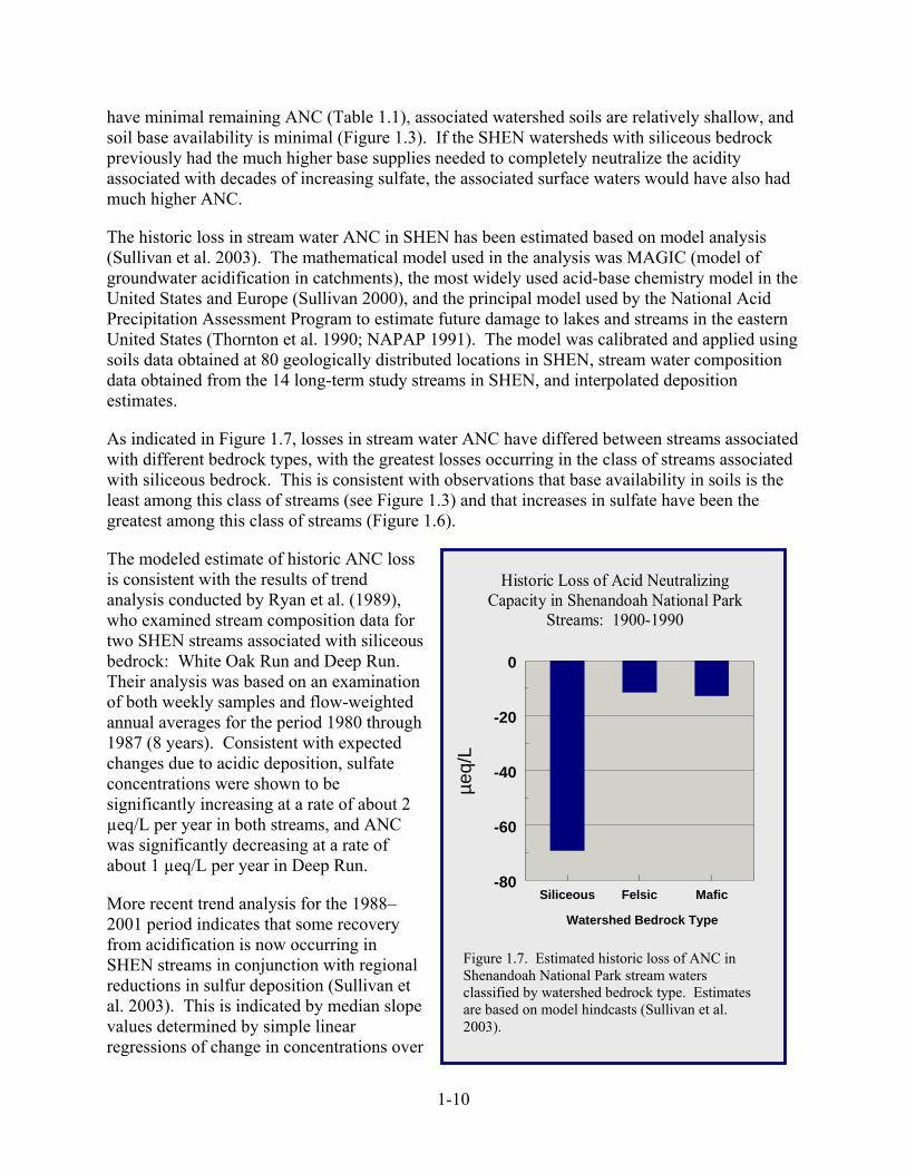
1-10

have minimal remaining ANC (Table 1.1), associated watershed soils are relatively shallow, and soil base availability is minimal (Figure 1.3). If the SHEN watersheds with siliceous bedrock previously had the much higher base supplies needed to completely neutralize the acidity associated with decades of increasing sulfate, the associated surface waters would have also had much higher ANC.

The historic loss in stream water ANC in SHEN has been estimated based on model analysis (Sullivan et al. 2003). The mathematical model used in the analysis was MAGIC (model of groundwater acidification in catchments), the most widely used acid-base chemistry model in the United States and Europe (Sullivan 2000), and the principal model used by the National Acid Precipitation Assessment Program to estimate future damage to lakes and streams in the eastern United States (Thornton et al. 1990; NAPAP 1991). The model was calibrated and applied using soils data obtained at 80 geologically distributed locations in SHEN, stream water composition data obtained from the 14 long-term study streams in SHEN, and interpolated deposition estimates.

As indicated in Figure 1.7, losses in stream water ANC have differed between streams associated with different bedrock types, with the greatest losses occurring in the class of streams associated with siliceous bedrock. This is consistent with observations that base availability in soils is the least among this class of streams (see Figure 1.3) and that increases in sulfate have been the greatest among this class of streams (Figure 1.6).

The modeled estimate of historic ANC loss is consistent with the results of trend analysis conducted by Ryan et al. (1989), who examined stream composition data for two SHEN streams associated with siliceous bedrock: White Oak Run and Deep Run. Their analysis was based on an examination of both weekly samples and flow-weighted annual averages for the period 1980 through 1987 (8 years). Consistent with expected changes due to acidic deposition, sulfate concentrations were shown to be significantly increasing at a rate of about 2 µeq/L per year in both streams, and ANC was significantly decreasing at a rate of about 1 µeq/L per year in Deep Run.

More recent trend analysis for the 1988–2001 period indicates that some recovery from acidification is now occurring in SHEN streams in conjunction with regional reductions in sulfur deposition (Sullivan et al. 2003). This is indicated by median slope values determined by simple linear regressions of change in concentrations over

Siliceous Felsic Mafic-80

-60

-40

-20

0

µeq/

L

Watershed Bedrock Type

Historic Loss of Acid Neutralizing Capacity in Shenandoah National Park

Streams: 1900-1990

Figure 1.11: Estimated historic loss of ANC in Shenandoah National Park stream waters classified by watershed bedrock type. Estimates are based on model hindcasts (Sullivan et al., 2003).

Figure Figure 1.7. Estimated historic loss of ANC in Shenandoah National Park stream waters classified by watershed bedrock type. Estimates are based on model hindcasts (Sullivan et al. 2003).

1-11

time. Consistent with recovery from acidification, sulfate concentrations decreased at a rate of –0.229 µeq/L per year, and ANC increased at a rate of 0.168 µeq/L per year. For both constituents, the median slope values are statistically significant.

This observation of recovery is an encouraging indication that reductions in sulfur emissions and deposition can have beneficial results. Similar evidence for recovery of surface waters has recently been observed for other regions in the United States that have been affected by acidic deposition (Stoddard et al. 2003). However, it should be noted that the degree of apparent recovery among SHEN streams is very small compared with the degree of recovery observed in most of the other regions (see description of regional trends in Section 3.4), and that other factors, such as changes forest nutrient cycling associated with insect infestation (Webb et al. 1995) or climate-driven changes in hydrologic conditions (Driscoll et al. 2001), may be partially responsible for the observed trends.

It should also be noted that the degree of apparent recovery among SHEN streams for the 1988–2001 period is minor in relation to the magnitude of past acidification. Moreover, the contrast between recent recovery and historic acidification is even greater when only the more-sensitive streams associated with siliceous bedrock are considered.

Whereas the median estimated historic increase in sulfate for SHEN streams is 55.7 µeq/L, the median observed decrease for is 3.2 µeq/L, or 5.8%.

Whereas the median estimated historic loss in ANC for SHEN streams is 20.3 µeq/L, the recent observed median increase is 2.3 µeq/L, or 11.6%.

Whereas the median historic loss of ANC in streams associated with siliceous bedrock is 69.2 µeq/L, the recent median increase is 2.0 µeq/L, or 2.9%.

Finally, it should be recognized that the eventual magnitude of recovery will be limited by both the magnitude of reductions in sulfur deposition and the magnitude of cumulative damage due to base-depletion in watershed soils.

1.4.3 Shenandoah National Park: Acidification Effects on Fish

Effects of stream acidification on fish in the streams of SHEN were recently quantified through the Fish in Sensitive Habitats (FISH) Project (Bulger et al. 1999). The FISH project was an integrated multi-discipline study of fish communities in the SWAS project study streams in SHEN (see Figure 1.2). The research included intensive basin-wide surveys of stream habitat structure and fish species distribution, in-stream and in-laboratory bioassays, collection of fish physiological data, and investigation of spatial and temporal variation in stream water composition.

Results of the FISH project demonstrate that major effects of stream acidification on fish in SHEN occur at different ecosystem levels: 1) effects on single organisms (reduced condition factor); 2) population-level effects (increased mortality); and 3) community-level effects (reduced species richness). The FISH project thus served to link water quality effects of acidic deposition to adverse effects (both lethal and sub-lethal) on fish communities in SHEN streams.

1-12

Effects on Individuals: Because fish may be adversely affected by acidification before conditions have deteriorated sufficiently to cause mortality, the FISH project focused on indicators of sub-lethal stress. The blacknose dace, which is one of the more-common fish species in the central Appalachian region, was selected for study of condition factor across the acid-base gradient represented in SHEN streams. Condition factor is an index used by fish physiologists to describe the relationship between a fish’s weight and length. Fish with higher condition factor values are more robust than fish with lower condition factor values, and a low condition factor value is usually interpreted as a sign of low or depleted energy reserves. Condition factor values for blacknose dace collected from 11 SHEN streams were positively correlated with several indicators of acid-base status. The strongest relationship was with minimum pH observed in the preceding three years (the life span of the blacknose dace). The difference in condition factor between Paine Run (low ANC) and Piney River (high ANC) was about 11 percent, a difference that has been associated with diminished survival and recruitment success in other fish species. The FISH project investigators suggested that the differences in blacknose dace condition factor among SHEN streams may occur because maintenance of internal chemistry in the more-acidic streams requires energy that might otherwise be diverted to growth (Dennis and Bulger 1999).

Effects on Populations: Another component of the FISH project examined the survival of brook trout eggs and fry in three intensively studied streams representing the acidification gradient and different bedrock types present in SHEN. These streams were Paine Run, Staunton River, and Piney River. Six 1–3 month-long bioassays were conducted on each stream during which brook trout eggs were placed into artificial gravel nests which could be withdrawn periodically to determine rates of mortality. Brook trout eggs (and hatching fry) were selected for study because they represent the most-sensitive life stages of the brook trout. In four of the bioassays, differential mortality could only be attributed to ANC differences between the three streams. In each of these four bioassays, the trout eggs and fry in Piney River (high ANC) showed higher survival rates than in Paine Run (low ANC). Results for Staunton River (intermediate ANC) were mixed. Bulger et al. (1999) concluded that both chronic and episodic acid water chemistry, including elevated acidity and aluminum concentrations, reduced survivorship in the low-ANC stream. It is difficult to separate episodic effects from chronic effects in terms of their importance for fish, because low-ANC streams, as discussed previously, are more prone to extreme acid episodes. However, storm flows that occurred simultaneously in all three streams during two of the bioassays resulted in differential mortality among the three streams. Survivorship for the two bioassays was 5 and 0 percent in Paine Run, 4 and 85 percent in Staunton River, and 80 and 85 percent in Piney River. These results suggest that episodic acidification may be the principal mode of acidification impact on fish populations in SHEN’s low-ANC streams.

Effects on Communities: Perhaps the most import finding of the FISH project is the strong dependence of fish species richness on the acid-base status of stream water (Figure 1.8). Although acidification has been shown to reduce species richness (the number of species in a defined area) by eliminating sensitive species from fish communities (Baker and Christensen 1991), complete fish community records for SHEN streams are too recent (begun in the 1990s) to demonstrate historic loss of species from streams. However, there is a strong statistical relationship between the number of fish species present in streams now and stream acid-base status. Streams with low ANC host fewer species. This relationship suggests that the more-

1-13

sensitive fish species have disappeared in the past from acidifying SHEN streams and that additional species will disappear in the future unless effective steps are taken to prevent further stream acidification.

Figure 1.12: Relationship between number of fish species and minimum ANC recorded in Shenandoah National Park streams (from Bulger et al., 1999b).

0 20 40 60 80 100 120 140 160Acid Neutralizing Capacity (µeq/L)

0

2

4

6

8

10

Num

ber o

f Spe

cies

Fish Species Richness and Stream Water ANC

Figure 1.8 Figure 1.8. Relationship between number of fish species and minimum ANC recorded in Shenandoah National Park streams (from Bulger et al. 1996b).

2-15

Chapter 2: An Assessment of Areas of Concern in Shenandoah National Park with Respect to Adverse Effects of Acidic Deposition

The summary material presented in Chapter 1 demonstrated that the central Appalachians in general and the Shenandoah National park in particular are subject to adverse effects from acidic deposition. The mechanisms of soil and water acidification and their relationship to landscape characteristics were outlined, and occurrences of adverse effects on aquatic organisms were discussed. The most severe effects of acidic deposition can be attributed to the coincidence of elevated rates of acidic deposition and sensitive landscapes (watersheds). The central Appalachian area and SHEN are exposed to some of the highest acidic deposition in the U.S. and contain some of the most acid sensitive (poorly buffered) landscape in the eastern U.S. Stream acidification has occurred and adverse effects on aquatic biota associated with stream water acidification have been demonstrated in SHEN. Soil acidification is also likely to be occurring also in SHEN and with possible adverse effects on terrestrial ecosystems.

The purpose of this chapter is to present an assessment of the extent of the possible adverse effects of acidic deposition in SHEN. The approach is to develop maps of the park highlighting areas of concern with respect to the adverse effects on aquatic and terrestrial systems. The maps can be constructed to display past, present, and future areas of concern in response to changing levels of acidic deposition. In order to map the effects of acidic deposition on aquatic and terrestrial systems in SHEN it is necessary to know: a) the response mechanisms of water and soils to acidic deposition; b) the relationships between the soil and water chemical responses and the biological effects; and c) how these mechanisms and responses are distributed on the landscape.

The mapping procedure presented here is based on the knowledge gained through the long-term and process level studies carried out in the intensive Shenandoah Watershed Study (SWAS) sites within the park. The detailed information concerning adverse effects developed at the SWAS sites is extrapolated to the park using landscape information (particularly the geology) that is available parkwide. Historical maps are developed based on estimated historical deposition. Future maps are presented for 3 scenarios of future deposition based on possible policy decisions regarding control of emissions.

2.1 Assessment Mapping Approach

The development of maps of adverse effects of acidic deposition in SHEN involves three distinct steps with a number of tasks within each. The details of each of these tasks are contained in other chapters of this report. The general approach is summarized here and references are given to other chapters in the report for details.

Step 1. Adverse effects on aquatic and terrestrial biota must be discerned and the relationship of these effects to water and soil chemical properties must be established.

Step 2. The responses of soil and water chemical properties to changes in acidic deposition must be quantified and a model of these responses developed to allow simulation of past and future conditions under differing acidic deposition regimes.

2-16

Step 3. The hindcast and forecast responses of soil and water chemical properties must be interpreted in terms of the level of concern for adverse effects represented by the responses, and these levels (categories) of concern must be mapped onto the landscape of the park.

Step 1. Adverse effects of stream acidification on aquatic biota are summarized in Chapter 1 for fish and presented in more detail in Chapter 8 for fish and aquatic macroinvertebrates. For the mapping of adverse effects of stream acidification, the ANC of surface waters will be adopted as the key water chemical variable (see discussion in Chapter 8). Adverse effects of soil acidification on terrestrial biota have not been conclusively demonstrated in SHEN, in part because most acidification research in SHEN has been focused on surface waters and observations of possible effects on terrestrial biota have not been made. Soil acidification has been shown to affect forests in other areas and is suspected to be of concern in SHEN (see discussion in Chapter 8). For mapping of adverse effects of soil acidification, the base saturation of soils (BS) will be adopted as the key soil chemical variable.

Step 2. Current observed responses of soil and water chemical properties to acidic deposition are summarized in Chapter 1 and given in detail in Chapter 5 and Chapter 6. Current levels of acidic deposition are summarized in Chapter 4, as are the source areas for deposition in SHEN. The latter are important for deriving historical and future deposition levels in SHEN based on emissions estimates. The process based model (MAGIC) used to simulate the effects of acidic deposition on soil and water chemical properties is described in Chapter 7. The effects modeling using MAGIC was performed for the 14 SWAS study watersheds in SHEN.

Step 3. The simulations for the 14 study watersheds were extrapolated to the entire park in order to construct maps of areas of concern with respect to adverse effects of acidic deposition in SHEN. The extrapolations were accomplished using landscape characteristics of the park (in particular, the bedrock geology) presented in Chapter 2. Two types of maps were produced, one for areas of concern for surface water conditions (based on extrapolated ANC) and one for areas of concern for soil conditions (based on extrapolated BS). The categories of concern that were mapped for soil and surface water conditions were related to observed (or inferred) adverse effects in Chapter 8.

2.2 Categories of Concern for Assessment Mapping

Four categories of concern were adopted for the maps of soil and surface water conditions: 1) Low Concern; 2) Moderate Concern; 3) Elevated Concern; 4) Acute Concern. The same category names are used for maps of adverse effects on both surface water and soils. The expected or observed biological effects for each category are summarized below separately for surface water condition maps and soil condition maps.

2.2.1 Surface Waters

The categories of concern for surface waters are based on observed effects in SHEN for a number of aquatic organisms (see Chapter 8) and are thus relatively robust. The categories are based on simulated or observed average stream water ANC at any point in time. The ranges of

2-17

ANC and the expected effects for each category of concern in surface waters are summarized below.

Low Concern. Surface waters with average ANC greater than 100 ueq/L. Reproducing brook trout populations expected where habitat is suitable. Fish species richness probably unaffected. Diversity and/or evenness of aquatic macroinvertebrate communities unaffected. Number of families and/or number of individuals of aquatic insects unaffected.

Moderate Concern. Surface waters with average ANC in the range 50–100 ueq/L. Reproducing brook trout populations expected where habitat is suitable. Fish species richness much reduced. Diversity and/or evenness of aquatic macroinvertebrate communities begin to decline. Number of families and/or number of individuals of aquatic insects begin to decline.

Elevated Concern. Surface Waters with average ANC in the range 0–50 ueq/L. Brook trout populations sensitive and variable, lethal and sub-lethal effects possible. Fish species richness much reduced. Diversity and/or evenness of macroinvertebrate communities decline markedly. Number of families of aquatic insects declines markedly. Number of individuals in most aquatic insect families declines markedly. Number of individuals of acidophilic aquatic insect families increases sharply.

Acute Concern. Surface Waters with average ANC less than 0 ueq/L. Lethal effects on brook trout populations probable. Complete extirpation of fish populations expected (species richness equal zero) Extremely low diversity and/or evenness of aquatic macroinvertebrates communities. Extremely reduced number of families of aquatic insects. Extremely reduced numbers of individuals of most aquatic insect families. Large numbers of individuals of acidophilic aquatic insect families.

2.2.2 Soils

The categories of concern for soils are somewhat problematic in that direct observations of adverse effects of acidification are lacking in SHEN for terrestrial organisms. Nonetheless, there exist strong correlations between soil base saturation and measures of base cation availability for both forests and streams in SHEN (Chapter 8). In addition, there are observations in other areas supporting the use of these categories of concern in SHEN (Chapter 8). Because the relationships for effects of soil acidification are weaker than for surface waters, the expected effects for each category are less specific than for surface waters, but nonetheless represent best current knowledge. The ranges of soil base saturation and the expected effects for each category of concern in soils are summarized below.

Low Concern. Soils with average BS greater than 20%. No effects. Base cation availability for forests and surface waters not affected.

Moderate Concern. Soils with average BS in the range 10–20%. Moderate effects probable. Base cation availability for forests reduced and forest growth probably slowed. Base cation availability for surface waters reduced and moderate effects on aquatic biota

expected (lowered stream water ANC).

2-18

Elevated Concern. Soils with average BS in the range 5–10%. Moderate effects certain and severe effects probable. Base cation availability for forests greatly reduced with resultant risk of mortality from

various stresses (particularly if the base saturation was previously above 10% during the life of the tree).

Base cation availability for surface waters greatly reduced producing sharp declines in stream water ANC (particularly during storm events) and resultant moderate to sever effects on stream water biota.

Acute Concern. Soils with average BS less than 5%. Severe effects certain. High risk of forest mortality from various stresses including direct acidification effects on

roots and seedlings. Surface water ANC’s are likely to be in the range of severe biological effects (certainly

episodically and perhaps chronically). 2.3 Landscape Mapping

Current observations of water and soil conditions in SHEN and the observed relationships among stream and soil chemical properties and biological responses are based on the long-term monitoring data and process information derived from the 14 SWAS study watersheds (Figure 2.1). Model simulations of past and future soil and water conditions are also based on these 14 watersheds (Chapter 7). To extrapolate these results to the whole park and provide a map of areas of concern, a template to receive the extrapolated results is needed. Because our current conceptual and quantitative understanding is based on watersheds as a basic unit of study, it makes sense to use watersheds as the basic unit for extrapolation.

Using Digital Elevation Model (DEM) data for SHEN, individual watersheds within the park can be defined (Figure 2.1). Based on the DEM analysis, there are 231 individual watersheds lying completely or mostly within the boundaries of SHEN. It is important to note that the boundaries of SHEN (politically drawn) do not necessarily coincide with the boundaries of the watersheds derived from the DEM data. The result is that there are a number of small areas along the boundaries of the park that will not be included in the assessment. Nonetheless, the watershed approach provides a reasonably good overall coverage of the SHEN landscape (>95% coverage) for the assessment.

Extrapolation from the 14 SWAS study watersheds to the 231 mapping watersheds was accomplished using the distribution of bedrock geology within each watershed and the geographical location of the center of each watershed. Each of the 231 mapping watersheds was associated with one of the SWAS study watersheds (1:1 matching) in a two step procedure.

2-19

Figure 2.1. Left panel: Map of Shenandoah National Park showing the location of the 14 SWAS study watersheds and the dominate bedrock geology in the park. Right panel: Map of Shenandoah National Park showing the 231 watersheds used to extrapolate from the SWAS study sites to the park landscape.

First, the percentages of basaltic, granitic, and siliciclastic bedrock were derived for each watershed (231 mapped and 14 study watersheds) based on GIS data (Chapter 3). The “geologic distance” between a given mapping watershed and each of the study watersheds was then calculated. This “geological distance” was defined as the Euclidian distance in the 3-space defined by the observed percentages of basaltic, granitic and siliciclastic bedrock for each pair of watersheds. That is, the geologic distance (DistG12) between catchment 1 and 2 is:

DistG12 = sqrt[ (%B1 - %B2)2 + (%G1 - %G2)2 + (%S1 - %S2)2 ]

where %B is the percent basaltic bedrock, %G is the percent granitic bedrock, and %S is the percent siliciclastic bedrock, the subscripts refer to watershed 1 and 2 and “sqrt” is the square root operator. The mapping watershed was then paired with study watershed with the “minimum geologic distance” – the study watershed that was most similar in the sense of bedrock geology.

If the geological makeup of a mapping watershed resulted in that watershed being paired with more than one study watershed (“minimum geologic distances” to more than one study watershed being the same), a second step was invoked. The mapping watershed in question was

Major Bedrock Classes

Siliciclastic – greatest sensitivity to acidification Granitic – intermediate sensitivity to acidification Basaltic – least sensitive to acidification

2-20

paired with the study watershed that had the “minimum geological distance” and ALSO the minimum geographical distance (most similar geologically and closest in the landscape).

During the classification procedure there were 62 mapping watersheds that were uniquely associated with only one study watershed such that the secondary criterion of physical proximity was not invoked. There were 54 mapping watersheds associated with predominately basaltic study watersheds, 55 mapping watersheds associated with predominately granitic study watersheds, and 60 mapping watersheds associated with predominately siliciclastic study watersheds for which proximity was invoked to achieve a unique match. The number of mapping watersheds associated with each of the SWAS study watersheds after both criteria were applied is shown in Table 2.1.

Table 2.1. The site IDs, geological classes (dominate bedrock) and watershed areas for the 14 SWAS study sites in Shenandoah National Park. The number of mapping watersheds (231 total) associated with each of the study watersheds is given in the last column (see discussion in text).

Site ID Stream Geological Class Watershed area

km2 Mapping

Watersheds VT51 Jeremys Run Basalt 22.0 18 VT60 Piney River Basalt 12.6 18 VT66 Rose River Basalt 23.7 30 VT75 Whiteoak Canyon Basalt 14.1 24 VT61 North Fork Thornton River Basalt 19.1 4 VT58 Brokenback Run Granite 9.8 22 VT62 Hazel River Granite 13.2 30 NFDR North Fork Dry Run Granite 2.3 10 VT59 Staunton River Granite 10.5 15 DR01 Deep Run Siliciclastic 3.1 2 VT36 Meadow Run Siliciclastic 9.0 16 VT35 Paine Run Siliciclastic 12.4 4 VT53 Twomile Run Siliciclastic 5.6 34 WOR1 White Oak Run Siliciclastic 5.1 4

2.4 Acidification Response Modeling

Simulation modeling was used to evaluate the historical and future changes in the extent of damage to aquatic and soil resources in SHEN in response to changing levels of acidic deposition. These simulations were performed for 14 study watersheds in SHEN for which detailed soils and surface water data were available. Historical impacts are based on model responses to historical deposition in the park. Future impacts are based on simulated responses to various scenarios of future emissions reductions. The alternative future emissions scenarios were specified on the basis of existing and substantially more stringent regulations, available

2-21

emissions control technologies using the Regional Acid Deposition Model (RADM) to estimate future sulfate (SO4

2-) deposition values at SHEN. The effects modeling was conducted using the Model of Acidification of Groundwater in Catchments (MAGIC). Details deposition inputs and of the calibration of the effects model for each of the 14 study watersheds are given in Chapter 7 along with an analysis of goodness-of-fit to calibration data and uncertainty in simulations for the 14 sites.

The median simulated results from the suite of calibrations for each study site (see Chapter 7) were used for extrapolation to the 231 watersheds on the landscape maps. As a measure of the reliability of combining simulation results with the landscape mapping procedures, Figures 2.2 and 2.3 show a comparison of the landscape maps derived from simulations at the 14 study sites with the landscape maps derived from observed data at the 14 study sites (for maps of water conditions and soil conditions respectively).

2.5 Historical Deposition Effects and Areas of Concern

Historical simulations were run for the 14 study watersheds to estimate the effects of acidic deposition in SHEN in past years. Historical deposition for these simulations was estimated using historical emissions estimates for the SHEN airshed (Chapter 3) in a scaling procedure described in detail in Chapter 7. The results of the simulations at the 14 study watersheds were extrapolated to the 231 mapping watersheds for three points in sensitive areas that were historically of “moderate concern” did not change category by 1980 (mostly the sensitive watersheds in the middle and northern management districts of the park). However, the status of a large number of watersheds in the southern district deteriorated in that same period (more so for stream condition than soil condition).

It is also interesting to note that both soil and surface water conditions have apparently not changed from 1980 to the present (Figures 2.4 and 2.5) despite the rather large decreases in acidic deposition that have occurred during that time. This observation is consistent with recent published work based on observed regional responses of streams in the central Appalachian area (Stoddard et al. 2003, Webb et al. 2004).

2.6 Future Forecast Scenarios

Scenarios of future emissions were developed for this report following U.S. Environmental Protection Agency (EPA) methods regarding preparation of emissions inventory input into air quality modeling for policy analysis and rule making purposes (for details of these methods applied to SHEN, see Chapter 7 and also see Sullivan et al. 2003). Five future forecast scenarios were considered in this study: constant deposition at 1990 levels for the entire future period (a “reference” scenario), and four additional scenarios representing emissions controls policy currently in effect (base case) with four alternative adjustments in future years. These deposition scenarios were used to drive the simulation model for the 14 study watersheds with the results available to be extrapolated to the 231 mapping watersheds.

2-22

Simulated

Year 2000

Observed

Year 2000

Acute ConcernElevated ConcernModerate ConcernLow Concern

Stream Conditions

(Calk, ueq/L)

Simulated

Year 2000

Observed

Year 2000

Acute ConcernElevated ConcernModerate ConcernLow Concern

Stream Conditions

(Calk, ueq/L)

Figure 2.2. Landscape maps showing areas of concern for adverse effects from acidic deposition on surface water conditions in Shenandoah National Park. The figure compares maps generated from model simulated data (left) and observed data (right) for the 14 SWAS study sites extrapolated to the 231 mapping watersheds. Surface water conditions are based on simulated or observed stream water ANC (ueq/L). Expected biological effects in each category of concern are discussed in the text. Enlarged versions of each map are available in Appendix A.

2-23

Simulated

Year 2000

Observed

Year 2000

Acute ConcernElevated ConcernModerate ConcernLow Concern

Soil Conditions

(Base Saturation %)

Simulated

Year 2000

Observed

Year 2000

Acute ConcernElevated ConcernModerate ConcernLow Concern

Soil Conditions

(Base Saturation %)

Figure 2.3. Landscape maps showing areas of concern for adverse effects from acidic deposition on soil conditions in Shenandoah National Park. The figure compares maps generated from model simulated data (left) and observed data (right) for the 14 SWAS study sites extrapolated to the 231 mapping watersheds. Soil conditions are based on simulated or observed soil base saturation (%). Expected biological effects in each category of concern are discussed in the text. Enlarged versions of each map are available in Appendix A.

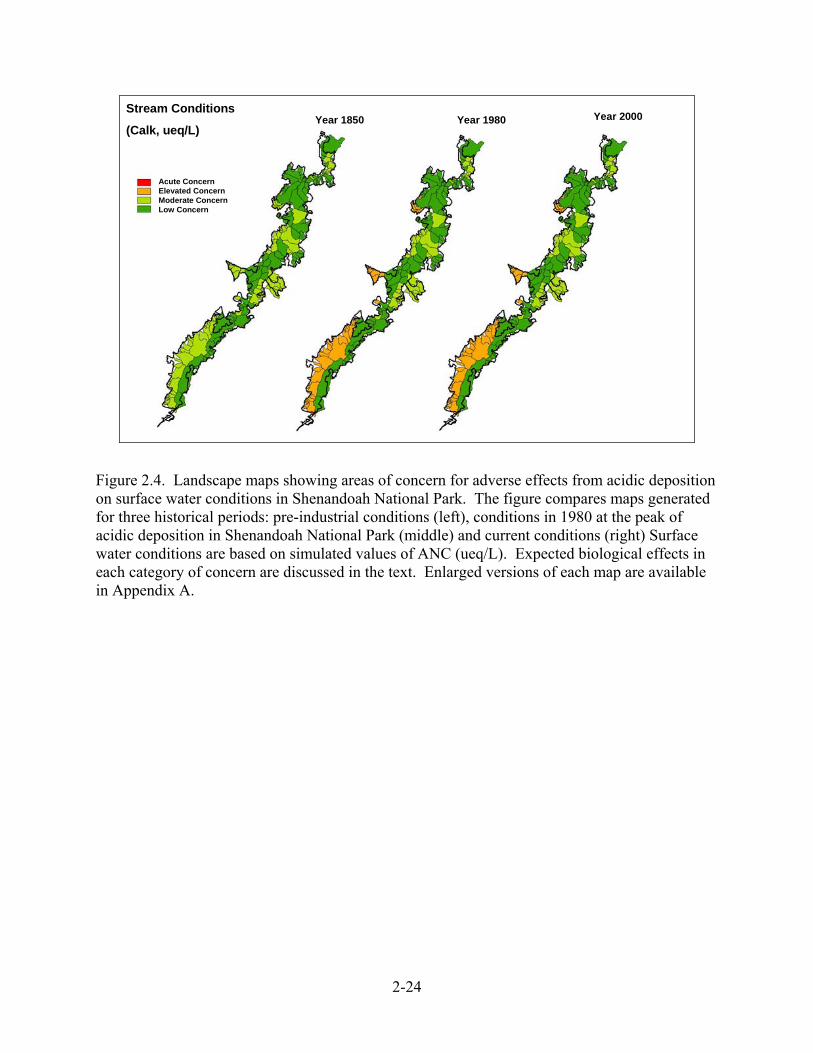
2-24

Year 1850 Year 1980Stream Conditions

(Calk, ueq/L)Year 2000

Acute ConcernElevated ConcernModerate ConcernLow Concern

Year 1850 Year 1980Stream Conditions

(Calk, ueq/L)Year 2000

Acute ConcernElevated ConcernModerate ConcernLow Concern

Figure 2.4. Landscape maps showing areas of concern for adverse effects from acidic deposition on surface water conditions in Shenandoah National Park. The figure compares maps generated for three historical periods: pre-industrial conditions (left), conditions in 1980 at the peak of acidic deposition in Shenandoah National Park (middle) and current conditions (right) Surface water conditions are based on simulated values of ANC (ueq/L). Expected biological effects in each category of concern are discussed in the text. Enlarged versions of each map are available in Appendix A.

2-25

Figure 2.5. Landscape maps showing areas of concern for adverse effects from acidic deposition on soil conditions in Shenandoah National Park. The figure compares maps generated for three historical periods: pre-industrial conditions (left), conditions in 1980 at the peak of acidic deposition in Shenandoah National Park (middle) and current conditions (right). Soil conditions are based on simulated values of soil base saturation (%). Expected biological effects in each category of concern are discussed in the text. Enlarged versions of each map are available in Appendix A.

The base case deposition for the four alternate scenarios was established using base emissions inventories representing the future with economic assumptions obtained from the Bureau of Economic Analysis and emissions controls representative of the laws, rules, and regulations already on the books and final as of the date of preparation of the inventory. These various control constraints in this base case include Federal, state and local requirements for emissions control for a wide variety of environmental and human health goals (see Chapter 7 for details). The alternate future emissions scenarios modified the base case in the following particulars:

Scenario 1. Base case with the NOx State Implementation Plan (SIP) Call - Assumes reasonable economic growth and emissions limitations according to existing regulations as of summer, 2000. Projections are provided to 2010.

Scenario 2. Base Projected to 2020 - Same assumptions as Scenario 1, but projected to 2020 to allow for continued implementation of Tier II Vehicle Standards and full implementation of Title IV and Heavy Duty Diesel Vehicle standards.

Year 1850 Year 1980Soil Conditions

(Base Saturation %)Year 2000

Acute ConcernElevated ConcernModerate ConcernLow Concern

Year 1850 Year 1980Soil Conditions

(Base Saturation %)Year 2000

Acute ConcernElevated ConcernModerate ConcernLow Concern

2-26

Scenario 3. Additional Stringent Utility Controls - Adds to Scenario 2 additional Electric Generating Unit (EGU) controls.

Scenario 4. Additional Stringent Controls on Utility, Industry-Point, and Mobile Sources - Adds to Scenario 3 additional, non-EGU emissions reductions.

The annual deposition of sulfur and nitrogen projected at SHEN under each of the scenarios is provided in Table 7.1 (Chapter 7). The deposition of S and to a lesser extent N is projected to decline substantially from the reference case (constant deposition) under all four alternate scenarios.

Examining the results of the simulation modeling for these five scenarios at the 14 study watersheds with respect to changes in stream water ANC and soil base saturation (Figures 2.6a, b, c) shows that the responses of both ANC and BS differ under for the scenarios considered, and that the magnitude of the responses varied among the study sites.

These simulation results at the 14 study sites (Figure 2.6) suggests that maps extrapolating these results to the whole park would show changes in the extent and location of areas of concern in SHEN. It should be noted, however, that the responses to the five scenarios can be grouped into three sets of responses. For all study watersheds, the responses of both ANC and soil BS to scenarios 1 and 2 are nearly identical, and the responses to scenarios 3 and 4 are also nearly identical. It will be sufficient, therefore, when mapping the response to these scenarios only to present maps for constant deposition, scenario 2, and scenario 4.

2-27

Figure 2.6a. MAGIC model projections of stream water ANC (upper five panels) and of soil base saturation (lower five panels) for constant deposition at 1990 levels and for four emissions control scenarios. Plots are presented for the five study watersheds on basaltic bedrock. The emissions controls scenarios are described in the text.

Jeremys Run VT51

100

120

140

160

180

200

1990 2010 2030 2050 2070 2090 2110

Cal

k, u

eq/L

Piney River VT60

140

160

180

200

220

240

1990 2010 2030 2050 2070 2090 2110

Cal

k, u

eq/L

Nf Thornton River VT61

200

220

240

260

280

300

1990 2010 2030 2050 2070 2090 2110

Cal

k, u

eq/L

Rose River VT66

100

120

140

160

180

200

1990 2010 2030 2050 2070 2090 2110

Cal

k, u

eq/L

White Oak Canyon R VT75

60

80

100

120

140

160

1990 2010 2030 2050 2070 2090 2110

Cal

k, u

eq/L

Jeremys Run VT51

26

28

30

32

34

1990 2010 2030 2050 2070 2090 2110

BS%

Piney River VT60

32

34

36

38

40

1990 2010 2030 2050 2070 2090 2110

BS%

Nf Thornton River VT61

50

52

54

56

58

1990 2010 2030 2050 2070 2090 2110

BS%

Rose River VT66

42

44

46

48

50

1990 2010 2030 2050 2070 2090 2110

BS%

White Oak Canyon R VT75

28

30

32

34

36

1990 2010 2030 2050 2070 2090 2110

BS%

1214

19952010202520402055207020852100

Scenario 1

Scenario 2

Scenario 3

Scenario 4

Constant Dep

SWAS/VTSSS sites on Basaltic Bedrock

Jeremys Run VT51

100

120

140

160

180

200

1990 2010 2030 2050 2070 2090 2110

Cal

k, u

eq/L

Piney River VT60

140

160

180

200

220

240

1990 2010 2030 2050 2070 2090 2110

Cal

k, u

eq/L

Nf Thornton River VT61

200

220

240

260

280

300

1990 2010 2030 2050 2070 2090 2110

Cal

k, u

eq/L

Rose River VT66

100

120

140

160

180

200

1990 2010 2030 2050 2070 2090 2110

Cal

k, u

eq/L

White Oak Canyon R VT75

60

80

100

120

140

160

1990 2010 2030 2050 2070 2090 2110

Cal

k, u

eq/L

Jeremys Run VT51

26

28

30

32

34

1990 2010 2030 2050 2070 2090 2110

BS%

Piney River VT60

32

34

36

38

40

1990 2010 2030 2050 2070 2090 2110

BS%

Nf Thornton River VT61

50

52

54

56

58

1990 2010 2030 2050 2070 2090 2110

BS%

Rose River VT66

42

44

46

48

50

1990 2010 2030 2050 2070 2090 2110

BS%

White Oak Canyon R VT75

28

30

32

34

36

1990 2010 2030 2050 2070 2090 2110

BS%

1214

19952010202520402055207020852100

Scenario 1

Scenario 2

Scenario 3

Scenario 4

Constant Dep

SWAS/VTSSS sites on Basaltic Bedrock

2-28

Figure 2.6b. MAGIC model projections of stream water ANC (upper four panels) and of soil base saturation (lower four panels) for constant deposition at 1990 levels and for four emissions control scenarios. Plots are presented for the five study watersheds on granitic bedrock. The emissions controls scenarios are described in the text.

North Fork of Dry Run NFDR

-20

0

20

40

60

80

1990 2010 2030 2050 2070 2090 2110C

alk,

ueq

/L

Brokenback Run VT58

20

40

60

80

100

120

1990 2010 2030 2050 2070 2090 2110

Cal

k, u

eq/L

Staunton River VT59

20

40

60

80

100

120

1990 2010 2030 2050 2070 2090 2110

Cal

k, u

eq/L

Hazel Run VT62

40

60

80

100

120

140

1990 2010 2030 2050 2070 2090 2110

Cal

k, u

eq/L

North Fork of Dry Run NFDR

6

8

10

12

14

1990 2010 2030 2050 2070 2090 2110

BS%

Brokenback Run VT58

8

10

12

14

16

1990 2010 2030 2050 2070 2090 2110

BS

%

Staunton River VT59

22

24

26

28

30

1990 2010 2030 2050 2070 2090 2110

BS

%

Hazel Run VT62

16

18

20

22

24

1990 2010 2030 2050 2070 2090 2110

BS

%

1214

19952010202520402055207020852100

Scenario 1

Scenario 2

Scenario 3

Scenario 4

Constant Dep

SWAS/VTSSS sites on Granitic Bedrock

North Fork of Dry Run NFDR

-20

0

20

40

60

80

1990 2010 2030 2050 2070 2090 2110C

alk,

ueq

/L

Brokenback Run VT58

20

40

60

80

100

120

1990 2010 2030 2050 2070 2090 2110

Cal

k, u

eq/L

Staunton River VT59

20

40

60

80

100

120

1990 2010 2030 2050 2070 2090 2110

Cal

k, u

eq/L

Hazel Run VT62

40

60

80

100

120

140

1990 2010 2030 2050 2070 2090 2110

Cal

k, u

eq/L

North Fork of Dry Run NFDR

6

8

10

12

14

1990 2010 2030 2050 2070 2090 2110

BS%

Brokenback Run VT58

8

10

12

14

16

1990 2010 2030 2050 2070 2090 2110

BS

%

Staunton River VT59

22

24

26

28

30

1990 2010 2030 2050 2070 2090 2110

BS

%

Hazel Run VT62

16

18

20

22

24

1990 2010 2030 2050 2070 2090 2110

BS

%

1214

19952010202520402055207020852100

Scenario 1

Scenario 2

Scenario 3

Scenario 4

Constant Dep

SWAS/VTSSS sites on Granitic Bedrock

2-29

Figure 2.6c. MAGIC model projections of stream water ANC (upper five panels) and of soil base saturation (lower five panels) for constant deposition at 1990 levels and for four emissions control scenarios. Plots are presented for the five study watersheds on siliciclastic bedrock. The emissions controls scenarios are described in the text.

Deep Run DR01

-40

-20

0

20

40

60

1990 2010 2030 2050 2070 2090 2110C

alk,

ueq

/L

Paine Run VT35

-20

0

20

40

60

80

1990 2010 2030 2050 2070 2090 2110

Cal

k, u

eq/L

Meadow Run VT36

-20

0

20

40

60

80

1990 2010 2030 2050 2070 2090 2110

Cal

k, u

eq/L

Two Mile Run VT53

-20

0

20

40

60

80

1990 2010 2030 2050 2070 2090 2110

Cal

k, u

eq/L

White Oak Run WOR1

-40

-20

0

20

40

60

1990 2010 2030 2050 2070 2090 2110

Cal

k, u

eq/L

Deep Run DR01

10

12

14

16

18

1990 2010 2030 2050 2070 2090 2110

BS

%

Paine Run VT35

16

18

20

22

24

1990 2010 2030 2050 2070 2090 2110

BS%

Meadow Run VT36

10

12

14

16

18

1990 2010 2030 2050 2070 2090 2110

BS

%

1214

19952010202520402055207020852100

Scenario 1

Scenario 2

Scenario 3

Scenario 4

Constant Dep

SWAS/VTSSS sites on Siliciclastic Bedrock

Two Mile Run VT53

22

24

26

28

30

1990 2010 2030 2050 2070 2090 2110

BS%

White Oak Run WOR1

2

4

6

8

10

1990 2010 2030 2050 2070 2090 2110

BS%

Deep Run DR01

-40

-20

0

20

40

60

1990 2010 2030 2050 2070 2090 2110C

alk,

ueq

/L

Paine Run VT35

-20

0

20

40

60

80

1990 2010 2030 2050 2070 2090 2110

Cal

k, u

eq/L

Meadow Run VT36

-20

0

20

40

60

80

1990 2010 2030 2050 2070 2090 2110

Cal

k, u

eq/L

Two Mile Run VT53

-20

0

20

40

60

80

1990 2010 2030 2050 2070 2090 2110

Cal

k, u

eq/L

White Oak Run WOR1

-40

-20

0

20

40

60

1990 2010 2030 2050 2070 2090 2110

Cal

k, u

eq/L

Deep Run DR01

10

12

14

16

18

1990 2010 2030 2050 2070 2090 2110

BS

%

Paine Run VT35

16

18

20

22

24

1990 2010 2030 2050 2070 2090 2110

BS%

Meadow Run VT36

10

12

14

16

18

1990 2010 2030 2050 2070 2090 2110

BS

%

1214

19952010202520402055207020852100

Scenario 1

Scenario 2

Scenario 3

Scenario 4

Constant Dep

SWAS/VTSSS sites on Siliciclastic Bedrock

Two Mile Run VT53

22

24

26

28

30

1990 2010 2030 2050 2070 2090 2110

BS%

White Oak Run WOR1

2

4

6

8

10

1990 2010 2030 2050 2070 2090 2110

BS%

2-30

2.7 Future Deposition Effects and Areas of Concern

Simulations of future responses to the three deposition scenarios were run for the 14 study watersheds to estimate the effects of acidic deposition in SHEN in future years. The results of the simulations were extrapolated to the 231 mapping watersheds for two points in time - the year 2020 (to estimate responses expected immediately upon completion of the emissions controls program) and the year 2100 (to estimate additional changes resulting from delayed responses after the emissions controls programs were completed).

Landscape maps showing areas of concern are presented for both surface water conditions (Figure 2.7, year 2020; Figure 2.8, year 2100) and soils conditions (Figure 2.9, year 2020; Figure 2.10, years 2100). On each figure conditions are shown for the year 2000 (approximately current conditions) and for the conditions in the year in question (either 2020 or 2100) for each of the three future deposition scenarios.

Neither soils conditions nor stream conditions show cause for “acute concern” at the present time (year 2000 in Figures 2.7 and 2.9). However, both soils and streams have areas of “elevated concern” for adverse effects of acidic deposition in 2000, with stream conditions showing the greatest geographical extent of areas of that “elevated concern”.

Under the constant deposition scenario, stream conditions begin to develop some areas of “acute concern” by the year 2020 (Figure 2.7), mostly in the southwestern areas of SHEN. These areas of “acute concern” for stream conditions expand to include most of the western slope of the southern district of the park by the year 2100 under constant deposition (Figure 2.8). Soil conditions appear unchanged under constant deposition in the year 2020 (Figure 2.9). However, the soil condition map for 2100 shows that soil acidification is proceeding in SHEN (Figure 2.10) and constant deposition over that period will result in some isolated areas of “acute concern” for adverse effects on soils, again in the southwestern areas of SHEN.

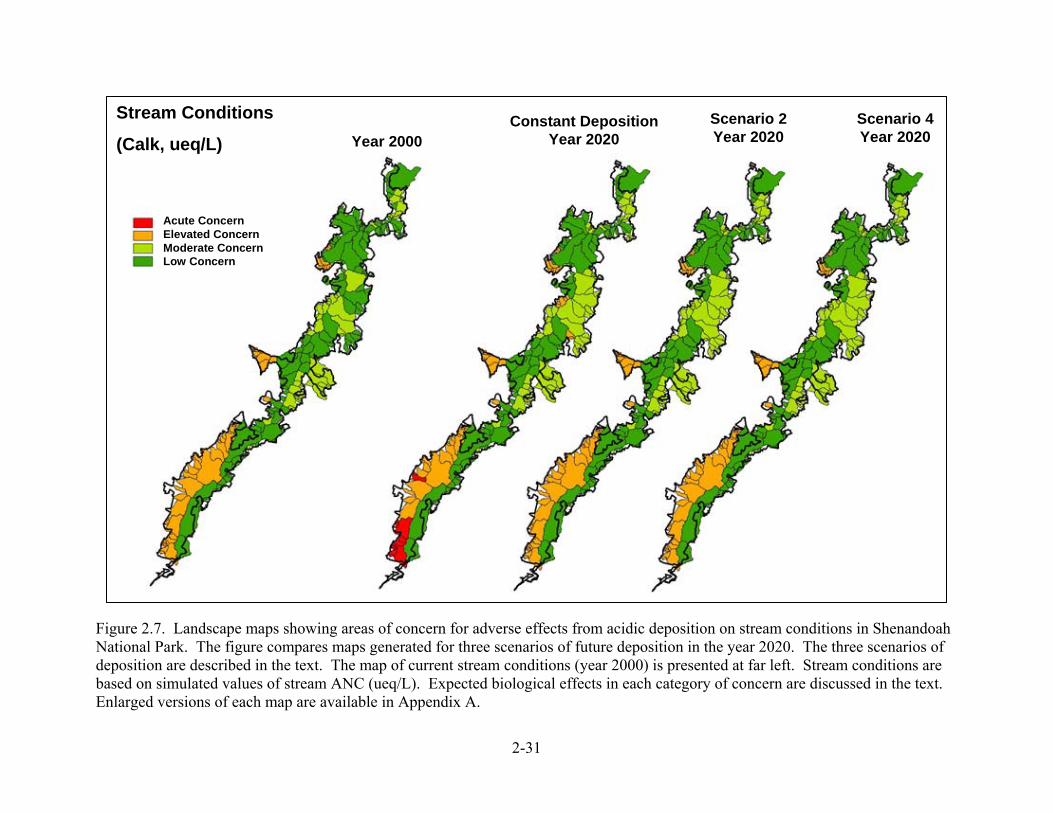
2-31

Figure 2.7. Landscape maps showing areas of concern for adverse effects from acidic deposition on stream conditions in Shenandoah National Park. The figure compares maps generated for three scenarios of future deposition in the year 2020. The three scenarios of deposition are described in the text. The map of current stream conditions (year 2000) is presented at far left. Stream conditions are based on simulated values of stream ANC (ueq/L). Expected biological effects in each category of concern are discussed in the text. Enlarged versions of each map are available in Appendix A.

Year 2000Constant Deposition

Year 2020Stream Conditions

(Calk, ueq/L)Scenario 2Year 2020

Scenario 4Year 2020

Acute ConcernElevated ConcernModerate ConcernLow Concern

Year 2000Constant Deposition

Year 2020Stream Conditions

(Calk, ueq/L)Scenario 2Year 2020

Scenario 4Year 2020

Acute ConcernElevated ConcernModerate ConcernLow Concern

2-32

Figure 2.8. Landscape maps showing areas of concern for adverse effects from acidic deposition on stream conditions in Shenandoah National Park. The figure compares maps generated for three scenarios of future deposition in the year 2100. The three scenarios of deposition are described in the text. The map of current stream conditions (year 2000) is presented at far left. Stream conditions are based on simulated values of stream ANC (ueq/L). Expected biological effects in each category of concern are discussed in the text. Enlarged versions of each map are available in Appendix A.

Year 2000Constant Deposition

Year 2100Stream Conditions

(Calk, ueq/L)Scenario 2Year 2100

Scenario 4Year 2100

Acute ConcernElevated ConcernModerate ConcernLow Concern

Year 2000Constant Deposition

Year 2100Stream Conditions

(Calk, ueq/L)Scenario 2Year 2100

Scenario 4Year 2100

Acute ConcernElevated ConcernModerate ConcernLow Concern

2-33

Figure 2.9. Landscape maps showing areas of concern for adverse effects from acidic deposition on soil conditions in Shenandoah National Park. The figure compares maps generated for three scenarios of future deposition in the year 2020. The three scenarios of deposition are described in the text. The map of current soil conditions (year 2000) is presented at far left. Soil conditions are based on simulated values of soil base saturation (%). Expected biological effects in each category of concern are discussed in the text. Enlarged versions of each map are available in Appendix A.

Year 2000Constant Deposition

Year 2020Soil Conditions

(Base Saturation %)Scenario 2Year 2020

Scenario 4Year 2020

Acute ConcernElevated ConcernModerate ConcernLow Concern

Year 2000Constant Deposition

Year 2020Soil Conditions

(Base Saturation %)Scenario 2Year 2020

Scenario 4Year 2020

Acute ConcernElevated ConcernModerate ConcernLow Concern

2-34

Figure 2.10. Landscape maps showing areas of concern for adverse effects from acidic deposition on soil conditions in Shenandoah National Park. The figure compares maps generated for three scenarios of future deposition in the year 2100. The three scenarios of deposition are described in the text. The map of current soil conditions (year 2000) is presented at far left. Soil conditions are based on simulated values of soil base saturation (%). Expected biological effects in each category of concern are discussed in the text. Enlarged versions of each map are available in Appendix A.

Year 2000Constant Deposition

Year 2100Soil Conditions

(Base Saturation %)Scenario 2Year 2100

Scenario 4Year 2100

Acute ConcernElevated ConcernModerate ConcernLow Concern

Year 2000Constant Deposition

Year 2100Soil Conditions

(Base Saturation %)Scenario 2Year 2100

Scenario 4Year 2100

Acute ConcernElevated ConcernModerate ConcernLow Concern

2-35

Projected soil conditions for the two scenarios of reduced deposition are the same in year 2020 (Figure 2.9). Both scenarios show slight further deterioration of soil condition by year 2020 relative to soil conditions in year 2000 (in a couple of watersheds in the southern district of SHEN). By 2100 the benefits of the deposition reductions for soil conditions relative to constant deposition can readily be seen (Figure 2.10). But when the effects are compared to soil conditions in 2000, both future reduction scenarios show further deterioration of soil conditions, i.e. soil acidification. There are, however, no discernible differences in the pattern of the further soil acidification between the two reduction scenarios.

Projected stream conditions show more response to the two scenarios of future deposition reduction than do projected soil conditions. In the short-term (by year 2020) both deposition reduction scenarios prevent the development of areas of “acute concern” for stream conditions that become established under constant deposition (Figure 2.7). There are no apparent differences in stream condition response, however, between the two reduction scenarios in the short-term (Figure 2.7).

In the long-term responses of stream condition (Figure 2.8) the differences among the three forecast scenarios are clearly seen. Under constant deposition, stream conditions worsen compared to current conditions (Figure 2.8) with large areas of “acute concern” developing as discussed above. There are also important long-term differences in stream condition between the two scenarios of reduced deposition.

Future deposition scenario 2 resulted in moderate changes in simulated ANC and BS at the study sites (Figure 2.6). This scenario maps onto the landscape of SHEN in 2100 in a pattern that includes no areas of “acute concern”. In fact, the mapped response to scenario 2 in year 2100 is identical to current stream conditions. Scenario 2 apparently prevents further deterioration of stream conditions, but produces no real improvement.

Future deposition scenario 4 resulted in the largest changes in simulated ANC and BS at the study sites (Figure 2.6). Scenario 4 maps onto the landscape at SHEN as a distinct improvement in stream conditions over both the constant deposition scenario and the modest deposition reductions of Scenario 2. Stream conditions in SHEN in 2100 under Scenario 4 show improvement relative even to present day conditions in that approximately half the area that is currently of “elevated concern” in the southern district of the park improves to “moderate concern” by 2100.

2.8 Conclusions

Although baseline, pre-industrial resource conditions are not well known, the analysis here suggests that ranges of both soil and stream conditions that would occur in SHEN in the absence of air pollution impacts would not include any areas of “acute concern” and/or ”elevated concern”. However, the historical mapping exercise also suggests that large areas of SHEN, especially in the southern district, may have always been of “moderate concern” reflecting the inherent sensitivity of the siliciclastic bedrock that dominates the southern district.

Simulation and mapping of watershed responses to historical changes in acidic deposition (from pre-industrial to current) suggest that large areas of SHEN have suffered deterioration of both

2-36

soil and stream conditions. The changes in soil condition have been relatively modest up to the present time, with small areas in the southern district of SHEN moving from “moderate concern” (the historical baseline) to “elevated concern” as a result of leaching of base cations from the soils in these areas. Deterioration in stream conditions has been more severe, with large areas in the southern district and some smaller areas in the central and northern districts moving from “moderate concern” to “elevated concern”. Neither soil nor stream conditions have shown any improvement from 1980 to the present in response to the decline in acidic deposition over the last 25 years.

With respect to future soil conditions, the assessment suggests that the responses of soil conditions are relatively slow. In the short term (by year 2020) neither improvement nor further deterioration is likely to be observed in soil condition regardless of the future deposition scenario considered. However, by the year 2100 it becomes clear that constant deposition would produce worsening soil conditions in SHEN with the development of areas of “acute concern” in the southern district. Perhaps more importantly, while the two scenarios of reduced future deposition did not produce worsening soil conditions, neither did they indicate any improvement in soil condition even in the long term. It is possible that emissions controls activities (and therefore emissions reductions) currently being considered in the policy arena would all be insufficient to reverse the soil acidification that has occurred in SHEN and start soil conditions on a path to recovery to pre-industrial conditions.

With respect to future stream conditions, the assessment suggests that the responses of stream conditions are relatively more rapid than those of soils. In the short term (by year 2020) while constant deposition would likely produce further deterioration in stream condition, the two scenarios of future deposition reductions do nothing to reverse the deterioration of stream condition that has occurred in SHEN. In the long term (by year 2100) the effects of the two deposition reduction scenarios begin to diverge. The moderate deposition reduction scenario still produces no improvement in stream conditions relative to current conditions, even by 2100. The largest deposition reduction scenario, by contrast, produces modest improvements in stream conditions by 2100. It is important to note, however, that even the relatively large deposition reductions of this scenario do not result in a return of stream conditions in SHEN to the pre-industrial state. It is unlikely that the pre-industrial state for streams in SHEN can be reached until deposition reductions sufficient to stop the soil acidification (discussed above) in SHEN are achieved.

3-37

Chapter 3: The Environmental Setting of Shenandoah National Park

3.1 Background

Shenandoah National Park (SHEN) is an excellent example of the Blue Ridge/Central Appalachian biome. Figure 3.1 shows the park boundary and its division into three management districts. Also indicated are the locations of Federally designated wilderness areas and air quality monitoring stations. Figure 3.2 (a, b, and c) shows the location of roads, trails, streams, and scenic historic overlooks within the park. SHEN is known for its scenic beauty, outstanding natural features and biota, and historic sites. There have been significant changes in land use prior to and since the establishment of the park. Formerly the location of farmsteads and other industry, land in the park has been allowed to revert to a more natural state since park formation in 1935. However, extensive evidence still remains of the long history of human use of the land.

Significant park features include the following:

Skyline Drive. This scenic 165 km drive, shown in Figure 3.2, provides the opportunity for views of the Blue Ridge Mountains and surrounding areas. The road was designed and constructed in the 1930s to provide scenic views into the Piedmont Plateau to the east and the Shenandoah Valley to the west. Overlooks were constructed so that motorists could stop at intervals along the drive and enjoy the scenic vistas (Shenandoah National Park 2001).

Appalachian National Scenic Trail. The segment of the Appalachian National Scenic Trail that runs through SHEN (shown as the trail that generally parallels Skyline Drive in Figure 3.2) is the backbone of the park’s trail system.

Natural resources. The natural features and biota of the park include well-exposed rock strata of the Appalachians, which is one of the oldest mountain ranges in the world. The park comprises one of the nation’s most diverse botanical reserves and diverse wildlife habitats.

Wilderness. Congressionally-designated wilderness area within the park is the largest in the Mid-Atlantic states and provides a comparatively accessible opportunity for solitude, study, and experience in a natural area (Shenandoah National Park 1998a).

Historic resources. There are over 135 buildings listed on the National Register of Historic Places.

3-38

Figure 3.1. Shenandoah National Park and division into three management districts. Also shown are the locations of federally designated wilderness areas and air quality monitoring stations. The air quality stations at Dickey Ridge and Sawmill Run are no longer active.

Dickey RidgeAir Quality StationDickey RidgeAir Quality Station

Big MeadowsAir Quality Station (active)

Sawmill Run Air Quality Station

South District

Central District

North District

HWY211

HWY33

Management Districts

0 6 12 18 24Miles

LegendNational Park BoundaryWilderness BoundaryHighwayAir Quality Stations

Shenandoah National Park Management Districts

N

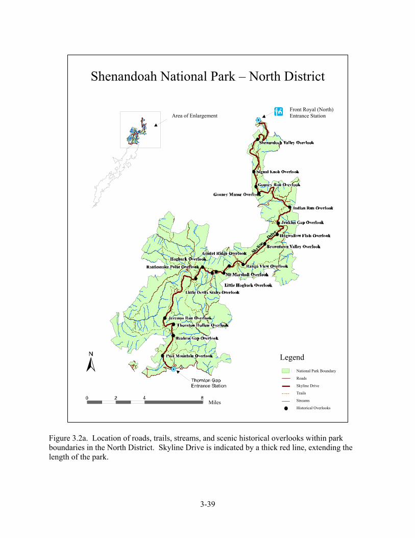
3-39

Figure 3.2a. Location of roads, trails, streams, and scenic historical overlooks within park boundaries in the North District. Skyline Drive is indicated by a thick red line, extending the length of the park.

Shenandoah National Park – North District

Area of Enlargement Front Royal (North) Entrance Station

Legend National Park Boundary

Roads

Skyline Drive

Trails

Streams

Historical Overlooks Miles

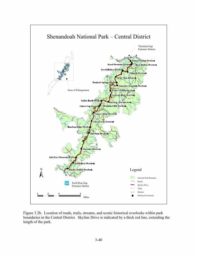
3-40

Figure 3.2b. Location of roads, trails, streams, and scenic historical overlooks within park boundaries in the Central District. Skyline Drive is indicated by a thick red line, extending the length of the park.

National Park Boundary

Roads

Skyline Drive

Trails

Streams

Historical Overlooks

Legend

Area of Enlargement

Thornton Gap Entrance Station

Swift Run Gap Entrance Station

Miles

Shenandoah National Park – Central District

3-41

Figure 3.2c. Location of roads, trails, streams, and scenic historical overlooks within park boundaries in the South District. Skyline Drive is indicated by a thick red line, extending the length of the park.

Swift Run Gap Entrance Station

Area of Enlargement

Shenandoah National Park – South District

Legend

National Park Boundary

Roads

Skyline Drive

Trails

Streams

Historical Overlooks

Rockfish (South) Entrance Station

Miles

3-42

The mountainous ridge of the park grades into the Valley and Ridge Province to the west and the Piedmont Province to the east. The montane-upland Blue Ridge Province extends from Pennsylvania to northern Georgia. Most physiographers apply the Blue Ridge Province name to all contiguous high mountains underlain by crystalline rocks from south central Pennsylvania to northeastern Georgia, including SHEN and Great Smoky Mountains National Park. The Northern Blue Ridge (Roanoke River to Pennsylvania) is narrow (3–20 km wide overall), whereas the Southern Blue Ridge (Roanoke River to Georgia) widens to nearly 100 km, and increases in height southward. The Blue Ridge rocks are largely resistant to weathering, and streams are mostly of the softwater (low in calcium and magnesium) type.

The Blue Ridge Mountains in which SHEN is located are part of the Appalachian Range. The mountains are comprised of a series of long parallel folds with a single crest of rounded peaks and lower ridges that lies in a northeast to southwest direction. Elevation within the park ranges from 146 m at Front Royal to 1,234 m at Hawksbill Peak. Within the park, there are more than two dozen peaks that are over 900 m high. The land adjacent to the park is changing rapidly from recreational forest, agricultural, and seasonal residential uses to year- round residential use.

Interest in preserving areas in the southern Appalachian Mountains began near the turn of the 20th century. In 1924, the Southern Appalachian National Park Committee was appointed by the Secretary of the Interior to investigate the possible existence of sites suitable for the establishment of a national park. The result of the committee’s work was an act that was passed in February, 1925 that directed the Secretary of the Interior to determine the boundaries and areas within the Blue Ridge Mountains of Virginia that could be recommended as a new national park. A subsequent act was passed in May, 1926 authorizing SHEN. Its provisions included that the lands could be secured by the United States only by public or private donation, and that the tract include approximately 210,800 ha. The task proved to be quite complicated and costly, and Congress reduced the minimum requirement to 64,735 ha. By 1935, the deeds were ready and the Commonwealth of Virginia donated about 71,400 ha to the Department of the Interior. On July 3, 1936, President Franklin D. Roosevelt dedicated SHEN “to the present and future generations of America for the recreation and re-creation which we shall find here.” The total area of the park is now 79,889 ha.

SHEN was intended to be a sample of the central Appalachian portion of primitive America, but approximately half of the forest was cleared at the time of park formation (Reed Engle, National Park Service, pers. comm.). The establishment of the park did, however, offer protection to what remained of central Appalachian plants and animals in portions of the park that were still forested, and nature continued its restorative process. The park is now about 95% forested. Some of the animals that had been greatly reduced or eliminated have returned or have been reintroduced. So complete was the regeneration in the first four decades, that in 1976 nearly 132,370 ha were deemed of suitable primitive character to be included in the National Wilderness Preservation System.

Several areas of the park have received special recognition due to the significance of natural and cultural resources. For example, in 1985, the Shaver Hollow watershed was designated as the first Research Natural Area in a National Park Service (NPS) unit in eastern deciduous forest. It serves as a focal area for intensive watershed research within the park. In addition, in 1996 Skyline Drive and associated developed areas at Simmons Gap, Big Meadows, Piney River,

3-43

Pinnacles, Dickey Ridge, and Park Headquarters were listed on the National Register of Historical Places.

SHEN has become significant for the following reasons:

• The park provides a traditional national park experience in the east. • It is close to large metropolitan populations, providing relatively good accessibility to

millions of citizens. • Establishment of this park represented a conscious change in human use of the land.

With ongoing vegetation recovery, the park has become a sizeable forested area, with large areas of designated wilderness.

• It includes developed areas that are listed on, or determined to be eligible for, the National Register or as national historical landmarks.

• The park includes the longest segment of the Appalachian National Scenic Trail that occurs in a national park.

Central to the significance of the park are the rural agricultural landscapes that surround it. These lands are the primary components of the vistas from Skyline Drive. They are additional components of the ecosystem that support park wildlife and other values that are significant to the purposes for which the park was initially established. There are large blocks of undeveloped natural uplands, which contrast with the valley mosaic of privately owned farmland, forests, and settled areas

3.2 Climate

The Atlantic Ocean, and in particular the Gulf Stream, plays an important role in Virginia’s precipitation regime. Winter storms generally track from the west to the east, and in the vicinity of the east coast move to the northeast paralleling the coast and the Gulf Stream. This shift to the northeast results partly from the tendency of storms to follow the boundary between the cold land and the warm Gulf Stream. When sufficiently cold air comes into Virginia from the west and the northwest, frontal storms can bring heavy snowfall. Thunderstorms occur in all months of the year, but are most common during summer. Precipitation is well distributed throughout the year, with a maximum in September and minimum in February. Storms and high runoff conditions can occur year-round at SHEN. Most locations receive 100 to 150 cm of precipitation per year. South to southwest winds predominate, with secondary maximum frequency from the north. Lower elevation areas of the park experience modified continental climate, with mild winters and warm, humid summers. The mean annual temperature in the lowland area at Luray averages 12°C, and average annual precipitation is 91 cm, with about 43 cm of snow.

Higher elevation areas of the park experience winters that are moderately cold and summers that are relatively cool. The mean annual temperature at Big Meadows averages about 9°C. Mean maximum daily temperatures in July average about 6°C cooler at Big Meadows than in the lowland areas of the park. Temperatures in January range from about -7° to 4°C and in July from about 14° to 24°C. The average annual precipitation at Big Meadows is 132 cm, which includes about 94 cm of snow. Snow and ice are common in winter, but they usually melt

3-44

quickly, leaving the ground bare. Occasional major snow or ice storms can cause considerable damage to the trees within the park.

3.3 Scenery

In its report to Congress, the Southern Appalachian National Park Committee highlighted the importance of scenery to the purpose and national significance of SHEN. The committee identified a possible sky-line drive as the greatest single feature of the area that was to become SHEN, and noted that the Blue Ridge mountains of northern Virginia met aesthetic requirements including but not limited to… “mountain scenery with inspiring perspectives and delightful details”…that contains…“forests, shrubs and flowers, and mountain streams, with picturesque cascades and waterfalls overhung with foliage … .” The 163-km (105-mi) Skyline Drive was constructed by the Civilian Conservation Corps from 1931 to 1939. Most of the 157-km (101-mi) segment of the Appalachian National Scenic Trail found within the park was constructed by the Potomac Appalachian Trail Club in the 1930s. Today, the Appalachian National Scenic Trail forms the backbone for the park’s extensive trails network totaling about 800 km (500 mi). Since the park’s creation in 1935, millions of visitors have enjoyed the views from numerous vistas within the park along both the Drive and park trails.

3.4 Surface Waters

High gradient is a chief feature of high-elevation streams in Virginia. Pools are interspersed with riffles, rapids, cascades and falls. Stream bottoms are chiefly comprised of large gravel, rubble, boulder and bedrock. Streams are cool or even cold in summer, typically clear, and rain-caused turbidity clears rapidly (Jenkins and Burkhead 1993). Patrick (1996) described typical Mid-Atlantic high-gradient mountain streams as heavily shaded in summer, having very few macrophytes and filamentous algae, with main primary productivity by diatoms. This description is also reflective of the mainly first-, second- and third-order streams of SHEN. Wallace et al. (1992) defined high-gradient streams as those with longitudinal gradients exceeding 0.15% slope (1.5 m per km), consistent with other definitions. Such streams typically occur between 330 and 2000 m above sea level. There are many such streams within the Valley and Ridge and Blue Ridge physiographic provinces, as well as in the Piedmont. The Blue Ridge (in which SHEN is located) is covered in dense deciduous and coniferous forests, with steep slopes up to 30%. High-gradient streams of the Blue Ridge are typically dendritic; stream density may be as high as 6.2 km/km2. Streams in adjacent hollows may have different slopes and stream chemistry due to differences in bedrock composition.

Although acidic deposition is ubiquitous regionally, its interaction with local geological formations determines where effects on stream chemistry will occur. Stream concentrations of important ions (calcium, magnesium, sodium, potassium, chloride, nitrate, sulfate) are usually low in regional mountain streams. Concentrations of nitrate, ammonium, and phosphate may be very low (0.001–0.004 mg/L as nitrogen or phosphorus for each) in forested streams draining crystalline watersheds. Stream pH typically decreases with increasing elevation, as is the case within SHEN (Bulger et al. 1999).

There are 42 watershed basins on the west side of SHEN and 28 watershed basins on the east. In many places, the streams drop over ledges, creating waterfalls up to 28 m high. There are about

3-45

72 perennial streams in the park (Figure 3.2), and over 50 of those contain native brook trout (Salvelinus fontinalis; Shenandoah National Park 1998b). Almost all of the streams in the park are lower-order streams that drain into three major river basins, the Potomac River to the west and the Rappahannock and James Rivers to the east. This headwater status increases their potential sensitivity to adverse impacts from acidic deposition for a variety of reasons. In general, headwater streams are more likely than lower-elevation streams to be underlain by relatively homogeneous bedrock and soils, in many cases having low base cation supply. In addition, higher-elevation watershed areas are more likely to have shallow soils, exhibit greater base cation leaching losses due to higher precipitation, and receive smaller base cation contributions from weathering due to colder temperatures.

3.5 Geology

The geology of the park represents one of its most outstanding natural resources. Exposed formations of the Blue Ridge Mountains are among the oldest in North America. The geologic history of the park has been the subject of frequent investigations by geologists and university students. There are seven principal rock types that form the bedrock of the area, as described in Shenandoah National Park (1998b) and shown in Figure 3.3.

There are granitic rocks, known as Old Rag Granite and the Pedlar Formation, which exceed one billion years in age. They cover about 8% and 25% of the park area, respectively. The plutonic rocks of these two formations are among the oldest exposed rocks in the Appalachian Mountains (Gathright 1976).

The Swift Run Formation is a conglomerate of debris from granitic rocks and the volcanism which laid down the Catoctin Formation. It is about 600 million years old and covers about 1% of the park.

The Catoctin Formation is comprised of many layers of metamorphosed volcanic rocks, which were derived from a series of volcanic eruptions that began about 600 million years ago. The Catoctin rocks dominate the central and northern park sections and cover about 38% of the park. Dense greenstone, which formed from lava, makes up much of the Catoctin Formation and underlies most of the high ridges (Gathright 1976).

The other three rock types found in SHEN are metamorphosed sedimentary rocks, about 500 million years old. The Chilhowee Formation is exposed along western slopes in the southern portions of the park. The Hampton Member is the most extensive, covering about 17% of the park. It is a thick deposit (~ 600 m) of phyllite and shale in the lower sections and interbedded metasandstone and phyllite with intermittent quartzite in the upper sections. The Weverton Member, a sequence of interbedded quartzite, phyllite, and metasandstone, is of limited distribution in the park.

3-46

Figure 3.3. Lithologic and geological sensitivity maps of Shenandoah National Park. Lithology was taken from Gathright (1976). Geologic sensitivity classes are arranged in the legend from most (siliciclastic) to least (carbonate) sensitive to acidification. They can be derived from the lithological coverage as follows: siliciclastic (Erwin, Hampton, Weverton), granitic (Old Rag Granite, Pedlar, Swift Run), basaltic (Catoctin).

±0 10 205Miles

Geologic Sensitivity Class

SiliciclasticArgillaceous

GraniticBasaltic

Carbonate

LithologyCatoctin

Erwin (Antietam)Hampton (Harpers)Old Rag GranitePedlar

Swift RunWeverton

Data Not Available

Shenandoah National ParkLithology and Geological Sensitivity

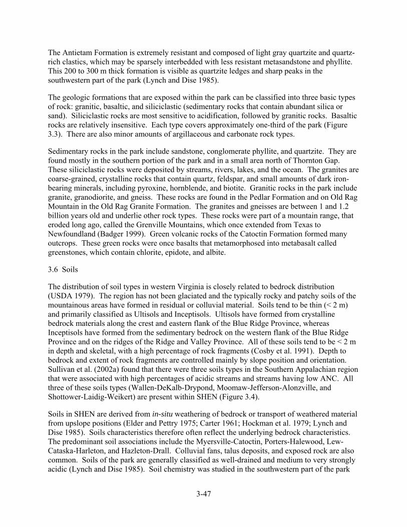
3-47

The Antietam Formation is extremely resistant and composed of light gray quartzite and quartz-rich clastics, which may be sparsely interbedded with less resistant metasandstone and phyllite. This 200 to 300 m thick formation is visible as quartzite ledges and sharp peaks in the southwestern part of the park (Lynch and Dise 1985).

The geologic formations that are exposed within the park can be classified into three basic types of rock: granitic, basaltic, and siliciclastic (sedimentary rocks that contain abundant silica or sand). Siliciclastic rocks are most sensitive to acidification, followed by granitic rocks. Basaltic rocks are relatively insensitive. Each type covers approximately one-third of the park (Figure 3.3). There are also minor amounts of argillaceous and carbonate rock types.

Sedimentary rocks in the park include sandstone, conglomerate phyllite, and quartzite. They are found mostly in the southern portion of the park and in a small area north of Thornton Gap. These siliciclastic rocks were deposited by streams, rivers, lakes, and the ocean. The granites are coarse-grained, crystalline rocks that contain quartz, feldspar, and small amounts of dark iron-bearing minerals, including pyroxine, hornblende, and biotite. Granitic rocks in the park include granite, granodiorite, and gneiss. These rocks are found in the Pedlar Formation and on Old Rag Mountain in the Old Rag Granite Formation. The granites and gneisses are between 1 and 1.2 billion years old and underlie other rock types. These rocks were part of a mountain range, that eroded long ago, called the Grenville Mountains, which once extended from Texas to Newfoundland (Badger 1999). Green volcanic rocks of the Catoctin Formation formed many outcrops. These green rocks were once basalts that metamorphosed into metabasalt called greenstones, which contain chlorite, epidote, and albite.

3.6 Soils

The distribution of soil types in western Virginia is closely related to bedrock distribution (USDA 1979). The region has not been glaciated and the typically rocky and patchy soils of the mountainous areas have formed in residual or colluvial material. Soils tend to be thin (< 2 m) and primarily classified as Ultisols and Inceptisols. Ultisols have formed from crystalline bedrock materials along the crest and eastern flank of the Blue Ridge Province, whereas Inceptisols have formed from the sedimentary bedrock on the western flank of the Blue Ridge Province and on the ridges of the Ridge and Valley Province. All of these soils tend to be < 2 m in depth and skeletal, with a high percentage of rock fragments (Cosby et al. 1991). Depth to bedrock and extent of rock fragments are controlled mainly by slope position and orientation. Sullivan et al. (2002a) found that there were three soils types in the Southern Appalachian region that were associated with high percentages of acidic streams and streams having low ANC. All three of these soils types (Wallen-DeKalb-Drypond, Moomaw-Jefferson-Alonzville, and Shottower-Laidig-Weikert) are present within SHEN (Figure 3.4).

Soils in SHEN are derived from in-situ weathering of bedrock or transport of weathered material from upslope positions (Elder and Pettry 1975; Carter 1961; Hockman et al. 1979; Lynch and Dise 1985). Soils characteristics therefore often reflect the underlying bedrock characteristics. The predominant soil associations include the Myersville-Catoctin, Porters-Halewood, Lew-Cataska-Harleton, and Hazleton-Drall. Colluvial fans, talus deposits, and exposed rock are also common. Soils of the park are generally classified as well-drained and medium to very strongly acidic (Lynch and Dise 1985). Soil chemistry was studied in the southwestern part of the park

3-48

Figure 3.4. Soils types in Shenandoah National Park. All soil types in the legend are present within the park, but several are present only in very small areas.

Shenandoah National ParkSoil Types

Soil TypesBERKS-WEIKERT-LAIDIGCATOCTIN-MYERSVILLE-ROCK OUTCROPFREDERICK-CARBO-TIMBERVILLEHAYESVILLE-PARKER-PEAKSMOOMAW-JEFFERSON-ALONZVILLESHOTTOWER-LAIDIG-WEIKERTWALLEN-DEKALB-DRYPOND

0 10 205Miles

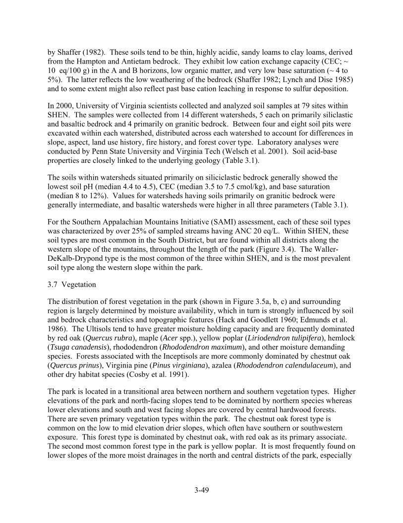
3-49

by Shaffer (1982). These soils tend to be thin, highly acidic, sandy loams to clay loams, derived from the Hampton and Antietam bedrock. They exhibit low cation exchange capacity (CEC; ~ 10 eq/100 g) in the A and B horizons, low organic matter, and very low base saturation (~ 4 to 5%). The latter reflects the low weathering of the bedrock (Shaffer 1982; Lynch and Dise 1985) and to some extent might also reflect past base cation leaching in response to sulfur deposition.

In 2000, University of Virginia scientists collected and analyzed soil samples at 79 sites within SHEN. The samples were collected from 14 different watersheds, 5 each on primarily siliclastic and basaltic bedrock and 4 primarily on granitic bedrock. Between four and eight soil pits were excavated within each watershed, distributed across each watershed to account for differences in slope, aspect, land use history, fire history, and forest cover type. Laboratory analyses were conducted by Penn State University and Virginia Tech (Welsch et al. 2001). Soil acid-base properties are closely linked to the underlying geology (Table 3.1).

The soils within watersheds situated primarily on siliciclastic bedrock generally showed the lowest soil pH (median 4.4 to 4.5), CEC (median 3.5 to 7.5 cmol/kg), and base saturation (median 8 to 12%). Values for watersheds having soils primarily on granitic bedrock were generally intermediate, and basaltic watersheds were higher in all three parameters (Table 3.1).

For the Southern Appalachian Mountains Initiative (SAMI) assessment, each of these soil types was characterized by over 25% of sampled streams having ANC 20 eq/L. Within SHEN, these soil types are most common in the South District, but are found within all districts along the western slope of the mountains, throughout the length of the park (Figure 3.4). The Waller-DeKalb-Drypond type is the most common of the three within SHEN, and is the most prevalent soil type along the western slope within the park.

3.7 Vegetation

The distribution of forest vegetation in the park (shown in Figure 3.5a, b, c) and surrounding region is largely determined by moisture availability, which in turn is strongly influenced by soil and bedrock characteristics and topographic features (Hack and Goodlett 1960; Edmunds et al. 1986). The Ultisols tend to have greater moisture holding capacity and are frequently dominated by red oak (Quercus rubra), maple (Acer spp.), yellow poplar (Liriodendron tulipifera), hemlock (Tsuga canadensis), rhododendron (Rhododendron maximum), and other moisture demanding species. Forests associated with the Inceptisols are more commonly dominated by chestnut oak (Quercus prinus), Virginia pine (Pinus virginiana), azalea (Rhododendron calendulaceum), and other dry habitat species (Cosby et al. 1991).

The park is located in a transitional area between northern and southern vegetation types. Higher elevations of the park and north-facing slopes tend to be dominated by northern species whereas lower elevations and south and west facing slopes are covered by central hardwood forests. There are seven primary vegetation types within the park. The chestnut oak forest type is common on the low to mid elevation drier slopes, which often have southern or southwestern exposure. This forest type is dominated by chestnut oak, with red oak as its primary associate. The second most common forest type in the park is yellow poplar. It is most frequently found on lower slopes of the more moist drainages in the north and central districts of the park, especially

3-50

Table 3.1. Interquartile distribution of pH, cation exchange capacity (CEC), and percent base saturation for soil samplesa collected in Shenandoah National Park study watersheds during the 2000 soil survey.

pH CEC (cmol/kg) % Base Saturation Site ID Watershed N 25th Med 75th 25th Med 75th 25th Med 75th Siliciclastic Bedrock Classb

VT35 Paine Run 6 4.4 4.5 4.7 3.7 5.7 5.7 7.1 10.0 24.9 WOR1 White Oak Run 6 4.3 4.4 4.4 4.8 7.5 7.8 5.3 7.5 8.5 DR01 Deep Run 5 4.3 4.4 4.5 3.9 5.0 5.8 7.2 8.9 10.8 VT36 Meadow Run 6 4.4 4.4 4.5 3.1 3.5 7.6 7.8 8.7 11.3 VT53 Twomile Run 5 4.3 4.5 4.5 4.6 6.0 6.9 11.7 12.3 13.6

Granitic Bedrock Class VT59 Staunton River 6 4.7 4.8 4.9 6.5 7.5 9.2 9.1 13.9 29.5 NFDR NF of Dry Run 5 4.4 4.5 4.7 7.3 8.0 9.2 7.5 10.8 12.4 VT58 Brokenback Run 5 4.6 4.7 4.7 7.3 8.4 9.6 6.0 6.7 9.7 VT62 Hazel River 4 4.5 4.7 4.8 5.3 5.3 6.5 12.3 12.8 21.6

Basaltic Bedrock Class VT60 Piney River 6 4.7 5.0 5.3 7.3 7.7 10.0 17.0 24.0 57.0 VT66 Rose River 8 4.8 5.0 5.3 7.3 10.1 10.7 19.1 38.0 63.5 VT75 White Oak Canyon 6 4.9 5.1 5.5 7.1 7.5 9.3 15.6 32.8 43.4 VT61 NF of Thornton River 7 5.1 5.2 5.3 7.7 9.6 10.8 35.6 54.4 71.2 VT51 Jeremys Run 4 4.7 5.0 5.3 6.3 7.6 7.7 15.0 22.8 46.1

a Samples collected from mineral soil >20cm depth b Watersheds are stratified according to the predominant bedrock class present in each watershed.

on north and east facing slopes. Yellow birch (Betula alleghaniensis), hemlock, white pine (Pinus strobus), and white oak (Quercus alba) are common associates. Cove hardwood is the third most common forest type, and is comprised of ash (Fraxinus sp.), red oak, and basswood (Tilia americana). It is located mostly on moist sites in the hollows and along stream drainages. The red oak forest type is found over a fairly broad range of environmental conditions. It occupies the most mesic ridgetops and side slopes. Red oak is dominant in this forest type, which also includes mockernut hickory (Carya tomentosa), pignut hickory (C. glabra), chestnut oak, and white oak. The pine forest type includes eastern white pine (Pinus strobus), Virginia pine, and pitch pine (P. rigida). These species are primarily successional and are found on previously disturbed sites. Black locust (Robinia pseudoacacia) is an early successional forest type that is found in recently disturbed areas. It also includes black cherry (Prunus serotina), tree of heaven (Ailanthus altissima), and Virginia pine. Moist sites in association with spring seeps, streams, north facing slopes, and shaded drainage bottoms are often covered with hemlock forests, which occur in pure stands.

Big Meadows is a large (48 ha) high-elevation grass/shrub plant community that was maintained as a meadow in historic times by grazing and burning, and later by burning and mowing. A small bog occurs in its northeast corner, where many plant species are found that do not occur elsewhere in the park.

3-51

Figure 3.5a Major forest types in the North District of Shenandoah National Park.

±

Area of Enlargement

0 4 82Miles

Forest TypesPineHemlockBlack LocustCove HardwoodChestnut OakRed OakYellow PoplarOpenRockData Not Available

Shenandoah National Park - North DistrictForest Types

3-52

Figure 3.5b Major forest types in the Central District of Shenandoah National Park.

±Forest Types

PineHemlockBlack LocustCove HardwoodChestnut OakRed OakYellow PoplarOpenRockData Not Available

0 4 82Miles

Area of Enlargement

Shenandoah National Park - Central DistrictForest Types

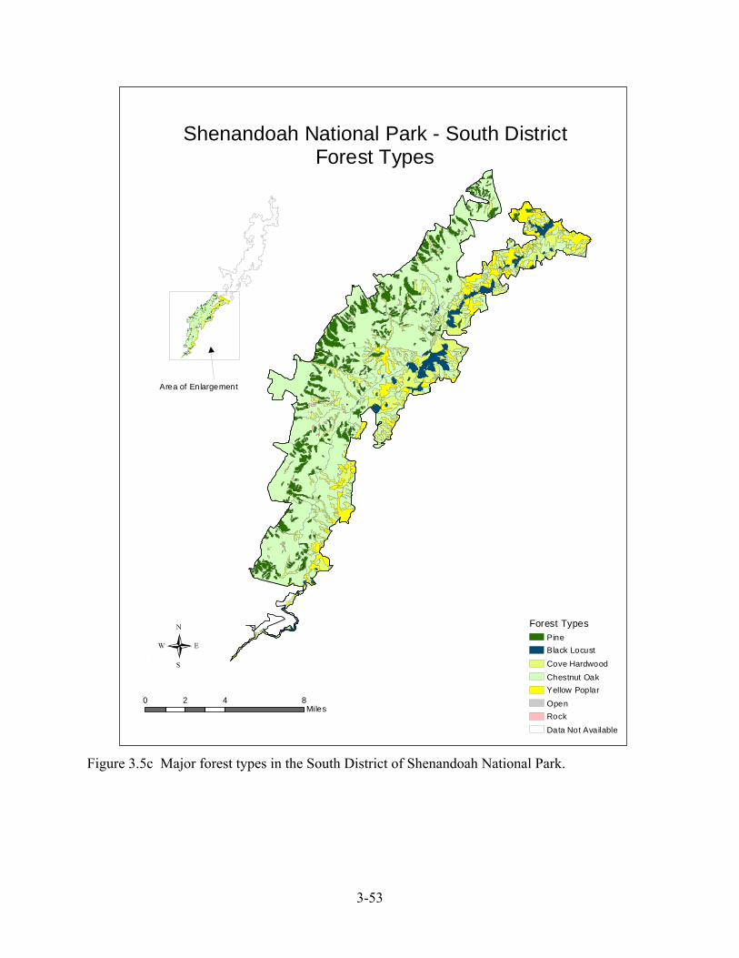
3-53

Figure 3.5c Major forest types in the South District of Shenandoah National Park.

0 4 82Miles

Forest TypesPineBlack LocustCove HardwoodChestnut OakYellow PoplarOpenRockData Not Available

±

Area of Enlargement

Shenandoah National Park - South DistrictForest Types

3-54

Limberlost is a high-elevation area of seeps and springs that contains an extensive old growth stand of eastern hemlock and red spruce (Picea rubens). The area also contains speckled alder (Alnus rugosa), Canada yew (Taxus canadensis), and the only occurrence in Virginia of alder-leaved buckthorn (Rhamnus alnifolia).

Cliffs and rocky north- and west-facing slopes support fragile populations of plants, including some boreal species such as balsam fir (Abies balsamea), mountain sandwort (Minuartia groenlandica), and bearberry (Arctostaphylos uva-ursi) at the tops of the highest peaks (e.g., Hawksbill, Stony Man and Old Rag). Crescent Rock, Black Rock, Hawksbill Summit, Stony Man Summit, and Old Rag Summit face prevailing winds and include heaths such as minnie bush (Menziesia pilosa) and northern bush honeysuckle (Diervilla lonicera), and crevice plants such as Allegheny stonecrop (Sedum telephioides), Michaux’s saxifrage (Saxifrage michauxii), and three-toothed cinquefoil (Potentilla tridentata).

3.8 Wildlife

Explorers to the Shenandoah Valley and Blue Ridge Mountains in the early 1700s reported an abundance and variety of animals, some of which have since been extirpated. Woodland bison (Bison bison), the largest of Shenandoah’s original fauna, inhabited the valleys and low-elevation foothills with one documented trail crossing the Blue Ridge at Rockfish Gap. Eastern elk (Cervus canadensis) originally occurred throughout the entire northern Shenandoah Valley, including surrounding ridges. Timber wolves (Canis lupus) and mountain lions (Felis concolor) were also among the region’s original inhabitants and together with the black bear (Ursus americanus), constituted the primary predators of large mammal species. As European settlers cleared the land, introduced exotic species, and hunted native animals, both the abundance and variety of wildlife decreased, with total elimination of some species. However, since the establishment of the park, some species have been reintroduced and some have naturally reestablished. Currently, the park sustains populations of white tailed deer (Odocoileus virginianus), black bear, bobcat (Lynx rufus), opossum (Didelphis virginiana), racoon (Procyon lotor), skunk (Mephitis mephitis), gray fox (Urocyon cinereoargenteus), and eastern cottontail (Sylvilagus floridanus; Shenandoah National Park 1993). There are over 200 species of resident and transient birds known to use the park’s habitats, including turkey (Meleagris gallopavo). Sixty-one species of reptiles and amphibians have been recorded within the park. The Shenandoah salamander (Plethodon shenandoah) was listed as an endangered species in 1989. Its range is very limited and includes four areas located in the park at high elevation on rocky talus slopes (Shenandoah National Park 1998b).

3.9 Disturbance

The forests of SHEN exist in an environment that includes insects and pathogens, competition and plant community dynamics, and abiotic factors, including air pollutants and disturbance. To understand how terrestrial ecosystems respond to air pollution requires an understanding of how plants normally grow in a stressful environment, in addition to the details of their response to pollutants and potential alterations in normal growth.

Forests make difficult experimental subjects. Plants grow in a variety of soils, in populations of mixed sizes and species, and under variable climatic conditions. Forests in national parks are

3-55

even less amenable to experimentation—they are to be protected, studied, and enjoyed, not instrumented, poked, and prodded. On the other hand, it is important to understand how anthropogenic stresses affect the health and vigor of the forest.

SHEN comprises one of the nation’s most diverse botanical reserves. The documented flora of the park includes over 1,400 species of plants. From the 1720s to the establishment of the park, much of the area was cleared. The invasion of nonnative insects and pathogens during the 20th century seriously impacted the vegetation communities of the park. The chestnut blight (Endothia parasitica), a canker disease which kills American chestnuts (Castanea dentata), entered the United States in the early part of the 20th century. The disease spread quickly throughout the eastern United States. All chestnut trees in the park were affected by this disease. By about 1940, only remnant chestnut sprout growth existed. The loss of this tree species had a large impact on the structure and composition of park forests because some stands had contained 50% or greater numbers of chestnuts.

The gypsy moth (Lymantria dispar), which was introduced into the United States in the 1860s, began to impact the forests of the park in 1986. Because the preferred food of gypsy moths is oak, the forests of the park which were predominantly oak were vulnerable to widespread impact. Initial effects included defoliation of oaks, with as much as 16,000 ha defoliated in 1989 alone. Repeated defoliations, coupled with several years of drought, caused widespread oak mortality in the late 1980s and early 1990s. An introduced fungus (Entomophaga maimaiga), which attacks gypsy moths, reduced gypsy moth populations in the early 1990s. By 1996, effects on the forest canopies of the park were dramatically curtailed. The nonnative hemlock woolly adelgid (Adelges tsuga) and the native southern pine beetle (Dendroctonus frontalis) have also had dramatic impacts on park forests.

Based on records kept since 1935, the park has approximately eight naturally-occurring fires per year. These fires tend to remain small, and are easily suppressed except during times of drought. Large fires within the park are overwhelmingly human-caused fires. The most notable of these was the Shenandoah Complex Fire, which burned 9,350 ha of park land in the fall of 2000. A fire management plan was prepared for the park (Shenandoah National Park 1993), with a primary objective of fire suppression. The plan details suppression strategies, prevention criteria, interagency cooperation, and programs to prevent adverse impacts of wildfire to life, property, and adjacent lands. In addition, increased emphasis is being directed towards prescribed fire components to determine appropriate actions regarding natural and management-ignited prescribed fires. The park is in the final review draft phase of updating its fire management plan.

4-57

Chapter 4: Acidic Deposition in Shenandoah National Park

Acidic deposition in Shenandoah National Park (SHEN) is the result of distant and local (including in-park) pollutant emissions. Based upon pollutant transformations and lifetimes in the atmosphere and on regional climatology, the various emissions sources contribute in varying degree to pollutant loading or exposure in the park. The purpose of this section is to summarize regional and local emissions and assess the effects of atmospheric transport processes. Major air pollution source regions and states affecting the park are identified. The analysis below concerns sources of pollutant emissions external to SHEN. Sullivan et al. (2003) give a summary of air pollution sources within SHEN and compare these with the local Virginia counties surrounding the park.

4.1 Sources of Acidic Deposition Arriving at Shenandoah National Park

Acidic deposition derives primarily from the emissions of sulfur dioxide (SO2), nitrogen oxides (NOx), and ammonia (NH3), the chemical modification and long-range transport of these compounds in the atmosphere and their subsequent return to the earth’s surface in dry or wet form.

Sulfur dioxide (SO2) is a product of fossil fuel, primarily coal and oil, combustion. Some of the largest emitters are coal-fired electric power plants and smelters. Although more stringent regulations have reduced emissions over the last 30 years, SO2 continues to be a pollutant of concern in many areas of the United States, including throughout the Southeast. SO2 is a precursor of pollutants which cause acidic deposition.

Nitrogen oxides (NOx) and ammonia (NH3) are also precursors for pollutants that cause acidic deposition. All high-temperature combustion processes emit NOx. Automobiles and stationary fossil fuel burning systems are the major anthropogenic (human-caused) sources of NOx emissions in the United States. Naturally-occurring NOx compounds originate from soils, wildfire, lightning, and decomposition. Ammonia sources are primarily from agricultural activities.

State-level sulfur (S) and nitrogen (N) 1990 emissions data were compiled for this project from the annual National Emissions Trend inventory, as revised in October 2000 by the U.S. Environmental Protection Agency (U.S. EPA 2000a). The area source emissions were taken from version 3.01a, the mobile source emissions from version 3.00, and the point source emissions from version 2.00. In all cases, mobile (e.g., on-highway cars, light trucks, and heavy trucks), area-stationary (e.g., commercial and residential heating and vented emissions from commercial buildings), and area-nonroad (off-road vehicles, tractors, construction equipment, locomotives, and ships) emissions were developed at the county level, whereas point source locations were defined in terms of their latitude and longitude.

In addition, 1996 emissions data were derived from the annual National Emissions Trend inventory (U.S. EPA 2000a). The point source emissions for electricity generating units (EGUs) and non-EGUs were taken from version 3.12, and the stationary area-source emissions from version 3.11. Other 1996 emissions were developed by EPA as part of their regulatory analysis of heavy-duty engine and vehicle standards and highway diesel fuel rulemaking. The majority of

4-58

the mobile nonroad source emissions were developed using EPA’s draft NONROAD model, while aircraft, commercial marine, and locomotives (not in NONROAD) were estimated separately (U.S. EPA 2000b). The combined categories of all nonroad emissions are combined in the category “area-nonroad emissions”. For 1996 mobile source emissions, the on-highway vehicle emission inventory created in 1998 was updated. In particular, a new vehicle miles traveled (VMT) mapping from the Highway Performance Monitoring System data to MOBILE5b was developed by EPA and the latest information on 1996 control programs was used, including Inspection and Maintenance programs, Reformulated Gasoline use, Oxygenated Gasoline use, and the Low Emission Vehicle program. Details are provided in U.S. EPA (2000b). The 1996 Case reflects 1990 Clean Air Act Amendments (CAAA) Title IV Phase I implementation of EGU sulfur dioxide (SO2) and nitrogen oxide (NOx) emission reductions.

The airsheds of SHEN contain numerous major stationary sources of air pollution. Emissions from mobile sources and many stationary sources are expected to increase with substantial population and industrial growth in Virginia and other airshed states (Shenandoah National Park 1998b). More Prevention of Significant Deterioration (PSD) air permit applications have been reviewed by the National Park Service (NPS) Air Resources Division (ARD) for SHEN than for any other NPS area (Figure 4.1).

Figure 4.1 New source permit reviews during the period January 1987 to June 2002.

0 5 10 15 20 25 30 35 40 45 50 55 60 65 70 75

Acadia

Craters of the Moon

Everglades

Grand Canyon

Great Smoky Mts

Haleakala

Hawaii Volcanoes

Mammoth Cave

Mount Rainier

Rocky Mountain

Shenandoah

Virgin Islands

Voyageurs

Number of New Source Permit Reviews

4-59

In addition, SHEN and Great Smoky Mountains National Park are two Class I parks where the NPS has been able to compile an overwhelming amount of data indicating that resources are damaged by human-caused air pollution (NPS 1990; NPS 2000).

4.1.1 Patterns of Atmospheric Transport

Long-range atmospheric transport is involved with each of the pollutants responsible for acidic deposition affecting SHEN. Sources can have a reach of many hundred kilometers (km) in the prevailing wind direction. The regional reach of these pollutant emissions has been well established by the acid rain programs in North America and Europe (Binkowski et al. 1990; Dennis et al. 1990; Langner and Rodhe 1991; NAPAP 1991; Hov and Hjøllo 1994; U.S. EPA 1995; Wojcik and Chang 1997).

4.1.1.1 Source Areas: Sullivan et al. (2003) used an extended version of the Regional Acid Deposition Model (RADM; Chang et al. 1987), termed the Extended RADM (Dennis and Mathur 2001), to model air pollution transport and deposition for SHEN. The RADM is an Eulerian (fixed-grid) model that was developed under the National Acidic Precipitation Assessment Program as a state-of-the-science model to address regional gas-photochemistry, aqueous chemistry, cloud processes, transport, and wet and dry deposition (Chang et al. 1990).

Figure 4.2 shows examples of the reach of emission source subregions responsible for S deposition, oxidized N deposition, reduced N deposition and haze-forming SO4

2- air concentrations, as determined by RADM. The emissions are from a 160x160 km square centered at the joining of the state boundaries of West Virginia, Kentucky, and Ohio in the Ohio River Valley. The contour divisions show the distance from the sources to which one must travel to count up one-fourth, one-half, etc. of the total ground-level pollution contributed by the source over the entire eastern North American domain of the model. The deposition loads (kg/ha) or pollutant concentrations (Fg/m3) along each contour are constrained to have the same magnitude, which sets the shape of the contour. Thus, the shape of the contours about each source subregion shows how the pollutant lifetimes and the climatological mix of wind directions that results in a “prevailing” wind direction combine to produce the overall pattern of pollutant loading or exposure. The contours go farthest away from the source region in the direction of the “prevailing winds” and are closest to the source region in directions “against” the “prevailing” wind.

For all three pollutants, the 25% contour, the area nearest the source with the highest deposition and concentration, is shifted eastward with a tilt to the east-northeast. The 50% contour is further shifted and tilted to the northeast. This is the result of the “prevailing” winds. They tend to transport the pollutant mostly in an arc from the north-northeast to the east. What we see for this particular source subregion in the Ohio River Valley is that the same level of pollution ends up three times farther to the east than to the west. The SO4

2- air concentrations show two main influences: the direction of the “prevailing” winds and the latitudinal variation in the frequency of cloud cover (increasing to the south).

The “reach” of SO42- air concentrations, stemming from SO2, is longest (650–950 km). The

reach of NH3 emissions or reduced N relative to nutrient deposition is the shortest (around 400 km), and the oxides of N and S in terms of acidic deposition have a reach that is in-between

4-60

Figure 4.2. Range of influence of (a) sulfur deposition, (b) oxidized nitrogen deposition, (c) reduced nitrogen deposition, and (d) sulfate air concentrations expressed as the percent contribution from Subregion 20, a 160x160 km square centered at the joining of the state boundaries of WV, KY, and OH in the Ohio River Valley.

a. b.

c. d.

4-61

(550–650 km and 600–700 km, respectively). Comparing Figure 4.2a with 4.2d, SO42- air

concentrations also occur much farther to the southeast, compared to S deposition, because SO2 is very efficiently converted to SO4

2- in clouds and the frequency of clouds is higher in the south. The effect of clouds influences the shape and apparent “reach” of SO4

2- air concentrations produced from SO2 emissions from a particular source region.

Hence, we expect pollutants that are emitted within a few hundred km (generally 200 km but up to 300 km for very large sources) of a receptor area (the park) of concern to be very important to the existence of pollution in the receptor area. We also expect pollutants that are emitted within several hundred km still to be important enough to need to consider their responsibility for a portion of the pollution.

The discussion presented here of the relative responsibility of regional sources of emissions to air pollution and deposition in SHEN from the perspective of the major airshed contributing pollution to the park is derived from Sullivan et al. (2003). They focused on two main species of emissions: NOx, responsible for oxidized N deposition (in the form of nitric acid and particulate nitrate), O3 production, and (beyond scope of their analysis) NO3

- air concentrations; and SO2, responsible for S deposition and SO4

2- air concentrations. The geographic pattern of emissions was based on data from the early 1990s, due to the availability of model studies to support this analysis. The airshed view is irrespective of political boundaries and only considers the climatological patterns of transport, transformation and loading/exposure to the end point of interest (the park). Sullivan et al. (2003) also explored the relative importance of emissions from several states surrounding SHEN as contributors to the pollution levels in the park. States included were those identified in the airshed analysis as generally being “upwind” of, or in close proximity to, SHEN. Each viewpoint regarding the sources of pollution affecting the park for the 1990 conditions is discussed.

4.1.1.2 Airsheds: Airsheds are more difficult to define than watersheds, because there are no clear boundaries in the atmosphere as there are for surface hydrology. Pollutant concentrations in the atmosphere progressively diminish after they are formed or after they are emitted from a source as they travel downwind, until they become effectively unimportant. The drawing of a major airshed around a geographic region of interest depicts the boundary within which sources of emissions are deemed to contribute substantially to the pollution in the region and outside of which sources are deemed to play a less important role. The approach used to develop the airsheds for this project was based on analyses presented by Dennis (1997).

The panels in Figure 4.3 show the boundaries (in black) of the major airsheds for SHEN for oxidized N deposition (wet + dry), S deposition (wet + dry) and SO4

2- air concentrations, respectively. The major airsheds are very large compared to the park. As presented in Table 4.1, all three major airsheds of SHEN are approximately a million square kilometers in area. The airsheds for oxidized N and S deposition are the same size and nominally cover 13 states. The airshed for SO4

2- air concentrations is slightly smaller, has a different shape and nominally covers 12 states. The shape of the airsheds is determined by the multi-year climatology of pollutant transport, transformation and loss. The boundary is farthest away from SHEN in the direction from which the climatological mix of synoptic meteorological patterns are most conducive to long-range transport in the direction of SHEN (the western or southwestern side). The boundary is closest to SHEN in the direction from which the synoptic patterns are least

4-62

Figure 4.3. Major airsheds for Shenandoah National Park for (a) oxidized nitrogen deposition, (b) sulfur deposition, (c) sulfate air concentrations. Countours show the percent contribution areas.

a. b.

c.

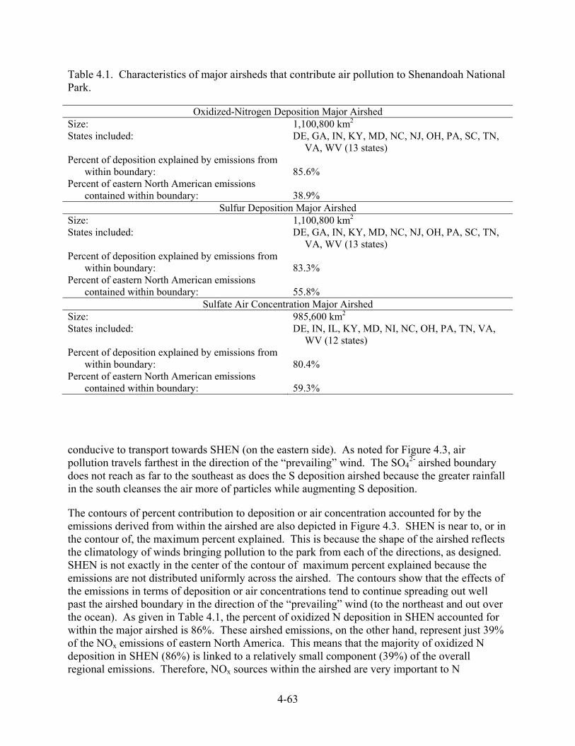
4-63

Table 4.1. Characteristics of major airsheds that contribute air pollution to Shenandoah National Park.

Oxidized-Nitrogen Deposition Major Airshed Size: 1,100,800 km2 States included: DE, GA, IN, KY, MD, NC, NJ, OH, PA, SC, TN,

VA, WV (13 states) Percent of deposition explained by emissions from

within boundary: 85.6%

Percent of eastern North American emissions contained within boundary:

38.9%

Sulfur Deposition Major Airshed Size: 1,100,800 km2 States included: DE, GA, IN, KY, MD, NC, NJ, OH, PA, SC, TN,

VA, WV (13 states) Percent of deposition explained by emissions from

within boundary: 83.3%

Percent of eastern North American emissions contained within boundary:

55.8%

Sulfate Air Concentration Major Airshed Size: 985,600 km2 States included: DE, IN, IL, KY, MD, NI, NC, OH, PA, TN, VA,

WV (12 states) Percent of deposition explained by emissions from

within boundary: 80.4%

Percent of eastern North American emissions contained within boundary:

59.3%

conducive to transport towards SHEN (on the eastern side). As noted for Figure 4.3, air pollution travels farthest in the direction of the “prevailing” wind. The SO4

2- airshed boundary does not reach as far to the southeast as does the S deposition airshed because the greater rainfall in the south cleanses the air more of particles while augmenting S deposition.

The contours of percent contribution to deposition or air concentration accounted for by the emissions derived from within the airshed are also depicted in Figure 4.3. SHEN is near to, or in the contour of, the maximum percent explained. This is because the shape of the airshed reflects the climatology of winds bringing pollution to the park from each of the directions, as designed. SHEN is not exactly in the center of the contour of maximum percent explained because the emissions are not distributed uniformly across the airshed. The contours show that the effects of the emissions in terms of deposition or air concentrations tend to continue spreading out well past the airshed boundary in the direction of the “prevailing” wind (to the northeast and out over the ocean). As given in Table 4.1, the percent of oxidized N deposition in SHEN accounted for within the major airshed is 86%. These airshed emissions, on the other hand, represent just 39% of the NOx emissions of eastern North America. This means that the majority of oxidized N deposition in SHEN (86%) is linked to a relatively small component (39%) of the overall regional emissions. Therefore, NOx sources within the airshed are very important to N

4-64

deposition within the park. Similarly, the percentages of S deposition and SO42- air

concentrations accounted for by SO2 emissions from within the major airsheds are 83% and 80%, respectively. The SO2 airshed emissions represent 59% of the eastern North American sulfur oxide (SOx) emissions.

Table 4.2 gives the emissions of the 15 states nominally covered by any of the airsheds. Because they are included in the SHEN airsheds, these are the states whose emissions have the greatest bearing on the air quality conditions and deposition in SHEN. The emissions of the 13 states included within the S and N deposition airsheds and the 12 states included within the SO4

2- airshed are also summed in the table. Even though the assembly of airshed emissions does not follow state boundaries, the percent of the eastern North American emissions accounted for by the 13-state and 12-state totals given in Table 4.2 are very close to the percentages for the airshed emissions given in Table 4.1.

Not all of the emissions within the airshed contribute equally to the deposition or air concentrations in SHEN. Emissions closer to the park contribute relatively more. Larger emissions sources also contribute relatively more, but proximity is very important. The three airsheds were subdivided into 4 geographic domains, as shown in Figure 4.4. The subdivisions are: local domain, inner domain, middle annulus, and outer annulus. The subdivisions for the oxidized N and S deposition airsheds are comparable. The local domain is the source region that

Table 4.2. 1990 emissions for the states nominally covered by Shenandoah National Park airsheds.

State SO2 (tons/yr) NOx (tons/yr) VOC (tons/yr) CO (tons/yr) Delaware 100,000 102,989 62,194 269,066Georgia 1,000,330 687,001 547,448 3,534,801Illinois 1,261,534 922,261 716,925 3,122,795Indiana 1,920,416 905,979 541,288 2,301,532Kentucky 1,034,272 674,772 394,980 1,413,270Maryland 435,774 354,842 271,811 1,472,063Michigan 726,298 887,552 868,822 3,481,743New Jersey 310,629 542,496 540,420 1,841,841New York 867,415 844,656 996,945 3,892,413North Carolina 487,616 577,599 673,225 2,755,837Ohio 2,736,237 1,156,094 849,155 4,138,869Pennsylvania 1,517,739 1,081,534 827,894 4,180,528South Carolina 292,567 353,655 369,211 1,598,653Tennessee 1,077,345 727,134 569,692 2,076,405Virginia 403,610 564,357 570,977 2,443,994West Virginia 1,074,715 568,976 200,413 843,463

13-state S&N deposition airshed set 12,391,250 8,297,428 6,418,708 28,870,322% North American emissions 56.3% 40.3% 30.6% 37.5% 12-state SO4

2- airshed set 12,775,556 8,524,089 6,547,376 28,499,565% North American emissions 58.1% 41.4% 31.2% 37.1%

Total all 16 states 15,246,497 10,951,897 9,001,400 39,367,273

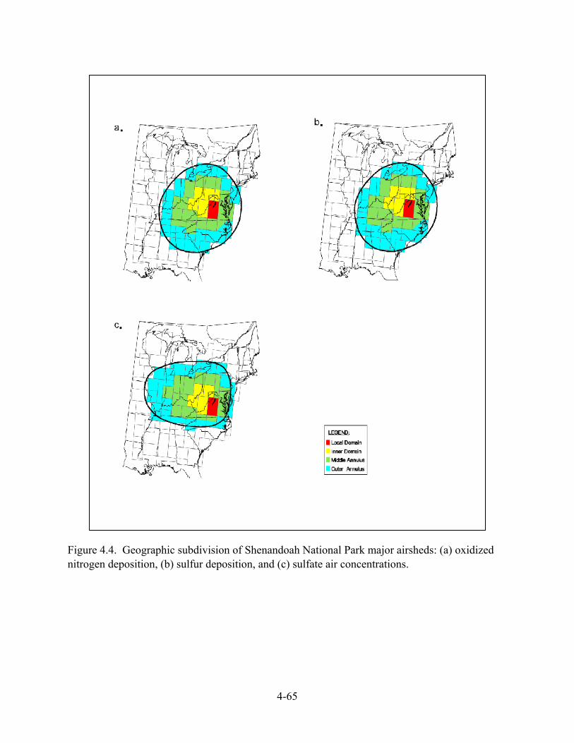
4-65

Figure 4.4. Geographic subdivision of Shenandoah National Park major airsheds: (a) oxidized nitrogen deposition, (b) sulfur deposition, and (c) sulfate air concentrations.

4-66

includes SHEN, the receptor region of interest. The inner domain represents the climatologically next most important group of emissions after the local domain in terms of potential importance of emissions affecting SHEN. The inner domain is asymmetric to the west of the park because that is the direction of the influential “prevailing” winds. The middle and outer annuluses subdivide the rest of the airshed in a climatologically consistent manner. The percent of the deposition or air concentrations in SHEN explained by the emissions from each geographic subdivision is given in Table 4.3, along with the percent of eastern North American emissions within each subdivision. The relative efficiency with which a unit of emissions will produce an effect at SHEN is represented by dividing the % Deposition or % Air Concentration number by the % Emissions number. The relative efficiency is given in the last column of Table 4.3.

The effectiveness of the local domain emissions on pollution in SHEN is very high, even though the local emissions are quite low relative to other, more distant emissions sources. The emissions of the next most important geographic subdivision, the Inner Domain, are much less effective at contributing to SHEN’s pollution. For deposition, the farther away the geographic subdivision is from the park, the less efficient its emissions are at causing an effect at SHEN.

Table 4.3. Contributions from geographic subdivisions of Shenandoah National Park major airsheds and efficiency for causing pollution in the park.

Geographic Subdivision % Deposition/Air Concentration % Emissions Efficiency Local Domain

Ox-Nitrogen Dep 10.3 0.39 26.4 Sulfur Dep 4.8 0.16 30.0 Sulfate Air Conc. 5.5 0.16 34.4

Inner Domain Ox-Nitrogen Dep 26.4 6.3 4.2 Sulfur Dep 34.8 14.4 2.4 Sulfate Air Conc. 25.8 14.3 1.8

Middle Annulus Ox-Nitrogen Dep 32.6 13.7 2.4 Sulfur Dep 27.1 17.0 1.6 Sulfate Air Conc. 24.1 17.3 1.4

Outer Annulus Ox-Nitrogen Dep 16.3 18.5 0.88 Sulfur Dep 16.6 24.2 0.69 Sulfate Air Conc. 25.0 27.6 0.91

Outside Major Airshed Ox-Nitrogen Dep 14.4 61.1 0.24 Sulfur Dep 16.7 44.2 0.38 Sulfate Air Conc. 19.6 40.7 0.48

Efficiency = (%Deposition or %Air Concentration)/(%Emissions)

4-67

From the Inner Domain to the Outer Annulus, the efficiency decreases by factors of 4.8 and 3.5 for oxidized N and S deposition, respectively. For SO4

2- air concentrations, because SO42- has a

longer lifetime and is produced in transit from SO2 at an overall moderate rate, the efficiency of emissions for producing SO4

2- particles over SHEN only decreases by a factor of two from the Inner Domain to the Outer Annulus. The in-transit production can replenish some of the SO4

2- lost to dilution, deposition and transport into the upper troposphere. As a result, the percent contributed to SO4

2- at SHEN from the three non-local domains is the same, in contrast to the results found for deposition. As shown in Table 4.4, for the constellation of 1990 emissions, about 60% of the deposition and 50% of the air concentrations in SHEN come from the Inner plus Middle Domains. A clear majority comes from the three innermost domains (including Local).

Table 4.4. Percent of the pollution in Shenandoah National Park explained by accumulating geographic subdivisions of the major airsheds.

Geographic Subdivision Oxidized Nitrogen Deposition Sulfur Deposition Sulfate Air Concentration Local 10.3 % 4.8 % 5.5 % Local + Inner 36.7 % 39.6 % 31.3 % Inner + Middle 59.0% 61.9% 49.9% Local + Inner + Middle 69.3 % 66.7 % 55.4 % Local + Inner + Middle + Outer 85.6 % 83.3 % 80.4 %

In summary, the major airsheds for SHEN are large and they cover many states. Emissions from within the major airsheds account for a large fraction of the pollution in the park. The shape of the airshed is asymmetric to account for the climatology of transport (“prevailing” winds). Not all emissions are equal; local, nearby emissions are exceedingly important and, generally, emissions within about 200 km are much more efficient in producing pollution in SHEN (on a per ton emitted basis) than those from farther away (Table 4.3).

4.1.1.3 Top Five Air Pollutant Source Sub-regions for SHEN: To provide a sense of the importance of the size of the emissions together with proximity, we labeled the top five source subregions based on the percent of pollution at SHEN explained by each (Figure 4.5). The top five source regions together account for 40%, 46%, and 35% of the oxidized N deposition, S deposition and SO4

2- air concentrations, respectively. The top 5 source subregions for oxidized N deposition cluster around and include the SHEN local domain, which is labeled number 1 in Figure 4.5. For S deposition, the fact that significant nearby (non-local domain) emissions exist together with very large emissions from sources along the Ohio River Valley determines the top five source subregions. The source subregion centered on the joint intersection of the boundaries of Ohio, West Virginia, and Kentucky is number 1. This is the same source subregion presented in Figure 4.2. For SO4

2- air concentrations, local sources and long-range transport from the

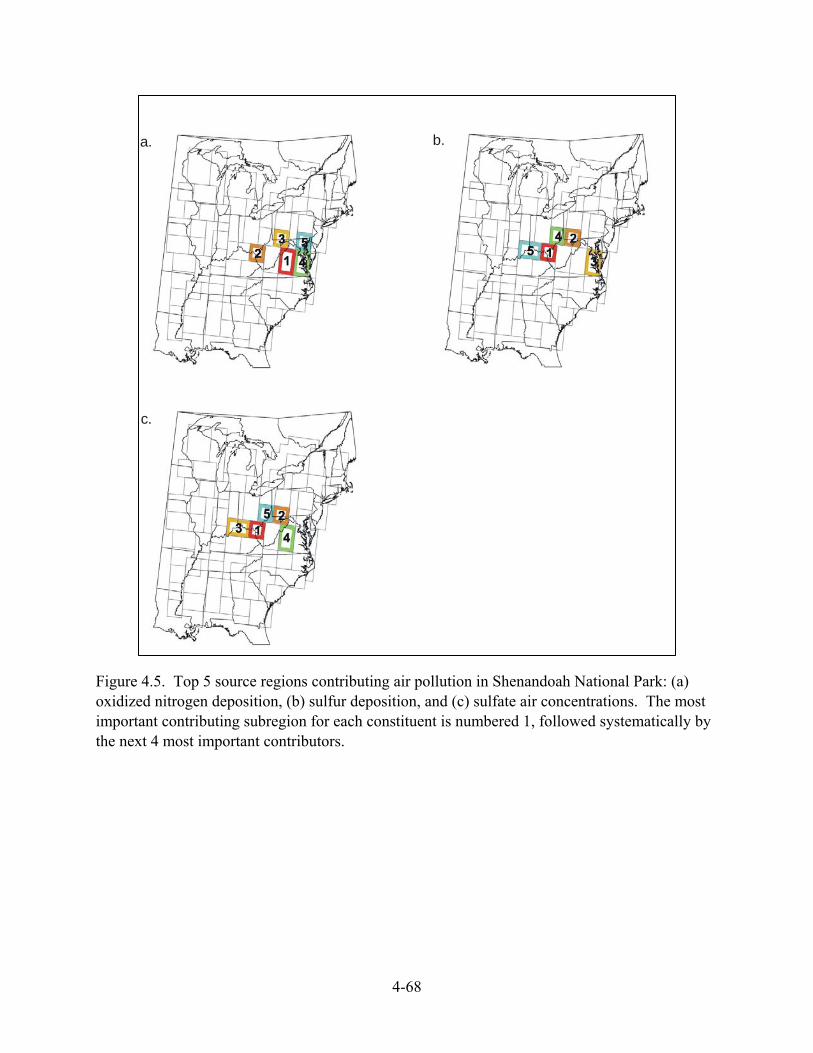
4-68

Figure 4.5. Top 5 source regions contributing air pollution in Shenandoah National Park: (a) oxidized nitrogen deposition, (b) sulfur deposition, and (c) sulfate air concentrations. The most important contributing subregion for each constituent is numbered 1, followed systematically by the next 4 most important contributors.

a. b.

c.

4-69

northwest and west are most important, with the source subregions spreading out to the west. The same source subregion is most important for SO4

2- air concentrations as for S deposition.

4.1.1.4 Relative Contributions by State: Table 4.5 gives the breakdown of relative contributions of emissions to air pollution or deposition within SHEN by state, of the 13 states included in the analysis. The list of states began with the 12 states associated with the SHEN SO4

2- airshed. New York was added because its emissions were large and were roughly similar in distance from SHEN as those from New Jersey. Differences in importance of New York and New Jersey as contributors to air pollution in SHEN highlight the importance of the directional effect of the climatology of transport to SHEN. The states are presented in rank order of contribution for each pollutant. The overall percent explained by the 13 states is consistent with the percent explained by the emissions from within the airsheds. Color contour maps of the percent contribution of the number 1 ranked state are shown in Figure 4.6 for S deposition (West Virginia), oxidized N deposition (Virginia), and SO4

2- air concentrations (Ohio), respectively.

Table 4.5. Percent of the pollution in Shenandoah National Park explained by state emissions, expressed as the individual state (adjusted) contributions to deposition and atmospheric concentrations (with sulfur nonlinearity adjustment).

State Sulfur Deposition State NOx Deposition State SO42- Air Concentrations

West Virginia 16.8% Virginia 14.4% Ohio 11.9% Ohio 15.5% West Virginia 12.3% Virginia 11.8% Virginia 10.1% Ohio 10.9% West Virginia 11.7% Pennsylvania 9.9% Pennsylvania 10.7% Pennsylvania 10.6% Kentucky 6.9% North Carolina 7.8% Kentucky 7.0% Tennessee 5.4% Maryland 7.4% Indiana 5.8% Maryland 4.6% Kentucky 7.0% Tennessee 5.6% Indiana 4.4% Tennessee 4.5% North Carolina 5.1% North Carolina 3.8% Indiana 3.4% Illinois 3.8% Illinois 2.9% Illinois 2.9% Maryland 3.5% Michigan 1.1% Michigan 2.1% New York 1.7% New York 0.8% New York 1.6% Michigan 1.3% Delaware 0.4% Delaware 0.5% Delaware 0.5% Top 3 States 42.4% Top 3 States 37.6% Top 3 States 35.4% Top 5 States 59.2% Top 5 States 56.0% Top 5 States 53.0% Top 10 States 80.3% Top 10 States 81.2% Top 10 States 76.8% All States* 82.6% All States 85.4% All States 80.3% * Includes the 13 states that were part of this analysis

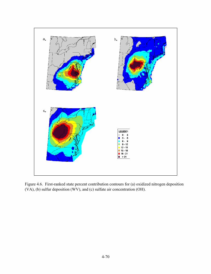
4-70

Figure 4.6. First-ranked state percent contribution contours for (a) oxidized nitrogen deposition (VA), (b) sulfur deposition (WV), and (c) sulfate air concentration (OH).

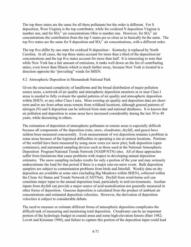
4-71

The top three states are the same for all three pollutants but the order is different. For S deposition, West Virginia is the top contributor, while for oxidized N deposition Virginia is number one, and for SO4

2- air concentrations Ohio is number one. However, for SO42- air

concentrations the contribution from the top 3 states are so close as to basically be the same. The top five states are the same for S deposition and SO4

2- air concentrations, with a different order.

The top five differ by one state for oxidized N deposition - Kentucky is replaced by North Carolina. In all cases, the top three states account for more than a third of the deposition/air concentrations and the top five states account for more than half. It is interesting to note that while New York has a fair amount of emissions, it ranks well down on the list of contributing states, even lower than Illinois which is much farther away, because New York is located in a direction opposite the “prevailing” winds for SHEN.

4.2 Atmospheric Deposition in Shenandoah National Park

Given the structural complexity of landforms and the broad distribution of major pollution source areas, a network of air quality and atmospheric deposition monitors in or near Class I areas is needed to fully evaluate the spatial patterns of air quality and atmospheric deposition within SHEN, or any other Class I area. Most existing air quality and deposition data are short-term and/or are from urban areas remote from wildland locations, although general patterns of nitrogen (N) and S deposition can be inferred from state and national databases. It is known that air pollution and deposition in some areas have increased considerably during the last 30 to 40 years, while decreasing in others.

The estimation of deposition of atmospheric pollutants in remote areas is especially difficult because all components of the deposition (rain, snow, cloudwater, dryfall, and gases) have seldom been measured concurrently. Even measurement of wet deposition remains a problem in some areas because of the logistical difficulties in operating a site at remote locations. Portions of the wetfall have been measured by using snow cores (or snow pits), bulk deposition (open containers), and automated sampling devices such as those used at the National Atmospheric Deposition Program/National Trends Network (NADP/NTN) sites. All of these approaches suffer from limitations that cause problems with respect to developing annual deposition estimates. The snow sampling includes results for only a portion of the year and may seriously underestimate the load for that period if there is a major rain-on-snow event. Bulk deposition samplers are subject to contamination problems from birds and litterfall. Weekly data on dry deposition are available at some sites (including Big Meadows within SHEN), collected within the Clean Air Status and Trends Network (CASTNet). Dryfall from wind-borne soil can constitute major input to the annual deposition load, particularly in arid environments. Aeolian inputs from dryfall can provide a major source of acid neutralization not generally measured in other forms of deposition. Gaseous deposition is calculated from the product of ambient air concentrations and estimated deposition velocities. However, the derivation of deposition velocities is subject to considerable debate.

The need to measure or estimate different forms of atmospheric deposition complicates the difficult task of measuring and monitoring total deposition. Cloudwater can be an important portion of the hydrologic budget in coastal areas and some high-elevation forests (Harr 1982; Lovett and Kinsman 1990), and failure to capture this portion of the deposition input could lead

4-72

to underestimation of annual deposition. Furthermore, cloudwater chemistry has the potential to be more acidic than rainfall (Weathers et al. 1988). Due to these limitations, there is considerable uncertainty regarding the amount of current deposition (wet, dry, cloud) of atmospheric pollutants in any of the Class I areas in the United States.

Dry deposition approximates, or is slightly less than, wet deposition for most ions at most sites; for example, dry deposition constituted 30 to 50% of total deposition of most ions at most Integrated Forest Study (IFS) sites throughout the eastern United States (Johnson and Lindberg 1992). Cloud water deposition contributed substantially to total ionic deposition at only two high-elevation IFS sites: Whiteface Mt., NY (1,000 m) and near Clingman’s Dome, NC (1,740 m), ranging from about 20% of total for base cations at Whiteface Mt. to 50% of total for sulfate (SO4

2-) at the North Carolina site. Estimates of wet, dry, and cloud deposition were generated by Shannon (1998) at multiple sites throughout the southeastern United States using the Advanced Statistical Trajectory Regional Air Pollution (ASTRAP) model, suggesting that the sum of dry plus cloud deposition was approximately equal to wet deposition, for both S and N, throughout the region (Sullivan et al. 2002a). These model estimates are in general agreement with data derived from NADP and CASTNet monitoring at Big Meadows in SHEN.

4.2.1 Atmospheric Deposition Monitoring Efforts in Shenandoah National Park

The Shenandoah National Park air quality monitoring and research program has acquired information about key air pollutants that can degrade visibility, injure or impact growth and vitality of plant species sensitive to ground-level (tropospheric) ozone (O3), acidify streams, impact aquatic biota, leach nutrients from soils, erode buildings and materials, or harm human health. Sullivan et al. (2003) summarize the park's comprehensive visibility, ambient air quality, and deposition monitoring and research program. Table 4.6 summarizes the Atmospheric Deposition Monitoring activities in SHEN.

4-73

Table 4.6. Monitoring activities at Shenandoah National Park relevant to acidic deposition.

Program Location Years Visability/Particulate Matter

Amonium IMPROVE Research Big Meadows 1997–present Mass-independent Sulfur Isotopic

Compositions in Sulfate Qerosols Special Research Big Meadows 2001

Ambient Air Quality Sulfur Dioxide NPS Sawmill Run 1984–1994

(summers) Meteorology NPS Big Meadows 1988–present Meteorology NPS Sawmill Run 1987–1994

(summers) Meteorology NPS Dickey Ridge 1989–1994

(summers) Low-level Sulfur Dioxide, Carbon

Monoxide Enhanced Ozone Monitoring

Research Big Meadows 1995–present

Atmospheric Deposition Wet Acid Deposition National Atmospheric

Deposition Program Big Meadows 1981–present

Wet Acid Deposition University of Virginia North Fork Dry Run (Pinnacles)

1986–present

Wet Acid Deposition University of Virginia White Oak Run 1980–present Wet Acid Deposition USGS Weakley Hollow 1982–present Dry Acid Deposition, Nitric Acid,

Sulfate, Nitrate, Sulfur Dioxide Clean Air Status and Trends

Network Big Meadows 1988–present

Cloud chemistry Cloud Water Project Loft Mountain 1984–1985 Cloud chemistry EPA Mountain Cloud Chemistry

Program North Fork Dry Run

Watershed – 3 locations

1986–1988

Cloud chemistry Shenandoah Cloud and Photochemistry Experiment

Pinnacles 1990

Mercury in Precipitation Mercury Deposition Network Big Meadows 2002–present Precipitation Sulfur Isotopes USGS Groundwater Studies Big Meadows 1989–present

4-74

4.2.2 Historical Deposition of S and N at Shenandoah National Park:

Historical levels of S and N deposition prior to about 1980 in and near SHEN are not well known. However, Shannon (1998) provided estimates of historical deposition during the period 1900 to 1990 at SHEN, as part of the Southern Appalachian Mountains Initiative (SAMI) assessment (Sullivan et al. 2002a). These estimates (Table 4.7) were based on historical emissions data and were constructed with the Advanced Statistical Trajectory Regional Air Pollution (ASTRAP) model (Shannon 1981, 1985), including wet, dry, and cloud forms of deposition. Estimates of pre-industrial (i.e., pre-1850) deposition of S and N are not available, but are assumed to have been substantially lower than Shannon’s (1998) estimates for 1900.

Table 4.7. Estimates of historical deposition in Shenandoah National Park of sulfur and oxidized nitrogen at five year intervals, normalized to 1990 and expressed as a percentage of the 1990 values (Shannon 1998).

S Deposition (Percent of 1990 Value)a

Nitrate-N Deposition (Percent of 1990 Value)a

Wet Dry Cloud Total Wet Dry Cloud Total 1900 30 33 42 34 14 14 13 14 1905 42 47 60 47 18 18 18 18 1910 52 58 75 59 22 24 24 23 1915 62 69 90 70 25 27 28 26 1920 66 73 98 75 27 29 30 28 1925 72 79 106 81 36 36 35 36 1930 65 72 98 74 40 38 37 39 1935 53 58 82 60 32 31 30 31 1940 64 69 97 72 36 36 37 36 1945 83 90 132 96 48 46 48 48 1950 78 83 126 90 53 52 54 53 1955 78 83 114 87 60 60 61 61 1960 87 90 125 96 71 70 72 71 1965 92 102 102 96 79 78 72 77 1970 113 121 116 116 92 90 84 90 1975 116 118 102 113 98 94 86 94 1980 104 104 90 100 102 97 90 97 1985 97 96 86 95 97 96 96 97 1990 100 100 100 100 100 100 100 100

aFor reference, five-year average values, centered on 1990, of total deposition of S and N were 13 and 7.6 kg/ha/yr, respectively

4.2.3 Ambient Atmospheric Deposition at Shenandoah National Park:

Some data are available regarding all forms of deposition in SHEN, wet, dry and cloud.

Wet Deposition: An NADP/NTN wet deposition monitoring station has been in operation at Big Meadows (elevation 1,074 m) since 1981. Precipitation volume and the concentrations of major ions in precipitation are reported. Wet deposition of each ion is calculated as the product of the precipitation volume and ionic concentration in precipitation.

4-75

Annual wet deposition measurements and interpolated isopleths of SO42-, NO3

-, and inorganic N (NH4

+ plus NO3-, as N) for the year 2001 are shown for the eastern United States in Figures 4.7

to 4.9. These are recent annual data available from the NADP/NTN monitoring program. Compared with other locations in the eastern United States, SHEN and the rest of western Virginia receive relatively high wet deposition of S (expressed on the map as SO4

2-), and moderately high wet deposition of NH4

+ and NO3-. Among Class I national parks, SHEN and

GRSM receive the highest S and NO3-N deposition. In general, S and N wet deposition values tend to be higher to the west and north of SHEN, but lower to the southeast of the park.

The concentrations of major ions measured in precipitation and measured precipitation amounts within SHEN are given in Table 4.8. Data are available for three monitoring stations within the park: Big Meadows (1981–2000), White Oak Run (1980–2000) and North Fork Dry Run (1987–2000). Annual average precipitation at the monitoring stations, over the period of record, ranged from 91 cm at White Oak Run to 135 cm at Big Meadows. The Big Meadows site generally showed lower concentrations of major ions in precipitation than did the other two sites, with average SO4

2-, NO3-, and sum of base cation concentrations equal to 31, 14, and 9 Feq/L,

respectively (Table 4.8).

Wet deposition fluxes (kg/ha/yr) were determined at each of the three wet deposition monitoring stations in the park for each year of available data. Annual average wet S deposition at Big Meadows varied over the period of record from about 2 to 10 kg/ha/yr, with an average of 6.7 kg/ha/yr (Table 4.9). Both NH4

+ and NO3- wet deposition varied during most years between 1

and about 3 kg N/ha/yr, with averages of 2.0 and 2.6 kg N/ha/yr, respectively at Big Meadows. The annual average wet deposition of total N (NH4

+ plus NO3-) at Big Meadows, White Oak

Run, and North Fork Dry Run during the periods of record were generally similar: 4.6, 3.8, and 4.8 kg N/ha/yr respectively (Table 4.9). Average annual wet S deposition was also similar among sites (6.7 to 7.1 kg S/ha/yr).

Dry Deposition: Dry deposition fluxes were estimated at Big Meadows by CASTNet for the period 1991 through 1998, although data were incomplete for 1994 (Table 4.10). Dry deposition estimates for S and N were slightly lower than the respective wet deposition estimates (about 73% and 70% for S and N, respectively), in agreement with ASTRAP model estimates provided by Shannon (1998) for use in the SAMI assessment (Sullivan et al. 2002a).

Cloud Deposition: Cloud deposition can be substantial in some cases, particularly at high-elevation sites that are immersed in clouds more than 25% of the time (Mohnen 1988a, b; Lovett and Kinsman 1990). The percent of total S deposition contributed by cloud deposition has been estimated to range from near zero for lower-elevation sites (< 1,000 m) to over 50% at higher elevation (Lovett and Kinsman 1990). At SHEN, most of the park lies below 1,000 m elevation. Cloud deposition is therefore not expected to constitute a sizeable component of total deposition to acid-sensitive watersheds within the park. This assumption is in agreement with measured (Mohren 1988b; Weathers et al. 1988) and modeled (Shannon 1998) values for cloud deposition of S in SHEN.

4-76

Figure 4.7. Annual wet deposition of sulfate throughout the eastern United States during 2001. Note that sulfur deposition expressed as kg S/ha/yr (units routinely used elsewhere in this report) is approximately 33% of sulfate deposition expressed kg SO4/ha/yr (as shown on this NADP map). Source: http://nadp.sws.uiuc.edu.

Sulfate ion wet deposition, 2001

National Atmospheric Deposition Proram/National Trends Network http://nadp.sws.uiuc.edu

4-77

Figure 4.8. Annual wet deposition of nitrate throughout the eastern United States during 2001. Note that nitrogen deposition expressed as kg N/ha/yr (units routinely used elsewhere in this report) is approximately 23% of nitrate deposition expressed kg NO3/ha/yr (as shown on this NADP map). Source: http://nadp.sws.uiuc.edu

National Atmospheric Deposition Proram/National Trends Network http://nadp.sws.uiuc.edu

Nitrate ion wet deposition, 2001

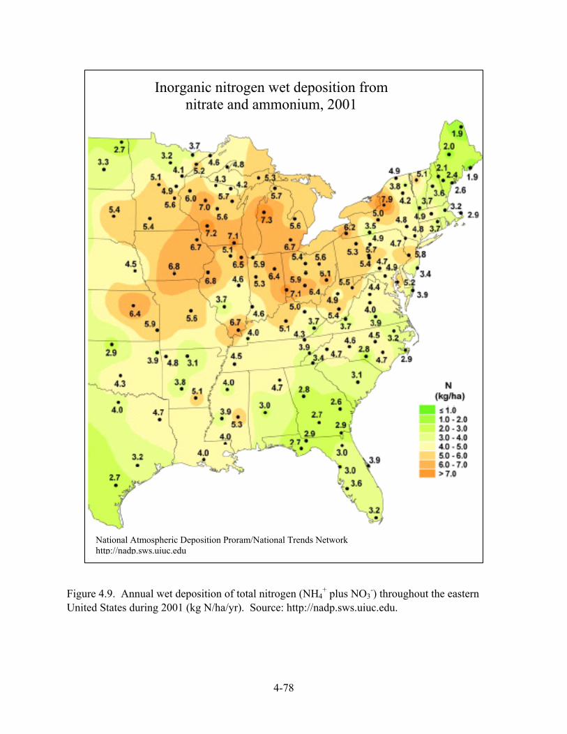
4-78

Figure 4.9. Annual wet deposition of total nitrogen (NH4+ plus NO3

-) throughout the eastern United States during 2001 (kg N/ha/yr). Source: http://nadp.sws.uiuc.edu.

National Atmospheric Deposition Proram/National Trends Network http://nadp.sws.uiuc.edu

Inorganic nitrogen wet deposition from nitrate and ammonium, 2001

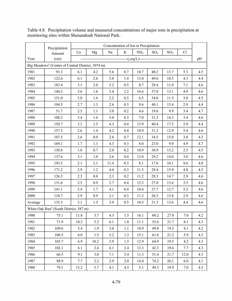
4-79

Table 4.8. Precipitation volume and measured concentrations of major ions in precipitation at monitoring sites within Shenandoah National Park.

Concentration of Ion in Precipitation

Ca Mg Na K NH4 SO4 NO3 Cl

Year

Precipitation Amount

(cm) -------------------------------------(Feq/L)---------------------------------- pH

Big Meadowsa (Center of Central District, 1074 m)

1981 93.3 6.1 4.2 5.6 0.7 10.7 40.2 13.7 5.3 4.5

1982 122.6 6.1 2.6 5.8 1.4 13.0 49.6 18.5 4.3 4.4

1983 183.4 3.1 2.0 5.2 0.5 8.7 29.4 11.9 7.1 4.6

1984 144.2 3.6 1.6 3.4 2.2 16.6 37.0 13.1 4.9 4.6

1985 151.0 3.0 1.6 2.2 0.3 6.5 34.0 11.5 3.0 4.5

1986 104.5 2.7 1.3 2.6 0.3 9.6 40.1 15.4 2.9 4.4

1987 51.7 2.5 1.1 3.0 0.2 4.6 19.6 9.9 3.4 4.7

1988 108.2 3.4 1.6 3.0 0.3 7.0 31.2 14.3 3.4 4.6

1989 150.7 3.1 1.5 4.3 0.4 13.9 40.4 17.5 5.9 4.4

1990 157.5 2.6 1.4 4.2 0.4 10.9 31.2 12.9 5.4 4.6

1991 107.5 2.6 0.9 2.6 0.7 12.1 34.5 15.0 3.8 4.5

1992 169.1 1.7 1.1 4.3 0.3 8.0 23.0 9.9 4.9 4.7

1993 150.8 1.8 0.7 2.0 0.2 10.9 30.9 13.2 2.5 4.5

1994 137.6 3.1 1.0 2.6 0.4 12.0 29.2 14.0 3.0 4.6

1995 193.5 2.1 2.1 11.4 0.3 8.1 17.0 10.1 9.6 4.8

1996 171.2 2.9 1.2 4.4 0.3 11.5 28.4 15.9 4.8 4.5

1997 126.5 2.3 0.8 2.3 0.2 11.2 29.3 14.7 2.9 4.6

1998 131.6 2.5 0.9 2.7 0.4 12.3 27.0 13.6 3.5 4.6

1999 141.1 3.4 1.7 4.1 0.4 10.4 27.7 12.7 5.2 4.6

2000 110.7 2.9 0.9 2.1 0.3 11.2 26.3 13.8 2.9 4.6

Average 135.3 3.1 1.5 3.9 0.5 10.5 31.3 13.6 4.4 4.6

White Oak Runa (South District, 387 m)

1980 75.1 11.8 3.7 4.3 1.5 16.1 60.2 27.0 7.0 4.2

1981 71.9 10.2 3.2 6.1 1.8 11.1 55.6 21.7 8.1 4.3

1982 109.6 5.4 1.9 3.0 1.1 10.9 49.0 19.5 4.1 4.2

1983 106.5 6.0 1.5 5.2 1.3 15.1 61.8 21.2 5.9 4.3

1984 103.7 6.9 10.2 3.9 1.5 12.9 64.9 19.5 4.2 4.3

1985 102.1 6.1 2.4 6.1 2.4 13.3 42.3 19.6 7.7 4.3

1986 66.5 9.1 3.0 7.1 3.4 11.3 51.4 21.7 12.0 4.3

1987 88.9 7.7 2.2 2.9 2.0 14.4 74.2 26.1 6.0 4.1

1988 79.1 13.2 3.7 4.1 4.5 5.1 49.3 19.9 7.0 4.3

4-80

Table 4.8. Precipitation volume and measured concentrations of major ions in precipitation at monitoring sites within Shenandoah National Park (continued).

Concentration of Ion in Precipitation

Ca Mg Na K NH4 SO4 NO3 Cl

Year

Precipitation Amount

(cm) -------------------------------------(Feq/L)---------------------------------- pH

White Oak Run (continued)

1989 125.3 7.4 2.3 2.2 1.8 5.1 48.3 16.0 5.1 4.3

1990 89.9 8.1 3.1 4.9 2.9 7.1 41.2 16.2 7.9 4.3

1991 97.0 8.0 2.0 2.3 1.8 12.4 48.4 20.3 4.6 4.3

1992 105.2 4.7 2.1 4.5 1.6 8.3 40.6 17.1 6.7 4.3

1993 95.6 5.6 1.9 2.6 2.0 7.6 43.5 17.6 5.0 4.3

1994 68.1 7.1 2.5 3.2 2.6 10.9 45.1 21.3 5.8 4.3

1995 70.5 7.1 3.4 8.4 1.9 6.8 28.8 14.8 11.4 4.5

1996 105.3 8.5 2.8 6.0 1.8 9.9 32.9 24.4 8.5 4.4

1997 86.9 7.1 2.2 4.0 2.3 10.9 36.7 15.6 5.6 4.4

1998 100.1 6.0 1.8 1.9 1.4 9.3 28.9 16.1 4.1 4.5

1999 86.9 8.5 2.6 4.1 1.5 9.2 39.2 19.7 7.3 4.3

2000 79.0 9.1 2.7 2.4 2.5 9.3 36.9 20.0 4.0 4.4

Average 91.1 7.8 2.9 4.2 2.1 10.5 46.8 19.9 6.6 4.3

North Fork Dry Runa (North End of Central District, 1014 m)

1987 121.8 4.6 2.3 4.1 4.3 17.4 52.8 19.6 5.7 4.4

1988 88.4 9.2 3.9 3.9 3.6 17.5 52.3 20.8 5.2 4.4

1989 132.3 5.7 3.1 3.0 3.1 11.9 29.2 18.8 4.9 4.5

1990 135.5 6.4 2.5 4.5 5.3 15.0 36.2 15.9 5.9 4.5

1991 85.9 7.2 2.2 3.1 5.0 15.8 51.1 19.6 5.3 4.3

1992 129.5 4.3 2.4 4.9 3.9 8.0 30.6 13.0 6.6 4.5

1993 100.6 9.1 3.1 3.5 7.0 11.8 49.1 21.7 6.0 4.3

1994 97.6 9.0 3.1 3.3 5.6 14.5 47.7 21.2 5.4 4.4

1995 123.2 6.5 3.2 6.5 3.7 9.0 35.7 17.3 9.2 4.5

1996 125.7 6.9 2.8 4.3 6.2 8.2 33.3 17.9 6.3 4.5

1997 110.3 4.9 1.8 2.2 3.0 12.7 38.3 15.9 4.4 4.4

1998 118.6 3.3 1.2 2.9 0.8 10.3 30.4 17.0 4.5 4.5

1999 115.4 3.9 1.8 4.6 1.4 11.5 34.9 15.7 6.9 4.5

2000 113.3 4.3 1.5 2.4 1.0 12.7 31.1 17.5 3.5 4.5

Average 114.1 6.1 2.5 3.8 3.9 12.6 39.5 18.0 5.7 4.5 aData were collected at Big Meadows by the National Atmospheric Deposition Program (http://nadp.sws.uiuc.edu) and at White Oak Run and North Fork Dry Run by the SWAS (University of Virginia, Department of Environmental Sciences).

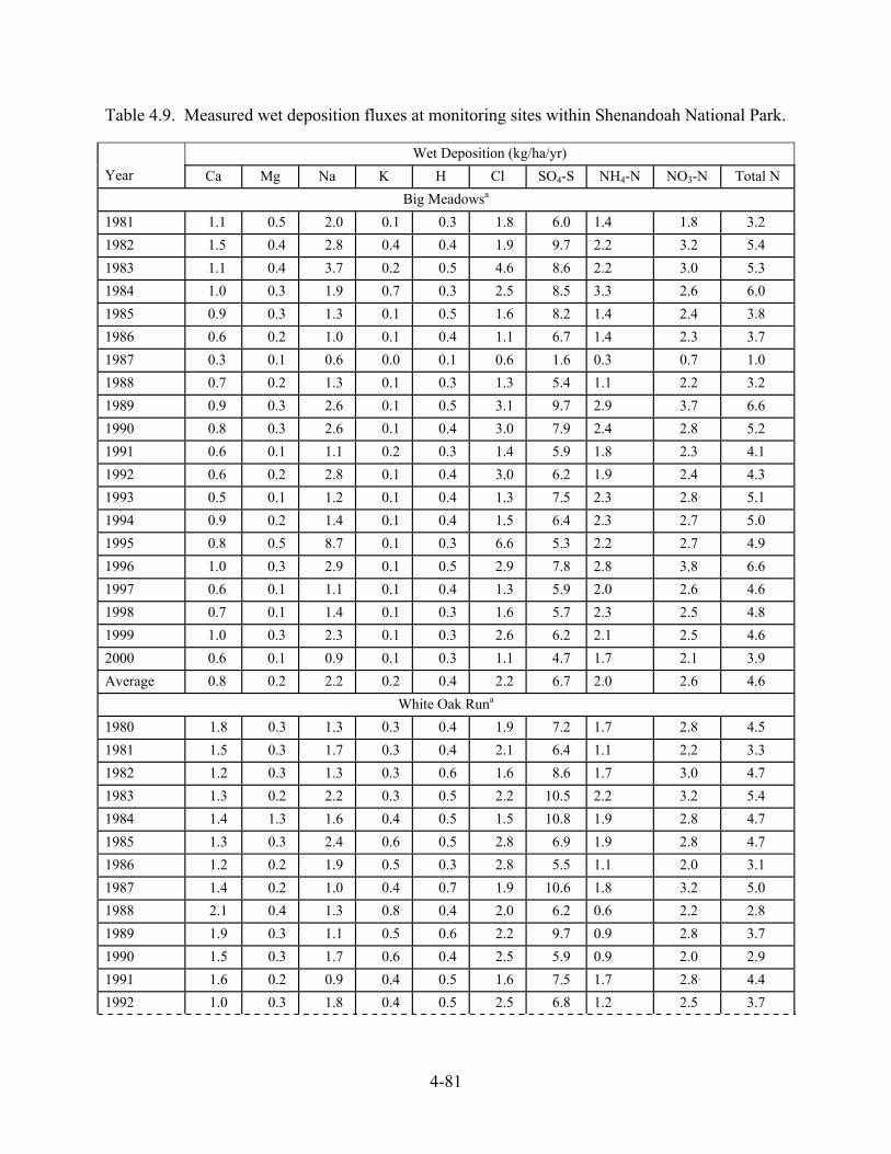
4-81

Table 4.9. Measured wet deposition fluxes at monitoring sites within Shenandoah National Park.

Wet Deposition (kg/ha/yr) Year Ca Mg Na K H Cl SO4-S NH4-N NO3-N Total N

Big Meadowsa 1981 1.1 0.5 2.0 0.1 0.3 1.8 6.0 1.4 1.8 3.2 1982 1.5 0.4 2.8 0.4 0.4 1.9 9.7 2.2 3.2 5.4 1983 1.1 0.4 3.7 0.2 0.5 4.6 8.6 2.2 3.0 5.3 1984 1.0 0.3 1.9 0.7 0.3 2.5 8.5 3.3 2.6 6.0 1985 0.9 0.3 1.3 0.1 0.5 1.6 8.2 1.4 2.4 3.8 1986 0.6 0.2 1.0 0.1 0.4 1.1 6.7 1.4 2.3 3.7 1987 0.3 0.1 0.6 0.0 0.1 0.6 1.6 0.3 0.7 1.0 1988 0.7 0.2 1.3 0.1 0.3 1.3 5.4 1.1 2.2 3.2 1989 0.9 0.3 2.6 0.1 0.5 3.1 9.7 2.9 3.7 6.6 1990 0.8 0.3 2.6 0.1 0.4 3.0 7.9 2.4 2.8 5.2 1991 0.6 0.1 1.1 0.2 0.3 1.4 5.9 1.8 2.3 4.1 1992 0.6 0.2 2.8 0.1 0.4 3.0 6.2 1.9 2.4 4.3 1993 0.5 0.1 1.2 0.1 0.4 1.3 7.5 2.3 2.8 5.1 1994 0.9 0.2 1.4 0.1 0.4 1.5 6.4 2.3 2.7 5.0 1995 0.8 0.5 8.7 0.1 0.3 6.6 5.3 2.2 2.7 4.9 1996 1.0 0.3 2.9 0.1 0.5 2.9 7.8 2.8 3.8 6.6 1997 0.6 0.1 1.1 0.1 0.4 1.3 5.9 2.0 2.6 4.6 1998 0.7 0.1 1.4 0.1 0.3 1.6 5.7 2.3 2.5 4.8 1999 1.0 0.3 2.3 0.1 0.3 2.6 6.2 2.1 2.5 4.6 2000 0.6 0.1 0.9 0.1 0.3 1.1 4.7 1.7 2.1 3.9 Average 0.8 0.2 2.2 0.2 0.4 2.2 6.7 2.0 2.6 4.6

White Oak Runa 1980 1.8 0.3 1.3 0.3 0.4 1.9 7.2 1.7 2.8 4.5 1981 1.5 0.3 1.7 0.3 0.4 2.1 6.4 1.1 2.2 3.3 1982 1.2 0.3 1.3 0.3 0.6 1.6 8.6 1.7 3.0 4.7 1983 1.3 0.2 2.2 0.3 0.5 2.2 10.5 2.2 3.2 5.4 1984 1.4 1.3 1.6 0.4 0.5 1.5 10.8 1.9 2.8 4.7 1985 1.3 0.3 2.4 0.6 0.5 2.8 6.9 1.9 2.8 4.7 1986 1.2 0.2 1.9 0.5 0.3 2.8 5.5 1.1 2.0 3.1 1987 1.4 0.2 1.0 0.4 0.7 1.9 10.6 1.8 3.2 5.0 1988 2.1 0.4 1.3 0.8 0.4 2.0 6.2 0.6 2.2 2.8 1989 1.9 0.3 1.1 0.5 0.6 2.2 9.7 0.9 2.8 3.7 1990 1.5 0.3 1.7 0.6 0.4 2.5 5.9 0.9 2.0 2.9 1991 1.6 0.2 0.9 0.4 0.5 1.6 7.5 1.7 2.8 4.4 1992 1.0 0.3 1.8 0.4 0.5 2.5 6.8 1.2 2.5 3.7

4-82

Table 4.9. Measured wet deposition fluxes at monitoring sites within Shenandoah National Park (continued).

Wet Deposition (kg/ha/yr)

Year Ca Mg Na K H Cl SO4-S NH4-N NO3-N Total N 1993 1.1 0.2 1.0 0.4 0.5 1.7 6.6 1.0 2.4 3.4 1994 1.0 0.2 0.8 0.4 0.4 1.4 4.9 1.0 2.0 3.1 1995 1.0 0.3 2.3 0.3 0.2 2.8 3.2 0.7 1.5 2.1 1996 1.8 0.4 2.5 0.4 0.5 3.2 5.5 1.5 3.6 5.1 1997 1.2 0.2 1.3 0.5 0.4 1.7 5.1 1.3 1.9 3.2

1998 1.2 0.2 0.8 0.3 0.3 1.4 4.6 1.3 2.3 3.6

1999 1.5 0.3 1.4 0.3 0.4 2.3 5.5 1.1 2.4 3.5

2000 1.4 0.3 0.7 0.4 0.3 1.1 4.7 1.0 2.2 3.2

Average 1.4 0.3 1.5 0.4 0.4 2.1 7.0 1.5 2.6 3.8

North Fork Dry Runa

1987 1.1 0.3 2.0 1.2 0.5 2.5 10.3 3.0 3.3 6.3

1988 1.6 0.4 1.4 0.7 0.4 1.6 7.4 2.2 2.6 4.7

1989 1.5 0.5 1.6 0.9 0.4 2.3 6.2 2.2 3.5 5.7

1990 1.7 0.4 2.4 1.7 0.4 2.8 7.8 2.9 3.0 5.9

1991 1.2 0.2 1.0 1.0 0.4 1.6 7.0 1.9 2.4 4.3

1992 1.1 0.4 2.5 1.2 0.4 3.0 6.3 1.5 2.3 3.8

1993 1.8 0.4 1.4 1.6 0.5 2.1 7.9 1.7 3.1 4.7

1994 1.8 0.4 1.3 1.3 0.4 1.9 7.5 2.0 2.9 4.9

1995 1.6 0.5 3.1 1.1 0.4 4.0 7.0 1.6 3.0 4.6

1996 1.7 0.4 2.1 1.8 0.4 2.8 6.7 1.4 3.1 4.6

1997 1.1 0.2 1.0 0.8 0.4 1.7 6.8 2.0 2.5 4.4

1998 0.8 0.2 1.3 0.2 0.4 1.9 5.8 1.7 2.8 4.5

1999 0.9 0.3 2.1 0.4 0.4 2.8 6.5 1.9 2.5 4.4

2000 1.0 0.2 1.1 0.3 0.3 1.4 5.6 2.0 2.8 4.8

Average 1.4 0.3 1.7 1.0 0.4 2.3 7.1 2.0 2.8 4.8 aData were collected at Big Meadows by the National Atmospheric Deposition Program (http://nadp.sws.uiuc.edu) and at White Oak Run and North Fork Dry Run by the SWAS (University of Virginia, Department of Environmental Sciences)

4-83

Table 4.10. Estimated dry deposition fluxes at Big Meadows, based on data and calculations from CASTNet (http://www.epa.gov/castnet/).

Dry deposition (kg/ha/yr) Yeara SO2 SO4 HNO3 NO3 NH4 Total S Total N 1991 4.0 0.8 2.6 0.0 0.1 4.8 2.8 1992 5.1 0.8 2.7 0.0 0.1 5.8 2.9 1993 5.3 0.9 3.0 0.0 0.2 6.2 3.2 1995 3.4 0.7 3.3 0.1 0.2 4.1 3.5 1996 3.3 0.7 2.8 0.0 0.1 4.0 3.0 1997 3.5 0.7 3.1 0.0 0.2 4.2 3.3 1998 4.3 0.8 3.3 0.0 0.2 5.1 3.6 Average 4.4 1.3 3.4 0.5 0.7 4.9 3.2 aData were not available for all four quarters for 1994.

Estes (1990) collected and analyzed cloud water samples in the North Fork Dry Run watershed in SHEN (1,014 m) during the period 1986–1987. Highly concentrated cloudwater events (those having H+ plus SO4

2- concentration greater than 400 Feq/L) were more likely to be associated with NW or ESE wind trajectories than with other trajectories, were most common in summer, and were likely to occur in the presence of a stagnant high pressure system. Such highly concentrated acidic cloudwater events tended to be of relatively short duration, typically less than 20 hours long.

Cloud water data had also been collected earlier, during the Cloud Water Project (Weathers et al. 1988) at Loft Mountain in SHEN (~ 1,000 m), yielding similar median concentrations of major ions in cloud water at the North Fork Dry Run and Loft Mountain sites (SO4

2- . 200–300 Feq/L, NO3

- . 120 Feq/L). Mean concentrations of SO42- in cloudwater collected during the Mountain

Cloud Chemistry Project (MCCP) at Mt. Mitchell, NC (2,006 m) and Whitetop Mt., VA (1,680 m) were more than double those found at the SHEN sites, and concentrations of NO3

-, NH4+, and

H+ were also considerably higher at the Mt. Mitchell and Whitetop Mt. sites (Estes 1990). Elevations within SHEN are considerably lower than the sites included in the MCCP; many peaks in SHEN are above 900 m elevation, but the highest point in the park is only 1,234 m, at Hawksbill Mountain.

During the period 1995 to 1998, average total S deposition was 10.5 kg/ha/yr and average total N deposition was 8.6 kg/ha/yr at Big Meadows, the only site in SHEN for which both wet and dry deposition estimates are available directly from monitoring station data. The S deposition varies, based on the RADM simulation, decreasing from north to south within the park by less than 12%. East-west differences would be expected to be larger due to elevational changes and orographic effects, but the meteorological model resolution (80-km native prediction interpolated to a 20-km grid) was too coarse to resolve the Shenandoah topography, making it impossible to differentiate within-park east-west variability.

4-84

4.2.4 Trends in Atmospheric Deposition at Shenandoah National Park

Reductions in the S component of acidic deposition have generally followed the recent reductions in SO2 emissions. Preliminary analysis for the eastern United States indicates that total S deposition, which includes dissolved, particulate, and gaseous forms, declined by an average of 26% between 1989 and 1998 (U.S. EPA 2000a). Of more specific relevance to SHEN, wet deposition of S in the mid-Appalachian area (West Virginia and Virginia, as well as areas to the north), declined by 23% between the periods of 1983–94 and 1995–98 (USGAO 2000). Legislated reductions in SO2 emissions were largely responsible for these reductions in S deposition, and additional, albeit smaller, reductions can be anticipated though 2010.

NADP wet deposition monitoring data are available for Big Meadows since 1981. Annual average wet deposition has declined at many sites in the eastern United States, including Big Meadows (Figure 4.10). Lynch et al. (1996) noted substantial decreases since 1995 in the concentration of SO4

2- in precipitation and in wet S deposition at some NADP stations in and immediately downwind of the Ohio River Valley. These decreases were attributed by Lynch et al. (1996) to implementation of Phase I of the CAAA, Title IV.

Data from the wet deposition monitoring stations at White Oak Run and North Fork Dry Run showed generally declining patterns in wet deposition of S (Figure 4.10), total N (Figure 4.10), NH4

+-N (Figure 4.11), and NO3--N (Figure 4.11) throughout the period of record. At each site,

however, year-to-year variability was generally high. There is an indication of pronounced consistent variability in wet S deposition among the three sites, despite the substantial year-to-year variation at each site. The overall patterns of annual S deposition values at these sites were generally within 10 to 15% of each other throughout the period of record. At the Big Meadows monitoring station, S wet deposition data suggested a declining pattern since 1981, but N wet deposition data (total N, NO3

--N, NH4+-N) did not (Figures 4.10 and 4.11).

Over the 1981 to 2000 period of record, wet N deposition at Big Meadows has varied substantially, generally between about 3 and 7 kg N/ha/yr. There is no indication of large long- term increases or decreases in wet N deposition, although there has been a relatively consistent short-term decline over the last five years at Big Meadows (Figure 4.10 and 4.11). Additional data will be required to determine whether this apparent downward trend is meaningful.

4-85

Figure 4.10. Wet sulfur deposition (left panels) and wet inorganic nitrogen deposition (right panels) for the period of record at three monitoring sites in Shenandoah National Park. Best-fit linear regression lines are added. (Data obtained from NADP website and from the University of Virginia).

White Oak Run

y = -0.2187x + 442.09R2 = 0.4062

0.0

2.0

4.0

6.0

8.0

10.0

12.0

1979 1981 1983 1985 1987 1989 1991 1993 1995 1997 1999 2001

Year

Sulfu

r Wet

Dep

ositi

on (k

gS/h

a/yr

)

North Fork Dry Run

y = -0.1807x + 367.29R2 = 0.4233

0.0

2.0

4.0

6.0

8.0

10.0

12.0

1979 1981 1983 1985 1987 1989 1991 1993 1995 1997 1999 2001

Year

Sulfu

r Wet

Dep

ositi

on (k

gS/h

a/yr

)

Big Meadows

y = -0.1117x + 229.03R2 = 0.1225

0.0

2.0

4.0

6.0

8.0

10.0

12.0

1979 1981 1983 1985 1987 1989 1991 1993 1995 1997 1999 2001

Year

Sulfu

r Wet

Dep

ositi

on (k

gS/h

a/yr

)White Oak Run

y = -0.0625x + 128.25R2 = 0.1897

0.0

1.0

2.0

3.0

4.0

5.0

6.0

7.0

1979 1981 1983 1985 1987 1989 1991 1993 1995 1997 1999 2001

Year

Tota

l Nitr

ogen

Wet

Dep

ositi

on

(kgN

/ha/

yr)

North Fork Dry Run

y = -0.0884x + 181.02R2 = 0.2951

0.0

1.0

2.0

3.0

4.0

5.0

6.0

7.0

1979 1981 1983 1985 1987 1989 1991 1993 1995 1997 1999 2001

Year

Tota

l Nitr

ogen

Wet

Dep

ositi

on

(kgN

/ha/

yr)

Big Meadows

y = 0.0326x - 60.396R2 = 0.023

0.0

1.0

2.0

3.0

4.0

5.0

6.0

7.0

1979 1981 1983 1985 1987 1989 1991 1993 1995 1997 1999 2001

Year

Tota

l Nitr

ogen

Wet

Dep

ositi

on

(kgN

/ha/

yr)

4-86

Figure 4.11. Wet ammonium deposition (left panels) and wet nitrate deposition (right panels) for the period of record at three monitoring sites in Shenandoah National Park. Best-fit linear regression lines are added. (Data obtained from NADP website and from the University of Virginia).

White Oak Run

y = -0.0322x + 65.457R2 = 0.2043

0.0

1.0

2.0

3.0

4.0

1979 1981 1983 1985 1987 1989 1991 1993 1995 1997 1999 2001

Year

Am

mon

ium

Wet

Dep

ositi

on (k

gN/h

a/yr

)

North Fork Dry Run

y = -0.0619x + 125.46R2 = 0.3166

0.0

1.0

2.0

3.0

4.0

1979 1981 1983 1985 1987 1989 1991 1993 1995 1997 1999 2001

Year

Am

mon

ium

Wet

Dep

ositi

on (k

gN/h

a/yr

)

Big Meadows

y = 0.0186x - 34.992R2 = 0.0265

0.0

1.0

2.0

3.0

4.0

1979 1981 1983 1985 1987 1989 1991 1993 1995 1997 1999 2001

Year

Am

mon

ium

Wet

Dep

ositi

on (k

gN/h

a/yr

)White Oak Run

y = -0.0303x + 62.796R2 = 0.1316

0.0

1.0

2.0

3.0

4.0

5.0

1979 1981 1983 1985 1987 1989 1991 1993 1995 1997 1999 2001

Year

Nitr

ate

Wet

Dep

ositi

on (k

gN/h

a/yr

)

North Fork Dry Run

y = -0.0264x + 55.565R2 = 0.096

0.0

1.0

2.0

3.0

4.0

5.0

1979 1981 1983 1985 1987 1989 1991 1993 1995 1997 1999 2001

Year

Nitr

ate

Wet

Dep

ositi

on (k

gN/h

a/yr

)

Big Meadows

y = 0.014x - 25.404R2 = 0.0159

0.0

1.0

2.0

3.0

4.0

5.0

1979 1981 1983 1985 1987 1989 1991 1993 1995 1997 1999 2001

Year

Nitr

ate

Wet

Dep

ositi

on (k

gN/h

a/yr

)

5-87

Chapter 5: Current Status of Water and Soil Acidification in Shenandoah National Park

Information concerning the status of streams within SHEN relative to acidic deposition was provided through the Shenandoah Watershed Study (SWAS), a cooperative program of the Department of Environmental Sciences at the University of Virginia and the National Park Service (NPS). The primary scientific objective of the SWAS program has been to improve understanding of watershed processes and hydro-biogeochemical conditions in forested watersheds in SHEN and within the larger central Appalachian Mountain region. The primary on-going resource management objective is to detect and assess hydro-biogeochemical changes that are occurring in relatively pristine ecosystems in response to acidic deposition.

The current watershed data collection involves 14 primary study watersheds (Figure 5.1), including a combination of discharge gauging, routine quarterly and weekly water quality sampling, and high-frequency episodic, or storm-flow, sampling (Galloway et al. 1999). In addition, a number of extensive stream chemistry surveys, fish population surveys, and other watershed data collection efforts have been conducted throughout the park in support of various research efforts. The SWAS program is presently coordinated with the Virginia Trout Stream

Figure 5.1 Primary study watersheds in Shenandoah National Park shown in relation to the distribution of major bedrock types in the park.

Siliciclastic – greatest sensitivity to acidification

Granitic – intermediate sensitivity to acidification

Basaltic – least sensitivity to acidification

Major bedrock classes:

5-88

Sensitivity Study (VTSSS), which extends quarterly sampling to an additional 51 native brook trout (Salvelinus fontinalis) streams located on public lands throughout western Virginia (primarily in the George Washington and Jefferson National Forests).

Aquatic effects research at SHEN has contributed significantly to the development of scientific understanding of watershed processes that control aquatic effects of acidic deposition (c.f., Galloway et al. 1983, 1984). In particular, this research has contributed to our understanding of relationships between geology and sensitivity to acidification (Lynch and Dise 1985; Bricker and Rice 1989) and of the effects of forest insect infestation on episodic chemical processes (Webb et al. 1995; Eshleman et al. 2001). The Model of Acidification of Groundwater in Catchments (MAGIC) model (Cosby et al. 1985a, b, c) of watershed response was initially developed largely using data collected within SHEN. MAGIC was the principal model used by the National Acid Precipitation Assessment Program (NAPAP) to estimate future damage to lakes and streams in the eastern United States (Thornton et al. 1990; NAPAP 1991) and is now the most widely used acid-base chemistry model in the United States and Europe (Sullivan 2000).

During the past two decades, the SWAS program has developed a uniquely comprehensive watershed database for SHEN, while making major contributions to scientific understanding of surface water acidification and the biogeochemistry of forested mountain watersheds. Data and analyses provided through SWAS have contributed significantly to regional and national assessments of acidic deposition effects, including several that led to enactment of the Clean Air Act Amendments (CAAA) of 1990 (e.g., Baker et al. 1990b; NAPAP 1991; Cosby et al. 1991). More recently, the SWAS and VTSSS programs have provided some of the most comprehensive data available for use in the aquatic effects assessment conducted as part of the Southern Appalachian Mountain Initiative (SAMI), a multistate, multiagency effort to address the air pollution problem in the southern Appalachian region (Sullivan et al. 2002a). The combined SWAS and VTSSS programs presently contribute data to the U.S. Environmental Protection Agency (EPA) for use in Congressionally mandated evaluation of air pollution control program benefits relative to acidic-deposition effects on sensitive surface waters. As a consequence of this extensive monitoring, research, and assessment activity, SHEN is a leader among the national parks with respect to park-specific knowledge of acidic deposition effects and watershed ecosystem conditions in general.

Sulfur (S) is the primary determinant of precipitation acidity and sulfate (SO42-) is the dominant

acid anion associated with acidic streams, both in the central Appalachian Mountains region and within SHEN. Although a substantial proportion of atmospherically deposited S is retained in watershed soils, SO4

2- concentrations in western Virginia mountain streams appear to have increased dramatically as a consequence of acidic deposition. Elevated stream water SO4

2- concentrations, low acid neutralizing capacity (ANC), and the base-poor status of watershed soils provide evidence of acidification of a substantial portion of the mountain streams in SHEN and among native brook trout streams throughout western Virginia. Such acidification is partly a consequence of past and current S deposition.

Nitrate (NO3-) concentrations measured in stream water are generally negligible, except in

association with forest defoliation by the gypsy moth (Lymantria dispar; Webb et al. 1995; Eshleman et al. 1998, 2001). In the absence of severe disturbance, nitrogen (N) is generally tightly cycled within SHEN watersheds and does not contribute significantly to stream water

5-89

acidification. This is likely a consequence of the 1) observation that levels of N deposition in SHEN are lower than in other forested areas with documented effects on stream waters, 2) past landscape disturbance, and 3) prevalence of deciduous forest types, which seem to have a higher N demand than coniferous forests.

5.1 Current Status of Stream Water Chemistry

The distributions of stream water ANC, SO42-, and sum of base cation concentrations for the

streams that have been recently monitored in SHEN are given in Table 5.1. There are large differences (i.e., up to a factor of three among monitored sites) in median stream water SO4

2- concentrations. There are also distinct patterns in the distribution of sites having high versus low stream water SO4

2- concentration, despite the fact that S deposition appears to be relatively uniform across the park (Galloway et al. 1999). Data for all quarterly samples during all seasons are summarized in Table 5.1a. In the following tables (5.1b through 5.1e), quarterly data for each season are presented separately. Sulfate concentrations tend to be higher and ANC values tend to be lower during winter and spring than during summer and fall.

With the exception of three previously established weekly sampling sites, the primary SWAS watersheds shown in Figure 5.1 were selected for quarterly stream water sampling following a near-census sampling survey (n = 344) of western Virginia’s native brook trout streams conducted in 1987 through the VTSSS program. Results of the VTSSS survey were reported by Webb et al. (1989) and Cosby et al. (1991) and incorporated into regional analyses by Baker et al. (1990a) and Herlihy et al. (1993). In addition to providing a baseline against which to measure future change, the VTSSS survey revealed the sensitivity of many of the region's mountain headwater streams to the effects of acidic deposition. Following the survey, a subset of surveyed streams was selected for continued long-term water quality monitoring.

Selection of the long-term monitoring streams, including those presently maintained by the SWAS program in SHEN and by the VTSSS program in the larger western Virginia area, involved systematic identification of geologically-representative streams with minimal current watershed disturbance. The objective was to select the subset of second or third order streams that most closely represented the range of regional variation in watershed responsiveness to acidic deposition effects, while minimizing the confounding influence of other anthropogenic factors. Within SHEN, the process essentially involved selection of all the second or third order streams that met the disturbance criteria. That is, most of the park’s larger streams were selected except those that had significant disturbance factors within the watersheds such as campgrounds, restaurants, visitor centers, waste-water treatment facilities, or roads subject to salt treatment. An additional few of streams were not selected due to access problems.

The selection of long-term monitoring streams provided a reasonably unbiased representation of streams on the three major bedrock types in SHEN. As indicated in Table 5.2, the proportional representation of bedrock type by the primary SWAS study watersheds closely corresponded to the proportional distribution of bedrock types in SHEN. In addition, it has been shown that stream water ANC distributions for the SWAS study watersheds, classified by predominant bedrock type, generally correspond to the distribution of observed ANC concentrations for the three major SHEN bedrock types (Webb et al. 1993; Galloway et al. 1999).

5-90

Table 5.1a. Interquartile distributions of ANC, sulfate (SO4), and sum of base cations (SBC = Ca+Mg+Na+K) for Shenandoah National Park study streams during the period 1988 to 2001 for ALL quarterly samples.a

Percent of Watershed Area ANC (ueq/L) SO4 (ueq/L) SBC (ueq/L) Site ID

Watershed Siliciclastic Granitic Basaltic 25th median 75th 25th median 75th 25th median 75th

Siliciclastic Bedrock Class

DR01 Deep Run 100 0 0 0.3 1.9 5.1 88.8 102.0 107.3 129.7 132.7 137.4

PAIN Paine Run 100 0 0 2.9 6.4 10.6 106.4 110.8 115.5 144.9 150.1 156.6

VT36 Meadow Run 100 0 0 -3.9 -1.3 1.0 78.3 87.3 92.6 108.3 113.1 118.3

VT53 Twomile Run 100 0 0 9.4 12.8 22.8 88.9 98.3 104.1 139.4 143.1 147.8

WOR1 White Oak Run 100 0 0 15.7 21.6 39.7 73.9 77.8 81.9 134.9 148.2 167.2

Granitic Bedrock Class

NFDR North Fork Dry Run 0 100 0 45.1 59.5 83.4 92.9 97.5 101.7 209.2 223.7 252.7

VT58 Brokenback Run 0 93 7 66.8 83.6 108.9 37.5 41.4 44.9 152.5 165.9 185.8

STAN Staunton River 0 100 0 73.6 81.4 101.2 39.7 42.4 45.4 154.8 161.1 177.7

VT62 Hazel River 0 100 0 77.7 93.0 112.1 33.8 38.3 41.8 163.9 175.8 196.0

Basaltic Bedrock Class

VT51 Jeremys Run 31 0 69 140.6 179.5 260.1 105.0 119.2 130.0 328.3 366.6 408.6

PINE Piney River 0 31 69 166.2 207.4 300.4 54.0 62.5 69.4 311.7 341.3 396.5

VT61 North Fork Thornton R. 5 27 68 217.3 266.5 363.6 67.5 78.8 92.4 381.0 416.1 478.0

VT66 Rose River 0 9 91 112.8 141.6 186.2 47.1 51.3 57.6 243.9 265.1 294.3

VT75 White Oak Canyon Run 0 14 86 101.7 130.4 172.7 45.4 51.4 58.3 221.9 247.8 275.2 aThe data cover 14 water years except for VT75 (11 years).

5-91

Table 5.1b. Interquartile distributions of ANC, sulfate (SO4), and sum of base cations (SBC = Ca+Mg+Na+K) for Shenandoah National Park study streams during the period 1988 to 2001 for WINTER quarterly samples (sampled in the last week of January).a

Percent of Watershed Area ANC (ueq/L) SO4 (ueq/L) SBC (ueq/L) Site ID

Watershed Siliciclastic Granitic Basaltic 25th median 75th 25th median 75th 25th median 75th

Siliciclastic Bedrock Class

DR01 Deep Run 100 0 0 -0.4 0.3 1.7 105.3 108.9 111.2 133.8 137.4 137.7

PAIN Paine Run 100 0 0 1.2 2.9 4.4 110.2 113.9 116.1 144.8 149.5 155.3

VT36 Meadow Run 100 0 0 -4.6 -2.4 _0.8 89.4 92.3 101.8 115.3 118.2 124.6

VT53 Twomile Run 100 0 0 4.6 7.8 10.3 100.3 105.7 108.6 141.1 143.9 147.5

WOR1 White Oak Run 100 0 0 13.1 15.3 17.1 74.1 79.6 82.5 132.1 133.9 148.0

Granitic Bedrock Class

NFDR North Fork Dry Run 0 100 0 32.4 35.3 44.1 96.8 101.1 110.1 194.4 207.4 225.5

VT58 Brokenback Run 0 93 7 49.4 57.9 65.6 42.7 45.3 51.4 140.7 146.2 156.8

STAN Staunton River 0 100 0 68.0 71.2 74.4 42.3 47.0 50.0 152.2 153.3 157.4

VT62 Hazel River 0 100 0 59.5 65.8 75.7 39.4 42.5 46.4 152.4 155.6 173.4

Basaltic Bedrock Class

VT51 Jeremys Run 31 0 69 110.5 120.8 137.8 128.6 133.6 138.6 313.5 320.7 328.3

PINE Piney River 0 31 69 138.3 145.1 159.3 68.3 71.8 76.2 278.8 296.4 307.8

VT61 North Fork Thornton R. 5 27 68 177.1 190.5 205.8 92.4 95.0 96.6 358.7 364.5 378.0

VT66 Rose River 0 9 91 96.1 102.8 108.0 56.1 58.4 61.3 230.0 231.6 245.3

VT75 White Oak Canyon Run 0 14 86 87.0 89.4 99.6 55.3 59.4 60.6 210.1 212.8 220.3 aThe data cover 14 water years except for VT75 (11 years).

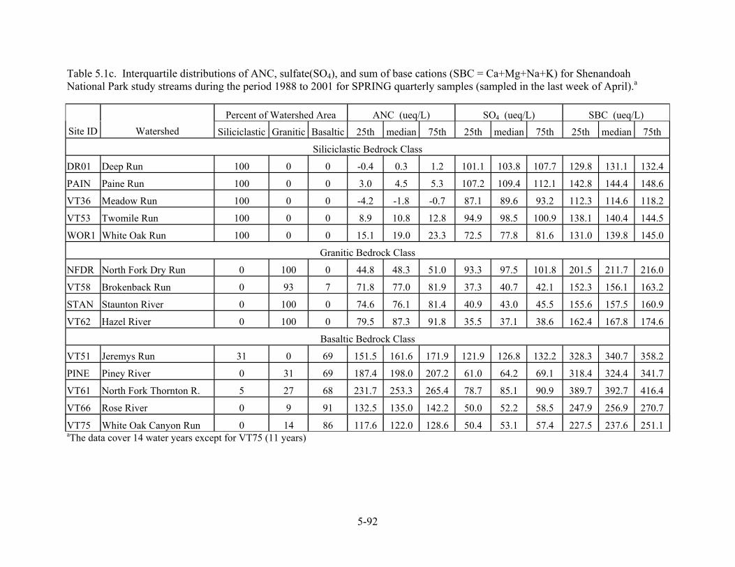
5-92

Table 5.1c. Interquartile distributions of ANC, sulfate(SO4), and sum of base cations (SBC = Ca+Mg+Na+K) for Shenandoah National Park study streams during the period 1988 to 2001 for SPRING quarterly samples (sampled in the last week of April).a

Percent of Watershed Area ANC (ueq/L) SO4 (ueq/L) SBC (ueq/L) Site ID

Watershed Siliciclastic Granitic Basaltic 25th median 75th 25th median 75th 25th median 75th

Siliciclastic Bedrock Class

DR01 Deep Run 100 0 0 -0.4 0.3 1.2 101.1 103.8 107.7 129.8 131.1 132.4

PAIN Paine Run 100 0 0 3.0 4.5 5.3 107.2 109.4 112.1 142.8 144.4 148.6

VT36 Meadow Run 100 0 0 -4.2 -1.8 -0.7 87.1 89.6 93.2 112.3 114.6 118.2

VT53 Twomile Run 100 0 0 8.9 10.8 12.8 94.9 98.5 100.9 138.1 140.4 144.5

WOR1 White Oak Run 100 0 0 15.1 19.0 23.3 72.5 77.8 81.6 131.0 139.8 145.0

Granitic Bedrock Class

NFDR North Fork Dry Run 0 100 0 44.8 48.3 51.0 93.3 97.5 101.8 201.5 211.7 216.0

VT58 Brokenback Run 0 93 7 71.8 77.0 81.9 37.3 40.7 42.1 152.3 156.1 163.2

STAN Staunton River 0 100 0 74.6 76.1 81.4 40.9 43.0 45.5 155.6 157.5 160.9

VT62 Hazel River 0 100 0 79.5 87.3 91.8 35.5 37.1 38.6 162.4 167.8 174.6

Basaltic Bedrock Class

VT51 Jeremys Run 31 0 69 151.5 161.6 171.9 121.9 126.8 132.2 328.3 340.7 358.2

PINE Piney River 0 31 69 187.4 198.0 207.2 61.0 64.2 69.1 318.4 324.4 341.7

VT61 North Fork Thornton R. 5 27 68 231.7 253.3 265.4 78.7 85.1 90.9 389.7 392.7 416.4

VT66 Rose River 0 9 91 132.5 135.0 142.2 50.0 52.2 58.5 247.9 256.9 270.7

VT75 White Oak Canyon Run 0 14 86 117.6 122.0 128.6 50.4 53.1 57.4 227.5 237.6 251.1 aThe data cover 14 water years except for VT75 (11 years)

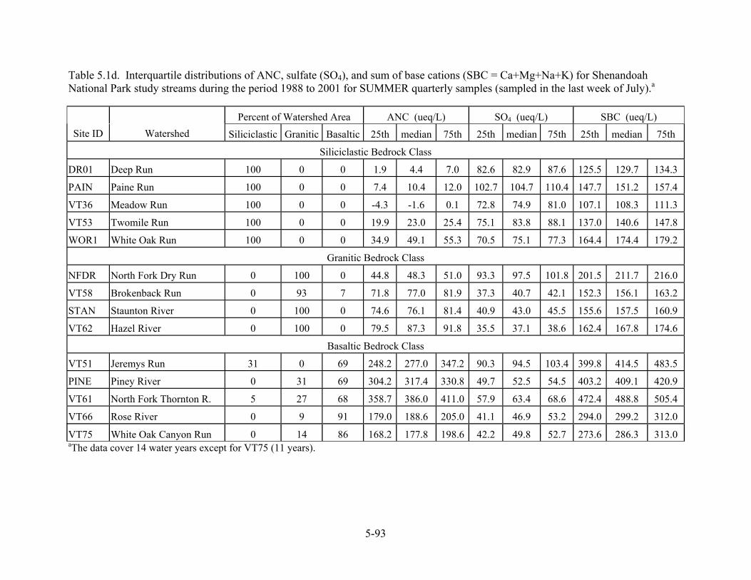
5-93

Table 5.1d. Interquartile distributions of ANC, sulfate (SO4), and sum of base cations (SBC = Ca+Mg+Na+K) for Shenandoah National Park study streams during the period 1988 to 2001 for SUMMER quarterly samples (sampled in the last week of July).a

Percent of Watershed Area ANC (ueq/L) SO4 (ueq/L) SBC (ueq/L) Site ID

Watershed Siliciclastic Granitic Basaltic 25th median 75th 25th median 75th 25th median 75th

Siliciclastic Bedrock Class

DR01 Deep Run 100 0 0 1.9 4.4 7.0 82.6 82.9 87.6 125.5 129.7 134.3

PAIN Paine Run 100 0 0 7.4 10.4 12.0 102.7 104.7 110.4 147.7 151.2 157.4

VT36 Meadow Run 100 0 0 -4.3 -1.6 0.1 72.8 74.9 81.0 107.1 108.3 111.3

VT53 Twomile Run 100 0 0 19.9 23.0 25.4 75.1 83.8 88.1 137.0 140.6 147.8

WOR1 White Oak Run 100 0 0 34.9 49.1 55.3 70.5 75.1 77.3 164.4 174.4 179.2

Granitic Bedrock Class

NFDR North Fork Dry Run 0 100 0 44.8 48.3 51.0 93.3 97.5 101.8 201.5 211.7 216.0

VT58 Brokenback Run 0 93 7 71.8 77.0 81.9 37.3 40.7 42.1 152.3 156.1 163.2

STAN Staunton River 0 100 0 74.6 76.1 81.4 40.9 43.0 45.5 155.6 157.5 160.9

VT62 Hazel River 0 100 0 79.5 87.3 91.8 35.5 37.1 38.6 162.4 167.8 174.6

Basaltic Bedrock Class

VT51 Jeremys Run 31 0 69 248.2 277.0 347.2 90.3 94.5 103.4 399.8 414.5 483.5

PINE Piney River 0 31 69 304.2 317.4 330.8 49.7 52.5 54.5 403.2 409.1 420.9

VT61 North Fork Thornton R. 5 27 68 358.7 386.0 411.0 57.9 63.4 68.6 472.4 488.8 505.4

VT66 Rose River 0 9 91 179.0 188.6 205.0 41.1 46.9 53.2 294.0 299.2 312.0

VT75 White Oak Canyon Run 0 14 86 168.2 177.8 198.6 42.2 49.8 52.7 273.6 286.3 313.0 aThe data cover 14 water years except for VT75 (11 years).

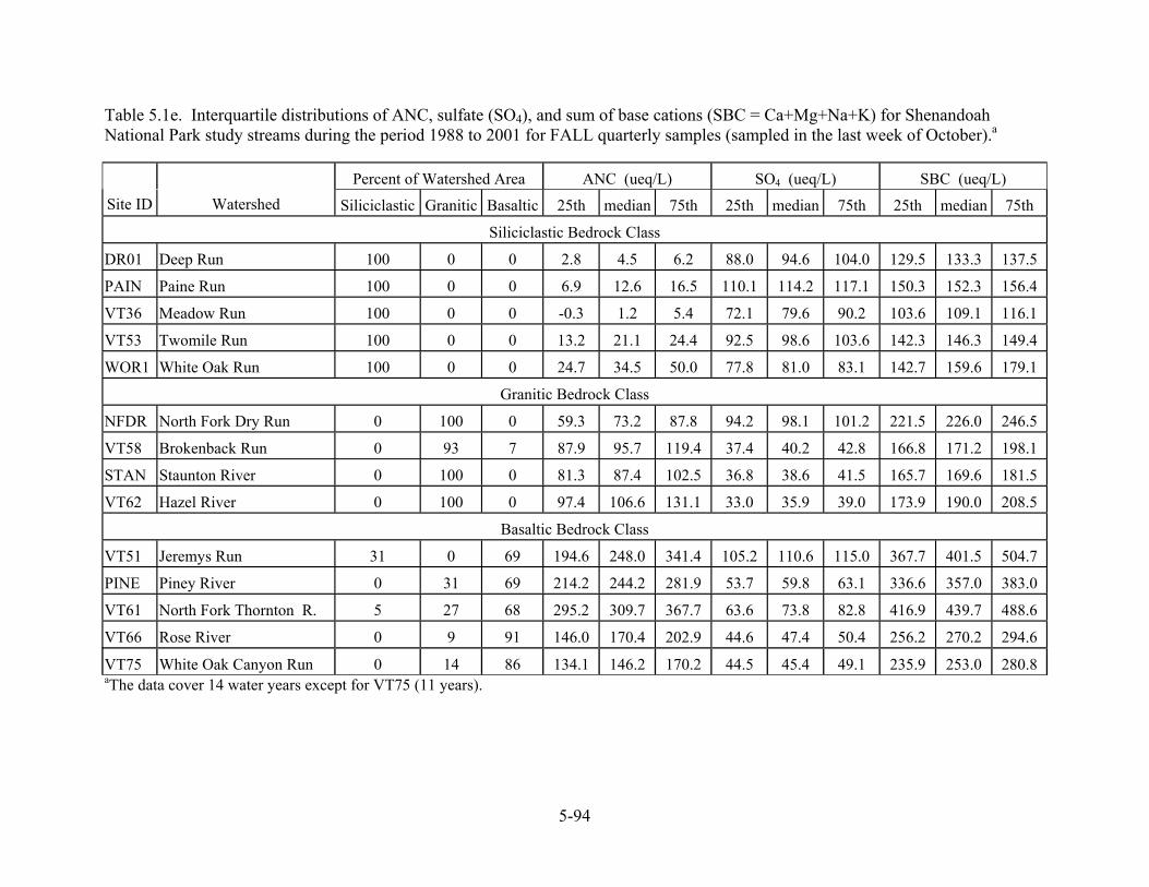
5-94

Table 5.1e. Interquartile distributions of ANC, sulfate (SO4), and sum of base cations (SBC = Ca+Mg+Na+K) for Shenandoah National Park study streams during the period 1988 to 2001 for FALL quarterly samples (sampled in the last week of October).a

Percent of Watershed Area ANC (ueq/L) SO4 (ueq/L) SBC (ueq/L) Site ID

Watershed Siliciclastic Granitic Basaltic 25th median 75th 25th median 75th 25th median 75th

Siliciclastic Bedrock Class

DR01 Deep Run 100 0 0 2.8 4.5 6.2 88.0 94.6 104.0 129.5 133.3 137.5

PAIN Paine Run 100 0 0 6.9 12.6 16.5 110.1 114.2 117.1 150.3 152.3 156.4

VT36 Meadow Run 100 0 0 -0.3 1.2 5.4 72.1 79.6 90.2 103.6 109.1 116.1

VT53 Twomile Run 100 0 0 13.2 21.1 24.4 92.5 98.6 103.6 142.3 146.3 149.4

WOR1 White Oak Run 100 0 0 24.7 34.5 50.0 77.8 81.0 83.1 142.7 159.6 179.1

Granitic Bedrock Class

NFDR North Fork Dry Run 0 100 0 59.3 73.2 87.8 94.2 98.1 101.2 221.5 226.0 246.5

VT58 Brokenback Run 0 93 7 87.9 95.7 119.4 37.4 40.2 42.8 166.8 171.2 198.1

STAN Staunton River 0 100 0 81.3 87.4 102.5 36.8 38.6 41.5 165.7 169.6 181.5

VT62 Hazel River 0 100 0 97.4 106.6 131.1 33.0 35.9 39.0 173.9 190.0 208.5

Basaltic Bedrock Class

VT51 Jeremys Run 31 0 69 194.6 248.0 341.4 105.2 110.6 115.0 367.7 401.5 504.7

PINE Piney River 0 31 69 214.2 244.2 281.9 53.7 59.8 63.1 336.6 357.0 383.0

VT61 North Fork Thornton R. 5 27 68 295.2 309.7 367.7 63.6 73.8 82.8 416.9 439.7 488.6

VT66 Rose River 0 9 91 146.0 170.4 202.9 44.6 47.4 50.4 256.2 270.2 294.6

VT75 White Oak Canyon Run 0 14 86 134.1 146.2 170.2 44.5 45.4 49.1 235.9 253.0 280.8 aThe data cover 14 water years except for VT75 (11 years).

5-95

Table 5.2. Bedrock distribution in Shenandoah National Park and SWAS watersheds.

Percent Bedrock Coveragea Site ID Stream

Watershed Area (km2) Siliciclastic Granitic Basaltic

VT51 Jeremys Run 22.0 31.0 0.0 69.0 VT61 North Fork Thornton River 19.1 5.2 27.0 67.8 VT60 Piney River (PINE) 12.4 0.0 31.3 68.7 VT58 Brokenback Run 9.9 0.0 93.4 6.6 VT62 Hazel River 13.2 0.0 100.0 0.0 NFDR North Fork Dry Run 2.3 0.0 100.0 0.0 VT66 Rose River 23.7 0.0 9.1 90.9 VT59 Staunton River (STAN) 10.5 0.0 100.0 0.0 VT75 Whiteoak Canyon Run 14.1 0.0 14.1 85.9 DR01 Deep Run 3.1 100.0 0.0 0.0 VT36 Meadow Run 8.9 100.0 0.0 0.0 VT35 Paine Run (PAIN) 12.4 100.0 0.0 0.0 VT53 Twomile Run 5.6 100.0 0.0 0.0 WOR1 White Oak Run 5.1 100.0 0.0 0.0 Total SWAS Watersheds 162.3 26.4 29.8 43.7 Total Shenandoah National Park 797.0 28.8 32.4 38.8 aPercent of the watershed area underlain by bedrock within each of the major geologic sensitivity classes.

5.2. Relationships Between Geology and Stream Water Chemistry

The SHEN landscape includes three major geologic sensitivity types: siliciclastic (quartzite and sandstone), granitic, and basaltic (Figure 5.1). Each of these bedrock types influences about one-third of the stream length in the park.

All of the primary SWAS streams on siliciclastic bedrock monitored during the period 1988 to 1999 had relatively high median SO4

2- concentration (76–109 Feq/L), whereas three of four streams monitored on granitic bedrock had SO4

2- concentration < 43 Feq/L. Sulfate concentrations in streams draining basaltic bedrock were more variable, ranging from 52 to 127 Feq/L. Stream water base cation concentrations and ANC also varied dramatically from site to site. Median stream water base cation concentrations were generally lowest in the watersheds on siliciclastic bedrock, and this could reflect lower base cation supply from watershed soils and/or greater base cation depletion of soils caused by leaching of SO4

2- to streams. Base cation concentrations were substantially higher (median > 235 Feq/L) in watersheds on basaltic bedrock.

There are many streams on siliciclastic bedrock in the park that have chronic ANC in the range where adverse effects are likely to occur on sensitive aquatic biota and where episodic acidification to ANC values near or below zero frequently occur during hydrological events. The streams that are most susceptible to adverse chronic or episodic effects on in-stream biota are those having chronic ANC less than about 50 Feq/L, especially those having chronic ANC less than about 20 Feq/L. These are also primarily on siliciclastic bedrock (Table 5.1).

5-96

The observed patterns in stream water chemistry are strongly related to patterns in bedrock geology within the park (Figure 5.1). In fact, geological type, soils conditions that developed from underlying geology, and water chemistry conditions are all closely interrelated within SHEN. This is partly because rock and soils materials in SHEN and elsewhere in the Southeast were not transported from place to place (and thereby mixed) by the process of glaciation. Relationships between water chemistry and geology within SHEN have been known for some time. Lynch and Dise (1985) reported results from six synoptic surveys of 56 streams that drain SHEN. Concentrations of silica, base cations, and ANC were strongly related to the distribution of geologic formations. The effects of acidification were often greatest in watersheds underlain by the Antietam Formation, which had stream water pH averaging 5.0 and ANC averaging -7 Feq/L. Lynch and Dise (1985) found that flow-weighted stream water ANC decreased in order of the underlying geologic formation as follows:

basaltic (Catoctin formation) > granitic (Pedlar and Old Rag formations) > siliciclastic (Hampton and Antietam formations)

Regression relationships suggested that stream water ANC would generally range from about 175 Feq/L on the Catoctin Formation to -7 Feq/L on the Antietam Formation. After accounting for variations in stream water chemistry with geology, Lynch and Dise (1985) further found lower stream water ANC on the western side of the park, as compared with the eastern side. The authors speculated that this could be due to the upwind sources of acidic deposition being in closer proximity to the park’s western border, which results in greater S deposition on west-facing slopes. However, there are also soils differences between east- and west-facing slopes, which might be important.

Additional perspective concerning the relationship between stream water chemistry and geology in SHEN is provided by the 1992 survey of sub-watersheds within the primary study watersheds (Table 5.3). Whereas Lynch and Dise (1985) derived regression models to predict stream water composition as function of multiple bedrock types, the 1992 survey provides an opportunity to examine the composition of stream waters associated with single bedrock types. From the relatively large number of small watersheds sampled in the survey, subsets of 62 siliciclastic, 46 granitic, and 15 basaltic subwatersheds were identified. Table 5.3 presents descriptive statistics for measurements of ANC, pH, sum of base cations, and SO4

2- concentrations obtained for the subset of the 1992 survey samples (n = 123) associated with single bedrock types. The bedrock-related differences in ANC and pH distributions are consistent with expectations based on the earlier Lynch and Dise (1985) analysis.

As indicated in Table 5.3, stream water ANC and pH values were lowest for the surveyed siliciclastic subwatersheds and highest for basaltic subwatersheds. Almost half of the sampled streams in siliciclastic subwatersheds had ANC in the chronically acidic range (< 0 Feq/L) in which lethal effects on brook trout are probable (see Chapter 8). The balance of the streams associated with siliciclastic bedrock had ANC in the episodically acidic range (having chronic ANC in the range 0–20 Feq/L) in which sub-lethal or lethal effects are possible. Many of the streams associated with the granitic bedrock type were in the indeterminate range (20–50 Feq/L). In contrast, the streams associated with the basaltic bedrock type had ANC values that were well within the suitable range for brook trout.

5-97

Table 5.3. Range and distribution of stream water concentrations within Shenandoah National Park associated with major bedrock classes: Spring 1992 Synoptic Survey (Galloway et al. 1999).

n Minimum 25% Median 75% Maximum ANC (ueq/L)

Siliciclastic 62 -18.1 -1.0 1.2 3.7 12.8 Granitic 46 22.0 47.2 58.7 67.0 130.4 Basaltic 15 33.7 97.0 149.2 179.0 226.7

pH Siliciclastic 62 4.8 5.4 5.6 5.7 6.0 Granitic 46 6.0 6.7 6.8 6.8 7.1 Basaltic 15 6.6 6.9 7.1 7.2 7.3

Sum of Base Cations (ueq/L) Siliciclastic 62 92.1 138.1 168.2 190.4 272.1 Granitic 46 89.5 136.7 147.7 161.3 243.5 Basaltic 15 138.0 232.0 369.5 381.1 450.9

Sulfate (ueq/L) Siliciclastic 62 67.2 88.5 97.2 104.8 177.8 Granitic 46 13.4 30.1 36.6 42.1 96.3 Basaltic 15 12.3 36.2 62.2 97.9 164.3 Notes: (1) The data were obtained for watersheds underlain by a single bedrock type. (2) 25% and 75% refer to the 25th and 75th percentile values. 50 percent of all the values are within the interquartile range, as bounded by the 25th and 75th percentile values.

The pH values for the streams in the 1992 survey displayed a similar relationship with bedrock type, with the streams having lowest pH being associated with siliciclastic bedrock and those having highest pH associated with basaltic bedrock. All of the streams on siliciclastic bedrock had pH < 6, identified by Baker and Christiansen (1991) as too acidic for some acid-sensitive fish species.

Sulfate concentration values for streams in the 1992 survey also differed among bedrock types. This difference is critically important with respect to the observed stream water ANC, which is determined by the relative concentrations of base cations and acid anions. Whereas both the siliciclastic and basaltic bedrock types were associated with relatively high stream water SO4

2- concentrations, the siliciclastic bedrock type was associated with much lower base cation concentrations, and therefore lower stream water ANC. In contrast, streams on granitic bedrock exhibited both low base cation and low SO4

2- concentrations, with resulting intermediate ANC.

The observed differences in stream water SO4 2- concentrations for the major bedrock types in

SHEN primarily reflect differences in SO4 2- retention properties of the associated soils.

Watersheds in the southeastern United States commonly retain more than 50% of deposited S (Rochelle and Church 1987; Turner et al. 1990). This S retention is attributed to SO4

2- adsorption in the old and highly-weathered southeastern soils (Galloway et al. 1983; Baker et al.

5-98

1991). Although there are other mechanisms of S retention or immobilization in watersheds, including S reduction and biological uptake, these are generally considered less important on regional or park-specific scales than is adsorption, particularly in upland forests (Turner et al. 1990). Regardless of mechanism, S retention in watersheds reduces the potential for the acidification of surface waters that is associated with increasing concentrations and mobility of SO4

2-. However, S retention by adsorption is a capacity-limited process. As the finite adsorption capacity of watershed soils is exhausted, SO4

2- concentrations can increase in surface waters, potentially contributing to greater acidification (Johnson and Cole 1980, Munson and Gherini 1991; Church et al. 1992). Moreover, as indicated by the available soil and water quality data for SHEN, there can be substantial variation in S retention capacity among watersheds in close geographic proximity.

5.3. Relationships Between Soils and Stream Water Chemistry

A common measure of base availability in soils is the percent base saturation, which represents the fraction of exchange sites (or cation exchange capacity [CEC]) occupied by base cations. Base saturation values in the range of 10−20% have been cited as threshold values for incomplete acid neutralization and leaching of aluminum (Al) from soil to surface waters (Reuss and Johnson 1986; Binkley et al. 1989; Cronan and Schofield 1990). Data from the 2000 soil survey conducted by the University of Virginia (Welsch et al. 2001) are summarized in Table 5.4 for each of the study watersheds.

Table 5.4. Interquartile distribution of pH, cation exchange capacity (CEC), and percent base saturation for soil samples collected in Shenandoah National Park study watersheds during the 2000 soil survey.

pH CEC (cmol/kg) % Base Saturation Site ID Watershed n 25th Med 75th 25th Med 75th 25th Med 75th

Siliciclastic Bedrock Class PAIN Paine Run 6 4.4 4.5 4.7 3.7 5.7 5.7 7.1 10.0 24.9 WOR1 White Oak Run 6 4.3 4.4 4.4 4.8 7.5 7.8 5.3 7.5 8.5 DR01 Deep Run 5 4.3 4.4 4.5 3.9 5. 5.8 7.2 8.9 10.8 VT36 Meadow Run 6 4.4 4.4 4.5 3.1 3.5 7.6 7.8 8.7 11.3 VT53 Twomile Run 5 4.3 4.5 4.5 4.6 6.0 6.9 11.7 12.3 13.6

Granitic Bedrock Class STAN Staunton River 6 4.7 4.8 4.9 6.5 7.5 9.2 9.1 13.9 29.5 NFDR NF of Dry Run 5 4.4 4.5 4.7 7.3 8. 9.2 7.5 10.8 12.4 VT58 Brokenback Run 5 4.6 4.7 4.7 7.3 8.4 9.6 6.0 6.7 9.7 VT62 Hazel River 4 4.5 4.7 4.8 5.3 5.3 6.5 12.3 12.8 21.6

Basaltic Bedrock Class PINE Piney River 6 4.7 5.0 5.3 7.3 7.7 10.0 17.0 24.0 57.0 VT66 Rose River 8 4.8 5.0 5.3 7.3 10.1 10.7 19.1 38.0 63.5 VT75 White Oak Canyon 6 4.9 5.1 5.5 7.1 7.5 9.3 15.6 32.8 43.4 VT61 NF of Thornton R. 7 5.1 5.2 5.3 7.7 9.6 10.8 35.6 54.4 71.2 VT51 Jeremys Run 4 4.7 5.0 5.3 6.3 7.6 7.7 15.0 22.8 46.1 Notes: Samples collected from mineral soil >20 cm depth. Watersheds are stratified according to the predominant bedrock class present in each.

5-99

As indicated in Figure 5.2, median base saturation was generally less than 10% for mineral soils associated with siliciclastic bedrock and less than about 14% for mineral soils associated with granitic bedrock in the park. The present low base cation availability in soils of watersheds underlain by siliciclastic or granitic bedrock is probably due to a combination of low base cation content of the parent bedrock and depletion by previous land use and decades of accelerated leaching by acidic deposition. The relative importance of these factors is not known. This low base cation availability suggests the potential for leaching of Al to streams.

A clear relationship was found between stream water ANC and measured soil base saturation among the SWAS watersheds (Figure 5.3). All watersheds that were characterized by soil base saturation less than 15% had average stream water ANC < 100 Feq/L. Watersheds that had higher soil base saturation (all of which were > 22%) were dominated by the basaltic bedrock type and had average stream water ANC > 100 Feq/L. Lowest base saturation values (7 to 14%) were found in the siliciclastic and granitic watersheds, with much higher values in the basaltic watersheds. We do not advocate using the relationship between stream water ANC and soil base saturation, shown in Figure 5.3, for predictive purposes, however. Within a particular bedrock class, soil base saturation is not a good predictor of stream water ANC. In addition, the ranges of base saturation among the study watersheds were similar for the siliciclastic and granitic types, despite the clear separation in stream water ANC (Figure 5.3).

The data presented in Table 5.4 are based on soils data stratified by watershed, and each watershed was geologically classified based on the predominant bedrock type found within the watershed. However, a watershed that was primarily underlain by granitic bedrock may have included, for example, one or more soil pits located over basaltic bedrock. We therefore reanalyzed the soils data by classifying all soil pits according to the underlying bedrock type, irrespective of the predominant bedrock class within the watershed in which the soil pit was located. The results of this analysis, shown in Table 5.5, illustrate a more distinct separation of soils characteristics across bedrock types, especially for the mineral soil layer (> 20 cm depth). For example, the interquartile ranges (25th to 75th percentile) for base saturation in the mineral soil were 8 to 14%, 10 to 32%, and 22 to 59% for the siliciclastic, granitic, and basaltic classes, respectively. Soil pH showed almost a complete interquartile separation, with interquartile ranges in the mineral soil of 4.4 to 4.6, 4.7 to 5.0, and 4.9 to 5.3 for the three respective bedrock types. Cation exchange capacity values were lower in the siliciclastic soils (interquartile range in the mineral soil of 3.7 to 7.5) than in the other two bedrock types, which showed similar CEC values (Table 5.5).

5.4 Regional Context

In a regional context, SHEN is a major focal point of aquatic effects of S deposition, due largely to the prevalence of siliciclastic bedrock geology. Based on the two extensive probability sampling programs for stream water chemistry within the region (National Stream Survey [NSS, Herlihy et al. 1993] and Environmental Monitoring and Assessment Program [EMAP, Herlihy et al. 2000]), there are about 11,300 km of wadeable stream in western Virginia. Data collected in EMAP showed about 10% of this stream length with ANC # 50 Feq/L, and 5% with ANC # 20 Feq/L. Many of these low-ANC streams are located in and around SHEN. The median value of stream water ANC within the SAMI region was 172 Feq/L, based on an extrapolation of data

5-100

Figure 5.2. Median percent base saturation for soils associated with Shenandoah National Park’s three bedrock types. Brackets delimit interquartile ranges. The base saturation of soils derived from siliciclastic and granitic bedrock is too low for effective buffering of acidic deposition in many watersheds. The data were obtained for mineral-horizon soil samples collected in the summer of 2000 at 79 geologically distributed sites in Shenandoah National Park (Welsch et al. 2001).

Siliciclastic Granitic Basaltic0%

10%

20%

30%

40%

50%

60%B

ase

Satu

ratio

n

5-101

Figure 5.3 Median spring ANC of streams in SWAS watersheds during the period 1988 to 1999 versus median base saturation of watershed soils. Soils data were collected by the University of Virginia during the summer of 2000 (Welsch et al. 2001).

Table 5.5. Interquartile distributions for each bedrock class of pH, cation exchange capacity (CEC), and percent base saturation for all soil pits excavated during the 2000 soil survey.

pH CEC (cmol/kg) % Base Saturation Soil Layer n 25th Med 75th 25th Med 75th 25th Med 75th

Siliciclastic Bedrock Class Surface soil 28 4.1 4.2 4.4 6.9 10.5 13.5 9.9 15.3 28.3 Mineral soil 28 4.4 4.5 4.6 3.7 5.7 7.5 7.5 9.6 13.7

Granitic Bedrock Class Surface soil 26 4.3 4.6 4.9 6.9 10.1 13.2 17.2 31.1 46.0 Mineral soil 26 4.7 4.8 5.0 6.9 8.1 10.5 10.1 13.9 32.3

Basaltic Bedrock Class Surface soil 25 4.7 5.3 5.6 9.5 10.3 15.1 29.0 46.6 74.5 Mineral soil 25 4.9 5.1 5.3 7.4 8.1 10.1 22.0 42.1 58.8 Notes: Surface soil collected from depth <20 cm; mineral soil collected from depth >20 cm. Each soil pit was classified into a bedrock class based on the location of the soil pit, irrespective of the predominant bedrock class within the watershed in which the soil pit was located.

0 10 20 30 40 50 60

Soil Base Saturation (%)

-50

0

50

100

150

200

250

300

AN

C (µ

eq/L

)Siliciclastic

Granitic

Basaltic

Bedrock Class

0 10 20 30 40 50 60

Soil Base Saturation (%)

-50

0

50

100

150

200

250

300

AN

C (µ

eq/L

)Siliciclastic

Granitic

Basaltic

Bedrock Class

5-102

from 154 NSS upstream reach sample sites to a population of 19,940 streams (Sullivan et al. 2002a). In contrast, the median ANC for 47 streams within SHEN was 82 Feq/L (Herlihy et al. 1996).

6-103

Chapter 6: Current Trends in Water Acidification in Shenandoah National Park

Although SHEN has the longest continuous record of stream water composition in a national park and among the longest anywhere in the United States, the record only goes back to 1979 for two streams. The 14 SWAS streams that are located in the park (Figure 5.1) have quarterly water quality data on all 14 streams extending back to 1988. The quarterly samples from these streams are used here to examine the trends in stream water chemistry in the park over the period 1988 to 2001 (data actually cover the 14 water years from Oct. 1987 to Sept. 2001). Trends within the park are placed in a regional context by comparing results with trends calculated for the 65 VTSSS long-term monitoring streams which cover the western part of Virginia. The VTSSS trends are also based on quarterly stream water samples, which were taken contemporaneously with the SWAS stream samples.

Field and Laboratory Methods

As indicated above, SWAS data collection in SHEN includes a combination of quarterly, weekly, and higher-frequency water quality sampling on 14 streams and continuous discharge measurement on five streams, as well as determination of precipitation amount and composition at two locations. The routine field work schedule involves weekly visits (requiring two to three days per week) to six stream sites for water quality sampling, maintenance of discharge gauges, and maintenance of, and retrieval of samples from, automatic high-runoff sampling systems. Two precipitation sampling sites are also visited on a weekly basis for maintenance, collection of data, and retrieval of samples. Stream water samples are also collected on a quarterly basis by SHEN staff at an additional eight sites.

Chemical Analysis

Chemical analysis of all stream water and precipitation samples is performed at the SWAS program laboratory at the University of Virginia. Analyses are conducted for all major chemical properties and constituents, including pH, acid neutralization capacity (ANC), conductivity, sulfate, nitrate, chloride, ammonium, calcium ion, magnesium ion, sodium ion, potassium ion, silica, and dissolved aluminum. The accompanying data report describes analytical methods and lists chemical composition and quality assurance data. The complete Standard Operating Procedure document for sample analysis can be accessed from the SWAS program website: http://swas.evsc.virginia.edu.

In the remainder of this chapter the statistical methods, data, and general results are presented first, followed by discussion of observed trends in individual water quality constituents.

6.1 Trend Analyses: Statistical Methods, Data, and General Results

Trends were calculated for individual ions in stream water using all quarterly samples for all 14 years of the data record using two techniques: 1) simple linear regressions (SLR) of changes in ionic concentration over time; and 2) the seasonal Kendal tau test (SKT; Hirsch et al. 1982; Hirsch and Slack 1984), a commonly applied nonparametric test for monotonic trends in seasonally-varying water quality data. The slope estimates from the SKT and the SLR were compared and found to be essentially the same for all solutes and streams analyzed (Sullivan et

6-104

al. 2003). In the discussion that follows, all trends are derived from the slope of the SLR technique and are in units of ueq/L/year, unless otherwise specified. Significance of trends, where expressed, is based on statistically significant deviations of the regression slope from a value of zero (the standard test of significance in simple linear regression analyses). Sullivan et al. (2003) present expanded graphical displays of time series of individual ions and distributions of trends data for the 14 study sites and for the VTSSS sites.

The 14 SWAS streams and 65 VTSSS streams cover a range of bedrock geology and occur within two physiographic provinces in western Virginia. This allows examination of the patterns of trends on different parts of the landscape. The quarterly nature of the data allows examination of seasonal trends in solute concentrations by performing the SLR analyses separately on winter, spring, summer and fall quarter samples. In these seasonal analyses, there will be 14 data points in the regressions as opposed to 56 data points (4x14) in the regression analyses when all quarters are used for annual trend estimation.

Given that trend estimates are available for a number of streams in the park (or in western Virginia, or on a particular bedrock type, or in a particular physiographic province), it is sometimes useful to have a single measure of stream water solute behavior for a region or group of streams. In such cases, the median value of the trend estimates for a solute for all streams within a group is used. The use of the median trend to summarize the regional response is common. For instance, median trends were used in the most recent EPA report to Congress concerning surface water responses to acidic deposition (Stoddard et al. 2003). The statistical significance of regional trends as represented by the median of a population of trend estimates is determined by calculating confidence limits about the median value in the distribution of all slopes in the analysis (SAS Institute Inc. 1988; Altman et al. 2000).

The utility of using the median trend for the 14 monitored streams in the park can be illustrated by examining the individual trends for all streams for a given solute (Figure 6.1). For example, ANC increased during the period of record at most streams, whereas SO4

2- and NO3-

concentrations generally decreased. Using the median provides a summary of the direction and magnitude of change in the population of streams. It is important to note that for a given solute and group of streams all trends may be in the same direction and of the same magnitude as the median trend. However, it is frequently the case that the magnitudes and even the directions of trends in some streams may be very different from the medians. An examination of plots for all of the ranked slope distributions for all solutes, partitioned by season, physiography or lithology, would be at best tedious and at worst confusing. In order to elucidate and understand the general patterns in the trends of stream water chemistry, and their relationship to season and to the landscape, the median slope values (median trends) for each solute will be used to discuss the patterns in trends in stream water chemistry in SHEN.

The median trends for each solute in the 14 SWAS streams are summarized in Table 6.1 along with the median trends for the 65 VTSSS streams for the same solutes and period. Note that the 14 SWAS streams are also included in the analyses of the 65 VTSSS streams. Median trends were also calculated for the basic stream water chemistry data disaggregated by season and physiographic province or bedrock geology (Table 6.1).

6-105

Figure 6.1. Trends in solute concentrations for the 14 SWAS streams in Shenandoah National Park (ueq/L/yr). The trends are the slopes of simple linear regressions on all quarterly data for 14 years (1988 to 2001; n=56). For each solute, the trends have been sorted from lowest to highest to display the range of estimated trends in a given solute across the 14 streams. Each bar represents one stream.

ANC

-0.50

0.00

0.50

1.00

1.50

2.00

2.50

trend

(ue

q/L/

yr)

H

-0.06-0.05-0.04-0.03-0.02-0.010.000.010.020.030.04

trend

(ue

q/L/

yr)

SBC

-2.50-2.00-1.50-1.00-0.500.000.501.001.50

trend

(ue

q/L/

yr)

SAA

-2.50

-2.00

-1.50

-1.00

-0.50

0.00

0.50

trend

(ue

q/L/

yr)

SO4

-1.20-1.00-0.80-0.60-0.40-0.200.000.200.40

trend

(ue

q/L/

yr)

NO3

-1.40-1.20-1.00-0.80-0.60-0.40-0.200.000.200.40

trend

(ue

q/L/

yr)

CL

-0.40-0.30-0.20-0.100.000.100.200.300.400.50

trend

(ue

q/L/

yr)

SIO2

-2.00

-1.50

-1.00

-0.50

0.00

0.50

trend

(ue

q/L/

yr)

CA

-1.00-0.80-0.60-0.40-0.200.000.200.400.600.80

trend

(ue

q/L/

yr)

MG

-1.00-0.80-0.60-0.40-0.200.000.200.400.60

trend

(ue

q/L/

yr)

NA

-0.50

-0.40

-0.30

-0.20

-0.10

0.00

0.10

0.20

trend

(ue

q/L/

yr)

K

-0.20

-0.15

-0.10

-0.05

0.00

0.05

0.10

0.15

trend

(ue

q/L/

yr)

ANC

-0.50

0.00

0.50

1.00

1.50

2.00

2.50

trend

(ue

q/L/

yr)

H

-0.06-0.05-0.04-0.03-0.02-0.010.000.010.020.030.04

trend

(ue

q/L/

yr)

SBC

-2.50-2.00-1.50-1.00-0.500.000.501.001.50

trend

(ue

q/L/

yr)

SAA

-2.50

-2.00

-1.50

-1.00

-0.50

0.00

0.50

trend

(ue

q/L/

yr)

SO4

-1.20-1.00-0.80-0.60-0.40-0.200.000.200.40

trend

(ue

q/L/

yr)

NO3

-1.40-1.20-1.00-0.80-0.60-0.40-0.200.000.200.40

trend

(ue

q/L/

yr)

CL

-0.40-0.30-0.20-0.100.000.100.200.300.400.50

trend

(ue

q/L/

yr)

SIO2

-2.00

-1.50

-1.00

-0.50

0.00

0.50

trend

(ue

q/L/

yr)

CA

-1.00-0.80-0.60-0.40-0.200.000.200.400.600.80

trend

(ue

q/L/

yr)

MG

-1.00-0.80-0.60-0.40-0.200.000.200.400.60

trend

(ue

q/L/

yr)

NA

-0.50

-0.40

-0.30

-0.20

-0.10

0.00

0.10

0.20

trend

(ue

q/L/

yr)

K

-0.20

-0.15

-0.10

-0.05

0.00

0.05

0.10

0.15

trend

(ue

q/L/

yr)

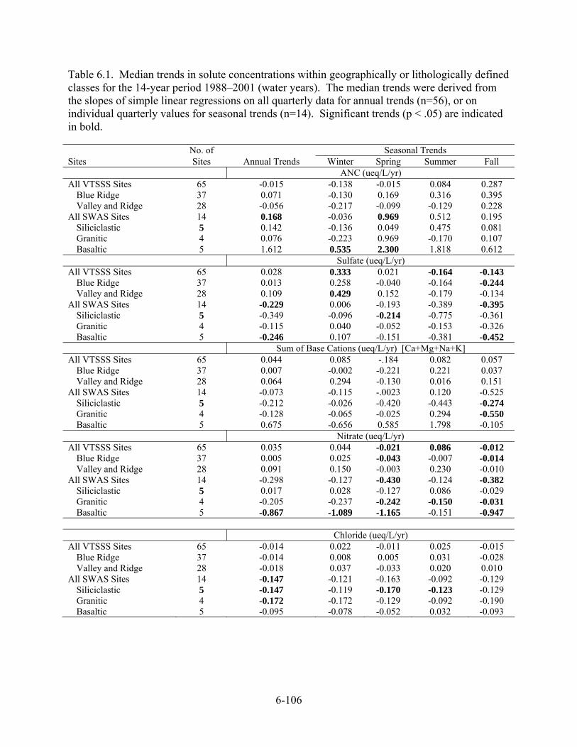
6-106

Table 6.1. Median trends in solute concentrations within geographically or lithologically defined classes for the 14-year period 1988–2001 (water years). The median trends were derived from the slopes of simple linear regressions on all quarterly data for annual trends (n=56), or on individual quarterly values for seasonal trends (n=14). Significant trends (p < .05) are indicated in bold.

No. of Seasonal Trends Sites Sites Annual Trends Winter Spring Summer Fall ANC (ueq/L/yr) All VTSSS Sites 65 -0.015 -0.138 -0.015 0.084 0.287

Blue Ridge 37 0.071 -0.130 0.169 0.316 0.395 Valley and Ridge 28 -0.056 -0.217 -0.099 -0.129 0.228

All SWAS Sites 14 0.168 -0.036 0.969 0.512 0.195 Siliciclastic 5 0.142 -0.136 0.049 0.475 0.081 Granitic 4 0.076 -0.223 0.969 -0.170 0.107 Basaltic 5 1.612 0.535 2.300 1.818 0.612

Sulfate (ueq/L/yr) All VTSSS Sites 65 0.028 0.333 0.021 -0.164 -0.143

Blue Ridge 37 0.013 0.258 -0.040 -0.164 -0.244 Valley and Ridge 28 0.109 0.429 0.152 -0.179 -0.134

All SWAS Sites 14 -0.229 0.006 -0.193 -0.389 -0.395 Siliciclastic 5 -0.349 -0.096 -0.214 -0.775 -0.361 Granitic 4 -0.115 0.040 -0.052 -0.153 -0.326 Basaltic 5 -0.246 0.107 -0.151 -0.381 -0.452

Sum of Base Cations (ueq/L/yr) [Ca+Mg+Na+K] All VTSSS Sites 65 0.044 0.085 -.184 0.082 0.057

Blue Ridge 37 0.007 -0.002 -0.221 0.221 0.037 Valley and Ridge 28 0.064 0.294 -0.130 0.016 0.151

All SWAS Sites 14 -0.073 -0.115 -.0023 0.120 -0.525 Siliciclastic 5 -0.212 -0.026 -0.420 -0.443 -0.274 Granitic 4 -0.128 -0.065 -0.025 0.294 -0.550 Basaltic 5 0.675 -0.656 0.585 1.798 -0.105

Nitrate (ueq/L/yr) All VTSSS Sites 65 0.035 0.044 -0.021 0.086 -0.012

Blue Ridge 37 0.005 0.025 -0.043 -0.007 -0.014 Valley and Ridge 28 0.091 0.150 -0.003 0.230 -0.010

All SWAS Sites 14 -0.298 -0.127 -0.430 -0.124 -0.382 Siliciclastic 5 0.017 0.028 -0.127 0.086 -0.029 Granitic 4 -0.205 -0.237 -0.242 -0.150 -0.031 Basaltic 5 -0.867 -1.089 -1.165 -0.151 -0.947

Chloride (ueq/L/yr) All VTSSS Sites 65 -0.014 0.022 -0.011 0.025 -0.015

Blue Ridge 37 -0.014 0.008 0.005 0.031 -0.028 Valley and Ridge 28 -0.018 0.037 -0.033 0.020 0.010

All SWAS Sites 14 -0.147 -0.121 -0.163 -0.092 -0.129 Siliciclastic 5 -0.147 -0.119 -0.170 -0.123 -0.129 Granitic 4 -0.172 -0.172 -0.129 -0.092 -0.190 Basaltic 5 -0.095 -0.078 -0.052 0.032 -0.093

6-107

Table 6.1. Median trends in solute concentrations within geographically or lithologically defined classes for the 14-year period 1988–2001 (water years). The median trends were derived from the slopes of simple linear regressions on all quarterly data for annual trends (n=56), or on individual quarterly values for seasonal trends (n=14). Significant trends (p < .05) are indicated in bold (continued).

No. of Seasonal Trends Sites Sites Annual Trends Winter Spring Summer Fall Sum of Acid Anions (ueq/L/yr) [SO4+Cl+NO3] All VTSSS Sites 65 0.094 0.490 -0.021 0.086 -0.251

Blue Ridge 37 -0.084 0.367 -0.255 -0.227 -0.355 Valley and Ridge 28 0.197 0.717 0.197 0.305 -0.080

All SWAS Sites 14 -0.619 -0.411 -0.814 -0.559 -0.655 Siliciclastic 5 -0.613 -0.148 -0.717 -0.343 -0.624 Granitic 4 -0.302 -0.046 -0.324 -0.721 -0.556 Basaltic 5 -1.228 -1.445 -1.726 -0.554 -1.572

Hydrogen Ion (ueq/L/yr) All VTSSS Sites 65 0.007 0.016 0.010 0.006 -0.004

Blue Ridge 37 0.007 0.010 0.008 0.005 -0.003 Valley and Ridge 28 0.008 0.032 0.011 0.006 -0.012

All SWAS Sites 14 0.007 0.015 0.004 0.000 0.000 Siliciclastic 5 0.015 0.043 0.006 -0.038 -0.054 Granitic 4 0.010 0.020 0.005 0.010 -0.004 Basaltic 5 0.006 0.008 0.003 0.004 0.003

Calcium Ion (ueq/L/yr) All VTSSS Sites 65 0.078 0.151 0.031 0.076 0.048

Blue Ridge 37 0.125 0.128 0.047 0.163 0.062 Valley and Ridge 28 0.066 0.218 0.024 0.033 0.008

All SWAS Sites 14 0.163 0.215 0.220 0.156 0.005 Siliciclastic 5 0.161 0.314 0.053 0.088 0.062 Granitic 4 -0.008 0.161 0.098 0.025 -0.261 Basaltic 5 0.422 -0.084 0.413 0.972 0.009

Magnesium Ion (ueq/L/yr) All VTSSS Sites 65 0.007 0.030 -0.041 0.082 0.024

Blue Ridge 37 -0.015 0.008 -0.048 0.004 -0.004 Valley and Ridge 28 0.041 0.114 -0.033 0.112 0.127

All SWAS Sites 14 -0.082 -0.033 -0.107 -0.075 -0.179 Siliciclastic 5 -0.273 -0.057 -0.283 -0.270 -0.256 Granitic 4 -0.103 -0.004 0.017 -0.020 -0.116 Basaltic 5 0.204 -0.356 0.057 0.625 -0.026

Sodium Ion (ueq/L/yr) All VTSSS Sites 65 -0.020 -0.043 -0.076 -0.005 0.025

Blue Ridge 37 -0.018 -0.103 -0.086 0.168 0.034 Valley and Ridge 28 -0.030 -0.026 -0.073 -0.012 0.016

All SWAS Sites 14 -0.121 -0.226 -0.188 0.039 -0.123 Siliciclastic 5 -0.163 -0.226 -0.234 -0.063 -0.112 Granitic 4 -0.127 -0.352 -0.209 0.274 -0.219 Basaltic 5 0.086 -0.214 0.002 0.208 -0.058

6-108

Table 6.1. Median trends in solute concentrations within geographically or lithologically defined classes for the 14-year period 1988–2001 (water years). The median trends were derived from the slopes of simple linear regressions on all quarterly data for annual trends (n=56), or on individual quarterly values for seasonal trends (n=14). Significant trends (p < .05) are indicated in bold (continued).

No. of Seasonal Trends Sites Sites Annual Trends Winter Spring Summer Fall Potassium Ion (ueq/L/yr) All VTSSS Sites 65 -0.043 -0.013 -0.040 -0.070 -0.095

Blue Ridge 37 -0.034 -0.019 -0.018 -0.025 -0.085 Valley and Ridge 28 -0.067 -0.007 -0.067 -0.087 -0.103

All SWAS Sites 14 0.007 0.048 0.019 0.020 -0.075 Siliciclastic 5 -0.006 0.074 0.031 -0.105 -0.207 Granitic 4 0.033 0.048 0.059 0.089 -0.047 Basaltic 5 -0.025 0.043 0.006 0.009 -0.085

Silica (um/L/yr) All VTSSS Sites 65 -0.079 -0.107 -0.120 -0.151 0.115

Blue Ridge 37 -0.130 -0.171 -0.285 -0.151 0.104 Valley and Ridge 28 -0.057 -0.083 -0.017 -0.169 0.157

All SWAS Sites 14 -0.601 -0.472 -0.340 -0.863 -0.639 Siliciclastic 5 -0.242 -0.098 -0.307 -0.097 -0.218 Granitic 4 -0.705 -0.647 -0.340 -1.096 -0.639 Basaltic 5 -0.972 -0.607 -0.404 -1.384 -1.623

CALKa (ueq/L/yr) All VTSSS Sites 65 0.042 -0.302 -0.104 0.138 0.294

Blue Ridge 37 0.177 -0.290 0.116 0.602 0.295 Valley and Ridge 28 -0.171 -0.347 -0.317 -0.380 0.258

All SWAS Sites 14 0.294 0.164 0.439 0.668 0.076 Siliciclastic 5 0.177 0.131 0.309 0.206 0.007 Granitic 4 0.211 -0.128 0.270 0.623 0.006 Basaltic 5 1.805 0.911 2.311 2.352 1.141

a CALK is calculated charge-balance ANC (CALK=SBC-SAA)

6-109

The general trends in stream water chemistry in the park can be understood by considering the behavior of SO4

2-, the sum of the base cations (SBC = Ca+Mg+Na+K), and ANC. Median annual and seasonal trends for ANC, SO4

2-, and SBC determined for streams within geographically and lithologically defined classes are displayed in Figures 6.2 through 6.4. These median trends are extracted from Table 6.1 and presented graphically to aid discussion. The significance of any of the trends in the figures can be determined by reference to Table 6.1. Although most of the median trend values for are small and not significant, geographic, lithologic, and seasonal patterns are evident.

6.2 Trends in Acid Neutralizing Capacity (ANC)

The median annual trend in ANC was positive (increasing) for the group of 14 study streams in SHEN, as well as for all of the lithologically defined subsets of streams (Figure 6.2). In contrast, the median ANC decreased on an annual basis for the 65 study streams in western Virginia. Thus, although there is some evidence for some recovery from acidification effects on stream water composition among the SHEN streams, there is evidence for continuing acidification among streams in the larger region, which encompasses those in SHEN. This observation of continuing acidification among the study streams in the larger western Virginia region is consistent with trend results reported by Stoddard et al. (2003), who evaluated trends among the same set of streams for the 1990–2000 period. It should be noted that the observed median annual trends in ANC in both SHEN and the western Virginia region are quite small; when considered over the 14-year period, the median ANC change in stream waters is only +2.4 ueq/L in SHEN and –0.2 ueq/L in western Virginia.

It should also be noted that the observed median annual trends differ for western Virginia streams classified by physiographic province. Median trends were negative (decreasing) for streams in the Valley and Ridge province and positive (increasing) for streams in the Blue Ridge province, which includes the SHEN area. Thus, there is some evidence for a recovery gradient between the two provinces, as well as between the park and western Virginia as a whole.

Additional patterns in ANC trends were evident among the different seasons. Most notably, the median trend values in winter contrasted with those of the other seasons, generally showing a negative (decreasing) trend in median ANC. Only the SHEN streams associated with basaltic bedrock showed a increasing value for median ANC trend in winter. In contrast, the median trend values for the fall season were increasing for all of the defined classes of streams. These observed seasonal differences in median ANC trends may have biological significance because winter is the period of the year when the most acid-sensitive life stages of the brook trout (eggs and fry) are present in the streams of SHEN and western Virginia (Figure 6.5).

6.3 Sulfate Trends

The level of SO42- leaching, which is the principal acidifying process, and the availability of

exchangeable base cations, which serve to neutralize acidity, determine both acidification and recovery of streams in the central Appalachian region. Plots of median trends in stream water SO4

2- (Figure 6.3) are consistent with the observation that changes in SO42- mobility are largely

driving both the acidification and recovery processes in the streams of SHEN and the adjacent mountainous region. The median annual trend in SO4

2- concentration was decreasing for all the

6-110

Figure 6.2. Median values of annual and seasonal trends (in ueq/L) in stream water ANC concentrations among VTSSS and SWAS watersheds: 1988-2001. The median values are from distributions of ANC trends determined for streams within classes defined by physiography or lithology. The annual trends are based on simple linear regressions on all quarterly data for 14 years (n=56). Seasonal trends are based on individual quarterly values for 14 years (n=14).

All Virginia SitesBlue Ridge Sites

Valley and Ridge Sites---------------------------

All SNP SitesSNP Siliciclastic Sites

SNP Granitic SitesSNP Basaltic Sites

-1.00 -0.50 0.00 0.50 1.00 1.50 2.00 2.50

All Virginia SitesBlue Ridge Sites

Valley and Ridge Sites---------------------------

All SNP SitesSNP Siliciclastic Sites

SNP Granitic SitesSNP Basaltic Sites

-1.00 -0.50 0.00 0.50 1.00 1.50 2.00 2.50

All Virginia SitesBlue Ridge Sites

Valley and Ridge Sites---------------------------

All SNP SitesSNP Siliciclastic Sites

SNP Granitic SitesSNP Basaltic Sites

-1.00 -0.50 0.00 0.50 1.00 1.50 2.00 2.50

All Virginia SitesBlue Ridge Sites

Valley and Ridge Sites---------------------------

All SNP SitesSNP Siliciclastic Sites

SNP Granitic SitesSNP Basaltic Sites

-1.00 -0.50 0.00 0.50 1.00 1.50 2.00 2.50

All Virginia SitesBlue Ridge Sites

Valley and Ridge Sites---------------------------

All SNP SitesSNP Siliciclastic Sites

SNP Granitic SitesSNP Basaltic Sites

-1.00 -0.50 0.00 0.50 1.00 1.50 2.00 2.50

Annual

Winter

Spring

Summer

Fall

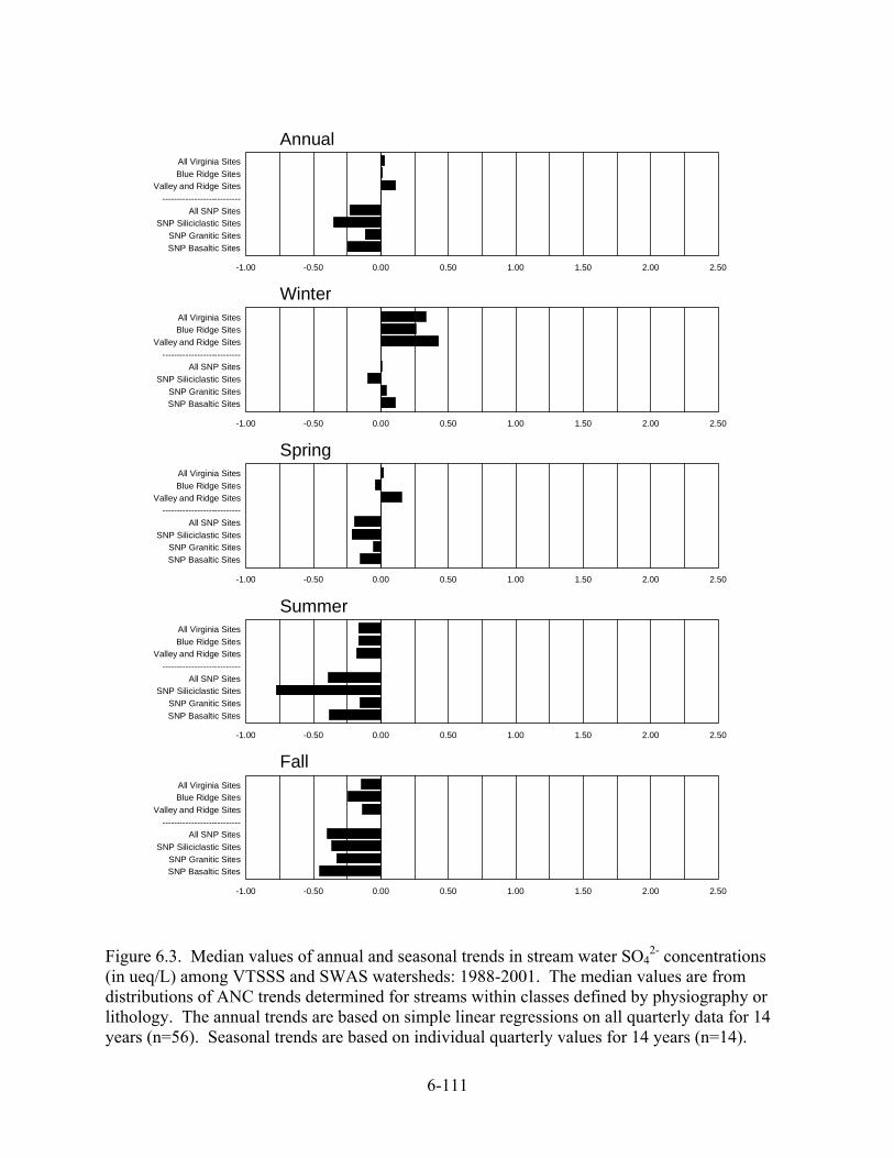
6-111

Figure 6.3. Median values of annual and seasonal trends in stream water SO42- concentrations

(in ueq/L) among VTSSS and SWAS watersheds: 1988-2001. The median values are from distributions of ANC trends determined for streams within classes defined by physiography or lithology. The annual trends are based on simple linear regressions on all quarterly data for 14 years (n=56). Seasonal trends are based on individual quarterly values for 14 years (n=14).

All Virginia SitesBlue Ridge Sites

Valley and Ridge Sites---------------------------

All SNP SitesSNP Siliciclastic Sites

SNP Granitic SitesSNP Basaltic Sites

-1.00 -0.50 0.00 0.50 1.00 1.50 2.00 2.50

All Virginia SitesBlue Ridge Sites

Valley and Ridge Sites---------------------------

All SNP SitesSNP Siliciclastic Sites

SNP Granitic SitesSNP Basaltic Sites

-1.00 -0.50 0.00 0.50 1.00 1.50 2.00 2.50

All Virginia SitesBlue Ridge Sites

Valley and Ridge Sites---------------------------

All SNP SitesSNP Siliciclastic Sites

SNP Granitic SitesSNP Basaltic Sites

-1.00 -0.50 0.00 0.50 1.00 1.50 2.00 2.50

All Virginia SitesBlue Ridge Sites

Valley and Ridge Sites---------------------------

All SNP SitesSNP Siliciclastic Sites

SNP Granitic SitesSNP Basaltic Sites

-1.00 -0.50 0.00 0.50 1.00 1.50 2.00 2.50

All Virginia SitesBlue Ridge Sites

Valley and Ridge Sites---------------------------

All SNP SitesSNP Siliciclastic Sites

SNP Granitic SitesSNP Basaltic Sites

-1.00 -0.50 0.00 0.50 1.00 1.50 2.00 2.50

Annual

Winter

Spring

Summer

Fall

6-112

Figure 6.4. Median values of annual and seasonal trends in stream water SBC concentrations (in ueq/L) among VTSSS and SWAS watersheds: 1988–2001. The median values are from distributions of ANC trends determined for streams within classes defined by physiography or lithology. The annual trends are based on simple linear regressions on all quarterly data for 14 years (n=56). Seasonal trends are based on individual quarterly values for 14 years (n=14).

All Virginia SitesBlue Ridge Sites

Valley and Ridge Sites---------------------------

All SNP SitesSNP Siliciclastic Sites

SNP Granitic SitesSNP Basaltic Sites

-1.00 -0.50 0.00 0.50 1.00 1.50 2.00 2.50

All Virginia SitesBlue Ridge Sites

Valley and Ridge Sites---------------------------

All SNP SitesSNP Siliciclastic Sites

SNP Granitic SitesSNP Basaltic Sites

-1.00 -0.50 0.00 0.50 1.00 1.50 2.00 2.50

All Virginia SitesBlue Ridge Sites

Valley and Ridge Sites---------------------------

All SNP SitesSNP Siliciclastic Sites

SNP Granitic SitesSNP Basaltic Sites

-1.00 -0.50 0.00 0.50 1.00 1.50 2.00 2.50

All Virginia SitesBlue Ridge Sites

Valley and Ridge Sites---------------------------

All SNP SitesSNP Siliciclastic Sites

SNP Granitic SitesSNP Basaltic Sites

-1.00 -0.50 0.00 0.50 1.00 1.50 2.00 2.50

All Virginia SitesBlue Ridge Sites

Valley and Ridge Sites---------------------------

All SNP SitesSNP Siliciclastic Sites

SNP Granitic SitesSNP Basaltic Sites

-1.00 -0.50 0.00 0.50 1.00 1.50 2.00 2.50

Annual

Winter

Spring

Summer

Fall

6-113

Figure 6.5. The life stages of brook trout when the species shows the greatest sensitivity to acidification.

streams in SHEN, including each of the lithologically-defined subgroups. A decreasing median annual trend in SO4

2- concentration was associated with a increasing median annual trend in ANC.

Again, a different pattern is evident for the median annual trends in SO42- among the streams in

the larger western Virginia region. The observed median annual trend in SO42- concentration

was increasing for the regional streams. For the Virginia streams, as well as the streams in the Valley and Ridge province, an increasing median annual trend in SO4

2- concentration was associated with a decreasing median annual trend in ANC. It thus appears that recent differences in stream water ANC trends between SHEN and the larger western Virginia region, although relatively small in terms of absolute magnitude, may be largely attributed to differences in stream water SO4

2- trends between the two defined areas.

A plot of SO42- trends for individual study streams in the western Virginia region (Figure 6.6)

suggests that these observed differences in SO42- trends can be explained as a consequence of S

retention dynamics. Although correlations are observed between sulfur deposition measured in precipitation and sulfate concentrations measured in surface waters (Kaufmann 1988; Baker et al. 1990a), sulfur is not fully mobile in many watersheds systems; some watersheds accumulate or retain sulfur, a process which has the effect of reducing acidity in soil and surface water. Although most watersheds in the northeastern United States do not retain significant amounts of sulfur, watersheds in the southeastern United States commonly retain more than 50 percent of deposited sulfur (Rochelle and Church 1987; Turner et al. 1990). This difference in sulfur retention between the two regions is attributed to greater sulfate adsorption capacity in the older and more-weathered southeastern soils (Galloway et al. 1983; Baker et al. 1991).

Acid-Sensitive Life Stages of Brook Trout

6-114

Figure 6.6. Trends in stream water SO42- concentrations in relation to median SO4

2- concentrations for VTSSS and SWAS streams. Trends and medians are based on quarterly sampling data (1988–2001). SWAS study streams (located in Shenandoah National Park) are indicated with red symbols.

Seasonal patterns in median SO42- concentration trends indicate that the difference in ANC

change between winter and the rest of the year is also largely a function of SO42- trends. The

largest and most general increases in median SO42- concentrations were observed during winter.

Sulfate concentration trends were generally decreasing in other seasons.

As indicated in Figure 6.6, the streams with the largest decreasing trends in SO42- concentration

over the 14-year period, including many in the park, were generally those with higher median SO4

2- concentrations. This observation is consistent with the expectation that stream water SO42-

concentrations in the southern Appalachian Mountains in general are determined by the S adsorption properties of watershed soils and the level of watershed exposure to S deposition.

For watersheds with high S deposition and relatively little retention, stream water SO42-

concentrations will be high. Decreases in S deposition may then result in decreases in stream water SO4

2- concentrations. For watersheds that more strongly retain S, stream water SO42-

concentrations will be lower. Decreases in S deposition may then either result in no change in stream water SO4

2- concentrations or SO42- concentrations may actually continue to increase as

the retention capacity of watershed soils is depleted.

0 25 50 75 100 125

Median SO 42- (µeq /L)

-1.5

-1.0

-0.5

0.0

0.5

1.0

1.5

SO 42-

Tre

nd (

µeq/L

/yr)

Tren

d (µ

eq/L

/yr)

Median SO42- (µeq/L)

6-115

6.4 Trends in Base Cation Concentrations

The plots of median trends in the sum of base cation concentrations are also informative (Figure 6.4), and suggest that base cation availability is a limiting factor with respect to recovery of streams in SHEN and western Virginia. The median annual trends in the sum of base cations were decreasing in all SHEN streams except streams associated with basaltic bedrock. As indicated in Table 6.1 and Figure 6.4, streams on basaltic bedrock had relatively high base cation concentrations and soils on basaltic bedrock had relatively high base cation availability. For the streams on relatively base-poor siliciclastic or granitic bedrock, the observed decrease in the sum of base cations coincident with the decrease in SO4

2- concentrations suggested that low availability of base cations limited recovery of ANC.

It is also notable that although there was much seasonal variation in median trends in the sum of base cations, the SHEN streams with the most consistently decreasing trends were on siliciclastic bedrock. This may be an indication of base cation depletion in watershed soils, given that the soils on siliciclastic bedrock had notably low base cation availability (see Figure 6.4). For this subset of streams in particular, ANC recovery may be limited by base cation availability and additional acidification may be expected to occur as the watershed base cation supplies are further depleted, especially if S deposition remains relatively high.

6.5. Summary of Trends in Stream Water Chemistry in Shenandoah National Park

In summary, it appears that the streams in SHEN are showing signs of recovery, whereas the streams in the larger western Virginia region are not. Moreover, the patterns of trends in ANC and SO4

2- are consistent with expectations for recovery. Considered in relation to the regional-scale analysis of Stoddard et al. (2003), these observations suggest that evidence for decreasing SO4

2- concentrations and increasing ANC in SHEN streams may reflect a north-to-south recovery gradient in the eastern United States. It should be noted, however, that the changes in both ANC and SO4

2- concentrations in SHEN and western Virginia are small compared to those reported for other regions by Stoddard et al. (2003), are confounded by seasonal differences, and in many cases are not statistically significant.

7-117

Chapter 7: Simulation of Soil and Water Acidification Responses in Shenandoah National Park

The purpose of this chapter is to describe the modeling used to evaluate historical and potential future air pollution impacts on sensitive receptors in Shenandoah National Park (SHEN). Simulation modeling was used to evaluate possible future changes in the extent of damage to aquatic and soil resources in SHEN in response to changing levels of acidic deposition. The assessment in Chapter 2 is based in part on these simulation results. Historical impacts are based on model responses to historical deposition in the park. Future impacts are based on simulated responses to various scenarios of future emissions reductions. The alternative future emissions scenarios were specified on the basis of existing and substantially more stringent regulations, available emissions control technologies using the Regional Acid Deposition Model (RADM) to estimate future sulfate (SO4

2-) deposition values at SHEN.

The effects modeling was conducted using the Model of Acidification of Groundwater in Catchments (MAGIC). The MAGIC model of acidification is a model that has been extensively subjected to the process of testing and confirmation over a 15-year period and thousands of applications. MAGIC has been used in scientific studies, as a tool in establishing management practices, and as an aid in making policy decisions regarding controls on emissions and deposition. Overall, the model has proven to be robust, reliable, and useful in all of these activities.

The reader is referred to Appendix B for procedural details of the acid deposition effects modeling undertaken for this project (descriptions of the model, input data, calibration procedures, estimation of uncertainty, and evaluation of model goodness-of-fit). This chapter describes the sites selected for modeling, the deposition scenarios used for simulation, and the results that are relevant to the assessment presented inChapter2.

Of particular relevance here is a presentation of the simulated output of the MAGIC model for a number of variables so that the “reasonableness” of the modeling results for each of the scenarios can be demonstrated. The MAGIC model simulates the geochemical responses of the selected catchments. The assessment maps in Chapter 2 provide an estimate of risk for adverse biological effects from acid deposition based on the projected geochemical response. Understanding the projected pattern of biological responses can be facilitated by an examination of the projected geochemical responses, especially the relative magnitude of geochemical responses across the different deposition scenarios.

7.1. Description of Sites Selected for Modeling

Fourteen streams were selected for aquatic effects modeling, to represent the range of geologic sensitivity and stream water ANC found in SHEN (Figure 5.1). The 14 streams chosen are all of the streams in SHEN for which water quality data are available in sufficient quantity and of sufficient quality for use in calibrating MAGIC to a long-term database. These streams are routinely sampled as part of the Shenandoah Watershed Study (SWAS) and the Virginia Trout Stream Sensitivity Study (VTSSS). The frequency of sampling ranges from weekly (6 streams) to quarterly (8 streams) and all streams have at least 12 years of monitoring data available. Five streams are underlain by rocks from each of the siliciclastic and basaltic geologic sensitivity

7-118

classes. Four streams represent the granitic sensitivity class. The siliciclastic watersheds included four streams having ANC between 0 and 16 Feq/L (Paine, Deep, Meadow, and Twomile Runs), and one stream (White Oak Run) having ANC = 26 Feq/L. The stream water ANC in the granitic watersheds ranged from 60 (North Fork Dry Run) to 102 (Hazel River) Feq/L, and for the basaltic watersheds ranged from 126 (White Oak Canyon Run) to 258 (North Fork of Thornton River) Feq/L.

Chapters 5 and 6 provide a detailed analysis of the current status and trends of acidification in these catchments.

7.2 Future Deposition Scenarios Used for Simulations

Scenarios of future emissions were developed for this report following U.S. Environmental Protection Agency (EPA) methods regarding preparation of emissions inventory input into air quality modeling for policy analysis and rule making purposes (for details of these methods applied to SHEN, see Sullivan et al. 2003). A base emissions inventory was created representing the future with economic assumptions obtained from the Bureau of Economic Analysis and emissions controls representative of the laws, rules, and regulations already on the books and final as of the date of preparation of the inventory. These various control constraints include Federal, state and local requirements for emissions control for a wide variety of environmental and human health goals.

This report relies upon EPA projected emissions developed for the Heavy-Duty Engine and Vehicle Standards and Highway Diesel Fuel Rulemaking for the 1996, 2010 and 2020 base emissions for all sources other than electricity generation. Electricity generation emissions were modeled using the Integrated Planning Model (IPM) to develop the base emissions estimates for electricity generation for 2020. Additional control constraints were applied to the generation system nationwide to reflect the various levels of additional control considered. In addition, a control scenario was developed by E.H. Pechan and Associates under EPA contract for stationary point sources, representing the limit of current commercially available control technology. Finally, a set of mobile source emissions estimates were developed by Dyntel Corp., under contract to the EPA, reflecting the limit of technology for highway automobiles and light duty trucks based upon a California Air Resources Board (CARB) analysis of this sector (CARB 2001).

The 1990 base case and future emissions estimates were thus developed for this assessment based on existing regulations and future economic assumptions. Four emissions scenarios were implemented:

Scenario 1. Base with NOx State Implementation Plan (SIP) Call - Assumes reasonable economic growth and emissions limitations according to existing regulations as of summer, 2000. Projections are provided to 2010.

Scenario 2. Base Projected to 2020 - Same assumptions as Scenario 1, but projected to 2020 to allow for continued implementation of Tier II Vehicle Standards and full implementation of Title IV and Heavy Duty Diesel Vehicle standards.

7-119

Scenario 3. Additional Stringent Utility Controls - Adds to Scenario 2 additional Electric Generating Unit (EGU) controls.

Scenario 4. Additional Stringent Controls on Utility, Industry-Point, and Mobile Sources - Adds to Scenario 3 additional, non-EGU emissions reductions.

The annual deposition of S and nitrogen (N) projected at SHEN under each of the scenarios is provided in Table 7.1. The deposition of S and, to a lesser extent, N is projected to decline substantially from the 1990 base under all scenarios.

Table 7.1 Annual deposition of sulfur and nitrogen projected by the Enhanced Regional Acid Deposition Model for the four scenarios.

Constituent 1990 Base Scenario 1 Scenario 2 Scenario 3 Scenario 4 Total Sulfura (kg-S/ha/yr) 12.96 8.66 8.20 4.06 3.25 Total Nitrogenb (kg-N/ha/yr) 7.63 5.70 4.88 4.40 3.98 aTotal sulfur deposition includes wet deposition of SO4

2- and dry deposition of gaseous SO2 and particulate SO42-.

bTotal nitrogen deposition includes wet deposition of NO3- and NH4

+ ; dry deposition of gaseous NO2, HNO3, and NH3 ; and dry deposition of particulate NO3

- and NH4+. Ammonium total deposition was assumed to remain

constant at 2.16 kg-N/ha/yr.

7.3 Modeling Results

MAGIC was successfully calibrated to all modeled watersheds. Results of predicted versus observed chemistry in the calibration year are shown for all 14 modeled sites (Figure 5.1). Agreement was very good for all variables, with the possible exception of pH. See the graphs and discussion of model goodness-of-fit to calibration data in Appendix B. Demonstrated agreement between predicted and observed stream water chemistry during the calibration period (as shown in Appendix B) does not necessarily demonstrate, however, that the model structure and fundamental assumptions are sufficiently accurate and representative of major watershed processes to yield correct simulations of future conditions. But the MAGIC model has been confirmed in several studies that have examined model performance in comparison with independent estimates or measurements of chemical change (c.f., Cosby et al. 1995, 1996; Sullivan et al. 1996) and has been found to be reliable.

Future stream water chemistry was simulated for each site throughout the period 1990 to 2100, based on the scenario of continued constant deposition at 1990 levels and the four future emissions control scenarios. Hindcast simulation results are shown in Figure 7.1, suggesting substantial acidification of the modeling sites that occur on siliciclastic bedrock. Among the modeling sites on granitic bedrock, North Fork Dry Run showed evidence of moderate historic acidification, whereas other modeling sites on granitic bedrock and all of the sites on basaltic bedrock showed little historic acidification (Figure 7.1). The inferred pre-industrial ANC of all

7-120

Deep Run DR01

0

40

80

120

160

1850 1875 1900 1925 1950 1975 2000

ueq/

L

Paine Run VT35

0

40

80

120

160

1850 1875 1900 1925 1950 1975 2000

ueq/

L

Meadow Run VT36

0

40

80

120

160

1850 1875 1900 1925 1950 1975 2000ue

q/L

0200

19952010202520402055207020852100

SBC

NO3

SO4

Calk

AQRV sites on Siliciclastic Bedrock

Two Mile Run VT53

0

40

80

120

160

1850 1875 1900 1925 1950 1975 2000

ueq/

L

White Oak Run WOR1

0

40

80

120

160

1850 1875 1900 1925 1950 1975 2000

ueq/

L

North Fork of Dry Run NFDR

0

50

100

150

200

250

1850 1875 1900 1925 1950 1975 2000

ueq/

L

Brokenback Run VT58

0

50

100

150

200

250

1850 1875 1900 1925 1950 1975 2000

ueq/

L

Staunton River VT59

0

50

100

150

200

250

1850 1875 1900 1925 1950 1975 2000

ueq/

L

Hazel Run VT62

0

50

100

150

200

250

1850 1875 1900 1925 1950 1975 2000

ueq/

L

AQRV sites on Granitic Bedrock

Jeremys Run VT51

0

100

200

300

400

500

1850 1875 1900 1925 1950 1975 2000

ueq/

L

Piney River VT60

0

100

200

300

400

500

1850 1875 1900 1925 1950 1975 2000

ueq/

L

Nf Thornton River VT61

0

100

200

300

400

500

1850 1875 1900 1925 1950 1975 2000

ueq/

L

Rose River VT66

0

50

100

150

200

250

300

1850 1875 1900 1925 1950 1975 2000

ueq/

L

White Oak Canyon R VT75

0

50

100

150

200

250

300

1850 1875 1900 1925 1950 1975 2000

ueq/

L

0200

19952010202520402055207020852100

SBC

NO3

SO4

Calk

AQRV sites on Basaltic Bedrock

Figure 7.1. MAGIC model simulations of historical stream water concentrations of SO4, NO3, sum of base cations (SBC = Ca+Mg+Na+K), and ANC (Calk =SBC-SO4-NO3) for modeled sites on the three bedrock types in Shenandoah National Park – Siliciclastic (upper left), Basaltic (upper right), and Granitic (lower right).

7-121

of the siliciclastic sites and of North Fork Dry Run ranged between about 60 and 90 Feq/L, whereas other sites were inferred to have had pre-industrial ANC near or above 100 Feq/L.

Projected future concentrations of sulfate (SO42-), nitrate (NO3

-), sum of base cations (SBC=Ca+Mg+Ma+K), and charge balance ANC (Calk=SBC-SO4-NO3) are presented in Figures 7.2 through 7.5. Simulated ANC values are also tabulated (Table 7.2) for each of the modeled sites and scenarios. Simulated pH values are also tabulated (Table 7.3) for each site and for each scenario. Sulfate concentrations in stream water were projected to increase at all sites under the scenario of continued constant deposition. Under the four emissions control scenarios, stream water SO4

2- concentrations were projected to decrease at all of the sites on siliciclastic bedrock, but results were mixed for the various scenarios applied to sites on granitic and basaltic bedrock. The most stringent emissions control strategy (Scenario 4) resulted in substantial (> 25 Feq/L) projected decreases in stream water SO4

2- concentrations (Figure 7.2).

Changes in stream water NO3- concentration in response to the scenarios were either negligible

or were projected decreases in concentration that were less than about 12 Feq/L (Figure 7.3). Changes in stream water base cation concentrations were projected to be smallest for the siliciclastic sites, which generally have the lowest base cation concentrations currently, and did not differ substantially among simulations. Base cation leaching was projected to be largest under continued constant deposition and progressively smaller with increasingly stringent emissions control scenarios (Figure 7.4). Projected changes in base cation concentrations were largest for the basaltic sites.

The combined effects of modeled changes in SO42- and base cations resulted in projected future

changes in stream water ANC that ranged from less than 10 Feq/L for some siliciclastic sites under Scenarios 1 and 2 to projected ANC increases of more than 40 Feq/L at Deep Run and Paine Run for Scenarios 3 and 4 (Figure 7.5). All siliciclastic sites were projected to become acidic (ANC # 0) by the year 2050 under continued deposition at 1990 levels. White Oak Run was projected to nearly become acidic under Scenarios 1 and 2 by 2100, but other sites on siliciclastic bedrock were projected to increase ANC in the future under all emissions control scenarios. In contrast, the majority of the sites on granitic and basaltic bedrock showed projected decreases in ANC under most of the scenarios, largely in response to changes in S adsorption on soils in response to continued S deposition.

We expect that episodic ANC depressions will be superimposed on these projected future chronic ANC values. We lack an approach to rigorously quantify the extent of episodic changes in ANC that would occur in the future, but we expect that such episodic ANC variability would be similar to current episodic behavior. In general, typical episodic ANC depressions of streams of the siliciclastic type within SHEN would be expected to be in the range of about 5 to 10 Feq/L, such as have been observed for Paine Run, White Oak Run, and Deep Run (see Figure 5.1; Sullivan et al. 2003). In contrast, streams on granitic and basaltic bedrock are expected to continue to exhibit somewhat larger episodic ANC depressions, such as the 20 to 30 Feq/L depressions found for Staunton River and North Fork Dry Run, and the greater than 40 Feq/L depressions found for Piney River (See Figure 5.1; Sullivan et al. 2003). Such episodes are most likely to be accompanied by adverse biological effects in streams in which episodic ANC falls near or below zero.

7-122

Deep Run DR01

0

25

50

75

100

125

150

1990 2010 2030 2050 2070 2090 2110

SO4,

ueq

/L

Paine Run VT35

0

25

50

75

100

125

150

1990 2010 2030 2050 2070 2090 2110

SO4,

ueq

/L

Meadow Run VT36

0

25

50

75

100

125

150

1990 2010 2030 2050 2070 2090 2110

SO4,

ueq

/L

0200

19952010202520402055207020852100

AQRV Scen 1

AQRV Scen 2

AQRV Scen 3

AQRV Scen 4

Constant Dep

AQRV sites on Siliciclastic Bedrock

Two Mile Run VT53

0

25

50

75

100

125

150

1990 2010 2030 2050 2070 2090 2110

SO4,

ueq

/L

White Oak Run WOR1

0

25

50

75

100

125

150

1990 2010 2030 2050 2070 2090 2110

SO4,

ueq

/L

Figure 7.2. MAGIC model simulations of future stream water concentrations of SO4 under the scenario of constant deposition and the four emissions control scenarios (described in the text) for modeled sites on the three bedrock types in Shenandoah National Park – Siliciclastic (upper left), Basaltic (upper right), and Granitic (lower right).

North Fork of Dry Run NFDR

0

25

50

75

100

125

150

1990 2010 2030 2050 2070 2090 2110

SO4,

ueq

/L

Brokenback Run VT58

0

25

50

75

100

125

150

1990 2010 2030 2050 2070 2090 2110

SO

4, u

eq/L

Staunton River VT59

0

25

50

75

100

125

150

1990 2010 2030 2050 2070 2090 2110

SO4,

ueq

/L

Hazel Run VT62

0

25

50

75

100

125

150

1990 2010 2030 2050 2070 2090 2110

SO4,

ueq

/LAQRV sites on Granitic Bedrock

Jeremys Run VT51

0

25

50

75

100

125

150

1990 2010 2030 2050 2070 2090 2110

SO4,

ueq

/L

Piney River VT60

0

25

50

75

100

125

150

1990 2010 2030 2050 2070 2090 2110

SO4,

ueq

/L

Nf Thornton River VT61

0

25

50

75

100

125

150

1990 2010 2030 2050 2070 2090 2110

SO4,

ueq

/L

Rose River VT66

0

25

50

75

100

125

150

1990 2010 2030 2050 2070 2090 2110

SO4,

ueq

/L

White Oak Canyon R VT75

0

25

50

75

100

125

150

1990 2010 2030 2050 2070 2090 2110

SO4,

ueq

/L

0200

19952010202520402055207020852100

AQRV Scen 1

AQRV Scen 2

AQRV Scen 3

AQRV Scen 4

Constant Dep

AQRV sites on Basaltic Bedrock

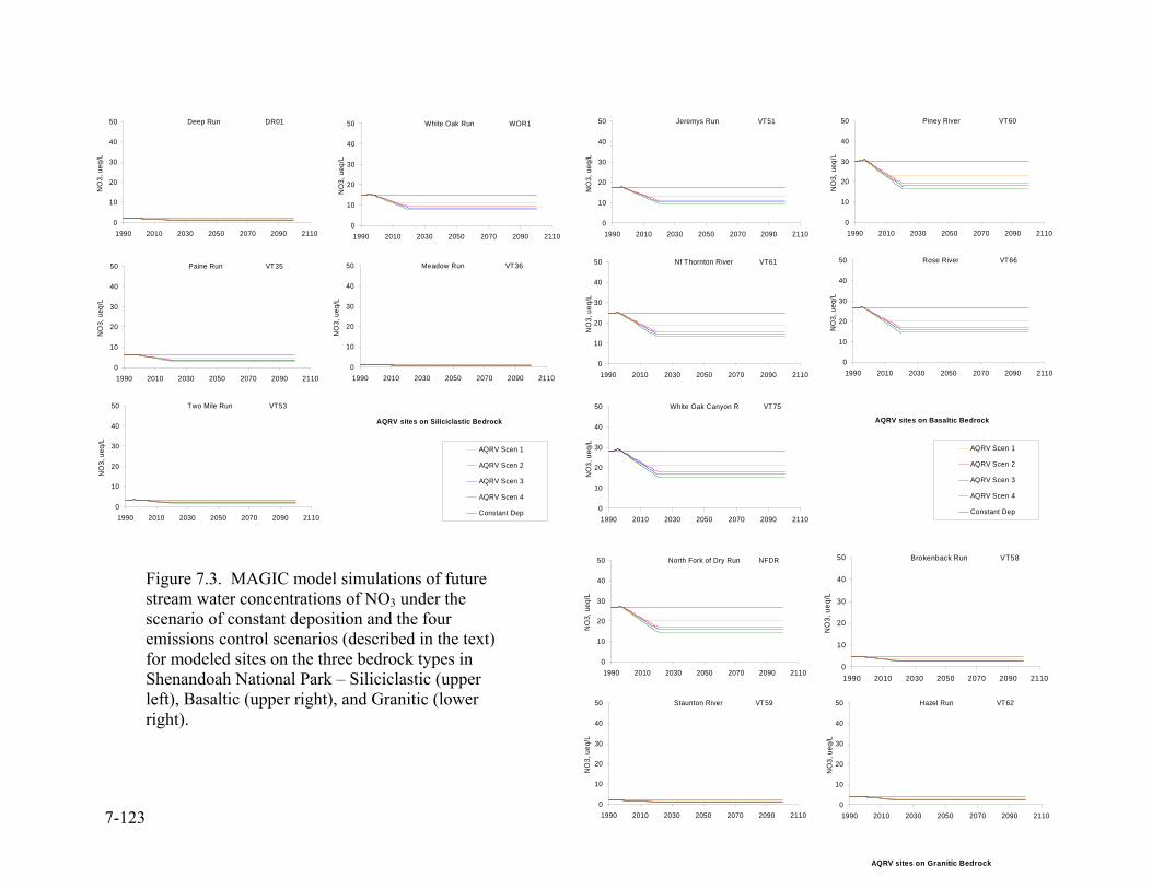
7-123

Deep Run DR01

0

10

20

30

40

50

1990 2010 2030 2050 2070 2090 2110

NO

3, u

eq/L

Paine Run VT35

0

10

20

30

40

50

1990 2010 2030 2050 2070 2090 2110

NO

3, u

eq/L

Meadow Run VT36

0

10

20

30

40

50

1990 2010 2030 2050 2070 2090 2110

NO

3, u

eq/L

05

19952010202520402055207020852100

AQRV Scen 1

AQRV Scen 2

AQRV Scen 3

AQRV Scen 4

Constant Dep

AQRV sites on Siliciclastic Bedrock

Two Mile Run VT53

0

10

20

30

40

50

1990 2010 2030 2050 2070 2090 2110

NO

3, u

eq/L

White Oak Run WOR1

0

10

20

30

40

50

1990 2010 2030 2050 2070 2090 2110

NO

3, u

eq/L

Figure 7.3. MAGIC model simulations of future stream water concentrations of NO3 under the scenario of constant deposition and the four emissions control scenarios (described in the text) for modeled sites on the three bedrock types in Shenandoah National Park – Siliciclastic (upper left), Basaltic (upper right), and Granitic (lower right).

North Fork of Dry Run NFDR

0

10

20

30

40

50

1990 2010 2030 2050 2070 2090 2110

NO

3, u

eq/L

Brokenback Run VT58

0

10

20

30

40

50

1990 2010 2030 2050 2070 2090 2110

NO

3, u

eq/L

Staunton River VT59

0

10

20

30

40

50

1990 2010 2030 2050 2070 2090 2110

NO

3, u

eq/L

Hazel Run VT62

0

10

20

30

40

50

1990 2010 2030 2050 2070 2090 2110

NO

3, u

eq/L

AQRV sites on Granitic Bedrock

Jeremys Run VT51

0

10

20

30

40

50

1990 2010 2030 2050 2070 2090 2110

NO

3, u

eq/L

Piney River VT60

0

10

20

30

40

50

1990 2010 2030 2050 2070 2090 2110

NO

3, u

eq/L

Nf Thornton River VT61

0

10

20

30

40

50

1990 2010 2030 2050 2070 2090 2110

NO

3, u

eq/L

Rose River VT66

0

10

20

30

40

50

1990 2010 2030 2050 2070 2090 2110

NO

3, u

eq/L

White Oak Canyon R VT75

0

10

20

30

40

50

1990 2010 2030 2050 2070 2090 2110

NO

3, u

eq/L

05

19952010202520402055207020852100

AQRV Scen 1

AQRV Scen 2

AQRV Scen 3

AQRV Scen 4

Constant Dep

AQRV sites on Basaltic Bedrock

7-124

Deep Run DR01

0

50

100

150

200

1990 2010 2030 2050 2070 2090 2110

SB

C, u

eq/L

Paine Run VT35

0

50

100

150

200

1990 2010 2030 2050 2070 2090 2110

SB

C, u

eq/L

Meadow Run VT36

0

50

100

150

200

1990 2010 2030 2050 2070 2090 2110

SBC

, ueq

/L

0200

19952010202520402055207020852100

AQRV Scen 1

AQRV Scen 2

AQRV Scen 3

AQRV Scen 4

Constant Dep

AQRV sites on Siliciclastic Bedrock

Two Mile Run VT53

0

50

100

150

200

1990 2010 2030 2050 2070 2090 2110

SB

C, u

eq/L

White Oak Run WOR1

0

50

100

150

200

1990 2010 2030 2050 2070 2090 2110

SB

C, u

eq/L

Figure 7.4. MAGIC model simulations of future stream water concentrations of sum of base cations (SBC=Ca+Mg+Na+K) under the scenario of constant deposition and the four emissions control scenarios (described in the text) for modeled sites on the three bedrock types in Shenandoah National Park – Siliciclastic (upper left), Basaltic (upper right), and Granitic (lower right).

North Fork of Dry Run NFDR

100

150

200

250

300

1990 2010 2030 2050 2070 2090 2110

SBC

, ueq

/L

Brokenback Run VT58

100

150

200

250

300

1990 2010 2030 2050 2070 2090 2110

SB

C, u

eq/L

Staunton River VT59

100

150

200

250

300

1990 2010 2030 2050 2070 2090 2110

SBC

, ueq

/L

Hazel Run VT62

100

150

200

250

300

1990 2010 2030 2050 2070 2090 2110

SBC

, ueq

/L

AQRV sites on Granitic Bedrock

Jeremys Run VT51

200

250

300

350

400

1990 2010 2030 2050 2070 2090 2110

SBC

, ueq

/L

Piney River VT60

250

300

350

400

450

1990 2010 2030 2050 2070 2090 2110

SBC

, ueq

/L

Nf Thornton River VT61

300

350

400

450

500

1990 2010 2030 2050 2070 2090 2110

SB

C, u

eq/L

Rose River VT66

150

200

250

300

350

1990 2010 2030 2050 2070 2090 2110

SBC

, ueq

/L

White Oak Canyon R VT75

150

200

250

300

350

1990 2010 2030 2050 2070 2090 2110

SBC

, ueq

/L

0200

19952010202520402055207020852100

AQRV Scen 1

AQRV Scen 2

AQRV Scen 3

AQRV Scen 4

Constant Dep

AQRV sites on Basaltic Bedrock

7-125

Deep Run DR01

-40

-20

0

20

40

60

1990 2010 2030 2050 2070 2090 2110

Cal

k, u

eq/L

Paine Run VT35

-20

0

20

40

60

80

1990 2010 2030 2050 2070 2090 2110

Cal

k, u

eq/L

Meadow Run VT36

-20

0

20

40

60

80

1990 2010 2030 2050 2070 2090 2110

Cal

k, u

eq/L

-1000100

19952010202520402055207020852100

AQRV Scen 1

AQRV Scen 2

AQRV Scen 3

AQRV Scen 4

Constant Dep

AQRV sites on Siliciclastic Bedrock

Two Mile Run VT53

-20

0

20

40

60

80

1990 2010 2030 2050 2070 2090 2110

Cal

k, u

eq/L

White Oak Run WOR1

-40

-20

0

20

40

60

1990 2010 2030 2050 2070 2090 2110

Cal

k, u

eq/L

Figure 7.5. MAGIC model simulations of future stream water concentrations of charge balance ANC (Calk=SBC-SO4-NO3) under the scenario of constant deposition and the four emissions control scenarios (described in the text) for modeled sites on the three bedrock types in Shenandoah National Park – Siliciclastic (upper left), Basaltic (upper right) and Granitic (lower right).

North Fork of Dry Run NFDR

-20

0

20

40

60

80

1990 2010 2030 2050 2070 2090 2110

Cal

k, u

eq/L

Brokenback Run VT58

20

40

60

80

100

120

1990 2010 2030 2050 2070 2090 2110

Cal

k, u

eq/L

Staunton River VT59

20

40

60

80

100

120

1990 2010 2030 2050 2070 2090 2110

Cal

k, u

eq/L

Hazel Run VT62

40

60

80

100

120

140

1990 2010 2030 2050 2070 2090 2110

Cal

k, u

eq/L

AQRV sites on Granitic Bedrock

Jeremys Run VT51

100

120

140

160

180

200

1990 2010 2030 2050 2070 2090 2110

Cal

k, u

eq/L

Piney River VT60

140

160

180

200

220

240

1990 2010 2030 2050 2070 2090 2110

Cal

k, u

eq/L

Nf Thornton River VT61

200

220

240

260

280

300

1990 2010 2030 2050 2070 2090 2110

Cal

k, u

eq/L

Rose River VT66

100

120

140

160

180

200

1990 2010 2030 2050 2070 2090 2110

Cal

k, u

eq/L

White Oak Canyon R VT75

60

80

100

120

140

160

1990 2010 2030 2050 2070 2090 2110

Cal

k, u

eq/L

-1000100

19952010202520402055207020852100

AQRV Scen 1

AQRV Scen 2

AQRV Scen 3

AQRV Scen 4

Constant Dep

AQRV sites on Basaltic Bedrock

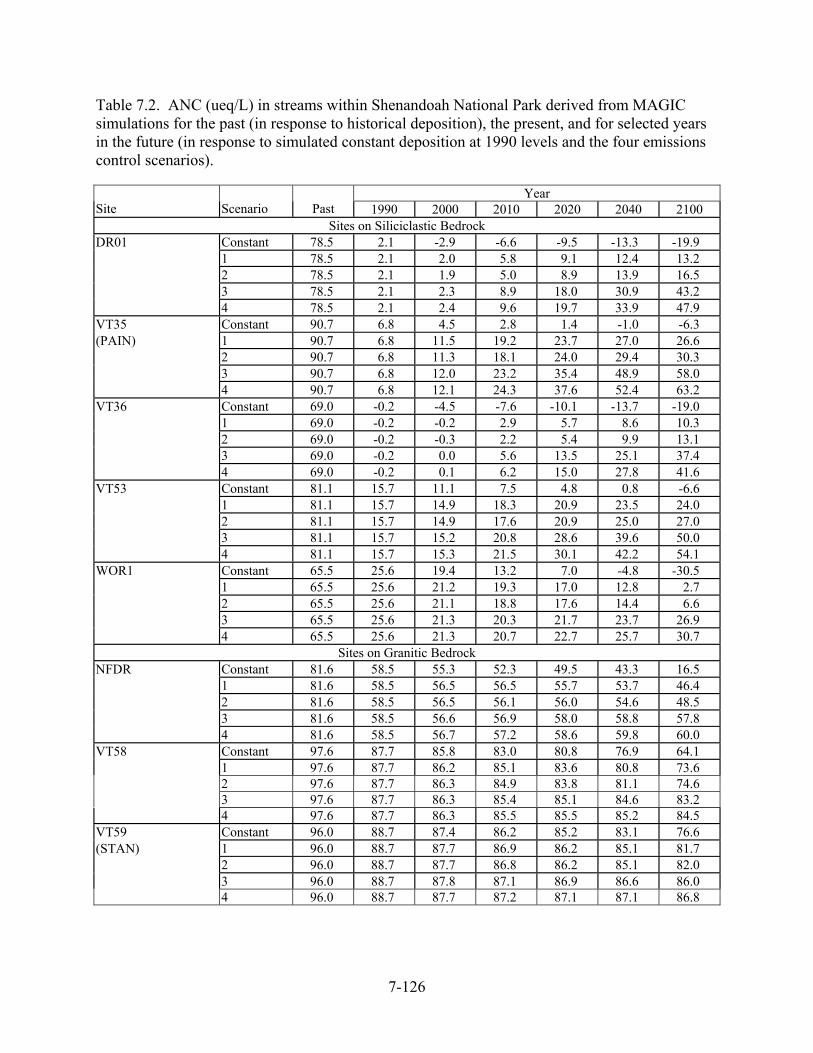
7-126

Table 7.2. ANC (ueq/L) in streams within Shenandoah National Park derived from MAGIC simulations for the past (in response to historical deposition), the present, and for selected years in the future (in response to simulated constant deposition at 1990 levels and the four emissions control scenarios).

Year Site

Scenario

Past 1990 2000 2010 2020 2040 2100

Sites on Siliciclastic Bedrock DR01 Constant 78.5 2.1 -2.9 -6.6 -9.5 -13.3 -19.9 1 78.5 2.1 2.0 5.8 9.1 12.4 13.2 2 78.5 2.1 1.9 5.0 8.9 13.9 16.5 3 78.5 2.1 2.3 8.9 18.0 30.9 43.2 4 78.5 2.1 2.4 9.6 19.7 33.9 47.9 VT35 Constant 90.7 6.8 4.5 2.8 1.4 -1.0 -6.3 (PAIN) 1 90.7 6.8 11.5 19.2 23.7 27.0 26.6 2 90.7 6.8 11.3 18.1 24.0 29.4 30.3 3 90.7 6.8 12.0 23.2 35.4 48.9 58.0 4 90.7 6.8 12.1 24.3 37.6 52.4 63.2 VT36 Constant 69.0 -0.2 -4.5 -7.6 -10.1 -13.7 -19.0 1 69.0 -0.2 -0.2 2.9 5.7 8.6 10.3 2 69.0 -0.2 -0.3 2.2 5.4 9.9 13.1 3 69.0 -0.2 0.0 5.6 13.5 25.1 37.4 4 69.0 -0.2 0.1 6.2 15.0 27.8 41.6 VT53 Constant 81.1 15.7 11.1 7.5 4.8 0.8 -6.6 1 81.1 15.7 14.9 18.3 20.9 23.5 24.0 2 81.1 15.7 14.9 17.6 20.9 25.0 27.0 3 81.1 15.7 15.2 20.8 28.6 39.6 50.0 4 81.1 15.7 15.3 21.5 30.1 42.2 54.1 WOR1 Constant 65.5 25.6 19.4 13.2 7.0 -4.8 -30.5 1 65.5 25.6 21.2 19.3 17.0 12.8 2.7 2 65.5 25.6 21.1 18.8 17.6 14.4 6.6 3 65.5 25.6 21.3 20.3 21.7 23.7 26.9 4 65.5 25.6 21.3 20.7 22.7 25.7 30.7

Sites on Granitic Bedrock NFDR Constant 81.6 58.5 55.3 52.3 49.5 43.3 16.5 1 81.6 58.5 56.5 56.5 55.7 53.7 46.4 2 81.6 58.5 56.5 56.1 56.0 54.6 48.5 3 81.6 58.5 56.6 56.9 58.0 58.8 57.8 4 81.6 58.5 56.7 57.2 58.6 59.8 60.0 VT58 Constant 97.6 87.7 85.8 83.0 80.8 76.9 64.1 1 97.6 87.7 86.2 85.1 83.6 80.8 73.6 2 97.6 87.7 86.3 84.9 83.8 81.1 74.6 3 97.6 87.7 86.3 85.4 85.1 84.6 83.2 4 97.6 87.7 86.3 85.5 85.5 85.2 84.5 VT59 Constant 96.0 88.7 87.4 86.2 85.2 83.1 76.6 (STAN) 1 96.0 88.7 87.7 86.9 86.2 85.1 81.7 2 96.0 88.7 87.7 86.8 86.2 85.1 82.0 3 96.0 88.7 87.8 87.1 86.9 86.6 86.0 4 96.0 88.7 87.7 87.2 87.1 87.1 86.8

7-127

Table 7.2. ANC (ueq/L) in streams within Shenandoah National Park derived from MAGIC simulations for the past (in response to historical deposition), the present, and for selected years in the future (in response to simulated constant deposition at 1990 levels and the four emissions control scenarios) (continued).

Year Site Scenario Past 1990 2000 2010 2020 2040 2100 VT62 Constant 115.6 102.4 100.3 98.4 96.3 91.8 77.4 1 115.6 102.4 100.7 99.7 98.6 96.0 88.6 2 115.6 102.4 100.6 99.6 98.7 96.4 89.6 3 115.6 102.4 100.7 99.9 99.5 98.9 97.3 4 115.6 102.4 100.7 100.0 99.8 99.5 98.3

Sites on Basaltic Bedrock VT51 Constant 191.0 167.7 166.6 165.5 164.6 163.1 157.9 1 191.0 167.7 167.7 168.6 168.9 168.3 165.5 2 191.0 167.7 167.7 168.5 168.9 169.0 166.4 3 191.0 167.7 167.8 169.3 171.3 173.2 173.6 4 191.0 167.7 168.0 169.7 171.7 174.0 175.1 VT60 Constant 218.3 206.3 204.9 203.6 202.5 200.4 194.9 (PINE) 1 218.3 206.3 205.3 205.1 204.4 203.2 200.0 2 218.3 206.3 205.3 205.0 204.9 203.7 200.8 3 218.3 206.3 205.4 205.3 205.7 205.6 204.8 4 218.3 206.3 205.3 205.5 206.1 206.2 205.6 VT61 Constant 276.9 259.4 257.8 256.2 254.7 252.3 246.7 1 276.9 259.4 258.4 258.3 257.7 256.7 253.6 2 276.9 259.4 258.3 258.0 258.0 257.2 254.7 3 276.9 259.4 258.5 258.6 259.3 259.8 260.1 4 276.9 259.4 258.5 258.8 259.7 260.5 261.3 VT66 Constant 159.4 149.8 148.9 148.1 147.4 145.9 141.1 1 159.4 149.8 149.2 149.2 148.7 148.0 145.9 2 159.4 149.8 149.2 149.0 149.1 148.4 146.6 3 159.4 149.8 149.2 149.3 149.7 149.7 149.3 4 159.4 149.8 149.2 149.3 150.2 150.3 150.0 VT75 Constant 143.0 130.1 128.9 127.8 126.7 124.6 119.1 1 143.0 130.1 129.2 129.2 128.6 127.4 124.2 2 143.0 130.1 129.2 129.0 129.0 127.9 125.0 3 143.0 130.1 129.2 129.3 129.6 129.3 128.5 4 143.0 130.1 129.3 129.4 130.0 129.8 129.3

7-128

Table 7.3. pH in streams within Shenandoah National Park derived from MAGIC simulations for the past (in response to historical emissions), the present, and for selected years in the future (in response to simulated constant deposition at 1990 levels and the four emissions control scenarios).

Year Site Scenario Past 1990 2000 2010 2020 2040 2100

Sites on Siliciclastic Bedrock DR01 Constant 7.1 5.4 5.1 5.0 4.9 4.9 4.8 1 7.1 5.4 5.4 5.6 5.8 6.0 6.1 2 7.1 5.4 5.4 5.6 5.8 6.1 6.2 3 7.1 5.4 5.4 5.8 6.2 6.6 6.8 4 7.1 5.4 5.4 5.9 6.3 6.6 6.8 VT35 Constant 7.1 5.7 5.6 5.4 5.4 5.2 5.0 (PAIN) 1 7.1 5.7 6.0 6.3 6.4 6.5 6.5 2 7.1 5.7 6.0 6.2 6.4 6.5 6.6 3 7.1 5.7 6.0 6.4 6.6 6.8 6.9 4 7.1 5.7 6.0 6.4 6.7 6.8 6.9 VT36 Constant 7.0 5.3 5.1 5.0 4.9 4.9 4.8 1 7.0 5.3 5.3 5.5 5.6 5.8 5.9 2 7.0 5.3 5.3 5.4 5.6 5.9 6.0 3 7.0 5.3 5.3 5.6 6.1 6.4 6.7 4 7.0 5.3 5.3 5.7 6.1 6.5 6.7 VT53 Constant 7.1 6.2 5.9 5.7 5.6 5.3 5.0 1 7.1 6.2 6.1 6.3 6.3 6.4 6.4 2 7.1 6.2 6.1 6.2 6.3 6.4 6.5 3 7.1 6.2 6.1 6.3 6.5 6.7 6.8 4 7.1 6.2 6.1 6.4 6.6 6.7 6.9 WOR1 Constant 7.0 6.5 6.3 6.1 5.7 5.1 4.7 1 7.0 6.5 6.3 6.3 6.2 6.0 5.4 2 7.0 6.5 6.3 6.3 6.2 6.1 5.7 3 7.0 6.5 6.3 6.3 6.4 6.4 6.5 4 7.0 6.5 6.3 6.3 6.4 6.5 6.6

Sites on Granitic Bedrock NFDR Constant 7.1 6.9 6.9 6.8 6.8 6.7 6.2 1 7.1 6.9 6.9 6.9 6.9 6.9 6.8 2 7.1 6.9 6.9 6.9 6.9 6.9 6.8 3 7.1 6.9 6.9 6.9 6.9 6.9 6.9 4 7.1 6.9 6.9 6.9 6.9 6.9 6.9 VT58 Constant 7.2 7.1 7.1 7.1 7.1 7.0 6.9 1 7.2 7.1 7.1 7.1 7.1 7.1 7.0 2 7.2 7.1 7.1 7.1 7.1 7.1 7.0 3 7.2 7.1 7.1 7.1 7.1 7.1 7.1 4 7.2 7.1 7.1 7.1 7.1 7.1 7.1 VT59 Constant 7.1 7.1 7.1 7.1 7.1 7.1 7.0 (STAN) 1 7.1 7.1 7.1 7.1 7.1 7.1 7.1 2 7.1 7.1 7.1 7.1 7.1 7.1 7.1 3 7.1 7.1 7.1 7.1 7.1 7.1 7.1 4 7.1 7.1 7.1 7.1 7.1 7.1 7.1

7-129

Table 7.3. pH in streams within Shenandoah National Park derived from MAGIC simulations for the past (in response to historical emissions), the present, and for selected years in the future (in response to simulated constant deposition at 1990 levels and the four emissions control scenarios) (continued).

Year Site Scenario Past 1990 2000 2010 2020 2040 2100

Sites on Granitic Bedrock (cont.) VT62 Constant 7.2 7.2 7.2 7.2 7.1 7.1 7.0 1 7.2 7.2 7.2 7.2 7.2 7.1 7.1 2 7.2 7.2 7.2 7.2 7.2 7.1 7.1 3 7.2 7.2 7.2 7.2 7.2 7.2 7.2 4 7.2 7.2 7.2 7.2 7.2 7.2 7.2

Sites on Balsatic Bedrock VT51 Constant 7.5 7.4 7.4 7.4 7.4 7.4 7.4 1 7.5 7.4 7.4 7.4 7.4 7.4 7.4 2 7.5 7.4 7.4 7.4 7.4 7.4 7.4 3 7.5 7.4 7.4 7.4 7.4 7.4 7.4 4 7.5 7.4 7.4 7.4 7.4 7.4 7.4 VT60 Constant 7.5 7.5 7.5 7.5 7.5 7.5 7.5 (PINE) 1 7.5 7.5 7.5 7.5 7.5 7.5 7.5 2 7.5 7.5 7.5 7.5 7.5 7.5 7.5 3 7.5 7.5 7.5 7.5 7.5 7.5 7.5 4 7.5 7.5 7.5 7.5 7.5 7.5 7.5 VT61 Constant 7.6 7.6 7.6 7.6 7.6 7.6 7.6 1 7.6 7.6 7.6 7.6 7.6 7.6 7.6 2 7.6 7.6 7.6 7.6 7.6 7.6 7.6 3 7.6 7.6 7.6 7.6 7.6 7.6 7.6 4 7.6 7.6 7.6 7.6 7.6 7.6 7.6 VT66 Constant 7.4 7.4 7.3 7.3 7.3 7.3 7.3 1 7.4 7.4 7.3 7.3 7.3 7.3 7.3 2 7.4 7.4 7.3 7.3 7.3 7.3 7.3 3 7.4 7.4 7.3 7.3 7.4 7.4 7.3 4 7.4 7.4 7.3 7.3 7.4 7.4 7.4 VT75 Constant 7.3 7.3 7.3 7.3 7.3 7.3 7.2 1 7.3 7.3 7.3 7.3 7.3 7.3 7.3 2 7.3 7.3 7.3 7.3 7.3 7.3 7.3 3 7.3 7.3 7.3 7.3 7.3 7.3 7.3 4 7.3 7.3 7.3 7.3 7.3 7.3 7.3

8-131

Chapter 8: Stream and Soil Acidification and the Responses of Aquatic and Forest Resources in Shenandoah National Park

The purpose of this chapter is to summarize the current state of knowledge of acidification effects on aquatic and terrestrial systems within Shenandoah National Park (SHEN). In particular, the information presented here is used to define the response categories that are used to map areas of concern with respect to adverse effects of acidic deposition in SHEN (see Chapter 2). The first two sections of this chapter provide a general overview of acidification effects in aquatic and terrestrial systems. Specific information for Shenandoah National Park (SHEN) is presented in subsequent sections.

8.1 Overview of Stream Acidification Effects

Aquatic biodiversity in the southern Appalachian region is very high. Southern Appalachian streams contain a rich diversity of invertebrate and fish species. Local species richness depends on thermal regime, water chemistry, patterns of discharge, plus substrate type and geomorphology (Wallace et al. 1992).

Acidification of waters in the Southern Appalachian Mountains region occurs against a backdrop of highly modified streams and rivers. About 98% of the free-flowing freshwater communities in the United States have been drastically altered, and only about 20% are of high enough quality to warrant Federal protection (Sullivan et al. 2003). To date, only about 1,600 km of streams and rivers have been given conservation status; only about 10% of these are east of the Mississippi River (Sullivan et al. 2003). Acidification of streams in the region primarily affects two groups of aquatic organisms – macroinvertebrates and fish.

8.1.1 Aquatic Macroinvertebrates

Macroinvertebrates are defined as animals without backbones, which can be seen with the unaided eye, usually larger than 0.025 cm (0.01 inches) in at least one dimension. Aquatic benthic macroinvertebrates occur on the bottoms of streams or lakes, in or among substrates such as stones (gravel, cobble, etc.), plants, or wood. In lower order streams, the immature aquatic insects represent most of the macroinvertebrates, together with mollusks and crustaceans. The community contains many species of known sensitivity to stresses such as acidification or sedimentation. As with other groups, counts of taxa (such as families, genera or species) at impacted versus unimpacted sites are often lower due to loss of sensitive taxa, so lower species richness or absence of specific taxa is often taken to indicate impacts (SAMAB 1996).

Macroinvertebrate ecological roles in aquatic communities are diverse. Invertebrate species richness in the region is probably the greatest in North America, with many endemic species. Indeed, the regional invertebrate fauna includes many as yet undescribed species. The cool, high mountain streams in the region contain species that are usually only found further north. Many regional taxa have evolved rather elaborate morphological and behavioral adaptations for maintaining their positions in high-gradient streams with high current velocity (Wallace et al. 1992).

8-132

8.1.2 Fish

Fish diversity is quite high in the southern Appalachian area, which is widely regarded as one of the most diverse landscapes in the Temperate Zone (SAMAB 1996). There are about 950 freshwater fish species in North America (Jenkins and Burkhead 1993), of which about 485 species can be found in the Southeast, about 210 species in Virginia (Jenkins and Burkhead 1993), and more than 30 species in SHEN. Regional habitat diversity and intraspecific genetic diversity are also regarded as high. Thus, the Southeast is a unique national biodiversity resource for fish.

These unique characteristics have been extensively documented by the Southern Appalachian Assessment (SAA) ( SAMAB 1996). The SAA was a comprehensive, interagency assessment, begun in 1994 and completed in 1996. It was designed to collect and analyze ecological, social and economic data. The information is intended to facilitate an ecosystem-based approach to management of the natural resources on public lands within the assessment area (which includes SHEN). Unfortunately, the Southern Appalachian Assessment concluded that 70% of sampled stream locations showed moderate to severe fish community degradation, and that about 50% of the stream length in West Virginia and Virginia showed habitat impairment (SAMAB 1996).

Fish communities of high-gradient southern Appalachian streams may contain a variety of species, but are often dominated by trout, especially brook trout. Of the 15.1 million ha (37.4 million ac) in the southern Appalachian region (as defined by SAMAB 1996), 5.9 million ha (14.6 million ac [39%]) are in the range of native brook trout, with up to 53,000 km (33,000 mi) of potential native brook trout streams. This includes over 19,000 km (12,000 mi) of trout streams in Virginia (SAMAB 1996). There has been little regional ecological research on other species except in biogeographic and systematic studies, although Jenkins and Burkhead (1993) provided much ecological information on the fish species of Virginia.

There are, nevertheless, clear patterns in species distribution from headwaters to rivers, which can also be seen in community comparisons among reaches at different elevations; the clearest pattern is that species richness increases in a downstream direction. This is thought to result from the rather small number of upstream species, which must tolerate simultaneously highest current velocities and lowest pH values. The highest-elevation fish species is usually brook trout, typically joined downstream by dace (e.g., blacknose dace, Rhinichthys atratulus), a sculpin (e.g. mottled sculpin, Cottus bairdi) and a darter (e.g. fantail darter, Etheostoma flabellare), and perhaps by introduced brown (Salmo trutta) or rainbow (Oncorhynchus mykiss) trout (Wallace et al. 1992). In the context of acidification, the introduced trout are both more acid-sensitive than brook trout, and will not be present in acidified waters. Proceeding downstream, other dace, darters, chubs, shiners, suckers and others are often present.

The fish of the southern Appalachians are all primarily insect predators. Trout, some dace, and some chubs are midwater and surface feeders, catching drifting aquatic invertebrates and terrestrial insects. Sculpins, darters, most chubs and minnows, and some dace feed primarily on benthic invertebrates, searching on and in the rock and gravel streambed, and some overturn rocks in their search. Because of limited primary production in such streams (due to shading across their entire width in summer), herbivores such as stonerollers occur only in somewhat

8-133

larger streams with open canopy and lower gradient. Detritivore fish are uncommon in high-gradient streams in the region (Wallace et al. 1992).

Estimates of fish predation pressure on stream invertebrates suggest that pressure is substantial, but not more than invertebrate production. The fish community as a whole and brook trout in particular depend heavily on allochthonous (terrestrial) production, and terrestrial insects may make up 50% of trout diets. This terrestrial connection is direct in the case of fish feeding on terrestrial insects, and indirect in the case of stream invertebrate prey feeding on terrestrial detritus. Thus, effects on fish resources can be attributed in part to the alterations of water quality (acidification, sedimentation) and also to removal of terrestrial energy and food additions through activities such as forest removal. Most small, high-gradient southern Appalachian streams, especially those that drain crystalline bedrock, have very low invertebrate production. A considerable portion of this production goes to predaceous invertebrates. In small, fishless, headwater streams, production of salamanders is similar to fish production in larger downstream reaches. Secondary production of carnivorous invertebrates is likely to be strongly influenced by local availability of food resources (Wallace et al. 1992).

8.2 Effects of Stream Acidification in Shenandoah National Park

A number of studies have been conducted within SHEN and throughout western Virginia examining the effects of stream acidification on aquatic biota. Whole system experiments, mesocosm experiments, and field surveys have demonstrated major shifts in species composition and decreases in species richness with increasing acidity. The range of sensitivity to acidification varies among fish species, and to a greater extent among invertebrate species. These experiments were summarized and their relevance to SHEN were detailed by Sullivan et al. (2003). The sections below revisit those data and analyses to extract information necessary to define the response categories that are used to map areas of concern for adverse effects of acidic deposition in SHEN (see Chapter 2).

8.2.1 Acidification Effects on Aquatic Invertebrates in Shenandoah National Park

Benthic macroinvertebrates have been monitored in SHEN streams since 1986 as part of the Long-Term Ecological Monitoring System (LTEMS). They have several characteristics that make them useful for biomonitoring (Moeykens and Voshell 2002):

• Benthic macroinvertebrates occur in almost all types of freshwater habitats. • There are many different taxa which include a wide range of sensitivity to environmental

stress. • They have mostly sedentary habits and are therefore likely to be exposed to ambient

pollution or environmental stress. • The duration of their life histories are sufficiently long such that they will likely be exposed

to the environmental stress that is present, and the community will not recover so quickly that the impact will go undetected.

• Sampling the benthic macroinvertebrate assemblage is relatively simple and does not require complicated equipment or great effort.

• Taxonomic identification is almost always easy to the family level and usually easy to the genus level.

8-134

Since 1986, the benthic macroinvertebrate community at 17 core LTEMS sites in SHEN has been sampled at least once per year, and in 1995 SHEN personnel began to sample other sites with the goal of eventually sampling every permanent stream within park boundaries (Moeykens and Voshell 2002). The sampling techniques and LTEMS protocols were described by Voshell and Hiner (1990). The data summarized here cover samples taken between June 1988 and June 2000 (12 years) and include 43 streams.

There are five phyla of benthic macroinvertebrates represented in the samples from SHEN streams: Annelida (principally Oligochaeta), Arthropoda (including Insecta, Arachnida, and Crustacea), Mollusca (including Bivalvia and Gastropoda), Nematoda, and Platyhelminthes (principally Turbellaria).

Of particular importance to the ecology of the streams in the park are the aquatic insects (Class Insecta). There are nine orders of aquatic insects present in the SHEN LTEMS samples: Coleoptera, Collembola, Diptera, Ephemeroptera (mayflies), Hemiptera, Megaloptera, Odonata, Plecoptera (stoneflies), and Trichoptera (caddisflies). From these nine orders of aquatic insects, 79 families have been collected in SHEN streams. Not all families are present in each stream. The total number of insect families found in a given stream during the sampling period varies from 21 to 56 (Sullivan et al. 2003).

Some aquatic insect families are represented in only a few streams and some families are found in all streams (Sullivan et al. 2003). Nine families (Helicopsychidae, Ptychopteridae, Stratiomyiidae, Potamanthidae, Siplonuridae, Belostomatidae, Notonectidae, Haliplidae, and Helophoridae) have each been found in only one stream within SHEN (not all in the same stream). On the other hand, nine other families (Hydropsychidae, Chironomidae, Tipulidae, Baetidae, Ephemerellidae, Heptageniidae, Leuctridae, Perlodidae, and Psephenidae) have been found in all 43 streams sampled.

8.2.1.1 Previous Studies of Invertebrates in Streams in Shenandoah National Park and Related Areas: Moeykens and Voshell (2002) examined the LTEMS data, comparing them with stream water chemistry in the park. Their analysis was based on interpretation of 10 chemical and physical variables measured at 89 sites in SHEN (28 low-ANC sites and 61 higher-ANC sites) for which macroinvertebrate data were available. They compared their results for SHEN streams with similar analyses for 45 sites (13 low-ANC sites and 32 higher-ANC sites) elsewhere in the Blue Ridge ecoregion of Virginia. The macroinvertebrate communities in both data sets were characterized with 12 robust variables thought to represent the ecological function and composition of these communities. Moeykens and Voshell (2002) concluded that the higher-ANC streams in SHEN had “superior ecological condition” which was comparable to the best that can be found among the streams in the broader Blue Ridge ecoregion. However, they also concluded that acidification of stream water causes the only conspicuous degradation of macroinvertebrate communities in some low-ANC SHEN streams. Other disturbances, such as fire and flood, did not appear to have had noticeable long-term effects on the streams. Moeykens and Voshell (2002) concluded that acidified streams in SHEN host fewer invertebrate taxa and fewer functional groups than streams with higher pH and ANC. Similar findings were reported earlier for SHEN streams by Feldman and Connor (1992).

8-135

Though not part of SHEN, the proximity of the St. Mary’s River (30 km south of SHEN) makes the recent analyses of changes in macroinvertebrate communities in that stream pertinent to this analysis for SHEN streams. As described by Kauffman et al. (1999), the record for St. Mary’s River provides a unique opportunity to compare reliable macroinvertebrate data on an acidified stream over a 60-year time span. Surber (1951) collected the earliest benthic data for St. Mary’s River. Starting in August of 1935, and continuing for two years, he collected 20 samples per month from the river’s main stem. Subsequent data were collected by the Virginia Department of Game and Inland Fisheries (VDGIF) in 1976 and then biennially beginning in 1986 (Kauffman et al. 1999) using methods comparable to those used for the 1930s collections. The VDGIF data were collected at six evenly spaced locations extending the length of the main stem above the Wilderness boundary. The later collections were made in June, and only June data are used in the following comparisons.

As summarized by Kauffman et al. (1999), changes in the St. Mary’s River benthic community are consistent with stream water acidification. Whereas 29–32 benthic taxa were documented in the 1930s, no more than 22 benthic taxa were observed in the 1990s. Acid-sensitive taxa have generally declined in abundance and some may have been extirpated. In contrast, certain acid-tolerant taxa have increased in abundance, apparently due to less competition from acid-sensitive taxa.

The total abundance of mayfly (Ephemeroptera) larva in the St. Mary’s River has dramatically decreased over the 60-year period, and two of the mayfly genera, Paraleptophlebia and Epeorus, were last collected in 1976. Mayflies are known to decline in species abundance and richness with increasing acidity (Peterson and Van Eeckhautz 1992; Kobuszewski and Perry 1993). The total abundance of caddisfly (Trichoptera) larva also declined dramatically over the 60-year period of record. Baker et al. (1990b) indicated that caddisflies exhibit a wide range of response to acidity, with some species affected by even moderate acidity levels. The total abundance of the larva of the stonefly (Plecoptera) genera Leuctra/Alloperla has dramatically increased over the 60-year period. Increased abundance of these stoneflies in acidified waters has been well documented (Kimmel and Murphy 1985). Another insect family that has prospered in St. Mary’s River is the midge (Chironomidae), whose larval population has increased ten fold since the 1930s collections. Increased midge abundance in acidified waters has also been well documented (Kimmel and Murphy 1985; Baker et al. 1990b).

Many stream invertebrate communities are dominated by early life stages of insects that have great dispersal abilities as flying adults. Thus, with many local sources of colonists and the possibility of continual re-colonization, it would be expected that invertebrate biodiversity would continuously remain high in such streams. However, in affected streams in SHEN is probably the case that diversity is continually being suppressed by acidity levels. In all likelihood (by analogy to the St. Mary’s study), currently acidified SHEN streams hosted more diverse invertebrate communities in pre-industrial times. Given the relatively rapid recovery time (about 3 years) of stream invertebrate communities from disturbance, more productive and diverse invertebrate communities might be among the first positive results of lower acid deposition. On the other hand, if stream water ANC declines further, we can expect macroinvertebrate diversity to decrease (Sullivan et al. 2003).

8-136

8.2.1.2 Stream water ANC Relationships for Aquatic Invertebrates in Shenandoah Nationl Park Streams: In order to define the response categories that are used to map areas of concern for adverse effects of acidic deposition in SHEN (see Chapter 2), quantitative relationships between invertebrate communities and stream water quality in SHEN streams are needed. The data from the SHEN-LTEMS aquatic macroinvertebrate data base and the SWAS quarterly stream water data (Chapters 5 and 6) were used in this study to derive such relationships for aquatic invertebrates. The objective was to describe and quantify the correlations between stream water chemistry (primarily ANC) and various measures of invertebrate community status in the streams.

The 14 SWAS streams in the park (Figure 5.1) have quarterly water quality data extending back to 1988. The means, maxima, and minima of solute concentrations in these streams were calculated for the period 1988 to 2001 for use in the analyses (Table 8.1). The LTEMS benthic invertebrate data for the period June 1988 through June 2000 for the 14 SWAS streams were selected for comparison with water quality data. Because of their importance to park streams and the known sensitivity of many taxa to acidification, this analysis was limited to the data collected on aquatic insects (class Insecta of the phylum Arthropoda).

Of the nine orders of aquatic insects found in SHEN streams, there were three which were most abundant both in terms of frequency of occurrence in samples and total numbers of individuals collected: Ephemeroptera (mayflies); Plecoptera (stoneflies); and Trichoptera (caddisflies). The use of these three orders as indicators of acidification response in streams is well established

Table 8.1. Minimum, average, and maximum ANC values in the 14 SWAS study streams during the period 1988 to 2001 for all quarterly samples. The data cover 14 water years except for VT75 (11 years).

ANC (ueq/L) Site ID

Watershed Minimum Average Maximum

Siliciclastic Bedrock Class DR01 Deep Run -9.5 2.9 24.4 VT35 (PAIN) Paine Run -1.3 7.0 19.5 VT36 Meadow Run -11.4 -1.3 6.2 VT53 Twomile Creek 2.8 15.2 38.6 WOR1 White Oak Run 3.6 27.7 58.6

Granitic Bedrock Class NFDR North Fork Dry Run 22.5 65.6 187.8 VT58 Brokenback Run 44.0 87.9 155.4 VT59 (STAN) Staunton River 46.1 87.3 189.4 VT62 Hazel River 54.4 95.6 163.6

Basaltic Bedrock Class VT51 Jeremys Run 93.7 217.2 542.5 VT60 (PINE) Piney River 118.7 228.4 382.9 VT61 North Fork Thornton River 156.2 286.6 452.9 VT66 Rose River 94.4 150.2 229.2 VT75 White Oak Canyon Run 81.2 138.6 237.2

8-137

(c.f., SAMAB 1996). Strong relationships for all three orders were observed between mean and minimum stream water ANC and the average numbers of families in each order (Figure 8.1), and between mean and minimum stream water ANC and the average numbers of individuals in each order (Figure 8.2).

The dashed lines on the plots of numbers vs average ANC are intended to draw attention to the relationships in the ANC regions above and below ANC = 100 ueq/L. The number of families within an order declines in many streams as average ANC falls below 100 ueq/L (Figure 8.1). Changes in the number of individuals within an order are more pronounced and more complex as average ANC falls below 100 ueq/L (Figure 8.2).

Numbers of individuals of Ephemeroptera and Trichoptera decline (as do the number of families in these orders) as average ANC falls below 100 ueq/L. The order Plecoptera, however, has a number of acidophilic families and even though the number of families declines as average ANC falls below 100 ueq/L, the number of individuals actually increases as the acidophilic families become established.

These differences in aquatic invertebrate responses above and below average ANC of 100 ueq/L are consistent with the definitions of the stream response categories that are used to map areas of concern for adverse effects of acidic deposition in SHEN (Chapter 2). In those definitions, streams with average ANC above 100 ueq/L are categorized as of “Low Concern”, streams with average ANC in the range 50–100 ueq/L are categorized as of “Moderate Concern”, streams with average ANC in the range 0–50 ueq/L are categorized as of “Elevated Concern”, and streams with average ANC below 0 ueq/L are categorized as of “Acute Concern”. The use of average ANC (rather than minimum ANC) in this analysis is important for linking the aquatic invertebrate responses to the MAGIC model forecasts of future stream ANC because the model forecasts the average ANC of a stream in any year (rather than the minimum).

Two additional measures of aquatic invertebrate community structure were also used to examine acidification effects on all nine orders (and associated families) of insects present in the streams. Diversity and evenness values were calculated using the Shannon-Weaver indices (Diversity = - ∑(i=1,S) Pi ln(Pi) and Evenness = D / Dmax = D / lnS where P is the probability of an individual belonging to the group (i), and S is the total number of groups). Diversity and evenness values were calculated in terms of both orders and families. The Shannon-Weaver diversity index has effectively quantified the differences (Kimmel and Murphy 1985; Smith et al. 1990), or lack of differences (Rosemond et al. 1992), in diversity between high and low ANC in earlier aquatic insect studies.

As with the simple measures of family or individual richness examined above, these measures of diversity and evenness were also strongly related to the ANC of stream water for the 14 SWAS streams (Figures 8.3 and 8.4). Diversity and evenness both decline as stream water ANC declines. This pattern is the same whether the indices are calculated based on the Orders of the insects present in the streams or the Families of the insects present in the streams.

8-138

Figure 8.1. Average number of families in a sample of a given order of aquatic insects for each of the 14 SWAS study streams in Shenandoah National Park versus the mean (left) or minimum (right) ANC of each stream. The stream ANC values are based on quarterly samples from 1988 to 2001. Invertebrate samples are contemporaneous. Results are presented for the orders Ephemeroptera (top), Plecoptera (center), and Tricoptera (bottom). Linear regression (black line) equations and correlations are given on each diagram. Dashed lines are discussed in the text.

Ephemeroptera y = 0.0037x + 3.95R2 = 0.4997

2

3

4

5

6

7

8

-50 0 50 100 150 200 250 300Average ANC

Ave

rage

Num

ber o

f Fam

ilies

Ephemeroptera y = 0.0067x + 3.9932R2 = 0.5192

2

3

4

5

6

7

8

-50 0 50 100 150 200Minimum ANC

Ave

rage

Num

ber o

f Fam

ilies

Plecoptera y = 0.0026x + 4.8765R2 = 0.2903

2

3

4

5

6

7

8

-50 0 50 100 150 200 250 300Average ANC

Ave

rage

Num

ber o

f Fam

ilies

Plecoptera y = 0.0045x + 4.9107R2 = 0.2909

2

3

4

5

6

7

8

-50 0 50 100 150 200Minimum ANC

Ave

rage

Num

ber o

f Fam

ilies

Tricoptera y = 0.0035x + 4.9251R2 = 0.1543

2

3

4

5

6

7

8

-50 0 50 100 150 200 250 300Average ANC

Ave

rage

Num

ber o

f Fam

ilies

Tricoptera y = 0.0068x + 4.9404R2 = 0.1875

2

3

4

5

6

7

8

-50 0 50 100 150 200Minimum ANC

Ave

rage

Num

ber o

f Fam

ilies

Ephemeroptera y = 0.0037x + 3.95R2 = 0.4997

2

3

4

5

6

7

8

-50 0 50 100 150 200 250 300Average ANC

Ave

rage

Num

ber o

f Fam

ilies

Ephemeroptera y = 0.0067x + 3.9932R2 = 0.5192

2

3

4

5

6

7

8

-50 0 50 100 150 200Minimum ANC

Ave

rage

Num

ber o

f Fam

ilies

Plecoptera y = 0.0026x + 4.8765R2 = 0.2903

2

3

4

5

6

7

8

-50 0 50 100 150 200 250 300Average ANC

Ave

rage

Num

ber o

f Fam

ilies

Plecoptera y = 0.0045x + 4.9107R2 = 0.2909

2

3

4

5

6

7

8

-50 0 50 100 150 200Minimum ANC

Ave

rage

Num

ber o

f Fam

ilies

Tricoptera y = 0.0035x + 4.9251R2 = 0.1543

2

3

4

5

6

7

8

-50 0 50 100 150 200 250 300Average ANC

Ave

rage

Num

ber o

f Fam

ilies

Tricoptera y = 0.0068x + 4.9404R2 = 0.1875

2

3

4

5

6

7

8

-50 0 50 100 150 200Minimum ANC

Ave

rage

Num

ber o

f Fam

ilies

Ephemeroptera y = 0.0037x + 3.95R2 = 0.4997

2

3

4

5

6

7

8

-50 0 50 100 150 200 250 300Average ANC

Ave

rage

Num

ber o

f Fam

ilies

Ephemeroptera y = 0.0067x + 3.9932R2 = 0.5192

2

3

4

5

6

7

8

-50 0 50 100 150 200Minimum ANC

Ave

rage

Num

ber o

f Fam

ilies

Plecoptera y = 0.0026x + 4.8765R2 = 0.2903

2

3

4

5

6

7

8

-50 0 50 100 150 200 250 300Average ANC

Ave

rage

Num

ber o

f Fam

ilies

Plecoptera y = 0.0045x + 4.9107R2 = 0.2909

2

3

4

5

6

7

8

-50 0 50 100 150 200Minimum ANC

Ave

rage

Num

ber o

f Fam

ilies

Tricoptera y = 0.0035x + 4.9251R2 = 0.1543

2

3

4

5

6

7

8

-50 0 50 100 150 200 250 300Average ANC

Ave

rage

Num

ber o

f Fam

ilies

Tricoptera y = 0.0068x + 4.9404R2 = 0.1875

2

3

4

5

6

7

8

-50 0 50 100 150 200Minimum ANC

Ave

rage

Num

ber o

f Fam

ilies

8-139

Figure 8.2. Average number of individuals in a sample of a given order of aquatic insects for each of the 14 SWAS study streams in Shenandoah National Park versus the mean (left) or minimum (right) ANC of each stream. The stream ANC values are based on quarterly samples from 1988 to 2001. Invertebrate samples are contemporaneous. Results are presented for the orders Ephemeroptera (top), Plecoptera (center), and Tricoptera (bottom). Linear regression (black line) equations and correlations are given on each diagram. Dashed lines are discussed in the text.

Ephemeroptera y = 0.684x + 107.38R2 = 0.6181

0

100

200

300

400

-50 0 50 100 150 200 250 300Average ANC

Ave

rage

Num

ber o

f Ind

ivid

uals

Ephemeroptera y = 1.2805x + 112.61R2 = 0.7009

0

100

200

300

400

-50 0 50 100 150 200Minimum ANC

Ave

rage

Num

ber o

f Ind

ivid

uals

Plecoptera y = -0.0065x + 184.15R2 = 6E-05

0

100

200

300

400

-50 0 50 100 150 200 250 300Average ANC

Ave

rage

Num

ber o

f Ind

ivid

uals

Plecoptera y = -0.0108x + 184.03R2 = 5E-05

0

100

200

300

400

-50 0 50 100 150 200Minimum ANC

Ave

rage

Num

ber o

f Ind

ivid

uals

Tricoptera y = 0.3135x + 48.427R2 = 0.3995

0

100

200

300

400

-50 0 50 100 150 200 250 300Average ANC

Ave

rage

Num

ber o

f Ind

ivid

uals

Tricoptera y = 0.5886x + 50.739R2 = 0.4556

0

100

200

300

400

-50 0 50 100 150 200Minimum ANC

Ave

rage

Num

ber o

f Ind

ivid

uals

Ephemeroptera y = 0.684x + 107.38R2 = 0.6181

0

100

200

300

400

-50 0 50 100 150 200 250 300Average ANC

Ave

rage

Num

ber o

f Ind

ivid

uals

Ephemeroptera y = 1.2805x + 112.61R2 = 0.7009

0

100

200

300

400

-50 0 50 100 150 200Minimum ANC

Ave

rage

Num

ber o

f Ind

ivid

uals

Plecoptera y = -0.0065x + 184.15R2 = 6E-05

0

100

200

300

400

-50 0 50 100 150 200 250 300Average ANC

Ave

rage

Num

ber o

f Ind

ivid

uals

Plecoptera y = -0.0108x + 184.03R2 = 5E-05

0

100

200

300

400

-50 0 50 100 150 200Minimum ANC

Ave

rage

Num

ber o

f Ind

ivid

uals

Tricoptera y = 0.3135x + 48.427R2 = 0.3995

0

100

200

300

400

-50 0 50 100 150 200 250 300Average ANC

Ave

rage

Num

ber o

f Ind

ivid

uals

Tricoptera y = 0.5886x + 50.739R2 = 0.4556

0

100

200

300

400

-50 0 50 100 150 200Minimum ANC

Ave

rage

Num

ber o

f Ind

ivid

uals

Ephemeroptera y = 0.684x + 107.38R2 = 0.6181

0

100

200

300

400

-50 0 50 100 150 200 250 300Average ANC

Ave

rage

Num

ber o

f Ind

ivid

uals

Ephemeroptera y = 1.2805x + 112.61R2 = 0.7009

0

100

200

300

400

-50 0 50 100 150 200Minimum ANC

Ave

rage

Num

ber o

f Ind

ivid

uals

Plecoptera y = -0.0065x + 184.15R2 = 6E-05

0

100

200

300

400

-50 0 50 100 150 200 250 300Average ANC

Ave

rage

Num

ber o

f Ind

ivid

uals

Plecoptera y = -0.0108x + 184.03R2 = 5E-05

0

100

200

300

400

-50 0 50 100 150 200Minimum ANC

Ave

rage

Num

ber o

f Ind

ivid

uals

Tricoptera y = 0.3135x + 48.427R2 = 0.3995

0

100

200

300

400

-50 0 50 100 150 200 250 300Average ANC

Ave

rage

Num

ber o

f Ind

ivid

uals

Tricoptera y = 0.5886x + 50.739R2 = 0.4556

0

100

200

300

400

-50 0 50 100 150 200Minimum ANC

Ave

rage

Num

ber o

f Ind

ivid

uals

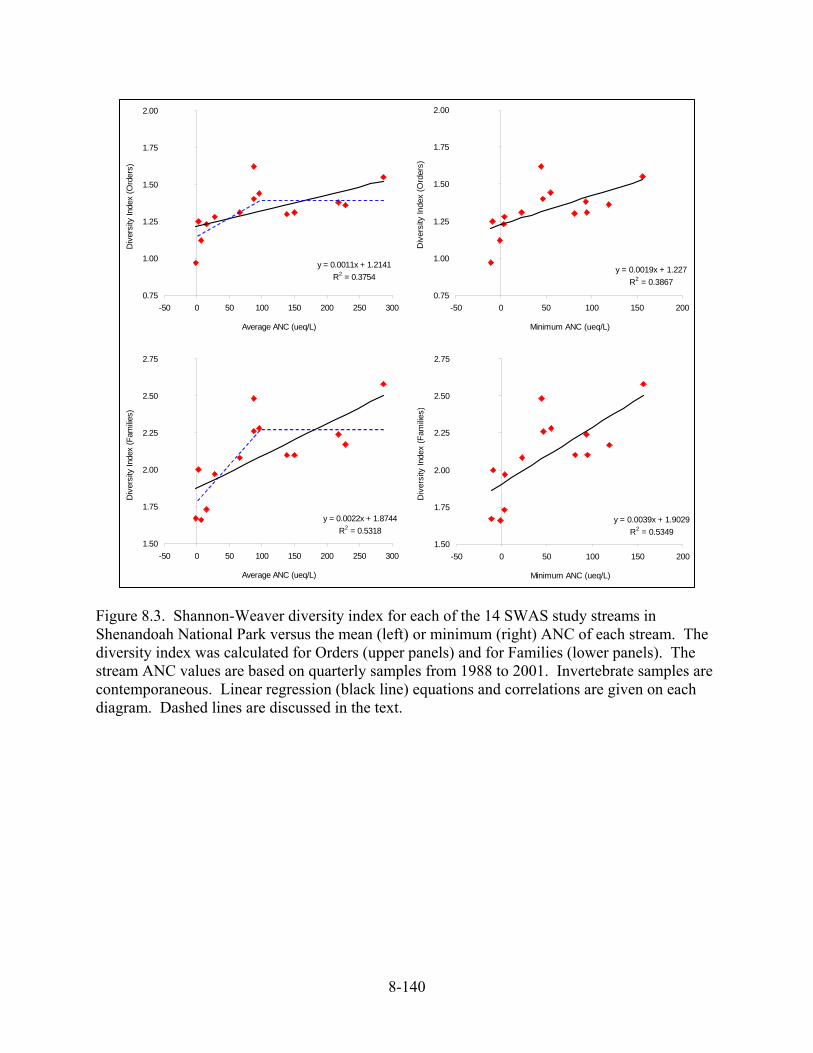
8-140

Figure 8.3. Shannon-Weaver diversity index for each of the 14 SWAS study streams in Shenandoah National Park versus the mean (left) or minimum (right) ANC of each stream. The diversity index was calculated for Orders (upper panels) and for Families (lower panels). The stream ANC values are based on quarterly samples from 1988 to 2001. Invertebrate samples are contemporaneous. Linear regression (black line) equations and correlations are given on each diagram. Dashed lines are discussed in the text.

y = 0.0011x + 1.2141R2 = 0.3754

0.75

1.00

1.25

1.50

1.75

2.00

-50 0 50 100 150 200 250 300

Average ANC (ueq/L)

Div

ersi

ty In

dex

(Ord

ers)

y = 0.0019x + 1.227R2 = 0.3867

0.75

1.00

1.25

1.50

1.75

2.00

-50 0 50 100 150 200

Minimum ANC (ueq/L)

Div

ersi

ty In

dex

(Ord

ers)

y = 0.0022x + 1.8744R2 = 0.5318

1.50

1.75

2.00

2.25

2.50

2.75

-50 0 50 100 150 200 250 300

Average ANC (ueq/L)

Div

ersi

ty In

dex

(Fam

ilies)

y = 0.0039x + 1.9029R2 = 0.5349

1.50

1.75

2.00

2.25

2.50

2.75

-50 0 50 100 150 200

Minimum ANC (ueq/L)

Div

ersi

ty In

dex

(Fam

ilies)

y = 0.0011x + 1.2141R2 = 0.3754

0.75

1.00

1.25

1.50

1.75

2.00

-50 0 50 100 150 200 250 300

Average ANC (ueq/L)

Div

ersi

ty In

dex

(Ord

ers)

y = 0.0019x + 1.227R2 = 0.3867

0.75

1.00

1.25

1.50

1.75

2.00

-50 0 50 100 150 200

Minimum ANC (ueq/L)

Div

ersi

ty In

dex

(Ord

ers)

y = 0.0022x + 1.8744R2 = 0.5318

1.50

1.75

2.00

2.25

2.50

2.75

-50 0 50 100 150 200 250 300

Average ANC (ueq/L)

Div

ersi

ty In

dex

(Fam

ilies)

y = 0.0039x + 1.9029R2 = 0.5349

1.50

1.75

2.00

2.25

2.50

2.75

-50 0 50 100 150 200

Minimum ANC (ueq/L)

Div

ersi

ty In

dex

(Fam

ilies)

y = 0.0011x + 1.2141R2 = 0.3754

0.75

1.00

1.25

1.50

1.75

2.00

-50 0 50 100 150 200 250 300

Average ANC (ueq/L)

Div

ersi

ty In

dex

(Ord

ers)

y = 0.0019x + 1.227R2 = 0.3867

0.75

1.00

1.25

1.50

1.75

2.00

-50 0 50 100 150 200

Minimum ANC (ueq/L)

Div

ersi

ty In

dex

(Ord

ers)

y = 0.0022x + 1.8744R2 = 0.5318

1.50

1.75

2.00

2.25

2.50

2.75

-50 0 50 100 150 200 250 300

Average ANC (ueq/L)

Div

ersi

ty In

dex

(Fam

ilies)

y = 0.0039x + 1.9029R2 = 0.5349

1.50

1.75

2.00

2.25

2.50

2.75

-50 0 50 100 150 200

Minimum ANC (ueq/L)

Div

ersi

ty In

dex

(Fam

ilies)

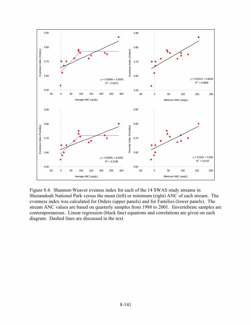
8-141

Figure 8.4. Shannon-Weaver eveness index for each of the 14 SWAS study streams in Shenandoah National Park versus the mean (left) or minimum (right) ANC of each stream. The evenness index was calculated for Orders (upper panels) and for Families (lower panels). The stream ANC values are based on quarterly samples from 1988 to 2001. Iinvertebrate samples are contemporaneous. Linear regression (black line) equations and correlations are given on each diagram. Dashed lines are discussed in the text.

y = 0.0006x + 0.6555R2 = 0.5671

0.50

0.60

0.70

0.80

0.90

-50 0 50 100 150 200 250 300

Average ANC (ueq/L)

Even

ness

Inde

x (O

rder

s)

y = 0.0012x + 0.6634R2 = 0.5806

0.50

0.60

0.70

0.80

0.90

-50 0 50 100 150 200

Minimum ANC (ueq/L)

Even

ness

Inde

x (O

rder

s)

y = 0.0006x + 0.6204R2 = 0.5785

0.50

0.60

0.70

0.80

0.90

-50 0 50 100 150 200 250 300

Average ANC (ueq/L)

Even

ness

Inde

x (F

amilie

s)

y = 0.001x + 0.628R2 = 0.5737

0.50

0.60

0.70

0.80

0.90

-50 0 50 100 150 200

Minimum ANC (ueq/L)

Div

ersi

ty In

dex

(Fam

ilies)

y = 0.0006x + 0.6555R2 = 0.5671

0.50

0.60

0.70

0.80

0.90

-50 0 50 100 150 200 250 300

Average ANC (ueq/L)

Even

ness

Inde

x (O

rder

s)

y = 0.0012x + 0.6634R2 = 0.5806

0.50

0.60

0.70

0.80

0.90

-50 0 50 100 150 200

Minimum ANC (ueq/L)

Even

ness

Inde

x (O

rder

s)

y = 0.0006x + 0.6204R2 = 0.5785

0.50

0.60

0.70

0.80

0.90

-50 0 50 100 150 200 250 300

Average ANC (ueq/L)

Even

ness

Inde

x (F

amilie

s)

y = 0.001x + 0.628R2 = 0.5737

0.50

0.60

0.70

0.80

0.90

-50 0 50 100 150 200

Minimum ANC (ueq/L)

Div

ersi

ty In

dex

(Fam

ilies)

y = 0.0006x + 0.6555R2 = 0.5671

0.50

0.60

0.70

0.80

0.90

-50 0 50 100 150 200 250 300

Average ANC (ueq/L)

Even

ness

Inde

x (O

rder

s)

y = 0.0012x + 0.6634R2 = 0.5806

0.50

0.60

0.70

0.80

0.90

-50 0 50 100 150 200

Minimum ANC (ueq/L)

Even

ness

Inde

x (O

rder

s)

y = 0.0006x + 0.6204R2 = 0.5785

0.50

0.60

0.70

0.80

0.90

-50 0 50 100 150 200 250 300

Average ANC (ueq/L)

Even

ness

Inde

x (F

amilie

s)

y = 0.001x + 0.628R2 = 0.5737

0.50

0.60

0.70

0.80

0.90

-50 0 50 100 150 200

Minimum ANC (ueq/L)

Div

ersi

ty In

dex

(Fam

ilies)

8-142

The dashed lines on the plots of diversity vs average ANC and evenness vs average ANC are intended to draw attention to the relationships in the ANC regions above and below ANC = 100 ueq/L. Both diversity and evenness decline in many streams as average ANC falls below 100 ueq/L (Figures 8.3 and 8.4). This is consistent with the responses seen above for family and individual richness – as the number of families decreases and the numbers of individuals in the remaining families also decreases (except for the few acidophilic families) the diversity and evenness of the community declines.

These differences in aquatic invertebrate community structure above and below average ANC of 100 ueq/L are also consistent with the definitions of the stream response categories that are used to map areas of concern with respect to adverse effects from acidic deposition in SHEN (Chapter 2). Streams with average ANC above 100 ueq/L are of “Low Concern”, and the diversity and evenness of these communities appears generally unaffected, while streams in the other concern categories (“Moderate”, Elevated” and “Acute”) show decreases in diversity and evenness. As before, the use of average ANC (rather than minimum ANC) in this analysis is important for linking the aquatic invertebrate responses to the MAGIC model forecasts of future stream ANC.

8.2.2 Acidification Effects on Fish in Shenandoah National Park

Although there are known differences in acid sensitivity among fish species, experimentally-determined acid sensitivities are available for only a minority of freshwater fish species. For example, of 35 species of fish found in SHEN, the critical pH is known for only nine (Table 8.2). Baker and Christensen (1991) reported critical pH values for 25 species of fish. They defined critical pH as the threshold for significant adverse effects on fish populations. The range of response within species depends on differences in sensitivity among life stages, and on different exposure concentrations of calcium (Ca2+) and Al. These ranges, based on multiple studies for each species, are shown in Table 8.2. To cite a few examples, blacknose dace (Rhinichthys atratulus) is regarded as very sensitive to acid stress, because population loss due to acidification has been documented in this species at pH values as high as 6.1; in field bioassays, embryo mortality has been attributed to acid stress at pH values as high as 5.9. Embryo mortality has occurred in common shiner (Luxilus cornutus) at pH values as high as 6.0. Although the critical pH range for rainbow trout (Oncorhynchus mykiss) is designated as 4.9–5.6, adult and juvenile mortality have occurred at pH values as high as 5.9. Brown trout (Salmo trutta) population loss has occurred over the pH range of 4.8–6.0, and brook trout fry mortality has occurred over the range of 4.8–5.9 (Baker and Christensen 1991).

It is the difference in acid tolerance among species that produces a gradual decline in species richness as acidification progresses, with the most sensitive species lost first. Some Blue Ridge streams can become too acidic even for brook trout, as evidenced by the absence of the species from streams with mean pH < 5.0 in Great Smoky Mountains National Park (Elwood et al. 1991).

Relatively less is known about changes in fish biomass, density and condition (robustness of individual fish) which occur in the course of acidification. Such changes result in part from both indirect and direct interactions within the fish community. Loss of sensitive individuals within species (such as early life stages) may reduce competition for food among the survivors, resulting in better growth rates, survival, or condition. Similarly, competitive release (increase in

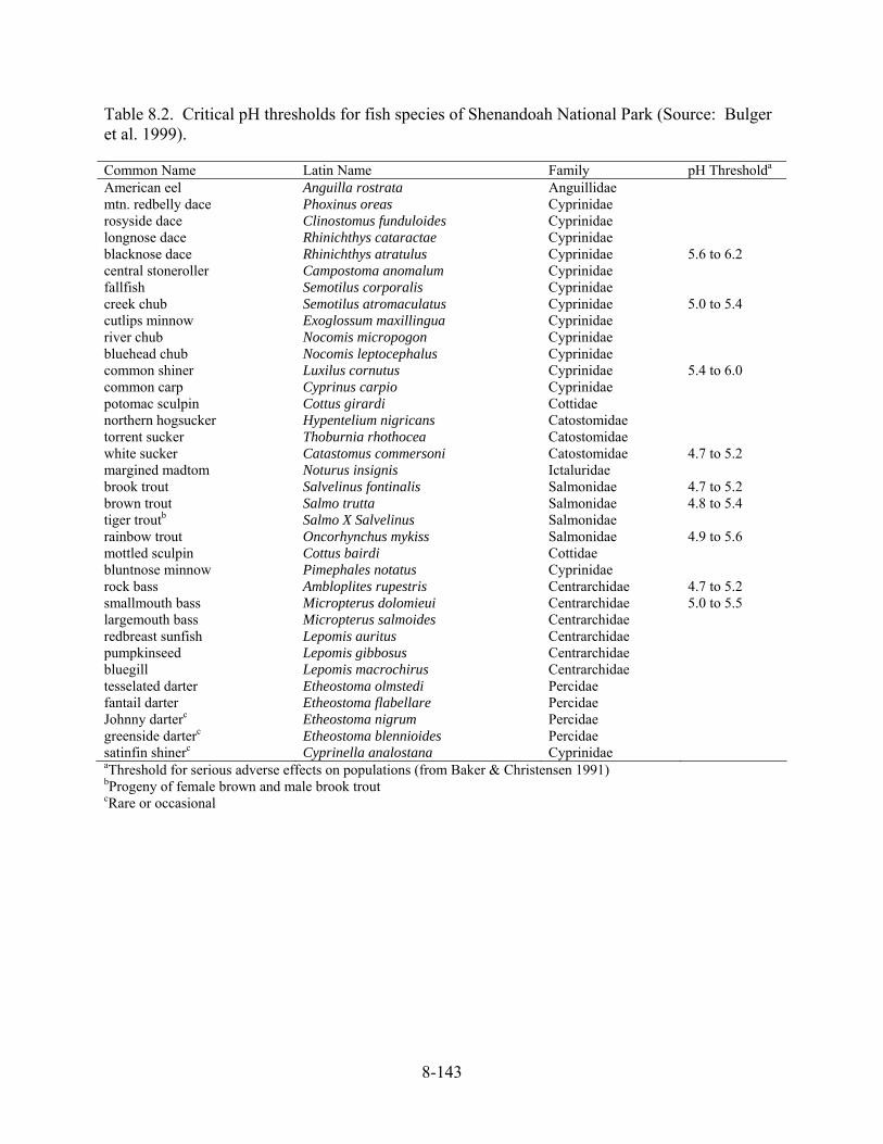
8-143

Table 8.2. Critical pH thresholds for fish species of Shenandoah National Park (Source: Bulger et al. 1999).

Common Name Latin Name Family pH Thresholda American eel Anguilla rostrata Anguillidae mtn. redbelly dace Phoxinus oreas Cyprinidae rosyside dace Clinostomus funduloides Cyprinidae longnose dace Rhinichthys cataractae Cyprinidae blacknose dace Rhinichthys atratulus Cyprinidae 5.6 to 6.2 central stoneroller Campostoma anomalum Cyprinidae fallfish Semotilus corporalis Cyprinidae creek chub Semotilus atromaculatus Cyprinidae 5.0 to 5.4 cutlips minnow Exoglossum maxillingua Cyprinidae river chub Nocomis micropogon Cyprinidae bluehead chub Nocomis leptocephalus Cyprinidae common shiner Luxilus cornutus Cyprinidae 5.4 to 6.0 common carp Cyprinus carpio Cyprinidae potomac sculpin Cottus girardi Cottidae northern hogsucker Hypentelium nigricans Catostomidae torrent sucker Thoburnia rhothocea Catostomidae white sucker Catastomus commersoni Catostomidae 4.7 to 5.2 margined madtom Noturus insignis Ictaluridae brook trout Salvelinus fontinalis Salmonidae 4.7 to 5.2 brown trout Salmo trutta Salmonidae 4.8 to 5.4 tiger troutb Salmo X Salvelinus Salmonidae rainbow trout Oncorhynchus mykiss Salmonidae 4.9 to 5.6 mottled sculpin Cottus bairdi Cottidae bluntnose minnow Pimephales notatus Cyprinidae rock bass Ambloplites rupestris Centrarchidae 4.7 to 5.2 smallmouth bass Micropterus dolomieui Centrarchidae 5.0 to 5.5 largemouth bass Micropterus salmoides Centrarchidae redbreast sunfish Lepomis auritus Centrarchidae pumpkinseed Lepomis gibbosus Centrarchidae bluegill Lepomis macrochirus Centrarchidae tesselated darter Etheostoma olmstedi Percidae fantail darter Etheostoma flabellare Percidae Johnny darterc Etheostoma nigrum Percidae greenside darterc Etheostoma blennioides Percidae satinfin shinerc Cyprinella analostana Cyprinidae aThreshold for serious adverse effects on populations (from Baker & Christensen 1991) bProgeny of female brown and male brook trout cRare or occasional

8-144

growth or abundance subsequent to removal of a competitor) may result from the loss of a sensitive species, with positive effects on the density, growth, or survival of competitor population(s) of other species (Baker et al. 1990b). In some cases where acidification continued, transient positive effects on size of surviving fish were shortly followed by extirpation (Bulger et al. 1993).

8.2.2.1 Previous Studies of Fish in Streams in Shenandoah National Park and Related Areas: The three-year FISH study of stream acidification in SHEN demonstrated negative effects on fish from both chronic and episodic acidification (Bulger et al. 1999). Biological differences in low- versus high-ANC streams included species richness, population density, condition factor (a measure of robustness in individual fish), age, size, and field bioassay survival. Of particular note is that both episodic and chronic mortality occurred in young brook trout exposed in a low-ANC stream, but not in a high-ANC stream (MacAvoy and Bulger 1995), and that blacknose dace in low-ANC streams were in poor condition relative to blacknose dace in higher-ANC streams (Dennis et al 1995; Dennis and Bulger 1995).

The effects of acidification on fish have been well documented for the St. Mary’s River (Bugas et al. 1999). Fourteen fish species have been collected in St. Mary’s River since 1976; only four remained as of 1998. Rosyside dace (Clinostomus funduloides) and torrent sucker (Thoburnia rhothocea) were last present in 1996; Johnny darter (Etheostoma nigrum) and brown trout were last present in 1994; rainbow trout and longnose dace (Rhinichthys cataractae) were last present in 1992; bluehead chub (Nocomis leptocephalus) and smallmouth bass (Micropterus dolomieui) were last present in 1990 and 1988, respectively; white sucker (Catastomus commersoni) and central stoneroller (Campostoma anomalum) were last present in 1986. Of the four remaining species, three (blacknose dace, fantail darter [Etheostoma flabellare]), and mottled sculpin [Cottus bairdi]) have declined in density and/or biomass; the fourth remaining species is brook trout, the region's most acid tolerant species; this population has fluctuated, and reproductive success has been sporadic. Blacknose dace, once abundant throughout the river, remain only at the lowest sampling station, which has the highest pH, and at such low numbers (five individuals in 1998) that they might be strays from downstream. For some of the species (smallmouth bass, white sucker, the three trout, and blacknose dace) the critical pH is known (see Table 8.2), and their decline and/or extirpation, given the pH of the river, is not surprising. Based on trend analysis over the period 1987–1997, the St. Mary’s River, near SHEN, is continuing to acidify (Webb and Deviney 1999).

Recent analyses (Bulger et al. 1998, 2000) divided Virginia's mountain streams into four categories of acid-base status, to compare the number of streams in each category at present with estimated numbers in pre-industrial times and in the future. Within SHEN, streams that are chronically or episodically acidic are the most likely to have experienced adverse biological effects from acidic deposition to date. They are also the streams most at risk for future damage. These streams are found primarily on siliciclastic bedrock.

8.2.2.2 New Studies of Fish in Streams in Shenandoah National Park from this Project: This study extended the SNP:FISH project (Bulger et al. 1999) to evaluate the acid sensitivity of five additional species of fish in SHEN using in situ bioassays -blacknose dace, longnose dace, mottled sculpin, mountain redbelly dace, and rosyside dace (Krawczel 2004). Paired bioassays (acidic treatment, neutral control) were conducted in Meadow Run (acidic treatment stream) and

8-145

the Rapidan River (non-acidic control stream). The bioassays were repeated twice during two different time periods in the autumn of 2003. An analysis of stream chemistry during the two periods verified that the stream chemistry was more acidic in the treatment stream (Meadow Run) during the second bioassay time period (mean pH=5.17) than the first (mean pH=5.32).

Mortality was not observed for any species during the first bioassay time period in either stream, although a statistical analysis suggested sub-lethal stresses occurred for longnose dace and rosyside dace in Meadow Run. Mortality was observed during the second bioassay time period in Meadow Run for all species except mottled sculpin, which may have experienced sub-lethal stress in that period. No mortality was observed during either bioassay time period in the Rapidan River (the neutral control).

The study concluded that fish can exhibit two types of response to stream chemistry that lead to mortality. In an acute response, fish die when chemical conditions reach a certain threshold level. In a cumulative dose response, fish die due to chronic exposure to low pH or high Al3+ over time (accumulation of H+ or Al3+ on the gill epithelium over time). This study suggests a cumulative dose mortality response in which fish begin to die when the total Al3+ exposure reaches 900 ug/L in less than 15 days (stream Al3+ concentrations > 60 ug/L per day for 15 days).

Differential fish mortality was observed across the five species used in this study. From most to least sensitive, the relative ranking of the five species is as follows: longnose dace, mountain redbelly dace, blacknose dace, rosyside dace, and mottled sculpin (Krawczel 2004).

8.2.2.3 Stream Water ANC Relationships for Fish in Shenandoah National Park Streams: ANC criteria have often been used in place of pH and/or aluminum criteria for evaluation of potential acidification effects on fish communities. The utility of these criteria lies in the association between ANC and the surface water constituents that directly contribute to or ameliorate acidity-related stress, in particular pH, Ca2+, and Al. The use of ANC criteria facilitates the coupling of models of fish response to acidification to the biogeochemical models that are used to estimate past of future stream water conditions because, in general, the biogeochemical models provide more reliable estimates of ANC than of pH. This section summarizes what is known concerning fish responses to stream water ANC in SHEN in two ways – those that relate individual species mortality to ANC (focusing on brook trout as the most important recreational species in SHEN) and those that relate community species richness to ANC (focusing on the biodiversity of all fish species with SHEN).

Brook Trout: The early life stages of brook trout are most sensitive to adverse impacts from acidification (Bulger et al. 2000). These early life stages occur in SHEN throughout the cold season in general, and the winter in particular. For this reason, data presented in Chapter 6 suggesting ongoing winter season acidification trends for streams within SHEN are of particular concern.

Bulger et al. (2000) developed ANC thresholds for brook trout response to acidification in forested headwater catchments in western Virginia (Table 8.3). Note that because brook trout are comparatively acid tolerant, adverse effects on many other fish species should be expected at relatively higher ANC values.

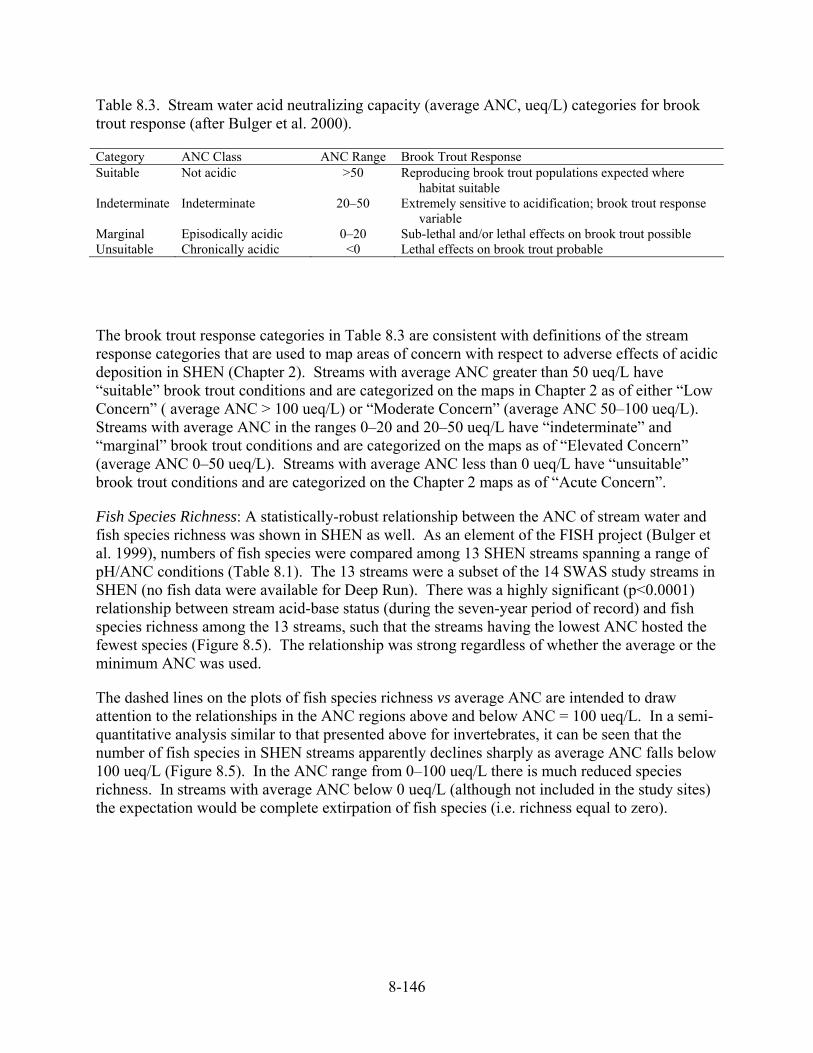
8-146

Table 8.3. Stream water acid neutralizing capacity (average ANC, ueq/L) categories for brook trout response (after Bulger et al. 2000).

Category ANC Class ANC Range Brook Trout Response Suitable Not acidic >50 Reproducing brook trout populations expected where

habitat suitable Indeterminate Indeterminate 20–50 Extremely sensitive to acidification; brook trout response

variable Marginal Episodically acidic 0–20 Sub-lethal and/or lethal effects on brook trout possible Unsuitable Chronically acidic <0 Lethal effects on brook trout probable

The brook trout response categories in Table 8.3 are consistent with definitions of the stream response categories that are used to map areas of concern with respect to adverse effects of acidic deposition in SHEN (Chapter 2). Streams with average ANC greater than 50 ueq/L have “suitable” brook trout conditions and are categorized on the maps in Chapter 2 as of either “Low Concern” ( average ANC > 100 ueq/L) or “Moderate Concern” (average ANC 50–100 ueq/L). Streams with average ANC in the ranges 0–20 and 20–50 ueq/L have “indeterminate” and “marginal” brook trout conditions and are categorized on the maps as of “Elevated Concern” (average ANC 0–50 ueq/L). Streams with average ANC less than 0 ueq/L have “unsuitable” brook trout conditions and are categorized on the Chapter 2 maps as of “Acute Concern”.

Fish Species Richness: A statistically-robust relationship between the ANC of stream water and fish species richness was shown in SHEN as well. As an element of the FISH project (Bulger et al. 1999), numbers of fish species were compared among 13 SHEN streams spanning a range of pH/ANC conditions (Table 8.1). The 13 streams were a subset of the 14 SWAS study streams in SHEN (no fish data were available for Deep Run). There was a highly significant (p<0.0001) relationship between stream acid-base status (during the seven-year period of record) and fish species richness among the 13 streams, such that the streams having the lowest ANC hosted the fewest species (Figure 8.5). The relationship was strong regardless of whether the average or the minimum ANC was used.

The dashed lines on the plots of fish species richness vs average ANC are intended to draw attention to the relationships in the ANC regions above and below ANC = 100 ueq/L. In a semi-quantitative analysis similar to that presented above for invertebrates, it can be seen that the number of fish species in SHEN streams apparently declines sharply as average ANC falls below 100 ueq/L (Figure 8.5). In the ANC range from 0–100 ueq/L there is much reduced species richness. In streams with average ANC below 0 ueq/L (although not included in the study sites) the expectation would be complete extirpation of fish species (i.e. richness equal to zero).

8-147

Figure 8.5. Number of fish species (species richness) in each of 13 SWAS study streams in Shenandoah National Park versus the mean (left) or minimum (right) ANC of each stream. The stream ANC values are based on quarterly samples from 1988 to 2001. The fish species richness samples are contemporaneous. Linear regression (black line) equations and correlations are given on each diagram. The dashed line is discussed in the text.

These differences in observed fish species over the observed range of average ANC are consistent with the definitions of the stream response categories that are used to map areas of concern with respect to adverse effects of acidic deposition in SHEN (Chapter 2). Streams with average ANC above 100 ueq/L are mapped as of “Low Concern” and species richness in these streams appears not to be strongly affected by acidic deposition. Streams with average ANC in the range 0–100 ueq/L (streams of “Moderate” and “Elevated” concern on the maps) have significantly reduced fish species richness. Streams with average ANC below 0 ueq/L (streams of “Acute Concern” on the maps) would be expected to have minimal species richness (zero or at most one fish species).

8.3 Overview of Soil Acidification Effects

8.3.1 Soil Base Cation Status

Calcium and other base cations are major components of surface water acid-base chemistry, and are also important nutrients that are taken up through plant roots in dissolved form. Base cations are typically found in abundance in rocks and soils, but a large fraction of the base cation stores are bound in mineral structures and are unavailable to plants. The pool of dissolved base cations resides in the soil as cations that are adsorbed to negatively-charged exchange sites. They can become desorbed in exchange for H+ or Aln+, and are thus termed exchangeable cations. The process of weathering gradually breaks down rocks and minerals, returning their stored base cations to the soil in dissolved form and thereby contributing to the pool of adsorbed base

y = 0.0246x + 2.1076R2 = 0.7616

0

1

2

3

4

5

6

7

8

9

10

-50 0 50 100 150 200 250 300

Average ANC (ueq/L)

Num

ber o

f Fis

h Sp

ecie

s

y = 0.0464x + 2.253R2 = 0.8643

0

1

2

3

4

5

6

7

8

9

10

-50 0 50 100 150 200

Minimum ANC (ueq/L)

Num

ber o

f Fis

h Sp

ecie

s

y = 0.0246x + 2.1076R2 = 0.7616

0

1

2

3

4

5

6

7

8

9

10

-50 0 50 100 150 200 250 300

Average ANC (ueq/L)

Num

ber o

f Fis

h Sp

ecie

s

y = 0.0464x + 2.253R2 = 0.8643

0

1

2

3

4

5

6

7

8

9

10

-50 0 50 100 150 200

Minimum ANC (ueq/L)

Num

ber o

f Fis

h Sp

ecie

s

y = 0.0246x + 2.1076R2 = 0.7616

0

1

2

3

4

5

6

7

8

9

10

-50 0 50 100 150 200 250 300

Average ANC (ueq/L)

Num

ber o

f Fis

h Sp

ecie

s

y = 0.0464x + 2.253R2 = 0.8643

0

1

2

3

4

5

6

7

8

9

10

-50 0 50 100 150 200

Minimum ANC (ueq/L)

Num

ber o

f Fis

h Sp

ecie

s

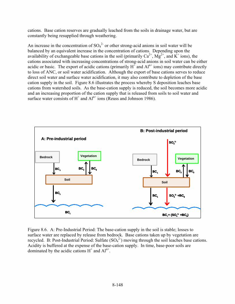
8-148

cations. Base cation reserves are gradually leached from the soils in drainage water, but are constantly being resupplied through weathering.

An increase in the concentration of SO42- or other strong-acid anions in soil water will be

balanced by an equivalent increase in the concentration of cations. Depending upon the availability of exchangeable base cations in the soil (primarily Ca2+, Mg2+, and K+ ions), the cations associated with increasing concentrations of strong-acid anions in soil water can be either acidic or basic. The export of acidic cations (primarily H+ and Aln+ ions) may contribute directly to loss of ANC, or soil water acidification. Although the export of base cations serves to reduce direct soil water and surface water acidification, it may also contribute to depletion of the base cation supply in the soil. Figure 8.6 illustrates the process whereby S deposition leaches base cations from watershed soils. As the base-cation supply is reduced, the soil becomes more acidic and an increasing proportion of the cation supply that is released from soils to soil water and surface water consists of H+ and Aln+ ions (Reuss and Johnson 1986).

Figure 8.6. A: Pre-Industrial Period: The base-cation supply in the soil is stable; losses to surface water are replaced by release from bedrock. Base cations taken up by vegetation are recycled. B: Post-Industrial Period: Sulfate (SO4

2-) moving through the soil leaches base cations. Acidity is buffered at the expense of the base-cation supply. In time, base-poor soils are dominated by the acidic cations H+ and Aln+.

BC1

Soil

VegetationBedrock

BC2 BC2BC1

BC1

BC1

Soil

VegetationBedrock

BC2 BC2BC1

BC1

A: Pre-industrial period

B: Post-industrial period

SO42-

BC1+ (SO42- +BC3)

Soil

VegetationBedrock

BC2 BC2BC1

BC1 SO42- +BC3

SO42-

BC1+ (SO42- +BC3)

Soil

VegetationBedrock

BC2 BC2BC1

BC1 SO42- +BC3

BC1

Soil

VegetationBedrock

BC2 BC2BC1

BC1

BC1

Soil

VegetationBedrock

BC2 BC2BC1

BC1

A: Pre-industrial period

B: Post-industrial period

SO42-

BC1+ (SO42- +BC3)

Soil

VegetationBedrock

BC2 BC2BC1

BC1 SO42- +BC3

SO42-

BC1+ (SO42- +BC3)

Soil

VegetationBedrock

BC2 BC2BC1

BC1 SO42- +BC3

8-149

The supply of base cations to watershed soils can be external or internal. External sources include atmospheric deposition of base cations. Internal watershed sources are the main sources of base cations in most upland drainage waters of the eastern United States (Baker 1991). The primary internal sources of base cations in most watersheds are weathering and soil exchange. By comparison with exchange reactions, weathering occurs at relatively slow and constant rates (Turner et al. 1990; Munson and Gherini 1991). Thus, the main source of cations for acid neutralization in most watersheds is the accumulated supply of exchangeable base cations in the soil. However, the size of this supply, and thus the degree to which soil and surface water acidification occurs, is ultimately determined in large part by the weathering of base cations in watershed bedrock. As reflected in the low ANC and low base cation concentrations of stream waters, most of the ridges in the central Appalachian Mountain region are underlain by base-poor bedrock (Webb et al. 1989; Church et al. 1992; Herlihy et al. 1993).

8.3.2 Forest and Surface Water Responses

Base cation availability in soils is an important buffer for protecting surface waters from acidic deposition. It is well known that elevated leaching of base cations by acidic deposition might deplete the soil of exchangeable bases faster than they are resupplied via weathering (Cowling and Dochinger 1980). However, scientific appreciation of the importance of this response has increased with the realization that watersheds are generally not exhibiting much ANC and pH recovery in response to recent decreases in S deposition (Lawrence and Huntington 1999; Driscoll et al. 2001). In many areas this low level of recovery can be at least partially attributed to decreased base cation concentrations in surface water, which may indicate base cation depletion from soils.

Base cation availability in soils is also a central component of forest nutrition. Calcium (Ca2+) is an essential component for wood formation and cell wall maintenance in trees (Lawrence et al. 1995). Calcium limitation has been shown to adversely influence disease resistance, wound repair, frost hardiness, and lignin synthesis (McLaughlin and Wimmer 1999). Magnesium (Mg2+) is at the center of chlorophyll and serves as an enzyme cofactor in processes such as the phosphorylation of ADP to form ATP (Binkley 1986). Potassium (K+) is an enzyme activator and plays a central role in stomatal conductance (Binkley 1986).

Soil acidification and/or base cation loss can be inferred from studies of elemental budgets (c.f., Binkley and Richter 1987). In addition to leaching by acidic deposition, there is a general tendency for some hardwood trees to accumulate Ca2+, especially oak and hickory species, and this can cause Ca2+ depletion and soil acidification. Such effects can be exacerbated by both tree harvesting and acidic deposition (Johnson et al. 1988). While calcium limitation has not been shown to be significant in eastern hardwood forests to date, several studies have suggested impending Ca2+ depletion with intensive harvesting (Johnson et al. 1988; Federer et al. 1989; Johnson and Todd 1990).

Recent evidence indicates that declining base cation reserves in forest soils are ongoing and bedrock weathering rates are not fast enough to supply the necessary replenishment (Huntington 2000). Of particular note in the forests of the southeastern U.S. are evidence of base cation depletion in loblolly pine (Pinus taeda L.) (Binkley et al. 1989) and oak-hickory (Quercus-Carya) (Johnson and Todd 1987) forests. Budgets of spruce-fir and hardwood sites in Maine,

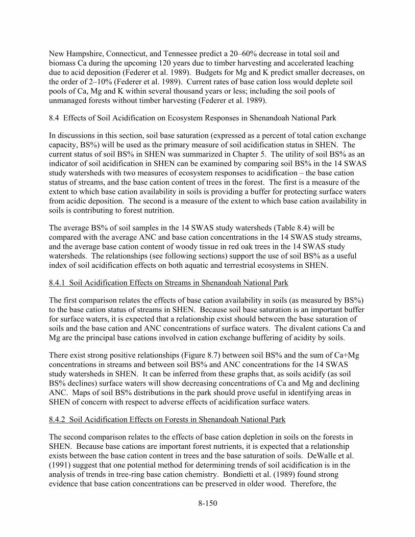
8-150

New Hampshire, Connecticut, and Tennessee predict a 20–60% decrease in total soil and biomass Ca during the upcoming 120 years due to timber harvesting and accelerated leaching due to acid deposition (Federer et al. 1989). Budgets for Mg and K predict smaller decreases, on the order of 2–10% (Federer et al. 1989). Current rates of base cation loss would deplete soil pools of Ca, Mg and K within several thousand years or less; including the soil pools of unmanaged forests without timber harvesting (Federer et al. 1989).

8.4 Effects of Soil Acidification on Ecosystem Responses in Shenandoah National Park

In discussions in this section, soil base saturation (expressed as a percent of total cation exchange capacity, BS%) will be used as the primary measure of soil acidification status in SHEN. The current status of soil BS% in SHEN was summarized in Chapter 5. The utility of soil BS% as an indicator of soil acidification in SHEN can be examined by comparing soil BS% in the 14 SWAS study watersheds with two measures of ecosystem responses to acidification – the base cation status of streams, and the base cation content of trees in the forest. The first is a measure of the extent to which base cation availability in soils is providing a buffer for protecting surface waters from acidic deposition. The second is a measure of the extent to which base cation availability in soils is contributing to forest nutrition.

The average BS% of soil samples in the 14 SWAS study watersheds (Table 8.4) will be compared with the average ANC and base cation concentrations in the 14 SWAS study streams, and the average base cation content of woody tissue in red oak trees in the 14 SWAS study watersheds. The relationships (see following sections) support the use of soil BS% as a useful index of soil acidification effects on both aquatic and terrestrial ecosystems in SHEN.

8.4.1 Soil Acidification Effects on Streams in Shenandoah National Park

The first comparison relates the effects of base cation availability in soils (as measured by BS%) to the base cation status of streams in SHEN. Because soil base saturation is an important buffer for surface waters, it is expected that a relationship exist should between the base saturation of soils and the base cation and ANC concentrations of surface waters. The divalent cations Ca and Mg are the principal base cations involved in cation exchange buffering of acidity by soils.

There exist strong positive relationships (Figure 8.7) between soil BS% and the sum of Ca+Mg concentrations in streams and between soil BS% and ANC concentrations for the 14 SWAS study watersheds in SHEN. It can be inferred from these graphs that, as soils acidify (as soil BS% declines) surface waters will show decreasing concentrations of Ca and Mg and declining ANC. Maps of soil BS% distributions in the park should prove useful in identifying areas in SHEN of concern with respect to adverse effects of acidification surface waters.

8.4.2 Soil Acidification Effects on Forests in Shenandoah National Park

The second comparison relates to the effects of base cation depletion in soils on the forests in SHEN. Because base cations are important forest nutrients, it is expected that a relationship exists between the base cation content in trees and the base saturation of soils. DeWalle et al. (1991) suggest that one potential method for determining trends of soil acidification is in the analysis of trends in tree-ring base cation chemistry. Bondietti et al. (1989) found strong evidence that base cation concentrations can be preserved in older wood. Therefore, the

8-151

Table 8.4. Minimum, average, and maximum soil base saturation (BS) values in the 14 SWAS Watersheds. These data are for vertically aggregated soil samples. Between 4 and 6 soil pits were sampled in each watershed.

BS (%) Site ID Watershed Minimum Average Maximum

Siliciclastic Bedrock Class DR01 Deep Run 7.0 11.3 18.8 VT35 (PAIN) Paine Run 10.5 21.8 40.3 VT36 Meadow Run 8.2 13.7 19.7 VT53 Twomile Creek 12.5 26.8 38.8 WOR1 White Oak Run 5.5 8.5 13.3

Granitic Bedrock Class NFDR North Fork Dry Run 7.6 13.1 15.6 VT58 Brokenback Run 7.6 13.9 24.3 VT59 (STAN) Staunton River 8.7 25.4 53.2 VT62 Hazel River 14.4 21.5 32.2

Basaltic Bedrock Class VT51 Jeremys Run 17.6 34.6 49.7 VT60 (PINE) Piney River 16.7 38.9 70.4 VT61 North Fork Thornton River 27.2 53.9 66.9 VT66 Rose River 18.2 43.5 66.3 VT75 White Oak Canyon Run 12.7 32.9 58.1

Figure 8.7. Average ANC (left panel; ueq/L) and average Ca+Mg concentrations (right panel; ueq/L) in the 14 SWAS study streams in Shenandoah National Park versus the average base saturation (%) of the soils in each watershed. The stream ANC and Ca+Mg values are based on quarterly samples from 1988 to 2001. The soils were sampled in 2001. Between 4 and 6 soil pits were sampled in each watershed. Linear regression (black line) equations and correlations are given on each diagram.

y = 5.7942x - 48.256R2 = 0.7233

-50

0

50

100

150

200

250

300

350

0 10 20 30 40 50 60

average soil BS%

aver

age

stre

am A

NC

ueq

/L

y = 5.4527x + 9.6518R2 = 0.6993

0

50

100

150

200

250

300

350

0 10 20 30 40 50 60

average soil BS%

aver

age

stre

am C

a+M

g co

ncen

tratio

n ue

q/L

y = 5.7942x - 48.256R2 = 0.7233

-50

0

50

100

150

200

250

300

350

0 10 20 30 40 50 60

average soil BS%

aver

age

stre

am A

NC

ueq

/L

y = 5.4527x + 9.6518R2 = 0.6993

0

50

100

150

200

250

300

350

0 10 20 30 40 50 60

average soil BS%

aver

age

stre

am C

a+M

g co

ncen

tratio

n ue

q/L

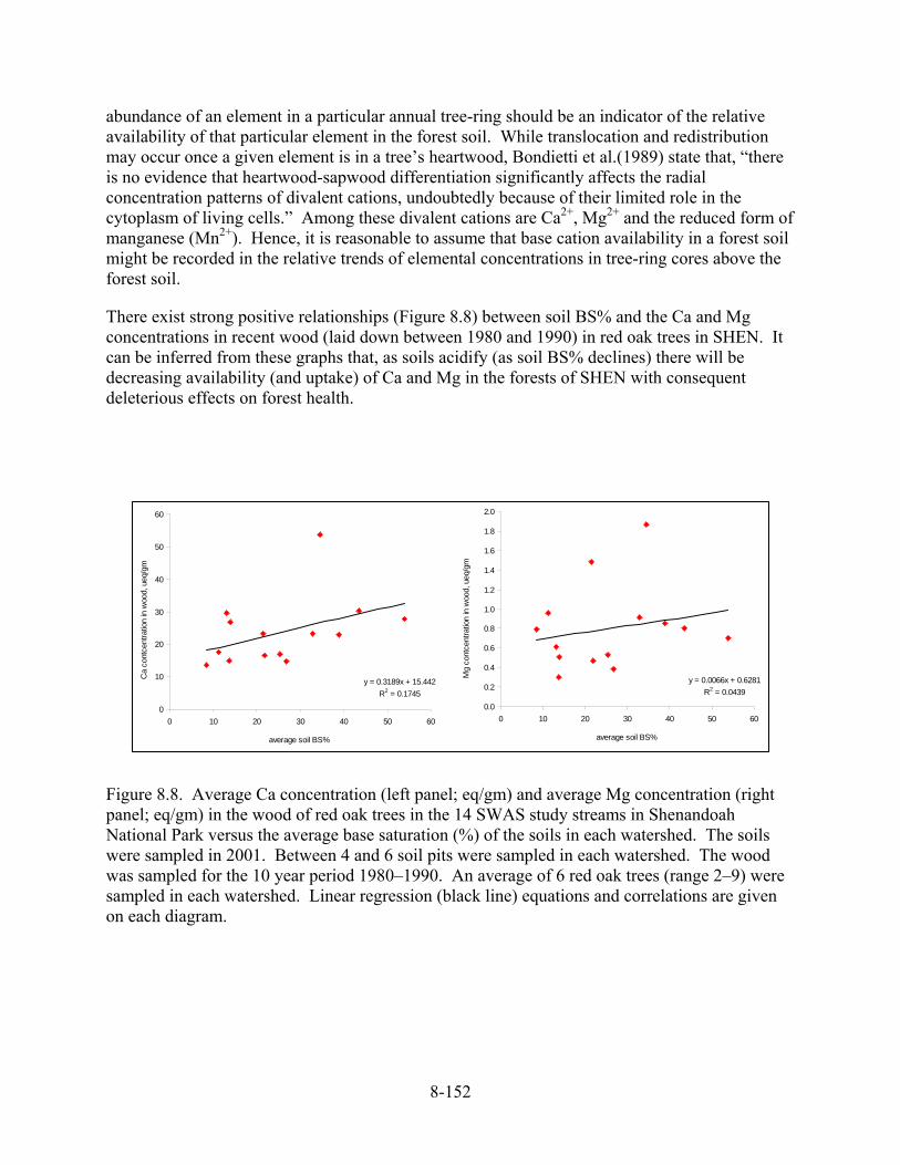
8-152

abundance of an element in a particular annual tree-ring should be an indicator of the relative availability of that particular element in the forest soil. While translocation and redistribution may occur once a given element is in a tree’s heartwood, Bondietti et al.(1989) state that, “there is no evidence that heartwood-sapwood differentiation significantly affects the radial concentration patterns of divalent cations, undoubtedly because of their limited role in the cytoplasm of living cells.” Among these divalent cations are Ca2+, Mg2+ and the reduced form of manganese (Mn2+). Hence, it is reasonable to assume that base cation availability in a forest soil might be recorded in the relative trends of elemental concentrations in tree-ring cores above the forest soil.

There exist strong positive relationships (Figure 8.8) between soil BS% and the Ca and Mg concentrations in recent wood (laid down between 1980 and 1990) in red oak trees in SHEN. It can be inferred from these graphs that, as soils acidify (as soil BS% declines) there will be decreasing availability (and uptake) of Ca and Mg in the forests of SHEN with consequent deleterious effects on forest health.

Figure 8.8. Average Ca concentration (left panel; eq/gm) and average Mg concentration (right panel; eq/gm) in the wood of red oak trees in the 14 SWAS study streams in Shenandoah National Park versus the average base saturation (%) of the soils in each watershed. The soils were sampled in 2001. Between 4 and 6 soil pits were sampled in each watershed. The wood was sampled for the 10 year period 1980–1990. An average of 6 red oak trees (range 2–9) were sampled in each watershed. Linear regression (black line) equations and correlations are given on each diagram.

y = 0.3189x + 15.442R2 = 0.1745

0

10

20

30

40

50

60

0 10 20 30 40 50 60

average soil BS%

Ca

cont

cent

ratio

n in

woo

d, u

eq/g

m

y = 0.0066x + 0.6281R2 = 0.0439

0.0

0.2

0.4

0.6

0.8

1.0

1.2

1.4

1.6

1.8

2.0

0 10 20 30 40 50 60

average soil BS%

Mg

cont

cent

ratio

n in

woo

d, u

eq/g

m

y = 0.3189x + 15.442R2 = 0.1745

0

10

20

30

40

50

60

0 10 20 30 40 50 60

average soil BS%

Ca

cont

cent

ratio

n in

woo

d, u

eq/g

m

y = 0.0066x + 0.6281R2 = 0.0439

0.0

0.2

0.4

0.6

0.8

1.0

1.2

1.4

1.6

1.8

2.0

0 10 20 30 40 50 60

average soil BS%

Mg

cont

cent

ratio

n in

woo

d, u

eq/g

m

8-153

8.4.3 Soil Base Saturation % Categories for Soil Acidification Responses

The analyses above indicate that soil BS% is related to soil acidification effects in both streams and forests in SHEN. However, the ranges of observed soil acidification responses in SHEN (especially with respect to forest health effects) do not extend very far into the “damaged” region. Therefore the selection of thresholds which can be used to define categories of soil acidification based on soil BS% is somewhat problematic in SHEN. The BS% response categories used for the maps in Chapter 2 were derived from a consideration of the responses described above in SHEN and the responses observed in other regions of the northeastern and mid-Atlantic US. The latter are summarized below. This material was largely derived from a discussion with Dr. Greg Lawrence of the USGS (pers. comm., 2006).

With respect to soil BS% relationships to surface water acidification, Lawrence et al. (1997) and Lawrence (2002) derived the following categories based on a statistical analysis of the B horizons of soils in forested watersheds in the Adirondack region of NY. For base saturation less than 8% severe effects on surface water biota are expected during high flows. For base saturation in the range 8–12% moderate effects are expected. For base saturation in the range 12–17% slight effects are expected. For watersheds with base saturation greater than 17% no effects were detectable.

Dr. Lawrence pointed out (pers. comm., 2006) that there is less information available to identify the critical levels of base saturation for trees, although it's clear that growth and health are related to base saturation. There is evidence that it's the change in base saturation over the life of the tree that is more important than an actual threshold, at least for red and norway spruce. In other words, a tree might be okay growing (albeit slowly) in soil with a base saturation of 15%, if that value remains fairly constant, but they found that growth of Norway Spruce in Russia showed a strong adverse effect when base saturation decreased from 30% to 20 % over three decades.

Nonetheless, Dr. Lawrence suggested that, based on research to date, the following categories of base saturation might be promulgated for forest responses. Above 20% base saturation no adverse effects are expected on forests. In the range 10–20% base saturation forest growth will be slowed. Below 10% base saturation, there would be the risk of mortality from various stresses, particularly if the base saturation was previously above 10% during the life of the tree.

Dr. Lawrence suggested that combining what was known of both forest and surface water acidification effects, reasonable categories for sol BS% would be: greater than 20% no effects; in the range 10–20% moderate effects would be probable; below 10% moderate effects would be certain and severe effects would be probable. We used these categories for analysis of soil acidification effects in SHEN (see Chapter 2) with the additional refinement of dividing the lower category into two ranges: 0–5% and 5–10%.

9-155

9. References

Altman, D., T. Bryant, M. Gardner, and D. Machin. 2000. Statistics with Confidence. BMJ Books. London.

Badger, R. L. 1999. Geology Along Skyline Drive, Shenandoah National Park, Virginia. A Self-Guided Tour for Motorists. Falcon Publishing, Inc. Helena, MT. 100 pp.

Baker, J. P., D. P. Bernard, S. W. Christensen, M. J. Sale, J. Freda, K. Heltcher, D. Marmorek, L. Rowe, P. Scanlon, G. Suter, W. Warren-Hicks, and P. Welbourn. 1990b. Biological Effects of Changes in Surface Water Acid-base Chemistry. SOS/T Report 13. Acid Precipitation Assessment Program. Washington, DC.

Baker, J. P., and S. W. Christensen. 1991. Effects of acidification on biological communities. In Charles, D.F. (ed.). Acidic Deposition and Aquatic Ecosystems. Springer-Verlag. New York. Pp. 83–106.

Baker, L. A. 1991. Ion enrichment analysis for the Regional Case Studies Project. In Charles, D.F. (ed.). Acidic Deposition and Aquatic Ecosystems: Regional Case Studies. Springer-Verlag. New York. pp. 641–644.

Baker, L. A., A. T. Herlihy, P. R. Kaufmann, and J. M. Eilers. 1991. Acidic lakes and streams in the United States: the role of acidic deposition. Science 252:1151–1154.

Baker, L. A., P. R. Kaufmann, A. T. Herlihy, and J. M. Eilers. 1990a. Current Status of Surface Water Acid-Base Chemistry. State of the Science SOS/T 9, National Acid Precipitation Program.

Binkley, D. 1986. Forest Nutrition Management. John Wiley and Sons, Inc. New York. Pp. 2–8.

Binkley, D., C. Driscoll, H. L. Allen, P. Schoeneberger, and D. McAvoy. 1989. Acidic Deposition and Forest Soils: Context and Case Studies in the Southeastern U.S. Springer-Verlag. Ecological Studies No. 72. New York. 149 p.

Binkley, D., and D. Richter. 1987. Nutrient cycles and H+ budgets of forest ecosystems. Adv. Ecol. Res. 16:1–51.

Binkowski, F. S., and U. Shankar. 1995. The Regional Particulate Matter Model, 1. Model description and preliminary results. J. Geophys. Res. 100(26):191–209.

Bondietti, E. A., C. F. Baes, III, and S.B. McLaughlin. 1989. Radial trends in cation ratios in tree rings as indicators of the impact of atmospheric deposition on forests. Canadian Journal of Forest Research 19:586–594.

Brakke, D. F., A. Henriksen, and S. A. Norton. 1989. Estimated background concentrations of sulfate in dilute lakes. Water Resour. Bull. 25:247–253.

9-156

Bricker, O.P. and K.C. Rice. 1989. Acidic deposition to streams – a geology-based method predicts their sensitivity. Environ. Sci. Technol. 23:379–385.

Bugas, P. E., Jr., L. O. Mohn, and J. W. Kauffman. 1999. Impacts of acid deposition on fish populations in the St. Marys River, Augusta County, Virginia. Banisteria 13:191–200.

Bulger, A. J., B. J. Cosby, C. A. Dolloff, K. N. Eshleman, J. R. Webb, and J. N. Galloway. 1999. SNP:FISH. Shenandoah National Park: Fish In Sensitive Habitats. Project Final report. Volume I: Project Description and Summary of Results; Volume II: Stream Water Chemistry and Discharge, and Synoptic Water Quality Surveys; Volume III: Basin-wide Habitat and Population Inventories, and Behavioral Responses to Acid in a Laboratory Stream; Volume IV: Stream Bioassays, Aluminum Toxicity, Species Richness and Stream Chemistry, and Models of Susceptibility to Acidification. Project Completion Report to the National Park Service. Cooperative Agreement CA-4000-2-1007, Supplemental Agreement #2. Dept. of Environmental Sciences, University of Virginia, Charlottesville.

Bulger, A. J., B. J. Cosby, and J. R. Webb. 1998. Acid Rain: Current and projected status of coldwater fish communities in the Southeastern U.S. in the context of continued acid deposition. Trout Unlimited. Arlington Virginia. 28 p.

Bulger, A. J., B. J. Cosby, and J. R. Webb. 2000. Current, reconstructed past and projected future status of brook trout (Salvelinus fontinalis) streams in Virginia. Can. J. Fish. Aq. Sci. 57:1515–1523.

Bulger, A. J., L. Lien, B. J. Cosby, and A. Henriksen. 1993. Trout status and chemistry from the Norwegian thousand lake survey: statistical analysis. Can. J. Fish. Aq. Sci. 50(3):575–585.

California Air Resources Board (CAB). 2001. Buyers’ Guide to Cleaner Cars, published on the web at http://arbis.arb.ca.gov/msprot/CCBG/ccbg.htm. March 13, 2001.

Carter, J. B. 1961. Soil survey of Rappahannock County, Virginia. USDA Soil Conservation Service. 85 pp.

Chang, J. S., F. S. Binkowski, N. L. Seaman, J. N. McHenry, D. Byun, P. J. Samson, W. R. Stockwell, C. J. Walcek, S. Madronich, P. Middleton, J. E. Pleim., and H. H. Lansford. 1990. The Regional Acid Deposition Model and engineering model. NAPAP SOS/T Report No. 4. In National Acid Precipitation Assessment Program: State of Science and Technology, Vol 1. National Acid Precipitation Assessment Program. Washington, DC.

Chang, J. S., R. A. Brost, I. S. A. Isaksen, S. Madronich, P. Middleton,, W. R. Stockwell, and C. J. Walcek. 1987. A three-dimensional Eulerian acid deposition model: Physical concepts and formation. J. Geophys. Res. 92(14):681–700.

9-157

Church, M. R., P. W. Shaffer, K. W. Thornton, D. L. Cassell, C. I. Liff, M. G. Johnson, D. A. Lammers, J. J. Lee, G. R. Holdren, J. S. Kern, L. H. Liegel, S. M. Pierson, D. L. Stevens, B. P. Rochelle, and R. S. Turner. 1992. Direct/Delayed Response Project: Future Effects of Long-Term Sulfur Deposition on Stream Chemistry in the Mid-Appalachian Region of the Eastern United States. U.S. Environmental Agency. EPA/600/R-92/186. Washington, DC. 384 pp.

Cosby, B. J., A. Jenkins, R. C. Ferrier, J. D. Miller, and T. A. B. Walker. 1990. Modeling stream acidification in afforested catchments: Long-term reconstructions at two sites in central Scotland. Journal of Hydrology 120:143–162.

Cosby, B. J., G. M. Hornberger, J. N. Galloway, and R. F. Wright. 1985c. Time scales of catchment acidification: a quantitative model for estimating freshwater acidification. Environ. Sci. Technol. 19:1144–1149.

Cosby, B. J., P. F. Ryan, J. R. Webb, G. M. Hornberger, and J. N. Galloway. 1991. Mountains of West Virginia. In: Charles, D.F. (Ed.). Acidic Deposition and Aquatic Ecosystems. Regional Case Studies. Springer-Verlag. New York. Pp. 297–318.

Cosby, B. J., R. F. Wright, and E. Gjessing. 1995. An acidification model (MAGIC) with organic acids evaluated using whole-catchment manipulations in Norway. J. Hydrol. 170:101–122.

Cosby, B. J., R. F. Wright, G. M. Hornberger, and J. N. Galloway. 1985a. Modeling the effects of acid deposition: assessment of a lumped parameter model of soil water and stream water chemistry. Water Resour. Res. 21:51–63.

Cosby, B.J., R. F. Wright, G. M. Hornberger, and J. N. Galloway. 1985b. Modeling the effects of acid deposition: estimation of long-term water quality responses in a small forested catchment. Water Resour. Res. 21:1591–1601.

Cosby, B. J., S. A. Norton, and J. S. Kahl. 1996. Using a paired-catchment manipulation experiment to evaluate a catchment-scale biogeochemical model. Sci. Tot. Environ. 183:49–66.

Cowling, E. B., and L. S. Dochinger. 1980. Effects of acidic precipitation on health and productivity of forests: USDA Forest Service Technical Report. PSW-43. Pp. 165–173.

Cronan, C. S., and C. L. Schofield. 1990. Relationships between aqueous aluminum and acidic deposition in forested watersheds of North America and northern Europe. Environ. Sci. Technol. 24:1100–1105.

Dennis, R. L. 1997. Using the Regional Acid Deposition Model to determine the nitrogen deposition airshed of the Chesapeake Bay watershed, in Baker, J.E. (ed.). Atmospheric Deposition of Contaminants to the Great Lakes and Coastal Waters. SETAC Press. Pensacola, FL. Pp 393–413.

9-158

Dennis, R. L., F. S. Binkowski, T. L. Clark, J. N. McHenry, S. Reynolds, and S. K. Seilkop. 1990. Evaluation of Regional Acid Deposition Models: Appendix 5F: Selected Applications of RADM (Part II). NAPAP State of Science and Technology Report No 5. In Acidic Deposition: State of Science and Technology, Volume 1. National Acid Precipitation Assessment Program, Washington, DC.

Dennis R. L., and R. Mathur. 2001. Airshed domains for modeling atmospheric deposition of oxidized and reduced nitrogen to the Neuse/Pamlico system of North Carolina. Hydrolog. Sci. Technol., Special Issue, 17(1–4):107–117.

Dennis, T. E., and A. J. Bulger. 1995. Condition factor and whole-body sodium concentration in a freshwater fish: evidence of acidification stress and possible ionoregulatory over-compensation. Water Air Soil Pollut. 85:377–382.

Dennis, T. E., S. E. MacAvoy, M. B. Steg, and A. J. Bulger. 1995. The association of water chemistry variables and fish condition in streams of Shenandoah National Park (USA). Water Air Soil Pollut. 85:365–370.

Dennis, T. E., and A. J. Bulger. 1999. The susceptibility of blacknose dace (Rhinichthys atratulus) to acidification in Shenandoah National Park. In A. B. Bulger, B. J. Cosby, C. A. Dolloff, K. N. Eshleman, J. N. Galloway, and J. R. Webb. henandoah National Park Fish in Sensitive Habitats. Project Final Report, Volume IV, Chapter 6B. See Bulger et al. (1999a) for complete citation.

DeWalle, D. R., B. R. Swistock, R. G. Sayre, and W. E. Sharpe. 1991. Spatial variation of sapwood chemistry with soil acidity in Appalachian forests. Journal of Environmental Quality 20: 86–491.

Driscoll, C. T., G. B. Lawrence, A. J. Bulger, T. J. Butler, C. C. Cronan, C. Eager, K. L. Lambert, G. E. Likens, J. L. Stoddard, and K. C. Weathers. 2001. Acidic Deposition in the Northeastern United States: Sources and inputs, ecosystem effects, and management strategies. Bioscience 51:180–198.

Driscoll, C. T., R. M. Newton, C. P. Gubala, J. P Baker, and S. W. Christenson. 1991. Adirondack Mountains. In D. F. Charles (Ed). Acid Deposition and Aquatic Ecosystems: Regional Case Studies. Springer-Verlag. New York.

Edmunds, W. J., D. D. Rector, N. O. Wilson, and T. L. Arnold. 1986. Properties, Classification, and Upland Oak Site Quality for Residual Soils Derived from Shales, Phyllites, Siltstones, and Sandstones in Southwestern Virginia. Bulletin 86-5. July. Virginia Agricultural Experiment Station.

Elder, J. H., and D. E. Pettry. 1975. Soil Survey of Madison County, Virginia. USDA Soil Conservation Survey. 143 pp.

Elwood, J. W. 1991. Southeast Overview. In Charles, D. F. (ed.). Acidic Deposition and Aquatic Ecosystems. Springer-Verlag. New York. Pp. 291–295.

9-159

Elwood, J. W., M. J. Sale, P. R. Kaufmann, and G. F. Cada. 1991. The Southern Blue Ridge Province. In Charles, D. F. (ed.). Acidic Deposition and Aquatic Ecosystems. Springer-Verlag. New York Pp. 319–364.

Eshleman, K. N. 1988. Predicting regional episodic acidification of surface waters using empirical models. Water Resour. Res. 34:1118–1126.

Eshleman, K. N., D. A. Fiscus, N. M. Castro, J. R. Webb, and F. A. Deviney, Jr. 2001. Computation and visualization of regional-scale forest disturbance and associated dissolved nitrogen export from Shenandoah National Park, Virginia. The Scientific World 1(S2):539–547.

Eshleman, K. N., and K. E. Hyer. 1999. Discharge and water chemistry at the three intensive sites. In Bulger, A .J., B .J. Cosby, C. A. Dolloff, K. N. Eshleman, J. R. Webb, and J. N. Galloway. Shenandoah National Park: Fish in Sensitive Habitats. Project Final Report - Vol. II. Stream Water Chemistry and Discharge, and Synoptic Water Quality Surveys. Pp. 51–92.

Eshleman, K. N., R. P. Morgan, II, J. R. Webb, F. A. Deviney, and J. N. Galloway. 1998. Temporal patterns of nitrogen leakage from mid-Appalachian forested watersheds: Role of insect defoliation. Water Resour. Res. 34:2005–2016.

Eshleman, K. N., T. D. Davies, M. Tranter, and P. J. Wigington, Jr. 1995. A two-component mixing model for predicting regional episodic acidification of surface waters during spring snowmelt periods. Water Resour. Res. 31:1011–1021.

Estes, M. J. 1990. The chemical composition of cloud water in the Shenandoah National Park and its variation with long-range atmospheric transport and season. Masters Thesis. Department of Environmental Sciences, University of Virginia, Charlottesville.

Federer, C. A., J. W. Hornbeck, L. M. Tritton, C. W. Martin, R. S. Pierce, and C. T. Smith. 1989. Long-term depletion of calcium and other nutrients in eastern U.S. forests. Environ. Manage. 13:593–601.

Feldman, R., and E. Connor. 1992. The relationship between pH and community structure of invertebrates in streams of the Shenandoah National Park, Virginia, U.S.A. Freshw. Biol. 27:261–276.

Galloway, J. N., F. A, Deviney, Jr., and J. R. Webb. 1999. Shenandoah Watershed Study Data Assessment: 1980–1993. Project Final Report. Submitted to National Park Service. Luray, VA.

Galloway, J. N., G. E. Likens, and M. E. Hawley. 1984. Acid precipitation: natural versus anthropogenic components. Science 226:829–831.

Galloway, J. N., S. A. Norton, and M. R. Church. 1983. Freshwater acidification from atmospheric deposition of sulfuric acid: a conceptual model. Environ. Sci. Tech. 17:541–545.

9-160

Gathright, T. M., II. 1976. Geology of The Shenandoah National Park, Virginia. Virginia Division of Mineral Resources Bulletin 86. Charlottesville. 93 pp.

Hack, J. T., and J. C. Goodlett. 1960. Geomorphology and Forest Ecology of a Mountain Region in the Central Appalachians. Prof. Paper 347. U.S. Geol. Surv. Reston, VA.

Harr, R. D. 1982. Fog drip in the Bull Run Municipal Watershed, Oregon. Water Resour. Bull. 18:785–789.

Herlihy, A. T., D. P. Larsen, S. G. Paulsen, N. S. Urquhart, and B. J. Rosenbaum. 2000. Designing a spatially balanced, randomized site selection process for regional stream surveys: the EMAP Mid-Atlantic Pilot Study. Environ. Monit. Assess. 63:95–113.

Herlihy, A. T., P. R. Kaufmann, J. L. Stoddard, K. N. Eshleman, and A. J. Bulger. 1996. Effects of acidic deposition on aquatic resources in the Southern Appalachians with a special focus on Class I wilderness areas. Report prepared for the Southern Appalachian Mountains Initiative (SAMI). Asheville, NC.

Herlihy, A. T., P. R. Kaufmann, M. R. Church, P. J. Wigington, Jr., J. R. Webb, and M. J. Sale. 1993. The effects of acid deposition on streams in the Appalachian Mountain and Piedmont region of the mid-Atlantic United States. Water Resour. Res. 29:2687–2703.

Hirsch, R.M. and J.R. Slack, 1984. A nonparametric trend test for seasonal data with serial dependence. Water Res. Res. 20:727.

Hirsch, R. M., J. R. Slack, and R. A. Smith. 1982. Techniques of trend analysis for monthly water quality analysis. Water Resour. Res. 18:107.

Hockman, J. R., J. C. McKinney, T. R. Burruss, D. Jones, R. E. Modesitt, L. G. Manhart, and W. R. Waite. 1979. Soil survey of Augusta County, Virginia. USDA Soil Conservation Service. 249 pp.

Hov, Ø., and B. A. Hjøllo. 1994. Transport distance of ammonia and ammonium in Northern Europe 2. Its relation to emissions of SO2 and NOx. J. Geophys. Res. 99:749–755.

Huntington, T. G. 2000. The potential for calcium depletion in forest ecosystems of southeastern United States: Review and analysis. Global Biogeochemical Cycles 4:623.

Hyer, K. E., J. R. Webb, and K. N. Eshleman. 1995. Episodic acidification of three streams in Shenandoah National Park, Virginia, USA. Water Air Soil Pollut. 85:523–528

Jenkins, A., P. G. Whitehead, B. J. Cosby, and H. J. B. Birks. 1990. Modeling long term acidification: a comparison with diatom reconstructions and the implications for reversibility. Phil. Trans. R. Soc. Lond. B. 327:435–440.

Jenkins, R. E., and N. M. Burkhead. 1993. Freshwater Fishes of Virginia. American Fisheries Society. Bethesda, MD. 1,079 pp.

9-161

Johnson, D. W., and D. E. Todd. 1987. Nutrient export by leaching and whole tree harvesting in a loblolly pine and mixed-oak forest. Plant Soil 102:99–109.

Johnson, D. W., and D. E. Todd. 1990. Nutrient cycling in forests of Walker Branch Watershed Tennessee: roles of uptake and leaching in causing soil changes. J. Environ. Qual. 19:97–104.

Johnson, D. W., and D. W. Cole. 1980. Mobility in soils: relevance to nutrient transport from forest ecosystems. Environ. Internat. 3:79–90.

Johnson, D. W., J. M. Kelly, W. T. Swank, D. W. Cole, H. Miegroet, J. W. Hornbeck, R. S. Pierce, and D. Van Lear. 1988. The effects of leaching and whole-tree harvesting on cation budgets of several forests. J. Environ. Qual. 17:418–424.

Johnson, D. W., and S. E. Lindberg, eds. 1992. Atmospheric Deposition and Forest Nutrient Cycling: A Synthesis of the Integrated Forest Study. Springer-Verlag. NY. 707 pp.

Kauffman, J. W., L. O. Mohn, and P. E. Bugas, Jr. 1999. Effects of Acidification on Benthic Fauna in St. Marys River, Augusta County, VA. Banisteria 13:183–190.

Kaufmann, P. R., A. T. Herlihy, J. W. Elwood, M. E. Mitch, W. S. Overton, M. J. Sale, J. J. Messer, K. A. Cougar, D. V. Peck, K. H. Reckhow, A. J. Kinney, S. J. Christie, D. D. Brown, C. A. Hagley, and H. I. Jager. 1988. Chemical Characteristics of Streams in the Mid-Atlantic and Southeastern United States. Volume I: Population Descriptions and Physico-Chemical Relationships. EPA/600/3-88/021a. U.S. Environmental Protection Agency. Washington, DC.

Kimmel, W. G., and D. J. Murphy. 1985. Macroinvertebrate community structure and detritus processing rates in two southern Pennsylvania streams acidified by atmospheric deposition. Hydrobiologia. 124:97–102.

Kobuszewski, D. M., and S. A. Perry. 1993. Aquatic insect community structure in an acidic and circumneutral stream in the Appalachian mountains of West Virginia. J. Freshw. Ecol. 8:37–45.

Krawczel, J. A. 2004. The Acid Sensitivity of Five Fish Species in Shenandoah National Park Determined Using In Situ Bioassays. Masters Thesis. Department of Environmental Sciences, University of Virginia.

Langner, J., and H. Rodhe. 1991. A global three-dimensional model of the tropospheric sulfur cycle. J. Atmos. Chem. 13:225–263.

Lawrence, G. B., and T. G. Huntington. 1999. Soil-calcium depletion linked to acid rain and forest growth in the eastern United States. USGS WRIR 98-4267.

Lawrence, G. B., M. B. David, and W. C. Shortle. 1995. A new mechanism for calcium loss in forest soils. Nature 378:162–165.

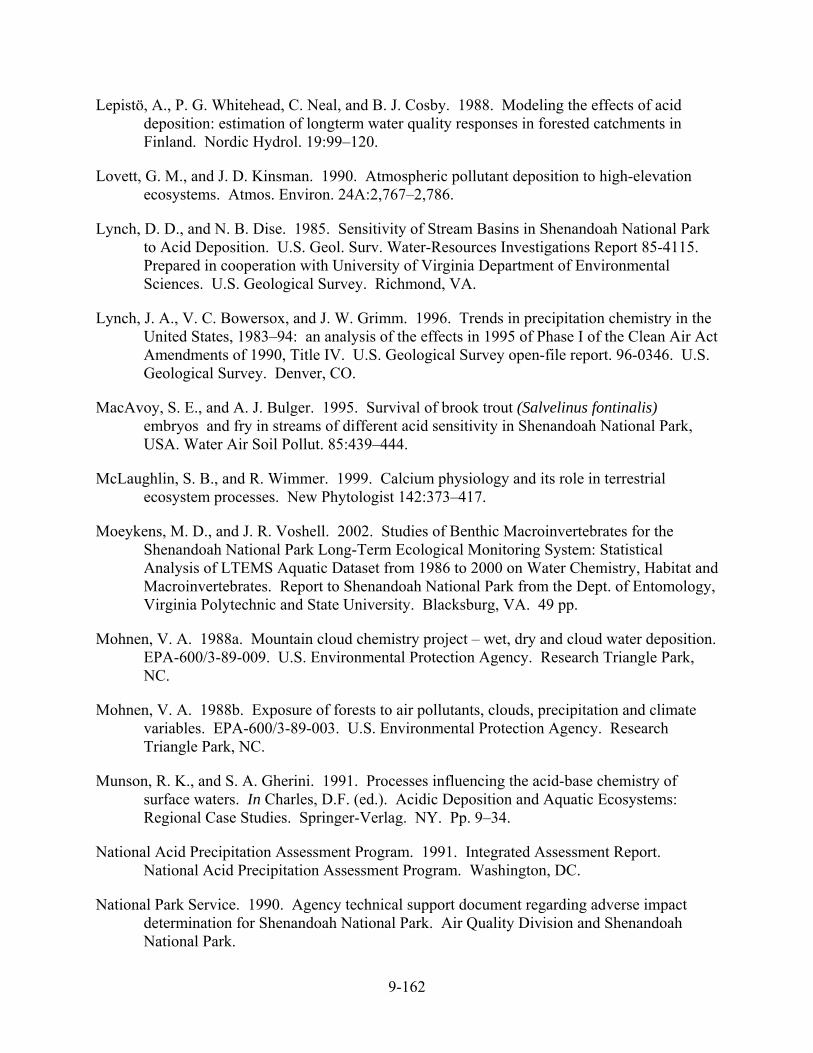
9-162

Lepistö, A., P. G. Whitehead, C. Neal, and B. J. Cosby. 1988. Modeling the effects of acid deposition: estimation of longterm water quality responses in forested catchments in Finland. Nordic Hydrol. 19:99–120.

Lovett, G. M., and J. D. Kinsman. 1990. Atmospheric pollutant deposition to high-elevation ecosystems. Atmos. Environ. 24A:2,767–2,786.

Lynch, D. D., and N. B. Dise. 1985. Sensitivity of Stream Basins in Shenandoah National Park to Acid Deposition. U.S. Geol. Surv. Water-Resources Investigations Report 85-4115. Prepared in cooperation with University of Virginia Department of Environmental Sciences. U.S. Geological Survey. Richmond, VA.

Lynch, J. A., V. C. Bowersox, and J. W. Grimm. 1996. Trends in precipitation chemistry in the United States, 1983–94: an analysis of the effects in 1995 of Phase I of the Clean Air Act Amendments of 1990, Title IV. U.S. Geological Survey open-file report. 96-0346. U.S. Geological Survey. Denver, CO.

MacAvoy, S. E., and A. J. Bulger. 1995. Survival of brook trout (Salvelinus fontinalis) embryos and fry in streams of different acid sensitivity in Shenandoah National Park, USA. Water Air Soil Pollut. 85:439–444.

McLaughlin, S. B., and R. Wimmer. 1999. Calcium physiology and its role in terrestrial ecosystem processes. New Phytologist 142:373–417.

Moeykens, M. D., and J. R. Voshell. 2002. Studies of Benthic Macroinvertebrates for the Shenandoah National Park Long-Term Ecological Monitoring System: Statistical Analysis of LTEMS Aquatic Dataset from 1986 to 2000 on Water Chemistry, Habitat and Macroinvertebrates. Report to Shenandoah National Park from the Dept. of Entomology, Virginia Polytechnic and State University. Blacksburg, VA. 49 pp.

Mohnen, V. A. 1988a. Mountain cloud chemistry project – wet, dry and cloud water deposition. EPA-600/3-89-009. U.S. Environmental Protection Agency. Research Triangle Park, NC.

Mohnen, V. A. 1988b. Exposure of forests to air pollutants, clouds, precipitation and climate variables. EPA-600/3-89-003. U.S. Environmental Protection Agency. Research Triangle Park, NC.

Munson, R. K., and S. A. Gherini. 1991. Processes influencing the acid-base chemistry of surface waters. In Charles, D.F. (ed.). Acidic Deposition and Aquatic Ecosystems: Regional Case Studies. Springer-Verlag. NY. Pp. 9–34.

National Acid Precipitation Assessment Program. 1991. Integrated Assessment Report. National Acid Precipitation Assessment Program. Washington, DC.

National Park Service. 1990. Agency technical support document regarding adverse impact determination for Shenandoah National Park. Air Quality Division and Shenandoah National Park.

9-163

National Park Service. 2000. Agency technical support document regarding the Department of the Interior request for a U.S. Environmental Protection Agency rule to restore and protect air quality values in Class I national parks and wilderness areas.

Patrick, R. 1996. Rivers of the United States. Volume III. The Eastern and Southeastern States. John Wiley and Sons. NY. 829 pp.

Peterson, R. H., and L. Van Eeckhaute. 1992. Distribution of Ephemeroptera, Plecoptera, and Trichoptera of maritime catchments differing in pH. Freshw. Biol. 27:65–78.

Reuss, J. O., and D. W. Johnson. 1986. Acid deposition and the acidification of soil and water. Springer-Verlag. NY.

Rochelle, B. P., and M. R. Church. 1987. Regional patterns of sulfur retention in watersheds of the eastern U.S. Water Air Soil Pollut. 36:61–73.

Rosemond, A. D., S. R. Reice, J. W. Elwood, and P. J. Mulholland. 1992. The effects of stream acidity on benthic invertebrate communities in the south-eastern United States. Freshwater Biology 27:193–209.

Rosenbrock, H. H. 1960. An automatic method for finding the greatest or least value of a function. Computer J. 3:175–184.

Ryan, P. F., G. M. Hornberger, B. J. Cosby, J. N. Galloway, J. R. Webb, and E. B. Rastetter. 1989. Changes in the chemical composition of stream water in two catchments in the Shenandoah National Park, VA, in response to atmospheric deposition of sulfur. Water Resources Research 25:2091.

SAS Institute Inc. 1988. SAS/STAT User's Guide. Release 6.03 Edition. SAS Institute, Inc. Cary, NC.

Sale, M. J., P. R. Kaufmann, H. I. Jager, J. M. Coe, K. A. Cougan, A. J. Kinney, M. E. Mitch, and W. S. Overton. 1988. Chemical Characteristics of Streams in the Mid-Atlantic and Southeastern United States. Volume II: Streams Sampled, Descriptive Statistics, and Compendium of Physical and Chemical Data. WPA/600/3- 88/021b. U.S. Environmental Protection Agency. Washington, DC.

Shaffer, P. W. 1982. Soil and bedrock mineralogy: Soil chemistry in the SWAS watersheds. Appendix VII. In Galloway, J. N., G. M. Hornberger, and K. J. Beven. Shenandoah watershed acidification study: three year summary report, September 1979–September 1982. Department of Environmental Sciences, University of Virginia. Charlottesville. 31 pp.

Shannon, J. D. 1981. A model of regional long-term average sulfur atmospheric pollution, surface removal, and net horizontal flux. Atmos. Environ. 15:689–701.

9-164

Shannon, J. D. 1985. User's Guide for the Advanced Statistical Trajectory Regional Air Pollution (ASTRAP) Model. U. S. Environmental Protection Agency Report EPA/600/8-85/016 (NTIS PB85-236784/XAB).

Shannon, J. D. 1998. Calculation of Trends from 1900 through 1990 for Sulfur and NOx-N Deposition Concentrations of Sulfate and Nitrate in Precipitation, and Atmospheric Concentrations of SOx and NOx Species over the Southern Appalachians. Report to SAMI. April 1998.

Shenandoah National Park. 1998a. Backcountry & Wilderness Management Plan. U.S. Dept. of Interior. National Park Service.

Shenandoah National Park. 1998b. Resource Management Plan. U.S. Dept. of the Interior. National Park Service.

Shenandoah National Park. 1993. Wildland Fire Management Plan. U.S. Dept. of the Interior. National Park Service.

Shenandoah National Park. 2001. Comprehensive Interpretive Plan. U.S. Dept. of the Interior. National Park Service.

Smith, M. E., B. J. Wyskowski, C. M. Brooks, C. T. Driscoll, and C. C. Cosentini. 1990. Relationships between acidity and benthic invertebrates of low-order woodland streams in the Adirondack Mountains, New York. Canadian Journal of Fisheries and Aquatic Sciences 47:1,318–1,329.

Southern Appalachian Man and the Biosphere (SAMAB). 1996. Southern Appalachian Man and the Biosphere. The Southern Appalachian Assessment Aquatics Technical Report. Report 2 of 5. Atlanta. USDA, Forest Service, Southern Region.

Stoddard, J. L., J. S. Kahl, F. A. Deviney, D. R. DeWalle, C. T. Driscoll, A. T. Herlihy, J. H. Kellogg, P. S. Murdoch, J. R. Webb, and K. E. Webster. 2003. Response of surface water chemistry to the Clean Air Act Amendments of 1990. EPA/620/R-03/001. U.S. Environmental Protection Agency. Washington, DC.

Sullivan, T. J. 1991. Long-term temporal changes in surface water chemistry, in Acid Deposition and Aquatic Ecosystems: Regional Case Studies, edited by D. F. Charles. Springer-Verlag. NY.

Sullivan, T. J. 2000. Aquatic Effects of Acidic Deposition. Lewis Publ. Boca Raton, FL. 373 pp.

Sullivan, T. J., B. J. Cosby, C. T. Driscoll, D. F. Charles, and H. F. Hemond. 1996. Influence of organic acids on model projections of lake acidification. Water Air Soil Pollut. 91:271–282.

9-165

Sullivan, T. J.; B. J. Cosby, J. A. Laurence, R. L. Dennis, K. Savig, J. R. Webb, A. J. Bulger, M. Scruggs, C. Gordon, J. Ray, E. H. Lee, W. E. Hogsett, H. Wayne, D. Miller, and J. S. Kern. 2003. Assessment of Air Quality and Related Values in Shenandoah National Park. U.S. Department of the Interior. Philadelphia, PA. NPS/NERCHAL/NRTR--03/090.

Sullivan, T. J., B. J. Cosby, J. R. Webb, K. U. Snyder, A. T. Herlihy, A. J. Bulger, E. H. Gilbert, and D. Moore. 2002a. Assessment of the effects of acidic deposition on aquatic resources in the Southern Appalachian Mountains. Report prepared for the Southern Appalachian Mountains Initiative (SAMI). E&S Environmental Chemistry, Inc. Corvallis, OR. (Available at www.esenvironmental.com/sami_download.htm)

Sullivan, T. J., D. W. Johnson, and R. Munson. 2002b. Assessment of effects of acid deposition on forest resources in the Southern Appalachian Mountains. Report prepared for the Southern Appalachian Mountains Initiative (SAMI). E&S Environmental Chemistry, Inc. Corvallis, OR. (Available at www.esenvironmental.com/sami_download.htm)

Surber, E. W. 1951. Bottom fauna and temperature conditions in relation to trout management in St. Marys River, Augusta County, Virginia. Virginia J. Sci. 2:190–202.

Thornton, K., D. Marmorek, and P. Ryan. 1990. Methods for Projecting Future Changes in Surface Water Acid-Base Chemistry. State of the Science, SOS/T 14, National Acid Precipitation Assessment Program, Washington, DC.

Turner, R. S., R. B. Cook, H. van Miegroet, D. W. Johnson, J. W. Elwood, O. P. Bricker, S. E. Lindberg, and G. M. Hornberger. 1990. Watershed and Lake Processes Affecting Chronic Surface Water Acid-Base Chemistry. State of the Science, SOS/T 10. National Acid Precipitation Assessment Program. Washington, DC.

U.S. Department of Agriculture. 1979. General soil map of Virginia. U.S.D.A., Soil Conservation Service. Lanham, MD.

U.S. Environmental Protection Agency. 1995. Acid Deposition Standard Feasibility Study: Report to Congress. EPA Report No. 430-R-95-001a. Office of Air and Radiation, Acid Rain Division. Washington, DC.

U.S. Environmental Protection Agency. 2001a. Draft Guidance for Tracking Progress Under the Regional Haze Rule. U.S. EPA. Office of Air Quality Planning and Standards. Research Triangle Park, NC. September 27, 2001.

U.S. Environmental Protection Agency. 2002b. IPM Documentation. U.S. Environmental Protection Agency Web Page: http://www.epa.gov/airmarkets/epa-ipm/index.html.

U.S. General Accounting Office (USGAO). 2000. Acid Rain: Emissions Trends and Effects in the Eastern United States. GAO/RCED-00-47, U.S. General Accounting Office, Washington, D.C.

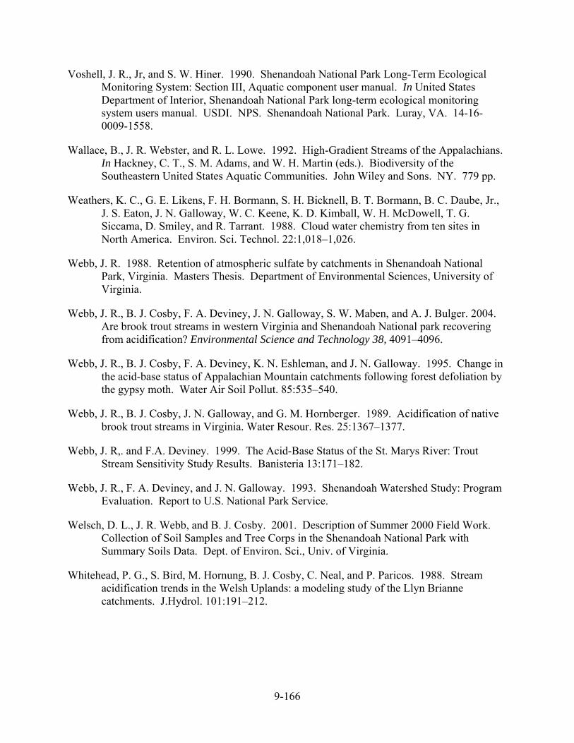
9-166

Voshell, J. R., Jr, and S. W. Hiner. 1990. Shenandoah National Park Long-Term Ecological Monitoring System: Section III, Aquatic component user manual. In United States Department of Interior, Shenandoah National Park long-term ecological monitoring system users manual. USDI. NPS. Shenandoah National Park. Luray, VA. 14-16-0009-1558.

Wallace, B., J. R. Webster, and R. L. Lowe. 1992. High-Gradient Streams of the Appalachians. In Hackney, C. T., S. M. Adams, and W. H. Martin (eds.). Biodiversity of the Southeastern United States Aquatic Communities. John Wiley and Sons. NY. 779 pp.

Weathers, K. C., G. E. Likens, F. H. Bormann, S. H. Bicknell, B. T. Bormann, B. C. Daube, Jr., J. S. Eaton, J. N. Galloway, W. C. Keene, K. D. Kimball, W. H. McDowell, T. G. Siccama, D. Smiley, and R. Tarrant. 1988. Cloud water chemistry from ten sites in North America. Environ. Sci. Technol. 22:1,018–1,026.

Webb, J. R. 1988. Retention of atmospheric sulfate by catchments in Shenandoah National Park, Virginia. Masters Thesis. Department of Environmental Sciences, University of Virginia.

Webb, J. R., B. J. Cosby, F. A. Deviney, J. N. Galloway, S. W. Maben, and A. J. Bulger. 2004. Are brook trout streams in western Virginia and Shenandoah National park recovering from acidification? Environmental Science and Technology 38, 4091–4096.

Webb, J. R., B. J. Cosby, F. A. Deviney, K. N. Eshleman, and J. N. Galloway. 1995. Change in the acid-base status of Appalachian Mountain catchments following forest defoliation by the gypsy moth. Water Air Soil Pollut. 85:535–540.

Webb, J. R., B. J. Cosby, J. N. Galloway, and G. M. Hornberger. 1989. Acidification of native brook trout streams in Virginia. Water Resour. Res. 25:1367–1377.

Webb, J. R,. and F.A. Deviney. 1999. The Acid-Base Status of the St. Marys River: Trout Stream Sensitivity Study Results. Banisteria 13:171–182.

Webb, J. R., F. A. Deviney, and J. N. Galloway. 1993. Shenandoah Watershed Study: Program Evaluation. Report to U.S. National Park Service.

Welsch, D. L., J. R. Webb, and B. J. Cosby. 2001. Description of Summer 2000 Field Work. Collection of Soil Samples and Tree Corps in the Shenandoah National Park with Summary Soils Data. Dept. of Environ. Sci., Univ. of Virginia.

Whitehead, P. G., S. Bird, M. Hornung, B. J. Cosby, C. Neal, and P. Paricos. 1988. Stream acidification trends in the Welsh Uplands: a modeling study of the Llyn Brianne catchments. J.Hydrol. 101:191–212.

9-167

Wigington, P. J., J. P. Baker, D. R. DeWalle, W. A. Kretser, P. S. Murdoch, H. A. Simonin, J. Van Sickle, M. K. McDowell, D. V. Peck, and W. R. Barchet. 1993. Episodic acidification of streams in the northeastern United States: Chemical and biological results of the Episodic Response Project. EPA/600/R-93/190. U.S. Environmental Protection Agency. Washington, DC.

Wojcik, G. S., and J. S. Chang. 1997. A re-evaluation of sulfur budgets, lifetimes, and scavenging ratios for Eastern North America. J. Atmos. Chem. 26:109–145.

Wright, R. F., B. J. Cosby, M. B. Flaten, and J. O. Reuss. 1990. Evaluation of an acidification model with data from manipulated catchments in Norway. Nature 343:53–55.

Wright, R. F., B. J. Cosby, R. C. Ferrier, A. Jenkins, A. J. Bulger, and R. Harriman. 1994. Changes in the acidification of lochs in Galloway, southwestern Scotland, 1979–1988: the MAGIC model used to evaluate the role of afforestation, calculate critical loads, and predict fish status. J. Hydrol. 161:257–285.

A-169

Appendix A. Enlarged Assessment Maps from Figures in Chapter 2 The purpose of this appendix is to provide enlarged versions of the assessment maps presented in Chapter 2 (in order to show greater detail). The appendix contains only the figures listed below. The reader is referred to Chapter 2 for additional information and a detailed discussion of the figures. Index for Appendix A Page

Figure 2.2. ............................................................................................................................. A-170

Figure 2.3. ............................................................................................................................. A-172

Figure 2.4. ............................................................................................................................. A-174

Figure 2.5. ............................................................................................................................. A-177

Figure 2.7. ............................................................................................................................. A-180

Figure 2.8. ............................................................................................................................. A-184

Figure 2.9. ............................................................................................................................. A-188

Figure 2.10. ........................................................................................................................... A-192

A-170

Acute ConcernElevated ConcernModerate ConcernLow Concern

Stream Conditions

(Calk, ueq/L)

Simulated

Year 2000

Figure 2-2. (Extract A - Enlarged). Landscape map showing areas of concern for adverse effects from acidic deposition on surface water conditions in SHEN. Model simulated data for the 14 SWAS study sites extrapolated to the 231 mapping watersheds. Surface water conditions are based on simulated streamwater ANC (ueq/L). Expected biological effects in each category of concern are discussed in the text in Chapter 2.

Acute ConcernElevated ConcernModerate ConcernLow Concern

Stream Conditions

(Calk, ueq/L)

Acute ConcernElevated ConcernModerate ConcernLow Concern

Stream Conditions

(Calk, ueq/L)

Acute ConcernElevated ConcernModerate ConcernLow Concern

Acute ConcernElevated ConcernModerate ConcernLow Concern

Stream Conditions

(Calk, ueq/L)

Simulated

Year 2000

Figure 2-2. (Extract A - Enlarged). Landscape map showing areas of concern for adverse effects from acidic deposition on surface water conditions in SHEN. Model simulated data for the 14 SWAS study sites extrapolated to the 231 mapping watersheds. Surface water conditions are based on simulated streamwater ANC (ueq/L). Expected biological effects in each category of concern are discussed in the text in Chapter 2.

A-171

Acute ConcernElevated ConcernModerate ConcernLow Concern

Stream Conditions

(Calk, ueq/L)

Observed

Year 2000

Figure 2-2. (Extract B - Enlarged). Landscape map showing areas of concern for adverse effects from acidic deposition on surface water conditions in SHEN. Observed data for the 14 SWAS study sites extrapolated to the 231 mapping watersheds. Surface water conditions are based on observed streamwater ANC (ueq/L). Expected biological effects in each category of concern are discussed in the text in Chapter 2.

Acute ConcernElevated ConcernModerate ConcernLow Concern

Stream Conditions

(Calk, ueq/L)

Acute ConcernElevated ConcernModerate ConcernLow Concern

Stream Conditions

(Calk, ueq/L)

Acute ConcernElevated ConcernModerate ConcernLow Concern

Acute ConcernElevated ConcernModerate ConcernLow Concern

Stream Conditions

(Calk, ueq/L)

Observed

Year 2000

Figure 2-2. (Extract B - Enlarged). Landscape map showing areas of concern for adverse effects from acidic deposition on surface water conditions in SHEN. Observed data for the 14 SWAS study sites extrapolated to the 231 mapping watersheds. Surface water conditions are based on observed streamwater ANC (ueq/L). Expected biological effects in each category of concern are discussed in the text in Chapter 2.

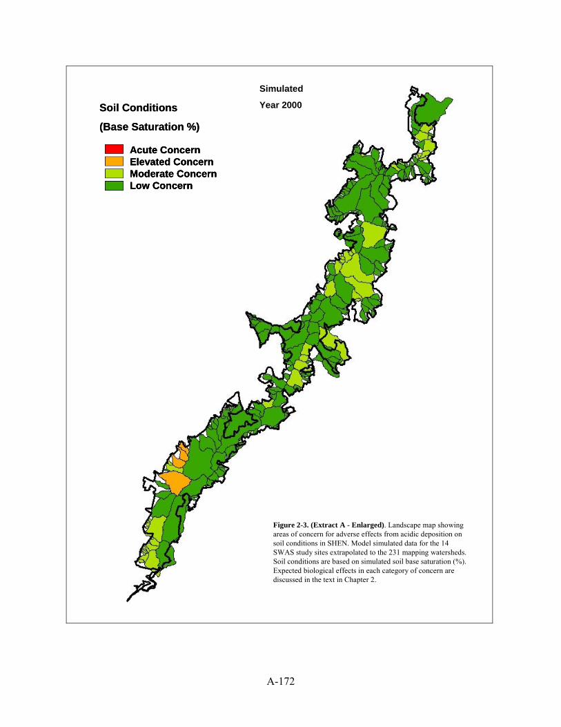
A-172

Acute ConcernElevated ConcernModerate ConcernLow Concern

Soil Conditions

(Base Saturation %)

Simulated

Year 2000

Figure 2-3. (Extract A - Enlarged). Landscape map showing areas of concern for adverse effects from acidic deposition on soil conditions in SHEN. Model simulated data for the 14 SWAS study sites extrapolated to the 231 mapping watersheds. Soil conditions are based on simulated soil base saturation (%).Expected biological effects in each category of concern are discussed in the text in Chapter 2.

Acute ConcernElevated ConcernModerate ConcernLow Concern

Soil Conditions

(Base Saturation %)

Acute ConcernElevated ConcernModerate ConcernLow Concern

Soil Conditions

(Base Saturation %)

Acute ConcernElevated ConcernModerate ConcernLow Concern

Acute ConcernElevated ConcernModerate ConcernLow Concern

Soil Conditions

(Base Saturation %)

Simulated

Year 2000

Figure 2-3. (Extract A - Enlarged). Landscape map showing areas of concern for adverse effects from acidic deposition on soil conditions in SHEN. Model simulated data for the 14 SWAS study sites extrapolated to the 231 mapping watersheds. Soil conditions are based on simulated soil base saturation (%).Expected biological effects in each category of concern are discussed in the text in Chapter 2.

A-173

Acute ConcernElevated ConcernModerate ConcernLow Concern

Soil Conditions

(Base Saturation %)

Observed

Year 2000

Figure 2-3. (Extract B - Enlarged). Landscape map showing areas of concern for adverse effects from acidic deposition on soil conditions in SHEN. Observed data for the 14 SWAS study sites extrapolated to the 231 mapping watersheds. Soil conditions are based on observed soil base saturation (%). Expected biological effects in each category of concern are discussed in the text in Chapter 2.

Acute ConcernElevated ConcernModerate ConcernLow Concern

Soil Conditions

(Base Saturation %)

Acute ConcernElevated ConcernModerate ConcernLow Concern

Soil Conditions

(Base Saturation %)

Acute ConcernElevated ConcernModerate ConcernLow Concern

Acute ConcernElevated ConcernModerate ConcernLow Concern

Soil Conditions

(Base Saturation %)

Observed

Year 2000

Figure 2-3. (Extract B - Enlarged). Landscape map showing areas of concern for adverse effects from acidic deposition on soil conditions in SHEN. Observed data for the 14 SWAS study sites extrapolated to the 231 mapping watersheds. Soil conditions are based on observed soil base saturation (%). Expected biological effects in each category of concern are discussed in the text in Chapter 2.

A-174

Acute ConcernElevated ConcernModerate ConcernLow Concern

Stream Conditions

(Calk, ueq/L)

Simulated

Year 1850

Figure 2-4. (Extract A – Enlarged) Landscape map showing areas of concern for adverse effects from acidic deposition on surface water conditions in SHEN. The figure shows the map generated for pre-industrial conditions. Surface water conditions are based on simulated values of ANC (ueq/L). Expected biological effects in each category of concern are discussed in Chapter 2.

Acute ConcernElevated ConcernModerate ConcernLow Concern

Stream Conditions

(Calk, ueq/L)

Acute ConcernElevated ConcernModerate ConcernLow Concern

Stream Conditions

(Calk, ueq/L)

Acute ConcernElevated ConcernModerate ConcernLow Concern

Acute ConcernElevated ConcernModerate ConcernLow Concern

Stream Conditions

(Calk, ueq/L)

Simulated

Year 1850

Figure 2-4. (Extract A – Enlarged) Landscape map showing areas of concern for adverse effects from acidic deposition on surface water conditions in SHEN. The figure shows the map generated for pre-industrial conditions. Surface water conditions are based on simulated values of ANC (ueq/L). Expected biological effects in each category of concern are discussed in Chapter 2.

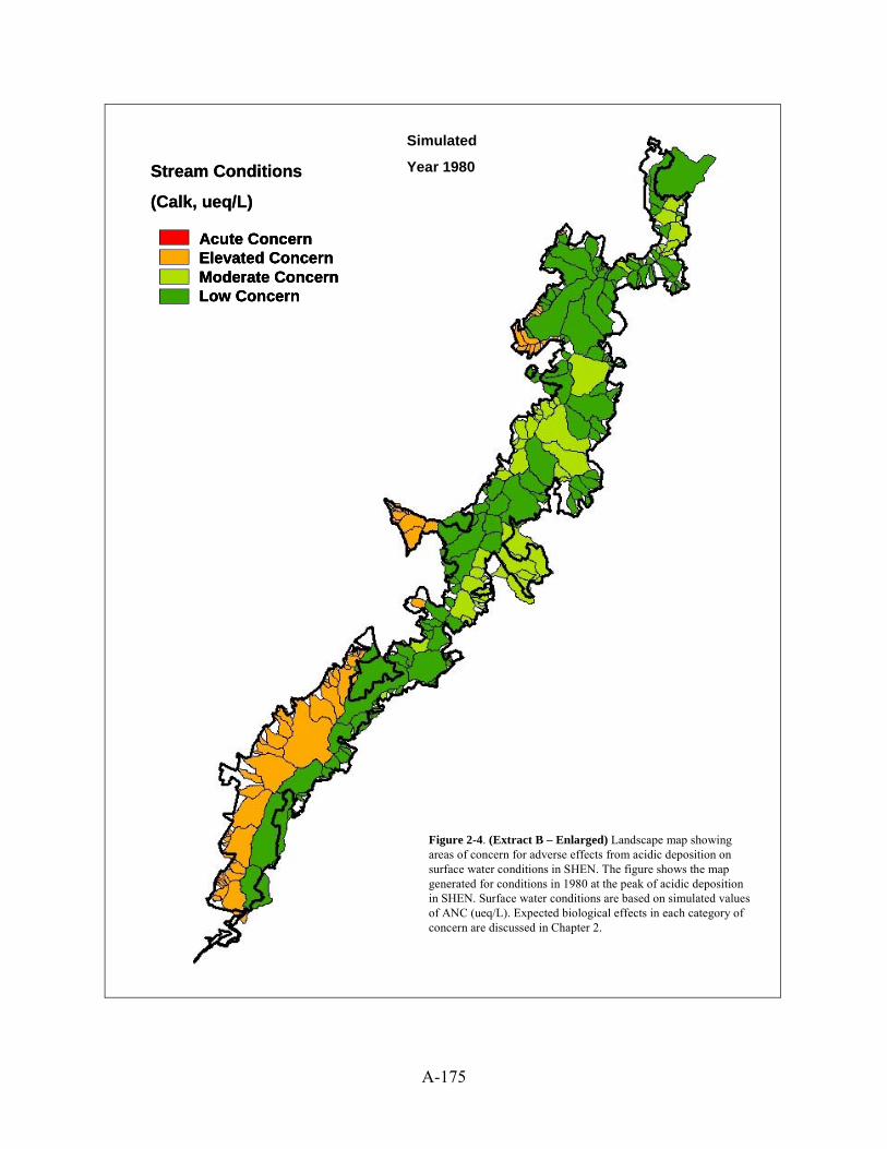
A-175

Acute ConcernElevated ConcernModerate ConcernLow Concern

Stream Conditions

(Calk, ueq/L)

Simulated

Year 1980

Figure 2-4. (Extract B – Enlarged) Landscape map showing areas of concern for adverse effects from acidic deposition on surface water conditions in SHEN. The figure shows the map generated for conditions in 1980 at the peak of acidic deposition in SHEN. Surface water conditions are based on simulated values of ANC (ueq/L). Expected biological effects in each category of concern are discussed in Chapter 2.

Acute ConcernElevated ConcernModerate ConcernLow Concern

Stream Conditions

(Calk, ueq/L)

Acute ConcernElevated ConcernModerate ConcernLow Concern

Stream Conditions

(Calk, ueq/L)

Acute ConcernElevated ConcernModerate ConcernLow Concern

Acute ConcernElevated ConcernModerate ConcernLow Concern

Stream Conditions

(Calk, ueq/L)

Simulated

Year 1980

Figure 2-4. (Extract B – Enlarged) Landscape map showing areas of concern for adverse effects from acidic deposition on surface water conditions in SHEN. The figure shows the map generated for conditions in 1980 at the peak of acidic deposition in SHEN. Surface water conditions are based on simulated values of ANC (ueq/L). Expected biological effects in each category of concern are discussed in Chapter 2.

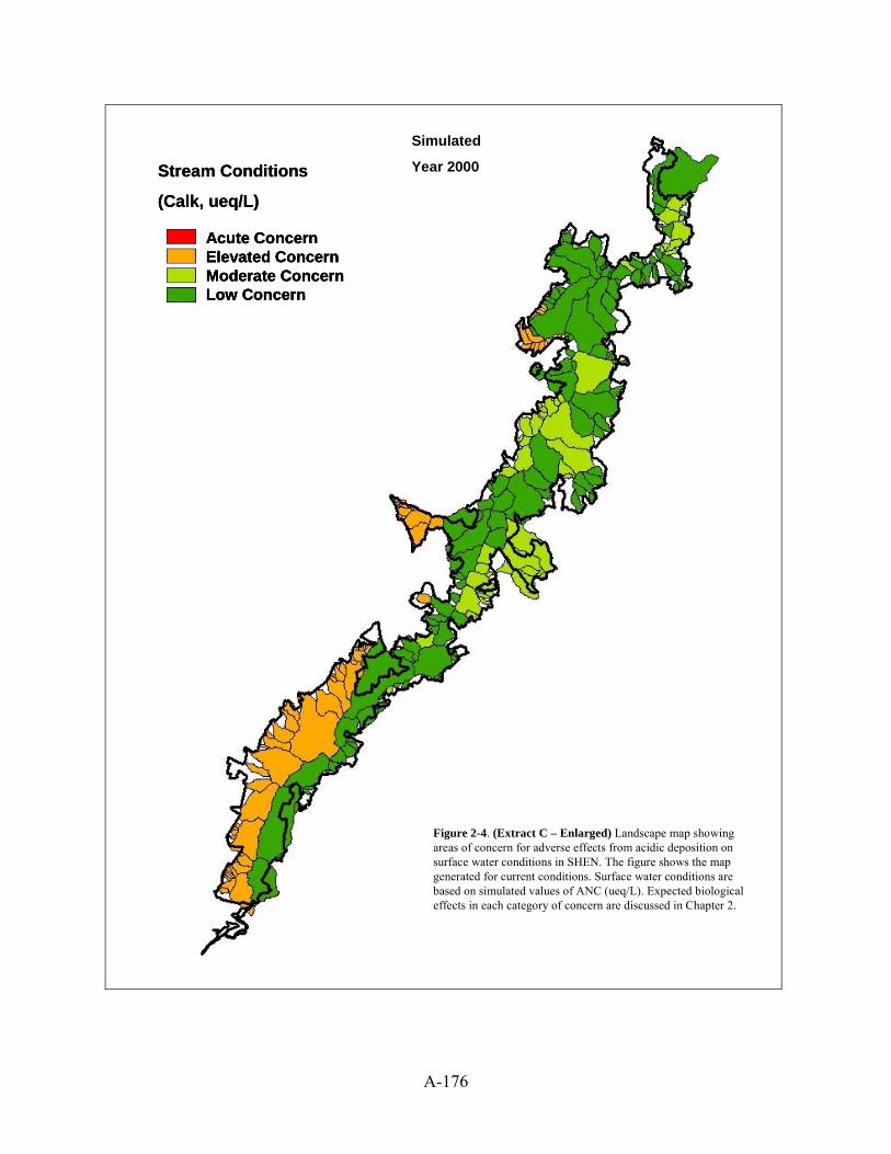
A-176

Acute ConcernElevated ConcernModerate ConcernLow Concern

Stream Conditions

(Calk, ueq/L)

Simulated

Year 2000

Figure 2-4. (Extract C – Enlarged) Landscape map showing areas of concern for adverse effects from acidic deposition on surface water conditions in SHEN. The figure shows the map generated for current conditions. Surface water conditions are based on simulated values of ANC (ueq/L). Expected biological effects in each category of concern are discussed in Chapter 2.

Acute ConcernElevated ConcernModerate ConcernLow Concern

Stream Conditions

(Calk, ueq/L)

Acute ConcernElevated ConcernModerate ConcernLow Concern

Stream Conditions

(Calk, ueq/L)

Acute ConcernElevated ConcernModerate ConcernLow Concern

Acute ConcernElevated ConcernModerate ConcernLow Concern

Stream Conditions

(Calk, ueq/L)

Simulated

Year 2000

Figure 2-4. (Extract C – Enlarged) Landscape map showing areas of concern for adverse effects from acidic deposition on surface water conditions in SHEN. The figure shows the map generated for current conditions. Surface water conditions are based on simulated values of ANC (ueq/L). Expected biological effects in each category of concern are discussed in Chapter 2.

A-177

Acute ConcernElevated ConcernModerate ConcernLow Concern

Soil Conditions

(Base Saturation %)

Simulated

Year 1850

Figure 2-5. (Extract A – Enlarged) Landscape map showing areas of concern for adverse effects from acidic deposition on soil conditions in SHEN. The figure shows the map generated for pre-industrial conditions. Soil conditions are based on simulated values of soil base saturation (%). Expected biological effects in each category of concern are discussed in Chapter 2.

Acute ConcernElevated ConcernModerate ConcernLow Concern

Soil Conditions

(Base Saturation %)

Acute ConcernElevated ConcernModerate ConcernLow Concern

Soil Conditions

(Base Saturation %)

Acute ConcernElevated ConcernModerate ConcernLow Concern

Acute ConcernElevated ConcernModerate ConcernLow Concern

Soil Conditions

(Base Saturation %)

Simulated

Year 1850

Figure 2-5. (Extract A – Enlarged) Landscape map showing areas of concern for adverse effects from acidic deposition on soil conditions in SHEN. The figure shows the map generated for pre-industrial conditions. Soil conditions are based on simulated values of soil base saturation (%). Expected biological effects in each category of concern are discussed in Chapter 2.

A-178

Acute ConcernElevated ConcernModerate ConcernLow Concern

Soil Conditions

(Base Saturation %)

Simulated

Year 1980

Figure 2-5. (Extract B – Enlarged) Landscape map showing areas of concern for adverse effects from acidic deposition on soil conditions in SHEN. The figure shows the map generated for conditions in 1980 at the peak of acidic deposition in SHEN. Soil conditions are based on simulated values of soil base saturation(%). Expected biological effects in each category of concern arediscussed in Chapter 2.

Acute ConcernElevated ConcernModerate ConcernLow Concern

Soil Conditions

(Base Saturation %)

Acute ConcernElevated ConcernModerate ConcernLow Concern

Soil Conditions

(Base Saturation %)

Acute ConcernElevated ConcernModerate ConcernLow Concern

Acute ConcernElevated ConcernModerate ConcernLow Concern

Soil Conditions

(Base Saturation %)

Simulated

Year 1980

Figure 2-5. (Extract B – Enlarged) Landscape map showing areas of concern for adverse effects from acidic deposition on soil conditions in SHEN. The figure shows the map generated for conditions in 1980 at the peak of acidic deposition in SHEN. Soil conditions are based on simulated values of soil base saturation(%). Expected biological effects in each category of concern arediscussed in Chapter 2.

A-179

Acute ConcernElevated ConcernModerate ConcernLow Concern

Soil Conditions

(Base Saturation %)

Simulated

Year 2000

Figure 2-5. (Extract C – Enlarged) Landscape map showing areas of concern for adverse effects from acidic deposition on soil conditions in SHEN. The figure shows the map generated for current conditions. Soil conditions are based on simulated values of soil base saturation (%). Expected biological effects in eachcategory of concern are discussed in Chapter 2.

Acute ConcernElevated ConcernModerate ConcernLow Concern

Soil Conditions

(Base Saturation %)

Acute ConcernElevated ConcernModerate ConcernLow Concern

Soil Conditions

(Base Saturation %)

Acute ConcernElevated ConcernModerate ConcernLow Concern

Acute ConcernElevated ConcernModerate ConcernLow Concern

Soil Conditions

(Base Saturation %)

Simulated

Year 2000

Figure 2-5. (Extract C – Enlarged) Landscape map showing areas of concern for adverse effects from acidic deposition on soil conditions in SHEN. The figure shows the map generated for current conditions. Soil conditions are based on simulated values of soil base saturation (%). Expected biological effects in eachcategory of concern are discussed in Chapter 2.

A-180

Acute ConcernElevated ConcernModerate ConcernLow Concern

Stream Conditions

(Calk, ueq/L)

Simulated

Year 2000

Figure 2-7. (Extract A – Enlarged) Landscape map showing areas of concern for adverse effects from acidic deposition on stream conditions in SHEN. The figure shows the map generated for current stream conditions (year 2000). Stream conditions arebased on simulated values of stream ANC (ueq/L). Expected biological effects in each category of concern are discussed in the Chapter 2.

Acute ConcernElevated ConcernModerate ConcernLow Concern

Stream Conditions

(Calk, ueq/L)

Acute ConcernElevated ConcernModerate ConcernLow Concern

Stream Conditions

(Calk, ueq/L)

Acute ConcernElevated ConcernModerate ConcernLow Concern

Acute ConcernElevated ConcernModerate ConcernLow Concern

Stream Conditions

(Calk, ueq/L)

Simulated

Year 2000

Figure 2-7. (Extract A – Enlarged) Landscape map showing areas of concern for adverse effects from acidic deposition on stream conditions in SHEN. The figure shows the map generated for current stream conditions (year 2000). Stream conditions arebased on simulated values of stream ANC (ueq/L). Expected biological effects in each category of concern are discussed in the Chapter 2.

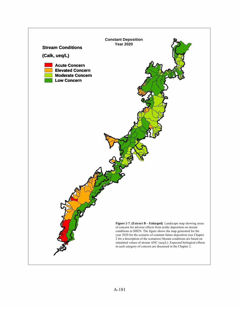
A-181

Acute ConcernElevated ConcernModerate ConcernLow Concern

Stream Conditions

(Calk, ueq/L)

Constant DepositionYear 2020

Figure 2-7. (Extract B – Enlarged) Landscape map showing areas of concern for adverse effects from acidic deposition on stream conditions in SHEN. The figure shows the map generated for the year 2020 for the scenario of constant future deposition (see Chapter 2 for a description of the scenarios) Stream conditions are based on simulated values of stream ANC (ueq/L). Expected biological effects in each category of concern are discussed in the Chapter 2.

Acute ConcernElevated ConcernModerate ConcernLow Concern

Stream Conditions

(Calk, ueq/L)

Acute ConcernElevated ConcernModerate ConcernLow Concern

Stream Conditions

(Calk, ueq/L)

Acute ConcernElevated ConcernModerate ConcernLow Concern

Acute ConcernElevated ConcernModerate ConcernLow Concern

Stream Conditions

(Calk, ueq/L)

Constant DepositionYear 2020

Figure 2-7. (Extract B – Enlarged) Landscape map showing areas of concern for adverse effects from acidic deposition on stream conditions in SHEN. The figure shows the map generated for the year 2020 for the scenario of constant future deposition (see Chapter 2 for a description of the scenarios) Stream conditions are based on simulated values of stream ANC (ueq/L). Expected biological effects in each category of concern are discussed in the Chapter 2.

A-182

Acute ConcernElevated ConcernModerate ConcernLow Concern

Stream Conditions

(Calk, ueq/L)

Scenario 2Year 2020

Figure 2-7. (Extract C – Enlarged) Landscape map showing areas of concern for adverse effects from acidic deposition on stream conditions in SHEN. The figure shows the map generated for the year 2020 for the Scenario 2 future deposition (see Chapter 2 for a description of the scenarios) Stream conditions are based on simulated values of stream ANC (ueq/L). Expected biological effects in each category of concern are discussed in the Chapter 2.

Acute ConcernElevated ConcernModerate ConcernLow Concern

Stream Conditions

(Calk, ueq/L)

Acute ConcernElevated ConcernModerate ConcernLow Concern

Stream Conditions

(Calk, ueq/L)

Acute ConcernElevated ConcernModerate ConcernLow Concern

Acute ConcernElevated ConcernModerate ConcernLow Concern

Stream Conditions

(Calk, ueq/L)

Scenario 2Year 2020

Figure 2-7. (Extract C – Enlarged) Landscape map showing areas of concern for adverse effects from acidic deposition on stream conditions in SHEN. The figure shows the map generated for the year 2020 for the Scenario 2 future deposition (see Chapter 2 for a description of the scenarios) Stream conditions are based on simulated values of stream ANC (ueq/L). Expected biological effects in each category of concern are discussed in the Chapter 2.

A-183

Acute ConcernElevated ConcernModerate ConcernLow Concern

Stream Conditions

(Calk, ueq/L)

Scenario 4Year 2020

Figure 2-7. (Extract D – Enlarged) Landscape map showing areas of concern for adverse effects from acidic deposition on stream conditions in SHEN. The figure shows the map generated for the year 2020 for the Scenario 4 future deposition (see Chapter 2 for a description of the scenarios) Stream conditions are based on simulated values of stream ANC (ueq/L). Expected biological effects in each category of concern are discussed in the Chapter 2.

Acute ConcernElevated ConcernModerate ConcernLow Concern

Stream Conditions

(Calk, ueq/L)

Acute ConcernElevated ConcernModerate ConcernLow Concern

Stream Conditions

(Calk, ueq/L)

Acute ConcernElevated ConcernModerate ConcernLow Concern

Acute ConcernElevated ConcernModerate ConcernLow Concern

Stream Conditions

(Calk, ueq/L)

Scenario 4Year 2020

Figure 2-7. (Extract D – Enlarged) Landscape map showing areas of concern for adverse effects from acidic deposition on stream conditions in SHEN. The figure shows the map generated for the year 2020 for the Scenario 4 future deposition (see Chapter 2 for a description of the scenarios) Stream conditions are based on simulated values of stream ANC (ueq/L). Expected biological effects in each category of concern are discussed in the Chapter 2.

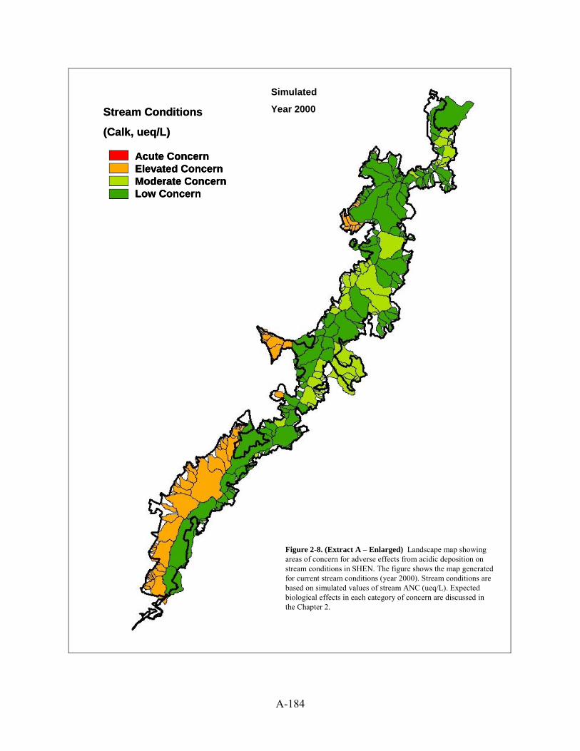
A-184

Acute ConcernElevated ConcernModerate ConcernLow Concern

Stream Conditions

(Calk, ueq/L)

Simulated

Year 2000

Figure 2-8. (Extract A – Enlarged) Landscape map showing areas of concern for adverse effects from acidic deposition on stream conditions in SHEN. The figure shows the map generated for current stream conditions (year 2000). Stream conditions arebased on simulated values of stream ANC (ueq/L). Expected biological effects in each category of concern are discussed in the Chapter 2.

Acute ConcernElevated ConcernModerate ConcernLow Concern

Stream Conditions

(Calk, ueq/L)

Acute ConcernElevated ConcernModerate ConcernLow Concern

Stream Conditions

(Calk, ueq/L)

Acute ConcernElevated ConcernModerate ConcernLow Concern

Acute ConcernElevated ConcernModerate ConcernLow Concern

Stream Conditions

(Calk, ueq/L)

Simulated

Year 2000

Figure 2-8. (Extract A – Enlarged) Landscape map showing areas of concern for adverse effects from acidic deposition on stream conditions in SHEN. The figure shows the map generated for current stream conditions (year 2000). Stream conditions arebased on simulated values of stream ANC (ueq/L). Expected biological effects in each category of concern are discussed in the Chapter 2.

A-185

Acute ConcernElevated ConcernModerate ConcernLow Concern

Stream Conditions

(Calk, ueq/L)

Constant DepositionYear 2100

Figure 2-8. (Extract B – Enlarged) Landscape map showing areas of concern for adverse effects from acidic deposition on stream conditions in SHEN. The figure shows the map generated for the year 2100 for the scenario of constant future deposition (see Chapter 2 for a description of the scenarios) Stream conditions are based on simulated values of stream ANC (ueq/L). Expected biological effects in each category of concern are discussed in the Chapter 2.

Acute ConcernElevated ConcernModerate ConcernLow Concern

Stream Conditions

(Calk, ueq/L)

Acute ConcernElevated ConcernModerate ConcernLow Concern

Stream Conditions

(Calk, ueq/L)

Acute ConcernElevated ConcernModerate ConcernLow Concern

Acute ConcernElevated ConcernModerate ConcernLow Concern

Stream Conditions

(Calk, ueq/L)

Constant DepositionYear 2100

Figure 2-8. (Extract B – Enlarged) Landscape map showing areas of concern for adverse effects from acidic deposition on stream conditions in SHEN. The figure shows the map generated for the year 2100 for the scenario of constant future deposition (see Chapter 2 for a description of the scenarios) Stream conditions are based on simulated values of stream ANC (ueq/L). Expected biological effects in each category of concern are discussed in the Chapter 2.

A-186

Acute ConcernElevated ConcernModerate ConcernLow Concern

Stream Conditions

(Calk, ueq/L)

Scenario 2Year 2100

Figure 2-8. (Extract C – Enlarged) Landscape map showing areas of concern for adverse effects from acidic deposition on stream conditions in SHEN. The figure shows the map generated for the year 2100 for the Scenario 2 future deposition (see Chapter 2 for a description of the scenarios) Stream conditions are based on simulated values of stream ANC (ueq/L). Expected biological effects in each category of concern are discussed in the Chapter 2.

Acute ConcernElevated ConcernModerate ConcernLow Concern

Stream Conditions

(Calk, ueq/L)

Acute ConcernElevated ConcernModerate ConcernLow Concern

Stream Conditions

(Calk, ueq/L)

Acute ConcernElevated ConcernModerate ConcernLow Concern

Acute ConcernElevated ConcernModerate ConcernLow Concern

Stream Conditions

(Calk, ueq/L)

Scenario 2Year 2100

Figure 2-8. (Extract C – Enlarged) Landscape map showing areas of concern for adverse effects from acidic deposition on stream conditions in SHEN. The figure shows the map generated for the year 2100 for the Scenario 2 future deposition (see Chapter 2 for a description of the scenarios) Stream conditions are based on simulated values of stream ANC (ueq/L). Expected biological effects in each category of concern are discussed in the Chapter 2.

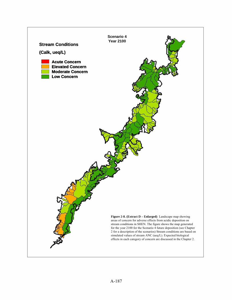
A-187

Acute ConcernElevated ConcernModerate ConcernLow Concern

Stream Conditions

(Calk, ueq/L)

Scenario 4Year 2100

Figure 2-8. (Extract D – Enlarged) Landscape map showing areas of concern for adverse effects from acidic deposition on stream conditions in SHEN. The figure shows the map generated for the year 2100 for the Scenario 4 future deposition (see Chapter 2 for a description of the scenarios) Stream conditions are based on simulated values of stream ANC (ueq/L). Expected biological effects in each category of concern are discussed in the Chapter 2.

Acute ConcernElevated ConcernModerate ConcernLow Concern

Stream Conditions

(Calk, ueq/L)

Acute ConcernElevated ConcernModerate ConcernLow Concern

Stream Conditions

(Calk, ueq/L)

Acute ConcernElevated ConcernModerate ConcernLow Concern

Acute ConcernElevated ConcernModerate ConcernLow Concern

Stream Conditions

(Calk, ueq/L)

Scenario 4Year 2100

Figure 2-8. (Extract D – Enlarged) Landscape map showing areas of concern for adverse effects from acidic deposition on stream conditions in SHEN. The figure shows the map generated for the year 2100 for the Scenario 4 future deposition (see Chapter 2 for a description of the scenarios) Stream conditions are based on simulated values of stream ANC (ueq/L). Expected biological effects in each category of concern are discussed in the Chapter 2.

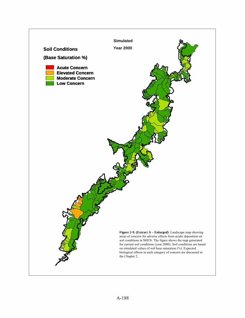
A-188

Acute ConcernElevated ConcernModerate ConcernLow Concern

Soil Conditions

(Base Saturation %)

Simulated

Year 2000

Figure 2-9. (Extract A – Enlarged) Landscape map showing areas of concern for adverse effects from acidic deposition on soil conditions in SHEN. The figure shows the map generated for current soil conditions (year 2000). Soil conditions are based on simulated values of soil base saturation (%). Expected biological effects in each category of concern are discussed in the Chapter 2.

Acute ConcernElevated ConcernModerate ConcernLow Concern

Soil Conditions

(Base Saturation %)

Acute ConcernElevated ConcernModerate ConcernLow Concern

Soil Conditions

(Base Saturation %)

Acute ConcernElevated ConcernModerate ConcernLow Concern

Acute ConcernElevated ConcernModerate ConcernLow Concern

Soil Conditions

(Base Saturation %)

Simulated

Year 2000

Figure 2-9. (Extract A – Enlarged) Landscape map showing areas of concern for adverse effects from acidic deposition on soil conditions in SHEN. The figure shows the map generated for current soil conditions (year 2000). Soil conditions are based on simulated values of soil base saturation (%). Expected biological effects in each category of concern are discussed in the Chapter 2.

A-189

Acute ConcernElevated ConcernModerate ConcernLow Concern

Soil Conditions

(Base Saturation %)

Constant DepositionYear 2020

Figure 2-9. (Extract B – Enlarged) Landscape map showing areas of concern for adverse effects from acidic deposition on soil conditions in SHEN. The figure shows the map generated for the year 2020 for the scenario of constant future deposition (see Chapter 2 for a description of the scenarios). Soil conditions are based on simulated values of soil base saturation (%). Expected biological effects in each category of concern are discussed in the Chapter 2.

Acute ConcernElevated ConcernModerate ConcernLow Concern

Soil Conditions

(Base Saturation %)

Acute ConcernElevated ConcernModerate ConcernLow Concern

Soil Conditions

(Base Saturation %)

Acute ConcernElevated ConcernModerate ConcernLow Concern

Acute ConcernElevated ConcernModerate ConcernLow Concern

Soil Conditions

(Base Saturation %)

Constant DepositionYear 2020

Figure 2-9. (Extract B – Enlarged) Landscape map showing areas of concern for adverse effects from acidic deposition on soil conditions in SHEN. The figure shows the map generated for the year 2020 for the scenario of constant future deposition (see Chapter 2 for a description of the scenarios). Soil conditions are based on simulated values of soil base saturation (%). Expected biological effects in each category of concern are discussed in the Chapter 2.

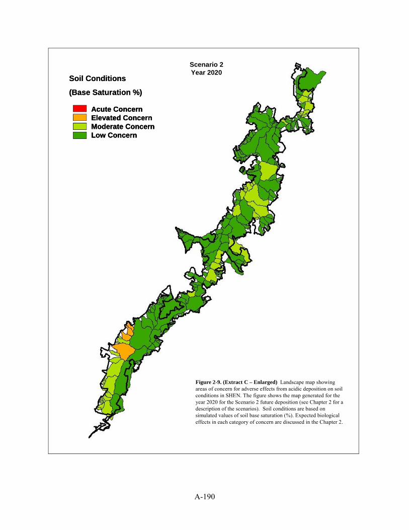
A-190

Acute ConcernElevated ConcernModerate ConcernLow Concern

Soil Conditions

(Base Saturation %)

Scenario 2Year 2020

Figure 2-9. (Extract C – Enlarged) Landscape map showing areas of concern for adverse effects from acidic deposition on soil conditions in SHEN. The figure shows the map generated for the year 2020 for the Scenario 2 future deposition (see Chapter 2 for a description of the scenarios). Soil conditions are based on simulated values of soil base saturation (%). Expected biological effects in each category of concern are discussed in the Chapter 2.

Acute ConcernElevated ConcernModerate ConcernLow Concern

Soil Conditions

(Base Saturation %)

Acute ConcernElevated ConcernModerate ConcernLow Concern

Soil Conditions

(Base Saturation %)

Acute ConcernElevated ConcernModerate ConcernLow Concern

Acute ConcernElevated ConcernModerate ConcernLow Concern

Soil Conditions

(Base Saturation %)

Scenario 2Year 2020

Figure 2-9. (Extract C – Enlarged) Landscape map showing areas of concern for adverse effects from acidic deposition on soil conditions in SHEN. The figure shows the map generated for the year 2020 for the Scenario 2 future deposition (see Chapter 2 for a description of the scenarios). Soil conditions are based on simulated values of soil base saturation (%). Expected biological effects in each category of concern are discussed in the Chapter 2.

A-191

Acute ConcernElevated ConcernModerate ConcernLow Concern

Soil Conditions

(Base Saturation %)

Scenario 4Year 2020

Figure 2-9. (Extract D – Enlarged) Landscape map showing areas of concern for adverse effects from acidic deposition on soil conditions in SHEN. The figure shows the map generated for the year 2020 for the Scenario 4 future deposition (see Chapter 2 for a description of the scenarios). Soil conditions are based on simulated values of soil base saturation (%). Expected biological effects in each category of concern are discussed in the Chapter 2.

Acute ConcernElevated ConcernModerate ConcernLow Concern

Soil Conditions

(Base Saturation %)

Acute ConcernElevated ConcernModerate ConcernLow Concern

Soil Conditions

(Base Saturation %)

Acute ConcernElevated ConcernModerate ConcernLow Concern

Acute ConcernElevated ConcernModerate ConcernLow Concern

Soil Conditions

(Base Saturation %)

Scenario 4Year 2020

Figure 2-9. (Extract D – Enlarged) Landscape map showing areas of concern for adverse effects from acidic deposition on soil conditions in SHEN. The figure shows the map generated for the year 2020 for the Scenario 4 future deposition (see Chapter 2 for a description of the scenarios). Soil conditions are based on simulated values of soil base saturation (%). Expected biological effects in each category of concern are discussed in the Chapter 2.

A-192

Acute ConcernElevated ConcernModerate ConcernLow Concern

Soil Conditions

(Base Saturation %)

Simulated

Year 2000

Figure 2-10. (Extract A – Enlarged) Landscape map showing areas of concern for adverse effects from acidic deposition on soil conditions in SHEN. The figure shows the map generated for current soil conditions (year 2000). Soil conditions are based on simulated values of soil base saturation (%). Expected biological effects in each category of concern are discussed in the Chapter 2.

Acute ConcernElevated ConcernModerate ConcernLow Concern

Soil Conditions

(Base Saturation %)

Acute ConcernElevated ConcernModerate ConcernLow Concern

Soil Conditions

(Base Saturation %)

Acute ConcernElevated ConcernModerate ConcernLow Concern

Acute ConcernElevated ConcernModerate ConcernLow Concern

Soil Conditions

(Base Saturation %)

Simulated

Year 2000

Figure 2-10. (Extract A – Enlarged) Landscape map showing areas of concern for adverse effects from acidic deposition on soil conditions in SHEN. The figure shows the map generated for current soil conditions (year 2000). Soil conditions are based on simulated values of soil base saturation (%). Expected biological effects in each category of concern are discussed in the Chapter 2.

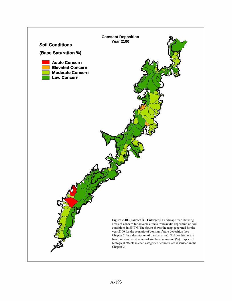
A-193

Acute ConcernElevated ConcernModerate ConcernLow Concern

Soil Conditions

(Base Saturation %)

Constant DepositionYear 2100

Figure 2-10. (Extract B – Enlarged) Landscape map showing areas of concern for adverse effects from acidic deposition on soil conditions in SHEN. The figure shows the map generated for the year 2100 for the scenario of constant future deposition (see Chapter 2 for a description of the scenarios). Soil conditions are based on simulated values of soil base saturation (%). Expected biological effects in each category of concern are discussed in the Chapter 2.

Acute ConcernElevated ConcernModerate ConcernLow Concern

Soil Conditions

(Base Saturation %)

Acute ConcernElevated ConcernModerate ConcernLow Concern

Soil Conditions

(Base Saturation %)

Acute ConcernElevated ConcernModerate ConcernLow Concern

Acute ConcernElevated ConcernModerate ConcernLow Concern

Soil Conditions

(Base Saturation %)

Constant DepositionYear 2100

Figure 2-10. (Extract B – Enlarged) Landscape map showing areas of concern for adverse effects from acidic deposition on soil conditions in SHEN. The figure shows the map generated for the year 2100 for the scenario of constant future deposition (see Chapter 2 for a description of the scenarios). Soil conditions are based on simulated values of soil base saturation (%). Expected biological effects in each category of concern are discussed in the Chapter 2.

A-194

Acute ConcernElevated ConcernModerate ConcernLow Concern

Soil Conditions

(Base Saturation %)

Scenario 2Year 2100

Figure 2-10. (Extract C – Enlarged) Landscape map showing areas of concern for adverse effects from acidic deposition on soil conditions in SHEN. The figure shows the map generated for the year 2100 for the Scenario 2 future deposition (see Chapter 2 for a description of the scenarios). Soil conditions are based on simulated values of soil base saturation (%). Expected biological effects in each category of concern are discussed in the Chapter 2.

Acute ConcernElevated ConcernModerate ConcernLow Concern

Soil Conditions

(Base Saturation %)

Acute ConcernElevated ConcernModerate ConcernLow Concern

Soil Conditions

(Base Saturation %)

Acute ConcernElevated ConcernModerate ConcernLow Concern

Acute ConcernElevated ConcernModerate ConcernLow Concern

Soil Conditions

(Base Saturation %)

Scenario 2Year 2100

Figure 2-10. (Extract C – Enlarged) Landscape map showing areas of concern for adverse effects from acidic deposition on soil conditions in SHEN. The figure shows the map generated for the year 2100 for the Scenario 2 future deposition (see Chapter 2 for a description of the scenarios). Soil conditions are based on simulated values of soil base saturation (%). Expected biological effects in each category of concern are discussed in the Chapter 2.

A-195

Acute ConcernElevated ConcernModerate ConcernLow Concern

Soil Conditions

(Base Saturation %)

Scenario 4Year 2100

Figure 2-10. (Extract D – Enlarged) Landscape map showing areas of concern for adverse effects from acidic deposition on soil conditions in SHEN. The figure shows the map generated for the year 2100 for the Scenario 4 future deposition (see Chapter 2 for a description of the scenarios). Soil conditions are based on simulated values of soil base saturation (%). Expected biological effects in each category of concern are discussed in the Chapter 2.

Acute ConcernElevated ConcernModerate ConcernLow Concern

Soil Conditions

(Base Saturation %)

Acute ConcernElevated ConcernModerate ConcernLow Concern

Soil Conditions

(Base Saturation %)

Acute ConcernElevated ConcernModerate ConcernLow Concern

Acute ConcernElevated ConcernModerate ConcernLow Concern

Soil Conditions

(Base Saturation %)

Scenario 4Year 2100

Figure 2-10. (Extract D – Enlarged) Landscape map showing areas of concern for adverse effects from acidic deposition on soil conditions in SHEN. The figure shows the map generated for the year 2100 for the Scenario 4 future deposition (see Chapter 2 for a description of the scenarios). Soil conditions are based on simulated values of soil base saturation (%). Expected biological effects in each category of concern are discussed in the Chapter 2.

B-197

Appendix B. Details of the Acid Deposition Effects Modeling using MAGIC. The purpose of this appendix is to provide the background details of the acid deposition effects modeling used in this project (model description, input data, calibration, and evaluation of model goodness-of-fit). The reader is referred to Chapter 7 for the details of the simulation results.

Index for Appendix B Page

B.1 Description of the MAGIC Model .................................................................................. B-198

B.2 Application and Calibration of MAGIC .......................................................................... B-199

B.3 Deposition and Meteorology Data .................................................................................. B-200

B.3.1 Model Requirements and Observed Data ......................................................... B-200

B.3.2 Deposition Inputs for MAGIC ......................................................................... B-202

B.3.3 Specification of Deposition for Future Projections .......................................... B-205

B.4 Protocol for MAGIC Calibration and Simulation at Individual Sites ............................. B-205

B.4.1 Calibration Data ............................................................................................... B-206

B.4.2 Calibration and Simulation Procedures ............................................................ B-208

B.4.3 Performance Analysis ...................................................................................... B-209

B.4.4 Analysis of Uncertainty .................................................................................... B-209

B.5 Modeling Results ............................................................................................................. B-202

B-198

B.1 Description of the MAGIC Model

The principal tools that can be used to evaluate the potential response of aquatic resources to changes in acidic deposition are mathematical models. One of the prominent models developed to estimate acidification of lakes and streams is MAGIC (Model of Acidification of Groundwater In Catchments, Cosby et al. 1985a-c). MAGIC was the principal model used by the National Acid Precipitation Assessment Program (NAPAP) in assessment of potential future damage to lakes and streams in the eastern United States (NAPAP 1991, Thornton et al. 1990). Most recently MAGIC has been the principal model used for aquatic assessment in the Southern Appalachian Mountain Initiative Assessment activities (Sullivan et al. 2002a, b). The validity of the model has been confirmed by comparison with estimates of lake acidification inferred from paleolimnological reconstructions of historical lake changes in pH (Sullivan et al. 1991, 1996) and with the results of several catchment-scale experimental acidification and de-acidification experiments (e.g., Cosby et al. 1995, 1996). MAGIC has been used to reconstruct the history of acidification and to simulate future trends on a regional basis and in a large number of individual watersheds in both North America and Europe (e.g., Lepisto et al. 1988; Whitehead et al. 1988; Cosby et al. 1990, 1996; Jenkins et al. 1990; Wright et al. 1990, 1994). Information contained in this Appendix was taken from the model summary provided by Sullivan et al. (2002a, b).

MAGIC is a lumped-parameter model of intermediate complexity, developed to predict the long-term effects of acidic deposition on surface water chemistry. The model simulates soil solution chemistry and surface water chemistry to predict the monthly and annual average concentrations of the major ions in these waters. MAGIC consists of: 1) a section in which the concentrations of major ions are assumed to be governed by simultaneous reactions involving sulfate adsorption, cation exchange, dissolution-precipitation- speciation of aluminum and dissolution-speciation of inorganic carbon; and 2) a mass balance section in which the flux of major ions to and from the soil is assumed to be controlled by atmospheric inputs, chemical weathering, net uptake and loss to biomass and runoff. At the heart of MAGIC is the size of the pool of exchangeable base cations in the soil. As the fluxes to and from this pool change over time in response to changes in atmospheric deposition, the chemical equilibria between soil and soil solution shift to give changes in surface water chemistry. The degree and rate of change of surface water acidity thus depend both on flux factors and the inherent characteristics of the affected soils.

Cation exchange is modeled using equilibrium (Gaines-Thomas) equations with selectivity coefficients for each base cation and aluminum. Sulfate adsorption is represented by a Langmuir isotherm. Aluminum dissolution and precipitation are assumed to be controlled by equilibrium with a solid phase of aluminum trihydroxide. Aluminum speciation is calculated by considering hydrolysis reactions as well as complexation with sulfate and fluoride. Effects of carbon dioxide on pH and on the speciation of inorganic carbon are computed from equilibrium equations. Organic acids are represented in the model as tri-protic analogues. First-order rates are used for retention (uptake) of nitrate and ammonium in the catchment. Weathering rates are assumed to be constant. A set of mass balance equations for base cations and strong acid anions are included. Given a description of the historical deposition at a site, the model equations are solved numerically to give long-term reconstructions of surface water chemistry (for complete details of the model see Cosby et al. 1985 a–c).

B-199

B.2 Application and Calibration of MAGIC

Atmospheric deposition and net uptake-release fluxes for the base cations and strong acid anions are required as inputs to the model. These inputs are generally assumed to be uniform over the catchment. Atmospheric fluxes are calculated from concentrations of the ions in precipitation and the rainfall volume into the watershed. The atmospheric fluxes of the ions must be corrected for dry deposition of gas, particulates and aerosols and for inputs in cloud/fog water. An estimate of the streamflow volume must also be provided to the model. In general, the model is implemented using average hydrologic conditions and meteorological conditions in annual or seasonal simulations. Mean annual or mean monthly deposition, precipitation and streamflow are used to drive the model. The model is not designed to provide temporal resolution greater than monthly. Most simulations are based on annual average conditions. Values for soil and stream water temperature, partial pressure of carbon dioxide in the soil and stream water, and organic acid concentrations in soilwater and stream water must also be provided.

As implemented for this project, MAGIC is a two-compartment representation of each watershed. Atmospheric deposition enters the soil compartment and the equilibrium equations are used to calculate soil water chemistry. The water is then routed to the stream compartment, and the appropriate equilibrium equations are reapplied to calculate stream water chemistry.

Once initial conditions (initial values of variables in the equilibrium equations) have been established, the equilibrium equations are solved for soil water and stream water concentrations of the remaining variables. These concentrations are used to calculate the stream water output fluxes of the model for the first time step. The mass balance equations are (numerically) integrated over the time step, providing new values for the total amounts of base cations and strong acid anions in the system. These in turn are used to calculate new values of the remaining variables and new stream water fluxes. The output from MAGIC is thus a time trace for all major chemical constituents for the period of time chosen for the integration.

The aggregated nature of the model requires that it be calibrated to observed data from a watershed before it can be used to examine potential system response. Calibration is achieved by setting the values of certain parameters within the model which can be directly measured or observed in the system of interest (called “fixed” parameters). The model is then run (using observed atmospheric and hydrologic inputs) and the output (stream water and soil chemical variables, called “criterion” variables) are compared to observed values of these variables. If the observed and simulated values differ, the values of another set of parameters in the model (called “optimized” parameters) are adjusted to improve the fit. After a number of iterations, the simulated-minus-observed values of the criterion variables usually converge to zero (within some specified tolerance). The model is then considered calibrated. If new assumptions (or values) for any of the fixed variables or inputs to the model are subsequently adopted, the model must be re-calibrated by re-adjusting the optimized parameters until the simulated-minus-observed values of the criterion variables again fall within the specified tolerance.

Because the estimates of the fixed parameters and deposition inputs are subject to uncertainties, a "fuzzy" optimization procedure can be implemented for calibrating the model. The fuzzy optimization procedure consists of multiple calibrations of each watershed using random values of the fixed parameters drawn from the observed possible range of values, and random values of

B-200

deposition from the range of model estimates. Each of the multiple calibrations begins with (1) a random selection of values of fixed parameters and deposition, and (2) a random selection of the starting values of the adjustable parameters. The adjustable parameters are then optimized using the Rosenbrock (1960) algorithm to achieve a minimum error fit to the target variables. This procedure is undertaken ten times for each stream. The final calibrated model is represented by the ensemble of parameter values and variable values of the successful calibrations.

Calibrations are based on volume-weighted mean annual fluxes for a given period of observation. The length of the period of observation used for calibration is variable, but model output will be more reliable if the annual flux estimates used in calibration are based on a number of years rather than just one year. There is considerable year-to-year variability in atmospheric deposition and catchment runoff. Averaging over a number of years reduces the likelihood that an “outlier” year (very dry, etc.) constitutes the primary data on which model forecasts are based. On the other hand, averaging over too long a period may remove important trends in the data that need to be simulated by the model. For this study, the model was calibrated using five-year average values of deposition and five years of stream water data.

The model results presented in this report are based on the median values of the simulated water quality variables from the multiple calibrations of each site. The use of median values for each stream helps to assure that the simulated responses are neither over- nor underestimates, but approximate the most likely behavior of each stream (given the assumptions inherent in the model and the data used to constrain and calibrate the model). The uncertainty analyses make use of the maximum and minimum simulated values from the multiple calibrations for each site to calculate uncertainty “widths” (or confidence intervals) around the median simulated values.

B.3 Deposition and Meteorology Data used for MAGIC Calibration

B.3.1 Model Requirements and Observed Data

MAGIC requires as atmospheric inputs estimates of the annual precipitation volume (m/yr) and the total annual deposition (eq/ha/yr) of eight ions: Ca, Mg, Na, K, NH4, SO4, Cl, and NO3. These total deposition data are required at each site for each year of the calibration period (the years for which observed stream water data are used for calibrating the model to each site). Estimated total deposition data are also required for the 140 years preceding the calibration period as part of the calibration protocol for MAGIC, and for each year of any future scenario that will be run using MAGIC.

Total deposition of an ion at a particular site for any year can be represented as combined wet, dry, and in some cases cloud deposition. Inputs to the model are specified as wet deposition (the annual flux in meq/m2/yr) and a dry and cloud deposition enhancement factor (DDF, unitless) used to multiply the wet deposition in order to get total deposition:

TotDep = WetDep * DDF where:

DDF = 1 + DryDep / WetDep

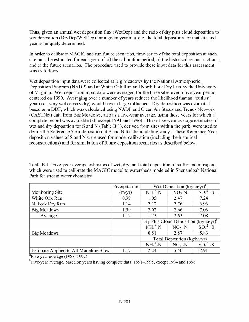
B-201

Thus, given an annual wet deposition flux (WetDep) and the ratio of dry plus cloud deposition to wet deposition (DryDep/WetDep) for a given year at a site, the total deposition for that site and year is uniquely determined.

In order to calibrate MAGIC and run future scenarios, time-series of the total deposition at each site must be estimated for each year of: a) the calibration period; b) the historical reconstructions; and c) the future scenarios. The procedure used to provide these input data for this assessment was as follows.

Wet deposition input data were collected at Big Meadows by the National Atmospheric Deposition Program (NADP) and at White Oak Run and North Fork Dry Run by the University of Virginia. Wet deposition input data were averaged for the three sites over a five-year period centered on 1990. Averaging over a number of years reduces the likelihood that an “outlier” year (i.e., very wet or very dry) would have a large influence. Dry deposition was estimated based on a DDF, which was calculated using NADP and Clean Air Status and Trends Network (CASTNet) data from Big Meadows, also as a five-year average, using those years for which a complete record was available (all except 1994 and 1996). These five-year average estimates of wet and dry deposition for S and N (Table B.1), derived from sites within the park, were used to define the Reference Year deposition of S and N for the modeling study. These Reference Year deposition values of S and N were used for model calibration (including the historical reconstructions) and for simulation of future deposition scenarios as described below.

Table B.1. Five-year average estimates of wet, dry, and total deposition of sulfur and nitrogen, which were used to calibrate the MAGIC model to watersheds modeled in Shenandoah National Park for stream water chemistry

Wet Deposition (kg/ha/yr)a Monitoring Site

Precipitation(m/yr) NH4

+-N NO3–N SO4

2–-S White Oak Run 0.99 1.05 2.47 7.24 N. Fork Dry Run 1.14 2.12 2.76 6.96 Big Meadows 1.39 2.02 2.66 7.03

Average 1.17 1.73 2.63 7.08 Dry Plus Cloud Deposition (kg/ha/yr)b

NH4+-N NO3

--N SO42–-S

Big Meadows 0.51 2.87 5.83 Total Deposition (kg/ha/yr) NH4

+-N NO3--N SO4

2–-S Estimate Applied to All Modeling Sites 1.17 2.24 5.50 12.91

aFive-year average (1988–1992) bFive-year average, based on years having complete data: 1991–1998, except 1994 and 1996

B-202

Given the Reference Year deposition values, the deposition data for historical and calibration periods can be calculated using the Reference Year absolute values and scaled time series of wet deposition and DDF that give the values for a given year as a fraction of the Reference Year value. For instance, to calculate the total deposition of a particular ion in some historical year j:

TotDep(j) = [WetDep(0) * WetDepScale(j) ] * [ DDF(0) * DDF Scale(j)]

where WetDep(0) is the Reference Year wet deposition (meq/m2/yr) of the ion, WetDepScale(j) is the scaled value of wet deposition in year j (expressed as a fraction of the wet deposition in the Reference Year), DDF(0) is the dry deposition factor for the ion for the Reference Year, and DDFScale(j) is the scaled value of the dry deposition factor in year j (expressed as a fraction of the DDF in the Reference Year). In constructing the historical deposition data, the scaled sequences of wet deposition and DDF were derived from simulations using the Advanced Statistical Trajectory Regional Air Pollution (ASTRAP) model (Shannon 1998).

Given the same Reference Year deposition values, the deposition data for the future deposition scenarios can be calculated using the Reference Year absolute values and a scaled time series of changes in total deposition to give the total deposition values for a given future year as a fraction of the Reference Year value. For instance, to calculate the total deposition of a particular ion in some future year j:

TotDep(j) = [ WetDep(0) * DDF(0) ] * TotDep Scale(j)

where WetDep(0) is the Reference Year wet deposition (meq/m2/yr) of the ion, DDF(0) is the dry deposition factor for the ion for the Reference Year, and TotDepScale(j) is the scaled value of the total deposition factor in year j (expressed as a fraction of the total deposition in the Reference Year).

B.3.2 Deposition Inputs for MAGIC

Four deposition inputs are required for each of the eight deposition ions in MAGIC in order to set the total deposition for all years required in the calibrations and future simulations:

1) the absolute value of wet deposition at the site for the Reference Year (meq/m2/yr);

2) the absolute value of DDF (calculated from the DryDep/WetDep ratios) for the site for the Reference Year, (unitless);

3) time series of scaled values of wet deposition and scaled values of DDF covering all historical years necessary to calibrate the model (scaled to the Reference Year);

4) time series of scaled values of future total deposition covering all future years of interest to the scenario runs (scaled to the Reference Year).

The absolute value of wet deposition is time and space-specific, varying geographically and from year to year. It is desirable to have the estimates of wet deposition take into account the geographic location of the site as well as the year for which calibration data are available. The Reference Year wet deposition (derived above) for the park provides a single value for the

B-203

deposition of each ion for the whole park for the Reference Year. To provide an estimate of the spatial variation in wet deposition across the 14 modeling sites within the park, the Reference Year average deposition values were corrected for geographical location and elevation using scaled deposition data for each ion at each site derived from the spatially explicit deposition model of Lynch et al. (1996). The Lynch model is based on spatial and elevational interpolation of wet deposition values of each ion from the NADP monitoring network. The outputs of the Lynch model for each of the 14 modeling sites were averaged over the same five-year period (1988–1992) to provide spatial patterns of wet deposition within the park over the period used to define the Reference Year. The resulting spatially-dependent wet deposition data were used for each site when calibrating MAGIC (Table B.2). This spatial extrapolation procedure insures that the average deposition values of each ion across the 14 sites (Table B.2) are equal to the Reference Year deposition values for the whole park.

The absolute value of the DDF specifies the ratio between the absolute amounts of wet and total deposition. This ratio is less variable in time and space than is the estimate of total deposition. That is, if in a given year the wet deposition goes up, then the total deposition usually goes up also (and conversely). Estimates of the DDF used for MAGIC may, therefore, be derived from a procedure that uses park-wide data (i.e., lacks spatial resolution). As described previously, the DDF values for S and N were derived from observed data for the Reference Year at a single site within the park, Big Meadows. The same DDF was used for S and N for all 14 modeling sites (Table B.2). DDF values for chloride (Cl-) and the base cations were calculated by assuming that Cl- inputs and outputs should be in balance across the park. A single DDF (dry enhancement) of Cl- inputs was calculated for the whole park such that the average mass balance (input-output) for Cl- across all 14 sites was equal to zero. This same DDF was used for Cl- for all 14 sites (Table B.2). The added Cl- was balanced by base cations. A DDF for each base cation at each site was calculated using the ratio of the four base cations in wet deposition at each site. The DDF’s for base cations thus vary from site-to-site but result in an exact balance for the added Cl- at each site (Table B.2).

Similarly, the time series of scaled sequences used for MAGIC simulations do not require detailed spatial resolution. That is, if for any given year the deposition goes up at one site, it also goes up at neighboring sites within the park. Time series of wet deposition and DDF were derived from the ASTRAP model (Shannon 1998), which produced wet, dry, and cloud deposition estimates of S and oxidized nitrogen (NOx) every five years starting in 1900 and ending in 1990 for the Big Meadows site as part of the Southern Appalachian Mountains Initiative (SAMI) project (Sullivan et al., 2002a). The ASTRAP model outputs are smoothed estimates of deposition roughly equivalent to a ten-year moving average centered on each of the output years. Modeling sites for this project were assigned the historical sequences of the ASTRAP Big Meadows output. The time-series of wet deposition and DDF from 1900 to 1990 were normalized to the 1990 values to provide scaled historical sequences for the MAGIC calibration and reconstruction simulations. The same scaled historical sequences of wet deposition and DDF for S and N were used at all 14 sites (Table B.3). Historical sequences of base cation and Cl- deposition were assumed to be constant.

B-204

Table B.2. Wet and dry deposition input data for Shenandoah National Park sitesa.

Concentration in Precipitation (1990 Reference

Year) Dry Deposition Factor (DDF)

Site Discharge

(cm/yr) Precip. (m/yr)

Yield(%) Ca Mg Na K NH4 SO4 Cl NO3 Ca Mg Na K NH4 SO4 NO3 Cl

VT36 0.705 1.071 0.66 5.3 2.1 3.6 2.0 10.8 36.8 5.4 15.4 1.76 1.76 1.76 1.76 1.25 1.83 2.08 2.8DR01 0.779 1.271 0.61 5.9 2.2 3.8 2.5 10.6 41.1 5.3 17.9 1.67 1.67 1.67 1.67 1.25 1.83 2.08 2.8VT35 (PAIN) 0.814 1.213 0.67 6.0 2.3 4.0 2.6 10.4 41.4 5.6 18.3 1.68 1.68 1.68 1.68 1.25 1.83 2.08 2.8VT53 0.885 1.332 0.66 6.0 2.4 4.1 2.7 10.4 41.4 5.7 18.5 1.68 1.68 1.68 1.68 1.25 1.83 2.08 2.8WOR1 0.891 1.280 0.70 6.0 2.3 3.9 2.6 10.7 41.6 5.5 18.2 1.67 1.67 1.67 1.67 1.25 1.83 2.08 2.8NFDR 0.649 1.343 0.48 5.0 2.0 3.6 1.9 10.4 35.3 5.3 14.5 1.76 1.76 1.76 1.76 1.25 1.83 2.08 2.8VT58 0.744 1.172 0.63 5.4 2.1 3.5 2.0 10.7 37.1 5.3 15.4 1.73 1.73 1.73 1.73 1.25 1.83 2.08 2.8VT59 (STAN) 0.750 1.188 0.63 5.6 2.2 3.8 2.3 10.5 39.6 5.4 17.0 1.70 1.70 1.70 1.70 1.25 1.83 2.08 2.8VT62 0.712 1.163 0.61 5.0 2.1 3.6 2.0 10.8 36.3 5.4 15.1 1.76 1.76 1.76 1.76 1.25 1.83 2.08 2.8VT75 0.578 1.123 0.51 4.8 2.0 3.7 1.9 10.4 34.6 5.4 14.3 1.78 1.78 1.78 1.78 1.25 1.83 2.08 2.8VT66 0.526 1.066 0.49 4.6 2.0 3.9 1.9 10.1 33.6 5.5 13.8 1.80 1.80 1.80 1.80 1.25 1.83 2.08 2.8VT51 0.522 1.107 0.47 4.7 2.0 3.9 2.0 10.3 34.7 5.5 14.4 1.79 1.79 1.79 1.79 1.25 1.83 2.08 2.8VT60 (PINE) 0.530 1.053 0.50 4.8 2.0 3.7 1.9 10.6 35.3 5.5 14.6 1.78 1.78 1.78 1.78 1.25 1.83 2.08 2.8VT61 0.517 1.055 0.49 5.2 2.1 3.7 2.0 10.7 36.5 5.5 15.2 1.76 1.76 1.76 1.76 1.25 1.83 2.08 2.8a Yield and reference year deposition data were adjusted as necessary to produce mass-balance for chloride.

B-205

Table B.3. Assignment of historical deposition sequences at Shenandoah National Park, based on ASTRAP modeled deposition.

Year Scaled Sequence 1850 1900 1915 1920 1925 1935 1945 1950 1960 1965 1975 1980 1985 1990 Wet S 0.050 0.302 0.620 0.717 0.526 0.829 0.776 0.870 0.920 1.161 0.973 1.000 S DDF 1.112 1.112 1.138 1.154 1.106 1.048 0.977 0.970 0.972 1.000 Wet N 0.000 0.143 0.247 0.363 0.321 0.481 0.531 0.712 0.787 0.977 0.970 1.000 N DDF 0.989 0.989 1.054 0.988 1.000 0.976 0.960 0.960 0.995 1.000 Notes: Sequence values were multiplied by wet deposition and DDF values that were measured or estimated for the

reference year (1990) in order to estimate total deposition for past years. The 1850 values of these sequences are assumed for the historical reconstruction as follows: wet deposition

sequences were assumed to decline to near zero and DDF sequences were assumed to remain constant at 1900 values.

B.3.3 Specification of Deposition for Future Projections

For a given future scenario, the deposition in future years was specified as a fraction of the total deposition in the reference year. In that the future deposition changes were specified only as changes in total deposition, these were implemented in MAGIC by assuming that wet, dry and cloud deposition all change by the same relative amount. The percent changes in total S and N deposition calculated for the emissions control scenarios described in Chapter 7 using the RADM model are given in Table B.4. The modeled percent changes in S deposition are slightly smaller than percent changes in S emissions, whereas the model percent changes in NOx deposition are slightly larger than percent changes in NOx emissions (Table B.3).

B.4 Protocol for MAGIC Calibration and Simulation at Individual Sites

The aggregated nature of the MAGIC model requires that it be calibrated to observed data from a system before it can be used to examine potential system response. Calibration is achieved by setting the values of certain parameters within the model that can be directly measured or observed in the system of interest (called fixed parameters). The model is then run (using observed and/or assumed atmospheric and hydrologic inputs) and the outputs (stream water and soil chemical variables - called criterion variables) are compared to observed values of these variables. If the observed and simulated values differ, the values of another set of parameters in the model (called optimized parameters) are adjusted to improve the fit. After a number of iterations, the simulated-minus-observed values of the criterion variables usually converge to zero (within some specified tolerance). The model is then considered calibrated. If new assumptions (or values) for any of the fixed variables or inputs to the model are subsequently adopted, the model must be re-calibrated by re-adjusting the optimized parameters until the simulated-minus-observed values of the criterion variables again fall within the specified tolerance. The model and its application methods for this assessment generally conform with the approach followed in the SAMI Assessment (Sullivan et al., 2002a, 2003).

B-206

Table B.4. Percent changes in sulfur and nitrogen deposition relative to 1990 base, calculated for future emissions control scenarios.

Scenario and Year All 1 2 3 4

Constituent 1996 2010 2020 2020 2020 Sulfur 20.2 -33.2 -36.7 -68.7 74.9 Oxidized Nitrogen +2.7 -35.2 50.3 59.0 -66.8 Reduced Nitrogen +29.9 26.1 25.7 29.6 +20.0

B.4.1 Calibration Data

The calibration procedure requires that stream water quality, soil chemical and physical characteristics, and atmospheric deposition data be available for each stream. The water quality data needed for calibration are the concentrations of the individual base cations (Ca2+, Mg2+, Na+, and K+) and acid anions (Cl-, SO4

2-, NO3-) and the stream pH. The soil data used in the model

include soil depth and bulk density, soil pH, soil cation-exchange capacity, and exchangeable bases on the soil (Ca2+, Mg2+, Na+, and K+). The atmospheric deposition inputs to the model must be estimates of total deposition, not just wet deposition.

Ideally, the MAGIC water quality calibration data would be the volume-weighted annual average values of each water quality variable. However, the eight VTSSS streams included in this study do not have discharge data available, and only have water quality data on a quarterly basis. It is thus not possible to derive a volume-weighted annual average value for the water quality variables at these sites. Discharge gauges and weekly water quality sampling at the other six sites allowed calculation of the volume-weighted annual average for those streams. Those averages were most similar to the spring quarter sample in each of the streams. Therefore, the spring quarterly data were selected for calibration at all sites (even in watersheds for which weekly water quality data were available) to ensure compatibility of calibration results across all streams. The averages of spring quarterly samples over the five year period from 1988–1992 were used for calibration at each site (Table B.5).

Soils data for model calibration were derived as areally averaged values of soil parameters determined from four to eight soil pits excavated within each of the 14 watersheds in 2000. The soils data for the individual soil horizons at each sampling site were averaged based on horizon, depth, and bulk density to obtain single vertically aggregated values for each soil pit. The vertically aggregated data were then spatially averaged to provide a single value for each soil variable in each watershed. Details of the soils data used for calibration at each site are given in Table B.6. The deposition values used for calibration are summarized in Tables B.2 and B.3.

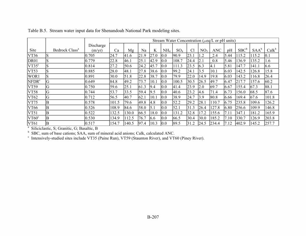
B-207

Table B.5. Stream water input data for Shenandoah National Park modeling sites.

Stream Water Concentration (Feq/L or pH units)

Site Bedrock Classa

Discharge

(m/yr) Ca Mg Na K NH4 SO4 Cl NO3 ANC pH SBCb SAAb Calkb

VT36 S 0.705 24.7 41.6 21.9 27.0 0.0 90.9 23.1 1.2 _2.4 5.44 115.2 115.2 0.1 DR01 S 0.779 22.8 46.1 25.1 42.9 0.0 108.7 24.4 2.1 _0.8 5.46 136.9 135.2 1.6 VT35c S 0.814 27.2 50.6 24.2 45.7 0.0 111.3 23.5 6.3 4.1 5.81 147.7 141.1 6.6 VT53 S 0.885 28.0 48.1 27.8 38.6 0.0 99.2 24.1 3.5 10.1 6.03 142.5 126.8 15.8 WOR1 S 0.891 30.0 51.8 22.8 38.7 0.0 79.9 22.0 14.9 19.8 6.03 143.2 116.8 26.4 NFDRc G 0.649 84.8 49.2 73.7 10.1 0.0 100.5 30.5 26.5 49.7 6.47 217.7 157.6 60.2 VT59 G 0.750 59.6 25.1 61.3 9.4 0.0 41.4 23.9 2.0 69.7 6.67 155.4 67.3 88.1 VT58 G 0.744 53.7 33.5 59.4 9.5 0.0 40.6 23.2 4.6 71.4 6.73 156.0 68.5 87.6 VT62 G 0.712 56.5 40.7 62.1 10.1 0.0 38.9 24.7 3.9 80.8 6.66 169.4 67.6 101.8 VT75 B 0.578 101.5 79.6 49.8 4.8 0.0 52.2 29.2 28.1 110.7 6.75 235.8 109.6 126.2 VT66 B 0.526 108.9 84.6 58.0 5.1 0.0 52.1 31.3 26.4 127.8 6.80 256.6 109.9 146.8 VT51 B 0.522 132.5 130.0 66.5 18.0 0.0 131.2 32.8 17.2 155.6 7.11 347.1 181.2 165.9 VT60c B 0.530 134.9 112.5 76.7 6.6 0.0 66.5 30.4 30.0 185.2 7.10 330.7 126.9 203.8 VT61 B 0.517 154.7 140.5 97.4 10.3 0.0 89.5 31.2 24.5 234.4 7.12 402.9 145.2 257.7 a Siliciclastic, S; Granitic, G; Basaltic, B b SBC, sum of base cations; SAA, sum of mineral acid anions; Calk, calculated ANC. c Intensively-studied sites include VT35 (Paine Run), VT59 (Staunton River), and VT60 (Piney River).

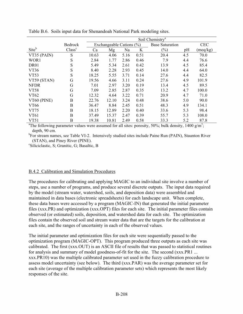
B-208

Table B.6. Soils input data for Shenandoah National Park modeling sites.

Soil Chemistrya Exchangeable Cations (%)

Siteb Bedrock Classc Ca Mg Na K

Base Saturation (%) pH

CEC (meq/kg)

VT35 (PAIN) S 10.63 4.06 5.16 0.51 20.4 4.5 70.0 WOR1 S 2.84 1.77 2.86 0.46 7.9 4.4 76.6 DR01 S 5.49 5.34 2.61 0.42 13.9 4.5 85.4 VT36 S 8.40 2.28 2.93 0.45 14.0 4.4 64.0 VT53 S 18.25 5.55 3.71 0.14 27.6 4.4 82.5 VT59 (STAN) G 19.56 4.66 3.11 0.24 27.6 4.9 101.9 NFDR G 7.01 2.97 3.20 0.19 13.4 4.5 89.5 VT58 G 7.09 2.85 2.87 0.35 13.2 4.7 100.0 VT62 G 12.32 4.64 3.22 0.71 20.9 4.7 71.0 VT60 (PINE) B 22.76 12.10 3.24 0.48 38.6 5.0 90.0 VT66 B 36.47 8.84 2.45 0.51 48.3 4.9 134.1 VT75 B 18.15 12.89 2.20 0.40 33.6 5.3 98.4 VT61 B 37.49 15.37 2.47 0.39 55.7 5.3 108.0 VT51 B 19.38 10.81 2.49 0.58 33.3 5.2 87.8 aThe following parameter values were assumed for all sites: porosity, 50%; bulk density, 1400 g/m3;

depth, 90 cm. bFor stream names, see Table VI-2. Intensively studied sites include Paine Run (PAIN), Staunton River

(STAN), and Piney River (PINE). cSiliciclastic, S; Granitic, G; Basaltic, B

B.4.2 Calibration and Simulation Procedures

The procedures for calibrating and applying MAGIC to an individual site involve a number of steps, use a number of programs, and produce several discrete outputs. The input data required by the model (stream water, watershed, soils, and deposition data) were assembled and maintained in data bases (electronic spreadsheets) for each landscape unit. When complete, these data bases were accessed by a program (MAGIC-IN) that generated the initial parameter files (xxx.PR) and optimization (xxx.OPT) files for each site. The initial parameter files contain observed (or estimated) soils, deposition, and watershed data for each site. The optimization files contain the observed soil and stream water data that are the targets for the calibration at each site, and the ranges of uncertainty in each of the observed values.

The initial parameter and optimization files for each site were sequentially passed to the optimization program (MAGIC-OPT). This program produced three outputs as each site was calibrated. The first (xxx.OUT) is an ASCII file of results that was passed to statistical routines for analysis and summary of model goodness-of-fit for the site. The second (xxx.PR1 ... xxx.PR10) was the multiple calibrated parameter set used in the fuzzy calibration procedure to assess model uncertainty (see below). The third (xxx.PAR) was the average parameter set for each site (average of the multiple calibration parameter sets) which represents the most likely responses of the site.

B-209

The multiple calibrated parameter set (xxx.PR1…xxx.pr10) for each site was used by the program MAGIC-RUN with estimates of historical or future deposition to produce two outputs: 1) reconstructions of historical change at the site; or 2) forecasts of most likely future responses for the applied future deposition scenario. The multiple calibrated parameter sets were also used with the same estimates of future deposition and the program MAGIC-RUN to produce an analysis of the uncertainty in model projections for that scenario. The results of the uncertainty analysis are in the form of an electronic spreadsheet giving simulated ranges (upper and lower values) for all modeled variables for each year of each scenario at the site.

B.4.3 Performance Analysis

The multiple calibration procedure for each site produced summary statistics (mean, standard deviation, maximum and minimum) for the observed values, the simulated values and the differences (simulated-observed values) of each of the 15 stream variables and each of the 7 soil variables simulated for each of the sites. In addition, plots of simulated versus observed values for stream variables were constructed (Figures B.1 and B.2). These analyses showed that the model calibration results were not biased and did not contain unacceptably large residual errors.

B.4.4 Analysis of Uncertainty

The estimates of the fixed parameters, the deposition inputs (past, current, and future), and the target variable values to which the model is calibrated all contain uncertainties. The multiple optimization procedure that was implemented for calibrating the model allows estimation of the effects of these uncertainties on simulated values from the calibrated model.

The procedure consists of multiple calibrations of each site using random values of the fixed parameters drawn from the observed range of values, and random values of deposition from the range of atmospheric model estimates. Each of the multiple calibrations begin with 1) a random selection of values of fixed parameters and deposition, and 2) a random selection of the starting values of the adjustable parameters. The adjustable parameters are then optimized to achieve a minimum error fit to the target variables. This procedure is repeated ten times for each site. The final calibrated model is represented by the ensemble of parameter values of all of the successful calibrations. To provide an estimate of the uncertainty (or reliability) of a simulated response to a given scenario, all of the ensemble parameter sets are run using the scenario. For any year in the scenario, the largest and smallest values of a simulated variable define the upper and lower confidence bounds for that site's response for the scenario under consideration. Applied for all variables and all years of the scenario, this procedure results in a band of simulated values through time that encompasses the likely response of the site for any point in the scenario. The distributions of these uncertainty estimates for each landscape unit can be regionalized to provide overall estimates of uncertainty for a scenario.

B-210

Figure B.1. Calibration results for the MAGIC model, expressed as predicted versus observed values in the calibration year for sulfate, nitrate, sum of base cations (SBC), sum of mineral acid anions (SAA), calculated ANC (CALK), and pH. Equality lines (1:1) are added for reference.

SO4

0

20

40

60

80

100

120

140

0 50 100 150Observed

Sim

ulat

edNO3

0

5

10

15

20

25

30

35

0 10 20 30 40Observed

Sim

ulat

ed

SBC

0

50

100

150

200

250

300

350

400

450

0 100 200 300 400 500Observed

Sim

ulat

ed

SAA

0

20

40

60

80

100

120

140

160

180

200

0 50 100 150 200Observed

Sim

ulat

ed

CALK

-50

0

50

100

150

200

250

300

-100 0 100 200 300Observed

Sim

ulat

ed

PH

3

4

5

6

7

8

3 4 5 6 7 8Observed

Sim

ulat

ed

B-211

Figure B.2. Simulated versus observed soils characteristics for modeled watersheds in Shenandoah National Park, expressed as exchangeable Ca, Mg, Na, and K, base saturation, and soil pH. Equality lines (1:1) are added for reference.

BS1

0

10

20

30

40

50

60

0 20 40 60Observed

Sim

ulat

ed

PH1

3

4

5

6

3 4 5 6Observed

Sim

ulat

ed

ECA1

0

5

10

15

20

25

30

35

40

0 10 20 30 40Observed

Sim

ulat

edEMG1

0

2

4

6

8

10

12

14

16

18

0 5 10 15 20Observed

Sim

ulat

ed

ENA1

0

1

2

3

4

5

6

0 1 2 3 4 5 6Observed

Sim

ulat

ed

EK1

0

1

0 1Observed

Sim

ulat

ed

B-212

The variations between predicted and observed chemistry (Figures B.1 and B.2) may reflect the uncertainty in model structure and performance more accurately than do the results of multiple calibrations. Natural systems respond to processes and rates that are only partially captured by the model formulation. In addition, there is uncertainty associated with the measured values. Thus, it is not surprising that there is some divergence between simulated and observed values.

B.5 Modeling Results

MAGIC was successfully calibrated to all 14 modeled watersheds for this project. Agreement was very good for all variables, with the possible exception of pH. The MAGIC model calculates pH using a number of constituents, including the charge-balance ANC and the concentrations of dissolved organic carbon (DOC) and aluminum (Al). Values for DOC and/or Al were missing from some of the model site databases. This introduced additional uncertainty into the estimates of pH for the calibration year.

A further check on the success of the calibration procedure can be made by comparing yearly time series of simulated values with the observed values at each site for the period of observed data (1988–1997, Figure B.3). While the model misses some of the observed year-to-year variability, the general agreement with the 10 years of observed data is good at each site. The model was calibrated to the average of the first five years of the observed data. The second five years of data at each site were not used in the calibration procedure.

Future stream water chemistry was simulated for each site throughout the period 1990 to 2100, based on the scenario of continued constant deposition at 1990 levels and the four future emissions control scenarios described in Chapter 7. Both forecast and hindcast simulation results for those scenarios are presented graphically and discussed in Chapter 7. The purpose of this appendix is to provide the background details of the acid deposition effects modeling used in this project (calibration and evaluation of model goodness-of-fit). The reader is referred to Chapter 7 for the details of the simulation results.

B-213

Deep Run DR01

-40

-20

0

20

40

60

1987 1989 1991 1993 1995 1997

ueq/

L

White Oak Run WOR1

-40

-20

0

20

40

60

1987 1989 1991 1993 1995 1997

ueq/

L

Paine Run VT35

-40

-20

0

20

40

60

1987 1989 1991 1993 1995 1997

ueq/

L

Meadow Run VT36

-40

-20

0

20

40

60

1987 1989 1991 1993 1995 1997

ueq/

L

Twomile Run VT53

-40

-20

0

20

40

60

1987 1989 1991 1993 1995 1997

ueq/

L

Calk (ueq/L)

0

2 04 0

6 08 0

1 00

1 2 0

1 4 0

1 9 8 5 1 9 9 0 1 9 9 5 2 0 00

Simulated

Observed

AQRV sites on Siliciclastic Bedrock

Figure B.3a. Simulated versus observed ANC over a ten-year period for modeling sites on siliciclastic bedrock. The calibration period for these sites was 1988–1992 (5-year average).

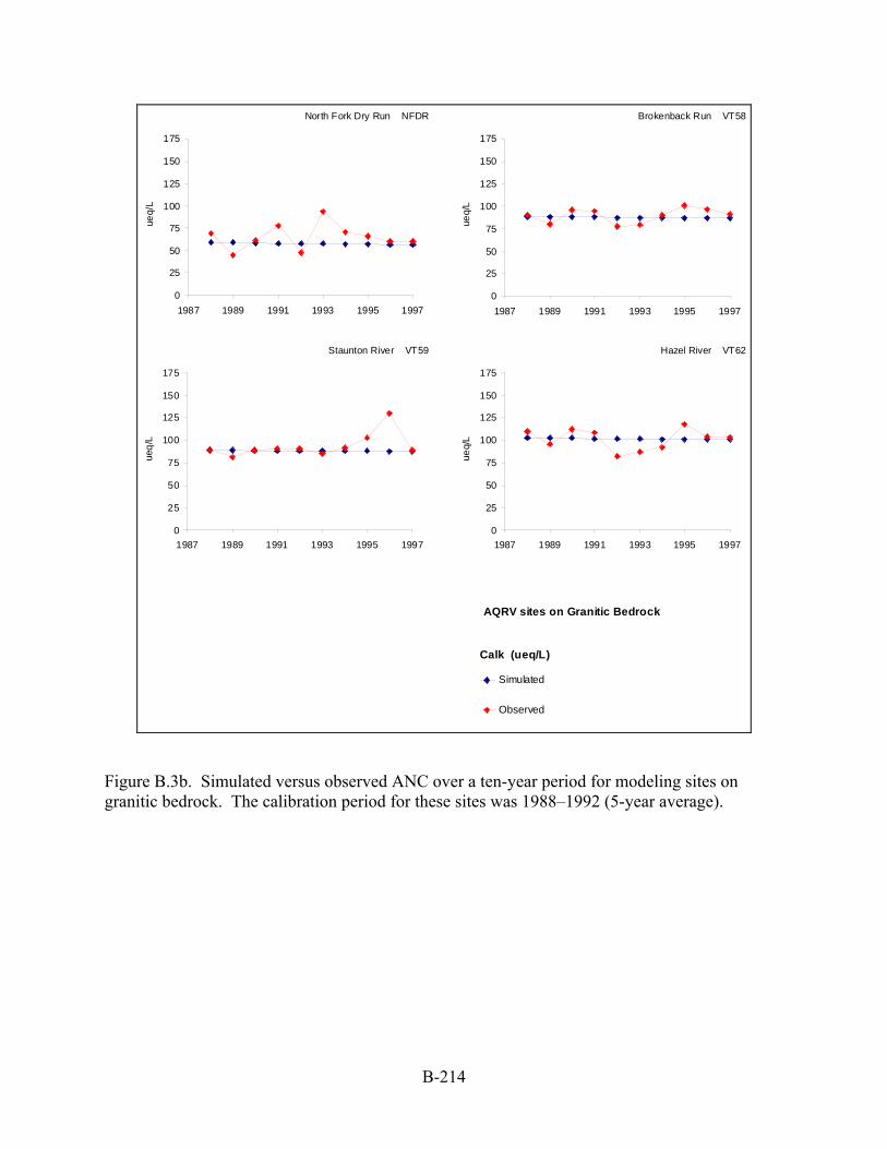
B-214

North Fork Dry Run NFDR

0

25

50

75

100

125

150

175

1987 1989 1991 1993 1995 1997

ueq/

L

Brokenback Run VT58

0

25

50

75

100

125

150

175

1987 1989 1991 1993 1995 1997

ueq/

L

Staunton River VT59

0

25

50

75

100

125

150

175

1987 1989 1991 1993 1995 1997

ueq/

L

Hazel River VT62

0

25

50

75

100

125

150

175

1987 1989 1991 1993 1995 1997

ueq/

L

Calk (ueq/L)

0

2 04 0

6 08 0

1 00

1 2 0

1 4 0

1 9 8 5 1 9 9 0 1 9 9 5 2 0 00

Simulated

Observed

AQRV sites on Granitic Bedrock

Figure B.3b. Simulated versus observed ANC over a ten-year period for modeling sites on granitic bedrock. The calibration period for these sites was 1988–1992 (5-year average).

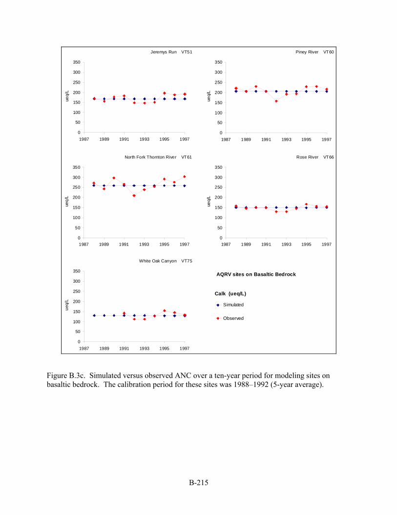
B-215

Jeremys Run VT51

0

50

100

150

200

250

300

350

1987 1989 1991 1993 1995 1997

ueq/

L

Piney River VT60

0

50

100

150

200

250

300

350

1987 1989 1991 1993 1995 1997

ueq/

L

North Fork Thornton River VT61

0

50

100

150

200

250

300

350

1987 1989 1991 1993 1995 1997

ueq/

L

Rose River VT66

0

50

100

150

200

250

300

350

1987 1989 1991 1993 1995 1997

ueq/

L

White Oak Canyon VT75

0

50

100

150

200

250

300

350

1987 1989 1991 1993 1995 1997

ueq/

L

Calk (ueq/L)

0

2 04 0

6 08 0

1 00

1 2 0

1 4 0

1 9 8 5 1 9 9 0 1 9 9 5 2 0 00

Simulated

Observed

AQRV sites on Basaltic Bedrock

Figure B.3c. Simulated versus observed ANC over a ten-year period for modeling sites on basaltic bedrock. The calibration period for these sites was 1988–1992 (5-year average).

As the nation's primary conservation agency, the Department of the Interior has responsibility for most of our nationally owned public land and natural resources. This includes fostering sound use of our land and water resources; protecting our fish, wildlife, and biological diversity; preserving the environmental and cultural values of our national parks and historical places; and providing for the enjoyment of life through outdoor recreation. The department assesses our energy and mineral resources and works to ensure that their development is in the best interests of all our people by encouraging stewardship and citizen participation in their care. The department also has a major responsibility for American Indian reservation communities and for people who live in island territories under U.S. administration.

NPS D-302 November 2006

National Park Service U.S. Department of the Interior

Northeast Region Natural Resource Stewardship and Science 200 Chestnut Street Philadelphia, Pennsylvania 19106-2878 http://www.nps.gov/nero/science/

EXPERIENCE YOUR AMERICA TM