Achieving quantum computation with quantum dot spin qubits Von der Fakultät für Mathematik, Informatik und Naturwissenschaften der RWTH Aachen University zur Erlangung des akademischen Grades eines Doktors der Naturwissenschaften genehmigte Dissertation vorgelegt von Diplom-Physiker Sebastian Johannes Mehl aus Woerden (Niederlande) Berichter: Universitätsprofessor Dr. David DiVincenzo Universitätsprofessor Dr. Hendrik Bluhm Universitätsprofessor Dr. Guido Burkard Tag der mündlichen Prüfung: 28.11.2014 Diese Dissertation ist auf den Internetseiten der Hochschulbibliothek online verfügbar.

Welcome message from author
This document is posted to help you gain knowledge. Please leave a comment to let me know what you think about it! Share it to your friends and learn new things together.
Transcript

Achieving quantum computation withquantum dot spin qubits
Von der Fakultät für Mathematik, Informatik und Naturwissenschaftender RWTH Aachen University zur Erlangung des akademischen Gradeseines Doktors der Naturwissenschaften genehmigte Dissertation
vorgelegt von
Diplom-PhysikerSebastian Johannes Mehl
aus Woerden (Niederlande)
Berichter: Universitätsprofessor Dr. David DiVincenzoUniversitätsprofessor Dr. Hendrik BluhmUniversitätsprofessor Dr. Guido Burkard
Tag der mündlichen Prüfung: 28.11.2014
Diese Dissertation ist auf den Internetseiten der Hochschulbibliothek online verfügbar.


Summary
A two-level quantum system is the building block of a quantum computer. Thispair of quantum states defines the computational unit of a quantum computer, andit is called a quantum bit or qubit in analogy to the bit that is the binary unit of aclassical computer. The spin of a single electron naturally defines such a two-levelquantum system. A quantum dot can be tuned to the single-electron regime, and anarray of singly occupied quantum dots provides a multi-qubit register. This thesisdescribes the multielectron encoding of a spin qubit using a pair or a trio of quantumdots, and it analyzes the coherence properties and manipulation protocols of thissystem.
The singlet-triplet qubit, coded using the singlet state and the spinless triplet stateof a pair of singly occupied quantum dots, can be controlled all electrically when ap-plying voltages to gates close to the quantum dot structure. Rapid, subnanosecondmodifications of the double quantum dot’s charge configuration have been realizedsuccessfully. A small magnetic field gradient across the double quantum dot enablesuniversal qubit control. Two modifications of the normal singlet-triplet encodingare introduced. (1) The six-electron configuration of a double quantum dot encodesa singlet-triplet qubit in the same way as for the two-electron double quantum dot.Two electrons at each quantum dot are irrelevant for the qubit manipulations be-cause they are paired in a singlet state; the remaining two electrons encode thequbit. The qubit’s wave function is immune to charge noise at moderate out-of-plane magnetic fields. (2) A singlet-triplet qubit encoded using two quantum dotsof different sizes has an orbital state degeneracy of the singlet state and the spinlesstriplet state at finite out-of-plane magnetic fields. Spin-orbit interactions lift thisstate degeneracy, while the magnitude of the state coupling is determined by the sizedifference of the QDs. This setup enables the manipulations of singlet-triplet qubitswithout the need for magnetic field gradients. Finally, two-qubit gates betweensinglet-triplet qubits are proposed that use mediated exchange interactions via onequantum state. These operations are well controlled and highly noise insensitive.
Orbital interactions alone can control spin qubits coded in a three electron Hilbertspace. For example, the exchange-only qubit is encoded using three singly occupiedquantum dots. The exchange interactions of two quantum dot pairs need to bemodified to manipulate this qubit. The noise sensitivity of the exchange-only qubitis discussed. Alternatively, a three-electron qubit at a double quantum dot can beoperated when single electrons are transferred between the quantum dots. Fast,subnanosecond manipulations of the double quantum dot’s charge configuration arerequired to realize single-qubit gates. A novel two-qubit pulse gate for the three-electron double quantum dot qubit is proposed.
iii


Zusammenfassung
Ein quantenmechanisches Zweiniveausystem ist der Grundbaustein eines Quanten-computers. Es definiert die Recheneinheit eines Quantencomputers, die auch alsQuantenbit oder Qubit bezeichnet wird. Diese Definition ist analog zu der einesBits, der binären Recheneinheit eines klassischen Computers. Der Spin eines einzel-nen Elektrons wird natürlicherweise durch ein Zweiniveausystem beschrieben. EinQuantenpunkt kann mit nur einem Elektron besetzt sein, sodass mehrere Quan-tenpunkte ein Qubitregister ergeben. Diese Arbeit beschreibt Qubitdefinitionen imSpinsektor von mehreren Elektronen, die auf zwei oder drei Quantenpunkte verteiltsind. Insbesondere werden die Kohärenzeigenschaften dieser Systeme beschrieben,sowie Protokolle für quantenmechanische Rechnungen diskutiert.
Das Singulett-Triplett Qubit, das durch das Singulett und den spinfreien Tri-plettzustand von zwei Elektronen eines Doppelquantenpunkts definiert ist, kannmit elektrischen Gatterspannungen manipuliert werden. Für solche Doppelquan-tenpunkte ist es gelungen in Experimenten quantenmechanische Rechenprotokollezu realisieren. Wenn ein Magnetfeldgradient zwischen den beiden Quantenpunk-ten vorhanden ist, kann dieses Qubit vollständig kontrolliert werden. In dieser Ar-beit werden zwei Modifikationen des Singulett-Triplett Qubits vorgestellt. (1) SechsElektronen können genauso wie zwei Elektronen ein Singulett-Triplett Qubit definie-ren. Zwei Elektronen werden jeweils auf einem Quantenpunkt gepaart, sodass diesefür Quantenoperationen irrelevant sind. Die restlichen beiden Elektronen definierendas Qubit. Solche Singulett-Triplett Qubits sind bei moderaten Magnetfeldern im-mun gegenüber Ladungsrauschen. (2) Wenn man für das Singulett-Triplett Qubitzwei Quantenpunkte unterschiedlicher Größe verwendet, dann kann das Energiedia-gramm eine Entartung zwischen den Qubitzuständen haben. Diese wird durch dieSpin-Bahn Wechselwirkung aufgehoben und das Qubit benötigt für die volle Quan-tenkontrolle keinen Magnetfeldgradienten mehr. Zusätzlich werden Quantengatterzwischen zwei Singulett-Triplett Qubits beschrieben, wenn die beiden Qubits übereinen Quantenzustand gekoppelt sind. Diese Gatter können gut kontrolliert werdenund haben hervorragende Kohärenzeigenschaften.
Orbitale Wechselwirkungen genügen um Spinqubits zu kontrollieren, die im Hil-bertraum dreier Elektronen definiert sind. So gibt es ein Qubit, das einzig durchdie Austauschwechselwirkungen zwischen drei Elektronen auf drei Quantenpunktenkontrolliert werden kann. Diese Arbeit beschreibt die Kohärenzeigenschaften die-ses Qubits. Zusätzlich wird ein Qubit beschrieben, das mit drei Elektronen in einerDoppelquantenpunktstruktur definiert ist. Quantengatter für dieses Qubit benötigenOperationen, die schneller als Nanosekunden sind. Da solche Operationen für diesesQubit experimentell realisiert wurden, stellt diese Arbeit Quantengatter zwischenzwei solcher Qubits nach demselben Prinzip vor.
v


Abbreviations
Appx. AppendixCNOT controlled NOTCPHASE controlled phaseCT charge trapDLZC degenerate Landau-Zener crossingDM Davies ModelDQD double quantum dotFig. figureGaAs gallium arsenideH.c. Hermitian conjugateHQ hybrid qubitInAs indium arsenideISTQ inverted singlet-triplet qubitLZ Landau-ZenerNMR nuclear magnetic resonanceQD quantum dotQS quantum stateP phosphorusrms root mean squareSec. sectionSi siliconSOI spin-orbit interactionSTQ singlet-triplet qubitSW Schrieffer-WolffTab. tableTLF two-level fluctuatorTQD triple quantum dot
vii

Contents
1 Introduction 11.1 Why Quantum Computation? . . . . . . . . . . . . . . . . . . . . . . 11.2 Requirements for Quantum Computation . . . . . . . . . . . . . . . 31.3 Physical Implementation of a Quantum Computer . . . . . . . . . . 51.4 Outline of the Thesis . . . . . . . . . . . . . . . . . . . . . . . . . . . 6
2 Quantum Dot Qubits 92.1 Charge Qubit . . . . . . . . . . . . . . . . . . . . . . . . . . . . . . . 102.2 Loss-DiVincenzo Qubit . . . . . . . . . . . . . . . . . . . . . . . . . 102.3 ST0 Qubit . . . . . . . . . . . . . . . . . . . . . . . . . . . . . . . . 122.4 Exchange-Only Qubit . . . . . . . . . . . . . . . . . . . . . . . . . . 132.5 Madison Qubit . . . . . . . . . . . . . . . . . . . . . . . . . . . . . . 15
3 Noise Description 173.1 Physical Noise Picture . . . . . . . . . . . . . . . . . . . . . . . . . . 173.2 Hyperfine Interactions . . . . . . . . . . . . . . . . . . . . . . . . . . 193.3 Charge Noise . . . . . . . . . . . . . . . . . . . . . . . . . . . . . . . 203.4 Spin-Orbit Interactions and Phonons . . . . . . . . . . . . . . . . . . 21
4 Static and Resonant Manipulations of Encoded Spin Qubits 234.1 Model . . . . . . . . . . . . . . . . . . . . . . . . . . . . . . . . . . . 24
4.1.1 Singlet-Triplet Qubit (cf. Sec. 2.3) . . . . . . . . . . . . . . . 244.1.2 Triple Quantum Dot Qubit (cf. Sec. 2.4) . . . . . . . . . . . . 254.1.3 Noise of Encoded Spin Qubits . . . . . . . . . . . . . . . . . . 274.1.4 General Hamiltonian . . . . . . . . . . . . . . . . . . . . . . . 28
4.2 Static Time Evolutions . . . . . . . . . . . . . . . . . . . . . . . . . 304.2.1 Single-Qubit Gates . . . . . . . . . . . . . . . . . . . . . . . . 304.2.2 Two-Qubit Gates . . . . . . . . . . . . . . . . . . . . . . . . . 31
4.3 Driven Time Evolutions . . . . . . . . . . . . . . . . . . . . . . . . . 334.3.1 Single-Qubit Gates . . . . . . . . . . . . . . . . . . . . . . . . 334.3.2 Two-Qubit Gates . . . . . . . . . . . . . . . . . . . . . . . . . 36
4.4 Noise Discussion for Encoded Spin Qubits . . . . . . . . . . . . . . . 40
Appendices 464.A Characterization of Classical Noise . . . . . . . . . . . . . . . . . . . 464.B Characterization of Entangling Properties . . . . . . . . . . . . . . . 464.C Large Amplitude Driving . . . . . . . . . . . . . . . . . . . . . . . . 48
ix
Contents
5 Noise-Protected Gate for Six-Electron Double-Dot Qubits 495.1 Introduction . . . . . . . . . . . . . . . . . . . . . . . . . . . . . . . . 505.2 Model . . . . . . . . . . . . . . . . . . . . . . . . . . . . . . . . . . . 505.3 Charge Noise . . . . . . . . . . . . . . . . . . . . . . . . . . . . . . . 525.4 Robust Single-Qubit Gating . . . . . . . . . . . . . . . . . . . . . . . 555.5 Conclusion . . . . . . . . . . . . . . . . . . . . . . . . . . . . . . . . . 56
Appendices 585.A Description of the Fidelity Analysis . . . . . . . . . . . . . . . . . . . 58
6 Inverted Singlet-Triplet Qubit Coded on a Two-Electron Double QuantumDot 616.1 Introduction . . . . . . . . . . . . . . . . . . . . . . . . . . . . . . . . 626.2 Model . . . . . . . . . . . . . . . . . . . . . . . . . . . . . . . . . . . 636.3 Calculation of ∆so . . . . . . . . . . . . . . . . . . . . . . . . . . . . 656.4 Qubit Manipulations . . . . . . . . . . . . . . . . . . . . . . . . . . . 69
6.4.1 Single-Qubit Gates . . . . . . . . . . . . . . . . . . . . . . . . 696.4.2 Two-Qubit Gates . . . . . . . . . . . . . . . . . . . . . . . . . 70
6.5 Discussion and Conclusion . . . . . . . . . . . . . . . . . . . . . . . . 72
Appendices 746.A Full Calculation of ∆so from SOIs . . . . . . . . . . . . . . . . . . . 746.B Doubly Occupied Single QDs . . . . . . . . . . . . . . . . . . . . . . 756.C Spin-Orbit Parameters . . . . . . . . . . . . . . . . . . . . . . . . . . 76
7 Two-Qubit Couplings of Singlet-Triplet Qubits Mediated by One QuantumState 797.1 Introduction . . . . . . . . . . . . . . . . . . . . . . . . . . . . . . . . 807.2 Model . . . . . . . . . . . . . . . . . . . . . . . . . . . . . . . . . . . 817.3 Entangling Operations . . . . . . . . . . . . . . . . . . . . . . . . . . 82
7.3.1 Empty or Doubly Occupied QS . . . . . . . . . . . . . . . . . 827.3.2 Singly Occupied QS . . . . . . . . . . . . . . . . . . . . . . . 84
7.4 Gate Performance and Noise Properties . . . . . . . . . . . . . . . . 867.4.1 Fabrication Errors . . . . . . . . . . . . . . . . . . . . . . . . 867.4.2 Hyperfine Interactions . . . . . . . . . . . . . . . . . . . . . . 877.4.3 Spin-Orbit Interactions . . . . . . . . . . . . . . . . . . . . . . 897.4.4 Charge Noise . . . . . . . . . . . . . . . . . . . . . . . . . . . 89
7.5 Conclusion . . . . . . . . . . . . . . . . . . . . . . . . . . . . . . . . 90
Appendices 927.A Gate Description . . . . . . . . . . . . . . . . . . . . . . . . . . . . . 92
7.A.1 Characterization of Entangling Gates . . . . . . . . . . . . . . 927.A.2 Fidelity Analysis . . . . . . . . . . . . . . . . . . . . . . . . . 92
x

Contents
7.B Orbital Hamiltonian . . . . . . . . . . . . . . . . . . . . . . . . . . . 927.B.1 Empty QS . . . . . . . . . . . . . . . . . . . . . . . . . . . . . 937.B.2 Singly Occupied QS . . . . . . . . . . . . . . . . . . . . . . . . 957.B.3 Doubly Occupied QS . . . . . . . . . . . . . . . . . . . . . . 95
7.C Spin-Orbit Interactions . . . . . . . . . . . . . . . . . . . . . . . . . 957.D Numerical Gate Search . . . . . . . . . . . . . . . . . . . . . . . . . 977.E Gate Sequences . . . . . . . . . . . . . . . . . . . . . . . . . . . . . . 98
7.E.1 Full Gate Sequences for CNOT Operations . . . . . . . . . . . 987.E.2 Numerical Values . . . . . . . . . . . . . . . . . . . . . . . . . 98
8 Noise Analysis of Qubits Implemented in Triple Quantum Dot Systems 998.1 Introduction . . . . . . . . . . . . . . . . . . . . . . . . . . . . . . . 1008.2 Model . . . . . . . . . . . . . . . . . . . . . . . . . . . . . . . . . . . 102
8.2.1 Triple Dot Hamiltonian . . . . . . . . . . . . . . . . . . . . . 1028.2.2 Subspace and Subsystem Qubits . . . . . . . . . . . . . . . . 1048.2.3 Noise Description . . . . . . . . . . . . . . . . . . . . . . . . 105
8.3 Approach to Model Real Systems . . . . . . . . . . . . . . . . . . . . 1068.3.1 System Parameters . . . . . . . . . . . . . . . . . . . . . . . . 1068.3.2 Transition Rates for the Noise Description . . . . . . . . . . . 107
8.4 Analysis of the Time Evolution . . . . . . . . . . . . . . . . . . . . . 1128.4.1 Subspace Qubit . . . . . . . . . . . . . . . . . . . . . . . . . 1138.4.2 Subsystem Qubit . . . . . . . . . . . . . . . . . . . . . . . . . 115
8.5 Effective Errors . . . . . . . . . . . . . . . . . . . . . . . . . . . . . . 1178.5.1 Subspace Qubit . . . . . . . . . . . . . . . . . . . . . . . . . 1188.5.2 Subsystem Qubit . . . . . . . . . . . . . . . . . . . . . . . . . 124
8.6 Summary and Outlook . . . . . . . . . . . . . . . . . . . . . . . . . . 126
Appendices 1288.A Simplification of the Analysis . . . . . . . . . . . . . . . . . . . . . . 128
8.A.1 Rotating Frame . . . . . . . . . . . . . . . . . . . . . . . . . 1288.A.2 Symmetry of Phase Noise . . . . . . . . . . . . . . . . . . . . 1288.A.3 High Symmetry Regimes . . . . . . . . . . . . . . . . . . . . 128
8.B Descriptions of the Initial Time Evolution . . . . . . . . . . . . . . . 1308.B.1 Subspace Qubit . . . . . . . . . . . . . . . . . . . . . . . . . 1318.B.2 Subsystem Qubit . . . . . . . . . . . . . . . . . . . . . . . . . 132
8.C Long Time Limit of the Time Evolution . . . . . . . . . . . . . . . . 1338.D Error Analysis of the Single-Qubit Time Evolution . . . . . . . . . . 135
8.D.1 Solid State Approach . . . . . . . . . . . . . . . . . . . . . . 1358.D.2 Information Theoretical Approach . . . . . . . . . . . . . . . 1368.D.3 Error Rates in Our Model . . . . . . . . . . . . . . . . . . . . 138
8.E Model Systems . . . . . . . . . . . . . . . . . . . . . . . . . . . . . . 1398.E.1 Model 1: Pure Relaxation . . . . . . . . . . . . . . . . . . . . 1408.E.2 Model 2: Pure Dephasing . . . . . . . . . . . . . . . . . . . . 1418.E.3 Model 3: Two State Leakage . . . . . . . . . . . . . . . . . . 141
xi
Contents
8.E.4 Model 4: Internal Transitions of the Subsystem Qubit . . . . 142
9 Two-Qubit Pulse Gate for the Three-Electron Double Quantum Dot Qubit 1439.1 Introduction . . . . . . . . . . . . . . . . . . . . . . . . . . . . . . . . 1449.2 Setup . . . . . . . . . . . . . . . . . . . . . . . . . . . . . . . . . . . 1459.3 Two-Qubit Pulse Gate . . . . . . . . . . . . . . . . . . . . . . . . . . 1469.4 Gate Performance and Noise Properties . . . . . . . . . . . . . . . . 149
9.4.1 Charge Noise . . . . . . . . . . . . . . . . . . . . . . . . . . . 1509.4.2 Hyperfine Interactions . . . . . . . . . . . . . . . . . . . . . . 150
9.5 Conclusion . . . . . . . . . . . . . . . . . . . . . . . . . . . . . . . . 151
Appendices 1539.A Fidelity Description of Noisy Gates . . . . . . . . . . . . . . . . . . . 1539.B Extended Basis . . . . . . . . . . . . . . . . . . . . . . . . . . . . . . 153
10 Summary and Outlook 15510.1 Summary . . . . . . . . . . . . . . . . . . . . . . . . . . . . . . . . . 15510.2 The Way Ahead . . . . . . . . . . . . . . . . . . . . . . . . . . . . . . 156
xii

CHAPTER 1
Introduction
“how can we simulate the quantum mechanics? (...) We can giveup on our rule about what the computer was, we can say: Let thecomputer itself be build of quantum mechanical elements which obeyquantum mechanical laws (...) I’m not happy with all the analysesthat go with just the classical theory, because nature isn’t classical(...) and if you want to make a simulation of nature, you’d bettermake it quantum mechanical” (Feynman, 1982 [1])
1.1 Why Quantum Computation?
Richard Feynman suggested in 1982 that a computer should follow quantum mechan-ical laws to simulate quantum physics efficiently [1]. Our everyday computer, whichis called a classical computer in the following, very often uses quantum mechanicaleffects. However, the computation does not rely on quantum mechanics. The com-putational unit - the bit - can realize two discrete values “0” and “1”. Additionally,the calculations of classical computers can be irreversible. In Feynman’s proposal,a quantum computer works fundamentally differently from a classical computer. Inparticular, the calculations are reversible and follow the rules of quantum mechanicsin every aspect. The following two examples describe quantum mechanical effectsthat lack a classical analogue:Quantum superpositions — The computational unit of a quantum computer is a
quantum mechanical two-level system, which is called a quantum bit or qubit. Notethat a physical system suited to realize a quantum computer can be very abstract,and the encoding of a qubit only requires that a two-level quantum system can beidentified in a much larger Hilbert space. These two quantum states are labeled by|0〉 and |1〉 , similar to classical bits. However, quantum mechanics permits thatwave functions have information in |0〉 and |1〉 at the same time. These wavefunctions are in a superposition of |0〉 and |1〉 . The description with classicalprobability densities for quantum mechanical wave functions is insufficient (cf., e.g.,Ref. [2, 3]). Quantum mechanics offers an additional phase freedom that has noclassical analogue.
Young’s double-slit experiment from the early history of quantum mechanicsproves the existence of the phase degree of freedom (cf., e.g., Ref. [4]). The im-age of a light beam is collected at a screen after passing through a barrier with two
1

1 Introduction
slits. Each slit alone would generate its own picture. In the experiment, the lightbeam passes through every slit with equal probabilities. The image at the screencan be explained by the interference of two coherent waves that emerge from the twoslits. This result is consistent with a wave picture of light. One can, however, lowerthe intensity of the light source so that only one photon at a time passes throughthe barrier. The image collected from many photons shows also the interferencepattern, even though a single photon cannot interfere with a second photon afterpassing through the barrier. Classical physics does not explain these results, butquantum mechanics offers a simple explanation. The photon’s wave function splitsat the barrier where it goes with equal probabilities through both slits. The proba-bility amplitudes that emerge from the two slits interfere with each other and createthe image at the screen.
Quantum entanglement — Quantum mechanical experiments with two qubits areeven more surprising. The bipartite wave function is not necessarily separable intotwo independent wave functions. This phenomenon is called entanglement. Einstein,Podolsky, and Rosen described consequences of quantum mechanical entanglementthat seem to be in contradiction to our classical world [5]. Their thought experiment,leading to what is nowadays known as the EPR paradox, rejects our classical pictureof local reality (cf., e.g., Ref. [4, 6]). From our everyday life, we expect that physicalsystems are described by observables that are determined independently of theirmeasurements. In other words, observations should not influence the physical reality.The locality principle says that physically disconnected systems cannot influenceeach other. In the EPR paradox, an entangled photon pair |ψ〉 ∝ |↑↓〉 − |↓↑〉 issent to the observers A and B. The first entry of |ψ〉 is obtained by A, the secondone by B. The two observers are far away from each other, and their measurementsare locally disconnected. Each observer can measure his quantum state in twoorthogonal measurement bases σx and σz. In the experiment, first A measures hisphoton, then B measures. If A measures in the σz-basis, then the measurementoutcome of B is determined with certainty in the σz-basis, but the measurement inthe σx-basis is undetermined and can give two different results. If A measures in theσx-basis, then the measurement outcome of B is determined only in the σx-basis, butnot in the σz-basis. The EPR paradox shows that the physical reality of B (whichmeasurement basis is determined) depends on the measurement of A. The classicalpicture of local reality cannot hold.
Feynman postulated a quantum computer because classical computers cannot sim-ulate quantum physics efficiently [1]. Today, quantum simulations of small quantumsystems are possible [7]. It was shown that quantum computers outperform classicalcomputers even further. Quantum computers can realize all computations of clas-sical computers, but also quantum algorithms run on quantum computers that areimpossible on classical computers [8]. Deutsch described the first problem that issolved more efficiently by a quantum computer than by any classical algorithm [9].It should be determined if a function f : 0, 1 → 0, 1 is balanced or constant. Abalanced function is characterized by f (0) 6= f (1), while a constant function gives
2

1.2 Requirements for Quantum Computation
f (0) = f (1). One solution is described by Preskill [10]: a two-qubit quantum reg-ister is initialized to | init〉 = 1√
2[|0〉 + |1〉 ] ⊗ 1√
2[|0〉 − |1〉 ]. The unitary function
Uf (|x, y〉) = |x, y ⊕ f (x)〉 leaves the first entry untouched, but it gives for the sec-ond entry the exclusive or operation of y and f (x) [called y⊕f (x)]. The result for thesecond entry is 1 if y differs from f (x), but it is 0 otherwise. Acting with Uf on thequantum state | init〉 gives Uf (| init〉) ∝
[(−1)f(0) |0〉 + (−1)f(1) |1〉
]⊗ [|0〉 − |1〉 ].
The first factor is 1√2
[|0〉 + |1〉 ] for a constant function, but it is 1√2
[|0〉 − |1〉 ]for a balanced function. The measurement of the first qubit in the σx-basis solvesDeutsch’s problem because it gives “+1” for a constant function and “-1” for a bal-anced function.
Deutsch’s algorithm might seem to be useless, but it still shows that a quantumcomputer can solve a problem more efficiently than any classical computer. Thesolution of Deutsch’s problem is obtained in one run on a quantum computer, whilea classical algorithm needs two calculations. After the first classical calculation,which might give f (0) = 0, it is undetermined if f (1) = 0 and the function isconstant, or if f (1) = 1 and the function is balanced. More advanced quantum codeshave been developed since the proposal of Deutsch’s algorithm [11–13]: the Groveralgorithm is a search algorithm that finds from a register of length N one desiredentry |w〉 . It uses a function, where every function call rotates the initial state| init〉 towards the desired state |w〉 more efficiently than randomly choosing entriesfrom the register. Shor described how a quantum computer factors large numbersinto primes efficiently [14]. There is no classical algorithm known that solves thisproblem efficiently; cryptography relies on the principle that large numbers cannotbe factored easily. Quantum computers have become interesting for industrial usesince the proposal of Shor’s algorithm. So far, however, only small numbers havebeen factored into primes using Shor’s algorithm because no quantum computerwith more than a few qubits has been available (cf., e.g., the factoring of 15 into theprime factors 3 and 5 using superconducting qubits in Ref. [15]).
1.2 Requirements for Quantum Computation
A quantum computer has to fulfill the following five requirements that are definedfollowing Ref. [16].
(1) Well defined qubit and scalable system of qubits — Two quantum states |0〉and |1〉 encode one qubit. A qubit can realize any superposition of |0〉 and |1〉 :
|ψ〉 = eiα[cos (θ/2) |1〉 + eiφ sin (θ/2) |0〉
]. (1.1)
The phase α is only detectable when the qubit states are compared with anotherquantum state; α represents the global phase freedom of a quantum state. Allstates |ψ〉 can be mapped to the surface of a sphere - the Bloch sphere [6] - by thefunction f : ρ → X. f maps the density matrix ρ = |ψ〉 〈ψ| to the Bloch vectorX = (X, Y, Z)T that has the components Xi = tr (σiρ), i = 1, . . . , 3. |1〉 and |0〉
3

1 Introduction
are mapped to the north pole and the south pole; all equal superpositions of |1〉and |0〉 lie on the equator. θ and φ are the polar and azimuthal rotation angles ofa spherical coordinate system. Fig. 1.1 sketches the Bloch sphere representation ofa quantum state.
Of course, a single qubit is not sufficient to realize a quantum computer, and thequbit encoding must be scalable to many qubits.
Figure 1.1: Bloch sphere picture of a quantum state |ψ〉 =eiα[cos (θ/2) |1〉 + eiφ sin (θ/2) |0〉
]. All single-qubit states are mapped
to the surface of a sphere. |1〉 and |0〉 are on the north pole and on thesouth pole; all equal superpositions of |1〉 and |0〉 lie on the equator.|ψ〉 is characterized by the polar and azimuthal rotation angles θ andφ, according to the description in a spherical coordinate system.
(2) Initialization — One must be able to initialize the quantum system to a purestate. The initialization to the ground state of all qubits |0 . . . 0〉 is often easiest.(3) Readout — The quantum system must be read out at the end of a calculation.
If the readout is slightly imperfect, then the results of identical calculations stillprovide sufficient information about the quantum state.
(4) Universal set of quantum gates — The time evolution of any quantum systemcan be simulated using a universal set of quantum gates. It was shown that acomplete set of single-qubit operations and the controlled NOT (CNOT) operation,
CNOT =
1 0 0 00 1 0 00 0 0 10 0 1 0
(1.2)
(written in the two-qubit computation basis |11〉 , |10〉 , |01〉 , and |00〉), provideuniversal quantum control [17].
(5) Relevant coherence times gate operation time — The quantum systemmust conserve all the state information, which include the phase coherences between
4
1.3 Physical Implementation of a Quantum Computer
quantum states. Quantum algorithms were developed that correct for errors of thequbit, while it is important that the errors do not accumulate before they can becorrected by a quantum error correction protocol (cf., e.g., Ref. [6]). Therefore, thecoherence times of the quantum states must be longer than the gate operation times.
1.3 Physical Implementation of a Quantum Computer
Our everyday experience tells us that quantum phenomena are hard to observe, andeven more, that the quantum coherence is hard to preserve. Currently, quantumcomputers can preserve the coherences between a few qubits. It is very demandingto fulfill all the five requirements for quantum computation from Sec. 1.2 at thesame time. The main subject of this thesis are spin quantum computers encodedusing quantum dot (QD) qubits. Ref. [18] has suggested this qubit encoding for thefirst time (cf. also Ref. [19]). The following solutions of the five requirements forquantum computation from Sec. 1.2 were described.
(1) A singly occupied QD, or even easier one unpaired excess electron of a gate-defined QD, provides a spin-1
2degree of freedom that can be used to encode quantum
information. The fabrication of several QDs of this kind is possible, which realizesa multi-qubit register.
(2) External magnetic fields separate |1〉 = |↑〉 and |0〉 = |↓〉 energetically. Theenergy splitting is larger than the thermal energy at low cryogenic temperatures(< few hundred milikelvin) and at moderate external magnetic fields (few hundredmilitesla for GaAs QDs). Thermal relaxation prepares the qubit in its ground state.
(3) The spin of a QD electron can be determined through a spin valve or whenthis electron is transferred to a paramagnetic QD.
(4) The local magnetic fields at the QDs provide full single-qubit control. The spincan be controlled by electron spin resonance, similar to the experiments in the fieldof nuclear magnetic resonance. Note that all spin-1
2pairs must be controlled selec-
tively. Two-qubit gates were described that use the exchange interactions betweenneighboring QDs. If a second electron is added to a QD, then the Pauli exclu-sion principle favors a singlet configuration. Virtual electron tunnelings betweentwo singly occupied QDs lower the singlet energy compared to the energy of alltriplets (antiferromagnetic exchange). Two-qubit exchange gates can be controlledall electrically when the tunnel couplings are modified.
(5) Many semiconducting materials have weak spin-orbit interactions (SOIs),which isolates the spin part of the electron wave function from the orbital partof the electron wave function. The spin is now well protected from electric noise.Ideally, QD electrons are disturbed only weakly by magnetic noise (cf. Sec. 3.2).
Rapid progress has been made in the coherent control of spin qubits since theirproposal in 1998. The impressive finding of Ref. [18] is that qubits are well protectedif they are encoded using the spin degree of freedom of confined electrons. Never-theless, these qubits are well tunable. Especially the manipulations of the exchangeinteractions between neighboring QDs have turned out to be extremely successful.
5

1 Introduction
Chapter 2 reviews many important experiments for multi-QD devices.Note that there are alternative methods to fabricate spin qubits. Donor-bound
spin qubits are closely related to the QD spin qubits [20]. A phosphorus donorin a silicon heterostructure binds a single electron. The electron’s spin and thephosphorus’ nuclear spin (P is a spin-1
2nucleus) provide the possibility to encode
a qubit. Recently impressive progress was made on the control of the electronspin and the nuclear spin for donor-bound spin qubits [21–23]. Self-assembled QDsprovide another class of spin qubits [24]. GaAs and InAs have a lattice mismatch,which allows the growth of InAs QDs at the interface of GaAs and InAs. Self-assembled QDs are usually manipulated optically, which makes the gates of thesespin qubits distinct from the gates for spin qubits encoded using gate-defined QDs.Self-assembled QDs are not discussed any further.
There are many other systems that encode qubits. Superconducting qubits shouldbe named as the important alternative in the solid state [25, 26]. Superconductivityis probably the most well known macroscopic quantum phenomenon. The resistancesof some metals vanish at low temperatures. Electrons are paired into Cooper pairsand allow lossless electric currents. A superconducting element can be describedby a LC circuit. The flux trough the inductor L and the charge on the capacitorC are conjugate variables. The LC circuit is the electric realization of a harmonicoscillator, and two eigenstates encode one qubit. A nonlinear circuit element, whichis provided by the Josephson junction, breaks the equidistant level spacing andenables driven state transitions.
1.4 Outline of the Thesis
This thesis examines QD spin qubits and their ability to realize quantum computa-tion.
Chapter 2 introduces all the qubit encodings that are used in the remaining partsof the thesis. An array of QDs, each with a fixed electron configuration, offers avariety of qubit encodings: among them are the singlet-triplet qubit, the exchange-only qubit, and the Madison qubit. This chapter should also serve as a referenceguide to the most common manipulation protocols for spin qubits, and it includesa comprehensive review of important spin qubit experiments.
Chapter 3 describes noise models for QD spin qubits. A qubit must be wellprotected from external influences to realize quantum computation. This chapterdescribes the noise channels from hyperfine interactions, from charge traps, and fromSOIs.
Chapter 4 analyzes manipulation protocols for spin qubits. It focuses on twoprominent qubit encodings, which are the singlet-triplet qubit and the exchange-only qubit. Single-qubit gates and one maximally entangling two-qubit gate areconvenient for universal quantum computation. Static and resonant single-qubitgates are well established for encoded spin qubits. Two-qubit gates are analyzed thatrely on the Coulomb interactions between the electrons of the different qubits. The
6

1.4 Outline of the Thesis
aim of this chapter is to discuss the robustness of different manipulation protocolsin the presence of realistic noise sources.
Chapter 5 is a reprint of Ref. [27]. An exchange gate for singlet-triplet qubits isproposed that is protected from charge noise. The normal exchange gate tunes thequbit from the (1, 1) configuration, where the two electrons are spatially separated,towards (0, 2), where one QD is empty and the other one is doubly occupied. Thenoise protected exchange gate relies on two principles. (1) Very high bias is appliedand the qubit is pulsed far into (0, 2). Not only the singlet state permits the chargetransfer, but also the spin blockade of the triplet state is lifted. (2) The exchangegate is even more favorable between the (3, 3) and (2, 4) charge configurations ofmany-electron QDs at finite out-of-plane magnetic fields.
Chapter 6 examines the encoding of a singlet-triplet qubit in the setup of onelarge QD and one small QD. The two electron singlet state is the ground state ofthe strongly confined QD, but the two electron triplet state is the ground state ofthe weakly confined QD. Modifications of the charge configurations, together withSOIs, realize universal control of this qubit.
Chapter 7 is a reprint of Ref. [28], and it describes two-qubit gates between singlet-triplet qubits that are coupled via one quantum state. An array of five QDs can beimagined, where two pairs of singly occupied QDs encode two qubits. The quantumstate can be empty, singly occupied, or doubly occupied. All these setups have shortgate sequences which realize entangling gates for singlet-triplet qubits. The optimalsequence needs just one operation that involves the mediating quantum state. Theperformances of these entangling gates under realistic noise sources are analyzed.
Chapter 8 reproduces the results of Ref. [29] with minor changes. This chapteranalyzes the noise properties of spin qubits that are encoded using three singlyoccupied QDs. The coherence properties of these triple QD spin qubits are analyzedusing a master equation description. All relevant parameters for triple QD spinqubits are extracted from existing measurements of single QD spin qubits and doubleQD spin qubits.
Chapter 9 describes an entangling gate for the three-electron double QD qubit(the “Madison” qubit). The fast transfer of electrons between QDs (“pulse gate”)realizes a two-qubit gate for this qubit encoding. This gate avoids leakage fromthe computational subspace in a multi-pulse sequence. The pulse-gated two-qubitoperation for the three-electron double QD qubit attends the pulse-gated single-qubit operations that have been implemented experimentally.
Chapter 10 summarizes the results of the thesis and proposes possible futureexperiments. This chapter suggests an alternative concept to refocus noise for tripleQD spin qubits through the application of pulsed magnetic fields, and it describesthe coupling between two exchange-only qubits via a cavity.
7


CHAPTER 2
Quantum Dot Qubits
This chapter describes different qubit encodings for elec-trons which are confined at quantum dots. A shortoverview of important experiments is given.a
a This review does not attempt to be complete, and it focuses on the qubitencodings that are used in the remaining part of the thesis.
Figure 2.1: Different encodings for quantum dot qubits. |1〉 and |0〉 sketch the quan-tum states that encode quantum information; the black dots representelectrons. Two different positions of one electron at a pair of quantumdots encode the charge qubits. The electron spin encodes quantum infor-mation for the Loss-DiVincenzo qubit, the ST0 qubit, and the exchange-only qubit. The Madison qubit is a spin qubit in its idle configuration,but it is a charge qubit during the manipulation procedure.
9

2 Quantum Dot Qubits
2.1 Charge Qubit
The charge qubit is introduced due to its simplicity. One electron at a doublequantum dot (DQD) realizes a charge qubit. Reaching the single-electron regimeat quantum dots (QDs) is well established, and also the fabrication of QD arrays ispossible [30, 31]. |1〉 = |L〉 and |0〉 = |R〉 provide a two-level quantum system forthe charge qubit, and these states describe if the electron is confined at the left QD(QDL) or the right QD (QDR). The electron can be positioned at QDL or at QDR
depending on the voltages VL or VR that are applied at electric gates close to thesample: ε ∼ eVL − eVR. ε < 0 favors the
(nQDL , nQDR
)= (1, 0) configuration of the
charge qubit, but ε > 0 favors (0, 1). The transfer of electrons between the QDs isallowed, and it is described by the tunnel coupling t. The charge qubit is describedby the effective Hamiltonian
H = εσz + tσx. (2.1)
σz = |1〉 〈1| − |0〉 〈0| and σx = |1〉 〈0| + |0〉 〈1| are Pauli operators.The charge qubit can be initialized and read out easily because the charge degree
of freedom is well accessible in experiments using electric fields. Consequently, thecharge qubit is also very sensitive to electric field fluctuations. The charge qubitlooses its phase coherence within nanoseconds due to electric field fluctuations insemiconductors [32–34], which arguably makes the charge qubit useless for quan-tum computation. Nevertheless, coherent manipulations of charge qubits have beenshown using picosecond manipulations of ε [35].
charge qubit+ qubit definition, manipulation, initialization, readout
− sensitivity to electric field fluctuations
2.2 Loss-DiVincenzo Qubit
Ref. [18] recognizes the problem of electric field fluctuations for the charge qubit,and it suggests the encoding of quantum information into the spin degree of freedomof a single electron. |1〉 = |↑〉 and |0〉 = |↓〉 describe the spin orientations of anexcess electron on a QD. Magnetic fields separate |1〉 and |0〉 energetically. Electricfield fluctuations influence the Loss-DiVincenzo qubit only weakly because ideally|1〉 and |0〉 occupy the same charge state.The exchange interaction Hex provides two-qubit control of the single-electron
spin qubit [18]. Two singly occupied QDs in close proximity permit the transferof electrons between the QDs. If the DQD is tuned to
(nQD1
, nQD2
)= (1, 1), then
(2, 0) and (0, 2) are only virtually occupied. The Pauli exclusion principle requiresthat the two electrons are in a singlet configuration if they fill the same quantumstate on a QD. All doubly occupied QDs in a triplet configuration require an orbital
10

2.2 Loss-DiVincenzo Qubit
excited state, and usually they have higher energy than the two-electron QDs in asinglet configuration. The following derivation shows that these spin selection rulesfor the virtually occupied states in (2, 0) and (0, 2) provide an effective exchangeinteraction in the (1, 1) configuration.
The Hamiltonian H = t∑
i,j∈1,2,i 6=j,σ
(c†iσcjσ + H.c.
)describes the electron hop-
ping between QD1 and QD2. c(†)iσ is the annihilation (creation) operator of an electron
at position i with spin σ, H.c. is the Hermitian conjugate of the preceding term, andt is the tunnel coupling. The states c†1↑c
†2↑ |0〉 , c
†1↑c†2↓ |0〉 , c
†1↓c†2↑ |0〉 , and c†1↓c
†2↓ |0〉
are the possible electron configurations in (1, 1). |0〉 is the vacuum state. Thedoubly occupied configurations are strongly unfavored. Only the (2, 0) singlet state(c†1↑c
†1↓ |0〉) and the (0, 2) singlet state (c†2↑c
†2↓ |0〉) are considered, which are higher
in energy by UL and UR. UL, UR > 0 are called the addition energies. ε ∼ eV1− eV2
models electric fields, which are applied at gates close to the DQD. The DQD istuned towards (0, 2) for ε > 0, but (2, 0) is favored for ε < 0. The effective Hamilto-nian in the basis c†1↑c
†2↑ |0〉 , c
†1↑c†2↓ |0〉 , c
†1↓c†2↑ |0〉 , c
†1↓c†2↓ |0〉 , c
†1↑c†1↓ |0〉 , and c
†2↑c†2↓ |0〉
is 0 0 0 0 0 00 0 0 0 t t0 0 0 0 −t −t0 0 0 0 0 00 t −t 0 UL + ε 00 t −t 0 0 UR − ε
. (2.2)
The states in (2, 0) and (0, 2) are only virtually occupied in the (1, 1) configurationif UL + ε, UR− ε t > 0. These states are removed in second order Schrieffer-Wolffperturbation theory [18, 36], and the antiferromagnetic exchange Hamiltonian isconstructed:
Hex (ε) =J (ε)
4σ1 · σ2. (2.3)
σi =(σix, σ
iy, σ
iz
)T is the vector of Pauli matrices at QDi, and J (ε) = 2t2
UL−ε+ 2t2
UR+ε> 0
is the exchange constant. Note that the formula for the exchange constant J (ε) isonly valid in (1, 1) with UL, UR t, |ε|. Ref. [18] proposes experiments that modify tto control J (ε), but experiments have shown that it is more favorable to modify thedetuning ε between QD1 and QD2. With this method, subnanosecond modificationsof J (ε) were demonstrated [37–39].The qubit encoding for the single-spin qubit, where all qubit states have identical
charge configurations, provides a challenge for the qubit readout and the single-qubitmanipulations. A single-spin qubit can be read out indirectly using a second singlyoccupied QD in close proximity. Only the combined singlet configuration allowsthe tunneling to the readout QD for small detunings between the two QDs, butall triplet configurations remain in (1, 1). This phenomenon is called the Pauli spinblockade [31]. The charge configurations of a (0, 2) singlet state can be distinguished
11

2 Quantum Dot Qubits
from the (1, 1) triplet states using a quantum point contact [40, 41] or a sensingQD [42, 43]. Pulsed transverse magnetic fields have been applied for single-spinmanipulations [44]. Electron spin resonance experiments remain challenging forarrays of QDs because it is very difficult to selectively apply pulsed magnetic fieldsto every QD [45]. Electrically driven electron spin resonance can be used instead[46–49]. Applying local electric fields to a QD is simple. Electric fields couple tothe spins indirectly, e.g. through local magnetic fields (hyperfine interactions ormicro magnets) or through spin-orbit interactions. Nevertheless, the experiments ofRefs. [46–49] did not realized high-fidelity single-qubit manipulations.
Loss-DiVincenzo qubit / single-spin qubit+ qubit definition, noise properties, two-qubit gates
− single-qubit gates
2.3 ST0 Qubit
Because the exchange interactions are well-controlled in experiments, it is appealingto encode quantum information using qubits that have single-qubit exchange gates.The sz = 0 configurations of a two-electron DQD in
(nQD1
, nQD2
)= (1, 1) can be
used [50–52]. The sz = ±1 subspaces are energetically separated from the sz = 0subspace at large global magnetic fields. The logical qubit states are the sz = 0
triplet state |1〉 =√
12
(|↑↓〉 + |↓↑〉) and the singlet state |0〉 =√
12
(|↑↓〉 − |↓↑〉),where the first entry characterizes QD1 and the second entry describes QD2. Thisqubit is called the ST0 qubit. One additional mechanism is needed for full single-qubit control, and, e.g., a magnetic field gradient in the direction parallel to theglobal magnetic field ∆B = Bz
QD1−Bz
QD2realizes universal single-qubit control (cf.
Fig. 2.2). A magnetic field gradient can be created by polarizing the nuclear spinbath [53, 54] or by using micro magnets [48, 55, 56]. The magnetic field gradientis permitted to be static [57], while the exchange interaction can be tuned rapidlyusing electric gates near the QDs. The readout uses the Pauli spin-blockade, similarto the readout of a single-electron spin qubit with a neighboring singly occupiedQD. Initialization of the ST0 qubit is simple because the singlet state is stronglyfavored in (2, 0) and (0, 2).
ST0 qubits have excellent coherence properties. ST0 qubits are encoded in aweak decoherence free subspace, which means that global magnetic field fluctuationsparallel to the external magnetic do not cause dephasing [58, 59]. Nuclear spins causelocal magnetic field fluctuations that are low frequency, but low-frequency noise iscanceled in refocusing experiments [60–62].
The realization of two-quit gates for ST0 qubits remains challenging. It wasproposed to use the exchange interactions [50] or the Coulomb interactions [51, 57]between neighboring DQDs. So far, exchange-based two-qubit gates have not been
12

2.4 Exchange-Only Qubit
implemented experimentally, and Coulomb-based two-qubit gates have not providedhigh coherence times [63, 64].
Figure 2.2: Single-qubit control of the ST0 qubit on the Bloch spere. |1〉 =√12
(|↑↓〉 + |↓↑〉) and |0〉 =√
12
(|↑↓〉 − |↓↑〉) are the sz = 0 tripletstate and the singlet state. The exchange interaction J (ε) generatesphase evolutions between |1〉 and |0〉 , and a magnetic field gradient∆B = Bz
QD1−Bz
QD2drives qubit rotations.
ST0 qubit / two-electron double-dot qubit+ noise properties, single-qubit gates, initialization, readout
− two-qubit gates
2.4 Exchange-Only Qubit
An encoded qubit using three singly occupied QDs in(nQD1
, nQD2, nQD3
)= (1, 1, 1)
provides universal control through the exchange interactions [65]. The S = 12,
sz = 12subspace is two-dimensional and encodes a qubit (“the subspace qubit”) with
the basis states:
|1〉 =
√2
3|↓〉 ⊗ |↑↑〉 −
√1
6|↑〉 ⊗ [|↑↓〉 + |↓↑〉 ] , (2.4)
|0〉 =
√1
2|↑〉 ⊗ [|↑↓〉 − |↓↑〉 ] . (2.5)
Each entry of this state notation labels one spin orientation of |QD1,QD2,QD3〉 .The exchange interaction between QD2 and QD3 (H23 = J23
4σ2·σ3) separates |1〉 and
13
2 Quantum Dot Qubits
|0〉 energetically: (H23)|1〉 ,|0〉 = J23
(1/4 00 −3/4
). The exchange interaction
between QD1 and QD2 (H12 = J12
4σ1 · σ2) couples |1〉 and |0〉 : (H12)|1〉 ,|0〉 =
J12
(−1/2 −
√3/4
−√
3/4 0
). The time evolution under H12 describes a precession
on the Bloch sphere in the xz-plane around an axis with the polar angle 4π/3.|+〉 = −1
2|1〉 +
√3
2|0〉 has the energy J12
4and |−〉 =
√3
2|1〉 + 1
2|0〉 has the energy
−3J12
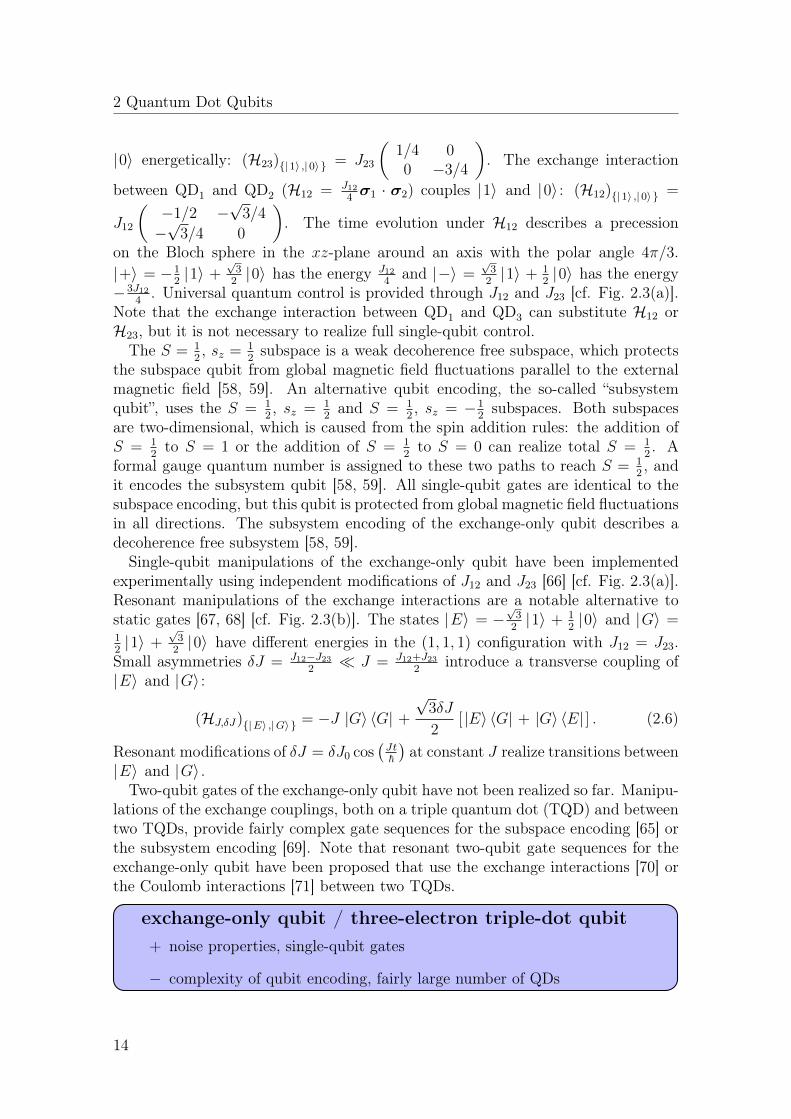
4. Universal quantum control is provided through J12 and J23 [cf. Fig. 2.3(a)].
Note that the exchange interaction between QD1 and QD3 can substitute H12 orH23, but it is not necessary to realize full single-qubit control.
The S = 12, sz = 1
2subspace is a weak decoherence free subspace, which protects
the subspace qubit from global magnetic field fluctuations parallel to the externalmagnetic field [58, 59]. An alternative qubit encoding, the so-called “subsystemqubit”, uses the S = 1
2, sz = 1
2and S = 1
2, sz = −1
2subspaces. Both subspaces
are two-dimensional, which is caused from the spin addition rules: the addition ofS = 1
2to S = 1 or the addition of S = 1
2to S = 0 can realize total S = 1
2. A
formal gauge quantum number is assigned to these two paths to reach S = 12, and
it encodes the subsystem qubit [58, 59]. All single-qubit gates are identical to thesubspace encoding, but this qubit is protected from global magnetic field fluctuationsin all directions. The subsystem encoding of the exchange-only qubit describes adecoherence free subsystem [58, 59].
Single-qubit manipulations of the exchange-only qubit have been implementedexperimentally using independent modifications of J12 and J23 [66] [cf. Fig. 2.3(a)].Resonant manipulations of the exchange interactions are a notable alternative tostatic gates [67, 68] [cf. Fig. 2.3(b)]. The states |E〉 = −
√3
2|1〉 + 1
2|0〉 and |G〉 =
12|1〉 +
√3
2|0〉 have different energies in the (1, 1, 1) configuration with J12 = J23.
Small asymmetries δJ = J12−J23
2 J = J12+J23
2introduce a transverse coupling of
|E〉 and |G〉 :
(HJ,δJ)|E〉 ,|G〉 = −J |G〉 〈G| +
√3δJ
2[ |E〉 〈G| + |G〉 〈E| ] . (2.6)
Resonant modifications of δJ = δJ0 cos(Jt~
)at constant J realize transitions between
|E〉 and |G〉 .Two-qubit gates of the exchange-only qubit have not been realized so far. Manipu-
lations of the exchange couplings, both on a triple quantum dot (TQD) and betweentwo TQDs, provide fairly complex gate sequences for the subspace encoding [65] orthe subsystem encoding [69]. Note that resonant two-qubit gate sequences for theexchange-only qubit have been proposed that use the exchange interactions [70] orthe Coulomb interactions [71] between two TQDs.
exchange-only qubit / three-electron triple-dot qubit+ noise properties, single-qubit gates
− complexity of qubit encoding, fairly large number of QDs
14
2.5 Madison Qubit
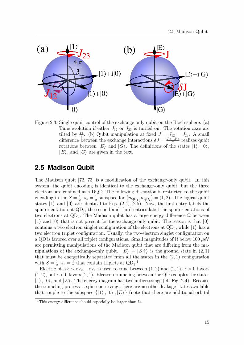
Figure 2.3: Single-qubit control of the exchange-only qubit on the Bloch sphere. (a)Time evolution if either J12 or J23 is turned on. The rotation axes aretilted by 4π
3. (b) Qubit manipulation at fixed J = J12 = J23. A small
difference between the exchange interactions δJ = J12−J23
2realizes qubit
rotations between |E〉 and |G〉 . The definitions of the states |1〉 , |0〉 ,|E〉 , and |G〉 are given in the text.
2.5 Madison Qubit
The Madison qubit [72, 73] is a modification of the exchange-only qubit. In thissystem, the qubit encoding is identical to the exchange-only qubit, but the threeelectrons are confined at a DQD. The following discussion is restricted to the qubitencoding in the S = 1
2, sz = 1
2subspace for
(nQD1
, nQD2
)= (1, 2). The logical qubit
states |1〉 and |0〉 are identical to Eqs. (2.4)-(2.5). Now, the first entry labels thespin orientation at QD1; the second and third entries label the spin orientations oftwo electrons at QD2. The Madison qubit has a large energy difference Ω between|1〉 and |0〉 that is not present for the exchange-only qubit. The reason is that |0〉contains a two electron singlet configuration of the electrons at QD2, while |1〉 has atwo electron triplet configuration. Usually, the two-electron singlet configuration ona QD is favored over all triplet configurations. Small magnitudes of Ω below 100 µeVare permitting manipulations of the Madison qubit that are differing from the ma-nipulations of the exchange-only qubit. |E〉 = |S ↑〉 is the ground state in (2, 1)that must be energetically separated from all the states in the (2, 1) configurationwith S = 1
2, sz = 1
2that contain triplets at QD1.1
Electric bias ε ∼ eV2 − eV1 is used to tune between (1, 2) and (2, 1). ε > 0 favors(1, 2), but ε < 0 favors (2, 1). Electron tunneling between the QDs couples the states|1〉 , |0〉 , and |E〉 . The energy diagram has two anticrossings (cf. Fig. 2.4). Becausethe tunneling process is spin conserving, there are no other leakage states availablethat couple to the subspace |1〉 , |0〉 , |E〉 (note that there are additional orbital
1This energy difference should especially be larger than Ω.
15
2 Quantum Dot Qubits
[or valley] excited states in S = 12, sz = 1
2both in (1, 2) and (2, 1), but these states
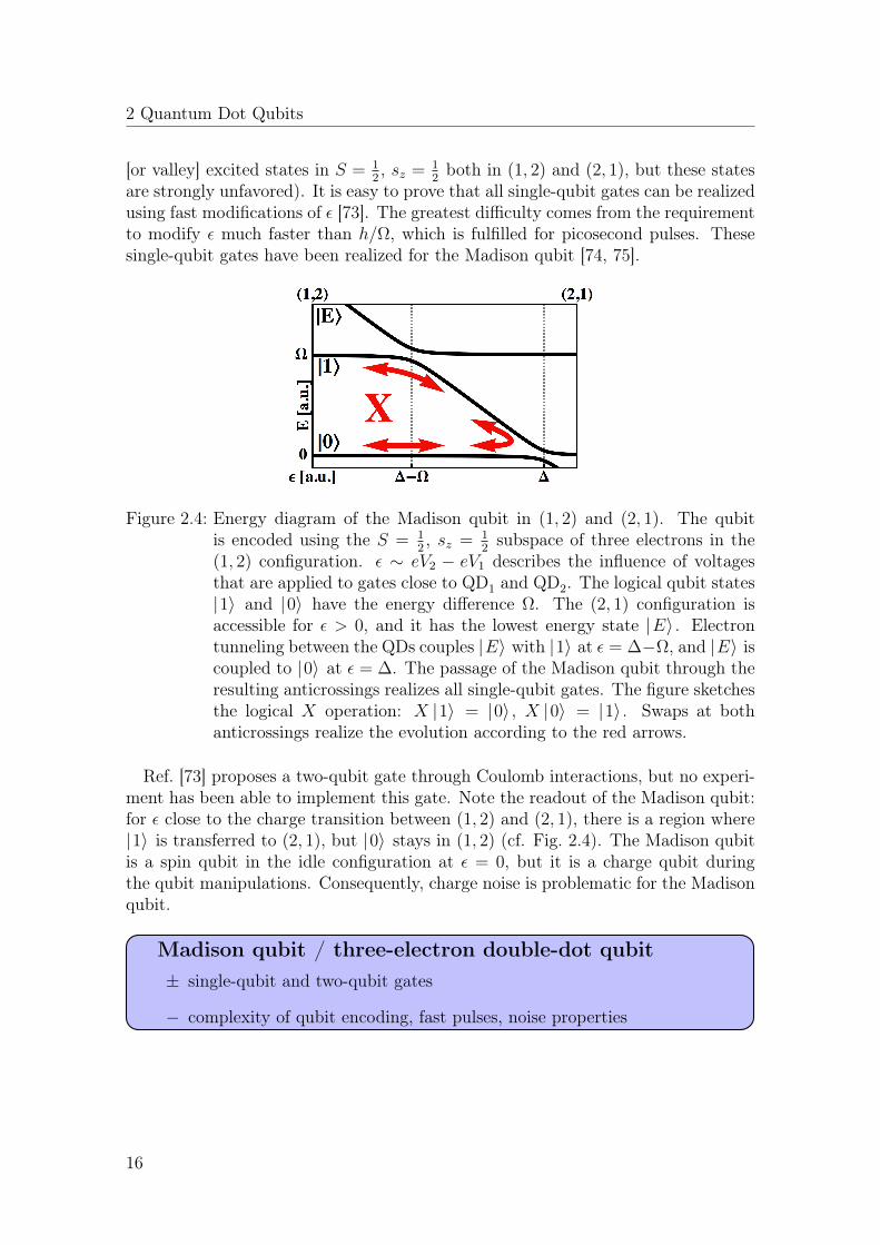
are strongly unfavored). It is easy to prove that all single-qubit gates can be realizedusing fast modifications of ε [73]. The greatest difficulty comes from the requirementto modify ε much faster than h/Ω, which is fulfilled for picosecond pulses. Thesesingle-qubit gates have been realized for the Madison qubit [74, 75].
Figure 2.4: Energy diagram of the Madison qubit in (1, 2) and (2, 1). The qubitis encoded using the S = 1
2, sz = 1
2subspace of three electrons in the
(1, 2) configuration. ε ∼ eV2 − eV1 describes the influence of voltagesthat are applied to gates close to QD1 and QD2. The logical qubit states|1〉 and |0〉 have the energy difference Ω. The (2, 1) configuration isaccessible for ε > 0, and it has the lowest energy state |E〉 . Electrontunneling between the QDs couples |E〉 with |1〉 at ε = ∆−Ω, and |E〉 iscoupled to |0〉 at ε = ∆. The passage of the Madison qubit through theresulting anticrossings realizes all single-qubit gates. The figure sketchesthe logical X operation: X |1〉 = |0〉 , X |0〉 = |1〉 . Swaps at bothanticrossings realize the evolution according to the red arrows.
Ref. [73] proposes a two-qubit gate through Coulomb interactions, but no experi-ment has been able to implement this gate. Note the readout of the Madison qubit:for ε close to the charge transition between (1, 2) and (2, 1), there is a region where|1〉 is transferred to (2, 1), but |0〉 stays in (1, 2) (cf. Fig. 2.4). The Madison qubitis a spin qubit in the idle configuration at ε = 0, but it is a charge qubit duringthe qubit manipulations. Consequently, charge noise is problematic for the Madisonqubit.
Madison qubit / three-electron double-dot qubit± single-qubit and two-qubit gates
− complexity of qubit encoding, fast pulses, noise properties
16

CHAPTER 3
Noise Description
The time evolution of spin qubits is not ideal because aquantum dot interacts with a macroscopic environment.This chapter introduces a phenomenological noise descrip-tion for spin qubits. Additionally, the noise channels gen-erated from hyperfine interactions, charge noise, and spin-orbit interactions are introduced.
3.1 Physical Noise Picture
Following Sec. 1.2, a qubit should store quantum information much longer than thetimescale of qubit manipulations. Typical noise descriptions of solid-state quantumexperiments use the language of nuclear magnetic resonance [76, 77]. The relaxationtime T1 and the dephasing time T2 characterize two possibilities to loose quantuminformation (cf. Refs. [6, 78, 79] for a phenomenological description of these noisemodels). A relaxation process describes the evolution of the excited state |1〉 to theground state |0〉 by the relaxation rate Γ = (T1)−1:
d
dt
X (t)Y (t)Z (t)
= −
Γ/2 0 00 Γ/2 00 0 Γ
X (t)Y (t)Z (t)
. (3.1)
Fig. 3.1(a) describes the time evolution of the Bloch sphere (cf. Sec. 1.2): the Blochsphere contracts to the ground state |0〉 . The pure dephasing rate Γφ = (Tφ)−1
destroys the phase coherences between superpositions:
d
dt
X (t)Y (t)Z (t)
= −
Γφ 0 00 Γφ 00 0 0
X (t)Y (t)Z (t)
. (3.2)
Pure dephasing causes that the Bloch sphere becomes ellipsoidal, while the majoraxis is aligned to the z-axis [cf. Fig. 3.1(b)]. Note that Γφ and Γ contribute to thedephasing rate Γ2 = (T2)−1, which describes how fast phase coherence is lost:
Γ2 =Γ
2+ Γφ,
1
T2
=1
2T1
+1
Tφ. (3.3)
17

3 Noise Description
Eq. (3.3) describes the fundamental limit of the dephasing time T2 < 2T1.A quantum system contains other quantum states besides |1〉 and |0〉 . The evo-
lution from the qubit subspace to these states is called leakage. Leakage reduces thepopulation of the qubit subspace, and it can be extracted from the time evolution of aquantum state |ψ (0)〉 = eiα
[cos (θ/2) |1〉 + eiφ sin (θ/2) |0〉
], ρ (0) = |ψ (0)〉 〈ψ (0)| :
O (t) = 〈1 |ρ (t)| 1〉+ 〈0 |ρ (t)| 0〉 . (3.4)
Figure 3.1: Description of relaxation and dephasing on the Bloch sphere. (a) Relax-ation processes transfers the excited state |1〉 to the ground state |0〉 ,and the Bloch sphere shrinks to |0〉 . (b) Pure dephasing deforms theBloch sphere to an ellipsoid. The phase coherences of superpositions of|1〉 and |0〉 are lost. Note that relaxation processes destroy also thephase coherences.
The fidelity describes the quality of a disturbed time evolution Ud. Ud deviatesfrom the ideal time evolution Ui, and Uall = U−1
i Ud differs from 1. The most mean-ingful characterization of a noisy quantum channel is obtained from the minimizationover all possible qubit states |ψ〉 [6]:
Fmin = min|ψ〉 tr(|ψ〉 〈ψ| Uall |ψ〉 〈ψ| U−1
all
). (3.5)
Fmin is often difficult to calculate. Noisy quantum processes can be described whencomparing the quantum system Q (Q encodes the qubit) with a reference system R(R is the identical copy of Q). Q evolves with Uall, but R is static. The entanglementfidelity F of a combined quantum state of R and Q (|RQ〉) is defined as [6, 80, 81]:
F = Tr[ρRQ1R ⊗ (Uall)Q ρRQ1R ⊗
(U−1all
)Q
], (3.6)
with ρRQ = |RQ〉 〈RQ| . Note that F in Eq. (3.6) is a function of the state |RQ〉 .The characterization of a noisy quantum channel (and therefore the definition of a
18
3.2 Hyperfine Interactions
gate fidelity) relies on the idea that an ideal quantum channel must conserve the en-tanglement between R andQ [6]. Therefore, the maximally entangled state |RQ〉1 =√
12
(|11〉 + |00〉) characterizes the gate fidelity of single-qubit operations and themaximally entangled state |RQ〉2 = 1
2
(|1111〉 + |0110〉 + |1001〉 + |0000〉
)char-
acterizes the gate fidelity of two-qubit operations with the definition of Eq. (3.6).1F = 1 for ideal processes and 0 ≤ F ≤ 1. Note that Eq. (3.6) with |RQ〉1 and|RQ〉2 characterizes also the leakage from the computational subspace.
3.2 Hyperfine Interactions
QD electrons interact with the nuclear spins of the semiconductor [83]. Experimentsare usually done at large external magnetic fields, which causes a difference betweenthe electron Zeeman splitting and the nuclear Zeeman splitting. As a consequence,the probability for a simultaneous spin flip of the electron spin and the nuclear spinis small.
The dominant noise channel of nuclear spin noise is caused by the uncertaintyof the nuclear spin distribution. Every nuclei has a small magnetic moment thatinteracts through the Fermi contact hyperfine interaction with the electron. Anelectron bound at a QD interacts with a macroscopic magnetic field that is created bythe nuclei: H = gµB
2Bnuc ·σ, with Bnuc =
∑iAi
(|ψi|2 ν
)Ii [84, 85]. g is the electron
g-factor, µB is the Bohr magneton, Ii is the ith nuclear spin, Ai is the materialdependent coupling constant of the ith nucleus, and |ψi| is the electron’s envelopeat the unit cell of volume ν of the ith nucleus. Bnuc is called the Overhauser field.One can treat the magnetic field as static during one measurement, but there arevariations ofBnuc between successive measurements. The magnetic field fluctuationsat a QD can be described by the rms value of the uncertainty in Bnuc [52, 84, 86]:
σBnuc ∝√|Bnuc|2 =
√∑i
Ii (Ii + 1)A2i
(|ψi|2 ν
)2. (3.7)
If one assumes that the distribution of the nuclear spins is smooth, then∑
i |ψi|4 ν2 →
ν∫Vdr |ψi|4 ≈ ν
V= 1
N, where V is the QD volume and N is the total number of
the nuclei that interact with the electron. One electron typically interacts with 106
nuclear spins for GaAs QDs, giving gµB2σBnuc ≈ 50 neV and σBnuc = 5 mT [87]. Si
QDs are becoming popular because a QD electron in Si interacts with fewer finitespin nuclei than for GaAs QDs. Natural Si has only ∼ 5000 finite spin nuclei thatinteract with the QD electron (gµB
2σBnuc ≈ 1.5 neV, σBnuc ≈ 25 µT) [87]. There
1 One can prove easily that |RQ〉 1 and |RQ〉 2 are maximally entangled states when calculating thevon Neumann entropy S (x) = −tr [x log2(x)] for the reduced density matrices ρR = trQ (ρRQ)and ρQ = trR (ρRQ). S (ρR) = S (ρQ) = 1 for |RQ〉 1 and S (ρR) = S (ρQ) = 2 for |RQ〉 2,which are the maximal entanglement entropies reachable for two-qubit and four-qubit Hilbertspaces [82].
19
3 Noise Description
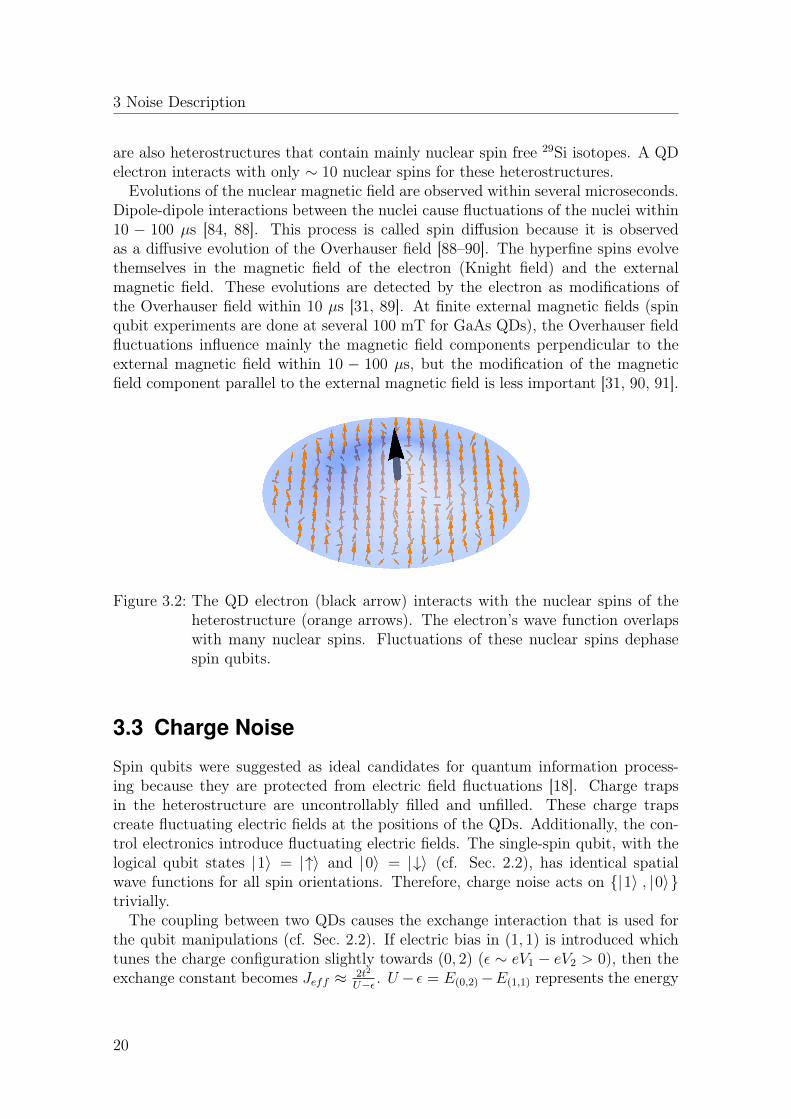
are also heterostructures that contain mainly nuclear spin free 29Si isotopes. A QDelectron interacts with only ∼ 10 nuclear spins for these heterostructures.Evolutions of the nuclear magnetic field are observed within several microseconds.
Dipole-dipole interactions between the nuclei cause fluctuations of the nuclei within10 − 100 µs [84, 88]. This process is called spin diffusion because it is observedas a diffusive evolution of the Overhauser field [88–90]. The hyperfine spins evolvethemselves in the magnetic field of the electron (Knight field) and the externalmagnetic field. These evolutions are detected by the electron as modifications ofthe Overhauser field within 10 µs [31, 89]. At finite external magnetic fields (spinqubit experiments are done at several 100 mT for GaAs QDs), the Overhauser fieldfluctuations influence mainly the magnetic field components perpendicular to theexternal magnetic field within 10 − 100 µs, but the modification of the magneticfield component parallel to the external magnetic field is less important [31, 90, 91].
Figure 3.2: The QD electron (black arrow) interacts with the nuclear spins of theheterostructure (orange arrows). The electron’s wave function overlapswith many nuclear spins. Fluctuations of these nuclear spins dephasespin qubits.
3.3 Charge Noise
Spin qubits were suggested as ideal candidates for quantum information process-ing because they are protected from electric field fluctuations [18]. Charge trapsin the heterostructure are uncontrollably filled and unfilled. These charge trapscreate fluctuating electric fields at the positions of the QDs. Additionally, the con-trol electronics introduce fluctuating electric fields. The single-spin qubit, with thelogical qubit states |1〉 = |↑〉 and |0〉 = |↓〉 (cf. Sec. 2.2), has identical spatialwave functions for all spin orientations. Therefore, charge noise acts on |1〉 , |0〉trivially.
The coupling between two QDs causes the exchange interaction that is used forthe qubit manipulations (cf. Sec. 2.2). If electric bias in (1, 1) is introduced whichtunes the charge configuration slightly towards (0, 2) (ε ∼ eV1 − eV2 > 0), then theexchange constant becomes Jeff ≈ 2t2
U−ε . U − ε = E(0,2)−E(1,1) represents the energy
20

3.4 Spin-Orbit Interactions and Phonons
difference between the (0, 2) charge configuration and the (1, 1) charge configuration.t is the tunnel coupling between the QDs. Charge noise introduces small fluctuationsδε between different charge configurations. As U ε and U − ε |δε|, thesefluctuations influence the exchange interaction by:
δJeff ≈2t2
U − (ε+ δε)≈ Jeff
(1 +
δε
U − ε
)≈ Jeff
(1 +
δε
U
). (3.8)
Typical QD setups have an uncertainty in ε of the rms σδε with the magnitudeσδεU
= 10−2− 10−3. For example, σδε ≈ 5 µeV was measured in Ref. [34], which givesσδεU≈ 5 · 10−3 for U ≈ 1 meV [30].2 Raising ε increases Jeff , but larger ε introduce
at the same time a slightly higher (0, 2) population for the singlet state than forthe triplet states. A spin qubit is disturbed stronger by charge noise at larger Jeffbecause it obtains some character of a charge qubit [94]. Note that this descriptionis valid only for small electric bias where the charge distribution remains mainly in(1, 1). Very high bias can show reduced sensitivity to charge noise (cf. Chapter 5).
The exchange interactions fluctuate slowly, and the dominant effects of chargenoise in spin qubit experiments can be described by quasi-static noise. Note thatsmall, finite frequency fluctuations of the exchange interactions were detected in thefrequency range 20 kHz - 1 MHz [93]. The noise spectrum scales like ω−0.7. Anotherexperiment verified the low-frequency character of charge noise and detected a ω−0.8
spectrum [95].
3.4 Spin-Orbit Interactions and Phonons
Spin-orbit interactions (SOIs) are less important for GaAs and Si QDs because thespin precession lengths (> 10 µm) are much larger than the QD sizes (< 100 nm).SOIs couple the orbital component and the spin component of the electron wavefunction. Phonons can now flip single spins [96]. Phonons are eigenmodes of thelattice vibrations, and they couple to the orbital part of the wave function (cf., e.g.,Ref. [97]). The spin relaxation time of a single-electron spin at a QD is stronglymagnetic field dependent [98], and it depends on the shape of the QD [99]. Singlespin relaxation times are, however, usually very long and exceed 1 ms easily [98, 100].
2A similar approximation was extracted in Ref. [92] from the experiment of Ref. [93]:Jeff
(1 + δε
ε0
)with σδε
ε0≈ 3 · 10−2 is used.
21


CHAPTER 4
Static and Resonant Manipulationsof Encoded Spin Qubits
This chapter analyzes manipulation protocols for spinqubits. Two promising qubit encodings for quantum dot(QD) spin qubits are analyzed. The singlet-triplet qubitencodes quantum information using the singlet state andthe sz = 0 triplet state of a pair of electrons that are con-fined using a double QD. The S = 1
2, sz = 1
2subspace of
three electrons that are confined using a trio of QDs en-codes quantum information for the triple QD qubit. Nu-clear spins and charge traps influence the electron spin inGaAs heterostructures. These noise channels are detectedas low-frequency noise by spin qubits. Single-qubit gatesand two-qubit gates can be realized using evolutions un-der static Hamiltonians and using evolutions under time-dependent Hamiltonians. Favorable manipulation proto-cols for spin qubits in gate-defined GaAs QDs with thegiven noise sources are described.
23

4 Static and Resonant Manipulations of Encoded Spin Qubits
4.1 Model
4.1.1 Singlet-Triplet Qubit (cf. Sec. 2.3)
The singlet-triplet qubit (STQ) encodes quantum information in the sz = 0 subspaceof two electrons that are confined using a double quantum dot (DQD) [50, 52]. Thequantum dots (QDs) are labeled by QD1 and QD2 (cf. Fig. 4.1).Single-qubit interactions — The STQ Hamiltonian in the
(nQD1
, nQD2
)= (1, 1)
configuration,
HDQD =J12
4σ1 · σ2 +
∆Ez2
(σz1 − σz2) +Ez2
(σz1 + σz2) , (4.1)
contains the exchange interaction J12 between the QDs, a magnetic field gradientacross the DQD ∆Ez =
Ez1−Ez22
, and a global magnetic field Ez =Ez1+Ez2
2, with
Ez ∆Ez > 0. σi = (σxi , σyi , σ
zi )T are the Pauli matrices at QDi; Ei is the local
magnetic field at QDi.1 The charge transitions from (1, 1) to (2, 0) and from (1, 1) to(0, 2) are described by the tunnel coupling τ , and they cause the exchange interactionJ12 = 2τ2
U1+ 2τ2
U2(cf. Sec. 2.2). The addition energy Ui is needed to add a second
electron to QDi.
Figure 4.1: Array of two DQDs (1) and (2). The electron transfer between a pair ofQDs on DQD(i) is permitted, and it is described by the tunnel couplingτ (i). The addition energy U
(i)j is needed to add a second electron to
QD(i)j ; n(i)
j is the electron number at QD(i)j . The electrostatic coupling
between DQD(1) and DQD(2) is determined mainly by the occupationsof QD(1)
2 and QD(2)1 .
Eq. (4.1) is projected to the sz = 0 subspace, which is spanned by the singletstate |S〉 and the sz = 0 triplet state |T0〉 :
H|T0〉 ,|S〉 DQD =
J12
2σz + ∆Ezσx. (4.2)
1 The magnetic fields Ezi , Ez, and ∆Ez are described in energy units. Ez2 is used instead of the
Zeeman Hamiltonian gµBB2 , where g is the electron g-factor, µB is the Bohr magneton, and B
is the magnetic field strength.
24

4.1 Model
σx = |T0〉 〈S| + |S〉 〈T0| and σz = |T0〉 〈T0| − |S〉 〈S| are Pauli operators. Eq. (4.2)neglects constant energy shifts of the sz = 0 subspace.Two-qubit interactions — Only the singlet state |S〉 has small contributions in
(2, 0) and (0, 2): |S〉 ∝ |S1,1〉 +√
2τU1|S2,0〉 +
√2τU2|S0,2〉 . The weights in (2, 0) and
(0, 2) for U1, U2 τ are:
|〈(2, 0) |S〉|2 = 2
(τ
U1
)2
, |〈(0, 2) |S〉|2 = 2
(τ
U2
)2
. (4.3)
Coulomb interactions couple two STQs [51]. An array of two DQDs [labeled by (1)and by (2)] is considered (cf. Fig. 4.1), where the coupling is determined mainly bythe occupations of the neighboring QDs n(1)
2 and n(2)1 : V = e2
4πε0εrdn
(1)2 n
(2)1 . d is the
distance between these QDs, e is the elementary charge, ε0 is the dielectric constant,and εr is the relative permittivity. The interaction can be rewritten to
V = Xσ(1)z σ(2)
z , with X =e2
4πε0εrd
(τ (1)
U(1)2
)2(τ (2)
U(2)1
)2
, (4.4)
using Eq. (4.3) and neglecting local energy shifts.Qubit manipulations — The exchange interaction J12 = J0
12 + ε (t) can be tunedexperimentally. J0
12 is constant, and ε (t) can be controlled below nanoseconds [37].Note that modifications of J (1)
12 are possible at constant J (2)12 and at constant X . A
setup should be analyzed, where the array of DQDs in (1, 1)(1) and (1, 1)(2) is tunedslightly towards (0, 2)(1), and (2, 0)(2). As a consequence U (1)
2 , U (2)1 U
(1)1 , U (2)
2 . Amodification of the addition energy U (1)
2 is introduced (described by U (1)2 −ξ), which
tunes J (1)12 ≈
(2τ2
U2−ξ
)(1)
but leaves J (2)12 ≈
(2τ2
U1
)(2)
unchanged. At the same time
X ∝(
τ2
(U2−ξ)2
)(1)
. An expansion for ξ U(1)2 gives J (1)
12 ≈(
2τ2
U2
)(1)
+
(τ (1)
U(1)2
)2
2ξ and
X ∝≈
(τ (1)
U(1)2
)2
+
(τ (1)
U(1)2
)22ξ
U(1)2
. X is unchanged for small modifications of J (1)12 because
the factor 2ξ
U(1)2
is small.
4.1.2 Triple Quantum Dot Qubit (cf. Sec. 2.4)
Triple quantum dot (TQD) spin qubits are encoded in the S = 12, sz = 1
2spin
subspace of three electrons confined at a trio of QDs [65]. The TQD qubit is alsocalled the exchange-only qubit because full qubit control is possible only throughthe exchange interactions [65]. The three QDs that encode a single TQD qubit arelabeled by QD1, QD2, and QD3 (cf. Fig. 4.2).Single-qubit interactions — The TQD Hamiltonian in the
(nQD1
, nQD2, nQD3
)=
(1, 1, 1) configuration,
HTQD =J12
4σ1 · σ2 +
J23
4σ2 · σ3 +
Ez2
(σz1 + σz2 + σz3) , (4.5)
25

4 Static and Resonant Manipulations of Encoded Spin Qubits
contains the exchange interaction J12 between QD1 and QD2, the exchange in-teraction J23 between QD2 and QD3, and a global magnetic field Ez.1 Insteadof J12 and J23, the sum of the exchange interactions J = J12+J23
2and the dif-
ference of the exchange interactions ∆J = J12−J23
2are used. Eq. (4.5) is pro-
jected onto the S = 12, sz = 1
2subspace, with the basis |1〉 = |↑〉2 ⊗ |S〉1,3 and
|0〉 =√
13|↑〉2 ⊗ |T0〉1,3 −
√23|↓〉2 ⊗ |T+〉1,3:
H|1〉 ,|0〉 TQD =J
2σz +
√3∆J
2σx. (4.6)
σx = |1〉 〈0| + |0〉 〈1| and σz = |1〉 〈1| − |0〉 〈0| are Pauli operators.Two-qubit interactions — Coulomb interactions couple two TQD qubits [labeled
by (1) and by (2)]. The interaction between the (1, 0, 2)(1) configuration of TQD(1)
and the (2, 0, 1)(2) configuration of TQD(2) dominates the qubit coupling when thetwo TQDs are aligned according to Fig. 4.2. Only the states |↑〉1⊗|S〉2,3 for TQD(1)
and |↑〉3⊗|S〉1,2 for TQD(2) permit this charge transfer [68, 71]. The tunnel couplingcauses a state hybridization of each singlet state in (1, 1) with the singlet states in(2, 0) and (0, 2), similar to the case of DQDs: |S1,1〉1,2 → |S1,1〉1,2 +
√2τU1|S2,0〉1,2 +
√2τU2|S0,2〉1,2 and |S1,1〉2,3 → |S1,1〉2,3 +
√2τU2|S2,0〉2,3 +
√2τU3|S0,2〉2,3. An arbitrary
single-qubit state |ψ〉 = eiα[cos (ϑ/2) |1〉 + eiϕ sin (ϑ/2) |0〉 ], which is described by aglobal phase α and the Bloch sphere angles ϑ and ϕ (cf. Fig. 1.1) [6], has the statehybridization:
|〈(2, 0, 1) |ψ〉|2 = 2
(τ
U1
)2[
1
2− 1
4cos (ϑ)−
√3
4sin (ϑ) cos (ϕ)
], (4.7)
|〈(1, 0, 2) |ψ〉|2 = 2
(τ
U3
)2[
1
2− 1
4cos (ϑ) +
√3
4sin (ϑ) cos (ϕ)
]. (4.8)
Electrons at QD(1)3 and QD(2)
1 are the distance d apart, and they interact throughV = e2
4πε0εrdn
(1)3 n
(2)1 (cf. Fig. 4.2). The interaction between two TQD qubits is
rewritten using Eq. (4.7) and Eq. (4.8):
V = X
(1
2σ(1)z −
√3
2σ(1)x
)(1
2σ(2)z +
√3
2σ(2)x
),
with X =e2
4πε0εrd
(τ (1)
U(1)3
)2(τ (2)
U(2)1
)2
. (4.9)
Eq. (4.7) and Eq. (4.8) cause also single-qubit energy shifts, which can be neglectedfor X J12, J23. Note that Ref. [71] gives additional coupling Hamiltonians forgeometries which differ from linear QD arrays.Qubit manipulations — Modifications of ∆J are possible at constant J [66, 68].
The couplings for QD1 with QD2 and for QD2 with QD3 are assumed to be identical.
26
4.1 Model
The parameter ξ describes the difference between U1 and U3 (U1 = U − ξ andU3 = U + ξ). The exchange interactions for U2 U1, U3 τ > 0 are J12 = 2τ2
U−ξ
and J23 = 2τ2
U+ξ. An expansion for U |ξ| gives J = 2τ2
Uand ∆J = τ2
U2 2ξ. Xremains unchanged for small modifications of the single-qubit parameters, similarto the argumentation for STQs.
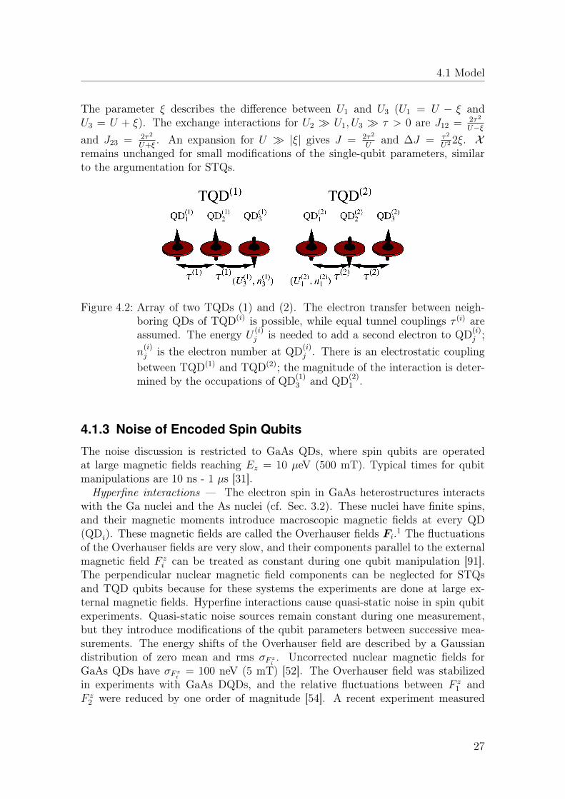
Figure 4.2: Array of two TQDs (1) and (2). The electron transfer between neigh-boring QDs of TQD(i) is possible, while equal tunnel couplings τ (i) areassumed. The energy U (i)
j is needed to add a second electron to QD(i)j ;
n(i)j is the electron number at QD(i)
j . There is an electrostatic couplingbetween TQD(1) and TQD(2); the magnitude of the interaction is deter-mined by the occupations of QD(1)
3 and QD(2)1 .
4.1.3 Noise of Encoded Spin Qubits
The noise discussion is restricted to GaAs QDs, where spin qubits are operatedat large magnetic fields reaching Ez = 10 µeV (500 mT). Typical times for qubitmanipulations are 10 ns - 1 µs [31].Hyperfine interactions — The electron spin in GaAs heterostructures interacts
with the Ga nuclei and the As nuclei (cf. Sec. 3.2). These nuclei have finite spins,and their magnetic moments introduce macroscopic magnetic fields at every QD(QDi). These magnetic fields are called the Overhauser fields Fi.1 The fluctuationsof the Overhauser fields are very slow, and their components parallel to the externalmagnetic field F z
i can be treated as constant during one qubit manipulation [91].The perpendicular nuclear magnetic field components can be neglected for STQsand TQD qubits because for these systems the experiments are done at large ex-ternal magnetic fields. Hyperfine interactions cause quasi-static noise in spin qubitexperiments. Quasi-static noise sources remain constant during one measurement,but they introduce modifications of the qubit parameters between successive mea-surements. The energy shifts of the Overhauser field are described by a Gaussiandistribution of zero mean and rms σF zi . Uncorrected nuclear magnetic fields forGaAs QDs have σF zi = 100 neV (5 mT) [52]. The Overhauser field was stabilizedin experiments with GaAs DQDs, and the relative fluctuations between F z
1 andF z
2 were reduced by one order of magnitude [54]. A recent experiment measured
27

4 Static and Resonant Manipulations of Encoded Spin Qubits
the Overhauser field for GaAs DQDs and adjusted the manipulation protocol in afeedback loop [101]. This approach lowered σ∆Fz by another order of magnitude.
STQs have an uncertainty in ∆Ez =Ez1−Ez2
2that is caused by the local Overhauser
fields at QD1 (F z1 ) and at QD2 (F z
2 ). The rms of the uncertainty in ∆Ez is σ∆Ez =12
√σ2F z1
+ σ2F z2, when assuming uncorrelated magnetic field fluctuations at the QDs.
The TQD Hamiltonian HTQD from Eq. (4.5) and the Hamiltonians describing theOverhauser fields Fi at QDi (Hz =
∑i=1,2,3
Fi2· σi)1 are projected to the sz = 1
2
subspace for TQD qubits with the computational basis |1〉 and |0〉 (introduced inSec. 4.1.2), and the leakage state
∣∣∣Q 12
⟩=√
13
(|↑↑↓〉 + |↑↓↑〉 + |↓↑↑〉),
H|1〉 ,|0〉 ,|Q 1
2〉
=
J2− F z1−2F z2 +F z3
6
√3∆J2
+F z1−F z3
2√
3
F z1−F z3√6√
3∆J2
+F z1−F z3
2√
3−J
2+
F z1−2F z2 +F z36
−F z1−2F z2 +F z33√
2F z1−F z3√
6−F z1−2F z2 +F z3
3√
2J
. (4.10)
J |F zi | for qubit manipulations, which allows the simplification of Eq. (4.10):
H|1〉 ,|0〉 ≈(J
2− F z
1 − 2F z2 + F z
3
6
)σz +
√3∆J
2σx, (4.11)
with σz = |1〉 〈1| − |0〉 〈0| and σx = |1〉 〈0| + |0〉 〈1| . The nuclear spins cause anuncertainty in J of the rms σB = 1
6
√σ2F z1
+ 4σ2F z2
+ σ2F z3
when assuming uncorrelatedmagnetic field fluctuations at the QDs.Charge noise — Charge noise introduces low-frequency fluctuations of the ex-
change interaction Jij between the neighboring QDs QDi and QDj. Typically, thequasi-static noise contribution is described by the ratio of Jij to its rms σJij , whichis of the order of
σJijJij≈ 10−2 − 10−3 (cf. Sec. 3.3). Charge noise introduces an
uncertainty in the exchange interaction J12 for STQs [cf. Eq. (4.2)] of the rms σJ12 .The energy splitting J for TQD qubits [cf. Eq. (4.6)] has an uncertainty with therms σJ = 1
2
√σ2J12
+ σ2J23
when the fluctuations of J12 are treated as independentfrom the fluctuations of J23. Fluctuations of ∆J for TQD qubits can be neglectedfor ∆J J . Ref. [93] measured charge noise for STQs and characterized thesefluctuations by the formula J12
(1 + δJ12
J12
)with σδJ12
J12≈ 3 · 10−2. This finding is
consistent with the measurements of charge noise for TQD qubits [66]. Note thatcharge noise also has a small finite-frequency noise contribution. A ω−0.7 spectrumwas extracted up to 1 MHz [93].
4.1.4 General Hamiltonian
Single-qubit interactions — The Hamiltonian
H =∆ + δt
2σz + ε (t) [cos (θ)σz − sin (θ)σx] (4.12)
28

4.1 Model
characterizes a qubit in its energy eigenbasis with the energy difference ∆ |ε (t)| >0. |1〉 is the excited state, and |0〉 is the ground state. ε (t) is controlled in exper-iments, e.g. when external potentials are modified. ε (t) enables time-dependentqubit manipulations.
STQs are described by Eq. (4.2),
H|T0〉 ,|S〉 DQD =
J12
2σz + ∆Ezσx, (4.13)
and can be manipulated by J12 = J012 +2ε (t). A basis transformation UH|T0〉 ,|S〉
DQD U †
realizes Eq. (4.12), with U =
(cos(θ2
)sin(θ2
)− sin
(θ2
)cos(θ2
) ), ∆2
=
√(J0
12
2
)2
+ (∆Ez)2, and
tan (θ) = ∆EzJ0
12/2. The resulting energy eigenbasis of Eq. (4.12) is |1〉 = cos
(θ2
)|T0〉 +
sin(θ2
)|S〉 for the excited state and |0〉 = − sin
(θ2
)|T0〉+cos
(θ2
)|S〉 for the ground
state. Large exchange interactions J012 ∆Ez give |1〉 = |T0〉 and |0〉 = |S〉 ,
but large magnetic field gradients ∆Ez J012 give |1〉 = |↑↓〉 and |0〉 = − |↓↑〉
(|QD1,QD2〉 is the spin configuration of the DQD). Note that the transverse com-ponent ∼ σx in Eq. (4.12) is important only when J0
12 . ∆Ez.The TQD Hamiltonian from Eq. (4.6),
H|1〉 ,|0〉 TQD =J
2σz +
√3∆J
2σx, (4.14)
is already in the form of Eq. (4.12) with ∆ = J , ε (t) =√
3∆J2
, and θ = −π2. The
second term of Eq. (4.14) permits qubit manipulations; it has only a component∼ σx, but it lacks a component ∼ σz.Noise — δt in Eq. (4.12) is a classical variable that describes noise of encoded
spin qubits. The noise discussion is restricted to Gaussian noise, assuming thatthe fluctuations are caused by a large number of independent random processes[102]. The following discussion considers longitudinal noise, i.e. noise that commuteswith ∆
2σz. The fluctuations of δt are always low frequency compared to ∆/h and
∆ δt (cf. Sec. 4.1.3). The transverse noise components (∼ σx and ∼ σy) areneglected because these terms oscillate rapidly in a rotating frame with ∆
2σz. Note
that longitudinal drivings (e.g. A cos(
∆t~
)σz) with large driving amplitudes forbid
this approximation (cf. Appx. 4.C).Two-qubit interactions — The qubit labels (1) and (2) are introduced to describe
the interactions between two qubits. The Coulomb interactions between two encodedqubits are described by the Hamiltonian
V = X(c1σ
(1)z − s1σ
(1)x
) (c2σ
(2)z − s2σ
(2)x
). (4.15)
The abbreviations ci = cos(φ(i))and si = sin
(φ(i))are introduced; φ(1) and φ(2) are
rotation angles.The coupling between two STQs is described in Eq. (4.4), which gives Eq. (4.15)
after the same basis transformation as for the single-qubit Hamiltonian. The ro-
tating angles are tan(φ(1))
=
(∆E
(1)z
(J012/2)
(1)
)for DQD(1) and tan
(φ(2))
=
(∆E
(2)z
(J012/2)
(2)
)
29
4 Static and Resonant Manipulations of Encoded Spin Qubits
for DQD(2). Eq. (4.15) contains only the σ(1)z σ
(2)z term for (J0
12)(1) ∆E
(1)z and
(J012)
(2) ∆E(2)z , but it contains only the σ(1)
x σ(2)x term for ∆E
(1)z (J0
12)(1) and
∆E(2)z (J0
12)(2).
The interaction between two TQD qubits, according to Eq. (4.9), is described byEq. (4.15) with φ(1) = π/3 and φ(2) = −π/3. This interaction always contains theterm σ
(1)z σ
(2)z and the term σ
(1)x σ
(2)x .
4.2 Static Time Evolutions
4.2.1 Single-Qubit Gates
Static time evolutions are described by Eq. (4.12) with ε = 0. The analysis is donein the rotating frame with ∆
2σz: X (t)
Y (t)Z (t)
=
cos(
1~
∫ t0dt′ δt′
)− sin
(1~
∫ t0dt′ δt′
)0
sin(
1~
∫ t0dt′ δt′
)cos(
1~
∫ t0dt′ δt′
)0
0 0 1
X (0)
Y (0)Z (0)
. (4.16)
ρ (t) is the density matrix in the rotating frame; σx, σy, and σz are the Pauli matrices,and
X (t) , Y (t) , Z (t)
=tr [σxρ (t)] , tr [σyρ (t)] , tr [σzρ (t)]
. Averaging the
trajectories of Eq. (4.16) over many δt gives: 〈X (t)〉〈Y (t)〉〈Z (t)〉
=
e−∫∞−∞ dω S(ω)Fω 0 0
0 e−∫∞−∞ dω S(ω)Fω 0
0 0 1
〈X (0)〉〈Y (0)〉〈Z (0)〉
, (4.17)
with Fω = 12~2
∫ t0dt′∫ t
0t′′e−2πiω(t′−t′′) = 1
2π2~2
(sin(πωt)
ω
)2
. 〈. . .〉 is the classical averagethat describes the mean result of many trajectories. S (ω) is the spectral function ofδt, which characterizes the time correlations between δt and δt′ (cf. Appx. 4.A). δtfulfills
⟨e±
i~∫ t0 dt′ δt′⟩
= e− 1
2
⟨( 1~∫ t0 dt′ δt′)
2⟩, which is always true for Gaussian variables
[103–105].Low-frequency noise — δt remains constant during one experiment (t < texp) for
quasi-static noise sources, but it varies between successive measurements. Note thatthe time evolution in Eq. (4.17) is determined by an integral in ω over S (ω)Fω. Fωhas major weight in ω ∈
[−1
t, 1t
]. Quasi-static noise sources cover the full spectrum
S (ω) at t < texp and allow the approximation∫∞−∞ dω S (ω)Fω ≈ F0σ
2δ , where
σδ is the rms of δt. Superpositions of |1〉 and |0〉 show a Gaussian decay law forquasi-static noise sources,
〈X (t)〉 ≈ e−12(σδt~ )
2︸ ︷︷ ︸≈1− 1
2(σδt~ )2
〈X (0)〉 , 〈Y (t)〉 ≈ e−12(σδt~ )
2︸ ︷︷ ︸≈1− 1
2(σδt~ )2
〈Y (0)〉 , (4.18)
30

4.2 Static Time Evolutions
and the energy eigenstates remain static 〈Z (t)〉 = 〈Z (0)〉.Finite-frequency noise — Approximating
(sin(πωt)
ω
)2
≈ π2tδ (0) for large t [106]gives:
〈X (t)〉 ≈ e−t2S(0)
~2︸ ︷︷ ︸≈1− t
2S(0)
~2
〈X (0)〉 , 〈Y (t)〉 ≈ e−t2S(0)
~2︸ ︷︷ ︸≈1− t
2S(0)
~2
〈Y (0)〉 . (4.19)
The decay is exponential, and it is caused by the zero-frequency content of thenoise spectrum. For a valid approximation, S (ω) must be smooth over the intervalω ∈
[−1
t, 1t
]where F (ω) has dominant weight. This result agrees with the Bloch-
Redfield approximation [76], and it is formally equivalent to the calculation usingFermi’s golden rule [3]. Energy eigenstates are constant 〈Z (t)〉 = 〈Z (0)〉. 〈Z (t)〉decays only through transverse noise at the frequency of the energy splitting ∆
h[76].
In any case, transverse noise is not included in the model of Eq. (4.12).
4.2.2 Two-Qubit Gates
Maximally entangling two-qubit gates are constructed using Eq. (4.12) with ε = 0and Eq. (4.15):
H =∆(1) + δ
(1)t
2σ(1)z +
∆(2) + δ(2)t
2σ(2)z
+ X[c1c2σ
(1)z σ(2)
z + s1s2σ(1)x σ(2)
x − c1s2σ(1)z σ(2)
x − s1c2σ(1)x σ(2)
z
]. (4.20)
The following analysis is restricted to si > 0 and ci > 0, but a generalization istrivial.
(1.) ∆(1) = ∆(2) — Two identical qubits with ∆ = ∆(1) = ∆(2) allow entanglinggates. Transforming Eq. (4.20) to the rotating frame with ∆
2
[σ
(1)z + σ
(2)z
]gives:
H′ ≈δ(1)t
2σ(1)z +
δ(2)t
2σ(2)z + X
[c1c2σ
(1)z σ(2)
z +s1s2
2
(σ(1)x σ(2)
x + σ(1)y σ(2)
y
) ]. (4.21)
Eq. (4.21) neglects the rapidly oscillating terms e±i∆t~ and e±i
2∆t~ , and it contains
the two-qubit interactions σ(1)z σ
(2)z and σ(1)
x σ(2)x + σ
(1)y σ
(2)y . A single time evolution is
maximally entangling if only the first term or if only the second term is present. Thefirst term alone creates a CNOT operation, the second term alone creates a
√iSWAP
operation (cf. Appx. 4.B). For arbitrary ratios of the first term and the second term,two time evolutions under Eq. (4.21), for the time tcomb/2 each, construct maximallyentangling gates if a single-qubit operation between these two time evolutions isintroduced [cf. Eq. (4.64)]. Overall, a time evolution for tcomb = π~
I under Eq. (4.21)is needed for a two-qubit gate, where the interaction strength I characterizes thegate time. If the first term of Eq. (4.21) dominates, then I = 4X c1c2, and if thesecond term of Eq. (4.21) dominates, then I = 4X s1s2.
31
4 Static and Resonant Manipulations of Encoded Spin Qubits
The time evolution under the Hamiltonian of Eq. (4.21) for c1 = c2 = 1 has theleast favorable noise properties. The entanglement fidelity F for the noisy timeevolution under Eq. (4.20) can be calculated:
F = cos2
(1
2~
∫ t
0
dt′ δ(1)t′
)cos2
(1
2~
∫ t
0
dt′ δ(2)t′
). (4.22)
The definition of Eq. (3.6) is used for the entanglement fidelity F , with the noisy
time evolution Ud = e− it~
[δ(1)t2σ
(1)z +
δ(2)t2σ
(2)z +Xσ(1)
z σ(2)z
]and the ideal time evolution Ui =
e−it~ Xσ
(1)z σ
(2)z . Eq. (4.22) is averaged over classical noise sources with independent
fluctuations on (1) and (2):
〈F 〉 =1
4
(1 + e−
∫∞−∞ dω S(1)(ω)Fω
)(1 + e−
∫∞−∞ dω S(2)(ω)Fω
)≈ 1−
∫∞−∞ dω S
(1) (ω)Fω2
−∫∞−∞ dω S
(2) (ω)Fω2
, (4.23)
with Fω = 12π2~2
(sin(πωt)
ω
)2
. The fidelity decay in Eq. (4.23) has the same characteras for the single-qubit time evolution in Eq. (4.17).
The time evolution under the Hamiltonian of Eq. (4.21) for s1 = s2 = 1 canhave better noise properties. Only the parts of the noise terms that commutewith the two-qubit interaction are important if δ(1)
t , δ(2)t X . In this case, all
the other terms oscillate rapidly in a rotating frame with the dominant interactionX2
(σ
(1)x σ
(2)x + σ
(1)y σ
(2)y
)of Eq. (4.21). Consequently, the noise terms can be neglected
using a rotating wave approximation.(2.) ∆(1) 6= ∆(2) — A different entangling operation is constructed for ∆(1),∆(2)
∆(1)−∆(2) X > 0. Eq. (4.20) is described in the rotating frame with ∆(1)
2σ
(1)z +
∆(2)
2σ
(2)z :
H′ ≈δ(1)t
2σ(1)z +
δ(2)t
2σ(2)z + X c1c2σ
(1)z σ(2)
z . (4.24)
Eq. (4.24) neglects the rapidly oscillating terms e±i∆(1)t
~ and e±i∆(2)t
~ , and only thetwo-qubit interaction X c1c2σ
(1)z σ
(2)z remains. The evolution under Eq. (4.24) for the
time tCNOT = π~I generates a CNOT operation (cf. Appx. 4.B), with I = 4X c1c2.
The fidelity for time evolutions under Eq. (4.24) decays according to:
〈F 〉 =1
4
(1 + e−
∫∞−∞ dω S(1)(ω)Fω
)(1 + e−
∫∞−∞ dω S(2)(ω)Fω
)≈ 1−
∫∞−∞ dω S
(1) (ω)Fω2
−∫∞−∞ dω S
(2) (ω)Fω2
, (4.25)
with Fω = 12π2~2
(sin(πωt)
ω
)2
.
32

4.3 Driven Time Evolutions
4.3 Driven Time Evolutions
4.3.1 Single-Qubit Gates
The time evolution under the Hamiltonian of Eq. (4.12) is analyzed with periodicmodifications of −ε (t) sin (θ) = A cos
(∆t~
).2 The transverse driving component
ε (t) cos (θ) can be neglected for ∆ |A|. δt is static during one driving period h∆
for spin qubits under the influence of low-frequency noise (cf. Sec. 4.1.3). Eq. (4.12)is transformed to a rotating frame with ∆
2σz:
H′ ≈ δt2σz +
A2σx. (4.27)
Eq. (4.27) neglects the rapidly rotating terms e±i2∆t~ using a rotating wave approxi-
mation [107]. Ahis called the Rabi frequency, which describes the periodicity of the
static time evolution in the rotating frame. δt2σz is transverse to the quantization
axis in Eq. (4.27), and it can be neglected for |A| |δt| if fluctuations of δt are lowfrequency compared to A
h.
Nevertheless, a noise discussion is given for driven time evolutions. Eq. (4.27) istransformed to the rotating frame with A
2σx:
H′′ = δt2
[sin
(At~
)σy + cos
(At~
)σz
]. (4.28)
The time evolution under the Hamiltonian of Eq. (4.28) can be expressed in secondorder in δt:3 〈X (t)〉〈Y (t)〉〈Z (t)〉
=
13 −∫ ∞−∞
dω S (ω)
2F1ω 0 0
0 F1ω + F2
ω −F3ω
0 −F3ω F1
ω −F2ω
〈X (0)〉〈Y (0)〉〈Z (0)〉
,
(4.29)
2 More general modulations of ε (t) can be described by the equivalent procedure. The h∆
periodic modulations of ε (t) are decomposed in a Fourier series ε (t) =∑n∈Z ane
−in∆t~ ,
an = 1h/∆
∫ h/∆0
dt′ ε (t′) ein∆~ t
′. Eq. (4.12) is averaged over one period h
∆ in the rotating framewith ∆
2 σz:
H′ ≈ − sin (θ)∑n∈N
(αnσx + βnσy) +δt2σz, αn = <e (an) , βn = =m (an) . (4.26)
α1 and β1 are the Fourier coefficients of the cosine and sine functions with the frequency ∆h ;
αn and βn with n > 1 describe higher order harmonics. Note that this treatment is valid onlyfor |an| ∆.
3 The propagator U from H′′ of Eq. (4.28) is expanded to second order in δt [3]: U ≈ 1 −i~∫ t
0dt′ H′′ (t′)− 1
~2
∫ t0dt′∫ t′
0dt′′ H′′ (t′)H′′ (t′′).
33

4 Static and Resonant Manipulations of Encoded Spin Qubits
where 13 is the identity matrix, and
F1ω =
1
4π2~2
(sin[πt(Ah− ω
)]Ah− ω
)2
, (4.30)
F2ω =
1
4π2~2
cos(2πA
ht)
Ah
sin(πt[Ah
+ ω])
sin(πt[Ah− ω
])Ah− ω
, (4.31)
F3ω =
1
4π2~2
sin(2πA
ht)
Ah
sin(πt[Ah
+ ω])
sin(πt[Ah− ω
])Ah− ω
. (4.32)
Low-frequency noise — The approximation∫∞−∞ dω S (ω)F iω ≈ F i0σ2
δ gives:
〈X (t)〉〈Y (t)〉〈Z (t)〉
=
13 − 2 sin2
(At2~
)(σδA
)2
1 0 0
0 cos2(At
2~
)− sin(At~ )
2
0 − sin(At~ )2
sin2(At
2~
) 〈X (0)〉〈Y (0)〉〈Z (0)〉
.
(4.33)
Eq. (4.33) describes the initial time evolution under quasi-static noise. F iω fromEqs. (4.30)-(4.32) have dominant weights in
[Ah− 1
t, Ah
+ 1t
]. The full spectrum S (ω)
of a quasi-static noise source is covered for t hA
( hA
is the Rabi period) becausea quasi-static noise spectrum has all content near S (0). Interestingly, the earlytime evolution has the same decay law as for the undriven evolution in Eq. (4.18).Superpositions decay quadratically:
⟨X (t)
X (0) = 1
⟩≈
[1− 1
2
(σδt
~
)2],
⟨Y (t)
Y (0) = 1
⟩≈
[1− 1
2
(σδt
~
)2], (4.34)
but energy eigenstates decay slower⟨
Z(t)Z(0)=1
⟩≈[1− 1
8(Aσδ)2 ( t
~
)4]. Fig. 4.3 shows
the time evolution under the Hamiltonian of Eq. (4.28) for driven Rabi rotationsunder quasi-static noise. The early time evolution proves the Gaussian decay lawfor superpositions; energy eigenstates decay slower.
The decay is partially recovered after one Rabi period. An exact calculation ofthe time evolution in the long time limit for quasi-static noise is possible. Thetrajectory is averaged over many realizations of δt, where δt follows a Gaussianprobability distribution. The stationary phases are extracted for the resulting tra-
jectories: the integral over δt of a quickly oscillating function eit
√A2+δ2t~ weighted by
a real function g (δt) can be approximated for large t as∫∞−∞ dδt g (dδt) e
it
√A2+δ2t~ ≈
34

4.3 Driven Time Evolutions
g (0)√
2πA~teiAt~ +π
4 , which gives:
〈X (t)〉〈Y (t)〉〈Z (t)〉
=
I1 0 00 I2 (t) −I2 (t) + (1− I1) sin
(At~
)0 I2 (t) I2 (t) + (1− I1) sin
(At~
) 〈X (0)〉
〈Y (0)〉〈Z (0)〉
, (4.35)
I1 =π
2
AσδeA2
2σ2δ Erfc
(A√2σδ
), I2 (t) =
√A~2σ2
δ t. (4.36)
Erfc is the complementary error function. A power law decay ∝√A~
2σ2δ t
for 〈Y (t)〉and 〈Z (t)〉 is obtained, which was described in the past (cf. Refs. [108, 109]).
XYZ
e-12 It Σ∆
ÑM2
0.25 0.5 0.75 1 1.25
0.85
0.9
0.95
1.
tTR
XX
HtL
XH0
L=
1\,
XY
HtL
YH0
L=
1\,
XZ
HtL
ZH0
L=
1\
Figure 4.3: Early time evolution for the driven qubit under quasi-static noise. Thetime evolution under the Hamiltonian of Eq. (4.28) is simulated withA/σδ = 4. TR = h
A is the period of one Rabi rotation. The earlytime evolution for superpositions at t TR is described by Eq. (4.34)(gray line). The superpositions decay more quickly than the energyeigenstates.
Finite-frequency noise — For finite-frequency noise, the approximations∫ ∞−∞
dω S (ω)F1ω ≈
t
4~2S (A/h) , (4.37)∫ ∞
−∞dω S (ω)F2
ω ≈1
2~sin(At
~
)cos(At
~
)A
S (A/h) , (4.38)∫ ∞−∞
dω S (ω)F3ω ≈
1
2~sin2
(At~
)A
S (A/h) , (4.39)
are used.(
sin(πt(Ah −ω))Ah−ω
)2
≈ π2tδ(Ah− ω
)and
sin(πt(Ah −ω))Ah−ω ≈ πδ
(Ah− ω
)are valid
for large t [106]. These approximations need a smooth spectrum S (ω) for ω ∈[Ah− 1
t, Ah
+ 1t
]because F iω from Eqs. (4.30)-(4.32) have the largest weight in this
35

4 Static and Resonant Manipulations of Encoded Spin Qubits
interval. The time evolution of Eq. (4.29) can be expressed using Eqs. (4.37)-(4.39): 〈X (t)〉〈Y (t)〉〈Z (t)〉
=
13 −
S (A/h)
2~2
[ t 0 00 t
20
0 0 t2
+sin(At
~
)A/~
×
0 0 00 cos
(At~
)− sin
(At~
)0 − sin
(At~
)− cos
(At~
)] 〈X (0)〉
〈Y (0)〉〈Z (0)〉
. (4.40)
Only noise at the Rabi frequency S (A/h) contributes to Eq. (4.40), which hasbeen recognized earlier [104, 110]. An intuitive explanation is that the noise has atransverse character after the rotating wave approximation in Eq. (4.27). Note thatthe energy quantization axis in Eq. (4.27) points in the x-direction. The second termof Eq. (4.40) describes the relaxation with an exponential decay law (cf. Eq. (3.1)with the relaxation rate Γ = S(A/h)
2~2 ). The third term describes oscillating functionsthat are neglected in the Bloch-Redfield description [76, 111].Summary — In summary, the transverse noise of Eq. (4.27) influences the time
evolution by the quasi-static contribution and by the finite-frequency contribution.Initially quasi-static noise causes a Gaussian decay, which has the same characteras for the static time evolution. The decay is partially recovered after one Rabiperiod, and a much slower power law decay is seen. Finite-frequency noise is mostimportant at the Rabi frequency. In total, noise of a resonantly driven qubit can beneglected for A δt and if S
(Ah
)is small.
4.3.2 Two-Qubit Gates
Entangling operations for driven qubits are an alternative to entangling operationsfor static qubits. The general two-qubit Hamiltonian is considered according toEq. (4.12) and Eq. (4.15):
H =∆(1) + δ
(1)t
2σ(1)z +A(1) cos
(2πω(1)t
)σ(1)x +
∆(2) + δ(2)t
2σ(2)z +A(2) cos
(2πω(2)t
)σ(2)x
+ X[c1c2σ
(1)z σ(2)
z + s1s2σ(1)x σ(2)
x − c1s2σ(1)z σ(2)
x − s1c2σ(1)x σ(2)
z
]. (4.41)
Similar to the single-qubit analysis, only the transverse driving components areconsidered because the longitudinal driving terms can be neglected for ∆(1) A(1)
and ∆(2) A(2). Spin qubits have ∆(1),∆(2) X , and only driving amplitudesA(1) and A(2) are analyzed which are larger than X . The following discussion isrestricted to si > 0 and ci > 0, but generalizations to other parameters are trivial.Two entangling protocols are introduced: the “on-resonance protocol” drives one
qubit or both qubits resonantly: ω(1) = ∆(1)
h, ω(2) = ∆(2)
h. One qubit, e.g. (1), is
driven at the transition frequency of qubit (2) for the “cross-resonance protocol”:ω(1) = ∆(2)
h.
36
4.3 Driven Time Evolutions
On-resonance protocol — Eq. (4.41) is discussed with the resonance conditionsω(1) = ∆(1)
hand ω(2) = ∆(2)
h. First, Eq. (4.41) is transformed to the rotating frame
with ∆(1)
2σ
(1)z + ∆(2)
2σ
(2)z :
H′ ≈ δ(1)t
2σ(1)z +
A(1)
2σ(1)x +
δ(2)t
2σ(2)z +
A(2)
2σ(2)x + X
[c1c2σ
(1)z σ(2)
z +s1s2
2
(4.42)
sin([
∆(1) −∆(2)]t/~) [σ(1)x σ(2)
y − σ(1)y σ(2)
x
]+ cos
([∆(1) −∆(2)
]t/~) [σ(1)x σ(2)
x + σ(1)y σ(2)
y
]].
The rapidly oscillating terms e±i∆(1)t
~ and e±i∆(2)t
~ were neglected to reach Eq. (4.42).Secondly, Eq. (4.42) is transformed to the rotating frame with A(1)
2σ
(1)x + A(2)
2σ
(2)x :
H′′ ≈δ(1)t
2
[cos(A(1)t/~
)σ(1)z + sin
(A(1)t/~
)σ(1)y
](4.43)
+δ
(2)t
2
[cos(A(2)t/~
)σ(2)z + sin
(A(2)t/~
)σ(2)y
]+X2
−c1c2 cos
([A(1) −A(2)
]t/~) [σ(1)y σ(2)
y + σ(1)z σ(2)
z
]−+ s1s2
sin([
∆(1) −∆(2)]t/~) [σ(1)x
[cos(A(2)t/~
)σ(2)y − sin
(A(2)t/~
)σ(2)z
]−−−−−−−−−−−−−−
[cos(A(1)t/~
)σ(1)y − sin
(A(1)t/~
)σ(1)z
]σ(2)x
]−−−−+ cos
([∆(1) −∆(2)
]t/~) [ [
cos(A(1)t/~
)σ(1)y − sin
(A(1)t/~
)σ(1)z
]−−−−−−−−−
[cos(A(2)t/~
)σ(2)y − sin
(A(2)t/~
)σ(2)z
]+ σ(1)
x σ(2)x
].
Some terms are neglected in Eq. (4.43) that do not play a role in the followinganalysis. There are different possibilities to construct entangling operations:(1.) ∆(1) = ∆(2), A(1) > 0, A(2) = 0 — If only qubit (1) is driven and the driving
amplitude A(1) > 0 is large, then Eq. (4.43) can be simplified:
H′′ ≈δ(2)t
2σ(2)z +
X s1s2
2σ(1)x σ(2)
x . (4.44)
The noise δ(1)t of the driven qubit (1) can be neglected for large A(1). Also the
single-qubit noise term δ(2)t
2σ
(2)z can be neglected if X s1s2 δ
(2)t . The time evolution
under Eq. (4.44) realizes a CNOT gate after tCNOT = π~I according to Appx. 4.B,
with I = 2X s1s2.(2.) ∆(1) 6= ∆(2), A(1) = ∆(1) − ∆(2) > 0, A(2) = 0 — If qubit (1) is driven
and the driving amplitude matches the energy difference between the qubits, thenEq. (4.43) becomes:
H′′ ≈δ(2)t
2σ(2)z +
X s1s2
4
[σ(1)y σ(2)
y − σ(1)z σ(2)
x
]. (4.45)
37

4 Static and Resonant Manipulations of Encoded Spin Qubits
Noise of the driven qubit δ(1)t can be neglected for large A(1), and the remaining
single-qubit term δ(2)t
2σ
(2)z can be neglected for Xs1s2
2 δ
(2)t . Eq. (4.45) constructs a
CNOT operation after the evolution time tCNOT = π~I , according to Appx. 4.B with
I = 2X s1s2.(3.) ∆(1) = ∆(2), A(1) = A(2) > 0 — If both qubits are driven with equal driving
amplitudes A(1) = A(2) δ(1)t , δ
(2)t , then all single-qubit noise contribution can be
neglected. The effective two-qubit Hamiltonian from Eq. (4.43) becomes:
H′′ ≈X2
c1c2
[σ(1)y σ(2)
y + σ(1)z σ(2)
z
]+ s1s2
[σ(1)x σ(2)
x +σ
(1)y σ
(2)y + σ
(1)z σ
(2)z
2
]. (4.46)
The interactions σ(1)y σ
(2)y + σ
(1)z σ
(2)z and σ(1)
x σ(2)x +
σ(1)y σ
(2)y +σ
(1)z σ
(2)z
2of Eq. (4.46) are
maximally entangling (cf. Appx. 4.B). Arbitrary ratios of these two terms constructa maximally entangling gate with two time evolutions under Eq. (4.46), each of thelength tcomb/2 = π~
2I with I = 2X(c1c2 + s1s2
2
). A single-qubit gate has to be applied
between the entangling operations [cf. Eq. (4.64)].(4.) ∆(1) 6= ∆(2), A(1) = A(2) > 0, ∆(1) − ∆(2) = A(1) + A(2) [112] — Driving
both qubits at their eigenfrequencies, while A(1) +A(2) = ∆(1) −∆(2) > 0, gives forequal Rabi frequencies:
H′′ =X2
c1c2
[σ(1)y σ(2)
y + σ(1)z σ(2)
z
]+s1s2
4
[σ(1)y σ(2)
y − σ(1)z σ(2)
z
] . (4.47)
The single-qubit noise terms δ(1)t and δ(2)
t can be neglected for large driving am-plitudes. The interactions σ(1)
y σ(2)y + σ
(1)z σ
(2)z and σ(1)
y σ(2)y − σ(1)
z σ(2)z of Eq. (4.47) are
maximally entangling. An entangling gate can be constructed for the Hamiltonian ofEq. (4.47) with the trick of Eq. (4.64). The interaction strength I = 2X
(c1c2 + s1s2
4
)is extracted, and an evolution time tcomb = π~
I under Eq. (4.47) is needed.Cross-resonance protocol — The cross-resonant protocol was introduced to en-
tangle two qubits that interact with σ(1)x σ
(2)x [113]. One drives one qubit, e.g. (1),
with the driving amplitude A(1) at the transition frequency of the other qubitω(1) = ∆(2)
h. Qubit (2) is undriven (A(2) = 0). The only requirement is that
∆(1),∆(2) ∆(1) −∆(2) A(1) 0. The following discussion generalizes the cal-culations of Ref. [113] for the Hamiltonian of Eq. (4.41) and classical noise sources.First, Eq. (4.41) is transformed to the rotating frame with ∆(2)
2
(σ
(1)z + σ
(2)z
):
H′ ≈∆(1) −∆(2) + δ(1)t
2σ(1)z +
A(1)
2σ(1)x +
δ(2)t
2σ(2)z
+ Xc1c2σ
(1)z σ(2)
z +s1s2
2
[σ(1)x σ(2)
x + σ(1)y σ(2)
y
]. (4.48)
Eq. (4.48) neglects the rapidly oscillating terms e±i2∆(2)t
~ . The single-qubit descrip-
tion of qubit (1) can be diagonalized by the rotation U2 =
(cos(α1
2
)sin(α1
2
)− sin
(α1
2
)cos(α1
2
) )(1)
,
38

4.3 Driven Time Evolutions
with tan (α1) = A(1)
∆(1)−∆(2) :
H′′ =U2H′U †2
≈
√(A(1))
2+ (∆(1) −∆(2))
2
2σ(1)z +
δ(1)t
2
(cos (α1)σ(1)
z − sin (α1)σ(1)x
)+δ
(2)t
2σ(2)z
+ X
[c1c2
(cos (α1)σ(1)
z − sin (α1)σ(1)x
)σ(2)z
−−−+s1s2
2
((sin (α1)σ(1)
z + cos (α1)σ(1)x
)σ(2)x + σ(1)
y σ(2)y
)]
≈
√(A(1))
2+ (∆(1) −∆(2))
2
2σ(1)z +
δ(1)t cos (α1)
2σ(1)z +
δ(2)t
2σ(2)z
+ Xσ(1)z
[c1c2 cos (α1)σ(2)
z +s1s2
2sin (α1)σ(2)
x
]. (4.49)
In the second step of Eq. (4.49), all terms were neglected that do not commute
with√
(A(1))2+(∆(1)−∆(2))
2
2σ
(1)z because
√(A(1))
2+ (∆(1) −∆(2))
2 is large (it should
especially be larger than δ(1)t and δ(2)
t ).After this approximation, the two-qubit couplings c1c2σ
(1)z σ
(2)z and s1s2
2σ
(1)z σ
(2)x
remain. c1c2 cos (α1)σ(2)z has been influenced weakly by the approximations done so
far because cos (α1) = ∆(1)−∆(2)√(A(1))
2+(∆(1)−∆(2))
2 ≈ 1. s1s22
cos (α1) increases linearly with
the driving amplitude because sin (α1) = A(1)√(A(1))
2+(∆(1)−∆(2))
2 ≈ A(1)
∆(1)−∆(2) . Only
this term is present if the two-qubit interaction in Eq. (4.41) contains exclusivelythe σ(1)
x σ(2)x interaction (s1 = s2 = 1). This effective interaction vanishes without
driving, but it increases linearly with A(1), which is also the appealing property ofthe cross-resonance protocol. Note that other known protocols are less sensitive to
A(1) (e.g. off-resonant driving gives control over σ(1)x σ
(2)x , scaling
(A(1)
∆(1)−∆(2)
)4
for
A(1) ∣∣∆(1) −∆(2)
∣∣ [113–115]).Eq. (4.49) is transformed to the rotating frame with
√(A(1))
2+(∆(1)−∆(2))
2
2σ
(1)z :
H′′′ ≈δ(1)t cos (α1)
2σ(1)z +
δ(2)t
2σ(2)z + Xσ(1)
z
[s1s2
2sin (α1)︸ ︷︷ ︸=x1
σ(2)x + c1c2 cos (α1)︸ ︷︷ ︸
=x2
σ(2)z
].
(4.50)
The two-qubit coupling is equivalent to σ(1)z σ
(2)z up to a single-qubit basis rotation
of qubit (2) U4 =
(cos(α2
2
)sin(α2
2
)− sin
(α2
2
)cos(α2
2
) )(2)
, with x1 = s1s22
sin (α1), x2 = c1c2
39
4 Static and Resonant Manipulations of Encoded Spin Qubits
cos (α1), tan (α2) = x1
x2, x =
√x2
1 + x22, and
H′′′′ =U4H′′′U †4 ≈δ
(1)t cos (α1)
2σ(1)z +
δ(2)t cos (α2)
2σ(2)z + Xxσ(1)
z σ(2)z . (4.51)
Eq. (4.51) neglects contributions of of the noise operator δ(2)t
2U4σ
(2)z U †4 that do not
commute with σ(1)z σ
(2)z , assuming Xx δ
(2)t . Note that cos (α2) = 0 if the two-qubit
coupling in Eq. (4.41) contains exclusively the σ(1)x σ
(2)x interaction (s1 = s2 = 1).
Eq. (4.51) constructs CNOT operations according to Appx. 4.B after the evolutiontime tCNOT = π~
I , with
I ≈ 4X
√(c1c2)2 + (s1s2)2
(A(1)/2
∆(1) −∆(2)
)2
. (4.52)
The entanglement fidelity for time evolutions under Eq. (4.51) decays similarly tothe static evolution in Sec. 4.2.2:
〈F 〉 =1
4
(1 + e− cos2(α1)
∫∞−∞ dω S(1)(ω)Fω
)(1 + e− cos2(α2)
∫∞−∞ dω S(2)(ω)Fω
)≈ 1−
cos2 (α1)∫∞−∞ dω S
(1) (ω)Fω2
−cos2 (α2)
∫∞−∞ dω S
(2) (ω)Fω2
, (4.53)
with Fω = 12π2~2
(sin(πωt)
ω
)2
.The finding of Eq. (4.53) is that the cross-resonance protocol can protect the qubit
from local noise of qubit (2) if the Hamiltonian of Eq. (4.42) contains only the two-qubit interaction σ(1)
x σ(2)x (s1 = s2 = 1). Noise of qubit (1) remains critical because
this qubit is not driven on resonance. There were two crucial approximations to
derive Eq. (4.53): (1.)√
(A(1))2
+ (∆(1) −∆(2))2 δ
(1)t was used in Eq. (4.49), and
(2.) Xx δ(2)t was used in Eq. (4.51). (1.) is easily fulfilled because ∆(1) −∆(2)
0. (2.) is more problematic. This property is fulfilled if the resulting two-qubitinteraction Xx in Eq. (4.51) is larger than the single-qubit fluctuation δ(2)
t .
4.4 Noise Discussion for Encoded Spin Qubits
Single-qubit gates — Typical manipulation times for spin qubits are texp = 10 ns -1 µs [31]. Quasi-static noise sources remain unchanged during texp, but they fluctuatebetween successive measurements. The noise spectrum of a quasi-static noise sourceS (ω) has its full information for ω < 1
texp. Quasi-static noise is equally problematic
for static single-qubit gates [cf. Eq. (4.18)] and for driven single-qubit gates [cf.Eq. (4.34)]. All qubit superpositions decay quadratically ∼
(1− 1
2
(σδt~
)2), and
the decay is determined by the rms of δt. The decay for driven single-qubit gates is
40

4.4 Noise Discussion for Encoded Spin Qubits
partially recovered after one Rabi period, and the long time limit shows only a powerlaw decay ∼
√A~
2σ2δ t. Finite-frequency noise generates a decay law that is determined
by the low-frequency part of the spectrum for static time evolutions ∼(
1− t2S(0)~2
)[cf. Eq. (4.19)]. In contrast, driven evolutions are sensitive to the noise at the Rabifrequency A
h, with the decay law ∼
(1− t
2S(A/h)
~2
)[cf. Eq. (4.40)]. In conclusion,
single-qubit manipulations favor driven time evolutions over static time evolutionsfor a finite-frequency noise spectrum that decays with ω. There is, however, nofundamental advantage of a driven gate over a static gate for a short time evolutionunder quasi-static noise. Driven gates have a lower sensitivity to quasi-static noise inthe long time limit compared to static gates because the noise is partially refocusedafter a full Rabi period.Two-qubit gates — There are different protocols for two-qubit manipulations.
The entangling operations rely on the longitudinal two-qubit coupling X c1c2σ(1)z σ
(2)z
or the transverse two-qubit coupling X s1s2σ(1)x σ
(2)x . The times of the entangling gates
were derived as π~I , where I is fixed by the entangling protocol (cf. Appx. 4.B). The
following table summarizes the effective interactions I for the entangling protocolsof Sec. 4.2.2 and Sec. 4.3.2. All constants describe the parameters of the encodedspin qubits as introduced in Sec. 4.1.4. ∆(1) is the single-qubit energy splitting, ω(1)
is the driving frequency, and A(1) is the driving amplitude of qubit (1) [and similarlyfor qubit (2)]. This summary is restricted to c1, c2 > 0, s1, s2 > 0, A(1,2) > 0, and∆(1) −∆(2) ≥ 0, but a generalization to other parameters is trivial.
Protocol I/Xundriven protocol: A(1) = A(2) = 0
∆(1) = ∆(2) 4c1c2 or 4s1s2
∆(1) 6= ∆(2) 4c1c2
on-resonance protocol: ω(1) = ∆(1)
h, ω(2) = ∆(2)
h
A(1) > 0 A(2) = 0:∆(1) = ∆(2)
2s1s2∆(1) 6= ∆(2), A(1) = ∆(1) −∆(2)
A(1) = A(2) > 0:∆(1) = ∆(2) 2c1c2 + s1s2
∆(1) 6= ∆(2), A(1) +A(2) = ∆(1) −∆(2) 2c1c2 + s1s22
cross-resonance protocol: ω(1) = ∆(2)
h
∆(1) 6= ∆(2), A(1) > 0, A(2) = 0 4
√(c1c2)2 + (s1s2)2
(A(1)/2
∆(1)−∆(2)
)2
The “undriven protocol” entangles the qubits for a static system (cf. Sec. 4.2.2). Inthis case, the transverse two-qubit coupling entangles the qubits only for ∆(1) = ∆(2),
41

4 Static and Resonant Manipulations of Encoded Spin Qubits
while the longitudinal two-qubit coupling can also be used for ∆(1) 6= ∆(2). The “on-resonance protocol” entangles the qubits when one qubit is driven resonantly, orwhen both qubits are driven resonantly (cf. Sec. 4.3.2). Driving only one qubitenables entangling operations with the σ(1)
x σ(2)x interaction, but both the σ(1)
x σ(2)x
interaction and the σ(1)z σ
(2)z interaction can be used when both qubits are driven
resonantly. The “cross-resonance” protocol is an interesting alternative to the on-resonance protocol. Here, only one of the qubits is driven, and the driving frequencyis in resonance with the other qubit. The magnitude of I is controlled by the drivingamplitude.The noise properties of the undriven protocol are poor, especially for a σ(1)
z σ(2)z
interaction [cf. Eq. (4.23) and Eq. (4.25)]. A resonantly driven qubit is alwaysprotected from single-qubit noise for large driving amplitudes (cf. the conclusion fordriven single-qubit gates in Sec. 4.3.1: quasi-static noise is only important for shorttime evolutions, but it is partially refocused in the long time limit; finite-frequencynoise is only important at the Rabi frequency; driven entangling operations alwaysaverage over many Rabi periods). Therefore resonant entangling protocols generallyhave better noise properties than the static entangling protocols. If only one qubitis driven, then the noise of the undriven qubit is critical if it is comparable to theresulting two-qubit interaction I. The cross-resonance protocol can only partiallycorrect for the noise of the undriven qubit [cf. Eq. (4.53)].Note that the two-qubit interactions must not affect the single-qubit gates. One
can apply single-qubit gates that are fast enough that the weak two-qubit couplingsdo not play a role. An alternative is a tuning procedure that reduces X during thesingle-qubit operations. However, it is most convenient if the two-qubit interactionscan be neglected during the single-qubit operations. This is the case for the σ(1)
x σ(2)x
interaction if ∆(1) 6= ∆(2). Static time evolutions do not affect the neighboringqubit if ∆(1) − ∆(2) 0; also driven single-qubit manipulations do not affect theneighboring qubit if A(1),A(2) 6=
∣∣∆(1) −∆(2)∣∣. There are only effective two-qubit
interactions for the on-resonance protocol or for the cross-resonance protocol.Singlet-triplet qubits — The manipulations of STQs require the exchange in-
teractions J (1)12 and J
(2)12 , the magnetic field gradients ∆E
(1)z and ∆E
(2)z across the
DQDs, and the Coulomb coupling X between two STQs (cf. Sec. 4.1.1). ∆E(1)z ,
∆E(2)z , and X remain static during the qubit manipulations, but J (1)
12 and J (2)12 can
be manipulated below nanoseconds [37, 53]. J (1)12 and J (2)
12 are always positive, andthe polarizations of the nuclear spin bath can realize magnitudes of ∆E
(i)z similar to
J(i)12 , for i = 1, 2.Maximal polarizations of DQD qubits of ∆Ez ≈ 6 µeV were reported (Ref. [53]
extracted 230 mT in GaAs DQDs). The exchange interaction J12 can be much largeror much smaller than ∆Ez. J12 < 10−3 µeV was reported deep in (1, 1), but theexchange interaction can increase to J12 > 100 µeV in (0, 2) [93].4 For state of the artDQD experiments, the uncertainty of the hyperfine interactions can be as small as
4It is questionable if the name exchange interaction is meaningful for a DQD in (0, 2) becausethere J12 describes the singlet-triplet energy difference of a doubly occupied QD.
42

4.4 Noise Discussion for Encoded Spin Qubits
σ∆Ez ≈ 10 neV for stabilized magnetic field gradients in GaAs DQDs. σJ12 dependson the size of J12 with σJ12
J12≈ 10−2−10−3 (cf. Sec. 4.1.3). σJ12 can be neglected deep
in (1, 1) where ∆Ez > J12, but it is important for J12 > ∆Ez. Static single-qubitgates at J12 > ∆Ez were realized [53], and recently also driven single-qubit gatesat ∆Ez > J12 were implemented [101]. State of the art experiments can realizeexcellent single-qubit control of STQs at low uncertainties of σJ12 and σ∆Ez .X is determined by the distance d between the STQs and by the population of the
neighboring QDs. If the array of two DQDs in (1, 1)(1) and (1, 1)(2) is tuned slightly
towards (0, 2)(1) and (2, 0)(2), then X = e2
64πε0εrd
J(1)12
U(1)2
J(2)12
U(2)1
. Note that the appearanceof the two-qubit interaction changes with the relative size between the exchange-interactions and the magnetic field strengths: (1) The two-qubit interaction fromCoulomb couplings is proportional to σ(1)
x σ(2)x if ∆E
(1)
z > J(1)12 and ∆E
(2)
z > J(2)12 . (2)
When the system is tuned to (0, 2)(1) and (2, 0)(2), then J (1)12 , J (2)
12 , and X increase.Now the resulting two-qubit coupling is proportional to σ(1)
z σ(2)z .
The coupling constant X between two STQs is usually not large enough that itis at the same time larger than σ
(1,2)J12
and σ(1,2)∆Ez
. Fig. 4.4 shows a comparison ofJ
(1,2)12 , ∆E
(1,2)z , σ(1,2)
J12, σ(1,2)
∆Ez, and X for the setup of two DQDs according to Fig. 4.1,
with a distance d = 200 nm between QD(1)2 and QD(2)
1 . X increases only whenU = U
(1)2 = U
(2)1 is lowered, i.e. when the system is tuned towards (0, 2)(1) and
(2, 0)(2). So far, Coulomb based two-qubit gates have not been successful for STQs[64]. Metallic gates can be used to increase the coupling strength between two STQs[116].Triple quantum dot qubits — The exchange interactions provide full single-qubit
control of the TQD qubit. This qubit can be operated at J = J12 = J23. ∆J =J12−J23
2 J can be controlled electrically, and it is used for driven single-qubit
manipulations (cf. Sec. 4.1.2). Magnitudes of J = J12+J23
2= 5 µeV were realized for
TQDs [67]. The exchange interactions in the (1, 1, 1) configuration are exceptionallylarge because the electron at QD2 is made unstable and the virtual occupations of(2, 0, 1) and (1, 0, 2) increase. The magnetic field fluctuations cause an uncertaintyin J with the rms σB ≈ 100 neV for uncorrected hyperfine baths. Charge noiseintroduces fluctuations in J of the magnitude σJ
J≈ 10−2 − 10−3 (cf. Sec. 4.1.3).
The linear arrangement of two TQDs (1) and (2), according to Fig. 4.2, providestwo-qubit interactions with the σ(1)
x σ(2)x and σ(1)
z σ(2)z terms. Both static and driven
entangling gates can be implemented. The coupling constant X depends on the oc-cupations of (1, 0, 2)(1) and (2, 0, 1)(2), and it is approximated as X = e2
64πε0εrdJ(1)
U(1)3
J(2)
U(2)1
.
Fig. 4.5 compares J (1,2), σ(1,2)B , σ(1,2)
J , and X for the distance d = 200 nm betweenQD(1)
3 and QD(2)1 , for U = U
(1)3 = U
(2)1 . Lowering U increases X , but especially σ(1)
B
and σ(2)B remain large compared to X . The magnetic field fluctuations must be low-
ered to reduce σ(1,2)B . The same methods as for GaAs DQDs can be used to reduce
σ(1,2)B . Note that a magnetic field gradient is only needed for the control of STQs
[50], but it is superfluous for TQD qubits [65]. Therefore, Si heterostructures are
43

4 Static and Resonant Manipulations of Encoded Spin Qubits
X
J12H1,2L
DEzH1,2L
100 mT
10 mT
ΣJ12
H1,2LΣ
DEz
H1,2L
100 200 500 1000 2000
0.01
0.1
1
10
U @ΜeVD
E@Μ
eVD
Figure 4.4: Parameters of two STQs (1) and (2). The exchange interaction J(1)12 is
determined from the tunnel coupling τ (1) = 20 µeV and the additionenergies. Here, DQD(1) in (1, 1) is tuned slightly towards (0, 2) andU = U
(1)2 . Magnetic field gradients ∆E
(1)z are sketched that correspond
to 10− 100 mT in GaAs. Nuclear spins introduce an uncertainty σ(1)∆Ez
,while optimal values are smaller than 10 neV. Charge noise introduces
an uncertaintyσ
(1)J12
J(1)12
< 10−2. DQD(2) is a mirror copy of DQD(1), with
U = U(1)2 = U
(2)1 (cf. Fig. 4.1). The charge coupling X between (1) and
(2) is sketched for a distance d = 200 nm between QD(1)2 and QD(2)
1 , andεr = 12.5 for GaAs heterostructures [117].
especially favorable for TQD qubits. σ(1,2)B is by several orders of magnitude lower
in Si TQDs compared to GaAs TQDs [87].Summary — This chapter has characterized static and driven single-qubit gates
for STQs and TQD qubits. Both approaches can realize high-fidelity single-qubitgates. Spin qubits suffer mainly from the uncertainty of the nuclear spin distri-bution of the heterostructure and from charge noise. The uncertainties of thesenoise sources are low enough to realize high-fidelity single-qubit gates in state ofthe art experiments. Two-qubit gates that rely on Coulomb interactions are moreproblematic. Nuclear spin fluctuations and charge noise cause quasi-static noise,which introduces uncertainties of the single-qubit parameters. A variety of protocolswere discussed that implement two-qubit gates. They rely on the σ(1)
x σ(2)x and/or
the σ(1)z σ
(2)z interactions between the two qubits. Only the on-resonance protocol
corrects for single-qubit noise. For all the other protocols, the effective couplingconstant I must be larger than the single-qubit uncertainties.Currently, experiments have not realized Coulomb based entangling operations.
A metallic gate between the DQDs was suggested for STQs, which increases theCoulomb couplings between QDs. Si QDs can be useful for TQD qubits because Sicontains less finite spin nuclei. Even though the coherence times in state of the artGaAs QD experiments are not high enough to realize the proposed entangling opera-tions, there is a high chance that Coulomb based two-qubit gates with high fidelities
44
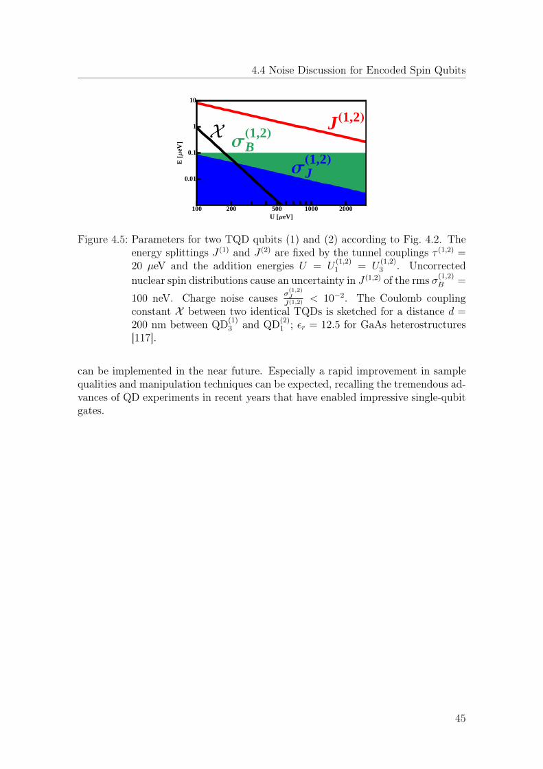
4.4 Noise Discussion for Encoded Spin Qubits
XJH1,2L
ΣJH1,2L
ΣBH1,2L
100 200 500 1000 2000
0.01
0.1
1
10
U @ΜeVD
E@Μ
eVD
Figure 4.5: Parameters for two TQD qubits (1) and (2) according to Fig. 4.2. Theenergy splittings J (1) and J (2) are fixed by the tunnel couplings τ (1,2) =20 µeV and the addition energies U = U
(1,2)1 = U
(1,2)3 . Uncorrected
nuclear spin distributions cause an uncertainty in J (1,2) of the rms σ(1,2)B =
100 neV. Charge noise causes σ(1,2)J
J(1,2) < 10−2. The Coulomb couplingconstant X between two identical TQDs is sketched for a distance d =200 nm between QD(1)
3 and QD(2)1 ; εr = 12.5 for GaAs heterostructures
[117].
can be implemented in the near future. Especially a rapid improvement in samplequalities and manipulation techniques can be expected, recalling the tremendous ad-vances of QD experiments in recent years that have enabled impressive single-qubitgates.
45
Appendix
4.A Characterization of Classical Noise
δt is a noisy classical variable that is characterized by the probability distributionPδ and the correlation function Cδ [102]. The mean value µδ = 〈δt〉 and the standarddeviation σδ =
√〈δ2t 〉 determine a Gaussian probability distribution:
Pδ = e−(δt−µδ√
2σδ
)2
/√
2πσδ. (4.54)
This work considers δt with µδ = 0. 〈. . .〉 is the probability average. The correlationfunction Cδ (t, t′) = 〈δtδt′〉 describes correlations between different times t and t′.The noise sources are assumed to be stationary with Cδ (t, t′) = Cδ (t− t′). Thespectral function S (ω) is defined as the Fourier transform of Cδ (t):
S (ω) =
∫ ∞−∞
dt e2πiωtCδ (t) , Cδ (t) =
∫ ∞−∞
dω e−2πiωtS (ω) . (4.55)
Note that S (ω) / (J2 · s) ∈ R, and ω has the unit s−1. S (−ω) = S (ω) becauseCδ (−t) = Cδ (t). σδ can be determined by σ2
δ =∫∞−∞ dω S (ω).
4.B Characterization of Entangling Properties
A gate is maximally entangling, when it creates a maximally entangled state froma separable state. The Makhlin invariants [118, 119],
G1 = tr2 (m) / [16 det(m)] ∈ C, (4.56)G2 =
[tr2(m)− tr(m2)
]/ [4 det(m)] ∈ R, (4.57)
describe the entangling properties of a gate. m = MTBMB, where MB is the repre-
sentation of the gate in the Bell basis. Additional single-qubit operations before andafter this gate operation do not change the Makhlin invariants. All gate sequenceswith the same Makhlin invariants have the equivalent entangling properties. There-fore, the three real values γ = arg (G1), |G1|, and G2 are sufficient to characterize agate operation. They need to fulfill
sin2 (γ) ≤ 4 |G1| ≤ 1, (4.58)cos (γ) (cos(γ)−G2) ≥ 0, (4.59)
to be maximally entangling.
46
4.B Characterization of Entangling Properties
CNOT class — Both the controlled NOT operation (CNOT) and the controlledphase (CPHASE) operation are maximally entangling. These gates, and all equiva-lent gates, are characterized by G1 = 0 and G2 = 1. The two-qubit interactions,
I4σ(1)x σ(2)
x ,I4σ(1)y σ(2)
y ,I4σ(1)z σ(2)
z , (4.60)
create a CNOT after the time tCNOT = π~I .√
iSWAP class — The iSWAP = e−iπ
4
(σ
(1)x σ
(2)x +σ
(1)y σ
(2)y
)is the natural entangling
gate for the σ(1)x σ
(2)x + σ
(1)y σ
(2)y interaction [120]. Indeed, also the square root of
the iSWAP is maximally entangling with G1 = 14and G2 = 1. The two-qubit
interactions,
I8
(σ(1)x σ(2)
x ± σ(1)y σ(2)
y
),I8
(σ(1)y σ(2)
y ± σ(1)z σ(2)
z
),I8
(σ(1)y σ(2)
y ± σ(1)x σ(2)
z
), (4.61)
create a√iSWAP gate after the time t√iSWAP = π~
I . Note that the interaction
I4
(σ(1)x σ(2)
x +σ
(1)y σ
(2)y + σ
(1)z σ
(2)z
2
), (4.62)
is also maximally entangling after t = π~I . This maximally entangling gate can be
called√HSWAP. The Makhlin invariants of
√HSWAP are G1 = −1
4and G2 = −1.(√
HSWAP)2
is related to the iSWAP operation by single-qubit basis rotations thatconsist of Hadamard gates.General class — Arbitrary Hamiltonians of the form
I4
(ξ1σ
(1)x σ(2)
x + ξ2σ(1)y σ(2)
y + σ(1)z σ(2)
z
), (4.63)
with ξ1, ξ2 < 1, construct maximally entangling operations using two time evolutionsof the length t1 = π~
2I , when the time evolutions are separated by a single-qubitrotation around the z-axis:
e−iπ
8
(ξ1σ
(1)x σ
(2)x +ξ2σ
(1)y σ
(2)y +σ
(1)z σ
(2)z
)e−i
π2σ
(2)z e−iπ
8
(ξ1σ
(1)x σ
(2)x +ξ2σ
(1)y σ
(2)y +σ
(1)z σ
(2)z
)∼ CNOT.
(4.64)
The single-qubit operation e−iπ2σ
(2)z cancels the time evolution of the σ(1)
x σ(2)x and
σ(1)y σ
(2)y interactions. Note that an equivalent construction of Eq. (4.64) can be used
when the σ(1)x σ
(2)x interaction or the σ(1)
y σ(2)y interaction dominates. The total period
of the evolution under Eq. (4.63) is tcomb = 2t1 = π~I .
47

4 Static and Resonant Manipulations of Encoded Spin Qubits
4.C Large Amplitude Driving
A driven Hamiltonian shows a completely different behavior for large driving am-plitudes. The Hamiltonian
H =∆
2σz +
δ⊥t2σx + ε (t)σz, (4.65)
should be analyzed. ε (t) is not necessarily small compared to ∆2, and it is periodic
with the period h/∆. It is useful to go to a rotating frame with ∆2σz + ε (t)σz [107]:
H′ ≈ δ⊥t2
(0 e−
i~ [∆t+2
∫ t0 dt′ε(t′)]
ei~ [∆t+2
∫ t0 dt′ε(t′)] 0
). (4.66)
Eq. (4.66) assumes that δ⊥t is static during one driving period. Because the functione
2i~∫ t0 dt′ε(t′) has the period h/∆, it can be expanded in a Fourier series e
2i~∫ t0 dt′ε(t′) =∑
n∈Z ane−in∆t
~ with an = 1h/∆
∫ h/∆0
dt′ e2i~∫ t′0 dt′′ε(t′′)ein
∆t′~ . Only the resonant terms
a1 and a−1 are kept in Eq. (4.66) because all other terms oscillate rapidly: H′ ≈δ⊥t2
(<e (a1)σx + =m (a1)σy). One example is the case of harmonic driving ε (t) =A cos
(∆t~
), with a1 = a−1 = −J1
(2A∆
). J1 (x) is the Bessel function of the first kind
and the first order that is large only for finite x, but J1 (x) vanishes for x→ 0. Theeffective Hamiltonian becomes H′ ≈ − δ⊥t
2A∆σx for A ∆.
48

CHAPTER 5
Noise-Protected Gate forSix-Electron Double-Dot Qubits
Singlet-triplet spin qubits in six-electron double quantumdots, in moderate magnetic fields, can show superior im-munity to charge noise. This immunity results from thesymmetry of orbitals in the second energy shell of circularquantum dots: singlet and triplet states in this shell haveidentical charge distributions. Our phase-gate simulations,which include 1/f charge noise from fluctuating traps, showthat this symmetry is most effectively exploited if the gateoperation switches rapidly between sweet spots deep inthe (3,3) and (4,2) charge stability regions; fidelities veryclose to one are predicted if subnanosecond switching canbe performed.
The results of this chapter were published in:
Sebastian Mehl and David P. DiVincenzo:Noise-protected gate for six-electron double-dot qubit,Phys. Rev. B 88, 161408(R) (2013).Copyright 2013 by the American Physical Society.
49

5 Noise-Protected Gate for Six-Electron Double-Dot Qubits
5.1 Introduction
The spin degree of freedom of the few-electron quantum dot (QD) is an excellentbuilding block for a qubit. While a single electron spin may serve directly as a qubit[18], the difficulty of single-qubit operations makes it desirable to encode a qubit ina multielectron state. Considerable success has been achieved with a two-electronencoding [50], in which the singlet and spinless triplet levels of the double quantumdot (DQD) define a logical qubit [31]. Electric pulses, applied on the microsecondscale, permit all necessary one- [37, 40] and two-qubit [63, 64] operations whensupplemented by magnetic field gradients [53, 55, 121].
This chapter addresses the crucial exchange gate, which has provided a route toimpressive progress in the singlet-triplet qubit [37, 40]. In this gate a DQD is movedaway from the “neutral” electron distribution, i.e. having one electron on each QD[referred to as (1, 1)] to one having a slight bias towards double occupancy of oneQD [e.g. the left QD: (2, 0)]. Only the singlet configuration permits the electrontransfer from (1, 1) to (2, 0), while the transfer from the triplet state is blocked(Pauli spin blockade). Exchange gates allow fast qubit manipulations since theycouple strongly to the charge instead of the spin degree of freedom. But new noisemechanism consequently emerge: low-frequency switching of charge traps become amajor problem [52, 94, 122].
Here we show that, paradoxically, the exchange gate will be much less susceptibleto change noise if the DQD is pulsed fully from the (1, 1) to the (2, 0) regime. Pulsingfar into the (2, 0) region also lifts the spin blockade for the triplet state, as an excitedorbital state becomes energetically accessible [93, 123]. The singlet-triplet splittingis highly protected from charge noise deep in the (2, 0) region. We show that thefidelity of exchange gates will be excellent under two conditions: (1) the pulse riseand fall times should be subnanosecond, and (2) the electrons should be in thesecond shell, so that singlet and triplet states have the same charge distribution.This means that the best exchange gate is predicted to occur for the six-electronDQD with four nonparticipating “core” electrons, so that the desired transition isactually between (3, 3) and (4, 2).Presently only one other approach has been proposed to mitigate charge noise.
There is the suggestion to encode singlet-triplet qubits using many-electron QDs(N > 3), so that background electrons may screen charge fluctuations [124–126].This approach involves strong renormalizations of the QD’s one-particle wave func-tions when interacting with charge traps; our approach is quite distinct, involvingonly weak state renormalizations.
5.2 Model
Our description of DQDs starts with the single-particle eigenstates of a circular QDwith the confining potential V (x, y) = mω0
2r2 [83, 127]. The kinetic energy term ℘2
2m
contains the kinematic momentum operator ℘ = ~i∇ + eA. e > 0 is the electric
50

5.2 Model
charge, m is the effective mass, and A = B2
(−y, x, 0)T describes orbital effects ofthe magnetic field B in the symmetric gauge that is restricted to the out-of-planedirection. The single-particle eigenstates are the Fock-Darwin (FD) states ψn,l (ρ, φ)
= (mΩ/~)|n|+1
2
√n!
π(n+|l|)! L|l|n [(mΩ/~) ρ2] e−ilφρ|l| e−
mΩ2~ ρ
2 , with n ∈ N0 and l ∈ Z. We
use polar coordinates (ρ, φ), while Lji (x) are the generalized Laguerre polynomials.States of the same energy shell all have the same value of 2n+ |l|, with the energiesEn,l = (2n+ |l|+ 1) ~Ω− l~ωc [128, 129], ωc = eB
2m, and Ω2 = ω2
0 + ω2c . We consider
moderate B fields: the degeneracies En,l, for the same l, are lifted; but En,l withdifferent n do not cross (ωc/ω0 1). The single-particle eigenstates are groupedinto “atomic” energy shells [30]. The ground state ψ0,0 is well separated from thefirst two excited states ψ0,±1.
We employ a description for few-electron DQDs that takes into account multipleenergy levels and electron-electron interactions [130, 131]. As in the work of Burkardet al. [83], we construct a Hubbard model building upon the FD states. In contrastto more numerically oriented techniques, such an approach heavily relies on thechosen basis as couplings to other states are neglected. It has the advantage thatall obtained results can be understood analytically. For two-electron DQDs, weinclude only the (1, 1), (2, 0), and (0, 2) electron configurations. The singlet (S) andsz = 0 triplet (T) states can be written as the product of spin and orbital parts:ΨS/T = φ1, φ2s/a ⊗ | ↑↓〉∓| ↓↑〉√
2. The electrons occupy states φi, which need to be
symmetrized/antisymmetrized for the S/T-state (as indicated by •, •s/a).
In general, we cannot use a single FD state ψn,l for the description of the states φ1/2
directly. But in the (1, 1) configuration, φ1/2 is close to the FD ground state ψL/R0,0 onthe left/right QD. In the (2, 0) and (0, 2) singlet configurations, both electrons fillthe same orbital ground state, close to ψL/R0,0 on the respective QD. For the triplet,the Pauli exclusion principle requires two different states to be occupied, so that oneelectron is in ψL/R0,0 and the second electron is in ψL/R0,1 . As in atoms, the first electronshell ψL/R0,0 is completed with two electrons in a singlet. We assume that in the six-electron configuration the first two electrons on each QD complete this first shell.We then adopt a frozen-core approximation. Therefore, the (3, 3) configuration fora six-electron DQD is equivalent to the (1, 1) configuration for a two-electron DQD[and similarly the (4, 2)/(2, 4) and (2, 0)/(0, 2) configurations]. One just needs touse the appropriate orbital wave function of these “valence” electrons. The valenceorbital ground state is then ψL/R0,1 , while the first excited state is ψL/R0,−1.
The two-electron DQD Hamiltonian is expressed in the basis (1, 1)S/T , (2, 0)S/T ,and (0, 2)S/T [and equivalently, without further specification, (3, 3)S/T , (4, 2)S/T , and
51

5 Noise-Protected Gate for Six-Electron Double-Dot Qubits
(2, 4)S/T for the six-electron DQD]:
H =
0 0 τS 0 τS 00 0 0 τT 0 τTτS 0 US − ε 0 0 00 τT 0 UT − ε 0 0τS 0 0 0 US + ε 00 τT 0 0 0 UT + ε
. (5.1)
The diagonal entries describe the energies of the states. The difference between the(1, 1)S matrix element and (1, 1)T matrix element is neglected, since it is usuallysmall [83]. Unequally occupied QDs are higher in energy by US/T . For simplicitywe assume identical QDs on the left and the right. ∆ ≡ UT − US is the energydifference between the doubly occupied states. Electrostatic bias, modeled by theparameter ε, influences the relative state energies of uniform and unequal electronarrangements. The off-diagonal elements in Eq. (5.1) describe the spin-conservinghopping process of the electrons between the dots.Fig. 5.1 shows the energy spectrum as a function of ε. Close to the state degen-
eracies |ε| = Uσ, the hopping processes hybridize electron configurations of the sametotal spin. The ground state ES/ET is shown in blue/red. At ε = 0, both energylevels are mainly in the (1, 1) charge configuration, and their energy difference isminimal. ES and ET are lowered in energy for increasing bias due to the transferof electrons between the QDs. For large ε, the ground states are close to (2, 0)S,Twith an energy difference ∆; we indicate one point deep in the (2, 0) region as the“high-bias” configuration ε = εHB.Our treatment of the few-electron DQD is not self-consistent; it employs energy
spectra of single-particle states, which are successively filled with electrons. TheFD-states are a valid ansatz for the description of few-electron QDs if the electron-electron interaction influences the single-particle energies weakly or shifts all energylevels by a fixed value. The last scenario is consistent with the calculations ofGüçlü et al., where the addition energy of interacting electrons has a constant offsetcompared to the noninteracting case (cf. Ref. [133]1). This is consistent with theconstant-interaction model, introduced by Averin and Likharev [134, 135], in whichthe energy spectrum of QDs remains unchanged when an electron is added to orremoved from a QD.
5.3 Charge Noise
Charge noise is generally modeled by a random distribution of classical two-levelfluctuators (TLFs), which couple electrostatically to QDs [136, 137]. If the occupa-tions of the charge traps (CTs) vary with a broad distribution of fluctuation rates,
1A reasonable value of the constant rs in Ref. [133] for QDs that are used for quantum computationis rs = 2.
52

5.3 Charge Noise
Figure 5.1: Energy diagram for two- and six-electron DQDs, as described byEq. (5.1). Electrostatic bias, modeled by ε, transfers one electron fromthe uniform electron distribution on the two QDs towards two excesselectrons on the left QD. The blue/red line represents the singlet/tripletground state ES/T ; black curves are excited states. Charge noise gen-erates fluctuations between ES and ET , as described in the main text.The electron configurations are highly insensitive to charge noise at ε = 0(the “neutral” electron configuration) and ε = εHB (the “high-bias” con-figuration far away from the two anticrossings). The inset shows thecharge stability diagram following van der Wiel et al. [132]. (nL, nR) isthe stable charge configuration for the left QD and the right QD. VL/Rdescribes electrostatic voltages applied to the left/right QD; red arrowsindicate gate tunings corresponding to the energy diagram.
1/f noise is generated. The coherence of the qubit decreases as seen by the timeevolutions of superpositions:
〈σx〉 (t) =
⟨e−i
∫ t0 dt′ EST (t′)
~
⟩≈ e
−(tT2
)2
σidealx (t) . (5.2)
EST (t) is the time-varying energy difference of the qubit levels, which deviates fromthe ideal value due to the coupling to TLFs: δEST = EST − 〈EST 〉. 〈. . . 〉 describesthe average result of many experiments. Assuming a static environment during onerun, the coherence time T2 is related to the statistics of the TLFs: T−1
2 = σδE/√
4π;σ2δE =
∫∞−∞ dt δE
2 (t) [94, 104, 138, 139].We analyze the relative energy shift of the qubit levels of a DQD which couples
to a CT. In first-order perturbation theory, the fluctuation of the singlet-tripletsplitting is described by [140]:
δE(1)ST = 〈ΨT |eΦCT |ΨT 〉 − 〈ΨS |eΦCT |ΨS〉 . (5.3)
ΦCT is the electrostatic potential of a CT. Since for QDs that are suitable for qubitsCTs are at some distance from the QD center, we make a multipole expansion of ΦCT :ΦCT ≈ Φ (r0)−E (r0) ·r− 1
2[∂iEj (r0)] rirj [141]. r0 is the position of the CT relative
53

5 Noise-Protected Gate for Six-Electron Double-Dot Qubits
to the center of the DQD, r is the QD electron coordinate. This expansion resolvesthe coupling of a TLF into dipole (−E·d) and quadrupole [−(1/2) (∂iEj)·Qij] terms;di = e 〈Ψ |ri|Ψ〉, and Qij = e 〈Ψ |rirj|Ψ〉 are the first two electric moments of theDQD. We analyze two points in the charge stability diagram ε = 0 and ε = εHB(“sweet spots”, introduced in Fig. 5.1) at which the coupling to TLFs is weak. Highcouplings are obtained if the qubit states have different dipole moments, whichgenerate energy shifts scaling like, e.g., 1/r2
0.The eigenstates of the singlet-triplet qubit of Eq. (5.1) can be approximated at
ε = 0: ΨS/T ∝ |11〉S/T −τS/TUS/T
(|0, 2〉S/T + |2, 0〉S/T
).2 These states have equiv-
alent dipole moments for the two qubit levels; the charge distribution of a DQDarranged in the x-direction has mirror symmetry to the y-z plane. The quadrupolecontribution describes the spread of the charge distributions. The unequal degreeof hybridization of the singlet state and the triplet state creates different variances
in the x-direction: δE(1)ST ≈
[(τSUS
)2
−(τTUT
)2]· ed
20
4· e
4πε0εr
(x2
0
r50− 1
r30
). The first
factor describes the hybridizations for the singlet and the triplet, the second factorinvolves the interdot distance d0 of the DQD, and the third factor is the gradientcontribution of the electric field of the TLF. It describes an energy shift proportionalto the hybridization of the ground state
(τS/T/US/T
)2, which decays like 1/r30 in the
TLF-QD distance. A similar expression holds for the six-electron DQD.Considering the two-electron DQD for high bias (ε = εHB), the left QD is lower
in energy than the right QD. We assume we are far away from the transition regionin which the valence electrons occupy single-particle eigenstates of the left QD. Forthe singlet both electrons are placed into ψL0,0; for the triplet one electron occupiesψL0,0, the other ψL0,1. The dipole contributions to Eq. (5.3) vanish because the chargedistribution of ΨS and ΨT are both centered at the left QD. The quadrupole contri-bution of Eq. (5.3) is δE(1)
ST ≈(
e~4mΩ
)·(
e4πε0εr
)(x2
0+y20
r50− 2
z20
r50
). The first factor comes
from the different spread of the density of the qubit states, while the second factordescribes the influence of the CT. We find a 1/r3
0-scaling in the CT-QD distance asfor the low-bias sweet spot.
The situation improves for six-electron DQDs. As the valence electrons’ wavefunctions ψ0,±1 are complex conjugates of each other, not only the quadrupole termof Eq. (5.3), but all multipole contributions vanish. δE
(1)ST depends only on the
charge density of the single-electron wave functions, as eΦCT in Eq. (5.3) containsexclusively single-particle operators. The second-order dipole contribution of TLFs
2We assume two identical QDs for simplicity. However, one can also finds a sweet spot for distinctQDs. Then ΨS/T has different weights in (2, 0) and (0, 2) at the (1, 1)-sweet spot; additionally,the sweet spot is not in the center of a charge stability region. Charge traps dominantly coupleto DQDs via their electric field, which induces a small shift in the bias parameter ε. Thismechanism generates no dephasing at the minimum of [ET − ES ] (ε). We note that it mightwell be desirable to use one weakly and one strongly confined QD in future experiments. Astrongly confined QD simplifies qubit initializations, while the large QD can be used for theexchange manipulations.
54
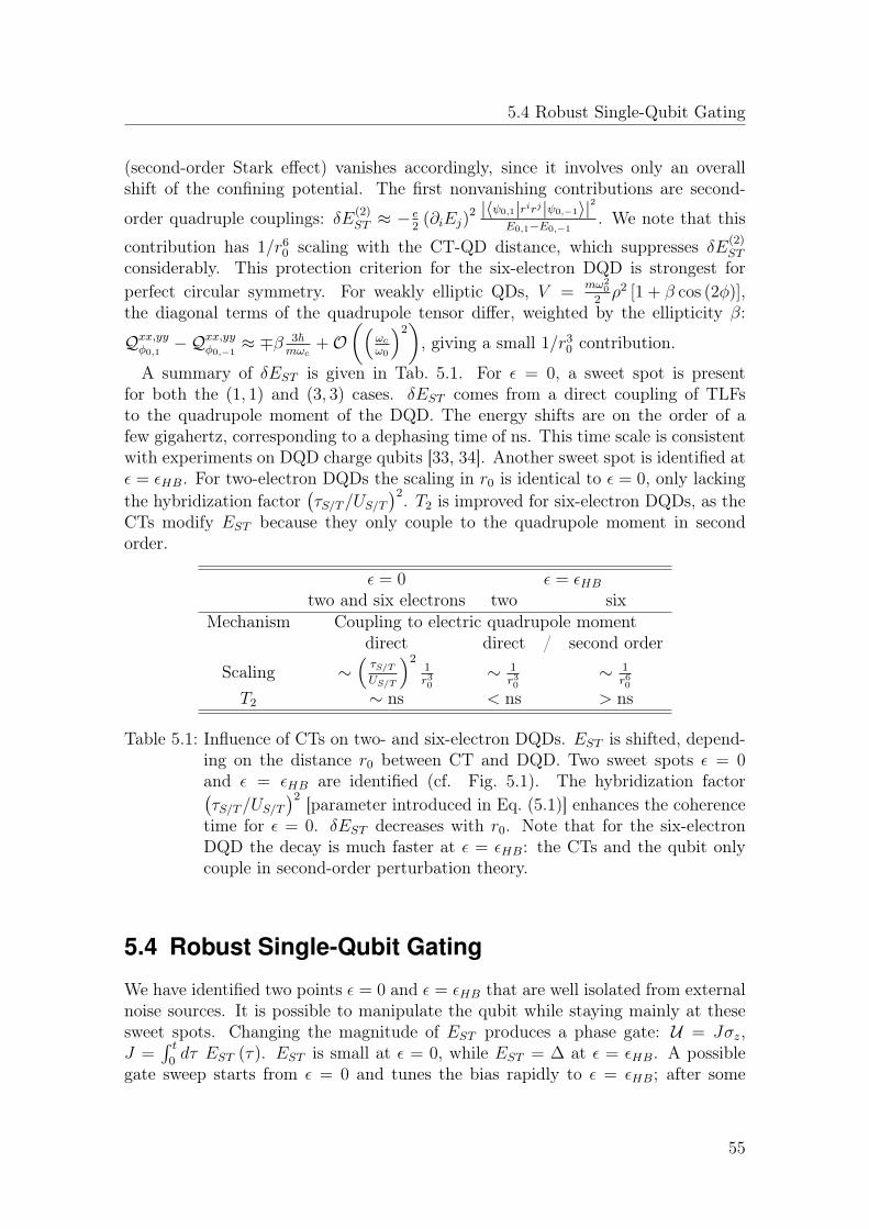
5.4 Robust Single-Qubit Gating
(second-order Stark effect) vanishes accordingly, since it involves only an overallshift of the confining potential. The first nonvanishing contributions are second-
order quadruple couplings: δE(2)ST ≈ − e
2(∂iEj)
2 |〈ψ0,1|rirj|ψ0,−1〉|2E0,1−E0,−1
. We note that this
contribution has 1/r60 scaling with the CT-QD distance, which suppresses δE(2)
ST
considerably. This protection criterion for the six-electron DQD is strongest forperfect circular symmetry. For weakly elliptic QDs, V =
mω20
2ρ2 [1 + β cos (2φ)],
the diagonal terms of the quadrupole tensor differ, weighted by the ellipticity β:
Qxx,yyφ0,1−Qxx,yyφ0,−1
≈ ∓β 3~mωc
+O((
ωcω0
)2), giving a small 1/r3
0 contribution.
A summary of δEST is given in Tab. 5.1. For ε = 0, a sweet spot is presentfor both the (1, 1) and (3, 3) cases. δEST comes from a direct coupling of TLFsto the quadrupole moment of the DQD. The energy shifts are on the order of afew gigahertz, corresponding to a dephasing time of ns. This time scale is consistentwith experiments on DQD charge qubits [33, 34]. Another sweet spot is identified atε = εHB. For two-electron DQDs the scaling in r0 is identical to ε = 0, only lackingthe hybridization factor
(τS/T/US/T
)2. T2 is improved for six-electron DQDs, as theCTs modify EST because they only couple to the quadrupole moment in secondorder.
ε = 0 ε = εHBtwo and six electrons two six
Mechanism Coupling to electric quadrupole momentdirect direct / second order
Scaling ∼(τS/TUS/T
)21r30
∼ 1r30
∼ 1r60
T2 ∼ ns < ns > ns
Table 5.1: Influence of CTs on two- and six-electron DQDs. EST is shifted, depend-ing on the distance r0 between CT and DQD. Two sweet spots ε = 0and ε = εHB are identified (cf. Fig. 5.1). The hybridization factor(τS/T/US/T
)2 [parameter introduced in Eq. (5.1)] enhances the coherencetime for ε = 0. δEST decreases with r0. Note that for the six-electronDQD the decay is much faster at ε = εHB: the CTs and the qubit onlycouple in second-order perturbation theory.
5.4 Robust Single-Qubit Gating
We have identified two points ε = 0 and ε = εHB that are well isolated from externalnoise sources. It is possible to manipulate the qubit while staying mainly at thesesweet spots. Changing the magnitude of EST produces a phase gate: U = Jσz,J =
∫ t0dτ EST (τ). EST is small at ε = 0, while EST = ∆ at ε = εHB. A possible
gate sweep starts from ε = 0 and tunes the bias rapidly to ε = εHB; after some
55
5 Noise-Protected Gate for Six-Electron Double-Dot Qubits
waiting time the bias is brought back to ε = 0 (cf. inset of Fig. 5.2). While themanipulation must be fast to avoid charge noise, it should still be adiabatic withrespect to the coupling to excited states (cf. Fig. 5.1). The slew rate is limited bythe leakage to higher states, which is approximated with the transition probabilityat a Landau-Zener crossing of strength τ which is crossed with the velocity vslew
[142]: PLZ = e−2π τ2
~vslew . Since the tunnel coupling enters PLZ quadratically, realisticvalues of τ allow very fast manipulations with permitted pulse lengths far belownanoseconds.
We show a fidelity analysis of a π-phase gate for a two- and a six-electron DQDin Fig. 5.2. The slew rates are fixed through PLZ to produce negligible leakage(cf. Appx. 5.A for further information about the specific parameter choice and thesetup of the simulation). We use similar densities of the CTs for the two- and six-electron DQDs, which are positioned randomly around the DQD to generate 1/fnoise; the coupling to CTs vary the parameter ∆ through electrostatic couplingsto the DQD potential. We exclude a volume around the QD, where no CTs arepermitted; such nearby TLFs make the DQD completely nonfunctional as a qubit.We take the excluded volume for two-electron DQDs to be considerably larger thanfor the six-electron system. Fluctuations in the coupling τ or in the pulse profilesare disregarded. The sweet spots, especially ε = εHB, offer the advantage that ESTdoes not change over a wide range of ε.The fidelity of the gate, both for the two-electron and the six-electron systems
(blue/red), is low for small tunnel couplings τ . The fidelity increases very quicklywith τ for six-electron DQDs and reaches an ideal value very close to 1. The improve-ment of the fidelity for the two-electron system is much slower. We approximate thecurves according to Eq. (5.2), yielding a coherence time of 1.5 ns for the two-electronsystem and 29.3 ns for the six-electron case. Steps seen for the two-electron systemare generated by different waiting times in (2, 0) when constructing a π-phase gate;a one-parameter fit to Eq. (5.2) cannot completely reproduce these results.
5.5 Conclusion
We propose a fast and robust way to manipulate singlet-triplet qubits (STQs) via ahigh-bias phase gate. Contrary to current realizations of phase gates, our approachworks by going to high bias. The qubit couples to CTs weakly, and we manipulaterapidly between two sweet spots. The “high-bias” sweet spot εHB is not at a specificpoint in the charge diagram; there is a large range of parameters where EST isconstant. Note that the Rabi rotation gate needed for full qubit control is envisionedto occur also at a sweet spot (at ε = 0), employing magnetic field gradients. It isworth pointing out that the proposed high-bias phase gate works also as a maximallyentangling two-qubit gate for single-QD qubits [18].
It would be favorable for our proposal that DQDs have a small singlet-triplet en-ergy splitting at ε = εHB (∆, cf. Fig. 5.1) to give comfortable electrical manipulation
56
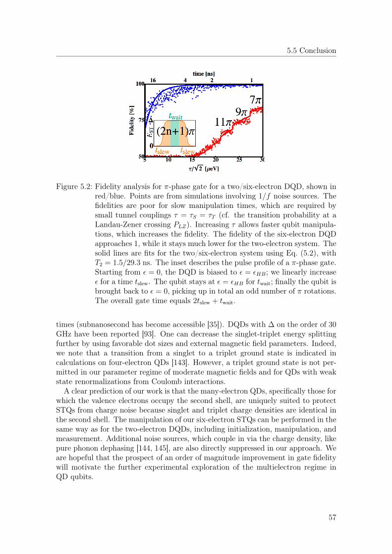
5.5 Conclusion
Figure 5.2: Fidelity analysis for π-phase gate for a two/six-electron DQD, shown inred/blue. Points are from simulations involving 1/f noise sources. Thefidelities are poor for slow manipulation times, which are required bysmall tunnel couplings τ = τS = τT (cf. the transition probability at aLandau-Zener crossing PLZ). Increasing τ allows faster qubit manipula-tions, which increases the fidelity. The fidelity of the six-electron DQDapproaches 1, while it stays much lower for the two-electron system. Thesolid lines are fits for the two/six-electron system using Eq. (5.2), withT2 = 1.5/29.3 ns. The inset describes the pulse profile of a π-phase gate.Starting from ε = 0, the DQD is biased to ε = εHB; we linearly increaseε for a time tslew. The qubit stays at ε = εHB for twait; finally the qubit isbrought back to ε = 0, picking up in total an odd number of π rotations.The overall gate time equals 2tslew + twait.
times (subnanosecond has become accessible [35]). DQDs with ∆ on the order of 30GHz have been reported [93]. One can decrease the singlet-triplet energy splittingfurther by using favorable dot sizes and external magnetic field parameters. Indeed,we note that a transition from a singlet to a triplet ground state is indicated incalculations on four-electron QDs [143]. However, a triplet ground state is not per-mitted in our parameter regime of moderate magnetic fields and for QDs with weakstate renormalizations from Coulomb interactions.
A clear prediction of our work is that the many-electron QDs, specifically those forwhich the valence electrons occupy the second shell, are uniquely suited to protectSTQs from charge noise because singlet and triplet charge densities are identical inthe second shell. The manipulation of our six-electron STQs can be performed in thesame way as for the two-electron DQDs, including initialization, manipulation, andmeasurement. Additional noise sources, which couple in via the charge density, likepure phonon dephasing [144, 145], are also directly suppressed in our approach. Weare hopeful that the prospect of an order of magnitude improvement in gate fidelitywill motivate the further experimental exploration of the multielectron regime inQD qubits.
57

Appendix
5.A Description of the Fidelity Analysis
We model charge noise acting on DQDs by a random distribution of charge traps,being either filled or empty (cf. Fig. 5.3). The time evolution during an exchangegate is determined numerically using quantum process tomography [6]. We gener-ate a distribution of TLFs with a broad range of switching rates γ for each run ofthe simulation. A reasonable probability distribution is P (γ) ∼ 1/γ [146]. Thecharge distribution is constant during one run of the simulation, while the poten-tial fluctuates between successive simulations. This scenario mimics consecutivemeasurements with a long time between the measurements.
The coupling strength of the DQD and a TLF is determined by their distance. Asdescribed in the main text, we take the shift in the singlet-triplet splitting δEST asthe only dynamic variable. For the (2, 0) and (4, 2) configurations, the energy shiftsare:
δE(2,0)ST =
(e~
4mω0
)(e
4πε0εr
)(x2
0 + y20
r50
− 2z2
0
r50
)+O
[(ωc/ω0)2] , (5.4)
δE(4,2)ST =
9
16
(~
m2ω30
)(ωcω0
)(e2
4πε0εr
)2(
(x20 + y2
0)2
r100
)+O
[(ωc/ω0)2] . (5.5)
The excessively occupied QD is positioned in the x-y plane at the coordinate origin,while charge traps occupy the space around the DQD.
We use material parameters of GaAs. The confining strength ~ω0 = 3 meV isa common approximation for QDs [83]. ωc/ω0 = 0.1 describes moderate externalmagnetic fields of 0.7 T . The singlet-triplet splitting ∆ is rather small, consistentwith Dial et al. [93]. All parameters are summarized in Tab. 5.1.
The electron distribution can be approximated by the spread of the ground statewave function: aB ≡
√~
mω0≈ 20 nm. We use 250 TLFs with a distance [2.5, 15] aB
from the coordinate origin for the six-electron system. For the two-electron system,we need to exclude a larger volume around the DQD. Otherwise, the energy shiftsdue to Eq. (5.4) destroy the qubit fidelity completely. To generate the same densityof TLFs around the DQD, we include 196 charge traps with a distance [15, 25] aBfrom the origin.
58
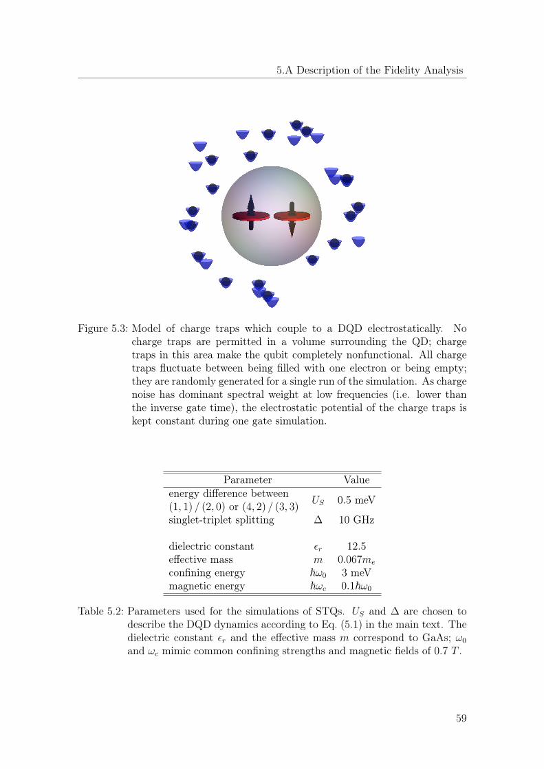
5.A Description of the Fidelity Analysis
Figure 5.3: Model of charge traps which couple to a DQD electrostatically. Nocharge traps are permitted in a volume surrounding the QD; chargetraps in this area make the qubit completely nonfunctional. All chargetraps fluctuate between being filled with one electron or being empty;they are randomly generated for a single run of the simulation. As chargenoise has dominant spectral weight at low frequencies (i.e. lower thanthe inverse gate time), the electrostatic potential of the charge traps iskept constant during one gate simulation.
Parameter Valueenergy difference between
US 0.5 meV(1, 1) / (2, 0) or (4, 2) / (3, 3)singlet-triplet splitting ∆ 10 GHz
dielectric constant εr 12.5effective mass m 0.067me
confining energy ~ω0 3 meVmagnetic energy ~ωc 0.1~ω0
Table 5.2: Parameters used for the simulations of STQs. US and ∆ are chosen todescribe the DQD dynamics according to Eq. (5.1) in the main text. Thedielectric constant εr and the effective mass m correspond to GaAs; ω0
and ωc mimic common confining strengths and magnetic fields of 0.7 T .
59


CHAPTER 6
Inverted Singlet-Triplet Qubit Codedon a Two-Electron Double Quantum
Dot
The sz = 0 spin configuration of two electrons confined ata double quantum dot (DQD) encodes the singlet-tripletqubit (STQ). We introduce the inverted STQ (ISTQ)that emerges from the setup of two quantum dots (QDs)differing significantly in size and out-of-plane magneticfields. The strongly confined QD has a two-electron sin-glet ground state, but the weakly confined QD has a two-electron triplet ground state. Spin-orbit interactions actnontrivially on the sz = 0 subspace and provide universalcontrol of the ISTQ together with electrostatic manipula-tions of the charge configuration. GaAs and InAs DQDscan be operated as ISTQs under realistic noise conditions.
The results of this chapter were submitted for publication after the preliminaryversion of the thesis was handed in, and they were published in:
Sebastian Mehl and David P. DiVincenzo:Inverted singlet-triplet qubit coded on a two-electron double quantum dot,Phys. Rev. B 90, 195424 (2014).Copyright 2014 by the American Physical Society.
61

6 Inverted Singlet-Triplet Qubit Coded on a Two-Electron Double Quantum Dot
6.1 Introduction
Encoded spin qubits in a two-electron configuration have become popular since theseminal experiment by Petta et al. [37]. Single electrons are trapped using gate-defined quantum dots (QDs) in semiconducting nanostructures [31]. The spin is usedas the information carrier [18]. We consider the qubit encoding using the sz = 0 spinsubspace of two electrons [50, 51, 57]. The passage between different charge config-urations realizes single-qubit control electrostatically. Applying voltages at metallicgates close to the structure enables the transfer of electrons between the QDs. The(1, 1) configuration labels separated electrons on the two QDs; two electrons occupya single QD in (2, 0) and (0, 2).
In this chapter, we explore a two-electron double quantum dot (DQD) under theinfluence of magnetic fields and spin-orbit interactions (SOIs). The qubit is encodedusing the singlet |S〉 and spinless triplet |T 〉 states, similar to common singlet-tripletqubits (STQs) [50, 51, 57]. Our setup has an energy degeneracy of |S〉 and |T 〉 in(1, 1) that is a consequence of the competition between the confining potential andthe Coulomb interactions. In the absence of SOIs, out-of-plane magnetic fields favortriplets, while the confining potential favors singlets. We call this qubit invertedSTQ (ISTQ) because it differs from normal STQs by the occurrence of a singlet-triplet inversion. We realize an ISTQs with one strongly confined QD and one weaklyconfined QD. |T 〉 is the ground state for one QD when it is doubly occupied, butthe other QD has a singlet ground state. SOIs couple |S〉 and |T 〉 . In contrast tothe setup with two QDs differing significantly in size, it was argued that SOIs acttrivially on the sz = 0 subspace for two identical QDs [147, 148].The encoding in the sz = 0 subspace is optimal because the qubit encoding is
protected from hyperfine interactions. Nuclear spins generate local magnetic fieldfluctuations δBhyp. Mainly the component δBq
hyp parallel to the external magneticfieldB influences the sz = 0 subspace [122]. Fluctuations in δBq
hyp are low frequencyand can be corrected using refocusing techniques [61, 91]. Especially, the ISTQ issuperior to the two-electron encoding that uses the singlet state |S〉 and the sz = 1triplet state |T+〉 [149–152]. There is also an energy degeneracy of |S〉 and |T+〉in this setup, but hyperfine interactions induce noise with larger weights at higherfrequencies [91].
The main purpose of this chapter is to explore the ISTQ encoding. We showthat SOIs act nontrivially on the sz = 0 subspace. The influence of SOIs can bedescribed by an effective magnetic field difference between the QDs. The effectivelocal magnetic field depends on the confining potential of the wave functions. ISTQsare controlled using electrostatic voltages, which tune the DQD between differentcharge configurations. DQDs that consist of QDs with different sizes realize ISTQsthat can be operated in the presence of realistic noise sources. A DQD that iscoded using two distinct QDs gives also other perspectives: a strongly confined QDis favorable for the initialization and the readout of STQs. A weakly confined QDmay be favorable for qubit manipulations [27]. We are convinced that this setup
62
6.2 Model
is likely to be explored as the search for alternative spin qubit designs continues[74, 75, 126]. Operating STQs coded using two QDs with different sizes as ISTQsis achieved by applying sufficiently large out-of-plane magnetic fields.
The organization of this chapter is as follows. Sec. 6.2 introduces the model toconstruct ISTQs and describes the qubit encoding. Sec. 6.3 characterizes SOIs asa source to influence the sz = 0 subspace. We describe different possibilities tomanipulate the ISTQ in Sec. 6.4 and discuss its performance in Sec. 6.5.
6.2 Model
Our study includes the orbital Hamiltonian H0, external magnetic fields H1, andSOIs H2. The orbital Hamiltonian for two electrons in gate-defined lateral DQDs isdescribed by:
H0 =∑i=1,2
[℘2i
2m+ V (xi)
]+ V (x1,x2) . (6.1)
The orbital contributions of the magnetic field component perpendicular to thelateral direction (called the z-direction) are included by the kinematic momentumoperator ℘ = ~
i∇ + eA. e > 0 is the electric charge, m is the effective mass,
and A = Bz2
(−y, x, 0)T describes orbital effects from the out-of-plane magneticfield component Bz in the symmetric gauge. Orbital contributions from in-planemagnetic fields are weak for strong confining potentials in the z-direction. V (x)is the single-particle potential that includes external electric fields. Two QDs arepresent at the positions (±a, 0, 0)T . V (x1,x2) is the Coulomb interaction. Magneticfields couple directly to the spins through the Zeeman Hamiltonian:
H1 =gµB
2B ·
∑i=1,2
σi. (6.2)
σ = (σx, σy, σz)T is the vector of Pauli matrices, B is the magnetic field, g is the
g-factor, and µB is the Bohr magneton.
We include two orbitals at each QD: the single-dot ground|L〉 , |R〉
and the
single-dot excited states ∣∣L⟩ , ∣∣R⟩ . We consider only the sz = 0 subspace, since
states with sz 6= 0 are far away in energy during qubit manipulations. The wavefunctions of the singlet state (S) and spinless triplet state (T) of different charge
63

6 Inverted Singlet-Triplet Qubit Coded on a Two-Electron Double Quantum Dot
configurations (nL, nR) are:
|S1,1〉 =1√2
(c†L,↑c
†R,↓ − c
†L,↓c
†R,↑
)|0〉 , (6.3)∣∣S2,0/0,2
⟩=(c†L/R,↑c
†L/R,↓
)|0〉 , (6.4)
|T1,1〉 =1√2
(c†L,↑c
†R,↓ + c†L,↓c
†R,↑
)|0〉 , (6.5)∣∣T2,0/0,2
⟩=
1√2
(c†L/R,↑c
†L/R,↓ + c†L/R,↓c
†L/R,↑
)|0〉 , (6.6)
where |0〉 is the vacuum state and c†iσ is the creation operator of an electron inorbital i with spin σ. We use a Hubbard model to describe the (2, 0), (1, 1), and(0, 2) configurations [83, 153]. The electrons are on separate QDs in (1, 1). Theorbital ground states are filled with two electrons for the singlets |S2,0〉 and |S0,2〉 ;the Pauli exclusion principle requires that electrons fill different orbitals for |T2,0〉and |T0,2〉 . Orbital effects of H0 and H1 are described by:
H =
0 tLs tRstLs UL + ε 0tRs 0 UR + Ω(0,2) − ε
⊕ 0 tLt tRt
tLt UL + Ω(2,0) + ε 0tRt 0 UR − ε
. (6.7)
Eq. (6.7) is written in the basis |S1,1〉 , |S2,0〉 , |S0,2〉 , |T1,1〉 , |T2,0〉 , |T0,2〉. Thereal constants tL,Rs,t characterize the spin-conserving hopping processes of electronsfrom (1, 1) towards two electrons on the same QD. The relative energies of (2, 0) and(0, 2) are tunable by voltages VL and VR at gates near the left and right QD; we modelthem by the parameter ε = 〈L |eVL|L〉 − 〈R |eVR|R〉 ≈
⟨L |eVL|L
⟩−⟨R |eVR|R
⟩.
The left QD is doubly occupied for ε→ −∞ (and similarly the right QD for ε→∞).The electrons are separated on different QDs for ε ∼ 0.As above, one needs to overcome the charging energies UL of the left QD or UR
of the right QD to add two electrons to the same QD. One QD (e.g. QDL) is in thenormal configuration and has a singlet ground state, but |T0,2〉 is the ground state ofQDR. The singlet is the ground state in the absence of magnetic fields [154]. Doublyoccupied QDs with ET < ES are obtained at finite out-of-plane magnetic fields alsofor sz = 0 [155, 156]. Finite values of Bz decrease the sizes of the orbital wavefunctions and raise the Coulomb repulsions between the electrons. Electrons preferto minimize the Coulomb repulsion, which makes triplets favorable. The inversionfrom a singlet to a triplet ground state was experimentally detected at Bz = 1.5 Tin elongated GaAs QDs [157]. A theoretical study predicts an orbital singlet-tripletinversion at Bz = 0.5 T in weakly confined, circular GaAs QDs [148]. However,ISTQs only require a triplet ground state for one of the two QDs, which is realizedfor one strongly confined QD and one weakly confined QD (cf. Fig. 6.1). UL + Ω(2,0)
and UR + Ω(0,2) are the energies to reach the first excited, doubly occupied states.
Ω(2,0) = ET2,0 − ES2,0 > 0, Ω(0,2) = ES0,2 − ET0,2 > 0, (6.8)
64

6.3 Calculation of ∆so
are the energy differences of the doubly occupied states. We neglect matrix elementsbetween (2, 0) and (0, 2) of the same spin [83] because their contributions are weak.
Figure 6.1: STQ coded on an inverted DQD. Each QD contains one electron. Mod-ifications of the confining potentials allow an electron transfer to reacha doubly occupied QD. QDL has a two-electron singlet ground state;for QDR the spinless triplet state is lower in energy. The out-of-planecomponent Bz of the magnetic field favors triplets, but the confiningenergy favors singlets. The magnetic field B is tilted by the angle φfrom the dot-connection axis ex and by the out-of-plane angle θ fromez. The [1, 0, 0]-direction of the lattice is rotated by the angle ξ fromex. We introduce additionally the rotation angle ρ between B and the[1, 0, 0]-direction.
Fig. 6.2 shows a typical energy diagram of the sz = 0 subspace in the chargeconfigurations (2, 0), (1, 1), and (0, 2). Eq. (6.7) describes a state crossing of thesinglet |S〉 and sz = 0 triplet state |T 〉 . |S2,0〉 is the ground state deep in (2, 0),while |T0,2〉 is the ground state in (0, 2). |S1,1〉 and |S2,0〉 have the same orbitalenergies at ε = −UL; |T1,1〉 and |T0,2〉 are at equal energies at ε = UR. Similarly,there is a state degeneracy of |T1,1〉 and |T2,0〉 at ε = −
(UL + Ω(2,0)
). |S1,1〉 and
|S0,2〉 have the same energy at ε = UR+Ω(0,2). Electron tunneling between the QDshybridizes states of different charge configurations. The singlet ground state |S〉 isdegenerate with sz = 0 triplet state |T 〉 in (1, 1) because the tunnel couplings tL,Rs,tare smaller than UL, UR, Ω(2,0), and Ω(0,2). We label this point by ε∗. The nextsection describes SOIs, which couple |S〉 and |T 〉 by ∆so at ε∗.
6.3 Calculation of ∆so
We consider QDs fabricated in the crystal’s (0, 0, 1) plane. The strong confiningpotential in the z-direction causes interactions between the electron spins and thein-plane momentum components. SOIs are described by:
H2 =α
~∑i=1,2
[σx′℘y′ − σy′℘x′ ]i +β
~∑i=1,2
[−σx′℘x′ + σy′℘y′ ]i . (6.9)
65

6 Inverted Singlet-Triplet Qubit Coded on a Two-Electron Double Quantum Dot
Figure 6.2: Energy diagram of a STQ as a function of the electrostatic bias ε ac-cording to Eq. (6.7) and Eq. (6.9). The blue and red lines describe theenergies of the lowest singlet ES and spinless triplet ET ; black lines showexcited states. The left dotted line labels the charge transition point atε = −UL, where ES1,1 and ES2,0 have the same energies (similarly ET1,1
and ET0,2 have equal energies at ε = UR). We obtain a (2, 0) singletground state at ε < 0, while ε > 0 favors the (0, 2) triplet. ES and ETcross at ε∗. SOIs couple ES and ET . The inset shows the region aroundε∗. The dashed curves are energy levels in the absence of SOIs.
The first term, which is called the Rashba SOI,1 is caused by the broken structureinversion symmetry from the confining potential in the z-direction [158]. The secondterm, called the Dresselhaus SOI,1 is present for a crystal lattice without inversionsymmetry [159]. x′ and y′ label the [1, 0, 0]-direction and [0, 1, 0]-direction of thelattice. [1, 0, 0] is rotated by the angle ξ from ex, which is the vector connectingthe QD centers (cf. Fig. 6.1). Large spin-orbit (SO) effects are expected whenelectrons are free to move, which is possible between the QDs in the ex-direction.We consider only the SO contributions that involve the momentum componentin the ex-direction (℘x) and extract from Eq. (6.9) H2 = Ξ
~ ·∑
i=1,2 [℘xσ]i, withΞ = (−β cos (2ξ) ,−α− β cos (2ξ) , 0)T . Additional contributions from the in-planemomentum component perpendicular to ex are discussed in Appx. 6.A.
H0 from Eq. (6.1) dominates over the SO contributions. We apply a unitarytransformation U = ei(S1+S2), with Si = mxi
~2 Ξ · σi [160–162]. U was introduced toremove SOIs to second order for confined systems. This transformation turns outto be useful because the transformed Hamiltonian is only position dependent. Notethat the equivalent transformation was used in Refs. [147, 148] to show that SOIsact trivially on the sz = 0 subspace for a highly symmetric DQD. The transformed
1 The Rashba constant α and the Dresselhaus constant β have the units Jm. lαso = ~2
2mα andlβso = ~2
2mβ are the Rashba and Dresselhaus spin precession lengths that have the units m.
66

6.3 Calculation of ∆so
Hamiltonian reads:
U(H0 +H1 + H2
)U † =H0 −
m
~2|Ξ|2 +
gµB2
∑i=1,2j∈N
B[j]eff (xi) · σi, (6.10)
B[j]eff (x) ≡ 1
j!
(2m
~2x
)j[( . . . ( B × Ξ)× . . . )×Ξ︸ ︷︷ ︸
j times
] . (6.11)
H0 remains formally unchanged. Besides the constant energy shift −m~2 |Ξ|2, there
are only position dependent terms (note the restriction to the x-direction). Eq. (6.10)couples only states of the same charge sector because the orbital states are stronglyconfined at the QD’s position. We restrict the discussion to the contribution in (1, 1).Contributions from (2, 0) and (0, 2) are negligible, as described in Appx. 6.B. The
charge configuration is confined to a small area compared to the SO scale(
~2
2m|Ξ|
)2
,with the result that terms in Eq. (6.11) with higher order in j are less important.The external magnetic field is rotated by the polar angle θ from the [0, 0, 1]-
direction and the azimuthal angle φ from ex [cf. Fig. 6.1]. We fix the spin quan-tization axis parallel to B. The components of Eq. (6.11) that are parallel to theexternal magnetic field
(B
[j]eff
)qcouple |S1,1〉 and |T1,1〉 , while the perpendicular com-
ponents couple subspaces of different sz. We assume that the states |L〉 and |R〉 arestrongly confined at the QD position, with 〈L |x|R〉 = 〈L |x2|R〉 = 0, 〈R |x|R〉 =−〈L |x|L〉 = a. We introduce the variances of the orbitals
⟨L∣∣(x− a)2
∣∣L⟩ = varLand
⟨R∣∣(x+ a)2
∣∣R⟩ = varR. Note that |L〉 and |R〉 are transformed by U afterEq. (6.10).The effective Hamiltonian in (1, 1), including SOIs to second order, is written
in the basis |S1,1〉 from Eq. (6.3), |T1,1〉 from Eq. (6.5),∣∣T+
1,1
⟩= c†L↑c
†R↑ |0〉 , and∣∣T−1,1⟩ = c†L↓c
†R↓ |0〉 :
H(1,1) = EZ
0 0 0 00 0 0 00 0 1 00 0 0 −1
− i√2EZ2ma
~2Ξ⊥
0 0 1 10 0 0 0−1 0 0 0−1 0 0 0
(6.12)
− EZ(
2m
~2
)2
Ξ2⊥ (varL − varR)
0 1 0 01 0 0 00 0 1 00 0 0 −1
+√
2EZ
(2m
~2
)2
ΞqΞ⊥
×
0 0 −varL−varR
2varL−varR
2
0 0(varL+varR
2− 2a2
) (varL+varR2
− 3a2)
−varL−varR2
(varL+varR2
− 2a2)
0 0var−varR
2
(varL+varR2
− 3a2)
0 0
,
with the Zeeman energy EZ = gµB2|B|. Ξq = |Ξ| cos [] (Ξ,B)] is the component of
Ξ parallel to B, and Ξ⊥ = |Ξ| sin [] (Ξ,B)] is the component of Ξ perpendicular
67
6 Inverted Singlet-Triplet Qubit Coded on a Two-Electron Double Quantum Dot
to B (all components are determined by the angle ] (Ξ,B) between the vectors Ξand B, cf. Fig. 6.1).
The first term in Eq. (6.12) represents the Zeeman interaction that shifts∣∣T+
1,1
⟩and
∣∣T−1,1⟩ relative to the sz = 0 energy levels. This term dominates over all SOcontributions. The second term in Eq. (6.12) couples |S1,1〉 with
∣∣T+1,1
⟩and |S1,1〉
with∣∣T−1,1⟩ . This term was discussed in great detail in Refs. [147, 148]. It does
not couple |S1,1〉 and |T1,1〉 . Note that the coupling to the triplet states does notcause an energy shift of |S1,1〉 in second order Schrieffer-Wolff perturbation theory[36] because the couplings between |S1,1〉 and
∣∣T+1,1
⟩and between |S1,1〉 and
∣∣T−1,1⟩cancel each other.
The dominant SO contribution on the sz = 0 subspace is obtained from the thirdterm of Eq. (6.12). This term represents the component of the effective magneticfield parallel to B, which is second order in the SOI:
(B
[2]eff
)q
= −B2
(2m~2
)2Ξ2⊥x
2 [cf.
Eq. (6.11)].(B
[2]eff
)qrealizes a direct coupling between |S1,1〉 and |T1,1〉 : ∆so ≈
EZvarR−varL
l2so. We introduce the length scale lso = ~2
2m|Ξ⊥|. The fourth term in
Eq. (6.12) gives small corrections to ∆so. Appx. 6.A describes the angular depen-dency of ∆so and extends the analysis of SOIs using all terms of Eq. (6.9).
The smallest possible values for lso are on the order of the Rashba and Dres-selhaus spin precession lengths lαso and lβso. Typically, GaAs heterostructures havespin precession lengths lαso, lβso & 1 µm for the Rashba and the Dresselhaus SOIs(cf. Appx. 6.C). The variances of the orbital wave functions can be approximatedusing the noninteracting descriptions of electrons that are confined at QDs. TheFock-Darwin states are the solutions of the noninteracting eigenvalue problem oftwo-dimensional circular QDs [128, 129]. The variances of these wave functions aredirectly related to the confining potentials as var ≈ l20, when assuming a harmonic
confining potential that has the magnitude ~ω0 with l0 =√
~mω0
[1 +
(eBz
2mω0
)2]−1/4
.
Normal values for strongly confined QDs in GaAs are ~ω0 = 3 meV and l0 = 20 nm[83]. Weakly confined QDs in GaAs of ~ω0 = 0.1 meV have l0 = 100 nm. We obtain,for lso = 1 µm and B = 500 mT, ∆so = 0.1 µeV (∆so/h ≈ 25 MHz).Small band gap materials tend to have stronger SOIs. SOIs are, for example, by
one order of magnitude larger in InAs than in GaAs (lαso = 1.1 µm for GaAs andlαso = 0.14 µm for InAs, cf. Appx. 6.C). Furthermore, the variances of the wavefunctions of InAs QDs are potentially larger than of GaAs QDs due to the smallereffective mass. It should therefore be possible to reach values of ∆so ≈ 1 µeV(∆so/h ≈ 250 MHz).The coupling between |S〉 and |T 〉 at ε∗ can be approximated by ∆so ≈ EZ
varR−varLl2so
,as one can see from Eq. (6.7). The state coupling is determined by the weights of|S1,1〉 in |S〉 and |T1,1〉 in |T 〉 at ε∗. ε∗ is close to the center of (1, 1) because tL,Rs,tare much smaller than UL, UR, Ω(2,0), and Ω(0,2). Therefore |S1,1〉 and |T1,1〉 haveweights close to unity.
In summary, SOIs couple |S〉 and |T 〉 via their state contributions in (1, 1).
68
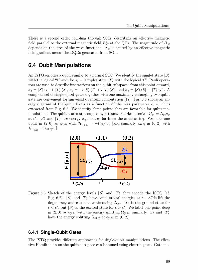
6.4 Qubit Manipulations
There is a second order coupling through SOIs, describing an effective magneticfield parallel to the external magnetic field Bq
eff at the QDs. The magnitude of Bqeff
depends on the sizes of the wave functions. ∆so is caused by an effective magneticfield gradient across the DQDs generated from SOIs.
6.4 Qubit Manipulations
An ISTQ encodes a qubit similar to a normal STQ. We identify the singlet state |S〉with the logical “1” and the sz = 0 triplet state |T 〉 with the logical “0”. Pauli opera-tors are used to describe interactions on the qubit subspace: from this point onward,σx = |S〉 〈T | + |T 〉 〈S| , σy = −i |S〉 〈T | + i |T 〉 〈S| , and σz = |S〉 〈S| − |T 〉 〈T | . Acomplete set of single-qubit gates together with one maximally-entangling two-qubitgate are convenient for universal quantum computation [17]. Fig. 6.3 shows an en-ergy diagram of the qubit levels as a function of the bias parameter ε, which isextracted from Fig. 6.2. We identify three points that are favorable for qubit ma-nipulations. The qubit states are coupled by a transverse Hamiltonian Hε∗ = ∆soσxat ε∗. |S〉 and |T 〉 are energy eigenstates far from the anticrossing. We label onepoint in (2, 0) as ε(2,0) with Hε(2,0)
= −Ω(2,0)σz [and similarly ε(0,2) in (0, 2) withHε(0,2)
= Ω(0,2)σz].
Figure 6.3: Sketch of the energy levels |S〉 and |T 〉 that encode the ISTQ (cf.Fig. 6.2). |S〉 and |T 〉 have equal orbital energies at ε∗. SOIs lift thedegeneracy and cause an anticrossing ∆so. |S〉 is the ground state forε < ε∗, but |S〉 is the excited state for ε > ε∗. We label one point deepin (2, 0) by ε(2,0) with the energy splitting Ω(2,0) [similarly |S〉 and |T 〉have the energy splitting Ω(0,2) at ε(0,2) in (0, 2)].
6.4.1 Single-Qubit Gates
The ISTQ provides different approaches for single-qubit manipulations. The effec-tive Hamiltonian on the qubit subspace can be tuned using electric gates. Gate ma-
69

6 Inverted Singlet-Triplet Qubit Coded on a Two-Electron Double Quantum Dot
nipulations rotate the direction of an effective magnetic field. A magnetic field in thez-direction is applied at ε(2,0) in (2, 0) and ε(0,2) in (0, 2). Ω(2,0) and Ω(0,2) correspondto the energy differences of |S〉 and |T 〉 . The effective magnetic field direction istilted to the x-axis in (1, 1). It points exactly along ex at ε∗ and has a magnitude ∆so.Rotations around the z-axis and x-axis can be generated when the qubit is tuned fastbetween ε(2,0), ε(0,2), and ε∗. The qubit manipulation time τ must be diabatic withthe SOI, but adiabatic to the orbital Hamiltonian: h/∆so τ h/Ω(2,0), h/Ω(0,2)
[52]. The timescale of single-qubit gates is determined by h/Ω(2,0), h/Ω(0,2), andh/∆so; it should be in the range of 10 MHz to a few GHz. Larger values make thegates too fast to be controlled by electronics. Smaller values require long gate times.
We describe two other possibilities for single-qubit control that are practical if∆so is either very large or very small. A large value of ∆so permits resonant Rabidriving, which has already been successful for a qubit encoded in triple QDs [67, 68].The effective Hamiltonian at ε∗ is H = Ω (ε)σz + ∆soσx. Transitions are driven byΩ (ε) = 2Ω0 cos (2∆sot/~ + ψ). If Ω0 ∆so, then one obtains after a rotatingwave approximation the static Hamiltonian H′ = Ω0 [−σy sin (ψ) + σz cos (ψ)]. Auniversal set of single-qubit gates can be generated when the phase ψ is adjusted.
Rabi driving becomes impractical for small ∆so because the gate times increase.We propose another possibility of driven gates that are described by the Landau-Zener (LZ) model [142, 150, 163]. Traversing the anticrossing in a time similar toτ = h/∆so generates single-qubit rotations. For large transition amplitudes, as forthe sweep from ε(2,0) to ε(0,2), the time evolution [142, 150, 163],
ULZ = e−iζRσze−iγσye−iζLσz , (6.13)
is decomposed into phase accumulations (through ζR and ζL) and one rotationaround an orthogonal axis. The phase accumulations ζR and ζL are determined bythe adiabatic evolution under the energy splitting Ω (t)σz and the Stückelberg phase.The essential part is the rotation around the y-axis by the angle γ = γLZ + π/2,
with sin (γLZ) =√PLZ , PLZ = e−
2∆2so
~v . v = dE/dt|ε∗ is the linearized velocity at ε∗.For example, the state |0〉 is transferred to an equal superposition of |0〉 and |1〉for PLZ = 1
2.
6.4.2 Two-Qubit Gates
Two-qubit gates can be realized using Coulomb interactions between two ISTQs[51]. We consider a linear arrangement of four QDs and label the two DQDs by (L)
and (R) (cf. Fig. 6.4). QD(L)R and QD(R)
L are closest to each other, and the electronconfigurations n(L)
R at QD(L)R and n
(R)L at QD(R)
L dominate the Coulomb couplingbetween the ISTQs [68, 71]: Hint = e2
4πε0εrdn
(L)R n
(R)L . d is the distance between QD(L)
R
and QD(R)L , ε0 is the dielectric constant, and εr is the relative permittivity. Hint
leaves the spin at ISTQ(L) and the spin at ISTQ(R) unchanged and can only cause
70
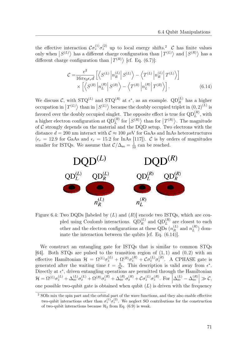
6.4 Qubit Manipulations
the effective interaction Cσ(1)z σ
(2)z up to local energy shifts.2 C has finite values
only when∣∣S(L)
⟩has a different charge configuration than
∣∣T (L)⟩and
∣∣S(R)⟩has a
different charge configuration than∣∣T (R)
⟩[cf. Eq. (6.7)]:
C =e2
16πε0εrd
[⟨S(L)
∣∣∣n(L)R
∣∣∣S(L)⟩−⟨T (L)
∣∣∣n(L)R
∣∣∣T (L)⟩]
×[⟨S(R)
∣∣∣n(R)L
∣∣∣S(R)⟩−⟨T (R)
∣∣∣n(R)L
∣∣∣T (R)⟩]. (6.14)
We discuss C, with STQ(L) and STQ(R) at ε∗, as an example. QD(L)R has a higher
occupation in∣∣T (L)
⟩than in
∣∣S(L)⟩because the doubly occupied triplet in (0, 2)(L) is
favored over the doubly occupied singlet. The opposite effect is true for QD(R)L , with
a higher electron configuration at QD(R)L for
∣∣S(R)⟩than for
∣∣T (R)⟩. The magnitude
of C strongly depends on the material and the DQD setup. Two electrons with thedistance d = 200 nm interact with C ≈ 100 µeV for GaAs and InAs heterostructures(εr = 12.9 for GaAs and εr = 15.2 for InAs [117]). C is by orders of magnitudessmaller for ISTQs. We assume that C/∆so = 1
10can be reached.
Figure 6.4: Two DQDs [labeled by (L) and (R)] encode two ISTQs, which are cou-pled using Coulomb interactions. QD(L)
R and QD(R)L are closest to each
other and the electron configurations at these QDs (n(L)R and n(R)
L ) dom-inate the interaction between the qubits [cf. Eq. (6.14)].
We construct an entangling gate for ISTQs that is similar to common STQs[64]. Both STQs are pulsed to the transition region of (1, 1) and (0, 2) with aneffective Hamiltonian H = Ω(L)σ
(L)z + Ω(R)σ
(R)z + Cσ(L)
z σ(R)z . A CPHASE gate is
generated after the waiting time t = h8C . This description is valid away from ε∗.
Directly at ε∗, driven entangling operations are permitted through the HamiltonianH = Ω(L)σ
(L)z + ∆
(L)so σ
(L)x + Ω(R)σ
(R)z + ∆
(R)so σ
(R)x + Cσ(L)
z σ(R)z . For
∣∣∣∆(L)so −∆
(R)so
∣∣∣ C,one possible two-qubit gate is obtained when qubit (L) is driven with the frequency
2 SOIs mix the spin part and the orbital part of the wave functions, and they also enable effectivetwo-qubit interactions other than σ
(1)z σ
(2)z . We neglect SO contributions for the construction
of two-qubit interactions because H2 from Eq. (6.9) is weak.
71

6 Inverted Singlet-Triplet Qubit Coded on a Two-Electron Double Quantum Dot
2∆(R)so /h. These driven gates are popular for superconducting qubits [113, 164–166].
The requirement is again that ∆(L)so and ∆
(R)so reach magnitudes of µeV to obtain fast
gate operations.
6.5 Discussion and Conclusion
An ISTQ with a finite ∆so provides universal control of the sz = 0 subspace. Oper-ations mainly at ε∗ in (1, 1) and ε(0,2) in (0, 2) are very favorable because the qubitis protected from small fluctuations in ε. Ω(0,2)/h in (0, 2) should not exceed a fewGHz to control phase accumulations at ε(0,2). Note that the out-of-plane magneticfield component Bz determines the magnitude of Ω(0,2). Obtaining large ∆so is mostcritical. The size of ∆so depends on the confining energies of the QDs and the mag-nitude of the SOIs. Values of ∆so ≈ µeV will be needed for driven Rabi-gates. Weshowed that these magnitudes are obtained for two QDs differing strongly in size.This setup is also promising due to other reasons. Strongly confined QDs are idealfor the initialization and readout of STQs. A weakly confined QD can be very usefulfor qubit manipulations (cf. also Ref. [27]).
One major challenge arises from the hyperfine interactions. Nuclear spins coupleto the electrons that are confined at QDs by creating local magnetic field fluctua-tions δBhyp. δBhyp has primarily low-frequency variations and can be consideredas static during one experiment, but it gives random contributions between suc-cessive measurements [91, 122]. An approximation for the component parallel to
the external magnetic field is δBqhyp =
∑ν Bν√Iν(Iν+1)√N
[52]. ν labels the differentnuclear spin isotopes of the semiconductor, which have the spin I. B contains ma-terial dependent coupling constants of the isotope, and N is the number of nucleiinteracting with an electron that is confined at a QD. For the ISTQ, δBq
hyp cou-ples |S1,1〉 from Eq. (6.3) and |T1,1〉 from Eq. (6.5) by ∆hyp equivalently to ∆so:∆hyp = gµB
(⟨L∣∣δBq
hyp
∣∣L⟩− ⟨R ∣∣δBqhyp
∣∣R⟩). The electrons at GaAs QDs typicallyinteract with 106 nuclear spins with δBq
hyp ≈ 5 mT giving ∆hyp ≈ 100 neV. Weaklyconfined QDs have larger ∆hyp because the electron wave function interacts withmore nuclear spins. Also InAs QDs have larger ∆hyp. Indium isotopes are spin-9/2nuclei, in contrast to Ga and As nuclei that are spin-3/2. Because of the equivalentinfluences of hyperfine interactions and SOIs, ∆so should be significantly larger than∆hyp. Refocusing techniques can be applied for ∆so > ∆hyp because the magneticfield fluctuations are low frequency [91].Charge noise is another source of decoherence. The filling and unfilling of charge
traps cause fluctuating electric fields at the positions of the DQDs. If the qubitis operated as a charge qubit, then charge noise dephases the ISTQ [27, 94, 122].Charge fluctuations are dominantly low frequency and lead typically to energy shiftsδEC = µeV between different charge states [34, 93]. The phase coherences betweencharge states are lost within a few ns. The most significant influence of charge noisecan be described by small fluctuations in ε [93]. Charge noise is less important at
72
6.5 Discussion and Conclusion
ε∗, ε(2,0), and ε(0,2) because small fluctuations in ε do not dephase the qubit.In summary, we have discussed a two-electron qubit encoding in the sz = 0
subspace for an ISTQ. The out-of-plane magnetic field is used to generate a levelcrossing of |S〉 and |T 〉 that is not present for normal STQs. SOIs couple |S〉 and|T 〉 if the sizes of the QDs differ. Different variances of the wave functions of the QDorbitals cause an effective magnetic field difference across the DQD. A DQD thatconsists of two unequal QDs can be a promising spin qubit also for other reasons.It has one QD with a large singlet-triplet splitting and one QD with a small singlet-triplet splitting already without external magnetic fields. The strongly confined QDis ideal for the qubit initialization and the readout, while the weakly confined QD issuitable for the qubit manipulations. We suggest ISTQs in GaAs and InAs becausethey provide sufficiently large ∆so.
Hyperfine interactions and charge noise dephase ISTQs. Hyperfine interactionscause dephasing mainly in (1, 1) through low-frequency magnetic field fluctuations.Nuclear spins and SOIs couple to ISTQs in the same way. It is very important tofabricate ISTQs, where ∆so is larger than the fluctuation ∆hyp from nuclear spins.Nuclear spin noise can be refocused for ISTQs because fluctuations in ∆hyp are lowfrequency. Charge noise dephases the qubit in the transition region between differ-ent charge sectors. Charge noise will be dealt with most efficiently if the ISTQ isoperated only at ε∗ and deep in (0, 2). All qubit operations require fast manipu-lation periods between different charge configurations, which has been achieved inprevious experiments [74, 75]. Motivated by the search for alternative spin qubitdesigns [74, 75, 126], we are hopeful that DQDs are explored where the QDs arediffering significantly in size. Realizing an ISTQ in a DQD of two different QDswill be possible by simply tilting the magnetic field out-of-plane. The perspectiveof universal electrostatic control which uses only a static SO-induced anticrossingshould further motivate the exploration of this setup.
73

Appendix
6.A Full Calculation of ∆so from SOIs
Besides H2 = Ξ~ ·∑
i=1,2 [℘xσ]i, with Ξ = (−β cos (2ξ) ,−α− β sin (2ξ) , 0)T , de-scribing the momentum component connecting the QDs, there is also the in-planeperpendicular momentum component ˜H2 = Ψ
~ ·∑
i=1,2 [℘yσ]i, with Ψ =(α −
β sin (2ξ) , β cos (2ξ) , 0)T . ˜H2 matters for QDs, in which the electrons have space to
move in the y-direction. Now, we discuss the extreme case of circular QDs. We as-sume, additionally to the properties of |L〉 and |R〉 that were introduced in Sec. 6.3,〈L |y|L〉 = 〈R |y|R〉 = 0, 〈L |y2|L〉 = varL, 〈R |y2|R〉 = varR, and that |L〉 and|R〉 are separable into a x-part and y-part.
We apply the transformation U = ei(S1+S2), with Si = m~2 [℘xΞ + ℘yΨ]i · σi. The
transformed Hamiltonian U(H0 +H1 + H2 +
˜H2
)U † contains similar terms as in
Eq. (6.10). Formally, H0 remains unchanged, and there is an overal energy shift−m
~2
(|Ξ|2 + |Ψ|2
). H1 from Eq. (6.2) gives a position dependent magnetic field
UH1U † =gµB
2
∑i=1,2j∈N
B[j]eff (xi) · σi, (6.15)
B[j]eff (x) ≡ 1
j!
(2m
~2
)j (. . . (B × (Ξx+ Ψy)) . . . )× (Ξx+ Ψy)︸ ︷︷ ︸j times
. (6.16)
We extract from Eq. (6.16) the effective magnetic field component parallel to Bin second order of the SOIs:(
B[2]eff
)q≈ −B
2
(2m
~2
)2 (Ξ2⊥x
2 + Ψ2⊥y
2). (6.17)
Eq. (6.17) neglects mixed terms in the position operators (∼ xy) and couples |S1,1〉and |T1,1〉 by ∆Z
so = EZvarR−varL
(lZso)2 with lZso = ~2
2m√
Ξ2⊥+Ψ2
⊥(which we call the Zeeman
spin precession length). Ξ⊥ = |Ξ| sin [] (Ξ,B)] and Ψ⊥ = |Ψ| sin [] (Ψ,B)] are thecomponents of Ξ and Ψ perpendicular to the external magnetic field (cf. Fig. 6.1).Note that lZso is on the order of the Rashba and Dresselhaus spin precession length,which is smaller than the confining radius of the QD wave functions.The transformation of H2 +
˜H2 adds additional contributions, dominated by:
mΞ×Ψ
~3·∑i=1,2
σi
[(lz)i −
mωc2
(x2i + y2
i
)], (6.18)
74

6.B Doubly Occupied Single QDs
with lz = pxy− pyx, and ωc = eBzm
. Especially the second term in Eq. (6.18) couples|S1,1〉 and |T1,1〉 directly by an effective magnetic field parallel to B:
(B
[2]eff,o
)q
= −~ωc/8gµB
2
(2m
~2
)2
(Ξ×Ψ)q(x2 + y2
). (6.19)
(Ξ×Ψ)q is the component parallel toB, which can be positive or negative.(B
[2]eff,o
)q
is determined by the orbital contribution of the magnetic field ~ωc instead of theZeeman energy EZ = gµB
2|B|. It describes the magnetic field produced by the
orbital motion of electrons. We introduce the orbital spin precession length (loso)2 =(
~2
2m
)21
(Ξ×Ψ)q, with which we write ∆o
so = ~ωc2
varL−varR(loso)2 .
Eq. (6.17) and Eq. (6.19) couple |S1,1〉 and |T1,1〉 by a magnetic field gradientacross the DQD, similar to the consideration in the main text:
∆so = (varR − varL)
(EZ
(lZso)2 +
~ωc/2(loso)
2
). (6.20)
Whether the Zeeman contribution EZ(lZso)2 or the orbital contribution ~ωc/2
(loso)2 dominatesEq. (6.20) depends in detail on the DQD. The orbital contribution should be domi-nant if the QDs are circular because ~ωc is usually larger than EZ :
∣∣∣~ωcEZ
∣∣∣ ≈ 135 for
GaAs and∣∣∣~ωcEZ
∣∣∣ ≈ 12 for InAs (cf. Appx. 6.C). If the DQD setup prefers one spatialdirection, then the Zeeman contribution dominates.
We analyze the angular dependencies of ∆so, which are influenced by the directionof the magnetic field B, the orientation of the crystal lattice, and the dot connectionaxis ex (cf. Fig. 6.1). The Zeeman spin precession length gives
(lZso)−2 ∝ Ξ2
⊥+Ψ2⊥ =
2 (α2 + β2) + sin2 (θ) α2 + β2 + 2αβ sin [2 (φ− ξ)]. SO contributions are maximalfor out-of-plane magnetic fields, but they can vanish for in-plane magnetic fields.This is exactly the case if there is no coordinate of the SO field perpendicularto the magnetic field. (loso)
−2 ∝ (Ξ×Ψ)q = (α2 − β2) cos (θ) is independent ofthe orientation of the crystal lattice. Orbital effects are maximal for out-of-planemagnetic fields, but they vanish for in-plane orientations.
6.B Doubly Occupied Single QDs
A doubly occupied single QD with the center at (a, 0, 0)T is described by:
∑i=1,2
[℘2i
2m+ V (xi)
]+ V (x1,x2)︸ ︷︷ ︸
H0
+gµB
2B ·
∑i=1,2
σi︸ ︷︷ ︸H1
, (6.21)
75

6 Inverted Singlet-Triplet Qubit Coded on a Two-Electron Double Quantum Dot
and H2 = Ξ~ ·∑
i=1,2 [℘xσ]i. We apply a unitary transformation U = ei(S1+S2), withSi = m
~2 (xi − a) Ξ · σi. −ma~2 Ξ · σi generates a constant, position dependent phase
shift of the transformed states. The transformed Hamiltonian,
U (H0 +H1 +H2)U † = H0 −m
~2|Ξ|2 +
gµB2
∑i=1,2
Beff (xi) · σi, (6.22)
describes a position dependent magnetic field:
Beff (x) ≡
sin (2ρ)
12− cos
[2mΞ~2 (x− a)
]sin (ρ) sin
[2mΞ~2 (x− a)
]0
+
001
[sin2 (ρ) cos
(2mΞ
~2(x− a)
)+ cos2 (ρ)
] . (6.23)
ρ is the rotation angle between B and Ξ, Ξ = |Ξ|. Note that there is a simplegeometric relation between the angle ρ and the angles θ, φ, and ξ (cf. Fig. 6.1)Beff (x) does not couple |S〉 and |T 〉 below the quadratic order in the position.Here, a different spread of the singlet and triplet wave functions will be seen. Wecan neglect these contributions to ∆so because |S〉 and |T 〉 have low weights in(2, 0) and (0, 2) at ε∗.
6.C Spin-Orbit Parameters
We introduce the Rashba and Dresselhaus SOIs for typical semiconductors to buildQDs following Refs. [36, 167, 168]. Rashba SOI is caused by the broken structureinversion symmetry through the confining potential. The Rashba parameter α isdetermined by the confining electric field Ez and a material constant αR: α =αREz [167]. Typical values for Ez are 0.1 mV nm−1. We introduce the Rashba spinprecession length lαso = ~2
2mα. Dresselhaus SOI is present for a semiconducting lattice
without inversion symmetry. The Dresselhaus parameter β is determined by a bandparameter βD and the size of the wave function in the z-direction 〈k2
z〉: β = βD 〈k2z〉.
Typical values are 〈k2z〉 = (10 nm)−1. We introduce the Dresselhaus spin precession
length lβso = ~2
2mβ.
Typical parameters for GaAs, Si, and InAs are summarized in Tab. 6.1. Conduc-tion band electrons in Si have weak SOIs. Electrons in GaAs heterostructures havemicrometer spin precession lengths. SOIs are by one order of magnitude larger inInAs than in GaAs because InAs has a much smaller band gap.
76

6.C Spin-Orbit Parameters
g m/me α [meV nm] lαso [µm] β [meV nm] lβso [µm]GaAs −0.44 0.067 0.52 1.1 0.28 2.0Si 2 0.19 0.01 20 - -InAs −14.9 0.023 11.7 0.14 0.27 6.1
Table 6.1: Parameters for the Rashba (α) and the Dresselhaus (β) SOIs, as describedin the main text. The effective mass for the conduction band electronm (compared to the free electron mass me) and the g-factor are takenfrom Refs. [167–169]. The following band parameters are used: αGaAs
R =
5.2 eÅ2, αSiR = 0.11 eÅ2, αInAs
R = 117.1 eÅ2, βGaAsR = 5.2 eÅ2, and βInAs
R =
117.1 eÅ2 [36, 167, 170]. We introduce the Rasba spin precession lengthlαso = ~2
2mαand the Dresselhaus spin precession length lβso = ~2
2mβ. Si crystals
have a center of inversion, which excludes the Rashba SOI.
77

CHAPTER 7
Two-Qubit Couplings ofSinglet-Triplet Qubits Mediated by
One Quantum State
We describe high-fidelity entangling gates between singlet-triplet qubits (STQs) which are coupled via one quantumstate (QS). The QS can be provided by a quantum dot itselfor by another confined system. The orbital energies of theQS are tunable using an electric gate close to the QS, whichchanges the interactions between the STQs independent oftheir single-qubit parameters. Short gating sequences ex-ist for the controlled NOT (CNOT) operations. We showthat realistic quantum dot setups permit excellent entan-gling operations with gate infidelities below 10−3, whichis lower than the quantum error correction threshold ofthe surface code. We consider limitations from fabricationerrors, hyperfine interactions, spin-orbit interactions, andcharge noise in GaAs and Si heterostructures.
The results of this chapter were published in:
Sebastian Mehl, Hendrik Bluhm, and David P. DiVincenzo:Two-qubit couplings of singlet-triplet qubits mediated by one quantum state,Phys. Rev. B, 90, 045404 (2014).Copyright 2014 by the American Physical Society.
79
7 Two-Qubit Couplings of Singlet-Triplet Qubits Mediated by One Quantum State
7.1 Introduction
A spin-based quantum computer can be realized using singlet-triplet qubits (STQs)[50–52]. One qubit is encoded in the sz = 0 spin subspace of two singly occupiedquantum dots (QDs). Single-qubit control is provided by the exchange interactionbetween the electrons on the two QDs [37, 40] and a magnetic field gradient over thedouble quantum dot (DQD) [48, 53–55, 121, 171]. The magnitude of the exchangeinteraction can be tuned rapidly using electric gates near the QDs. Single-qubitcontrol of a STQ is extremely successful for gate-defined QDs in GaAs [53, 55]and Si [39]; low-frequency noise is successfully eliminated in decoupling experiments[60, 61].
Two-qubit gates are more demanding for STQs. Two approaches have beensuggested. Electrostatic couplings between STQs provide two-qubit interactions[51, 57]. When a DQD is biased using electric fields, only the singlet state allowsthe transfer of one electron to the doubly occupied configuration on one QD. Thecharge configurations of the singlet and the triplet states differ for a biased DQD.Coulomb interactions create an energy shift for one STQ conditioned on the state ofthe other STQ [51, 57]. A controlled phase gate was demonstrated experimentally[64]. However, electrostatic couplings are usually weak, which makes these opera-tions slow. Alternatively, direct exchange interactions between the DQDs can beused. This approach was originally introduced for single-electron spin qubits [18].The realization of direct exchange gates between STQs has not been successful sofar. The DQDs must be close to each other to allow an overlap of the electrons’ wavefunctions. Note that optical manipulations of QDs provide additional possibilitiesfor entangling operations. A two-qubit gate with 80% fidelity was demonstratedusing laser driving to an excited quantum state (QS) [172].
In this chapter we explore indirect exchange interactions between STQs via oneQS. This approach was already proposed in passing in Ref. [18]. We explore therich opportunities of mediated couplings while considering all possible charge con-figurations of the QS. The QS can be empty, singly occupied, or filled with twoelectrons. Each charge configuration permits entangling operations for STQs. Wedescribe entangling gate sequences which are shorter than all earlier proposals fordirect exchange interactions [50, 173] and do not require the interaction strengthsto be raised to unrealistically large values [50]. Our gate sequences are high fi-delity even without applying complicated noise corrections [174]. Gate infidelitiesbelow 10−3 can be realized in GaAs and Si heterostructures with existing manipula-tion techniques, enabling quantum error correction using the surface code (cf., e.g.,Ref. [175]). The possibility to tune two-qubit interactions directly using a gate closeto the QS makes mediated exchange gates superior to direct exchange gates.
The main findings of this chapter are explicit, simple two-qubit gate sequencesfor STQs, which are mediated by one QS. A single QS can be provided by one QDitself or by another confined system. We also provide expressions for the resultingmediated exchange coupling. The magnetic field gradients are fixed at a constant
80

7.2 Model
value and have magnitudes similar to the mediated exchange interactions.1 For anempty or a doubly occupied QS, the two-qubit entangling operations via the QS areneeded only once if the magnetic field gradients are identical across the DQDs. Sucha one-step entangling gate through exchange interactions has never been describedbefore. Two entangling operations together with one single-qubit operation createa controlled NOT (CNOT) for magnetic field gradients of opposite signs. A singlyoccupied QS allows a CNOT operation with two (three) entangling operations withthe QS together with single-qubit gates for equal (opposite) magnetic field gradientsacross the DQDs. These gate sequences realize high-fidelity entangling operationsfor STQs encoded in GaAs and Si QDs.
The organization of this chapter is as follows. Sec. 7.2 introduces the model thatis used for the manipulation of STQs. The gate sequences that realize entanglingoperations are constructed in Sec. 7.3. These sequences differ depending on theoccupation of the QS. The gate performances are discussed in Sec. 7.4. We includelimitations from fabrication errors, hyperfine interactions, spin-orbit interactions(SOIs), and charge noise. Sec. 7.5 summarizes the results.
7.2 Model
We consider an array of four singly occupied QDs (QD1-QD4); two QD pairs arecoupled by one QS [cf. Fig. 7.1(a)]. QD1 and QD2 encode one STQ, which wecall STQL (QD3 and QD4 encode STQR). A large global magnetic field splits theenergies of the sz = 0 and the sz = ±1 subspaces of a DQD. We identify the compu-tational subspace with the electron configurations
|↑↓〉L,R , |↓↑〉L,R
on STQL,R as
the logical qubit states|1〉L,R , |0〉L,R
. The electron configurations |↑↑〉 , |↓↓〉
on the DQDs represent leakage states. Energy P is needed to fill a QD with oneelectron, Q is needed for the second electron. For the QS, energy U is needed toadd one electron, and ∆ is needed for a second electron [cf. Fig. 7.1(b)].
We assume ideal single-qubit gates. In a simplified setting, phase evolutions aregenerated by the Hamiltonian τz = |1〉 〈1|− |0〉 〈0| ; τx = |1〉 〈0|+ |0〉 〈1| creates tran-sitions between the qubit states. A magnetic field gradient ∆BL over STQL causes,through ∆BL
2(σz1 − σz2),1 a phase evolution ∆BLτ
Lz . σ
x,y,zi are the Pauli matrices at
QDi. Exchange interactionsJL4
(σ1 · σ2 − 1) generate qubit rotations JL2τLx . σi is the
vector of Pauli matrices on QDi, 1 is the identity operation, and JL is the exchangecoefficient between electrons on QD1 and QD2. We label the exchange gates byXLε = e−i2π
ε4
[σ1·σ2−1], with ε = JLth, and the phase gates by ZL
β = e−i2πβ2 [σz1−σz2], with
β = ∆BLth
. In practice, more complicated gate sequences will likely be needed. Asshown in Ref. [92], taking relevant experimental details into account, such as finitebandwidth and discrete sampling times, high-fidelity single-qubit gates can indeed
1 The magnetic fields are always described in energy units, thus we write the Zeeman Hamiltoniang2µBB · σ as 1
2B · σ, where µB is the Bohr magneton and g is the effective g-factor.
81

7 Two-Qubit Couplings of Singlet-Triplet Qubits Mediated by One Quantum State
be realized with appropriate tuning protocols. The approach taken there could beextended to accommodate such details for our two–qubit gates as well. Equivalentdescriptions apply for STQR. We assume in the whole chapter that single-qubitgates are ideal; it is particularly important that independent phase evolutions ofSTQL and STQR can be realized.
Figure 7.1: Coupling of two STQs via one QS. (a) Four gate-defined QDs, which areshown in red, define two STQs. Each QD is filled with one electron. Aglobal magnetic field acts on all QDs. There is a small, static magneticfield gradient across the left/right DQD ∆BL/R. We assume identicalmagnetic field gradients ∆B = ∆BL = ±∆BR; the magnetic fields areequal at the QS and averaged across the DQDs. Exchange interactionstogether with ∆BL and ∆BR are sufficient to control the sz = 0 subspace.One QS, which can be provided by another QD, couples STQL andSTQR. (b) Orbital energy levels of the QDs and the QS: adding oneelectron at the QD requires the energy P , the second electron requiresQ. The first electron at the QS costs the energy U , and the secondelectron costs ∆. Adding one electron to the QDs requires the energy Q.The magnitudes of U and ∆ can be tuned using an electric gate close tothe QS.
7.3 Entangling Operations
7.3.1 Empty or Doubly Occupied QS
A nontrivial two-qubit interaction between STQL and STQR can be mediated byan empty or a doubly occupied QS. The configuration with four electrons and anempty QS, which we denote (1, 1, 0, 1, 1), is the ground state if the Fermi energy
82

7.3 Entangling Operations
EF fulfills EF & 4P and EF < (3P + U, 2P + U + ∆, 3P +Q). The ground-state is(1, 1, 2, 1, 1) with six electrons and a doubly occupied QS if EF & 4P + U + ∆ andEF < (4P + U +Q, 4P + 2Q, 3P +Q+ U + ∆).Virtual couplings of the STQs with the QS cause an effective exchange interaction
between QD2 and QD3:
Heff =Jeff
4(σ2 · σ3 − 1) . (7.1)
The exchange coefficient Jeff can be derived by J0eff = 4t4
(U−P)2
(2
U+∆−2P + 1Q−P
)for
an empty QS and J2eff = 4t4
(Q−∆)2
(2
2Q−(U+∆)+ 1Q−P
)for a doubly occupied QS (cf.
Appx. 7.B). The tunnel coupling t describes the transfer of electrons between QD2
or QD3 and the QS. t is much smaller than any orbital energy differences, whichallows us to derive effective low-energy Hamiltonians using Schrieffer-Wolff (SW)perturbation theory [36, 176]. Spin effects are relevant in fourth-order SW. Addingtwo electrons to a quantum level is only permitted in the singlet configuration,making the singlet energy lower. We assume that we can tune Jeff in Eq. (7.1)to magnitudes similar to ∆BL/R and restrict ∆B = ∆BL = ±∆BR. The averagemagnetic fields across each DQD and at the QS are also taken to be identical. Thetime evolution is described by
U±ε,β = e−i2πε4
(σ2·σ3−1)+β2 ([σz1−σz2]±[σz3−σz4]), (7.2)
with β = ∆Bth
, ε =Jeff t
h.
There exists a perfect entangler, which is equivalent to a CNOT by single-qubit op-erations, with only one exchange operation for ∆BL = ∆BR: U+
1/2,√
3/4[Fig. 7.2(a)].
Leakage from the computational subspace is absent. One can prove easily thatU+
1/2,√
3/4is maximally entangling by calculating the Makhlin invariants [118] (cf.
Appx. 7.A). This entangling gate uses the exchange operations only once. In pre-vious studies, exchange gates were described that needed the exchange interactionstwice [50, 173]. Even though these studies relate to direct exchange interactionsbetween STQs, our gate can be used without change in these setups.
The values (ε, β) =(
12,√
34
)are not the only possible parameters that describe a
CNOT. Evaluating U+ε,β from Eq. (7.2) on the sz = 0 subspace shows that leakage
out of the computational subspace is proportional to sin
(2π√β2 +
(ε2
)2): leakage
is absent for 2√β2 +
(ε2
)2 ∈ N. The Makhlin invariants are G1 = cos2 (πε), G2 =
1 + 2G1 under this condition. We obtain a CNOT operation with G1 = 0, G2 = 1for ε ∈ (2N + 1)/2.Magnetic field gradients of opposite signs ∆BL = −∆BR also permit entangling
operations. There is no entangling operation with one coupling to the QS: gateswithout leakage from the computational subspace have the Makhlin invariants G1 =
83

7 Two-Qubit Couplings of Singlet-Triplet Qubits Mediated by One Quantum State
1, G2 = 3 and are equivalent to single-qubit operations [118]. Up to local unitaries,CNOT is constructed by U−ε,βZL
1/2U−ε,β, with ε = (2N+ 1)/4 and finite β [Fig. 7.2(b)].
The entangling properties of this sequence are untouched by the value of β, whichmeans that this operation is independent of the ratio of ∆B and Jeff . Levy proposedan equivalent gate sequence for direct exchange interactions between STQs withoutany magnetic field gradients during the entangling operation [50].
HaL H1,1,0,1,1L or H1,1,2,1,1L:DEL=DER
L
R
QD1
QD2
QD3
QD4
HbL H1,1,0,1,1L or H1,1,2,1,1L:DEL=–DER
L
R
QD1
QD2
QD3
QD4
HcL H1,1,1,1,1L: DEL=DER
L
R
QD1
QD2
QD3
QD4
HdL H1,1,1,1,1L: DEL=–DER
L
R
QD1
QD2
QD3
QD4
U+
12, 3 4U-
14,Β
Z12
U-
14,Β
U+
6 31 , 10 31
X Φ
U+
6 31 , 10 31
U-2Ψ1,Ψ1– 1–8 Ψ1
2
ZΨ2
ZΨ3
U-2Ψ4,Ψ4– 1–8 Ψ4
2
ZΨ2
ZΨ3
U-2Ψ1,Ψ1– 1–8 Ψ1
2
Figure 7.2: Entangling gates that are equivalent to a CNOT up to single-qubit oper-ations for two STQs coded on QD1,2 and QD3,4. We denote the configu-rations by the electron numbers at (QD1,QD2,QS,QD3,QD4). The DQDsare coupled via one QS (cf. Fig. 7.1). Entangling operations betweentwo STQs mediated by an empty or a doubly occupied QS for (a) equaland (b) opposite magnetic field gradients. The CNOT operation requiresone/two entangling operation according to Eq. (7.2). Entangling oper-ations mediated by a singly occupied QS for (c) equal and (d) oppositemagnetic field gradients. This setup requires two/three entangling oper-ations according to Eq. (7.4). All gate sequences and parameters (β, φ,ψ1−4) are discussed in the text.
7.3.2 Singly Occupied QS
Constructing two-qubit gates for STQs mediated by a singly occupied QS is morechallenging because this setup involves more leakage states. The (1, 1, 1, 1, 1) con-figuration is the ground state for EF & 4P + U and EF < (4P +Q, 3P + U + ∆).
84

7.3 Entangling Operations
The mediated interactions between QD2 and QD3 can be described by the exchangeinteractions with the QS:
Heff =J1eff
4[(σ2 · σQS − 1) + (σQS · σ3 − 1)] . (7.3)
J1eff = 2t2
(1Q−U + 1
∆−P
)(cf. Appx. 7.B) describes direct exchange interactions
between QD2,3 and the QS. The couplings between QD2,3 and the QS are identical.Global magnetic fields are sufficiently strong to consider only one sz subspace ofall five electrons (we choose sz = 1
2). Besides the computational subspace, which
is spanned by |↑, ↓, ↑, ↓〉 , |↑, ↓, ↓, ↑〉 , |↓, ↑, ↑, ↓〉 , |↓, ↑, ↓, ↑〉 on QD1-QD4 coupled to|↑〉 on the QS, there are six leakage states in the same sz subspace. We take themagnetic field gradients on STQL and STQR to be identical ∆B = ∆BL = ±∆BR.Average magnetic fields across each DQD and at the QS are taken to be equal; thetime evolution is described by
U±ε,β = e−i2πε4 [(σ2·σQS−1)+(σQS ·σ3−1)]+β
2 ([σz1−σz2]±[σz3−σz4]), (7.4)
with β = ∆Bth
, ε =J1eff t
h.
There is an entangling gate for ∆BL = ∆BR that uses U+
6/√
31,√
10/31twice together
with one single-qubit rotation. The operation U+
6/√
31,√
10/31does not cause leakage
from the computational subspace and describes the time evolution:e2πi(4−
√10)/√
31 0 0
0 e8πi/√
31 0 00 0 1 0
0 0 0 e2πi(4+√
10)/√
31
. (7.5)
U+
6/√
31,√
10/31alone is not maximally entangling, as it is described by the Makhlin
invariants G1 = cos2(4π/√
31)≈ 0.40, G2 = 1 + 2G1 ≈ 1.80. The sequence
U+
6/√
31,√
10/31XLφU+
6/√
31,√
10/31[cf. Fig. 7.2(c)] has the Makhlin invariants G1 =[
cos2(4π/√
31)− cos (2πφ) sin2
(4π/√
31) ]2, G2 = 1 + 2G1. φ =
arccos[cot2(4π/√
31)]2π
constructs a gate equivalent to a CNOT; one solution is φ ≈ 0.133001. We did notfind any shorter sequences for maximally entangling gates.
We show for completeness also the shortest possible entangling operation thatwe found if the magnetic field gradients are opposite ∆BL = −∆BR. A CNOToperation needs three entangling operations with the QS. Single-qubit phase gatesare used between the entangling operations. We get in the notation of Eq. (7.4):U−
2ψ1,−ψ1−√
1−8ψ21
ZLψ2ZRψ3U−
2ψ4,−ψ4−√
1−8ψ24
ZLψ2ZRψ3U−
2ψ1,−ψ1−√
1−8ψ21
[Fig. 7.2(d)]. Numer-
ical values for ψ1 − ψ4 are given Appx. 7.E.
85
7 Two-Qubit Couplings of Singlet-Triplet Qubits Mediated by One Quantum State
7.4 Gate Performance and Noise Properties
Entangling two STQs via one QS has advantages compared to direct exchange cou-plings between STQs. The state energies of the QS are directly tunable using electricgates without affecting the DQDs. It has turned out in experiments that manip-ulating state energies is easier (cf. especially Ref. [37]) than tuning tunnel cou-plings [18]. Consequently, the setup with a mediating QS also simplifies the real-ization of entangling operations for weak tunnel couplings t. Magnitudes of t areon the order of 20 µeV and the addition energy Q reaches a few meV for single-qubit operations [52]. Exchange operations are possible with megahertz frequencies:ν = (2t2/Q)/h ≈ 200 MHz. Reaching large t is very critical for two-qubit gates.DQDs are preferably some distance apart from each other; t decreases exponentiallywith this distance. One can raise the mediated interaction for small t by signifi-cantly lowering U and ∆; the mediated interactions can be completely turned offfor large U and ∆. It should be possible to raise Jeff to magnitudes similar to∆B. Manipulation frequencies of 200 MHz are sufficient for fast gate operations;experiments with magnetic field gradients with this order of magnitude have beencarried out [53, 61]. Note that two-qubit interactions are tunable independent ofthe single-qubit parameters.
7.4.1 Fabrication Errors
A real system may not fulfill all restrictions of the proposed setup due to fabricationerrors:(1) In our gate constructions, the magnetic field gradients have the same mag-
nitudes across the DQDs while only their signs are allowed to differ. The averagemagnetic field across each DQD is equal to the field at the QS. In reality, only thelocal magnetic fields at QD2, QD3, and the QS matter for the proposed gate se-quences. QD1 and QD4 are decoupled during the entangling operations. Shifts intheir local magnetic fields can be corrected by single-qubit operations. Local mag-netic field shifts at the QS are only critical when the QS is singly occupied. In thecases of an empty and a doubly occupied QS, states with an unpaired electron atthe QS are only virtually occupied.(2) The gate construction for the entangling gates assumes that all QDs are iden-
tical, especially QD2 and QD3 have equal couplings to the QS. The following dis-cussion shows that the gate sequences of Fig. 7.2 permit more general setups, butthe robustness against altering the QD parameters depends on the occupation ofthe QS.Empty/doubly occupied QS – In the cases of an empty QS and a doubly occupied
QS, the gate sequences of Fig. 7.2(a)-(b) can be used if QD2 and QD3 differ. Eq. (7.1)remains valid with a modified exchange constant. In fourth-order SW perturbationtheory, there is only a modification of the existing exchange term if QD2 differs from
86

7.4 Gate Performance and Noise Properties
QD3:
J0eff =
∑i=1,2
2t21t22
(U − Pi)2 (Q2i−1 − Pi)+
2t21t22
U + ∆−∑
i=1,2Pi
×
(2∏i=1,2
1
(U − Pi)+∑i=1,2
1
(U − Pi)2
), (7.6)
J2eff =
∑i=1,2
2t21t22
(Qi −∆)2 (Qi − P2i−1)+
2t21t22∑
i=1,2Qi − (U + ∆)
×
(2∏i=1,2
1
(Qi −∆)+∑i=1,2
1
(Qi −∆)2
). (7.7)
t1(2) is the tunnel coupling between QD2(3) and the QS. P1(2) is the addition energyfor an electron to QD2(3); the second electron costs Q1(2).Singly occupied QS – In the case of a singly occupied QS, unequal qubit parameters
disturb the entangling gates. Differences in the fabrication of QD2 and QD3 matterfor the entangling operations of Fig. 7.2(c)-(d). The exchange coupling betweenQD2 and the QS then differs from J1
eff between QD3 and the QS. We use instead ofEq. (7.3) a total exchange Hamiltonian:
Heff =J1eff
4[(σ2 · σQS − 1) + (σQS · σ3 − 1)] +
δJ
4(σ2 · σQS − σQS · σ3) , (7.8)
where δJ is the difference in the exchange constants, and J1eff is their average value.
Fig. 7.3 shows the gate infidelities as a function of δJ/J1eff . Only strong asymmetries
of δJ/J1eff & 1% generate gate infidelities of more than 0.1% for the sequences of
Fig. 7.2(c)-(d).
7.4.2 Hyperfine Interactions
Hyperfine interactions generate fluctuating magnetic fields locally at the positionsof the QDs and the QS. Fluctuations of the nuclear spins are low frequency; theycan be treated as static during one entangling operation and only have differentdistributions for subsequent measurements [122]. A random component δBz parallelto the magnetic field gives the main contribution for strong global magnetic fields.For uncorrected nuclear spin baths, typical values for δBz are 100 neV (5 mT) inGaAs QDs [52] and 3 neV (25 µT) for Si QDs [87]. δBz was suppressed to 10 neV(0.5 mT) in GaAs QDs by preparing the nuclear spin bath in a narrowed state withsmaller fluctuations [54]. We use these values as the rms of a Gaussian distributionfor δBz
i at each QD and at the QS [52]. We average 1000 nuclear distributions witha random δBzi
2σiz at each QD and the QS and assume ideal single-qubit gates.
Fig. 7.4 shows the gate infidelities 1−F of the gate sequences from Fig. 7.2(a)-(d)as a function of δBz/Jeff . These gate sequences have infidelities of several percent
87

7 Two-Qubit Couplings of Singlet-Triplet Qubits Mediated by One Quantum State
HcLHdL
10-110-210-3
10-1
10-2
10-3
10-4
10-5
10-6
0
∆JJeff1
1-F
Figure 7.3: Gate infidelities 1 − F of the entangling gates of Fig. 7.2(c)-(d) for un-equal exchange couplings J1
eff of QD2 with the QS and QD3 with theQS. The difference of the exchange constants δJ to their average valueJ1eff is varied in Eq. (7.8).
for GaAs QDs with uncorrected nuclear spin baths, but the errors are suppressed bytwo orders of magnitude when using a narrowed nuclear spin distribution. One candecrease δBz further by measuring the local hyperfine fields and adjusting the gatesequences in a feedback loop [101]. All gate sequences reach infidelities of 0.1% forSi QDs. δBz can be suppressed by one order of magnitude in isotopically purified Sicompared to natural Si; these heterostructures contain fewer finite-spin nuclei (29Si).
HaLHbL
HcLHdL
GaAs
Si
10-110-2
10-1
10-2
10-3
10-4
10-5
10-6
0
∆BzJeff
1-F
Figure 7.4: Gate infidelities of the entanglement gates of Fig. 7.2(a)-(d) due to ran-dom, local hyperfine fields δBz
i for Jeff/h = 200 MHz. We vary the ratioof the magnetic field uncertainty δBz and the exchange constant Jeff .Gray lines mark typical δBz for GaAs and Si QDs. Note that the gatefidelities for GaAs QDs increase strongly when a narrowed distributionof the nuclear spins [54] is used instead of an uncorrected spin bath [52].
88

7.4 Gate Performance and Noise Properties
7.4.3 Spin-Orbit Interactions
SOIs cause additional errors. The spin rotates slightly when an electron is trans-ferred between localized states. SOIs renormalize the exchange constants weakly.Anisotropic exchange terms introduce errors (cf. Appx. 7.C) [177, 178]. We assumethat the magnetic field is oriented in the plane of the QDs, so that the spin-orbit(SO) field is also restricted to this plane. The effective mediated exchange constantis chosen to be Jeff/h = 200 MHz, and the external global external magnetic fieldis fixed to B/h = 2.5 GHz. This magnetic field strength corresponds to 400 mT inGaAs and 100 mT in Si. d ≈ 200 nm is a typical distance between localized states.Larger values of d increase the influence of SOIs but decrease the tunnel couplingsbetween localized states. We introduce common SOI parameters [167, 168]: typi-cal SO lengths are around lso ≈ 2 µm in GaAs samples. Note that experimentallymeasured values for lso in GaAs QDs can be much larger [46, 179] and are stronglyprobe dependent [167]. The effective mass in Si heterostructures is nearly threetimes larger than in GaAs; nanostructures in Si are about two times smaller than inGaAs, while lso is approximately one order of magnitude larger. We use d = 100 nmand lso = 10 µm for Si QDs.
The gate infidelities 1−F for the sequences of Fig. 7.2(a)-(d) are shown in Fig. 7.5.We assume ideal single-qubit operations. The fidelity analysis shows that SOIs haveonly a minor effect on the gate sequences. In the worst case, the gate infidelitiesreach a few percent for GaAs QDs. The errors are several orders of magnitudes lowerfor Si QDs. SOIs are less critical if the external magnetic field is perpendicular tothe SO field. In this case, SOIs couple states of different sz, which have largeenergy differences [173]. The gate sequences in Ref. [173] were constructed to beoptimal with respect to the Dzyaloshinskii-Moriya interaction, which is one part ofthe anisotropic exchange terms. In any case, our analysis shows that SOIs haveonly a weak influence on the entangling operations and the gate infidelities hardlyincrease above 10−3.
7.4.4 Charge Noise
Charge traps of the substrate are uncontrollably filled and unfilled with electrons.These fluctuations, called charge noise, create low-frequency fluctuations of the elec-tric fields at the position of the QDs. We model the dominant effect of charge noisethrough a zero-frequency fluctuation δε (t) of the energy difference C between differ-ent charge configurations. Jeff is also controlled by C:
J0eff ≈ J2
eff ≈4t4
[C + δε (t)]3, J1
eff ≈2t2
C + δε (t). (7.9)
We disregard, for the case of an empty QS, the occupations of states with two elec-trons at the QS and approximate C ≈ U −P ≈ U+∆−2P
2. For a doubly occupied QS,
we disregard all the states other than in (1, 2, 1, 1, 1), (1, 1, 1, 2, 1), and (1, 2, 0, 2, 1).We approximate C ≈ Q − ∆ ≈ 2Q−(U+∆)
2. Charge noise is introduced through the
89

7 Two-Qubit Couplings of Singlet-Triplet Qubits Mediated by One Quantum State
HaLHbL
HcLHdL
GaAsSi
10-110-2
10-1
10-2
10-3
10-4
10-5
10-6
10-7
10-8
0
dlso
1-F
(a) B ⊥ S
HaLHbL
HcLHdL
GaAsSi
10-110-2
10-1
10-2
10-3
10-4
10-5
10-6
10-7
10-8
0
dlso
1-F
(b) B ‖ S
Figure 7.5: Gate infidelities for the gate sequences of Fig. 7.2(a)-(d) with SOIs forJeff/h = 200 MHz. Gray lines mark typical SO parameters for GaAsand Si QDs. B describes the external magnetic field, and S points alongthe spin-orbit field (cf. Appx. 7.C).
random variable δε (t) of a Gaussian distribution with the rms δε; the fidelity isaveraged over 1000 random values of δε (t). Energy fluctuations in GaAs chargequbits were measured at a few µeV (1 µeV/h ≈ 0.24 GHz) [34, 93]. Charge noise inSi QDs may be assumed to be of the same order of magnitude.Fig. 7.6 shows the influence of charge noise for exchange gates of Jeff/h =
200 MHz for ideal single-qubit gates. Charge noise is critical for small t. The oc-cupations of energy levels different from the initial charge configuration are higherto reach large Jeff for small t. Entangling operations via an empty and a doublyoccupied QS are more susceptible to charge noise than the operations with a singlyoccupied QS. J0
eff and J2eff require a larger population of the excited energy levels
to reach magnitudes similar to J1eff . In any case, tunnel couplings of t/h > 3 GHz
at δε/h = 0.1 GHz realize entangling operations that have infidelities of less than0.1%.
7.5 Conclusion
We have shown that exchange-based entangling operations for two STQs are possiblethrough mediated exchange couplings with one QS. One additional QD or anotherconfined system can provide this QS. The strength of the mediated interactionscan be tuned to magnitudes similar to the static magnetic field gradients acrossthe DQDs. It can be controlled independent of the STQs. If the QS is empty ordoubly occupied, one needs to use interactions of the QS and the STQs only once ifthe magnetic field gradients across the DQDs have the same signs. The entanglingoperations are needed twice for STQs with magnetic field gradients of opposite signs.These gating sequences are also applicable for direct exchange interactions betweenSTQs. A singly occupied QS has slightly lower entangling ability. One needs two
90

7.5 Conclusion
HaL HbL∆Εh=1 GHz
∆Εh=0.1 GHz
∆Εh=10 MHz1 2 3 4 5 6 7
10-1
10-2
10-3
10-4
10-5
10-6
010 20 30
th @GHzD
1-F
Ch @GHzD
(a) empty/doubly occupied QS
HcL HdL∆Εh=1 GHz
∆Εh=0.1 GHz
∆Εh=10 MHz
1 2 3 4 5 6 7
10-1
10-2
10-3
10-4
10-5
10-6
10-7
10-8
0100 200 300 400 500
th @GHzD
1-F
Ch @GHzD
(b) singly occupied QS
Figure 7.6: Gate infidelity for the gate sequence of Fig. 7.2(a)-(d) under charge noiseδε for Jeff/h = 200 MHz. Curves for δε/h = 1 GHz, δε/h = 0.1 GHz,and δε/h = 10 MHz are shown.
operations with the QS if ∆BL and ∆BR are equal but three if they are opposite toeach other. Note that another possibility to couple spin qubits via a mediating QDwas proposed recently [180]. However, the entangling mechanism is distinct fromour approach; it uses two QSs of a multielectron QD.
Hyperfine interactions introduce major errors if the mediated interactions are ofthe same size as the uncertainty of the hyperfine fields. Hyperfine interactions canbe critical for GaAs QDs; narrowing the nuclear spin distributions for GaAs QDsor choosing Si QDs greatly improves the gate fidelities. Other noise sources andsmall fabrication errors are less important. In total, optimal gate infidelities of ourentangling operations in realistic systems are lower than 10−3, which is below thethreshold of quantum error correction for the surface code [175].
Entangling STQs through mediated exchange interactions is very promising, espe-cially since larger arrays of QDs are currently becoming available [66, 67, 181, 182].Using multielectron QDs for the mediated coupling is also beneficial. The addi-tion energies in these systems are suppressed. Multielectron QDs were successfullyexplored recently [126]. High-fidelity two-qubit gate operations with excellent con-trol should justify the effort of fabricating one QS between the DQDs, rather thancoupling them directly.
91
Appendix
7.A Gate Description
7.A.1 Characterization of Entangling Gates
The Makhlin invariants [118, 119] characterize the entangling properties of a gate.The values
G1 = tr2 (m) / [16 det(m)] ∈ C, (7.10)G2 =
[tr2(m)− tr(m2)
]/ [4 det(m)] ∈ R, (7.11)
fully characterize two-qubit operations, independent of additional single-qubit op-erations before and after the gate. m = MT
BMB, where MB is the representationof the gate in the Bell-basis. A gate is a perfect entangler if it creates a maximallyentangled state from a separable state. It needs to fulfill sin2 (γ) ≤ 4 |G1| ≤ 1 andcos (γ) [cos(γ)−G2] ≥ 0 for G1 = |G1| eiγ. One example is a controlled NOT op-eration (CNOT), which is characterized by G1 = 0 and G2 = 1. We also searchedfor the square root of a SWAP gate, with G1 = i/4 and G2 = 0. The sequences wefound for
√SWAP required more entangling operations with the QS than for the
CNOT.
7.A.2 Fidelity Analysis
A disturbed operation Ud is characterized by the entanglement fidelity [6, 81]:
F = tr[ρRS1R ⊗
(U−1i Ud
)SρRS1R ⊗
(U−1d Ui
)S
]. (7.12)
Ui describes the ideal time evolution. We double the state space to two identicalHilbert spaces R and S. ρRS = |ψ〉 〈ψ| represents a maximally entangled stateon the larger Hilbert space, e.g., |ψ〉 = (|0000〉 + |0110〉 + |1001〉 + |1111〉) /2. Freaches unity for perfect gates. This definition captures also leakage errors of thequbit.Ud differs from Ui through systematic or random errors. We describe random er-
rors with a parameter ξ that modifies Ud (ξ) between different runs of the experimentand obeys a classical probability distribution f (ξ). The fidelity F is calculated byaveraging Eq. (7.12) over many instances of Ud (ξ), giving F =
∫dξ f (ξ)F (ξ).
7.B Orbital Hamiltonian
Our description of the system uses the orbital energies of the charge configurationsand the transition matrix elements between them. We include in this study QD2,
92
7.B Orbital Hamiltonian
QD3, and the QS while considering one orbital at each position (cf. Fig. 7.1). Eachenergy level can be empty, singly occupied, or doubly occupied. This treatmentcorresponds to a Hund-Mulliken approximation [83]. We describe the electron con-figurations by the electron numbers on the QDs and the QS:
(nQD2
, nQS, nQD3
). The
electron transfer between the QDs and the QS is described by the spin-conservinghopping Hamiltonian:
Ht = t∑
i∈2,3,σ
(c†iσcQSσ + H.c.
). (7.13)
c(†)iσ is the annihilation (creation) operator of an electron at position i with spin σ,H.c. is the Hermitian conjugate of the preceding term, and t ∈ R is the tunnelcoupling.Adding one electron to a QD requires energy P , and the second electron requiresQ. One electron at the QS requires energy U , and a second electron requires ∆[cf. Fig. 7.1(b)]. We disregard global magnetic fields as we consider a global szsubspace in the study of the main text. We assume that the energy shifts fromlocal magnetic fields are small compared to the orbital energy scales, especially themagnetic field gradients across the DQDs should fulfill ∆B (P ,Q, U,∆). ∆B canreach 2.5 µeV (100 mT) [53, 55], which corresponds to the manipulation frequency∆B/h ≈ 600 MHz for GaAs nanostructures. Note that the global magnetic field Bis large compared to ∆B [B = 10 µeV (400 mT) is a common choice]. The orbitalenergy scales are usually on the order of a few meV [52]. Similar considerationsare valid for Si QDs. Note that QD1 and QD4 are omitted in the following discus-sion because they are decoupled during the entangling operations. QD1 and QD4
are always singly occupied and add the energies 2P to all electron configurationsconsidered in the main text.
7.B.1 Empty QS
The electron configurations can be tuned to (1, 0, 1) with an empty QS. The Fermienergy fulfills EF & 2P and EF < (P + U,U + ∆,P +Q). One can reach theelectron configurations (1, 1, 0) and (0, 1, 1) after one electron transfer. Configura-tions (2, 0, 0), (0, 2, 0), and (0, 0, 2) are reached after two hopping events. Ht fromEq. (7.13) couples states of the same number of spin-up and spin-down electrons onQD2, QD3, and the QS. The problem can be separated into different sz subspacesNsz = N↑QD2,QS,QD3
−N↓QD2,QS,QD3when deriving effective Hamiltonians.
The discussions of the Nsz = ±2 subspaces are equivalent. We show only theNsz = 2 subspace. The state notation is fixed to |QD2 ↑,QD2 ↓,QS ↑,QS ↓,QD3 ↑,QD3 ↓〉 .We obtain in the basis |1, 0, 0, 0, 1, 0〉 , |1, 0, 1, 0, 0, 0〉 , and |0, 0, 1, 0, 1, 0〉 the Hamil-
93

7 Two-Qubit Couplings of Singlet-Triplet Qubits Mediated by One Quantum State
tonian:
HNsz=2 =
2P −t −t−t P + U 0−t 0 P + U
︸︷︷︸P
22P ︸ ︷︷ ︸Q
P + U P + U
. (7.14)
HNsz=2 provides a perfect example where Schrieffer-Wolff (SW) perturbation theorycan be used [36, 176]. It describes two energetically separated subspaces, which areweakly coupled. The ground-state subspace P consists of the state |1, 0, 0, 0, 1, 0〉 .All other states are part of the excited subspace Q. The effective Hamiltonian onP in fourth-order SW perturbation theory [36] describes an energy shift: shift =
− 2t2
U−P + 1U−P
(2t2
U−P
)2
.We use the basis |1, 0, 0, 0, 0, 1〉 , |0, 1, 0, 0, 1, 0〉 , |1, 0, 0, 1, 0, 0〉 , |0, 1, 1, 0, 0, 0〉 ,|0, 0, 0, 1, 1, 0〉 , |0, 0, 1, 0, 0, 1〉 , |0, 0, 1, 1, 0, 0〉 , |1, 1, 0, 0, 0, 0〉 , and |0, 0, 0, 0, 1, 1〉 forNsz = 0. The total Hamiltonian,
HNsz=0 =
2P 0 t 0 0 t 0 0 00 2P 0 t t 0 0 0 0
t 0 P + U 0 0 0 t t 00 t 0 P + U 0 0 −t −t 00 t 0 0 P + U 0 −t 0 −tt 0 0 0 0 P + U t 0 t0 0 t −t −t t U + ∆ 0 00 0 t −t 0 0 0 P +Q 00 0 0 0 −t t 0 0 P +Q
︸ ︷︷ ︸P
2P 2P ︸ ︷︷ ︸Q
P + U P + U P + UP + U P + U U + ∆ P +Q P +Q
,
(7.15)
splits into two weakly coupled subspaces P (at zero energy) and Q (at higherenergy). We derive again an effective Hamiltonian on P in fourth-order SW pertur-bation theory:
HP ≈ shift 1 +J0eff
2
(−1 11 −1
), (7.16)
which includes the same energy shift as for Nsz = ±2. We introduced J0eff = 4t4
(U−P)2(2
U+∆−2P + 1Q−P
).
The total low-energy Hamiltonian on the subspace spanned by the states |1, 0, 0, 0, 1, 0〉 ,|1, 0, 0, 0, 0, 1〉 , |0, 1, 0, 0, 1, 0〉 , and |0, 1, 0, 0, 0, 1〉 is
Ht ≈J0eff
4(σ2 · σ3 − 1) . (7.17)
The effective exchange interaction J0eff lowers only the singlet energy, while it
keeps all triplet states untouched. Note that a constant energy shift is neglectedin Eq. (7.17).
94

7.C Spin-Orbit Interactions
7.B.2 Singly Occupied QS
The low-energy subspace of a singly occupied QS consists of the states with theelectron configurations (1, 1, 1). We reach it for EF & 2P + U and EF < (2P +Q,P+U +∆). The interaction between QD2 and the QS can be separated from theinteraction between QD3 and the QS because couplings to excited states are weak.Ht from Eq. (7.13) introduces exchange interactions on the low-energy subspace.No couplings are possible for
(nQD2
, nQS)
= (1, 1) in the |↑, ↑〉/|↓, ↓〉 configurations.Singlet pairing lowers the energy of the singlet configuration on QD2 and QS. Ht
couples to the singlets in (1, 1), (2, 0) and (0, 2). It is straightforward to derive aneffective Hamiltonian in second-order SW perturbation theory:
Ht ≈J1eff
4(σ2 · σQS − 1) , (7.18)
with J1eff = 2t2
(1Q−U + 1
∆−P
). The same result holds for the coupling of the QS to
QD3.
7.B.3 Doubly Occupied QS
The last possible case is one doubly occupied QS. The electron configuration (1, 2, 1)is the ground state for EF & 2P + U + ∆ and EF <
(2P + U +Q, 2 (P +Q) ,P +
Q+U +∆). From the (1, 2, 1) configuration, one can reach, with the transfer of one
electron, the (2, 1, 1) and (1, 1, 2) configurations. After a second electron transfer,one can reach the configurations (2, 2, 0), (0, 2, 2), and (2, 0, 2). Deriving an effectiveHamiltonian is equivalent to the case of an empty QS. In fourth order SW, we obtainan effective exchange Hamiltonian between QD2 and QD3:
Ht ≈J2eff
4(σ2 · σ3 − 1) , (7.19)
with J2eff = 4t4
(Q−∆)2
(2
2Q−(U+∆)+ 1Q−P
). This effect explains the antiferromagnetism
of many materials; it is called superexchange in the field of magnetism [183, 184].
7.C Spin-Orbit Interactions
SOIs cause spin rotations when an electron moves between localized states. Weassume a linear QD arrangement [cf. Fig. 7.1(a)] and describe the influence of SOIsby [178]
Hso = iS ·∑σσ′
(c†2σσσσ′cQSσ′ + c†QSσσσσ′c3σ′ + H.c.
). (7.20)
σ = (σx, σy, σz)T is a vector of Pauli matrices. iS describes the transition matrix
element between localized states generated by the SOI. It was shown that S can be
95
7 Two-Qubit Couplings of Singlet-Triplet Qubits Mediated by One Quantum State
represented by a real vector [185]. S defines the direction of the SO field. Thereis a common approximation for localized states which are a distance d apart: S =|S| ≈ tξ, with ξ = d
lsoand lso being the spin-precession length [185–187]. ξ 1 for
normal GaAs and Si QD pairs.The low-energy Hamiltonian becomes anisotropic when we include, in addition toHt in Eq. (7.13), the SOIs through Hso from Eq. (7.20). We obtain in fourth-orderSW perturbation theory additional terms: (1) empty QS,
H0so ≈
1
(U − P)2
(2
U + ∆− 2P+
1
Q−P
)×− S2
[(6t2 − S2
)σ2 · σ3 +
(2t2 + S2
)1]
+ 4t(t2 − S2
)S · (σ2 × σ3) + 8t2 (S · σ2) (S · σ3)
, (7.21)
(2) singly occupied QS,
H1so ≈
(1
Q− U+
1
∆− P
)×− S2
2
[(σ2 · σQS + 1) + (σQS · σ3 + 1)
]+ tS ·
[(σ2 × σQS) + (σQS × σ3)
]+ (S · σ2) (S · σQS) + (S · σQS) (S · σ3)
, (7.22)
and (3) doubly occupied QS,
H2so ≈
1
(Q−∆)2
(2
2Q− (U + ∆)+
1
Q−P
)×− S2
[(6t2 − S2
)σ2 · σ3 +
(2t2 + S2
)1]
+ 4t(t2 − S2
)S · (σ2 × σ3) + 8t2 (S · σ2) (S · σ3)
. (7.23)
For all charge configurations of the QS, SOIs influence the low-energy subspacesimilarly. The first term renormalizes the exchange constant. The last two termsdescribe an anisotropic (super-) exchange interaction. The second term is the dom-inant contribution, as it scales linearly with S for S t. This term is called theDzyaloshinskii-Moriya interaction in the literature [188–190]. We simplify the ex-pressions in Eqs. (7.21)-(7.23) for S t, while we ignore the small renormalization
96
7.D Numerical Gate Search
of the exchange constant:
H0so ≈ J0
eff
[ξeS · (σ2 × σ3) + 2ξ2 (eS · σ2) (eS · σ3)
], (7.24)
H1so ≈ J1
eff
ξ
2eS ·
[(σ2 × σQS) + (σQS × σ3)
]+ξ2
2
[(eS · σ2) (eS · σQS) + (eS · σQS) (eS · σ3)
], (7.25)
H2so ≈ J2
eff
[ξeS · (σ2 × σ3) + 2ξ2 (eS · σ2) (eS · σ3)
]. (7.26)
eS is the unit vector that points along the SO field.
7.D Numerical Gate Search
We use a numerical gate search algorithm (cf. Ref. [65]), which works similar to thealgorithm described by Fong and Wandzura [69]. We define an objective function f ,that describes the deviation of a gate sequence from an ideal gate. The ideal gate isreached at f = 0. An example is the construction of a CNOT on the computationalsubspace P . The unitary operation on the leakage subspace Q is arbitrary, but thematrix elements between P and Q must vanish. We can search for a CNOT up tolocal unitary gates. These gate sequences have the Makhlin invariants G1 = 0 andG2 = 1. We construct the objective function f = ‖G1 (UPP )‖ + ‖G2 (UPP )− 1‖ +‖UPQ‖ ≥ 0, where ‖. . . ‖ describes a matrix norm, and Uij is the projected gatesequence PiUPj. f = 0 for ideal gates.A gate operation is defined by a sequence of single-qubit operations and two-qubit
gates. X and Z rotations, which construct a universal set of single-qubit gates, arecharacterized by one parameter (cf. description in the main text). The two-qubitgates considered require two parameters. The numerical gate search is constructedin a three step program:
(1) Initialization — A large number of possible gates is constructed with arbitraryparameters for the single and the two-qubit gates.
(2) Gate optimization — All gate sequences are optimized. We minimize theobjective function f . We minimize randomly one, two, or all gates. Most of thetime the minimization procedure does not converge.
(3) Gate selection — We analyze the sequences created in step (2). If the idealgate is not reached to some accuracy by one gate sequence, we go back to step (2).We keep a collection of gate sequences which are closest to f = 0 and drop sequenceswhich are far away from the ideal gate.
The obtained gate can usually be simplified. One may especially remove somesingle-qubit operations from the sequence.
97

7 Two-Qubit Couplings of Singlet-Triplet Qubits Mediated by One Quantum State
7.E Gate Sequences
7.E.1 Full Gate Sequences for CNOT Operations
We describe the gate sequences to construct a CNOT operation on the computationalsubspace in the basis |↑, ↓, ↑, ↓〉 , |↑, ↓, ↓, ↑〉 , |↓, ↑, ↑, ↓〉 , and |↓, ↑, ↓, ↑〉 using one(for an empty/doubly occupied QS) and two (for a singly occupied QS) entanglingoperations with the QS.
(1) Empty/doubly occupied QS, ∆BL = ∆BR:
CPHASE = ZL(3−√
3)/8ZR
(3−√
3)/8U+
1/2,√
3/4, (7.27)
CNOT = 1⊗H × CPHASE× 1⊗H, (7.28)1⊗H = XR
1/4ZR1/8X
R1/4. (7.29)
(2) Singly occupied QS, ∆BL = ∆BR:
CNOT = UEU+
6/√
31,√
10/31XLφU+
6/√
31,√
10/31UI , (7.30)
UE = XL2φ1ZLφ2XR
2φ3ZR
1/8XR1/4, (7.31)
UI = XL2φ4ZLφ5XL
2φ6XR
1/4ZR1/8. (7.32)
7.E.2 Numerical Values
The numerical values for the gate sequence of Fig. 7.2(d) and Eqs. (7.31)-(7.32) are:
φ1 = 0.29863890926183401, (7.33)φ2 = 0.39562438490324259, (7.34)φ3 = 0.44782756169938542, (7.35)φ4 = 0.97098194934834639, (7.36)φ5 = 0.30231205192017918, (7.37)φ6 = 0.34055840199539983, (7.38)
ψ1 = 0.25112650148258442, (7.39)ψ2 = 0.63771948242765397, (7.40)ψ3 = 0.93365278621170444, (7.41)ψ4 = 0.22651273139644371. (7.42)
98

CHAPTER 8
Noise Analysis of QubitsImplemented in Triple Quantum Dot
Systems in a Davies MasterEquation Approach
We analyze the influence of noise for qubits implementedusing a triple quantum dot spin system. We give a de-tailed description of the physical realization and developerror models for the dominant external noise sources. Weuse a Davies master equation approach to describe theirinfluence on the qubit. The triple dot system contains twomeaningful realizations of a qubit: we consider a subspaceand a subsystem of the full Hilbert space to implementthe qubit. The main goal of this chapter is to test if oneof these implementations is favorable when the qubit in-teracts with realistic environments. When performing thenoise analysis, we extract the initial time evolution of thequbit using a Nakajima-Zwanzig approach. We find thatthe initial time evolution, which is essential for qubit ap-plications, decouples from the long time dynamics of thesystem. We extract probabilities for the qubit errors of de-phasing, relaxation and leakage. Using the Davies modelto describe the environment simplifies the noise analysis.It allows us to construct simple toy models, which closelydescribe the error probabilities.
The results of this chapter were published in:
Sebastian Mehl and David P. DiVincenzo:Noise analysis of qubits implemented in triple quantum dot systems in a Daviesmaster equation approach,Phys. Rev. B 87, 195309 (2013).Copyright 2013 by the American Physical Society.
99
8 Noise Analysis of Qubits Implemented in Triple Quantum Dot Systems
8.1 Introduction
The spin eigenstates of the electron provide one of the most natural representationsof a qubit - the building block of a logical unit in a quantum computer. In re-cent years great progress in the fabrication and the control of quantum dots (QDs)containing only one electron has been reported [31]. This progress is essential if aspin-based quantum computer is to be realized. The first proposal of a spin-basedquantum computer used the spin of a single electron in a QD as a qubit [18]. Inthis proposal, single-qubit rotations are performed by pulsed magnetic fields, and atwo-qubit gate is achieved by the Heisenberg coupling of two neighboring electrostat-ically tuned QDs. Since electrostatic control of a qubit is achievable on much fastertime scales than the control of pulsed external magnetic fields, single-qubit rotationsbased on the exchange interaction were proposed [50, 51]. Here an encoded qubit inthe Hilbert space of two singly occupied spin QDs is used. The singlet and spinlesstriplet levels on the two dots define the qubit. Manipulations of singlet-triplet qubits(STQ) have been achieved experimentally [37, 40]. For universal quantum computa-tion the STQ requires, in addition to the intradot exchange interaction, a magneticfield gradient between the two QDs. It was natural to ask if a different coding of thequbit would enable universal computation with the exchange interaction alone; thisis realized if the qubit is embodied by the states of three singly occupied QDs [65].The exchange coupling of at least two of the three dot pairs should be controllable.Laird et al. [191] and Gaudreau et al. [192] showed this universal exchange controlof the three-electron states in a trio of QDs experimentally.
The objective of this chapter is to explore in detail the robustness of this triplequantum dot (TQD) qubit in contact with a realistic set of environments. Wehave two major alternatives to assess, since the spin Hilbert space of the TQD canaccommodate a qubit in two fundamentally different ways [69, 193, 194]. Recall thatthree spin-1
2degrees of freedom combine to form four “doublets” (total spin-1
2) and
four “quadruplets” (total spin-32). The first approach is to use two of the four doublet
energy eigenstates of this system as the qubit levels. To manipulate the qubit, weneed to control only the subspace spanned by these two states. Consequently thisqubit is called the subspace qubit. However, there is a second alternative: working inthe four-dimensional space of states with the total spin quantum number 1/2, oneconsiders the space as a tensor product of two two-dimensional subsystems. One ofthese two-dimensional subsystems is taken as the coded qubit. This qubit is referredto as the subsystem qubit [193]. Note that, although more abstract, this notion ofa subsystem is mathematically identical to that of an ordinary subsystem, e.g., thestates of one QD in a collection of many QDs.
A TQD offers both a subspace and a subsystem that are immune against varioustypes of global noise [58, 59]. Defined in a subsystem a qubit is immune againststrong collective decoherence, and in a subspace it is protected from weak collectivedecoherence [65, 191]. Strong collective decoherence is any noise acting globally onthe TQD. Weak collective decoherence involves just global phase noise. Interaction
100

8.2 Model
with the real environment is not simply described by either of these limits, so ourcoded qubits will be susceptible to decoherence. However, the goal is to identifythe encoded qubit that is as robust as possible against external influences with thelongest possible relaxation and dephasing time scales.
This chapter presents calculations of the robustness of the subspace and subsys-tem qubit coupled to realistic environments for semiconducting spin qubits in TQDsystems. We give a detailed description of the qubit implementation and analyze thetime evolution of the noisy qubit. We employ a specific Markov approximation thatdescribes the weak coupling limit of the QD to its surroundings. This model wasintroduced by Davies [195], and it is called the Davies model (DM) in the following.We analyze the influence of noise and extract error probabilities for relaxation anddephasing phenomena, as well as for the leakage to other parts of the Hilbert space.
Our numerical simulations show that the initial time evolution behaves differentlyfrom the long time evolution of the qubit. Since we are mainly interested in theerrors of qubit manipulations that are achieved on short time scales, we focus on thedescription of the initial time evolution. We develop an effective master equationfor the description of the qubit, while removing the influence of the environmentusing a Nakajima-Zwanzig approach [196, 197]. The Nakajima-Zwanzig approachespecially helps to develop a description for the initial time evolution. We analyzethe initial dynamics in detail and describe how error probabilities can be extracted.The description in the DM allows us to controllably sort the generated dynamicsof the QD into groups of transition terms. This special structure strongly restrictsthe time evolution of the qubit. Additionally, it helps to analyze the generateddynamics. We describe the error probabilities using a few simple toy models.
While rather lengthy, we believe that this chapter will be useful as a handbookdescribing the many possible decoherence and relaxation scenarios that can arisefor the TQD qubit. As more experiments are done to explore the various possibleencodings of qubits in these systems, the results here should serve as a guide to helpin arriving at the optimal design for making further progress towards functioningmultiqubit structures.
The organization of this chapter is as follows. In Sec. 8.2 we introduce the modelanalyzed in this chapter. We construct the TQD Hamiltonian, describe the qubitimplementation, and introduce the noise model. In Sec. 8.3 we describe the modelingof real spin qubits. Besides the description of the TQD system, we also introduce thenoise parameters. In Sec. 8.4 we analyze the full time evolution of the qubit, whilein Sec. 8.5 error rates for the initial time evolution are extracted. We conclude witha summary and an outlook in Sec. 8.6. The appendix contains a detailed descriptionof the techniques used in the main text of the chapter.
101

8 Noise Analysis of Qubits Implemented in Triple Quantum Dot Systems
1
2
3×
×
×
t t
Figure 8.1: Layout of the TQD setup. Each QD is occupied with one electron.Neighboring dot pairs are tunnel coupled with the coupling strength t.An external electric bias is used to occupy either QD1 or QD3 with twoelectrons.
8.2 Model
8.2.1 Triple Dot Hamiltonian
The effective Hamiltonian H describing the TQD contains the exchange interactionbetween two neighboring QD pairs. Additionally, a global magnetic field is added.Our notations follow those of Ref. [191],
H =J12
4
(σ1 · σ2 − 1
)+J23
4
(σ2 · σ3 − 1
)− Ez
2
∑i=1,...,3
σiz, (8.1)
where Ez is the Zeeman energy, σix,y,z are the Pauli matrices at QDi, and J12 (J23)represents the Heisenberg exchange interaction between two neighboring dots. J12
and J23 can be modified by applying an electric field on the outer dots.The coupling parameters J12 and J23 can be derived from a three-site Hubbard
Hamiltonian describing the QDs in Fig. 8.1:
HHubbard =∑α,s
εαnα,s +∑α
Uαnα,↑nα,↓ + t∑〈α,β〉,s
(a†α,saβ,s + H.c.
). (8.2)
εα is the single particle energy, Uα is the Coulomb repulsion, H.c. is the Hermitianconjugate of the preceding term, and t is the tunnel coupling between neighboringQDs. For simplicity, we take only tunneling into account for the left (right) QDwith QD2 (〈1, 2〉 and 〈2, 3〉). Additionally, we assume that these tunnel couplingsare equal. When going from HHubbard to H, we take into account single occupationof all three qubits [(1, 1, 1) configuration] and use electric bias to go to a doublyoccupied left and right QD [(2, 0, 1) and (1, 0, 2) configurations]. For the doublyoccupied states, we consider only the orbital ground state.
In analogy to the case of double quantum dots (DQDs) [52, 122], we describe allthree charge regimes in a common basis. We eliminate the states of higher energy byadiabatic elimination [51] and work only with the low-energy subspace of all possible
102

8.2 Model
charge distributions. This approach is adopted from adiabatic manipulation proto-cols, where the manipulation velocities are slower than transition rates to excitedstates. Therefore, the evolution is restricted to the low-energy subspace. t causestransitions between the singlet states of all charge distributions. We eliminate theexcited states separately for the charge transitions to (2, 0, 1) and (1, 0, 2). Onearrives at the exchange parameters:
J12 =ε− − ε
2+
√(ε− − ε
2
)2
+ 2t2, J23 =ε− ε+
2+
√(ε− ε+
2
)2
+ 2t2. (8.3)
The bias parameter ε lowers the energy of the left QD for ε < 0, while the rightQD is favored for ε > 0. ε− is the bias at which (1, 1, 1) and (2, 0, 1) have the sameenergy in the absence of the tunnel coupling (and similarly for ε+).1 The eigenstatesof the Hamiltonian H are
Q 32
= |↑↑↑〉 , (8.4)
Q 12
=1√3
(|↑↑↓〉 + |↑↓↑〉 + |↓↑↑〉) , (8.5)
∆ 12
=(J12 − J23 + Ω) |↑↑↓〉+ (J23 − Ω) |↑↓↑〉 − J12 |↓↑↑〉√
4Ω2 + 2Ω (J12 − 2J23), (8.6)
∆′12
=(−J12 + J23 + Ω) |↑↑↓〉 − (J23 + Ω) |↑↓↑〉+ J12 |↓↑↑〉√
4Ω2 + 2Ω (2J23 − J12), (8.7)
where Ω =√J2
12 + J223 − J12J23. We introduce the notation W 1
2to label the sz = 1
2
subspace (W ∈ Q,∆,∆′). The remaining eigenstates are obtained when flippingall three spins. Q 3
2and W 1
2correspond to Q− 3
2and W− 1
2. The eigenenergies of H
are
EQk = −k · Ez, k ∈±3
2,±1
2
, (8.8)
E∆± 12
= −1
2(J12 + J23 − Ω)∓ Ez
2, (8.9)
E∆′± 1
2
= −1
2(J12 + J23 + Ω)∓ Ez
2. (8.10)
Fig. 8.2 shows the energy diagram. We introduce three quantum numbers (l, S, sz),which fully characterize the eigenstates. S describes the total spin of the eigenstates.S = 3/2 for all Qk, and S = 1/2 for the remaining ones. The sz-quantum numberlabels the spin projection in the z-direction. It has the values ±3/2 and ±1/2.Furthermore, we introduce a third, formal quantum number l. It distinguishes ∆k
(l = 1) and ∆′k (l = 0).
1These parameters are related to the ones from the Hubbard Hamiltonian in Eq. (8.2) by ε− ≡− (ε1 − ε2 + U1) and ε+ ≡ ε3 − ε2 + U3
103
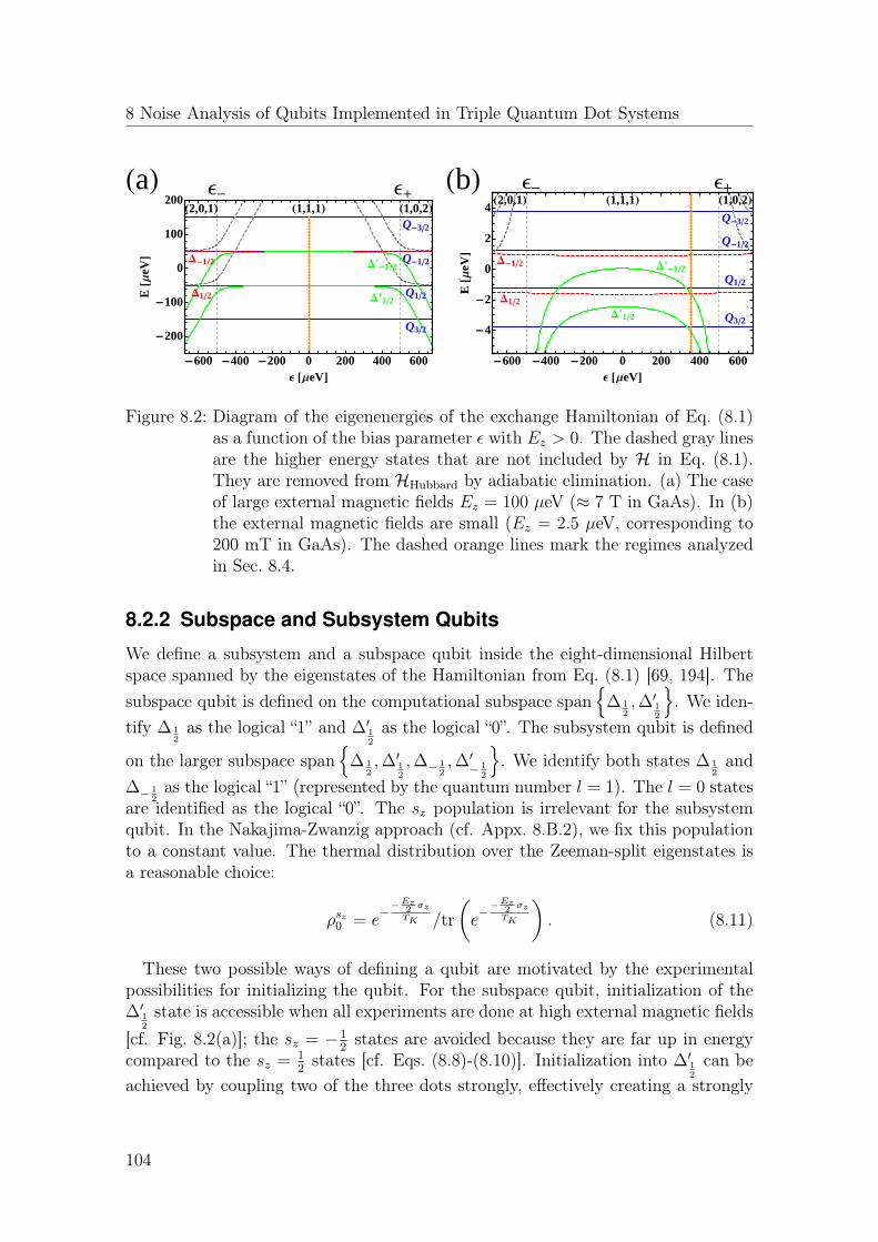
8 Noise Analysis of Qubits Implemented in Triple Quantum Dot Systems
H2,0,1L H1,0,2LH1,1,1LQ-32
Q-12
Q12
Q32
D-12
D12
D'-12
D'12
-600 -400 -200 0 200 400 600
-200
-100
0
100
200
Ε @ΜeVD
E@Μ
eVD
HaLΕ
-Ε
+ H2,0,1L H1,0,2LH1,1,1L
Q-32
Q-12
Q12
Q32
D-12
D12
D'-12
D'12
-600 -400 -200 0 200 400 600
-4
-2
0
2
4
Ε @ΜeVD
E@Μ
eVD
HbL Ε-
Ε+
Figure 8.2: Diagram of the eigenenergies of the exchange Hamiltonian of Eq. (8.1)as a function of the bias parameter ε with Ez > 0. The dashed gray linesare the higher energy states that are not included by H in Eq. (8.1).They are removed from HHubbard by adiabatic elimination. (a) The caseof large external magnetic fields Ez = 100 µeV (≈ 7 T in GaAs). In (b)the external magnetic fields are small (Ez = 2.5 µeV, corresponding to200 mT in GaAs). The dashed orange lines mark the regimes analyzedin Sec. 8.4.
8.2.2 Subspace and Subsystem Qubits
We define a subsystem and a subspace qubit inside the eight-dimensional Hilbertspace spanned by the eigenstates of the Hamiltonian from Eq. (8.1) [69, 194]. Thesubspace qubit is defined on the computational subspace span
∆ 1
2,∆′1
2
. We iden-
tify ∆ 12as the logical “1” and ∆′1
2
as the logical “0”. The subsystem qubit is defined
on the larger subspace span
∆ 12,∆′1
2
,∆− 12,∆′− 1
2
. We identify both states ∆ 1
2and
∆− 12as the logical “1” (represented by the quantum number l = 1). The l = 0 states
are identified as the logical “0”. The sz population is irrelevant for the subsystemqubit. In the Nakajima-Zwanzig approach (cf. Appx. 8.B.2), we fix this populationto a constant value. The thermal distribution over the Zeeman-split eigenstates isa reasonable choice:
ρsz0 = e−−
Ez2 σzTK /tr
(e−−
Ez2 σzTK
). (8.11)
These two possible ways of defining a qubit are motivated by the experimentalpossibilities for initializing the qubit. For the subspace qubit, initialization of the∆′1
2
state is accessible when all experiments are done at high external magnetic fields[cf. Fig. 8.2(a)]; the sz = −1
2states are avoided because they are far up in energy
compared to the sz = 12states [cf. Eqs. (8.8)-(8.10)]. Initialization into ∆′1
2
can beachieved by coupling two of the three dots strongly, effectively creating a strongly
104

8.2 Model
coupled DQD and an uncoupled single QD. ∆′12
is described by a singlet eigenstateon the DQD, while the ∆ 1
2state involves triplet eigenstates. Now the initialization
is identical to the initialization of the STQ in DQDs [52]. The uncoupled single QDneeds to be in its ground state |↑〉 .For the subsystem qubit the initialization works in the same way. Here, however,
it does not matter if we initialize ∆′12
or ∆′− 12
; both states are labeled by l = 0.These states differ only by the populations of the weakly coupled single QD. Forthe subsystem qubit it is satisfactory to produce a thermal distribution betweenthe spin-up and spin-down states on the weakly coupled QD, which is describedby Eq. (8.11). The strongly coupled QD should again be initialized into the singletstate. The initialization of the subsystem qubit can be accomplished at any magneticfield strengths.
8.2.3 Noise Description
We introduce a Lindblad master equation on the eight-dimensional Hilbert space tostudy the influence of noise for TQDs:
ρ (t) = (L0 + LD) ρ (t) = −i [H, ρ (t)] + LD (ρ (t)) . (8.12)
We set ~ = 1 and kB = 1. Additionally to the coherent evolution, given by−i [H, ρ (t)], there is a dissipative Lindblad term LD (ρ (t)) =
∑AΥAD [A] (ρ (t)),
where D [A] (B) ≡ ABA†− 12
(A†AB +BA†A
). The coupling of an external bath is
described by the operators A. ΥA ∈ R determines the coupling strength. We ana-lyze the effects of dephasing and relaxation from external baths. Dephasing of spinqubits is generated by fluctuating magnetic fields parallel to the external magneticfield. Relaxation is generated by fluctuating perpendicular magnetic fields. A canact globally on the TQD or it can be separable to each QD:
Lglob (ρ) = ΥzD [Z] (ρ) + ΥxD [X] (ρ) , (8.13)
Lloc (ρ) =∑i=1,2,3
ΥziD[σiz]
(ρ) + ΥxiD[σix]
(ρ), (8.14)
with Z =∑
i=1,2,3 σiz and X =
∑i=1,2,3 σ
ix.
This model represents a specific Markov approximation to describe the time evo-lution of an open quantum system [195]. The procedure of making a Markov approx-imations is not strict mathematically [198]. We modify Eq. (8.13) and Eq. (8.14) inour analysis and introduce a different Markov approximation. Our goal is to makesure that the system equilibrates in the long time limit. We adopt the descriptionfrom Ref. [199]. This specific Markov approximation was introduced by Davies forthe weak coupling limit of a system and a bath [195]. The modified Lindbladian inthe DM is:
LD (ρ) =∑A,ω
h (A, ω)D [Aω] (ρ) . (8.15)
105

8 Noise Analysis of Qubits Implemented in Triple Quantum Dot Systems
All coupling operators A are decomposed into transition terms between equidistantenergy eigenstates of H:
A =∑ω
Aω. (8.16)
A is grouped into terms Aω that are defined by
〈A |Aω|B〉 =
〈A |Aω|B〉 if EA − EB = ω,0 otherwise. (8.17)
The rate of quantum jumps h (A, ω) ∈ R is set by the transition frequencies ω be-tween energy eigenstates of the system induced from the bath. Note that h (A, ω)fulfills the detailed balance condition between positive and negative energy differ-ences:
h (A,−ω) = e− ωTK h (A, ω) . (8.18)
As shown by Spohn [200], the Gibbs state is a fixed point of the dynamics in theDM:
LD(e− HTK
)= 0. (8.19)
We neglect the tilde on the redefined Lindbladian from Eq. (8.15) in the remainderof this chapter. When inspecting the energy diagrams in Fig. 8.2, one sometimesfinds that sets of energy levels become equidistant at specific exchange interactions,which are not equidistant for each ε. We do not add these “accidental” degeneraciesto the DM in Eq. (8.15).
8.3 Approach to Model Real Systems
8.3.1 System Parameters
All system parameters to define the Hamiltonian of Eq. (8.1) are matching theTQD experiments of Ref. [192] (cf. especially the Supplemental Material). Theseparameters are summarized in Tab. 8.1. We use a typical time scale δt of 10 ns todescribe qubit experiments.2 The temperature TK is set to 125 mK (∼ 10 µeV). Ahigh magnetic field accounts for the case Ez TK , while the low magnetic field casedescribes the opposite limit (Ez . TK). When deriving predictions for the initialtime evolution, we never go far into the regime of doubly occupied QDs. We restrictε to the interval [ε−, ε+]. The tunnel coupling parameter t is also extracted fromRef. [192].3
2We refer especially to typical qubit manipulation times. In Ref. [192] pulse times well below 10ns are used.
3In Ref. [192] the tunnel couplings T are defined differently than the parameters t in Eq. (8.2).However, the two constants are connected by T = t/
√2.
106

8.3 Approach to Model Real Systems
Value Sizeδt 10 nsTK 10 µeV (≈ 125 mK)
Magnetic field strength High: 7 T (Ez ≈ 100 µeV)Low: 200 mT (Ez ≈ 2.5 µeV)
Exchange interaction parameter ε+ = |ε−| = 500 µeVt = 14 µeV
Analyzed interval of ε [−500 µeV, 500 µeV]
Table 8.1: Characteristic values for the analysis of GaAs TQDs according toRef. [192].
8.3.2 Transition Rates for the Noise Description
Our model does not contain a microscopic description of the environment. Theinfluence of the surroundings in the DM is modeled only by the generated transitionrates between quantum states (cf. Sec. 8.2.3). Especially we focus in our analysison experiments for GaAs QDs because this material has been used in all previousexperiments for TQDs [191, 192].
Hyperfine interactions — As in the experiments on single QDs and DQDs, thenuclear magnetic fields are also one major source of noise for TQDs. The magneticmoments of the nuclei in GaAs couple through the hyperfine interactions to thespin of the electron. Extensive studies of the generated dynamics were carried outfor single QDs [201–204] and for DQDs [122]. Also very recently a study of TQDsappeared [205]. We do not follow the arguments of these publications in detail, butwe extract transition rates for our analysis.
The nuclear magnetic moments add up to a macroscopic magnetic field in a semi-classical picture [31, 84]. Fluctuations of the nuclear spins are slow compared tothe precession time of the electron spin in this magnetic field. For the initial timeevolution of the electron, the nuclear magnetic field can therefore be described asstatic. Due to the large number of spins interacting with the electron, one ap-proximates the magnitude of the nuclear magnetic fields by a Gaussian distribu-tion with zero mean and the rms δEnuc [representing the probability distribution
f (B) = 1√2πδEnuc
e− B2
2δE2nuc ]. A typical value for GaAs QDs is δEnuc ≈ 0.3 µeV.
Nuclear spins generate spin dephasing and relaxation locally at the QDs. Weintroduce two transition rates [cf. Eq. (8.15)] that exponentially decrease with the
107
8 Noise Analysis of Qubits Implemented in Triple Quantum Dot Systems
transition energies ω:
h(σiz/σ
ix, ω)
=
Υz,xi e
− ω2
2δE2nuc for ω ≥ 0,
Υz,xi e
−(
ω2
2δE2nuc+ ωTK
)for ω < 0.
(8.20)
h (σiz, ω) arises from local magnetic field fluctuations at QDi (i = 1, 2, 3) in thedirection of the external magnetic field. These operations lead to dephasing of in-dividual spins. h (σix, ω) describes local spin relaxation through in-plane magneticfield fluctuations (coupling through raising and lowering operators σix = σi+ + σi−
4).Quantum jumps between energy levels are permitted at energy differences smallerthan or in the range of δEnuc. We argue that both the transitions generated fromfluctuating out-of-plane magnetic fields and from in-plane magnetic fields were ob-served in previous experiments. We especially refer to experiments of single QDsand DQDs:
A fluctuating magnetic field parallel to the static external field leads to dephas-ing for single QDs, and a fluctuating perpendicular magnetic field causes spin flips.In experiments, the time evolution of a single spin [SBnuc (t) = tr (σρBnuc (t)) =tr(σeiHBnuc tρ (0) e−iHBnuc t)] is measured, and the result is averaged over many runsof the experiment. For a single measurement, the Hamiltonian HBnuc that corre-sponds to a specific nuclear spin distribution Bnuc determines the time evolution(cf. Fig. 8.3). The final result reflects the ensemble average over the nuclear spindistribution 〈S (t)〉 ≡
∫dB SB (t) f (B).
Without external magnetic fields, the time evolution is completely determined bythe fluctuating magnetic field HB = B
2σz (cf. Ref. [84]). When we calculate the
time evolution and average it over f (B), we see that the component perpendicularto the magnetic field decreases exponentially:
〈Sx (t)〉 = e−δE2
nuct2
2 Sx (0) . (8.21)
Since there is no fixed quantization axis of the qubit, one expects that all componentsof the spin decrease. Therefore, the semiclassical analysis predicts a Gaussian decaywith a time constant (δEnuc)
−1. The DM describes this behavior by a transitionrate Υz,x
i = δEnuc. This is the value of Eq. (8.20) at ω = 0. The energy difference ωis determined by the external magnetic field. In the absence of magnetic fields, Υz
i
and Υxi must be indistinguishable.
At fixed external magnetic Ez (cf. Fig. 8.3), a fluctuating parallel magnetic fieldHB = Ez+B
2σz generates dephasing of the transverse spin components. Now the spin
precesses, however, with the angular frequency Ez around the z-axis:
〈Sx (t)〉 = e−δE2
nuct2
2 [Sx (0) cos (Ezt)− Sy (0) sin (Ezt)] . (8.22)
4In single-spin experiments fluctuating in-plane magnetic fields, both in the x-direction and they-direction, cause spin flips. The generated dynamics is very similar. We just consider thecoupling operators σix, since they are directly related to single-spin flips σ±
108

8.3 Approach to Model Real Systems
Figure 8.3: Semiclassical picture used for the time evolution of a single electron spinin a distribution of nuclear spin configurations. The nuclear spin intro-duces a static magnetic field for every measurement, but the magneticfield is varying between every run of the experiment. A constant externalmagnetic field Ez is applied in the z-direction.
This is also reflected in the DM. The transition rates for single-spin dephasing areindependent of the energy difference. σiz causes only transitions between identicalspin states, which is reflected by the transition rate h (σiz, 0).
At finite external magnetic fields, the relaxations decrease with(
ωδEnuc
)2
. We cansee this when calculating the time evolution for a fluctuating perpendicular magneticfield for an initially spin-up polarized particle (Z0 = 1 and HB = ω
2σz + B
2σx):
ZB (t) =E2z +B2 cos (Ezt)
E2z +B2
. (8.23)
When expanding in (B/Ez) and averaging over the field distribution f (B), we get
〈Z (t)〉 ≈ Z0 −1− cos (ωt)(
ω2
E2nuc
)2 . (8.24)
Since in the DM relaxation always contains the parameter h (σix, ω), we use a Gaus-sian dependence on the energy difference. It describes a quadratic dependence on(
ωδEnuc
)for finite ω, when
(ω
δEnuc
)2
1.To extract parameters for h (σiz, ω) at finite energy differences, we can consider
DQD experiments. A fluctuating local magnetic field parallel to the static externalfield causes transitions of the STQ between the singlet state |S0〉 and the sz = 0triplet state |T0〉 . On the relevant subspace the local, parallel magnetic field actslike a perpendicular magnetic field:
Bσiz = B (σx)|S0〉 ,|T0〉 . (8.25)
109

8 Noise Analysis of Qubits Implemented in Triple Quantum Dot Systems
In the DM, the fluctuating parallel magnetic field involves quantum jumps between|S0〉 and |T0〉 at the energy difference of these two states: h (σiz, ω). Using the samedescription as for single QDs before, the transition rates decrease exponentially withthe energy difference of the levels.
Transitions between the sz = 0 states with the sz 6= 0 states are possible throughlocal raising and lowering operators. They are generated through perpendicularmagnetic field fluctuations h (σix, ω) at the energy difference ω of the sz = 0 andsz 6= 0 states. The transition rates are highly sensitive to ω. This result was alsoobserved in experiments with DQD qubits. The transition rates of (20 ns)−1 at zeromagnetic fields and (150 ns)−1 at 100 mT approximately match these results [40] (cf.Fig. 8.4). For weakly coupled STQs, the energy difference ω is directly determinedby the external magnetic field.
Interestingly, we automatically describe in the DM the large transition rates atthe crossings of levels with different spin quantum numbers. The |S0〉 -|T+〉 cross-ing is extensively studied in DQD experiments [37]. TQDs have doublet-quadrupletcrossings that were analyzed in the experiment by Gaudreau et al. [192]. The ex-periments showed a large enhancement of transition rates near these level crossings,with nanosecond transition times. The transition rates decrease quickly away fromthe level crossing.
H20 nsL-1
Ω®0
H150 ΜsL-1
B®100 mT
-2 -1 0 1 21
100
104
106
1
100
104
106
Ω @ΜeVD
hHΣ
zi Σxi
,ΩL
@s-
1 D
Figure 8.4: Hyperfine interactions cause dephasing and relaxation through localmagnetic field fluctuations on each QD. Dephasing and relaxation aregenerated by the transition rates h (σiz/σ
ix, ω) according to Eq. (8.20).
The marked points refer to the results from DQD experiments that aredescribed in the text.
Interactions with phonons — Additionally, relaxations are generated by inter-actions of the QD with electric fields, e.g. from polar phonons. However, directtransitions are forbidden between different spin states of the same orbital level bythe dipole selection rule. They must be mediated by another process like spin-orbitinteractions (SOIs). In single QD experiments, relaxation times of about 1 s at mag-netic fields of 1 T and 0.5 ms for a magnetic field of 5 T were identified [98]. Thescaling law of ω3E2
z governs the transitions by piezoelectric phonons between Zeemansplit QD eigenstates for single-qubit experiments. The phonon energy must match
110

8.3 Approach to Model Real Systems
the energy difference of the states, resulting in the ω3 scaling law. The Zeemansplit eigenstates are mixed by SOIs, which causes the E2
z dependence. Therefore,experiments and theory suggest relaxation rates modeled as
h(σix, ω
)= Ξx
i
∣∣∣∣ ω3E2z
1− e−ωTK
∣∣∣∣ . (8.26)
Eq. (8.26) should also apply for TQDs. The coupling operators are again local spinflip operators σix = σ+
i + σ−i at QDi. A picture of the generated transition rates,including the results from single-qubit experiments, is shown in Fig. 8.5.
0 s-1
Ω®0
H1 sL-1 B®1T
H0.5 msL-1 B®5T
-100 -50 0 50 1000.1
1
10
100
1000
104
0.1
1
10
100
1000
104
Ω @ΜeVD
hHΣ
Xi,Ω
L@s
-1 D
Figure 8.5: Relaxation rates h (σix, ω) generated from piezoelectric phonons accord-ing to Eq. (8.26). The experimentally observed time scales from Ref. [98]are shown in red.
For DQD experiments in the weak coupling regime, transition rates were identifiedthat are consistent with this picture [38]. At high bias (readout regime) other effectscause transitions between different charge states [52]. We do not include these effectsin our model since we do not analyze the readout regime (ε > ε+ or ε < ε−). Electron-phonon interactions can also lead to pure spin dephasing [144, 145], but so far thiseffects has never been observed experimentally. It should be weaker than dephasingdue to nuclear spins, as described in the previous section.
Mechanism Constant ValueLocal dephasing and relaxation through nuclear spins Υz,x
i1
20 ns
Local spin relaxation through phonons Ξxi 2 · 10−6 1
s µeV5
Table 8.2: Transition mechanisms describing noise for TQDs and parameter esti-mates.
Summary and description of the noise regimes — We have identified two influ-ences of the qubit environment, which should be most important for TQD exper-iments. Nuclear spins cause large error rates through the random distribution oftheir magnetic moments. Direct spin flips are generated by phonons, which couple
111

8 Noise Analysis of Qubits Implemented in Triple Quantum Dot Systems
to spins indirectly via SOIs. Note that charge fluctuations cause an additional noiseterm for TQDs. Electric fields are applied to manipulate the qubit through the ex-change interaction. Charge noise introduces electric field fluctuations. This problemhas been pointed out for DQDs already [94]. Especially for strong electrostatic bias,charge dipoles are created and charge fluctuations will gain influence. Here we studyonly the weak bias regime and do not take charge fluctuations into account.
Our analysis will show that the noise mechanism can be distinguished at differentparameter regimes. A summary is given in Tab. 8.3. For phase noise, we describenuclear spin noise through the transition rates h (σiz, ω) from Eq. (8.20). This inter-action causes major errors for energy differences smaller and in the range of the rmsof δEnuc (cf. Fig. 8.4). This parameter regime is called “Regime 1” in the following.
Local spin relaxation can cause large transition rates in two completely differentregimes (cf. Fig. 8.6). The interactions with phonons will be dominant for large en-ergy differences and at high external magnetic fields, while the hyperfine interactionwill determine the relaxation process at small energy differences. Since these twoeffects are important in different parameter regimes, we can easily separate theirinfluences. We call the two parameter ranges “Regime 2” and “Regime 3”.
Regime 1 Local phase noise h (σiz, ω) generated from fluctuating nuclear spins.Strong influence at small energy differences.
Regime 2 Local spin relaxation h (σix, ω) from the interaction with phonons. Stronginfluence at large energy differences and large external magnetic fields.
Regime 3Local spin relaxation h (σix, ω) from the interaction with nuclear spins.Dominant relaxation mechanism at small energy differences, independentof the external magnetic field.
Table 8.3: Noise in TQD experiments.
8.4 Analysis of the Time Evolution
We discuss the time evolution of the subspace qubit and the subsystem qubit in thenoisy environment of Sec. 8.3.2. We numerically calculate the time evolution on thefull eight-dimensional Hilbert space. Because we are only interested in the noisypart of the evolution, we solve the full master equation in the rotating frame withrespect to the ideal Hamiltonian from Eq. (8.1):
ρ (t) = Lrotρ (t) . (8.27)
Lrot is identical to LD from the DM of Eq. (8.15), as described in Appx. 8.A.1.From the time evolution of the full density matrix ρ (t), we calculate the time
evolution of the qubit’s population O (t) = tr [Pρ (t)]. P is a linear map, which
112

8.4 Analysis of the Time Evolution
Figure 8.6: Transition rates h (σix, ω) for local spin relaxation as a function of theenergy difference ω and the external magnetic field Ez. The influencesof hyperfine interactions (Regime 2) and phonon interactions (Regime3) can be distinguished.
constructs from ρ (t) only the relevant part describing the qubit (cf. Appx. 8.B). Ad-ditionally, we extract the trajectory on the Bloch sphere P (t) = [X (t) , Y (t) , Z (t)]with Pi (t) = tr [σiPρ (t)]. For the subspace qubit, we use the map PP fromEq. (8.36). It projects from the full eight-dimensional Hilbert space on the two-dimensional Hilbert space that defines the subspace qubit. To describe the subsys-tem qubit, we use the combination P = PSPP . PP is a projective map, similar to theconstruction of the subspace qubit. PP projects, however, on the four-dimensionalsubspace span
∆ 1
2,∆′1
2
,∆− 12,∆′− 1
2
for the subsystem qubit (cf. Appx. 8.B.2). PS
is defined in Eq. (8.41).Our aim is to show that we can describe the initial time evolution [0, δt] =
[0, 10] ns by an effective description derived in Appx. 8.B. We use a Nakajima-Zwanzig approach and compare the numerical solution of the full master equationwith the solution of this effective description. We use Eq. (8.37) for the subspacequbit and Eq. (8.44) for the subsystem qubit, where we keep noise terms in first(second)-order for the first (second)-order Born approximation. Even though wemodel the time evolution quite generally, it will turn out that the environment in-fluences the qubit evolution dominantly through transition rates from three differentnoise regimes.
8.4.1 Subspace Qubit
The subspace qubit is defined on the subspace span
∆ 12,∆′1
2
(cf. Sec. 8.2.1). We
discuss it using the parameters from Sec. 8.3.1. span
∆ 12,∆′1
2
is a decoherence-free
subspace with respect to global phase noise D [Z] (weak collective decoherence, cf.Sec. 8.1). Other global noise (e.g. through the Lindblad operators D [X] and D [Y ],
113
8 Noise Analysis of Qubits Implemented in Triple Quantum Dot Systems
with X, Y ≡∑
i=1,2,3 σix,y) will, however, lead to leakage from the computational
subspace. Leakage will separately bring the l = 1 and l = 0 states to thermalequilibrium. However, since the subspace qubit can be operated only in the limitof large external magnetic fields, the resulting leakage probability will be negligible.For Ez = 100 µeV and TK = 10 µeV only a fraction e−
EzTK /
(1 + e
− EzTK
)≈ 4.5 · 10−5
of the probability will leak out of the computational subspace. In any case, weargued in Sec. 8.3.2 that the external environment dominantly couples through localinteractions.Regime 1 — Local phase noise turns out to be critical for the subspace qubit.
We discuss in the following an unbiased TQD (ε = 0). Additionally, we includephase noise generated from fluctuating nuclear spins [cf. h (σiz, ω) from Eq. (8.20)].We include phase noise on all three QDs. The parameters Υz
1 = (20 ns−1), Υz2 =
(30 ns−1), and Υz3 = (40 ns−1) describe the common noise strengths for fluctuating
nuclear spins (cf. Tab. 8.2). Local phase noise generates large transition rates onlybetween states with small energy differences (Regime 1, cf. Tab. 8.3).
A qubit initialized in the sz = 12subspace will only undergo transitions within this
subspace. Since the energy differences of all three energy levels are comparable tothe thermal energy [cf. Eqs. (8.8)-(8.10)], a considerable part of the qubit populationleaks to Q 1
2. The finite energy difference of the two-qubit levels leads in the long time
limit to a finite polarization on the z-axis Z∞. Fig. 8.7 shows the time evolutionfor the unbiased subspace qubit (ε = 0). It is initially in a pure excited state[P (0) = (0, 0, 1), cf. Fig. 8.7(a)] or in a superposition of ∆ 1
2and ∆′1
2
[cf. Fig. 8.7(b)].For the initial time evolution (orange interval) the Born approximation in Eq. (8.37)gives a highly accurate description. One can see that the thermalization happenswithin microseconds. Simple arguments can be used to predict the long time limitof the time evolution. Appx. 8.C predicts O∞ ≈ 0.66 and P∞ ≈ (0, 0,−0.03). Thesmall value of the polarization in the long time limit (Z∞ ≈ −0.03) reflects thatthe thermal energy TK is large compared to the energy splitting of the qubit levels[TK = 10 µeV; cf. energy diagram in Fig. 8.2(a)].Regime 2 — Local spin relaxation of the subspace qubit at high magnetic fields
will predominantly depopulate the qubit by the transitions from the qubit eigen-states ∆ 1
2and ∆′1
2
to states with different sz-quantum numbers. Fig. 8.8 shows thetime evolution of the subspace qubit at ε = 0 and Ez = 100 µeV. Large transitionrates are generated from the interaction with piezoelectric phonons. These rates arehighly enhanced at high energy differences and for large external magnetic fields(Regime 2, cf. Tab. 8.3). We use the following parameters: Ξx = 2 · 10−6 1
s µeV5 ,Ξx = 1.5 · 10−6 1
s µeV5 , and Ξx3 = 1 · 10−6 1
s µeV5 (cf. Tab. 8.2). At low electric bias,we only see phonon-generated transitions to Q 3
2. Fig. 8.8 shows that the transitions
empty the qubit’s population completely, but the time evolution is very slow. Over-all, phonons generate considerable changes only on microsecond time scales. Thefirst-order Born approximation is already sufficient for the description of the qubitdynamics.Regime 3 — Local spin relaxation from fluctuating nuclear spins can be ne-
114

8.4 Analysis of the Time Evolution
0 10 20 30 40 50
0.6
0.8
1
O(t
)
Lindblad equationfirst order Bornsecond order Bornt → ∞
0 1 2
0.6
0.8
1t[µs]
0 10 20 30 40 50
0.6
0.8
1
t [ns]
Z(t
)
0 1 20
0.5
1
t[µs]
(a) P (0) = (0, 0, 1)
0 10 20 30 40 50
0.8
0.9
1
O(t
)
0 1 2
0.8
1t[µs]
0
0.5
1
X(t
)
Lindblad equationfirst order Bornsecond order Bornt → ∞
0 10 20 30 40 50−0.2
−0.1
0
t [ns]
Z(t
)
0 1 2−0.2−0.1
0
t[µs]
(b) P (0) = (0, 1, 0)
Figure 8.7: Evolution of the subspace qubit at ε = 0 µeV and Ez = 100 µeV.The qubit is subjected to local phase noise from nuclear spins [Υz
1 =(20 ns−1), Υz
2 = (30 ns−1), Υz3 = (40 ns−1)]. The orange region marks
a typical time interval for qubit experiments; blue lines represent theresults from the first-order Born approximation, and red lines are cal-culated in the second-order Born approximation. The insets show theevolution on longer time scales, where the green lines represent the longtime limit.
glected. This mechanism is only dominant at small energy differences (Regime 3; cf.Tab. 8.3). For large external magnetic fields, the unbiased subspace qubit does nothave a state with a different sz-quantum number that is close to the qubit states(cf. Fig. 8.2).
8.4.2 Subsystem Qubit
A subsystem qubit is coded in the formally introduced l-quantum number. We iden-tify ∆±1/2 and ∆′±1/2 as the qubit levels (cf. Sec. 8.2.1). A subsystem qubit is definedin a decoherence-free subsystem of all interactions acting globally on the three QDs(strong collective decoherence; cf. Sec. 8.1). Hence, all global noise mechanisms willbe irrelevant. In any case, we argued in Sec. 8.2.3 that local interactions dominatethe noise properties in TQD experiments.Regime 1 — Local phase noise will have the same effect on the subsystem qubit
and the subspace qubit. As described in the symmetry discussion in Appx. 8.A.2,phase noise will act separately on the sz = ±1
2subspaces. It will, however, never mix
them. Additionally, the action is identical on both subspaces. Since the transitionrates from the interactions with nuclear spins are assumed to be independent of themagnetic field strength [cf. Eq. (8.20)], the time evolution is also identical. Largetransition rates are generated for energy levels that are close in energy (Regime 1;
115

8 Noise Analysis of Qubits Implemented in Triple Quantum Dot Systems
0 50 100 150 200 250
0
0.5
1
O(t
)
Lindblad equationfirst order Bornsecond order Bornt → ∞
0 50 100 150 200 2500
0.5
1
t[µs]
Z(t
)
(a) P (0) = (0, 0, 1)
0 50 100 150 200 250
0
0.5
1
O(t
)
Lindblad equationfirst order Bornsecond order Bornt → ∞
0
0.5
1
X(t
)
0 50 100 150 200 250
−4
−2
0
t[µs]
Z(t
)/10
3
(b) P (0) = (0, 1, 0)
Figure 8.8: Time evolution from local spin relaxation for the subspace qubit gen-erated by the interaction with piezoelectric phonons for ε = 0 andEz = 100 µeV. We choose Ξx = 2 · 10−6 1
s µeV5 , Ξx = 1.5 · 10−6 1s µeV5 ,
and Ξx3 = 1 · 10−6 1
s µeV5 . The numerical solution of the full master equa-tion (black lines), the first-order (blue lines), and the second-order (redlines) Born approximations are identical. The qubit depopulates in thelong time limit.
cf. Tab. 8.3).Regime 2 — For local spin relaxations the description of the subsystem qubit
is comparable to the subspace qubit for large external magnetic fields. We canespecially see that the sz distribution is close to a pure sz = +1
2state [cf. Eq. (8.11)].
Regime 3 — Local spin relaxation will gain in importance for small magnetic fields.In the low-bias regime (i.e., small |ε|), relaxation rates generated from the interactionwith phonons are small. We can prove this by inspecting the transition rates h (σix, ω)for small magnetic fields Ez [cf. Eq. (8.26)]. On the other hand, fluctuating nuclearspins can strongly mix different sz states. This effect will be critical especially atthe points of level crossings. The relaxation effects through nuclear magnetic fieldsare highly enhanced at small energy differences [cf. h (σx, ω) in Eq. (8.20)]. Thisdominant noise mechanism is summarized in Regime 3 of Tab. 8.3.
We simulate the qubit evolution at ε = 354.6 µeV and Ez = 2.5 µeV. Here, twodifferent doublet levels and also doublet and quadruplet levels are close in energy[cf. Fig. 8.2(b)]. All results are shown in Fig. 8.9. We use the following transitionparameters to model the hyperfine interaction: Υx
1 = (20 ns−1), Υx2 = (30 ns−1),
Υx3 = (40 ns−1) (cf. Tab. 8.2).Local spin relaxation, generated from fluctuating nuclear spins, especially mixes
two subspaces. First of all, the subspace spanQ1/2,∆1/2,∆
′−1/2
is strongly mixed.
Second, also transitions between the levels ∆′1/2 and Q3/2 are strong. We observe thethermalization of both subspaces in the long time dynamics. One can calculate the
116

8.5 Effective Errors
0 10 20 30 40 50
0.98
1
1.02
O(t
)
0 0.250.8
0.9
1
t[µs]
0 10 20 30 40 500.4
0.6
0.8
1
t [ns]
Z(t
)
Lindblad equationfirst order Bornsecond order Bornt → ∞
(a) P (0) = (0, 0, 1)
0 10 20 30 40 50
0.9
1
O(t
)
0 0.25
0.81
t[µs]
0.5
1
X(t
)
Lindblad equationfirst order Bornsecond order Bornt → ∞
0 0.250
1t[µs]
0 10 20 30 40 500
0.05
t [ns]
Z(t
) 0 0.25
0
0.1
t[µs]
(b) P (0) = (0, 1, 0)
Figure 8.9: Time evolution of the subsystem qubit through local spin relaxationsfrom hyperfine interactions at Ez = 2.5 µeV and ε = 354.6 µeV[cf. Fig. 8.2(b)]. We use Υx
1 = (20 ns−1), Υx2 = (30 ns−1), and
Υx3 = (40 ns−1). The orange region marks a typical time scale of qubit
experiments. Here, the second-order Born approximation and the re-sults from the full master equation match closely. The insets show thelong time evolution of the qubit. We see that the thermalization occurswithin microseconds.
resulting occupation of the computational subspace from the initial density matrix(cf. Appx. 8.C). For the time evolution of the excited state, we calculate O∞ ≈ 0.82and P∞ ≈ (0, 0, 0.44) [cf. Fig. 8.9(a)]. A superposition of ∆ 1
2and ∆′1
2
evolves toO∞ ≈ 0.70 and P∞ ≈ (0, 0, 0.08) [cf. Fig. 8.9(b)]. The long time evolution can beseparated from the initial time evolution (orange region). The initial time evolutionon the interval [0, 10] ns can be described by the second-order Born approximation.
8.5 Effective Errors
The main goal of the following analysis is to extract and quantify the coherenceproperties of the subspace encoding and the subsystem encoding for TQD qubits.One is usually interested in the time evolution of the qubit on short time scales,not on the equilibration of the system. We saw in the previous section that we candevelop an effective description of the initial time evolution (cf. Appx. 8.B). Weuse this description to extract errors for the initial time evolution (cf. Appx. 8.D).We will show that all errors can be described by only four toy models, which areintroduced in Appx. 8.E.
We numerically simulate the time evolution of the qubit for different initial densitymatrices ρ (0). We map ρ (t) to the corresponding point P (t) = tr [σρ (t)] on the
117

8 Noise Analysis of Qubits Implemented in Triple Quantum Dot Systems
Bloch sphere, with σ = (σx, σy, σz). The analysis is done in the rotating framewith respect to H from Eq. (8.1) (cf. Appx. 8.A.1). We extract the errors fromthe simulations of the full master equation and compare them with the results ofthe corresponding Nakajima-Zwanzig equation in second-order Born approximation(Eq. (8.37) for the subspace qubit and Eq. (8.44) for the subsystem qubit). Sec. 8.4showed that these descriptions match very closely for the initial time evolution.
Seven parameters are sufficient to describe the time evolution of the TQD qubits(cf. Appx. 8.D). We extract the rates ΓPi0,1,2 at three different points P1 = (0, 0, 1),P2 = (1, 0, 0), and P3 = (0, 0,−1) of the Bloch sphere. ΓPi0 is the leakage rate,ΓPi1 is the relaxation rate, and ΓPi2 is the dephasing rate (cf. Appx. 8.D.1). We usethe terminology “upper pole”, “equator”, and “lower pole” for P1, P2, and P3. Thetrajectories starting at the upper and the lower poles are restricted to the z-axis,which sets ΓP1,P3
2 = 0.To quantify noise, we compare the error rates Γ
Pji to the time of the experiment
δt.(
ΓPji δt
)describes an error that measures the leakage probability
(ΓPj0 δt
), the
relaxation probability(
ΓPj1 δt
), and the dephasing probability
(ΓPj2 δt
). The entan-
glement fidelity F , defined in Eq. (8.69), describes the accumulated error at differentinitial states. We use the deviation of the entanglement fidelity from its ideal value,1− F , to quantify the overall error.
8.5.1 Subspace Qubit
Regime 1 — First, we analyze the subspace qubit in (1, 1, 1) with local phase noisefrom the interaction with nuclear magnetic fields. As discussed in Sec. 8.3.2, phasenoise generates large errors only for small energy differences (Regime 1, cf. Tab. 8.3).Simulations for local phase noise are shown in Fig. 8.11. We analyze phase noise onQD1 and QD2 separately, and we use Υz
1,2 = (20 ns)−1 (cf. Tab. 8.2).All error can be explained by the transition rates in the DM. Quantum jump
operations are only possible for the same sz eigenstates. The total spin quantumnumber S is not preserved, because the interactions are local. Initially, only ∆ 1
2
and ∆′12
are occupied. Phase noise mixes the sz = 12subspace (cf. Fig. 8.10). Note
that the energy differences in the sz = 12subspace are small or comparable to the
thermal energy, and the transition rates for positive and negative energy differencesare similar. We group the transition rates into three sets; each set corresponds tothe error processes of a toy models in Appx. 8.E. The transition rates of these toymodels match to a high degree the results of the numerical solution of the full masterequation and the calculations using the second-order Born approximation.
• Local phase noise on QD1 [cf. Fig. 8.11(a)]:
Model 1 from Appx. 8.E.1 determines ΓP11 and ΓP3
1 . The interactions withnuclear spins generate direct transitions between the qubit levels. These ratesare large if the states are close in energy [cf. h (σiz, ω) in Eq. (8.20)]. Hence,
118

8.5 Effective Errors
Model 1
Model 3Q12
Model 2
D12
D'12
-500 0 500-53
-52
-51
-50
Ε @ΜeVD
E@Μ
eVD
Figure 8.10: Energy diagram of the subspace qubit with the major transition ratesgenerated from local phase noise. The energy diagram shows onlythe relevant energy levels [cf. Fig. 8.2(a)]. The transition rates aregrouped into three sets that are described by the toy models analyzedin Appx. 8.E. Model 1 describes pure relaxation of the qubit states(black arrows, cf. Appx. 8.E.1), model 2 describes pure dephasing ofthe qubit states (gray arrows, cf. Appx. 8.E.2), and model 3 character-izes leakage of the qubit states to one state in the surroundings (orangearrows, cf. Appx. 8.E.3).
the error rates ΓP11 and ΓP3
1 vanish quickly with increasing ε. Only a largedifference of the transition rate from ∆ 1
2to ∆′1
2
compared to the reversed
effect causes large ΓP21 and ΓP2
2 in model 1. In our case, both rates are eithervery similar (for small ε) or both small (for finite ε). Therefore, model 1 doesnot describe ΓP2
1 and ΓP22 .
The transitions between ∆ 12, ∆′1
2
, and Q 12determine ΓP1
0 , ΓP20 , ΓP3
0 , and
ΓP21 . Model 3 in Appx. 8.E.3 describes these error rates. We point out two
important characteristics: first, the transition rate from ∆ 12to Q 1
2is larger
than the transition rate from ∆′12
to Q 12because smaller energy differences
enhance the transition rates [cf. h (σ1z , ω) in Eq. (8.20)]. Second, ΓP1
0 , ΓP20 ,
and ΓP21 are larger for ε > 0 than for ε < 0 because the transition amplitude∣∣∣⟨Q 1
2|σ1z |∆ 1
2
⟩∣∣∣ is larger at positive bias than at negative bias.
Model 2 describes ΓP22 (cf. Appx. 8.E.2). ΓP2
2 vanishes when the energy levelfluctuations at both levels are equal [cf. Eq. (8.81)]. We can determine thispoint analytically
(⟨∆ 1
2|σ1z |∆ 1
2
⟩=⟨
∆′12
|σ1z |∆′1
2
⟩)and find J12 = 2J23. We
approximate ε ≈ − ε+3
for the parameters in our calculation. Additionally, ΓP22
dominates (1− F ).
ΓP30 is not correctly described by the three error models for phase noise
on QD1. The transition rates strongly depend on the energy differences [cf.h (σ1
z , ω) in Eq. (8.20)]. Instead of a direct transition(
∆′12
→ Q 12
), we observe
119

8 Noise Analysis of Qubits Implemented in Triple Quantum Dot Systems
G0P1
×∆t
G1P1
×∆t
G2P2
×∆t
G0P2
×∆t
G1P2
×∆t
G0P3
×∆t
G1P3
×∆t
1-F
0
10%
20%
-400 0 400Ε @ΜeVD
0
5%
10%
-400 0 400Ε @ΜeVD
-400 0 400
0
0.01%
0.02%
Ε @ΜeVD
0
0.25%
0.5%
0
5%
10%
0
0.2%
0.4%
-400 0 4000
20%
40%
Ε @ΜeVD-400 0 400
0
7.5%
15%
Ε @ΜeVD
Full SolutionBornModel Approx.
3
1
2
3
3
3
1
(a) Υz1 = (20 ns)−1, Υz
2 = Υz3 = 0
G0P1
×∆t
G1P1
×∆t
G2P2
×∆t
G0P2
×∆t
G1P2
×∆t
G0P3
×∆t
G1P3
×∆t
1-F
0
2%
4%
-400 0 400Ε @ΜeVD
0
1.5%
3%
-400 0 400Ε @ΜeVD
-400 0 400
0
0.005%
0.01%
Ε @ΜeVD
0
0.01%
0.02%
0
1%
2%
0
0.01%
0.02%
-400 0 4000
20%
40%
Ε @ΜeVD-400 0 400
0
3%
6%
Ε @ΜeVD
Full SolutionBornModel Approx.
3
1
2
3
3
3
1
(b) Υz2 = (20 ns)−1, Υz
1 = Υz3 = 0
Figure 8.11: Errors from local phase noise for the subspace qubit at Ez = 100 µeV.We take into account the influence of nuclear spins through the tran-sition rates from Eq. (8.20). The error rates are extracted from thenumerical simulations of the full master equation (blue lines) and thesecond-order Born approximation (green lines). The red lines describeeffective errors from simple toy models. The red numbers describe thetoy model system from Appx. 8.E.
120
8.5 Effective Errors
a two-step process(
∆′12
→ ∆ 12→ Q 1
2
).
• Local phase noise on QD2 [cf. Fig. 8.11(b)]:
Local phase noise on QD2 does not cause transitions from ∆ 12at ε = 0. ∆ 1
2
involves a singlet state on QD1 and QD3, while the remaining states containtriplets (cf. Fig. 8.16). ∆ 1
2is protected from local noise on QD2. Therefore,
ΓP10 (ε = 0) = 0, ΓP1
1 (ε = 0) = 0, and ΓP31 (ε = 0) = 0.
The remaining features of the transition rates can be understood from theirstrong energy dependence [cf. h (σ2
z , ω) in Eq. (8.20)]. Transitions from ∆ 12
and ∆′12
to Q 12describe leakage errors ΓP1,P2,P3
0 through model 3. Leakage from
∆′12
(ΓP3
0
)strongly decreases at finite bias because the energy difference to Q 1
2
increases. The leakage error from ∆ 12
(ΓP1
0
)has the opposite characteristic.
ΓP20 and ΓP2
1 are mainly determined by the average value of ΓP10 and ΓP3
0 .ΓP2
0 = ΓP21 ≈
ΓP11
2because ΓP1
0 ΓP30 .
Model 1 describes the relaxations of ∆ 12and ∆ 1
2
′
(ΓP1,P3
1
). The energy
difference between ∆ 12and ∆′1
2
is minimal at ε = 0 (cf. Fig. 8.10). Therelaxation rate h (σ2
z , ω) is large for small ε.
Model 2 in Appx. 8.E.2 describes ΓP22 . We can calculate the difference in
the energy fluctuation of ∆ 12and ∆′1
2
,
⟨∆ 1
2
∣∣σ2z
∣∣∆ 12
⟩−⟨
∆′12
∣∣σ2z
∣∣∆′12
⟩=
2
3
J12 + J23√J2
12 − J12J23 + J223
, (8.28)
which has the limits 23for J12
J23 and 4
3for J12 = J23. Model 2 dominates
also (1− F ).
In summary, local phase noise induces large errors to the time evolution of the sub-space qubit. Especially pure dephasing, as described by model 2 (cf. Appx. 8.E.2),limits the coherence of the TQD. Large errors are generated via phase noise on QD1
for strong external bias, while phase noise on QD2 is critical for the unbiased dot.Phase noise is always most critical when it acts on the eigenstates of a single QD.Regime 2 — Next we analyze errors of the subspace qubit though local spin
relaxation for small ε (ε ∈ [ε−, ε+]). Local spin flips can generate transitions with∆sz = ±1; also S is not preserved. Transition rates through hyperfine interactionsare highly suppressed due to the large energy difference of states with different sz.A large value of ω is required for nanosecond phonon-mediated transitions (Regime2, cf. Tab. 8.3). Fig. 8.12(a) sketches the two dominant transition rates at Ez =100 µeV. Fig. 8.13 shows the error probabilities for these parameters.We explain Fig. 8.13 in detail. First, we analyze the transition amplitudes from
∆ 12and ∆′1
2
to Q 32. These amplitudes are drawn as a function of the external bias
121
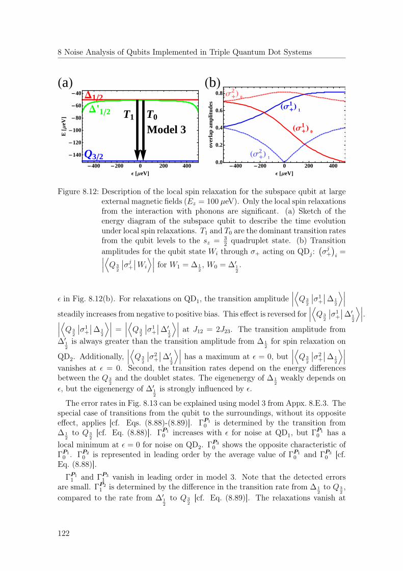
8 Noise Analysis of Qubits Implemented in Triple Quantum Dot Systems
Model 3T0
Q32
T1
D12
D'12
-400 -200 0 200 400
-140
-120
-100
-80
-60
-40
Ε @ΜeVD
E@Μ
eVD
HaL
HΣ+
1 L 1
HΣ+
1 L 0
HΣ+
2 L 1
HΣ+
2 L 0
-400 -200 0 200 4000.0
0.2
0.4
0.6
0.8
Ε @ΜeVD
over
lap
ampl
itud
es
HbL
Figure 8.12: Description of the local spin relaxation for the subspace qubit at largeexternal magnetic fields (Ez = 100 µeV). Only the local spin relaxationsfrom the interaction with phonons are significant. (a) Sketch of theenergy diagram of the subspace qubit to describe the time evolutionunder local spin relaxations. T1 and T0 are the dominant transition ratesfrom the qubit levels to the sz = 3
2quadruplet state. (b) Transition
amplitudes for the qubit state Wi through σ+ acting on QDj:(σj+)i
=∣∣∣⟨Q 32
∣∣σj+∣∣Wi
⟩∣∣∣ for W1 = ∆ 12, W0 = ∆′1
2
.
ε in Fig. 8.12(b). For relaxations on QD1, the transition amplitude∣∣∣⟨Q 3
2
∣∣σ1+
∣∣∆ 12
⟩∣∣∣steadily increases from negative to positive bias. This effect is reversed for
∣∣∣⟨Q 32
∣∣σ1+
∣∣∆′12
⟩∣∣∣.∣∣∣⟨Q 32
∣∣σ1+
∣∣∆ 12
⟩∣∣∣ =∣∣∣⟨Q 3
2
∣∣σ1+
∣∣∆′12
⟩∣∣∣ at J12 = 2J23. The transition amplitude from∆′1
2
is always greater than the transition amplitude from ∆ 12for spin relaxation on
QD2. Additionally,∣∣∣⟨Q 3
2
∣∣σ2+
∣∣∆′12
⟩∣∣∣ has a maximum at ε = 0, but∣∣∣⟨Q 3
2
∣∣σ2+
∣∣∆ 12
⟩∣∣∣vanishes at ε = 0. Second, the transition rates depend on the energy differencesbetween the Q 3
2and the doublet states. The eigenenergy of ∆ 1
2weakly depends on
ε, but the eigenenergy of ∆′12
is strongly influenced by ε.
The error rates in Fig. 8.13 can be explained using model 3 from Appx. 8.E.3. Thespecial case of transitions from the qubit to the surroundings, without its oppositeeffect, applies [cf. Eqs. (8.88)-(8.89)]. ΓP1
0 is determined by the transition from∆ 1
2to Q 3
2[cf. Eq. (8.88)]. ΓP1
0 increases with ε for noise at QD1, but ΓP10 has a
local minimum at ε = 0 for noise on QD2. ΓP30 shows the opposite characteristic of
ΓP10 . ΓP2
0 is represented in leading order by the average value of ΓP10 and ΓP3
0 [cf.Eq. (8.88)].
ΓP11 and ΓP3
1 vanish in leading order in model 3. Note that the detected errorsare small. ΓP2
1 is determined by the difference in the transition rate from ∆ 12to Q 3
2,
compared to the rate from ∆′12
to Q 32[cf. Eq. (8.89)]. The relaxations vanish at
122

8.5 Effective Errors
G0P1
×∆t
G1P1
×∆t
G2P2
×∆t
G0P2
×∆t
G1P2
×∆t
G0P3
×∆t
G1P3
×∆t
1-F
0
5×10⁻⁵
1×10⁻⁴
-400 0 400Ε @ΜeVD
0
2×10⁻⁵
4×10⁻⁵
-400 0 400Ε @ΜeVD
-400 0 400
0
0.004%
0.008%
Ε @ΜeVD
0
2×10-13
4×10-13
0
2×10⁻⁵
4×10⁻⁵
0
1×10-13
2×10-13
-400 0 4000
1×10⁻⁹
2×10⁻⁹
Ε @ΜeVD-400 0 400
0
0.003%
0.006%
Ε @ΜeVD
Full SolutionBornModel Approx.
(a) Ξx1 = 2 · 10−6 1s µeV5 , Ξx2 = Ξx3 = 0
G0P1
×∆t
G1P1
×∆t
G2P2
×∆t
G0P2
×∆t
G1P2
×∆t
G0P3
×∆t
G1P3
×∆t
1-F
0
1×10⁻⁵
2×10⁻⁵
-400 0 400Ε @ΜeVD
0
2×10⁻⁵
4×10⁻⁵
-400 0 400Ε @ΜeVD
-400 0 400
0
0.004%
0.008%
Ε @ΜeVD
0
2×10-13
4×10-13
0
2×10⁻⁵
4×10⁻⁵
0
5×10-14
1×10-13
-400 0 4000
1×10⁻⁹
2×10⁻⁹
Ε @ΜeVD-400 0 400
0
0.003%
0.006%
Ε @ΜeVD
Full SolutionBornModel Approx.
(b) Ξx2 = 2 · 10−6 1s µeV5 , Ξx1 = Ξx3 = 0
Figure 8.13: Errors from local spin relaxation generated from interactions withphonons for the subspace qubit in (1, 1, 1) at Ez = 100 µeV. Theblue lines are calculated from the numerical simulation of the full mas-ter equation. The green lines are obtained from the second-order Bornapproximation. The red lines represent the results from the analysis ofmodel 3, which involve only two transition rates (cf. description in themain text).
123
8 Noise Analysis of Qubits Implemented in Triple Quantum Dot Systems
J12 = 2J23 for noise acting on QD1. ΓP22 shows a similar characteristic.
In total, F is close to 1, and it does not show a characteristic dependency on εfor local noise on QD1 or QD2.
8.5.2 Subsystem Qubit
For large external magnetic fields, the subsystem qubit is equivalent to the sub-space qubit. Additionally, phase noise is identical for the subsystem qubit and thesubspace qubit at small external magnetic fields (cf. Appx. 8.A.2). The subsystemqubit differs from the subspace qubit only at small external fields and for local spinrelaxations. We analyze the subsystem qubit only for magnetic field strengths com-parable to the thermal energy. Here, both the sz = 1
2subspace and the sz = −1
2
subspace are initially occupied [cf. Eq. (8.11)].Regime 3 — Levels of different sz-quantum numbers already cross for small ε.
Hyperfine interactions can generate transitions between these levels through localspin flips. S is not preserved by local interactions. Fig. 8.14 shows the error ratesfrom the local spin relaxations on QD1 and QD2. Relaxations from phonons arenot detectable for the subsystem qubit within nanoseconds, because larger energydifferences are needed.
Phase noise from hyperfine interactions generates large transition rates only ifenergy levels of different sz-quantum numbers are close in energy (Regime 3, cf.Tab. 8.3). This is the case at the positions of level crossings in the energy diagrams(cf. Fig. 8.15). Two sets of transitions are important. First, doublet states coupleto quadruplet states (model 3 in Appx. 8.E.3). Only the transitions from the l = 1states to the quadruplet states are possible because local spin flips change the sz-quantum number. Leakage from the l = 0 states are highly suppressed. Theirenergies significantly differ from the energies of the quadruplet states of differentsz-quantum number. Second, there are transitions between the subsystem states∆ 1
2and ∆′− 1
2
, as described with model 4 in Appx. 8.E.4.
All effects can be summarized easily. Model 4 determines ΓP11 , ΓP3
1 , and ΓP22 .
Model 3 describes ΓP20 and ΓP3
0 . ΓP21 is determined by model 3 because model 4
requires different transition rates for the transitions from ∆ 12to ∆′− 1
2
compared to
the opposite evolution. ΓP10 is not correctly described by model 3 and model 4. ΓP1
0
is determined by a second-order process (∆ 12→ ∆′− 1
2
→ Q′12
).The errors are symmetric for ε > 0 and ε < 0 for noise on QD2, but they are
suppressed for noise on QD1 and ε > 0. ∆′12
have a singlet state on QD2 and QD3
for ε > 0 (cf. Fig. 8.16). Noise on QD1 leaves this singlet untouched, and ∆′12
doesnot couple to any other states (they contain triplets at QD2 and QD3).
Overall, we find that fluctuating nuclear spins can generate major errors of thesubsystem qubit at the points of level crossings. The asymmetry of the error ratesfor spin relaxation on QD1 between positive and negative bias is a very interestingresult. Fluctuating nuclear spins generate nearly no errors at positive bias because
124

8.5 Effective Errors
G0P1
×∆t
G1P1
×∆t
G2P2
×∆t
G0P2
×∆t
G1P2
×∆t
G0P3
×∆t
G1P3
×∆t
1-F
0
1%
2%
-400 0 400Ε @ΜeVD
0
2.5%
5%
-400 0 400Ε @ΜeVD
-400 0 400
0
5%
10%
Ε @ΜeVD
0
3%
6%
0
2.5%
5%
0
3%
6%
-400 0 4000
5%
10%
Ε @ΜeVD-400 0 400
0
5%
10%
Ε @ΜeVD
Full SolutionBornModel Approx.
3
4
4
3
3
3
4
(a) Υx1 = (20 ns)−1, Υx
2 = Υx3 = 0
G0P1
×∆t
G1P1
×∆t
G2P2
×∆t
G0P2
×∆t
G1P2
×∆t
G0P3
×∆t
G1P3
×∆t
1-F
0
1%
2%
-400 0 400Ε @ΜeVD
0
2.5%
5%
-400 0 400Ε @ΜeVD
-400 0 400
0
5%
10%
Ε @ΜeVD
0
3%
6%
0
2.5%
5%
0
3%
3%
-400 0 4000
2.5%
5%
Ε @ΜeVD-400 0 400
0
5%
10%
Ε @ΜeVD
Full SolutionBornModel Approx.
3
4
4
3
3
3
4
(b) Υx2 = (20 ns)−1, Υx
1 = Υx3 = 0
Figure 8.14: Errors of the subsystem qubit generated by local spin relaxations forsmall external magnetic fields (Ez = 2.5 µeV). Large error rates aredetected at the points of level crossings. Errors at positive detuningare highly suppressed for noise acting on QD1. The blue lines representthe calculations of the full master equation, the green lines representthe second-order Born approximation, and the red lines show the re-sults from the analysis of model 3 (cf. Appx. 8.E.3) and model 4 (cf.Appx. 8.E.4).
125

8 Noise Analysis of Qubits Implemented in Triple Quantum Dot Systems
Q12
Q32
Model 3
D-12D'-12
D'12
Model 3
Model 4D12
-500 0 500
-4
-3
-2
-1
0
1
Ε @ΜeVD
E@Μ
eVD
Figure 8.15: Transition diagram for the subsystem qubit when hyperfine interac-tions generate local spin flips. Large error rates are observed only atthe region of level crossings. They can be described by the leakagetransitions to a quadruplet state (model 3 from Appx. 8.E.3) or by theinternal transitions between two states of the subsystem qubit (model4 from Appx. 8.E.4).
there the TQD is approaching a high-symmetry regime (cf. Appx. 8.A.3).
8.6 Summary and Outlook
The exchange-only qubit has been analyzed with two different qubit codings in theHilbert space of three singly occupied QDs: the subspace qubit and the subsystemqubit. The leakage, relaxation, and decoherence dynamics of both qubit encodingshave been calculated with the noise channels of nuclear spins and phonons takeninto account. These interactions are described in the DM, a particular Markovapproximation with a transparent quantum-jump interpretation and consistent long-time behavior. The systematics of the early time dynamics, which is of highestinterest for qubit experiments, is distinct from the long time evolution. We havefocused on the initial time evolution and have extracted errors for the subspace qubitand the subsystem qubit. We can describe all the results by relating them to justfour toy models, whose time evolution can be calculated analytically.
For local phase noise, arising from the interaction with fluctuating nuclear spins,the influence on the subsystem qubit and the subspace qubit is identical. Localphase noise is critical for GaAs systems; it is the strongest mechanism for the lossof phase coherence. Sizable errors for both the subspace qubit and the subsystemqubit arise after just 10 ns.The influence of local spin relaxation is distinct for the subspace qubit and the
subsystem qubit. Since the subspace qubit is always operated at large externalmagnetic fields, spin relaxations from the interactions with phonons need to beconsidered. This effect generates large transition rates only between energy levelswith large energy differences. Our analysis shows that in GaAs systems, operated
126

8.6 Summary and Outlook
at large external magnetic fields, only small errors are generated. Operations atsmall magnetic fields are permitted for the subsystem qubit. Here, only local spinrelaxations from the interactions with nuclear magnetic fields are important. Theseinteractions generate large errors at the crossings of energy levels of different sz-quantum numbers. This process has a very interesting property for phase noiseacting locally on one of the outer QDs. Errors can be highly suppressed dependingon the sign of the bias parameter ε.
To state our results briefly, our analysis shows that in GaAs samples (large nu-clear spin bath) the subsystem and the subspace qubits have about equally goodcoherence properties. Both qubit implementation schemes suffer from local phasenoise, generated from fluctuating nuclear spins. Spin relaxation from nuclear spinswill be important only at the points of level crossings. If these points can be avoidedwhen manipulating the qubit, spin relaxations induced by fluctuating nuclear spinsare negligible. If one attempts to use the crossing points in the energy level diagramfor qubit manipulations (cf. the attempt to manipulate a STQ at crossing pointsin the energy diagram [150]), one has to pay attention to fluctuating nuclear spins.Interactions with phonons will usually be less important. This mechanism will onlybe significant if there are strong external magnetic fields and large energy differ-ences. The interaction with phonons can completely depopulate the qubit, but inGaAs systems this evolution only occurs on the microsecond time scale.
Nuclear spin noise for GaAs TQD qubits can be corrected with similar methodsas for DQD qubits. Since nuclear spin induced dephasing is caused by low-frequencynoise, one can apply refocusing protocols, which have already enhanced the coher-ence properties for DQDs [61]. Another possibility is to consider materials containingfewer nuclear spins. Working with silicon heterostructures is a reasonable approach,as experiments are catching up to the state of the art in GaAs [39]. One advantageof both the subspace qubit and the subsystem qubit is the full controllability of thequbit through the exchange interaction [65]. One does not rely on polarized nuclearmagnetic fields [53, 121] or micromagnets [55] as for GaAs STQs.
Overall, it is a very interesting task to test the local nature of the error models.Especially for the influence of nuclear spins, which behave on short time scales likeclassical fluctuating magnetic fields, the local influence of the qubit dynamics isworth testing. Such an experiment would require the control of the randomness ofthe nuclear spins at the positions of the different QDs. If it is possible to reducethe randomness at two of the three QDs, with the result that the nuclear spin noiseacts dominantly on one of the three QDs, one can test the different scaling behaviorof the error rates with the bias parameter ε. Furthermore, our analysis method inthe DM should be helpful for the descriptions of other coded qubits implementedin more complex Hilbert spaces. We show in detail for the TQD qubit how theinteractions with complicated baths can be reduced to just an effective evolution forthe coded qubit itself. Such an analysis could be extended to other coding strategieswhen the need arises.
127
Appendix
8.A Simplification of the Analysis
8.A.1 Rotating Frame
When analyzing the master equation, we are interested in the deviation of the qubitevolution from the free evolution L0 due to the dissipative Lindblad term LD (cf.Sec. 8.2.3). Therefore, it is meaningful to go for the analysis to a rotating framewith respect to the Hamiltonian H from Eq. (8.1):
ρ (t)→ ρrot (t) = Urot (t) ρ (t)U †rot (t) , (8.29)
with Urot (t) = eiHt. This approach automatically leads to a redefinition of theLindbladian L0 +LD → Lrot. Due to the general conditions of the DM in Eq. (8.15),the Lindbladian in the rotating frame equals the original dissipative Lindbladian:Lrot = LD. LD consists of a sum of terms; the coupling operators Aω appear twichin each term, once as a Hermitian conjugate. When the coupling operators A(†)
ω arewritten in the eigenenergy representation of the Hamiltonian H from Eq. (8.1), toeach entry a complex argument eiωt is added. The phase ω represents the energydifference of the states that are coupled by Aω. Since all Lindblad operators aregrouped to couple only equidistant energy levels, these complex factors cancel out.
8.A.2 Symmetry of Phase Noise
We want to point out a key symmetry for phase noise that simplifies our consid-erations. The action of phase noise through the coupling operators σiz (i = 1, 2, 3)has equal effects on the sz = 1
2subspace and the sz = −1
2subspace (involving
also the quadruplet levels). It mixes within these subspaces, but never couples sub-spaces of different sz-quantum numbers. Furthermore, the corresponding matrixelements in the sz = 1
2subspace and the sz = −1
2subspace are, up to a sign,
identical. This result can be understood by the symmetry operation which flipsthe spins on all dots Uflip. It transforms a state from the sz = +1
2subspace to
the corresponding sz = −12subspace and vice versa. Also UflipσizU
†flip = −σiz and⟨
W1/2 |σiz|V1/2
⟩= −
⟨W−1/2 |σiz|V−1/2
⟩, for W,V ∈ ∆,∆′, Q. Since in every dis-
sipative term these matrix elements appear twice, the factor “−1” drops out. Thissymmetry was also identified in Ref. [205].
8.A.3 High Symmetry Regimes
We point out high symmetry regimes of the TQD that help us to understand limitsof the error rates in Sec. 8.5.
128

8.A Simplification of the Analysis
First, without bias we effectively have a spin-0 or a spin-1 particle from the elec-trons of QD1 and QD3 coupled to a spin-1/2 particle on QD2: The exchange inter-action Hamiltonian simplifies because J12 = J23 = J and J12σ1 · σ2 + J23σ2 · σ3 =J σ2 · (σ1 + σ3). We can construct eigenstates of the TQD Hamiltonian H fromEq. (8.1) using spin-1/2 eigenstates on QD2 and singlet-triplet levels on QD1 andQD3.
Second, in the case of large positive (negative) detuning J23 (J12) is dominant. Wecan ignore the coupling of one QD. Hence, the model describes a strongly coupledDQD and an uncoupled spin-1/2 level. The eigenstates for the Hamiltonian inEq. (8.1) can again be constructed from the singlet-triplet eigenstates of the DQDand the single electron eigenstates of the uncoupled QD. Fig. 8.16 summarize alleigenstates. The corresponding sz = −1
2states can be obtained by flipping all spins.
Additional symmetries simplify the understanding of local noise. First of all,noise on QD1 is equivalent to noise on QD3 when changing the sign of ε. Thisproperty is true only because the tunnel coupling between QD1 and QD2 is identicalto the tunnel coupling between QD2 and QD3 in our analysis. Additionally, weuse |ε+| = |ε−|. Therefore, we never analyze noise on QD3. Local noise on QD2
is equivalent for positive and negative bias for the same reason. Second, for largenegative detuning it does not matter if the noise is acting on QD1 or QD2. Thisresult is just a consequence of the situation described earlier. For large negativedetuning, we couple QD1 and QD2 strongly, while QD3 is effectively decoupled.
1 3
2
1 3
2
1 3
2
Ε®-¥ Ε=0 Ε®¥
Q12:
D12:
D
'12:
2 3 È\3ÄÈT0\1,2
+ 1 3 ȯ\3ÄÈT+
\1,2
2 3 È\2ÄÈT0\1,3
+ 1 3 ȯ\2ÄÈT+
\1,3
2 3 È\1ÄÈT0\2,3
+ 1 3 ȯ\1ÄÈT+
\2,3
-È\3ÄÈS0\1,2
È\2ÄÈS0\1,3
È\1ÄÈS0\2,3
- 1 3 È\3ÄÈT0\1,2
+ 2 3 ȯ\3ÄÈT+
\1,2
1 3 È\2ÄÈT0\1,3
- 2 3 ȯ\2ÄÈT+
\1,3
1 3 È\1ÄÈT0\2,3
- 2 3 ȯ\1ÄÈT+
\2,3
Figure 8.16: High-symmetry regimes of the TQD Hamiltonian from Eq. (8.1) inthe limits of high bias (ε = ±∞) and no bias. The sz = 1
2eigenstates
always describe composite systems of two-electron DQD coupled to onespin-1/2 QD.
129

8 Noise Analysis of Qubits Implemented in Triple Quantum Dot Systems
8.B Descriptions of the Initial Time Evolution
In qubit experiments, one is usually interested in the time evolution of the qubit onshort time scales. The Nakajima-Zwanzig approach constructs an effective masterequation for the initial time evolution [196, 197]. The “common” master equationdescribes the time evolution of the full system (with its multiqubit Hilbert space)in a first-order differential equation. Using the Nakajima-Zwanzig approach, onecan reduce this equation to the relevant part of the Hilbert space describing justthe qubit. In general, the problem of solving this lower dimensional equation isnot easier than solving for the dynamics of the full system. We simplify this lowerdimensional equation using a few additional assumptions.
One identifies a relevant part of the Hilbert space Hrel ⊂ H, which is used todefine the qubit. A linear map P constructs from the full density matrix only therelevant part:
ρrel (t) = Pρ (t) . (8.30)
We need only two properties for the map P to be physically meaningful. First, themap should act on the relevant part of the density matrix like the identity operation.One disposes the condition:
P2 = P . (8.31)
Second, an observable F on the relevant part of the Hilbert space should be describedin the same way by Pρ (t) and ρ (t). We require:
tr (FP•) = tr (F•) . (8.32)
• represents an arbitrary element of the Liouville space. Finally, for our later pur-pose we also add a third characteristic. Initially, the qubit is decoupled from thesurroundings, which gives Pρ (0) = ρ (0). This requirement is equivalent to thecriterion to initialize the qubit into a controlled state.
With these three assumptions, we simplify:
ρ (t) = Lρ (t) . (8.33)
For the upcoming analysis, L can consist of a coherent time evolution L0 (•) =−i [H, •], and it may also include a dissipative Lindblad term LD (•) =
∑AΥAD [A] (•).
One can exactly rewrite Eq. (8.33) for the relevant part ρrel (t) with a time-retardedequation [196, 197]:
ρrel (t) =PLPρrel (t) +
∫ t
0
dt′ PLQeQLQ(t−t′)QLPρrel (t′) . (8.34)
Eq. (8.34) is called the Nakajima-Zwanzig equation. We introduced the projectorQ = 1− P .
130
8.B Descriptions of the Initial Time Evolution
To describe the initial time evolution, we divide the full Hilbert space into arelevant part A and an irrelevant part B. L0 = LA+LB describes the time evolutionsof A and B separately. LAB connects A and B. The time evolution should bedominated by L0, while LAB describes only a “small” term. The second-order Bornapproximation keeps all the terms containing LAB up to the second order. TheNakajima-Zwanzig equation in second-order Born approximation reads
ρP (t) = (PLAP + PLABP) ρP (t) +
∫ t
0
dt′ PLABQeQ(LA+LB)Q(t−t′)QLABPρP (t′) .
(8.35)
8.B.1 Subspace Qubit
The subspace qubit needs only parts of the full Hilbertspace, i.e. one uses a mapPP made up of projectors. The relevant and irrelevant parts, called A and B inEq. (8.35), are subspaces of the full Hilbert space. We call them P and Q, respec-tively. PP constructs from ρ (t) ∈ H ' Cd the relevant density matrix on subspaceP . ρP (t) is only nonzero in HP ' C2 (2 < d). PP keeps from the full density matrixonly the relevant components:
PP : ρ =
(ρP ρ+
ρ− ρQ
)→(ρP 00 0
). (8.36)
QP is implicitly defined as 1 − PP . A bra-ket notation of superoperators turnsout to be very useful to rewrite Eq. (8.35) (cf. Ref. [111] for an introduction).We use round brackets for superstates in Liouville space. The superprojectors |i) (i|project onto the corresponding part of the density matrix. They divide the Liouvillespace into four subspaces, which we label by i, i ∈ P,Q,+,−. We can rewrite allsuperoperators in this notation and identify projected superoperators. They describetransitions between two of these Liouville subspaces. The superoperator LP =|P ) LPP (P | has only components connecting superstates from P and P . LQ =|Q) LQQ (Q| never acts on the relevant subspace. The remaining superoperatorLPQ =
∑A,B∈P,Q,+,−AB/∈PP,QQ
|A) LAB (B| couples the subspaces P and Q; additionally, it
has contributions to the off-diagonal terms of the density matrix.Using this notation, one can rewrite Eq. (8.35) for the linear map PP from
Eq. (8.36). We arrive at a master equation on the relevant subspace P :
ρP (t) =LPPρP (t) +
∫ t
0
dt′ LPQeLQQ(t−t′)LQPρ
P (t′)
+ (LP+L+P + LP−L−P )
∫ t
0
dt′ ρP (t′) . (8.37)
131

8 Noise Analysis of Qubits Implemented in Triple Quantum Dot Systems
8.B.2 Subsystem Qubit
In general, one is interested not only in dividing the Hilbert space into two subsys-tems, but also in defining a subsystem inside a subspace of the full Hilbert space:
H =
HS ⊗HB︸ ︷︷ ︸HP
⊕HQ. (8.38)
We need this approach for the definition of the subsystem qubit (cf. Sec. 8.2.2). Here,we first project on a four-dimensional subspace P = span
∆ 1
2,∆′1
2
,∆− 12,∆′− 1
2
.
Inside the subspace P , we identify a two-dimensional subsystem S. S is specified bythe formal quantum number l, and B is characterized by the sz-quantum number(cf. Sec. 8.2.2).
The projection of the master equation on the subspace P works in the sameway as described in Appx. 8.B.1. We only need to use a projector P = PP on afour-dimensional subspace. We now study the modification of the effective masterequation due to the introduction of the subsystem S in the subspace P . We startwith the master equation ρ (t) = L (t) ρ (t) with a time-dependent superoperatordefined in Eq. (8.37):
L (t) = LPP + T (t) , (8.39)
with T (t) ρP (t) =
∫ t
0
dt′
LPQeLQQ(t−t′)LQP + LP+L+P + LP−L−P︸ ︷︷ ︸Σ(t−t′)
ρP (t′) .
(8.40)
T (t) integrates the density matrix over all past times. To describe the evolution onthe subsystem, one uses a linear map P = PS consisting of a partial trace:
PS : ρP (t)→ ρB0 trB[ρP (t)
]︸ ︷︷ ︸ρS(t)
. (8.41)
The linear map PS especially fulfills the properties of Eq. (8.31) and Eq. (8.32).It extracts the density matrix of the subsystem ρS (t) from the density matrix ofthe subspace ρP (t). It should be emphasized that we exclude the entanglementbetween S and B through Eq. (8.41). We fix the subsystem B to a static valueρB0 . The effective master equation on the subsystem S can be rewritten for thetime-dependent superoperator from Eq. (8.39) [196, 197]:
d
dtρS (t) =PSL (t)PSρS (t) +
∫ t
0
dt′ PSL (t)QSV (t, t′)QSL (t′)PSρS (t′) , (8.42)
withd
dtV (t, t′) = QSL (t)V (t, t′) . (8.43)
132

8.C Long Time Limit of the Time Evolution
We extract the errors for the initial time evolution in the analysis of TQDs. Forthis purpose, we can rewrite Eq. (8.42) and Eq. (8.43) for the description of shorttimes. We divide the Lindblad operator LPP from Eq. (8.39) into a part which actsjust on the qubit subsystem S (LS) or the irrelevant subsystem B (LB) individually.The remaining dissipative term is then identified by the operator LSB. LSB shouldbe small compared to LS and LB. We get the effective master equation in second-order Born approximation:
d
dtρS (t) =PS [LS + LSB + T (t)]PSρS (t)
+
∫ t
0
dt′ PSLSBe(LS+LB)(t−t′)QSLSBPSρS (t′) . (8.44)
8.C Long Time Limit of the Time Evolution
We can calculate the long time behavior of the models of Sec. 8.4 analytically becausethe system equilibrates to thermal equilibrium in the DM. One needs to pay attentionthat only subspaces that are connected by internal transitions equilibrate.
For the subspace qubit under the influence of phase noise (cf. Sec. 8.4.1), we canrestrict ourselves to the subspace
Q 1
2,∆ 1
2,∆′1
2
. In the long time limit, the density
matrix will show partial equilibration:
ρ
Q 1
2,∆ 1
2,∆′1
2
∞ =
e−EQ1/2TK 0 0
0 e−E∆1/2TK 0
0 0 e−E
∆′1/2
TK
/∑
i∈Q 1
2,∆ 1
2,∆′1
2
(e− EiTK
). (8.45)
The long time limit for the population of the subspace qubit can be obtained fromthe leakage to Q 1
2:
O∞ = 1− e−EQ1/2TK
e−EQ1/2TK + e
−E∆1/2TK + e
−E
∆′1/2
TK
. (8.46)
Since the off-diagonal elements of the density matrix vanish, it is clear that X∞ = 0.The long time limit of the qubit’s polarization can be calculated from the differencein the populations of ∆ 1
2and ∆′1
2
:
Z∞ =e−E∆1/2TK − e−
E∆′
1/2TK
e−EQ1/2TK + e
−E∆1/2TK + e
−E
∆′1/2
TK
. (8.47)
Eq. (8.46) and Eq. (8.47) are used to calculate the long time limit for the qubitevolution in Sec. 8.4.1 (cf. Fig. 8.7).
133
8 Noise Analysis of Qubits Implemented in Triple Quantum Dot Systems
The subsystem qubit with local spin relaxations has a description that is slightlymore complicated. Sec. 8.4.2 analyzes the specific situation of phase noise near thecrossing points of energy levels [cf. the orange line in Fig. 8.2(b)]. We take intoaccount only the transitions that occur within microseconds. The time evolution islimited to two subspaces:
ssp1 =Q 1
2,∆ 1
2,∆′− 1
2
, ssp2 =
Q 3
2,∆′1
2
. (8.48)
In both subspaces thermal equilibrium is reached. The transition rates betweenthese two subspaces and to the remaining states are very small. Only the l = 0 andl = 1 states are occupied at t = 0 for a subsystem qubit (cf. Sec. 8.2.2). The initialdensity matrix [cf. Eq. (8.11)],
ρ (0) =
(P11 P10
P01 P00
)⊗ ρsz0 , (8.49)
determines the part that is initially part of ssp1 (Ossp1), of ssp2 (Ossp2), or remainsunchanged (Ou = 1−Ossp1 −Ossp2). The initial population of ssp1 depends on theoccupations of the states ∆ 1
2and ∆′− 1
2
. It can be described by the entries P11 andP00 of ρ (0) from Eq. (8.49), which are itself related to the initial polarization Pz (0):
Ossp1 =1 + Pz (0)
2
1
1 + e− EzTK
+1− Pz (0)
2
e− EzTK
1 + e− EzTK
. (8.50)
For ssp2 only the initial occupation of ∆′12
plays a role, which leads to
Ossp2 =1− Pz (0)
2
1
1 + e− EzTK
. (8.51)
The final population of the subsystem qubit is determined by all the transition ratesto the quadruplet states:
O∞ =1−OQ 12
−OQ 32
(8.52)
=1−Ossp1 e−EQ1/2TK
e−EQ1/2TK + e
−E∆1/2TK + e
−E
∆′−1/2TK
−Ossp2 e−EQ3/2TK
e−EQ3/2TK + e
−E
∆′1/2
TK
.
All superpositions vanish in the long time limit (X∞ = 0), and the final polarizationcan be calculated from the differences in the populations of the l = 0 states and thel = 1 states:
Z∞ =Ol=0 −Ol=1 (8.53)
=Ou +Ossp1 e−E∆1/2TK − e−
E∆′−1/2TK
e−EQ1/2TK + e
−E∆1/2TK + e
−E
∆′−1/2TK
−Ossp2 e−E
∆′1/2
TK
e−EQ3/2TK + e
−E
∆′1/2
TK
.
Eq. (8.52) and Eq. (8.53), together with Eqs. (8.50)-(8.51), can be used to describethe long time limit for the subsystem qubit in Sec. 8.4.2 (cf. Fig. 8.9).
134
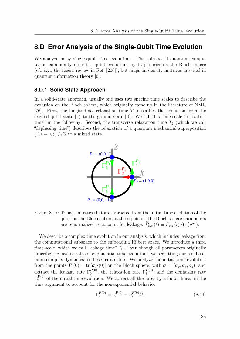
8.D Error Analysis of the Single-Qubit Time Evolution
8.D Error Analysis of the Single-Qubit Time Evolution
We analyze noisy single-qubit time evolutions. The spin-based quantum compu-tation community describes qubit evolutions by trajectories on the Bloch sphere(cf., e.g., the recent review in Ref. [206]), but maps on density matrices are used inquantum information theory [6].
8.D.1 Solid State Approach
In a solid-state approach, usually one uses two specific time scales to describe theevolution on the Bloch sphere, which originally came up in the literature of NMR[76]. First, the longitudinal relaxation time T1 describes the evolution from theexcited qubit state |1〉 to the ground state |0〉 . We call this time scale “relaxationtime” in the following. Second, the transverse relaxation time T2 (which we call“dephasing time”) describes the relaxation of a quantum mechanical superposition(|1〉 + |0〉) /
√2 to a mixed state.
G1P2
G2P2
G1P1
G1P3
X`
Z`
P1 = H0,0,1L
P2 = H1,0,0L
P3 = H0,0,-1L
Figure 8.17: Transition rates that are extracted from the initial time evolution of thequbit on the Bloch sphere at three points. The Bloch sphere parametersare renormalized to account for leakage: Px,z (t) ≡ Px,z (t) /tr
(ρrel).
We describe a complex time evolution in our analysis, which includes leakage fromthe computational subspace to the embedding Hilbert space. We introduce a thirdtime scale, which we call “leakage time” T0. Even though all parameters originallydescribe the inverse rates of exponential time evolutions, we are fitting our results ofmore complex dynamics to these parameters. We analyze the initial time evolutionfrom the points P (0) = tr [σρ (0)] on the Bloch sphere, with σ = (σx, σy, σz), andextract the leakage rate Γ
P (0)0 , the relaxation rate Γ
P (0)1 , and the dephasing rate
ΓP (0)2 of the initial time evolution. We correct all the rates by a factor linear in the
time argument to account for the nonexponential behavior:
ΓP (0)i ≡ γ
P (0)i + ϕ
P (0)i δt, (8.54)
135

8 Noise Analysis of Qubits Implemented in Triple Quantum Dot Systems
with(γP (0)i , ϕ
P (0)i
)∈ R. The leakage time TP (0)
0 is described by the corresponding
leakage rate ΓP (0)0 =
(TP (0)0
)−1
of the evolution of the relevant part of the densitymatrix (cf. Appx. 8.B):
OP (0) (δt) ≈[1− Γ
P (0)0 δt+
(ΓP (0)0
)2 δt2
2
]. (8.55)
We renormalize all Bloch sphere parameters by the trace of the relevant part of thedensity matrix [Pi (t) = Pi (t) /tr
(ρrel (t)
)] because leakage depopulates the qubit.
We assign the relaxation time TP (0)1 =
(ΓP (0)1
)−1
to the evolution from Pz (0) and
use the final polarization Z∞:
Pz (δt) ≈Pz (0)
[1− Γ
P (0)1 δt+
(ΓP (0)1
)2 δt2
2
]+ Z∞
[ΓP (0)1 δt−
(ΓP (0)1
)2 δt2
2
].
(8.56)
Dephasing describes the loss of phase coherence of a qubit. We especially refer tothe relaxation of quantum mechanical superpositions to a mixed state. Dephasingon the Bloch sphere describes an evolution from a point on the surface of the Bloch
sphere to the z-axis. We extract the dephasing time TP (0)2 =
(2Γ
P (0)2
)−1
from theinitial time evolution:
Px (δt) ≈[1− Γ
P (0)2 δt+
(ΓP (0)2
)2 δt2
2
]Px (0) . (8.57)
Following the discussions of Appx. 8.D.3, we can restrict the analysis to just oneplane (e.g. the x-z-plane). It is sufficient to extract the parameters Γ
P (0)0 , Γ
P (0)1 ,
and ΓP (0)2 only for three values of P (0), i.e. only at three points on the surface of
the Bloch sphere, to describe the full time evolution of the qubit (cf. Appx. 8.D.3).From the upper and lower poles P (0) = P1(3) = (0, 0, (−) 1), we extract the leakageand the relaxation rates to the opposite poles. These trajectories follow the z-axis because of the properties of the DM (cf. Appx. 8.D.3). From one point ofthe equator, e.g. P (0) = P2 = (1, 0, 0), we extract the leakage, relaxation, anddephasing rates. The relaxation rate is extracted from the time evolution to thenorth pole or to the south pole. Initially just one of the rates, defined in Eq. (8.56),is positive. This positive number defines the relaxation rate ΓP2
1 . Fig. 8.17 sketchesall transition rates on the Bloch sphere.
8.D.2 Information Theoretical Approach
Usually, one describes the time evolution through the completely positive linear mapεδt in quantum information theory. εδt constructs from the initial density matrix
136
8.D Error Analysis of the Single-Qubit Time Evolution
ρ (0), the density matrix at some later time ρ (δt):
ρ (δt) = εδt [ρ (0)] . (8.58)
εδt is trace decreasing in our analysis, since we also take into account leakage to thesurrounding. Due to the special trajectory generated in our model (cf. Appx. 8.D.3),we only need seven free parameters to completely describe the initial time evolutionof our system. Since the map εδt is linear, it is fixed by its action on the four purestates |0〉 , |1〉 , and
∣∣∣ +(i)
⟩≡(|1〉 + 1
(i)|0〉)/√
2:
ε ( |1〉 〈1|) =a1 |1〉 〈1| + a2 |0〉 〈0| , (8.59)ε ( |0〉 〈0|) =a3 |1〉 〈1| + a4 |0〉 〈0| , (8.60)
ε
(∣∣∣∣ +
(i)
⟩⟨+
(i)
∣∣∣∣) =a5 |1〉 〈1| + a6 |0〉 〈0| + a7
∣∣∣∣ +
(i)
⟩⟨+
(i)
∣∣∣∣ . (8.61)
It is straightforward to relate the parameters a1 − a7 to the rates ΓPji that were
defined earlier [cf. Eqs. (8.55)-(8.57)]:
a1 =1−(ΓP1
0 + ΓP11
)δt+
(ΓP1
0 + ΓP11
)2 δt2
2+O
(δt3), (8.62)
a2 =ΓP11 δt− ΓP1
1
(ΓP1
0 +ΓP1
1
2
)δt2 +O
(δt3), (8.63)
a3 =ΓP31 δt− ΓP3
1
(ΓP3
0 +ΓP3
1
2
)δt2 +O
(δt3), (8.64)
a4 =1−(ΓP3
0 + ΓP31
)δt+
(ΓP3
0 + ΓP31
)2 δt2
2+O
(δt3), (8.65)
a5 =ΓP2
1 + ΓP12
2δt−
(ΓP2
0
(ΓP2
1 + ΓP22
)+
(ΓP2
1
)2+(ΓP1
2
)2
2
)δt2
2+O
(δt3), (8.66)
a6 =−ΓP2
1 + ΓP12
2δt+
(ΓP2
1 − ΓP22
)(ΓP2
0 +ΓP2
1 + ΓP12
2
)δt2
2+O
(δt3), (8.67)
a7 =1−(ΓP2
0 + ΓP22
)δt+
(ΓP2
0 + ΓP22
)2 δt2
2+O
(δt3). (8.68)
Various properties of interest can be calculated from the map εδt. One exampleis the entanglement fidelity F = tr
[ρRG (1⊗ εδt)
(ρRQ
)]. ρRQ is the maximally
entangled state of the noisy quantum system Q and the reference system R: ρRQ =∑ij |ii〉 〈jj| /2. It describes how well the entanglement between two systems is
preserved through a noisy quantum channel εδt [81]:
F =1−[(
ΓP10 + ΓP1
1
)+(ΓP3
0 + ΓP31
)+ 2
(ΓP2
0 + ΓP22
)] δt4
+[(
ΓP10 + ΓP1
1
)2+(ΓP3
0 + ΓP31
)2+ 2
(ΓP2
0 + ΓP22
)2] δt2
8+O
(δt3). (8.69)
137
8 Noise Analysis of Qubits Implemented in Triple Quantum Dot Systems
8.D.3 Error Rates in Our Model
We will show that it is sufficient to use a set of seven parameters to describe theinitial time evolution. The initial evolution is a trajectory on the Bloch spherewith full rotation symmetry around the z-axis and reflection symmetry to any planecontaining the z-axis. Consequently, we can restrict all analysis to one plane (e.g.the x-z-plane). Additionally, the trajectory starting on the north pole or the southpole of the Bloch sphere is strictly restricted to the z-axis.
These symmetries are justified by the analysis of the problem in the DM usingquantum jump terms [cf. Eqs. (8.13)-(8.15)]. The dissipative terms of the DM aregrouped to generate transitions between equidistant energy levels through D [Aω].The Lindblad operator is the generator of the time evolution for the density matrix.It maps the initial density matrix to the density matrix at some later time:
ρ (δt) = eLδtρ (0) =
(1 + Lδt+ L2 δt
2
2+ . . .
)ρ (0) . (8.70)
All combinations D [Aω]D [Bµ]D [Cν ] . . . will act on the initial density matrix togenerate the density matrix at some later time. We start with a density matrix
ρ (0) =
(O0+Z0
2X0−iY0
2X0+iY0
2O0−Z0
2
)S= 1
2,sz= 1
2
⊕ (02)S= 12,sz=− 1
2⊕ (04)S= 3
2(8.71)
for the subspace qubit. Initially there is no population in
∆− 12,∆′− 1
2
and in the
quadruplet subspace. We will prove (cf. below) that the action of any combinationof quantum jumps on the density matrix leads to a density matrix of this form:
Ln (ρ (0)) =
(α1O0 + α2Z0 α3 (X0 − iY0)α3 (X0 + iY0) α4O0 + α5Z0
)S= 1
2,sz= 1
2
(8.72)
⊕(
β1O0 + β2Z0 β3 (X0 − iY0)β3 (X0 + iY0) β4O0 + β5Z0
)S= 1
2,sz=− 1
2
⊕
γ1O0 + γ2Z0 0 0 0
0 γ3O0 + γ4Z0 0 00 0 γ5O0 + γ6Z0 00 0 0 γ7O0 + γ8Z0
S= 3
2
.
The coefficients (αi, βi, γi) are real numbers representing the action of quantumjumps between energy levels. Eq. (8.72) shows that the projected part on the qubitsubspace will have the same ratio of the x-polarization and y-polarization as for theinitial density matrix. The trace evolution and the z-evolution depend, however,on the initial z-polarization of the qubit. Since this finding is true for all terms ofEq. (8.70), it is also true for ρ (δt). Given these restrictions on the generated densitymatrix, the trajectory on the Bloch sphere will have the specific form describedearlier.
138

8.E Model Systems
We prove Eq. (8.72). All quantum jump transitions can be grouped into two sets.First, there are transitions involving only the computational subspace. They canrepresent pure relaxation (model 1 in Appx. 8.E.1) or pure dephasing (model 2 inAppx. 8.E.2). These models generate transitions in the computational subspace via
the coupling operators A ∈(
β1 00 β2
),
(0 β3
0 0
),
(0 0β4 0
), with βi ∈ R.
ρ0 =
(α1O0 + α2Z0 α3 (X0 − iY0)α3 (X0 + iY0) α4O0 + α5Z0
)will remain unchanged after the action of
one dissipative term D [A] (ρ0), only the constants αi are modified.Transitions involving the remaining Hilbert space will again have two distinct
features. First, there are quantum jump terms involving just transitions betweentwo energy levels. One can calculate the action in a three-dimensional Hilbert spacespanned by the qubit levels and the coupled external level. An easy calculationshows that the structure of an initial density matrix,
ρ0 =
α1O0 + α2Z0 α3 (X0 − iY0) 0α3 (X0 + iY0) α4O0 + α5Z0 0
0 0 α6O0 + α7Z0
, (8.73)
remains unchanged. Only the constants αi will be modified to different real numbers.Second, there are quantum jumps involving more than three energy levels. They
can be made up of all the transitions introduced so far while acting on the sub-spaces separately. Consequently, they also preserve the structure above. Otherwise,they couple the computational subspace to
(S = 1
2, sz = −1
2
)involving correlated
quantum jumps between the same l eigenstates. These transitions also preserve theoff-diagonal elements of the density matrix on the computational subspace. Theynever mix diagonal and off-diagonal elements.
The same result is obtained for the subsystem qubit. All arguments remain validbecause the initial density matrix of the subsystem qubit is equivalent to Eq. (8.72):
ρ (0) =
(O0+Z0
2X0−iY0
2X0+iY0
2O0−Z0
2
)l
⊗
1
1+e− EzTK
0
0 e− EzTK
1+e− EzTK
sz
⊕ (04)S= 32
=1
1 + e− EzTK
(O0+Z0
2X0−iY0
2X0+iY0
2O0−Z0
2
)S= 1
2,sz= 1
2
⊕ e− EzTK
1 + e− EzTK
(O0+Z0
2X0−iY0
2X0+iY0
2O0−Z0
2
)S= 1
2,sz=− 1
2
⊕ (04)S= 32. (8.74)
8.E Model Systems
Fig. 8.18 shows four model systems that describe the effective error rates of theTQD qubits. Energy eigenstates are coupled through quantum jumps in the DM.
139

8 Noise Analysis of Qubits Implemented in Triple Quantum Dot Systems
Transitions are possible between the qubit levels |1〉 and |0〉 , and also to otherstates of the embedding Hilbert space |Out〉 . The strength of the quantum jumps isspecified by the coefficients Υi ∈ R, which are determined by two constants. First ofall, there are the transition rates h (A, ω) that are extracted from experiments [forthe interaction with nuclear spins, cf. h (σiz/σ
ix, ω) in Eq. (8.20); for the interaction
with phonons, cf. h (σix, ω) in Eq. (8.26)]. Second, we also need the matrix elementsof the transition operator between the energy eigenstates [cf. Eq. (8.17)]. In total, Υi
can be negative, and only the positive numbers Υ2i describe a rate. In the following,
we describe all the four toy models individually.
È0\
È1\
U+
U-
(a) Model 1
È0\
È1\U
1
U
0
(b) Model 2
È0\
È1\
ÈOut\
U1+U1-
U0+U0-
(c) Model 3
È0-12\
È1-12\
È012\
È112\
U10 U01
(d) Model 4
Figure 8.18: Toy models that describe the time evolution of TQD qubits.
8.E.1 Model 1: Pure Relaxation
The model of pure relaxation describes the transitions in a two-level system throughraising and lowering operators: Υ±σ± [cf. Fig. 8.18(a)]. The master equation,
ρ (t) = D [Υ+σ+] (ρ (t)) +D [Υ−σ−] (ρ (t)) (8.75)= Υ2
+D [σ+] (ρ (t)) + Υ2−D [σ−] (ρ (t)) , (8.76)
can be solved easily. Assuming Υ2− > Υ2
+, we get:
ΓP1,P2,P3
0 = 0, ΓP11 = Υ2
− −1
2Υ2
+Υ2−δt, (8.77)
ΓP21 =
(Υ2− −Υ2
+
)− 1
2Υ2
+
(Υ2− −Υ2
+
)δt, (8.78)
ΓP13 = Υ2
+ −1
2Υ2
+Υ2−δt, ΓP2
2 =1
2
(Υ2
+ + Υ2−). (8.79)
There is no leakage in this model. The relaxations from P1 and P3 are determinedby the transitions to the opposite pole. The combination of the two transition ratesgives a reduction of the overall error. At P2, we initially see relaxation to the lowerpole with a rate determined by the difference of the two transition rates.
140

8.E Model Systems
8.E.2 Model 2: Pure Dephasing
Pure dephasing [cf. Fig. 8.18(b)] is described in the DM by the coupling operator:
A =
(Υ1 00 Υ0
). (8.80)
When solving the master equation ρ (t) = D [A] (ρ (t)), we extract the followingtransition rates:
ΓP1,P2,P3
0 = 0, ΓP1,P2,P3
1 = 0, ΓP22 =
1
2(Υ1 −Υ0)2 . (8.81)
The coupling operator from Eq. (8.80) generates neither relaxation nor leakage. Adescribes fluctuating energy levels, which leads to pure phase noise.
8.E.3 Model 3: Two State Leakage
In our calculations, we need to describe leakage of the qubit states to one state ofthe embedding Hilbert space [cf. Fig. 8.18(c)]. When solving the master equation,
ρ (t) =D[Υ1+σ
1→Out+
](ρ (t)) +D
[Υ1−σ
1→Out−
](ρ (t)) (8.82)
+D[Υ0+σ
0→Out+
](ρ (t)) +D
[Υ0−σ
0→Out−
](ρ (t)) ,
we extract the error rates (assuming Υ21+ > Υ2
0+):
ΓP10 =Υ2
1+ −Υ21+
(Υ2
1− + Υ20−) δt
2, (8.83)
ΓP20 =
Υ21+ + Υ2
0+
2−(Υ2
1+ −Υ20+
)2+ 2
(Υ2
1+ + Υ20+
) (Υ2
1− + Υ20−)
8δt, (8.84)
ΓP30 =Υ2
0+ −Υ20+
(Υ2
1− + Υ20−) δt
2, ΓP1
1 = Υ21+Υ2
0−δt
2, (8.85)
ΓP21 =
Υ21+ −Υ2
0+
2+
(Υ2
1+ −Υ20+
)2 − 2(Υ2
1+ + Υ20+
) (Υ2
1− −Υ20−)
8δt, (8.86)
ΓP31 =Υ2
0+Υ21−δt
2, ΓP2
2 =
(Υ2
1+ −Υ20+
)2+ 2
(Υ2
1+ + Υ20+
) (Υ2
1− + Υ20−)
8δt. (8.87)
We consider two special cases of this model. First, only the transition rates fromthe qubit levels to the surroundings are significant for the subspace qubit. We setΥ1+ = Υ1, Υ0+ = Υ2, and Υ1− = Υ0− = 0 to obtain:
ΓP10 =Υ2
1, ΓP20 =
Υ21 + Υ2
2
2− (Υ2
1 −Υ22)
2
8δt, ΓP3
0 = Υ22, (8.88)
ΓP11 =0, ΓP2
1 =Υ2
1 −Υ22
2+
(Υ21 + Υ2
2)2
8δt, ΓP3
1 = 0, ΓP22 =
(Υ21 −Υ2
2)2
8. (8.89)
141

8 Noise Analysis of Qubits Implemented in Triple Quantum Dot Systems
Here, for the north pole and the south pole (P1 and P3) no relaxations are generatedand only leakage occurs.
Second, we describe for the subsystem qubit the transition of one qubit level tothe surrounding. For Υ0+ = Υ+ and Υ0− = Υ−, with Υ1+ = Υ1− = 0, we get
ΓP10 =0, ΓP2
0 =Υ2
+
2−
Υ2+
8
(Υ2
+ + 2Υ2−)δt, ΓP3
0 = Υ2+ −
1
2Υ2
+Υ2−δt, (8.90)
ΓP11 =0, ΓP2
1 =Υ2
+
2+
Υ2+
8
(Υ2
+ − 2Υ2−)δt, ΓP3
1 = 0, ΓP22 =
Υ2+
8
(Υ2
+ + 2Υ2−)δt.
(8.91)
Leakage and relaxation are absent at P1. On the south pole P3, we observe pureleakage.
8.E.4 Model 4: Internal Transitions of the Subsystem Qubit
We extract error rates at the crossing of two energy levels for the subsystem qubit.We can solve the Davies master equation ρ (t) = D [A] (ρ (t)) for the toy model ofFig. 8.18(d). For Υ2
10 > e− EzTK Υ2
01, we get the errors:
ΓP1,P2,P3
0 =0, (8.92)
ΓP11 =
Υ210
1 + e− EzTK
− Υ210
1 + e− EzTK
(e− EzTK
1 + e− EzTK
Υ210 + Υ2
01
)δt
2, (8.93)
ΓP21 =
Υ210 − e
− EzTK Υ2
01
1 + e− EzTK
+
(Υ2
10 − e− EzTK Υ2
01
1 + e− EzTK
)(e− EzTK (Υ2
10 + Υ201)
1 + e− EzTK
+ Υ201
)δt
2,
(8.94)
ΓP31 =
e− EzTK
1 + e− EzTK
Υ201 −
e− EzTK
1 + e− EzTK
Υ201
(Υ2
10 +e− EzTK
1 + e− EzTK
Υ201
)δt
2, (8.95)
ΓP22 =
Υ210 + e
− EzTK Υ2
01
2(
1 + e− EzTK
) − e− EzTK(
1 + e− EzTK
)2
(Υ2
10 −Υ201
)2 δt
8. (8.96)
142

CHAPTER 9
Two-Qubit Pulse Gate for theThree-Electron Double Quantum Dot
Qubit
The three-electron configuration of gate-defined doublequantum dots encodes a promising qubit for quantum in-formation processing. We propose a two-qubit entanglinggate using a pulse-gated manipulation procedure. Therequirements for high-fidelity entangling operations areequivalent to the requirements for the pulse-gated single-qubit manipulations that were successfully implementedfor Si QDs. Our two-qubit gate completes the universal setof all-pulse-gated operations for the three-electron double-dot qubit and paves the way for a scalable setup to achievequantum computation.
After the preliminary version of the thesis was handed in, the results of thischapter were submitted for publication to Physical Review B.
143

9 Two-Qubit Pulse Gate for the Three-Electron Double Quantum Dot Qubit
9.1 Introduction
The name hybrid qubit (HQ) was coined for the encoded qubit in a three-electronconfiguration on a gate-defined double quantum dot (DQD) [72, 73].1 The HQ is aspin qubit in its idle configuration, but it is a charge qubit during the manipulationprocedure. Recently, impressive progress was made for the single-qubit control of aHQ in Si [74, 75]. It was argued that single-qubit gates were implemented, whosefidelities exceed 85 % for X-rotations and 94 % for Z-rotations [75]. These manip-ulations rely on the transfer of one electron between quantum dots (QDs) [73–75].Subnanosecond gate pulses were successfully applied to transfer the third electronbetween singly occupied QDs. A two-qubit entangling gate for HQs was suggestedtheoretically that uses electrostatic couplings [73]. If the charge configuration ofone HQ is changed, then Coulomb interactions modify the electric field at the posi-tion of the other HQ. Note the equivalent construction for a controlled phase gate(CPHASE) for singlet-triplet qubits in two-electron DQDs [31].
Using Coulomb interactions for entangling operations can be critical. Even thoughelectrostatic couplings are long-ranged, they are generally weak and they are stronglydisturbed by charge noise [64]. We propose an alternative two-qubit gate. Two HQsbrought into close proximity enable the transfer of electrons. We construct a two-qubit gate that works similar to the pulse-gated single-qubit manipulations. Ourapproach requires fast control of the charge configurations on the four QDs throughsubnanosecond pulse times at gates close to the QDs. A two-qubit manipulationscheme of the same principle as for the single-qubit gates is highly promising becausesingle-qubit pulse gates have been implemented with great success [74, 75].
The central requirement of the entangling operation is the tuning of one two-qubitstate (here |0L0R〉) to a degeneracy point with one leakage state |E〉 . |0L0R〉 picksup a nontrivial phase, while all other two-qubit states evolve trivially. Note that asimilar construction for an entangling operation [207] has been implemented withimpressive fidelities [208–210] for superconducting qubits. The couplings to otherleakage states must be avoided during the operation. We propose a two-step proce-dure. First, we tune |1L1R〉 and |0L1R〉 away from the initial charge configurationto protect these states from leakage. |1L0R〉 and |0L0R〉 remain unchanged at thesame time. We have then reached the readout regime of the second HQ. The secondpart of the tuning procedure corrects the passage of |1L0R〉 through the anticrossingwith |E〉 , at a point where |1L0R〉 is degenerate with the leakage state |L〉 . We callthis anticrossing degenerate Landau-Zener crossing (DLZC) because it is describedby a generalization of the Landau-Zener model [211, 212].
We focus on pulse-gated entangling operations for HQs in gate-defined Si QDs.Even though our entangling operation is not specifically related to the material andthe qubit design, gate-defined Si QDs are the first candidate where our two-qubitpulse gate might be implemented because Si QDs were used for single-qubit pulsegates [74, 75]. We discuss therefore specifically the noise sources that are dominant
1This qubit is called the Madison qubit in the remaining part of the thesis.
144

9.2 Setup
for experiments involving gate-defined Si QDs. The proposed two-qubit pulse gatescan be directly implemented with the existing methods of the single-qubit pulsegates. It will turn out that high-fidelity two-qubit entangling operations require lowcharge noise.
The organization of this chapter is as follows. Sec. 9.2 introduces the model todescribe a pair of three-electron DQDs. Sec. 9.3 constructs the two-qubit gate.Sec. 9.4 discusses the noise properties of the entangling operation, and Sec. 9.5summarizes all the results.
9.2 Setup
We consider an array of four QDs, which are labeled by QD1-QD4 [cf. Fig. 9.1].One qubit is encoded using a three-electron configuration on two QDs. QD1 andQD2 encode HQL, and QD3 and QD4 encode HQR. We describe the system bya Hubbard model, which includes two orbital states at each QD. The transfer ofelectrons between neighboring QDs is possible but weak, unless the system is biasedusing electric gates. A large global magnetic field is applied, which separates statesof different sz energetically. The S = 1
2, sz = 1
2spin subspace of three electrons
encodes a qubit [65].
The single-qubit states for HQL are |1L〉 =√
23|↓ T+〉 −
√13|↑ T0〉 and |0L〉 =
|↑ S〉 . The first entry in the state notation labels electrons at QD1, and the secondentry labels electrons at QD2. QD1 is singly occupied, but two electrons are pairedat QD2. |S〉 = c†i↑c
†i↓ |0〉 is the two-electron singlet state at QDi, |T+〉 = c†i↑c
†i↑ |0〉 ,
|T0〉 = 1√2
(c†i↑c
†i↓ + c†i↓c
†i↑
)|0〉 , and |T−〉 = c†i↓c
†i↓ |0〉 are triplet states at QDi. c
(†)iσ is
the (creation) annihilation operator of one electron in state |i〉 of QDi with spin σ,|i〉 and
∣∣i⟩ are the ground state and the first excited state at QDi,2 and |0〉 is thevacuum state. Similar considerations hold for HQR, where QD3 is singly occupiedand QD4 is filled with two electrons. We assume that a two-electron triplet at QD1
or at QD3 is strongly unfavored compared to a two-electron triplet at QD2 or atQD4. These conditions were fulfilled for the HQs in Ref. [74] and Ref. [75].
We assign the energy E0 = 0 to |0L0R〉 in (1, 2, 1, 2). |1L0R〉 , |0L1R〉 , and |1L1R〉are higher in energy by ΩL, ΩR, and ΩL + ΩR. The excited states |1L〉 and |1R〉involve a triplet on a doubly occupied QD that is higher in energy than the singletconfigurations of |0L〉 and |0R〉 . Single-qubit gates are not the focus of this work,but we briefly review: all single-qubit gates are applicable through evolutions under
2 Note that∣∣ i⟩ can be an orbital excited state or a valley excited state in Si. |2〉 and
∣∣2⟩determine the energy difference between |0L〉 and |1L〉 . Our two-qubit gate relies on a largersinglet-triplet energy difference for the two-electron configuration at QD1 compared to QD2.Equivalent discussions hold for HQR. In contrast, GaAs QDs lack valley excited states; onecan realize the same entangling gate using one large QD and one small QD. Then, the energydifference between the two-electron singlet and the two-electron triplet depends on the confiningstrength of the wave functions.
145

9 Two-Qubit Pulse Gate for the Three-Electron Double Quantum Dot Qubit
σLx , σLz , σRx , and σRz . σx = |1〉 〈0| + |0〉 〈1| and σz = |1〉 〈1| − |0〉 〈0| are the Paulioperators on the corresponding qubit subspace. They are applied by transferringone electron from QD2 to QD1 for HQL (and QD4 to QD3 for HQR). Depending onthe pulse profile, pure phase evolutions (described by the operators σLz and σRz ) orspin flips (described by the operators σLx and σRx ) are created [73–75].
Figure 9.1: Array of QDs that is used to define and couple HQs. The four red QDsencode two HQs; we call them HQL and HQR. Black dots representelectrons. We label the charge configurations by the electron numbers(nQD1
, nQD2, nQD3
, nQD4
). (1, 2, 1, 2) is the idle configuration. Applying
voltages to gates close to the QDs provides universal single-qubit controland realizes a CPHASE gate by the transfer of single electrons betweenthe QDs. We describe the manipulation protocols in the text. Theencoding scheme can be scaled up trivially, as shown by the blue QDs.
9.3 Two-Qubit Pulse Gate
Two-qubit operations are constructed using the transfer of electrons between neigh-boring QDs. We describe the charge transfer between (1, 2, 1, 2) and (1, 2, 2, 1) byH34 = τ1
∑σ∈↑,↓
(c†3σc4σ + H.c.
)+ τ2
∑σ∈↑,↓
(c†3σc4σ + H.c.
), where τ1, τ2 are
tunnel couplings between states from neighboring QDs, and H.c. labels the Her-mitian conjugate of the preceding term. ε43 = eV4 − eV3 describes the transferof electrons through applied voltages at gates close to QD3 and QD4. Loweringthe potential at QD3 compared to QD4 favors (1, 2, 2, 1) (ε43 > 0), but (1, 2, 1, 2)is favored for the opposite case (ε43 < 0). (1, 2, 1, 2) and (1, 2, 2, 1) have identi-cal energies at ε43 = ∆43 > ΩL,ΩR. Similar considerations hold for the manip-ulation between (1, 2, 1, 2) and (1, 1, 2, 2), which is described by ε23 = eV2 − eV3
and H23 = τ3
∑σ∈↑,↓
(c†2σc3σ + H.c.
)+ τ4
∑σ∈↑,↓
(c†
2σc3σ + H.c.
). (1, 2, 1, 2) and
(1, 1, 2, 2) have identical energies at ε23 = ∆23 > ΩL,ΩR.We construct an entangling operation in a two-step manipulation procedure, which
is shown in Fig. 9.2. In the first step, we tune ε43 and pulse from (1, 2, 1, 2) towards(1, 2, 2, 1). Only |1R〉 is transferred to |B〉 = |(S ↑)R〉 because |1R〉 is unfavored
146

9.3 Two-Qubit Pulse Gate
Figure 9.2: Energy diagram of two coupled HQs with sz = 1 in (1, 2, 1, 2), (1, 2, 2, 1),and (1, 1, 2, 2). The red and the orange lines describe the computationalbasis, and the black lines are leakage states. (1, 2, 1, 2) is favored with-out external bias. (a) shows the pulsing towards (1, 2, 2, 1), which ismodeled through ε43 = eV4 − eV3 describing the potentials at QD3 andQD4. The states |1L1R〉 and |1LB〉 as well as |0L1R〉 and |0LB〉 areswapped at ε43 = ∆43 − ΩR. Two of the four state combinations fromthe computational basis remain in (1, 2, 1, 2) at ε43 = ε∗43. (b) showsthe second step of the manipulation. ε23 = eV2 − eV3 models the po-tentials at QD2 and QD3. As a consequence, only |1L0R〉 and |0L0R〉can be tuned to (1, 2, 2, 1), but |1LB〉 and |0LB〉 are blocked. The non-trivial part of the entangling gate is a π-phase evolution of |0L0R〉 atε23 = ∆23. |1L0R〉 is degenerate with |L〉 and passes through a DLZC atε23 = ∆23 − ΩL. Leakage from the computational subspace is preventedby the pulse cycle that involves waiting times at ε23 = ∆23 − ΩL and atε23 = ε∗23 (cf. description in the text). The setup is brought back to theinitial configuration in the end, by first changing ε23 and then changingε43. Perfect state crossings are marked where transitions are forbiddenfrom spin-selection rules (blue) or from charge-selection rules (purple).The waiting times t1, t2, tw, and tπ are given in the main text.
energetically compared to |0R〉 , which remains in (1, 2). The tuning uses a rapidpulse to ε43 = ∆43 − ΩR. H34 couples |1R〉 and |B〉 by
√32τ2. The occupations
of |1R〉 and |B〉 swap after the waiting time t1 = h2√
6τ2. Afterwards, we pulse to
ε43 = ε∗43, which is far away from all anticrossings. |B〉 and |0R〉 have the energydifference Ω∗R at ε43 = ε∗43. Note that ε43 = ε∗43 is in the readout regime of HQR:|1R〉 is in (2, 1), but |0R〉 is in (1, 2).
In the second step, gate pulses modify ε23 at fixed ε43 = ε∗43. The charge configu-ration is pulsed towards (1, 1, 2, 2). States in (1, 2, 2, 1) remain unchanged because
147

9 Two-Qubit Pulse Gate for the Three-Electron Double Quantum Dot Qubit
they need the transfer of two electrons to reach (1, 1, 2, 2). We introduce the states:
|L〉 =[√1
6|↑ T0 ↑〉 −
√3
2|↑ T+ ↓〉 +
1
2√
3|↓ T+ ↑〉
]⊗ |S〉 , (9.1)
|β〉 =1
2
[√2 |↑ T0 ↑〉 + |↑ T+ ↓〉 + |↓ T+ ↑〉
]⊗ |S〉 . (9.2)
|E〉 = |↑↑ SS〉 is the ground state in (1, 1, 2, 2) with sz = 1. H23 couples |0L0R〉 ,|1L0R〉 , |L〉 , and |E〉 , while |β〉 is decoupled. When approaching (1, 1, 2, 2), firstthe anticrossing of |1L0R〉 , |L〉 , and |E〉 is reached at ε23 = ∆23 − ΩL:
H23 (ε23) ≈
ΩL 0 τ4√6
0 ΩL −2τ4√3
τ4√6−2τ4√
3∆23 − ε23
. (9.3)
|0L0R〉 hybridizes with |E〉 only at ε23 = ∆23. |E〉 has lower energy than |1L0R〉at ε23 = ε∗23, but |0L0R〉 is still the ground state.
The passage through the anticrossing at ε23 = ∆23−ΩL is critical for the construc-tion of the entangling operation. H23 describes within the subspace |1L0R〉 , |L〉 , |E〉a DLZC [cf. Eq. (9.3)]. A basis transformation partially diagonalizes Eq. (9.3):|T1〉 = 1
3|1L0R〉−2
√2
3|L〉 and |E〉 have the overlap
√2/3τ4, but |T2〉 = 2
√2
3|1L0R〉+
13|L〉 is decoupled. |T1〉 and |E〉 swap at ε23 = ∆23 − ΩL after t2 = h
2√
6τ4. We in-
troduce the waiting time tw at ε23 = ε∗23, where |E〉 has the energy ΩL/2. tw mustcompensate after the full cycle the relative phase evolution between |T1〉 and |T2〉 ;as a consequence, |1L0R〉 does not leak to |L〉 . Simple mathematics shows that thisis the case for tw = h
(2nΩL− 1
τ3
)> 0 with n ∈ N.
The time evolution at ε23 = ∆23 constructs the central part of the entanglinggate. H23 couples |0L0R〉 and |E〉 by τ3. The states on the subspace |0L0R〉 , |E〉pick up a π-phase factor after the waiting time tπ = h
2τ3: e−iπσx = −1. All other
states of the computational basis evolve trivially with the energies ΩL, Ω∗R, andΩL + Ω∗R. Finally the setup is tuned back to the initial configuration with swaps atε23 = ∆23−ΩL and ε43 = ∆43−ΩR generated after the waiting times t2 = h
2√
6τ4and
t1 = h2√
6τ2.
In total, the described pulse cycle realizes a CPHASE gate in the basis |1L1R〉 ,|1L0R〉 , |0L1R〉 , and |0L0R〉 when permitting additional single-qubit phase gates:
Uε43=∆43−ΩR (t1)Uε23=∆23−ΩL (t2)Uε23=∆23 (tπ) (9.4)× Uε23=ε∗23
(tw)Uε23=∆23−ΩL (t2)Uε43=∆43−ΩR (t1)
= eiπ(p1+p2)
2+1Z
− p14
L Z− p2
4R CPHASE,
with Zφi = e−i2πσ
izφ, p1 = Ω∗R
(1τ3− 2√
2/3
τ4− 4n
ΩL
), and p2 = ΩL
(1τ3− 2√
2/3
τ4
). Uε (t)
describes the time evolution at ε for the waiting time t. We have constructed aphase shift on HQR conditioned on the state of HQL.
148
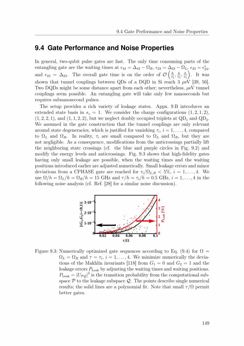
9.4 Gate Performance and Noise Properties
9.4 Gate Performance and Noise Properties
In general, two-qubit pulse gates are fast. The only time consuming parts of theentangling gate are the waiting times at ε43 = ∆43 − ΩR, ε23 = ∆23 − ΩL, ε23 = ε∗23,and ε23 = ∆23. The overall gate time is on the order of O
(hτ2, hτ3, hτ4
). It was
shown that tunnel couplings between QDs of a DQD in Si reach 3 µeV [39, 56].Two DQDs might be some distance apart from each other; nevertheless, µeV tunnelcouplings seem possible. An entangling gate will take only few nanoseconds butrequires subnanosecond pulses.
The setup provides a rich variety of leakage states. Appx. 9.B introduces anextended state basis in sz = 1. We consider the charge configurations (1, 2, 1, 2),(1, 2, 2, 1), and (1, 1, 2, 2), but we neglect doubly occupied triplets at QD1 and QD3.We assumed in the gate construction that the tunnel couplings are only relevantaround state degeneracies, which is justified for vanishing τi, i = 1, . . . , 4, comparedto ΩL and ΩR. In reality, τi are small compared to ΩL and ΩR, but they arenot negligible. As a consequence, modifications from the anticrossings partially liftthe neighboring state crossings (cf. the blue and purple circles in Fig. 9.2) andmodify the energy levels and anticrossings. Fig. 9.3 shows that high-fidelity gateshaving only small leakage are possible, when the waiting times and the waitingpositions introduced earlier are adjusted numerically. Small leakage errors and minordeviations from a CPHASE gate are reached for τi/ΩL,R < 5%, i = 1, . . . , 4. Weuse Ω/h = ΩL/h = ΩR/h = 15 GHz and τ/h = τi/h = 0.5 GHz, i = 1, . . . , 4 in thefollowing noise analysis (cf. Ref. [28] for a similar noise discussion).
0.02 0.04 0.06 0.08 0.1
3×10⁻³
2×10⁻³
1×10⁻³
0
4
3
2
1
0
ΤW
HG
1,G
2L-
H0,1
L¤
PL
eak
@%D
Figure 9.3: Numerically optimized gate sequences according to Eq. (9.4) for Ω =ΩL = ΩR and τ = τi, i = 1, . . . , 4. We minimize numerically the devia-tions of the Makhlin invariants [118] from G1 = 0 and G2 = 1 and theleakage errors PLeak by adjusting the waiting times and waiting positions.PLeak = |UPQ|2 is the transition probability from the computational sub-space P to the leakage subspace Q. The points describe single numericalresults; the solid lines are a polynomial fit. Note that small τ/Ω permitbetter gates.
149
9 Two-Qubit Pulse Gate for the Three-Electron Double Quantum Dot Qubit
9.4.1 Charge Noise
Charge traps of the heterostructure introduce low-frequency electric field fluctua-tions [34, 93]. Their influence is weak for spin qubits, but it increases for chargequbits [27, 94]. Consequently, HQs are protected from charge noise only in the idleconfiguration. We model charge noise by an energy fluctuation between differentcharge configurations. We introduce no fluctuations during one gate simulation,but use modifications between successive runs. The fluctuations follow a Gaussianprobability distribution of rms δε. Note that we simulate the numerically optimizedgate sequence of Eq. (9.4).
Fig. 9.4 shows the gate fidelity F , which is defined in Appx. 9.A, while δε isvaried. F decreases rapidly with δε. A Gaussian decay is seen for small δε. Thedecay constant shows that τ is the relevant energy scale of the entangling gate.The coherence is lost if δε increases beyond τ because a typical gate misses theanticrossings of Fig. 9.2. Noisy gate sequences keep only the diagonal entries of thedensity matrix, but they remove all off-diagonal entries leading to F = 0.25.Charge noise was measured in GaAs QDs to cause energy fluctuations of the
magnitude 1 µeV [34] (1 µeV/h ≈ 0.2 GHz). For high-fidelity pulse-gated entanglingoperations, δε must be smaller than τ that reaches typically a few µeV in Si HQs.
9.4.2 Hyperfine Interactions
Nuclear spins couple to HQs, and they cause low-frequency magnetic field fluctua-tions [31, 52]. The applied magnetic fields [Ez/h > 3 GHz (> 100 mT)] are largerthan the uncertainty in the magnetic field from the nuclear spins in typical QD ex-periments in Si [δEz/h < 3 MHz (< 100 µT)], and we restrict the error analysis tothe total sz = 1 subspace. We simulate the numerically optimized pulse sequence ofEq. (9.4) under magnetic field fluctuations. The variations of the magnetic fields atevery QD are determined by a Gaussian probability distribution with the rms δEz(in energy units).Fig. 9.4 shows that F decreases rapidly with δEz. Again, a Gaussian decay is
observed with a decay constant determined by τ for small δEz. The influence ofhyperfine interactions differs from charge noise. Local magnetic fields lift the statecrossings that are protected by the spin-selection rules (cf. blue markings in Fig. 9.2).Not only is the coherence lost for large δEz, but leakage further suppresses F . Wecan approximate the limit of large δEz with F = 9/64. All off-diagonal entries ofthe density matrix are removed. Additionally, some states are mixed with leakagestates. |1L1R〉 goes to a mixed state with three other states; |1L0R〉 and |0L1R〉mix with one other state each.Si is a popular QD material because the number of finite-spin nuclei is small
[168]. Nevertheless, noise from nuclear spins was identified to be dominant in thefirst spin qubit manipulations of gate-defined Si QDs [39]. δEz/h = 7.5 · 10−4 GHzin natural Si (cf. Ref. [87]) is sufficient for nearly perfect two-qubit pulse gates. Thefluctuations of the nuclear spins decrease further for isotopically purified Si instead
150

9.5 Conclusion
of natural Si.
e-I Τ
k ∆ΕM2
, k»5.1
e-J Τ
k ∆EzN2
, k»8.8
0 0.1 0.2 0.3 0.4 0.50
0.25
0.5
0.75
1
∆Εh, ∆Ezh @GHzD
F
Figure 9.4: Fidelity analysis for numerically optimized CPHASE gates under chargenoise (black) and nuclear spin noise (red) at ΩL/h = ΩR/h = 15 GHzand τ/h = τi/h = 0.5 GHz, i = 1, . . . , 4. Energy fluctuations δε betweendifferent charge configurations model charge noise. Nuclear spins causelocal, low-frequency magnetic field fluctuations of the energy δEz. Wedescribe both noise sources by a classical probability distribution withthe rms δε (for charge noise) and δEz (for nuclear spin noise). Thefidelity F is extracted from 1000 gate simulations according to Eq. (9.4).Increasing uncertainties suppress F strongly till F saturate at 0.25 (forcharge noise) and 9/64 (for nuclear spin noise) (cf. the vertical lines).The initial decay of F is described by a Gaussian decay law (cf. thedotted lines).
9.5 Conclusion
We have constructed a two-qubit pulse gate for the HQ - an encoded qubit in athree-electron configuration on a gate-defined DQD. Applying fast voltage pulses atgates close to the QDs enables the transfer of single electrons between QDs. Wetune the setup to the anticrossing of |0L0R〉 with the leakage state |E〉 . |0L0R〉picks up a nontrivial phase without leaking to |E〉 , while all other two-qubit statesaccumulate trivial phases. The main challenge of the entangling gate is to avoidleakage to other states. We use a two-step procedure. (1) we pulse the right HQto the readout configuration. Here, |1R〉 goes to (2, 1), but |0R〉 stays in (1, 2). (2)|0L1R〉 passes through a DLZC during the pulse cycle. The pulse profile is adjustedto avoid leakage after the full pulse cycle. Note that an adiabatic manipulationprotocol can substitute the pulse-gated manipulation3.
3 All energy levels follow the lowest energy states for adiabatic manipulation protocols. Thenontrivial part of the entangling gate is also obtained at the degeneracy of |0L0R〉 with |E〉 .The pulse shape must compensate for the pulsing through the DLZC of |1L0R〉 , |L〉 , |E〉.
151

9 Two-Qubit Pulse Gate for the Three-Electron Double Quantum Dot Qubit
Cross-couplings between anticrossings, charge noise, and nuclear spin noise intro-duce errors for our pulse-gated two-qubit operation. Cross-couplings of anticrossingsare problematic as they open state crossings. Also these mechanism slightly influ-ence the energy levels and the sizes of the anticrossings. Reasonably small values ofτ/Ω . 5% still permit excellent gates through pulse shaping. Charge noise is prob-lematic because the gate tunes the HQs between different charge configurations.Current QD experiments suggest that charge noise is critical for our pulse-gatedentangling operation. Nuclear spins are unimportant for the pulse-gated entanglingoperation of HQs in natural Si and, even more, for isotopically purified Si. We arehopeful that material improvements and advances in fabrication techniques for SiQDs still allow an experimental realization of this gate in the near future.
Pulse gates provide universal control of HQs through single-qubit operations,which have been implemented experimentally [74, 75], and our two-qubit entan-gling gate. Because this setup can be scaled up trivially (cf. Fig. 9.1), furtherexperimental progress should be stimulated to realize all-pulse-gated manipulationsof HQs.
152
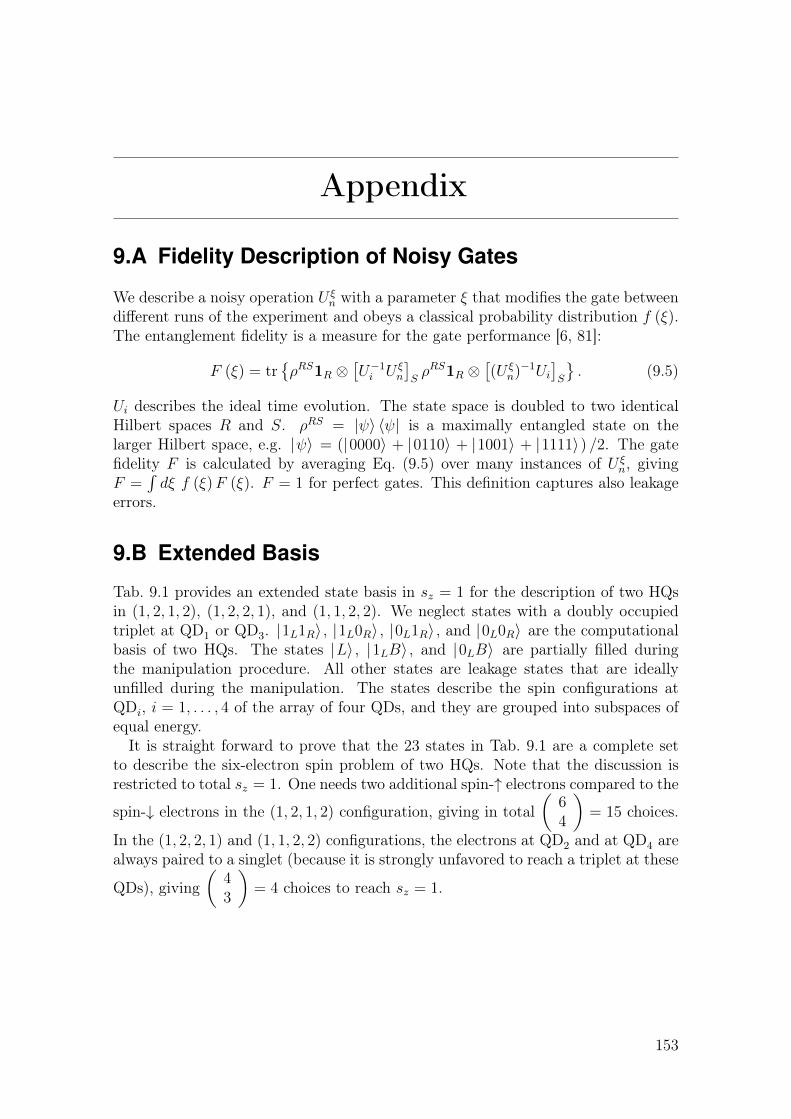
Appendix
9.A Fidelity Description of Noisy Gates
We describe a noisy operation U ξn with a parameter ξ that modifies the gate between
different runs of the experiment and obeys a classical probability distribution f (ξ).The entanglement fidelity is a measure for the gate performance [6, 81]:
F (ξ) = trρRS1R ⊗
[U−1i U ξ
n
]SρRS1R ⊗
[(U ξ
n)−1Ui]S
. (9.5)
Ui describes the ideal time evolution. The state space is doubled to two identicalHilbert spaces R and S. ρRS = |ψ〉 〈ψ| is a maximally entangled state on thelarger Hilbert space, e.g. |ψ〉 = (|0000〉 + |0110〉 + |1001〉 + |1111〉) /2. The gatefidelity F is calculated by averaging Eq. (9.5) over many instances of U ξ
n, givingF =
∫dξ f (ξ)F (ξ). F = 1 for perfect gates. This definition captures also leakage
errors.
9.B Extended Basis
Tab. 9.1 provides an extended state basis in sz = 1 for the description of two HQsin (1, 2, 1, 2), (1, 2, 2, 1), and (1, 1, 2, 2). We neglect states with a doubly occupiedtriplet at QD1 or QD3. |1L1R〉 , |1L0R〉 , |0L1R〉 , and |0L0R〉 are the computationalbasis of two HQs. The states |L〉 , |1LB〉 , and |0LB〉 are partially filled duringthe manipulation procedure. All other states are leakage states that are ideallyunfilled during the manipulation. The states describe the spin configurations atQDi, i = 1, . . . , 4 of the array of four QDs, and they are grouped into subspaces ofequal energy.
It is straight forward to prove that the 23 states in Tab. 9.1 are a complete setto describe the six-electron spin problem of two HQs. Note that the discussion isrestricted to total sz = 1. One needs two additional spin-↑ electrons compared to the
spin-↓ electrons in the (1, 2, 1, 2) configuration, giving in total(
64
)= 15 choices.
In the (1, 2, 2, 1) and (1, 1, 2, 2) configurations, the electrons at QD2 and at QD4 arealways paired to a singlet (because it is strongly unfavored to reach a triplet at these
QDs), giving(
43
)= 4 choices to reach sz = 1.
153
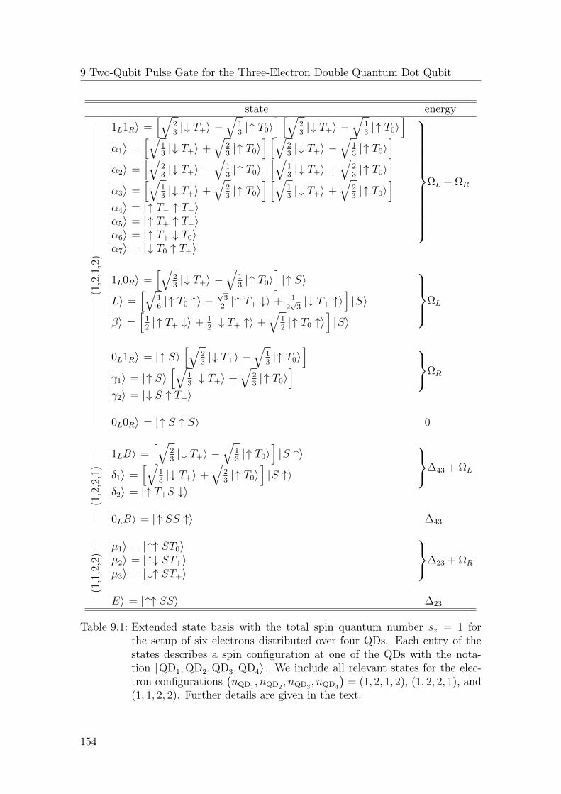
9 Two-Qubit Pulse Gate for the Three-Electron Double Quantum Dot Qubit
state energy———————————–(1,2,1,2)———————————– |1L1R〉 =
[√23|↓ T+〉 −
√13|↑ T0〉
] [√23|↓ T+〉 −
√13|↑ T0〉
] ΩL + ΩR
|α1〉 =[√
13|↓ T+〉 +
√23|↑ T0〉
] [√23|↓ T+〉 −
√13|↑ T0〉
]|α2〉 =
[√23|↓ T+〉 −
√13|↑ T0〉
] [√13|↓ T+〉 +
√23|↑ T0〉
]|α3〉 =
[√13|↓ T+〉 +
√23|↑ T0〉
] [√13|↓ T+〉 +
√23|↑ T0〉
]|α4〉 = |↑ T− ↑ T+〉|α5〉 = |↑ T+ ↑ T−〉|α6〉 = |↑ T+ ↓ T0〉|α7〉 = |↓ T0 ↑ T+〉
|1L0R〉 =[√
23|↓ T+〉 −
√13|↑ T0〉
]|↑ S〉
ΩL|L〉 =[√
16|↑ T0 ↑〉 −
√3
2|↑ T+ ↓〉 + 1
2√
3|↓ T+ ↑〉
]|S〉
|β〉 =[
12|↑ T+ ↓〉 + 1
2|↓ T+ ↑〉 +
√12|↑ T0 ↑〉
]|S〉
|0L1R〉 = |↑ S〉[√
23|↓ T+〉 −
√13|↑ T0〉
] ΩR|γ1〉 = |↑ S〉[√
13|↓ T+〉 +
√23|↑ T0〉
]|γ2〉 = |↓ S ↑ T+〉
|0L0R〉 = |↑ S ↑ S〉 0
—(1,2,2,1)— |1LB〉 =
[√23|↓ T+〉 −
√13|↑ T0〉
]|S ↑〉
∆43 + ΩL|δ1〉 =[√
13|↓ T+〉 +
√23|↑ T0〉
]|S ↑〉
|δ2〉 = |↑ T+S ↓〉
|0LB〉 = |↑ SS ↑〉 ∆43
–(1,1,2,2)– |µ1〉 = |↑↑ ST0〉
∆23 + ΩR|µ2〉 = |↑↓ ST+〉|µ3〉 = |↓↑ ST+〉
|E〉 = |↑↑ SS〉 ∆23
Table 9.1: Extended state basis with the total spin quantum number sz = 1 forthe setup of six electrons distributed over four QDs. Each entry of thestates describes a spin configuration at one of the QDs with the nota-tion |QD1,QD2,QD3,QD4〉 . We include all relevant states for the elec-tron configurations
(nQD1
, nQD2, nQD3
, nQD4
)= (1, 2, 1, 2), (1, 2, 2, 1), and
(1, 1, 2, 2). Further details are given in the text.
154

CHAPTER 10
Summary and Outlook
“The journey to this destination [quantum computation] will leadto many new scientific and technological developments with myriadpotential societal and economic benefits. (...) The journey aheadwill be challenging but it is one that will lead to unprecedented ad-vances in both fundamental scientific understanding and practicalnew technologies.” (R. Hughes, 2004 [213])
10.1 Summary
Quantum dot (QD) spin qubits are promising candidates to realize a quantum com-puter because they can fulfill all the five requirements for quantum computationof Sec. 1.2. Typical realizations are QDs in GaAs and Silicon heterostructures.Ref. [18] should be highlighted in which the spin qubit quantum computer has beenproposed for the first time. An electron is a spin-1
2particle, which is described by a
two-level quantum system. Therefore, electron spin is a natural candidate to encodea qubit. The spin is well protected from electric noise in semiconductors with weakspin-orbit interactions, but magnetic interactions dephase QD spin qubits. Today,finite-spin nuclei cause the dominant noise channel for spin qubits. These nucleihave small magnetic moments, but they collectively create macroscopic magneticfield fluctuations at a QD. The central proposal of Ref. [18] is a two-qubit gate forQD spin qubits that uses the exchange interaction between neighboring QD elec-trons. The electron transfer between two singly occupied QDs is allowed in a setupof two QDs in close proximity, but only the singlet configuration of the electronspermits this transfer for small detunings between the QDs.
Especially two-qubit exchange gates between single-spin qubits have been ex-tremely successful [37]. In contrast, the manipulations of single electron spins stillremain very challenging. Therefore, it is appealing to encode spin qubits in morethan one QD to realize qubits that have single-qubit exchange gates. The simplestexample is the singlet-triplet qubit (STQ) that is encoded using a two-electron dou-ble quantum dot (DQD) [50]. The control over the exchange interaction is sufficientto realize full single-qubit control for experiments at large global magnetic fieldswith a small magnetic field gradient across the DQD. Excellent single-qubit gatesfor STQs have been realized for GaAs DQDs [53, 54] and for Si DQDs [39, 56].
Chapter 5 and Chapter 6 describe STQs that are encoded in unconventional
155

10 Summary and Outlook
DQD setups. Chapter 5 introduces a STQ coded using multielectron QDs. Thisqubit encoding protects the exchange gate from charge noise. Charge traps in theheterostructure are uncontrollably filled with electrons, which causes electric fieldfluctuations at the position of the QD. A six-electron DQD has a charge configu-ration that protects this qubit much better from electric field fluctuations than thecharge configuration of the two-electron DQD. Chapter 6 analyzes a DQD that con-tains one large QD and one small QD. The strongly confined QD has a two-electronsinglet ground state, but the sz = 0 triplet state is lower in energy for the weaklyconfined QD. Spin-orbit interactions couple the logical qubit states of the STQ,and full single-qubit control is provided using electric manipulations of the chargeconfiguration.
Experiments have not realized high-fidelity two-qubit gates so far. Chapter 4describes how Coulomb interactions between DQDs enable two-qubit gates, andChapter 7 analyzes mediated entangling operations via one QS. The second ap-proach provides short, high-fidelity entangling operations for STQs that are wellcontrolled experimentally. These operations can readily be implemented because allthe necessary manipulation techniques have been realized in experiments.
The three-electron spin qubit can be controlled by the orbital interactions alone[65]. Chapter 8 analyzes the exchange-only qubit that is encoded using three singlyoccupied QDs, and the coherence properties of this qubit are extracted. The three-electron configuration at a DQD encodes a qubit (the “Madison qubit”) in a similarway as for the exchange-only qubit. The Madison qubit is only protected from chargenoise in its idle configuration, but pulse gates, which are very sensitive to chargenoise, manipulate the Madison qubit. These operations are, however, extremelyfast, and the Madison qubit can remain in its idle state for most of the time. Single-qubit gates for the Madison qubit were realized with impressive fidelities [74, 75].Chapter 9 describes a two-qubit gate for the Madison qubit of the same principle asfor the existing single-qubit gates.
In summary, many different spin qubit encodings have been suggested and imple-mented. Nevertheless, universal single-qubit control and a high-fidelity two-qubitgate have not been realized for the same setup. STQs are an outstanding candi-date to realize this universal qubit control. There are excellent single-qubit gatesfor STQs already, and the proposal of the mediated exchange gate in Chapter 7completes the set of high-fidelity gates that are required for the universal control ofthis qubit.
10.2 The Way Ahead
It remains interesting to see how the research field of spin qubit quantum computa-tion develops, especially when considering the many possibilities for how technologycan advance. The following pages propose two specific experiments for triple quan-tum dots (TQDs) that have the potential to advance the field of spin qubit quantumcomputation.
156

10.2 The Way Ahead
Noise cancellation by global magnetic fields — Finite spin nuclei cause local,low-frequency magnetic field fluctuations at every QD that have been identifiedto be the dominant dephasing mechanism in TQD spin qubit experiments [66, 67]Global magnetic fields can refocus this noise channel for the exchange-only qubit.1Fig. 10.1(a) shows the setup of three singly occupied QDs. The current through amicrowave transmission line induces a weak magnetic field that is perpendicular tothe global, external magnetic field. A single-spin qubit at gate-defined QDs [44] anda donor-bound spin qubit [21–23] have been manipulated with magnetic field pulsescreated from a microwave transmission line. The specific nature of the exchange-only qubit allows the refocusing of the nuclear spin noise with global magnetic fieldsacross all three QDs.
HbL
BzBx
J,DJS=
1
2, sz=-
1
2
S=1
2, sz=
1
2
È11\
È01\
È10\
È00\
Figure 10.1: Correction of low-frequency noise for the exchange-only qubit. (a)Setup of three singly occupied QDs and a microwave transmission line.The exchange-only qubit can be controlled by the exchange interactionsJ12 and J23. Electric currents through the microwave transmission linegenerate a magnetic fields Bx that has the same magnitude at everyQD. Bx is perpendicular to the global magnetic field Bz at the QDs.(b) Energy diagram of the TQD qubit. Two equivalent S = 1
2subspaces
(labeled by the sz quantum number) are present for the TQD qubit,and they are energetically separated by the applied external magneticfield. A formal quantum number l is assigned to the states in each szsubspace. The state notation
∣∣n 12− sz
⟩describes the computational
basis, with n, 12− sz ∈ 1, 0. The sum of the exchange interactions
J = J12+J23
2and their difference ∆J = J12−J23
2control an exchange-only
qubit coded in each of these subspaces. Local magnetic field fluctu-ations change the energy diagram with antisymmetric fluctuations ofthe subspaces sz = 1
2and sz = −1
2(shown in red). Bx drives transi-
tions between these subspaces. This mechanism can be used for noisecorrections.
The TQD qubit encoding should be reviewed briefly (cf. Sec. 2.4, Chapter 4,1I thank Charles Marcus and Mark Rudner for pointing out to me the antisymmetric “breathing”characteristic of nuclear spin noise for TQDs.
157

10 Summary and Outlook
and Chapter 8). This qubit is encoded using three singly occupied QDs. The spinaddition rules determine a pair of two-dimensional subspaces. These subspaces aredescribed by the spin quantum numbers S = 1
2, sz = 1
2and S = 1
2, sz = −1
2. Total
S = 12can be constructed by either adding S = 1
2to S = 0 or by adding S = 1
2to
S = 1. A formal quantum number l is assigned to these two paths. The four basisstates of S = 1
2, which are labeled by
∣∣ l 12− sz
⟩, are:
|11〉 = − |↓〉2 ⊗ |S〉1,3|01〉 =
√13|↓〉2 ⊗ |T0〉1,3 −
√23|↑〉2 ⊗ |T−〉1,3
S =
1
2, sz = −1
2, (10.1)
|10〉 = |↑〉2 ⊗ |S〉1,3|00〉 =
√13|↑〉2 ⊗ |T0〉1,3 −
√23|↓〉2 ⊗ |T+〉1,3
S =
1
2, sz =
1
2. (10.2)
|S〉 ij =(|↑↓〉 ij − |↓↑〉 ij
)/√
2 is the singlet state of the electrons at QDi and QDj;
|T+〉 ij = |↑↑〉 ij, |T0〉 ij =(|↑↓〉 ij + |↓↑〉 ij
)/√
2, and |T−〉 ij = |↓↓〉 ij are the tripletstates of the electrons at QDi and QDj. The proposed refocusing protocol is idealfor the exchange-only qubit in the subsystem encoding, which encodes the qubits inthe l quantum number [29]. The sz quantum number will only be used for the noisecorrections. A linear QD setup [cf. Fig. 10.1(a)] contains the exchange interactionbetween QD1 and QD2 (J12
4σ1 · σ2) and the exchange interaction between QD2 and
QD3 (J23
4σ2 · σ3). The effective Hamiltonian for the S = 1
2subspace is:
H =J
2σlz ⊗ 1sz +
Ez2
1l ⊗ σszz + ε (t)σlx ⊗ 1sz + Ex (t) 1l ⊗ σszx +δt2σlz ⊗ σszz , (10.3)
where σx = |1〉 〈0| + |0〉 〈1| and σz = |1〉 〈1| − |0〉 〈0| are Pauli operators. The firstterm describes the sum of the exchange interactions J = J12+J23
2, and the second
term describes the global magnetic field Ez = −gµBBz for Bz = B1z = B2
z = B3z .
These two terms are kept constant. The difference between the exchange interactionsε (t) =
√3
4(J12 − J23) can be tuned slightly at constant J . ε (t) provides universal
single qubit control (cf. Chapter 4). Ex (t) = −gµB2Bx, with Bx = B1
x = B2x =
B3x, is the global magnetic field created by electric currents through the microwave
transmission line; Bix is perpendicular to Bz at the QDs. Ex (t) will be used to
refocus quasi-static noise.The last term in Eq. (10.3) describes the dominant noise channel for exchange-
only qubits that is caused by local magnetic field fluctuations (cf. Chapter 4). Thetransverse noise components can be neglected at large J . Note that the energyfluctuations are antisymmetric between the sz subspaces. In other words, the fluc-tuation for the sz = −1
2subspace is δt
2σlz, but it is − δt
2σlz for the sz = 1
2subspace.
Fast pulses that change the sz quantum number at constant l refocus slow fluctua-tions in δt. Turning Ex (t) = A cos
(Ezt~
)on for the time h
2A at ε (t) = 0 flips the szspin configuration. This operation is called
(1l ⊗Xsz
). A noisy time evolution for
the time τ , which is called (1)τ , can be corrected using the sequence(1l ⊗Xsz
)(1)τ/2
(1l ⊗Xsz
)(1)τ/2 . (10.4)
158
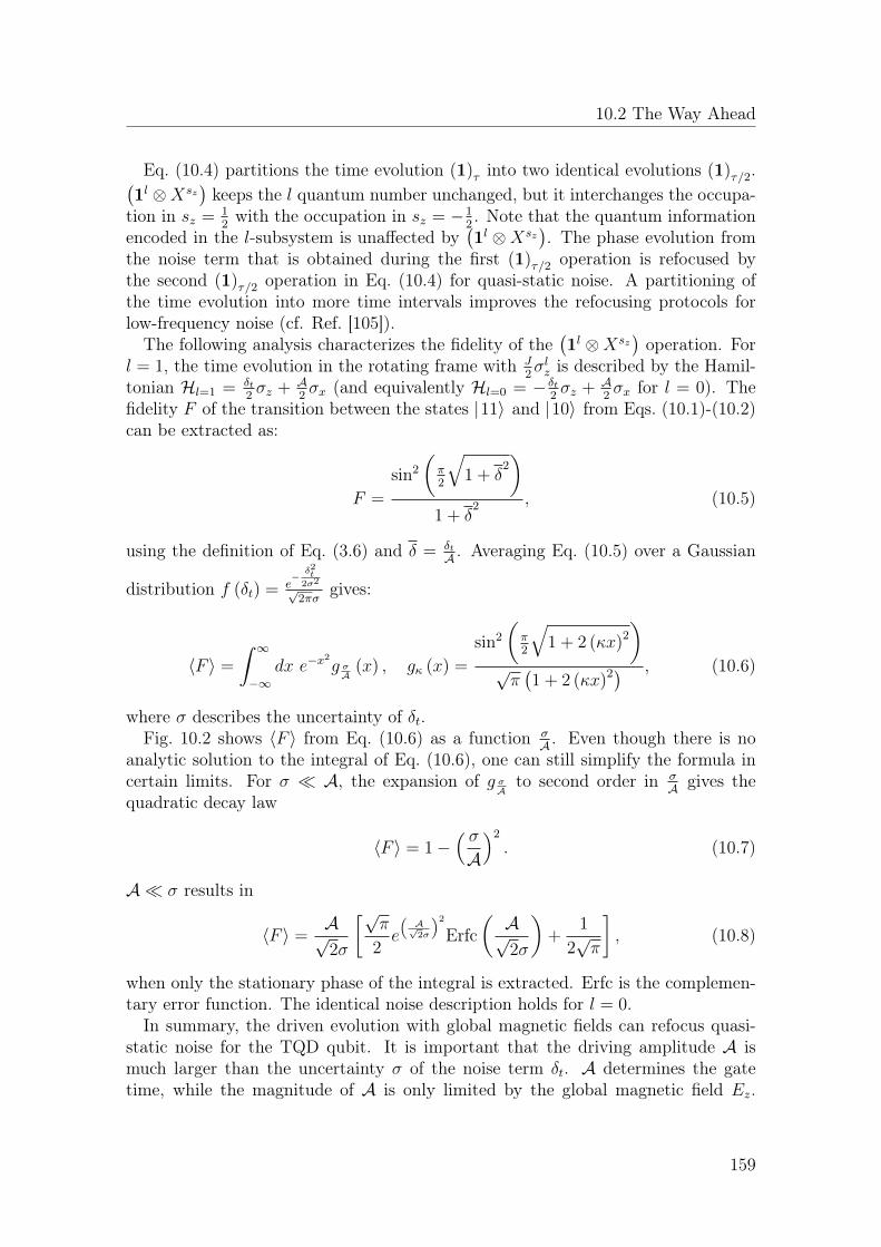
10.2 The Way Ahead
Eq. (10.4) partitions the time evolution (1)τ into two identical evolutions (1)τ/2.(1l ⊗Xsz
)keeps the l quantum number unchanged, but it interchanges the occupa-
tion in sz = 12with the occupation in sz = −1
2. Note that the quantum information
encoded in the l-subsystem is unaffected by(1l ⊗Xsz
). The phase evolution from
the noise term that is obtained during the first (1)τ/2 operation is refocused bythe second (1)τ/2 operation in Eq. (10.4) for quasi-static noise. A partitioning ofthe time evolution into more time intervals improves the refocusing protocols forlow-frequency noise (cf. Ref. [105]).
The following analysis characterizes the fidelity of the(1l ⊗Xsz
)operation. For
l = 1, the time evolution in the rotating frame with J2σlz is described by the Hamil-
tonian Hl=1 = δt2σz + A
2σx (and equivalently Hl=0 = − δt
2σz + A
2σx for l = 0). The
fidelity F of the transition between the states |11〉 and |10〉 from Eqs. (10.1)-(10.2)can be extracted as:
F =
sin2
(π2
√1 + δ
2)
1 + δ2 , (10.5)
using the definition of Eq. (3.6) and δ = δtA . Averaging Eq. (10.5) over a Gaussian
distribution f (δt) = e−δ2t
2σ2√
2πσgives:
〈F 〉 =
∫ ∞−∞
dx e−x2
g σA
(x) , gκ (x) =
sin2
(π2
√1 + 2 (κx)2
)√π(1 + 2 (κx)2) , (10.6)
where σ describes the uncertainty of δt.Fig. 10.2 shows 〈F 〉 from Eq. (10.6) as a function σ
A . Even though there is noanalytic solution to the integral of Eq. (10.6), one can still simplify the formula incertain limits. For σ A, the expansion of g σ
Ato second order in σ
A gives thequadratic decay law
〈F 〉 = 1−( σA
)2
. (10.7)
A σ results in
〈F 〉 =A√2σ
[√π
2e
(A√2σ
)2
Erfc(A√2σ
)+
1
2√π
], (10.8)
when only the stationary phase of the integral is extracted. Erfc is the complemen-tary error function. The identical noise description holds for l = 0.
In summary, the driven evolution with global magnetic fields can refocus quasi-static noise for the TQD qubit. It is important that the driving amplitude A ismuch larger than the uncertainty σ of the noise term δt. A determines the gatetime, while the magnitude of A is only limited by the global magnetic field Ez.
159

10 Summary and Outlook
0.0 0.2 0.4 0.6 0.8 1.00.0
0.2
0.4
0.6
0.8
1.0
ΣA
XF\
Figure 10.2: Fidelity of the time evolution for the time h2A with the Hamiltonian
Hl=1,0 = ± δt2σz + A
2σx and the noisy variable δt. 〈F 〉 decays with σ
A ,where σ is the uncertainty of δt. The blue dashed line describes aquadratic decay law, according to Eq. (10.7), which is valid for σ A.The red line describes the result of Eq. (10.8), which is valid for σ A.
Note that these refocusing gates can be much faster than the refocusing gates thatuse electric modifications of ε (t). For them, the driving amplitude of ε (t) is limitedby J when the equivalent driven refocusing protocol should be applied.Cavity QED and the exchange-only qubit — TQD qubits have the potential to
couple to a cavity strongly, while the TQDs are still operated at their optimaloperating point. In contrast, large coupling strengths between a cavity and a STQare only obtained when the DQD is operated far from its optimal operating point,which is the symmetric (1, 1) configuration [214, 215]. These STQs now have shortcoherence times because charge noise couples very efficiently to STQs that are tunedaway from the (1, 1) configuration. Note also the proposal for cavity couplings to thetunneling barrier of a DQD [216]. However, the manipulation of tunnel couplingsthrough electric fields has already failed to realize coherent qubit control.
The so-called resonant exchange qubit is coded using a symmetric TQD in the(nQD1
, nQD2, nQD3
) = (1, 1, 1) configuration (cf. Fig. 10.3) [68]. The definitions ofSec. 2.4 are used, while the couplings between QD1 and QD2 and between QD2 andQD3 have the same magnitudes. The tunnel coupling between QD1 and QD2 equalsthe tunnel coupling between QD2 and QD3 (and it is called τ). The electron fillingof QD2 is made unfavorable, which increases the occupations in (2, 0, 1) and (1, 0, 2).The addition energy U1 (U3) to add a second electron to QD1 (QD3) is much smallerthan the addition energy to add a second electron to QD2. As a consequence, theexchange interactions J12 ≈ 2τ2
U1and J23 ≈ 2τ2
U3increase. The optimal operation
point of an exchange-only qubit is realized for J12 = J23. The coherence times ofresonant exchange qubits in GaAs TQDs are astonishingly long (Ref. [67] extracteddephasing times of 10 µs).The exchange-only qubit has the excited qubit state |1〉 = |↑〉2 ⊗ |S〉1,3 and
160
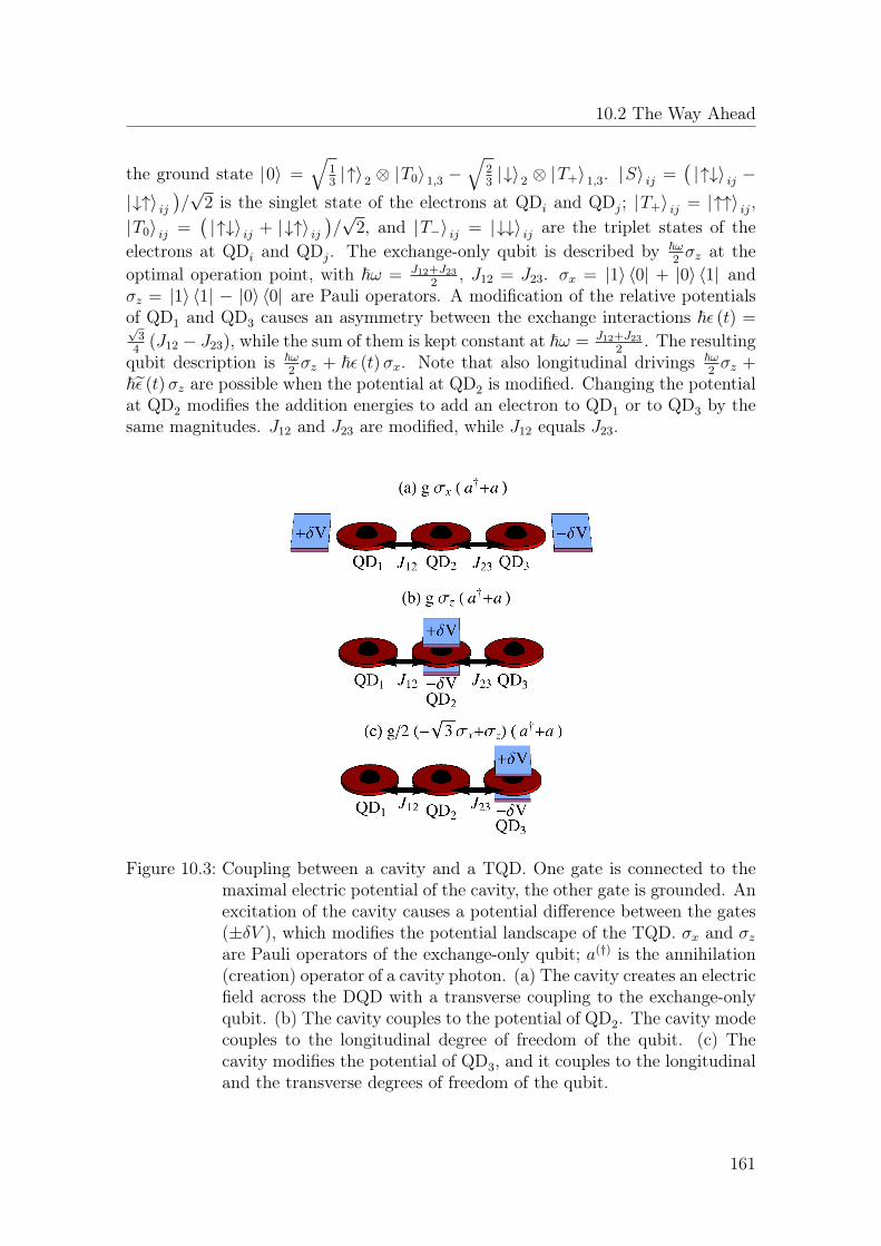
10.2 The Way Ahead
the ground state |0〉 =√
13|↑〉2 ⊗ |T0〉1,3 −
√23|↓〉2 ⊗ |T+〉1,3. |S〉 ij =
(|↑↓〉 ij −
|↓↑〉 ij)/√
2 is the singlet state of the electrons at QDi and QDj; |T+〉 ij = |↑↑〉 ij,|T0〉 ij =
(|↑↓〉 ij + |↓↑〉 ij
)/√
2, and |T−〉 ij = |↓↓〉 ij are the triplet states of theelectrons at QDi and QDj. The exchange-only qubit is described by ~ω
2σz at the
optimal operation point, with ~ω = J12+J23
2, J12 = J23. σx = |1〉 〈0| + |0〉 〈1| and
σz = |1〉 〈1| − |0〉 〈0| are Pauli operators. A modification of the relative potentialsof QD1 and QD3 causes an asymmetry between the exchange interactions ~ε (t) =√
34
(J12 − J23), while the sum of them is kept constant at ~ω = J12+J23
2. The resulting
qubit description is ~ω2σz + ~ε (t)σx. Note that also longitudinal drivings ~ω
2σz +
~ε (t)σz are possible when the potential at QD2 is modified. Changing the potentialat QD2 modifies the addition energies to add an electron to QD1 or to QD3 by thesame magnitudes. J12 and J23 are modified, while J12 equals J23.
Figure 10.3: Coupling between a cavity and a TQD. One gate is connected to themaximal electric potential of the cavity, the other gate is grounded. Anexcitation of the cavity causes a potential difference between the gates(±δV ), which modifies the potential landscape of the TQD. σx and σzare Pauli operators of the exchange-only qubit; a(†) is the annihilation(creation) operator of a cavity photon. (a) The cavity creates an electricfield across the DQD with a transverse coupling to the exchange-onlyqubit. (b) The cavity couples to the potential of QD2. The cavity modecouples to the longitudinal degree of freedom of the qubit. (c) Thecavity modifies the potential of QD3, and it couples to the longitudinaland the transverse degrees of freedom of the qubit.
161

10 Summary and Outlook
The electromagnetic modes of a cavity can couple capacitively to the charge con-figuration of a TQD. A setup is envisioned where one electric gate is connected to amicrowave transmission line at the maximal amplitude of the electric field. The sec-ond gate is connected to the ground electrode of the cavity. If the cavity is excited,then there is a potential difference between these contacts. A similar setup was usedto couple a cavity to gate-defined DQDs in GaAs [217, 218]. Fig. 10.3 proposes threedifferent setups that connect a cavity and a TQD. In the setup of Fig. 10.3(a), thecavity creates a global electric field across the TQD. A potential difference betweenQD1 and QD3 couples the states |1〉 and |0〉 , which has an interaction ∝ σx on thecomputational subspace. If the cavity changes the potential at QD2, as described inFig. 10.3(b), then it modifies the energy difference between |1〉 and |0〉 , which hasan interaction ∝ σz on the computational subspace. Finally, if the cavity modifiesthe potential at QD3, as described in Fig. 10.3(c), then only J23 is modified. Thecavity mode acts on the computational subspace ∝
(−√
32σx + 1
2σz
).
Potential changes of a few µeV can be realized through single excitations of cavityphotons [217, 218]. Ideally, spin qubits are immune to small changes of the electro-static potentials. Also STQs have to be tuned far away from their ideal operationpoint in the (1, 1) configuration to be sensitive to µeV potential modifications. In atrade-off, the influence of charge noise increases, but the coherence times of STQsdecrease. The resonant exchange-only qubit is operated in a regime with large hy-bridizations between the (1, 1, 1), (2, 0, 1), and (1, 0, 2) charge configurations, whileit still keeps high coherence times. The mixing between the different charge con-figurations depends on the qubit state, and a state-dependent dipole moment iscreated. An excited cavity mode creates a local electric field that couples to thisstate dependent dipole moment. Therefore, the exchange-only qubit is sensitive toµeV potential changes generated from cavity photons at its optimal operating point.
The system of two exchange-only qubits [labeled by (1) and (2)] that are coupledto the same cavity is described by
H =∑j=1,2
~ωj2σ(j)z + ~ωR
(a†a+
1
2
)+∑j=1,2
~gj(−sjσ(j)
x + cjσ(j)z
) (a† + a
). (10.9)
The first term in Eq. (10.9) describes two exchange-only qubits at their optimaloperation points. The second term describes a single mode of a cavity, which hasthe resonance frequency ωR. a(†) is the annihilation (creation) operator of a photonat frequency ωR. The third term describes the capacitive coupling between thecavity and the qubits. cj = cos (θj) and sj = sin (θj) describe the rotation angleθj. The case cj = 1 is called the longitudinal coupling, and sj = 1 is called thetransverse coupling. Note that the rotation angles are −π
2, 0, and π
3in the setups of
Fig. 10.3(a)-(c).For weak interactions between the cavity and the qubits gj ωj, ωR, effective in-
teractions between the two qubits are caused by virtual excitations of the cavity if thecavity is detuned from the qubits (|ωR − ωj| 0). The couplings between the cav-ity and the qubits can be removed perturbatively [219–221]. H0 =
∑j=1,2
~ωj2σ
(j)z +
162

10.2 The Way Ahead
~ωR(a†a+ 1
2
)is the dominant part of the Hamiltonian, and H1 =
∑j=1,2 ~g(j)(
−sjσ(j)x + cjσ
(j)z
) (a† + a
)is a small perturbation. The operators S(j) = S(j)
t +S(j)l
are constructed, with[S(1) + S(2),H0
]= −H1. S(j)
t = −gjsj[
1ωj−ωR
(σ
(j)+ a− σ(j)
− a†)
+
1ωj+ωR
(σ
(j)+ a† − σ(j)
− a) ]
removes the transverse qubit coupling, and S(j)l = gjcj
1ωRσ
(j)z(
a† − a)removes the longitudinal term. σ(j)
± =σ
(j)x ±iσ
(j)y
2are the ladder operators.
The transformed Hamiltonian H′ = eS(1)+S(2)H e−(S(1)+S(2)) is simplified in second-
order Schrieffer-Wolff perturbation theory to
H′ ≈H0 +1
2
[S(1) + S(2),H1
]=∑j
~ω(j)
2σ(j)z + ~ωR
(a†a+
1
2
)− 2~g1g2c1c2
ωRσ(1)z σ(2)
z
+~g1g2s1s2
2
∑j=1,2
(1
ωj − ωR− 1
ωj + ωR
)σ(1)x σ(2)
x . (10.10)
The descriptions of the cavity and the qubits remain formally unchanged. Thequbit’s eigenfrequency is modified to ωi = ωj + (gjsj)
2(
1ω1−ωR
+ 1ω1+ωR
)(1 + 2a†a+
a†a† + aa) from the ac Stark shift and the ac Lamb shift [219, 220]. The third andthe fourth terms of Eq. (10.10) are effective interactions between the qubits that canbe used for entangling operations. The σ(1)
z σ(2)z interaction can create a CPHASE
gate, and the σ(1)x σ
(2)x interaction can create a
√iSWAP gate (cf. Chapter 4). Note
that either a pure transverse coupling (s1 = s2 = 1) or a pure longitudinal coupling(c1 = c2 = 1) to the qubit subspace is favorable for these entangling operationsbecause either the third or the fourth term of Eq. (10.10) is maximized.
Cavity-qubit setups that contain both the longitudinal and the transverse cou-pling terms (ci 6= 0 and si 6= 0), as in the setup in Fig. 10.3(c), are ideal for atuning protocol with sideband transitions. Sideband transitions provide universalcontrol of qubits that are coupled to a cavity, when the cavity can be driven with mi-crowave signals of different frequencies [222]. Manipulation protocols with sidebandtransitions are used for qubit encodings using trapped ions [223] or trapped neutralatoms [224]. A drive of the cavity HD = ~εD
(a†e−iωDt + aeiωDt
)renormalizes the
energy splittings of the qubits ˜ωj = ωj + 2ωj−ωD
(gjsjεDωR−ωD
)2
, and it introduces simul-taneous transitions of the cavity and the qubits. Additionally to the Hamiltonianin Eq. (10.10), a coupling term of the cavity and the qubits appears [220]2:
−2~εD∑j=1,2
g2j cjsj
(ωj − ωD) (ωR − ωD)
(σ
(j)+ e−iωDt + σ
(j)− e
iωDt) (a† + a
)(10.11)
2Minor errors of Ref. [220] are corrected.
163

10 Summary and Outlook
Eq. (10.11) is finite only for a mixed longitudinal and transverse couplings (ci 6= 0and si 6= 0), and the drive gains influence only when the cavity is driven at specificfrequencies. The blue sideband transition at ωD = ˜ωj + ωR excites both the qubitand the cavity. The red sideband transition at ωD = ˜ωj−ωR drives an excited stateof the qubit to the ground state, while it destroys one photon.
164

Bibliography
[1] R. P. Feynman, Int. J. Theor. Phys. 21, 467 (1982).
[2] J. J. Sakurai and S. F. Tuan, Modern Quantum Mechanics (Addison-Wesley,Reading, 1994).
[3] A. Messiah, Quantenmechanik, Vol. 1 und 2 (DeGruyter, Berlin, 1979).
[4] G. Benenti, G. Casati, and G. Strini, Principles of Quantum Computation andInformation - Volume I: Basic Concepts (World Scientific, Singapore, 2004).
[5] A. Einstein, B. Podolsky, and N. Rosen, Phys. Rev. 47, 777 (1935).
[6] M. A. Nielsen and I. L. Chuang, Quantum Computation and Quantum Infor-mation (Cambridge University Press, Cambridge, 2000).
[7] I. M. Georgescu, S. Ashhab, and F. Nori, Rev. Mod. Phys. 86, 153 (2014).
[8] D. Deutsch, Physics World 57 (1992).
[9] D. Deutsch, Proc. R. Soc. Lond. A 400, 97 (1985).
[10] J. Preskill, Lecture notes for physics 229: Quantum information and compu-tation, California Institute of Technology (1998).
[11] N. D. Mermin, Quantum Computer Science (Cambridge University Press,Cambridge, 2007).
[12] J. Kempe, Quantum Algorithm, edited by D. Bruß and G. Leuchs, Lectureson Quantum Information (Wiley-VCH, Weinheim, 2007).
[13] B. Kraus, Topics in Quantum Information, edited by D. DiVincenzo, QuantumInformation Processing (Forschungszentrum Jülich, Jülich, 2013).
[14] P. W. Shor, SIAM J. Comput. 26, 1484 (1997).
[15] E. Lucero, R. Barends, Y. Chen, J. Kelly, M. Mariantoni, A. Megrant,P. O’Malley, D. Sank, A. Vainsencher, J. Wenner, T. White, Y. Yin, A. N.Cleland, and J. M. Martinis, Nat. Phys. 8, 719 (2012).
[16] D. P. DiVincenzo, Fortschr. Phys. 48, 9 (2000).
[17] A. Barenco, C. H. Bennett, R. Cleve, D. P. DiVincenzo, N. Margolus, P. Shor,T. Sleator, J. A. Smolin, and H. Weinfurter, Phys. Rev. A 52, 3457 (1995).
165

Bibliography
[18] D. Loss and D. P. DiVincenzo, Phys. Rev. A 57, 120 (1998).
[19] D. P. DiVincenzo and D. Loss, Superlattice Microst. 23, 419 (1998).
[20] B. E. Kane, Nature (London) 393, 133 (1998).
[21] J. J. Pla, K. Y. Tan, J. P. Dehollain, W. H. Lim, J. J. L. Morton, D. N.Jamieson, A. S. Dzurak, and A. Morello, Nature (London) 489, 541 (2012).
[22] J. J. Pla, K. Y. Tan, J. P. Dehollain, W. H. Lim, J. J. L. Morton, F. A.Zwanenburg, D. N. Jamieson, A. S. Dzurak, and A. Morello, Nature (London)496, 334 (2013).
[23] J. T. Muhonen, J. P. Dehollain, A. Laucht, F. E. Hudson, T. Sekiguchi, K. M.Itoh, D. N. Jamieson, J. C. McCallum, A. S. Dzurak, and A. Morello, Nat.Nanotechnol. 9, 986 (2014).
[24] R. J. Warburton, Nature Mater. 12, 483 (2013).
[25] M. H. Devoret, A. Wallraff, and J. M. Martinis, arXiv:cond-mat/0411174[cond-mat.mes-hall] (2004).
[26] M. H. Devoret and R. J. Schoelkopf, Science 339, 1169 (2013).
[27] S. Mehl and D. P. DiVincenzo, Phys. Rev. B 88, 161408 (2013).
[28] S. Mehl, H. Bluhm, and D. P. DiVincenzo, Phys. Rev. B 90, 045404 (2014).
[29] S. Mehl and D. P. DiVincenzo, Phys. Rev. B 87, 195309 (2013).
[30] L. P. Kouwenhoven, D. G. Austing, and S. Tarucha, Rep. Prog. Phys. 64, 701(2001).
[31] R. Hanson, L. P. Kouwenhoven, J. R. Petta, S. Tarucha, and L. M. K. Van-dersypen, Rev. Mod. Phys. 79, 1217 (2007).
[32] T. Hayashi, T. Fujisawa, H. D. Cheong, Y. H. Jeong, and Y. Hirayama, Phys.Rev. Lett. 91, 226804 (2003).
[33] J. R. Petta, A. C. Johnson, C. M. Marcus, M. P. Hanson, and A. C. Gossard,Phys. Rev. Lett. 93, 186802 (2004).
[34] K. D. Petersson, J. R. Petta, H. Lu, and A. C. Gossard, Phys. Rev. Lett.105, 246804 (2010).
[35] G. Cao, H.-O. Li, T. Tu, L. Wang, C. Zhou, M. Xiao, G.-C. Guo, H.-W. Jiang,and G.-P. Guo, Nat. Commun. 4, 1401 (2013).
166

Bibliography
[36] R. Winkler, Spin–Orbit Coupling Effects in Two-Dimensional Electron andHole Systems, Springer Tracts in Modern Physics Vol. 191 (Springer, Berlin,2010).
[37] J. R. Petta, A. C. Johnson, J. M. Taylor, E. A. Laird, A. Yacoby, M. D. Lukin,C. M. Marcus, M. P. Hanson, and A. C. Gossard, Science 309, 2180 (2005).
[38] K. C. Nowack, M. Shafiei, M. Laforest, G. E. D. K. Prawiroatmodjo, L. R.Schreiber, C. Reichl, W. Wegscheider, and L. M. K. Vandersypen, Science333, 1269 (2011).
[39] B. M. Maune, M. G. Borselli, B. Huang, T. D. Ladd, P. W. Deelman, K. S.Holabird, A. A. Kiselev, I. Alvarado-Rodriguez, R. S. Ross, A. E. Schmitz,M. Sokolich, C. A. Watson, M. F. Gyure, and A. T. Hunter, Nature (London)481, 344 (2012).
[40] A. C. Johnson, J. R. Petta, J. M. Taylor, A. Yacoby, M. D. Lukin, C. M.Marcus, M. P. Hanson, and A. C. Gossard, Nature (London) 435, 925 (2005).
[41] C. Barthel, D. J. Reilly, C. M. Marcus, M. P. Hanson, and A. C. Gossard,Phys. Rev. Lett. 103, 160503 (2009).
[42] D. J. Reilly, C. M. Marcus, M. P. Hanson, and A. C. Gossard, Appl. Phys.Lett. 91, 162101 (2007).
[43] C. Barthel, M. Kjærgaard, J. Medford, M. Stopa, C. M. Marcus, M. P. Hanson,and A. C. Gossard, Phys. Rev. B 81, 161308 (2010).
[44] F. H. L. Koppens, C. Buizert, K.-J. Tielrooij, I. T. Vink, K. C. Nowack,T. Meunier, L. P. Kouwenhoven, and L. M. K. Vandersypen, Nature (London)442, 766 (2006).
[45] I. T. Vink, K. C. Nowack, F. H. L. Koppens, J. Danon, Y. V. Nazarov, andL. M. K. Vandersypen, Nat. Phys. 5, 764 (2009).
[46] K. C. Nowack, F. H. L. Koppens, Y. V. Nazarov, and L. M. K. Vandersypen,Science 318, 1430 (2007).
[47] E. A. Laird, C. Barthel, E. I. Rashba, C. M. Marcus, M. P. Hanson, and A. C.Gossard, Phys. Rev. Lett. 99, 246601 (2007).
[48] M. Pioro-Ladrière, T. Obata, Y. Tokura, Y.-S. Shin, T. Kubo, K. Yoshida,T. Taniyama, and S. Tarucha, Nat. Phys. 4, 776 (2008).
[49] M. Shafiei, K. C. Nowack, C. Reichl, W. Wegscheider, and L. M. K. Vander-sypen, Phys. Rev. Lett. 110, 107601 (2013).
[50] J. Levy, Phys. Rev. Lett. 89, 147902 (2002).
167

Bibliography
[51] J. M. Taylor, H.-A. Engel, W. Dür, A. Yacoby, C. M. Marcus, P. Zoller, andM. D. Lukin, Nat. Phys. 1, 177 (2005).
[52] J. M. Taylor, J. R. Petta, A. C. Johnson, A. Yacoby, C. M. Marcus, andM. D. Lukin, Phys. Rev. B 76, 035315 (2007).
[53] S. Foletti, H. Bluhm, D. Mahalu, V. Umansky, and A. Yacoby, Nat. Phys. 5,903 (2009).
[54] H. Bluhm, S. Foletti, D. Mahalu, V. Umansky, and A. Yacoby, Phys. Rev.Lett. 105, 216803 (2010).
[55] R. Brunner, Y.-S. Shin, T. Obata, M. Pioro-Ladrière, T. Kubo, K. Yoshida,T. Taniyama, Y. Tokura, and S. Tarucha, Phys. Rev. Lett. 107, 146801(2011).
[56] X. Wu, D. R. Ward, J. R. Prance, D. Kim, J. K. Gamble, R. T. Mohr, Z. Shi,D. E. Savage, M. G. Lagally, M. Friesen, S. N. Coppersmith, and M. A.Eriksson, Proc. Natl. Acad. Sci. 111, 11938 (2014).
[57] R. Hanson and G. Burkard, Phys. Rev. Lett. 98, 050502 (2007).
[58] J. Kempe, D. Bacon, D. A. Lidar, and K. B. Whaley, Phys. Rev. A 63, 042307(2001).
[59] D. A. Lidar and K. B. Whaley, Decoherence-Free Subspaces and Subsys-tems, edited by F. Benatti and R. Floreanini, Irreversible Quantum Dynamics(Springer, Berlin, 2003).
[60] C. Barthel, J. Medford, C. M. Marcus, M. P. Hanson, and A. C. Gossard,Phys. Rev. Lett. 105, 266808 (2010).
[61] H. Bluhm, S. Foletti, I. Neder, M. Rudner, D. Mahalu, V. Umansky, andA. Yacoby, Nat. Phys. 7, 109 (2011).
[62] J. Medford, L. Cywinski, C. Barthel, C. M. Marcus, M. P. Hanson, and A. C.Gossard, Phys. Rev. Lett. 108, 086802 (2012).
[63] I. van Weperen, B. D. Armstrong, E. A. Laird, J. Medford, C. M. Marcus,M. P. Hanson, and A. C. Gossard, Phys. Rev. Lett. 107, 030506 (2011).
[64] M. D. Shulman, O. E. Dial, S. P. Harvey, H. Bluhm, V. Umansky, andA. Yacoby, Science 336, 202 (2012).
[65] D. P. DiVincenzo, D. Bacon, J. Kempe, G. Burkard, and K. B. Whaley,Nature (London) 408, 339 (2000).
168
Bibliography
[66] J. Medford, J. Beil, J. M. Taylor, S. D. Bartlett, A. C. Doherty, E. I. Rashba,D. P. DiVincenzo, H. Lu, A. C. Gossard, and C. M. Marcus, Nat. Nanotechnol.8, 654 (2013).
[67] J. Medford, J. Beil, J. M. Taylor, E. I. Rashba, H. Lu, A. C. Gossard, andC. M. Marcus, Phys. Rev. Lett. 111, 050501 (2013).
[68] J. M. Taylor, V. Srinivasa, and J. Medford, Phys. Rev. Lett. 111, 050502(2013).
[69] B. H. Fong and S. M. Wandzura, Quantum Inf. Comput. 11, 1003 (2011).
[70] A. C. Doherty and M. P. Wardrop, Phys. Rev. Lett. 111, 050503 (2013).
[71] A. Pal, E. I. Rashba, and B. I. Halperin, Phys. Rev. X 4, 011012 (2014).
[72] Z. Shi, C. B. Simmons, J. R. Prance, J. K. Gamble, T. S. Koh, Y.-P. Shim,X. Hu, D. E. Savage, M. G. Lagally, M. A. Eriksson, M. Friesen, and S. N.Coppersmith, Phys. Rev. Lett. 108, 140503 (2012).
[73] T. S. Koh, J. K. Gamble, M. Friesen, M. A. Eriksson, and S. N. Coppersmith,Phys. Rev. Lett. 109, 250503 (2012).
[74] Z. Shi, C. B. Simmons, D. R. Ward, J. R. Prance, X. Wu, T. S. Koh, J. K.Gamble, D. E. Savage, M. G. Lagally, M. Friesen, S. N. Coppersmith, andM. A. Eriksson, Nat. Commun. 5, 3020 (2014).
[75] D. Kim, Z. Shi, C. B. Simmons, D. R. Ward, J. R. Prance, T. S. Koh, J. K.Gamble, D. E. Savage, M. G. Lagally, M. Friesen, S. N. Coppersmith, andM. A. Eriksson, Nature (London) 511, 70 (2014).
[76] C. P. Slichter, Principles of Magnetic Resonance (Springer, Berlin, 1990).
[77] L. M. K. Vandersypen and I. L. Chuang, Rev. Mod. Phys. 76, 1037 (2005).
[78] F. Marquardt and A. Püttmann, arXiv:0809.4403 [quant-ph] (2008).
[79] L. Chirolli and G. Burkard, Adv. Phys. 57, 225 (2008).
[80] H. Barnum, M. A. Nielsen, and B. Schumacher, Phys. Rev. A 57, 4153 (1998).
[81] D. C. Marinescu and G. M. Marinescu, Classical and Quantum Information(Elsevier, Amsterdam, 2012).
[82] C. W. J. Beenakker, arXiv:cond-mat/0508488 [cond-mat.mes-hall] (2005).
[83] G. Burkard, D. Loss, and D. P. DiVincenzo, Phys. Rev. B 59, 2070 (1999).
[84] I. A. Merkulov, A. L. Efros, and M. Rosen, Phys. Rev. B 65, 205309 (2002).
169

Bibliography
[85] W. A. Coish and J. Baugh, Phys. Status Solidi B 246, 2203 (2009).
[86] J. Schliemann, A. Khaetskii, and D. Loss, J. Phys.: Condens. Matter 15,R1809 (2003).
[87] L. V. C. Assali, H. M. Petrilli, R. B. Capaz, B. Koiller, X. Hu, and S. DasSarma, Phys. Rev. B 83, 165301 (2011).
[88] R. de Sousa, Topics Appl. Physics 115, 183 (2009).
[89] J. M. Taylor, Hyperfine interactions and quantum information processing inquantum dots, Ph.D. thesis, Harvard University Cambridge, Massachusetts(2006).
[90] D. J. Reilly, J. M. Taylor, E. A. Laird, J. R. Petta, C. M. Marcus, M. P.Hanson, and A. C. Gossard, Phys. Rev. Lett. 101, 236803 (2008).
[91] I. Neder, M. S. Rudner, H. Bluhm, S. Foletti, B. I. Halperin, and A. Yacoby,Phys. Rev. B 84, 035441 (2011).
[92] P. Cerfontaine, T. Botzem, D. P. DiVincenzo, and H. Bluhm, Phys. Rev. Lett.113, 150501 (2014).
[93] O. E. Dial, M. D. Shulman, S. P. Harvey, H. Bluhm, V. Umansky, andA. Yacoby, Phys. Rev. Lett. 110, 146804 (2013).
[94] X. Hu and S. Das Sarma, Phys. Rev. Lett. 96, 100501 (2006).
[95] A. V. Kuhlmann, J. Houel, A. Ludwig, L. Greuter, D. Reuter, A. D. Wieck,M. Poggio, and R. J. Warburton, Nat. Phys. 9, 570 (2013).
[96] V. N. Golovach, A. Khaetskii, and D. Loss, Phys. Rev. Lett. 93, 016601(2004).
[97] V. F. Gantmakher, Carrier Scattering in Metals and Semiconductors (NorthHolland, Amsterdam, 1987).
[98] S. Amasha, K. MacLean, I. Radu, D. M. Zumbuhl, M. A. Kastner, M. P.Hanson, and A. C. Gossard, arXiv:cond-mat/0607110 [cond-mat.mes-hall](2006).
[99] S. Amasha, K. MacLean, I. P. Radu, D. M. Zumbühl, M. A. Kastner, M. P.Hanson, and A. C. Gossard, Phys. Rev. Lett. 100, 046803 (2008).
[100] J. M. Elzerman, R. Hanson, L. H. W. van Beveren, B. Witkamp, L. M. K.Vandersypen, and L. P. Kouwenhoven, Nature (London) 430, 431 (2004).
[101] M. D. Shulman, S. P. Harvey, J. M. Nichol, S. D. Bartlett, A. C. Doherty,V. Umansky, and A. Yacoby, Nat. Commun. 5, 5156 (2014).
170

Bibliography
[102] K. Jacobs, Stochastic Processes for Physicists: Understanding Noisy Systems(Cambridge University Press, Cambridge, 2010).
[103] A. Cottet, Implementation of a quantum bit in a superconducting circuit, Ph.D.thesis, Université Paris VI (2002).
[104] G. Ithier, E. Collin, P. Joyez, P. J. Meeson, D. Vion, D. Esteve, F. Chiarello,A. Shnirman, Y. Makhlin, J. Schriefl, and G. Schön, Phys. Rev. B 72, 134519(2005).
[105] L. Cywiński, R. M. Lutchyn, C. P. Nave, and S. Das Sarma, Phys. Rev. B77, 174509 (2008).
[106] S. Großmann, Mathematischer Einführungskurs für die Physik, Vol. 9 (B. G.Teubner, Wiesbaden, 2004).
[107] Y. V. Nazarov and Y. M. Blanter, Quantum Transport: Introduction toNanoscience (Cambridge University Press, Cambridge, 2009).
[108] D. Klauser, W. A. Coish, and D. Loss, Phys. Rev. B 73, 205302 (2006).
[109] F. H. L. Koppens, D. Klauser, W. A. Coish, K. C. Nowack, L. P. Kouwenhoven,D. Loss, and L. M. K. Vandersypen, Phys. Rev. Lett. 99, 106803 (2007).
[110] E. Geva, R. Kosloff, and J. L. Skinner, J. Chem. Phys. 102, 8541 (1995).
[111] K. Blum, Density Matrix Theory and Applications (Plenum, New York, 1996).
[112] C. Rigetti, A. Blais, and M. Devoret, Phys. Rev. Lett. 94, 240502 (2005).
[113] C. Rigetti and M. Devoret, Phys. Rev. B 81, 134507 (2010).
[114] S. Ashhab, S. Matsuo, N. Hatakenaka, and F. Nori, Phys. Rev. B 74, 184504(2006).
[115] S. Ashhab and F. Nori, Phys. Rev. B 76, 132513 (2007).
[116] L. Trifunovic, O. Dial, M. Trif, J. R. Wootton, R. Abebe, A. Yacoby, andD. Loss, Phys. Rev. X 2, 011006 (2012).
[117] Ioffe Institute, Electronic archive: New Semiconductor Materials. Character-istics and Properties (http://www.ioffe.ru/SVA/NSM/, 2001).
[118] Y. Makhlin, Quantum Inf. Process. 1, 243 (2002).
[119] J. Zhang, J. Vala, S. Sastry, and K. B. Whaley, Phys. Rev. A 67, 042313(2003).
[120] N. Schuch and J. Siewert, Phys. Rev. A 67, 032301 (2003).
171

Bibliography
[121] M. Gullans, J. J. Krich, J. M. Taylor, H. Bluhm, B. I. Halperin, C. M. Marcus,M. Stopa, A. Yacoby, and M. D. Lukin, Phys. Rev. Lett. 104, 226807 (2010).
[122] W. A. Coish and D. Loss, Phys. Rev. B 72, 125337 (2005).
[123] E. Nielsen, R. W. Young, R. P. Muller, and M. S. Carroll, Phys. Rev. B 82,075319 (2010).
[124] E. Barnes, J. P. Kestner, N. T. T. Nguyen, and S. Das Sarma, Phys. Rev. B84, 235309 (2011).
[125] E. Nielsen, E. Barnes, J. P. Kestner, and S. Das Sarma, Phys. Rev. B 88,195131 (2013).
[126] A. P. Higginbotham, F. Kuemmeth, M. P. Hanson, A. C. Gossard, and C. M.Marcus, Phys. Rev. Lett. 112, 026801 (2014).
[127] D. K. Ferry, S. M. Goodnick, and J. Bird, Transport in Nanostructures:Chapter 6 (Cambridge University Press, Cambridge, 2009).
[128] V. Fock, Z. Phys. 47, 446 (1928).
[129] C. G. Darwin, Proc. Cambridge Philos. Soc. 27, 86 (1931).
[130] S. Yang, X. Wang, and S. Das Sarma, Phys. Rev. B 83, 161301 (2011).
[131] X. Wang, S. Yang, and S. Das Sarma, Phys. Rev. B 84, 115301 (2011).
[132] W. van der Wiel, S. D. Franceschi, J. M. Elzerman, T. Fujisawa, S. Tarucha,and L. P. Kouwenhoven, Rev. Mod. Phys. 75, 1 (2002).
[133] A. D. Güçlü, A. Ghosal, C. J. Umrigar, and H. U. Baranger, Phys. Rev. B77, 041301 (2008).
[134] D. V. Averin and K. K. Likharev, J. Low Temp. Phys. 62, 345 (1986).
[135] D. V. Averin, A. N. Korotkov, and K. K. Likharev, Phys. Rev. B 44, 6199(1991).
[136] Y. M. Galperin, B. L. Altshuler, J. Bergli, and D. V. Shantsev, Phys. Rev.Lett. 96, 097009 (2006).
[137] J. Schriefl, Y. Makhlin, A. Shnirman, and G. Schön, New J. Phys. 8, 1 (2006).
[138] Y. Nakamura, Y. A. Pashkin, T. Yamamoto, and J. S. Tsai, Phys. Rev. Lett.88, 047901 (2002).
[139] Y. Makhlin and A. Shnirman, Phys. Rev. Lett. 92, 178301 (2004).
[140] G. Ramon and X. Hu, Phys. Rev. B 81, 045304 (2010).
172

Bibliography
[141] J. D. Jackson, Classical Electrodynamics, 3rd ed. (Wiley, 1999).
[142] S. N. Shevchenko, S. Ashhab, and F. Nori, Phys. Rep. 492, 1 (2010).
[143] J. Kyriakidis, J. Phys.: Condens. Matter 17, 2715 (2005).
[144] X. Hu, Phys. Rev. B 83, 165322 (2011).
[145] J. K. Gamble, M. Friesen, S. N. Coppersmith, and X. Hu, Phys. Rev. B 86,035302 (2012).
[146] G. Burkard, Phys. Rev. B 79, 125317 (2009).
[147] F. Baruffa, P. Stano, and J. Fabian, Phys. Rev. Lett. 104, 126401 (2010).
[148] F. Baruffa, P. Stano, and J. Fabian, Phys. Rev. B 82, 045311 (2010).
[149] J. R. Petta, H. Lu, and A. C. Gossard, Science 327, 669 (2010).
[150] H. Ribeiro, J. R. Petta, and G. Burkard, Phys. Rev. B 82, 115445 (2010).
[151] H. Ribeiro, G. Burkard, J. R. Petta, H. Lu, and A. C. Gossard, Phys. Rev.Lett. 110, 086804 (2013).
[152] H. Ribeiro, J. R. Petta, and G. Burkard, Phys. Rev. B 87, 235318 (2013).
[153] X. Hu and S. Das Sarma, Phys. Rev. A 61, 062301 (2000).
[154] E. Lieb and D. Mattis, Phys. Rev. 125, 164 (1962).
[155] U. Merkt, J. Huser, and M. Wagner, Phys. Rev. B 43, 7320 (1991).
[156] M. Wagner, U. Merkt, and A. Chaplik, Phys. Rev. B 45, 1951 (1992).
[157] D. M. Zumbühl, C. M. Marcus, M. P. Hanson, and A. C. Gossard, Phys. Rev.Lett. 93, 256801 (2004).
[158] E. I. Rashba, Sov. Phys. Solid State 2, 1224 (1960).
[159] G. Dresselhaus, Phys. Rev. 100, 580 (1955).
[160] A. Khaetskii and Y. V. Nazarov, Phys. Rev. B 61, 12639 (2000).
[161] I. L. Aleiner and V. I. Fal’ko, Phys. Rev. Lett. 87, 256801 (2001).
[162] L. S. Levitov and E. I. Rashba, Phys. Rev. B 67, 115324 (2003).
[163] N. V. Vitanov and B. M. Garraway, Phys. Rev. A 53, 4288 (1996).
[164] G. S. Paraoanu, Phys. Rev. B 74, 140504 (2006).
173
Bibliography
[165] J. M. Chow, A. D. Córcoles, J. M. Gambetta, C. Rigetti, B. R. Johnson,J. A. Smolin, J. R. Rozen, G. A. Keefe, M. B. Rothwell, M. B. Ketchen, andM. Steffen, Phys. Rev. Lett. 107, 080502 (2011).
[166] J. M. Chow, J. M. Gambetta, A. D. Córcoles, S. T. Merkel, J. A. Smolin,C. Rigetti, S. Poletto, G. A. Keefe, M. B. Rothwell, J. R. Rozen, M. B.Ketchen, and M. Steffen, Phys. Rev. Lett. 109, 060501 (2012).
[167] T. Ihn, Semiconductor Nanostructures: Quantum States and Electronic Trans-port (Oxford University Press, New York, 2010).
[168] F. A. Zwanenburg, A. S. Dzurak, A. Morello, M. Y. Simmons, L. C. L. Hol-lenberg, G. Klimeck, S. Rogge, S. N. Coppersmith, and M. A. Eriksson, Rev.Mod. Phys. 85, 961 (2013).
[169] M. Thalakulam, C. B. Simmons, B. M. Rosemeyer, D. E. Savage, M. G. La-gally, M. Friesen, S. N. Coppersmith, and M. A. Eriksson, Appl. Phys. Lett.96, 183104 (2010).
[170] C. Tahan and R. Joynt, Phys. Rev. B 71, 075315 (2005).
[171] Y. Tokura, W. G. van der Wiel, T. Obata, and S. Tarucha, Phys. Rev. Lett.96, 047202 (2006).
[172] D. Kim, S. G. Carter, A. Greilich, A. S. Bracker, and D. Gammon, Nat. Phys.7, 223 (2011).
[173] J. Klinovaja, D. Stepanenko, B. I. Halperin, and D. Loss, Phys. Rev. B 86,085423 (2012).
[174] J. P. Kestner, X. Wang, L. S. Bishop, E. Barnes, and S. Das Sarma, Phys.Rev. Lett. 110, 140502 (2013).
[175] A. G. Fowler, M. Mariantoni, J. M. Martinis, and A. N. Cleland, Phys. Rev.A 86, 032324 (2012).
[176] S. Bravyi, D. P. DiVincenzo, and D. Loss, Ann. Phys. (N.Y.) 326, 2793(2011).
[177] G. Burkard and D. Loss, Phys. Rev. Lett. 88, 047903 (2002).
[178] D. Stepanenko, N. E. Bonesteel, D. P. DiVincenzo, G. Burkard, and D. Loss,Phys. Rev. B 68, 115306 (2003).
[179] D. M. Zumbühl, J. B. Miller, C. M. Marcus, K. Campman, and A. C. Gossard,Phys. Rev. Lett. 89, 276803 (2002).
[180] V. Srinivasa, H. Xu, and J. M. Taylor, arXiv:1312.1711 [cond-mat.mes-hall](2013).
174
Bibliography
[181] F. R. Braakman, P. Barthelemy, C. Reichl, W. Wegscheider, and L. M. K.Vandersypen, Nat. Nanotechnol. 8, 432 (2013).
[182] F. R. Braakman, P. Barthelemy, C. Reichl, W. Wegscheider, and L. M. K.Vandersypen, Appl. Phys. Lett. 102, 112110 (2013).
[183] P. W. Anderson, Phys. Rev. 79, 350 (1950).
[184] D. C. Mattis, Theory of Magnetism Made Simple (World Scientific, Singapore,2006).
[185] D. Stepanenko, M. Rudner, B. I. Halperin, and D. Loss, Phys. Rev. B 85,075416 (2012).
[186] J. Danon, Phys. Rev. B 88, 075306 (2013).
[187] I. Neder, M. S. Rudner, and B. I. Halperin, Phys. Rev. B 89, 085403 (2014).
[188] I. Dzyaloshinsky, J. Phys. Chem. Solids 4, 241 (1958).
[189] T. Moriya, Phys. Rev. Lett. 4, 228 (1960).
[190] T. Moriya, Phys. Rev. 120, 91 (1960).
[191] E. A. Laird, J. M. Taylor, D. P. DiVincenzo, C. M. Marcus, M. P. Hanson,and A. C. Gossard, Phys. Rev. B 82, 075403 (2010).
[192] L. Gaudreau, G. Granger, A. Kam, G. C. Aers, S. A. Studenikin, P. Zawadzki,M. Pioro-Ladriere, Z. R. Wasilewski, and A. S. Sachrajda, Nat. Phys. 8, 54(2012).
[193] L. Viola, E. Knill, and R. Laflamme, J. Phys. A: Math. Gen. 34, 7067 (2001).
[194] J. R. West and B. H. Fong, New J. Phys. 14, 083002 (2012).
[195] E. B. Davies, Comm. Math. Phys. 39, 91 (1974).
[196] E. Fick and G. Sauermann, Quantenstatistik dynamischer Prozesse (HarriDeutsch, 1983).
[197] E. Fick and G. Sauermann, The Quantum Statistics of Dynamic Processes(Springer, 1990).
[198] M. Celio and D. Loss, Phys. A 158, 769 (1989).
[199] S. Bravyi and J. Haah, Phys. Rev. Lett. 111, 200501 (2013).
[200] H. Spohn, Lett. Math. Phys. 2, 33 (1977).
[201] W. A. Coish and D. Loss, Phys. Rev. B 70, 195340 (2004).
175
Bibliography
[202] W. A. Coish, J. Fischer, and D. Loss, Phys. Rev. B 81, 165315 (2010).
[203] L. Cywinski, W. M. Witzel, and S. Das Sarma, Phys. Rev. Lett. 102, 057601(2009).
[204] L. Cywinski, W. M. Witzel, and S. Das Sarma, Phys. Rev. B 79, 245314(2009).
[205] T. D. Ladd, Phys. Rev. B 86, 125408 (2012).
[206] C. Kloeffel and D. Loss, Annu. Rev. Condens. Matter Phys. 4, 51 (2013).
[207] F. W. Strauch, P. R. Johnson, A. J. Dragt, C. J. Lobb, J. R. Anderson, andF. C. Wellstood, Phys. Rev. Lett. 91, 167005 (2003).
[208] L. DiCarlo, J. M. Chow, J. M. Gambetta, L. S. Bishop, B. R. Johnson, D. I.Schuster, J. Majer, A. Blais, L. Frunzio, S. M. Girvin, and R. J. Schoelkopf,Nature (London) 460, 240 (2009).
[209] L. DiCarlo, M. D. Reed, L. Sun, B. R. Johnson, J. M. Chow, J. M. Gam-betta, L. Frunzio, S. M. Girvin, M. H. Devoret, and R. J. Schoelkopf, Nature(London) 467, 574 (2010).
[210] R. Barends, J. Kelly, A. Megrant, A. Veitia, D. Sank, E. Jeffrey, T. C.White, J. Mutus, A. G. Fowler, B. Campbell, Y. Chen, Z. Chen, B. Chiaro,A. Dunsworth, C. Neill, P. O’Malley, P. Roushan, A. Vainsencher, J. Wenner,A. N. Korotkov, A. N. Cleland, and J. M. Martinis, Nature (London) 508,500 (2014).
[211] T. Usuki, Phys. Rev. B 56, 13360 (1997).
[212] G. S. Vasilev, S. S. Ivanov, and N. V. Vitanov, Phys. Rev. A 75, 013417(2007).
[213] R. Hughes, A Quantum Information Science and Technology Roadmap, Part 1:Quantum Computation, Tech. Rep. (Los Alamos National Laboratory, 2004).
[214] G. Burkard and A. Imamoglu, Phys. Rev. B 74, 041307 (2006).
[215] J. M. Taylor and M. D. Lukin, arXiv:cond-mat/0605144 [cond-mat.mes-hall](2006).
[216] P.-Q. Jin, M. Marthaler, A. Shnirman, and G. Schön, Phys. Rev. Lett. 108,190506 (2012).
[217] T. Frey, P. J. and Leek, M. Beck, A. Blais, T. Ihn, K. Ensslin, and A. Wallraff,Phys. Rev. Lett. 108, 046807 (2012).
176

Bibliography
[218] H. Toida, T. Nakajima, and S. Komiyama, Phys. Rev. Lett. 110, 066802(2013).
[219] A. Blais, R.-S. Huang, A. Wallraff, S. M. Girvin, and R. J. Schoelkopf, Phys.Rev. A 69, 062320 (2004).
[220] A. Blais, J. Gambetta, A. Wallraff, D. I. Schuster, S. M. Girvin, M. H. Devoret,and R. J. Schoelkopf, Phys. Rev. A 75, 032329 (2007).
[221] G. D. Mahan, Many-Particle Physics, Vol. 3 (Springer, New York, 2000).
[222] A. M. Childs and I. L. Chuang, Phys. Rev. A 63, 012306 (2000).
[223] J. I. Cirac and P. Zoller, Phys. Rev. Lett. 74, 4091 (1995).
[224] T. Pellizzari, S. A. Gardiner, J. I. Cirac, and P. Zoller, Phys. Rev. Lett. 75,3788 (1995).
177

Acknowledgments
First of all, I want to thank my supervisor Prof. DiVincenzo for his constant supportand all his helpful advices during this thesis. I enjoyed it a lot to work on thisinteresting topic, and I am thankful for all the freedom that I had to develop ownideas and projects. Besides physics, I learned that a general physical understandingis much more important than any fancy calculations.
I thank Prof. Bluhm for many helpful discussions during the thesis and for beinga member of my PhD committee. I am glad that I was allowed to spend my Friday’sworking time in his group, and I profited a lot from the discussions about relevanttopics for spin qubit experiments. I also thank Prof. Burkard and Prof. Honerkampfor agreeing to become members of my PhD committee.
This work was mainly done in the Institute for Theoretical Nanoelectronics atForschungszentrum Jülich. I am thankful to all the people that spent their timethere together with me and for all the discussions about physics and other topics.Especially I want to mention Gianluigi, Hoa, Luise, Lukas, Maciek, Michael, Theo,the whole lunch group, and the Jülich’s football team.
I am thankful to the IQI team, not only since I am an official member of thegroup, but also for many useful physics discussions. I will not forget the early daysof my PhD time together with Christoph, François, Firat, and Piotr. And, of course,not to forget Hélène for her administrative support.
I also thank the Quantum Technology group in Aachen for providing me with afree desk. Besides Hendrik, I want to mention Pascal and Tim, who work hard onrealizing spin qubit experiments in GaAs, and the SiGe team of Lars with all itsmembers. I was especially happy about my Friday’s office day in Aachen togetherwith Arne, Richard, and Tim.
Besides Luise for her administrative support, I thank all the other administrativestaff members in Jülich. I thank Maarten for allowing me to fill his computercluster with numerical calculations. I am also grateful to everybody who providesfree software and develops free software packages. Especially I want to mention thePython project3 and Rok Žitko’s SNEG library4.I thank Prof. Marcus for the chance to visit his group in Copenhagen. I thank
all the other people that I have forgotten to mention that have supported me withdiscussions and advices during my PhD time and during my physics education.
Last but not least, I want to thank my family and friends that have alwayssupported me, and especially I am thankful to Susanne for all her support andher patience during the work on my PhD thesis.
3https://www.python.org/4http://nrgljubljana.ijs.si/sneg/
179
Related Documents