Achieving precise mechanical control in intrinsically noisy ...

PAPER • OPEN ACCESS

Achieving precise mechanical control inintrinsically noisy systemsTo cite this article: Wenlian Lu et al 2013 New J. Phys. 15 063012

View the article online for updates and enhancements.

You may also likeMetasurface supporting broadband circulardichroism for reflected and transmittedfields simultaneouslyM Amin, O Siddiqui and M Farhat

-

Bacterial filamentation acceleratescolonization of adhesive spots embeddedin biopassive surfacesJens Möller, Philippe Emge, Ima AvalosVizcarra et al.

-

Design and modeling of an acousticallyexcited double-paddle scannerKhaled M Ahmida and Luiz Otávio SFerreira

-

This content was downloaded from IP address 65.21.229.84 on 15/09/2022 at 22:44

Achieving precise mechanical control in intrinsicallynoisy systems

Wenlian Lu1,2,3, Jianfeng Feng1,2,4, Shun-Ichi Amari3

and David Waxman1

1 Centre for Computational Systems Biology and School of MathematicalSciences, Fudan University, Shanghai 200433, People’s Republic of China2 Centre for Scientific Computing, University of Warwick, Coventry CV4 7AL,UK3 Brain Science Institute, RIKEN, Wako-shi, Saitama 351-0198, JapanE-mail: [email protected]

New Journal of Physics 15 (2013) 063012 (25pp)Received 2 January 2013Published 10 June 2013Online at http://www.njp.org/doi:10.1088/1367-2630/15/6/063012

Abstract. How can precise control be realized in intrinsically noisy systems?Here, we develop a general theoretical framework that provides a way ofachieving precise control in signal-dependent noisy environments. When thecontrol signal has Poisson or supra-Poisson noise, precise control is not possible.If, however, the control signal has sub-Poisson noise, then precise control ispossible. For this case, the precise control solution is not a function, but a rapidlyvarying random process that must be averaged with respect to a governingprobability density functional. Our theoretical approach is applied to the controlof straight-trajectory arm movement. Sub-Poisson noise in the control signalis shown to be capable of leading to precise control. Intriguingly, the controlsignal for this system has a natural counterpart, namely the bursting pulsesof neurons—trains of Dirac-delta functions—in biological systems to achieveprecise control performance.

S Online supplementary data available from stacks.iop.org/NJP/15/063012/mmedia

4 Author to whom any correspondence should be addressed.

Content from this work may be used under the terms of the Creative Commons Attribution 3.0 licence.Any further distribution of this work must maintain attribution to the author(s) and the title of the work, journal

citation and DOI.

New Journal of Physics 15 (2013) 0630121367-2630/13/063012+25$33.00 © IOP Publishing Ltd and Deutsche Physikalische Gesellschaft

2

Contents

1. Introduction 22. Model and mathematical formulation 33. Young measure optimal solutions 54. Precise control performance 95. Application and example 106. Conclusions 187. Methods 19

7.1. Numerical methods for the optimization solution . . . . . . . . . . . . . . . . 197.2. Neuronal pulse trains approximating Young measure solutions . . . . . . . . . 20

Acknowledgments 20Appendix A. Derivation of formula (8) 20Appendix B. Derivation of precise control performance (13) 24References 25

1. Introduction

Many mechanical and biological systems are controlled by signals that contain noise. Thisposes a problem. The noise apparently corrupts the control signal, thereby preventing precisecontrol. However, precise control can be realized, despite the occurrence of noise, as has beendemonstrated experimentally in biological systems. For example, in neural-motor control, asreported in [1], the movement error is believed to be mainly due to inaccuracies of the neural-sensor system, and not associated with the neural-motor system.

The minimum-variance principle proposed in [2, 3] has greatly influenced the theoreticalstudy of biological computation. Assuming that the magnitude of the noise in a system dependsstrongly on the magnitude of the signal, the conclusion of [2, 3] is that a biological system iscontrolled by minimizing the execution error.

A key feature of the control signal in a biological system is that biological computationoften only takes on a finite number of values. For example, ‘bursting’ neuronal pulses in theneural-motor system control seem very likely to have only three states, namely inactive, excitedand inhibited. This kind of signal (neuronal pulses) can be abstracted as a dynamic trajectorythat is zero for most of the time, but intermittently takes a very large value. Generally, this kindof signal looks like a train of irregularly spaced Dirac-delta functions. In this work, we shalltheoretically investigate the way in which signals in realistic biological systems are associatedwith precise control performance. We shall use bursting neuronal pulse trains as a prototypicalexample of this phenomenon.

In a biological system, noise is believed to be inevitable and essential; it is part of abiological signal and, for example, the magnitude of the noise typically depends strongly onthe magnitude of the signal [2, 3]. One characteristic of the noise in a system is the dispersionindex, α, which describes the statistical regularity of the control signal. When the variance inthe control signal is proportional to the 2αth power of the mean control signal, the dispersionindex of the control noise is said to be α. It was shown in [2, 3] and elsewhere (e.g. [4, 5])that an optimal solution of analytic form can be found when the stochastic control signal is

New Journal of Physics 15 (2013) 063012 (http://www.njp.org/)

3

supra-Poisson, i.e. when α > 0.5. However, the resulting control is not precise and a non-zeroexecution error arises. In recent papers, a novel approach was proposed to find the optimalsolution for control of a neural membrane [6], and a model of saccadic eye movement [7]. Itwas shown that if the noise of the control signal is more regular than a Poisson process (i.e. if it issub-Poisson, with α < 0.5), then the execution error can be shown to reduce towards zero [6, 7].This work employed the theory of Young measures [13, 14] and involved a very specific sortof solution (a ‘relaxed optimal parameterized measure solution’). We note that many biologicalsignals are more regular than a Poisson process: e.g. within in vivo experiments, it has often beenobserved that neuronal pulse signals are sub-Poisson in character (α < 0.5) [15, 16]. However,in [6, 7], only a one-dimensional linear model was studied in detail. Thus the results and methodscannot be applied to the control of general dynamical systems. The work of [6, 7], however,leads to a much harder problem: the general mathematical link between the regularity of thesignal’s noise and the control performance that can be achieved.

In this work we establish some general mathematical principles linking the regularity ofthe noise in a control signal with the precision of the resulting control performance, for generalnonlinear dynamical systems of high dimension. We establish a general theoretical frameworkthat yields precise control from a noisy controller using modern mathematical tools. The controlsignal is formulated as a Gaussian (random) process with a signal-dependent variance. Ourresults show that if the control signal is more regular than a Poisson process (i.e. if α < 0.5), thenthe control optimization problem naturally involves solutions with a specific singular character(parameterized measure optimal solutions), which can achieve precise control performance. Inother words, we show how to achieve results where the variance in control performance can bemade arbitrarily small. This is in clear contrast to the situation where the control signals arePoisson or more random than Poisson (α > 0.5), where the optimal control signal is an ordinaryfunction, not a parameterized measure, and the variance in control performance does notapproach zero. The new results can be applied to a large class of control problems in nonlineardynamical systems of high dimension. We shall illustrate the new sort of solutions with anexample of neural-motor control, given by the control of straight-trajectory arm movements,where neural pulses act as the control signals. We show how pulse trains may be realized innature, which lead towards the optimization of control performance.

2. Model and mathematical formulation

To establish a theoretical approach to the problem of noisy control, we shall consider thefollowing general system:

dx

dt= a(x(t), t) + b(x(t), t)u(t), (1)

where t is time (t > 0), x(t) = [x1(t), . . . , xn(t)]T is a column vector of ‘coordinates’ describingthe state of the system to be controlled (a T-superscript denotes transpose) and u(t) =

[u1(t), . . . , um]T is a column vector of the signals used to control the x system. The dynamicalbehaviour of the x system, in the absence of a control signal, is determined by a(x, t) andb(x, t), where a(x, t) consists of n functions: a(x, t) = [a1(x, t), . . . , an(x, t)]T and b(x, t) is ann × m ‘gain matrix’ with elements bi j(x, t). The system (1) is a generalization of the dynamicalsystems studied in the literature [2, 3, 6, 7].

New Journal of Physics 15 (2013) 063012 (http://www.njp.org/)

4

As stated above, the control signal, u(t), contains noise. We follow Harris’s work [2, 3] onsignal-dependent noise theory by modelling the components of the control signal as

ui(t) = λi(t) + ζi(t), (2)

where λi(t) is the mean control signal at time t of the i th component of u(t) and all noise(randomness) is contained in ζi(t). In particular, we take the ζi(t) to be independent Gaussianwhite noises obeying E[ζi(t)] = 0, E[ζi(t)ζ j(t ′)] = σi(t)σ j(t ′)δ(t − t ′)δi j , where E [·] denotesexpectation, δ(·) is the Dirac-delta function and δi j is the Kronecker delta. The quantities σi(t),which play the role of standard deviations of the ζi(t), are taken to explicitly depend on themean magnitudes of the control signals:

σi(t) = κi |λi(t)|α, (3)

where κi is a positive constant and α is the dispersion index of the control process (describedabove).

Thus, we can formulate the dynamical system, equation (1), as a system of Ito diffusionequations:

dx = A(x, t, λ) dt + B(x, t, λ) dWt , (4)

where (i) Wt = [W1,t , . . . , Wm,t ]T contains m independent standard Wiener processes; (ii) thequantity A(x, t, λ) denotes the column vector [A1(x, t, λ), . . . , An(x, t, λ)]T, the i th componentof which has the form Ai(x, t, λ) = ai(x, t) +

∑mj=1 bi j(x, t)λ j ; and (iii) the quantity B(x, t, λ)

is the matrix, the (i, j)th element of which is given by Bi j(x, t, λ) = bi j(x, t)κ j |λ j |α, where

i = 1, . . . , n and j = 1, . . . , m. We make the assumption that the range of each λi is bounded:−MY 6 λi 6 MY with MY a positive constant. Let � = [−MY, MY]m be the region where thecontrol signal takes values, with m denoting the m-order Cartesian product. Let 4 be the statespace of x . In this paper we assume it is bounded.

Let us now introduce the function φ(x, t) = [φ1(x, t), . . . , φk(x, t)]T, which represents theobjective that is to be controlled and optimized. For example, for a linear output we can takeφ(x, t) = Cx for some k × n matrix C ; in the case that we control the magnitude of x , we cantake φ(x, t) =‖x‖2; we may even allow dependence on time, for example if the output decaysexponentially with time, we can take exp(−γ t)x(t) for some constant γ > 0.

The aim of the control problem we consider here is (i) to ensure the expected trajectoryof the objective φ(x(t), t) reaches a specified target at a given time, T , and (ii) to minimizethe execution error accumulated by the system, during the time, R, that the system is requiredto spend at the ‘target’ [2, 3, 6–11]. In the present context, we take the motion to start at timet = 0 and subject to the initial condition x(0). The target has coordinates z(t) and we need tochoose the controller, u(t), so that for the time interval T 6 t 6 T + R the expected state ofthe objective φ(x(t), t) of the system satisfies E[φ(x(t), t)] = z(t). The accumulated executionerror is

∫ T +RT

∑i var (φi(x(t), t)) dt and we require this to be minimized.

Statistical properties of x(t) can be written in terms of p(x, t), the probability density ofthe state of the system (4) at time t , which satisfies the Fokker–Planck equation

∂p(x, t)

∂t= L ◦ p , p(x, 0) = δ(x − x(0)), t ∈ [0, T + R] (5)

New Journal of Physics 15 (2013) 063012 (http://www.njp.org/)

5

with

L ◦ p = −

n∑i=1

∂[ai(x, t) +∑m

j=1 bi j(x, t)λ j(t))p(x, t)]

∂xi

+1

2

n∑i, j=1

∂2{∑m

k=1 κ2k bik(x, t)b jk(x, t)|λk(t)|2α p(x, t)}

∂xi∂x j.

Three important quantities are the following:

(A) The accumulated execution error:∫ T +R

T

∫4

‖φ(x, t) − z(t)‖2 p(x, t) dx dt .

(B) The expectation condition on x(t):∫

4φ(x, t)p(x, t) dx = z(t), for all t in the interval

T 6 t 6 R + T .

(C) The dynamical equation of p(x, t) described as (5).

3. Young measure optimal solutions

To illustrate the idea of the solutions we introduce here, namely Young measure optimalsolutions, we provide a simple example. Consider the situation where x and u are one-dimensional functions, while a(x, t) = px , b(x, t) = q , κ = 1, z(t) = z0 and φ(x, t) = x . Thus(1) becomes

dx

dt= px + qu. (6)

This has the solution x(t) = x0 exp(pt) +∫ t

0 exp(p(t − s))qλ(s) ds +∫ t

0 exp(p(t − s))q|λ(s)|α dWs . Thus, its expectation is E(x(t)) = x0 exp(pt) +

∫ t0 exp(p(t − s))qλ(s) ds

and its variance is var(x(t)) =∫ t

0 exp(2p(t − s))q2|λ(s)|2α ds. The solution of the optimization

problem is the minimum of the following functional:

H [λ] =

∫ T +R

T

∫ t

0exp(2p(t − s))q2

|λ(s)|2α ds dt

+∫ T +R

T

{γ (t)[x0 exp(pt) +

∫ t

0exp(p(t − s))qλ(s) ds − z0]

}dt

=

∫ T +R

T{[g(t)|λ(t)|2α

− f (t)λ(t)] + µ(t)} dt (7)

with

g(t) =

q2

2p [exp(2p(T + R − t)) − exp(2p(T − t))], t 6 T,

q2

2p [exp(2p(T + R − t)) − 1], T + R > t > T,

f (t) =

−∫ T +R

T qγ (s) exp(p(s − t)) ds, t 6 T,

−∫ T +R

t qγ (s) exp(p(s − t)) ds, T + R > t > T,

µ(t) = γ (t)[x0 exp(pt) − z0],

for some integrable function γ (t), which serves as a Lagrange auxiliary multiplier.

New Journal of Physics 15 (2013) 063012 (http://www.njp.org/)

6

0 2 4 6 8 10−20

−10

0

10

20

ξi

g i|ξi|2α

−f iξ i

minumum pointminumum point

minumum point

(a)

0 0.1 0.2−0.4

−0.2

0

0.2

0.4

ξi

g i|ξi|2α

−f iξ i

(b)

0 5 10−2

0

2

4

ξi

d(g i|ξ

i|2α−

f iξ i)/dξ

i

(c)

Figure 1. Illustration of possible minimum points of the function gi(t)|ξi |2α

−

fi(t)ξi in hi(t, ξi) with respect to the variable ξi with gi(t) = 1, fi(t) = 2 andMY = 10 for α = 0.8 > 0.5 (blue curves) and α = 0.25 < 0.5 (red curves): (a)plots of gi(t)|ξi |

2α− fi(t)ξi with respect to ξi for α = 0.8 (blue) and α = 0.25

(red) and their minimum points; (b) inner plot of gi(t)|ξi |2α

− fi(t)ξi for ξi ∈

[0, 0.2] to show that ξi = 0 does have a minimum point for α = 0.25 (red); (c)plots of the derivatives of gi(t)|ξi |

2α− fi(t)ξi with respect to ξi for α = 0.8 (blue)

and α = 0.25 (red).

In the general case, we minimize (A) using (B) and (C) as constraints via the introductionof appropriate x and t dependent Lagrange multipliers. This leads to a functional of the meancontrol signal, H [λ], with the form H [λ] =

∫ T +RT h(t, λ(t)) dt (see below and appendix A).

Let us use ξ = [ξ1, . . . , ξm]T to denote the value of λ(t) at a given time of t , i.e. ξ = λ(t); ξ willserve as a variable of the Young measure (see below). We find

h(t, ξ) =

m∑i=1

[gi(t)|ξi |2α

− fi(t)ξi ] + z(t), (8)

where gi(t), fi(t) and z(t) are functions with respect to t but are independent of the variable ξ .The abstract Hamiltonian minimum (maximum) principle [12] provides a necessary

condition for the optimal solution of minimizing (A) with (B) and (C), which is composedof the points in the domain of definition of λ, namely �, that minimize the function h(t, ξ)

in (8), at each time, t , which is named Hamiltonian integrand. This principle tells us that theoptimal solution should pick values of the minimum of h(t, ξ) with respect to ξ , for each t .

If the control signal is supra-Poisson or Poisson, namely the dispersion index α > 0.5, foreach t ∈ [0, T + R], the Hamiltonian integrand h(t, ξ) is convex (or semi-convex) with respectto ξ and so has a unique minimum point with respect to each ξi . So, the optimal solution is adeterministic function of time: for each t0, λi(t0) can be regarded as the picking value at theminimum point of h(t, ξ) for t = t0.

When α < 1/2, namely when the control signal is sub-Poisson, it follows that h(t, ξ)

is no longer a convex function. Figure 1 shows the possible minimum points of the term

New Journal of Physics 15 (2013) 063012 (http://www.njp.org/)

7

Table 1. Summary of the possible minimum points of (8).

gi (t) > 0 gi (t) < 0

α > 0.5 One point in [−MY, MY] {MY} or {−MY}

α < 0.5 {0, MY} or {0, −MY} {MY} or {−MY}

gi(t)|ξi |2α

− fi(t)ξi with gi(t) > 0 and fi(t) > 0. From the assumption that the range of eachξi is bounded, namely −MY 6 ξi 6 MY, it then directly follows, from the form of h(t, ξ), thatthe value of ξi that optimizes h(t, ξ) is not unique; there are three possible minimum values:−MY, 0 and MY, as shown in table 1. So, no explicit function λ(t) exists that is the optimalsolution of the optimization problem (A)–(C). However, an infimum of (8) does exist.

Proceeding intuitively, we first make an arbitrary choice of one of the three optimal valuesfor ξi (namely one of −MY, 0 and MY) and then average over all possible choices at eachtime. With ηt,i(ξ) the probability density of ξi at time t , the average is carried out using thedistribution (probability density functional) η[λ] ∝

∏t,iηt,i(ξ) which represents independent

choices of the control signal at each time. Thus, for example, the functional H [λ] becomesfunctionally averaged over λ(·) according to

∫ T +RT

(∫h(t, λ)η[λ]d[λ]

)dt . The optimization

problem has thus shifted from determining a function (as required when α > 1/2) to determininga probability density functional, η[λ]. This intuitively motivated procedure is confirmed byoptimization theory—and this leads us to Young measure theory.

Let us spell it out in a mathematical way. Young measure theory [13, 14] provides a solutionto an optimization problem where a solution, which was a function, becomes a linear functionalof a parameterized measure. By way of explanation, a function, λ(t), yields a single value foreach t , but a parameterized measure {ηt(·)} yields a set of values on which a measure (i.e. aweighting) ηt(·) is defined for each t . A functional with respect to a parameterized measurecan be treated in a similar way to a solution that is an explicit function, by averaging over theset of values of the parameterized measure at each t . In detail, a functional of the form H [λ] =∫ T

0 h(t, λ(t)) dt , of an explicit function, λ(t), can have its definition extended to a parameterized

measure ηt(·), namely H [η] =∫ T

0

∫�

h(t, ξ)ηt(dξ) dt . In this sense, an explicit function can beregarded as a special solution that is a ‘parameterized concentrated measure’ (i.e. involvinga Dirac-delta function) in that we can write H [λ] =

∫ T0

∫�

h(t, ξ)δ(ξ − λ(t)) dξ dt . Thus, wecan make the equivalence between the explicit function λ(t) and a parameterized concentratedmeasure {δ(ξ − λ(t))}t and then replace this concentrated measure, when appropriate, by aYoung measure.

Technically, a Young measure is a class of parameterized measures that are relativelyweak*-compact such that the Lebesgue function space can be regarded as its dense subset inthe way mentioned above. Thus, by enlarging the solution space from the function space to the(larger) Young measure space, we can find a solution in the larger space and the minimum valueof the optimization problem, in the Young measure space, coincides with the infimum in theLebesgue function space.

For any function r(x, t, ξ), we denote a symbol · as the inner product of r(x, t, ξ) over theparameterized measure ηt(dξ), by averaging r(x, t, ξ) with respect to ξ via ηt(·). That is wedefine r(x, t, ξ) · ηt to represent

∫�

r(x, t, ξ)ηt(dξ). In this way we can rewrite the optimization

New Journal of Physics 15 (2013) 063012 (http://www.njp.org/)

8

problem (A)–(C) asmin

η

∫ T +RT

∫4

‖φ(x, t) − z(t)‖2 p(x, t) dx dt

s.t. ∂p(x,t)∂t = [(L · η) ◦ p](x, t), on [0, T ] × 4, p(x, 0) = p0(x),

x ∈ 4, t ∈ [0, T + R],∫4

φ(x, t)p(x, t) dx = z(t), on [T, T + R], η ∈ Y.

(9)

Here, Y denotes the Young measure space, which is defined on the state space 4 with t ∈

[0, T + R], while η = {ηt(·)} denotes a shorthand for the Young measure associated with control;(L · η) ◦ p is defined as

[L · η] ◦ p =

∫�

L(t, x, ξ) ◦ p(x, t)ηt(dξ)

=

∫�

−

n∑i=1

∂[Ai(x, t, ξ)p(x, t)]

∂xi

+1

2

n∑i, j=1

∂2{[B(x, t, ξ)BT(x, t, ξ)]i j p(x, t)}

∂xi∂x j

ηt(dξ)

=

∫�

−

n∑i=1

∂[ai(x, t) +∑m

j=1 bi j(x, t)ξ j)p(x, t)]

∂xi

+1

2

n∑i, j=1

∂2{∑m

k=1 κ2k bik(x, t)b jk(x, t)|ξk|

2α p(x, t)}

∂xi∂x j

ηt(dξ).

So, we can study the relaxation problem (9) instead of the original one, (A)–(C). We assumethat the constraints in (9) admit a non-empty set of λ(t), which guarantees that the problem (9)has a solution. We also assume the existence and uniqueness of the Cauchy problem of theFokker–Planck equation (5).

The abstract Hamiltonian minimum (maximum) principle (theorem 4.1.17 [12]) alsoprovides a similar necessary condition for the Young measure solution of (9), if it admits asolution, that is composed of the points in � which minimize the integrand of the underlying‘abstract Hamiltonian’. By employing variational calculus with respect to the Young measure,we can derive the form (8) for the Hamiltonian integrand. See appendix A for details.

Via this principle, the problem conceptively reduces to finding the minimum points ofh(t, ξ). From table 1, for a sufficiently large MY, it can be seen that if α < 0.5, then the minimumpoints for each t with gi(t) > 0 may be TWO points {0, MY} or {−MY, 0}. Hence, in the caseof α < 0.5, the optimal solution of (9) is a measure on {MY, 0} or {−MY, 0}. This implies thatthe optimal solution of (9) should have the form ηt(·) = η1,t(·)×, . . . , ηm,t(·), where × standsfor the Cartesian product, and each ηi,t we adopt is a measure on {−MY, 0, MY}:

ηi,t(·) = µi(t)δMY(·) + νi(t)δ−MY(·) + [1 − µi(t) − νi(t)]δ0(·), (10)

where µi(t) and νi(t) are non-negative weight functions. The optimization problem correspondsto the determination of µi(t) and νi(t). Averaging with respect to η corresponds to the optimal

New Journal of Physics 15 (2013) 063012 (http://www.njp.org/)

9

control signal when the noise is sub-Poisson (α < 0.5). This assignment of a probability densityfor the solution at each time is known in the mathematical literature as a Young measure [12–14].For all i and t , the weight functions satisfy (i) µi(t) + νi(t)6 1 and (ii) µi(t)νi(t) = 0 (owing tothe properties mentioned above that h(t, ξi) cannot simultaneously have both MY and −MY asoptimal).

Consider the simple one-dimensional system (6). We shall provide the explicit form of theoptimal control signal u(t) as a Young measure. Taking expectation for both sides in (6), wehave

dE (x)

dt= pE(x) + qλ(t).

Since we only minimize the variance in [T, T + R] for some T > 0 and R > 0, the control signalu(t) for t ∈ [0, T ) is picked so that the expectation of x(t) can reach z0 at time t = T . After somesimple calculations, we find a deterministic λ(t) as follows:

λ(t) =z0 − x0 exp(pT )

T qexp(p(−T + t)), t ∈ [0, T ],

such that E(x(T )) = z0. Then we pick λ(t) = −pz0/q for t ∈ [T, T + R] such thatdE(x(t))/dt = 0 for all t ∈ [T, T + R]. Hence, E(x(t)) = z0 for all t ∈ [T, T + R]. In the interval[T, T + R], as discussed above, for a sufficiently large MY, the optimal solution of λ(t) shouldbe a Young measure that picks values in {0, MY, −MY}. To sum up, we can construct the optimalλ(t) as follows:

ηt(·) =

δλ(t)(·), t ∈ [0, T ),

δMY(·)−pz0

q MY+ δ0(·)[1 + pz0

q MY], t ∈ [T, T + R] if − pz0/q > 0 or

δ−MY(·)pz0

q MY+ δ0(·)[1 −

pz0

q MY], t ∈ [T, T + R] if pz0/q > 0.

It can be seen that in [0, T ), ηt(·) is in fact a deterministic function the same as λ(t).

4. Precise control performance

We now illustrate the control performance when the noise is sub-Poisson. For the generalnonlinear system (1), we cannot obtain an explicit expression for the probability densityfunctional η[λ], equation (10), or the value of the variance (execution error). However, wecan adopt a non-optimal probability density functional that illustrates the property of the exactsystem, that the execution error becomes arbitrarily small when the bound of the control signal,MY, becomes arbitrarily large. In the simple case (6), we note that if there is a u(t), such thatE(x(t)) = z(t), then the variance becomes, expressed by the Young measure η(·),

var(x(t)) =

∫ t

0

∫ MY

−MY

exp(2p(t − s))q2|ξ |

2αη(dξ) ds

=

∫ t

0exp(2p(t − s))q2 M2α

Y

|u(s)|

MYds,

which converges to zero as MY → ∞, due to α < 0.5. That is, the minimized execution errorcan be arbitrarily small if the bound of the control signal, MY, becomes sufficiently large.

New Journal of Physics 15 (2013) 063012 (http://www.njp.org/)

10

In fact, this phenomenon holds for general cases. The non-optimal probability densityfunctional is motivated by assuming that there is a deterministic control signal u(t) that controlsthe dynamical system

dx

dt= A(x, t, u(t)), (11)

which is the original system (1), with the noise removed. The deterministic control signal u(t)causes x(t) to precisely achieve the target trajectory x(t) = z(t) for T 6 t 6 T + R.

Then, we add the noise with the signal-dependent variance: σi = κi |λi |α with some α < 0.5,

which leads to a stochastic differential equation, dx = A(x, t, λ(t)) dt + B(x, t, λ(t)) dWt . Thenon-optimal probability density that is appropriate for time t , namely ηt,i(ξ), is constructed tohave a mean over the control values {−MY, 0, MY}, which equals u(t). This probability densityis

ηi,t(λi) =|ui(t)|

MYδσ(t)MY(λi) +

(1 −

|ui(t)|

MY

)δ0(λi), (12)

where σ(t) = sign(ui(t)) and, by definition, ui(t) =∫ MY

−MYλi ηi,t(λi) dλi . We establish in

appendix B that the expectation condition ((B) above) holds asymptotically when MY → ∞,

which shows that the non-optimal probability density functional is appropriately ‘close’ to theoptimal functional. The accumulated execution error associated with the non-optimal functionalis estimated as

minη

√∫ T +R

Tvar[x(t))] dt = O

(1

M1/2−α

Y

)(13)

and, in this way, optimal performance of control, with sub-Poisson noise, can be seen to becomeprecise as MY is made large. By contrast, if α > 0.5, the accumulated execution error is alwaysgreater than some positive constant.

To gain an intuitive understanding of why the effects of noise are eliminated for α < 0.5,we discretize the time t into small bins of identical size 1t . Using the ‘noiseless control’ui(t), we divide the time bin [t, t + 1t] into two complementary intervals, [t, t + |u(t)|1t/MY]and [t + |u(t)|1t/MY, t + 1t], and assign λi = σ(t)MY for the first interval and λi = 0 forthe second. When 1t → 0, the effect of the control signal λi(t) on the system approachesthat of ui(t), although λi(t) and ui(t) are quite different. The variance of the noise in thefirst interval is κi M2α

Y and is 0 in the second. Hence, the overall noise effect of the bin isσ 2

i =κi |ui (t)|

MY· M2α

Y = κi |ui(t)|M2α−1Y . Remarkably, this tends to zero as MY → ∞ if α < 1/2

(i.e. for sub-Poisson noise). The discretization presented may be regarded as a formal stochasticrealization of the probability density functional (Young measure) adopted. The interpretationabove can be verified in a rigorous mathematical way. See appendix B for details.

5. Application and example

Let us now consider an application of this work: the control of straight-trajectory armmovement, which has been widely studied [8–11] and applied to robotic control. The dynamicsof such structures are often formalized in terms of coordinate transformations. Nonlinearityarises from the geometry of the joints. The change in spatial location of the hand that results

New Journal of Physics 15 (2013) 063012 (http://www.njp.org/)

11

P

Q

H=(x1(t),x

2(t))

Targetθ1

θ2

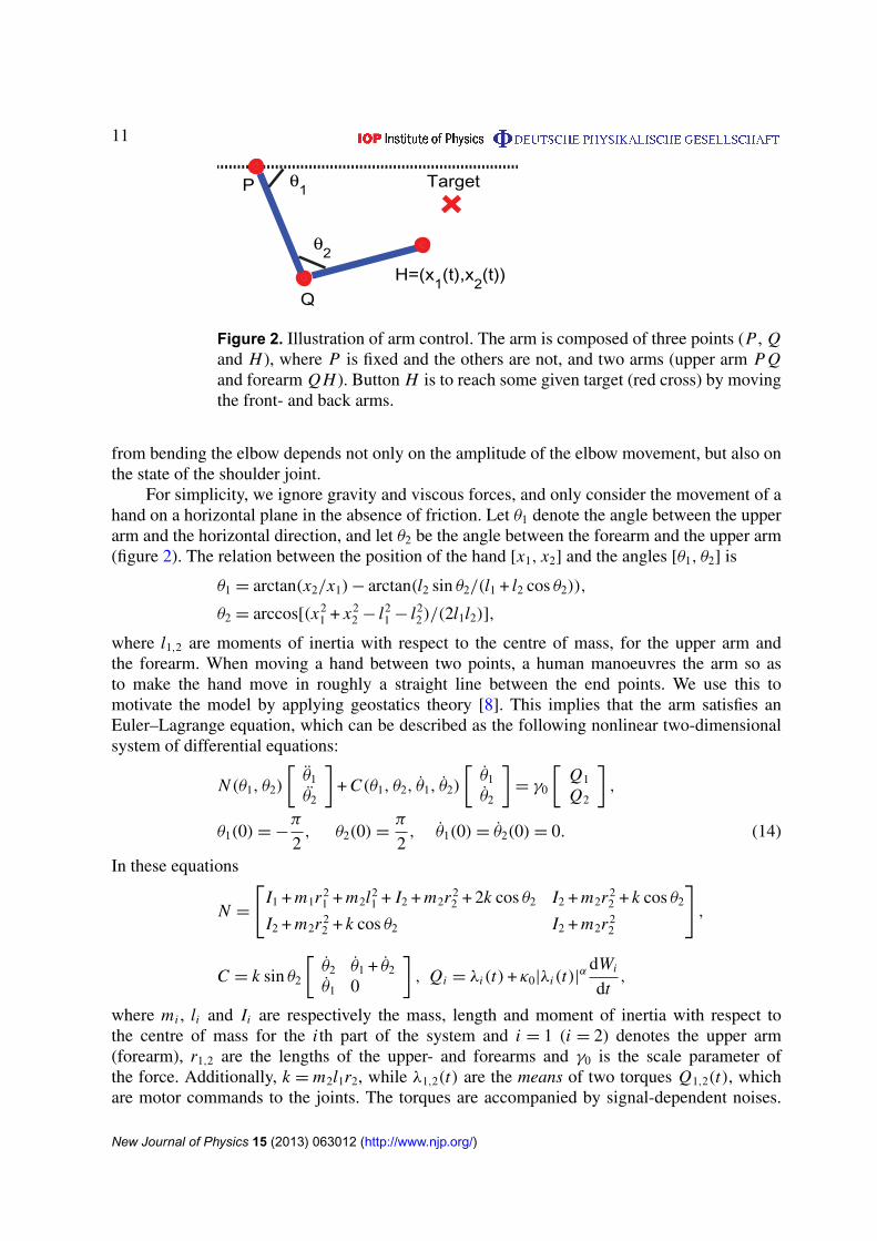
Figure 2. Illustration of arm control. The arm is composed of three points (P , Qand H ), where P is fixed and the others are not, and two arms (upper arm P Qand forearm Q H ). Button H is to reach some given target (red cross) by movingthe front- and back arms.

from bending the elbow depends not only on the amplitude of the elbow movement, but also onthe state of the shoulder joint.

For simplicity, we ignore gravity and viscous forces, and only consider the movement of ahand on a horizontal plane in the absence of friction. Let θ1 denote the angle between the upperarm and the horizontal direction, and let θ2 be the angle between the forearm and the upper arm(figure 2). The relation between the position of the hand [x1, x2] and the angles [θ1, θ2] is

θ1 = arctan(x2/x1) − arctan(l2 sin θ2/(l1 + l2 cos θ2)),

θ2 = arccos[(x21 + x2

2 − l21 − l2

2)/(2l1l2)],

where l1,2 are moments of inertia with respect to the centre of mass, for the upper arm andthe forearm. When moving a hand between two points, a human manoeuvres the arm so asto make the hand move in roughly a straight line between the end points. We use this tomotivate the model by applying geostatics theory [8]. This implies that the arm satisfies anEuler–Lagrange equation, which can be described as the following nonlinear two-dimensionalsystem of differential equations:

N (θ1, θ2)

[θ1

θ2

]+ C(θ1, θ2, θ1, θ2)

[θ1

θ2

]= γ0

[Q1

Q2

],

θ1(0) = −π

2, θ2(0) =

π

2, θ1(0) = θ2(0) = 0. (14)

In these equations

N =

[I1 + m1r 2

1 + m2l21 + I2 + m2r 2

2 + 2k cos θ2 I2 + m2r 22 + k cos θ2

I2 + m2r 22 + k cos θ2 I2 + m2r 2

2

],

C = k sin θ2

[θ2 θ1 + θ2

θ1 0

], Qi = λi(t) + κ0|λi(t)|

α dWi

dt,

where mi , li and Ii are respectively the mass, length and moment of inertia with respect tothe centre of mass for the i th part of the system and i = 1 (i = 2) denotes the upper arm(forearm), r1,2 are the lengths of the upper- and forearms and γ0 is the scale parameter ofthe force. Additionally, k = m2l1r2, while λ1,2(t) are the means of two torques Q1,2(t), whichare motor commands to the joints. The torques are accompanied by signal-dependent noises.

New Journal of Physics 15 (2013) 063012 (http://www.njp.org/)

12

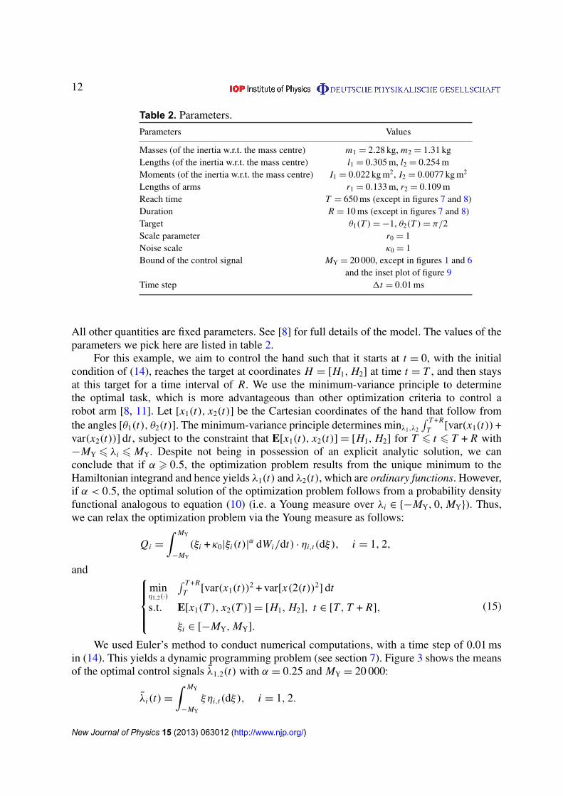
Table 2. Parameters.

Parameters Values

Masses (of the inertia w.r.t. the mass centre) m1 = 2.28 kg, m2 = 1.31 kgLengths (of the inertia w.r.t. the mass centre) l1 = 0.305 m, l2 = 0.254 mMoments (of the inertia w.r.t. the mass centre) I1 = 0.022 kg m2, I2 = 0.0077 kg m2

Lengths of arms r1 = 0.133 m, r2 = 0.109 mReach time T = 650 ms (except in figures 7 and 8)Duration R = 10 ms (except in figures 7 and 8)Target θ1(T ) = −1, θ2(T ) = π/2Scale parameter r0 = 1Noise scale κ0 = 1Bound of the control signal MY = 20 000, except in figures 1 and 6

and the inset plot of figure 9Time step 1t = 0.01 ms

All other quantities are fixed parameters. See [8] for full details of the model. The values of theparameters we pick here are listed in table 2.

For this example, we aim to control the hand such that it starts at t = 0, with the initialcondition of (14), reaches the target at coordinates H = [H1, H2] at time t = T , and then staysat this target for a time interval of R. We use the minimum-variance principle to determinethe optimal task, which is more advantageous than other optimization criteria to control arobot arm [8, 11]. Let [x1(t), x2(t)] be the Cartesian coordinates of the hand that follow fromthe angles [θ1(t), θ2(t)]. The minimum-variance principle determines minλ1,λ2

∫ T +RT [var(x1(t)) +

var(x2(t))] dt , subject to the constraint that E[x1(t), x2(t)] = [H1, H2] for T 6 t 6 T + R with−MY 6 λi 6 MY. Despite not being in possession of an explicit analytic solution, we canconclude that if α > 0.5, the optimization problem results from the unique minimum to theHamiltonian integrand and hence yields λ1(t) and λ2(t), which are ordinary functions. However,if α < 0.5, the optimal solution of the optimization problem follows from a probability densityfunctional analogous to equation (10) (i.e. a Young measure over λi ∈ {−MY, 0, MY}). Thus,we can relax the optimization problem via the Young measure as follows:

Qi =

∫ MY

−MY

(ξi + κ0|ξi(t)|α dWi/dt) · ηi,t(dξ), i = 1, 2,

and minη1,2(·)

∫ T +RT [var(x1(t))2 + var[x(2(t))2] dt

s.t. E[x1(T ), x2(T )] = [H1, H2], t ∈ [T, T + R],

ξi ∈ [−MY, MY].

(15)

We used Euler’s method to conduct numerical computations, with a time step of 0.01 msin (14). This yields a dynamic programming problem (see section 7). Figure 3 shows the meansof the optimal control signals λ1,2(t) with α = 0.25 and MY = 20 000:

λi(t) =

∫ MY

−MY

ξηi,t(dξ), i = 1, 2.

New Journal of Physics 15 (2013) 063012 (http://www.njp.org/)

13

0 0.1 0.2 0.3 0.4 0.5 0.6−2

−1.5

−1

−0.5

0

0.5

1

1.5

2

Mea

ns o

f λ1,

2(t)

Time (sec)

Figure 3. Means of the optimal control signals λ1(t) (blue solid) and λ2 (greensolid) in the straight-trajectory arm movement example with α = 0.25 and MY =

20 000. The blue and red dash vertical lines stand for the start and end time pointsof the duration of reaching the target, respectively.

According to the form of the optimal Young measure, the optimal solution should be

ηi,t(ds) =

[

λi (t)MY

δMY(s) + (1 −λi (t)MY

)δ0(s)]

ds, λi(t) > 0,[|λi (t)|

MYδ−MY(s) + (1 −

|λi (t)|MY

)δ0(s)]

ds, λi(t) < 0,

δ0(s) ds otherwise.

It can be shown (derivation not given in this work) that in the absence of the noise term,the arm can be accurately controlled to reach a given target for any T > 0. In this case, figure 4shows the dynamics of the angles, angle velocities and accelerations, in the controlled system,without noise. See, in comparison, the dynamical system with noise, whose dynamics of theangles, angle velocities and accelerations are illustrated in figure 5, and are exactly the same asthose in the case with noise removed. However, the acceleration dynamics of a noisy dynamicsystem appear to be discontinuous since the control signals, that have noises and are addedto the right-hand sides of the mechanical equations, are discontinuous (noisy) in a numericalrealization. However, according to the theory of stochastic differential equations [17], equation(14) has a continuous solution. Hence, these discontinuous acceleration dynamics lead to verysmooth dynamics of velocities and angles, as shown in figure 5.

Figures 6(a) and (b) illustrate that the probability density functional, for this problem,contains optimal control signals that are similar to neural pulses. Despite the optimal solutionnot being an ordinary function when α < 0.5, the trajectories of the angles θ1 and θ2 ofthe arm appear to be quite smooth, as shown in figure 5(a), and the target is reachedvery precisely if the value of MY is large. By comparison, when α > 0.5 the outcomehas a standard deviation between 4 and 6 cm, which may lead to failure to reach thetarget. A direct comparison between the execution error of the cases α = 0.8(> 0.5) and

New Journal of Physics 15 (2013) 063012 (http://www.njp.org/)

14

0 0.1 0.2 0.3 0.4 0.5 0.6−2

0

2

θ 1,2

(a)

0 0.1 0.2 0.3 0.4 0.5 0.6−2

0

2

dθ1,

2/dt

(b)

0 0.1 0.2 0.3 0.4 0.5 0.6−10

0

10

d2 θ 1,2/d

t2

Time (sec)

(c)

Figure 4. Optimal control of the straight-trajectory arm movement model withparameters listed in table 2. The target is set by θ1(T ) = −1 and θ2(T ) =

π

2 butwithout noise: dynamics of the angles (a), angle velocities (b) and accelerations(c) (blue solid curves for those of θ1 and green solid curves for θ2). The blue andred dash vertical lines stand for the start and end time points of the duration ofreaching the target.

0 0.1 0.2 0.3 0.4 0.5 0.6−2

0

2

θ 1,2 (a)

0 0.1 0.2 0.3 0.4 0.5 0.6−2

0

2

dθ1,

2/dt (b)

0 0.1 0.2 0.3 0.4 0.5 0.6−20

0

20

d2 θ 1,2/d

t2

Time (sec)

(c)

Figure 5. Optimal control of the straight-trajectory arm movement model withnoise and the same model parameters as in figure 4 and α = 0.25, MY = 20 000:dynamics of the angles (a), angle velocities (b) and accelerations (c) (blue solidcurves for those of θ1 and red solid curves for θ2). The blue and red dash verticallines stand for the start and end time points of the duration of reaching the target.

New Journal of Physics 15 (2013) 063012 (http://www.njp.org/)

15

0.1 0.12 0.14 0.16 0.18 0.20

5λ 1

(a)

0.1 0.12 0.14 0.16 0.18 0.20

5

Time (sec)

λ 2

(b)

Figure 6. Optimal control signal of the Young measure of the straight-trajectoryarm movement model with noise; illustrations for λ1 (a) and λ2 (b) in discretetime with MY = 5, where the width of each bar stands for the measure of MY ateach time bin.

α = 0.25(< 0.5) is shown in the supplementary movies (‘Movie 1’ and ‘Movie 2’ availablefrom stacks.iop.org/NJP/15/063012/mmedia) of arm movements of both cases. Our conclusionis that a Young measure optimal solution, in the case of sub-Poisson control signals, can realizea precise control performance even in the presence of noise. However, Poisson or supra-Poissoncontrol signals cannot realize a precise control performance, despite the existence of an explicitoptimal solution in this case. Thus α < 0.5 significantly reduces execution error compared withα > 0.5.

With different T (the starting time of reaching the target) and R (the duration of reachingthe target), under sub-Poisson noise, i.e. α < 0.5, the system can be precisely controlled byoptimal Young measure signals with a sufficiently large MY. Since the target is in the reachableregion of the arm, it implies that the original differential system of (14) with the noise removedcan be controlled for any T > 0 and R > 0 [8, 9]. According to the discussion in appendix B(theorem 2), the execution error can be arbitrarily small when MY is sufficiently large. However,for a smaller T , the more rapid the control, the larger the means of the control signals. As for theduration R, by picking the control signals as fixed values (zeros in this example) such that thevelocities keep zeros, the arm will stay at the target for arbitrarily long or short times. Similarly,with a large MY, the error (variance) of staying at the target can be very small. To illustrate thesearguments, we take T = 100 ms and R = 100 ms for example (all other parameters are the sameas above). Figure 7 shows that the means of the optimal Young measure control signals beforereaching the target have larger amplitudes than those when T = 650 ms, and figure 8 shows thatthe arm can be precisely controlled to reach and stay at the target.

The movement error depends strongly on the value of the dispersion index, α, and thebound of the control signal, MY. Figure 9 indicates a quantitative difference in the executionerror between the two cases α < 0.5 and α > 0.5, if α is close to (but less than) 0.5. Theexecution error can be appreciable unless a large MY is used. For example if α = 0.45, as infigure 9, the square root of the execution error is approximately 0.6 cm when MY = 20 000.From (13), the error decreases as MY increases, behaving approximately as a power law, asillustrated in the inner plot of figure 9. The logarithm of the square root of the execution erroris found to depend approximately linearly on the logarithm of MY when α = 0.25, with a slopeclose to −0.25, in good agreement with the theoretical estimate (13).

New Journal of Physics 15 (2013) 063012 (http://www.njp.org/)

16

0 0.05 0.1 0.15 0.2−100

−50

0

50

100

Mea

ns o

f λ1,

2(t)

Time (sec)

Figure 7. Means of the optimal control signals λ1(t) (blue solid) and λ2(t)(green solid) in the straight-trajectory arm movement example with T = 100 sand R = 100 ms. The blue and red dash vertical lines stand for the start and endtime points of the duration of reaching the target.

0 0.05 0.1 0.15 0.2−2

0

2

θ

0 0.05 0.1 0.15 0.2−20

0

20

dθ/d

t

0 0.05 0.1 0.15 0.2−500

0

500

d2 θ/dt

2

Time (sec)

Figure 8. Optimal control of the straight-trajectory arm movement model withnoise with T = 100 and R = 100 ms: dynamics of the angles (a), angle velocities(b) and accelerations (c) (blue solid curves for those of θ1 and red solid curvesfor θ2). The blue and red dash vertical lines stand for the start and end time pointsof the duration of reaching the target.

We note that in a biological context, a set of neuronal pulse trains can achieve precisecontrol in the presence of noise. This could be a natural way to approximately implementthe probability density functional when α < 0.5. All the other parameters are the same asabove (α = 0.25). The firing rates are illustrated in figures 6(a) and (b) and broadly coincide

New Journal of Physics 15 (2013) 063012 (http://www.njp.org/)

17

0 0.2 0.4 0.6 0.8 10

0.01

0.02

0.03

0.04

0.05

0.06

α

Mea

n V

aria

nces

100

103

0

0.02

0.04

0.06

MY

Mea

n V

aria

nces

Figure 9. Performance of optimal control of the straight-trajectory armmovement model: relationship between executive error measured by meanstandard variance and dispersion index α with MY = 20 000 and log–log plot(inner plot) of the relationship between executive error and bound of the Youngmeasure MY with α = 0.25 where the dash line is a reference line with slope−1/2 + α = −0.25 , as shown in (13).

0 200 400 600−4

−2

0

2

Time (msec)Noi

sy C

ontr

ol S

igna

l u1* (t

)

0 200 400 600−0.5

0

0.5

Time (msec)Noi

sy C

ontr

ol S

igna

l u2* (t

)

0 200 400 600

50

100

150

200

Time (msec)

Neu

rons

0 200 400 600

50

100

150

200

Time (msec)

Neu

rons

(a) (b)

(c) (d)

Figure 10. Spiking control of the straight-trajectory arm movement model: (a)approximation of the first component (u∗

1(t)) of the optimal Young measurecontrol signal by spike trains; (b) approximation of the second component(u∗

2(t)) of the optimal Young measure control signal by spike trains; (c) and(d) approximation of the optimal control signal Q1,2 by spike trains of a set ofneurons.

with the probability density functional we have discussed. In particular, at each time t , theprobability ηi,t can be approximated by the fraction of the neurons that are firing, with the meanfiring rates equal to the means of the control signals (see section 7). The approximations ofthe components of the noisy control signals are shown in figures 10(a) and (b), respectively.

New Journal of Physics 15 (2013) 063012 (http://www.njp.org/)

18

Figures 10(c) and (d) illustrate such an implementation of the optimal solution by neuronalpulse trains. Using the pulse trains as control signals, we can realize precise movementcontrol. We enclose two videos ‘Movie 3’ and ‘Movie 4’ (available from stacks.iop.org/NJP/15/063012/mmedia) to demonstrate the efficiency of the control by pulse trains with twodifferent targets. As they show, the targets are precisely accessed by the arm. We point out thatthe larger the ensemble, the more precise the control performance, because a large number of theneurons in an ensemble can theoretically lead to a large MY as mentioned above, which resultsin an improvement of the approximation of a Young measure and decreases the execution erroras stated in (13).

We note that these kinds of patterns of pulse trains have been widely reported inexperiments, for example, the synchronous neural bursting reported in [18]. This may providea mathematical rationale for the nervous system to adopt pulse-like signals to realize motorcontrol.

6. Conclusions

In this paper, we have provided a general mathematical framework for controlling a classof stochastic dynamical systems with random control signals whose noisy variance can beregarded as a function of the signal magnitude. If the dispersion index, α, is < 0.5, which isthe case when the control signal is sub-Poisson, an optimal solution of explicit function doesnot exist but has to be replaced by a Young measure solution. This parameterized measurecan lead to precise control performance, where the controlling error can become arbitrarilysmall. We have illustrated this theoretical result via a widely studied problem of arm movementcontrol.

In the control problem of biological and robotic systems, large control signals are neededfor rapid movement control [21]. When noise occurs, this will cause imprecision in the controlperformance. As pointed out in [9, 22–25], a trade-off should be considered when conductingrapid control with noise. In this paper, we still use a ‘large’ control signal but with differentcontexts. With sub-Poisson noise, we proved that a sufficiently large MY, i.e. a sufficientlylarge region of the control signal values, can lead to precise control performance. Hence, alarge region of control signal values plays a crucial role in realizing precise control in noisyenvironments, for both ‘slow’ and ‘rapid’ movement control. In numerical examples, the largerthe MY we pick, the smaller the control error, as shown in the inset plot of figure 9 as wellas (13) (theorem 2 in appendix B).

Implementation of the Young measure approach in biological control appears to be anatural way of achieving precise execution error in the presence of sub-Poisson noise. Inparticular, in the neural-motor control example illustrated above, the optimal solution in thecase of α < 0.5 is quite interesting. Assume we have an ensemble of neurons that fire pulsessynchronously within a sequence of non-overlapping time windows, as depicted in figures 6(C)and (D). We see that the firing neurons yield control signals that are very close, in form, tothe type of Young measure solution. This conclusion may provide a mathematical rationale forthe nervous system to adopt pulse-like trains to realize motor control. Additionally, we pointout that our approach may have significant ramifications in other fields, including robot motorcontrol and sparse functional estimation, which are issues of our future research.

New Journal of Physics 15 (2013) 063012 (http://www.njp.org/)

19

7. Methods

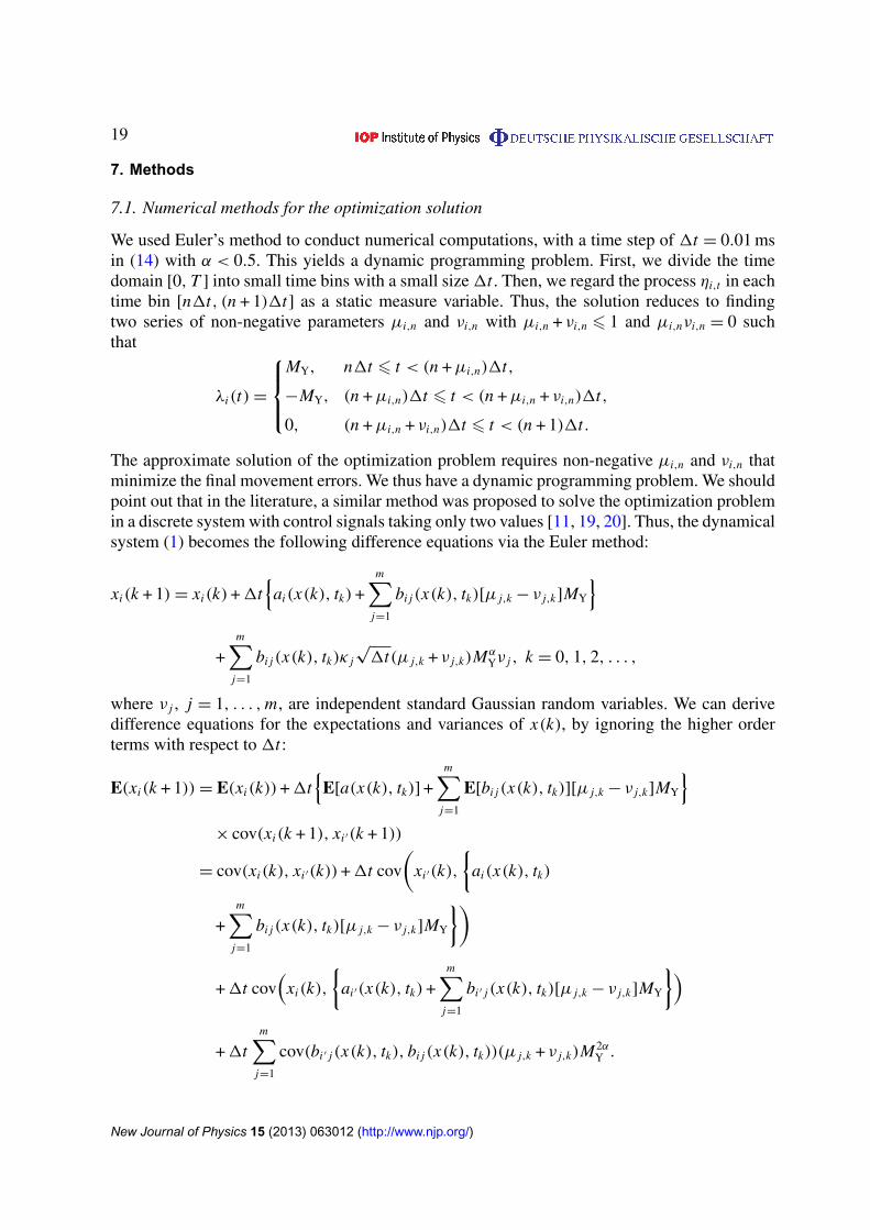
7.1. Numerical methods for the optimization solution

We used Euler’s method to conduct numerical computations, with a time step of 1t = 0.01 msin (14) with α < 0.5. This yields a dynamic programming problem. First, we divide the timedomain [0, T ] into small time bins with a small size 1t . Then, we regard the process ηi,t in eachtime bin [n1t, (n + 1)1t] as a static measure variable. Thus, the solution reduces to findingtwo series of non-negative parameters µi,n and νi,n with µi,n + νi,n 6 1 and µi,nνi,n = 0 suchthat

λi(t) =

MY, n1t 6 t < (n + µi,n)1t,

−MY, (n + µi,n)1t 6 t < (n + µi,n + νi,n)1t,

0, (n + µi,n + νi,n)1t 6 t < (n + 1)1t.

The approximate solution of the optimization problem requires non-negative µi,n and νi,n thatminimize the final movement errors. We thus have a dynamic programming problem. We shouldpoint out that in the literature, a similar method was proposed to solve the optimization problemin a discrete system with control signals taking only two values [11, 19, 20]. Thus, the dynamicalsystem (1) becomes the following difference equations via the Euler method:

xi(k + 1) = xi(k) + 1t{

ai(x(k), tk) +m∑

j=1

bi j(x(k), tk)[µ j,k − ν j,k]MY

}

+m∑

j=1

bi j(x(k), tk)κ j

√1t(µ j,k + ν j,k)Mα

Yν j , k = 0, 1, 2, . . . ,

where ν j , j = 1, . . . , m, are independent standard Gaussian random variables. We can derivedifference equations for the expectations and variances of x(k), by ignoring the higher orderterms with respect to 1t :

E(xi(k + 1)) = E(xi(k)) + 1t{

E[a(x(k), tk)] +m∑

j=1

E[bi j(x(k), tk)][µ j,k − ν j,k]MY

}× cov(xi(k + 1), xi ′(k + 1))

= cov(xi(k), xi ′(k)) + 1t cov

(xi ′(k),

{ai(x(k), tk)

+m∑

j=1

bi j(x(k), tk)[µ j,k − ν j,k]MY

})

+ 1t cov(

xi(k),

{ai ′(x(k), tk) +

m∑j=1

bi ′ j(x(k), tk)[µ j,k − ν j,k]MY

})

+ 1tm∑

j=1

cov(bi ′ j(x(k), tk), bi j(x(k), tk))(µ j,k + ν j,k)M2αY .

New Journal of Physics 15 (2013) 063012 (http://www.njp.org/)

20

Thus, equation (9) becomes the following discrete optimization problem:min

µi,k ,νi,k

∑k var(φ(x(k), tk))

s.t. E(φ(x(k), tk)) = z(tk), µi,k + νi,k 6 1,

µi,k > 0, νi,k > 0

(16)

with x(k) a Gaussian random vector with expectation E(x(k)) and covariance matrixcov(x(k), x(k)).

7.2. Neuronal pulse trains approximating Young measure solutions

At each time t , the measure η∗

t can be approximated by the fraction of the neuron ensembles thatare firing. In detail, assume that the means of the optimal control signals are Rt,i(ξ), i = 1, 2,and there is one ensemble of excitatory neurons and another ensemble of inhibitory neurons. Afraction of the neurons fire so that the mean firing rates satisfy

λ∗

i (t) = γ {E[Rexti (t)] − E[Rinh

i (t)]},

where Rexti (t) and Rinh

i (t) are the firing rates of the excitatory and inhibitory neurons,respectively, and γ is a scalar factor. In the presence of sub-Poisson noise, the noisy controlsignals u∗

i (t) = λ∗

i (t) + ζi(t) are approximated by

u∗

i (t) = γ[Rext

i (t) − Rinhi (t)

].

Both ensembles of neurons are imposed with baseline activities, which bound the minimumfiring rates away from zeros, given the spontaneous activities of neurons when no explicit signalis transferred. A numerical approach involves discretizing time t into small bins of identical size1t . The firing rates can be easily estimated by averaging the population activities in a time bin.We have used 400 neurons to control the system, with two ensembles of neurons with equivalentnumbers that approximate the first and second components of the control signal, respectively.Each neuron ensemble has 200 neurons with 100 excitatory and 100 inhibitory neurons.

Acknowledgments

WLL is jointly supported by the Marie Curie International Incoming Fellowship from theEuropean Commission (no. FP7-PEOPLE-2011-IIF-302421), the National Natural SciencesFoundation of China (no. 61273309), the Shanghai Rising-Star Program (under grantno. 11QA1400400), the Shanghai Guidance of Science and Technology (SGST) (no.09DZ2272900) and the Laboratory of Mathematics for Nonlinear Science, Fudan University.JFF is supported by the State Key Program of National Natural Science of China (grantno. 91230201). WLL also acknowledges Dr Enrico Rossoni previously from the Centrefor Scientific Computing, the University of Warwic, and Dr Tian Ge from the Centre forComputational Systems Biology at Fudan University for their help with codes of straight-trajectory arm movement and neural pulse control.

Appendix A. Derivation of formula (8)

Let W be the time-varying p.d.f. p(x, t) that is second-order continuous differentiable withrespect to x and t that is embedded in the Sobolev function space W 2,2; W1 be the function

New Journal of Physics 15 (2013) 063012 (http://www.njp.org/)

21

space of p(x, t0), regarded as a function with respect to x with a fixed t0; and W2 be the functionspace of p(x0, t), regarded as a function with respect to t with a given x0. The spaces W1,2 canbe regarded as being embedded in W . In addition, let W be the function space where the imageL[W ] is embedded; L be the space of linear operator L, denoted above; L (Z , E) be the spacecomposed of bounded linear operator from linear space Z to E ; and Z∗ be the dual space of thelinear space Z : Z∗

= L (Z ,R). Furthermore, let Y be the tangent space of the Young measurespace Y: Y = {η − η′ : η, η′

∈ Y}. For simplicity, we do not specify the spaces and just providethe formalistic algebras, and then the following is similar to chapter 4.3 in [12] with appropriatemodifications.

Define

8(p) =

∫ T +R

T

∫4

‖φ(x, t) − z(t)‖2 p(x, t) dx dt,

5(p, η) =

(∂p

∂t− (L · η) ◦ p, p(x, 0) − p0(x)

),

J (p) =

∫4

φ(x, t)p(x, t) dx − z(t). (A.1)

Thus, (9) can be rewritten as{min

η8(p)

s.t. 5(p, η) = 0, J (p) = 0.(A.2)

The Gateaux differentials of these maps with respect to p(x, t), denoted by ∇p·, are

(∇p8) ◦ ( p − p) =

∫ T +R

T

∫4

‖φ(x, t) − z(t)‖2[ p(x, t) − p(x, t)] dx dt,

(∇p5) ◦ ( p − p) =

(∂( p − p)

∂t− (L · η) ◦ ( p − p), p(x, 0) − p(x, 0)

),

(∇p J ) ◦ ( p − p) =

∫4

φ(x, t)[ p(x, t) − p(x, t)] dx

for two time-varying p.d.f.s p, p ∈ W . Here, ∇p8 ∈ W ∗, ∇p5 ∈ L (W, W × W1), ∇p J ∈

L (W, W2). And the differentials of these maps with respect to the Young measure η are

(∇η8) · (η − η) = 0,

(∇η5) · (η − η) = ((L ◦ p) · (η − η), 0),

(∇η J ) · (η − η) = 0

for the two Young measures η, η ∈ Y. Here, ∇η8 ∈ Y∗, ∇η5 ∈ L (Y, W × W1) and ∇η J ∈

L (Y, W2)

Then, we are in a position to derive the result of (8) by the following theorem, as aconsequence from theorem 4.1.17 in [12].

Theorem 1. 8 : W → W ∗, 5 : W ×Y→ R and J : W → W2 as defined in (A.1). Assume that(i) the trajectory of x(t) in (4) is bounded almost surely; (ii) a(x, t), b(x, t) and φ(x, t) areC2 with respect to (x, t). Let (η∗, p∗) be the optimal solution of (9). Then, there are some

New Journal of Physics 15 (2013) 063012 (http://www.njp.org/)

22

λ1 ∈ L (W × W1, W ∗), λ2 = [λ21, λ22]T with λ21 ∈ L (W , W2) and λ22 ∈ L (W1, , W2) , suchthat

λ1 ◦ ∇p5(p∗, η∗) = ∇p8(p∗), λ2 ◦ ∇p5(p∗, η∗) = ∇p J (p∗), (A.3)

and the abstract maximum principle

η∗

t {minima of h(t, ξ) w.r.t ξ} = 1, ∀t ∈ [0, T + R] (A.4)

holds with the ‘abstract Hamiltonian’:

h(t, ξ) = −

∫4

p∗(x, t){ n∑

i=1

Ai(x, t, ξ)∂µ1

∂xi

+1

2

n∑i, j=1

[B(x, t, ξ)B(x, t, ξ)T]i j∂2µ1

∂xi∂x j

}dx . (A.5)

Proof. Under the conditions in this theorem, we can conclude that the Fokker–Planck equationhas a unique solution p(η) that is continuously dependent on η from the theory of stochasticdifferential equations [17]; 5(·, η) : W → W ∗ is the Frechet differentiable at p = π(η) becausex(t) is assumed to be almost surely bounded; 5(p, ·) : Y→ W ∗ and J (in fact ∇η J = 0) isGateaux equi-differentiable around p ∈ W because p ∈ W ⊂ W 2,2 with (x, t) bounded5; thepartial differential ∇η5 is weak continuous with respect to η because it is linearly dependenton η.

In addition, from the existence and uniqueness of the Fokker–Planck equation, ∇p5(p, η) :W → Im(∇p5(p, η)) ⊂ W × W1 has a bounded inverse. This implies that the following adjointequation

µ ◦ ∇p5 = ∇p8 + c(t) ◦ ∇p J

has a solution for p = p(η), denoted by µ. Let µ = [µ1, µ2], which should be a solution of thefollowing equation:

∂µ1

∂t + (L∗· η∗) ◦ µ1 = −‖φ(x, t) − z(t)‖2

− c(t)φ(x, t),

µ2(x) = µ1(x, 0),

µ1(x, T + R) = 0, t ∈ [0, T + R], x ∈ 4

(A.6)

with the dual operator L∗ of L (the operator in the back-forward Kolmogorov equation) stilldependent on (x, t) and the value of λ(t) (namely ξ in Young measure):

L∗◦ q =

n∑i=1

ai(x, t, ξ)∂q

∂xi+

1

2

n∑i, j=1

[B(x, t, ξ)BT(x, t, ξ)]i j∂2q

∂xi x j.

We pick λ1,2(t) with µ1 = λ1 + c(t)λ21 and µ2 = λ1 + c(t)λ22. So λ1,2 should satisfyequation (A.3). In fact, λ1,2 can be regarded as functions (or generalized functions) with respectto (x, t).

5 See [12] for details of the definitions of Frechet differential, Gateaux equi-differential and partial differential,which are extended from those of the functional/operator on function space.

New Journal of Physics 15 (2013) 063012 (http://www.njp.org/)

23

Thus, the conditions of lemma 1.3.16 in [12] can be verified, which implies that thegradients of the maps 8 and J with respect to η, by regarding p = p(η) from 5(p, η) = 0,are as follows:

∂8 = ∇η8 − λ1 ◦ ∇η5, ∂ J = ∇η J − λ2 ◦ ∇η5.

From the abstract Hamiltonian minimum principle (theorem 4.1.17 in [12]), applied to eachsolution of (9), denoted by η∗, there exists a non-zero function c(t) such that

H(η) = ∂8(η∗) · η + 〈c(t), ∂ J (η∗) · η〉, ∀η ∈ Y (A.7)

is an ‘abstract Hamiltonian’ with respect to η. With the definitions of λ1,2, (A.7) becomes

H(η) = ∇η8 · η + c∇η J · η − 〈µ, ∇η5 · η〉 = −〈µ, ∇η5 · η〉

owing to ∇η8 = ∇η J = 0.By specifying µ with λ1,2, we have

H(η) = − 〈µ, ∇η5 · η〉 = −〈µ1, [L ◦ p∗] · η〉 = −〈p∗, [L∗◦ µ1] · η〉

= −

∫ T +R

0

∫4

∫�

p∗

{ n∑i=1

ai(x, t, ξ)∂µ1

∂xi

+1

2

n∑i, j=1

[B(x, t, ξ)B(x, t, ξ)T]i j∂2µ1

∂xi∂x j

}ηt(dξ) dx dt,

where p∗ stands for the time-varying density corresponding to the optimal Young measuresolution η∗. From this, letting ξ = λ, we have the ‘abstract Hamiltonian’ in the form of (A.5) asthe Hamiltonian integrand of H(·).

The Hamiltonian abstract minimum (maximum) principle indicates that the optimal Youngmeasure η∗

t is only concentrated at the minimum points of h(t, ξ) with respect to ξ for each t .That is, (A.4) holds. This completes the proof. ut

From this theorem, since the variances depend on the magnitude of the signal as describedin (3), removing the terms without ξ , it is equivalent to looking at the minima of h(t, ξ) in theform of

h(t, ξ) =

m∑i=1

hi(t, ξi), hi(t, ξi) = gi(t)|ξi |2α

− fi(t)ξi (A.8)

instead of h(t, ξ), where

fi(t) =

m∑j=1

∫4

p∗(x, t)b j i(x, t)∂µ1

∂xidx,

gi(t) = −κ2

i

2

m∑j,k=1

∫4

p∗(x, t)b j i(x, t)bki(x, t)∂2µ1

∂x j∂xkdx .

This gives formula (8).

New Journal of Physics 15 (2013) 063012 (http://www.njp.org/)

24

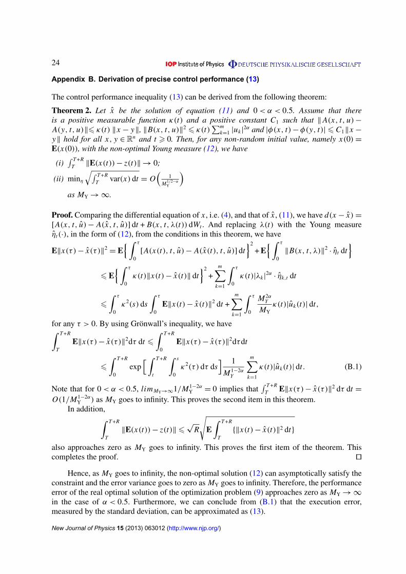
Appendix B. Derivation of precise control performance (13)

The control performance inequality (13) can be derived from the following theorem:

Theorem 2. Let x be the solution of equation (11) and 0 < α < 0.5. Assume that thereis a positive measurable function κ(t) and a positive constant C1 such that ‖ A(x, t, u) −

A(y, t, u)‖6 κ(t) ‖x − y‖, ‖B(x, t, u)‖2 6 κ(t)∑m

k=1 |uk|2α and |φ(x, t) − φ(y, t)|6 C1‖x −

y‖ hold for all x, y ∈ Rn and t > 0. Then, for any non-random initial value, namely x(0) =

E(x(0)), with the non-optimal Young measure (12), we have

(i)∫ T +R

T ‖E(x(t)) − z(t)‖ → 0;

(ii) minη

√∫ T +RT var(x) dt = O

(1

M1/2−αY

)as MY → ∞.

Proof. Comparing the differential equation of x , i.e. (4), and that of x , (11), we have d(x − x) =

[A(x, t, u) − A(x, t, u)] dt + B(x, t, λ(t)) dWt . And replacing λ(t) with the Young measureηt(·), in the form of (12), from the conditions in this theorem, we have

E‖x(τ ) − x(τ )‖2= E

{ ∫ τ

0[A(x(t), t, u) − A(x(t), t, u)] dt

}2

+ E{ ∫ τ

0‖B(x, t, λ)‖2

· ηt dt}

6 E{ ∫ τ

0κ(t)‖x(t) − x(t)‖ dt

}2

+m∑

k=1

∫ τ

0κ(t)|λk|

2α· ηk,t dt

6

∫ τ

0κ2(s) ds

∫ τ

0E‖x(t) − x(t)‖2 dt +

m∑k=1

∫ τ

0

M2αY

MYκ(t)|uk(t)| dt,

for any τ > 0. By using Gronwall’s inequality, we have∫ T +R

TE‖x(τ ) − x(τ )‖2dτ dt 6

∫ T +R

0E‖x(τ ) − x(τ )‖2dτdt

6

∫ T +R

0exp

[ ∫ T +R

t

∫ s

0κ2(τ ) dτ ds

] 1

M1−2αY

m∑k=1

κ(t)|uk(t)| dt. (B.1)

Note that for 0 < α < 0.5, limMY→∞1/M1−2αY = 0 implies that

∫ T +RT E‖x(τ ) − x(τ )‖2 dτ dt =

O(1/M1−2αY ) as MY goes to infinity. This proves the second item in this theorem.

In addition,∫ T +R

T‖E(x(t)) − z(t)‖6

√R

√E∫ T +R

T{‖x(t) − x(t)‖2 dt}

also approaches zero as MY goes to infinity. This proves the first item of the theorem. Thiscompletes the proof. ut

Hence, as MY goes to infinity, the non-optimal solution (12) can asymptotically satisfy theconstraint and the error variance goes to zero as MY goes to infinity. Therefore, the performanceerror of the real optimal solution of the optimization problem (9) approaches zero as MY → ∞

in the case of α < 0.5. Furthermore, we can conclude from (B.1) that the execution error,measured by the standard deviation, can be approximated as (13).

New Journal of Physics 15 (2013) 063012 (http://www.njp.org/)

25

References

[1] Osborne L C, Lisberger S G and Bialek W 2005 Nature 437 412–6[2] Harris C M and Wolpert D M 1998 Nature 394 780–4[3] Harris C M 1998 J. Neurosci. Methods 83 73–88[4] Feng J F and Zhang K W 2002 J. Phys. A: Math. Gen. 35 7287–304[5] Feng J F, Tartaglia G and Tirozzi B 2004 J. Phys. A: Math. Gen. 37 4685–700[6] Feng J F and Tuckwell H C 2003 Phys. Rev. Lett. 91 018101[7] Rossoni E, Kang J and Feng J F 2010 Biol. Cybern. 102 441–50[8] Winter D A 2004 Biomechanics and Motor Control of Human Movement (New York: Wiley-Interscience)[9] Simmons G and Demiris Y 2005 J. Robot. Syst. 22 677–90

[10] Tanaka H, Krakauer J and Qian N 2006 J. Neurophysiol. 95 3875–86[11] Ikeda S and Sakaguchi Y 2009 Proc. Joint 48th IEEE CDC and 28th CCC p 4499[12] Roubıcek T 1997 Relaxation in Optimization Theory and Variational Calculus (Berlin: Walter de Gruyter)[13] Young L C 1937 C. R. Soc. Sci. Lett. Varsovie, Cl. III 30 212–34[14] Young L C 1942 Ann. Math. 43 84–103

Young L C 1942 Ann. Math. 43 530–44[15] Horton P, Bonny L, Nicol A U, Kendrick K M and Feng J F 2005 J. Neurosci. Methods 146 22–41[16] Christen M, Nicol A U, Kendrick K M, Ott T and Stoop R 2006 Neuroreport 17 1499–502[17] Øksendal B 1998 Stochastic Differential Equations: An Introduction and Applications (Berlin: Springer)[18] Rossoni E, Feng J F, Tirozzi B, Brown D, Leng G and Moos F 2008 PLoS Comput. Biol. 4 e1000123[19] Shimada T and Aihara K 2008 Math. Biosci. 214 134–9[20] Hirata Y, Bruchovsky N and Aihara K 2010 J. Theor. Biol. 264 517–27[21] Richardso R et al 2005 Control Eng. Pract. 13 291–303[22] Todorov E and Jordan M J 2002 Nature Neurosci. 5 1226–35[23] Kitazawa K 2002 Neurosci. Res. 43 289–94[24] Mussa-Ivaldi F A and Solla S A 2004 IEEE J. Ocean. Eng. 29 640–50[25] Chhabra M and Jacobs R A 2006 J. Neurosci. 26 10883–7

New Journal of Physics 15 (2013) 063012 (http://www.njp.org/)