Publ. Astron. Soc. Japan (2019) 71 (5), R1 (1–118) doi: 10.1093/pasj/psz084 Review R1-1 Review Achievements of Hinode in the first eleven years Hinode Review Team, Khalid AL-JANABI, 1 Patrick ANTOLIN , 2,† Deborah BAKER, 1 Luis R. BELLOT RUBIO , 3 Louisa BRADLEY, 1 David H. BROOKS , 4 Rebecca CENTENO , 5 J. Leonard CULHANE, 1 Giulio DEL ZANNA, 6 George A. DOSCHEK, 7 Lyndsay FLETCHER , 8,‡ Hirohisa HARA, 9, 10 Louise K. HARRA, 1,§ Andrew S. HILLIER , 6, 11 Shinsuke IMADA, 12 James A. KLIMCHUK , 13 John T. MARISKA, 7 Tiago M. D. PEREIRA , 14 Katharine K. REEVES , 15 Taro SAKAO , 16, 17 Takashi SAKURAI , 9, ∗ Toshifumi SHIMIZU , 16, 18 Masumi SHIMOJO , 9, 10 Daikou SHIOTA , 12, 19 Sami K. SOLANKI , 20 Alphonse C. STERLING , 21 Yingna SU, 22 Yoshinori SUEMATSU , 9, 10 Theodore D. TARBELL, 23,| Sanjiv K. TIWARI , 21, 23, 24, 25 Shin TORIUMI , 9, Ignacio UGARTE-URRA , 4 Harry P. WARREN , 7 Tetsuya WATANABE, 9, 10 and Peter R. YOUNG 4, ∗∗ 1 UCL – Mullard Space Science Laboratory, Holmbury St. Mary, Dorking, Surrey, RH5 6NT, UK 2 School of Mathematics and Statistics, University of St. Andrews, St. Andrews, Fife, KY16 9SS, UK 3 Instituto de Astrof´ ısica de Andaluc´ ıa (CSIC), Apdo. 3004, E-18080 Granada, Spain 4 College of Science, George Mason University, 4400 University Drive, Fairfax, VA 22030, USA 5 High Altitude Observatory, NCAR, Boulder, CO 80301, USA 6 Department of Applied Mathematics and Theoretical Physics, University of Cambridge, Wilberforce Road, Cambridge, CB3 0WA, UK 7 Space Science Division, Naval Research Laboratory, 4555 Overlook Avenue SW, Washington, DC 20375, USA 8 SUPA School of Physics and Astronomy, University of Glasgow, Glasgow G12 8QQ, UK 9 National Astronomical Observatory of Japan, 2-21-1 Osawa, Mitaka, Tokyo 181-8588, Japan 10 Department of Astronomical Science, The Graduate University for Advanced Studies (SOKENDAI), 2-21-1 Osawa, Mitaka, Tokyo 181-8588, Japan 11 College of Engineering, Mathematics and Physical Sciences, University of Exeter, Exeter EX4 4QF, UK 12 Institute for Space-Earth Environmental Research, Nagoya University, Furo-cho, Chikusa-ku, Nagoya, Aichi 464-8601, Japan 13 Heliophysics Science Division, NASA Goddard Space Flight Center, Greenbelt, MD 20771, USA 14 Rosseland Centre for Solar Physics, University of Oslo, Blindern, 0315 Oslo, Norway 15 Harvard-Smithsonian Center for Astrophysics, 60 Garden St., Cambridge, MA 20138, USA 16 Institute of Space and Astronautical Science, Japan Aerospace Exploration Agency, 3-1-1 Yoshinodai, Chuo-ku, Sagamihara, Kanagawa 229-5210, Japan 17 Department of Space and Astronautical Science, The Graduate University for Advanced Studies (SOKENDAI), 3-1-1 Yoshinodai, Chuo-ku, Sagamihara, Kanagawa 229-5210, Japan C The Author(s) 2019. Published by Oxford University Press on behalf of the Astronomical Society of Japan. This is an Open Access article distributed under the terms of the Creative Commons Attribution License (http://creativecommons.org/licenses/by/4.0/), which permits unrestricted reuse, distribution, and reproduction in any medium, provided the original work is properly cited. Downloaded from https://academic.oup.com/pasj/article-abstract/71/5/R1/5589096 by guest on 04 February 2020

Welcome message from author
This document is posted to help you gain knowledge. Please leave a comment to let me know what you think about it! Share it to your friends and learn new things together.
Transcript

Publ. Astron. Soc. Japan (2019) 71 (5), R1 (1–118)doi: 10.1093/pasj/psz084
Review
R1-1
Review
Achievements of Hinode in the first eleven years
Hinode Review Team, Khalid AL-JANABI,1 Patrick ANTOLIN ,2,†
Deborah BAKER,1 Luis R. BELLOT RUBIO ,3 Louisa BRADLEY,1
David H. BROOKS ,4 Rebecca CENTENO ,5 J. Leonard CULHANE,1
Giulio DEL ZANNA,6 George A. DOSCHEK,7 Lyndsay FLETCHER ,8,‡
Hirohisa HARA,9,10 Louise K. HARRA,1,§ Andrew S. HILLIER ,6,11
Shinsuke IMADA,12 James A. KLIMCHUK ,13 John T. MARISKA,7
Tiago M. D. PEREIRA ,14 Katharine K. REEVES ,15 Taro SAKAO ,16,17
Takashi SAKURAI ,9,∗ Toshifumi SHIMIZU ,16,18 Masumi SHIMOJO ,9,10
Daikou SHIOTA ,12,19 Sami K. SOLANKI ,20 Alphonse C. STERLING ,21
Yingna SU,22 Yoshinori SUEMATSU ,9,10 Theodore D. TARBELL,23,|
Sanjiv K. TIWARI ,21,23,24,25 Shin TORIUMI ,9,� Ignacio UGARTE-URRA ,4
Harry P. WARREN ,7 Tetsuya WATANABE,9,10 and Peter R. YOUNG4,∗∗
1UCL – Mullard Space Science Laboratory, Holmbury St. Mary, Dorking, Surrey, RH5 6NT, UK2School of Mathematics and Statistics, University of St. Andrews, St. Andrews, Fife, KY16 9SS, UK3Instituto de Astrofısica de Andalucıa (CSIC), Apdo. 3004, E-18080 Granada, Spain4College of Science, George Mason University, 4400 University Drive, Fairfax, VA 22030, USA5High Altitude Observatory, NCAR, Boulder, CO 80301, USA6Department of Applied Mathematics and Theoretical Physics, University of Cambridge, WilberforceRoad, Cambridge, CB3 0WA, UK
7Space Science Division, Naval Research Laboratory, 4555 Overlook Avenue SW, Washington, DC 20375,USA
8SUPA School of Physics and Astronomy, University of Glasgow, Glasgow G12 8QQ, UK9National Astronomical Observatory of Japan, 2-21-1 Osawa, Mitaka, Tokyo 181-8588, Japan10Department of Astronomical Science, The Graduate University for Advanced Studies (SOKENDAI),
2-21-1 Osawa, Mitaka, Tokyo 181-8588, Japan11College of Engineering, Mathematics and Physical Sciences, University of Exeter, Exeter EX4 4QF, UK12Institute for Space-Earth Environmental Research, Nagoya University, Furo-cho, Chikusa-ku, Nagoya,
Aichi 464-8601, Japan13Heliophysics Science Division, NASA Goddard Space Flight Center, Greenbelt, MD 20771, USA14Rosseland Centre for Solar Physics, University of Oslo, Blindern, 0315 Oslo, Norway15Harvard-Smithsonian Center for Astrophysics, 60 Garden St., Cambridge, MA 20138, USA16Institute of Space and Astronautical Science, Japan Aerospace Exploration Agency, 3-1-1 Yoshinodai,
Chuo-ku, Sagamihara, Kanagawa 229-5210, Japan17Department of Space and Astronautical Science, The Graduate University for Advanced Studies
(SOKENDAI), 3-1-1 Yoshinodai, Chuo-ku, Sagamihara, Kanagawa 229-5210, Japan
C© The Author(s) 2019. Published by Oxford University Press on behalf of the Astronomical Society of Japan. This is an Open Access article distributed under the terms of theCreative Commons Attribution License (http://creativecommons.org/licenses/by/4.0/), which permits unrestricted reuse, distribution, and reproduction in any medium, providedthe original work is properly cited.
Dow
nloaded from https://academ
ic.oup.com/pasj/article-abstract/71/5/R
1/5589096 by guest on 04 February 2020
R1-2 Publications of the Astronomical Society of Japan (2019), Vol. 71, No. 5
18Department of Earth and Planetary Science, The University of Tokyo, 7-3-1 Hongo, Bunkyo-ku, Tokyo113-0033, Japan
19Space Environment Laboratory, Applied Electromagnetic Research Institute, National Institute of Infor-mation and Communications Technology (NICT), 4-2-1 Nukui-Kita-machi, Koganei, Tokyo 184-8795,Japan
20Max Planck Institute for Solar System Research, Justus-von-Liebig-Weg 3, D-37077 Goettingen,Germany
21Heliophysics and Planetary Science Branch, NASA Marshall Space Flight Center, Huntsville, AL 35812,USA
22Key Laboratory for Dark Matter and Space Science, Purple Mountain Observatory, Chinese Academyof Sciences, Nanjing 210008, China
23Lockheed Martin Solar and Astrophysics Laboratory, 3251 Hanover Street, Palo Alto, CA 94304, USA24Center for Space Plasma and Aeronomic Research, University of Alabama in Huntsville, Huntsville,
AL 35805, USA25Bay Area Environmental Research Institute, NASA Research Park, Moffett Field, CA 94035, USA∗E-mail: [email protected]†Present address: Department of Mathematics, Physics and Electrical Engineering, Northumbria University, Newcastleupon Tyne, NE1 8ST, UK.
‡Present address: Rosseland Centre for Solar Physics, University of Oslo, P.O.Box 1029, Blindern, NO-0315 Oslo, Norway.§Present address: PMOD/WRC, Dorfstrasse 33, CH-7260 Davos Dorf, Switzerland ETh-Zurich, HIT building, Honggerberg,Switzerland.
|Deceased on 2019 April 11.#Present address: Institute of Space and Astronautical Science, Japan Aerospace Exploration Agency, 3-1-1 Yoshinodai,Chuo-ku, Sagamihara, Kanagawa 229-5210, Japan
∗∗Present address: NASA Goddard Space Flight Center, Code 671, Greenbelt, MD 20771, USA
Received 2017 December 7; Accepted 2019 August 1
Abstract
Hinode is Japan’s third solar mission following Hinotori (1981–1982) and Yohkoh (1991–2001): it was launched on 2006 September 22 and is in operation currently. Hinode carriesthree instruments: the Solar Optical Telescope, the X-Ray Telescope, and the EUV ImagingSpectrometer. These instruments were built under international collaboration with theNational Aeronautics and Space Administration and the UK Science and TechnologyFacilities Council, and its operation has been contributed to by the European SpaceAgency and the Norwegian Space Center. After describing the satellite operations andgiving a performance evaluation of the three instruments, reviews are presented onmajor scientific discoveries by Hinode in the first eleven years (one solar cycle long)of its operation. This review article concludes with future prospects for solar physicsresearch based on the achievements of Hinode.
Key words: Sun: activity — Sun: atmosphere — Sun: flares — Sun: magnetic fields — sunspots
Table of contents
1. Introduction. . . . . . . . . . . . . . . . . . . . . . . . . . . . . . . . . . . . . 3T. Watanabe
2. Mission operation and instrument performance . . 52.1. Mission operation . . . . . . . . . . . . . . . . . . . . . . . . . . . . . . 5
T. Shimizu2.2. Solar Optical Telescope (SOT) . . . . . . . . . . . . . . . . . . 6
Y. Suematsu & T. D. Tarbell
2.3. X-ray Telescope (XRT) . . . . . . . . . . . . . . . . . . . . . . . . . 10T. Sakao
2.4. EUV Imaging Spectrometer (EIS). . . . . . . . . . . . . . . . 13K. Al-Janabi, D. Baker, L. Bradley, D. H. Brooks,J. L. Culhane, G. Del Zanna, G. Doschek, H. Hara,L. Harra, S. Imada, J. Mariska, I. Ugarte-Urra,H. P. Warren, T. Watanabe, & P. Young
3. Quiet Sun . . . . . . . . . . . . . . . . . . . . . . . . . . . . . . . . . . . . . . . 15
Dow
nloaded from https://academ
ic.oup.com/pasj/article-abstract/71/5/R
1/5589096 by guest on 04 February 2020
Publications of the Astronomical Society of Japan (2019), Vol. 71, No. 5 R1-3
3.1. Quiet-Sun magnetism: Flux tubes, horizontalfields, and intra-network fields. . . . . . . . . . . . . . . . . 15L. R. Bellot Rubio
3.2. The quiet-Sun magnetism and the solar cycle . . . . 23R. Centeno
3.3. Spicules . . . . . . . . . . . . . . . . . . . . . . . . . . . . . . . . . . . . . . . . 26T. M. D. Pereira
4. Polar region activities . . . . . . . . . . . . . . . . . . . . . . . . . . . . 294.1. Magnetic patches in polar regions . . . . . . . . . . . . . . 29
D. Shiota4.2. Coronal activities in polar regions . . . . . . . . . . . . . . 31
M. Shimojo5. Prominences: Structures and flows . . . . . . . . . . . . . . . 335.1. Active region vs. quiescent prominence
structuring and dynamics. . . . . . . . . . . . . . . . . . . . . . 33A. S. Hillier
5.2. Prominence thermal and velocity structure asseen with EIS and XRT . . . . . . . . . . . . . . . . . . . . . . . 35A. S. Hillier
5.3. Prominence plumes and the magneticRayleigh–Taylor instability . . . . . . . . . . . . . . . . . . . . 36A. S. Hillier
5.4. MHD turbulence in prominences . . . . . . . . . . . . . . . 37A. S. Hillier
5.5. Coronal rain . . . . . . . . . . . . . . . . . . . . . . . . . . . . . . . . . . . 37P. Antolin & A. S. Hillier
5.6. Summarizing prominence dynamics with Hinode 38A. S. Hillier
6. Heating of the upper atmosphere . . . . . . . . . . . . . . . . 396.1. Observational signatures of chromospheric and
coronal heating by transverse MHD waves. . . . . 39P. Antolin
6.2. Nanoflare heating: Observations and theory. . . . . 47J. A. Klimchuk
7. Active regions . . . . . . . . . . . . . . . . . . . . . . . . . . . . . . . . . . . 507.1. Sunspot structure. . . . . . . . . . . . . . . . . . . . . . . . . . . . . . . 50
S. K. Tiwari7.2. Coronal jets . . . . . . . . . . . . . . . . . . . . . . . . . . . . . . . . . . . . 59
A. C. Sterling7.3. Emerging flux . . . . . . . . . . . . . . . . . . . . . . . . . . . . . . . . . . 63
S. Toriumi7.4. Active region loops . . . . . . . . . . . . . . . . . . . . . . . . . . . . . 69
H. P. Warren8. Flares and coronal mass ejections . . . . . . . . . . . . . . . . 778.1. Flare energy build-up: Theory and observations . 77
Y. Su8.2. Flare observations: Energy release and emission
from flares . . . . . . . . . . . . . . . . . . . . . . . . . . . . . . . . . . . . 82L. Fletcher
8.3. Initiation of CMEs . . . . . . . . . . . . . . . . . . . . . . . . . . . . . 88K. K. Reeves
9. Slow solar wind and active-region outflow . . . . . . . 93
D. H. Brooks10. Future prospects . . . . . . . . . . . . . . . . . . . . . . . . . . . . . . . . . 96
S. K. SolankiAcknowledgments . . . . . . . . . . . . . . . . . . . . . . . . . . . . . . . . . . . 101Appendix. List of abbreviations . . . . . . . . . . . . . . . . . . . . . . 101References . . . . . . . . . . . . . . . . . . . . . . . . . . . . . . . . . . . . . . . . . . .102
Overall arrangements by T. Sakurai
1 Introduction
The Institute of Space and Astronautical Science, JapanAerospace Exploration Agency (ISAS/JAXA), successfullylaunched the M-V Launch Vehicle No. 7 (M-V-7) withSOLAR-B aboard at 6:36 am on 2006 September 23 JST(21:36 UTC on September 22) from the Uchinoura SpaceCenter (USC): the spacecraft was nicknamed “Hinode,”meaning “sunrise” in Japanese.
This is the third Japanese solar physics mission followingHinotori (ASTRO-A; Kondo 1982) and Yohkoh (SOLAR-A; Ogawara et al. 1991). The spinning satellite Hinotoriwas launched in 1981, and aimed to observe high-energyaspects of solar activity in X-rays and γ -rays. The scientificimpact of the X-ray observations from Hinotori on solarflare research was thoroughly reviewed by Tanaka (1987).Superhot components seen in hydrogen-like iron emissionlines were first discovered by the onboard flat crystal spec-trometers (Tanaka 1986), and Hinotori proposed threetypes (A, B, and C) for flare classification through its mor-phological and spectral observations in X-rays.
The Yohkoh satellite was three-axis stabilized, and it waslaunched on 1991 August 30. The mission continued scien-tific operations for more than a decade until the spacecraftlost its attitude control during the annular eclipse on 2001December 14. The Yohkoh mission found various kinds ofmagnetic structures and active phenomena emerging in thesolar corona, and confirmed that solar flares were poweredby magnetic reconnection (Uchida et al. 1996). Hard X-raysources were detected “above the loop-top region” to iden-tify the reconnection region, which is also the site for par-ticle acceleration in solar flares (Masuda et al. 1994). In softX-rays the flaring loops often present the shape of cusps, thestructure that the standard models expect in the process ofmagnetic reconnection taking place high in the solar corona(Tsuneta 1996). Sheared coronal loops followed by ejectionof plasma clouds and sudden coronal dimming during solarflares (Sterling et al. 2000), X-ray jets (Shimojo et al. 1996),and tiny microflares in active regions (Shimizu 1995) haveall been recognized as manifestations of magnetic reconnec-tion, and dynamical evolutions of these phenomena wereobserved for the first time by the Soft X-ray Telescope (SXT)experiment on Yohkoh (Tsuneta et al. 1991), which regis-tered more than one million whole-Sun X-ray images, and
Dow
nloaded from https://academ
ic.oup.com/pasj/article-abstract/71/5/R
1/5589096 by guest on 04 February 2020
R1-4 Publications of the Astronomical Society of Japan (2019), Vol. 71, No. 5
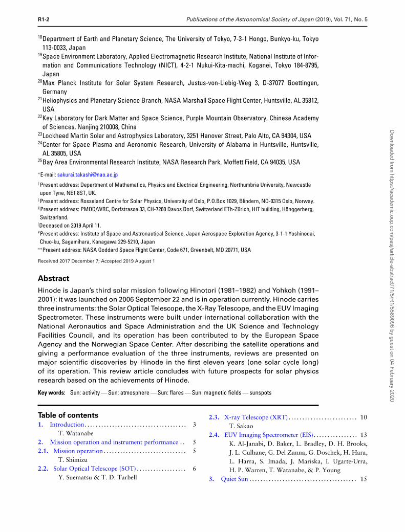
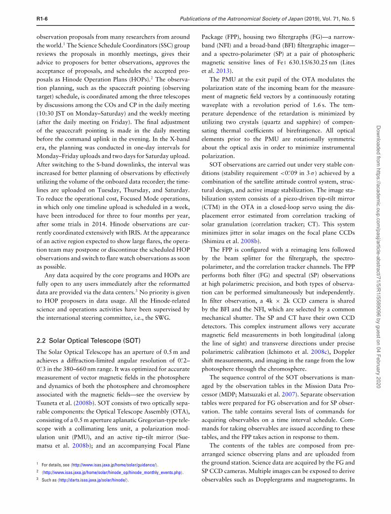
Fig. 1. Hinode spacecraft. On the left-hand-side panel, we can see EIS to the left and XRT to the right of the satellite body. At its center is SOT, withthe focal-plane package (FPP) on our side. (Color online)
they were finally combined into 3 × 10⁵ composite imagesin order to increase the dynamic range of each image bycarefully calibrating the on-orbit performance of the space-craft (Acton 2016).
Based on these discoveries of its predecessors, the Hinodemission (Kosugi et al. 2007) was designed to address thefundamental question of how magnetic fields interact withthe ionized atmosphere to produce solar variability. Themajor scientific goals of the Hinode mission are: (a) under-standing the processes of magnetic field generation andtransport, including magnetic modulation of solar lumi-nosity; (b) investigation of the processes responsible forenergy transfer from the photosphere to the corona and forheating and structuring the chromosphere and the corona;and (c) identification of the mechanism responsible foreruptive phenomena, such as flares and coronal mass ejec-tions (CMEs) in the context of the space weather of theSun–Earth system.
The Hinode satellite (figure 1) contains three instru-ments dedicated to observing the Sun: the Solar OpticalTelescope (SOT), the X-Ray Telescope (XRT), and theEUV Imaging Spectrometer (EIS). These instruments weredeveloped by ISAS/JAXA in cooperation with the NationalAstronomical Observatory of Japan (NAOJ) as domesticpartner, and the National Aeronautics and Space Adminis-tration (NASA; US) and the Science and Technology Facil-ities Council (STFC; UK) as international partners. TheEuropean Space Agency (ESA) and Norwegian SpaceCenter (NSC) provide downlink stations (Sakurai 2008).The spacecraft completed its major initial operations
including orbit adjustment to a Sun-synchronous orbit andperformance verification of the attitude control system inearly 2006 October.
All the data taken by Hinode have been open to thepublic since the successful completion of the commissioningphase in 2007 May. This open data policy was approvedand adopted by the Hinode Science Working Group (SWG),the top-level science steering group that is attended by theprincipal investigators (PIs) and the project managers (PMs)representing each space agency. It was founded in 2003 todiscuss all the issues involved in enhancing the scientificoutputs from the Hinode mission. The SWG encouragessimultaneous and collaborative observations with othersolar observation satellites and ground-based facilities, andespecially coordination among the three instruments onboard Hinode.
The Hinode SWG also recommends holding sciencemeetings regularly. The tenth-anniversary science meetingof the Hinode launch was held at Sakata and Hirata Hall inNagoya University on 2016 September 5–8. More than 160solar physicists attended this meeting from 14 countries.Taking advantage of the above opportunity, this reviewpaper has been completed as a joint work among the invitedspeakers to the meeting for each science topic, as well asPMs and instrument PIs, to assess the Hinode scientificachievements thoroughly during the first decade since itslaunch.
Throughout this article, the following non-SI units andtheir abbreviations are used: gauss (G), hectogauss (hG),kilogauss (kG), maxwell (Mx). MK means 106 K. One
Dow
nloaded from https://academ
ic.oup.com/pasj/article-abstract/71/5/R
1/5589096 by guest on 04 February 2020
Publications of the Astronomical Society of Japan (2019), Vol. 71, No. 5 R1-5
arcsec on the solar surface seen from the Earth at 1 au cor-responds to 726 km. The Appendix contains a list of abbre-viations used in this article for instrument names and so on.
2 Mission operation and instrument
performance
2.1 Mission operation
The Hinode satellite (Kosugi et al. 2007), launched on2006 September 22 (UTC), went through orbit mainte-nance maneuvers, and was finally installed into a circular,sun-synchronous polar orbit of about 685 km altitude and98.◦1 inclination. This orbit has provided continuous solarviewing conditions for a duration of nine months each year,with an eclipse season from early May to early August inwhich a night period with a longest duration of 20 minexists every 98 min orbital period. This sun-synchronouscondition is expected to be maintained until at least 2020without any orbit maneuvers.
The spacecraft system functions and their performanceare healthy, excepting for an anomaly in the X-band mis-sion data downlink channel. Starting at the end of 2007,the onboard X-band modulator began to produce irregularsignals in the latter half of each contact with the groundstations. The frequency of the occurrence increased withtime, and finally the X-band downlink function becameunavailable. After 2008 March, the mission data down-link path was switched to the S-band backup path. Sincethe bandwidth of the S-band path (262 kbps) is about16 times lower than that of the X-band path (4 Mbps),we have increased the number of downlink passes byadding many ground stations to the Hinode downlink net-work, with strong support from the space agencies. Since2009 we have typically gained 43–54 downlink passesper day, providing about 7–10 hr as the total downlinkduration per day. By efficiently utilizing the data volumeavailable from scheduled downlink passes, although lim-ited to 15%–20% of the data volume in the X-band era(40–50 Gbits), the observation planning of each telescopehas been carried out with best-tuned observing parameters,including the field of view (FOV), the number of wave-lengths observed, pixel summation, and image compres-sion, for meeting the scientific objectives of each observa-tion. The cadence of observations may be reduced to fit thetelemetry resource. Data-demanding observations, such ashigh-cadence and highest spatial resolution observations,may be restricted to a minimum required duration withreduced FOV sizes and number of observables. The 24 hrcontinuous observations may be given up by inserting idleperiods of observations when data-demanding observationsare scheduled. The available data volume is shared amongthe three instruments with a typical ratio of SOT:XRT:EIS
= 70%:15%:15%, which can be changed depending onobservations.
High spatial resolution is one of the important sci-entific accomplishments achieved by Hinode. The space-craft is stabilized by the attitude and orbit control system(AOCS) in three axes with its Z-axis pointed to the Sun.The AOCS primarily uses four momentum wheels as theactuators, with signals of sub-arcsec accuracy from twofine sun sensors (Ultra-Fine Sun Sensor; UFSS) for thesolar direction, an inertial reference unit comprising fourgyros for detecting temporal changes of attitude with veryhigh accuracy, and a star tracker for determining the rollof the spacecraft. The spacecraft jitter is measured to be0.′′1–0.′′2 (σ ) in 10 s, and 0.′′3 (σ ) in 60 s in magnitude,which is sufficient for XRT and EIS observations. A muchhigher stability of the SOT images is achieved by an imagestabilization system (see sub-subsection 2.2.1). It is notedthat the spin speed of the momentum wheels, which shouldbe controlled around ±1800 rpm, shows a gradual drift andthe high-frequency micro-vibration excited by the wheelsmay give fairly large jitter of the order of 0.′′3 (3 σ ) to theSOT images when the speed becomes around 2200 rpm. Toavoid such degraded performance, the reset operation of themomentum wheels’ speed has been carried out every 3–4 yr.The co-alignment among the telescopes with the orbitalperiod behavior of the telescope pointing has been mon-itored by performing a co-alignment program run repeat-edly during the mission (Shimizu et al. 2007; Minesugi et al.2013).
The mission operations, i.e., daily commanding andtelemetry checking, have been conducted from SagamiharaSpacecraft Operation Center (SSOC) in ISAS. The SSOCis in real-time contact with the Hinode spacecraft in lim-ited periods from Monday through Saturday via antennasat Uchinoura and in the JAXA Ground Network. The plan-ning of the three telescope operations is coordinated bya Chief Planner (CP), whose duties include scheduling thespacecraft pointing and merging instrument commands intoan integrated spacecraft load. Telescope science operationsare carried out by Chief Observers (COs). Each CO isresponsible for developing the observation sequence for thetelescope and coordinating this plan with other telescopeplans as well as with the scientists requesting the observa-tions. The CO activities are performed with the participa-tion of scientists and graduate students from cooperatinginstitutes and universities in Japan as well as from the insti-tutes and universities involved in the instrument develop-ment in the US, UK, and Norway. All the CO activitieswere performed at SSOC for a few years after the launch,but remote planning from his/her home institute was intro-duced for the COs’ activities.
In addition to the observation plans led by each instru-ment team (core programs), the Hinode team has accepted
Dow
nloaded from https://academ
ic.oup.com/pasj/article-abstract/71/5/R
1/5589096 by guest on 04 February 2020
R1-6 Publications of the Astronomical Society of Japan (2019), Vol. 71, No. 5
observation proposals from many researchers from aroundthe world.1 The Science Schedule Coordinators (SSC) groupreviews the proposals in monthly meetings, gives theiradvice to proposers for better observations, approves theacceptance of proposals, and schedules the accepted pro-posals as Hinode Operation Plans (HOPs).2 The observa-tion planning, such as the spacecraft pointing (observingtarget) schedule, is coordinated among the three telescopesby discussions among the COs and CP in the daily meeting(10:30 JST on Monday–Saturday) and the weekly meeting(after the daily meeting on Friday). The final adjustmentof the spacecraft pointing is made in the daily meetingbefore the command uplink in the evening. In the X-bandera, the planning was conducted in one-day intervals forMonday–Friday uploads and two days for Saturday upload.After switching to the S-band downlinks, the interval wasincreased for better planning of observations by effectivelyutilizing the volume of the onboard data recorder; the time-lines are uploaded on Tuesday, Thursday, and Saturday.To reduce the operational cost, Focused Mode operations,in which only one timeline upload is scheduled in a week,have been introduced for three to four months per year,after some trials in 2014. Hinode observations are cur-rently coordinated extensively with IRIS. At the appearanceof an active region expected to show large flares, the opera-tion team may postpone or discontinue the scheduled HOPobservations and switch to flare watch observations as soonas possible.
Any data acquired by the core programs and HOPs arefully open to any users immediately after the reformatteddata are provided via the data centers.3 No priority is givento HOP proposers in data usage. All the Hinode-relatedscience and operations activities have been supervised bythe international steering committee, i.e., the SWG.
2.2 Solar Optical Telescope (SOT)
The Solar Optical Telescope has an aperture of 0.5 m andachieves a diffraction-limited angular resolution of 0.′′2–0.′′3 in the 380–660 nm range. It was optimized for accuratemeasurement of vector magnetic fields in the photosphereand dynamics of both the photosphere and chromosphereassociated with the magnetic fields—see the overview byTsuneta et al. (2008b). SOT consists of two optically sepa-rable components: the Optical Telescope Assembly (OTA),consisting of a 0.5 m aperture aplanatic Gregorian-type tele-scope with a collimating lens unit, a polarization mod-ulation unit (PMU), and an active tip–tilt mirror (Sue-matsu et al. 2008b); and an accompanying Focal Plane
1 For details, see 〈http://www.isas.jaxa.jp/home/solar/guidance/〉.2 〈http://www.isas.jaxa.jp/home/solar/hinode_op/hinode_monthly_events.php〉.3 Such as 〈http://darts.isas.jaxa.jp/solar/hinode/〉.
Package (FPP), housing two filtergraphs (FG)—a narrow-band (NFI) and a broad-band (BFI) filtergraphic imager—and a spectro-polarimeter (SP) at a pair of photosphericmagnetic sensitive lines of Fe I 630.15/630.25 nm (Liteset al. 2013).
The PMU at the exit pupil of the OTA modulates thepolarization state of the incoming beam for the measure-ment of magnetic field vectors by a continuously rotatingwaveplate with a revolution period of 1.6 s. The tem-perature dependence of the retardation is minimized byutilizing two crystals (quartz and sapphire) of compen-sating thermal coefficients of birefringence. All opticalelements prior to the PMU are rotationally symmetricabout the optical axis in order to minimize instrumentalpolarization.
SOT observations are carried out under very stable con-ditions (stability requirement <0.′′09 in 3 σ ) achieved by acombination of the satellite attitude control system, struc-tural design, and active image stabilization. The image sta-bilization system consists of a piezo-driven tip–tilt mirror(CTM) in the OTA in a closed-loop servo using the dis-placement error estimated from correlation tracking ofsolar granulation (correlation tracker; CT). This systemminimizes jitter in solar images on the focal plane CCDs(Shimizu et al. 2008b).
The FPP is configured with a reimaging lens followedby the beam splitter for the filtergraph, the spectro-polarimeter, and the correlation tracker channels. The FPPperforms both filter (FG) and spectral (SP) observationsat high polarimetric precision, and both types of observa-tion can be performed simultaneously but independently.In filter observation, a 4k × 2k CCD camera is sharedby the BFI and the NFI, which are selected by a commonmechanical shutter. The SP and CT have their own CCDdetectors. This complex instrument allows very accuratemagnetic field measurements in both longitudinal (alongthe line of sight) and transverse directions under precisepolarimetric calibration (Ichimoto et al. 2008c), Dopplershift measurements, and imaging in the range from the lowphotosphere through the chromosphere.
The sequence control of the SOT observations is man-aged by the observation tables in the Mission Data Pro-cessor (MDP; Matsuzaki et al. 2007). Separate observationtables were prepared for FG observation and for SP obser-vation. The table contains several lists of commands foracquiring observables on a time interval schedule. Com-mands for taking observables are issued according to thesetables, and the FPP takes action in response to them.
The contents of the tables are composed from pre-arranged science observing plans and are uploaded fromthe ground station. Science data are acquired by the FG andSP CCD cameras. Multiple images can be exposed to deriveobservables such as Dopplergrams and magnetograms. In
Dow
nloaded from https://academ
ic.oup.com/pasj/article-abstract/71/5/R
1/5589096 by guest on 04 February 2020
Publications of the Astronomical Society of Japan (2019), Vol. 71, No. 5 R1-7
these cases, exposed data are processed in the FPP in realtime to reduce the amount of data. For example, in thecase of the SP, spectra are exposed and read out continu-ously 16 times per rotation of the polarization modulator,and the raw spectra are added and subtracted on board inreal time to be demodulated, generating Stokes I, Q, U,and V spectral images. The processed science data are thentransferred to the MDP via a high-speed parallel interface.Because of the limited telemetry downlink bandwidth, dataare compressed in pixel depth (16 to 12 bit compression) aswell as in two-dimensional image planes (image compres-sion). The MDP re-forms the compressed data into CCSDS(Consultative Committee for Space Data Systems) packetsand sends them to the Data Handling Unit (DHU) forrecording in the Data Recorder (DR).
The MDP has eight kinds of lookup tables to performthe 16 to 12 bit compression with different compressioncurves. For image compression of SOT data, two algo-rithms are available for different compression parametertables: one is 12 bit JPEG DCT (discrete cosine transform)lossy compression and the other is 12 bit DPCM (differen-tial pulse code modulation) lossless compression. Typically,filtergram data can be compressed to 3 bits pixel−1 by theJPEG algorithm and Stokes vector data to 1.5 bits pixel−1
when the noise due to lossy compression is comparable tothe photon noise level in the data, although the compressionratio is highly dependent upon the nature of the images.
2.2.1 On-orbit performanceThe on-orbit performance of SOT has generally proved tobe excellent and met or exceeded all prelaunch requirementsfor the BFI, SP, and CT. However, it turned out soon afterthe first-light observation that images from the NFI con-tained the blemishes that degraded or obscured the imageover part of the FOV. These were caused by air bubbles inan index-matching oil inside the tunable birefringent (Lyot)filter. In the following, some key aspects of on-orbit perfor-mance of SOT are given.
Optical performance. The image stabilization is criticalfor high-resolution and high-precision polarimetric obser-vations. It was evaluated by the displacement of an imagetaken by the CT camera at 580 Hz with respect to a ref-erence image fixed for ∼40 s. While the CT servo is on,the image stability gets as high as 0.′′01 root mean square(rms) in both X and Y directions (X in solar east–west,Y in north–south directions), which is about three timessmaller than the requirement. It was confirmed that movingmechanisms in the three telescopes of Hinode do not pro-duce a significant degradation of the SOT images duringtheir movement except for the visible-light shutter (VLS) ofXRT, which produces an SOT image jitter of about 0.′′4 rmsduring the period of its movement (∼0.5 s). However, the
influence of the XRT VLS on the SOT observation is neg-ligibly small since the frequency of its usage is sufficientlylow.
The BFI produces photometric images with broad spec-tral coverage in six bands [CN band (388.3 nm), Ca II H line(366.8 nm), G band (430.5 nm), and three continuum bands(450.4 nm, 555.0 nm, 668.4 nm)] at the highest spatial res-olution available from SOT (0.′′0541 per pixel sampling)and at a rapid cadence (<10 s typical, minimum 1.6 s for asmaller FOV) over a 218′′ × 109′′ FOV. Exposure times aretypically 0.03–0.8 s, but longer exposures are possible. TheBFI is capable of accurate measurements of proper motionand temperature in the photosphere, and of high-resolutionimaging of some structures in the chromosphere, and mea-surements in the three shortest wavelength bands permitidentification of sites of kilogauss-strength magnetic fieldoutside sunspots.
Diffraction-limited optical performance of the BFI wasconfirmed using a point-like structure seen in G-bandimages. The size of the point-like structure is fairly close tothat from a theoretical point spread function (PSF) for theobserving wavelength (Suematsu et al. 2008b). The PSFsfor all BFI wavelengths were also measured by Mathew,Zakharov, and Solanki (2009) using Mercury transit dataof 2006 November (see also Wedemeyer-Bohm 2008).The dark disk-like Mercury images were convolved witha model PSF, generated by a combination of four two-dimensional Gaussians, to fit the observed intensity pro-files. The narrowest Gaussian in all cases closely repro-duces the theoretical angular resolution of the OTA, whilethe remaining Gaussians with much broader widths mainlyaccount for the scattered light in the OTA.
In the case of the SP, the intensity contrast of gran-ulations observed by the SP was compared with thosefrom three-dimensional (3D) radiative magnetohydrody-namic (MHD) simulations to estimate its PSF (Danilovicet al. 2008). It was confirmed that the observed con-trast is reproduced well by the convolution of thesynthetic image from the MHD simulation with a PSFderived from the shape of the OTA entrance pupil havinga slight defocus aberration in which the Strehl ratio is closeto 0.8.
As expected, a gradual change in the best focus posi-tion was observed, which is mainly caused by dehydrationshrinkage in space of the CFRP (carbon-fiber-reinforcedplastics) truss pipes connecting the primary with the sec-ondary mirror of the OTA. However, it unexpectedlyturned out that the focus also changes according to thechange in pointing on the solar disk; however, the focusoffset is about seven steps in reimaging lens displace-ment (0.17 mm step−1) from disk-center to limb pointing.Although the cause of this focus change is not well under-stood, the response is fast enough to allow us to readjust
Dow
nloaded from https://academ
ic.oup.com/pasj/article-abstract/71/5/R
1/5589096 by guest on 04 February 2020
R1-8 Publications of the Astronomical Society of Japan (2019), Vol. 71, No. 5
the reimaging lens position at each maneuver of the satel-lite during operation. During the eclipse season (from earlyMay to early August), a large focus drift (∼12 steps) occurs∼30 min from the dawn in each orbit. This is a predictedbehavior caused by thermal deformation by the day/nightcycle of the heat-dump-mirror cylinder and its supportingspider which can displace the secondary mirror. The eclipseseason is certainly a degraded performance period forSOT. The gradual focus drift almost ended after 2011when the dehydration of the CFRP slowed down and thetemperature of the OTA became stable by heater con-trol, although the short-term focus change due to pointingchange still remains and is corrected during operation.
The BFI has a chromatic aberration which was unex-pectedly recognized after the launch. Then, it was noticedthat a relay lens of the BFI had been flipped from theoriginal optical design in the ground test to have co-focuswith NFI and SP, which works in air but not in vacuum.The focus difference between 388 nm and 668 nm is aboutnine steps (= 1.53 mm of the reimaging lens displacement).If the reimaging lens is set at the center of the chro-matic aberration, the focus offset is about four steps atthe longest or shortest wavelength, and the correspondingwave-front error is 21 nm rms. Thus the impact of thechromatic aberration is small, but not negligible when weobserve in two extreme wavelengths simultaneously. Thereis no evidence of chromatic aberration in the NFI, andthe SP is well co-focused with the BFI 668 nm (Ichimotoet al. 2008b).
It was confirmed in an early commissioning phase thatthe light levels in individual observing wavelengths wereclose to those predicted from the ground Sun tests. It turnedout, however, that the throughputs of all observing wave-lengths have decreased monotonically in such a manner thatthose of shorter wavelengths have steeper degradation. Atthe beginning of 2011, the throughput became about 32%at 388.3 nm, 40% at 396.8 nm, 62% at 430.2 nm, 77% inthe blue continuum, and 87%–89% in the green and redcontinua. The throughputs at the two shorter wavelengthshave recovered since then up to 50%–55% and becomestable, while those at longer wavelengths keep decreasing.The SP (630.2 nm) throughput has become 64% in the tenyears since first light; accordingly, the signal-to-noise ratiohas gone down to 80%. The causes of the degradation andrecovery are not identified, although contaminants accumu-lating on the OTA optics and cleaning by atomic oxygenin the phase of high solar activity might be possibilities.The baking of the FG CCD did not help in recovering thethroughput.Spectro-polarimeter. The SP is designed to be operatedflexibly in mapping observing regions, allowing one to per-form suitable observations depending on science objectives.It has a number of modes of operation: Normal Map, Fast
Map, Dynamics, and Deep Magnetogram. The NormalMap mode produces polarimetric accuracy in the polar-ization continuum of about 0.0012 Ic with 4.8 s integrationand the spatial sampling of 0.′′16 × 0.′′16 (Lites et al. 2008).It takes 83 min to scan a 160′′-wide area, large enough tocover a moderate-sized active region. By reducing the scan-ning size, the cadence becomes faster (50 s for mapping a1.′′6-wide area). The Fast Map mode, which is mostly usedto save telemetry, provides 30 min cadence for 160′′-widescanning with polarimetric accuracy of 0.1% but a 0.′′32sampling. The Dynamics mode provides higher cadence(18 s for a 1.′′6-wide area) with a 0.′′16 sampling, althoughat lower polarimetric accuracy.
In Deep Magnetogram mode, photons can be accumu-lated over many rotations of the polarization modulator,as long as the data do not overflow the CCD summingregisters. This allows one to achieve a very high degree ofpolarization accuracy in very quiet regions, at the expenseof time resolution. Using this mode for data of an effectiveintegration time of 67.2 s, the rms noise in the polarizationcontinuum of the spectra was estimated to be about 3 ×10⁻⁴, corresponding to 1 σ noise levels of 0.6 G and 20.1 Gfor the longitudinal and transverse components of magneticflux density, respectively (Lites et al. 2008).
The SP shows an orbital drift of the spectral image onthe CCD with an amplitude of about 10 pixels (p–p) inboth directions along and perpendicular to the slit. Thecause is displacement of the Littrow mirror due to thermaldeformation of the FPP structure according to the orbitalmotion. The drift rate was minimized by optimizing thetemperature settings of the operational heaters attached tothe FPP structure, and is finally corrected by the calibrationsoftware SP_PREP (Lites & Ichimoto 2013).Narrow-band Filtergraphic Imager. The NFI providesintensity, Doppler, and full Stokes polarimetric imaging athigh spatial resolution (0.′′08 per pixel sampling) in anyone of ten spectral lines [including the Fe lines (525.0 nm,557.6 nm, 630.2 nm), having a range of sensitivity to theZeeman effect, Mg I b2 (517.3 nm), Na D1 (89.6 nm),and Hα] over the full FOV (328′′ × 164′′). The spec-tral lines span the photosphere to the lower chromo-sphere for diagnosis of dynamical behavior of magneticand velocity fields at the lower atmosphere. The passbandof the Lyot filter is 9 pm and the wavelength center istunable to several positions in a spectral line and itsnearby continuum. It is noted that the edges of the fullFOV are slightly vignetted due to the limited size of theoptical elements of the Lyot filter residing in a telecentricbeam. The unvignetted area is 264′′ in diameter. Expo-sure times are typically 0.1–1.6 s, but longer exposuresare possible.
Shutterless modes with the frame transfer operation ofthe CCD are used for higher time resolution (1.6–4.8 s) and
Dow
nloaded from https://academ
ic.oup.com/pasj/article-abstract/71/5/R
1/5589096 by guest on 04 February 2020
Publications of the Astronomical Society of Japan (2019), Vol. 71, No. 5 R1-9
polarimetric sensitivity, although the FOV is restricted bya focal plane mask. With a 0.1 s exposure, 16 images aretaken in a revolution of the PMU waveplate. These imagesare successively added or subtracted in the four slots ofthe smart memory to create the Stokes IQUV images. Themodulation frequency is two per PMU rotation for V andfour per PMU rotation for Q and U.
Images of the NFI contained blemishes due to bubblesin the oil of the Lyot filter which degraded or obscuredthe image over part of the FOV. They distorted and movedwhen the Lyot filter was tuned. For this reason, NFI usuallyran in one spectral line at one or a small number of wave-lengths for a sequence of observations. Rapid switchingbetween spectral lines was inhibited in its operation. Tosuppress the disturbance by the bubbles, it was requiredto block four tuning elements out of eight. This situationlimited the capability of tuning the filter, but some usefulschemes were still available. New software to enable suchoperations was successfully uploaded twice, in 2007 Apriland September, and tuning schemes have been developedand tested which permit tuning to different positions ina line profile without disturbing the bubbles. Thus, 50%–75% of the FOV remained usable in most NFI observations.
Doppler and magnetogram observations usingtwo wavelengths remained possible. However, multi-wavelength scans of Stokes parameters, for vector fieldinversion, had become generally impossible. Wavelengthscans in Hα were also severely curtailed because of thebubble motion they caused. These limitations interferedwith some science goals regarding rapid evolution of vectormagnetic fields and chromospheric structure and dynamicsin active regions, flares, and prominences.
It was also found that the transmission of the blockingfilters was degrading rapidly. The cause was identified asfilter coating damage due to solar UV flux. Five of the sixblocking filters have zinc sulfide coating layers which absorbUV light below ∼420 nm and change its index of refraction.As a result, the transmission profiles shifted to the blue andwere badly distorted (Title 1974). The Fe I 630.2 nm filterwas severely damaged and quickly became unusable; about60% of throughput was lost in a year from first light. Sinceonly the blocking filter for Na I D1 589 nm is durable againstthe UV, this filter is always inserted in the beam during theidle time, to slow the degradation of other filters. Thus, themagnetograms and Dopplergrams in the Na I D1 line wereused in most NFI observations.
In 2010 the filter bubbles disappeared, either dissolvingback into the oil or moving out of view. For about twoyears, NFI observations with multiple lines and wavelengthsettings were possible using the whole FOV, though withlimitations on the usage of the vulnerable blocking filters.Early in 2013 a bubble reappeared at a location where it didnot move with tuning but caused image degradation over
part of the field. Users of NFI data from this period shouldcontact the SOT team if they have questions about the imagequality of specific datasets. Many observing programs usedoffsets from the center of the FOV to put the target in anarea with uncompromised image quality.
2.2.2 Conclusions and future observingThe Solar Optical Telescope is the largest state-of-artoptical telescope yet flown in space to observe the Sun. Ithas exhibited excellent performance on-orbit for more thaneleven years. Many excellent papers have been published todate as given elsewhere in this review paper using SOT’sunprecedentedly high-quality data for the sub-photosphere(local helioseismology) through the chromosphere.
Although ground-based telescopes make observations ofthe same type and at the same wavelengths as the SOT,the telescope in space derives great advantages from theuniformity of its observing conditions: (1) high resolutionat all times over all of its FOV, (2) continuous temporalcoverage, and (3) unprecedented polarimetric sensitivity atsmall spatial scales. Discovery of waves on spicules andprominence threads, bubbles and instabilities in promi-nences, and penumbral microjets are examples of the firstadvantage. Continuous, multi-day studies of the emergenceand evolution of network and intra-network magnetic fluxare enabled by the second. All three advantages contributeto the spectro-polarimetric contributions to understandingboth global and local dynamos, with cycle-long observa-tions of the polar fields and of the weak, quiet Sun fields atall latitudes.
Magnetic fields transport energy into the upper atmo-sphere through emerging fields, propagating waves, andwork done on existing magnetic footpoints by photosphericmotions. Free energy can be stored in magnetic fields,which is dissipated via magnetic reconnection and inducesMHD instability and eruptions. Therefore, to understandthe origin of solar active phenomena, it is very importantto measure the underlying magnetic fields accurately, withhigh spatial resolution and good temporal coverage of theirresolution.
Higher temporal, spatial, and velocity resolution thanwhat previous satellites provided has allowed us to mea-sure waves in the atmosphere in a way we were unableto do before. Previous attempts to detect MHD wavesusing ground-based observations have yielded ambiguousresults, but SOT has opened the door to these waves beingobserved in many different circumstances; the waves maycarry enough energy to heat the corona and accelerate thesolar wind in the quiet Sun.
The SOT observations of active regions provided someevidence that an average vertical Poynting flux, in whichphotospheric motion shuffles the footpoints of coronal
Dow
nloaded from https://academ
ic.oup.com/pasj/article-abstract/71/5/R
1/5589096 by guest on 04 February 2020
R1-10 Publications of the Astronomical Society of Japan (2019), Vol. 71, No. 5
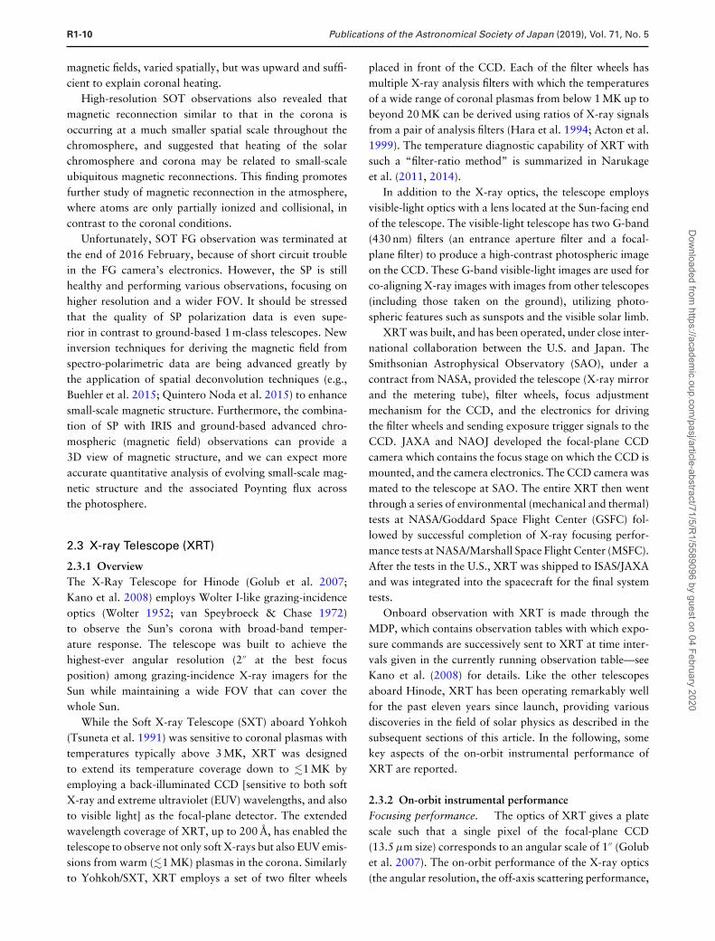
magnetic fields, varied spatially, but was upward and suffi-cient to explain coronal heating.
High-resolution SOT observations also revealed thatmagnetic reconnection similar to that in the corona isoccurring at a much smaller spatial scale throughout thechromosphere, and suggested that heating of the solarchromosphere and corona may be related to small-scaleubiquitous magnetic reconnections. This finding promotesfurther study of magnetic reconnection in the atmosphere,where atoms are only partially ionized and collisional, incontrast to the coronal conditions.
Unfortunately, SOT FG observation was terminated atthe end of 2016 February, because of short circuit troublein the FG camera’s electronics. However, the SP is stillhealthy and performing various observations, focusing onhigher resolution and a wider FOV. It should be stressedthat the quality of SP polarization data is even supe-rior in contrast to ground-based 1 m-class telescopes. Newinversion techniques for deriving the magnetic field fromspectro-polarimetric data are being advanced greatly bythe application of spatial deconvolution techniques (e.g.,Buehler et al. 2015; Quintero Noda et al. 2015) to enhancesmall-scale magnetic structure. Furthermore, the combina-tion of SP with IRIS and ground-based advanced chro-mospheric (magnetic field) observations can provide a3D view of magnetic structure, and we can expect moreaccurate quantitative analysis of evolving small-scale mag-netic structure and the associated Poynting flux acrossthe photosphere.
2.3 X-ray Telescope (XRT)
2.3.1 OverviewThe X-Ray Telescope for Hinode (Golub et al. 2007;Kano et al. 2008) employs Wolter I-like grazing-incidenceoptics (Wolter 1952; van Speybroeck & Chase 1972)to observe the Sun’s corona with broad-band temper-ature response. The telescope was built to achieve thehighest-ever angular resolution (2′′ at the best focusposition) among grazing-incidence X-ray imagers for theSun while maintaining a wide FOV that can cover thewhole Sun.
While the Soft X-ray Telescope (SXT) aboard Yohkoh(Tsuneta et al. 1991) was sensitive to coronal plasmas withtemperatures typically above 3 MK, XRT was designedto extend its temperature coverage down to �1 MK byemploying a back-illuminated CCD [sensitive to both softX-ray and extreme ultraviolet (EUV) wavelengths, and alsoto visible light] as the focal-plane detector. The extendedwavelength coverage of XRT, up to 200 A, has enabled thetelescope to observe not only soft X-rays but also EUV emis-sions from warm (�1 MK) plasmas in the corona. Similarlyto Yohkoh/SXT, XRT employs a set of two filter wheels
placed in front of the CCD. Each of the filter wheels hasmultiple X-ray analysis filters with which the temperaturesof a wide range of coronal plasmas from below 1 MK up tobeyond 20 MK can be derived using ratios of X-ray signalsfrom a pair of analysis filters (Hara et al. 1994; Acton et al.1999). The temperature diagnostic capability of XRT withsuch a “filter-ratio method” is summarized in Narukageet al. (2011, 2014).
In addition to the X-ray optics, the telescope employsvisible-light optics with a lens located at the Sun-facing endof the telescope. The visible-light telescope has two G-band(430 nm) filters (an entrance aperture filter and a focal-plane filter) to produce a high-contrast photospheric imageon the CCD. These G-band visible-light images are used forco-aligning X-ray images with images from other telescopes(including those taken on the ground), utilizing photo-spheric features such as sunspots and the visible solar limb.
XRT was built, and has been operated, under close inter-national collaboration between the U.S. and Japan. TheSmithsonian Astrophysical Observatory (SAO), under acontract from NASA, provided the telescope (X-ray mirrorand the metering tube), filter wheels, focus adjustmentmechanism for the CCD, and the electronics for drivingthe filter wheels and sending exposure trigger signals to theCCD. JAXA and NAOJ developed the focal-plane CCDcamera which contains the focus stage on which the CCD ismounted, and the camera electronics. The CCD camera wasmated to the telescope at SAO. The entire XRT then wentthrough a series of environmental (mechanical and thermal)tests at NASA/Goddard Space Flight Center (GSFC) fol-lowed by successful completion of X-ray focusing perfor-mance tests at NASA/Marshall Space Flight Center (MSFC).After the tests in the U.S., XRT was shipped to ISAS/JAXAand was integrated into the spacecraft for the final systemtests.
Onboard observation with XRT is made through theMDP, which contains observation tables with which expo-sure commands are successively sent to XRT at time inter-vals given in the currently running observation table—seeKano et al. (2008) for details. Like the other telescopesaboard Hinode, XRT has been operating remarkably wellfor the past eleven years since launch, providing variousdiscoveries in the field of solar physics as described in thesubsequent sections of this article. In the following, somekey aspects of the on-orbit instrumental performance ofXRT are reported.
2.3.2 On-orbit instrumental performanceFocusing performance. The optics of XRT gives a platescale such that a single pixel of the focal-plane CCD(13.5 μm size) corresponds to an angular scale of 1′′ (Golubet al. 2007). The on-orbit performance of the X-ray optics(the angular resolution, the off-axis scattering performance,
Dow
nloaded from https://academ
ic.oup.com/pasj/article-abstract/71/5/R
1/5589096 by guest on 04 February 2020
Publications of the Astronomical Society of Japan (2019), Vol. 71, No. 5 R1-11
and the plate scale) of XRT has been studied by severalauthors using XRT observation of the transit of Mercuryin front of the Sun (Shimizu et al. 2007; Weber et al.2007), through image co-alignment studies (Yoshimura &McKenzie 2015), and using XRT images of the Venustransit (Afshari et al. 2016). To the best of our knowledge,the XRT optics has been stably providing superior X-rayimaging performance that is fully consistent with prelaunchmeasurements. Discussion of the effect of vignetting of theXRT mirror, together with comprehensive characterizationof the image signal outputs from the CCD, is given byKobelski et al. (2014b).
In general, the Wolter I optics exhibits some image cur-vature around the focal point—see, e.g., figure 3 of Golubet al. (2007). This, in turn, implies that one can have high-spatial-resolution images with a relatively narrow FOV inan image plane placed at around the best on-axis focusposition while modest-resolution images with a wide FOVin another image plane placed ahead (nearer to the Sun)of the best focus position. By moving the focus stage alongthe optical axis, XRT adopts two CCD positions; one isreferred to as the “Narrow Field Focus” and the other asthe “Wide Field Focus.” The former puts the imaging sur-face of the CCD 81 μm ahead of the best on-axis focusposition determined by the preflight focusing performancetests. This gives an rms blur diameter of less than 1′′ for anoff-axis angle up to >8′. The Narrow Field Focus positionis used for most XRT images that are taken with a limitedFOV. The Wide Field Focus, for which the CCD is placed251 μm ahead of the best on-axis focus position, is typicallyused for synoptic full-Sun images, which have been regu-larly taken twice a day (usually at around 6 UT and 18 UTof each day) to observe, e.g., long-term variations of thecorona in multiple X-ray analysis filters. This focus posi-tion provides images with less than 2′′ rms blur diameterfor an extended off-axis angle up to ∼15′. The absolutefocus position is calibrated once every week by referringto a built-in mechanical reference in the focus adjustmentmechanism.
Temperature diagnostics with X-ray analysis filters. Pre-cise calibration of X-ray analysis filters is key for derivingcorrect filter-ratio temperatures with XRT. In addition toprelaunch calibration of the filters with X-rays as reportedin Golub et al. (2007), the thicknesses of all the X-rayanalysis filters were further calibrated using on-orbit databy Narukage et al. (2011). The focal-plane CCD and theanalysis filters have been suffering from molecular contam-ination which deteriorates the sensitivity of the XRT, inparticular at longer X-ray wavelengths. On-orbit calibra-tion was performed together with characterizing the pos-sible chemical composition of the contamination materialand its time-dependent accumulation thickness onto the
CCD and each of the analysis filters. Such characteriza-tion of the molecular contamination is detailed in Narukageet al. (2011). In order to minimize permanent accumula-tion of the contaminants on the CCD, XRT conducts aregular CCD decontamination bake-out once every threeweeks. Each bake-out lasts for three days, during which theCCD temperature is kept between +30
◦C and +35
◦C. The
interval and the duration of the CCD bake-out have beendetermined to minimize the impact on observations whileremoving most, if not all, contaminants accumulated onthe CCD.
The calibration of the filter thicknesses made inNarukage et al. (2011) was based chiefly on quiet-Sun datadue to the low solar activity during the period in which thecalibration was made. This has left some room for furtherrefinement of the filter thicknesses for thicker filters thatare used for observing hot plasmas in active regions and inflares. An update to the calibration using active region datawas made in Narukage et al. (2014) which improved thecharacterizing thicknesses of the thicker filters.Image co-alignment. Precise knowledge of the positionof each XRT image with respect to the solar disk isindispensable for co-aligning XRT data with images fromother telescopes/facilities. Effort to establish co-alignmentbetween images from multiple instruments including XRTwas initiated soon after launch (the first one being theco-alignment effort between SOT and XRT; Shimizu et al.2007) and is still ongoing. Extensive characterizationof XRT co-alignment features utilizing Hinode’s UFSS(Tsuno et al. 2008) and the 335 A band of the AtmosphericImager Assembly onboard the Solar Dynamics Observa-tory (SDO/AIA; Lemen et al. 2012) was conducted byYoshimura and McKenzie (2015). Their work has enabledco-aligning XRT images with an accuracy much betterthan 1′′.
Some part of the entrance filter of XRT was brokenon orbit: first on 2012 May 9 and secondly on 2015June 14, with two additional small breaks in 2017 Mayand 2018 May. Note that a similar break in the entrancefilters was also experienced by Yohkoh/SXT, whose visible-light contamination of X-ray images was carefully studiedand characterized by Acton (2016). The increased levelof visible-light contamination through the X-ray opticspath forced a shortening of exposure durations for takingG-band images; they can still be taken without satu-ration in the CCD output, but it turned out that theshortest exposure time (1 ms) had to be adopted after thesecond break. In addition to the increased G-band inten-sity on the CCD, stray-light features also appeared inG-band images. These features can be removed by takinga G-band image with the shutter (VLS) closed and sub-tracting that image from the corresponding image takenwith the VLS open. As well as the impact on visible-light
Dow
nloaded from https://academ
ic.oup.com/pasj/article-abstract/71/5/R
1/5589096 by guest on 04 February 2020
R1-12 Publications of the Astronomical Society of Japan (2019), Vol. 71, No. 5
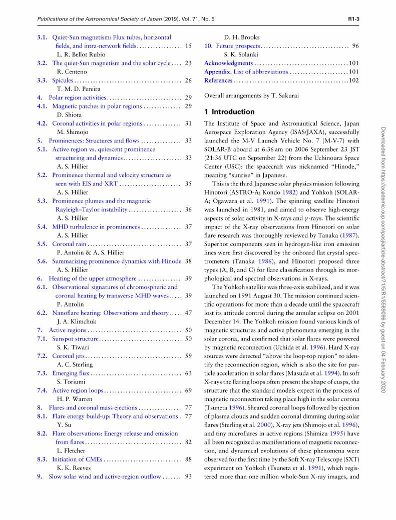
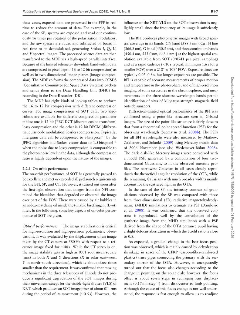
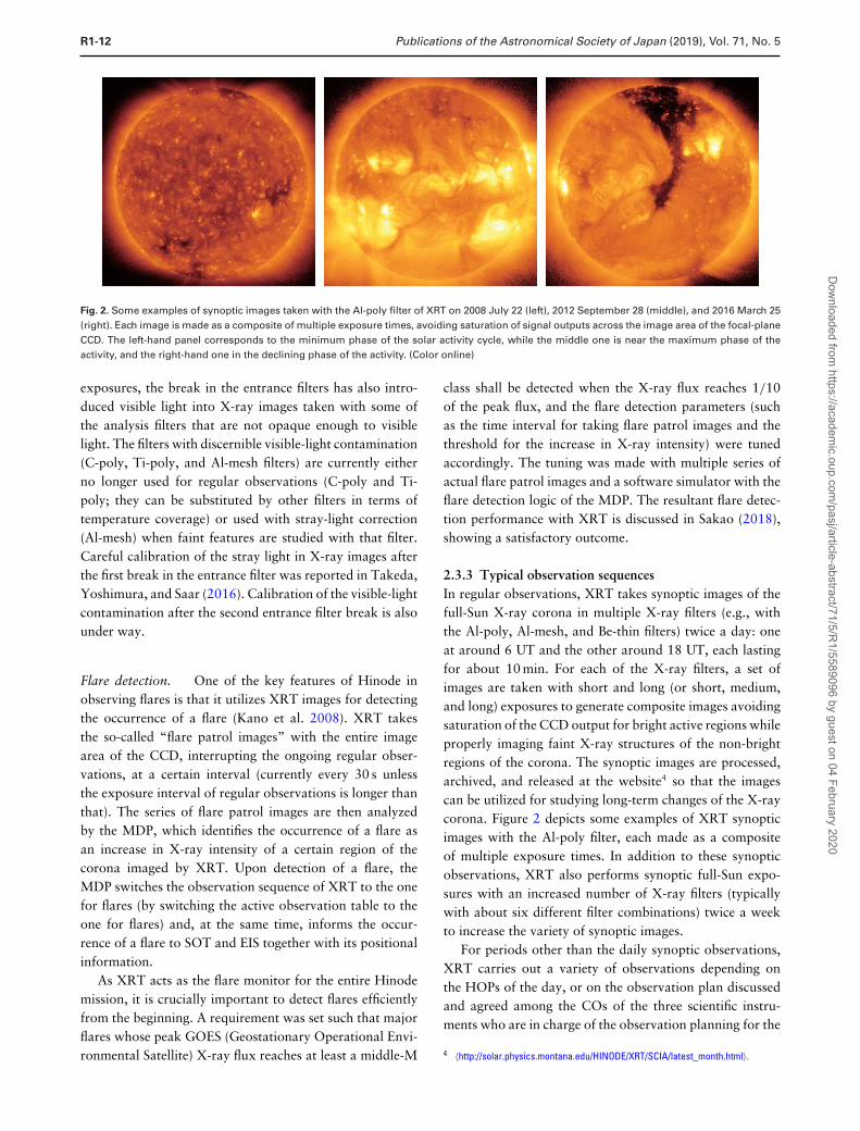
Fig. 2. Some examples of synoptic images taken with the Al-poly filter of XRT on 2008 July 22 (left), 2012 September 28 (middle), and 2016 March 25(right). Each image is made as a composite of multiple exposure times, avoiding saturation of signal outputs across the image area of the focal-planeCCD. The left-hand panel corresponds to the minimum phase of the solar activity cycle, while the middle one is near the maximum phase of theactivity, and the right-hand one in the declining phase of the activity. (Color online)
exposures, the break in the entrance filters has also intro-duced visible light into X-ray images taken with some ofthe analysis filters that are not opaque enough to visiblelight. The filters with discernible visible-light contamination(C-poly, Ti-poly, and Al-mesh filters) are currently eitherno longer used for regular observations (C-poly and Ti-poly; they can be substituted by other filters in terms oftemperature coverage) or used with stray-light correction(Al-mesh) when faint features are studied with that filter.Careful calibration of the stray light in X-ray images afterthe first break in the entrance filter was reported in Takeda,Yoshimura, and Saar (2016). Calibration of the visible-lightcontamination after the second entrance filter break is alsounder way.
Flare detection. One of the key features of Hinode inobserving flares is that it utilizes XRT images for detectingthe occurrence of a flare (Kano et al. 2008). XRT takesthe so-called “flare patrol images” with the entire imagearea of the CCD, interrupting the ongoing regular obser-vations, at a certain interval (currently every 30 s unlessthe exposure interval of regular observations is longer thanthat). The series of flare patrol images are then analyzedby the MDP, which identifies the occurrence of a flare asan increase in X-ray intensity of a certain region of thecorona imaged by XRT. Upon detection of a flare, theMDP switches the observation sequence of XRT to the onefor flares (by switching the active observation table to theone for flares) and, at the same time, informs the occur-rence of a flare to SOT and EIS together with its positionalinformation.
As XRT acts as the flare monitor for the entire Hinodemission, it is crucially important to detect flares efficientlyfrom the beginning. A requirement was set such that majorflares whose peak GOES (Geostationary Operational Envi-ronmental Satellite) X-ray flux reaches at least a middle-M
class shall be detected when the X-ray flux reaches 1/10of the peak flux, and the flare detection parameters (suchas the time interval for taking flare patrol images and thethreshold for the increase in X-ray intensity) were tunedaccordingly. The tuning was made with multiple series ofactual flare patrol images and a software simulator with theflare detection logic of the MDP. The resultant flare detec-tion performance with XRT is discussed in Sakao (2018),showing a satisfactory outcome.
2.3.3 Typical observation sequencesIn regular observations, XRT takes synoptic images of thefull-Sun X-ray corona in multiple X-ray filters (e.g., withthe Al-poly, Al-mesh, and Be-thin filters) twice a day: oneat around 6 UT and the other around 18 UT, each lastingfor about 10 min. For each of the X-ray filters, a set ofimages are taken with short and long (or short, medium,and long) exposures to generate composite images avoidingsaturation of the CCD output for bright active regions whileproperly imaging faint X-ray structures of the non-brightregions of the corona. The synoptic images are processed,archived, and released at the website4 so that the imagescan be utilized for studying long-term changes of the X-raycorona. Figure 2 depicts some examples of XRT synopticimages with the Al-poly filter, each made as a compositeof multiple exposure times. In addition to these synopticobservations, XRT also performs synoptic full-Sun expo-sures with an increased number of X-ray filters (typicallywith about six different filter combinations) twice a weekto increase the variety of synoptic images.
For periods other than the daily synoptic observations,XRT carries out a variety of observations depending onthe HOPs of the day, or on the observation plan discussedand agreed among the COs of the three scientific instru-ments who are in charge of the observation planning for the
4 〈http://solar.physics.montana.edu/HINODE/XRT/SCIA/latest_month.html〉.
Dow
nloaded from https://academ
ic.oup.com/pasj/article-abstract/71/5/R
1/5589096 by guest on 04 February 2020
Publications of the Astronomical Society of Japan (2019), Vol. 71, No. 5 R1-13
relevant day. The non-synoptic, regular observations typi-cally consist of observing the target on the Sun with a limitedFOV (by reading out limited image areas on the CCD suchas 512 × 512 or 384 × 384 pixel areas out of the entireimage area of 2048 × 2048 pixels) to increase the expo-sure cadence by reducing the data volume of the imagestaken. These images are taken with the Narrow Field Focusposition (see sub-subsection 2.3.2, Focusing performance).
When a flare is detected by the MDP, XRT starts toobserve the flare by performing a sequence of exposuresdefined in the MDP flare-observing table. With the flare-observing table, XRT takes images of the flare with rel-atively thick analysis filters (such as the Be-thin, Be-med,and Al-thick filters) which are suited to observing the hotplasmas created by the flare. At the same time, images withthin analysis filter(s) (e.g., Al-thin) are also taken at aninterval of ∼15 s with a large FOV (17′ × 17′) to coverthe entire flaring region in the corona. With this seriesof exposures, XRT has been capturing, in addition to thebright flaring loops, faint plasma features present aroundthe flaring area such as supra-arcade downflows and ejec-tion of plasmoids.
2.3.4 Conclusions and future prospectsSince the beginning of Hinode observations, XRT has beenproviding excellent X-ray images of the Sun’s corona, con-tributing to various new findings in the field of solar physicsas reported in this article. A set of XRT analysis soft-ware is available in the SolarSoft IDL (Interactive DataLanguage) tree (Freeland & Handy 1998), and interestedreaders can readily analyze XRT data following the XRTAnalysis Guide.5 With an increase in the default telemetryallocation for XRT (23% as compared to the previous valueof 15%) after the middle of 2016, XRT is now capableof taking X-ray images of the corona with higher expo-sure cadence and/or with larger FOV than before. This hasenabled us to carry out XRT observations with increasedflexibility and variation in the images to be taken, thusoffering the possibility of revealing further new aspects ofthe X-ray Sun.
2.4 EUV Imaging Spectrometer (EIS)
The EUV Imaging Spectrometer (Culhane et al. 2007) wasdesigned to observe and understand many of the physicalprocesses that occur in the solar corona and upper tran-sition region. Its primary science objectives include under-standing coronal heating, the onset of CMEs and flares,and the origin of the solar wind. The EIS design representsa significant advance in spatial resolution, effective area,
5 Available at 〈http://xrt.cfa.harvard.edu/resources/documents/XAG/XAG.pdf〉.
and temperature coverage over many previous spectrom-eters. To complement the detailed science reviews givenelsewhere in this paper, here we give a brief overview ofthe EIS instrument and provide information on its on-orbitperformance.
2.4.1 EIS observingEIS observes emission lines in the wavelength ranges 170–210 A and 250–290 A. The range of emission lines availableprovides density diagnostics, FIP (first ionization poten-tial effect) measurements, Doppler velocities, line widths,and emission measure distributions. Telemetry constraints,however, often limit the number of spectral windows thatcan be returned during an observation. Line selection wasdiscussed in detail in Young et al. (2007). Informationon the high-temperature lines observed in active regions(e.g., Ca XIV–Ca XVII, Fe XVII) and flares (e.g., Fe XXII–Fe XIV)was provided in Watanabe et al. (2007) and Warren et al.(2008).
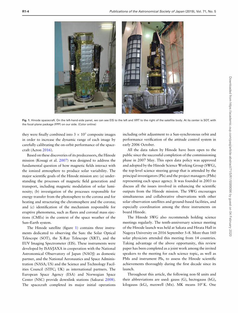
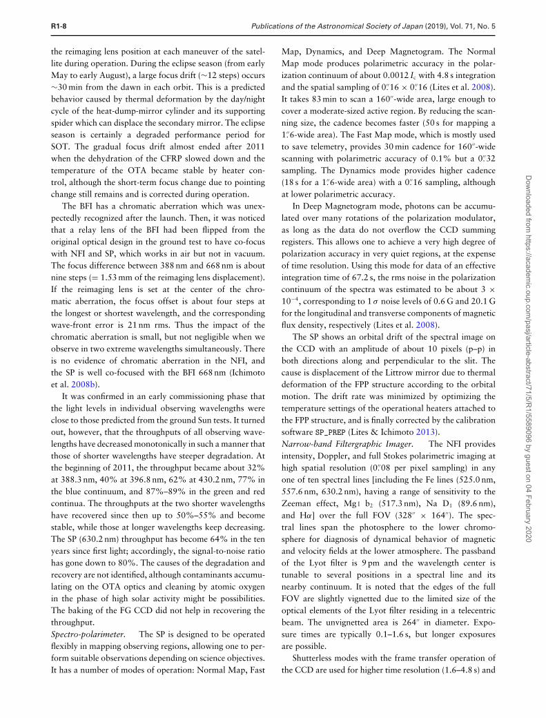
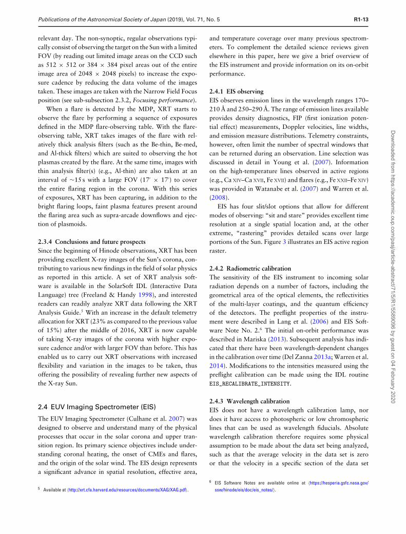
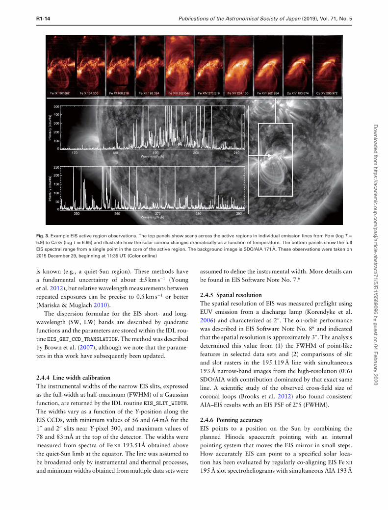
EIS has four slit/slot options that allow for differentmodes of observing: “sit and stare” provides excellent timeresolution at a single spatial location and, at the otherextreme, “rastering” provides detailed scans over largeportions of the Sun. Figure 3 illustrates an EIS active regionraster.
2.4.2 Radiometric calibrationThe sensitivity of the EIS instrument to incoming solarradiation depends on a number of factors, including thegeometrical area of the optical elements, the reflectivitiesof the multi-layer coatings, and the quantum efficiencyof the detectors. The preflight properties of the instru-ment were described in Lang et al. (2006) and EIS Soft-ware Note No. 2.6 The initial on-orbit performance wasdescribed in Mariska (2013). Subsequent analysis has indi-cated that there have been wavelength-dependent changesin the calibration over time (Del Zanna 2013a; Warren et al.2014). Modifications to the intensities measured using thepreflight calibration can be made using the IDL routineEIS_RECALIBRATE_INTENSITY.
2.4.3 Wavelength calibrationEIS does not have a wavelength calibration lamp, nordoes it have access to photospheric or low chromosphericlines that can be used as wavelength fiducials. Absolutewavelength calibration therefore requires some physicalassumption to be made about the data set being analyzed,such as that the average velocity in the data set is zeroor that the velocity in a specific section of the data set
6 EIS Software Notes are available online at 〈https://hesperia.gsfc.nasa.gov/ssw/hinode/eis/doc/eis_notes/〉.
Dow
nloaded from https://academ
ic.oup.com/pasj/article-abstract/71/5/R
1/5589096 by guest on 04 February 2020
R1-14 Publications of the Astronomical Society of Japan (2019), Vol. 71, No. 5
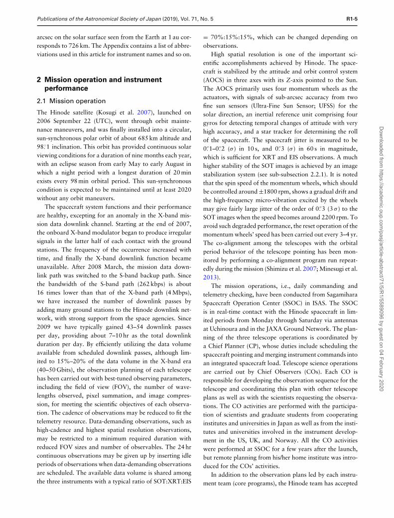
Fig. 3. Example EIS active region observations. The top panels show scans across the active regions in individual emission lines from Fe IX (log T =5.9) to Ca XV (log T = 6.65) and illustrate how the solar corona changes dramatically as a function of temperature. The bottom panels show the fullEIS spectral range from a single point in the core of the active region. The background image is SDO/AIA 171 A. These observations were taken on2015 December 29, beginning at 11:35 UT. (Color online)
is known (e.g., a quiet-Sun region). These methods havea fundamental uncertainty of about ±5 km s−1 (Younget al. 2012), but relative wavelength measurements betweenrepeated exposures can be precise to 0.5 km s−1 or better(Mariska & Muglach 2010).
The dispersion formulae for the EIS short- and long-wavelength (SW, LW) bands are described by quadraticfunctions and the parameters are stored within the IDL rou-tine EIS_GET_CCD_TRANSLATION. The method was describedby Brown et al. (2007), although we note that the parame-ters in this work have subsequently been updated.
2.4.4 Line width calibrationThe instrumental widths of the narrow EIS slits, expressedas the full-width at half-maximum (FWHM) of a Gaussianfunction, are returned by the IDL routine EIS_SLIT_WIDTH.The widths vary as a function of the Y-position along theEIS CCDs, with minimum values of 56 and 64 mA for the1′′ and 2′′ slits near Y-pixel 300, and maximum values of78 and 83 mA at the top of the detector. The widths weremeasured from spectra of Fe XII 193.51A obtained abovethe quiet-Sun limb at the equator. The line was assumed tobe broadened only by instrumental and thermal processes,and minimum widths obtained from multiple data sets were
assumed to define the instrumental width. More details canbe found in EIS Software Note No. 7.6
2.4.5 Spatial resolutionThe spatial resolution of EIS was measured preflight usingEUV emission from a discharge lamp (Korendyke et al.2006) and characterized as 2′′. The on-orbit performancewas described in EIS Software Note No. 86 and indicatedthat the spatial resolution is approximately 3′′. The analysisdetermined this value from (1) the FWHM of point-likefeatures in selected data sets and (2) comparisons of slitand slot rasters in the 195.119 A line with simultaneous193 A narrow-band images from the high-resolution (0.′′6)SDO/AIA with contribution dominated by that exact sameline. A scientific study of the observed cross-field size ofcoronal loops (Brooks et al. 2012) also found consistentAIA–EIS results with an EIS PSF of 2.′′5 (FWHM).
2.4.6 Pointing accuracyEIS points to a position on the Sun by combining theplanned Hinode spacecraft pointing with an internalpointing system that moves the EIS mirror in small steps.How accurately EIS can point to a specified solar loca-tion has been evaluated by regularly co-aligning EIS Fe XII
195 A slot spectroheliograms with simultaneous AIA 193 A
Dow
nloaded from https://academ
ic.oup.com/pasj/article-abstract/71/5/R
1/5589096 by guest on 04 February 2020
Publications of the Astronomical Society of Japan (2019), Vol. 71, No. 5 R1-15
wavelength-channel images, which provide a well-definedsolar coordinate system. These observations show that ina yearly cycle the EIS solar coordinates derived from com-bining actual Hinode spacecraft pointing data with the EISmirror position data vary from true solar coordinates in apredictable manner by about 25′′ in X and 50′′ in Y. Theselong-term variations have been accounted for in the EISplanning and analysis software. Using this software, it isgenerally possible to determine the location of the EIS sliton the Sun to better than 5′′ in both X and Y. EIS SoftwareNote No. 206 provides additional details.
Once EIS has pointed at a fixed position on the Sun,the actual location will fluctuate due to spacecraft pointingvariations and thermal fluctuations around the orbit. Onlylimited analysis has been performed to determine the extentof these changes. Analyses of co-aligned EIS slot imagesobtained over a one-day period showed regular fluctuationsin EIS pointing on orbital time scales and more randomvariations over several hours. Over an orbit, a fixed EIS slitor slot position on the Sun fluctuates by up to 2′′ in X and4′′ in Y. Over a day, a fixed EIS pointing can vary by up to6′′ in X and 10′′ in Y. EIS Software Note No. 96 provides apreliminary analysis of these pointing variations.
2.4.7 Warm and hot pixelsThe CCDs on EIS have performed exceptionally well, withtests demonstrating that they are clean and do not requiredecontamination. However, the CCDs have developed anincreasing number of hot and warm pixels since launch. Thehot pixels were caused by radiation damage and appearas pixels with energy of mean value > 50 σ of the noiselevel σ . In addition there are warm pixels that have meanvalues between 5 σ and 50 σ . These have been tracked sincelaunch, and warm and hot pixel maps are provided thatallow them to be dealt with within the calibration. How-ever, at the end of 2015 the numbers of these damagedpixels reached a level close to impacting the science, soa bakeout plan was developed and carried out. The firstbakeout took place in 2016 February for three days, andresulted in a reduction in the hot pixels by 67% and a reduc-tion in the warm pixels by 9%. We will continue to carryout regular bakeouts.
2.4.8 Conclusions and future observingSince the middle of 2016, a new regime of higher telemetrybecame available to EIS. Regular observing increased ourtelemetry allocation from 15% to 23%, and in circum-stances where we require more for an additional sci-ence mode this can be requested. This allows users tochoose more spectral lines or to use a higher time cadenceand larger FOV. Users should aim to take advantage ofthe additional telemetry and contact the Science Schedule
Coordinators about their plans (J. L. Culhane, J. Mariska,and T. Watanabe).
3 Quiet Sun
3.1 Quiet-Sun magnetism: Flux tubes, horizontalfields, and intra-network fields
Observing the quiet Sun is challenging. Magnetic fields thereare structured on small spatial scales and produce very weakpolarization signals. Thus, progress in this area demandshigh-spatial-resolution and high-sensitivity observations.
Hinode has revolutionized our understanding of quiet-Sun magnetic fields thanks to its unique observational capa-bilities. Hinode/SOT-SP is the first slit spectro-polarimeterflown in space. As such, it provides seeing-free observa-tions in two spectral lines at a nearly diffraction-limitedangular resolution of 0.′′32. The SP is complemented bythe NFI, an imaging magnetograph that has been used toobserve large portions of the solar surface with significantlybetter spatial resolution and sensitivity than the MichelsonDoppler Imager on the Solar and Heliospheric Observa-tory (SOHO/MDI; Scherrer et al. 1995) or the Helio-seismic Magnetic Imager on the Solar Dynamics Obser-vatory (SDO/HMI; Scherrer et al. 2012).
High polarimetric sensitivity and high spatial resolutionare indeed the main advantages of Hinode for quiet-Sunstudies. The SP routinely reaches a noise level of 10−3 to10−4 of the continuum intensity, making it possible to detectthe very weak fields of the inter-network. The unprece-dented angular resolution of SP and NFI, on the other hand,helps reduce the mixing of different magnetic structures inthe pixel. One can then use simpler models to interpretthe observations. Another advantage of high spatial reso-lution is the generally larger fraction of the pixel occupiedby the magnetic field. Thanks to the increased magneticfilling factors, the polarization signals are stronger and lessaffected by noise. They also show much clearer signaturesof the physical processes at work. For example, StokesV profiles with a bump in the red lobe have been associ-ated with magnetic bubbles descending in the photosphere(Quintero Noda et al. 2014), while single-lobed profiles arecaused by vertical discontinuities of the atmospheric param-eters (Sainz Dalda et al. 2012; Viticchie 2012). Similarly,absorption dips in the blue wing of quiet-Sun intensity pro-files have been related to supersonic granular flows (BellotRubio 2009; Vitas et al. 2011).
The combination of these capabilities, still unsurpassedfrom the ground, has allowed Hinode to make significantdiscoveries since 2006. Some of the main results obtained inthe area of quiet-Sun magnetism are presented below. Wewill focus on the structure and formation of intense mag-netic flux tubes, the magnetic properties of inter-network
Dow
nloaded from https://academ
ic.oup.com/pasj/article-abstract/71/5/R
1/5589096 by guest on 04 February 2020
R1-16 Publications of the Astronomical Society of Japan (2019), Vol. 71, No. 5
fields, the appearance and disappearance of magnetic flux inthe solar inter-network, the interaction of quiet-Sun fieldswith ambient fields, the flux budget of the quiet Sun, andthe origin of network and inter-network fields. Importantfindings by ground-based telescopes and other space assetswill be included as needed to provide a complete picture ofour current understanding of quiet-Sun magnetism.
3.1.1 Stokes inversionMany of the advances described in this section and insubsection 7.1 have been possible thanks to the applica-tion of sophisticated Stokes inversion codes. For a reviewof inversion techniques, their strengths and limitations,see del Toro Iniesta and Ruiz Cobo (2016). Most of theHinode/SOT-SP observations of the quiet Sun have beeninverted assuming Milne–Eddington atmospheres in whichthe magnetic and dynamic parameters are constant withheight (Skumanich & Lites 1987). These inversions cannotreproduce asymmetric Stokes profiles but are very robustand have become the method of choice for the analysisof noisy measurements and data with limited wavelengthsampling. Milne–Eddington inversions provide some kindof average of the atmospheric parameters along the line ofsight (Westendorp Plaza et al. 1998; Orozco Suarez et al.2010). Codes used to interpret polarimetric observationsthat can handle gradients of the parameters include SIR(Ruiz Cobo & del Toro Iniesta 1992), SPINOR (Frutigeret al. 2000), and NICOLE (Socas-Navarro et al. 2015).These codes are able to fit asymmetric Stokes profiles, deliv-ering more realistic results. However, their sensitivity tonoise is also larger. The SIRGAUSS and SIRJUMP codes(Bellot Rubio 2003) make it possible to model the existenceof a Gaussian perturbation or a sharp discontinuity in oneor all the parameters at some height within the line-formingregion. They also can retrieve arbitrary stratifications of theatmospheric parameters.
Although we do not have to deal with the effects ofthe Earth’s atmosphere in the spectro-polarimetric data ofHinode, we do have to deal with the spatial and spectraldegradation caused by the telescope and the detector. Inparticular, the spectral degradation was taken into accountby Orozco Suarez et al. (2007b) using the local stray lightas a second atmospheric component, which was consideredto be contributed by telescope diffraction and not by unre-solved small-scale structure. In this method of inversions,a significant amount of the signal (∼75% due to telescopediffraction) gets subtracted from each pixel, thus signifi-cantly reducing the signal-to-noise ratio of the results. Toproperly take into account the spatial degradation causedby the telescope diffraction, van Noort (2012) developeda new method, spatially coupled inversion, in which thespectro-polarimetric data are degraded in a known way,
using the telescope PSF, and the atmospheric parametersover the whole FOV are simultaneously constrained.
In the spatially coupled inversion, the Stokes profiles forall pixels in a given FOV are synthesized and convolvedwith the PSF of the telescope, and then these are matchedto the observed Stokes profiles until the χ2 merit func-tion is minimized. Finally, physical parameters are inferred.This method allows accurate fitting of Stokes profiles overa large FOV, and improves the signal-to-noise ratio andspatial resolution of the inversion results. Further, the spa-tially coupled inversion can be carried out at a higher pixelresolution than that of the observed magnetogram by arti-ficially refining the pixel grid of the solution, thus resolvingadditional substructures down to the diffraction limit of thetelescope, which were not resolved with earlier, pixel-based,inversions of Hinode/SOT-SP data.
3.1.2 Small-scale magnetic flux tubes in the quiet SunTraditionally, strong flux concentrations in the quiet Sunhave been modeled as magnetic flux tubes, a theoreticalconcept put forward by Spruit (1976) and others. Flux tubesare evacuated magnetic structures that fan out with heightowing to the exponential decrease of the gas pressure inthe solar atmosphere. With field strengths of order 1.5 kGand diameters of 100–200 km at optical depth unity, theyoften show up as bright points in continuum intensity andmolecular bands. This is because of the reduction of theopacity in the tubes, which allows one to see deeper, hencehotter, layers of the photosphere.
Much of our knowledge of quiet-Sun magnetic elements,particularly in network and plage regions, comes from theinversion of spectro-polarimetric data at moderate spatialresolution, considering them to be thin flux tubes (e.g.,Bellot Rubio et al. 2000; Frutiger & Solanki 2001). Despitethe success of this approach, the flux-tube model itself couldnot be verified for many years because of insufficient spa-tial resolution. One actually needs to go below a few 0.′′1to single out individual tubes and demonstrate their exis-tence. This was achieved for the first time by Lagg et al.(2010) using IMaX, the magnetograph of the SUNRISEballoon-borne telescope (Martınez Pillet et al. 2011). Lagget al. (2010) inverted the Stokes profiles of the temperature-sensitive Fe I 525.02 nm line from an isolated network ele-ment and showed that a simple Milne–Eddington atmo-sphere with a magnetic filling factor of unity was capableof providing a good fit to the observations. The magneticproperties derived from the inversion were found to be com-patible with semi-empirical plage flux-tube models based onspectro-polarimetric measurements at lower resolution, inparticular the field strength of 1450 G. Lagg et al. (2010)observed nearly flat intensity profiles emerging from the flux
Dow
nloaded from https://academ
ic.oup.com/pasj/article-abstract/71/5/R
1/5589096 by guest on 04 February 2020
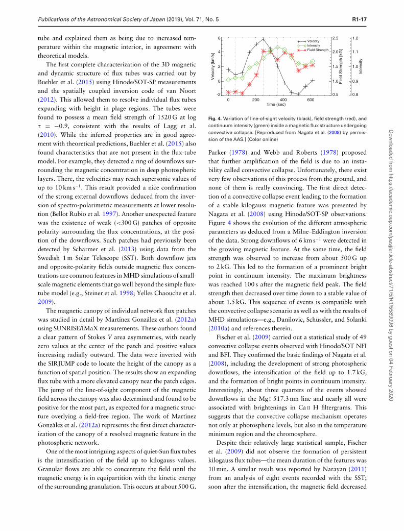
Publications of the Astronomical Society of Japan (2019), Vol. 71, No. 5 R1-17
tube and explained them as being due to increased tem-perature within the magnetic interior, in agreement withtheoretical models.
The first complete characterization of the 3D magneticand dynamic structure of flux tubes was carried out byBuehler et al. (2015) using Hinode/SOT-SP measurementsand the spatially coupled inversion code of van Noort(2012). This allowed them to resolve individual flux tubesexpanding with height in plage regions. The tubes werefound to possess a mean field strength of 1520 G at logτ = −0.9, consistent with the results of Lagg et al.(2010). While the inferred properties are in good agree-ment with theoretical predictions, Buehler et al. (2015) alsofound characteristics that are not present in the flux-tubemodel. For example, they detected a ring of downflows sur-rounding the magnetic concentration in deep photosphericlayers. There, the velocities may reach supersonic values ofup to 10 km s−1. This result provided a nice confirmationof the strong external downflows deduced from the inver-sion of spectro-polarimetric measurements at lower resolu-tion (Bellot Rubio et al. 1997). Another unexpected featurewas the existence of weak (<300 G) patches of oppositepolarity surrounding the flux concentrations, at the posi-tion of the downflows. Such patches had previously beendetected by Scharmer et al. (2013) using data from theSwedish 1 m Solar Telescope (SST). Both downflow jetsand opposite-polarity fields outside magnetic flux concen-trations are common features in MHD simulations of small-scale magnetic elements that go well beyond the simple flux-tube model (e.g., Steiner et al. 1998; Yelles Chaouche et al.2009).
The magnetic canopy of individual network flux patcheswas studied in detail by Martınez Gonzalez et al. (2012a)using SUNRISE/IMaX measurements. These authors founda clear pattern of Stokes V area asymmetries, with nearlyzero values at the center of the patch and positive valuesincreasing radially outward. The data were inverted withthe SIRJUMP code to locate the height of the canopy as afunction of spatial position. The results show an expandingflux tube with a more elevated canopy near the patch edges.The jump of the line-of-sight component of the magneticfield across the canopy was also determined and found to bepositive for the most part, as expected for a magnetic struc-ture overlying a field-free region. The work of MartınezGonzalez et al. (2012a) represents the first direct character-ization of the canopy of a resolved magnetic feature in thephotospheric network.
One of the most intriguing aspects of quiet-Sun flux tubesis the intensification of the field up to kilogauss values.Granular flows are able to concentrate the field until themagnetic energy is in equipartition with the kinetic energyof the surrounding granulation. This occurs at about 500 G.
0 200 400 600time (sec)
-2
0
2
4
6
Vel
ocity
[km
/s]
VelocityIntensityField Strength
0.5
1.0
1.5
2.0
2.5
Fie
ld S
tren
gth
[kG
]
0.8
0.9
1.0
1.1
1.2
Inte
nsity
Fig. 4. Variation of line-of-sight velocity (black), field strength (red), andcontinuum intensity (green) inside a magnetic flux structure undergoingconvective collapse. [Reproduced from Nagata et al. (2008) by permis-sion of the AAS.] (Color online)
Parker (1978) and Webb and Roberts (1978) proposedthat further amplification of the field is due to an insta-bility called convective collapse. Unfortunately, there existvery few observations of this process from the ground, andnone of them is really convincing. The first direct detec-tion of a convective collapse event leading to the formationof a stable kilogauss magnetic feature was presented byNagata et al. (2008) using Hinode/SOT-SP observations.Figure 4 shows the evolution of the different atmosphericparameters as deduced from a Milne–Eddington inversionof the data. Strong downflows of 6 km s−1 were detected inthe growing magnetic feature. At the same time, the fieldstrength was observed to increase from about 500 G upto 2 kG. This led to the formation of a prominent brightpoint in continuum intensity. The maximum brightnesswas reached 100 s after the magnetic field peak. The fieldstrength then decreased over time down to a stable value ofabout 1.5 kG. This sequence of events is compatible withthe convective collapse scenario as well as with the results ofMHD simulations—e.g., Danilovic, Schussler, and Solanki(2010a) and references therein.
Fischer et al. (2009) carried out a statistical study of 49convective collapse events observed with Hinode/SOT NFIand BFI. They confirmed the basic findings of Nagata et al.(2008), including the development of strong photosphericdownflows, the intensification of the field up to 1.7 kG,and the formation of bright points in continuum intensity.Interestingly, about three quarters of the events showeddownflows in the Mg I 517.3 nm line and nearly all wereassociated with brightenings in Ca II H filtergrams. Thissuggests that the convective collapse mechanism operatesnot only at photospheric levels, but also in the temperatureminimum region and the chromosphere.
Despite their relatively large statistical sample, Fischeret al. (2009) did not observe the formation of persistentkilogauss flux tubes—the mean duration of the features was10 min. A similar result was reported by Narayan (2011)from an analysis of eight events recorded with the SST;soon after the intensification, the magnetic field decreased
Dow
nloaded from https://academ
ic.oup.com/pasj/article-abstract/71/5/R
1/5589096 by guest on 04 February 2020
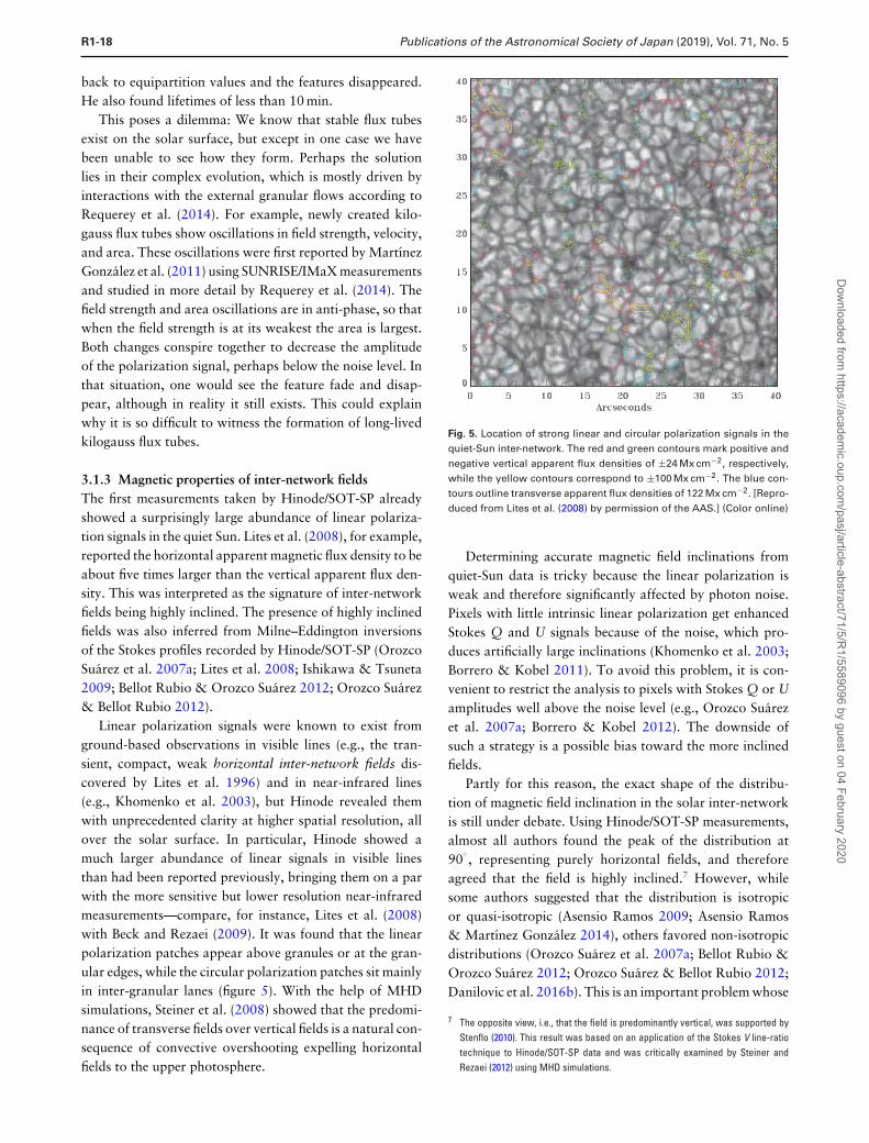
R1-18 Publications of the Astronomical Society of Japan (2019), Vol. 71, No. 5
back to equipartition values and the features disappeared.He also found lifetimes of less than 10 min.
This poses a dilemma: We know that stable flux tubesexist on the solar surface, but except in one case we havebeen unable to see how they form. Perhaps the solutionlies in their complex evolution, which is mostly driven byinteractions with the external granular flows according toRequerey et al. (2014). For example, newly created kilo-gauss flux tubes show oscillations in field strength, velocity,and area. These oscillations were first reported by MartınezGonzalez et al. (2011) using SUNRISE/IMaX measurementsand studied in more detail by Requerey et al. (2014). Thefield strength and area oscillations are in anti-phase, so thatwhen the field strength is at its weakest the area is largest.Both changes conspire together to decrease the amplitudeof the polarization signal, perhaps below the noise level. Inthat situation, one would see the feature fade and disap-pear, although in reality it still exists. This could explainwhy it is so difficult to witness the formation of long-livedkilogauss flux tubes.
3.1.3 Magnetic properties of inter-network fieldsThe first measurements taken by Hinode/SOT-SP alreadyshowed a surprisingly large abundance of linear polariza-tion signals in the quiet Sun. Lites et al. (2008), for example,reported the horizontal apparent magnetic flux density to beabout five times larger than the vertical apparent flux den-sity. This was interpreted as the signature of inter-networkfields being highly inclined. The presence of highly inclinedfields was also inferred from Milne–Eddington inversionsof the Stokes profiles recorded by Hinode/SOT-SP (OrozcoSuarez et al. 2007a; Lites et al. 2008; Ishikawa & Tsuneta2009; Bellot Rubio & Orozco Suarez 2012; Orozco Suarez& Bellot Rubio 2012).
Linear polarization signals were known to exist fromground-based observations in visible lines (e.g., the tran-sient, compact, weak horizontal inter-network fields dis-covered by Lites et al. 1996) and in near-infrared lines(e.g., Khomenko et al. 2003), but Hinode revealed themwith unprecedented clarity at higher spatial resolution, allover the solar surface. In particular, Hinode showed amuch larger abundance of linear signals in visible linesthan had been reported previously, bringing them on a parwith the more sensitive but lower resolution near-infraredmeasurements—compare, for instance, Lites et al. (2008)with Beck and Rezaei (2009). It was found that the linearpolarization patches appear above granules or at the gran-ular edges, while the circular polarization patches sit mainlyin inter-granular lanes (figure 5). With the help of MHDsimulations, Steiner et al. (2008) showed that the predomi-nance of transverse fields over vertical fields is a natural con-sequence of convective overshooting expelling horizontalfields to the upper photosphere.
Fig. 5. Location of strong linear and circular polarization signals in thequiet-Sun inter-network. The red and green contours mark positive andnegative vertical apparent flux densities of ±24 Mx cm−2, respectively,while the yellow contours correspond to ±100 Mx cm−2. The blue con-tours outline transverse apparent flux densities of 122 Mx cm−2. [Repro-duced from Lites et al. (2008) by permission of the AAS.] (Color online)
Determining accurate magnetic field inclinations fromquiet-Sun data is tricky because the linear polarization isweak and therefore significantly affected by photon noise.Pixels with little intrinsic linear polarization get enhancedStokes Q and U signals because of the noise, which pro-duces artificially large inclinations (Khomenko et al. 2003;Borrero & Kobel 2011). To avoid this problem, it is con-venient to restrict the analysis to pixels with Stokes Q or Uamplitudes well above the noise level (e.g., Orozco Suarezet al. 2007a; Borrero & Kobel 2012). The downside ofsuch a strategy is a possible bias toward the more inclinedfields.
Partly for this reason, the exact shape of the distribu-tion of magnetic field inclination in the solar inter-networkis still under debate. Using Hinode/SOT-SP measurements,almost all authors found the peak of the distribution at90
◦, representing purely horizontal fields, and therefore
agreed that the field is highly inclined.7 However, whilesome authors suggested that the distribution is isotropicor quasi-isotropic (Asensio Ramos 2009; Asensio Ramos& Martınez Gonzalez 2014), others favored non-isotropicdistributions (Orozco Suarez et al. 2007a; Bellot Rubio &Orozco Suarez 2012; Orozco Suarez & Bellot Rubio 2012;Danilovic et al. 2016b). This is an important problem whose
7 The opposite view, i.e., that the field is predominantly vertical, was supported byStenflo (2010). This result was based on an application of the Stokes V line-ratiotechnique to Hinode/SOT-SP data and was critically examined by Steiner andRezaei (2012) using MHD simulations.
Dow
nloaded from https://academ
ic.oup.com/pasj/article-abstract/71/5/R
1/5589096 by guest on 04 February 2020
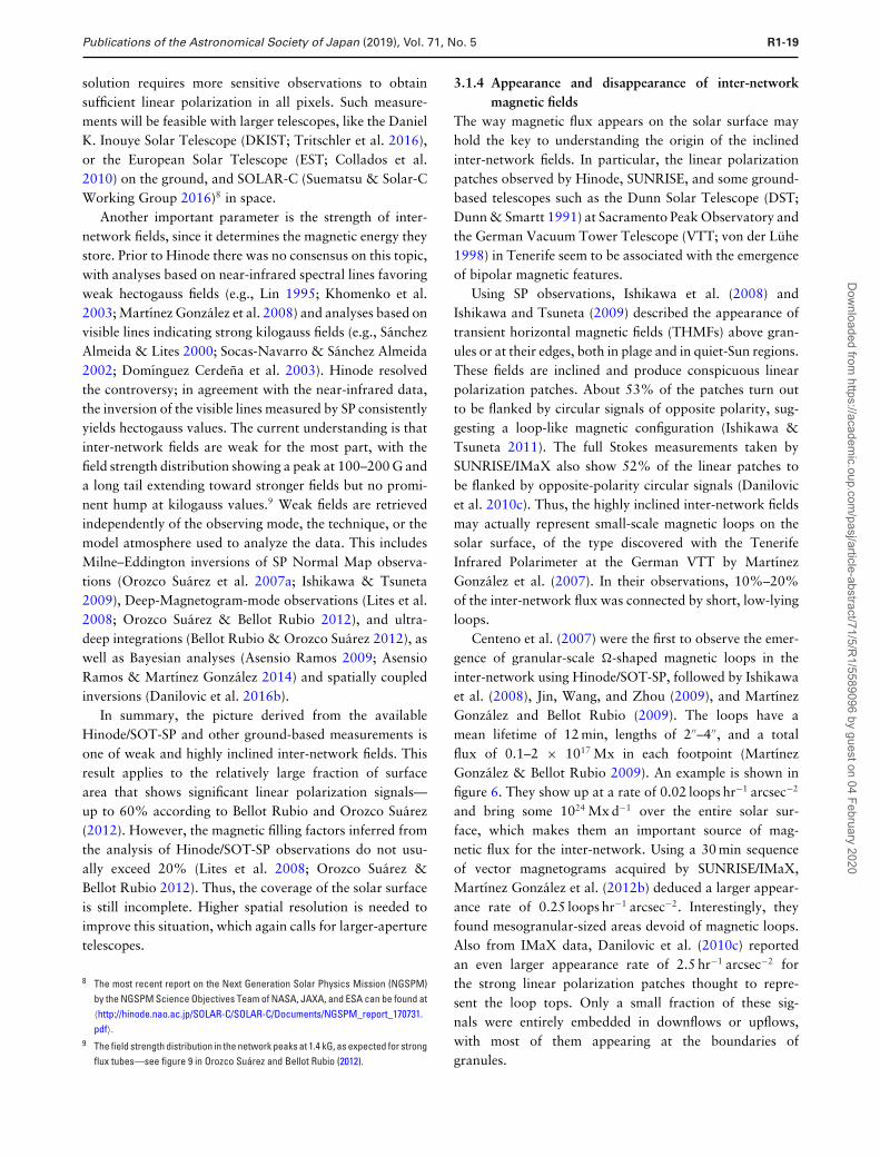
Publications of the Astronomical Society of Japan (2019), Vol. 71, No. 5 R1-19
solution requires more sensitive observations to obtainsufficient linear polarization in all pixels. Such measure-ments will be feasible with larger telescopes, like the DanielK. Inouye Solar Telescope (DKIST; Tritschler et al. 2016),or the European Solar Telescope (EST; Collados et al.2010) on the ground, and SOLAR-C (Suematsu & Solar-CWorking Group 2016)8 in space.
Another important parameter is the strength of inter-network fields, since it determines the magnetic energy theystore. Prior to Hinode there was no consensus on this topic,with analyses based on near-infrared spectral lines favoringweak hectogauss fields (e.g., Lin 1995; Khomenko et al.2003; Martınez Gonzalez et al. 2008) and analyses based onvisible lines indicating strong kilogauss fields (e.g., SanchezAlmeida & Lites 2000; Socas-Navarro & Sanchez Almeida2002; Domınguez Cerdena et al. 2003). Hinode resolvedthe controversy; in agreement with the near-infrared data,the inversion of the visible lines measured by SP consistentlyyields hectogauss values. The current understanding is thatinter-network fields are weak for the most part, with thefield strength distribution showing a peak at 100–200 G anda long tail extending toward stronger fields but no promi-nent hump at kilogauss values.9 Weak fields are retrievedindependently of the observing mode, the technique, or themodel atmosphere used to analyze the data. This includesMilne–Eddington inversions of SP Normal Map observa-tions (Orozco Suarez et al. 2007a; Ishikawa & Tsuneta2009), Deep-Magnetogram-mode observations (Lites et al.2008; Orozco Suarez & Bellot Rubio 2012), and ultra-deep integrations (Bellot Rubio & Orozco Suarez 2012), aswell as Bayesian analyses (Asensio Ramos 2009; AsensioRamos & Martınez Gonzalez 2014) and spatially coupledinversions (Danilovic et al. 2016b).
In summary, the picture derived from the availableHinode/SOT-SP and other ground-based measurements isone of weak and highly inclined inter-network fields. Thisresult applies to the relatively large fraction of surfacearea that shows significant linear polarization signals—up to 60% according to Bellot Rubio and Orozco Suarez(2012). However, the magnetic filling factors inferred fromthe analysis of Hinode/SOT-SP observations do not usu-ally exceed 20% (Lites et al. 2008; Orozco Suarez &Bellot Rubio 2012). Thus, the coverage of the solar surfaceis still incomplete. Higher spatial resolution is needed toimprove this situation, which again calls for larger-aperturetelescopes.
8 The most recent report on the Next Generation Solar Physics Mission (NGSPM)by the NGSPM Science Objectives Team of NASA, JAXA, and ESA can be found at〈http://hinode.nao.ac.jp/SOLAR-C/SOLAR-C/Documents/NGSPM_report_170731.pdf〉.
9 The field strength distribution in the network peaks at 1.4 kG, as expected for strongflux tubes—see figure 9 in Orozco Suarez and Bellot Rubio (2012).
3.1.4 Appearance and disappearance of inter-networkmagnetic fields
The way magnetic flux appears on the solar surface mayhold the key to understanding the origin of the inclinedinter-network fields. In particular, the linear polarizationpatches observed by Hinode, SUNRISE, and some ground-based telescopes such as the Dunn Solar Telescope (DST;Dunn & Smartt 1991) at Sacramento Peak Observatory andthe German Vacuum Tower Telescope (VTT; von der Luhe1998) in Tenerife seem to be associated with the emergenceof bipolar magnetic features.
Using SP observations, Ishikawa et al. (2008) andIshikawa and Tsuneta (2009) described the appearance oftransient horizontal magnetic fields (THMFs) above gran-ules or at their edges, both in plage and in quiet-Sun regions.These fields are inclined and produce conspicuous linearpolarization patches. About 53% of the patches turn outto be flanked by circular signals of opposite polarity, sug-gesting a loop-like magnetic configuration (Ishikawa &Tsuneta 2011). The full Stokes measurements taken bySUNRISE/IMaX also show 52% of the linear patches tobe flanked by opposite-polarity circular signals (Danilovicet al. 2010c). Thus, the highly inclined inter-network fieldsmay actually represent small-scale magnetic loops on thesolar surface, of the type discovered with the TenerifeInfrared Polarimeter at the German VTT by MartınezGonzalez et al. (2007). In their observations, 10%–20%of the inter-network flux was connected by short, low-lyingloops.
Centeno et al. (2007) were the first to observe the emer-gence of granular-scale �-shaped magnetic loops in theinter-network using Hinode/SOT-SP, followed by Ishikawaet al. (2008), Jin, Wang, and Zhou (2009), and MartınezGonzalez and Bellot Rubio (2009). The loops have amean lifetime of 12 min, lengths of 2′′–4′′, and a totalflux of 0.1–2 × 10¹⁷ Mx in each footpoint (MartınezGonzalez & Bellot Rubio 2009). An example is shown infigure 6. They show up at a rate of 0.02 loops hr−1 arcsec−2
and bring some 1024 Mx d−1 over the entire solar sur-face, which makes them an important source of mag-netic flux for the inter-network. Using a 30 min sequenceof vector magnetograms acquired by SUNRISE/IMaX,Martınez Gonzalez et al. (2012b) deduced a larger appear-ance rate of 0.25 loops hr−1 arcsec−2. Interestingly, theyfound mesogranular-sized areas devoid of magnetic loops.Also from IMaX data, Danilovic et al. (2010c) reportedan even larger appearance rate of 2.5 hr−1 arcsec−2 forthe strong linear polarization patches thought to repre-sent the loop tops. Only a small fraction of these sig-nals were entirely embedded in downflows or upflows,with most of them appearing at the boundaries ofgranules.
Dow
nloaded from https://academ
ic.oup.com/pasj/article-abstract/71/5/R
1/5589096 by guest on 04 February 2020
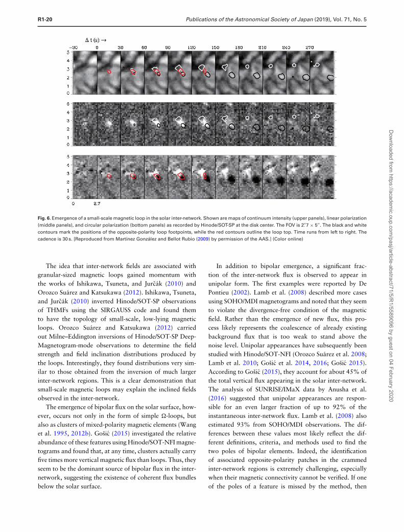
R1-20 Publications of the Astronomical Society of Japan (2019), Vol. 71, No. 5
Fig. 6. Emergence of a small-scale magnetic loop in the solar inter-network. Shown are maps of continuum intensity (upper panels), linear polarization(middle panels), and circular polarization (bottom panels) as recorded by Hinode/SOT-SP at the disk center. The FOV is 2.′′7 × 5′′. The black and whitecontours mark the positions of the opposite-polarity loop footpoints, while the red contours outline the loop top. Time runs from left to right. Thecadence is 30 s. [Reproduced from Martınez Gonzalez and Bellot Rubio (2009) by permission of the AAS.] (Color online)
The idea that inter-network fields are associated withgranular-sized magnetic loops gained momentum withthe works of Ishikawa, Tsuneta, and Jurcak (2010) andOrozco Suarez and Katsukawa (2012). Ishikawa, Tsuneta,and Jurcak (2010) inverted Hinode/SOT-SP observationsof THMFs using the SIRGAUSS code and found themto have the topology of small-scale, low-lying magneticloops. Orozco Suarez and Katsukawa (2012) carriedout Milne–Eddington inversions of Hinode/SOT-SP Deep-Magnetogram-mode observations to determine the fieldstrength and field inclination distributions produced bythe loops. Interestingly, they found distributions very sim-ilar to those obtained from the inversion of much largerinter-network regions. This is a clear demonstration thatsmall-scale magnetic loops may explain the inclined fieldsobserved in the inter-network.
The emergence of bipolar flux on the solar surface, how-ever, occurs not only in the form of simple �-loops, butalso as clusters of mixed-polarity magnetic elements (Wanget al. 1995, 2012b). Gosic (2015) investigated the relativeabundance of these features using Hinode/SOT-NFI magne-tograms and found that, at any time, clusters actually carryfive times more vertical magnetic flux than loops. Thus, theyseem to be the dominant source of bipolar flux in the inter-network, suggesting the existence of coherent flux bundlesbelow the solar surface.
In addition to bipolar emergence, a significant frac-tion of the inter-network flux is observed to appear inunipolar form. The first examples were reported by DePontieu (2002). Lamb et al. (2008) described more casesusing SOHO/MDI magnetograms and noted that they seemto violate the divergence-free condition of the magneticfield. Rather than the emergence of new flux, this pro-cess likely represents the coalescence of already existingbackground flux that is too weak to stand above thenoise level. Unipolar appearances have subsequently beenstudied with Hinode/SOT-NFI (Orozco Suarez et al. 2008;Lamb et al. 2010; Gosic et al. 2014, 2016; Gosic 2015).According to Gosic (2015), they account for about 45% ofthe total vertical flux appearing in the solar inter-network.The analysis of SUNRISE/IMaX data by Anusha et al.(2016) suggested that unipolar appearances are respon-sible for an even larger fraction of up to 92% of theinstantaneous inter-network flux. Lamb et al. (2008) alsoestimated 93% from SOHO/MDI observations. The dif-ferences between these values most likely reflect the dif-ferent definitions, criteria, and methods used to find thetwo poles of bipolar elements. Indeed, the identificationof associated opposite-polarity patches in the crammedinter-network regions is extremely challenging, especiallywhen their magnetic connectivity cannot be verified. If oneof the poles of a feature is missed by the method, then
Dow
nloaded from https://academ
ic.oup.com/pasj/article-abstract/71/5/R
1/5589096 by guest on 04 February 2020
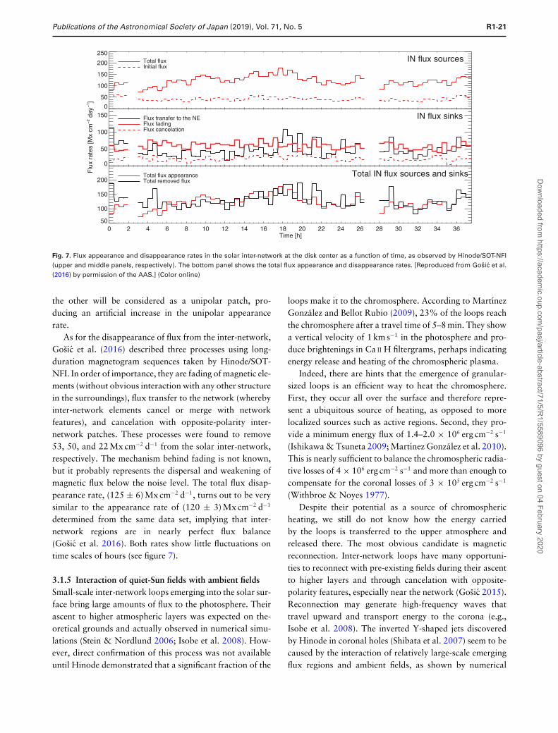
Publications of the Astronomical Society of Japan (2019), Vol. 71, No. 5 R1-21
0
50
100
150
200
250Total fluxInitial flux
IN flux sources
0
50
100
150
Flu
x ra
tes
[Mx
cm−
2 day
−1 ]
Flux transfer to the NEFlux fadingFlux cancelation
IN flux sinks
50
100
150
200Total flux appearanceTotal removed flux
Total IN flux sources and sinks
0 2 4 6 8 10 12 14 16 18 20 22 24 26 28 30 32 34 36Time [h]
Fig. 7. Flux appearance and disappearance rates in the solar inter-network at the disk center as a function of time, as observed by Hinode/SOT-NFI(upper and middle panels, respectively). The bottom panel shows the total flux appearance and disappearance rates. [Reproduced from Gosic et al.(2016) by permission of the AAS.] (Color online)
the other will be considered as a unipolar patch, pro-ducing an artificial increase in the unipolar appearancerate.
As for the disappearance of flux from the inter-network,Gosic et al. (2016) described three processes using long-duration magnetogram sequences taken by Hinode/SOT-NFI. In order of importance, they are fading of magnetic ele-ments (without obvious interaction with any other structurein the surroundings), flux transfer to the network (wherebyinter-network elements cancel or merge with networkfeatures), and cancelation with opposite-polarity inter-network patches. These processes were found to remove53, 50, and 22 Mx cm−2 d−1 from the solar inter-network,respectively. The mechanism behind fading is not known,but it probably represents the dispersal and weakening ofmagnetic flux below the noise level. The total flux disap-pearance rate, (125 ± 6) Mx cm−2 d−1, turns out to be verysimilar to the appearance rate of (120 ± 3) Mx cm−2 d−1
determined from the same data set, implying that inter-network regions are in nearly perfect flux balance(Gosic et al. 2016). Both rates show little fluctuations ontime scales of hours (see figure 7).
3.1.5 Interaction of quiet-Sun fields with ambient fieldsSmall-scale inter-network loops emerging into the solar sur-face bring large amounts of flux to the photosphere. Theirascent to higher atmospheric layers was expected on the-oretical grounds and actually observed in numerical simu-lations (Stein & Nordlund 2006; Isobe et al. 2008). How-ever, direct confirmation of this process was not availableuntil Hinode demonstrated that a significant fraction of the
loops make it to the chromosphere. According to MartınezGonzalez and Bellot Rubio (2009), 23% of the loops reachthe chromosphere after a travel time of 5–8 min. They showa vertical velocity of 1 km s−1 in the photosphere and pro-duce brightenings in Ca II H filtergrams, perhaps indicatingenergy release and heating of the chromospheric plasma.
Indeed, there are hints that the emergence of granular-sized loops is an efficient way to heat the chromosphere.First, they occur all over the surface and therefore repre-sent a ubiquitous source of heating, as opposed to morelocalized sources such as active regions. Second, they pro-vide a minimum energy flux of 1.4–2.0 × 10⁶ erg cm−2 s−1
(Ishikawa & Tsuneta 2009; Martınez Gonzalez et al. 2010).This is nearly sufficient to balance the chromospheric radia-tive losses of 4 × 10⁶ erg cm−2 s−1 and more than enough tocompensate for the coronal losses of 3 × 10⁵ erg cm−2 s−1
(Withbroe & Noyes 1977).Despite their potential as a source of chromospheric
heating, we still do not know how the energy carriedby the loops is transferred to the upper atmosphere andreleased there. The most obvious candidate is magneticreconnection. Inter-network loops have many opportuni-ties to reconnect with pre-existing fields during their ascentto higher layers and through cancelation with opposite-polarity features, especially near the network (Gosic 2015).Reconnection may generate high-frequency waves thattravel upward and transport energy to the corona (e.g.,Isobe et al. 2008). The inverted Y-shaped jets discoveredby Hinode in coronal holes (Shibata et al. 2007) seem to becaused by the interaction of relatively large-scale emergingflux regions and ambient fields, as shown by numerical
Dow
nloaded from https://academ
ic.oup.com/pasj/article-abstract/71/5/R
1/5589096 by guest on 04 February 2020
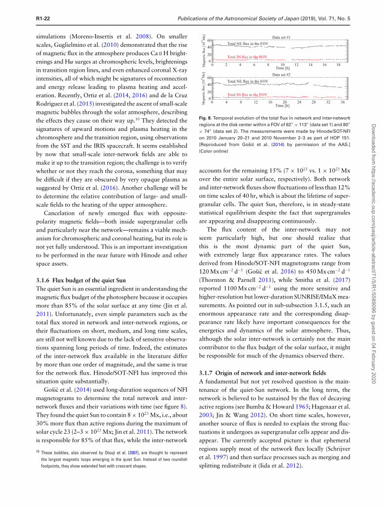
R1-22 Publications of the Astronomical Society of Japan (2019), Vol. 71, No. 5
simulations (Moreno-Insertis et al. 2008). On smallerscales, Guglielmino et al. (2010) demonstrated that the riseof magnetic flux in the atmosphere produces Ca II H bright-enings and Hα surges at chromospheric levels, brighteningsin transition region lines, and even enhanced coronal X-rayintensities, all of which might be signatures of reconnectionand energy release leading to plasma heating and accel-eration. Recently, Ortiz et al. (2014, 2016) and de la CruzRodrıguez et al. (2015) investigated the ascent of small-scalemagnetic bubbles through the solar atmosphere, describingthe effects they cause on their way up.10 They detected thesignatures of upward motions and plasma heating in thechromosphere and the transition region, using observationsfrom the SST and the IRIS spacecraft. It seems establishedby now that small-scale inter-network fields are able tomake it up to the transition region; the challenge is to verifywhether or not they reach the corona, something that maybe difficult if they are obscured by very opaque plasma assuggested by Ortiz et al. (2016). Another challenge will beto determine the relative contribution of large- and small-scale fields to the heating of the upper atmosphere.
Cancelation of newly emerged flux with opposite-polarity magnetic fields—both inside supergranular cellsand particularly near the network—remains a viable mech-anism for chromospheric and coronal heating, but its role isnot yet fully understood. This is an important investigationto be performed in the near future with Hinode and otherspace assets.
3.1.6 Flux budget of the quiet SunThe quiet Sun is an essential ingredient in understanding themagnetic flux budget of the photosphere because it occupiesmore than 85% of the solar surface at any time (Jin et al.2011). Unfortunately, even simple parameters such as thetotal flux stored in network and inter-network regions, ortheir fluctuations on short, medium, and long time scales,are still not well known due to the lack of sensitive observa-tions spanning long periods of time. Indeed, the estimatesof the inter-network flux available in the literature differby more than one order of magnitude, and the same is truefor the network flux. Hinode/SOT-NFI has improved thissituation quite substantially.
Gosic et al. (2014) used long-duration sequences of NFImagnetograms to determine the total network and inter-network fluxes and their variations with time (see figure 8).They found the quiet Sun to contain 8 × 10²³ Mx, i.e., about30% more flux than active regions during the maximum ofsolar cycle 23 (2–3 × 10²³ Mx; Jin et al. 2011). The networkis responsible for 85% of that flux, while the inter-network
10 These bubbles, also observed by Otsuji et al. (2007), are thought to representthe largest magnetic loops emerging in the quiet Sun. Instead of two roundishfootpoints, they show extended feet with crescent shapes.
Total IN flux in the FOV
Total IN flux in the FOV
Fig. 8. Temporal evolution of the total flux in network and inter-networkregions at the disk center within a FOV of 82′′ × 113′′ (data set 1) and 80′′
× 74′′ (data set 2). The measurements were made by Hinode/SOT-NFIon 2010 January 20–21 and 2010 November 2–3 as part of HOP 151.[Reproduced from Gosic et al. (2014) by permission of the AAS.](Color online)
accounts for the remaining 15% (7 × 10²³ vs. 1 × 10²³ Mxover the entire solar surface, respectively). Both networkand inter-network fluxes show fluctuations of less than 12%on time scales of 40 hr, which is about the lifetime of super-granular cells. The quiet Sun, therefore, is in steady-statestatistical equilibrium despite the fact that supergranulesare appearing and disappearing continuously.
The flux content of the inter-network may notseem particularly high, but one should realize thatthis is the most dynamic part of the quiet Sun,with extremely large flux appearance rates. The valuesderived from Hinode/SOT-NFI magnetograms range from120 Mx cm−2 d−1 (Gosic et al. 2016) to 450 Mx cm−2 d−1
(Thornton & Parnell 2011), while Smitha et al. (2017)reported 1100 Mx cm−2 d−1 using the more sensitive andhigher-resolution but lower-duration SUNRISE/IMaX mea-surements. As pointed out in sub-subsection 3.1.5, such anenormous appearance rate and the corresponding disap-pearance rate likely have important consequences for theenergetics and dynamics of the solar atmosphere. Thus,although the solar inter-network is certainly not the maincontributor to the flux budget of the solar surface, it mightbe responsible for much of the dynamics observed there.
3.1.7 Origin of network and inter-network fieldsA fundamental but not yet resolved question is the main-tenance of the quiet-Sun network. In the long term, thenetwork is believed to be sustained by the flux of decayingactive regions (see Bumba & Howard 1965; Hagenaar et al.2003; Jin & Wang 2012). On short time scales, however,another source of flux is needed to explain the strong fluc-tuations it undergoes as supergranular cells appear and dis-appear. The currently accepted picture is that ephemeralregions supply most of the network flux locally (Schrijveret al. 1997) and then surface processes such as merging andsplitting redistribute it (Iida et al. 2012).
Dow
nloaded from https://academ
ic.oup.com/pasj/article-abstract/71/5/R
1/5589096 by guest on 04 February 2020
Publications of the Astronomical Society of Japan (2019), Vol. 71, No. 5 R1-23
Hinode has challenged our views by showing that inter-network elements deposit an enormous amount of fluxin the network, outweighing ephemeral regions by far(Gosic et al. 2014). This result confirmed earlier sug-gestions by Zhang et al. (1998) and demonstrated thatthe inter-network is a very important, hitherto unknownsource of flux for the network.11 However, the pictureis still incomplete. Due to the continuous transfer ofpositive and negative flux from the inter-network, theunsigned network flux should increase in a steady fashion.Since this is not observed to occur, a mechanism capableof efficiently removing the flux supplied by the inter-network must be in place. Such a mechanism remains to bediscovered.
The origin of inter-network fields is also unclear. Twomain scenarios have been proposed. One is the globaldynamo responsible for the solar activity cycle. The otheris a local dynamo driven by turbulent granular flows (e.g.,Danilovic et al. 2010b). If the inter-network flux is pro-duced by the global dynamo, some variation of the totalflux or its latitudinal distribution should be observed as thecycle progresses. On the contrary, no significant changeswill occur if a local surface dynamo is responsible forthe inter-network flux. Thus, the existence of solar-cycle-related variations of the flux may help distinguish betweenthe two scenarios. This is why they have been searchedfor vigorously in the last years, as described in the nextsubsection.
3.2 The quiet-Sun magnetism and the solar cycle
The question of whether the magnetic constituents of thequietest parts of the Sun change with the solar cycle has beentackled sporadically over the past decades. This problemis riddled with challenges. On the one hand, the use ofhigh-sensitivity, high-resolution spectro-polarimetric obser-vations is imperative for the detection of the small-scale,and often weak, magnetic fields of the quiet Sun. On theother hand, long-term observation programs, of the orderof one solar cycle (or longer), would be required to teaseout the cyclic nature of these fields, if it indeed exists. And,of course, when it comes to comparing intrinsically weaksmall-scale magnetic signals measured at different epochs,consistency in the observations and the analysis techniquesbecomes important to rule out changes due to instrumentaland environmental biases (namely, it is important to usethe same telescope/instrument setup, compare data with
11 Actually, some of the ephemeral regions detected in previous studies could havebeen clusters of unresolved inter-network magnetic elements.
the same spatial resolution, and use the same interpreta-tion methods throughout the different epochs of observa-tion). But why should we take on this challenge at all, then?The turbulent decay of active regions throughout the solarcycle carries magnetism that cascades from the largest tothe smallest spatial scales. It is in the latter where a possiblecompeting mechanism may be at play. Numerical simula-tions have shown that the convective motions of the solarphotosphere might be able to amplify the magnetic energyat the smallest spatial scales as long as there is a magneticseed (Vogler & Schussler 2007). This local convectivelydriven dynamo takes place at granular scales and couldbe responsible for a significant amount of the quiet-Sunmagnetism. But what fraction? We do not know yet. Thisquestion is connected to that of the existence of a basal flux,i.e., a ground level of magnetic activity that is present evenwhen no active regions populate the face of the Sun. In aneffort to measure this basal flux, Stenflo (2012) analyzed14 years of daily records of SOHO/MDI data. He arrivedat the conclusion that there must be a mean unsigned mag-netic flux density of around 3 G that exists regardless ofthe presence of sunspots. Unsigned magnetic flux refers tothe total magnetic flux (regardless of sign) in a given area,while signed flux refers to the imbalance of positive versusnegative magnetic flux. It is known, however, that the mea-sured value of the unsigned magnetic flux density becomeslarger as the spatial resolution of the observation increases(Sanchez Almeida & Martınez Gonzalez 2011). This shouldput under scrutiny the 3 G value reported by Stenflo (2012).Also, as the author himself pointed out, this measured fluxcould simply be the remnant of active region decay that doesnot have time to completely dissipate before the cycle rampsup again, thus prevailing during the solar minimum. Recentestimates point at network relaxation times of around 2.9 yr(Thibault et al. 2014), which is longer than the durationof a typical minimum. However, if a convectively drivenlocal dynamo dictated the nature of the inter-network mag-netism, the basal flux level would likely remain constantduring epochs of grand minima (Hathaway 2015), whichare characterized by a pronounced absence of sunspots forvery long periods of time.
A conceptually simple way to determine which of thesetwo mechanisms is responsible for the magnetism of theinter-network is to measure the variations of these small-scale magnetic fields throughout the solar cycle. If theywere a result of the dispersion of global dynamo fieldscascading through the scale spectrum, one would expectto see some sort of cyclic variation in the inter-networkmagnetism. If, on the other hand, a local dynamo domi-nated the generation of these magnetic signals, it shouldoperate regardless of the solar cycle and show no long-termvariations.
Dow
nloaded from https://academ
ic.oup.com/pasj/article-abstract/71/5/R
1/5589096 by guest on 04 February 2020
R1-24 Publications of the Astronomical Society of Japan (2019), Vol. 71, No. 5
Early works on this topic focused their attention onproperties of the quiet Sun believed to be potentially sen-sitive to changes of the magnetic field. By analyzing thevariation of the statistical size of granules, Macris et al.(1984) found that this property showed a significant anti-correlation with the Wolf sunspot number. It is worth men-tioning that this work was carried out over a full 11 yrcycle of data with ground-based observations from twotelescopes, counting the granules by hand on paper prints.Using 33 yr of data from the McMath-Pierce Solar Tele-scope on Kitt Peak (Arizona), Livingston et al. (2005) mea-sured the Ca II K-line brightness at disk center during theentire span of the data, finding absolutely no variation.Arguing that Ca II K line is a reliable proxy for solar mag-netism, they concluded that the quiet-Sun magnetic fieldspresent no significant variation with the waxing and waningof the large-scale cycle. Of course, a large caveat of thesestudies is that none of them looked at magnetism directly.
In 2007, the Instituto Ricerche Solari Locarno (IRSOL,Switzerland) started a synoptic program of monthly mea-surements of Stokes I, Q, and V in three spectral regionsand at five position angles around the limb of the Sun, withthe aim of detecting variations in the Hanle depolariza-tion of the Stokes Q signatures of certain molecular andatomic lines. Through the measurement of the differentialHanle effect in C2 lines over the course of two years cen-tered around the past solar minimum, Kleint et al. (2011)reported no appreciable changes during this time. How-ever, the short duration of the observations renders thisresult inconclusive.
The SOT onboard Hinode, and in particular its SP, haverevolutionized our knowledge of the photospheric quiet-Sun magnetism. Not only its high spatial and spectral res-olutions and its large polarimetric sensitivity, but also theconsistent image quality and the versatile operation modeshave contributed to a very prolific scientific outcome. Now,more than a decade since its launch, a significant fractionof the solar cycle has been covered by the mission, and thebenefits of long-term observations and synoptic programsare starting to show.
Shiota et al. (2012) studied the reversal of the polar fieldsby analyzing data from the synoptic HOP 81. Monthlyscans of the poles done with Hinode/SOT-SP from 2008 to2012 revealed that the radial components of the magneticfields in the polar regions consist of two distinct popula-tions; one that comprises the large flux concentrations ofthe same magnetic polarity as the dominant polar field,and another one made of smaller concentrations of mixedpolarity and overall balanced magnetic flux (i.e., zero signedflux). While the former changes with the solar polar cycleand is responsible for the polar reversal, the latter seems toremain constant throughout the time series, behaving like a
basal flux component likely generated by a local dynamo.Of course, polar observations taken from the ecliptic alwayssuffer from foreshortening and magnetic disambiguationissues.
With a somewhat similar approach, Buehler, Lagg, andSolanki (2013) analyzed quiet-Sun maps taken at diskcenter between 2006 and 2012 with Hinode/SOT-SP. Byrestricting their study to disk center alone, they ensured thatthe magnetic fields from the activity belts did not intrudein their FOV. After applying different thresholds to the cir-cular and the linear polarizations, they selected all the pixelswith polarization signals above the noise level and they ranstatistics of the sizes and the flux in the magnetic patchesthey found (a patch is a continuous area of pixels that meetthe selection criteria). The authors found no evidence ofchange in either the distribution of flux or sizes of the mag-netic patches beyond the 1 σ significance throughout the sixyears of data. As the authors pointed out, though, the resultsobtained are highly dependent on one particular aspect ofthe data processing, namely, a spatial convolution with asmoothing function, the intent of which was to equalize thecontrast among the continuum intensity images throughoutthe time series. This step was taken in order to ensure thatall the data sets had the same spatial resolution. However,it is possible that the granulation contrast is not actuallyconstant, since it is likely to change with the activity cyclefollowing the fluctuating number of bright points.
A year later, Lites, Centeno, and McIntosh (2014) pub-lished a study of seven years of pole-to-pole quiet-Sundata from another monthly synoptic program, the irradi-ance program (HOP 79). These data provided not onlythe evolution of the quiet Sun during the solar cycle, butalso its center-to-limb variation (CLV) along the centralmeridian. The data processing was carefully designed tohomogenize all data sets and avoid the noise. In this paper,the authors carefully selected pixels that showed polariza-tion signals unambiguously above the noise level to pre-vent spurious results. At the same time, they left out of theanalysis any visible network concentration as well as con-servative buffer regions surrounding them. The stringentand rather cautious thresholding ensured that all selectedpixels belonged exclusively to the inter-network and har-bored only the weakest magnetic fields of the Sun. Theyfound that these fields displayed a rather obvious center-to-limb pattern which did not change throughout the cycle.Figure 9 shows the variation of the line-of-sight (LOS)unsigned magnetic flux density as a function of time, for(a) all the measured flux, for (b and c) the internetworkareas only, and for (d) the weakest magnetized regions ofthe Sun. The top row shows the maps as a function ofsolar latitude (measured from the solar equator), while thelower row presents the results as a function of disk angle
Dow
nloaded from https://academ
ic.oup.com/pasj/article-abstract/71/5/R
1/5589096 by guest on 04 February 2020
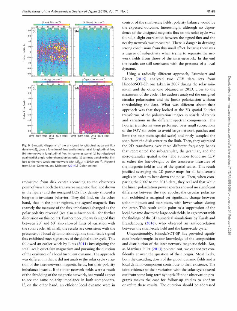
Publications of the Astronomical Society of Japan (2019), Vol. 71, No. 5 R1-25
(a) (b)
(c) (d)
Fig. 9. Synoptic diagrams of the unsigned longitudinal apparent fluxdensity (|BL
app|) as a function of time and latitude: (a) all longitudinal flux;(b) inter-network longitudinal flux; (c) same as panel (b) but displayedagainst disk angle rather than solar latitude; (d) same as panel (c) but lim-ited to the very weak inter-network with |BL
app| < 20 Mx cm−2. [Figure 4from Lites, Centeno, and McIntosh (2014).] (Color online)
(measured from disk center according to the observer’spoint of view). Both the transverse magnetic flux (not shownin the figure) and the unsigned LOS flux density showed along-term invariant behavior. They did find, on the otherhand, that in the polar regions, the signed magnetic flux(namely the measure of the flux imbalance) changed as thepolar polarity reversed (see also subsection 4.1 for furtherdiscussion on this point). Furthermore, the weak signed fluxbetween 20
◦and 60
◦also showed hints of variation with
the solar cycle. All in all, the results are consistent with thepresence of a local dynamo, although the small-scale signedflux exhibited trace signatures of the global solar cycle. Thisfollowed an earlier work by Lites (2011) investigating thesmall-scale quiet-Sun magnetism and pursuing the questionof the existence of a local turbulent dynamo. The approachwas different in that it did not analyze the solar cycle varia-tion of the inter-network magnetic fields, but their polarityimbalance instead. If the inter-network fields were a resultof the shredding of the magnetic network, one would expectto see the same polarity imbalance in both components.If, on the other hand, an efficient local dynamo were in
control of the small-scale fields, polarity balance would bethe expected outcome. Interestingly, although no depen-dence of the unsigned magnetic flux on the solar cycle wasfound, a slight correlation between the signed flux and thenearby network was measured. There is danger in drawingstrong conclusions from this small effect, because there wasa degree of subjectivity when trying to separate the net-work fields from those of the inter-network. In the endthe results are still consistent with the presence of a localdynamo.
Using a radically different approach, Faurobert andRicort (2015) analyzed two CLV data sets fromHinode/SOT-SP, one taken in 2007 during the solar min-imum and the other one obtained in 2013, close to themaximum of the cycle. The authors analyzed the unsignedcircular polarization and the linear polarization withoutthresholding the data. What was different about theirapproach was that they looked at the 2D spatial Fouriertransforms of the polarization images in search of trendsand variations in the different spectral components. TheFourier transforms were performed over small subsectionsof the FOV (in order to avoid large network patches andlimit the maximum spatial scale) and finely sampled thespan from the disk center to the limb. Then, they averagedthe 2D transforms over three different frequency bandsthat represented the sub-granular, the granular, and themeso-granular spatial scales. The authors found no CLVin either the line-of-sight or the transverse measures ofthe magnetic field at any of the spatial scales. This resultjustified averaging the 2D power maps for all heliocentricangles in order to beat down the noise. Then, when com-paring the 2007 to the 2013 data, they realized that whilethe linear polarization power spectra showed no significantdifference between the two epochs, the circular polariza-tion exhibited a marginal yet significant change betweensolar minimum and maximum, with lower values duringthe latter. This result could point to a suppression of thelocal dynamo due to the large-scale fields, in agreement withthe findings of the 3D numerical simulations by Karak andBrandenburg (2016), who observed an anti-correlationbetween the small-scale field and the large-scale cycle.
Unquestionably, Hinode/SOT-SP has provided signifi-cant breakthroughs in our knowledge of the compositionand distribution of the inter-network magnetic fields. But,as Martınez Pillet (2013) pointed out, we cannot yet con-fidently answer the question of their origin. Most likely,both the cascading down of the global dynamo fields and alocal dynamo component contribute to their existence. Thefaint evidence of their variation with the solar cycle teasedout from some long-term synoptic Hinode observation pro-grams makes the case for follow-up studies to confirmor refute these results. The question should be addressed
Dow
nloaded from https://academ
ic.oup.com/pasj/article-abstract/71/5/R
1/5589096 by guest on 04 February 2020
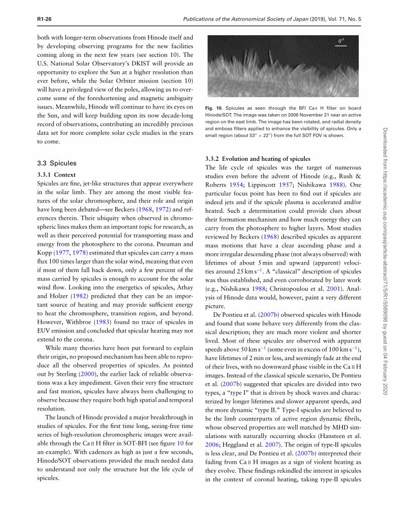
R1-26 Publications of the Astronomical Society of Japan (2019), Vol. 71, No. 5
both with longer-term observations from Hinode itself andby developing observing programs for the new facilitiescoming along in the next few years (see section 10). TheU.S. National Solar Observatory’s DKIST will provide anopportunity to explore the Sun at a higher resolution thanever before, while the Solar Orbiter mission (section 10)will have a privileged view of the poles, allowing us to over-come some of the foreshortening and magnetic ambiguityissues. Meanwhile, Hinode will continue to have its eyes onthe Sun, and will keep building upon its now decade-longrecord of observations, contributing an incredibly preciousdata set for more complete solar cycle studies in the yearsto come.
3.3 Spicules
3.3.1 ContextSpicules are fine, jet-like structures that appear everywherein the solar limb. They are among the most visible fea-tures of the solar chromosphere, and their role and originhave long been debated—see Beckers (1968, 1972) and ref-erences therein. Their ubiquity when observed in chromo-spheric lines makes them an important topic for research, aswell as their perceived potential for transporting mass andenergy from the photosphere to the corona. Pneuman andKopp (1977, 1978) estimated that spicules can carry a massflux 100 times larger than the solar wind, meaning that evenif most of them fall back down, only a few percent of themass carried by spicules is enough to account for the solarwind flow. Looking into the energetics of spicules, Athayand Holzer (1982) predicted that they can be an impor-tant source of heating and may provide sufficient energyto heat the chromosphere, transition region, and beyond.However, Withbroe (1983) found no trace of spicules inEUV emission and concluded that spicular heating may notextend to the corona.
While many theories have been put forward to explaintheir origin, no proposed mechanism has been able to repro-duce all the observed properties of spicules. As pointedout by Sterling (2000), the earlier lack of reliable observa-tions was a key impediment. Given their very fine structureand fast motion, spicules have always been challenging toobserve because they require both high spatial and temporalresolution.
The launch of Hinode provided a major breakthrough instudies of spicules. For the first time long, seeing-free timeseries of high-resolution chromospheric images were avail-able through the Ca II H filter in SOT-BFI (see figure 10 foran example). With cadences as high as just a few seconds,Hinode/SOT observations provided the much needed datato understand not only the structure but the life cycle ofspicules.
Fig. 10. Spicules as seen through the BFI Ca II H filter on boardHinode/SOT. The image was taken on 2006 November 21 near an activeregion on the east limb. The image has been rotated, and radial densityand emboss filters applied to enhance the visibility of spicules. Only asmall region (about 53′′ × 22′′) from the full SOT FOV is shown.
3.3.2 Evolution and heating of spiculesThe life cycle of spicules was the target of numerousstudies even before the advent of Hinode (e.g., Rush &Roberts 1954; Lippincott 1957; Nishikawa 1988). Oneparticular focus point has been to find out if spicules areindeed jets and if the spicule plasma is accelerated and/orheated. Such a determination could provide clues abouttheir formation mechanism and how much energy they cancarry from the photosphere to higher layers. Most studiesreviewed by Beckers (1968) described spicules as apparentmass motions that have a clear ascending phase and amore irregular descending phase (not always observed) withlifetimes of about 5 min and upward (apparent) veloci-ties around 25 km s−1. A “classical” description of spiculeswas thus established, and even corroborated by later work(e.g., Nishikawa 1988; Christopoulou et al. 2001). Anal-ysis of Hinode data would, however, paint a very differentpicture.
De Pontieu et al. (2007b) observed spicules with Hinodeand found that some behave very differently from the clas-sical description; they are much more violent and shorterlived. Most of these spicules are observed with apparentspeeds above 50 km s−1 (some even in excess of 100 km s−1),have lifetimes of 2 min or less, and seemingly fade at the endof their lives, with no downward phase visible in the Ca II Himages. Instead of the classical spicule scenario, De Pontieuet al. (2007b) suggested that spicules are divided into twotypes, a “type I” that is driven by shock waves and charac-terized by longer lifetimes and slower apparent speeds, andthe more dynamic “type II.” Type-I spicules are believed tobe the limb counterparts of active region dynamic fibrils,whose observed properties are well matched by MHD sim-ulations with naturally occurring shocks (Hansteen et al.2006; Heggland et al. 2007). The origin of type-II spiculesis less clear, and De Pontieu et al. (2007b) interpreted theirfading from Ca II H images as a sign of violent heating asthey evolve. These findings rekindled the interest in spiculesin the context of coronal heating, taking type-II spicules
Dow
nloaded from https://academ
ic.oup.com/pasj/article-abstract/71/5/R
1/5589096 by guest on 04 February 2020
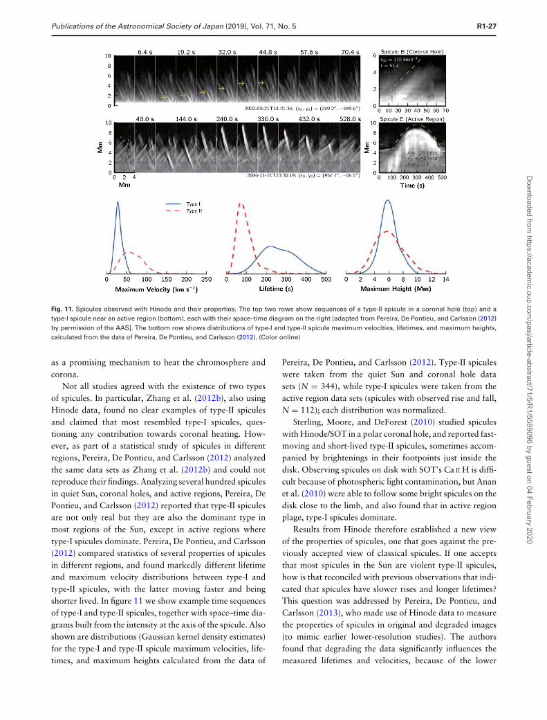
Publications of the Astronomical Society of Japan (2019), Vol. 71, No. 5 R1-27
Fig. 11. Spicules observed with Hinode and their properties. The top two rows show sequences of a type-II spicule in a coronal hole (top) and atype-I spicule near an active region (bottom), each with their space–time diagram on the right [adapted from Pereira, De Pontieu, and Carlsson (2012)by permission of the AAS]. The bottom row shows distributions of type-I and type-II spicule maximum velocities, lifetimes, and maximum heights,calculated from the data of Pereira, De Pontieu, and Carlsson (2012). (Color online)
as a promising mechanism to heat the chromosphere andcorona.
Not all studies agreed with the existence of two typesof spicules. In particular, Zhang et al. (2012b), also usingHinode data, found no clear examples of type-II spiculesand claimed that most resembled type-I spicules, ques-tioning any contribution towards coronal heating. How-ever, as part of a statistical study of spicules in differentregions, Pereira, De Pontieu, and Carlsson (2012) analyzedthe same data sets as Zhang et al. (2012b) and could notreproduce their findings. Analyzing several hundred spiculesin quiet Sun, coronal holes, and active regions, Pereira, DePontieu, and Carlsson (2012) reported that type-II spiculesare not only real but they are also the dominant type inmost regions of the Sun, except in active regions wheretype-I spicules dominate. Pereira, De Pontieu, and Carlsson(2012) compared statistics of several properties of spiculesin different regions, and found markedly different lifetimeand maximum velocity distributions between type-I andtype-II spicules, with the latter moving faster and beingshorter lived. In figure 11 we show example time sequencesof type-I and type-II spicules, together with space–time dia-grams built from the intensity at the axis of the spicule. Alsoshown are distributions (Gaussian kernel density estimates)for the type-I and type-II spicule maximum velocities, life-times, and maximum heights calculated from the data of
Pereira, De Pontieu, and Carlsson (2012). Type-II spiculeswere taken from the quiet Sun and coronal hole datasets (N = 344), while type-I spicules were taken from theactive region data sets (spicules with observed rise and fall,N = 112); each distribution was normalized.
Sterling, Moore, and DeForest (2010) studied spiculeswith Hinode/SOT in a polar coronal hole, and reported fast-moving and short-lived type-II spicules, sometimes accom-panied by brightenings in their footpoints just inside thedisk. Observing spicules on disk with SOT’s Ca II H is diffi-cult because of photospheric light contamination, but Ananet al. (2010) were able to follow some bright spicules on thedisk close to the limb, and also found that in active regionplage, type-I spicules dominate.
Results from Hinode therefore established a new viewof the properties of spicules, one that goes against the pre-viously accepted view of classical spicules. If one acceptsthat most spicules in the Sun are violent type-II spicules,how is that reconciled with previous observations that indi-cated that spicules have slower rises and longer lifetimes?This question was addressed by Pereira, De Pontieu, andCarlsson (2013), who made use of Hinode data to measurethe properties of spicules in original and degraded images(to mimic earlier lower-resolution studies). The authorsfound that degrading the data significantly influences themeasured lifetimes and velocities, because of the lower
Dow
nloaded from https://academ
ic.oup.com/pasj/article-abstract/71/5/R
1/5589096 by guest on 04 February 2020
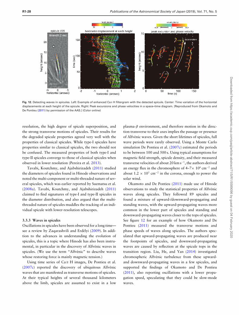
R1-28 Publications of the Astronomical Society of Japan (2019), Vol. 71, No. 5
Fig. 12. Detecting waves in spicules. Left: Example of enhanced Ca II H filtergram with the detected spicule. Center: Time variation of the horizontaldisplacements at each height of the spicule. Right: Peak excursions and phase velocities in a space–time diagram. [Reproduced from Okamoto andDe Pontieu (2011) by permission of the AAS.] (Color online)
resolution, the high degree of spicule superposition, andthe strong transverse motions of spicules. Their results forthe degraded spicule properties agreed very well with theproperties of classical spicules. While type-I spicules haveproperties similar to classical spicules, the two should notbe confused. The measured properties of both type-I andtype-II spicules converge to those of classical spicules whenobserved in lower resolution (Pereira et al. 2013).
Tavabi, Koutchmy, and Ajabshirizadeh (2011) studiedthe diameters of spicules found in Hinode observations andnoted the multi-component or multi-threaded nature of sev-eral spicules, which was earlier reported by Suematsu et al.(2008a). Tavabi, Koutchmy, and Ajabshirizadeh (2011)claimed to find signatures of type-I and type-II spicules inthe diameter distribution, and also argued that the multi-threaded nature of spicules muddles the tracking of an indi-vidual spicule with lower-resolution telescopes.
3.3.3 Waves in spiculesOscillations in spicules have been observed for a long time—see a review by Zaqarashvili and Erdelyi (2009). In addi-tion to the advances in understanding the evolution ofspicules, this is a topic where Hinode has also been instru-mental, in particular in the discovery of Alfvenic waves inspicules. (We use the term “Alfvenic” to describe waveswhose restoring force is mainly magnetic tension.)
Using time series of Ca II H images, De Pontieu et al.(2007c) reported the discovery of ubiquitous Alfvenicwaves that are manifested as transverse motions of spicules.At their typical heights of several thousand kilometersabove the limb, spicules are assumed to exist in a low
plasma-β environment, and therefore motion in the direc-tion transverse to their axes implies the passage or presenceof Alfvenic waves. Given the short lifetimes of spicules, fullwave periods were rarely observed. Using a Monte Carlosimulation De Pontieu et al. (2007c) estimated the periodsto be between 100 and 500 s. Using typical assumptions formagnetic field strength, spicule density, and their measuredtransverse velocities of about 20 km s−1, the authors derivedan energy flux in the chromosphere of 4–7× 106 cm−2 andabout 1.2 × 105 cm−2 in the corona, enough to power thesolar wind.
Okamoto and De Pontieu (2011) made use of Hinodeobservations to study the statistical properties of Alfvenicwaves along spicules. They followed 89 spicules andfound a mixture of upward-/downward-propagating andstanding waves, with the upward-propagating waves morecommon in the lower part of spicules and standing anddownward-propagating waves closer to the tops of spicules.See figure 12 for an example of how Okamoto and DePontieu (2011) measured the transverse motions andphase speeds of waves along spicules. The authors spec-ulated that upward-propagating waves are produced nearthe footpoints of spicules, and downward-propagatingwaves are caused by reflection at the spicule tops in thetransition region. Liu, He, and Yan (2014) investigatedchromospheric Alfvenic turbulence from these upward-and downward-propagating waves in a few spicules, andsupported the findings of Okamoto and De Pontieu(2011), also reporting oscillations with a lower propa-gation speed, speculating that they could be slow-modewaves.
Dow
nloaded from https://academ
ic.oup.com/pasj/article-abstract/71/5/R
1/5589096 by guest on 04 February 2020
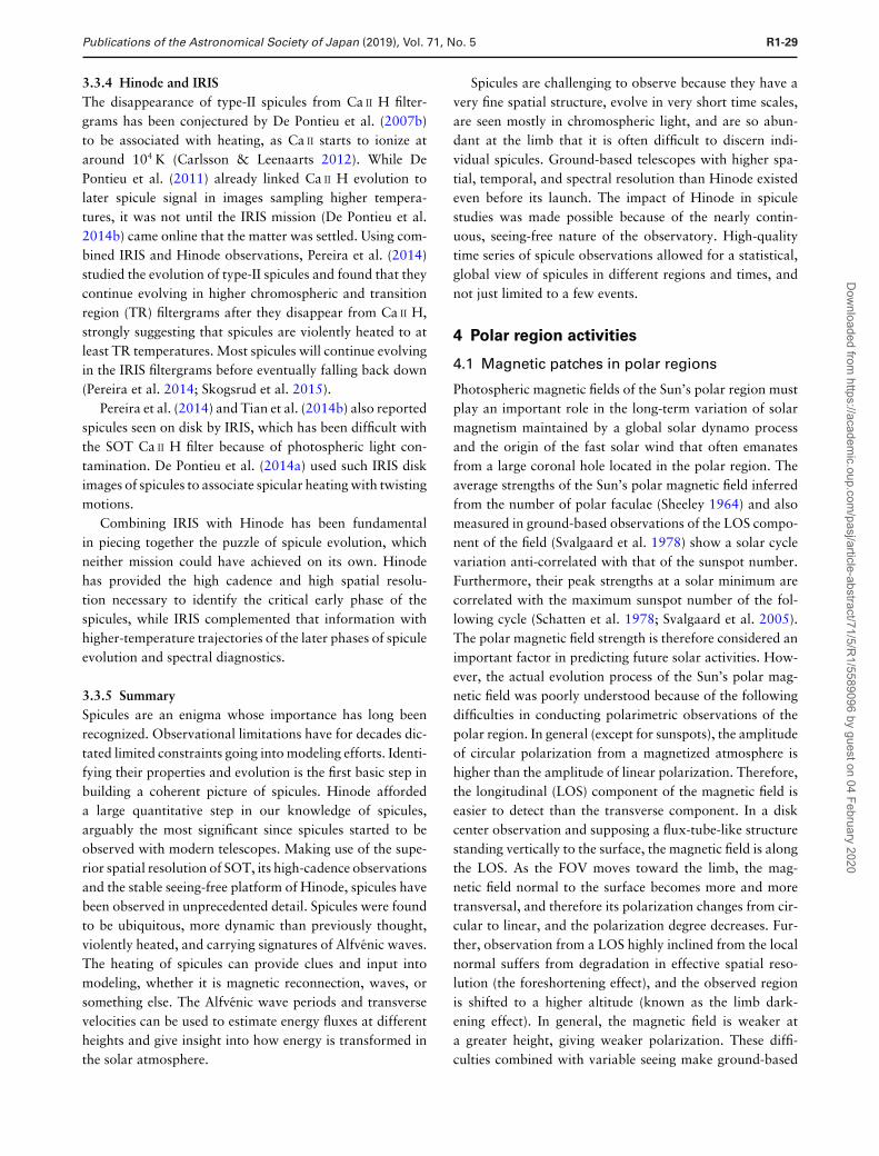
Publications of the Astronomical Society of Japan (2019), Vol. 71, No. 5 R1-29
3.3.4 Hinode and IRISThe disappearance of type-II spicules from Ca II H filter-grams has been conjectured by De Pontieu et al. (2007b)to be associated with heating, as Ca II starts to ionize ataround 104 K (Carlsson & Leenaarts 2012). While DePontieu et al. (2011) already linked Ca II H evolution tolater spicule signal in images sampling higher tempera-tures, it was not until the IRIS mission (De Pontieu et al.2014b) came online that the matter was settled. Using com-bined IRIS and Hinode observations, Pereira et al. (2014)studied the evolution of type-II spicules and found that theycontinue evolving in higher chromospheric and transitionregion (TR) filtergrams after they disappear from Ca II H,strongly suggesting that spicules are violently heated to atleast TR temperatures. Most spicules will continue evolvingin the IRIS filtergrams before eventually falling back down(Pereira et al. 2014; Skogsrud et al. 2015).
Pereira et al. (2014) and Tian et al. (2014b) also reportedspicules seen on disk by IRIS, which has been difficult withthe SOT Ca II H filter because of photospheric light con-tamination. De Pontieu et al. (2014a) used such IRIS diskimages of spicules to associate spicular heating with twistingmotions.
Combining IRIS with Hinode has been fundamentalin piecing together the puzzle of spicule evolution, whichneither mission could have achieved on its own. Hinodehas provided the high cadence and high spatial resolu-tion necessary to identify the critical early phase of thespicules, while IRIS complemented that information withhigher-temperature trajectories of the later phases of spiculeevolution and spectral diagnostics.
3.3.5 SummarySpicules are an enigma whose importance has long beenrecognized. Observational limitations have for decades dic-tated limited constraints going into modeling efforts. Identi-fying their properties and evolution is the first basic step inbuilding a coherent picture of spicules. Hinode affordeda large quantitative step in our knowledge of spicules,arguably the most significant since spicules started to beobserved with modern telescopes. Making use of the supe-rior spatial resolution of SOT, its high-cadence observationsand the stable seeing-free platform of Hinode, spicules havebeen observed in unprecedented detail. Spicules were foundto be ubiquitous, more dynamic than previously thought,violently heated, and carrying signatures of Alfvenic waves.The heating of spicules can provide clues and input intomodeling, whether it is magnetic reconnection, waves, orsomething else. The Alfvenic wave periods and transversevelocities can be used to estimate energy fluxes at differentheights and give insight into how energy is transformed inthe solar atmosphere.
Spicules are challenging to observe because they have avery fine spatial structure, evolve in very short time scales,are seen mostly in chromospheric light, and are so abun-dant at the limb that it is often difficult to discern indi-vidual spicules. Ground-based telescopes with higher spa-tial, temporal, and spectral resolution than Hinode existedeven before its launch. The impact of Hinode in spiculestudies was made possible because of the nearly contin-uous, seeing-free nature of the observatory. High-qualitytime series of spicule observations allowed for a statistical,global view of spicules in different regions and times, andnot just limited to a few events.
4 Polar region activities
4.1 Magnetic patches in polar regions
Photospheric magnetic fields of the Sun’s polar region mustplay an important role in the long-term variation of solarmagnetism maintained by a global solar dynamo processand the origin of the fast solar wind that often emanatesfrom a large coronal hole located in the polar region. Theaverage strengths of the Sun’s polar magnetic field inferredfrom the number of polar faculae (Sheeley 1964) and alsomeasured in ground-based observations of the LOS compo-nent of the field (Svalgaard et al. 1978) show a solar cyclevariation anti-correlated with that of the sunspot number.Furthermore, their peak strengths at a solar minimum arecorrelated with the maximum sunspot number of the fol-lowing cycle (Schatten et al. 1978; Svalgaard et al. 2005).The polar magnetic field strength is therefore considered animportant factor in predicting future solar activities. How-ever, the actual evolution process of the Sun’s polar mag-netic field was poorly understood because of the followingdifficulties in conducting polarimetric observations of thepolar region. In general (except for sunspots), the amplitudeof circular polarization from a magnetized atmosphere ishigher than the amplitude of linear polarization. Therefore,the longitudinal (LOS) component of the magnetic field iseasier to detect than the transverse component. In a diskcenter observation and supposing a flux-tube-like structurestanding vertically to the surface, the magnetic field is alongthe LOS. As the FOV moves toward the limb, the mag-netic field normal to the surface becomes more and moretransversal, and therefore its polarization changes from cir-cular to linear, and the polarization degree decreases. Fur-ther, observation from a LOS highly inclined from the localnormal suffers from degradation in effective spatial reso-lution (the foreshortening effect), and the observed regionis shifted to a higher altitude (known as the limb dark-ening effect). In general, the magnetic field is weaker ata greater height, giving weaker polarization. These diffi-culties combined with variable seeing make ground-based
Dow
nloaded from https://academ
ic.oup.com/pasj/article-abstract/71/5/R
1/5589096 by guest on 04 February 2020
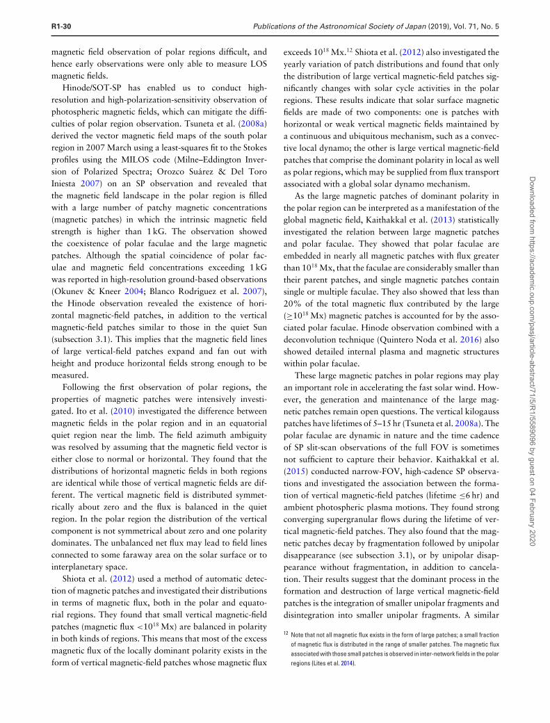
R1-30 Publications of the Astronomical Society of Japan (2019), Vol. 71, No. 5
magnetic field observation of polar regions difficult, andhence early observations were only able to measure LOSmagnetic fields.
Hinode/SOT-SP has enabled us to conduct high-resolution and high-polarization-sensitivity observation ofphotospheric magnetic fields, which can mitigate the diffi-culties of polar region observation. Tsuneta et al. (2008a)derived the vector magnetic field maps of the south polarregion in 2007 March using a least-squares fit to the Stokesprofiles using the MILOS code (Milne–Eddington Inver-sion of Polarized Spectra; Orozco Suarez & Del ToroIniesta 2007) on an SP observation and revealed thatthe magnetic field landscape in the polar region is filledwith a large number of patchy magnetic concentrations(magnetic patches) in which the intrinsic magnetic fieldstrength is higher than 1 kG. The observation showedthe coexistence of polar faculae and the large magneticpatches. Although the spatial coincidence of polar fac-ulae and magnetic field concentrations exceeding 1 kGwas reported in high-resolution ground-based observations(Okunev & Kneer 2004; Blanco Rodrıguez et al. 2007),the Hinode observation revealed the existence of hori-zontal magnetic-field patches, in addition to the verticalmagnetic-field patches similar to those in the quiet Sun(subsection 3.1). This implies that the magnetic field linesof large vertical-field patches expand and fan out withheight and produce horizontal fields strong enough to bemeasured.
Following the first observation of polar regions, theproperties of magnetic patches were intensively investi-gated. Ito et al. (2010) investigated the difference betweenmagnetic fields in the polar region and in an equatorialquiet region near the limb. The field azimuth ambiguitywas resolved by assuming that the magnetic field vector iseither close to normal or horizontal. They found that thedistributions of horizontal magnetic fields in both regionsare identical while those of vertical magnetic fields are dif-ferent. The vertical magnetic field is distributed symmet-rically about zero and the flux is balanced in the quietregion. In the polar region the distribution of the verticalcomponent is not symmetrical about zero and one polaritydominates. The unbalanced net flux may lead to field linesconnected to some faraway area on the solar surface or tointerplanetary space.
Shiota et al. (2012) used a method of automatic detec-tion of magnetic patches and investigated their distributionsin terms of magnetic flux, both in the polar and equato-rial regions. They found that small vertical magnetic-fieldpatches (magnetic flux <1018 Mx) are balanced in polarityin both kinds of regions. This means that most of the excessmagnetic flux of the locally dominant polarity exists in theform of vertical magnetic-field patches whose magnetic flux
exceeds 1018 Mx.12 Shiota et al. (2012) also investigated theyearly variation of patch distributions and found that onlythe distribution of large vertical magnetic-field patches sig-nificantly changes with solar cycle activities in the polarregions. These results indicate that solar surface magneticfields are made of two components: one is patches withhorizontal or weak vertical magnetic fields maintained bya continuous and ubiquitous mechanism, such as a convec-tive local dynamo; the other is large vertical magnetic-fieldpatches that comprise the dominant polarity in local as wellas polar regions, which may be supplied from flux transportassociated with a global solar dynamo mechanism.
As the large magnetic patches of dominant polarity inthe polar region can be interpreted as a manifestation of theglobal magnetic field, Kaithakkal et al. (2013) statisticallyinvestigated the relation between large magnetic patchesand polar faculae. They showed that polar faculae areembedded in nearly all magnetic patches with flux greaterthan 1018 Mx, that the faculae are considerably smaller thantheir parent patches, and single magnetic patches containsingle or multiple faculae. They also showed that less than20% of the total magnetic flux contributed by the large(≥1018 Mx) magnetic patches is accounted for by the asso-ciated polar faculae. Hinode observation combined with adeconvolution technique (Quintero Noda et al. 2016) alsoshowed detailed internal plasma and magnetic structureswithin polar faculae.
These large magnetic patches in polar regions may playan important role in accelerating the fast solar wind. How-ever, the generation and maintenance of the large mag-netic patches remain open questions. The vertical kilogausspatches have lifetimes of 5–15 hr (Tsuneta et al. 2008a). Thepolar faculae are dynamic in nature and the time cadenceof SP slit-scan observations of the full FOV is sometimesnot sufficient to capture their behavior. Kaithakkal et al.(2015) conducted narrow-FOV, high-cadence SP observa-tions and investigated the association between the forma-tion of vertical magnetic-field patches (lifetime ≤6 hr) andambient photospheric plasma motions. They found strongconverging supergranular flows during the lifetime of ver-tical magnetic-field patches. They also found that the mag-netic patches decay by fragmentation followed by unipolardisappearance (see subsection 3.1), or by unipolar disap-pearance without fragmentation, in addition to cancela-tion. Their results suggest that the dominant process in theformation and destruction of large vertical magnetic-fieldpatches is the integration of smaller unipolar fragments anddisintegration into smaller unipolar fragments. A similar
12 Note that not all magnetic flux exists in the form of large patches; a small fractionof magnetic flux is distributed in the range of smaller patches. The magnetic fluxassociated with those small patches is observed in inter-network fields in the polarregions (Lites et al. 2014).
Dow
nloaded from https://academ
ic.oup.com/pasj/article-abstract/71/5/R
1/5589096 by guest on 04 February 2020
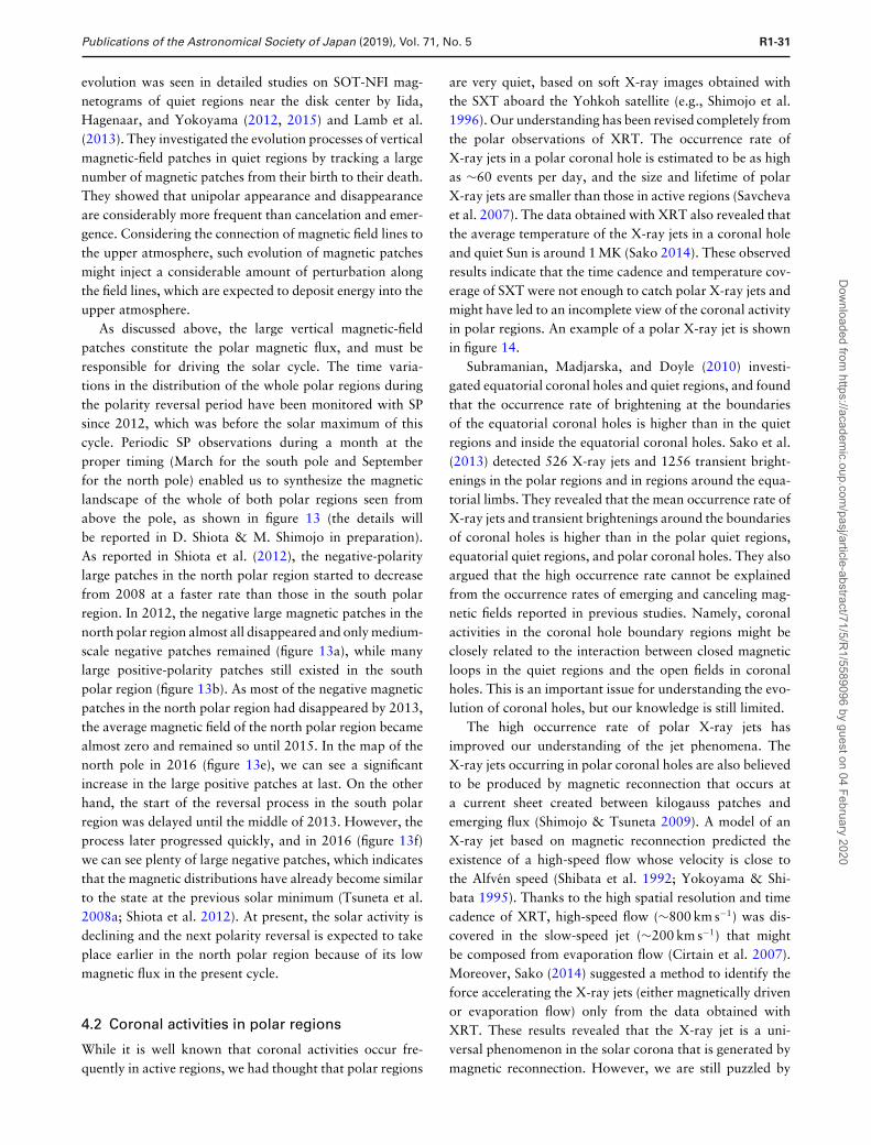
Publications of the Astronomical Society of Japan (2019), Vol. 71, No. 5 R1-31
evolution was seen in detailed studies on SOT-NFI mag-netograms of quiet regions near the disk center by Iida,Hagenaar, and Yokoyama (2012, 2015) and Lamb et al.(2013). They investigated the evolution processes of verticalmagnetic-field patches in quiet regions by tracking a largenumber of magnetic patches from their birth to their death.They showed that unipolar appearance and disappearanceare considerably more frequent than cancelation and emer-gence. Considering the connection of magnetic field lines tothe upper atmosphere, such evolution of magnetic patchesmight inject a considerable amount of perturbation alongthe field lines, which are expected to deposit energy into theupper atmosphere.
As discussed above, the large vertical magnetic-fieldpatches constitute the polar magnetic flux, and must beresponsible for driving the solar cycle. The time varia-tions in the distribution of the whole polar regions duringthe polarity reversal period have been monitored with SPsince 2012, which was before the solar maximum of thiscycle. Periodic SP observations during a month at theproper timing (March for the south pole and Septemberfor the north pole) enabled us to synthesize the magneticlandscape of the whole of both polar regions seen fromabove the pole, as shown in figure 13 (the details willbe reported in D. Shiota & M. Shimojo in preparation).As reported in Shiota et al. (2012), the negative-polaritylarge patches in the north polar region started to decreasefrom 2008 at a faster rate than those in the south polarregion. In 2012, the negative large magnetic patches in thenorth polar region almost all disappeared and only medium-scale negative patches remained (figure 13a), while manylarge positive-polarity patches still existed in the southpolar region (figure 13b). As most of the negative magneticpatches in the north polar region had disappeared by 2013,the average magnetic field of the north polar region becamealmost zero and remained so until 2015. In the map of thenorth pole in 2016 (figure 13e), we can see a significantincrease in the large positive patches at last. On the otherhand, the start of the reversal process in the south polarregion was delayed until the middle of 2013. However, theprocess later progressed quickly, and in 2016 (figure 13f)we can see plenty of large negative patches, which indicatesthat the magnetic distributions have already become similarto the state at the previous solar minimum (Tsuneta et al.2008a; Shiota et al. 2012). At present, the solar activity isdeclining and the next polarity reversal is expected to takeplace earlier in the north polar region because of its lowmagnetic flux in the present cycle.
4.2 Coronal activities in polar regions
While it is well known that coronal activities occur fre-quently in active regions, we had thought that polar regions
are very quiet, based on soft X-ray images obtained withthe SXT aboard the Yohkoh satellite (e.g., Shimojo et al.1996). Our understanding has been revised completely fromthe polar observations of XRT. The occurrence rate ofX-ray jets in a polar coronal hole is estimated to be as highas ∼60 events per day, and the size and lifetime of polarX-ray jets are smaller than those in active regions (Savchevaet al. 2007). The data obtained with XRT also revealed thatthe average temperature of the X-ray jets in a coronal holeand quiet Sun is around 1 MK (Sako 2014). These observedresults indicate that the time cadence and temperature cov-erage of SXT were not enough to catch polar X-ray jets andmight have led to an incomplete view of the coronal activityin polar regions. An example of a polar X-ray jet is shownin figure 14.
Subramanian, Madjarska, and Doyle (2010) investi-gated equatorial coronal holes and quiet regions, and foundthat the occurrence rate of brightening at the boundariesof the equatorial coronal holes is higher than in the quietregions and inside the equatorial coronal holes. Sako et al.(2013) detected 526 X-ray jets and 1256 transient bright-enings in the polar regions and in regions around the equa-torial limbs. They revealed that the mean occurrence rate ofX-ray jets and transient brightenings around the boundariesof coronal holes is higher than in the polar quiet regions,equatorial quiet regions, and polar coronal holes. They alsoargued that the high occurrence rate cannot be explainedfrom the occurrence rates of emerging and canceling mag-netic fields reported in previous studies. Namely, coronalactivities in the coronal hole boundary regions might beclosely related to the interaction between closed magneticloops in the quiet regions and the open fields in coronalholes. This is an important issue for understanding the evo-lution of coronal holes, but our knowledge is still limited.
The high occurrence rate of polar X-ray jets hasimproved our understanding of the jet phenomena. TheX-ray jets occurring in polar coronal holes are also believedto be produced by magnetic reconnection that occurs ata current sheet created between kilogauss patches andemerging flux (Shimojo & Tsuneta 2009). A model of anX-ray jet based on magnetic reconnection predicted theexistence of a high-speed flow whose velocity is close tothe Alfven speed (Shibata et al. 1992; Yokoyama & Shi-bata 1995). Thanks to the high spatial resolution and timecadence of XRT, high-speed flow (∼800 km s−1) was dis-covered in the slow-speed jet (∼200 km s−1) that mightbe composed from evaporation flow (Cirtain et al. 2007).Moreover, Sako (2014) suggested a method to identify theforce accelerating the X-ray jets (either magnetically drivenor evaporation flow) only from the data obtained withXRT. These results revealed that the X-ray jet is a uni-versal phenomenon in the solar corona that is generated bymagnetic reconnection. However, we are still puzzled by
Dow
nloaded from https://academ
ic.oup.com/pasj/article-abstract/71/5/R
1/5589096 by guest on 04 February 2020
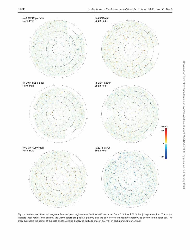
R1-32 Publications of the Astronomical Society of Japan (2019), Vol. 71, No. 5
Fig. 13. Landscapes of vertical magnetic fields of polar regions from 2012 to 2016 (extracted from D. Shiota & M. Shimojo in preparation). The colorsindicate local vertical flux density; the warm colors are positive polarity and the cool colors are negative polarity, as shown in the color bar. Thecross symbol is the center of the pole and the circles display co-latitude lines of every 5◦ in each panel. (Color online)
Dow
nloaded from https://academ
ic.oup.com/pasj/article-abstract/71/5/R
1/5589096 by guest on 04 February 2020
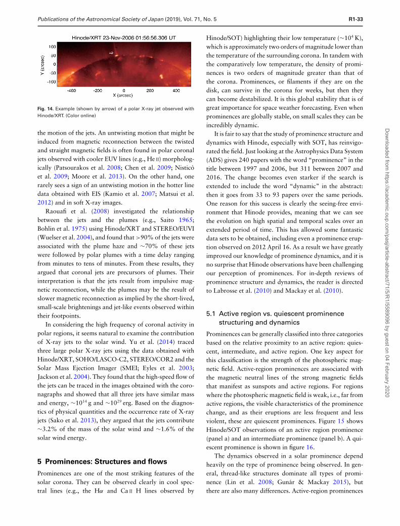
Publications of the Astronomical Society of Japan (2019), Vol. 71, No. 5 R1-33
Fig. 14. Example (shown by arrow) of a polar X-ray jet observed withHinode/XRT. (Color online)
the motion of the jets. An untwisting motion that might beinduced from magnetic reconnection between the twistedand straight magnetic fields is often found in polar coronaljets observed with cooler EUV lines (e.g., He II) morpholog-ically (Patsourakos et al. 2008; Chen et al. 2009; Nisticoet al. 2009; Moore et al. 2013). On the other hand, onerarely sees a sign of an untwisting motion in the hotter linedata obtained with EIS (Kamio et al. 2007; Matsui et al.2012) and in soft X-ray images.
Raouafi et al. (2008) investigated the relationshipbetween the jets and the plumes (e.g., Saito 1965;Bohlin et al. 1975) using Hinode/XRT and STEREO/EUVI(Wuelser et al. 2004), and found that >90% of the jets wereassociated with the plume haze and ∼70% of these jetswere followed by polar plumes with a time delay rangingfrom minutes to tens of minutes. From these results, theyargued that coronal jets are precursors of plumes. Theirinterpretation is that the jets result from impulsive mag-netic reconnection, while the plumes may be the result ofslower magnetic reconnection as implied by the short-lived,small-scale brightenings and jet-like events observed withintheir footpoints.
In considering the high frequency of coronal activity inpolar regions, it seems natural to examine the contributionof X-ray jets to the solar wind. Yu et al. (2014) tracedthree large polar X-ray jets using the data obtained withHinode/XRT, SOHO/LASCO-C2, STEREO/COR2 and theSolar Mass Ejection Imager (SMEI; Eyles et al. 2003;Jackson et al. 2004). They found that the high-speed flow ofthe jets can be traced in the images obtained with the coro-nagraphs and showed that all three jets have similar massand energy, ∼1014 g and ∼1029 erg. Based on the diagnos-tics of physical quantities and the occurrence rate of X-rayjets (Sako et al. 2013), they argued that the jets contribute∼3.2% of the mass of the solar wind and ∼1.6% of thesolar wind energy.
5 Prominences: Structures and flows
Prominences are one of the most striking features of thesolar corona. They can be observed clearly in cool spec-tral lines (e.g., the Hα and Ca II H lines observed by
Hinode/SOT) highlighting their low temperature (∼104 K),which is approximately two orders of magnitude lower thanthe temperature of the surrounding corona. In tandem withthe comparatively low temperature, the density of promi-nences is two orders of magnitude greater than that ofthe corona. Prominences, or filaments if they are on thedisk, can survive in the corona for weeks, but then theycan become destabilized. It is this global stability that is ofgreat importance for space weather forecasting. Even whenprominences are globally stable, on small scales they can beincredibly dynamic.
It is fair to say that the study of prominence structure anddynamics with Hinode, especially with SOT, has reinvigo-rated the field. Just looking at the Astrophysics Data System(ADS) gives 240 papers with the word “prominence” in thetitle between 1997 and 2006, but 311 between 2007 and2016. The change becomes even starker if the search isextended to include the word “dynamic” in the abstract:then it goes from 33 to 93 papers over the same periods.One reason for this success is clearly the seeing-free envi-ronment that Hinode provides, meaning that we can seethe evolution on high spatial and temporal scales over anextended period of time. This has allowed some fantasticdata sets to be obtained, including even a prominence erup-tion observed on 2012 April 16. As a result we have greatlyimproved our knowledge of prominence dynamics, and it isno surprise that Hinode observations have been challengingour perception of prominences. For in-depth reviews ofprominence structure and dynamics, the reader is directedto Labrosse et al. (2010) and Mackay et al. (2010).
5.1 Active region vs. quiescent prominencestructuring and dynamics
Prominences can be generally classified into three categoriesbased on the relative proximity to an active region: quies-cent, intermediate, and active region. One key aspect forthis classification is the strength of the photospheric mag-netic field. Active-region prominences are associated withthe magnetic neutral lines of the strong magnetic fieldsthat manifest as sunspots and active regions. For regionswhere the photospheric magnetic field is weak, i.e., far fromactive regions, the visible characteristics of the prominencechange, and as their eruptions are less frequent and lessviolent, these are quiescent prominences. Figure 15 showsHinode/SOT observations of an active region prominence(panel a) and an intermediate prominence (panel b). A qui-escent prominence is shown in figure 16.
The dynamics observed in a solar prominence dependheavily on the type of prominence being observed. In gen-eral, thread-like structures dominate all types of promi-nence (Lin et al. 2008; Gunar & Mackay 2015), butthere are also many differences. Active-region prominences
Dow
nloaded from https://academ
ic.oup.com/pasj/article-abstract/71/5/R
1/5589096 by guest on 04 February 2020
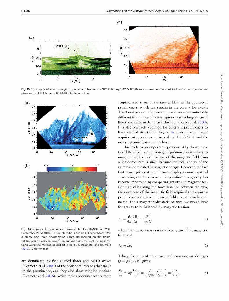
R1-34 Publications of the Astronomical Society of Japan (2019), Vol. 71, No. 5
Fig. 15. (a) Example of an active region prominence observed on 2007 February 8, 17:24 UT (this also shows coronal rain). (b) Intermediate prominenceobserved on 2008 January 16, 01:00 UT. (Color online)
Fig. 16. Quiescent prominence observed by Hinode/SOT on 2008September 29 at 10:02 UT. (a) Intensity in the Ca II H broadband filter;a plume and three downflowing knots are marked on the figure.(b) Doppler velocity in km s−1 as derived from the SOT Hα observa-tions using the method described in Hillier, Matsumoto, and Ichimoto(2017). (Color online)
are dominated by field-aligned flows and MHD waves(Okamoto et al. 2007) of the horizontal threads that makeup the prominence, and they also show winding motions(Okamoto et al. 2016). Active-region prominences are more
eruptive, and as such have shorter lifetimes than quiescentprominences, which can remain in the corona for weeks.The flow dynamics of quiescent prominences are noticeablydifferent from those of active regions, with a huge range offlows orientated in the vertical direction (Berger et al. 2008).It is also relatively common for quiescent prominences tohave vertical structuring. Figure 16 gives an example ofa quiescent prominence observed by Hinode/SOT and themany dynamic features they host.
This leads to an important question: Why do we havethis difference? For active-region prominences it is easy toimagine that the perturbation of the magnetic field froma force-free state is small because the total energy of thesystem is dominated by magnetic energy. However, the factthat many quiescent prominences display so much verticalstructuring can be seen as an implication that gravity hasbecome important. By comparing gravity and magnetic ten-sion and calculating the force balance between the two,the curvature of the magnetic field required to support aprominence for a given magnetic field strength can be esti-mated. For a magnetohydrostatic balance, we would lookfor gravity to be balanced by magnetic tension:
FT = Bx
4π
∂ Bz
∂x∼ B2
4π L, (1)
where L is the necessary radius of curvature of the magneticfield, and
FG = ρg. (2)
Taking the ratio of these two, and assuming an ideal gas(p = ρRGT/μ), gives
FG
FT∼ ρg
4π LB2
= pB2/8π
gμ
RGTL2
= β
2L�
, (3)
Dow
nloaded from https://academ
ic.oup.com/pasj/article-abstract/71/5/R
1/5589096 by guest on 04 February 2020
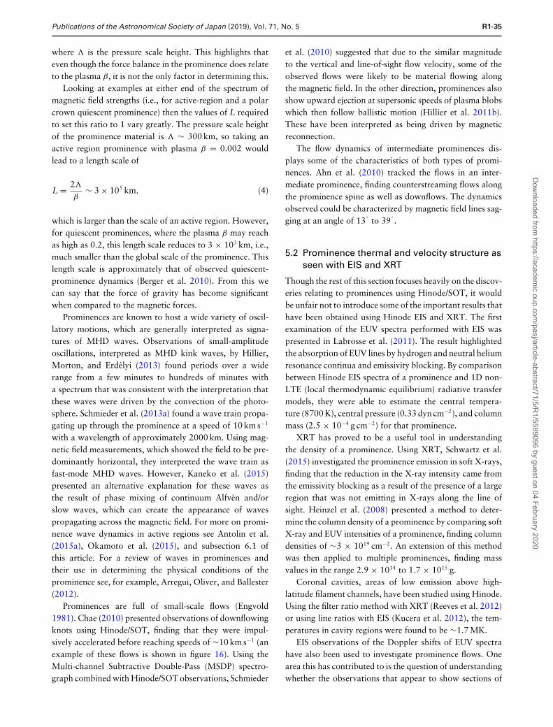
Publications of the Astronomical Society of Japan (2019), Vol. 71, No. 5 R1-35
where � is the pressure scale height. This highlights thateven though the force balance in the prominence does relateto the plasma β, it is not the only factor in determining this.
Looking at examples at either end of the spectrum ofmagnetic field strengths (i.e., for active-region and a polarcrown quiescent prominence) then the values of L requiredto set this ratio to 1 vary greatly. The pressure scale heightof the prominence material is � ∼ 300 km, so taking anactive region prominence with plasma β = 0.002 wouldlead to a length scale of
L = 2�
β∼ 3 × 10⁵ km, (4)
which is larger than the scale of an active region. However,for quiescent prominences, where the plasma β may reachas high as 0.2, this length scale reduces to 3 × 10³ km, i.e.,much smaller than the global scale of the prominence. Thislength scale is approximately that of observed quiescent-prominence dynamics (Berger et al. 2010). From this wecan say that the force of gravity has become significantwhen compared to the magnetic forces.
Prominences are known to host a wide variety of oscil-latory motions, which are generally interpreted as signa-tures of MHD waves. Observations of small-amplitudeoscillations, interpreted as MHD kink waves, by Hillier,Morton, and Erdelyi (2013) found periods over a widerange from a few minutes to hundreds of minutes witha spectrum that was consistent with the interpretation thatthese waves were driven by the convection of the photo-sphere. Schmieder et al. (2013a) found a wave train propa-gating up through the prominence at a speed of 10 km s−1
with a wavelength of approximately 2000 km. Using mag-netic field measurements, which showed the field to be pre-dominantly horizontal, they interpreted the wave train asfast-mode MHD waves. However, Kaneko et al. (2015)presented an alternative explanation for these waves asthe result of phase mixing of continuum Alfven and/orslow waves, which can create the appearance of wavespropagating across the magnetic field. For more on promi-nence wave dynamics in active regions see Antolin et al.(2015a), Okamoto et al. (2015), and subsection 6.1 ofthis article. For a review of waves in prominences andtheir use in determining the physical conditions of theprominence see, for example, Arregui, Oliver, and Ballester(2012).
Prominences are full of small-scale flows (Engvold1981). Chae (2010) presented observations of downflowingknots using Hinode/SOT, finding that they were impul-sively accelerated before reaching speeds of ∼10 km s−1 (anexample of these flows is shown in figure 16). Using theMulti-channel Subtractive Double-Pass (MSDP) spectro-graph combined with Hinode/SOT observations, Schmieder
et al. (2010) suggested that due to the similar magnitudeto the vertical and line-of-sight flow velocity, some of theobserved flows were likely to be material flowing alongthe magnetic field. In the other direction, prominences alsoshow upward ejection at supersonic speeds of plasma blobswhich then follow ballistic motion (Hillier et al. 2011b).These have been interpreted as being driven by magneticreconnection.
The flow dynamics of intermediate prominences dis-plays some of the characteristics of both types of promi-nences. Ahn et al. (2010) tracked the flows in an inter-mediate prominence, finding counterstreaming flows alongthe prominence spine as well as downflows. The dynamicsobserved could be characterized by magnetic field lines sag-ging at an angle of 13
◦to 39
◦.
5.2 Prominence thermal and velocity structure asseen with EIS and XRT
Though the rest of this section focuses heavily on the discov-eries relating to prominences using Hinode/SOT, it wouldbe unfair not to introduce some of the important results thathave been obtained using Hinode EIS and XRT. The firstexamination of the EUV spectra performed with EIS waspresented in Labrosse et al. (2011). The result highlightedthe absorption of EUV lines by hydrogen and neutral heliumresonance continua and emissivity blocking. By comparisonbetween Hinode EIS spectra of a prominence and 1D non-LTE (local thermodynamic equilibrium) radiative transfermodels, they were able to estimate the central tempera-ture (8700 K), central pressure (0.33 dyn cm−2), and columnmass (2.5 × 10⁻⁴ g cm−2) for that prominence.
XRT has proved to be a useful tool in understandingthe density of a prominence. Using XRT, Schwartz et al.(2015) investigated the prominence emission in soft X-rays,finding that the reduction in the X-ray intensity came fromthe emissivity blocking as a result of the presence of a largeregion that was not emitting in X-rays along the line ofsight. Heinzel et al. (2008) presented a method to deter-mine the column density of a prominence by comparing softX-ray and EUV intensities of a prominence, finding columndensities of ∼3 × 1019 cm−2. An extension of this methodwas then applied to multiple prominences, finding massvalues in the range 2.9 × 10¹⁴ to 1.7 × 10¹⁵ g.
Coronal cavities, areas of low emission above high-latitude filament channels, have been studied using Hinode.Using the filter ratio method with XRT (Reeves et al. 2012)or using line ratios with EIS (Kucera et al. 2012), the tem-peratures in cavity regions were found to be ∼1.7 MK.
EIS observations of the Doppler shifts of EUV spectrahave also been used to investigate prominence flows. Onearea this has contributed to is the question of understandingwhether the observations that appear to show sections of
Dow
nloaded from https://academ
ic.oup.com/pasj/article-abstract/71/5/R
1/5589096 by guest on 04 February 2020
R1-36 Publications of the Astronomical Society of Japan (2019), Vol. 71, No. 5
prominences as rotating columns, known as tornado promi-nences (Wedemeyer et al. 2013), are really observing arotating structure. Levens et al. (2015) used EIS to investi-gate one such prominence and found that at temperaturesof log T = 6.0 there was the split Doppler-shift pattern thatcould be expected for a rotating prominence. However, thispossible signature of rotation was not clear in the lowertemperatures.
5.3 Prominence plumes and the magneticRayleigh–Taylor instability
Prominence plumes are plumes that rise up through theprominence material, and are dark in the cool spectrallines in which prominence material can be observed. Theseplumes were first observed by Stellmacher and Wiehr (1973)and were simultaneously rediscovered by Berger et al.(2008) and de Toma et al. (2008). These plumes are clearlyobserved in many quiescent prominences where they rise upat constant velocities, normally between 10 and 30 km s−1,with widths of a few thousand kilometers (Berger et al.2010). An example of a plume is shown in figure 16.
These plumes often form from bubbles that appearbeneath the prominence (Berger et al. 2010). By modeling aprominence as a linear force-free field, that is, by assumingthat the prominence is formed of the upward-orientateddips in the magnetic field that has a current but zero Lorentzforce and inserting a magnetic bubble underneath it, Dudıket al. (2012) were able to show that the emergence of mag-netic flux beneath a prominence qualitatively resembles theobservational formation of a bubble beneath a prominence.Berger et al. (2011) used SDO/AIA to analyze two bub-bles, finding that they contained a measurable excess ofhot plasma but at densities similar to those of the corona.Though some caution needs to be taken, as Gunar et al.(2014) showed that small amounts of cool material in theforeground and background may make the bubble be clearin Hα but not visible in Ca II H and He II 304 A due totheir greater optical depth, the resulting prominence-coronatransition region emission in 171 A may result in artifi-cially inflated estimates of temperature if sufficient care isnot taken. Due to the large density difference between theprominence and the bubble below, the plumes are hypoth-esized to be driven by the magnetic Rayleigh–Taylor insta-bility (Ryutova et al. 2010; Hillier 2018).
The magnetic Rayleigh–Taylor instability is a funda-mental instability of magnetized fluids and happens when adense fluid is supported against gravity above a lighter fluid.As this situation has excess gravitational potential energy,the boundary between the two fluids is unstable to pertur-bations, which form rising and falling plumes. A horizontalmagnetic field means that magnetic tension can work to
suppress the instability from forming structure in the direc-tion of the magnetic field. The linear growth rate (σ ) ofthe instability for an incompressible plane-parallel atmo-sphere with a uniform horizontal magnetic field is given by(Chandrasekhar 1961)
σ =√
Akg − k · B2π(ρ+ + ρ−)
, (5)
where A is the Atwood number defined as A = (ρ+ −ρ−)/(ρ+ + ρ−), with the + and − symbols denoting theregions above and below the discontinuity, g is constantgravity, and k is the wavenumber.
In trying to understand how this instability develops inprominences, a number of attempts have been made tonumerically model these dynamics. Hillier et al. (2011a,2012a) studied local simulations of the development of themagnetic Rayleigh–Taylor instability in the Kippenhahn–Schluter prominence model (Kippenhahn & Schluter 1957).The plumes formed in these simulations were driven bya quasi-interchange mode which allowed magnetic fieldlines to glide passed each other. The simulated plumesalso reached a constant velocity and were quantita-tively and qualitatively similar to the observed plumes.A number of authors have now investigated the devel-opment of plumes in global prominence models, showingthat they can be important for creating vertical structuring(Terradas et al. 2015; Xia & Keppens 2016a, 2016b)and result in convection and turbulence in the prominence(Keppens et al. 2015). Another interesting area of researchthat has developed from this was demonstrated byKhomenko et al. (2014), who studied the evolution of themagnetic Rayleigh–Taylor instability in a prominence butincluding the effects of partial ionization, which are impor-tant because of the low ionization of the prominence mate-rial. These simulations showed that the dynamics drivenby the instability could result locally in large velocity driftsbetween the ionized and neutral species.
A number of attempts have been made to use thelinear and non-linear instability conditions to estimate thestrength of the magnetic field in prominences. Ryutova et al.(2010) used equation (5) for the linear growth of the insta-bility with measurements of the wavelength and growth ratefrom the observations and, assuming the angle between thewave vector and magnetic field, were able to infer a mag-netic field strength of 6 G. However, as laid out in the dis-cussion of Carlyle et al. (2014) and in Hillier (2016), thegrowth rate as given in equation (5) is unbounded withwavenumber, so more physics has to be included in themodel to give a unique solution for the strength of the mag-netic field. Looking at the non-linear stages of the plume
Dow
nloaded from https://academ
ic.oup.com/pasj/article-abstract/71/5/R
1/5589096 by guest on 04 February 2020
Publications of the Astronomical Society of Japan (2019), Vol. 71, No. 5 R1-37
development, Hillier, Hillier, and Tripathi (2012b) pro-posed a model for the compression of prominence materialby a plume, and applying this to a prominence plume theywere able to determine the plasma β to be ∼0.5.
5.4 MHD turbulence in prominences
The huge range of dynamic flows in prominences take placein a regime with high magnetic Reynolds number and highReynolds number. These are exactly the conditions thatare likely to allow flows to become turbulent, a statementwhich is somewhat qualitatively verified by the highly com-plex dynamics of the plumes and flows seen in prominences(Berger et al. 2010). The high spatial and temporal resolu-tion of SOT has provided an opportunity to investigate therole of MHD turbulence in the solar atmosphere.
The simplest concept of turbulence is that of incompress-ible hydrodynamic turbulence in a homogeneous system,i.e., Kolmogorov turbulence, where dimensional analysistells us that the velocity power spectra scales as k−5/3
(Kolmogorov 1941). The inclusion of a magnetic field, aswith the magnetic Rayleigh–Taylor instability, adds a direc-tionality to the system. In this regime the phenomenolog-ical model of MHD turbulence is the non-linear interactionof counter-propagating Alfven wave packets that resonatewith each other, producing new components of the wavepacket that are of higher frequency. When the perturba-tions to the magnetic field are small, weakly non-lineartheory holds and results in spectra perpendicular to themagnetic field that scale as k−2
⊥ . It is predicted that given asufficiently large inertial range, the non-linearity of the tur-bulence would increase until it becomes strongly non-linear.For the fully non-linear case, two competing theories exist:critical balance, which gives spectra of k−5/3
⊥ (Goldreich &Sridhar 1995), and increasing dynamic alignment betweenvelocity and magnetic fluctuations with decreasing scale,which gives k−3/2
⊥ (Boldyrev 2005).The first attempt to quantify turbulence in prominences
with SOT data was performed by Leonardis, Chapman, andFoullon (2012). Looking at correlations between intensityfluctuations in the prominence, both spatially and tempo-rally, they found power laws. The exponents of these powerlaws were inconsistent with those predicted by any currentMHD turbulence theory, but analysis of the fluctuationsrevealed intermittency and the multi-fractal nature of thefluctuations, both consistent with the interpretation thatquiescent prominences host turbulence. Another interestingfeature of the results in this paper was the existence of abreak in the spatial power laws at scales of a few thou-sand kilometers, which is consistent with the scale of manydynamic features of the observed prominence.
Freed et al. (2016) investigated the plane-of-the-skyvelocity, obtained through feature tracking, of the sameprominence as studied in Leonardis, Chapman, and Foullon(2012). From the measured velocity field they calculated thepower spectral density and determined the power spectra,finding exponents of the power-law fit to the power spectrain the range −1 to −1.6. They were also able to place lowerlimits on the kinetic energy and enstrophy density of theprominence motions as ε ∼ 0.22–7.04 km2 s−2 and ω ∼1.43–13.69 × 10⁻¹⁶ s−2.
Complementing these studies, Hillier, Matsumoto, andIchimoto (2017) investigated the Doppler velocity of aprominence as reconstructed from an SOT Dopplergram(see figure 16b). Using structure functions to analyze thevelocity differences, the spectra at larger scales were foundto be consistent with strong MHD turbulence (rp/4, wherep is the order of the structure function), and consistentwith weak MHD turbulence at small scales (rp/2) with thebreak in the power law at the same scale as that found byLeonardis, Chapman, and Foullon (2012). This transitionis the opposite of what is expected from the non-linearity ofturbulence increasing as we go to smaller and smaller scales,and as such a different explanation is required. The authorsproposed that the break in the power law could be as a resultof a transition from the global dynamics of the prominence-corona system to local dynamics in the prominence. Underthe assumption that the smaller scales exhibit weakly non-linear MHD turbulence, Hillier, Matsumoto, and Ichimoto(2017) estimated the diffusion across the magnetic field byreconnection diffusion (Lazarian et al. 2012) to be ηrec ∼4 × 1010 cm2 s−1, for appropriate parameters for a quies-cent prominence, which is of order similar to the estimatedambipolar diffusion, and a few orders of magnitude greaterthan the Ohmic diffusion. However, when estimating theheating rate as a result of the turbulence this was found tobe 10−8 erg s−1 cm−3, which is small and unlikely to be ofimportance.
5.5 Coronal rain
Coronal rain is a phenomenon strongly related to promi-nences, and has also become an active field of researchin solar physics in the last decade. Since its first descrip-tion in the 1970s (Kawaguchi 1970; Leroy 1972), this phe-nomenon was largely thought to be an uncommon, spo-radic phenomenon of active regions (Schrijver 2001). Thisview has dramatically changed thanks to observations thatstarted with Hinode (Antolin et al. 2010), and we nowknow that it is a very common and recurrent phenomenon.
Coronal rain corresponds to cool and dense flows thatappear in a time scale of minutes, mostly in active regioncoronal loops. The rain can be observed to flow down
Dow
nloaded from https://academ
ic.oup.com/pasj/article-abstract/71/5/R
1/5589096 by guest on 04 February 2020
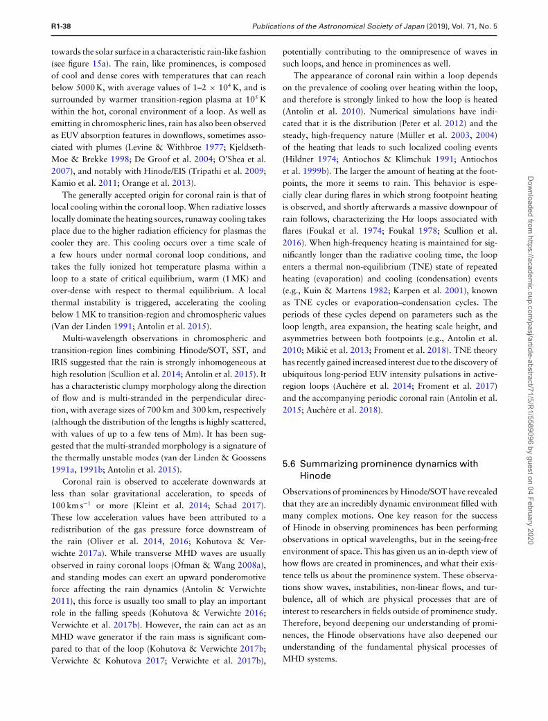
R1-38 Publications of the Astronomical Society of Japan (2019), Vol. 71, No. 5
towards the solar surface in a characteristic rain-like fashion(see figure 15a). The rain, like prominences, is composedof cool and dense cores with temperatures that can reachbelow 5000 K, with average values of 1–2 × 10⁴ K, and issurrounded by warmer transition-region plasma at 105 Kwithin the hot, coronal environment of a loop. As well asemitting in chromospheric lines, rain has also been observedas EUV absorption features in downflows, sometimes asso-ciated with plumes (Levine & Withbroe 1977; Kjeldseth-Moe & Brekke 1998; De Groof et al. 2004; O’Shea et al.2007), and notably with Hinode/EIS (Tripathi et al. 2009;Kamio et al. 2011; Orange et al. 2013).
The generally accepted origin for coronal rain is that oflocal cooling within the coronal loop. When radiative losseslocally dominate the heating sources, runaway cooling takesplace due to the higher radiation efficiency for plasmas thecooler they are. This cooling occurs over a time scale ofa few hours under normal coronal loop conditions, andtakes the fully ionized hot temperature plasma within aloop to a state of critical equilibrium, warm (1 MK) andover-dense with respect to thermal equilibrium. A localthermal instability is triggered, accelerating the coolingbelow 1 MK to transition-region and chromospheric values(Van der Linden 1991; Antolin et al. 2015).
Multi-wavelength observations in chromospheric andtransition-region lines combining Hinode/SOT, SST, andIRIS suggested that the rain is strongly inhomogeneous athigh resolution (Scullion et al. 2014; Antolin et al. 2015). Ithas a characteristic clumpy morphology along the directionof flow and is multi-stranded in the perpendicular direc-tion, with average sizes of 700 km and 300 km, respectively(although the distribution of the lengths is highly scattered,with values of up to a few tens of Mm). It has been sug-gested that the multi-stranded morphology is a signature ofthe thermally unstable modes (van der Linden & Goossens1991a, 1991b; Antolin et al. 2015).
Coronal rain is observed to accelerate downwards atless than solar gravitational acceleration, to speeds of100 km s−1 or more (Kleint et al. 2014; Schad 2017).These low acceleration values have been attributed to aredistribution of the gas pressure force downstream ofthe rain (Oliver et al. 2014, 2016; Kohutova & Ver-wichte 2017a). While transverse MHD waves are usuallyobserved in rainy coronal loops (Ofman & Wang 2008a),and standing modes can exert an upward ponderomotiveforce affecting the rain dynamics (Antolin & Verwichte2011), this force is usually too small to play an importantrole in the falling speeds (Kohutova & Verwichte 2016;Verwichte et al. 2017b). However, the rain can act as anMHD wave generator if the rain mass is significant com-pared to that of the loop (Kohutova & Verwichte 2017b;Verwichte & Kohutova 2017; Verwichte et al. 2017b),
potentially contributing to the omnipresence of waves insuch loops, and hence in prominences as well.
The appearance of coronal rain within a loop dependson the prevalence of cooling over heating within the loop,and therefore is strongly linked to how the loop is heated(Antolin et al. 2010). Numerical simulations have indi-cated that it is the distribution (Peter et al. 2012) and thesteady, high-frequency nature (Muller et al. 2003, 2004)of the heating that leads to such localized cooling events(Hildner 1974; Antiochos & Klimchuk 1991; Antiochoset al. 1999b). The larger the amount of heating at the foot-points, the more it seems to rain. This behavior is espe-cially clear during flares in which strong footpoint heatingis observed, and shortly afterwards a massive downpour ofrain follows, characterizing the Hα loops associated withflares (Foukal et al. 1974; Foukal 1978; Scullion et al.2016). When high-frequency heating is maintained for sig-nificantly longer than the radiative cooling time, the loopenters a thermal non-equilibrium (TNE) state of repeatedheating (evaporation) and cooling (condensation) events(e.g., Kuin & Martens 1982; Karpen et al. 2001), knownas TNE cycles or evaporation–condensation cycles. Theperiods of these cycles depend on parameters such as theloop length, area expansion, the heating scale height, andasymmetries between both footpoints (e.g., Antolin et al.2010; Mikic et al. 2013; Froment et al. 2018). TNE theoryhas recently gained increased interest due to the discovery ofubiquitous long-period EUV intensity pulsations in active-region loops (Auchere et al. 2014; Froment et al. 2017)and the accompanying periodic coronal rain (Antolin et al.2015; Auchere et al. 2018).
5.6 Summarizing prominence dynamics withHinode
Observations of prominences by Hinode/SOT have revealedthat they are an incredibly dynamic environment filled withmany complex motions. One key reason for the successof Hinode in observing prominences has been performingobservations in optical wavelengths, but in the seeing-freeenvironment of space. This has given us an in-depth view ofhow flows are created in prominences, and what their exis-tence tells us about the prominence system. These observa-tions show waves, instabilities, non-linear flows, and tur-bulence, all of which are physical processes that are ofinterest to researchers in fields outside of prominence study.Therefore, beyond deepening our understanding of promi-nences, the Hinode observations have also deepened ourunderstanding of the fundamental physical processes ofMHD systems.
Dow
nloaded from https://academ
ic.oup.com/pasj/article-abstract/71/5/R
1/5589096 by guest on 04 February 2020
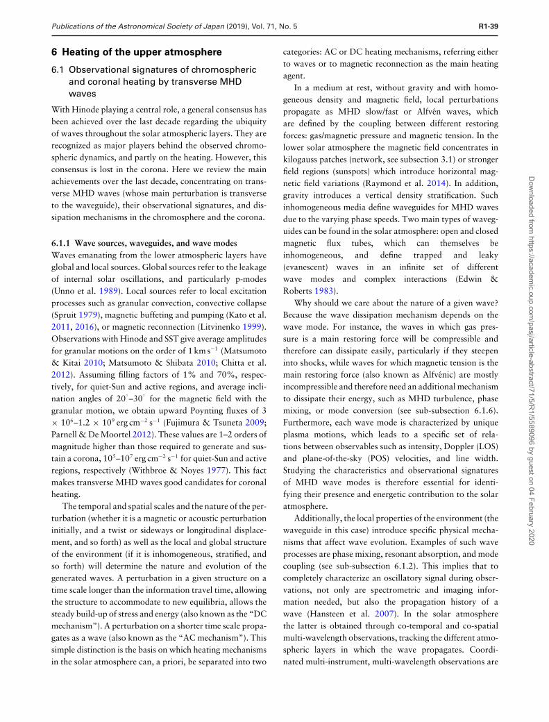
Publications of the Astronomical Society of Japan (2019), Vol. 71, No. 5 R1-39
6 Heating of the upper atmosphere
6.1 Observational signatures of chromosphericand coronal heating by transverse MHDwaves
With Hinode playing a central role, a general consensus hasbeen achieved over the last decade regarding the ubiquityof waves throughout the solar atmospheric layers. They arerecognized as major players behind the observed chromo-spheric dynamics, and partly on the heating. However, thisconsensus is lost in the corona. Here we review the mainachievements over the last decade, concentrating on trans-verse MHD waves (whose main perturbation is transverseto the waveguide), their observational signatures, and dis-sipation mechanisms in the chromosphere and the corona.
6.1.1 Wave sources, waveguides, and wave modesWaves emanating from the lower atmospheric layers haveglobal and local sources. Global sources refer to the leakageof internal solar oscillations, and particularly p-modes(Unno et al. 1989). Local sources refer to local excitationprocesses such as granular convection, convective collapse(Spruit 1979), magnetic buffeting and pumping (Kato et al.2011, 2016), or magnetic reconnection (Litvinenko 1999).Observations with Hinode and SST give average amplitudesfor granular motions on the order of 1 km s−1 (Matsumoto& Kitai 2010; Matsumoto & Shibata 2010; Chitta et al.2012). Assuming filling factors of 1% and 70%, respec-tively, for quiet-Sun and active regions, and average incli-nation angles of 20
◦–30
◦for the magnetic field with the
granular motion, we obtain upward Poynting fluxes of 3× 10⁶–1.2 × 10⁹ erg cm−2 s−1 (Fujimura & Tsuneta 2009;Parnell & De Moortel 2012). These values are 1–2 orders ofmagnitude higher than those required to generate and sus-tain a corona, 105–107 erg cm−2 s−1 for quiet-Sun and activeregions, respectively (Withbroe & Noyes 1977). This factmakes transverse MHD waves good candidates for coronalheating.
The temporal and spatial scales and the nature of the per-turbation (whether it is a magnetic or acoustic perturbationinitially, and a twist or sideways or longitudinal displace-ment, and so forth) as well as the local and global structureof the environment (if it is inhomogeneous, stratified, andso forth) will determine the nature and evolution of thegenerated waves. A perturbation in a given structure on atime scale longer than the information travel time, allowingthe structure to accommodate to new equilibria, allows thesteady build-up of stress and energy (also known as the “DCmechanism”). A perturbation on a shorter time scale propa-gates as a wave (also known as the “AC mechanism”). Thissimple distinction is the basis on which heating mechanismsin the solar atmosphere can, a priori, be separated into two
categories: AC or DC heating mechanisms, referring eitherto waves or to magnetic reconnection as the main heatingagent.
In a medium at rest, without gravity and with homo-geneous density and magnetic field, local perturbationspropagate as MHD slow/fast or Alfven waves, whichare defined by the coupling between different restoringforces: gas/magnetic pressure and magnetic tension. In thelower solar atmosphere the magnetic field concentrates inkilogauss patches (network, see subsection 3.1) or strongerfield regions (sunspots) which introduce horizontal mag-netic field variations (Raymond et al. 2014). In addition,gravity introduces a vertical density stratification. Suchinhomogeneous media define waveguides for MHD wavesdue to the varying phase speeds. Two main types of waveg-uides can be found in the solar atmosphere: open and closedmagnetic flux tubes, which can themselves beinhomogeneous, and define trapped and leaky(evanescent) waves in an infinite set of differentwave modes and complex interactions (Edwin &Roberts 1983).
Why should we care about the nature of a given wave?Because the wave dissipation mechanism depends on thewave mode. For instance, the waves in which gas pres-sure is a main restoring force will be compressible andtherefore can dissipate easily, particularly if they steepeninto shocks, while waves for which magnetic tension is themain restoring force (also known as Alfvenic) are mostlyincompressible and therefore need an additional mechanismto dissipate their energy, such as MHD turbulence, phasemixing, or mode conversion (see sub-subsection 6.1.6).Furthermore, each wave mode is characterized by uniqueplasma motions, which leads to a specific set of rela-tions between observables such as intensity, Doppler (LOS)and plane-of-the-sky (POS) velocities, and line width.Studying the characteristics and observational signaturesof MHD wave modes is therefore essential for identi-fying their presence and energetic contribution to the solaratmosphere.
Additionally, the local properties of the environment (thewaveguide in this case) introduce specific physical mecha-nisms that affect wave evolution. Examples of such waveprocesses are phase mixing, resonant absorption, and modecoupling (see sub-subsection 6.1.2). This implies that tocompletely characterize an oscillatory signal during obser-vations, not only are spectrometric and imaging infor-mation needed, but also the propagation history of awave (Hansteen et al. 2007). In the solar atmospherethe latter is obtained through co-temporal and co-spatialmulti-wavelength observations, tracking the different atmo-spheric layers in which the wave propagates. Coordi-nated multi-instrument, multi-wavelength observations are
Dow
nloaded from https://academ
ic.oup.com/pasj/article-abstract/71/5/R
1/5589096 by guest on 04 February 2020
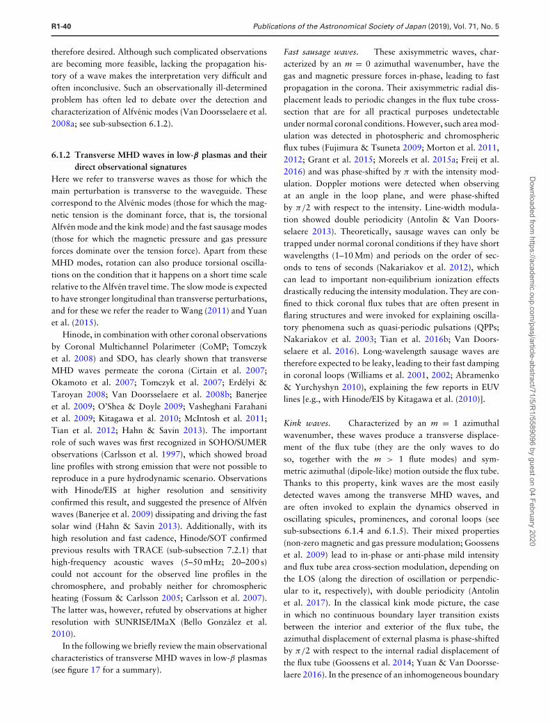
R1-40 Publications of the Astronomical Society of Japan (2019), Vol. 71, No. 5
therefore desired. Although such complicated observationsare becoming more feasible, lacking the propagation his-tory of a wave makes the interpretation very difficult andoften inconclusive. Such an observationally ill-determinedproblem has often led to debate over the detection andcharacterization of Alfvenic modes (Van Doorsselaere et al.2008a; see sub-subsection 6.1.2).
6.1.2 Transverse MHD waves in low-β plasmas and theirdirect observational signatures
Here we refer to transverse waves as those for which themain perturbation is transverse to the waveguide. Thesecorrespond to the Alvenic modes (those for which the mag-netic tension is the dominant force, that is, the torsionalAlfven mode and the kink mode) and the fast sausage modes(those for which the magnetic pressure and gas pressureforces dominate over the tension force). Apart from theseMHD modes, rotation can also produce torsional oscilla-tions on the condition that it happens on a short time scalerelative to the Alfven travel time. The slow mode is expectedto have stronger longitudinal than transverse perturbations,and for these we refer the reader to Wang (2011) and Yuanet al. (2015).
Hinode, in combination with other coronal observationsby Coronal Multichannel Polarimeter (CoMP; Tomczyket al. 2008) and SDO, has clearly shown that transverseMHD waves permeate the corona (Cirtain et al. 2007;Okamoto et al. 2007; Tomczyk et al. 2007; Erdelyi &Taroyan 2008; Van Doorsselaere et al. 2008b; Banerjeeet al. 2009; O’Shea & Doyle 2009; Vasheghani Farahaniet al. 2009; Kitagawa et al. 2010; McIntosh et al. 2011;Tian et al. 2012; Hahn & Savin 2013). The importantrole of such waves was first recognized in SOHO/SUMERobservations (Carlsson et al. 1997), which showed broadline profiles with strong emission that were not possible toreproduce in a pure hydrodynamic scenario. Observationswith Hinode/EIS at higher resolution and sensitivityconfirmed this result, and suggested the presence of Alfvenwaves (Banerjee et al. 2009) dissipating and driving the fastsolar wind (Hahn & Savin 2013). Additionally, with itshigh resolution and fast cadence, Hinode/SOT confirmedprevious results with TRACE (sub-subsection 7.2.1) thathigh-frequency acoustic waves (5–50 mHz; 20–200 s)could not account for the observed line profiles in thechromosphere, and probably neither for chromosphericheating (Fossum & Carlsson 2005; Carlsson et al. 2007).The latter was, however, refuted by observations at higherresolution with SUNRISE/IMaX (Bello Gonzalez et al.2010).
In the following we briefly review the main observationalcharacteristics of transverse MHD waves in low-β plasmas(see figure 17 for a summary).
Fast sausage waves. These axisymmetric waves, char-acterized by an m = 0 azimuthal wavenumber, have thegas and magnetic pressure forces in-phase, leading to fastpropagation in the corona. Their axisymmetric radial dis-placement leads to periodic changes in the flux tube cross-section that are for all practical purposes undetectableunder normal coronal conditions. However, such area mod-ulation was detected in photospheric and chromosphericflux tubes (Fujimura & Tsuneta 2009; Morton et al. 2011,2012; Grant et al. 2015; Moreels et al. 2015a; Freij et al.2016) and was phase-shifted by π with the intensity mod-ulation. Doppler motions were detected when observingat an angle in the loop plane, and were phase-shiftedby π/2 with respect to the intensity. Line-width modula-tion showed double periodicity (Antolin & Van Doors-selaere 2013). Theoretically, sausage waves can only betrapped under normal coronal conditions if they have shortwavelengths (1–10 Mm) and periods on the order of sec-onds to tens of seconds (Nakariakov et al. 2012), whichcan lead to important non-equilibrium ionization effectsdrastically reducing the intensity modulation. They are con-fined to thick coronal flux tubes that are often present inflaring structures and were invoked for explaining oscilla-tory phenomena such as quasi-periodic pulsations (QPPs;Nakariakov et al. 2003; Tian et al. 2016b; Van Doors-selaere et al. 2016). Long-wavelength sausage waves aretherefore expected to be leaky, leading to their fast dampingin coronal loops (Williams et al. 2001, 2002; Abramenko& Yurchyshyn 2010), explaining the few reports in EUVlines [e.g., with Hinode/EIS by Kitagawa et al. (2010)].
Kink waves. Characterized by an m = 1 azimuthalwavenumber, these waves produce a transverse displace-ment of the flux tube (they are the only waves to doso, together with the m > 1 flute modes) and sym-metric azimuthal (dipole-like) motion outside the flux tube.Thanks to this property, kink waves are the most easilydetected waves among the transverse MHD waves, andare often invoked to explain the dynamics observed inoscillating spicules, prominences, and coronal loops (seesub-subsections 6.1.4 and 6.1.5). Their mixed properties(non-zero magnetic and gas pressure modulation; Goossenset al. 2009) lead to in-phase or anti-phase mild intensityand flux tube area cross-section modulation, depending onthe LOS (along the direction of oscillation or perpendic-ular to it, respectively), with double periodicity (Antolinet al. 2017). In the classical kink mode picture, the casein which no continuous boundary layer transition existsbetween the interior and exterior of the flux tube, theazimuthal displacement of external plasma is phase-shiftedby π/2 with respect to the internal radial displacement ofthe flux tube (Goossens et al. 2014; Yuan & Van Doorsse-laere 2016). In the presence of an inhomogeneous boundary
Dow
nloaded from https://academ
ic.oup.com/pasj/article-abstract/71/5/R
1/5589096 by guest on 04 February 2020
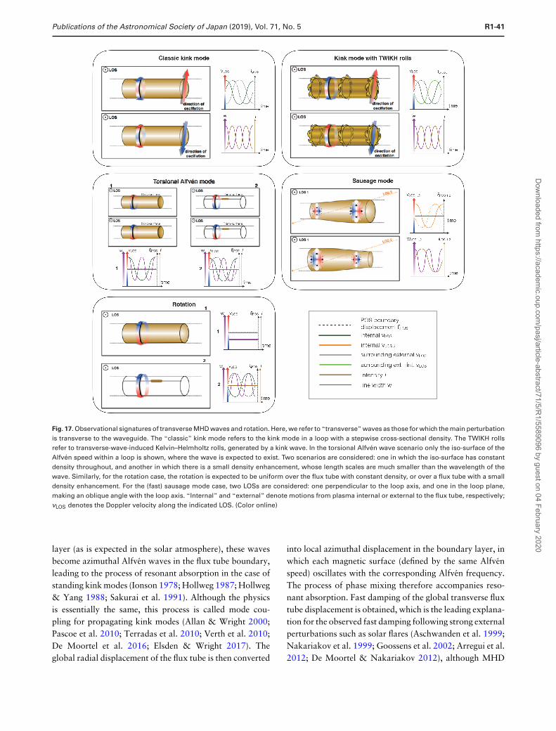
Publications of the Astronomical Society of Japan (2019), Vol. 71, No. 5 R1-41
Fig. 17. Observational signatures of transverse MHD waves and rotation. Here, we refer to “transverse” waves as those for which the main perturbationis transverse to the waveguide. The “classic” kink mode refers to the kink mode in a loop with a stepwise cross-sectional density. The TWIKH rollsrefer to transverse-wave-induced Kelvin–Helmholtz rolls, generated by a kink wave. In the torsional Alfven wave scenario only the iso-surface of theAlfven speed within a loop is shown, where the wave is expected to exist. Two scenarios are considered: one in which the iso-surface has constantdensity throughout, and another in which there is a small density enhancement, whose length scales are much smaller than the wavelength of thewave. Similarly, for the rotation case, the rotation is expected to be uniform over the flux tube with constant density, or over a flux tube with a smalldensity enhancement. For the (fast) sausage mode case, two LOSs are considered: one perpendicular to the loop axis, and one in the loop plane,making an oblique angle with the loop axis. “Internal” and “external” denote motions from plasma internal or external to the flux tube, respectively;vLOS denotes the Doppler velocity along the indicated LOS. (Color online)
layer (as is expected in the solar atmosphere), these wavesbecome azimuthal Alfven waves in the flux tube boundary,leading to the process of resonant absorption in the case ofstanding kink modes (Ionson 1978; Hollweg 1987; Hollweg& Yang 1988; Sakurai et al. 1991). Although the physicsis essentially the same, this process is called mode cou-pling for propagating kink modes (Allan & Wright 2000;Pascoe et al. 2010; Terradas et al. 2010; Verth et al. 2010;De Moortel et al. 2016; Elsden & Wright 2017). Theglobal radial displacement of the flux tube is then converted
into local azimuthal displacement in the boundary layer, inwhich each magnetic surface (defined by the same Alfvenspeed) oscillates with the corresponding Alfven frequency.The process of phase mixing therefore accompanies reso-nant absorption. Fast damping of the global transverse fluxtube displacement is obtained, which is the leading explana-tion for the observed fast damping following strong externalperturbations such as solar flares (Aschwanden et al. 1999;Nakariakov et al. 1999; Goossens et al. 2002; Arregui et al.2012; De Moortel & Nakariakov 2012), although MHD
Dow
nloaded from https://academ
ic.oup.com/pasj/article-abstract/71/5/R
1/5589096 by guest on 04 February 2020
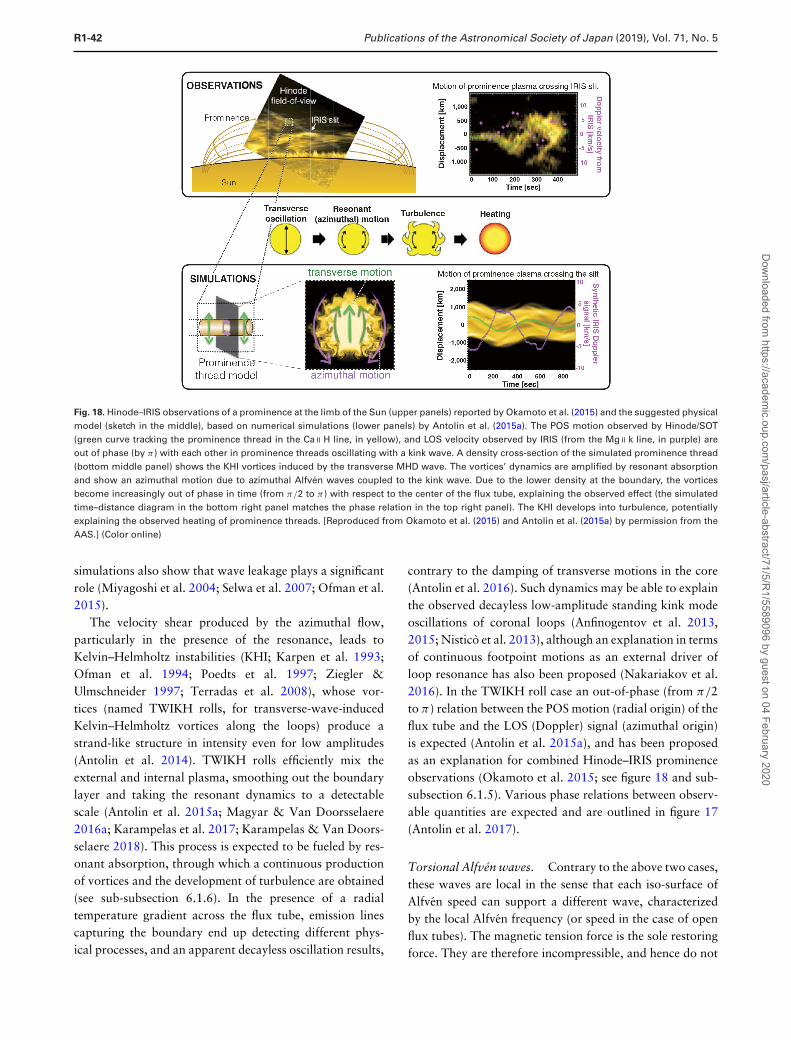
R1-42 Publications of the Astronomical Society of Japan (2019), Vol. 71, No. 5
Fig. 18. Hinode–IRIS observations of a prominence at the limb of the Sun (upper panels) reported by Okamoto et al. (2015) and the suggested physicalmodel (sketch in the middle), based on numerical simulations (lower panels) by Antolin et al. (2015a). The POS motion observed by Hinode/SOT(green curve tracking the prominence thread in the Ca II H line, in yellow), and LOS velocity observed by IRIS (from the Mg II k line, in purple) areout of phase (by π) with each other in prominence threads oscillating with a kink wave. A density cross-section of the simulated prominence thread(bottom middle panel) shows the KHI vortices induced by the transverse MHD wave. The vortices’ dynamics are amplified by resonant absorptionand show an azimuthal motion due to azimuthal Alfven waves coupled to the kink wave. Due to the lower density at the boundary, the vorticesbecome increasingly out of phase in time (from π/2 to π) with respect to the center of the flux tube, explaining the observed effect (the simulatedtime–distance diagram in the bottom right panel matches the phase relation in the top right panel). The KHI develops into turbulence, potentiallyexplaining the observed heating of prominence threads. [Reproduced from Okamoto et al. (2015) and Antolin et al. (2015a) by permission from theAAS.] (Color online)
simulations also show that wave leakage plays a significantrole (Miyagoshi et al. 2004; Selwa et al. 2007; Ofman et al.2015).
The velocity shear produced by the azimuthal flow,particularly in the presence of the resonance, leads toKelvin–Helmholtz instabilities (KHI; Karpen et al. 1993;Ofman et al. 1994; Poedts et al. 1997; Ziegler &Ulmschneider 1997; Terradas et al. 2008), whose vor-tices (named TWIKH rolls, for transverse-wave-inducedKelvin–Helmholtz vortices along the loops) produce astrand-like structure in intensity even for low amplitudes(Antolin et al. 2014). TWIKH rolls efficiently mix theexternal and internal plasma, smoothing out the boundarylayer and taking the resonant dynamics to a detectablescale (Antolin et al. 2015a; Magyar & Van Doorsselaere2016a; Karampelas et al. 2017; Karampelas & Van Doors-selaere 2018). This process is expected to be fueled by res-onant absorption, through which a continuous productionof vortices and the development of turbulence are obtained(see sub-subsection 6.1.6). In the presence of a radialtemperature gradient across the flux tube, emission linescapturing the boundary end up detecting different phys-ical processes, and an apparent decayless oscillation results,
contrary to the damping of transverse motions in the core(Antolin et al. 2016). Such dynamics may be able to explainthe observed decayless low-amplitude standing kink modeoscillations of coronal loops (Anfinogentov et al. 2013,2015; Nistico et al. 2013), although an explanation in termsof continuous footpoint motions as an external driver ofloop resonance has also been proposed (Nakariakov et al.2016). In the TWIKH roll case an out-of-phase (from π/2to π) relation between the POS motion (radial origin) of theflux tube and the LOS (Doppler) signal (azimuthal origin)is expected (Antolin et al. 2015a), and has been proposedas an explanation for combined Hinode–IRIS prominenceobservations (Okamoto et al. 2015; see figure 18 and sub-subsection 6.1.5). Various phase relations between observ-able quantities are expected and are outlined in figure 17(Antolin et al. 2017).
Torsional Alfven waves. Contrary to the above two cases,these waves are local in the sense that each iso-surface ofAlfven speed can support a different wave, characterizedby the local Alfven frequency (or speed in the case of openflux tubes). The magnetic tension force is the sole restoringforce. They are therefore incompressible, and hence do not
Dow
nloaded from https://academ
ic.oup.com/pasj/article-abstract/71/5/R
1/5589096 by guest on 04 February 2020
Publications of the Astronomical Society of Japan (2019), Vol. 71, No. 5 R1-43
lead to intensity modulations in the absence of other phys-ical mechanisms. Their axisymmetric motions (m = 0, asthe sausage mode) are purely azimuthal, leading to oppositeDoppler signatures from one edge to the radially oppositeedge for a given magnetic surface in a flux tube (Goossenset al. 2014). However, if the flux tube is strongly inhomo-geneous, contrary to the above cases, the local character ofthe torsional Alfven waves would quickly lead to negligibleDoppler motions for a given LOS, due to strong LOS inte-gration of different Doppler signals. On the other hand, thesame process leads to double periodicity in the line broad-ening, radially symmetric from one side of the flux tube tothe radially opposite side. Furthermore, the local characterof these waves makes them unable to transversely displacethe entire waveguide. However, if a density enhancementhas a spatial scale much smaller than the wavelength of theAlfven wave, the azimuthal motions of the surface couldlead to POS displacements of the small structure. The phaseshift between the LOS velocity and the POS motion thendepends on the amplitude of the transverse displacementproduced by the wave with respect to the loop radius. Ingeneral, we would expect this ratio to be small, leadingto a π/2 phase shift between the LOS velocity and thePOS motion. The localized azimuthal motions of torsionalAlfven waves are again expected to lead to dynamic instabil-ities such as Kelvin–Helmholtz (Browning & Priest 1984),which would further increase the LOS Doppler superposi-tion and the line width from the KHI turbulence.
The detection of Alfven waves in the closed configura-tion of coronal magnetic field lines (torsional or the clas-sical shear Alfven waves in inhomogeneous and homoge-neous media, respectively) has been a constant struggle inthe history of solar physics, largely due to their localizednature. The few observational reports of Alfven waves havebased their results on the periodic broadening of spectrallines, and the absence of co-spatial/co-temporal intensityperturbations (Hara & Ichimoto 1999; Jess et al. 2009;McIntosh et al. 2011; Mathioudakis et al. 2013; see sub-subsection 6.1.6). Unfortunately, to date, proper forwardmodeling of torsional Alfven waves from 3D MHD simula-tions is scarce. This would allow a better characterization oftheir observable features for comparison with observations.
6.1.3 MHD wave mechanisms in the lower solar atmo-sphere
Waves in photospheric flux tubes are the most straightfor-ward to observe and interpret. Since photons are producedin LTE conditions, intensity is determined by the Planckfunction, which is completely determined by the localtemperature. Based on Hinode/SOT observations, Fujimuraand Tsuneta (2009), Moreels and Van Doorsselaere (2013),and Moreels et al. (2015b) have managed to thoroughly
characterize the phase relations between observable quan-tities produced by MHD waves. We refer the reader to thesepapers and the review by Jess et al. (2015) for details.
Unless being generated in situ through processes such asmagnetic reconnection, any wave in the corona initially gen-erated in the photosphere must pass first through the chro-mosphere, a region that is characterized on one side by thechange from gas-pressure-dominated to magnetically dom-inated dynamics, making this region rich in wave processes,and on the other side by the complicated radiative transfereffects, which complicate the determination of cause andeffect from wave dynamics (and therefore also the interpre-tation of observational signatures).
Density stratification throughout the photosphere andlower chromosphere produces shock steepening in acousticand slow MHD waves, leading to the conversion of mostof their power into heat. The effect of these shocks isseen as one of the primary causes behind the dynamics oftype-I spicules (subsection 3.3 and sub-subsection 6.1.4).Parabolic paths and lower-than-gravity deceleration afterthe shock passage are some of their telltale signatures.The role of the magnetic field in slow-mode waves can beappreciated in inclined waveguides with respect to gravity.The effective gravity reduces the acoustic cut-off frequency,leading to the so-called ramp effect (Michalitsanos 1973;Bel & Leroy 1977; Suematsu 1990; De Pontieu et al. 2004)and the elongation of type-I spicules and other jet-like struc-ture such as fibrils and mottles (De Pontieu et al. 2007a;Heggland et al. 2007, 2009). Density steepening also pro-duces linear mode conversion due to the passage from high-β to low-β plasmas. The increase in phase speeds alongflux tubes produces effects such as wave reflection andrefraction, which are particularly important for fast modes(Rosenthal et al. 2002; Bogdan et al. 2003). The absence ofwave power around magnetic field concentrations such aspores or sunspots observed with Hinode/SOT (Nagashimaet al. 2007; Lawrence & Cadavid 2012), the so-called mag-netic shadows, finds a partial explanation in these waveprocesses (Judge et al. 2001; Nutto et al. 2012). The effectis now more generally known as “acoustic power suppres-sion” and involves other mechanisms such as emissivityreduction and local suppression (Chou et al. 2009).
The expected large magnetic field expansion in thelower atmosphere, together with density stratification andthe presence of density inhomogeneities along the field,introduces non-linear effects (involving, for example, theponderomotive force and the deformation of the waveshape) that can produce efficient mode conversion, par-ticularly from Alfven waves into longitudinal slow- andfast-mode waves. The longitudinal waves can then easilysteepen into shocks and drive dense jets of plasma upwards,thereby generating spicules (Hollweg et al. 1982; Kudoh &
Dow
nloaded from https://academ
ic.oup.com/pasj/article-abstract/71/5/R
1/5589096 by guest on 04 February 2020
R1-44 Publications of the Astronomical Society of Japan (2019), Vol. 71, No. 5
Shibata 1999; Matsumoto & Shibata 2010; Cranmer &Woolsey 2015; Brady & Arber 2016; Iijima & Yokoyama2017) and heating both the chromosphere and the corona(Moriyasu et al. 2004; Antolin et al. 2008; Antolin & Shi-bata 2010). Despite being investigated well theoretically,this process has yet to be directly observed, largely due tothe difficulty in detecting Alfven waves in the lower atmo-sphere (see sub-subsection 6.1.2). However, many multi-wavelength observational studies exist that strongly suggestthis process at work (Fujimura & Tsuneta 2009; Jess et al.2012; Kanoh et al. 2016), and particularly in the gener-ation of high-frequency transverse oscillations in spicules(He et al. 2009b; Kuridze et al. 2012; Shetye et al. 2016;Shoda & Yokoyama 2018b).
Around the reflection point of the fast modes, a secondlinear mode conversion is expected to occur due to thestrong change of the Alfven speed with height (Cally &Goossens 2008; Cally & Hansen 2011; Cally 2017). Thistime, fast modes can mode convert to Alfvenic modes(predominantly torsional Alfven and kink modes in thepresence of density structuring) in a process analogousto the resonant absorption/mode coupling mechanism indense flux tubes (see sub-subsection 6.1.2). This pro-cess can effectively occur throughout the chromosphereand leads to an inherited 5 min period in the Alfvenicwaves. This double mode conversion mechanism from p-modes to Alfvenic modes could provide an explanationfor recent observations of Alfvenic waves permeating thecorona with a 5 min peak in their power spectrum (Mortonet al. 2016).
Without the mode conversion mechanisms discussedabove, it has been argued that the energy from Alfvenwaves generated in the low solar atmosphere is not expectedto reach the corona. Particularly for high-frequency waves(with periods of 1–50 s), the Alfven waves are expected todissipate most of their energy in the partially ionized chro-mosphere through ion-neutral collisions (Osterbrock 1961;De Pontieu et al. 2001; Vranjes et al. 2008) and ambipolardiffusion (Arber et al. 2016; Shelyag et al. 2016). The latterseems to be particularly important in the upper chromo-sphere and in strong field regions (Khomenko & Collados2012; Martınez-Sykora et al. 2015; Soler et al. 2015) andhas recently been proposed as a key ingredient for gener-ating higher-energy spicules (see subsection 3.3 and sub-subsection 6.1.4).
6.1.4 Lessons from spicule observationsObservations primarily with Hinode/SOT and SST havesuggested the existence of two types of spicules, a sub-ject which is still under debate (see subsection 3.3). Type-IIspicules seem to differ from their type-I counterparts mainlyin their higher speeds, heating from chromospheric to at
least TR temperatures, their transverse motion (swayingand torsional), and a multi-stranded structure (Suematsuet al. 2008a; Skogsrud et al. 2014, 2015; Pereira et al.2016). These different characteristics suggest different phys-ical mechanisms at the source and during the evolution oftype-II spicules.
The multi-strand structure observed in spicules, both inintensity and Doppler imaging, raises an important ques-tion about the real nature of the spicule. Is it the collectivegroup of strands or each separate strand? The collectivebehavior in the dynamics, in both longitudinal and trans-verse motions, suggests the former, that is, the spicule as agroup of collectively moving strands. This transverse coher-ence in spicules allows the definition of spicules as “bushes,”the boundaries of which have not, however, been properlydefined in observations (Rutten 2012; Antolin et al. 2018b).This transverse coherence suggests waveguides of 103 kmor more in width (Skogsrud et al. 2014). Due to the localnature of torsional Alfven waves, as opposed to collectivemodes such as the kink mode (or the sausage mode), theobserved behavior suggests that the mechanisms respon-sible for their transverse dynamics are kink modes ratherthan torsional Alfven modes. However, for torsional Alfvenmodes, as mentioned in sub-subsection 6.1.2, the inhomo-geneity introduced by spicules should be much smaller thanthe wavelength of the torsional Alfven waves. Observationswith Hinode/SOT, however, suggest that this is not likely(Okamoto & De Pontieu 2011; Morton 2014). Nonethe-less, the torsional Alfven wave interpretation was recentlysupported by Srivastava et al. (2017), albeit a proper for-ward modeling was lacking, and a clear link betweenthe numerical modeling and the observations was notestablished.
The combination of the KHI and resonant absorptionthat accompanies the kink mode (TWIKH rolls) has beenshown to produce a strand-like structure, leading to col-lective behavior whose dynamics and intensity evolution inchromospheric lines seem to match that observed in type-IIspicules (Antolin et al. 2018b). However, this mechanismalone seems to fail in reproducing the intensity increasein higher-temperature lines characteristic of these jets. Thissuggests that other mechanisms, such as magnetic reconnec-tion in the lower atmosphere, probably play a major rolein the generation of spicules, and that their morphologymay be a by-product of kink modes and dynamic insta-bilities generated in the process (Kuridze et al. 2016). Anexample of such a process has been observed with Hinodeand reported by He et al. (2009a), in which magnetic recon-nection leads to a propagating kink mode along a spicule.Another example is that reported by Jess et al. (2012). Arecently proposed and compelling mechanism is ambipolardiffusion, through which the magnetic tension is amplified
Dow
nloaded from https://academ
ic.oup.com/pasj/article-abstract/71/5/R
1/5589096 by guest on 04 February 2020
Publications of the Astronomical Society of Japan (2019), Vol. 71, No. 5 R1-45
and generates Alfvenic waves and structures matching type-II spicules (Martınez-Sykora et al. 2017).
The strong transversely oscillating amplitudes, furthercombined with the high longitudinal speeds found in type-II spicules, suggest an important upward wave energyflux of 4–7× 10⁶ erg cm−2 s−1, sufficient for chromosphericand coronal heating (De Pontieu et al. 2007c, 2011;Srivastava et al. 2017; Martınez-Sykora et al. 2018). Sim-ilar amplitudes are also seen in other transversely oscillatingstructures in the chromosphere, such as fibrils and mot-tles (Kuridze et al. 2012; Morton et al. 2012), which havebeen interpreted as kink or fast sausage modes. In the caseof sausage modes, a 5% propagation of these compressivewaves into the corona would suffice for heating the ambientcorona. However, in the case of kink modes, such ampli-tudes are significantly reduced to 1–7× 10⁵ erg cm−2 s−1 dueto the small filling factor of the waves (assuming 5%–15%values; Van Doorsselaere et al. 2014).
6.1.5 Observations of coronal structures: Where does thewave energy go?
The amplitudes of transverse MHD waves in the coronaare often reported to be on the order of a few km s−1 undernormal non-flaring conditions (De Moortel & Nakari-akov 2012; Arregui 2015). Taking usual coronal values forthe Alfven speed and density, the observed energy fluxesare on the order of 1–10 × 104 erg cm−2 s−1. Compared tothe chromospheric observations (see sub-subsection 6.1.4),the amplitudes turn out to be at least an order of magni-tude smaller. Where does the rest of the energy go? Are wedetecting all the wave power? Do transverse MHD wavesplay any role in the heating of the solar corona?
Several factors have been proposed as possible explana-tions for the observed energy discrepancy. Besides actualdissipation, the extreme LOS superposition in the coronacombined with insufficient instrumental power, and waveprocesses that concentrate wave power in hard-to-detectspatial scales are all candidates at play that need to beconstrained. Among these wave processes, of particularimportance is resonant absorption (known as mode cou-pling in the case of propagating waves), which concentrateswave power in the small inhomogeneous layers of loopsin the form of azimuthal Alfven waves (whose motionsare undetectable with imaging instruments). It has beenshown that the combination of the LOS superposition andresonant absorption in kink modes leads to an underes-timation of the wave energy of 80%–90%, potentiallyexplaining the wave energy gap (De Moortel & Pascoe2012; Antolin et al. 2017). All these processes readilyexplain the absence of power in POS transverse displace-ments, and suggest that the best instruments for detectingthe true wave-energy budget in the solar corona arespectrometers.
Observations of wave power in prominences and rainyloops with Hinode/SOT, SST, and IRIS shed light on the roleof LOS superposition and insufficient instrumental power.Thanks to their cold and dense chromospheric conditions,prominences allow high-resolution observations into theMHD processes of high- to low-β plasmas. Being high in thecorona they also suffer from less LOS superposition (Schadet al. 2016). As such, transverse MHD waves in the coronahave been readily detected in these structures by registeringthe POS motion with high-resolution instruments such asHinode/SOT and also in Doppler velocities with SST/CRISP(Okamoto et al. 2007, 2015; Berger et al. 2008; Antolin &Verwichte 2011; Lin 2011; Arregui et al. 2012; Kohutova& Verwichte 2016; Verwichte et al. 2017b). In generalthe waves have lower energy flux, 1–10 × 104 erg cm−2 s−1
(a factor of 10–100), than at chromospheric heights, albeita large variation with maximum observed values on theorder of 1 × 10⁶ erg cm−2 s−1. This suggests that if thewaves originate in the lower atmosphere, either an energycascade to smaller length scales occurs and the waves even-tually dissipate and/or a larger role is played in “hiding”the wave energy by wave processes such as mode cou-pling and resonant absorption. As is seen in coronal-line observations, characteristic signatures include strongdamping following external perturbations such as flares(Ofman & Wang 2008b), but also small-amplitude decay-less (Ning et al. 2009) and even amplified oscillations(Antolin & Verwichte 2011; Verwichte et al. 2017b).At these higher resolutions the structure appears multi-stranded and, as in spicules, a strong collective transversemotion is also observed. It is also possible that transverseMHD waves are generated in situ through colliding flows,a scenario that has recently been observed by Hinode/SOTand IRIS, supported by numerical simulations (Antolinet al. 2018a).
Coordinated observations with IRIS and Hinode/SOTby Okamoto et al. (2015) have paved the way for howwe could actually detect wave heating in action in thecorona. In this case the fine dynamics of a prominence wasobserved in imaging and spectroscopy, allowing the recon-struction of the 3D wave motion and possible dissipation.Strong transverse coherence in transverse MHD oscilla-tions, not only in the POS displacement but also in the LOSvelocity (figure 18) were observed, together with promi-nence threads fading in chromospheric lines and appearingin TR lines, suggestive of wave dissipation and heating. Inparticular, out-of-phase (from π/2 to π) behavior betweenthe POS motion observed with Hinode/SOT and the LOSvelocity detected with IRIS was also reported. All these fea-tures were successfully explained with a 3D MHD model ofTWIKH rolls, in which the resonant absorption mechanismcombines with the KHI and leads to turbulence (Antolinet al. 2015a). It is, however, still unclear how much and
Dow
nloaded from https://academ
ic.oup.com/pasj/article-abstract/71/5/R
1/5589096 by guest on 04 February 2020
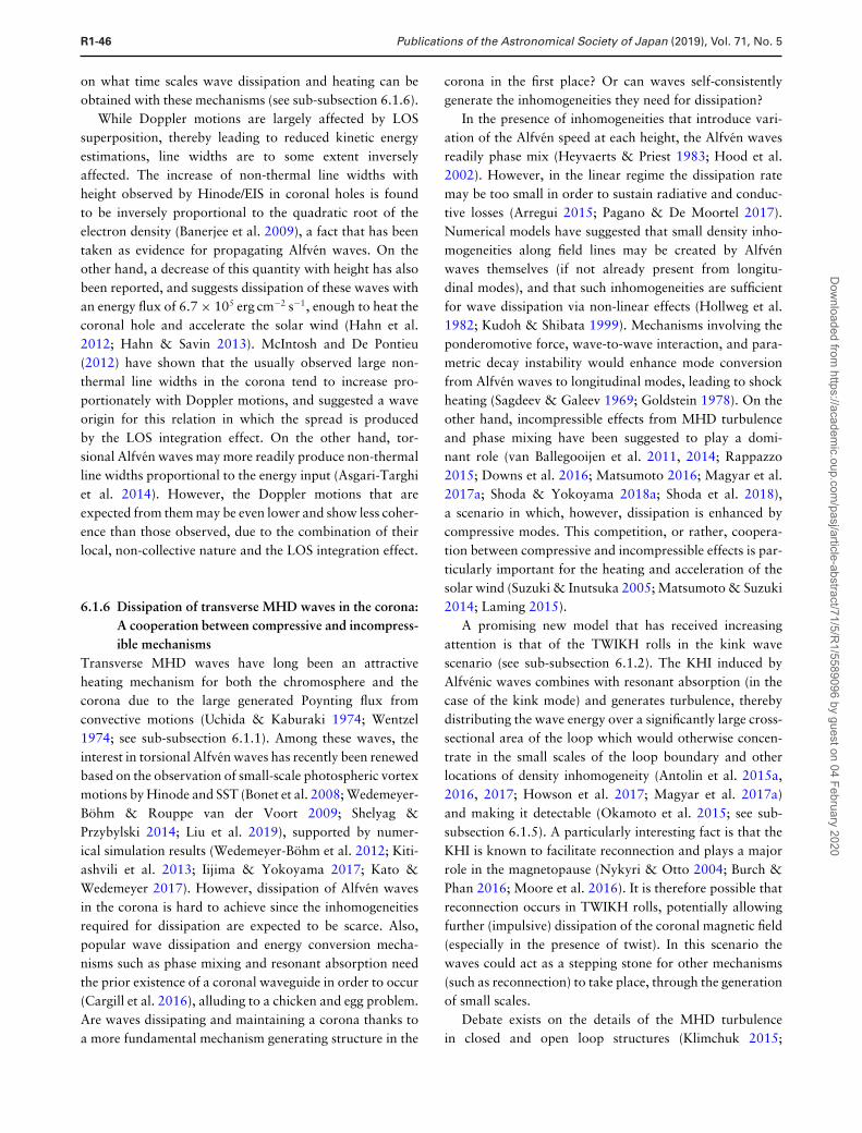
R1-46 Publications of the Astronomical Society of Japan (2019), Vol. 71, No. 5
on what time scales wave dissipation and heating can beobtained with these mechanisms (see sub-subsection 6.1.6).
While Doppler motions are largely affected by LOSsuperposition, thereby leading to reduced kinetic energyestimations, line widths are to some extent inverselyaffected. The increase of non-thermal line widths withheight observed by Hinode/EIS in coronal holes is foundto be inversely proportional to the quadratic root of theelectron density (Banerjee et al. 2009), a fact that has beentaken as evidence for propagating Alfven waves. On theother hand, a decrease of this quantity with height has alsobeen reported, and suggests dissipation of these waves withan energy flux of 6.7 × 10⁵ erg cm−2 s−1, enough to heat thecoronal hole and accelerate the solar wind (Hahn et al.2012; Hahn & Savin 2013). McIntosh and De Pontieu(2012) have shown that the usually observed large non-thermal line widths in the corona tend to increase pro-portionately with Doppler motions, and suggested a waveorigin for this relation in which the spread is producedby the LOS integration effect. On the other hand, tor-sional Alfven waves may more readily produce non-thermalline widths proportional to the energy input (Asgari-Targhiet al. 2014). However, the Doppler motions that areexpected from them may be even lower and show less coher-ence than those observed, due to the combination of theirlocal, non-collective nature and the LOS integration effect.
6.1.6 Dissipation of transverse MHD waves in the corona:A cooperation between compressive and incompress-ible mechanisms
Transverse MHD waves have long been an attractiveheating mechanism for both the chromosphere and thecorona due to the large generated Poynting flux fromconvective motions (Uchida & Kaburaki 1974; Wentzel1974; see sub-subsection 6.1.1). Among these waves, theinterest in torsional Alfven waves has recently been renewedbased on the observation of small-scale photospheric vortexmotions by Hinode and SST (Bonet et al. 2008; Wedemeyer-Bohm & Rouppe van der Voort 2009; Shelyag &Przybylski 2014; Liu et al. 2019), supported by numer-ical simulation results (Wedemeyer-Bohm et al. 2012; Kiti-ashvili et al. 2013; Iijima & Yokoyama 2017; Kato &Wedemeyer 2017). However, dissipation of Alfven wavesin the corona is hard to achieve since the inhomogeneitiesrequired for dissipation are expected to be scarce. Also,popular wave dissipation and energy conversion mecha-nisms such as phase mixing and resonant absorption needthe prior existence of a coronal waveguide in order to occur(Cargill et al. 2016), alluding to a chicken and egg problem.Are waves dissipating and maintaining a corona thanks toa more fundamental mechanism generating structure in the
corona in the first place? Or can waves self-consistentlygenerate the inhomogeneities they need for dissipation?
In the presence of inhomogeneities that introduce vari-ation of the Alfven speed at each height, the Alfven wavesreadily phase mix (Heyvaerts & Priest 1983; Hood et al.2002). However, in the linear regime the dissipation ratemay be too small in order to sustain radiative and conduc-tive losses (Arregui 2015; Pagano & De Moortel 2017).Numerical models have suggested that small density inho-mogeneities along field lines may be created by Alfvenwaves themselves (if not already present from longitu-dinal modes), and that such inhomogeneities are sufficientfor wave dissipation via non-linear effects (Hollweg et al.1982; Kudoh & Shibata 1999). Mechanisms involving theponderomotive force, wave-to-wave interaction, and para-metric decay instability would enhance mode conversionfrom Alfven waves to longitudinal modes, leading to shockheating (Sagdeev & Galeev 1969; Goldstein 1978). On theother hand, incompressible effects from MHD turbulenceand phase mixing have been suggested to play a domi-nant role (van Ballegooijen et al. 2011, 2014; Rappazzo2015; Downs et al. 2016; Matsumoto 2016; Magyar et al.2017a; Shoda & Yokoyama 2018a; Shoda et al. 2018),a scenario in which, however, dissipation is enhanced bycompressive modes. This competition, or rather, coopera-tion between compressive and incompressible effects is par-ticularly important for the heating and acceleration of thesolar wind (Suzuki & Inutsuka 2005; Matsumoto & Suzuki2014; Laming 2015).
A promising new model that has received increasingattention is that of the TWIKH rolls in the kink wavescenario (see sub-subsection 6.1.2). The KHI induced byAlfvenic waves combines with resonant absorption (in thecase of the kink mode) and generates turbulence, therebydistributing the wave energy over a significantly large cross-sectional area of the loop which would otherwise concen-trate in the small scales of the loop boundary and otherlocations of density inhomogeneity (Antolin et al. 2015a,2016, 2017; Howson et al. 2017; Magyar et al. 2017a)and making it detectable (Okamoto et al. 2015; see sub-subsection 6.1.5). A particularly interesting fact is that theKHI is known to facilitate reconnection and plays a majorrole in the magnetopause (Nykyri & Otto 2004; Burch &Phan 2016; Moore et al. 2016). It is therefore possible thatreconnection occurs in TWIKH rolls, potentially allowingfurther (impulsive) dissipation of the coronal magnetic field(especially in the presence of twist). In this scenario thewaves could act as a stepping stone for other mechanisms(such as reconnection) to take place, through the generationof small scales.
Debate exists on the details of the MHD turbulencein closed and open loop structures (Klimchuk 2015;
Dow
nloaded from https://academ
ic.oup.com/pasj/article-abstract/71/5/R
1/5589096 by guest on 04 February 2020
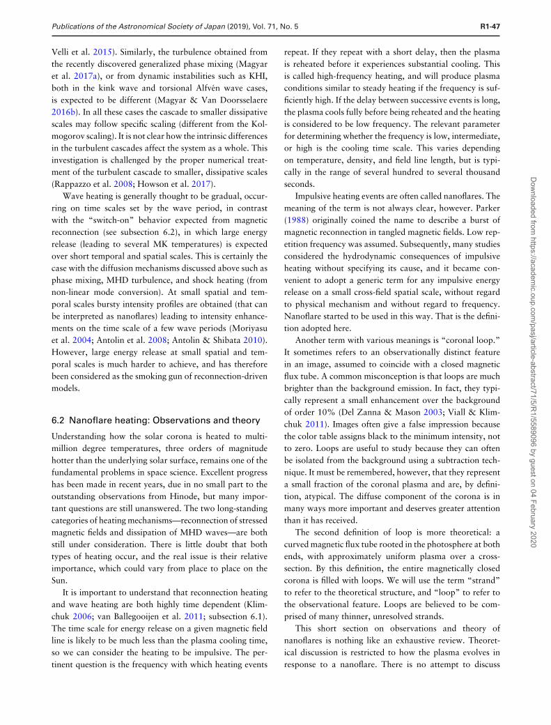
Publications of the Astronomical Society of Japan (2019), Vol. 71, No. 5 R1-47
Velli et al. 2015). Similarly, the turbulence obtained fromthe recently discovered generalized phase mixing (Magyaret al. 2017a), or from dynamic instabilities such as KHI,both in the kink wave and torsional Alfven wave cases,is expected to be different (Magyar & Van Doorsselaere2016b). In all these cases the cascade to smaller dissipativescales may follow specific scaling (different from the Kol-mogorov scaling). It is not clear how the intrinsic differencesin the turbulent cascades affect the system as a whole. Thisinvestigation is challenged by the proper numerical treat-ment of the turbulent cascade to smaller, dissipative scales(Rappazzo et al. 2008; Howson et al. 2017).
Wave heating is generally thought to be gradual, occur-ring on time scales set by the wave period, in contrastwith the “switch-on” behavior expected from magneticreconnection (see subsection 6.2), in which large energyrelease (leading to several MK temperatures) is expectedover short temporal and spatial scales. This is certainly thecase with the diffusion mechanisms discussed above such asphase mixing, MHD turbulence, and shock heating (fromnon-linear mode conversion). At small spatial and tem-poral scales bursty intensity profiles are obtained (that canbe interpreted as nanoflares) leading to intensity enhance-ments on the time scale of a few wave periods (Moriyasuet al. 2004; Antolin et al. 2008; Antolin & Shibata 2010).However, large energy release at small spatial and tem-poral scales is much harder to achieve, and has thereforebeen considered as the smoking gun of reconnection-drivenmodels.
6.2 Nanoflare heating: Observations and theory
Understanding how the solar corona is heated to multi-million degree temperatures, three orders of magnitudehotter than the underlying solar surface, remains one of thefundamental problems in space science. Excellent progresshas been made in recent years, due in no small part to theoutstanding observations from Hinode, but many impor-tant questions are still unanswered. The two long-standingcategories of heating mechanisms—reconnection of stressedmagnetic fields and dissipation of MHD waves—are bothstill under consideration. There is little doubt that bothtypes of heating occur, and the real issue is their relativeimportance, which could vary from place to place on theSun.
It is important to understand that reconnection heatingand wave heating are both highly time dependent (Klim-chuk 2006; van Ballegooijen et al. 2011; subsection 6.1).The time scale for energy release on a given magnetic fieldline is likely to be much less than the plasma cooling time,so we can consider the heating to be impulsive. The per-tinent question is the frequency with which heating events
repeat. If they repeat with a short delay, then the plasmais reheated before it experiences substantial cooling. Thisis called high-frequency heating, and will produce plasmaconditions similar to steady heating if the frequency is suf-ficiently high. If the delay between successive events is long,the plasma cools fully before being reheated and the heatingis considered to be low frequency. The relevant parameterfor determining whether the frequency is low, intermediate,or high is the cooling time scale. This varies dependingon temperature, density, and field line length, but is typi-cally in the range of several hundred to several thousandseconds.
Impulsive heating events are often called nanoflares. Themeaning of the term is not always clear, however. Parker(1988) originally coined the name to describe a burst ofmagnetic reconnection in tangled magnetic fields. Low rep-etition frequency was assumed. Subsequently, many studiesconsidered the hydrodynamic consequences of impulsiveheating without specifying its cause, and it became con-venient to adopt a generic term for any impulsive energyrelease on a small cross-field spatial scale, without regardto physical mechanism and without regard to frequency.Nanoflare started to be used in this way. That is the defini-tion adopted here.
Another term with various meanings is “coronal loop.”It sometimes refers to an observationally distinct featurein an image, assumed to coincide with a closed magneticflux tube. A common misconception is that loops are muchbrighter than the background emission. In fact, they typi-cally represent a small enhancement over the backgroundof order 10% (Del Zanna & Mason 2003; Viall & Klim-chuk 2011). Images often give a false impression becausethe color table assigns black to the minimum intensity, notto zero. Loops are useful to study because they can oftenbe isolated from the background using a subtraction tech-nique. It must be remembered, however, that they representa small fraction of the coronal plasma and are, by defini-tion, atypical. The diffuse component of the corona is inmany ways more important and deserves greater attentionthan it has received.
The second definition of loop is more theoretical: acurved magnetic flux tube rooted in the photosphere at bothends, with approximately uniform plasma over a cross-section. By this definition, the entire magnetically closedcorona is filled with loops. We will use the term “strand”to refer to the theoretical structure, and “loop” to refer tothe observational feature. Loops are believed to be com-prised of many thinner, unresolved strands.
This short section on observations and theory ofnanoflares is nothing like an exhaustive review. Theoret-ical discussion is restricted to how the plasma evolves inresponse to a nanoflare. There is no attempt to discuss
Dow
nloaded from https://academ
ic.oup.com/pasj/article-abstract/71/5/R
1/5589096 by guest on 04 February 2020
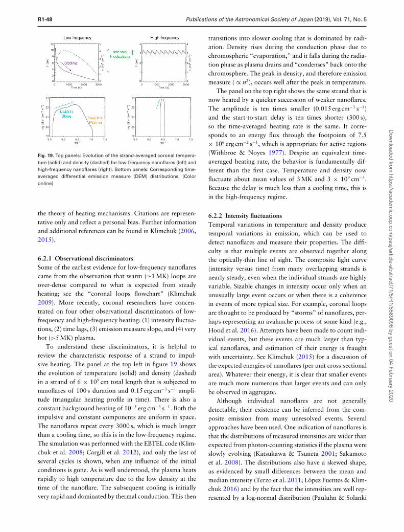
R1-48 Publications of the Astronomical Society of Japan (2019), Vol. 71, No. 5
Fig. 19. Top panels: Evolution of the strand-averaged coronal tempera-ture (solid) and density (dashed) for low-frequency nanoflares (left) andhigh-frequency nanoflares (right). Bottom panels: Corresponding time-averaged differential emission measure (DEM) distributions. (Coloronline)
the theory of heating mechanisms. Citations are represen-tative only and reflect a personal bias. Further informationand additional references can be found in Klimchuk (2006,2015).
6.2.1 Observational discriminatorsSome of the earliest evidence for low-frequency nanoflarescame from the observation that warm (∼1 MK) loops areover-dense compared to what is expected from steadyheating; see the “coronal loops flowchart” (Klimchuk2009). More recently, coronal researchers have concen-trated on four other observational discriminators of low-frequency and high-frequency heating: (1) intensity fluctua-tions, (2) time lags, (3) emission measure slope, and (4) veryhot (>5 MK) plasma.
To understand these discriminators, it is helpful toreview the characteristic response of a strand to impul-sive heating. The panel at the top left in figure 19 showsthe evolution of temperature (solid) and density (dashed)in a strand of 6 × 109 cm total length that is subjected tonanoflares of 100 s duration and 0.15 erg cm−3 s−1 ampli-tude (triangular heating profile in time). There is also aconstant background heating of 10−5 erg cm−3 s−1. Both theimpulsive and constant components are uniform in space.The nanoflares repeat every 3000 s, which is much longerthan a cooling time, so this is in the low-frequency regime.The simulation was performed with the EBTEL code (Klim-chuk et al. 2008; Cargill et al. 2012), and only the last ofseveral cycles is shown, when any influence of the initialconditions is gone. As is well understood, the plasma heatsrapidly to high temperature due to the low density at thetime of the nanoflare. The subsequent cooling is initiallyvery rapid and dominated by thermal conduction. This then
transitions into slower cooling that is dominated by radi-ation. Density rises during the conduction phase due tochromospheric “evaporation,” and it falls during the radia-tion phase as plasma drains and “condenses” back onto thechromosphere. The peak in density, and therefore emissionmeasure ( ∝ n2), occurs well after the peak in temperature.
The panel on the top right shows the same strand that isnow heated by a quicker succession of weaker nanoflares.The amplitude is ten times smaller (0.015 erg cm−3 s−1)and the start-to-start delay is ten times shorter (300 s),so the time-averaged heating rate is the same. It corre-sponds to an energy flux through the footpoints of 7.5× 10⁶ erg cm−2 s−1, which is appropriate for active regions(Withbroe & Noyes 1977). Despite an equivalent time-averaged heating rate, the behavior is fundamentally dif-ferent than the first case. Temperature and density nowfluctuate about mean values of 3 MK and 3 × 109 cm−3.Because the delay is much less than a cooling time, this isin the high-frequency regime.
6.2.2 Intensity fluctuationsTemporal variations in temperature and density producetemporal variations in emission, which can be used todetect nanoflares and measure their properties. The diffi-culty is that multiple events are observed together alongthe optically-thin line of sight. The composite light curve(intensity versus time) from many overlapping strands isnearly steady, even when the individual strands are highlyvariable. Sizable changes in intensity occur only when anunusually large event occurs or when there is a coherencein events of more typical size. For example, coronal loopsare thought to be produced by “storms” of nanoflares, per-haps representing an avalanche process of some kind (e.g.,Hood et al. 2016). Attempts have been made to count indi-vidual events, but these events are much larger than typ-ical nanoflares, and estimation of their energy is fraughtwith uncertainty. See Klimchuk (2015) for a discussion ofthe expected energies of nanoflares (per unit cross-sectionalarea). Whatever their energy, it is clear that smaller eventsare much more numerous than larger events and can onlybe observed in aggregate.
Although individual nanoflares are not generallydetectable, their existence can be inferred from the com-posite emission from many unresolved events. Severalapproaches have been used. One indication of nanoflares isthat the distributions of measured intensities are wider thanexpected from photon-counting statistics if the plasma wereslowly evolving (Katsukawa & Tsuneta 2001; Sakamotoet al. 2008). The distributions also have a skewed shape,as evidenced by small differences between the mean andmedian intensity (Terzo et al. 2011; Lopez Fuentes & Klim-chuk 2016) and by the fact that the intensities are well rep-resented by a log-normal distribution (Pauluhn & Solanki
Dow
nloaded from https://academ
ic.oup.com/pasj/article-abstract/71/5/R
1/5589096 by guest on 04 February 2020
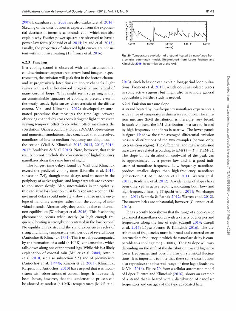
Publications of the Astronomical Society of Japan (2019), Vol. 71, No. 5 R1-49
2007; Bazarghan et al. 2008; see also Cadavid et al. 2016).Skewing of the distributions is expected from the exponen-tial decrease in intensity as strands cool, which can alsoexplain why Fourier power spectra are observed to have apower-law form (Cadavid et al. 2014; Ireland et al. 2015).Finally, the properties of observed light curves are consis-tent with impulsive heating (Tajfirouze et al. 2016).
6.2.3 Time lagsIf a cooling strand is observed with an instrument thatcan discriminate temperature (narrow-band imager or spec-trometer), the emission will peak first in the hottest channeland at progressively later times in cooler channels. Lightcurves with a clear hot-to-cool progression are typical ofmany coronal loops. What might seem surprising is thatan unmistakable signature of cooling is present even inthe nearly steady light curves characteristic of the diffusecorona. Viall and Klimchuk (2012) developed an auto-mated procedure that measures the time lags betweenobserving channels by cross correlating the light curves withvarying temporal offset to see which offset maximizes thecorrelation. Using a combination of SDO/AIA observationsand numerical simulations, they concluded that unresolvednanoflares of low to medium frequency are ubiquitous inthe corona (Viall & Klimchuk 2012, 2013, 2015, 2016,2017; Bradshaw & Viall 2016). Note, however, that theirresults do not preclude the co-existence of high-frequencynanoflares along the same lines of sight.
The longest time delays found by Viall and Klimchukexceed the predicted cooling times (Lionello et al. 2016;subsection 7.4), though these delays tend to occur in theperiphery of active regions, and longer strands are expectedto cool more slowly. Also, uncertainties in the optically-thin radiative loss function must be taken into account. Themeasured delays could indicate a slow change in the enve-lope of nanoflare energies rather than the cooling of indi-vidual strands. Alternatively, they could be due to thermalnon-equilibrium (Winebarger et al. 2016). This fascinatingphenomenon occurs when steady (or high enough fre-quency) heating is strongly concentrated in the low corona.No equilibrium exists, and the stand experiences cycles ofrising and falling temperature with periods of several hours(Antiochos & Klimchuk 1991). This is usually accompaniedby the formation of a cold (∼104 K) condensation, whichfalls down along one of the strand legs. While this is a likelyexplanation of coronal rain (Muller et al. 2004; Antolinet al. 2010; see also subsection 5.5) and of prominences(Antiochos et al. 1999b; Karpen et al. 2003), Klimchuk,Karpen, and Antiochos (2010) have argued that it is incon-sistent with observations of coronal loops. It has recentlybeen shown, however, that the condensation process canbe aborted at modest (∼1 MK) temperatures (Mikic et al.
Fig. 20. Temperature evolution of a strand heated by nanoflares froma cellular automaton model. [Reproduced from Lopez Fuentes andKlimchuk (2016) by permission of the AAS.]
2013). Such behavior can explain long-period loop pulsa-tions (Froment et al. 2015), which occur in isolated placesin some active regions, but might also have more generalapplicability. Further study is needed.
6.2.4 Emission measure slopeA strand heated by low-frequency nanoflares experiences awide range of temperatures during its evolution. The emis-sion measure (EM) distribution is therefore very broad.In stark contrast, the EM distribution of a strand heatedby high-frequency nanoflares is narrow. The lower panelsin figure 19 show the time-averaged differential emissionmeasure distributions of the two examples (corona only;no transition region). The differential and regular emissionmeasures are related according to EM(T) = T × DEM(T).The slope of the distribution coolward of the peak canbe approximated by a power law and is a good indi-cator of nanoflare frequency. Low-frequency nanoflaresproduce smaller slopes than high-frequency nanoflares(subsection 7.4; Mulu-Moore et al. 2011; Warren et al.2011a; Bradshaw et al. 2012). A wide range of slopes havebeen observed in active regions, indicating both low- andhigh-frequency heating (Tripathi et al. 2011; Winebargeret al. 2011; Schmelz & Pathak 2012; Warren et al. 2012).The uncertainties are substantial, however (Guennou et al.2013).
It has recently been shown that the range of slopes can beexplained if nanoflares occur with a variety of energies andfrequencies along the line of sight (Cargill 2014; Cargillet al. 2015; Lopez Fuentes & Klimchuk 2016). The dis-tribution of frequencies must be broad and centered on anintermediate frequency in which the nanoflare delay is com-parable to a cooling time (∼1000 s). The EM slope will varydepending on the shift of the distribution toward higher orlower frequencies and possibly also on statistical fluctua-tions. It is important to note that these same distributionsalso reproduce the observed range of time lags (Bradshaw& Viall 2016). Figure 20, from a cellular automaton modelof Lopez Fuentes and Klimchuk (2016), shows an exampleof a strand that is heated with a distribution of nanoflarefrequencies and energies of the type advocated here.
Dow
nloaded from https://academ
ic.oup.com/pasj/article-abstract/71/5/R
1/5589096 by guest on 04 February 2020
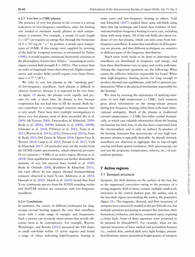
R1-50 Publications of the Astronomical Society of Japan (2019), Vol. 71, No. 5
6.2.5 Very hot (>5 MK) plasmaThe presence of very hot plasma in the corona is a strongindication of low-frequency nanoflares, since the heatingrate needed to maintain steady plasma at such temper-atures is extreme. For example, a strand of total lengthL = 1010 cm requires an energy flux through the footpointsof 4 × 10⁸ erg cm−2 s−1 to produce a steady apex temper-ature of 10 MK. If this energy were supplied by stressingof the field by footpoint motions, as envisioned by Parker(1988), it would require continuous horizontal velocities inthe photosphere of more than 10 km s−1 (assuming an activeregion coronal field strength B = 100 G). This is more thanan order of magnitude faster than observed. Higher temper-atures and weaker fields would require even faster flows,since v ∝ T7/2/(B2L).
We refer to very hot plasma as the “smoking gun”of low-frequency nanoflares. Such plasma is difficult toobserve, however, because it is expected to be very faint.As figure 19 shows, the plasma cools rapidly and per-sists for only a short time. Its density is low becauseevaporation has not had time to fill the strand. Both fac-tors contribute to a time-averaged emission measure thatis very small. There have been multiple investigations todetect very hot plasma, most of them successful (Ko et al.2009; McTiernan 2009; Patsourakos & Klimchuk 2009;Reale et al. 2009a, 2009b; Schmelz et al. 2009a, 2009b;Sylwester et al. 2010; O’Dwyer et al. 2011; Testa et al.2011; Warren et al. 2011a, 2012; Teriaca et al. 2012a; Testa& Reale 2012; Del Zanna & Mason 2014; Ugarte-Urra &Warren 2014; Caspi et al. 2015; Parenti et al. 2017; Viall& Klimchuk 2017). Of particular note are the results fromthe EUNIS rocket spectrometer, which observed pervasiveFe XIX emission (∼9 MK) in an active region (Brosius et al.2014). Non-equilibrium ionization can further diminish theintensity of very hot spectral lines (Golub et al. 1989;Reale & Orlando 2008; Bradshaw & Klimchuk 2011),but such effects do not impact thermal bremsstrahlungemission observed in hard X-rays (Ishikawa et al. 2014;Hannah et al. 2016). Marsh et al. (2018) found that hardX-ray continuum spectra from the FOXSI sounding rocketand NuSTAR mission are consistent with low-frequencynanoflares.
6.2.6 ConclusionsIn summary, the variety of different techniques for diag-nosing coronal heating support the view that nanoflaresoccur with a wide range of energies and frequencies.Such a picture can reconcile observations that would oth-erwise seem to be contradictory. For example, Warren,Winebarger, and Brooks (2012) measured the EM slopesin small sub-fields within 15 active regions and founda range of values indicating high-frequency heating in
some cases and low-frequency heating in others. Vialland Klimchuk (2017) studied these same sub-fields usingtheir time lag technique and found clear evidence of low-and intermediate-frequency heating in every case, includingthose with steep slopes. All of the sub-fields also show evi-dence of very hot plasma, which can only come from low-frequency nanoflares. It seems that nanoflares of all frequen-cies are present, and that different techniques are sensitiveto different parts of the frequency distribution.
Much more work needs to be done to determine hownanoflares are distributed in frequency and energy, andhow these distributions vary in space and evolve with time.Among the important questions are the following: Whatcauses the collective behavior responsible for loops? Whendoes high-frequency heating persist for long enough toproduce thermal non-equilibrium, with full or aborted con-densations? What is the physical mechanism responsible forthe heating?
We close by stressing the importance of studying emis-sions of very high temperature (>5 MK). Such emissiongives direct information on the energy-release processduring low-frequency heating, when there is the least obser-vational ambiguity. Much of the plasma at traditionalcoronal temperatures (∼2 MK) has either cooled dramati-cally, in which case valuable information about the heatingmechanism has been lost, or else has been evaporated fromthe chromosphere and is only an indirect by-product ofthe heating. Emission line spectroscopy of very high tem-perature plasma is especially desirable. As already stressed,nanoflares are observed in aggregate due to line-of-sightoverlap and finite spatial resolution. Only spectroscopy cansort out the properties (temperature, velocity, etc.) of non-uniform plasmas.
7 Active regions
7.1 Sunspot structure
Sunspots, the dark features on the surface of the Sun dueto the suppressed convection owing to the presence of astrong magnetic field in them, contain multiple small-scalestructures in the central darkest part, the umbra, and inthe less-dark region surrounding the umbra, the penumbra(figure 21). The magnetic, thermal, and flow structures ofsunspots were extensively studied in the pre-Hinode era, butmultiple questions pertaining to sunspot fine structure, theirformation, evolution, and decay, remained open, requiringa closer look. Some of these questions were proposed tobe pursued by Hinode/SOT. For example, what are theinternal structures of basic umbral and penumbral features(i.e., umbral dots, umbral dark area, light bridges, penum-bral filaments, spines, penumbral bright grains) of sunspots
Dow
nloaded from https://academ
ic.oup.com/pasj/article-abstract/71/5/R
1/5589096 by guest on 04 February 2020
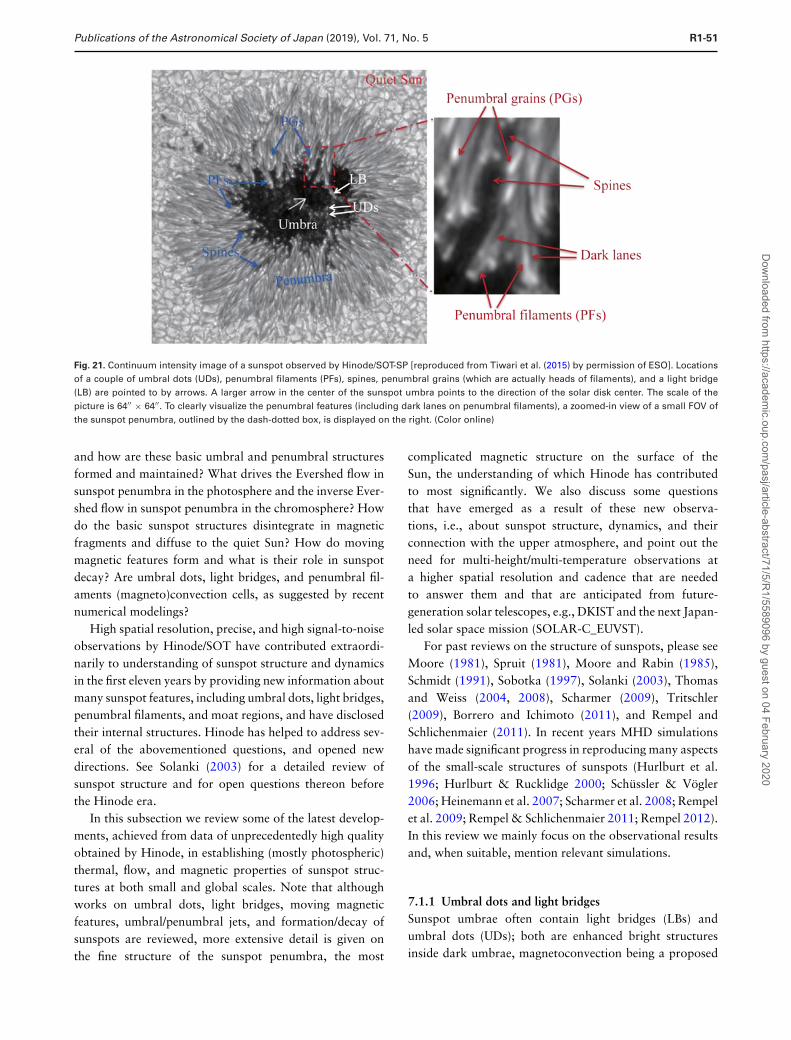
Publications of the Astronomical Society of Japan (2019), Vol. 71, No. 5 R1-51
Fig. 21. Continuum intensity image of a sunspot observed by Hinode/SOT-SP [reproduced from Tiwari et al. (2015) by permission of ESO]. Locationsof a couple of umbral dots (UDs), penumbral filaments (PFs), spines, penumbral grains (which are actually heads of filaments), and a light bridge(LB) are pointed to by arrows. A larger arrow in the center of the sunspot umbra points to the direction of the solar disk center. The scale of thepicture is 64′′ × 64′′. To clearly visualize the penumbral features (including dark lanes on penumbral filaments), a zoomed-in view of a small FOV ofthe sunspot penumbra, outlined by the dash-dotted box, is displayed on the right. (Color online)
and how are these basic umbral and penumbral structuresformed and maintained? What drives the Evershed flow insunspot penumbra in the photosphere and the inverse Ever-shed flow in sunspot penumbra in the chromosphere? Howdo the basic sunspot structures disintegrate in magneticfragments and diffuse to the quiet Sun? How do movingmagnetic features form and what is their role in sunspotdecay? Are umbral dots, light bridges, and penumbral fil-aments (magneto)convection cells, as suggested by recentnumerical modelings?
High spatial resolution, precise, and high signal-to-noiseobservations by Hinode/SOT have contributed extraordi-narily to understanding of sunspot structure and dynamicsin the first eleven years by providing new information aboutmany sunspot features, including umbral dots, light bridges,penumbral filaments, and moat regions, and have disclosedtheir internal structures. Hinode has helped to address sev-eral of the abovementioned questions, and opened newdirections. See Solanki (2003) for a detailed review ofsunspot structure and for open questions thereon beforethe Hinode era.
In this subsection we review some of the latest develop-ments, achieved from data of unprecedentedly high qualityobtained by Hinode, in establishing (mostly photospheric)thermal, flow, and magnetic properties of sunspot struc-tures at both small and global scales. Note that althoughworks on umbral dots, light bridges, moving magneticfeatures, umbral/penumbral jets, and formation/decay ofsunspots are reviewed, more extensive detail is given onthe fine structure of the sunspot penumbra, the most
complicated magnetic structure on the surface of theSun, the understanding of which Hinode has contributedto most significantly. We also discuss some questionsthat have emerged as a result of these new observa-tions, i.e., about sunspot structure, dynamics, and theirconnection with the upper atmosphere, and point out theneed for multi-height/multi-temperature observations ata higher spatial resolution and cadence that are neededto answer them and that are anticipated from future-generation solar telescopes, e.g., DKIST and the next Japan-led solar space mission (SOLAR-C_EUVST).
For past reviews on the structure of sunspots, please seeMoore (1981), Spruit (1981), Moore and Rabin (1985),Schmidt (1991), Sobotka (1997), Solanki (2003), Thomasand Weiss (2004, 2008), Scharmer (2009), Tritschler(2009), Borrero and Ichimoto (2011), and Rempel andSchlichenmaier (2011). In recent years MHD simulationshave made significant progress in reproducing many aspectsof the small-scale structures of sunspots (Hurlburt et al.1996; Hurlburt & Rucklidge 2000; Schussler & Vogler2006; Heinemann et al. 2007; Scharmer et al. 2008; Rempelet al. 2009; Rempel & Schlichenmaier 2011; Rempel 2012).In this review we mainly focus on the observational resultsand, when suitable, mention relevant simulations.
7.1.1 Umbral dots and light bridgesSunspot umbrae often contain light bridges (LBs) andumbral dots (UDs); both are enhanced bright structuresinside dark umbrae, magnetoconvection being a proposed
Dow
nloaded from https://academ
ic.oup.com/pasj/article-abstract/71/5/R
1/5589096 by guest on 04 February 2020
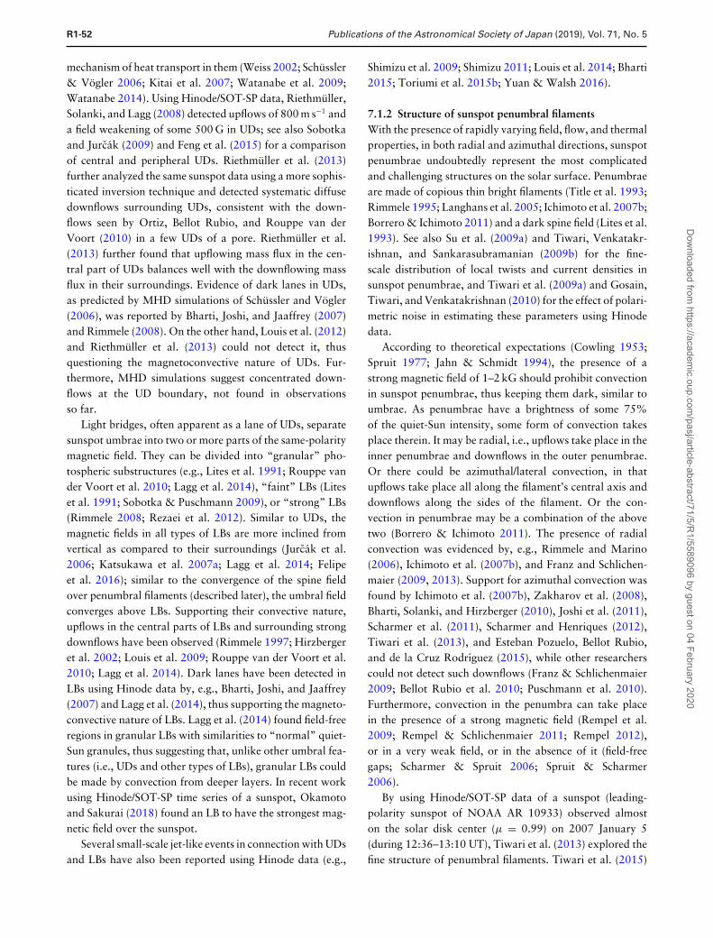
R1-52 Publications of the Astronomical Society of Japan (2019), Vol. 71, No. 5
mechanism of heat transport in them (Weiss 2002; Schussler& Vogler 2006; Kitai et al. 2007; Watanabe et al. 2009;Watanabe 2014). Using Hinode/SOT-SP data, Riethmuller,Solanki, and Lagg (2008) detected upflows of 800 m s−1 anda field weakening of some 500 G in UDs; see also Sobotkaand Jurcak (2009) and Feng et al. (2015) for a comparisonof central and peripheral UDs. Riethmuller et al. (2013)further analyzed the same sunspot data using a more sophis-ticated inversion technique and detected systematic diffusedownflows surrounding UDs, consistent with the down-flows seen by Ortiz, Bellot Rubio, and Rouppe van derVoort (2010) in a few UDs of a pore. Riethmuller et al.(2013) further found that upflowing mass flux in the cen-tral part of UDs balances well with the downflowing massflux in their surroundings. Evidence of dark lanes in UDs,as predicted by MHD simulations of Schussler and Vogler(2006), was reported by Bharti, Joshi, and Jaaffrey (2007)and Rimmele (2008). On the other hand, Louis et al. (2012)and Riethmuller et al. (2013) could not detect it, thusquestioning the magnetoconvective nature of UDs. Fur-thermore, MHD simulations suggest concentrated down-flows at the UD boundary, not found in observationsso far.
Light bridges, often apparent as a lane of UDs, separatesunspot umbrae into two or more parts of the same-polaritymagnetic field. They can be divided into “granular” pho-tospheric substructures (e.g., Lites et al. 1991; Rouppe vander Voort et al. 2010; Lagg et al. 2014), “faint” LBs (Liteset al. 1991; Sobotka & Puschmann 2009), or “strong” LBs(Rimmele 2008; Rezaei et al. 2012). Similar to UDs, themagnetic fields in all types of LBs are more inclined fromvertical as compared to their surroundings (Jurcak et al.2006; Katsukawa et al. 2007a; Lagg et al. 2014; Felipeet al. 2016); similar to the convergence of the spine fieldover penumbral filaments (described later), the umbral fieldconverges above LBs. Supporting their convective nature,upflows in the central parts of LBs and surrounding strongdownflows have been observed (Rimmele 1997; Hirzbergeret al. 2002; Louis et al. 2009; Rouppe van der Voort et al.2010; Lagg et al. 2014). Dark lanes have been detected inLBs using Hinode data by, e.g., Bharti, Joshi, and Jaaffrey(2007) and Lagg et al. (2014), thus supporting the magneto-convective nature of LBs. Lagg et al. (2014) found field-freeregions in granular LBs with similarities to “normal” quiet-Sun granules, thus suggesting that, unlike other umbral fea-tures (i.e., UDs and other types of LBs), granular LBs couldbe made by convection from deeper layers. In recent workusing Hinode/SOT-SP time series of a sunspot, Okamotoand Sakurai (2018) found an LB to have the strongest mag-netic field over the sunspot.
Several small-scale jet-like events in connection with UDsand LBs have also been reported using Hinode data (e.g.,
Shimizu et al. 2009; Shimizu 2011; Louis et al. 2014; Bharti2015; Toriumi et al. 2015b; Yuan & Walsh 2016).
7.1.2 Structure of sunspot penumbral filamentsWith the presence of rapidly varying field, flow, and thermalproperties, in both radial and azimuthal directions, sunspotpenumbrae undoubtedly represent the most complicatedand challenging structures on the solar surface. Penumbraeare made of copious thin bright filaments (Title et al. 1993;Rimmele 1995; Langhans et al. 2005; Ichimoto et al. 2007b;Borrero & Ichimoto 2011) and a dark spine field (Lites et al.1993). See also Su et al. (2009a) and Tiwari, Venkatakr-ishnan, and Sankarasubramanian (2009b) for the fine-scale distribution of local twists and current densities insunspot penumbrae, and Tiwari et al. (2009a) and Gosain,Tiwari, and Venkatakrishnan (2010) for the effect of polari-metric noise in estimating these parameters using Hinodedata.
According to theoretical expectations (Cowling 1953;Spruit 1977; Jahn & Schmidt 1994), the presence of astrong magnetic field of 1–2 kG should prohibit convectionin sunspot penumbrae, thus keeping them dark, similar toumbrae. As penumbrae have a brightness of some 75%of the quiet-Sun intensity, some form of convection takesplace therein. It may be radial, i.e., upflows take place in theinner penumbrae and downflows in the outer penumbrae.Or there could be azimuthal/lateral convection, in thatupflows take place all along the filament’s central axis anddownflows along the sides of the filament. Or the con-vection in penumbrae may be a combination of the abovetwo (Borrero & Ichimoto 2011). The presence of radialconvection was evidenced by, e.g., Rimmele and Marino(2006), Ichimoto et al. (2007b), and Franz and Schlichen-maier (2009, 2013). Support for azimuthal convection wasfound by Ichimoto et al. (2007b), Zakharov et al. (2008),Bharti, Solanki, and Hirzberger (2010), Joshi et al. (2011),Scharmer et al. (2011), Scharmer and Henriques (2012),Tiwari et al. (2013), and Esteban Pozuelo, Bellot Rubio,and de la Cruz Rodrıguez (2015), while other researcherscould not detect such downflows (Franz & Schlichenmaier2009; Bellot Rubio et al. 2010; Puschmann et al. 2010).Furthermore, convection in the penumbra can take placein the presence of a strong magnetic field (Rempel et al.2009; Rempel & Schlichenmaier 2011; Rempel 2012),or in a very weak field, or in the absence of it (field-freegaps; Scharmer & Spruit 2006; Spruit & Scharmer2006).
By using Hinode/SOT-SP data of a sunspot (leading-polarity sunspot of NOAA AR 10933) observed almoston the solar disk center (μ = 0.99) on 2007 January 5(during 12:36–13:10 UT), Tiwari et al. (2013) explored thefine structure of penumbral filaments. Tiwari et al. (2015)
Dow
nloaded from https://academ
ic.oup.com/pasj/article-abstract/71/5/R
1/5589096 by guest on 04 February 2020
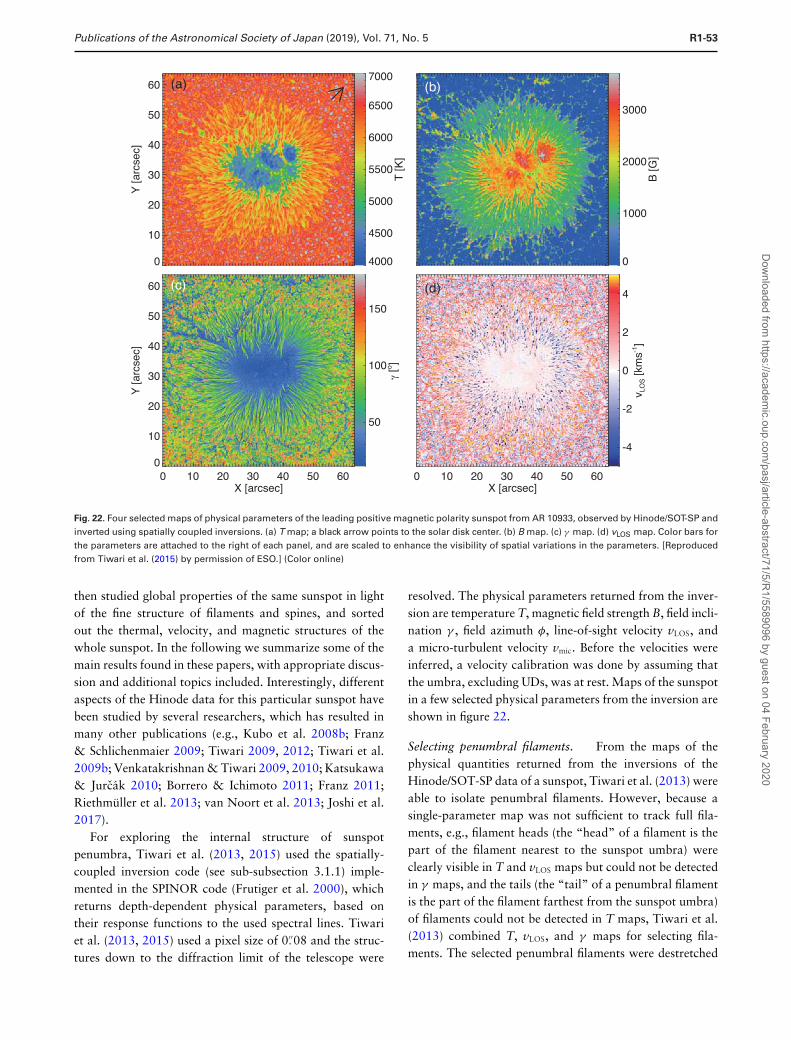
Publications of the Astronomical Society of Japan (2019), Vol. 71, No. 5 R1-53
4000
4500
5000
5500
6000
6500
7000
T [K
]
0
10
20
30
40
50
60
Y [a
rcse
c]
(a)
0
1000
2000
3000
B [G
]
(b)
50
100
150
γ [o ]
0 10 20 30 40 50 60X [arcsec]
0
10
20
30
40
50
60
Y [a
rcse
c]
(c)
-4
-2
0
2
4
v LO
S [k
ms-1
]
0 10 20 30 40 50 60X [arcsec]
(d)
Fig. 22. Four selected maps of physical parameters of the leading positive magnetic polarity sunspot from AR 10933, observed by Hinode/SOT-SP andinverted using spatially coupled inversions. (a) T map; a black arrow points to the solar disk center. (b) B map. (c) γ map. (d) vLOS map. Color bars forthe parameters are attached to the right of each panel, and are scaled to enhance the visibility of spatial variations in the parameters. [Reproducedfrom Tiwari et al. (2015) by permission of ESO.] (Color online)
then studied global properties of the same sunspot in lightof the fine structure of filaments and spines, and sortedout the thermal, velocity, and magnetic structures of thewhole sunspot. In the following we summarize some of themain results found in these papers, with appropriate discus-sion and additional topics included. Interestingly, differentaspects of the Hinode data for this particular sunspot havebeen studied by several researchers, which has resulted inmany other publications (e.g., Kubo et al. 2008b; Franz& Schlichenmaier 2009; Tiwari 2009, 2012; Tiwari et al.2009b; Venkatakrishnan & Tiwari 2009, 2010; Katsukawa& Jurcak 2010; Borrero & Ichimoto 2011; Franz 2011;Riethmuller et al. 2013; van Noort et al. 2013; Joshi et al.2017).
For exploring the internal structure of sunspotpenumbra, Tiwari et al. (2013, 2015) used the spatially-coupled inversion code (see sub-subsection 3.1.1) imple-mented in the SPINOR code (Frutiger et al. 2000), whichreturns depth-dependent physical parameters, based ontheir response functions to the used spectral lines. Tiwariet al. (2013, 2015) used a pixel size of 0.′′08 and the struc-tures down to the diffraction limit of the telescope were
resolved. The physical parameters returned from the inver-sion are temperature T, magnetic field strength B, field incli-nation γ , field azimuth φ, line-of-sight velocity vLOS, anda micro-turbulent velocity vmic. Before the velocities wereinferred, a velocity calibration was done by assuming thatthe umbra, excluding UDs, was at rest. Maps of the sunspotin a few selected physical parameters from the inversion areshown in figure 22.
Selecting penumbral filaments. From the maps of thephysical quantities returned from the inversions of theHinode/SOT-SP data of a sunspot, Tiwari et al. (2013) wereable to isolate penumbral filaments. However, because asingle-parameter map was not sufficient to track full fila-ments, e.g., filament heads (the “head” of a filament is thepart of the filament nearest to the sunspot umbra) wereclearly visible in T and vLOS maps but could not be detectedin γ maps, and the tails (the “tail” of a penumbral filamentis the part of the filament farthest from the sunspot umbra)of filaments could not be detected in T maps, Tiwari et al.(2013) combined T, vLOS, and γ maps for selecting fila-ments. The selected penumbral filaments were destretched
Dow
nloaded from https://academ
ic.oup.com/pasj/article-abstract/71/5/R
1/5589096 by guest on 04 February 2020
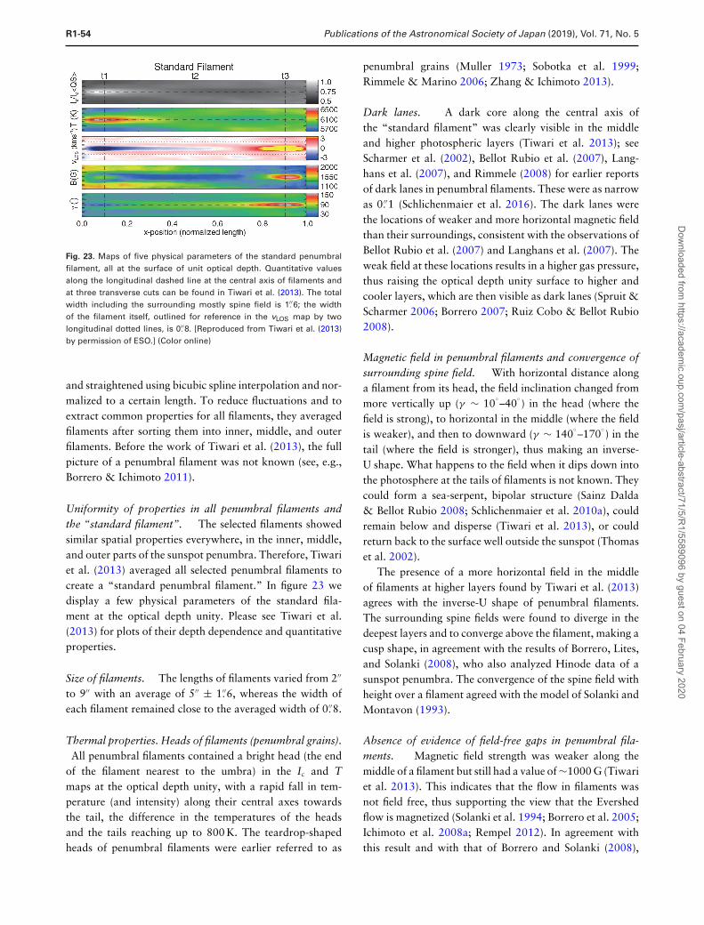
R1-54 Publications of the Astronomical Society of Japan (2019), Vol. 71, No. 5
Fig. 23. Maps of five physical parameters of the standard penumbralfilament, all at the surface of unit optical depth. Quantitative valuesalong the longitudinal dashed line at the central axis of filaments andat three transverse cuts can be found in Tiwari et al. (2013). The totalwidth including the surrounding mostly spine field is 1.′′6; the widthof the filament itself, outlined for reference in the vLOS map by twolongitudinal dotted lines, is 0.′′8. [Reproduced from Tiwari et al. (2013)by permission of ESO.] (Color online)
and straightened using bicubic spline interpolation and nor-malized to a certain length. To reduce fluctuations and toextract common properties for all filaments, they averagedfilaments after sorting them into inner, middle, and outerfilaments. Before the work of Tiwari et al. (2013), the fullpicture of a penumbral filament was not known (see, e.g.,Borrero & Ichimoto 2011).
Uniformity of properties in all penumbral filaments andthe “standard filament”. The selected filaments showedsimilar spatial properties everywhere, in the inner, middle,and outer parts of the sunspot penumbra. Therefore, Tiwariet al. (2013) averaged all selected penumbral filaments tocreate a “standard penumbral filament.” In figure 23 wedisplay a few physical parameters of the standard fila-ment at the optical depth unity. Please see Tiwari et al.(2013) for plots of their depth dependence and quantitativeproperties.
Size of filaments. The lengths of filaments varied from 2′′
to 9′′ with an average of 5′′ ± 1.′′6, whereas the width ofeach filament remained close to the averaged width of 0.′′8.
Thermal properties. Heads of filaments (penumbral grains).All penumbral filaments contained a bright head (the end
of the filament nearest to the umbra) in the Ic and Tmaps at the optical depth unity, with a rapid fall in tem-perature (and intensity) along their central axes towardsthe tail, the difference in the temperatures of the headsand the tails reaching up to 800 K. The teardrop-shapedheads of penumbral filaments were earlier referred to as
penumbral grains (Muller 1973; Sobotka et al. 1999;Rimmele & Marino 2006; Zhang & Ichimoto 2013).
Dark lanes. A dark core along the central axis ofthe “standard filament” was clearly visible in the middleand higher photospheric layers (Tiwari et al. 2013); seeScharmer et al. (2002), Bellot Rubio et al. (2007), Lang-hans et al. (2007), and Rimmele (2008) for earlier reportsof dark lanes in penumbral filaments. These were as narrowas 0.′′1 (Schlichenmaier et al. 2016). The dark lanes werethe locations of weaker and more horizontal magnetic fieldthan their surroundings, consistent with the observations ofBellot Rubio et al. (2007) and Langhans et al. (2007). Theweak field at these locations results in a higher gas pressure,thus raising the optical depth unity surface to higher andcooler layers, which are then visible as dark lanes (Spruit &Scharmer 2006; Borrero 2007; Ruiz Cobo & Bellot Rubio2008).
Magnetic field in penumbral filaments and convergence ofsurrounding spine field. With horizontal distance alonga filament from its head, the field inclination changed frommore vertically up (γ ∼ 10
◦–40
◦) in the head (where the
field is strong), to horizontal in the middle (where the fieldis weaker), and then to downward (γ ∼ 140
◦–170
◦) in the
tail (where the field is stronger), thus making an inverse-U shape. What happens to the field when it dips down intothe photosphere at the tails of filaments is not known. Theycould form a sea-serpent, bipolar structure (Sainz Dalda& Bellot Rubio 2008; Schlichenmaier et al. 2010a), couldremain below and disperse (Tiwari et al. 2013), or couldreturn back to the surface well outside the sunspot (Thomaset al. 2002).
The presence of a more horizontal field in the middleof filaments at higher layers found by Tiwari et al. (2013)agrees with the inverse-U shape of penumbral filaments.The surrounding spine fields were found to diverge in thedeepest layers and to converge above the filament, making acusp shape, in agreement with the results of Borrero, Lites,and Solanki (2008), who also analyzed Hinode data of asunspot penumbra. The convergence of the spine field withheight over a filament agreed with the model of Solanki andMontavon (1993).
Absence of evidence of field-free gaps in penumbral fila-ments. Magnetic field strength was weaker along themiddle of a filament but still had a value of ∼1000 G (Tiwariet al. 2013). This indicates that the flow in filaments wasnot field free, thus supporting the view that the Evershedflow is magnetized (Solanki et al. 1994; Borrero et al. 2005;Ichimoto et al. 2008a; Rempel 2012). In agreement withthis result and with that of Borrero and Solanki (2008),
Dow
nloaded from https://academ
ic.oup.com/pasj/article-abstract/71/5/R
1/5589096 by guest on 04 February 2020
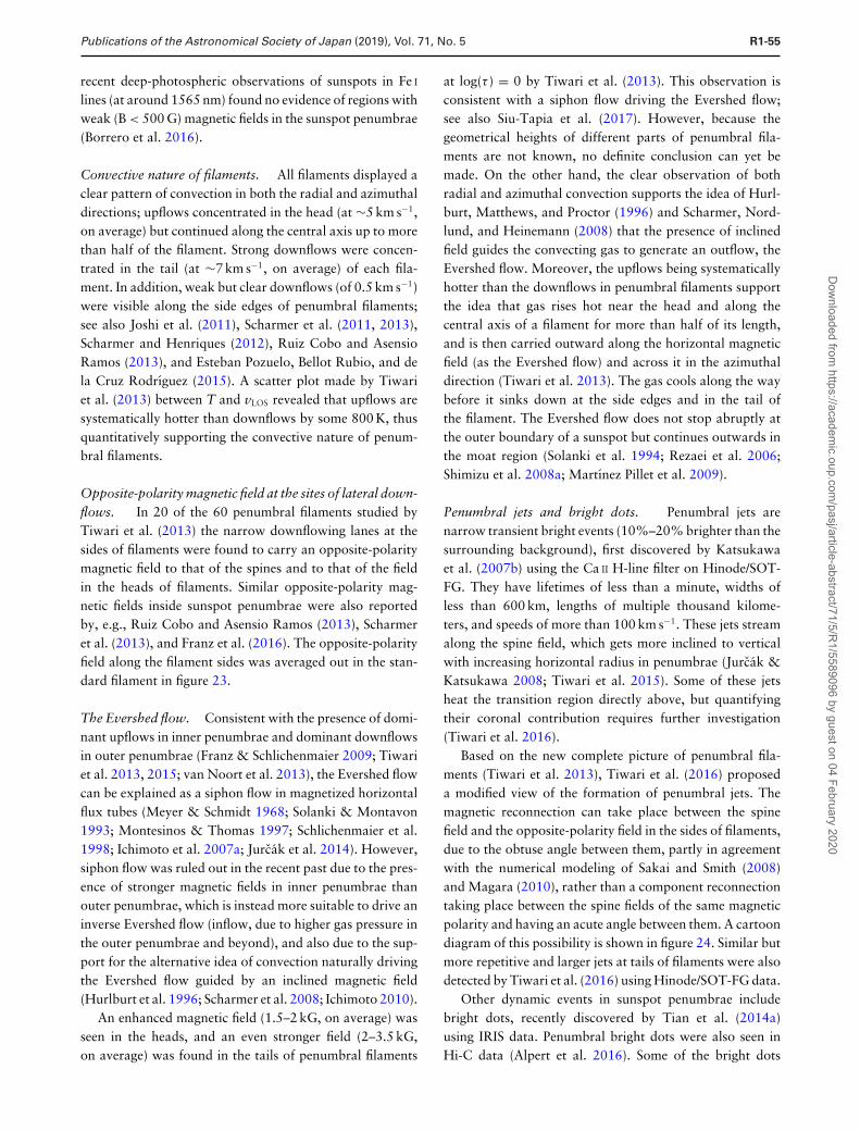
Publications of the Astronomical Society of Japan (2019), Vol. 71, No. 5 R1-55
recent deep-photospheric observations of sunspots in Fe I
lines (at around 1565 nm) found no evidence of regions withweak (B < 500 G) magnetic fields in the sunspot penumbrae(Borrero et al. 2016).
Convective nature of filaments. All filaments displayed aclear pattern of convection in both the radial and azimuthaldirections; upflows concentrated in the head (at ∼5 km s−1,on average) but continued along the central axis up to morethan half of the filament. Strong downflows were concen-trated in the tail (at ∼7 km s−1, on average) of each fila-ment. In addition, weak but clear downflows (of 0.5 km s−1)were visible along the side edges of penumbral filaments;see also Joshi et al. (2011), Scharmer et al. (2011, 2013),Scharmer and Henriques (2012), Ruiz Cobo and AsensioRamos (2013), and Esteban Pozuelo, Bellot Rubio, and dela Cruz Rodrıguez (2015). A scatter plot made by Tiwariet al. (2013) between T and vLOS revealed that upflows aresystematically hotter than downflows by some 800 K, thusquantitatively supporting the convective nature of penum-bral filaments.
Opposite-polarity magnetic field at the sites of lateral down-flows. In 20 of the 60 penumbral filaments studied byTiwari et al. (2013) the narrow downflowing lanes at thesides of filaments were found to carry an opposite-polaritymagnetic field to that of the spines and to that of the fieldin the heads of filaments. Similar opposite-polarity mag-netic fields inside sunspot penumbrae were also reportedby, e.g., Ruiz Cobo and Asensio Ramos (2013), Scharmeret al. (2013), and Franz et al. (2016). The opposite-polarityfield along the filament sides was averaged out in the stan-dard filament in figure 23.
The Evershed flow. Consistent with the presence of domi-nant upflows in inner penumbrae and dominant downflowsin outer penumbrae (Franz & Schlichenmaier 2009; Tiwariet al. 2013, 2015; van Noort et al. 2013), the Evershed flowcan be explained as a siphon flow in magnetized horizontalflux tubes (Meyer & Schmidt 1968; Solanki & Montavon1993; Montesinos & Thomas 1997; Schlichenmaier et al.1998; Ichimoto et al. 2007a; Jurcak et al. 2014). However,siphon flow was ruled out in the recent past due to the pres-ence of stronger magnetic fields in inner penumbrae thanouter penumbrae, which is instead more suitable to drive aninverse Evershed flow (inflow, due to higher gas pressure inthe outer penumbrae and beyond), and also due to the sup-port for the alternative idea of convection naturally drivingthe Evershed flow guided by an inclined magnetic field(Hurlburt et al. 1996; Scharmer et al. 2008; Ichimoto 2010).
An enhanced magnetic field (1.5–2 kG, on average) wasseen in the heads, and an even stronger field (2–3.5 kG,on average) was found in the tails of penumbral filaments
at log(τ ) = 0 by Tiwari et al. (2013). This observation isconsistent with a siphon flow driving the Evershed flow;see also Siu-Tapia et al. (2017). However, because thegeometrical heights of different parts of penumbral fila-ments are not known, no definite conclusion can yet bemade. On the other hand, the clear observation of bothradial and azimuthal convection supports the idea of Hurl-burt, Matthews, and Proctor (1996) and Scharmer, Nord-lund, and Heinemann (2008) that the presence of inclinedfield guides the convecting gas to generate an outflow, theEvershed flow. Moreover, the upflows being systematicallyhotter than the downflows in penumbral filaments supportthe idea that gas rises hot near the head and along thecentral axis of a filament for more than half of its length,and is then carried outward along the horizontal magneticfield (as the Evershed flow) and across it in the azimuthaldirection (Tiwari et al. 2013). The gas cools along the waybefore it sinks down at the side edges and in the tail ofthe filament. The Evershed flow does not stop abruptly atthe outer boundary of a sunspot but continues outwards inthe moat region (Solanki et al. 1994; Rezaei et al. 2006;Shimizu et al. 2008a; Martınez Pillet et al. 2009).
Penumbral jets and bright dots. Penumbral jets arenarrow transient bright events (10%–20% brighter than thesurrounding background), first discovered by Katsukawaet al. (2007b) using the Ca II H-line filter on Hinode/SOT-FG. They have lifetimes of less than a minute, widths ofless than 600 km, lengths of multiple thousand kilome-ters, and speeds of more than 100 km s−1. These jets streamalong the spine field, which gets more inclined to verticalwith increasing horizontal radius in penumbrae (Jurcak &Katsukawa 2008; Tiwari et al. 2015). Some of these jetsheat the transition region directly above, but quantifyingtheir coronal contribution requires further investigation(Tiwari et al. 2016).
Based on the new complete picture of penumbral fila-ments (Tiwari et al. 2013), Tiwari et al. (2016) proposeda modified view of the formation of penumbral jets. Themagnetic reconnection can take place between the spinefield and the opposite-polarity field in the sides of filaments,due to the obtuse angle between them, partly in agreementwith the numerical modeling of Sakai and Smith (2008)and Magara (2010), rather than a component reconnectiontaking place between the spine fields of the same magneticpolarity and having an acute angle between them. A cartoondiagram of this possibility is shown in figure 24. Similar butmore repetitive and larger jets at tails of filaments were alsodetected by Tiwari et al. (2016) using Hinode/SOT-FG data.
Other dynamic events in sunspot penumbrae includebright dots, recently discovered by Tian et al. (2014a)using IRIS data. Penumbral bright dots were also seen inHi-C data (Alpert et al. 2016). Some of the bright dots
Dow
nloaded from https://academ
ic.oup.com/pasj/article-abstract/71/5/R
1/5589096 by guest on 04 February 2020
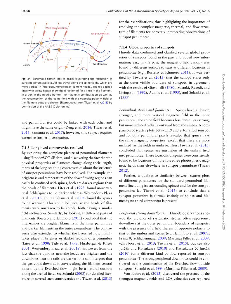
R1-56 Publications of the Astronomical Society of Japan (2019), Vol. 71, No. 5
Fig. 24. Schematic sketch (not to scale) illustrating the formation ofsunspot penumbral jets. All jets travel along the spine fields, which aremore vertical in inner penumbrae (near filament heads). The red dashedlines with arrow heads show the direction of field lines in the filament.In a box in the middle bottom the magnetic configuration as well asthe reconnection of the spine field with the opposite-polarity field atthe filament edge are shown. [Reproduced from Tiwari et al. (2016) bypermission of the AAS.] (Color online)
and penumbral jets could be linked with each other andmight have the same origin (Deng et al. 2016; Tiwari et al.2016; Samanta et al. 2017); however, this subject requiresextensive further investigation.
7.1.3 Long-lived controversies resolvedBy exploring the complete picture of penumbral filamentsusing Hinode/SOT-SP data, and discovering the fact that thephysical properties of filaments change along their length,many of the long-standing controversies about the structureof sunspot penumbrae have been resolved. For example, thebrightness and temperature of the downflowing regions caneasily be confused with spines; both are darker regions thanthe heads of filaments. Lites et al. (1993) found more ver-tical fields/spines to be darker whereas Westendorp Plazaet al. (2001b) and Langhans et al. (2005) found the spinesto be warmer. This could be because the heads of fila-ments were mistaken to be spines, both having a similarfield inclination. Similarly, by looking at different parts offilaments Borrero and Ichimoto (2011) concluded that theinter-spines are brighter filaments in the inner penumbraeand darker filaments in the outer penumbrae. The contro-versy also extended to whether the Evershed flow mainlytakes place in brighter or darker regions of a penumbra(Lites et al. 1990; Title et al. 1993; Hirzberger & Kneer2001; Westendorp Plaza et al. 2001a). However, from thefact that the upflows near the heads are brighter and thedownflows near the tails are darker, one can interpret thatthe gas cools down as it travels along the filament centralaxis; thus the Evershed flow might be a natural outflowalong the arched field. See Solanki (2003) for detailed liter-ature on several such controversies and Tiwari et al. (2013)
for their clarifications, thus highlighting the importance ofresolving the complex magnetic, thermal, and flow struc-ture of filaments for correctly interpreting observations ofsunspot penumbrae.
7.1.4 Global properties of sunspotsHinode data confirmed and clarified several global prop-erties of sunspots found in the past and added new infor-mation; e.g., in the past, the magnetic field canopy wasfound by different authors to start at different locations inpenumbrae (e.g., Borrero & Ichimoto 2011). It was ver-ified by Tiwari et al. (2015) that the canopy starts onlyat the outer visible boundary of sunspots, in agreementwith the results of Giovanelli (1980), Solanki, Rueedi, andLivingston (1992), Adams et al. (1993), and Solanki et al.(1999).
Penumbral spines and filaments. Spines have a denser,stronger, and more vertical magnetic field in the innerpenumbra. The spine field becomes less dense, less strong,but more inclined radially outward from the umbra. A com-parison of scatter plots between B and γ for a full sunspotand for only penumbral pixels revealed that spines havethe same magnetic properties (except that these are moreinclined) as the fields in umbrae. Thus, Tiwari et al. (2015)concluded that spines are intrusions of the umbral fieldinto penumbrae. These locations of spines were consistentlyfound to be locations of more force-free photospheric mag-netic fields than elsewhere in sunspot penumbrae (Tiwari2012).
Further, a qualitative similarity between scatter plotsof different parameters for the standard penumbral fila-ment (including its surrounding spines) and for the sunspotpenumbra led Tiwari et al. (2015) to conclude that asunspot penumbra is formed entirely of spines and fila-ments; no third component is present.
Peripheral strong downflows. Hinode observations sho-wed the presence of systematic strong, often supersonic,downflows at the outer penumbral boundary of sunspots,with the presence of a field therein of opposite polarity tothat of the umbra and spines (e.g., Ichimoto et al. 2007a;Franz & Schlichenmaier 2009; Martınez Pillet et al. 2009;van Noort et al. 2013; Tiwari et al. 2015), but see alsoJurcak and Katsukawa (2010) and Katsukawa & Jurcak(2010) for a different kind of flow reported in sunspotpenumbrae. The strong peripheral downflows could be con-sidered as the continuation of the Evershed flow outsidesunspots (Solanki et al. 1994; Martınez Pillet et al. 2009).
Van Noort et al. (2013) discovered the presence of thestrongest magnetic fields and LOS velocities ever reported
Dow
nloaded from https://academ
ic.oup.com/pasj/article-abstract/71/5/R
1/5589096 by guest on 04 February 2020
Publications of the Astronomical Society of Japan (2019), Vol. 71, No. 5 R1-57
in the photosphere, exceeding 7 kG and 20 km s−1, respec-tively, in a few locations at the periphery of sunspots. Theyfound a linear correlation between the downflow veloci-ties and the field strength, which was in good agreementwith MHD simulations. Possibly these peculiar downflowsare induced by the accumulation and intensification of thepenumbral magnetic field by the Evershed flow. This isimplied by the finding that these locations of strong down-flows at the periphery of sunspots were the locations wherethe tails of several penumbral filaments converge (Tiwariet al. 2013; van Noort et al. 2013).
Field gradients in sunspots. Generally, the field strengthin sunspots decreases with increasing horizontal radius andheight (Westendorp Plaza et al. 2001b; Mathew et al. 2003;Borrero & Ichimoto 2011; Tiwari et al. 2015). A decreasein the average field strength from 2800 G in the umbrato 700 G at the outer penumbral boundary in the deepestlayers was found in a sunspot observed by Hinode (Tiwariet al. 2015). The sunspot umbra showed an average ver-tical field gradient of 1400 G km−1 in the deepest layersthat dropped rapidly with height, reaching 0.95 G km−1 atlog(τ ) = −2.5.
However, in addition to the canopy structure seen atthe outer penumbral boundary, an inverse field gradient(field increasing with height) was found in the inner-middlepenumbrae (Tiwari et al. 2015). Joshi et al. (2017) inves-tigated this particular property of sunspots in detail. Theyalso found the presence of an inverse gradient in MHD sim-ulations. A closer look revealed the dominance of inversegradients near the heads of penumbral filaments. Theobserved inverse field gradient could be a result of spinefields converging above filaments, the Stokes V signal can-celation at filament edges, or an artefact caused by a highlycorrugated optical-depth-unity surface in inner penumbrae(Tiwari et al. 2015; Joshi et al. 2017). See a recent reviewon the height dependence of magnetic fields in sunspots byBalthasar (2018).
Moving magnetic features and sunspot decay. Movingmagnetic features (MMFs; see figure 25) are small unipolaror bipolar structures of sizes <2′′ and lifetimes of 10 minto 10 hr. These move radially outward starting fromthe sunspot penumbra (or from within the moat region)with speeds of <2 km s−1 and eventually disappear in thenetwork fields (Sheeley 1969; Harvey & Harvey 1973;Brickhouse & Labonte 1988; Hagenaar & Shine 2005;Ravindra 2006; Sainz Dalda & Bellot Rubio 2008; Limet al. 2012; Li & Zhang 2013). Although MMFs areprominent sunspot features, they are also found in pores(Zuccarello et al. 2009; Criscuoli et al. 2012; Verma et al.
Fig. 25. Line-of-sight magnetic field maps of the upper right quarter ofa sunspot penumbra, including its surrounding moat region, observedby SOT-SP in Normal Map mode, thus having a pixel size of 0.′′16. Theevolution of eight moving magnetic features are outlined by circles,each in a different color: red (panels a–c), yellow (panels a–e), orange(panels a–f), violet (panels c–f), green (panels a–f), blue (panels a–c),cyan (panels a–f), and ivory (panels a–f). The SP data used in this figurewere inverted at the Community Spectropolarimetric Analysis Center〈http://www2.hao.ucar.edu/csac〉. (Color online)
2012; Kaithakkal et al. 2017). Using Hinode/SOT magne-tograms, Li and Zhang (2013) found that half of MMFsin a sunspot were produced within the penumbra and theother half originated within the moat region. They foundthat most of the MMFs formed in the moat were due to fluxemergence. Once MMFs were formed, they started decayingby flux cancelation. The Evershed flow has been linked withthe formation of MMFs (Martınez Pillet 2002; Zhang et al.2007; Kubo et al. 2008a; Rempel 2015), but for an alerna-tive view see Lohner-Bottcher and Schlichenmaier (2013).
MMFs are proposed to play a crucial role in thedecay of sunspots (Harvey & Harvey 1973; MartınezPillet 2002; Hagenaar & Shine 2005). Consistent with theresults of Hagenaar and Shine (2005), using Hinode/SOTdata Kubo et al. (2008a, 2008b) showed that indecaying sunspots the rate of the loss of magnetic flux(8 × 10¹⁵ Mx s−1) in sunspots is very similar to the rate ofthe magnetic flux carried outwards by MMFs, thus takingseveral weeks for a sunspot of 1022 Mx to completely decay.Kubo et al. (2008a) also showed that positive and negativepolarities balance each other in the moat region, suggestingthat most of the sunspot flux is transported to the moatregion and then outward by MMFs, and then removed byflux cancelation in the network regions. The rate of fluxtransport by moat flows is consistent with that found in
Dow
nloaded from https://academ
ic.oup.com/pasj/article-abstract/71/5/R
1/5589096 by guest on 04 February 2020
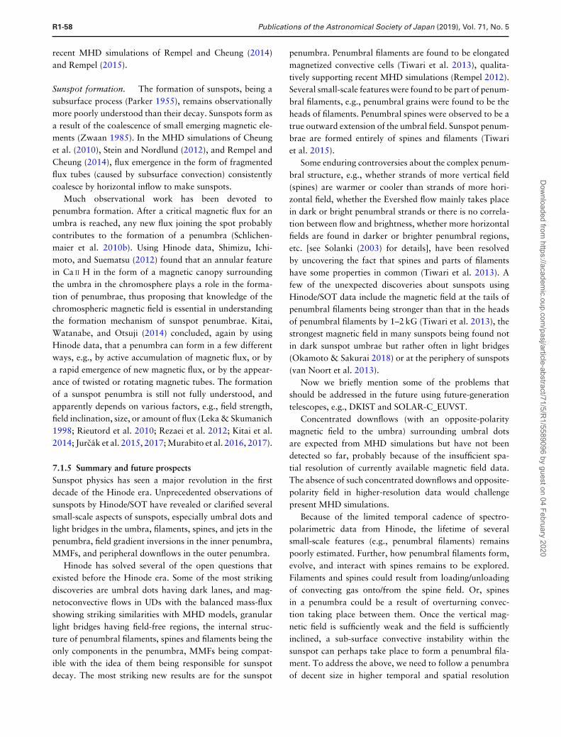
R1-58 Publications of the Astronomical Society of Japan (2019), Vol. 71, No. 5
recent MHD simulations of Rempel and Cheung (2014)and Rempel (2015).
Sunspot formation. The formation of sunspots, being asubsurface process (Parker 1955), remains observationallymore poorly understood than their decay. Sunspots form asa result of the coalescence of small emerging magnetic ele-ments (Zwaan 1985). In the MHD simulations of Cheunget al. (2010), Stein and Nordlund (2012), and Rempel andCheung (2014), flux emergence in the form of fragmentedflux tubes (caused by subsurface convection) consistentlycoalesce by horizontal inflow to make sunspots.
Much observational work has been devoted topenumbra formation. After a critical magnetic flux for anumbra is reached, any new flux joining the spot probablycontributes to the formation of a penumbra (Schlichen-maier et al. 2010b). Using Hinode data, Shimizu, Ichi-moto, and Suematsu (2012) found that an annular featurein Ca II H in the form of a magnetic canopy surroundingthe umbra in the chromosphere plays a role in the forma-tion of penumbrae, thus proposing that knowledge of thechromospheric magnetic field is essential in understandingthe formation mechanism of sunspot penumbrae. Kitai,Watanabe, and Otsuji (2014) concluded, again by usingHinode data, that a penumbra can form in a few differentways, e.g., by active accumulation of magnetic flux, or bya rapid emergence of new magnetic flux, or by the appear-ance of twisted or rotating magnetic tubes. The formationof a sunspot penumbra is still not fully understood, andapparently depends on various factors, e.g., field strength,field inclination, size, or amount of flux (Leka & Skumanich1998; Rieutord et al. 2010; Rezaei et al. 2012; Kitai et al.2014; Jurcak et al. 2015, 2017; Murabito et al. 2016, 2017).
7.1.5 Summary and future prospectsSunspot physics has seen a major revolution in the firstdecade of the Hinode era. Unprecedented observations ofsunspots by Hinode/SOT have revealed or clarified severalsmall-scale aspects of sunspots, especially umbral dots andlight bridges in the umbra, filaments, spines, and jets in thepenumbra, field gradient inversions in the inner penumbra,MMFs, and peripheral downflows in the outer penumbra.
Hinode has solved several of the open questions thatexisted before the Hinode era. Some of the most strikingdiscoveries are umbral dots having dark lanes, and mag-netoconvective flows in UDs with the balanced mass-fluxshowing striking similarities with MHD models, granularlight bridges having field-free regions, the internal struc-ture of penumbral filaments, spines and filaments being theonly components in the penumbra, MMFs being compat-ible with the idea of them being responsible for sunspotdecay. The most striking new results are for the sunspot
penumbra. Penumbral filaments are found to be elongatedmagnetized convective cells (Tiwari et al. 2013), qualita-tively supporting recent MHD simulations (Rempel 2012).Several small-scale features were found to be part of penum-bral filaments, e.g., penumbral grains were found to be theheads of filaments. Penumbral spines were observed to be atrue outward extension of the umbral field. Sunspot penum-brae are formed entirely of spines and filaments (Tiwariet al. 2015).
Some enduring controversies about the complex penum-bral structure, e.g., whether strands of more vertical field(spines) are warmer or cooler than strands of more hori-zontal field, whether the Evershed flow mainly takes placein dark or bright penumbral strands or there is no correla-tion between flow and brightness, whether more horizontalfields are found in darker or brighter penumbral regions,etc. [see Solanki (2003) for details], have been resolvedby uncovering the fact that spines and parts of filamentshave some properties in common (Tiwari et al. 2013). Afew of the unexpected discoveries about sunspots usingHinode/SOT data include the magnetic field at the tails ofpenumbral filaments being stronger than that in the headsof penumbral filaments by 1–2 kG (Tiwari et al. 2013), thestrongest magnetic field in many sunspots being found notin dark sunspot umbrae but rather often in light bridges(Okamoto & Sakurai 2018) or at the periphery of sunspots(van Noort et al. 2013).
Now we briefly mention some of the problems thatshould be addressed in the future using future-generationtelescopes, e.g., DKIST and SOLAR-C_EUVST.
Concentrated downflows (with an opposite-polaritymagnetic field to the umbra) surrounding umbral dotsare expected from MHD simulations but have not beendetected so far, probably because of the insufficient spa-tial resolution of currently available magnetic field data.The absence of such concentrated downflows and opposite-polarity field in higher-resolution data would challengepresent MHD simulations.
Because of the limited temporal cadence of spectro-polarimetric data from Hinode, the lifetime of severalsmall-scale features (e.g., penumbral filaments) remainspoorly estimated. Further, how penumbral filaments form,evolve, and interact with spines remains to be explored.Filaments and spines could result from loading/unloadingof convecting gas onto/from the spine field. Or, spinesin a penumbra could be a result of overturning convec-tion taking place between them. Once the vertical mag-netic field is sufficiently weak and the field is sufficientlyinclined, a sub-surface convective instability within thesunspot can perhaps take place to form a penumbral fila-ment. To address the above, we need to follow a penumbraof decent size in higher temporal and spatial resolution
Dow
nloaded from https://academ
ic.oup.com/pasj/article-abstract/71/5/R
1/5589096 by guest on 04 February 2020
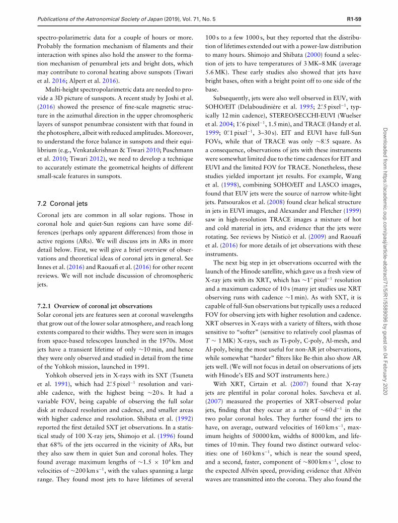
Publications of the Astronomical Society of Japan (2019), Vol. 71, No. 5 R1-59
spectro-polarimetric data for a couple of hours or more.Probably the formation mechanism of filaments and theirinteraction with spines also hold the answer to the forma-tion mechanism of penumbral jets and bright dots, whichmay contribute to coronal heating above sunspots (Tiwariet al. 2016; Alpert et al. 2016).
Multi-height spectropolarimetric data are needed to pro-vide a 3D picture of sunspots. A recent study by Joshi et al.(2016) showed the presence of fine-scale magnetic struc-ture in the azimuthal direction in the upper chromosphericlayers of sunspot penumbrae consistent with that found inthe photosphere, albeit with reduced amplitudes. Moreover,to understand the force balance in sunspots and their equi-librium (e.g., Venkatakrishnan & Tiwari 2010; Puschmannet al. 2010; Tiwari 2012), we need to develop a techniqueto accurately estimate the geometrical heights of differentsmall-scale features in sunspots.
7.2 Coronal jets
Coronal jets are common in all solar regions. Those incoronal hole and quiet-Sun regions can have some dif-ferences (perhaps only apparent differences) from those inactive regions (ARs). We will discuss jets in ARs in moredetail below. First, we will give a brief overview of obser-vations and theoretical ideas of coronal jets in general. SeeInnes et al. (2016) and Raouafi et al. (2016) for other recentreviews. We will not include discussion of chromosphericjets.
7.2.1 Overview of coronal jet observationsSolar coronal jets are features seen at coronal wavelengthsthat grow out of the lower solar atmosphere, and reach longextents compared to their widths. They were seen in imagesfrom space-based telescopes launched in the 1970s. Mostjets have a transient lifetime of only ∼10 min, and hencethey were only observed and studied in detail from the timeof the Yohkoh mission, launched in 1991.
Yohkoh observed jets in X-rays with its SXT (Tsunetaet al. 1991), which had 2.′′5 pixel−1 resolution and vari-able cadence, with the highest being ∼20 s. It had avariable FOV, being capable of observing the full solardisk at reduced resolution and cadence, and smaller areaswith higher cadence and resolution. Shibata et al. (1992)reported the first detailed SXT jet observations. In a statis-tical study of 100 X-ray jets, Shimojo et al. (1996) foundthat 68% of the jets occurred in the vicinity of ARs, butthey also saw them in quiet Sun and coronal holes. Theyfound average maximum lengths of ∼1.5 × 10⁴ km andvelocities of ∼200 km s−1, with the values spanning a largerange. They found most jets to have lifetimes of several
100 s to a few 1000 s, but they reported that the distribu-tion of lifetimes extended out with a power-law distributionto many hours. Shimojo and Shibata (2000) found a selec-tion of jets to have temperatures of 3 MK–8 MK (average5.6 MK). These early studies also showed that jets havebright bases, often with a bright point off to one side of thebase.
Subsequently, jets were also well observed in EUV, withSOHO/EIT (Delaboudiniere et al. 1995; 2.′′5 pixel−1, typ-ically 12 min cadence), STEREO/SECCHI-EUVI (Wuelseret al. 2004; 1.′′6 pixel−1, 1.5 min), and TRACE (Handy et al.1999; 0.′′1 pixel−1, 3–30 s). EIT and EUVI have full-SunFOVs, while that of TRACE was only ∼8.′5 square. Asa consequence, observations of jets with these instrumentswere somewhat limited due to the time cadences for EIT andEUVI and the limited FOV for TRACE. Nonetheless, thesestudies yielded important jet results. For example, Wanget al. (1998), combining SOHO/EIT and LASCO images,found that EUV jets were the source of narrow white-lightjets. Patsourakos et al. (2008) found clear helical structurein jets in EUVI images, and Alexander and Fletcher (1999)saw in high-resolution TRACE images a mixture of hotand cold material in jets, and evidence that the jets wererotating. See reviews by Nistico et al. (2009) and Raouafiet al. (2016) for more details of jet observations with theseinstruments.
The next big step in jet observations occurred with thelaunch of the Hinode satellite, which gave us a fresh view ofX-ray jets with its XRT, which has ∼1′′ pixel−1 resolutionand a maximum cadence of 10 s (many jet studies use XRTobserving runs with cadence ∼1 min). As with SXT, it iscapable of full-Sun observations but typically uses a reducedFOV for observing jets with higher resolution and cadence.XRT observes in X-rays with a variety of filters, with thosesensitive to “softer” (sensitive to relatively cool plasmas ofT ∼ 1 MK) X-rays, such as Ti-poly, C-poly, Al-mesh, andAl-poly, being the most useful for non-AR jet observations,while somewhat “harder” filters like Be-thin also show ARjets well. (We will not focus in detail on observations of jetswith Hinode’s EIS and SOT instruments here.)
With XRT, Cirtain et al. (2007) found that X-rayjets are plentiful in polar coronal holes. Savcheva et al.(2007) measured the properties of XRT-observed polarjets, finding that they occur at a rate of ∼60 d−1 in thetwo polar coronal holes. They further found the jets tohave, on average, outward velocities of 160 km s−1, max-imum heights of 50000 km, widths of 8000 km, and life-times of 10 min. They found two distinct outward veloc-ities: one of 160 km s−1, which is near the sound speed,and a second, faster, component of ∼800 km s−1, close tothe expected Alfven speed, providing evidence that Alfvenwaves are transmitted into the corona. They also found the
Dow
nloaded from https://academ
ic.oup.com/pasj/article-abstract/71/5/R
1/5589096 by guest on 04 February 2020
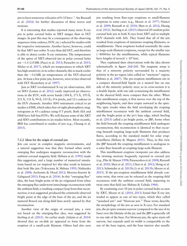
R1-60 Publications of the Astronomical Society of Japan (2019), Vol. 71, No. 5
jets to have transverse velocities of 0–35 km s−1. See Raouafiet al. (2016) for further discussion of these waves andmotions.
It is interesting that studies reported many more X-rayjets in polar coronal holes in XRT images than in SXTimages. In part this may be a consequence of the observingsequences (time cadence, FOV, etc.) selected for studies withthe respective instruments. Another factor, however, couldbe that XRT sees softer X-rays than did SXT, and thereforeis able to detect cooler X-ray emissions. The temperaturesof the spires of XRT-observed jets in polar coronal holesare ∼1.5–2.0 MK (Pucci et al. 2013; Paraschiv et al. 2015;Mulay et al. 2017), which are temperatures to which XRThas high sensitivity in its softer channels; this is much coolerthan the ∼5.6 MK jet temperatures of the SXT-observedjets. At least a few polar jets, however, were in fact observedwith SXT (Koutchmy et al. 1997).
Just as XRT revolutionized X-ray jet observations, AIAon SDO (Lemen et al. 2012) vastly improved jet observa-tions in the EUV, with seven bands (304 A, 171 A, 193 A,211 A, 131 A, 94 A, 335 A), 0.′′6 pixels, and 12 s cadence inthe EUV channels. Another SDO instrument critical to jetstudies is HMI, which takes line-of-sight photospheric mag-netograms at 45 s cadence using 0.′′5 pixels. Both AIA andHMI have full-Sun FOVs. We will discuss some of the XRTand SDO contributions to jet studies below. Most recently,IRIS has contributed to studies of jets (e.g., Cheung et al.2015).
7.2.2 Ideas for the origin of coronal jetsJets can occur in complex magnetic environments, anda natural suggestion was that they formed when newlyemerging flux undergoes magnetic reconnection with theambient coronal magnetic field. Shibata et al. (1992) madethis suggestion, and a large number of numerical simula-tions based on (or inspired by) this idea result in featuresthat look like jets (Yokoyama & Shibata 1995; Nishizukaet al. 2008; Archontis & Hood 2013; Moreno-Insertis &Galsgaard 2013; Fang et al. 2014). In this “emerging flux”idea, the base bright point of the jet originated from whenthe emerging flux underwent interchange reconnection withthe ambient field; a resulting compact loop from that recon-nection, it was suggested, produced the commonly observedbright point at the edge of the base of the jet, and the jetmaterial flowed out along field lines newly opened by thatreconnection.
Another view of the origin of coronal jets, a viewnot based on the emerging-flux idea, was suggested bySterling et al. (2015). An earlier study (Adams et al. 2014)showed that an on-disk jet appeared to form from theeruption of a small-scale filament. Others had also seen
jets resulting from flare-type eruptions or small-filamenteruptions in some cases (e.g., Moore et al. 1977; Nisticoet al. 2009; Raouafi et al. 2010; Shen et al. 2012; Huanget al. 2012). Sterling et al. (2015) observed 20 random polarcoronal hole jets in both X-rays from XRT and in multipleEUV channels with AIA. They found that all of the jetsresulted from eruptions of miniature erupting filaments, orminifilaments. These eruptions looked essentially the sameas large-scale filament eruptions, except for the smaller size(∼8000 km for the minifilaments, while typical filamentshave lengths of several × 104 km).
They explained their observations with the idea shownschematically in figure 26d–26f. The magnetic setup isthat of a minority polarity surrounded by a majoritypolarity in the jet region (also called an “anemone” region;Shibata et al. 2007). The pre-eruption minifilament sits ina compact sheared-field bipole on a neutral line on oneside of the minority polarity area; so in cross-section it isa double bipole, with one side (containing the minifilamentin the sheared field) more compact than the other. Whenthat minifilament erupts, it first moves over the top of theneighboring bipole, and then erupts outward in the spire.The spire results when the field enveloping the eruptingminifilament reconnects with the ambient coronal field,and the bright point at the jet’s base edge, which Sterlinget al. (2015) called a jet bright point, or JBP, forms whenthe field beneath the erupting minifilament field undergoesreconnection; this reconnection is identical to that occur-ring beneath erupting large-scale filaments that producesflares, according to the standard model for solar erup-tions/flares (Shibata & Magara 2011). Thus, in this viewthe JBP beneath the erupting minifilament is analogous toa solar flare beneath an erupting large-scale filament.
This minifilament eruption viewpoint can also addressthe twisting motions frequently reported in coronal jets(e.g., Pike & Mason 1998; Patsourakos et al. 2008; Raouafiet al. 2010; Shen et al. 2011; Chen et al. 2012; Hong et al.2013; Schmieder et al. 2013b; Li et al. 2015b; Moore et al.2015). If the pre-eruption minifilament field already con-tains twist, that twist can be released as the erupting fieldreconnects with the ambient coronal field, imparting itstwist onto that field (see Shibata & Uchida 1986).
By examining over 50 jets in polar coronal holes as seenby XRT, Moore et al. (2010, 2013) found that X-ray jetstended to appear as one of two types, which they called“standard jets” and “blowout jets.” These terms describethe morphology of the jets as seen in X-rays: For standardjets, the jet spire remains narrow (compared to the size of itsbase) over the lifetime of the jet, and the JBP is generally offto one side of the base. For blowout jets, the spire starts offnarrow, but expands until its width is comparable to thesize of the base region, and the base interior also usually
Dow
nloaded from https://academ
ic.oup.com/pasj/article-abstract/71/5/R
1/5589096 by guest on 04 February 2020
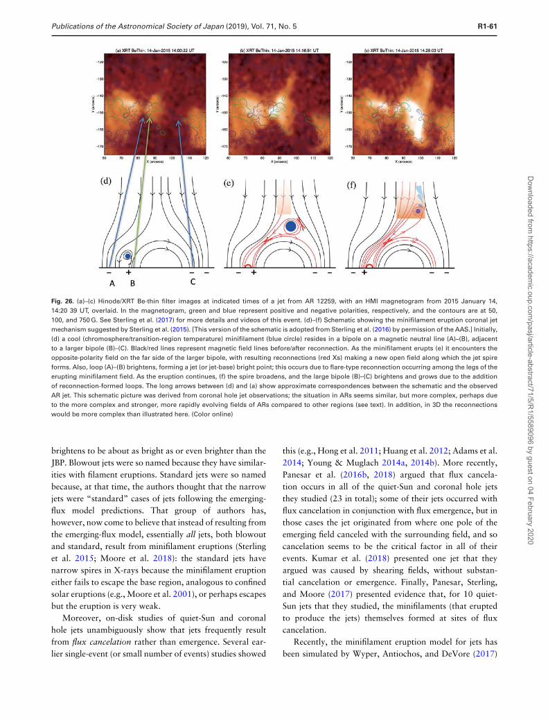
Publications of the Astronomical Society of Japan (2019), Vol. 71, No. 5 R1-61
Fig. 26. (a)–(c) Hinode/XRT Be-thin filter images at indicated times of a jet from AR 12259, with an HMI magnetogram from 2015 January 14,14:20 39 UT, overlaid. In the magnetogram, green and blue represent positive and negative polarities, respectively, and the contours are at 50,100, and 750 G. See Sterling et al. (2017) for more details and videos of this event. (d)–(f) Schematic showing the minifilament eruption coronal jetmechanism suggested by Sterling et al. (2015). [This version of the schematic is adopted from Sterling et al. (2016) by permission of the AAS.] Initially,(d) a cool (chromosphere/transition-region temperature) minifilament (blue circle) resides in a bipole on a magnetic neutral line (A)–(B), adjacentto a larger bipole (B)–(C). Black/red lines represent magnetic field lines before/after reconnection. As the minifilament erupts (e) it encounters theopposite-polarity field on the far side of the larger bipole, with resulting reconnections (red Xs) making a new open field along which the jet spireforms. Also, loop (A)–(B) brightens, forming a jet (or jet-base) bright point; this occurs due to flare-type reconnection occurring among the legs of theerupting minifilament field. As the eruption continues, (f) the spire broadens, and the large bipole (B)–(C) brightens and grows due to the additionof reconnection-formed loops. The long arrows between (d) and (a) show approximate correspondences between the schematic and the observedAR jet. This schematic picture was derived from coronal hole jet observations; the situation in ARs seems similar, but more complex, perhaps dueto the more complex and stronger, more rapidly evolving fields of ARs compared to other regions (see text). In addition, in 3D the reconnectionswould be more complex than illustrated here. (Color online)
brightens to be about as bright as or even brighter than theJBP. Blowout jets were so named because they have similar-ities with filament eruptions. Standard jets were so namedbecause, at that time, the authors thought that the narrowjets were “standard” cases of jets following the emerging-flux model predictions. That group of authors has,however, now come to believe that instead of resulting fromthe emerging-flux model, essentially all jets, both blowoutand standard, result from minifilament eruptions (Sterlinget al. 2015; Moore et al. 2018): the standard jets havenarrow spires in X-rays because the minifilament eruptioneither fails to escape the base region, analogous to confinedsolar eruptions (e.g., Moore et al. 2001), or perhaps escapesbut the eruption is very weak.
Moreover, on-disk studies of quiet-Sun and coronalhole jets unambiguously show that jets frequently resultfrom flux cancelation rather than emergence. Several ear-lier single-event (or small number of events) studies showed
this (e.g., Hong et al. 2011; Huang et al. 2012; Adams et al.2014; Young & Muglach 2014a, 2014b). More recently,Panesar et al. (2016b, 2018) argued that flux cancela-tion occurs in all of the quiet-Sun and coronal hole jetsthey studied (23 in total); some of their jets occurred withflux cancelation in conjunction with flux emergence, but inthose cases the jet originated from where one pole of theemerging field canceled with the surrounding field, and socancelation seems to be the critical factor in all of theirevents. Kumar et al. (2018) presented one jet that theyargued was caused by shearing fields, without substan-tial cancelation or emergence. Finally, Panesar, Sterling,and Moore (2017) presented evidence that, for 10 quiet-Sun jets that they studied, the minifilaments (that eruptedto produce the jets) themselves formed at sites of fluxcancelation.
Recently, the minifilament eruption model for jets hasbeen simulated by Wyper, Antiochos, and DeVore (2017)
Dow
nloaded from https://academ
ic.oup.com/pasj/article-abstract/71/5/R
1/5589096 by guest on 04 February 2020
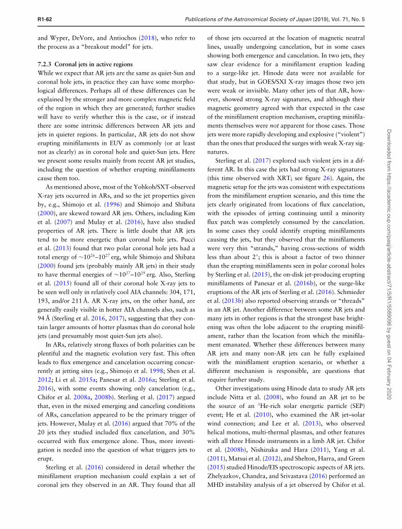
R1-62 Publications of the Astronomical Society of Japan (2019), Vol. 71, No. 5
and Wyper, DeVore, and Antiochos (2018), who refer tothe process as a “breakout model” for jets.
7.2.3 Coronal jets in active regionsWhile we expect that AR jets are the same as quiet-Sun andcoronal hole jets, in practice they can have some morpho-logical differences. Perhaps all of these differences can beexplained by the stronger and more complex magnetic fieldof the region in which they are generated; further studieswill have to verify whether this is the case, or if insteadthere are some intrinsic differences between AR jets andjets in quieter regions. In particular, AR jets do not showerupting minifilaments in EUV as commonly (or at leastnot as clearly) as in coronal hole and quiet-Sun jets. Herewe present some results mainly from recent AR jet studies,including the question of whether erupting minifilamentscause them too.
As mentioned above, most of the Yohkoh/SXT-observedX-ray jets occurred in ARs, and so the jet properties givenby, e.g., Shimojo et al. (1996) and Shimojo and Shibata(2000), are skewed toward AR jets. Others, including Kimet al. (2007) and Mulay et al. (2016), have also studiedproperties of AR jets. There is little doubt that AR jetstend to be more energetic than coronal hole jets. Pucciet al. (2013) found that two polar coronal hole jets had atotal energy of ∼1026–1027 erg, while Shimojo and Shibata(2000) found jets (probably mainly AR jets) in their studyto have thermal energies of ∼1027–1029 erg. Also, Sterlinget al. (2015) found all of their coronal hole X-ray jets tobe seen well only in relatively cool AIA channels: 304, 171,193, and/or 211 A. AR X-ray jets, on the other hand, aregenerally easily visible in hotter AIA channels also, such as94 A (Sterling et al. 2016, 2017), suggesting that they con-tain larger amounts of hotter plasmas than do coronal holejets (and presumably most quiet-Sun jets also).
In ARs, relatively strong fluxes of both polarities can beplentiful and the magnetic evolution very fast. This oftenleads to flux emergence and cancelation occurring concur-rently at jetting sites (e.g., Shimojo et al. 1998; Shen et al.2012; Li et al. 2015a; Panesar et al. 2016a; Sterling et al.2016), with some events showing only cancelation (e.g.,Chifor et al. 2008a, 2008b). Sterling et al. (2017) arguedthat, even in the mixed emerging and canceling conditionsof ARs, cancelation appeared to be the primary trigger ofjets. However, Mulay et al. (2016) argued that 70% of the20 jets they studied included flux cancelation, and 30%occurred with flux emergence alone. Thus, more investi-gation is needed into the question of what triggers jets toerupt.
Sterling et al. (2016) considered in detail whether theminifilament eruption mechanism could explain a set ofcoronal jets they observed in an AR. They found that all
of those jets occurred at the location of magnetic neutrallines, usually undergoing cancelation, but in some casesshowing both emergence and cancelation. In two jets, theysaw clear evidence for a minifilament eruption leadingto a surge-like jet. Hinode data were not available forthat study, but in GOES/SXI X-ray images those two jetswere weak or invisible. Many other jets of that AR, how-ever, showed strong X-ray signatures, and although theirmagnetic geometry agreed with that expected in the caseof the minifilament eruption mechanism, erupting minifila-ments themselves were not apparent for those cases. Thosejets were more rapidly developing and explosive (“violent”)than the ones that produced the surges with weak X-ray sig-natures.
Sterling et al. (2017) explored such violent jets in a dif-ferent AR. In this case the jets had strong X-ray signatures(this time observed with XRT; see figure 26). Again, themagnetic setup for the jets was consistent with expectationsfrom the minifilament eruption scenario, and this time thejets clearly originated from locations of flux cancelation,with the episodes of jetting continuing until a minorityflux patch was completely consumed by the cancelation.In some cases they could identify erupting minifilamentscausing the jets, but they observed that the minifilamentswere very thin “strands,” having cross-sections of widthless than about 2′′; this is about a factor of two thinnerthan the erupting minifilaments seen in polar coronal holesby Sterling et al. (2015), the on-disk jet-producing eruptingminifilaments of Panesar et al. (2016b), or the surge-likeeruptions of the AR jets of Sterling et al. (2016). Schmiederet al. (2013b) also reported observing strands or “threads”in an AR jet. Another difference between some AR jets andmany jets in other regions is that the strongest base bright-ening was often the lobe adjacent to the erupting minifil-ament, rather than the location from which the minifila-ment emanated. Whether these differences between manyAR jets and many non-AR jets can be fully explainedwith the minifilament eruption scenario, or whether adifferent mechanism is responsible, are questions thatrequire further study.
Other investigations using Hinode data to study AR jetsinclude Nitta et al. (2008), who found an AR jet to bethe source of an 3He-rich solar energetic particle (SEP)event; He et al. (2010), who examined the AR jet–solarwind connection; and Lee et al. (2013), who observedhelical motions, multi-thermal plasmas, and other featureswith all three Hinode instruments in a limb AR jet. Chiforet al. (2008b), Nishizuka and Hara (2011), Yang et al.(2011), Matsui et al. (2012), and Shelton, Harra, and Green(2015) studied Hinode/EIS spectroscopic aspects of AR jets.Zhelyazkov, Chandra, and Srivastava (2016) performed anMHD instability analysis of a jet observed by Chifor et al.
Dow
nloaded from https://academ
ic.oup.com/pasj/article-abstract/71/5/R
1/5589096 by guest on 04 February 2020
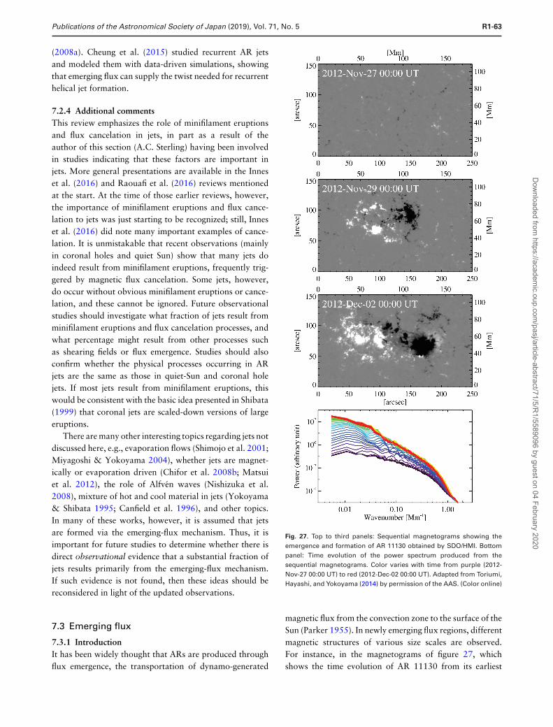
Publications of the Astronomical Society of Japan (2019), Vol. 71, No. 5 R1-63
(2008a). Cheung et al. (2015) studied recurrent AR jetsand modeled them with data-driven simulations, showingthat emerging flux can supply the twist needed for recurrenthelical jet formation.
7.2.4 Additional commentsThis review emphasizes the role of minifilament eruptionsand flux cancelation in jets, in part as a result of theauthor of this section (A.C. Sterling) having been involvedin studies indicating that these factors are important injets. More general presentations are available in the Inneset al. (2016) and Raouafi et al. (2016) reviews mentionedat the start. At the time of those earlier reviews, however,the importance of minifilament eruptions and flux cance-lation to jets was just starting to be recognized; still, Inneset al. (2016) did note many important examples of cance-lation. It is unmistakable that recent observations (mainlyin coronal holes and quiet Sun) show that many jets doindeed result from minifilament eruptions, frequently trig-gered by magnetic flux cancelation. Some jets, however,do occur without obvious minifilament eruptions or cance-lation, and these cannot be ignored. Future observationalstudies should investigate what fraction of jets result fromminifilament eruptions and flux cancelation processes, andwhat percentage might result from other processes suchas shearing fields or flux emergence. Studies should alsoconfirm whether the physical processes occurring in ARjets are the same as those in quiet-Sun and coronal holejets. If most jets result from minifilament eruptions, thiswould be consistent with the basic idea presented in Shibata(1999) that coronal jets are scaled-down versions of largeeruptions.
There are many other interesting topics regarding jets notdiscussed here, e.g., evaporation flows (Shimojo et al. 2001;Miyagoshi & Yokoyama 2004), whether jets are magnet-ically or evaporation driven (Chifor et al. 2008b; Matsuiet al. 2012), the role of Alfven waves (Nishizuka et al.2008), mixture of hot and cool material in jets (Yokoyama& Shibata 1995; Canfield et al. 1996), and other topics.In many of these works, however, it is assumed that jetsare formed via the emerging-flux mechanism. Thus, it isimportant for future studies to determine whether there isdirect observational evidence that a substantial fraction ofjets results primarily from the emerging-flux mechanism.If such evidence is not found, then these ideas should bereconsidered in light of the updated observations.
7.3 Emerging flux
7.3.1 IntroductionIt has been widely thought that ARs are produced throughflux emergence, the transportation of dynamo-generated
Fig. 27. Top to third panels: Sequential magnetograms showing theemergence and formation of AR 11130 obtained by SDO/HMI. Bottompanel: Time evolution of the power spectrum produced from thesequential magnetograms. Color varies with time from purple (2012-Nov-27 00:00 UT) to red (2012-Dec-02 00:00 UT). Adapted from Toriumi,Hayashi, and Yokoyama (2014) by permission of the AAS. (Color online)
magnetic flux from the convection zone to the surface of theSun (Parker 1955). In newly emerging flux regions, differentmagnetic structures of various size scales are observed.For instance, in the magnetograms of figure 27, whichshows the time evolution of AR 11130 from its earliest
Dow
nloaded from https://academ
ic.oup.com/pasj/article-abstract/71/5/R
1/5589096 by guest on 04 February 2020
R1-64 Publications of the Astronomical Society of Japan (2019), Vol. 71, No. 5
stage, one may find that the AR appears as tiny mag-netic elements of positive and negative polarities. These ele-ments merge together to form larger structures, i.e., pores(radius 0.7–1.8 × 10³ km) and sunspots (radius 4–28 ×103 km)—values adopted from Zwaan (1987). Typically,as a whole, ARs show a “cell division”-like separation ofboth polarities and develop into a bipolar configuration(third panel). The growth of magnetic structures is clearlyseen in the power spectrum (bottom panel). Here, the slopebecomes steeper with time, indicating that the larger struc-tures are transported to the surface from below in the laterphase and/or they are gradually formed around the surfacevia interactions between magnetic elements (i.e., inversecascade).
Over the course of their evolution, emerging flux regionsproduce a number of activity phenomena including minia-ture energy-releasing events as represented by Ellermanbombs, plasma ejections such as Hα surges and X-ray jets,and catastrophic eruptions, i.e., flares and CMEs. In thissection we review the Hinode observations of flux emer-gence and some related activity phenomena in the earliestphase in the AR development.
7.3.2 Before the Sun risesBefore the launch of Hinode, when the mission was stillcalled SOLAR-B, a number of meetings were held to dis-cuss science objectives and possible observation proposals.Motivated by space observations (e.g., Yohkoh, SOHO,and TRACE), high-resolution ground-based observations(e.g., SST), and the state-of-the-art 3D numerical simula-tions realized in the 1990s and early 2000s, various topicswere actively proposed. We introduce here several sci-ence targets discussed in one such conference, the SixthSOLAR-B Science Meeting, held in Kyoto in 2005November, i.e., just one year before the Hinode launch.
The first topic was flux emergence and the resultantmagnetic reconnection with ambient fields. On the theoret-ical side, Moreno-Insertis (2007) and Isobe et al. (2007a)showed MHD simulations of flux emergence that intro-duced pre-existing coronal fields (Yokoyama & Shibata1995; Archontis et al. 2005; Isobe et al. 2005) and empha-sized the importance of observing the magnetic reconnec-tion between emerging and pre-existing magnetic systems.They suggested, for example, that EIS will observe the cur-rent layer that forms between the two magnetic systemsand the flow fields around the reconnection region (i.e.,inflows and outflows). Kurokawa et al. (2007) introducedthe observations of Hα surges emanating from emergingflux regions. They pointed out that the ejections will becaused by magnetic reconnection occurring in the loweratmosphere between the emerging field and the pre-existingfield of opposite polarities (Yoshimura et al. 2003). They
expected that such magnetic evolutions will be observed bySOT.
Another observation target was the coronal evolutionin response to flux emergence. Yoshimura (2007) com-pared the photospheric magnetic flux (SOHO/MDI) andthe coronal brightness in EUV (TRACE), and found that theEUV brightness increased in pace with the enhancement ofthe magnetic flux, which indicated that the magnetic fieldscontinuously heated the corona. Such dynamic evolutionsmay be revealed with the combination of Hinode’s threeinstruments.
Scharmer et al. (2007), Stein, Benson, and Nordlund(2007), and Title (2007) discussed the importance of mag-netoconvection from both theoretical and observationalaspects. For example, radiative MHD simulation of fluxtube emergence by Cheung, Schussler, and Moreno-Insertis(2005) showed that bright and elongated granular cells areformed as the flux appears at the photosphere. Because theemerged horizontal fields guide the plasma flows, the gran-ular cells become elongated and aligned to the direction ofthe magnetic fields. The close coupling of magnetic fieldand convection, seen not only in the quiet Sun but also inthe earliest phase of AR evolution, was expected to be afavorable target for the Hinode mission, as stated by Lites(2007) in the summary review of the conference.
7.3.3 Hinode eraSince being launched successfully in 2006 September,Hinode has conducted numerous observations of a varietyof solar phenomena. However, because of the limited FOV,especially of SOT, it has always been challenging to detectAR-scale flux emergence events. Also, in the first few yearsof the Hinode mission the Sun was at the cycle minimumand thus there were not many ARs. However, these con-straints led to the successful detection of granular-sizedemergence events.
Centeno et al. (2007) focused on the quiet-Sun inter-network region using Hinode/SOT-SP and found that asthe granular cell turned over, positive and negative polari-ties that sandwiched the horizontal flux became separated(figure 28a). The eventual disappearance of the horizontalflux (final panel) indicated the emergence of an �-shapedloop. This is a perfect example of an emerging magneticfield coupled with or driven by local granulation, which waspredicted by the numerical simulations. Also, Guglielminoet al. (2008) detected the chromospheric brightenings inCa II H in association with small-scale emergence, whileMartınez Gonzalez et al. (2010) estimated the emer-gence speed to be ∼3 km s−1 (photosphere) to ∼12 km s−1
(chromosphere). These are the representative observationsof granular-scale emergence and its impact on the upperatmosphere (Isobe et al. 2008). For further descriptions of
Dow
nloaded from https://academ
ic.oup.com/pasj/article-abstract/71/5/R
1/5589096 by guest on 04 February 2020
Publications of the Astronomical Society of Japan (2019), Vol. 71, No. 5 R1-65
the quiet-Sun magnetism, readers are referred to subsec-tions 3.1 and 3.2.
From a theoretical point of view, one of the significantachievements in the Hinode era is the establishment of the“two-step emergence” model, in which the magnetic fluxrising in the convection zone slows down due to the strongstratification and drastically deforms its shape in the lat-eral direction (pancaking), driving strong plasma outflowsahead (e.g., Cheung et al. 2010; Toriumi & Yokoyama2010, 2011). Figure 29 presents a 3D simulation of alarge-scale emergence. Here, the flux tube experiences atemporal deceleration and flattening before it expands intothe photosphere and above. One of the most strikingobservational demonstrations of the two-step process isthe Hinode and Hida observation by Otsuji et al. (2007,2010). They found that the emerging flux first underwenta horizontal expansion in the photosphere at a speed of∼3 km s−1, and then started rising into the chromosphere at∼1 km s−1, later increasing to ∼2 km s−1. The clear consis-tency of the theory and observation symbolizes the successof the Hinode mission. In this period, the ascension, deceler-ation, and escaping outflows of the magnetic flux were alsoobserved with other methodologies (e.g., Grigor’ev et al.2007; Ilonidis et al. 2011; Toriumi et al. 2012, 2013b;Khlystova 2013), which further fostered our understandingof flux emergence.
Chromospheric anemone jets observed near the limb byShibata et al. (2007) indicated the possibility that the small-scale magnetic reconnection between the emerging fluxand the pre-existing field occurs ubiquitously in the solaratmosphere. Multi-wavelength analysis of the reconnectionwas reported by Guglielmino et al. (2010). It was foundthat the small-scale emergence within an AR was associ-ated with chromospheric, transition-region, and coronalbrightenings as well as chromospheric surge ejections. Withthe support of magnetic field extrapolation, they revealedthat the overall scenario is in line with the above mech-anism; namely, the interaction between the emerging fluxand the pre-existing ambient fields. A similar event wasdetected by collaborative observation with SOT and theNew Solar Telescope (NST) of the Big Bear Solar Obser-vatory (Yurchyshyn et al. 2010). It is now thought that jetejections caused by emerging flux and ambient field occurat a wide range of scales (see subsection 7.2).
One of the earliest detections of AR-scale flux emergenceevents was given by Magara (2008). Figure 28b clearlyshows that the fragmented magnetic elements merged todevelop a large bipolar structure; see the scale differencefrom figure 28a. Such large-scale evolutions of emergingmagnetic flux and the resultant spot motion are importantfor the build-up of the free magnetic energy and the supplyof shear and helicity that are essential to the flare eruptions
(e.g., Magara 2009). It is also believed that emerging fluxcan trigger flares and CMEs (e.g., Kusano et al. 2012). Seesection 8 for further details.
The atmospheric response to the photospheric flux evo-lution was also investigated. One of the earliest attemptswas made by Hansteen et al. (2007), who used SOT andEIS to reveal that a dark dimming region appeared andexpanded in He II and Fe XII about 30 min after the fluxemerges in the photosphere. Del Zanna (2008b) inves-tigated the Doppler shift of coronal lines in AR 10926(Magara 2008; figure 28b) and found that the blueshiftsappeared in lower hot (3 MK) loops, which was ascribed tothe continuous flux emergence. Harra et al. (2010) analyzedthe same AR and detected the formation of coronal loopsat the locations of newly emerging magnetic elements. Theyfound blueshifts with enhanced intensities and line widthsat the edges of the emerging flux region (figure 28c), whichthey interpreted as the onset of AR outflow that could con-tribute to the slow solar wind (Sakao et al. 2007). Furtherreview of the coronal response to AR evolution is found insection 9.
Yet another topic that we should mention is the sta-tistical investigations. Analyzing the high-cadence, high-resolution polarimetric imaging data of Hinode/SOT-NFI,Thornton and Parnell (2011) found that the frequency offlux emergence shows a power-law distribution over nearlyseven orders of magnitude from AR-scale (1023 Mx) togranular-scale (1016 Mx) events (figure 28d). The obtainedpower-law index was less than −2, indicating that mostof the newly supplied flux to the surface layer is fromsmall-scale events and that the emergence rate is inde-pendent of the solar cycle. Otsuji et al. (2011) analyzedmore than 100 events with total magnetic flux from3 × 1017 to 3 × 10²¹ Mx and found that the maximumseparation distance, flux growth rate, and mean separa-tion speed of the bipoles showed power-law relations withthe total flux (figure 28e). Applying the feature-trackingmethod to sequential magnetograms, Iida, Hagenaar, andYokoyama (2012) detected flux emergence events or, moreprecisely, separating motions of positive and negativepolarities. These Hinode observations clearly revealed thescale-free nature of magnetic flux emergence.
During the past ten years, numerical simulations of fluxemergence have been extensively developed and becomeincreasingly sophisticated, which allows more direct com-parisons between modeling and Hinode observations. Forexample, Cheung et al. (2008) conducted flux emergencesimulations that took into account the effect of radia-tive transfer and compared them with SOT observations.They successfully reproduced the observational character-istics in emerging flux regions, such as elongated gran-ules and flux cancelation (Cheung et al. 2010; Rempel &
Dow
nloaded from https://academ
ic.oup.com/pasj/article-abstract/71/5/R
1/5589096 by guest on 04 February 2020
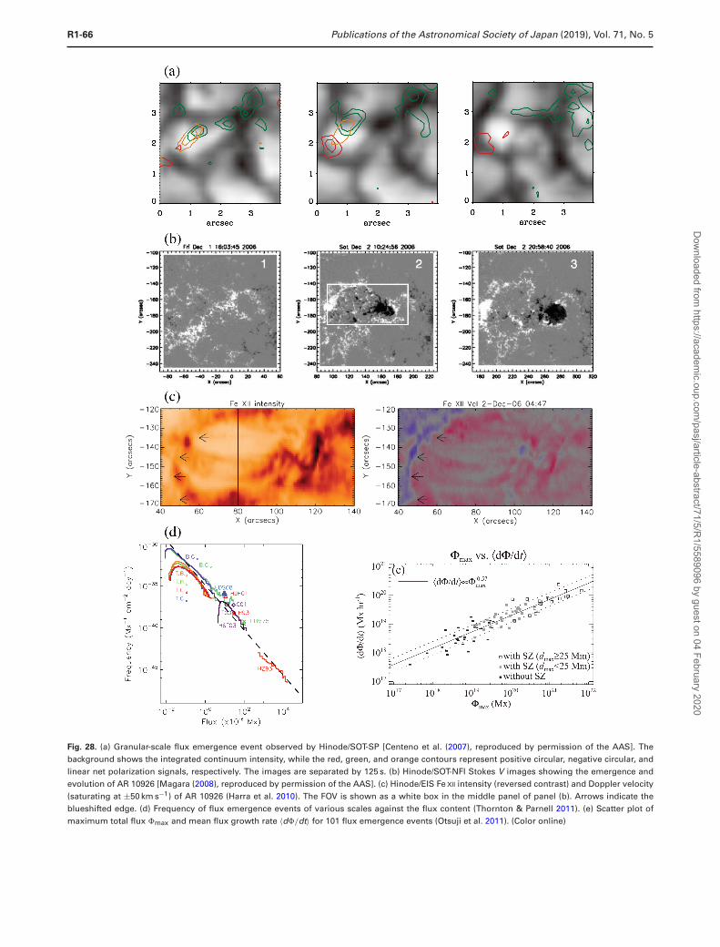
R1-66 Publications of the Astronomical Society of Japan (2019), Vol. 71, No. 5
Fig. 28. (a) Granular-scale flux emergence event observed by Hinode/SOT-SP [Centeno et al. (2007), reproduced by permission of the AAS]. Thebackground shows the integrated continuum intensity, while the red, green, and orange contours represent positive circular, negative circular, andlinear net polarization signals, respectively. The images are separated by 125 s. (b) Hinode/SOT-NFI Stokes V images showing the emergence andevolution of AR 10926 [Magara (2008), reproduced by permission of the AAS]. (c) Hinode/EIS Fe XII intensity (reversed contrast) and Doppler velocity(saturating at ±50 km s−1) of AR 10926 (Harra et al. 2010). The FOV is shown as a white box in the middle panel of panel (b). Arrows indicate theblueshifted edge. (d) Frequency of flux emergence events of various scales against the flux content (Thornton & Parnell 2011). (e) Scatter plot ofmaximum total flux �max and mean flux growth rate 〈d�/dt〉 for 101 flux emergence events (Otsuji et al. 2011). (Color online)
Dow
nloaded from https://academ
ic.oup.com/pasj/article-abstract/71/5/R
1/5589096 by guest on 04 February 2020
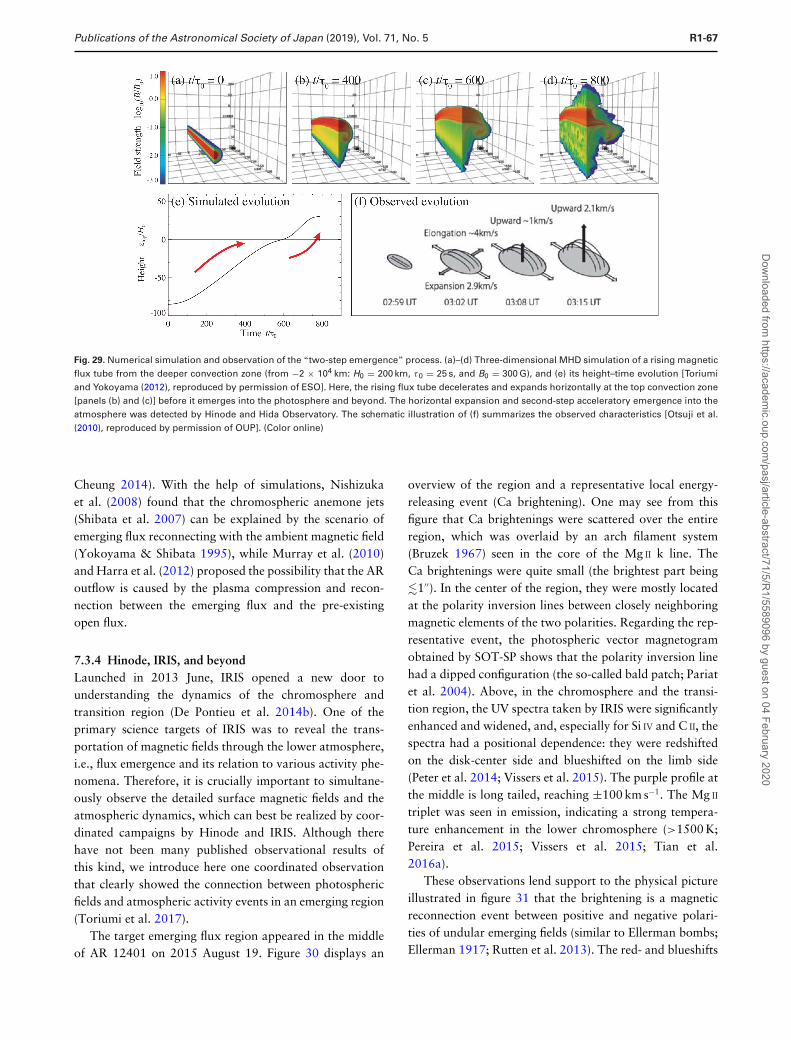
Publications of the Astronomical Society of Japan (2019), Vol. 71, No. 5 R1-67
Fig. 29. Numerical simulation and observation of the “two-step emergence” process. (a)–(d) Three-dimensional MHD simulation of a rising magneticflux tube from the deeper convection zone (from −2 × 10⁴ km: H0 = 200 km, τ0 = 25 s, and B0 = 300 G), and (e) its height–time evolution [Toriumiand Yokoyama (2012), reproduced by permission of ESO]. Here, the rising flux tube decelerates and expands horizontally at the top convection zone[panels (b) and (c)] before it emerges into the photosphere and beyond. The horizontal expansion and second-step acceleratory emergence into theatmosphere was detected by Hinode and Hida Observatory. The schematic illustration of (f) summarizes the observed characteristics [Otsuji et al.(2010), reproduced by permission of OUP]. (Color online)
Cheung 2014). With the help of simulations, Nishizukaet al. (2008) found that the chromospheric anemone jets(Shibata et al. 2007) can be explained by the scenario ofemerging flux reconnecting with the ambient magnetic field(Yokoyama & Shibata 1995), while Murray et al. (2010)and Harra et al. (2012) proposed the possibility that the ARoutflow is caused by the plasma compression and recon-nection between the emerging flux and the pre-existingopen flux.
7.3.4 Hinode, IRIS, and beyondLaunched in 2013 June, IRIS opened a new door tounderstanding the dynamics of the chromosphere andtransition region (De Pontieu et al. 2014b). One of theprimary science targets of IRIS was to reveal the trans-portation of magnetic fields through the lower atmosphere,i.e., flux emergence and its relation to various activity phe-nomena. Therefore, it is crucially important to simultane-ously observe the detailed surface magnetic fields and theatmospheric dynamics, which can best be realized by coor-dinated campaigns by Hinode and IRIS. Although therehave not been many published observational results ofthis kind, we introduce here one coordinated observationthat clearly showed the connection between photosphericfields and atmospheric activity events in an emerging region(Toriumi et al. 2017).
The target emerging flux region appeared in the middleof AR 12401 on 2015 August 19. Figure 30 displays an
overview of the region and a representative local energy-releasing event (Ca brightening). One may see from thisfigure that Ca brightenings were scattered over the entireregion, which was overlaid by an arch filament system(Bruzek 1967) seen in the core of the Mg II k line. TheCa brightenings were quite small (the brightest part being�1′′). In the center of the region, they were mostly locatedat the polarity inversion lines between closely neighboringmagnetic elements of the two polarities. Regarding the rep-resentative event, the photospheric vector magnetogramobtained by SOT-SP shows that the polarity inversion linehad a dipped configuration (the so-called bald patch; Pariatet al. 2004). Above, in the chromosphere and the transi-tion region, the UV spectra taken by IRIS were significantlyenhanced and widened, and, especially for Si IV and C II, thespectra had a positional dependence: they were redshiftedon the disk-center side and blueshifted on the limb side(Peter et al. 2014; Vissers et al. 2015). The purple profile atthe middle is long tailed, reaching ±100 km s−1. The Mg II
triplet was seen in emission, indicating a strong tempera-ture enhancement in the lower chromosphere (>1500 K;Pereira et al. 2015; Vissers et al. 2015; Tian et al.2016a).
These observations lend support to the physical pictureillustrated in figure 31 that the brightening is a magneticreconnection event between positive and negative polari-ties of undular emerging fields (similar to Ellerman bombs;Ellerman 1917; Rutten et al. 2013). The red- and blueshifts
Dow
nloaded from https://academ
ic.oup.com/pasj/article-abstract/71/5/R
1/5589096 by guest on 04 February 2020
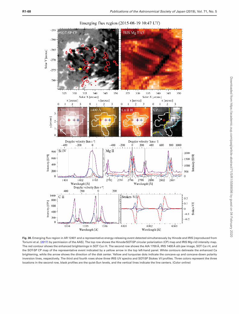
R1-68 Publications of the Astronomical Society of Japan (2019), Vol. 71, No. 5
Fig. 30. Emerging flux region in AR 12401 and a representative energy-releasing event detected simultaneously by Hinode and IRIS [reproduced fromToriumi et al. (2017) by permission of the AAS]. The top row shows the Hinode/SOT-SP circular polarization (CP) map and IRIS Mg II k3 intensity map.The red contour shows the enhanced brightenings in SOT Ca II H. The second row shows the AIA 1700 A, IRIS 1400 A slit-jaw image, SOT Ca II H, andthe SOT-SP CP map of the representative event indicated by a yellow arrow in the top left-hand panel. White contours delineate the enhanced Cabrightening, while the arrow shows the direction of the disk center. Yellow and turquoise dots indicate the concave-up and concave-down polarityinversion lines, respectively. The third and fourth rows show three IRIS UV spectra and SOT-SP Stokes V/I profiles. Three colors represent the threelocations in the second row, black profiles are the quiet-Sun levels, and the vertical lines indicate the line centers. (Color online)
Dow
nloaded from https://academ
ic.oup.com/pasj/article-abstract/71/5/R
1/5589096 by guest on 04 February 2020
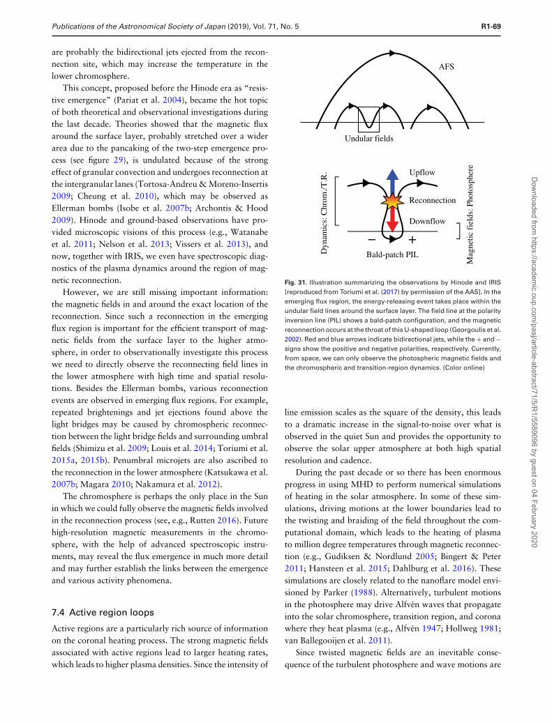
Publications of the Astronomical Society of Japan (2019), Vol. 71, No. 5 R1-69
are probably the bidirectional jets ejected from the recon-nection site, which may increase the temperature in thelower chromosphere.
This concept, proposed before the Hinode era as “resis-tive emergence” (Pariat et al. 2004), became the hot topicof both theoretical and observational investigations duringthe last decade. Theories showed that the magnetic fluxaround the surface layer, probably stretched over a widerarea due to the pancaking of the two-step emergence pro-cess (see figure 29), is undulated because of the strongeffect of granular convection and undergoes reconnection atthe intergranular lanes (Tortosa-Andreu & Moreno-Insertis2009; Cheung et al. 2010), which may be observed asEllerman bombs (Isobe et al. 2007b; Archontis & Hood2009). Hinode and ground-based observations have pro-vided microscopic visions of this process (e.g., Watanabeet al. 2011; Nelson et al. 2013; Vissers et al. 2013), andnow, together with IRIS, we even have spectroscopic diag-nostics of the plasma dynamics around the region of mag-netic reconnection.
However, we are still missing important information:the magnetic fields in and around the exact location of thereconnection. Since such a reconnection in the emergingflux region is important for the efficient transport of mag-netic fields from the surface layer to the higher atmo-sphere, in order to observationally investigate this processwe need to directly observe the reconnecting field lines inthe lower atmosphere with high time and spatial resolu-tions. Besides the Ellerman bombs, various reconnectionevents are observed in emerging flux regions. For example,repeated brightenings and jet ejections found above thelight bridges may be caused by chromospheric reconnec-tion between the light bridge fields and surrounding umbralfields (Shimizu et al. 2009; Louis et al. 2014; Toriumi et al.2015a, 2015b). Penumbral microjets are also ascribed tothe reconnection in the lower atmosphere (Katsukawa et al.2007b; Magara 2010; Nakamura et al. 2012).
The chromosphere is perhaps the only place in the Sunin which we could fully observe the magnetic fields involvedin the reconnection process (see, e.g., Rutten 2016). Futurehigh-resolution magnetic measurements in the chromo-sphere, with the help of advanced spectroscopic instru-ments, may reveal the flux emergence in much more detailand may further establish the links between the emergenceand various activity phenomena.
7.4 Active region loops
Active regions are a particularly rich source of informationon the coronal heating process. The strong magnetic fieldsassociated with active regions lead to larger heating rates,which leads to higher plasma densities. Since the intensity of
Bald-patch PIL
+−
Upflow
Reconnection
Downflow
Dyn
amic
s: C
hrom
./T.R
.
Mag
netic
fie
lds:
Pho
tosp
here
AFS
Undular fields
Fig. 31. Illustration summarizing the observations by Hinode and IRIS[reproduced from Toriumi et al. (2017) by permission of the AAS]. In theemerging flux region, the energy-releasing event takes place within theundular field lines around the surface layer. The field line at the polarityinversion line (PIL) shows a bald-patch configuration, and the magneticreconnection occurs at the throat of this U-shaped loop (Georgoulis et al.2002). Red and blue arrows indicate bidirectional jets, while the + and −signs show the positive and negative polarities, respectively. Currently,from space, we can only observe the photospheric magnetic fields andthe chromospheric and transition-region dynamics. (Color online)
line emission scales as the square of the density, this leadsto a dramatic increase in the signal-to-noise over what isobserved in the quiet Sun and provides the opportunity toobserve the solar upper atmosphere at both high spatialresolution and cadence.
During the past decade or so there has been enormousprogress in using MHD to perform numerical simulationsof heating in the solar atmosphere. In some of these sim-ulations, driving motions at the lower boundaries lead tothe twisting and braiding of the field throughout the com-putational domain, which leads to the heating of plasmato million degree temperatures through magnetic reconnec-tion (e.g., Gudiksen & Nordlund 2005; Bingert & Peter2011; Hansteen et al. 2015; Dahlburg et al. 2016). Thesesimulations are closely related to the nanoflare model envi-sioned by Parker (1988). Alternatively, turbulent motionsin the photosphere may drive Alfven waves that propagateinto the solar chromosphere, transition region, and coronawhere they heat plasma (e.g., Alfven 1947; Hollweg 1981;van Ballegooijen et al. 2011).
Since twisted magnetic fields are an inevitable conse-quence of the turbulent photosphere and wave motions are
Dow
nloaded from https://academ
ic.oup.com/pasj/article-abstract/71/5/R
1/5589096 by guest on 04 February 2020
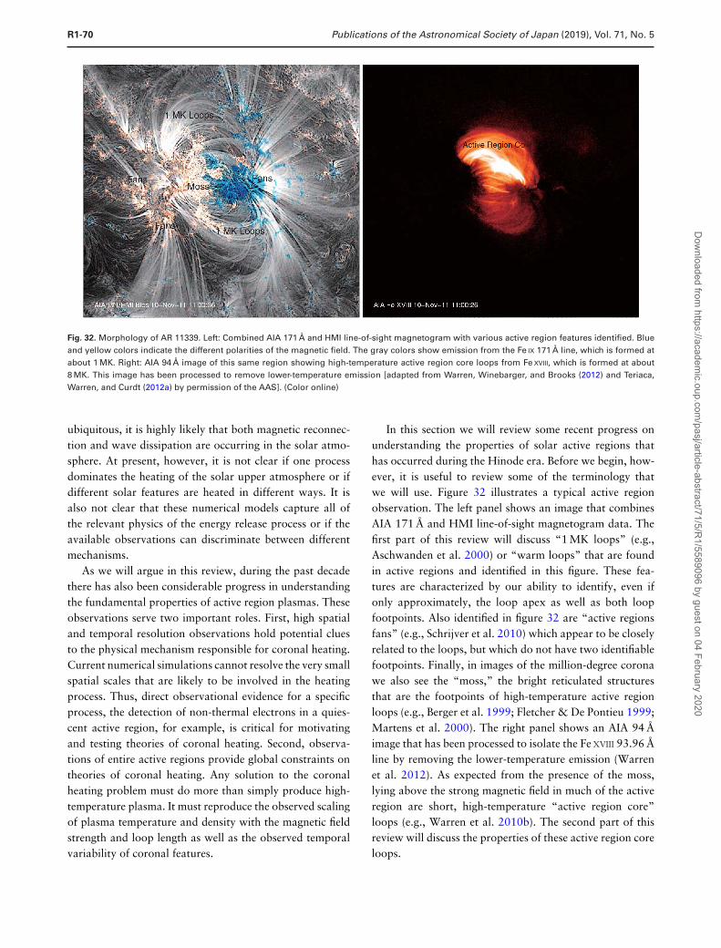
R1-70 Publications of the Astronomical Society of Japan (2019), Vol. 71, No. 5
Fig. 32. Morphology of AR 11339. Left: Combined AIA 171 A and HMI line-of-sight magnetogram with various active region features identified. Blueand yellow colors indicate the different polarities of the magnetic field. The gray colors show emission from the Fe IX 171 A line, which is formed atabout 1 MK. Right: AIA 94 A image of this same region showing high-temperature active region core loops from Fe XVIII, which is formed at about8 MK. This image has been processed to remove lower-temperature emission [adapted from Warren, Winebarger, and Brooks (2012) and Teriaca,Warren, and Curdt (2012a) by permission of the AAS]. (Color online)
ubiquitous, it is highly likely that both magnetic reconnec-tion and wave dissipation are occurring in the solar atmo-sphere. At present, however, it is not clear if one processdominates the heating of the solar upper atmosphere or ifdifferent solar features are heated in different ways. It isalso not clear that these numerical models capture all ofthe relevant physics of the energy release process or if theavailable observations can discriminate between differentmechanisms.
As we will argue in this review, during the past decadethere has also been considerable progress in understandingthe fundamental properties of active region plasmas. Theseobservations serve two important roles. First, high spatialand temporal resolution observations hold potential cluesto the physical mechanism responsible for coronal heating.Current numerical simulations cannot resolve the very smallspatial scales that are likely to be involved in the heatingprocess. Thus, direct observational evidence for a specificprocess, the detection of non-thermal electrons in a quies-cent active region, for example, is critical for motivatingand testing theories of coronal heating. Second, observa-tions of entire active regions provide global constraints ontheories of coronal heating. Any solution to the coronalheating problem must do more than simply produce high-temperature plasma. It must reproduce the observed scalingof plasma temperature and density with the magnetic fieldstrength and loop length as well as the observed temporalvariability of coronal features.
In this section we will review some recent progress onunderstanding the properties of solar active regions thathas occurred during the Hinode era. Before we begin, how-ever, it is useful to review some of the terminology thatwe will use. Figure 32 illustrates a typical active regionobservation. The left panel shows an image that combinesAIA 171 A and HMI line-of-sight magnetogram data. Thefirst part of this review will discuss “1 MK loops” (e.g.,Aschwanden et al. 2000) or “warm loops” that are foundin active regions and identified in this figure. These fea-tures are characterized by our ability to identify, even ifonly approximately, the loop apex as well as both loopfootpoints. Also identified in figure 32 are “active regionsfans” (e.g., Schrijver et al. 2010) which appear to be closelyrelated to the loops, but which do not have two identifiablefootpoints. Finally, in images of the million-degree coronawe also see the “moss,” the bright reticulated structuresthat are the footpoints of high-temperature active regionloops (e.g., Berger et al. 1999; Fletcher & De Pontieu 1999;Martens et al. 2000). The right panel shows an AIA 94 Aimage that has been processed to isolate the Fe XVIII 93.96 Aline by removing the lower-temperature emission (Warrenet al. 2012). As expected from the presence of the moss,lying above the strong magnetic field in much of the activeregion are short, high-temperature “active region core”loops (e.g., Warren et al. 2010b). The second part of thisreview will discuss the properties of these active region coreloops.
Dow
nloaded from https://academ
ic.oup.com/pasj/article-abstract/71/5/R
1/5589096 by guest on 04 February 2020
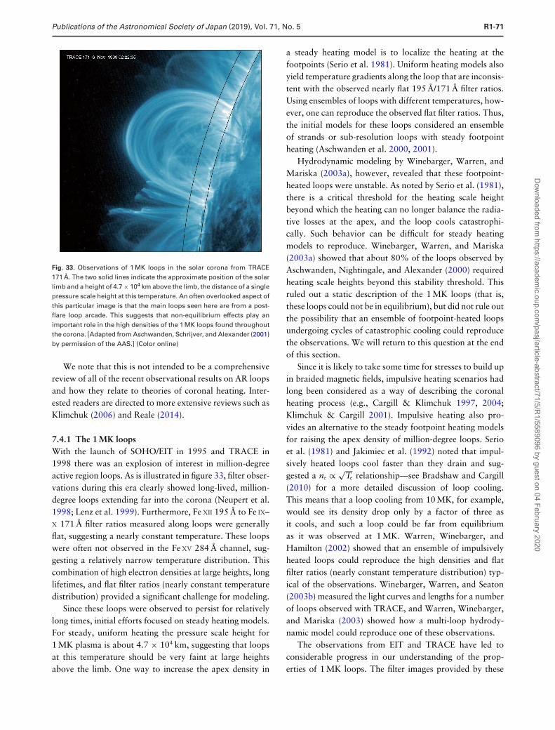
Publications of the Astronomical Society of Japan (2019), Vol. 71, No. 5 R1-71
Fig. 33. Observations of 1 MK loops in the solar corona from TRACE171 A. The two solid lines indicate the approximate position of the solarlimb and a height of 4.7 × 10⁴ km above the limb, the distance of a singlepressure scale height at this temperature. An often overlooked aspect ofthis particular image is that the main loops seen here are from a post-flare loop arcade. This suggests that non-equilibrium effects play animportant role in the high densities of the 1 MK loops found throughoutthe corona. [Adapted from Aschwanden, Schrijver, and Alexander (2001)by permission of the AAS.] (Color online)
We note that this is not intended to be a comprehensivereview of all of the recent observational results on AR loopsand how they relate to theories of coronal heating. Inter-ested readers are directed to more extensive reviews such asKlimchuk (2006) and Reale (2014).
7.4.1 The 1 MK loopsWith the launch of SOHO/EIT in 1995 and TRACE in1998 there was an explosion of interest in million-degreeactive region loops. As is illustrated in figure 33, filter obser-vations during this era clearly showed long-lived, million-degree loops extending far into the corona (Neupert et al.1998; Lenz et al. 1999). Furthermore, Fe XII 195 A to Fe IX–X 171 A filter ratios measured along loops were generallyflat, suggesting a nearly constant temperature. These loopswere often not observed in the Fe XV 284 A channel, sug-gesting a relatively narrow temperature distribution. Thiscombination of high electron densities at large heights, longlifetimes, and flat filter ratios (nearly constant temperaturedistribution) provided a significant challenge for modeling.
Since these loops were observed to persist for relativelylong times, initial efforts focused on steady heating models.For steady, uniform heating the pressure scale height for1 MK plasma is about 4.7 × 10⁴ km, suggesting that loopsat this temperature should be very faint at large heightsabove the limb. One way to increase the apex density in
a steady heating model is to localize the heating at thefootpoints (Serio et al. 1981). Uniform heating models alsoyield temperature gradients along the loop that are inconsis-tent with the observed nearly flat 195 A/171 A filter ratios.Using ensembles of loops with different temperatures, how-ever, one can reproduce the observed flat filter ratios. Thus,the initial models for these loops considered an ensembleof strands or sub-resolution loops with steady footpointheating (Aschwanden et al. 2000, 2001).
Hydrodynamic modeling by Winebarger, Warren, andMariska (2003a), however, revealed that these footpoint-heated loops were unstable. As noted by Serio et al. (1981),there is a critical threshold for the heating scale heightbeyond which the heating can no longer balance the radia-tive losses at the apex, and the loop cools catastrophi-cally. Such behavior can be difficult for steady heatingmodels to reproduce. Winebarger, Warren, and Mariska(2003a) showed that about 80% of the loops observed byAschwanden, Nightingale, and Alexander (2000) requiredheating scale heights beyond this stability threshold. Thisruled out a static description of the 1 MK loops (that is,these loops could not be in equilibrium), but did not rule outthe possibility that an ensemble of footpoint-heated loopsundergoing cycles of catastrophic cooling could reproducethe observations. We will return to this question at the endof this section.
Since it is likely to take some time for stresses to build upin braided magnetic fields, impulsive heating scenarios hadlong been considered as a way of describing the coronalheating process (e.g., Cargill & Klimchuk 1997, 2004;Klimchuk & Cargill 2001). Impulsive heating also pro-vides an alternative to the steady footpoint heating modelsfor raising the apex density of million-degree loops. Serioet al. (1981) and Jakimiec et al. (1992) noted that impul-sively heated loops cool faster than they drain and sug-gested a ne ∝ √
Te relationship—see Bradshaw and Cargill(2010) for a more detailed discussion of loop cooling.This means that a loop cooling from 10 MK, for example,would see its density drop only by a factor of three asit cools, and such a loop could be far from equilibriumas it was observed at 1 MK. Warren, Winebarger, andHamilton (2002) showed that an ensemble of impulsivelyheated loops could reproduce the high densities and flatfilter ratios (nearly constant temperature distribution) typ-ical of the observations. Winebarger, Warren, and Seaton(2003b) measured the light curves and lengths for a numberof loops observed with TRACE, and Warren, Winebarger,and Mariska (2003) showed how a multi-loop hydrody-namic model could reproduce one of these observations.
The observations from EIT and TRACE have led toconsiderable progress in our understanding of the prop-erties of 1 MK loops. The filter images provided by these
Dow
nloaded from https://academ
ic.oup.com/pasj/article-abstract/71/5/R
1/5589096 by guest on 04 February 2020
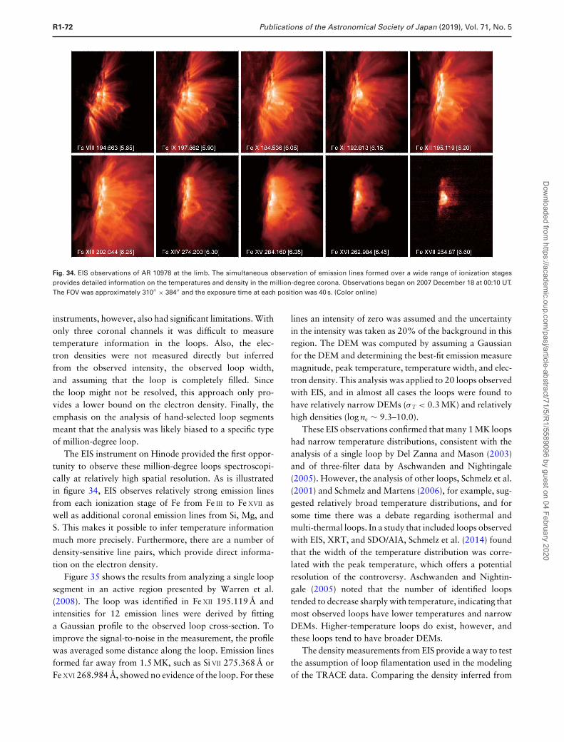
R1-72 Publications of the Astronomical Society of Japan (2019), Vol. 71, No. 5
Fig. 34. EIS observations of AR 10978 at the limb. The simultaneous observation of emission lines formed over a wide range of ionization stagesprovides detailed information on the temperatures and density in the million-degree corona. Observations began on 2007 December 18 at 00:10 UT.The FOV was approximately 310′′ × 384′′ and the exposure time at each position was 40 s. (Color online)
instruments, however, also had significant limitations. Withonly three coronal channels it was difficult to measuretemperature information in the loops. Also, the elec-tron densities were not measured directly but inferredfrom the observed intensity, the observed loop width,and assuming that the loop is completely filled. Sincethe loop might not be resolved, this approach only pro-vides a lower bound on the electron density. Finally, theemphasis on the analysis of hand-selected loop segmentsmeant that the analysis was likely biased to a specific typeof million-degree loop.
The EIS instrument on Hinode provided the first oppor-tunity to observe these million-degree loops spectroscopi-cally at relatively high spatial resolution. As is illustratedin figure 34, EIS observes relatively strong emission linesfrom each ionization stage of Fe from Fe III to Fe XVII aswell as additional coronal emission lines from Si, Mg, andS. This makes it possible to infer temperature informationmuch more precisely. Furthermore, there are a number ofdensity-sensitive line pairs, which provide direct informa-tion on the electron density.
Figure 35 shows the results from analyzing a single loopsegment in an active region presented by Warren et al.(2008). The loop was identified in Fe XII 195.119 A andintensities for 12 emission lines were derived by fittinga Gaussian profile to the observed loop cross-section. Toimprove the signal-to-noise in the measurement, the profilewas averaged some distance along the loop. Emission linesformed far away from 1.5 MK, such as Si VII 275.368 A orFe XVI 268.984 A, showed no evidence of the loop. For these
lines an intensity of zero was assumed and the uncertaintyin the intensity was taken as 20% of the background in thisregion. The DEM was computed by assuming a Gaussianfor the DEM and determining the best-fit emission measuremagnitude, peak temperature, temperature width, and elec-tron density. This analysis was applied to 20 loops observedwith EIS, and in almost all cases the loops were found tohave relatively narrow DEMs (σ T < 0.3 MK) and relativelyhigh densities (log ne ∼ 9.3–10.0).
These EIS observations confirmed that many 1 MK loopshad narrow temperature distributions, consistent with theanalysis of a single loop by Del Zanna and Mason (2003)and of three-filter data by Aschwanden and Nightingale(2005). However, the analysis of other loops, Schmelz et al.(2001) and Schmelz and Martens (2006), for example, sug-gested relatively broad temperature distributions, and forsome time there was a debate regarding isothermal andmulti-thermal loops. In a study that included loops observedwith EIS, XRT, and SDO/AIA, Schmelz et al. (2014) foundthat the width of the temperature distribution was corre-lated with the peak temperature, which offers a potentialresolution of the controversy. Aschwanden and Nightin-gale (2005) noted that the number of identified loopstended to decrease sharply with temperature, indicating thatmost observed loops have lower temperatures and narrowDEMs. Higher-temperature loops do exist, however, andthese loops tend to have broader DEMs.
The density measurements from EIS provide a way to testthe assumption of loop filamentation used in the modelingof the TRACE data. Comparing the density inferred from
Dow
nloaded from https://academ
ic.oup.com/pasj/article-abstract/71/5/R
1/5589096 by guest on 04 February 2020
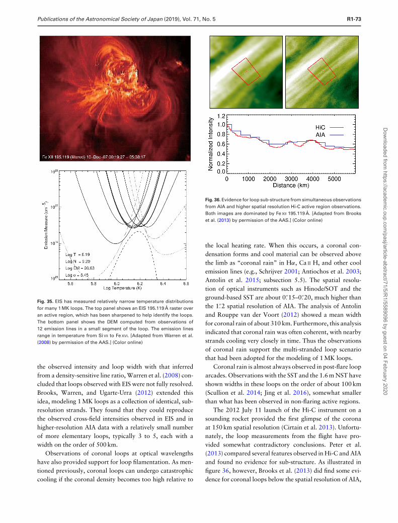
Publications of the Astronomical Society of Japan (2019), Vol. 71, No. 5 R1-73
Fig. 35. EIS has measured relatively narrow temperature distributionsfor many 1 MK loops. The top panel shows an EIS 195.119 A raster overan active region, which has been sharpened to help identify the loops.The bottom panel shows the DEM computed from observations of12 emission lines in a small segment of the loop. The emission linesrange in temperature from Si VII to Fe XVI. [Adapted from Warren et al.(2008) by permission of the AAS.] (Color online)
the observed intensity and loop width with that inferredfrom a density-sensitive line ratio, Warren et al. (2008) con-cluded that loops observed with EIS were not fully resolved.Brooks, Warren, and Ugarte-Urra (2012) extended thisidea, modeling 1 MK loops as a collection of identical, sub-resolution strands. They found that they could reproducethe observed cross-field intensities observed in EIS and inhigher-resolution AIA data with a relatively small numberof more elementary loops, typically 3 to 5, each with awidth on the order of 500 km.
Observations of coronal loops at optical wavelengthshave also provided support for loop filamentation. As men-tioned previously, coronal loops can undergo catastrophiccooling if the coronal density becomes too high relative to
Fig. 36. Evidence for loop sub-structure from simultaneous observationsfrom AIA and higher spatial resolution Hi-C active region observations.Both images are dominated by Fe XII 195.119 A. [Adapted from Brookset al. (2013) by permission of the AAS.] (Color online)
the local heating rate. When this occurs, a coronal con-densation forms and cool material can be observed abovethe limb as “coronal rain” in Hα, Ca II H, and other coolemission lines (e.g., Schrijver 2001; Antiochos et al. 2003;Antolin et al. 2015; subsection 5.5). The spatial resolu-tion of optical instruments such as Hinode/SOT and theground-based SST are about 0.′′15–0.′′20, much higher thanthe 1.′′2 spatial resolution of AIA. The analysis of Antolinand Rouppe van der Voort (2012) showed a mean widthfor coronal rain of about 310 km. Furthermore, this analysisindicated that coronal rain was often coherent, with nearbystrands cooling very closely in time. Thus the observationsof coronal rain support the multi-stranded loop scenariothat had been adopted for the modeling of 1 MK loops.
Coronal rain is almost always observed in post-flare looparcades. Observations with the SST and the 1.6 m NST haveshown widths in these loops on the order of about 100 km(Scullion et al. 2014; Jing et al. 2016), somewhat smallerthan what has been observed in non-flaring active regions.
The 2012 July 11 launch of the Hi-C instrument on asounding rocket provided the first glimpse of the coronaat 150 km spatial resolution (Cirtain et al. 2013). Unfortu-nately, the loop measurements from the flight have pro-vided somewhat contradictory conclusions. Peter et al.(2013) compared several features observed in Hi-C and AIAand found no evidence for sub-structure. As illustrated infigure 36, however, Brooks et al. (2013) did find some evi-dence for coronal loops below the spatial resolution of AIA,
Dow
nloaded from https://academ
ic.oup.com/pasj/article-abstract/71/5/R
1/5589096 by guest on 04 February 2020
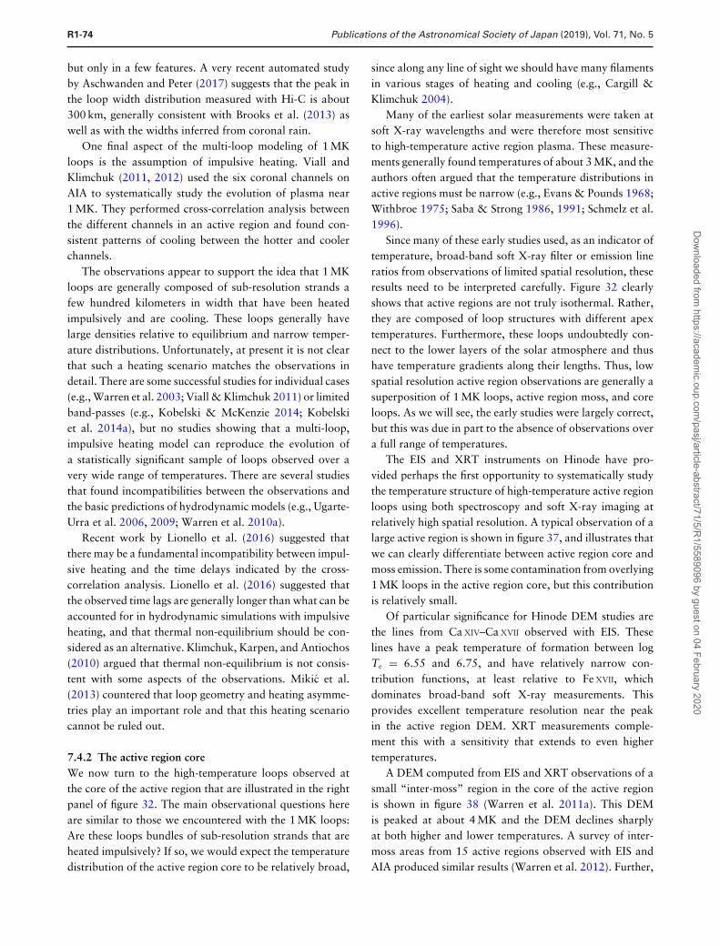
R1-74 Publications of the Astronomical Society of Japan (2019), Vol. 71, No. 5
but only in a few features. A very recent automated studyby Aschwanden and Peter (2017) suggests that the peak inthe loop width distribution measured with Hi-C is about300 km, generally consistent with Brooks et al. (2013) aswell as with the widths inferred from coronal rain.
One final aspect of the multi-loop modeling of 1 MKloops is the assumption of impulsive heating. Viall andKlimchuk (2011, 2012) used the six coronal channels onAIA to systematically study the evolution of plasma near1 MK. They performed cross-correlation analysis betweenthe different channels in an active region and found con-sistent patterns of cooling between the hotter and coolerchannels.
The observations appear to support the idea that 1 MKloops are generally composed of sub-resolution strands afew hundred kilometers in width that have been heatedimpulsively and are cooling. These loops generally havelarge densities relative to equilibrium and narrow temper-ature distributions. Unfortunately, at present it is not clearthat such a heating scenario matches the observations indetail. There are some successful studies for individual cases(e.g., Warren et al. 2003; Viall & Klimchuk 2011) or limitedband-passes (e.g., Kobelski & McKenzie 2014; Kobelskiet al. 2014a), but no studies showing that a multi-loop,impulsive heating model can reproduce the evolution ofa statistically significant sample of loops observed over avery wide range of temperatures. There are several studiesthat found incompatibilities between the observations andthe basic predictions of hydrodynamic models (e.g., Ugarte-Urra et al. 2006, 2009; Warren et al. 2010a).
Recent work by Lionello et al. (2016) suggested thatthere may be a fundamental incompatibility between impul-sive heating and the time delays indicated by the cross-correlation analysis. Lionello et al. (2016) suggested thatthe observed time lags are generally longer than what can beaccounted for in hydrodynamic simulations with impulsiveheating, and that thermal non-equilibrium should be con-sidered as an alternative. Klimchuk, Karpen, and Antiochos(2010) argued that thermal non-equilibrium is not consis-tent with some aspects of the observations. Mikic et al.(2013) countered that loop geometry and heating asymme-tries play an important role and that this heating scenariocannot be ruled out.
7.4.2 The active region coreWe now turn to the high-temperature loops observed atthe core of the active region that are illustrated in the rightpanel of figure 32. The main observational questions hereare similar to those we encountered with the 1 MK loops:Are these loops bundles of sub-resolution strands that areheated impulsively? If so, we would expect the temperaturedistribution of the active region core to be relatively broad,
since along any line of sight we should have many filamentsin various stages of heating and cooling (e.g., Cargill &Klimchuk 2004).
Many of the earliest solar measurements were taken atsoft X-ray wavelengths and were therefore most sensitiveto high-temperature active region plasma. These measure-ments generally found temperatures of about 3 MK, and theauthors often argued that the temperature distributions inactive regions must be narrow (e.g., Evans & Pounds 1968;Withbroe 1975; Saba & Strong 1986, 1991; Schmelz et al.1996).
Since many of these early studies used, as an indicator oftemperature, broad-band soft X-ray filter or emission lineratios from observations of limited spatial resolution, theseresults need to be interpreted carefully. Figure 32 clearlyshows that active regions are not truly isothermal. Rather,they are composed of loop structures with different apextemperatures. Furthermore, these loops undoubtedly con-nect to the lower layers of the solar atmosphere and thushave temperature gradients along their lengths. Thus, lowspatial resolution active region observations are generally asuperposition of 1 MK loops, active region moss, and coreloops. As we will see, the early studies were largely correct,but this was due in part to the absence of observations overa full range of temperatures.
The EIS and XRT instruments on Hinode have pro-vided perhaps the first opportunity to systematically studythe temperature structure of high-temperature active regionloops using both spectroscopy and soft X-ray imaging atrelatively high spatial resolution. A typical observation of alarge active region is shown in figure 37, and illustrates thatwe can clearly differentiate between active region core andmoss emission. There is some contamination from overlying1 MK loops in the active region core, but this contributionis relatively small.
Of particular significance for Hinode DEM studies arethe lines from Ca XIV–Ca XVII observed with EIS. Theselines have a peak temperature of formation between logTe = 6.55 and 6.75, and have relatively narrow con-tribution functions, at least relative to Fe XVII, whichdominates broad-band soft X-ray measurements. Thisprovides excellent temperature resolution near the peakin the active region DEM. XRT measurements comple-ment this with a sensitivity that extends to even highertemperatures.
A DEM computed from EIS and XRT observations of asmall “inter-moss” region in the core of the active regionis shown in figure 38 (Warren et al. 2011a). This DEMis peaked at about 4 MK and the DEM declines sharplyat both higher and lower temperatures. A survey of inter-moss areas from 15 active regions observed with EIS andAIA produced similar results (Warren et al. 2012). Further,
Dow
nloaded from https://academ
ic.oup.com/pasj/article-abstract/71/5/R
1/5589096 by guest on 04 February 2020
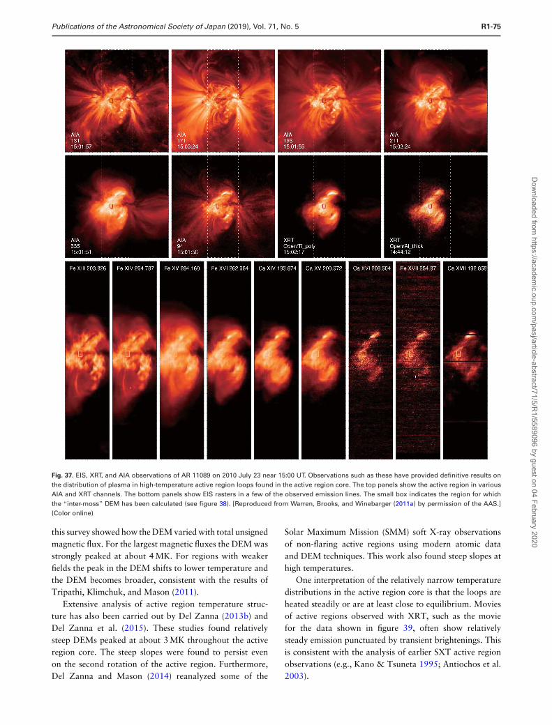
Publications of the Astronomical Society of Japan (2019), Vol. 71, No. 5 R1-75
Fig. 37. EIS, XRT, and AIA observations of AR 11089 on 2010 July 23 near 15:00 UT. Observations such as these have provided definitive results onthe distribution of plasma in high-temperature active region loops found in the active region core. The top panels show the active region in variousAIA and XRT channels. The bottom panels show EIS rasters in a few of the observed emission lines. The small box indicates the region for whichthe “inter-moss” DEM has been calculated (see figure 38). [Reproduced from Warren, Brooks, and Winebarger (2011a) by permission of the AAS.](Color online)
this survey showed how the DEM varied with total unsignedmagnetic flux. For the largest magnetic fluxes the DEM wasstrongly peaked at about 4 MK. For regions with weakerfields the peak in the DEM shifts to lower temperature andthe DEM becomes broader, consistent with the results ofTripathi, Klimchuk, and Mason (2011).
Extensive analysis of active region temperature struc-ture has also been carried out by Del Zanna (2013b) andDel Zanna et al. (2015). These studies found relativelysteep DEMs peaked at about 3 MK throughout the activeregion core. The steep slopes were found to persist evenon the second rotation of the active region. Furthermore,Del Zanna and Mason (2014) reanalyzed some of the
Solar Maximum Mission (SMM) soft X-ray observationsof non-flaring active regions using modern atomic dataand DEM techniques. This work also found steep slopes athigh temperatures.
One interpretation of the relatively narrow temperaturedistributions in the active region core is that the loops areheated steadily or are at least close to equilibrium. Moviesof active regions observed with XRT, such as the moviefor the data shown in figure 39, often show relativelysteady emission punctuated by transient brightenings. Thisis consistent with the analysis of earlier SXT active regionobservations (e.g., Kano & Tsuneta 1995; Antiochos et al.2003).
Dow
nloaded from https://academ
ic.oup.com/pasj/article-abstract/71/5/R
1/5589096 by guest on 04 February 2020
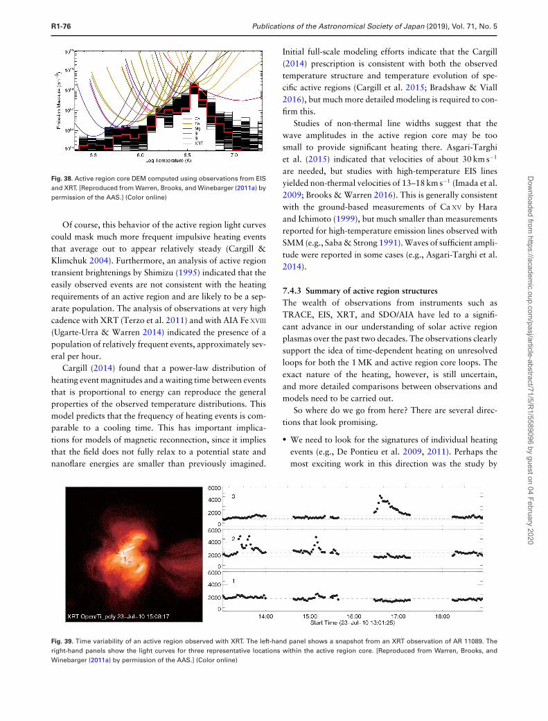
R1-76 Publications of the Astronomical Society of Japan (2019), Vol. 71, No. 5
Fig. 38. Active region core DEM computed using observations from EISand XRT. [Reproduced from Warren, Brooks, and Winebarger (2011a) bypermission of the AAS.] (Color online)
Of course, this behavior of the active region light curvescould mask much more frequent impulsive heating eventsthat average out to appear relatively steady (Cargill &Klimchuk 2004). Furthermore, an analysis of active regiontransient brightenings by Shimizu (1995) indicated that theeasily observed events are not consistent with the heatingrequirements of an active region and are likely to be a sep-arate population. The analysis of observations at very highcadence with XRT (Terzo et al. 2011) and with AIA Fe XVIII
(Ugarte-Urra & Warren 2014) indicated the presence of apopulation of relatively frequent events, approximately sev-eral per hour.
Cargill (2014) found that a power-law distribution ofheating event magnitudes and a waiting time between eventsthat is proportional to energy can reproduce the generalproperties of the observed temperature distributions. Thismodel predicts that the frequency of heating events is com-parable to a cooling time. This has important implica-tions for models of magnetic reconnection, since it impliesthat the field does not fully relax to a potential state andnanoflare energies are smaller than previously imagined.
Initial full-scale modeling efforts indicate that the Cargill(2014) prescription is consistent with both the observedtemperature structure and temperature evolution of spe-cific active regions (Cargill et al. 2015; Bradshaw & Viall2016), but much more detailed modeling is required to con-firm this.
Studies of non-thermal line widths suggest that thewave amplitudes in the active region core may be toosmall to provide significant heating there. Asgari-Targhiet al. (2015) indicated that velocities of about 30 km s−1
are needed, but studies with high-temperature EIS linesyielded non-thermal velocities of 13–18 km s−1 (Imada et al.2009; Brooks & Warren 2016). This is generally consistentwith the ground-based measurements of Ca XV by Haraand Ichimoto (1999), but much smaller than measurementsreported for high-temperature emission lines observed withSMM (e.g., Saba & Strong 1991). Waves of sufficient ampli-tude were reported in some cases (e.g., Asgari-Targhi et al.2014).
7.4.3 Summary of active region structuresThe wealth of observations from instruments such asTRACE, EIS, XRT, and SDO/AIA have led to a signifi-cant advance in our understanding of solar active regionplasmas over the past two decades. The observations clearlysupport the idea of time-dependent heating on unresolvedloops for both the 1 MK and active region core loops. Theexact nature of the heating, however, is still uncertain,and more detailed comparisons between observations andmodels need to be carried out.
So where do we go from here? There are several direc-tions that look promising.
� We need to look for the signatures of individual heatingevents (e.g., De Pontieu et al. 2009, 2011). Perhaps themost exciting work in this direction was the study by
Fig. 39. Time variability of an active region observed with XRT. The left-hand panel shows a snapshot from an XRT observation of AR 11089. Theright-hand panels show the light curves for three representative locations within the active region core. [Reproduced from Warren, Brooks, andWinebarger (2011a) by permission of the AAS.] (Color online)
Dow
nloaded from https://academ
ic.oup.com/pasj/article-abstract/71/5/R
1/5589096 by guest on 04 February 2020
Publications of the Astronomical Society of Japan (2019), Vol. 71, No. 5 R1-77
Testa et al. (2013, 2014), who showed that instrumentssuch as HiC and IRIS appear to have the cadence andspatial resolution necessary to isolate and follow the evo-lution of very small-scale heating events in the solar upperatmosphere.
� We need to improve our ability to extrapolate photo-spheric magnetic field measurements into the corona. Ithas long been recognized that the heating of the solaratmosphere is intimately related to the magnetic field, butwe still cannot adequately describe how the field interactswith the complex environment of the solar chromosphereand forms the observed topology of the corona (e.g.,De Rosa et al. 2009).
� We need to routinely resolve and follow what are cur-rently unresolved loops using both imaging and spec-troscopy over the full range of temperatures. The directobservations of loops with Hi-C, observations of coronalrain with optical instruments, and the indirect evidencefrom modeling indicate that a spatial resolution of about150 km with a cadence of a few seconds, and simulta-neous coverage of the photosphere, chromosphere, tran-sition region, and corona, should be sufficient to resolvethese loops.
8 Flares and coronal mass ejections
8.1 Flare energy build-up: Theory andobservations
8.1.1 IntroductionIt is generally accepted that solar flares, prominence erup-tions, and CMEs are different manifestations of a singlephysical process thought to be powered by the release ofmagnetic free energy stored in the corona prior to the activ-ities. Storage of magnetic free energy requires non-potentialmagnetic fields, and it is therefore associated with shear ortwist in the coronal fields away from the potential, current-free state (Priest & Forbes 2002). There are two groupsof competing models for the pre-eruption magnetic con-figuration. One group assumes that a twisted flux rope ispresent in the region above the polarity inversion line (PIL)on the photosphere (Forbes & Isenberg 1991; Wu et al.1997; Gibson & Low 1998; Krall et al. 2000; Roussevet al. 2003). The other group begins with an untwisted,but highly sheared, magnetic field (Mikic & Linker 1994;Antiochos et al. 1999a; Amari et al. 2003; Manchester2003). In both cases, the flux rope or the sheared arcadeis held down by the tension of the overlying coronalarcade.
The free energy can build up as a result of the emergenceof sheared magnetic fields from below the photosphere(Leka et al. 1996; Schrijver et al. 2005; Schrijver 2007),
shearing motions or rotations of the photospheric foot-points (Gesztelyi 1984; Zirin & Wang 1990), and the can-celation of flux in the photosphere (Martin et al. 1985; Liviet al. 1989). How can we explain the long-duration energystorage phase, lasting from a few days to a few weeks?Is the flux rope pre-existing or produced during eruption?Is the magnetic free energy already contained in the pre-emergence flux, and are there any contributions from thedifferential rotation or convective flows? Is the rotation ofa sunspot driven by the Lorentz force of the sunspot’s mag-netic field itself? To address these key questions we need tostudy the evolution of the highly non-potential region priorto, during, and after the flares. During the past decade, lotsof progress has been made on flare energy storage based onHinode observations.
8.1.2 Hinode observationsShortly after launch, Hinode took excellent observationsof one large active region, NOAA 10930, which produceda series of X-class flares. Observations made by XRT andSOT aboard Hinode suggested that the gradual formationof the non-potential magnetic fields in this active regionwas caused by the rotation and west-to-east motion of anemerging sunspot (Su et al. 2007; see figures 40 and 41).Min and Chae (2009) found that the positive-polaritysunspot rotated counterclockwise about its center by 540
◦
from 2006 December 10 to 14, and the increase in the rota-tion speed was closely related to the growth of the sunspot.The analysis suggested that the rotation of the sunspotmay have been closely related to the dynamic developmentof an emerging twisted flux tube. Ravindra, Yoshimura,and Dasso (2011) found that the positive-polarity sunspotrotated about 260
◦in the last three days, while the negative-
polarity sunspot did not complete rotation of more than 20◦
in five days starting from 2006 December 9. The negative-polarity sunspot changed its direction of rotation five timesover five days and injected both positive and negative typesof spin helicity flux into the corona. The observed reversalin the sign of spinning and braiding helicity flux may havebeen the signature of the emergence of a twisted flux tubepossessing the writhe of opposite signs, which is consis-tent with the findings of Tiwari (2009). Zhang, Kitai, andTakizawa (2012a) found that the main contribution tohelicity accumulation came from the flux emergence effect,while the dynamic transient evolution came from the shuf-fling motion effect. The observational results further indi-cated that for AR 10930 the apparent rotational motionin the following sunspot was the real shuffling motion onthe solar surface. Harra et al. (2009) found an increase inthe coronal spectral line widths observed by EIS, begin-ning after the time of saturation of the injected helicity asmeasured by Magara and Tsuneta (2008). In addition, this
Dow
nloaded from https://academ
ic.oup.com/pasj/article-abstract/71/5/R
1/5589096 by guest on 04 February 2020
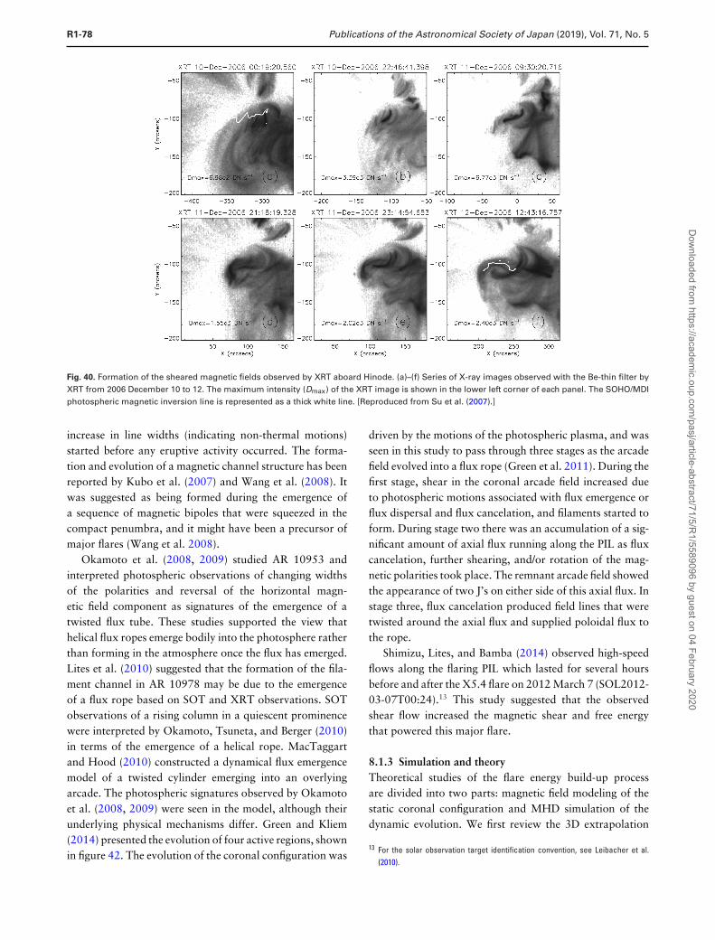
R1-78 Publications of the Astronomical Society of Japan (2019), Vol. 71, No. 5
Fig. 40. Formation of the sheared magnetic fields observed by XRT aboard Hinode. (a)–(f) Series of X-ray images observed with the Be-thin filter byXRT from 2006 December 10 to 12. The maximum intensity (Dmax) of the XRT image is shown in the lower left corner of each panel. The SOHO/MDIphotospheric magnetic inversion line is represented as a thick white line. [Reproduced from Su et al. (2007).]
increase in line widths (indicating non-thermal motions)started before any eruptive activity occurred. The forma-tion and evolution of a magnetic channel structure has beenreported by Kubo et al. (2007) and Wang et al. (2008). Itwas suggested as being formed during the emergence ofa sequence of magnetic bipoles that were squeezed in thecompact penumbra, and it might have been a precursor ofmajor flares (Wang et al. 2008).
Okamoto et al. (2008, 2009) studied AR 10953 andinterpreted photospheric observations of changing widthsof the polarities and reversal of the horizontal magn-etic field component as signatures of the emergence of atwisted flux tube. These studies supported the view thathelical flux ropes emerge bodily into the photosphere ratherthan forming in the atmosphere once the flux has emerged.Lites et al. (2010) suggested that the formation of the fila-ment channel in AR 10978 may be due to the emergenceof a flux rope based on SOT and XRT observations. SOTobservations of a rising column in a quiescent prominencewere interpreted by Okamoto, Tsuneta, and Berger (2010)in terms of the emergence of a helical rope. MacTaggartand Hood (2010) constructed a dynamical flux emergencemodel of a twisted cylinder emerging into an overlyingarcade. The photospheric signatures observed by Okamotoet al. (2008, 2009) were seen in the model, although theirunderlying physical mechanisms differ. Green and Kliem(2014) presented the evolution of four active regions, shownin figure 42. The evolution of the coronal configuration was
driven by the motions of the photospheric plasma, and wasseen in this study to pass through three stages as the arcadefield evolved into a flux rope (Green et al. 2011). During thefirst stage, shear in the coronal arcade field increased dueto photospheric motions associated with flux emergence orflux dispersal and flux cancelation, and filaments started toform. During stage two there was an accumulation of a sig-nificant amount of axial flux running along the PIL as fluxcancelation, further shearing, and/or rotation of the mag-netic polarities took place. The remnant arcade field showedthe appearance of two J’s on either side of this axial flux. Instage three, flux cancelation produced field lines that weretwisted around the axial flux and supplied poloidal flux tothe rope.
Shimizu, Lites, and Bamba (2014) observed high-speedflows along the flaring PIL which lasted for several hoursbefore and after the X5.4 flare on 2012 March 7 (SOL2012-03-07T00:24).13 This study suggested that the observedshear flow increased the magnetic shear and free energythat powered this major flare.
8.1.3 Simulation and theoryTheoretical studies of the flare energy build-up processare divided into two parts: magnetic field modeling of thestatic coronal configuration and MHD simulation of thedynamic evolution. We first review the 3D extrapolation
13 For the solar observation target identification convention, see Leibacher et al.(2010).
Dow
nloaded from https://academ
ic.oup.com/pasj/article-abstract/71/5/R
1/5589096 by guest on 04 February 2020
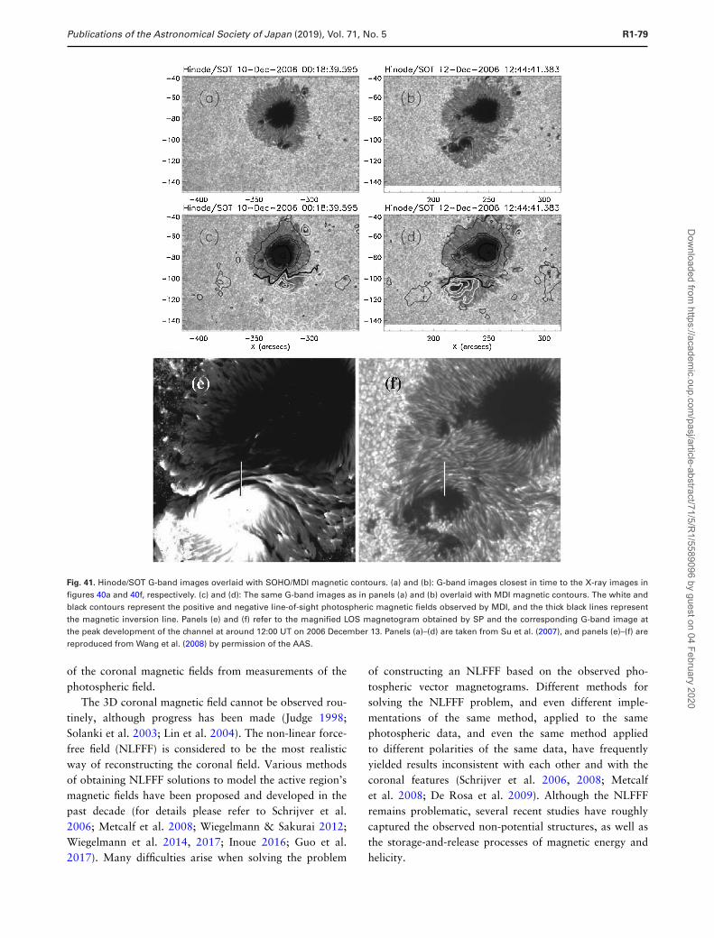
Publications of the Astronomical Society of Japan (2019), Vol. 71, No. 5 R1-79
Fig. 41. Hinode/SOT G-band images overlaid with SOHO/MDI magnetic contours. (a) and (b): G-band images closest in time to the X-ray images infigures 40a and 40f, respectively. (c) and (d): The same G-band images as in panels (a) and (b) overlaid with MDI magnetic contours. The white andblack contours represent the positive and negative line-of-sight photospheric magnetic fields observed by MDI, and the thick black lines representthe magnetic inversion line. Panels (e) and (f) refer to the magnified LOS magnetogram obtained by SP and the corresponding G-band image atthe peak development of the channel at around 12:00 UT on 2006 December 13. Panels (a)–(d) are taken from Su et al. (2007), and panels (e)–(f) arereproduced from Wang et al. (2008) by permission of the AAS.
of the coronal magnetic fields from measurements of thephotospheric field.
The 3D coronal magnetic field cannot be observed rou-tinely, although progress has been made (Judge 1998;Solanki et al. 2003; Lin et al. 2004). The non-linear force-free field (NLFFF) is considered to be the most realisticway of reconstructing the coronal field. Various methodsof obtaining NLFFF solutions to model the active region’smagnetic fields have been proposed and developed in thepast decade (for details please refer to Schrijver et al.2006; Metcalf et al. 2008; Wiegelmann & Sakurai 2012;Wiegelmann et al. 2014, 2017; Inoue 2016; Guo et al.2017). Many difficulties arise when solving the problem
of constructing an NLFFF based on the observed pho-tospheric vector magnetograms. Different methods forsolving the NLFFF problem, and even different imple-mentations of the same method, applied to the samephotospheric data, and even the same method appliedto different polarities of the same data, have frequentlyyielded results inconsistent with each other and with thecoronal features (Schrijver et al. 2006, 2008; Metcalfet al. 2008; De Rosa et al. 2009). Although the NLFFFremains problematic, several recent studies have roughlycaptured the observed non-potential structures, as well asthe storage-and-release processes of magnetic energy andhelicity.
Dow
nloaded from https://academ
ic.oup.com/pasj/article-abstract/71/5/R
1/5589096 by guest on 04 February 2020
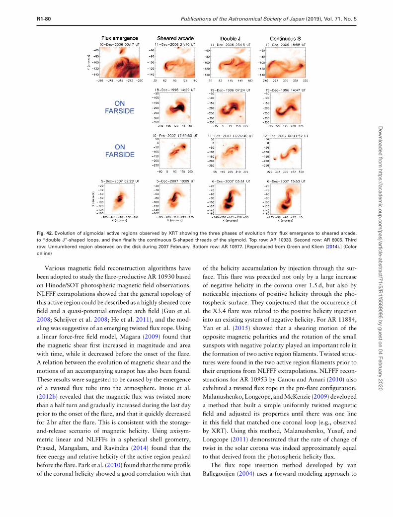
R1-80 Publications of the Astronomical Society of Japan (2019), Vol. 71, No. 5
Fig. 42. Evolution of sigmoidal active regions observed by XRT showing the three phases of evolution from flux emergence to sheared arcade,to “double J”-shaped loops, and then finally the continuous S-shaped threads of the sigmoid. Top row: AR 10930. Second row: AR 8005. Thirdrow: Unnumbered region observed on the disk during 2007 February. Bottom row: AR 10977. [Reproduced from Green and Kliem (2014).] (Coloronline)
Various magnetic field reconstruction algorithms havebeen adopted to study the flare-productive AR 10930 basedon Hinode/SOT photospheric magnetic field observations.NLFFF extrapolations showed that the general topology ofthis active region could be described as a highly sheared corefield and a quasi-potential envelope arch field (Guo et al.2008; Schrijver et al. 2008; He et al. 2011), and the mod-eling was suggestive of an emerging twisted flux rope. Usinga linear force-free field model, Magara (2009) found thatthe magnetic shear first increased in magnitude and areawith time, while it decreased before the onset of the flare.A relation between the evolution of magnetic shear and themotions of an accompanying sunspot has also been found.These results were suggested to be caused by the emergenceof a twisted flux tube into the atmosphere. Inoue et al.(2012b) revealed that the magnetic flux was twisted morethan a half turn and gradually increased during the last dayprior to the onset of the flare, and that it quickly decreasedfor 2 hr after the flare. This is consistent with the storage-and-release scenario of magnetic helicity. Using axisym-metric linear and NLFFFs in a spherical shell geometry,Prasad, Mangalam, and Ravindra (2014) found that thefree energy and relative helicity of the active region peakedbefore the flare. Park et al. (2010) found that the time profileof the coronal helicity showed a good correlation with that
of the helicity accumulation by injection through the sur-face. This flare was preceded not only by a large increaseof negative helicity in the corona over 1.5 d, but also bynoticeable injections of positive helicity through the pho-tospheric surface. They conjectured that the occurrence ofthe X3.4 flare was related to the positive helicity injectioninto an existing system of negative helicity. For AR 11884,Yan et al. (2015) showed that a shearing motion of theopposite magnetic polarities and the rotation of the smallsunspots with negative polarity played an important role inthe formation of two active region filaments. Twisted struc-tures were found in the two active region filaments prior totheir eruptions from NLFFF extrapolations. NLFFF recon-structions for AR 10953 by Canou and Amari (2010) alsoexhibited a twisted flux rope in the pre-flare configuration.Malanushenko, Longcope, and McKenzie (2009) developeda method that built a simple uniformly twisted magneticfield and adjusted its properties until there was one linein this field that matched one coronal loop (e.g., observedby XRT). Using this method, Malanushenko, Yusuf, andLongcope (2011) demonstrated that the rate of change oftwist in the solar corona was indeed approximately equalto that derived from the photospheric helicity flux.
The flux rope insertion method developed by vanBallegooijen (2004) uses a forward modeling approach to
Dow
nloaded from https://academ
ic.oup.com/pasj/article-abstract/71/5/R
1/5589096 by guest on 04 February 2020
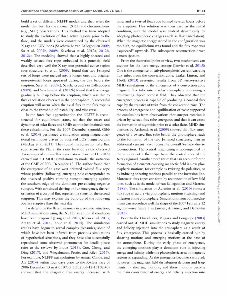
Publications of the Astronomical Society of Japan (2019), Vol. 71, No. 5 R1-81
build a set of different NLFFF models and then select themodel that best fits the coronal (XRT) and chromospheric(e.g., SOT) observations. This method has been adoptedto study the evolution of three active regions prior to theflare, and the models were constrained by the observedX-ray and EUV loops (Savcheva & van Ballegooijen 2009;Su et al. 2009b, 2009c; Savcheva et al. 2012a, 2012b,2012c). The modeling showed that a highly sheared andweakly twisted flux rope embedded in a potential fielddescribed very well the X-ray non-potential active regioncore structure. Su et al. (2009c) found that two J-shapedsets of loops were merged into a longer one, and brighternon-potential loops appeared during the day before theeruption. Su et al. (2009c), Savcheva and van Ballegooijen(2009), and Savcheva et al. (2012b) found that free energygradually built up before the eruption, which was due toflux cancelation observed in the photosphere. A successfuleruption will occur when the axial flux in the flux rope isclose to the threshold of instability, and vice versa.
In the force-free approximation the NLFFF is recon-structed for equilibrium states, so that the onset anddynamics of solar flares and CMEs cannot be obtained fromthese calculations. For the 2007 December sigmoid, Gibbet al. (2014) performed a simulation using magnetofric-tional techniques driven by observed LOS magnetograms(Mackay et al. 2011). They found the formation of a fluxrope across the PIL at the same location as the observedX-ray sigmoid during flux cancelation. Fan (2011, 2016)carried out 3D MHD simulations to model the initiationof the CME of 2006 December 13. The author found thatthe emergence of an east–west-oriented twisted flux ropewhose positive (following) emerging pole corresponded tothe observed positive rotating sunspot emerging againstthe southern edge of the dominant pre-existing negativesunspot. With continued driving of flux emergence, the ref-ormation of a coronal flux rope set the stage for the seconderuption. This may explain the build-up of the followingX-class eruptive flare the next day.
To determine the flare dynamics in a realistic situation,MHD simulations using the NLFFF as an initial conditionhave been proposed (Jiang et al. 2013; Kliem et al. 2013;Amari et al. 2014; Inoue et al. 2014). The simulationresults have begun to reveal complex dynamics, some ofwhich have not been inferred from previous simulationsof hypothetical situations, and they have also successfullyreproduced some observed phenomena; for details pleaserefer to the reviews by Inoue (2016), Guo, Cheng, andDing (2017), and Wiegelmann, Petrie, and Riley (2017).For example, NLFFF extrapolations by Amari, Canou, andAly (2014) within four days prior to the X-class flare of2006 December 13 in AR 10930 (SOL2006-12-13T02:40)showed that the magnetic free energy increased with
time, and a twisted flux rope formed several hours beforethe eruption. This solution was then used as the initialcondition, and the model was evolved dynamically byadopting photospheric changes (such as flux cancelation).When the magnetic energy stored in the configuration wastoo high, no equilibrium was found and the flux rope was“squeezed” upwards. The subsequent reconnection drovea mass ejection.
From the theoretical point of view, two mechanisms canaccount for the flare energy storage (Janvier et al. 2015):One is the emergence of sub-photospheric current-carryingflux tubes from the convection zone. Leake, Linton, andTorok (2013) presented results from 3D visco-resistiveMHD simulations of the emergence of a convection zonemagnetic flux tube into a solar atmosphere containing apre-existing dipole coronal field. They observed that theemergence process is capable of producing a coronal fluxrope by the transfer of twist from the convection zone. Theprocess of emergence and equilibration of twist supportedthe conclusions from observations that sunspot rotation isdriven by twisted flux tube emergence and that it can causethe formation of sigmoids prior to a solar flare. MHD sim-ulations by Archontis et al. (2009) showed that flux emer-gence of a twisted flux tube below the photosphere leadsto the formation of the two J-shaped structures, then anadditional current layer forms the overall S-shape due toreconnection. The central brightening is accompanied bythe eruption of a flux rope from the central area of theX-ray sigmoid. Another mechanism that can account for theformation of a current-carrying magnetic field is slow pho-tospheric motions, for example by twisting the polarities, orby inducing shearing motions parallel to the inversion line.Moreover, flux ropes can form by reconnection of low fieldlines, such as in the model of van Ballegooijen and Martens(1989). The simulation of Aulanier et al. (2010) forms aflux rope structure via photospheric motions (twisting) anddiffusion at the photosphere. Simulations from both mecha-nisms can reproduce well the shape of the 2007 February 12sigmoid—see figure 5 in Janvier, Aulanier, and Demoulin(2015).
Prior to the Hinode era, Magara and Longcope (2003)carried out 3D MHD simulations to study magnetic energyand helicity injection into the atmosphere as a result offlux emergence. This process is basically carried out byshearing motions and emerging motions at the base ofthe atmosphere. During the early phase of emergence,the emerging motions play a dominant role in injectingenergy and helicity while the photospheric area of magneticregions is expanding. As the emergence becomes saturated,however, the magnetic field distribution deforms and frag-ments by shearing motions, and these motions becomethe main contributor of energy and helicity injection into
Dow
nloaded from https://academ
ic.oup.com/pasj/article-abstract/71/5/R
1/5589096 by guest on 04 February 2020
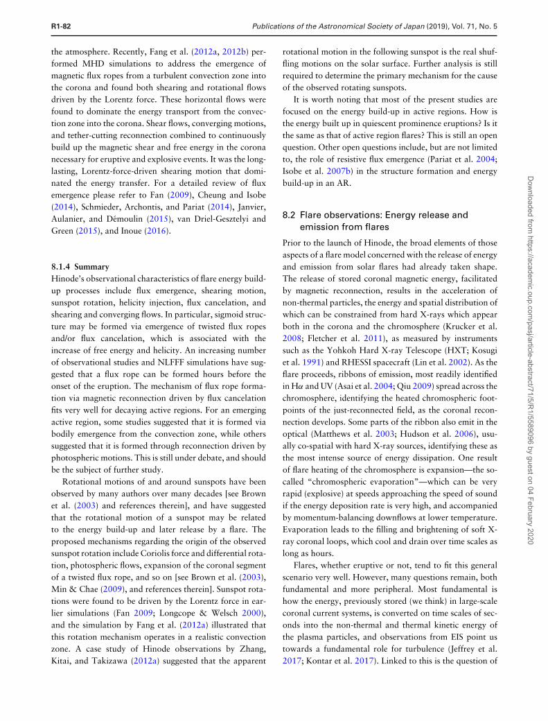
R1-82 Publications of the Astronomical Society of Japan (2019), Vol. 71, No. 5
the atmosphere. Recently, Fang et al. (2012a, 2012b) per-formed MHD simulations to address the emergence ofmagnetic flux ropes from a turbulent convection zone intothe corona and found both shearing and rotational flowsdriven by the Lorentz force. These horizontal flows werefound to dominate the energy transport from the convec-tion zone into the corona. Shear flows, converging motions,and tether-cutting reconnection combined to continuouslybuild up the magnetic shear and free energy in the coronanecessary for eruptive and explosive events. It was the long-lasting, Lorentz-force-driven shearing motion that domi-nated the energy transfer. For a detailed review of fluxemergence please refer to Fan (2009), Cheung and Isobe(2014), Schmieder, Archontis, and Pariat (2014), Janvier,Aulanier, and Demoulin (2015), van Driel-Gesztelyi andGreen (2015), and Inoue (2016).
8.1.4 SummaryHinode’s observational characteristics of flare energy build-up processes include flux emergence, shearing motion,sunspot rotation, helicity injection, flux cancelation, andshearing and converging flows. In particular, sigmoid struc-ture may be formed via emergence of twisted flux ropesand/or flux cancelation, which is associated with theincrease of free energy and helicity. An increasing numberof observational studies and NLFFF simulations have sug-gested that a flux rope can be formed hours before theonset of the eruption. The mechanism of flux rope forma-tion via magnetic reconnection driven by flux cancelationfits very well for decaying active regions. For an emergingactive region, some studies suggested that it is formed viabodily emergence from the convection zone, while otherssuggested that it is formed through reconnection driven byphotospheric motions. This is still under debate, and shouldbe the subject of further study.
Rotational motions of and around sunspots have beenobserved by many authors over many decades [see Brownet al. (2003) and references therein], and have suggestedthat the rotational motion of a sunspot may be relatedto the energy build-up and later release by a flare. Theproposed mechanisms regarding the origin of the observedsunspot rotation include Coriolis force and differential rota-tion, photospheric flows, expansion of the coronal segmentof a twisted flux rope, and so on [see Brown et al. (2003),Min & Chae (2009), and references therein]. Sunspot rota-tions were found to be driven by the Lorentz force in ear-lier simulations (Fan 2009; Longcope & Welsch 2000),and the simulation by Fang et al. (2012a) illustrated thatthis rotation mechanism operates in a realistic convectionzone. A case study of Hinode observations by Zhang,Kitai, and Takizawa (2012a) suggested that the apparent
rotational motion in the following sunspot is the real shuf-fling motions on the solar surface. Further analysis is stillrequired to determine the primary mechanism for the causeof the observed rotating sunspots.
It is worth noting that most of the present studies arefocused on the energy build-up in active regions. How isthe energy built up in quiescent prominence eruptions? Is itthe same as that of active region flares? This is still an openquestion. Other open questions include, but are not limitedto, the role of resistive flux emergence (Pariat et al. 2004;Isobe et al. 2007b) in the structure formation and energybuild-up in an AR.
8.2 Flare observations: Energy release andemission from flares
Prior to the launch of Hinode, the broad elements of thoseaspects of a flare model concerned with the release of energyand emission from solar flares had already taken shape.The release of stored coronal magnetic energy, facilitatedby magnetic reconnection, results in the acceleration ofnon-thermal particles, the energy and spatial distribution ofwhich can be constrained from hard X-rays which appearboth in the corona and the chromosphere (Krucker et al.2008; Fletcher et al. 2011), as measured by instrumentssuch as the Yohkoh Hard X-ray Telescope (HXT; Kosugiet al. 1991) and RHESSI spacecraft (Lin et al. 2002). As theflare proceeds, ribbons of emission, most readily identifiedin Hα and UV (Asai et al. 2004; Qiu 2009) spread across thechromosphere, identifying the heated chromospheric foot-points of the just-reconnected field, as the coronal recon-nection develops. Some parts of the ribbon also emit in theoptical (Matthews et al. 2003; Hudson et al. 2006), usu-ally co-spatial with hard X-ray sources, identifying these asthe most intense source of energy dissipation. One resultof flare heating of the chromosphere is expansion—the so-called “chromospheric evaporation”—which can be veryrapid (explosive) at speeds approaching the speed of soundif the energy deposition rate is very high, and accompaniedby momentum-balancing downflows at lower temperature.Evaporation leads to the filling and brightening of soft X-ray coronal loops, which cool and drain over time scales aslong as hours.
Flares, whether eruptive or not, tend to fit this generalscenario very well. However, many questions remain, bothfundamental and more peripheral. Most fundamental ishow the energy, previously stored (we think) in large-scalecoronal current systems, is converted on time scales of sec-onds into the non-thermal and thermal kinetic energy ofthe plasma particles, and observations from EIS point ustowards a fundamental role for turbulence (Jeffrey et al.2017; Kontar et al. 2017). Linked to this is the question of
Dow
nloaded from https://academ
ic.oup.com/pasj/article-abstract/71/5/R
1/5589096 by guest on 04 February 2020
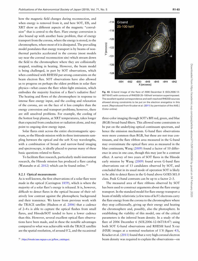
Publications of the Astronomical Society of Japan (2019), Vol. 71, No. 5 R1-83
how the magnetic field changes during reconnection, andwhen energy is removed from it, and here SOT, EIS, andXRT show us different aspects of the magnetic “convul-sion” that is central to the flare. Flare energy conversion isalso bound up with another basic problem, that of energytransport from the corona, where the energy is stored, to thechromosphere, where most of it is dissipated. The prevailingmodel postulates that energy transport is by beams of non-thermal particles accelerated in the corona (most modelssay near the coronal reconnection site) which stream downthe field to the chromosphere where they are collisionallystopped, resulting in heating. However, the beam modelis being challenged, in part by SOT observations, whichwhen combined with RHESSI put strong constraints on thebeam electron flux. SOT observations have also allowedus to progress on perhaps the oldest problem in solar flarephysics—what causes the flare white-light emission, whichembodies the majority fraction of a flare’s radiative flux?The heating and flows of the chromosphere in response tointense flare energy input, and the cooling and relaxationof the corona, are on the face of it less complex than theenergy conversion and transport problems; however, thereare still unsolved problems. For example, the cooling ofthe hottest loop plasma, at XRT temperatures, takes longerthan expected from conduction or radiation alone, and maypoint to ongoing slow energy input.
Solar flares emit across the entire electromagnetic spec-trum, so the Hinode mission with its three instruments sam-pling between the optical and the soft X-ray wavelengths,with a combination of broad- and narrow-band imagingand spectroscopy, is ideally placed to pursue many of thesebasic questions related to flares.
To facilitate flare research, particularly multi-instrumentresearch, the Hinode mission has produced a flare catalog(Watanabe et al. 2012) which can be found online.14
8.2.1 Optical measurementsAs is well known, the first observations of a solar flare weremade in the optical (Carrington 1859), which is where themajority of a solar flare’s energy is released. It is, however,difficult to detect flares in the optical because of their rel-atively low contrast against the photospheric backgroundand their transience. We know from previous work withthe TRACE satellite (Hudson et al. 2006) that a cadenceof 2–4 s is able to capture the optical flashes from smallflares, and Hinode/SOT tended to have a lower cadencethan this. However, several excellent optical flare observa-tions have been made, and in these the notable advantagescompared to what was achievable with the TRACE satelliteare the spatial resolution, of around 0.′′2, and the occasional
14 〈https://hinode.isee.nagoya-u.ac.jp/flare_catalogue〉.
Fig. 43. G-band image of the flare of 2006 December 6 (SOL2006-12-06T18:47) with contours of RHESSI 25–100 keV emission superimposed.The excellent spatial correspondence and well-resolved RHESSI sourcesallowed strong constraints to be put on the electron energetics in thisevent. [Reproduced from Krucker et al. (2011) by permission of the AAS.](Color online)
three-color imaging through SOT’s BFI red, green, and blue(RGB) broad-band filters. This allowed some constraints tobe put on the underlying optical continuum spectrum, andhence the emission mechanism. G-band flare observationswere more common than RGB, but these are not true con-tinuum, and the flare ribbon area measured in the G-bandmay overestimate the optical flare area as measured in theblue continuum; Wang (2009) found a factor of 10 differ-ence in area in one case, though this may just be a contrasteffect. A survey of two years of SOT flares in the Hinodeearly mission by Wang (2009) found seven G-band flareobservations out of 13 candidates observed by SOT, andconcluded that in its usual mode of operation SOT is likelyto be able to detect flares in the G-band above GOES M1.0class. Peak G-band contrasts can be up to a factor 2–3.
The measured area of flare ribbons observed by SOThas been used to construct arguments about the flare energytransport. In the standard model for flare energy transport abeam of mildly relativistic (a few tens of keV) electrons carrythe flare energy from the corona to the chromosphere wherethey stop collisionally, giving up their energy and heatingthe chromosphere and, possibly, also the photosphere. Inestablishing the viability of this model, one of the criticalparameters is the inferred beam density. In a study of theflare of 2006 December 6 (SOL2006-12-06T18:47) usingboth SOT G-band observations and RHESSI hard X-ray(HXR) images at a nominal resolution of 1.′′8 (figure 43),Krucker et al. (2011) found that a very high coronal electronbeam density was required to explain the observations—on
Dow
nloaded from https://academ
ic.oup.com/pasj/article-abstract/71/5/R
1/5589096 by guest on 04 February 2020
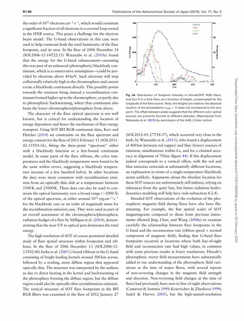
R1-84 Publications of the Astronomical Society of Japan (2019), Vol. 71, No. 5
the order of 1020 electrons cm−2 s−1, which would constitutea significant fraction of all electrons in a coronal loop rootedin the HXR source. This poses a challenge for the electronbeam model. The G-band observations in this case wereused to help constrain both the total luminosity of the flarefootpoint, and its area. In the flare of 2006 December 14(SOL2006-12-14T22:15) Watanabe et al. (2010a) foundthat the energy for the G-band enhancement—assumingthis was part of an enhanced (photospheric) blackbody con-tinuum, which is a conservative assumption—could be pro-vided by electrons above 40 keV. Such electrons will stopcollisionally relatively high in the chromosphere and cannotexcite a blackbody continuum directly. This possibly pointstowards the emission being instead a recombination con-tinuum formed higher up in the chromosphere, or partly dueto photospheric backwarming, where that continuum alsoheats the lower chromosphere/photosphere from above.
The character of the flare optical spectrum is not wellknown, but is critical for understanding the location ofenergy deposition and hence the mechanism of flare energytransport. Using SOT-BFI RGB continuum data, Kerr andFletcher (2014) set constraints on the flare spectrum andenergy content for the flare of 2011 February 15 (SOL2011-02-15T01:56), fitting the three-point “spectrum” eitherwith a blackbody function or a free-bound continuummodel. In some parts of the flare ribbons, the color tem-peratures and the blackbody temperature were found to bethe same within errors, suggesting a blackbody tempera-ture increase of a few hundred kelvin. In other locationsthe data were more consistent with recombination emis-sion from an optically-thin slab at a temperature between5500 K and 25000 K. These data can also be used to con-strain the optical luminosity over a broad range (∼2000 A)of the optical spectrum, at either around 1026 erg cm−2 s−1
for the blackbody case or an order of magnitude more forthe recombination emission case. They were used as part ofan overall assessment of the chromospheric/photosphericradiation budget of a flare by Milligan et al. (2014), demon-strating that the near-UV to optical part dominates the totalenergy.
The high resolution of SOT of course permitted detailedstudy of flare spatial structure within footpoints and rib-bons. In the flare of 2006 December 13 (SOL2006-12-13T02:40) Isobe et al. (2007c) found ribbons in the G-bandconsisting of bright leading kernels around 500 km across,followed by a trailing, more diffuse region that appearedoptically thin. The structure was interpreted by the authorsas due to direct heating in the kernel and backwarming ofthe photosphere forming the diffuse region, but the diffuseregion could also be optically-thin recombination emission.The vertical structure of SOT flare footpoints in the BFIRGB filters was examined in the flare of 2012 January 27
Fig. 44. Distribution of footpoint intensity in Hinode/SOT RGB filters,and Ca II H in a limb flare, as a function of height, compensated for thelongitude of the flare source. Note, the heights are relative; the absolutelocation of the photosphere (τ500 = 1) does not correspond to the zeropoint. The offset between peaks suggests that the different color opticalsources are primarily formed at different altitudes. [Reproduced fromWatanabe et al. (2013) by permission of the AAS.] (Color online)
(SOL2012-01-27T18:37), which occurred very close to thelimb, by Watanabe et al. (2013), who found a displacementof 400 km between red (upper) and blue (lower) sources ofemission, simultaneous within 6 s, and for a claimed accu-racy in alignment of 70 km (figure 44). If this displacementindeed corresponds to a vertical offset, with the red andblue emission centroids at substantially different locations,an explanation in terms of a single-temperature blackbodyseems unlikely. Arguments about the absolute location forthese SOT sources are unfortunately still indirect, relying oninferences from the quiet Sun, but future radiation hydro-dynamics modeling will help here (sub-subsection 8.2.4).
Detailed SOT observations of the evolution of the pho-tospheric magnetic field during flares have also been illu-minating. For example, the fine spatial scales of SOTmagnetograms compared to those from previous instru-ments allowed Jing, Chae, and Wang (2008a) to examinecarefully the relationship between flare footpoints in theG band and the reconnection rate (ribbon speed × normalcomponent of magnetic field), finding that G-band flarefootpoints occurred at locations where both line-of-sightfield and reconnection rate had high values, in commonwith some previous results at lower resolutions. Hinode’sphotospheric vector field measurements have substantiallyadded to our understanding of the photospheric field vari-ations at the time of major flares, with several reportsof non-reversing changes in the magnetic field strengthand direction. Non-reversing field changes at the time offlares had previously been seen in line-of-sight observations(Cameron & Sammis 1999; Kosovichev & Zharkova 1999;Sudol & Harvey 2005), but the high-spatial-resolution
Dow
nloaded from https://academ
ic.oup.com/pasj/article-abstract/71/5/R
1/5589096 by guest on 04 February 2020
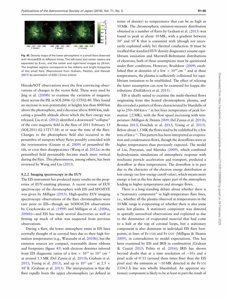
Publications of the Astronomical Society of Japan (2019), Vol. 71, No. 5 R1-85
Fig. 45. Density maps of the lower atmosphere in a small flare observedwith Hinode/EIS at different times. The left-hand and center rasters areseparated by 8 min, and the center and right-hand images by 29 min.The brightest regions correspond to the ribbons and bright footpointsof this small flare. [Reproduced from Graham, Fletcher, and Hannah(2011) by permission of ESO.] (Color online)
Hinode/SOT observations were the first convincing obser-vations of changes in the vector field. These were used byJing et al. (2008b) to examine the variation of magneticshear across the PIL in SOL2006-12-13T02:40. They foundan increase in non-potentiality at heights less than 8000 kmabove the photosphere, and a decrease above 8000 km, indi-cating a possible altitude above which the flare energy wasreleased. Liu et al. (2012) identified a downward “collapse”of the core magnetic field in the flare of 2011 February 13(SOL2011-02-13T17:38) at or near the time of the flare.Changes to the photospheric field also occurred in thepenumbra of sunspots where flares possibly coincided withthe reorientation (Gosain et al. 2009) of penumbral fib-rils, or even their disappearance (Wang et al. 2012a) as thepenumbral field presumably became much more verticalduring the flare. This phenomenon, among others, has beenreviewed by Wang and Liu (2015).
8.2.2 Imaging spectroscopy in the EUVThe EIS instrument has produced many results on the prop-erties of EUV-emitting plasmas. A recent review of EUVspectroscopy of the chromosphere with EIS and SDO/EVEwas given by Milligan (2015). High-quality EUV imagingspectroscopy observations of the flare chromosphere wererare prior to EIS—though see SOHO/CDS observationsby Czaykowska et al. (1999) and Milligan et al. (2006a,2006b)—and EIS has made several discoveries as well asfirming up much of what was suspected from previousobservations.
During a flare, the lower atmosphere emits in EIS linesnormally thought of as coronal lines due to their high for-mation temperatures (e.g., Watanabe et al. 2010b), but theemission sources are compact, reasonably dense ribbonsand footpoints (figure 45) with electron densities inferredfrom EIS diagnostic ratios of a few × 1010 to 1011 cm−3
at around 1.5 MK (Del Zanna et al. 2011b; Graham et al.2011; Young et al. 2013), and up to 1012 cm−3 at 2.5 ×10⁵ K (Graham et al. 2015). The interpretation is that theflare rapidly heats the upper chromosphere (as defined in
terms of density) to temperatures that can be as high as10 MK. The chromospheric emission-measure distributionobtained in a number of flares by Graham et al. (2013) wasfound to peak at about 10 MK, with a gradient between105 and 107 K that is consistent with (though not neces-sarily explained solely by) thermal conduction. It must berecalled that standard EUV density diagnostics assume equi-librium ionization and Maxwell–Boltzmann distributionsof electrons; both of these assumptions must be questionedunder flare conditions. However, Bradshaw (2009) estab-lished that at densities of a few × 1010 cm−3 and at thesetemperatures, the plasma is sufficiently collisional for equi-librium ionization to be established. The effect of relaxingthe latter assumption can now be examined for kappa dis-tributions (Dzifcakova et al. 2015).
EIS is ideally suited to examine the multi-thermal flowsoriginating from this heated chromospheric plasma, andthis revealed a pattern of flows characterized by blueshifts ofup to 250–300 km s−1 in hot lines (temperature of peak for-mation �2 MK), with the flow speed increasing with tem-perature (Milligan & Dennis 2009; Del Zanna et al. 2011b;Brosius 2013; Doschek et al. 2013; Young et al. 2013).Below about 1.5 MK the flows tend to be redshifted by a fewtens of km s−1. This pattern has been interpreted as evapora-tion and condensation flows, though the downflows were athigher temperatures than previously expected. The modelof Liu, Petrosian, and Mariska (2009), which combinedhydrodynamic simulations of atmospheric response withstochastic particle acceleration and transport, predicted adownflow at these temperatures. The downflow is in partdue to the character of the electron energy distribution atlow energy (no low-energy cutoff value), which means moreenergy is lost in the less dense upper part of the atmosphereleading to higher temperatures and stronger flows.
There is a long-standing debate about whether there isa “stationary component” in high-temperature flare lines,i.e., whether all the plasma observed at temperatures in the10 MK range is evaporating or whether there is also somestatic hot plasma. A stationary component was detectedin spatially unresolved observations and explained as dueto the dominance of evaporated material that had cometo a halt at the top of coronal loops, but a stationarycomponent is also dominant in individual EIS flare foot-points, in lines of Fe XXIII and Fe XXIV (Milligan & Dennis2009), in contradiction to model expectations. This hasbeen examined by EIS and IRIS in combination (Graham& Cauzzi 2015; Polito et al. 2016); IRIS has shownbeyond doubt that at a time resolution of ∼10 s and apixel scale of 0.′′33 (around three times finer than the EISpixel size) the emission at ∼10 MK detected in the Fe XXI
1354.1 A line was wholly blueshifted. An apparent sta-tionary component is likely to be at least in part the result of
Dow
nloaded from https://academ
ic.oup.com/pasj/article-abstract/71/5/R
1/5589096 by guest on 04 February 2020
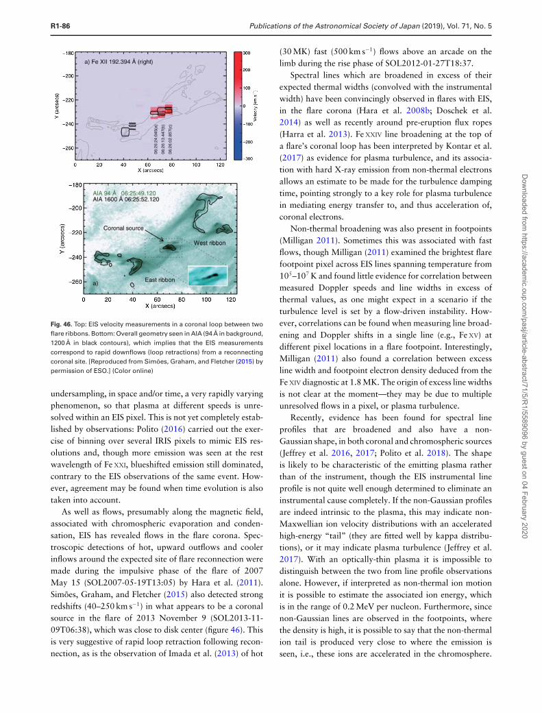
R1-86 Publications of the Astronomical Society of Japan (2019), Vol. 71, No. 5
Fig. 46. Top: EIS velocity measurements in a coronal loop between twoflare ribbons. Bottom: Overall geometry seen in AIA (94 A in background,1200 A in black contours), which implies that the EIS measurementscorrespond to rapid downflows (loop retractions) from a reconnectingcoronal site. [Reproduced from Simoes, Graham, and Fletcher (2015) bypermission of ESO.] (Color online)
undersampling, in space and/or time, a very rapidly varyingphenomenon, so that plasma at different speeds is unre-solved within an EIS pixel. This is not yet completely estab-lished by observations: Polito (2016) carried out the exer-cise of binning over several IRIS pixels to mimic EIS res-olutions and, though more emission was seen at the restwavelength of Fe XXI, blueshifted emission still dominated,contrary to the EIS observations of the same event. How-ever, agreement may be found when time evolution is alsotaken into account.
As well as flows, presumably along the magnetic field,associated with chromospheric evaporation and conden-sation, EIS has revealed flows in the flare corona. Spec-troscopic detections of hot, upward outflows and coolerinflows around the expected site of flare reconnection weremade during the impulsive phase of the flare of 2007May 15 (SOL2007-05-19T13:05) by Hara et al. (2011).Simoes, Graham, and Fletcher (2015) also detected strongredshifts (40–250 km s−1) in what appears to be a coronalsource in the flare of 2013 November 9 (SOL2013-11-09T06:38), which was close to disk center (figure 46). Thisis very suggestive of rapid loop retraction following recon-nection, as is the observation of Imada et al. (2013) of hot
(30 MK) fast (500 km s−1) flows above an arcade on thelimb during the rise phase of SOL2012-01-27T18:37.
Spectral lines which are broadened in excess of theirexpected thermal widths (convolved with the instrumentalwidth) have been convincingly observed in flares with EIS,in the flare corona (Hara et al. 2008b; Doschek et al.2014) as well as recently around pre-eruption flux ropes(Harra et al. 2013). Fe XXIV line broadening at the top ofa flare’s coronal loop has been interpreted by Kontar et al.(2017) as evidence for plasma turbulence, and its associa-tion with hard X-ray emission from non-thermal electronsallows an estimate to be made for the turbulence dampingtime, pointing strongly to a key role for plasma turbulencein mediating energy transfer to, and thus acceleration of,coronal electrons.
Non-thermal broadening was also present in footpoints(Milligan 2011). Sometimes this was associated with fastflows, though Milligan (2011) examined the brightest flarefootpoint pixel across EIS lines spanning temperature from105–107 K and found little evidence for correlation betweenmeasured Doppler speeds and line widths in excess ofthermal values, as one might expect in a scenario if theturbulence level is set by a flow-driven instability. How-ever, correlations can be found when measuring line broad-ening and Doppler shifts in a single line (e.g., Fe XV) atdifferent pixel locations in a flare footpoint. Interestingly,Milligan (2011) also found a correlation between excessline width and footpoint electron density deduced from theFe XIV diagnostic at 1.8 MK. The origin of excess line widthsis not clear at the moment—they may be due to multipleunresolved flows in a pixel, or plasma turbulence.
Recently, evidence has been found for spectral lineprofiles that are broadened and also have a non-Gaussian shape, in both coronal and chromospheric sources(Jeffrey et al. 2016, 2017; Polito et al. 2018). The shapeis likely to be characteristic of the emitting plasma ratherthan of the instrument, though the EIS instrumental lineprofile is not quite well enough determined to eliminate aninstrumental cause completely. If the non-Gaussian profilesare indeed intrinsic to the plasma, this may indicate non-Maxwellian ion velocity distributions with an acceleratedhigh-energy “tail” (they are fitted well by kappa distribu-tions), or it may indicate plasma turbulence (Jeffrey et al.2017). With an optically-thin plasma it is impossible todistinguish between the two from line profile observationsalone. However, if interpreted as non-thermal ion motionit is possible to estimate the associated ion energy, whichis in the range of 0.2 MeV per nucleon. Furthermore, sincenon-Gaussian lines are observed in the footpoints, wherethe density is high, it is possible to say that the non-thermalion tail is produced very close to where the emission isseen, i.e., these ions are accelerated in the chromosphere.
Dow
nloaded from https://academ
ic.oup.com/pasj/article-abstract/71/5/R
1/5589096 by guest on 04 February 2020
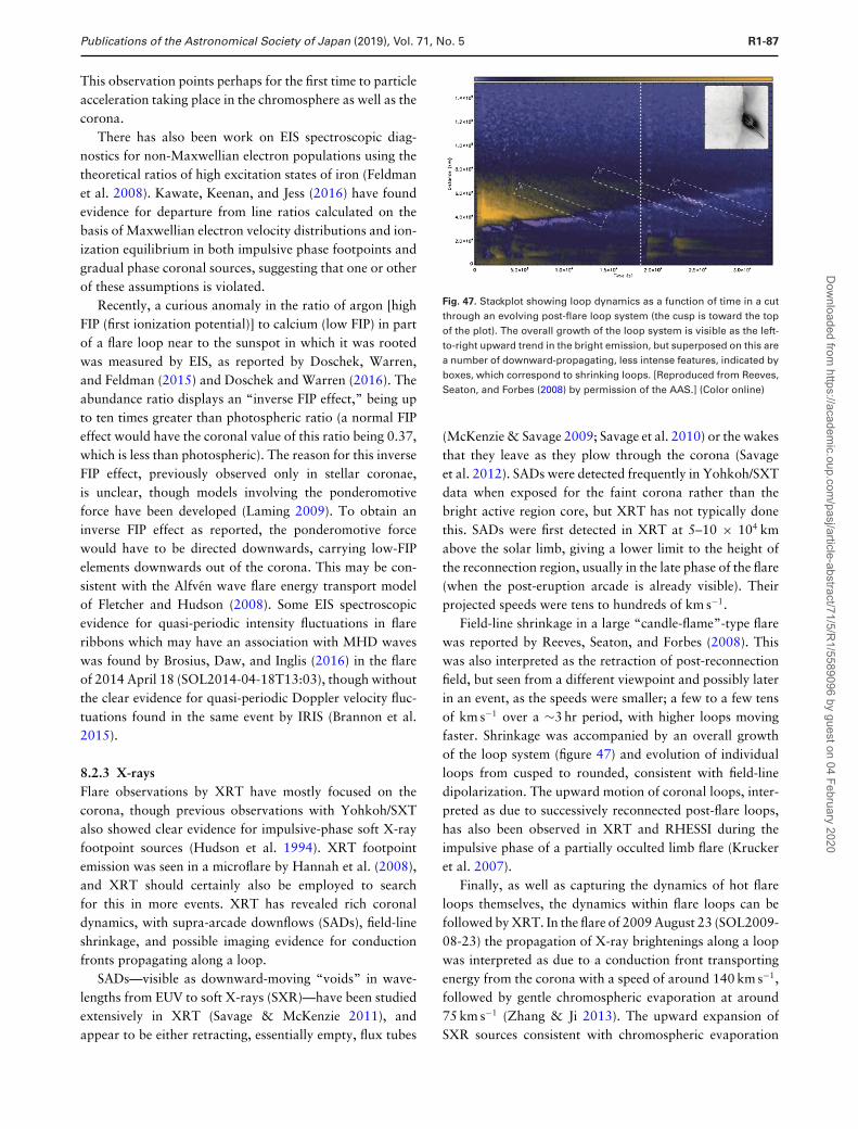
Publications of the Astronomical Society of Japan (2019), Vol. 71, No. 5 R1-87
This observation points perhaps for the first time to particleacceleration taking place in the chromosphere as well as thecorona.
There has also been work on EIS spectroscopic diag-nostics for non-Maxwellian electron populations using thetheoretical ratios of high excitation states of iron (Feldmanet al. 2008). Kawate, Keenan, and Jess (2016) have foundevidence for departure from line ratios calculated on thebasis of Maxwellian electron velocity distributions and ion-ization equilibrium in both impulsive phase footpoints andgradual phase coronal sources, suggesting that one or otherof these assumptions is violated.
Recently, a curious anomaly in the ratio of argon [highFIP (first ionization potential)] to calcium (low FIP) in partof a flare loop near to the sunspot in which it was rootedwas measured by EIS, as reported by Doschek, Warren,and Feldman (2015) and Doschek and Warren (2016). Theabundance ratio displays an “inverse FIP effect,” being upto ten times greater than photospheric ratio (a normal FIPeffect would have the coronal value of this ratio being 0.37,which is less than photospheric). The reason for this inverseFIP effect, previously observed only in stellar coronae,is unclear, though models involving the ponderomotiveforce have been developed (Laming 2009). To obtain aninverse FIP effect as reported, the ponderomotive forcewould have to be directed downwards, carrying low-FIPelements downwards out of the corona. This may be con-sistent with the Alfven wave flare energy transport modelof Fletcher and Hudson (2008). Some EIS spectroscopicevidence for quasi-periodic intensity fluctuations in flareribbons which may have an association with MHD waveswas found by Brosius, Daw, and Inglis (2016) in the flareof 2014 April 18 (SOL2014-04-18T13:03), though withoutthe clear evidence for quasi-periodic Doppler velocity fluc-tuations found in the same event by IRIS (Brannon et al.2015).
8.2.3 X-raysFlare observations by XRT have mostly focused on thecorona, though previous observations with Yohkoh/SXTalso showed clear evidence for impulsive-phase soft X-rayfootpoint sources (Hudson et al. 1994). XRT footpointemission was seen in a microflare by Hannah et al. (2008),and XRT should certainly also be employed to searchfor this in more events. XRT has revealed rich coronaldynamics, with supra-arcade downflows (SADs), field-lineshrinkage, and possible imaging evidence for conductionfronts propagating along a loop.
SADs—visible as downward-moving “voids” in wave-lengths from EUV to soft X-rays (SXR)—have been studiedextensively in XRT (Savage & McKenzie 2011), andappear to be either retracting, essentially empty, flux tubes
Fig. 47. Stackplot showing loop dynamics as a function of time in a cutthrough an evolving post-flare loop system (the cusp is toward the topof the plot). The overall growth of the loop system is visible as the left-to-right upward trend in the bright emission, but superposed on this area number of downward-propagating, less intense features, indicated byboxes, which correspond to shrinking loops. [Reproduced from Reeves,Seaton, and Forbes (2008) by permission of the AAS.] (Color online)
(McKenzie & Savage 2009; Savage et al. 2010) or the wakesthat they leave as they plow through the corona (Savageet al. 2012). SADs were detected frequently in Yohkoh/SXTdata when exposed for the faint corona rather than thebright active region core, but XRT has not typically donethis. SADs were first detected in XRT at 5–10 × 104 kmabove the solar limb, giving a lower limit to the height ofthe reconnection region, usually in the late phase of the flare(when the post-eruption arcade is already visible). Theirprojected speeds were tens to hundreds of km s−1.
Field-line shrinkage in a large “candle-flame”-type flarewas reported by Reeves, Seaton, and Forbes (2008). Thiswas also interpreted as the retraction of post-reconnectionfield, but seen from a different viewpoint and possibly laterin an event, as the speeds were smaller; a few to a few tensof km s−1 over a ∼3 hr period, with higher loops movingfaster. Shrinkage was accompanied by an overall growthof the loop system (figure 47) and evolution of individualloops from cusped to rounded, consistent with field-linedipolarization. The upward motion of coronal loops, inter-preted as due to successively reconnected post-flare loops,has also been observed in XRT and RHESSI during theimpulsive phase of a partially occulted limb flare (Kruckeret al. 2007).
Finally, as well as capturing the dynamics of hot flareloops themselves, the dynamics within flare loops can befollowed by XRT. In the flare of 2009 August 23 (SOL2009-08-23) the propagation of X-ray brightenings along a loopwas interpreted as due to a conduction front transportingenergy from the corona with a speed of around 140 km s−1,followed by gentle chromospheric evaporation at around75 km s−1 (Zhang & Ji 2013). The upward expansion ofSXR sources consistent with chromospheric evaporation
Dow
nloaded from https://academ
ic.oup.com/pasj/article-abstract/71/5/R
1/5589096 by guest on 04 February 2020
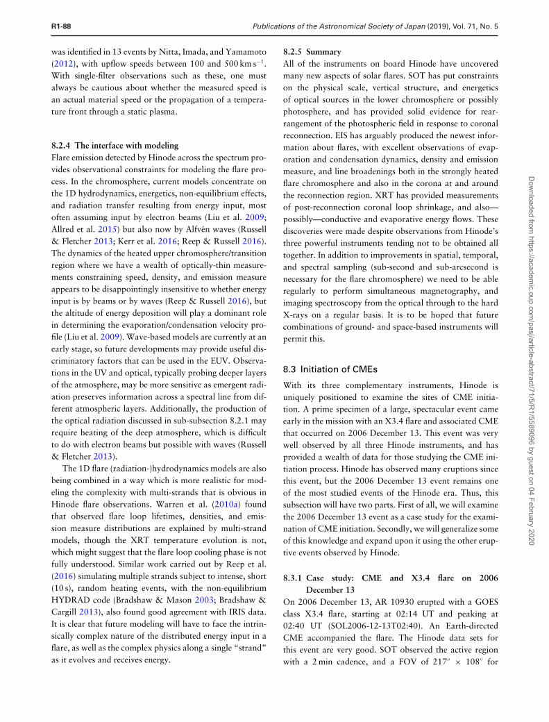
R1-88 Publications of the Astronomical Society of Japan (2019), Vol. 71, No. 5
was identified in 13 events by Nitta, Imada, and Yamamoto(2012), with upflow speeds between 100 and 500 km s−1.With single-filter observations such as these, one mustalways be cautious about whether the measured speed isan actual material speed or the propagation of a tempera-ture front through a static plasma.
8.2.4 The interface with modelingFlare emission detected by Hinode across the spectrum pro-vides observational constraints for modeling the flare pro-cess. In the chromosphere, current models concentrate onthe 1D hydrodynamics, energetics, non-equilibrium effects,and radiation transfer resulting from energy input, mostoften assuming input by electron beams (Liu et al. 2009;Allred et al. 2015) but also now by Alfven waves (Russell& Fletcher 2013; Kerr et al. 2016; Reep & Russell 2016).The dynamics of the heated upper chromosphere/transitionregion where we have a wealth of optically-thin measure-ments constraining speed, density, and emission measureappears to be disappointingly insensitive to whether energyinput is by beams or by waves (Reep & Russell 2016), butthe altitude of energy deposition will play a dominant rolein determining the evaporation/condensation velocity pro-file (Liu et al. 2009). Wave-based models are currently at anearly stage, so future developments may provide useful dis-criminatory factors that can be used in the EUV. Observa-tions in the UV and optical, typically probing deeper layersof the atmosphere, may be more sensitive as emergent radi-ation preserves information across a spectral line from dif-ferent atmospheric layers. Additionally, the production ofthe optical radiation discussed in sub-subsection 8.2.1 mayrequire heating of the deep atmosphere, which is difficultto do with electron beams but possible with waves (Russell& Fletcher 2013).
The 1D flare (radiation-)hydrodynamics models are alsobeing combined in a way which is more realistic for mod-eling the complexity with multi-strands that is obvious inHinode flare observations. Warren et al. (2010a) foundthat observed flare loop lifetimes, densities, and emis-sion measure distributions are explained by multi-strandmodels, though the XRT temperature evolution is not,which might suggest that the flare loop cooling phase is notfully understood. Similar work carried out by Reep et al.(2016) simulating multiple strands subject to intense, short(10 s), random heating events, with the non-equilibriumHYDRAD code (Bradshaw & Mason 2003; Bradshaw &Cargill 2013), also found good agreement with IRIS data.It is clear that future modeling will have to face the intrin-sically complex nature of the distributed energy input in aflare, as well as the complex physics along a single “strand”as it evolves and receives energy.
8.2.5 SummaryAll of the instruments on board Hinode have uncoveredmany new aspects of solar flares. SOT has put constraintson the physical scale, vertical structure, and energeticsof optical sources in the lower chromosphere or possiblyphotosphere, and has provided solid evidence for rear-rangement of the photospheric field in response to coronalreconnection. EIS has arguably produced the newest infor-mation about flares, with excellent observations of evap-oration and condensation dynamics, density and emissionmeasure, and line broadenings both in the strongly heatedflare chromosphere and also in the corona at and aroundthe reconnection region. XRT has provided measurementsof post-reconnection coronal loop shrinkage, and also—possibly—conductive and evaporative energy flows. Thesediscoveries were made despite observations from Hinode’sthree powerful instruments tending not to be obtained alltogether. In addition to improvements in spatial, temporal,and spectral sampling (sub-second and sub-arcsecond isnecessary for the flare chromosphere) we need to be ableregularly to perform simultaneous magnetography, andimaging spectroscopy from the optical through to the hardX-rays on a regular basis. It is to be hoped that futurecombinations of ground- and space-based instruments willpermit this.
8.3 Initiation of CMEs
With its three complementary instruments, Hinode isuniquely positioned to examine the sites of CME initia-tion. A prime specimen of a large, spectacular event cameearly in the mission with an X3.4 flare and associated CMEthat occurred on 2006 December 13. This event was verywell observed by all three Hinode instruments, and hasprovided a wealth of data for those studying the CME ini-tiation process. Hinode has observed many eruptions sincethis event, but the 2006 December 13 event remains oneof the most studied events of the Hinode era. Thus, thissubsection will have two parts. First of all, we will examinethe 2006 December 13 event as a case study for the exami-nation of CME initiation. Secondly, we will generalize someof this knowledge and expand upon it using the other erup-tive events observed by Hinode.
8.3.1 Case study: CME and X3.4 flare on 2006December 13
On 2006 December 13, AR 10930 erupted with a GOESclass X3.4 flare, starting at 02:14 UT and peaking at02:40 UT (SOL2006-12-13T02:40). An Earth-directedCME accompanied the flare. The Hinode data sets forthis event are very good. SOT observed the active regionwith a 2 min cadence, and a FOV of 217′′ × 108′′ for
Dow
nloaded from https://academ
ic.oup.com/pasj/article-abstract/71/5/R
1/5589096 by guest on 04 February 2020
Publications of the Astronomical Society of Japan (2019), Vol. 71, No. 5 R1-89
Fig. 48. G-band observations from SOT a few days prior to the 2006December 13 eruption. The image is overlaid with arrows representingthe vector magnetic field. [Reproduced from Magara and Tsuneta(2008).] (Color online)
Ca-line images and 327′′ × 163′′ for Stokes V/I images.XRT observed the active region with the Be-thin filter, a1 min cadence, and a FOV of 512′′ × 512′′. EIS observedthe region with a raster with a 1′′ step and a 512′′ × 256′′
FOV, and included a wealth of EUV lines, including Fe VIII,Fe X, Fe XI, Fe XII, Fe XIII, Fe XIV, Fe XV, Ca XVIII, and He II.
Observations of the magnetic field from SOT andcoronal loops from XRT made it clear that magnetic shearplayed an important role in this eruption. AR 10930 con-sisted of a large sunspot of negative magnetic polarity witha smaller spot of positive polarity nestled to the south, asshown in figure 48. As AR 10930 evolved, images andvector magnetograms from SOT showed that there wasflux emergence in the positive spot, which rotated clock-wise around the negative spot, building up shear. Prior tothe flare, images from XRT showed highly sheared loops inthe core of the active region, in the same location as a fila-ment observed in the TRACE EUV observations (Su et al.2007). Just before the eruption, the shear was weakenedslightly, suggesting that the fields from the emerging fluxregion were reconnecting with existing fields prior to theeruption, which may have played a role in the initiation ofthe CME (Magara & Tsuneta 2008).
Another quantity that implied flux emergence as impor-tant to this eruption is the magnetic helicity. Magara andTsuneta (2008) used SOT to measure the change in thehelicity prior to the flare, and found that it saturated abouta day before the flare. MHD models show that helicity tendsto saturate after the axis of a flux rope moves through the
Sun’s surface, and a current sheet can form underneath theflux rope (Magara & Longcope 2003). Magara and Tsuneta(2008) postulated that it was reconnection at this currentsheet that ultimately caused the flux rope to lose equilibriumand erupt.
Many different authors have used NLFFF modeling tounderstand the magnetic structure in AR 10930 (Guo et al.2008; Jing et al. 2008b; Schrijver et al. 2008; Wang et al.2008; Lim et al. 2010; He et al. 2011, 2014; Inoue et al.2011, 2012a, 2012b; Prasad et al. 2014). A comparisonof these models is beyond the scope of this section, but acomparison of different NLFFF methods can be found inSchrijver et al. (2008). NLFFF models are not dynamic, butnonetheless they can give clues to the eruption trigger mech-anism. Several studies (Inoue et al. 2011, 2012a, 2012b)used NLFFF models to examine the amount of twist in dif-ferent parts of AR 10930. These studies concluded that theamount of twist in the part of the AR where the eruptionoccurred was not sufficient for a kink instability to triggerthe eruption. Instead, Inoue et al. (2012b) concluded thatthe trigger could be due to reconnection between oppositelytwisted field lines. Guo et al. (2008) similarly concludedthat a reconnection-driven tether-cutting mechanism wasresponsible for the eruption based on NLFFF models beforeand after the eruption.
There are alternate scenarios for the eruption, however.Close inspection of the boundary between the positive andnegative polarity in AR 10930 shows a small opposite-polarity incursion, which could be related to the triggeringof the eruption after the flux rope has emerged (Kusanoet al. 2012; Bamba et al. 2013). MHD modeling by Kusanoet al. (2012) indicated that an opposite-polarity triggeringfield was likely to produce an eruption before the onset ofreconnection. The opposite-polarity incursion existed forseveral hours before the CME was initiated, suggesting thatthe trigger needs some further condition to occur. Bambaet al. (2013) found that the magnetic flux in this region rosesteadily until the flare onset, indicating that the flux musthave risen to a critical level before the eruption occurred.These observations show the importance of the high spa-tial resolution of Hinode/SOT in studying the triggeringmechanism of CMEs, an important component of spaceweather.
Fan (2011, 2016) used an MHD simulation to model thiseruption as a twisted, east–west-oriented flux rope emergingfrom below the Sun’s surface. The flux rope was slowlyemerged into the corona, which added twist, and then iterupted dynamically. The pre-flare configuration is qualita-tively similar to the X-ray images showing a pre-eruptionconfiguration, as shown in figure 49. In contrast to theNLFFF modeling, the eruption trigger in the simulation iseither the kink or torus instability (or both), based on the
Dow
nloaded from https://academ
ic.oup.com/pasj/article-abstract/71/5/R
1/5589096 by guest on 04 February 2020
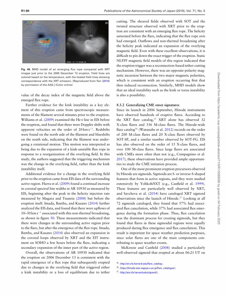
R1-90 Publications of the Astronomical Society of Japan (2019), Vol. 71, No. 5
Fig. 49. MHD model of an emerging flux rope compared with XRTimages just prior to the 2006 December 13 eruption. Field lines arecolored based on the temperature, with the heated field lines showingcorrespondence with the XRT emission. [Reproduced from Fan (2016)by permission of the AAS.] (Color online)
value of the decay index of the magnetic field above theemerged flux rope.
Further evidence for the kink instability as a key ele-ment of this eruption came from spectroscopic measure-ments of the filament several minutes prior to the eruption.Williams et al. (2009) examined the He II line in EIS beforethe eruption, and found that there were Doppler shifts withapparent velocities on the order of 20 km s−1. Redshiftswere found on the north side of the filament and blueshiftson the south side, indicating that the filament was under-going a rotational motion. This motion was interpreted asbeing due to the expansion of a kink-unstable flux rope inresponse to a reorganization of the overlying field. In thisstudy, the authors suggested that the triggering mechanismwas the change in the overlying field, rather than the kinkinstability itself.
Additional evidence for a change in the overlying fieldprior to the eruption came from EIS data of the surroundingactive region. Harra et al. (2009) found a continual increasein coronal spectral line widths in AR 10930 as measured byEIS, beginning after the peak in the helicity injection ratemeasured by Magara and Tsuneta (2008) but before theeruption itself. Imada, Bamba, and Kusano (2014) furtheranalyzed the EIS data, and found that there were upflows of10–30 km s−1 associated with this non-thermal broadening,as shown in figure 50. These measurements indicated thatthere were changes in the surrounding active region priorto the flare, but after the emergence of the flux rope. Imada,Bamba, and Kusano (2014) also observed an expansion inthe coronal loops observed by XRT and the EIT instru-ment on SOHO a few hours before the flare, indicating asecondary expansion of the inner part of the active region.
Overall, the observations of AR 10930 indicated thatthe eruption on 2006 December 13 is consistent with therapid emergence of a flux rope that subsequently erupteddue to changes in the overlying field that triggered eithera kink instability or a loss of equilibrium due to tether
cutting. The sheared fields observed with SOT and thetwisted structure observed with XRT prior to the erup-tion are consistent with an emerging flux rope. The helicitysaturated before the flare, indicating that the flux rope axishad emerged. Outflows and non-thermal broadening afterthe helicity peak indicated an expansion of the overlyingmagnetic field. Even with these excellent observations, it isdifficult to pin down the exact trigger of the eruption. StaticNLFFF magnetic field models of this region indicated thatthe eruption trigger was a reconnection-based tether-cuttingmechanism. However, there was an opposite-polarity mag-netic incursion between the two major magnetic polarities,which is consistent with an eruption occurring first thatthen induced reconnection. Similarly, MHD models showthat an ideal instability such as the kink or torus instabilityis also a possibility.
8.3.2 Generalizing CME onset signaturesSince its launch in 2006 September, Hinode instrumentshave observed hundreds of eruptive flares. According tothe XRT flare catalog,15 XRT alone has observed 32X-class flares and 336 M-class flares. The Hinode-wideflare catalog16 (Watanabe et al. 2012) records on the orderof 200 M-class flares and 20 X-class flares observed bySOT-SP, and a similar number observed by SOT-FG. EIShas also observed on the order of 15 X-class flares, andover 100 M-class flares. Since large flares are associatedwith CMEs more often than not (e.g., Compagnino et al.2017), these observations have provided ample opportuni-ties to study the CME initiation process.
One of the most prominent eruption precursors observedby Hinode are sigmoids. Sigmoids are S- or inverse-S-shapedfeatures that form in active regions, and they were studiedextensively by Yohkoh/SXT (e.g., Canfield et al. 1999).These features are particularly well observed by XRT,and Savcheva et al. (2014) have cataloged XRT sigmoidobservations since the launch of Hinode.17 Looking at all72 sigmoids cataloged, they found that 57% had associ-ated flux cancelation, while 37% had associated flux emer-gence during the formation phase. Thus, flux cancelationwas the dominant process for creating sigmoids, but theyfound that flares in these sigmoidal regions were equallyproduced during flux emergence and flux cancelation. Thisresult is important for space weather prediction purposes,since solar flares are one of the main components con-tributing to space weather events.
McKenzie and Canfield (2008) studied a particularlywell-observed sigmoid that erupted at about 06:21 UT on
15 〈http://xrt.cfa.harvard.edu/flare_catalog〉.16 〈https://hinode.isee.nagoya-u.ac.jp/flare_catalogue/〉.17 〈http://aia.cfa.harvard.edu/sigmoid/〉.
Dow
nloaded from https://academ
ic.oup.com/pasj/article-abstract/71/5/R
1/5589096 by guest on 04 February 2020
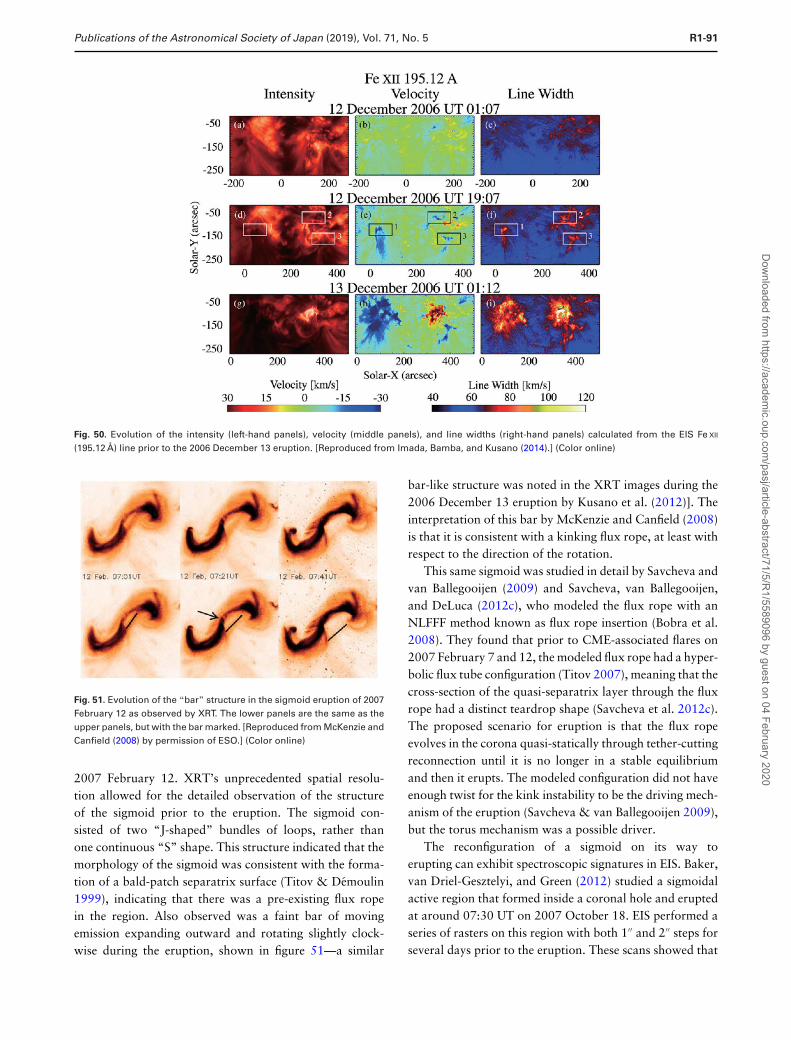
Publications of the Astronomical Society of Japan (2019), Vol. 71, No. 5 R1-91
Fig. 50. Evolution of the intensity (left-hand panels), velocity (middle panels), and line widths (right-hand panels) calculated from the EIS Fe XII
(195.12 A) line prior to the 2006 December 13 eruption. [Reproduced from Imada, Bamba, and Kusano (2014).] (Color online)
Fig. 51. Evolution of the “bar” structure in the sigmoid eruption of 2007February 12 as observed by XRT. The lower panels are the same as theupper panels, but with the bar marked. [Reproduced from McKenzie andCanfield (2008) by permission of ESO.] (Color online)
2007 February 12. XRT’s unprecedented spatial resolu-tion allowed for the detailed observation of the structureof the sigmoid prior to the eruption. The sigmoid con-sisted of two “J-shaped” bundles of loops, rather thanone continuous “S” shape. This structure indicated that themorphology of the sigmoid was consistent with the forma-tion of a bald-patch separatrix surface (Titov & Demoulin1999), indicating that there was a pre-existing flux ropein the region. Also observed was a faint bar of movingemission expanding outward and rotating slightly clock-wise during the eruption, shown in figure 51—a similar
bar-like structure was noted in the XRT images during the2006 December 13 eruption by Kusano et al. (2012)]. Theinterpretation of this bar by McKenzie and Canfield (2008)is that it is consistent with a kinking flux rope, at least withrespect to the direction of the rotation.
This same sigmoid was studied in detail by Savcheva andvan Ballegooijen (2009) and Savcheva, van Ballegooijen,and DeLuca (2012c), who modeled the flux rope with anNLFFF method known as flux rope insertion (Bobra et al.2008). They found that prior to CME-associated flares on2007 February 7 and 12, the modeled flux rope had a hyper-bolic flux tube configuration (Titov 2007), meaning that thecross-section of the quasi-separatrix layer through the fluxrope had a distinct teardrop shape (Savcheva et al. 2012c).The proposed scenario for eruption is that the flux ropeevolves in the corona quasi-statically through tether-cuttingreconnection until it is no longer in a stable equilibriumand then it erupts. The modeled configuration did not haveenough twist for the kink instability to be the driving mech-anism of the eruption (Savcheva & van Ballegooijen 2009),but the torus mechanism was a possible driver.
The reconfiguration of a sigmoid on its way toerupting can exhibit spectroscopic signatures in EIS. Baker,van Driel-Gesztelyi, and Green (2012) studied a sigmoidalactive region that formed inside a coronal hole and eruptedat around 07:30 UT on 2007 October 18. EIS performed aseries of rasters on this region with both 1′′ and 2′′ steps forseveral days prior to the eruption. These scans showed that
Dow
nloaded from https://academ
ic.oup.com/pasj/article-abstract/71/5/R
1/5589096 by guest on 04 February 2020
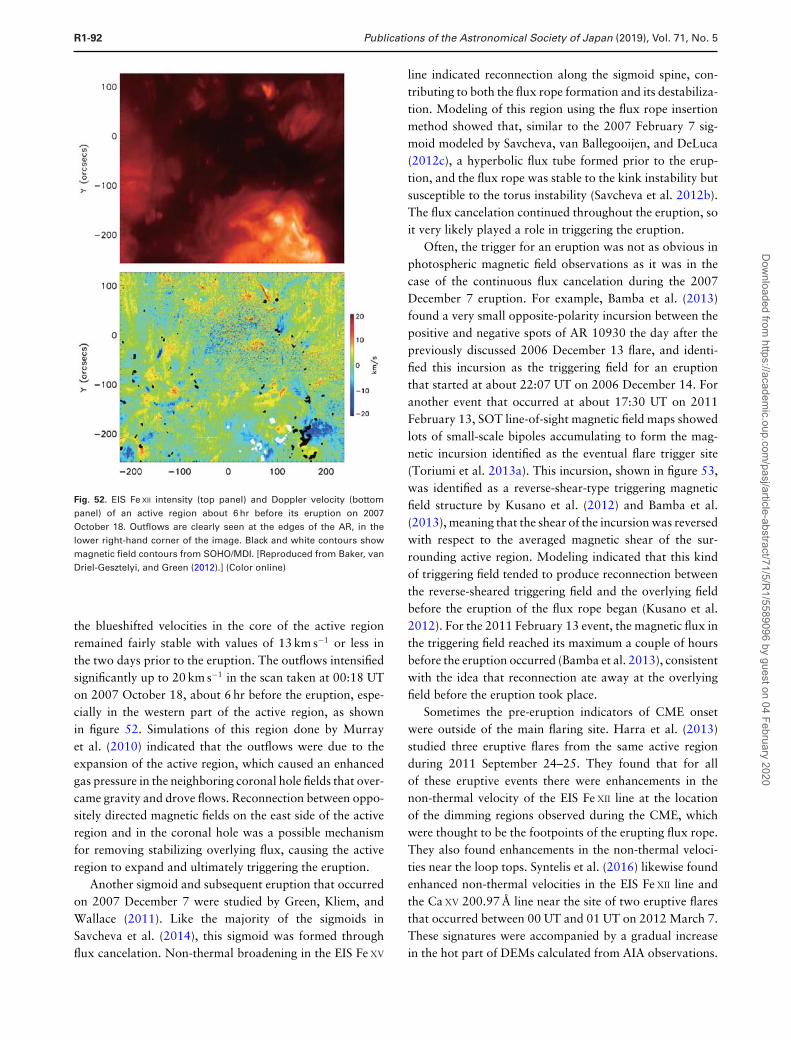
R1-92 Publications of the Astronomical Society of Japan (2019), Vol. 71, No. 5
Fig. 52. EIS Fe XII intensity (top panel) and Doppler velocity (bottompanel) of an active region about 6 hr before its eruption on 2007October 18. Outflows are clearly seen at the edges of the AR, in thelower right-hand corner of the image. Black and white contours showmagnetic field contours from SOHO/MDI. [Reproduced from Baker, vanDriel-Gesztelyi, and Green (2012).] (Color online)
the blueshifted velocities in the core of the active regionremained fairly stable with values of 13 km s−1 or less inthe two days prior to the eruption. The outflows intensifiedsignificantly up to 20 km s−1 in the scan taken at 00:18 UTon 2007 October 18, about 6 hr before the eruption, espe-cially in the western part of the active region, as shownin figure 52. Simulations of this region done by Murrayet al. (2010) indicated that the outflows were due to theexpansion of the active region, which caused an enhancedgas pressure in the neighboring coronal hole fields that over-came gravity and drove flows. Reconnection between oppo-sitely directed magnetic fields on the east side of the activeregion and in the coronal hole was a possible mechanismfor removing stabilizing overlying flux, causing the activeregion to expand and ultimately triggering the eruption.
Another sigmoid and subsequent eruption that occurredon 2007 December 7 were studied by Green, Kliem, andWallace (2011). Like the majority of the sigmoids inSavcheva et al. (2014), this sigmoid was formed throughflux cancelation. Non-thermal broadening in the EIS Fe XV
line indicated reconnection along the sigmoid spine, con-tributing to both the flux rope formation and its destabiliza-tion. Modeling of this region using the flux rope insertionmethod showed that, similar to the 2007 February 7 sig-moid modeled by Savcheva, van Ballegooijen, and DeLuca(2012c), a hyperbolic flux tube formed prior to the erup-tion, and the flux rope was stable to the kink instability butsusceptible to the torus instability (Savcheva et al. 2012b).The flux cancelation continued throughout the eruption, soit very likely played a role in triggering the eruption.
Often, the trigger for an eruption was not as obvious inphotospheric magnetic field observations as it was in thecase of the continuous flux cancelation during the 2007December 7 eruption. For example, Bamba et al. (2013)found a very small opposite-polarity incursion between thepositive and negative spots of AR 10930 the day after thepreviously discussed 2006 December 13 flare, and identi-fied this incursion as the triggering field for an eruptionthat started at about 22:07 UT on 2006 December 14. Foranother event that occurred at about 17:30 UT on 2011February 13, SOT line-of-sight magnetic field maps showedlots of small-scale bipoles accumulating to form the mag-netic incursion identified as the eventual flare trigger site(Toriumi et al. 2013a). This incursion, shown in figure 53,was identified as a reverse-shear-type triggering magneticfield structure by Kusano et al. (2012) and Bamba et al.(2013), meaning that the shear of the incursion was reversedwith respect to the averaged magnetic shear of the sur-rounding active region. Modeling indicated that this kindof triggering field tended to produce reconnection betweenthe reverse-sheared triggering field and the overlying fieldbefore the eruption of the flux rope began (Kusano et al.2012). For the 2011 February 13 event, the magnetic flux inthe triggering field reached its maximum a couple of hoursbefore the eruption occurred (Bamba et al. 2013), consistentwith the idea that reconnection ate away at the overlyingfield before the eruption took place.
Sometimes the pre-eruption indicators of CME onsetwere outside of the main flaring site. Harra et al. (2013)studied three eruptive flares from the same active regionduring 2011 September 24–25. They found that for allof these eruptive events there were enhancements in thenon-thermal velocity of the EIS Fe XII line at the locationof the dimming regions observed during the CME, whichwere thought to be the footpoints of the erupting flux rope.They also found enhancements in the non-thermal veloci-ties near the loop tops. Syntelis et al. (2016) likewise foundenhanced non-thermal velocities in the EIS Fe XII line andthe Ca XV 200.97 A line near the site of two eruptive flaresthat occurred between 00 UT and 01 UT on 2012 March 7.These signatures were accompanied by a gradual increasein the hot part of DEMs calculated from AIA observations.
Dow
nloaded from https://academ
ic.oup.com/pasj/article-abstract/71/5/R
1/5589096 by guest on 04 February 2020
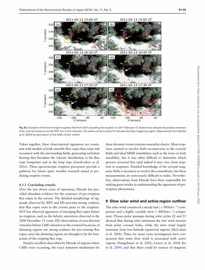
Publications of the Astronomical Society of Japan (2019), Vol. 71, No. 5 R1-93
Fig. 53. Evolution of the line-of-sight magnetic field from SOT preceding the eruption on 2011 February 13. Green lines indicate the polarity inversionlines, and red contours are the SOT Ca II H line intensity. The yellow circle in panel (f) indicates the flare triggering region. [Reproduced from Bambaet al. (2013) by permission of the AAS.] (Color online)
Taken together, these observational signatures are consis-tent with models of kink-unstable flux ropes that erupt andreconnect with the surrounding fields, generating turbulentheating that broadens the velocity distribution in the fluxrope footpoints and at the loop tops (Gordovskyy et al.2016). These spectroscopic eruption precursors provide apathway for future space weather research aimed at pre-dicting eruptive events.
8.3.3 Concluding remarksOver the last eleven years of operation, Hinode has pro-vided abundant evidence for the existence of pre-eruptionflux ropes in the corona. The detailed morphology of sig-moids observed by XRT and EIS provides strong evidencethat flux ropes exist in the corona prior to the eruption.SOT has observed signatures of emerging flux ropes beforean eruption, such as the helicity saturation observed in the2006 December 13 event. EIS observations of non-thermalvelocities before CME initiation in the eventual locations ofdimming regions are strong evidence for pre-existing fluxropes, since the dimming regions are thought to be the foot-points of the erupting flux rope.
Despite excellent data taken by Hinode of regions whereCMEs were occurring, the exact initiation mechanism for
these dynamic events remains somewhat elusive. Most erup-tions seemed to involve both reconnection in the coronalfields and ideal MHD instabilities such as the torus or kinkinstability, but it was often difficult to determine whichprocess occurred first (and indeed it may vary from erup-tion to eruption). Detailed knowledge of the coronal mag-netic fields is necessary to resolve this conundrum, but thesemeasurements are notoriously difficult to make. Neverthe-less, observations from Hinode have been responsible formaking great strides in understanding the signatures of pre-eruption phenomena.
9 Slow solar wind and active-region outflow
The solar wind consists of a steady fast (>700 km s−1) com-ponent and a highly variable slow (∼400 km s−1) compo-nent. Ulysses polar passages during solar cycles 22 and 23showed that during solar minimum the fast wind streamsfrom polar coronal holes, while the slow wind largelyemanates from low-latitude equatorial regions (McComaset al. 2008). Thus, for many years investigators have con-jectured that some slow wind is associated with activeregions (Neugebauer et al. 2002; Liewer et al. 2004; Koet al. 2006) and that these could be sources of magnetic
Dow
nloaded from https://academ
ic.oup.com/pasj/article-abstract/71/5/R
1/5589096 by guest on 04 February 2020
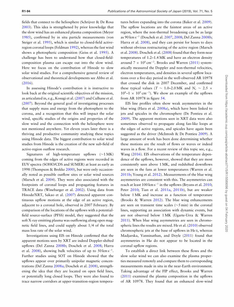
R1-94 Publications of the Astronomical Society of Japan (2019), Vol. 71, No. 5
fields that connect to the heliosphere (Schrijver & De Rosa2003). This idea is strengthened by prior knowledge thatthe slow wind has an enhanced plasma composition (Meyer1985), confirmed by in situ particle measurements (vonSteiger et al. 1995), which is similar to closed-field active-region coronal loops (Feldman 1992), whereas the fast windshows a photospheric composition (Geiss et al. 1995). Achallenge has been to understand how that closed-field-composition plasma can escape out into the slow wind.Here we focus on the contribution of Hinode to slowsolar wind studies. For a comprehensive general review ofobservational and theoretical developments see Abbo et al.(2016).
In assessing Hinode’s contribution it is instructive tolook back at the original scientific objectives of the mission,as articulated in, e.g., Kosugi et al. (2007) and Culhane et al.(2007). Beyond the general goal of investigating processesthat supply mass and energy from the photosphere to thecorona, and a recognition that this will impact the solarwind, specific studies of the origins and properties of theslow wind and the connection with the heliosphere werenot mentioned anywhere. Yet eleven years later there is athriving and productive community studying these topicsusing Hinode data. The biggest contribution to solar windstudies from Hinode is the creation of the new sub-field ofactive-region outflow research.
Signatures of high-temperature upflows (∼1 MK)coming from the edges of active regions were recorded inEUV spectra (SOHO/CDS and SUMER) at least as early as1998 (Thompson & Brekke 2000), but were only occasion-ally noted as possible outflow sites or solar wind sources(Marsch et al. 2004). They were also associated with thefootpoints of coronal loops and propagating features inTRACE data (Winebarger et al. 2002). Using data fromHinode/XRT, Sakao et al. (2007) detected apparent con-tinuous upflow motions at the edge of an active region,adjacent to a coronal hole, observed in 2007 February. Bycomparison of the locations of the upflows with a potential-field source-surface (PFSS) model, they suggested that thesoft X-ray emitting plasma was outflowing along open mag-netic field lines, and could supply about 1/4 of the totalmass loss rate of the solar wind.
Investigations using EIS on Hinode confirmed that theapparent motions seen by XRT are indeed Doppler-shiftedupflows (Del Zanna 2008b; Doschek et al. 2008; Harraet al. 2008), showing bulk velocities of up to 50 km s−1.Further studies using SOT on Hinode showed that theupflows appear over primarily unipolar magnetic concen-trations (Del Zanna 2008a; Doschek et al. 2008), strength-ening the idea that they are located on open field lines,or potentially long closed loops. They were also found totrace narrow corridors at upper-transition-region tempera-
tures before expanding into the corona (Baker et al. 2009).The upflow locations are the faintest areas of an activeregion, where the non-thermal broadening can be as largeas 90 km s−1 (Doschek et al. 2007, 2008; Del Zanna 2008b;Harra et al. 2008), and they can persist for hours to dayswithout obvious restructuring of the active region (Marschet al. 2008). Doschek et al. (2008) found that they form neartemperatures of 1.2–1.4 MK and have an electron densityaround 7 × 108 cm−3. Brooks and Warren (2011) system-atically measured the Doppler and non-thermal velocities,electron temperatures, and densities in several upflow loca-tions over a five-day period in the well-observed AR 10978that crossed the disk in 2007 December, and confirmedthese typical values (T ∼ 1.0–2.0 MK and Ne ∼ 2.5 ×10⁸–1 × 109 cm−3). We show an example of the upflowsfrom AR 10978 in figure 54.
EIS line profiles often show weak asymmetries in theblue wing (Hara et al. 2008a), which have been linked tojets and spicules in the chromosphere (De Pontieu et al.2009). The apparent motions seen in XRT data were alsosometimes observed to propagate along fan-like loops atthe edges of active regions, and spicules have again beensuggested as the driver (McIntosh & De Pontieu 2009). Alarge amount of work has been done determining whetherthese motions are the result of flows or waves or indeedwaves in a flow. For a recent review of this topic see, e.g.,Wang (2016). EIS observations of the temperature depen-dence of the upflows, however, showed that they are mostconsistently seen above 1 MK, and redshifted downflowsare seen in the fans at lower temperatures (Warren et al.2011b; Young et al. 2012). Measurements of the blue wingasymmetries are consistent with this. The asymmetries canreach at least 100 km s−1 in the upflows (Bryans et al. 2010;Peter 2010; Tian et al. 2011a, 2011b), but are weakerbelow 1 MK and increase as a function of temperature(Brooks & Warren 2012). The blue wing enhancementsare seen on transient time scales (∼5 min) in the coronallines, supporting an association with dynamic events, butare not observed below 1 MK (Ugarte-Urra & Warren2011). When blue wing asymmetries are seen in chromo-spheric lines the results are mixed. He et al. (2010) observedchromospheric jets at the base of upflows in He II, whereasMadjarska, Vanninathan, and Doyle (2011) found thatasymmetries in Hα do not appear to be located in thecoronal upflow regions.
To establish a direct link between these flows and theslow solar wind we can also examine the plasma proper-ties measured remotely and compare them to correspondingmeasurements made in situ in the near-Earth environment.Taking advantage of the FIP effect, Brooks and Warren(2011) examined the plasma composition in the upflowsof AR 10978. They found that an enhanced slow-wind
Dow
nloaded from https://academ
ic.oup.com/pasj/article-abstract/71/5/R
1/5589096 by guest on 04 February 2020
Publications of the Astronomical Society of Japan (2019), Vol. 71, No. 5 R1-95
Fig. 54. Top left: XRT Al-poly/Open image of AR 10978 as it approached disk center in 2007 December. Top right: PFSS extrapolation of the open fieldaround the AR. Bottom left: EIS Fe XII 192.394 A spectral image of the AR. Bottom center: Doppler velocity map derived from the EIS Fe XII 192.394 Adata. Bottom right: Non-thermal velocity map derived from the EIS Fe XII 192.394 A data following the method of Brooks and Warren (2016). Note thatthe open field in the extrapolation anchors close to the upflows but they are not necessarily co-spatial. We discuss the importance of understandingthe magnetic topology in the text. (Color online)
composition persistently flowed from the AR for the fullfive days of their observations. In fact, the measurementsmade when the flows from the western side of AR 10978were directed towards Earth were found to be consistentwith values obtained in situ several days later by the ioncomposition spectrometer SWICS on the ACE spacecraft.Brooks and Warren (2012) performed a similar analysisfor the asymmetric high-speed component of the flowsand found that they also showed an enhanced slow-windcomposition, suggesting that the high-speed and bulk flowsmay share a common formation mechanism. Furthermore,Culhane et al. (2014) examined Fe/O ratios obtained bySWICS, and found evidence of a response to AR 10978’spassage through disk center. In a study of a separate AR,Slemzin et al. (2013) also provided support for a connec-tion by linking measurements made in situ by ACE andother observatories to the AR source using ballistic back-mapping and a PFSS model.
These observations have inspired new theoreticalthinking on the formation of the upflows, and whether
the magnetic topology is such that they truly become out-flows that connect to the heliosphere. From magnetic fieldextrapolations, Baker et al. (2009) found that the narrowcorridors at the base of the upflows coincide with surfaceprojections of quasi-separatrix layers (QSLs) in the corona.These are regions of strong gradients in magnetic connec-tivity, and are prime sites for processes such as interchangereconnection (Fisk et al. 1998) between the closed AR fieldand surrounding open, or distantly connected, field. If thereis a nearby coronal hole, then in a sense this process is sim-ilar to other models of the source and formation of the slowwind, such as the S-web (web of separatrices) model (Anti-ochos et al. 2011), that do not involve ARs but describeinterchange reconnection along coronal hole boundaries(Higginson et al. 2017).
Murray et al. (2010) have shown that the continualexpansion of evolving ARs in coronal holes can drive andaccelerate flows along the open field in the vicinity of sep-aratrix surfaces. Del Zanna et al. (2011a) expanded thissuggestion to propose a similar scenario of AR growth
Dow
nloaded from https://academ
ic.oup.com/pasj/article-abstract/71/5/R
1/5589096 by guest on 04 February 2020
R1-96 Publications of the Astronomical Society of Japan (2019), Vol. 71, No. 5
maintaining continuous reconnection across separatrices atthe null point they located in the coronal magnetic fieldtopology derived from potential and linear force-free fieldextrapolations. In this scenario, pressure gradients developfollowing reconnection between the cooler open-field linesand the hot loops of the AR core, and this appears tobe consistent with numerical hydrodynamic simulations(Bradshaw et al. 2011). If an interchange mechanism isreally operating in QSLs to drive the flows, it might alsobe possible to detect signatures of that process in radiomeasurements. Interestingly, Del Zanna et al. (2011a) didindeed find evidence of a correspondence between flow loca-tions and radio noise storms.
So, the model of interchange reconnection at QSLs isbeginning to produce a compelling picture of the flows.AR expansion and growth drive the interchange reconnec-tion, which provides the mechanism to transfer slow-wind-composition plasma from closed AR loops to open fieldand expel the material. The flows are seen as propagatingfeatures in XRT movies and Doppler-shifted upflows in EISdata. Radio noise storms are indicative of the reconnectionprocess. EIS elemental abundance measurements confirmedthat the composition is enhanced as in the slow wind, andwhen the plasma has had time to travel to the Earth envi-ronment, in situ measurements of the composition are con-sistent with those measured with EIS.
There are, however, some issues that cloud this inter-pretation. Most importantly, the magnetic field topologyis not always consistent with this picture. Culhane et al.(2014), for example, found that AR 10978—the region thatshowed slow wind compositional signatures at ACE—wascompletely covered by a closed helmet streamer. Further-more, in a study of seven ARs, Edwards et al. (2016) foundthat most of them did not have high-reaching or open fieldin the vicinity of the upflows. Only in one AR, adjacent toa coronal hole as in Sakao et al. (2007), was an outflowchannel found. If an adjacent coronal hole is a prerequisitefor the development of open field, then the upflows may notbe true outflows in general; see also Fazakerley, Harra, andvan Driel-Gesztelyi (2016). Boutry et al. (2012) also foundthat a sizeable fraction of mass flux (1/5 in their example)propagated away from the upflow area along long loopsthat connected to distant ARs. So not all of the outwardlypropagating mass flux necessarily escapes to interplanetaryspace.
Culhane et al. (2014) and Mandrini et al. (2015)have addressed the example of AR 10978 with a detailedtopological study using a PFSS model. They found thatclosed-field plasma could escape along a novel pathway viaa two-step reconnection process. First, the AR closed loopsreconnected with large-scale network field, producinglong loops that anchored close to the high-latitude open
field associated with a northern coronal hole where ahigh-altitude null point was also located. AR plasmatraveled along these new loops, and in a second step,interchange reconnection with the open field released theplasma. This suggested that closed-field plasma can escapeinto the solar wind, even when it appears unlikely.
Such complex escape pathways may not be necessary ingeneral, however. van Driel-Gesztelyi et al. (2012) showedhow the presence of two bipolar ARs on disk could createa quadrupolar magnetic configuration allowing the pres-ence of a null point where AR plasma can be channeledinto the slow wind. Taking a different approach, Brooks,Ugarte-Urra, and Warren (2015) designed a novel observingsequence to scan the entire solar disk with EIS, and com-bined the observations with a PFSS model to try to locateall regions of open field that show upflows with a slow-wind composition. They found numerous areas of slow-wind-composition outflow on open magnetic field. Despitea downward revision of the outflow mass flux comparedto Sakao et al. (2007), based on spectroscopic densitiesand velocities, they found that the outflow regions couldaccount for most of the mass-loss rate of the solar wind asbenchmarked against ACE measurements.
There are, of course, alternative slow-solar-wind modelsthat may provide an explanation for the outflows. Theoriesthat do not involve loop opening, such as wave/turbulencemodels (Cranmer 2012), have difficulty explaining howenhanced composition plasma is supplied to the slow wind,since the most widely studied models of the FIP effectassume that plasma must be confined for some time in orderfor the fractionation mechanism to operate (Laming 2004,2012). Leaving aside the models, EIS measurements showthat one can have slow-wind-composition plasma on openmagnetic field. Whether this is proof that loops have beenopened, or is a new clue to understanding wave and FIPeffect models, remains to be seen. In any case, Hinode hasshown that it is no longer correct to state that the slow windonly has the same composition as the closed-field corona. Infact, many areas of open field have the same composition.
10 Future prospects
During the last eleven years solar physics has made remark-able progress and Hinode has been a key contributor tothese advances, as is amply demonstrated by the earliersections of this review paper. In this section we considerthe prospects for progress in the next eleven years. To alarge extent any speculation on future advances is based onextrapolating from the progress that has occurred in pastyears, while taking into account the influence of (observa-tional and/or theoretical) instruments already under devel-opment or planned. The biggest uncertainty for such an
Dow
nloaded from https://academ
ic.oup.com/pasj/article-abstract/71/5/R
1/5589096 by guest on 04 February 2020
Publications of the Astronomical Society of Japan (2019), Vol. 71, No. 5 R1-97
exercise is posed by the emergence of new ideas that canadvance the field in unpredictable ways. In addition, anypredictions will be colored by the experience and interestsof the person making them. Nonetheless, it is abundantlyclear that, barring serious technical problems, Hinode willcontinue to play an important role in the years to come,in particular when acting together with other resources.Many past investigations have already made use of Hinodedata obtained in conjunction with other space missionssuch as SOHO (Domingo et al. 1995), SDO (Pesnell et al.2012), and more recently IRIS (De Pontieu et al. 2014b),as well as with various ground-based telescopes, such asthe Dunn Solar Telescope (DST; Dunn & Smartt 1991),the German Vacuum Tower Telescope (VTT; von der Luhe1998), the Swedish Solar Telescope (SST; Scharmer et al.2003), the Goode Solar Telescope (GST; Goode et al.2010), GREGOR (Schmidt et al. 2012), and very recentlywith ALMA (Shimojo et al. 2017b). In future we expect abonanza from joint observations with projects under devel-opment, such as DKIST (Tritschler et al. 2016), the ParkerSolar Probe (Fox et al. 2016), and Solar Orbiter (Mulleret al. 2013), but also with, e.g., the SUNRISE mission(Solanki et al. 2010, 2017; Barthol et al. 2011) during itsupcoming third flight.
Let us start a brief tour of some of the sub-fields of solarphysics by considering the solar interior. There, interesthas focused on differential rotation, meridional circulation,and turbulent convection, i.e., on the key flows driving theglobal solar dynamo and hence leading to the productionof the Sun’s large-scale magnetic field that forms sunspotsand active regions. Considerable progress has been achievedover the last decade (Gizon et al. 2010; Hanasoge et al.2016; Howe 2016; Zhao & Chen 2016). However, con-siderable inconsistencies and gaps in our knowledge exist,particularly of the strength of the turbulent convection(Hanasoge et al. 2012; Greer et al. 2015), and quite gener-ally of the flows near the poles. In addition, the structure andmagnitude of these flows in the lower convection zone arerather poorly known. This is particularly true for the merid-ional circulation, where it is even unclear at which depththe return flow (i.e., from pole to equator) takes place andwhether there is a single meridional circulation cell or mul-tiple cells at different depths (Zhao et al. 2013; Rajaguru& Antia 2015).
A number of advances have been made in under-standing the global solar dynamo in the last decade. Three-dimensional simulations of the entire convection zone haveprogressed considerably, allowing direct numerical simu-lations of a dynamo residing in the convection zone (e.g.,Kapyla et al. 2016). In parallel, the Babcock–Leighton-typedynamo, with the surface field playing a key role (Cameron
& Schussler 2015), has made a remarkable comeback. Thelong-standing problem of maintaining a large-scale fieldeven in the presence of a high Reynolds number has recentlybeen solved by Hotta, Rempel, and Yokoyama (2016).The importance of polar fields for the global dynamo hasbeen clarified by, e.g., Wang and Sheeley (2009), while theimportant role of sunspot or active region tilt angles forbuilding up the polar fields at activity minimum has alsobeen demonstrated (Dasi-Espuig et al. 2010, 2013; Jianget al. 2014).
One of the major breakthroughs of the last decadehas been the demonstration that a small-scale turbulentdynamo is viable under “realistic” solar photospheric con-ditions (Vogler & Schussler 2007). More recent simula-tions with lower numerical viscosity have been carried outby Rempel (2014) and Hotta, Rempel, and Yokoyama(2015), and the results of such simulations are by now wellestablished—see also the reviews by Brandenburg, Sokoloff,and Subramanian (2012) and Borrero et al. (2015). Obser-vational support has come largely from data obtained withHinode/SOT. Such data have demonstrated that there isno variation of the magnetic flux in the inter-network overthe solar cycle (Buehler et al. 2013; Lites et al. 2014; Jin &Wang 2015), and have also shown to high accuracy that theSOT-SP high-resolution observations are consistent withthe results of small-scale dynamo simulations (Danilovicet al. 2010b, 2016a).
In spite of these advances, our understanding of thedynamo remains rather incomplete. An important openquestion is the location of the global solar dynamo (besidesthe solar surface): Does it reside in the overshoot layerbelow the convection zone, in the lower convection zone,throughout the convection zone, or in the shear layer nearthe solar surface?
To make progress in these topics it will be necessary toobserve the Sun from new vantage points with an instru-ment measuring velocities and taking vector magnetograms.It is hoped that the deeper parts of the convection zone canbe better probed by observing the p-mode oscillations fromtwo different directions (with a technique dubbed stereo-scopic helioseismology). With regard to the surface mag-netic field, so far the most detailed maps of the magneticfield at the solar poles have been made by using Hinodedata (see subsection 4.1). Only high-resolution observa-tions from outside the ecliptic will be able to go beyondwhat Hinode has achieved. Such observations will be pro-vided by the PHI instrument (Solanki et al. 2015) on SolarOrbiter from heliographic latitudes higher than 30
◦during
its extended mission phase. Nonetheless, continuing regularcoverage of the polar fields by Hinode also remains impor-tant for the future, not just to bridge the time until Solar
Dow
nloaded from https://academ
ic.oup.com/pasj/article-abstract/71/5/R
1/5589096 by guest on 04 February 2020
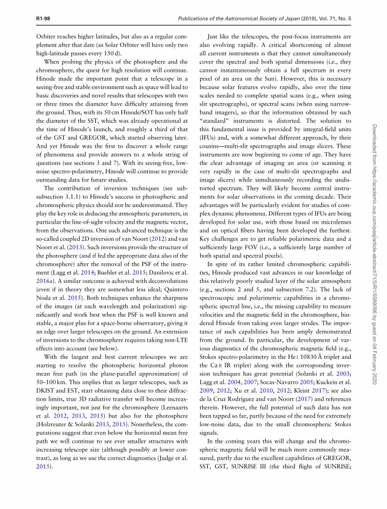
R1-98 Publications of the Astronomical Society of Japan (2019), Vol. 71, No. 5
Orbiter reaches higher latitudes, but also as a regular com-plement after that date (as Solar Orbiter will have only twohigh-latitude passes every 150 d).
When probing the physics of the photosphere and thechromosphere, the quest for high resolution will continue.Hinode made the important point that a telescope in aseeing-free and stable environment such as space will lead tobasic discoveries and novel results that telescopes with twoor three times the diameter have difficulty attaining fromthe ground. Thus, with its 50 cm Hinode/SOT has only halfthe diameter of the SST, which was already operational atthe time of Hinode’s launch, and roughly a third of thatof the GST and GREGOR, which started observing later.And yet Hinode was the first to discover a whole rangeof phenomena and provide answers to a whole string ofquestions (see sections 3 and 7). With its seeing-free, low-noise spectro-polarimetry, Hinode will continue to provideoutstanding data for future studies.
The contribution of inversion techniques (see sub-subsection 3.1.1) to Hinode’s success in photospheric andchromospheric physics should not be underestimated. Theyplay the key role in deducing the atmospheric parameters, inparticular the line-of-sight velocity and the magnetic vector,from the observations. One such advanced technique is theso-called coupled 2D inversion of van Noort (2012) and vanNoort et al. (2013). Such inversions provide the structure ofthe photosphere (and if fed the appropriate data also of thechromosphere) after the removal of the PSF of the instru-ment (Lagg et al. 2014; Buehler et al. 2015; Danilovic et al.2016a). A similar outcome is achieved with deconvolutions(even if in theory they are somewhat less ideal; QuinteroNoda et al. 2015). Both techniques enhance the sharpnessof the images (at each wavelength and polarization) sig-nificantly and work best when the PSF is well known andstable, a major plus for a space-borne observatory, giving itan edge over larger telescopes on the ground. An extensionof inversions to the chromosphere requires taking non-LTEeffects into account (see below).
With the largest and best current telescopes we arestarting to resolve the photospheric horizontal photonmean free path (in the plane-parallel approximation) of50–100 km. This implies that as larger telescopes, such asDKIST and EST, start obtaining data close to their diffrac-tion limits, true 3D radiative transfer will become increas-ingly important, not just for the chromosphere (Leenaartset al. 2012, 2013, 2015) but also for the photosphere(Holzreuter & Solanki 2013, 2015). Nonetheless, the com-putations suggest that even below the horizontal mean freepath we will continue to see ever smaller structures withincreasing telescope size (although possibly at lower con-trast), as long as we use the correct diagnostics (Judge et al.2015).
Just like the telescopes, the post-focus instruments arealso evolving rapidly. A critical shortcoming of almostall current instruments is that they cannot simultaneouslycover the spectral and both spatial dimensions (i.e., theycannot instantaneously obtain a full spectrum in everypixel of an area on the Sun). However, this is necessarybecause solar features evolve rapidly, also over the timescales needed to complete spatial scans (e.g., when usingslit spectrographs), or spectral scans (when using narrow-band imagers), so that the information obtained by such“standard” instruments is distorted. The solution tothis fundamental issue is provided by integral-field units(IFUs) and, with a somewhat different approach, by theircousins—multi-slit spectrographs and image slicers. Theseinstruments are now beginning to come of age. They havethe clear advantage of imaging an area (or scanning itvery rapidly in the case of multi-slit spectrographs andimage slicers) while simultaneously recording the undis-torted spectrum. They will likely become central instru-ments for solar observations in the coming decade. Theiradvantages will be particularly evident for studies of com-plex dynamic phenomena. Different types of IFUs are beingdeveloped for solar use, with those based on microlensesand on optical fibers having been developed the furthest.Key challenges are to get reliable polarimetric data and asufficiently large FOV (i.e., a sufficiently large number ofboth spatial and spectral pixels).
In spite of its rather limited chromospheric capabili-ties, Hinode produced vast advances in our knowledge ofthis relatively poorly studied layer of the solar atmosphere(e.g., sections 2 and 5, and subsection 7.2). The lack ofspectroscopic and polarimetric capabilities in a chromo-spheric spectral line, i.e., the missing capability to measurevelocities and the magnetic field in the chromosphere, hin-dered Hinode from taking even larger strides. The impor-tance of such capabilities has been amply demonstratedfrom the ground. In particular, the development of var-ious diagnostics of the chromospheric magnetic field (e.g.,Stokes spectro-polarimetry in the He I 10830 A triplet andthe Ca II IR triplet) along with the corresponding inver-sion techniques has great potential (Solanki et al. 2003;Lagg et al. 2004, 2007; Socas-Navarro 2005; Kuckein et al.2009, 2012; Xu et al. 2010, 2012; Kleint 2017); see alsode la Cruz Rodrıguez and van Noort (2017) and referencestherein. However, the full potential of such data has notbeen tapped so far, partly because of the need for extremelylow-noise data, due to the small chromospheric Stokessignals.
In the coming years this will change and the chromo-spheric magnetic field will be much more commonly mea-sured, partly due to the excellent capabilities of GREGOR,SST, GST, SUNRISE III (the third flight of SUNRISE;
Dow
nloaded from https://academ
ic.oup.com/pasj/article-abstract/71/5/R
1/5589096 by guest on 04 February 2020
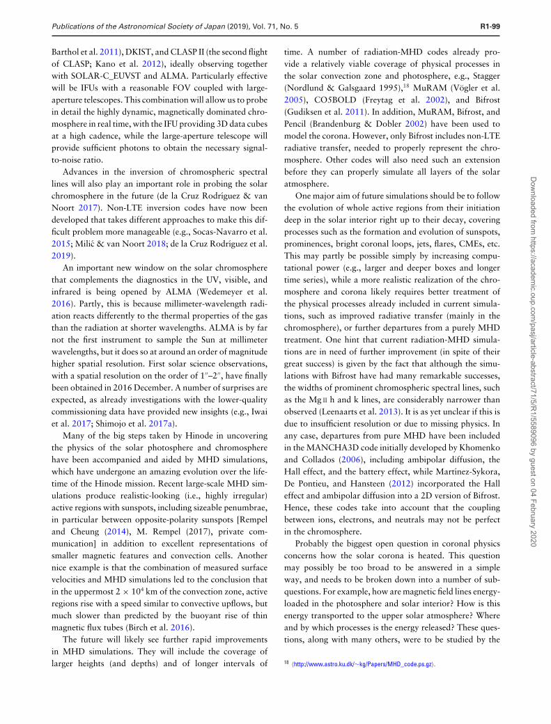
Publications of the Astronomical Society of Japan (2019), Vol. 71, No. 5 R1-99
Barthol et al. 2011), DKIST, and CLASP II (the second flightof CLASP; Kano et al. 2012), ideally observing togetherwith SOLAR-C_EUVST and ALMA. Particularly effectivewill be IFUs with a reasonable FOV coupled with large-aperture telescopes. This combination will allow us to probein detail the highly dynamic, magnetically dominated chro-mosphere in real time, with the IFU providing 3D data cubesat a high cadence, while the large-aperture telescope willprovide sufficient photons to obtain the necessary signal-to-noise ratio.
Advances in the inversion of chromospheric spectrallines will also play an important role in probing the solarchromosphere in the future (de la Cruz Rodrıguez & vanNoort 2017). Non-LTE inversion codes have now beendeveloped that takes different approaches to make this dif-ficult problem more manageable (e.g., Socas-Navarro et al.2015; Milic & van Noort 2018; de la Cruz Rodrıguez et al.2019).
An important new window on the solar chromospherethat complements the diagnostics in the UV, visible, andinfrared is being opened by ALMA (Wedemeyer et al.2016). Partly, this is because millimeter-wavelength radi-ation reacts differently to the thermal properties of the gasthan the radiation at shorter wavelengths. ALMA is by farnot the first instrument to sample the Sun at millimeterwavelengths, but it does so at around an order of magnitudehigher spatial resolution. First solar science observations,with a spatial resolution on the order of 1′′–2′′, have finallybeen obtained in 2016 December. A number of surprises areexpected, as already investigations with the lower-qualitycommissioning data have provided new insights (e.g., Iwaiet al. 2017; Shimojo et al. 2017a).
Many of the big steps taken by Hinode in uncoveringthe physics of the solar photosphere and chromospherehave been accompanied and aided by MHD simulations,which have undergone an amazing evolution over the life-time of the Hinode mission. Recent large-scale MHD sim-ulations produce realistic-looking (i.e., highly irregular)active regions with sunspots, including sizeable penumbrae,in particular between opposite-polarity sunspots [Rempeland Cheung (2014), M. Rempel (2017), private com-munication] in addition to excellent representations ofsmaller magnetic features and convection cells. Anothernice example is that the combination of measured surfacevelocities and MHD simulations led to the conclusion thatin the uppermost 2 × 10⁴ km of the convection zone, activeregions rise with a speed similar to convective upflows, butmuch slower than predicted by the buoyant rise of thinmagnetic flux tubes (Birch et al. 2016).
The future will likely see further rapid improvementsin MHD simulations. They will include the coverage oflarger heights (and depths) and of longer intervals of
time. A number of radiation-MHD codes already pro-vide a relatively viable coverage of physical processes inthe solar convection zone and photosphere, e.g., Stagger(Nordlund & Galsgaard 1995),18 MuRAM (Vogler et al.2005), CO5BOLD (Freytag et al. 2002), and Bifrost(Gudiksen et al. 2011). In addition, MuRAM, Bifrost, andPencil (Brandenburg & Dobler 2002) have been used tomodel the corona. However, only Bifrost includes non-LTEradiative transfer, needed to properly represent the chro-mosphere. Other codes will also need such an extensionbefore they can properly simulate all layers of the solaratmosphere.
One major aim of future simulations should be to followthe evolution of whole active regions from their initiationdeep in the solar interior right up to their decay, coveringprocesses such as the formation and evolution of sunspots,prominences, bright coronal loops, jets, flares, CMEs, etc.This may partly be possible simply by increasing compu-tational power (e.g., larger and deeper boxes and longertime series), while a more realistic realization of the chro-mosphere and corona likely requires better treatment ofthe physical processes already included in current simula-tions, such as improved radiative transfer (mainly in thechromosphere), or further departures from a purely MHDtreatment. One hint that current radiation-MHD simula-tions are in need of further improvement (in spite of theirgreat success) is given by the fact that although the simu-lations with Bifrost have had many remarkable successes,the widths of prominent chromospheric spectral lines, suchas the Mg II h and k lines, are considerably narrower thanobserved (Leenaarts et al. 2013). It is as yet unclear if this isdue to insufficient resolution or due to missing physics. Inany case, departures from pure MHD have been includedin the MANCHA3D code initially developed by Khomenkoand Collados (2006), including ambipolar diffusion, theHall effect, and the battery effect, while Martınez-Sykora,De Pontieu, and Hansteen (2012) incorporated the Halleffect and ambipolar diffusion into a 2D version of Bifrost.Hence, these codes take into account that the couplingbetween ions, electrons, and neutrals may not be perfectin the chromosphere.
Probably the biggest open question in coronal physicsconcerns how the solar corona is heated. This questionmay possibly be too broad to be answered in a simpleway, and needs to be broken down into a number of sub-questions. For example, how are magnetic field lines energy-loaded in the photosphere and solar interior? How is thisenergy transported to the upper solar atmosphere? Whereand by which processes is the energy released? These ques-tions, along with many others, were to be studied by the
18 〈http://www.astro.ku.dk/∼kg/Papers/MHD_code.ps.gz〉.
Dow
nloaded from https://academ
ic.oup.com/pasj/article-abstract/71/5/R
1/5589096 by guest on 04 February 2020
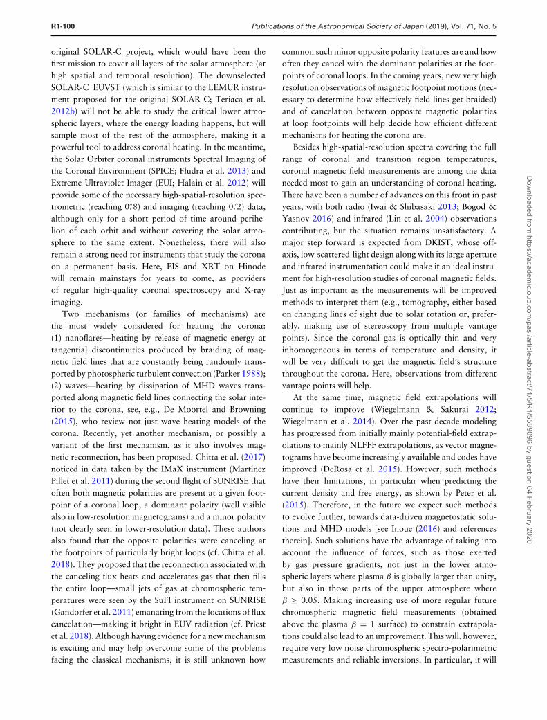
R1-100 Publications of the Astronomical Society of Japan (2019), Vol. 71, No. 5
original SOLAR-C project, which would have been thefirst mission to cover all layers of the solar atmosphere (athigh spatial and temporal resolution). The downselectedSOLAR-C_EUVST (which is similar to the LEMUR instru-ment proposed for the original SOLAR-C; Teriaca et al.2012b) will not be able to study the critical lower atmo-spheric layers, where the energy loading happens, but willsample most of the rest of the atmosphere, making it apowerful tool to address coronal heating. In the meantime,the Solar Orbiter coronal instruments Spectral Imaging ofthe Coronal Environment (SPICE; Fludra et al. 2013) andExtreme Ultraviolet Imager (EUI; Halain et al. 2012) willprovide some of the necessary high-spatial-resolution spec-trometric (reaching 0.′′8) and imaging (reaching 0.′′2) data,although only for a short period of time around perihe-lion of each orbit and without covering the solar atmo-sphere to the same extent. Nonetheless, there will alsoremain a strong need for instruments that study the coronaon a permanent basis. Here, EIS and XRT on Hinodewill remain mainstays for years to come, as providersof regular high-quality coronal spectroscopy and X-rayimaging.
Two mechanisms (or families of mechanisms) arethe most widely considered for heating the corona:(1) nanoflares—heating by release of magnetic energy attangential discontinuities produced by braiding of mag-netic field lines that are constantly being randomly trans-ported by photospheric turbulent convection (Parker 1988);(2) waves—heating by dissipation of MHD waves trans-ported along magnetic field lines connecting the solar inte-rior to the corona, see, e.g., De Moortel and Browning(2015), who review not just wave heating models of thecorona. Recently, yet another mechanism, or possibly avariant of the first mechanism, as it also involves mag-netic reconnection, has been proposed. Chitta et al. (2017)noticed in data taken by the IMaX instrument (MartınezPillet et al. 2011) during the second flight of SUNRISE thatoften both magnetic polarities are present at a given foot-point of a coronal loop, a dominant polarity (well visiblealso in low-resolution magnetograms) and a minor polarity(not clearly seen in lower-resolution data). These authorsalso found that the opposite polarities were canceling atthe footpoints of particularly bright loops (cf. Chitta et al.2018). They proposed that the reconnection associated withthe canceling flux heats and accelerates gas that then fillsthe entire loop—small jets of gas at chromospheric tem-peratures were seen by the SuFI instrument on SUNRISE(Gandorfer et al. 2011) emanating from the locations of fluxcancelation—making it bright in EUV radiation (cf. Priestet al. 2018). Although having evidence for a new mechanismis exciting and may help overcome some of the problemsfacing the classical mechanisms, it is still unknown how
common such minor opposite polarity features are and howoften they cancel with the dominant polarities at the foot-points of coronal loops. In the coming years, new very highresolution observations of magnetic footpoint motions (nec-essary to determine how effectively field lines get braided)and of cancelation between opposite magnetic polaritiesat loop footpoints will help decide how efficient differentmechanisms for heating the corona are.
Besides high-spatial-resolution spectra covering the fullrange of coronal and transition region temperatures,coronal magnetic field measurements are among the dataneeded most to gain an understanding of coronal heating.There have been a number of advances on this front in pastyears, with both radio (Iwai & Shibasaki 2013; Bogod &Yasnov 2016) and infrared (Lin et al. 2004) observationscontributing, but the situation remains unsatisfactory. Amajor step forward is expected from DKIST, whose off-axis, low-scattered-light design along with its large apertureand infrared instrumentation could make it an ideal instru-ment for high-resolution studies of coronal magnetic fields.Just as important as the measurements will be improvedmethods to interpret them (e.g., tomography, either basedon changing lines of sight due to solar rotation or, prefer-ably, making use of stereoscopy from multiple vantagepoints). Since the coronal gas is optically thin and veryinhomogeneous in terms of temperature and density, itwill be very difficult to get the magnetic field’s structurethroughout the corona. Here, observations from differentvantage points will help.
At the same time, magnetic field extrapolations willcontinue to improve (Wiegelmann & Sakurai 2012;Wiegelmann et al. 2014). Over the past decade modelinghas progressed from initially mainly potential-field extrap-olations to mainly NLFFF extrapolations, as vector magne-tograms have become increasingly available and codes haveimproved (DeRosa et al. 2015). However, such methodshave their limitations, in particular when predicting thecurrent density and free energy, as shown by Peter et al.(2015). Therefore, in the future we expect such methodsto evolve further, towards data-driven magnetostatic solu-tions and MHD models [see Inoue (2016) and referencestherein]. Such solutions have the advantage of taking intoaccount the influence of forces, such as those exertedby gas pressure gradients, not just in the lower atmo-spheric layers where plasma β is globally larger than unity,but also in those parts of the upper atmosphere whereβ ≥ 0.05. Making increasing use of more regular futurechromospheric magnetic field measurements (obtainedabove the plasma β = 1 surface) to constrain extrapola-tions could also lead to an improvement. This will, however,require very low noise chromospheric spectro-polarimetricmeasurements and reliable inversions. In particular, it will
Dow
nloaded from https://academ
ic.oup.com/pasj/article-abstract/71/5/R
1/5589096 by guest on 04 February 2020
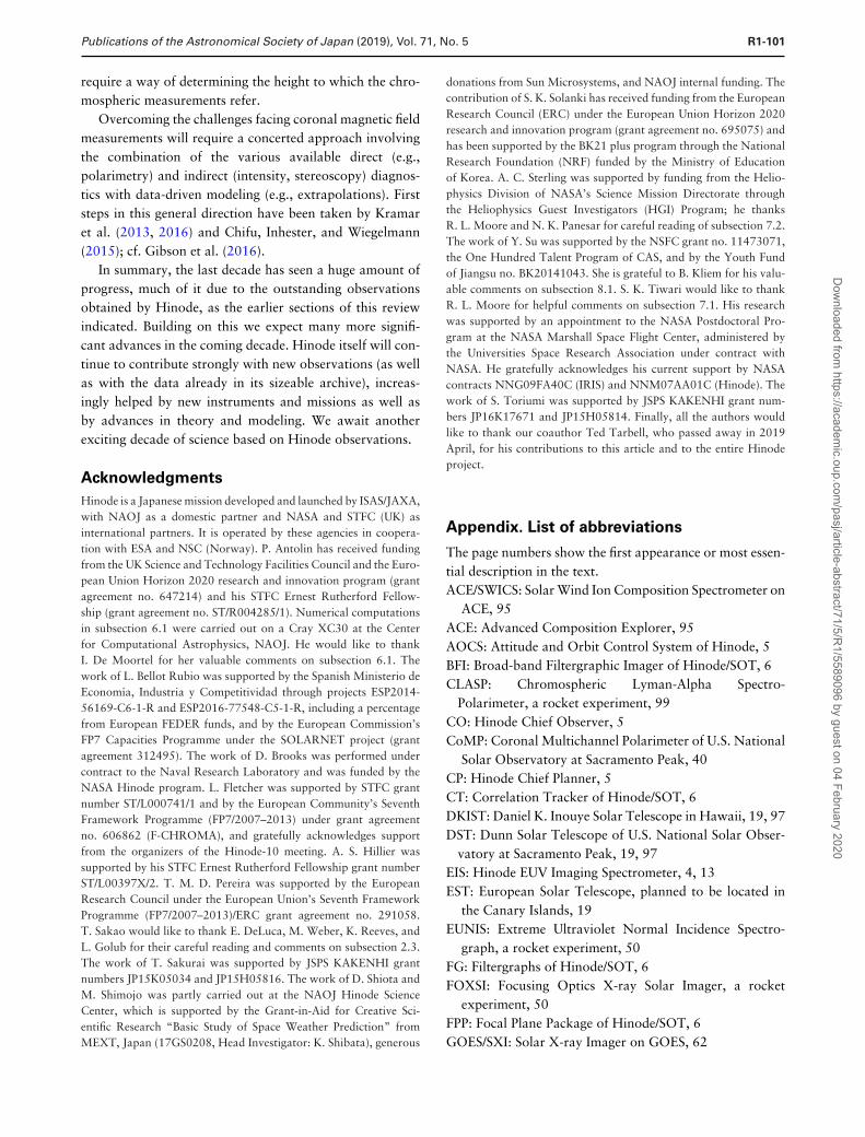
Publications of the Astronomical Society of Japan (2019), Vol. 71, No. 5 R1-101
require a way of determining the height to which the chro-mospheric measurements refer.
Overcoming the challenges facing coronal magnetic fieldmeasurements will require a concerted approach involvingthe combination of the various available direct (e.g.,polarimetry) and indirect (intensity, stereoscopy) diagnos-tics with data-driven modeling (e.g., extrapolations). Firststeps in this general direction have been taken by Kramaret al. (2013, 2016) and Chifu, Inhester, and Wiegelmann(2015); cf. Gibson et al. (2016).
In summary, the last decade has seen a huge amount ofprogress, much of it due to the outstanding observationsobtained by Hinode, as the earlier sections of this reviewindicated. Building on this we expect many more signifi-cant advances in the coming decade. Hinode itself will con-tinue to contribute strongly with new observations (as wellas with the data already in its sizeable archive), increas-ingly helped by new instruments and missions as well asby advances in theory and modeling. We await anotherexciting decade of science based on Hinode observations.
Acknowledgments
Hinode is a Japanese mission developed and launched by ISAS/JAXA,with NAOJ as a domestic partner and NASA and STFC (UK) asinternational partners. It is operated by these agencies in coopera-tion with ESA and NSC (Norway). P. Antolin has received fundingfrom the UK Science and Technology Facilities Council and the Euro-pean Union Horizon 2020 research and innovation program (grantagreement no. 647214) and his STFC Ernest Rutherford Fellow-ship (grant agreement no. ST/R004285/1). Numerical computationsin subsection 6.1 were carried out on a Cray XC30 at the Centerfor Computational Astrophysics, NAOJ. He would like to thankI. De Moortel for her valuable comments on subsection 6.1. Thework of L. Bellot Rubio was supported by the Spanish Ministerio deEconomıa, Industria y Competitividad through projects ESP2014-56169-C6-1-R and ESP2016-77548-C5-1-R, including a percentagefrom European FEDER funds, and by the European Commission’sFP7 Capacities Programme under the SOLARNET project (grantagreement 312495). The work of D. Brooks was performed undercontract to the Naval Research Laboratory and was funded by theNASA Hinode program. L. Fletcher was supported by STFC grantnumber ST/L000741/1 and by the European Community’s SeventhFramework Programme (FP7/2007–2013) under grant agreementno. 606862 (F-CHROMA), and gratefully acknowledges supportfrom the organizers of the Hinode-10 meeting. A. S. Hillier wassupported by his STFC Ernest Rutherford Fellowship grant numberST/L00397X/2. T. M. D. Pereira was supported by the EuropeanResearch Council under the European Union’s Seventh FrameworkProgramme (FP7/2007–2013)/ERC grant agreement no. 291058.T. Sakao would like to thank E. DeLuca, M. Weber, K. Reeves, andL. Golub for their careful reading and comments on subsection 2.3.The work of T. Sakurai was supported by JSPS KAKENHI grantnumbers JP15K05034 and JP15H05816. The work of D. Shiota andM. Shimojo was partly carried out at the NAOJ Hinode ScienceCenter, which is supported by the Grant-in-Aid for Creative Sci-entific Research “Basic Study of Space Weather Prediction” fromMEXT, Japan (17GS0208, Head Investigator: K. Shibata), generous
donations from Sun Microsystems, and NAOJ internal funding. Thecontribution of S. K. Solanki has received funding from the EuropeanResearch Council (ERC) under the European Union Horizon 2020research and innovation program (grant agreement no. 695075) andhas been supported by the BK21 plus program through the NationalResearch Foundation (NRF) funded by the Ministry of Educationof Korea. A. C. Sterling was supported by funding from the Helio-physics Division of NASA’s Science Mission Directorate throughthe Heliophysics Guest Investigators (HGI) Program; he thanksR. L. Moore and N. K. Panesar for careful reading of subsection 7.2.The work of Y. Su was supported by the NSFC grant no. 11473071,the One Hundred Talent Program of CAS, and by the Youth Fundof Jiangsu no. BK20141043. She is grateful to B. Kliem for his valu-able comments on subsection 8.1. S. K. Tiwari would like to thankR. L. Moore for helpful comments on subsection 7.1. His researchwas supported by an appointment to the NASA Postdoctoral Pro-gram at the NASA Marshall Space Flight Center, administered bythe Universities Space Research Association under contract withNASA. He gratefully acknowledges his current support by NASAcontracts NNG09FA40C (IRIS) and NNM07AA01C (Hinode). Thework of S. Toriumi was supported by JSPS KAKENHI grant num-bers JP16K17671 and JP15H05814. Finally, all the authors wouldlike to thank our coauthor Ted Tarbell, who passed away in 2019April, for his contributions to this article and to the entire Hinodeproject.
Appendix. List of abbreviations
The page numbers show the first appearance or most essen-tial description in the text.ACE/SWICS: Solar Wind Ion Composition Spectrometer on
ACE, 95ACE: Advanced Composition Explorer, 95AOCS: Attitude and Orbit Control System of Hinode, 5BFI: Broad-band Filtergraphic Imager of Hinode/SOT, 6CLASP: Chromospheric Lyman-Alpha Spectro-
Polarimeter, a rocket experiment, 99CO: Hinode Chief Observer, 5CoMP: Coronal Multichannel Polarimeter of U.S. National
Solar Observatory at Sacramento Peak, 40CP: Hinode Chief Planner, 5CT: Correlation Tracker of Hinode/SOT, 6DKIST: Daniel K. Inouye Solar Telescope in Hawaii, 19, 97DST: Dunn Solar Telescope of U.S. National Solar Obser-
vatory at Sacramento Peak, 19, 97EIS: Hinode EUV Imaging Spectrometer, 4, 13EST: European Solar Telescope, planned to be located in
the Canary Islands, 19EUNIS: Extreme Ultraviolet Normal Incidence Spectro-
graph, a rocket experiment, 50FG: Filtergraphs of Hinode/SOT, 6FOXSI: Focusing Optics X-ray Solar Imager, a rocket
experiment, 50FPP: Focal Plane Package of Hinode/SOT, 6GOES/SXI: Solar X-ray Imager on GOES, 62
Dow
nloaded from https://academ
ic.oup.com/pasj/article-abstract/71/5/R
1/5589096 by guest on 04 February 2020

R1-102 Publications of the Astronomical Society of Japan (2019), Vol. 71, No. 5
GOES: Geostationary Operational Environmental Satellite,12, 62
GST: Goode Solar Telescope (New Solar Telescope) atBig Bear Solar Observatory, New Jersey Institute ofTechnology (NJIT), 97
Hi-C: High Resolution Coronal Imager, a rocket experi-ment, 55
HOP: Hinode Operation Plan, 6HXT: Yokhoh Hard X-ray Telescope, 82IRIS: Interface Region Imaging Spectrometer, 29LEMUR: Large European Module for Solar Ultraviolet
Research, a proposal for SOLAR-C, 100MDP: Mission Data Processor of Hinode, 6NFI: Narrow-band Filtergraphic Imager of Hinode/SOT,
6, 8NST: New Solar Telescope (Goode Solar Telescope) at
Big Bear Solar Observatory, New Jersey Institute ofTechnology (NJIT), 65
NuSTAR: Nuclear Spectroscopic Telescope Array, 50OTA: Optical Telescope Assembly of Hinode/SOT, 6PMU: Polarization Modulation Unit of Hinode/SOT, 6RHESSI: Reuven Ramaty High-Energy Solar Spectroscopic
Imager, 82SDO/AIA: Atmospheric Imaging Assembly on SDO, 11SDO/HMI: Helioseismic Magnetic Imager on SDO, 15SDO: Solar Dynamics Observatory, 11SMEI: Solar Mass Ejection Imager, 33SMM: Solar Maximum Mission, 75SO/EUI: Extreme Ultraviolet Imager on Solar Orbiter, 100SO/PHI: Polarimetric and Helioseismic Imager on Solar
Orbiter, 97SO/SPICE: Spectral Imaging of the Coronal Environment
on Solar Orbiter, 100SOHO/CDS: Coronal Diagnostic Spectrometer on SOHO,
85SOHO/EIT: Extreme-Ultraviolet Imaging Telescope on
SOHO, 59SOHO/LASCO: Large-Angle and Spectrometric Corona-
graph on SOHO, 33SOHO/MDI: Michelson Doppler Imager on SOHO, 15SOHO/SUMER: Solar Ultraviolet Measurements of
Emitted Radiation experiment on SOHO, 40SOHO: Solar and Heliospheric Observatory, 15SOLAR-C_EUVST: SOLAR-C Extreme Ultra-Violet High-
Throughput Spectroscopic Telescope, 99SOT: Hinode Solar Optical Telescope, 4, 6SP: Spectro-polarimeter of Hinode/SOT, 6, 8SSOC: Sagamihara Spacecraft Operation Center, 5SST: Swedish Solar Telescope in La Palma, 17STEREO/COR2: Outer Coronagraph on STEREO, 33STEREO/SECCHI-EUVI: Extreme Ultraviolet Imager
in Sun Earth Connection Coronal and Heliospheric
Investigation (SECCHI) instrument suite of STEREO,59
STEREO: Solar-Terrestrial Relations Observatory, 33SUNRISE/IMaX: Imaging Magnetograph Experiment on
the SUNRISE balloon-borne telescope, 16, 100SUNRISE/SuFI: SUNRISE Filter Imager, 100SWG: The Hinode Science Working Group, 4SXT: Yokhoh Soft X-ray Telescope, 3TRACE: Transition Region and Coronal Explorer, 59UFSS: Ultra-Fine Sun Sensor of Hinode, 5USC: Uchinoura Space Center, ISAS/JAXA, 3VLS: Visible Light Shutter of Hinode/XRT, 7VTT: German Vacuum Tower Telescope in Tenerife, 19XRT: Hinode X-Ray Telescope, 4, 10
References
Abbo, L., et al. 2016, Space Sci. Rev., 201, 55Abramenko, V., & Yurchyshyn, V. 2010, ApJ, 722, 122Acton, L. W. 2016, Sol. Phys., 291, 643Acton, L. W., Weston, D. C., & Bruner, M. E. 1999, JGR, 104,
14827Adams, M., Solanki, S. K., Hagyard, M., & Moore, R. L. 1993, Sol.
Phys., 148, 201Adams, M., Sterling, A. C., Moore, R. L., & Gary, G. A. 2014, ApJ,
783, 11Afshari, M., Peres, G., Jibben, P. R., Petralia, A., Reale, F., &
Weber, M. 2016, AJ, 152, 107Ahn, K., Chae, J., Cao, W., & Goode, P. R. 2010, ApJ, 721, 74Alexander, D., & Fletcher, L. 1999, Sol. Phys., 190, 167Alfven, H. 1947, MNRAS, 107, 211Allan, W., & Wright, A. N. 2000, J. Geophys. Res., 105, 317Allred, J. C., Kowalski, A. F., & Carlsson, M. 2015, ApJ, 809, 104Alpert, S. E., Tiwari, S. K., Moore, R. L., Winebarger, A. R., &
Savage, S. L. 2016, ApJ, 822, 35Amari, T., Canou, A., & Aly, J.-J. 2014, Nature, 514, 465Amari, T., Luciani, J. F., Aly, J. J., Mikic, Z., & Linker, J. 2003,
ApJ, 585, 1073Anan, T., et al. 2010, PASJ, 62, 871Anfinogentov, S., Nistico, G., & Nakariakov, V. M. 2013, A&A,
560, A107Anfinogentov, S. A., Nakariakov, V. M., & Nistico, G. 2015, A&A,
583, A136Antiochos, S. K., DeVore, C. R., & Klimchuk, J. A. 1999a, ApJ, 510,
485Antiochos, S. K., Karpen, J. T., DeLuca, E. E., Golub, L., &
Hamilton, P. 2003, ApJ, 590, 547Antiochos, S. K., & Klimchuk, J. A. 1991, ApJ, 378, 372Antiochos, S. K., MacNeice, P. J., Spicer, D. S., & Klimchuk, J. A.
1999b, ApJ, 512, 985Antiochos, S. K., Mikic, Z., Titov, V. S., Lionello, R., & Linker, J. A.
2011, ApJ, 731, 112Antolin, P., De Moortel, I., Van Doorsselaere, T., & Yokoyama, T.
2016, ApJ, 830, L22Antolin, P., De Moortel, I., Van Doorsselaere, T., & Yokoyama, T.
2017, ApJ, 836, 219
Dow
nloaded from https://academ
ic.oup.com/pasj/article-abstract/71/5/R
1/5589096 by guest on 04 February 2020

Publications of the Astronomical Society of Japan (2019), Vol. 71, No. 5 R1-103
Antolin, P., Okamoto, T. J., De Pontieu, B., Uitenbroek, H.,Van Doorsselaere, T., & Yokoyama, T. 2015a, ApJ,809, 72
Antolin, P., Pagano, P., De Moortel, I., & Nakariakov, V. M. 2018a,ApJ, 861, L15
Antolin, P., & Rouppe van der Voort, L. 2012, ApJ, 745, 152Antolin, P., Schmit, D., Pereira, T. M. D., De Pontieu, B., &
De Moortel, I. 2018b, ApJ, 856, 44Antolin, P., & Shibata, K. 2010, ApJ, 712, 494Antolin, P., Shibata, K., Kudoh, T., Shiota, D., & Brooks, D. 2008,
ApJ, 688, 669Antolin, P., Shibata, K., & Vissers, G. 2010, ApJ, 716, 154Antolin, P., & Van Doorsselaere, T. 2013, A&A, 555, A74Antolin, P., & Verwichte, E. 2011, ApJ, 736, 121Antolin, P., Vissers, G., Pereira, T. M. D., Rouppe van der Voort,
L., & Scullion, E. 2015, ApJ, 806, 81Antolin, P., Yokoyama, T., & Van Doorsselaere, T. 2014, ApJ, 787,
L22Anusha, L. S., Solanki, S. K., Hirzberger, J., & Feller, A. 2016,
arXiv:1608.08499Arber, T. D., Brady, C. S., & Shelyag, S. 2016, ApJ, 817, 94Archontis, V., & Hood, A. W. 2009, A&A, 508, 1469Archontis, V., & Hood, A. W. 2013, ApJ, 769, L21Archontis, V., Hood, A. W., Savcheva, A., Golub, L., & Deluca, E.
2009, ApJ, 691, 1276Archontis, V., Moreno-Insertis, F., Galsgaard, K., & Hood, A. W.
2005, ApJ, 635, 1299Arregui, I. 2015, Philos. Trans. R. Soc. Lond. A, 373, 20140261Arregui, I., Oliver, R., & Ballester, J. L. 2012, Living Rev. Sol. Phys.,
9, 2Asai, A., Yokoyama, T., Shimojo, M., Masuda, S., Kurokawa, H.,
& Shibata, K. 2004, ApJ, 611, 557Aschwanden, M. J., Fletcher, L., Schrijver, C. J., & Alexander, D.
1999, ApJ, 520, 880Aschwanden, M. J., & Nightingale, R. W. 2005, ApJ, 633,
499Aschwanden, M. J., Nightingale, R. W., & Alexander, D. 2000, ApJ,
541, 1059Aschwanden, M. J., & Peter, H. 2017, ApJ, 840, 4Aschwanden, M. J., Schrijver, C. J., & Alexander, D. 2001, ApJ,
550, 1036Asensio Ramos, A. 2009, ApJ, 701, 1032Asensio Ramos, A., & Martınez Gonzalez, M. J. 2014, A&A, 572,
A98Asgari-Targhi, M., Schmelz, J. T., Imada, S., Pathak, S., & Christian,
G. M. 2015, ApJ, 807, 146Asgari-Targhi, M., van Ballegooijen, A. A., & Imada, S. 2014, ApJ,
786, 28Athay, R. G., & Holzer, T. E. 1982, ApJ, 255, 743Auchere, F., Bocchialini, K., Solomon, J., & Tison, E. 2014, A&A,
563, A8Auchere, F., Froment, C., Soubrie, E., Antolin, P., Oliver, R., &
Pelouze, G. 2018, ApJ, 853, 176Aulanier, G., Torok, T., Demoulin, P., & DeLuca, E. E. 2010, ApJ,
708, 314Baker, D., van Driel-Gesztelyi, L., & Green, L. M. 2012, Sol. Phys.,
276, 219Baker, D., van Driel-Gesztelyi, L., Mandrini, C. H., Demoulin, P., &
Murray, M. J. 2009, ApJ, 705, 926
Balthasar, H. 2018, Sol. Phys., 293, 120Bamba, Y., Kusano, K., Yamamoto, T. T., & Okamoto, T. J. 2013,
ApJ, 778, 48Banerjee, D., Perez-Suarez, D., & Doyle, J. G. 2009, A&A, 501, L15Barthol, P., et al. 2011, Sol. Phys., 268, 1Bazarghan, M., Safari, H., Innes, D. E., Karami, E., & Solanki, S. K.
2008, A&A, 492, L13Beck, C., & Rezaei, R. 2009, A&A, 502, 969Beckers, J. M. 1968, Sol. Phys., 3, 367Beckers, J. M. 1972, ARA&A, 10, 73Bel, N., & Leroy, B. 1977, A&A, 55, 239Bello Gonzalez, N., et al. 2010, ApJ, 723, L134Bellot Rubio, L. R. 2003, in ASP Conf. Ser., 307, Solar Polarization,
ed. J. Trujillo-Bueno & J. Sanchez Almeida (San Francisco:ASP), 301
Bellot Rubio, L. R. 2009, ApJ, 700, 284Bellot Rubio, L. R., et al. 2007, ApJ, 668, L91Bellot Rubio, L. R., & Orozco Suarez, D. 2012, ApJ, 757, 19Bellot Rubio, L. R., Ruiz Cobo, B., & Collados, M. 1997, ApJ, 478,
L45Bellot Rubio, L. R., Ruiz Cobo, B., & Collados, M. 2000, ApJ, 535,
489Bellot Rubio, L. R., Schlichenmaier, R., & Langhans, K. 2010, ApJ,
725, 11Berger, T., et al. 2011, Nature, 472, 197Berger, T. E., et al. 2008, ApJ, 676, L89Berger, T. E., et al. 2010, ApJ, 716, 1288Berger, T. E., de Pontieu, B., Fletcher, L., Schrijver, C. J., Tarbell,
T. D., & Title, A. M. 1999, Sol. Phys., 190, 409Bharti, L. 2015, MNRAS, 452, L16Bharti, L., Joshi, C., & Jaaffrey, S. N. A. 2007, ApJ, 669, L57Bharti, L., Solanki, S. K., & Hirzberger, J. 2010, ApJ, 722, L194Bingert, S., & Peter, H. 2011, A&A, 530, A112Birch, A. C., Schunker, H., Braun, D. C., Cameron, R., Gizon, L.,
Lo ptien, B., & Rempel, M. 2016, Sci. Adv., 2, e1600557Blanco Rodrıguez, J., Okunev, O. V., Puschmann, K. G., Kneer, F.,
& Sanchez-Andrade Nuno, B. 2007, A&A, 474, 251Bobra, M. G., van Ballegooijen, A. A., & DeLuca, E. E. 2008, ApJ,
672, 1209Bogdan, T. J., et al. 2003, ApJ, 599, 626Bogod, V. M., & Yasnov, L. V. 2016, Sol. Phys., 291, 3317Bohlin, J. D., Sheeley, N. R., & Tousey, R. 1975, in Space Research
XV, ed.Rycroft, M. J. (Berlin: Akademie-Verlag), 651Boldyrev, S. 2005, ApJ, 626, L37Bonet, J. A., Marquez, I., Sanchez Almeida, J., Cabello, I., &
Domingo, V. 2008, ApJ, 687, L131Borrero, J. M. 2007, A&A, 471, 967Borrero, J. M., et al. 2016, A&A, 596, A2Borrero, J. M., & Ichimoto, K. 2011, Living Rev. Sol. Phys., 8, 4Borrero, J. M., Jafarzadeh, S., Schussler, M., & Solanki, S. K. 2017,
Space Sci. Rev., 210, 275Borrero, J. M., & Kobel, P. 2011, A&A, 527, A29Borrero, J. M., & Kobel, P. 2012, A&A, 547, A89Borrero, J. M., Lagg, A., Solanki, S. K., & Collados, M. 2005, A&A,
436, 333Borrero, J. M., Lites, B. W., & Solanki, S. K. 2008, A&A, 481, L13Borrero, J. M., & Solanki, S. K. 2008, ApJ, 687, 668Boutry, C., Buchlin, E., Vial, J.-C., & Regnier, S. 2012, ApJ, 752, 13Bradshaw, S. J. 2009, A&A, 502, 409
Dow
nloaded from https://academ
ic.oup.com/pasj/article-abstract/71/5/R
1/5589096 by guest on 04 February 2020

R1-104 Publications of the Astronomical Society of Japan (2019), Vol. 71, No. 5
Bradshaw, S. J., Aulanier, G., & Del Zanna, G. 2011, ApJ, 743, 66Bradshaw, S. J., & Cargill, P. J. 2010, ApJ, 717, 163Bradshaw, S. J., & Cargill, P. J. 2013, ApJ, 770, 12Bradshaw, S. J., & Klimchuk, J. A. 2011, ApJS, 194, 26Bradshaw, S. J., Klimchuk, J. A., & Reep, J. W. 2012, ApJ, 758, 53Bradshaw, S. J., & Mason, H. E. 2003, A&A, 401, 699Bradshaw, S. J., & Viall, N. M. 2016, ApJ, 821, 63Brady, C. S., & Arber, T. D. 2016, ApJ, 829, 80Brandenburg, A., & Dobler, W. 2002, Comput. Phys. Commun.,
147, 471Brandenburg, A., Sokoloff, D., & Subramanian, K. 2012, Space Sci.
Rev., 169, 123Brannon, S. R., Longcope, D. W., & Qiu, J. 2015, ApJ, 810, 4Brickhouse, N. S., & Labonte, B. J. 1988, Sol. Phys., 115, 43Brooks, D. H., Ugarte-Urra, I., & Warren, H. P. 2015, Nature
Commun., 6, 5947Brooks, D. H., & Warren, H. P. 2011, ApJ, 727, L13Brooks, D. H., & Warren, H. P. 2012, ApJ, 760, L5Brooks, D. H., & Warren, H. P. 2016, ApJ, 820, 63Brooks, D. H., Warren, H. P., & Ugarte-Urra, I. 2012, ApJ, 755,
L33Brooks, D. H., Warren, H. P., Ugarte-Urra, I., & Winebarger, A. R.
2013, ApJ, 772, L19Brosius, J. W. 2013, ApJ, 762, 133Brosius, J. W., Daw, A. N., & Inglis, A. R. 2016, ApJ, 830, 101Brosius, J. W., Daw, A. N., & Rabin, D. M. 2014, ApJ, 790, 112Brown, C. M., et al. 2007, PASJ, 59, S865Brown, D. S., Nightingale, R. W., Alexander, D., Schrijver, C. J.,
Metcalf, T. R., Shine, R. A., Title, A. M., & Wolfson, C. J.2003, Sol. Phys., 216, 79
Browning, P. K., & Priest, E. R. 1984, A&A, 131, 283Bruzek, A. 1967, Sol. Phys., 2, 451Bryans, P., Young, P. R., & Doschek, G. A. 2010, ApJ, 715,
1012Buehler, D., Lagg, A., & Solanki, S. K. 2013, A&A, 555, A33Buehler, D., Lagg, A., Solanki, S. K., & van Noort, M. 2015, A&A,
576, A27Bumba, V., & Howard, R. 1965, ApJ, 141, 1502Burch, J. L., & Phan, T. D. 2016, Geophys. Res. Lett., 43, 8327Cadavid, A. C., Lawrence, J. K., Christian, D. J., Jess, D. B., &
Nigro, G. 2014, ApJ, 795, 48Cadavid, A. C., Rivera, Y. J., Lawrence, J. K., Christian, D. J.,
Jennings, P. J., & Rappazzo, A. F. 2016, ApJ, 831, 186Cally, P. S. 2017, MNRAS, 466, 413Cally, P. S., & Goossens, M. 2008, Sol. Phys., 251, 251Cally, P. S., & Hansen, S. C. 2011, ApJ, 738, 119Cameron, R., & Sammis, I. 1999, ApJ, 525, L61Cameron, R., & Schussler, M. 2015, Science, 347, 1333Canfield, R. C., Hudson, H. S., & McKenzie, D. E. 1999, Geophys.
Res. Lett., 26, 627Canfield, R. C., Reardon, K. P., Leka, K. D., Shibata, K.,
Yokoyama, T., & Shimojo, M. 1996, ApJ, 464, 1016Canou, A., & Amari, T. 2010, ApJ, 715, 1566Cargill, P. J. 2014, ApJ, 784, 49Cargill, P. J., Bradshaw, S. J., & Klimchuk, J. A. 2012, ApJ, 752,
161Cargill, P. J., De Moortel, I., & Kiddie, G. 2016, ApJ, 823, 31Cargill, P. J., & Klimchuk, J. A. 1997, ApJ, 478, 799Cargill, P. J., & Klimchuk, J. A. 2004, ApJ, 605, 911
Cargill, P. J., Warren, H. P., & Bradshaw, S. J. 2015, Philos. Trans.R. Soc. Lond. A, 373, 20140260
Carlsson, M., et al. 2007, PASJ, 59, S663Carlsson, M., Judge, P. G., & Wilhelm, K. 1997, ApJ, 486, L63Carlsson, M., & Leenaarts, J. 2012, A&A, 539, A39Carlyle, J., Williams, D. R., van Driel-Gesztelyi, L., Innes, D.,
Hillier, A., & Matthews, S. 2014, ApJ, 782, 87Carrington, R. C. 1859, MNRAS, 20, 13Caspi, A., Woods, T. N., & Warren, H. P. 2015, ApJ, 802, L2Centeno, R., et al. 2007, ApJ, 666, L137Chae, J. 2010, ApJ, 714, 618Chandrasekhar, S. 1961, Hydrodynamic and Hydromagnetic
Stability (Oxford: Clarendon)Chen, H., Jiang, Y., & Ma, S. 2009, Sol. Phys., 255, 79Chen, H.-D., Zhang, J., & Ma, S.-L. 2012, Res. Astron. Astrophys.,
12, 573Cheung, M., Schussler, M., & Moreno-Insertis, F. 2005, in ESA SP-
596, Chromospheric and Coronal Magnetic Fields, ed. D. E.Innes et al. (Noordwijk: ESA), 54.1
Cheung, M. C. M., et al. 2015, ApJ, 801, 83Cheung, M. C. M., & Isobe, H. 2014, Living Rev. Sol. Phys.,
11, 3Cheung, M. C. M., Rempel, M., Title, A. M., & Schussler, M. 2010,
ApJ, 720, 233Cheung, M. C. M., Schussler, M., Tarbell, T. D., & Title, A. M.
2008, ApJ, 687, 1373Chifor, C., et al. 2008a, A&A, 491, 279Chifor, C., Young, P. R., Isobe, H., Mason, H. E., Tripathi, D.,
Hara, H., & Yokoyama, T. 2008b, A&A, 481, L57Chifu, I., Inhester, B., & Wiegelmann, T. 2015, A&A, 577, A123Chitta, L. P., et al. 2017, ApJS, 229, 4Chitta, L. P., Peter, H., & Solanki, S. K. 2018, A&A, 615, L9Chitta, L. P., van Ballegooijen, A. A., Rouppe van der Voort, L.,
DeLuca, E. E., & Kariyappa, R. 2012, ApJ, 752, 48Chou, D.-Y., Liang, Z.-C., Yang, M.-H., Zhao, H., & Sun, M.-T.
2009, ApJ, 696, L106Christopoulou, E. B., Georgakilas, A. A., & Koutchmy, S. 2001,
Sol. Phys., 199, 61Cirtain, J. W., et al. 2007, Science, 318, 1580Cirtain, J. W., et al. 2013, Nature, 493, 501Collados, M., et al. 2010, Astron. Nachr., 331, 615Compagnino, A., Romano, P., & Zuccarello, F. 2017, Sol. Phys.,
292, 5Cowling, T. G. 1953, in The Sun, ed. G. P. Kuiper (Chicago: Chicago
University Press), 532Cranmer, S. R. 2012, Space Sci. Rev., 172, 145Cranmer, S. R., & Woolsey, L. N. 2015, ApJ, 812, 71Criscuoli, S., Del Moro, D., Giannattasio, F., Viticchie, B.,
Giorgi, F., Ermolli, I., Zuccarello, F., & Berrilli, F. 2012, A&A,546, A26
Culhane, J. L., et al. 2007, Sol. Phys., 243, 19Culhane, J. L., et al. 2014, Sol. Phys., 289, 3799Czaykowska, A., De Pontieu, B., Alexander, D., & Rank, G. 1999,
ApJ, 521, L75Dahlburg, R. B., Einaudi, G., Taylor, B. D., Ugarte-Urra, I., Warren,
H. P., Rappazzo, A. F., & Velli, M. 2016, ApJ, 817, 47Danilovic, S., et al. 2010c, ApJ, 723, L149Danilovic, S., Gandorfer, A., Lagg, A., Schussler, M., Solanki, S. K.,
Vogler, A., Katsukawa, Y., & Tsuneta, S. 2008, A&A, 484, L17
Dow
nloaded from https://academ
ic.oup.com/pasj/article-abstract/71/5/R
1/5589096 by guest on 04 February 2020

Publications of the Astronomical Society of Japan (2019), Vol. 71, No. 5 R1-105
Danilovic, S., Rempel, M., van Noort, M., & Cameron, R. 2016a,A&A, 594, A103
Danilovic, S., Schussler, M., & Solanki, S. K. 2010a, A&A, 509, A76Danilovic, S., Schussler, M., & Solanki, S. K. 2010b, A&A, 513, A1Danilovic, S., van Noort, M., & Rempel, M. 2016b, A&A, 593, A93Dasi-Espuig, M., Solanki, S. K., Krivova, N. A., Cameron, R., &
Penuela, T. 2010, A&A, 518, A7Dasi-Espuig, M., Solanki, S. K., Krivova, N. A., Cameron, R., &
Penuela, T. 2013, A&A, 556, C3De Groof, A., Berghmans, D., van Driel-Gesztelyi, L., & Poedts, S.
2004, A&A, 415, 1141de la Cruz Rodrıguez, J., Hansteen, V., Bellot-Rubio, L., & Ortiz, A.
2015, ApJ, 810, 145de la Cruz Rodrıguez, J., Leenaarts, J., Danilovic, S., &
Uitenbroek, H. 2019, A&A, 623, A74de la Cruz Rodrıguez, J., & van Noort, M. 2017, Space Sci. Rev.,
210, 109De Moortel, I., & Browning, P. 2015, Philos. Trans. R. Soc. Lond.
A, 373, 20140269De Moortel, I., & Nakariakov, V. M. 2012, Philos. Trans. R. Soc.
Lond. A, 370, 3193De Moortel, I., & Pascoe, D. J. 2012, ApJ, 746, 31De Moortel, I., Pascoe, D. J., Wright, A. N., & Hood, A. W. 2016,
Plasma Phys. Control. Fusion, 58, 014001De Pontieu, B. 2002, ApJ, 569, 474De Pontieu, B., et al. 2007b, PASJ, 59, S655De Pontieu, B., et al. 2007c, Science, 318, 1574De Pontieu, B., et al. 2011, Science, 331, 55De Pontieu, B., et al. 2014a, Science, 346, 1255732De Pontieu, B., et al. 2014b, Sol. Phys., 289, 2733De Pontieu, B., Erdelyi, R., & James, S. P. 2004, Nature, 430, 536De Pontieu, B., Hansteen, V. H., Rouppe van der Voort, L.,
van Noort, M., & Carlsson, M. 2007a, ApJ, 655, 624De Pontieu, B., McIntosh, S. W., Hansteen, V. H., & Schrijver, C. J.
2009, ApJ, 701, L1De Pontieu, B., Martens, P. C. H., & Hudson, H. S. 2001, ApJ, 558,
859De Rosa, M. L., et al. 2009, ApJ, 696, 1780de Toma, G., Casini, R., Burkepile, J. T., & Low, B. C. 2008, ApJ,
687, L123del Toro Iniesta, J. C., & Ruiz Cobo, B. 2016, Living Rev. Sol. Phys.,
13, 4Del Zanna, G. 2008a, in ASP Conf. Ser., 397, First Results From
Hinode, ed. S. A. Matthews et al. (San Francisco: ASP), 87Del Zanna, G. 2008b, A&A, 481, L49Del Zanna, G. 2013a, A&A, 555, A47Del Zanna, G. 2013b, A&A, 558, A73Del Zanna, G., Aulanier, G., Klein, K.-L., & Torok, T. 2011a, A&A,
526, A137Del Zanna, G., & Mason, H. E. 2003, A&A, 406, 1089Del Zanna, G., & Mason, H. E. 2014, A&A, 565, A14Del Zanna, G., Mitra-Kraev, U., Bradshaw, S. J., Mason, H. E., &
Asai, A. 2011b, A&A, 526, A1Del Zanna, G., Tripathi, D., Mason, H., Subramanian, S., &
O’Dwyer, B. 2015, A&A, 573, A104Delaboudiniere, J.-P., et al. 1995, Sol. Phys., 162, 291Deng, N., Yurchyshyn, V., Tian, H., Kleint, L., Liu, C., Xu, Y., &
Wang, H. 2016, ApJ, 829, 103
DeRosa, M. L., et al. 2015, ApJ, 811, 107Domingo, V., Fleck, B., & Poland, A. I. 1995, Sol. Phys., 162, 1Domınguez Cerdena, I., Kneer, F., & Sanchez Almeida, J. 2003, ApJ,
582, L55Doschek, G. A., McKenzie, D. E., & Warren, H. P. 2014, ApJ, 788,
26Doschek, G. A., Mariska, J. T., Warren, H. P., Culhane, L.,
Watanabe, T., Young, P. R., Mason, H. E., & Dere, K. P. 2007,PASJ, 59, S707
Doschek, G. A., & Warren, H. P. 2016, ApJ, 825, 36Doschek, G. A., Warren, H. P., & Feldman, U. 2015, ApJ, 808, L7Doschek, G. A., Warren, H. P., Mariska, J. T., Muglach, K., Culhane,
J. L., Hara, H., & Watanabe, T. 2008, ApJ, 686, 1362Doschek, G. A., Warren, H. P., & Young, P. R. 2013, ApJ, 767, 55Downs, C., Lionello, R., Mikic, Z., Linker, J. A., & Velli, M. 2016,
ApJ, 832, 180Dudık, J., Aulanier, G., Schmieder, B., Zapior, M., & Heinzel, P.
2012, ApJ, 761, 9Dunn, R. B., & Smartt, R. N. 1991, Adv. Space Res., 11, 139Dzifcakova, E., Dudık, J., Kotrc, P., Farnık, F., & Zemanova, A.
2015, ApJS, 217, 14Edwards, S. J., Parnell, C. E., Harra, L. K., Culhane, J. L., & Brooks,
D. H. 2016, Sol. Phys., 291, 117Edwin, P. M., & Roberts, B. 1983, Sol. Phys., 88, 179Ellerman, F. 1917, ApJ, 46, 298Elsden, T., & Wright, A. N. 2017, JGR: Space Phys., 122, 3247Engvold, O. 1981, Sol. Phys., 70, 315Erdelyi, R., & Taroyan, Y. 2008, A&A, 489, L49Esteban Pozuelo, S., Bellot Rubio, L. R., & de la Cruz Rodrıguez, J.
2015, ApJ, 803, 93Evans, K., & Pounds, K. A. 1968, ApJ, 152, 319Eyles, C. J., et al. 2003, Sol. Phys., 217, 319Fan, Y. 2009, Living Rev. Sol. Phys., 6, 4Fan, Y. 2011, ApJ, 740, 68Fan, Y. 2016, ApJ, 824, 93Fang, F., Fan, Y., & McIntosh, S. W. 2014, ApJ, 789, L19Fang, F., Manchester, W., IV, Abbett, W. P., & van der Holst, B.
2012a, ApJ, 754, 15Fang, F., Manchester, W., IV, Abbett, W. P., & van der Holst, B.
2012b, ApJ, 745, 37Faurobert, M., & Ricort, G. 2015, A&A, 582, A95Fazakerley, A. N., Harra, L. K., & van Driel-Gesztelyi, L. 2016, ApJ,
823, 145Feldman, U. 1992, Phys. Scr., 46, 202Feldman, U., Ralchenko, Y., & Landi, E. 2008, ApJ, 684, 707Felipe, T., et al. 2016, A&A, 596, A59Feng, S., Zhao, Y., Yang, Y., Ji, K., Deng, H., & Wang, F. 2015, Sol.
Phys., 290, 1119Fischer, C. E., de Wijn, A. G., Centeno, R., Lites, B. W., & Keller,
C. U. 2009, A&A, 504, 583Fisk, L. A., Schwadron, N. A., & Zurbuchen, T. H. 1998, Space Sci.
Rev., 86, 51Fletcher, L., et al. 2011, Space Sci. Rev., 159, 19Fletcher, L., & De Pontieu, B. 1999, ApJ, 520, L135Fletcher, L., & Hudson, H. S. 2008, ApJ, 675, 1645Fludra, A., et al. 2013, in Proc. SPIE, 8862, Solar Physics and
Space Weather Instrumentation V, ed. S. Fineschi & J. Fennelly(Bellingham, WA: SPIE), 88620F
Dow
nloaded from https://academ
ic.oup.com/pasj/article-abstract/71/5/R
1/5589096 by guest on 04 February 2020

R1-106 Publications of the Astronomical Society of Japan (2019), Vol. 71, No. 5
Forbes, T. G., & Isenberg, P. A. 1991, ApJ, 373, 294Fossum, A., & Carlsson, M. 2005, Nature, 435, 919Foukal, P. 1978, ApJ, 223, 1046Foukal, P. V., Noyes, R. W., Reeves, E. M., Schmahl, E. J., Timothy,
J. G., Vernazza, J. E., Wilhbroe, G. L., & Huber, M. C. E. 1974,ApJ, 193, L143
Fox, N. J., et al. 2016, Space Sci. Rev., 204, 7Franz, M. 2011, PhD thesis, Albert-Ludwigs-Universitat FreiburgFranz, M., et al. 2016, A&A, 596, A4Franz, M., & Schlichenmaier, R. 2009, A&A, 508, 1453Franz, M., & Schlichenmaier, R. 2013, A&A, 550, A97Freed, M. S., McKenzie, D. E., Longcope, D. W., & Wilburn, M.
2016, ApJ, 818, 57Freeland, S. L., & Handy, B. N. 1998, Sol. Phys., 182, 497Freij, N., Dorotovic, I., Morton, R. J., Ruderman, M. S.,
Karlovsky, V., & Erdelyi, R. 2016, ApJ, 817, 44Freytag, B., Steffen, M., & Dorch, B. 2002, Astron. Nachr., 323,
213Froment, C., Auchere, F., Aulanier, G., Mikic, Z., Bocchialini, K.,
Buchlin, E., & Solomon, J. 2017, ApJ, 835, 272Froment, C., Auchere, F., Bocchialini, K., Buchlin, E., Guennou, C.,
& Solomon, J. 2015, ApJ, 807, 158Froment, C., Auchere, F., Mikic, Z., Aulanier, G.,
Bocchialini, K., Buchlin, E., Solomon, J., & Soubrie, E. 2018,ApJ, 855, 52
Frutiger, C., & Solanki, S. K. 2001, A&A, 369, 646Frutiger, C., Solanki, S. K., Fligge, M., & Bruls, J. H. M. J. 2000,
A&A, 358, 1109Fujimura, D., & Tsuneta, S. 2009, ApJ, 702, 1443Gandorfer, A., et al. 2011, Sol. Phys., 268, 35Geiss, J., Gloeckler, G., & von Steiger, R. 1995, Space Sci. Rev., 72,
49Georgoulis, M. K., Rust, D. M., Bernasconi, P. N., & Schmieder, B.
2002, ApJ, 575, 506Gesztelyi, L. 1984, Adv. Space Res., 4, 19Gibb, G. P. S., Mackay, D. H., Green, L. M., & Meyer, K. A. 2014,
ApJ, 782, 71Gibson, S., et al. 2016, Front. Astron. Space Sci., 3, 8Gibson, S. E., & Low, B. C. 1998, ApJ, 493, 460Giovanelli, R. G. 1980, Sol. Phys., 68, 49Gizon, L., Birch, A. C., & Spruit, H. C. 2010, ARA&A, 48, 289Goldreich, P., & Sridhar, S. 1995, ApJ, 438, 763Goldstein, M. L. 1978, ApJ, 219, 700Golub, L., et al. 2007, Sol. Phys., 243, 63Golub, L., Hartquist, T. W., & Quillen, A. C. 1989, Sol. Phys., 122,
245Goode, P. R., Coulter, R., Gorceix, N., Yurchyshyn, V., & Cao, W.
2010, Astron. Nachr., 331, 620Goossens, M., Andries, J., & Aschwanden, M. J. 2002, A&A, 394,
L39Goossens, M., Soler, R., Terradas, J., Van Doorsselaere, T., &
Verth, G. 2014, ApJ, 788, 9Goossens, M., Terradas, J., Andries, J., Arregui, I., & Ballester, J. L.
2009, A&A, 503, 213Gordovskyy, M., Kontar, E. P., & Browning, P. K. 2016, A&A, 589,
A104Gosain, S., Tiwari, S. K., & Venkatakrishnan, P. 2010, ApJ, 720,
1281
Gosain, S., Venkatakrishnan, P., & Tiwari, S. K. 2009, ApJ, 706,L240
Gosic, M. 2015, PhD thesis, Universidad de Granada, SpainGosic, M., Bellot Rubio, L. R., del Toro Iniesta, J. C.,
Orozco Suarez, D., & Katsukawa, Y. 2016, ApJ, 820, 35Gosic, M., Bellot Rubio, L. R., Orozco Suarez, D., Katsukawa, Y.,
& del Toro Iniesta, J. C. 2014, ApJ, 797, 49Graham, D. R., & Cauzzi, G. 2015, ApJ, 807, L22Graham, D. R., Fletcher, L., & Hannah, I. G. 2011, A&A, 532, A27Graham, D. R., Fletcher, L., & Labrosse, N. 2015, A&A, 584, A6Graham, D. R., Hannah, I. G., Fletcher, L., & Milligan, R. O. 2013,
ApJ, 767, 83Grant, S. D. T., et al. 2015, ApJ, 806, 132Green, L. M., & Kliem, B. 2014, in IAU Symp., 300, Nature of
Prominences and their Role in Space Weather, ed. B. Schmiederet al. (Cambridge: Cambridge University Press), 209
Green, L. M., Kliem, B., & Wallace, A. J. 2011, A&A, 526, A2Greer, B. J., Hindman, B. W., Featherstone, N. A., & Toomre, J.
2015, ApJ, 803, L17Grigor’ev, V. M., Ermakova, L. V., & Khlystova, A. I. 2007, Astron.
Lett., 33, 766Gudiksen, B. V., Carlsson, M., Hansteen, V. H., Hayek, W.,
Leenaarts, J., & Martınez-Sykora, J. 2011, A&A, 531, A154Gudiksen, B. V., & Nordlund, A. 2005, ApJ, 618, 1020Guennou, C., Auchere, F., Klimchuk, J. A., Bocchialini, K., &
Parenti, S. 2013, ApJ, 774, 31Guglielmino, S. L., Bellot Rubio, L. R., Zuccarello, F., Aulanier, G.,
Vargas Domınguez, S., & Kamio, S. 2010, ApJ, 724, 1083Guglielmino, S. L., Zuccarello, F., Romano, P., & Bellot Rubio, L. R.
2008, ApJ, 688, L111Gunar, S., & Mackay, D. H. 2015, ApJ, 803, 64Gunar, S., Schwartz, P., Dudık, J., Schmieder, B., Heinzel, P., &
Jurcak, J. 2014, A&A, 567, A123Guo, Y., Cheng, X., & Ding, M. 2017, Sci. Chin. Earth Sci., 60,
1408Guo, Y., Ding, M. D., Wiegelmann, T., & Li, H. 2008, ApJ, 679,
1629Hagenaar, H. J., Schrijver, C. J., & Title, A. M. 2003, ApJ, 584,
1107Hagenaar, H. J., & Shine, R. A. 2005, ApJ, 635, 659Hahn, M., Landi, E., & Savin, D. W. 2012, ApJ, 753, 36Hahn, M., & Savin, D. W. 2013, ApJ, 776, 78Halain, J.-P., et al. 2012, in Proc. SPIE, 8443, Space Telescopes
and Instrumentation 2012: Ultraviolet to Gamma Ray, ed.T. Takahashi et al. (Bellingham, WA: SPIE), 844307
Hanasoge, S., Gizon, L., & Sreenivasan, K. R. 2016, Annu. Rev.Fluid Mech., 48, 191
Hanasoge, S. M., Duvall, T. L., & Sreenivasan, K. R. 2012, Proc.Natl. Acad. Sci., 109, 11928
Handy, B. N., et al. 1999, Sol. Phys., 187, 229Hannah, I. G., et al. 2016, ApJ, 820, L14Hannah, I. G., Krucker, S., Hudson, H. S., Christe, S., & Lin, R. P.
2008, A&A, 481, L45Hansteen, V., Guerreiro, N., De Pontieu, B., & Carlsson, M. 2015,
ApJ, 811, 106Hansteen, V. H., et al. 2007, PASJ, 59, S699Hansteen, V. H., De Pontieu, B., Rouppe van der Voort, L.,
van Noort, M., & Carlsson, M. 2006, ApJ, 647, L73
Dow
nloaded from https://academ
ic.oup.com/pasj/article-abstract/71/5/R
1/5589096 by guest on 04 February 2020

Publications of the Astronomical Society of Japan (2019), Vol. 71, No. 5 R1-107
Hara, H., & Ichimoto, K. 1999, ApJ, 513, 969Hara, H., Tsuneta, S., Lemen, J. R., Acton, L. W., & McTiernan,
J. M. 1994, PASJ, 44, L135Hara, H., Watanabe, T., Harra, L. K., Culhane, J. L., & Young, P. R.
2011, ApJ, 741, 107Hara, H., Watanabe, T., Harra, L. K., Culhane, J. L., Young, P. R.,
Mariska, J. T., & Doschek, G. A. 2008a, ApJ, 678, L67Hara, H., Watanabe, T., Matsuzaki, K., Harra, L. K., Culhane, J. L.,
Cargill, P., Mariska, J. T., & Doschek, G. A. 2008b, PASJ, 60,275
Harra, L. K., Archontis, V., Pedram, E., Hood, A. W., Shelton, D. L.,& van Driel-Gesztelyi, L. 2012, Sol. Phys., 278, 47
Harra, L. K., Magara, T., Hara, H., Tsuneta, S., Okamoto, T. J., &Wallace, A. J. 2010, Sol. Phys., 263, 105
Harra, L. K., Matthews, S., Culhane, J. L., Cheung, M. C. M.,Kontar, E. P., & Hara, H. 2013, ApJ, 774, 122
Harra, L. K., Sakao, T., Mandrini, C. H., Hara, H., Imada, S., Young,P. R., van Driel-Gesztelyi, L., & Baker, D. 2008, ApJ, 676, L147
Harra, L. K., Williams, D. R., Wallace, A. J., Magara, T., Hara, H.,Tsuneta, S., Sterling, A. C., & Doschek, G. A. 2009, ApJ, 691,L99
Harvey, K., & Harvey, J. 1973, Sol. Phys., 28, 61Hathaway, D. H. 2015, Living Rev. Sol. Phys., 12, 4He, H., Wang, H., & Yan, Y. 2011, J. Geophys. Res., 116, A01101He, H., Wang, H., Yan, Y., Chen, P. F., & Fang, C. 2014, J. Geophys.
Res., 119, 3286He, J., Marsch, E., Tu, C., & Tian, H. 2009a, ApJ, 705, L217He, J.-S., Marsch, E., Tu, C.-Y., Guo, L.-J., & Tian, H. 2010, A&A,
516, A14He, J.-S., Tu, C.-Y., Marsch, E., Guo, L.-J., Yao, S., & Tian, H.
2009b, A&A, 497, 525Heggland, L., De Pontieu, B., & Hansteen, V. H. 2007, ApJ, 666,
1277Heggland, L., De Pontieu, B., & Hansteen, V. H. 2009, ApJ, 702, 1Heinemann, T., Nordlund, A., Scharmer, G. B., & Spruit, H. C.
2007, ApJ, 669, 1390Heinzel, P., et al. 2008, ApJ, 686, 1383Heyvaerts, J., & Priest, E. R. 1983, A&A, 117, 220Higginson, A. K., Antiochos, S. K., DeVore, C. R., Wyper, P. F., &
Zurbuchen, T. H. 2017, ApJ, 837, 113Hildner, E. 1974, Sol. Phys., 35, 123Hillier, A. 2018, Rev. Mod. Plasma Phys., 2, 1Hillier, A., Berger, T., Isobe, H., & Shibata, K. 2012a, ApJ, 746, 120Hillier, A., Hillier, R., & Tripathi, D. 2012b, ApJ, 761, 106Hillier, A., Isobe, H., Shibata, K., & Berger, T. 2011a, ApJ, 736, L1Hillier, A., Isobe, H., & Watanabe, H. 2011b, PASJ, 63, 19Hillier, A., Matsumoto, T., & Ichimoto, K. 2017, A&A, 597,
A111Hillier, A., Morton, R. J., & Erdelyi, R. 2013, ApJ, 779, L16Hillier, A. S. 2016, MNRAS, 462, 2256Hirzberger, J., Bonet, J. A., Sobotka, M., Vazquez, M., &
Hanslmeier, A. 2002, A&A, 383, 275Hirzberger, J., & Kneer, F. 2001, A&A, 378, 1078Hollweg, J. V. 1981, Sol. Phys., 70, 25Hollweg, J. V. 1987, ApJ, 312, 880Hollweg, J. V., Jackson, S., & Galloway, D. 1982, Sol. Phys., 75, 35Hollweg, J. V., & Yang, G. 1988, J. Geophys. Res., 93, 5423Holzreuter, R., & Solanki, S. K. 2013, A&A, 558, A20Holzreuter, R., & Solanki, S. K. 2015, A&A, 582, A101
Hong, J., Jiang, Y., Zheng, R., Yang, J., Bi, Y., & Yang, B. 2011,ApJ, 738, L20
Hong, J.-C., Jiang, Y.-C., Yang, J.-Y., Zheng, R.-S., Bi, Y., Li, H.-D.,Yang, B., & Yang, D. 2013, Res. Astron. Astrophys., 13, 253
Hood, A. W., Brooks, S. J., & Wright, A. N. 2002, Proc. Roy. Soc.Lond. Ser. A, 458, 2307
Hood, A. W., Cargill, P. J., Browning, P. K., & Tam, K. V. 2016,ApJ, 817, 5
Hotta, H., Rempel, M., & Yokoyama, T. 2015, ApJ, 803, 42Hotta, H., Rempel, M., & Yokoyama, T. 2016, Science, 351, 1427Howe, R. 2016, Asian J. Phys., 25, 311Howson, T., De Moortel, I., & Antolin, P. 2017, A&A, 602, A74Huang, Z., Madjarska, M. S., Doyle, J. G., & Lamb, D. A. 2012,
A&A, 548, 62Hudson, H. S., Strong, K. T., Dennis, B. R., Zarro, D., Inda, M.,
Kosugi, T., & Sakao, T. 1994, ApJ, 422, L25Hudson, H. S., Wolfson, C. J., & Metcalf, T. R. 2006, Sol. Phys.,
234, 79Hurlburt, N. E., Matthews, P. C., & Proctor, M. R. E. 1996, ApJ,
457, 933Hurlburt, N. E., & Rucklidge, A. M. 2000, MNRAS, 314, 793Ichimoto, K. 2010, in Magnetic Coupling between the Interior and
Atmosphere of the Sun, ed. S. S. Hasan & R. J. Rutten (Berlin:Springer), 186
Ichimoto, K., et al. 2007a, PASJ, 59, S593Ichimoto, K., et al. 2007b, Science, 318, 1597Ichimoto, K., et al. 2008a, A&A, 481, L9Ichimoto, K., et al. 2008b, in ASP Conf. Ser., 397, First Results From
Hinode, ed. S. A. Matthews et al. (San Francisco: ASP), 5Ichimoto, K., et al. 2008c, Sol. Phys., 249, 233Iida, Y., Hagenaar, H. J., & Yokoyama, T. 2012, ApJ, 752, 149Iida, Y., Hagenaar, H. J., & Yokoyama, T. 2015, ApJ, 814, 134Iijima, H., & Yokoyama, T. 2017, ApJ, 848, 38Ilonidis, S., Zhao, J., & Kosovichev, A. 2011, Science, 333, 993Imada, S., Aoki, K., Hara, H., Watanabe, T., Harra, L. K., &
Shimizu, T. 2013, ApJ, 776, L11Imada, S., Bamba, Y., & Kusano, K. 2014, PASJ, 66, S17Imada, S., Hara, H., & Watanabe, T. 2009, ApJ, 705, L208Innes, D. E., Bucık, R., Guo, L.-J., & Nitta, N. 2016, Astron. Nachr.,
337, 1024Inoue, S. 2016, Prog. Earth Planet. Sci., 3, 19Inoue, S., Hayashi, K., Magara, T., Choe, G. S., & Park, Y. D. 2014,
ApJ, 788, 182Inoue, S., Kusano, K., Magara, T., Shiota, D., & Yamamoto, T. T.
2011, ApJ, 738, 161Inoue, S., Magara, T., Watari, S., & Choe, G. S. 2012a, ApJ, 747,
65Inoue, S., Shiota, D., Yamamoto, T. T., Pandey, V. S., Magara, T.,
& Choe, G. S. 2012b, ApJ, 760, 17Ionson, J. A. 1978, ApJ, 226, 650Ireland, J., McAteer, R. T. J., & Inglis, A. R. 2015, ApJ, 798, 1Ishikawa, R., et al. 2008, A&A, 481, L25Ishikawa, R., & Tsuneta, S. 2009, A&A, 495, 607Ishikawa, R., & Tsuneta, S. 2011, ApJ, 735, 74Ishikawa, R., Tsuneta, S., & Jurcak, J. 2010, ApJ, 713, 1310Ishikawa, S., et al. 2014, PASJ, 66, S15Isobe, H., et al. 2007c, PASJ, 59, S807Isobe, H., Miyagoshi, T., Shibata, K., & Yokoyama, T. 2005,
Nature, 434, 478
Dow
nloaded from https://academ
ic.oup.com/pasj/article-abstract/71/5/R
1/5589096 by guest on 04 February 2020

R1-108 Publications of the Astronomical Society of Japan (2019), Vol. 71, No. 5
Isobe, H., Miyagoshi, T., Shibata, K., & Yokoyama, T. 2007a, inASP Conf. Ser., 369, New Solar Physics with Solar-B Mission,ed. K. Shibata et al. (San Francisco: ASP), 355
Isobe, H., Proctor, M. R. E., & Weiss, N. O. 2008, ApJ, 679, L57Isobe, H., Tripathi, D., & Archontis, V. 2007b, ApJ, 657, L53Ito, H., Tsuneta, S., Shiota, D., Tokumaru, M., & Fujiki, K. 2010,
ApJ, 719, 131Iwai, K., Loukitcheva, M., Shimojo, M., Solanki, S. K., & White,
S. M. 2017, ApJ, 841, L20Iwai, K., & Shibasaki, K. 2013, PASJ, 65, S14Jackson, B. V., et al. 2004, Sol. Phys., 225, 177Jahn, K., & Schmidt, H. U. 1994, A&A, 290, 295Jakimiec, J., Sylwester, B., Sylwester, J., Serio, S., Peres, G., &
Reale, F. 1992, A&A, 253, 269Janvier, M., Aulanier, G., & Demoulin, P. 2015, Sol. Phys., 290,
3425Jeffrey, N. L. S., Fletcher, L., & Labrosse, N. 2016, A&A, 590, A99Jeffrey, N. L. S., Fletcher, L., & Labrosse, N. 2017, ApJ, 836, 35Jess, D. B., Mathioudakis, M., Erdelyi, R., Crockett, P. J., Keenan,
F. P., & Christian, D. J. 2009, Science, 323, 1582Jess, D. B., Morton, R. J., Verth, G., Fedun, V., Grant, S. D. T., &
Giagkiozis, I. 2015, Space Sci. Rev., 190, 103Jess, D. B., Pascoe, D. J., Christian, D. J., Mathioudakis, M., Keys,
P. H., & Keenan, F. P. 2012, ApJ, 744, L5Jiang, C., Feng, X., Wu, S. T., & Hu, Q. 2013, ApJ, 771, L30Jiang, J., Cameron, R. H., & Schussler, M. 2014, ApJ, 791, 5Jin, C., Wang, J., & Zhou, G. 2009, ApJ, 697, 693Jin, C. L., & Wang, J. X. 2012, ApJ, 745, 39Jin, C. L., & Wang, J. X. 2015, ApJ, 807, 70Jin, C. L., Wang, J. X., Song, Q., & Zhao, H. 2011, ApJ, 731, 37Jing, J., Chae, J., & Wang, H. 2008a, ApJ, 672, L73Jing, J., Wiegelmann, T., Suematsu, Y., Kubo, M., & Wang, H.
2008b, ApJ, 676, L81Jing, J., Xu, Y., Cao, W., Liu, C., Gary, D., & Wang, H. 2016, Sci.
Rep., 6, 24319Joshi, J., et al. 2016, A&A, 596, A8Joshi, J., Lagg, A., Hirzberger, J., Solanki, S. K., & Tiwari, S. K.
2017, A&A, 599, A35Joshi, J., Pietarila, A., Hirzberger, J., Solanki, S. K., Aznar Cuadrado,
R., & Merenda, L. 2011, ApJ, 734, L18Judge, P. G. 1998, ApJ, 500, 1009Judge, P. G., Kleint, L., Uitenbroek, H., Rempel, M., Suematsu, Y.,
& Tsuneta, S. 2015, Sol. Phys., 290, 979Judge, P. G., Tarbell, T. D., & Wilhelm, K. 2001, ApJ, 554, 424Jurcak, J., Bello Gonzalez, N., Schlichenmaier, R., & Rezaei, R.
2015, A&A, 580, L1Jurcak, J., Bello Gonzalez, N., Schlichenmaier, R., & Rezaei, R.
2017, A&A, 597, A60Jurcak, J., Bellot Rubio, L. R., & Sobotka, M. 2014, A&A, 564,
A91Jurcak, J., & Katsukawa, Y. 2008, A&A, 488, L33Jurcak, J., & Katsukawa, Y. 2010, A&A, 524, A21Jurcak, J., Martınez Pillet, V., & Sobotka, M. 2006, A&A, 453,
1079Kaithakkal, A. J., et al. 2017, ApJS, 229, 13Kaithakkal, A. J., Suematsu, Y., Kubo, M., Iida, Y., Shiota, D., &
Tsuneta, S. 2015, ApJ, 799, 139Kaithakkal, A. J., Suematsu, Y., Kubo, M., Shiota, D., &
Tsuneta, S. 2013, ApJ, 776, 122
Kamio, S., Curdt, W., Teriaca, L., & Innes, D. E. 2011, A&A, 529,A21
Kamio, S., Hara, H., Watanabe, T., Matsuzaki, K., Shibata, K.,Culhane, L., & Warren, H. P. 2007, PASJ, 59, S757
Kaneko, T., Goossens, M., Soler, R., Terradas, J., Van Doorsse-laere, T., Yokoyama, T., & Wright, A. N. 2015, ApJ, 812,121
Kano, R., et al. 2008, Sol. Phys., 249, 263Kano, R., et al. 2012, in Proc. SPIE, 8443, Space Telescopes
and Instrumentation 2012: Ultraviolet to Gamma Ray, ed.T. Takahashi et al. (Bellingham, WA: SPIE), 84434F
Kano, R., & Tsuneta, S. 1995, ApJ, 454, 934Kanoh, R., Shimizu, T., & Imada, S. 2016, ApJ, 831, 24Kapyla, M. J., Kapyla, P. J., Olspert, N., Brandenburg, A.,
Warnecke, J., Karak, B. B., & Pelt, J. 2016, A&A, 589, A56Karak, B. B., & Brandenburg, A. 2016, ApJ, 816, 28Karampelas, K., & Van Doorsselaere, T. 2018, A&A, 610, L9Karampelas, K., Van Doorsselaere, T., & Antolin, P. 2017, A&A,
604, A130Karpen, J. T., Antiochos, S. K., Dahlburg, R. B., & Spicer, D. S.
1993, ApJ, 403, 769Karpen, J. T., Antiochos, S. K., Hohensee, M., Klimchuk, J. A., &
MacNeice, P. J. 2001, ApJ, 553, L85Karpen, J. T., Antiochos, S. K., Klimchuk, J. A., & MacNeice, P. J.
2003, ApJ, 593, 1187Kato, Y., Steiner, O., Hansteen, V., Gudiksen, B., Wedemeyer, S., &
Carlsson, M. 2016, ApJ, 827, 7Kato, Y., Steiner, O., Steffen, M., & Suematsu, Y. 2011, ApJ, 730,
L24Kato, Y., & Wedemeyer, S. 2017, A&A, 601, A135Katsukawa, Y., et al. 2007a, PASJ, 59, S577Katsukawa, Y., et al. 2007b, Science, 318, 1594Katsukawa, Y., & Jurcak, J. 2010, A&A, 524, A20Katsukawa, Y., & Tsuneta, S. 2001, ApJ, 557, 343Kawaguchi, I. 1970, PASJ, 22, 405Kawate, T., Keenan, F. P., & Jess, D. B. 2016, ApJ, 826, 3Keppens, R., Xia, C., & Porth, O. 2015, ApJ, 806, L13Kerr, G. S., & Fletcher, L. 2014, ApJ, 783, 98Kerr, G. S., Fletcher, L., Russell, A. J. B., & Allred, J. C. 2016, ApJ,
827, 101Khlystova, A. 2013, Sol. Phys., 284, 343Khomenko, E., & Collados, M. 2006, ApJ, 653, 739Khomenko, E., & Collados, M. 2012, ApJ, 747, 87Khomenko, E., Dıaz, A., de Vicente, A., Collados, M., & Luna, M.
2014, A&A, 565, A45Khomenko, E. V., Collados, M., Solanki, S. K., Lagg, A., &
Trujillo Bueno, J. 2003, A&A, 408, 1115Kim, Y.-H., Moon, Y.-J., Park, Y.-D., Sakurai, T., Chae, J., Cho,
K. S., & Bong, S.-C. 2007, PASJ, 59, S763Kippenhahn, R., & Schluter, A. 1957, ZAp, 43, 36Kitagawa, N., Yokoyama, T., Imada, S., & Hara, H. 2010, ApJ,
721, 744Kitai, R., et al. 2007, PASJ, 59, S585Kitai, R., Watanabe, H., & Otsuji, K. 2014, PASJ, 66, S11Kitiashvili, I. N., Kosovichev, A. G., Lele, S. K., Mansour, N. N., &
Wray, A. A. 2013, ApJ, 770, 37Kjeldseth-Moe, O., & Brekke, P. 1998, Sol. Phys., 182, 73Kleint, L. 2017, ApJ, 834, 26Kleint, L., et al. 2014, ApJ, 789, L42
Dow
nloaded from https://academ
ic.oup.com/pasj/article-abstract/71/5/R
1/5589096 by guest on 04 February 2020

Publications of the Astronomical Society of Japan (2019), Vol. 71, No. 5 R1-109
Kleint, L., Shapiro, A. I., Berdyugina, S. V., & Bianda, M. 2011,A&A, 536, A47
Kliem, B., Su, Y. N., van Ballegooijen, A. A., & DeLuca, E. E. 2013,ApJ, 779, 129
Klimchuk, J. A. 2006, Sol. Phys., 234, 41Klimchuk, J. A. 2009, in ASP Conf. Ser., 415, The Second Hinode
Science Meeting: Beyond Discovery – Toward Understanding,ed. B. Lites et al. (San Francisco: ASP), 221
Klimchuk, J. A. 2015, Philos. Trans. R. Soc. Lond. A, 373, 20140256Klimchuk, J. A., & Cargill, P. J. 2001, ApJ, 553, 440Klimchuk, J. A., Karpen, J. T., & Antiochos, S. K. 2010, ApJ, 714,
1239Klimchuk, J. A., Patsourakos, S., & Cargill, P. J. 2008, ApJ, 682,
1351Ko, Y.-K., Doschek, G. A., Warren, H. P., & Young, P. R. 2009,
ApJ, 697, 1956Ko, Y.-K., Raymond, J. C., Zurbuchen, T. H., Riley, P., Raines,
J. M., & Strachan, L. 2006, ApJ, 646, 1275Kobelski, A. R., & McKenzie, D. E. 2014, ApJ, 794, 119Kobelski, A. R., McKenzie, D. E., & Donachie, M. 2014a, ApJ, 786,
82Kobelski, A. R., Saar, S. H., Weber, M. A., McKenzie, D. E., &
Reeves, K. K. 2014b, Sol. Phys., 289, 2781Kohutova, P., & Verwichte, E. 2016, ApJ, 827, 39Kohutova, P., & Verwichte, E. 2017a, A&A, 602, A23Kohutova, P., & Verwichte, E. 2017b, A&A, 606, A120Kolmogorov, A. 1941, Akademiia Nauk SSSR Doklady, 30, 301Kondo, I. 1982, in Hinotori Symposium on Solar Flares, ed.
Y. Tanaka (Tokyo: Institute of Space and Astronautical Sci-ence), 3
Kontar, E. P., Perez, J. E., Harra, L. K., Kuznetsov, A. A., Emslie,A. G., Jeffrey, N. L. S., Bian, N. H., & Dennis, B. R. 2017, Phys.Rev. Lett., 118, 155101
Korendyke, C. M., et al. 2006, Appl. Opt., 45, 8674Kosovichev, A. G., & Zharkova, V. V. 1999, Sol. Phys., 190, 459Kosugi, T., et al. 1991, Sol. Phys., 136, 17Kosugi, T., et al. 2007, Sol. Phys., 243, 3Koutchmy, S., Hara, H., Suematsu, Y., & Reardon, K. 1997, A&A,
320, L33Krall, J., Chen, J., & Santoro, R. 2000, ApJ, 539, 964Kramar, M., Inhester, B., Lin, H., & Davila, J. 2013, ApJ, 775, 25Kramar, M., Lin, H., & Tomczyk, S. 2016, ApJ, 819, L36Krucker, S., et al. 2008, A&AR, 16, 155Krucker, S., Hannah, I. G., & Lin, R. P. 2007, ApJ, 671, L193Krucker, S., Hudson, H. S., Jeffrey, N. L. S., Battaglia, M., Kontar,
E. P., Benz, A. O., Csillaghy, A., & Lin, R. P. 2011, ApJ, 739,96
Kubo, M., et al. 2007, PASJ, 59, S779Kubo, M., et al. 2008b, ApJ, 681, 1677Kubo, M., Lites, B. W., Shimizu, T., & Ichimoto, K. 2008a, ApJ,
686, 1447Kucera, T. A., Gibson, S. E., Schmit, D. J., Landi, E., & Tripathi, D.
2012, ApJ, 757, 73Kuckein, C., Centeno, R., Martınez Pillet, V., Casini, R.,
Manso Sainz, R., & Shimizu, T. 2009, A&A, 501, 1113Kuckein, C., Martınez Pillet, V., & Centeno, R. 2012, A&A, 539,
A131Kudoh, T., & Shibata, K. 1999, ApJ, 514, 493
Kuin, N. P. M., & Martens, P. C. H. 1982, A&A, 108, L1Kumar, P., Karpen, J. T., Antiochos, S. K., Wyper, P. F., DeVore,
C. R., & DeForest, C. E. 2018, ApJ, 854, 155Kuridze, D., Morton, R. J., Erdelyi, R., Dorrian, G. D.,
Mathioudakis, M., Jess, D. B., & Keenan, F. P. 2012, ApJ, 750,51
Kuridze, D., Zaqarashvili, T. V., Henriques, V., Math-ioudakis, M., Keenan, F. P., & Hanslmeier, A. 2016, ApJ,830, 133
Kurokawa, H., Liu, Y., Sano, S., & Ishii, T. T. 2007, in ASP Conf.Ser., 369, New Solar Physics with Solar-B Mission, ed. K. Shibataet al. (San Francisco: ASP), 347
Kusano, K., Bamba, Y., Yamamoto, T. T., Iida, Y., Toriumi, S., &Asai, A. 2012, ApJ, 760, 31
Labrosse, N., Heinzel, P., Vial, J.-C., Kucera, T., Parenti, S.,Gunar, S., Schmieder, B., & Kilper, G. 2010, Space Sci. Rev.,151, 243
Labrosse, N., Schmieder, B., Heinzel, P., & Watanabe, T. 2011,A&A, 531, A69
Lagg, A., et al. 2010, ApJ, 723, L164Lagg, A., Solanki, S. K., van Noort, M., & Danilovic, S. 2014, A&A,
568, A60Lagg, A., Woch, J., Krupp, N., & Solanki, S. K. 2004, A&A, 414,
1109Lagg, A., Woch, J., Solanki, S. K., & Krupp, N. 2007, A&A, 462,
1147Lamb, D. A., DeForest, C. E., Hagenaar, H. J., Parnell, C. E., &
Welsch, B. T. 2008, ApJ, 674, 520Lamb, D. A., DeForest, C. E., Hagenaar, H. J., Parnell, C. E., &
Welsch, B. T. 2010, ApJ, 720, 1405Lamb, D. A., Howard, T. A., DeForest, C. E., Parnell, C. E., &
Welsch, B. T. 2013, ApJ, 774, 127Laming, J. M. 2004, ApJ, 614, 1063Laming, J. M. 2009, ApJ, 695, 954Laming, J. M. 2012, ApJ, 744, 115Laming, J. M. 2015, Living Rev. Sol. Phys., 12, 2Lang, J., et al. 2006, Appl. Opt., 45, 8689Langhans, K., Scharmer, G. B., Kiselman, D., & Lofdahl, M. G.
2007, A&A, 464, 763Langhans, K., Scharmer, G. B., Kiselman, D., Lofdahl, M. G., &
Berger, T. E. 2005, A&A, 436, 1087Lawrence, J. K., & Cadavid, A. C. 2012, Sol. Phys., 280, 125Lazarian, A., Eyink, G. L., & Vishniac, E. T. 2012, Phys. Plasmas,
19, 012105Leake, J. E., Linton, M. G., & Torok, T. 2013, ApJ, 778, 99Lee, K.-S., Innes, D. E., Moon, Y.-J., Shibata, K., Lee, J.-Y., & Park,
Y.-D. 2013, ApJ, 766, 1Leenaarts, J., Carlsson, M., & Rouppe van der Voort, L. 2012, ApJ,
749, 136Leenaarts, J., Carlsson, M., & Rouppe van der Voort, L. 2015, ApJ,
802, 136Leenaarts, J., Pereira, T. M. D., Carlsson, M., Uitenbroek, H., &
De Pontieu, B. 2013, ApJ, 772, 90Leibacher, J., Sakurai, T., Schrijver, C. J., & van Driel-Gesztelyi, L.
2010, Sol. Phys., 263, 1Leka, K. D., Canfield, R. C., McClymont, A. N., &
van Driel-Gesztelyi, L. 1996, ApJ, 462, 547Leka, K. D., & Skumanich, A. 1998, ApJ, 507, 454
Dow
nloaded from https://academ
ic.oup.com/pasj/article-abstract/71/5/R
1/5589096 by guest on 04 February 2020

R1-110 Publications of the Astronomical Society of Japan (2019), Vol. 71, No. 5
Lemen, J. R., et al. 2012, Sol. Phys., 275, 17Lenz, D. D., DeLuca, E. E., Golub, L., Rosner, R., & Bookbinder,
J. A. 1999, ApJ, 517, L155Leonardis, E., Chapman, S. C., & Foullon, C. 2012, ApJ, 745, 185Leroy, J. 1972, Sol. Phys., 25, 413Levens, P. J., Labrosse, N., Fletcher, L., & Schmieder, B. 2015, A&A,
582, A27Levine, R. H., & Withbroe, G. L. 1977, Sol. Phys., 51, 83Li, H. D., Jiang, Y. C., Yang, J. Y., Bi, Y., & Liang, H. F. 2015a,
Ap&SS, 359, 44Li, X., Yang, S., Chen, H., Li, T., & Zhang, J. 2015b, ApJ, 814, L13Li, X., & Zhang, H. 2013, ApJ, 771, 22Liewer, P. C., Neugebauer, M., & Zurbuchen, T. 2004, Sol. Phys.,
223, 209Lim, E.-K., Chae, J., Jing, J., Wang, H., & Wiegelmann, T. 2010,
ApJ, 719, 403Lim, E.-K., Yurchyshyn, V., & Goode, P. 2012, ApJ, 753, 89Lin, H. 1995, ApJ, 446, 421Lin, H., Kuhn, J. R., & Coulter, R. 2004, ApJ, 613, L177Lin, R. P., et al. 2002, Sol. Phys., 210, 3Lin, Y. 2011, Space Sci. Rev., 158, 237Lin, Y., Martin, S. F., & Engvold, O. 2008, in ASP Conf. Ser., 383,
Subsurface and Atmospheric Influences on Solar Activity, ed.R. Howe et al. (San Francisco: ASP), 235
Lionello, R., Alexander, C. E., Winebarger, A. R., Linker, J. A., &Mikic, Z. 2016, ApJ, 818, 129
Lippincott, S. L. 1957, Smithsonian Contr. Astrophys., 2, 15Lites, B. W. 2007, in ASP Conf. Ser., 369, New Solar Physics with
Solar-B Mission, ed. K. Shibata et al. (San Francisco: ASP),579
Lites, B. W. 2011, ApJ, 737, 52Lites, B. W., et al. 2008, ApJ, 672, 1237Lites, B. W., et al. 2010, ApJ, 718, 474Lites, B. W., et al. 2013, Sol. Phys., 283, 579Lites, B. W., Bida, T. A., Johannesson, A., & Scharmer, G. B. 1991,
ApJ, 373, 683Lites, B. W., Centeno, R., & McIntosh, S. W. 2014, PASJ, 66, S4Lites, B. W., Elmore, D. F., Seagraves, P., & Skumanich, A. P. 1993,
ApJ, 418, 928Lites, B. W., & Ichimoto, K. 2013, Sol. Phys., 283, 601Lites, B. W., Leka, K. D., Skumanich, A., Martinez Pillet, V., &
Shimizu, T. 1996, ApJ, 460, 1019Lites, B. W., Skumanich, A., & Scharmer, G. B. 1990, ApJ, 355, 329Litvinenko, Y. E. 1999, ApJ, 515, 435Liu, C., et al. 2012, ApJ, 745, L4Liu, J., Nelson, C. J., & Erdelyi, R. 2019, ApJ, 872, 22Liu, W., Petrosian, V., & Mariska, J. T. 2009, ApJ, 702, 1553Liu, Z.-X., He, J.-S., & Yan, L.-M. 2014, Res. Astron. Astrophys.,
14, 299Livi, S. H. B., Martin, S., Wang, H., & Ai, G. 1989, Sol. Phys., 121,
197Livingston, W., Gray, D., Wallace, L., & White, O. R. 2005, in ASP
Conf. Ser., 346, Large-scale Structures and their Role in SolarActivity, ed. K. Sankarasubramanian et al. (San Francisco: ASP),353
Lohner-Bottcher, J., & Schlichenmaier, R. 2013, A&A, 551, A105Longcope, D. W., & Welsch, B. T. 2000, ApJ, 545, 1089Lopez Fuentes, M., & Klimchuk, J. A. 2016, ApJ, 828, 86
Louis, R. E., Beck, C., & Ichimoto, K. 2014, A&A, 567, A96Louis, R. E., Bellot Rubio, L. R., Mathew, S. K., & Venkatakrishnan,
P. 2009, ApJ, 704, L29Louis, R. E., Mathew, S. K., Bellot Rubio, L. R., Ichimoto, K.,
Ravindra, B., & Raja Bayanna, A. 2012, ApJ, 752, 109Mackay, D. H., Green, L. M., & van Ballegooijen, A. 2011, ApJ,
729, 97Mackay, D. H., Karpen, J. T., Ballester, J. L., Schmieder, B., &
Aulanier, G. 2010, Space Sci. Rev., 151, 333McComas, D. J., Ebert, R. W., Elliott, H. A., Goldstein, B. E.,
Gosling, J. T., Schwadron, N. A., & Skoug, R. M. 2008, Geo-phys. Res. Lett., 35, L18103
McIntosh, S. W., & De Pontieu, B. 2009, ApJ, 706, L80McIntosh, S. W., & De Pontieu, B. 2012, ApJ, 761, 138McIntosh, S. W., de Pontieu, B., Carlsson, M., Hansteen, V.,
Boerner, P., & Goossens, M. 2011, Nature, 475, 477McKenzie, D. E., & Canfield, R. C. 2008, A&A, 481, L65McKenzie, D. E., & Savage, S. L. 2009, ApJ, 697, 1569Macris, C. J., Mueller, R., Rosch, J., & Roudier, T. 1984, in
Small-Scale Dynamical Processes in Quiet Stellar Atmospheres,ed. S. L. Keil (Sunspot, NM: National Solar Observatory),265
MacTaggart, D., & Hood, A. W. 2010, ApJ, 716, L219McTiernan, J. M. 2009, ApJ, 697, 94Madjarska, M. S., Vanninathan, K., & Doyle, J. G. 2011, A&A,
532, L1Magara, T. 2008, ApJ, 685, L91Magara, T. 2009, ApJ, 702, 386Magara, T. 2010, ApJ, 715, L40Magara, T., & Longcope, D. W. 2003, ApJ, 586, 630Magara, T., & Tsuneta, S. 2008, PASJ, 60, 1181Magyar, N., & Van Doorsselaere, T. 2016a, A&A, 595, A81Magyar, N., & Van Doorsselaere, T. 2016b, ApJ, 823, 82Magyar, N., Van Doorsselaere, T., & Goossens, M. 2017a, Sci. Rep.,
7, 14820Malanushenko, A., Longcope, D. W., & McKenzie, D. E. 2009, ApJ,
707, 1044Malanushenko, A., Yusuf, M. H., & Longcope, D. W. 2011, ApJ,
736, 97Manchester, W. 2003, JGR: Space Phys., 108, 1162Mandrini, C. H., et al. 2015, ApJ, 809, 73Mariska, J. T. 2013, Sol. Phys., 282, 629Mariska, J. T., & Muglach, K. 2010, ApJ, 713, 573Marsch, E., Tian, H., Sun, J., Curdt, W., & Wiegelmann, T. 2008,
ApJ, 685, 1262Marsch, E., Wiegelmann, T., & Xia, L. D. 2004, A&A, 428, 629Marsh, A., Glesener, L., Klimchuk, J. A., Bradshaw, S., Smith, D.,
& Hannah, I. 2018, ApJ, 864, 5Martens, P. C. H., Kankelborg, C. C., & Berger, T. E. 2000, ApJ,
537, 471Martin, S. F., Livi, S. H. B., & Wang, J. 1985, Aust. J. Phys., 38,
929Martınez Gonzalez, M. J., et al. 2011, ApJ, 730, L37Martınez Gonzalez, M. J., & Bellot Rubio, L. R. 2009, ApJ, 700,
1391Martınez Gonzalez, M. J., Bellot Rubio, L. R., Solanki, S. K.,
Martınez Pillet, V., Del Toro Iniesta, J. C., Barthol, P., &Schmidt, W. 2012a, ApJ, 758, L40
Dow
nloaded from https://academ
ic.oup.com/pasj/article-abstract/71/5/R
1/5589096 by guest on 04 February 2020

Publications of the Astronomical Society of Japan (2019), Vol. 71, No. 5 R1-111
Martınez Gonzalez, M. J., Collados, M., Ruiz Cobo, B., & Beck, C.2008, A&A, 477, 953
Martınez Gonzalez, M. J., Collados, M., Ruiz Cobo, B., & Solanki,S. K. 2007, A&A, 469, L39
Martınez Gonzalez, M. J., Manso Sainz, R., Asensio Ramos, A., &Bellot Rubio, L. R. 2010, ApJ, 714, L94
Martınez Gonzalez, M. J., Manso Sainz, R., Asensio Ramos, A., &Hijano, E. 2012b, ApJ, 755, 175
Martınez Pillet, V. 2002, Astron. Nachr., 323, 342Martınez Pillet, V. 2013, Space Sci. Rev., 178, 141Martınez Pillet, V., et al. 2011, Sol. Phys., 268, 57Martınez Pillet, V., Katsukawa, Y., Puschmann, K. G., &
Ruiz Cobo, B. 2009, ApJ, 701, L79Martınez-Sykora, J., De Pontieu, B., De Moortel, I., Hansteen, V. H.,
& Carlsson, M. 2018, ApJ, 860, 116Martınez-Sykora, J., De Pontieu, B., & Hansteen, V. 2012, ApJ, 753,
161Martınez-Sykora, J., De Pontieu, B., Hansteen, V., & Carlsson, M.
2015, Philos. Trans. R. Soc. Lond. A, 373, 20140268Martınez-Sykora, J., De Pontieu, B., Hansteen, V. H.,
Rouppe van der Voort, L., Carlsson, M., & Pereira, T. M. D.2017, Science, 356, 1269
Masuda, S., Kosugi, T., Hara, H., Tsuneta, S., & Ogawara, Y. 1994,Nature, 371, 495
Mathew, S. K., et al. 2003, A&A, 410, 695Mathew, S. K., Zakharov, V., & Solanki, S. K. 2009, A&A, 501,
L19Mathioudakis, M., Jess, D. B., & Erdelyi, R. 2013, Space Sci. Rev.,
175, 1Matsui, Y., Yokoyama, T., Kitagawa, N., & Imada, S. 2012, ApJ,
759, 15Matsumoto, T. 2016, MNRAS, 463, 502Matsumoto, T., & Kitai, R. 2010, ApJ, 716, L19Matsumoto, T., & Shibata, K. 2010, ApJ, 710, 1857Matsumoto, T., & Suzuki, T. K. 2014, MNRAS, 440, 971Matsuzaki, K., Shimojo, M., Tarbell, T. D., Harra, L. K., & Deluca,
E. E. 2007, Sol. Phys., 243, 87Matthews, S. A., van Driel-Gesztelyi, L., Hudson, H. S., & Nitta,
N. V. 2003, A&A, 409, 1107Metcalf, T. R., et al. 2008, Sol. Phys., 247, 269Meyer, F., & Schmidt, H. U. 1968, Mitt. Astronomischen Ges.
Hamburg, 25, 194Meyer, J.-P. 1985, ApJS, 57, 173Michalitsanos, A. G. 1973, Sol. Phys., 30, 47Mikic, Z., & Linker, J. A. 1994, ApJ, 430, 898Mikic, Z., Lionello, R., Mok, Y., Linker, J. A., & Winebarger, A. R.
2013, ApJ, 773, 94Milic, I., & van Noort, M. 2018, A&A, 617, A24Milligan, R. O. 2011, ApJ, 740, 70Milligan, R. O. 2015, Sol. Phys., 290, 3399Milligan, R. O., et al. 2014, ApJ, 793, 70Milligan, R. O., & Dennis, B. R. 2009, ApJ, 699, 968Milligan, R. O., Gallagher, P. T., Mathioudakis, M., Bloomfield,
D. S., Keenan, F. P., & Schwartz, R. A. 2006a, ApJ, 638, L117Milligan, R. O., Gallagher, P. T., Mathioudakis, M., & Keenan, F. P.
2006b, ApJ, 642, L169Min, S., & Chae, J. 2009, Sol. Phys., 258, 203Minesugi, K., Tabata, M., Shimizu, T., Sakao, T., & Katsukawa, Y.
2013, Trans. Jpn Soc. Aeronaut. Space Sci, 56, 104
Miyagoshi, T., & Yokoyama, T. 2004, ApJ, 614, 1042Miyagoshi, T., Yokoyama, T., & Shimojo, M. 2004, PASJ, 56, 207Montesinos, B., & Thomas, J. H. 1997, Nature, 390, 485Moore, R., & Rabin, D. 1985, ARA&A, 23, 239Moore, R. L. 1981, Space Sci. Rev., 28, 387Moore, R. L., Cirtain, J. W., Sterling, A. C., & Falconer, D. A. 2010,
ApJ, 720, 757Moore, R. L., Sterling, A. C., & Falconer, D. A. 2015, ApJ, 806, 11Moore, R. L., Sterling, A. C., Falconer, D. A., & Robe, D. 2013,
ApJ, 769, 134Moore, R. L., Sterling, A. C., Hudson, H. S., & Lemen, J. R. 2001,
ApJ, 552, 833Moore, R. L., Sterling, A. C., & Panesar, N. K. 2018, ApJ, 859, 3Moore, R. L., Tang, F., Bohlin, J. D., & Golub, L. 1977, Sol. Phys.,
218, 286Moore, T. W., Nykyri, K., & Dimmock, A. P. 2016, Nature Phys.,
12, 1164Moreels, M. G., Freij, N., Erdelyi, R., Van Doorsselaere, T., &
Verth, G. 2015a, A&A, 579, A73Moreels, M. G., & Van Doorsselaere, T. 2013, A&A, 551, A137Moreels, M. G., Van Doorsselaere, T., Grant, S. D. T., Jess, D. B.,
& Goossens, M. 2015b, A&A, 578, A60Moreno-Insertis, F. 2007, in ASP Conf. Ser., 369, New Solar Physics
with Solar-B Mission, ed. K. Shibata et al. (San Francisco: ASP),335
Moreno-Insertis, F., & Galsgaard, K. 2013, ApJ, 771, 20Moreno-Insertis, F., Galsgaard, K., & Ugarte-Urra, I. 2008, ApJ,
673, L211Moriyasu, S., Kudoh, T., Yokoyama, T., & Shibata, K. 2004, ApJ,
601, L107Morton, R. J. 2014, A&A, 566, A90Morton, R. J., Erdelyi, R., Jess, D. B., & Mathioudakis, M. 2011,
ApJ, 729, L18Morton, R. J., Tomczyk, S., & Pinto, R. F. 2016, ApJ, 828, 89Morton, R. J., Verth, G., Jess, D. B., Kuridze, D., Ruderman, M. S.,
Mathioudakis, M., & Erdelyi, R. 2012, Nature Commun., 3,1315
Mulay, S. M., Tripathi, D., Del Zanna, G., & Mason, H. 2016,A&A, 589, 79
Mulay, S. M., Tripathi, D., Del Zanna, G., & Mason, H. 2017,A&A, 598, 11
Muller, D., Marsden, R. G., St. Cyr, O. C., & Gilbert, H. R. 2013,Sol. Phys., 285, 25
Muller, D. A. N., Hansteen, V. H., & Peter, H. 2003, A&A, 411,605
Muller, D. A. N., Peter, H., & Hansteen, V. H. 2004, A&A, 424,289
Muller, R. 1973, Sol. Phys., 29, 55Mulu-Moore, F. M., Winebarger, A. R., & Warren, H. P. 2011, ApJ,
742, L6Murabito, M., Romano, P., Guglielmino, S. L., & Zuccarello, F.
2017, ApJ, 834, 76Murabito, M., Romano, P., Guglielmino, S. L., Zuccarello, F., &
Solanki, S. K. 2016, ApJ, 825, 75Murray, M. J., Baker, D., van Driel-Gesztelyi, L., & Sun, J. 2010,
Sol. Phys., 261, 253Nagashima, K., et al. 2007, PASJ, 59, S631Nagata, S., et al. 2008, ApJ, 677, L145Nakamura, N., Shibata, K., & Isobe, H. 2012, ApJ, 761, 87
Dow
nloaded from https://academ
ic.oup.com/pasj/article-abstract/71/5/R
1/5589096 by guest on 04 February 2020

R1-112 Publications of the Astronomical Society of Japan (2019), Vol. 71, No. 5
Nakariakov, V. M., Anfinogentov, S. A., Nistico, G., & Lee, D.-H.2016, A&A, 591, L5
Nakariakov, V. M., Hornsey, C., & Melnikov, V. F. 2012, ApJ, 761,134
Nakariakov, V. M., Melnikov, V. F., & Reznikova, V. E. 2003,A&A, 412, L7
Nakariakov, V. M., Ofman, L., Deluca, E. E., Roberts, B., & Davila,J. M. 1999, Science, 285, 862
Narayan, G. 2011, A&A, 529, A79Narukage, N., et al. 2011, Sol. Phys., 269, 169Narukage, N., Sakao, T., Kano, R., Shimojo, M., Winebarger, A.,
Weber, M., & Reeves, K. K. 2014, Sol. Phys., 289, 1029Nelson, C. J., Shelyag, S., Mathioudakis, M., Doyle, J. G.,
Madjarska, M. S., Uitenbroek, H., & Erdelyi, R. 2013, ApJ,779, 125
Neugebauer, M., Liewer, P. C., Smith, E. J., Skoug, R. M., &Zurbuchen, T. H. 2002, J. Geophys. Res., 107, 1488
Neupert, W. M., et al. 1998, Sol. Phys., 183, 305Ning, Z., Cao, W., Okamoto, T. J., Ichimoto, K., & Qu, Z. Q. 2009,
A&A, 499, 595Nishikawa, T. 1988, PASJ, 40, 613Nishizuka, N., & Hara, H. 2011, ApJ, 737, L43Nishizuka, N., Shimizu, M., Nakamura, T., Otsuji, K., Okamoto,
T. J., Katsukawa, Y., & Shibata, K. 2008, ApJ, 683, L83Nistico, G., Bothmer, V., Patsourakos, S., & Zimbardo, G. 2009,
Sol. Phys., 259, 87Nistico, G., Nakariakov, V. M., & Verwichte, E. 2013, A&A, 552,
A57Nitta, N. V., Mason, G. M., Wiedenbeck, M. E., Cohen, C. M. S.,
Krucker, S., Hannah, I. G., Shimojo, M., & Shibata, K. 2008,ApJ, 675, L125
Nitta, S., Imada, S., & Yamamoto, T. T. 2012, Sol. Phys., 276, 183Nutto, C., Steiner, O., & Roth, M. 2012, A&A, 542, L30Nykyri, K., & Otto, A. 2004, Ann. Geophys., 22, 935O’Dwyer, B., Del Zanna, G., Mason, H. E., Sterling, A. C.,
Tripathi, D., & Young, P. R. 2011, A&A, 525, A137Ofman, L., Davila, J. M., & Steinolfson, R. S. 1994, Geophys. Res.
Lett., 21, 2259Ofman, L., Parisi, M., & Srivastava, A. K. 2015, A&A, 582, A75Ofman, L., & Wang, T. J. 2008a, A&A, 482, L9Ofman, L., & Wang, T. J. 2008b, A&A, 482, L9Ogawara, Y., Takano, T., Kato, T., Kosugi, T., Tsuneta, S.,
Watanabe, T., Kondo, I., & Uchida, Y. 1991, Sol. Phys., 136, 1Okamoto, T. J., et al. 2007, Science, 318, 1577Okamoto, T. J., et al. 2008, ApJ, 673, L215Okamoto, T. J., et al. 2009, ApJ, 697, 913Okamoto, T. J., Antolin, P., De Pontieu, B., Uitenbroek, H.,
Van Doorsselaere, T., & Yokoyama, T. 2015, ApJ, 809, 71Okamoto, T. J., & De Pontieu, B. 2011, ApJ, 736, L24Okamoto, T. J., Liu, W., & Tsuneta, S. 2016, ApJ, 831, 126Okamoto, T. J., & Sakurai, T. 2018, ApJ, 852, L16Okamoto, T. J., Tsuneta, S., & Berger, T. E. 2010, ApJ, 719,
583Okunev, O. V., & Kneer, F. 2004, A&A, 425, 321Oliver, R., Soler, R., Terradas, J., & Zaqarashvili, T. V. 2016, ApJ,
818, 128Oliver, R., Soler, R., Terradas, J., Zaqarashvili, T. V., & Kho-
dachenko, M. L. 2014, ApJ, 784, 21
Orange, N. B., Chesny, D. L., Oluseyi, H. M., Hesterly, K.,Patel, M., & Champey, P. 2013, ApJ, 778, 90
Orozco Suarez, D., et al. 2007a, ApJ, 670, L61Orozco Suarez, D., et al. 2007b, PASJ, 59, S837Orozco Suarez, D., & Bellot Rubio, L. R. 2012, ApJ, 751, 2Orozco Suarez, D., Bellot Rubio, L. R., del Toro Iniesta, J. C., &
Tsuneta, S. 2008, A&A, 481, L33Orozco Suarez, D., Bellot Rubio, L. R., Vogler, A., & Del Toro
Iniesta, J. C. 2010, A&A, 518, A2Orozco Suarez, D., & Del Toro Iniesta, J. C. 2007, A&A, 462,
1137Orozco Suarez, D., & Katsukawa, Y. 2012, ApJ, 746, 182Ortiz, A., Bellot Rubio, L. R., Hansteen, V. H., de la Cruz Rodrıguez,
J., & Rouppe van der Voort, L. 2014, ApJ, 781, 126Ortiz, A., Bellot Rubio, L. R., & Rouppe van der Voort, L. 2010,
ApJ, 713, 1282Ortiz, A., Hansteen, V. H., Bellot Rubio, L. R., de la Cruz Rodrıguez,
J., De Pontieu, B., Carlsson, M., & Rouppe van der Voort, L.2016, ApJ, 825, 93
O’Shea, E., Banerjee, D., & Doyle, J. G. 2007, A&A, 475, L25O’Shea, E., & Doyle, J. G. 2009, A&A, 494, 355Osterbrock, D. E. 1961, ApJ, 134, 347Otsuji, K., et al. 2007, PASJ, 59, S649Otsuji, K., Kitai, R., Ichimoto, K., & Shibata, K. 2011, PASJ, 63,
1047Otsuji, K., Kitai, R., Matsumoto, T., Ichimoto, K., Ueno, S.,
Nagata, S., Isobe, H., & Shibata, K. 2010, PASJ, 62, 893Pagano, P., & De Moortel, I. 2017, A&A, 601, A107Panesar, N. K., Sterling, A. C., & Moore, R. L. 2016a, ApJ, 822,
L23Panesar, N. K., Sterling, A. C., Moore, R. L., & Chakrapani, P.
2016b, ApJ, 832, L7Panesar, N. K., Sterling, A. C., & Moore, R. L. 2017, ApJ, 844, 131Panesar, N. K., Sterling, A. C., & Moore, R. L. 2018, ApJ,
853, 189Paraschiv, A. R., Bemporad, A., & Sterling, A. C. 2015, A&A, 579,
A96Parenti, S., del Zanna, G., Petralia, A., Reale, F., Teriaca, L.,
Testa, P., & Mason, H. E. 2017, ApJ, 846, 25Pariat, E., Aulanier, G., Schmieder, B., Georgoulis, M. K., Rust,
D. M., & Bernasconi, P. N. 2004, ApJ, 614, 1099Park, S.-H., Chae, J., Jing, J., Tan, C., & Wang, H. 2010, ApJ, 720,
1102Parker, E. N. 1955, ApJ, 121, 491Parker, E. N. 1978, ApJ, 221, 368Parker, E. N. 1988, ApJ, 330, 474Parnell, C. E., & De Moortel, I. 2012, Philos. Trans. R. Soc. Lond.
A, 370, 3217Pascoe, D. J., Wright, A. N., & De Moortel, I. 2010, ApJ, 711, 990Patsourakos, S., & Klimchuk, J. A. 2009, ApJ, 696, 760Patsourakos, S., Pariat, E., Vourlidas, A., Antiochos, S. K., &
Wuelser, J. P. 2008, ApJ, 680, L73Pauluhn, A., & Solanki, S. K. 2007, A&A, 462, 311Pereira, T. M. D., et al. 2014, ApJ, 792, L15Pereira, T. M. D., Carlsson, M., De Pontieu, B., & Hansteen, V.
2015, ApJ, 806, 14Pereira, T. M. D., De Pontieu, B., & Carlsson, M. 2012, ApJ, 759,
18
Dow
nloaded from https://academ
ic.oup.com/pasj/article-abstract/71/5/R
1/5589096 by guest on 04 February 2020

Publications of the Astronomical Society of Japan (2019), Vol. 71, No. 5 R1-113
Pereira, T. M. D., De Pontieu, B., & Carlsson, M. 2013, ApJ, 764,69
Pereira, T. M. D., Rouppe van der Voort, L., & Carlsson, M. 2016,ApJ, 824, 65
Pesnell, W. D., Thompson, B. J., & Chamberlin, P. C. 2012, Sol.Phys., 275, 3
Peter, H. 2010, A&A, 521, A51Peter, H., et al. 2013, A&A, 556, A104Peter, H., et al. 2014, Science, 346, 1255726Peter, H., Bingert, S., & Kamio, S. 2012, A&A, 537, A152Peter, H., Warnecke, J., Chitta, L. P., & Cameron, R. H. 2015, A&A,
584, A68Pike, C. D., & Mason, H. E. 1998, Sol. Phys., 182, 333Pneuman, G. W., & Kopp, R. A. 1977, A&A, 55, 305Pneuman, G. W., & Kopp, R. A. 1978, Sol. Phys., 57, 49Poedts, S., Toth, G., Belien, A. J. C., & Goedbloed, J. P. 1997, Sol.
Phys., 172, 45Polito, V. 2016, PhD thesis, University of CambridgePolito, V., Dudık, J., Kasparova, J., Dzifcakova, E., Reeves, K. K.,
Testa, P., & Chen, B. 2018, ApJ, 864, 63Polito, V., Reep, J. W., Reeves, K. K., Simoes, P. J. A., Dudık, J.,
Del Zanna, G., Mason, H. E., & Golub, L. 2016, ApJ, 816,89
Prasad, A., Mangalam, A., & Ravindra, B. 2014, ApJ, 786, 81Priest, E. R., Chitta, L. P., & Syntelis, P. 2018, ApJ, 862, L24Priest, E. R., & Forbes, T. G. 2002, A&AR, 10, 313Pucci, S., Poletto, G., Sterling, A. C., & Romoli, M. 2013, ApJ, 776,
16Puschmann, K. G., Ruiz Cobo, B., & Martınez Pillet, V. 2010, ApJ,
720, 1417Qiu, J. 2009, ApJ, 692, 1110Quintero Noda, C., Asensio Ramos, A., Orozco Suarez, D., &
Ruiz Cobo, B. 2015, A&A, 579, A3Quintero Noda, C., Ruiz Cobo, B., & Orozco Suarez, D. 2014,
A&A, 566, A139Quintero Noda, C., Suematsu, Y., Ruiz Cobo, B., Shimizu, T., &
Asensio Ramos, A. 2016, MNRAS, 460, 956Rajaguru, S. P., & Antia, H. M. 2015, ApJ, 813, 114Raouafi, N. E., et al. 2016, Space Sci. Rev., 201, 1Raouafi, N.-E., Georgoulis, M. K., Rust, D. M., & Bernasconi, P. N.
2010, ApJ, 718, 981Raouafi, N.-E., Petrie, G. J. D., Norton, A. A., Henney, C. J., &
Solanki, S. K. 2008, ApJ, 682, L137Rappazzo, A. F. 2015, ApJ, 815, 8Rappazzo, A. F., Velli, M., Einaudi, G., & Dahlburg, R. B. 2008,
ApJ, 677, 1348Ravindra, B. 2006, Sol. Phys., 237, 297Ravindra, B., Yoshimura, K., & Dasso, S. 2011, ApJ, 743, 33Raymond, J. C., McCauley, P. I., Cranmer, S. R., & Downs, C. 2014,
ApJ, 788, 152Reale, F. 2014, Living Rev. Sol. Phys., 11, 4Reale, F., McTiernan, J. M., & Testa, P. 2009a, ApJ, 704, L58Reale, F., & Orlando, S. 2008, ApJ, 684, 715Reale, F., Testa, P., Klimchuk, J. A., & Parenti, S. 2009b, ApJ, 698,
756Reep, J. W., & Russell, A. J. B. 2016, ApJ, 818, L20Reep, J. W., Warren, H. P., Crump, N. A., & Simoes, P. J. A. 2016,
ApJ, 827, 145
Reeves, K. K., Gibson, S. E., Kucera, T. A., Hudson, H. S., &Kano, R. 2012, ApJ, 746, 146
Reeves, K. K., Seaton, D. B., & Forbes, T. G. 2008, ApJ, 675, 868Rempel, M. 2012, ApJ, 750, 62Rempel, M. 2014, ApJ, 789, 132Rempel, M. 2015, ApJ, 814, 125Rempel, M., & Cheung, M. C. M. 2014, ApJ, 785, 90Rempel, M., & Schlichenmaier, R. 2011, Living Rev. Sol. Phys., 8,
doi:10.12942/lrsp-2011-3Rempel, M., Schussler, M., & Knolker, M. 2009, ApJ, 691, 640Requerey, I. S., Del Toro Iniesta, J. C., Bellot Rubio, L. R., Bonet,
J. A., Martınez Pillet, V., Solanki, S. K., & Schmidt, W. 2014,ApJ, 789, 6
Rezaei, R., Bello Gonzalez, N., & Schlichenmaier, R. 2012, A&A,537, A19
Rezaei, R., Schlichenmaier, R., Beck, C., & Bellot Rubio, L. R. 2006,A&A, 454, 975
Riethmuller, T. L., Solanki, S. K., & Lagg, A. 2008, ApJ, 678, L157Riethmuller, T. L., Solanki, S. K., van Noort, M., & Tiwari, S. K.
2013, A&A, 554, A53Rieutord, M., Roudier, T., Rincon, F., Malherbe, J.-M.,
Meunier, N., Berger, T., & Frank, Z. 2010, A&A, 512, A4Rimmele, T. 2008, ApJ, 672, 684Rimmele, T., & Marino, J. 2006, ApJ, 646, 593Rimmele, T. R. 1995, A&A, 298, 260Rimmele, T. R. 1997, ApJ, 490, 458Rosenthal, C. S., et al. 2002, ApJ, 564, 508Rouppe van der Voort, L., Bellot Rubio, L. R., & Ortiz, A. 2010,
ApJ, 718, L78Roussev, I. I., Forbes, T. G., Gombosi, T. I., Sokolov, I. V., DeZeeuw,
D. L., & Birn, J. 2003, ApJ, 588, L45Ruiz Cobo, B., & Asensio Ramos, A. 2013, A&A, 549, L4Ruiz Cobo, B., & Bellot Rubio, L. R. 2008, A&A, 488, 749Ruiz Cobo, B., & del Toro Iniesta, J. C. 1992, ApJ, 398, 375Rush, J. H., & Roberts, W. O. 1954, Aust. J. Phys., 7, 230Russell, A. J. B., & Fletcher, L. 2013, ApJ, 765, 81Rutten, R. J. 2012, Philos. Trans. R. Soc. Lond. A, 370, 3129Rutten, R. J. 2016, A&A, 590, A124Rutten, R. J., Vissers, G. J. M., Rouppe van der Voort, L. H. M.,
Sutterlin, P., & Vitas, N. 2013, J. Phys. Conf. Ser., 440,012007
Ryutova, M., Berger, T., Frank, Z., Tarbell, T., & Title, A. 2010,Sol. Phys., 267, 75
Saba, J. L. R., & Strong, K. T. 1986, Adv. Space Res., 6, 37Saba, J. L. R., & Strong, K. T. 1991, Adv. Space Res., 11, 117Sagdeev, R. Z., & Galeev, A. A. 1969, Nonlinear Plasma Theory
(New York: Benjamin)Sainz Dalda, A., & Bellot Rubio, L. R. 2008, A&A, 481, L21Sainz Dalda, A., Martınez-Sykora, J., Bellot Rubio, L., & Title, A.
2012, ApJ, 748, 38Saito, K. 1965, PASJ, 17, 1Sakai, J. I., & Smith, P. D. 2008, ApJ, 687, L127Sakamoto, Y., Tsuneta, S., & Vekstein, G. 2008, ApJ, 689, 1421Sakao, T. 2018, in 449, First Ten Years of Hinode Solar On-Orbit
Observatory, ed. T. Shimizu et al. (Singapore: Springer), 43Sakao, T., et al. 2007, Science, 318, 1585Sako, N. 2014, PhD thesis, The Graduate University for Advaned
Studies (SOKENDAI)
Dow
nloaded from https://academ
ic.oup.com/pasj/article-abstract/71/5/R
1/5589096 by guest on 04 February 2020

R1-114 Publications of the Astronomical Society of Japan (2019), Vol. 71, No. 5
Sako, N., Shimojo, M., Watanabe, T., & Sekii, T. 2013, ApJ, 775,22
Sakurai, T. ed. 2008, The Hinode Mission (New York: Springer-Verlag)
Sakurai, T., Goossens, M., & Hollweg, J. V. 1991, Sol. Phys., 133,227
Samanta, T., Tian, H., Banerjee, D., & Schanche, N. 2017, ApJ, 835,L19
Sanchez Almeida, J., & Lites, B. W. 2000, ApJ, 532, 1215Sanchez Almeida, J., & Martınez Gonzalez, M. 2011, in ASP Conf.
Ser., 437, Solar Polarization 6, ed. J. R. Kuhn et al. (San Fran-cisco: ASP), 451
Savage, S. L., & McKenzie, D. E. 2011, ApJ, 730, 98Savage, S. L., McKenzie, D. E., & Reeves, K. K. 2012, ApJ, 747, L40Savage, S. L., McKenzie, D. E., Reeves, K. K., Forbes, T. G., &
Longcope, D. W. 2010, ApJ, 722, 329Savcheva, A., et al. 2007, PASJ, 59, S771Savcheva, A., Pariat, E., van Ballegooijen, A., Aulanier, G., &
DeLuca, E. 2012a, ApJ, 750, 15Savcheva, A., & van Ballegooijen, A. 2009, ApJ, 703, 1766Savcheva, A. S., Green, L. M., van Ballegooijen, A. A., & DeLuca,
E. E. 2012b, ApJ, 759, 105Savcheva, A. S., McKillop, S. C., McCauley, P. I., Hanson, E. M., &
DeLuca, E. E. 2014, Sol. Phys., 289, 3297Savcheva, A. S., van Ballegooijen, A. A., & DeLuca, E. E. 2012c,
ApJ, 744, 78Schad, T. 2017, Sol. Phys., 292, 132Schad, T. A., Penn, M. J., Lin, H., & Judge, P. G. 2016, ApJ, 833, 5Scharmer, G. B. 2009, Space Sci. Rev., 144, 229Scharmer, G. B., Bjelksjo, K., Korhonen, T. K., Lindberg, B., &
Petterson, B. 2003, in Proc. SPIE, 4853, Innovative Telescopesand Instrumentation for Solar Astrophysics, ed. S. L. Keil &S. V. Avakyan (Bellingham, WA: SPIE), 341
Scharmer, G. B., de la Cruz Rodriguez, J., Sutterlin, P., & Henriques,V. M. J. 2013, A&A, 553, A63
Scharmer, G. B., Gudiksen, B. V., Kiselman, D., Lofdahl, M. G., &Rouppe van der Voort, L. H. M. 2002, Nature, 420, 151
Scharmer, G. B., & Henriques, V. M. J. 2012, A&A, 540, A19Scharmer, G. B., Henriques, V. M. J., Kiselman, D., &
de la Cruz Rodrıguez, J. 2011, Science, 333, 316Scharmer, G. B., Langhans, K., Kiselman, D., & Lofdahl, M. G.
2007, in ASP Conf. Ser., 369, New Solar Physics with Solar-BMission, ed. K. Shibata et al. (San Francisco: ASP), 71
Scharmer, G. B., Nordlund, A., & Heinemann, T. 2008, ApJ, 677,L149
Scharmer, G. B., & Spruit, H. C. 2006, A&A, 460, 605Schatten, K. H., Scherrer, P. H., Svalgaard, L., & Wilcox, J. M. 1978,
Geophys. Res. Lett., 5, 411Scherrer, P. H., et al. 1995, Sol. Phys., 162, 129Scherrer, P. H., et al. 2012, Sol. Phys., 275, 207Schlichenmaier, R., et al. 2016, A&A, 596, A7Schlichenmaier, R., Bello Gonzalez, N., Rezaei, R., & Waldmann,
T. A. 2010a, Astron. Nachr., 331, 563Schlichenmaier, R., Jahn, K., & Schmidt, H. U. 1998, ApJ, 493,
L121Schlichenmaier, R., Rezaei, R., Bello Gonzalez, N., & Waldmann,
T. A. 2010b, A&A, 512, L1Schmelz, J. T., et al. 2009b, ApJ, 704, 863Schmelz, J. T., & Martens, P. C. H. 2006, ApJ, 636, L49
Schmelz, J. T., & Pathak, S. 2012, ApJ, 756, 126Schmelz, J. T., Pathak, S., Brooks, D. H., Christian, G. M., &
Dhaliwal, R. S. 2014, ApJ, 795, 171Schmelz, J. T., Saar, S. H., DeLuca, E. E., Golub, L., Kashyap,
V. L., Weber, M. A., & Klimchuk, J. A. 2009a, ApJ, 693,L131
Schmelz, J. T., Saba, J. L. R., Ghosh, D., & Strong, K. T. 1996, ApJ,473, 519
Schmelz, J. T., Scopes, R. T., Cirtain, J. W., Winter, H. D., & Allen,J. D. 2001, ApJ, 556, 896
Schmidt, H. U. 1991, Geophys. Astrophys. Fluid Dynamics, 62, 249Schmidt, W., et al. 2012, Astron. Nachr., 333, 796Schmieder, B., et al. 2013b, A&A, 559, 1Schmieder, B., Archontis, V., & Pariat, E. 2014, Space Sci. Rev., 186,
227Schmieder, B., Chandra, R., Berlicki, A., & Mein, P. 2010, A&A,
514, A68Schmieder, B., Kucera, T. A., Knizhnik, K., Luna, M., Lopez-Ariste,
A., & Toot, D. 2013a, ApJ, 777, 108Schrijver, C. J. 2001, Sol. Phys., 198, 325Schrijver, C. J. 2007, ApJ, 655, L117Schrijver, C. J., et al. 2006, Sol. Phys., 235, 161Schrijver, C. J., et al. 2008, ApJ, 675, 1637Schrijver, C. J., & De Rosa, M. L. 2003, Sol. Phys., 212, 165Schrijver, C. J., De Rosa, M. L., & Title, A. M. 2010, ApJ, 719,
1083Schrijver, C. J., De Rosa, M. L., Title, A. M., & Metcalf, T. R. 2005,
ApJ, 628, 501Schrijver, C. J., Title, A. M., van Ballegooijen, A. A., Hagenaar, H. J.,
& Shine, R. A. 1997, ApJ, 487, 424Schussler, M., & Vogler, A. 2006, ApJ, 641, L73Schwartz, P., Jejcic, S., Heinzel, P., Anzer, U., & Jibben, P. R. 2015,
ApJ, 807, 97Scullion, E., Rouppe van der Voort, L., Antolin, P., Wedemeyer, S.,
Vissers, G., Kontar, E. P., & Gallagher, P. T. 2016, ApJ, 833,184
Scullion, E., Rouppe van der Voort, L., Wedemeyer, S., &Antolin, P. 2014, ApJ, 797, 36
Selwa, M., Murawski, K., Solanki, S. K., & Wang, T. J. 2007, A&A,462, 1127
Serio, S., Peres, G., Vaiana, G. S., Golub, L., & Rosner, R. 1981,ApJ, 243, 288
Sheeley, N. R., Jr. 1964, ApJ, 140, 731Sheeley, N. R., Jr. 1969, Sol. Phys., 9, 347Shelton, D., Harra, L., & Green, L. 2015, Sol. Phys., 290, 753Shelyag, S., Khomenko, E., de Vicente, A., & Przybylski, D. 2016,
ApJ, 819, L11Shelyag, S., & Przybylski, D. 2014, PASJ, 66, S9Shen, Y., Liu, Y., Su, J., & Deng, Y. 2012, ApJ, 745, 164Shen, Y., Liu, Y., Su, J., & Ibrahim, A. 2011, ApJ, 735, 43Shetye, J., Doyle, J. G., Scullion, E., Nelson, C. J., Kuridze, D.,
Henriques, V., Woeger, F., & Ray, T. 2016, A&A, 589, A3Shibata, K. 1999, Ap&SS, 264, 129Shibata, K., et al. 1992, PASJ, 44, L173Shibata, K., et al. 2007, Science, 318, 1591Shibata, K., & Magara, T. 2011, Living Rev. Sol. Phys., 8, 6Shibata, K., & Uchida, Y. 1986, Sol. Phys., 103, 299Shimizu, T. 1995, PASJ, 47, 251Shimizu, T. 2011, ApJ, 738, 83
Dow
nloaded from https://academ
ic.oup.com/pasj/article-abstract/71/5/R
1/5589096 by guest on 04 February 2020

Publications of the Astronomical Society of Japan (2019), Vol. 71, No. 5 R1-115
Shimizu, T., et al. 2007, PASJ, 59, S845Shimizu, T., et al. 2008a, ApJ, 680, 1467Shimizu, T., et al. 2008b, Sol. Phys., 249, 221Shimizu, T., et al. 2009, ApJ, 696, L66Shimizu, T., Ichimoto, K., & Suematsu, Y. 2012, ApJ, 747, L18Shimizu, T., Lites, B. W., & Bamba, Y. 2014, PASJ, 66, S14Shimojo, M., et al. 2017b, Sol. Phys., 292, 87Shimojo, M., Hashimoto, S., Shibata, K., Hirayama, T., Hudson,
H. S., & Acton, L. W. 1996, PASJ, 48, 123Shimojo, M., Hudson, H. S., White, S. M., Bastian, T. S., & Iwai, K.
2017a, ApJ, 841, L5Shimojo, M., & Shibata, K. 2000, ApJ, 542, 1100Shimojo, M., Shibata, K. T. H., & Harvey, K. L. 1998, Sol. Phys.,
178, 379Shimojo, M., Shibata, K., Yokoyama, T., & Hori, K. 2001, ApJ,
550, 1051Shimojo, M., & Tsuneta, S. 2009, ApJ, 706, L145Shiota, D., Tsuneta, S., Shimojo, M., Sako, N., Orozco Suarez, D.,
& Ishikawa, R. 2012, ApJ, 753, 157Shoda, M., & Yokoyama, T. 2018a, ApJ, 859, L17Shoda, M., & Yokoyama, T. 2018b, ApJ, 854, 9Shoda, M., Yokoyama, T., & Suzuki, T. K. 2018, ApJ, 853, 190Simoes, P. J. A., Graham, D. R., & Fletcher, L. 2015, A&A, 577,
A68Siu-Tapia, A., Lagg, A., Solanki, S. K., van Noort, M., & Jurcak, J.
2017, A&A, 607, A36Skogsrud, H., Rouppe van der Voort, L., & De Pontieu, B. 2014,
ApJ, 795, L23Skogsrud, H., Rouppe van der Voort, L., De Pontieu, B., & Pereira,
T. M. D. 2015, ApJ, 806, 170Skumanich, A., & Lites, B. W. 1987, ApJ, 322, 473Slemzin, V., Harra, L., Urnov, A., Kuzin, S., Goryaev, F., & Bergh-
mans, D. 2013, Sol. Phys., 286, 157Smitha, H. N., Anusha, L. S., Solanki, S. K., & Riethmuller, T. L.
2017, ApJS, 229, 17Sobotka, M. 1997, in ASP Conf. Ser., 118, 1st Advances in Solar
Physics Euroconference. Advances in Physics of Sunspots, ed.B. Schmieder et al. (San Francisco: ASP), 155
Sobotka, M., Brandt, P. N., & Simon, G. W. 1999, A&A, 348, 621Sobotka, M., & Jurcak, J. 2009, ApJ, 694, 1080Sobotka, M., & Puschmann, K. G. 2009, A&A, 504, 575Socas-Navarro, H. 2005, ApJ, 631, L167Socas-Navarro, H., de la Cruz Rodrıguez, J., Asensio Ramos, A.,
Trujillo Bueno, J., & Ruiz Cobo, B. 2015, A&A, 577, A7Socas-Navarro, H., & Sanchez Almeida, J. 2002, ApJ, 565, 1323Solanki, S. K. 2003, A&AR, 11, 153Solanki, S. K., et al. 2010, ApJ, 723, L127Solanki, S. K., et al. 2017, ApJS, 229, 2Solanki, S. K., del Toro Iniesta, J. C., Woch, J., Gandorfer, A.,
Hirzberger, J., Schmidt, W., Appourchaux, T., & Alvarez-Herrero, A. 2015, in IAU Symp. 305, Polarimetry, ed. K. N.Nagendra et al. (Cambridge: Cambridge University Press), 108
Solanki, S. K., Finsterle, W., Ruedi, I., & Livingston, W. 1999, A&A,347, L27
Solanki, S. K., Lagg, A., Woch, J., Krupp, N., & Collados, M. 2003,Nature, 425, 692
Solanki, S. K., & Montavon, C. A. P. 1993, A&A, 275, 283Solanki, S. K., Montavon, C. A. P., & Livingston, W. 1994, A&A,
283, 221
Solanki, S. K., Rueedi, I., & Livingston, W. 1992, A&A, 263, 339Soler, R., Carbonell, M., & Ballester, J. L. 2015, ApJ, 810, 146Spruit, H. C. 1976, Sol. Phys., 50, 269Spruit, H. C. 1977, Sol. Phys., 55, 3Spruit, H. C. 1979, Sol. Phys., 61, 363Spruit, H. C. 1981, Space Sci. Rev., 28, 435Spruit, H. C., & Scharmer, G. B. 2006, A&A, 447, 343Srivastava, A. K., et al. 2017, Sci. Rep., 7, 43147Stein, R. F., Benson, D., & Nordlund, A. 2007, in ASP Conf. Ser.,
369, New Solar Physics with Solar-B Mission, ed. K. Shibataet al. (San Francisco: ASP), 87
Stein, R. F., & Nordlund, A. 2006, ApJ, 642, 1246Stein, R. F., & Nordlund, A. 2012, ApJ, 753, L13Steiner, O., Grossmann-Doerth, U., Knolker, M., & Schussler, M.
1998, ApJ, 495, 468Steiner, O., & Rezaei, R. 2012, in ASP Conf. Ser., 456, Fifth Hinode
Science Meeting, ed. L. Golub et al. (San Francisco: ASP), 3Steiner, O., Rezaei, R., Schaffenberger, W., & Wedemeyer-Bohm, S.
2008, ApJ, 680, L85Stellmacher, G., & Wiehr, E. 1973, A&A, 24, 321Stenflo, J. O. 2010, A&A, 517, A37Stenflo, J. O. 2012, A&A, 547, A93Sterling, A. C. 2000, Sol. Phys., 196, 79Sterling, A. C., Hudson, H. S., Thompson, B. J., & Zarro, D. M.
2000, ApJ, 532, 628Sterling, A. C., Moore, R. L., & DeForest, C. E. 2010, ApJ, 714, L1Sterling, A. C., Moore, R. L., Falconer, D. A., & Adams, M. 2015,
Nature, 523, 437Sterling, A. C., Moore, R. L., Falconer, D. A., Panesar, N. K.,
Akiyama, S., Yashiro, S., & Gopalswamy, N. 2016, ApJ, 821,100
Sterling, A. C., Moore, R. L., Falconer, D. A., Panesar, N.-K., &Martinez, F. 2017, ApJ, 844, 28
Su, Y., et al. 2007, PASJ, 59, S785Su, J. T., Sakurai, T., Suematsu, Y., Hagino, M., & Liu, Y. 2009a,
ApJ, 697, L103Su, Y., van Ballegooijen, A., Lites, B. W., Deluca, E. E., Golub, L.,
Grigis, P. C., Huang, G., & Ji, H. 2009b, ApJ, 691, 105Su, Y., van Ballegooijen, A., Schmieder, B., Berlicki, A., Guo, Y.,
Golub, L., & Huang, G. 2009c, ApJ, 704, 341Subramanian, S., Madjarska, M. S., & Doyle, J. G. 2010, A&A, 516,
A50Sudol, J. J., & Harvey, J. W. 2005, ApJ, 635, 647Suematsu, Y. 1990, in Progress of Seismology of the Sun and Stars,
ed. Y. Osaki & H. Shibahashi (Berlin: Springer Verlag), 211Suematsu, Y., et al. 2008b, Sol. Phys., 249, 197Suematsu, Y., Ichimoto, K., Katsukawa, Y., Shimizu, T., Okamoto,
T., Tsuneta, S., Tarbell, T., & Shine, R. A. 2008a, in ASP Conf.Ser., 397, First Results From Hinode, ed. S. A. Matthews et al.(San Francisco: ASP), 27
Suematsu, Y., & Solar-C Working Group 2016, in ASP Conf.Ser., 504, Coimbra Solar Physics Meeting: Ground-based SolarObservations in the Space Instrumentation Era, ed. I. Dorotovicet al. (San Francisco: ASP), 299
Suzuki, T. K., & Inutsuka, S. 2005, ApJ, 632, L49Svalgaard, L., Cliver, E. W., & Kamide, Y. 2005, Geophys. Res.
Lett., 32, L01104Svalgaard, L., Duvall, T. L., Jr., & Scherrer, P. H. 1978, Sol. Phys.,
58, 225
Dow
nloaded from https://academ
ic.oup.com/pasj/article-abstract/71/5/R
1/5589096 by guest on 04 February 2020

R1-116 Publications of the Astronomical Society of Japan (2019), Vol. 71, No. 5
Sylwester, B., Sylwester, J., & Phillips, K. J. H. 2010, A&A, 514,A82
Syntelis, P., Gontikakis, C., Patsourakos, S., & Tsinganos, K. 2016,A&A, 588, A16
Tajfirouze, E., Reale, F., Petralia, A., & Testa, P. 2016, ApJ, 816, 12Takeda, A., Yoshimura, K., & Saar, S. H. 2016, Sol. Phys., 291, 317Tanaka, K. 1986, PASJ, 38, 225Tanaka, K. 1987, PASJ, 39, 1Tavabi, E., Koutchmy, S., & Ajabshirizadeh, A. 2011, Nature, 16,
296Teriaca, L., et al. 2012b, Exp. Astron., 34, 273Teriaca, L., Warren, H. P., & Curdt, W. 2012a, ApJ, 754, L40Terradas, J., Andries, J., Goossens, M., Arregui, I., Oliver, R., &
Ballester, J. L. 2008, ApJ, 687, L115Terradas, J., Goossens, M., & Verth, G. 2010, A&A, 524, A23Terradas, J., Soler, R., Luna, M., Oliver, R., & Ballester, J. L. 2015,
ApJ, 799, 94Terzo, S., Reale, F., Miceli, M., Klimchuk, J. A., Kano, R., &
Tsuneta, S. 2011, ApJ, 736, 111Testa, P., et al. 2013, ApJ, 770, L1Testa, P., et al. 2014, Science, 346, 1255724Testa, P., & Reale, F. 2012, ApJ, 750, L10Testa, P., Reale, F., Landi, E., DeLuca, E. E., & Kashyap, V. 2011,
ApJ, 728, 30Thibault, K., Charbonneau, P., & Beland, M. 2014, ApJ, 796, 19Thomas, J. H., & Weiss, N. O. 2004, ARA&A, 42, 517Thomas, J. H., & Weiss, N. O. 2008, Sunspots and Starspots
(Cambridge: Cambridge University Press)Thomas, J. H., Weiss, N. O., Tobias, S. M., & Brummell, N. H.
2002, Nature, 420, 390Thompson, W. T., & Brekke, P. 2000, Sol. Phys., 195, 45Thornton, L. M., & Parnell, C. E. 2011, Sol. Phys., 269, 13Tian, H., et al. 2014b, Science, 346, 1255711Tian, H., Kleint, L., Peter, H., Weber, M., Testa, P., DeLuca, E.,
Golub, L., & Schanche, N. 2014a, ApJ, 790, L29Tian, H., McIntosh, S. W., & De Pontieu, B. 2011a, ApJ,
727, L37Tian, H., McIntosh, S. W., De Pontieu, B., Martınez-Sykora, J.,
Sechler, M., & Wang, X. 2011b, ApJ, 738, 18Tian, H., McIntosh, S. W., Wang, T., Ofman, L., De Pontieu, B.,
Innes, D. E., & Peter, H. 2012, ApJ, 759, 144Tian, H., Xu, Z., He, J., & Madsen, C. 2016a, ApJ, 824, 96Tian, H., Young, P. R., Reeves, K. K., Wang, T., Antolin, P.,
Chen, B., & He, J. 2016b, ApJ, 823, L16Title, A. M. 1974, Appl. Opt., 13, 2680Title, A. M. 2007, in ASP Conf. Ser., 369, New Solar Physics with
Solar-B Mission, ed. K. Shibata et al. (San Francisco: ASP), 125Title, A. M., Frank, Z. A., Shine, R. A., Tarbell, T. D., Topka, K. P.,
Scharmer, G., & Schmidt, W. 1993, ApJ, 403, 780Titov, V. S. 2007, ApJ, 660, 863Titov, V. S., & Demoulin, P. 1999, A&A, 351, 707Tiwari, S. K. 2009, PhD thesis, Udaipur Solar Observatory/Physical
Research LaboratoryTiwari, S. K. 2012, ApJ, 744, 65Tiwari, S. K., Moore, R. L., Winebarger, A. R., & Alpert, S. E. 2016,
ApJ, 816, 92Tiwari, S. K., van Noort, M., Lagg, A., & Solanki, S. K. 2013, A&A,
557, A25
Tiwari, S. K., van Noort, M., Solanki, S. K., & Lagg, A. 2015, A&A,583, A119
Tiwari, S. K., Venkatakrishnan, P., Gosain, S., & Joshi, J. 2009a,ApJ, 700, 199
Tiwari, S. K., Venkatakrishnan, P., & Sankarasubramanian, K.2009b, ApJ, 702, L133
Tomczyk, S., et al. 2008, Sol. Phys., 247, 411Tomczyk, S., McIntosh, S. W., Keil, S. L., Judge, P. G., Schad, T.,
Seeley, D. H., & Edmondson, J. 2007, Science, 317, 1192Toriumi, S., Cheung, M. C. M., & Katsukawa, Y. 2015a, ApJ, 811,
138Toriumi, S., Hayashi, K., & Yokoyama, T. 2012, ApJ, 751, 154Toriumi, S., Hayashi, K., & Yokoyama, T. 2014, ApJ, 794, 19Toriumi, S., Iida, Y., Bamba, Y., Kusano, K., Imada, S., & Inoue, S.
2013a, ApJ, 773, 128Toriumi, S., Ilonidis, S., Sekii, T., & Yokoyama, T. 2013b, ApJ, 770,
L11Toriumi, S., Katsukawa, Y., & Cheung, M. C. M. 2015b, ApJ, 811,
137Toriumi, S., Katsukawa, Y., & Cheung, M. C. M. 2017, ApJ, 836,
63Toriumi, S., & Yokoyama, T. 2010, ApJ, 714, 505Toriumi, S., & Yokoyama, T. 2011, ApJ, 735, 126Toriumi, S., & Yokoyama, T. 2012, A&A, 539, A22Tortosa-Andreu, A., & Moreno-Insertis, F. 2009, A&A, 507, 949Tripathi, D., Klimchuk, J. A., & Mason, H. E. 2011, ApJ, 740, 111Tripathi, D., Mason, H. E., Dwivedi, B. N., del Zanna, G., & Young,
P. R. 2009, ApJ, 694, 1256Tritschler, A., et al. 2016, Astron. Nachr., 337, 1064Tritschler, A. 2009, in ASP Conf. Ser., 415, The Second Hinode
Science Meeting: Beyond Discovery – Toward Understanding,ed. B. Lites et al. (San Francisco: ASP), 339
Tsuneta, S. 1996, ApJ, 456, 840Tsuneta, S., et al. 1991, Sol. Phys., 136, 37Tsuneta, S., et al. 2008a, ApJ, 688, 1374Tsuneta, S., et al. 2008b, Sol. Phys., 249, 167Tsuno, K., Yamamoto, T., Kubo, M., Shimizu, T., Hirokawa, E., &
Hashimoto, T. 2008, Poster presented at Int. Conf. Space Optics2008
Uchida, Y., & Kaburaki, O. 1974, Sol. Phys., 35, 451Uchida, Y., Kosugi, T., & Hudson, H. S. ed. 1996, Proc. IAU Colloq.
153, Magnetodynamic Phenomena in the Solar Atmosphere.Prototypes of Stellar Magnetic Activity (Dordrecht: KluwerAcademic Publishers)
Ugarte-Urra, I., & Warren, H. P. 2011, ApJ, 730, 37Ugarte-Urra, I., & Warren, H. P. 2014, ApJ, 783, 12Ugarte-Urra, I., Warren, H. P., & Brooks, D. H. 2009, ApJ, 695,
642Ugarte-Urra, I., Winebarger, A. R., & Warren, H. P. 2006, ApJ, 643,
1245Unno, W., Osaki, Y., Ando, H., Saio, H., & Shibahashi, H. 1989,
Nonradial Oscillations of Stars (Tokyo: University of TokyoPress)
van Ballegooijen, A. A. 2004, ApJ, 612, 519van Ballegooijen, A. A., Asgari-Targhi, M., & Berger, M. A. 2014,
ApJ, 787, 87van Ballegooijen, A. A., Asgari-Targhi, M., Cranmer, S. R., &
DeLuca, E. E. 2011, ApJ, 736, 3
Dow
nloaded from https://academ
ic.oup.com/pasj/article-abstract/71/5/R
1/5589096 by guest on 04 February 2020

Publications of the Astronomical Society of Japan (2019), Vol. 71, No. 5 R1-117
van Ballegooijen, A. A., & Martens, P. C. H. 1989, ApJ, 343, 971Van der Linden, R. A. M. 1991, PhD thesis, K. U. Leuvenvan der Linden, R. A. M., & Goossens, M. 1991a, Sol. Phys., 134,
247van der Linden, R. A. M., & Goossens, M. 1991b, Sol. Phys., 131,
79Van Doorsselaere, T., Gijsen, S. E., Andries, J., & Verth, G. 2014,
ApJ, 795, 18Van Doorsselaere, T., Kupriyanova, E. G., & Yuan, D. 2016, Sol.
Phys., 291, 3143Van Doorsselaere, T., Nakariakov, V. M., & Verwichte, E. 2008a,
ApJ, 676, L73Van Doorsselaere, T., Nakariakov, V. M., Young, P. R., &
Verwichte, E. 2008b, A&A, 487, L17van Driel-Gesztelyi, L., et al. 2012, Sol. Phys., 281, 237van Driel-Gesztelyi, L., & Green, L. M. 2015, Living Rev. Sol. Phys.,
12, 1van Noort, M. 2012, A&A, 548, A5van Noort, M., Lagg, A., Tiwari, S. K., & Solanki, S. K. 2013, A&A,
557, A24van Speybroeck, L., & Chase, R. 1972, Ap. Opt., 11, 440Vasheghani Farahani, S., Van Doorsselaere, T., Verwichte, E., &
Nakariakov, V. M. 2009, A&A, 498, L29Velli, M., Pucci, F., Rappazzo, F., & Tenerani, A. 2015, Philos.
Trans. R. Soc. Lond. A, 373, 20140262Venkatakrishnan, P., & Tiwari, S. K. 2009, ApJ, 706, L114Venkatakrishnan, P., & Tiwari, S. K. 2010, A&A, 516, L5Verma, M., Balthasar, H., Deng, N., Liu, C., Shimizu, T., Wang, H.,
& Denker, C. 2012, A&A, 538, A109Verth, G., Terradas, J., & Goossens, M. 2010, ApJ, 718, L102Verwichte, E., Antolin, P., Rowlands, G., Kohutova, P., &
Neukirch, T. 2017b, A&A, 598, A57Verwichte, E., & Kohutova, P. 2017, A&A, 601, L2Viall, N. M., & Klimchuk, J. A. 2011, ApJ, 738, 24Viall, N. M., & Klimchuk, J. A. 2012, ApJ, 753, 35Viall, N. M., & Klimchuk, J. A. 2013, ApJ, 771, 115Viall, N. M., & Klimchuk, J. A. 2015, ApJ, 799, 58Viall, N. M., & Klimchuk, J. A. 2016, ApJ, 828, 76Viall, N. M., & Klimchuk, J. A. 2017, ApJ, 842, 108Vissers, G. J. M., Rouppe van der Voort, L. H. M., & Rutten, R. J.
2013, ApJ, 774, 32Vissers, G. J. M., Rouppe van der Voort, L. H. M., Rutten, R. J.,
Carlsson, M., & De Pontieu, B. 2015, ApJ, 812, 11Vitas, N., Fischer, C. E., Vogler, A., & Keller, C. U. 2011, A&A,
532, A110Viticchie, B. 2012, ApJ, 747, L36Vogler, A., & Schussler, M. 2007, A&A, 465, L43Vogler, A., Shelyag, S., Schussler, M., Cattaneo, F., Emonet, T., &
Linde, T. 2005, A&A, 429, 335von der Luhe, O. 1998, New Astron. Rev., 42, 493von Steiger, R., Schweingruber, R. F. W., Geiss, J., & Gloeckler, G.
1995, Adv. Space Res., 15Vranjes, J., Poedts, S., Pandey, B. P., & de Pontieu, B. 2008, A&A,
478, 553Wang, H., Deng, N., & Liu, C. 2012a, ApJ, 748, 76Wang, H., Jing, J., Tan, C., Wiegelmann, T., & Kubo, M. 2008, ApJ,
687, 658Wang, H., & Liu, C. 2015, Res. Astron. Astrophys., 15, 145Wang, H.-M. 2009, Res. Astron. Astrophys., 9, 127
Wang, J., Wang, H., Tang, F., Lee, J. W., & Zirin, H. 1995, Sol.Phys., 160, 277
Wang, J., Zhou, G., Jin, C., & Li, H. 2012b, Sol. Phys., 278, 299Wang, T. 2011, Space Sci. Rev., 158, 397Wang, T. J. 2016, AGU Geophys. Monogr. Ser., 216, 395Wang, Y.-M., et al. 1998, ApJ, 508, 899Wang, Y.-M., & Sheeley, N. R. 2009, ApJ, 694, L11Warren, H. P., Brooks, D. H., & Winebarger, A. R. 2011a, ApJ,
734, 90Warren, H. P., Kim, D. M., DeGiorgi, A. M., & Ugarte-Urra, I.
2010a, ApJ, 713, 1095Warren, H. P., Ugarte-Urra, I., Doschek, G. A., Brooks, D. H., &
Williams, D. R. 2008, ApJ, 686, L131Warren, H. P., Ugarte-Urra, I., & Landi, E. 2014, ApJS, 213, 11Warren, H. P., Ugarte-Urra, I., Young, P. R., & Stenborg, G. 2011b,
ApJ, 727, 58Warren, H. P., Winebarger, A. R., & Brooks, D. H. 2010b, ApJ,
711, 228Warren, H. P., Winebarger, A. R., & Brooks, D. H. 2012, ApJ, 759,
141Warren, H. P., Winebarger, A. R., & Hamilton, P. S. 2002, ApJ,
579, L41Warren, H. P., Winebarger, A. R., & Mariska, J. T. 2003, ApJ, 593,
1174Watanabe, H. 2014, PASJ, 66, S1Watanabe, H., Kitai, R., & Ichimoto, K. 2009, ApJ, 702, 1048Watanabe, H., Vissers, G., Kitai, R., Rouppe van der Voort, L., &
Rutten, R. J. 2011, ApJ, 736, 71Watanabe, K., Krucker, S., Hudson, H., Shimizu, T., Masuda, S., &
Ichimoto, K. 2010a, ApJ, 715, 651Watanabe, K., Masuda, S., & Segawa, T. 2012, Sol. Phys., 279, 317Watanabe, K., Shimizu, T., Masuda, S., Ichimoto, K., & Ohno, M.
2013, ApJ, 776, 123Watanabe, T., Hara, H., Culhane, L., Harra, L. K., Doschek, G. A.,
Mariska, J. T., & Young, P. R. 2007, PASJ, 59, S669Watanabe, T., Hara, H., Sterling, A. C., & Harra, L. K. 2010b, ApJ,
719, 213Webb, A. R., & Roberts, B. 1978, Sol. Phys., 59, 249Weber, M., Deluca, E. E., Golub, L., Cirtain, J., Kano, R., Sakao,
T., Shibasaki, K., & Narukage, N. 2007, PASJ, 59, S853Wedemeyer, S., et al. 2016, Space Sci. Rev., 200, 1Wedemeyer, S., Scullion, E., Rouppe van der Voort, L., Bosnjak, A.,
& Antolin, P. 2013, ApJ, 774, 123Wedemeyer-Bohm, S. 2008, A&A, 487, 399Wedemeyer-Bohm, S., & Rouppe van der Voort, L. 2009, A&A,
507, L9Wedemeyer-Bohm, S., Scullion, E., Steiner, O., Rouppe van der
Voort, L., de La Cruz Rodriguez, J., Fedun, V., & Erdelyi, R.2012, Nature, 486, 505
Weiss, N. O. 2002, Astron. Nachr., 323, 371Wentzel, D. G. 1974, Sol. Phys., 39, 129Westendorp Plaza, C., del Toro Iniesta, J. C., Ruiz Cobo, B., &
Martınez Pillet, V. 2001a, ApJ, 547, 1148Westendorp Plaza, C., del Toro Iniesta, J. C., Ruiz Cobo, B.,
Martınez Pillet, V., Lites, B. W., & Skumanich, A. 1998, ApJ,494, 453
Westendorp Plaza, C., del Toro Iniesta, J. C., Ruiz Cobo, B.,Martınez Pillet, V., Lites, B. W., & Skumanich, A. 2001b, ApJ,547, 1130
Dow
nloaded from https://academ
ic.oup.com/pasj/article-abstract/71/5/R
1/5589096 by guest on 04 February 2020

R1-118 Publications of the Astronomical Society of Japan (2019), Vol. 71, No. 5
Wiegelmann, T., Petrie, G. J. D., & Riley, P. 2017, Space Sci. Rev.,210, 249
Wiegelmann, T., & Sakurai, T. 2012, Living Rev. Sol. Phys., 9, 5Wiegelmann, T., Thalmann, J. K., & Solanki, S. K. 2014, A&AR,
22, 78Williams, D. R., et al. 2001, MNRAS, 326, 428Williams, D. R., Harra, L. K., Brooks, D. H., Imada, S., & Hansteen,
V. H. 2009, PASJ, 61, 493Williams, D. R., Mathioudakis, M., Gallagher, P. T., Phillips,
K. J. H., McAteer, R. T. J., Keenan, F. P., Rudawy, P., &Katsiyannis, A. C. 2002, MNRAS, 336, 747
Winebarger, A. R., Lionello, R., Downs, C., Mikic, Z., Linker, J., &Mok, Y. 2016, ApJ, 831, 172
Winebarger, A. R., Schmelz, J. T., Warren, H. P., Saar, S. H., &Kashyap, V. L. 2011, ApJ, 740, 2
Winebarger, A. R., Warren, H., van Ballegooijen, A., DeLuca, E. E.,& Golub, L. 2002, ApJ, 567, L89
Winebarger, A. R., Warren, H. P., & Mariska, J. T. 2003a, ApJ,587, 439
Winebarger, A. R., Warren, H. P., & Seaton, D. B. 2003b, ApJ, 593,1164
Withbroe, G. L. 1975, Sol. Phys., 45, 301Withbroe, G. L. 1983, ApJ, 267, 825Withbroe, G. L., & Noyes, R. W. 1977, ARA&A, 15, 363Wolter, H. 1952, Ann. Phys., 445, 94Wu, S. T., et al. 1997, Sol. Phys., 175, 719Wuelser, J.-P., et al. 2004, in Proc. SPIE, 5171, Telescopes and
Instrumentation for Solar Astrophysics, ed. S. Fineschi & M. A.Gummin (Bellingham, WA: SPIE), 111
Wyper, P. F., Antiochos, S. K., & DeVore, C. R. 2017, Nature, 544,452
Wyper, P. F., DeVore, C. R., & Antiochos, S. K. 2018, ApJ,852, 98
Xia, C., & Keppens, R. 2016a, ApJ, 823, 22Xia, C., & Keppens, R. 2016b, ApJ, 825, L29Xu, Z., Lagg, A., Solanki, S., & Liu, Y. 2012, ApJ, 749, 138Xu, Z., Lagg, A., & Solanki, S. K. 2010, A&A, 520, A77Yan, X. L., Xue, Z. K., Pan, G. M., Wang, J. C., Xiang, Y. Y., Kong,
D. F., & Yang, L. H. 2015, ApJS, 219, 17Yang, L.-H., Jiang, Y.-C., Yang, J.-Y., Bi, Y., Zheng, R.-S., & Hong,
J.-C. 2011, Res. Astron. Astrophys., 11, 1229Yelles Chaouche, L., Solanki, S. K., & Schussler, M. 2009, A&A,
504, 595Yokoyama, T., & Shibata, K. 1995, Nature, 375, 42
Yoshimura, K. 2007, in ASP Conf. Ser., 369, New Solar Physics withSolar-B Mission, ed. K. Shibata et al. (San Francisco: ASP), 385
Yoshimura, K., Kurokawa, H., Shimojo, M., & Shine, R. 2003,PASJ, 55, 313
Yoshimura, K., & McKenzie, D. E. 2015, Sol. Phys., 290, 2355Young, P. R., et al. 2007, PASJ, 59, S857Young, P. R., Doschek, G. A., Warren, H. P., & Hara, H. 2013, ApJ,
766, 127Young, P. R., & Muglach, K. 2014a, PASJ, 66, S12Young, P. R., & Muglach, K. 2014b, Sol. Phys., 289, 3313Young, P. R., O’Dwyer, B., & Mason, H. E. 2012, ApJ, 744, 14Yu, H.-S., Jackson, B. V., Buffington, A., Hick, P. P., Shimojo, M.,
& Sako, N. 2014, ApJ, 784, 166Yuan, D., & Van Doorsselaere, T. 2016, ApJS, 223, 23Yuan, D., Van Doorsselaere, T., Banerjee, D., & Antolin, P. 2015,
ApJ, 807, 98Yuan, D., & Walsh, R. W. 2016, A&A, 594, A101Yurchyshyn, V. B., Goode, P. R., Abramenko, V. I., Chae, J., Cao,
W., Andic, A., & Ahn, K. 2010, ApJ, 722, 1970Zakharov, V., Hirzberger, J., Riethmuller, T. L., Solanki, S. K., &
Kobel, P. 2008, A&A, 488, L17Zaqarashvili, T. V., & Erdelyi, R. 2009, Space Sci. Rev.,
149, 355Zhang, J., Lin, G., Wang, J., Wang, H., & Zirin, H. 1998, A&A,
338, 322Zhang, J., Solanki, S. K., Woch, J., & Wang, J. 2007, A&A, 471,
1035Zhang, Q. M., & Ji, H. S. 2013, A&A, 557, L5Zhang, Y., & Ichimoto, K. 2013, A&A, 560, A77Zhang, Y., Kitai, R., & Takizawa, K. 2012a, ApJ, 751, 85Zhang, Y. Z., Shibata, K., Wang, J. X., Mao, X. J., Matsumoto, T.,
Liu, Y., & Su, J. T. 2012b, ApJ, 750, 16Zhao, J., Bogart, R. S., Kosovichev, A. G., Duvall, T. L., Jr., &
Hartlep, T. 2013, ApJ, 774, L29Zhao, J., & Chen, R. 2016, Asian J. Phys., 25Zhelyazkov, I., Chandra, R., & Srivastava, A. K. 2016, Ap&SS, 361,
51Ziegler, U., & Ulmschneider, P. 1997, A&A, 327, 854Zirin, H., & Wang, H. 1990, Sol. Phys., 125, 45Zuccarello, F., Romano, P., Guglielmino, S. L., Centrone, M.,
Criscuoli, S., Ermolli, I., Berrilli, F., & Del Moro, D. 2009,A&A, 500, L5
Zwaan, C. 1985, Sol. Phys., 100, 397Zwaan, C. 1987, ARA&A, 25, 83
Dow
nloaded from https://academ
ic.oup.com/pasj/article-abstract/71/5/R
1/5589096 by guest on 04 February 2020
Related Documents