accurate dynamic and steady-state predictions in real - CORE

NEW APPROACH TO DYNAMIC DISTILLATION

SIMULATION: ACCURATE DYNAMIC AND

STEADY-STATE PREDICTIONS

IN REAL-TIME

By

VICTOR LAMONT RICE

Bachelor of Science in Chemical Engineering

Oklahoma State University Stillwater, Oklahoma

1977

Master of Chemical Engineering Oklahoma State University

Stillwater, Oklahoma 1977

Submitted to the Faculty of the Graduate College of the Oklahoma State University

in partial fulfillment of the requirements for the Degree of

DOCTOR OF PHILOSOPHY December, 1988

Oklahoma State Univ. Library

NEW APPROACH TO DYNAMIC DISTILLATION

SIMULATION: ACCURATE DYNAMIC AND

STEADY -STATE PREDICTIONS

IN REAL-TIME

Thesis Approved:

Dean of Graduate College

ii

13asss4

PREFACE

The goal of this study was to produce a dynamic simulation system that could be

used to simulate the transient responses of distillation columns. The major

constraints placed on the development of this system were:

• The simulation must provide real-time responses

• The amount of computer horsepower required should not be prohibitive

• The system should be modular in nature to facilitate easy re-configuration

• The targeted applications would be hydrocarbon systems

Subject to these constraints, a complete dynamic simulation was developed. This

simulation system will allow the dynamic simulation of most of the distillation

columns found in refineries and a good number of the distillation columns found in

petrochemical plants. The simulation system consists of a number of algorithms

(blocks) which are linked together to form the desired flow sheet. Several new

algorithms were developed. This was necessary because current methods would

have resulted in one or more of the above constraints being violated. In addition,

the overall approach taken to the problem of dynamic simulation is different and

provides a considerable number of advantages over the currently employed

methods.

I appreciate and am highly grateful for the considerable patience exhibited by my

iii

thesis adviser, Dr. Jan Wagner. His help and consideration during this project was

very important. I would like to thank all the members of the chemical engineering

staff. At various times I relied on each of them for guidance during this project. I

would also thank the department for the generous financial support I was given

during my work at the university.

I am deeply indebted to my parents and family for their moral support during the

course of this project. This work could not have been completed if not for my

parents being there when I needed them.

Finally, I wish to dedicate this work to the memory of Dr. John H. Erbar, a teacher

and a friend.

iv

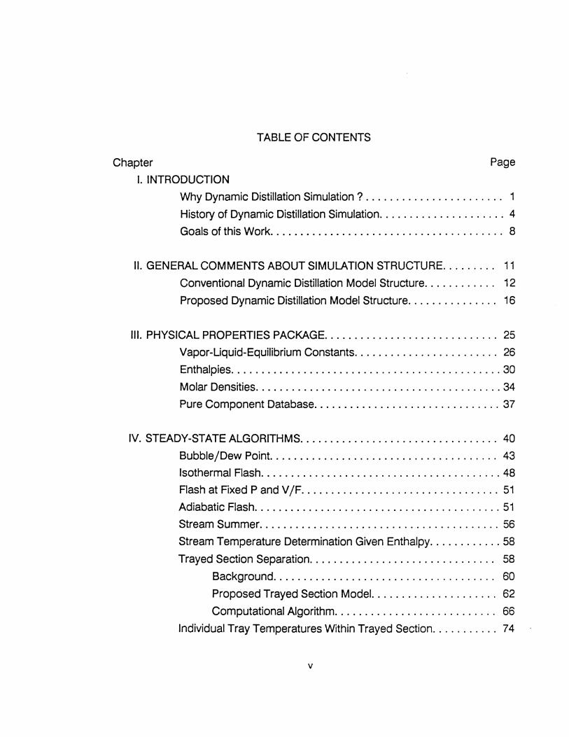
TABLE OF CONTENTS

Chapter Page

I. INTRODUCTION

Why Dynamic Distillation Simulation ? . . . . . . . . . . . . . . . . . . . . . . . 1

History of Dynamic Distillation Simulation. . . . . . . . . . . . . . . . . . . . . 4

Goals of this Work. . . . . . . . . . . . . . . . . . . . . . . . . . . . . . . . . . . . . . . 8

II. GENERAL COMMENTS ABOUT SIMULATION STRUCTURE. . . . . . . . . 11

Conventional Dynamic Distillation Model Structure. . . . . . . . . . . . 12

Proposed Dynamic Distillation Model Structure. . . . . . . . . . . . . . . 16

Ill. PHYSICAL PROPERTIES PACKAGE. ............................ 25

Vapor-Liquid-Equilibrium Constants ........................ 26

Enthalpies ............................................. 30

Molar Densities ......................................... 34

Pure Component Database. . . . . . . . . . . . . . . . . . . . . . . . . . . . . . . 37

IV. STEADY-STATE ALGORITHMS ................................. 40

Bubble/Dew Point. ..................................... 43

Isothermal Flash ........................................ 48

Flash at Fixed P and V /F ................................. 51

Adiabatic Flash ......................................... 51

Stream Summer ........................................ 56

Stream Temperature Determination Given Enthalpy ............ 58

Trayed Section Separation. . . . . . . . . . . . . . . . . . . . . . . . . . . . . . . 58

Background. . . . . . . . . . . . . . . . . . . . . . . . . . . . . . . . . . . . . 60

Proposed Trayed Section Model. . . . . . . . . . . . . . . . . . . . . 62

Computational Algorithm. . . . . . . . . . . . . . . . . . . . . . . . . . . 66

Individual Tray Temperatures Within Trayed Section ........... 74

v

Chapter Page

Condenser/Reboile~ ................................... 76

Theory ............................................... 76

Computational Algorithm. . . . . . . . . . . . . . . . . . . . . . . . . . . 78

Initialization and NTU. . . . . . . . . . . . . . . . . . . . . . . . 78

Convergence. . . . . . . . . . . . . . . . . . . . . . . . . . . . . . . 80

Low /High CP Checking. . . . . . . . . . . . . . . . . . . . . . . 82

V. UNSTEADY STATE ALGORITHMS ............................... 85

Unsteady State Heat and Mass Balance

for Variable Volume Holdup ............................... 87


for Constant Volume Holdup .............................. 89

Unsteady State Component Balance for Liquid Holdup ......... 91

Dead Time. . . . . . . . . . . . . . . . . . . . . . . . . . . . . . . . . . . . . . . . . . . . 91

Vapor Holdup .......................................... 94

Trayed Section Hydraulics ................................ 94

VI. MISCELLANEOUS FACILITIES. . . . . . . . . . . . . . . . . . . . . . . . . . . . . . . . . 99

Stream TBP Calculation .................................. 99

Simulator Database Manipulation

and Documentation. . . . . . . . . . . . . . . . . . . . . . . . . . . . . . . . . . . . 1 03

VII. GENERAL SIMULATION STRUCTURE. . . . . . . . . . . . . . . . . . . . . . . . . . 111

VIII. MODEL VERIFICATION ...................................... 133

Property Predictions. . . . . . . . . . . . . . . . . . . . . . . . . . . . . . . . . . . 133

Steady State Results. . . . . . . . . . . . . . . . . . . . . . . . . . . . . . . . . . . 135

Transient Response Results. . . . . . . . . . . . . . . . . . . . . . . . . . . . . 135

IX. EXAMPLE APPLICATION: COMPUTER BASED, OPERATOR TRAINING

SYSTEM APPLIED TO DISTILLATION COLUMN OPERATION ........ 147

vi

Chapter Page

X. SUMMARY, CONCLUSIONS, AND RECOMMENDATIONS .......... 156

REFERENCES. . . . . . . . . . . . . . . . . . . . . . . . . . . . . . . . . . . . . . . . . . . . . . . . . . . 158

vii

LIST OF TABLES

Table Page

I. Constants for Edmister K-value Model. ....................... 28

II. Pure Component Database List. ............................ 38

Ill. Thermodynamics Package Comparison

MAXI*SIM vs Proposed System ............................ 134

IV. Proposed Model vs Rigorous Model Comparison

Butane/Pentane Splitter .................................. 136

V. Proposed Model vs Rigorous Model Comparison

Butane/Pentane Splitter- Tray Temperature Profile. . . . . . . . . . . . 138

VI. Column Configuration Data for Example

Column of Wong and Wood. . . . . . . . . . . . . . . . . . . . . . . . . . . . . . . 141

viii

LIST OF FIGURES

Figure Page

1. Distillation Trayed Section. . . . . . . . . . . . . . . . . . . . . . . . . . . . . . . . . 18

2. Simulation Block Structure ................................. 20

3. Simple Distillation Column. . . . . . . . . . . . . . . . . . . . . . . . . . . . . . . . . 21

4. lntegraton Error and Process Gain. . . . . . . . . . . . . . . . . . . . . . . . . . 23

5. Logic Flow Diagram- K-value Algorithm ..................... 31

6. Logic Flow Diagram- Stream Enthalpy ...................... 32

7. Logic Flow Diagram - Molar Stream Density. . . . . . . . . . . . . . . . . . 36

8. Structure Definition for Stream Vector ........................ 42

9. Logic Flow Diagram- Bubble/Dew Point. .................... 45

10. Logic Flow Diagram - Isothermal Flash. . . . . . . . . . . . . . . . . . . . . . 49

11. Logic Flow Diagram - Flash @ Constant P and V /F. . . . . . . . . . . . 52

12. Logic Flow Diagram - Adiabatic Flash. . . . . . . . . . . . . . . . . . . . . . . 54

13. Logic Flow Diagram- Stream Summer ....................... 57

14. Logic Flow Diagram- Stream Temperature Given Enthalpy ...... 59 ix

15. Logic Flow Diagram - Distilation Trayed Section

Initialization. . . . . . . . . . . . . . . . . . . . . . . . . 67

16. Logic Flow Diagram- Distilation Trayed Section Heat

Balance ............................. 69

17. Logic Flow Diagram- Distilation Trayed Section

Mass Balance. . . . . . . . . . . . . . . . . . . . . . . . 70


TP Convergence. . . . . . . . . . . . . . . . . . . . . . 72


D /F Convergence. . . . . . . . . . . . . . . . . . . . . 73

20. Logic Flow Diagram - Condenser Algorithm

Initialization and NTU Calc. . . . . . . . . . . . . 79


Convergence Section. . . . . . . . . . . . . . . . . . 81


Low /High Cp Limit Checking ......... 0 0 • 83

23. Logic Flow Diagram- Unsteady State Heat and Mass Balance

Variable Volume Liquid Holdup ....... 0 ••• 88

24. Logic Flow Diagram- Unsteady State Heat and Mass Balance

Constant Volume Liquid Holdup ... 0 •••••• 90

25. Logic Flow Diagram- Unsteady State Component Balance ...... 92

26. Logic Flow Diagram - Pure Dead Time ...................... 0 93

X

27. Dead Time Array Structure ................................ 95

28. Logic Flow Diagram - Stream TBP Algorithm. . . . . . . . . . . . . . . . . 1 00

29. Database Dump Example Output. . . . . . . . . . . . . . . . . . . . . . . . . . 105

30. Process Flow Diagram for Atmospheric Crude Tower .......... 112

31. Simulation System Block Flow

Atmospheric Crude Column, Bottom Section. . . . . . . . . . . . . . . . . 113


Atmospheric Crude Column, Light Gas Oil Section. . . . . . . . . . . . 114


Atmospheric Crude Column, Kerosene Section. . . . . . . . . . . . . . . 115


Atmospheric Crude Column, Heavy Virgin Haphtha Section. . . . . 116


Atmospheric Crude Column, Overhead Section. . . . . . . . . . . . . . . 117

36. Atmospheric Crude Column

Source Code for Steady State Treatment. . . . . . . . . . . . . . . . . . . . 119

37. Atmospheric Crude Column

Source Code for Unsteady State Treatment. . . . . . . . . . . . . . . . . . 126

38. Light Gas Oil Section- Process Flow ........................ 130

39. Proposed Model vs Rigorous Model Comparison

Tray Temperature Profile- C4/C5 Splitter .................... 137

40. Proposed Model vs Rigorous Model Comparison xi

Tray Temperature Profile - Debutanizer. . . . . . . . . . . . . . . . . . . . 139

41. Response of the Distillate Propane Composition

to a 1 0 percent Decrease in Reflux. . . . . . . . . . . . . . . . . . . . . . . . . 142


to a 10 percent Increase in Steam Rate. . . . . . . . . . . . . . . . . . . . . 143


to a 10 percent Decrease in Feed Rate. . . . . . . . . . . . . . . . . . . . . . 144

44. Instructional System Software Components .................. 151

xii

NOMENCLATURE

A,B,C,D = constants in ideal gas heat capacity correlation

AU = area * overall heat transfer coefficient

C = stream heat capacity, flow*C P

CP = component heat capacity

0 = distillate flow

DH = enthalpy departure

E = internal energy

Em = murphree tray efficiency

F = molar flow

f = frac of component recovered in bottoms of a trayed section

H =enthalpy

HL = liquid holdup moles

HTC = hydraulic time constant

h = time increment

K1 = ideal solution K-value

KR = Raoult's Law K-value

L = liquid flow

N = number of theoretical stages, or moles

P =pressure

po = pure component vapor pressure

q = heat transfer rate

qmax = maximum possible q from NTU method

qs = fraction of a given component in stream LN+,

R = ideal gas constant

S = stripping factor

T = temperature

T P = mass balance convergence variable in trayed section algorithm

t =time

xiii

V = liquid molar volume or vapor flow rate

x = liquid mole fraction

y = vapor mole fraction

y· = composition of vapor in equilibrium with tray liquid

L\Hv = heat of vaporization

-y = activity coefficient

c:; = error tolerance

~ = heat transfer effectiveness or integration error term

rr = system pressure

w = accentric factor

Subscripts:

c = critical property

= property for component i

in = inlet property

m = mixture property

n = value at nth time step or property at tray n

out = outlet property

r = reduced property

sat = property of saturated stream

Superscripts:

ID = ideal gas state property

v = vapor property

= liquid property

xiv

CHAPTER I

INTRODUCTION

Why Dynamic Distillation Simulation?

In recent years there has been a dramatic increase in the use of

sophisticated control systems in the fluid processing industry, but unfortunately

problems have often arisen in the design and tuning of these complex systems

because the dynamic properties of the process to be controlled were not well

understood. Dynamic simulators provide tools whereby the unsteady state

behavior of these processes can be studied under the influence of various control

configurations. However, the utility of these programs has always been somewhat

limited by the very primitive or excessively complex methods used to calculate the

dynamic responses. In the first case the results provided by the simulation are at

best only qualitatively correct and thus are useful only for very general studies.

They provide little to the engineer involved in the actual design and testing of

control schemes. The second case provides much higher quality results. However,

these are at the expense of reasonable compute times and stable solutions.

Another area which could benefit from a robust and fast dynamic

simulation is education. Education here is used in a very general sense (i.e.,

industry or academia, process dynamics or process control, etc.). There is no

substitute for "hand's on" experience in the teaching of any subject. The lack of

1

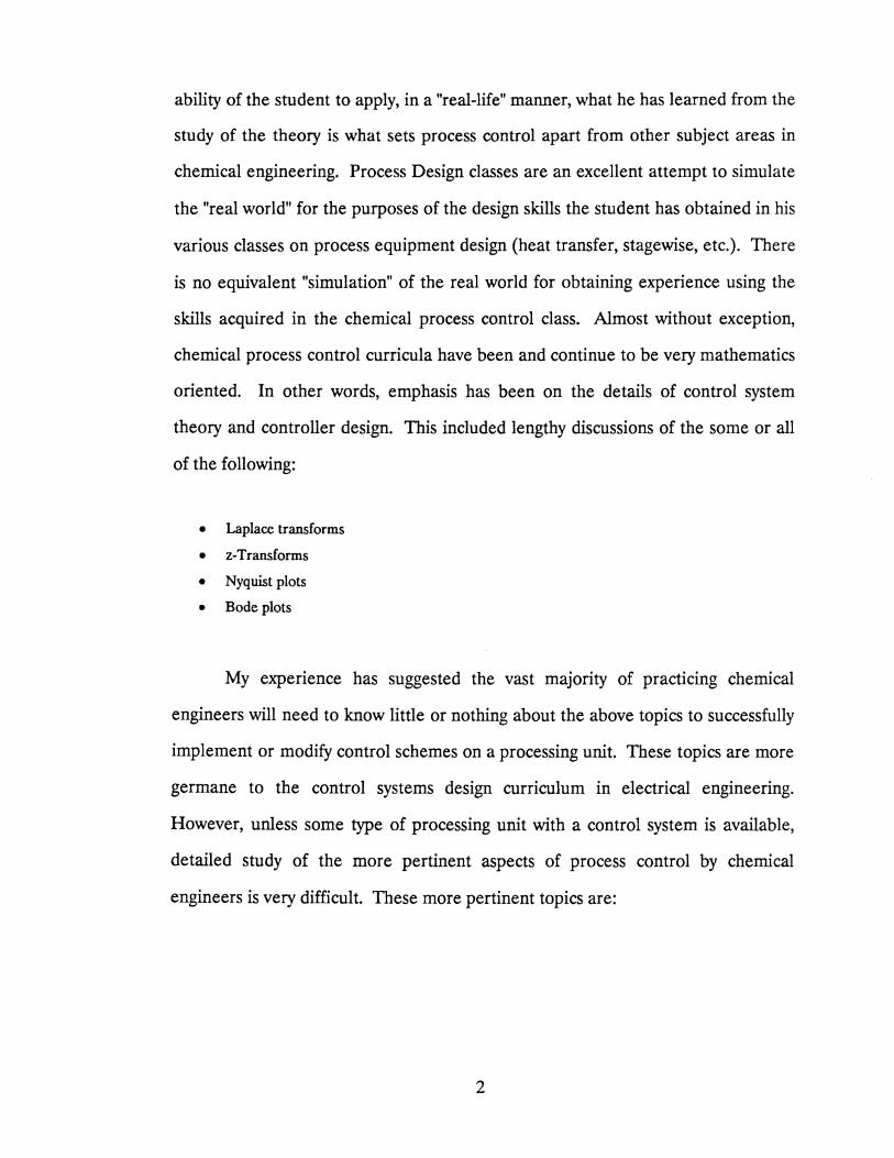
ability of the student to apply, in a "real-life" manner, what he has learned from the

study of the theory is what sets process control apart from other subject areas in

chemical engineering. Process Design classes are an excellent attempt to simulate

the "real world" for the purposes of the design skills the student has obtained in his

various classes on process equipment design (heat transfer, stagewise, etc.). There

is no equivalent "simulation" of the real world for obtaining experience using the

skills acquired in the chemical process control class. Almost without exception,

chemical process control curricula have been and continue to be very mathematics

oriented. In other words, emphasis has been on the details of control system

theory and controller design. This included lengthy discussions of the some or all

of the following:

• Laplace transforms

• z-Transforms

• Nyquist plots

• Bode plots

My experience has suggested the vast majority of practicing chemical

engineers will need to know little or nothing about the above topics to successfully

implement or modify control schemes on a processing unit. These topics are more

germane to the control systems design curriculum in electrical engineering.

However, unless some type of processing unit with a control system is available,

detailed study of the more pertinent aspects of process control by chemical

engineers is very difficult. These more pertinent topics are:

2

• identification of control objectives

• selection of appropriate measurements and manipulated variables

• determination of loops connecting these variables

• identification of appropriate control laws

I do not want to suggest the elimination of the discussion of the

mathematical aspects of controller design. However, if the student has the ability

to implement and test control strategies on a processing unit, the mathematics

mentioned above could be considerably de-emphasized in preference to the more

pertinent subject areas just mentioned. This approach would allow the student

practical experience using the analytical tools and design methods available, rather

than spending most of the time going through detailed mathematical derivations of

these tools.

These areas of process control scheme design and testing and process

dynamics/ control teaching highlight the need for a dynamic model (or package)

that is flexible enough to handle different column (or columns) configurations and

is versatile enough to allow the study of different processes and operations (e.g.,

start-up and shut-down). It should be able to solve large industrial problems and

should be numerically robust, efficient and reliable. These goals should be

accomplished without the need for major expenses in computer hardware.

3

History of Dynamic Distillation Simulation

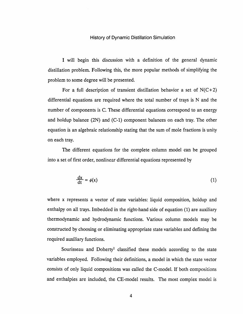
I will begin this discussion with a definition of the general dynamic

distillation problem. Following this, the more popular methods of simplifying the

problem to some degree will be presented.

For a full description of transient distillation behavior a set of N(C+ 2)

differential equations are required where the total number of trays is N and the

number of components is C. These differential equations correspond to an energy

and holdup balance (2N) and (C-1) component balances on each tray. The other

equation is an algebraic relationship stating that the sum of mole fractions is unity

on each tray.

The different equations for the complete column model can be grouped

into a set of first order, nonlinear differential equations represented by

~ = if>(x) (1)

where x represents a vector of state variables: liquid composition, holdup and

enthalpy on all trays. Imbedded in the right-hand side of equation (1) are auxiliary

thermodynamic and hydrodynamic functions. Various column models may be

constructed by choosing or eliminating appropriate state variables and defining the

required auxiliary functions.

Sourisseau and Doherty1 classified these models according to the state

variables employed. Following their definitions, a model in which the state vector

consists of only liquid compositions was called the C-model. If both compositions

and enthalpies are included, the CE-model results. The most complex model is

4

the CHE-model and has a differential equation for each state variable on each tray

(composition, enthalpy and holdup). Traditionally, a popular model is the

constant molar-overflow model (CMO-model), which assumes fast holdup and

energy changes.

Sourisseau and Doherty studied all five dynamic models (classified as CHE,

CE, CH, C, and CMO ) for various distillation problems involving relatively ideal

mixtures. They concluded that steady-state and transient response results for all

the models were in good agreement. Furthermore, they concluded that the CH,

CHE and CE models were too time consuming considering the little additional

information obtained; they preferred the use of the C or CMO models. These

conclusions are not surprising since it is well known that the significant dynamics in

distillation processes are retained by the differential equations modeling liquid

phase compositions.

Since the early 1950's attempts have been made to do dynamic distillation

simulation using one of the model types above. The advent of analog computers in

the early 1950's allowed attempts to model distillation dynamics in a reasonably

realistic manner2, but simplifications were enforced by the limitations of the analog

equipment. More wide spread availability and use of digital computers in the

1960's promoted a new attack on the dynamics problem, but most of the earlier

simplifications remained. For instance, Huckaba et aL 3 limited their attention to

binary distillation at constant pressure, with constant liquid holdups and negligible

vapor holdups. Waggoner and Holland4 required independent specification of the

transient behavior of the liquid holdups, and vapor holdup was, once again,

neglected. Varying liquid holdups were treated very effectively by Peiser and

GraverS, but vapor holdup was again discounted. More recent simulations include

a linearized, dynamic model produced by Rademaker6. However, it should be

5

noted that, although very useful for stability analysis and control system design,

linearized models apply only in the region of the chosen operating point and will

be unable to track, accurately, large disturbances such as might occur at startup

and shutdown.

Up to this point the discussion has focused on the problems in modeling the

physical system. However, once the physical model has been defined, the problem

of the numerical methods required to solve the physical model must be addressed.

A full-order dynamic simulation of a multistage separation process will lead, in all

but the simplest case, to a large, stiff system of nonlinear algebraic and differential

equations. Early digital modeling work was carried out before the ready

availability of continuous system simulation languages ( CSSL )', and a noticeable

feature of many of the published papers of this period is the attention paid by the

authors to the selection of a suitable integration algorithm3•8• Some methods used

were reasonably conventional time marching techniques, but others4 required

extensive nonlinear iteration at each time step. At present, several complete,

stand-alone, numerical integration packages are available for incorporation into a

general simulation system. This relieves the simulationist from the drudgery of

implementing his own version of a numerical integration algorithm. This approach

usually yields a fairly robust (not completely) solution scheme for a given physical

model of the distillation process.

In light of the above discussion, the current state-of-art in dynamic

simulation suffers from two problems:

• Solutions can become numerically unstable

• Solutions can require very long compute times

These may not be significant problems depending on the particular

application in question. However, the goals of this study required these items be

6

dealt with and eliminated ( or at least significantly reduced ).

The last item to be discussed in this section is the topic of general

simulation architecture. There are two different numerical approaches to simulate

the dynamics of an integrated process:

• The various sub-systems are integrated with a single algorithm

• Each sub-system has its own algorithm

The first approach considers all linked sub-systems as one single large

system. A single algorithm, explicit or implicit, is used to simulate the dynamics of

the whole system. Time is advanced the same amount at each step for each

sub-system no matter if it is stiff or not. Typical examples of simulators using

variants of this type are:

• MIMIC9

• CSMP10

• DYNSYS11

• SPEED UP12

• ASCEND13

In modular integration, each sub-system is integrated independently with

independent error control. Explicit and implicit integration algorithms are used to

integrate non-stiff and stiff sub-systems separately. An example of a simulator

using modular integration is MODCOMP14•

Modular integration may have the following advantages over lumped

integration:

7

• The simulation can be more efficient because:

each sub-system uses an integration algorithm which is best suited to that

sub-system

each dynamic simulator has its own error control

all dynamic simulators can operate in parallel

• The software can be completely modular and therefore easier to maintain

Most chemical and petroleum process are examples of systems with stiff

and non-stiff components. The modular approach to integration permits the use of

explicit integration algorithms for the non-stiff sub-systems and implicit integration

algorithms for stiff systems. Independent error control in the individual dynamic

simulators insures that the proper step size is taken in each sub-system. Thus, the

efficiency of the overall simulation is not adversely influenced by the step size in

any single sub-system.

Lastly, because of the separate integration algorithms for the individual

sub-systems, debugging of the computer program for modular simulation can be

reasonably simple. Each simulator can be tested independently to locate any

possible programming errors. In contrast, the location of errors in highly integrated

computer software can be very difficult and time consuming. In addition, a

modular simulation can be expanded with little or no disturbance to existing

programs.

Goal of This Work

The tendency for numerical differentiation calculations to introduce

instabilities into the integration and in particular the large amounts of computation

time required for both the numerical integration and the phase equilibria

calculations made conventional dynamic simulation techniques incompatible with

8

the goal of this project which was to create a dynamic simulation system with the

following characteristics:

• Provide dynamic process responses for the typical refmery process units

• Provide these responses in real-time ( or faster )

• Provide responses with the accuracy required in the design, testing, and tuning of

process control schemes

• Provide these responses with a minimal investment in computer hardware (i.e.

minicomputer at worst, PC at best)

In order to provide accurate, dynamic process responses in real-time

without requiring a large investment in computer hardware, an entirely new

approach to dynamic simulation was taken. However, this approach was believed

necessary in order to provide a dynamic simulation system that would be of

practical use. The use of steady-state process design simulators is a common place

occurrence in the life of a chemical engineer. However, very few will ever use a

dynamic process simulator, even though the need often arises for one. This is due

to one or more of the following:

• An expert is required to set up a flow sheet to simulate.

• The actual time required to complete the simulation could be from 10 to 100 times

the interval simulated.

• The calculation may become unstable during the course of the run requiring

resubmitting the job after either decreasing the disturbance desired or modifying the

simulated process to get around the stability problem.

• The prospective user cannot justify the hardware expense required to implement the

dynamic simulation system.

The result of this project is a dynamic simulation system that does eliminate

the above objections to current simulation systems. The following chapters discuss

in detail the techniques developed to meet the goals stated above. However,

before discussing the details of the simulation system, the following chapter briefly

presents the conventional model technique for distillation to provide a contrast

with the techniques proposed in this study. In addition, the general philosophy and

9

structure of the simulation system will be presented to enhance the detailed

discussions.

10

CHAPTER II

GENERAL COMMENTS ABOUT SIMULATION

MODEL STRUCTURE

The proposed distillation modeling technique carnes out dynamic

distillation simulation by assembling various types of modules in a manner which

approximates the physical situation. This modular approach to simulation allows

almost any distillation configuration to be represented by combinations of a small

number of basic module types. The most important of these is the counter-current

mass transfer stage. This module must determine the properties of the out-going

liquid and vapor streams, given the time dependent variables of the input streams

and certain information about the characteristics of the tray. The dynamic

behavior of the stage is determined by the rates at which it accumulates material

and energy. Assuming perfect mixing in both phases and the absence of chemical

reactions, the mole balances can be written as:

(2)

The corresponding energy balance is:

(3)

11

In order to use these equations to determine the output stream variables,

assumptions must be made, and it is in these assumptions that the model

developed in this study differs significantly from the conventional model. In order

to put this approach in perspective, the development of the conventional model

structure will be reviewed.

Conventional Dynamic Distillation

Model Structure

To develop the conventional dynamic distillation model, the following

assumptions are made:

1) Assume the vapor leaving a stage is in thermodynamic equilibrium with the

liquid leaving that stage

Although this assumption is never truly valid it is a reasonable assumption. In

some cases, however, particularly for absorption and stripping, it can cause

gross errors in the calculated results. Two methods are commonly used to

circumvent this problem, the simplest of which is to use a ratio of simulated

ideal trays to actual trays which roughly corresponds to the observed tower

efficiency (i.e. a 20 tray tower that is roughly 50% efficient would be simulated

with a model having 10 trays). A somewhat more sophisticated approach is the

use of Murphee tray efficiencies. These are defined as:

(4)

12

where y• represents the composition of the vapor in equilibrium with the tray

liquid. Although commonly used, these have little in the way of a theoretical

basis.

2) Assume the vapor holdup is negligible

For the vast majority of situations this assumption is reasonable, but

inaccuracies can occur in high pressure towers where the liquid/vapor density

ratio is small. For instance the density ratio in a column operating at

atmospheric pressure and room temperature would be of the order of 1000 to

1, while ratios of fewer than 10 to 1 are common in gas plant absorbers. Thus,

the vapor holdup in the gas plant absorber represents a much larger fraction of

the total holdup than is the case in the atmospheric column.

3) Assume the total holdup on the plate is constant

This assumption is quite reasonable for small excursions from steady state,

particularly if it is the volumetric holdup which is held constant while the molar

holdup floats with changes in the liquid density. Simonsmeier15 compared

simulations which had large differences in the value of the assumed holdup and

found only slight variations in the results.

4) Assume the total plate enthalpy does not change

This is applicable only if assumption (3) has been made and even then it may

introduce considerable error if the liquid composition changes markedly during

the course of the simulation.

13

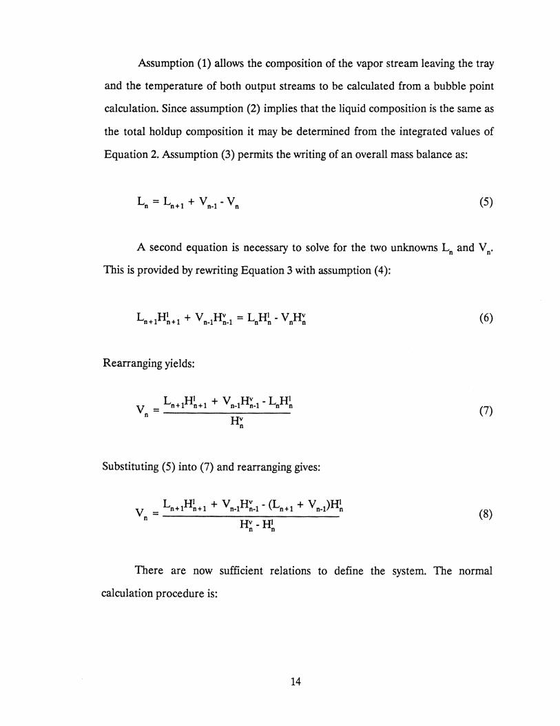
Assumption ( 1) allows the composition of the vapor stream leaving the tray

and the temperature of both output streams to be calculated from a bubble point

calculation. Since assumption (2) implies that the liquid composition is the same as

the total holdup composition it may be determined from the integrated values of

Equation 2. Assumption (3) permits the writing of an overall mass balance as:

(5)

A second equation is necessary to solve for the two unknowns Ln and V0 •

This is provided by rewriting Equation 3 with assumption ( 4 ):

(6)

Rearranging yields:

(7)

Substituting (5) into (7) and rearranging gives:

y = Ln+lH~+l + Vn-lH~-1- (Ln+l + Vn-l)H~ n Hv- HI

n n

(8)

There are now sufficient relations to define the system. The normal

calculation procedure is:

14

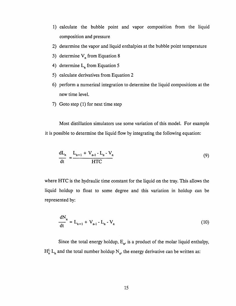
1) calculate the bubble point and vapor composition from the liquid

composition and pressure

2) determine the vapor and liquid enthalpies at the bubble point temperature

3) determine Vn from Equation 8

4) determine L0 from Equation 5

5) calculate derivatives from Equation 2

6) perform a numerical integration to determine the liquid compositions at the

new time level.

7) Go to step ( 1) for next time step

Most distillation simulators use some variation of this model. For example

it is possible to determine the liquid flow by integrating the following equation:

=------- (9) HTC

where HTC is the hydraulic time constant for the liquid on the tray. This allows the

liquid holdup to float to some degree and this variation in holdup can be

represented by:

(10)

Since the total energy holdup, E0 , is a product of the molar liquid enthalpy,

H~ Ln and the total number holdup N0 , the energy derivative can be written as:

15

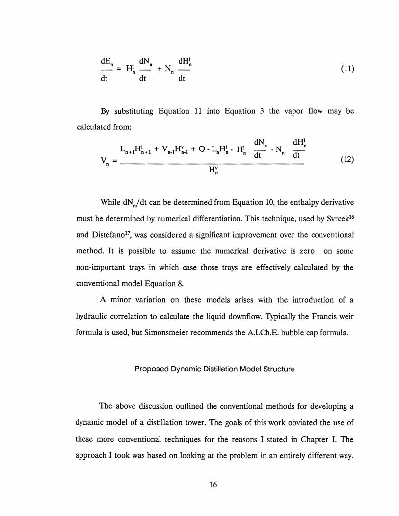
dN dH1 n n

H 1 - +N-n n (11) dt dt dt

By substituting Equation 11 into Equation 3 the vapor flow may be

calculated from:

While dNn/dt can be determined from Equation 10, the enthalpy derivative

must be determined by numerical differentiation. This technique, used by Svrcek16

and Distefano17, was considered a significant improvement over the conventional

method. It is possible to assume the numerical derivative is zero on some

non-important trays in which case those trays are effectively calculated by the

conventional model Equation 8.

A minor variation on these models anses with the introduction of a

hydraulic correlation to calculate the liquid downflow. Typically the Francis weir

formula is used, but Simonsmeier recommends the AI.Ch.E. bubble cap formula.

Proposed Dynamic Distillation Model Structure

The above discussion outlined the conventional methods for developing a

dynamic model of a distillation tower. The goals of this work obviated the use of

these more conventional techniques for the reasons I stated in Chapter I. The

approach I took was based on looking at the problem in an entirely different way.

16

The thought process behind this different approach will be explained in this

section.

I will begin by referencing Figure 1. This figure represents a trayed

distillation tower section. This simple figure shows the basic flows of liquid and

vapor in a distillation tower. With this figure in mind, consider the following two

assumptions:

• There is no holdup volume

• There is no transportation lag of liquid from tray to tray

These are non-realistic assumptions for any realizable tower configuration.

However, the only dynamics associated with a tower meeting these assumptions

would be due to:

• mass transfer restrictions (diffusion effects)

• sensible heat capacity of the metal making up the tower

Under most industrial situations the above two effects have a negligible

impact on the overall tower dynamics. Thus, the model based on these assumptions

would yield a tower simulation with virtually no dynamics. This model would be

difficult to solve due to the very high derivatives resulting from the above

assumptions. However, with no limiting assumptions about the thermodynamics

(vapor-liquid-equilibria), an essentially steady-state model has been produced.

This hypothetical case serves to illustrate the most significant contribution

to the overall tower dynamics is due solely to the liquid system, since in the above

no assumptions were made regarding the V-L-E algorithm. This leads to the

assumption that the V-L-E calculations could be separated from the liquid

17

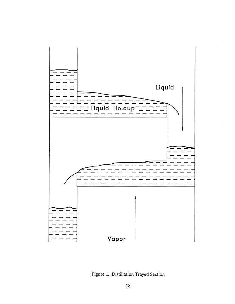
Liquid

-_-_-_-_-_-Liquid Holdup-_-_-_-_

Vapor

Figure 1. Distillation Trayed Section

18

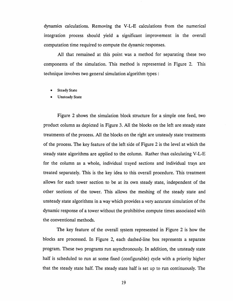
dynamics calculations. Removing the V-L-E calculations from the numerical

integration process should yield a significant improvement in the overall

computation time required to compute the dynamic responses.

All that remained at this point was a method for separating these two

components of the simulation. This method is represented in Figure 2. This

technique involves two general simulation algorithm types :

• Steady State

• Unsteady State

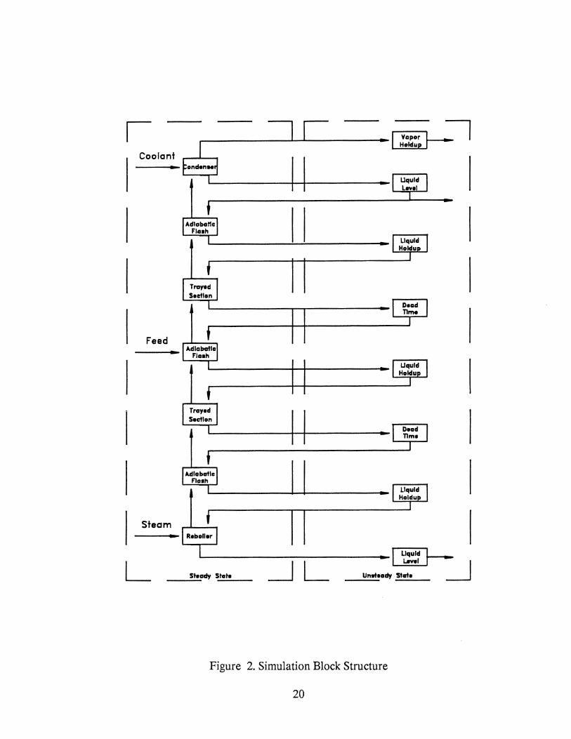
Figure 2 shows the simulation block structure for a simple one feed, two

product column as depicted in Figure 3. All the blocks on the left are steady state

treatments of the process. All the blocks on the right are unsteady state treatments

of the process. The key feature of the left side of Figure 2 is the level at which the

steady state algorithms are applied to the column. Rather than calculating V-L-E

for the column as a whole, individual trayed sections and individual trays are

treated separately. This is the key idea to this overall procedure. This treatment

allows for each tower section to be at its own steady state, independent of the

other sections of the tower. This allows the meshing of the steady state and

unsteady state algorithms in a way which provides a very accurate simulation of the

dynamic response of a tower without the prohibitive compute times associated with

the conventional methods.

The key feature of the overall system represented in Figure 2 is how the

blocks are processed. In Figure 2, each dashed-line box represents a separate

program. These two programs run asynchronously. In addition, the unsteady state

half is scheduled to run at some fixed ( configurable) cycle with a priority higher

that the steady state half. The steady state half is set up to run continuously. The

19

Coolant

Feed

Steam

...

Uqulcl Lwei -

L ___ s_te:ady--S~ta~te~~~~~--_j----L------U-n.t--tea-~ r;;o-_j

Figure 2. Simulation Block Structure

20

Feed

Condenser

Distillate Product

Reboiler

Bottoms Product

Figure 3. Simple Distillation Column

21

unsteady state program takes about 1-2 sec to run on a DEC MicroVa.x II and is

scheduled to run every 5 sees. The steady state half runs in whatever time is left.

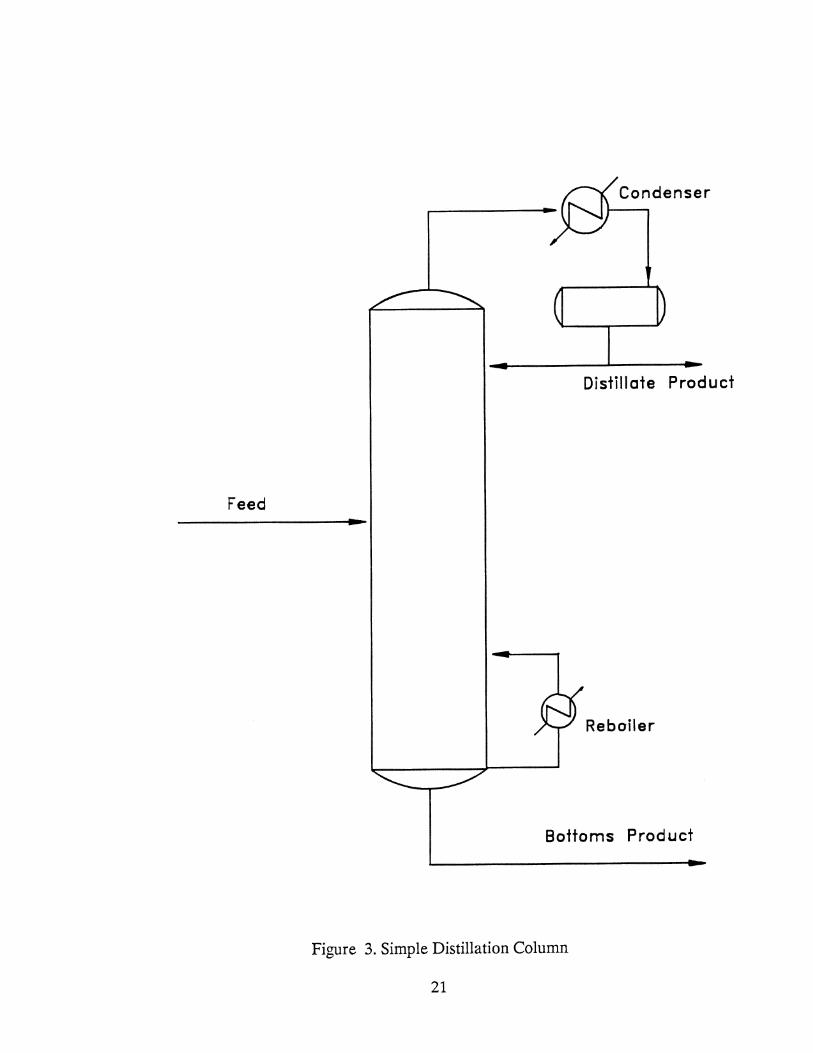
Before I conclude this section, I want to touch on one last subject. That

subject is integration error. In the best of circumstances some integration error will

be accumulated as the equations are integrated for some simulated time span.

Figure 4 illustrates this point. This figure represents a dynamic response curve for

some hypothetical process parameter of interest. Point A is a predefined steady

state for the process to which the dynamic simulation is initialized. Point B is the

value of this hypothetical parameter after moving the process to a new steady state.

The value of the hypothetical parameter at both steady states can be determined

with a rigorous steady state simulator (i.e. points A and C). However, the path the

process takes in getting from one steady state to another can only be determined

from an unsteady state treatment.

Figure 4 shows a discrepancy between the unsteady state simulator and the

steady state simulator at the final steady state of the process. This discrepancy is

due to the accumulation of integration error. Steps can be taken to reduce this

accumulated error. However, these steps require greater and greater amounts of

CPU time to achieve this goal. The simulation system proposed in this work will

not suffer from this accumulation of integration error. This is becuase of the

explicit steady state treatment used for the V-L-E. In addition, this goal is reached

without excessive requirements in computer hardware.

The steady state error in the unsteady state analysis of the process can be

directly translated into an error in the estimation of the process gain. Since one of

the proposed uses of this system is in the design and testing of process control

schemes, a good estimation of the process gain is very important. The method

presented in Figure 2 will yield a dynamic simulator that will yield process gain

22

c: 0

<..:)

II) II) (1.)

u u 0 ....

a. c ·-0 (.')

(/) (/) Q)

u 0 l....

a... .... 0 .... "'C ....

UJ c 0

c (1.) 0 E L.. - 0 0 ·-.... ,_

L.. 0') L.. (1.) "'0 w - (1.)

c: -0 c :J 0 E -Vl 0

l.... 0') Q)

+-c

. ..q-

Q) l.... :::l 0')

u_

23

predictions with the accuracy available from steady state simulators.

With this very brief introduction to the proposed new method, I will

proceed by describing the various components of the above system:

• Physical properties package

• Steady state algorithms

• Unsteady state algorithms

Mter presenting the details of the system components, I will describe in

detail how these components can be combined to yield a dynamic simulation of

practically any proposed flow sheet. Following this is a discussion of model

accuracy. Next, several applications for this proposed system will be presented.

Lastly, the summary, conclusions, and recommendations for further work will be

presented.

24

CHAPTER Ill

PHYSICAL PROPERTIES PACKAGE

Although the reliable prediction of the dynamic behavior of a distillation

column is dependent on the numerical method(s) of solution, the accuracy of the

predictions is directly related to the characterization of the systems phase

behavior and transport properties. In addition, the physical properties package is

the most frequently executed package in a dynamic simulation system. Tyreus et al.

discussed the effect of these calculations. 18 They studied the dynamics of a 40 tray

binary distillation column in response to a step change in feed composition. Using

an explicit Euler integration scheme, they found about 400,000 iterative

bubble-point calculations were required. Thus, for multiple column,

multi-component configurations the number of property evaluations could easily

approach several million. This large amount of property evaluations could increase

by 3 to 6 times if a more complicated implicit integration technique is used. This

all suggested to me great care was needed in selecting the physical properties

package.

In order to select the most efficient property algorithm, some assumption

needs to be made regarding the type of chemical compounds to be dealt with. If

this assumption is not made, a very general algorithm must be selected which may

provide capabilities which are not required and which may put an undue

computational burden on the system. The properties prediction package presented

25

in the following sections is intended to apply to hydrocarbon systems and the

following additional compounds:

• rare gases

• nitrogen

• carbon monoxide

• water

• carbon dioxide

• hydrogen (small amounts)

This component slate will allow most distillation systems in a refinery to be

simulated. The computational impact of confining selection to hydrocarbon

systems is significant. However, this still allows the simulation of most of the

practical applications in refineries and many of the applications in the chemicals

industry.

This assumed component slate allows the use of property prediction

algorithms which are based on the principle of corresponding states. The two

major benefits of algorithms of this type are:

• they are computationally very efficient (i.e. they are fast)

• the component data required are readily available

The following sections describe each of the components of the property

prediction package in the simulation system.

Vapor -Liquid-Equilibrium Constants

The algorithm chosen for the prediction of vapor-liquid-equilibrium is one

26

developed by Edmister.19 This approach is based on the corresponding states

principle. The K-values produced by Edmister's method conform to the ideal

solution theory for mixtures. The basis and applicability of Edmister's method is

discussed in some detail in a previous paper of mine.20 The equations describing

the algorithm are as follows:

For KR < 1.0:

Y = Ao + A 1[(1 + ~X)eX/2 - 1]

Ao = ao + atZ + a2Z2 + ~Z3

~ = a4 + a5Z + a6Z2 + a.,Z3

~ = ag + a;z + atoZ2 + at3z3

For KR > 1.0:

y = ~ + A4X2 + AsX3

~ = at2 + a13Z + at4Z2

A4 = ats + at6Z + at7Z2

As = ats + at9Z + ~oz2

where :Y =In K1

X= lnKR =In~

(13)

(14)

(15)

(16)

(17)

(18)

(19)

(20)

(21)

(22)

(23)

The values of the 21 regression coefficients, as determined by Edmister, (a0

- ~0) are given in Table I for three ranges of reduced pressure.

27

Constants

ao a, a2 a3 a4 as as a7 as ae a,o a,,

TABLE I

CONSTANTS FOR EDMISTER K-VALUE MODEL

p < 1.0

+0.72354688 -0.11955262 -0.019175521 -0.00079043357 -0.092938874 -0.089253134 -0.02120992 -0.0011023254 +0.83485814 -1.7510463 -1.7882516 -0.20255145

+0.55823912 -0.22417339 -0.026665354 -0.0046116207 +0.035372461 +0.0067313403 -0.00060208161 -0.002218345 -0.0004783554

FORK < 1.0 , 1.0 < p < 10.0

+0.71613974 +0.11010362 -0.009820518 +0.00085139636 -0.031743583 -0.077912651 -0.012739586 -0.035998746 +3.4719935 -2.4128931 +0.74548583 -0.13713069

FORK > 1.0 r

+0.56319800 -0.20762898 -0.001581164 -0.0001901561 +0.023954299 ·0.00380481 ·0.0017300384 -0.0022414988 +0.0013698449

28

p > 10.0

+0.93322546 -0.29838149 +0.036108945 -0.0018123488 -1.4698873 +1.5375645 -0.71906421 +0.089098628 -0.33924284 +1.3802654 -0.64746142 +0.074000484

+0.3986012 -0.1933524 +0.02388513 +0.17430118 -0.082957315 +0.010571085 -0.032969708 +0.021278044 -0.0032276668

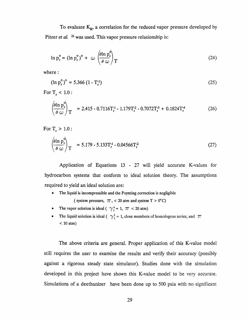
To evaluate KR, a correlation for the reduced vapor pressure developed by

Pitzer et aL 21 was used. This vapor pressure relationship is:

(24)

where:

0 0 1 (ln Pr) = 5.366 (1 - T; ) (25)

For Tr < 1.0:

~:! ;) T = 2.415 - 0. 71161';1 - 1.1791';' - 0. 70721';3 + 0.1824 T;' (26)

For Tr > 1.0:

~~n !;) T = 5.179 - 5.1331';1 - 0.04566T-( (27)

Application of Equations 13 - 27 will yield accurate K-values for

hydrocarbon systems that conform to ideal solution theory. The assumptions

required to yield an ideal solution are:

• The liquid is incompressible and the Poynting correction is negligible

(system pressure, 1T, < 20 atm and system T > 0°C)

• The vapor solution is ideal ( 1'i = 1, 1T < 20 atm)

• The liquid solution is ideal ( 1' l = 1, close members of homologous series, and 1T

< 10 atm)

The above criteria are general. Proper application of this K-value model

still requires the user to examine the results and verify their accuracy (possibly

against a rigorous steady state simulator). Studies done with the simulation

developed in this project have shown this K-value model to be very accurate.

Simulations of a deethanizer have been done up to 500 psia with no significant

29

loss in accuracy as compared to the results from the Soave- Redlich-Kwong model.

The section on model verification will present these results.

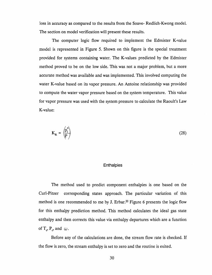
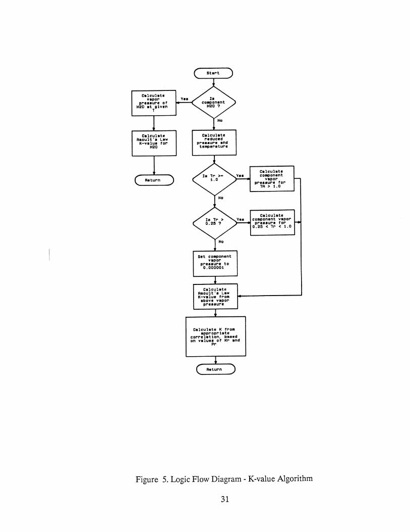
The computer logic flow required to implement the Edmister K-value

model is represented in Figure 5. Shown on this figure is the special treatment

provided for systems containing water. The K-values predicted by the Edmister

method proved to be on the low side. This was not a major problem, but a more

accurate method was available and was implemented. This involved computing the

water K-value based on its vapor pressure. An Antoine relationship was provided

to compute the water vapor pressure based on the system temperature. This value

for vapor pressure was used with the system pressure to calculate the Raoult's Law

K-value:

(28)

Enthalpies

The method used to predict component enthalpies is one based on the

Curl-Pitzer corresponding states approach. The particular variation of this

method is one recommended to me by J. Erbar.22 Figure 6 presents the logic flow

for this enthalpy prediction method. This method calculates the ideal gas state

enthalpy and then corrects this value via enthalpy departures which are a function

ofTc, Pc, and w.

Before any of the calculations are done, the stream flow rate is checked. If

the flow is zero, the stream enthalpy is set to zero and the routine is exited.

30

Calcuhte v•por

preaaure of H20 at g1ven

T

Calculate Raoult'a Law

K-value for H20

Calculate reduced

preaaure and temperature

Set component vapor

pressure to 0.000001

Calculate Raoult 's Law K-value from

abov-e vapor proeaaure

Calculate K from approprhte

correlat1on, based on values of Kr and

Pr

Calculate component

vapor preaaure for

TR > 1. 0

Calculate component vapor

proeaaure for o. 25 < Tr < 1. o

Figure 5. Logic Flow Diagram- K-value Algorithm

31

Set stream enthalpy to

zero

Return

Calculate liquid

enthalpy departures

terms

Ini tial1ze internal

variables and counters

Calc mixture critical T,

P, and accentric

factor

Calc mixture ideal gsa

state enthalpy

Calc stream enthalpy departure

Calc stream enthalpy

Calc vapor enthalpy

departures terms

Figure 6. Logic Flow Diagram - Stream Enthalpy

32

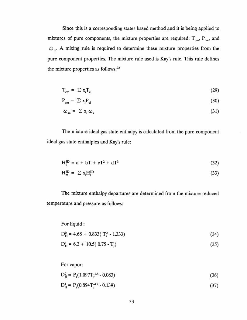
Since this is a corresponding states based method and it is being applied to

mixtures of pure components, the mixture properties are required: T em• P em• and

w m· A mixing rule is required to determine these mixture properties from the

pure component properties. The mixture rule used is Kay's rule. This rule defines

the mixture properties as follows: 22

w = ~x.w. m 1 1

(29)

(30)

(31)

The mixture ideal gas state enthalpy is calculated from the pure component

ideal gas state enthalpies and Kay's rule:

H~0 = a + bT + cT2 + dT3 1

H 10 = ~ x.H~0 m 1 1

(32)

(33)

The mixture enthalpy departures are determined from the mixture reduced

temperature and pressure as follows:

For liquid:

D~ = 4.68 + 0.833( T;1 - 1.333)

Dk = 6.2 + 10.5( 0.75- Tr)

For vapor:

D~ = Pr(1.097T;t.6 - 0.083)

Dk = P/0.894T:·2 - 0.139)

33

(34)

(35)

(36)

(37)

(38)

The total mixture enthalpy then results from subtracting the enthalpy

departure from the ideal gas state enthalpy:

H = H10 -D m H (39)

This is a very straight forward algorithm which is also very computationally

efficient. The algorithm provides accurate predictions of stream enthalpies. Some

examples of these predictions will be discussed in the model verification section.

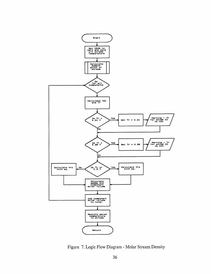
Molar Density

The method of Gunn and Yamada23 was chosen for the liquid molar density

estimation algorithm. This algorithm will yield the pure component liquid molar

density for saturated liquids. The assumption of saturated liquid for distillation

column simulation does not introduce any significant error. The only stream where

this assumption may introduce some error is the reflux if it is subcooled. Amagat's

Law is used to calculate the stream molar density from the pure component molar

density.

The saturated liquid volume, V, is defined in terms of a scaling parameter,

V sc"

v v = v~o) ( 1 - w r ) sc

(40)

34

This scaling parameter is defined in terms of the volume at Tr = 0.6.

v v = 0.6

sc 0.38962 - 0.0866 w (41)

V0.6 is the saturated liquid molar volume at a reduced temperature of 0.6. If V0.6 is

estimated from the following:

v sc = RTC ( 0.2920- 0.0967 w ) PC

In Equation 40 V~0) and f are functions of reduced temperature.

For 0.2 ~ Tr ~ 0.8

(42)

V~0) = 0.33593- 0.33953Tr + 1.51941T/- 2.02512T/ + 1.11422Tr4 (43)

For 0.8 < Tr < 1.0

V~0) = 1.0 + 1.3(1- Tr)05log(1-Tr)- 0.50879(1- Tr)- 0.91534(1- Tr)2 (44)

For 0.2 ~ Tr < 1.0

f = 0.29607- 0.09045Tr- 0.04842(1 - Tr)2 (45)

This method appears to be one of the most accurate available for saturated

liquid volumes.24 It should not be used above Tr = 0.99; the V~0) function becomes

undefined at Tr = 1.

Figure 7 presents the logic flow for this density algorithm. Checks are made

for Tr values below 0.21 and above 0.98. If these limiting values are exceeded, they

are reset to the limits and an informational warning is logged. Experience with

35

Calculate Vro w1th eq.

No

Set DENS to zero and eave ott atream temperature

Calculate bubble

po1ht of at ream

Calculate Vac and Tr

Calc-ulate gamma end component

I'Cler- volume

Add component "alar volume

to total

Reator-e aaved temperature to at.ream

Yea

Yee

Yee

Set Tr • 0.21

Set Tr" • 0.98

C•lculate Vr-o w1th eq.

Figure 7. Logic Flow Diagram - Molar Stream Density

36

many simulations shows these limits are rarely violated and resetting to the limits

does not introduce any significant error.

This algorithm provides the molar density for any stream. However, in most

cases, the actual value displayed is either a volumetric or mass flow rate. If a

volumetric or mass flow rate is requested, the appropriate conversion factor is

applied to the molar density to yield the requested type of flow rate. The currently

available options are:

• B /D (barrels per day )

• GPM (gallons per minute )

• PPH ( pounds per hour )

• MPH ( moles per hour )

Pure Component Database

All the above property prediction algorithms require certain pure

component data. A built-in pure component database is provided to supply all the

required pure component data. Table II shows the compounds now accounted for

in the database. The component ID No. is used to access the data associated with

the compound. The data available for each compound listed in Table II are:

• Critical temperature, Tc COR)

• Critical pressure, Pc (psia)

• Accentric factor, W

• Molecular weight, MW

• Normal boiling point, Tb COR)

• Ideal gas state heat capacity constants, a, b, c, d

Besides the compounds listed m Table II, user provided

pseudo-components can be added to the database. All the pure component data

37

TABLE II

PURE COMPONENT DATABASE LIST

Component Component Component Component

IDNo. Name IDNo. Name

1 METHANE 31 P-XYLENE

2 ETHANE 32 ETHYL-BZ

3 PROPANE 33 STYRENE

4 NBUTANE 34 ETHYLENE

5 NPENTANE 35 PROPENE

6 NHEXANE 36 1-BUTENE

7 HEPTANE 37 CIS-2-C4

8 OCTANE 38 TRN-2-C4

9 NONANE 39 2-C1-C3=

10 DE CANE 40 1-CS=

11 UNDECANE 41 1-HEXENE

12 DO DE CANE 42 CYCLO-CS

13 TRIDECAN 43 C1CYC-C5

14 TETRAC10 44 CYCLO-C6

15 PENTAC10 45 C1CYC-C6

16 HEXAC10 46 NH3

17 HEPTAC10 47 ARGON

18 OCTAC10 48 C02

19 ISO-C4 49 co 20 ISO-C5 50 ETHANOL

21 NEO-CS 51 HELIUM

22 ISO-C6 52 H2

23 3-C1-C5 53 H2S

24 2 2-DMC4 54 KRYPTON

25 2 3-DMC4 55 METHANOL

26 METHYLC6 56 NITROGEN

27 BENZENE 57 OXYGEN

28 TOLUENE 58 XENON

29 0-XYLENE 59 WATER

30 M-XYLENE

38

listed above must be provided for the user generated pseudo-component. This

provision was provided for simulating heavy-oil towers ( e.g. atmospheric crude

distillation ) where the stream compositions are stated in terms of boiling points

instead of discrete mole fractions. Here the user must characterize the stream

composition in terms of several pseudo-components whose properties will depend

on the true-boiling-point curve defining the stream composition. At present this

characterization function is not incorporated into the proposed simulation

system. Several programs exist which perform this function (e.g. MAXI*SIM).

The source for the pure component data was Edmister's book19 where

possible. These data proved to yield the most accurate K-values when compared to

a full Soave-Redlich-Kwong (SRK) prediction. This is the obvious result of

Edmister using these critical property data in his regression to obtain the 21

constants listed in Table I.

39

CHAPTER IV

STEADY STATE ALGORITHMS

The various steady state algorithms used in the simulation system will be

described in this chapter. Several guiding principles affected the development of

these steady state algorithms:

• calculations must be robust

Unlike steady state simulations, a real-time dynamic simulation must always provide

a reasonable answer. In a steady state simulation, the user can be prompted for a

better guess for some particular input parameter if a non-convergence occurs. This

luxury does not exist in a real-time dynamic simulation. Since the simulation is

marching ahead in time, the solution at each time step must be at the very least

qualitatively correct. The success of a real-time dynamic simulation depends on the

process responses being available and correct. The development of each steady state

algorithm was done with this overriding constraint considered.

• calculations must be as fast as possible

Since this is a real-time simulation, the simulation must provide calculated

responses as fast as the actual process responds. This requires efficient calculation

techniques and special treatment in some cases. This is a somewhat general

criterion and required a case-by-case analysis to yield the fastest possible algorithms

while still maintaining the robustness aspect. This case-by-case analysis required

not only considering the underlying chemical engineering principles involved but

also the implementation techniques ( i.e. computer science principles ).

Before proceeding to the detailed discussion of each algorithm, I want to

describe the structure provided to link these algorithms together to yield the

simulation of a flow sheet. The basic technique used is the stream vector concept.

40

This is a technique common in steady state simulators. This technique amounts to

defining a vector which contains all the information required to define the

thermodynamic state of a given stream. Any additional information deemed

necessary or convenient can be added to this stream vector (e.g. transport

properties ). These stream vectors are then used to link algorithms, or blocks,

together by considering each stream vector as being either an input stream or

output stream from the block.

The technique used to define these stream vectors is the first example of

computer science principles being taken advantage of to yield a significant

improvement in the execution speed of the simulation system. Typically, stream

vectors are built using arrays. Usually a two dimensional array is used. One index

points to a particular stream property and the other index points to the properties

for a particular stream. Another possibility is a one dimensional array using offsets

calculated from a stream index (e.g. MAXI*SIM). This one dimensional approach

can yield significant speed improvements when accessing data from the array

structure. The technique used in the VAX implementation of this simulation

system is based on "structures." VAX Fortran provides a construct known as

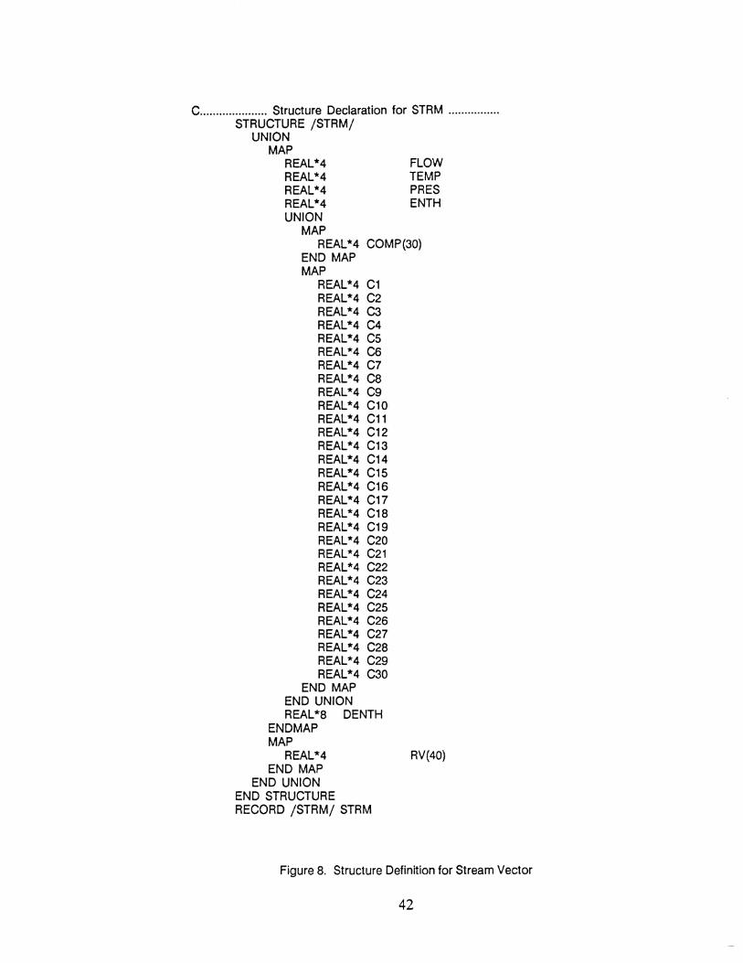
structures. I will not provide a discussion of structures here. However, Figure 8

shows the structure definition for the stream vector. The significance of structure

use is in the transfer of stream data from one stream to another. The particular

architecture of this simulation system requires copying the contents of one stream

vector to another stream vector often. In the original implementation, using two

dimensional arrays, this was accomplished using "DO" loops where each individual

element of one vector was copied to the corresponding element of another vector.

The current implementation with an array of structures involves a single

instruction when copying the contents of one vector to another. This yielded a

41

C ..................... Structure Declaration for STRM ............... . STRUCTURE /STRM/

UNION MAP

REAL*4 REAL*4 REAL*4 REAL*4 UNION

MAP

FLOW TEMP PRES ENTH

REAL *4 COMP(30) END MAP MAP

REAL*4 C1 REAL*4 C2 REAL*4 C3 REAL*4 C4 REAL*4 C5 REAL*4 C6 REAL*4 C7 REAL*4 C8 REAL*4 C9 REAL*4 C10 REAL*4 C11 REAL*4 C12 REAL*4 C13 REAL*4 C14 REAL *4 C15 REAL*4 C16 REAL*4 C17 REAL*4 C18 REAL*4 C19 REAL*4 C20 REAL*4 C21 REAL*4 C22 REAL*4 C23 REAL*4 C24 REAL*4 C25 REAL*4 C26 REAL*4 C27 REAL*4 C28 REAL*4 C29 REAL*4 C30

END MAP END UNION REAL*8 DENTH

END MAP MAP

REAL*4 END MAP

END UNION END STRUCTURE RECORD /STRM/ STRM

RV(40)

Figure 8. Structure Definition for Stream Vector

42

350% increase in execution speed for doing this copy operation.

Another characteristic of the simulation structure was taken advantage of to

dramatically improve the calculation efficiency. The simulation structure, as

described in Figure 2, involves a continuous cycle through a group of steady state

algorithms. Most of these algorithms use some type of trial-and-error procedure.

The timely convergence of these procedures depends on the quality of the initial

guess, as it would in a normal steady state simulator. In this system, the initial

guess for any convergence procedure is the last converged solution. This results in

any particular trial and error procedure converging in one or two iterations,

typically. The quality of this initial guess is a function of the slope of the current

transient and the number of steady state blocks making up the flow sheet. As the

number of steady state blocks increases, or the slope of the transient increases; the

difference between the current inputs and the inputs present during the last

convergence increases. This degrades the quality of the last converged solution as

an initial guess. However, even in the worst case, this initial guess is much better

than one arrived at with typical approaches used in one-shot steady state

simulations.

The following sections describe the individual steady state algorithms in

detail. Notice that most of these algorithms have as input at least two stream

indices. This provides the link between process blocks.

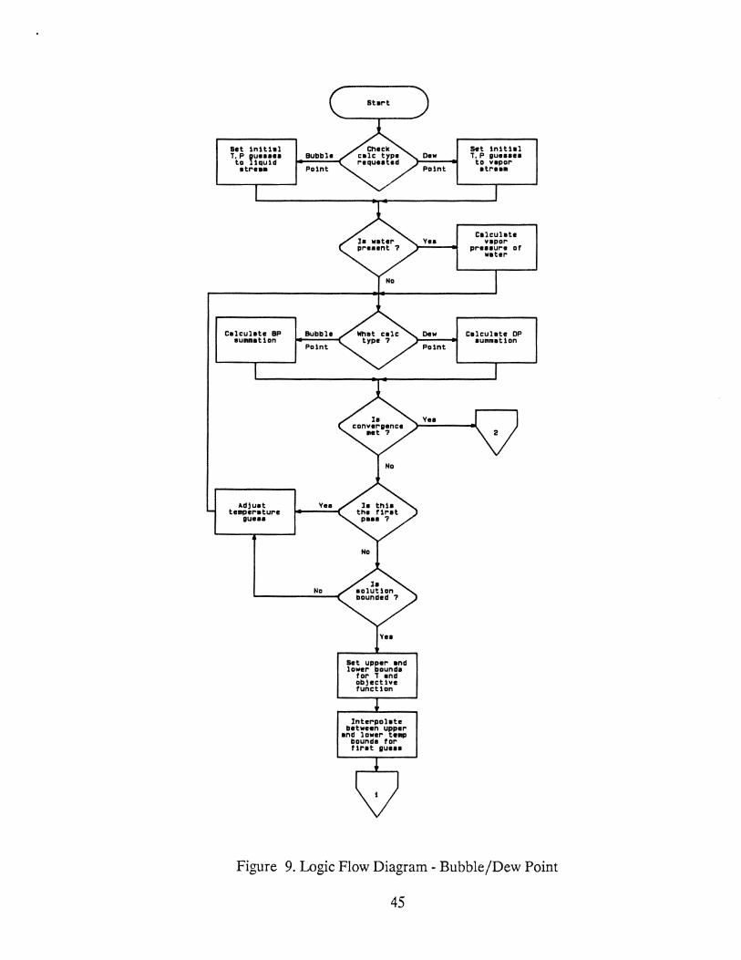
Bubble Point j Dew Point Algorithm

There are several algorithms presented in this section which are rarely

called explicitly by the user. The Bubble/Dew Point algorithm is one of these. This

algorithm is typically called by a higher level routine. The logic flow for this

43

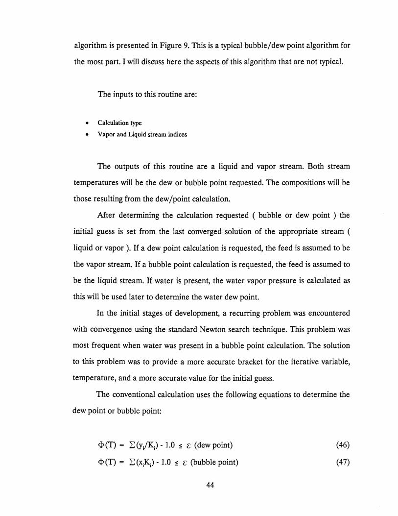
algorithm is presented in Figure 9. This is a typical bubble/dew point algorithm for

the most part. I will discuss here the aspects of this algorithm that are not typical.

The inputs to this routine are:

• Calculation type

• Vapor and Liquid stream indices

The outputs of this routine are a liquid and vapor stream. Both stream

temperatures will be the dew or bubble point requested. The compositions will be

those resulting from the dew /point calculation.

After determining the calculation requested ( bubble or dew point ) the

initial guess is set from the last converged solution of the appropriate stream (

liquid or vapor). If a dew point calculation is requested, the feed is assumed to be

the vapor stream. If a bubble point calculation is requested, the feed is assumed to

be the liquid stream. If water is present, the water vapor pressure is calculated as

this will be used later to determine the water dew point.

In the initial stages of development, a recurring problem was encountered

with convergence using the standard Newton search technique. This problem was

most frequent when water was present in a bubble point calculation. The solution

to this problem was to provide a more accurate bracket for the iterative variable,

temperature, and a more accurate value for the initial guess.

The conventional calculation uses the following equations to determine the

dew point or bubble point:

<I> (T) = 2: (yJK) - 1.0 ~ E (dew point)

<I> (T) = 2: (xiK) - 1.0 ~ E (bubble point)

44

(46)

(47)

Celculete BP eummat1on

Ad}uat tel!per-etur-e

gueea

Point

Point

No

~~:.~P~=~n~~d IOI" T and ob}ectlve function

lnte!"polate between upper

and 1 ower- tel!p bounde tol" flr-et guua

Set tnlthl T,P gueaeea to vapol" atl"ea•

Calculate vapor

pressure or we tel"

Calculate OP aummatlon

Figure 9. Logic Flow Diagram- Bubble/Dew Point

45

C•lculate BP •umm•t1cn

with current T Point

v ••

Bubble

Paint.

Calcul•t• Newton update

to T

Normalize compaaitiana

D•w Pc1nt

Calculate CP auiNftaticn

wttt"' current. .,.

Ve• Sat. 70LD - 7 >...;,.;.;;. __ ,. "TNI!W• (1'U+1'L.) /2.

Yea A•••t 1ower

D•w Paint.

bound• tor 7 and s

Calculate DP aummat1an

with curr•nt. 1'+1

Vea Clem~ updated 7 to a 30"

cnana•

cnack for t-1'20 DP below t-IC

Dl"

Figure 9. continued

46

A temperature is guessed and K-values determined at each temperature

until the above functions convergence to zero within a given tolerance, E. A

Newton convergence technique is typically used to accelerate the convergence.

However, a faster method is used here by making modifications to Equations 46

and 47 to yield a more nearly linear function on which to apply the convergence

technique. Since Ki is related to vapor pressure, one improvement would be:

~ (T) = In[ :E (yJK)] (or xi~) ~ E (48)

Since the vapor pressure is related to T·l, a further improvement would be:

(49)

In most cases encountered with hydrocarbon system, Equation 49 results in

a plot that is very nearly a straight line. Thus, the bubble point or dew point can be

obtained from a linear interpolation of Equation 49 between T0 and T1. Here, T0 is

the initial guess. The determination of T1 involves a stepping procedure. The

temperature is stepped in the appropriate direction until the function of Equation

49 changes sign. This yields T0 and T1 as the brackets for the solution. The initial

guess for the conventional Newton convergence is provided by the following:

(50)

This provides a very robust determination of the bubble or dew point.

The last check made is for a dew point calculation involving a system with

47

water. If this is the case, the water dew point is calculated. If this water dew point

is above the calculated hydrocarbon dew point, the dew point returned by this

routine is set to the water dew point.

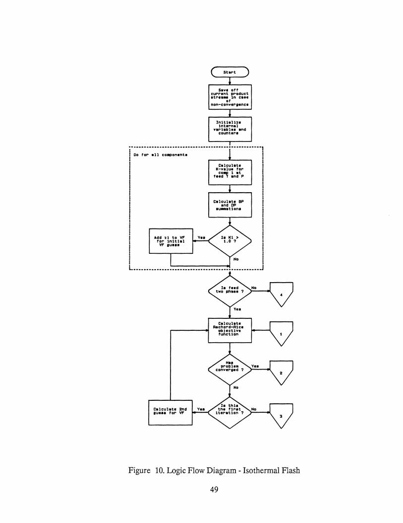
Isothermal Flash Algorithm

This is another algorithm that is rarely explicitly used by the user. Several

of the higher level routines use this algorithm to determine the vapor /liquid split

for a stream at a specified temperature and pressure. The logic flow for this

algorithm is described in Figure 10.

The inputs to this routine are feed, liquid product, and vapor product

stream indices.

The first action taken in this algorithm is representative of several other

algorithms. The last converged output streams are saved in scratch stream vectors.

If the unfortunate event of non-convergence occurs, these saved stream values are

restored to the current output streams and control is returned to the calling

routine. This is the worst case regarding convergence.

After initializing internal variables and counters, a check is made on the

phase of the system. This is accomplished via the functions described in Equations

46 and 47 with the specified T and P. If the result of either of these function

evaluations is less than 0.0, the stream is a one phase system. Here the normal

flash calculation is skipped and the state of the output streams is set appropriately.

If the stream is two phase, a standard flash calculation is done using the

Rachord-Rice objective function with a Newton search technique.

Two possibilities exist for non-convergence:

48

c Start

' S•ve atr current pl'"aduct etreell8 1n case

Df non-convergence

~ ln1t1•l1n 1ntern•l

nl'"18blea •nd countel'"e

I •••••••••••••••••••••••••••••••••••••••••••••••••••• 1 I Do fal'" ell component•

I I

I I I I i

Add 11 to VF for 1n1thl

VF i1UB88

C•lculete 2nd gu••• fal'" VF

C•lcul•te K-v•lu• far

fe~~, !n:tp

C•lculate BP •nd DP

aUIIIIIIBt1ane

C•lculate R•chord-R1c•

abject1ve function

Figure 10. Logic Flow Diagram - Isothermal Flash

49

Set fraction liquid to 1.0

Set l1qu1d product equal

to feed

Set vapor product now to %era with T and P equal

to feed

Check upper and lower

l1•1t• on VF end reaet

Calculate change in VF and obj tunc

Calculate new gue•• far VF

from Newton convergenr:•

Re•tor-e prev1au• r:anverged ealutlon

Set fract1 on liquid to 0.0

Set vapor product equal

to feed

Set ltquid product now ta %era with T and P equal

ta feed

Figure 10. continued

50

Calculate both product CDIIIPD81t 1 one

Calculate both

product enthalpin

Calculate teed enthalpy troll product enthalp1ee

• The maximum number of iterations are reached before the convergence tolerance is

met.

• At some point, no improvement in the objective function results from the guessed

value of V /F.

In either of these cases, a second tolerance becomes important. The current

value of the objective function is compared with this second tolerance. If the

current objective function is less than this second tolerance, the calculation

proceeds as if convergence was met normally. If this second tolerance is not met,

the last converged output stream vectors are restored to the current output stream

vectors and control is returned to the calling routine.

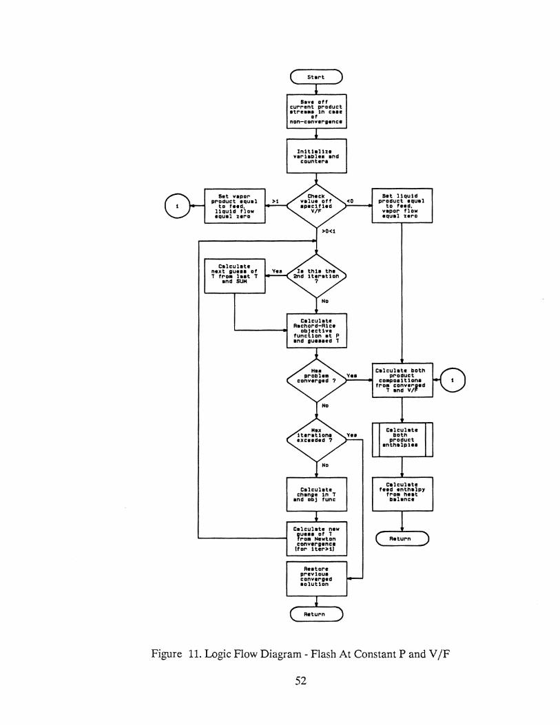
Flash at Constant P and V /F Algorithm

This routine is normally called by the Adiabatic Flash routine. In some

cases during the adiabatic flash calculation, the temperature of a given stream at a

given temperature and vapor fraction is needed. Other routines call this algorithm

as well.


• The stream indices for the feed, liquid and vapor products

• The specified vapor fraction

The logic flow for this algorithm is described in Figure 11. This algorithm is

very similar to the isothermal flash algorithm. Here the iteration variable is

temperature instead of vapor fraction.

51

Set vapor product equal

to feed, l1QU1d flow equal zero

Calculate next gueaa of T from laat T

and SUM

Save off current product atre••• :ln caee

of non-convergence

ln1t1alhe var1.abl•• and

count era

Calculate Rachard-Rtce

ablect1ve function at P end gueaeed T

Calculate change 1n i

end ollj func

Calculate new

'~~:·..:~t!n convergence !tor 1ter>1l

Rea tare prevloue converged oolut1on

Set l1qu1d product equal

to feed, vapor flow equal zero

Calculate llotn

product enthelp1ee

Calculate feed enthalpy

from heat balance

Figure 11. Logic Flow Diagram- Flash At Constant P and V /F

52

Adiabatic Flash

This routine is typically utilized by the user to account for single trays in a

distillation column where discontinuities in the vapor /liquid traffic are introduced

(e.g. feed tray, draw tray, etc.) There is considerable logic in this algorithm to

insure the return of at least a qualitative answer. The logic flow for this algorithm

is presented in Figure 12.


• Number of input streams

• Input stream indices

• Additional heat input

At present, the adiabatic flash routine can accept up to 5 individual feed

streams. The first action taken in this algorithm is to combine these input streams

into one. As the flows are added together, a record of how many, and which, of the

input flows are negligible is kept. During the course of a simulation run any or all

of these input flows can become zero. The pressure of the combined stream is set

equal to the lowest pressure among the input streams. At this point the combined

feed flow is checked. If it is negligible, the products are zeroed out and control is

returned to the calling routine. If the combined feed flow is the result of only one

input having a significant flow, a simple isothermal flash is done. If none of these

alternatives apply, the composition of the combined feed is determined.

The first precaution taken to insure convergence is the calculation of the

53

Collbtne vartoue feeds 1nto one lup

to five}

calculate dew and bubble pta to set m1n and

IIBX T and H

Calculate the enthalpy of

each feed stream and sum

for HSPEC

Set f 1rat temp guess to last

converged T and clamp wtth TB

and TO

1ero out vapor and

l1qu1d product streams

Execute 1 stmple

taothermal flesh

Feed 18 all vapor, no

atgnit 1cant temp effect -

set vapor-feed

return

return

return

Figure 12. Logic Flow Diagram - Adiabatic Flash

54

Reset lower Hmlt clamps tar H. T. FQ

Colculate V/F via lever rule us1ng upper and lower enthalpy

l1111t&

Calc Flash at constant P and

V/F to determine

teatper•ture

Calculate 1aotr.er11al flash at guessed T

ond f .. d P

Calculate callb1ned er.t~m~ of

products

Colculate rel•t1ve error

1n calculoted enthalpy versus

feed ent!lelpy

Yes

Calculate new guesa far"' T via Newton-Raphson

convergence

No

TNEli • 111d point of TU

and TL

Return

TOLD • TNEW HOLD • tl>lEW TNEW by eq.

Reset upper 11•1t clamps

for H. l. FD


55

No

Colculate V/F v1• lever rule

'---........ using upper and lower entholpy

l1m1ts

Calc Flash at constant P and

V/F to detorm1ne

teatperature

Return

dew and bubble points of the feed. These are used as the initial upper and lower

limits. These are used to generate an initial guess for temperature if a prior

converged value is not available.

The rest of the algorithm is a standard adiabatic flash, except for the

convergence section. Several actions are taken in the convergence section to insure

the return of a solution.

The upper and lower limits on the convergence variables, temperature,

enthalpy and vapor fraction, are examined at each step in the iteration. As the

solution proceeds towards convergence these limits are reset. At any point, if the

current temperature guess results in a calculated enthalpy outside the current

limits, the next guess for temperature is the average of the current upper and lower

limits. Otherwise, a Newton search determines the next guess.

In addition, the difference between the current upper and lower

temperature is calculated. If this difference is small (i.e. less than .1 OF), the

convergence is considered to be close enough to allow the use of the lever rule to

determine the vapor fraction. The vapor fraction is determined from the current

upper and lower limits on vapor fraction and enthalpy and the specified enthalpy

(i.e. the sum of the enthalpy of the input streams). A constant P and V /F flash is

then done with this V /F. This yields the temperature of the system.

This lever rule option is also used when the maximum number of iterations

is exceeded.

Stream Summer Algorithm

This is a very simple algorithm to add together two streams of the same

phase. The logic flow for this algorithm is presented in Figure 13. Mter checking

56

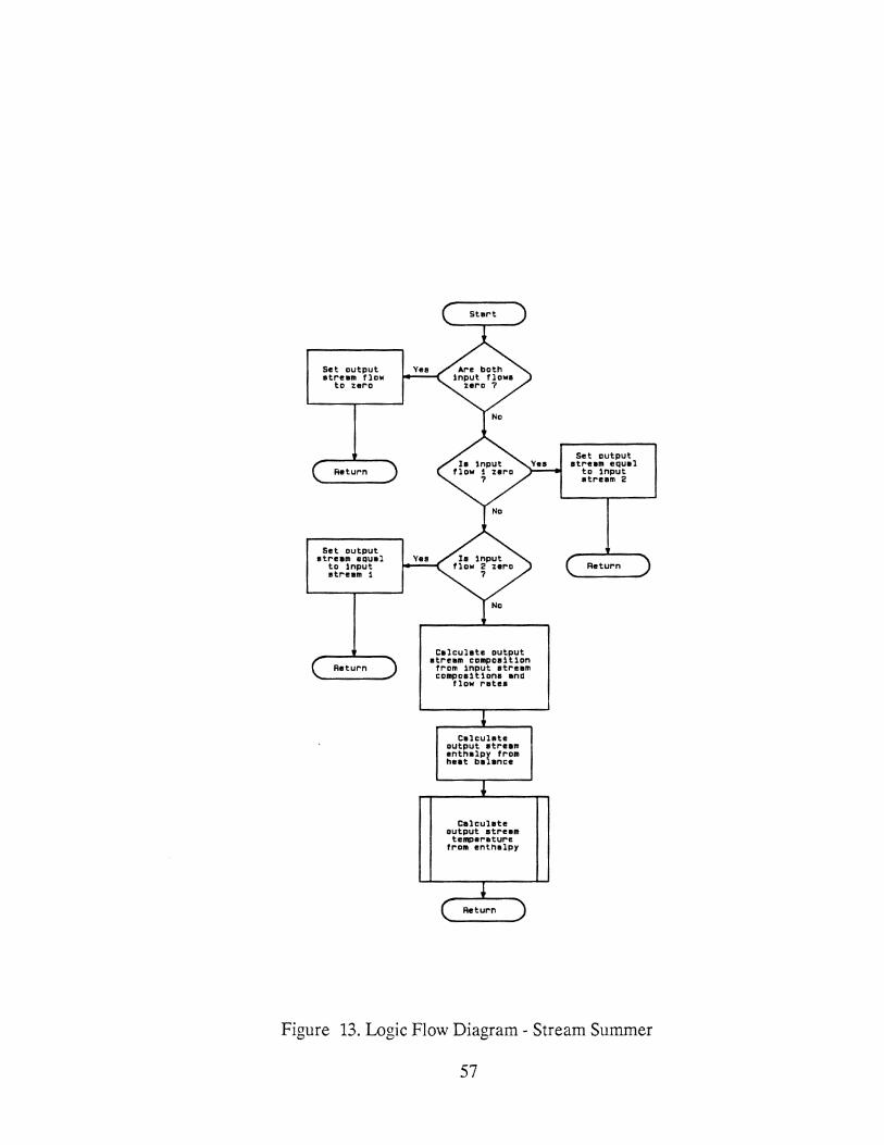
Set output stream tlow

to zera

Set output stream &QUill

to input stream 1

Return

Cal eulete output atream campas1t1an

from 1nput atream compoa1t1ons and

flow ratea

Calculate output stream

temperetur""e fr'Om enthalpy

Set output stream equel

to input atream 2

Figure 13. Logic Flow Diagram- Stream Summer

57

for zero flow input streams, the output stream composition is calculated.

Following this, the output stream enthalpy is calculated. From this information the

output stream temperature is calculated.

Stream Temperature Determination Given Enthalpy

This is another support routine which is called by several of the other

routines. Often, a particular routine yields a stream at a given enthalpy but no

specific temperature. This algorithm determines the stream temperature at the

specified enthalpy. The logic flow for this routine is presented in Figure 14. The

inputs to this routine are:

• Input stream index

• Input stream phase

Basically, this calculation is a heat balance. The stream temperature is

varied to close the heat balance. The initial stream temperature is used as the

initial guess for temperature. As in the adiabatic flash algorithm, the upper and

lower limits for the iteration variables, temperature and enthalpy, are updated for

each iteration. These limits are used to help insure a convergence. A Newton

search is used to close the heat balance.

Distillation Trayed Section Algorithm

The Distillation Trayed Section algorithm is one of the two major building

blocks for constructing a distillation column. The other is the Adiabatic Flash

58

Reset lower l1m1ta lor

enth and temp

TOLD • TNEW HOLD • HNEW TNEW •

TNEW11L05

Calc feed heat:

flowltenth

Calc 1n1thl lower and

upper l1m1ta lor calc enth

and te11111

Calc enth or atream

at eaau11ed

temp

Calc stream heat:

llowllenth

Calc error 1n calc h••t v• actual heat

Set new T to average or upper and

l ewer limit a

ChiiP new T to average of

upper ad lower 11 .. 1 ta

Reaet upper l1m1ta lor

enth and temp

Calc change 1n calculated

enth

Calc new gueae for T !rom Newton convergence

Figure 14. Logic Flow Diagram- Stream Temperature Given Enthalpy

59

algorithm. The most marked difference between this dynamic simulation and

standard rigorous dynamic simulation involves my treatment of distillation trayed

sections. For this reason, I will describe in some detail the basis for the approach I

took. I will begin with some background that lead me to explore other avenues for

handling trayed sections. Following this~ the detailed derivations of the appropriate

relationships will be presented. Lastly, the computational algorithm will be

described.

Background

The rigorous simulation of distillation column dynamics is one of the most

computationally intensive dynamic simulation problems that exists. In addition~ my

previous experience with simulations of this type has revealed a frustrating

tendency for the calculations to become unstable. This is due to the presence of

differential equations having very small time constants .compared to the dominant

time constants in the set of differential equations that define the distillation

column. Moreover~ these time constants vary with the conditions within the column

which means the system will be conditionally stable. These unstable situations can

be compensated for in several ways including increasingly small integration step

sizes, or logic that will detect these high stiffness conditions and adjust the

integration technique appropriately. In any case, these types of simulations require

very lengthy CPU times per time step, which requires a very powerful computer to

maintain real time operation. My goal was then to develop a less computationally

intensive method to provide all the attributes provided by a completely rigorous

model that were necessary to meet the goals I set forth in the beginning of this

document without reproducing the undesirable attributes of the rigorous system.

60

Since most of a distillation column is trayed sections, effectively handling this piece

would amount to a major step towards my goal.

The general approach I developed was described in Chapter II. This

involves treating the V-L-E for the trayed sections with a steady state approach.

The most generally accurate steady-state simulation techniques are those based on

a rigorous tray-by-tray calculation. They incorporate both heat and mass balances

on each tray in the column. Generally, these rigorous solution techniques can

require upwards of 60 seconds to converge on main-frame class computers. Since

the goal of this work was to utilize mini-computer class machines, the execution

time per time step would be prohibitive. In addition, a disadvantage of rigorous

solution techniques is they often exhibit difficulty converging to a solution. This

failure to converge is a very serious problem in real time environment, as discussed

earlier.

One approach to reducing this excessive execution time was proposed by

Mamedov.25 This method involves polynomial fitting of the column using either

real plant data or a rigorous model of a column, i.e. generate a wide range of

solutions of the rigorous model and then fit these results in a polynomial form.

This method would be reasonable for a small number of independent and

dependent variables of interest, but as this number grows the generation of data

and the fitting problem become astronomical. In addition, this would prevent

changing the column configuration easily. This type of method is also impractical

when the operating point of the column can vary widely, potentially from startup to

shutdown in my case.

Between these two extremes of rigorous and elementary models lie a whole

range of "simplified" model techniques which, generally speaking, attempt to

61

reduce the model execution time via making certain assumptions about the column

operation.

Proposed Trayed Section Model

The simplified model I developed which best satisfies the time and accuracy

requirements of this project is based on the sectioning technique of Smith and

Brinkley.26 Any distillation column can be divided into sections bounded by

discontinuities in the vapor /liquid traffic. Conditions within each section are

assumed unifo~ i.e. constant flow rates and constant relative volatilities. The

mathematical technique of finite differences can then be used to relate the

composition of the products to the composition of the feeds and the number of

theoretical plates without intermediate tray compositions appearing explicitly in

the equations. Since all previous applications of this sectioning technique

considered the column as a whole, including auxiliaries, I derived the appropriate

equations to predict the separation in any given section by itself.

This derivation begins a with mass balance around stage n + 1. All the

equations in this derivation are written for any given component. A component

subscript is omitted for the sake of simplicity.

(46)

(47)

62

Rearranging gives

X - rKn+lvn+l n+2 L

n+2

L ] K V + ~ X + n+l n+l = 0 L n+l L

n+2 n+2

(48)

The rates and K-values within the column section under consideration must

be assumed constant if a simple mathematical solution of the difference equation

is desired. Making these assumptions and writing the equation in operator form

gives:

(49)

or (50)

The properties of the E operator are discussed by Wylie.27 Let S1 and S2

represent the two roots

S1 = KV/L

The solution is then

The constants can be eliminated as follows:

By definition V NYN = (1 - f)A

where: f = fraction of a given component which is recovered in

the bottoms stream

(51)

(52)

A= the total amount of the given component entering the column

63

Then

Yn = (1- f)A

vn (53)

(1- f)A xn = K V

n n

(54)

Substitution gives

(1- f)A

KnVn = c SN + c 1 2 (55)

A balance around stage N will yield an expression for xN_1

Y = ~xN + V NYN + ~+lxN+1 N-1 V V V N-1 N-1 N-1

(56)

(57)

where: 'L. = fraction of a given component which enters in stream ~ + 1

Substituting for xN, YN• and ~+lxN+ 1 in the balance around stage N and

dropping the subscripts on the rate terms gives

L(1 - f)A + (1 - f)A _ ACJ.s YN-1 = K'T2 v v v- n

(58)

Now replace yN_1 with Kx:N_1 and solve for xN-l

(1 - f)A ~ L 'L. ] xN-1 = KV Lkv + 1 -y-::y (59)

Equations 55 and 59 can now be used to solve for the constants in Equation

52

64

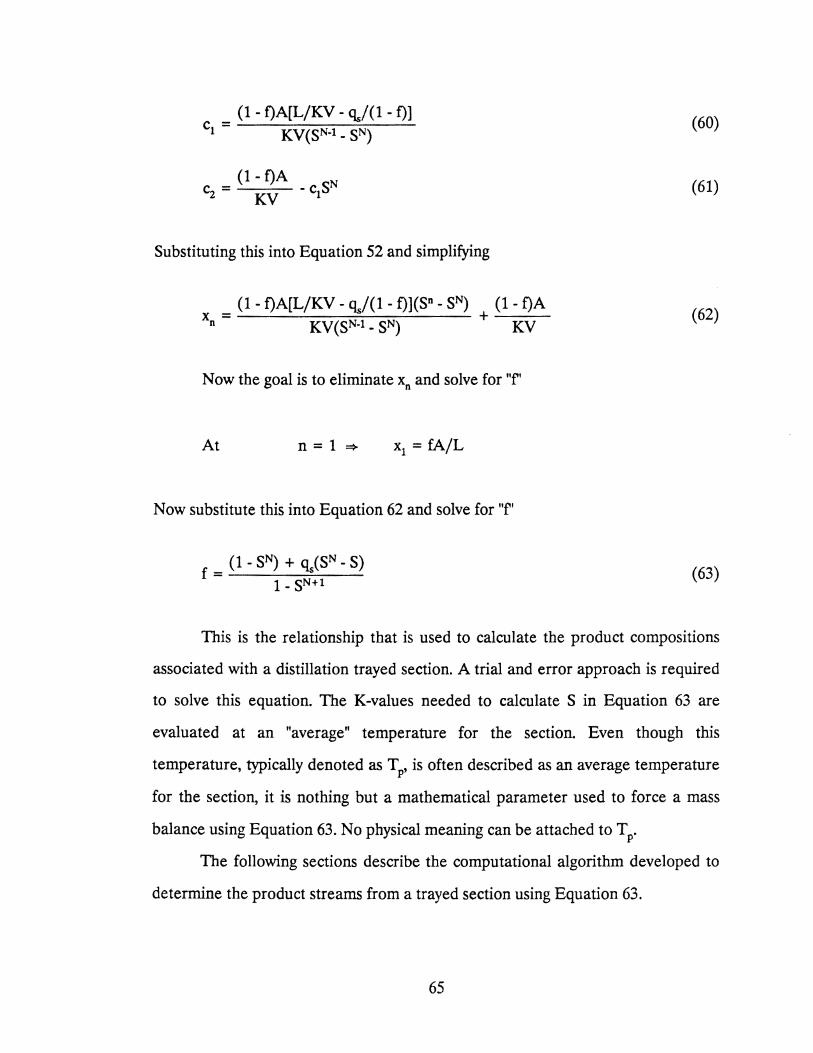
(1- f)A[L/KV- Cis/(1- f)] cl = KV(SN-1 - SN)

(1- f)A c2 = KV

Substituting this into Equation 52 and simplifying

(1 - f)A[L/KV- 'Is/(1 - f)](S"- SN) (1- f)A X = ---------,...,=--~--- + ---

n KV(SN-l- SN) KV

Now the goal is to eliminate X0 and solve for "f'

At n = 1 =>

Now substitute this into Equation 62 and solve for "f'

f = (1 - SN) + Cis(SN - S) 1 - SN+l

(60)

(61)

(62)

(63)

This is the relationship that is used to calculate the product compositions

associated with a distillation trayed section. A trial and error approach is required

to solve this equation. The K-values needed to calculate S in Equation 63 are

evaluated at an "average" temperature for the section. Even though this

temperature, typically denoted as TP, is often described as an average temperature

for the section, it is nothing but a mathematical parameter used to force a mass

balance using Equation 63. No physical meaning can be attached to TP.

The following sections describe the computational algorithm developed to

determine the product streams from a trayed section using Equation 63.

65

Computational Algorithm

The algorithm used to solve the distillation trayed section based on

Equation 63 will be described in 5 parts:

• Initialization

• Heat Balance

• Mass Balance

• Mass Balance Convergence

• Heat Balance Convergence

Initialization The logic flow described in this section is presented in

Figure 15. As in previous algorithms, the first action taken is saving the last

converged solutions for the product streams in scratch stream vectors for later use

in case of non-convergence. After some flag and counter initializations, the total

feed to the section is calculated. Then the individual feeds are checked for a

significant flow rate. During the course of a simulation it is possible for either or

both feeds to become very small or zero. Here, the product streams are set

according to which stream is negligible. Control is returned to the calling routine

at this point.

The outer iteration loop is entered if both feed streams are significant. This

outer iteration loop is a heat balance around the section. This is a very significant

part of this algorithm. The standard application of the Smith-Brinkley sectioning

technique assumes constant molar overflow. For a trayed section calculation this

translates into:

• the vapor product flow rate equals the vapor feed flow rate

• the liquid product flow rate equals the liquid feed flow rate

66

let both product tempe to vepor temp

set d1et1llete compoe1Uon

to vepor COIIP081 t1 on

let botto.,. co•poeH 1 on to reflux

coMpoe1t 1on

Return

Seve product atreau 1n c•••

of nan-convergence

In1t1e11u fleD• end count era

Set d1•Ullet• end bottou

product preeeure

Celculete totel feed:

Yepor + reflux

Celc f1ret gu••• for OF

frDII le8t HERR

Celc as velue•

Calc TP •• everege of reflux end v•por teMp•

Calc f1ret gu••• for OF:

le•t OF • 1.02

Figure 15. Logic Flow Diagram - Distillation Trayed

Section: Initialization

67

Celc f1ret gue•• foro OF: vapor/feed

For many types of columns operating under normal conditions, this

assumption does not introduce significant error. However, my goal for this

simulation was to allow accurate simulation of a wide variety of tower types (e.g.

steam stripped) operating under potentially unusual conditions (e.g. startup or

shutdown). For these cases the assumptions of constant molar overflow was not

sufficiently accurate. This is immediately obvious for steam stripped towers where

the mass transfer towards the bottom of the tower is essentially unidirectional.

Rather than attempt to solve the above derivation without assuming

constant molar overflow (i.e. constant vapor and liquid rates within the section),

the heat balance approach was taken. The standard application of the Smith

Brinkley technique requires D /F be specified either explicitly or implicitly. Here

D /F was used as the convergence variable to close the heat balance. As before, the

initial guess for D /F is the value from the last converged solution. The values for

'Is are determined before entering this heat balance loop.

Heat Balance Figure 16 represents the logic flow of this section. After

updating the upper and lower limits of heat balance error and D jF, new values of

the product flow are calculated from the current value of D /F. These flows are

then used to calculate the average liquid and vapor flows in the section. At this

point the mass balance loop can be calculated. Once the mass balance loop has

closed, the temperature and enthalpy of each product stream is determined from

the stream composition returned from the mass balance calculation. This allows

the determination of the heat balance error. If convergence is not met, a new value

of D /F is determined; and the loop is repeated.

Mass Balance As indicated by Figure 17, this portion of the algorithm is

the standard Smith-Brinkley approach. The product compositions are determined

from Equation 63 via the logic shown in the figure. Once the compositions are

calculated, they are normalized and a mass balance error is calculated. If

68

Reeet upper end lower

ch11pe for HEAR end OF

HLERA • HERR OFL • OF OF• tunc IOFL, HLERR)

Celcuhte aver•a•

reflux end vapor now•

M••• Balance

Loop t•ee •epa,..ate

figure)

Calc dew pt end

:~:~m:t:'

Calc bubble pt end

enthalpy of bottou

Calc heat behnce tar

CDlUIIn .. cuan

Set: OFL • OF HLEFIA • HEAR

Calculate new value at OF I••• eeperete

t 111urel


Section: Heat Balance

69

LEAR • ERR LTP • TP TP • tunc IL TP, LEAR)

, •••••••••••••••••••••••••••••••••••••••••••••••••••••••••••••••••••• 1 I Do tor all co~onanta I I I I K~:;~ua I I' at TP and I'

Pavg I I

I I

I i I

I ! ! I I i !

Calc btma tree uatng L'H~~!tal

Calc atr1pptng

hctar, SN

Calc d1atilhte

and btu co~oat1t1an far COIIIPDnant

Calc btlla frac uatng

atandar-d aq.

L. ................................................................... J

NDI"IIaltza product

ca~aa1t1ana

Calc 11aaa bal err baud an

•••llaat at real!

Calculate new value Df TP

(aeparate figure)

Return


Section: Mass Balance

70

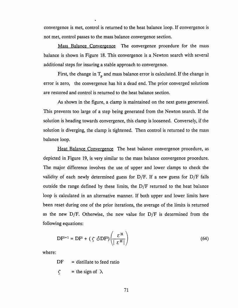
convergence is met, control is returned to the heat balance loop. If convergence is

not met, control passes to the mass balance convergence section.

Mass Balance Conver~ence The convergence procedure for the mass

balance is shown in Figure 18. This convergence is a Newton search with several

additional steps for insuring a stable approach to convergence.

First, the change in TP and mass balance error is calculated. If the change in

error is zero, the convergence has hit a dead end. The prior converged solutions

are restored and control is returned to the heat balance section.

As shown in the figure, a clamp is maintained on the next guess generated.

This prevents too large of a step being generated from the Newton search. If the

solution is heading towards convergence, this clamp is loosened. Conversely, if the

solution is diverging, the clamp is tightened. Then control is returned to the mass

balance loop.

Heat Balance Convergence The heat balance convergence procedure, as

depicted in Figure 19, is very similar to the mass balance convergence procedure.

The major difference involves the use of upper and lower clamps to check the

validity of each newly determined guess for D /F. If a new guess for D /F falls

outside the range defined by these limits, the D /F returned to the heat balance

loop is calculated in an alternative manner. If both upper and lower limits have

been reset during one of the prior iterations, the average of the limits is returned

as the new D /F. Otherwise, the new value for D /F is determined from the

following equations:

(64)

where:

DF = distillate to feed ratio

~ = the sign of A

71

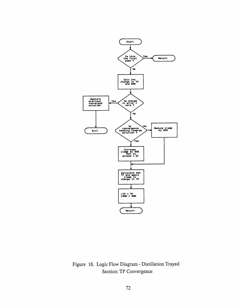
~a tare prev1oua converged eolut1an

Calc the ch•nll• 1n TP

•nd ERA

Increeac ClaiiP II)' 20.1:

(nat ta uc .. d 1.0)

Celculete new TP and app}y

cleiiiJ) to chan11e 1n TP

LTP • TP LEAR • ERR

~duce cl•IIP by !lOX


Section: TP Convergence

72

New OF 1e ever•a• of

la_,.. end upper- U•1t•

R .. tar-e prevtou• converged ealut1an

New OF • tunc IOF, HERR)

Celcuhte ellen .. tn OF

end HEAR

Check law •nd

htr .:;~-=er eppr-apt•te ane

C•lculete ,.,. OF fr-a• Newton

converaence

DFL • OF HLERR • HERR

Reduce cleoop by !lOX

Figure 19. Logic Flow Diagram- Distillation Trayed

Section: D /F Convergence

73

£ H = absolute error in heat balance

o = step weighting factor, default is 0.5

Individual Tray Temperatures Within a Trayed Section

Values for individual tray temperatures within a trayed section are often

required in the design and development of control schemes. These are used as

either indicators or control points. The trayed section algorithm described in the

previous section does not provide these values for individual tray temperatures.

However, the same assumptions and analysis which yielded the equation for trayed

section separation can be used to derive an equation for the temperature of any

tray within the section.

This derivation will begin with Equation 62. This equation provides for the

prediction of the liquid composition present on any tray within the section. This

can be simplified via the following steps:

Dx0 1-f=A

Substituting this into Equation 62 yields

x = Dx0 j[s-1 - qJ(l - t)](S0 - SN) + ] n KV [ (SN-1- SN) 1

Now to elimnate Cis

74

(65)

(66)

(67)

Substituting this into Equation 66 and simplifying yields

X =-D I D Dx [sn-N-l -1 + (1 - sn-N)Lx /Dx ]

n L 1- S (68)

After the trayed section separation has been determined, the above

equation will yield the liquid composition on any tray in the section. At this point a

simple bubble point will yield the tray temperature.

I would like to emphasize at this point the above tray temperature

determination does not consider the liquid dynamics within the section. The

product composition from the trayed section algorithm is based on an average

liquid and vapor flow for the section. Thus the predicted tray temperatures are

based on the same assumption since these product compositions are inputs to the

above algorithm. There are two approaches available to deal with this error:

• The output from the tray temperature algorithm can be passed through a second

order plus dead time fllter. This will approximate the effect of liquid dynamics in the

section.

• Even though no discontinuity may exist at the tray in question, the column can be

split at this point as if a discontinuity did exist. The adiabatic flash algorithm can be

used to calculate the tray where the temperature is desired.

The second approach is much more accurate. The degree of accuracy

required will determine which of the above two approaches is the most

appropriate.

75

Condenser jReboiler Algorithm

Many distillation columns employ the use of overhead condensers and

partial reboilers. The steady state treatment of these pieces of equipment amounts

to a heat exchanger rating which involves a stream phase change on at least one

side of the exchanger. A survey of the literature revealed the only algorithms

available to solve this type of rating calculation involved the solution of a set of

differential equations developed by the classical approach of defining a steady

state heat balance across an infinitesimal section of the exchanger. This set of

differential equations is then integrated over the length of the exchanger. In

addition, this method requires very good estimates of the local heat transfer

coefficient to make accurate predictions of the overall heat transfer occurring. I

developed a new algorithm that neither requires the solution many differential

equations or the accurate estimate of any local heat transfer coefficients. The

following discussion will begin with a presentation of the theory behind the

method. Following the computational algorithm will be presented.

Theory

The method developed for rating heat exchangers where one or both

streams can be undergoing a phase change is based on a method used to rate heat

exchangers where no phase changes are occurring. The method is usually referred

to as the "NTU" method.28 The equations defining the NTU method for exchanger

rating are given below.

76

NTU = AUavfCmin

{ = <P(NTU, Cmin/Cmax' flow arrangement)

also

= Ch(Th,in- Th,out) = ~(Tc,out- Tc,in)

Cmin(T h,in- Tc,in) Cmin(Th,in - Tc,in)

(69)

(70)

(71)

The one input parameter to this algorithm that has prevented its

application to systems involving a phase change is the stream heat capacity, cp,

used in the calculation of the stream thermal capacity rate. However,

consideration of two facts regarding the physical meaning of heat capacity reveals

a technique that will allow the NTU method to be used to rate exchangers that

involve phase change.

• The heat capacity defmes the change in enthalpy of a stream as the temperature

changes. Therefore, the heat capacity for a pure component undergoing a phase

change is infinity since its enthalpy is changing with no corresponding change in

temperature. Taking this one step farther, there should exist an effective heat

capacity for a multicomponent stream undergoing a phase change that corresponds

to the actual heat transfer taking place and the value of this effective heat capacity

should be something less than infinity. However, the value of this effective heat

capacity cannot be determined a priori.

• At the correct value of this effective heat capacity for a multicomponent mixture, the

heat balance around the exchanger should close.

These two observations lead to the development of a trial and error

algorithm that effectively searches for the correct value of the effective heat

capacity of the stream undergoing the phase change that yields a closure on the

heat valance for the heat exchanger. When a converged solution is reached, the

thermodynamic state of both streams exiting the exchanger is available.

Before discussing the details of the computational algorithm, some

discussion regarding Equation 70 is in order. This equation form depends on the

77

geometry of the exchanger. These various equation forms are tabulated in various

sources, the book by Kay and London28 being one of the best. Two equation forms

are available in this algorithm, shell and tube and cross flow. These two forms will

handle most configurations encountered in overhead condensers (e.g. water cooler,

air-cooler, etc.) and partial reboilers. If other forms are required, these can be

incorporated into this algorithm with little difficulty.

Computational Algorithm

The detailed discussion of the computational algorithm required to

implement the method described above will be presented in three sections

• • •

Initialization and NTU section

Convergence section

Low /High CP Limit Checking section

This discussion below describes the condenser algorithm. The reboiler

algorithm is identical to this except for the NTU equation forms used.

Initialization and NTU Figure 20 presents the logic flow for this section.

After counter and flag initializations, a check is made to determine if what type of

fluid is on the side opposite the process. The two possibilities are:

• one phase stream

• phase changing stream (i.e. condensing or vaporizing)

For a phase changing stream, the stream's saturation temperature and heat

of vaporization are calculated. These two properties are a function of the stream

pressure via the following relationships:

78

Set vapor and l1qu1d atreem temperature to coolant ta~~t~~arature

Coolant

Calculate aaturat1on hlftllerature and heat of

vapor hatton

TCO • TCI VAPOR • FEED No L1qU1d

Plrform flaah an

teed to obta1n feed

enthalpy

Reaet all countera and

tlega

Na

Calculate the hot and cold atrea111 outlet

atatea frDII the NTU Mthad

Calculate the heat balance

tar the exchanger from NTU

Perform an tao thermal

fluh an the teed at the

above outlet T

Calc. HEX h .. t balance from

teed 1nlet and outlet

cand1t1ana

Calculate heat balance

error

Figure 20. Logic Flow Diagram - Condenser Algorithm:

Initialization and NTU Calculation

79

Rea tore ortg1nal valuae of

feed T and p

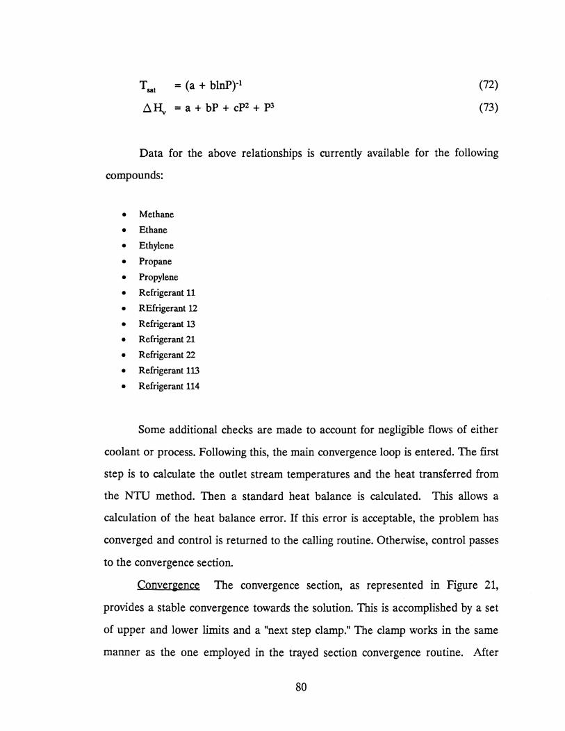
= (a + blnP)-1

~I\, = a + bP + cP2 + P3

(72)

(73)

Data for the above relationships is currently available for the following

compounds:

• Methane

• Ethane

• Ethylene

• Propane

• Propylene

• Refrigerant 11

• REfrigerant 12

• Refrigerant 13

• Refrigerant 21

• Refrigerant 22

• Refrigerant 113

• Refrigerant 114

Some additional checks are made to account for negligible flows of either

coolant or process. Following this, the main convergence loop is entered. The first

step is to calculate the outlet stream temperatures and the heat transferred from

the NTU method. Then a standard heat balance is calculated. This allows a

calculation of the heat balance error. If this error is acceptable, the problem has

converged and control is returned to the calling routine. Otherwise, control passes

to the convergence section.

Convergence The convergence section, as represented in Figure 21,

provides a stable convergence towards the solution. This is accomplished by a set

of upper and lower limits and a "next step clamp." The clamp works in the same

manner as the one employed in the trayed section convergence routine. After

80

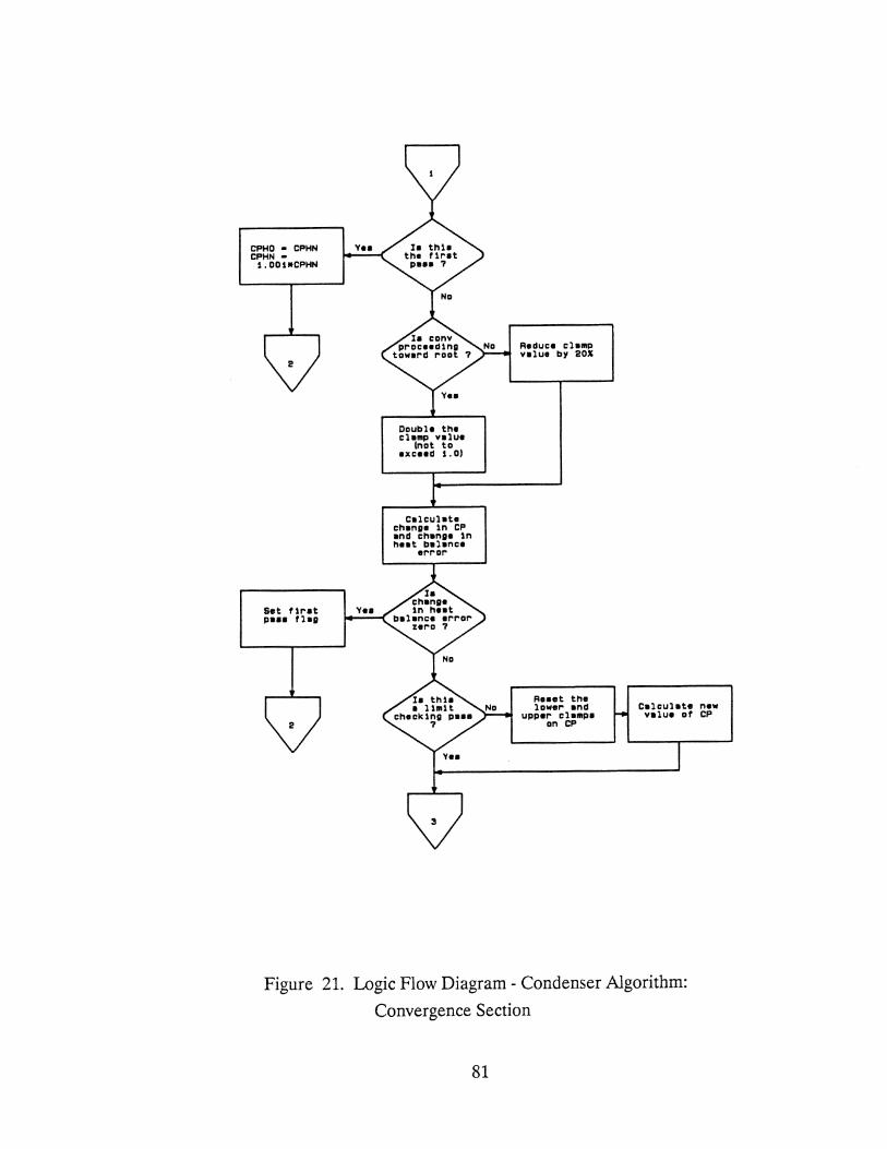
CPHD • CPHN CPHN •

i.DDSotCPHN

Set f1r-at peaa flag

Double the c1e111p value

(not to exceed 1. D)

Calculate change 1n CP end change 1n heat balance

er-r-or-

Vee

Reduce cle111p value by 20X

Reaet the lower- end

upper- clelllpe an CP

Calculate new value of CP

Figure 21. Logic Flow Diagram- Condenser Algorithm:

Convergence Section

81

checking and setting a new value for this clamp, a check is made on the change in

the heat balance error. If this error is zero, then a dead end has been reached in

the convergence. An effective step discovered for this occurrence is to restart the

calculation with an effective cp guess generated with the first pass equation as

shown Figure 21. This usually gets the convergence off dead center and results in a

solution.

The last step in this section involves the upper and lower limits on CP.

These limits are reset; and a new value of CP is calculated, if the current pass is not

a limit checking pass. The new guess is determined from a Newton search. The

purpose of a limit checking pass is described in the next section.

Low /High CP Limit Checking As in all the other steady state algorithms,

the initial guess for the convergence variable, CP here, is the value from the last

converged solution. Additionally, the initial upper and lower limits are those

resulting from the last converged solution. However, I found that these limits were

frequently causing convergence problems as they did not span the solution. One

solution would have been to reset the upper and lower limits to arbitrarily high and

low values on each call to this routine. However, this proved to waste some very

valuable information about where the solution was. The alternative I arrived at is

represented in Figure 22.

As has been done in previous algorithms, the newly guessed value, cp here,

is compared against the current limits. If this newly guessed value is outside the

range specified by these limits, the new guess is reset to the average of the limit

values. However, for this algorithm, this limit clamping is allowed to occur only a

fixed number of times at either boundary. If this number is exceeded, an

assumption is made that the corresponding limit may be wrong. The new guess for

CP at this point is set equal to the corresponding limit and a limiting checking

iteration is executed. During this iteration no updates are done to either the limits

82

lncre-nt low llalt

¥1Dl•t1Dft count:.•,.

Cf'\•ck taw llJRlt: c,. n•w •

CP" lOW fl•c•lc o•i fYnc

CP1•ok "1.gP1 ll .. tt.: Cfli' n•w • Rec•~: :~f"ttunc

A8etor• prlor conv•r••a •olutlon

C•lCYl•t• n•w to"' 11M1t •nil ,.eaet ct• ...

t:.o t..O

C•lcul•t:.• new ,,., 1 t.tlllt

•nil r•••t cl••P to i..O

Figure 22. Logic Flow Diagram - Condenser Algorithm:

Low /High CP Limit Checking

83

or the active cp value. The objective function resulting from this limiting cp value

is compared with the last good iteration objective function. If these two objective

functions do not differ in sign, the corresponding limit is most likely too tight. In

this case, the limit is moved out an amount which is a function of the current heat

balance error magnitude. With the limit reset, a new CP guess is generated as an

average of the limits and the convergence procedure continues. Currently, the

maximum number of times a limit clamping can occur before a limit checking pass

is performed is 5.

84

CHAPTERV

UNSTEADY STATE ALGORITHMS

The purpose of the unsteady state algorithms is to account for the process

lags associated with the liquid and vapor holdups in the column. The liquid

holdups are present on each tray and in the reboiler and condenser systems. These

liquid holdups cause lags in all properties associated with the liquid as it makes its

way down the column. The dynamics associated with the vapor in the column are

generally very fast. Therefore, the vapor holdup in the column proper is ignored.

The vapor holdup in the overhead system is what determines the column pressure.

The following algorithms were developed to account for the above mentioned

effects.

The differential equations involved in these algorithms require a delta time

for the integration. The delta time is the actual time difference between the

current time and the time the algorithm was last executed. This is the real time

component of the system.

Before beginning the discussion of the individual algorithms, I would like to

present a brief discussion of the integration method used in these algorithms.

The integration technique used in the following algorithms is a predictor

corrector type. One of the simplest pairs consists of the point-slope predictor and

the trapezoidal corrector:

85

Predictor:

Yn+1 = Yn-1 + 2hYn (74)

Corrector: h Yn+1 = Yn + z (Yn+1 + Yn)

-h3 T = -y(3) t n+1 12 n ':, 2

(75)

This is the integration technique used in the following algorithms. The first

step of the calculational procedure is the use of the predictor to compute y2 based

on the known value of y0• The value of y;, needed in the predictor formula, is

found by a starting procedure. Two methods commonly used to find y1 are (1)

Euler's method (the first two terms of the Taylor's series) and (2) the first three

terms of the Taylor's series. The starting procedure used here is Euler's method.

After the procedure has been initiated, previously computed values of Yn-1 andy'

are used in the predictor to predict Yn+l' and this value of Yn+l is then used in the

-differential equation to compute Yn+r This value of Yn+1 is used in the corrector to

compute Yn+l' which may be further improved by iteration between the corrector

and the differential equation. The added accuracy provided by this further

iteration was not sufficient to warrant its use considering the extra compute time it

required.

Even when the truncation and roundoff errors are negligible, numerical

methods are subject to instabilities which cause the error [y(t0 +1)- Yn+1] to become

unbounded as the number of time steps is increased without bound. Symbols Yn+1

and y(tn+1) are used to denote the calculated and the exact values of the variables

at time tn+P respectively. These instabilities arise because the solutions for the

numerical methods differ from those of the differential equations which they are

used to approximate.

The above integration technique was chosen for both its simplicity and its

86

error propagation characteristics. The trapezoidal rule is an "A" stable method29•

Very few methods can be classified as A stable. Dahlquist30•31 has proved two

important theorems about A stability. First, he showed that an explicit k step

method cannot be A stable. Secondly, he showed that the order of an A stable

linear method cannot exceed 2, and that the trapezoidal rule has the smallest

truncation error of these second-order methods.


for Variable Volume Liquid Holdup

This algorithm provides most of the dynamics associated with a distillation

column. Both the external surge volumes (e.g. reflux drum, kettle reboiler, etc.)

and the internal surge volumes (i.e. downcomer holdup) are handled with this

algorithm. The logic flow for this algorithm is presented in Figure 23.

The first item calculated by this algorithm is the new amount of holdup

liquid resulting from an unsteady state mass balance:

D. moles = Fin - F out (76)

The new level of liquid is then calculated from this new volume. Next, the

integrations for the holdup composition and enthalpy are done after checking the

current level. If this level is below a specified limit, the transients associated with

this small amount of holdup would be very high. In this case, the integrations are

bypassed and the output stream is set equal to the input stream. This avoids some

possible instabilities in the numerical integrations.

The first integrations done are for the composition. This IS a separate

algorithm which will be described later. The next integration is for the holdup

87

( Start )

! l Calculate Calculate

IIDlal' veeeel enthalpy dena1ty troll unateedy at teed atete heat

balance

~ t ClllC IIDle Calc veeael

balance tar te~ePef'eture veaeel ta get enf~:¥~Y delta llalee

.~ 1 Calc IIDlaf' inventory ) change tra11 Aetuf'n

delta IIDlee end delta t1H

~ Calc new

YDlUH ff'DII new •alar

1nventof'y end IIDhr dene1ty

j Calc new

level 10-10011 fi'DII car-relation

Set outlet etre•• equal Yea le th1a

ta teed the t1r-et etf'CIIII paae ?

No

( ) Set outlet Retur-n etr-e•• P ta

teed P

Set out let etf'eea equal Na le cUf'f'ent

to teed voluH ot HC etreea > 0.1 ?

Yea

Calculate new veael

( COIIP081 t1on Retuf'n troll unateady

CDiePonent balance

I

Figure 23. Logic Flow Diagram- Unsteady State Heat and Mass

Balance: Variable Volume Liquid Holdup

88

enthalpy. The differential equation for this relationship is

dHout dt

(77)

With this new value of holdup enthalpy, the temperature of the system can

be determined from an algorithm described in the last chapter.


for Constant Volume Liquid Holdup

This algorithm is identical to the previous one but with no allowed variation

in the amount of liquid holdup. The logic flow for this algorithm is presented in

Figure 24. This algorithm was included to account for those cases where it was

prudent or beneficial to treat a specific surge volume as being constant. One

example of this use involves a distillation trayed section. Often, a reasonable

assumption is the amount of liquid, by volume, is constant for a section of trays.

This assumption obviates the need to account for the tray hydraulics vis-a-vis the

downcomer system. Instead, this algorithm can be used by specifying as one input

the volume for the holdup which will be constant. This results in a significant

savings in execution time required to model the trayed section.

Since, this algorithm assumes input and output flows are equal for the

purposes of the holdup variation, a call to the second order filter is provided to

allow for some variation in the output flow response if desired.

89

c start

Put 1n~ut flo" t ru 2nd order filter

Calc outlet etream

compoaH1on v1a uneteady-atate

component balance

I a outlet No J

a tre am t1 o" \. Return

> zero ?

Yea

Calc outlet atream enthalpy

from unateady-atata lleat balance

Calc outlet etree111 teii!P

troll calculated entnalpy

( Return )

Figure 24. Logic Flow Diagram - Unsteady State Heat and Mass

Balance: Constant Volume Liquid Holdup

90

Unsteady State Component Balance for Liquid Holdup

This is a straight-forward algorithm to integrate the differential equations

describing the composition of a liquid holdup. Figure 25 describes the logic flow

for this algorithm.

The differential equation defining the composition of a liquid holdup is

~~ = F.x .. -F .x .+x .-- HL ~ . ~ dHL) dt m m,1 out,1 out,1 out,1 dt / (78)

This equation is integrated to obtain the complete composition of a liquid

holdup as a function of time.

Pure Dead Time Algorithm

This is the one purely empirical component of the simulation system. Some

applications may require the use of this algorithm in lieu of a more rigorous

treatment, either to reduce the required execution time per pass or to account for

a real pure dead time process (e.g. liquid flow through a length of pipe). Figure 26

presents the logic flow for this algorithm.

The initial portion of this algorithm determines how many calls to this

algorithm are made during an entire pass of the unsteady state program. This is

accomplished on the first pass of the program. The purpose of this action is to

conserve the amount of storage required by this dead time algorithm.

Once this total number of calls has been determined, a ring type array

91

Set outlet stream equal No

to feed stream

Return

Start

Yes

Solve for new outlet stream

composition via unsteady-state

component balance

Return

Figure 25. Logic Flow Diagram - Unsteady State

Component Balance

92

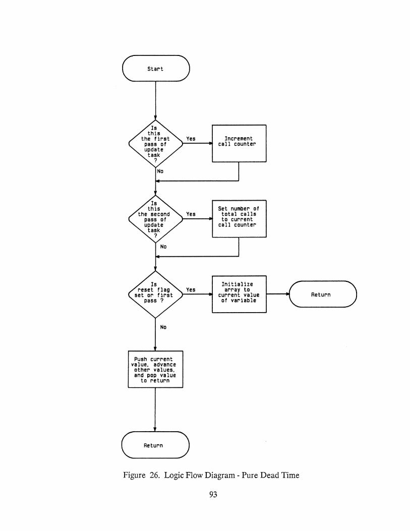
Start

No

Push current value, advance other values, and pop value

to return

Return

Yes Increment call counter

Set number of Yes total calls

Yes

to current call counter

Initialize array to

current value of variable

Figure 26. Logic Flow Diagram - Pure Dead Time

93

Return

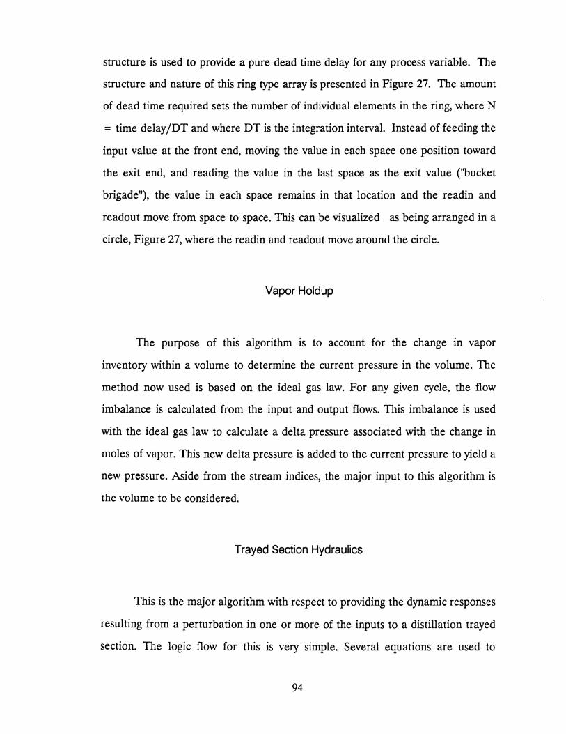
structure is used to provide a pure dead time delay for any process variable. The

structure and nature of this ring type array is presented in Figure 27. The amount

of dead time required sets the number of individual elements in the ring, where N

= time delay /DT and where DT is the integration interval. Instead of feeding the

input value at the front end, moving the value in each space one position toward

the exit end, and reading the value in the last space as the exit value ("bucket

brigade"), the value in each space remains in that location and the readin and

readout move from space to space. This can be visualized as being arranged in a

circle, Figure 27, where the readin and readout move around the circle.

Vapor Holdup

The purpose of this algorithm is to account for the change in vapor

inventory within a volume to determine the current pressure in the volume. The

method now used is based on the ideal gas law. For any given cycle, the flow

imbalance is calculated from the input and output flows. This imbalance is used

with the ideal gas law to calculate a delta pressure associated with the change in

moles of vapor. This new delta pressure is added to the current pressure to yield a

new pressure. Aside from the stream indices, the major input to this algorithm is

the volume to be considered.

Trayed Section Hydraulics

This is the major algorithm with respect to providing the dynamic responses

resulting from a perturbation in one or more of the inputs to a distillation trayed

section. The logic flow for this is very simple. Several equations are used to

94

Y--

"Bucket Brigade" Method

Ring Array Method

Figure 27. Dead Time Array Structure

95

t--- YL

YL

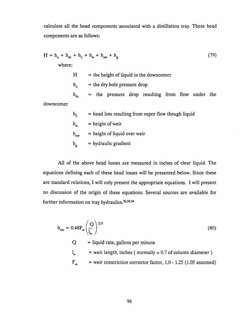
calculate all the head components associated with a distillation tray. These head

components are as follows:

H = h0 + hdc + hL + ~ + how + hg

where:

H

ho

= the height of liquid in the downcomer

= the dry hole pressure drop

(79)

hdc = the pressure drop resulting from flow under the

downcomer

hL

~

how

hg

= head loss resulting from vapor flow though liquid

= height of weir

= height of liquid over weir

= hydraulic gradient

All of the above head losses are measured in inches of clear liquid. The

equations defining each of these head losses will be presented below. Since these

are standard relations, I will only present the appropriate equations. I will present

no discussion of the origin of these equations. Several sources are available for

further information on tray hydraulics.32•33•34

( Q) 2/3 h = 048F -ow . w ~

Q = liquid rate, gallons per minute

(80)

lw = weir length, inches ( normally ~ 0. 7 of column diameter )

F w = weir constriction corrector factor, 1.0- 1.25 (1.05 assumed)

96

ho = 0.186 (uo)2 Pv \co p, (81)

u0 = vapor velocity through holes, ft/sec

c. = discharge coefficient = 1.09 ~d~) '·"

dH = hole diameter, inches

L = plate thichness, inches

Pv• p 1 =vapor and liquid density, lb/ft3

hdc = 0.057 (_9_) 2

A de

(82)

Adc = clearance area under downcomer, in2

hL = {3 (~ + how + 0.5hg) (83)

f3 = aeration factor, 0.6- 1.0 (assumed 0.7)

hg = 0.24 + 0.725hw- 0.29hwua p~5 + 4.480/z (84)

z = (D + ~)/2

D = tower diameter, inches

U8 = velocity based on active area, ft/sec

The above equations are intended to yield the height of the liquid in the

downcomer for design purposes. In this proposed application, the desired quantity

is the liquid flow from the tray, Q, resulting from a specified height of liquid in the

downcomer, H. However, the outlet flow appears implicitly in the above equation

system. Therefore, a trial-and-error solution technique is employed to arrive at the

flow rate of liquid off the tray. The complete calculational sequence is as follows:

97

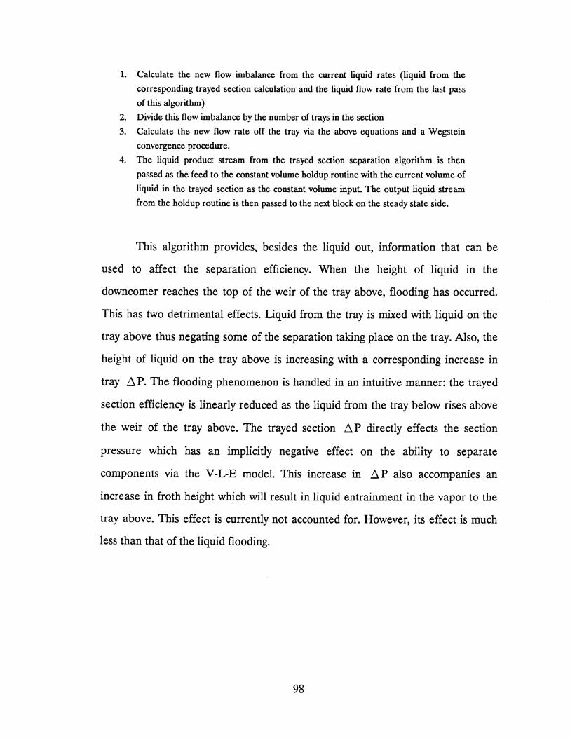
1. Calculate the new flow imbalance from the current liquid rates (liquid from the

corresponding trayed section calculation and the liquid flow rate from the last pass

of this algorithm)

2. Divide this flow imbalance by the number of trays in the section

3. Calculate the new flow rate off the tray via the above equations and a Wegstein

convergence procedure.

4. The liquid product stream from the trayed section separation algorithm is then

passed as the feed to the constant volume holdup routine with the current volume of

liquid in the trayed section as the constant volume input. The output liquid stream

from the holdup routine is then passed to the next block on the steady state side.

This algorithm provides, besides the liquid out, information that can be

used to affect the separation efficiency. When the height of liquid in the

downcomer reaches the top of the weir of the tray above, flooding has occurred.

This has two detrimental effects. Liquid from the tray is mixed with liquid on the

tray above thus negating some of the separation taking place on the tray. Also, the

height of liquid on the tray above is increasing with a corresponding increase in

tray ~ P. The flooding phenomenon is handled in an intuitive manner: the trayed

section efficiency is linearly reduced as the liquid from the tray below rises above

the weir of the tray above. The trayed section ~ P directly effects the section

pressure which has an implicitly negative effect on the ability to separate

components via the V-L-E model. This increase in ~p also accompanies an

increase in froth height which will result in liquid entrainment in the vapor to the

tray above. This effect is currently not accounted for. However, its effect is much

less than that of the liquid flooding.

98

CHAPTER VI

MISCELLANEOUS FACILITIES

This chapter describes several miscellaneous facilities which were

developed for this simulation system. These comprise both additional algorithms

available for building a simulation and stand alone programs for documentation of

results from the simulation and modifying certain aspects of an active simulation.

Determination of Stream True Boiling Curve from

Stream Discrete Component Composition

Many distillation applications in a refinery involve the processing of "heavy

oil" streams. Distillation of heavy oil streams is characterized by true boiling point

curves for both feed composition specification and product composition

specification. The algorithm described in this section addresses the problem of

providing product compositions in terms of true boiling point curves. Other

commonly available facilities are used for converting the feed composition from

true boiling point data to discrete component data (e.g. MAXI*SIM,

CHEMSHARE, etc.).

This algorithm takes as input any stream composition in the simulator

system and generates an equivalent true boiling curve. The logic flow for this

algorithm is presented in Figure 28.

99

I I I I l I I

I !

Ae11ove H20 Vee •nd nor••l12.a

CDIIPOe1t1Dn

Bet COIIPDe1t ton L---------------~of ~!r:n:n~2 to

lncre-nt COIIIPOnent

counter'"

nor11el1u COIIPOdt1on

Celcuhte •ohr dene1t1ee of

ca.-ponent• end tot.l etree11

ln1t18Hze verteblee end

counter•

ln1t1el1n COIIIPOnent

counter to f1ret COIIPOnent

preeent

C•lcuhte volu•e tr•ct1on ot current component •nd •dd to •ccuiiUl•ted volu•e tr•ctton

Add current component'• volu••

wetgl'lted nor11•l bo111nll po1nt to •tre•• 1n1t1•1

bo111nll potnt

L.-·····································--·----·----·----·---··------Figure 28. Logic Flow Diagram - Stream TBP Algorithm

100

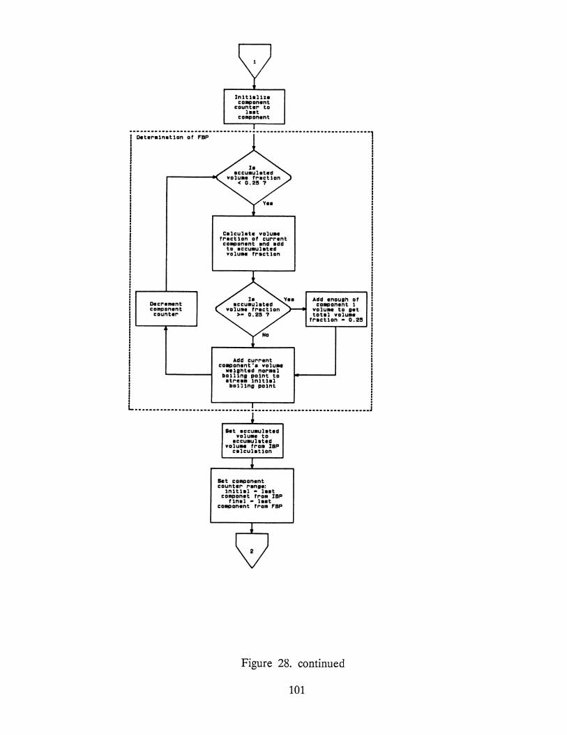
In1t1al1ze COIIPOnent

counter ta hat

co111ponent

i-~;;~:~~;;;;~·;;·;;;·············································1 I

I I I I i i I !

I : ! I :

I i I : i I

Decrellttlnt component

cauntero

Calculate volu•• tract1on ol current COIIPOnent and add to aCCUMUlated voluiH tract1on

Add current component'• volu ..

we1ghted norllal bo111ng po1nt to

atrea11 1n1thl bo1l1ng po1nt

Add enough of coaponent 1

voluiH to gat total volume

tract1on • 0.2!!

I . . . i.. •••••.•••••••••••••••••••.•••••••••••••••••••••••••••••••••.••••• j

let aCCUINlBted voluae to

BCCUIIUlated volu .. troll l8P

calculat1on

let co111ponent counter r•nae:

1n1t1el • laat co111ponat tro11 IBP

t 1nal • hat coaponent troll FBP


101

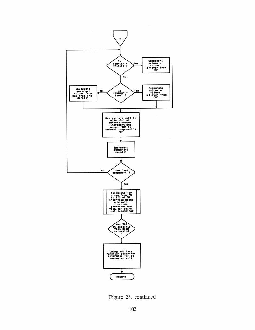
Celcuhte component

volume from 11ol free end

dene1ty

No

Set current volX to 111d-pa1nt af

current voluiH 1ncreMnt end

current TBP ta current component••

NBP

IncreMnt COIIIPOnent

counter

Celcuhte TBP curve from !IX to 9!1X at !IX

intervale uelng erblhry function

generetar and volll. TBP pelra juat deter111ned

Ualng erb1tary function generator

deter111ne TBP at requaated volX

COIIIPDnent valu•• •

volume lertaver frail

IBP

CDIIpDnent volu•• •

YO]UIIe le rtaver from

FBP


102

The first step is the removal of any water that may be present in the stream.

The lab procedure which provides a true boiling point analyses uses samples from

which the water has been removed. In addition, any light ends (i.e. propane and

lighter) are also removed as this material is weathered off as the sample is worked

with. The density routine is then called to yield the individual component molar

densities which will be used later.

The first major section determines the initial and final boiling points of the

stream. This is accomplished by considering the initial and final 0.25 vol% of the

stream. In this volume, the volume average normal boiling points of all

components present constitute the corresponding true boiling point. As the last

component volume is reached which hits the 0.25 vol% limit, any excess is carried

over into the next section.

After the initial and final boiling points have been determined, the main

part of the curve is determined. This is done by stepping through each discrete

component in turn and calculating its volume from its mole fraction and molar

density. As each new volume is calculated the current (TBP,vol%) pair is the

current component's normal boiling point and the mid-point of the current volume

increment.

After the above (TBP,vol%) pairs have been determined, they are used to

calculate TBP curve points at 5 vol% intervals from 5% to 95% via interpolation.

Lastly, if a specific vol% point has been requested, it is determined by

interpolation.

Simulator Database Manipulation and Documentation

Several programs were developed to both manipulate the contents of the

simulator database and document its contents:

103

Database Dump

This program provides an output very similar to what could be expected from a

typical steady state simulator. It consists of the full contents of any or all stream

vectors, various equipment configuration parameters and other miscellaneous data

(e.g. convergences tolerances). An example of this output is represented if Figure

29.

Stream Vector Manipulation Several programs were developed to manipulate the

contents of any stream vector while the simulation is running. Any item in the

stream vector can be changed. An example of where this would be useful is

simulating responses of a distillation column resulting from a feed composition

change.

Process Equipment Configuration This utility allows for most of the flow sheet to

be configured interactively. All the equipment configuration parameters can be

defined and modified via this utility.

104

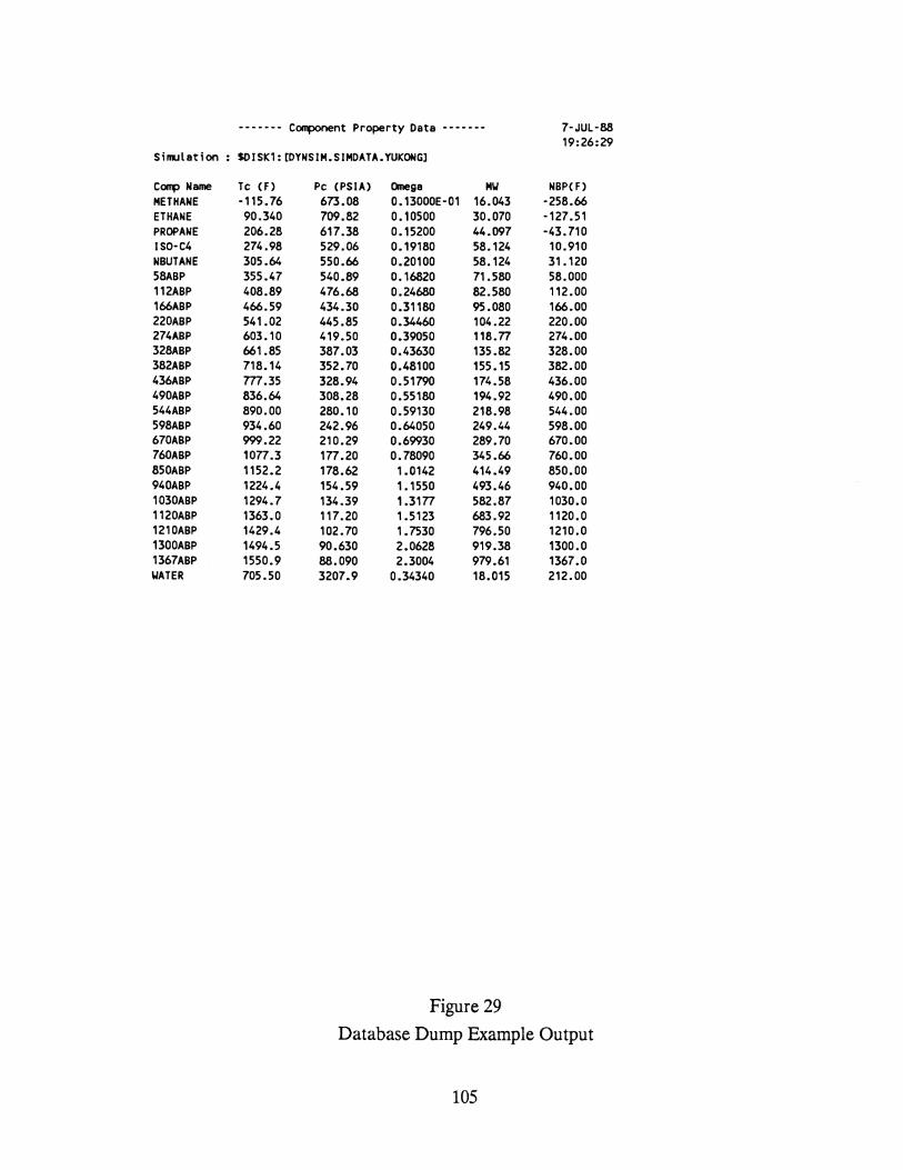
------- Component Property Data ------- 7-JUL-88 19:26:29

Sirulation SDISK1: [DYNSIM.SIMDATA.YUKONG]

C~ Name Tc (F) Pc (PSIA) Omega MIJ NBP(F) METHANE -115.76 673.08 0.13000E-01 16.043 -258.66 ETHANE 90.340 709.82 0.10500 30.070 -127.51 PROPANE 206.28 617.38 0.15200 44.097 -43.710 ISO·C4 274.98 529.06 0.19180 58.124 10.910 NBUTANE 305.64 550.66 0.20100 58.124 31.120 58ABP 355.47 540.89 0.16820 71.580 58.000 112ABP 408.89 476.68 0.24680 82.580 112.00 166ABP 466.59 434.30 0.31180 95.080 166.00 220ABP 541.02 445.85 0.34460 104.22 220.00 274ABP 603.10 419.50 0.39050 11s.n 274.00 328ABP 661.85 387.03 0.43630 135.82 328.00 382ABP 718.14 352.70 0.48100 155.15 382.00 436ABP m.35 328.94 0.51790 174.58 436.00 490ABP 836.64 308.28 0.55180 194.92 490.00 544ABP 890.00 280.10 0.59130 218.98 544.00 598ABP 934.60 242.96 0.64050 249.44 598.00 670ABP 999.22 210.29 0.69930 289.70 670.00 760ABP 1on.3 1n.2o 0.78090 345.66 760.00 850ABP 1152.2 178.62 1.0142 414.49 850.00 940ABP 1224.4 154.59 1.1550 493.46 940.00 1030ABP 1294.7 134.39 1.31n 582.87 1030.0 1120ABP 1363.0 117.20 1.5123 683.92 1120.0 1210ABP 1429.4 102.70 1. 7530 796.50 1210.0 1300ABP 1494.5 90.630 2.0628 919.38 1300.0 1367ABP 1550.9 88.090 2.3004 979.61 1367.0 WATER 705.50 3207.9 0.34340 18.015 212.00

Figure 29

Database Dump Example Output

105

------- Component Property Data ------- 7-JUL-88 19:26:29

Simulation: SOISK1:[DYNSIM.SIMDATA.YUKONGl

METHANE ETHANE PROPANE ISO·C4 NBUTANE 58ABP 112ABP 166ABP 220ABP 274ABP 328ABP 382ABP 436ABP 490ABP 544ABP 598ABP 670ABP 760ABP 850ABP 940ABP 1030ABP 1120ABP 1210ABP 1300ABP 1367ABP WATER

Ideal 4.59n 1.2929

-1.0086 -2.1289

-0.58543 6.1830 4.7792

0.27131 -2.4622 -3.9938 -4.4794 -5.2609 -6.1634 -8.5025 -9.4754 -9.3431 -10.047 -10.200 -10.500 -10.900 -11.461 -13.123 -15.010 -19.592 -22.367 7.7010

Gas State Heat Capacity Constants 0.12447E·01 0.28567E-05 ·0.27031E-08 0.42535E-01 -0.16570E-04 0.20815E-08 0.73150E-01 ·0.37889E-04 0.76n8E·08 0.10020 -0.55802E·04 0.12191E-07 0.93586E-01 -0.48483E-04 0.97432E-08 0.81556E-01 ·0.26071E-04 0.19620E-08 0.99764E-01 -0.32715E-04 0.21640E·08 0.13179 ·0.45001E-04 0.22830E·08 0.14431 -0.50092E-04 0.22470E-08 0.17306 -0.60381E-04 0.24820E-08 0.18916 ·0.66035E-04 0.27nOE-08 0.22250 -0.78518E-04 0.31140E-08 0.24323 ·0.85027E-04 0.33980E-08 0.28127 ·0.98732E-04 0.36550E-08 0.30280 -0.10638E·03 0.40240E-08 0.35841 -0.12537E-03 0.45920E-08 0.41671 ·0.14565E-03 0.52430E·08 0.49000 -0.17000E-03 0.60920E-08 0.54000 -0.21000E-03 0.72320E-08 0.72000 ·0.25000E-03 0.85360E·08 0.87350 -0.30220E-03 0.10011E-07

1.0001 -0.34609E-03 0.11680E-07 1.1439 ·0.39576E·03 0.13540E-07 1.4932 -0.51659E·03 0.15564E-07 1.7047 -0.58975E-03 0.16287E-07

0.45950E-03 0.25210E-05 ·0.85900E-09


106

-----·- Component Property Data -------

Simulation: SDISK1:[DYNSIM.SIMDATA.YUKONG]

Edmister V·L-E Correlation Constants

7-JUL-88 19:26:29

REGC: 0.72354686E+OO 0.71613973E+OO 0.55823910E+OO 0.56319797E+OO REGC:-0.11955262E+00-0.11010362E+00-0.22417340E+00-0.20762898E+OO REGC:-0.19175520E-01-0.98205181E-02·0.26665354E·01·0.15811640E·02 REGC:·0.79043355E-03 0.85139635E·03 O.OOOOOOOOE+OO O.OOOOOOOOE+OO REGC:-0.92938878E-01-0.31743582E·01-0.41162069E·OZ-0.19015610E-03 REGC:-0.89253135E·01·0.77912651E-01 0.3537246ZE·01 0.23954298E·01 REGC:-0.21210993E-01·0.12739586E-01 0.67313402E-02-0.38048101E-02 REGC:-0.11023254E-02-0.35998747E-01 O.OOOOOOOOE+OO O.OOOOOOOOE+OO REGC: 0.83485812E+OO 0.34719934E+01·0.60208159E·03·0.17300384E·02 REGC:-0.17510463E+01-0.24128931E+01-0.22183449E·02·0.22414988E-02 REGC:-0.17882516E+01 0.74548584E+00-0.47835539E·03 0.13698449E-02 REGC:-0.20255145E+00-0.13713069E+OO O.OOOOOOOOE+OO O.OOOOOOOOE+OO

HEAT MEDIUM DATA: O.OOOOOOOOE+OO O.OOOOOOOOE+OO O.OOOOOOOOE+OO O.OOOOOOOOE+OO O.OOOOOOOOE+OO O.OOOOOOOOE+OO


107

------- Simulator Configuration Data

Simulation: $DISK1:[DYNSIM.SIMDATA.YUKONG] Tolerances :

CONTOL = 0.0001000 REBTOL = 0.0001000 AFLTOL = 0.0001000 BDTOL = 0.0000100 DSTOL = 0.0000100 NCOMP = 26

Col~..r~n data NSECT = 12 Section # 1 NT = 2 NTR'S -Section # 2 NT = 3 NTR'S -Section # 3 NT = 2 NTR'S -Section # 4 NT 2 NTR'S -Section # 5 NT = 2 NTR'S -Section # 6 NT = 2 NTR'S -Section # 7 NT = 6 NTR'S -Section # 8 NT = 6 NTR'S -Section # 9 NT = 3 NTR'S -Section # 10 NT 6 NTR'S -Section # 11 NT = 6 NTR'S -Section # 12 NT = 6 NTR'S -Pressure Factor = 1.0000000

Stream data : LK/HK Indices 2 3

Condenser data Condenser Type = 2 Coolant Cp = 6.9800000 AMIN = 10000.000 RHLDP = 100.0 CONV CPH = 138.74776

Reboiler data : CONV CPC = O.OOOOOOOOE+OO BHLDP = 50.0

Econ data ISCT = 0 NSTR = 0 NSTM = 0 ITU : 2 1 0 0 1

Value of process flags:

0 0 0 0

0 0 0 0 0 0 0 0 0 0 0 0 0 0 0 0 0 0 0 0 0 0 0 0 0 0 0 0 0 0 0 0 0 0 0 0

0 0 0 0 0 0 0 0 0 0 0 0

UPDMES First Pass (FPUPD) = F Boiling Points for Stream Comps. CBPC) = T Calculate OVHD Pressure CPCALC) = T Mass Flow Units Used (MASS) = F Vacuum System Used (JETS) = F Column is Steam Stripped CH20) = T Stream Compositions in ~T% C~TFRAC) = F


108

7-JUL -88 19:26:29

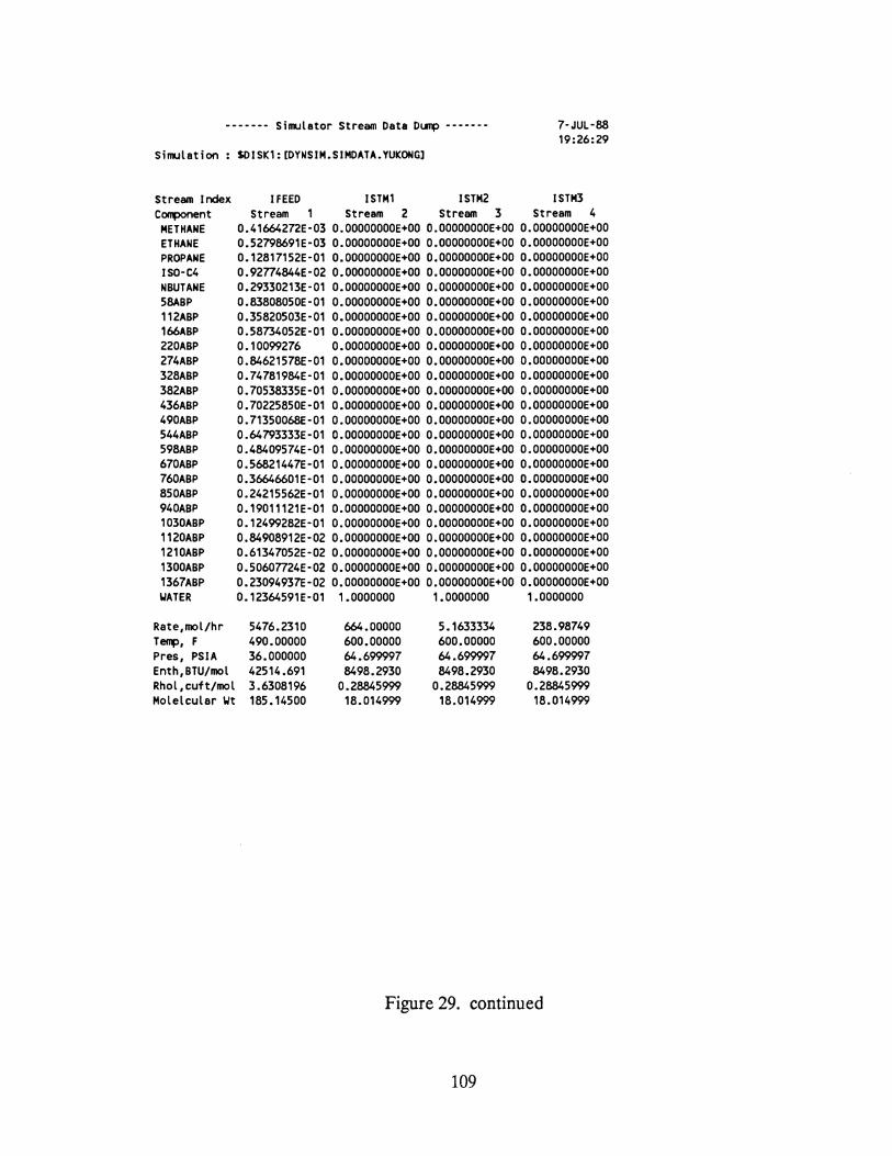
------- Simulator Stream Data Dump ------- 7-JUL-88 19:26:29

Simulation : SDISK1:[DYNSIM.SIMDATA.YUKONGJ

Stream Index COfllX>Oent

METHANE ETHANE PROPANE ISO·C4 NBUTANE 58ABP 112ABP 166ABP 220ABP 274ABP 328ABP 382ABP 436ABP 490ABP 544ABP 598ABP 670ABP 760ABP 850ABP 940ABP 1030ABP 1120ABP 1210ABP 1300ABP 1367ABP WATER

Rate,mol/hr T~, F Pres, PSIA Enth,BTU/mol Rhol,cuft/mol Molelcular Wt

!FEED ISTM1 ISTM2 ISTM3 Stream 1 Stream 2 Stream 3 Stream 4

0.41664272E·03 O.OOOOOOOOE+OO O.OOOOOOOOE+OO O.OOOOOOOOE+OO 0.52798691E·03 O.OOOOOOOOE+OO O.OOOOOOOOE+OO O.OOOOOOOOE+OO 0.12817152E-01 O.OOOOOOOOE+OO O.OOOOOOOOE+OO O.OOOOOOOOE+OO 0.92774844E-02 O.OOOOOOOOE+OO O.OOOOOOOOE+OO O.OOOOOOOOE+OO 0.29330213E·01 O.OOOOOOOOE+OO O.OOOOOOOOE+OO O.OOOOOOOOE+OO 0.83808050E-01 O.OOOOOOOOE+OO O.OOOOOOOOE+OO O.OOOOOOOOE+OO 0.35820503E·01 O.OOOOOOOOE+OO O.OOOOOOOOE+OO O.OOOOOOOOE+OO 0.58734052E·01 O.OOOOOOOOE+OO O.OOOOOOOOE+OO O.OOOOOOOOE+OO 0.10099276 O.OOOOOOOOE+OO O.OOOOOOOOE+OO O.OOOOOOOOE+OO 0.84621578E·01 O.OOOOOOOOE+OO O.OOOOOOOOE+OO O.OOOOOOOOE+OO 0.74781984E·01 O.OOOOOOOOE+OO O.OOOOOOOOE+OO O.OOOOOOOOE+OO 0.70538335E·01 O.OOOOOOOOE+OO O.OOOOOOOOE+OO O.OOOOOOOOE+OO 0.70225850E·01 O.OOOOOOOOE+OO O.OOOOOOOOE+OO O.OOOOOOOOE+OO 0.71350068E·01 O.OOOOOOOOE+OO O.OOOOOOOOE+OO O.OOOOOOOOE+OO 0.64793333E·01 O.OOOOOOOOE+OO O.OOOOOOOOE+OO O.OOOOOOOOE+OO 0.48409574E·01 O.OOOOOOOOE+OO O.OOOOOOOOE+OO O.OOOOOOOOE+OO 0.56821447E·01 O.OOOOOOOOE+OO O.OOOOOOOOE+OO O.OOOOOOOOE+OO 0.36646601E·01 O.OOOOOOOOE+OO O.OOOOOOOOE+OO O.OOOOOOOOE+OO 0.24215562E·01 O.OOOOOOOOE+OO O.OOOOOOOOE+OO O.OOOOOOOOE+OO 0.19011121E·01 O.OOOOOOOOE+OO O.OOOOOOOOE+OO O.OOOOOOOOE+OO 0.12499282E·01 O.OOOOOOOOE+OO O.OOOOOOOOE+OO O.OOOOOOOOE+OO 0.84908912E-02 O.OOOOOOOOE+OO O.OOOOOOOOE+OO O.OOOOOOOOE+OO 0.61347052E·02 O.OOOOOOOOE+OO O.OOOOOOOOE+OO O.OOOOOOOOE+OO 0.50607724E·02 O.OOOOOOOOE+OO O.OOOOOOOOE+OO O.OOOOOOOOE+OO 0.23094937E·02 O.OOOOOOOOE+OO O.OOOOOOOOE+OO O.OOOOOOOOE+OO 0.12364591E·01 1.0000000 1.0000000 1.0000000

5476.2310 490.00000 36.000000 42514.691 3.6308196 185.14500

664.00000 600.00000 64.699997 8498.2930

0.28845999 18.014999

5.1633334 600.00000 64.699997 8498.2930

0.28845999 18.014999

238.98749 600.00000 64.699997 8498.2930

0.28845999 18.014999


109

------- Simulator Stream Data Dump ------- 7-JUL-88 19:26:29

Simulation: SOISK1:[0YNSIM.SIMDATA.YUKONGl

Stream Index C:~nt

METHANE ETHANE PROPANE ISO-C:4 NBUTANE 58ABP 112ABP 166ABP 220ABP 274ABP 328ABP 382ABP 436ABP 490ABP 544ABP 598ABP 670ABP 760ABP 850ABP 940ABP 1030ABP 1120ABP 1210ABP 1300ABP 1367ABP \lATER

Rate,mol/hr TE!q), F Pres, PSIA Enth,BTU/mol Rhol,cuft/mol Molelcular \Jt

ISTM4 !VB JVO IV1 Stream 5 Stream 6 Stream 7 Stream 8

O.OOOOOOOOE+OO 0.33099770E-09 0.35009491E·05 0.40316160E·03 O.OOOOOOOOE+OO 0.20733804E-08 0.75714051E-05 0.51113113E·03 O.OOOOOOOOE+OO 0.21528098E-06 0.29933406E-03 0. 12416366E·01 O.OOOOOOOOE+OO 0.46005104E-06 0.31204306E-03 0.89943008E-02 O.OOOOOOOOE+OO 0.17262247E-05 0.10452265E-02 0.28439134E-01 O.OOOOOOOOE+OO 0.83575060E-05 0.35699783E-02 0.81303872E-01 O.OOOOOOOOE+OO 0.85659967E-05 0.20541688E-02 0.34788258E-01 O.OOOOOOOOE+OO 0.32152886E-04 0.44720257E-02 0.57120670E-01 O.OOOOOOOOE+OO 0.10863873E-03 0.97075272E-02 0.98361656E-01 O.OOOOOOOOE+OO 0.20364845E-03 0.10770285E-01 0.82603380E-01 O.OOOOOOOOE+OO 0.47221992E-03 0.13399454E-01 0.73255375E-01 O.OOOOOOOOE+OO 0.13109918E-02 0.18711273E-01 0.69494836E-01 O.OOOOOOOOE+OO 0.38015877E-02 0.27766338E-01 0.69708169E-01 O.OOOOOOOOE+OO 0.10388952E-01 0.40906183E-01 0.71229495E-01 O.OOOOOOOOE+OO 0.20735823E·01 0.48673667E-01 0.64021222E-01 O.OOOOOOOOE+OO 0.24806930E-01 0.40388916E-01 0.45624007E-01 O.OOOOOOOOE+OO 0.36013916E-01 0.44102948E-01 0.46474244E-01 O.OOOOOOOOE+OO 0.20624107E-01 0.21694889E-01 0.22511810E-01 O.OOOOOOOOE+OO 0.49861935E-02 0.50917184E-02 0.52869450E-02 O.OOOOOOOOE+OO 0.11882290E-02 0.12281579E-02 0.12769978E-02 O.OOOOOOOOE+OO 0.20560452E-03 0.21982483E-03 0.22895809E-03 O.OOOOOOOOE+OO 0.30309036E-04 0.33959317E-04 0.35441848E-04 O.OOOOOOOOE+OO 0.36063025E-05 0.42833817E-05 0.44802473E-05 O.OOOOOOOOE+OO 0.31938663E-06 0.41378303E-06 0.43414818E-06 O.OOOOOOOOE+OO 0.22633698E-07 0.28070708E-07 0.29302475E-07 1.0000000 0.87506747 0.70553625 0.12590574

3.2733333 758.43274 917.30029 5662.9800 600.00000 605.16180 616.15497 625.14630 64.699997 35.693794 34.993793 34.993793 8498.2930 19377.320 29029.246 49904.500

0.28845999 4.9429789 4.0981722 3.0729241 18.014999 49.848145 77.368279 135.61243


110

CHAPTER VII

GENERAL SIMULATION STRUCTURE

The intent of this chapter is to further define the general structure of this

simulation system using a specific example. This example uses practically every

aspect of this simulation system. Sections of source code will be presented to show

how various blocks are utilized in the development of a flow sheet.

Figure 30 describes the process flow for an Atmospheric Crude Distillation

tower. This distillation is one of the more complex distillation processes found in

the refining/petrochemical industry. It is also one of the most difficult steady state

simulation problems. Thus, this should be a good example to highlight the

capabilities of the proposed simulation system.

The first exercise involved in setting up a simulation of the tower in Figure

30 is doing a steady state simulation of the tower. This is not absolutely necessary,

but if the capability is available, it will prove very useful. Here it serves two

purposes. As a by-product of the steady state simulation, the original TBP specified

crude feed composition is converted to discrete components with the requisite

properties for the dynamic simulation. Also, good estimates of the number of

theoretical plates in each section is available from the steady state simulation.

The next step is actually building the flow sheet using the various blocks as

required. Completing this exercise on paper first is a good idea. This helps in

keeping the code simple and organized. Figures 31 - 35 show the block structure

111

~ ~

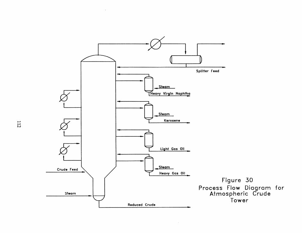
N

g-

g-

g-Crude Feed

Steam

--------

Reduced Crude

Steam

Kerosene

,. Steam

Heavy Gas Oil

Splitter Feed

Figure 30 Process Flow Diagram for

Atmospheric Crude Tower

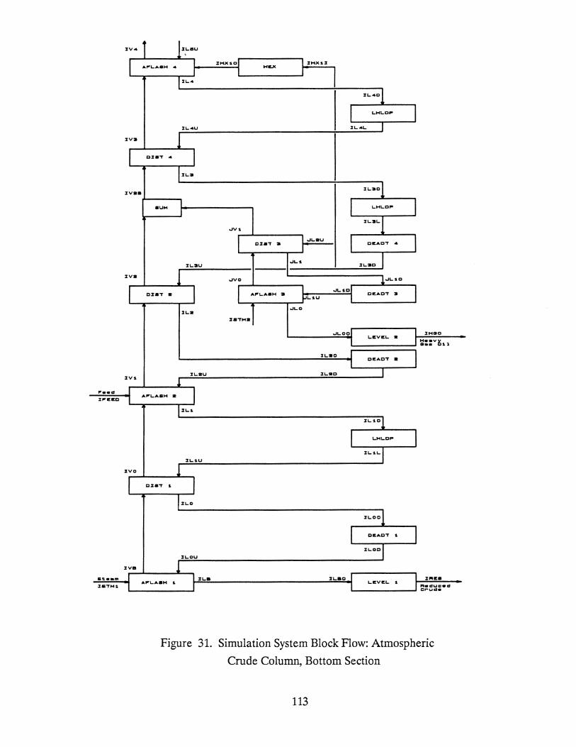
,.. .. ~:~ %P"I!IlC

ate•m .lii'TMS.

7V4l l;t,L.ISU

I A.prL.A&H 4 I n•x•ol HIVC

I 7HX.%

I I J 7L.4

%L40l

I LHL.DP J %L.<4U .XL.. 4L. J

:zva

I a.xaT .... I 7LOI

.xvaa 21-:JtQ!

8UM I I l L.HL.D,_ I

..Jv• , ...... !

I c:raT a I ..JLau l DI!.ACT 4 I I .......

7LOIC J :tL.~U

7va o.IVO _1..JL.~Q

I C%8'T R I I ..,,...~... .... ,... a I ..JL.•cl OEAD"T 3 I ...... u I

%8TM21

o.IL.O %L2

..JLoc;:>l I .lHCI'D

I L.I!.VEL.. a

J ~==v~il :tL.ao _I

DI!ADT a I I %L..2U .lL.8C J 7V.

.1 I

-I AprL..ABH 2 I 7L..

~L..S.O!

I L.HL.D .. I %L..1.U

%L. u ... ,

:zvo l I c:r•T t. I

l:LO

!I:L..OO!

I ClltACT t. I :n .. ou

:u ... ool lVB l I I l:L.B :rL.ao J

1-ltVI!.L. i I "''""• I

A.PI"L..A8M S. I I ( A•duc:•d

Cr'"Ucl•

Figure 31. Simulation System Block Flow: Atmospheric

Crude Column, Bottom Section

113

IV 7 l I f.fi'LASH I!

IV II

I DJST II

I VII

I DIST II

IV4

l JLIIU

h IL7

lL70

l LHLDP J JL7L

JL.7U

I JLII

ILIID

l l.HLDP J ILBL

I DEADi 1!1

J Jl.IID

Jl"il"

I fi'L.ASH III"il. J

l.I!VI!l. :0 J I I JX!IJ

JJI'SV II" iLL

I HI!X I I HI!X I JX!ID JX:!ID

I HI!X I I HI!X IIX2D J

L!:V!:L <4 J I ILV:oll

!IU

IX-40 JLV30 LGDPA

lLV3U

~ WLVL i I lLB01 J I ILG02 J I JLGC:O J LIL.GO

I HI!X

I I HI!X

I I HI!X

JL.Unt

ILBU

ILII

I Lao

I DI!ADT II I IL~D

1 JL!IU


Crude Column, LGO Section

114

•

G•• 011

I V10

I V9

I vas

I VB

I V7

IL11U

I IHX20 IHX2I AFLASH 10

I HEX

IL10

IL100

LHLDP

ILiOU IL10L

DIST 9 I IL9

IL90

SUM I LHLDP

IL9L

KV1

KL2U DIST 8 DEADT 9

KL1 IL9U IL9D

KVO i_KL10

I KL1D DIST 7 AFLASH 9 DEADT 8

I<LiU

KLO ILB

ISTM3

KLOO LEVEL 5

ILBO DEADT 7

ILBD

!ILBU


Crude Column, Kerosene Section

115

IKRO

Kerosene

lV13

IV12

lV11

IV11

1V10

IL14U

A FLASH

1L13U

OISi 12

SUM

1L12L

LV1

OlSi 11

LVO

OlSi 10 AFLASH 11

LLO 1L11

ISiM4

LLOO IHVN

Heavy Virgin Naphtha

IL110

IL11D

IL11U


Crude Column, HVN Section

116

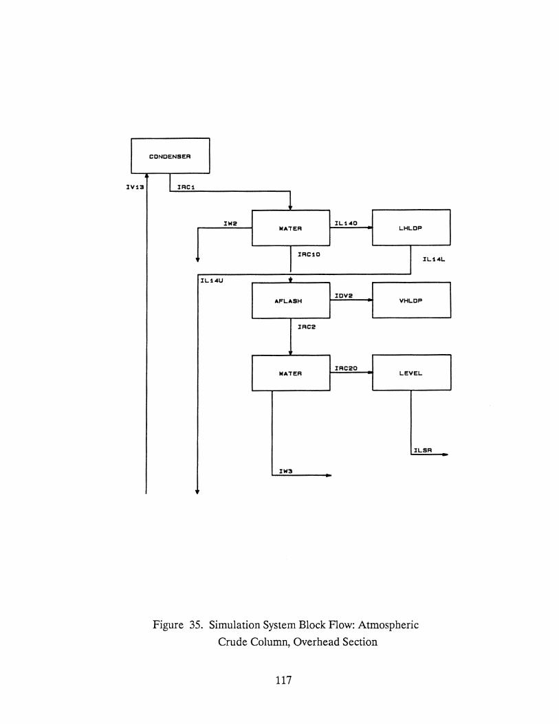
I V13

CONDENSER

I IRC1

IW2 IL140 WATER LHLOF'

IRC10 IL14L

IL14U .. lOV2

A FLASH VHLOF'

IRC2

IRC20 WATER LEVEL

ILSR

lW3


Crude Column, Overhead Section

117

that will simulate the tower shown in Figure 30. The code resulting from these

figures is shown in Figures 36 and 37. Figure 36 represents the steady state half of

the simulation and Figure 37 represents the dynamic half.

These figures show in detail the method of simulating the tower via the

various blocks described in Chapters 5 and 6. The one item I will discuss in further

detail is the light gas oil (LGO) section. This section highlights some of the

benefits offered by a dynamic simulation system over and above its obvious use as

compared with a steady state simulation.

Figure 38 shows in more detail the configuration of the LGO side stream

section. A normal steady state simulation (e.g. Chemshare , Process , HYSIM ) of

a crude column is a very difficult convergence problem. This problem is usually

simplified by simulating the crude column as a complete system of equations

rather than a system of interlinked blocks. Thus, the normal steady state crude

column module is a large matrix which is then solved by normal matrix solution

techniques. This eliminates the problem of having to explicitly close all the recycle

streams shown in Figure 30. However, this approach reduces the degree of

flexibility the simulationist has in configuring the crude column. The LGO section

shown in Figure 38 presents a problem for the normal steady state model. This

LGO side stream section is not standard and cannot be exactly reproduced with

these steady state models. These models expect a standard side stream system.

This LGO section presents no problems for the proposed simulation system. The

simulation can be configured to exactly represent the process flow shown in Figure

38. Figure 32 shows the block arrangement which exactly represents the actual

process.

In addition, another problem with the steady state crude modules

mentioned above is convergence. Even with the matrix approach mentioned,

118

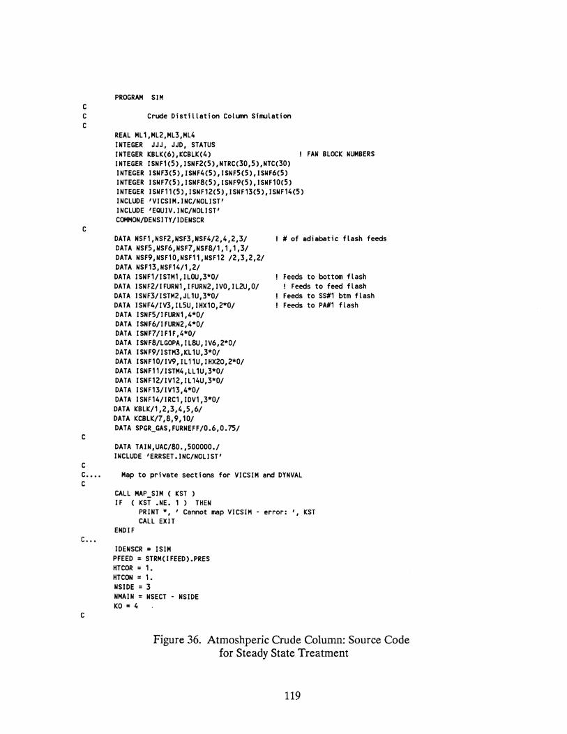
c c c

c

c

c

PROGRAM SJM

Crude Distillation Column Simulation

REAL ML1,ML2,ML3,ML4 INTEGER JJJ, JJD, STATUS INTEGER KBLK(6),KCBLK(4) FAN BLOCK NUMBERS INTEGER ISNF1(5),1SNF2(5),NTRC(30,5),NTC(30) INTEGER ISNF3(5),1SNF4(5),1SNF5(5),1SNF6(5) INTEGER ISNF7(5),JSNF8(5),1SNF9(5),1SNF10(5) INTEGER ISNF11(5),1SNF12(5),1SNF13(5),1SNF14(5) INCLUDE 'VICSIM.INC/NOLIST' INCLUDE 'EQUIV.INC/NOLIST' COMMON/DENSITY/IDENSCR

DATA NSF1,NSF2,NSF3,NSF4/2,4,2,3/ DATA NSF5,NSF6,NSF7,NSF8/1,1,1,3/ DATA NSF9,NSF10,NSF11,NSF12 /2,3,2,2/ DATA NSF13,NSF14/1,2/ DATA ISNF1/ISTM1,1LOU,3*0/ DATA ISNF2/IFURN1,1FURN2,1VO,IL2U,O/ DATA ISNF3/ISTM2,JL1U,3*0/ DATA ISNF4/IV3,1L5U,IHX10,2*0/ DATA ISNF5/IFURN1,4*0/ DATA ISNF6/IFURN2,4*0/ DATA ISNF7/IF1F,4*0/ DATA ISNF8/LGOPA,IL8U,IV6,2*0/ DATA ISNF9/ISTM3,KL1U,3*0/ DATA ISNF10/JV9,IL11U,IHX20,2*0/ DATA ISNF11/ISTM4,LL1U,3*0/ DATA ISNF12/IV12,IL14U,3*0/ DATA ISNF13/IV13,4*0/ DATA ISNF14/IRC1,IDV1,3*0/ DATA KBLK/1,2,3,4,5,6/ DATA KCBLK/7,8,9,10/ DATA SPGR_GAS,FURNEFF/0.6,0.75/

DATA TAIN,UAC/80.,500000./ INCLUDE 'ERRSET.INC/NOLIST'

I # of adiabatic flash feeds

Feeds to bottom flash ! Feeds to feed flash Feeds to SS#1 btm flash Feeds to PA#1 flash

c.... Map to private sections for VICSIM and DYNVAL c

c ...

c

CALL MAP_SIM ( KST ) IF ( KST .NE. 1 ) THEN

PRINT *, ' Cannot map VICSIM - error: ' KST CALL EXIT

END IF

IDENSCR = ISIM PFEED = STRM(IFEED).PRES HTCOR = 1. HTCON = 1. NSIDE = 3 NMAIN = NSECT • NSIDE KO = 4

Figure 36. Atmoshperic Crude Column: Source Code for Steady State Treatment

119

10 CONTINUE STATUS= LIBS~AIT (1.) STRM(ILG01) = STRM(IF1LL) T1 = SECNDS(O.) STADD = 0. FCORR = 1.

DO 12 !C1 = 1,NSECT NTCCIC1) = NT(IC1)*FCORR DO 13 IC2 = 1,5

NTRCCIC1,IC2) = NTR(IC1,1C2)*FCORR 13 CONTINUE 12 CONTINUE

c----------------------~~~--~~-----------------------c Bottom Tray Adiabatic Flash c

STRM(!LOU) = STRMC!LOD) DPCF = NMAIN*DPCOL STRMCILOU).PRES = PTOP+DPCF CALL ENTH ClSTM1,0) CALL AFLASHCNSF1,ISNF1,1VB,lLB,0.,1)

D ~RITECKO,*)' STEAM TRAY TEMP =' ,STRMCIVB).TEMP c

c----------~~------~~--~~------~~---------------c Column Calculation, Flash Zone Section c

c

STRMCIL1U) = STRM(IL1L) STRMCIVB).PRES = PTOP+NMAIN*DPCOL STRM(IL1U).PRES = PTOP+(NMAIN-1)*DPCOL CALL DISTHCIVB,IVO,ILO,lL1U,NTC(1),1)

c---------------------------------------------------------c c

Feed Furnace Section

STRM(IFEED).TEMP = 490. CALL FLASH ClFEED,ISCR1,1SCR2,FQ) STRM(IFURN1) = STRM(IFEED) STRM(IFURN2) = STRMCIFEED) FDEN = RHOLCIFEED) STRM(IFURN1).FL~ = FC501*FDEN STRM(IFURN2).FL~ = FC801*FDEN STRM(IFEED).FL~ = STRMCIFURN1).FLOW + STRM(IFURN2).FL~ QADD1 = FC524 * 1000.* ( 1430. * SPGR_GAS + 95. ) * FURNEFF QADD2 = FC805 * 1000.* ( 1430. * SPGR_GAS + 95. ) * FURNEFF CALL AFLASH(NSF5,!SNF5,1SCR2,ISCR3,QADD1,5) STRM(IFURN1).TEMP = STRM(ISCR2).TEMP STRM(IFURN1).ENTH = CSTRM(ISCR2).ENTH*STRM(ISCR2).FLOW +

STRMCISCR3).ENTH*STRM(ISCR3).FL~)/STRM(IFURN1).FLO~

STRMCIFURN1).DENTH = STRM(IFURN1).ENTH CALL AFLASH(NSF6,1SNF6,1SCR2,ISCR3,QADD2,6) STRMCIFURN2).TEMP = STRM(ISCR2).TEMP STRMCIFURN2).ENTH = (STRMCISCR2).ENTH*STRM(ISCR2).FL~ +

STRMCISCR3).ENTH*STRM(!SCR3).Fl~)/STRM(IFURN2).FLOW

STRM(IFURN2).DENTH = STRM(IFURN2).ENTH TFRN1 = STRM(IFURN1).TEMP TFRN2 = STRM(IFURN2).TEMP

c----------------------------------------------------------c Feed Tray Adiabatic Flash Section c

STRMCIL2U) = STRMCIL2D) DPCF = (NMAIN-1)*DPCOL STRM(IL2U).PRES = PTOP+DPCF STRM(!VO).PRES = PTOP+DPCF


120

CALL AFLASH(NSF2,ISNF2,IV1,IL1,0.,2) c

c----------------------------------~---------------------c Column Section Calc., HGO Section c

c

STRM(IL3U) = STRMCIL30) STRMCIV1).PRES = STRM(IVO).PRES STRMCIL3U).PRES = PTOP+(NMAIN-2)*0PCOL STRM(JL2U) = STRM(IL3U) STRM(IHX11) = STRM(IL3U) RHOSS1 = RHOL(IL3U) STRM(JL2U).FLOW = FC564*RHOSS1 STRMCIHX11).FLOW = FC835*RHOSS1 IF (STRM(JL2U).FLOW + STRMCIHX1I).FLOW .GT. STRM(IL3U).FLOW) THEN

STRMCIHX1I).FLOW = (FC835 * STRMCIL3U).FLOW)/(FC835+FC564) STRMCJL2U).FLOU = STRM(IL3U).FLOW • STRM(IHX1l).FLOW STRM(IL3U).FLOW = 0.

ELSE STRMCIL3U).FLOW = STRM(IL3U).FLOW - STRMCIHX1I).FLOU -

STRMCJL2U).FLOW END IF Fi564 = STRMCJL2U).FLOW/RHOSS1 Fl835 = STRM(IHX1I).FLOW/RHOSS1

CALL D I STHCI V1, IV2, I L2,.I L3U, NTC(2) ,2)

c-------------------------------------------------------c HGO Side Stripper BTM Adiabatic Flash c

c

STRM(JL1U) = STRM(JL1D) DPCF = (NMAIN·1)*DPCOL STRM(JL1U).PRES = PTOP+DPCF STRMCJVO).PRES = PTOP+DPCF CALL ENTH (ISTM2,0) CALL AFLASH(NSF3,ISNF3,JVO,JL0,0.,3)

c·------------~----~--~----~~--~---------------c Column Section Calc., HGO Side Stripper c

c

STRMCJV1).PRES = PTOP+CNMAIN-2)*DPCOL CALL DISTH(JVO,JV1,JL1,JL2U,NTC(3),3)

c ________________________________________________________ __ C Add SS#1 Vapor and HGO section vapor c

CALL SUM (JV1,IV2,IV2S,O) c

c----------------------------------------------------------c PA#1 Heat Exchanger Section c

STRM(IHX10) = STRMCIHX11) STRMCIHX10).TEMP = 365. CALL ENTH (IHX10,3)

c------------~----~~--~--------~----------------------c Column Calculation, PA#1 Section c

c

STRMCIL4U) = STRM(IL4L) STRMCIV3).PRES = PTOP+(NMAIN·3)*DPCOL STRM(IL4U).PRES = STRM(IV3).PRES CALL DISTH(IV2S,IV3,1L3,IL4U,NTC(4),4)

c--------------------------~--~~~--~-------------c HGO PA Return Tray Adiabatic Flash Section c


121

STRH(ILSU) = STRH(ILSD) DPCF = (NHAIN·3)*DPCOL STRHCILSU) PRES • PTOP+DPCF STRH(IV4) PRES • PTOP+DPCF CALL AFLASH(NSF4,1SNF4,1V4,1L4,0 ,4)

c------------~----------------------------------------.... C Column Section Above HGO PA Return c

c

STRHCIL6U) = STRM(IL6D) STRH(IF1F) = STRH(IL6U) STRH(IXSI) = STRM(IL6U) RHOSS1 = RHOL(IL6U) STRH(IF1F) FLOW= FC569*RHOSS1 STRM(IXSI) FLOW= FC547*RHOSS1 IF (STRM(IF1F) FLOW+ STRH(IXSI) FLOW GT STRH(IL6U) FLOW) THEN

STRMCIF1F) FLOW = (FC569 * STRMCIL6U) FLOW)/(FC569+FC547) STRM(IX51) FLOW = STRM(IL6U) FLOW • STRM(IF1F) FLOW STRM(IL6U) FLOW = 0

ELSE STRH(IL6U) FLOW = STRM(IL6U) FLOW • STRH(IF1F) FLOW •

STRHCIXSI) FLOW END IF Fl569 = STRH(IF1F) FLOW/RHOSS1 Fl547 = STRM(IXSI) FLOW/RHOSS1 STRM(IVS) PRES = PTOP+(NMAIN·4)*DPCOL STRM(IL6U) PRES = STRM(IV5) PRES CALL DISTH(IV4,1V5,1L5,1L6U,NTC(5),5)

c--------------------------------------------------------c LGO Section Column Calc

c

STRM(IL7U) = STRM(IL7L) STRM(IV6) PRES = PTOP+(NMAIN·5)*DPCOL STRM(IL7U) PRES = STRMCIV6) PRES CALL DISTH(IVS,IV6,1L6,1L7U,NTC(6),6)

c----------------------------------------------------------c LGO Vacuum Flash Drum

C······

Pl902 = 12 STRH(IF1F) PRES = Pl902 QAOO = 1 CALL AFLASH(NSF7,1SNF7,1F1V,IF1L,QAD0,7) STRH(IX30) = STRM(IF1V) STRM(IX30) TEMP = MAX (STRM(IF1V) TEMP • 240 , 250 )

C··· Water Cooler on Flash Vapor out of feed preheat STRM(IX20) = STRM(IX30) STRM(IX20) TEMP = 170 CALL RMVH20 (IW1,1X20)

c

c .................................................. ~-------------------------------------------------------------------c LGO Pumparound C···· W1ll eventually put HEX's 1n here

STRM(IX40) = STRM(IXSI) STRH(IX40) TEMP = MAX (300 , STRM(IXSI) TEMP • 160 ) CALL ENTH (IX40,3)

C Add condensed flash vapor and punparound

c

STRM(ILV3U) = STRM(ILV30) STRM(ILV3U) PRES = (NMAIN·S)*DPCOL + PTOP CALL SUM (IX40,1LV3U,LGOPA,3)

c--------------------------------------------------------c LGO PA return tray ad1abat1c flash STRM(IL8U) = STRM(IL8D)

F1gure 36 contmued

122

c

DPCF E (NMAIN-5)*DPCOL STRM(IL8U).PRES = PTOP+DPCF STRMCIV6).PRES = PTOP+DPCF CALL AFLASH(NSF8,1SNF8,IV7,IL7,0.,8)

c---------------------------------------------------------c c

Column Section Calc., KERO Section

STRM(IL9U) = STRM(IL90) STRM(IL9U).PRES = PTOP+(NMAIN-6)*DPCOL STRM(KL2U) = STRM(IL9U) STRM(IHX21) = STRM(IL9U) RHOSS1 = RHOL(IL9U) STRM(KL2U).FLOW = FC571*RHOSS1 STRM(IHX2I).FLOW = FC683*RHOSS1 IF (STRM(KL2U).FLOW + STRM(IHX2I).FLOW .GT. STRM(IL9U).FLOW) THEN

STRM(IHX2I).FLOW = (FC683 * STRM(IL9U).FLOW)/(FC683+FC571) STRMCKL2U).FLOW = STRM(IL9U).FLOW • STRMCIHX21).FLOW STRM(IL9U).FLOW = 0.

ELSE STRMCIL9U).FLOW = STRMCIL9U).FLOW · STRMCIHX21).FLOW •

STRM(KL2U).FLOW END IF FI571 = STRM(KL2U).FLOW/RHOSS1 FI683 = STRM(IHX2I).FLOW/RHOSS1

CALL DISTH(IV7,IV8,IL8,IL9U,NTC(7),7) c

c----------~~~~--~------~~~~~---------------c KERO Side Stripper BTM Adiabatic Flash c

c

STRM(KL1U) = STRM(KL10) DPCF = (NMAIN-6)*DPCOL STRM(KL1U).PRES = PTOP+DPCF STRM(KVO).PRES = PTOP+DPCF CALL ENTH (ISTM3,0) CALL AFLASH(NSF9,ISNF9,KVO,KL0,0.,9)

c ______________________________________________________ _ c c

c

Column Section Calc., KERO Side Stripper

STRM(KV1).PRES = PTOP+(NMAIN-6)*0PCOL CALL DISTHCKVO,KV1,KL1,KL2U,NTC(8),8)

c----------------------------------------------------------c Add SS#3 Vapor and KERO section vapor c

CALL SUM CKV1,IV8,1V8S,O) c

c-------------------------------------------------------c KERO PA Heat Exchanger Section c

STRM(IHX20) = STRMCIHX21) STRMCIHX20).TEMP =MAX (222.7, STRM(IHX2I).TEMP • 115.) CALL ENTH (IHX20,3) c ______________________________________________________ _

C Column Calculation, KERO Section c

c

STRMCIL10U) = STRMCIL10L) STRM(IV9).PRES = PTOP+CNMAIN·7)*DPCOL STRM(IL10U).PRES = STRM(IV9).PRES CALL DISTH(IV8S,IV9,IL9,1L10U,NTC(9),9)

c----------------------------------------------------------Figure 36. continued

123

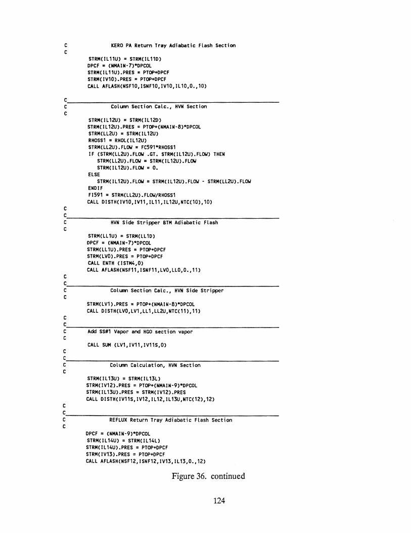
c c

KERO PA Return Tray Adiabatic Flash Section

STRMCIL11U) = STRM(IL11D) DPCF = CNMAIN·7)*DPCOL STRM(IL11U).PRES = PTOP+DPCF STRMCIV10).PRES = PTOP+OPCF CALL AFLASHCNSF10,ISNF10,IV10,IL10,0., 10)

c------------~------~--~--------~-------------------c Column Section Calc., HVN Section c

c

STRMCIL12U) = STRMCIL12D) STRM(IL12U).PRES = PTOP+(NMAIN·8)*DPCOL STRMCLL2U) = STRMCIL12U) RHOSS1 = RHOL(IL12U) STRM(LL2U).FLOW = FC591*RHOSS1 IF (STRMCLL2U).FLOW .GT. STRMCIL12U).FLOW) THEN

STRMCLL2U).FLOW = STRM(IL12U).FLOW STRMCIL12U).FLOW = 0.

ELSE STRM(IL12U).FLOW = STRMCIL12U).FLOW · STRMCLL2U).FLOW

END IF Fl591 = STRMCLL2U).FLOW/RHOSS1

CALL DISTHCIV10,1V11,IL11,IL12U,NTCC10), 10)

c ______________________________________________________ _ C HVN Side Stripper BTM Adiabatic Flash c

c

STRMCLL1U) = STRMCLL1D) DPCF = (NMAIN·7)*DPCOL STRM(LL1U).PRES = PTOP+OPCF STRM(LVO).PRES = PTOP+DPCF CALL ENTH CISTM4,0)

CALL AFLASH(NSF11,1SNF11,LVO,LL0,0.,11)

c ______________________________________________________ _ c c

c

Column Section Calc., HVN Side Stripper

STRMCLV1).PRES = PTOP+(NMAIN·8)*DPCOL CALL DISTH(LVO,LV1,LL1,LL2U,NTCC11),11)

c------~--~-------------------------------------------c Add SS#1 Vapor and HGO section vapor c

CALL SUM (LV1,1V11,IV11S,0) c

c------------~----~~--~--------~----------------------c Column Calculation, HVN Section c

c

STRMCIL13U) = STRMCIL13L) STRMCIV12).PRES = PTOP+(NMAIN·9)*DPCOL STRM(IL13U).PRES = STRM(IV12).PRES CALL DISTH(IV11S,IV12,IL12,IL13U,NTC(12),12)

c----------~~~----------~--~~~--~-------------c REFLUX Return Tray Adiabatic Flash Section c

DPCF = (NMAIN·9)*0PCOL STRM(IL14U) = STRM(IL14L) STRM(IL14U).PRES = PTOP+DPCF STRMCIV13).PRES = PTOP+DPCF CALL AFLASHCNSF12,1SNF12,IV13,1L13,0.,12)


124

c---------------------------------------------------------c OVHD Condenser System c C... CON1_DUTY = ·1.E06*HC724

CON2_DUTY = ·1.E06*HC726 AIRFL~ = 300000. * HC724/100. + 100000. UAC = FC667 * 3.E03 STRM(IV13).PRES = PTOP - 2.85 I COND DELP CALL CONDEN CIV13,1DV1,1RC1,AIRFL~,TAIN,TAOUT,UAC,O.)

CALL RMVH20 (IW2,IRC1) STRM(IL14) = STRM(IRC1) STRM(IL14).PRES = PTOP I REFLUX PUMP DELP REFDEN = RHOL CIRC1) STRMCIL14).FL~ = MIN C STRM(IRC1).FL~, FC622*REFDEN) FI622 = STRM(IL14).FLOW/REFDEN STRM(IRC1).FLOW = STRMCIRC1).FLOW - STRM(IL14).FLOW STRMCIRC10) = STRMCIRC1) STRM(IDV1).PRES = PTOP · 5.7 COND DELP STRM(IRC1).PRES = PTOP • 5.7 COND DELP CALL AFLASH (NSF14,1SNF14,IDV2,1RC2,CON2_DUTY, 13) IF (STRM(IDV2).TEMP .LT. 76.) THEN

STRM(IRC1).TEMP = 76. STRM(IDV1).TEMP = 76. CALL ENTH CIRC1,3) STRM(IDV1).DENTH = 0. CALL AFLASH (NSF14,1SNF14,1DV2,1RC2,0.,13)

END IF

c

CALL RMVH20 (I~,IRC2) STRM(IRC20) = STRM(IRC2) STRMCIDVO) = STRMCIDV2)

c ______________________________________________________ _ T2 = SECNDS(T1) PI659 = T2 GOTO 10

3100 CONTINUE CALL EXIT END


125

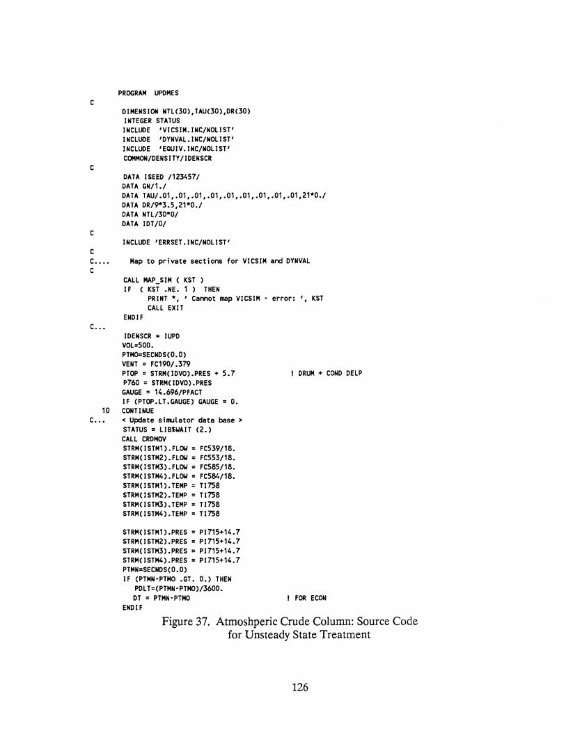
c

c

c

c

PROGRAM UPDMES

DIMENSION NTL(30),TAU(30),DR(30) INTEGER STATUS INCLUDE 'VICSIM.INC/NOLIST' INCLUDE 'DYNVAL.INC/NOLIST' INCLUDE 'ECUIV.INC/NOLIST' COMMON/DENSITY/IDENSCR

DATA !SEED /123457/ DATA GN/1./ DATA TAU/.01,.01,.01,.01,.01,.01,.01,.01,.01,21*0./ DATA DR/9*3.5,21*0./ DATA NTL/30*0/ DATA IDT/0/

INCLUDE 'ERRSET.INC/NOLIST'

C.... Map to private sections for VICSIM and DYNVAL c

CALL MAP_SIM ( KST ) IF ( KST .NE. 1 ) THEN

ENOl F

PRINT*, 1 Cannot map VICSIM- error: ', KST CALL EXIT

c ..• IDENSCR = IUPD

VOL=500. PTMO=SECNDS(O.O) VENT = FC190/.379 PTOP = STRM(IDVO).PRES + 5.7 P760 = STRM(IDVO).PRES GAUGE = 14.696/PFACT IF (PTOP.LT.GAUGE) GAUGE= 0.

10 CONTINUE c... <Update simulator data base>

STATUS = LIB$~AIT (2.) CALL CRDMOV STRM(ISTM1).FLOW = FC539/18. STRMCISTM2).FLOW = FC553/18. STRM(ISTM3).FLOW = FC585/18. STRM(ISTM4).FLOW = FC584/18. STRM(ISTM1).TEMP = TI758 STRM(!STM2).TEMP = Tl758 STRM(ISTH3).TEMP = TI758 STRM(ISTM4).TEMP = Ti758

STRM(ISTH1).PRES = PI715+14.7 STRH(ISTM2).PRES = P1715+14.7 STRMCISTM3).PRES = PI715+14.7 STRH(ISTM4).PRES = PI715+14.7 PTMN=SECNDSCO.O) IF (PTMN·PTMO .GT. 0.) THEN

POLT=CPTMN·PTM0)/3600. DT = PTMN·PTMO

END IF

DRUM + COND DELP

I FOR ECON

Figure 37. Atmoshperic Crude Column: Source Code for Unsteady State Treatment

126

c

Pl676 = OT OTSUB = OT IF ( OTSUB .EC. 0 ) OTSUB = .0001 PTHO = PTMN IF CIOT.EQ.O) THEN

IOT=1 ELSE

00 5 1=1,NSECT NTLN = OEOT(I)/(DTSUB/60.) IF (NTLN.GT.NTL(I)) NTL(l)=MIN(99,NTLN)

5 CONTINUE END IF IF (PCALC) THEN

DMV = CSTRMCIDVO).FL~- PC760V/.379 + PC760M/.379)*PDLT TAVG = STRM(IOVO).TEMP DPI760 = (0MV*10.73*TAVG*.6)/VOL P760 = MAX(14.7,P760 + DPI760) P760 = MIN(P760,0VHDPM) FI1844 = PC760V

END IF STRM(IDVO).PRES = P760 PTOP = P760 + 5.7 PI760= P760/PFACT - GAUGE PI857=PI760+(DELP+9.*DPCOL + 5.7)/PFACT

I DRUM + COND DELP

COLUMN DP + FLOOD DP

c. ______________________________________________________ _

C** THE FOLL~ING SIMULATES NPSH LOSS FOR REFLUX AND BTMS PUMPS C AND PASSES THE FL~S BACK TO CONTROLLERS AS MEASUREMENTS. c

F1744 = LC540 FI565 = FC565 FI570 = FC570 FI906 = LC903 FI572 = FC572 FI592 = FC592 FI751 = FC751 STRM(JLOO) = STRM(JLO) IF(LISSO.LT.3.2) THEN

FI565 = FC565 * RAN(ISEED)/10. IF (LI550.EQ.0.) F1565 = MINCSTRMCJLOO).FLO~/RHOL(JLOO) ,FI565)

ENDIF STRM(ILBO) = STRM(ILB) IF(LI540.LT.3.2) THEN

Fl744 = LC540 * RANCISEED)/10. IF CLI540.EC.0.) FI744 = MINCSTRMCILBO).FL~/RHOLCILBO) ,F1744)

END IF STRM(IF1LO) = STRMCIF1L) IFCLI548.LT.3.2) THEN

F1570 = FC570 * RANCISEED)/10. IF (LI548.EQ.0.) F1570 = MIN(STRM(IF1LO).FL~/RHOLCIF1LO) ,F1570)

END IF STRM(ILV3l) = STRMCIX20) IFCLI903.LT.3.2) THEN

FI906 = LC903 * RAN(ISEED)/10. IF CLI903.EC.0.) F1906 = MIN(STRMCILV3I).FL~/RHOLCILV31) ,FI906)

ENOl F STRM(KLOO) = STRMCKLO) IFCLI582.LT.3.2) THEN

FI572 = FC572 * RAN(ISEED)/10. IF CLI582.EC.0.) FI572 = MINCSTRM(KLOO).FLO~/RHOLCKLOO) ,FI572)

END IF


127

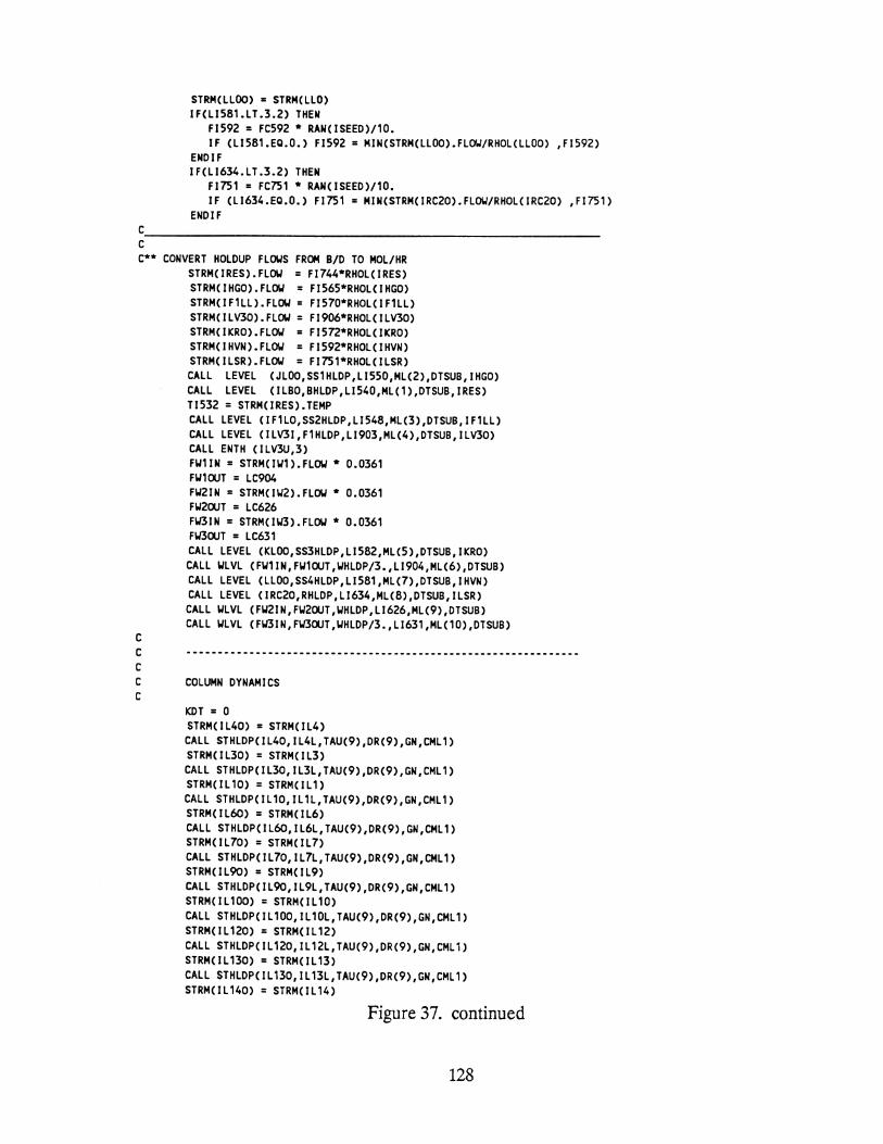
STRM(LLOO) • STRMCLLO) IF(LI581.LT.3.2) THEN

FI592 = FC592 * RAN(ISEED)/10. IF (LI581.E0.0.) FI592 = MIN(STRMCLLOO).FL~/RHOLCLLOO) ,FI592)

END IF IFCLI634.LT.3.2) THEN

F1751 = FC751 * RAN(ISEED)/10. IF (LI634.E0.0.) Fl751 = MIN(STRM(IRC20).FL~/RHOL(IRC20) ,FI751)

ENOl F

c---------------------------------------------------------c C** CONVERT HOLDUP FL~S FROM B/D TO MOL/HR

STRMCIRES).FL~ = FI744*RHOLCIRES) STRMCIHGO).FL~ = F1565*RHOL(IHGO) STRMCIF1LL).FL~ = F1570*RHOL(IF1LL) STRM(ILV30).FL~ = F1906*RHOLCILV30) STRM(IKRO).FL~ = F1572*RHOL(IKRO) STRM(IHVN).FL~ = F1592*RHOL(IHVN) STRM(ILSR).FL~ = FI751*RHOL(ILSR)

c

CALL LEVEL (JLOO,SS1HLDP,LI550,ML(2),DTSUB,IHGO) CALL LEVEL CILBO,BHLDP,LI540,ML(1),0TSUB,IRES) Tl532 = STRM(IRES).TEMP CALL LEVEL (IF1LO,SS2HLDP,LI548,ML(3),DTSUB,IF1LL) CALL LEVEL CILV31,F1HLDP,LI903,ML(4),DTSUB,ILV30) CALL ENTH (ILV3U,3) FW11N = STRMCIW1).FL~ * 0.0361 FW10UT = LC904 FW21N = STRMCIW2).FL~ * 0.0361 FW20UT = LC626 FW3IN = STRMCIW3).FL~ * 0.0361 FW30UT = LC631 CALL LEVEL (KLOO,SS3HLDP,LI582,ML(5),DTSUB,IKRO)

CALL WLVL (FW11N,FW10UT,WHLDP/3.,LI904,MLC6),0TSUB) CALL LEVEL (LLOO,SS4HLDP,LI581,ML(7),DTSUB,IHVN) CALL LEVEL (IRC20,RHLDP,LI634,MLC8),DTSUB,ILSR)

CALL WLVL (FW21N,FW20UT,WHLDP,LI626,MLC9),DTSUB) CALL WLVL (FW31N,FW30UT,WHLDP/3.,LI631,MLC10),DTSUB)

c ---------------------------------------------------------------c C COLUMN DYNAMICS c

KDT = 0 STRMCIL40) = STRMCIL4) CALL STHLDP(IL40,1L4L,TAU(9),DR(9),GN,CML1) STRM(IL30) = STRMCIL3) CALL STHLDP(IL30,IL3L,TAU(9),DR(9),GN,CML1) STRMCIL10) = STRM(IL1) CALL STHLDP(IL10,1L1L,TAU(9),DR(9),GN,CML1) STRM(IL60) = STRMCIL6) CALL STHLDP(IL60,1L6L,TAU(9),DR(9),GN,CML1) STRMCIL70) = STRMCIL7) CALL STHLDP(IL70,IL7L,TAU(9),DR(9),GN,CML1) STRM(IL90) = STRM(IL9) CALL STHLDPCIL90,IL9L,TAUC9),DR(9),GN,CML1) STRM(IL100) = STRM(IL10) CALL STHLDP(IL100,IL10L,TAU(9),DR(9),GN,CML1) STRM(IL120) = STRM(IL12) CALL STHLDPCIL120,IL12L,TAU(9),DRC9),GN,CML1) STRM(IL130) = STRM(IL13) CALL STHLDPCIL130,IL13L,TAUC9),DR(9),GN,CML1) STRM(IL140) = STRM(IL14)


128

c CALL STHLOP(IL140,IL14L,TAU(9),0R(9),GN,CML1)

CALL STDEDT CIL3L,IL3D,NTL(4),KDT) STRHCJL10) = STRH(JL1) CALL STDEDT (JL1D,JL1D,NTL(3),KDT) STRH(IL20) = STRH(IL2) CALL STDEDT (IL20,1L2D,NTL(2),KDT) STRH(ILOO) = STRH(ILO) CALL STDEDT (ILOO,ILOD,NTL(1),KDT) CALL STDEDT (IL6L,IL60,NTL(6),KDT) STRH(IL50) = STRH(ILS) CALL STOEDT (ILSO,ILSO,NTL(S),KDT) STRH(IL80) = STRH(IL8) CALL STDEDT (IL80,IL8D,NTL(7),KDT) STRH(KL10) = STRH(KL1) CALL STOEDT (KL10,KL1D,NTL(8),KDT) CALL STDEDT (IL9L,IL90,NTL(9),KDT) STRH(IL110) = STRH(IL11) CALL STDEDT (IL110,IL11D,NTL(10),KDT) STRH(LL10) = STRH(LL1) CALL STDEDT (LL10,LL1D,NTL(11),KOT) CALL STDEOT (IL12L,IL12D,NTL(12),KDT)

C.... Put tray temps below feed into OEAOT if no steam change occured CALL VLAG (TFRN1,TI517,TAU(8),0R(8),GN) CALL VLAG (TFRN2,TC813,TAU(8),0R(8),GN) CALL VLAG (STRH(IL10).TEHP,TI740,TAU(8),0R(8),GN) CALL VLAG (STRH(IL30).TEHP,TI538,TAU(8),DR(8),GN) CALL VLAG CSTRHCIHX10).TEHP,T1933,TAU(8),0R(8),GN) CALL VLAG (STRH(IHGO).TEHP,TI970,TAU(8),DR(8),GN) CALL VLAG (STRHCIL60).TEMP,TI537,TAU(8),DR(8),GN) CALL VLAG (STRH(IX40).TEMP,TI968,TAU(8),0R(8),GN) CALL VLAG (STRH(LGOPA).TEMP,TI932,TAU(8),0R(8),GN) CALL VLAG CSTRHCIF1LL).TEHP,TI976,TAU(8),0R(8),GN) CALL VLAG (STRH(ILV31).TEHP,TI902,TAU(8),0R(8),GN) CALL VLAG (STRM(IL90).TEMP,TI536,TAU(8),0R(8),GN) CALL VLAG (STRM(IKRO).TEMP,TI956,TAU(8),DR(8),GN) CALL VLAG (STRM(IHX20).TEMP,TI931,TAU(8),0R(8),GN) CALL VLAG (STRM(IL120).TEMP,TI535,TAU(8),0R(8),GN) CALL VLAG (STRM(IHVN).TEMP,TI983,TAU(8),0R(8),GN) CALL VLAG (STRM(IL130).TEMP,TI534,TAU(8),0R(8),GN) CALL VLAG (STRM(IRC10).TEMP,TI621,TAU(8),0R(8),GN) CALL VLAG (STRM(IRC20).TEMP,TI636,TAU(8),DR(8),GN) Tl953 = 77. Tl528 = 498. FI614 = FC501+FC801 FI2000 = STRM(IL2D).FL~/RHOL(IL20)

c ...........................•...•.••......•.......•...•..........•............. FPUPD = .FALSE. GOTO 10

3100 CONTINUE CALL EXIT END


129

~ VJ 0

light Gas Oil Draw

cw I Steam

Water

Light Gas Oil Product

Figure 38. Light Gas Oil Section

getting one of these models to converge is an exercise in tenacity. Once a

converged solution has been obtained for a given configuration, delta cases are

typically desired. A change of less than 3% in any one input parameter, can result

in a non-convergence again. This makes the exercise of doing many case studies a

very time consuming procedure. However, for the proposed simulation system,

overall convergence is not a consideration. Since this is a dynamic model, one

simply makes the required change (e.g. feed rate change, yield change, etc.) and

waits for the model to reach a new steady state. Depending on the perturbation,

this could take anywhere from 15 minutes to 3 hours. But, you can be assured of

an answer at the end.

The last item I will discuss regarding the simulation structure is the problem

of synchronizing the operation of the steady state and unsteady state programs. A

potential conflict is possible because the liquid stream calculated by one side is an

input to the other side. Thus, if one side is currently attempting to calculate a given

liquid stream, this liquid stream cannot be taken as input to the other side until

convergence has been met. The solution chosen for this problem is a stream

vector buffering system. As indicated in the block figures, the liquid stream index

which is the input to one side is not the output stream index from the

corresponding block on the other side. Upon completion of its calculations, a given

block yielding a liquid stream as product will transfer the converged liquid stream

to another stream vector which is the one used as input on the other side. This

buffering mechanism prevents any given block from taking as input an

unconverged liquid stream.

One last item needs to be discussed before closing this chapter. As this is a

real time simulation system, there are two other functionalities required to

effectively use simulations developed with it. These two are a graphic interface and

131

a process control system. Development of these additional items was not in the

scope of this work. In fact, the simulation system of this work was intentionally

developed to be independent of the interface and control system. This would allow

the simulation system to be easily interfaced to any system which would supply the

additional functions of graphic interface and control. Since its development, this

simulation system has been interfaced to several control/interface systems with

very effective results.

This concludes the simulation structure discussion. The distillation column

of Figure 30 along with a few others will be used in the next chapter to presents

some results regarding this simulation systems accuracy, both steady state and

unsteady state.

132

CHAPTER VIII

MODEL VERIFICATION

This chapter presents some comparisons between results from the proposed

model and results from other sources to shed some light on the suitability of this

modeling system for performing dynamic simulations of distillation columns.

Property Predictions

The first aspect which will be verified for accuracy is the property

predictions package. Table ITI shows the results of a simple isothermal flash on an

aromatics stream. This table compares the results from the proposed model and

MAXI*SIM. The MAXI*SIM package used the Soave-Redlich-Kwong equation of

state for predicting K-values and enthalpies. Densities are predicted with a

modified form of the Hankinson-Thompson model. 35

This table shows an excellent agreement between the proposed model and

MAXI*SIM for all properties associated with this system. This data verifies an

accurate implementation of the property prediction algorithms discussed in

Chapter 3. The accuracy of the algorithms themselves is documented elsewhere

and well known. Other examples will not be presented as this would simply verify

the implementation and not the methods themselves.

133

~ V.> -+:>.

TABLE I II THERMODYNAMICS PACKAGE COMPARISON

MAXI*SIM VS PROPOSED SYSTEM

Isothermal Flash at 250"F and 18 psia

Component Feed Vapor Liquid

This Work MAXI*SIM This Work MAXI*SIM

Benzene 0.2108 0.3370 0.3370 0.1407 0.1416

Toluene 0.4262 0.4441 0.4496 0.4165 0.4134 0-Xylene 0.1500 0.0830 0.0812 0.1862 0.1876

M-Xylene 0.0890 0.0549 0.0543 0.1075 0.1080

P-Xylene 0.0937 0.0591 0.0582 0.1125 0.1131 Ethyl Bz 0.0313 0.0193 0.0198 0.0365 0.0363

Flow Rate, mol/hr 21350 7515.4 7559.4 13834.6 13790.7

Enthalpy, Btu/mol 9679.5 12417.0 -3414.7 -1247.0 Enthalpy Difference 13094.2 13664.0

Density, cuft/mol 1.919 1.994

Dew Point, "F 264.3 264.5

Bubb 1 e Point . · F 240.6 240.7

K-value

This Work MAXI*SIM

2.4134 2.3795

1.0662 1.0875

0.4455 0.4326

0.5105 0.5022

0.5252 0.5144

0.5289 0.5473

Steady State Results

The next characteristic of this model to be verified for accuracy is the

prediction of the steady state performance of a distillation column given a set of

column configuration and operating parameters. Table IV presents a comparison

of the results from the proposed model with the results from a rigorous tray-by-tray

algorithm (MAXI*SIM) for the particular case of a butane/pentane splitter.

Inspection of these data show the differences in the predicted product stream

compositions is negligible. The predicted tray temperatures for this column are

presented in Figure 39 and Table V. The predicted tray temperatures for the

proposed model came from the tray temperature algorithm discussed in Chapter 4.

The maximum error in the proposed model calculation occurs around the feed tray

and amounts to about 3°F. However, toward the terminal ends of the column,

where control points are typically located, the error is around toP or less. This

accuracy is more than adequate for the intended purposes of this model.

Figure 40 presents the final comparison for tray temperatures. This figure

shows the predicted tray temperatures for a simple debutanizer. The feed tray is

tray 4. Again, the agreement between this model and MAXI*SIM is excellent with

the largest deviation around the feed tray.

Transient Response Results

The last aspect of this model to verify is the predicted transient responses

135

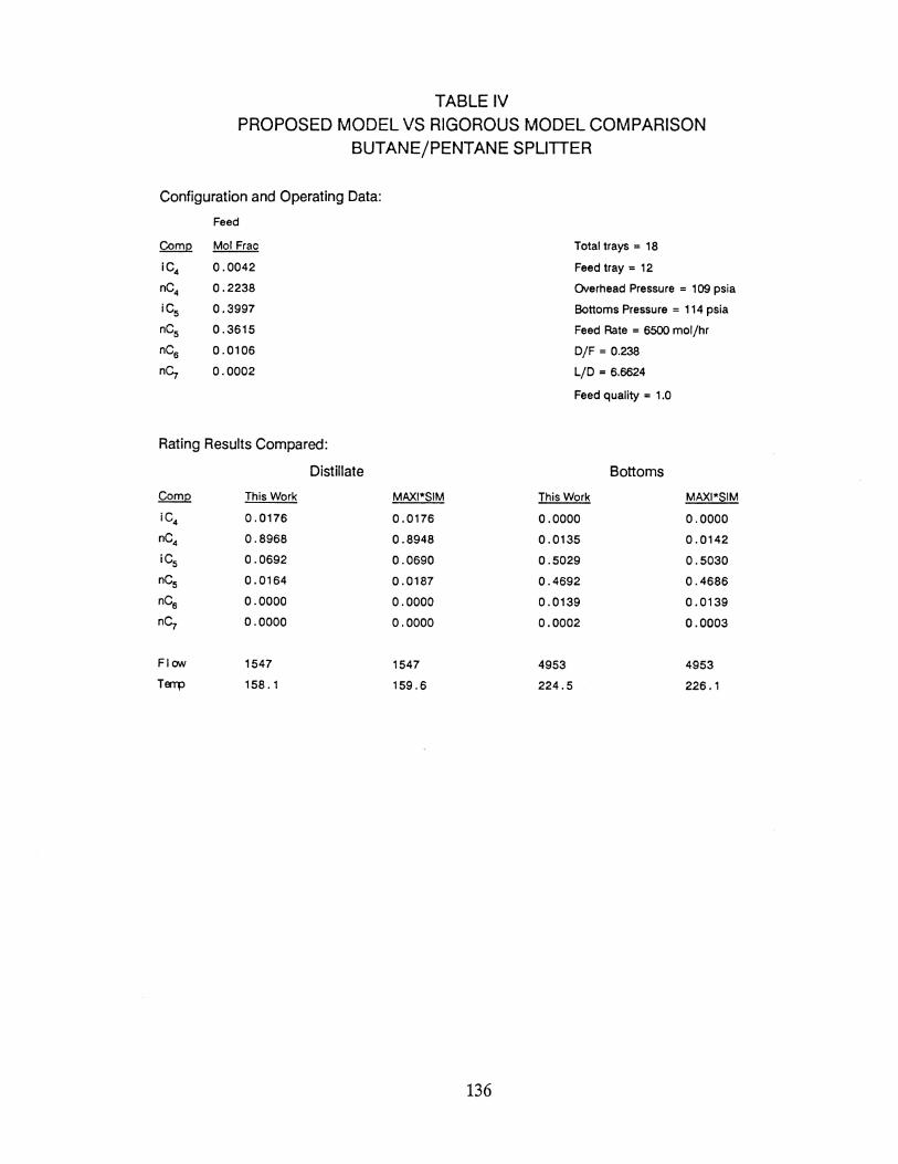
TABLE IV PROPOSED MODEL VS RIGOROUS MODEL COMPARISON

BUTANE/PENTANE SPLITTER

Configuration and Operating Data:

Feed

Comp Mol Frac

iC4 0.0042

nC4 0.2238

iC5 0.3997

nC5 0.3615

nC6 0.0106

nc;. 0.0002

Rating Results Compared:

Distillate

Comp This Work

iC4 0.0176

nC4 0.8968

iC5 0.0692

nC5 0.0164

nC6 0.0000

nc;. 0.0000

Flow 1547

Temp 158. 1

MAXI*SIM

0.0176

0.8948

0.0690

0.0187

0.0000

0.0000

1547

159.6

136

Total trays = 18

Feed tray = 12

Overhead Pressure = 109 psi a

Bottoms Pressure = 114 psia

Feed Rate = 6500 molfhr

D/F = 0.238

L/D = 6.6624

Feed quality = 1.0

Bottoms

This Work MAXI*SIM

0.0000 0.0000

0.0135 0.0142

0.5029 0.5030

0.4692 0.4686

0.0139 0.0139

0.0002 0.0003

4953 4953

224.5 226.1

C1) .....

CD .....

r-.....

CD .....

U'l .....

-d' .....

"" .....

N .....

s.. ..... CLl .....

..0 s 0 :::1 ..... z >.Q) td s..

E-< CD

r-

CD

U'l

-d'

"" N

.....

0

D

!::::,

60.0 80.0

Figure 39.

MAXI*SIM

New Algorithm

100.0 120.0 140.0 160.0 180.0 Tray Temperature, Deg F

Proposed Model vs Rigorous Model Comparison Tray Temperature Profile: C4/C5 Sphtter

137

Tray No.

18{top tray)

17

16

15

14

13

12

11

10

9

8

7

6

5

4

3

2

1 ( r ebo i I e r )

Table V Proposed Model vs Rigorous Model Comparison

Butane/Pentane Splitter- Tray Temperature Profile

Temperature, oF

This Work

158.1

164.1

171 .9

180.7

189.7

198.6

202.1

205.4

208.4

211.0

213.4

215.5

217.3

218.9

220.3

221.6

222.9

224.1

138

MAXI*SIM

159.6

165.4

173.0

181.8

190.2

197.3

199.7

202.4

205.3

208.2

211 . 1

213.9

216.4

218.7

220.7

222.5

224.2

226.1

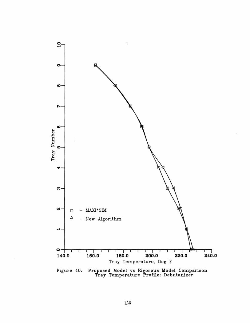
D

D.

MAXI*SIM

New Algorithm

0-+~r-,--r--r-,--.--r-,--.--r-,--.--r-,--.--r-~~--~~

140.0 160.0 180.0 200.0 220.0 240.0 Tray Temperature, Deg F

Figure 40. Proposed Model vs Rigorous Model Comparison Tray Temperature Profile: Debutanizer

139

for a given distillation column, the main purpose of the model. Unfortunately,

usable transient response data for distillation columns (or any other process for

that matter), either plant based or predictions, is very hard to come by. For many

published sets of plant operating data, the required information for creating a

simulation of the column is not provided. Therefore, assumptions about the

column would be required for setting up a simulation for comparison with the

published transient response data. This would invalidate the comparison. The

same holds true for many published sets of transient response data taken from

simulations.

A recent paper by Wong and Wood36 presented some transient response

data and enough configuration information about the column to allow a simulation

to be developed for comparison. Table VI shows the configuration information for

the column. Using a simulation of this column, the dynamic behavior was studied

for disturbances in feed flow rate, reboiler heat input and reflux flow rate. The

results from three of the cases presented in this paper will be compared to results

generated from the proposed model.

Figure 41 shows the first of these transient response curves. This figure

shows the response of the distillate propane to a 10% decrease in reflux rate. Even

the general shape of the two curves are similar, considerable differences are

apparent. On figures 41-43, two points are indicated on the ordinate. Both the

initial and final mole fractions for propane were determined via MAXI*SIM runs.

These points are marked. Figure 41 clearly shows a good agreement between this

model and MAXI*SIM at the initial and final conditions. This figure also shows a

poor ability of the Wong and Wood model to accurately predict steady state

values. Unfortunately, the specific V-L-E algorithm used by Wong and Wood was

not described in their paper. Therefore, the reason for this steady state

140

Table VI COLUMN CONFIGURATION DATA FOR EXAMPLE

COLUMN OF WONG AND WOOD

Tray holdup : 14 kmol Feed Rate : 0.8333 kmoljsec

Reboiler holdup :50 kmol Reflux Rate : 1.500 kmoljsec

Condenser holdup : 50kmol Reflux Ratio :3.173

Tray efficiency :100% Condenser Duty :7.883 kW

Column pressure : 2400 kPa Reboiler Duty :8.333 kW

Number of stages : 30 (excluding condenser)

Feed Tray : 12

Feed temperature : 353 OK

Feed Pressure : 2400 kPa

Column is equipped with a partial condenser and total reboiler

Feed Composition (mol%):

Ethane 3.0

Propylene 40.0

Propane 15.0

iso-Butane 15.0

cis-2-Butene 27.0

141

f-oo" ~ N

~ 0 ...... ..... u ttl ~ -

0.30

0.28

v 0.26 ....... 0 s v ..... ttl ....... ........

~ 0.24 ..... Q

q ..... ::t: ....:I

0.22

0.20 0.0

Rigorous Steady State at Initial Conditions

Wong and Wood

Rigorous Steady State Value Ending Conditions

5.0 10.0 15.0 Time, minutes

This Work

20.0 25.0

Figure 41. Response of the Distillate Propane Composition to a 10 percent Decrease in Reflux Rate

30.0

0.30

0.28

1:1 0 ...... ~ 0 ro s... -Q) 0.26 ,._, 0

El Q) ~ ro ........ ........ ......

~ ~ 0.24 ~ ..... w 0

Q ..... ~ .....:1

0.22

0.20 0.0

Rigorous Steady State Value at Initial Conditions

Rigorous Steady State Value Ending Conditions

5.0 10.0 15.0 Time, minutes

Wong and Wood

This Work

20.0 25.0

Figure 42. Response of the Distillate Propane Composition to a 10 percent Increase in Steam Rate

30.0

0.30

0.28

1=1 0 ....... .,_, (.)

ttl r... ..... Q) 0.26

....... 0 s Q) .,_, ttl I ...... ...... :g 0.24

!--' ....... ..p.. Q r ..p..

0 ..... ::.:: H

0.22

0.20 0.0

Rie.orous JSte$dv State Value

- - - - - - - -Rigorous Steady State Value Ending Conditions

5.0 10.0 15.0 20.0 Time, minutes

Figure 43. Response of Distillate Propane Composition to a 10 percent Decrease in Feed Rate

Wong and Wood

This Work

25.0 30.0

discrepancy cannot be explained precisely. The two most likely causes are

inaccurate V-L-E predictions and excessive numerical integration errors. Which of

these may be the cause cannot be determined from the paper. However, some

useful information is still available from this response. As can be seen from the

figure, inverse response behavior is exhibited. This inverse response is a well

known behavior under certain conditions. Consideration of this behavior can be

very important in the design of advanced process control schemes. The fact that

the proposed model exhibits this inverse behavior is significant and is another

indication of its accuracy.

Figure 42 shows the transient response of the distillate propane to a 10%

increase in the heat input to the tower. Again, there is a significant discrepancy at

steady state between the model of Wong and Wood and the steady state model,

MAXI* SIM. The proposed model generates a response similar to the previous

case and results in a steady state value that is in good agreement with MAXI*SIM.

Also, an inverse response behavior is exhibited. This behavior can be better

explained by considering the individual component molar flows during the course

of this run. Initially both component flow rates increase as the heat input

increases. As expected the light key flow would increase faster than the heavy key.

However, at some point all the light key in the feed is going overhead, thus this

flow can not increase any more. Thus this flow stabilizes as the heavy key flow

continues to increase. This sequence results in the mole fraction response curves

seen in Figure 42.

Figure 43 shows the response of the distillate propane to a 10% decrease in

tower feed rate. This case is very similar to the last case. The net effect is an

increase in the steam/feed ratio just as it was in the last case. Thus, similar

response curves would be expected and in fact that is the case.

145

These compansons show this model does predict reasonable response

curves including prediction of inverse response behavior. In addition, as expected

from the theory presented in Chapter 4, the steady state predictions of this model

are in excellent agreement with a rigorous steady state model.

146

CHAPTER IX

EXAMPLE APPLICATION: COMPUTER BASED, INTERACTIVE OPERATOR

TRAINING SYSTEM APPLIED TO DISTILLATION

COLUMN OPERATION

Objectives

In 1985, I became involved with HiTech Interactive Training, Inc. This was

a small company consisting of experienced operator trainers, instructional

designers, and chemical engineers. This company was formed to create a

state-of-the-art computerized operator training system. After preliminary

research, we became convinced that microcomputers had advanced in their

capabilities to the point a viable process simulator could be installed on this lower

cost hardware. In addition, hardware and software were becoming available to

allow the interfacing of a microcomputer and a laser video disc player for a

practical interactive instructional delivery system with capacity for our application.

When we were considering what an effective interactive process simulator

training system would look like, we decided it needed these basic elements:

• The training should being a preliminary overview of the major concepts on which

the process to be simulated is based. We were convinced that what is desirable in a

competent operator goes beyond a conditioned response to knowing "when this

variable goes in this direction, I turn this knob to the left". He should know why.

• The operation of the simulator itself must not stand in the way of the operator

learning the process. The simulator controls must be simple enough to ensure the

147

majority of the learning takes place learning the process.

• When the trainee is in a simulation session, the trainee/system interaction should

not be in a question/answer format. We decided the trainee should be allowed to

operate the simulator without interruption as long as he is keeping the process

stable and is not about to go into an alarm condition. However, if a limit violation

should occur, the student should be interrupted and given automatic remedial

instruction on what went wrong, which brings me to the next point.

• The remedial instruction, when delivered, should be done in an intelligent fashion.

In other words, the suggestion or remediation should be the result of an evaluation

of several process variables, and their rates of change, which are related to the

primary process upset. In effect, the system would choose the best solution from a

library of possible solutions, instead of a one problem/one solution approach.

• An objective measure of the trainee's performance on the simulator must be

available.

• The trainer should have the option of customizing operating situations to

resemble ones common in his plant.

• Finally, the system should operate as a self-instructional module. The immediate

presence and expense of the trainer should not be necessary for guided learning to

take place. Additionally, being able to place the system in the control room itself

should be possible, thus eliminating the requirement the operator leave his station

for training purposes.

Hardware Overview

At this point, we determined what hardware to use in order to implement

these objectives subject to two constraints:

• The computer system must support interactive video. Interactive video was essential

for the instructional/remedial aspects of our objectives.

• All the hardware should be available from a single manufacturer. This was felt

necessary to ensure effective maintenance and service support on this relatively new

technology.

The objectives just discussed along with these two constraints led us to the

Digital Equipment Corporation (DEC) for our hardware. With two exceptions, all

the hardware we needed was available as the DEC IVIS system which consists of a

Professional 380 microcomputer, a high resolution color monitor, a laser videodisc

148

player, and an interface device called the IVIS backpack. We have also added the

DEC LASO printer and the EECO compressed audio decoder.

The Pro-380 computer system uses the LSI-11/23+ CPU which is a 16 bit

processor. This system can address over one megabyte of main memory and has a

10 megabyte hard disk drive. The IVIS backpack is the interface that allows

software within the Pro-380 computer to randomly access audio and video frames

on the video disc.

The EECO decoder was necessitated by the amount of audio we needed for

the remedial messages. A typical linear format videodisc provides 1/30th of a

second of audio per video frame, or 30 minutes of audio per side. The EECO

decoder allows us to get 10 seconds of audio per frame which yields 150 hours of

audio on one side of a videodisc.

Software Overview

With the hardware now defined, we had to go about the task of developing

the software that would accomplish the objectives that we set forward. To

accomplish these objectives, we essentially had to do two things with the software.

We had to realistically simulate a computer control room for the operator and we

had to provide software that could intelligently deliver remediations to the

operator during his simulation sessions.

We developed five major pieces of software to accomplish these objectives:

• A man-machine interface

• A complete process control system

• A realistic dynamic process simulation

• An intelligent instructional delivery system

• An extensive menu system

These 5 software systems run concurrently in a multi-tasking environment

149

(DEC RSX-llM + operating system) on the Pro-380 and communicate with each

other through global common areas as depicted in Figure 44. The following

sections describe each of these software systems and how they interact with each

other.

Man-machine Interface

The man-machine interface or, as we called it, the console system, allows

the operator to both inspect the status of the process that he is operating and also

allows him to affect the process with appropriate inputs through the keyboard.

Using the standard DEC keyboard, we structured this interface to be as simple as

possible. This was done by utilizing the top row function keys, the cursor keys,

and the numeric keypad. The QWERTY keypad is inoperative during a

simulation session. The operator can inspect the status of his process by accessing

process flow diagrams, alarm displays, trend displays, stream analysis displays, and

controller faceplates through the function keys. He can also affect the process

through these function keys by turning pumps on and off, turning fans on and off,

and opening or closing block and bypass valves. He can affect the process through

the numeric keypad by entering new values for controller setpoints or controller

outputs. All the necessary live process data for the numerous graphics displays is

communicated to the console system by the process control control system (BPR).

Likewise, the console system communicates to both the BPR and the instructional

delivery system (IDS) any actions the operator has taken in order to affect the

process.

Process Control System

150

...... U1 ......

Process Information -- Process

Simulation

Process Control Information

User

Interface

Graphics Information

---Instructional Information

• Instructional

Delivery

System

Simulated Measurements

--

---

Flows

------

----

Remedial Delivery

r Process

Control

System

I Man -machine

Interface

• Student Actions

Figure 44. Instructional System Software Components

The BPR is a complete set of control algorithms. It has a modular structure

and contains some 20 distinct algorithms, or blocks that can be configured to

define any control scheme required. The BPR reacts to inputs the operator makes

through the console keyboard as he tries to affect the process. These inputs from

the console will eventually result in some change in one or more flow rates that is

then communicated to the dynamic simulation system. In addition, any process

upsets or equipment malfunctions that have been setup for a particular problem

are communicated to the BPR by the IDS at the predetermined time they are to

occur.

Dynamic Process Simulation

This function is provided by the simulation system of this thesis. A critical

element of this entire training system was a "real-time" dynamic simulation. This

was absolutely necessary to create the atmosphere of a control room. The dynamic

simulation accepts changes in flow rates from the BPR and generates the dynamic

process responses that each particular type of distillation column would normally

exhibit. These responses are then communicated back to the BPR as simulated live

process measurements.

Instructional Delivezy System

The IDS is the software that essentially simulates the instructor. The IDS

monitors both the process conditions through communicating with the BPR and

any action the operator may take through communications with the console

system. It then determines at any point in time if the operator deserves a particular

remedial sequence. The determination of whether a particular remedial sequence

152

is required is a function of several different variables including whether the

primary variable is violating a particular limit, the value of several other process

parameters associated with this primary variable, the rates of change of all of these

different variables, whether or not the operator has taken a corrective action in the

recent past and how long ago the last remedial sequence was delivered. After

examining these variables, the IDS determines if in fact this remedial sequence is

required and, if so, suspends the process simulation, determines the correct audio

and video frame numbers on the videodisc that contain the remedial sequence in

question, sends these requests to the console system which then displays this

remedial sequence on the operators CRT.

Menu System

The last major piece of software is the menu system. The courseware

developer uses this system to build customized problem situations. The student

then uses this system to select the particular problem he has been asked to solve.

This system defines various databases during the building of a problem and then

sets up these various databases when a student chooses a particular problem.

Training System

I would now like to describe how we used the complete system described

above to develop an operator training system for distillation. To satisfy the

desirable characteristics for a control room based interactive system, which

delineated earlier, the training package was divided into 5 phases:

• Phase I, which we called "Concepts", reviews the primary concepts of the distillation

process. This phase uses audio/visual instruction and a workbook.

153

• Phase II, "Keyboard Instruction", prepares the student for operation of the simulator

controls. This phase teaches the operator specifically how to operate the system

keyboard to control the simulator. In this way we put off the possibility that the

operation of the simulator will interfere with the learning of the distillation process

itself.

• In Phase III we begin to utilize the compressed audio capability of the system. In

this phase operator is given normal operational changes to make to the distillation

column. He must also identify and correct equipment failures which will

occasionally occur in a refinery. During this phase the IDS monitors key variables in

the process. If one of these key variables goes outside certain limits, the computer

decides first of all whether remedial instruction is called for. In the event this

situation calls for remediation, the appropriate audio/video sequence is selected and

displayed. The operator may also ask for help. The IDS will select the appropriate

help for him based on his stage and progress through the problem solution and

display it to him from the videodisc source. The Phase Ill problems were

pre programmed.

• In Phase IV, "Process Dynamics", the courseware developer builds customized

problems by choosing from a variety of process changes and equipment

malfunctions, which he may select through a series of menus. These can occur in any

sequence and at various times during the operators session on the simulator. Phase

IV also provides automatic audio/visual remediation to reduce the likelihood of the

same incorrect operating practices in the future. The operator may also choose from

a menu of helps in this phase.

• Finally, in Phase V, "Performance Measurement", remediation is no longer

available. This is the testing phase. The course developer may defme the same

problems he defined in Phase IV, but this time the operators performance without

help from remedial instruction. is evaluated on the basis of his economic efficiency

in operating the column. The simulator system calculates for any given process

change or upset the operational cost for what would be the ideal solution. This then

becomes the highest possible score the operator could achieve. His actual

performance is then observed, a comparison is made with the ideal performance,

and an efficiency rating is assigned.

Dynamic Simulator Significance

The major hurtle to overcome in the development of the training system

was providing a dynamic simulation which would yield realistic process responses in

154

real-time on a microcomputer. After several false starts, I was contacted. The

simulation I had developed met all the requirements of this training system. In

addition, the dynamic simulation systems modular structure allowed the course

developer to easily configure the simulation system for any particular column of

interest.

155

CHAPTER X

SUMMARY AND RECOMMENDATIONS

Summary

The results of this work are a set of algorithms, both steady and unsteady

state, which can be used as building blocks to create a dynamic simulation of

practically any distillation tower. This simulation system will run in real-time,

depending on both the size of the flowsheet and the computer hardware. The

example of the crude tower was implemented on a DEC Micro VAX. This crude

tower simulation reached to capacity of the Micro VAX for executing in real-time.

Any addition to this flow sheet would have resulted in computes times that would

have been excessive. However, this crude tower simulation is equivalent to 13

simple two products towers.

The results presented in chapter 8 verify the steady state accuracy of this

simulation system. The results presented regarding the transient response

predictions are less concrete due to the source of data for comparison. However,

these results at least verify the directions of responses are reasonable.

Several new algorithms were developed for incorporation into this dynamic

simulation system which would also be useful as stand alone algorithms in steady

state applications. A new technique for rating heat exchangers where the fluid is

undergoing a phase change on one or both sides of the exchanger was presented.

156

This algorithm could prove very useful as on on-line tool for keeping track of

exchanger performance. A method for determining the individual tray

temperatures in a trayed section was presented. This provides information

previously available only from rigorous tray-by-tray routines.

Recommendations

A major weakness in the current system is the user interface for building up

a flow sheet. A significant amount of work would be required to develop a friendly,

bullet-proof interface system. However, an interface of this type would significantly

enhance the utility of the simulation system.

More work needs to be done to verify the accuracy of the transient response

predictions. This should probably be accomplished via comparisons to a fully

rigorous dynamic simulation. The availability and quality of measured transient

response curves does not seem to be sufficient for this task.

157

REFERENCES

(1) Sourisseau, K.D. and M.F. Doherty, "Dynamic Simulation of Stiff

Distillation Systems," J.A.C.C., San Francisco (1980).

(2) Lapidus, L. and N.R. Amundson: Ind. Eng. Chern., 42, 1071-1078.

(3) Huckaba, C. E., F.P. May and F.R. Franke: Chern. Eng. Prog. Symp. Ser.,

vol 59, No. 46 (1963), pp. 38-47.

(4) Waggoner, R.C. and C.D. Holland: AIChE J., vol 11, No 1 (1965), pp.

112-120.

(5) Peiser, A.M. and S.S. Grover: Chern. Engr. Prog., vol58, No 9 (1962), pp.

65-70.

(6) Rademaker, 0., J.E. Rijnsdorp and A. Maarleveld: Dynamics and Control

of Continuous Distillation Units, Elsevier, 1975.

(7) Augustin, D.C., J.C. Strauss, M.S. Fineberg, B.B. Johnson, R.N.

Linebarger and E.J. Sansom: Simulation, vol21, No 6 (1967), pp. 281-301.

(8) Mah, R.S.H., S. Michaelson and R.W.H. Sargent: Chern. Eng. Sci., vol17

(1962), pp. 619-639.

(9) Sansom, E.J. and H.E. Petersen: "MIMIC A Digital Simulation Program,"

SESCA International Memo 65-12, Wright-Paterson Air Force Base,

Ohio, May 1965.

(10) IBM: Continuous System Modelling Program CSMP 1.3,IBM Program No.

H20-0367-3.

(11) Barney, J.R., R.S. Ahluwalia and AI. Johnson: DYNSYS 2.0 User's

Manual, University of Western Ontario, London, Ontario, Canada, 1975.

158

(12) Perkins, J.D. and R.W.H. Sargent: "SPEEDUP: A Computer Program for

Steady State and Dynamic Simulation and Design of Chemical

Processes,''A/ChE Symposium Series, vol 78, No 214 (1982).

(13) Westerberg, A: "ASCEND II An Advanced System for Chemical

Engineering Design," Proceedings of the 11th Annual Pittsburg Conference,

Part 2, Systems and Control, ISA, 1980.

(14) EXXON: Modular Dynamic Distillation Control Model (MODCOMP),

Version 1.0, EXXON Program 36985, 1976.

(15) Simonsmeier, U.F., R. Bilec and R.K Wood: "Rigorous Dynamic Models

of a Binary Distillation Column,'' 27th Can. Chern. Eng. Conf., Oct. 23- 27,

Calgary, 1977.

(16) Svrcek, W.Y.: Dynamic Response of a Binary Distillation Column, Ph.D.

Thesis, Dept. Chern. Eng., Univ. Alberta, 1967.

(17) Distefano, G.P.: "Mathematical Modelling and Numerical Integration of

Multicomponent Batch Distillation Equations,'' J. 14, 190, 1968.

(18) Tyreus, B.D., W.L. Luyben and W.E. Schiesser: "Stiffness in Distillation

Models and the Use of an Implicit Integration Method to Reduce

Computation Times," Ind. Engng. Chern. Process Des. Dev., vol 14, No 427.

(19) Edmister, W.C.: Applied Hydrocarbon Thermodynamics, vol II, Gulf

Publishing Co., Houston, 1961, pp. 101-115.

(20) Rice, V.L.: "Program Performs Vapor-Liquid Equilibrium Calculations,"

Chemical Engineering, vol 89, No. 13 (June 28, 1982), pp. 77-86.

(21) Pitzer, K.S., et al: Appendix 1, Lewis and Randall, Thermodynamics, 2nd

ed, McGraw-Hill, New York, 1961.

159

(22) Erbar, J.H.: Personal communication, 1983.

(23) Gunn, R.D. and T. Yamada: AIChE 1, 17: 1341 (1971).

(24) Reid, C.R., J.M. Prausnitz and T.K. Sherwood: The Properties of Gases

and Liquids, McGraw-Hill, New York, 1977, p. 67.

(25) Mamedov, G.E.: "Polynomial Mathematical Model for Multicomponent

Distillation," International Chemical Engineering, vol. 18, No. 1, January

1978.

(26) Smith, B.D. and W.K. Brinkley: "General Short-Cut Equation for

Equilibrium Stage Processes," A.l.Ch.E. 1, vol. 6, No. 3 (1960),

pp.446-450.

(27) Wylie, Jr., C.R.: Advanced Engineering Mathematics, 1st ed.,

McGraw-Hill Book Company, Inc., New York, 1951, pp.502-503

(28) Kays, W.M. and AL. London: Compact Heat Exchangers, 3rd ed.,

McGraw-Hill, New York, 1984, pp. 16-17.

(29) Holland, C.D. and A.I. Liapis: Computer Methods for Solving Dynamic

Separation Problems, McGraw-Hill, New York, 1983, p. 27.

(30) Dahlquist, L.: "A Special Stability Problem for Linear Multistep

Methods," BIT, vol 3, No. 27, 1963.

(31) Dahlquist, L.: "Convergence and Stability in the Numerical Integration of

Ordinary Differential Equations," Math. Scan., vol4, No. 33, 1956.

(32) Holland, C.D. : Fundamentals of Multicomponent Distillation,

McGraw-Hill Book Company, Inc., New York, 1981.

160

(33) Smith, B.D. :Design of Equilibrium Stage Processes, McGraw- Hill Book

Company, Inc., New York, 1963.

(34) Van Winkel, M. : Distillation, McGraw-Hill Book Company, inc., New

York, 1967.

(35) Wong, T.T. and R.K. Wood : "Dynamic Simulation of Multicomponent

Distillation Columns," SCSC 1985 Proceedings, Chicago, Dlinois, July

1985.

(36) Edgar, T., R. Mah and G. Reklaitis: "Use of Computers in Chemical

Engineering Education," Chemical Engineering Progress, vol. 81, No. 9,

1985.

161

VITA

Victor Lamont Rice

Candidate for the Degree of

Doctor of Philosophy

Thesis: NEW APPROACH TO DYNAMIC DISTILlATION SIMUlATION:

ACCURATE DYNAMIC AND STEADY-STATE PREDICTIONS IN REAL-TIME

Major Field: Chemical Engineering

Biographical:

Personal Data: Born in San Antonio, Texas, December 21, 1953, the son of Jack L. and Catherine

J. Rice. Married Donna S. Howard on August 17, 1974. Daughter, Sarah E., born August 6,

1978.

Education: Graduated from Purcell High School, Purcell, Oklahoma, in May, 1968. Received

Bachelor of Science Degree in Chemical Engineering from Oklahoma State University in

May, 1977; received Master of Chemical Engineering from Oklahoma State University in

May, 1977; completed requirements for the Doctor of Philosophy degree at Oklahoma State

University in December, 1988.

Professional Experience: Teaching Assistant, Department of Chemical Engineering, Oklahoma

State University, August, 1976, to May, 19TI; Technical Services Engineer, Amoco Oil

Company, May, 1977, to March, 1978; Operations Engineering, Amoco Oil Company,

March, 1978, to March, 1980; Refmery Control Engineer, Arabian American Oil Company,

March 1980, to March 1982; Instructor, Department of Chemical Engineering, Oklahoma

State University, June, 1982, to June, 1984; Head Simulationist, Hitech Interactive Training,

October, 1984, to September, 1986; Principal Research Engineer, Combustion Engineering

Simeon, September, 1986, to present.

accurate dynamic and steady-state predictions in real - CORE

Documents