ACCURATE DETERMINATION OF DISSIPATED CREEP STRAIN ENERGY AND ITS EFFECT ON LOAD- AND TEMPERATURE-INDUCED CRACKING OF ASPHALT PAVEMENT By JAESEUNG KIM A DISSERTATION PRESENTED TO THE GRADUATE SCHOOL OF THE UNIVERSITY OF FLORIDA IN PARTIAL FULFILLMENT OF THE REQUIREMENTS FOR THE DEGREE OF DOCTOR OF PHILOSOPHY UNIVERSITY OF FLORIDA 2005

Welcome message from author
This document is posted to help you gain knowledge. Please leave a comment to let me know what you think about it! Share it to your friends and learn new things together.
Transcript
ACCURATE DETERMINATION OF DISSIPATED CREEP STRAIN ENERGY AND ITS EFFECT ON LOAD- AND TEMPERATURE-INDUCED CRACKING OF
ASPHALT PAVEMENT
By
JAESEUNG KIM
A DISSERTATION PRESENTED TO THE GRADUATE SCHOOL OF THE UNIVERSITY OF FLORIDA IN PARTIAL FULFILLMENT
OF THE REQUIREMENTS FOR THE DEGREE OF DOCTOR OF PHILOSOPHY
UNIVERSITY OF FLORIDA
2005

Copyright 2005
by
Jaeseung Kim

ACKNOWLEDGMENTS
I would like to thank my adviser and chairman of my supervisory committee, Dr.
Reynaldo Roque. He always listened and respected my opinion. All tasks were
accomplished under his support and guidance. I would like to offer heartfelt gratefulness
and respect to him. I will never forget his help. I also thank Dr. Bjorn Birgisson, my
cochair, for the generous contribution of his discussion, his support, encouragement, and
precious guidance. Special thanks go to the other members of my advisory committee
(Dr. Mang Tia, Dr. Dennis R. Hiltunen, and Dr. Bhavani V. Sankar).
Special thanks go to Mr. George Lopp and Miss. Tanya Riedhammer for their
support in the laboratory and their valuable advice. I would like to thank the former
graduate student, Adam P. Jajliardo, for generous help. I also would like to thank Sungho
Kim, Dr. Booil Kim, Dr. Christos A. Drakos, and Byungil Kim for their friendship and
encouragement. I appreciate the friendship of all the students in the materials group of the
Department of Civil and Coastal Engineering at University of Florida.
Lastly, I would like to thank my father, Yangjin Kim, my mother, Sinja Min, my
sister, Lee-Eun Kim, my wife, Soojung Lee, and my son, Bryan Kim, for their endless
trust, encouragement, and support. I would also like to thank all my family and friends
who have also supported me.
iii
TABLE OF CONTENTS page
ACKNOWLEDGMENTS ................................................................................................. iii
LIST OF TABLES............................................................................................................ vii
LIST OF FIGURES ........................................................................................................... ix
ABSTRACT...................................................................................................................... xii
CHAPTER
1 INTRODUCTION ........................................................................................................1
1.1 Background.............................................................................................................1 1.2 Hypothesis ..............................................................................................................3 1.3 Objectives ...............................................................................................................3 1.4 Scope.......................................................................................................................3
2 LITERATURE REVIEW .............................................................................................5
2.1 Cracking Mechanisms within Asphalt Mixtures ....................................................5 2.1.1 Fatigue Cracking Models .............................................................................5 2.1.2 Dissipated Energy in Fatigue........................................................................6 2.1.3 Continuum Damage Mechanics Model ........................................................7 2.1.4 HMA Fracture Mechanics ............................................................................9
2.1.4.1 Observation of threshold ....................................................................9 2.1.4.2 Determination of DCSE and DCSE limit (threshold) ......................10 2.1.4.3 Energy-based fracture mechanics.....................................................12 2.1.4.4 Energy Ratio.....................................................................................13
2.1.5 Thermal Cracking.......................................................................................14 2.2 Cracking Mechanisms Associated with Pavement Structure ...............................15
2.2.1 Classic Fatigue Cracking............................................................................15 2.2.2 Load-Induced Top-Down Cracking ...........................................................16
3 TEST SECTIONS, MATERIALS, AND METHODS...............................................18
3.1 Locations and Condition.......................................................................................18 3.1.1 Group I........................................................................................................19 3.1.2 Group II ......................................................................................................19
iv
3.2 Traffic Volume .....................................................................................................20 3.3 General Observation .............................................................................................21 3.4 Pavement Structure...............................................................................................22
3.4.1 Falling Weight Deflectometer Testing .......................................................22 3.4.2 Layer Moduli ..............................................................................................23 3.4.3 Stress Analysis............................................................................................24
3.5 Materials and Methods .........................................................................................25 3.5.1 Materials Preparation..................................................................................26 3.5.2 Measurement of Volumetric and Binder Properties ...................................26 3.5.3 Measurement of Mixture Properties ...........................................................26
3.5.3.1 Experimental design of Superpave IDT ...........................................27 3.5.3.2 Description of testing types..............................................................28 3.5.3.3 Data analysis ....................................................................................28
3.6 Experimental Results ............................................................................................29 3.6.1 Volumetric and Binder Properties ..............................................................29 3.6.2 Mixture Test Results...................................................................................30
3.6.2.1 Resilient modulus test ......................................................................30 3.6.2.2 Creep compliance test ......................................................................30 3.6.2.3 Tensile strength test..........................................................................32
4 DETERMINATION OF ENERGY DISSIPATION ..................................................35
4.1 Materials and Methods .........................................................................................35 4.1.1 Materials .....................................................................................................35 4.1.2 Complex Modulus Test ..............................................................................36
4.1.2.1 Overviews.........................................................................................36 4.1.2.2 Testing procedure.............................................................................36
4.1.3 Static Creep Test.........................................................................................37 4.2 Determination of Dissipated Energy ....................................................................38
4.2.1 Experimental Determination of Dissipated Energy Based on Hysteresis Loop ...........................................................................................................38
4.2.2 Dissipated Energy from Static Creep Test Data.........................................39 4.2.3 Dissipated Energy for General Loading Conditions ..................................40 4.2.4 Dissipated Energy from Cyclic Creep Test ................................................42
4.3 Data Interpretation ................................................................................................44 4.4 Analysis and Findings...........................................................................................46 4.5 Analysis by Use of Rheological Model ................................................................48
5 INTEGRATION OF THERMAL FRACTURE IN THE HMA FRACTURE MODEL ......................................................................................................................54
5.1 Review of the Past Work ......................................................................................54 5.1.1 TC Model....................................................................................................54 5.1.2 Conversion of Creep Compliance to Relaxation Modulus.........................54 5.1.3 Time-Temperature Superposition Principle and Master Curve Fit ............56 5.1.4 Thermal Stress Prediction...........................................................................57
5.2 Development of Basic Algorithm for HMA Thermal Fracture Model.................60
v

5.2.1 Development of Thermal Creep Strain Prediction .....................................60 5.2.2 Dissipated Creep Strain Energy and Energy Transfer................................62
5.3 HMA Thermal Fracture Model.............................................................................63 5.3.1 Physical Model, Temperature Variation, and Assumptions.......................63 5.3.2 General Concept of HMA Thermal Fracture Model ..................................65 5.3.3 Software Development ...............................................................................67
5.4 Evaluation of HMA Thermal Fracture Model ......................................................68 5.4.1 Parametric Study ........................................................................................68 5.4.2 Evaluation of Material Characteristics Related to Thermal Cracking........70 5.4.3 Evaluation of Pavement Performance Related to Thermal Cracking.........72
6 FIELD PERFORMANCE EVALUATION BASED ON COMBINED EFFECT OF TEMPERATURE AND LOAD ...........................................................................75
6.1 Evaluation of Load-Induced Top-Down Cracking Performance..........................75 6.2 Consideration of Load Effect to Top-down Cracking Performance.....................77 6.2 Energy Ratio Correction .......................................................................................78 6.4 Further Analysis....................................................................................................80
7 SUMMARY, CONCLUSIONS AND RECOMMENDATIONS ..............................86
7.1 Summary...............................................................................................................86 7.1.1 Evaluation of Energy Dissipation...............................................................86 7.1.2 Evaluation of HMA Thermal Fracture Model............................................88 7.1.3 Combination of Temperature and Load Effect...........................................88 7.1.4 Increase of Performance Related to Mixture’s Rheology ..........................89
7.2 Conclusions...........................................................................................................90 7.3 Recommendations.................................................................................................90
APPENDIX
A SUMMARY OF NON-DESTRUCTIVE TESTING (FWD) .....................................92
B INDIRECT TENSILE TEST RESUTLS....................................................................98
LIST OF REFERENCES.................................................................................................101
BIOGRAPHICAL SKETCH ...........................................................................................104
vi
LIST OF TABLES
Table page 3-1. Location and Condition of Group I ............................................................................18
3-2. Location and Condition of Group II ...........................................................................19
3-3. Traffic Volumes of Group II ......................................................................................21
3-4. Thickness of Layers....................................................................................................24
3-5. Backcalculated Moduli ...............................................................................................24
3-6. Binder’s Viscosity ......................................................................................................28
3-7. Mixture’s Air void Content ........................................................................................28
4-1. Energy from Hysteresis Loop and Static Creep Test .................................................45
4-2. Energy from Cyclic and Static Creep Test .................................................................46
5-1. User-Dependant Inputs of HMA Thermal Fracture Model ........................................71
5-2. Regional Temperature of Individual Sections ............................................................73
A-1. Location A .................................................................................................................92
A-1. Location B .................................................................................................................92
B-1. Resilient Modulus Test Results at 0°C ......................................................................98
B-2. Creep Compliance Test Results at 0°C......................................................................98
B-3. Tensile Strength Test Results at 0°C .........................................................................98
B-4. Resilient Modulus Test Results at 10°C ....................................................................99
B-5. Creep Compliance Test Results at 10°C....................................................................99
B-6. Tensile Strength Test Results at 10°C .......................................................................99
B-7. Resilient Modulus Test Results at 20°C ..................................................................100
vii

B-8. Creep Compliance Test Results at 20°C..................................................................100
B-9. Tensile Strength Test Results at 20°C .....................................................................100
viii
LIST OF FIGURES
Figure page 2-1. Crack Propagation in Asphalt Mixture.......................................................................10
2-2. Typical Strain-Time Behavior during Static Creep....................................................11
2-3. Determination of DCSE Limit....................................................................................12
2-4. Stress Distribution near the Crack Tip ......................................................................12
3-1. Location of Sections (Group II).................................................................................20
3-2. Cracked Section..........................................................................................................21
3-3. Cored Mixture in Cracked Section .............................................................................22
3-4. Deflections from FWD Results ..................................................................................23
3-5. Tensile Stresses Calculated at the Bottom of AC of Four-Layer System ..................25
3-6. Superpave Indirect Tensile Test (IDT).......................................................................27
3-7. Plot of Binder’s Viscosity ..........................................................................................29
3-8. Plot of Mixture’s Air Void Content............................................................................29
3-9. Resilient Modulus.......................................................................................................30
3-10. D1 value ....................................................................................................................31
3-11. m-value .....................................................................................................................31
3-12. Rate of Creep Strain Compliance .............................................................................32
3-13. Tensile Strength........................................................................................................33
3-14. Failure Strain ............................................................................................................33
3-15. Fracture Energy ........................................................................................................34
3-16. Dissipated Creep Strain Energy................................................................................34
ix
4-1. Oscillating Stress, Strain and Phase lag......................................................................38
4-2. Combining Cyclic and Creep Response .....................................................................42
4-3. Data Fitting of Stress-Strain Response for Cyclic Test..............................................44
4-4. Energy from Hysteresis Loop and Static Creep Test .................................................47
4-5. Energy from Cyclic and Static Creep Test .................................................................48
4-6. Burgers Model ............................................................................................................48
4-7. Conventional Energy Approach vs. Dissipated Energy from Burgers Model Fit ......51
4-8. Conventional Energy Approach vs. Dissipated Energy from Maxwell Model Fit ....53
5-1. Two Maxwell Models Connected in Parallel .............................................................56
5-2. Physical Model ...........................................................................................................64
5-3. General Concept of HMA Thermal Fracture Model ..................................................66
5-4. General Steps of HMA Thermal Fracture Model.......................................................67
5-5. Effect of Cooling Rates ..............................................................................................69
5-6. Effect of Thermal Coefficients ...................................................................................69
5-7. Effect of Temperatures ...............................................................................................70
5-8. Thermal Crack Development Based on Material’s Characteristics............................71
5-9. Thermal Crack Development Based on Field Performance .......................................73
6-1. Energy Ratio ...............................................................................................................76
6-2. Integrated Failure Time ..............................................................................................79
6-3. Energy Ratio Correction.............................................................................................80
6-4. Creep Responses Corresponding to Viscoelastic Rheology Model ...........................81
6-5. Effect of Elasticity ......................................................................................................83
6-6. Effect of Delayed Elasticity........................................................................................83
6-7. Effect of Viscosity ......................................................................................................84
6-8. Energy Ratio Corrections Corresponding to the Coefficients ....................................84
x
A-1. Deflections of I 10-8C at Location A ........................................................................93
A-2. Deflections of I 10-8C at Location B ........................................................................93
A-3. Deflections of I 10-9U at Location A........................................................................94
A-4. Deflections of I 10-9U at Location B ........................................................................94
A-5. Deflections of SR 471C at Location A......................................................................95
A-6. Deflections of SR 471C at Location B ......................................................................95
A-7. Deflections of SR 19U at Location A........................................................................96
A-8. Deflections of SR 19U at Location B........................................................................96
A-9. Deflections of SR 997U at Location A......................................................................97
A-10. Deflections of SR 997U at Location B....................................................................97
xi

Abstract of Dissertation Presented to the Graduate School of the University of Florida in Partial Fulfillment of the Requirements for the Degree of Doctor of Philosophy
ACCURATE DETERMINATION OF DISSIPATED CREEP STRAIN ENERGY AND ITS EFFECT ON LOAD- AND TEMPERATURE-INDUCED CRACKING OF
ASPHALT PAVEMENT
By
Jaeseung Kim
December 2005
Chair: Reynaldo Roque Cochair: Bjorn Birgisson Department: Civil and Costal Engineering
An asphalt mixture's ability to dissipate energy without fracturing is directly related
to cracking performance of asphalt pavement. Therefore, it is critical to accurately
determine the rate of dissipated creep strain energy (DCSE) accumulation in asphalt
mixture subjected to load- and/or temperature-induced stresses. In the laboratory, the
dissipated energy per load cycle is commonly determined as the area of the hysteresis
loop developed during cyclic loading of asphalt mixture. However, it is unclear whether
all dissipated energy determined in this manner is irreversible and associated with
damage, or whether it is at least partially reversible and not fully associated with damage.
For a range of asphalt mixtures, the area of the hysteresis loop appeared to be strongly
affected by the delayed elastic behavior of the mixture, even when cyclic response had
reached steady-state conditions. Furthermore, it is generally not possible to reliably
separate reversible from irreversible dissipated energy in the hysteresis loop using
xii

conventional complex modulus data. Consequently, it is recommended that irreversible
dissipated energy be determined using rheological parameters obtained from static creep
test data.
Field observations indicate that both traffic and thermal stress affect top-down
cracking performance of pavement. Further evaluation of these observations will require
the development and use of cracking models that can consider the combined effects of
load and temperature. A rigorous analytical model was developed to assess the effect of
thermal loading condition and mixture properties on DCSE and cracking. Accumulation
of DCSE in mixture subjected to thermal stresses is much less straightforward than for
load-induced stresses, and performance may be affected by rheological aspects of the
mixture other than creep (e.g., delayed elasticity). Appropriate equations were developed
to calculate thermal stress development and DCSE accumulation for pavement subjected
to thermal loading cycles. Calculations performed with the resulting model verified that
thermal effects can affect top-down cracking performance. It was also found that delayed
elasticity plays an important role in thermal stress development and cracking. Therefore,
mixtures where rheological behavior exhibits lower rate of creep and higher levels of
delayed elasticity would help mitigate the development of top-down cracking.
xiii
CHAPTER 1 INTRODUCTION
1.1 Background
It is generally recognized that a mixture's ability to dissipate energy without
fracturing is directly related to cracking performance of asphalt pavement. Zhang et al.
(2001) identified the presence of a dissipated energy threshold, which defines a mixture’s
energy tolerance prior to fracturing. They also determined that mixture viscosity was
identified as a key property that determines the rate of damage accumulation in mixtures.
Currently, the rate of dissipated energy accumulation can be determined experimentally
for specified loading conditions from either cyclic or static creep test data. For static
creep tests, the dissipated energy is simply the product of the applied stress and the
amount of viscous strain developed at any given time. For cyclic test, the dissipated
energy per load cycle is commonly determined as the area of the hysteresis loop
developed during cyclic loading. However, it is unclear whether all dissipated energy
determined in this manner is irreversible and associated with damage, or whether it is at
least partially reversible and not fully associated with damage. Understanding the nature
of the energy associated with the hysteresis loop during cyclic loading is of critical
importance, because misinterpretation would lead to significant errors in the predicted
cracking performance of mixtures.
Temperature-induced cracking is a major distress mode in asphalt pavement. Daily
or seasonal temperature change leads to development of tensile stresses in the restrained
asphalt surface layer. Currently, several different thermal cracking models with empirical
1

2
and/or analytical approaches have been developed, but none of them appears to
incorporate a fundamental crack growth model associated with damage accumulation and
the dissipated energy threshold in asphalt mixture. In fact, the fracture of viscoelastic
materials may be well explained by the energy-based HMA fracture mechanics model
developed by Zhang et al. (2001), but their framework has not been used to predict
temperature-induced crack development, and it is currently limited to only the evaluation
of load-induced crack performance. Therefore, it is expected that a proper thermal
cracking model, which is able to incorporate the HMA fracture model, may provide a
reasonable and reliable basis to assess for the thermal cracking performance of asphalt
pavement, as well as the combined effect of load and thermal stress that may lead to top-
down cracking.
Top-down cracking or surface-initiated longitudinal wheel path cracking is
considered a common distress mode in flexible pavement. Top-down cracking research at
University of Florida, recently led to the introduction of the concept of Energy Ratio,
which integrated the HMA fracture model and the structural characteristics of asphalt
pavement, to accurately distinguish between pavements that exhibited top-down cracking
and those that did not (Roque et al, 2004). However, this work was limited to evaluation
of the effect of traffic loads alone. Thermal stresses may have a significant effect on the
development of top-down cracking in asphalt pavement. Consequently, it may be
expected that load-induced crack performance combined with the effect of temperature
may provide a more accurate and reliable estimation of pavement performance associated
with top-down cracking.
3
1.2 Hypothesis
Two hypotheses were investigated:
1. DCSE accumulation in asphalt mixture cannot be reliably determined from conventional complex modulus data
2. DCSE induced by thermal stresses affects top-down cracking performance of pavements.
1.3 Objectives
Evaluation these hypotheses involved investigation in three primary subject area:
experimental determination of DCSE accumulation in asphalt mixture, determination of
DCSE induced by temperature change in pavement, and evaluation of the effect of
temperature-induced DCSE on top-down cracking performance. Detailed objectives
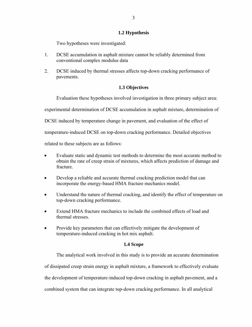
related to these subjects are as follows:
• Evaluate static and dynamic test methods to determine the most accurate method to obtain the rate of creep strain of mixtures, which affects prediction of damage and fracture.
• Develop a reliable and accurate thermal cracking prediction model that can incorporate the energy-based HMA fracture mechanics model.
• Understand the nature of thermal cracking, and identify the effect of temperature on top-down cracking performance.
• Extend HMA fracture mechanics to include the combined effects of load and thermal stresses.
• Provide key parameters that can effectively mitigate the development of temperature-induced cracking in hot mix asphalt.
1.4 Scope
The analytical work involved in this study is to provide an accurate determination
of dissipated creep strain energy in asphalt mixture, a framework to effectively evaluate
the development of temperature-induced top-down cracking in asphalt pavement, and a
combined system that can integrate top-down cracking performance. In all analytical

4
work, the theory of linear viscoelasticity and HMA fracture mechanics are central to the
approach used.
The experimental portion of this study involved eleven dense graded mixtures
obtained from pavements throughout the state of Florida. The eleven pavement sections
involved were evaluated as part of a larger study to investigate top down cracking
performance. The mixtures were composed of a variety of aggregates, including
limestones and granites typically used in the state. The work has involved a
comprehensive set of measurements obtained both in the field and in the laboratory.
Multiple cores were obtained from each section and brought back to the laboratory for
testing. A complete set of laboratory tests was performed to determine volumetric
properties, binder properties, and mechanical properties of the mixtures using the
Superpave IDT.

CHAPTER 2 LITERATURE REVIEW
The primary purpose of this section is to summarize the current understanding of
cracking mechanisms and damage criteria in the area of design and evaluation of flexible
pavement. From the literature review, it is generally agreed that the primary causes of
pavement cracking can be divided into two categories: material failure and structural
failure. Several types of evaluation approaches have been developed on the basis of
different types of mechanisms to evaluate cracking caused by material properties. The
following sections provide an explanation of the basic mechanisms and approaches used
to evaluate the performance of asphalt pavement.
2.1 Cracking Mechanisms within Asphalt Mixtures
2.1.1 Fatigue Cracking Models
Earlier work to predict fatigue cracking of asphalt mixtures was primarily
performed using fatigue tests. The allowable number of load repetition determined at
failure of the test specimen was considered the life of the asphalt mixture. A more
advanced approach, able to account for the effect of pavement structure was developed
by calibrating on the basis of tensile strain in the asphalt pavement. Different types of
equations proposed by many researchers have been widely used as damage criteria. A
typical predictive equation for fatigue cracking is given as
3211 )( ff
tf EfN ε= (2-1) where E1 = HMA modulus εt = tensile strain at the bottom of HMA f1,f2,f3 = transfer coefficients Nf = allowable number of load repetitions
5

6
where transfer coefficients, which relate HMA tensile strain or modulus to the allowable
number of load repetitions, vary between investigators. However, due to lack of a
fundamental mechanism, the approach is somewhat limited, and more mechanistic
approaches are being employed.
2.1.2 Dissipated Energy in Fatigue
When a load is applied to a material there will be a stress that induces a strain. The
area under the stress strain curve represents the energy being input to the material. When
the load is removed from the material, the stress is removed and strain is recovered. If the
loading and unloading curves coincide, all the energy put into the material is recovered
after the load is removed. If the two curves do not coincide, then some energy was lost or
dissipated in the material.
Current applications of dissipated energy to describe fatigue behavior assume that
all dissipated energy represents damage done to the material. In actuality this may be not
true. Only a portion of the total energy that is dissipated may be used in damaging the
material. Ghuzlan and Carpenter (2000) indicate that use of the cumulative dissipated
energy only indirectly recognizes the fact that not all dissipated energy is inducing
damage, without directly determining the value of the damage being done to the material.
The failure criteria proposed by these authors was defined as the change in dissipated
energy between cycles divided by the total dissipated energy at the prior load cycle.
Plotting the values of this ratio versus load cycles results in a decreasing trend during
early cycles, then a constant trend for quite a long time, and then increases rapidly. The
plateau value of the ratio was recommend as the failure of mixtures.

7
This energy ratio approaches proposed by Ghuzlan and Carpenter (2000), which
evaluates what is going on during cyclic loading by looking at the relative change in
dissipated energy between load cycles, appears to adequately identify when failure occurs
in the asphalt mixture. However, the approach does not provide for the determination of
fundamental energy failure limits. In addition, it does not provide fundamental
parameters that allow for the prediction of accumulated dissipated creep strain energy and
fracture.
2.1.3 Continuum Damage Mechanics Model
The behavior of asphalt concrete is not yet fully understood. The reason is that
asphalt concrete, which is mainly asphalt binder combined with aggregates, exhibits
significantly different and more complex material behavior than other common
construction materials (e.g., steel, concrete, and wood). The theory of viscoelasticity is
important in helping to explain the time-dependent nature of vicoelastic materials like
asphalt mixture. One widely used viscoelastic fracture mechanism was developed based
on Schapery’s work (Schapery, 1984) where pseudo elastic strain (Equation 2-2) derived
from hereditary integrals is a fundamental to the evaluation of damage in mixtures. The
advantage of introducing pseudo strain is that it can be related to stresses through
Hooke’s law. Thus, if a linear elastic solution is known for a particular geometry, it is
possible to determine the corresponding linear viscoelastic solution through the
hereditary integral.
∫ −=t
RR d
ddtE
E 0)(1 τ
τετε (2-2)
where ε = uniaxial strain εR = pseudo elastic strain ER = reference modulus that is an arbitrary constant E(t) = uniaxial relaxation modulus
8
T = elapsed time from specimen fabrication and the time of interest τ = time when loading began
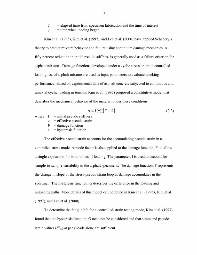
Kim et al. (1995), Kim et al. (1997), and Lee et al. (2000) have applied Schapery’s
theory to predict mixture behavior and failure using continuum damage mechanics. A
fifty percent reduction in initial pseudo stiffness is generally used as a failure criterion for
asphalt mixtures. Damage functions developed under a cyclic stress or strain controlled
loading test of asphalt mixture are used as input parameters to evaluate cracking
performance. Based on experimental data of asphalt concrete subjected to continuous and
uniaxial cyclic loading in tension, Kim et al. (1997) proposed a constitutive model that
describes the mechanical behavior of the material under these conditions:
[ ]GFI Re += )(εσ (2-3)
where I = initial pseudo stiffness ε = effective pseudo strain F = damage function G = hysteresis function
The effective pseudo strain accounts for the accumulating pseudo strain in a
controlled stress mode. A mode factor is also applied to the damage function, F, to allow
a single expression for both modes of loading. The parameter, I is used to account for
sample-to-sample variability in the asphalt specimens. The damage function, F represents
the change in slope of the stress-pseudo strain loop as damage accumulates in the
specimen. The hysteresis function, G describes the difference in the loading and
unloading paths. More details of this model can be found in Kim et al. (1995), Kim et al.
(1997), and Lee et al. (2000).
To determine the fatigue life for a controlled-strain testing mode, Kim et al. (1997)
found that the hysteresis function, G need not be considered and that stress and pseudo
strain values (εRm) at peak loads alone are sufficient.

9
[ ]CSI Rmm )(εσ = (2-4)
where I = initial pseudo stiffness C = coefficient of secant pseudo stiffness reduction S = internal state variable
Except for the use of pseudo strain, this approach appears similar to the classic
forms based on fatigue damage approaches. As mentioned earlier, the evaluation of
cracking performance is more fundamentally related to fracture parameters such as
tensile strength, tensile strain, and fracture energy, which can only be reliably obtained
from fracture test in tension. Critical stress redistribution occurring after crack initiation
is also an important factor affecting cracking performance of mixture. Therefore, a more
fundamental approach, which takes these effects into account, is necessary.
2.1.4 HMA Fracture Mechanics
Cracking mechanisms in asphalt mixtures may be more fundamentally understood
by way of fracture mechanics. An HMA fracture model developed by Zhang et al. (2001)
at University of Florida has provided a fundamental mechanism for evaluating the
performance of asphalt mixtures and understanding the physical behavior of composite
viscoelastic material. HMA fracture mechanics primarily consists of two principal
theories: theory of linear viscoelasticity and energy-based fracture mechanics. From each
theory, specialized theories associated with asphalt mixtures were developed and verified
experimentally. The following explanations may aid to understand the basic principles of
HMA fracture mechanics.
2.1.4.1 Observation of threshold
The concept of the existence of a fundamental crack growth threshold is central to
the HMA fracture mechanics framework presented by Zhang, et al. (2001). The concept
is based on the observation that micro-damage (i.e., damage not associated with crack
10
initiation or crack growth) appears to be fully healable, while macro-damage (i.e.,
damage associated with crack initiation or growth) does not appear to be healable. This
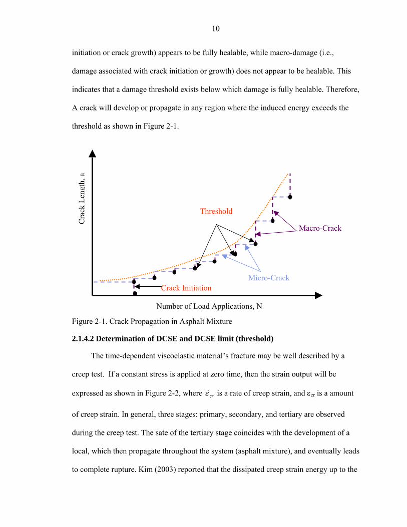
indicates that a damage threshold exists below which damage is fully healable. Therefore,
A crack will develop or propagate in any region where the induced energy exceeds the
threshold as shown in Figure 2-1.
Macro-Crack
Crack Initiation
Cra
ck L
engt
h, a
Threshold
Micro-Crack
Number of Load Applications, N
Figure 2-1. Crack Propagation in Asphalt Mixture
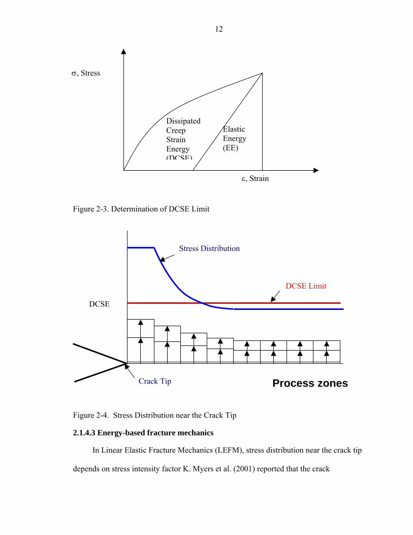
2.1.4.2 Determination of DCSE and DCSE limit (threshold)
The time-dependent viscoelastic material’s fracture may be well described by a
creep test. If a constant stress is applied at zero time, then the strain output will be
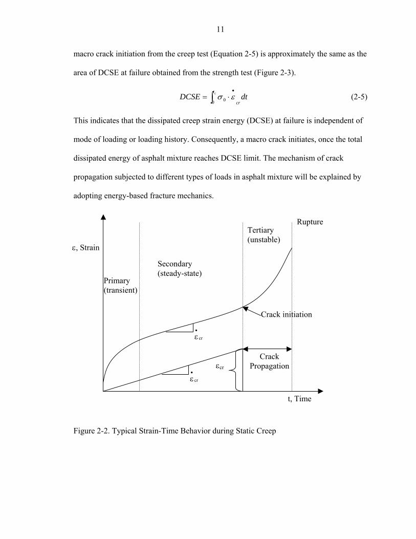
expressed as shown in Figure 2-2, where crε& is a rate of creep strain, and εcr is a amount
of creep strain. In general, three stages: primary, secondary, and tertiary are observed
during the creep test. The sate of the tertiary stage coincides with the development of a
local, which then propagate throughout the system (asphalt mixture), and eventually leads
to complete rupture. Kim (2003) reported that the dissipated creep strain energy up to the
11
macro crack initiation from the creep test (Equation 2-5) is approximately the same as the
area of DCSE at failure obtained from the strength test (Figure 2-3).
dtDCSEcr
tc
∫•
⋅=0 0 εσ (2-5)
This indicates that the dissipated creep strain energy (DCSE) at failure is independent of
mode of loading or loading history. Consequently, a macro crack initiates, once the total
dissipated energy of asphalt mixture reaches DCSE limit. The mechanism of crack
propagation subjected to different types of loads in asphalt mixture will be explained by
adopting energy-based fracture mechanics.
cr
•
ε
Tertiary (unstable)
Primary (transient)
Secondary (steady-state)
εcr
cr
•
ε
Crack Propagation
Crack initiation
Rupture
ε, Strain
t, Time
Figure 2-2. Typical Strain-Time Behavior during Static Creep
12
Elastic Energy (EE)
Dissipated Creep Strain Energy (DCSE)
ε, Strain
σ, Stress
Figure 2-3. Determination of DCSE Limit
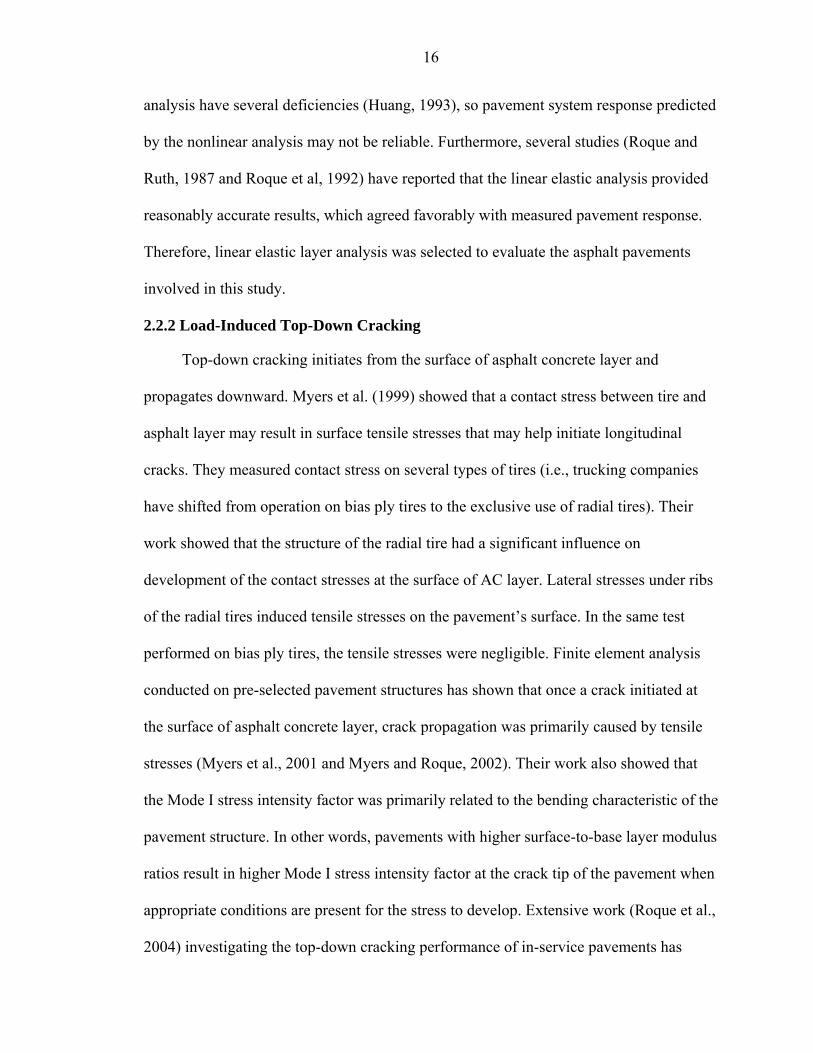
Process zones
DCSE Limit
Crack Tip
Stress Distribution
DCSE
Figure 2-4. Stress Distribution near the Crack Tip
2.1.4.3 Energy-based fracture mechanics
In Linear Elastic Fracture Mechanics (LEFM), stress distribution near the crack tip
depends on stress intensity factor K. Myers et al. (2001) reported that the crack

13
propagation of flexible pavement was primarily a tensile failure, which is driven by the
mode I stress intensity factor KI. Zhang et al. (2001) successfully applied the LEFM,
combining the threshold concept and limits presented above to asphalt mixtures. In their
study, crack propagation induced by applying repeated haversine loading in the indirect
tensile test was successfully predicted with their energy-based crack model.
The basic elements of the crack growth law used are illustrated in Figure 2-4,
which shows a generalized stress distribution in the vicinity of a crack subjected to
uniform tension. The specific stress distribution for a given loading condition will depend
on specific loading condition and the failure limits of the specific mixture. The HMA
fracture mechanics framework separated the area in front of the crack tip into a series of
“process zones.” The crack will propagate by the length of one of the process zones when
strain energy representing damage in that zone exceeds the appropriate energy threshold.
More detailed procedures in calculating crack propagation are specified in Zhang et al.
(2001).
2.1.4.4 Energy Ratio
From the engineering point of view, it is obvious that any theoretical model not
correlated to field performance data may not be reliable or even applicable. Roque et al.
(2004) have presented Energy Ratio (ER), which integrated the HMA Fracture Model
and effects of pavement structural characteristics to predict top-down cracking
performance of mixtures. Mixtures gathered from cracked and uncracked sections were
used to evaluate the reliability of ER. FWD tests were performed to define the structural
characteristics of all the sections. Standard Superpave IDT tests were conducted on cores
from twenty-two field sections, and each material property was analyzed with the HMA
fracture model to obtain the ER. Energy Ratio (ER) is defined as DCSE limit of the

14
mixture over DCSE minimum, which is the minimum DCSE required for good cracking
performance that serve as a single criterion for cracking performance considers both
asphalt mixture properties and pavement characteristics. The Energy Ratio is calculated
as follows:
[ ]1
98.2
81.3 1046.2)36.6(00299.0Dm
StDCSEER Limit
⋅⋅+−⋅
=−−σ (2-6)
where all parameters: applied stress σ, failure strength St, D1 and m values should be
properly obtained from structural analysis and Superpave IDT. The Energy Ratio must be
greater than 1.0 for the mixture to be acceptable.
2.1.5 Thermal Cracking
The primary mechanism generally associated with temperature-induced thermal
cracking is a “top-down” initiation and propagation. Contraction strains induced by
pavement cooling lead to thermal tensile stress development in the restrained surface layer
where thermal stress is greatest at the surface of the pavement because pavement
temperature is lowest at the surface and temperature changes are highest there. Even though
the major distress of the thermal stress is known as transverse cracking, the effect of daily
temperature cooling cycles may have a significant influence on the development of top-
down cracking. Dauzats and Rampal (1987) surveyed several pavement sections located
in the south of France where pavements are subjected to extreme thermal stresses. Top-
down cracks in these sections were observed 3 to 5 years after construction of the road.
Therefore, thermal stress may significantly contribute to the development of top-down
cracking.
Several different thermal cracking models have been developed using empirical
and/or analytical approaches. TC model (Hiltunen and Roque, 1994) developed based on

15
the theory of linear viscoelasticity appears to be more comprehensive than other models
in the literature. However, their approach essentially did not incorporate a fundamental
damage development of asphalt mixtures. Conversely, the HMA Fracture Model (Zhang
et al., 2001), which was developed based on energy-based fracture mechanism, has not
been used to predict thermal cracking of asphalt pavements. Consequently, it appears
desirable to develop a proper thermal cracking model, which is able to incorporate the
HMA fracture model.
In addition, Lytton et al. (1983) and Roque and Ruth (1990) have noted that
thermal cracking is significantly affected by the material properties of asphalt concrete
and environmental conditions. Although it is known that pavement thickness may have
some effects on thermal cracking, the significance of pavement structure is not yet clear.
Therefore, in development of a thermal crack model, which will be introduced in Chapter
6, the effect of pavement structure was not considered.
2.2 Cracking Mechanisms Associated with Pavement Structure
2.2.1 Classic Fatigue Cracking
Fatigue cracking or load-induced cracking of flexible pavement is caused by
repeated traffic loading. The cracks initiate at the bottom of the asphalt concrete layer,
and then propagate to the surface due to the highest tensile stress or strain at the bottom
of AC layer. It is well known that the asphalt pavement structure can be represented as a
layered system (e.g. asphalt concrete, base, subbase, and subgrade), which can be
analyzed using either linear elastic or nonlinear layer analysis. Due to its convenience,
linear elastic layer analysis is widely used and appears to be a reasonably accurate to
predict surface lager response. However, unbound layers may be more accurately
represented by use of nonlinear analysis. Currently, the systems available for nonlinear
16
analysis have several deficiencies (Huang, 1993), so pavement system response predicted
by the nonlinear analysis may not be reliable. Furthermore, several studies (Roque and
Ruth, 1987 and Roque et al, 1992) have reported that the linear elastic analysis provided
reasonably accurate results, which agreed favorably with measured pavement response.
Therefore, linear elastic layer analysis was selected to evaluate the asphalt pavements
involved in this study.
2.2.2 Load-Induced Top-Down Cracking
Top-down cracking initiates from the surface of asphalt concrete layer and
propagates downward. Myers et al. (1999) showed that a contact stress between tire and
asphalt layer may result in surface tensile stresses that may help initiate longitudinal
cracks. They measured contact stress on several types of tires (i.e., trucking companies
have shifted from operation on bias ply tires to the exclusive use of radial tires). Their
work showed that the structure of the radial tire had a significant influence on
development of the contact stresses at the surface of AC layer. Lateral stresses under ribs
of the radial tires induced tensile stresses on the pavement’s surface. In the same test
performed on bias ply tires, the tensile stresses were negligible. Finite element analysis
conducted on pre-selected pavement structures has shown that once a crack initiated at
the surface of asphalt concrete layer, crack propagation was primarily caused by tensile
stresses (Myers et al., 2001 and Myers and Roque, 2002). Their work also showed that
the Mode I stress intensity factor was primarily related to the bending characteristic of the
pavement structure. In other words, pavements with higher surface-to-base layer modulus
ratios result in higher Mode I stress intensity factor at the crack tip of the pavement when
appropriate conditions are present for the stress to develop. Extensive work (Roque et al.,
2004) investigating the top-down cracking performance of in-service pavements has

17
shown that a tensile stress obtained from the bottom of AC layer could serve as a
substitute of estimation of relative tensile stresses present at the surface of AC layer. As a
result, the tensile stress at the bottom of AC appears to be a suitable parameter to describe
the structural characteristics of asphalt pavement.
CHAPTER 3 TEST SECTIONS, MATERIALS, AND METHODS
Multi-year study involved multiple sets of test section has been conducted in
Florida to investigate top-down performance of the in-service asphalt pavements. Two
sets of top-down cracking projects were chosen for this study from among the available
sections. This chapter will provide locations and condition, field evaluation, and binder
and mixture properties of the pavement sections that were used in this study.
3.1 Locations and Condition
Eleven pavement sections were evaluated as part of this study. These sections were
divided into two groups (Group I and II). A general description of these sections is
presented below.
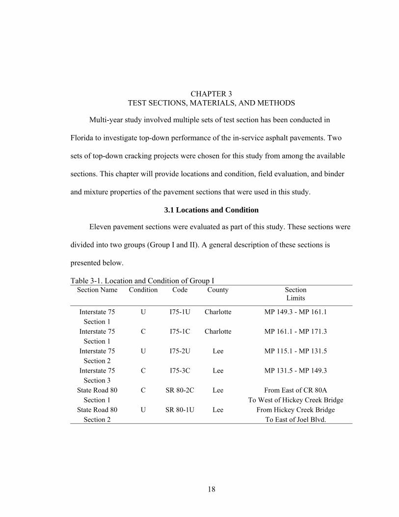
Table 3-1. Location and Condition of Group I Section Name Condition Code County Section
Limits
Interstate 75 U I75-1U Charlotte MP 149.3 - MP 161.1 Section 1
Interstate 75 C I75-1C Charlotte MP 161.1 - MP 171.3 Section 1
Interstate 75 U I75-2U Lee MP 115.1 - MP 131.5 Section 2
Interstate 75 C I75-3C Lee MP 131.5 - MP 149.3 Section 3
State Road 80 C SR 80-2C Lee From East of CR 80A Section 1 To West of Hickey Creek Bridge
State Road 80 U SR 80-1U Lee From Hickey Creek Bridge Section 2 To East of Joel Blvd.
18

19
3.1.1 Group I
This group consists of six pavement sections (Table 3-1) evaluated by Jajliardo
(2003), (Table 3-1), which exhibited good and poor top-down cracking performance. A
thorough description of the six sections, including experiment results and evaluation
appears in Jajliardo (2003).
3.1.2 Group II
An additional five test sections (Table 3-2) were cored from four different locations
(Figure 3-1) were selected for study. General descriptions of these sections are presented
below.
Table 3-2. Location and Condition of Group II Section Name Condition Code Country Section
Limits Interstate 10
Section 8 C I10-8C Suwannee The west side of US-129: MP 15.144 -MP 18.000
Interstate 10 Section 9 U I10-9U Suwannee The west side of US-129: MP 18.000 -
MP 21.474
State Road 471 C SR 471C Sumter The northbound lane three miles north of the Withlacoochee River
State Road 19 C SR 19C Lake The southbound lane five miles south of S.R. 40
State Road 997 U SR 997U Dade The northbound lane 7.6 miles south of US-27
• First, two adjacent sections, section 8 and section 9 located in I-10 in Suwannee
Country, North Florida were selected, where section 8 had exhibited significant top-down cracking, but section 9 was not cracked. Since those sections were connected, they had similar external conditions such as traffic volume and environment. In addition the age since construction was identical (about 7 to 8 years).
• Second, state road 471 and state road 19 located in Sumter County and Lake County, Central Florida respectively were selected to evaluate the top-down cracking performance. Both sections were constructed using hot-in-place recycling, and both exhibited significant top-down cracking after only 2 to 3 years of sevice.

20
• Last, state road 997 is one of the most excellent performing sections. State road 997 located in Dade County, South Florida has shown good performance without any visual cracks during 40 years of service, making it one of the most interesting sections in this project.
Group I
SR 997U
SR 471C
SR 19C
I10-8C I10-9U
Figure 3-1. Location of Sections (Group II)
3.2 Traffic Volume
The traffic volumes obtained from each section are shown in Table 3-3. These
values are expressed in thousands of ESALS.
21
Table 3-3. Traffic Volumes of Group II Sections ESAL/year×1000 I10-1C 392 I10-1U 392 SR 471 26 SR 19 51
SR 997 89
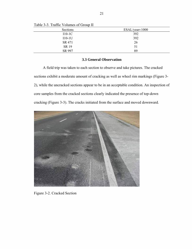
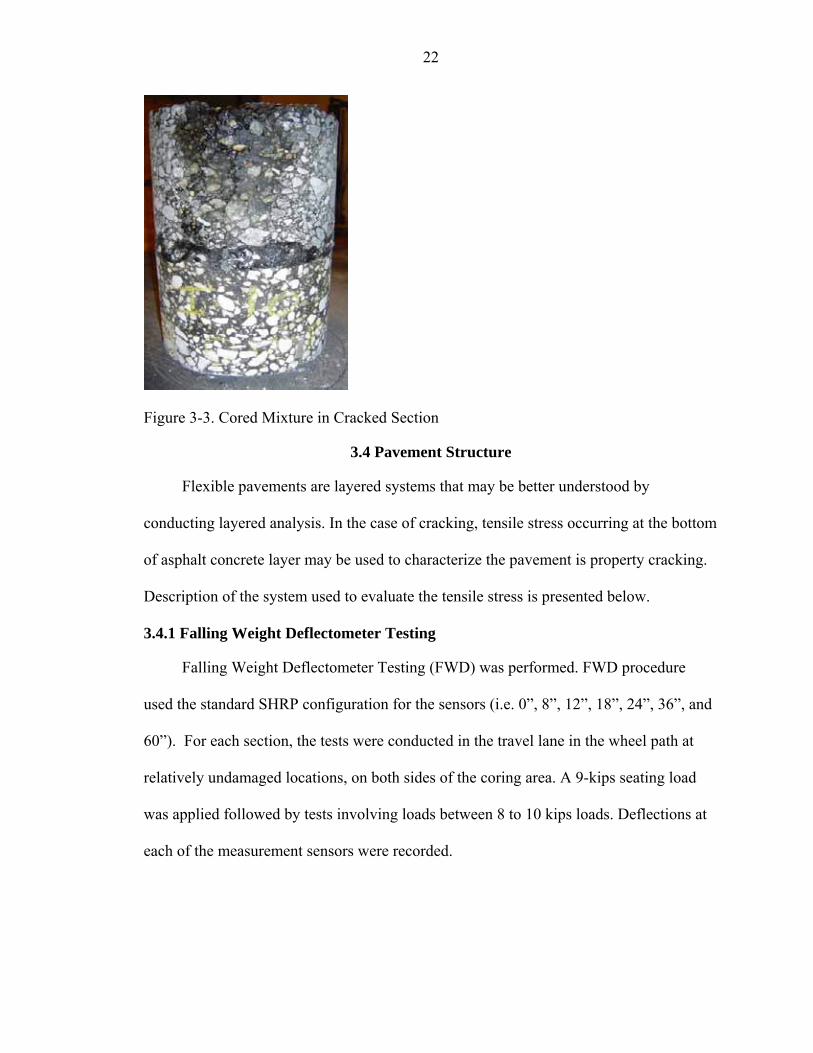
3.3 General Observation
A field trip was taken to each section to observe and take pictures. The cracked
sections exhibit a moderate amount of cracking as well as wheel rim markings (Figure 3-
2), while the uncracked sections appear to be in an acceptable condition. An inspection of
core samples from the cracked sections clearly indicated the presence of top-down
cracking (Figure 3-3). The cracks initiated from the surface and moved downward.
Figure 3-2. Cracked Section
22
Figure 3-3. Cored Mixture in Cracked Section
3.4 Pavement Structure
Flexible pavements are layered systems that may be better understood by
conducting layered analysis. In the case of cracking, tensile stress occurring at the bottom
of asphalt concrete layer may be used to characterize the pavement is property cracking.
Description of the system used to evaluate the tensile stress is presented below.
3.4.1 Falling Weight Deflectometer Testing
Falling Weight Deflectometer Testing (FWD) was performed. FWD procedure
used the standard SHRP configuration for the sensors (i.e. 0”, 8”, 12”, 18”, 24”, 36”, and
60”). For each section, the tests were conducted in the travel lane in the wheel path at
relatively undamaged locations, on both sides of the coring area. A 9-kips seating load
was applied followed by tests involving loads between 8 to 10 kips loads. Deflections at
each of the measurement sensors were recorded.
23
0
2
4
6
8
10
12
14
16
18
0 10 20 30 40 50 60 70
Distance (in)
Def
lect
ion
(in) I10 - 8C
I10 - 9USR 471CSR 19CSR 997U
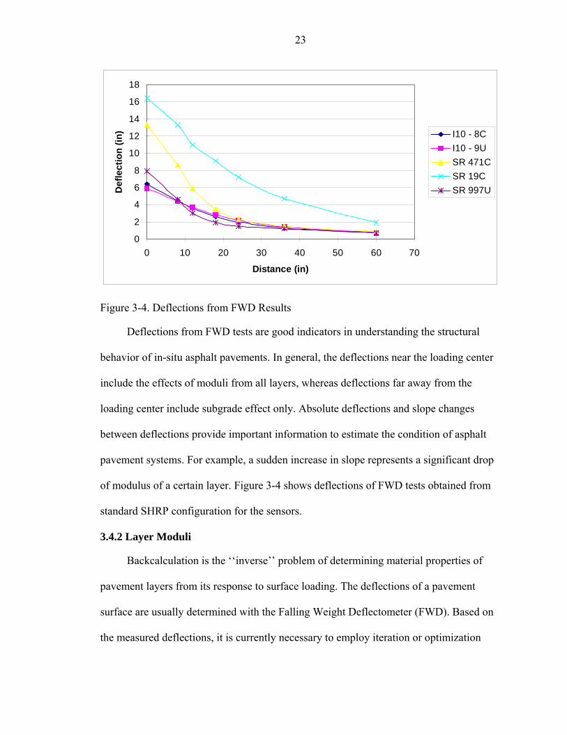
Figure 3-4. Deflections from FWD Results
Deflections from FWD tests are good indicators in understanding the structural
behavior of in-situ asphalt pavements. In general, the deflections near the loading center
include the effects of moduli from all layers, whereas deflections far away from the
loading center include subgrade effect only. Absolute deflections and slope changes
between deflections provide important information to estimate the condition of asphalt
pavement systems. For example, a sudden increase in slope represents a significant drop
of modulus of a certain layer. Figure 3-4 shows deflections of FWD tests obtained from
standard SHRP configuration for the sensors.
3.4.2 Layer Moduli
Backcalculation is the ‘‘inverse’’ problem of determining material properties of
pavement layers from its response to surface loading. The deflections of a pavement
surface are usually determined with the Falling Weight Deflectometer (FWD). Based on
the measured deflections, it is currently necessary to employ iteration or optimization
24
schemes to calculate theoretical deflections by varying the material properties until a
‘‘tolerable’’ match of measured deflection is obtained.
In the process of back calculation, elastic layer analysis program (BISDEF) was
used to assess the modulus value of each layer. A measured thickness of cored asphalt
mixture was used as for an asphalt layer thickness, which typical thickness of 12 inches
was assumed for the base and subbase layers (Table 3-4). The backcalculated moduli of
AC, base, subbase, and subgrade were then obtained. Moduli of five sections obtained in
this way are given in Table 3-5. More details of the calculated versus measured
deflections are given in Appendix A.
Table 3-4. Thickness of Layers Layers I10 - 8C I10 - 9U SR 471C SR 19C SR 997U
AC (psi) 7.20 7.40 2.58 2.39 2.17 Base (psi) 12 12 12 12 12
Subbase (psi) 12 12 12 12 12 Subgrade (psi) 240 240 240 240 240
Table 3-5. Backcalculated Moduli
Layers I10 - 8C I10 - 9U SR 471C SR 19C SR 997U AC (psi) 1428138 1481319 1112923 1348368 1703227
Base (psi) 55724 65179 27408 77971 75413 SubBase (psi) 54532 41414 136649 2644 315397 Subgrade (psi) 38868 46606 36107 27179 52389
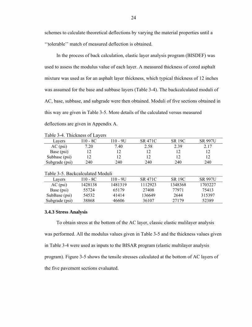
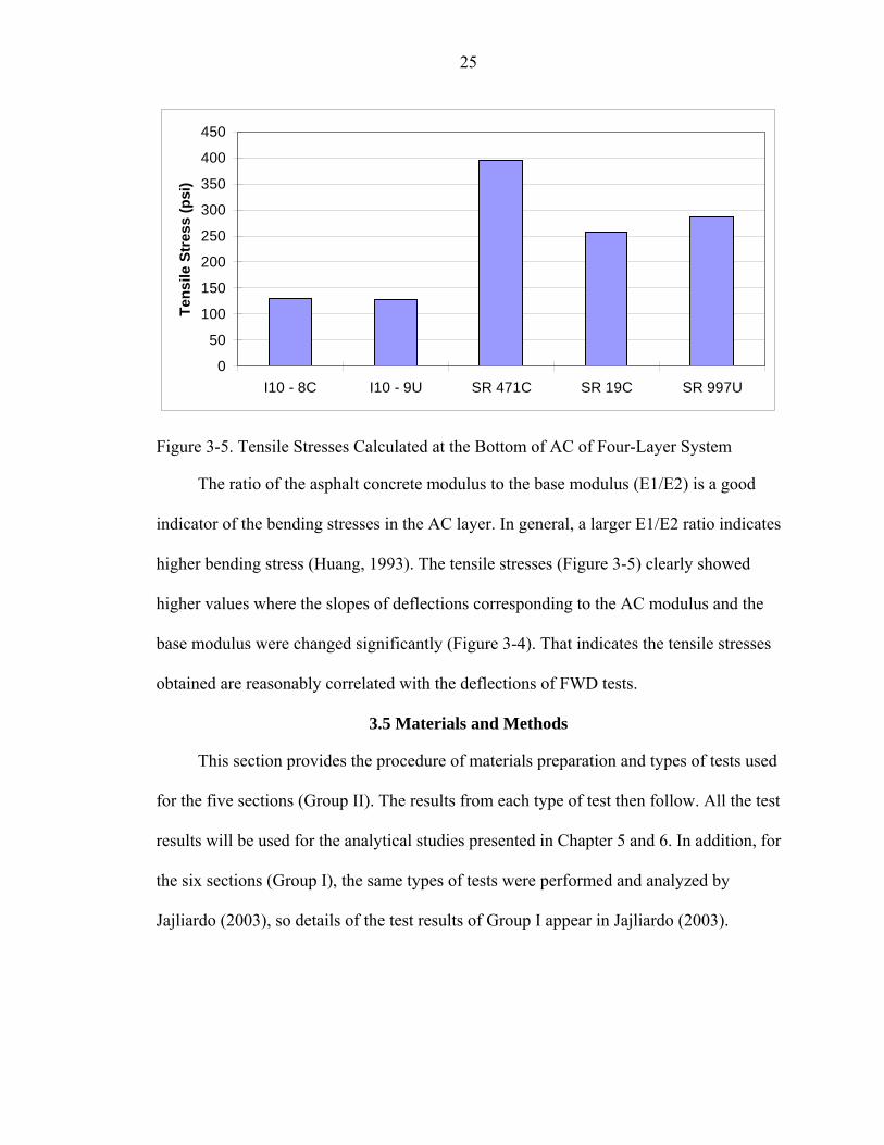
3.4.3 Stress Analysis
To obtain stress at the bottom of the AC layer, classic elastic mulilayer analysis
was performed. All the modulus values given in Table 3-5 and the thickness values given
in Table 3-4 were used as inputs to the BISAR program (elastic multilayer analysis
program). Figure 3-5 shows the tensile stresses calculated at the bottom of AC layers of
the five pavement sections evaluated.
25
0
50
100
150
200
250
300
350
400
450
I10 - 8C I10 - 9U SR 471C SR 19C SR 997U
Tens
ile S
tres
s (p
si)
Figure 3-5. Tensile Stresses Calculated at the Bottom of AC of Four-Layer System
The ratio of the asphalt concrete modulus to the base modulus (E1/E2) is a good
indicator of the bending stresses in the AC layer. In general, a larger E1/E2 ratio indicates
higher bending stress (Huang, 1993). The tensile stresses (Figure 3-5) clearly showed
higher values where the slopes of deflections corresponding to the AC modulus and the
base modulus were changed significantly (Figure 3-4). That indicates the tensile stresses
obtained are reasonably correlated with the deflections of FWD tests.
3.5 Materials and Methods
This section provides the procedure of materials preparation and types of tests used
for the five sections (Group II). The results from each type of test then follow. All the test
results will be used for the analytical studies presented in Chapter 5 and 6. In addition, for
the six sections (Group I), the same types of tests were performed and analyzed by
Jajliardo (2003), so details of the test results of Group I appear in Jajliardo (2003).
26
3.5.1 Materials Preparation
Eighteen 6 in. diameter cores were obtained from between wheel paths, and
eighteen cores were obtained in the outer wheel path of the traffic lane of each test
section. The coring location was carefully selected through field inspection as being
representative in terms of the overall performance of the section. In cracked areas, great
care was taken to assure that wheel path cores were not taken through cracks in the
pavement. All cores were carefully marked the direction of traffic loading. Upon
inspection in the laboratory, the thickness of each lift was measured and recorded.
Approximately 1.5 in. thick slices of the surface mixture were taken for testing.
The bulk specific gravity of all the sliced specimens was measured and then dried. A
number of slices were used for extraction and recovery of binder, and determination of
maximum theoretical density of the mixture. The remaining cores were used to mixture
tests using standard Superpave IDT: resilient modulus, creep compliance, and strength
tests.
3.5.2 Measurement of Volumetric and Binder Properties
Bulk specific gravity tests (AASHTO T-166) and maximum specific gravity tests
(AASHTO T-209) were performed to determine in-place air voids. Binders were
extracted and recovered binders obtained through extraction and recovery tests (SHRP B-
006) and viscosity was determined using the rotational viscometer (ASTM D 4402).
More details with respect to the testing procedures are specified in the references.
3.5.3 Measurement of Mixture Properties
Although several types of tests (e.g., uniaxial and triaxial compression, beam
flexure, hollow cylinder, etc.) are being used to test of asphalt mixtures, cracking is
essentially associated with tensile properties of mixtures. From that standpoint, the
27
Superpave indirect tensile test (IDT) developed as part of the Strategic Highway
Research Program (SHRP) was used to determine tensile properties from field cores.
Superpave IDT was used to perform three types of tests: resilient modulus, creep
compliance, and tensile strength. General descriptions associated with the testing and
data analysis system are presented below.
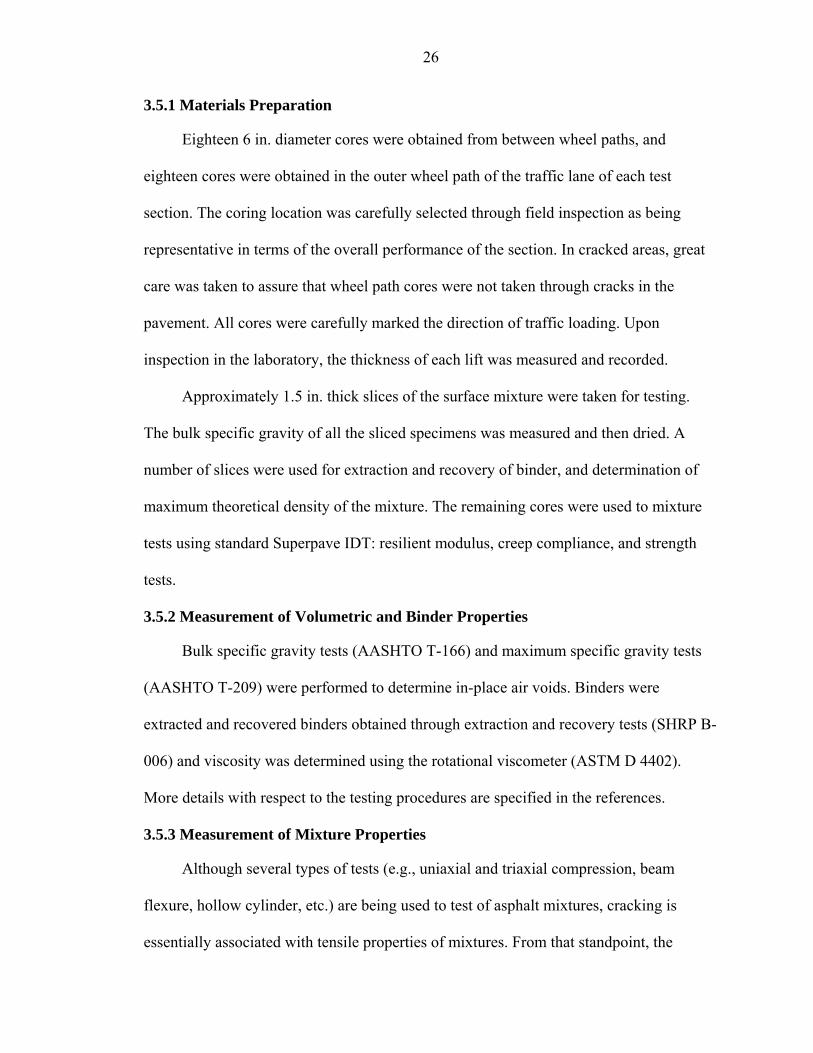
3.5.3.1 Experimental design of Superpave IDT
The testing system used included a servo hydraulic testing machine and
extensometers mounted on the specimen for measuring displacement (Figure 3-6). The
measurement system is attached close to the center of specimen, but 1.5 in. gage length is
commonly used for properly assessing aggregate effects. Three specimens (6 in. diameter
by about 1.5 in. thick) cut from the asphalt mixture are required to perform one set of
Superpave IDT tests at one temperature. Three test temperatures, 0, 10, and 20°C, which
are typical low in-service temperatures in Florida, were used. More detail procedures are
specified in Roque et al. (1997).
Figure 3-6. Superpave Indirect Tensile Test (IDT)
28
3.5.3.2 Description of testing types
Three types of tests, resilient modulus, creep compliance, and tensile strength, were
performed for each set of three specimens. The resilient modulus test is performed in a
load-controlled mode by applying a repeated haversine waveform load to the specimen
for a period of 0.1 second followed by a rest period of 0.9 seconds. The load is selected to
keep the repeated horizontal strain between 100 and 300 micro-strain during the resilient
modulus test (Roque and Buttlar, 1992). The creep compliance test is also performed in
the load-controlled mode by applying a monotonic static load to the specimen for a
period of 1000 seconds. The load is selected to maintain the accumulative horizontal
strain below 1000 micro-strain (Buttlar and Roque, 1994). The strength test is performed
in a displacement-controlled mode. A rate of load ram displacement of 50m/min was
used.
3.5.3.3 Data analysis
The data analysis procedures developed by Roque et al (1997) were used ot
determine resilient modulus, creep compliance, tensile strength, failure strain, fracture
energy, and dissipated creep strain energy to failure.
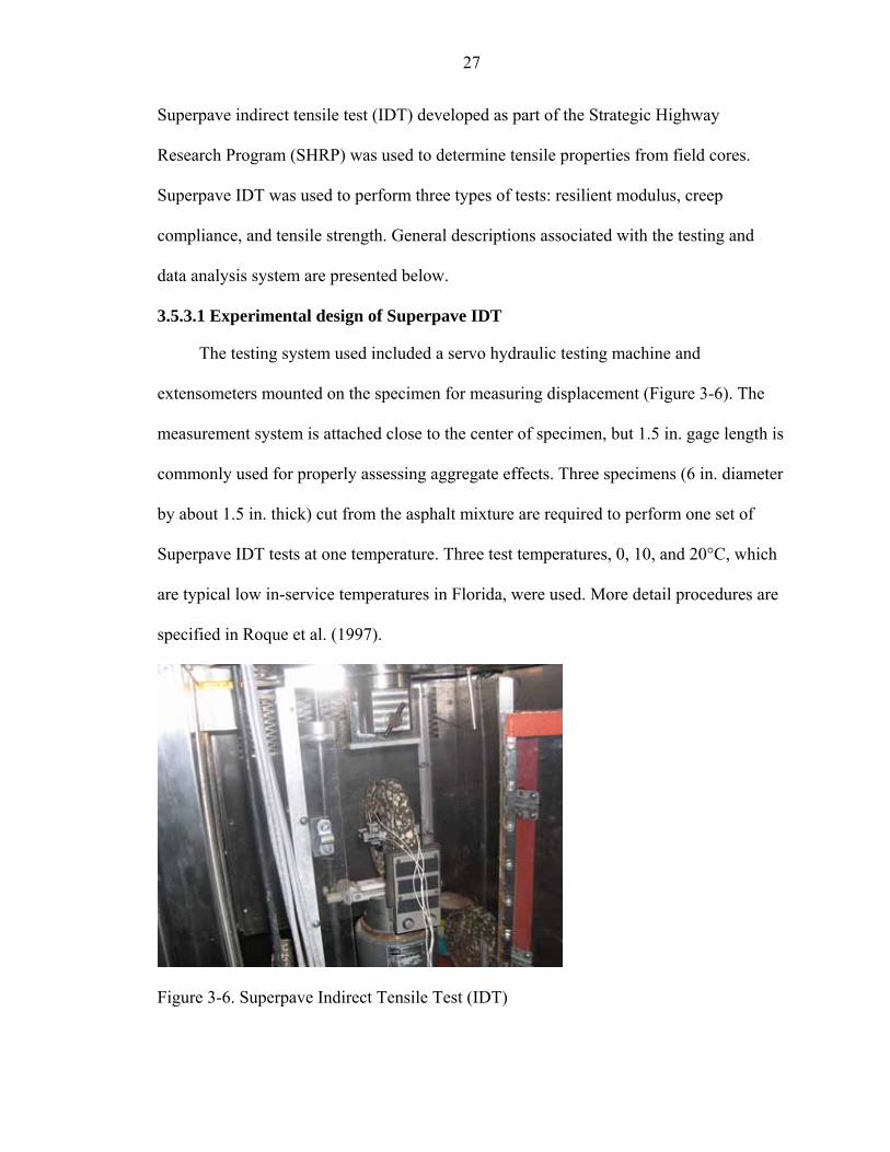
Table 3-6. Binder’s Viscosity Name Viscosity (cP) I10-8C 5689298 I10-9U 6158008
SR 471C 682359 SR 19C 442163
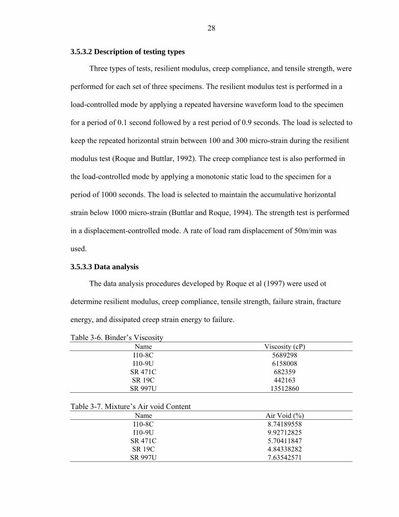
SR 997U 13512860 Table 3-7. Mixture’s Air void Content
Name Air Void (%) I10-8C 8.74189558 I10-9U 9.92712825
SR 471C 5.70411847 SR 19C 4.84338282
SR 997U 7.63542571
29
3.6 Experimental Results
3.6.1 Volumetric and Binder Properties
Extraction and recovery tests, and viscometer tests performed on binders from the
five test sections (Group II). The absolute viscosity of binders presented in Table 3-6 and
Figure 3-7). Air voids obtained from bulk specific gravity and maximum specific gravity
tests are presented in Table 3-7 and Figure 3-8.
0
2000000
4000000
6000000
8000000
10000000
12000000
14000000
16000000
I10-8C I10-9U SR 471C SR 19C SR 997U
Visc
osity
(cP)
Figure 3-7. Plot of Binder’s Viscosity
0
2
4
6
8
10
12
I10-8C I10-9U SR 471C SR 19C SR 997U
Air
Void
(%)
Figure 3-8. Plot of Mixture’s Air Void Content
30
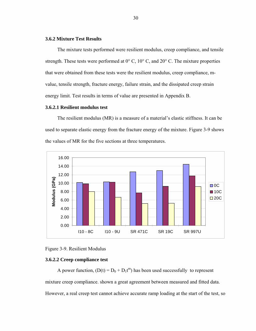
3.6.2 Mixture Test Results
The mixture tests performed were resilient modulus, creep compliance, and tensile
strength. These tests were performed at 0° C, 10° C, and 20° C. The mixture properties
that were obtained from these tests were the resilient modulus, creep compliance, m-
value, tensile strength, fracture energy, failure strain, and the dissipated creep strain
energy limit. Test results in terms of value are presented in Appendix B.
3.6.2.1 Resilient modulus test
The resilient modulus (MR) is a measure of a material’s elastic stiffness. It can be
used to separate elastic energy from the fracture energy of the mixture. Figure 3-9 shows
the values of MR for the five sections at three temperatures.
0.00
2.00
4.00
6.00
8.00
10.00
12.00
14.00
16.00
I10 - 8C I10 - 9U SR 471C SR 19C SR 997U
Mod
ulus
(GPa
)
0C10C20C
Figure 3-9. Resilient Modulus
3.6.2.2 Creep compliance test
A power function, (D(t) = D0 + D1tm) has been used successfully to represent
mixture creep compliance. shown a great agreement between measured and fitted data.
However, a real creep test cannot achieve accurate ramp loading at the start of the test, so
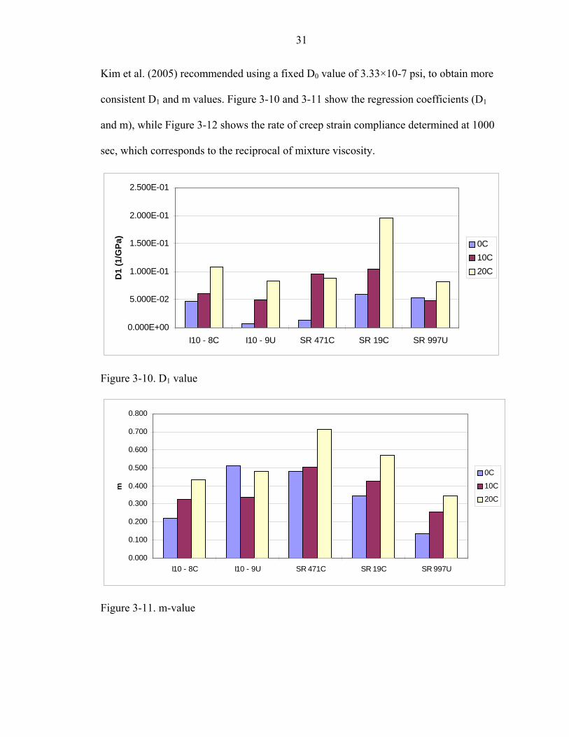
31
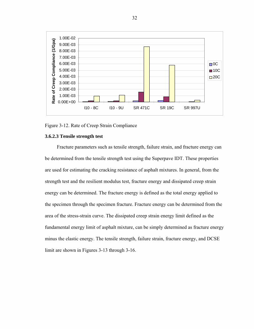
Kim et al. (2005) recommended using a fixed D0 value of 3.33×10⁻⁷ psi, to obtain more
consistent D1 and m values. Figure 3-10 and 3-11 show the regression coefficients (D1
and m), while Figure 3-12 shows the rate of creep strain compliance determined at 1000
sec, which corresponds to the reciprocal of mixture viscosity.
0.000E+00
5.000E-02
1.000E-01
1.500E-01
2.000E-01
2.500E-01
I10 - 8C I10 - 9U SR 471C SR 19C SR 997U
D1
(1/G
Pa)
0C10C20C
Figure 3-10. D1 value
0.000
0.100
0.200
0.300
0.400
0.500
0.600
0.700
0.800
I10 - 8C I10 - 9U SR 471C SR 19C SR 997U
m
0C
10C
20C
Figure 3-11. m-value
32
0.00E+001.00E-032.00E-033.00E-034.00E-035.00E-036.00E-037.00E-038.00E-039.00E-031.00E-02
I10 - 8C I10 - 9U SR 471C SR 19C SR 997U
Rat
e of
Cre
ep C
ompl
ianc
e (1
/Gpa
)
0C10C20C
Figure 3-12. Rate of Creep Strain Compliance
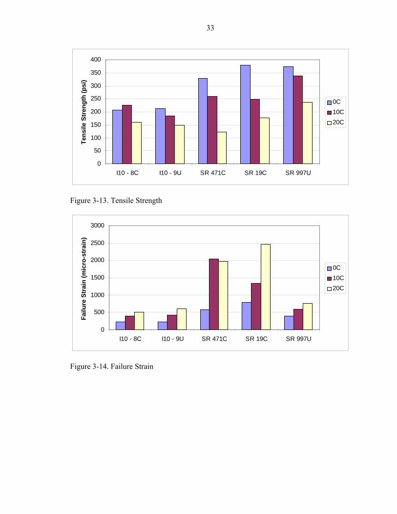
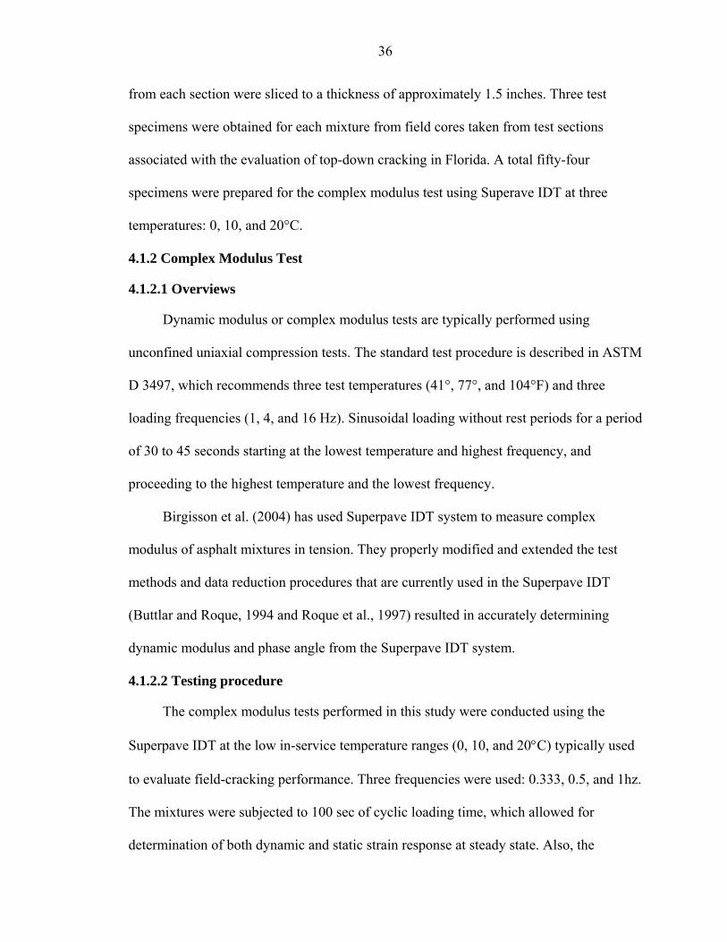
3.6.2.3 Tensile strength test
Fracture parameters such as tensile strength, failure strain, and fracture energy can
be determined from the tensile strength test using the Superpave IDT. These properties
are used for estimating the cracking resistance of asphalt mixtures. In general, from the
strength test and the resilient modulus test, fracture energy and dissipated creep strain
energy can be determined. The fracture energy is defined as the total energy applied to
the specimen through the specimen fracture. Fracture energy can be determined from the
area of the stress-strain curve. The dissipated creep strain energy limit defined as the
fundamental energy limit of asphalt mixture, can be simply determined as fracture energy
minus the elastic energy. The tensile strength, failure strain, fracture energy, and DCSE
limit are shown in Figures 3-13 through 3-16.
33
0
50
100
150
200
250
300
350
400
I10 - 8C I10 - 9U SR 471C SR 19C SR 997U
Tens
ile S
tren
gth
(psi
)
0C10C20C
Figure 3-13. Tensile Strength
0
500
1000
1500
2000
2500
3000
I10 - 8C I10 - 9U SR 471C SR 19C SR 997U
Failu
re S
trai
n (m
icro
-str
ain)
0C10C20C
Figure 3-14. Failure Strain
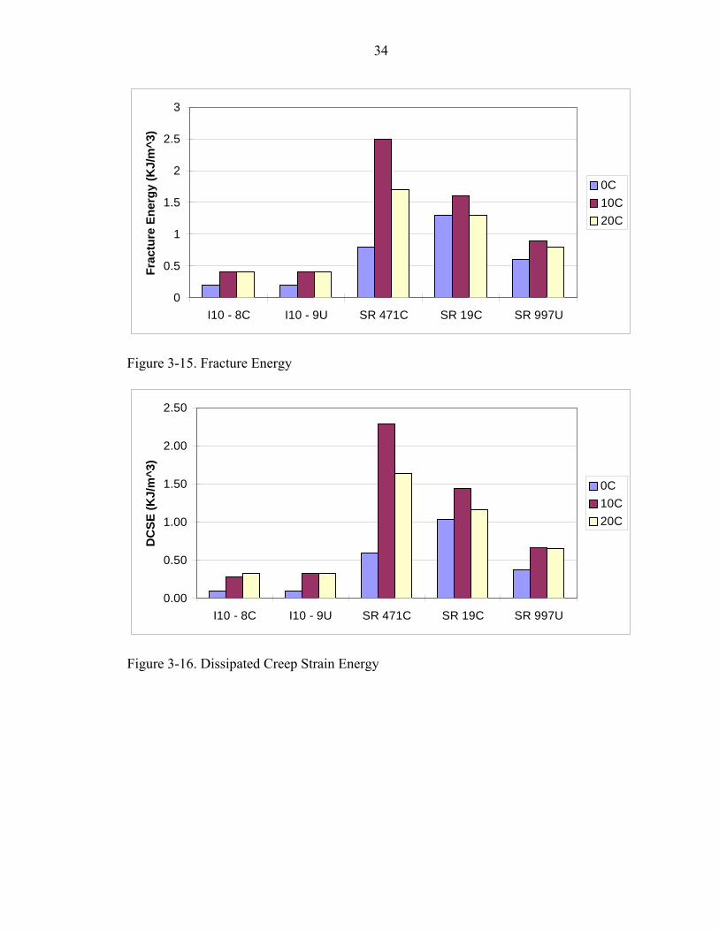
34
0
0.5
1
1.5
2
2.5
3
I10 - 8C I10 - 9U SR 471C SR 19C SR 997U
Frac
ture
Ene
rgy
(KJ/
m^3
)
0C10C20C
Figure 3-15. Fracture Energy
0.00
0.50
1.00
1.50
2.00
2.50
I10 - 8C I10 - 9U SR 471C SR 19C SR 997U
DC
SE (K
J/m
^3)
0C10C20C
Figure 3-16. Dissipated Creep Strain Energy

CHAPTER 4 DETERMINATION OF ENERGY DISSIPATION
The relationship between dissipated energy and fracture can be clearly illustrated
by using the HMA fracture mechanics model developed at the University of Florida. This
model, which has been verified with extensive laboratory and field testing, is based on
the principle that both crack initiation and crack growth are controlled by a mixture’s
tolerance to dissipated creep strain energy induced by applied loads. Specifically, a crack
will initiate and/or grow when the energy dissipated by the asphalt mixture exceeds the
dissipated creep strain energy limit of the mixture at any point in the material.
It is of interest to determine whether other test methods can be used to obtain the
rate of dissipated energy accumulation in asphalt mixtures. Of particular interest, is the
determination of dissipated energy from cyclic test data, since complex modulus testing
has become more common for asphalt mixture, and offers the promise of shorter testing
times and/or improved accuracy in determination of properties. Dissipated energy is
commonly determined from cyclic test data. The basic approach to determining rate of
dissipated energy accumulation for either static or cyclic creep tests is covered in the
following sections.
4.1 Materials and Methods
4.1.1 Materials
Mixtures obtained from six dense-graded sections were tested (Group I). Four
sections were from I-75: two in Charlotte County and two in Lee County, FL. The other
two test sections were from SR 80 in Lee County, Florida. Six-inch diameter cores taken
35
36
from each section were sliced to a thickness of approximately 1.5 inches. Three test
specimens were obtained for each mixture from field cores taken from test sections
associated with the evaluation of top-down cracking in Florida. A total fifty-four
specimens were prepared for the complex modulus test using Superave IDT at three
temperatures: 0, 10, and 20°C.
4.1.2 Complex Modulus Test
4.1.2.1 Overviews
Dynamic modulus or complex modulus tests are typically performed using
unconfined uniaxial compression tests. The standard test procedure is described in ASTM
D 3497, which recommends three test temperatures (41°, 77°, and 104°F) and three
loading frequencies (1, 4, and 16 Hz). Sinusoidal loading without rest periods for a period
of 30 to 45 seconds starting at the lowest temperature and highest frequency, and
proceeding to the highest temperature and the lowest frequency.
Birgisson et al. (2004) has used Superpave IDT system to measure complex
modulus of asphalt mixtures in tension. They properly modified and extended the test
methods and data reduction procedures that are currently used in the Superpave IDT
(Buttlar and Roque, 1994 and Roque et al., 1997) resulted in accurately determining
dynamic modulus and phase angle from the Superpave IDT system.
4.1.2.2 Testing procedure
The complex modulus tests performed in this study were conducted using the
Superpave IDT at the low in-service temperature ranges (0, 10, and 20°C) typically used
to evaluate field-cracking performance. Three frequencies were used: 0.333, 0.5, and 1hz.
The mixtures were subjected to 100 sec of cyclic loading time, which allowed for
determination of both dynamic and static strain response at steady state. Also, the

37
continuous sinusoidal load applied to the specimen was selected to maintain the
horizontal strain amplitude between 35 and 65 micro strain, which was decided from the
results of tens of preliminary tests. Additional details on the testing procedure used are as
follows:
• After cutting, all specimens were allowed to dry in a constant humidity chamber for a period of two days.
• Four brass gage points (5/16-inch diameter by 1/8-inch thick) were affixed with epoxy to each specimen face.
• Extensometers were mounted on the specimen. Horizontal and vertical deformations were measured on each side of the specimen.
• The test specimen was placed into the load frame. A seating load of 8 to 15 pounds was applied to the test specimen to ensure proper contact of the loading heads.
• The specimen was loaded by applying a repeated and continuous sinusoidal load, where strain level by one cyclic load was adjusted between 35 and 65 micro-strain.
• When the applied load was determined, a total of 100 sec loading time were applied to the specimen, and the computer software began recording the test data.
4.1.3 Static Creep Test
Although linear viscoelastic superposition principle indicates that creep response
from the average stress of complex modulus test should be identical to that from the static
creep test, to increase comparative purpose, static creep tests were performed after
complex modulus tests were done. The static creep tests were performed in the load-
controlled mode by applying a monotonic static load to the specimen for a period of 100
seconds, which is identical to the loading period of the complex modulus test used, and
the same temperature range (0, 10, and 20°C) was also identically used in the creep test.
In addition, the load is selected below a total accumulative horizontal strain of 500 micro-
strain. Details of testing procedure are described in Buttlar and Roque (1994).
38
4.2 Determination of Dissipated Energy
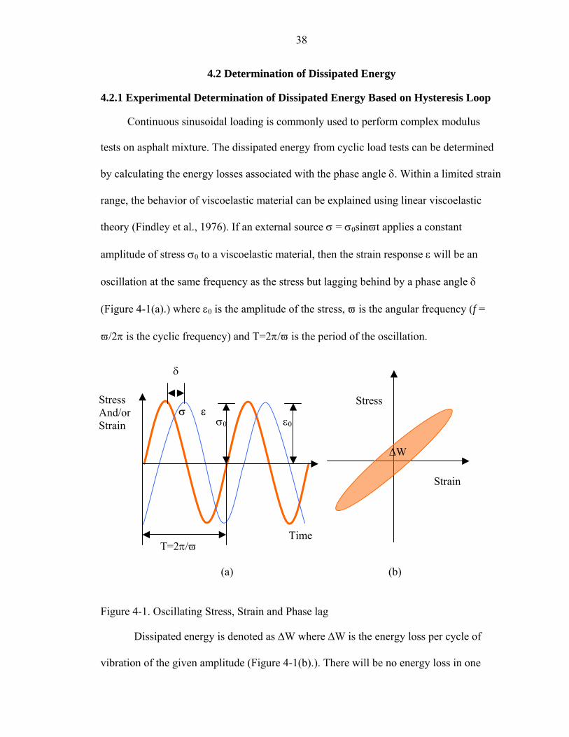
4.2.1 Experimental Determination of Dissipated Energy Based on Hysteresis Loop
Continuous sinusoidal loading is commonly used to perform complex modulus
tests on asphalt mixture. The dissipated energy from cyclic load tests can be determined
by calculating the energy losses associated with the phase angle δ. Within a limited strain
range, the behavior of viscoelastic material can be explained using linear viscoelastic
theory (Findley et al., 1976). If an external source σ = σ0sinϖt applies a constant
amplitude of stress σ0 to a viscoelastic material, then the strain response ε will be an
oscillation at the same frequency as the stress but lagging behind by a phase angle δ
(Figure 4-1(a).) where ε0 is the amplitude of the stress, ϖ is the angular frequency (f =
ϖ/2π is the cyclic frequency) and T=2π/ϖ is the period of the oscillation.
∆W
Strain
Stress
TimeT=2π/ϖ
ε σ
δ
ε0σ0
Stress And/or Strain
(a) (b)
Figure 4-1. Oscillating Stress, Strain and Phase lag
Dissipated energy is denoted as ∆W where ∆W is the energy loss per cycle of
vibration of the given amplitude (Figure 4-1(b).). There will be no energy loss in one
39
cycle if the stress and the strain are in phase, and hence δ = 0. The amount of energy loss
during one complete cycle can be calculated by integrating the increment of work done σ
dε over complete cycle of period T, as follows
∆W = ∫ε
σT
0
dtdtd (4-1)
Inserting σ = σ0sinϖt and dε/dt = ϖε0cos(ϖt - δ) into Equation 4-1, Equation 4-2 is
obtained.
∆W = (4-2) ∫ δ−ω⋅ωωσεT
000 dt)tcos(tsin
Integration of Equation 4-2 yields the following expression for energy loss per cycle.
∆W = πσ0ε0sinδ (4-3)
Equation 4-3 represents the internal loop area shown in Figure 4-1(b), which is the
dissipated energy per cycle.
4.2.2 Dissipated Energy from Static Creep Test Data
Figure 2-2 shows typical strain response during a constant load static creep test. As
shown in the Figure 2-2, the creep response can generally be separated into three distinct
stages. The first stage is the primary or transient stage where the response is highly
nonlinear due to the presence of delayed elasticity. The secondary stage begins once most
or all of the delayed elastic response has finished, and only the viscous response remains
such that the strain-time relationship becomes linear. The creep strain rate is
determined as the slope of this linear portion of the curve. The total creep strain can be
determined as the rate of creep multiplied by the time of loading. An increase in the rate
of creep strain signifies the start of the tertiary stage, which coincides with crack
cr
•
ε
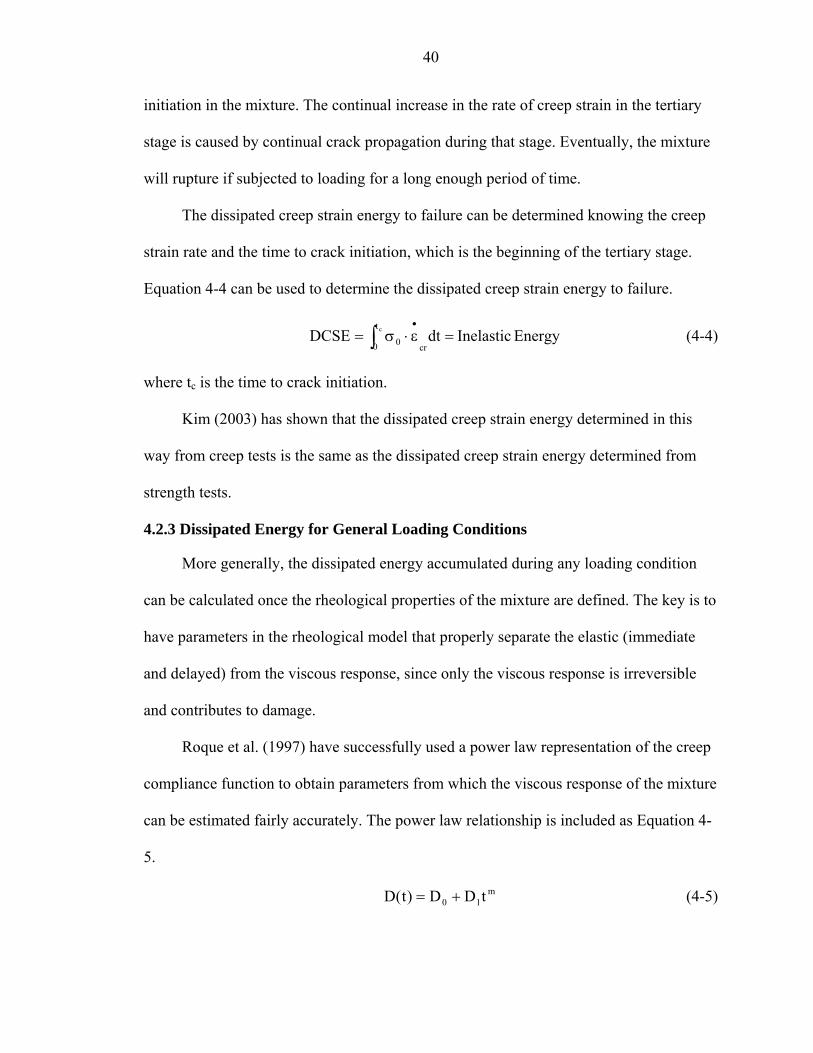
40
initiation in the mixture. The continual increase in the rate of creep strain in the tertiary
stage is caused by continual crack propagation during that stage. Eventually, the mixture
will rupture if subjected to loading for a long enough period of time.
The dissipated creep strain energy to failure can be determined knowing the creep
strain rate and the time to crack initiation, which is the beginning of the tertiary stage.
Equation 4-4 can be used to determine the dissipated creep strain energy to failure.
Energy Inelastic dtDCSEcr
t
0 0c =ε⋅σ= ∫
•
(4-4)
where tc is the time to crack initiation.
Kim (2003) has shown that the dissipated creep strain energy determined in this
way from creep tests is the same as the dissipated creep strain energy determined from
strength tests.
4.2.3 Dissipated Energy for General Loading Conditions
More generally, the dissipated energy accumulated during any loading condition
can be calculated once the rheological properties of the mixture are defined. The key is to
have parameters in the rheological model that properly separate the elastic (immediate
and delayed) from the viscous response, since only the viscous response is irreversible
and contributes to damage.
Roque et al. (1997) have successfully used a power law representation of the creep
compliance function to obtain parameters from which the viscous response of the mixture
can be estimated fairly accurately. The power law relationship is included as Equation 4-
5.
m10 tDD)t(D += (4-5)
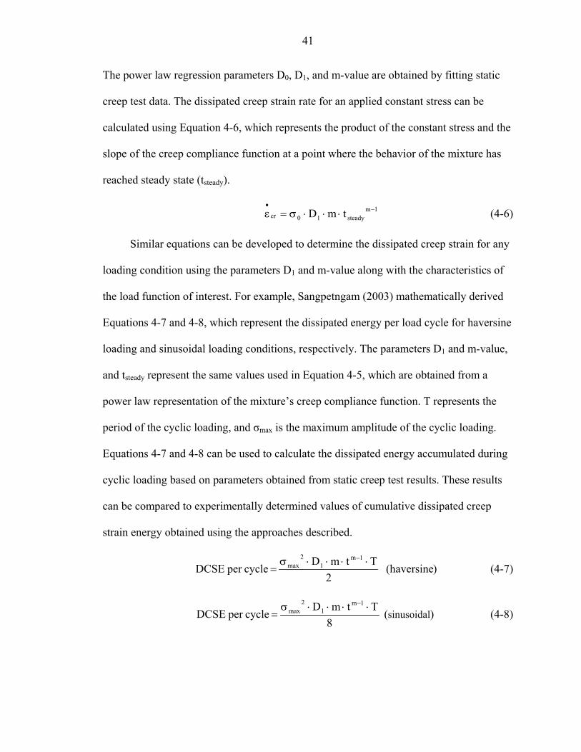
41
The power law regression parameters D0, D1, and m-value are obtained by fitting static
creep test data. The dissipated creep strain rate for an applied constant stress can be
calculated using Equation 4-6, which represents the product of the constant stress and the
slope of the creep compliance function at a point where the behavior of the mixture has
reached steady state (tsteady).
1msteady10cr tmD −
•
⋅⋅⋅σ=ε (4-6)
Similar equations can be developed to determine the dissipated creep strain for any
loading condition using the parameters D1 and m-value along with the characteristics of
the load function of interest. For example, Sangpetngam (2003) mathematically derived
Equations 4-7 and 4-8, which represent the dissipated energy per load cycle for haversine
loading and sinusoidal loading conditions, respectively. The parameters D1 and m-value,
and tsteady represent the same values used in Equation 4-5, which are obtained from a
power law representation of the mixture’s creep compliance function. T represents the
period of the cyclic loading, and σmax is the maximum amplitude of the cyclic loading.
Equations 4-7 and 4-8 can be used to calculate the dissipated energy accumulated during
cyclic loading based on parameters obtained from static creep test results. These results
can be compared to experimentally determined values of cumulative dissipated creep
strain energy obtained using the approaches described.
)(haversine 2
TtmD cycleper DCSE
1m1
2max ⋅⋅⋅⋅σ
=−
(4-7)
)( 8
TtmD cycleper DCSE sinusoidal
1m1
2max ⋅⋅⋅⋅σ
=−
(4-8)
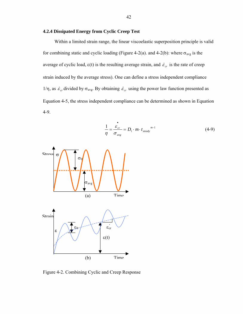
42
4.2.4 Dissipated Energy from Cyclic Creep Test
Within a limited strain range, the linear viscoelastic superposition principle is valid
for combining static and cyclic loading (Figure 4-2(a). and 4-2(b): where σavg is the
average of cyclic load, ε(t) is the resulting average strain, and crε& is the rate of creep
strain induced by the average stress). One can define a stress independent compliance
1/η, as crε& divided by σavg. By obtaining crε& using the power law function presented as
Equation 4-5, the stress independent compliance can be determined as shown in Equation
4-9.
11
1 −
•
⋅⋅== msteady
avg
cr tmDσε
η (4-9)
(a) Time
σavg
σ0 Stress σ
εcr
(b)
.ε
Time
Strain
ε(t)
ε0
Figure 4-2. Combining Cyclic and Creep Response
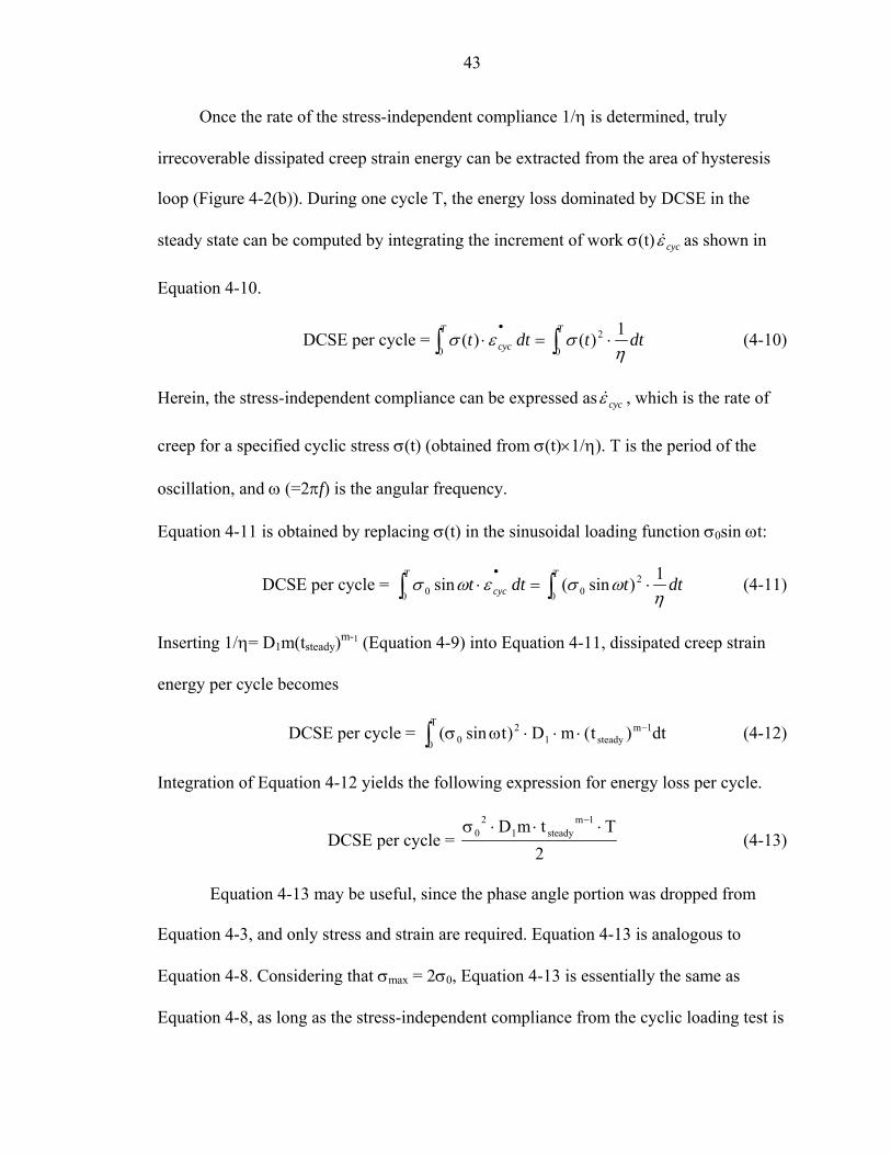
43
Once the rate of the stress-independent compliance 1/η is determined, truly
irrecoverable dissipated creep strain energy can be extracted from the area of hysteresis
loop (Figure 4-2(b)). During one cycle T, the energy loss dominated by DCSE in the
steady state can be computed by integrating the increment of work σ(t) cycε& as shown in
Equation 4-10.
DCSE per cycle = ∫∫ ⋅=⋅• TT
cyc dttdtt0
2
0
1)()(η
σεσ (4-10)
Herein, the stress-independent compliance can be expressed as cycε& , which is the rate of
creep for a specified cyclic stress σ(t) (obtained from σ(t)×1/η). T is the period of the
oscillation, and ω (=2πf) is the angular frequency.
Equation 4-11 is obtained by replacing σ(t) in the sinusoidal loading function σ0sin ωt:
DCSE per cycle = ∫∫ ⋅=⋅• TT
cyc dttdtt0
200 0
1)sin(sinη
ωσεωσ (4-11)
Inserting 1/η= D1m(tsteady)m-1 (Equation 4-9) into Equation 4-11, dissipated creep strain
energy per cycle becomes
DCSE per cycle = (4-12) dt)t(mD)tsin(T
0
1msteady1
20∫ −⋅⋅⋅ωσ
Integration of Equation 4-12 yields the following expression for energy loss per cycle.
DCSE per cycle = 2
TtmD 1msteady1
20 ⋅⋅⋅σ −
(4-13)
Equation 4-13 may be useful, since the phase angle portion was dropped from
Equation 4-3, and only stress and strain are required. Equation 4-13 is analogous to
Equation 4-8. Considering that σmax = 2σ0, Equation 4-13 is essentially the same as
Equation 4-8, as long as the stress-independent compliance from the cyclic loading test is
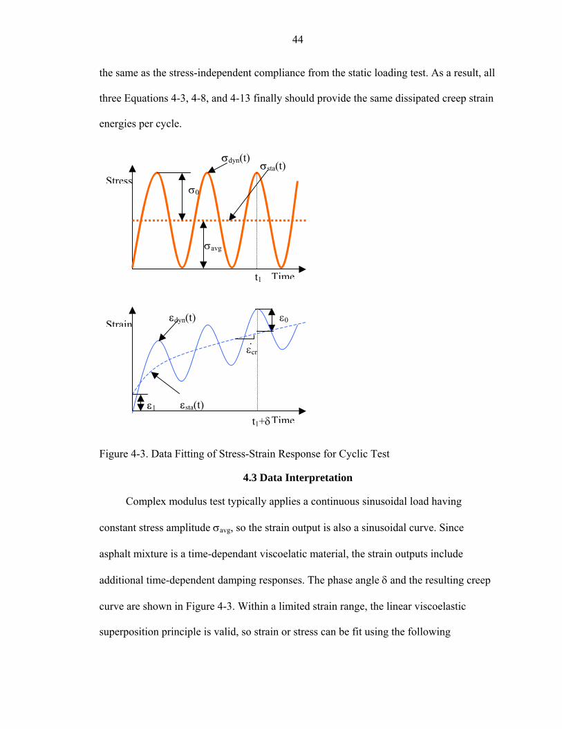
44
the same as the stress-independent compliance from the static loading test. As a result, all
three Equations 4-3, 4-8, and 4-13 finally should provide the same dissipated creep strain
energies per cycle.
t1
σsta(t) σdyn(t)
Time
σavg
σ0 Stress
ε1 εsta(t)
εdyn(t)
imeTt1+δ
Strain ε0
ε .
cr
Figure 4-3. Data Fitting of Stress-Strain Response for Cyclic Test
4.3 Data Interpretation
Complex modulus test typically applies a continuous sinusoidal load having
constant stress amplitude σavg, so the strain output is also a sinusoidal curve. Since
asphalt mixture is a time-dependant viscoelatic material, the strain outputs include
additional time-dependent damping responses. The phase angle δ and the resulting creep
curve are shown in Figure 4-3. Within a limited strain range, the linear viscoelastic
superposition principle is valid, so strain or stress can be fit using the following

45
functions: (4-14) through (4-17), Sinusoidal stress, average stress, sinusoidal strain and
creep strain is noted as σdyn, σsta, εdyn, and εsta respectively, and ω is the angular frequency
of a given complex modulus test. During the test, complex modulus (dynamic modulus
and phase angle) was determined at the average of five loading cycles, which were
recorded immediately before the end of the 100-sec loading time.
avgsta )t( σ=σ (4-14)
)tsin()t( 0dyn ω⋅σ=σ (4-15)
m21sta t)t( ⋅ε+ε=ε (4-16)
)t()tsin()t( sta0dyn ε+δ−ω⋅ε=ε (4-17)
Table 4-1. Energy from Hysteresis Loop and Static Creep Test Frequencies (hz) 0.333 0.5 1 0.333 0.5 1
Name Temp. (°C)
Energy from Hysteresis Loop (KJ/m^3)
Energy from Static Creep Test (KJ/m^3)
I75-1C 0 1.96E-02 1.96E-02 1.81E-02 4.82E-04 3.13E-04 1.41E-04 I75-1U 0 1.79E-02 1.88E-02 1.57E-02 4.14E-04 2.46E-04 1.54E-04 I75-3C 0 1.69E-02 1.83E-02 1.73E-02 4.80E-04 2.85E-04 1.52E-04 I75-2U 0 1.55E-02 1.17E-02 8.62E-03 2.34E-04 1.64E-04 7.43E-05 SR-1C 0 4.28E-02 4.72E-02 4.10E-02 1.15E-03 6.61E-04 3.49E-04 SR-2U 0 8.65E-03 9.59E-03 8.48E-03 2.72E-04 1.76E-04 5.79E-05 I75-1C 10 4.17E-02 4.12E-02 3.35E-02 1.95E-03 1.33E-03 6.33E-04 I75-1U 10 4.22E-02 4.16E-02 3.47E-02 1.33E-03 1.12E-03 5.63E-04 I75-3C 10 3.73E-02 3.30E-02 2.99E-02 1.46E-03 9.84E-04 5.56E-04 I75-2U 10 1.08E-02 1.59E-02 1.30E-02 8.08E-04 5.49E-04 2.68E-04 SR-1C 10 9.39E-02 8.46E-02 7.08E-02 3.28E-03 2.40E-03 1.16E-03 SR-2U 10 2.36E-02 2.09E-02 1.95E-02 5.77E-04 3.55E-04 1.67E-04 I75-1C 20 7.26E-02 5.72E-02 5.23E-02 4.31E-03 2.73E-03 1.52E-03 I75-1U 20 8.11E-02 7.07E-02 5.45E-02 3.66E-03 2.61E-03 1.43E-03 I75-3C 20 7.90E-02 6.90E-02 5.43E-02 5.42E-03 3.80E-03 1.92E-03 I75-2U 20 3.53E-02 2.99E-02 2.35E-02 2.20E-03 1.43E-03 6.94E-04 SR-1C 20 1.81E-01 1.72E-01 1.24E-01 9.22E-03 6.45E-03 2.99E-03 SR-2U 20 4.05E-02 4.19E-02 3.15E-02 1.31E-03 9.16E-04 4.78E-04
Equations )sin(*0 δ
σπ ⋅=
E
2)(
1
12
0 TtmD msteady
−
=σ

46
4.4 Analysis and Findings
If only irreversible energy dissipation is present during cyclic loading in the steady
state, then the dissipated energy determined from the hysteresis loop should equal the
dissipated creep strain energy (DCSE) predicted from viscous response parameters
obtained from static creep tests. In order to directly compare the dissipated energy per
cycle from the cyclic and the creep test, the same stress level was used.
Table 4-2. Energy from Cyclic and Static Creep Test Frequencies (hz) 0.333 0.5 1 0.333 0.5 1
Name Temp. (°C)
Energy Cyclic Test (KJ/m^3) Energy from Static Creep Test (KJ/m^3)
I75-1C 0 5.43E-04 3.62E-04 1.81E-04 4.82E-04 3.13E-04 1.41E-04 I75-1U 0 6.10E-04 4.07E-04 2.04E-04 4.14E-04 2.46E-04 1.54E-04 I75-3C 0 5.27E-04 3.52E-04 1.76E-04 4.80E-04 2.85E-04 1.52E-04 I75-2U 0 2.41E-04 1.61E-04 8.04E-05 2.34E-04 1.64E-04 7.43E-05 SR-1C 0 8.55E-04 5.70E-04 2.85E-04 1.15E-03 6.61E-04 3.49E-04 SR-2U 0 1.31E-04 8.75E-05 4.37E-05 2.72E-04 1.76E-04 5.79E-05 I75-1C 10 1.89E-03 1.26E-03 6.31E-04 1.95E-03 1.33E-03 6.33E-04 I75-1U 10 1.74E-03 1.16E-03 5.79E-04 1.33E-03 1.12E-03 5.63E-04 I75-3C 10 1.55E-03 1.03E-03 5.17E-04 1.46E-03 9.84E-04 5.56E-04 I75-2U 10 9.27E-04 6.18E-04 3.09E-04 8.08E-04 5.49E-04 2.68E-04 SR-1C 10 4.06E-03 2.71E-03 1.35E-03 3.28E-03 2.40E-03 1.16E-03 SR-2U 10 6.04E-04 4.03E-04 2.01E-04 5.77E-04 3.55E-04 1.67E-04 I75-1C 20 3.57E-03 2.38E-03 1.19E-03 4.31E-03 2.73E-03 1.52E-03 I75-1U 20 4.44E-03 2.96E-03 1.48E-03 3.66E-03 2.61E-03 1.43E-03 I75-3C 20 5.14E-03 3.43E-03 1.71E-03 5.42E-03 3.80E-03 1.92E-03 I75-2U 20 1.94E-03 1.29E-03 6.46E-04 2.20E-03 1.43E-03 6.94E-04 SR-1C 20 8.76E-03 5.84E-03 2.92E-03 9.22E-03 6.45E-03 2.99E-03 SR-2U 20 1.45E-03 9.67E-04 4.84E-04 1.31E-03 9.16E-04 4.78E-04
Equations 2
11
20 TtmD m
steady ⋅⋅⋅=
−••σ
: from cyclic response • 2)( 1
12
0 TtmD msteady ⋅⋅⋅
=−σ
Table 4-1 and Table 4-2 show a comparison of energies computed using the
different approaches. The equations used, which are stemmed from Equation 4-3,
Equation 4-8, and Equation 4-13 are shown in the tables, where σ0 is the half of the stress
applied, |E*| is dynamic modulus, and other parameters have the same meaning as in their
original equations.

47
The dissipated energy per cycle based on the phase angle was much greater than the
DCSE per cycle from creep test results, regardless of section, temperature, or frequency
of loading. The comparison is shown Figure 4-4. This appears to indicate that the
dissipated energy associated with the hysteresis loop includes responses other than just
viscous response and is not a good predictor of the DCSE per cycle.
0.000
0.050
0.100
0.150
0.200
0.000 0.050 0.100 0.150 0.200
DCSE/cycle from Static Creep Test (kJ/m^3)
DE/
cycl
e fr
om H
yste
resi
s Lo
op
(kJ/
m^3
) 0.33hz0.5hz1hz
Figure 4-4. Energy from Hysteresis Loop and Static Creep Test
The dissipated energy per cycle was also determined using creep parameters
obtained from the creep portion of the cyclic load tests. The results are presented in Table
4-2, and are compared to values determined using static creep test data in Figure 4-5. In
all cases, good agreement was observed between the cyclic and static creep tests. This
indicates that the stress-independent compliance η determined from cyclic creep tests is
essentially the same as the creep compliance determined from static creep.
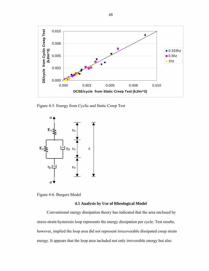
48
0.000
0.003
0.005
0.008
0.010
0.000 0.003 0.005 0.008 0.010
DCSE/cycle from Static Creep Test (kJ/m^3)
DE/
cycl
e fr
om C
yclic
Cre
ep T
est
(kJ/
m^3
) 0.333hz0.5hz1hz
Figure 4-5. Energy from Cyclic and Static Creep Test
η2 ε
σ
ε3
ε2
ε1
E2
η1
E1
σ
Figure 4-6. Burgers Model
4.5 Analysis by Use of Rheological Model
Conventional energy dissipation theory has indicated that the area enclosed by
stress-strain hysteresis loop represents the energy dissipation per cycle. Test results,
however, implied the loop area did not represent irrecoverable dissipated creep strain
energy. It appears that the loop area included not only irreversible energy but also
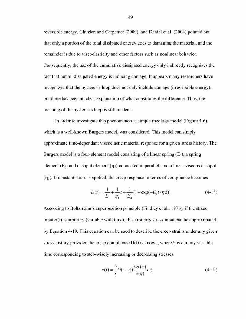
49
reversible energy. Ghuzlan and Carpenter (2000), and Daniel et al. (2004) pointed out
that only a portion of the total dissipated energy goes to damaging the material, and the
remainder is due to viscoelasticity and other factors such as nonlinear behavior.
Consequently, the use of the cumulative dissipated energy only indirectly recognizes the
fact that not all dissipated energy is inducing damage. It appears many researchers have
recognized that the hysteresis loop does not only include damage (irreversible energy),
but there has been no clear explanation of what constitutes the difference. Thus, the
meaning of the hysteresis loop is still unclear.
In order to investigate this phenomenon, a simple rheology model (Figure 4-6),
which is a well-known Burgers model, was considered. This model can simply
approximate time-dependant viscoelastic material response for a given stress history. The
Burgers model is a four-element model consisting of a linear spring (E1), a spring
element (E2) and dashpot element (η2) connected in parallel, and a linear viscous dashpot
(η1). If constant stress is applied, the creep response in terms of compliance becomes
))2/exp(1(111)( 2211
ηη
tEE
tE
tD −−++= (4-18)
According to Boltzmann’s superposition principle (Findley et al., 1976), if the stress
input σ(t) is arbitrary (variable with time), this arbitrary stress input can be approximated
by Equation 4-19. This equation can be used to describe the creep strains under any given
stress history provided the creep compliance D(t) is known, where ξ is dummy variable
time corresponding to step-wisely increasing or decreasing stresses.
∫ ∂∂
−=t
dtDt0 )(
)()()( ξξξσξε (4-19)
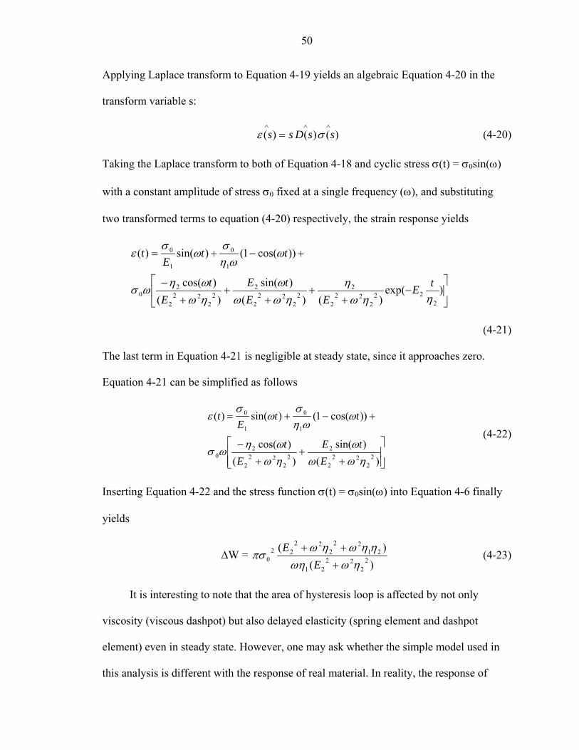
50
Applying Laplace transform to Equation 4-19 yields an algebraic Equation 4-20 in the
transform variable s:
∧∧∧
= )()()( ssDss σε (4-20)
Taking the Laplace transform to both of Equation 4-18 and cyclic stress σ(t) = σ0sin(ω)
with a constant amplitude of stress σ0 fixed at a single frequency (ω), and substituting
two transformed terms to equation (4-20) respectively, the strain response yields
⎥⎦
⎤⎢⎣
⎡−
++
++
+−
+−+=
)exp()()(
)sin()(
)cos(
))cos(1()sin()(
222
222
2
22
222
2
22
222
2
20
1
0
1
0
ηηωη
ηωωω
ηωωη
ωσ
ωωη
σω
σε
tEEE
tEE
t
ttE
t
(4-21)
The last term in Equation 4-21 is negligible at steady state, since it approaches zero.
Equation 4-21 can be simplified as follows
⎥⎥⎦
⎤
⎢⎢⎣
⎡
++
+
−
+−+=
)()sin(
)()cos(
))cos(1()sin()(
22
222
22
222
2
20
1
0
1
0
ηωωω
ηωωη
ωσ
ωωη
σω
σε
EtE
Et
ttE
t
(4-22)
Inserting Equation 4-22 and the stress function σ(t) = σ0sin(ω) into Equation 4-6 finally
yields
∆W = )(
)(2
222
21
2122
222
220 ηωωη
ηηωηωπσ
+++
EE (4-23)
It is interesting to note that the area of hysteresis loop is affected by not only
viscosity (viscous dashpot) but also delayed elasticity (spring element and dashpot
element) even in steady state. However, one may ask whether the simple model used in
this analysis is different with the response of real material. In reality, the response of
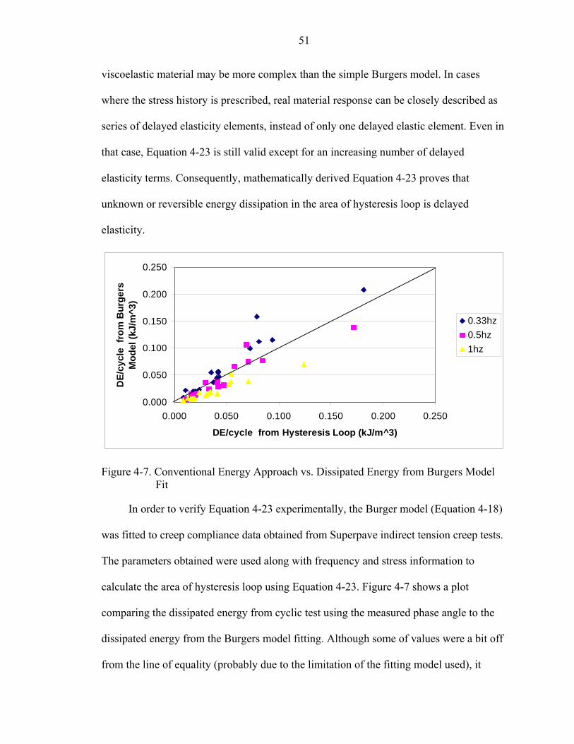
51
viscoelastic material may be more complex than the simple Burgers model. In cases
where the stress history is prescribed, real material response can be closely described as
series of delayed elasticity elements, instead of only one delayed elastic element. Even in
that case, Equation 4-23 is still valid except for an increasing number of delayed
elasticity terms. Consequently, mathematically derived Equation 4-23 proves that
unknown or reversible energy dissipation in the area of hysteresis loop is delayed
elasticity.
0.000
0.050
0.100
0.150
0.200
0.250
0.000 0.050 0.100 0.150 0.200 0.250
DE/cycle from Hysteresis Loop (kJ/m^3)
DE/
cycl
e fr
om B
urge
rsM
odel
(kJ/
m^3
)
0.33hz0.5hz1hz
Figure 4-7. Conventional Energy Approach vs. Dissipated Energy from Burgers Model
Fit
In order to verify Equation 4-23 experimentally, the Burger model (Equation 4-18)
was fitted to creep compliance data obtained from Superpave indirect tension creep tests.
The parameters obtained were used along with frequency and stress information to
calculate the area of hysteresis loop using Equation 4-23. Figure 4-7 shows a plot
comparing the dissipated energy from cyclic test using the measured phase angle to the
dissipated energy from the Burgers model fitting. Although some of values were a bit off
from the line of equality (probably due to the limitation of the fitting model used), it

52
clearly showed good agreement. It indicates that the area of hysteresis loop is dominated
by both delayed elasticity and viscous response. So, it is emphasized that the delayed
elasticity remains even in steady state.
To enhance the comparison, the former assumption that the area of hysteresis loop
is only dominated by unrecoverable damage (viscosity) was investigated with the same
fitting model. Since the dashpot (η2) has no effect in steady state in the former
assumption, only the first two terms are relevant in Equation 4-22, and the remaining E2
is combined with E1. It becomes a well-known Maxwell model as given in Equation 4-24.
))cos(1()sin()(1
00 ttE
t ωωη
σω
σε −+= (4-24)
where
21 /1/11
EEE
+=
Likewise, dissipated energy found by inserting Equation 4-24 and stress function into
Equation 4-6 yields
∆W = 1
20 ωη
πσ (4-25)
Figure 4-8 shows a plot comparing the dissipated energy from cyclic testing using
the phase angle to the dissipated energy obtained from the Maxwell model fit. Once
again, the dissipated energies from cyclic test were much higher than the energies from
the Maxwell model fitting results, which includes only the effects of viscous or dissipated
creep strain energy.
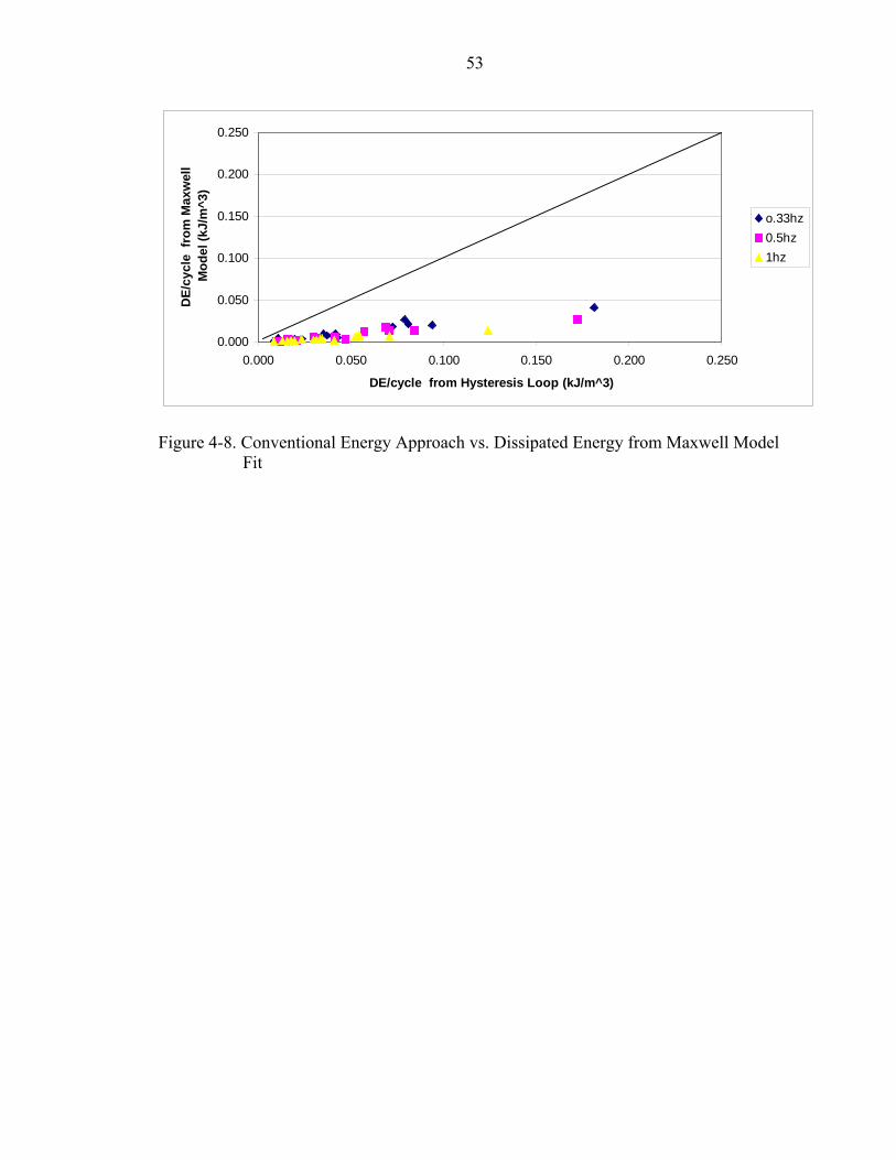
53
0.000
0.050
0.100
0.150
0.200
0.250
0.000 0.050 0.100 0.150 0.200 0.250
DE/cycle from Hysteresis Loop (kJ/m^3)
DE/
cycl
e fr
om M
axw
ell
Mod
el (k
J/m
^3)
o.33hz0.5hz1hz
Figure 4-8. Conventional Energy Approach vs. Dissipated Energy from Maxwell Model
Fit

CHAPTER 5 INTEGRATION OF THERMAL FRACTURE IN THE HMA FRACTURE MODEL
5.1 Review of the Past Work
5.1.1 TC Model
A mechanics-based thermal cracking performance model (TCMODEL) that was
developed as part of the Strategic Highway Research Program (SHRP) consists of two
main mechanisms: theory of linear viscoelasticity and linear elastic fracture mechanics. A
system to predict thermal stresses in asphalt pavement was developed on the basis of the
theory of linear viscoelasticity. The analytical derivations developed from the model that
will be incorporated in the system used in this research are explained below.
5.1.2 Conversion of Creep Compliance to Relaxation Modulus
The physical behavior of asphalt mixture can be approximated by theory of linear
viscoelasticity. The primary difference between linear elasticity and linear viscoelasticity
is time dependency. The time-dependent behavior of linear viscoelastic materials may be
studied by means of two types of experiments: creep and stress relaxation. Since creep
and stress relaxation phenomena are two aspects of the same viscoelastic behavior of
material, they are obviously related. In other words, one can be predicted if the other is
known. Therefore, the relaxation modulus is generally converted from a more convenient
stress-controlled creep compliance test.
The theoretical derivation for converting creep compliance to relaxation modulus
may be easily explained by a simple rheology model (Figure 4-6), which is the well-
known Burgers model. The Burgers model is a four-element model consisting of a linear
54

55
spring (E1), a spring element (E2) and dashpot element (η2) connected in parallel, and a
linear viscous dashpot (η1). If constant stress is applied, the creep response in terms of
compliance becomes
))2/exp(1(111)( 2211
ηη
tEE
tE
tD −−++= (5-1)
According to Boltzmann’s superposition principle (Findley et al., 1976), if the stress
input σ(t) is arbitrary (variable with time), this arbitrary stress input can be approximated
by Equation 5-2. This equation can be used to describe the creep strains under any given
stress history provided the creep compliance D(t) is known, where ξ is dummy variable
time corresponding to step-wise increasing or decreasing stresses.
∫ ∂∂
−=t
dtDt0 )(
)()()( ξξξσξε (5-2)
Applying Laplace transform to Equation 5-2 yields an algebraic Equation 5-3 in the
transform variable s:
∧∧∧
= )()()( ssDss σε (5-3)
Taking the Laplace transforms to both the creep compliance (Equation 5-1) and constant
input strain ε0, and substituting two transformed terms to Equation 5-3 respectively, the
stress response yields
2
21
21
2
2
2
1
1
1
2
2110
)()(1
)()(
sEE
sEEE
sEs ηηηηη
ηηηεσ
++++
+=
∧
(5-4)
Expanding Equation 5-4 by partial fractions and performing inverse Laplace
transformation yields

56
))exp()exp(()(2
21
10 λλεσ tCtCt −+−= (5-5)
The relaxation modulus becomes
)exp()exp()(2
21
1 λλtCtCtE −+−= (5-6)
The coefficients C1 and C2, and λ1 and λ1 correspond to E1 and E2, and η1 and
η2 of two Maxwell models connected in parallel as shown in Figure 5-1. As a result, a
generalized model, which has elastic response (spring), viscous response (dashpot), and
delayed elasticity with multiple retardation times can be mathematically converted to
multiple Maxwell models connected in parallel.
ε
ε
E2 E1
η1 η2
Figure 5-1. Two Maxwell Models Connected in Parallel
5.1.3 Time-Temperature Superposition Principle and Master Curve Fit
Theoretical and experimental results indicate that for linear viscoelastic materials,
the effect of time and temperature can be combined into a single parameter through the
concept of the time-temperature superposition principle. From a proper set of creep or
relaxation tests under different temperature levels the master curve can be generated by
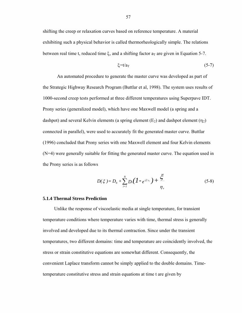
57
shifting the creep or relaxation curves based on reference temperature. A material
exhibiting such a physical behavior is called thermorheologically simple. The relations
between real time t, reduced time ξ, and a shifting factor aT are given in Equation 5-7.
ξ=t/aT (5-7)
An automated procedure to generate the master curve was developed as part of
the Strategic Highway Research Program (Buttlar et al, 1998). The system uses results of
1000-second creep tests performed at three different temperatures using Superpave IDT.
Prony series (generalized model), which have one Maxwell model (a spring and a
dashpot) and several Kelvin elements (a spring element (E2) and dashpot element (η2)
connected in parallel), were used to accurately fit the generated master curve. Buttlar
(1996) concluded that Prony series with one Maxwell element and four Kelvin elements
(N=4) were generally suitable for fitting the generated master curve. The equation used in
the Prony series is as follows
ηξ
ξτξ
v
/-i
N
=1i
+ )-(1 eD + D = )D( i∑0 (5-8)
5.1.4 Thermal Stress Prediction
Unlike the response of viscoelastic media at single temperature, for transient
temperature conditions where temperature varies with time, thermal stress is generally
involved and developed due to its thermal contraction. Since under the transient
temperatures, two different domains: time and temperature are coincidently involved, the
stress or strain constitutive equations are somewhat different. Consequently, the
convenient Laplace transform cannot be simply applied to the double domains. Time-
temperature constitutive stress and strain equations at time t are given by
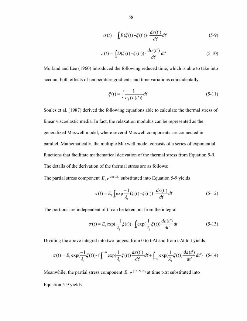
58
'')'())'()(()(
0dt
dttdttEt
t εξξσ ⋅−= ∫ (5-9)
''
)'())'()(()(0
dtdt
tdttDtt σξξε ⋅−= ∫ (5-10)
Morland and Lee (1960) introduced the following reduced time, which is able to take into
account both effects of temperature gradients and time variations coincidentally.
∫=t
T
dttTa
t0
'))'((
1)(ξ (5-11)
Soules et al. (1987) derived the following equations able to calculate the thermal stress of
linear viscoelastic media. In fact, the relaxation modulus can be represented as the
generalized Maxwell model, where several Maxwell components are connected in
parallel. Mathematically, the multiple Maxwell model consists of a series of exponential
functions that facilitate mathematical derivation of the thermal stress from Equation 5-9.
The details of the derivation of the thermal stress are as follows:
The partial stress component substituted into Equation 5-9 yields eE /t- 1)(1
λξ
'')'())'()((1exp)(
01
1 dtdt
tdttEtt εξξ
λσ ⋅−
−= ∫ (5-12)
The portions are independent of t’ can be taken out from the integral.
'')'())(1exp())(1exp()(
011
1 dtdt
tdttEtt εξ
λξ
λσ ∫⋅
−= (5-13)
Dividing the above integral into two ranges: from 0 to t-∆t and from t-∆t to t yields
}'')'())(1exp('
')'())(1exp({))(1exp()(
10
111 dt
dttdtdt
dttdttEt
t
tt
tt εξλ
εξλ
ξλ
σ ∫∫ ∆−
∆−+⋅
−= (5-14)
Meanwhile, the partial stress component at time t-∆t substituted into
Equation 5-9 yields
eE /tt- 1)(1
λξ ∆−

59
'')'())(1exp())(1exp()(
011
1 dtdt
tdtttEtttt εξ
λξ
λσ ∫
∆−⋅∆−
−=∆− (5-15)
The first term of Equation 5-14 can be replaced by Equation 5-15, which yields
}'')'())(1exp(
))(1exp(
)({))(1exp()(1
11
11 dt
dttdt
ttE
tttEtt
tt
εξλξ
λ
σξλ
σ ∫ ∆−+
∆−−
∆−⋅
−= (5-16)
The last term of Equation 5-16 can be rewritten as follows
t
tt
dttd
dt
td
t
∆−
⎥⎥⎥⎥⎥⎥
⎦
⎤
⎢⎢⎢⎢⎢⎢
⎣
⎡
⋅')'(
'
))'(1(
))'(1exp(
1
1 ε
ξλ
ξλ =
t
tttdtdt
∆−⎥⎦
⎤⎢⎣
⎡⋅
)'()'())'(1exp(
11 ξ
εξλ
λ (5-17)
Note that
b
a
b
a
dxxfdxfdxxf
⎥⎥⎥⎥
⎦
⎤
⎢⎢⎢⎢
⎣
⎡
=∫ ))(())(exp())(exp(
Assuming the dε(t’)/dξ(t’) is constant between t-∆t and t, Equation 5-17 becomes
⎥⎦
⎤⎢⎣
⎡∆−−
∆−−∆−−
=⎥⎦
⎤⎢⎣
⎡
∆−
))(1exp())(1exp()()()()())'(1exp(
)'()'(
111
11 ttt
ttttttt
tdtd
t
tt
ξλ
ξλξξ
εελξλξ
ελ
(5-18)
Substituting Equation 5-18 into 5-16 finally yields
))}]()((1exp{1[))()((
)())}()((1exp{)(1
11
1
tttttt
Etttttt ∆−−−
−∆−−
∆=∆−∆−−
−− ξξ
λξξελσξξ
λσ
(5-19)
Equation 5-19 deals with only one term of relaxation modulus. The rest of stress
components should be added up.
(t)i
1+N
1=i
= (t) σσ ∑ (5-20)

60
Lastly, the final equation of thermal stress prediction (Equation 5-20) can be determined
numerically using the finite difference method.
5.2 Development of Basic Algorithm for HMA Thermal Fracture Model
5.2.1 Development of Thermal Creep Strain Prediction
Although the power model has been successfully used as a fitting function of the
creep behavior for linear viscoelastic materials, its mathematical deficiency does not
allow predicting the thermal stress of viscoelastic materials under multiple temperature
ranges that indicates thermal creep strain should be predicted by viscosity ηv (Equation 5-
8) obtained from the Prony series rather than the power model. Therefore, the thermal
creep strain prediction equations were derived from the time-temperature constitutive
strain equation combined with the irreversible creep component, ηv in a similar manner
that was used in the thermal stress prediction. Equations to calculate the thermal creep
strain prediction are correspondent to the principle of linear viscoelasticity theory.
Considering only the viscous component representing the rate of damage of viscoelastic
media, Equation 5-8 becomes
ηξ
ξ = )D( (5-23)
Substituting Equation 5-23 into Equation 5-10 yields the following equation representing
only irreversible creep strain.
''
)'())'()((1)(0
dtdt
tdtttt
crσ
ξξη
ε ⋅−= ∫ (5-24)
The portions are independent of t’ can be taken out from the integral, which yields
Equation 5-26.

61
''
)'())'()((1)(0
dtdt
tdtttt
crσ
ξξη
ε ⋅−= ∫ (5-25)
]''
)'()'(''
)'()([1)(00
dtdt
tdtdtdt
tdtttt
cr ∫∫ ⋅−=σ
ξσ
ξη
ε (5-26)
Since the thermal stress σ(t) at time t was determined from the thermal stress prediction
above, the thermal stress σ(t) is independent of t’, so it can be taken out from the integral.
Equation 5-26 becomes
]''
)'()'()()([1)(0
dtdt
tdttttt
cr ∫ ⋅−=σ
ξσξη
ε (5-27)
Dividing the above integral into two ranges: from 0 to t-∆t and from t-∆t to t becomes
}]'
)'()'(''
)'()'({)()([1)(0
dtdt
tdtdtdt
tdttttt
tt
ttcr ∫∫ ∆−
∆−⋅+⋅−=
σξ
σξσξ
ηε (5-28)
Meanwhile, the creep strain at time t-∆t is obtained from Equation 5-24 as follows
''
)'())'()((1)(0
dtdt
tdttttttt
crσ
ξξη
ε ⋅−∆−=∆− ∫∆−
(5-29)
Taking out the portions are independent to t’ becomes
]''
)'()'(''
)'()([1)(00
dtdt
tdtdtdt
tdtttttttt
cr ∫∫∆−∆−
⋅−∆−=∆−σ
ξσ
ξη
ε (5-30)
The stress σ(t-∆t) at t-∆t determined from the thermal stress prediction above can be
taken out, so Equation 5-30 becomes
]''
)'()'()()([1)(0
dtdt
tdttttttttt
cr ∫∆−
⋅−∆−∆−=∆−σ
ξσξη
ε (5-31)
The integral from 0 to t-∆t in Equation 5-31 is rearranged as follows
)()()(''
)'()'(
0ttttttdt
dttd
t crtt
∆−−∆−∆−=⋅∫∆−
ηεσξσ
ξ (5-32)
The first integral term of Equation 5-28 can be replaced by Equation 5-32 that yields
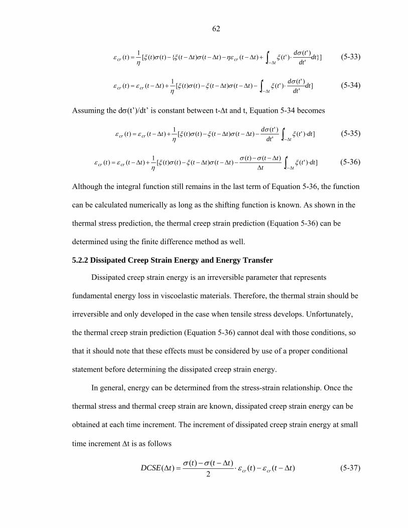
62
}]'
)'()'()()()({)()([1)( dtdt
tdttttttttttt
ttcrcr ∫ ∆−
⋅+∆−−∆−∆−−=σ
ξηεσξσξη
ε (5-33)
]'
)'()'()()()()([1)()( dtdt
tdttttttttttt
ttcrcr ∫ ∆−
⋅−∆−∆−−+∆−=σ
ξσξσξη
εε (5-34)
Assuming the dσ(t’)/dt’ is constant between t-∆t and t, Equation 5-34 becomes
])'('
)'()()()()([1)()( dttdt
tdtttttttttt
ttcrcr ∫ ∆−
⋅−∆−∆−−+∆−= ξσ
σξσξη
εε (5-35)
])'()()()()()()([1)()( dttt
ttttttttttttt
ttcrcr ∫ ∆−
⋅∆
∆−−−∆−∆−−+∆−= ξ
σσσξσξ
ηεε (5-36)
Although the integral function still remains in the last term of Equation 5-36, the function
can be calculated numerically as long as the shifting function is known. As shown in the
thermal stress prediction, the thermal creep strain prediction (Equation 5-36) can be
determined using the finite difference method as well.
5.2.2 Dissipated Creep Strain Energy and Energy Transfer
Dissipated creep strain energy is an irreversible parameter that represents
fundamental energy loss in viscoelastic materials. Therefore, the thermal strain should be
irreversible and only developed in the case when tensile stress develops. Unfortunately,
the thermal creep strain prediction (Equation 5-36) cannot deal with those conditions, so
that it should note that these effects must be considered by use of a proper conditional
statement before determining the dissipated creep strain energy.
In general, energy can be determined from the stress-strain relationship. Once the
thermal stress and thermal creep strain are known, dissipated creep strain energy can be
obtained at each time increment. The increment of dissipated creep strain energy at small
time increment ∆t is as follows
)()(2
)()()( tttttttDCSE crcr ∆−−⋅∆−−
=∆ εεσσ (5-37)
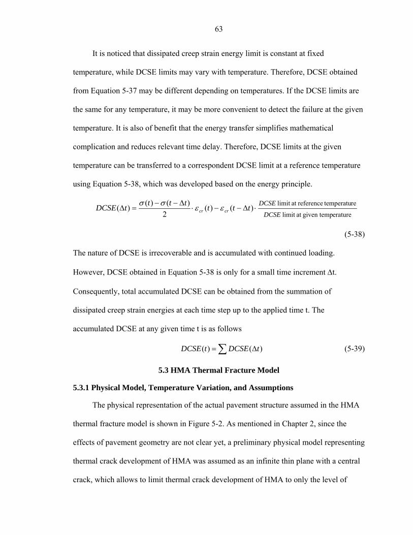
63
It is noticed that dissipated creep strain energy limit is constant at fixed
temperature, while DCSE limits may vary with temperature. Therefore, DCSE obtained
from Equation 5-37 may be different depending on temperatures. If the DCSE limits are
the same for any temperature, it may be more convenient to detect the failure at the given
temperature. It is also of benefit that the energy transfer simplifies mathematical
complication and reduces relevant time delay. Therefore, DCSE limits at the given
temperature can be transferred to a correspondent DCSE limit at a reference temperature
using Equation 5-38, which was developed based on the energy principle.
eraturegiven tempat limit
re temperatureferenceat limit )()(2
)()()(DCSE
DCSEtttttttDCSE crcr ⋅∆−−⋅∆−−
=∆ εεσσ
(5-38)
The nature of DCSE is irrecoverable and is accumulated with continued loading.
However, DCSE obtained in Equation 5-38 is only for a small time increment ∆t.
Consequently, total accumulated DCSE can be obtained from the summation of
dissipated creep strain energies at each time step up to the applied time t. The
accumulated DCSE at any given time t is as follows
∑ ∆= )()( tDCSEtDCSE (5-39)
5.3 HMA Thermal Fracture Model
5.3.1 Physical Model, Temperature Variation, and Assumptions
The physical representation of the actual pavement structure assumed in the HMA
thermal fracture model is shown in Figure 5-2. As mentioned in Chapter 2, since the
effects of pavement geometry are not clear yet, a preliminary physical model representing
thermal crack development of HMA was assumed as an infinite thin plane with a central
crack, which allows to limit thermal crack development of HMA to only the level of
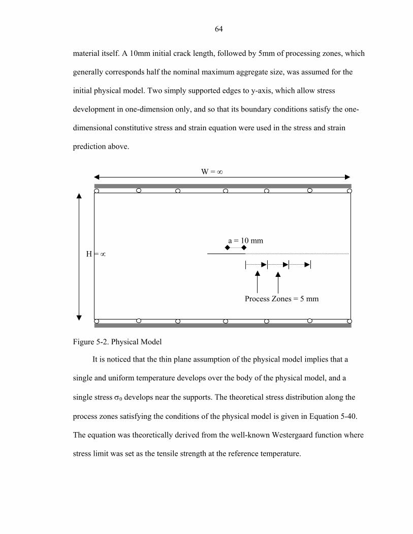
64
material itself. A 10mm initial crack length, followed by 5mm of processing zones, which
generally corresponds half the nominal maximum aggregate size, was assumed for the
initial physical model. Two simply supported edges to y-axis, which allow stress
development in one-dimension only, and so that its boundary conditions satisfy the one-
dimensional constitutive stress and strain equation were used in the stress and strain
prediction above.
W = ∞
H = ∝
a = 10 mm
Process Zones = 5 mm
Figure 5-2. Physical Model
It is noticed that the thin plane assumption of the physical model implies that a
single and uniform temperature develops over the body of the physical model, and a
single stress σ0 develops near the supports. The theoretical stress distribution along the
process zones satisfying the conditions of the physical model is given in Equation 5-40.
The equation was theoretically derived from the well-known Westergaard function where
stress limit was set as the tensile strength at the reference temperature.
65
)2()(0
arrar
y ++
=σσ (5-40)
where σ0 is stress, a is crack length, and r is distance measured from the crack tip.
From field observations (Roque et al., 1993), a general pattern of the daily or
seasonal temperature variation of pavement’s surface appears to have a cyclic form, so
that the external source of the temperature variation may be reasonably represented as a
sinusoidal function. The benefit of the sinusoidal function is to allow the continuous and
successive application of fatigue loading to the physical model. It also allows continuous
development of crack propagation through the body.
5.3.2 General Concept of HMA Thermal Fracture Model
The general concept of HMA thermal fracture model consists of four steps:
defining the process zones, predicting thermal stresses, calculating average stresses
within each process zone, and calculating and assigning DCSE within each individual
process zone. Average stresses over the process zones calculated by the thermal stress at
small time increments are used to get the DCSEs over the process zones. The DCSEs
obtained are then assigned to each process zone, which were previously defined. An
overall procedure for crack development along the process zones used the time-increment
iteration process is shown in Figure 5-3. During the iteration process, a process zone near
the crack tip is failed when the total accumulated DCSE reached DCSE limit. At the same
time, the stress distribution along the processing zones is changed by the increase of
crack length, so the stress redistribution should be assigned and considered in the next
step.

66
Calculate Average Calculate Accumulated DCSE
DCSE Stress
DCSE limit
Zone 1 Zone 2 Zone N
Stress 1 at Time 1 Stress 2 at Time 2
Stress N at Time N …
Predict Thermal Stress
Thermal Stress N
Thermal Stress 1
Thermal Stress 2
Time 1 Time 2 Time N
Iteration
…
Define Zones
Figure 5-3. General Concept of HMA Thermal Fracture Model
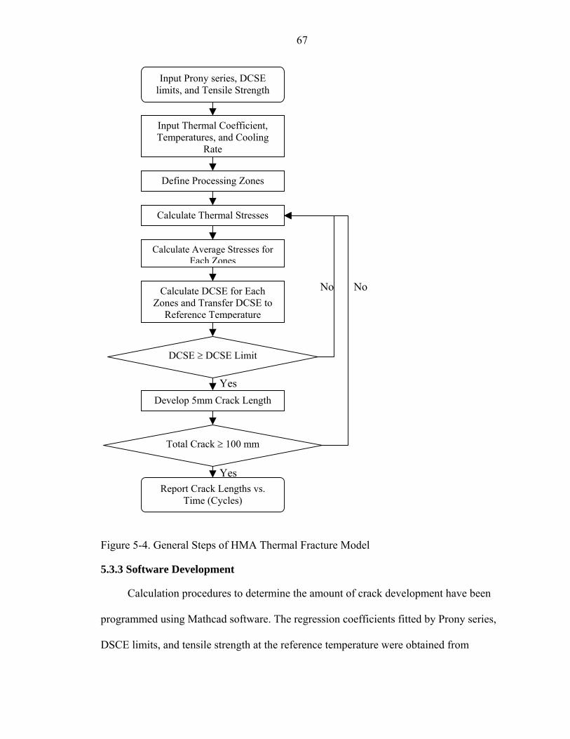
67
Input Thermal Coefficient, Temperatures, and Cooling
Rate
Define Processing Zones
Calculate Thermal Stresses
Calculate Average Stresses for Each Zones
Calculate DCSE for Each Zones and Transfer DCSE to
Reference Temperature
Total Crack ≥ 100 mm
Develop 5mm Crack Length
DCSE ≥ DCSE Limit
Yes
Yes
No
Report Crack Lengths vs. Time (Cycles)
Input Prony series, DCSE limits, and Tensile Strength
No
Figure 5-4. General Steps of HMA Thermal Fracture Model
5.3.3 Software Development
Calculation procedures to determine the amount of crack development have been
programmed using Mathcad software. The regression coefficients fitted by Prony series,
DSCE limits, and tensile strength at the reference temperature were obtained from
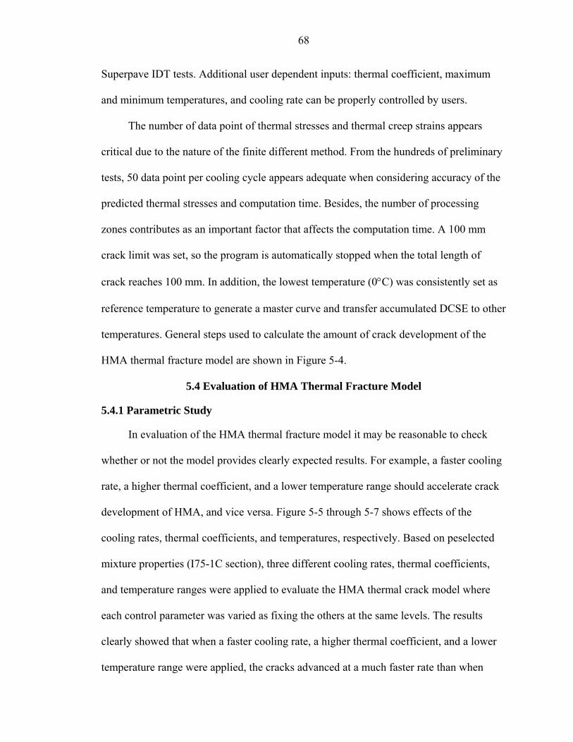
68
Superpave IDT tests. Additional user dependent inputs: thermal coefficient, maximum
and minimum temperatures, and cooling rate can be properly controlled by users.
The number of data point of thermal stresses and thermal creep strains appears
critical due to the nature of the finite different method. From the hundreds of preliminary
tests, 50 data point per cooling cycle appears adequate when considering accuracy of the
predicted thermal stresses and computation time. Besides, the number of processing
zones contributes as an important factor that affects the computation time. A 100 mm
crack limit was set, so the program is automatically stopped when the total length of
crack reaches 100 mm. In addition, the lowest temperature (0°C) was consistently set as
reference temperature to generate a master curve and transfer accumulated DCSE to other
temperatures. General steps used to calculate the amount of crack development of the
HMA thermal fracture model are shown in Figure 5-4.
5.4 Evaluation of HMA Thermal Fracture Model
5.4.1 Parametric Study
In evaluation of the HMA thermal fracture model it may be reasonable to check
whether or not the model provides clearly expected results. For example, a faster cooling
rate, a higher thermal coefficient, and a lower temperature range should accelerate crack
development of HMA, and vice versa. Figure 5-5 through 5-7 shows effects of the
cooling rates, thermal coefficients, and temperatures, respectively. Based on peselected
mixture properties (I75-1C section), three different cooling rates, thermal coefficients,
and temperature ranges were applied to evaluate the HMA thermal crack model where
each control parameter was varied as fixing the others at the same levels. The results
clearly showed that when a faster cooling rate, a higher thermal coefficient, and a lower
temperature range were applied, the cracks advanced at a much faster rate than when

69
other conditions were applied. These results are clearly in accordance with the expected
results.
0
20
40
60
80
100
120
0.00E+00 5.00E+05 1.00E+06 1.50E+06 2.00E+06 2.50E+06
Time (sec)
Cra
ck L
engt
h (m
m)
1C/hour 5C/hour 10C/hour
Figure 5-5. Effect of Cooling Rates
0
20
40
60
80
100
120
0.00E+00 4.00E+04 8.00E+04 1.20E+05 1.60E+05 2.00E+05
Time (sec)
Cra
ck L
engt
h (m
m)
2.0 X 10^-5 1/C 3.0 X 10^-5 1/C 4.0 X 10^-5 1/C
Figure 5-6. Effect of Thermal Coefficients
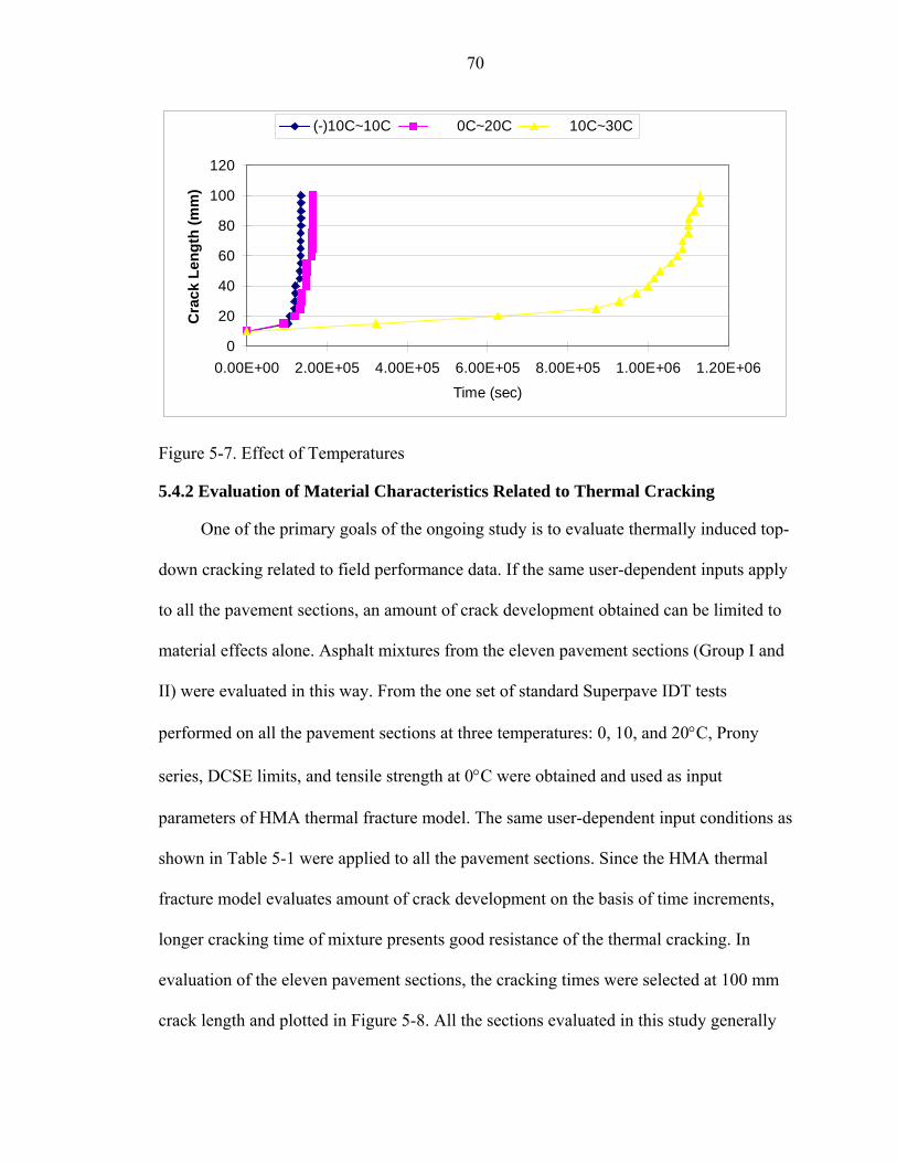
70
0
20
40
60
80
100
120
0.00E+00 2.00E+05 4.00E+05 6.00E+05 8.00E+05 1.00E+06 1.20E+06
Time (sec)
Cra
ck L
engt
h (m
m)
(-)10C~10C 0C~20C 10C~30C
Figure 5-7. Effect of Temperatures
5.4.2 Evaluation of Material Characteristics Related to Thermal Cracking
One of the primary goals of the ongoing study is to evaluate thermally induced top-
down cracking related to field performance data. If the same user-dependent inputs apply
to all the pavement sections, an amount of crack development obtained can be limited to
material effects alone. Asphalt mixtures from the eleven pavement sections (Group I and
II) were evaluated in this way. From the one set of standard Superpave IDT tests
performed on all the pavement sections at three temperatures: 0, 10, and 20°C, Prony
series, DCSE limits, and tensile strength at 0°C were obtained and used as input
parameters of HMA thermal fracture model. The same user-dependent input conditions as
shown in Table 5-1 were applied to all the pavement sections. Since the HMA thermal
fracture model evaluates amount of crack development on the basis of time increments,
longer cracking time of mixture presents good resistance of the thermal cracking. In
evaluation of the eleven pavement sections, the cracking times were selected at 100 mm
crack length and plotted in Figure 5-8. All the sections evaluated in this study generally
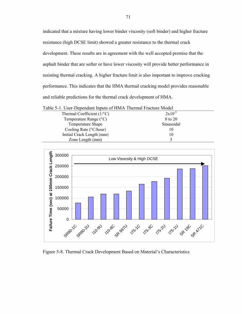
71
indicated that a mixture having lower binder viscosity (soft binder) and higher fracture
resistance (high DCSE limit) showed a greater resistance to the thermal crack
development. These results are in agreement with the well accepted premise that the
asphalt binder that are softer or have lower viscosity will provide better performance in
resisting thermal cracking. A higher fracture limit is also important to improve cracking
performance. This indicates that the HMA thermal cracking model provides reasonable
and reliable predictions for the thermal crack development of HMA.
Table 5-1. User-Dependant Inputs of HMA Thermal Fracture Model Thermal Coefficient (1/°C) 2x10⁻⁵
Temperature Range (°C) 0 to 20 Temperature Shape Sinusoidal
Cooling Rate (°C/hour) 10 Initial Crack Length (mm) 10
Zone Length (mm) 5
0
50000
100000
150000
200000
250000
300000
SR80-1C
SR80-2U
I10-9U
I10-8C
SR 997U
I75-1C
I75-3C
I75-2U
I75-1U
SR 19C
SR 471CFa
ilure
Tim
e (s
ec) a
t 100
mm
Cra
ck L
engt
h
Low Visocsity & High DCSE
Figure 5-8. Thermal Crack Development Based on Material’s Characteristics
72
5.4.3 Evaluation of Pavement Performance Related to Thermal Cracking
To evaluate the model’s performance related to in-service pavement sections,
regional temperature of each section is an important input parameter. However, if the
input temperature range is out of the temperature range that was used in the tests for
asphalt mixtures, it may provide inaccurate prediction, and as mentioned earlier,
increasing temperature increases computation time due to the nature of the finite different
method. From inspection of the field temperature data, the data consists of two primary
factors: mean air temperature and range in air temperature. According to the parametric
study, higher temperature increased crack resistance of asphalt pavement while
increasing cooling rate reduces pavement performance. Therefore, a simple equation
(Equation 5-41) was developed upon the concept that the increase of annual mean air
temperature may increase the cracking performance while the broad range in air
temperature may decrease the performance.
CFT = FT x AMT / RMT (5-41) where CFT = Calibrated Failure Time FT = Failure Time AMT = Annual Mean Air Temperature RMT = Range in Annual Mean Air Temperature
(Annual Max. Mean Temp. – Annual Min. Mean Temp.) The annual mean air temperatures and the ranges in air temperature (difference between
maximum and minimum mean air temperatures) recorded at each pavement section are
given in Table 5-2. The failure time at 100 mm crack length and two regional temperature
inputs of each section were used to calculate the calibrated failure times (Figure 5-9).

73
Table 5-2. Regional Temperature of Individual Sections Sections Annual Mean Air Temp. Range in Annual Mean Air Temperature SR80-1C 22.92 13.08 I10-8C 21.08 13.25 I75-1C 23.17 11.58 I75-3C 22.92 13.08 SR 19C 21.42 13.08
SR 471C 22.42 12.83 SR80-2U 22.92 13.08 I10-9U 21.08 13.25
SR 997U 23.25 10.17 I75-2U 22.92 13.08 I75-1U 23.17 11.58
0
100000
200000
300000
400000
500000
600000
SR80-1C
I10-8C
I75-3C
I75-1C
SR 19C
SR 471C
SR80-2U
I10-9U
SR 997U
I75-2U
I75-1U
Cal
ibra
ted
Failu
re T
ime
(sec
) at 1
00m
m
Cra
ck L
engt
h
Cracked Sections Uncracked Sections
Figure 5-9. Thermal Crack Development Based on Field Performance
As shown in Figure 5-9 two types of pavement sections where the symbol ‘C’
represents a cracked section while the symbol ‘U’ represents a uncracked section indicate
that the top-down cracking performance did not uniquely relate to thermal cracking
prediction through the model. It appears that load-induced damage is far more significant
than that temperature induced damage, which explains the lack of correlation with the
performance data in the field. In fact, the annual mean temperature in Florida is much
higher than other states. Therefore, only a combined model that integrates top-down

74
cracking performance associated with loading and thermal effects is needed to provide
more accurate predictions related to pavement performance data.
CHAPTER 6 FIELD PERFORMANCE EVALUATION BASED ON COMBINED EFFECT OF
TEMPERATURE AND LOAD
It was recognized that thermal cracking alone was not directly related to the top-
down cracking performance. It appears that performance data evaluated in this study was
gathered from a limited area (the state of Florida), so that the thermal effect may be
smaller than for other areas. However, this phenomenon doesn’t mean the thermal effect
is negligible in this area because the nature of thermal cracking is fundamentally related
to the top-down cracking development.
Prior work done by Roque et al. (2004) introduced the concept of Energy Ratio
(ER), which integrated HMA fracture model and the structural characteristics of asphalt
pavement. ER was determined to accurately distinguish between pavements that
exhibited top-down cracking and those that did not. However, this system was limited to
the evaluation of load-induced top-down cracking. Consequently, by combining the
concept of Energy Ratio with the system developed for the evaluation of thermal
cracking performance, it is expected that Energy Ratio may provide a more accurate
estimation for the pavements exhibited to top-down cracking.
6.1 Evaluation of Load-Induced Top-Down Cracking Performance
As explained in Chapter 2, the Energy Ratio was developed based on field
performance data, where DCSE limit over minimum DCSE requirement is a critical
definition. For eleven pavement sections, the Energy Ratios were determined using
Equation 6-1 where applied stress σ, and all other input parameters: failure strength St,
75
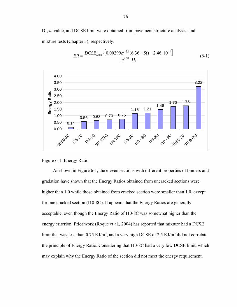
76
D1, m value, and DCSE limit were obtained from pavement structure analysis, and
mixture tests (Chapter 3), respectively.
[ ]1
98.2
81.3 1046.2)36.6(00299.0Dm
StDCSEER Limit
⋅⋅+−⋅
=−−σ (6-1)
0.140.56 0.63 0.70 0.75
1.16 1.211.46
1.70 1.75
3.22
0.00
0.50
1.00
1.50
2.00
2.50
3.00
3.50
4.00
SR80-1C
I75-3C
I75-1C
SR 471C
SR 19C
I75-1U
I10 - 8
CI75
-2U
I10 - 9
U
SR80-2U
SR 997U
Ener
gy R
atio
Figure 6-1. Energy Ratio
As shown in Figure 6-1, the eleven sections with different properties of binders and
gradation have shown that the Energy Ratios obtained from uncracked sections were
higher than 1.0 while those obtained from cracked section were smaller than 1.0, except
for one cracked section (I10-8C). It appears that the Energy Ratios are generally
acceptable, even though the Energy Ratio of I10-8C was somewhat higher than the
energy criterion. Prior work (Roque et al., 2004) has reported that mixture had a DCSE
limit that was less than 0.75 KJ/m3, and a very high DCSE of 2.5 KJ/m3 did not correlate
the principle of Energy Ratio. Considering that I10-8C had a very low DCSE limit, which
may explain why the Energy Ratio of the section did not meet the energy requirement.

77
However, even though the Energy Ratio showed well-matched results on the
pavements with cracked and uncraked condition, individual cracked condition of each
section was not directly matched with a visual observation for the cracked sections. For
example, I10-8C, which had relatively heavy top-down cracks over the surface of asphalt
layer, had showed relatively a higher ER value, while SR 471 that recently showed top-
down cracks had shown relatively low ER value. Of particular interest, it is noticed that
the unmatched performance sections came from the northern area (Figure 3-1). These
observations indicate that the top-down cracking performance may be affected by the
effect of thermal stress. Consequently, the evaluation of top-down cracking performance
with thermal effect may provide an accurate prediction of top-down cracking
performance in pavement.
6.2 Consideration of Load Effect to Top-down Cracking Performance
It appears that regional temperature has an influence on development of the top-
down cracking. In fact, the annual mean temperature and the temperature-cooling rate in
Florida is much higher and lower than other states, which indicates the effect of
temperature may be less significant. On the other hand, it can be imagined that in
northern area where relatively lower temperature are dominant, top-down cracking
performance may be more significantly affected by the thermal effect. In this case, the
performance evaluated by the effect of traffic loads alone may not be reliable.
Consequently, the only way to reliably estimate the top-down cracking performance
appears to assemble two different aspects of mechanisms.
To quantify both loading and thermal effects, it is important to understand the
principle of Energy Ratio. The Energy Ratio, which is defined as dissipated creep strain
energy threshold of the mixture divided by minimum dissipated creep strain energy
78
required. It is a single dimensionless parameter that was developed based on performance
data. By simply multiplying the ER to the calibrated failure time, the loading effect can
be transferred to a form of failure time (Equation 6-2). Consequently overall thermal and
loading effects are integrated as the failure time.
Figure 6-2 shows the integrated failure times of the eleven pavement sections. The
plot shows that the uncracked sections were clearly discriminated from the sections
exhibit top-down cracking. This indicates that when both temperature and load effects
were properly combined better correlation resulted with the top-down cracking
performance data. As a result, the integrated failure time was able to more effectively
distinguish the sections that exhibit top-down cracking.
However, it is noticed that the failure time alone may not be directly related to the
top-down cracking performance. A more efficient equation that can directly relate the
performance of in-situ pavements was developed in the similar manner that was used in
the Energy Ratio.
IFT = FT x AMT / RMT x ER (6-2) Where IFT = Integrated Failure Time FT = Failure Time AMT = Annual Mean Air Temperature RMT = Range in Annual Mean Air Temperature
(Annual Max. Mean Temp. – Annual Min. Mean Temp.) ER = Energy Ratio
6.2 Energy Ratio Correction
As shown in Figure 6-2, the performance of cracked and uncracked sections was
clearly discriminated by the single failure time, which is Minimum Time Requirement.
The Minimum Time Requirement is a unique parameter that is obtained from the field
performance data. As dividing the Integrated Failure Time by the Minimum Time
Requirement with the same time dimension, it can be transferred to the same form of the
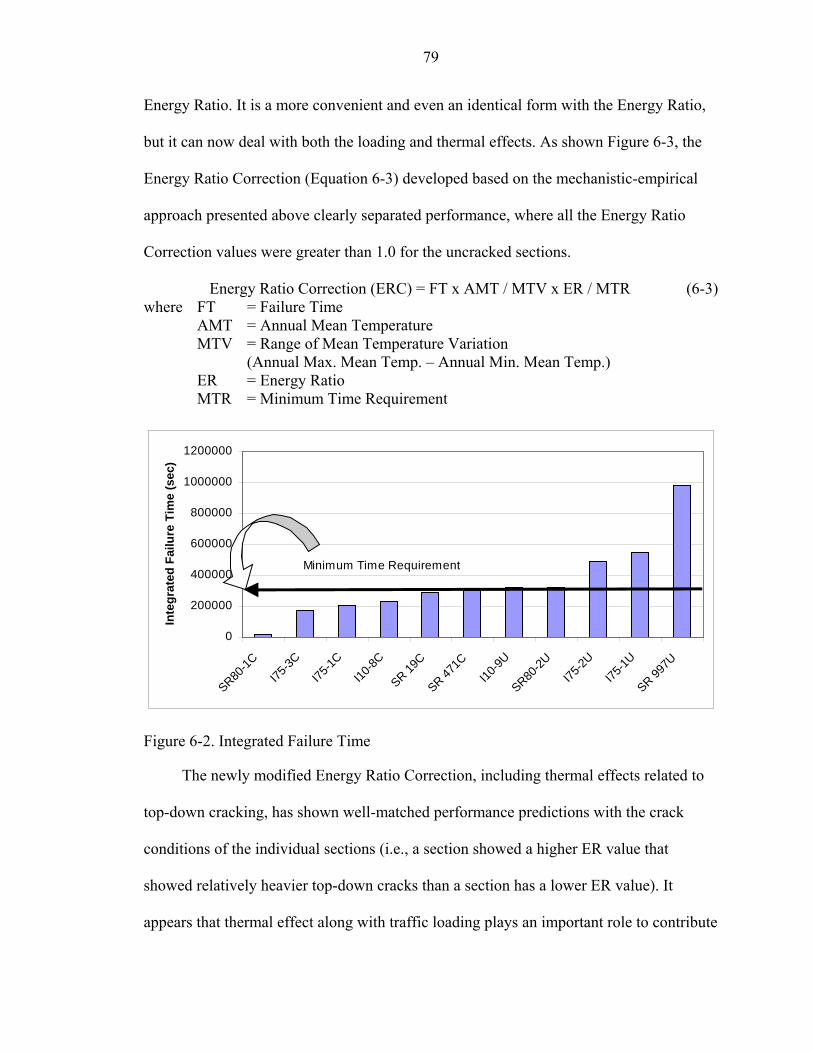
79
Energy Ratio. It is a more convenient and even an identical form with the Energy Ratio,
but it can now deal with both the loading and thermal effects. As shown Figure 6-3, the
Energy Ratio Correction (Equation 6-3) developed based on the mechanistic-empirical
approach presented above clearly separated performance, where all the Energy Ratio
Correction values were greater than 1.0 for the uncracked sections.
Energy Ratio Correction (ERC) = FT x AMT / MTV x ER / MTR (6-3) where FT = Failure Time AMT = Annual Mean Temperature MTV = Range of Mean Temperature Variation
(Annual Max. Mean Temp. – Annual Min. Mean Temp.) ER = Energy Ratio MTR = Minimum Time Requirement
0
200000
400000
600000
800000
1000000
1200000
SR80-1C
I75-3C
I75-1C
I10-8C
SR 19C
SR 471C
I10-9U
SR80-2U
I75-2U
I75-1U
SR 997U
Inte
grat
ed F
ailu
re T
ime
(sec
)
Minimum Time Requirement
Figure 6-2. Integrated Failure Time
The newly modified Energy Ratio Correction, including thermal effects related to
top-down cracking, has shown well-matched performance predictions with the crack
conditions of the individual sections (i.e., a section showed a higher ER value that
showed relatively heavier top-down cracks than a section has a lower ER value). It
appears that thermal effect along with traffic loading plays an important role to contribute
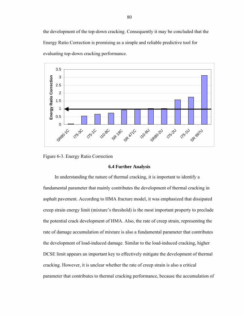
80
the development of the top-down cracking. Consequently it may be concluded that the
Energy Ratio Correction is promising as a simple and reliable predictive tool for
evaluating top-down cracking performance.
0
0.5
1
1.5
2
2.5
3
3.5
SR80-1C
I75-3C
I75-1C
I10-8C
SR 19C
SR 471C
I10-9U
SR80-2U
I75-2U
I75-1U
SR 997U
Ener
gy R
atio
Cor
rect
ion
Figure 6-3. Energy Ratio Correction
6.4 Further Analysis
In understanding the nature of thermal cracking, it is important to identify a
fundamental parameter that mainly contributes the development of thermal cracking in
asphalt pavement. According to HMA fracture model, it was emphasized that dissipated
creep strain energy limit (mixture’s threshold) is the most important property to preclude
the potential crack development of HMA. Also, the rate of creep strain, representing the
rate of damage accumulation of mixture is also a fundamental parameter that contributes
the development of load-induced damage. Similar to the load-induced cracking, higher
DCSE limit appears an important key to effectively mitigate the development of thermal
cracking. However, it is unclear whether the rate of creep strain is also a critical
parameter that contributes to thermal cracking performance, because the accumulation of

81
creep strain in mixtures subjected to thermal stresses is much less straightforward and
more complex to all other time dependent behavior will affect thermal cracking
development in HMA. Therefore, this complementary study is important in
understanding the nature of the thermal cracking.
Time
Cre
ep C
ompl
ianc
e
σ
σ
ηn
η2
η1
E2
En
E1
Figure 6-4. Creep Responses Corresponding to Viscoelastic Rheology Model
It is generally known that viscoelastic response can be expressed using a rheology
model. In cases where the stress history is prescribed, real material response can be
closely described as series of a elastic element, delayed elastic elements, and a viscous
element. The combined response under constant static stress is expressed in Figure 6-4
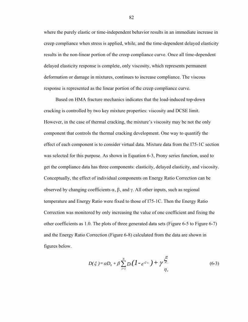
82
where the purely elastic or time-independent behavior results in an immediate increase in
creep compliance when stress is applied, while, and the time-dependent delayed elasticity
results in the non-linear portion of the creep compliance curve. Once all time-dependent
delayed elasticity response is complete, only viscosity, which represents permanent
deformation or damage in mixtures, continues to increase compliance. The viscous
response is represented as the linear portion of the creep compliance curve.
Based on HMA fracture mechanics indicates that the load-induced top-down
cracking is controlled by two key mixture properties: viscosity and DCSE limit.
However, in the case of thermal cracking, the mixture’s viscosity may be not the only
component that controls the thermal cracking development. One way to quantify the
effect of each component is to consider virtual data. Mixture data from the I75-1C section
was selected for this purpose. As shown in Equation 6-3, Prony series function, used to
get the compliance data has three components: elasticity, delayed elasticity, and viscosity.
Conceptually, the effect of individual components on Energy Ratio Correction can be
observed by changing coefficients α, β, and γ. All other inputs, such as regional
temperature and Energy Ratio were fixed to those of I75-1C. Then the Energy Ratio
Correction was monitored by only increasing the value of one coefficient and fixing the
other coefficients as 1.0. The plots of three generated data sets (Figure 6-5 to Figure 6-7)
and the Energy Ratio Correction (Figure 6-8) calculated from the data are shown in
figures below.
ηβαξ
ξγτξ
v
/-i
N
=1i
+ )-(1 eD + D = )D( i∑0 (6-3)
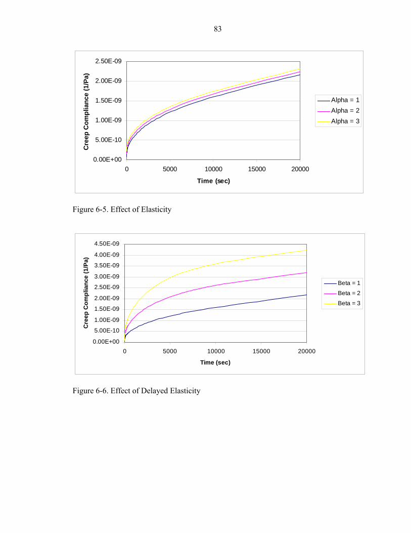
83
0.00E+00
5.00E-10
1.00E-09
1.50E-09
2.00E-09
2.50E-09
0 5000 10000 15000 20000
Time (sec)
Cre
ep C
ompl
ianc
e (1
/Pa)
Alpha = 1Alpha = 2Alpha = 3
Figure 6-5. Effect of Elasticity
0.00E+00
5.00E-10
1.00E-09
1.50E-09
2.00E-09
2.50E-09
3.00E-09
3.50E-09
4.00E-09
4.50E-09
0 5000 10000 15000 20000
Time (sec)
Cre
ep C
ompl
ianc
e (1
/Pa)
Beta = 1
Beta = 2
Beta = 3
Figure 6-6. Effect of Delayed Elasticity
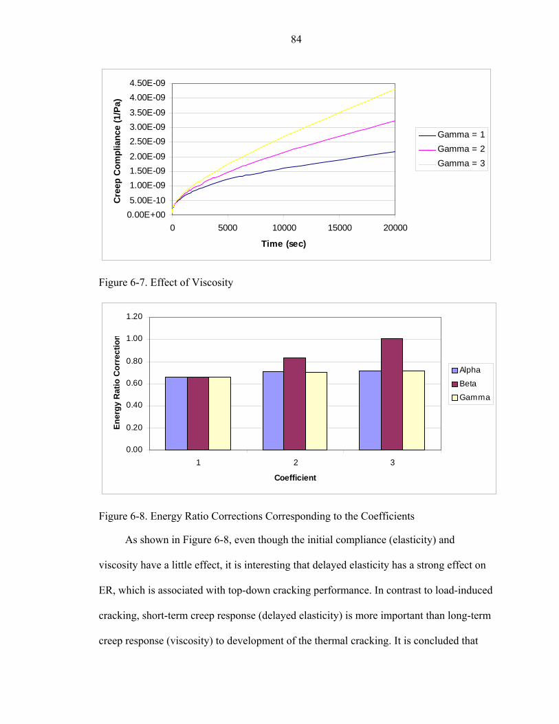
84
0.00E+005.00E-10
1.00E-091.50E-092.00E-09
2.50E-093.00E-093.50E-09
4.00E-094.50E-09
0 5000 10000 15000 20000
Time (sec)
Cre
ep C
ompl
ianc
e (1
/Pa)
Gamma = 1Gamma = 2Gamma = 3
Figure 6-7. Effect of Viscosity
0.00
0.20
0.40
0.60
0.80
1.00
1.20
1 2 3
Coefficient
Ener
gy R
atio
Cor
rect
ion
Alpha
Beta
Gamma
Figure 6-8. Energy Ratio Corrections Corresponding to the Coefficients
As shown in Figure 6-8, even though the initial compliance (elasticity) and
viscosity have a little effect, it is interesting that delayed elasticity has a strong effect on
ER, which is associated with top-down cracking performance. In contrast to load-induced
cracking, short-term creep response (delayed elasticity) is more important than long-term
creep response (viscosity) to development of the thermal cracking. It is concluded that

85
mixture with higher short-term creep response can also help to mitigate top-down
cracking.

CHAPTER 7 SUMMARY, CONCLUSIONS AND RECOMMENDATIONS
7.1 Summary
7.1.1 Evaluation of Energy Dissipation
Prior work performed on the fracture behavior of asphalt mixture has indicated that
damage in asphalt mixture is directly related to the development of dissipated creep strain
energy. This prior work has also shown that a dissipated creep strain energy threshold
exists, which defines the development (initiation or propagation) of macro cracks.
Consequently, it is of critical importance to be able to predict the rate of dissipated creep
strain energy development to evaluate the cracking performance of asphalt mixture.
The work performed in this study indicated that the dissipated energy determined
as the area of the hysteresis loop that develops during cyclic loading of asphalt mixture is
not a good measure of the dissipated creep strain energy that develops in the mixture,
which explains why it is not a good indicator of damage development and cracking
resistance of asphalt mixture. Results showed that the dissipated energy determined from
the hysteresis loop was far greater than the dissipated creep strain energy predicted from
the measured viscous response of the mixture. Further analysis indicated that the
difference in energy was clearly explained by the delayed elastic response of the mixture.
In fact, for the mixtures tested, the majority of the dissipated energy associated with the
hysteresis loop was caused by delayed elastic response.
In summary, it appears that an independent measure of the viscous response of
asphalt mixture is required to accurately predict or determine the dissipated creep strain
86

87
energy incurred during loading. Although theoretically this can be determined either from
static creep tests or from cyclic load tests at multiple frequencies, the results of the study
indicate that viscous response of mixtures can be obtained more accurately and reliably
from static creep tests. Because of the relatively short loading times involved, the
response of cyclic load tests performed at typical loading frequencies is generally
dominated by elastic and delayed elastic response, which makes it different and
impossible to isolate the viscous response accurately.
The fact that a large portion of the hysteresis loop is composed of delayed elastic
energy may result in misinterpretation of dissipated energy results and its relationship to
mixture cracking performance. Depending on their rheological characteristics, mixtures
exhibiting the same dissipated energy per load cycle may in fact have very different
resistance to the development of damage. A mixture whose response is strongly
influenced by delayed elasticity may be incurring little or no damage even though a
significant amount of dissipated energy is observed. Conversely, a mixture exhibiting the
same level of dissipated energy per load cycle may be incurring a significant amount of
micro damage if most of its response is associated with viscous behavior, as opposed to
delayed elastic behavior.
In conclusion, it appears that the absolute value of the dissipated energy
measurements obtained from the area of the hysteresis loop during cyclic load testing
should not be used to interpret the cracking performance of asphalt mixture. An
independent set of parameters that allows for the prediction of the viscous response of the
mixture is required for this purpose.

88
7.1.2 Evaluation of HMA Thermal Fracture Model
The HMA fracture model was based on theory of viscoelasticity and energy-based
fracture mechanics, which uniquely deals with fracture associated with a fundamental
dissipated creep strain energy loss in viscoelastic materials. Its damage principle and
crack growth law were favorably adapted to the development of HMA thermal fracture
model.
An HMA thermal fracture model was developed based on the same principle and
failure criteria used in the HMA fracture model. These involved inclusion of algorithms
to account for DCSE accumulation induced by temperature changes, which are distinctly
different them those associated with load-induced DCSE.
A parametric study was conducted to evaluate the model, and material
characteristics were clearly matched with expected results. These results indicated that
the HMA thermal fracture model developed has the potential to reliably evaluate the
performance of asphalt mixtures subjected to thermally induced damage. The model was
further evaluated using pavement performance data from test section in Florida. Predicted
performance using the HMA thermal fracture model with regional temperature effect
indicated that although the top-down cracking performance in Florida was most strongly
affected by traffic loading, thermal effects can also affect performance.
Consequently, it was concluded that a combined model able to deal with both
temperature-induced and load-induced crack performance provides a more realistic and
reliable estimation of pavement performance associated with top-down cracking.
7.1.3 Combination of Temperature and Load Effect
A modified Energy Ratio (ERC) was introduced that incorporates the effect of both
load and temperature-induced damage on top-down cracking. The parameter can be used

89
as a single criterion to evaluate top-down cracking performance of asphalt mixtures. Use
of the modified Energy Ratio (ERC) resulted in better correlation between predicted and
observed top-down cracking performance of pavement in Florid, indicating that the
approach developed properly accounts for the effect of temperature on top-down
cracking. Consequently, it may be concluded that the Energy Ratio Correction appears to
be promising as a more accurate and reliable predictive tool for evaluating top-down
cracking performance.
7.1.4 Increase of Performance Related to Mixture’s Rheology
In understanding the nature of thermal cracking it is important to identify a
fundamental parameters that most strongly to contribute the development of thermal
cracking in asphalt pavement. According to HMA fracture model, it appears that a lower
rate of creep and a higher DCSE limit play an important role to increase the top-down
cracking performance. However, further analysis indicates that delayed elasticity, which
is represented as short-term creep response of mixture’s rheology, is an important factor
that affects thermal cracking. Short-term creep response results in lower thermal stresses
developed in asphalt pavement that help to mitigate the potential contribution of the
thermal stresses on top-down cracking.
Although reduction of the rate of creep strain rate may reduce the thermal cracking
performance, the effect of the creep strain was less significant than that of the delayed
elasticity. In conclusion, an asphalt mixture that shows a lower rate of creep strain and
higher short-term creep may be the best combination to effectively mitigate top-down
cracking.

90
7.2 Conclusions
The findings of this study may be summarized as follows:
• The work performed in this study indicates that the dissipated energy determined as the area of the hysteresis loop appears to be composed of delayed elastic and viscous response. Consequently, it is not a good measure of the dissipated creep strain energy. Viscous response of mixtures should be obtained from static creep tests.
• An HMA thermal fracture model was developed based on the same principle and failure criteria used in the HMA fracture model. The performance evaluation of the model indicates that the HMA thermal fracture model developed has the potential to reliably evaluate the performance of asphalt mixtures subjected to thermally induced damage.
• Predicted performance using the HMA thermal fracture model with regional temperature effect indicated that although the top-down cracking performance in Florida was most strongly affected by traffic loading, thermal effects can also affect performance.
• A combined system (ERC) that incorporates the effect of both load- and temperature-induced damage on top-down cracking resulted in better correlation between predicted and observed top-down cracking performance. Consequently, the Energy Ratio Correction appears to be promising as a more accurate and reliable predictive tool for evaluating top-down cracking performance.
• Further analysis indicates that delayed elasticity strongly affects thermal cracking development. In conclusion, an asphalt mixture that shows a lower rate of creep strain and higher short-term creep may be the best combination to effectively mitigate top-down cracking.
7.3 Recommendations
The system developed in this study was only evaluated for a limited number of
sections throughout the state of Florida. The system should be evaluated in more
extended sections that gathered from a broad range in the nation, to include a broader
range of environmental conditions.
Although the system based on modified Energy Ratio (ERC) is practical to
pavement engineers, a more fundamental study should be performed to fully understand

91
pavement behavior. For example, a more mechanistic model needs to be developed to
predict crack growth induced by traffic loading and thermal stresses.

APPENDIX A SUMMARY OF NON-DESTRUCTIVE TESTING (FWD)
Table A-1. Location A I10 - 8C
I10 - 9U
SR 471C
SR 19C
SR 997U
Distance
(in) Measured Calculated Measured Calculated Measured Calculated Measured Calculated Measured Calculated
0 6.4 6.4 5.9 5.9 13.3 13.1 16.4 16.4 7.9 7.9 8 4.5 4.5 4.4 4.4 8.6 8.7 13.3 13.2 4.6 4.6 12 3.6 3.6 3.7 3.7 5.9 6 11 11.2 3 3 18 2.6 2.6 2.8 2.8 3.5 3.5 9.1 8.9 1.9 1.9 24 2 2 2.2 2.2 2.3 2.3 7.2 7.2 1.5 1.5 36 1.3 1.3 1.4 1.4 1.5 1.5 4.7 4.7 1.2 1.2 60 0.7 0.7 0.7 0.7 0.9 0.8 1.9 1.9 0.7 0.7
Table A-1. Location B I10 - 8C
I10 - 9U
SR 471C
SR 19C
SR 997U
Distance
(in) Measured Calculated Measured Calculated Measured Calculated Measured Calculated Measured Calculated
0 7.1 7.1 6.6 6.6 12.3 12.1 17.8 17.9 6.8 6.9 8 5.2 5.2 4.5 4.5 7.8 7.9 14.6 14.3 3.9 3.9 12 4.2 4.2 3.4 3.5 5.3 5.4 11.8 12.1 2.5 2.5 18 3.2 3.1 2.5 2.5 3.2 3.2 9.7 9.6 1.6 1.6 24 2.3 2.4 1.9 1.8 2.2 2.1 7.6 7.6 1.3 1.3 36 1.5 1.5 1.1 1.1 1.4 1.4 4.8 4.8 0.9 0.9 60 0.8 0.8 0.5 0.5 0.8 0.8 1.7 1.7 0.5 0.5
92
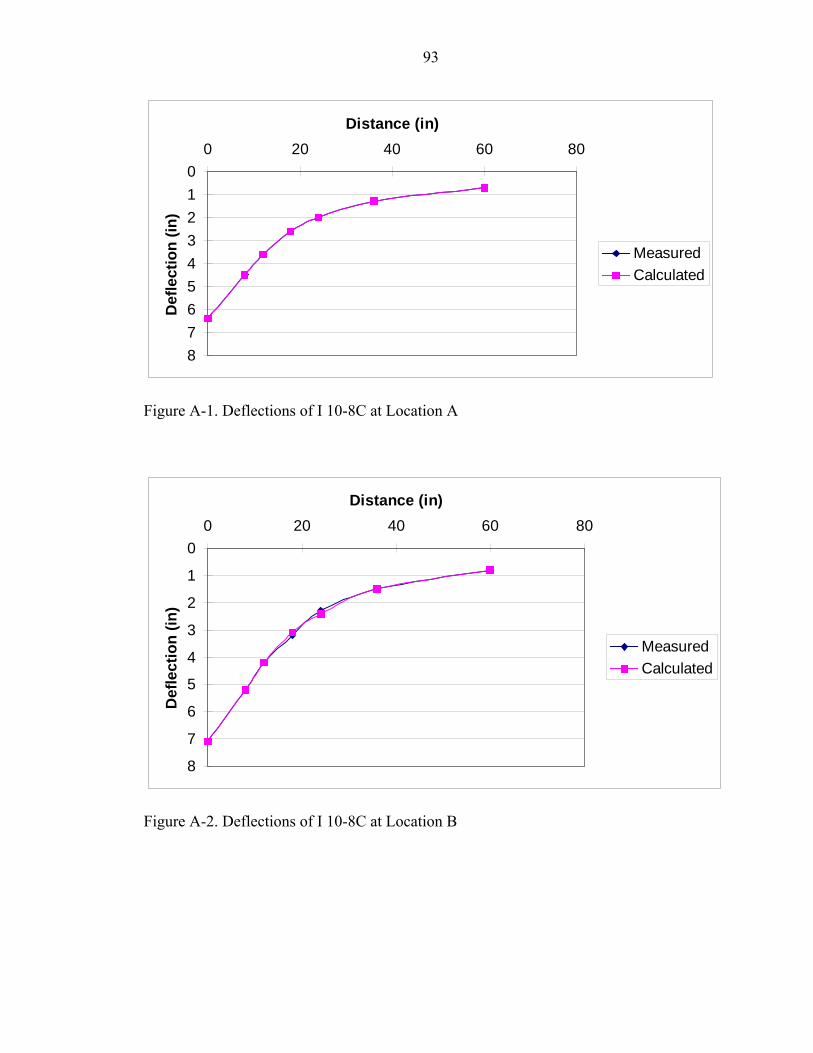
93
012345678
0 20 40 60 80Distance (in)
Def
lect
ion
(in)
MeasuredCalculated
Figure A-1. Deflections of I 10-8C at Location A
0
1
2
3
4
5
6
7
8
0 20 40 60 80Distance (in)
Def
lect
ion
(in)
MeasuredCalculated
Figure A-2. Deflections of I 10-8C at Location B
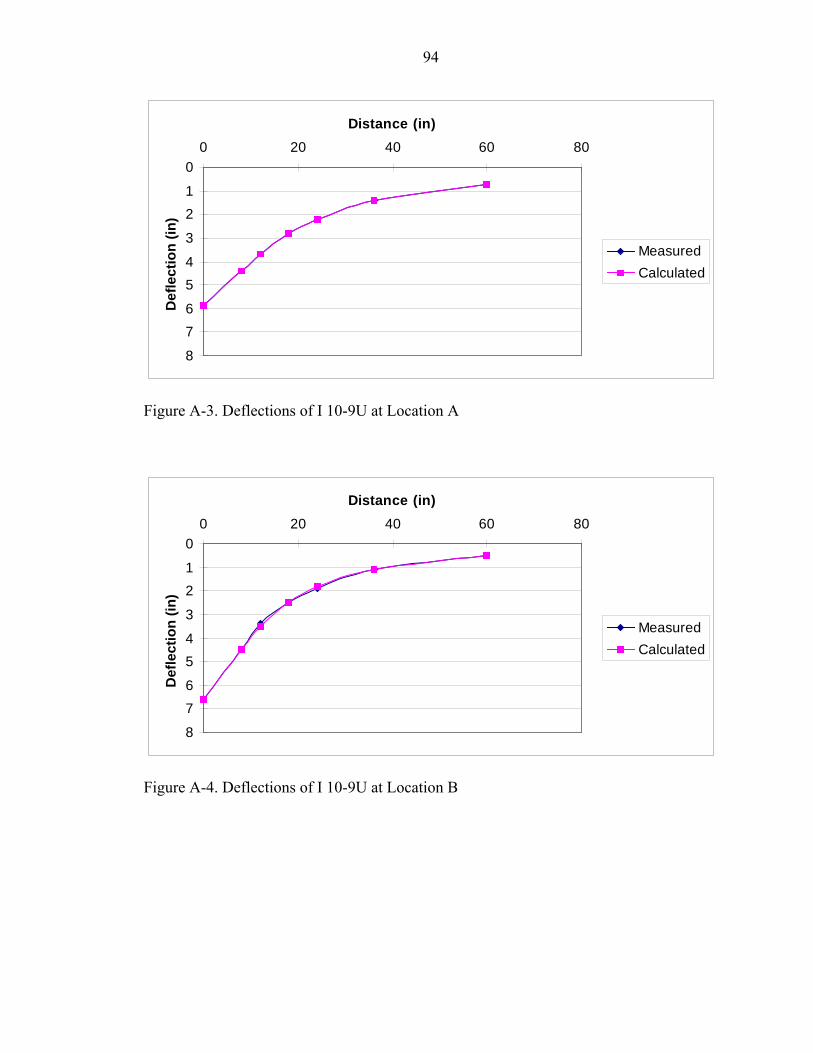
94
0
12
3
45
67
8
0 20 40 60 80
Distance (in)
Def
lect
ion
(in)
MeasuredCalculated
Figure A-3. Deflections of I 10-9U at Location A
0
12
3
45
67
8
0 20 40 60 80
Distance (in)
Def
lect
ion
(in)
MeasuredCalculated
Figure A-4. Deflections of I 10-9U at Location B
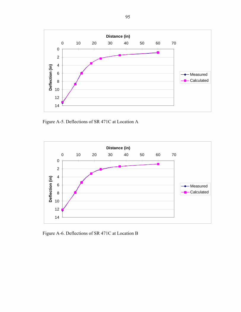
95
0
2
4
6
8
10
12
14
0 10 20 30 40 50 60 70
Distance (in)
Def
lect
ion
(in)
MeasuredCalculated
Figure A-5. Deflections of SR 471C at Location A
0
2
4
6
8
10
12
14
0 10 20 30 40 50 60 70
Distance (in)
Def
lect
ion
(in)
MeasuredCalculated
Figure A-6. Deflections of SR 471C at Location B
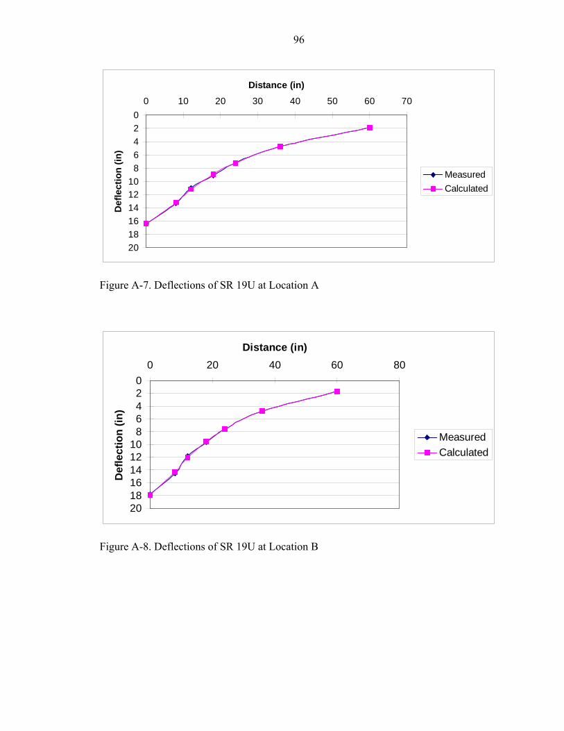
96
02468
101214161820
0 10 20 30 40 50 60 70
Distance (in)
Def
lect
ion
(in)
MeasuredCalculated
Figure A-7. Deflections of SR 19U at Location A
02468
101214161820
0 20 40 60 80Distance (in)
Def
lect
ion
(in)
MeasuredCalculated
Figure A-8. Deflections of SR 19U at Location B
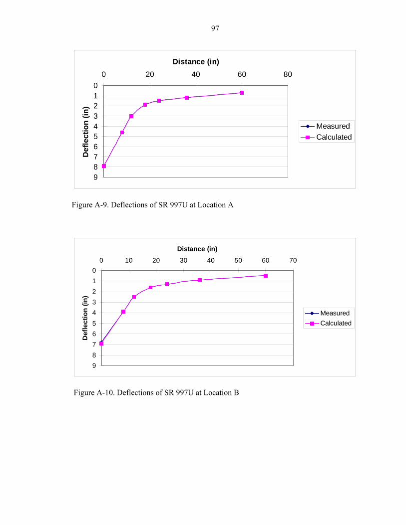
97
0123456789
0 20 40 60 80Distance (in)
Def
lect
ion
(in)
MeasuredCalculated
Figure A-9. Deflections of SR 997U at Location A
0123456789
0 10 20 30 40 50 60 70
Distance (in)
Def
lect
ion
(in)
MeasuredCalculated
Figure A-10. Deflections of SR 997U at Location B

APPENDIX B INDIRECT TENSILE TEST RESUTLS
Table B-1. Resilient Modulus Test Results at 0°C I10 - 8C I10 - 9U SR 471C SR 19C SR 997U Modulus (Gpa) 10.12 10.26 12.70 13.02 14.44
Table B-2. Creep Compliance Test Results at 0°C I10 - 8C I10 - 9U SR 471C SR 19C SR 997U
D1 (1/Gpa) 4.699E-02 6.461E-03 1.377E-02 5.985E-02 5.350E-02 m 0.222 0.511 0.478 0.344 0.136
Rate of Creep Compliance 4.82E-05 1.13E-04 1.78E-04 2.21E-04 1.85E-05
Table B-3. Tensile Strength Test Results at 0°C I10 - 8C I10 - 9U SR 471C SR 19C SR 997U
Tensile Strength (psi) 207 213 329 380 374
Failure Strain (µε) 219 227 569 782 397
Fracture Energy (KJ/m^3) 0.2 0.2 0.8 1.3 0.6
DCSE (KJ/m^3) 0.10 0.09 0.60 1.04 0.37
98
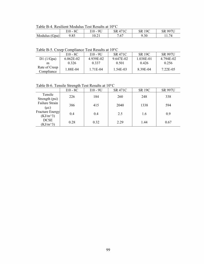
Table B-4. Resilient Modulus Test Results at 10°C I10 - 8C I10 - 9U SR 471C SR 19C SR 997U Modulus (Gpa) 9.85 10.21 7.67 9.30 11.74
Table B-5. Creep Compliance Test Results at 10°C I10 - 8C I10 - 9U SR 471C SR 19C SR 997U
D1 (1/Gpa) 6.062E-02 4.939E-02 9.647E-02 1.038E-01 4.794E-02 m 0.326 0.337 0.501 0.426 0.256
Rate of Creep Compliance 1.88E-04 1.71E-04 1.54E-03 8.39E-04 7.22E-05
Table B-6. Tensile Strength Test Results at 10°C I10 - 8C I10 - 9U SR 471C SR 19C SR 997U
Tensile Strength (psi) 226 184 260 248 338
Failure Strain (µε) 386 415 2040 1338 594
Fracture Energy (KJ/m^3) 0.4 0.4 2.5 1.6 0.9
DCSE (KJ/m^3) 0.28 0.32 2.29 1.44 0.67
99

100
Table B-7. Resilient Modulus Test Results at 20°C I10 - 8C I10 - 9U SR 471C SR 19C SR 997U Modulus (Gpa) 8.05 6.64 5.17 5.28 9.21
Table B-8. Creep Compliance Test Results at 20°C I10 - 8C I10 - 9U SR 471C SR 19C SR 997U
D1 (1/Gpa) 1.078E-01 8.323E-02 8.806E-02 1.955E-01 8.253E-02 m 0.434 0.478 0.713 0.572 0.343
Rate of Creep Compliance 9.38E-04 1.08E-03 8.66E-03 5.80E-03 3.04E-04
Table B-9. Tensile Strength Test Results at 20°C I10 - 8C I10 - 9U SR 471C SR 19C SR 997U
Tensile Strength (psi) 161 148 122 177 238
Failure Strain (µε) 500 607 1977 2472 750
Fracture Energy (KJ/m^3) 0.4 0.4 1.7 1.3 0.8
DCSE (KJ/m^3) 0.32 0.32 1.63 1.16 0.65
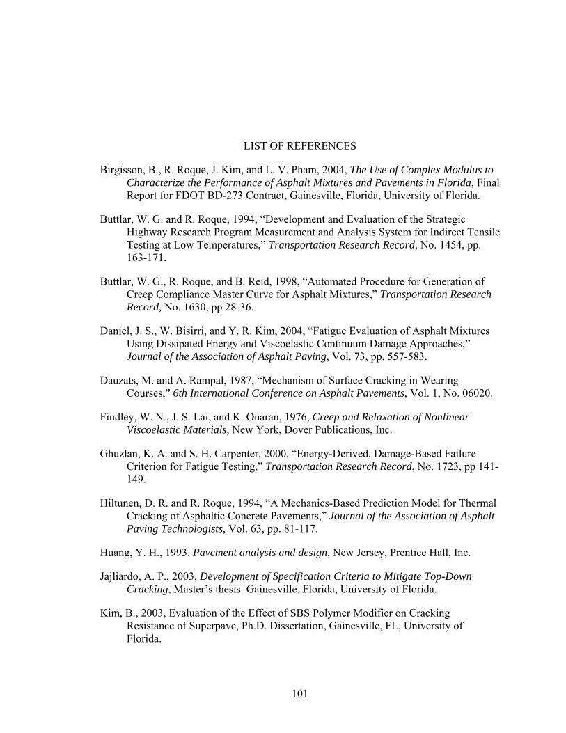
LIST OF REFERENCES
Birgisson, B., R. Roque, J. Kim, and L. V. Pham, 2004, The Use of Complex Modulus to Characterize the Performance of Asphalt Mixtures and Pavements in Florida, Final Report for FDOT BD-273 Contract, Gainesville, Florida, University of Florida.
Buttlar, W. G. and R. Roque, 1994, “Development and Evaluation of the Strategic Highway Research Program Measurement and Analysis System for Indirect Tensile Testing at Low Temperatures,” Transportation Research Record, No. 1454, pp. 163-171.
Buttlar, W. G., R. Roque, and B. Reid, 1998, “Automated Procedure for Generation of Creep Compliance Master Curve for Asphalt Mixtures,” Transportation Research Record, No. 1630, pp 28-36.
Daniel, J. S., W. Bisirri, and Y. R. Kim, 2004, “Fatigue Evaluation of Asphalt Mixtures Using Dissipated Energy and Viscoelastic Continuum Damage Approaches,” Journal of the Association of Asphalt Paving, Vol. 73, pp. 557-583.
Dauzats, M. and A. Rampal, 1987, “Mechanism of Surface Cracking in Wearing Courses,” 6th International Conference on Asphalt Pavements, Vol. 1, No. 06020.
Findley, W. N., J. S. Lai, and K. Onaran, 1976, Creep and Relaxation of Nonlinear Viscoelastic Materials, New York, Dover Publications, Inc.
Ghuzlan, K. A. and S. H. Carpenter, 2000, “Energy-Derived, Damage-Based Failure Criterion for Fatigue Testing,” Transportation Research Record, No. 1723, pp 141-149.
Hiltunen, D. R. and R. Roque, 1994, “A Mechanics-Based Prediction Model for Thermal Cracking of Asphaltic Concrete Pavements,” Journal of the Association of Asphalt Paving Technologists, Vol. 63, pp. 81-117.
Huang, Y. H., 1993. Pavement analysis and design, New Jersey, Prentice Hall, Inc.
Jajliardo, A. P., 2003, Development of Specification Criteria to Mitigate Top-Down Cracking, Master’s thesis. Gainesville, Florida, University of Florida.
Kim, B., 2003, Evaluation of the Effect of SBS Polymer Modifier on Cracking Resistance of Superpave, Ph.D. Dissertation, Gainesville, FL, University of Florida.
101

102
Kim, J., 2002, Complex Modulus from Indirect Tension Testing, Master’s thesis. Gainesville, Florida, University of Florida.
Kim, J., R. Roque, and B. Birgisson, September 2005, “Obtaining Creep Compliance Parameters Accurately from Static or Cyclic Creep Tests,” Journal of ASTM International, Vol. 2, No. 8.
Kim, Y. R., H. J. Lee, and D. N. Little, 1997, ‘‘Fatigue Characterization of Asphalt Concrete Using Viscoelasticity and Continuum Damage Theory,’’ Journal of the Association of Asphalt Paving Technologists, Vol. 66, pp. 520–569.
Kim, Y. R., Y. C. Lee, and H. J. Lee, 1995, ‘‘Correspondence Principle for Characterization of Asphalt Concrete,’’ Journal of Materials in Civil Engineering, ASCE, Vol. 7, pp. 59-68.
Lee, H. J., J. S. Daniel, and Y.R. Kim, 2000, “Continuum Damage Mechanics-Based Fatigue Model of Asphalt Concrete,” Journal of Materials in Civil Engineering, ASCE, Vol. 12, pp. 105-112.
Lytton, R. L., U. Shaumugham, and B. D. Garrett, 1983, Evaluation of SHRP indirect tension tester to mitigate cracking in asphalt concrete pavements and overlays, Final Report for FHWA TX-83, Texas, Texas Transportation Institute.
Morland, L. W. and E. H. Lee, 1960, “Stress Analysis for Linear Viscoelastic Materials with Temperature Variation,” Transaction of the Society of Rheology, Vol. 4, pp. 233-263.
Myers, L. A. and R. Roque, 2002, “Top-Down Crack Propagation in Bituminous Pavements and Implications for Pavement Management,” Journal of the Association of Asphalt Paving Technologists, Vol. 71, pp. 651-670.
Myers, L. A., R. Roque, and B. Birgisson, 2001, “Propagation Mechanisms for Surface-Initiated Longitudinal Wheel Path Cracks,” Transportation Research Record, No. 1778, pp. 113-122.
Myers, L. A., R. Roque, B. E. Ruth, and C. Drakos, 1999, “Measurement of Contact Stresses for Different Truck Tire Types to Evaluate Their Influence on Near-Surface Cracking And Rutting,” Transportation Research Record, No. 1655, pp. 175-184.
Roque, R., B. Birgisson, C. Drakos, and B. Dietrich, 2004, “Development and Field Evaluation of Energy-Based Criteria for Top-down Cracking Performance of Hot Mix Asphalt,” Journal of the Association of Asphalt Paving Technologists, Vol. 73, pp. 229-260.

103
Roque, R. and W. G. Buttlar, 1992, “The Development of a Measurement and Analysis System to Accurately Determine Asphalt Concrete Properties Using the Indirect Tensile Mode,” Journal of the Association of Asphalt Paving Technologists, Vol. 61, pp. 304-332.
Roque, R., W. G. Buttlar, B. E. Ruth, M. Tia, S. W. Dickison, and B. Reid, 1997, Evaluation of SHRP indirect tension tester to mitigate cracking in asphalt concrete pavements and overlays, Final Report for FDOT B-9885 Contract, Gainesville, FL, University of Florida.
Roque, R., D. R. Hiltunen, and S. M. Stoffels, 1993, “Field Validation of SHRP Asphalt Binder and Mixture Specification Tests to Control Thermal Cracking through Performance Modeling,” Journal of the Association of Asphalt Paving Technologists, Vol. 62, pp. 615-638.
Roque, R., P. Romero, and D. R. Hiltunen, 1992, “The Use of Linear Elastic Analysis to Predict the Nonlinear Response of Pavements,” 7th International Conference on Asphalt Pavements, Vol. 1, No. 07070.
Roque, R. and B. E. Ruth, 1987, “Materials Characterization and Response of Flexible Pavements at Low Temperatures,” Proceedings of the Association of Asphalt Paving Technologies, Vol. 56, pp. 130-167.
Roque, R. and B. E. Ruth, 1990, “Mechanisms and Modeling of Surface Cracking in Asphalt Pavements,” Proceedings of the Association of Asphalt Paving Technologies, Vol. 59, pp. 397-421.
Sangpetngam, B., 2003, Development and Evaluation of a Viscoelastic Boundary Element Method to Predict Asphalt Pavement Cracking, Ph.D. Dissertation, Gainesville, Florida, University of Florida.
Schapery, R.A., 1984, “Correspondence Principles and a Generalized J Integral for Large Deformation and Fracture Analysis of Viscoelatic Media,” International Journal of Fracture, Vol. 25, pp. 195-223.
Soules, T. F., R. F. Busbey, S. M. Rekhson, A. Markovasky, and M. A. Burke, 1987, “Finite-Element Calculation of Stresses in Glass Parts Undergoing Viscous Relaxation,” Journal of the American Ceramic Society, Vol. 70, No. 2, pp. 90-95.
Zhang, Z., R. Roque, B. Birgisson, and B. Sangpetngam, 2001, “Identification and Verification of a Suitable Crack Growth Law,” Journal of the Association of Asphalt Paving Technologists, Vol. 70, pp. 206-241.

BIOGRAPHICAL SKETCH
Jaeseung Kim was born on March 3, 1974, in Seoul, South Korea. After graduating
from Seoul High School, he enrolled in the Department of Civil Engineering at Myongji
University. In the middle of his studies, he served as a soldier in the Korean military. He
received a Bachelor of Engineering degree in February 1999.
His academic pursuit led him to attend the University of Florida in 2000. He
received the master’s degree in the Department of Civil and Coastal Engineering in
Spring of 2002 from the University of Florida. Immediately after graduation, he joined
the Ph.D. program of the materials group at the University of Florida and worked as a
graduate research assistant with his doctoral advisor, Dr. Reynaldo Roque.
He was involved in many projects related to the experimental testing and analytical
modeling of pavement materials and design. He is currently completing the Doctor of
Philosophy Degree in civil engineering at the University of Florida.
104
Related Documents


