ACCELERATING INDUCTION MACHINE FINITE-ELEMENT SIMULATION WITH PARALLEL PROCESSING BY CHRISTINE ANNE HAINES ROSS THESIS Submitted in partial fulfillment of the requirements for the degree of Master of Science in Electrical and Computer Engineering in the Graduate College of the University of Illinois at Urbana-Champaign, 2015 Urbana, Illinois Adviser: Professor Philip T. Krein

Welcome message from author
This document is posted to help you gain knowledge. Please leave a comment to let me know what you think about it! Share it to your friends and learn new things together.
Transcript

ACCELERATING INDUCTION MACHINE FINITE-ELEMENT SIMULATION WITH PARALLEL PROCESSING
BY
CHRISTINE ANNE HAINES ROSS
THESIS
Submitted in partial fulfillment of the requirements for the degree of Master of Science in Electrical and Computer Engineering
in the Graduate College of the University of Illinois at Urbana-Champaign, 2015
Urbana, Illinois
Adviser: Professor Philip T. Krein

ii
ABSTRACT
Finite element analysis used for detailed electromagnetic analysis and design of electric
machines is computationally intensive. A means of accelerating two-dimensional transient finite
element analysis, required for induction machine modeling, is explored using graphical processing
units (GPUs) for parallel processing. The graphical processing units, widely used for image
processing, can provide faster computation times than CPUs alone due to the thousands of small
processors that comprise the GPUs. Computations that are suitable for parallel processing using
GPUs are calculations that can be decomposed into subsections that are independent and can be
computed in parallel and reassembled. The steps and components of the transient finite element
simulation are analyzed to determine if using GPUs for calculations can speed up the simulation.
The dominant steps of the finite element simulation are preconditioner formation, computation of
the sparse iterative solution, and matrix-vector multiplication for magnetic flux density calculation.
Due to the sparsity of the finite element problem, GPU-implementation of the sparse iterative
solution did not result in faster computation times. The dominant speed-up achieved using the
GPUs resulted from matrix-vector multiplication. Simulation results for a benchmark nonlinear
magnetic material transient eddy current problem and linear magnetic material transient linear
induction machine problem are presented. The finite element analysis program is implemented
with MATLAB R2014a to compare sparse matrix format computations to readily available GPU
matrix and vector formats and Compute Unified Device Architecture (CUDA) functions linked to
MATLAB. Overall speed-up achieved for the simulations resulted in 1.2-3.5 times faster
computation of the finite element solution using a hybrid CPU/GPU implementation over the

iii
CPU-only implementation. The variation in speed-up is dependent on the sparsity and number of
unknowns of the problem.

iv
To My Supportive Family and Friends
v
ACKNOWLEDGMENTS
This project would not have been possible without the support of many people. Many
thanks to my advisor, Philip T. Krein, for his patience and technical guidance. Thanks to the
University of Illinois Graduate College for awarding me a SURGE Fellowship, and the Grainger
Center for Electric Machinery and Electromechanics for granting me research assistantships,
providing me with the financial means to complete this project. And finally, thanks to my
husband, parents, and numerous friends who endured this long process with me, always offering
support and love.

vi
TABLE OF CONTENTS
Chapter 1 Introduction .............................................................................................................. 1
Chapter 2 Magnetic Vector Potential Formulation and Finite Element Implementation ...... 3
2.1 Magnetic Vector Potential Formulation ...................................................................... 3
2.2 Finite Element Discretization ....................................................................................... 7
2.2.1 First-order elements ............................................................................................. 9
2.2.2 Second-order elements ...................................................................................... 11
2.3 Time Discretization .................................................................................................... 13
2.4 Sparse Iterative Linear Solvers .................................................................................. 15
2.5 Post-Processing ........................................................................................................... 18
2.5.1 Magnetic flux density ........................................................................................ 18
2.5.2 Eddy current density .......................................................................................... 20
2.5.3 Force from Maxwell Stress Tensor ................................................................... 21
2.6 Nonlinear Formulation ............................................................................................... 22
2.6.1 Nonlinear formulation for first-order elements ................................................ 27
2.6.2 Nonlinear formulation for second-order elements ........................................... 29
2.6.3 Relaxation factor ............................................................................................... 33
2.7 Implementation ........................................................................................................... 34
2.7.1 First-order, linear simulation ............................................................................. 35
2.7.2 Second-order, linear simulation ........................................................................ 37
2.7.3 First-order, nonlinear simulation ...................................................................... 38
2.7.4 Second-order, nonlinear simulation .................................................................. 39
vii
Chapter 3 Accelerating the Finite Element Simulation ......................................................... 41
3.1 Methods of Accelerating Finite Element Simulations .............................................. 41
3.1.1 Numerical methods ........................................................................................... 41
3.1.2 Parallel processing methods .............................................................................. 42
3.2 GPU Parallel Processing for the Finite Element Simulation .................................... 49
3.2.1 Components of FEA suitable for GPU parallel processing ............................. 49
3.2.2 Implementation methods for GPU parallel processing for FEA ...................... 51
Chapter 4 Simulation of the Benchmark Problem ................................................................. 61
4.1 Problem Description ................................................................................................... 61
4.2 GPU Parallel Processing Methods ............................................................................. 63
4.3 Simulation Results ...................................................................................................... 68
4.3.1 Linear magnetic material simulation results ..................................................... 70
4.3.2 Nonlinear magnetic material simulation results ............................................... 77
4.3.3 Benchmark problem simulation results summary ............................................ 93
Chapter 5 Linear Induction Machine Experiment and Simulation ....................................... 95
5.1 Experiment Description.............................................................................................. 95
5.2 FE Simulation of Experiment .................................................................................... 97
Chapter 6 Conclusion and Future Work .............................................................................. 105
Appendix A CUDA Source Code for MATLAB mex Function: Sparse Matrix-Vector
Multiplication Using CSR Format ................................................................................. 109
Appendix B CUDA Source Code for MATLAB mex Function: Biconjugate Gradient
Sparse Iterative Solver .................................................................................................... 113
Appendix C MATLAB Source Code for gcsparse Class Definition .................................. 116

viii
Appendix D Built-In MATLAB Functions that Support GPUArray for MATLAB
2012A .............................................................................................................................. 121
Appendix E Built-In MATLAB Functions that Support GPUArray for MATLAB
2014A .............................................................................................................................. 122
References ............................................................................................................................. 123

1
CHAPTER 1
INTRODUCTION
Electric machines constitute approximately two-thirds of all industrial electric power
consumption [1]. An improvement in efficiency to a large number of electric machines thus
conserves large amounts of electrical energy. This motivates improvements to electric machine
design to reduce inefficiencies.
Specifically, induction machines and permanent-magnet synchronous machines are two
types of machines that interest engineers and researchers. Induction machines are considered the
“work horse” of electric machines [2]. Specific uses of induction machines include air
conditioning units, pumps, hoists, servos, and bench tools. Most induction machines used today
use the same design for induction machines developed in the 1960s. Those induction machines
were intended to use electric line power from the power grid, i.e., at a fixed frequency. The
technology available today in power electronics enables variable-frequency control of induction
machines. Such a different control necessitates a change in design of induction machines in order
to efficiently operate them with this different control.
Present commonly used tools for electric machine design include analytical circuit
equivalents and finite-element models (FEM) [2], [3]. Analytical circuit equivalents of electric
machines are a fast way to design a machine but do not model the machines as accurately as finite-
element models because they cannot model the nonlinear magnetic behavior used in the
construction of electric machines. This is important because induction machines may be operated
near or at the magnetic saturation of the magnetically permeable material. However, finite-element
models can model the nonlinear magnetic material used in electric machines, but they can be time-
consuming to set up and simulate the machine. As a result, many electric machine designers use
2
analytical models to create an initial design, and then use finite-element models to verify the
design.
Decreasing the simulation time of a finite-element model of an electric machine makes the
finite-element model a more desirable design tool for electric machine design. Several approaches
have been used to decrease the simulation time. Numerical approaches include the shooting-
Newton method used to compute fewer iterations to obtain a steady-state solution [4]. Domain
decomposition is another technique used to divide a finite-element domain into smaller domains
for more efficient computation [5]. The approach examined in this thesis is to use parallel
programming to reduce the simulation time.

3
CHAPTER 2
MAGNETIC VECTOR POTENTIAL FORMULATION AND
FINITE ELEMENT IMPLEMENTATION
The electromagnetic fields for an electric machine involve magnetic flux density ( )B
through materials with different conductivity ( )σ , permeability ( )µ , permittivity (ε ), stationary
and moving parts, and excitation by applying voltage or current. The magnetic flux density is
solved for in a domain Ω with boundary Γ . The fields are described by Maxwell’s equations and
constitutive relations [6]:
t
∂∇× = −∂B
E (2.1)
t
∂∇× = +∂D
H J (2.2)
0∇⋅ =D (2.3)
0∇⋅ =B (2.4)
( ) 0σ∇ ⋅ =E (2.5)
ε=D E (2.6)
µ=B H (2.7)
where E is the electric field intensity, D is the electric flux density, H is the magnetic field
intensity, ε is the permittivity, and J is current density. Current density can be decomposed into
three parts: the impressed current sJ , eddy current σ E , and current induced by motion vσ ×B
where v is the velocity of the conductor with respect to B [3]. J is expressed as
2.1 Magnetic Vector Potential Formulation

4
vs σ σ= + ×J J E + B (2.8)
The magnetic vector potential A is used to simulate the electromagnetic fields. It is related
to the magnetic flux density by the equation
= ∇×B A (2.9)
These equations can be combined to form one equation that describes the electromagnetic
behavior of an electric machine. Substituting equation (2.1) into equation (2.9) and rearranging
yields
0t
∂ ∇ × = ∂
AE + (2.10)
The electric scalar potential V is defined as
t
V∂= −∇ −∂A
E (2.11)
Using the constitutive relations described by equations (2.6) and (2.7), substituting equations (2.8),
(2.9), and (2.11) into equation (2.2), and rearranging yields
( )2
2
1+ v
t t t s
VVσ ε ε σ σ
µ ∂ ∂ ∂ ∇× ∇× + + = −∇ + + × ∇× ∂ ∂ ∂
A AA J A (2.12)
The derivation considered here applies to isotropic media using scalars instead of dyads to
represent material properties [6]. Within each finite element subdomain, each type of material is
represented by scalar quantities of permittivity, permeability, and conductivity according to:
( , , , )
( , , , )
( . , , )
x y z t
x y z t
x y z t
ε εµ µσ σ
=
=
=
5
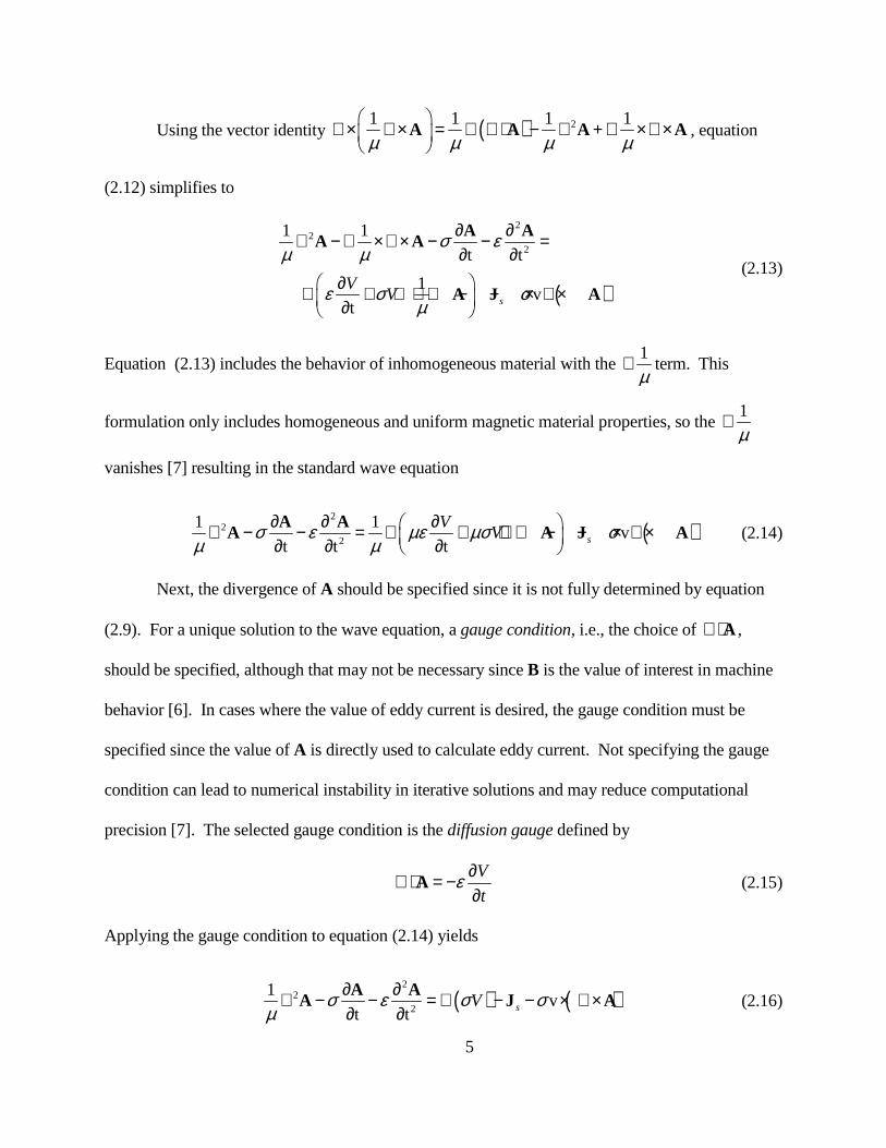
Using the vector identity ( ) 21 1 1 1
µ µ µ µ ∇× ∇× = ∇ ∇⋅ − ∇ ∇ ×∇×
A A A + A , equation
(2.12) simplifies to
( )
22
2
1 1
t t
1 v
t s
VV
σ εµ µ
ε σ σµ
∂ ∂∇ − ∇ ×∇× − − =∂ ∂
∂∇ + + ∇ ⋅ − − × ∇× ∂
A AA A
A J A
(2.13)
Equation (2.13) includes the behavior of inhomogeneous material with the 1
µ∇ term. This
formulation only includes homogeneous and uniform magnetic material properties, so the 1
µ∇
vanishes [7] resulting in the standard wave equation
( )2
22
1 1v
t t t s
VVσ ε µε µσ σ
µ µ∂ ∂ ∂ ∇ − − = ∇ + + ∇⋅ − − × ∇× ∂ ∂ ∂
A AA A J A (2.14)
Next, the divergence of A should be specified since it is not fully determined by equation
(2.9). For a unique solution to the wave equation, a gauge condition, i.e., the choice of ∇⋅A ,
should be specified, although that may not be necessary since B is the value of interest in machine
behavior [6]. In cases where the value of eddy current is desired, the gauge condition must be
specified since the value of A is directly used to calculate eddy current. Not specifying the gauge
condition can lead to numerical instability in iterative solutions and may reduce computational
precision [7]. The selected gauge condition is the diffusion gauge defined by
V
tε ∂∇⋅ = −
∂A (2.15)
Applying the gauge condition to equation (2.14) yields
( ) ( )2
22
1v
t t sVσ ε σ σµ
∂ ∂∇ − − = ∇ − − × ∇×∂ ∂A A
A J A (2.16)

6
This equation is simplified by neglecting the gradient of the electric scalar potential term, which is
a function of the current density resulting from low-frequency voltage source excitation and
resistance, and the magnetic vector potential second-derivative term, which is the displacement
current and is small for low-frequency applications [7]. These assumptions reduce equation (2.16)
to
( )21v
t sσ σµ
∂∇ − = − − × ∇×∂A
A J A (2.17)
This equation is the main equation that describes the electromagnetic behavior of electric
machines using magnetic vector potential. In a two-dimensional simulation, with impressed
current density applied in the z-direction, the magnetic vector potential only has a single
component, zA . Reducing the problem to two dimensions means that the simulation assumes the
electric machine has infinite axial length. When conducting simulation studies of electric machine
designs, this assumption is appropriate for preliminary and semi-detailed machine analysis. This
two-dimensional simplification of the electric machine analysis enables significantly faster
analysis. However, for detailed machine design and analysis, a three-dimensional simulation that
captures end turn effects should be conducted.
The velocity term of equation (2.17) can be eliminated by setting velocity to zero and
neglecting motion or by employing a frame of reference that is fixed with respect to the moving
component so that the relative velocity v becomes zero. This reference frame is created by fixing
the mesh to the surface of the moving component and moving or remeshing only the elements in
the air around the component [3]. To simplify the meshing and finite element implementation,
motion is neglected in this formulation.
7
Using the fact that magnetic vector potential only has a single component in the z-direction
for the two-dimensional analysis and neglecting motion, equation (2.17) reduces to
2 2
2 2
1
t
A A AJ
x yσ
µ ∂ ∂ ∂+ − = − ∂ ∂ ∂
(2.18)
where A is understood to be z-directed and only varies in the x- and y-directions, and J is the
impressed z-directed current density. Equation (2.18) is referred to as a magnetic diffusion
equation.
The Galerkin approach is used to derive the finite element equations. It is a special case of
the method of weighted residuals. The Galerkin method uses the weighting function of the same
form as the finite element shape function [6], [3], [7]. The magnetic vector potential within an
element is approximated by the sum of shape functions. With A denoting the approximation of A,
the magnetic vector potential within an element e is approximated by
1
ˆ ˆ( , )m
e e ei i
i
A N x y A=
=∑ (2.19)
for m nodes in the element and eiN element shape functions.
The residual r of equation (2.18) with the approximation of A denoted as A is
2 2
2 2
ˆ ˆ ˆ1
t
A A Ar J
x yσ
µ ∂ ∂ ∂= + − + ∂ ∂ ∂
(2.20)
The weighted residual for element e is
2 2
2 2
ˆ ˆ ˆ1 1, 2,...,
te
e e ei i e
A A AR N J dxdy i m
x yσ
µΩ
∂ ∂ ∂= + − + = ∂ ∂ ∂ ∫∫ (2.21)
2.2 Finite Element Discretization

8
where eΩ denotes the element domain. Integrating by parts, equation (2.21) can be written as
ˆ ˆ ˆ ˆ1 1ˆ ˆ ˆ
ˆ
t
e e
e e
e ee e e ei ii ie e
e e ei i
N NA A A AR dxdy N x y n d
x x y y x y
AN dxdy N J dxdy
µ µ
σ
Ω Γ
Ω Ω
∂ ∂∂ ∂ ∂ ∂= + − + ⋅ Γ ∂ ∂ ∂ ∂ ∂ ∂
∂− +∂
∫∫ ∫
∫∫ ∫∫
(2.22)
where eΓ denotes the contour enclosing eΩ and ˆen is the outward unit vector normal to eΓ .
To solve for the finite-element domain solution, the element weighted residuals,
represented by equation (2.22), are assembled by summation with the same equation with shape
functions for the other elements. The system residual should be zero so that the approximated A
equates to the actual A. For M elements, this system residual is described by
1
1
ˆ ˆ ˆ ˆ1 1ˆ ˆ ˆ
ˆ 0
t
e e
e e
e eMe e ei iie e
e
Me e ei i
e
N NA A A Adxdy N x y n d
x x y y x y
AN dxdy N J dxdy
µ µ
σ
= Ω Γ
= Ω Ω
∂ ∂∂ ∂ ∂ ∂ + − + ⋅ Γ + ∂ ∂ ∂ ∂ ∂ ∂
∂ − + = ∂
∑ ∫∫ ∫
∑ ∫∫ ∫∫
(2.23)
From the derivation in [6], the internal element sides do not contribute to the line integral. By
imposing the homogeneous Neumann boundary condition, which is defined by ˆ
0ˆe
A
n
∂ =∂
, the line
integral is zero. When the finite element method is used with other solution techniques, such as the
boundary element method or an analytical expression to represent techniques the air-gap region
solution [3], this may not be a suitable boundary condition. In that case, the line integral must be
evaluated [3]. This formulation only uses the finite element method, so the homogeneous
Neumann boundary condition is satisfactory and simplifies the solution calculation.

9
The reluctivity term is introduced, which is simply 1νµ
= . With the line integral term equal
to zero, the following equation shows equation (2.23) written in matrix form:
[ ] [ ] 1 1 1
ˆˆ 0
t
M M Me e e
e e e
AS A T Q
= = =
∂ + − = ∂ ∑ ∑ ∑ (2.24)
or even more compactly as
[ ] [ ] ˆ
ˆ 0t
AS A T Q
∂ + − = ∂ (2.25)
where it is understood that the S, T, and Q matrices are assembled by summing over the elements.
Entries in these matrices are given by:
e ee ej je e i i
ij
N NN NS dxdy
x x y yν
∂ ∂∂ ∂= + ∂ ∂ ∂ ∂ ∫∫ (2.26)
e e e eij i jT N N dxdyσ= ∫∫ (2.27)
e e ei iQ J N dxdy= ∫∫ (2.28)
for , 1,2,...,i j m= nodes per element. A and ˆ
t
A ∂ ∂
correspond to the jth node. The integrals in
these matrices can be evaluated analytically or numerically. The matrices depend on the element
order and corresponding shape function.
First-order elements consist of three nodes connected by three edges to form a triangle.
Figure 2.1 illustrates a first-order triangular element. For mesh consistency, they must be
2.2.1 First-order elements

10
numbered counterclockwise. The unknown function A varies linearly within each element and is
approximated as
ˆ ( , )e e e eA x y a b x c y= + + (2.29)
With m = 3, the shape functions which approximate ˆ eA according to equation (2.29) satisfy
equation (2.19). The derivation of the first-order shape functions can be found in [6] and [3]. For
first-order elements, the shape functions are given by
1
( , ) ( ) 1,2,32
e e e ej j j je
N x y x y jα β γ= + + =∆
(2.30)
with
1 2 3 2 3 1 2 3 1 3 2
2 3 1 3 1 2 3 1 2 1 3
3 1 2 1 2 3 1 2 3 2 1
; ; =x
; ; =x
; ; =x
e e e e e e e e e e e
e e e e e e e e e e e
e e e e e e e e e e e
x y y x y y x
x y y x y y x
x y y x y y x
α β γα β γα β γ
= − = − −
= − = − −
= − = − −
(2.31)
and
( )1 2 2 1
1
2 area of the element
e e e e e
e
β γ β γ∆ = −
= (2.32)
Using these shape functions, equations (2.26), (2.27), and (2.28) evaluate to
( ) ( )1
, , Q T =4 12 3
e e e e e e
i j i j ije e e e eij ij i
e
eS J
ν β β γ γ δσ
+ + ∆= =∆
∆ (2.33)
Figure 2.1 First-order triangular element
11
1 2
3
e
4
56
where ijδ = 1 when i = j, otherwise, ijδ = 0. Note that for this implementation, reluctivity and
conductivity are constant throughout the element.
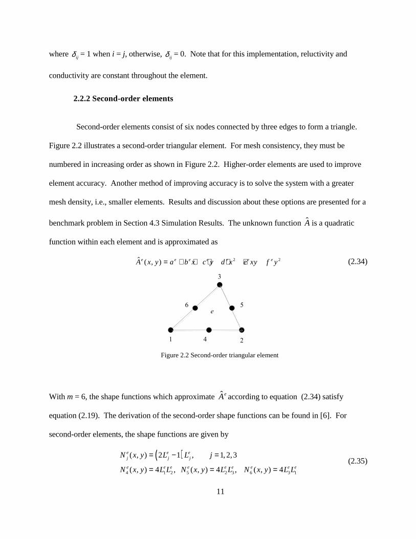
Second-order elements consist of six nodes connected by three edges to form a triangle.
Figure 2.2 illustrates a second-order triangular element. For mesh consistency, they must be
numbered in increasing order as shown in Figure 2.2. Higher-order elements are used to improve
element accuracy. Another method of improving accuracy is to solve the system with a greater
mesh density, i.e., smaller elements. Results and discussion about these options are presented for a
benchmark problem in Section 4.3 Simulation Results. The unknown function A is a quadratic
function within each element and is approximated as
2 2ˆ ( , )e e e e e e eA x y a b x c y d x e xy f y= + + + + + (2.34)
With m = 6, the shape functions which approximate ˆ eA according to equation (2.34) satisfy
equation (2.19). The derivation of the second-order shape functions can be found in [6]. For
second-order elements, the shape functions are given by
( )
4 1 2 5 2 3 6 3 1
( , ) 2 1 , 1,2,3
( , ) 4 , ( , ) 4 , ( , ) 4
e e ej j j
e e e e e e e e e
N x y L L j
N x y L L N x y L L N x y L L
= − =
= = = (2.35)
2.2.2 Second-order elements
Figure 2.2 Second-order triangular element

12
with
1
( , ) ( ) 1,2,32
e e e ej j j je
L x y x y jα β γ= + + =∆
(2.36)
and the same , , , and e e e ej j jα β γ ∆ as defined for first-order elements.
Using these shape functions, equations (2.26), (2.27), and (2.28) evaluate to
( )
( ) ( )
( ) ( )
14 24 12 16 36 13
25 35 23 15 26 34
2 2
44 1 2 1 2
2 2
55 2 3 2 3
66
4 1 , 1,2,3
124 4
, 3 34
, 03
2
32
32
ije e e e e eij i j i je
e e e e e e
e e e e e e
e e e e e ee
e e e e e ee
e e
S i j
S S S S S S
S S S S S S
S
S
S
δν β β γ γ
ν β β γ γ
ν β β γ γ
ν
−= + =
∆
= = = =
= = = = =
= + + + ∆ = + + + ∆
= ( ) ( )
( ) ( )
( ) ( )
2 2
3 1 3 1
22 245 2 3 1 3 1 2 2 2 3 1 3 1 2 2
22 246 1 3 2 3 1 2 1 1 3 2 3 1 2 1
56 3 1 2 1 2 3
31
2 231
2 231
23
e e e ee
e e e e e e e e e e e e e e e ee
e e e e e e e e e e e e e e e ee
e e e e e e e ee
S
S
S
β β γ γ
ν β β β β β β β γ γ γ γ γ γ γ
ν β β β β β β β γ γ γ γ γ γ γ
ν β β β β β β
+ + + ∆ = + + + + + + + ∆ = + + + + + + + ∆
= + +∆
( ) ( )22 23 3 1 2 1 2 3 32e e e e e e e eβ γ γ γ γ γ γ γ + + + + +
(2.37)
6 1 1 0 4 0
1 6 1 0 0 4
1 1 6 4 0 0
0 0 4 32 16 16
4 0 0 16 32 16
0 4 0 1
1
6 32
0
1
8
6
ee e
ijT σ
− − − − − − − − − − −
−
∆=
(2.38)

13
e
0 1,2,3
4,5,63
e
ei
i
J iQ
=∆ =
=
(2.39)
The discretized system of equations for magnetodynamic finite-element analysis varies
with time. To emphasize this, equation (2.25) can be written as
[ ] [ ] ˆ ( )ˆ( ) ( ) 0t
A tS A t T Q t
∂ + − = ∂ (2.40)
In the case where motion is not modeled or a fixed reference frame is used, the S, T, and mesh-
dependent sections of Q matrices are not time-dependent. Note that the Q matrix is shown to vary
with time, but that is only because the applied current density J may vary with time. If motion
were modeled with a reference frame, then elements in air are deformed with respect to time while
all other elements remain the same. In air, the conductivity is zero, so this element deformation
would not affect T and the mesh-dependent sections of Q. The S matrix would change with respect
to time [3].
For induction machines, the magnetic field is time-varying within a conducting region
which induces an electromotive force (emf) according to Faraday’s law described by equation
(2.1). This induced emf produces current, called eddy current, in conducting material normal to
the magnetic flux. The eddy currents in the rotor create magnetic poles that interact with the stator
poles created by the excitation current, causing the rotor to move. Modeling eddy current is
essential to simulate an induction machine, so a magnetostatic formulation is not suitable. Either a
time-harmonic or time-domain simulation can be used. Time-harmonic steady-state simulations,
2.3 Time Discretization

14
where the time-varying fields are sinusoidal and represented by a single frequency, are typically
represented by the Fourier transform of equation (2.18) [3]:
2 2
2 2
1 A Aj A J
x yωσ
µ ∂ ∂+ − = − ∂ ∂
(2.41)
The use of the time-domain simulation over the time-harmonic simulation is discussed in section
2.6 Nonlinear Formulation, where nonlinear magnetic material is addressed. For linear magnetic
material simulations, time-harmonic analysis described by equation (2.41) can be used for steady-
state simulations at a specified frequency. For linear or nonlinear magnetic material problems,
simulations not at steady-state or involving non-sinusoidal excitation require the solution of the
time-domain equation (2.40). For the simulations in this thesis, the time-domain formulation is
used to model all possible frequencies of electromagnetic behavior.
The stator ( sω ) and rotor ( rω ) frequencies are related according to the rotor slip s
according to
s r
s
sω ω
ω−= (2.42)
For a stationary time-domain formulation, the impressed current density is applied at slip
frequency instead of the stator frequency in order to represent the mechanical power and torque
produced on the rotor.
While the time-domain simulation enables eddy current simulation, the two-dimensional
simulation limits the accurate simulation of total machine core losses. The eddy currents in the
stator produce losses, called core losses, which the electric machine designer would like to
minimize. Core losses are reduced by using laminated sheets which are electrically insulated from
each other. The insulation is parallel to the direction of the magnetic flux density so that the eddy
currents which flow normally to the magnetic flux density can only flow in each laminated sheet
15
[1]. A two-dimensional time-varying simulation thus only models the eddy current due to one
lamination cross section.
The time-discretization of equation (2.40) follows the derivation in [3]. The time-
discretization method used is based on:
( ) 1
t t tt t t A AA A
t t tβ β
+∆+∆ −∂ ∂ + − = ∂ ∂ ∆ (2.43)
The t∆ symbol indicates the change in time. The constant β allows the difference method to be
easily changed. Note that when 0,β = the algorithm is forward difference, when 1,β = the
algorithm is backward difference, or when 0 1,β< < the algorithm is an intermediate type. When
1,
2β = the algorithm is the Crank-Nicolson method [8].
Using equation (2.43) to discretize time in equation (2.40) yields
[ ] [ ] [ ] [ ] 1 1 1 1ˆ ˆt t t t t tS T A T S A Q Q
t t
β ββ β β β
+∆ +∆ − −+ = − + + ∆ ∆ (2.44)
When reluctivity is linear, equation (2.44) is used to solve for ˆ t t
A+∆
at each time step.
The system defined by equation (2.44) is essentially a sparse linear system equivalent to the
typical
x b=A
This sparse linear system also applies to the nonlinear formulation described in section 2.6 when
solving for the change in magnetic vector potential used to update the next iteration. The matrix A
is sparse, b is a vector, and the system is solved for the vector x. For the sparse matrices solved
2.4 Sparse Iterative Linear Solvers

16
later in this thesis for time-domain formulations, the average density of nonzero elements in the
matrix relative to the total number of elements is 0.0012. For example, given this density, for a
10,000 by 10,000 element matrix, approximately 117,430 elements of the matrix are nonzero out
of the total 108 elements. An example of the matrix sparsity patterns is shown in Figure 2.3.
The assignment of the element and node numbering upon mesh generation affect the
sparsity structure of the matrix. For first-order elements, each element contributes nine nonzero
entries (3x3 matrix according to node numbering). For first-order elements, each element
contributes 36 nonzero entries (6x6 matrix according to node numbering).
There are several ways to solve the system. LU decomposition can be used. To solve the
system using LU decomposition with forward and backward substitution for n unknowns, 3( )O n
multiplication operations are performed if A and b are full. The number of operations required
when employing sparse LU decomposition techniques, such as those in [9]- [10], depends on the
number and ordering of nonzero entries in the matrix.
0 1000 2000 3000 4000 5000 6000
0
1000
2000
3000
4000
5000
6000
nz = 477690 0.5 1 1.5 2 2.5
x 104
0
0.5
1
1.5
2
2.5
x 104
nz = 257873
(a) (b) Figure 2.3 Matrix sparsity pattern for example time-domain meshes for
(a) first-order elements and (b) second-order elements

17
Sparse iterative linear solvers are another option to solve the system. In particular, Krylov
subspace methods can be used to solve the finite-element discretized system [11]. To solve the
system using a sparse iterative linear solver for n unknowns, A is no longer treated as having n n×
values, but rather only p nonzero values, and its inverse is found in terms of a linear combination
of its powers. For well-conditioned matrices, this should reduce the number of operations that are
performed to solve the system. Krylov subspace methods that use the Arnoldi [12] or Lanczos [13]
process, such as generalized minimum residual method (GMRES) method [14], [15], conjugate
gradient (CG) method [14], [16], bi-conjugate gradients (BiCG) method, and the bi-conjugate
gradients stabilized (BiCGStab) method [14], [17], are 2( )O n per iteration [18].
Finite element matrices can be ill-conditioned for the sparse iterative linear solvers. This
means that the iterative solvers require many iterations to solve the system to a specified tolerance.
Using a preconditioner can accelerate the convergence of the iterative solvers. While it takes a
certain number of operations to create the preconditioner, the decrease in number of iterations
required to solve the system using the preconditioner with the iterative solver may still require
fewer operations than using iterative solver without the preconditioner. A preconditioner is used
by solving the system
1 1x b− −=P A P (2.45)
Preconditioners used with iterative solvers are a computationally efficient way to find a matrix P
such that 1−P A is better conditioned than A. Two readily available preconditioners are the
incomplete LU (ILU) preconditioner [11] and incomplete Cholesky factorization preconditioner
[11], [19].
18
After computing the solution for the nodal magnetic vector potential, other values may be
computed from the solution in order to evaluate the physical behavior of the simulated problem.
These other values are considered to be “post-processed” values since they are computed after the
solution for A is found. The three post-processing values of interest in this thesis are the magnetic
flux density B, eddy current, and force.
The magnetic flux density is the first post-processed value of interest. Magnetic flux
density has physical meaning and can be measured, unlike magnetic vector potential. For the
linear ferromagnetic material model, magnetic flux density may be calculated outside of the
magnetic vector potential finite-element solution. To minimize memory storage, it is beneficial to
calculate the magnetic flux density at desired nodes or elements at each time step and store only
those values rather than both of the entire magnetic vector potential and magnetic flux density
solutions at each time step. For the nonlinear ferromagnetic material model, it is necessary to
calculate the magnetic flux density magnitude at each node or element at every iteration in order to
determine nonlinear reluctivity since reluctivity is a function of the square of magnetic vector
potential.
Recalling from equation (2.9) that B is the curl of A, so B varies in each element with one
degree of freedom less than A. For first-order elements, B is constant throughout the element. For
second-order elements, B varies linearly throughout the element. Theoretically, the lower order
elements decrease the accuracy of B. The element order accuracy and mesh density is examined in
the benchmark problem simulation results in Chapter 4.
2.5 Post-Processing
2.5.1 Magnetic flux density

19
Since B is the curl of A, and A only has a single component zA ,
ˆ ˆz zA Ax y
y x
∂ ∂−∂ ∂
B = (2.46)
The partial derivatives of zA are computed from the shape functions that describe ˆzA . B in terms
of shape functions is
1 1
( , ) ( , )ˆ ˆˆ ˆe em m
e i ii i
i i
N x y N x yx A y A
y x= =
∂ ∂−∂ ∂∑ ∑B = (2.47)
For first-order elements, this equates to
3 3
1 1
1 1ˆ ˆˆ ˆ2 2
e e ei i i ie e
i i
x A y Aγ β= =
−∆ ∆∑ ∑B = (2.48)
Notice that the magnetic flux density is constant throughout the element. For second-order
elements, the expressions becomes more complicated and equates to
( )( )( )
( )( ) ( )( )
( )( ) ( )( )
( )
3
21
2 1 1 1 1 2 2 2 42
3 2 2 2 2 3 3 3 52
3 12
1 ˆ2
1 ˆ
1 ˆ
1
ee e e e e ix i i i i iee
i
e e e e e e e e
e
e e e e e e e e
e
e e
e
B x y A
x y x y A
x y x y A
γγ α β γ
γ α β γ γ α β γ
γ α β γ γ α β γ
γ α
=
+ + − + ∆∆
+ + + + + + ∆
+ + + + + + ∆
∆
∑=
( ) ( )( )1 1 1 3 3 3 6ˆe e e e e ex y x y Aβ γ γ α β γ
+ + + + +
(2.49)

20
( )( )( )
( )( ) ( )( )
( )( ) ( )( )
( )
3
21
2 1 1 1 1 2 2 2 42
3 2 2 2 2 3 3 3 52
3 12
1 ˆ2
1 ˆ
1 ˆ
1
ee e e e e iy i i i i iee
i
e e e e e e e e
e
e e e e e e e e
e
e
e
B x y A
x y x y A
x y x y A
γβ α β γ
β α β γ β α β γ
β α β γ β α β γ
β α
=
− + + − − ∆∆
+ + + + + − ∆
+ + + + + − ∆
∆
∑=
( ) ( )( )1 1 1 3 3 3 6ˆe e e e e e ex y x y Aβ γ β α β γ
+ + + + +
(2.50)
ˆ ˆe e ex yB x B y+B = (2.51)
The eddy current density is modeled by magnetic vector potential derived from Maxwell’s
equations. Using equation (2.11) that relates electric field to magnetic vector potential, neglecting
the electric scalar potential, and knowing that
eddy σ=J E (2.52)
then eddy current in terms of magnetic vector potential is
teddy σ ∂= −
∂A
J (2.53)
In terms of time discretization using equation (2.43), eddy current density is calculated from the
magnetic vector potential solution at each time step by
( ) ( )1
t t t
t t teddy eddy
A AJ J
t
βσ
β β
+∆+∆
−−= −
∆ (2.54)
2.5.2 Eddy current density
21
The purpose of an electric machine is to produce force or torque to do work. Measuring or
computing these quantities is useful to evaluate the performance of the machine. There are several
methods to compute the force from a finite element simulation. The Ampere’s Force Law,
Maxwell Stress Method, and Virtual Work Method are considered in [3]. In this thesis, the
Maxwell Stress Method is used to compute force. It is used to find the total, not the local, force on
an object. Additionally, the Maxwell Stress Tensor formulation in the air gap should result in
accurate force calculation for linear and nonlinear magnetic material representation.
Following the derivation from [3], the volume force density can be written as the
divergence of the Maxwell Stress Tensor (MST) T
vp = ∇ ⋅T (2.55)
where T is derived as
22
22
0
22
1
21 1
21
2
x x y x z
y x y y z
z x z y z
B B B B B
B B B B B
B B B B B
µ
− = − −
B
T B
B
(2.56)
Integrating and using the vector divergence theorem, the total force can be expressed as
S
F dS= ⋅∫ T (2.57)
Taking this surface integration to be a cylindrical surface through the machine airgap, this
integration is reduced to a line for two-dimensional simulation to give force per unit depth. The
tangential ( tF ) and normal ( nF ) force components in newtons per meter can be calculated
according to
2.5.3 Force from Maxwell Stress Tensor
22
( )
0
2 2
0
2 2 2 2
2 2 2 2 2 2 2 2 2 2
22 2 2 2
2
( ) ( )
2 2
12
2
n tt t
L L
n tn n
L L
n t x y x y x y y x
n t x y x y x y y x x x x y x y y y
x y x y x y y x
B BF dF dl
B BF dF dl
B B B B s s s s B B
B B B s B B s s B s B s B B s s B s
B s B B s s B s B
µ
µ
= =
−= =
= − + −
− = − + − + +
= − + −
∫ ∫
∫ ∫
(2.58)
where the unit normal and tangential vectors to the integration path and tangential and normal
components of flux density are defined as
ˆ ˆ ˆ
ˆ ˆ ˆn x x y y
t y x x y
t x x y y
n x y y x
a s a s a
a s a s a
B B s B s
B B s B s
= +
= − +
= +
= − +
(2.59)
Including the nonlinear permeability of the ferromagnetic material involved in an electric
machine problem is necessary to obtain accurate simulations of magnetic flux saturation. Most
induction machines operate near or in the saturation region, so only modeling linear permeability
may yield inaccurate simulation results. To push the electric machines to their torque and power
density limitations, the machines are likely to operate near saturation.
The permeability or equivalent reluctivity in the constitutive relation shown by equation
(2.7) is nonlinear. It is a function of the local magnetic field. The most accurate physical
representation of the B-H relationship includes nonlinearity and hysteresis. The family of
hysteresis curves can be represented by a normal magnetization curve.
Figure 2.4 shows an example family of hysteresis curves. The dotted line represents a
2.6 Nonlinear Formulation

23
normal magnetization curve. For a specific steel, Figure 2.5 shows the initial magnetization
nonlinear B-H curve. This steel curve is used for the nonlinear simulation of the benchmark
problem described in Chapter 4. From this data, the reluctivity versus the square of magnetic flux
density is computed and illustrated in Figure 2.6.
Figure 2.4 Hysteresis curves and
normal magnetization curve
Figure 2.5 Nonlinear B-H curve for steel
0 0.5 1 1.5 2 2.5 3 3.5 4 4.5 5 5.5
x 104
0
0.5
1
1.5
2
H (A/m)
B (
T)
B-H Curve for Steel

24
Figure 2.6 Nonlinear reluctivity versus square of magnetic flux density for steel
As previously referenced, a time-domain simulation is preferred to accurately simulate how
nonlinear magnetic material affects the magnetic flux density. An effective permeability
approximation method based on average energy [3] can be used with the time-harmonic approach.
The time-domain method allows permeability to vary throughout the domain at each instant in
time, providing a more intuitive model of the nonlinearity of the magnetic permeability.
Additionally, time-domain simulation can include permeability hysteretic effects.
To model the nonlinearity of reluctivity, an iterative process is used to find the solution that
is consistent with the field solution. The process is summarized by first assuming an initial value,
solving the system, then correcting the reluctivity based on magnetic flux density solution. This
process continues until the change in either the magnetic vector potential or reluctivity is less than
a specified tolerance.
A common method of linearizing the system of nonlinear equations is the Newton-Raphson
method. For the nonlinear iterative solution, the existence and uniqueness of a unique stable
mathematical solution requires that the magnetization curve be monotonically increasing with their
first derivatives monotonically decreasing [7]. If the nonlinear function is monotonically
0 0.5 1 1.5 2 2.5 3 3.5 4 4.5 50
0.5
1
1.5
2
2.5
3
3.5x 10
4
B2 (T2)
ν (m
/H)
Nonlinear Reluctivity versus B2

25
increasing, the solution from the Newton-Raphson method will converge quadratically. The curve
in Figure 2.4 is not monotonically increasing. In order to guarantee convergence, the reluctivity in
the low flux density region can be approximated as constant. Most electric machinery is not
designed to operate in this region in steady-state, so this approximation is acceptable. For
applications where the low flux density behavior is important, the Newton-Raphson method may
use the change in permeability from one iteration to the next as the convergence criterion rather
than the change in magnetic vector potential [3].
A review of the Newton-Raphson method for a system of nonlinear equations follows.
Consider a system of nonlinear equations
( ) 0f x = (2.60)
where f represents a system of n equations, and xrepresents n variables 1 2, ,..., nx x x . An estimate
of the solution is ( )kx . An initial guess is used as the solution to (0)x . The iteration number is
represented by the superscript (k). The error is ( ) ( 1) ( )k k kx x x+∆ = − . The system of equations can
at iteration 1k + can be represented by
( ) ( )( ) 0k kf x x+ ∆ = (2.61)
This equation expanded in a Taylor series is
( )
( )( )( )
2( ) ( ) ( ) ( ) ( )
1 1
( ) ( ) 0, 1,2,...,k
n nk k k ki k
i i jj jj
j
x
ff x x f x x O
xx i n
= =
+ ∆ = ∂∂
+ ∆ + ∆ = =∑ ∑ (2.62)
Omitting the higher order term, this equation can be written in matrix form as
[ ] ( ) ( )
1 1( )k k
n n n nJ x f x
× × ×∆ = − (2.63)
where the Jacobian matrix J is given by

26
[ ]
( ) ( ) ( )
( ) ( ) ( )
( ) ( ) ( )
( ) ( ) ( )
( ) ( ) ( )
( ) ( ) ( )
1 1 1
1 2
2 2 2
1 2
1 2
...
...
...
k k k
k k k
k k k
n
n
n n n
n
x x x
x x x
x x x
f f f
x x x
f f f
x x x
f f f
x
J
x x
=
∂
∂ ∂∂ ∂ ∂
∂ ∂ ∂∂ ∂ ∂
∂ ∂ ∂∂ ∂ ∂
M M O M
(2.64)
Equation (2.63) is solved for ( )kx∆ . Then, ( 1)kx + is found by ( 1) ( ) ( )k k kx x x+ = + ∆ . The method
continues to iterate until
( )kx ε∆ < (2.65)
where ε is a specified tolerance.
The Newton-Raphson method is applied to the time-discretized finite-element equation
(2.44) to linearize the reluctivity. This derivation follows aspects of the magnetostatic and time-
domain modeling linearization using the Newton-Raphson method in [3] with some modifications
for handling second-order elements. The implementation of the Newton-Raphson method is
slightly different depending on the element order. For first-order elements, the reluctivity is
constant throughout each element, so the calculation of the Jacobian only involves the terms
2
2j jA A
ν ν∂ ∂ ∂=∂ ∂ ∂
BB
for j = 1,2,3. B is the magnitude of the magnetic flux density calculated from A.
More information about how B is calculated from A is included in section 2.6 about post-
processing. For second-order elements, the reluctivity now varies throughout the element. Since
reluctivity is not an analytical function of B, it is represented numerically as the reluctivity derived

27
from B at each element node. In that case, the Jacobian involves 2
2i i
j jA A
ν ν∂ ∂ ∂=∂ ∂ ∂
BB
for i, j =
1,2,3,4,5,6.
Consider the time-discretized equation (2.44) per element for first-order elements.
111 12 13 11 12 13
21 22 23 21 22 23 2
31 32 33 31 32 33 3
11 12 13 11 12 13
21 22 23 21 22 23
31 32 33 31 32 3
ˆ
ˆ
ˆ
1
t t
e
e
As s s t t t
s s s t t t A
s s s t t t A
t t t s s s
t t t s s s
t t t s s s
ν
β νβ
+∆ + =
− −
1 1 1
2 2 2
3 3 33
ˆ1ˆ
ˆ
tt t tA Q Q
A Q Q
Q QA
ββ
+∆ − + +
(2.66)
The subscripts denote local nodes 1, 2, and 3 for the element. Let , 1,2,3iF i = denote the ith
equation.
[ ] [ ]
[ ] [ ]
1
1 2 3 1 2 3 2
3
1
1 2 3 1 2 3 2
3
ˆ
ˆ
ˆ
ˆ1 1ˆ
ˆ
t t
ei i i i i i i
t
e t t ti i i i i i i i
A
F s s s t t t A
A
A
t t t s s s A Q Q
A
ν
β βνβ β
+∆
+∆
= + −
− − − − −
(2.67)
To find the derivatives necessary to form the Jacobian, equation (2.67) is differentiated with
respect to the nodal magnetic vector potential. Using the product and chain rules, the result is
23
21
e ee t ti
ij ij iq qt t eqj j
F Bs t s A
A B A
νν +∆+∆
=
∂ ∂ ∂= + + ∂ ∂ ∂ ∑ (2.68)
2.6.1 Nonlinear formulation for first-order elements

28
for , 1,2,3.i j = The ith Newton-Raphson equation is
1
21 2 3
3
t t
i i iit t t t t t
AF F F
A FA A A
A
+∆
+∆ +∆ +∆
∆ ∂ ∂ ∂ ∆ = − ∂ ∂ ∂ ∆
(2.69)
This can be written in matrix notation per element as
[ ] [ ]
[ ] [ ] [ ] [ ]
[ ]
1 1
t tt t t tk k k
t t t t t tt t tk k
S T G A
S T A T S A Q Q
ν
β βν νβ β
+∆+∆ +∆
+∆ +∆+∆
+ + ∆ =
− − − + + − + +
(2.70)
where
( )
23 3 3
1 1 11 1 1 1
, 23 3 3
2 2 22,1 1 1 2
23 3 3
3 3 31 1 1 3
0 0
[ ] 0 0
0 0
t tt t e
q q q q q qq q q
e t t et t kk q q q q q q
e t tq q q
ke
q q q q q qq q q k k
Bs A s A s A
A
BG s A s A s A
AB
Bs A s A s A
A
ν
+∆+∆
= = =
+∆+∆
+∆ = = =
= = =
∂ ∂ ∂ ∂=
∂ ∂ ∂
∂
∑ ∑ ∑
∑ ∑ ∑
∑ ∑ ∑
(2.71)
Note the “hats” are dropped from the nodal magnetic vector potential, but it is understood that
those values are estimated values. All values at time t t+ ∆ are the kth iteration values. The
Newton-Raphson equations for each are assembled to obtain a global system of equations.
For each time step, the Newton-Raphson iteration process can be summarized as follows:
1. Start with an initial guess 0A A= . When solving for t tA+∆ , set 1 .t t tA A+ ∆ =
2. Calculate ,e t tkB + ∆ , ,e t t
kν + ∆ , and the Jacobian values in equations (2.70) and (2.71) from
t tkA + ∆ values.
3. Assemble global matrices from element values according to equation (2.70) and (2.71).

29
4. Solve linear system of equations for .t t
kA
+∆∆
5. Update 1 .t t t t t tk k kA A A+ ∆ + ∆ + ∆
+ = + ∆ (2.72)
6. If t tkA ε+∆∆ < , stop the iteration process and set 1
t t t tkA A+ ∆ + ∆
+= . Otherwise, repeat the
iteration process from step 2 and continue.
Several calculations are required for step 2. The value of t tkν + ∆ is calculated by first determining
t tkB + ∆ from equation (2.46), then determining the value of t t
kν + ∆ according to the non-linear 2Bν −
curve at the point for ( )2t tkB +∆ . Note that the Jacobian values in equation (2.71) are calculated
differently for first- and second-order elements. The value of ( )
,
2,
e t tk
e t tkB
ν +∆
+∆
∂
∂is determined by taking
the derivative of the non-linear 2Bν − curve. The value of ( )2,
,
e t tk
t ti k
B
A
+∆
+∆
∂∂
, i = 1,2,3, for first-order
elements is derived from equations (2.46) and (2.48) that describes B as a function of Az. First,
note that
22
2e z zA AB
x y
∂ ∂ + ∂ ∂ = (2.73)
Squaring the x- and y-components of equation (2.48) and taking the derivative as a function of Aj
for j = 1,2,3 yields
( )
( ) ( )
2, 3 3
, ,2 21 1, 2 2
e t t e ek j je t t e t t
i i k i i kt t e ei ij k
BA A
A
γ βγ β
+∆+∆ +∆
+∆= =
∂= +
∂ ∆ ∆∑ ∑ (2.74)
The author has not found specific implementation methods for modeling nonlinear second-
order time-domain finite element methods. In [3], the nonlinear magnetostatic formulation is
2.6.2 Nonlinear formulation for second-order elements

30
described for first-order elements, but not for second-order elements nor for the magnetodynamic
(time-harmonic or time-domain) formulation. In [6], the linear two-dimensional time-harmonic
formulation is described for first- and second-order elements, and the general time-domain
discretization is discussed, but neither the nonlinear time-harmonic nor the nonlinear time-domain
formulation for second-order elements is described. In [7], first- and second-order element
implementations for the Helmholtz equation are described, first-order element solutions of the
Newton-Raphson iterations are shown, and time- and frequency-domain problems are discussed
including eddy-current analysis using magnetic vector potential, but the time-domain, nonlinear
implementation for second-order or higher-order elements is not explicitly described. In [20]
which is more mathematically based rather than application based for [3], [6], [7], higher-
dimensional element formulation is presented, and iterative methods are discussed, but the
application of second-order elements for a time-domain, nonlinear problem is not presented. The
following formulation was derived for second-order elements as an extension of the nonlinear
formulation for first-order elements.
For elements with nonlinear reluctivity which is a function of 2B , and B depends on
position within an element, reluctivity is also a function of position within an element and is no
longer constant as it is for first-order elements. As a result, the finite element discretization, time
discretization, and linearization should be repeated with elemental reluctivity replaced by ( ),x yν .
To numerically include the reluctivity variation within the element, the value of B is calculated at
each local node per element. Then, using the local nodal B values, the reluctivity and
corresponding 2B
ν∂∂
at each local node belonging to elements in the nonlinear material region is
calculated according to the nonlinear v-B2 curve for the magnetic material. If an analytical

31
expression is available for the v-B2 relationship, it may be analytically possible to determine the
variation of v across the element. In this case, a value and gradient could be assigned at each local
node per element. As seen in the example v-B2 in Figure 2.6, the derivative of this curve is
constant for certain ranges of B2. The reluctivity at each node belonging to elements in the linear
material region is assigned according to the relative reluctivity to that region. For elements in the
linear material region, the reluctivity is constant throughout the element.
With the reluctivity variation in mind, the matrix defined by equation (2.37) is redefined by
replacing eν with eiν . In this way, the finite element formulation is still the same as for first-order
elements, but a variation in reluctivity within an element is included.
The nonlinear finite-element formulation is the same as first-order elements except the
Jacobian values are different because reluctivity varies at each node. The Jacobian values become
26
21
t ti i ii ij ij iq qt t
qj i j
F Bs t s A
A B A
νν +∆+∆
=
∂ ∂ ∂= + + ∂ ∂ ∂ ∑ (2.75)
for , 1,2,...,6.i j = The Newton-Raphson equation can be written in matrix notation per element as
[ ] [ ] [ ]
[ ] [ ] [ ] [ ] [ ] [ ]
[ ]
1 1
t t t tt tk kk
t t tt t t t t t
kk
diag S T G A
diag S T A T diag S A Q Q
ν
β βν νβ β
+∆ +∆+∆
+∆ +∆ +∆
+ + ∆ =
− − − + + − + +
(2.76)
where
26
, 21
t t
t t i iij k iq q
qi j k
BG s A
B A
ν+∆
+∆
=
∂ ∂= ∂ ∂ ∑ (2.77)
The value of ,t ti kν +∆ is calculated in the same manner as for first-order elements by first determining
,t ti kB +∆ from equation (2.46), then determining the value of ,
t ti kν +∆ according to the non-linear 2Bν −

32
curve at the point for ( )2
,t ti kB +∆ . The value of
( ),
2
,
t ti k
t ti kB
ν +∆
+∆
∂
∂is determined by taking the derivative of
the non-linear 2Bν − curve. The value of ( )2
,
,
t ti k
t tj k
B
A
+∆
+∆
∂∂
, i,j = 1,2,…,6 for second-order elements is
derived from equations (2.46), (2.49), and (2.50) that describe B as a function of Az. First, note that
22
2 z zA AB
x y
∂ ∂ + ∂ ∂ = (2.78)
Rewriting equations (2.49) and (2.50) to simplify these expressions,
( )( )( )
( )( ) ( )( )
( )( ) ( )( )
( )
3
21
2 1 1 1 1 2 2 2 42
3 2 2 2 2 3 3 3 52
3 12
1 ˆ2
1 ˆ
1 ˆ
1
ee e e e e ix i i i i iee
i
e e e e e e e e
e
e e e e e e e e
e
e e
e
B x y A
x y x y A
x y x y A
γγ α β γ
γ α β γ γ α β γ
γ α β γ γ α β γ
γ α
=
+ + − + ∆∆
+ + + + + + ∆
+ + + + + + ∆
∆
∑=
( ) ( )( )1 1 1 3 3 3 6
6
1
ˆ
ˆ ( , )
e e e e e e
m mm
x y x y A
f x y A
β γ γ α β γ
=
+ + + + +
=∑
(2.79)

33
( )( )( )
( )( ) ( )( )
( )( ) ( )( )
( )
3
21
2 1 1 1 1 2 2 2 42
3 2 2 2 2 3 3 3 52
3 12
1 ˆ2
1 ˆ
1 ˆ
1
ee e e e e iy i i i i iee
i
e e e e e e e e
e
e e e e e e e e
e
e
e
B x y A
x y x y A
x y x y A
γβ α β γ
β α β γ β α β γ
β α β γ β α β γ
β α
=
− + + − − ∆∆
+ + + + + − ∆
+ + + + + − ∆
∆
∑=
( ) ( )( )1 1 1 3 3 3 6
6
1
ˆ
ˆ ( , )
e e e e e e e
m mm
x y x y A
g x y A
β γ β α β γ
=
+ + + + +
=∑
(2.80)
Squaring the x- and y-components of B from equations (2.79) and (2.80) and taking the derivative
as a function of Aj for j = 1,2,…,6 yields
( )2
6 6,
, ,1 1,
2 ( , ) ( , ) 2 ( , ) ( , )t ti k t t t t
j i i m i i m k j i i m i i m kt tm mj k
Bf x y f x y A g x y g x y A
A
+∆+∆ +∆
+∆= =
∂= +
∂ ∑ ∑ (2.81)
The Newton-Raphson equation for each element is assembled to obtain a global system of
equations.
Rather than always updating the next iteration value of the nodal magnetic vector potential
by , a relaxation factor α may be used according to
1t t t t t tk k kA A Aα+ ∆ + ∆ + ∆
+ = + ∆ (2.82)
to either over-relax or under-relax the update. The updated value is over-relaxed if 1α > , and this
theoretically reduces the number of iterations to achieve convergence as long as the update does
not overshoot the exact solution in which the method may not converge. The updated value is
2.6.3 Relaxation factor
34
under-relaxed if 0 1α< < . This may be necessary to achieve convergence with the Newton-
Raphson method so that the next updated value does not overshoot the solution.
A method of determining the relaxation factor to find the value ofα that minimizes the
objective function in equation (2.83) which is a function of the Galerkin residual [21], [22]. The
objective function is the sum of the values of the Galerkin residual each raised to the nth power.
Objective functions to the second and fourth powers were explored. Equation (2.84) shows the
Galerkin residual. Note that it is a function of the updated 1t tkA + ∆
+ which is a function of α .
1 , 1
nt tk i k
i
W H +∆+ +=∑ (2.83)
[ ] [ ] [ ] [ ] 1 1
1 1
t t t t t tt t t t tk k k
S T A T S A Q Qβ βν ν
β β+∆ +∆+∆ +∆
+ +
− − Η = + − − − −
(2.84)
The value of t tkν + ∆ may be updated to the value of 1
t tkν + ∆
+ which is a function of 1
t t
kA
+∆
+ . This option
was experimentally explored and did not seem to improve the convergence or reduce the number
of iterations to achieve convergence. Additionally, updating the value of 1t tkν + ∆
+ for each updated
1
t t
kA
+∆
+ for the values of α examined ( )0,0.1,0.2,...,2α = increases the computation time of each
iteration without necessarily any benefit. Instead, the relaxation factor α that allowed the solution
value to achieve convergence was determined through numerical experiments for the specific
problem. When an appropriate under-relaxation factor still does not yield a converged solution, the
mesh may need to be refined.
2.7 Implementation
Each of the time-domain finite-element simulations was programmed for and run using
MATLAB. While other programs, such as Maxwell Ansoft and JMAG, are available for finite
35
element simulations of electric machines, a program needed to be created so that the lines of code
could be manipulated in order to experiment with acceleration of the simulation. The time
discretization used for each of these simulations is the Crank-Nicolson method with β = 0.5
according to equation (2.43).
In addition to the Neumann boundary condition applied in the derivation described in
section 2.2 Finite Element Discretization, other boundary conditions must be applied to create a
nonsingular global matrix and obtain a unique solution for the finite element problem [3]. At each
point on the boundary of the mesh domain, the magnetic vector potential unknown or the normal
derivative must be specified. Additionally, in order for the global matrix to be nonsingular, the
magnetic vector potential must be defined for at least one specific node. For this application, the
homogeneous Dirichlet boundary condition is applied, resulting that for all nodes on the boundary
of the mesh domain, 0A = .
This section describes computer simulation implementation specifics for each type of
problem – first or second order elements, and linear or nonlinear simulations. For all matrices and
vectors stored and manipulated on the CPU, the MATLAB sparse matrix format is utilized to
improve computational efficiency and reduce memory usage.
2.7.1 First-order, linear simulation
The first-order element mesh for the benchmark and induction machine simulation was
generated using the MATLAB Partial Differential Equation (PDE) toolbox. This toolbox provides
the ability to create a mesh using the Delaunay triangulation algorithm for a specified geometry. It
generates a point matrix with the x- and y-coordinates of the points in the mesh, edge matrix, and

36
triangle matrix describing the element triangle corner points in counterclockwise order and the
corresponding element subdomain number.
For the simplest simulation using linear magnetic material and first-order elements, note
that conductivity and reluctivity are constant throughout the element. From implementation of
equation (2.44) using first-order matrices defined by equations (2.31)-(2.33), it is apparent that for
a fixed geometry and linear reluctivity, the [S] and [T] matrices do not vary with time, but the
magnetic vector potential and Q vectors do vary with time. As a result, the [S] and [T] matrices
only need to be computed once.
For a MATLAB script implementation, the [S] and [T] matrices are computed using the
MATLAB sparse matrix format. For each element, the contributions from each node are
calculated then summed over the elements to assemble the total [S] and [T] matrices. Because for
first-order, linear simulations these matrices are only calculated once, they are computed on the
CPU since the GPU will not yield a significant speed-up with this assembly, especially since the
matrices are sparse.
For each time step, the solution for the next time-step value of the magnetic vector potential
of equation (2.44) is solved for using the sparse iterative Krylov subspace solver biconjugate
gradients stabilized method using a function that implements the biconjugate gradients stabilized
method with preconditioner algorithm [11], [14], [17]. A similar MATLAB function “bicgstab” is
also available for comparison. Several types of solvers for use with preconditioners are readily
available functions in MATLAB. In addition to the biconjugate gradients stabilized method, the
biconjugate gradients, conjugate gradients squared, generalized minimum residual, least squares,
minimum residual, preconditioned conjugate gradients, quasi-minimal residual, and symmetric LQ
methods are available MATLAB functions. For the first-order, linear simulation, each of these

37
preconditioned solvers, except the quasi-minimal residual which was much slower, calculated the
solution in similar times. The biconjugate gradients stabilized method is chosen as the solver for
each type of simulation for consistency and calculation time comparison for different problem
sizes. For the biconjugate gradients stabilitized method used, the solver tolerance was 10-5. The
MATLAB built-in function “ichol” to form the sparse incomplete Cholesky factorization was used
to form the preconditioner. For this problem, the matrix is symmetric, positive definite, so the
incomplete Cholesky factorization is a suitable preconditioner. The modified incomplete Cholesky,
lower triangle preconditioner was formed using threshold dropping of tolerance 10-3. Once the
value for the magnetic vector potential was solved, the corresponding magnetic flux density per
element was computed by equation (2.48), and the eddy current density was computed by equation
(2.54)
2.7.2 Second-order, linear simulation
The second-order element mesh, specifically for the three additional nodes per element and
edges between elements used to determine boundary nodes, was generated with the MATLAB
PDE toolbox and the LehrFEM 2D finite element toolbox [23].
The second-order linear simulation follows the same simulation process as the first-order
linear simulation except with second-order defined matrices. These matrices are the [S] and [T] per
equations (2.37) and (2.38). Additionally, the magnetic flux density is calculated for each local
node per element according to equations (2.49) and (2.50). The same preconditioner was not used
for the second-order linear simulation as for the first-order linear simulation since it did not result
in a converging sparse iterative solution to the specified 10-5 tolerance. Instead, the lower
triangular, unmodified incomplete Cholesky factorization with zero fill was used for the
preconditioner.
38
2.7.3 First-order, nonlinear simulation
The nonlinear problem mesh is formed the same way as the linear problem mesh. The
nonlinear reluctivity vs. 2B and nonlinear 2B
ν∂∂
vs. 2B are each represented by a piecewise linear
interpolation function according to the nonlinear magnetic material properties.
The nonlinear simulation is set up to solve equation (2.70) with equation (2.71) using the
Newton-Raphson method to solve the nonlinear system of equations. The matrices [ ]T and [ ]S
without the associated ν are computed once at the beginning of the simulation. The nonlinear
iterative process outlined in section 2.6, Nonlinear Formulation, is implemented. For first-order
elements, the magnetic flux density and reluctivity are constant throughout the element and are
thus assigned per element. The Newton-Raphson residual ε used was 10-6. The incomplete
Cholesky factorization preconditioner resulted in pivoting errors when it was called to compute
and did not enable the biconjugate gradient stabilized solver to converge. Instead, the sparse
incomplete LU factorization preconditioner was used according to the MATLAB function “ilu.”
The row-sum modified incomplete LU Crout version factorization with drop tolerance 10-5 was
used and resulted in converged solutions for the biconjugate gradient stabilized solver. The sparse
iterative linear solver tolerance was 10-5.
An under-relaxation factor according to equation (2.82) was used for each Newton-
Raphson iteration and time step. The value of the relaxation factor was determined experimentally
using the value closest to 1 but still allowing the Newton-Raphson iteration to converge and not
overstep the solution. This approach minimizes the number of Newton-Raphson iterations while
still resulting in a converging solution.
39
In addition to the relaxation factor, the element size and time step difference t∆ affect the
Newton-Raphson convergence. For the first-order, nonlinear simulation, both coarse and fine
meshes for the benchmark problem and t∆ = 1 ms result in a converged solution.
2.7.4 Second-order, nonlinear simulation
The second-order, nonlinear simulation follows the same process as for the first-order,
nonlinear simulation. The second-order matrices were computed according to equations (2.37),
(2.38), (2.39), (2.76), (2.77), and (2.81). As described previously, the nonlinear reluctivity and
resulting 2B
ν∂∂
and 2B
A
∂∂
are computed for each local node per element. The magnetic flux density
is calculated for second-order elements by equations (2.49)-(2.51). The same incomplete LU
factorization type of preconditioner and iterative solver used for the first-order, nonlinear
simulation was used for this simulation.
The second-order, nonlinear simulation had Newton-Raphson convergence issues that did
not arise for the other simulation types. For the benchmark problem, the coarse mesh problem
could only converge for t∆ = 1 ms for simulation times 1-4 ms. Beyond that, smaller t∆ values
had to be used in order for the Newton-Rapshon iterations to converge to the 10-6 residual.
Solutions were calculated up to 27.487 ms with a t∆ = 0.001 ms. For subsequent times, it was
determined that for a reasonable computation time, the fine mesh needed to be used in order to
achieve convergence for a larger t∆ .
For the benchmark problem fine mesh, the solution converged for t∆ =1 ms for times 1-18
ms. For subsequent times, t∆ =0.5 ms resulted in converged solutions for times 18-20 ms, and t∆
=0.1 ms resulted in converged solutions for times 20-21.7 ms. The remaining part of the

40
simulation was not conducted due to the nonlinear convergence problems. Results are presented
for times 1-18 ms to show scalability of the GPU solution.
For the linear induction machine problem, the large air gap and excitation resulted in the
operation of the magnetic material in the linear region. Nonlinear problem solutions did achieve
convergence for the M19 steel representation using continuous analytical functions to represent v-
B2 and 2B
ν∂∂
. However, the results were similar to the linear magnetic material results, so they are
not presented.
A complete nonlinear solution of the benchmark problem is available for the first-order
elements, but not for the second-order elements due to the nonlinear convergence problem. This
convergence issue could potentially be resolved by using an even smaller t∆ , finer mesh, or a
continuous analytical expression of the nonlinear magnetic material properties instead of the
piecewise linear representation. For electric machine design and analysis problems, the higher-
order element simulations with nonlinear magnetic material should result in higher fidelity
solutions than for first-order elements. As part of the tradeoff of simulation detail and computation
time, the higher-order element simulations require a smaller time step or finer mesh than the first-
order element simulations to achieve convergence, resulting in a longer computation time. This
trade-off may be reasonable when detailed simulation results are desired, such as for magnetic
material saturation near tooth tips.

41
CHAPTER 3
ACCELERATING THE FINITE ELEMENT SIMULATION
The finite element simulation of a low-frequency nonlinear electromagnetic problem can be
accelerated using a numerical or parallel computing method or both. The Shooting-Newton [4]
numerical method was investigated. Multi-core and GPU parallel computation methods were also
studied.
3.1.1 Numerical methods
When the steady-state analysis of an electromagnetic problem is desired, there are
numerical approaches, such as the shooting-Newton method [4], that can be utilized. Additionally,
domain decomposition techniques can be utilized to subdivide the problem for different processing
techniques [5].
Methods for steady-state analysis reduce the need for a transient solution to achieve the
steady-state solution. For an induction machine, eddy current is represented through transient
analysis. For different machine topologies such as permanent magnet synchronous machines,
steady-state analysis can be utilized for machine nominal performance design.
One approach of the shooting-Newton method, which requires Gaussian elimination,
assessed for simulation acceleration involves a matrix-free Krylov-subspace approach [4]. The
shooting method approach is to find the periodic steady-state solution of the problem by comparing
the computed solution at the end of the period and determining if it matches the initial condition at
the start of the period. The method outlined in [4] was experimented for the benchmark problem
3.1 Methods of Accelerating Finite Element Simulations
42
later presented. For this specific type of finite element analysis, this method did not appear to
reduce the computation time because the numerical integration required a small change in time,
resulting in a longer computation time than the transient finite element analysis formulation.
3.1.2 Parallel processing methods
3.1.2.1 Multiple core
Multiple-core processors provide a means to accelerate certain simulations such as ordinary
differential equations. For an implementation in which each equation is independent, not related to
the solution of a separate set of equations or other variables, and can be implemented in any order,
the solution of these equations is easily solved in parallel. For the time-domain finite element
simulation, each time step of the solution must be computed sequentially, but it may be possible to
decompose the domain for each time step and compute the solution of each subsection in parallel
[5].
For example, MathWorks has developed a parallel for-loop that enables parallel for-loop
implementation across each core of a processor [24], [25]. The parallel ordinary differential
equation example describes the use of the parallel for-loop to solve a parameter sweep study of a
second-order ODE system [26]. First, the example solves 3500 ODEs in serial using the ode45
solver. Then, the example solves the same number of ODEs using the parallel for-loop. For a
processor with four cores, the speed-up of this example is tested to be approximately 3.63, which is
nearly linearly proportional to the number of cores. This is due to the fact that this loop has
minimal overhead in terms of data transfer.
Another means of multi-core processing and parallel loops is using single program multiple
data (SPMD) [27]. This type of processing is suitable for simulations that can be implemented in
43
any order and be solved in parallel. SPMD is a shared-memory approach using message passing.
One task per processor is executed, and each processor executes the same code. In this way, a
parallel loop can be implemented. An API readily available for shared memory multiprocessing is
Open Multi-Processing (OpenMP). It provides a means of multithread processing whereby a block
of code is executed in parallel [27].
Message Passing Interface (MPI) is a message-passing communication protocol developed
for parallel programming such as scalable cluster computing [27]. The computing nodes do not
share memory and interact through message passing. Programs that use MPI use a set of routines
callable from several types of programming languages, making MPI portable.
There are several examples from the literature about parallel processing applied to finite
element simulations using MPI and domain decomposition (DD) [5], [28], [29], [30], [31].
Applications of such simulations include structural dynamics and electromagnetic simulation of
electric machines. The application described in this thesis is the time-domain, nonlinear simulation
of an induction machine in two dimensions for a fixed position. The time domain simulation of
this problem is essential in order to simulate the eddy currents of the induction machine.
Examples from the literature include aspects of this type of simulation but not all in a single
simulation using one or more parallel processing methods.
A simulation by engineers in Tokyo [30] describes a method to parallelize the 2D, steady-
state analysis of nonlinear induction machine magnetic fields. The approach, called the parallel
time-periodic finite-element method (PTPFEM), parallelizes the simulation in the time-axis
direction rather than in each time step. The simulation approach taken in this thesis and typical
with domain decomposition is by each time step. By solving the equations for all nonlinear
unknowns at every time step for a period simultaneously, the problem is posed for a larger number
44
of equations which lends itself to greater speed up from parallelization in this approach. This is
useful for the steady-state analysis of the induction machine and not the transient. This thesis does
not necessarily focus on the steady-state simulation of the induction machine. In the early stages of
a machine design, it may be beneficial to understand the steady-state behavior of the machine. In
this case, an approach such as this may be useful. The authors use MPI communications for the
parallel processing. The BiCGstab2 method and localized ILU preconditioning are used. To
stabilize the convergence of the Newton-Raphson method, the authors apply the line search based
on the minimization of energy function. The authors claim, but do not quantify, that the
communication overhead associated with domain decomposition for parallel performance causes
the performance to suffer for small scale analysis. The example simulation described for an
induction machine includes 13,198 elements, 256 time steps to form a period, and 3,252,480
unknowns. A supercomputer is used for the simulation where each node consists of four AMD
Opteron 8356 processors, and the backward Euler method is used for time integration. The
PTPFEM simulation results were compared for 1, 8, 16, 32, 64, and 128 processes, as well as for
the transient approach called the time-periodic explicit error correction method, which is a time-
domain approach to find the steady-state solution faster than traditional time-domain approaches.
For a slip of 1, the PTPFEM approach achieved a speed-up of 7.06, and for a slip of 0.0588, the
PTPFEM approach sped up the solution by a factor of 8.4. The authors did not describe a means to
parallelize the time-domain approach and compare those results to the PTPFEM approach. As the
number of processes increases, the speed-up increases, showing the effectiveness of the PTPFEM
approach for highly parallel computation.
Another example of the use of MPI was done by researchers at the University of Alberta
[29]. A two-dimensional, transient, nonlinear simulation of an induction machine was

45
implemented using the Newton-Raphson method for linearization and domain decomposition.
The induction machine was simulated with an interbar rotor circuit model. The parallelization was
done with three PCs using 3.2 GHz Pentium D processors and MPICH2. The problem was of
similar size in this thesis for the first-order element simulation of the benchmark problem. In [29],
the finite element simulation consisted of 1941 nodes and 3534 first-order elements per time step.
For the simulation of 1000 time steps, three simulations were completed using different methods:
the traditional Newton-Raphson (NR) method, NR method with domain decomposition, and
parallelized NR with domain decomposition. The simulation times for these methods were 2270
s, 1581 s, and 395 s respectively. Comparing the serial and parallel NR with domain
decomposition techniques, the parallelized simulation resulted in a speed-up of 4. Note also that
domain decomposition resulted in a speed-up of 1.43, and comparing traditional NR with
parallelized NR with DD resulted in a speed-up of 5.75. This may show that depending on the
implementation of domain decomposition, further simulation speed-up may be obtained by using
domain decomposition with parallel processing such as with MPI.
A variation of parallel processing using MPI for a domain decomposition technique for
nonlinear dynamic finite element analysis was simulated for a structural dynamics problem [31].
The simulated problem requires the solution of second derivative differential equations, and the
unconditionally stable Newmark-β method is used for the time integration of the problem. The
parallel algorithm uses a method with overlapped domains with a predictor-corrector scheme. The
parallel algorithm is implemented on a cluster workstation using MPI. The number of partitioned
subdomains matches the number of processors. The algorithm was implemented for a mesh size
with 4710 unknowns and for a finer mesh with 17,322 unknowns. The larger mesh size provides a
slightly better speed-up than for a smaller mesh size, indicating the typical trend that the
46
performance of the parallel algorithm improves with increase in problem size. For 8 processors,
the smaller mesh speed-up was 4.7, and for the larger mesh the speed-up was approximately 5.
Researchers at the University of Tokyo and Kyushi University have also researched
domain-decomposition techniques applied to electromagnetic finite-element simulation [28]. They
applied the Heirarchical Domain Decomposition Method (HDDM) to a 3D nonlinear
magnetostatic problem. The domain decomposition technique allowed them to use parallel
computing with a supercomputer consisting of 64 nodes and 1024 cores. They investigated
different magnitudes of convergence criterion of two iterative solvers and how that affects the
computation time and convergence of the subdomain interface problem. The two iterative solvers
compared are the incomplete Cholesky-conjugate gradient method with shifted incomplete
Cholesky factorization preconditioner and the LU decomposition with pivoting. The specific
speed-up of the domain decomposition problem solved by the Supercomputer is not specified, but
they indicate that the problem had 1.2 billion degrees of freedom and solved in 4.8 hours with
approximately 80% of the time dedicated to computing and 16% of the time to communication. A
sequential solution for a smaller problem with 100 million degrees of freedom was solved in 4.5
hours. Assuming the supercomputer can solve the smaller 100 million degrees of freedom
problem in a proportional amount of time (which is not the case – the communication overhead
will likely increase), then the supercomputer may be able to solve this problem in 0.32 hours,
resulting in a potential speed-up of 14 due to the application of domain decomposition to multiple
cores and processors.
3.1.2.2 Graphical processing units
Graphical Processing Units (GPUs) can be utilized not only for graphics processing but
also for parallel computing [32], [33]. A GPU may consist of hundreds of cores that can be
utilized for multithreaded, single-instruction computation. Depending on the application, the
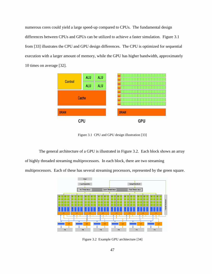
47
numerous cores could yield a large speed-up compared to CPUs. The fundamental design
differences between CPUs and GPUs can be utilized to achieve a faster simulation. Figure 3.1
from [33] illustrates the CPU and GPU design differences. The CPU is optimized for sequential
execution with a larger amount of memory, while the GPU has higher bandwidth, approximately
10 times on average [32].
Figure 3.1 CPU and GPU design illustration [33]
The general architecture of a GPU is illustrated in Figure 3.2. Each block shows an array
of highly threaded streaming multiprocessors. In each block, there are two streaming
multiprocessors. Each of these has several streaming processors, represented by the green square.
Figure 3.2 Example GPU architecture [34]

48
Figure 3.3 illustrates how the GPU memory, data transfer, and threads are structured. Each
device is composed of multiple grids which contain multiple blocks. Each block contains multiple
threads that can each be used to execute a single process. Each thread has access to local, global,
and shared memory. The shared memory is shared among the threads in each block. The kernel
function specifies the code that all threads should execute in parallel. This process is the SPMD
process. When the kernel is launched, it executes the parallel threads in the grid [32]. To utilize
the full capability of the GPU hardware, the threads should be adequately allocated to maximize
the parallelism.
The amount of speed-up that can be expected from GPU parallel processing depends on the
portion of the application that can be computed in parallel [32]. In most applications, only a
portion of the problem can be computed in parallel. Additionally, a practical speed-up ceiling
exists, such as a possible maximum of 100 times speed-up, which limits the expected simulation
speed-up.
Figure 3.3 Abstract representation of GPU structure [33], [32]

49
Interaction between the CPU and GPU within a program is similar to message passing
since there is limited shared memory between the processors. The data transfer between the CPU
and GPU thus contributes to the overhead of a hybrid CPU/GPU simulation and should be
minimized [32].
3.2 GPU Parallel Processing for the Finite Element Simulation
3.2.1 Components of FEA suitable for GPU parallel processing
There are several components in the finite element simulation, some of which may be
suitable for parallel processing and some which may not be. The components that are suitable are
parts where the computation can be distributed to multiple processors for parallel processing, then
reassembled for the domain solution to that component. The time-domain finite element
simulation for eddy-current problems requires the solution for each time step to be computed, and
the previous time step solution is required for the next time step computation. Thus, multiple time
steps cannot be distributed for parallel processing; one time step at a time must be considered
unless a different numerical method is used. Within each time step, there are several components
to the finite element simulation, as discussed in section 2.3 Time Discretization, section 2.6
Nonlinear Formulation, and section 2.7 Implementation.
1. Matrix assembly
2. Matrix multiplication: Magnetic flux density calculation (post processing for linear
formulation, used to determine nonlinear reluctivity for nonlinear formulation)
3. Matrix multiplication: [ ] t tkG +∆ for nonlinear formulation only based on nonlinear
reluctivity
50
4. Solution of the next time step t tA
+∆for the linear formulation, or iteration t t
kA
+∆∆
for the nonlinear formulation. Solution is computed using a sparse iterative solver with
preconditioner.
5. Nonlinear reluctivity and 2B
ν∂∂
determination based on 2Bν − for nonlinear magnetic
material only
6. Post processing: eddy current density, force calculation using multiplication
The finite-element mesh creation and assembly prior to computations for the magnetic vector
potential are not considered.
In addition to identifying the components where GPU parallel processing can speed up the
simulation, the CPU computation time percentage of each component should be understood. To
gain the most speed-up, ideally the components that require the longest computation time should
lend themselves to GPU parallel processing. In Chapter 4, Simulation of the Benchmark Problem,
the component computation time will be discussed for the linear and nonlinear formulation for
different mesh densities. The component with the longest computation time is formulation of the
preconditioner and sparse iterative solver solution, followed by matrix multiplication for the
magnetic flux density and [ ] t tkG +∆ , with the remaining components of matrix assembly, nonlinear
reluctivity determination, and eddy current density calculations requiring the shortest computation
times.
With the sparse iterative solver and matrix multiplications requiring longer computation
time than the other components, these components were chosen to study how GPUs can be used
for parallel processing with the goal to provide speed-up relative to the CPU simulation. The

51
remaining components are left on the CPU to form a hybrid CPU/GPU MATLAB-based
simulation. In particular, the MATLAB sparse matrix assembly and storage yields fast
computation times not readily achievable with the gpuArray format. There are numerous research
efforts that have studied how GPUs can be used for sparse matrix-vector multiplication and sparse
iterative solvers [35], [36], [37], [38], [39], [40], [41], [42], as is discussed in section 3.2.2.1
NVIDIA CUDA. This research studies how GPUs can be used to speed up these components to
form a hybrid CPU/GPU desktop-based MATLAB simulation for the time-domain finite element
analysis required for detailed electromagnetic induction machine analysis.
3.2.2 Implementation methods for GPU parallel processing for FEA
Several programming languages are available to use GPUs for parallel computing,
including OpenGL, OpenCL, Compute Unified Device Architecture (CUDA), and higher-level
language tools such as the parallel computing toolbox with MATLAB script programming
language. OpenGL is utilized for graphics programming and requires in-depth knowledge of the
programming language. CUDA, developed by NVIDIA, is an extension of C. This makes it more
accessible to programmers without the need to know graphics programming. This section focuses
on the use of CUDA, MATLAB extensions, and the MATLAB parallel computing toolbox.
3.2.2.1 NVIDIA CUDA
CUDA is a C-based programming language that extends C-programming for use with
GPUs for scientific parallel computing. In addition to the CUDA language, libraries have been
built to allow functions to be accessible to the average programmer and expand the use of CUDA.
In particular, for CUDA used for numerical solutions of partial differential equations, such as for
electromagnetic finite element simulation, the sparse linear algebra library CUSP [43] and
cuSPARSE library [44] provide useful functions. CUSP expands the Basic Linear Algebra Library
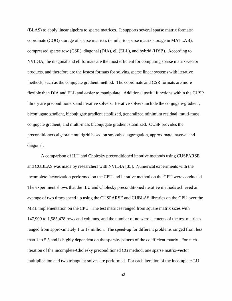
52
(BLAS) to apply linear algebra to sparse matrices. It supports several sparse matrix formats:
coordinate (COO) storage of sparse matrices (similar to sparse matrix storage in MATLAB),
compressed sparse row (CSR), diagonal (DIA), ell (ELL), and hybrid (HYB). According to
NVIDIA, the diagonal and ell formats are the most efficient for computing sparse matrix-vector
products, and therefore are the fastest formats for solving sparse linear systems with iterative
methods, such as the conjugate gradient method. The coordinate and CSR formats are more
flexible than DIA and ELL and easier to manipulate. Additional useful functions within the CUSP
library are preconditioners and iterative solvers. Iterative solvers include the conjugate-gradient,
biconjugate gradient, biconjugate gradient stabilized, generalized minimum residual, multi-mass
conjugate gradient, and multi-mass biconjugate gradient stabilized. CUSP provides the
preconditioners algebraic multigrid based on smoothed aggregation, approximate inverse, and
diagonal.
A comparison of ILU and Cholesky preconditioned iterative methods using CUSPARSE
and CUBLAS was made by researchers with NVIDIA [35]. Numerical experiments with the
incomplete factorization performed on the CPU and iterative method on the GPU were conducted.
The experiment shows that the ILU and Cholesky preconditioned iterative methods achieved an
average of two times speed-up using the CUSPARSE and CUBLAS libraries on the GPU over the
MKL implementation on the CPU. The test matrices ranged from square matrix sizes with
147,900 to 1,585,478 rows and columns, and the number of nonzero elements of the test matrices
ranged from approximately 1 to 17 million. The speed-up for different problems ranged from less
than 1 to 5.5 and is highly dependent on the sparsity pattern of the coefficient matrix. For each
iteration of the incomplete-Cholesky preconditioned CG method, one sparse matrix-vector
multiplication and two triangular solves are performed. For each iteration of the incomplete-LU

53
preconditioned BiCGStab iterative method, two sparse matrix-vector multiplications and four
triangular solves are performed. The total speed-up that can be achieved for a complete solution
will depend on the preconditioning time and number of iterations, not just the computation
required to perform one iteration. The majority of the computation time for both of these iterative
methods is spent for the triangular solve. Generally, the speed-up was greater for solutions
requiring a larger number of iterations and for less dense factorization. Denser factorization
inhibits the parallelism of these algorithms due to the dependence between rows in the sparse
triangular solver.
In [36], the authors also explore the use of GPUs for sparse matrix-vector products and
several preconditioning and iterative solver methods. Comparing CPU and GPU implementations
of the sparse triangular solve, the use of level scheduling can result in an improved matrix structure
more suitable for parallel computing. This type of sorting groups several unknowns into levels
such that the unknowns for one level can be computed at the same time, or in parallel [11]. The
ability of the GPU to speed up the computation of the parallel triangular solve depends on the
number of levels. Minimization of the number of levels improves the GPU computation time
speed-up. An example technique to reduce the number of levels is the Multiple Minimal Degree
ordering [45]. The greatest speed-up achieved using the GPU level scheduling sparse triangular
solve technique for the matrices tested was approximately 2.6 for a square matrix with 2.1 million
nonzero elements for a matrix size 525,000 x 525,000. The preconditioned iterative methods
considered were for the incomplete LU factorization, incomplete Cholesky factorization, block
Jacobi preconditioner, multi-color SSOR, and least-squares polynomial preconditioner. Certain
preconditioners were paired with the CG or GMRES iterative solver. For each of these
experiments, in many cases the triangular solves in the preconditioner were computed on the CPU

54
because the CPU computation time was faster than the GPU computation time. The greatest GPU
speed-up achieved for the cases considered was 4.3 for the GPU-accelerated ILUT-GMRES
method for the matrix with 8.8 million nonzeros for a matrix 1.27 million x 1.27 million. For the
sparse matrices used for the numerical experiments, the GPUs can be used to speed up the
computations, but their performance is limited for the sparse matrices compared to dense matrices.
3.2.2.2 MATLAB and extensions
There are several approaches to using GPUs with MATLAB script programs. With the
parallel computing toolbox, there is a gpuArray type that readily allows the user to convert an array
into this type and store the array on GPU as a full, single-precision array. This allows for direct
manipulation of the gpuArray with the MATLAB script. Another option is the use of mex files to
link a C, C++, or Fortran source file with the MATLAB program. This provides a means to pass
MATLAB variables to and from this function. With CUDA being an extension of C, this readily
allows the MATLAB program to call the CUDA program via the mex file. Additionally, a sparse
gpuArray format was developed by MATLAB users as an extension of the gpuArray type to
readily allow sparse matrix computation using gpuArray.
3.2.2.2.1 MATLAB gpuArray
A MATLAB gpuArray is stored on the GPU. Data can be created on the CPU and then
transferred to the GPU, resulting in communication time overhead, or created on the GPU. This is
accomplished using the gpuArray type. There are limitations to this type: the matrix must be non-
sparse (full) and of the data type single, double, int8, int16, int32, int64, uint8, uint16, uint64, or
logical. Thus, for problems well-suited to sparse matrix solvers, the use of GPUs and MATLAB
built-in functions will not inherently provide a faster computational speed. MathWorks has
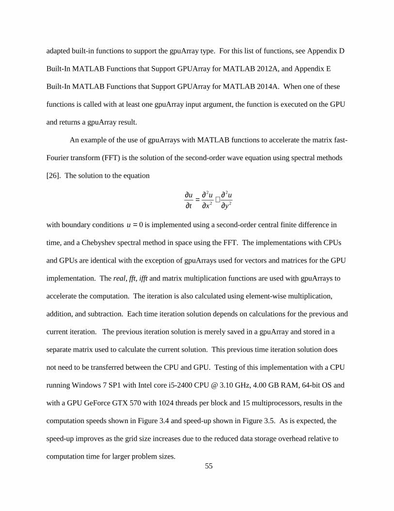
55
adapted built-in functions to support the gpuArray type. For this list of functions, see Appendix D
Built-In MATLAB Functions that Support GPUArray for MATLAB 2012A, and Appendix E
Built-In MATLAB Functions that Support GPUArray for MATLAB 2014A. When one of these
functions is called with at least one gpuArray input argument, the function is executed on the GPU
and returns a gpuArray result.
An example of the use of gpuArrays with MATLAB functions to accelerate the matrix fast-
Fourier transform (FFT) is the solution of the second-order wave equation using spectral methods
[26]. The solution to the equation
2 2
2 2
u u u
t x y
∂ ∂ ∂= +∂ ∂ ∂
with boundary conditions 0u = is implemented using a second-order central finite difference in
time, and a Chebyshev spectral method in space using the FFT. The implementations with CPUs
and GPUs are identical with the exception of gpuArrays used for vectors and matrices for the GPU
implementation. The real, fft, ifft and matrix multiplication functions are used with gpuArrays to
accelerate the computation. The iteration is also calculated using element-wise multiplication,
addition, and subtraction. Each time iteration solution depends on calculations for the previous and
current iteration. The previous iteration solution is merely saved in a gpuArray and stored in a
separate matrix used to calculate the current solution. This previous time iteration solution does
not need to be transferred between the CPU and GPU. Testing of this implementation with a CPU
running Windows 7 SP1 with Intel core i5-2400 CPU @ 3.10 GHz, 4.00 GB RAM, 64-bit OS and
with a GPU GeForce GTX 570 with 1024 threads per block and 15 multiprocessors, results in the
computation speeds shown in Figure 3.4 and speed-up shown in Figure 3.5. As is expected, the
speed-up improves as the grid size increases due to the reduced data storage overhead relative to
computation time for larger problem sizes.

56
Figure 3.4 Computation speed for CPU and GPU simulations using MATLAB ifft function with gpuArrays
Figure 3.5 Speed-up for MATLAB ifft function with gpuArrays
Another benchmark example of GPUs to CPUs developed by MathWorks is the mldivide
or backslash operator (\) used to calculate x from the system of equations x = A\b [24]. The time
measured is only the computation time to calculate x; it does not include the cost of transferring
data between the CPU and GPU or the time it takes to create a matrix. Note that since gpuArray
matrices are only defined for full matrices, the A matrix used with mldivide is a full matrix.
0 100 200 300 400 500 600 700 800 900 10000
2
4
6
8
10
12
Grid Size (N)
Spe
ed
Up
(CP
U/G
PU
tim
e) fo
r 50
itera
tions
Speed Up

57
Compared to CPU sparse matrix solutions with mldivide or CPU sparse iterative solvers, the full
matrix gpuArray mldivide computation time is much longer. Figure 3.6 shows the calculated
speed-ups for the mldivide function for several matrix sizes and single or double precision
matrices. The computation time for these calculations was done with the same CPU and GPU as
described for the previous example. Especially for single precision, the larger the matrix size, the
greater the speed-up. These matrix sizes are multiples of 1024 which facilitates greater speed-up
than for other multiples based on the single and double precision byte size. Although there are 15
processors available with the GeForce GTX 570, the speed-up for the largest matrix size with
single precision is approximately 4. The speed-up achieved depends on the algorithm
implementation.
Figure 3.6 Speed-up results for single and double precision calculations for MATLAB mldivide
3.2.2.2.2 MATLAB and MEX files
MEX files can be used to link MATLAB arrays with C files. They provide a means to link
CUDA code and libraries to gpuArray data on 64-bit platforms. Support for MEX files containing
1000 2000 3000 4000 5000 6000 7000 8000 90001
1.5
2
2.5
3
3.5
4
Matrix size
Spe
edup
Speedup of computations on GPU compared to CPU
Single-precision
Double-precision
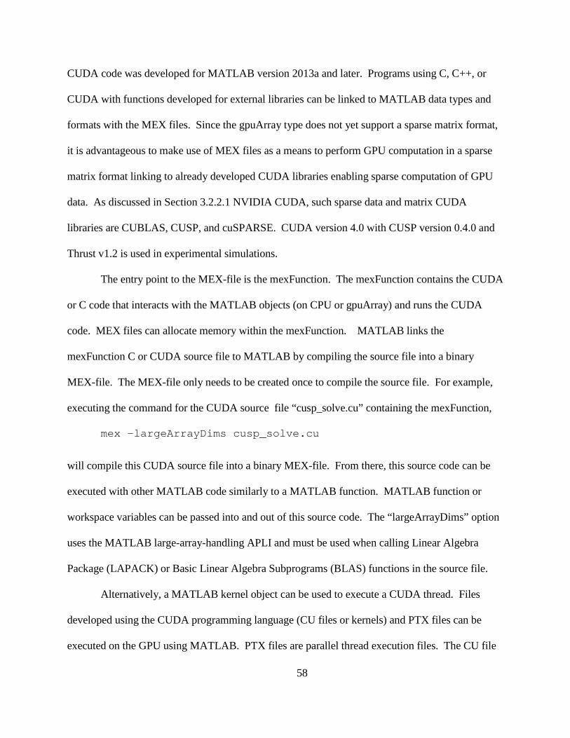
58
CUDA code was developed for MATLAB version 2013a and later. Programs using C, C++, or
CUDA with functions developed for external libraries can be linked to MATLAB data types and
formats with the MEX files. Since the gpuArray type does not yet support a sparse matrix format,
it is advantageous to make use of MEX files as a means to perform GPU computation in a sparse
matrix format linking to already developed CUDA libraries enabling sparse computation of GPU
data. As discussed in Section 3.2.2.1 NVIDIA CUDA, such sparse data and matrix CUDA
libraries are CUBLAS, CUSP, and cuSPARSE. CUDA version 4.0 with CUSP version 0.4.0 and
Thrust v1.2 is used in experimental simulations.
The entry point to the MEX-file is the mexFunction. The mexFunction contains the CUDA
or C code that interacts with the MATLAB objects (on CPU or gpuArray) and runs the CUDA
code. MEX files can allocate memory within the mexFunction. MATLAB links the
mexFunction C or CUDA source file to MATLAB by compiling the source file into a binary
MEX-file. The MEX-file only needs to be created once to compile the source file. For example,
executing the command for the CUDA source file “cusp_solve.cu” containing the mexFunction,
mex –largeArrayDims cusp_solve.cu
will compile this CUDA source file into a binary MEX-file. From there, this source code can be
executed with other MATLAB code similarly to a MATLAB function. MATLAB function or
workspace variables can be passed into and out of this source code. The “largeArrayDims” option
uses the MATLAB large-array-handling APLI and must be used when calling Linear Algebra
Package (LAPACK) or Basic Linear Algebra Subprograms (BLAS) functions in the source file.
Alternatively, a MATLAB kernel object can be used to execute a CUDA thread. Files
developed using the CUDA programming language (CU files or kernels) and PTX files can be
executed on the GPU using MATLAB. PTX files are parallel thread execution files. The CU file

59
must be compiled to create the PTX file using the nvcc compiler in the NVIDIA CUDA Toolkit.
For example,
nvcc -ptx myfun.cu
generates the file named myfun.ptx. Using the .cu and .ptx files, a MATLAB kernel object can be
created and used to evaluate the kernel
k = parallel.gpu.CUDAKernel('myfun.ptx', 'myfun.cu' );
The feval function is then used to evaluate the kernel on the GPU. Inputs can be from the
MATLAB workspace data on the CPU or gpuArray type. It may be more efficient to use
gpuArray objects as inputs to the kernel. The outputs of the kernel evaluation are gpuArray. The
CUDAKernel object is already compiled CUDA. Access to GPU memory must be pre-allocated
before execution of the kernel. The evaluation of the kernel returns a gpuArray, so transfer is not
required between the GPU and CPU.
3.2.2.2.3 Sparse gpuArray format
While the gpuArray format allows the user to readily convert CPU matrices and vectors to
GPU matrices and vectors, the gpuArray format is limited. As stated previously, a limited number
of MATLAB built-in functions are overloaded and useable with the gpuArray format.
Additionally, as of the time of this research, the gpuArray format is only available for full vector
and matrix formats. Only since MATLAB version R2015a has the gpuArray sparse format been
available, and the only function available with this format that could increase GPU performance
for the FEA problem is the matrix multiplication function. Finite element simulations involve
sparse matrices by nature, and they are typically large, involving at least thousands of unknowns.
The sparse matrix format allows this type of problem to be solved faster and with less memory
than an equivalent full matrix format. This motivated the need for a sparse gpuArray format.
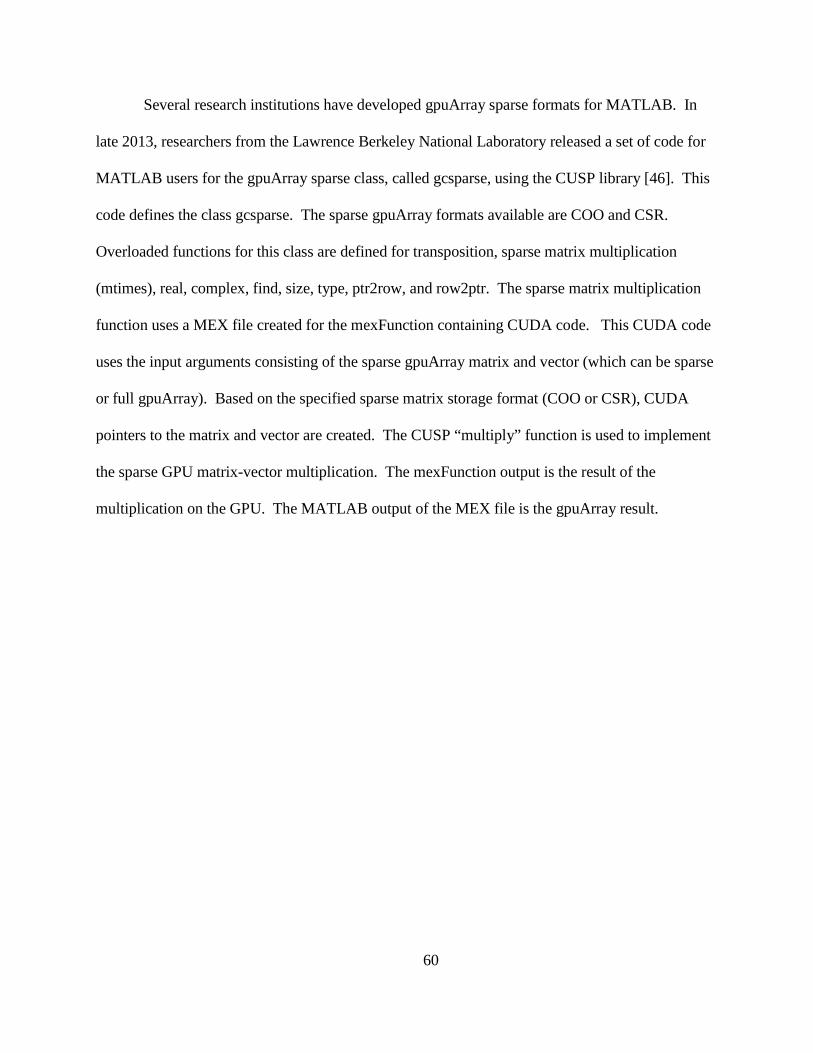
60
Several research institutions have developed gpuArray sparse formats for MATLAB. In
late 2013, researchers from the Lawrence Berkeley National Laboratory released a set of code for
MATLAB users for the gpuArray sparse class, called gcsparse, using the CUSP library [46]. This
code defines the class gcsparse. The sparse gpuArray formats available are COO and CSR.
Overloaded functions for this class are defined for transposition, sparse matrix multiplication
(mtimes), real, complex, find, size, type, ptr2row, and row2ptr. The sparse matrix multiplication
function uses a MEX file created for the mexFunction containing CUDA code. This CUDA code
uses the input arguments consisting of the sparse gpuArray matrix and vector (which can be sparse
or full gpuArray). Based on the specified sparse matrix storage format (COO or CSR), CUDA
pointers to the matrix and vector are created. The CUSP “multiply” function is used to implement
the sparse GPU matrix-vector multiplication. The mexFunction output is the result of the
multiplication on the GPU. The MATLAB output of the MEX file is the gpuArray result.
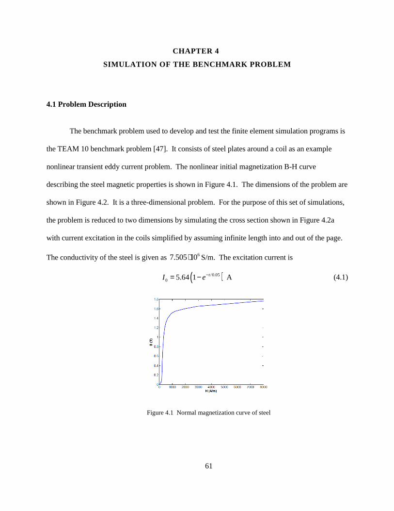
61
CHAPTER 4
SIMULATION OF THE BENCHMARK PROBLEM
The benchmark problem used to develop and test the finite element simulation programs is
the TEAM 10 benchmark problem [47]. It consists of steel plates around a coil as an example
nonlinear transient eddy current problem. The nonlinear initial magnetization B-H curve
describing the steel magnetic properties is shown in Figure 4.1. The dimensions of the problem are
shown in Figure 4.2. It is a three-dimensional problem. For the purpose of this set of simulations,
the problem is reduced to two dimensions by simulating the cross section shown in Figure 4.2a
with current excitation in the coils simplified by assuming infinite length into and out of the page.
The conductivity of the steel is given as 67.505 10⋅ S/m. The excitation current is
( )/0.050 5.64 1 AtI e−= − (4.1)
Figure 4.1 Normal magnetization curve of steel
4.1 Problem Description
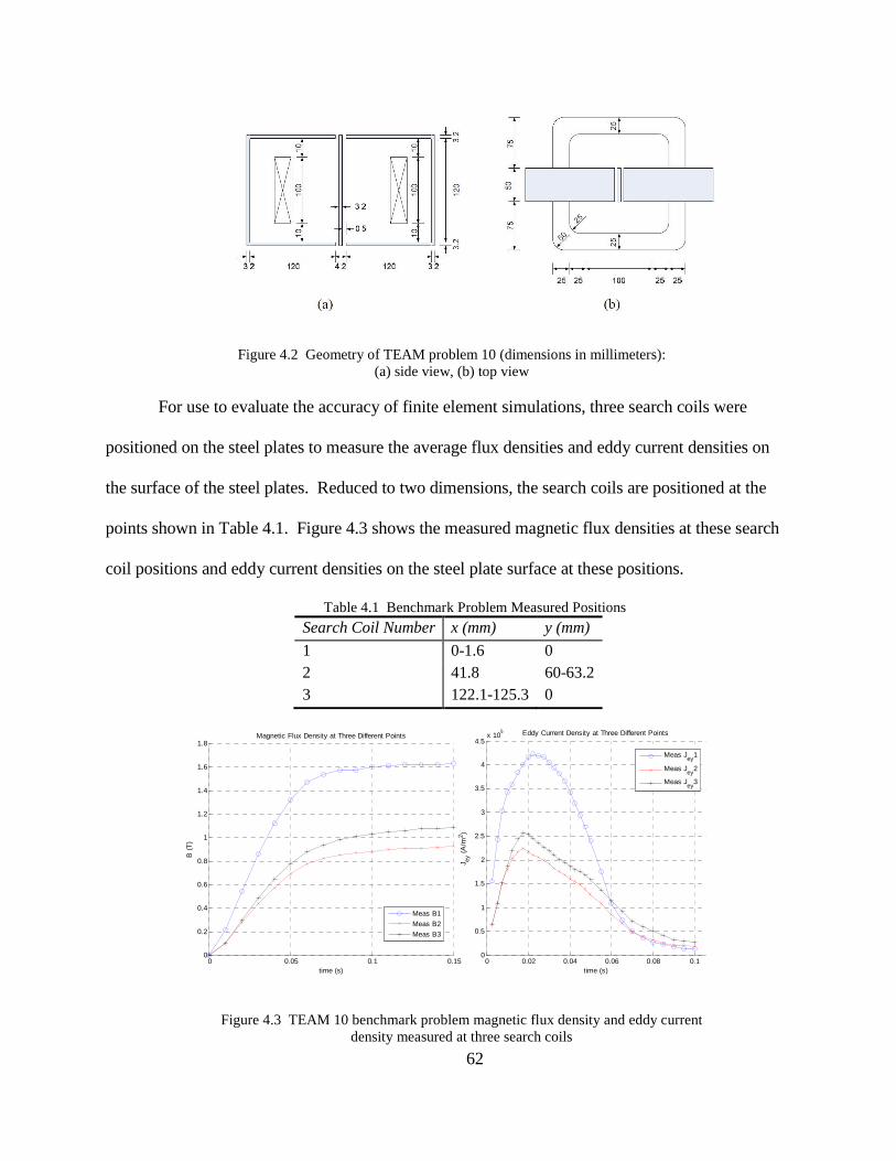
62
Figure 4.2 Geometry of TEAM problem 10 (dimensions in millimeters): (a) side view, (b) top view
For use to evaluate the accuracy of finite element simulations, three search coils were
positioned on the steel plates to measure the average flux densities and eddy current densities on
the surface of the steel plates. Reduced to two dimensions, the search coils are positioned at the
points shown in Table 4.1. Figure 4.3 shows the measured magnetic flux densities at these search
coil positions and eddy current densities on the steel plate surface at these positions.
Table 4.1 Benchmark Problem Measured Positions
Search Coil Number x (mm) y (mm)
1 0-1.6 0 2 41.8 60-63.2 3 122.1-125.3 0
Figure 4.3 TEAM 10 benchmark problem magnetic flux density and eddy current density measured at three search coils
0 0.05 0.1 0.150
0.2
0.4
0.6
0.8
1
1.2
1.4
1.6
1.8
time (s)
B (
T)
Magnetic Flux Density at Three Different Points
Meas B1
Meas B2
Meas B3
0 0.02 0.04 0.06 0.08 0.10
0.5
1
1.5
2
2.5
3
3.5
4
4.5x 10
5
time (s)
J ey (
A/m
2 )
Eddy Current Density at Three Different Points
Meas Jey
1
Meas Jey
2
Meas Jey
3

63
The hybrid GPU/CPU time-domain finite element program was developed to incorporate
GPU computation for the suitable FEA program components based on the CPU MATLAB linear
and nonlinear program implementation discussed in section 2.7 Implementation. For each type of
program – first-order linear, second-order linear, first-order nonlinear, and second-order nonlinear
– a hybrid GPU/CPU program was developed. The GPU parallel processing methods were the
same for each type of program.
For each program, the matrix assembly was computed on the CPU using MATLAB’s
sparse matrix storage and sparse matrix functions. Once the matrices are assembled, they are
converted to the sparse gpuArray format using the gcsparse class. This requires a conversion from
the CPU double format to the GPU single format. The CSR sparse matrix storage format is
utilized. The vectors used for computation including the magnetic vector potential solution are
stored as gpuArray vectors.
The gcsparse class is used in order to explore the GPU speed-up of the sparse matrix-vector
multiplication CUSP function “multiply.” Sparse matrix-vector multiplication using the CSR
sparse matrix storage format yielded accurate results, but when the COO storage format was used,
the results were inaccurate or nonsensical. As discussed in section 3.2.2.2.3 Sparse gpuArray
format, the gcsparse class overloaded multiplication function is defined using a MEX file that links
the MATLAB gpuArray inputs with the compiled CUDA source file mexFunction. The MEX
function uses the mxGPUArray type from the MATLAB mxGPU API to create pointers to the
MEX function inputs, perform calculations, and return outputs to MATLAB. The sparse matrix
multiplication source file for the CSR storage format creates pointers to the appropriate CSR-
format input matrix, allocates memory for the vector output, and calls the CUSP function multiply.
4.2 GPU Parallel Processing Methods

64
This MEX file is created once using the mex function to compile the CUDA source file. This
compilation time is not included in the GPU program computation time and only takes a few
seconds.
Using the sparse gpuArray matrix and gpuArray vector formats, the GPU sparse matrix-
vector multiplication is used to calculate the magnetic flux density for the linear and nonlinear
program, and 2B
A
∂∂
and SAterms for [ ] t tkG +∆ for the nonlinear program. The same syntax using the
“*” operator for matrix-vector multiplication is used. With the operator overloaded for the
gcsparse and gpuArray formats, MATLAB will use the gcsparse class multiplication function.
This allows the hybrid GPU/CPU program to be readily converted from the CPU program once the
sparse gpuArray and overloaded functions with MEX files are created.
The preconditioner is computed using the MATLAB function on the CPU given the CPU
sparse matrix inputs. As described in section 2.7 Implementation, the incomplete Cholesky
factorization is used for the linear simulation using the MATLAB “ichol” function, and the
incomplete LU factorization is used for the nonlinear simulation using the MATLAB “ilu”
function. These preconditioners are not defined in the CUSP library. The available
preconditioners in the CUSP library are variations on the Bridson outer product formulation
(approximate inverse), diagonal, and smoothed aggregation. In [35], the author investigates the
CPU and GPU computation time for the incomplete-LU factorization preconditioner formation
using different fill-ins from the preconditioner functions available in the cuSPARSE library from
the NVIDIA CUDA toolkit. The speed-up was highly dependent on the sparsity of the matrix, and
the matrix sizes were much larger, 3-17 million nonzero elements, than the matrix size for this
application, several thousand elements. In this application, only the CUSP library functions were

65
investigated. Using the preconditioner algorithm, a MATLAB script could be written using the
gpuArray matrix format. However, directly using the algorithm with the gpuArray matrix will not
yield speed-up since the direct algorithm steps through each element in the matrix sequentially. A
specialized CUDA program utilizing multithreading is needed in order to utilize the GPUs for
parallel processing. With the desire for direct CPU and GPU computation time comparisons for
the same functions and implementation, since the CUSP library did not have the same
preconditioners defined as used for the MATLAB CPU implementation, the preconditioner
formation was left on the CPU.
The biconjugate gradients stabilized sparse iterative solver computation time was explored
using the CPU and GPU. Using the CPU, the MATLAB “bicgstab” sparse iterative solver was
used. Additionally, two equivalent biconjugate gradient functions following the known algorithm,
with or without a preconditioner, were written [11]. These function can receive inputs that are
either CPU double sparse matrices/vectors or sparse or full gpuArray matrices/vectors. Note that
the bicgstab algorithm without a preconditioner requires two sparse matrix-vector multiplications
per iteration, and the bicgstab algorithm with a preconditioner requires two sparse matrix-vector
multiplications and two sparse matrix-vector solutions per iteration. For the CPU preconditioned
biconjugate gradient algorithm function, the matrix-vector solution is calculated using the
MATLAB “mldivide” function for sparse matrices.
For GPU biconjugate gradients iterative solver computation, several methods were
explored. The gpuArray matrix and vectors were used with the implemented algorithms with and
without preconditioners. The implementation of the bicgstab function without the preconditioner
is the same for the gpuArray format as for the CPU double sparse format. However, for the
implementation of the bicgstab function with the preconditioner, the same implementation for the

66
GPU cannot be used as for the CPU since the MATLAB “mldivide” function is only available for
full gpuArray formats. Instead, to implement this algorithm, the inverse of the preconditioner is
computed on the CPU using the MATLAB “inv” function. Then, in the bicgstab implemented
function with preconditioner for gpuArray and gcsparse, the preconditioner inverse is used to
require four sparse matrix-vector multiplications per iteration instead of two sparse matrix-vector
multiplications and two sparse matrix-vector solutions. The overhead required to compute the
preconditioner inverse is acceptable for small problems but not for larger problems such as the fine
mesh used for this benchmark problem. As a result, the bicgstab implemented function with
preconditioner for the gpuArray is not usable.
Another method for the sparse iterative solver explored is the CUSP “bicgstab” function
without a preconditioner through the MEX file. A CUDA mexFunction given MATLAB CPU
sparse input matrix and vectors to solve, allocates memory and transfers the matrix and vector to
the GPU in COO format, allocates space on the GPU for the solution, calls the Krylov “bicgstab”
function, and outputs the solution. This mexFunction was compiled as previously described to
create the mexFunction. This function with the CUSP bicgstab solver computed accurate results
for small problems, but for larger matrices applied to the benchmark problem, the solver did not
converge and output a diverging solution for the same problem that did converge using the CPU
MATLAB bicgstab function. As a result, this mexFunction was not usable for the finite element
simulations.
For several problem sizes, Table 4.2 shows a comparison of multiple CPU and GPU-
implemented un-preconditioned solver computation times. Speed-up is computed for the fastest
CPU solution over the fastest GPU solution. From this sample of problems analyzed, the density
of the matrix affects the speed-up achieved by the hybrid CPU/GPU program over the CPU
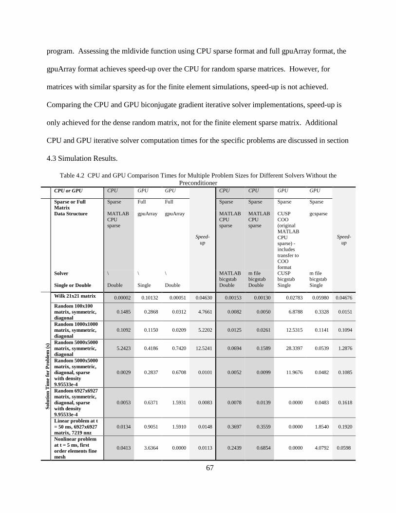
67
program. Assessing the mldivide function using CPU sparse format and full gpuArray format, the
gpuArray format achieves speed-up over the CPU for random sparse matrices. However, for
matrices with similar sparsity as for the finite element simulations, speed-up is not achieved.
Comparing the CPU and GPU biconjugate gradient iterative solver implementations, speed-up is
only achieved for the dense random matrix, not for the finite element sparse matrix. Additional
CPU and GPU iterative solver computation times for the specific problems are discussed in section
4.3 Simulation Results.
Table 4.2 CPU and GPU Comparison Times for Multiple Problem Sizes for Different Solvers Without the Preconditioner
CPU or GPU CPU GPU GPU
Speed-up
CPU CPU GPU GPU
Speed-up
Sparse or Full Matrix
Sparse Full Full Sparse Sparse Sparse Sparse
Data Structure MATLAB CPU sparse
gpuArray gpuArray MATLAB CPU sparse
MATLAB CPU sparse
CUSP COO (original MATLAB CPU sparse) - includes transfer to COO format
gcsparse
Solver \ \ \ MATLAB bicgstab
m file bicgstab
CUSP bicgstab
m file bicgstab
Single or Double Double Single Double Double Double Single Single
Solu
tion
Tim
e fo
r P
robl
em (
s)
Wilk 21x21 matrix 0.00002 0.10132 0.00051 0.04630 0.00153 0.00130 0.02783 0.05980 0.04676
Random 100x100 matrix, symmetric, diagonal
0.1485 0.2868 0.0312 4.7661 0.0082 0.0050 6.8788 0.3328 0.0151
Random 1000x1000 matrix, symmetric, diagonal
0.1092 0.1150 0.0209 5.2202 0.0125 0.0261 12.5315 0.1141 0.1094
Random 5000x5000 matrix, symmetric, diagonal
5.2423 0.4186 0.7420 12.5241 0.0694 0.1589 28.3397 0.0539 1.2876
Random 5000x5000 matrix, symmetric, diagonal, sparse with density 9.95533e-4
0.0029 0.2837 0.6708 0.0101 0.0052 0.0099 11.9676 0.0482 0.1085
Random 6927x6927 matrix, symmetric, diagonal, sparse with density 9.95533e-4
0.0053 0.6371 1.5931 0.0083 0.0078 0.0139 0.0000 0.0483 0.1618
Linear problem at t = 50 ms, 6927x6927 matrix, 7219 nnz
0.0134 0.9051 1.5910 0.0148 0.3697 0.3559 0.0000 1.8540 0.1920
Nonlinear problem at t = 5 ms, first order elements fine mesh
0.0413 3.6364 0.0000 0.0113 0.2439 0.6854 0.0000 4.0792 0.0598

68
4.3 Simulation Results
Following the finite element derivations for first-order and second-order linear and
nonlinear simulations, each of these simulations was developed for the TEAM 10 benchmark
problem geometry and material properties. The simulations were developed using MATLAB
scripts. On the CPU, the MATLAB sparse vector and matrix storage and operations were used.
On the GPU, the gpuArray, sparse gpuArray, and MEX files linked to CUDA file were used.
Computation time for the CPU and hybrid CPU/GPU simulations is determined using the “tic” and
“toc” MATLAB functions. All of the simulations for this thesis were conducted on the CPU using
an Intel Core i5-2400 CPU with 4 gigabytes of random-access memory. The Windows 7 64-bit
operating system was used. The GPU for personal computing used for these simulations is the
NVIDIA GeForce GTX 780 (Kepler architecture) GPU with 3 gigabytes of memory and compute
capability 3.5. The GTX 780 has 2304 CUDA cores. Final MATLAB simulation implementations
were developed for MATLAB R2014a.
For each type of simulation, a coarse and fine mesh of the geometry was used to assess
scalability of the GPU simulation. Table 4.3 describes the number of elements and nodes for each
type of simulation. Figure 4.4 illustrates the coarse mesh, and Figure 4.5 illustrates the fine mesh.
The blue elements represent the coils with impressed current density, magenta elements represent
the magnetic steel, and white elements represent air. The elements and nodes that are colored
differently show the tracked nodes and elements in the simulations. The magnetic vector potential
and magnetic flux density solution is calculated for the entire domain for each iteration or time
step, but only specified nodes and element solutions are saved for the entire transient simulation.

69
Table 4.3 Benchmark Problem Mesh Descriptions
Total Domain Nonlinear Region
Magnetic Material Model
Element Order
Mesh Number of Nonzero
Elements in Matrix
Number of Elements
Number of Nodes
Number of Elements
Number of Nodes
Line
ar First Fine 47769 14144 7219 0 0
Second Coarse 62973 3536 7219 0 0
Second Fine 257873 14144 28581 0 0
Non
-Li
near
First Coarse 11444 3536 1842 932 725
First Fine 47769 14144 7219 3728 2379
Second Fine 257873 14144 28581 3728 8483
Figure 4.4 Coarse mesh for benchmark problem
-0.1 -0.05 0 0.05 0.1
-0.06
-0.04
-0.02
0
0.02
0.04
0.06
Coarse Mesh for Benchmark Problem
x (m)
y (m
)

70
Figure 4.5 Fine mesh for benchmark problem
4.3.1.1 First-order elements with linear magnetic material
The first-order element, linear magnetic material solutions for the benchmark problem are
shown in Figure 4.6 for magnetic flux density and Figure 4.7 for eddy current density for the fine
mesh. The computed solutions at the nodes nearest to the search coils are used to compare to the
measured solutions, and those coordinates are shown in Table 4.4 The steel permeability is
represented linearly with relative permeability 1000rµ = . The CPU simulation uses the
biconjugate gradient algorithm implemented function with preconditioner using the MATLAB
double sparse format. The GPU simulation uses the same iterative solver function with the sparse
gpuArray single format.
-0.1 -0.05 0 0.05 0.1
-0.06
-0.04
-0.02
0
0.02
0.04
0.06
Fine Mesh for Benchmark Problem
x (m)
y (m
)
4.3.1 Linear magnetic material simulation results

71
Table 4.4 Tracked Solution Points for First-Order, Linear Program for Benchmark Problem
Measured Points Simulated Points
Search Coil Number x (mm) y (mm) x (mm) y (mm) 1 0-1.6 0 1.6 0 2 41.8 60-63.2 41 61.6 3 122.1-125.3 0 123.2 0
To show CPU and GPU program simulation time, Figure 4.8 shows the computation time
for the major components of the linear program for each time step. The major components
measured for each time step are the right-hand side vector calculation from equation (2.44), time to
solve for the magnetic vector potential using the sparse iterative solver, post-processing for
magnetic flux density, and post-processing for eddy current density. For the magnetic flux density
and iterative solver component computation times per time step, Figure 4.9 shows the CPU and
GPU computation times and speed-up. Note that the GPU computation times presented throughout
this thesis include the overhead to transfer data to the GPU from the CPU, and from the GPU back
to the CPU. The GPU computation time for the magnetic flux density results in approximately 4
times speed-up, but no speed-up – approximately 0.3 – for the sparse iterative solver with
preconditioner.
Figure 4.6 First-order element, linear material, magnetic flux density solution for fine mesh, compared to TEAM problem measured results at three points
0 0.05 0.1 0.150
0.2
0.4
0.6
0.8
1
1.2
1.4
1.6
1.8
time (s)
B (
T)
Magnetic Flux Density at Three Different Points
CPU S1CPU S2
CPU S3Meas B1
Meas B2Meas B3
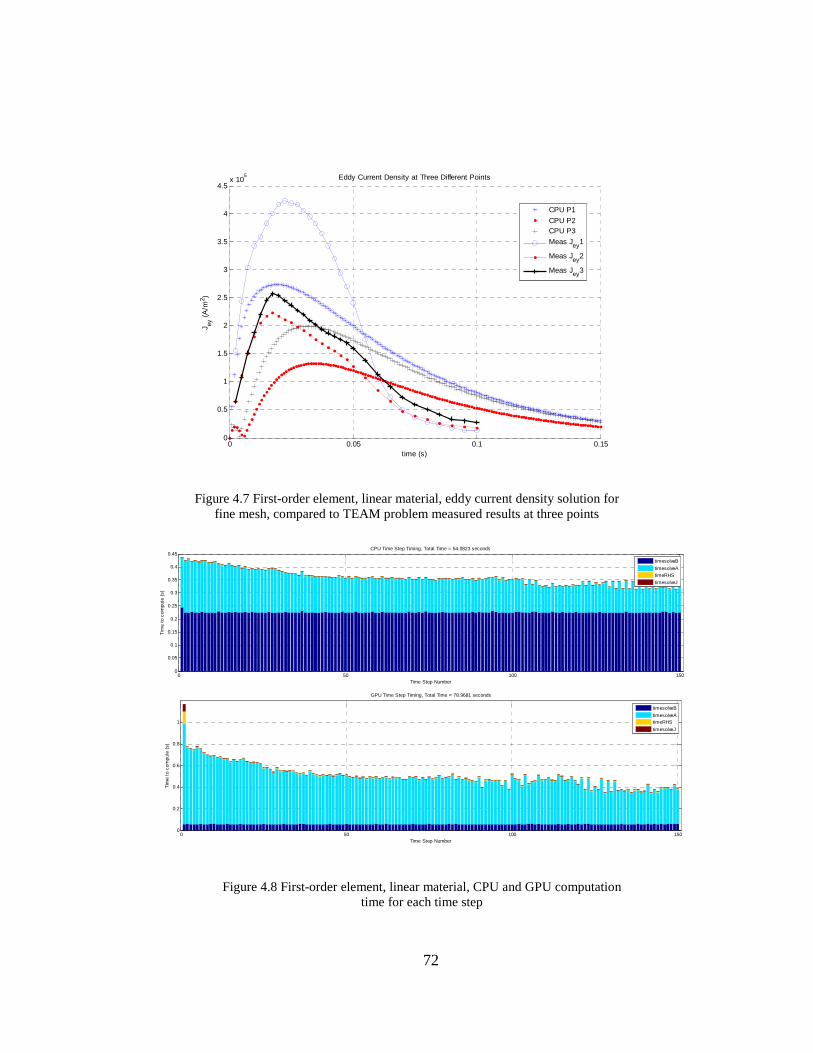
72
Figure 4.7 First-order element, linear material, eddy current density solution for fine mesh, compared to TEAM problem measured results at three points
Figure 4.8 First-order element, linear material, CPU and GPU computation time for each time step
0 0.05 0.1 0.150
0.5
1
1.5
2
2.5
3
3.5
4
4.5x 10
5
time (s)
J ey (
A/m
2 )
Eddy Current Density at Three Different Points
CPU P1
CPU P2CPU P3
Meas Jey1
Meas Jey2
Meas Jey3
0 50 100 1500
0.05
0.1
0.15
0.2
0.25
0.3
0.35
0.4
0.45CPU Time Step Timing, Total Time = 54.0823 seconds
Time Step Number
Tim
e to
com
pute
(s)
timesolveB
timesolveAtimeRHS
timesolveJ
0 50 100 1500
0.2
0.4
0.6
0.8
1
GPU Time Step Timing, Total Time = 78.9681 seconds
Time Step Number
Tim
e to
com
pute
(s)
timesolveB
timesolveAtimeRHS
timesolveJ

73
Figure 4.9 First-order element, linear material, CPU and GPU computation time comparison for magnetic flux density and magnetic vector potential
Table 4.5. CPU and GPU Simulation Computation Time Comparison for First-Order Elements, Linear Magnetic Material, Fine Mesh. Iterative solver is preconditioned.
Total for Simulation
Simulation Time(s)/Speed-up
Preconditioner Formation on CPU
Iterative Solver
Magnetic Flux Density
Total
CPU Time (s) 0.004 20.075 33.858 54.082 GPU Time (s) 0.746 66.733 8.388 78.968 Speed-up N/A 0.301 4.036 0.685 Hybrid CPU/GPU Time (s) 0.004 18.417 8.454 29.414 Speed-up N/A N/A 4.005 1.839
Table 4.5 summarizes the CPU and GPU computation time for the first-order, linear
element simulation for the fine mesh using the preconditioned iterative solver. For the CPU
simulation, the total magnetic flux density computation time was 33.86 seconds. Comparatively,
the total magnetic flux density computation for the GPU simulation was only 8.39 seconds due to
sparse gpuArray matrix-vector multiplication. This yields a total speed-up for the magnetic flux
0 50 100 1500.05
0.1
0.15
0.2
0.25Time to Solve B. Total Solve Time CPU = 54.0823, Total Solve Time GPU = 78.9681
Time Step Number
Com
puta
tion
Tim
e (s
)
CPU
GPU
0 50 100 1503.8
3.9
4
4.1
4.2
4.3
4.4
4.5Speedup = CPU/GPU for Time to Solve B
Time Step Number
Com
puta
tion
Tim
e (s
)
0 50 100 1500
0.1
0.2
0.3
0.4
0.5
0.6
0.7
0.8
0.9
1Time to Solve A
Time Step Number
Com
puta
tion
Tim
e (s
)
CPU
GPU
0 50 100 1500.2
0.3
0.4
0.5
0.6
0.7
0.8
0.9
1Speedup = CPU/GPU for Time to Solve A
Time Step Number
Com
puta
tion
Tim
e (s
)

74
density calculation of 4.04. However, the sparse gpuArray format did not yield a speed-up for the
sparse iterative solver. The total CPU sparse iterative solver calculation time was 20.075 seconds,
while the total GPU sparse iterative solver calculation time was 66.73 seconds. As a result, the
total computation time for the GPU simulation did not speed up the simulation compared to the
CPU simulation. For a hybrid CPU/GPU simulation that uses the sparse gpuArray format for
magnetic flux density calculation and the CPU sparse format for the CPU iterative solver
calculation, the simulation time is reduced by the GPU speed-up for the magnetic flux density
calculation. This saves approximately 25.4 seconds of computation time. With minimal GPU to
CPU transfer overhead, the resulting overall CPU/(hybrid CPU-GPU) speed-up is 1.84.
4.3.1.2 Second-order elements with linear magnetic material
Figure 4.10 Second-order element, linear material, magnetic flux density solution for coarse and
fine meshes, compared to TEAM problem measured results at three points
0 0.05 0.1 0.150
0.5
1
1.5
2
time (s)
B (
T)
Magnetic Flux Density at Three Different Points
CPU coarse S1
CPU coarse S2CPU coarse S3
Meas B1
Meas B2
Meas B3
CPU fine S1CPU fine S2
CPU fine S3

75
Figure 4.11 Second-order element, linear material, eddy current density solution for
coarse and fine meshes, compared to TEAM problem measured results at three points
The coarse and fine mesh computed solutions near the measured points for the second-
order, linear element simulation are shown in Figure 4.10 for magnetic flux density and Figure
4.11 for eddy current density. The solutions shown for the coarse and fine meshes are for the
tracked points shown in Table 4.6.
Table 4.6 Tracked Solution Points for Second-Order, Linear Program for Benchmark Problem
Measured Points Coarse Mesh Simulated Points
Fine Mesh Simulated Points
Search Coil Number x (mm) y (mm) x (mm) y (mm) x (mm) y (mm) 1 0-1.6 0 1.6 0 0.55 0 2 41.8 60-63.2 41 61.6 41 61.6 3 122.1-125.3 0 123.7 0 123.2 0
0 0.05 0.1 0.150
0.5
1
1.5
2
2.5
3
3.5
4
4.5x 10
5
time (s)
J ey (
A/m
2 )
Eddy Current Density at Three Different Points
CPU coarse P1CPU coarse P2
CPU coarse P3
Meas Jey1
Meas Jey2
Meas Jey3
CPU fine P1
CPU fine P2CPU fine P3
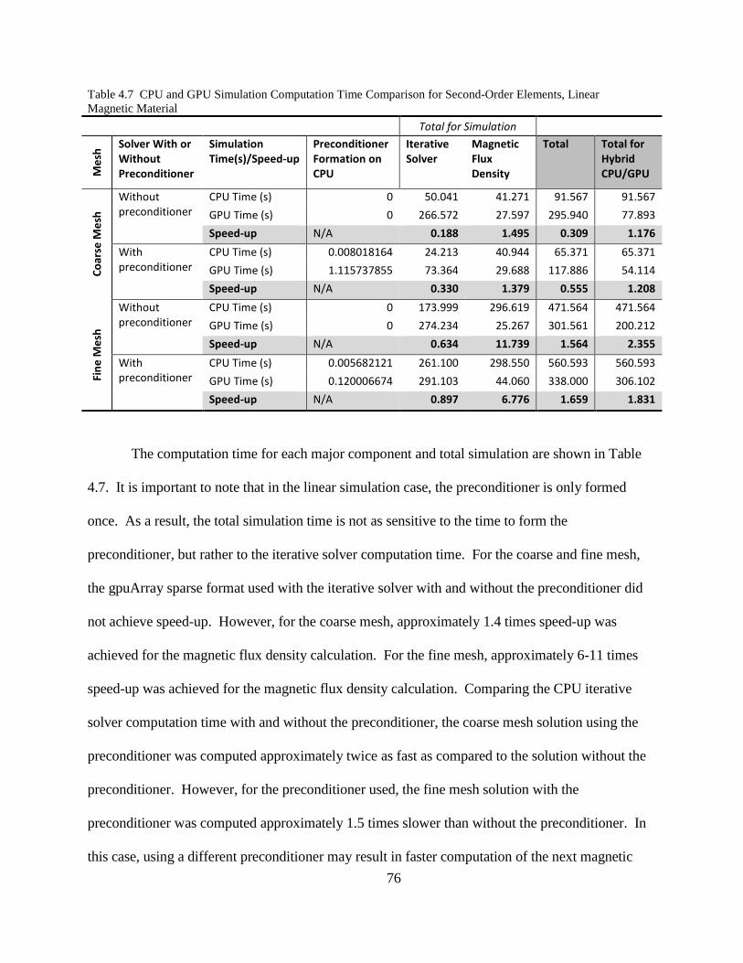
76
Table 4.7 CPU and GPU Simulation Computation Time Comparison for Second-Order Elements, Linear Magnetic Material Total for Simulation
Me
sh Solver With or
Without
Preconditioner
Simulation
Time(s)/Speed-up
Preconditioner
Formation on
CPU
Iterative
Solver
Magnetic
Flux
Density
Total Total for
Hybrid
CPU/GPU
Co
ars
e M
esh
Without
preconditioner
CPU Time (s) 0 50.041 41.271 91.567 91.567
GPU Time (s) 0 266.572 27.597 295.940 77.893
Speed-up N/A 0.188 1.495 0.309 1.176
With
preconditioner
CPU Time (s) 0.008018164 24.213 40.944 65.371 65.371
GPU Time (s) 1.115737855 73.364 29.688 117.886 54.114
Speed-up N/A 0.330 1.379 0.555 1.208
Fin
e M
esh
Without
preconditioner
CPU Time (s) 0 173.999 296.619 471.564 471.564
GPU Time (s) 0 274.234 25.267 301.561 200.212
Speed-up N/A 0.634 11.739 1.564 2.355
With
preconditioner
CPU Time (s) 0.005682121 261.100 298.550 560.593 560.593
GPU Time (s) 0.120006674 291.103 44.060 338.000 306.102
Speed-up N/A 0.897 6.776 1.659 1.831
The computation time for each major component and total simulation are shown in Table
4.7. It is important to note that in the linear simulation case, the preconditioner is only formed
once. As a result, the total simulation time is not as sensitive to the time to form the
preconditioner, but rather to the iterative solver computation time. For the coarse and fine mesh,
the gpuArray sparse format used with the iterative solver with and without the preconditioner did
not achieve speed-up. However, for the coarse mesh, approximately 1.4 times speed-up was
achieved for the magnetic flux density calculation. For the fine mesh, approximately 6-11 times
speed-up was achieved for the magnetic flux density calculation. Comparing the CPU iterative
solver computation time with and without the preconditioner, the coarse mesh solution using the
preconditioner was computed approximately twice as fast as compared to the solution without the
preconditioner. However, for the preconditioner used, the fine mesh solution with the
preconditioner was computed approximately 1.5 times slower than without the preconditioner. In
this case, using a different preconditioner may result in faster computation of the next magnetic
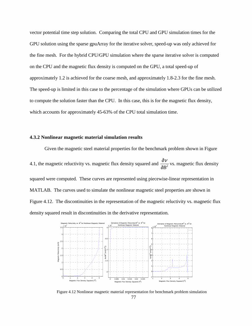
77
vector potential time step solution. Comparing the total CPU and GPU simulation times for the
GPU solution using the sparse gpuArray for the iterative solver, speed-up was only achieved for
the fine mesh. For the hybrid CPU/GPU simulation where the sparse iterative solver is computed
on the CPU and the magnetic flux density is computed on the GPU, a total speed-up of
approximately 1.2 is achieved for the coarse mesh, and approximately 1.8-2.3 for the fine mesh.
The speed-up is limited in this case to the percentage of the simulation where GPUs can be utilized
to compute the solution faster than the CPU. In this case, this is for the magnetic flux density,
which accounts for approximately 45-63% of the CPU total simulation time.
4.3.2 Nonlinear magnetic material simulation results
Given the magnetic steel material properties for the benchmark problem shown in Figure
4.1, the magnetic reluctivity vs. magnetic flux density squared and 2B
ν∂∂
vs. magnetic flux density
squared were computed. These curves are represented using piecewise-linear representation in
MATLAB. The curves used to simulate the nonlinear magnetic steel properties are shown in
Figure 4.12. The discontinuities in the representation of the magnetic reluctivity vs. magnetic flux
density squared result in discontinuities in the derivative representation.
Figure 4.12 Nonlinear magnetic material representation for benchmark problem simulation
0 1 2 3 4 50
0.5
1
1.5
2
2.5
3
3.5x 10
4
Magnetic Flux Density Squared (T2)
Mag
netic
Rel
uctiv
ity (
m/H
)
Magnetic Reluctivity vs. B2 for Nonlinear Magnetic Material
0 0.005 0.01 0.015 0.02 0.025
-2
-1.5
-1
-0.5
0x 10
7
Magnetic Flux Density Squared (T2)
d ν/d
B2 (
m/(
H*T
2 ))
Derivative of Magnetic Reluctivity/B2 vs. B2 for Nonlinear Magnetic Material
1 2 3 4 5-1
0
1
2
3
4
5
6
7
8x 10
4
Magnetic Flux Density Squared (T2)
d ν/d
B2 (
m/(
H*T
2 ))
Derivative of Magnetic Reluctivity/B2 vs. B2 for Nonlinear Magnetic Material

78
4.3.2.1 First-order elements with nonlinear magnetic material
Solutions for the computed magnetic vector potential, magnetic flux density, and eddy
current density were tracked at several elements and nodes. The first measured solution is tracked
at an outer node between the steel and air with an element in the middle of the steel. The second
and third measured solutions are each tracked at inner, middle, and outer nodes and elements. The
computed solutions at the middle nodes and elements match the measured solutions more closely
than those on the inner or outer elements or nodes. The inner computed solutions were calculated
at higher magnetic flux densities and eddy currents than measured, and the outer computed
solutions were at lower values than measured. The following solutions shown are for the middle
elements and nodes close to the measured solutions described by the coordinates in Table 4.8
Table 4.8 Tracked Solution Points for First-Order, Non-linear Program for Benchmark Problem
Measured Points Coarse Mesh Simulated Points
Fine Mesh Simulated Points
Search Coil Number x (mm) y (mm) x (mm) y (mm) x (mm) y (mm) 1 0-1.6 0 1.6 0 1.6 0 2 41.8 60-63.2 44.6 60 41 61.6 3 122.1-125.3 0 122.1 0 123.2 0
The computed transient solutions at the designated points for the coarse and fine mesh are
shown in Figure 4.13 for the magnetic flux density, Figure 4.14 for the eddy current density, and
Figure 4.15 for CPU and GPU calculations of eddy current density. The points tracked for the
coarse mesh more closely track the measured magnetic flux density solution than the fine mesh
points. Both mesh solutions show the nonlinear magnetic material impact on the solution
compared to the linear simulations. The fine mesh solution for the first eddy current density point
near the origin closely tracks the measured solution, but the other calculated solutions do not match
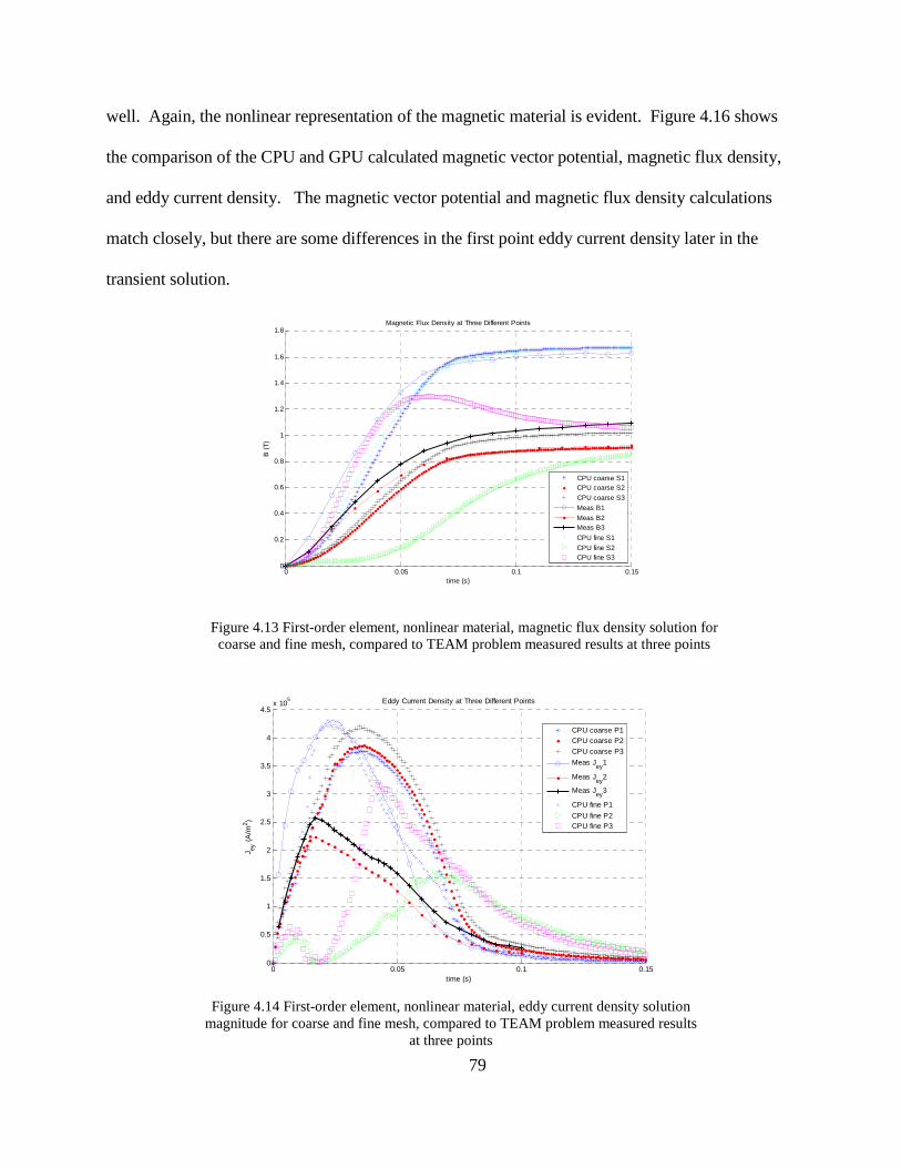
79
well. Again, the nonlinear representation of the magnetic material is evident. Figure 4.16 shows
the comparison of the CPU and GPU calculated magnetic vector potential, magnetic flux density,
and eddy current density. The magnetic vector potential and magnetic flux density calculations
match closely, but there are some differences in the first point eddy current density later in the
transient solution.
Figure 4.13 First-order element, nonlinear material, magnetic flux density solution for coarse and fine mesh, compared to TEAM problem measured results at three points
Figure 4.14 First-order element, nonlinear material, eddy current density solution
magnitude for coarse and fine mesh, compared to TEAM problem measured results at three points
0 0.05 0.1 0.150
0.2
0.4
0.6
0.8
1
1.2
1.4
1.6
1.8
time (s)
B (
T)
Magnetic Flux Density at Three Different Points
CPU coarse S1CPU coarse S2
CPU coarse S3
Meas B1
Meas B2Meas B3
CPU fine S1
CPU fine S2CPU fine S3
0 0.05 0.1 0.150
0.5
1
1.5
2
2.5
3
3.5
4
4.5x 10
5
time (s)
J ey (
A/m
2 )
Eddy Current Density at Three Different Points
CPU coarse P1CPU coarse P2
CPU coarse P3
Meas Jey
1
Meas Jey
2
Meas Jey
3
CPU fine P1
CPU fine P2CPU fine P3

80
Figure 4.15 First-order element, nonlinear material, eddy current density solution magnitude for fine mesh, GPU and CPU solutions, compared to
TEAM problem measured results at three points
Figure 4.16 First-order element eddy current solution for fine mesh, GPU and CPU solutions, percentage difference for magnetic vector potential, magnetic flux density,
and eddy current density computed solutions
0 0.05 0.1 0.150
0.5
1
1.5
2
2.5
3
3.5
4
4.5x 10
5
time (s)
J ey (
A/m
2 )
Eddy Current Density at Three Different Points
CPU S1CPU S2CPU S3
Meas B1
Meas B2Meas B3GPU S1
GPU S2GPU S3
0 0.05 0.1 0.15
0
0.1
0.2
0.3
0.4
time (s)
Diff
eren
ce f
or A
Sol
utio
n (%
) CPU and GPU Solution Percentage Differences for Three Solution Points
0 0.05 0.1 0.15
0
0.05
0.1
time (s)
Diff
eren
ce f
or B
Sol
utio
n (%
)
0 0.05 0.1 0.15
-300
-200
-100
0
time (s)Diff
eren
ce f
or J
eddy
Sol
utio
n (%
)
S1
S2
S3
S1
S2
S3
S1
S2
S3
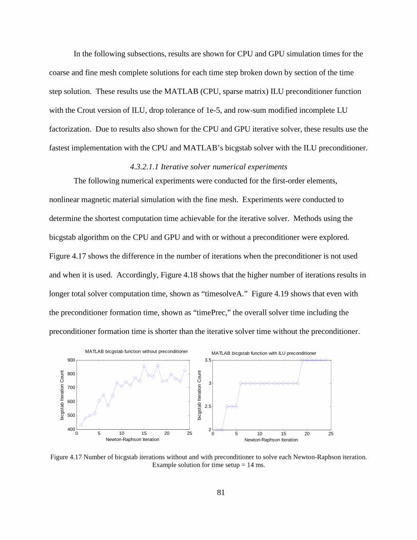
81
In the following subsections, results are shown for CPU and GPU simulation times for the
coarse and fine mesh complete solutions for each time step broken down by section of the time
step solution. These results use the MATLAB (CPU, sparse matrix) ILU preconditioner function
with the Crout version of ILU, drop tolerance of 1e-5, and row-sum modified incomplete LU
factorization. Due to results also shown for the CPU and GPU iterative solver, these results use the
fastest implementation with the CPU and MATLAB’s bicgstab solver with the ILU preconditioner.
4.3.2.1.1 Iterative solver numerical experiments
The following numerical experiments were conducted for the first-order elements,
nonlinear magnetic material simulation with the fine mesh. Experiments were conducted to
determine the shortest computation time achievable for the iterative solver. Methods using the
bicgstab algorithm on the CPU and GPU and with or without a preconditioner were explored.
Figure 4.17 shows the difference in the number of iterations when the preconditioner is not used
and when it is used. Accordingly, Figure 4.18 shows that the higher number of iterations results in
longer total solver computation time, shown as “timesolveA.” Figure 4.19 shows that even with
the preconditioner formation time, shown as “timePrec,” the overall solver time including the
preconditioner formation time is shorter than the iterative solver time without the preconditioner.
Figure 4.17 Number of bicgstab iterations without and with preconditioner to solve each Newton-Raphson iteration. Example solution for time setup = 14 ms.
0 5 10 15 20 25400
500
600
700
800
900
MATLAB bicgstab function without preconditioner
Newton-Raphson Iteration
bicg
stab
Ite
ratio
n C
ount
0 5 10 15 20 252
2.5
3
3.5
MATLAB bicgstab function with ILU preconditioner
Newton-Raphson Iteration
bicg
stab
Ite
ratio
n C
ount

82
Figure 4.18 Iterative solver time for MATLAB bicgstab function without preconditioner
Figure 4.19 Iterative solver time for MATLAB bicgstab function with preconditioner
0 5 10 150
50
100
150Time Step Timing
Time Step NumberT
ime
to c
ompu
te (
s)
timesolveB
timePrectimeSetuptimesolveA
timeQ
timeS
timeUpdatetimeUpdateT
timesolveJ
0 5 10 150
0.5
1
1.5
2Average Time Per Iteration for Key Computations
Time Step Number
Ave
rage
Ite
ratio
n C
ompu
tatio
n T
ime
(s)
Average Iteration timesolveB
Average Iteration timePrec
Average Iteration timeSetup
Average Iteration timesolveA
0 5 10 150
20
40
60
80
Time Step Number
Num
ber
of I
tera
tions
For Each Time Step, Number of Newton-Raphson Iterations to Converge to Residual = 1e-06
0 5 10 150
0.5
1
Time Step Number
Rel
axat
ion
Fac
tor
Relaxation Factor for Each Newton-Raphson Iteration at Each Time Step
1 2 3 4 5 6 7 8 9 10 11 12 13 14 150
50
100Time Step Timing
Time Step Number
Tim
e to
com
pute
(s)
timesolveBtimePrectimeSetup
timesolveA
timeQtimeS
timeUpdate
timeUpdateTtimesolveJ
1 2 3 4 5 6 7 8 9 10 11 12 13 14 150
0.2
0.4
0.6
0.8
Average Time Per Iteration for Key Computations
Time Step Number
Ave
rage
Ite
ratio
n C
ompu
tatio
n T
ime
(s)
Average Iteration timesolveB
Average Iteration timePrecAverage Iteration timeSetup
Average Iteration timesolveA
0 5 10 150
50
100
Time Step Number
Num
ber
of I
tera
tions
For Each Time Step, Number of Newton-Raphson Iterations to Converge to Residual = 1e-06
0 5 10 150
0.5
1
Time Step Number
Rel
axat
ion
Fac
tor
Relaxation Factor for Each Newton-Raphson Iteration at Each Time Step
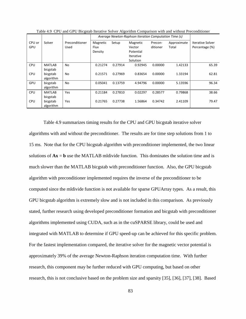
83
Table 4.9 CPU and GPU Bicgstab Iterative Solver Algorithm Comparison with and without Preconditioner Average Newton-Raphson Iteration Computation Time (s)
CPU or
GPU
Solver Preconditioner
Used
Magnetic
Flux
Density
Setup Magnetic
Vector
Potential
Iterative
Solution
Precon-
ditioner
Approximate
Total
Iterative Solver
Percentage (%)
CPU MATLAB
bicgstab
No 0.21274 0.27914 0.92945 0.00000 1.42133 65.39
CPU bicgstab
algorithm
No 0.21571 0.27969 0.83654 0.00000 1.33194 62.81
GPU bicgstab
algorithm
No 0.05041 0.13759 4.94796 0.00000 5.13596 96.34
CPU MATLAB
bicgstab
Yes 0.21184 0.27810 0.02297 0.28577 0.79868 38.66
CPU bicgstab
algorithm
Yes 0.21765 0.27738 1.56864 0.34742 2.41109 79.47
Table 4.9 summarizes timing results for the CPU and GPU bicgstab iterative solver
algorithms with and without the preconditioner. The results are for time step solutions from 1 to
15 ms. Note that for the CPU bicgstab algorithm with preconditioner implemented, the two linear
solutions of Ax = b use the MATLAB mldivide function. This dominates the solution time and is
much slower than the MATLAB bicgstab with preconditioner function. Also, the GPU bicgstab
algorithm with preconditioner implemented requires the inverse of the preconditioner to be
computed since the mldivide function is not available for sparse GPUArray types. As a result, this
GPU bicgstab algorithm is extremely slow and is not included in this comparison. As previously
stated, further research using developed preconditioner formation and bicgstab with preconditioner
algorithms implemented using CUDA, such as in the cuSPARSE library, could be used and
integrated with MATLAB to determine if GPU speed-up can be achieved for this specific problem.
For the fastest implementation compared, the iterative solver for the magnetic vector potential is
approximately 39% of the average Newton-Raphson iteration computation time. With further
research, this component may be further reduced with GPU computing, but based on other
research, this is not conclusive based on the problem size and sparsity [35], [36], [37], [38]. Based

84
on these results, the iterative solver method used for the hybrid CPU/GPU solutions is the CPU-
based MATLAB bicgstab function with the ILU preconditioner.
4.3.2.1.2 Iteration setup time breakdown
The results in Figure 4.20 and Figure 4.21 show the CPU and hybrid CPU/GPU simulation
setup computation time for the fine mesh solution.
Figure 4.20 Setup time breakdown for CPU
Figure 4.21 Setup time breakdown for GPU sparse
1 2 3 4 5 6 7 8 9 10 11 12 13 14 150
5
10
15
20
25
30timeSetup Breakdown
Time Step Number
Tim
e to
Com
pute
(s)
timeSetup-sub1
timeSetup-sub2timeSetup-sub3
timeSetup-sub4
1 2 3 4 5 6 7 8 9 10 11 12 13 14 150
0.05
0.1
0.15
0.2
0.25
0.3
0.35Average Time Per NR Iteration for timeSetup Breakdown
Time Step Number
Ave
rage
Ite
ratio
n C
ompu
tatio
n T
ime
(s)
timeSetup-sub1timeSetup-sub2timeSetup-sub3
timeSetup-sub4
1 2 3 4 5 6 7 8 9 10 11 12 13 14 150
5
10
15
timeSetup Breakdown
Time Step Number
Tim
e to
Com
pute
(s)
timeSetup-sub1
timeSetup-sub2
timeSetup-sub3
timeSetup-sub4
1 2 3 4 5 6 7 8 9 10 11 12 13 14 150
0.05
0.1
0.15
0.2
0.25
0.3
Average Time Per NR Iteration for timeSetup Breakdown
Time Step Number
Ave
rage
Ite
ratio
n C
ompu
tatio
n T
ime
(s)
timeSetup-sub1
timeSetup-sub2timeSetup-sub3
timeSetup-sub4

85
The setup computation required for each Newton-Raphson iteration is broken down into
four subsections. The subsections along with the hybrid CPU/GPU simulation implementation are:
• timeSetup-sub1 = look up ν and( )
,
2,
e t tk
e t tkB
ν +∆
+∆
∂
∂ based on B from fitted ν-B2 and 2B
ν∂∂
equations (CPU)
• timeSetup-sub2 = compute S with elemental ν (CPU), and compute right-hand side
vector (matrix multiplication and subtraction) (GPU sparse)
• timeSetup-sub3 = compute G from equation . 2e
i
B
A
∂∂
and SAare computed on the
GPU, and the sparse matrix assembly of G is done on the CPU.
• timeSetup-sub4 = compute the left-hand side matrix final addition (CPU).
The setup computation time results averaged over the Newton-Raphson iterations are
summarized by Table 4.10. The largest part of the CPU setup calculation time, subsection 3 to
compute G, can be parallel processed using the sparse gpuArray matrix-vector multiplication. This
subsection results in a speed-up of approximately 2.3, allowing for an overall setup time speed-up
of approximately 1.8.
Table 4.10 CPU and GPU Setup Time Comparison
Average Newton-Raphson Iteration Computation Time (s)
CPU or GPU Setup - sub 1 Setup - sub 2 Setup - sub 3 Setup - sub 4 Total
CPU 0.013749 0.018930 0.245237 0.000185 0.278102
GPU 0.013549 0.033317 0.107026 0.000175 0.154068
Speed-up CPU/GPU 1.014726 0.568162 2.291392 1.057076 1.805060
4.3.2.1.3 Transient CPU and hybrid CPU/GPU simulation results
The figures and tables in this section describe the transient simulation computation time for
the CPU and hybrid CPU/GPU implementations. In Figure 4.22, for a few sample time steps, the

86
CPU and hybrid CPU/GPU simulation computation times are broken down by major component to
illustrate the computation time percentage for each component and the GPU speed-up for each
component. The components are:
• timesolveB – time to compute the magnetic vector potential
• timePrec – time to form the preconditioner
• timeSetup – time to set up the Newton-Raphson iteration as described in Section 4.3.2.1.2
Iteration setup time breakdown
• timesolveA – time to solve for the next Newton-Raphson iteration magnetic vector
potential
• timeQ – time to calculate the next impressed current density
• timeS – time to assemble the S matrix
• timeUpdate – time to update the next magnetic vector potential iteration given the solution
for A∆
• timeUpdateT – when the A∆ is less than the specified tolerance, this is the time to save the
iteration solution as the time step solution and update the magnetic flux density and
reluctivity
• timesolveJ – time to compute the eddy current density

87
Figure 4.22 CPU and GPU computation time comparison for first-order elements, nonlinear magnetic material, fine mesh. Subset of CPU and GPU computation time for several time
steps including breakdown of computation time for key computations.
Table 4.11 CPU and GPU Computation Time Comparison for Average Newton-Raphson Iteration, First-Order Elements, Nonlinear Magnetic Material Problem
Average Newton-Raphson Iteration Computation Time
Over Total Transient Solution (s)
Mesh CPU or GPU Magnetic
Flux Density
Setup Magnetic Vector
Potential Iterative
Solution
Precon-
ditioner
Approx.
Total
Co
ars
e CPU 0.027664 0.053201 0.005250 0.019420 0.105535
GPU 0.022935 0.066776 0.005671 0.019508 0.114890
Speed-up 1.206207 0.796699 N/A N/A 0.918568
Fin
e CPU 0.218303 0.280088 0.036713 0.341196 0.876300
GPU 0.060477 0.151496 0.035943 0.283171 0.531087
Speed-up 3.609685 1.848813 N/A N/A 1.650013
46 47 48 49 50 510
10
20
30
Time Step Timing, CPU Total Time = 3439.9804 secondsGPU Total Time = 2214.9281 seconds
Time Step Number
Tim
e to
com
pute
(s)
timesolveBtimePrec
timeSetup
timesolveA
timeQtimeS
timeUpdate
timeUpdateTtimesolveJ
46 47 48 49 50 510
0.5
1CPU and GPU Average Time Per Iteration for Key Computations
Time Step Number
Ave
rage
Ite
ratio
n C
ompu
tatio
n T
ime
(s)
Average Iteration timesolveB
Average Iteration timePrecAverage Iteration timeSetup
Average Iteration timesolveA
0 50 100 1500
50
100
Time Step Number
Num
ber
of I
tera
tions
For Each Time Step, Number of Newton-Raphson Iterations to Converge to Residual = 1e-06
CPU Solution
GPU Solution
0 50 100 150
0.2
0.4
0.6
0.8
1
Time Step Number
Rel
axat
ion
Fac
tor
Relaxation Factor for Each Newton-Raphson Iteration at Each Time Step
CPU Solution
GPU Solution

88
Table 4.12 CPU and GPU Computation Time Comparison for Total Transient Solution, First-Order Elements,
Nonlinear Magnetic Material Problem
Total Transient Solution Computation Time (s)
Mesh CPU or GPU Magnetic
Flux Density
Setup Magnetic Vector
Potential Iterative
Solution
Precon-
ditioner
Total
Co
ars
e CPU 67.597 128.695 12.771 46.817 263.609
GPU 57.563 162.282 14.021 48.600 299.995
Speed-up 1.174 0.793 N/A N/A 0.879
Fin
e CPU 856.000 1084.896 138.784 1319.007 3439.980
GPU 253.529 622.615 149.140 1164.800 2214.928
Speed-up 3.376 1.742 N/A N/A 1.553
Note that the preconditioner formation and magnetic vector potential solver are computed
on the CPU for the total GPU solution. From previous discussions, this method was used to
improve the total computation time since it was not previously shown that speed-up was achieved
with the sparse GPU format using the same bicgstab algorithm. From these results averaging over
all the time step solutions and the average Newton-Raphson iteration computation times, Table
4.11 shows that the magnetic flux density GPU computation achieved an average speed-up of 1.2
for the coarse mesh and 3.6 for the fine mesh, and the setup achieved an average speed-up of 1.8
for the fine mesh. This is primarily due to the parallel processing of GPU sparse matrix-vector
multiplication. From the total transient computation time shown in Table 4.12, the GPU
implementation does not achieve speed-up for the coarse mesh, but for the fine mesh it achieves
approximately 1.55 speed-up.
4.3.2.2 Second-order elements with nonlinear magnetic material
The simulation of the second-order elements, nonlinear program required more
manipulation of the relaxation factor and time step difference in order to achieve convergence. For
the coarse mesh, the solution only converged for times 1 to 4 ms with a time step of 1 ms. For

89
solutions beyond that, time steps of 0.25 ms and incrementally smaller were required in order to
achieve convergence. A reason for the convergence issue is due to too large of a time step given
the mesh density, resulting in a larger change in magnetic vector potential for each iteration. As a
result, solutions are shown for the fine mesh only. The higher mesh density reduced the
convergence issues. For the fine mesh, solutions for times 1-18 ms converged for a time step of 1
ms. For solutions beyond 18 ms, a smaller time step is required to achieve convergence. Full
transient solutions are not presented. For the partial simulations up to 18 ms for the fine mesh, the
CPU and hybrid CPU/GPU simulation results are presented in Figure 4.23 and Figure 4.24 for the
points described in Table 4.13. As previously discussed, the iterative solver used for both the
CPU and hybrid CPU/GPU simulation is on the CPU using the MATLAB “bicgstab” function with
row-sum modified incomplete LU Crout version factorization with drop tolerance 10-5 for the
preconditioner. This was the fastest iterative solver implementation tested for this problem.
Table 4.13 Tracked Solution Points for Second-Order, Non-linear Program for Benchmark Problem
Measured Points Fine Mesh Simulated Points
Search Coil Number x (mm) y (mm) x (mm) y (mm) 1 0-1.6 0 0.5 0 2 41.8 60-63.2 41 61.6 3 122.1-125.3 0 123.2 0

90
Figure 4.23 Second-order element, nonlinear material, magnetic flux density solution for fine mesh, compared to TEAM problem measured results at three points
Figure 4.24 Second-order element, nonlinear material, eddy current density solution magnitude for fine mesh, compared to TEAM problem measured
results at three points
0 0.02 0.04 0.06 0.08 0.1 0.12 0.14 0.160
0.2
0.4
0.6
0.8
1
1.2
1.4
1.6
1.8
time (s)
B (
T)
Magnetic Flux Density at Three Different Points
CPU S1
CPU S2
CPU S3Meas B1
Meas B2
Meas B3
0 0.01 0.02 0.03 0.04 0.05 0.06 0.07 0.08 0.09 0.10
0.5
1
1.5
2
2.5
3
3.5
4
4.5x 10
5
time (s)
J ey (
A/m
2 )
Eddy Current Density at Three Different Points
CPU P1CPU P2
CPU P3
Meas Jey1
Meas Jey2
Meas Jey3
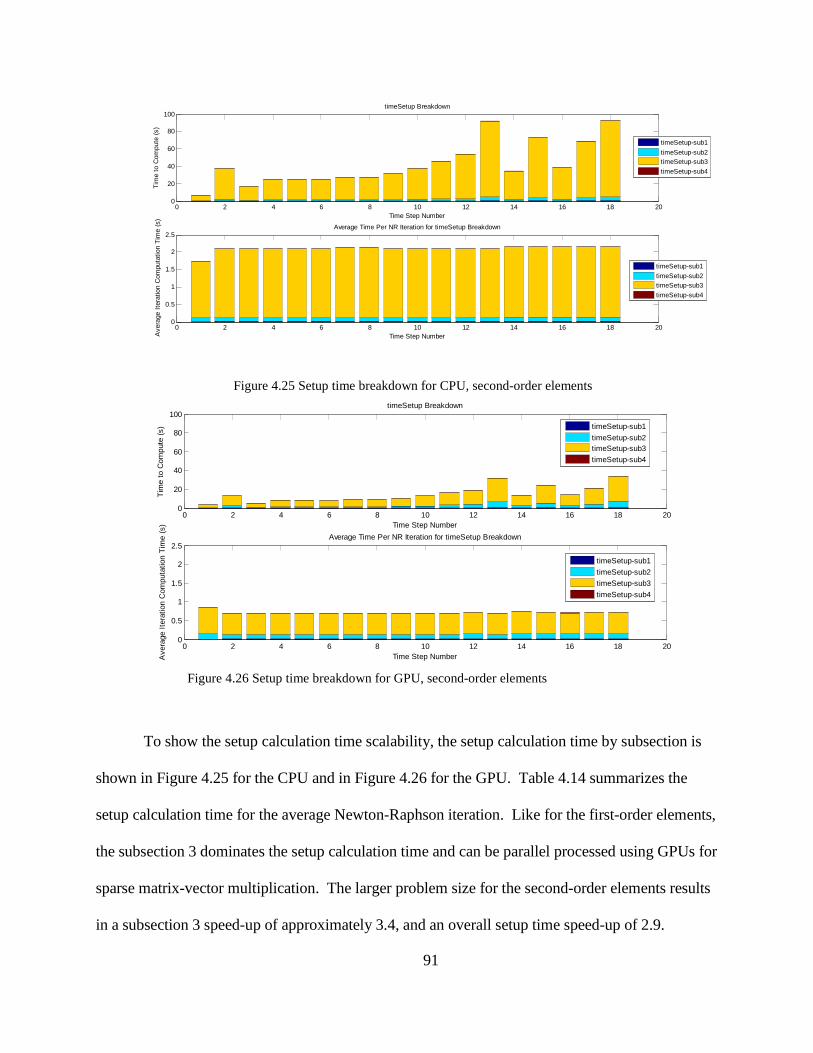
91
Figure 4.25 Setup time breakdown for CPU, second-order elements
Figure 4.26 Setup time breakdown for GPU, second-order elements
To show the setup calculation time scalability, the setup calculation time by subsection is
shown in Figure 4.25 for the CPU and in Figure 4.26 for the GPU. Table 4.14 summarizes the
setup calculation time for the average Newton-Raphson iteration. Like for the first-order elements,
the subsection 3 dominates the setup calculation time and can be parallel processed using GPUs for
sparse matrix-vector multiplication. The larger problem size for the second-order elements results
in a subsection 3 speed-up of approximately 3.4, and an overall setup time speed-up of 2.9.
0 2 4 6 8 10 12 14 16 18 200
20
40
60
80
100timeSetup Breakdown
Time Step Number
Tim
e to
Com
pute
(s)
timeSetup-sub1
timeSetup-sub2timeSetup-sub3
timeSetup-sub4
0 2 4 6 8 10 12 14 16 18 200
0.5
1
1.5
2
2.5Average Time Per NR Iteration for timeSetup Breakdown
Time Step NumberAve
rage
Ite
ratio
n C
ompu
tatio
n T
ime
(s)
timeSetup-sub1
timeSetup-sub2timeSetup-sub3
timeSetup-sub4
0 2 4 6 8 10 12 14 16 18 200
20
40
60
80
100timeSetup Breakdown
Time Step Number
Tim
e to
Com
pute
(s)
timeSetup-sub1
timeSetup-sub2timeSetup-sub3
timeSetup-sub4
0 2 4 6 8 10 12 14 16 18 200
0.5
1
1.5
2
2.5Average Time Per NR Iteration for timeSetup Breakdown
Time Step NumberAve
rage
Ite
ratio
n C
ompu
tatio
n T
ime
(s)
timeSetup-sub1
timeSetup-sub2
timeSetup-sub3
timeSetup-sub4
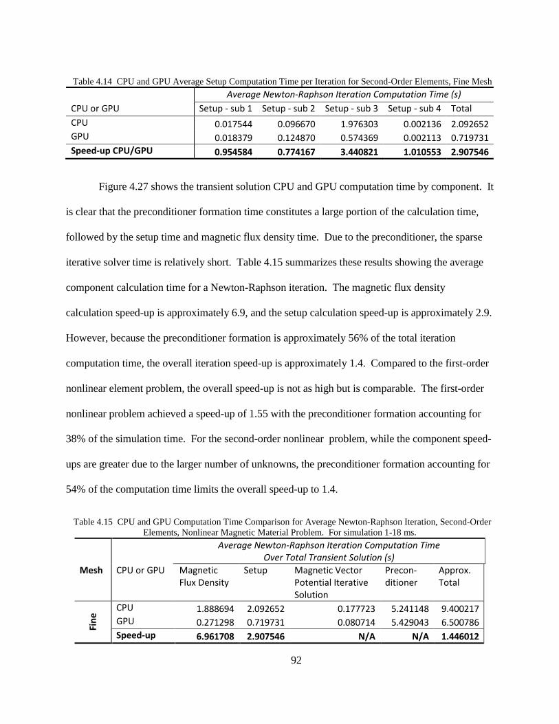
92
Table 4.14 CPU and GPU Average Setup Computation Time per Iteration for Second-Order Elements, Fine Mesh
Average Newton-Raphson Iteration Computation Time (s)
CPU or GPU Setup - sub 1 Setup - sub 2 Setup - sub 3 Setup - sub 4 Total
CPU 0.017544 0.096670 1.976303 0.002136 2.092652
GPU 0.018379 0.124870 0.574369 0.002113 0.719731
Speed-up CPU/GPU 0.954584 0.774167 3.440821 1.010553 2.907546
Figure 4.27 shows the transient solution CPU and GPU computation time by component. It
is clear that the preconditioner formation time constitutes a large portion of the calculation time,
followed by the setup time and magnetic flux density time. Due to the preconditioner, the sparse
iterative solver time is relatively short. Table 4.15 summarizes these results showing the average
component calculation time for a Newton-Raphson iteration. The magnetic flux density
calculation speed-up is approximately 6.9, and the setup calculation speed-up is approximately 2.9.
However, because the preconditioner formation is approximately 56% of the total iteration
computation time, the overall iteration speed-up is approximately 1.4. Compared to the first-order
nonlinear element problem, the overall speed-up is not as high but is comparable. The first-order
nonlinear problem achieved a speed-up of 1.55 with the preconditioner formation accounting for
38% of the simulation time. For the second-order nonlinear problem, while the component speed-
ups are greater due to the larger number of unknowns, the preconditioner formation accounting for
54% of the computation time limits the overall speed-up to 1.4.
Table 4.15 CPU and GPU Computation Time Comparison for Average Newton-Raphson Iteration, Second-Order Elements, Nonlinear Magnetic Material Problem. For simulation 1-18 ms.
Average Newton-Raphson Iteration Computation Time
Over Total Transient Solution (s)
Mesh CPU or GPU Magnetic
Flux Density
Setup Magnetic Vector
Potential Iterative
Solution
Precon-
ditioner
Approx.
Total
Fin
e CPU 1.888694 2.092652 0.177723 5.241148 9.400217
GPU 0.271298 0.719731 0.080714 5.429043 6.500786
Speed-up 6.961708 2.907546 N/A N/A 1.446012

93
Figure 4.27 CPU and GPU computation time comparison for second-order elements, nonlinear magnetic material, fine mesh.
4.3.3 Benchmark problem simulation results summary
Table 4.16 Simulation Results Summary for Benchmark Problem Computation Time (s)
Magnetic Material Model
Element Order
Mesh Preconditioned Number of Nodes
CPU Hybrid CPU/GPU
Speed-up
Line
ar First Fine Yes 7219 54.082 29.414 1.839
Second Coarse Yes 7219 65.371 54.114 1.208 Second Fine No 28581 471.564 200.212 2.355
Non
-Li
near
First Coarse Yes 1842 263.609 299.995 0.879 First Fine Yes 7219 3439.980 2214.928 1.553 Second Fine Yes 28581 3417.101 2395.973 1.426
For the discussed simulations, Table 4.16 summarizes the CPU and GPU simulation
computation times. It shows that as the problem scale increases for both the linear and nonlinear
1 2 3 4 5 6 7 8 9 10 11 12 13 14 15 16 17 180
200
400
600
Time Step Timing, CPU Total Time = 3417.1014 secondsGPU Total Time = 2395.9733 seconds
Time Step Number
Tim
e to
com
pute
(s)
timesolveB
timePrectimeSetup
timesolveA
timeQ
timeS
timeUpdatetimeUpdateT
timesolveJ
1 2 3 4 5 6 7 8 9 10 11 12 13 14 15 16 17 180
5
10CPU and GPU Average Time Per Iteration for Key Computations
Time Step Number
Ave
rage
Ite
ratio
n C
ompu
tatio
n T
ime
(s)
Average Iteration timesolveB
Average Iteration timePrecAverage Iteration timeSetup
Average Iteration timesolveA
0 2 4 6 8 10 12 14 16 180
20
40
60
Time Step Number
Num
ber
of I
tera
tions
For Each Time Step, Number of Newton-Raphson Iterations to Converge to Residual = 1e-06
CPU Solution
GPU Solution
0 2 4 6 8 10 12 14 16 18
0.4
0.6
0.8
1
Time Step Number
Rel
axat
ion
Fac
tor
Relaxation Factor for Each Newton-Raphson Iteration at Each Time Step
CPU Solution
GPU Solution

94
simulations, the speed-up achieved also increases. For the nonlinear simulation, due to the
significance of the preconditioner formation time which is only computed on the CPU for these
simulations, the overall speed-up is limited as the problem size increases.

95
CHAPTER 5
LINEAR INDUCTION MACHINE EXPERIMENT AND SIMULATION
The induction machine experiment chosen to estimate the validity of the finite element
CPU and GPU models is the double-sided stator linear induction machine (LIM). The machine is
described in [48]. Measurable experiments for the LIM with a solid aluminum rotor were
conducted. For the applied stator current and frequency from a constant volts-per-Hertz drive, the
force on the rotor for a steady-state locked position was measured by a spring scale. The linear
induction machine and experiment are depicted in Figure 5.1 from [49].
(a)
Figure 5.1(a) Laboratory LIM setup
5.1 Experiment Description

96
(b)
(c)
(d)
Figure 5.1(cont.) (b) subset of LIM geometry for 5 stator slots, (c) cross section of double stator and rotor showing 36 stator slots, and (d) experimental setup with calibration mass
The LIM is excited using symmetric three-phase excitation for a single-layered, series-
wound stator. There are 35 turns per slot, and the pole pitch is 3 cm accordingly. The stator

97
laminations are constructed with M19 steel. The solid aluminum rotor (alloy Al6061 with T611
temper) has conductivity 72.4662 x 10 S/mσ = . The rotor is free to move laterally parallel to the
stator.
The experiment conducted from [49] attached a nylon string to the LIM rotor. On one end,
the string was attached to a stabilizing spring scale, and on the other end, it was attached to a mass
through a pulley. The mass was known and used to calibrate the spring scale. For specified
operating frequencies, the drive excited the rotor so that force was created away from the spring
scale. The total force measured was read by the spring scale. In addition, the stator excitation
current was measured for the operating frequency.
From the measured results recorded in [49], the data point chosen for finite element
simulation is shown in Table 5.1. The volts-per-Hertz drive ratio excitation used is 40/60 Vs.
Table 5.1 LIM Experiment Measurements
fs (Hz) Is,RMS (A) F (meas.) (N)
14 8.64 7.20
Based on the LIM geometry shown in Figure 5.1, a mesh was created for a subset of the
geometry for the partial differential equation simulation. Taking advantage of the periodicity of
the machine, six stator slots were simulated. The fine mesh is shown in Figure 5.2. The a-, b-, and
c-phase excitation polarity is such that the windings for the three left-most slots are out of the page,
and the three right-most slots are into the page. This applies to both the upper and lower stators.
Additional domains are created in the air gap to more readily compute the force in it. The elements
or nodes along the specified y coordinate along the edge of the domain are used for force
5.2 FE Simulation of Experiment

98
calculation using the Maxwell stress tensor method. Figure 5.3 shows the fine mesh closer to the
rotor and air gap. The green-filled elements are the first-order elements used to calculate the force
in the air gap. The force along the edge of the rotor is also calculated.
Figure 5.2 Linear induction machine fine mesh for six stator slots
Several assumptions are made for numerical simulation of the LIM experiment. The steel
conductivity is assumed to be zero. The steel magnetic permeability is simulated as linear with an
approximate relative permeability of 8754rµ = [50]. The resulting solution is not as sensitive to
the saturation of the magnetic steel as other machine problems because the air gap is relatively
large. The winding slot fill is assumed to be 100%, resulting in the impressed current density
calculated over the entire winding area. The impressed current density is also even over the
winding area. As with the benchmark problem, the two-dimensional approximation of the LIM
results in the impressed current density simulated as infinite in the z-direction.
-0.1 -0.05 0 0.05 0.1-0.08
-0.06
-0.04
-0.02
0
0.02
0.04
0.06
0.08
x (m)
y (m
)
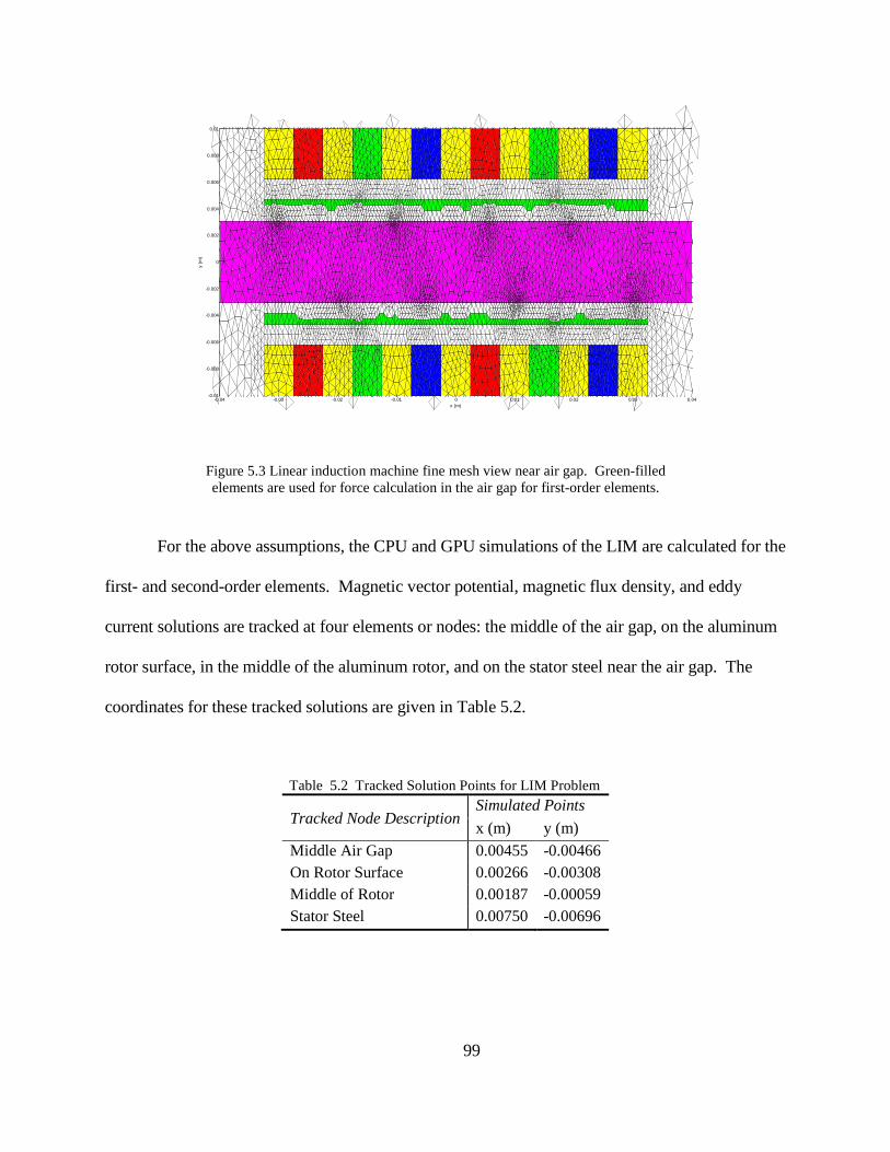
99
Figure 5.3 Linear induction machine fine mesh view near air gap. Green-filled elements are used for force calculation in the air gap for first-order elements.
For the above assumptions, the CPU and GPU simulations of the LIM are calculated for the
first- and second-order elements. Magnetic vector potential, magnetic flux density, and eddy
current solutions are tracked at four elements or nodes: the middle of the air gap, on the aluminum
rotor surface, in the middle of the aluminum rotor, and on the stator steel near the air gap. The
coordinates for these tracked solutions are given in Table 5.2.
Table 5.2 Tracked Solution Points for LIM Problem
Tracked Node Description Simulated Points
x (m) y (m)
Middle Air Gap 0.00455 -0.00466 On Rotor Surface 0.00266 -0.00308 Middle of Rotor 0.00187 -0.00059 Stator Steel 0.00750 -0.00696
-0.04 -0.03 -0.02 -0.01 0 0.01 0.02 0.03 0.04-0.01
-0.008
-0.006
-0.004
-0.002
0
0.002
0.004
0.006
0.008
0.01
x (m)
y (m
)

100
(a) (b)
Figure 5.4 Simulated magnetic flux density magnitude at tracked points for (a) first-order elements, and (b) second-order elements
The computed LIM magnetic flux density magnitude solutions for the first- and second-
order elements are shown in Figure 5.4. For both simulations, the highest magnetic flux density is
in the stator steel as expected for induction machine design. The periodicity of the solutions shown
for a 14 Hz excitation is due to the periodic excitation. Since the magnetic flux density magnitude
is shown, all values are positive. The oscillation within each period may be due to the numerical
time discretization of the simulation. The results shown are for a time step of 1 ms. When the time
step was reduced, the same oscillation within each period occurred, with one time step solution
lower or higher than the next. Comparing the first- and second-order magnetic flux density
solution magnitudes, the simulations match closely. The second-order elements simulated slightly
higher magnetic flux density in the stator steel.
0 0.05 0.1 0.150
0.05
0.1
0.15
0.2
0.25
0.3
0.35
0.4
0.45
0.5
time (s)
B (
T)
Magnetic Flux Density at Tracked Points - First-Order Elements
middle air gap
on rotor surface
middle of rotorstator steel
0 0.05 0.1 0.150
0.05
0.1
0.15
0.2
0.25
0.3
0.35
0.4
0.45
0.5
time (s)
B (
T)
Magnetic Flux Density at Tracked Points - Second-Order Elements
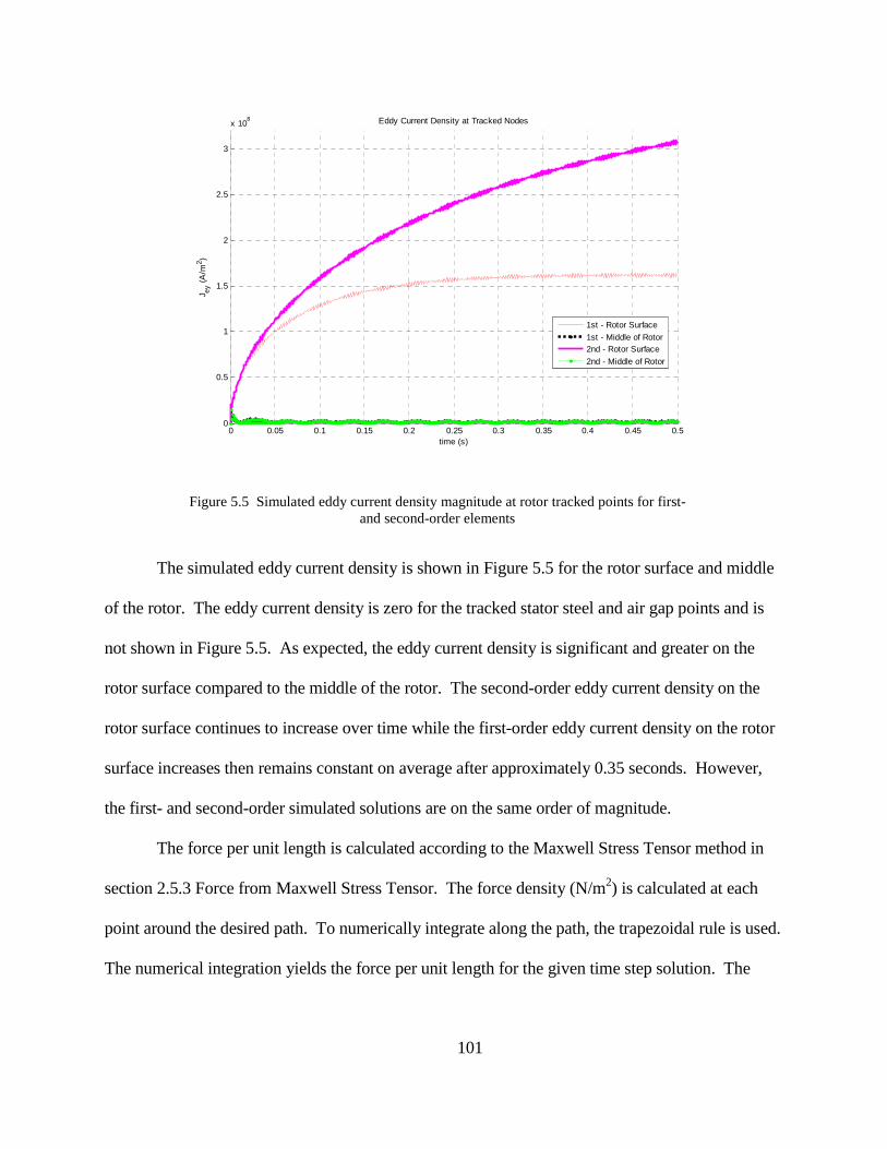
101
Figure 5.5 Simulated eddy current density magnitude at rotor tracked points for first- and second-order elements
The simulated eddy current density is shown in Figure 5.5 for the rotor surface and middle
of the rotor. The eddy current density is zero for the tracked stator steel and air gap points and is
not shown in Figure 5.5. As expected, the eddy current density is significant and greater on the
rotor surface compared to the middle of the rotor. The second-order eddy current density on the
rotor surface continues to increase over time while the first-order eddy current density on the rotor
surface increases then remains constant on average after approximately 0.35 seconds. However,
the first- and second-order simulated solutions are on the same order of magnitude.
The force per unit length is calculated according to the Maxwell Stress Tensor method in
section 2.5.3 Force from Maxwell Stress Tensor. The force density (N/m2) is calculated at each
point around the desired path. To numerically integrate along the path, the trapezoidal rule is used.
The numerical integration yields the force per unit length for the given time step solution. The
0 0.05 0.1 0.15 0.2 0.25 0.3 0.35 0.4 0.45 0.50
0.5
1
1.5
2
2.5
3
x 108
time (s)
J ey (
A/m
2 )
Eddy Current Density at Tracked Nodes
1st - Rotor Surface
1st - Middle of Rotor2nd - Rotor Surface
2nd - Middle of Rotor

102
results shown in Figure 5.6 are calculated in newtons based on multiplying the force per unit length
times the stator height for the air gap force or the rotor height for the force on the rotor surface.
The upper and lower forces are summed to calculate the force on the rotor. The total force
taken over the average of the last cycle simulated is shown in Table 5.3. Both the first- and
second-order simulated forces on the aluminum rotor edge are lower than the measured force. The
simulated force along the rotor edge is closer to the measured result than the simulated force along
the air gap. Factors that could contribute to the differences between measured and simulated
results are the two-dimensional approximation, and simulating a subset of the stator and stator
windings.
Table 5.3 Measured and Simulated LIM Force Calculations
Force (N)
Region Measured First-Order Elements
Simulation
Second-Order Elements
Simulation
Al Rotor Edge 7.20 4.40 3.61
Along Air Gap 7.20 0.16 0.08
(a)
Figure 5.6 Calculated tangential and normal force along LIM rotor
edge and middle of the air gap for (a) first-order elements
0 0.05 0.1 0.15-2
-1
0
1
2
time (s)
Cal
cula
ted
Tan
gent
ial F
orce
(N
)
Force Along Middle Air Gap
0 0.05 0.1 0.15
-4
-3
-2
-1
0
1
2
time (s)
Cal
cula
ted
Nor
mal
For
ce (
N)
0 0.1 0.2 0.3 0.4 0.5-2
-1
0
1
2
time (s)
Cal
cula
ted
Tan
gent
ial F
orce
(N
)
Force Along Rotor Edge
0 0.1 0.2 0.3 0.4 0.5
-4
-3
-2
-1
0
1
2
time (s)
Cal
cula
ted
Nor
mal
For
ce (
N)
Lower
Upper

103
(b)
Figure 5.6 (cont.) Calculated tangential and normal force along LIM rotor edge and middle of the
air gap for (b) second-order elements
The CPU and hybrid CPU/GPU simulations of the linear LIM problem were conducted to
compare computation time. The hybrid CPU/GPU simulation follows the implementation for the
benchmark problem for the first- and second-order elements with linear magnetic material. Due to
the large air gap, the steel will not normally saturate for this LIM experiment. As a result, the
magnetic permeability of the steel can be approximated linearly. The hybrid CPU/GPU simulation
uses the GPU for matrix-vector multiplication to form the right-hand side vector and to compute
the magnetic flux density. As discussed previously, the biconjugate gradient iterative solver is
implemented on the CPU using the MATLAB built-in function bicgstab, and the preconditioner is
formed on the CPU using the incomplete Cholesky factorization function ichol. Additionally, the
force density calculation is done on the CPU since it is computed element-wise. This type of
calculation is much faster on the CPU than the GPU.
0 0.05 0.1 0.15 0.2 0.25 0.3 0.35 0.4 0.45 0.5
-2
-1.5
-1
-0.5
0
0.5
1
1.5
2
time (s)
Cal
cula
ted
Tan
gent
ial F
orce
(N
)
Force Along Rotor Edge
0 0.05 0.1 0.15 0.2 0.25 0.3 0.35 0.4 0.45 0.5-4
-3
-2
-1
0
1
2
time (s)
Cal
cula
ted
Nor
mal
For
ce (
N)
0 0.05 0.1 0.15
-2
-1.5
-1
-0.5
0
0.5
1
1.5
2
time (s)
Cal
cula
ted
Tan
gent
ial F
orce
(N
)
Force Along Middle Air Gap
0 0.05 0.1 0.15-4
-3
-2
-1
0
1
2
time (s)
Cal
cula
ted
Nor
mal
For
ce (
N)
Lower
Upper

104
Table 5.4 LIM Problem Mesh Description
Total Domain
Magnetic Material Model
Element Order
Mesh Number of Nonzero
Elements in Matrix
Number of Elements
Number of Nodes
Line
ar First Fine 56517 16416 8281
Second Fine 297219 16416 32977
Table 5.5 CPU and hybrid CPU/GPU simulation times for LIM linear problem,
first- and second-order elements over 500 ms simulation
Total Time (s)
Preconditioner
Time (s)
Iterative
Solver
Magnetic Flux
Density
Total Time
(s)
Fir
st
Ord
er
CPU 0.006 23.984 73.330 111.322
GPU 0.005 9.973 15.353 38.567
Speed-up N/A N/A 4.776 2.886
Se
con
d
Ord
er
CPU 0.007 1550.500 676.252 2235.600
GPU 0.006 496.544 110.618 638.870
Speed-up N/A N/A 6.113 3.499
Table 5.4 shows the first- and second-order mesh descriptions. Table 5.5 shows the CPU
and hybrid CPU/GPU simulation times. While the iterative solver was calculated on the CPU for
both simulations, the hybrid CPU/GPU simulation calculated the iterative solution faster. For the
larger problem size for the second-order elements, greater speed-up is achieved. A speed-up of
approximately 4.7 and 6.1 was achieved for the first- and second-order magnetic flux density
calculation, respectively. The overall speed-up resulted in 2.8 for the first-order elements, and 3.5
for the second-order elements. The problem size for the LIM mesh is slightly larger than for the
benchmark problem. Using similar techniques, greater speed-up is achieved with the larger
problem size.

105
CHAPTER 6
CONCLUSION AND FUTURE WORK
The use of GPUs for parallel processing of the two-dimensional transient finite element
analysis problem was explored. Simulation results for the benchmark and linear induction
machine problems show which simulation GPUs can be used to speed up the finite element
analysis simulation computation time and where their functionality is limited. MATLAB
implementations of first- and second-order elements for linear and nonlinear magnetic material
were created, and the simulation results for these finite element analysis programs were presented.
For the sparsity and problem sizes simulated, the GPUs provided speed-up for a range of
approximately 4 to 11 times for sparse matrix-vector multiplication required for magnetic flux
density calculation and Jacobian formulation. However, GPUs did not speed up the sparse
iterative solver simulation time for each type of simulation. The CPU iterative solver used was the
MATLAB sparse-format based preconditioned biconjugate gradient stabilized method. These
CPU iterative solver times were compared to the CUDA biconjugate gradient functions explored
and linked to MATLAB and the preconditioned and un-preconditioned biconjugate gradient
stabilized method algorithm implementation using the sparse gpuArray format. Based on these
simulation results and prior research for GPU iterative solver implementations [35], [36], the
current algorithms available and implemented on the GPU do not result in faster computation times
for the GPU implementations for problems of this size (1842-32977 nodes). From [35], for
problem sizes ranging from 150,000 to 1.5 million rows and columns, speed-up achieved for the
incomplete-LU and Cholesky preconditioned BiCGStab and CG methods ranged from 1 to 5.5.
Different speed-up was achieved for different values of the preconditioner fill-in threshold. For
problems of varying sparsity, the average speed-up was approximately 2.2. From [36], the level

106
scheduling technique was used for the sparse triangular solve and several preconditioned iterative
methods on the GPU were explored for problems from 5,000 to 1.4 million rows and columns.
The greatest GPU speed-up achieved was 4.3 for the GPU-accelerated ILUT-GMRES method for
the matrix with 1.27 million rows and columns. Through use of algorithms favorable to
maximizing the parallel thread computations given the sparsity of the finite element matrix, such as
level scheduling in [36], it may be possible to improve the GPU performance of the biconjugate
gradient or GMRES solver over the CPU for two-dimensional finite element problem sizes.
However, the author expects these algorithms will provide limited improvements if any for this
problem size compared to the speed-up achieved for sparse matrix-vector multiplication.
To combine the simulation components with the fastest CPU and GPU computation times,
hybrid CPU/GPU simulation experiments were conducted. Matrix assembly, vector addition and
subtraction, preconditioner formation, and the sparse iterative solver were implemented on the
CPU, while the sparse matrix-vector multiplication operations were implemented on the GPU.
This required transferring matrices and vectors to and from the CPU and GPU. Such transfers
should be minimized since they contribute to GPU processing overhead. For the two-dimensional
problem sizes, this transfer time was minimal compared to the speed-up achieved for GPU sparse
matrix-vector multiplication. As a result, it was still advantageous to use GPUs for these parts of
the simulation.
These hybrid CPU/GPU simulation results were compared to the CPU-only simulation
results. Depending on the problem size, overall simulation speed-ups achieved for the benchmark
and LIM problems ranged from 2.3 to 3.5, with the largest problem size simulated consisting of
32977 nodes. The speed-up is limited by the component speed-up achieved and percentage of the
faster component computation time relative to the remainder of the simulation computation time.

107
The use of GPUs for parallel processing for even larger finite element analysis problems,
such as three-dimensional domains, will show the scalability and limitations of their processing
capabilities for electromagnetic analysis of electric machines. For larger scale problems, the
CUDA preconditioner and sparse iterative solver functions may provide speed-up, but this is
highly dependent on the sparsity of the problem. From three-dimensional mechanics finite element
problems with 147,900 rows and columns with 3.5 million nonzero elements analyzed in [35],
speed-up was not achieved for the fastest overall method tested - the preconditioned CG and
BiCGStab methods with 0 fill. For slower overall methods using higher fill in thresholds,
moderate speed-up of 1.1-6.28 was achieved. Ideally, speed-up on the GPU should be achieved for
the CPU fastest possible available method. For the triangular solve with level scheduling for the
3D Poisson problem in [36], the GPU implementation had a speed-up of approximately 2.3, and
the triangular solve of multi-color ILU with zero fill in had a speed-up of approximately 5.34 on
the GPU over the CPU.
Additionally, the scalability of the sparse matrix-vector multiplication can be explored for
the larger problem. For the sparse-matrix vector results presented, the GPU speed-up over the
CPU increased from 1.49 to 11 with increasing problem size in terms of the matrix number of
nonzero elements and the number of nodes in the mesh. From the 3D Poisson problem analyzed in
[36] with 85,000 rows and columns and 2.3 million nonzero elements, the greatest GPU sparse
matrix-vector multiplication achieved was approximately 5.3 using double precision floating point
arithmetic. As a result, the speed-up for sparse matrix-vector multiplication applied to three-
dimensional finite element problems is expected to be in the range of 5-10.
Along with finite element analysis, GPU parallel computing can be used for magnetic
equivalent circuits (MEC) [51], the boundary-element method [52], and finite element analysis
108
coupled to circuit equivalent models [3]. Each of these types of models requires the solution of a
system of equations. GPUs can be applied to the components of these types of models where they
are suitable for parallel processing, such as sparse matrix-vector multiplication or sparse iterative
solvers for large problem sizes.
Additionally, numerical and parallel processing techniques can be explored in conjunction
to further accelerate the more detailed electromagnetic simulation of the electric machine. Such an
approach could involve creating a hybrid three-dimensional MEC-FEA simulation by using MEC
to simulate flux density and field intensity for a certain transient duration, providing an estimated
initial condition for an FEA transient simulation. The MEC reluctance network could be mapped
to a similar FEA mesh, and then the FEA simulation could be used for more detailed analysis to
capture eddy current. GPUs could be applied to certain components of the MEC and FEA
simulations to further speed-up the simulation. Compared to an FEA-only CPU-based transient
analysis solution, such a hybrid approach along with the use of GPUs could result in faster
computation times.

109
APPENDIX A
CUDA SOURCE CODE FOR MATLAB MEX FUNCTION: SPARSE MATRIX-
VECTOR MULTIPLICATION USING CSR FORMAT
/* * Copyright (c) 2013, The Regents of the University of California, * through Lawrence Berkeley National Laboratory (subject to receipt of * any required approvals from U.S. Dept. of Energy) All rights reserved. * * Redistribution and use in source and binary forms, with or * without modification, are permitted provided that the * following conditions are met: * * * Redistributions of source code must retain the above * copyright notice, this list of conditions and the following * disclaimer. * * * Redistributions in binary form must reproduce the * above copyright notice, this list of conditions and the * following disclaimer in the documentation and/or other * materials provided with the distribution. * * * Neither the name of the University of California, * Berkeley, nor the names of its contributors may be used to * endorse or promote products derived from this software * without specific prior written permission. * * THIS SOFTWARE IS PROVIDED BY THE COPYRIGHT HOLDERS AND * CONTRIBUTORS "AS IS" AND ANY EXVPRESS OR IMPLIED WARRANTIES, * INCLUDING, BUT NOT LIMITED TO, THE IMPLIED WARRANTIES OF * MERCHANTABILITY AND FITNESS FOR A PARTICULAR PURPOSE ARE * DISCLAIMED. IN NO EVENT SHALL THE COPYRIGHT OWNER OR * CONTRIBUTORS BE LIABLE FOR ANY DIRECT, INDIRECT, INCIDENTAL, * SPECIAL, EXVEMPLARY, OR CONSEQUENTIAL DAMAGES (INCLUDING, * BUT NOT LIMITED TO, PROCUREMENT OF SUBSTITUTE GOODS OR * SERVICES; LOSS OF USE, DATA, OR PROFITS; OR BUSINESS * INTERRUPTION) HOWEVER CAUSED AND ON ANY THEORY OF LIABILITY, * WHETHER IN CONTRACT, STRICT LIABILITY, OR TORT (INCLUDING * NEGLIGENCE OR OTHERWISE) ARISING IN ANY WAY OUT OF THE USE * OF THIS SOFTWARE, EVEN IF ADVISED OF THE POSSIBILITY OF * SUCH DAMAGE. * * Stefano Marchesini, Lawrence Berkeley National Laboratory, 2013 */ #include <cuda.h> #include <cusp/complex.h> #include <cusp/blas.h> #include<cusp/csr_matrix.h> #include<cusp/multiply.h> #include <cusp/array1d.h> #include <cusp/copy.h> #include <thrust/device_ptr.h>
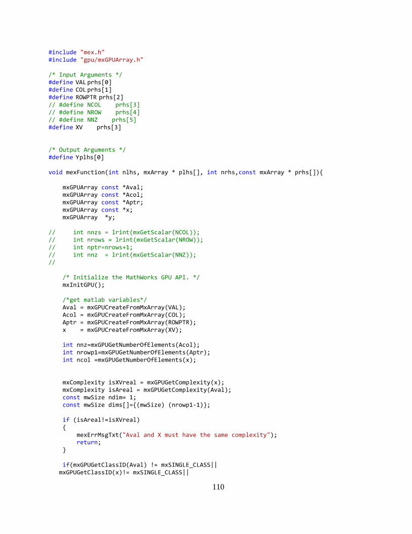
110
#include "mex.h" #include "gpu/mxGPUArray.h" /* Input Arguments */ #define VAL prhs[0] #define COL prhs[1] #define ROWPTR prhs[2] // #define NCOL prhs[3] // #define NROW prhs[4] // #define NNZ prhs[5] #define XV prhs[3] /* Output Arguments */ #define Y plhs[0] void mexFunction(int nlhs, mxArray * plhs[], int nrhs,const mxArray * prhs[]) mxGPUArray const *Aval; mxGPUArray const *Acol; mxGPUArray const *Aptr; mxGPUArray const *x; mxGPUArray *y; // int nnzs = lrint(mxGetScalar(NCOL)); // int nrows = lrint(mxGetScalar(NROW)); // int nptr=nrows+1; // int nnz = lrint(mxGetScalar(NNZ)); // /* Initialize the MathWorks GPU API. */ mxInitGPU(); /*get matlab variables*/ Aval = mxGPUCreateFromMxArray(VAL); Acol = mxGPUCreateFromMxArray(COL); Aptr = mxGPUCreateFromMxArray(ROWPTR); x = mxGPUCreateFromMxArray(XV); int nnz=mxGPUGetNumberOfElements(Acol); int nrowp1=mxGPUGetNumberOfElements(Aptr); int ncol =mxGPUGetNumberOfElements(x); mxComplexity isXVreal = mxGPUGetComplexity(x); mxComplexity isAreal = mxGPUGetComplexity(Aval); const mwSize ndim= 1; const mwSize dims[]=(mwSize) (nrowp1-1); if (isAreal!=isXVreal) mexErrMsgTxt("Aval and X must have the same complexity"); return; if(mxGPUGetClassID(Aval) != mxSINGLE_CLASS|| mxGPUGetClassID(x)!= mxSINGLE_CLASS||

111
mxGPUGetClassID(Aptr)!= mxINT32_CLASS|| mxGPUGetClassID(Acol)!= mxINT32_CLASS) mexErrMsgTxt("usage: gspmv(single, int32, int32, single)"); return; //create output vector y = mxGPUCreateGPUArray(ndim,dims,mxGPUGetClassID(x),isAreal, MX_GPU_DO_NOT_INITIALIZE); /* wrap indices from matlab */ typedef const int TI; /* the type for index */ TI *d_col =(TI *)(mxGPUGetDataReadOnly(Acol)); TI *d_ptr =(TI *)(mxGPUGetDataReadOnly(Aptr)); // wrap with thrust::device_ptr thrust::device_ptr<TI> wrap_d_col (d_col); thrust::device_ptr<TI> wrap_d_ptr (d_ptr); // wrap with array1d_view typedef typename cusp::array1d_view< thrust::device_ptr<TI> > idx2Av; // wrap index arrays idx2Av colIndex (wrap_d_col , wrap_d_col + nnz); idx2Av ptrIndex (wrap_d_ptr , wrap_d_ptr + nrowp1); if (isAreal!=mxREAL) typedef const cusp::complex<float> TA; /* the type for A */ typedef const cusp::complex<float> TXV; /* the type for X */ typedef cusp::complex<float> TYV; /* the type for Y */ // wrap with array1d_view typedef typename cusp::array1d_view< thrust::device_ptr<TA > > val2Av; typedef typename cusp::array1d_view< thrust::device_ptr<TXV > > x2Av; typedef typename cusp::array1d_view< thrust::device_ptr<TYV > > y2Av; /* pointers from matlab */ TA *d_val =(TA *)(mxGPUGetDataReadOnly(Aval)); TXV *d_x =(TXV *)(mxGPUGetDataReadOnly(x)); TYV *d_y =(TYV *)(mxGPUGetData(y)); // wrap with thrust::device_ptr thrust::device_ptr<TA > wrap_d_val (d_val); thrust::device_ptr<TXV > wrap_d_x (d_x); thrust::device_ptr<TYV > wrap_d_y (d_y); // wrap arrays val2Av valIndex (wrap_d_val , wrap_d_val + nnz); x2Av xIndex (wrap_d_x , wrap_d_x + ncol); y2Av yIndex(wrap_d_y, wrap_d_y+ nrowp1-1); // y2Av yIndex(wrap_d_y, wrap_d_y+ ncol); // combine info in CSR matrix typedef cusp::csr_matrix_view<idx2Av,idx2Av,val2Av> DeviceView; DeviceView As(nrowp1-1, ncol, nnz, ptrIndex, colIndex, valIndex); // multiply matrix
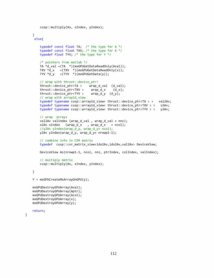
112
cusp::multiply(As, xIndex, yIndex); else typedef const float TA; /* the type for A */ typedef const float TXV; /* the type for X */ typedef float TYV; /* the type for Y */ /* pointers from matlab */ TA *d_val =(TA *)(mxGPUGetDataReadOnly(Aval)); TXV *d_x =(TXV *)(mxGPUGetDataReadOnly(x)); TYV *d_y =(TYV *)(mxGPUGetData(y)); // wrap with thrust::device_ptr! thrust::device_ptr<TA > wrap_d_val (d_val); thrust::device_ptr<TXV > wrap_d_x (d_x); thrust::device_ptr<TYV > wrap_d_y (d_y); // wrap with array1d_view typedef typename cusp::array1d_view< thrust::device_ptr<TA > > val2Av; typedef typename cusp::array1d_view< thrust::device_ptr<TXV > > x2Av; typedef typename cusp::array1d_view< thrust::device_ptr<TYV > > y2Av; // wrap arrays val2Av valIndex (wrap_d_val , wrap_d_val + nnz); x2Av xIndex (wrap_d_x , wrap_d_x + ncol); //y2Av yIndex(wrap_d_y, wrap_d_y+ ncol); y2Av yIndex(wrap_d_y, wrap_d_y+ nrowp1-1); // combine info in CSR matrix typedef cusp::csr_matrix_view<idx2Av,idx2Av,val2Av> DeviceView; DeviceView As(nrowp1-1, ncol, nnz, ptrIndex, colIndex, valIndex); // multiply matrix cusp::multiply(As, xIndex, yIndex); Y = mxGPUCreateMxArrayOnGPU(y); mxGPUDestroyGPUArray(Aval); mxGPUDestroyGPUArray(Aptr); mxGPUDestroyGPUArray(Acol); mxGPUDestroyGPUArray(x); mxGPUDestroyGPUArray(y); return;

113
APPENDIX B
CUDA SOURCE CODE FOR MATLAB MEX FUNCTION: BICONJUGATE
GRADIENT SPARSE ITERATIVE SOLVER
#include "mex.h" #include "cuda.h" #include "gpu/mxGPUArray.h" #include <string.h> #include <iostream> #include <time.h> #include <windows.h> #include <float.h> #define DEBUG 1 #include <cusp/blas.h> #include <cusp/copy.h> #include <cusp/gallery/random.h> #include <cusp/coo_matrix.h> #include <cusp/krylov/bicg.h> #include <cusp/krylov/bicgstab.h> #include <cusp/krylov/cg.h> #include <cusp/krylov/gmres.h> #include <cusp/io/matrix_market.h> void mexFunction (int nlhs, mxArray *plhs[], int nrhs, const mxArray *prhs[]) /* define timer variables */ /* unsigned int kernelTime; cutCreateTimer(&kernelTime); cutResetTimer(kernelTime);*/ LARGE_INTEGER frequency, start, end; double seconds; /* Read in one sparse matrix */ mwSize nnz_A = mxGetNzmax(prhs[0]); /* Create the three arrays needed to represent matrix in COO format */ mxArray *matlab_coo_A[] = mxCreateNumericArray(1, &nnz_A, mxDOUBLE_CLASS, mxREAL), mxCreateNumericArray(1, &nnz_A, mxDOUBLE_CLASS, mxREAL), mxCreateNumericArray(1, &nnz_A, mxDOUBLE_CLASS, mxREAL) ; mexCallMATLAB(3, matlab_coo_A, 1, (mxArray**)(&prhs[0]), "find"); /* Create a cusp matrix on the host */ cusp::coo_matrix<int, double, cusp::host_memory> A(mxGetM(prhs[0]), mxGetN(prhs[0]), nnz_A); double *row = (double*)mxGetData(matlab_coo_A[0]); double *col = (double*)mxGetData(matlab_coo_A[1]);

114
for (int i = 0; i < nnz_A; i++) A.row_indices[i] = row[i] - 1; A.column_indices[i] = col[i] - 1; memcpy(&A.values[0], mxGetData(matlab_coo_A[2]), sizeof(double) * nnz_A); /* Copy to GPU */ cusp::coo_matrix<int, double, cusp::device_memory> gpuA = A; /* A = gpuA; */ #if DEBUG cusp::io::write_matrix_market_file(A, "A.mtx"); #endif /* Read in a full vector */ mwSize A_num_rows = mxGetM(prhs[0]); cusp::array1d<double, cusp::host_memory> B(A_num_rows); memcpy(&B[0], mxGetData(prhs[1]), sizeof(double) * A_num_rows); /* Copy to GPU */ cusp::array1d<double, cusp::device_memory> gpuB = B; /* B = gpuB; */ #if DEBUG cusp::io::write_matrix_market_file(B, "B.mtx"); #endif /* Read in a full vector */ cusp::array1d<double, cusp::host_memory> x(A_num_rows); memcpy(&x[0], mxGetData(prhs[2]), sizeof(double) * A_num_rows); /* Copy to GPU */ cusp::array1d<double, cusp::device_memory> gpux = x; /* x = gpux; */ #if DEBUG cusp::io::write_matrix_market_file(x, "x.mtx"); #endif /* Read in one sparse matrix */ mwSize nnz_M = mxGetNzmax(prhs[3]); /* Create the three arrays needed to represent matrix in COO format */ mxArray *matlab_coo_M[] = mxCreateNumericArray(1, &nnz_M, mxDOUBLE_CLASS, mxREAL), mxCreateNumericArray(1, &nnz_M, mxDOUBLE_CLASS, mxREAL), mxCreateNumericArray(1, &nnz_M, mxDOUBLE_CLASS, mxREAL) ; mexCallMATLAB(3, matlab_coo_M, 1, (mxArray**)(&prhs[3]), "find"); /* Create a cusp matrix on the host */ cusp::coo_matrix<int, double, cusp::host_memory> M(mxGetM(prhs[3]), mxGetN(prhs[3]), nnz_M); double *rowM = (double*)mxGetData(matlab_coo_M[0]);

115
double *colM = (double*)mxGetData(matlab_coo_M[1]); for (int i = 0; i < nnz_M; i++) M.row_indices[i] = rowM[i] - 1; M.column_indices[i] = colM[i] - 1; memcpy(&M.values[0], mxGetData(matlab_coo_M[2]), sizeof(double) * nnz_M); /* Copy to GPU */ cusp::coo_matrix<int, double, cusp::device_memory> gpuM = M; /* A = gpuA; */ #if DEBUG cusp::io::write_matrix_market_file(M, "M.mtx"); #endif /* Allocate space for solution */ cusp::array1d<double, cusp::host_memory> x1(A_num_rows, 0); cusp::array1d<double, cusp::device_memory> gpux1 = x1; cusp::verbose_monitor<double> monitor(gpuB, 8000, 1e-5); //cutStartTimer(kernelTime); /* solve the linear systems */ QueryPerformanceFrequency(&frequency); QueryPerformanceCounter(&start); cusp::krylov::bicgstab(gpuA, gpux, gpuB, monitor); //cusp::krylov::cg(gpuA, gpux, gpuB, monitor); //cusp::krylov::gmres(gpuA, gpux, gpuB, 20, monitor); cudaDeviceSynchronize(); QueryPerformanceCounter(&end); // if any error, such as launch timeout, return maximum run time, seconds = (cudaGetLastError() == cudaSuccess) ? ((double)(end.QuadPart - start.QuadPart) / (double)frequency.QuadPart) : DBL_MAX; std::cout << seconds << std::endl; /*cudaThreadSynchronize(); cutStopTimer(kernelTime); printf("Time for the kernel: %f ms\n", cutGetTimerValue(kernelTime));*/ /* Copy result back */ x1 = gpux; /* Store in output array */ double *output = (double*)mxCalloc(A_num_rows, sizeof(double)); memcpy(output, &x1[0], A_num_rows * sizeof(double)); #if DEBUG cusp::io::write_matrix_market_file(x1, "xsolve.mtx"); #endif plhs[0] = mxCreateNumericArray(1, &A_num_rows, mxDOUBLE_CLASS, mxREAL); mxSetData(plhs[0], output);
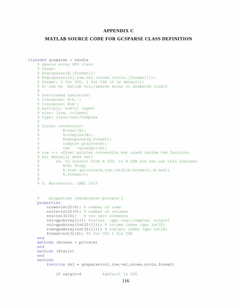
116
APPENDIX C
MATLAB SOURCE CODE FOR GCSPARSE CLASS DEFINITION
classdef gcsparse < handle % sparse array GPU class % Usage: % A=gcsparse(A,[format]); % A=gcsparse(col,row,val,[nrows,[ncols,[format]]]); % format: 0 for COO, 1 for CSR (0 is default); % A: can be matlab full/sparse array or gcsparse i tself % % overloaded operators: % transpose: B=A.'; % transpose: B=A'; % multiply: x=A*y; (spmv) % size: [row, columns] % type: class/real/complex % % format conversion: % B=real(A); % A=complex(B); % B=gcsparse(A,format); % rowptr= ptr2row(A); % row =grow2ptr(A); % row <-> offset pointer conversion may crash insid e the function, % but manually does not: % so, to convert from A COO, to B CSR one can use this instead: % B=A; %copy % B.row= gptr2row(A.row,int32(A.nrows+1),A .nnz); % B.format=1; % % S. Marchesini, LBNL 2013 % properties (SetAccess='private') properties nrows=int32(0); % number of rows ncols=int32(0); % number of columns nnz=int32(0); % non zero elements val=gpuArray([]); %values (gpu real/complex, single) col=gpuArray(int32([])); % column index (gpu int32) row=gpuArray(int32([])); % row/ptr index (gpu int32) format=int32(0); %0 for COO 1 for CSR end methods (Access = private) end methods (Static) end methods function obj = gcsparse(col,row,val,nrows,ncols,format) if nargin<6 %default is COO

117
format=int32(0); %COO else format=int32(format); end if (nargin<=2); %gcsparse(A,[format]) % get the sparse structure of A if nargin==2 %gcsparse(A,format) (format=row, second input) format=int32(row); %row is actually the second input else format=0; end if isa(col, 'gcsparse' ) % we are just converting here obj=col; %col is actually the fisrt input if obj.format==format %nothing to do... return elseif (obj.format==0 && format==1) obj.row=row2ptr(obj); %COO->CSR obj.format=format; elseif (obj.format==1 && format==0); %nptr=obj.nrows+1; %rowptr= gptr2row(obj.row,nptr,obj.nnz); ro wptr=ptr2row(col); %CSR-> COO % obj.row=gptr2row(obj.row,nptr,obj.nnz); obj.row=rowptr; obj.format=format; else fprintf( 'invalid' ); end return else % get val,col,row triplets from A (first input) [obj.nrows,obj.ncols]=size(col) ; %col is actually the fisrt input obj.nrows=gather(obj.nrows); obj.ncols=gather(obj.ncols); [obj.row,obj.col,obj.val]=find( col); obj.col=gpuArray(int32(obj.col( :))); obj.row=gpuArray(int32(obj.row( :))); obj.val=gpuArray((single(obj.va l(:)))); end if nargin==2 format=int32(row); %row is actually the second input end else obj.col=gpuArray(int32(col(:))); obj.row=gpuArray(int32(row(:))); obj.val=gpuArray(val(:)); obj.nrows=gather(int32(max(obj.row( :))));

118
obj.ncols=gather(int32(max(obj.col( :)))); obj.nnz=int32(obj.nnz); end obj.nnz=gather(int32(numel(obj.val))); % matlab to c indexing...: obj.col=obj.col-1; obj.row=obj.row-1; % increase nrows if input [nrows] is given if nargin>3 if (~isempty(nrows)) obj.nrows=gather(int32(max(obj. nrows,nrows))); end if nargin>4 if (~isempty(ncols)) obj.ncols=int32(max(obj.nco ls,ncols)); end end end % sort by rows [obj.row,unsort2sort]=sort(obj.row); obj.col=obj.col(unsort2sort); obj.val=obj.val(unsort2sort); obj.format=0; if format==1; % obj.row=coo2csr(obj); obj.row= row2ptr(obj); obj.format=1; end % 'hi' end function B=real(A) B=A; B.val=real(B.val); end function B=complex(A) B=A; if isreal(A.val); B.val=complex(B.val); end end function y = mtimes(A,x) %SpMV %SpMV with CUSP if A.format==0 % y=0; wait(gpuDevice()) y=gspmv_coo(A.val,A.col,A.row,A.nro ws, x); elseif A.format==1 % y=gspmv_csr(A.col,A.row,A.val,A.nrows,A.ncols,x) ; wait(gpuDevice()); y=gspmv_csr(A.val,A.col,A.row,x); end end function C= ctranspose(obj)

119
% format->coo->transpose->format C=gcsparse(obj,0); %convert to COO tmprow=C.col; %swap row and columns C.col=C.row; C.row=tmprow; tmp=C.nrows; C.nrows=obj.ncols; C.ncols=tmp; C.val=conj(obj.val); %conjugate C=gcsparse(C,obj.format); %revert to original format end function C= transpose(obj) C=gcsparse(obj,0); %convert to COO tmprow=C.col; %swap row and columns C.col=C.row; C.row=tmprow; tmp=C.nrows; C.nrows=obj.ncols; C.ncols=tmp; C=gcsparse(C,obj.format); end function [row,col,val]= find(obj) if obj.format==1; fprintf( 'it may not work, use COO\n' ) fprintf( '[col,row,val]=find(gcsparse(A,0))' ); % [~,row,~]=find(gcsparse(A,0)); nptr=int32(obj.nrows+1); ptr=obj.row+0; nnz=obj.nnz+0; row=gptr2row(ptr,nptr,nnz); % row=ptr2row(obj); row=row+1; if numel(row)<obj.nnz fprintf( 'did not work, use COO\n' ) end % row=gptr2row(obj.row,int32(obj.nr ows+1),obj.nnz); else row=obj.row+1; end col=obj.col+1; val=obj.val; end function m = size(obj) m=[obj.nrows obj.ncols]; end function m = type(obj) f0= classUnderlying(obj.val); if (isreal(obj.val)) fmt= 'Real' ; else fmt= 'Complex' ; end

120
m=[f0 ' ' fmt]; end function row= ptr2row(obj) % offset pointer to row conversion row= gptr2row(obj.row,int32(obj.nrows+1 ),obj.nnz); end function rowptr= row2ptr(obj) % row to offsets rowptr=grow2ptr(obj.row,(obj.nrows+1),( obj.nnz)); end end end

121
APPENDIX D
BUILT-IN MATLAB FUNCTIONS THAT SUPPORT GPUARRAY FOR MATLAB
2012A
Table D.1 shows the built-in functions that support gpuArray type that are available in the
parallel computing toolbox for MATLAB version 2012a.
Table D.1 Available Built-In Functions for MATLAB 2012a Parallel Computing Toolbox that Support GPUArray
abs conv2 floor log acos cos fprintf log10 acosh cosh full log1p acot cot gamma log2 acoth coth gammaln logical acsc csc gather lt acsch csch ge lu
all ctranspose gt mat2str any cumprod horzcat max
arrayfun cumsum hypot meshgrid asec det ifft min asech diag ifft2 minus asin diff ifftn mldivide asinh disp imag mod atan display ind2sub mrdivide atan2 dot int16 mtimes atanh double int2str ndgrid beta eig int32 ndims
betaln eps int64 ne bitand eq int8 norm bitcmp erf inv not bitor erfc ipermute num2str
bitshift erfcinv isempty numel bitxor erfcx isequal permute bsxfun erfinv isequaln plot (and related)
cast exp isfinite plus cat expm1 isinf power ceil filter islogical prod chol filter2 isnan qr
circshift find isreal rdivide classUnderlying fft issorted real
colon fft2 ldivide reallog complex fftn le realpow
conj fix length realsqrt conv
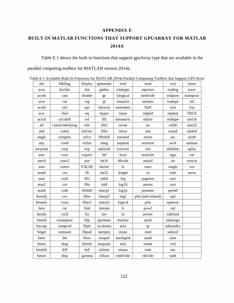
122
APPENDIX E
BUILT-IN MATLAB FUNCTIONS THAT SUPPORT GPUARRAY FOR MATLAB
2014A
Table E.1 shows the built-in functions that support gpuArray type that are available in the
parallel computing toolbox for MATLAB version 2014a.
Table E.1 Available Built-In Functions for MATLAB 2014a Parallel Computing Toolbox that Support GPUArray abs blkdiag display gammaln isinf mod real times
acos bsxfun dot gather isinteger mpower reallog trace
acosh cast double ge islogical mrdivide realpow transpose
acot cat eig gt ismatrix mtimes realsqrt tril
acoth ceil eps horzcat ismember NaN rem triu
acsc chol eq hypot isnan ndgrid repmat TRUE
acsch circshift erf ifft isnumeric ndims reshape uint16
all classUnderlying erfc ifft2 isreal ne rot90 uint32
and colon erfcinv ifftn isrow nnz round uint64
angle complex erfcx ifftshift issorted norm sec uint8
any cond erfinv imag issparse normest sech uminus
arrayfun conj exp ind2sub isvector not shiftdim uplus
asec conv expm1 Inf kron num2str sign var
asech conv2 eye int16 ldivide numel sin vertcat
asin convn FALSE int2str le ones single xor
asinh cos fft int32 length or sinh zeros
atan cosh fft2 int64 log pagefun size
atan2 cot fftn int8 log10 perms sort
atanh coth fftshift interp1 log1p permute sprintf
besselj cov filter interp2 log2 plot (and related) sqrt
bessely cross filter2 interp3 logical plus squeeze
beta csc find interpn lt pow2 std
betaln csch fix inv lu power sub2ind
bitand ctranspose flip ipermute mat2str prod subsasgn
bitcmp cumprod fliplr iscolumn max qr subsindex
bitget cumsum flipud isempty mean rand subsref
bitor det floor isequal meshgrid randi sum
bitset diag fprintf isequaln min randn svd
bitshift diff full isfinite minus rank tan
bitxor disp gamma isfloat mldivide rdivide tanh

123
REFERENCES
[1] F. J. Bartos, "Efficient motors can ease energy crunch," Control Engineering, pp. 63-70, May 2001.
[2] P. C. Krause and O. Wasynczuk, Electromechanical Motion Devices, McGraw-Hill, 1989.
[3] S. J. Salon, Finite Element Analysis of Electrical Machines, Norwell: Kluwer Academic Publishers, 1995.
[4] R. Telichevesky, K. Kundert and J. White, "Efficient steady-state analysis based on matrix-free Krylov-subspace methods," in 32nd ACM/IEEE Design Automation Conference, pp. 480-484, 1995.
[5] W. Yao, "Accurate, efficient, and stable domain decomposition methods for analysis of electromechanical problems," Ph.D. dissertation, University of Illinois at Urbana-Champaign, Urbana, IL, 2013.
[6] J. Jin, The Finite Element Method in Electromagnetics, New York: John Wiley & Sons, 2002.
[7] P. P. Silvester and R. L. Ferrari, Finite Elements for Electrical Engineers, Melbourne: Press Syndicate of the University of Cambridge, 1996.
[8] J. Crank and P. Nicolson, "A practical method for numerical evaluation of solutions of partial differential equations of the heat-conduction type," Proc. Camb. Phil. Soc., vol. 43, no. 1, pp. 50-67, 1947.
[9] W. F. Tinney, V. Brandwajn and S. M. Chan, "Sparse vector methods," Power Apparatus and Systems, IEEE Transactions on, vols. PAS-104, no. 2, pp. 295-301, 1985.
[10] S. M. Chan and V. Brandwajn, "Partial matrix refactorization," IEEE Transactions on Power Systems, vol. 1, no. 1, pp. 193-199, 1986.
[11] Y. Saad, Iterative Methods for Sparse Linear Systems, Cambridge University Press, 2003.
[12] W. E. Arnoldi, "The principle of minimized iterations in the solution of the matrix," Quarterly of Applied Mathematics, vol. 9, pp. 17-29, 1951.
[13] C. Lanczos, "An iteration method for the solution of the eigenvalue problem of linear differential and integral operators," Res. Nat’l Bur. Std, vol. 45, no. 4, pp. 255-282, 1950.
[14] R. Barrett et al., Templates for the Solution of Linear Systems: Building Blocks for Iterative Methods, Philadelphia, PA: SIAM, 1994.
[15] Y. Saad and M. H. Schultz, "GMRES: A generalized minimal residual algorithm for solving nonsymmetric linear systems," SIAM J. Sci. Stat. Comput, vol. 7, no. 3, pp. 856-869, 1986.
[16] P. Sonneveld, "CGS: A fast Lanczos-type solver for nonsymmetric linear systems," SIAM J. Sci. Stat. Comput., vol. 10, no. 1, pp. 36-52, 1989.
[17] H. A. van der Vorst, "BI-CGSTAB: A fast and smoothly converging variant of BI-CG for the solution of nonsymmetric linear systems," SIAM J. Sci. Stat. Comput., vol. 13, no. 2, pp. 631-644, 1992.

124
[18] M. T. Heath, Scientific Computing: An Introductory Survey, New York, NY: McGraw-Hill, 2002.
[19] T. A. Manteuffel, "An incomplete factorization technique for positive definite linear systems," Math. Comput, vol. 34, no. 150, pp. 473-497, 1980.
[20] S. C. Brenner and L. R. Scott, The Mathematical Theory of Finite Element Methods, New York: Springer Science + Business Media, 2010.
[21] T. Nakata, N. Takahashi, K. Fujiwara, N. Okamoto and K. Muramatsu, "Improvements of convergence characteristics of Newton-Raphson method for nonlinear magnetic field analysis," in IEEE Transactions on Magnetics, vol. 28, no. 2, pp. 1048-1051, 1992.
[22] K. Fujiwara, T. Nakata, N. Okamoto and K. Muramatsu, "Method for determining relaxation factor for modified Newton-Raphson method," in IEEE Transactions on Magnetics, vol. 29, no. 2, pp. 1962-1965, 1993.
[23] A. Burtscher, E. Fonn and P. Meury, "Swiss federal institute of technology Zurich department of mathematics handouts and lecture notes," [Online]. Available: https://www.math.ethz.ch/education/bachelor/lectures/fs2013/other/n_dgl/serien/edit/LehrFEM.zip. [Accessed April 2011].
[24] Mathworks Technical Staff, Parallel Computing Toolbox Documentation, The Mathworks, Inc., 2014.
[25] Mathworks Technical Staff, Parallel for-Loops (parfor) Documentation, The Mathworks, Inc., 2014.
[26] J. Doke, "MATLAB central file exchange - demo files for parallel computing with MATLAB on multicore desktops and GPUs webinar," 11 May 2011. [Online]. Available: http://www.mathworks.com/matlabcentral/fileexchange/31336-demo-files-for--parallel-computing-with-matlab-on-multicore-desktops-and-gpus--webinar/content/. [Accessed June 2011].
[27] M. J. Quinn, Parallel Programming in C with MPI and OpenMP, New York: McGraw-Hill, 2003.
[28] S.-I. Sugimoto, H. Kanayama, M. Ogino and S. Yoshimura, "Introduction of a direct method at subdomains in non-linear magnetostatic analysis with HDDM," in 2010 International Conference on Broadband, Wireless Computing, Communication and Applications, 2010, pp. 304-309.
[29] Y. Zhan and A. M. Knight, "Parallel time-stepped analysis of induction machines with Newton-Raphson iteration and domain decomposition," in IEEE Transactions on Magnetics, vol. 44, no. 6, pp. 1546-1549, 2008.
[30] Y. Takahashi et al., "Parallel time-periodic finite-element method for steady-state analysis of rotating machines," in IEEE Transactions on Magnetics, vol. 28, no. 2, pp. 1019-1022, 2012.
[31] C. Fu, "A parallel algorithm for nonlinear dynamic finite element analysis," Information Science and Engineering (ICISE), 2009 1st International Conference on, 2009, pp. 59-62.
[32] D. B. Kirk and W.-M. W. Hwu, Programming Massively Parallel Processors: A Hands-on Approach, Burlington: Morgan Kaufmann Publishers, 2010.
[33] NVIDIA Corporation, "NVIDIA CUDA toolkit documentation: CUDA C programming guide," March 2015. [Online]. Available: http://docs.nvidia.com/cuda/cuda-c-programming-guide/index.html. [Accessed March 2015].
125
[34] NVIDIA Corporation Technical Staff, "Technical brief: NVIDIA GeForce 8800 GPU architecture overview," NVIDIA Corporation, Santa Clara, CA, Tech. Rep. TB-02787-001_v01, 2006.
[35] M. Naumov, "Incomplete-LU and Cholesky preconditioned iterative methods using CUSPARSE and CUBLAS," NVIDIA Corporation, Santa Clara, CA, White Paper Tech. Rep., Jun. 2011.
[36] R. Li and Y. Saad, "GPU-Accelerated preconditioned iterative linear solvers," The Journal of Supercomputing, vol. 63, no. 2, pp. 443-466, 2013.
[37] A. Dziekonski, A. Lamecki and M. Mrozowski, "Jacobi and Gauss-Seidel preconditioned complex conjugate gradient method with GPU acceleration for finite element method," in Proceedings of the 40th European Microwave Conference, 2010, pp. 1305-1308.
[38] A. Dziekonski, A. Lamecki and M. Mrozowski, "Tuning a hybrid GPU-CPU V-cycle multilevel preconditioner for solving large real and complex systems of FEM equations," Antennas and Wireless Propagation Letters, IEEE, vol. 10, pp. 619-622, June 2011.
[39] N. Bell and M. Garland, "Efficient sparse matrix-vector multiplication on CUDA," NVIDIA Corporation, Santa Clara, CA, Tech. Rep. NVR-2008-004, 2008.
[40] A. Ashari, N. Sedaghati, J. Eisenlohr, S. Parthasarath and P. Sadayappan, "Fast sparse matrix-vector multiplication on GPUs for graph applications," in High Performance Computing, Networking, Storage and Analysis, SC14: International Conference for, 2014, pp. 781-792.
[41] Z. A. Taylor, M. Cheng and S. Ourselin, "High-speed nonlinear finite element analysis for surgical simulation using graphics processing units," IEEE Transactions on Medical Imaging, vol. 27, no. 5, pp. 650-663, 2008.
[42] R. Couturier and S. Domas, "Sparse systems solving on GPUs with GMRES," The Journal of Supercomputing, vol. 59, no. 3, pp. 1504-1516, 2012.
[43] NVIDIA Corporation, "Sparse linear algebra library based on thrust," [Online]. Available: http://cusplibrary.github.io/. [Accessed 2014].
[44] NVIDIA Corporation, "NVIDIA CUDA toolkit v7.0 documentation: cuSPARSE," 5 March 2015. [Online]. Available: http://docs.nvidia.com/cuda/cusparse/. [Accessed 2015].
[45] A. George and W. H. Liu, "The evolution of the minimum degree ordering algorithm," SIAM, vol. 31, no. 1, pp. 1-19, 1989.
[46] S. Marchesini, "MATLAB central file exchange: GPU sparse, accumarray, non-uniform grid," Lawrence Berkeley National Laboratory, December 2013. [Online]. Available: http://www.mathworks.com/matlabcentral/fileexchange/44423-gpu-sparse--accumarray--non-uniform-grid. [Accessed 2013].
[47] T. Nakata, N. Takahashi and K. Fujiwara, "Summary of results for benchmark problem 10 (steel plates around a coil)," in COMPEL - The International Journal for Computation and Mathematics in Electrical and Electronics Engineering, vol. 15, no. 2, pp. 103-112, 1995.
[48] J. Wells, P. Chapman and P. Krein, "Development and application of a linear induction machine for instructional laboratory use," in Proc. IEEE Power Electronics Specialists Conference, 2002, pp. 479-482.
[49] M. Magill, "A composite material approach towards induction machine design using planar layer models," M.S. thesis, University of Illinois at Urbana-Champaign, Urbana, IL, 2011.
126
[50] P. Pillay, "Improved design of motors for increased efficiency in residential and commerical buildings," U.S. Department of Energy, Washington, DC, Building Technologies Program Topical Report, 2008.
[51] M. Amrhein and P. T. Krein, "3-D magnetic equivalent circuit framework for modeling electromechanical devices," Energy Conversion, IEEE Transactions on, vol. 24, no. 2, pp. 397-405, 2009.
[52] A. J. Adzima, P. T. Krein and T. C. O'Connell, "Investigation of accelerating numerical-field analysis methods for electric machines with the incorporation of graphic-processor based parallel processing techniques," in Electric Ship Technologies Symposium, 2009. ESTS 2009. IEEE, 2009, pp. 59-64.
Related Documents


![arXiv:1210.2225v1 [math.RT] 8 Oct 2012 · 6.2. Characters of Finite Classical groups 19 7. Harish-Chandra Induction 20 7.1. Harish-Chandra Induction 20 7.2. Characters under Harish-Chandra](https://static.cupdf.com/doc/110x72/5f70192c974bee67ac1009f7/arxiv12102225v1-mathrt-8-oct-2012-62-characters-of-finite-classical-groups.jpg)


