Accelerating Flash Calculation through Deep Learning Methods · Accelerating Flash Calculation through Deep Learning Methods Yu Li KAUST CEMSE CBRC Tao Zhang KAUST PSE CTPL Shuyu

Accelerating Flash Calculation through DeepLearning Methods

Yu LiKAUSTCEMSECBRC

Tao ZhangKAUST

PSECTPL

Shuyu Sun ∗KAUST

PSECTPL

Xin Gao ∗KAUSTCEMSECBRC

Abstract

In the past two decades, researchers have made remarkable progress in acceleratingflash calculation, which is very useful in a variety of engineering processes. In thispaper, general phase splitting problem statements and flash calculation proceduresusing the Successive Substitution Method are reviewed, while the main shortagesare pointed out. Two acceleration methods, Newton’s method and the Sparse GridsMethod are presented afterwards as a comparison with the deep learning modelproposed in this paper. A detailed introduction from artificial neural networks todeep learning methods is provided here with the authors’ own remarks. Factors inthe deep learning model are investigated to show their effect on the final result. Aselected model based on that has been used in a flash calculation predictor withcomparison with other methods mentioned above. It is shown that results from theoptimized deep learning model meet the experimental data well with the shortestCPU time. More comparison with experimental data has been conducted to showthe robustness of our model.

1 Introduction

Vapor-liquid equilibrium (VLE) is of essential importance in modeling the multiphase and mul-ticomponent flow simulation for a number of engineering processes [23, 22]. Knowledge of theequilibrium conditions in mixtures can be obtained from data collected in direct experiment or usingthermodynamic models, including activity coefficients at low system pressure or fugacity coefficientsat high system pressure [18]. In the last two decades, the application of equilibrium calculationusing equations of state (EOS) that describes mixing rules with experience coefficients has beenproposed and widely discussed [7, 24, 25]. A realistic EOS, e.g., Peng-Robinson (PR EOS), isgenerally considered as an appropriate thermodynamic model to correlate and predict vapor–liquidequilibrium (VLE) conditions, due to the long-time improvement developed with applications indifferent aspects. The calculation procedures using EOS have been extensively studied and modified.The EOS parameters, describing concentration, combination and interaction between binary mixtures,can decide the accuracy in correlating the VLE process. In practice, such parameters are generallyobtained by fitting experimental data under the temperature at which VLE is required. However,in most EOS calculations, iterations are needed, which makes it less suitable for time sensitiveapplications. For cases like phase equilibrium in underground heated flow, as the concentrationof many possible components varies greatly in a wide range, it is difficult to correlate them andpredict the parameters exactly from experiments. Some very small concentrations of components areessential parts, which make the parameter calculation more difficult.

∗All correspondence should be addressed to Xin Gao ([email protected]) and Shuyu Sun([email protected]).

Preprint. Work in progress.

arX

iv:1

809.

0731

1v2

[cs

.CE

] 2

9 Se

p 20

18

To speed up flash calculation, attentions have been paid to other numerical tools, such as sparsegrids technology and artificial neural networks (ANN) [7, 27, 1, 26, 16, 17]. Sparse grids technologyis often considered preferable in coupling with flow as the surrogate model created in the offlinephase can be used repeatedly [26]. However, the generation of the surrogate model is still time-consuming. On the other hand, due to its ability to capture the relationship among large amountof variables, especially for non-linear correlations, ANN has attracted considerable attention forperforming acceleration. It has been reported that ANN has been used in the thermodynamicproperties calculation successfully, including vompressibility factor, vapour pressure and viscosity.For example, ANN has shown the efficiency, as well as the ability to estimate the shape factors anddensity of regregerants, which is a function of temperature, and then been extended to solve thecorresponding state model [16, 1, 17].

Since the breakthrough of AlexNet [9] in 2012, deep learning has made profound impact on both theindustry and the academia [10]. Not only has it revolutionized the computer vision field, improvingthe performance of image recognition and object detection dramatically [5, 19], and the naturallanguage processing field [3], setting new record for speed recognition and language translation, butit has also enabled machines to reach human level intelligence in some certain tasks, such as the Gogame [20]. In addition to those well-known tasks that deep learning is especially expert in, deeplearning has been applied to a broad range of problems, such as protein binding affinity prediction [4],enzyme function prediction [13], structure super-resolution reconstruction [14], the third generationsequencing modeling [12], particle accelerator data analysis [2] and modeling brain circuits [6]. Sucha great potential of deep learning comes from its significant performance improvement over thetraditional machine learning algorithms, such as support vector machine (SVM). The traditionalmachine learning methods usually consider just one layer non-linear combination of the input featureswhile the deep learning method can consider ultra-complex non-linear combination of the inputfeatures by taking advantage of multiple hidden layers. During training, the back propagationalgorithm increases the weight of the feature combination which is useful for the final classificationor regression problem to emphasize the useful features while decreases the weight of those unrelatedfeature combinations. In spite of the universal approximation theorem, which states that we canapproximate any continuous functions using a feed-forward network with a single hidden layercontaining a finite number of neurons, the success of deep learning shows the potential of fitting VLEusing multi-layer neural networks.

In this paper, binary components flash calculation accelerations are studied. We first introduce themain concept of flash calculation and general problem statement. After that, we explain a popularmethod in flash calculation, Successive Substitute Method, in details as well as the main shortage ofthis method. Some suggestions are presented based on our experience to help reach the equilibriumstate. Afterwards, two optimization methods, namely, the Newton’s method and the Sparse GridsMethod, are briefly introduced. Deep learning methods based on artificial neural networks arepresented in the following section. Our deep learning model is optimized based on the investigationof its testing behaviors with different factors and features. Then, all the four methods are applied inflash calculation test, and we show the comparison of their results and CPU time needed. The fastestdeep learning method is finally tested with various flash calculation problems, and compared withthe experimental data and results from classical SSM. Remarks are made and conclusions are drawnbased on the results and comparisons.

2 Flash Calculation Methods

2.1 General Phase Splitting Problem Statement

In two-phase compositional flow, component compositions change with the thermodynamic condi-tions, and that is what flash calculations determine. Phase splitting may occur with the changing oftemperature or pressure, which makes the composition determination more difficult. Wider propertiesat phase equilibrium statements can also be predicted through flash calculation, and the modelingand simulation have been widely reported in literatures [11, 15]. A general phase splitting problemis often defined with an assumption of a thermodynamic equilibrium state among the components.Common phase splitting problems include the NPT flash (T, P, x, y) and the NVT flash(T, V, x, y).For both types, temperature and pressure remain the same for all the phases, while other propertiesneed to be calculated based on the “thermodynamic equilibrium condition”. Fugacity is usually

2

selected to express the equilibrium condition of each component in engineering application, and NPTflash is more popular compared with NVT flash.

In a typical NPT phase splitting problem, we are given the following data as our input quantities:the moles of feed F (no need if interested in extensive quantities only); feed composition zi, i =1, · · · ,M ; temperature T , and pressure P and physical properties of components such as criticaltemperature Tc and critical pressure Pc. The purpose is to determine the vapor-phase compositionyi, i = 1, · · · ,M , and liquid-phase composition xi, i = 1, · · · ,M . Popular solutions include severaldifferent variants of the successive substitution method (SSM). Molar densities, mass densities andisothermal compressibility of each phase can be determined further based on the SSM result. Finally,the saturation of the flow, the partial molar volume of each species and the two-phase isothermalcompressibility of the flow can be calculated.

2.2 Successive Substitution Method

The Successive Substitution Method (SSM) is also known as Successive Substitution Iteration (SSI),which is mainly the updating of vapor-liquid equilibrium ratio, Ki,

yi = Kixi, i = 1, 2, · · · ,M, (1)

also known as the phase equilibrium constant, the partition constant or the distribution coefficieint,and can also be defined from

Ki = Ki(T, p, x1, · · · , xM , y1, · · · , yM ) =ϕLi (T, p, x1, x2, · · · , xM )

ϕVi (T, p, y1, y2, · · · , yM )

. (2)

The equilibrium condition is equivalent to pyi = Kixi. The fugacity can be computed by PR-EOS as

lnϕLi =

bLibL(ZL − 1

)− ln

(ZL −BL

)− AL

2√2BL

(2∑M

j=1 xjaLij

aL− bLibL

)lnZL + 2.414BL

ZL − 0.414BL,

(3)

lnϕVi =

bVibV(ZV − 1

)− ln

(ZV −BV

)− AV

2√2BV

(2∑M

j=1 yjaVij

aV− bVibV

)lnZV + 2.414BV

ZV − 0.414BV.

(4)

If the K-values are given, we can solve the Rachford-Rice equation for β:

M∑i=1

(Ki − 1)zi1 + β(Ki − 1)

= 0. (5)

The coefficient β is more convinced in the composition computation compared with K-values.

The detailed algorithm in SSM could be summarized into 5 steps:

Step 1. Prepare the parameters, including a and b, based on the critical pressures and temperatures ofeach component as well as their acentric factors.

a(Tc) =0.45724R2 T 2

c

pc, b = b(Tc) =

0.07780RTcpc

, a(T ) = a(Tc)(1 +m

(1− T 0.5

r

))2, (6)

where m is calculated by

m = 0.37464 + 1.54226ω − 0.26992ω2, for0 < ω < 0.5, (7)

3

m = 0.3796 + 1.485ω − 0.1644ω2 + 0.01667ω3, for0.1 < ω < 2.0. (8)

Step 2. Use the Wilson equation to calculate an initial guess of K and then determine β with theRachford-Rice procedure (i.e. by solving the Rachford-Rice equation, Eq. (5)):

KWilsoni =

pc,ip

exp

(5.37(1 + ωi)

(1− Tc,i

T

)). (9)

Step 3. Solve the following cubic equation to determine the compressibility factor, Z, based on thecalculation of A and B. Thus, fugacities for each phase can be estimated as Equation (3) and (4).

Z3 − (1−B) Z2 + (A− 2B − 3B2) Z − (AB −B2 −B3) = 0, whereA =a(T )p

R2T 2, B =

bp

RT.

(10)

Step 4. Check the equilibrium statement, which is often conducted with a convergence test:

∣∣∣∣fVifLi − 1

∣∣∣∣ < ε, (11)

where ε is the criterion.

Step 5. Update K if the criterion is not satisfied (the equilibrium state is not reached), and repeatsteps 3 and 4 until the equilibrium has been reached.

Knewi =

fLifVi

Koldi , (12)

where ϕVi =

fVi

yipand ϕL

i =fLi

xip.

It should be noted that in Step 3, two separate solutions of the cubic equation need to be conductedto calculate Z and then determine the phase molar volumes vL and vV . Obviously this procedurefor binary components is more difficult and complex compared to pure fluid flash calculation, as wemeet six roots (three for vapor and three for liquid). Further process should be considered for thesix roots, for example, the middle roots for vapor/liquid are discarded because they lead to unstablephases. Besides, the remaining roots need to be paired to calculate component fugacities, and theparing selection is a challenge as there are two roots for each phase. If the selection of paring iswrong, the whole procedure will fail with an unstable or metastable solution. Some experiences canbe referred to help make the pairing. For example, total Gibbs energy should be minimized for thecorrect equilibrium solution and sometimes the correct root for liquid should minimize the molarvolume. However, for most cases, the best root for vapor phase will maximize the molar volume.

These restrictions make the original SSM complex and unsteady. Sometimes the roots even fail topresent reasonable physical meanings and the root calculation often costs a significant portion of thetotal CPU time. As a result, an increasing number of studies have been carried out to optimize thismethod, including the Newton’s method, which is also based on PR-EOS and Sparse Grids method.

2.3 Newton’s Method

Newton-Raphson method, also known as Newton’s method, is an optimization procedure to succes-sively estimate the roots of a real-valued function: f(x) = 0.. Starting with a good initial guess, x0for f(x) = 0, a repeating updating will be conducted until a sufficiently accurate value is reached:

xn+1 = xn −f(xn)

f ′(xn). (13)

4

The Newton’s method can be summarized into 5 steps:

Step 1: Let n = 0 to obtain initial Ki from SSM, or the previous time step in simulations, etc.

Step 2: Given Ki, the initial estimate of β is obtained from the solution of the Rachford-Riceequation:

FM+1(K1,K2, · · · ,KM , β) =

M∑i=1

(Ki − 1)zi1 + β(Ki − 1)

= 0. (14)

Step 3: Solve the following linear system to get x(n+1):

JF (x(n))

(x(n+1) − x(n)

)= −F(x(n)), (15)

where

x(n) =

K

(n)1

K(n)2...

K(n)M

β(n)

, F(x(n)) =

F1(x

(n))F2(x

(n))...

FM (x(n))FRR(x

(n))

, (16)

Fi(K1,K2, · · · ,KM , β) = lnKi − lnϕLi + lnϕV

i = 0, (17)

FRR =

M∑i=1

yi −M∑i=1

xi. (18)

Step 4: Let n← n+ 1.

Step 5: Repeating step 3 and 4 until a sufficient accuracy is reached.

2.4 Sparse Grids Method

Various deformations have been proposed in sparse grids methods, while the main idea remains thesame [26]. The approximation of a function is calculated through a summation of a suitable set ofbasis functions. The basis functions are computed on the set of grid points where the original functionis evaluated. For the application in flash calculation, the sparse grids method is split into two steps:online phase and offline phase. A surrogate model is created during the offline phase, and in theonline phase it can be cheaply evaluated for the compositional flow simulation. The biggest advantageof this method is the repeatable usage of the surrogate model, so that only one determination of thismodel is needed, which greatly saves the computation effort. Generally, the CPU time used for theoffline phase (model creation) can be neglected.

Fourteen values are calculated from the original binary component flash calculation, and these valuesare called observables for the two components in the sparse grids method. To construct a surrogatemodel, twelve of these values are taken as the input values, while the remaining two observables,liquid and gas, are not considered in the surrogate model. All the fourteen values are presented inTable 1.

Obviously, the simplest and most straightforward approach for creating a surrogate model is to storeall the evaluations resulted from original flash calculations as listed in the above table on a regularCartesian grid. The problem is that this full grid surrogate can result in out-of-memory for large

5

Table 1: Observables in sparse grids methods for flash calculations

Observable Physical quantityxW1 Molar fraction of Component 1 in the oil phasexW2 Molar fraction of Component 2 in the oil phasexN1 Molar fraction of Component 1 in the gas phasexN2 Molar fraction of Component 2 in the gas phasexiW Molar density of oil phase (unit: mole/m2)xiN Molar density of gas phase (unit: mole/m2)

densiW Mass density of oil phase (unit: kg/m2)densiN Mass density of gas phase (unit: kg/m2)sW Saturationv1 Partial molar volume of Component 1v2 Partial molar volume of Component 2Cf Isothermal compressibility of the flow

Liquid Boolean variables, 1 for liquid.Gas Boolean variables, 1 for gas.

systems with high order of components. Besides, in fact, not all the grids are used during calculation,which causes the waste of memory.

So we move to the sparse grids method, which reduces the requirements of memory. The 12 adaptivesparse grid approximations Ss,i with i = 1, . . . , 12 are constructed. During the offline phase, eachSs,i starts with a basic low resolution sparse grid which is then refined in the areas with the highestsurplus. Since each flash calculation retrieves all the 12 output values, the construction of an Ss,i

can reuse values if a particular grid point, i.e. a parameter combination (p, z1), has already beenevaluated by a flash calculation for building another Ss,i. Using this method, the computation effortto create the surrogate model is largely reduced. It has been reported that, because all the observablescan be calculated through the original flash calculation, the union of all the grid points is sometimesused as the union sparse grids for each of the surrogates Ss,i, which increases significantly the datastored in memory but only a minor approximation accuracy will be obtained. Thus, it is not a goodidea to use the union sparse grids. It is also noted that due to the basis functions overlapping, Ss

will always present a slightly larger overhead evaluation compared with Sf (f for full grid surrogatemodel), but this overhead could be neglected.

3 Artificial Neural Networks

Artificial neural networks (ANNs) are computational models designed to incorporate and extract keyfeatures of the original inputs. Deep neural networks usually refer to those artificial neural networkswhich consist of multiple hidden layers. As shown in Figure 1, a deep fully connected neural networkis applied to model the VLE. Following the input layer, a number of fully connected hidden layers,with a certain number of nodes, stack over the other, whose final output is fed into another fullyconnected connected layer, which is the final output layer. Since we are fitting X and Y in our model,the final output layer contains two nodes, each of which predicts the value of one of the two variables.The activation function of this layer is fixed as linear. Naturally the proposed ANN input variablesinclude critical pressure (Pc), critical temperature (Tc) and acentric factor (ω) of the componentscomprising the mixture. As a result, the eight variables in Figure 1 are the above three factors foreach of the two components in the mixture, the temperature, and the pressure. The required C1 toC7 binary mixture experimental VLE data were gathered from the Korea Thermophysical PropertiesData Bank (KDB), of 1332 data points in total, with supplementary selection of consistency andapplicability. As instructed on the database, the expected mean relative error of the experimentaldata we used for training and validating the model is around 20%. A large range of pressures andtemperatures are considered while ensuring that the mixture does not enter into a critical state, whichis to confirm that a two-phase condition is ensured.

Due to the high complexity of the neural network model and the limited number of data (only 1332records in total), the trained model is subject to overfitting. To deal with the common and most

6

Figure 1: The neural network to model VLE.

serious issue in the deep learning field, we adopted weight decay as well as dropout [21] to handlethe problem. The model initialization can also influence the final result significantly. We utilizedXavier initializer to perform the model initialization. The whole package is developed using TFlearn.Trained on a workstation with one Maxwell Titan X card, the model converged in 10 minutes. Asimplified flow chart of our network model working process in each node is presented in Figure 2.

Figure 2: The flow chart of the simulation process in each node

Formally, for the i-th hidden layer, let ai denote the input of the layer, and yi to denote the output ofthe layer. Then we have:

yi = fi(Wi ∗ ai + bi), (19)

where Wi is the weight; bi is the bias; and fi is the activation functions of the i-th layer. For a networkwith multiple layers, the output of one hidden layer is the input of the next layer. For example, wecan represent the network in Figure 1 as:

o = f3(W3 ∗ f2(W2 ∗ f1(W1 ∗ x1 + b1) + b2) + b3), (20)

where o = (X,T ); f1, f2, f3 are the activation functions; W1,W2,W3 are the weights for each layer;b1,b2,b3 are the bias terms of each layer.

Here are the short explanations of the techniques used to obtain a practical network:

1. Weight decay: Overfitting is usually a serious issue in the deep learning field, which meansthat the learned model has almost perfect performance on the training data while performspoorly on the validation or testing data. The main reason of overfitting in this field is that themodel itself is composed of too many parameters while we do not have enough training data,

7

that is, the model is over-parameterized. In order to prevent the overfitting issue from hurtingthe model’s performance, we usually apply additional constraint on the model’s parametersto reduce the freedom of the model. In general, if the model is overfitted, the norm of theweight parameters is often very large. As a result, one way to avoid overfitting is to add anadditional constraint on the norm of the weight parameters and penalize large weights. Inpractice, we can add a regularization term, which is related to the norm of the weights, inthe loss function to make the model fit the training data and penalize large weights at thesame time. Formally, the original loss function for deep learning, which is the mean squaredloss in our problem, can be formulated as:

L =1

N

N∑n=1

‖o− o‖2 , (21)

where N is the total number of training data; o is the output of the model; o is the observedvalue. After adding the L2 weight decay term, the loss function becomes:

L =1

N

N∑n=1

‖o− o‖2 + λ ‖W‖22 , (22)

where W is the whole set of weight parameters of the model; λ is the regularizationcoefficient, i.e., how much we penalize over the large weights.

2. Dropout: Dropout is a very efficient method for dealing with overfitting in neural networks.This method reduces the freedom of the network by discarding nodes and connections of themodel during the training stage. For example, if we apply the dropout technique to a certainlayer with the keep probability as p (0 < p < 1), then, during each training stage, eachnode of that layer would first be evaluated independently with the probability of p beingkept or the probability of 1− p being discarded. If the nodes are discarded, all the nodesand connections are discarded from the model. After the dropout procedure, the reducednetwork is trained during the training stage. After that certain training stage, the discardednodes are inserted to the model with the original weights and the model enters the nexttraining cycle.

3. Xavier initializer: The initialization of the neural network model is of vital importance,which can affect the convergence speed and even the final model’s performance. If theweights are initialized with very small values, the variance of the input signal vanishesacross different layers and eventually drops to a very low value, which reduces the modelcomplexity and may hurt the model’s performance. If the weights are initialized with verylarge values, the variance of the input signal tends to increase rapidly across different layers.That may cause gradient vanishing or explosion, which increases the difficulty of traininga working model. Since we usually initialize the weights with a Gaussian distribution, tocontrol the variance of the signal, it is desirable to initialize the weights with a variance δto make the variance of the output of a layer the same as that of the input of the layer. Forexample, for Figure 2, we want:

var(y) = var(w1 ∗ a1 + w2 ∗ a2 + ...+ wn ∗ an + b)

= var(w1) ∗ var(a1) + var(w2) ∗ var(a2) + ...+ var(wn) ∗ var(an)(1)= n ∗ var(wi) ∗ var(ai), (23)

where (1) is because of the identity distribution assumption of all the wi and ai. Since wewant the variance of y the same as the variance of ai, we need:

n ∗ var(wi) = 1, (24)

as a result, we should initialize the weight of each layer using Gaussian distribution with thevariance as 1

n , where n is the number of weights in that layer. This initializer is known asthe Xavier initializer.

4. Batch normalization: Training deep learning model is notoriously time-consuming, becauseof the large number of parameters belonging to different layers. Not only is the optimizationfor such a large number of parameters internally time-consuming, but there are someundesirable properties of the multi-layer model which makes the convergence process slow.

8

Table 2: Physical properties of components involved in this paper

Component Tc(K) Pc(bar) ω

C1 190.6 46 0.0115C2 305.4 48.84 0.0908C3 369.8 42.46 0.1454C4 421.09 37.69 0.1886C5 467.85 34.24 0.2257C6 521.99 34.66 0.2564C7 557.09 32.62 0.2854

One property of the deep learning method is that the distribution of each layer’s inputmight change because the parameters of the previous layer are usually changed duringtraining, which is usually referred to as “internal covariate shift”. To solve the problem,batch normalization is proposed. In addition to normalize the original input of the model,which is the input of the first layer, this technique makes the normalization part of the modeland performs normalization on hidden layers for each training batch during the trainingstage. Batch normalization enables larger learning rates and can accelerate the convergencespeed by 10 times.

5. Activation functions: As shown in Equation (20), the activation function is where thenon-linearity and the expressiveness power of deep neural network models comes from.There are numerous activation functions: Rectified linear unit (ReLU), Parameteric rectifiedlinear unit (PReLU), TanH, Sigmoid, Softplus, Softsign, Leaky rectified linear unit (LeakyReLU), Exponential linear unit (ELU), and Scaled exponential linear unit (SELU). The mostcommonly used ones are ReLU

f(x) =

{0, if x < 0

x, if x ≥ 0,(25)

and Sigmoid:

σ(x) =1

1 + exp(−x). (26)

In Section 4, we show the performance of our model with different activation functions.

4 Results and Discussion

In this paper, to accelerate and optimize the original flash calculation using SSM, attempt has beenmade to use the deep learning method for the Vapour-Liquid equilibrium (VLE) calculation of thesystems C1 − C7 mixtures, including Methane, Ethane, Propane, N-Butane, N-Pentane, N-Hexane,N-Heptane in NPT kind flash. Two other accelerating methods, Newton’s Method and Sparse GridsMethod, are also introduced and used as a comparison. Physical properties of each componentare listed in Table 2. Essentially, as the Gibbs phase rule stipulates, two intensive properties arerequired to completely describe a binary two-phase system at equilibrium conditions. Temperatureand pressure are two such thermodynamic intensive properties conventionally selected, because ofthe relative ease with which they can be measured. Alongside temperature and pressure, the acentricfactor is also generally included in VLE phase equilibrium calculations to account for non-sphericityof molecules. The required C1 to C7 binary mixture experimental VLE data were gathered from theKorea Thermophysical Properties Data Bank (KDB), of totaling 1332 data points, with supplementaryselection of consistency and applicability. As instructed on the database, the expected mean relativeerror of the experimental data we used for training and validating the model is around 20%. A largerange of pressures and temperatures are considered while ensuring that the mixture does not enterinto a critical state, which is to confirm that a two-phase condition is ensured.

4.1 Training a Deep Learning Model

In this section, we briefly describe how we train a neural network on this problem. We use a neuralnetwork with the following configurations: the neural network has 5 layers, with 100 nodes within

9

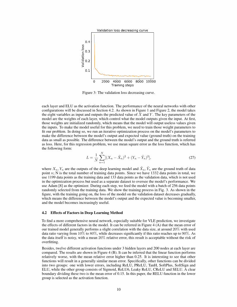
Figure 3: The validation loss decreasing curve.

each layer and ELU as the activation function. The performance of the neural networks with otherconfigurations will be discussed in Section 4.2. As shown in Figure 1 and Figure 2, the model takesthe eight variables as input and outputs the predicted value of X and Y . The key parameters of themodel are the weights of each layer, which control what the model outputs given the input. At first,those weights are initialized randomly, which means that the model will output useless values giventhe inputs. To make the model useful for this problem, we need to train those weight parameters tofit our problem. In doing so, we run an iterative optimization process on the model’s parameters tomake the difference between the model’s output and expected value (ground truth) on the trainingdata as small as possible. The difference between the model’s output and the ground truth is referredas loss. Here, for this regression problem, we use mean square error as the loss function, which hasthe following form:

L =1

N

N∑n=1

[(Xn − Xn)2 + (Yn − Yn)2], (27)

where Xn, Yn are the outputs of the deep learning model and Xn, Yn are the ground truth of datapoint n; N is the total number of training data points. Since we have 1332 data points in total, weuse 1199 data points as the training data and 133 data points as the validation data, which is not usedin the optimization process but used as a separate dataset to oversee the model’s performance. Weuse Adam [8] as the optimizer. During each step, we feed the model with a batch of 256 data pointsrandomly selected from the training data. We show the training process in Fig. 3. As shown in thefigure, with the training going on, the loss of the model on the validation dataset decreases gradually,which means the difference between the model’s output and the expected value is becoming smaller,and the model becomes increasingly useful.

4.2 Effects of Factors in Deep Learning Method

To find a more comprehensive neural network, especially suitable for VLE prediction, we investigatethe effects of different factors in the model. It can be referred in Figure 4 (A) that the mean error ofour trained model generally performs a slight correlation with the data size, at around 20% with useddata ratio varying from 10% to 80%, while decreases significantly if this ratio reaches up to 90%. Asthe data itself is noisy, with a mean 20% relative error, this result is acceptable without the risk ofoverfitting.

Besides, twelve different activation functions under 3 hidden layers and 200 nodes at each layer arecompared. The results are shown in Figure 4 (B). It can be inferred that the linear function performsrelatively worse, with the mean relative error higher than 0.25. It is interesting to see that otherfunctions will result in a generally similar mean error. Specifically, other functions can be dividedinto two groups: one with lower errors, including ReLU, PReLU, TanH, SoftPlus, SoftSign andELU, while the other group consists of Sigmoid, ReLU6, Leaky ReLU, CReLU and SELU. A clearboundary dividing these two is the mean error of 0.15. In this paper, the RELU function in the lowergroup is selected as the activation function.

10

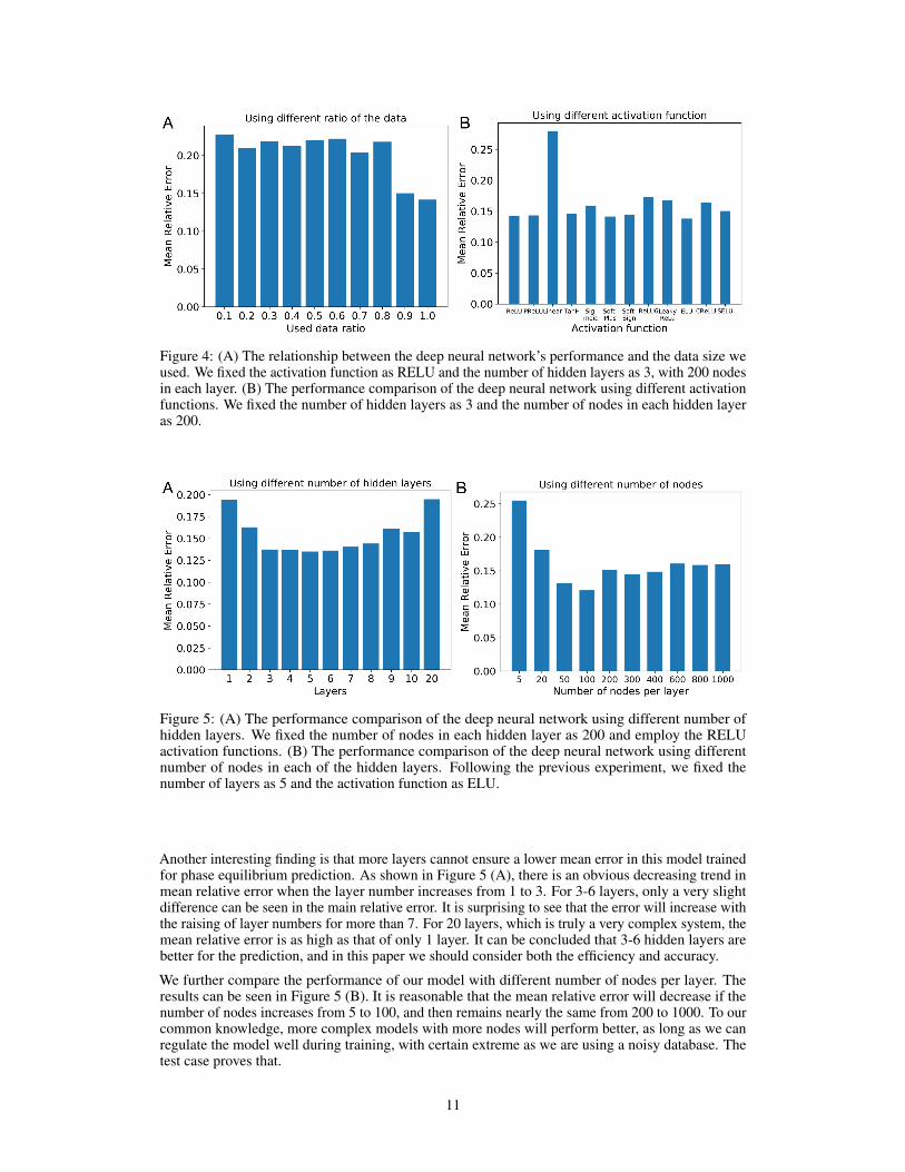
Figure 4: (A) The relationship between the deep neural network’s performance and the data size weused. We fixed the activation function as RELU and the number of hidden layers as 3, with 200 nodesin each layer. (B) The performance comparison of the deep neural network using different activationfunctions. We fixed the number of hidden layers as 3 and the number of nodes in each hidden layeras 200.

Figure 5: (A) The performance comparison of the deep neural network using different number ofhidden layers. We fixed the number of nodes in each hidden layer as 200 and employ the RELUactivation functions. (B) The performance comparison of the deep neural network using differentnumber of nodes in each of the hidden layers. Following the previous experiment, we fixed thenumber of layers as 5 and the activation function as ELU.

Another interesting finding is that more layers cannot ensure a lower mean error in this model trainedfor phase equilibrium prediction. As shown in Figure 5 (A), there is an obvious decreasing trend inmean relative error when the layer number increases from 1 to 3. For 3-6 layers, only a very slightdifference can be seen in the main relative error. It is surprising to see that the error will increase withthe raising of layer numbers for more than 7. For 20 layers, which is truly a very complex system, themean relative error is as high as that of only 1 layer. It can be concluded that 3-6 hidden layers arebetter for the prediction, and in this paper we should consider both the efficiency and accuracy.

We further compare the performance of our model with different number of nodes per layer. Theresults can be seen in Figure 5 (B). It is reasonable that the mean relative error will decrease if thenumber of nodes increases from 5 to 100, and then remains nearly the same from 200 to 1000. To ourcommon knowledge, more complex models with more nodes will perform better, as long as we canregulate the model well during training, with certain extreme as we are using a noisy database. Thetest case proves that.

11

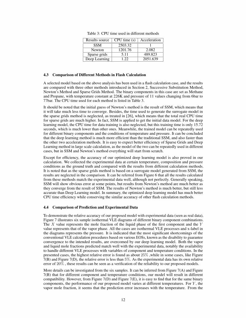
Table 3: CPU time used in different methods

Results source CPU time (s) AccelerationSSM 2503.32 1

Newton 1201.76 2.082Sparse grids 5.11 489.823

Deep Learning 1.22 2051.639

4.3 Comparison of Different Methods in Flash Calculation

A selected model based on the above analysis has been used in a flash calculation case, and the resultsare compared with three other methods introduced in Section 2, Successive Substitution Method,Newton’s Method and Sparse Grids Method. The binary components in this case are set as Methaneand Propane, with temperature constant at 226K and pressure of 11 values changing from 6bar to77bar. The CPU time used for each method is listed in Table 3.

It should be noted that the initial guess of Newton’s method is the result of SSM, which means thatit will take much less time to converge. Besides, the time used to generate the surrogate model inthe sparse grids method is neglected, as treated in [26], which means that the total real CPU timefor sparse grids are much higher. In fact, SSM is applied to get the initial data model. For the deeplearning model, the CPU time for data training is also neglected, but this training time is only 15.72seconds, which is much lower than other ones. Meanwhile, the trained model can be repeatedly usedfor different binary components and the conditions of temperature and pressure. It can be concludedthat the deep learning method is much more efficient than the traditional SSM, and also faster thanthe other two acceleration methods. It is easy to expect better efficiency of Sparse Grids and DeepLearning method in large scale calculation, as the model of the two can be repeatedly used in differentcases, but in SSM and Newton’s method everything will start from scratch.

Except for efficiency, the accuracy of our optimized deep learning model is also proved in ourcalculation. We collected the experimental data at certain temperature, composition and pressureconditions as the ground truth and compared with the results from different calculation methods.It is noted that as the sparse grids method is based on a surrogate model generated from SSM, theresults are neglected in the comparison. It can be referred from Figure 6 that all the results calculatedfrom these methods match the experimental data well, although not perfectly. Generally speaking,SSM will show obvious error at some points, but results from Newton’s method are much better asthey converge from the result of SSM. The results of Newton’s method is much better, but still lessaccurate than Deep Learning model. In summary, the optimized deep learning model has much betterCPU time efficiency while conserving the similar accuracy of other flash calculation methods.

4.4 Comparison of Prediction and Experimental Data

To demonstrate the relative accuracy of our proposed model with experimental data (seen as real data),Figure 7 illustrates six sample isothermal VLE diagrams of different binary component combinations.The X value represents the mole fraction of the liquid phase of the first component and the Yvalue represents that of the vapor phase. All the cases are isothermal VLE processes and x-label inthe diagrams represents the pressure. It is indicated that the most significant shortcomings of theconventional VLE calculation procedures based on various EOSs, known as the disability to guaranteeconvergence to the intended results, are overcomed by our deep learning model. Both the vaporand liquid mole fractions predicted match well with the experimental data, notably the availabilityto handle different VLE processes with variables of component and temperature conditions. In thepresented cases, the highest relative error is found as about 25% ,while in some cases, like Figure7(B) and Figure 7(D), the relative error is less than 5%. As the experimental data has its own relativeerror of 20% , these results can be seen as a verification of the reliability to our proposed models.

More details can be investigated from the six samples. It can be inferred from Figure 7(A) and Figure7(B) that for different component and temperature conditions, our model will result in differentcompatibility. However, from Figure 7(D) and Figure 7(E), it is easy to find that for the same binarycomponents, the performance of our proposed model varies at different temperatures. For Y , thevapor mole fraction, it seems that the prediction error increases with the temperature. From the

12

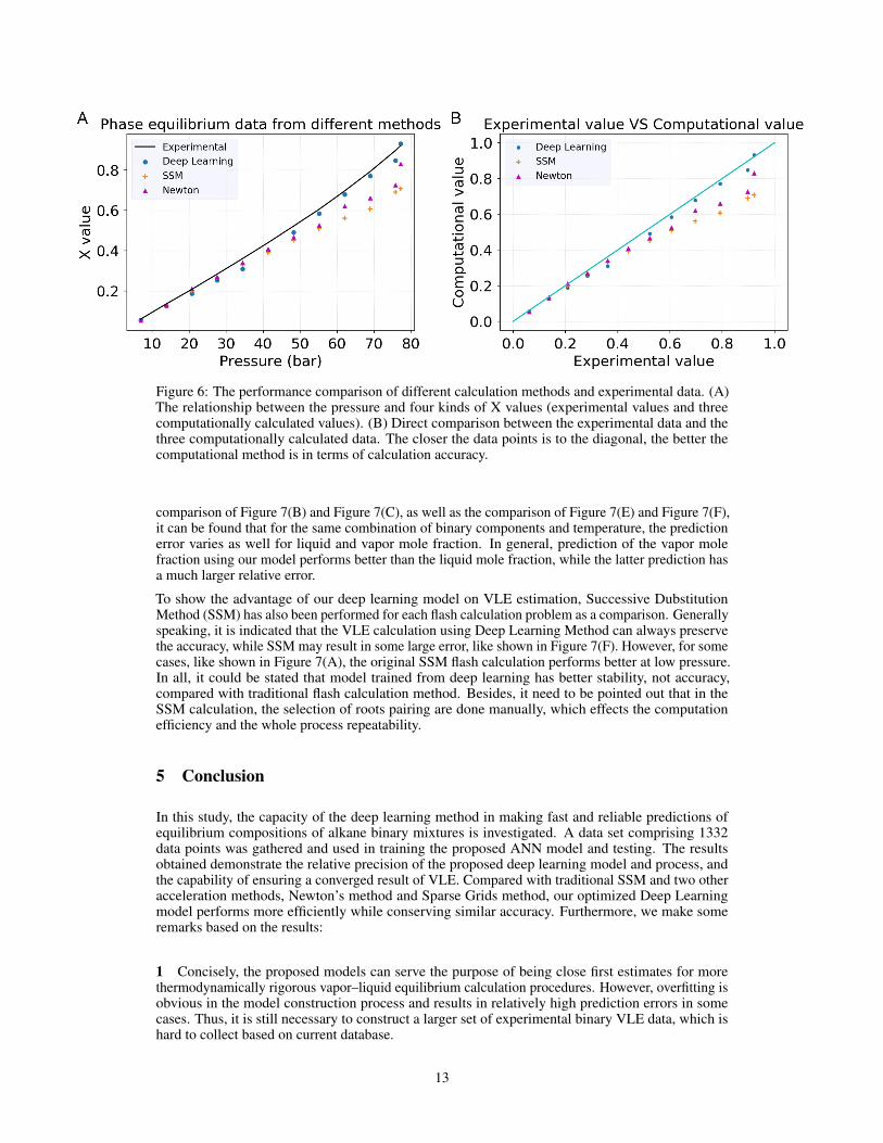
Figure 6: The performance comparison of different calculation methods and experimental data. (A)The relationship between the pressure and four kinds of X values (experimental values and threecomputationally calculated values). (B) Direct comparison between the experimental data and thethree computationally calculated data. The closer the data points is to the diagonal, the better thecomputational method is in terms of calculation accuracy.

comparison of Figure 7(B) and Figure 7(C), as well as the comparison of Figure 7(E) and Figure 7(F),it can be found that for the same combination of binary components and temperature, the predictionerror varies as well for liquid and vapor mole fraction. In general, prediction of the vapor molefraction using our model performs better than the liquid mole fraction, while the latter prediction hasa much larger relative error.

To show the advantage of our deep learning model on VLE estimation, Successive DubstitutionMethod (SSM) has also been performed for each flash calculation problem as a comparison. Generallyspeaking, it is indicated that the VLE calculation using Deep Learning Method can always preservethe accuracy, while SSM may result in some large error, like shown in Figure 7(F). However, for somecases, like shown in Figure 7(A), the original SSM flash calculation performs better at low pressure.In all, it could be stated that model trained from deep learning has better stability, not accuracy,compared with traditional flash calculation method. Besides, it need to be pointed out that in theSSM calculation, the selection of roots pairing are done manually, which effects the computationefficiency and the whole process repeatability.

5 Conclusion

In this study, the capacity of the deep learning method in making fast and reliable predictions ofequilibrium compositions of alkane binary mixtures is investigated. A data set comprising 1332data points was gathered and used in training the proposed ANN model and testing. The resultsobtained demonstrate the relative precision of the proposed deep learning model and process, andthe capability of ensuring a converged result of VLE. Compared with traditional SSM and two otheracceleration methods, Newton’s method and Sparse Grids method, our optimized Deep Learningmodel performs more efficiently while conserving similar accuracy. Furthermore, we make someremarks based on the results:

1 Concisely, the proposed models can serve the purpose of being close first estimates for morethermodynamically rigorous vapor–liquid equilibrium calculation procedures. However, overfitting isobvious in the model construction process and results in relatively high prediction errors in somecases. Thus, it is still necessary to construct a larger set of experimental binary VLE data, which ishard to collect based on current database.

13

Figure 7: VLE prediction with experimental data.

14

2 Another way to get large amount of data is to use flash calculation with EOS. However, it iscommonly acknowledged that the convergence and accuracy of current flash calculation methodscannot be ensured, as we have shown in Section 4. Besides, sometimes the results even have nophysical meanings and we need to exclude them manually. Thus, the application of flash calculationresults used as input data should be studied based on the selection and optimization of the calculationmethod, which remains to be the future work. Compared with traditional flash calculation method,our deep learning model will show better stability, which means that it can always ensure a reasonableresult with acceptable error. The problem of manul handling in the process of flash calculation shouldalso be treated carefully.

3 In our results, it can be concluded that there is no deep learning model perfectly fitting all theVLE conditions. Generally speaking, model performance is dependent on the training data and modelparameters. Our proposed model is constructed by the selection of the best factors, including dataratio, active function, layer and node numbers but the prediction error is still relatively high at somecases. Except for more training data, another potential solution is to find a better model combinedwith the feature of VLE process, especially the characteristics of EOSs.

Acknowledgments

The research reported in this publication was supported in part by funding from King Abdullah Uni-versity of Science and Technology (KAUST) through the grant BAS/1/1351-01-01 and BAS/1/1624-01-01.

References

[1] Ahmad Azari, Saeid Atashrouz, and Hamed Mirshekar. Prediction the vapor-liquid equilibria of co 2-containing binary refrigerantmixtures using artificial neural networks. ISRN Chemical Engineering, 2013, 2013.

[2] T. Ciodaro, D. Deva, J. M. de Seixas, and D. Damazio. Online particle detection with neural networks based on topological calorimetryinformation. 14th International Workshop on Advanced Computing and Analysis Techniques in Physics Research (Acat 2011), 368,2012.

[3] G. E. Dahl, D. Yu, L. Deng, and A. Acero. Context-dependent pre-trained deep neural networks for large-vocabulary speech recognition.Ieee Transactions on Audio Speech and Language Processing, 20(1):30–42, 2012.

[4] H. Dai, R. Umarov, H. Kuwahara, Y. Li, L. Song, and X. Gao. Sequence2vec: a novel embedding approach for modeling transcriptionfactor binding affinity landscape. Bioinformatics, 33(22):3575–3583, 2017.

[5] K. M. He, X. Y. Zhang, S. Q. Ren, and J. Sun. Deep residual learning for image recognition. 2016 Ieee Conference on Computer Visionand Pattern Recognition (Cpvr), pages 770–778, 2016.

[6] M. Helmstaedter, K. L. Briggman, S. C. Turaga, V. Jain, H. S. Seung, and W. Denk. Connectomic reconstruction of the inner plexiformlayer in the mouse retina (vol 500, pg 168, 2013). Nature, 514(7522), 2014.

[7] Maria C Iliuta, Ion Iliuta, and Faıçal Larachi. Vapour–liquid equilibrium data analysis for mixed solvent–electrolyte systems usingneural network models. Chemical engineering science, 55(15):2813–2825, 2000.

[8] Diederik Kingma and Jimmy Ba. Adam: A method for stochastic optimization. arXiv preprint arXiv:1412.6980, 2014.

[9] Alex Krizhevsky, Ilya Sutskever, and Geoffrey E Hinton. Imagenet classification with deep convolutional neural networks. Advancesin Neural Information Processing Systems 25, pages 1097–1105, 2012.

[10] Y. LeCun, Y. Bengio, and G. Hinton. Deep learning. Nature, 521(7553):436–44, 2015.

[11] Yiteng Li, Jisheng Kou, and Shuyu Sun. Numerical modeling of isothermal compositional grading by convex splitting methods. Journalof Natural Gas Science and Engineering, 43:207–221, 2017.

[12] Yu Li, Renmin Han, Chongwei Bi, Mo Li, Sheng Wang, and Xin Gao. Deepsimulator: a deep simulator for nanopore sequencing.Bioinformatics, 34(17):2899–2908, 2018.

[13] Yu Li, Sheng Wang, Ramzan Umarov, Bingqing Xie, Ming Fan, Lihua Li, and Xin Gao. Deepre: sequence-based enzyme ec numberprediction by deep learning. Bioinformatics, 34(5):760–769, 2018.

[14] Yu Li, Fan Xu, Fa Zhang, Pingyong Xu, Mingshu Zhang, Ming Fan, Lihua Li, Xin Gao, and Renmin Han. Dlbi: deep learning guidedbayesian inference for structure reconstruction of super-resolution fluorescence microscopy. Bioinformatics, 34(13):i284–i294, 2018.

15

[15] LX Nghiem and RA Heidemann. General acceleration procedure for multiphase flash calculation with application to oil-gas-watersystems. In Proceedings of the 2nd European Symposium on Enhanced Oil Recovery, pages 303–316, 1982.

[16] Viet D Nguyen, Raymond R Tan, Yolanda Brondial, and Tetsuo Fuchino. Prediction of vapor–liquid equilibrium data for ternarysystems using artificial neural networks. Fluid phase equilibria, 254(1-2):188–197, 2007.

[17] MR Nikkholgh, AR Moghadassi, F Parvizian, and SM Hosseini. Estimation of vapour–liquid equilibrium data for binary refrigerantsystems containing 1, 1, 1, 2, 3, 3, 3 heptafluoropropane (r227ea) by using artificial neural networks. The Canadian Journal of ChemicalEngineering, 88(2):200–207, 2010.

[18] John M Prausnitz, Rudiger N Lichtenthaler, and Edmundo Gomes de Azevedo. Molecular thermodynamics of fluid-phase equilibria.Pearson Education, 1998.

[19] Shaoqing Ren, Kaiming He, Ross Girshick, and Jian Sun. Faster R-CNN: Towards real-time object detection with region proposalnetworks. In Advances in Neural Information Processing Systems (NIPS), 2015.

[20] D. Silver, A. Huang, C. J. Maddison, A. Guez, L. Sifre, G. van den Driessche, J. Schrittwieser, I. Antonoglou, V. Panneershelvam,M. Lanctot, S. Dieleman, D. Grewe, J. Nham, N. Kalchbrenner, I. Sutskever, T. Lillicrap, M. Leach, K. Kavukcuoglu, T. Graepel, andD. Hassabis. Mastering the game of go with deep neural networks and tree search. Nature, 529(7587):484–9, 2016.

[21] N. Srivastava, G. Hinton, A. Krizhevsky, I. Sutskever, and R. Salakhutdinov. Dropout: A simple way to prevent neural networks fromoverfitting. Journal of Machine Learning Research, 15:1929–1958, 2014.

[22] Shuyu Sun and Mary F Wheeler. Symmetric and nonsymmetric discontinuous galerkin methods for reactive transport in porous media.SIAM Journal on Numerical Analysis, 43(1):195–219, 2005.

[23] Shuyu Sun and Mary F Wheeler. Discontinuous galerkin methods for simulating bioreactive transport of viruses in porous media.Advances in water resources, 30(6-7):1696–1710 2007.

[24] TC Tan, CM Chai, AT Tok, and KW Ho. Prediction and experimental verification of the salt effect on the vapour–liquid equilibrium ofwater–ethanol–2-propanol mixture. Fluid phase equilibria, 218(1):113–121, 2004.

[25] TC Tan, Rowell Tan, LH Soon, and SHP Ong. Prediction and experimental verification of the effect of salt on the vapour–liquidequilibrium of ethanol/1-propanol/water mixture. Fluid phase equilibria, 234(1):84–93, 2005.

[26] Yuanqing Wu. Parallel reservoir simulations with sparse grid techniques and applications to wormhole propagation, 2015.

[27] Yuanqing Wu, Christoph Kowitz, Shuyu Sun, and Amgad Salama. Speeding up the flash calculations in two-phase compositional flowsimulations–the application of sparse grids. Journal of Computational Physics, 285:88–99, 2015.

16