Accelerating 3-D GPU-based Motion Tracking for Ultrasound ...

applied sciences

Article

Accelerating 3-D GPU-based Motion Tracking forUltrasound Strain Elastography Using Sum-Tables:Analysis and Initial Results

Bo Peng 1,* , Shasha Luo 1, Zhengqiu Xu 1 and Jingfeng Jiang 2,*1 School of Computer Science, Southwest Petroleum University, Chengdu 610500, China;

[email protected] (S.L.); [email protected] (Z.X.)2 Department of Biomedical Engineering, Michigan Technological University, Houghton, MI 49931, USA* Correspondence: [email protected] (B.P.); [email protected] (J.J.);

Tel.: +86-28-83037189 (B.P.); +1-906-231-5669 (J.J.)

Received: 5 April 2019; Accepted: 8 May 2019; Published: 15 May 2019

Abstract: Now, with the availability of 3-D ultrasound data, a lot of research efforts are beingdevoted to developing 3-D ultrasound strain elastography (USE) systems. Because 3-D motiontracking, a core component in any 3-D USE system, is computationally intensive, a lot of effortsare under way to accelerate 3-D motion tracking. In the literature, the concept of Sum-Table hasbeen used in a serial computing environment to reduce the burden of computing signal correlation,which is the single most computationally intensive component in 3-D motion tracking. In this study,parallel programming using graphics processing units (GPU) is used in conjunction with the conceptof Sum-Table to improve the computational efficiency of 3-D motion tracking. To our knowledge,sum-tables have not been used in a GPU environment for 3-D motion tracking. Our main objectivehere is to investigate the feasibility of using sum-table-based normalized correlation coefficient(ST-NCC) method for the above-mentioned GPU-accelerated 3-D USE. More specifically, two differentimplementations of ST-NCC methods proposed by Lewis et al. and Luo-Konofagou are comparedagainst each other. During the performance comparison, the conventional method for calculatingthe normalized correlation coefficient (NCC) was used as the baseline. All three methods wereimplemented using compute unified device architecture (CUDA; Version 9.0, Nvidia Inc., CA, USA)and tested on a professional GeForce GTX TITAN X card (Nvidia Inc., CA, USA). Using 3-D ultrasounddata acquired during a tissue-mimicking phantom experiment, both displacement tracking accuracyand computational efficiency were evaluated for the above-mentioned three different methods.Based on data investigated, we found that under the GPU platform, Lou-Konofaguo method can stillimprove the computational efficiency (17–46%), as compared to the classic NCC method implementedinto the same GPU platform. However, the Lewis method does not improve the computationalefficiency in some configuration or improves the computational efficiency at a lower rate (7–23%)under the GPU parallel computing environment. Comparable displacement tracking accuracy wasobtained by both methods.

Keywords: motion tracking; ultrasound elastography; graphics processing unit; correlation;sum-table; block-matching

1. Introduction

Ultrasound strain elastography (USE) [1] can provide new information than that contained inB-Mode ultrasound images, which display only the amplitudes of envelope detected and decimatedecho signals. USE has been successfully used for breast lesion differentiation [2–4] because it is capableof visualizing elevated tissue hardness. The strain/modulus nonlinearity has been also explored

Appl. Sci. 2019, 9, 1991; doi:10.3390/app9101991 www.mdpi.com/journal/applsci

Appl. Sci. 2019, 9, 1991 2 of 16

by others in order to better characterize breast lesions [5–7]. Furthermore, a number of studiesin the literature has been devoted to understanding signal quality [8], image resolution [9,10] andcontrast [11,12] in USE. In this study, we solely focus on ultrasound-based motion tracking, because itplays a critically important role in USE.

Among all motion tracking algorithms [13], the block-matching algorithm is one of the most usedcorrelation-based methods and has been adopted by several prototype USE systems [14–21] due to itssimplicity. Furthermore, the block-matching algorithm can also be easily extended to include motionregularization or multi-scale tracking to deal with large tissue deformation. In the framework of blockmatching algorithm, similarity or correlation evaluation influences both motion tracking accuracy andcomputational efficiency [22]. The commonly used similarity/correlation evaluation metrics includesum absolute error, sum square error and (SSD), entropy, and normalized cross-correlation (NCC).NCC has been proved to be one of the best similarity matching criteria in block matching methods [22]and therefore, has been widely used in various ultrasound-based motion tracking algorithms.

One drawback of using the NCC as a correlation metric is that calculating NCC following thestandard protocol is computationally intensive, thereby limiting its use in many ultrasound techniquesrequiring real-time performance. Lewis proposed to use a pre-computed table in conjunction with afast Fourier Transform (FFT) to calculate NCC values. His method is often referred as to Sum-Table(ST) method now [23]. Luo et al. further modified Lewis’ approach [22] by replacing the requirementof using FFT with another ST. Both methods [22,23] have demonstrated that they can achieve almostthe same accuracy together with significantly faster calculation efficiency in a serial computingenvironment in which i.e., calculations are conducted by a central processing unit (CPU).

Several major vendors (e.g., General Electric, Siemens, Philips, Hitachi, Toshiba, Samsung Medison,etc.) have released their commercially-available USE packages. However, those clinical USE systemsall operate in 2D. However, continued efforts [16,19,24–28] are under the way to expand USE into 3-Dbecause 3-D tracking can significantly improve quality of strain elastograms [16,19].

Now FDA-approved 3-D automated breast ultrasound (ABUS) systems (e.g., GE InveniaTM;Siemens Acuson S2000 ABVS) have been released. It is our vision that with the availability ofGPU-acceleration, bringing 3-D breast USE into the clinical workflow becomes possible. In thelast decade, GPU-based parallel computing has been utilized to accelerate ultrasound-based motiontracking in several important applications including USE [21,29–31], shear wave elastography [32]and color Doppler imaging [33]. In particular, the work by Peng et al. [21] demonstrated that highquality strain data can be obtained for a reasonably large volume (e.g., 2.5× 2.5× 2.5 cm3) in 20 s.Consequently, investigating whether or not the concept of ST can be used to further improve 3-Dmotion tracking is a logical next step.

To this end, our primary goal is to investigate the feasibility of using ST in conjunction withGPUs to further accelerate 3-D motion tracking. Thus, two above-mentioned ST methods (i.e., Lewis’and Luo’s methods) were analyzed and implemented for parallel (GPU) and serial (CPU) computingsettings. The standard protocol of NCC calculation without the use of ST was used as the baseline inboth computing settings for a systematic comparison.

2. Materials and Methods

2.1. A Description of GPU-Accelerated Block-Matching Algorithm in USE

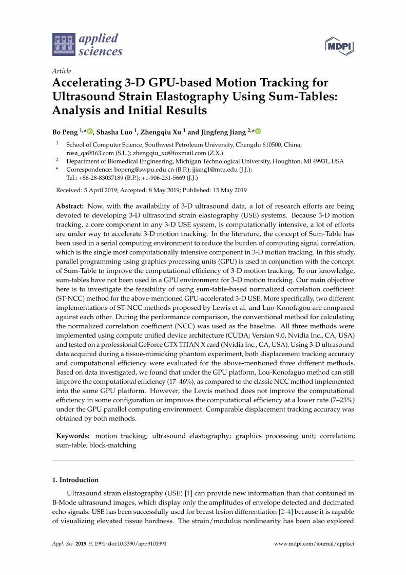
As shown in Figure 1, in order to estimate one displacement vector (dx, dy, dz) for an arbitrarylocation (x, y, z) from a pair of pre- and post-deformation ultrasound echo volumes, the block-matchingalgorithm can be largely divided into three steps: (1) selecting a pair of reference and target ultrasoundsignals from two successive ultrasound radio frequency (RF) fields based on a predetermined searchrange and a tracking kernel; (2) calculating an NCC value between the pair of selected referenceand target echo signals, generating a 3-D resultant NCC map for a given search range, and finding apeak from the NCC map; and (3) fitting NCC values around the peak NCC map to a 3-D quadratic

Appl. Sci. 2019, 9, 1991 3 of 16

surface [34] to find the estimated displacement vector. During the process, the tracking-kernel sizeand search range must be determined prior to the start of motion tracking. The location (x, y, z)here is referred to a location in the pre-deformation ultrasound each volume (i.e., the referencevolume). Thus, the (dx, dy, dz) represents the displacement vector by which the medium moved to thepost-deformation ultrasound echo volume (i.e., the target volume) from the reference volume. In theblock-matching algorithm, time-domain ultrasound echo signals are used to calculate correlation.

Figure 1. An illustrative diagram show how the calculation of NCC values with and without sum-tablesare integrated into ultrasound-based motion tracking. RF signal stands for radiofrequency ultrasoundecho signal.

As can be seen from the schematic diagram in Figure 1, Lewis’ and Luo’s methods both needto create sum tables prior to the calculation of NCC values in Step 1. Those sum-tables are usedas “lookup-tables” to replace the standard NCC calculations in order to reduce the computing time.The details of Step 1 for three different ways of calculating NCC values are discussed below. Steps 2and 3 are exactly the same for all three methods. Specifically, Step 2 is to find the maximum on theNCC map. Thus, an integer displacement vector can be determined for the location (x, y, z). Finally,in Step 3, the subs-sample displacement vector can be obtained by fitting a 3× 3× 3 matrix containingNCC values surrounding the maximum NCC value into a quadratic surface. Through Steps 2 and 3,the final axial, lateral and elevational displacements with sub-sampling precision can be obtained.

2.1.1. A Standard Protocol for Calculating NCC

Given one reference signal f and one target signal g, the NCC function over a search range(τx, τy, τz) can be calculated as follows:

RNCC(u, v, w, τx, τy, τz

)=

∑u+Wx−1m=u ∑

v+Wy−1n=v ∑w+Wz−1

k=w

{f (m, n, k) • g

(m− τx, n− τy, k− τz

)}√

∑u+Wx−1m=u ∑

v+Wy−1n=v ∑w+Wz−1

k=w

{f 2 (m, n, k)

}•∑u+Wx−1

m=u ∑v+Wy−1n=v ∑w+Wz−1

k=w

{g2(m− τx, n− τy, k− τz

)} (1)

where the dimensions of the reference and target windows (tracking kernels) are [u, u + Wx − 1],[v, v + Wy − 1], [w, w + Wz − 1] in the lateral, axial and elevational directions, respectively. Similarly,(Wx, Wy, Wz) are the tracking kernel dimensions in lateral, axial and elevational directions, respectively.In Equation (1), the origin of the reference window (tracking kernel) is (u, v, w) and [τx, τy, τz] is thesearch range defined below,

(τ1 ≤ τx ≤ τ2, τ3 ≤ τy ≤ τ4, τ5 ≤ τz ≤ τ6) (2)

In the block-matching algorithm, [τ1, τ2], [τ3, τ4] and [τ5, τ6] are pre-determined by the algorithm.For each 3-D shift (τx, τy, τz), Equation (1) can be used to obtain one NCC value. Thus, looping throughthe entire search range yields a 3-D NCC map.

Appl. Sci. 2019, 9, 1991 4 of 16

2.1.2. Lewis’ Sum-Table Method

When the block matching algorithm is used, significant overlaps among adjacent tracking kernelsexist, resulting in a lot of redundant computation. Thus, Lewis proposed to use pre-computedtables (also known as Sum-tables) to partially “memorize" some correlation between f and g [23].Together with Fourier Transform (FT), Lewis’ method can conceptually reduce the computationaldemands. More specifically, the numerator in Equation (1) is a convolution of the tracking kernelwithin the reference signal f with the corresponding tracking kernel of the reversed target signalg(−m,−n,−k) and can be computed by Fourier Transform (FT). The process is defined as follows:

∑m,n,k f (m, n, k) • g(m− τx, n− τy, k− τz

)= F−1

{F ( f )F ∗(g)

}(3)

where F stands for an FT operator. The complex conjugate accomplishes reversal of the template viathe FT’s time reversal property [23]. Equation( 3) was implemented via fast Fourier Transform (FFT)and thus, f and g were zero-padded to a common power of two.

Now referring to the calculation of the denominator in Equation (1), two sum tables were used:one for the reference signal f and the other for the target signal g. Let s2

f (u, v, w) and s2g(u, v, w) denotes

the created sum-tables for f and g, respectively. More details about setting up these two sum-table canbe found in Appendix A. Once these two tables become available, the calculation of denominator canbe conducted through a very efficient manner as follows,

∑u+Wx−1m=u ∑v+Wy−1

n=v ∑w+Wz−1k=w f 2 (m, n, k)

= s2f(u + Wx − 1, v+Wy − 1, w+Wz − 1

)− s2

f(u + Wx − 1, v+Wy − 1, w− 1

)− s2

f (u + Wx − 1, v− 1, w+Wz − 1)

− s2f(u− 1, v+Wy − 1, w+Wz − 1

)+s2

f (u− 1, v− 1, w+Wz − 1)

+s2f(u− 1, v+Wy − 1, w− 1

)+ s2

f (u + Wx − 1, v− 1, w− 1)

− s2f (u− 1, v− 1, w− 1)

(4)

∑u+Wx−1m=u ∑v+Wy−1

n=v ∑w+Wz−1k=w g2 (m + τx, n + τy, k + τz

)= s2

g(u + Wx − 1 + τx, v+Wy − 1 + τy, w + Wz − 1 + τz

)− s2

g(u + Wx − 1 + τx, v+Wy − 1 + τy, w− 1 + τz

)− s2

g(u + Wx − 1 + τx, v− 1 + τy, w + Wz − 1 + τz

)− s2

g(u− 1 + τx, v+Wy − 1 + τy, w + Wz − 1 + τz

)+ s2

g(u− 1 + τx, v− 1 + τy, w + Wz − 1 + τz

)+ s2

g(u− 1 + τx, v+Wy − 1 + τy, w− 1 + τz

)+ s2

g(u + Wx − 1 + τx, v− 1 + τy, w− 1 + τz

)− s2

g(u− 1 + τx, v− 1 + τy, w− 1 + τz

)

(5)

2.1.3. Luo-Konofagou Sum-Table Method

In Luo and Konofagou method [35], both the numerator and denominator of Equation (1) arecalculated using sum-tables. In addition to Equations (4) and (5), the numerator can be calculated asfollow using a set of sum-tables s f ,g(u, v, w) to look up pre-computed numbers,

Appl. Sci. 2019, 9, 1991 5 of 16

∑u+Wx−1m=u ∑v+Wy−1

n=v ∑w+Wz−1k=w f (m, n, k) • g

(m + τx, n + τy, k + τz

)= s f ,g

(u + Wx − 1, v+Wy − 1, w− 1 + Wz, τx, τy, τz

)− s f ,g

(u + Wx − 1, v+Wy − 1, w− 1, τx, τy, τz

)− s f ,g

(u + Wx − 1, v− 1, w− 1 + Wz, τx, τy, τz

)− s f ,g

(u− 1, v+Wy − 1, w− 1 + Wz, τx, τy, τz

)+ s f ,g

(u− 1, v− 1, w− 1 + Wz, τx, τy, τz

)+ s f ,g

(u− 1, v+Wy − 1, w− 1, τx, τy, τz

)+ s f ,g

(u + Wx − 1, v− 1, w− 1, τx, τy, τz

)− s f ,g

(u− 1, v− 1, w− 1, τx, τy, τz

)

(6)

According to Equations (4)–(6), the calculation of NCC can be simplified to addition andsubtraction operations. More formal analyses of algorithmic complexity and memory requirementscan be found in Appendices B and C.

2.2. GPU Implementation of Three NCC Calculation Methods

2.2.1. A Brief Description of GPU Computing

CUDA (Compute Unified Device Architecture) is a common parallel computing architecturelaunched by Nvidia (Nvidia Inc., Santa Clara, CA, USA). This architecture enables GPUs to solvecomplex computing problems in parallel. In CUDA, a KERNEL function is defined as a functionthat performs multi-threaded parallel computation. Similarly, a DEVICE function is defined as asingle-threaded function called by a KERNEL function on GPU. According to the memory structuredefined in CUDA, off-chip memory (global memory and texture memory) has a higher access delaythan on-chip memory (register, shared memory and constant memory). Consequently, the on-chipmemory should be given priority during programming in order to improve memory access efficiency.It is worth noting that the lower-case “kernel” is used for tracking kernels in this study, while theupper-case “KERNEL” is referred as to a GPU KERNEL function.

2.2.2. Block-Matching Using GPU Parallel Computing

The block-matching algorithm implemented in this study is the classic block-matchingalgorithm. Because of memory limitation, full 3-D block-matching tracking was first performedin a slice-by-slice manner. Thus, a full displacement vector field for a single slice consists of M× N(Axial × Lateral) displacement estimation locations; each displacement estimation location obtainsone 3-D displacement vector after the block-matching process. Because tracking displacements usingthe classic block-matching algorithm for each location is independent (i.e., no data dependency andrequirements regarding communication), in the CUDA programming structure, the M× N threadcan be launched through the KERNEL function (see Section 2.2.1). As shown in Figure 1, in orderto construct 3-D NCC map for each displacement estimation location, one NCC value needs to becalculated at a specified search location (τx, τy, τz). In the Step 1 (see Figure 1), given a search range(A[Axial], B[Lateral], C[Elevational]), the KERNEL function can start (M× N)× (A× B× C) CUDAthreads to obtain one 3-D NCC map to complete Step 1. Here, A = (τ2 − τ1 + 1), B = (τ4 − τ3 + 1)and C = (τ6 − τ5 + 1).

In the subsequent Steps 2 and 3 (see Figure 1), the number of CUDA threads in the KERNELfunctions are consistent with the total number of displacement estimation locations M× N. Basically,each CUDA thread invokes a DEVICE function to search the peak NCC value of the corresponding3-D NCC map (Step 2). Then, the same DEVICE function uses a quadratic fitting to obtain sub-sampleestimates (Step 3) [36].

Appl. Sci. 2019, 9, 1991 6 of 16

In the process of implementation, a few notable strategies were used. First, one-dimensionalthread structure was adopted to ensure the consistency of memory access. In other words,we attempted to ensure that adjacent threads read adjacent memory regions and try to satisfythe requirement of coalesced memory access. Second, RF data were stored in TEXTURE memory.Nvidia GPU TEXTURE memory technology can avoid the delay caused by cross-line reading. Third,some important variables (such as axial and lateral search range, tracking kernel size) are stored inGPU constant memory for rapid accesses.

2.2.3. Implementing A Standard NCC Calculation on CUDA

Under the above-mentioned parallel implementation framework, improving the efficiency formemory access was the most important consideration. This is because the calculation of a 3-D NCCmap will read each RF sample multiple times. In order to avoid this frequent data reading fromTEXTURE memory, we load each small part of RF echo data into on-chip memory during CUDAprogramming to improve memory access efficiency. The detailed GPU implementation of this methodis described in our early work [21].

2.2.4. Implementing Lewis’ Method on CUDA

In this study, the FFT function library cuFFT available in CUDA (Nvidia Inc., CA, USA) was usedto calculate the numerator of Equation (1). The cuFFT library provides a simple interface for computingFFTs on Nvidia GPUs. Also, the cuFFT library has been highly optimized and systematically tested forthe GPU parallel computing environment. In contrast, FFTW (http://www.fftw.org/) is a state-of-artfast FFT toolbox on CPU and was applied to implement Lewis’s method on CPU.

The calculation of the denominator in Equation (1) needs two sum-tables: one for the referenceRF signal and the other one for the target RF signal. In this study, a parallel scan algorithm proposedby Sengupta et al. [37] was adopted to perform rapid prefix sum (i.e., cumulative sum) computationfor each direction. The scan algorithm is based on an idea of balanced tree proposed by Blelloch [38].Equations can be found in Appendix A.

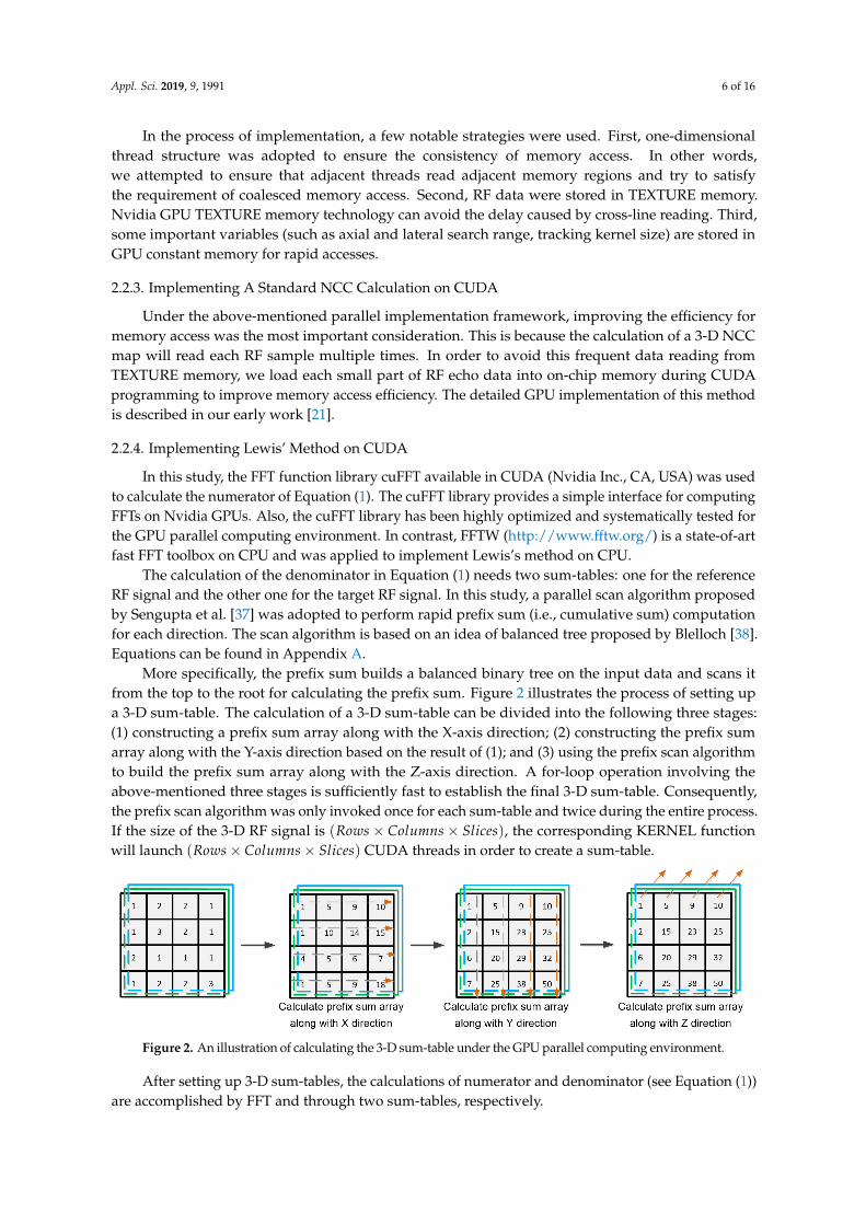
More specifically, the prefix sum builds a balanced binary tree on the input data and scans itfrom the top to the root for calculating the prefix sum. Figure 2 illustrates the process of setting upa 3-D sum-table. The calculation of a 3-D sum-table can be divided into the following three stages:(1) constructing a prefix sum array along with the X-axis direction; (2) constructing the prefix sumarray along with the Y-axis direction based on the result of (1); and (3) using the prefix scan algorithmto build the prefix sum array along with the Z-axis direction. A for-loop operation involving theabove-mentioned three stages is sufficiently fast to establish the final 3-D sum-table. Consequently,the prefix scan algorithm was only invoked once for each sum-table and twice during the entire process.If the size of the 3-D RF signal is (Rows× Columns× Slices), the corresponding KERNEL functionwill launch (Rows× Columns× Slices) CUDA threads in order to create a sum-table.

Figure 2. An illustration of calculating the 3-D sum-table under the GPU parallel computing environment.

After setting up 3-D sum-tables, the calculations of numerator and denominator (see Equation (1))are accomplished by FFT and through two sum-tables, respectively.

Appl. Sci. 2019, 9, 1991 7 of 16

2.2.5. Implementing Luo-Konofagou Method

Please recall that in the Luo-Konofagou method, computing the denominator in Equation (1) isthe same as Lewis’s method (see Section 2.2.4). Luo-Konofagou method replaced the FFT operation tosum-table method for computing the numerator. During this process, numerator’s calculation needs(τ2 − τ1 + 1) × (τ4 − τ3 + 1) × (τ6 − τ5 + 1) (i.e., A × B × C) sum-tables to represent the standardcross-correlation (CC) between the reference and target RF signals at a specified search location(τx, τy, τz). Thus, we need to launch (τ2− τ1 + 1)× (τ4− τ3 + 1)× (τ6− τ5 + 1)× (Rows×Columns×Slices) CUDA threads. It is easy to see that the number of threads and required memory become aburden to manage if the search range is very large.

2.3. Experimental Design and Data Analysis

2.3.1. A Tissue-Mimicking Phantom Experiment

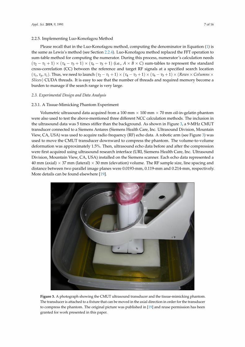
Volumetric ultrasound data acquired from a 100 mm × 100 mm × 70 mm oil-in-gelatin phantomwere also used to test the above-mentioned three different NCC calculation methods. The inclusion inthe ultrasound data was 5 times stiffer than the background. As shown in Figure 3, a 9-MHz CMUTtransducer connected to a Siemens Antares (Siemens Health Care, Inc. Ultrasound Division, MountainView, CA, USA) was used to acquire radio frequency (RF) echo data. A robotic arm (see Figure 3) wasused to move the CMUT transducer downward to compress the phantom. The volume-to-volumedeformation was approximately 1.5%. Then, ultrasound echo data before and after the compressionwere first acquired using ultrasound research interface (URI, Siemens Health Care, Inc. UltrasoundDivision, Mountain View, CA, USA) installed on the Siemens scanner. Each echo data represented a40 mm (axial) × 37 mm (lateral) × 30 mm (elevation) volume. The RF sample size, line spacing anddistance between two parallel image planes were 0.0193-mm, 0.119-mm and 0.214-mm, respectively.More details can be found elsewhere [19].

Figure 3. A photograph showing the CMUT ultrasound transducer and the tissue-mimicking phantom.The transducer is attached to a fixture that can be moved in the axial direction in order for the transducerto compress the phantom. The original picture was published in [19] and reuse permission has beengranted for work presented in this paper.

Appl. Sci. 2019, 9, 1991 8 of 16

2.3.2. Data Analysis

The GPU hardware used in this study is Nvidia GeForce GTX TITAN X (Nvidia Corp., Santa Clara,CA, USA). The GPU card comes along with 80 Stream Multiprocessors, along with a total of 5120 CUDAcomputing cores along with 12 GB of Memory. The GPU card is installed on a desktop workstationwith a Ubuntu operating system (version 16.04), Intel(R) Core(TM) i7-8700 CPU @ 3.20 GHz, and 16 GBof host memory. ANSI C and CUDA 9.0 were adopted for implementing all CPU and GPU algorithms.All testing was done under the MATLAB platform (Version 2016b, Mathworks Inc., Natick, MA, USA)and all implemented algorithms were invoked in the MATLAB environment through the MEX interface.

In total, six different implementations were done in this study: standard NCC in CPU,standard NCC in GPU, Lewis’ method in CPU and Lewis’ method in GPU, Luo-Konofagou methodin CPU and Luo-konofagou method in GPU. Hereafter, those six implementations are referred to asNCC-CPU, Lou-Konofagou-CPU, Lewis-CPU, NCC-GPU, Luo-Konofagou-GPU, and Lewis-GPU,respectively. In this paper, the performance is mainly compared from the following two aspects: (1)Evaluating whether or not a different implementation yields substantial errors and (2) comparingcomputational efficiency of those three methods, given motion tracking parameters and the computingenvironment (i.e., CPU or GPU).

3. Results

3.1. Comparisons of Accuracy Among Different Implementations

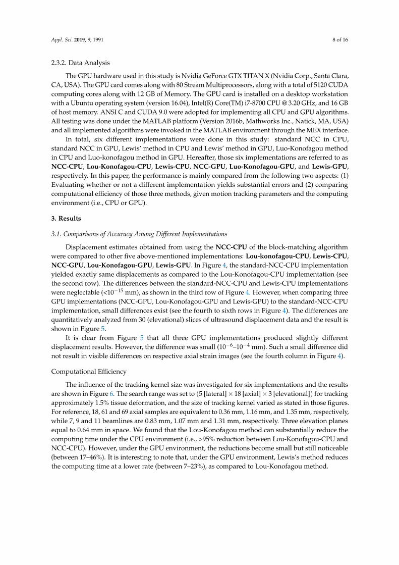
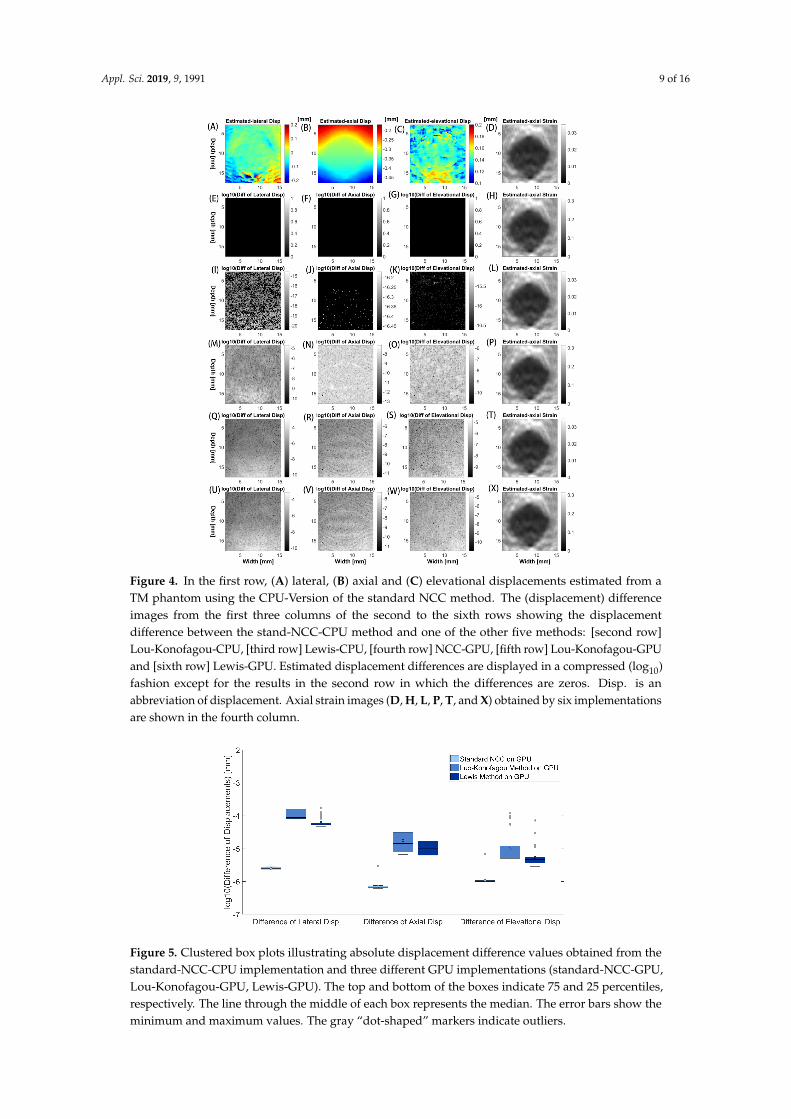
Displacement estimates obtained from using the NCC-CPU of the block-matching algorithmwere compared to other five above-mentioned implementations: Lou-konofagou-CPU, Lewis-CPU,NCC-GPU, Lou-Konofagou-GPU, Lewis-GPU. In Figure 4, the standard-NCC-CPU implementationyielded exactly same displacements as compared to the Lou-Konofagou-CPU implementation (seethe second row). The differences between the standard-NCC-CPU and Lewis-CPU implementationswere neglectable (<10−15 mm), as shown in the third row of Figure 4. However, when comparing threeGPU implementations (NCC-GPU, Lou-Konofagou-GPU and Lewis-GPU) to the standard-NCC-CPUimplementation, small differences exist (see the fourth to sixth rows in Figure 4). The differences arequantitatively analyzed from 30 (elevational) slices of ultrasound displacement data and the result isshown in Figure 5.

It is clear from Figure 5 that all three GPU implementations produced slightly differentdisplacement results. However, the difference was small (10−6–10−4 mm). Such a small difference didnot result in visible differences on respective axial strain images (see the fourth column in Figure 4).

Computational Efficiency

The influence of the tracking kernel size was investigated for six implementations and the resultsare shown in Figure 6. The search range was set to (5 [lateral]× 18 [axial]× 3 [elevational]) for trackingapproximately 1.5% tissue deformation, and the size of tracking kernel varied as stated in those figures.For reference, 18, 61 and 69 axial samples are equivalent to 0.36 mm, 1.16 mm, and 1.35 mm, respectively,while 7, 9 and 11 beamlines are 0.83 mm, 1.07 mm and 1.31 mm, respectively. Three elevation planesequal to 0.64 mm in space. We found that the Lou-Konofagou method can substantially reduce thecomputing time under the CPU environment (i.e., >95% reduction between Lou-Konofagou-CPU andNCC-CPU). However, under the GPU environment, the reductions become small but still noticeable(between 17–46%). It is interesting to note that, under the GPU environment, Lewis’s method reducesthe computing time at a lower rate (between 7–23%), as compared to Lou-Konofagou method.

Appl. Sci. 2019, 9, 1991 9 of 16

Figure 4. In the first row, (A) lateral, (B) axial and (C) elevational displacements estimated from aTM phantom using the CPU-Version of the standard NCC method. The (displacement) differenceimages from the first three columns of the second to the sixth rows showing the displacementdifference between the stand-NCC-CPU method and one of the other five methods: [second row]Lou-Konofagou-CPU, [third row] Lewis-CPU, [fourth row] NCC-GPU, [fifth row] Lou-Konofagou-GPUand [sixth row] Lewis-GPU. Estimated displacement differences are displayed in a compressed (log10)fashion except for the results in the second row in which the differences are zeros. Disp. is anabbreviation of displacement. Axial strain images (D, H, L, P, T, and X) obtained by six implementationsare shown in the fourth column.

Figure 5. Clustered box plots illustrating absolute displacement difference values obtained from thestandard-NCC-CPU implementation and three different GPU implementations (standard-NCC-GPU,Lou-Konofagou-GPU, Lewis-GPU). The top and bottom of the boxes indicate 75 and 25 percentiles,respectively. The line through the middle of each box represents the median. The error bars show theminimum and maximum values. The gray “dot-shaped” markers indicate outliers.

Appl. Sci. 2019, 9, 1991 10 of 16

Figure 6. Plots comparing computational efficiency under two different environments: (A) CPU and(B) GPU. In (A), the computing time is displayed in log10 scale. Computing time was estimated basedon the completion of 3-D motion tracking for a single slice of ultrasound data.

When the tracking kernel was fixed at 9 [1.07 mm; lateral] × 69 [1.35 mm; axial] × 3 [0.64 mm;elevational]). The computational efficiency was also examined when the search range had been varied.It is common to change the search range in USE to accommodate different frame-to-frame (2D) orvolume-to-volume (3-D) strain levels occurring in vivo. As shown in Figure 7, the required time tocomplete the motion tracking as the increase of search range. However, the trend of time reductionbetween the standard NCC method and the Lou-Konofagou method remained the same. In contrast,with the increase of the search range, time needed for Lewis’ method to complete the required trackingremains relatively steady (Figure 7).

Figure 7. Plot showing computing time when the search range changed under the (A,C) CPU and(B,D) GPU environments. In all plots, the computing time is displayed in log10 scale. Computing timewas estimated based on the completion of 3-D motion tracking for a single slice of ultrasound data.

Appl. Sci. 2019, 9, 1991 11 of 16

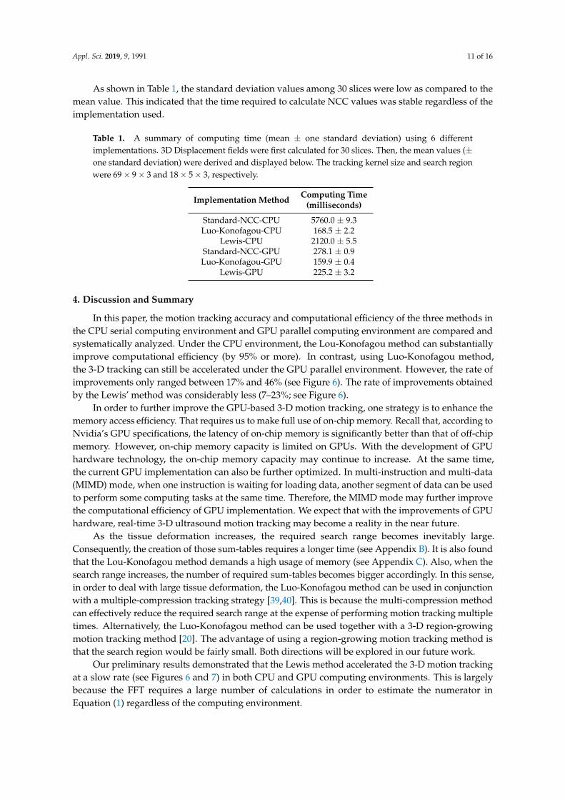
As shown in Table 1, the standard deviation values among 30 slices were low as compared to themean value. This indicated that the time required to calculate NCC values was stable regardless of theimplementation used.

Table 1. A summary of computing time (mean ± one standard deviation) using 6 differentimplementations. 3D Displacement fields were first calculated for 30 slices. Then, the mean values (±one standard deviation) were derived and displayed below. The tracking kernel size and search regionwere 69× 9× 3 and 18× 5× 3, respectively.

Implementation Method Computing Time(milliseconds)

Standard-NCC-CPU 5760.0 ± 9.3Luo-Konofagou-CPU 168.5 ± 2.2

Lewis-CPU 2120.0 ± 5.5Standard-NCC-GPU 278.1 ± 0.9Luo-Konofagou-GPU 159.9 ± 0.4

Lewis-GPU 225.2 ± 3.2

4. Discussion and Summary

In this paper, the motion tracking accuracy and computational efficiency of the three methods inthe CPU serial computing environment and GPU parallel computing environment are compared andsystematically analyzed. Under the CPU environment, the Lou-Konofagou method can substantiallyimprove computational efficiency (by 95% or more). In contrast, using Luo-Konofagou method,the 3-D tracking can still be accelerated under the GPU parallel environment. However, the rate ofimprovements only ranged between 17% and 46% (see Figure 6). The rate of improvements obtainedby the Lewis’ method was considerably less (7–23%; see Figure 6).

In order to further improve the GPU-based 3-D motion tracking, one strategy is to enhance thememory access efficiency. That requires us to make full use of on-chip memory. Recall that, according toNvidia’s GPU specifications, the latency of on-chip memory is significantly better than that of off-chipmemory. However, on-chip memory capacity is limited on GPUs. With the development of GPUhardware technology, the on-chip memory capacity may continue to increase. At the same time,the current GPU implementation can also be further optimized. In multi-instruction and multi-data(MIMD) mode, when one instruction is waiting for loading data, another segment of data can be usedto perform some computing tasks at the same time. Therefore, the MIMD mode may further improvethe computational efficiency of GPU implementation. We expect that with the improvements of GPUhardware, real-time 3-D ultrasound motion tracking may become a reality in the near future.

As the tissue deformation increases, the required search range becomes inevitably large.Consequently, the creation of those sum-tables requires a longer time (see Appendix B). It is also foundthat the Lou-Konofagou method demands a high usage of memory (see Appendix C). Also, when thesearch range increases, the number of required sum-tables becomes bigger accordingly. In this sense,in order to deal with large tissue deformation, the Luo-Konofagou method can be used in conjunctionwith a multiple-compression tracking strategy [39,40]. This is because the multi-compression methodcan effectively reduce the required search range at the expense of performing motion tracking multipletimes. Alternatively, the Luo-Konofagou method can be used together with a 3-D region-growingmotion tracking method [20]. The advantage of using a region-growing motion tracking method isthat the search region would be fairly small. Both directions will be explored in our future work.

Our preliminary results demonstrated that the Lewis method accelerated the 3-D motion trackingat a slow rate (see Figures 6 and 7) in both CPU and GPU computing environments. This is largelybecause the FFT requires a large number of calculations in order to estimate the numerator inEquation (1) regardless of the computing environment.

Appl. Sci. 2019, 9, 1991 12 of 16

Author Contributions: All authors discussed the original idea. B.P. and J.J. constructed the overall study designwith support from S.L. and Z.X.; B.P., S.L., Z.X. performed programming and conducted data analysis; B.P and J.J.drafted this manuscript; all authors provided critical feedback and reviewed the manuscript.

Funding: The project is funded in part by research grants from Scientific Innovation Program of Sichuan Province(Major Engineering Project: 2018RZ0093), Nanchong Scientific Council (Strategic Cooperation Program betweenUniversity and City: NC17SY4020), and US National Institutes of Health (R15-EB026197).

Conflicts of Interest: The authors declare no conflict of interest.

Appendix A. Setting up 3-D Sum-Tables for 3-D Ultrasound Echo Data

The sum tables in this study are defined as follows:

s2f =

u

∑m=0

v

∑n=0

w

∑k=0

f 2(m, n, k)

s2g =

u

∑m=0

v

∑n=0

w

∑k=0

g2(m, n, k)

s f ,g(u, v, w, τx, τy, τz) =u

∑m=0

v

∑n=0

w

∑k=0

f (m, n, k) · g(m + τx, n + τy, k + τz)

(A1)

Above definitions are similar to those defined by Luo and Konofaguo in 2D [22]. The 3-D sumtables can be constructed efficiently using the following three steps. First, the summation is performedin the u (lateral) direction for each v and w. Then, the summation was performed in the v (axial)direction for each u and w. Finally, the summation was performed in the w (elevational) direction foreach u and v. One illustrative example is shown in Figure 2. The constructing process of s2

f , s2g and s2

f ,gare given by (A1)–(A3) below.

s2f ,temp_u(u, v, w) = f 2

u,v,w + s2f ,temp_u(u− 1, v, w)

s2f ,temp_v(u, v, w) = s2

f ,temp_u(u, v, w) + s2g,temp_v(u, v− 1, w)

s2f (u, v, w) = s2

f ,temp_v(u, v, w) + s2f (u, v, w− 1)

(A2)

s2g,temp_u(u, v, w) = g2

u,v,w + s2g,temp_u(u− 1, v, w)

s2g,temp_v(u, v, w) = s2

g,temp_u(u, v, w) + s2g,temp_v(u, v− 1, w)

s2g(u, v, w) = s2

g,temp_v(u, v, w) + s2g(u, v, w− 1)

(A3)

s f ,g,temp_u(u, v, w, τx, τy, τz) = f (u, v, w) · g(u + τx, v + τy, w + τz) + s f ,g,temp_u(u− 1, v, w, τx, τy, τz)

s f ,g,temp_v(u, v, w, τx, τy, τz) = s f ,g,temp_u(u, v, w, τx, τy, τz) + s f ,g,temp_v(u, v− 1, w, τx, τy, τz)

s f ,g(u, v, w, τx, τy, τz) = s f ,g,temp_v(u, v, w, τx, τy, τz) + s f ,g(u, v, w− 1, τx, τy, τz)

(A4)

Appendix B. Analysis of Algorithmic Complexity for Sum-Table Methods

The complexity of calculating one NCC for 3-D block-matching is analyzed in the appendixfor the sake of completeness. The analysis of complexity for the 3-D case is an extension to thework done by Briechle and Hanebeck in 2D [41]. Under the framework of a 3-D block-matching,one-direction search ranges are Sx, Sy and Sz for lateral, axial and elevation directions, respectively.Of note, the one-direction search range above was defined as the maximal translation of the centerof the tracking kernel along one given direction (e.g., upward or downward). Given a 3-D trackingkernel with a size of Wx [lateral], Wy [axial] and Wz [elevational] samples, we need to get access toa segment of RF data whose size is at least Mx[lateral]×My[axial]×Mz[elevational] RF samples inorder to complete the calculations for one NCC values (see Equation (1)), where Mx = 2Sx + Wx + 1,My = 2Sy + Wy + 1 and Mz = 2Sz + Wz + 1.

Appl. Sci. 2019, 9, 1991 13 of 16

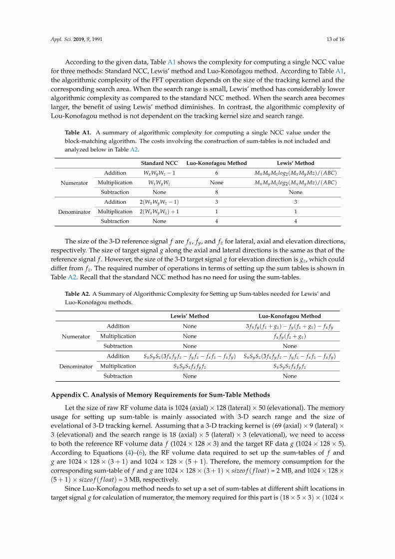
According to the given data, Table A1 shows the complexity for computing a single NCC valuefor three methods: Standard NCC, Lewis’ method and Luo-Konofagou method. According to Table A1,the algorithmic complexity of the FFT operation depends on the size of the tracking kernel and thecorresponding search area. When the search range is small, Lewis’ method has considerably loweralgorithmic complexity as compared to the standard NCC method. When the search area becomeslarger, the benefit of using Lewis’ method diminishes. In contrast, the algorithmic complexity ofLou-Konofagou method is not dependent on the tracking kernel size and search range.

Table A1. A summary of algorithmic complexity for computing a single NCC value under theblock-matching algorithm. The costs involving the construction of sum-tables is not included andanalyzed below in Table A2.

Standard NCC Luo-Konofagou Method Lewis’ Method

Numerator

Addition WxWyWz − 1 6 Mx My Mzlog2(Mx My Mz)/(ABC)

Multiplication WxWyWz None Mx My Mzlog2(Mx My Mz)/(ABC)

Subtraction None 8 None

Denominator

Addition 2(WxWyWz − 1) 3 3

Multiplication 2(WxWyWz) + 1 1 1

Subtraction None 4 4

The size of the 3-D reference signal f are fx, fy, and fz for lateral, axial and elevation directions,respectively. The size of target signal g along the axial and lateral directions is the same as that of thereference signal f . However, the size of the 3-D target signal g for elevation direction is gz, which coulddiffer from fz. The required number of operations in terms of setting up the sum tables is shown inTable A2. Recall that the standard NCC method has no need for using the sum-tables.

Table A2. A Summary of Algorithmic Complexity for Setting up Sum-tables needed for Lewis’ andLuo-Konofagou methods.

Lewis’ Method Luo-Konofagou Method

Numerator

Addition None 3 fx fy( fz + gz)− fy( fz + gz)− fx fy

Multiplication None fx fy( fz + gz)

Subtraction None None

Denominator

Addition SxSySz(3 fx fy fz − fy fz − fx fz − fx fy) SxSySz(3 fx fy fz − fy fz − fx fz − fx fy)

Multiplication SxSySz fx fy fz SxSySz fx fy fz

Subtraction None None

Appendix C. Analysis of Memory Requirements for Sum-Table Methods

Let the size of raw RF volume data is 1024 (axial)× 128 (lateral)× 50 (elevational). The memoryusage for setting up sum-table is mainly associated with 3-D search range and the size ofevelational of 3-D tracking kernel. Assuming that a 3-D tracking kernel is (69 (axial)× 9 (lateral)×3 (elevational) and the search range is 18 (axial) × 5 (lateral) × 3 (elevational), we need to accessto both the reference RF volume data f (1024× 128× 3) and the target RF data g (1024× 128× 5).According to Equations (4)–(6), the RF volume data required to set up the sum-tables of f andg are 1024× 128× (3 + 1) and 1024 × 128 × (5 + 1). Therefore, the memory consumption for thecorresponding sum-table of f and g are 1024× 128× (3 + 1)× sizeo f ( f loat) = 2 MB, and 1024× 128×(5 + 1)× sizeo f ( f loat) = 3 MB, respectively.

Since Luo-Konofagou method needs to set up a set of sum-tables at different shift locations intarget signal g for calculation of numerator, the memory required for this part is (18× 5× 3)× (1024×

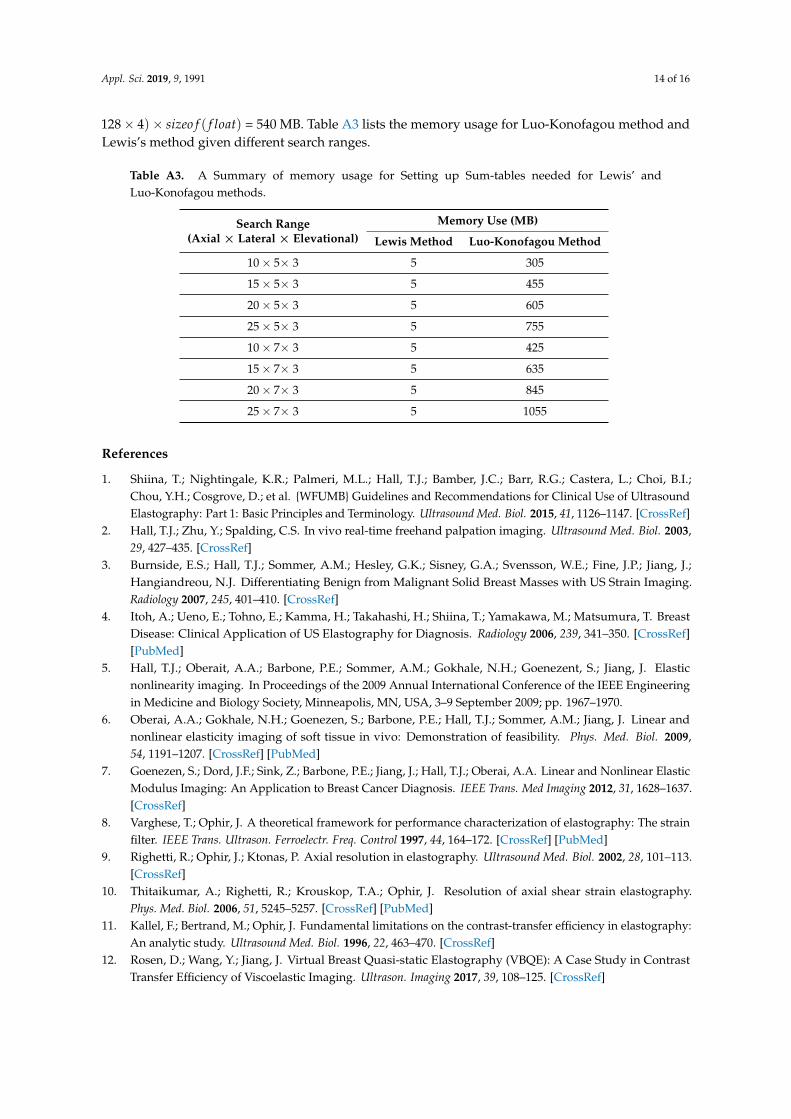
Appl. Sci. 2019, 9, 1991 14 of 16

128× 4)× sizeo f ( f loat) = 540 MB. Table A3 lists the memory usage for Luo-Konofagou method andLewis’s method given different search ranges.

Table A3. A Summary of memory usage for Setting up Sum-tables needed for Lewis’ andLuo-Konofagou methods.

Search Range(Axial × Lateral × Elevational)

Memory Use (MB)

Lewis Method Luo-Konofagou Method

10× 5× 3 5 305

15× 5× 3 5 455

20× 5× 3 5 605

25× 5× 3 5 755

10× 7× 3 5 425

15× 7× 3 5 635

20× 7× 3 5 845

25× 7× 3 5 1055

References

1. Shiina, T.; Nightingale, K.R.; Palmeri, M.L.; Hall, T.J.; Bamber, J.C.; Barr, R.G.; Castera, L.; Choi, B.I.;Chou, Y.H.; Cosgrove, D.; et al. {WFUMB} Guidelines and Recommendations for Clinical Use of UltrasoundElastography: Part 1: Basic Principles and Terminology. Ultrasound Med. Biol. 2015, 41, 1126–1147. [CrossRef]

2. Hall, T.J.; Zhu, Y.; Spalding, C.S. In vivo real-time freehand palpation imaging. Ultrasound Med. Biol. 2003,29, 427–435. [CrossRef]

3. Burnside, E.S.; Hall, T.J.; Sommer, A.M.; Hesley, G.K.; Sisney, G.A.; Svensson, W.E.; Fine, J.P.; Jiang, J.;Hangiandreou, N.J. Differentiating Benign from Malignant Solid Breast Masses with US Strain Imaging.Radiology 2007, 245, 401–410. [CrossRef]

4. Itoh, A.; Ueno, E.; Tohno, E.; Kamma, H.; Takahashi, H.; Shiina, T.; Yamakawa, M.; Matsumura, T. BreastDisease: Clinical Application of US Elastography for Diagnosis. Radiology 2006, 239, 341–350. [CrossRef][PubMed]

5. Hall, T.J.; Oberait, A.A.; Barbone, P.E.; Sommer, A.M.; Gokhale, N.H.; Goenezent, S.; Jiang, J. Elasticnonlinearity imaging. In Proceedings of the 2009 Annual International Conference of the IEEE Engineeringin Medicine and Biology Society, Minneapolis, MN, USA, 3–9 September 2009; pp. 1967–1970.

6. Oberai, A.A.; Gokhale, N.H.; Goenezen, S.; Barbone, P.E.; Hall, T.J.; Sommer, A.M.; Jiang, J. Linear andnonlinear elasticity imaging of soft tissue in vivo: Demonstration of feasibility. Phys. Med. Biol. 2009,54, 1191–1207. [CrossRef] [PubMed]

7. Goenezen, S.; Dord, J.F.; Sink, Z.; Barbone, P.E.; Jiang, J.; Hall, T.J.; Oberai, A.A. Linear and Nonlinear ElasticModulus Imaging: An Application to Breast Cancer Diagnosis. IEEE Trans. Med Imaging 2012, 31, 1628–1637.[CrossRef]

8. Varghese, T.; Ophir, J. A theoretical framework for performance characterization of elastography: The strainfilter. IEEE Trans. Ultrason. Ferroelectr. Freq. Control 1997, 44, 164–172. [CrossRef] [PubMed]

9. Righetti, R.; Ophir, J.; Ktonas, P. Axial resolution in elastography. Ultrasound Med. Biol. 2002, 28, 101–113.[CrossRef]

10. Thitaikumar, A.; Righetti, R.; Krouskop, T.A.; Ophir, J. Resolution of axial shear strain elastography.Phys. Med. Biol. 2006, 51, 5245–5257. [CrossRef] [PubMed]

11. Kallel, F.; Bertrand, M.; Ophir, J. Fundamental limitations on the contrast-transfer efficiency in elastography:An analytic study. Ultrasound Med. Biol. 1996, 22, 463–470. [CrossRef]

12. Rosen, D.; Wang, Y.; Jiang, J. Virtual Breast Quasi-static Elastography (VBQE): A Case Study in ContrastTransfer Efficiency of Viscoelastic Imaging. Ultrason. Imaging 2017, 39, 108–125. [CrossRef]

Appl. Sci. 2019, 9, 1991 15 of 16

13. Jiang, J.; Peng, B. Ultrasonic Methods for Assessment of Tissue Motion in Elastography. In UltrasoundElastography for Biomedical Applications and Medicine; John Wiley & Sons, Ltd.: Hoboken, NJ, USA, 2018;Chapter 4, pp. 35–70.

14. Zhu, Y.; Hall, T.J. A Modified Block Matching Method for Real-Time Freehand Strain Imaging.Ultrason. Imaging 2002, 24, 161–176. [CrossRef]

15. Li, P.C.; Lee, W.N. An Efficient Speckle Tracking Algorithm for Ultrasonic Imaging. Ultrason. Imaging 2002,24, 215–228. [CrossRef] [PubMed]

16. Chen, X.; Xie, H.; Erkamp, R.; Kim, K.; Jia, C.; Rubin, J.M.; O’Donnell, M. 3-D Correlation-Based SpeckleTracking. Ultrason. Imaging 2005, 27, 21–36. [CrossRef] [PubMed]

17. Jiang, J.; Hall, T.J. A parallelizable real-time motion tracking algorithm with applications to ultrasonic strainimaging. Phys. Med. Biol. 2007, 52, 3773–3790. [CrossRef] [PubMed]

18. Pellot-Barakat, C.; Frouin, F.; Insana, M.F.; Herment, A. Ultrasound elastography based on multiscaleestimations of regularized displacement fields. IEEE Trans. Med. Imaging 2004, 23, 153–163. [CrossRef][PubMed]

19. Fisher, T.G.; Hall, T.J.; Panda, S.; Richards, M.S.; Barbone, P.E.; Jiang, J.; Resnick, J.; Barnes, S. VolumetricElasticity Imaging with a 2-D CMUT Array. Ultrasound Med. Biol. 2010, 36, 978–990. [CrossRef]

20. Wang, Y.; Jiang, J.; Hall, T. A 3-D Region-Growing Motion-Tracking Method for Ultrasound ElasticityImaging. Ultrasound Med. Biol. 2018, 44, 1638–1653. [CrossRef] [PubMed]

21. Peng, B.; Wang, Y.; Hall, T.J.; Jiang, J. A GPU-Accelerated 3-D Coupled Subsample Estimation Algorithmfor Volumetric Breast Strain Elastography. IEEE Trans. Ultrason. Ferroelectr. Freq. Control 2017, 64, 694–705.[CrossRef]

22. Luo, J.; Konofagou, E.E. A fast normalized cross-correlation calculation method for motion estimation.IEEE Trans. Ultrason. Ferroelectr. Freq. Control 2010, 57, 1347–1357. [PubMed]

23. Lewis, J. Fast Template Matching. In Proceedings of the Canadian Image Processing and Pattern RecognitionSociety, Quebec City, QC, Canada, 15–19 May 1995; Vision Interface 95.

24. Insana, M.F.; Chaturvedi, P.; Hall, T.J.; gBilgen, M. 3-D companding using linear arrays for improved strainimaging. In Proceedings of the Ultrasonics Symposium, Toronto, ON, Canada, 5–8 October 1997; Volume 2,pp. 1435–1438.

25. Konofagou, E.E.; Ophir, J. Precision estimation and imaging of normal and shear components of the 3Dstrain tensor in elastography. Phys. Med. Biol. 2000, 45, 1553–1563. [CrossRef]

26. Patil, A.V.; Garson, C.D.; Hossack, J.A. 3D prostate elastography: Algorithm, simulations and experiments.Phys. Med. Biol. 2007, 52, 3643–3663. [CrossRef]

27. Rivaz, H.; Boctor, E.; Foroughi, P.; Zellars, R.; Fichtinger, G.; Hager, G. Ultrasound Elastography: A DynamicProgramming Approach. IEEE Trans. Med. Imaging 2008, 27, 1373–1377. [CrossRef]

28. Treece, G.M.; Lindop, J.E.; Gee, A.H.; Prager, R.W. Freehand ultrasound elastography with a 3-D probe.Ultrasound Med. Biol. 2008, 34, 463–474. [CrossRef]

29. Idzenga, T.; Gaburov, E.; Vermin, W.; Menssen, J.; Korte, C.L.D. Fast 2-D ultrasound strain imaging:The benefits of using a GPU. IEEE Trans. Ultrason. Ferroelectr. Freq. Control 2014, 61, 207–213. [CrossRef]

30. Yang, X.; Deka, S.; Righetti, R. A hybrid CPU-GPGPU approach for real-time elastography. IEEE Trans.Ultrason. Ferroelectr. Freq. Control. 2011, 58, 2631–2645. [CrossRef]

31. Deshmukh, N.P.; Kang, H.J.; Billings, S.D.; Taylor, R.H.; Hager, G.D.; Boctor, E.M. Elastography UsingMulti-Stream GPU: An Application to Online Tracked Ultrasound Elastography, In-Vivo and the da VinciSurgical System. PLoS ONE 2014, 9, 1–32. [CrossRef]

32. Rosenzweig, S.; Palmeri, M.; Nightingale, K. GPU-based real-time small displacement estimation withultrasound. IEEE Trans. Ultrason. Ferroelectr. Freq. Control 2011, 58, 399–405. [CrossRef]

33. Chang, L.W.; Hsu, K.H.; Li, P.C. GPU-based color Doppler ultrasound processing. In Proceedings of the2009 IEEE International Ultrasonics Symposium, Rome, Italy, 20–23 September 2009; pp. 1836–1839.

34. Azar, R.Z.; Goksel, O.; Salcudean, S.E. Sub-sample displacement estimation from digitized ultrasound RFsignals using multi-dimensional polynomial fitting of the cross-correlation function. IEEE Trans. Ultrason.Ferroelectr. Freq. Control 2010, 57, 2403–2420. [CrossRef]

35. Liu, D.; Ebbini, E.S. Real-Time 2-D Temperature Imaging Using Ultrasound. IEEE Trans. Biomed. Eng. 2010,57, 12–16.

Appl. Sci. 2019, 9, 1991 16 of 16

36. Peng, B.; Huang, L. A GPU-Accelerated High-quality Displacement Estimation Method and Its Applicationsin Strain Elastography. OptoElectron. Eng. 2016, 43, 83–88.

37. Sengupta, S.; Harris, M.; Garland, M.; Owens, J. Efficient Parallel Scan Algorithms for GPUs. In ScientificComputing with Multicore and Accelerators; Taylor & Francis: Abingdon, UK, 2011; pp. 413–442.

38. Blelloch, G.E. Scans as primitive parallel operations. IEEE Trans. Comput. 1989, 38, 1526–1538. [CrossRef]39. Varghese, T.; Ophir, J.; Céspedes, I. Noise reduction in elastograms using temporal stretching with

multicompression averaging. Ultrasound Med. Biol. 1996, 22, 1043–1052. [CrossRef]40. Jiang, J.; Hall, T.J. A coupled subsample displacement estimation method for ultrasound-based strain

elastography. Phys. Med. Biol. 2015, 60, 8347–8364. [CrossRef] [PubMed]41. Briechle, K.; Hanebeck, U.D. Template Matching Using Fast Normalized Cross Correlation. In Proceedings

SPIE, Optical Pattern Recognition XII; SPIE: Bellingham, WA, USA, 2001; Volume 4387, pp. 95–102.

c© 2019 by the authors. Licensee MDPI, Basel, Switzerland. This article is an open accessarticle distributed under the terms and conditions of the Creative Commons Attribution(CC BY) license (http://creativecommons.org/licenses/by/4.0/).