Accelerated Training for Matrix-norm Regularization

Accelerated Training for Matrix-normRegularization: A Boosting Approach

Xinhua Zhang∗, Yaoliang Yu and Dale SchuurmansDepartment of Computing Science, University of Alberta, Edmonton AB T6G 2E8, Canada

xinhua2,yaoliang,[email protected]

Abstract

Sparse learning models typically combine a smooth loss with a nonsmoothpenalty, such as trace norm. Although recent developments in sparse approxi-mation have offered promising solution methods, current approaches either applyonly to matrix-norm constrained problems or provide suboptimal convergencerates. In this paper, we propose a boosting method for regularized learning thatguarantees ε accuracy withinO(1/ε) iterations. Performance is further acceleratedby interlacing boosting with fixed-rank local optimization—exploiting a simplerlocal objective than previous work. The proposed method yields state-of-the-artperformance on large-scale problems. We also demonstrate an application to la-tent multiview learning for which we provide the first efficient weak-oracle.

1 IntroductionOur focus in this paper is on unsupervised learning problems such as matrix factorization or latentsubspace identification. Automatically uncovering latent factors that reveal important structure indata is a longstanding goal of machine learning research. Such an analysis not only provides un-derstanding, it can also facilitate subsequent data storage, retrieval and processing. We focus inparticular on coding or dictionary learning problems, where one seeks to decompose a data matrixX into an approximate factorization X = UV that minimizes reconstruction error while satisfyingother properties like low rank or sparsity in the factors. Since imposing a bound on the rank ornumber of non-zero elements generally makes the problem intractable, such constraints are usuallyreplaced by carefully designed regularizers that promote low rank or sparse solutions [1–3].

Interestingly, for a variety of dictionary constraints and regularizers, the problem is equivalent toa matrix-norm regularized problem on the reconstruction matrix X [1, 4]. One intensively studiedexample is the trace norm, which corresponds to bounding the Euclidean norm of the code vectors inU while penalizing V via its `21 norm. To solve trace norm regularized problems, variational meth-ods that optimize over U and V only guarantee local optimality, while proximal gradient algorithmsthat operate on X [5, 6] can achieve an ε accurate (global) solutions inO(1/

√ε) iterations, but these

require singular value thresholding [7] at each iteration, preventing application to large problems.

Recently, remarkable promise has been demonstrated for sparse approximation methods. [8] con-verts the trace norm problem into an optimization over positive semidefinite (PSD) matrices, thensolves the problem via greedy sparse approximation [9, 10]. [11] further generalizes the algorithmfrom trace norm to gauge functions [12], dispensing with the PSD conversion. However, theseschemes turn the regularization into a constraint. Despite their theoretical equivalence, many practi-cal applications require the solution to the regularized problem, e.g. when nested in another problem.

In this paper, we optimize the regularized objective directly by reformulating the problem in theframework of `1 penalized boosting [13, 14], allowing it to be solved with a general procedure de-veloped in Section 2. Each iteration of this procedure calls an oracle to find a weak hypothesis∗Xinhua Zhang is now at the National ICT Australia (NICTA), Machine Learning Group.

1

(typically a rank-one matrix) yielding the steepest local reduction of the (unregularized) loss. Theassociated weight is then determined by accounting for the `1 regularization. Our first key contri-bution is to establish that, when the loss is convex and smooth, the procedure finds an ε accuratesolution within O(1/ε) iterations. To the best of our knowledge, this is the first O(1/ε) objectivevalue rate that has been rigorously established for `1 regularized boosting. [15] considered a similarboosting approach, but required totally corrective updates. In addition, their rate characterizes thediminishment of the gradient, and is O(1/ε2) as opposed to O(1/ε) established here. [9–11, 16–18]establish similar rates, but only for the constrained version of the problem.

We also show in Section 3 how the empirical performance of `1 penalized boosting can be greatly im-proved by introducing an auxiliary rank-constrained local-optimization within each iteration. Inter-lacing rank constrained optimization with sparse updates has been shown effective in semi-definiteprogramming [19–21]. [22] applied the idea to trace norm optimization by factoring the reconstruc-tion matrix into two orthonormal matrices and a positive semi-definite matrix. Unfortunately, thisstrategy creates a very difficult constrained optimization problem, compelling [22] to resort to man-ifold techniques. Instead, we use a simpler variational representation of matrix norms that leads toa new local objective that is both unconstrained and smooth. This allows the application of muchsimpler and much more efficient solvers to greatly accelerate the overall optimization.

Underlying standard sparse approximation methods is an oracle that efficiently selects a weak hy-pothesis (using boosting terminology). Unfortunately these oracle problems are extremely challeng-ing except in limited cases [3, 11]. Our next major contribution, in Section 4, is to formulate anefficient oracle for latent multiview factorization models [2, 4], based on a positive semi-definiterelaxation that we prove incurs no gap.

Finally, we point out that our focus in this paper is on the optimization of convex problems that relaxthe “hard” rank constraint. We do not explicitly minimize the rank, which is different from [23].

Notation We use γK to denote the gauge induced by set K; ‖·‖∗ to denote the dual norm of ‖·‖;and ‖·‖F , ‖·‖tr and ‖·‖sp to denote the Frobenius norm, trace norm and spectral norm respectively.‖X‖R,1 denotes the row-wise norm

∑i ‖Xi:‖R, while 〈X,Y 〉 := tr(X ′Y ) denotes the inner prod-

uct. The notation X < 0 will denote positive semi-definite; X:i and Xi: stands for the i-th columnand i-th row of matrix X; and diag ci denotes a diagonal matrix with the (i, i)-th entry ci.

2 The Boosting Framework with `1 RegularizationConsider a coding problem where one is presented an n×mmatrix Z, whose columns correspond tom training examples. Our goal is to learn an n×k dictionary matrix U , consisting of k basis vectors,and a k ×m coefficient matrix V , such that UV approximates Z under some loss L(UV ). We sup-press the dependence on the data Z throughout the paper. To remove the scaling invariance betweenU and V , it is customary to restrict the bases, i.e. columns of U , to the unit ball of some norm ‖·‖C .Unfortunately, for a fixed k, this coding problem is known to be computationally tractable only forthe squared loss. To retain tractability for a variety of convex losses, a popular and successful recentapproach has been to avoid any “hard” constraint on the number of bases, i.e. k, and instead imposeregularizers on the matrix V that encourage a low rank or sparse solution.

To be more specific, the following optimization problem lies at the heart of many sparse learningmodels [e.g. 1, 3, 4, 24? ]:

minU :‖U:i‖C≤1

minV

L(UV ) + λ‖V ‖R,1, (1)

where λ ≥ 0 specifies the tradeoff between loss and regularization. The ‖·‖R norm in the block R-1norm provides the flexibility of promoting useful structures in the solution, e.g. `1 norm for sparsesolutions, `2 norm for low rank solutions, and block structured norms for group sparsity. To solve(1), we first reparameterize the rows of V by Vi: = σiVi:, where σi ≥ 0 and ‖Vi:‖R ≤ 1. Now (1)can be reformulated by introducing the reconstruction matrix X := UV :

(1) = minX

L(X) + λ minU,V :‖U:i‖C≤1,UV=X

‖V ‖R,1 = minX

L(X) + λ minσ,U,V :σ≥0,UΣV=X

∑i

σi, (2)

where Σ = diagσi, and U and V in the last minimization also carry norm constraints. (2) isilluminating in two respects. First it reveals that the regularizer essentially seeks a rank-one decom-position of the reconstruction matrix X , and penalizes the `1 norm of the combination coefficientsas a proxy of the “rank”. Second, the regularizer in (2) is now expressed precisely in the form of the

2

Algorithm 1: The vanilla boosting algorithm.Require: The weak hypothesis set A in (3).

1: Set X0 = 0, s0 = 0.2: for k = 1, 2, . . . do3: Hk ← argmin

H∈A〈∇L(Xk−1), H〉.

4: (ak, bk)←argmina≥0,b≥0

L(aXk−1+bHk) + λ(ask+b).

5: σ(k)i ← akσ

(k−1)i , A(k)

i ← A(k−1)i , ∀ i < k

σ(k)k ← bk, A(k)

k ← Hk.

6: Xk ←∑ki=1 σ

(k)i A

(k)i = akXk−1+bkHk,

sk ←∑ki=1 σ

(k)i = aksk−1 + bk.

7: end for

Algorithm 2: Boosting with local search.Require: A set of weak hypotheses A.

1: Set X0 = 0, U0 = V0 = Λ0 = [ ], s0 = 0.2: for k = 1, 2, . . . do3: (uk,vk)← argmin

uv′∈A〈∇L(Xk−1),uv′〉.

4: (ak, bk)←argmina≥0,b≥0

L(aXk−1+bukv′k)+λ(ask+b).

5: Uinit ← (Uk−1

√akΛk−1,

√bkuk),

Vinit ← (√akΛk−1Vk−1,

√bkvk)′.

6: Locally optimize g(U, V ) with initialvalue (Uinit, Vinit). Get a solution (Uk,Vk).

7: Xk←UkVk, Λk←diag‖U:i‖C‖Vi:‖R,sk ← 1

2

∑ki=1(‖U:i‖2C + ‖Vi:‖2R).

8: end for

gauge function γK induced by the convex hull K of the set1

A = uv′ : ‖u‖C ≤ 1, ‖v‖R ≤ 1. (3)

Since K is convex and symmetric (−K = K), the gauge function γK is in fact a norm, hence thesupport function of A defines the dual norm ||| · ||| (see e.g. [25, Proposition V.3.2.1]):

|||Λ||| := maxX∈A

tr(X ′Λ) = maxu,v:‖u‖C≤1,‖v‖R≤1

u′Λv = maxu:‖u‖C≤1

‖Λ′u‖∗R = maxv:‖v‖R≤1

‖Λv‖∗C , (4)

and the gauge function γK is simply its dual norm ||| · |||∗. For example, when ‖ · ‖R = ‖ · ‖C = ‖ · ‖2,we have ||| · ||| = ‖ · ‖sp, so the regularizer (as the dual norm) becomes ‖ · ‖tr. Another specialcase of this result was found in [4, Theorem 1], where again ‖ · ‖R = ‖ · ‖2 but ‖ · ‖C is morecomplicated than ‖ · ‖2. Note that the original proofs in [1, 4] are somewhat involved. Moreover,this gauge function framework is flexible enough to subsume a number of structurally regularizedproblems [11, 12], and it is certainly possible to devise other ‖ · ‖R and ‖ · ‖C norms that wouldinduce interesting matrix norms.

The gauge function framework also allows us to develop an efficient boosting algorithm for (2), byresorting to the following equivalent problem:

σ∗i , A∗i := argminσi≥0,Ai∈A

f(σi, Ai), where f(σi, Ai) := L(∑

i

σiAi

)+ λ

∑i

σi. (5)

The optimal solution X∗ of (2) can be easily recovered as∑iσ∗iA∗i . Note that in the boosting

terminology, A corresponds to the set of weak hypotheses.

2.1 The boosting algorithmTo solve (5) we propose the boosting strategy presented in Algorithm 1. At each iteration, a weakhypothesis Hk that yields the most rapid local decrease of the loss L is selected. Then Hk is com-bined with the previous ensemble by tuning its weights to optimize the regularized objective. Notethat in Step 5 all the weak hypotheses selected in the previous steps are scaled by the same value.

As the `1 regularizer requires the sum of all the weights, we introduce a variable sk that recursivelyupdates this sum in Step 6. In addition, Xk is used only in Step 3 and 4, which do not require itsexplicit expansion in terms of the elements of A. Therefore this expansion of Xk does not need tobe explicitly maintained and Step 5 is included only for conceptual clarity.

2.2 Rate of convergenceWe prove the convergence rate of Algorithm 1, under the standard assumption:

Assumption 1 L is bounded from below and has bounded sub-level sets. The problem (5) admitsat least one minimizer X∗. L is differentiable and satisfies the following inequality for all η ∈

1Recall that the gauge function γK is defined as γK(X) := inf∑i σi :

∑i σiAi =X, Ai∈K, σi ≥ 0.

3

[0, 1] and A,B in the (smallest) convex set that contains both X∗ and the sub-level set of f(0):L((1 − η)A + ηB) ≤ L(A) + η 〈B −A,∇L(A)〉 + CLη

2

2 . Here CL > 0 is a finite constant thatdepends only on L and X∗.

Theorem 1 (Rate of convergence) Under Assumption 1, Algorithm 1 finds an ε accurate solutionto (5) in O(1/ε) steps. More precisely, denoting f∗ as the minimum of (5), then

f(σ(k)i , A

(k)i )− f

∗ ≤ 4CLk + 2

. (6)

The proof is given in Appendix A. Note that the rate is independent of the regularization constant λ.

In the proof we fix the variable a in Step 4 of Algorithm 1 to be simply 2k+2 ; it should be clear that

setting a by line search will only accelerate the convergence. An even more aggressive scheme isthe totally corrective update [15], which in Step 4 finds the weights for all A(k)

i ’s selected so far:

minσi≥0

L

(k∑i=1

σiA(k)i

)+ λ

k∑i=1

σi. (7)

But in this case we will have to explicitly maintain the expansion of Xt in terms of the A(k)i ’s.

For boosting without regularization, the 1/ε rate of convergence is known to be optimal [26]. Weconjecture that 1/ε is also a lower bound for regularized boosting.Extensions Our proof technique allows the regularizer to be generalized to the form h(γK(X)),where h is a convex non-decreasing function over [0,∞). In (5), this replaces

∑i σi with h(

∑i σi).

By taking h(x) as the indicator h(x) = 0 if x ≤ 1;∞ otherwise, our rate can be straightforwardlytranslated into the constrained setting.

3 Local Optimization with Fixed RankIn Algorithm 1, Xk is determined by searching in the conic hull of Xk−1 and Hk.2 Suppose thereexists some auxiliary procedure that allows Xk to be further improved somehow to Yk (e.g. by localgreedy search), then the overall optimization can benefit from it. The only challenge, nevertheless,is how to restore the “context” from Yk, especially the bases Ai and their weights σi.

In particular, suppose we have an auxiliary function g and the following procedure is feasible:

1. Initialization: given an ensemble σi, Ai, there exists a S such that g(S) ≤ f(σi, Ai).

2. Local optimization: some (local) optimizer can find a T such that g(T ) ≤ g(S).

3. Recovery: one can recover an ensemble βi, Bi : βi ≥ 0, Bi ∈ A such that f(βi, Bi) ≤ g(T ).

Then obviously the new ensemble βi, Bi improves upon σi, Ai. This local search scheme canbe easily embedded into Algorithm 1 as follows. After Step 5, initialize S by σ(k)

i , A(k)i . Perform

local optimization and recover βi, Bi. Then replace Step 6 by Xk =∑i βiBi and sk =

∑i βi.

The rate of convergence will directly carry over. However, the major challenge here is the potentiallyexpensive step of recovery because little assumption or constraint is made on T .

Fortunately, a careful examination of Algorithm 1 reveals that a complete recovery of βi, Bi is notrequired. Indeed, only two “sufficient statistics” are needed: Xk and sk, and therefore it suffices torecover them only. Next we will show how this can be accomplished efficiently in (2) . Two simplepropositions will play a key role. Both proofs can be found in Appendix C.

Proposition 1 For the gauge γK induced by K, the convex hull of A in (3), we have

γK(X) = minU,V :UV=X

1

2

∑i

(‖U:i‖2C + ‖Vi:‖2R

). (8)

2 This does not mean Xk is a minimizer of L(X) + λγK(X) in that cone, because the bases are notoptimized simultaneously. Incidentally, this also shows why working with (5) turns out to be more convenient.

4

If ‖·‖R = ‖·‖C = ‖ · ‖2, then γK becomes the trace norm (as we saw before), and∑i(‖U:i‖2C +

‖Vi:‖2R) is simply ‖U‖2F + ‖V ‖2F . Then Proposition 1 is a well-known variational form of the tracenorm [27]. This motivates us to choose the auxiliary function as

g(U, V ) = L(UV ) +λ

2

∑i

(‖U:i‖2C + ‖Vi:‖2R

). (9)

Proposition 2 For any U ∈Rm×k and V∈Rk×n, there exist σi≥0, ui∈Rm, and vi∈Rn such that

UV =

k∑i=1

σiuiv′i, ‖ui‖C ≤ 1, ‖vi‖R ≤ 1,

k∑i=1

σi =1

2

k∑i=1

(‖U:i‖2C + ‖Vi:‖2R

). (10)

Now we can specify concrete details for local optimization in the context of matrix norms:

1. Initialize: given σi ≥ 0,uiv′i ∈ Aki=1, set (Uinit, Vinit) to satisfy g(Uinit, Vinit) = f(σi,uiv′i):

Uinit = (√σ1u1, . . . ,

√σkuk), and Vinit = (

√σ1v1, . . . ,

√σkvk)′. (11)

2. Locally optimize g(U, V ) with initialization (Uinit, Vinit), to obtain a solution (U∗, V ∗).

3. Recovery: use Proposition 2 to (conceptually) recover βi, ui, vi from (U∗, V ∗).

The key advantage of this procedure is that Proposition 2 allows Xk and sk to be computed directlyfrom (U∗, V ∗), keeping the recovery completely implicit:

Xk =

k∑i=1

βiuiv′i = U∗V ∗, and sk =

k∑i=1

σi =1

2

k∑i=1

(‖U∗:i‖

2C + ‖V ∗i: ‖

2R

). (12)

In addition, Proposition 2 ensures that locally improving the solution does not incur an incrementin the number of weak hypotheses. Using the same trick, the (Uinit, Vinit) in (11) for the (k + 1)-thiteration can also be formulated in terms of (U∗, V ∗). Different from the local optimization fortrace norm in [21] which naturally works on the original objective, our scheme requires a nontrivial(variational) reformulation of the objective based on Propositions 1 and 2.

The final algorithm is summarized in Algorithm 2, where U and V in Step 5 denote the column-wiseand row-wise normalized versions of U and V , respectively. Compared to the local optimization in[22], which is hampered by orthogonal and PSD constraints, our (local) objective in (9) is uncon-strained and smooth for many instances of ‖·‖C and ‖·‖R. This is plausible because no other con-straints (besides the norm constraint), such as orthogonality, are imposed on U and V in Proposition2. Thus the local optimization we face, albeit non-convex in general, is more amenable to efficientsolvers such as L-BFGS.

Remark Consider if one performs totally corrective update as in (7). Then all of the coefficientsand weak hypotheses from (U∗, V ∗) have to be considered, which can be computationally expen-sive. For example, in the case of trace norm, this leads to a full SVD on U∗V ∗. Although U∗ and V ∗usually have low rank, which can be exploited to ameliorate the complexity, it is clearly preferableto completely eliminate the recovery step, as in Algorithm 2.

4 Latent Generative Model with Multiple ViewsUnderlying most boosting algorithms is an oracle that identifies the steepest descent weak hypothesis(Step 3 of Algorithm 1). Approximate solutions often suffice [8, 9]. When ‖·‖R and ‖·‖C are bothEuclidean norms, this oracle can be efficiently computed via the leading left and right singular vectorpair. However, for most other interesting cases like low rank tensors, such an oracle is intractable[28]. In this section we discover that for an important problem of multiview learning, the oracle canbe surprisingly solved in polynomial time, yielding an efficient computational strategy.

Multiview learning analyzes multi-modal data, such as heterogeneous descriptions of text, image andvideo, by exploiting the implicit conditional independence structure. In this case, beyond a singledictionary U and coefficient matrix V that model a single view Z(1), multiple dictionaries U (k) areneeded to reconstruct multiple views Z(k), while keeping the latent representation V shared acrossall views. Formally the problem in multiview factorization is to optimize [2, 4]:

minU(1):‖U(1)

:i ‖C≤1

. . . minU(k):‖U(k)

:i ‖C≤1

minV

k∑t=1

Lt(U(t)V ) + λ ‖V ‖R,1 . (13)

5

We can easily re-express the problem as an equivalent “single” view formulation (1) by stacking allU (t) into the rows of a big matrix U , with a new column norm ‖U:i‖C := max

t=1...k‖U (t)

:i ‖C . Then

the constraints on U (t) in (13) can be equivalently written as ‖U:i‖C ≤ 1, and Algorithm 2 can bedirectly applied with two specializations. First the auxiliary function g(U, V ) in (9) becomes

g(U, V )=L(UV )+λ

2

∑i

((maxt=1...k

‖U (t):i ‖C

)2

+‖Vi:‖2R

)=L(UV )+

λ

2

∑i

(maxt=1...k

‖U (t):i ‖

2C+‖Vi:‖2R

)which can be locally optimized. The only challenge left is the oracle problem in (4), which takes thefollowing form when all norms are Euclidean:

max‖u‖C≤1,‖v‖≤1

u′Λv = max‖u‖C≤1

‖Λ′u‖2 = maxu:∀t,‖ut‖≤1

∥∥∥∥∑t

Λ′tut

∥∥∥∥2

. (14)

[4? ] considered the case where k = 2 and showed that exact solutions to (14) can be found effi-ciently. But their derivation does not seem to extend to k > 2. Fortunately there is still an interestingand tractable scenario. Consider multilabel classification with a small number of classes, and U (1)

and U (2) are two views of features (e.g. image and text). Then each class label corresponds to aview and the corresponding ut is univariate. Since there must be an optimal solution on the extremepoints of the feasible region, we can enumerate −1, 1 for ut (t ≥ 3) and for each assignment solvea subproblem of the following form that instantiates (14) (c is a constant vector)

(QP ) maxu1,u2

‖Λ′1u1 + Λ′2u2 + c‖2 , s.t. ‖u1‖ ≤ 1, ‖u2‖ ≤ 1. (15)

Due to inhomogeneity, the technique in [4] is not applicable. Rewrite (15) in matrix form(QP ) min

z〈M0, zz

′〉 s.t. 〈M1, zz′〉 ≤ 0 〈M2, zz

′〉 ≤ 0 〈I00, zz′〉 = 1, (16)

where z=

(ru1

u2

), M0 =−

(0 c′Λ′1 c′Λ′2

Λ1c Λ1Λ′1 Λ1Λ′2Λ2c Λ2Λ′1 Λ2Λ′2

), M1=

(−1I

0

), M2=

(−10

I

),

and I00 is a zero matrix with only the (1, 1)-th entry being 1. Let X = zz′, a semi-definite program-ming relaxation for (QP ) can be obtained by dropping the rank-one constraint:

(SP ) minX〈M0, X〉 , s.t. 〈M1, X〉 ≤ 0, 〈M2, X〉 ≤ 0, 〈I00, X〉 = 1, X 0. (17)

Its dual problem, which is also the Lagrange dual of (QP ), can be written as(SD) max

y0,y1,y2y0, s.t. Z := M0 − y0I00 + y1M1 + y2M2 0, y1 ≥ 0, y2 ≥ 0. (18)

(SD) is a convex problem that can be solved efficiently by, e.g., cutting plane methods. (SP ) isalso a convex semidefinite program (SDP) amenable for standard SDP solvers. However furtherrecovering the solution to (QP ) is not straightforward, because there may be a gap between theoptimal values of (SP ) and (QP ). The gap is zero (i.e. strong duality between (QP ) and (SD))only if the rank-one constraint that (SP ) dropped from (QP ) is automatically satisfied, i.e. if (SP )has a rank-one optimal solution.

Fortunately, as one of our main results, we prove that strong duality always holds for the particularproblem originating from (15). Our proof utilizes some recent development in optimization [29],and is relegated to Appendix D.

5 Experimental ResultsWe compared our Algorithm 2 with three state-of-the-art solvers for trace norm regularized objec-tives: MMBS3 [22], DHM [15], and JS [8]. JS was proposed for solving the constrained problem:minX L(X) s.t. ‖X‖tr ≤ ζ, which makes it hard to compare with solvers for the penalized prob-lem: minX L(X) + λ ‖X‖tr. As a workaround, we first chose a λ, and found the optimal solutionX∗ for the penalized problem. Then we set ζ = ‖X∗‖tr and finally solved the constrained problemby JS. In this case, it is only fair to compare how fast L(X) (loss) is decreased by various solvers,rather than L(X) + λ ‖X‖∗ (objective). DHM is sensitive to the estimate of the Lipschitz constantof the gradient of L, which we manually tuned for a small value such that DHM still converges.Since the code for MMBS is specialized to matrix completion, it was used only in this comparison.Traditional solvers such as proximal methods [6] were not included because they are much slower.

3 http://www.montefiore.ulg.ac.be/˜mishra/softwares/traceNorm.html

6

10−2 100 102

105

106

MovieLens−100k, λ = 20

Running time (seconds)

Obj

ectiv

e an

d lo

ss (

trai

ning

)

Ours−objOurs−lossMMBS−objMMBS−lossDHM−objDHM−lossJS−loss

(a) Objective & loss vs time (loglog)

10−2 100 1020.2

0.3

0.4

0.5

0.6

0.7

0.8

0.9

MovieLens−100k, λ = 20

Running time (seconds)

Tes

t err

or

OursMMBSDHMJS

(b) Test NMAE vs time (semilogx)

Figure 1: MovieLens100k.

100 102 104

106

107

MovieLens−1m, λ = 50

Running time (seconds)

Obj

ectiv

e an

d lo

ss (

trai

ning

)

Ours−objOurs−lossMMBS−objMMBS−lossDHM−objDHM−lossJS−loss

(a) Objective & loss vs time (loglog)

100 102 104

0.2

0.3

0.4

0.5

0.6

0.7

0.8

0.9

MovieLens−1m, λ = 50

Running time (seconds)

Tes

t err

or

OursMMBSDHMJS

(b) Test NMAE vs time (semilogx)

Figure 2: MovieLens1M.

100 102 104 106106

107

108

109MovieLens−10m, λ = 50

Running time (seconds)

Obj

ectiv

e an

d lo

ss (

trai

ning

)

Ours−objOurs−lossMMBS−objMMBS−lossDHM−objDHM−lossJS−loss

(a) Objective & loss vs time (loglog)

100 102 104 1060.1

0.2

0.3

0.4

0.5

0.6

0.7

0.8

0.9

MovieLens−10m, λ = 50

Running time (seconds)

Tes

t err

or

OursMMBSDHMJS

(b) Test NMAE vs time (semilogx)

Figure 3: MovieLens10M.

Comparison 1: Matrix completion We first compared all methods on a matrix completion prob-lem, using the standard datasets MovieLens100k, MovieLens1M, and MovieLens10M [6, 8, 21],which are sized 943× 1682, 6040× 3706, and 69878× 10677 respectively (#user× #movie). Theycontain 105, 106 and 107 movie ratings valued from 1 to 5, and the task is to predict the rating fora user on a movie. The training set was constructed by randomly selecting 50% ratings for eachuser, and the prediction is made on the rest 50% ratings. In Figure 1 to 3, we show how fast variousalgorithms drive down the training objective, training loss L (squared Euclidean distance), and thenormalized mean absolute error (NMAE) on the test data [see, e.g., 6, 8]. We tuned the λ to optimizethe test NMAE.

From Figure 1(a), 2(a), 3(a), it is clear that it takes much less amount of CPU time for our method toreduce the objective value (solid line) and the loss L (dashed line). This implies that local search andpartially corrective updates in our method are very effective. Not surprisingly MMBS is the closestto ours in terms of performance because it also adopts local optimization. However it is still slowerbecause their local search is conducted on a constrained manifold. In contrast, our local searchobjective is entirely unconstrained and smooth, which we manage to solve efficiently by L-BFGS.4

JS, though applied indirectly, is faster than DHM in reducing the loss. We observed that DHM keptrunning coordinate descent with a constant step size, while the totally corrective update was rarelytaken. We tried accelerating it by using a smaller value of the estimate of the Lipschitz constant ofthe gradient of L, but it leads to divergence after a rapid decrease of the objective for the first fewiterations. A hybrid approach might be useful.

We also studied the evolution of the NMAE performance on the test data. For this we compared thematrix reconstruction after each iteration against the ground truth. As plotted in Figure 1(b), 2(b),3(b), our approach achieves comparable (or better) NMAE in much less time than all other methods.

Comparison 2: multitask and multiclass learning Secondly, we tested on a multiclass classifi-cation problem with synthetic dataset. Following [15], we generated a dataset of D = 250 featuresand C = 100 classes. Each class c has 10 training examples and 10 test examples drawn inde-pendently and identically from a class-specific multivariate Gaussian N (µc,Σc). µc ∈ R250 hasthe last 200 coordinates being 0, and the top 50 coordinates were chosen uniformly random from−1, 1. The (i, j)-th element of Σc is 22(0.5)|i−j|. The task is to predict the class membership ofa given example. We used the logistic loss for a model matrix W ∈ RD×C . In particular, for each

4 http://www.cs.ubc.ca/˜pcarbo/lbfgsb-for-matlab.html

7

training example xi with labelyi ∈ 1, .., C, we defined anindividual loss Li(W ) as

Li(W ) = − log p(yi|xi;W ),

where for any class c,

p(c|xi;W )=Z−1i exp(W ′:cxi),

Zi=∑c

exp(W ′:cxi).

Then L(W ) is defined as theaverage of Li(W ) over thewhole training set. We foundthat λ = 0.01 yielded thelowest test classification er-ror; the corresponding resultsare given in Figure 4. Clearly,the intermediate models out-put by our scheme achievecomparable (or better) train-ing objective and test error inorders of magnitude less timethan those generated by DHMand JS.

100

102

10−1

100

101

102

Synthetic multiclass, λ = 0.01

Running time (seconds)

Obj

ectiv

e an

d lo

ss (

trai

ning

)

Ours−objOurs−lossDHM−objDHM−lossJS−loss

(a) Objective & loss vs time (loglog)

100

102

0.65

0.7

0.75

0.8

0.85

0.9

0.95

Multiclass, λ = 0.01

Running time (seconds)

Tes

t err

or

OursDHMJS

(b) Test error vs time (semilogx)

Figure 4: Multiclass classifica-tion with synthetic datset.

100

102

101

102

103

104

School multitask, λ = 0.1

Running time (seconds)

Obj

ectiv

e an

d lo

ss (

trai

ning

)

Ours−objOurs−lossDHM−objDHM−lossJS−loss

(a) Objective & loss vs time (loglog)

100

102

0

200

400

600

800

1000School Multitask, λ = 0.1

Running time (seconds)

Tes

t reg

ress

ion

erro

r

OursDHMJS

(b) Test error vs time (semilogx)

Figure 5: Multitask learning forschool dataset.

We also applied the solvers to a multitask learning problem withthe school dataset [24]. The task is to predict the score of15362 students from 139 secondary schools based on a numberof school-specific and student-specific attributes. Each school isconsidered as a task for which a predictor is learned. We used thefirst random split of training and testing data provided by [24] 5,and set λ so as to achieve the lowest test squared error. Again,as shown in Figure 5 our approach is much faster than DHM andJS in finding the optimal solution for training objective and testerror. As the problem requires a large λ, the trace norm penaltyis small, making the loss close to the objective.

102

103

100

101

102

Multiview Flickr, λ=0.001

Running time (seconds)

Obj

ectiv

e an

d lo

ss (

trai

ning

)

Ours−objOurs−lossAlt−objAlt−loss

Figure 6: Multiview training.

Comparison 3: Multiview learning Finally we perform an initial test on our global optimizationtechnique for learning latent models with multiple views. We used the Flickr dataset from NUS-WIDE [30]. Its first view is a 634 dimensional low-level feature, and the second view consists of1000 dimensional tags. The class labels correspond to the type of animals and we randomly chose 5types with 20 examples in each type. The task is to train the model in (13) with λ = 10−3. We usedsquared loss for the first view, and logistic loss for the other views.

We compared our method with a local optimization approach to solving (13). The local method firstfixes all U (t) and minimizes V , which is a convex problem that can be solved by FISTA [31]. Thenit fixes V and optimizes U (t), which is again convex. We let Alt refer to the scheme that alternatesthese updates to convergence. From Figure 6 it is clear that Alt is trapped by a locally optimalsolution, which is inferior to a globally optimal solution that our method is guaranteed to find. Ourmethod also reduces both the objective and the loss slightly faster than Alt.

6 Conclusion and OutlookWe have proposed a new boosting algorithm for a wide range of matrix norm regularized problems.It is closely related to generalized conditional gradient method [32]. We established the O(1/ε)convergence rate, and showed its empirical advantage over state-of-the-art solvers on large scaleproblems. We also applied the method to a novel problem, latent multiview learning, for which wedesigned a new efficient oracle. We plan to study randomized boosting with `1 regularization [33] ,and to extend the framework to more general nonlinear regularization [3].

5http://ttic.uchicago.edu/˜argyriou/code/mtl_feat/school_splits.tar

8

References[1] F. Bach, J. Mairal, and J. Ponce. Convex sparse matrix factorizations. arXiv:0812.1869v1, 2008.[2] H. Lee, R. Raina, A. Teichman, and A. Ng. Exponential family sparse coding with application to self-

taught learning. In IJCAI, 2009.[3] D. Bradley and J. Bagnell. Convex coding. In UAI, 2009.[4] X. Zhang, Y-L Yu, M. White, R. Huang, and D. Schuurmans. Convex sparse coding, subspace learning,

and semi-supervised extensions. In AAAI, 2011.[5] T. K. Pong, P. Tseng, S. Ji, and J. Ye. Trace norm regularization: Reformulations, algorithms, and multi-

task learning. SIAM Journal on Optimization, 20(6):3465–3489, 2010.[6] K-C Toh and S. Yun. An accelerated proximal gradient algorithm for nuclear norm regularized least

squares problems. Pacific Journal of Optimization, 6:615–640, 2010.[7] J-F Cai, E. J. Candes, and Z. Shen. A singular value thresholding algorithm for matrix completion. SIAM

Journal on Optimization, 20(4):1956–1982, 2010.[8] M. Jaggi and M. Sulovsky. A simple algorithm for nuclear norm regularized problems. In ICML, 2010.[9] E. Hazan. Sparse approximate solutions to semidefinite programs. In LATIN, 2008.

[10] K. L. Clarkson. Coresets, sparse greedy approximation, and the Frank-Wolfe algorithm. In SODA, 2008.[11] A. Tewari, P. Ravikumar, and I. S. Dhillon. Greedy algorithms for structurally constrained high dimen-

sional problems. In NIPS, 2011.[12] V. Chandrasekaran, B. Recht, P. A. Parrilo, and A. S. Willsky. The convex geometry of linear inverse

problems. Foundations of Computational Mathematics, 12(6):805–849, 2012.[13] Y. Bengio, N.L. Roux, P. Vincent, O. Delalleau, and P. Marcotte. Convex neural networks. In NIPS, 2005.[14] L. Mason, J. Baxter, P. L. Bartlett, and M. Frean. Functional gradient techniques for combining hypothe-

ses. In Advances in Large Margin Classifiers, pages 221–246, Cambridge, MA, 2000. MIT Press.[15] M. Dudik, Z. Harchaoui, and J. Malick. Lifted coordinate descent for learning with trace-norm regular-

izations. In AISTATS, 2012.[16] S. Shalev-Shwartz, N. Srebro, and T. Zhang. Trading accuracy for sparsity in optimization problems with

sparsity constraints. SIAM Journal on Optimization, 20:2807–2832, 2010.[17] X. Yuan and S. Yan. Forward basis selection for sparse approximation over dictionary. In AISTATS, 2012.[18] T. Zhang. Sequential greedy approximation for certain convex optimization problems. IEEE Trans.

Information Theory, 49(3):682–691, 2003.[19] S. Burer and R. Monteiro. Local minima and convergence in low-rank semidefinite programming. Math-

ematical Programming, 103(3):427–444, 2005.[20] M. Journee, F. Bach, P.-A. Absil, and R. Sepulchre. Low-rank optimization on the cone of positive

semidefinite matrices. SIAM Journal on Optimization, 20:2327C–2351, 2010.[21] S. Laue. A hybrid algorithm for convex semidefinite optimization. In ICML, 2012.[22] B. Mishra, G. Meyer, F. Bach, and R. Sepulchre. Low-rank optimization with trace norm penalty. Tech-

nical report, 2011. http://arxiv.org/abs/1112.2318.[23] S. Shalev-Shwartz, A. Gonen, and O. Shamir. Large-scale convex minimization with a low-rank con-

straint. In ICML, 2011.[24] A. Argyriou, T. Evgeniou, and M. Pontil. Convex multi-task feature learning. Machine Learning, 73(3):

243–272, 2008.[25] J-B Hiriart-Urruty and C. Lemarechal. Convex Analysis and Minimization Algorithms, I and II, volume

305 and 306. Springer-Verlag, 1993.[26] I. Mukherjee, C. Rudin, and R. Schapire. The rate of convergence of Adaboost. In COLT, 2011.[27] N. Srebro, J. Rennie, and T. Jaakkola. Maximum-margin matrix factorization. In NIPS, 2005.[28] C. Hillar and L-H Lim. Most tensor problems are NP-hard. arXiv:0911.1393v3, 2012.[29] W. Ai and S. Zhang. Strong duality for the CDT subproblem: A necessary and sufficient condition. SIAM

Journal on Optimization, 19:1735–1756, 2009.[30] T.S. Chua, J. Tang, R. Hong, H. Li, Z. Luo, and Y.T. Zhang. A real-world web image database from

national university of singapore. In International Conference on Image and Video Retrieval, 2009.[31] A. Beck and M. Teboulle. A fast iterative shrinkage-thresholding algorithm for linear inverse problems.

SIAM Journal on Imaging Sciences, 2(1):183–202, 2009.[32] K. Bredies, D. Lorenz, and P. Maass. A generalized conditional gradient method and its connection to an

iterative shrinkage method. Computational Optimization and Applications, 42:173–193, 2009.[33] Y. Nesterov. Efficiency of coordinate descent methods on huge-scale optimization problems. SIAM

Journal on Optimization, 22(2):341–362, 2012.

9

Supplementary Material for Accelerated Training forMatrix-norm Regularization: A Boosting Approach

A Proof of Theorem 1

In this section we prove the O(1/ε) convergence rate of the boosting Algorithm 1.

Theorem 1 (Rate of convergence) Under Assumption 1, Algorithm 1 finds an ε accurate solutionto (5) in O(1/ε) number of steps. More precisely, denoting f∗ as the minimum of (5), then

f(σ(k)i , A

(k)i )− f

∗ ≤ 4CLk + 2

.

Proof: Denoting s∗ =∑i σ∗i , where recall that A∗i , σ∗i is some optimal solution to (5). Our proof

is based upon the following observation:

f∗ = minAi∈A,σi≥0

L

(∑i

σiAi

)+ λ

∑i

σi

= minY ∈s∗K

L(Y ) + λs∗, (19)

where K is the convex hull of the set A.

Let sk :=∑i σ

(k)i . We prove Theorem 1 for a “weaker” version of Algorithm 1, where ak is set to

some constant 1− ηk. The following chain of inequalities consists the main part of our proof.f(Xk) = L(Xk) + λsk

(Definition of Xk, sk) = minρ≥0

L ((1− ηk)Xk−1 + ρηkHk) + λ(1− ηk)sk−1 + λρηk (20)

≤ L((1− ηk)Xk−1 + ηk(s∗Hk)) + λ(1− ηk)sk−1 + λs∗ηk

(Assumption 1) ≤ f(Xk−1) + ηk 〈s∗Hk −Xk−1,∇L(Xk−1)〉+CL2η2k − ληksk−1 + ληks

∗

(21)

(Definition of Hk) ≤ minY ∈s∗·A

f(Xk−1) + ηk 〈Y −Xk−1,∇L(Xk−1)〉+CL2η2k − ληksk−1 + ληks

∗

(Linearity) ≤ minY ∈s∗·K

f(Xk−1) + ηk 〈Y −Xk−1,∇L(Xk−1)〉+CL2η2k − ληksk−1 + ληks

∗

(22)

(Convexity of L) ≤ minY ∈s∗·K

f(Xk−1) + ηk(L(Y )− L(Xk−1)) +CL2η2k − ληksk−1 + ληks

∗

(Rearrangement) = (1− ηk)f(Xk−1) + ηk minY ∈s∗·K

(L(Y ) + λs∗

)+CL2η2k

(Observation (19)) = (1− ηk)f(Xk−1) + ηkf∗ +

CL2η2k,

hencef(Xk)− f∗ ≤ (1− ηk)(f(Xk−1)− f∗) +

CL2η2k.

Setting ηk = 2k+2 , and an easy induction argument establishes that

f(Xk)− f∗ ≤ 4CLk + 2

.

The proof, although completely elementary, does harness several interesting ideas. Note first that in,say, the analysis of the ordinary gradient algorithm, one usually upper bounds the convex functionL by its quadratic expansion

L(Y ) ≤ L(X) + 〈Y −X,∇L(X)〉+CL2‖Y −X‖2,

10

and then tries to minimize the quadratic upper bound; while in contrast, our analysis above takesperhaps a surprisingly loose step: upper bound L by the linear function

L(y) ≤ L(x) + 〈Y −X,∇L(X)〉+CL2.

The (huge) gain, of course, is the possibility of inequality (22), which allows us to select the nextupdate by optimizing over the (potentially much simpler) set A, instead of the convex hull K.

The next key ingredient in the proof is our observation (19), which is completely trivial, yet aftercombining it with the one dimensional line search over ρ ≥ 0 (or b in Algorithm 1), Algorithm 1behaves as if it knew the unknown but fixed constant s∗.

Some remarks regarding to Theorem 1 are in order.

• If the loss function L is only Lipchitz continuous, then one can apply the “smoothing” trick[34] to get O( 1

ε2 ) convergence rate for algorithm 1.• Our result heavily builds on previous work [10, 18], however, it seems that our treatment is

slightly more general. For instance, the `1 norm regularizer∑i σi can be readily replaced

by h(∑i σi), where h : R+ → R is some convex function. Essentially the same proof

would still go through. Take h as the indicator of some convex set recovers most previousresults, which all consider the constrained problem instead of the arguably more naturalregularized problem6.• The line search step in Algorithm 1 need not be solved exactly. We can derive essentially

the same rate as long as the error decays at the rate O( 1k ).

• The step size ηk = O( 1k ) is optimal, among constant ones, in the following sense. We

usually prefer large step sizes since they often than not result in faster convergence; onthe other hand, Algorithm 1 needs to be able to reset any σi to 0, which requires that thediscount factor

∏∞k=1(1−ηk) = 0. It is not hard to show that the latter condition is satisfied

iff∑∞k=1 ηk =∞, hence the near optimality of the step size O( 1

k ).

B Improved Rate When L is Strongly Convex

In this section, under an additional assumption, we improve the convergence rate in Theorem 1 byconsidering the totally corrective algorithm in (7).

Recall that strong convexity (with modulus µ) of L implies that

L(Y ) ≥ L(X) + 〈Y −X,∇L(X)〉+µ

2‖L−X‖2. (23)

Note that the constant µ depends on the choice of the norm ‖ · ‖. In the proof we fix the norm to beessentially `1, and we assume the set A consists of finitely many linearly independent atoms.

Theorem 2 Suppose Assumption 1 holds and L is furthermore strongly convex with modulus µ. LetA∗i , σ∗i be a minimzer of (5) and denote f∗ := f(A∗i , σ∗i ), s∗ :=

∑i σ∗i . Then the totally

corrective algorithm converges at least linearly. More precisely

f(σ(k)i , A

(k)i )− f

∗ ≤(

1−min

1

2,

2µ(s∗)2

m2CL

)k(f(0,0)− f∗),

where m is the number of non-zeros in σ∗i .

Our proof is essentially in the same spirit as that of [16, Theorem 2.8], see also [17, Theorem 2]. Itis a pleasant surprise that the latter proof extends without much difficulty to the regularized problemconsidered here.

Proof: In the proof we will use f(Xk) to denote L(Xk) +λ∑i σ

(k)i where Xk :=

∑ki=1 σ

(k)i A

(k)i .

6After completion of the first draft, we became aware of the recent paper [15], which proposed an algorithmsimilar as our totally corrective version in (7) for the regularized problem, but the rate proven there, O( 1

ε2), is

worse than the one presented in our Theorem 1.

11

Let us record the optimality condition in (7): ∀ τ ∈ Rk+, the following holds

k∑i=1

(〈A(k)i ,∇L(Xk)〉+ λ)(τi − σ(k)

i ) ≥ 0, (24)

where σ(k)i denotes the optimal solution in (7).

Take 0 ≤ η ≤ 1 whose value will be optimized later. Let sk :=∑ki=1 σ

(k)i . From Assumption 1 we

have

f((1− η)Xk + ηs∗Hk+1) = L((1− η)Xk + ηs∗Hk+1) + (1− η)λsk + ηλs∗

≤ f(Xk) + η 〈s∗Hk+1 −Xk,∇L(Xk)〉+CL2η2 + ηλ(s∗ − sk).

(25)

We need to define two index sets I and J , where I contains the indexes of the elements in A∗i butnot in A(k)

i while J contains the indexes of the elements in both A∗i and A(k)i . Note that we

can assume that I is nonempty since otherwise the current totally corrective step will find an optimalsolution.

Define r =∑i∈I σ

∗i , and by the definition of Hk+1,

r 〈s∗Hk+1,∇L(Xk)〉 ≤∑i∈I

s∗σ∗i 〈Ai,∇L(Xk)〉

=∑i∈I

(s∗σ∗i − (s∗ − r)σ(k)i ) 〈Ai,∇L(Xk)〉

≤∑i∈J

(s∗σ∗i − (s∗ − r)σ(k)i ) 〈Ai,∇L(Xk)〉+ λ(s∗ − r)(s∗ − sk)

= s∗(〈X∗ −Xk,∇L(Xk)〉+ λ(s∗ − sk))− λr(s∗ − sk) + r 〈Xk,∇L(Xk)〉

≤ s∗(f∗ − f(Xk)− µ

2‖σ∗ − σ(k)‖21)− λr(s∗ − sk) + r 〈Xk,∇L(Xk)〉 ,

(26)

where the last inequality follows from the strong convexity assumption, and the second inequalityfollows from the optimality of σ(k). Indeed, if J − I = ∅, then s∗ = r, hence we in fact have anequality. Assume otherwise, then the inequality follows from the optimality condition (24).

Now apply (26) to (25), we get

f((1− η)Xk + ηs∗Hk+1) ≤ f(Xk) + ηr 〈s∗Hk+1,∇L(Xk)〉 − r 〈Xk,∇L(Xk)〉

r+CL2η2 + ηλ(s∗ − sk)

≤ f(Xk)− ηs∗(f(Xk)− f∗ + µ

2 ‖σ∗ − σ(k)‖21)

r+CL2η2.

Apparently f(Xk+1) ≤ minη∈[0,1] f((1− η)Xk + ηs∗Hk+1), hence

f(Xk+1)− f∗ ≤ f(Xk)− f∗ − ηs∗(f(Xk)− f∗ + µ

2 ‖σ∗ − σ(k)‖21)

r+CL2η2.

Minimizing η on the right-hand side yields

f(Xk+1)− f∗ ≤ f(Xk)− f∗ −min

s∗δ

2r,δ2(s∗)2

2r2CL

,

where δ := f(Xk)− f∗ + µ2 ‖σ

∗ − σ(k)‖21 ≥ 0. It is easy to see that

s∗δ

2r≥ 1

2(f(Xk)− f∗).

12

On the other hand,

δ2(s∗)2

2r2CL≥ 2µ(f(Xk)− f∗)(s∗)2‖σ∗ − σ(k)‖21

r2CL≥

2µ(f(Xk)− f∗)(s∗)2∑i∈I(σ

∗i )2

CL(∑i∈I σ

∗i )2

(27)

≥ 2µ(f(Xk)− f∗)(s∗)2

CL|I|2≥ 2µ(f(Xk)− f∗)(s∗)2

CLm2=

2µ(s∗)2

CLm2(f(Xk)− f∗),

where recall that m is the number of nonzeros entries in σ∗i .Combining the above two estimates completes the proof:

f(Xk+1)− f∗ ≤(

1−min

1

2,

2µ(s∗)2

CLm2

)(f(Xk)− f∗).

C Proof of Proposition 1 and 2

Recall that K is the convex hull of A.

Proposition 1 γK(X) = minU,V :UV=X

12

∑i(‖U:i‖2C + ‖Vi:‖2R) = min

U,V :UV=X

∑i ‖U:i‖C ‖Vi:‖R.

Proof: This proof is similar in spirit to [35]. For any UV = X , we can write

X =∑i

‖U:i‖C ‖Vi:‖RU:i

‖U:i‖CVi:‖Vi:‖R

. (28)

So by the definition of gauge function,

γK(X) ≤∑i

‖U:i‖C ‖Vi:‖R ≤1

2

∑i

(‖U:i‖2C + ‖Vi:‖2R

). (29)

To attain equality, by the the definition of the gauge γK, there exist σi, U , and V which satisfy

‖U:i‖C = ‖Vi:‖R = 1,∑i

σiU:iVi: = X, γK(X) =∑i

σi, σi ≥ 0. (30)

Then define U:i =√σiU:i and Vi: =

√σiVi:. It is easy to verify that UV = X and

12 (‖U:i‖2C + ‖Vi:‖2R) =

∑i ‖U:i‖C ‖Vi:‖R =

∑i σi = γK(X).

Proposition 2 For any U ∈ Rm×k, V ∈ Rk×n, there exist αi ≥ 0, ‖α‖0 ≤ k and ui, vi such that

UV =∑i

αiuiv′i, ‖ui‖C ≤ 1, ‖vi‖R ≤ 1,

∑i

αi =1

2

∑i

(‖U:i‖2C + ‖Vi:‖2R).

Proof: Denote ai = ‖U:i‖C and bi = ‖Vi:‖R. Then

UV =∑i

aibiU:i

ai

Vi:bi

=∑i

1

2(a2i + b2i )︸ ︷︷ ︸:=αi

√aibi

12 (a2

i + b2i )

U:i

ai︸ ︷︷ ︸:=ui

√aibi

12 (a2

i + b2i )

Vi:bi︸ ︷︷ ︸

:=v′i

. (31)

Clearly ‖ui‖C ≤ 1, ‖vi‖R ≤ 1, and∑i αi = 1

2

∑i(‖U:i‖2C + ‖Vi:‖2R).

13

D Proof of the strong duality

The goal of this note is to solve the following problem:

(QP ) maxx,y‖Ax +By + c‖ , s.t. ‖x‖ ≤ 1, ‖y‖ ≤ 1. (32)

Here c is a non-zero vector, and all the norms are Euclidean. Let x ∈ Rm, y ∈ Rn, c ∈ Rt,A ∈ Rt×m and B ∈ Rt×n.

The problem is not convex in this form, because it is maximizing a positive semi-definite quadratic.To find a global solution, we first reformulate it. Define

z =

(rxy

), b =

(A′cB′c

)(33)

Q = −(A′A A′BB′A B′B

), M0 =

(0 −b′−b Q

)(34)

M1 =

( −1 01×m 01×n0m×1 Im×m 0m×n0n×1 0n×m 0n×n

)(35)

M2 =

( −1 01×m 01×n0m×1 0m×m 0m×n0n×1 0n×m In×n

). (36)

Then the problem (QP ) can be rewritten as

(QP ) maxz

z′M0z (37)

s.t. z′M1z ≤ 0 (38)

z′M2z ≤ 0 (39)

r2 = 1. (40)

Denote the inner product between matrices X and Y as X • Y := trX ′Y . Then we can furtherrewrite (QP ) as:

(QP ) minz

M0 • (zz′) (41)

s.t. M1 • (zz′) ≤ 0 (42)

M2 • (zz′) ≤ 0 (43)

I00 • (zz′) = 1, (44)

where I00 =

(1 01×(m+n)

0(m+n)×1 0(m+n)×(m+n)

). Then a natural SDP relaxation of (QP ) is

(SP ) minX

M0 •X (45)

s.t. M1 •X ≤ 0 (46)M2 •X ≤ 0 (47)I00 •X = 1, (48)

X 0. (49)

Note (SP ) is a convex problem, but there may be a gap between the optimal values of (SP ) and(QP ) because (SP ) dropped the rank-one constraint on X . The dual problem of (SP ) is

(SD) maxy0,y1,y2

y0 (50)

s.t. Z := M0 − y0I00 + y1M1 + y2M2 0 (51)y1 ≥ 0, y2 ≥ 0. (52)

With slight abuse of notation, we denote as QP , SP , and SD the optimal objective value of the re-spective problems. We may also write QP (A,B, c) to make explicit their dependence on (A,B, c).

14

Clearly SP = SD since the Slater’s condition is always met. However, QP ≥ SP because (SP )does not necessarily admit a rank-one optimal solution. The key conclusion of this note is to ruleout this possibility, and show that

QP (A,B, c) = SP (A,B, c) for all A,B, c, (strong duality). (53)

So there must be a rank-one optimal solution to (SP ), based on which we can easily recover anoptimal z for (QP ).

Generalization Note the b in (33) is determined by A, B and c and does not have full freedom.In this note we will prove a stronger result by dropping this constraint and consider for generalunconstrained b. Accordingly, we will show a slightly more general relationship:

QP (A,B,b) = SP (A,B,b) for all A,B,b, (strong duality). (54)

Besides proving (54), two computational issues need to be resolved. First, given the optimal yifor (SD), how to recover the optimal (x,y) for (QP ). The details are given in Section D.1.3.Second, how to solve (SD). We propose using the cutting plane method. Note there are onlythree variables in (SD), and the only tricky part is the positive semi-definite constraint (51). Forlow dimensional convex optimization, it is quite easy to approximate this (nontrivial) constraint bycutting planes, which relies on the oracle: given an assignment of yi, find a maximal violator of(51), i.e. argminu:‖u‖=1 u

′Zu (≤ 0). The solution is simply the eigenvector corresponding to theleast algebraically eigenvalue.

Notation The set of all n-by-n symmetric matrices is denoted as Sn×n, and the set of all n-by-npositive semi-definite matrices is denoted as Sn×n+ . det(A) is the determinant of a matrixA. Denotethe kernel (null space) of a linear map A as Ker(A), and the range of A as Im(A) (the span of thecolumn space of A).

D.1 Strong Duality

This section proves the strong duality. Our idea is similar to [36]. We first define a set of Properties(called Property I) over the optimal solutions of (SP ) and (SD). Next we show that if Property Idoes not hold, then strong duality is guaranteed. Finally we show that in our case, Property I cannever be met.

D.1.1 Property I

Let X and (Z, y0, y1, y2) be a pair of optimal solutions for (SP ) and (SD), respectively. The KKTcondition states

XZ = 0 (55)

yiMi • X = 0, i ∈ 1, 2 . (56)

We define a Property I in the same spirit as [36].

Definition 1 We say the optimal pair X and (Z, y0, y1, y2) has Property I if:

1. M1 • X = 0 and M2 • X = 0.

2. rank(Z) = m+ n− 1.

3. rank(X) = 2, and P3: there is a rank-one decomposition of X , X = x1x′1 + x2x

′2, such

that M1 • xix′i = 0 (i = 1, 2), and (M2 • x1x′1)(M2 • x2x

′2) < 0.

The concept of rank-one decomposition is available in subsection D.2. It is simple to symmetrizethe item 3 of Property I (i.e. swap the role of M1 and M2), but this is not needed for our purposes.Our key result is to use the Property I to characterize the case of strong duality.

Theorem 3 If (SP ) and (SD) have a pair of optimal solution X and (Z, y0, y1, y2) which do notsatisfy Property I, then strong duality holds, i.e. SP = QP and (SP ) has a rank-one optimalsolution.

15

Proof: Assume Property I does not hold, and we enumerate four exhaustive (but not mutuallyexclusive) possibilities.

Case 1: M1 • X 6= 0 orM2 • X 6= 0. Without loss of generality, supposeM2 • X 6= 0. Then y2 = 0by KKT condition (56). So when solving (SD), we can equivalently clamp y2 to 0 and optimizeonly in y0 and y1. This corresponds to solving (SP ) by ignoring the constraint (47). By [37], allextreme points of the new feasible region of (SP ) has rank 1, and so (SP ) must have an optimalsolution with rank 1.

Case 2: M1 • X = M2 • X = 0 and rank(X) 6= 2. Let r = rank(X). Obviously r > 0 sinceI00X = 1. If r = 1, then (SP ) already has a rank-one solution and (QP ) is solved. So we only needto consider the case r ≥ 3. By Proposition 6 with δ1 = δ2 = 0, there is a rank-one decompositionof X satisfying

X = x1x′1 + x2x

′2 + . . .+ xrx

′r (57)

M1 • xix′i = 0, for i = 1, . . . , r (58)

M2 • xix′i = 0, for i = 1, . . . , r − 2. (59)

By Proposition 3, we have Z(x1x′1) = 0. Let x1 = (t1,u

′1,v′1)′. Then

(58) ⇒ −s21 + ‖u1‖2 = 0 (60)

(59) ⇒ −s21 + ‖v1‖2 = 0. (61)

So if s1 = 0 then u1 = v1 = 0, which means x1 = 0. Contradiction. So s1 6= 0 and we caneasily see that X1 := x1x

′1/s

21 satisfies the KKT conditions (55) and (56), together with I00X1 = 1.

Hence x1x′1/s

21 is a rank-one optimal solution to (SP ) and x1/s1 is an optimal solution to (QP ).

Case 3: M1 • X = M2 • X = 0, rank(X) = 2, but P3 does not hold. By Proposition 4, there mustbe a rank-one decomposition X = x1x

′1 + x2x

′2 such that

M1 • (x1x′1) = M1 • (x2x

′2) = 0. (62)

So the failure of P3 implies

M2 • x1x′1 = M2 • x2x

′2 = 0, (63)

because M2 •x1x′1 +M2 •x2x

′2 = M2 • X = 0. Using exactly the same argument as in Case 2, we

conclude that s1, the first element of x1, is non-zero, and x1x′1/s

21 is a rank-one optimal solution to

(SP ). Obviously, x2x′2/s

22 is also a rank-one solution to (SP ), where s2 is the first element of x2.

Case 4: M1•X = M2•X = 0, rank(X) = 2,M1•(x1x′1) = M1•(x2x

′2) = 0, (M2•x1x

′1)(M2•

x2x′2) < 0, and rank(Z) 6= m+ n− 1. By Sylvester’s inequality,

rank(Z) + rank(X)− (m+ n+ 1) ≤ rank(ZX). (64)

Now rank(X) = 2 and ZX = 0, so rank(Z) ≤ m + n − 1. Therefore in this particular caserank(Z) ≤ m+ n− 2. So by 0.4.5(d) of [38],

rank(X + Z) ≤ rank(X) + rank(Z) (65)≤ 2 + (m+ n− 2) = m+ n. (66)

Thus there must be a y 6= 0 such that (X + Z)y = 0, and

y′Xy + y′Zy = y′(X + Z)y = 0. (67)

Since both X and Z are positive semi-definite, we conclude that y ∈ Ker(X)∩Ker(Z). Now define

X := X + yy′ = x1x′1 + x2x

′2 + yy′. (68)

Obviously rank(X) = 3 and ZX = 0. Since

M1 • (x1x′1) = M1 • (x2x

′2) = 0 (69)

(M2 • x1x′1)(M2 • x2x

′2) < 0, (70)

16

so by Proposition 5 with δ1 = δ2 = 0, there must be an x such that X is rank-one decomposable atx and

M1 • xx′ = 0, M2 • xx′ = 0. (71)

Since ZX = 0, Proposition 3 implies Zx = 0 and so Z • xx′ = 0. Based on the satisfaction ofthe KKT conditions (55) and (56), we conclude that xx′/s2 is a rank-one optimal solution to (SP ),where s is the first element of x. s must be non-zero because of (71) and the same argument as inCase 2.

D.1.2 Strong Duality

Let us denote (A,B,b) collectively as Γ := (A,B,b), and define a “Frobenius” norm on Γ as‖Γ‖2 := ‖A‖2F + ‖B‖2F + ‖b‖2. Ideally we wish to show that for any Γ, the Property I does nothold for some solutions to (SP ) and (SD), hence strong duality holds (Theorem 3). However, thisis hard. So we resort to the argument of ε-perturbation.

Before proceeding, we first make a very simple rewriting of (QP ). Let p = max t,m, n. Bypadding zeros if necessary, we can expand A and B into p-by-p dimensional matrices, and c into anp dimensional vector. Let x and y be p dimensional too. Obviously, the optimal values of (QP ) and(SP ) in this new problem are the same as those in the original problem, respectively. Therefore,henceforth we will only consider square matrices A and B. For notational convenience, we just callall t, m, and n as n.

Of key importance is the Danskin’s theorem.

Lemma 1 (Danskin) Suppose f : Z × Ω → R is a continuous function, where Z ⊆ Rn is acompact set and Ω ⊆ Rm is an open set. For any z, ∇ωf(z, ω) exists and is continuous. Then themarginal function

φ(ω) := maxz∈Z

f(z, ω) (72)

is continuous.

Note that Danskin’s theorem does not require convexity. Let the z in Lemma 1 correspond to(x′,y′)′ in (QP ), ω to Γ, Z to x : ‖x‖ ≤ 1 × y : ‖y‖ ≤ 1, and Ω to the whole Euclideanspace. Then Lemma 1 implies that QP (Γ) is continuous in Γ. Similarly, SP (Γ) is continuous.

The continuity at Γ means that for any ε > 0, there exists δ > 0, such that for all Γ in the δneighborhood of Γ:

Bδ(Γ) :=

Γ :∥∥∥Γ− Γ

∥∥∥ < δ, (73)

we have ∣∣∣QP (Γ)−QP (Γ)∣∣∣ < ε, (74)∣∣∣SP (Γ)− SP (Γ)∣∣∣ < ε. (75)

Our key result will be the following theorem.

Theorem 4 For any Γ and δ > 0, there exists Γδ ∈ Bδ(Γ) such that strong duality holds at Γδ:

QP (Γδ) = SP (Γδ). (76)

Using Theorem 4, we can easily prove strong duality.

Corollary 1 QP (Γ) = SP (Γ) for all Γ.

Proof: It suffices to show that for any ε > 0,

|QP (Γ)− SP (Γ)| < 2ε. (77)

17

By continuity of QP and SP , there exists a δ > 0, such that (74) and (75) hold for all Γ ∈ Bδ(Γ).By Theorem 4, there exists Γδ ∈ Bδ(Γ) such that (76) holds. Combining it with (74) and (75) (withΓ = Γδ), we obtain (77).

Finally we prove Theorem 4.

Proof: Clearly Bδ/2(A,B,b) contains invertible matrices for any A, B, and δ > 0. Arbitrarilypick two such matrices and call them Aδ and Bδ . By Theorem 3, to establish (76) it suffices toshow that the corresponding (SP ) and (SD) problems at (Aδ, Bδ) have a pair of optimal solutionsX and (Z, y0, y1, y2) which do not satisfy Property I. We will focus on the second condition:rank(Z) = 2n− 1.

If rank(Z) 6= 2n − 1, then by Theorem 3 strong duality holds at Γδ := (Aδ, Bδ,b). Otherwisesuppose rank(Z) = 2n− 1. Noting (51), we have

Z = M0 − y0I00 + y1M1 + y2M2 =

(−y0 − y1 − y2 −b′

−b R

), (78)

where R =

(y1I −A′δAδ −A′δBδ−B′δAδ y2I −B′δBδ

). (79)

Note that for any given y1 and y2, (SD) maximizes y0 subject to Z 0. By Proposition 7, weknow that

2n− 1 = rank(Z) = rank(R). (80)

Denote P = y1I − A′δAδ and Q = y2I − B′δBδ . Then by Proposition 8, we have rank(P ) +rank(Q) = 2n− 1 or 2n. Now we discuss three cases.

Case 1: rank(P ) = n and rank(Q) = n−1. By Schur complement, we haveQ B′δAδP−1A′δBδ .So by Exercise 4.3.14 of [38],

λmin(Q) ≥ λmin(B′δAδP−1A′δBδ), (81)

where λmin stands for the smallest eigenvalue. SinceAδ andBδ are both invertible,B′δAδP−1A′δBδ

must be positive definite and its smallest eigenvalue is strictly positive. But rank(Q) = n − 1,meaning the minimum eigenvalue of Q is 0. So contraction with (81).

Case 2: rank(P ) = n− 1 and rank(Q) = n. Same argument as for Case 1.

Case 3: rank(P ) = rank(Q) = n. Since rank(R) = 2n−1,Rmust have an eigen-vector u0 whosecorresponding eigen-value is 0. In fact u0 is unique up to negation. By Proposition 7, b ∈ Im(R),so b′u0 = 0. Now perturb the b in Z in the direction of u0:

Z(t) =

(−y0(t)− y1(t)− y2(t) −b′ − tu′0

−b− tu0 R(t)

), t ∈ R, (82)

where yi(t) are the optimal solutions for SD(Aδ, Bδ,b+ tu0) and R(t) uses yi(t). Denote P (t) =

y1(t)I−A′δAδ and Q(t) = y2(t)I−B′δBδ . If there exists t ∈ (−δ/2, δ/2) such that rank(Z(t)) 6=2n−1, then (Aδ, Bδ,b+tu0) is the Γδ in Theorem 4. Otherwise, rank(Z(t)) = 2n−1 for all |t| <δ/2 and by the same argument as in Case 1 and 2, we conclude that rank(P (t)) = rank(Q(t)) = n,∀ t. Since rank(R(t)) = rank(Z(t)) = 2n − 1, R(t) must have an eigen-vector u(t) whosecorresponding eigen-value is 0. Clearly u(t) is unique up to the sign, and we can set u(0) = u0. ByProposition 7, b + tu0 must be in the range of R(t). If we can show that u(t) = (1 + ct)u0 + o(t)where limt→0 o(t)/t = 0 and c ∈ R is independent of t, then

0 = (b + tu0)′u(t) = (b + tu0)′((1 + ct)u0 + o(t)) = t+ ct2 + b′o(t) + tu′0o(t). (83)

Dividing both sides by t and driving t to 0, we get 0 = 1 + 0 + 0 + 0. Contradiction.

To show u(t) = (1 + ct)u0 + o(t), we need to analyze the gradient of u(t) at t = 0. First weshow yi(t) is differentiable in t at t = 0 for i = 1, 2. Since rank(P (t)) = rank(Q(t)) = n and

18

rank(R(t)) = 2n − 1, we have 0 = det(R(t)) = det(P (t)) · det(Q(t) − B′δAδP (t)−1A′δBδ). Inconjunction with Schur complement, we get

y2(t) = λmax

(B′δBδ +B′δAδ(y1(t)I −A′δAδ)−1A′δBδ

), (84)

y1(t) = λmax

(A′δAδ +A′δBδ(y2(t)I −B′δBδ)−1B′δAδ

). (85)

So a larger y1(t) implies a smaller y2(t) and a smaller y1(t) implies a larger y2(t). By Proposition7,

(y1(t), y2(t)) = argminy1,y2

y1 + y2 + (b + tu0)′(y1I −A′δAδ −A′δBδ−B′δAδ y2I −B′δBδ

)†(b + tu0). (86)

In general, pseudo-inverse is not even continuous. However, since we know that rank(R(t)) =2n − 1 (constant rank), so the pseudo-inverse is differentiable in R(t) [39]. So y1(t) and y2(t) aredifferentiable in t at t = 0.

By Theorem 1 of [40], we know there exists a choice of the sign for u(t) which satisfies

∂u(t)

∂t

∣∣∣∣t=0

= u0

∑ij

Aij∂Rij(t)

∂t

∣∣∣∣t=0

, where A = −R(0)† (87)

= u0

(y′1(0)

n∑i=1

Aii + y′2(0)

2n∑i=n+1

Aii

). (88)

Setting c := y′1(0)∑ni=1Aii + y′2(0)

∑2ni=n+1Aii yields u(t) = (1 + ct)u0 + o(t).

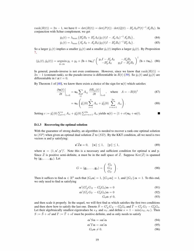
D.1.3 Recovering the optimal solution

With the guarantee of strong duality, an algorithm is needed to recover a rank-one optimal solutionto (SP ) when given an optimal dual solution Z to (SD). By the KKT condition, all we need is twovectors x and y satisfying:

z′Zz = 0, ‖x‖ ≤ 1, ‖y‖ ≤ 1, (89)

where z = (1,x′,y′)′. Note this is a necessary and sufficient condition for optimal x and y.Since Z is positive semi-definite, z must be in the null space of Z. Suppose Ker(Z) is spannedby (g1, . . . ,gk). Let

G = (g1, . . . ,gk) =

(G0

GXGY

). (90)

Then it suffices to find α ∈ Rk such that |G0α| = 1, ‖GXα‖ = 1, and ‖GY ‖α = 1. To this end,we only need to find α satisfying

α′(G′XGX −G′0G0)α = 0 (91)

α′(G′YGY −G′0G0)α = 0 (92)G0α 6= 0, (93)

and then scale it properly. In the sequel, we will first find α which satisfies the first two conditionsand then show how to satisfy the last one. Denote S = G′XGX −G′0G0 and T = G′YGY −G′0G0.Let their algebraically smallest eigenvalues be sX and sY , and define s = 1 −min(sX , sY ). ThenS := S + sI and T := T + sI must be positive definite, and α only needs to satisfy

α′Sα = sα′α (94)

α′Tα = sα′α (95)G0α 6= 0. (96)

19

Denote α = α/ ‖α‖, then it is equivalent to

α′Sα = s (97)

α′T α = s (98)G0α 6= 0. (99)

Because both S and T are positive semidefinite, by [38, Corollary 4.6.12] there exists a nonsin-gular matrix R such that RSR′ = I and RTR′ is real diagonal. In fact this R can be con-structed analytically. Let S have eigen-decomposition S = UDU ′ where D is diagonal. DenoteH = U

√DU ′ and let HTH have eigen-decomposition HTH = V ΛV ′. Then R can be simply

chose as R = V ′H−1 = V UD−1/2U ′. Let RTR′ be diag σi. Denote β = Rα, then β onlyneeds to satisfy

β′β = s (100)

β′Σβ = s (101)

G0R−1β 6= 0. (102)

It is easy to find a β which satisfies the first two constraints, because it is guaranteed that there existsa β which satisfies all the three conditions. Once we get such a β, suppose G0R

−1β = 0. Thenwe can flip the sign of one of its nonzero components. If its product with G0R

−1 is still 0, then itmeans the corresponding entry in G0R

−1 is 0. But G0R−1 cannot be straight 0 because that would

imply G0 is a zero vector which violates the assumption that G is the basis of Ker(Z). Thereforewe can always find a β which satisfies (100) to (102).

D.2 Preliminaries in Matrix Analysis

D.2.1 Matrix Rank-one decomposition

Let X be a n-by-n positive semi-definite matrix with rank(X) = r. Then a set of r vectorsx1, . . . ,xr in Rn is called a rank-one decomposition of X if X =

∑ri=1 xix

′i.

It is noteworthy that the xi’s are not necessarily orthogonal to each other (x′ixj = 0 for i 6= j), butthey must be linearly independent. This leads to the following useful result.

Proposition 3 Suppose ZX = 0 and x1, . . . ,xr is a rank-one decomposition of X . Then Zxi =0, ∀ i.

Proof: Denote yi := Zxi. Suppose otherwise y1 6= 0. Since ZX = 0, we have

0 = X ′Z ′y1 =

r∑i=1

xix′iZ′y1 =

r∑i=1

(y′iy1)xi. (103)

Since y1 6= 0, this violates the linear independence of x1, . . . ,xr.

X is called rank-one decomposable at a vector x1 if there exist other r − 1 vectors x2, . . . ,xr suchthat X =

∑ri=1 xix

′i.

The following three theorems play an important role in our proof.

Proposition 4 (Corollary 4 of [41]) Suppose X ∈ Sn×n+ with rank(X) = r. Z ∈ Sn×n andZ • X ≥ 0. Then there must be a rank-one decomposition of X = x1x

′1 + . . . + xrx

′r such that

Z • (xix′i) = Z •X/r for all i = 1, . . . , r.

Proposition 5 (Lemma 3.3 of [36]) Suppose X ∈ Sn×n+ with rank r ≥ 3. A1, A2 ∈ Sn×n. Letx1, . . . ,xr be a rank-one decomposition of X . If

A1 • x1x′1 = A1 • x2x

′2 = δ1 (104)

(A2 • x1x′1 − δ2)(A2 • x2x

′2 − δ2) < 0, (105)

then there is a vector y ∈ Rn such that X is rank-one decomposable at y and

A1 • yy′ = δ1, A2 • yy′ = δ2. (106)

20

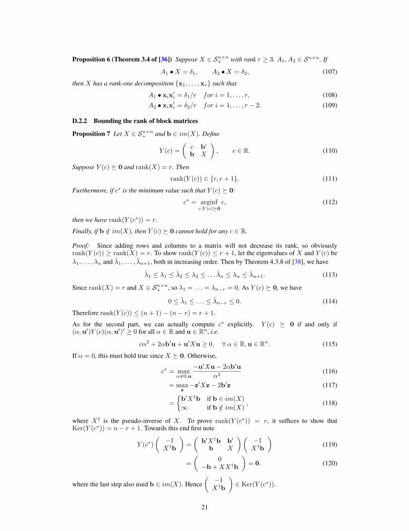
Proposition 6 (Theorem 3.4 of [36]) Suppose X ∈ Sn×n+ with rank r ≥ 3. A1, A2 ∈ Sn×n. If

A1 •X = δ1, A2 •X = δ2, (107)

then X has a rank-one decomposition x1, . . . ,xr such that

A1 • xix′i = δ1/r for i = 1, . . . , r, (108)

A2 • xix′i = δ2/r for i = 1, . . . , r − 2. (109)

D.2.2 Bounding the rank of block matrices

Proposition 7 Let X ∈ Sn×n+ and b ∈ im(X). Define

Y (c) =

(c b′

b X

), c ∈ R. (110)

Suppose Y (c) 0 and rank(X) = r. Then

rank(Y (c)) ∈ r, r + 1. (111)

Furthermore, if c∗ is the minimum value such that Y (c) 0:

c∗ = arginfc:Y (c)0

c, (112)

then we have rank(Y (c∗)) = r.

Finally, if b /∈ im(X), then Y (c) 0 cannot hold for any c ∈ R.

Proof: Since adding rows and columns to a matrix will not decrease its rank, so obviouslyrank(Y (c)) ≥ rank(X) = r. To show rank(Y (c)) ≤ r + 1, let the eigenvalues of X and Y (c) beλ1, . . . , λn and λ1, . . . , λn+1, both in increasing order. Then by Theorem 4.3.8 of [38], we have

λ1 ≤ λ1 ≤ λ2 ≤ λ2 ≤ . . . λn ≤ λn ≤ λn+1. (113)

Since rank(X) = r and X ∈ Sn×n+ , so λ1 = . . . = λn−r = 0. As Y (c) 0, we have

0 ≤ λ1 ≤ . . . ≤ λn−r ≤ 0. (114)

Therefore rank(Y (c)) ≤ (n+ 1)− (n− r) = r + 1.

As for the second part, we can actually compute c∗ explicitly. Y (c) 0 if and only if(α,u′)Y (c)(α,u′)′ ≥ 0 for all α ∈ R and u ∈ Rn, i.e.

cα2 + 2αb′u + u′Xu ≥ 0, ∀ α ∈ R,u ∈ Rn. (115)

If α = 0, this must hold true since X 0. Otherwise,

c∗ = maxα6=0,u

−u′Xu− 2αb′u

α2(116)

= maxz−z′Xz− 2b′z (117)

=

b′X†b if b ∈ im(X)

∞ if b /∈ im(X), (118)

where X† is the pseudo-inverse of X . To prove rank(Y (c∗)) = r, it suffices to show thatKer(Y (c∗)) = n− r + 1. Towards this end first note

Y (c∗)

(−1X†b

)=

(b′X†b b′

b X

)(−1X†b

)(119)

=

(0

−b +XX†b

)= 0. (120)

where the last step also used b ∈ im(X). Hence(−1X†b

)∈ Ker(Y (c∗)).

21

Furthermore, rank(X) = r implies there are n − r linearly independent vectors u1, . . . ,un−r ∈Ker(X). As b ∈ im(X), so b′ui = 0 for all i. Therefore

Y (c∗)

(0ui

)=

(c∗ b′

b X

)(0ui

)=

(b′uiXui

)= 0. (121)

Clearly(−1X†b

),

(0u1

), . . . ,

(0

un−r

)are linearly independent, so Ker(Y (c∗)) ≥ n−r+1,

i.e. rank(Y (c∗)) ≤ r.

Finally, it is obvious from (118) that no c ∈ R makes Y (c) 0 if b /∈ im(X).

Proposition 8 Let P , Q, R be n-by-n matrices, and

Z =

(P RR′ Q

). (122)

Suppose Z 0 and rank(Z) = 2n − 1. Denote r = rank(P ) and s = rank(Q). Then r + s ∈2n− 1, 2n.

Proof: Let Ker(P ) be spanned by u1, . . . ,un−r, and Ker(Q) be spanned by v1, . . . ,vn−s. Denote

ui =

(ui0

)and vi =

(0vi

). Then

u′iZui = u′iPu′i = 0. (123)

Since Z 0, so ui ∈ Ker(Z). Similarly vi ∈ Ker(Z). Clearly u1, . . . , un−r, v1, . . . , vn−s arelinearly independent, therefore

2n− 1 = rank(Z) ≤ 2n− (n− r)− (n− s) = r + s. (124)

So r + s ∈ 2n− 1, 2n.

Auxiliary References[34] Y. Nesterov. Smooth minimization of non-smooth functions. Mathematical Programming,

103:127–152, 2005.[35] F. Bach, J. Mairal, and J. Ponce. Convex sparse matrix factorizations. arXiv:0812.1869v1,

2008.[36] W. Ai and S. Zhang. Strong duality for the CDT subproblem: A necessary and sufficient

condition. SIAM Journal on Optimization, 19:1735–1756, 2009.[37] G. Pataki. On the rank of extreme matrices in semidefinite programs and the multiplicity of

optimal eigenvalues. Math. Oper. Res., 23(2):339–358, 1998.[38] R. A. Horn and C. R. Johnson. Matrix Analysis. Cambridge University Press, Cambridge,

1985.[39] G. H. Golub and V. Pereyra. The differentiation of pseudo-inverses and nonlinear least squares

problems whose variables separate. SIAM Journal on Numerical Analysis, 10(2):413–432,1973.

[40] J. R. Magnus. On differentiating eigenvalues and eigenvectors. Econometric Theory, 1(2):179–191, 1985.

[41] J. Sturm and S. Zhang. On cones of nonnegative quadratic functions. Mathematics of Opera-tions Research, 28:246–267, 2003.

22