Accelerated reconstruction of a compressively sampled data stream Pantelis Sopasakis * , Nikolaos Freris † , Panos Patrinos ] * IMT School for Advanced Studies Lucca, Italy, † NYU, Abu Dhabi, United Arab Emirates, ] ESAT, KU Leuven, Belgium. August 31, 2016

Welcome message from author
This document is posted to help you gain knowledge. Please leave a comment to let me know what you think about it! Share it to your friends and learn new things together.
Transcript

Accelerated reconstruction of a compressivelysampled data stream
Pantelis Sopasakis∗,Nikolaos Freris†, Panos Patrinos]
∗ IMT School for Advanced Studies Lucca, Italy,† NYU, Abu Dhabi, United Arab Emirates,
] ESAT, KU Leuven, Belgium.
August 31, 2016

Contribution
The proposed methodology is an order of magnitude faster compared toall state-of-the-art methods for recursive compressed sensing.
1 / 22

I. Recursive Compressed Sensing

Problem statement
Suppose a sparsely sampled signal y ∈ IRm is produced by
y = Ax+ w
where x ∈ IRn (n� m) is s-sparse and A is the sampling matrix and wis a noise signal.
Problem. Retrieve x from y.
2 / 22

Sparse Sampling
3 / 22
Requirement
Matrix A must satisfy the restricted isometry property
(1− δs)‖x‖2 ≤ ‖Ax‖2 ≤ (1 + δs)‖x‖2,
for all x. A typical choice is a random A with entries drawn fromN (0, 1
m) with m = 4s.
4 / 22

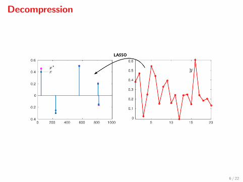
Decompression
Assuming
I w ∼ N (0, σ2I)
I the smallest element of |x| is not too small (> 8σ√2 lnn)
I λ = 2σ√2 lnn
then, the LASSO solution
x? = argminx
1
2‖Ax− y‖2 + λ‖x‖1,
and x have the same support whp.
5 / 22
Decompression
6 / 22
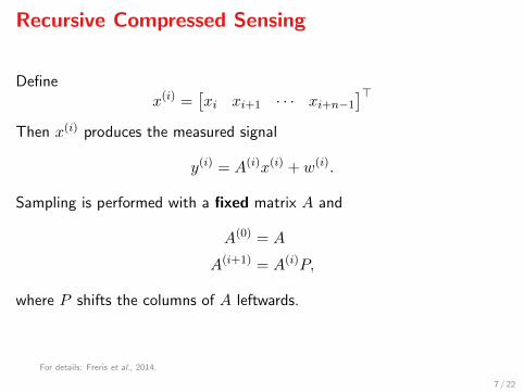
Recursive Compressed Sensing
Definex(i) =
[xi xi+1 · · · xi+n−1
]>Then x(i) produces the measured signal
y(i) = A(i)x(i) + w(i).
Sampling is performed with a fixed matrix A and
A(0) = A
A(i+1) = A(i)P,
where P shifts the columns of A leftwards.
For details: Freris et al., 2014.
7 / 22
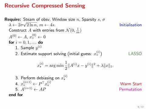
Recursive Compressed Sensing
Require: Steam of obsv, Window size n, Sparsity s, σλ← 2σ
√2 lnn, m← 4s. Initialisation
Construct A with entries from N (0, 1m)
A(0) ← A, x(0)◦ ← 0
for i = 0, 1, . . . do1. Sample y(i)
2. Estimate support solving (initial guess: x(i)◦ ) LASSO
x(i)? = argmin
1
2‖A(i)x− y(i)‖2 + λ‖x‖1.
3. Perform debiasing on x(i)?
4. x(i+1)◦ ← P>x
(i)? Warm Start
5. A(i+1) ← AP Permutationend for
8 / 22

II. Forward-Backward Newton

Optimality Conditions
LASSO problem
minimise 12‖Ax− y‖
2︸ ︷︷ ︸f
+λ‖x‖1︸ ︷︷ ︸g
Optimality conditions:
−∇f(x?) ∈ ∂g(x?),
with ∇f(x) = A>(Ax− y) and ∂g(x)i = λ sign(xi) for xi 6= 0,∂g(x)i = [−λ, λ] for xi = 0, so
−∇if(x?) = λ sign(x?i ), for x?i 6= 0,
|∇jf(x?)| ≤ λ, for x?j = 0
9 / 22

Optimality Conditions
If we knew
α = {i : x?i 6= 0},β = {i : x?i = 0}
then
A>αAαx?α = A>α y + λ sign(x?α).
Goal. Devise a method to determine α efficiently.
10 / 22
Optimality Conditions
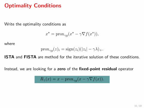
Write the optimality conditions as
x? = proxγg(x? − γ∇f(x?)),
whereproxγg(z)i = sign(zi)(|zi| − γλ)+.
ISTA and FISTA are method for the iterative solution of these conditions.
Instead, we are looking for a zero of the fixed-point residual operator
Rγ(x) = x− proxγg(x− γ∇f(x)).
11 / 22

(The Forward-Backward Envelope)
x
ϕ(x)
ϕγ
f + gϕγ
12 / 22

(The Forward-Backward Envelope)
The forward-backward envelope is defined as
ϕγ(x) = minz
{f(x) +∇f(x)>(z − x) + g(z) + 1
2γ ‖z − x‖2}
In our case ϕγ is smooth with
∇ϕγ(x) = (I − γ∇2f(x))Rγ(x).
Key property.
argmin f + g = argminϕγ = zer∇ϕγ = zerRγ
ϕγ is C1 but not C2.
13 / 22

B-subdifferential
For a mapping F : IRn → IRn which is almost-everywhere diff/ble, wedefine its B-subdifferential to be
∂BF (x) :=
{B ∈ IRn×n
∣∣∣∣ ∃{xν}ν : xν → x,F ′(xν) exists, F ′(xν)→ B
}
Facchinei & Pang, 2004.
14 / 22

Forward-Backward Newton
The proposed algorithm is
xk+1 = xk − τkH−1k Rγ(xk),
Hk ∈ ∂BRγ(xk).
When close to the solution all Hk are nonsingular. Take
Hk = I − Pk(I − γA>A),
where P is diagonal with Pii = 1 iff i ∈ αk := {i : |xki − γ∇if(xki )| > γλ}.
The scalars τk are chosen by a simple line search algorithm to ensure global convergence.
15 / 22

The algorithm
... can be concisely written as
xk+1 = xk + τkdk,
where dk is the solution of
dkβk = −(Rγ(xk))βkγA>αkAαkd
kαk
= −(Rγ(xk))αk − γA>αkAβkd
kβk.
For global convergence we require
ϕγ(xk+1) ≤ ϕγ(xk) + ζτk∇ϕγ(xk)>dk.
Converges locally quadratically; i.e., like exp(−ck2).
16 / 22

Further acceleration
The algorithm can be further accelerated by
1. A continuation strategy (changing λ while solving)
2. Updating the Cholesky factorisation of A>αAα
Please, see our paper for details.
17 / 22

III. Numerical Results

We are comparing the proposed method with
I ISTA (or proximal gradient method)
I FISTA (accelerated ISTA)
I ADMM
I L1LS
18 / 22

Simulations
For a 10%-sparse stream
Window size ×10 4
0.5 1 1.5 2
Ave
rag
e r
un
tim
e [
s]
10 -1
10 0
10 1
FBN
FISTA
ADMM
L1LS
19 / 22

Simulations
For n = 5000 and different sparsities
Sparsity [%]
0 5 10 15
Ave
rag
e r
un
tim
e [
s]
10 -1
10 0
FBN
FISTA
ADMM
L1LS
20 / 22

Conclusions
I A semi-smooth Newton method for LASSO
I Enabling very fast RCS
I 10 times faster than SoA algorithms
21 / 22

Thank you for your attention.
22 / 22
Related Documents


![GPU-accelerated data expansion for the Marching Cubes ... · Extract iso-surface via Marching Cubes Scalar field is sampled over 3D grid Marching Cubes [Lorensen87] —Marches through](https://static.cupdf.com/doc/110x72/5f59a4a397733378820cfae2/gpu-accelerated-data-expansion-for-the-marching-cubes-extract-iso-surface-via.jpg)