AC 2012-3242: TEACHING ADAPTIVE FILTERS AND …

AC 2012-3242: TEACHING ADAPTIVE FILTERS AND APPLICATIONSIN ELECTRICAL AND COMPUTER ENGINEERING TECHNOLOGY PRO-GRAM

Prof. Jean Jiang, Purdue University, North Central

Jean Jiang is currently with the College of Engineering and Technology at Purdue University, NorthCentral, Westville, Ind. She received her Ph.D. degree in electrical engineering from the Universityof New Mexico in 1992. Her principal technical areas are in digital signal processing, adaptive signalprocessing, and control systems. She has published a number of papers in these areas. She has co-authoredtwo textbooks: Fundamentals of Analog and Digital Signal Processing, Second Edition, AuthorHouse,2008; and Analog Signal Processing and Filter Design, Linus Publications, 2009.

Prof. Li Tan, Purdue University, North Central

Li Tan is currently with the College of Engineering and Technology at Purdue University North Central,Westville, Ind. He received his Ph.D. degree in electrical engineering from the University of New Mexicoin 1992. Tan is a Senior Member of IEEE. His principal technical areas include digital signal processing,adaptive signal processing, and digital communications. He has published a number of papers in theseareas. He has authored and co-authored three textbooks: Digital Signal Processing:Fundamentals andApplications, Elsevier/Academic Press, 2008; Fundamentals of Analog and Digital Signal Processing,Second Edition, AuthorHouse, 2008; and Analog Signal Processing and Filter Design, Linus Publications,2009.

c©American Society for Engineering Education, 2012

Page 25.1238.1

Teaching Adaptive Filters and Applications in Electrical and Computer

Engineering Technology Program

Abstract

In this paper, we present our pedagogy and our experiences with teaching adaptive filters

combined with applications in an advanced digital signal processing (DSP) course. This course is

the second DSP course offered in the electrical and computer engineering technology (ECET)

program according to the current trend of the DSP industry and students’ interests in their career

development. A significant component of this course is adaptive filtering applications1-7

. A

prerequisite for students is a working knowledge of the Laplace transform, Fourier series,

Fourier transform, z-transform, discrete Fourier transform, digital filter design, and real-time

DSP coding skills with TMS320C6713, a high-performance floating-point digital signal

processor8-9

(DSP board) by Texas Instruments, acquired through the first DSP course. Although

adaptive filtering is an exciting topic which allows for the exploration of many real-life

applications, teaching this topic is often challenging due to its relatively heavy reliance on

advanced mathematics. It is possible for the traditional mathematics used for the adaptive

filtering theory to be minimized so that engineering technology students can more easily

understand and grasp key concepts. With the MATLAB software tool, students can simulate and

verify different adaptive filtering applications. To enhance hands-on learning, students are

required to implement adaptive filtering techniques taught during the lectures using a

TMS320C6713. Furthermore, it can be shown that a TMS320C6713 with its stereo channels

proves an effective and flexible tool for various DSP implementations.

In this paper, we first focus on describing the pedagogy for teaching adaptive filter principles

along with MATLAB simulations; then, we illustrate real-time DSP hands-on labs and projects

with various applications. We will examine the assessment based on our collected data from

course evaluations, student surveys and course work, and finally we will address possible

improvement based on our assessment.

I. Introduction

The application of adaptive digital filtering technology has been found widely in modern

electronic products, communication and control systems, computer peripherals, and multimedia

devices1-7

. In the area of digital signal processing (DSP) education for the engineering

technology curriculum, the adaptive filter theory and techniques are considered to be advanced

topics to be covered during the student’s senior year. The trend of using adaptive filters in the

industry has generated an increasing demand for engineering technology graduates with this

particular working knowledge and skills. Many engineering technology programs have already

offered a standard initial DSP course in their undergraduate curricula, particularly in the

electrical and computer engineering technology (ECET) curriculum. The first DSP course

generally covers basic techniques such as finite impulse response (FIR) filter design, infinite

impulse response (IIR) filter design, FIR and IIR filter applications, discrete Fourier transform

(DFT), and the signal spectral algorithm. To keep the pace with the DSP industry, our ECET

curriculum has advanced to offer a second DSP course covering a broad range of topics which

Page 25.1238.2

include adaptive filtering, waveform compression and coding, multi-rate DSP, image and video

processing.

Teaching adaptive filters to ECET students in the second DSP course appears challenging

because it requires applying relatively advanced mathematics with the optimization theory in a

matrix form to develop concepts. However, with our teaching pedagogy, this barrier can be

overcome through illustrating the topic using a single coefficient adaptive filter. MATLAB is a

necessary tool used to verify adaptive theory and perform simulations of various adaptive

filtering applications. To motivate our technology students oriented about hands-on experience,

we required them to perform real-time DSP using a floating-point digital signal processor8-9

,

TMS320C6713 (development starter kit), to develop a comprehensive adaptive filtering project

such as noise cancellation, and to demonstrate their working projects in class.

In this paper, we will describe the course prerequisites, course topics, and outline learning

outcomes. With a focus on adaptive filtering techniques, we will describe our teaching pedagogy,

MATLAB simulations, and hands-on real-time DSP labs and projects. Finally, we will examine

the course assessment according to our collected data from the course evaluations, student

surveys and course work, and then we will address possible improvement based on our

assessment.

II. Learning Outcomes and Laboratories

The adaptive filter techniques are covered in our advanced DSP course (ECET 499) offered

during the senior year, involving a 16-week class schedule with three-hour lectures and three-

hour labs each week. Four weeks are allocated to covering adaptive filters. Prior to this second

DSP course, the pre-requisite courses are: Introduction to Microcontrollers (ECET 209), Circuit

Analysis Courses (ECET 207, ECET 257), Analog Network Signal Processing (ECET 307), and

real-time DSP (ECET 357). Figure 1 shows a flowchart for the related courses.

Analog Network

Signal Procssing

(ECET 307)

Digial Signal Processing

(ECET 357)

Advanced DSP

(ECET 499)

Circuit Analysis

(ECET 207)

(ECET 257)

Microcontrollers

(ECET 209)

Figure 1. Flowchart of DSP-related courses.

As shown in Figure 1, students in ECET209 gain background knowledge about the processor

architecture, interface concepts, and basic C programming skills. The required skills of complex

algebra and circuit analysis are covered in circuit courses such as AC Circuit Analysis (ECET

207) and Power and RF Electronics (ECET 257). Our Analog Network Signal Processing (ECET

307) course10

studies very important fundamental subjects: the Laplace transform, circuit

Page 25.1238.3

analysis using the Laplace transform, the Fourier series, and filter design concepts. These

subjects are used extensively in the real-time DSP course (ECET 357), in which FIR filter

design, IIR filter design, discrete Fourier transform (DFT), and signal spectrum and their

applications are investigated. More importantly, the students are equipped with programming

skills for using a floating-point digital signal processor, TMS320C6713, after successfully

completing the first DSP course (ECET 357).

The advanced DSP course (ECET 499) as shown in Figure 1 covers the following key topics: (1)

adaptive filters with applications such as noise cancellation, system modeling and echo

cancellation; (2) waveform coding and compression including pulse code modulation (PCM),

mu-law compression, adaptive differential PCM (ADPCM) and windowed discrete-cosine

transform (DCT); (3) multi-rate DSP including sampling rate conversion and polyphase

implementations; (4) image equalization and noise filtering; (5) image segmentation, pseudo-

color generation and JPEG data compression; (6) other advanced DSP applications. These topics

are covered through Chapters 10 to 13 in the DSP textbook1. The labs and projects are listed in

Table 1.

Table 1. List of labs for ECET 499.

Lab 1. Adaptive noise cancelling

Lab 2. Adaptive system modeling

Lab 3. PCM codec, mu-law compression, and ADPCM codec, transform coding with

applications to speech signal

Lab 4. Sampling rate conversion and polyphase implementations

Lab 5. Image processing basics

Lab 6. Image processing: edge detection, pseudo color generation and JPEG color

image compression

Project: Real-time DSP project: tonal noise cancellation

Notice that for labs 1-4 and course projects, students are required to perform MATLAB

simulations first and then are required to focus on hands-on real-time DSP implementations

using the TMS320C6713 board(s). The specific learning outcomes for adaptive filtering

techniques are listed below:

Learning outcome 1: Given an objective function such the mean squared error (MSE) function, develop an adaptive

filter that seeks to minimize the given objective function by iteratively adjusting its parameters (such as its impulse

response coefficients) to achieve the design goal in real time and under varying conditions.

Learning outcome 2: Apply real-time adaptive filtering techniques for applications such as noise cancellation and

system modeling.

Labs 1-2 and course project listed in Table 1 are designed to fulfill these learning outcomes.

A. Pedagogy for Teaching Adaptive Filter Techniques

Our pedagogy for teaching adaptive filters includes the following steps: (1) using a single

coefficient FIR filter to develop its Wiener filter solution; (2) introducing a single coefficient

Page 25.1238.4

steepest descent algorithm; (3) developing a single coefficient least mean square (LMS)

algorithm; (4) extending a single coefficient LMS adaptive FIR filter to a standard LMS adaptive

FIR filter; (5) performing MATLAB simulations for concept verifications.

Figure 2 shows a Wiener filter for noise cancellation, where a single coefficient filter is used for

illustration; that is, ( ) ( )y n wx n . w is the adaptive coefficient and ( )y n is the Wiener filter

output, which approximates the noise ( )n n in the corrupted signal.

e n( )

x n( )

d n s n n n( ) ( ) ( )

y n( )Wiener fi l ter

Output

Noise

Signal and noise

Figure 2 Wiener filter for noise cancellation.

The enhanced signal ( )e n is given by

( ) ( ) ( )e n d n wx n

Taking statistical expectation of the square of error leads to a quadratic function 2 22J wP w R

where 2 ( )J E e n is the mean square error or output power. When it is minimized, the noise

power is maximally reduced. Since 2 2 ( )E d n (auto-correlation or power of the corrupted

signal), ( ) ( )P E d n x n (cross-correlation), and 2 ( )R E x n are constants, J is a quadratic

function of w as shown below: J

ww*

Jmin

Figure 3 MSE quadratic function.

The best coefficient (optimal) *w is unique which is corresponding to the minimum MSE error

minJ . By taking derivative of J and setting it to zero leads the solution as * 1w R P

A couple of numerical examples for finding the minimum locations of quadratic functions are

given to develop the optimization concepts. Next, a steepest descent algorithm that is capable of

minimizing the MSE function sample by sample to locate the filter coefficient(s) is introduced as

follows: Page 25.1238.5

1n n

dJw w

dw

constant controlling speed of convergence and /dJ dw is the gradient of the MSE function.

The steepest descent method is more efficient since the matrix inverse of 1R (for N filter

coefficients) is not needed. Several numerical examples with a single coefficient filter are

provided to show how iterations approach the optimal coefficient. To develop the LMS

algorithm in terms of the sample based processing, a gradient /dJ dw can be approximated by its

instantaneous value; that is,

( ) ( )

2 ( ) ( ) 2 ( ) ( )d d n wx ndJ

d n wx n e n x ndw dw

Substituting the instantaneous /dJ dw to the steepest descent algorithm, the LMS algorithm for

updating a single coefficient is achieved:

1 2 ( ) ( )n nw w e n x n

Finally by omitting iteration time index n and extending one coefficient filter to N coefficient

filter, a standard LMS algorithm is obtained and listed in Table 2.

Table 2. LMS adaptive FIR filter with N filter coefficients.

(1) Initialize (0)w , (1)w , … ( 1)w N to arbitrary values

(2) Read ( )d n , ( )x n , and perform digital filtering

( ) (0) ( ) (1) ( 1) ( 1) ( 1)y n w x n w x n w N x n N

(3) Compute the output error

( ) ( ) ( )e n d n y n

(4) Update each filter coefficient using the LMS algorithm

for 0, , 1i N

( ) ( ) 2 ( ) ( )w i w i e n x n i

To illustrate the functionality of an adaptive filter, MATLAB examples for noise cancellation

and system modeling are provided. The principle of noise cancellation is shown in Figure 4.

y n( )

d n s n n n( ) ( ) ( )

x n( )

e n d n y n s n( ) ( ) ( ) ~( )

ADC

ADC

DAC

Adaptive fi lter

LMS algorithm

Noise

Signal and noise Error signal

Figure 4. Noise canceller using an adaptive filter.

The noise cancellation system in Figure 4 is assumed to have the following specifications: a

sample rate = 8000 Hz; speech corrupted by a Gaussian noise with a power of 1 and delayed by 5

samples from a white noise source; and an adaptive FIR filter used to remove the noise, where

Page 25.1238.6

the number of FIR filter coefficients = 21 and the convergence factor for the LMS algorithm is

chosen to be 0.01. The speech waveforms and speech spectral plots for the original, corrupted

reference noise and the clean one are plotted in Figure 5, respectively. It is observed that the

enhanced speech waveform and spectrum are very close to the originals. The LMS algorithm

converges after approximately 400 iterations and is very effective for noise cancellation.

0 200 400 600 800 1000 1200 1400 1600 1800 2000-1

0

1

Orig.

speech

0 200 400 600 800 1000 1200 1400 1600 1800 2000-5

0

5

Corr

upt.

speech

0 200 400 600 800 1000 1200 1400 1600 1800 2000-5

0

5

Ref.

nois

e

0 200 400 600 800 1000 1200 1400 1600 1800 2000-1

0

1

Cle

an s

peech

Number of samples

0 500 1000 1500 2000 2500 3000 3500 40000

0.05

0.1

Orig.

spectr

um

0 500 1000 1500 2000 2500 3000 3500 40000

0.05

0.1

0.15

Corr

upt.

spectr

um

0 500 1000 1500 2000 2500 3000 3500 40000

0.05

0.1

0.15

Cle

an s

pectr

um

Frequency (Hz) Figure 5. Original speech, corrupted speech, reference noise and clean speech.

Another typical MATLAB example is system modeling, in which an adaptive FIR filter is

applied to track the behavior of an unknown system by monitoring the unknown system’s input

and output. Figure 6 depicts the configuration of the system modeling.

0 500 1000 1500 2000 2500 3000 3500 4000-200

-100

0

100

200

Frequency (Hertz)

Phase (

degre

es)

0 500 1000 1500 2000 2500 3000 3500 4000-80

-60

-40

-20

0

Frequency (Hertz)

Magnitude R

esponse (

dB

)

(a). Unknown system frequency response

x n( )

d n( )

y n( )

e n( )

Unknown system

Adaptive

FIR fi lter

Input

Output

(b) Block diagram

Figure 6 Adaptive filter for system modeling.

Page 25.1238.7

As shown in the figure, ( )y n is approaching the unknown system output during the adaptive

process. Since both the unknown system and the adaptive filter use the same input, the transfer

function of the adaptive filter will approximate the unknown system’s transfer function. In the

simulation, the unknown system shown in Figure 6 is assumed to be a 4th

-order band-pass IIR

filter, in which 3-dB lower and upper cut-off frequencies are 1400 Hz and 1600 Hz with a

sampling rate of 8000 Hz. The system input contains 500 Hz, 1500 Hz, and 2500 Hz tones and

its waveform ( )x n is displayed in the left top plot in Figure 7. The output of the unknown

system is expected to contain the 1500 Hz tone only, since the other two tones are rejected by the

unknown system. An adaptive FIR filter with 21 coefficients is used to model the band-pass

unknown system, and the convergence factor of the adaptive filter is set to be 0.01. In the time

domain, the output waveforms of the unknown system ( )d n and adaptive filter output ( )y n are

almost identical after the LMS algorithm converges around 70 samples. The error signal ( )e n is

also plotted to show how the adaptive filter keeps tracking the unknown system output with no

difference.

0 100 200 300 400 500 600 700 800

-2

0

2

Syste

m input

0 100 200 300 400 500 600 700 800

-1

0

1

Syste

m o

utp

ut

0 100 200 300 400 500 600 700 800

-1

0

1

AD

F o

utp

ut

0 100 200 300 400 500 600 700 800

-1

0

1

Err

or

Number of samples

0 500 1000 1500 2000 2500 3000 3500 40000

0.5

1S

yst.

input

spect.

0 500 1000 1500 2000 2500 3000 3500 40000

0.5

1

Syst.

outp

ut

spect.

0 500 1000 1500 2000 2500 3000 3500 40000

0.5

1

AD

F o

utp

ut

spect.

Frequency (Hz) Figure 7 Unknown system output, adaptive filter output and error output.

In the frequency domain, the first plot shows the input frequency components of 500 Hz, 1500

Hz, and 2500 Hz. The second plot shows the unknown system output spectrum with the 1500 Hz

tone while the third plot displays the adaptive filter output spectrum with the 1500 Hz tone. It is

apparent that the adaptive filter tracks the characteristics of the unknown system.

B. Real-time Laboratory Content

Each adaptive filtering lab consists of two portions: MATLAB simulation and real-time DSP

implementation with a single DSP board. The MATLAB simulation must be completed prior to

the real-time implementation. We only describe real-time hands-on labs and projects. A single

DSP board setup and program segment for verifying input and output signals are shown in

Figure 8a and Figure 8b, respectively, where the sampling rate is 8000 samples per second.

Page 25.1238.8

TI TMS320C6713

DSP Board

Computer

Left Line In

(LCI)

Right Line In

(RCI)

Left Line Out

(LCO)

Right Line Out

(RCO)

Signal

Generator

Oscil loscope

Figure 8a Real-time DSP laboratory setup.

float xL[1]={0.0};

float xR[1]={0};

float yL[1]={0.0};

float yR[1]={0,0};

interrupt void c_int11()

{

float lc; /*left channel input */

float rc; /*right channel input */

float lcnew; /*left channel output */

float rcnew; /*right channel output */

int i;

//Left channel and right channel inputs

AIC23_data.combo=input_sample();

lc=(float) (AIC23_data.channel[LEFT]);

rc= (float) (AIC23_data.channel[RIGHT]);

// Insert DSP algorithm below

xL[0]=lc; /* Input from the left channel */

xR[0]=rc; /* Input from the right channel */

yL[0]=xL[0]; /* simplest DSP equation for the left channel*/

yR[0]=xR[0]; /* simplest DSP equation for the right channel*/

// End of the DSP algorithm

lcnew=yL[0];

rcnew=yR[0];

AIC23_data.channel[LEFT]=(short) lcnew;

AIC23_data.channel[RIGHT]=(short) rcnew;

output_sample(AIC23_data.combo);

}

Page 25.1238.9

Figure 8b. Program segment for verifying input and output.

A configuration for Lab 1 (adaptive noise cancellation) is shown in Figure 9a, where the primary

signal is a generated sinusoid and corrupted internally by a reference noise from the analog to

digital conversion (ADC) channel. The reference noise can be set as a tonal noise fed via a

function generator or from other noise source using microphone and amplifier. The output

(difference between the corrupted signal and the adaptive filter output) presents a restored clean

signal, similar to the original one from the internal digital oscillator. The sample program

segment is given in Figure 9b.

Noise

from line in

Sinewave generator

Adaptive

FIR filter

x n n( ) ( )

( )y n ADF output

e n( ) Output

( )d n corrupted signal

( )Channel simulated

( ) sinusoidyy n

( )n n noiseDAC

ADC

( )xn n

TI TMS320C6713

DSP Board

Left Line In

(LCI)

Right Line In

(RCI)

Left Line Out

(LCO)

Right Line Out

(RCO)

Noise source

(from generator)

Oscilloscope

( )xn n( )e n

RCI not used

RCO not used

Figure 9a Laboratory setup for noise cancellation using a LMS adaptive filter.

float b[2]={0.0, 0.587785}; /*Numerical coefficients for the 800 Hz digital oscillator*/

float a[3]={1, -1.618034, 1};/*Denominator coefficients for the digital oscillator*/

float x[2]={5000, 0.0}; /*Set up the input as an impulse function*/

float yy[3]={0.0,0.0,0.};

float xn[20]={0,0,0,0,0,0,0,0,0,0,0,0,0,0,0,0,0,0,0,0}; /*Reference input buffer*/

float w[20]={0,0,0,0,0,0,0,0,0,0,0,0,0,0,0,0,0,0,0,0}; /*adaptive filter coefficients*/

float d[1]={0.0}; /* Corrupted signal*/

float y[1]={0,0}; /* Adaptive filter output */

float e[1]={0.0}; /* Enhanced signal */

float mu=0.000000000004; /*Adaptive filter convergence factor*/


{





int i;





Page 25.1238.10


yy[0]=b[0]*x[0]+b[1]*x[1]-a[1]*yy[1]+a[2]*yy[2]; /* Generate 800 Hz tone*/

d[0]=yy[0]+0.5*xn[5]; /*Corrupted signal: d(n)=yy(n)+0.5*xn(n-5)*/

for(i=1;i>0;i--) /*Update the digital oscillator input buffer*/

{ x[i]=x[i-1]; }

x[0]=0;

for(i=2;i>0;i--) /*Update the digital oscillator output buffer*/

{ yy[i]=yy[i-1]; }

for(i=19;i>0;i--) /*Update the reference noise buffer input buffer*/

{ xn[i]=xn[i-1]; }

xn[0]=lc;

// Adaptive filter

y[0]=0;

for(i=0;i<20; i++)

{ y[0]=y[0]+w[i]*xn[i];}

e[0]=d[0]-y[0]; /* Enhanced output */

for(i=0;i<20; i++)

{ w[i]=w[i]+2*mu*e[0]*xn[i];} /* LMS algorithm */


lcnew=e[0]; /* Send to DAC */

rcnew=rc; /* keep the original data */




}

Figure 9b. Program segment for noise cancellation in Lab 1.

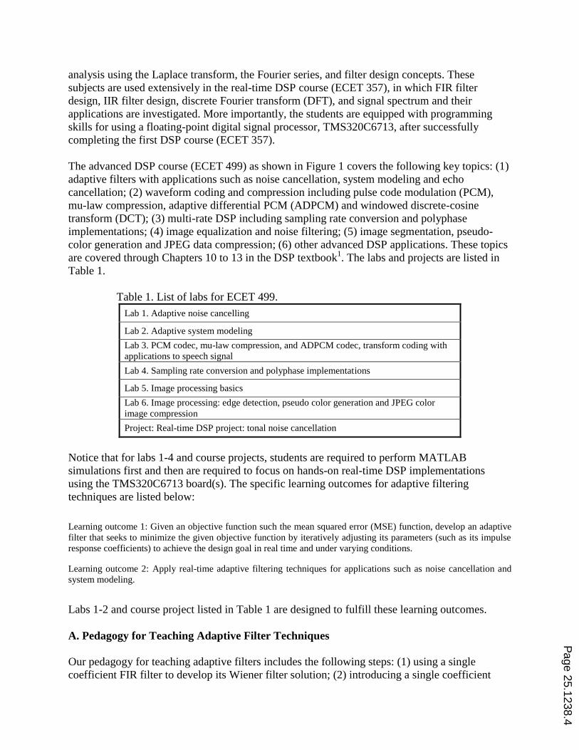
The implementation of system modeling in lab 2 is displayed in Figure 10a, where the input is

fed from a function generator. The unknown system is a band-pass filter with a lower cut-off

frequency of 1400 Hz and an upper cut-off frequency of 1600 Hz. When the input frequency is

swept from 200 Hz to 3000 Hz, the output shows a maximum peak when the frequency is dialed

to around 1500 Hz. Hence, the adaptive filter acts like the unknown system. Figure 10b shows

the sample program segment.

x n( )

d n( )

y n( )

e n( )

Unknown system

Adaptive

FIR fi lter

Input

Output

TI TMS320C6713

DSP Board

Left Line In

(LCI)

Right Line In

(RCI)

Left Line Out

(LCO)

Right Line Out

(RCO)

Signal

Generator

Oscil loscope

( )x n( )y n

( )e n

RCI not used

Page 25.1238.11

Figure 10a. Laboratory setup for system modeling using a LMS adaptive filter.

/*Numerical coefficients */

/*for the bandpass filter (unknown system) with fL=1.4 kHz, fH=1.6 kHz*/

float b[5]={ 0.005542761540433, 0.000000000000002, -0.011085523080870,

0.000000000000003 0.005542761540431};

/*Denominator coefficients */

/*for the bandpass filter (unknown system) with fL=1.4 kHz, fH=1.6 kHz*/

float a[5]={ 1.000000000000000, -1.450496619180500. 2.306093105231476,

-1.297577189144526 0.800817049322883};

float xn[40]={0,0,0,0,0,0,0,0,0,0,0,0,0,0,0,0,0,0,0,0,

0,0,0,0,0,0,0,0,0,0,0,0,0,0,0,0,0,0,0,0}; /*Reference input buffer*/

float w[40]={0,0,0,0,0,0,0,0,0,0,0,0,0,0,0,0,0,0,0,0,

0,0,0,0,0,0,0,0,0,0,0,0,0,0,0,0,0,0,0,0}; /*adaptive filter coefficients*/

float d[1]={0.0}; /*Unknown system output */

float y[1]={0,0}; /* Adaptive filter output */

float e[1]={0.0}; /* Error signal */

float mu=0.000000000002; /*Adaptive filter convergence factor*/


{





int i;






for(i=39;i>0;i--) /*Update the input buffer*/

{ x[i]=x[i-1]; }

x[0]=lc;

d[0]=b[0]*x[0]+ b[1]*x[1]+ b[2]*x[2]+ b[3]*x[3]+ b[4]*x[4]

-a[1]*d[1]-a[2]*d[2]- a[3]*d[3]- a[4]*d[4]; /*Unknown system output*/

// Adaptive filter

y[0]=0;

for(i=0;i<40; i++)

{ y[0]=y[0]+w[i]*x[i];}

e[0]=d[0]-y[0]; /* Error output */

for(i=0;i<40; i++)

{ w[i]=w[i]+2*mu*e[0]*x[i];} /* LMS algorithm */


lcnew=y[0]; /* Send the tracked output */

rcnew=e[0]; /* Send the error signal*/




}

Figure 10b. Program segment for system modeling in Lab 2.

Page 25.1238.12

Finally, a course project is assigned. Students are divided into groups (two persons per group) to

develop their selected DSP projects and to generate their design reports. At the end of the

semester, everybody is required to demonstrate his/her project to the entire class so that the

students can learn from each other. During the project’s developing phase, students can obtain

advice from their instructor and work on their projects under the supervision of their instructor.

Figure 11 shows an example of a tonal noise reduction system that uses two TI DSP boards. The

first DSP board is used to create a real-time corrupted signal mixed by the mono audio source

(Left Line In [LCI1]) from any audio device, and the tonal noise (Right Line In [RCI1])

generated from the function generator. The output (Left line Out [LCO1]) is the corrupted signal,

which is fed to the second DSP board for a noise cancellation application. The second DSP board

receives the corrupted signal ( ) ( ) ( )d n s n n n from channel LCI2 (Left Line In). The tonal

noise ( )n n in the corrupted signal is then cancelled by the adaptive FIR filter output ( )y n using

the reference noise input ( )x n (Right Line In [RCI2]). Finally, the enhanced signal ( )e n is sent

to the output (Left Line Out [LCO2]) to produce a clean mono audio signal.

y n( )

d n s n n n( ) ( ) ( )

x n( )

e n d n y n s n( ) ( ) ( ) ~( )

ADC

ADC

DAC

Adaptive fi lter

LMS algorithm

Noise

Signal and noise Error signal

(a) Block diagram for adaptive noise cancellation

TI TMS320C6713

DSP Board 2

Left Line In

LCI2

Right Line In

RCI2

Left Line Out

LCO2

Right Line Out

RCO2

Mono Audio

Source

TI TMS320C6713

DSP Board 1

Left Line In

LCI1

Right Line In

RCI1

Left Line Out

LCO1

Right Line Out

RCO1

Tonal

Reference

Noise

Corrupted

Audio

Mixing audio

and tonal noise

FIR adaptive

fi ltering

Enhanced

Audio

( )s n

( )x n ( )d n

( )x n

( )s n

RCO1 not used

RCO2 not used

(b) Laboratory setup for adaptive noise cancellation.

Figure 11 Tonal noise cancellation with the LMS adaptive FIR filter.

Page 25.1238.13

III. Learning Outcome Assessment

The assessment presented here consists of a total of 12 student responses and is derived from our

collected data from the course offered in spring of 2010 and fall of 2010. At the end of each

semester, we conducted a student self-assessment. A student survey was given before the final

exam asking each student to evaluate his/her achievement in the learning outcomes. Students

were asked to select one of the following five (5) choices: understand well, understand,

somewhat understand, somewhat confused, and confused. For statistical purposes, the five

choices were assigned the scores of 5, 4, 3, 2, and 1, respectively. The average rating scores for

learning outcomes are listed in row 2 Table 3.

Table 3. Student survey and instructor assessment. Learning Outcomes O1 O2

Student Survey 4.3 4.5

Instructor assessment 4.1 4.6

An instructor assessment based on the final exams and laboratory projects was also conducted. In

order to do this, we designed a final exam in which the course learning outcome 1 was covered

by the problems. We then computed the average points from all the students for the problem(s).

The average rating on a scale from 1 to 5 was obtained by dividing the average points by the

designated points for that problem(s) and then multiplying the result by 5. Outcome 2 was

similarly assessed based on the student’s adaptive filter labs and projects. The instructor

assessment is included in row 3 of Table 3.

The rating scores from the student survey and the ones from the instructor were consistent. The

rating for course leaning outcome 1 (O1) had a slightly bigger gap, in which the score from

instructor rating was lower than the one from the student survey by 0.2. There is a smaller gap

for O2. These discrepancies indicate that our ECET students were strong in hand-on

applications.

We also conducted another student survey regarding our real-time adaptive filter labs. A set of

questions, which are listed in Table 4, was given to students for evaluation. The students were

allowed to select one of the following five (5) choices: strongly agree, agree, somewhat agree,

disagree and strongly disagree. The corresponding rating scores were designated as 5, 4, 3, 2, and

1, respectively. Each average rating score is listed in Table 5.

Table 4. Survey questions for real-time DSP labs. Q1. Do you feel you can significantly grasp concepts of adaptive signal

processing by working on real-time DSP coding?

Q2. Are you excited to work on real-time adaptive filter labs and projects?

Q3. Do you feel that real-time adaptive filtering is absolutely necessary in this

course?

Q4. Does real-time coding of adaptive filters improve your problem solving

ability?

Q5. Do you want more real-time adaptive filtering labs and projects in this

course?

Q6. Do you want to learn more on DSP subjects and applications if possible in

Page 25.1238.14

the future?

Table 5. Student survey for real-time adaptive filter labs. Question No. Q1 Q2 Q3 Q4 Q5 Q6

Student Survey 4.3 5.0 4.8 4.7 4.8 4.8

The average rating scores shown in Table 5 indicated the following:

(1) Students strongly agreed that learning adaptive filters should involve real-time

adaptive filter labs, which improved their problem solving ability.

(2) Most of the students remained excited about the course, since the hands-on real-time

laboratories motivated them.

(3) Students were eager to learn more about real-time adaptive filter subjects.

(4) The rating score for grasping adaptive concepts from adaptive filter labs was

relatively low in comparison to the others. This indicated that students had not only learnt

concepts from labs but also from class lectures, homework assignments, and MATLAB

simulations.

V. Course Improvement

Based on our experiences in teaching adaptive filters with real-time DSP labs, we felt that the

topic is well covered with suitable lectures and laboratories. We also felt that one particular

prerequisite course, Real-time Digital Signal Processing (ECET 357), plays a very important role

for students’ success in the second DSP course. We will continue to keep the standard in

developing student real-time DSP skills. We would also like to encourage students to develop

more comprehensive and challenging projects in the area of adaptive filtering such as echo

cancellation, active noise control, adaptive IIR filters, etc.

VI. Conclusion

We have presented our pedagogy and our experiences with teaching adaptive filter techniques

with both MATLAB simulations and real-time adaptive filter laboratories. From our assessment,

we have found that hands-on real-time adaptive filter labs with practical applications can

motivate students to achieve learning objectives and can increase students’ levels of interest in

the area of DSP. We also expect that students will apply their gained knowledge and skills in

adaptive filters to their senior design projects.

Bibliography

1. L. Tan, Digital Signal Processing: Fundamentals and Applications, Elsevier, 2008.

2. L. Tan and J. Jiang, A Simple DSP Laboratory Project for Teaching Real-Time Signal Sampling Rate

Conversions, the Interface Technology Journal, Vol. 9, No. 1, Fall 2008.

3. N. Kehtaranavaz, and B., Simsek, C6x-Based Digital Signal Processing, Prentice Hall, Upper Saddle River,

New Jersey 07458, 2000.

4. L. Tan, J. Jiang, “Teaching Advanced Digital Signal Processing with Multimedia Applications in Engineering

Technology Programs,” 2009 Proceedings of the American Society for Engineering Education, Austin, Texas,

June 2009.

Page 25.1238.15

5. Ifeachor, Emmanuel and Jervis, Barrie. Digital Signal Processing, A Practical Approach, Prentice-Hall

Publishing, 2002.

6. H. Wu and S. Kuo, “Teaching Challenge in Hands-on DSP Experiments for Night-School Students,” EURASIP

Journal on Advances in Signal Processing, Vol. 2008, Article ID 570896, June 2008.

7. C. Wicks, “Lessons Learned: Teaching Real-Time Signal Processing,” IEEE Signal Processing Magazine, pp.

181-185, November 2009.

8. Texas Instruments, TMS320C6x CPU and Instruction Set Reference Guide, Literature ID# SPRU 189C, Texas

Instruments, Dallas, Texas, 1998.

9. Texas Instruments, Code Composer Studio: Getting Started Guide, Texas Instruments, Dallas, Texas, 2001.

10. L. Tan, J. Jiang, Analog Signal Processing and Filter Design, Linus Publications, 2009.

Page 25.1238.16

AC 2012-3242: TEACHING ADAPTIVE FILTERS AND …

Documents