AC 2007-791: LABORATORY-SCALE STEAM POWER PLANT STUDY — RANKINE CYCLER™ COMPREHENSIVE EXPERIMENTAL ANALYSIS Andrew Gerhart, Lawrence Technological University Andrew Gerhart is an assistant professor of mechanical engineering at Lawrence Technological University. He is actively involved in ASEE, the American Society of Mechanical Engineers, and the Engineering Society of Detroit. He serves as Faculty Advisor for the American Institute of Aeronautics and Astronautics Student Chapter at LTU and is the Thermal-Fluids Laboratory Coordinator. He serves on the ASME PTC committee on Air-Cooled Condensers. Philip Gerhart, University of Evansville Philip Gerhart is the Dean of the College of Engineering and Computer Science and a professor of mechanical and civil engineering at the University of Evansville in Indiana. He is a member of the ASEE Engineering Deans Council. He is a fellow of the American Society of Mechanical Engineers and serves on their Board on Performance Test Codes. He chairs the PTC committee on Steam Generators and is vice-chair of the committee on Fans. © American Society for Engineering Education, 2007

Welcome message from author
This document is posted to help you gain knowledge. Please leave a comment to let me know what you think about it! Share it to your friends and learn new things together.
Transcript
AC 2007-791: LABORATORY-SCALE STEAM POWER PLANT STUDY —RANKINE CYCLER™ COMPREHENSIVE EXPERIMENTAL ANALYSIS
Andrew Gerhart, Lawrence Technological UniversityAndrew Gerhart is an assistant professor of mechanical engineering at Lawrence TechnologicalUniversity. He is actively involved in ASEE, the American Society of Mechanical Engineers, andthe Engineering Society of Detroit. He serves as Faculty Advisor for the American Institute ofAeronautics and Astronautics Student Chapter at LTU and is the Thermal-Fluids LaboratoryCoordinator. He serves on the ASME PTC committee on Air-Cooled Condensers.
Philip Gerhart, University of EvansvillePhilip Gerhart is the Dean of the College of Engineering and Computer Science and a professorof mechanical and civil engineering at the University of Evansville in Indiana. He is a member ofthe ASEE Engineering Deans Council. He is a fellow of the American Society of MechanicalEngineers and serves on their Board on Performance Test Codes. He chairs the PTC committeeon Steam Generators and is vice-chair of the committee on Fans.
© American Society for Engineering Education, 2007
Laboratory-Scale Steam Power Plant Study – Rankine Cycler™
Comprehensive Experimental Analysis
Abstract
The Rankine Cycler™ steam turbine system, produced by Turbine Technologies, Ltd., is a table-
top-sized working model of a fossil-fueled steam power plant. It is a tool for hands-on teaching
of fundamentals of thermodynamics, fluid mechanics, heat transfer, and instrumentation systems
in an undergraduate laboratory.
Inevitably, when a power generation plant is scaled-down and it has few efficiency-enhancing
components (e.g., feedwater heaters), energy losses in components will be magnified,
substantially lowering the cycle efficiency from values presented in textbooks and realized in
real world power plants. Therefore, faculty and students at two different universities undertook a
study of the Rankine Cycler to determine its effectiveness as a pedagogical tool and to
characterize the device with a comprehensive experimental analysis. This analysis can be useful
to faculty and students who use the equipment and can also be useful to potential customers of
Turbine Technologies.
This is the authors’ third and final paper about the Rankine Cycler, continuing the work started in
2004-05. In the first paper two important objectives were met. First, to determine the
effectiveness of the Rankine Cycler as a learning tool, an indirect assessment was performed
(i.e., a measure of student opinion). The results were positive. Second, a parametric study of the
effects of component losses on Rankine Cycler thermal efficiency was performed. The results
showed that the range of component losses used in the parametric study accurately reflect
experimental thermal efficiencies for the device, and pointed to future experimental work.
In the second paper, two further objectives were met. First, assessment of the RC’s effectiveness
as a learning tool was continued. The indirect assessment was extended through more student
surveys, and a more direct assessment was performed based on graded student reports and
exams. Assessment results were positive and pointed toward how the equipment can be used in
the best possible manner in the undergraduate curriculum. Second, experimental work
performed to characterize the Rankine Cycler was reported. Multiple steady state runs were
performed to seek the optimum operating point and methods for measuring steam flow more
accurately were proposed.
For this paper, significant experimental work was concluded to further characterize the Rankine
Cycler. First, more steady state runs were performed at higher voltages than previous tests to
determine an optimum operating point. Second, a method for accurate steam flow measurement
was developed. Third, the fuel (LP) flow calibration was verified. Fourth, the turbine and
generator were studied to discover discrepancies in power output. Finally, boiler efficiency is
discussed along with some recommendations.

1. Introduction
At colleges around the world, mechanical engineering students are required to learn something
about the Rankine cycle. Plants using this cycle with steam as the working fluid produce the
majority of the world’s electricity. For many students, this is simply a pencil-and-paper exercise,
and only ideal or theoretical Rankine cycles are analyzed. Therefore, many mechanical
engineering graduates have only a vague understanding of this nearly ubiquitous method of
power generation.
One of the best ways to enhance student learning about the steam power cycle is to visit an actual
power plant and perhaps analyze some data from the plant. Many students do not have the
option of visiting a power plant (because of location, time, or class size constraints), so the next
best option is to operate a working model of a steam power plant in a laboratory. There are
various arrangements of educational steam power generating laboratory models available, but all
but a few of these operate with a reciprocating piston engine instead of a turbine. The
educational units employing a piston are very costly and often too large for many university
laboratories. Most of the educational units employing a turbine are also too large. The “Rankine
Cyclerœ”, produced by Turbine Technologies Ltd. of Chetek, Wisconsin (hereinafter called the
“RC”), is a tabletop steam-electric power plant that looks and behaves similarly to a real steam
turbine power plant (see Figure 1). It also has the advantage of relatively low cost. About the
size of an office desk, the plant contains three of the four major components of a modern, full-
scale, fossil fuel fired electric generating station: boiler, turbine, and condenser. Note that the
RC does not operate in a true cycle (there is no pump); it is a once-through unit (see Figure 2).
Nonetheless, many of the key issues regarding steam power generation are illustrated by the
device.
The RC is outfitted with sensors to measure key properties. The data are displayed in real time
on a computer so that students can instantaneously observe the behavior of the plant under
differing scenarios. The unit burns propane to convert liquid water into high pressure, high
temperature steam (over 450flF and 120 psia) in a constant volume fire-tube boiler (see Figure 3).
The steam flows into a turbine causing it to spin (see Figure 4). The turbine is attached to a
generator which produces electricity. The generator can produce up to approximately 4 Watts.
The steam flows from the turbine through a relatively long exhaust tube to a condenser which
operates at atmospheric pressure and condenses about 1/6th
of the steam into liquid water. The
remaining steam is vented to the atmosphere. Because of the small scale of the unit, as well as
the high back-pressure, overall efficiency is inherently very low (on the order of a few
hundredths of one percent).
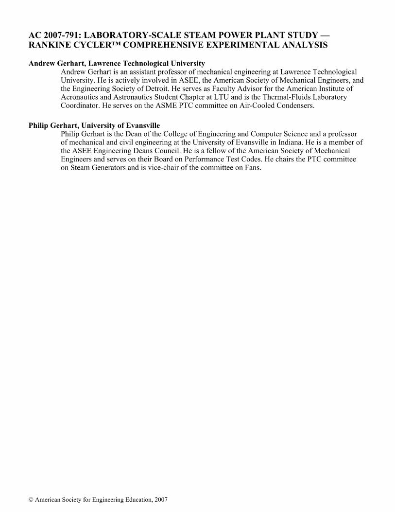
Figure 1. The Rankine Cycler. Note that newer models include a USB port data
acquisition system and laptop computer that is mounted to the tabletop1.
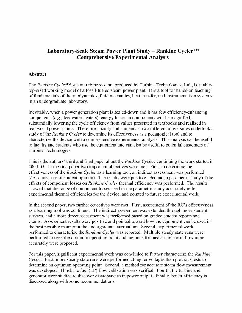
Figure 2: Schematic of the Rankine Cycler1.
AMPS VOLTS BOILER
TURBINE
CO
ND
EN
SE
R
-Qc
BURNER
CONDENSATE COLLECTION
TANK
GENERATOR
Ws out
LP / NATURAL GAS TANK
Fuel flow sensor
Boiler Pressure
Boiler Temperature
Turbine Inlet Temperature
& Pressure
Turbine Exit Temperature
& Pressure
Variable Resistive Load
Steam Admission Valve
Boiler Condenser
Turbine
(beneath round knob)
Generator
Exhaust Tube
(Orange)

Figure 3. The dual pass, flame-through tube type (constant volume) boiler, with super heat
dome1. See Appendix A for more details.
Figure 4. Single stage axial flow impulse steam turbine outside of its casing
1. See
Appendix A for more details.
Previous Study and Current Objectives Lawrence Technological University (LTU) and the
University of Evansville (UE) use the Rankine Cycler in an upper-level laboratory course, and
have completed a comprehensive study of the effectiveness of the RC. This is the third and final
paper, continuing the work started in 2004-05. In the first paper2, two important objectives were
met. First, to determine the effectiveness of the RC as a learning tool, an indirect assessment
was performed; students were surveyed to assess the RC as a learning tool. Preliminary results
showed that the RC and the associated calculations and reports performed quite well as a
learning tool, according to the students. They reported that their knowledge of the Rankine cycle
(and its associated thermodynamic concepts) increased. They indicated that discussing and
operating the RC are more valuable than performing calculations with the data. The level of the
material was appropriately challenging for upper-level engineering students. A few keys to
successful use of the RC were also given in the paper.

Second, a parametric study of the effects of component losses on RC thermal efficiency was
performed. The results showed that the range of component losses used in the parametric study
accurately reflects experimental thermal efficiencies, and the results pointed to future
experimental work that can be accomplished with the RC. The overall conclusion of the paper
was that the benefits of the RC seem to outweigh the idiosyncrasies of the device. For its
relatively low cost, the RC is useful in a mechanical engineering curriculum.
In the second paper3, two more objectives were met which extend and support the conclusions
and recommendations from the first paper. First, assessment of the RC’s effectiveness as a
learning tool was continued. The indirect assessment of the first paper was extended through
more student surveys (from both universities). With the larger sample of surveys, the results
from the first paper were verified. The indirect assessment was also used to compare the RC as a
learning tool between two universities with different geographical locations and RC learning
objectives. The results were favorable and very similar between each university. In addition to
the indirect assessment, a more direct assessment was performed based on graded exam
questions and graded student reports. The assessment of exam questions indicated that the
students understand the small-scale idiosyncrasies of the device, but do not understand how it
differs/compares to a full-scale plant. The graded student reports indicate that the concepts of
thermodynamics are reinforced through use of the RC, and that the students are relatively adept
at performing the associated thermodynamic analysis.
The second objective of the second paper was to extend the comprehensive technical analysis of
the RC. Multiple steady state runs were performed to seek the optimum operating point (i.e., the
load at which RC system or component efficiency is optimum). It was determined that a relative
maximum efficiency is not attainable with current component limitations. The RC should simply
be run at the highest possible load (i.e., wattage, voltage, etc.). Also, a method for measuring
steam flow rate easily and more accurately was suggested, and preliminary calculations with it
were favorable.
For the current paper, four final objectives are met through the completion of significant
experimental work which concludes characterization of the RC. First, several more steady state
runs were performed at higher voltages than previous tests to seek an optimum operating point.
Second, a method for accurate steam flow measurement was tested and is outlined. Third, the
fuel (LP) flow calibration was verified. Fourth, the turbine and generator were studied to
discover discrepancies in power output. In addition, boiler efficiency is discussed along with
some recommendations.
2. Optimum Operating Point
Typical ranges of data gathered from the RC are shown in Table 1. Because the RC has several
significant differences from and is much smaller than a real-world plant, the efficiencies
calculated from the data are inherently low. It would therefore be most beneficial for the
students to use the RC at its highest overall efficiency or optimum operating point.

Boiler Turbine Inlet Turbine Outlet
Pressure (psia) 60 – 120 20 – 27 17 – 19
Temperature (˚F) 350 – 600 300 – 450 275 – 400
Steam mass flow (lb/sec) 0.006 – 0.03
Fuel flow rate (lb/sec) 0.00038
Generator power (W) 2 - 5
Table 1. Typical ranges of RC experimental data.
Multiple steady state runs were carefully performed to determine the optimum operating point
(i.e., turbine/generator performance versus load). There are multiple experimental parameters to
investigate to determine optimum operating point. Figures 5 through 7 display three variations.
Figure 5 shows overall efficiency (generator power divided by fuel energy input) plotted against
generator power output. The relationship appears linear, so a straight line has been fit to the
data. The linear equation is shown on the figure along with the Pearson product moment
correlation coefficient (also known as the “r-squared value” which gives an indication of the
quality of the line fit with 1.0 being a perfect fit). The figure implies that there is not an
optimum point at which to operate the RC; it should simply be run at the highest possible load.
However, at some power output, the efficiency should begin to drop. According to the generator
manufacturer’s specifications, the maximum operating load may be the point at which the
generator RPM is nearly 4500. The data collected with a maximum of 4200 RPM have nearly
covered the operational range. It should be noted that it is difficult to maintain a generator RPM
over 4000 with long-term steady state conditions (i.e., > 60 seconds). Nonetheless, this data
would indicate that the RC should be operated at the highest achievable steady power output.
%Efficiency = 0.0116(Power) + 0.0003
R2 = 0.9996
0.000
0.010
0.020
0.030
0.040
0.050
0.060
0.070
0.0 1.0 2.0 3.0 4.0 5.0 6.0
Generator Power Output (W)
Ov
era
ll E
ffic
ien
cy
(%
)
Figure 5. Overall Efficiency vs. Power Output

Figure 6 shows overall efficiency plotted against generator voltage. Generator RPM is implicitly
indicated since it is related to DC output voltage by RPM = 366.7 V (information supplied by
Turbine Technologies, LTD.). The efficiency vs. voltage trend is similar to the one in Figure 5
but not as distinct. This reinforces the idea that the RC should be run at maximum loading
(maximum speed) for optimum conditions.
Figure 7 shows efficiency plotted with isentropic enthalpy drop from turbine inlet to atmospheric
outlet. The increasing trend is again apparent.
0.000
0.010
0.020
0.030
0.040
0.050
0.060
0.070
0 1 2 3 4 5 6 7 8 9 10 11 12 13
Voltage (RPM = 366.7 V)
Ov
era
ll E
ffic
ien
cy
(%
)
Figure 6. Overall Efficiency vs. Voltage/RPM
0.000
0.010
0.020
0.030
0.040
0.050
0.060
0.070
30 35 40 45 50 55 60
Isentropic enthalpy drop from turbine inlet to atmospheric outlet (BTU/lb)
Ov
era
ll E
ffic
ien
cy
(%
)
Figure 7. Overall Efficiency vs. Isentropic Enthalpy Drop from turbine inlet to
atmospheric outlet

3. Using Turbine Exhaust Tube Pressure Drop to Measure Steam Flow
Possibly the least satisfying aspect of running an experiment with the Rankine Cycler is
determining the steam flow rate. This requires marking the boiler water level (using a sight-
glass) at the beginning and end of the data collection period, waiting a few hours for the system
to cool, then draining and refilling the boiler, noting the volume of water added to move the level
between the two points on the sight-glass. The volume flow rate for the test is then determined
by dividing the make-up water volume by the elapsed time for the run*; mass flow would then be
obtained by multiplying by liquid water density. Steam mass flow rate determined by this
method is highly inaccurate because of the uncertainty involved in marking water level, in
draining and refilling the boiler, and in the differences in density between hot and cold water.
The uncertainty in steam flow rate is likely no better than 10% - probably higher when
inexperienced students are making the measurements. Clearly, a more direct and real-time steam
mass flow measurement is highly desirable.
Possible approaches to obtaining such measurements would involve the installation of a small-
scale flow meter such as an orifice or turbine meter. This would be problematic because it would
require purchasing another instrument and it would introduce yet another pressure drop into an
already highly inefficient system. Such devices would also require calibration, especially a
turbine meter which would be required to operate at elevated temperatures in the steam
environment.
An alternate approach that shows considerable promise is to use the turbine-to-condenser exhaust
tube pressure drop to indicate the steam flow rate. The exhaust tube is a surprising 34.5 inch (88
centimeters) long and contains several bends (See Figure 1 and Figure 8), making the effective
length even longer. The steam pressure drop through the tube is the order of 3 lb/in2 (21 kPa).
In a typical experimental run, the steam at the turbine exit is superheated, and the pressure drop
along the tube ensures that it remains superheated – facilitating modeling the steam as a gas. In
addition to giving a potentially reliable measurement of steam flow, the evaluation of the flow
rate requires students to apply methods from fluid mechanics (compressible or incompressible),
providing one more link between the laboratory and the classroom.
* An alternate method of determining water volume used for a test run: 1) Note the amount of water initially placed
in the boiler. 2) After the test run, let the unit cool and drain the remaining water into a graduated cylinder. 3)
Subtract initial volume from final volume. This method does not account for water used in the process of warming
up the unit.

Figure 8. The turbine exhaust tube as installed on the Rankine Cycler.
With measurements of the turbine exit pressure and temperature (essentially stagnation values)
available and knowing that the steam discharges to atmospheric pressure at the condenser, at
least four different flow models can be used to calculate the steam flow rate. In increasing order
of sophistication they are:
a. Model as incompressible flow in a pipe, using steam density determined from turbine
exhaust conditions
b. Model as incompressible pipe flow, but account for compressibility by using steam
density averaged between tube inlet (turbine exhaust) and tube exhaust conditions. This
requires using the energy equation to determine the steam exhaust temperature, use of the
steam tables, and a few cycles of iteration.
c. Model as compressible, adiabatic, frictional constant area flow (Fanno flow); treat steam
as an ideal gas
d. Model as compressible, adiabatic, frictional flow (Fanno flow); treat steam as a real gas,
using the adiabatic exponent from steam tables and a compressibility factor (pv = ZRT)
Essentially, these four models fall into two categories: “constant” density and Fanno flow.
Model a can be easily derived from Model b and Model c from Model d (by setting Z = 1) so
Exhaust Tube
only Model b and Model d will be developed here. In the subsection after model development,
the calibration of the exhaust tube as a flow measurement device is described, and a resulting
parameter for use in the models is determined. The final subsection compares the various steam
flow measurement methods.
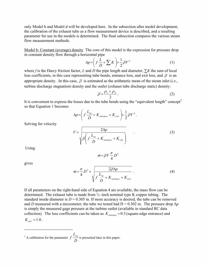
Model b: Constant (average) density The core of this model is the expression for pressure drop
in constant density flow through a horizontal pipe
2
2
1VK
D
Lfp t·Õ
ÖÔ
ÄÅÃ -?F Â (1)
where f is the Darcy friction factor, L and D the pipe length and diameter, ¬K the sum of local
loss coefficients, in this case representing tube bends, entrance loss, and exit loss, and t is an
appropriate density. In this case, t is estimated as the arithmetic mean of the steam inlet (i.e.,
turbine discharge stagnation) density and the outlet (exhaust tube discharge static) density:
2
21 ttt
-? . (2)
It is convenient to express the losses due to the tube bends using the “equivalent length” concept†
so that Equation 1 becomes
2
2
1VKK
D
Lfp exitentrance
eq t·ÕÕÖ
ÔÄÄÅ
Ã--?F .
Solving for velocity
ÕÕÖ
ÔÄÄÅ
Ã--
F?
exitentrance
eqKK
D
Lf
pV
t
2 . (3)
Using
2
4DVm
rt?%
gives
exitentrance
eqKK
D
Lf
pDm
--
F·?
tr 2
4
2% . (4)
If all parameters on the right-hand side of Equation 4 are available, the mass flow can be
determined. The exhaust tube is made from ¼ -inch nominal type K copper tubing. The
standard inside diameter is D = 0.305 in. If more accuracy is desired, the tube can be removed
and D measured with a micrometer; the tube we tested had D = 0.302 in. The pressure drop 〉p
is simply the measured gage pressure at the turbine outlet (available in standard RC data
collection). The loss coefficients can be taken as 5.0?entranceK (square-edge entrance) and
0.1?exitK .
† A calibration for the parameter D
Lf
eqis presented later in this paper.

Determining values for t and D
Lf
eq is somewhat more involved. For preliminary calculations,
f can be evaluated in the usual way, via the Moody Chart or Colebrook-White formula from the
Reynolds number (D
mVD
root %4
Re ?? ) and relative roughness‡. The equivalent length of the pipe
can be estimated from measurement of the actual length (we measured 34.5 inches) plus standard
handbook values for the equivalent length for the 5-90o and 2-45
o bends.
More accurate calculations of steam mass flow rate can be made by calibrating the exhaust tube
to obtain a more representative value for D
Lf
eq. Of course the presence of V (and t ) in the
Reynolds number make the calculations iterative.
The final item needed for Model b is the average density (See Equation 2). The inlet density 1t
can be easily determined because the RC data include exhaust temperature and pressure and the
steam is invariably superheated, so a steam table look-up§ gives the specific volume, * +111 ,Tpv ,
and 1
11
v?t . The tube outlet density is obtained by noting that the exhaust pressure, 2p is
atmospheric (zero gage). A second property for determining the exhaust density is obtained by
using the energy equation**
and assuming that the flow process is adiabatic, giving
2
2
221
Vhh -?
where h is enthalpy, and velocity at 1 is zero.
Solving for h2
* +42
2
2
111
2
212
8
2 D
mT,ph
Vhh
rt%
/?/? (5)
Finally,
* +222
2,
1
phv?t .
In practice, the calculations are iterative (we did them on a spreadsheet). The steps are:
1. Evaluate ot ,),( 111 hv from available 11 ,Tp data using steam property
information
2. Assume a value for m% (The value from the “drain-and-fill” method is a good
starting point)
‡ The exhaust tube is essentially smooth so 0…D
g
§ Actually, we used steam property software ** Left on their own, students will often assume an isentropic process for the tube flow. Although the entire Model b
is approximate, modeling a process whose central feature is fluid friction as isentropic is inappropriate.

3. Calculate Re and f
4. Calculate h2 from Equation 5 (assume 12 vv ? for the first cycle)
5. Determine 22 ,tv from h2, p2 using steam property information
6. Calculate t
7. Calculate a new value for m% from Equation 4 [recall * +gagepp 1?F ]
8. Return to step 3 and repeat until convergence
If mass flow evaluation using Model a is desired, the average steam density, t , is replaced by
the turbine exhaust/tube inlet density 1t and steps 4-6 of the iteration are omitted.
Model d: Adiabatic Compressible Flow of a Real Gas Any number of textbooks on Fluid
Mechanics and/or Gas Dynamics/Compressible Flow develop the theoretical model for adiabatic,
frictional flow of an ideal gas in a constant area duct; a process widely known as Fanno flow
(See, for example references 4,5,6,7,8). The NASA Compressed Gas Handbook9 extends the
model to real gasses by using the “compressibility factor” equation of state, ZRTpv ? . The
essence of the model is to replace “R” everywhere in ideal-gas relationships by “ZR.” In
addition, rather than using the ratio of specific heats, k, the NASA Compressed Gas Handbook
suggests the use of a generalized “isentropic exponent for real gasses,” ks (or i), so that, for
example, the speed of sound is
ZRTkc s? .
Note that values for Z can be obtained from a compressibility factor chart, and ks can be
determined from extensive steam tables (such as those published by ASME). The real gas Fanno
flow model can be adapted to determining the steam flow rate in the RC in a fairly
straightforward manner. Using the development in the NASA Compressed Gas Handbook as the
basis, the following equations and parameters are involved:
‚ Stagnation Properties: * + * + 0210102101 ,,, pppTTT RCRC ??
‚ Mach Number: 21 M,M;ZRTk
V
c
VM
s
?»
‚ Adiabatic flow, no work: 00201 TTT ??
‚ Mass flow rate (evaluated at tube inlet, 101101 ; ppTT ?? ) :
* +12
1
2
11
0
2
01
2
11
4
-/
/
ÕÖÔ
ÄÅÃ /-?
s
s
k
k
s
s Mk
MkZRT
Dpm
r% (6)
‚ Choking length parameter: * +
ÙÚ
×ÈÉ
Ç/-
---
/?
2
2
2
2*
)1(2
1ln
2
11
Mk
Mk
k
k
kM
M
D
Lf (7)
where L* is the length of duct (downstream from the point represented by M) that would
result in flow choking (M = 1)
‚ Stagnation pressure ratio function: * + * +12
1
2
0
0
1
121 /-
ÙÚ
×ÈÉ
Ç-/-
?s
s
k
k
s
s
* k
Mk
Mp
p (8)

where *
0p is the stagnation pressure that would exist at the choking point if the flow were to
become choked (i.e., if L = L*)
‚ Static-to-stagnation pressure ratio (valid for any flow process):
s
s
k
k
s Mk
p
p1
2
0 2
11
//
ÕÖÔ
ÄÅÃ /-? (9)
In flow through a pipe of length L, the Mach number changes from M1 to M2 in accordance with
the relationship
* + * +D
LfM
D
fLM
D
fL **
/? 12 (10)
where the first two terms are calculated by Equation 7 and the latter term from the actual pipe
values of f, L, and D. Additionally, the stagnation pressure change that occurs is calculated by:
* +
* +ÙÙÙÙ
Ú
×
ÈÈÈÈ
É
Ç
?
1*
0
0
2*
0
0
01
02
Mp
p
Mp
p
p
p (11)
where the two pressures on the left are the actual values and the pressure ratios on the right are
evaluated from M1 and M2 using Equation 8.
In theory, the Fanno flow model is complicated by the possibility of choking and the change of
the essential behavior of the flow that occurs at M = 1. Happily for the Rankine Cycler
application, the flow rates are low enough and the tube is short enough that the Mach numbers
remain well below 1.
For application to calculating the flow rate for the RC exhaust tube, we use the measured turbine
outlet/tube inlet pressure, p1, as p01, the measured turbine outlet/tube inlet temperature, T1, as T0,
the atmospheric (absolute) pressure as p2, and D
Lf
eq as
D
Lf . Issues involving f, Re, D and Leq
are identical to those for Model b, discussed above. The calculations now involve a nested
iteration. The object is to determine the inlet Mach number and mass flow rate that cause the
exit static pressure to match the atmospheric pressure. Calculations proceed as follows:
1. Determine values of R, Z, k, and µ appropriate for the steam temperature and
pressure.
2. Assume a value for M1 (0.2 ~ 0.25 is appropriate) to calculate * +1
*
MD
fL and
)( 1*
0
0 Mp
p
3. Calculate mass flow from Equation 6
4. Calculate Reynolds number and friction factor

5. Calculate D
Lf
eq and then * + * + Ù
Ú
×ÈÉ
Ç/?
D
LfM
D
fLM
D
fL eq
1
*
2
*
6. Calculate M2 from Equation 7 by iteration
7. Calculate p2 as * +* +
* +1*
0
0
2*
0
0
2
0
12
Mp
p
Mp
p
Mp
ppp ··?
{i.e.,[p1 × (Equation 9 with M2) × (Equation 8 with M2) / (Equation 8 with M1)]}
8. Compare calculated p2 to absolute atmospheric pressure; if they are not equal
adjust M1 and repeat steps 3-8.
For our calculations, we use an Excel®
spreadsheet. Step 6 is done by fixed point iteration
(actually, we iterate on 2
2M ); about 5 steps is sufficient, starting from an initial guess
12 1.1 MM ? . The overall iteration for M1 is done using the Excel Solver Add-In.
If a mass flow calculation using Model c (ideal gas)††
is desired, simply put Z =1 and use the
ratio of specific heats for k.
Calibration of Exhaust Tube as a Flow Measurement Device While the models outlined above
are interesting, accuracy of flow measurement depends on the information supplied to the model.
In practice, most flow measurement devices such as orifice plates, flow nozzles, or turbine
meters must be calibrated in order to achieve the best accuracy. Calibration data for these
devices is typically expressed in terms of a correction coefficient; for an orifice plate of diameter
d installed in a pipe of diameter D, the working equation would be * +42
14D
d
pdCm d
/
F·?
tr%
with the discharge coefficient, Cd determined by a set of calibration experiments.
While it would certainly be possible to use the correction coefficient approach to express a
calibration for the RC exhaust tube, it seemed more rational and straightforward to use
experimentally determined values for the friction-length parameter, D
Lf
eq. Of course, parts of
this parameter are easily determined, namely the actual tube length and diameter. Essentially,
calibration is required because of the indefinite nature of the friction factor, f, and, especially, the
equivalent length of the bends.
The friction-length parameter is expected to depend on the Reynolds number and, possibly, the
Mach number. Because the Mach number of the steam flow in the exhaust tube is reasonably
low (M ~ 0.25), it was assumed that Mach number effects on the friction-length parameter are
negligible. The calibration experiments were done using cold water. Figure 9 shows the
calibration apparatus.
†† For the actual conditions in a Rankine Cycler run, departure from ideal gas behavior is insignificant (Z à 1) and
there is no discernable difference between Model c and Model d
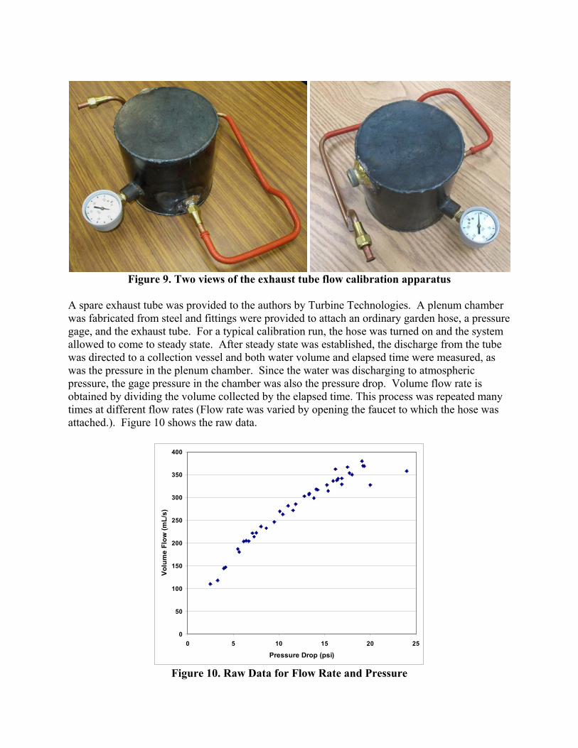
Figure 9. Two views of the exhaust tube flow calibration apparatus
A spare exhaust tube was provided to the authors by Turbine Technologies. A plenum chamber
was fabricated from steel and fittings were provided to attach an ordinary garden hose, a pressure
gage, and the exhaust tube. For a typical calibration run, the hose was turned on and the system
allowed to come to steady state. After steady state was established, the discharge from the tube
was directed to a collection vessel and both water volume and elapsed time were measured, as
was the pressure in the plenum chamber. Since the water was discharging to atmospheric
pressure, the gage pressure in the chamber was also the pressure drop. Volume flow rate is
obtained by dividing the volume collected by the elapsed time. This process was repeated many
times at different flow rates (Flow rate was varied by opening the faucet to which the hose was
attached.). Figure 10 shows the raw data.
0
50
100
150
200
250
300
350
400
0 5 10 15 20 25
Pressure Drop (psi)
Vo
lum
e F
low
(m
L/s
)
Figure 10. Raw Data for Flow Rate and Pressure

The data show a very clear trend, with the exception of the very highest flow rates, where it
appears that between two and six points are outliers. The discrepancy is likely attributed to
difficulty coordinating timing at high flow rates; the three most egregious outliers have been
dropped from the following analysis.
The data of most interest is friction-length parameter versus Reynolds number. The friction-
length parameter was calculated by
5.18 2
42
/F
?Q
Dp
D
Lf
eq
tr
where と is water density, Q is measured volume flow rate, and the “1.5” is the sum of loss
coefficients for the entrance and the exit. Reynolds number is calculated by prD
Q4Re? with p
the kinematic viscosity of the water. Figure 11 shows the friction-length parameter data.
2.0
2.2
2.4
2.6
2.8
3.0
3.2
3.4
3.6
3.8
4.0
2.0E+04 2.5E+04 3.0E+04 3.5E+04 4.0E+04 4.5E+04 5.0E+04 5.5E+04 6.0E+04
Reynolds Number
f(L
eq
/D)
Figure 11. Friction-Length Parameter as Function of Reynolds Number
It is possible to fit the data to a correlation equation; this would suggest 27.0.Re~ /
D
Lf
eq. This
relationship is suspect for two reasons. First, there is considerable scatter in the data, indicating
significant experimental error and little reason for confidence in the fit. Second, the data cover
only a small range of Reynolds number.‡‡
In order to bring more order to the data it was decided
to imbed the Reynolds number dependence in a standard equation for f and then use the
calibration data to determine a value for D
Leq. We chose the Petukov equation for f, mainly
because it is reported to be applicable over a wide range of Reynolds number10
:
‡‡ The actual flow in the RC exhaust tube has Re ~ 2.5x10⁴, which is at the low end of the calibration data.

* + 26417900
//? .ln(Re).f (12)
By dividing each value of D
Lf
eq by f calculated with Equation 12, the results shown in Figure 12
were obtained.
100
110
120
130
140
150
160
170
180
190
2.0E+04 2.5E+04 3.0E+04 3.5E+04 4.0E+04 4.5E+04 5.0E+04 5.5E+04 6.0E+04
Reynolds Number
Le
q/D
Figure 12. Equivalent Length vs. Reynolds Number from Calibration
Clearly D
Leq shows little systematic variation with Reynolds number (~Re
-.08 as-is; if the
remaining three “outlier” values are removed, then ~Re0.001
). The final recommendation is to use
a constant value for D
Leq, calculated by averaging the data
65.336.154 ‒?D
Leq (12)
Combining Equations 11 and 12, the calibration experiments imply that the following expression
be used when calculating Rankine Cycler steam flow from exhaust tube pressure drop data
* +2
64.1ln(Re)790.0
36.154
/?
D
Lf
eq (13)
This equation may be used with any of the flow models.
Comparison of Results for Flow Measurement Steam flow was determined for 8 sets of data
taken from Rankine Cycler runs using Method b, Method d, and the “drain and fill” process.
(The data were taken from the runs previously reported3 and are included in the previous section
on optimum operating point). Figure 13 shows a cross-plot of the flow data.

0.0E+00
1.0E-03
2.0E-03
3.0E-03
4.0E-03
5.0E-03
6.0E-03
0.0E+00 1.0E-03 2.0E-03 3.0E-03 4.0E-03 5.0E-03 6.0E-03
Steam Flow (kg/s) - Drain and Fill Method
Ste
am
Flo
w (kg/s
) - M
odels
b a
nd c
Model bModel d
Linear
Figure 13. Comparison of Three Methods for Measuring Steam Flow
If all three methods were in perfect agreement, the data points would fall on the straight line.
With experimental error, some scatter about the line would be expected. It is clear that Method b
and Method d agree quite well, but neither is in agreement with the “drain and fill” method.
Figures 14 and 15 show the flow measurements plotted against the parameter )(
)(
absoluteT
absolutep .
Figure 14 is for the turbine inlet and Figure 15 is for the turbine outlet.
0.00E+00
1.00E-03
2.00E-03
3.00E-03
4.00E-03
5.00E-03
6.00E-03
11.2 11.4 11.6 11.8 12 12.2 12.4 12.6 12.8 13
Pressure/SQRT(Temperature)@Turbine Inlet
Ste
am
Flo
w k
g/s
Drain/Fill
Model b
Model d
Figure 14. Measured Flow vs Turbine Inlet Compressible Flow Parameter

0.00E+00
1.00E-03
2.00E-03
3.00E-03
4.00E-03
5.00E-03
6.00E-03
5.3 5.4 5.5 5.6 5.7 5.8 5.9 6
Pressure/SQRT(Temperature) @ Turbine Exit
Ste
am
Flo
w k
g/s
Drain/Fill
Model b
Model d
Figure 15. Measured Flow vs Turbine Exit/Exhaust Tube Inlet Compressible Flow
Parameter
For any compressible flow process or device, the mass flow should correlate with Tp , at
least to a good approximation. It is clear that steam flow determined by Methods b and d
correlate reasonably well with this parameter; it is equally clear that steam flow determined by
“drain and fill” does not correlate.
Finally, consider correlation with the measured generator power output. Figure 16 shows steam
flow determined by Method b and by “drain and fill” plotted against power. One would expect
at least a rough correlation between flow and power if the turbine inlet properties are held
relatively constant.
1.0E-03
1.5E-03
2.0E-03
2.5E-03
3.0E-03
3.5E-03
4.0E-03
4.5E-03
5.0E-03
5.5E-03
6.0E-03
1 1.5 2 2.5 3
Generator Power (Watts)
Ste
am
Flo
w (
kg
/s)
Model b
Drain/Fill
Figure 16. Steam Flow vs Generator Power

While the situation is perhaps not as clear as the previous three figures, it is at least possible to
imagine a correlation between power and Method b flow, but again, there seems to be no
correlation between power and “drain and fill” flow.
There are two questions to be answered: First, which of the two exhaust tube based methods is
best; second, what is the best method for actually determining the steam flow? As shown in
Figures 12-14, there is little difference between values of steam flow calculated from the same
data by Methods b and d. Values calculated by Method b are always slightly lower than those
calculated by Method d; this is probably because b explicitly accounts for local losses at the tube
inlet while d ignores them. Because the Mach number is inherently low, the “average density”
model (Model b) is an excellent approximation to the actual compressible flow.
The second question is the more important; which type of method gives the better answer (or,
more significantly, which is closer to the correct answer). Unfortunately, the question of
absolute accuracy must remain open, because no “true” values for steam flow are available. It is
clear, however, that the “exhaust tube” methods are consistent with the basic physics of the
system and produce results with high precision, while the “drain and fill” method, at least as
executed by typical students, produces wildly varying, and hence unreliable, results. For this
reason alone, the exhaust tube methods are to be preferred.
Aside from the question of accuracy, there are three other reasons to prefer exhaust-tube-based
methods. First, the method can provide steam flow data in real time. It would certainly be
possible to incorporate coding in the data acquisition program to indicate steam flow
continuously in the same way that pressure, temperature, and fuel flow are. Second, all results
are in hand when the laboratory session is complete; there is no need to wait for the system to
cool and depressurize and then return to do the drain and fill. The third advantage is
pedagogical. The exhaust tube methods introduce the disciplines of fluid mechanics and
compressible flow into an RC experiment, thus enriching the learning experience.
For all of these reasons, the authors strongly recommend that users of the Rankine Cycler
abandon the “drain and fill ” procedure and instead use the exhaust tube method for steam flow
determination.
4. Fuel (LP) Flow Calibration
A second flow rate is needed for a Rankine Cycler experiment: the fuel gas (propane or natural
gas) flow§§
. Ultimately, the mass flow rate of propane is needed so that the energy input to the
unit can be determined. In addition to the fuel flow rate, the heating value of the fuel is required.
Generally likelihood of an error can be avoided by using a mass-based heating value with mass
flow rate as opposed to volume flow rate and volume-based heating value. This is because of the
inevitable confusion about what temperature and pressure to which the volume-based quantities
are referred.
§§ The RC units owned by LTU and UE both operate on liquid propane (LP) gas

The RC comes from the manufacturer equipped with an in-line turbine flow meter for fuel gas
volume flow measurement. The data are displayed on the computer in units of liters/minute.
There are two issues that might arise concerning this measurement. First, in some early units, a
volume flow correction factor was needed. Apparently, the turbine meters are calibrated with air
flow and in these early units, it was necessary to correct the volume flow by multiplying by a
factor corresponding to Density Propane
DensityAir; the manufacturer gave this factor as
5311
.. Later
units have this factor incorporated into the data acquisition software. The issue is knowing
which type of unit one has.
The second issue involves the seeming ubiquitous question of determining appropriate
conditions of pressure and temperature to associate with the volume flow. This is important
because users must either evaluate density to use with volume flow to obtain mass flow or,
alternately, obtain fuel volumetric heating values that match the volume flow reference. The
perennial question is: “Do I use the pressure and temperature values corresponding to those that
existed when the turbine meter was calibrated, or do I use values that exist in the laboratory
when the experiment was run, or do I use some ‘standard’ value?”
These two issues can be avoided by measuring mass flow instead of volume flow, or at least a
few mass flow measurements can be made simultaneously with the volume flow measurements
so that questions of pressure, temperature, and density can be sorted out. If the RC is fueled
from a “standard” propane bottle such as is used on a gas grill, obtaining a reference LP flow is
relatively easy. To do this, we set the propane bottle on a digital scale capable of high precision
measurement. Students simply note the indicated weight of the gas bottle at the beginning of a
run and at the end of a run. The difference in weight can be converted to mass and divided by
the elapsed time to determine the mass flow average. A few such runs can be used to cross-
check the volume flow-based data to determine if the “correction factor” is needed and to
determine appropriate values for reference pressure and density. Alternatively, the scales can be
used for every run to give an independent reading for fuel flow, enhancing accuracy.
The tank-weighing method was investigated at the University of Evansville, leading to a very
helpful outcome. When UE’s Rankine Cycler was acquired, the information available indicated
that it was an “old-type” unit which required that the indicated volume flow rate be corrected
from an “air” value to a “propane” value. The operational assumption was that the fuel flow
meter had been calibrated using air at 740 mm.Hg pressure and 23oC, so that the indicated
volume flow would be multiplied by 531
1.
to produce the correct propane flow. Mass flow
was then obtained by multiplying by the density of propane at 740 mm.Hg pressure and 23oC
(0.001764 kg/L). Table 2 shows the results of two runs made by students in Spring 2006.
Indicated Volume
Flow(L/min)
"Corrected" Volume Flow
(L/min) Propane
Used (kg) Time (min)
"Corrected" Mass Flow
(kg/min)
Uncorrected Mass Flow
(kg/min)
Mass Flow 〉m/〉t
(kg/min)
6.17 4.99 0.073 5.842 0.00880 0.01088 0.01250
6.19 5.00 0.055 5.068 0.00883 0.01092 0.01085
Table 2. Comparison of Fuel Flow Results

These data clearly indicated that the correction factor should not be applied in UE’s unit;
although it is inconclusive as to whether to use the propane density at the calibration conditions
of 740 mm.Hg and 23oC or at the actual laboratory conditions, which were fortuitously nearly
the same as the calibration conditions.
5. The Turbine Enigma
In attempting to model and evaluate the components of the Rankine Cycler, the authors have
uncovered some serious issues; collectively we call these the “Turbine Enigma”. In general,
there are discrepancies among the actual generator output, the calculated turbine output, and the
maximum theoretical output. The essential points are outlined as follows.
The following are either given (by the manufacturer) or assumed/deduced information about the
steam turbine, the generator, and the steam property data acquisition system:
‚ The turbine is a single-stage impulse type.
‚ The turbine is directly coupled to the generator so that
TURBINE RPM = GENERATOR RPM .
‚ GENERATOR RPM is related to DC output voltage by RPM = 366.7 V (this information
supplied by Turbine Technologies and verified in a 2006 e-mail correspondence).
‚ Sensors for turbine inlet steam properties ( p, T ) and outlet steam properties ( p, T ) are
located in (relatively) large volume “plenum” regions indicating that the properties
measured are stagnation values.
‚ Steam turbine wheel diameter is about 2.0 inches (Information supplied by Turbine
Technologies).
Using as a typical set of experimental data “Run 11/23/04-1” from LTU (reported to be
“excellent data” – data from this run were included in the authors’ previous paper2) the following
have been measured and calculated:
‚ Steam flow: 0.00305 kg/s (roughly verified by “turbine exhaust tube pressure drop”
calculation)
‚ Voltage: 6.03 V
‚ Generator Output Power: 1.99 W
‚ Enthalpy drop in turbine (from p, T measurements and steam tables): 10.65 Btu/lb
Using these values, various specific energy terms can be calculated:
‚ Enthalpy drop ( kgJBtuJkglblbBtu /700,24)/1054/2.2/65.10 ?··
‚ Specific work from enthalpy drop ( 0;0;0 …F?F… KEPEq so hw F… =) 24,700 J/kg
‚ Maximum possible work extraction by a single-stage impulse turbine (See Appendix A)
* +22
22
max 03.67.36660
20254.0
2
0.22
60
2
2222 Õ
ÖÔ
ÄÅÃ ·····?Õ
ÖÔ
ÄÅÃ??? V
V
RPM
in
minRPM
DrUw
rry
kgJw /2.69max …

‚ Specific work indicated by generator output kgJskg
W
m
Pw
gen/653
/00305.0
99.1???
%
The first point to note is that instead of maxwww hgen …… F as expected, we have hgen ww F…40
1,
which implies a very inefficient generator and/or a very low system mechanical efficiency.
Even more surprising is that max10wwgen … , which implies that the system violates both the First
and Second laws of thermodynamics, as well as Newton’s Second Law (in the form of the
Moment of Momentum equation)!
If we redo the calculations on a power basis instead of a specific work basis:
WPWPWP possibledropenthalpygen 21.0;75;99.1 max ???
again one unlikely and one “impossible” situation.
The differences between enthalpy drop work/power and generator values could possibly be
explained by heat loss to the relatively massive turbine housing and the surroundings, together
with mechanical and generator inefficiency (although significant heat loss would be one more
serious discrepancy between the RC and a real world power plant). Preliminary estimates seem
to imply that heat loss alone is not sufficient to account for the observed difference.
The discrepancy between maximum power and measured (electrical) power is more serious, as it
implies the violation of all three of Mechanical Engineering’s most sacred laws. The authors
have investigated several possibilities. Of course, an obvious culprit would be the comparison of
“theory” with the “real world”; however, the theory predicts the maximum work/power under
ideal conditions. The real work/power would certainly be expected to be lower than the ideal;
but a real power ten times the ideal is predicted.
The next suspect is the data. Independent measurements of generator voltage and current have
verified the RC-measured values – verifying the electrical power output. The steam flow is
certainly a questionable measurement, but the “standard” (drain-and-fill) method has been
verified by the exhaust tube pressure drop method. (Recall, we are searching for a 1000% effect
– not a 10% effect)
The final item to consider is the rotational speed. As noted above, the RPM/Voltage relationship
has been verified by the manufacturer by mounting a typical RC generator on a precision milling
machine spindle and measuring the voltage and speed. Separate stroboscopic measurements of
generator speed by the authors has essentially confirmed the speed at about 2200 RPM. No one
has confirmed the turbine rotor speed; however drawings and photographs of the disassembled
turbine indicate a direct drive between turbine wheel and generator.
It is instructive to consider what would be an appropriate speed for the turbine wheel, given the
actual size of the wheel, the existing nozzle and blade geometry and the actual operating
pressures and temperatures of the RC. First consider the steam velocity leaving the nozzle.
Using an ideal gas model for the superheated steam, the velocity can be calculated by

21
1
1 12
ÙÙÙ
Ú
×
ÈÈÈ
É
Ç
ÕÕÕ
Ö
Ô
ÄÄÄ
Å
Ã
ÕÕÖ
ÔÄÄÅ
Ã/···?
/k
k
etTurbineInl
austTurbineExhetTurbineInlpN
p
pTcC j
Using values typical for a Rankine Cycler run
psiapsigppsiapsigpRFTkRlbm
Btuc outinop 7.173;7.2410;760300;3.1;*
48.0 ?…?…?………
and assuming for the “slot” nozzles %75…Nj gives
sec
ft
lbfft
Btu
seclbf
lbmftR
Rlbm
BtuC 1007
*16.778
*
*174.32
7.24
7.171760
*48.075.02
21
2
231.0
1 ?ÙÙÚ
×
ÈÈÉ
Ç··Õ
ÕÖ
ÔÄÄÅ
ÃÕÖÔ
ÄÅÃ/····…
For the “optimum” impulse turbine, the blade speed should be about one-half the inlet absolute
velocity (2
1
1
…C
U), so the blade speed should be
sec
ftU 500… and the rotational speed for a 2-inch
wheel should be
RPMsec
rad
ft
sec
ft
r
U000,576000
0833.0
500
………?y .
The maximum work would then be
* + lbBtuUw /2016.778174.32/50022 22
max …··…?
which is much more in line with the observed enthalpy drop of about 10 Btu/lb.
Having exhausted all of the possibilities (electrical data, steam flow data, speed/voltage
correlation, turbine speed/generator speed relationship) the authors can find no rational
explanation for the generator work/power being (significantly) larger than the “maximum”
values. Any resolution of this dilemma would be very welcome.
6. Boiler Efficiency
If students are asked to develop a theoretical model of the entire unit, then information on boiler
efficiency is needed. In a typical power plant, boiler efficiency is defined by:
fuel
steam
Boiler)HHVm
)hm
fuelinEnergy
toSteamaddedHeat
%
%Fj ?» . (14)
For simple boilers (e.g., gas-fired units), efficiency may be determined from measurements of
the parameters in this equation. For actual power plant boilers, especially those fired by coal,

boiler efficiency is determined by using the so-called energy balance method (also called the loss
method), in which the energy losses per unit fuel energy input are subtracted from 100%. This
method has the advantage of higher accuracy but requires chemical analysis of the fuel and
measurements of exhaust temperature and chemical composition. The ASME Performance Test
Code for Fired Steam Generators can be consulted for details11
.
The parameters required for Equation 14 can be determined relatively easily, if not accurately.
Steam and fuel flow rates are determined as part of a typical RC experimental run, either by the
traditional methods or as discussed in this paper. Fuel HHV (Higher Heating Value) is also
determined in a typical run. The only questionable quantity is the enthalpy rise of the steam.
Boiler outlet enthalpy is easily determined from measured boiler pressure and temperature; it is
the boiler “inlet” enthalpy that is the problem. Of course, since the RC does not operate in a
steady flow mode, there is no “input” enthalpy during a run. That leaves three seemingly logical
choices for evaluating input enthalpy:
1. Assume hsteam in = 0 (Essentially, specifying the input as liquid at 32oF).
2. Evaluate the enthalpy of liquid water at the temperature of the make-up water used to
fill the boiler.
3. Use the enthalpy of saturated liquid water evaluated at the boiler discharge pressure
(or essentially, the enthalpy of the water that is being evaporated to steam during a
run).
In reality, none of these choices makes much sense; in fact using some of them can result in a
computed boiler efficiency greater than 100%! Choices 1 and 2 include the energy used to pre-
heat the water and heat up the boiler metal parts to the operating temperature as useful (steady
state) output, while choice 3 excludes any energy used to heat the water to saturation temperature
and is influenced by “free” heat from pre-heated boiler parts and by any steam that is generated
from dropping boiler pressure during the transient process. In short, because the boiler
undergoes a transient process, conventional concepts of boiler efficiency are meaningless, at
least in terms of measurement. If a value for boiler efficiency is desired for a comprehensive
steady-flow analytical model of the RC, it is safe to assume that the RC boiler efficiency is
around 85% which is within the typical range of 75% to 95% for full-scale power plant
boilers12***
.
It is perhaps meaningful to inquire about the boiler’s combustion efficiency, defined as the
energy generated by burning the fuel divided by the fuel heating value. Combustion efficiency is
less than 100% if some portion of the fuel is unburned. Determination of this efficiency would
require a chemical analysis of the boiler exhaust gas stream to determine the presence of
unburned carbon or hydrogen. Such an analysis is probably beyond the scope of an investigation
of the RC as a steam-cycle device. In any event, the combustion efficiency is probably very near
100% as the fuel is gas and the air supply and air/fuel mixing of the RC are well-designed.
*** For a gas-fired boiler such as that on the RC, the dominant losses would be “dry gas loss” (i.e., energy in the hot,
dry products of combustion in the exhaust stack) and “water from Hydrogen in fuel loss” (i.e., enthalpy of
vaporization of any H2O formed from combustion of Hydrogen).

7. Recommendations
Besides the general RC characterization given in this paper and the previous two papers2,3
, some
further work is recommended to characterize any given individual RC. The following three
studies may enhance the usefulness of the RC to determine parameters such as output and
efficiency.
1. Boiler Performance: If an RC user (e.g., student or instructor) deems boiler combustion
efficiency determination a useful exercise, it should be investigated for various operating
conditions. As a minimum, boiler combustion efficiency determination will require exhaust gas
unburned carbon and, possibly, hydrogen measurements.
2. Generator Performance: An investigation of generator efficiency, separate from the turbine,
should be made.
3. Second Law Analysis: An exercise of considerable educational value would be to conduct a
Second Law analysis of the unit. Because of its small scale, and high losses together with the
rather complete set of thermodynamic data available, the RC is an excellent device for
performing a second law analysis. Not only would the students benefit from performing a
second law analysis (a topic that receives little or no coverage in the required Thermodynamics
courses at LTU and UE), it would also give a better understanding of scaling drawbacks and help
identify the major sources of losses.
8. Conclusions
Pedagogical and experimental characterization of the Rankine Cycler has been carried out in
three papers, of which this is the last. Pedagogically, the RC has been shown to be a useful
device, as shown by both subjective and objective assessment2, 3
. Several experimental
investigations have been carried out; they have two general objectives:
‚ First, to suggest improvements to data collection methods and to investigate optimum
operating conditions
‚ Second, to experimentally characterize RC components, with the aim of allowing
users (faculty or students) to construct an analytical model of the unit.
We consider that the first objective has been successfully met. Major contributions are the
development of a more accurate, real-time method for measuring steam/water flow by using the
pressure drop along the exhaust tube, the investigation of a direct-weighing method for checking
fuel flow meter calibrations, and determining the optimum operating point for the unit.
The component characterizations are of less value. Our studies showed that the two major
components, the boiler and turbine, cannot be reasonably characterized from experiments. The
boiler efficiency cannot be determined because it is an ill-defined concept in this transient flow
system. Probably the most significant uncharacterized component is the turbine; the issue
identified by us as the “Turbine Enigma” is, at least to us, a barrier to any further attempts to

characterize the turbine performance. We were successful, however, in characterizing the
turbine exhaust tube!
Based on our extensive studies, we conclude that the Rankine Cycler is of most value 1) when
used to give the students an opportunity to observe and operate a real power plant, 2) when used
to generate real-world data for calculations, and 3) for illustrating real-time, computer-based data
acquisition in the thermal sciences. On the other hand, because of the idiosyncrasies of the
transient operation, the extremely small scale of the system, and the difficulties in characterizing
the principal components, the Rankine Cycler is not a good basis for an analytical model of a
power generating system. In conclusion, if used for the proper objectives, the educational
benefits of the RC can outweigh the idiosyncrasies of the device. For its relatively low cost, the
RC is useful in the mechanical engineering curriculum.
Acknowledgements
The authors would like to thank Turbine Technologies, Ltd.; Wolfgang Kutrieb, Perry Kuznar,
and Toby Kutrieb for their helpfulness, insights, and contributions to ensuring smooth running
devices; Juan Neira (LTU), Jonathan Corbett (UE), and Jesse Kahle (UE) for their experimental
work and initial set-up of the analysis Excel spreadsheets; and Amol Jambhekar (LTU) and
Mohammed Mazharuddin (LTU) for their experimental trials.
References
1. Turbine Technologies, Ltd., Steam Turbine Equipment, 2002.
2. Gerhart, A. L. and Gerhart, P. M., 2005, “Laboratory-Scale Steam Power Plant Study – Rankine CyclerTM
Effectiveness as a Learning Tool and its Component Losses,” Proceedings of the 2005 American Society
for Engineering Education Annual Conference and Exposition.
3. Gerhart, A. L. and Gerhart, P. M., 2006, “Laboratory-Scale Steam Power Plant Study – Rankine CyclerTM
Effectiveness as a Learning Tool and a Comprehensive Experimental Analysis,” Proceedings of the 2006
American Society for Engineering Education Annual Conference and Exposition.
4. Gerhart, P. M., Gross, R. J., and Hochstein, J. I., Fundamentals of Fluid Mechanics, 2nd ed., Addison-
Wesley, 1992.
5. Munson, B. R., Young, D. F., and Okiishi, T. H., Fundamentals of Fluid Mechanics, 5th ed., John Wiley &
Sons, 2006.
6. White, F.M., Fluid Mechanics, 5th ed., McGraw-Hill, 2003.
7. Shapiro, A., The Dynamics and Thermodynamics of Compressible Fluid Flow, Vol 1, Ronald Press, 1953.
8. Saad, M. A., Compressible Fluid Flow, 2nd ed., Prentice-Hall, 1993.
9. Kunkle, J. S., Wilson, S. D., and Cota, R. A., Compressed Gas Handbook, NASA SP 3045, National
Aeronautics and Space Administration, 1969.
10. Petukhov, B.S. in T.F. Irvine and J.P. Hartnett, Eds., Advances in Heat Transfer, Vol 6, Academic Press,
1978.
11. American Society of Mechanical Engineers; PTC 4; Performance Test Code for Fired Steam Generators;
American Society of Mechanical Engineers,; 1998
12. Black and Veatch, Edited by Drbal, L.F., Power Plant Engineering, 1996, Chapman & Hall, NY, p. 173

Appendices
A. Experimental Apparatus Descriptions1
The experimental hardware (Rankine Cycler™) consists of multiple components that make up
the necessary components for electrical power generation (utilizing water as the working fluid).
These components include:
1. Boiler
A stainless steel constructed, dual pass, flame-through tube type boiler, with super heat dome,
that includes front and rear doors. Both doors are insulated and open easily to reveal the gas
fired burner, flame tubes, hot surface igniter and general boiler construction. The boiler walls
are insulated to minimize heat loss. A side mounted sight glass indicates water level.
2. Combustion Burner / Blower
The custom manufactured burner is designed to operate on either LP or natural gas. A solid-state
controller automatically regulates boiler pressure via the initiation and termination of burner
operation. This U.L. approved system controls electronic ignition, gas flow control and flame
sensing.
3. Turbine
The axial flow steam turbine is mounted on a precision-machined stainless steel shaft, which is
supported by custom manufactured bronze bearings. Two oiler ports supply lubrication to the
bearings. The turbine includes a taper lock for precise mounting and is driven by steam that is
directed by an axial flow, bladed nozzle ring. The turbine output shaft is coupled to an AC/DC
generator.
4. Electric Generator
An electric generator, driven by the axial flow steam turbine, is of the brushless type. It is a
custom wound, 4-pole type and exhibits a safe/low voltage and amperage output. Both AC and
DC output poles are readily available for analysis (rpm output, waveform study, relationship
between amperage, voltage and power). A variable resistor load is operator adjustable and
allows for power output adjustments.
5. Condenser Tower
The seamless, metal-spun condenser tower features 4 stainless steel baffles and facilitates the
collection of water vapor. The condensed steam (water) is collected in the bottom of the tower
and can be easily drained for measurement/flow rate calculations.
6. Data Acquisition (Note: Newer RC models have an updated system that will operate through
the USB port of any newer PC.)
The experimental apparatus is also equipped with an integral computer data acquisition station,
which utilizes National Instruments™ data acquisition software (modified 2004 models).
The fully integrated data acquisition system includes 9 sensors. The sensor outputs are
conditioned and displayed in “real time”- on screen. Data can be stored and replayed. Run data

can be copied off to floppy for follow-on, individual student analysis. Data can be viewed in
Notepad, Excel and MSWord (all included).
The system is test run at the factory prior to delivery and the “factory test run” is stored on the
hard drive under the “My documents” folder. This file should be reviewed prior to operation, as
it gives the participant an overview of typical operating parameters and acquisition capability.
7. Sensors
Nine (9) sensors are installed at key system locations. Each sensor output lead is routed to a
centrally located terminal board. A shielded 64-pin cable routes all data to the installed data
acquisition card. This card is responsible for signal conditioning and analog to digital
conversion. Software and sensor calibration is accomplished at the factory prior to shipment.
Installed sensor list includes:
‚ Boiler pressure
‚ Boiler temperature
‚ Turbine inlet pressure
‚ Turbine inlet temperature
‚ Turbine exit pressure
‚ Turbine exit temperature
‚ Fuel flow
‚ Generator voltage output
‚ Generator amperage output
8. Overall System Dimensions
Length: 48.0 inches (122 cm)
Width: 30.0 inches (77 cm)
Height: 58.0 inches (148 cm)
B. Analysis of Axial Flow Impulse Turbine with Application to Rankine Cycler
Figure B.1 shows one blade of an axial flow impulse turbine. The linear speed of the blade is U
and is the product of blade radius and angular velocity (rotational speed). The blade speed is the
same on either side of the wheel. Station (1) is the inlet and station (2) is the discharge. In the
velocity diagrams, W is the velocity relative to the blade and C is the absolute velocity (relative
to the nozzle and casing).

Figure B.1 Axial Flow Impulse Turbine Blade with Velocity Diagrams
In an impulse turbine, all of the pressure drop occurs in the nozzle. This produces a relatively
large steam velocity (C1). Because the flow through the rotor occurs at constant pressure, an
impulse turbine can use partial admission, with a finite number of jets of steam placed around
the wheel. The Rankine Cycler turbine uses partial admission, with several slot nozzles directing
steam onto the turbine blades. Because there is no pressure drop in the wheel (blades), all of the
work is done by turning the fluid and there is a large change in C (C2 << C1).
An ideal impulse turbine stage has the following characteristics:
‚ The fluid enters and leaves the blade perfectly (W1 & W2 tangent to blade surface)
‚ There is no heat transfer
‚ There is no friction between fluid jet and blade
Combining the last two implies that the ideal flow process is isentropic.
Now consider the relationship between the inlet and outlet velocities. Since the pressure is
constant, the flow relative to the blade is neither accelerated nor decelerated, therefore
W2 = W1.
Conservation of mass for the (steady) flow through the stage demands
* + * +hsChsC aa ·?· 2211 tt
W1
U
C1
U = rの
U
C2
W2
Nozzle

where s is the blade-to-blade spacing, h is the blade height, and Ca is the axial velocity
component (perpendicular to U). Because pressure, entropy, and enthalpy are all unchanged
across the blade row, density is also unchanged and
21 aa CC ?
also, from the velocity diagram
2211 aaaa WCCW ???
This means that the altitude of both velocity triangles is the same.
Now consider the maximum possible specific work extraction from the steam. This will be
examined two different ways: from an energy perspective and from a momentum perspective.
Energy
Obviously, the maximum work extraction requires that the bulleted conditions above be satisfied
(no heat loss, no friction). Because there is no heat loss and no enthalpy change, the energy
balance becomes
22
2
2
2
1 CCw /?
(i.e., all of the work comes from changing the fluid kinetic energy). The inlet kinetic energy is
set by the nozzle process so C1 cannot be affected by the blade. The maximum work will be
realized when C2 is smallest. Because Ca2 is fixed by mass flow rate, C2 will be smallest when it
is perpendicular to U (i.e., when C2 = Ca2 and Cu2 = 0). Thus
2222
2
1
2
2
2
1
2
1
2
2
2
1max
UaaUa CCCCCCw ?
/-?/? because 21 aa CC ?
From the velocity diagrams
11 UU WUC -?
But
12 WW ? so 2
2
2
1 WW ?
and thus 2
2
2
2
2
1
2
1 aUaU WWWW -?- .
However
21 aa WW ? so 2
2
2
1 UU WW ?
and

21 UU WW ? .
For the maximum work condition, the exit diagram would be a right triangle, with UWU ?2
Substituting into the work equation
* + * + 2
22
1
2
1
max 2222
UUUWUC
w UU ?-
?-
?? .
Momentum
Euler’s turbine equation (from the Moment of Momentum equation) is
2211 UU CUCUw /?
Obviously, the work will be maximum when 022 ?UCU (i.e., when the outlet velocity is
perpendicular to U [once again, a right triangle]). The maximum work is
11max UCUw ?
From the analysis above
* + * + * + 2
211max 2UUUUWUUWUUUCw UUU ?-?-?-??
So by either energy or momentum, the maximum possible specific work output for an impulse
turbine is
wmax = 2U 2
Related Documents


