Abundance gradient slopes versus mass in spheroids

Mon. Not. R. Astron. Soc. 407, 1347–1359 (2010) doi:10.1111/j.1365-2966.2010.17007.x

Abundance gradient slopes versus mass in spheroids: predictionsby monolithic models

Antonio Pipino,1,2� Annibale D’Ercole,3 Cristina Chiappini4,5

and Francesca Matteucci1,5

1Dipartimento di Fisica, sez.di Astronomia, Universita di Trieste, Via G.B. Tiepolo 11, 34100 Trieste, Italy2Department of Physics and Astronomy, University of California, Los Angeles, 430 Portola Plaza, Box 951547, Los Angeles, CA 90095, USA3INAF–Osservatorio Astronomico di Bologna, via Ranzani 1, 40127 Bologna, Italy4Observatoire de Geneve, Universite de Geneve, 51 Chemin de Mailletes, CH1290 Sauverny, Switzerland5INAF, Osservatorio Astronomico di Trieste, Via G.B. Tiepolo 11, 34100 Trieste, Italy

Accepted 2010 May 10. Received 2010 April 26; in original form 2009 June 18

ABSTRACTWe investigate whether it is possible to explain the wide range of observed gradients inearly-type galaxies in the framework of monolithic models. To do so, we extend the set ofhydrodynamical simulations by Pipino et al. by including low-mass ellipticals and spiral (true)bulges. These models satisfy the mass–metallicity and the mass–[α/Fe] relations. The typicalmetallicity gradients predicted by our models have a slope of −0.3 dex per decade variationin radius, consistent with the mean values of several observational samples. However, we alsofind a few quite massive galaxies in which this slope is −0.5 dex per decade, in agreementwith some recent data. In particular, we find a mild dependence from the mass tracers when wetransform the stellar abundance gradients into radial variations of the Mg2 line-strength index,but not in the Mgb. We conclude that, rather than a mass–slope relation, is more appropriate tospeak of an increase in the scatter of the gradient slope with the galactic mass. We can explainsuch a behaviour with different efficiencies of star formation in the framework of the revisedmonolithic formation scenario, hence the scatter in the observed gradients should not be usedas an evidence of the need of mergers. Indeed, model galaxies that exhibit the steepest gradientslopes are preferentially those with the highest star formation efficiency at that given mass.

Key words: Galaxy: bulge – galaxies: bulges – galaxies: elliptical and lenticular, CD –galaxies: evolution – galaxies: formation.

1 IN T RO D U C T I O N

Negative metallicity radial gradients in the stellar populations area common feature in spheroids (e.g. Carollo, Danziger & Buson1993; Davies, Sadler & Peletier 1993) and must be predicted byevery theory for the formation of elliptical galaxies. A possible fin-gerprint of a given galaxy formation scenario might be the (lack of)correlation between gradient properties (e.g. the slope) and eitherglobal galactic properties (namely mass, stellar velocity disper-sion σ , total magnitude) or central ones (e.g. central metallicity or[〈α/Fe〉]). From the theoretical point of view, in fact, steep metallic-ity gradients are expected from classical dissipative collapse models(e.g. Larson 1974; Chiosi & Carraro 2002) and their (revised) up-to-date versions which start from semi-cosmological initial condi-tions (e.g. Kawata 2001; Kobayashi 2004). The abundance gradientarises because the stars form everywhere in a collapsing cloud and

�E-mail: [email protected]

then remain in orbit with a little inward motion,1 whereas the gassinks further in because of dissipation. This sinking gas contains thenew metals ejected by evolving stars so that an abundance gradientdevelops in the gas. As stars continue to form, their compositionreflects the gaseous abundance gradient. The original dissipativemodels predict a steepening of the gradient as the galactic mass in-creases, mainly because the central metallicity is quickly increasingwith mass,2 whereas the global one has a milder variation (Carlberg1984). At the same time, they predict metallicity gradient as steepas −0.5 dex per decade variation in radius. On the other hand, thefew attempts to study the gradients in the merger-based models hintfor very shallow (if any) gradient (Bekki & Shioya 1999), less steepthan the mean observational values and than the predictions from

1 Stars will spend most of their time near the apocentre of their orbit.2 The fit of the mass–metallicity relation, namely the increase of the meanmetal content in the stars as a function of galactic mass (O’Connel 1976),was the main success of these original models.

C© 2010 The Authors. Journal compilation C© 2010 RAS

Dow

nloaded from https://academ

ic.oup.com/m

nras/article/407/2/1347/1128554 by guest on 21 January 2022

1348 A. Pipino et al.

monolithic collapse models. Moreover, it seems that dry mergersflatten pre-existing gradients (Di Matteo et al. 2009). Indeed, whenthe two scenarios (monolithic collapse and mergers) are consideredas two possible channels working at the same time, the scatter inthe predicted gradients for such a population of galaxies seems tobe in agreement with observations (Kobayashi 2004).

More recently, observations showed that successful models forelliptical galaxies should also reproduce the [〈α/Fe〉]–mass relation(Worthey, Faber & Gonzalez 1992, Thomas et al. 2007) as well asthe observed gradients in the [〈α/Fe〉] ratios (Mehlert et al. 2003;Annibali et al. 2007; Sanchez-Blazquez et al. 2007; Rawle et al.2008). Indeed, these observations show that the slope in the [〈α/Fe〉]gradient has a typical value close to zero and does not correlate withmass.

These observations have been interpreted by Pipino, D’Ercole& Matteucci (2008a, hereafter Paper I) 1D hydrodynamical codeas the fact that the suggested outside-in mechanism for the forma-tion of the ellipticals is not the only process responsible for theformation of gradients in the abundance ratios. Other processesshould be considered such as the interplay between the star forma-tion (SF) time-scale and gas flows. While such an interplay flattensthe [〈α/Fe〉] gradient to the value required by observations, it stillenables galaxies to harbour gradients in [〈Fe/H〉] and [〈Z/H〉] inagreement with the most recent observations (see Section 2). Pipino,Matteucci & D’Ercole (2008b, Paper II) calibrated such a model bymeans of the resolved stellar populations in the Milky Way bulge.As a matter of fact, spiral true3 bulges remarkably follow manyfundamental constraints for ellipticals such as the mass–metallicityand the mass–[〈α/Fe〉] relations (see below), the only differencebeing that they might be rejuvenated systems (Thomas & Davies2006).

The aim of this paper is to explore a wider range of cases byextending the analysis of Paper I to lower masses, including bulges,and compare them to the latest observational results. In this way,we can study the correlation between gradient slopes and galacticmass (if any) in order to understand whether the monolithic galaxyformation scenario is in agreement with the recent observationalevidences.

In Section 2, we give a brief overview of the observations re-garding metallicity gradients in ellipticals. The main characteristicof the model are briefly described in Section 3. We characterize theglobal properties of our models in Section 4, present our results inSection 5, discuss them in Section 6 and draw our conclusions inSection 7.

2 TH E O B S E RVAT I O NA L BAC K G RO U N D

In general, observations show that the majority of ellipticals has astypical decrease in metallicity of 0.2–0.3 dex per decade in radius(e.g. Carollo et al. 1993; Davies et al. 1993). However, a large scatterin the gradient slope at a given galactic mass is also observed. Theexact slope depends on the line-strength index used to infer themetallicity. Below, we give a brief historical perspective for whatconcerns the relation between gradient slope and mass. We refer thereader to other works (e.g. Sanchez-Blazquez, Gorgas & Cardiel2006) for a review about the debate on the observations in theliterature.

3 In the rest of the paper, we will consider only the class of true bulges(Kormendy & Kennicutt 2004).

Indeed, a positive correlation of the metallicity gradient slopewith the galactic mass – namely gradients becoming more negativeat higher galactic masses – (in agreement with Larson 1974’s pre-diction), has been reported by Carollo et al. (1993), but only formasses lower than 1011 M�. In fact, Carollo et al. (1993) founda flattening of the observed gradients in the most massive galax-ies of their sample and ascribed this fact to: (i) an increase in theimportance of mergers or (ii) a less important role of dissipationin the formation of the most massive galaxies. The positive cor-relation of the slope with the galactic mass was later confirmedby some authors (e.g. Gonzalez & Gorgas 1996) over the entiremass range and denied by others who either found no statisticalevidence for such a correlation (e.g. Kobayashi & Arimoto 1999)or a very mild opposite trend (e.g. Annibali et al. 2007). We notethat several of the studied samples were quite small or not homoge-neous (e.g. Kobayashi & Arimoto 1999). In recent years, a positivecorrelation of gradient slope with mass has been suggested againby Forbes, Sanchez-Blazquez & Proctor (2005), Sanchez-Blazquezet al. (2007), for the entire mass range of elliptical galaxies. Ogandoet al. (2005), rather than a clear trend, noticed an increasing numberof E and S0 galaxies harbouring steep Mg2 gradients with increas-ing velocity dispersion. Interestingly, Spolaor et al. (2009) founda similar result for massive ellipticals, whereas, for the first time,detected a clear gradient slope–mass relation at the low-mass end(Fornax and Virgo dwarf). Spolaor et al.’s result has been ques-tioned by Koleva et al. (2009a), who do not observe any such atrend in another sample of dwarf galaxies in the Fornax cluster. Todate, no one has offered a convincing explanation for the discrep-ancy between observational results (unfortunately Koleva et al.’sand Spolaor et al.’s samples do not overlap!). One problem, ofcourse, is the small number statistics. Issues related to the reductionand analysis process have been excluded as a cause for this dis-crepancy (Koleva et al. 2009b). Moreover, as we will discuss laterin the comparison between our models and observations, differentauthors use different (combinations of) indices to estimate the age,α/Fe and metallicity indices. This is sufficient to make the inferredgradients appear either stronger or weaker (e.g. Sanchez-Blazquezet al. 2006). In addition, they use different Simple Stellar Popula-tion (SSP) libraries and minimization techniques to transform theirdata into metallicity (either [Z/H] or [Fe/H]) and ages, thus intro-ducing further issues in the interpretation (see Pipino, Matteucci &Chiappini 2006 for an extended discussion).

Bulges have gradients in metallicity (Goudfrooij, Gorgas &Jablonka 1999; Proctor, Sansom & Reid 2000) and [〈α/Fe〉] ra-tios (Jablonka, Gorgas & Goudfroij 2007) with the same propertiesas those in ellipticals. In particular, Jablonka et al. (2007) describedthe variation in the gradient slope as a function of mass as a mul-tistep process rather than a smooth transition in gradient amplitudewith velocity dispersion. According to the latter authors, at largemasses the dispersion among gradients is large but small gradientsare relatively rare. At smaller masses, instead, galaxies with veryweak gradients appear in larger number.

3 TH E MO D EL

We adopted a 1D hydrodynamical model (Frankenstein) that followsthe time evolution of the density of mass (ρ), momentum (m) andinternal energy (ε) of a galaxy, under the assumption of sphericalsymmetry. In order to solve the equation of hydrodynamics witha source term, we made use of the code presented in Ciotti et al.(1991), which is an improved version of the Bedogni & D’Ercole(1986) Eulerian, second-order, upwind integration scheme (see their

C© 2010 The Authors. Journal compilation C© 2010 RAS, MNRAS 407, 1347–1359

Dow


ic.oup.com/m


Gradients in spheroids 1349

appendix). Here, we report the gas-dynamics equations:

∂ρ

∂t+ ∇ · (ρu) = αρ∗ − �, (1)

∂�i

∂t+ ∇ · (�iu) = αiρ∗ − ��i/ρ, (2)

∂m

∂t+ ∇ · (mu) = ρg − (γ − 1)∇ε − �u, (3)

∂ε

∂t+ ∇ · (εu) = −(γ − 1)ε∇ · u − L

+ αρ∗

(ε0 + 1

2u2

)− �ε/ρ. (4)

The parameter γ = 5/3 is the ratio of the specific heats, g and uare the gravitational acceleration due to the total mass distribution(stars and dark haloes) and the fluid velocity, respectively. Thesource terms on the right-hand side of equations (1)–(4) describethe injection of total mass and energy in the gas due to the massreturn and energy input from the stars. α(t) = α∗(t) + αSN II(t) +αSN Ia(t) is the sum of the specific mass return rates from low-massstars and supernovae (SNe) of both Type II and Ia, respectively.ε0 = 3kT0/(2μmp) is the injection energy per unit mass due to theSN explosions and T0 is the injection temperature. The positivesource term on the right-hand side of the energy equation describesthe heating of the gas by SN blast waves and by the relative motion ofthe mass-losing stars and the interstellar medium (kinetic heating).� is the astration term due to SF. L = nenp�(T , Z) is the coolingrate per unit volume, where for the cooling law, �(T , Z), we adoptthe Sutherland & Dopita (1993) curves. This treatment allows usto implement a self-consistent dependence of the cooling curveon the metallicity (Z) in the present code. We do not allow thegas temperature to drop below 104 K, as the Sutherland & Dopita(1993) functions are calculated only above this limit. We are awarethat fixing the minimum gas temperature can be a limitation ofthe model, but this is done in order to avoid the complexity of thecooling at lower temperatures. Moreover, as it can be seen fromPaper I (figs 1 and 2), at the time of the occurrence of the winds(and actually for most of the pre-wind evolution) the majority ofthe models exhibit T � 104 K.

�i represents the mass density of the ith element and αi thespecific mass return rate for the same element, with

∑N

i=1 αi = α.Equation (2) represents a subsystem of four equations that followthe hydrodynamical evolution of four different ejected elements(namely H, He, O and Fe). This set of elements is good enoughto characterize our simulated elliptical galaxy from the chemicalevolution point of view. We divide the grid in 550 zones, 10-pc widein the innermost regions, and then slightly increase with a size ratiobetween adjacent zones equal to 1.03. At the same time, however,the size of the simulated box is roughly a factor of 10 larger than thestellar tidal radius. This is necessary to avoid possible perturbationsat the boundary affecting the galaxy and because we want to havea surrounding medium that acts as a gas reservoir for the models.We adopted a reflecting boundary condition in the centre of the gridand allowed for an outflow condition in the outermost point.

At every point of the mesh, we allow the SF to occur at thefollowing rate:

� = νρ = εSF

max(tcool, tff )ρ , (5)

where tcool and tff are the local cooling and free-fall time-scales,respectively, and εSF is a suitable SF parameter that contains all

the uncertainties on the time-scales of the SF process that cannotbe taken into account in the present modelling and will be takenas a free parameter in our models. In fact, SF is an inherently3D process which cannot be even approximately simulated by 1Dsimulations. Moreover, SF occurs on small scale, much smallerthan any possible mesh resolution when the whole galaxy must becovered by the numerical grid. We recall that the final efficiency,namely the fraction of gas that eventually turned into stars, is anoutput of the model.

We assume that the stars do not move from the grid points atwhich they have been formed, since we expect that the stars willspend most of their time close to their apocentre.

3.1 Chemical evolution

The nucleosynthetic products enter the mass conservation equationsvia several source terms, according to their stellar origin. A Salpeter(1955) initial mass function (IMF) constant in time in the range0.1–50 M� is assumed. We adopted the yields from Iwamoto et al.(1999, and references therein) for both SN Ia and SN II. The SN Iarate for a SSP formed at a given radius is calculated assuming thesingle degenerate scenario and the Matteucci & Recchi (2001) delaytime distribution. These quantities, as well as the evolution of singlelow and intermediate mass stars, were evaluated by adopting thestellar lifetimes given by Padovani & Matteucci (1993). The solarabundances – used to present our values in the ‘[〈〉]’ notation – aretaken from Asplund, Grevesse & Sauval (2005), unless otherwisestated. Note that, as far as gradient slopes are concerned, the actualsolar scale does not make any difference.

In order to study the mean properties of the stellar component inellipticals, we need average quantities related to the mean abundancepattern of the stars, which, in turn, can allow a comparison withthe observed integrated spectra. In particular, we make use of theluminosity-weighted mean stellar abundances. Following Arimoto& Yoshii (1987), we have

〈O/Fe〉V =∑k,l

nk,l(O/Fe)lLV ,k

/ ∑k,l

nk,lLV ,k , (6)

where nk,l is the number of stars binned in the interval centredaround (O/Fe)l with V-band luminosity LV,k. We then take the log-arithm and express the quantities in solar units. Similar equationshold for [〈Fe/H〉V ] and the global metallicity [〈Z/H〉V ]. Generally,the mass-averaged [Fe/H] and [Z/H] are slightly larger than theluminosity averaged ones, except for large galaxies (see Yoshii &Arimoto 1987). We will present our results in terms of [〈Fe/H〉V ]and [〈Z/H〉V ], because the luminosity-weighted mean is muchcloser to the actual observations and might differ from the mass-averaged, unless otherwise stated. Therefore, we drop the subscriptV in the remainder of the paper.

3.2 Model classification and initial conditions

The initial setup of the new simulations for low-mass ellipticals ispresented in Table 1, where the name of the model, the gas density(ρcore,gas) as well as the initial gas temperature, the SF parameterεSF and the dark matter (DM) halo mass are reported. In the sametable, we include also the models already presented in Paper I andthe bulges (see below).

We recall that in Paper I we defined the following two familiesof models according to the total initial DM and gas content: modelM – 2.2 × 1012 M� DM halo and ∼2 × 1011 M� of gas; model L– 5.7 × 1012 M� DM halo and ∼6.4 × 1011 M� of gas. The DM


Dow


ic.oup.com/m



Table 1. Input parameters.

Model ρcore,gas Initial εSF T MDM

(10−25 g cm−3) profile (K) 1011 M�Massive ellipticals (Paper I)

Ma1 0.6 IS 1 106 22Ma2 0.6 IS 10 104 22Ma3 0.6 IS 2 104 22Mb1 0.06 flat 1 107 22Mb2 0.2 flat 1 105 22Mb3 0.06 flat 10 106 22Mb4 0.6 flat 1 106 22La 0.6 IS 10 107 57Lb 0.6 flat 10 106 57

Low-mass ellipticals

E1a 0.3 flat 0.5 105 2E1b 0.3 IS 0.5 105 2E1c 0.3 IS 3 105 2E2a 0.01 flat 1 105 2E2b 0.03 flat 1 105 2E2c 0.02 flat 1 105 2E2d 0.02 flat 0.1 105 2E3a 0.02 flat 0.3 105 2E3b 0.02 flat 0.2 105 2E3c 0.02 flat 0.3 106 2E3d 0.02 flat 0.2 106 2E4a 0.02 flat 1 106 2E4b 0.007 flat 1 105 2E4c 0.007 flat 0.1 105 2E5 0.02 flat 3 105 2E6 0.02 flat 10 105 2

Bulges

bulge1 0.02 IS 1 106 20bulge2 6. IS 3 105 20bulge3 6. IS 3 106 20bulge4 0.02 flat 3 105 20bulge5 0.007 flat 3 105 20

Note. Models called E are low-mass ellipticals, whereas models called bulgeare spiral bulges. The flags flat and IS pertain to the initial gas distributionwhich can be either constant with radius (flat) or an IS, respectively. Themodel bulge3 has been used in Paper II for a calibration on the chemicalproperties of the resolved stars in the Milky Way bulge.

potential has been evaluated by assuming a distribution inverselyproportional to the square of the radius at large distances (Silich &Tenorio-Tagle 1998). These quantities have been chosen to ensurea final ratio between the mass of baryons in stars and the mass ofthe DM halo of around 0.1.

In order to model ellipticals less luminous than the ones presentedabove, we assume that the galaxy assembly occurs in a 0.3 timessmaller and 0.1 times lighter DM halo. This guarantees that wemodel ∼0.5–2 × 1010 M� galaxies (stellar mass) in ∼2 × 1011 M�DM haloes. Note, however, that the final mass in stars is determinedby the interplay between the SF efficiency and the duration of the SFprocess itself (regulated by infall and stellar feedback). Therefore,we may have two galaxies with the same DM potential and differingstellar masses because of the different evolutionary paths.

Concerning the bulges, instead, we assume that they are stellarsystems with mass ∼2 × 1010 M� embedded in a ∼100 times moremassive DM halo, since bulges occupy only the central part of theirlarge hosts. We neglect the presence of a disc, which requires amuch longer time-scale to be built (e.g. Zoccali et al. 2006 from the

observational viewpoint; Matteucci & Brocato 1990; Ballero et al.2007 from the theoretical one). Moreover, Sarajedini & Jablonka(2005) suggest a common scenario for the formation of bulges thatis not linked to the host galaxy formation. Finally, the observationswe are comparing our results to have been derived by accuratelyselecting edge-on galaxies. Therefore, the contamination from thediscs should be minimal.

To generate different models, we mainly vary the gas temperatureand the efficiency of SF as well as the initial gas density distribution.

In particular, the gas can initially be an isothermal sphere [modelsflagged as isothermal sphere (IS)] in equilibrium within the galacticpotential well (i.e. due to both DM and gas). The actual initialtemperature is lower than the virial temperature, in order to inducethe gas to collapse. This is an extreme case in which we let all thegas be accreted before the SF starts. In other models, instead, thegas has uniform distribution within the whole computational box(models flagged as flat). At variance with the previous models, inthis case we let the SF process start at the same time as the gasaccretion. The values for ρcore,gas are set in order not to have toomuch gas in the grid, namely higher than the typical baryon fractionin high-density environment (i.e. 1/5–1/10 as in galaxy cluster;e.g. McCarthy, Bower & Balogh 2007).

The initial gas temperature ranges from 104−5 K (cold–warm gas)to 106−7 K (virialized haloes). This range of temperature is consis-tent with the typical findings of simulations of high-redshift galaxyformation. In fact, a common assumption in galaxy formation mod-els has that the gas accreted by a DM halo is shock heated to thehost halo virial temperature (107 K) and only then is able to cooldown and feed SF (e.g. White & Rees 1978). This scenario justifiesthe models with a high initial temperature and IS gas profile, withthe only difference that the amount gas reservoir is not regulatedby any ‘cosmological’ infall history. Slightly different (high) initialtemperatures may be used to regulate/delay the infall rate on theactual protogalaxy. We note that the gas cools very rapidly, there-fore the actual starting value is less important than, e.g. the chosenεSF. Recent simulations show that the gas may be accreted throughcold filaments (e.g. Dekel & Birnboim 2006) streaming through theshock-heated gas. In this case, it will have temperatures of about104−5 K. The majority of the models presented here (flat profile andwarm temperature) are motivated by these recent results. The 1Dnature of our study hampers us to mode these ‘cold’ accretion flows,therefore we simply varied initial gas density and temperature inorder to give a reasonable approximation to this picture.

In general, we assume values for the SF parameter between0.1 and 10. These values guarantee SF rates of 10–500 M� yr−1

(cf. Paper I, fig. 8) in massive galaxies, comparable with the ob-servations of high-redshift star-forming objects. A preliminary ex-ploration of the parameter space returned that smaller values of theSF parameter give rise to too extended SF histories (and hence toolow [α/Fe] ratios). On the other hand, higher values would lead totoo small (in terms of stellar to total mass ratio) and too large (interms of Reff ) galaxies – similar to what happens when one adoptsa 100 per cent SN efficiency (cf. model MaSN, Paper I). In fact,the strong feedback from SNe halts the SF too early by preventingfurther accretion of gas. Such a galaxy would also have a too high[α/Fe]. These models have been discarded during the preliminaryanalysis that led to Paper I. Both the SN Ia and SN II efficiency isassumed to be constant εSN = 0.1 (see Paper I; Pipino et al. 2005).

We choose Reff,∗ as the radius that contains 1/2 of the stellar massand, therefore, is directly comparable with the observed effectiveradius, whereas we will refer to Rcore,∗ as the radius encompassing1/10 of the galactic stellar mass. We did not fix Rcore,∗ = 0.1Reff,∗


Dow


ic.oup.com/m



a priori, in order to have a more meaningful quantity, which maycarry information on the actual simulated stellar profile. In mostcases, this radius will correspond to ∼0.05–0.2Reff,∗, which is thetypical size of the aperture used in many observational works tomeasure the abundances in the innermost regions of ellipticals.

Finally, we did use the following notation for the metal-licity gradients in stars O/Fe = ([〈O/Fe〉]core − [〈O/Fe〉]eff )/log (Rcore,∗/Reff,∗); a similar expression applies for both the [〈Fe/H〉]and the [〈Z/H〉] ratios. Hence, the slope is calculated by a linearregression between the core and the half-mass radius, unless other-wise stated. Clearly, deviations from linearity can affect the actualslope at intermediate radii (see Fig. 3).

For all the models, the velocity dispersion σ is evaluated from therelation M = 4.65 × 105 (σ/km s−1)2 Reff/kpc M� (Burstein et al.1997). We warn the reader that we assume that our model galax-ies are virialized objects in order to assign them a stellar velocitydispersion from their mass and effective radius, because we do notmodel stellar kinematics.

4 R ESULTS: G LOBA L PRO PERTIESO F T H E MO D E L S

We start the analysis of our results by briefly discussing some gen-eral properties that hold for the entire sample of models – i.e. ellip-ticals and bulges – whose relevant predicted properties are listed inTable 2 (including massive ellipticals from Paper I). In particular,we show the final (i.e. after SF stops) values for the stellar mass andeffective radius, the [〈O/Fe〉] abundance ratio in the galactic centreand the gradients in [〈O/Fe〉] and [〈Z/H〉].

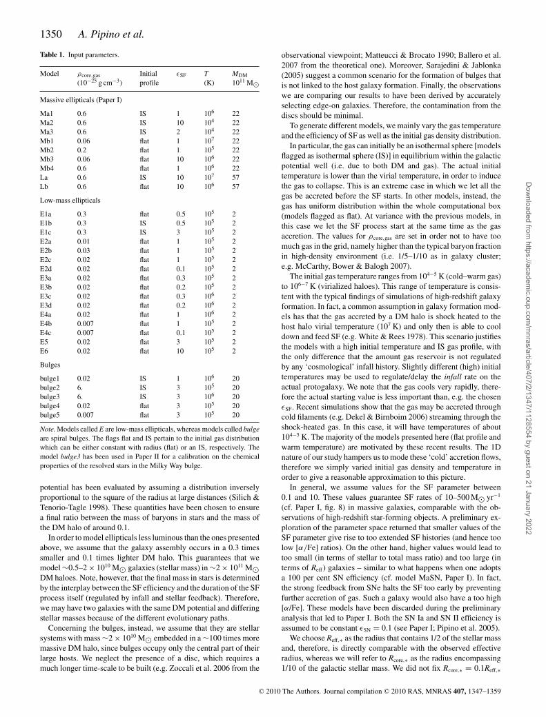
The relation between [α/Fe] and mass tracers (see e.g. Wortheyet al. 1992; Nelan et al. 2005; Thomas & Davies 2006) is satis-fied, as shown in Fig. 1. It is important to ensure that the mod-els fulfill such a relation, as it is the most severe test-bench for agalaxy formation scenario (see Pipino et al. 2009a). We note that themass–metallicity relation is also satisfied, since our massive objectshave an average stellar metallicity which is supersolar, whereas thesimulated low-mass ellipticals and bulges have solar metallicity atmost. More quantitatively, a linear fit to our model predictions gives[〈Z/H〉]core = −1.14 + 0.57log σ to be compared with the relation[〈Z/H〉]core = −1.06 + 0.55 log σ inferred by Thomas et al. (2005)within the same aperture for observed ellipticals. The robustnessof our predictions is supported by the fact that our models obeyto the above mentioned observational constraints. This ensures thatwe investigate the relation between abundance and abundance ra-tios gradients by means of models that are able to reproduce themain chemical properties of the ellipticals. Remarkably, the above-mentioned relations are in place already after 0.5–1 Gyr since thebeginning of the SF.

In the following two sections, we highlight other main featuresof model ellipticals and bulges, respectively.

4.1 Elliptical galaxies

In brief, we first recall from Paper I how the formation of a galaxyproceeds in our model. We take the case La as an example. Attimes earlier than 300 Myr, the gas is still accumulating in thecentral regions where the density increases by several orders ofmagnitude, with a uniform speed across the galaxy. The temperaturedrops due to cooling, and the SF can proceed at a very high rate(∼102−3 M� yr−1), at variance with the outermost regions, thatcomplete their build-up in the first 100 Myr. This implies that ametal rich medium, dominated by SN Ia ejecta, pollutes the gas

Table 2. Model results.

Model M∗ Reff,∗ [〈O/Fe〉∗,core] O/Fe Z/H

(1010 M�) (kpc)

Massive ellipticals (Paper I)

Ma1 6.0 12 0.29 0.02 −0.19Ma2 25. 7.7 0.22 −0.21 −0.52Ma3 25. 8.3 0.35 −0.17 −0.03Mb1 6.0 17 0.14 0.09 −0.20Mb2 3.0 8.7 0.33 0. −0.18Mb3 21 8.8 0.17 −0.08 −0.34Mb4 26 5.4 0.42 −0.08 −0.20La 26 29 0.14 0.19 −0.50Lb 29 21 0.12 0.32 −0.30

Low-mass ellipticals

E1a 0.74 1.7 0.08 −0.04 −0.26E1b 0.74 1.7 0.36 −0.13 −0.21E1c 0.74 1.7 0.28 −0.11 −0.21E2a 1.5 0.9 0.19 −0.03 −0.29E2b 1.8 0.6 0.14 +0.01 −0.29E2c 1.4 0.89 0.26 −0.04 −0.30E2d 0.27 2.3 0.17 +0.01 −0.29E3a 0.88 1.6 0.18 −0.005 −0.27E3b 0.65 1.1 0.11 +0.07 −0.28E3c 0.93 1.6 0.09 −0.01 −0.32E3d 0.6 1.1 0.03 +0.06 −0.25E4a 1 1.7 0.16 −0.21 −0.33E4b 0.35 0.6 0.22 −0.04 −0.36E4c 0.05 0.5 0.17 −0.01 −0.22E5 1 1.7 0.16 −0.20 −0.38E6 1 1.7 0.11 −0.16 −0.34

Bulges

bulge1 0.06 2 0. 0.09 −0.36bulge2 1.8 1 0.40 −0.07 −0.22bulge3 2.3 0.8 0.3 0.07 −0.36bulge4 3.7 0.7 0.29 0.00 −0.37bulge5 1.0 0.4 0.28 0.00 −0.30

Note. Models called E are low-mass ellipticals, whereas models called bulgeare spiral bulges. Values predicted after the SF has finished.

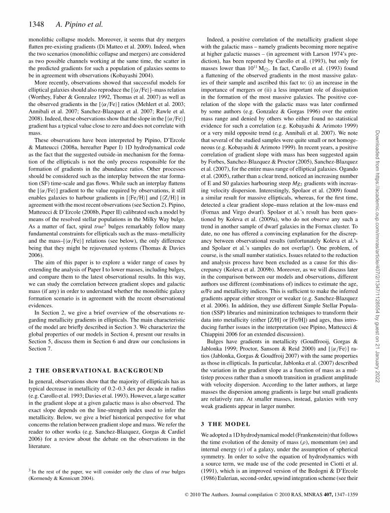
Figure 1. The [〈O/Fe〉]core–σ relation predicted for our model ellipticalsand bulges shown as crosses in the figure. Data from Thomas et al. (2007)are shown as contours. A liner regression to Thomas et al. (2007) is shownby a thin solid line. Note that in this plot we rescaled our [〈O/Fe〉] valuesin order to be consistent with the solar abundances used by Thomas et al.(2007). Spiral bulges obey to the same relation (Thomas & Davies 2006).


Dow


ic.oup.com/m



supply for the SF in the inner regions. After 400 Myr, the gas speedbecomes positive (i.e. out-flowing gas) at large radii, and at 500 Myralmost the entire galaxy experiences a galactic wind. At roughly1.2 Gyr, the amount of gas left inside the galaxy is below 2 per centof the stellar mass. This gas is very hot (around 1 keV) and stillflowing outside.

The galactic wind occurs first in the outer regions and then inthe more inner zones of the galaxy because the work to extract thegas from the outskirts is less than the work to extract the gas fromthe centre of the galaxy. The age differences between internal andexternal zones, however, are less than 1 Gyr and this ensures thatour models are globally α-enhanced. In this way, our models areconsistent with the observed age gradients (references in Section 2)and with the [α/Fe]–mass relation. The picture sketched above ap-plies to the lower mass models presented here. The fact that in ourgalaxy formation scenario the metallicity gradients arise becauseof the different times of occurrence of galactic winds in differentgalactic regions implies that the stellar metallicity is a function ofthe local escape velocity vesc for all the galaxies. In fact, in theregions where vesc is low (i.e. where the local potential is weaker),the galactic wind develops earlier and the gas is less processed thanin the regions where vesc is higher (see Martinelli, Matteucci &Colafrancesco 1998). Such a relation as been originally suggestedby several authors (e.g. Peletier et al. 1990; Davies et al. 1993) andnow confirmed by Scott et al. (2009). Here, we can also show thatthe local index vesc trend matches the global scaling (Scott et al.2009). In particular, we make use of the definition vesc = √

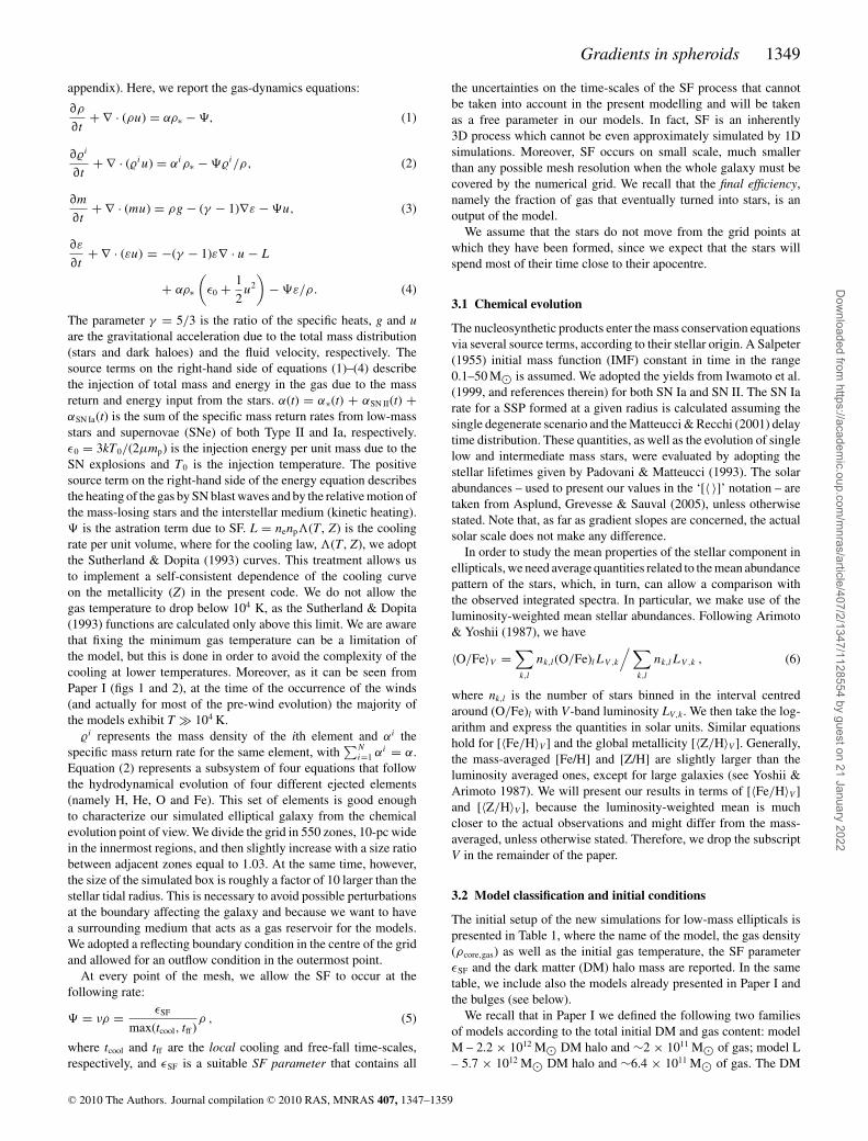
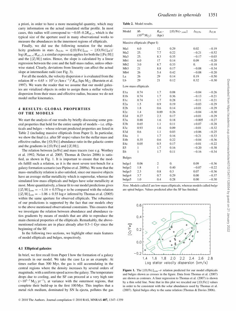
(−2�),where � is the potential due to stars and DM, in agreement withthe definition used by the observers. Some important caveats applyto this comparison. In observations, vesc depends on the modellingof the potential. Moreover, our models are spherically symmetric,whereas observed galaxies are not. In Fig. 2, we show that metal-licity (given by the index Mgb) versus vesc gradient slope for ourmodels. The central Mgb value for each model galaxy is given by anasterisk, whereas the value at 1Reff by a cross. Each couple of pointsconnected by a line represents a galaxy: this is the local relation.The dashed line is the observational global (i.e. the fit to the centralvalues of Mgb and vesc in observed galaxies) trend reported by Scottet al. (2009) along with the 3σ dispersion (dotted lines). We showthat the models presented in this paper reproduce the observed trendwithin the observed scatter. The fact that the each galactic region

Figure 2. Metallicity versus vesc gradient slope for our models. The centralMgb value for each model galaxy is given by an asterisk, whereas the valueat 1Reff by a cross. Each couple of points connected by a line represents agalaxy (the local relation). The dashed line is the global relation (Scott et al.2009) along with the 3σ dispersion (dotted lines).

follows the global trend strongly suggests the idea that a uniformprocess – like the monolithic collapse – is behind the formation ofthe gradients.

4.2 Galaxy bulges

Remarkably, all the results discussed in the previous sections applyto smaller objects (but embedded in much more massive haloes)such as the galaxy bulges, although the gradient slopes are slightlysmaller (see entries in Table 2). The main difference is that, dueto their host galaxy potential well, strong and long lasting windsdo not develop. We also find that the bulge formation is fast inagreement with the original suggestion by Matteucci & Brocato(1990), Elmegreen (1999) and the more recent work by Balleroet al. (2007).

We take advantage of the classical bulges as a further tool to cali-brate our models. Indeed, in Paper II (where we refer the reader forfurther details) we compared our model predictions to the propertiesof the resolved stellar population observed in the Milky Way bulgeby using the model bulge3 and found a remarkable agreement. Thismodel has a stellar mass of ∼2 × 1010 M� and a radius of ∼1 kpcin order to match the observed properties of our own Galaxy bulge(e.g. Minniti & Zoccali 2008). The same model reproduces thechemical constraints coming from the Bulge integrated light, in thatit predicts the following values for the indices Hβ = 1.61, Mg2 =0.29 and 〈Fe〉 = 2.46 in good agreement with the observed values ofHβ = 1.5 ± 0.6, Mg2 = 0.23 ± 0.04 and 〈Fe〉 = 2.15 ± 0.4 (Puziaet al. 2002). This is an important point that must be stressed: theabundances (and abundance gradients) that may be inferred fromthe analysis of Lick indices are average values. With resolved stellarpopulations (Paper II) is possible to show that the models presentedhere not only explains the average values, namely the mean proper-ties of a composite stellar population (CSP), but also their evolutionin the [O/Fe]–[Fe/H] plane, namely the composition of each SSPsthat make a CSP. Our fiducial model assumes Salpeter (1955) IMF,which successfully reproduces the properties of massive spheroids.In Paper II, we show that the stellar metallicity distribution pre-dicted by such a model reproduces the observed K-giant metal-licity distributions for the Milky Way bulge. We refer to Paper II(c.f. fig. 2) for the test of other possible IMFs, motivated by eitherobservations or theoretical efforts, which seems more appropriatefor bulges.

The reader should note that we present several other models forbulges which do not necessarily have properties – such as stellarmass or radius – similar to those of the Milky Way bulge.

5 TH E P R E D I C T E D G R A D I E N T S

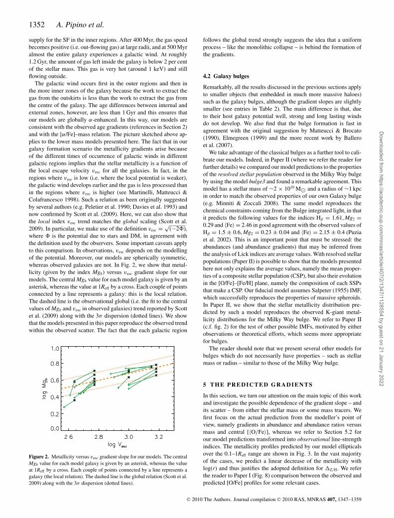
In this section, we turn our attention on the main topic of this workand investigate the possible dependence of the gradient slope – andits scatter – from either the stellar mass or some mass tracers. Wefirst focus on the actual prediction from the modeller’s point ofview, namely gradients in abundance and abundance ratios versusmass and central [〈O/Fe〉], whereas we refer to Section 5.2 forour model predictions transformed into observational line-strengthindices. The metallicity profiles predicted by our model ellipticalsover the 0.1–1Reff range are shown in Fig. 3. In the vast majorityof the cases, we predict a linear decrease of the metallicity withlog(r) and thus justifies the adopted definition for Z/H. We referthe reader to Paper I (Fig. 8) comparison between the observed andpredicted [O/Fe] profiles for some relevant cases.


Dow


ic.oup.com/m



Figure 3. Metallicity profiles predicted by our model ellipticals.

For elliptical galaxies, we make use of Mehlert et al.’s (2003)and Annibali et al.’s (2007) data sets, whose samples are larger thanOgando et al.’s one, although the former do not find such a strongcorrelation between gradient slope and mass as the latter (otherworks with less galaxies are not taken into account in order not tohave a poor statistics). For bulges, we adopt the data from Jablonkaet al. (2007), who explore a range in velocity dispersions similar tothe above-mentioned articles. Unfortunately, we cannot use a homo-geneous set of observables to constrain both the theoretical and theobservational predictions for several reasons. In the first place, inseveral articles the authors do not extract the [〈O/Fe〉] abundanceratio gradient from their line-strength indices (e.g. Kobayashi &Arimoto 1999; Ogando et al. 2005;4 Sanchez-Blazquez et al. 2006).Secondly, in all cases the stellar mass is not observed, whereas onlythe stellar velocity dispersion is given. Finally, several authors relyon a different subset of the Lick line-strength indices to infer themetallicity.

5.1 Theoretical relations with mass and mass tracers

With the above mentioned caveats in mind, in Fig. 4 we present ourpredictions regarding the theoretical relation between abundancegradients and mass tracers (namely the stellar velocity dispersionand the central [〈O/Fe〉]). The remainder of this section is devotedto fully describe Fig. 4.

5.1.1 Gradients in metallicity

Let us first focus on the upper row of Fig. 4: the total metallic-ity gradient. In the left-hand panel, we show the [〈Z/H〉] gradientslope in the stellar component predicted by our model for ellipticals

4 Notably, they could not convert the indices into abundances in severalgalaxies whose combination of index values fell outside Thomas, Maraston& Bender (2003) SSP libraries. We refer the reader to Pipino et al. (2006)and Paper I for a detailed discussion on the theoretical aspects of such aproblem. Here, we just mention that SSP libraries do not cover all the possi-ble combinations in the space [〈O/Fe〉]–〈Fe/H〉]–[〈Z/H〉], being typicallybuilt just as functions of two of them.

(hollow circles) and bulges (full dots) as a function of the stellarmass when all galaxies are considered. This is the actual predictionof our models. Formal linear regression fits to the entire sampleof model galaxies (solid line), to the galaxies with steepest gradi-ents (dotted line) and to dwarf ellipticals (dashed line) are shown.We predict a very mild trend in mass. In the high-mass region,our model predictions span a range in the gradient slopes similarto the observed values. Neither our models nor the three observa-tional samples (taken together) show any sign of (anti)correlation assuggested by any single sample. We therefore conclude that, in thismass range, it is more appropriate to speak of an increase in the scat-ter of the gradient slope at a fixed mass. If we take only the four lessmassive objects, we find a quite steep relation between metallicitygradient and galaxy mass, parallel to the locus of the galaxies withthe steepest gradients (we call it the maximum steepness boundaryline) similar to the predictions of the earlier monolithic collapsemodels. This finding seems to be in qualitative agreement with theobservational results by Spolaor et al. (2009). As for the points nearthe maximum steepness boundary, they always refer to the modelswith the highest SF efficiency at that given mass. We note anothertrend, symmetric to maximum steepness boundary with respect tothe solid line (trend of the entire sample), in the sense that at thehighest masses we have also the flattest gradients. This seems to goin the direction of Ogando et al. (2005), Spolaor et al. (2009) andJablonka et al. (2007) results. In particular, the scatter is minimumat masses below ∼1010 M�. These galaxies tend to have neithershallow metallicity gradients nor very steep ones.

In order to explain such findings, we first note that the formal lin-ear regression to our model predictions gives Z/H ∼ −0.04 log σ ,namely a value much smaller (in absolute value) than the slopeof the mass–metallicity relation [Z/H]core ∼ 0.57 log σ . Therefore,the relation between gradient slope and galactic mass cannot beexplained by the Carlberg (1984)’s argument (cf. Introduction; seealso Jablonka et al. 2007). In other words, the steepening of thegradient with mass is not due to the sole increasing metallicityof the galactic core, whereas the outermost regions of galaxiesdiffering in mass keep the same value for [〈Z/H〉]eff . Indeed, ithas been shown observationally that the metallicity of the entiregalaxy should obey to the mass–metallicity relation (e.g. Graveset al. 2007). Such a relation is satisfied by our models, for whichwe predict [Z/H]eff ∼ 0.53 log σ . Hence, Z/H ∼ [Z/H]eff(σ ) −[Z/H]core(σ ) ∼ 0.53 log σ − 0.57 log σ = −0.04 log σ .5 The reasonfor this increase in the global galaxy metallicity with mass is due tothe fact that the entire galaxies, not only their central cores, shouldform more efficiently as their mass increases in order to complywith the downsizing trend, namely they need to have [〈α/Fe〉] ra-tios greater than zero and positively correlated to the mass. Thisrequest renders the average gradient slope predicted by the revisedmonolithic models flatter than the earlier monolithic collapse mod-els a la Larson. However, galaxies with steep gradients still exists(e.g. models La and Lb) and lie on the maximum steepness bound-ary. On average, galaxies with mass ∼1010 M� feature gradientslopes quite close to the maximum steepness boundary, thereforethe scatter is small. At larger masses, the average gradient is nearlyone half of the maximum steepness boundary value at that mass,hence allowing for more intermediate possibilities.

It is interesting to understand what are the major causes for sucha range although we have unevenly sampled the parameter spaceand despite the not very high number of simulated galaxies. We

5 Note that in our simulations log(Rcore/Reff ) ∼ −1 in majority of the cases.


Dow


ic.oup.com/m



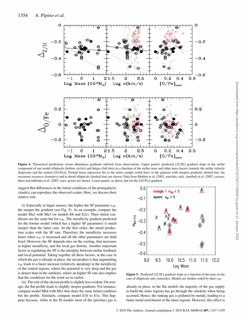
Figure 4. Theoretical predictions versus abundance gradients inferred from observations. Upper panels: predicted [〈Z/H〉] gradient slope in the stellarcomponent of our model ellipticals (hollow circles) and bulges (full dots) as a function of the stellar mass and other mass tracers (namely the stellar velocitydispersion and the central [〈O/Fe〉]). Formal linear regression fits to the entire sample (solid line), to the galaxies with steepest gradients (dotted line, themaximum steepness boundary) and to dwarf ellipticals (dashed line) are shown. Data from Mehlert et al. (2003, asterisks, red), Annibali et al. (2007, crosses,blue) and Jablonka et al. (2007, stars, green) are shown. Lower panels: as above, but for the [〈O/Fe〉] gradient.

suggest that differences in the initial conditions of the protogalacticcloud(s) can reproduce the observed scatter. Here, we discuss theirrelative role.

(i) Especially at larger masses, the higher the SF parameter εSF,the steeper the gradient (see Fig. 5). As an example, compare themodel Ma2 with Ma3 (or models E6 and E2c). Their initial con-ditions are the same but for εSF. The metallicity gradient predictedfor the former model (which has a higher SF parameter) is muchsteeper than the latter case. At the first order, the metal produc-tion scales with the SF rate. Therefore, the metallicity increasesfaster when εSF is increased and all the other parameters are heldfixed. However, the SF depends also on the cooling, that increasesat higher metallicity, and the local gas density. Another importantfactor in regulating the SF is the interplay between stellar feedbackand local potential. Taking together all these factors, in the case inwhich the gas is already in place, the net product is that augmentingεSF leads to a faster increase (relatively speaking) in the metallicityof the central regions, where the potential is very deep and the gasis denser than in the outskirts, where an higher SF rate also impliesthat the conditions for the wind set in earlier.

(ii) The role of the chosen profile is slightly less evident. On aver-age, the flat profile leads to slightly steeper gradients. For instance,compare model Mb4 with Ma1 that share the same initial conditionbut the profile. Similarly, compare model E1b to E1a. This hap-pens because, while in the IS models most of the (pristine) gas is

Figure 5. Predicted [〈Z/H〉] gradient slope as a function of the mass in thecase of ellipticals only (asterisks). Models are further coded by their εSF.

already in place, in the flat models the majority of the gas supplyto build the inner regions has go through the outskirts when beingaccreted. Hence, the sinking gas is polluted by metals, leading to afaster metal enrichment of the inner regions. However, this effect is


Dow


ic.oup.com/m



weaker than that caused by εSF. For instance, compare model Ma2with Mb4.

(iii) As for the temperature, starting from a higher value impliesa longer time for cooling the gas and feeding the SF process. In asense, the effect is similar to the difference between the flat caseversus the IS case. For instance, on the basis of the previous point wewould expect model Ma1 to exhibit a (slightly) shallower gradientthan the one of model Ma3. Instead, it is steeper. However, a higherinitial temperature is not enough to counterbalance the effect of alarge change in εSF (see model Ma1 versus Ma2).

(iv) For flat models, the initial gas density seems to be relativelyunimportant (e.g. compare models E2c and E4c) in the determiningthe slope of the metallicity gradient.

In conclusion, we do not find a parameter that fully governs thecreation of the gradient, even if εSF seems to be quite important.Different – but reasonable – combination of the input parameterslead to model properties that obey both the overall properties ob-served in elliptical galaxies and exhibit average metallicity gradientof −0.3 dex per decade in radius. Changes in the initial condi-tions within the same broad formation scenario create the scatter inthe predicted gradients at a single mass. These changes, therefore,should not be ascribed to different pictures for the formation of thegalaxies. They rather mimic cases in which the accretion from theprotogalactic clouds may be faster (e.g. the IS cases) or proceedthrough cold accretion through filaments (Dekel & Birnboim 2006,the flat case). They also show the different behaviour of modelswhere the SF is favoured (higher εSF, e.g. for the formation of themost massive galaxies) or disfavoured (models with high initialtemperature: the gas is accreted in pre-existing haloes and has tocool before forming stars).

In the middle and right-hand panels in the upper row of Fig. 4,we compare our model predictions to metallicity gradients in-ferred from observations (Mehlert et al. 2003; Annibali et al. 2007;Jablonka et al. 2007). Obviously, the above discussion on the causeof the (scatter in the) metallicity gradient applies also to the othermass tracers (σ and the central [〈O/Fe〉]). As explained above, how-ever, here we can compare our predictions with the values measuredby the observers. We can thus show that the predicted range as wellas the average gradient slope (−0.3 dex per decade in radius) are inagreement with observations. We note how different observationalgroups infer slightly different mean Z/H (e.g. compare the samplesin Fig. 4). For instance, in the literature average values either as lowas −0.22 ± 0.1 or as high as −0.34 ± 0.08 (Brough et al. 2007) canbe found,6 still consistent with each other, though. This might bedue to a different combination of line-strength indices used to inferthe variation in metallicity (see the analysis in Sanchez-Blazquezet al. 2006). Also, differences in the SSP library used to transformindices into abundances can create the offset. Moreover, small num-ber statistics can still bias the results as well as the fact that, evenin the same sample, metallicity gradients are not measured out tothe same radius. Some authors claim the difference is caused bythe environment, with field ellipticals featuring shallower gradientson average with respect to galaxies living in higher density regions(Sanchez-Blazquez et al. 2006). Such a suggestion might explainthe offset between the Mehlert et al. (2003) Coma cluster ellipticalsand the Annibali et al. (2007) spheroids.

6 We refer to table 4 in Spolaor et al. (2008, and references therein) for auseful comparison of the gradients in age, metallicity and α-enhancementinferred by the above-mentioned observations.

5.1.2 Gradients in abundance ratios

We now move to the analysis of the bottom row of Fig. 4. Noclear relation with mass is found for the [〈O/Fe〉] radial gradients.Indeed, as expected from Paper I and II, most of our models predicta nearly flat [〈O/Fe〉] gradient, with some showing either positiveor negative slopes.

In particular, we suggest the gradient in the [〈α/Fe〉] ratio tobe related to the interplay between the velocity of the radial flowsmoving from the outer to the inner galactic regions and the intensityand duration of the SF formation process at any radius. Clearly, alarger or smaller parameter of SF can have a strong influence on thisprocess. This result implies that we do not need the merger eventsin order to have a shallow [〈α/Fe〉] gradient.

In general, we find that in our models with O/Fe ≤ 0 the roleof both the gas flowing inwards and the SF time-scale increasing atlarge radii is non-negligible. The role of the initial temperature canbe important. If the galaxy formation process starts from hot gas(i.e. 106−7 K), we predict O/Fe ≥ 0 in the majority of the cases.They are thus similar to the quasi-monolithic chemical evolutionmodels of Pipino & Matteucci (2004) with non-interacting shellsin which the infall time-scale increases at shorter radii, whereas theSF efficiency is constant. On the other hand, models starting withcold (i.e. 104−5 K) gas seem to prefer a negative O/Fe.

The sole SF efficiency seems to affect the predicted absolutevalue of the gradient slope; in fact, all the models most effective informing stars exhibit the steepest slopes at the same time. Basically,an increase in the SF efficiency enhances the differences betweenthe inner core and the outskirts set by the other initial conditions.For instance, if the gas is already in place, a high efficiency informing stars boosts the outside-in process. In such a case, the SFprocess, which also locks the metals into the stars, is fast enough inthe central regions to avoid the contamination of the metals flowingfrom larger radii. In practice, we end up in the extreme case in whichthe gas flows can be neglected and O/Fe ∼ 0.2 as in the standardchemical evolution models (Pipino et al. 2006).

5.1.3 Correlations between gradients in metallicityand gradients in abundance ratios

The final part of the theoretical analysis involves the study of pos-sible correlations between gradients in metallicity and gradients inabundance ratios. As a confirmation of what said in Section 5.1.2,galaxies showing the steepest positive [〈O/Fe〉] gradient slopes havealso quite a strong radial decrease in the [〈Fe/H〉] ratio (Fig. 6).These galaxies are also the most massive ones. A correlation in thissense seems to be confirmed by the Annibali et al. (2007) data,whereas Mehlert et al.’s (2003) galaxies exhibit values for O/Fe

constant with Fe/H. A quantitative confirmation needs a samplestatistically richer. Perhaps, more interestingly, neither the observa-tions nor the models cover the region with O/Fe < 0 and Fe/H <

−0.4: galaxies with the steepest metallicity gradients undergo astrong outside-in formation process. In galaxies with O/Fe < 0 –namely, models that likely have a local SF efficiency decreasingwith galactocentric radius – the stellar feedback is more effectivein contrasting the metal-enhanced flows; therefore, the final Fe/H

is smaller (in absolute value), hence closer to the expectations frommodels which do not take into account gas flows within the galaxy.At the same time, we predict a paucity of galaxies in the region O/Fe > 0 and Fe/H > −0.2. More observations are needed toconfirm this suggestion. A lack of galaxies can also be noted on theupper-left corners in the left-hand panels in Fig. 4.


Dow


ic.oup.com/m



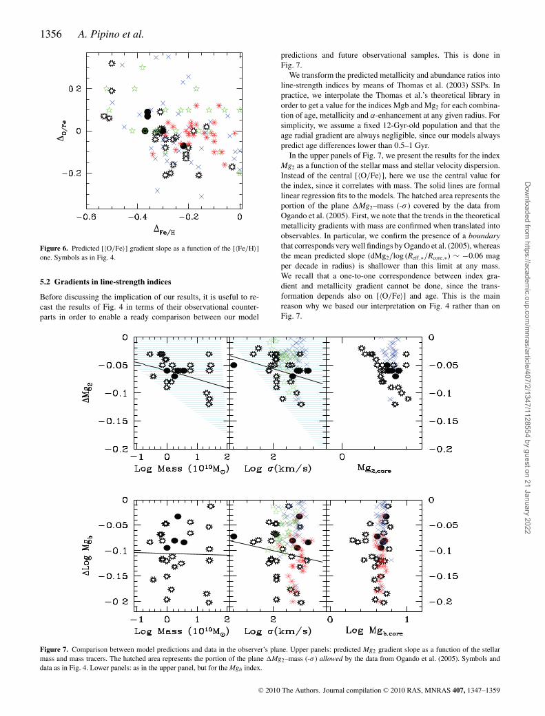
Figure 6. Predicted [〈O/Fe〉] gradient slope as a function of the [〈Fe/H〉]one. Symbols as in Fig. 4.

5.2 Gradients in line-strength indices

Before discussing the implication of our results, it is useful to re-cast the results of Fig. 4 in terms of their observational counter-parts in order to enable a ready comparison between our model

predictions and future observational samples. This is done inFig. 7.

We transform the predicted metallicity and abundance ratios intoline-strength indices by means of Thomas et al. (2003) SSPs. Inpractice, we interpolate the Thomas et al.’s theoretical library inorder to get a value for the indices Mgb and Mg2 for each combina-tion of age, metallicity and α-enhancement at any given radius. Forsimplicity, we assume a fixed 12-Gyr-old population and that theage radial gradient are always negligible, since our models alwayspredict age differences lower than 0.5–1 Gyr.

In the upper panels of Fig. 7, we present the results for the indexMg2 as a function of the stellar mass and stellar velocity dispersion.Instead of the central [〈O/Fe〉], here we use the central value forthe index, since it correlates with mass. The solid lines are formallinear regression fits to the models. The hatched area represents theportion of the plane Mg2–mass (-σ ) covered by the data fromOgando et al. (2005). First, we note that the trends in the theoreticalmetallicity gradients with mass are confirmed when translated intoobservables. In particular, we confirm the presence of a boundarythat corresponds very well findings by Ogando et al. (2005), whereasthe mean predicted slope (dMg2/log (Reff,∗/Rcore,∗) ∼ −0.06 magper decade in radius) is shallower than this limit at any mass.We recall that a one-to-one correspondence between index gra-dient and metallicity gradient cannot be done, since the trans-formation depends also on [〈O/Fe〉] and age. This is the mainreason why we based our interpretation on Fig. 4 rather than onFig. 7.

Figure 7. Comparison between model predictions and data in the observer’s plane. Upper panels: predicted Mg2 gradient slope as a function of the stellarmass and mass tracers. The hatched area represents the portion of the plane Mg2–mass (-σ ) allowed by the data from Ogando et al. (2005). Symbols anddata as in Fig. 4. Lower panels: as in the upper panel, but for the Mgb index.


Dow


ic.oup.com/m



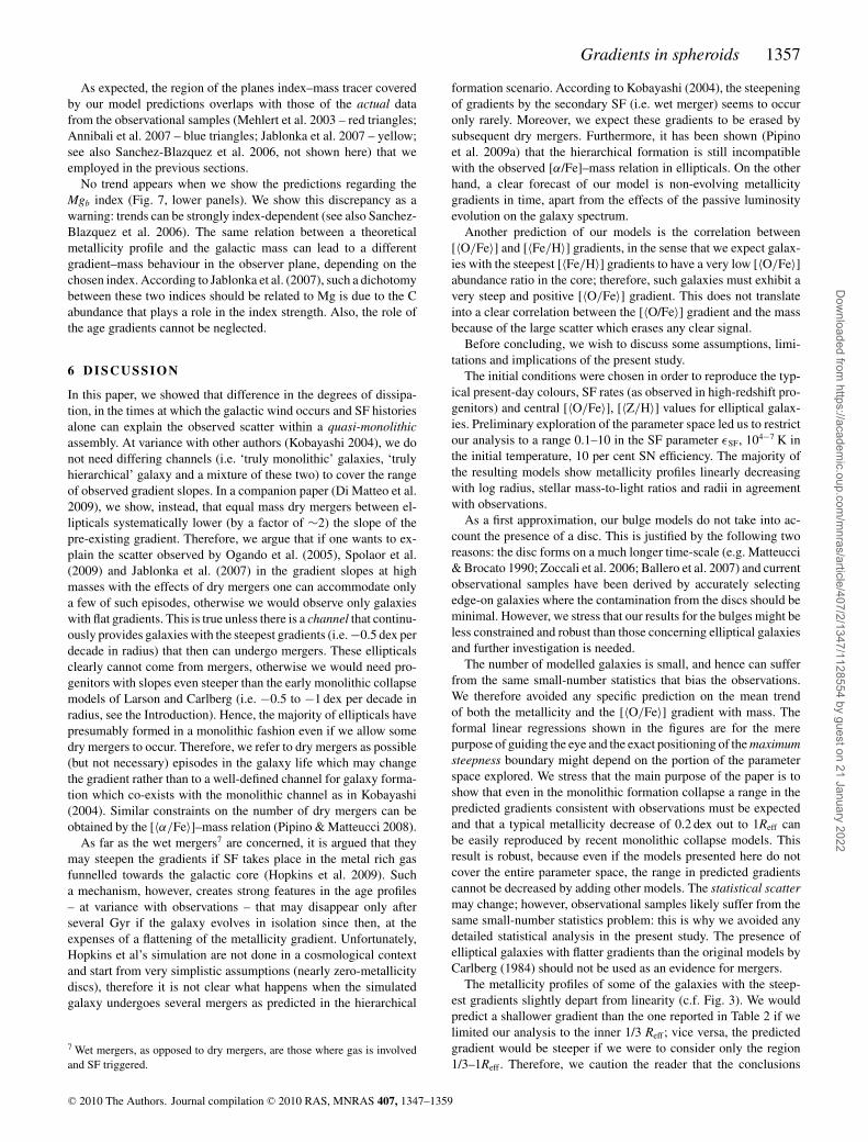
As expected, the region of the planes index–mass tracer coveredby our model predictions overlaps with those of the actual datafrom the observational samples (Mehlert et al. 2003 – red triangles;Annibali et al. 2007 – blue triangles; Jablonka et al. 2007 – yellow;see also Sanchez-Blazquez et al. 2006, not shown here) that weemployed in the previous sections.

No trend appears when we show the predictions regarding theMgb index (Fig. 7, lower panels). We show this discrepancy as awarning: trends can be strongly index-dependent (see also Sanchez-Blazquez et al. 2006). The same relation between a theoreticalmetallicity profile and the galactic mass can lead to a differentgradient–mass behaviour in the observer plane, depending on thechosen index. According to Jablonka et al. (2007), such a dichotomybetween these two indices should be related to Mg is due to the Cabundance that plays a role in the index strength. Also, the role ofthe age gradients cannot be neglected.

6 D ISCUSSION

In this paper, we showed that difference in the degrees of dissipa-tion, in the times at which the galactic wind occurs and SF historiesalone can explain the observed scatter within a quasi-monolithicassembly. At variance with other authors (Kobayashi 2004), we donot need differing channels (i.e. ‘truly monolithic’ galaxies, ‘trulyhierarchical’ galaxy and a mixture of these two) to cover the rangeof observed gradient slopes. In a companion paper (Di Matteo et al.2009), we show, instead, that equal mass dry mergers between el-lipticals systematically lower (by a factor of ∼2) the slope of thepre-existing gradient. Therefore, we argue that if one wants to ex-plain the scatter observed by Ogando et al. (2005), Spolaor et al.(2009) and Jablonka et al. (2007) in the gradient slopes at highmasses with the effects of dry mergers one can accommodate onlya few of such episodes, otherwise we would observe only galaxieswith flat gradients. This is true unless there is a channel that continu-ously provides galaxies with the steepest gradients (i.e. −0.5 dex perdecade in radius) that then can undergo mergers. These ellipticalsclearly cannot come from mergers, otherwise we would need pro-genitors with slopes even steeper than the early monolithic collapsemodels of Larson and Carlberg (i.e. −0.5 to −1 dex per decade inradius, see the Introduction). Hence, the majority of ellipticals havepresumably formed in a monolithic fashion even if we allow somedry mergers to occur. Therefore, we refer to dry mergers as possible(but not necessary) episodes in the galaxy life which may changethe gradient rather than to a well-defined channel for galaxy forma-tion which co-exists with the monolithic channel as in Kobayashi(2004). Similar constraints on the number of dry mergers can beobtained by the [〈α/Fe〉]–mass relation (Pipino & Matteucci 2008).

As far as the wet mergers7 are concerned, it is argued that theymay steepen the gradients if SF takes place in the metal rich gasfunnelled towards the galactic core (Hopkins et al. 2009). Sucha mechanism, however, creates strong features in the age profiles– at variance with observations – that may disappear only afterseveral Gyr if the galaxy evolves in isolation since then, at theexpenses of a flattening of the metallicity gradient. Unfortunately,Hopkins et al’s simulation are not done in a cosmological contextand start from very simplistic assumptions (nearly zero-metallicitydiscs), therefore it is not clear what happens when the simulatedgalaxy undergoes several mergers as predicted in the hierarchical

7 Wet mergers, as opposed to dry mergers, are those where gas is involvedand SF triggered.

formation scenario. According to Kobayashi (2004), the steepeningof gradients by the secondary SF (i.e. wet merger) seems to occuronly rarely. Moreover, we expect these gradients to be erased bysubsequent dry mergers. Furthermore, it has been shown (Pipinoet al. 2009a) that the hierarchical formation is still incompatiblewith the observed [α/Fe]–mass relation in ellipticals. On the otherhand, a clear forecast of our model is non-evolving metallicitygradients in time, apart from the effects of the passive luminosityevolution on the galaxy spectrum.

Another prediction of our models is the correlation between[〈O/Fe〉] and [〈Fe/H〉] gradients, in the sense that we expect galax-ies with the steepest [〈Fe/H〉] gradients to have a very low [〈O/Fe〉]abundance ratio in the core; therefore, such galaxies must exhibit avery steep and positive [〈O/Fe〉] gradient. This does not translateinto a clear correlation between the [〈O/Fe〉] gradient and the massbecause of the large scatter which erases any clear signal.

Before concluding, we wish to discuss some assumptions, limi-tations and implications of the present study.

The initial conditions were chosen in order to reproduce the typ-ical present-day colours, SF rates (as observed in high-redshift pro-genitors) and central [〈O/Fe〉], [〈Z/H〉] values for elliptical galax-ies. Preliminary exploration of the parameter space led us to restrictour analysis to a range 0.1–10 in the SF parameter εSF, 104−7 K inthe initial temperature, 10 per cent SN efficiency. The majority ofthe resulting models show metallicity profiles linearly decreasingwith log radius, stellar mass-to-light ratios and radii in agreementwith observations.

As a first approximation, our bulge models do not take into ac-count the presence of a disc. This is justified by the following tworeasons: the disc forms on a much longer time-scale (e.g. Matteucci& Brocato 1990; Zoccali et al. 2006; Ballero et al. 2007) and currentobservational samples have been derived by accurately selectingedge-on galaxies where the contamination from the discs should beminimal. However, we stress that our results for the bulges might beless constrained and robust than those concerning elliptical galaxiesand further investigation is needed.

The number of modelled galaxies is small, and hence can sufferfrom the same small-number statistics that bias the observations.We therefore avoided any specific prediction on the mean trendof both the metallicity and the [〈O/Fe〉] gradient with mass. Theformal linear regressions shown in the figures are for the merepurpose of guiding the eye and the exact positioning of the maximumsteepness boundary might depend on the portion of the parameterspace explored. We stress that the main purpose of the paper is toshow that even in the monolithic formation collapse a range in thepredicted gradients consistent with observations must be expectedand that a typical metallicity decrease of 0.2 dex out to 1Reff canbe easily reproduced by recent monolithic collapse models. Thisresult is robust, because even if the models presented here do notcover the entire parameter space, the range in predicted gradientscannot be decreased by adding other models. The statistical scattermay change; however, observational samples likely suffer from thesame small-number statistics problem: this is why we avoided anydetailed statistical analysis in the present study. The presence ofelliptical galaxies with flatter gradients than the original models byCarlberg (1984) should not be used as an evidence for mergers.

The metallicity profiles of some of the galaxies with the steep-est gradients slightly depart from linearity (c.f. Fig. 3). We wouldpredict a shallower gradient than the one reported in Table 2 if welimited our analysis to the inner 1/3 Reff ; vice versa, the predictedgradient would be steeper if we were to consider only the region1/3–1Reff . Therefore, we caution the reader that the conclusions


Dow


ic.oup.com/m



about the steepest gradients in our model galaxies and their relationwith the monolithic boundary might depend on the chosen radius. Adetailed comparison between model profiles and single well-studiedgalaxies over a large mass range will allow us to study the metal-licity gradients in their finer details and better constrain the modelspresented here.

Moreover, while most of our models obey to the mass–size re-lation for ellipticals (e.g. Shankar et al. 2010), some galaxies withsimilar mass (e.g. compare models Ma2 and La) have quite differ-ent radii. The former model has a radius consistent with those fornormal ellipticals of that mass (e.g. Shankar et al. 2010), the lat-ter is more typical of an early-type brightest cluster galaxy (BCG;e.g. Graham et al. 1996). We chose not to make any distinctionbetween BCGs and normal ellipticals in our models since gradientsmeasured in BCGs have traditionally been included in the sampleas the ones that we use and because there is no difference as faras the chemical properties are concerned (e.g. Brough et al. 2007;von der Linden et al. 2007). However, the reader should keep inmind that a structural difference between BCGs and normal ellip-ticals seems to exist, and BCGs seem to harbour steep gradients(e.g. Brough et al. 2007). Therefore, in light of the special role ofBCGs (e.g. von der Linden et al. 2007; Pipino et al. 2009b, and ref-erences therein), further and dedicated observations and modellingare required to ascertain if there is any systematic difference in themetallicity gradients with respect to more ordinary ellipticals andwhat is the cause.

Also, we remind that the majority of the observational works useMg as a proxy for the α elements, as can be easily observed inabsorption in the optical bands giving rise to the well-known Mg2

and Mgb Lick indices. However, the state-of-the-art SSPs libraries(Thomas et al. 2003; Lee & Worthey 2009) are computed as func-tions of the total α-enhancement and of the total metallicity. Thisis true also for the stellar tracks, where the O abundance dominatesthe opacity and hence the stellar evolution. The latest observationalresults (Mehlert et al. 2003; Annibali et al. 2007; Sanchez-Blazquezet al. 2007) that we contrasted to our predictions in this study havebeen translated into theoretical ones by means of these SSPs; there-fore, the above authors provide us with radial gradients in [α/Fe],instead of [Mg/Fe]. This is why in this paper we focus on the the-oretical evolution of the α elements by using O that is by far themost important.

Here, we briefly recall that both O and Mg come from the hy-drostatic burnings in massive stars, therefore they are produced inlockstep. It has been suggested recently (e.g. McWilliam et al. 2008)that this might not be true at solar (and above solar) metallicities.While this is an important effect in detailed chemical evolutionstudies, it has no importance when the luminosity weighted proper-ties of a composite stellar population are concerned. This happensbecause luminosity averages weigh more the stellar populations atlower metallicities (lower M/L), where the differences between Oand Mg production are negligible (if any). Finally, even if the abun-dance of O and Mg are offset by some fixed quantity (i.e. [O/H] =[Mg/H]+constant), the predicted gradient would be the same.

7 C O N C L U S I O N S

In this paper, we study the formation and evolution of ellipticalsand bulges by means of a hydrodynamical model (cf. Papers I andII, respectively) in order to understand the origin of the observedscatter in the abundance gradients of early-type galaxies. Here, wesummarize our main results.

(i) We find Z/H in the range −0.5 to −0.2 dex per decade inradius with a mean value of −0.3 dex per decade in radius, inagreement with the observations (e.g. Kobayashi & Arimoto 1999).

(ii) In agreement with Ogando et al. (2005) and Jablonka et al.(2007), we find that the scatter in the gradient slopes increases as afunction of mass. We reproduce such a scatter in the observationsby means of variation in the initial conditions in galaxy models.

(iii) Model galaxies which behave as the earlier monolithic col-lapse models by Larson (1974) and Carlberg (1984) define a max-imum steepness boundary in the metallicity (and index) gradientslope–mass plane. These galaxies are preferentially those with thehighest SF efficiency at that given mass.

(iv) No galaxies with gradients steeper (i.e. more negative) thanthe value given by the our predicted theoretical boundary are ob-served (Ogando et al. 2005; Spolaor et al. 2009, for ellipticals andJablonka et al. 2007 for bulges).

(v) No correlation between O/Fe and other galactic propertiesare found, in agreement with observations for ellipticals (Mehlertet al. 2003; Annibali et al. 2007) and bulges (Jablonka et al. 2007).

(vi) The abundance gradients, once transformed into line-strength indices, lead to dMg2/log (Rcore,∗/Reff,∗) ∼ −0.06 mag andd log Mgb/log (Rcore,∗/Reff,∗) ∼ −0.1 per decade in radius, again inagreement with the typical mean values measured for ellipticals andbulges.

(vii) We note that the behaviour of the gradient slope as a functionof the galactic mass strongly depends on the particular line-strengthindex used. In fact, the predicted Mg2 index gradient seems tocorrelate with mass, whereas the Mgb index gradient does not.

(viii) In Paper I, we demonstrated that the differential occurrenceof galactic winds (outside-in formation) alone can explain the ex-istence of the metallicity gradients discussed in this paper. Here,we add that this mechanism predicts a tight correlation betweenline-strength index and escape velocity gradients which has beenconfirmed by recent data (see Scott et al. 2009).

Larger, homogeneous and statistically meaningful observationalsample of gradients in elliptical galaxies out to one effective radiuscan confirm such a prediction and validate the model.

AC K N OW L E D G M E N T S

This work was partially supported by the Italian Space Agencythrough contract ASI-INAF I/016/07/0. FM, CC and AD ac-knowledge financial support from PRIN-MIUR 2007, Prot.N.2007JJC53X. CC acknowledges financial support from theSwiss National Science Foundation. We warmly thank P.Sanchez-Blazquez, M. Spolaor, D. Forbes, S. Faber, P. Jablonka,M. Cappellari, N. Scott and R. Davies for stimulating discussions.We thank the referee for comments that greatly improved the qualityof the presentation.

REFERENCES

Annibali F., Bressan A., Rampazzo R., Zeilinger W. W., Danese L., 2007,A&A, 463, 455

Arimoto N., Yoshii Y., 1987, A&A, 173, 23Asplund M., Grevesse N., Sauval A. J., 2005, in Barnes T. G., III, Bash F. N.,

eds, ASP Conf. Ser. Vol. 336. Cosmic Abundances as Records of StellarEvolution and Nucleosynthesis. Astron. Soc. Pac., San Francisco, p. 25

Ballero S., Matteucci F., Origlia L., Rich R. M., 2007, A&A, 467, 123Bedogni R., D’Ercole A., 1986, A&A, 157, 101Bekki K., Shioya Y., 1999, ApJ, 513, 108Brough S., Proctor R., Forbes D. A., Couch W. J., Collins C. A., Burke D. J.,

Mann R. G., 2007, MNRAS, 378, 1507


Dow


ic.oup.com/m



Burstein D., Bender R., Faber S. M., Nolthenius R., 1997, AJ, 114, 1365Carlberg R. G., 1984, ApJ, 286, 403Carollo C. M., Danziger I. J., Buson L., 1993, MNRAS, 265, 553Chiosi C., Carraro G., 2002, MNRAS, 335, 335Ciotti L., D’Ercole A., Pellegrini S., Renzini A., 1991, ApJ, 376, 380Davies R. L., Sadler E. M., Peletier R. F., 1993, MNRAS, 262, 650Dekel A., Birnboim Y., 2006, MNRAS, 368, 2Di Matteo P., Pipino A., Lehnert M. D., Combes F., Semelin B., 2009, A&A,

499, 427Elmegreen B. G., 1999, ApJ, 517, 103Forbes D. A., Sanchez-Blazquez P., Proctor R., 2005, MNRAS, 361, 6Gonzalez J. J., Gorgas J., 1996, in Buzzoni A., Renzini A., Serrano A., eds,

ASP Conf. Ser., Vol. 86, Fresh Views of Elliptical Galaxies. Astron. Soc.Pac., San Francisco, p. 225

Goudfrooij P., Gorgas J., Jablonka P., 1999, Ap&SS, 269, 109Graham A., Lauer T. R., Colless M., Postman M., 1996, ApJ, 465, 534Graves G. J., Faber S. M., Schiavon R. P., Yan R., 2007, ApJ, 671, 243Hopkins, P. F., Cox T. J., Dutta S. N., Hernquist L., Kormendy J., Lauer

T. R., 2009, ApJ, 181, 135Iwamoto K., Brachwitz F., Nomoto K., Kishimoto N., Umeda H., Hix W. R.,

Thielemann F. K., 1999, ApJS, 125, 439Jablonka P., Gorgas J., Goudfroij P., 2007, A&A, 474, 763Kawata D., 2001, ApJ, 558, 598Kobayashi C., 2004, MNRAS, 347, 740Kobayashi C., Arimoto N., 1999, ApJ, 527, 573Koleva M., Prugniel P., De Rijcke S., Zeilinger W. W., Michielsen D., 2009a,

AN, 330, 960Koleva M., de Rijcke S., Prugniel P., Zeilinger W. W., Michielsen D., 2009b,

MNRAS, 396, 2133Kormendy J., Kennicutt R. C., 2004, ARA&A, 42, 603Larson R. B., 1974, MNRAS, 166, 585Lee H.-C., Worthey G. D. A., 2009, AJ, 138, 1442McCarthy I. G., Bower R. G., Balogh M. L., 2007, MNRAS, 377, 1457McWilliam A., Matteuchi F., Ballero S., Rich R. M., Fulbright J. P., Cescutti

G., 2008, AJ, 136, 367Martinelli A., Matteucci F., Colafrancesco S., 1998, MNRAS, 298, 42Matteucci F., Brocato E., 1990, ApJ, 365, 539Matteucci F., Recchi S., 2001, ApJ, 558, 351Mehlert D., Thomas D., Saglia R. P., Bender R., Wegner G., 2003, A&A,

407, 423Minniti D., Zoccali M., 2008, in Bureau M., Athanassoula L., Barbury B.,

eds, Proc. Int. Astron. Union, IAU Symp. 245, Formation and Evolutionof Galaxy Bulges. IAU, p. 323

Nelan J. E., Smith R. J., Hudson M. J., Wegner G. A., Lucey J. R., MooreS. A. W., Quinney S. J., Suntzeff N. B., 2005, ApJ, 632, 137

O’Connel R. W., 1976, ApJ, 206, 370Ogando R. L. C., Maia M. A. G., Chiappini C., Pellegrini P. S., Schiavon R.

P., da Costa L. N., 2005, ApJ, 632, 61Padovani P., Matteucci F., 1993, ApJ, 416, 26

Peletier R. F., Davies R. L., Illingworth G. D., Davis L. E., Cawson M.,1990, AJ, 100, 1091

Pipino A., Matteucci F., 2004, MNRAS, 347, 968Pipino A., Matteucci F., 2008, A&A, 486, 763Pipino A., D’Ercole A., Matteucci F., 2008a, A&A, 484, 679 (Paper I)Pipino A., Matteucci F., D’Ercole A., 2008b, in Bureau M., Athanassoula

L., Barbury B., eds, Proc. IAU Symp. 245, Formation and Evolution ofGalaxy. Bulges. IAU, p. 19 (Paper II)

Pipino A., Devriendt J., Thomas D., Silk J., Kaviraj S., 2009a, A&A, 505,1075

Pipino A., Kaviraj S., Bildfell C., Babul A., Hoekstra H., Silk J., 2009b,MNRAS, 395, 462

Pipino A., Kawata D., Gibson B. K., Matteucci F., 2005, A &A, 434, 553Pipino A., Matteucci F., Chiappini C., 2006, ApJ, 638, 739Proctor R. N., Sansom A. E., Reid I. N., 2000, MNRAS, 311, 37Puzia T. H., Saglia R. P., Kissler-Patig M., Maraston C., Greggio L., Renzini

A., Ortolani S., 2002, A&A, 395, 45Rawle T. D., Smith R. J., Lucey J. R., Swinbank A. M., 2008, MNRAS, 289,

1891Salpeter E. E., 1955, ApJ, 121, 161Sanchez-Blazquez P., Forbes D. A., Strader J., Brodie J., Proctor R., 2007,

377, 759Sanchez-Blazquez P., Gorgas J., Cardiel N., 2006, A&A, 457, 82Sarajedini A., Jablonka P., 2005, AJ, 130, 1627Scott N. et al., 2009, MNRAS, 398, 1835Shankar F., Marulli F., Bernardi M., Dai X., Hyde J. B., Sheth R. K., 2010,

MNRAS, 403, 117Spolaor M., Forbes D. A., Proctor R. N., Hau G. K. T., Brough S., 2008,

MNRAS, 385, 675Spolaor M., Proctor R. N., Forbes D. A., Couch W. J., 2009, ApJ, 691, 138Silich S. A., Tenorio-Tagle G., 1998, MNRAS, 299, 249Sutherland R. S., Dopita M. A., 1993, ApJS, 88, 253Thomas D., Davies R., 2006, MNRAS, 366, 510Thomas D., Maraston C., Bender R., 2003, MNRAS, 339, 897Thomas D., Maraston C., Bender R., Mendes de Oliveira C., 2005, ApJ,

621, 673Thomas D., Maraston C., Schawinski K., Sarzi M., Joo S.-J., Kaviraj S., Yi

S. K., 2007, in Vazdekis A., Peletier R. F., eds, Proc. IAU Symp. 241,Stellar Populations as Building Blocks of Galaxies. Cambridge Univ.Press, Cambridge, p. 546

von der Linden A., Best P. N., Kauffmann G., White S. D. M., 2007,MNRAS, 379, 867

Yoshii Y., Arimoto N., 1987, A&A, 188, 13White S. D. M., Rees M. J., 1978, MNRAS, 183, 341Worthey G., Faber S. M., Gonzalez J. J., 1992, ApJ, 398, 69Zoccali M. et al., 2006, A&A, 457, 1

This paper has been typeset from a TEX/LATEX file prepared by the author.


Dow


ic.oup.com/m


Abundance gradient slopes versus mass in spheroids

Documents