Abstracting Soft Constraints

Abstracting Soft ConstraintS. Bistarelli1, P. Codognet2, Y. Georget3, F. Rossi41: Universit�a di Pisa, Dipartimento di Informatica, Corso Italia 40, 56125 Pisa, Italy.E-mail: [email protected]: University of Paris 6, LIP6, case 169, 4, Place Jussieu, 75 252 Paris Cedex 05,France. E-mail: [email protected]: INRIA Rocquencourt, BP 105, 78153 Le Chesnay, France. E-mail:[email protected]: Universit�a di Padova, Dipartimento di Matematica, Via Belzoni 7, 35131 Padova,Italy. E-mail: [email protected]. We propose an abstraction scheme for soft constraint prob-lems and we study its main properties. Processing the abstracted versionof a soft constraint problem can help us in many ways: for example, to�nd good approximations of the optimal solutions, or also to provide uswith information that can make the subsequent search for the best solu-tion easier. The results of this paper show that the proposed scheme ispromising; thus they can be used as a stable formal base for any experi-mental work speci�c to a particular class of soft constraint problems.1 IntroductionClassical constraint satisfaction problems (CSPs) [15] are a very convenient andexpressive formalism for many real-life problems, like scheduling, resource al-location, vehicle routing, timetabling, and many others [20]. However, many ofthese problems are often more faithfully represented as soft constraint satis-faction problems (SCSPs), which are just like classical CSPs except that eachassignment of values to variables in the constraints is associated to an elementtaken from a partially ordered set. These elements can then be interpreted aslevels of preference, or costs, or levels of certainty, or many other criteria.There are many formalizations of soft constraint problems. In this paperwe consider the one based on semirings [4, 3], where the semiring speci�es thepartially ordered set and the appropriate operation to use to combine constraintstogether.Although it is obvious that SCSPs are much more expressive than classicalCSPs, they are also more di�cult to process and to solve. Therefore, sometimesit may too costly to �nd all, or even only one, optimal solution. Also, althoughformally classical propagation techniques like arc-consistency [14] can be ex-tended to be applied also to SCSPs [4], even such techniques can be too costlyto be used, depending on the size and structure of the partial order associatedto the SCSP.For these reasons, it may be reasonable to 1) process an abstracted versionof a SCSP, which should be easier to handle, 2) derive some useful information

on the abstract problem, 3) bring back to the original problem some (or pos-sibly all) of this information, and then 4) continue the solution process on thetransformed problem. All this with the aim of �nding an optimal solution, or anapproximation of it, for the original SCSP, within the resource bounds we have.In this paper we propose an abstraction scheme for SCSPs which follows theclassical scheme described in [5] and adapts it to soft constraints: given an SCSP(the concrete one), we get an abstract SCSP by just changing the associatedsemiring, and relating the two structures (the concrete and the abstract one) viaa Galois insertion. Then, a deep study of the relationship between the concreteSCSP and the corresponding abstract one allows us to prove some results whichcan help in deriving useful information on the abstract problem and then takesome of the derived information back to the concrete problem.In particular, we can prove the following:{ All optimal solutions of the concrete SCSP are also optimal in the corre-sponding abstract SCSP (see Theorem 2). Thus, in order to �nd an optimalsolution of the concrete problem, we could �nd all the optimal solutions ofthe abstract problem, and then just check their optimality on the concreteSCSP.{ Given any optimal solution of the abstract problem, we can easily �nd up-per and lower bounds for an optimal solution for the concrete problem (seeTheorem 3). If we are satis�ed with these bounds, we could just take theoptimal solution for the abstract problem as a reasonable approximation ofan optimal solution for the concrete problem.{ If we apply some constraint propagation technique over the abstract problem,say P , obtaining a new abstract problem, say P 0, some of the information inP 0 can be inserted into P , obtaining a new concrete problem which is closerto its solution and thus easier to solve (see Theorem 4 and 6): for example, abranch-and-bound algorithm would explore a smaller (or equal) search treebefore �nding an optimal solution.The only other abstraction scheme for soft constraint problems we are awareof is the one in [7], where valued CSPs [18] are abstracted in order to producegood lower bounds for the optimal solutions. The concept of valued CSPs issimilar to our notion of SCSPs. In fact, one can pass from one formalization tothe other one without changing the solutions, provided that the partial order istotal [2]. However, our abstraction scheme is di�erent from the one in [7]. In fact,we are not only interested in �nding good lower bounds for the optimum, butalso in �nding the exact optimal solutions in a shorter time. Moreover, we don'tde�ne ad hoc abstraction functions but we follow the classical abstraction schemedevised in [5], with Galois insertions to relate the concrete and the abstractdomain, and locally correct functions on the abstract side. We think that this isimportant in that it allows to inherit many properties which have already beenproved for the classical case.When we abstract an SCSP, we only change its semiring, but not its structure(that is, the topology of its graph), nor its variable domains. In the future, we

will also investigate these kinds of abstractions and their possible combination.Some of these were already proposed in the literature [9, 11, 19], but only forclassical constraints.We are aware that this paper is just a �rst step towards the use of abstractionfor helping to �nd the solution of a soft constraint problem in a shorter time.More properties can probably be investigated and proved, and also an experi-mental phase is necessary to check the real practical value of our proposal. Weplan to perform such a phase within the clp(fd,S) system developed at INRIA[13], which can already solve soft constraints in the classical way (branch-and-bound plus propagation via partial arc-consistency).For reasons of space, this version of the paper does not contain the proofs ofthe theorems, although some informal discussion and motivations are given inthe text of the paper.2 BackgroundIn this section we recall the main notions about soft constraints [4] and abstractinterpretation [5], that will be useful for the developments and results of thispaper.2.1 Soft constraintsIn the literature there are many formalizations of the concept of soft constraints[18, 8, 12, 10]. Here we refer to the one described in [4, 3], which however can beshown to generalize and express many of the others [4, 2]. In a few words, a softconstraint is just a classical constraint where each instantiation of its variableshas an associated value from a partially ordered set. Combining constraints willthen have to take into account such additional values, and thus the formalismhas also to provide suitable operations for combination (�) and comparison (+)of tuples of values and constraints. This is why this formalization is based onthe concept of semiring, which is just a set plus two operations.A semiring is a tuple hA;+;�;0;1i such that: A is a set and 0;1 2 A; + iscommutative, associative and 0 is its unit element; � is associative, distributesover +, 1 is its unit element and 0 is its absorbing element. A c-semiring isa semiring hA;+;�;0;1i such that: + is idempotent with 1 as its absorbingelement and � is commutative.Let us consider the relation �S over A such that a �S b i� a+ b = b. Thenit is possible to prove that: �S is a partial order; + and � are monotone on �S ;0 is its minimum and 1 its maximum; hA;�Si is a complete lattice and + is itslub. Moreover, if � is idempotent, then hA;�Si is a complete distributive latticeand � is its glb. Informally, the relation � gives us a way to compare (some ofthe) tuples of values and constraints.Given a c-semiring S = hA;+;�;0;1i, a �nite set D (the domain of thevariables), and an ordered set of variables V , a constraint is a pair hdef; coniwhere con � V and def : Djconj ! A. Therefore, a constraint speci�es a set

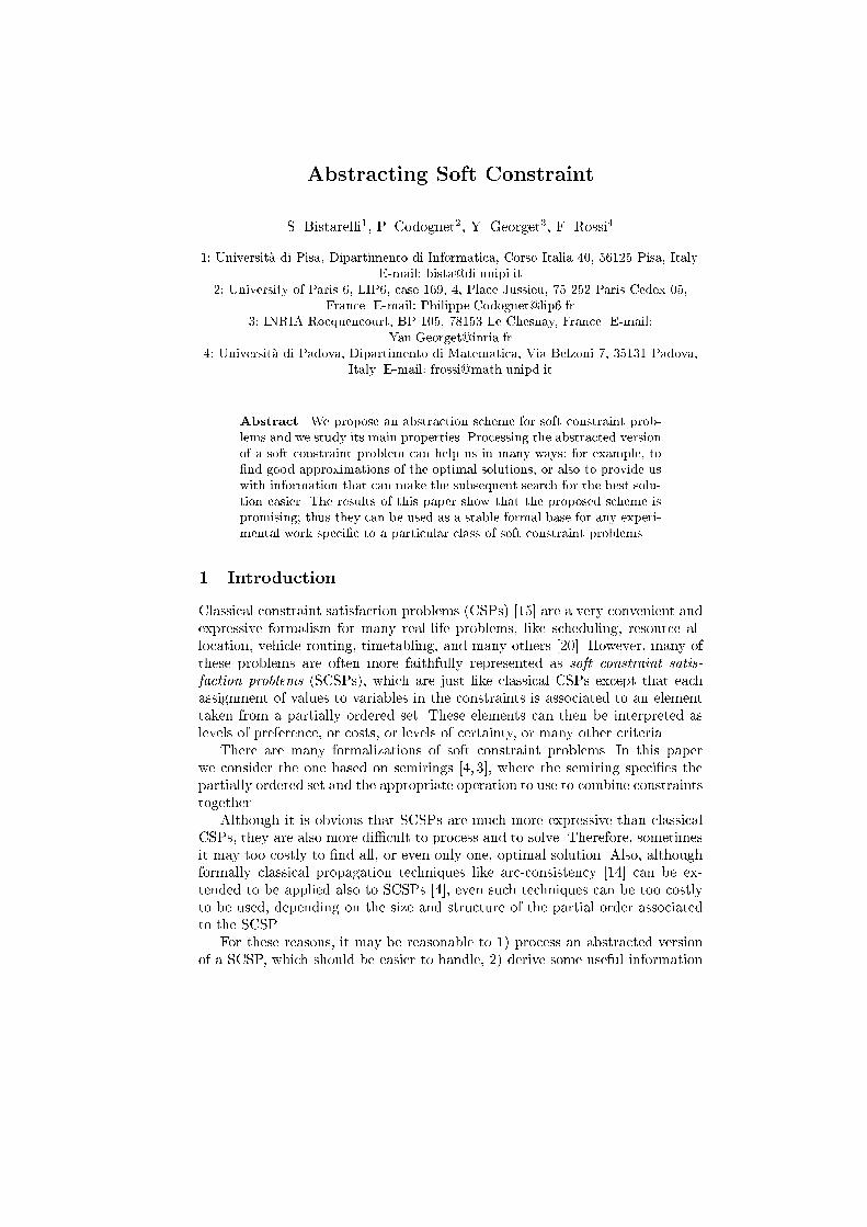
of variables (the ones in con), and assigns to each tuple of values of D of thesevariables an element of the semiring set A. This element can then be interpretedin several ways: as a level of preference, or as a cost, or as a probability, etc.,depending on the choice of the semiring operations.Constraints can be compared by looking at the semiring values associated tothe same tuples: Consider two constraints c1 = hdef1; coni and c2 = hdef2; coni,with jconj = k. Then c1 vS c2 if for all k-tuples t, def1(t) �S def2(t). Therelation vS is a partial order.A soft constraint satisfaction problem (SCSP) is a pair hC; coni where con �V and C is a set of constraints. Note that a classical CSP is a SCSP wherethe chosen c-semiring is: SCSP = hffalse; trueg;_;^; false; truei. Fuzzy CSPs[8, 16, 17] can instead be modeled in the SCSP framework by choosing the c-semiring: SFCSP = h[0; 1];max;min; 0; 1i. Figure 1 shows a fuzzy CSP. Variablesare inside circles, constraints are represented by undirected arcs, and semiringvalues are written to the right of the corresponding tuples. Here we assume thatthe domain D of the variables contains only elements a and b.a ... 0.9

b ... 0.5

a ... 0.9

b ... 0.1

aa ... 0.8

ab ... 0.2

ba ... 0

bb ... 0

X Y

Fig. 1. A fuzzy CSP.Given two constraints c1 = hdef1; con1i and c2 = hdef2; con2i, their com-bination c1 c2 is the constraint hdef; coni de�ned by con = con1 [ con2 anddef(t) = def1(t #concon1)�def(t #concon2). In words, combining two constraints meansbuilding a new constraint involving all the variables of the original ones, andwhich associates to each tuple of domain values for such variables a semiring el-ement which is obtained by multiplying the elements associated by the originalconstraints to the appropriate subtuples.Using the properties of � and +, it is easy to prove that: is associativeand commutative, and monotone over vC . Moreover, if � is idempotent, isidempotent as well.Given a constraint c = hdef; coni and a subset I of V , the projection of cover I , written c +I , is the constraint hdef 0; con0i where con0 = con \ I anddef 0(t0) = Pt=t#conI\con=t0 def(t). Informally, projecting means eliminating somevariables. This is done by associating to each tuple over the remaining variablesa semiring element which is the sum of the elements associated by the originalconstraint to all the extensions of this tuple over the eliminated variables.

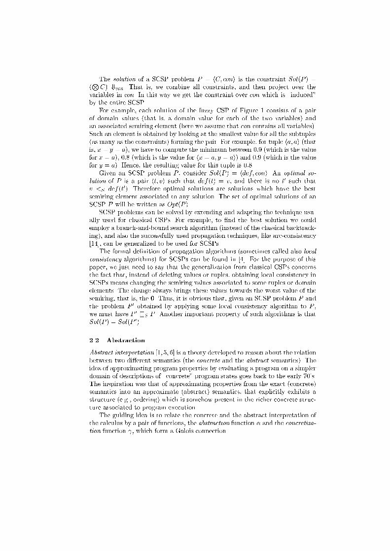
The solution of a SCSP problem P = hC; coni is the constraint Sol(P ) =(NC) +con. That is, we combine all constraints, and then project over thevariables in con. In this way we get the constraint over con which is \induced"by the entire SCSP.For example, each solution of the fuzzy CSP of Figure 1 consists of a pairof domain values (that is, a domain value for each of the two variables) andan associated semiring element (here we assume that con contains all variables).Such an element is obtained by looking at the smallest value for all the subtuples(as many as the constraints) forming the pair. For example, for tuple ha; ai (thatis, x = y = a), we have to compute the minimum between 0:9 (which is the valuefor x = a), 0:8 (which is the value for hx = a; y = ai) and 0:9 (which is the valuefor y = a). Hence, the resulting value for this tuple is 0:8.Given an SCSP problem P , consider Sol(P ) = hdef; coni. An optimal so-lution of P is a pair ht; vi such that def(t) = v, and there is no t0 such thatv <S def(t0). Therefore optimal solutions are solutions which have the bestsemiring element associated to any solution. The set of optimal solutions of anSCSP P will be written as Opt(P ).SCSP problems can be solved by extending and adapting the technique usu-ally used for classical CSPs. For example, to �nd the best solution we couldemploy a branch-and-bound search algorithm (instead of the classical backtrack-ing), and also the successfully used propagation techniques, like arc-consistency[14], can be generalized to be used for SCSPs.The formal de�nition of propagation algorithms (sometimes called also localconsistency algorithms) for SCSPs can be found in [4]. For the purpose of thispaper, we just need to say that the generalization from classical CSPs concernsthe fact that, instead of deleting values or tuples, obtaining local consistency inSCSPs means changing the semiring values associated to some tuples or domainelements. The change always brings these values towards the worst value of thesemiring, that is, the 0. Thus, it is obvious that, given an SCSP problem P andthe problem P 0 obtained by applying some local consistency algorithm to P ,we must have P 0 vS P . Another important property of such algorithms is thatSol(P ) = Sol(P 0).2.2 AbstractionAbstract interpretation [1, 5, 6] is a theory developed to reason about the relationbetween two di�erent semantics (the concrete and the abstract semantics). Theidea of approximating program properties by evaluating a program on a simplerdomain of descriptions of \concrete" program states goes back to the early 70's.The inspiration was that of approximating properties from the exact (concrete)semantics into an approximate (abstract) semantics, that explicitly exhibits astructure (e.g., ordering) which is somehow present in the richer concrete struc-ture associated to program execution.The guiding idea is to relate the concrete and the abstract interpretation ofthe calculus by a pair of functions, the abstraction function � and the concretiza-tion function , which form a Galois connection.

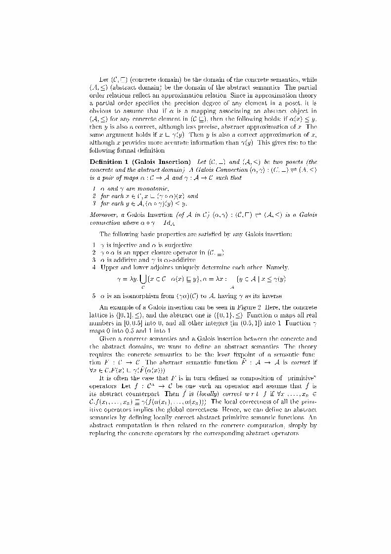
Let (C;v) (concrete domain) be the domain of the concrete semantics, while(A;�) (abstract domain) be the domain of the abstract semantics. The partialorder relations re ect an approximation relation. Since in approximation theorya partial order speci�es the precision degree of any element in a poset, it isobvious to assume that if � is a mapping associating an abstract object in(A;�) for any concrete element in (C v), then the following holds: if �(x) � y,then y is also a correct, although less precise, abstract approximation of x. Thesame argument holds if x v (y). Then y is also a correct approximation of x,although x provides more accurate information than (y). This gives rise to thefollowing formal de�nition.De�nition 1 (Galois Insertion). Let (C;v) and (A;�) be two posets (theconcrete and the abstract domain). A Galois Connection h�; i : (C;v)*) (A;�)is a pair of maps � : C ! A and : A ! C such that1. � and are monotonic,2. for each x 2 C; x v ( � �)(x) and3. for each y 2 A; (� � )(y) � y:Moreover, a Galois Insertion (of A in C) h�; i : (C;v) *) (A;�) is a Galoisconnection where � � = IdA.The following basic properties are satis�ed by any Galois insertion:1. is injective and � is surjective.2. � � is an upper closure operator in (C;v).3. � is additive and is co-additive.4. Upper and lower adjoints uniquely determine each other. Namely, = �y:[C fx 2 C j �(x) v yg; � = �x :\A fy 2 A j x � (y)5. � is an isomorphism from ( �)(C) to A, having as its inverse.An example of a Galois insertion can be seen in Figure 2. Here, the concretelattice is h[0; 1];�i, and the abstract one is hf0; 1g;�i. Function � maps all realnumbers in [0; 0:5] into 0, and all other integers (in (0:5; 1]) into 1. Function maps 0 into 0:5 and 1 into 1.Given a concrete semantics and a Galois insertion between the concrete andthe abstract domains, we want to de�ne an abstract semantics. The theoryrequires the concrete semantics to be the least �xpoint of a semantic func-tion F : C ! C. The abstract semantic function ~F : A ! A is correct if8x 2 C:F (x) v ( ~F (�(x))).It is often the case that F is in turn de�ned as composition of \primitive"operators. Let f : Cn ! C be one such an operator and assume that ~f isits abstract counterpart. Then ~f is (locally) correct w.r.t. f if 8x1; : : : ; xn 2C:f(x1; : : : ; xn) v ( ~f(�(x1); : : : ; �(xn))). The local correctness of all the prim-itive operators implies the global correctness. Hence, we can de�ne an abstractsemantics by de�ning locally correct abstract primitive semantic functions. Anabstract computation is then related to the concrete computation, simply byreplacing the concrete operators by the corresponding abstract operators.

1

0.5

}}

0

abstract latticeconcrete lattice

0

1

γ

α

α

γ

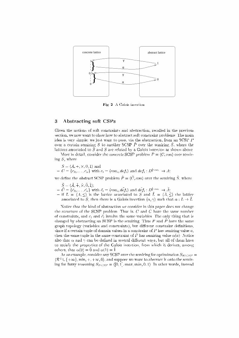
Fig. 2. A Galois insertion.3 Abstracting soft CSPsGiven the notions of soft constraints and abstraction, recalled in the previoussection, we now want to show how to abstract soft constraint problems. The mainidea is very simple: we just want to pass, via the abstraction, from an SCSP Pover a certain semiring S to another SCSP ~P over the semiring ~S, where thelattices associated to ~S and S are related by a Galois insertion as shown above.More in detail, consider the concrete SCSP problem P = hC; coni over semir-ing S, where{ S = hA;+;�; 0; 1i and{ C = fc0; : : : ; cng with ci = hconi; defii and defi : Djconij ! A;we de�ne the abstract SCSP problem ~P = h ~C; coni over the semiring ~S, where{ ~S = h ~A; ~+; ~�; ~0; ~1i;{ ~C = f ~c0; : : : ; ~cng with ~ci = hconi; ~defii and ~defi : Djconij ! ~A;{ if L = hA;�i is the lattice associated to S and ~L = h ~A; ~�i the latticeassociated to ~S, then there is a Galois insertion h�; i such that � : L! ~L.Notice that the kind of abstraction we consider in this paper does not changethe structure of the SCSP problem. That is, C and ~C have the same numberof constraints, and ci and ~ci involve the same variables. The only thing that ischanged by abstracting an SCSP is the semiring. Thus P and ~P have the samegraph topology (variables and constraints), but di�erent constraint de�nitions,since if a certain tuple of domain values in a constraint of P has semiring value a,then the same tuple in the same constraint of ~P has semiring value �(a). Noticealso that � and can be de�ned in several di�erent ways, but all of them haveto satisfy the properties of the Galois insertion, from which it derives, amongothers, that �(0) = ~0 and �(1) = ~1.As an example, consider any SCSP over the semiring for optimization SWCSP =hR+[f+1g;min;+;+1; 0i, and suppose we want to abstract it onto the semir-ing for fuzzy reasoning SFCSP = h[0; 1];max;min; 0; 1i. In other words, instead

of computing the minimum of the sum of all costs, we just want to compute theminimum of the maximum of all costs, and we want to normalise the costs over[0::1]. As noted above, the mapping � : hR+;�WCSP i ! h[0; 1];�FCSP i can bede�ned in di�erent ways. For example one can decide to map all the reals abovesome �xed real x onto 1 and then to divide the reals in [0; x] in several intervalsand map each of these intervals onto one element of [0; 1).Another example is the abstraction from the fuzzy semiring to the classicalone: SCSP = hf0; 1g;_;^; 0; 1i. Here function � maps each element of [0; 1] intoeither 0 or 1. For example, one could map all the elements in [0; x] onto 0, andall those in (x; 1] onto 1, for some �xed x. Figure 2 represents this example withx = 0:5.We have de�ned Galois insertions between two lattices hL;�Si and h~L; ~� ~Siof semiring values. However, for convenience, in the following we will often useGalois insertions between lattices of problems hPL;vSi and h ~PL; ~v ~Si where PLcontains problems over the concrete semiring and ~PL over the abstract semiring.This does not change the meaning of our abstraction, we are just upgrading theGalois insertion from semiring values to problems. Thus, when we will say that~P = �(P ), it will mean that ~P is obtained by P via the application of � to allthe semiring values appearing in P .4 Properties and advantages of the abstractionLet us consider the scheme depicted in Figure 3. Here and in the followingpictures, the left box contains the lattice of concrete problems, and the rightone the lattice of abstract problems. The partial order in each of these lattices isshown via dashed lines. Connections between the two lattices, via the abstractionand concretization functions, is shown via directed arrows. In the following, wewill call S = hA;+;�;0;1i the concrete semiring and ~S = h ~A; ~+; ~�; ~0; ~1i theabstract one. Thus we will always consider a Galois insertion h�; i : hA;�Si*)h ~A;� ~Si.abstract problemsconcrete problems

P

αγ

α

γ( (P))αα (P) = P

~

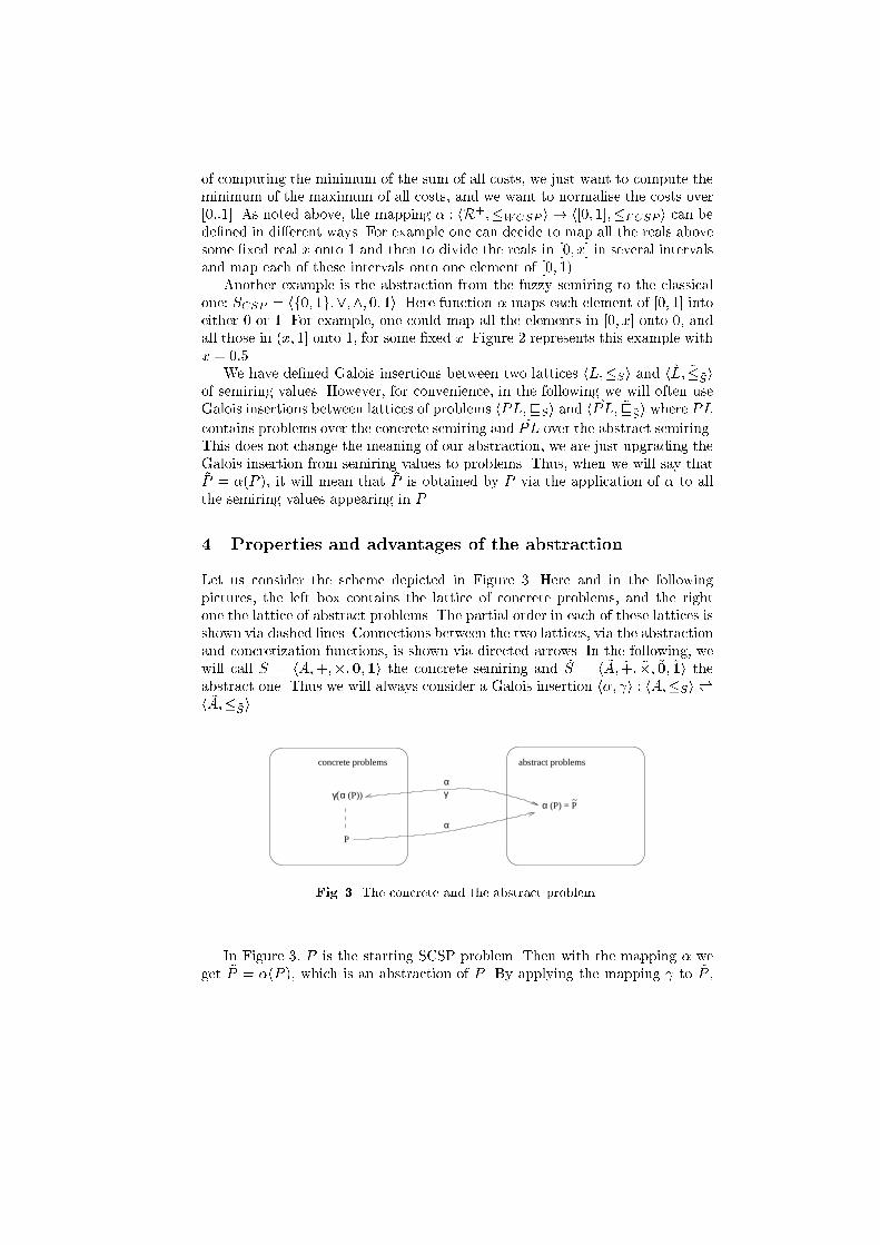
Fig. 3. The concrete and the abstract problem.In Figure 3, P is the starting SCSP problem. Then with the mapping � weget ~P = �(P ), which is an abstraction of P . By applying the mapping to ~P ,

we get the problem (�(P )). Let us �rst notice that these two problems (P and (�(P ))) are related by a precise property, as stated by the following theorem.Theorem 1. Given an SCSP problem P over S, we have that P vS (�(P )).We recall that this means that, for each tuple in each constraint, the semiringvalue associated to such a tuple in P is smaller (w.r.t.�S) than the correspondingvalue associated to the same tuple in (�(P )). This comes from the propertiesof the Galois insertion h�; i, in particular from the fact that, for each x, x �S (�(x)). Notice that this implies that, if a tuple in (�(P )) has semiring value0, then it must have value 0 also in P . This holds also for the solutions, whosesemiring value is obtained by combining the semiring values of several tuples.Corollary 1. Given an SCSP problem P over S, we have that Sol(P ) vSSol( (�(P )).We recall that Sol(P ) is just a constraint, which is obtained as N(C) +con.Thus the statement of this corollary comes just from the monotonicity of � and+. A consequence of this result is that, by passing from P to (�(P )), we mayloose some inconsistency but we will not introduce new ones. That is, if a solutionof (�(P )) has value 0, then this was true also in P .There is also an interesting relationship between the set of optimal solutionsof P and that of �(P ). In fact, if a certain tuple is optimal in P , then this sametuple is also optimal in �(P ). This again comes from the properties of a Galoisinsertion, in particular from the monotonicity of �.Theorem 2. Given an SCSP problem P over S, we have that Opt(P ) � Opt(�(P )).Therefore, the set of optimal solutions of the abstract problem contains all theoptimal solutions of the concrete problem. Thus, if we want to �nd an optimalsolution of the concrete problem, we could �nd all the optimal solutions of theabstract problem, and then use them on the concrete side to �nd an optimalsolution for the concrete problem. Assuming that working on the abstract sideis easier than on the concrete side, this method could help us �nd an optimalsolution of the concrete problem by looking at just a subset of tuples in theconcrete problem.Another point to notice is that any optimal solution, say t, of the abstractproblem, say with value ~v, has a value among v1; : : : ; vn in P , where �(v1) =: : : = �(vn) = ~v. Now, because of properties of the Galois insertion, there existsan optimal solution of P with value among the vi's. Thus, if we think thatapproximating the optimal value with a value within the bounds of v1; : : : ; vnis satisfactory, we can take t as an approximation of an optimal solution of P .More precisely, we have that (~v) is an upper bound of the value of an optimalsolution of P , and the value vi given by P to t is a lower bound.Theorem 3. Given an SCSP problem P over S, consider an optimal solutionof �(P ), say t, with semiring value ~v in �(P ) and v in P . Consider also the setV of all concrete semiring values such that �(vi) = ~v for all vi 2 V . Then thereexists an optimal solution �t of P , say with value �v, such that:

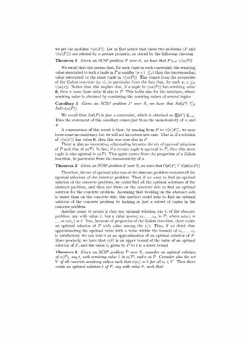
{ �v 2 V ;{ v � �v � (~v).Consider now what we can do on the abstract problem, �(P ). One possibilityis to apply an abstract function ~f , which can be, for example, a local consistencyalgorithm or also a solution algorithm. In the following, we will consider functions~f which are always intensive, that is, which bring the given problem closer to thebottom of the lattice. In fact, our goal is to solve an SCSP, thus going higher inthe lattice does not help in this task, since solving means combining constraintsand thus getting lower in the lattice. Also, the functions ~f we will considerwill always be locally correct with respect to any function fsol which solvesthe concrete problem. We will call such a property solution-correctness. Moreprecisely, given a problem P with constraint set C, fsol(P ) is a new problem P 0with the same topology as P whose tuples have semiring values possibly lower.Let us call C 0 the set of constraints of P 0. Then, for any constraint c0 2 C 0,c0 = (NC) +var(c0). In other words, fsol combines all constraints of P and thenprojects the resulting global constraint over each of the original constraints.De�nition 2. Given an SCSP problem P over S, consider a function ~f on�(P ). Then ~f is solution-correct if, given any fsol which solves P , ~f is locallycorrect w.r.t. fsol.We will also need the notion of safeness of a function, which just means thatit maintains all the solutions.De�nition 3. Given an SCSP problem P and a function f : PL ! PL, f issafe if Sol(P ) = Sol(f(P )).From ~f(�(P )), applying the concretization function , we get ( ~f(�(P ))),which therefore is again over the concrete semiring (the same as P ). The fol-lowing property says that, under certain conditions, P and P ( ~f(�(P ))) areequivalent. Figure 4 describes such a situation. In this �gure, we can see thatseveral partial order lines have been drawn. On the abstract side, function ~ftakes any element closer to the bottom, because of its intensiveness. On theconcrete side, P ( ~f(�(P ))) is smaller than both P and ( ~f(�(P ))) becauseof the properties of . Also, ( ~f(�(P ))) is smaller than (�(P )) because of themonotonicity of , ( ~f(�(P ))) is higher than fsol(P ) because of the solution-correctness of ~f , and fsol(P ) is smaller than P because of the way fsol(P ) isconstructed. Finally, if � is idempotent, then it coincides with the glb, thus wehave that P ( ~f(�(P ))) is higher than fsol(P ), because by de�nition the glbis the higher among all the lower bounds of P and ( ~f(�(P ))).Theorem 4. Given an SCSP problem P over S, consider a function ~f on �(P )which is safe, solution-correct, and intensive. Then, if � is idempotent, Sol(P ) =Sol(P ( ~f(�(P )))).This theorem does not say anything about the power of ~f , which could makemany modi�cations to �(P ) but could also not modify anything. In this last

(P)α

f(~ (P))α

f(~

f(~xO

P

f_sol(P)

γα

α

γα

γ( (P))α

(P)))αγ(

(P))αγ(P

x idempotent

concrete problems abstract problems

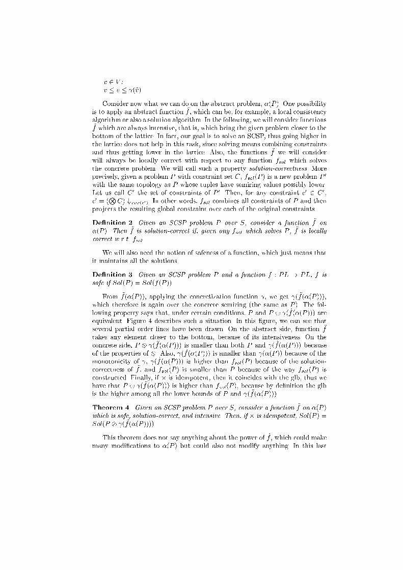
Fig. 4. The general abstraction scheme, with � idempotent.case, ( ~f(�(P ))) = (�(P )) w P (see Figure 5), so P ( ~f(�(P ))) = P , whichmeans that we have not gained anything in abstracting P . However, we canalways use the relationship between P and �(P ) (see Theorem 2 and 3) to �ndan approximation of the optimal solutions and of the inconsistencies of P .(P)α f(~ (P))α

f(~ (P))αγ

abstract problemsconcrete problems

P

αγ

α

== γ( (P))α

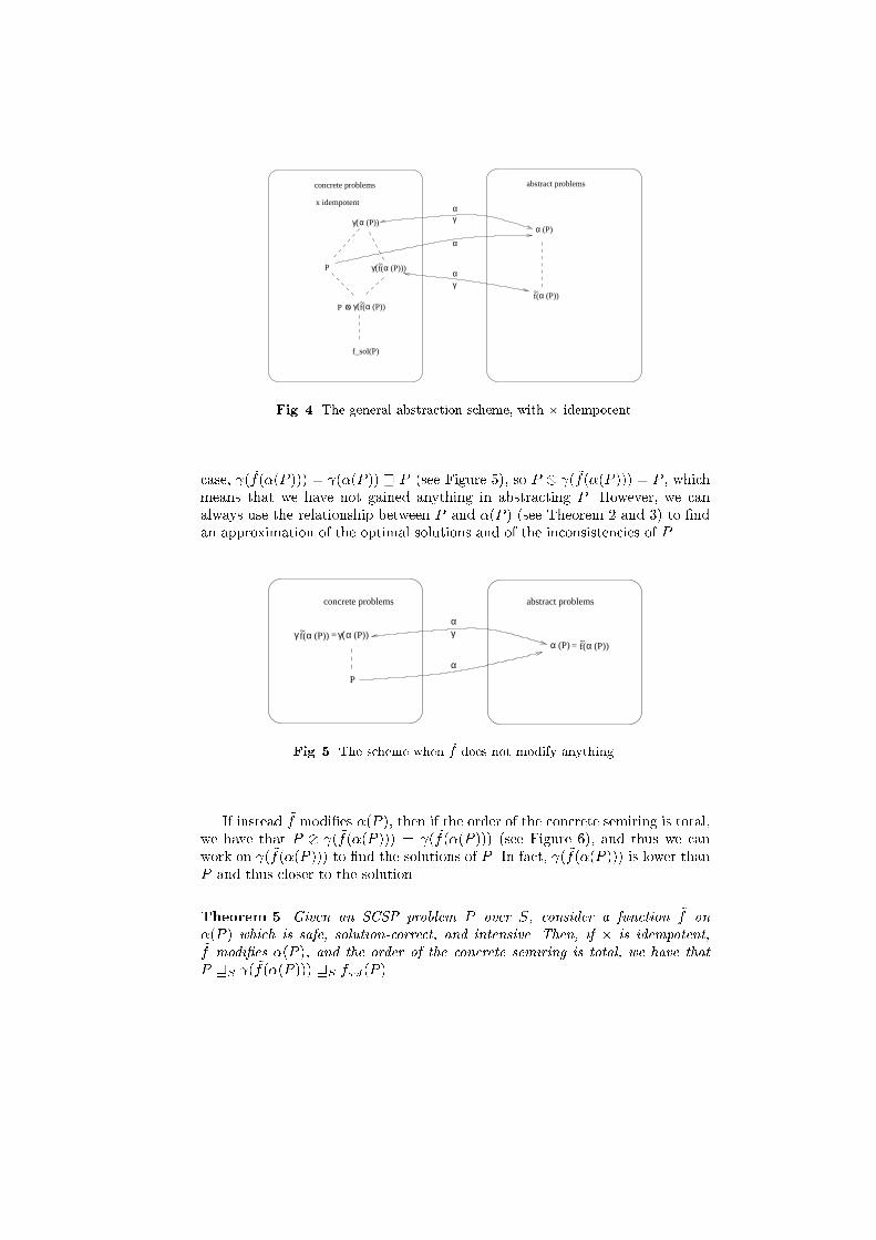
Fig. 5. The scheme when ~f does not modify anything.If instead ~f modi�es �(P ), then if the order of the concrete semiring is total,we have that P ( ~f(�(P ))) = ( ~f(�(P ))) (see Figure 6), and thus we canwork on ( ~f(�(P ))) to �nd the solutions of P . In fact, ( ~f(�(P ))) is lower thanP and thus closer to the solution.Theorem 5. Given an SCSP problem P over S, consider a function ~f on�(P ) which is safe, solution-correct, and intensive. Then, if � is idempotent,~f modi�es �(P ), and the order of the concrete semiring is total, we have thatP wS ( ~f(�(P ))) wS fsol(P ).

(P)α

f(~ (P))αf(~

total order

abstract problemsconcrete problems

P

f_sol(P)

αγ

α

α

γ( (P))α

(P)))αγ(

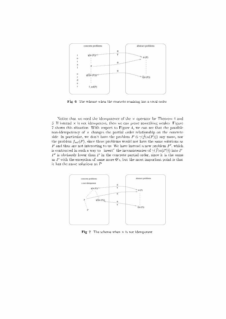
Fig. 6. The scheme when the concrete semiring has a total order.Notice that we need the idempotence of the � operator for Theorem 4 and5. If instead � is not idempotent, then we can prove something weaker. Figure7 shows this situation. With respect to Figure 4, we can see that the possiblenon-idempotency of � changes the partial order relationship on the concreteside. In particular, we don't have the problem P ( ~f(�(P ))) any more, northe problem fsol(P ), since these problems would not have the same solutions asP and thus are not interesting to us. We have instead a new problem P 0, whichis contructed in such a way to \insert" the inconsistencies of ( ~f(�(P ))) into P .P 0 is obviously lower than P in the concrete partial order, since it is the sameas P with the exception of some more 0's, but the most important point is thatit has the same solutions as P .(P)α

f(~ (P))α

f(~P

γα

α

γα

γ( (P))α

(P)))αγ(

x not idempotent

concrete problems abstract problems

P’Fig. 7. The scheme when � is not idempotent.

Theorem 6. Given an SCSP problem P over S, consider a function ~f on �(P )which is safe, solution-correct and intensive. Then, if � is not idempotent, con-sider P 0 to be the SCSP which is the same as P except for those tuples whichhave semiring value 0 in (�( ~f(P ))): these tuples are given value 0 also in P 0.Then we have that Sol(P ) = Sol(P 0).Summarizing, the above theorems can give us several hints on how to use theabstraction scheme to make the solution of P easier: If � is idempotent, thenwe can replace P with P (�( ~f(P ))), and get the same solutions (by Theorem4). If instead � is not idempotent, we can replace P with P 0 (by Theorem 6). Inany case, the point in passing from P to P (�( ~f(P ))) (or P 0) is that the newproblem should be easier to solve than P , since the semiring values of its tuplesare more explicit, that is, closer to the values of these tuples in a completelysolved problem.More precisely, consider a branch-and-bound algorithm to �nd an optimalsolution of P . Then, once a solution is found, its value will be used to cut awaysome branches, where the semiring value is worse than the value of the solutionalready found. Now, if the values of the tuples are worse in the new problemthan in P , each branch will have a worse value and thus we might cut awaymore branches. Therefore, the search tree of the new problem is smaller thanthat of P .Another point to notice is that, if using a greedy algorithm to �nd the initialsolution (to use later as a lower bound), this initial phase in the new problemwill lead to a better estimate, since the values of the tuples are worse in the newproblem and thus close to the optimum. In the extreme case in which the changefrom P to the new problem brings the semiring values of the tuples to coincidewith the value of their combination, it is possible to see that the initial solutionis already the optimal one.Notice also that, if � is not idempotent, a tuple of P 0 has either the samevalue as in P , or 0. Thus the initial estimate in P 0 is the same as that of P(since the initial solution must be a solution), but the search tree of P 0 is againsmaller than that of P , since there may be partial solutions which in P havevalue di�erent from 0 and in P 0 have value 0, and thus the global inconsistencymay be recognized earlier.The same reasoning used for Theorem 2 on �(P ) can also be applied to~f(�(P )). In fact, since ~f is safe, the solutions of ~f(�(P )) have the same valuesas those of �(P ). Thus also the optimal solution sets coincide. Therefore wehave that Opt( ~f (�(P ))) contains all the optimal solutions of P . This meansthat, in order to �nd an optimal solution of P , we can �nd all optimal solutionsof ~f(�(P )) and then use such a set to prune the search for an optimal solutionof P .Theorem 7. Given an SCSP problem P over S, consider a function ~f onP which is safe, solution-correct and intensive. Then we have that Opt(P ) �Opt( ~f(�(P ))).

Theorem 3 can be adapted to ~f(�(P )) as well, thus allowing us to use anoptimal solution of ~f(�(P )) to �nd both a lower and an upper bound of anoptimal solution of P .5 Conclusions and future workWe have proposed an abstraction scheme for abstracting soft constraint prob-lems, with the goal of �nding an optimal solution is a shorter time. The mainidea is to work on the abstract version of the problem and then bring back someuseful information to the concrete problem, to make it easier to solve.Future work will concern the comparison between our properties and theone of [7], the generalization of our scheme to abstract also domains and graphtopologies, and an experimental phase to assess the practical value of our pro-posal.References1. G. Birkho� and S. MacLane. A Survey of Modern Algebra. MacMillan, 1965.2. S. Bistarelli, H. Fargier, U. Montanari, F. Rossi, T. Schiex, and G. Verfaillie.Semiring-based CSPs and valued CSPs: Basic properties and comparison. In Over-Constrained Systems. Springer-Verlag, LNCS 1106, 1996.3. S. Bistarelli, U. Montanari, and F. Rossi. Constraint Solving over Semirings. InProc. IJCAI95. Morgan Kaufman, 1995.4. S. Bistarelli, U. Montanari, and F. Rossi. Semiring-based Constraint Solving andOptimization. Journal of the ACM, 44(2):201{236, March 1997.5. P. Cousot and R. Cousot. Abstract interpretation: A uni�ed lattice model for staticanalysis of programs by construction or approximation of �xpoints. In Fourth ACMSymp. Principles of Programming Languages, pages 238{252, 1977.6. P. Cousot and R. Cousot. Systematic design of program analyis. In Sixth ACMSymp. Principles of Programming Languages, pages 269{282, 1979.7. S. de Givry, G. Verfaille, , and T. Schiex. Bounding The Optimum of Con-straint Optimization Problems. In G. Smolka, editor, Proc. CP97, pages 405{419.Springer-Verlag, LNCS 1330, 1997.8. D. Dubois, H. Fargier, and H. Prade. The calculus of fuzzy restrictions as a basisfor exible constraint satisfaction. In Proc. IEEE International Conference onFuzzy Systems, pages 1131{1136. IEEE, 1993.9. Thomas Ellman. Synthesis of abstraction hierarchies for constraint satisfactionby clustering approximately equivalent objects. In Proceedings of InternationalConference on Machine Learning, pages 104{111, 1993.10. H. Fargier and J. Lang. Uncertainty in constraint satisfaction problems: a prob-abilistic approach. In Proc. European Conference on Symbolic and QualitativeApproaches to Reasoning and Uncertainty (ECSQARU), pages 97{104. Springer-Verlag, LNCS 747, 1993.11. E. C. Freuder and D Sabin. Interchangeability supports abstraction and refor-mulation for constraint satisfaction. In Proceedings of Symposium on Abstraction,Reformulation and Approximation (SARA'95), 1995.12. E. C. Freuder and R. J. Wallace. Partial constraint satisfaction. AI Journal, 58,1992.

13. Y. Georget and P. Codognet. Compiling semiring-based constraints withclp(FD,S). In M.Maher and J-F. Puget, editors, Proc. CP98. Springer-Verlag,LNCS 1520, 1998.14. A.K. Mackworth. Consistency in networks of relations. Arti�cial Intelligence,8(1):99{118, 1977.15. A.K. Mackworth. Constraint satisfaction. In Stuart C. Shapiro, editor, Encyclo-pedia of AI (second edition), volume 1, pages 285{293. John Wiley & Sons, 1992.16. Zs. Ruttkay. Fuzzy constraint satisfaction. In Proc. 3rd IEEE International Con-ference on Fuzzy Systems, pages 1263{1268, 1994.17. T. Schiex. Possibilistic constraint satisfaction problems, or \how to handle softconstraints?". In Proc. 8th Conf. of Uncertainty in AI, pages 269{275, 1992.18. T. Schiex, H. Fargier, and G. Verfaille. Valued Constraint Satisfaction Problems:Hard and Easy Problems. In Proc. IJCAI95, pages 631{637. Morgan Kaufmann,1995.19. R. Schrag and D. Miranker. An evaluation of domain reduction: Abstraction forunstructured csps. In Proceedings of the Symposium on Abstraction, Reformulation,and Approximation, pages 126{133, 1992.20. M. Wallace. Practical applications of constraint programming. Constraints: AnInternational Journal, 1, 1996.