ABSTRACT Title of Document: GENERATING UP-TO-DATE STARTING VALUES FOR DETAILED FORECASTING MODELS San Sampattavanija, Ph.D., 2008 Directed By: Professor Emeritus Clopper Almon, Department of Economics In economic forecasting, it is important that the forecasts be based on data that is both reliable and up-to-date. The most reliable data typically come from conducting a census. These censuses produce estimates with a long lag between the reference year and the date of publication. However, we also have other sources of economic data that are less reliable but published more frequently. These higher frequency data should be a source of useful information for analyzing economic activity in the current, incomplete year. The objective of this study is to use high frequency (monthly and quarterly) data to generate forecasts of the annual data from reliable sources used in an inter-industry forecasting model. The results will be used as starting values to improve the model's short-term forecast performance.

Welcome message from author
This document is posted to help you gain knowledge. Please leave a comment to let me know what you think about it! Share it to your friends and learn new things together.
Transcript

ABSTRACT
Title of Document: GENERATING UP-TO-DATE STARTING VALUES
FOR DETAILED FORECASTING MODELS
San Sampattavanija, Ph.D., 2008
Directed By: Professor Emeritus Clopper Almon, Department of
Economics
In economic forecasting, it is important that the forecasts be based on data that is
both reliable and up-to-date. The most reliable data typically come from conducting a
census. These censuses produce estimates with a long lag between the reference year and
the date of publication. However, we also have other sources of economic data that are
less reliable but published more frequently. These higher frequency data should be a
source of useful information for analyzing economic activity in the current, incomplete
year.
The objective of this study is to use high frequency (monthly and quarterly) data
to generate forecasts of the annual data from reliable sources used in an inter-industry
forecasting model. The results will be used as starting values to improve the model's
short-term forecast performance.

The distinguishing feature of this dissertation is that it studies the economic data
at the sectoral level as opposed to other studies that only try to generate aggregate data.
The aggregate data will be a by-product of these detailed estimates. Thus, we can forecast
the trends of the aggregates and observe sectors that contribute to these trends.
In this dissertation, I study data on four main aspectts of the U.S. economy: 1)
Personal consumption expenditures, 2) Investment in equipment and software, 3)
Investment in structures, and 4) Gross output.
By historical simulations, I find that the performance of the forecasts depends
heavily on the accuracy of the exogenous variables used in each forecast. The estimated
detailed values are consistent with the macroeconomic data, used as regressors in the
processes. Thus, generally, the results will be reliable as long as we have a good forecast
of macroeconomic variables.
The performance of the first-period forecast also depends on where in the
calendar year the last published data is. The closer to the end of the year, the better is the
accuracy of the forecast.

GENERATING UP-TO-DATE STARTING VALUES FOR DETAILED
FORECASTING MODELS
By
San Sampattavanija
Dissertation submitted to the Faculty of the Graduate School of theUniversity of Maryland, College Park, in partial fulfillment
of the requirements for the degree ofDoctor of Philosophy
2008
Advisory CommitteeProfessor Emeritus Clopper Almon, Chair Professor Ingmar Prucha Professor Mark P. Leone Associate Professor John Chao Dr. Jeffrey Werling
© Copyright by San Sampattavanija
2008

Dedication
To Praphis and Suvit Sampattavanija, my mother and father. Their love, encouragement, and patient has been and will always be a guiding light for me.
ii

Acknowledgements
I am deeply in debt to Professor Emeritus Clopper Almon, my advisor. His assistance and guidance are very important to the completion of this dissertation. I have learnt not only economics but also many other skills through the vast knowledge and experience of Professor Almon.
I also would like to thank other committee members: Professor Ingmar Prucha, Professor Mark Leone, Professor John Chao, and Dr. Jeff Werling for their comments and suggestions.
All the discussions with INFORUM staffs – Dr. Jeff Werling, Dr. Doug Meade, Dr. Doug Nyhus, Margaret McCarthy, and Dr. Ronald Horst -- were very beneficial and helped toward the completion of this work. I am also grateful to many discussions with Dr. Somprawin Manprasert.
Special thanks to all members of Thai UMCP students as well as all my friends and family for all encouragements and moral supports. Hospitality from Kulthida and Brian O'Neill is very important to my good health through my time in the Program.
Finally, I will not be able to complete this dissertation without love, encouragement and all the supports from my family especially my mother, Praphis Sampattavanija.
iii

Table of Contents
Dedication............................................................................................................................ii
Acknowledgements............................................................................................................iii
Table of Contents................................................................................................................iv
List of Tables.....................................................................................................................vii
List of Figures.....................................................................................................................ix
Chapter 1: Introduction........................................................................................................11.1 The Problem of the “Ragged End” of Historical Data for Long-term Modeling......11.2 The Scope of this Study............................................................................................21.3 Related Work.............................................................................................................31.4 Steps in the Solution of the Ragged-end Problem....................................................41.5 Outline of the study and guide to quick reading.......................................................5
Chapter 2: Measuring Real Growth.....................................................................................62.1 Hedonic Indexes........................................................................................................62.2 Runaway Deflators, Ideal and Chained Indexes, and Non-additivity.......................92.3 Remedies for Non-additivity...................................................................................152.4 Suggested Remedies................................................................................................16
Chapter 3. Personal Consumption Expenditure.................................................................223.1. What are Personal consumption expenditures?......................................................233.2. Broad trends in the structure of PCE .....................................................................263.3. Data for short-term forecasting of PCE.................................................................29
The dependent variables...........................................................................................29Explanatory variables...............................................................................................30Equations estimated..................................................................................................30Approach to the problem..........................................................................................32
3.4 Discussions of interesting detailed PCE equations' estimation results...................33New autos.................................................................................................................33Computers and peripherals.......................................................................................35Software....................................................................................................................36Pleasure aircraft........................................................................................................37Books and maps........................................................................................................39Coffee, tea and beverage materials...........................................................................40Women's and children's clothing and accessories....................................................41Gas and Oil...............................................................................................................42
iv

Housing.....................................................................................................................43Cell phone, local phone and long distance phone....................................................45Airlines.....................................................................................................................48Health insurance.......................................................................................................50Brokerage charges and investment counseling.........................................................51
3.5 Historical Simulations.............................................................................................52Total annual PCE......................................................................................................57Durable goods...........................................................................................................58Nondurable goods.....................................................................................................63Services.....................................................................................................................70
3.6 Short-term forecast of Personal consumption expenditures....................................783.6.1 Forecast assumptions.......................................................................................783.6.2 Outlook with plots and aggregates (annual series)..........................................79
Chapter 4: Private fixed Investment in Equipment and Software......................................904.1 Data for Private Fixed Investment in Equipment and Software.............................904.2 Approach to the problem.........................................................................................994.3 NIPA Investment in Equipment and Software by Asset Types Equations............1004.4 FAA Investment in Equipment and Software by Purchasing Industries Equations.....................................................................................................................................1064.5 Historical Simulations...........................................................................................1234.6 Forecast of Private Fixed Investment in Equipment and Software through 2008 134
Forecast Assumptions.............................................................................................134Outlook of Fixed Investment in Equipment and Software.....................................135
Chapter 5. Investment in Structures.................................................................................1455.1 Data and Estimation Approaches for Private Fixed Investment in Structures......1465.2 Approach to Forecast Investment in Structures....................................................153
5.2.1 Nonresidential Investment in Structures.......................................................1535.2.2 Residential Investment in Structures.............................................................156
5.3 Monthly VIP Equations.........................................................................................1565.4 Nonresidential Fixed Investment in Structures Equations....................................163
5.4.1 Quarterly Equations for VIP-based Nonresidential Fixed Investment in Structures................................................................................................................1635.4.2 Annual NIPA Nonresidential Fixed Investment in Structures Equations......171
5.5 Residential Fixed Investment in Structures Equations..........................................1805.5.1 Extending NIPA series using VIP-based Residential Construction...............1805.5.2 Quarterly Residential Fixed Investment in Structures Equations..................183
5.6 Historical Simulations...........................................................................................1865.7 Forecast of Fixed Investment in Structures between 2007 and 2008....................196
Forecast Assumptions.............................................................................................197Outlook of Fixed Investment in Structures by Asset Types in 2007 and 2008......197
Chapter 6: Gross Output by Industry...............................................................................209
v

6.1 Data on Gross Output and High-Frequency Explanatory Variables......................211Gross output by industry 1947 – 2005....................................................................211High-frequency explanatory variables...................................................................212
6.2 The Method ..........................................................................................................215Annual Equations...................................................................................................216Monthly Equations.................................................................................................219
6.3 Illustration and Evaluation of the Method ...........................................................2226.4 Forecast of Gross Output between 2006-2008......................................................249
Forecast assumptions..............................................................................................249Outlook of Gross Output by Industries..................................................................251
Chapter 7: Conclusion......................................................................................................263
Appendices.......................................................................................................................264Appendix 3.1: Personal Consumption Expenditures by Type of Product...................264Appendix 3.2: PCE categories to be calculated, 116 categories.................................269Appendix 3.3:..............................................................................................................271
Nominal equations..................................................................................................271Price index equations..............................................................................................300
Appendix 3.4: Plots of Detailed Annual PCE Forecast 2007-2008............................327Appendix 3.5: Results.................................................................................................347Appendix 4.1: Estimation Results for Nominal Value of annual Fixed Asset Accounts by Purchasing Industries.............................................................................................353Appendix 4.2: Detailed Forecast Results of NIPA Equipment and Software Investment.....................................................................................................................................365Appendix 4.3: Detailed Forecast Results of FAA by Purchasing Industries...............366Appendix 4.4: Plots of NIPA Equipment and Software Fixed Investment Forecast...368Appendix 4.5: Plots of FAA by Purchasing Industries Forecast.................................369Appendix 5.1: Regressions' Results of Annual Fixed Investment in Nonresidential Structures.....................................................................................................................380Appendix 6.1: Gross Domestic Product by Industry Categories, BEA......................384Appendix 6.2: Results from Historical Simulations...................................................387Appendix 6.3: Real Gross Output and Price Index Regressions.................................390Appendix 6.4: Regression Results for Monthly Equations.........................................413Appendix 6.5: Glossary of Variables used in Chapter 6.............................................443Appendix 6.6: Gross Output by Detailed industries in 2006-2008.............................445
Bibliography....................................................................................................................448
vi

List of Tables
Table 2.1: U.S. and World-Wide Sales of PC-type Computers............................................9Table 2.2: The Runaway Deflator Problem with Made-up Data.......................................10Table 2.3: The Ideal Index Controls Disparate Deflators..................................................13Table 2.4: Comparison of Real GDP components between Chain-weighted and Fixed-
weighted methods......................................................................................19Table 3.1: Nominal Gross Domestic Product [Billions of dollars]....................................22Table 3.2: Content of PCE.................................................................................................24Table 3.3: Nominal and Real Personal consumption expenditures between 1959-2005, by
Major categories.........................................................................................27Table 3.4: Personal consumption expenditures by Major types of product.......................29Table 3.5: Assumptions of exogenous variables used in the Second Historical Simulation
....................................................................................................................53Table 3.6: Results from Historical Simulations.................................................................54Table 3.7: Exogenous variables' assumption between July 2007 and December 2008.....79Table 3.8: Major aggregates of annual PCE Forecast 2007 and 2008...............................80Table 3.9: Growth rates of U.S. PCE 2000 - 2008.............................................................82Table 4.1: Quarterly Data on Equipment Investment. From NIPA Table 5.3.5 Quarterly92Table 4.2: Private fixed investment in equipment and software. ......................................94Table 4.3: Equipment Investment by Purchaser, from the Fixed Assets Accounts............97Table 4.4: Reconciliation of Equipment Investment in NIPA and FAA............................99Table 4.5: Estimation Results for Nominal values of Quarterly NIPA Fixed Investment in
Equipment and Software..........................................................................103Table 4.6: Estimation Results for Price indexes of Quarterly NIPA Fixed Investment in
Equipment and Software..........................................................................104Table 4.7: Assumptions of exogenous variables used in the Second Historical Simulation
..................................................................................................................124Table 4.8: Historical Simulations' Results in Major Investment Industries, Nominal.....125Table 4.9: Historical Simulations' Results in Detailed Investment Industries, Nominal. 126Table 4.10: Assumptions of exogenous variables used in fixed investment forecast......134Table 4.11: Summary of Forecast by Major Industry Groups.........................................136Table 4.12: Growth rates of Fixed Investment in Equipment and Software 2001-2008. 137Table 5.1: NIPA Quarterly Data on Investment in Structures..........................................145Table 5.2: NIPA Annual Table 5.4.5B Private Fixed Investment in Structures by Asset
Types........................................................................................................148Table 5.3: Construction Categories in the BEA Fixed Assets Accounts..........................149Table 5.4: Monthly Value of Construction Put in Place (VIP), Census Bureau .............149Table 5.5: Value of Construction Put in Place (VIP). Annual Data, Bureau of the Census
..................................................................................................................150Table 5.6: Comparison of NIPA and VIP Total Nonresidential Construction..................153Table 5.7: Integration of VIP with NIPA.........................................................................155Table 5.8: Assumptions of exogenous variables used in the Second Historical Simulation
vii

..................................................................................................................186Table 5.9: Historical Simulations' Results in Major and Detailed Investment Industries
..................................................................................................................187Table 5.10: Assumptions of exogenous variables used in forecasting fixed investment of
structures..................................................................................................197Table 5.11: Nominal Private Fixed Investment in Structures 2003-2008........................200Table 5.12: Growth Rate of Nominal Private Fixed Investment in Structures................201Table 6.1: How each variable of each 65 detailed industries is estimated.......................218Table 6.2: Lists of Exogenous Variables Used in the Monthly Equations.......................220Table 6.3: 65 detailed Industries Real Gross Output Simulations Results......................223Table 6.4: Assumptions of all exogenous variables used in the Second Historical
Simulation................................................................................................225Table 6.5: Percentage differences of the exogenous variables from the actual values....226Table 6.6: Assumptions of Exogenous Variables Used in Forecasting Gross Output......250Table 6.7: Outlook of Gross output by Industry Groups, 2006-2008..............................252
viii
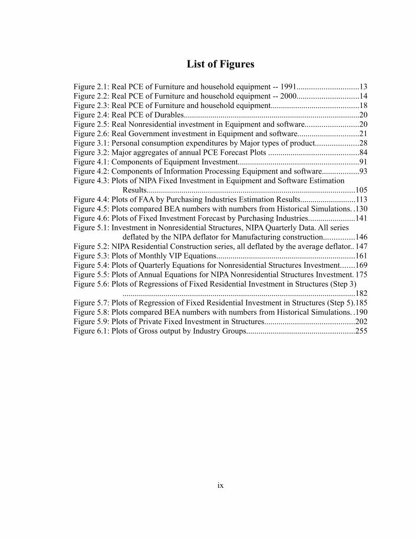
List of Figures
Figure 2.1: Real PCE of Furniture and household equipment -- 1991..............................13Figure 2.2: Real PCE of Furniture and household equipment -- 2000..............................14Figure 2.3: Real PCE of Furniture and household equipment...........................................18Figure 2.4: Real PCE of Durables......................................................................................20Figure 2.5: Real Nonresidential investment in Equipment and software..........................20Figure 2.6: Real Government investment in Equipment and software..............................21Figure 3.1: Personal consumption expenditures by Major types of product.....................28Figure 3.2: Major aggregates of annual PCE Forecast Plots ............................................84Figure 4.1: Components of Equipment Investment...........................................................91Figure 4.2: Components of Information Processing Equipment and software..................93Figure 4.3: Plots of NIPA Fixed Investment in Equipment and Software Estimation
Results......................................................................................................105Figure 4.4: Plots of FAA by Purchasing Industries Estimation Results...........................113Figure 4.5: Plots compared BEA numbers with numbers from Historical Simulations. .130Figure 4.6: Plots of Fixed Investment Forecast by Purchasing Industries.......................141Figure 5.1: Investment in Nonresidential Structures, NIPA Quarterly Data. All series
deflated by the NIPA deflator for Manufacturing construction...............146Figure 5.2: NIPA Residential Construction series, all deflated by the average deflator.. 147Figure 5.3: Plots of Monthly VIP Equations....................................................................161Figure 5.4: Plots of Quarterly Equations for Nonresidential Structures Investment.......169Figure 5.5: Plots of Annual Equations for NIPA Nonresidential Structures Investment. 175Figure 5.6: Plots of Regressions of Fixed Residential Investment in Structures (Step 3)
..................................................................................................................182Figure 5.7: Plots of Regression of Fixed Residential Investment in Structures (Step 5).185Figure 5.8: Plots compared BEA numbers with numbers from Historical Simulations. .190Figure 5.9: Plots of Private Fixed Investment in Structures............................................202Figure 6.1: Plots of Gross output by Industry Groups.....................................................255
ix
Chapter 1: Introduction
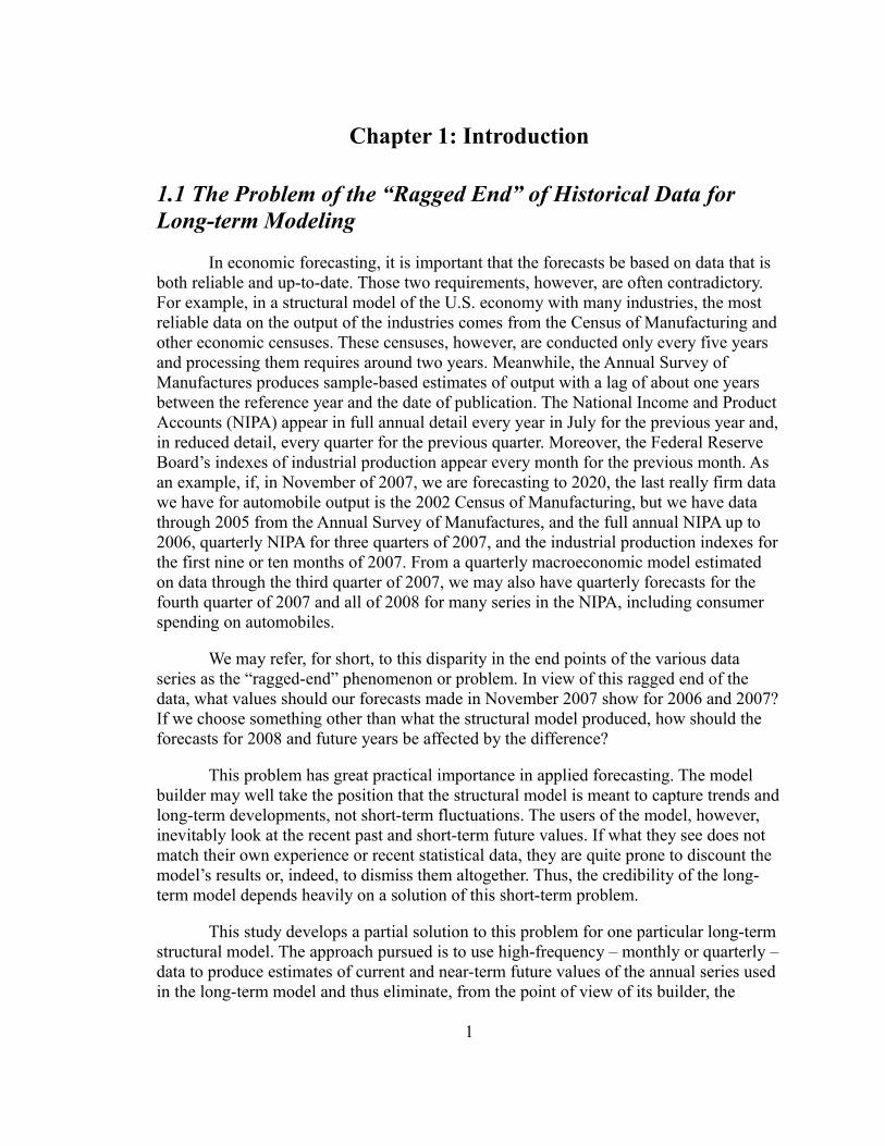
1.1 The Problem of the “Ragged End” of Historical Data for Long-term Modeling
In economic forecasting, it is important that the forecasts be based on data that is both reliable and up-to-date. Those two requirements, however, are often contradictory. For example, in a structural model of the U.S. economy with many industries, the most reliable data on the output of the industries comes from the Census of Manufacturing and other economic censuses. These censuses, however, are conducted only every five years and processing them requires around two years. Meanwhile, the Annual Survey of Manufactures produces sample-based estimates of output with a lag of about one years between the reference year and the date of publication. The National Income and Product Accounts (NIPA) appear in full annual detail every year in July for the previous year and, in reduced detail, every quarter for the previous quarter. Moreover, the Federal Reserve Board’s indexes of industrial production appear every month for the previous month. As an example, if, in November of 2007, we are forecasting to 2020, the last really firm data we have for automobile output is the 2002 Census of Manufacturing, but we have data through 2005 from the Annual Survey of Manufactures, and the full annual NIPA up to 2006, quarterly NIPA for three quarters of 2007, and the industrial production indexes for the first nine or ten months of 2007. From a quarterly macroeconomic model estimated on data through the third quarter of 2007, we may also have quarterly forecasts for the fourth quarter of 2007 and all of 2008 for many series in the NIPA, including consumer spending on automobiles.
We may refer, for short, to this disparity in the end points of the various data series as the “ragged-end” phenomenon or problem. In view of this ragged end of the data, what values should our forecasts made in November 2007 show for 2006 and 2007? If we choose something other than what the structural model produced, how should the forecasts for 2008 and future years be affected by the difference?
This problem has great practical importance in applied forecasting. The model builder may well take the position that the structural model is meant to capture trends and long-term developments, not short-term fluctuations. The users of the model, however, inevitably look at the recent past and short-term future values. If what they see does not match their own experience or recent statistical data, they are quite prone to discount the model’s results or, indeed, to dismiss them altogether. Thus, the credibility of the long-term model depends heavily on a solution of this short-term problem.
This study develops a partial solution to this problem for one particular long-term structural model. The approach pursued is to use high-frequency – monthly or quarterly – data to produce estimates of current and near-term future values of the annual series used in the long-term model and thus eliminate, from the point of view of its builder, the
1

ragged-end phenomenon. In the above example, we would produce “data” for series in the model up through the end of 2007, even though that year is not yet totally history. The equations of the long-term model would then be estimated through 2007 and forecast for 2008 and future years with possible adjustments for autocorrelated residuals. It would also be possible to use the forecast from the macroeconomic model to forecast the series of the structural model through 2008 and start the long-term forecast from that year as if it were already history. Naturally, one could forecast 2008 in both of these ways and then take an average as the starting point of the long-term forecast.
Ideally, all series used in the structural model should be extended in this way, so that the ragged-end problem completely disappears with a complete “flat-end” data set. In practice, the system of updating the series must be developed gradually. Until it is complete, the features of the structural model software for dealing with the ragged-end problem continue to be used. In effect, the model's equations are used to produce values for the series still missing from the flat-end data set.
Although simple in approach, to be effective this solution must include implementation of a computational procedure which quickly and almost automatically acquires the most recent data from the Internet (and other media), processes the data, extends the series, and re-estimates the equations of the structural model, including provision of adjustments for autocorrelated error terms.
1.2 The Scope of this Study
This study undertakes to develop such system in the context of the LIFT model developed by INFORUM at the University of Maryland. LIFT is a full-scale, multisectoral macroeconomic model. Sectoral input-output data build up macroeconomic or “mesoeconomic” forecasts. The database of the LIFT model includes numerous macroeconomic variables as well as input-output matrices. The model, as it stood as work began on this dissertation, has outputs and prices for 97 commodities, employment for 97 industries, personal consumption expenditure for 92 categories, and equipment investment for 55 categories. The value-added sectoring is comprised of 51 industries. Most equations in the model are estimated at an industry or product level, and the price and output solution by industry use the fundamental input-output identities. The LIFT model has been producing satisfactory long-term forecasts, but one of its weak spots has been in short-term forecasting. Prior to the present study, the LIFT database did not incorporate the most up-to-date (but perhaps unreliable) data available. Because of the ragged-end problem, the current year has been treated much as if it were a future year, with consequent discrepancies between the most recent statistical data and the estimates made by LIFT. The use of more accurate and up-to-date economic data to produce reasonable estimates of recent industry level data should improve the credibility of the model's results and the accuracy over the first year or two of forecast.
2

The procedures developed here use monthly or quarterly up-to-date data, such as the industrial production indexes, as indicators of the more basic (but not yet available) annual data for the previous year or two. The higher frequency data can also be used to forecast the basic data for the rest of the current, incomplete year and, towards the end of the year, for the following year.
The ideal of extending all series to obtain a complete flat-end annual data set has not been achieved. The flat-ended dataset does, however, now – as a result of the work described here -- include some of the most important series such as Personal consumption expenditures in 116 detailed categories, fixed investment in equipment and software, fixed investment in structures, and gross output of industries in full BEA 65 sector Input-Output detail. Significant series still missing are exports, imports, inventory change, and government expenditures in detailed sectors.
1.3 Related Work
One of the problems in working with high-frequency data is that it is subject to revision, especially in the first several periods after the first release. Croushore and Stark (2001) have discussed this problem and some alternative estimation methods in their works. When analysis of revisions began, a predictable pattern was discovered for some series. These patterns have now largely been eliminated by the producers of the series. I will therefore ignore the revision problem in this work, though we still have to keep in mind that we cannot compare models directly without considering the data vintage. For example, in an analysis of forecasts of industrial production indexes (IP), Diebold and Rudebusch (1991) used a real-time data set constructed using both preliminary and partially revised data on the composite leading index (CLI), which is constructed using only data that were available at time t-h (where t is the time index and h is the forecast horizon). In the context of linear forecasting models, they find that the performance of partially revised CLI data deteriorates substantially relative to revised data when used to predict the industrial production indexes. A number of other papers also address issues related to the real-time forecasting. For example, Trivellato and Rettore (1986) discuss the decomposition of forecasting errors into, among other things, the forecast error associated with preliminary data errors. A small sample of other related references includes Boschen and Grossman (1982), Mariano and Tanizaki (1994) and Patterson (1995). Swanson and White (1995) find that using adaptive models, such as an artificial neural networks model, for forecasting macroeconomic variables in a real-time setting can be useful when the variable of interest is the spot-forward interest-rate differential.
There have been many attempts to incorporate high-frequency information into existing economic forecasting models. Zadrozny (1990) built a single model that relates data of all frequencies. His attempt to build such a comprehensive model was unsuccessful. Litterman (1984) and Corrado and Reifschneider (1986) find that updating forecasts of the current quarter based on incoming monthly data is helpful. However, it is not helpful in forecasting for much longer horizons.
3

Miller and Chin (1996) try to combine the forecasts of two vector autoregression (VAR) models, a quarterly model and monthly model, using weights that maximize forecasting accuracy. The method is based on studies of Corrado and Greene (1988), Corrado and Haltmaier (1988), Fuhrer and Haltmaier (1988), Howrey, Hymans and Donihue (1991), and Rathjens and Robins (1993). Using the test of Christiano (1989), the method improves quarterly forecasts in a statistical significant way.
The forecasting models used in these studies, however, are much, much simpler than LIFT and their data demands almost minuscule in comparison. Most of these previous papers looked at only one or two macro-variables while here we have hundreds. Moreover, the researchers could take their time to fine-tune each method used. To be useful in practical, real-time forecasting, our system must work completely in a day or two.
1.4 Steps in the Solution of the Ragged-end Problem
The work of the solution developed here can be divided into five steps.
1. Update all data banks to have the most recent data both for annual data and for higher frequency data.
2. Re-estimate and run the quarterly macroeconomic model, in our case, QUEST. This step includes examination of the exogenous assumptions.
3. Extend high-frequency data to the end of current year and perhaps one year beyond by using time-series analysis and interpolated monthly data from the quarterly macroeconomic model.
4. Use this data to predict the annual series used in LIFT. This step produces the flat-end data set.
5. Re-estimate LIFT equations using this data.
Start LIFT with the base year in the last or next to last year of the flat-end data set. The Inforum software in which LIFT runs will automatically compute errors in the equations in the base year and adjust future year's predictions by these errors, diminished each year in a specified proportion, called rho.
The work which will be documented here is primarily steps 3 and 4. Other parts of the process are documented elsewhere, step 1 in Inforum files, step 2 in The Craft of Economic Modeling, vol. 2, and steps 5 in the LIFT documentation.
In Step 3, we work on each variable at its original frequency. This step is to get forecast estimates of the as-yet unannounced or future values of the explanatory variable. For example, in October 2007, the Federal Reserve Board published the Industrial Production Index (IPI) through September 2007. Thus, in this first step, we have to
4
calculate the value of the IPI from October 2007 (the current period) and the future values through the entire forecast period (e.g. until the end of 2008). Using time-series econometric techniques, more specifically, autoregressive moving average (ARMA) equation seems to be an appropriate way to begin work on the estimation.
Through experiments, I found that having a second-degree moving average error component in the regression equation could cause non-convergence problems in the nonlinear minimization technique used for the estimation because the algorithm falls into a flat part of the objective function. That experience suggested that automatic application of the procedure to a large number of series would prove infeasible. Although I have not yet encountered any problem in estimation with only a one-period moving-average error, I also did not find important improvement in the fit of the equation by using it. I will therefore actually use only autoregressive (AR) equations, though some of them will use variables in addition to the lagged values of the dependent variables.
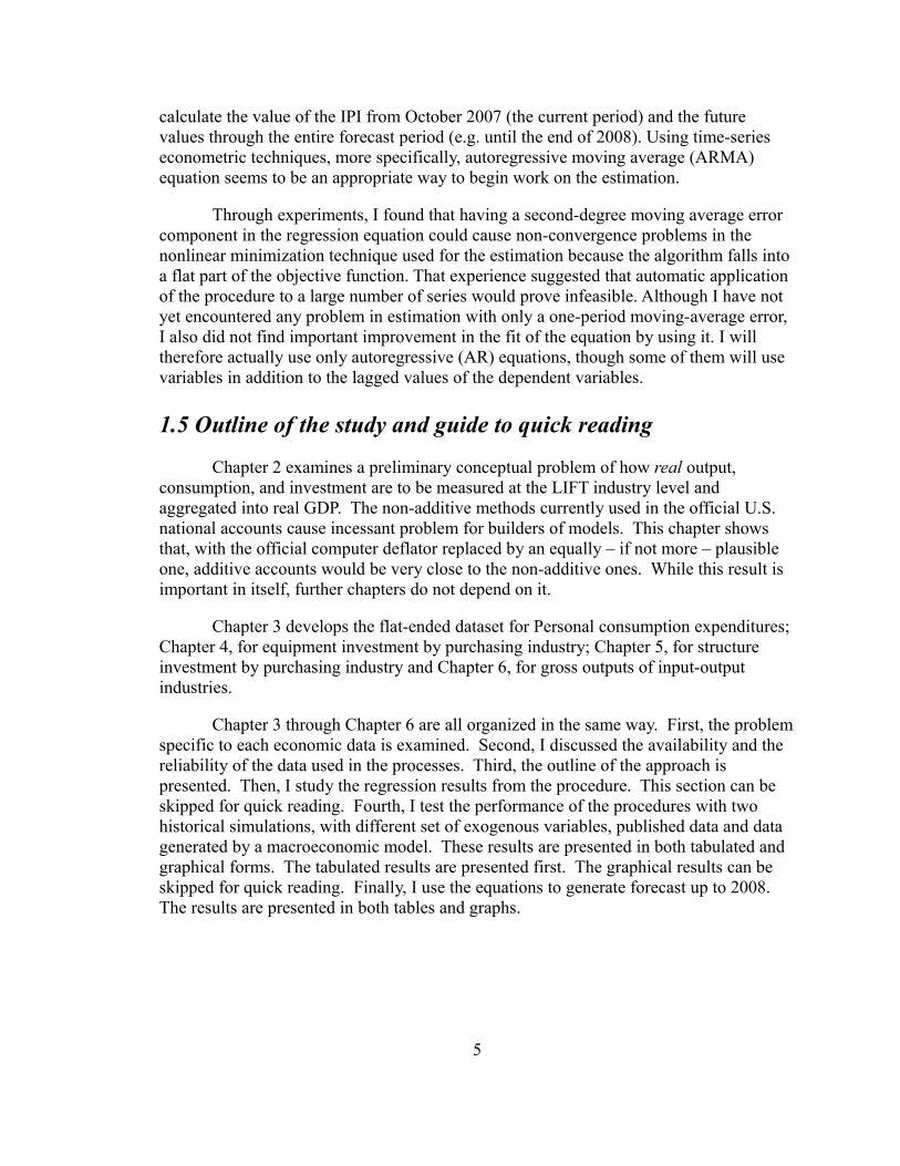
1.5 Outline of the study and guide to quick reading
Chapter 2 examines a preliminary conceptual problem of how real output, consumption, and investment are to be measured at the LIFT industry level and aggregated into real GDP. The non-additive methods currently used in the official U.S. national accounts cause incessant problem for builders of models. This chapter shows that, with the official computer deflator replaced by an equally – if not more – plausible one, additive accounts would be very close to the non-additive ones. While this result is important in itself, further chapters do not depend on it.
Chapter 3 develops the flat-ended dataset for Personal consumption expenditures; Chapter 4, for equipment investment by purchasing industry; Chapter 5, for structure investment by purchasing industry and Chapter 6, for gross outputs of input-output industries.
Chapter 3 through Chapter 6 are all organized in the same way. First, the problem specific to each economic data is examined. Second, I discussed the availability and the reliability of the data used in the processes. Third, the outline of the approach is presented. Then, I study the regression results from the procedure. This section can be skipped for quick reading. Fourth, I test the performance of the procedures with two historical simulations, with different set of exogenous variables, published data and data generated by a macroeconomic model. These results are presented in both tabulated and graphical forms. The tabulated results are presented first. The graphical results can be skipped for quick reading. Finally, I use the equations to generate forecast up to 2008. The results are presented in both tables and graphs.
5

Chapter 2: Measuring Real Growth
In 1995, the Bureau of Economic Analysis (BEA), the makers of the U.S. National accounts, introduced a change in the way it makes the constant price, real national accounts. There are two elements of the change: (1) between adjacent years, the Fisher “ideal” index is used instead of the Laspeyres index, and (2) real growth over periods of more than two years is calculated by multiplying (“chaining”) the growth ratios of the year-by-year growth. The resulting index, known as the chain-weighted index, may be appropriate for some purposes.. However, simple economic identities that hold in the nominal accounts are no longer valid in the chain-weighted real accounts. For example, real personal consumption expenditure is not equal to the sum of real expenditures on durables plus non-durables plus services. Moreover, real growth becomes path-dependent. The measure of real growth between year 1 and year N depends not only on prices and outputs in those two years but also on prices and outputs in all intervening years. If one's sole purpose is to make accounts, it perhaps does not matter that identities do not hold in real terms and that measures of growth are path-dependent; but, for building an economic model, these peculiarities can become a serious problem. For example, in an interindustry model, input-output theory requires that real industry output in any year should be the sum of sales to various intermediate uses in real terms in that year plus sales to several components of final demand, also in real terms for that year. If this simple identity is to be replaced by a complex formula involving square roots and prices and outputs in all years between the base year and the year in question, interindustry modeling becomes essentially impossible.
This study deals with the preparation of data for an interindustry model. It is therefore highly important that the data prepared in the ways described here be usable in such a model. In this chapter, therefore, I will explain why BEA moved away from fixed-weighted indexes, examine the problem in building economic models with chain-weighted national accounts, and offer some suggestions to get around the problems.
2.1 Hedonic Indexes1
In 1987, seemingly spurred by Robert Solow's remark “You can see the computer age everywhere but in the productivity statistics,”2 the BEA looked for a method to include the increased power and lower cost of computers into productivity as measured in the NIPA. Before explaining what BEA did, however, it is worth noting that productivity increases from the use of computers were already fully included in the NIPA. In so far as computers made manufacturing, banking, transportation, or trade more efficient, their contribution to productivity was accounted for in the NIPA. The only question was the
1 Some parts of the following background and suggestions are a summary of Clopper Almon's note, “Thoughts on Input-Output Models in National Accounting Systems with “Superlative” and Chain Weighted Indexes”, March 2005.
2 Solow, Robert M. “We'd Better Watch Out.” New York Times Book Review, July 12, 1987, p. 36.
6

evaluation of computers in investment, consumption, export, and import. At that time, before computers were a common household item, it was mainly a matter of pricing of computers in investment. Today, of course, the computers are also an important consumer durable.
The question was how to compare the “real” value of computers made in different years in making up a measure of investment “in constant prices.” BEA turned to the idea of a “hedonic” index of computer price, created with help from IBM, to solve this problem.
What is a hedonic index? The name is derived from Greek hedonikos, from hedone, pleasure. Thus, a hedonic index should measure the pleasure derived from the goods or services. In statistical practice, hedonics has a rather different meaning illustrated by the computer deflator. Traditional price indexes compare the cost of a typical market basket of goods in two different years. But in the case of computers, the same exact model specification is rarely sold for more than a year or two. Models go out of production often without a change in the maker's price. Thus, the market-basket approach would not work for computers. The “hedonic” approach used regression analysis to estimate what a particular computer model would have cost in a particular year had it been available in that year [Landefeld and Grimm, 2000].
In the study used for making the computer price index, the regression had the form
uMAMP bb 22
11= ,
where P is the price of a certain computer, M1 and M2 are physical characteristics (processor speed and capacity of the disk drive) of that equipment, and u is an error terms. The coefficients A, b1, and b2 are estimated by the regression over a number of computers in a particular base year [See Triplett, 1986 and Cole et al., 1986].
By applying the estimated coefficients to the physical characteristics of computers made in other years, we get estimates of what the prices of those machines would have been in the base year, had they been available at that time. We may call these estimates the “imputed” prices in the base year. By compared these imputed prices in the base year with the actual price in the forward year, BEA makes an index of the price between the two years. This is said to be the “hedonic” price index of computers. In BEA's implementation of it, it averaged a decline of 15.9 percent per year, continuously compounded, over the period 1980 – 2005.
The hedonic price index by itself has both pros and cons. Similar hedonic indexes have been employed to measure consumers’ relative valuations of products that have multiple qualities (or characteristics), [See Nerlove, 1995]. For example, hedonic price
7
indexes are commonly used in real estate assessment for tax purposes. The prices of properties that sell are regressed on characteristics such as square footage and number of baths. The result is then used to impute values to properties which have not sold.
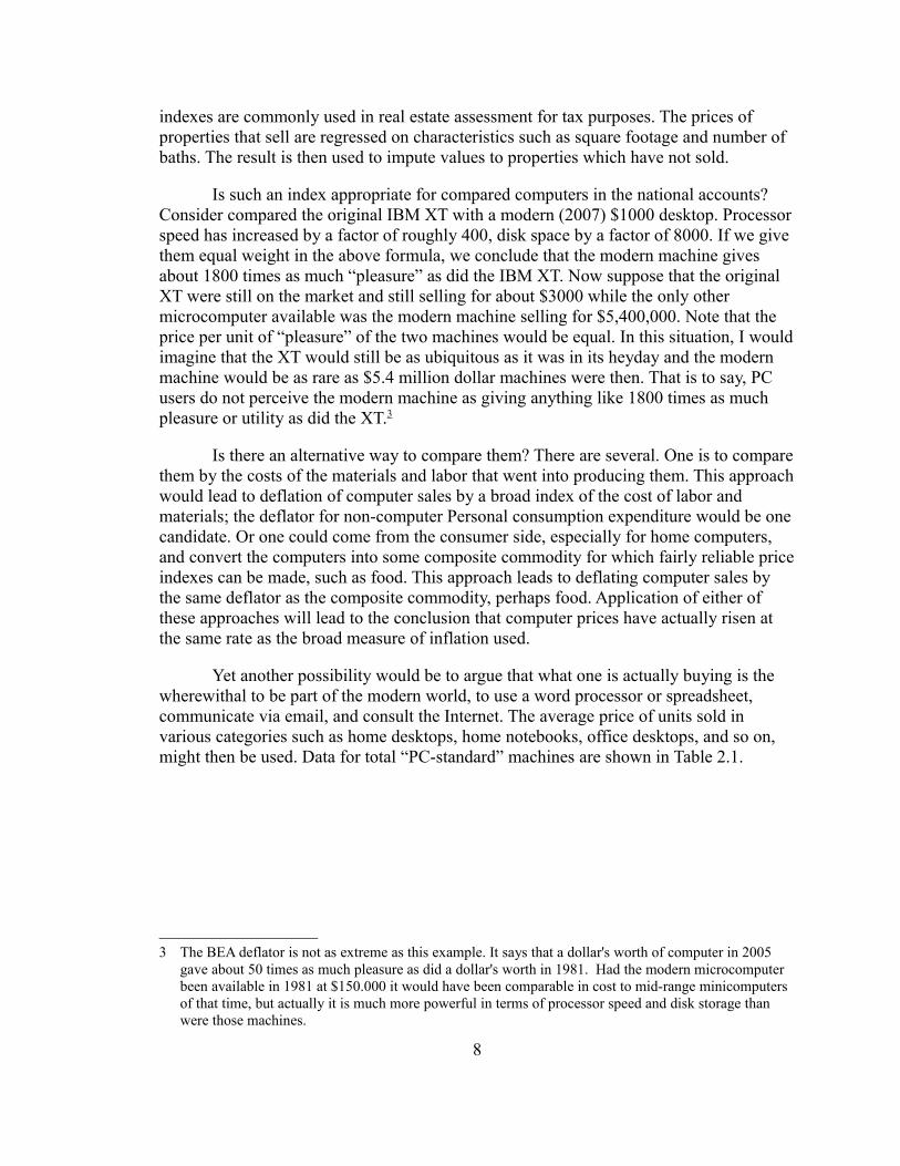
Is such an index appropriate for compared computers in the national accounts? Consider compared the original IBM XT with a modern (2007) $1000 desktop. Processor speed has increased by a factor of roughly 400, disk space by a factor of 8000. If we give them equal weight in the above formula, we conclude that the modern machine gives about 1800 times as much “pleasure” as did the IBM XT. Now suppose that the original XT were still on the market and still selling for about $3000 while the only other microcomputer available was the modern machine selling for $5,400,000. Note that the price per unit of “pleasure” of the two machines would be equal. In this situation, I would imagine that the XT would still be as ubiquitous as it was in its heyday and the modern machine would be as rare as $5.4 million dollar machines were then. That is to say, PC users do not perceive the modern machine as giving anything like 1800 times as much pleasure or utility as did the XT.3
Is there an alternative way to compare them? There are several. One is to compare them by the costs of the materials and labor that went into producing them. This approach would lead to deflation of computer sales by a broad index of the cost of labor and materials; the deflator for non-computer Personal consumption expenditure would be one candidate. Or one could come from the consumer side, especially for home computers, and convert the computers into some composite commodity for which fairly reliable price indexes can be made, such as food. This approach leads to deflating computer sales by the same deflator as the composite commodity, perhaps food. Application of either of these approaches will lead to the conclusion that computer prices have actually risen at the same rate as the broad measure of inflation used.
Yet another possibility would be to argue that what one is actually buying is the wherewithal to be part of the modern world, to use a word processor or spreadsheet, communicate via email, and consult the Internet. The average price of units sold in various categories such as home desktops, home notebooks, office desktops, and so on, might then be used. Data for total “PC-standard” machines are shown in Table 2.1.
3 The BEA deflator is not as extreme as this example. It says that a dollar's worth of computer in 2005 gave about 50 times as much pleasure as did a dollar's worth in 1981. Had the modern microcomputer been available in 1981 at $150.000 it would have been comparable in cost to mid-range minicomputers of that time, but actually it is much more powerful in terms of processor speed and disk storage than were those machines.
8

During the first ten years after 1981, there was negligible reduction in the price of the average unit. During the 1990's, the price of the average unit declined about 2.8 percent per year. In the new century, that rate has accelerated to about 4.4 percent in the USA and 5.0 percent worldwide. These numbers match subjective impressions that there has indeed been some decline in the 1990's in the cost of equipping oneself with an appropriately spiffy computer, and that the decline has accelerated a bit recently. But it is nowhere near the 16 percent per year average decline in the BEA deflator.
2.2 Runaway Deflators, Ideal and Chained Indexes, and Non-additivity
When it was used to “deflate” the value of computers in GDP, the BEA hedonic price index actually “inflated” the values of sales in years after the base of the deflator. This “inflation” soon led to a very high growth rate of calculated GDP. With the simple addition of the components of GDP in constant prices to get constant-price total GDP – the method used before introduction of the hedonic deflator – the rate of decline in the computer price gradually becomes the rate of growth of real GDP. Table 2.2 illustrates this phenomenon with data made up to show the problem -- and a solution -- in simple form.
In this table, GDP is made up of two products. The nominal yearly expenditures on Product 1 is shown in row 2; and that on product 2, in row 7. To keep the table very simple, both are constant at 100 billion dollars per year. The price indexes, shown in rows 3 and 8, however, are very different. They are both equal to 1.00 in year 4, but that of product 1, computers, falls at 25 percent per year while that of product 2, everything else, remains constant. These data imply that the real quantity of product 1 (row 4) has been growing at 25 percent per year, while that of product 2 (row 9) has been constant. Row 12 shows the simple sum of the two real quantities, and row 13 shows the annual growth ratio of this sum. In year 2, the growth rate is 8 percent; by year 9 it is up to 18 percent and by year 20, it is closing in on its 25 percent asymptotic growth rate.
9
Table 2.1: U.S. and World-Wide Sales of PC-type Computers
YearsUSA Worldwide USA Worldwide USA Worldwide USA Worldwide
1981-85 3.8 5.7 10.5 16.9 2763.2 2964.91986-90 28.1 60.3 76.4 181.0 2718.9 3001.7 -0.32% 0.25%1991-95 64.3 172.0 153.0 447.0 2379.5 2598.8 -2.50% -2.68%1966-00 162.0 444.0 335.0 1010.0 2067.9 2274.8 -2.62% -2.49%2001-06 267.0 855.0 424.0 1440.0 1588.0 1684.2 -4.64% -5.19%
Source: Computer Industry Almanac, http://www.c-i-a.com/pr0806.htm
Annual rate of decline$/unit$ billionMillion units

By period 23, the rate of real growth is approximately the rate of decline of the computer deflator, although in nominal terms computers remain only half of the total. The phenomenon could be described in headline language as “Runaway computer deflator steals GDP” or “Gresham's Law of Deflators.”4 A more sedate name for it might be the outlier index dominance problem.
When BEA first introduced the hedonic computer deflator, it did so in the context of constant-price accounts in which, as in this example, growth in quantities were weighted by shares in a fixed base year and total real GDP was just the sum of its various components. At first, it had the desired effect of increasing GDP growth by a few tenths of a percent per year. But the outlier index dominance problem soon began to appear. Far from not showing up in the productivity statistics, computers began to dominate the productivity and growth statistics. The BEA statisticians were properly concerned. They might have then well questioned the appropriateness of the hedonic computer price index, but instead they turned to a generic, almost arithmetic solution to the problem.5
As can be seen in Table 2.2, the problem arises because the share of the component with the rapidly declining price index keeps getting larger in “real” terms, so its rate of growth in “real” terms keeps getting a heavier and heavier weight in the total. An obvious solution to this problem is to re-weight the rates of growth of each product each year by the shares in the nominal total. Line 14 in the table shows the resulting growth ratios, which, in this example, turn out to be a constant 1.125 each year. Line 15
4 “Bad deflators drive out good.”5 It should be noted that computer is not the only product deflated with the hedonic index. BEA now also
uses hedonic index with other goods such as apparel and prepackaged software. With the exception of computers, these products do not lead to significant substitution bias. Landefeld and Grimm (2000) show that, for software prices, the contribution of software investment to real GDP growth is almost identical to its contribution to nominal GDP growth. The impact of prepackaged software hedonic price on the software deflator is offset by the price deflator of other software components such as custom software and own-account software.
10
Table 2.2: The Runaway Deflator Problem with Made-up Data1 Year 1 2 3 4 5 6 7 8 9 20 21 22 23 24
Product 12 Nominal value 100.0 100.0 100.0 100.0 100.0 100.0 100.0 100.0 100.0 ... 100.0 100.0 100.0 100.0 100.03 Price index 1.95 1.56 1.25 1.00 0.80 0.64 0.51 0.41 0.33 ... 0.03 0.02 0.02 0.01 0.014 Real quantity 51.2 64.0 80.0 100.0 125.0 156.3 195.3 244.1 305.2 ... 3552.7 4440.9 5551.1 6938.9 8673.65 Real growth ratio 1.25 1.25 1.25 1.25 1.25 1.25 1.25 1.25 ... 1.25 1.25 1.25 1.25 1.256 Nominal share 0.50 0.50 0.50 0.50 0.50 0.50 0.50 0.50 0.50 ... 0.50 0.50 0.50 0.50 0.50
Product 2 7 Nominal value 100.0 100.0 100.0 100.0 100.0 100.0 100.0 100.0 100.0 ... 100.0 100.0 100.0 100.0 100.08 Price index 1.00 1.00 1.00 1.00 1.00 1.00 1.00 1.00 1.00 ... 1.00 1.00 1.00 1.00 1.009 Real quantity 100.0 100.0 100.0 100.0 100.0 100.0 100.0 100.0 100.0 ... 100.0 100.0 100.0 100.0 100.010 Real growth ratio 1.000 1.000 1.000 1.000 1.000 1.000 1.000 1.000 ... 1.000 1.000 1.000 1.000 1.00011 Nominal share 0.500 0.500 0.500 0.500 0.500 0.500 0.500 0.500 0.500 ... 0.500 0.500 0.500 0.500 0.500
12 Sum of real quantities 151.2 164.0 180.0 200.0 225.0 256.3 295.3 344.1 405.2 ... 3652.7 4540.9 5651.1 7038.9 8773.613 Growth ratio of sum of real quantities 1.085 1.098 1.111 1.125 1.139 1.152 1.165 1.177 ... 1.242 1.243 1.244 1.246 1.24614 Nominal-share-weighted growth ratio 1.125 1.125 1.125 1.125 1.125 1.125 1.125 1.125 ... 1.125 1.125 1.125 1.125 1.12515 Chained real expenditure on combination 140.5 158.0 177.8 200.0 225.0 253.1 284.8 320.4 360.4 ... 1316.7 1481.2 1666.4 1874.7 2109.0

shows the GDP of the base year of the prices, year 4, moved forward and backward by these year-to-year growth ratios. This process is called chaining and the result is called a chain-weighted index of real GDP.
Notice, in particular, that the growth rate of the chain-weighted aggregate is above the growth rate of the simple sum in the years prior to the year after6 the base year of the prices, while it is below that rate in later years. In the simple-sum measure, the weight of the fast-growing item with the declining price is likely to be smaller than the current price share before the base year of the prices and larger after that year. This property, which is an empirical regularity rather than a mathematical certainty, shows up in virtually every real case we have seen. For GDP, it made it possible “to see the computer age ... in the productivity statistics” in the historical period before the base year of the prices yet avoid a runaway deflator problem in the future.
While chaining as shown in Table 2.2 is, by itself, a powerful antidote to outlier index dominance, BEA went one step further to limit the effects of the computer deflator. To get a better measure of year-to-year growth between adjacent years, it weighted the growth rates of the component products not only by their shares in the nominal values in the first year of a pair, as in Table 2.2, but also by the shares in the second year. The first of these growth measures is called the Laspeyres index while the second is called the Paasche index. They may multiplied together and the square root used as the “Fisher ideal” index7. In Table 2.2, there is no difference between the Paasche and Laspeyres index because the nominal shares are constant, but normally there will be a slight difference.
This description of the indexes in terms of weights on the growth rates of products is slightly different from the usual definition, so it is perhaps worthwhile to show their equivalence.
In the usual definitions, with ptn and qt
n as price and quantity of n (i) products at time t, respectively, the definitions are: [See “A Guide to the National Income and Product Accounts of the United States”, BEA]
the Laspeyres index: QtL=
∑n=1
N
pnt−1 qn
t
∑i=1
N
pit−1 qi
t−1,
6 The year after the base year is the year when prices in the base year are used as the base of the growth rate.
7 Irving Fisher, The Making of Index Numbers (Boston, 1922)
11
the Paasche index: QtP=
∑n=1
N
pnt qn
t
∑i=1
N
pit qi
t−1,
To convert this definition to one using share weights, we can write
Q1L=∑n=1
N
pn0 qn
1
∑i=1
N
Pi0 q i
0=∑n=1
N
pn0 qn
1 qn0
qn0
∑i=1
N
P i0 qi
0=∑n=1
N
pn0 qn
0 qn1
qn0
∑i=1
N
Pi0q i
0,
Q1L=∑
n=1
N
Sn0 qn
1
qn0 , where Sn
0=pn
0 qn0
∑i=1
N
pn0 qn
0
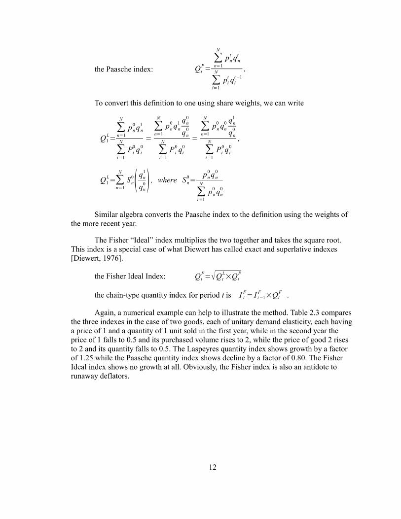
Similar algebra converts the Paasche index to the definition using the weights of the more recent year.
The Fisher “Ideal” index multiplies the two together and takes the square root. This index is a special case of what Diewert has called exact and superlative indexes [Diewert, 1976].
the Fisher Ideal Index: QtF=Qt
L×QtP
the chain-type quantity index for period t is I tF= I t−1
F ×QtF .
Again, a numerical example can help to illustrate the method. Table 2.3 compares the three indexes in the case of two goods, each of unitary demand elasticity, each having a price of 1 and a quantity of 1 unit sold in the first year, while in the second year the price of 1 falls to 0.5 and its purchased volume rises to 2, while the price of good 2 rises to 2 and its quantity falls to 0.5. The Laspeyres quantity index shows growth by a factor of 1.25 while the Paasche quantity index shows decline by a factor of 0.80. The Fisher Ideal index shows no growth at all. Obviously, the Fisher index is also an antidote to runaway deflators.
12
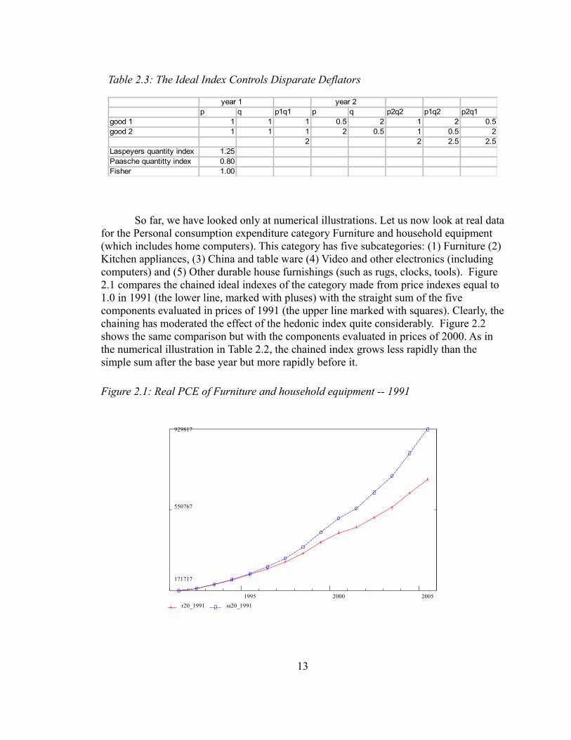
So far, we have looked only at numerical illustrations. Let us now look at real data for the Personal consumption expenditure category Furniture and household equipment (which includes home computers). This category has five subcategories: (1) Furniture (2) Kitchen appliances, (3) China and table ware (4) Video and other electronics (including computers) and (5) Other durable house furnishings (such as rugs, clocks, tools). Figure 2.1 compares the chained ideal indexes of the category made from price indexes equal to 1.0 in 1991 (the lower line, marked with pluses) with the straight sum of the five components evaluated in prices of 1991 (the upper line marked with squares). Clearly, the chaining has moderated the effect of the hedonic index quite considerably. Figure 2.2 shows the same comparison but with the components evaluated in prices of 2000. As in the numerical illustration in Table 2.2, the chained index grows less rapidly than the simple sum after the base year but more rapidly before it.
13
Table 2.3: The Ideal Index Controls Disparate Deflators
year 1 year 2p q p1q1 p q p2q2 p1q2 p2q1
good 1 1 1 1 0.5 2 1 2 0.5good 2 1 1 1 2 0.5 1 0.5 2
2 2 2.5 2.5Laspeyers quantity index 1.25Paasche quantitty index 0.80Fisher 1.00
Figure 2.1: Real PCE of Furniture and household equipment -- 1991
929817
550767
171717
1995 2000 2005 r20_1991 ss20_1991

To make this example, we have taken the indexes and prices of the sub-categories as data and combined them with the Fisher and chaining formula. It should be understood, however, that BEA works differently and in a way which cannot presently be replicated outside BEA. It maintains series on values and prices of thousands of products going into various components of GDP, and it publishes data at several levels of aggregation. For example, published data show, in increasing order of detail,
Gross domestic product (GDP)
Personal consumption expenditure (PCE)
Clothing
Men's shoes
The published real (constant-price) series for each of these categories is created directly from the most detailed data that BEA has. Thus, the published GDP series calculates the Fisher index directly from thousands of items and chains at the aggregate level. It makes no use of sub-aggregates. It will often not be the sum of its components. BEA warns the user of the accounts of this non-additivity by publishing a line in most constant-price tables called “Residual” defined as the difference between the whole and the sum of the parts. Indeed, no attention at all is paid, in calculating any real series to the values of its components above the finest level of detail available to BEA and in most cases not available outside. Thus, calculations of GDP pay no attention to the calculated real PCE; the calculated real PCE pays no attention to the calculation of real expenditures
14
Figure 2.2: Real PCE of Furniture and household equipment -- 2000
504878
313163
121449
1995 2000 2005 r20_2000 ss20

on Clothing, and so on. Given the nature of the Fisher formula and the chaining, it is therefore not possible to calculate precisely what BEA will get for a particular aggregate from knowledge of all the published components of that aggregate. Treating the finest level of published detail as if it were indeed the bottom level of data and applying the Fisher formula and chaining will not yield precisely the BEA version of the aggregate. There is, moreover, the problem that if one wants a real aggregate that BEA has not chosen to publish, for example, non-computer PCE, there is presently no way to calculate it precisely from the published detail.
Douglas Meade, who developed the chained ideal index functions for the G regression program, has made experimental calculations of published aggregates from published sub-aggregates and reported orally that the differences from the published aggregates are usually small and less than one gets by approximating the aggregate by addition of the all the pieces that compose it. While this is a consoling result, it would be nice not to have to rely on it. If BEA would release for each aggregate which it publishes a series on the value of the category each year in prices of the previous year, it would be possible to replicate the aggregates and perform other aggregations and get precisely the same results as BEA gets. Publication of such series is routine by some statistical offices.
2.3 Remedies for Non-additivity
We have seen that the breakdown of the national account identities in real aggregates – the Non-additivity problem -- is caused by two sources, (1) the Fisher index and (2) the chaining to create an index over several years. In general, a real aggregate value from the Fisher index will not equal to the sum of its parts. If B and C are two groups of products and A is the combination of the two groups, A0, B0, and C0 are their
values in year 0 and AF, BF and CF are their Fisher indexes between year 0 and year 1, then it is NOT in general true that
A0 AF = B0BF + C0CF
There is, however, one instance when this equations holds, namely when all the prices of the goods in both B and C grow at the same rate, as shown below.
Let pnt and qn
t represent vectors of prices and quantities of goods in group n at time t. pn
t is a row vector and qnt a column vector, so that their product is defined. We
consider two periods, t = 0 and 1, and two groups of goods, n = a and b. Then it is not generally true that value of group 1 in year 0 multiplied by the Fisher ideal index of that group between year 0 and year 1 plus the same thing for group 2 is equal to the Fisher ideal index of the combined group, that is
15

If, however, p1a= p0
a and p1b= p0
b for the same scalar λ then the left hand side is just the quantities of year 1 evaluated at the prices of year 0:
The right-hand side reduces to the same thing:
( ) ( )
( )
( )bbaa
bbaa
bbaabbaa
bbaa
bbaabbaa
bbaa
bbaa
bbaa
bbaabbaa
bbaa
bbaa
bbaa
bbaabbaa
qpqpqpqpqpqp
qpqp
qpqpqpqp
qpqp
qpqpqpqp
qpqpqpqp
qpqpqpqpqpqp
qpqpqpqp
qpqp
1010
0000
10100000
2
0000
10100000
0000
1010
0000
10100000
0101
1111
0000
10100000
+=
++
+=
++
+=
++
×++
+=++
×++
+λλλλ
In view of this fact, we should expect the chain-weighted real national accounts to have approximate additivity when all prices are growing more or less proportionally. It is only when there is an outlier likes the computer hedonic index that non-additivity becomes a major problem.
To summarize, two separate problems have been identified above. One is the question of what the appropriate computer price deflator should be. The other is the breakdown of the economic identities in the real national accounts with the use of chain-weighted Fisher indexes.
2.4 Suggested Remedies
We have seen that the BEA computer deflator is both somewhat implausible and fully capable of running away with real GDP if not controlled by chained ideal indexes. I have explored various alternatives such as using the food deflator for computers. Perhaps
16
bbaa
bb
bbbb
aa
aaaa
bb
bbbb
aa
aaaa
bb
bb
bb
bbbb
aa
aa
aa
aaaa
bb
bb
bb
bbbb
aa
aa
aa
aaaa
qpqpqpqp
qpqpqp
qp
qpqp
qpqpqp
qp
qpqp
qpqp
qpqpqp
qpqp
qpqpqp
qpqp
qpqpqp
qpqp
qp
1010
00
1000
00
1000
2
00
1000
2
00
1000
00
10
00
1000
00
10
00
1000
01
11
00
1000
01
11
00
1000
+=
+
=
+
=
×+×=×+×λλ
λλ
( ) bbaa
bbaa
bbaa
bbaabbaa
bb
bb
bb
bbbb
aa
aa
aa
aaaa
qpqpqpqp
qpqpqpqpqpqp
qpqp
qpqpqp
qpqp
qpqpqp
0101
1111
0000
10100000
01
11
00
1000
01
11
00
1000 +
+×++
+≠×+×

the most plausible one, however, is the average price of IBM-standard computers, presented in Table 2.1. It, however, is declining while nearly all other deflators are rising. Will it also “steal” real GDP and require non-additive formula to control it? To answer this question, I returned to the group of products studied above, the PCE category Furniture and household equipment. The lower two lines in Figure 2.3 show the aggregate for this group of products but with Computers and software deflated by average price deflator developed in Table 2.1. The lowest line (marked by the pluses) is the chained index; the line just above it (marked by squares) is the simple summation of the five components. The top line (marked by X’s ) is the BEA index rebased to 1991. The third line shows the BEA total for this category, rebased to 1991. Clearly, the substitution of the deflator with only moderate decline yields accounts in which it is not necessary to resort to chaining of ideal indexes to avoid a runaway deflator stealing the GDP. In fact, the use of these devices makes little difference over a fifteen-year horizon.
It should be stressed that the alternative computer deflator, which is declining, is substantially different from the price indexes of the other components of this aggregate, which are rising. Even so, the difference is not large enough for chaining to give an aggregate noticeably different from simple addition of the sub-components. The BEA computer deflator, however, is so far out of line with the other price indexes that even with chaining of ideal indexes, it produces a total category index which runs away from the other two indexes of the same thing.
Since this category of Personal consumption expenditure is more influenced by the computer deflator than any other, it seems reasonable to conclude at this point that replacement of the BEA computer deflator by an alternative that shows prices declining but at more moderate rates would give us improved national accounts in which there would be little difference between simple summation of components and chaining of ideal indexes. There would then be no reason not to make the aggregates by summation. Modeling could then be based on the additive accounts which have every claim to represent the economy as accurately or more accurately than those produced by BEA, supposing that BEA persists in its current methods, which seems likely. In that case, the model could also include adjustment factors by which the major BEA aggregates could be modified to match the corresponding aggregates in the additive accounts.
17

Encouraged by these results, I have used this computer deflator to produce a complete set of NIPA created by (1) applying the alternative deflator to computers wherever they appear in final demand and (2) otherwise accepting BEA series at the finest level publicly available, and (3) aggregating by simple addition. This set of accounts is available as a data bank for the G program. Table 2.4 and Figure 2.4, Figure 2.5, Figure 2.6 compare some of the aggregate series with the official BEA accounts.
18
Figure 2.3: Real PCE of Furniture and household equipment
695735
433727
171718
1995 2000 2005 r20_1991 ss20_1991 br20_1991

From Table 2.4, with a sensible computer deflator, it appears that there is essentially no difference between chained-weighted Fisher aggregates and straight-addition aggregates. Thus, simple additive accounts would serve us well by using a sensible computer deflator.
In Figure 2.4, 2.5, and 2.6, each picture shows three lines: 1) chained-weighted aggregate (represented by + line), 2) straight-summation aggregate (represented by box (□) line), and 3) the actual published series (represented by x line). The first two lines are calculated with the sensible computer deflator as shown in Table 2.4.
All three figures exhibit an interesting result. With the computer deflator generated from a hedonic index, BEA published numbers grows at a much faster rate than the other two lines, which used a more sensible computer deflator. Using the sensible deflator, chained and straight-summation aggregates generate nearly identical rate of growth noticeable trend, chained aggregates grow faster before the base year and slower after the base year.
19
Table 2.4: Comparison of Real GDP components between Chain-weighted and Fixed-weighted methods
chained
straight summation
percent difference chained
straight summation
percent difference chained
straight summation
percent difference
1 Personal consumption expenditures 5,860,591 5,895,356 0.59% 6,739,383 6,739,383 0.00% 7,547,953 7,576,582 0.38%2 Durable goods 671,962 673,471 0.22% 863,327 863,327 0.00% 1,052,923 1,062,050 0.87%3 Nondurable goods 1,725,338 1,731,646 0.37% 1,947,220 1,947,220 0.00% 2,179,183 2,185,735 0.30%4 Services 3,468,177 3,490,239 0.64% 3,928,836 3,928,836 0.00% 4,323,863 4,328,797 0.11%5 Fixed investment 1,372,050 1,373,829 0.13% 1,678,979 1,678,979 0.00% 1,683,147 1,677,618 -0.33%6 Nonresidential Structures 279,030 280,074 0.37% 313,185 313,185 0.00% 249,004 245,099 -1.57%7 Nonresidential Equipment and software 705,435 705,294 -0.02% 918,891 918,891 0.00% 872,118 873,380 0.14%8 Residential Structures 383,778 382,337 -0.38% 439,544 439,544 0.00% 551,269 550,150 -0.20%9 Residential Equipment 6,124 6,124 0.00% 7,359 7,359 0.00% 8,989 8,989 0.00%
10 Net exports of goods and services -96,490 -124,601 29.13% -379,600 -379,600 0.00% -585,494 -577,032 -1.45%11 Exports 952,624 953,566 0.10% 1,096,300 1,096,300 0.00% 1,122,346 1,126,540 0.37%12 Goods 673,312 673,366 0.01% 784,400 784,400 0.00% 786,356 790,440 0.52%13 Services 279,196 280,200 0.36% 311,900 311,900 0.00% 335,804 336,100 0.09%14 Imports 1,069,014 1,078,167 0.86% 1,475,900 1,475,900 0.00% 1,698,614 1,703,573 0.29%15 Goods 893,250 901,970 0.98% 1,243,600 1,243,600 0.00% 1,439,325 1,442,772 0.24%16 Services 175,563 176,200 0.36% 232,300 232,300 0.00% 260,269 260,800 0.20%17 Government consumption expenditures and gross investment 1,601,626 1,601,751 0.01% 1,721,500 1,721,500 0.00% 1,932,120 1,932,505 0.02%18 Federal 568,934 569,426 0.09% 578,700 578,700 0.00% 715,428 715,903 0.07%19 National defense 373,305 373,595 0.08% 370,300 370,300 0.00% 475,180 475,838 0.14%20 Nondefense 195,594 195,831 0.12% 208,400 208,400 0.00% 240,066 240,065 0.00%21 State and local 1,032,133 1,032,325 0.02% 1,142,800 1,142,800 0.00% 1,216,766 1,215,602 -0.10%
All numbers are in Million of 2000 dollars
1997 2000 (Base year) 2004

20
Figure 2.5: Real Nonresidential investment in Equipment and software Real Nonresidential investment in Equipment and Software Real Nonresidential investment in Equipment and Software
(Millions of 2000 dollars)984865
665381
345897
1995 2000 2005 ch_inv_nreq ss_inv_nreq bea_inv_nreq
Figure 2.4: Real PCE of Durables
Real PCE of Durables Real PCE of Durables Million of 2000 dollars
1145340
786620
427899
1995 2000 2005 ch_pce_dur ss_pce_dur bea_pce_dur

21
Figure 2.6: Real Government investment in Equipment and software Real Government investment in Equipment and Software Real Government investment in Equipment and Software
(Billions of 2000 dollars)153.4
121.0
88.6
1995 2000 2005 ch_gov_eq ss_gov_eq bea_gov_eq

Chapter 3. Personal Consumption Expenditure
Personal consumption expenditure (PCE) constitutes roughly 70 percent of U.S. final demand or Gross domestic product (GDP), as may be seen in Table 3.1.
Through the input-output relations, personal consumption affects virtually all industries, even those, such as heavy industrial chemicals, whose products never reach households in recognizable form. Moreover, since growth of output of industries selling directly or indirectly to consumers influences investment by those industries, makers of machinery and other investment goods feel the movements in PCE. These pervasive effects make it also a useful barometer for inflationary pressures. Good forecasting of PCE is, therefore, the foundation of good forecasting of the economy.
Fortunately, the Bureau of Economic Analysis (BEA) gives us a substantial statistical basis for the study of PCE by reporting these expenditures in a rather fine classification. The “underlying detail” tables released on the BEA website8 report PCE in 339 lines. Some of these are subtotals; but there are 233 lines of primary data. Names such as “Pork”, “Poultry”, “New domestic autos”, “Tires and tubes”, or “Dentists” give some idea of the level of detail. The largest primary data line is the imputed space rental value of “Owner-occupied stationary homes.” The distant second is “Non-profit hospitals.” These data are available with an annual, quarterly, or monthly frequency and are released each month with a lag of about a month. Annual PCE information for a year is first released at the end of March of the following year as preliminary data. It reaches a more mature state with the annual NIPA released at the end of July, but it continues to be revised for the next two years and then revised again with the next benchmark revision.
Forecasting PCE is facilitated by a fact that might at first seem to be difficulty: there are hundreds of millions of consumers. Unlike government spending and some components of investment, the decisions of a few individuals cannot swing the whole
8 http://www.bea.gov/national/nipaweb/nipa_underlying/DownSS2.asp
22
Table 3.1: Nominal Gross Domestic Product [Billions of dollars]
2000 2001 2002 2003 2004 2005Gross domestic product 9817.0 10128.0 10469.6 10960.8 11712.5 12455.8Personal consumption expenditures 6739.4 7055.0 7350.7 7703.6 8211.5 8742.4Share of PCE (PCE/GDP) , percent 68.65% 69.66% 70.21% 70.28% 70.11% 70.19%
Source: Bureau of Economic Analysis, December 21, 2006

PCE. That makes PCE well-suited to prediction by statistical methods. There can be, however, breaks in trends and hard-to-explain shifts is long-stable ratios, such as the drop in the personal savings rate in the 1990's.
This chapter first explains with some care, in section 1, what precisely PCE is. Section 2 then examines recent broad trends of the U.S. personal consumption expenditure, Section 3 outlines the techniques that will be employed for short-term prediction of PCE, Section 4 discusses the estimated equations, Section 5 discusses historical simulations and Section 6 shows a forecast up to 2008.
3.1. What are Personal consumption expenditures?
The name “Personal consumption expenditures” is deceptively simple. One is apt to say, “I am a person, and I know what my expenditures are, so I know what PCE is.” But it is not that simple. Here is the official BEA description:
Personal consumption expenditures (PCE) measures goods and services purchased by U.S. residents. PCE consists mainly of purchases of new goods and of services by individuals from private business. In addition, PCE includes purchases of new goods and of services by nonprofit institutions (including compensation of employees), net purchases of used goods by individuals and nonprofit institutions, and purchases abroad of goods and services by U.S. residents. PCE also includes purchases of certain goods and services provided by general government and government enterprises, such as tuition payments for higher education, charges for medical care, and charges for water and other sanitary services. Finally, PCE includes imputed purchases that keep PCE invariant to changes in the way that certain activities are carried out—for example, whether housing is rented or owned, whether financial services are explicitly charged, or whether employees are paid in cash or in kind.
Some of the differences between PCE and what an ordinary, “natural” person thinks of as expenditures should be emphasized. Here are four of them.
1. A home-owner thinks of his expenditures on housing as composed of his mortgage payments, his real estate taxes, and his outlays on painting, plumbing, and general maintenance. None of these are included in PCE. Instead, the home owner is considered to rent his house from a (fictitious) owner-occupied-house-renting industry. The home-owner's expenses just mentioned are treated as inputs to this industry and so appear in the intermediate portion of the input-output table. In so far as this industry makes a profit, that profit is considered as rental income to persons, so that personal savings is not affected by this treatment. Maintenance expenditures, however, may fluctuate considerably whereas the imputed rent is very stable. Thus, this treatment may reduce the volatility of PCE.
23

2. The father of a student at a private school or university sees the tuition he pays as one of his major expenditures. That tuition, however, does not show up as such in PCE. What shows up is the school's total expenditures, some paid for by tuition, some by endowment or gifts, some by grants. A private school, hospital, church, or charity is just as much a “person” as is the father.
3. Many households consider that they have an expenditure on interest on mortgage or credit-card debt. But none of it appears as such in PCE. As already explained, the mortgage interest is covered by imputed rent of owner-occupied housing and is paid by the owner-occupied housing industry. The credit-card interest is not part of PCE at all because it is not part of GDP, which is evaluated at the cash price of goods bought. Rather, the interest on credit-card and installment debt and non-mortgage borrowing is part of difference between Personal disposable income and PCE. (The other items in this difference are Personal savings and Net transfers to foreigners.)
4. Few if any households know or care how much they spend on “Services furnished without payment by financial intermediaries except life insurance carriers,” yet the PCE accounts say that they spend about as much on this arcane item as on gasoline and oil for their cars. These “expenditures” are derived as the difference between what banks and other financial intermediaries (except life insurance companies) earn on investments of depositors' funds less the interest they pay to the depositors. The same amount is added to imputed interest income of persons, so savings is not affected by the item.
24
Table 3.2: Content of PCE
1 Purchases of new goods and of services by individuals from business and government and purchases of the services of paid workers
2 Purchases of goods and services by nonprofit institutions from business, individuals, and government.
3 Net Purchases of used goods by individuals and nonprofit institutions from business and from government.
4 Purchases of goods and services abroad by U.S. Residents.5 Purchases imputed to keep PCE invariant to whether
- Housing and institutional structures and equipment are rented or owned.- Employees are paid in cash or in kind.- Farm products are sold or consumed on farms.- Saving, lending, and borrowing are direct or are intermediated.- Financial service charges are explicit or implicit.
Source: BEA, PERSONAL CONSUMPTION EXPENDITURES, METHODOLOGY PAPERS: U.S. Natonal Income and Product Accounts.
Category of expenditure

With these and a few lesser deviations, however, PCE does broadly match consumers' idea of household expenditure.
Each PCE category, that is, each of the over 220 lines of primary data mentioned above, is classified into one of three broad groups:
1. Durable goods are physical commodities that can be stored or inventoried and that have an average life of at least 3 years;
2. Nondurable goods are all other physical commodities that can be stored or inventoried; and
3. Services are commodities that cannot be stored and meant to be consumed at the place and time of purchase.
When a product has characteristics of more than one of these classifications (for example, restaurant meals), or where source data do not provide detail on type of product (for example, foreign travel), the product is classified by its dominant characteristic.
Consequently, the following products are included in Nondurable goods: restaurant meals; expenditures abroad by U.S. residents except for travel (e.g. expenditures of U.S. military and embassy personnel abroad); replacement parts whose installation cost is minimal; dealers’ margins on used equipment; and household appliances, such as televisions, even when they are included in the price of a new home.
The following products are included in Services: Food that is included in airline transportation and hospital charges; natural gas and electricity; goods and services that are included in current operating expense of nonprofit institutions e.g., office supplies; foreign travel by U.S. residents; expenditures in the United States by foreigners; repair services; defense research and development; and exports and imports of specific goods, mainly military equipment purchased and sold by the U.S. government.
The BEA’s benchmark input-output tables are used to create the numbers for PCE and its components during a comprehensive revision, which occurs every five years. The last comprehensive revision was released in 2003 for the year 1997. For these years, PCE is derived by a commodity flow analysis. That is, the production of a commodity is determined, imports are added and exports subtracted, and the result then divided among various uses, of which PCE is one. For non-benchmark years, nominal PCE is not estimated by starting with production data as in the benchmark year but by moving the PCE number found in the benchmark by interpolation and extrapolation indicators such as retail sales of the appropriate product. The same process is performed for quarterly and monthly PCE estimates in the non-benchmark years. The process is carried out at the level of thousands of products. The 220 series of the “underlying data” release are thus aggregates of series established at much finer detail.
25

3.2. Broad trends in the structure of PCE
The long-term patterns in the growth of consumption across different goods and services reflect interaction of many economic factors that affect consumer decision-making. Increasing wealth, changing demographics, technological progress, new products, and changing consumers’ preferences and lifestyles are important.
Increasing real incomes, accumulation of assets, and willingness to take on more debt increase spending on discretionary products more than spending on basic necessities. Technological innovations increase the variety of goods and services such as cellular phones and Internet service. These new products affect spending on old products by way of the consumer's budget constraint.
Table 3.3 shows U.S. PCE by broad category for selected years between 1959 (the beginning of the series of comparable data) and 2005. The top half of the table shows the data in current prices; the bottom half, chained indexes scaled to equal the current-price value in 2000. We shall refer to the series in current prices as “nominal” and to the chained indexes as “real”.
26

On average, real PCE grew 3.7 percent per year between 1959 and 2005, which was slightly faster then the total domestic demand growth rate of 3.56% during the same period.
The PCE share of nominal GDP increased from around 62% in 1959 to 70% in 2005 as shown in Table 3.3. This share increased steadily since World War II. During 1942-1945, the share of PCE in nominal GDP fell to about 52%, the lowest number since the beginning of data in 1929. The highest share ever recorded for PCE was 83% in 1932 when investment had collapsed and defense spending was minimal.
27
Table 3.3: Nominal and Real Personal consumption expenditures between 1959-2005, by Major categories
1959 1960 1970 1980 1990 1995 2000 2003 2004 2005 Personal consumption expenditures 317.6 331.7 648.5 1757.1 3839.9 4975.8 6739.4 7703.6 8211.5 8742.4Durable goods 42.7 43.3 85.0 214.2 474.2 611.6 863.3 942.7 986.3 1033.1 Motor vehicles and parts 18.9 19.7 35.5 87.0 212.8 266.7 386.5 431.7 437.9 448.2 Furniture and household equipment 18.1 18.0 35.7 86.7 171.6 228.6 312.9 331.5 356.5 377.2 Other 5.7 5.7 13.7 40.5 89.8 116.3 163.9 179.4 191.8 207.7Nondurable goods 148.5 152.8 272.0 696.1 1249.9 1485.1 1947.2 2190.2 2345.2 2539.3 Food 80.6 82.3 143.8 356.0 636.8 740.9 925.2 1046.0 1114.8 1201.4 Clothing and shoes 26.4 27.0 47.8 107.3 204.1 241.7 297.7 310.9 325.1 341.8 Gasoline, fuel oil, and other energy goods 15.3 15.8 26.3 102.1 124.1 133.3 191.5 209.6 248.8 302.1 Gasoline and oil 11.3 12.0 21.9 86.7 111.2 120.2 175.7 192.7 230.4 280.2 Fuel oil and coal 4.0 3.8 4.4 15.4 12.9 13.1 15.8 16.9 18.4 21.9 Other 26.1 27.7 54.1 130.6 285.0 369.2 532.9 623.7 656.5 694.0Services 126.5 135.6 291.5 846.9 2115.9 2879.1 3928.8 4570.8 4880.1 5170.0 Housing 45.0 48.2 94.1 256.2 597.9 764.4 1006.5 1161.8 1236.1 1304.1 Household operation 18.7 20.3 37.8 113.7 227.3 298.7 390.1 429.4 450.0 483.0 Electricity and gas 7.6 8.3 15.3 57.5 101.0 122.2 143.3 167.3 176.6 199.8 Other household operation 11.1 12.0 22.4 56.2 126.2 176.5 246.8 262.1 273.5 283.2 Transportation 10.6 11.2 24.0 65.2 147.7 207.7 291.3 297.3 307.8 320.4 Medical care 16.4 17.7 51.7 184.4 556.0 797.9 1026.8 1300.5 1395.7 1493.4 Recreation 6.4 6.9 15.1 43.6 125.9 187.9 268.3 317.7 341.6 360.6 Other 29.4 31.3 68.8 183.8 461.0 622.5 945.9 1064.0 1148.9 1208.4
1959 1960 1970 1980 1990 1995 2000 2003 2004 2005 Personal consumption expenditures 1554.4 1597.2 2452.0 3374.0 4770.2 5433.5 6739.4 7295.3 7577.1 7841.2Durable goods 93.5 95.3 169.5 257.2 453.5 552.6 863.3 1020.6 1085.7 1145.4 Motor vehicles and parts 60.5 64.2 102.9 144.1 256.1 272.3 386.5 442.1 450.3 452.9 Furniture and household equipment 21.8 21.6 40.3 64.8 119.9 173.3 312.9 397.8 446.0 490.6 Other 17.1 17.0 35.1 57.6 92.7 111.2 163.9 183.2 195.6 212.6Nondurable goods 652.3 661.8 923.7 1151.5 1484.0 1638.7 1947.2 2103.0 2179.2 2276.8 Food 404.0 407.1 541.6 635.8 784.4 827.1 925.2 977.7 1011.0 1065.7 Clothing and shoes 53.7 54.2 74.2 118.3 188.2 227.4 297.7 334.2 350.9 372.7 Gasoline, fuel oil, and other energy goods 90.0 91.2 130.4 137.1 158.5 173.0 191.5 198.5 200.5 199.5 Gasoline and oil 60.8 62.8 100.0 114.8 141.9 154.4 175.7 183.2 185.9 185.9 Fuel oil and coal 36.3 34.7 32.6 22.6 16.8 18.7 15.8 15.4 14.7 13.7 Other 125.3 131.0 210.3 278.2 361.0 414.1 532.9 593.2 618.5 643.9Services 816.9 853.5 1376.6 2000.6 2851.7 3259.9 3928.8 4178.9 4323.9 4436.7 Housing 242.4 255.6 410.9 613.1 802.1 887.6 1006.5 1051.9 1091.6 1122.6 Household operation 86.9 91.3 142.8 207.1 266.4 312.8 390.1 398.8 409.3 418.0 Electricity and gas 40.3 42.6 72.6 102.6 117.4 130.2 143.3 147.5 149.9 153.8 Other household operation 45.4 47.6 69.7 104.1 149.4 183.1 246.8 251.2 259.6 264.1 Transportation 68.7 70.9 108.6 139.5 195.7 231.8 291.3 280.6 284.0 284.4 Medical care 169.5 176.2 329.2 541.7 797.6 906.4 1026.8 1180.7 1217.3 1260.9 Recreation 32.4 33.9 52.6 91.4 170.6 219.2 268.3 290.8 304.8 313.1 Other 199.9 206.7 318.9 402.2 621.9 704.4 945.9 975.3 1016.0 1036.1
Source: BEA, NIPA April 12, 2007
Real PCE, [Billion of 2000 dollars]
Nominal PCE, [ Billion of dollars]

Services’ share of nominal consumer spending increased from 40 percent in 1959 to 59% in 2005, as shown in Figure 3.1. Medicare services, financial services, recreational services, and education and research services were the main contributors to this growth. According to Moran and McCully (2001), the increased share of services reflected the changes in public programs, demographics, average income and the increased of variety of choices available to the U.S. population. For example, payments by health insurance programs and government transfer programs such as Medicare and Medicaid, and the aging of the U.S. population contributed to the increased share of medical care services. Also, the increased share of recreation services partly corresponded to the increased wealth that supported consumption of new types of services such as cable television and the Internet.
Nondurable goods’ share of PCE decreased from 47 percent in 1959 to 29 percent in 2005. This decrease in share was common to most sub-categories of non-durables except prescription drugs, whose share rose as a result of changes in health insurance, Medicaid, and the aging of the population. Some of the decreases reflected falls in prices of products with inelastic demand. Such was, especially the case of clothing and shoes, where inexpensive imports became increasingly available.
28
Figure 3.1: Personal consumption expenditures by Major types of product
Figure 1: Shares of nominal Personal consumption expenditures
0%
10%
20%
30%
40%
50%
60%
70%19
50
1953
1956
1959
1962
1965
1968
1971
1974
1977
1980
1983
1986
1989
1992
1995
1998
2001
2004
Durable Nondurable Services

Durable goods’ share of PCE decreased from 13.4 percent in 1959 to 11.8 percent in 2005. This decline came mostly in new cars and household appliances, which have both seen the declining relative prices over this period.
It should be noted that the decreased shares of durable and nondurable PCE were not due to declining real consumption but to the relative price declines just mentioned and to the more rapid growth in services. In fact, as may be seen in Table 3.3, real PCE on both durables and nondurables increased between 1959 and 2005.
3.3. Data for short-term forecasting of PCE
The dependent variables
We have already mentioned that PCE data is available in 233 primary series. Some of these, however, come from the same input-output industries in the LIFT model or are so specific or small that little is gained by keeping them separate. From the 233 categories, I selected 116 categories covering the whole of consumption. Some of them are the primary, most detailed series; some of them are aggregates made by BEA. They can also be simply aggregated, without splits, into the 13 groups shown in Table 3.4 and called by BEA “Major types of products.” Headings for these 13 groups are shown in bold, italic type in Appendix 3.1. The 116 categories include 24 durable products, 41 nondurable products, and 51 services, Appendix 3.2. the large number of services categories reflects the recent trend of U.S. consumer spending to this area.
29
Table 3.4: Personal consumption expenditures by Major types of productPersonal consumption expenditures
Durable goods1 Motor vehicles and parts2 Furniture and household equipment3 Other
Nondurable goods4 Food5 Clothing and shoes6 Gasoline, fuel oil, and other energy goods7 Other
Services8 Housing9 Household operation10 Transportation11 Medical care12 Recreation13 Other
Source: BEA
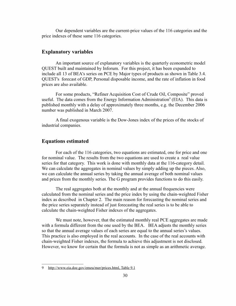
Our dependent variables are the current-price values of the 116 categories and the price indexes of these same 116 categories.
Explanatory variables
An important source of explanatory variables is the quarterly econometric model QUEST built and maintained by Inforum. For this project, it has been expanded to include all 13 of BEA's series on PCE by Major types of products as shown in Table 3.4. QUEST's forecast of GDP, Personal disposable income, and the rate of inflation in food prices are also available.
For some products, “Refiner Acquisition Cost of Crude Oil, Composite” proved useful. The data comes from the Energy Information Administration9 (EIA). This data is published monthly with a delay of approximately three months, e.g. the December 2006 number was published in March 2007.
A final exogenous variable is the Dow-Jones index of the prices of the stocks of industrial companies.
Equations estimated
For each of the 116 categories, two equations are estimated, one for price and one for nominal value. The results from the two equations are used to create a real value series for that category. This work is done with monthly data at the 116-category detail. We can calculate the aggregates in nominal values by simply adding up the pieces. Also, we can calculate the annual series by taking the annual average of both nominal values and prices from the monthly series. The G program provides functions to do this easily.
The real aggregates both at the monthly and at the annual frequencies were calculated from the nominal series and the price index by using the chain-weighted Fisher index as described in Chapter 2. The main reason for forecasting the nominal series and the price series separately instead of just forecasting the real series is to be able to calculate the chain-weighted Fisher indexes of the aggregates.
We must note, however, that the estimated monthly real PCE aggregates are made with a formula different from the one used by the BEA. BEA adjusts the monthly series so that the annual average values of each series are equal to the annual series’s values. This practice is also employed in the real accounts. In the case of the real accounts with chain-weighted Fisher indexes, the formula to achieve this adjustment is not disclosed. However, we know for certain that the formula is not as simple as an arithmetic average.
9 http://www.eia.doe.gov/emeu/mer/prices.html , Table 9.1
30
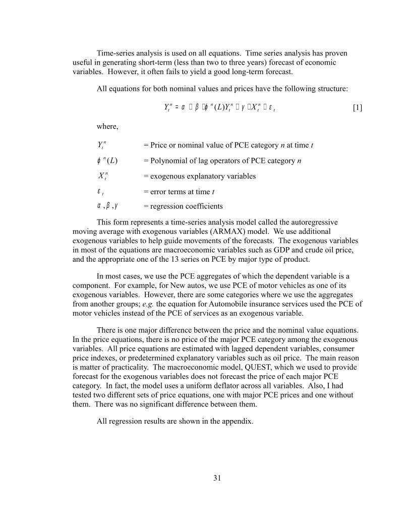
Time-series analysis is used on all equations. Time series analysis has proven useful in generating short-term (less than two to three years) forecast of economic variables. However, it often fails to yield a good long-term forecast.
All equations for both nominal values and prices have the following structure:
tnt
nt
nnt XYLY εγϕβα +⋅+⋅+= )( [1]
where,
ntY = Price or nominal value of PCE category n at time t
)(Lnϕ = Polynomial of lag operators of PCE category nntX = exogenous explanatory variables
tε = error terms at time t
γβα ,, = regression coefficients
This form represents a time-series analysis model called the autoregressive moving average with exogenous variables (ARMAX) model. We use additional exogenous variables to help guide movements of the forecasts. The exogenous variables in most of the equations are macroeconomic variables such as GDP and crude oil price, and the appropriate one of the 13 series on PCE by major type of product.
In most cases, we use the PCE aggregates of which the dependent variable is a component. For example, for New autos, we use PCE of motor vehicles as one of its exogenous variables. However, there are some categories where we use the aggregates from another groups; e.g. the equation for Automobile insurance services used the PCE of motor vehicles instead of the PCE of services as an exogenous variable.
There is one major difference between the price and the nominal value equations. In the price equations, there is no price of the major PCE category among the exogenous variables. All price equations are estimated with lagged dependent variables, consumer price indexes, or predetermined explanatory variables such as oil price. The main reason is matter of practicality. The macroeconomic model, QUEST, which we used to provide forecast for the exogenous variables does not forecast the price of each major PCE category. In fact, the model uses a uniform deflator across all variables. Also, I had tested two different sets of price equations, one with major PCE prices and one without them. There was no significant difference between them.
All regression results are shown in the appendix.
31

Approach to the problem
Here are the necessary steps for preparing the short-term forecast of PCE categories each time the interindustry model, LIFT, is being updated.
1. Prepare data banks for the G regression program with all the necessary data. They are: (1) the Underlying PCE tables from BEA, nominal, real and price index series in annual, quarterly, and monthly frequency, (2) monthly crude oil price data from the EIA, (3) the quarterly national accounts and a few other series in the QUIP databank which are used for the QUEST model10.
2. Re-estimate the forecasting equations: There are two sets of equations, one for nominal PCE series and one for the price indexes of PCE categories. During this step, we have two options. 1) Just re-estimate the regression equations or 2) Revise the structure of the equations and estimate the new ones. For example, the latter option is appropriate when the current equations produce an implausible forecast. In general, we only need to re-estimate the current equations with the updated data.
3. Creating with BUILD11 a model consisting solely of the equations estimated in step 2. Strictly speaking, we could avoid this step by putting into the command file for estimating the equations commands to rename the series with the forecasts automatically created by G. Building and running the model, however, requires less manual work and a produces a data bank containing only the historical and forecast series. Once this model is built, we run a historical simulation with it, that is, a “forecast” over the historical period with actual values of all exogenous variables. This is simply testing the accuracy of the equations as if we had perfect foresight for the exogenous variables.
4. Generating the exogenous variables for the forecast period. Update and run the QUEST model to obtain quarterly forecasts of a number of exogenous variables such as PCE by major type. These quarterly forecasts are then interpolated to monthly forecasts by G's @qtom() function.
5. Forecasting the detailed PCE series with the model from Step 3.
10 QUIP databank is the databank used in QUEST model. It contains most of the Quarterly NIPA tables and many macroeconomics variables including financial sector data.
11 BUILD is a executable program developed by INFORUM. BUILD creates C++ code of the model which will be compiled and ready for the user as an executable program. Go to www.inforum.umd.edu for more details.
32

3.4 Discussions of interesting detailed PCE equations' estimation results
In this section, I select some consumption categories to discuss the performance of the approach and to highlight some interesting observations. This section can be skipped without loss of understanding to the subsequent sections. Appendix 3.3 shows all regression results of both nominal PCE and the price index in 116 consumption categories.
The equations being discussed are estimated with historical data between January 1994 and June 2007. Regression results of both nominal PCE and its price index are presented for each product categories being discussed. The fitted graphs are also included. Please note that these equations will be re-estimated for each forecast if there is updated data for any series used in these equations.
New autos
The regression results for the nominal PCE of new autos (pce1) and the price index of new autos (cqp1) are shown above. The fitted graphs of both the nominal value and the price index are included below.
33
: 1 New autos (70) SEE = 3.77 RSQ = 0.8669 RHO = -0.28 Obser = 162 from 1994.001 SEE+1 = 3.62 RBSQ = 0.8652 DurH = -3.79 DoFree = 159 to 2007.006 MAPE = 3.06 Variable name Reg-Coef Mexval Elas NorRes Mean Beta 0 pce1 - - - - - - - - - - - - - - - - - 95.19 - - - 1 pce1[1] 0.91716 172.1 0.92 2.71 95.07 2 cdmv 0.25604 63.0 1.00 2.15 371.63 1.719 3 cdmv[1] -0.23550 46.8 -0.92 1.00 370.50 -1.592
: 1 New autos (70) SEE = 0.22 RSQ = 0.9856 RHO = 0.21 Obser = 162 from 1994.001 SEE+1 = 0.22 RBSQ = 0.9854 DurH = 2.75 DoFree = 158 to 2007.006 MAPE = 0.17 Variable name Reg-Coef Mexval Elas NorRes Mean Beta 0 cqp1 - - - - - - - - - - - - - - - - - 98.89 - - - 1 intercept 3.06750 1.5 0.03 69.58 1.00 2 cqp1[1] 0.95401 518.0 0.95 1.21 98.89 0.958 3 time -0.16709 5.3 -0.01 1.08 7.79 -0.347 4 gdpi 2.68918 3.8 0.03 1.00 1.04 0.295
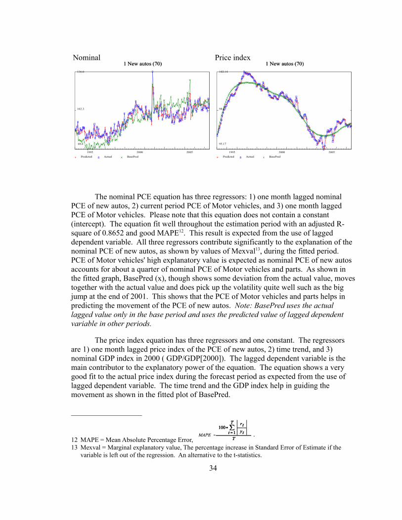
The nominal PCE equation has three regressors: 1) one month lagged nominal PCE of new autos, 2) current period PCE of Motor vehicles, and 3) one month lagged PCE of Motor vehicles. Please note that this equation does not contain a constant (intercept). The equation fit well throughout the estimation period with an adjusted R-square of 0.8652 and good MAPE12. This result is expected from the use of lagged dependent variable. All three regressors contribute significantly to the explanation of the nominal PCE of new autos, as shown by values of Mexval13, during the fitted period. PCE of Motor vehicles' high explanatory value is expected as nominal PCE of new autos accounts for about a quarter of nominal PCE of Motor vehicles and parts. As shown in the fitted graph, BasePred (x), though shows some deviation from the actual value, moves together with the actual value and does pick up the volatility quite well such as the big jump at the end of 2001. This shows that the PCE of Motor vehicles and parts helps in predicting the movement of the PCE of new autos. Note: BasePred uses the actual lagged value only in the base period and uses the predicted value of lagged dependent variable in other periods.
The price index equation has three regressors and one constant. The regressors are 1) one month lagged price index of the PCE of new autos, 2) time trend, and 3) nominal GDP index in 2000 ( GDP/GDP[2000]). The lagged dependent variable is the main contributor to the explanatory power of the equation. The equation shows a very good fit to the actual price index during the forecast period as expected from the use of lagged dependent variable. The time trend and the GDP index help in guiding the movement as shown in the fitted plot of BasePred.
12 MAPE = Mean Absolute Percentage Error, 13 Mexval = Marginal explanatory value, The percentage increase in Standard Error of Estimate if the
variable is left out of the regression. An alternative to the t-statistics.
34
Nominal Price index 1 New autos (70) 1 New autos (70)
136.0
102.3
68.6
1995 2000 2005 Predicted Actual BasePred
1 New autos (70) 1 New autos (70)102.14
98.65
95.17
1995 2000 2005 Predicted Actual BasePred

Overall, our approach provide satisfactory results in estimating the nominal PCE of new autos and its price index.
Computers and peripherals
In the last two decades, we have seen the increase in private consumption of computers and peripherals. The nominal PCE of computers and peripherals increases from less than one billion dollars in the early 1980s to 46.9 billion dollars in 2006. During the same period, we also observed the fall in price of computers sold to consumers.
As earlier discussed in Chapter 2, the falling price and the expansion of investment and consumption in computer product affected the way real value is calculated. In this analysis, the price index being estimated is the price index published by the BEA.
The nominal PCE equation contains three regressors without constant terms: 1) one month lagged nominal PCE of computers and peripherals, 2) current period nominal PCE of Furniture and household equipment, and 3) one month lagged nominal PCE of Furniture and household equipment. The equation provides a very good fit with adjusted R-square of 0.9987. The fitted plot confirms the regression result with BasePred shows that the nominal PCE of Furniture and household equipment helps move the series quite well.
35
: 9 Computers and peripherals SEE = 0.34 RSQ = 0.9987 RHO = -0.23 Obser = 162 from 1994.001 SEE+1 = 0.33 RBSQ = 0.9987 DurH = -2.91 DoFree = 159 to 2007.006 MAPE = 0.81 Variable name Reg-Coef Mexval Elas NorRes Mean Beta 0 pce9 - - - - - - - - - - - - - - - - - 31.93 - - - 1 pce9[1] 0.98606 855.1 0.98 1.80 31.70 2 cdfur 0.10535 31.7 1.01 1.69 306.14 0.666 3 cdfur[1] -0.10360 30.1 -0.99 1.00 304.81 -0.655
: 9 Computers and peripherals SEE = 4.94 RSQ = 0.9996 RHO = -0.04 Obser = 162 from 1994.001 SEE+1 = 4.93 RBSQ = 0.9996 DurH = -1.44 DoFree = 160 to 2007.006 MAPE = 1.06 Variable name Reg-Coef Mexval Elas NorRes Mean Beta 0 cqp9 - - - - - - - - - - - - - - - - - 209.02 - - - 1 cqp9[1] 1.31230 72.7 1.34 1.13 213.87 2 cqp9[2] -0.32579 6.2 -0.34 1.00 218.76 -0.337

The price index equation has two regressors without constant terms: 1) one month lagged price index of the PCE and 2) two month lagged price index of the PCE. The estimated values have reasonable mexvals and reasonable signs. The result fits well with the actual series during the estimated period as shown by both the R-square and the fitted plot.
Software
Software purchase generally follows the purchase of computers. It is not surprising to observe the increase in nominal PCE of software in the last two decades. The price of software has been falling but not as rapidly as the price of computers, especially since 1998.
36
Nominal Price Index 9 Computers and peripherals 9 Computers and peripherals
50.0
31.6
13.1
1995 2000 2005 Predicted Actual BasePred
9 Computers and peripherals 9 Computers and peripherals 808
416
24
1995 2000 2005 Predicted Actual BasePred
: 10 Software SEE = 0.11 RSQ = 0.9987 RHO = -0.19 Obser = 162 from 1994.001 SEE+1 = 0.11 RBSQ = 0.9987 DurH = -2.71 DoFree = 158 to 2007.006 MAPE = 0.86 Variable name Reg-Coef Mexval Elas NorRes Mean Beta 0 pce10 - - - - - - - - - - - - - - - - - 9.74 - - - 1 intercept -0.68115 3.0 -0.07 789.92 1.00 2 pce10[1] 0.88163 117.9 0.88 1.73 9.67 0.881 3 cdfur 0.03262 30.1 1.03 1.37 306.14 0.634 4 cdfur[1] -0.02655 16.9 -0.83 1.00 304.81 -0.516
: 10 Software SEE = 2.49 RSQ = 0.9993 RHO = -0.05 Obser = 162 from 1994.001 SEE+1 = 2.48 RBSQ = 0.9992 DurH = -1.68 DoFree = 160 to 2007.006 MAPE = 1.10 Variable name Reg-Coef Mexval Elas NorRes Mean Beta 0 cqp10 - - - - - - - - - - - - - - - - - 134.75 - - - 1 cqp10[1] 1.33541 74.8 1.36 1.14 136.73 2 cqp10[2] -0.34628 6.9 -0.36 1.00 138.74 -0.361

The equation for the nominal PCE has three regressors and an intercept. The results show that all three regressors have good Mexvals and reasonable signs. The equation also provides a very good close fit as shown by the adjusted R-square (0.9987) and the fitted plot over the test period. Shown in the fitted plot, the BasePred fits extremely well with the actual series which gives us confidence in this equation for the purpose of forecasting.
The price index results show good fit with very high adjusted R-square and very good MAPE. The coefficients of each regressors have reasonable signs and significant Mexvals. Although the BasePred does not fit to the actual series as well as the nominal equation, BasePred plot tracks the trend of the price index fairly well.
Pleasure aircraft
Pleasure aircraft is a luxury item which its consumption typically fluctuate with the economy. It is interesting to see the effectiveness of our approach in forecasting this type of products.
37
Nominal Price index 10 Software 10 Software
15.4
9.8
4.1
1995 2000 2005 Predicted Actual BasePred
10 Software 10 Software 383
204
25
1995 2000 2005 Predicted Actual BasePred

For pleasure aircraft, the nominal PCE equation has 4 regressors: 1) one-month lagged nominal PCE of pleasure aircraft, 2) two-month lagged nominal PCE of pleasure aircraft, 3) current period nominal PCE of other durable goods, and 4) one-month lagged nominal PCE of other durable goods. The equation fits well throughout the test period with R-square of 0.9417. All regressors have reasonable Mexvals and correct signs. BasePred shows a nice fit to the actual series over the test period.
38
: 22 Pleasure aircraft SEE = 0.06 RSQ = 0.9417 RHO = 0.08 Obser = 162 from 1994.001 SEE+1 = 0.06 RBSQ = 0.9406 DurH = 3.49 DoFree = 158 to 2007.006 MAPE = 4.20 Variable name Reg-Coef Mexval Elas NorRes Mean Beta 0 pce22 - - - - - - - - - - - - - - - - - 1.18 - - - 1 pce22[1] 0.25150 4.2 0.25 2.03 1.17 2 pce22[2] 0.28120 4.4 0.28 1.66 1.17 0.279 3 cdoth 0.01710 16.7 2.33 1.20 160.33 2.165 4 cdoth[2] -0.01376 9.5 -1.86 1.00 158.87 -1.738
: 22 Pleasure aircraft SEE = 0.61 RSQ = 0.9648 RHO = 0.02 Obser = 162 from 1994.001 SEE+1 = 0.61 RBSQ = 0.9644 DurH = 0.31 DoFree = 159 to 2007.006 MAPE = 0.46 Variable name Reg-Coef Mexval Elas NorRes Mean Beta 0 cqp22 - - - - - - - - - - - - - - - - - 99.20 - - - 1 intercept 7.98910 2.7 0.08 28.44 1.00 2 cqp22[1] 0.90658 148.4 0.91 1.04 99.12 0.909 3 gdpi 1.29332 2.1 0.01 1.00 1.04 0.082
Nominal Price index 22 Pleasure aircraft 22 Pleasure aircraft
107.3
100.3
93.3
1995 2000 2005 Predicted Actual BasePred
22 Pleasure aircraft 22 Pleasure aircraft 1.75
1.19
0.62
1995 2000 2005 Predicted Actual BasePred

The price index equation has two regressors and a constant. The regressors are one-month lagged price index of PCE of pleasure aircraft and the GDP index. The lagged dependent variable is the main contributor in explaining the price index over the test period. The BasePred shows that the equation captures increasing trend in the price index over time but fails to capture the volatility of the price index.
Books and maps
All three regressors in the nominal PCE equation of books and maps have good Mexvals. The equation provides a good fit with adjusted R-square of 0.9926 and MAPE of 1.44 percent. The fitted plots show a very good fit in both the predicted value and the BasePred, which track the actual series quite well.
39
: 24 Books and maps SEE = 0.63 RSQ = 0.9926 RHO = -0.08 Obser = 162 from 1994.001 SEE+1 = 0.63 RBSQ = 0.9925 DurH = -2.58 DoFree = 159 to 2007.006 MAPE = 1.44 Variable name Reg-Coef Mexval Elas NorRes Mean Beta 0 pce24 - - - - - - - - - - - - - - - - - 33.22 - - - 1 pce24[1] 0.49170 11.7 0.49 1.27 33.06 2 pce24[2] 0.35913 7.4 0.36 1.06 32.91 0.361 3 cdoth[1] 0.03219 2.8 0.15 1.00 159.60 0.145
: 24 Books and maps SEE = 0.63 RSQ = 0.9660 RHO = -0.06 Obser = 162 from 1994.001 SEE+1 = 0.63 RBSQ = 0.9658 DurH = -0.80 DoFree = 160 to 2007.006 MAPE = 0.45 Variable name Reg-Coef Mexval Elas NorRes Mean Beta 0 cqp24 - - - - - - - - - - - - - - - - - 100.46 - - - 1 cqp24[1] 1.00183 6663.5 1.00 1.01 100.39 2 time -0.01465 0.4 -0.00 1.00 7.79 -0.017
Nominal Price index 24 Books and maps 24 Books and maps
105.1
98.6
92.1
1995 2000 2005 Predicted Actual BasePred
24 Books and maps 24 Books and maps 45.7
32.7
19.7
1995 2000 2005 Predicted Actual BasePred

The price index result shows a good fit with adjusted R-square of 0.996 and MAPE of 0.45 percent. The coefficients of each regressors have reasonable signs. The BasePred plot shows that the equation tracks the long-term trend of the price index quite well but fails to capture any volatility during the test period.
Coffee, tea and beverage materials
The result shows that the nominal PCE of coffee, tea and beverage materials can be estimated quite accurately during the test period with the one-month lagged dependent variable and the current period nominal PCE of food. The closeness of fit statistics are quite good with an adjusted R-square of 0.9989 and MAPE of 0.56 percent. The BasePred plot shows good behavior in tracking the trend of the nominal PCE during the test period.
40
: 39 Coffee, tea and beverage materials SEE = 0.10 RSQ = 0.9989 RHO = -0.08 Obser = 162 from 1994.001 SEE+1 = 0.09 RBSQ = 0.9989 DurH = -1.03 DoFree = 159 to 2007.006 MAPE = 0.56 Variable name Reg-Coef Mexval Elas NorRes Mean Beta 0 pce39 - - - - - - - - - - - - - - - - - 12.14 - - - 1 intercept -0.18382 2.2 -0.02 932.11 1.00 2 pce39[1] 0.94007 336.1 0.93 1.08 12.07 0.937 3 cnfood 0.00102 4.0 0.08 1.00 954.45 0.063
: 39 Coffee, tea and beverage materials SEE = 1.64 RSQ = 0.9544 RHO = 0.06 Obser = 162 from 1994.001 SEE+1 = 1.63 RBSQ = 0.9535 DurH = 1.33 DoFree = 158 to 2007.006 MAPE = 0.85 Variable name Reg-Coef Mexval Elas NorRes Mean Beta 0 cqp39 - - - - - - - - - - - - - - - - - 98.99 - - - 1 intercept 7.73683 6.8 0.08 21.92 1.00 2 cqp39[1] 1.45147 103.5 1.45 1.50 98.73 1.513 3 cqp39[2] -0.54702 21.8 -0.54 1.03 98.46 -0.594 4 gdpi 1.75147 1.6 0.02 1.00 1.04 0.047

The price index of PCE of coffee, tea and beverage materials had two big spikes in the mid 1990s caused by concerns about frost in Brazil, the biggest coffee producer at the time. The BasePred plot shows that the equation cannot track these volatility (as they were caused by natural cause) in a long-term forecast. On the other hand, the predicted value tracks the actual series quite well with the help of the lagged dependent variables. Overall, the regressors of the price index equation have reasonable Mexvals and signs. The result seems to fit the actual series well during the test period with high adjusted R-square and low MAPE.
Women's and children's clothing and accessories
41
Nominal Price index 39 Coffee, tea and beverage materials 39 Coffee, tea and beverage materials
18.1
12.5
7.0
1995 2000 2005 Predicted Actual BasePred
39 Coffee, tea and beverage materials 39 Coffee, tea and beverage materials112.8
90.3
67.9
1995 2000 2005 Predicted Actual BasePred
: 50 Women's and children's clothing and accessories except shoes SEE = 0.34 RSQ = 0.9997 RHO = -0.29 Obser = 162 from 1994.001 SEE+1 = 0.33 RBSQ = 0.9997 DurH = -3.75 DoFree = 159 to 2007.006 MAPE = 0.17 Variable name Reg-Coef Mexval Elas NorRes Mean Beta 0 pce50 - - - - - - - - - - - - - - - - - 154.72 - - - 1 pce50[1] 0.94225 306.0 0.94 34.29 154.30 2 cncloth 0.52801 483.7 1.00 10.80 293.63 1.032 3 cncloth[1] -0.49765 228.6 -0.94 1.00 292.79 -0.969
: 50 Women's and children's clothing and accessories except shoes SEE = 0.70 RSQ = 0.9903 RHO = -0.11 Obser = 162 from 1994.001 SEE+1 = 0.69 RBSQ = 0.9902 DurH = -1.43 DoFree = 159 to 2007.006 MAPE = 0.53 Variable name Reg-Coef Mexval Elas NorRes Mean Beta 0 cqp50 - - - - - - - - - - - - - - - - - 99.77 - - - 1 cqp50[1] 0.99784 6966.3 1.00 1.01 99.93 2 crude 0.01123 0.6 0.00 1.01 28.35 0.024 3 crude[11] -0.01038 0.4 -0.00 1.00 25.51 -0.019
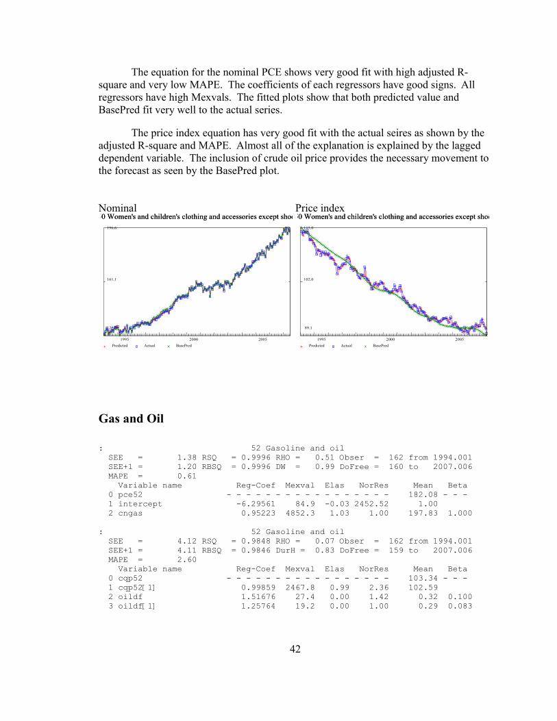
The equation for the nominal PCE shows very good fit with high adjusted R-square and very low MAPE. The coefficients of each regressors have good signs. All regressors have high Mexvals. The fitted plots show that both predicted value and BasePred fit very well to the actual series.
The price index equation has very good fit with the actual seires as shown by the adjusted R-square and MAPE. Almost all of the explanation is explained by the lagged dependent variable. The inclusion of crude oil price provides the necessary movement to the forecast as seen by the BasePred plot.
Gas and Oil
42
Nominal Price index 50 Women's and children's clothing and accessories except shoes 50 Women's and children's clothing and accessories except shoes
115.0
102.0
89.1
1995 2000 2005 Predicted Actual BasePred
: 52 Gasoline and oil SEE = 1.38 RSQ = 0.9996 RHO = 0.51 Obser = 162 from 1994.001 SEE+1 = 1.20 RBSQ = 0.9996 DW = 0.99 DoFree = 160 to 2007.006 MAPE = 0.61 Variable name Reg-Coef Mexval Elas NorRes Mean Beta 0 pce52 - - - - - - - - - - - - - - - - - 182.08 - - - 1 intercept -6.29561 84.9 -0.03 2452.52 1.00 2 cngas 0.95223 4852.3 1.03 1.00 197.83 1.000
: 52 Gasoline and oil SEE = 4.12 RSQ = 0.9848 RHO = 0.07 Obser = 162 from 1994.001 SEE+1 = 4.11 RBSQ = 0.9846 DurH = 0.83 DoFree = 159 to 2007.006 MAPE = 2.60 Variable name Reg-Coef Mexval Elas NorRes Mean Beta 0 cqp52 - - - - - - - - - - - - - - - - - 103.34 - - - 1 cqp52[1] 0.99859 2467.8 0.99 2.36 102.59 2 oildf 1.51676 27.4 0.00 1.42 0.32 0.100 3 oildf[1] 1.25764 19.2 0.00 1.00 0.29 0.083
50 Women's and children's clothing and accessories except shoes 50 Women's and children's clothing and accessories except shoes196.6
161.1
125.7
1995 2000 2005 Predicted Actual BasePred

The nominal PCE equation of Gasoline and oil has only the nominal PCE of Gasoline, fuel oil, and other energy goods. There is no lagged dependent variable. The Mexvals of the nominal PCE of Gasoline, fuel oil, and other energy goods is very high because the nominal PCE of Gasoline and oil contribute around 90 percent to the nominal PCE of Gasoline, fuel oil, and other energy goods throughout the test period. The closeness of fit statistics, both adjusted R-square and MAPE, are very good. The fitted plot shows excellent fit as well.
The price equation has 3 regressors and no constant. The first differences of crude oil price, both current period and one-month lagged, are quite good in capturing the volatility of the price index as shown by the fitted plot of BasePred. In general, all coefficients have reasonable Mexvals and the closeness of fit statistics are quite good.
Housing
The PCE of housing is the only detailed PCE in this analysis that is equal exactly to the major aggregate PCE of housing. Thus, we use only the lagged dependent variables in both the nominal PCE and the price index equations without the intercept.
43
Nominal Price index 52 Gasoline and oil 52 Gasoline and oil
372
242
111
1995 2000 2005 Predicted Actual
52 Gasoline and oil 52 Gasoline and oil 206
132
59
1995 2000 2005 Predicted Actual BasePred

Both equations show very good closeness of fit statistics with very high explanatory value. The fitted plots show very good fit from both predicted value and BasePred plots.
44
: 66 Housing SEE = 1.57 RSQ = 0.9999 RHO = 0.20 Obser = 162 from 1994.001 SEE+1 = 1.54 RBSQ = 0.9999 DurH = 2.60 DoFree = 161 to 2007.006 MAPE = 0.11 Variable name Reg-Coef Mexval Elas NorRes Mean Beta 0 pce66 - - - - - - - - - - - - - - - - - 1034.87 - - - 1 pce66[1] 1.00457 67319.6 1.00 1.00 1030.18
: 66 Housing SEE = 0.09 RSQ = 0.9999 RHO = 0.33 Obser = 162 from 1994.001 SEE+1 = 0.08 RBSQ = 0.9999 DurH = 4.18 DoFree = 161 to 2007.006 MAPE = 0.07 Variable name Reg-Coef Mexval Elas NorRes Mean Beta 0 cqp66 - - - - - - - - - - - - - - - - - 101.82 - - - 1 cqp66[1] 1.00258 119334.6 1.00 1.00 101.56
Nominal Price index 66 Housing 66 Housing
1468
1086
704
1995 2000 2005 Predicted Actual BasePred
66 Housing 66 Housing124.8
103.6
82.4
1995 2000 2005 Predicted Actual BasePred
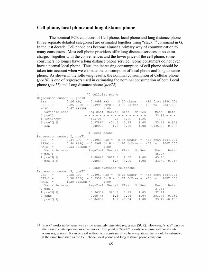
Cell phone, local phone and long distance phone
The nominal PCE equations of Cell phone, local phone and long distance phone (three separate detailed categories) are estimated together using “stack”14 command in G. In the last decade, Cell phone has become almost a primary way of communication to many consumers. Most cell phone providers offer long distance services at no extra charge. Together with the conveniences and the lower price of the cell phone, some consumers no longer have a long distance phone service. Some consumers do not even have a normal local phone. Thus, the increasing consumption of cell phone should be taken into account when we estimate the consumption of local phone and long distance phone. As shown in the following results, the nominal consumption of Cellular phone (pce70) is one of regressors used in estimating the nominal consumption of both Local phone (pce71) and Long distance phone (pce72).
14 “stack” works in the same way as the seemingly unrelated regression (SUR). However, “stack” pays no attention to contemporaneous covariances. The point of “stack” is only to impose soft constraints across regressions. It can be used without any constraint if we have equations that should be estimated at the same time such as the Cell phone, local phone and long distance phone equations.
45
: 70 Cellular phoneRegression number 1, pce70 SEE = 0.26 RSQ = 0.9998 RHO = 0.30 Obser = 486 from 1994.001 SEE+1 = 0.25 RBSQ = 0.9998 DurH = 3.77 DoFree = 478 to 2007.006 MAPE = 0.67 SEESUR = 1.00 Variable name Reg-Coef Mexval Elas NorRes Mean Beta 0 pce70 - - - - - - - - - - - - - - - - - 33.89 - - - 1 intercept -1.57216 0.8 -0.05 1.25 1.00 2 pce70[1] 0.97867 404.5 0.97 1.00 33.49 0.973 3 gdp 0.00027 1.0 0.08 1.00 9935.29 0.028
: 71 Local phoneRegression number 2, pce71 SEE = 0.34 RSQ = 0.9969 RHO = 0.15 Obser = 486 from 1994.001 SEE+1 = 0.34 RBSQ = 0.9969 DurH = 1.92 DoFree = 478 to 2007.006 MAPE = 0.53 SEESUR = 1.00 Variable name Reg-Coef Mexval Elas NorRes Mean Beta 4 pce71 - - - - - - - - - - - - - - - - - 45.75 - - - 1 pce71[1] 1.00646 3016.6 1.00 1.00 45.65 2 pce70[1] -0.00590 1.2 -0.00 1.00 33.49 -0.018
: 72 Long distance telephoneRegression number 3, pce72 SEE = 0.58 RSQ = 0.9957 RHO = 0.08 Obser = 486 from 1994.001 SEE+1 = 0.58 RBSQ = 0.9956 DurH = 1.01 DoFree = 478 to 2007.006 MAPE = 1.20 SEESUR = 1.00 Variable name Reg-Coef Mexval Elas NorRes Mean Beta 7 pce72 - - - - - - - - - - - - - - - - - 37.36 - - - 1 pce72[1] 0.96332 325.2 0.97 1.05 37.44 2 csho 0.00745 1.5 0.08 1.04 391.48 0.059 3 pce70[1] -0.04859 1.9 -0.04 1.00 33.49 -0.106

The regressions' results are very satisfactory. We have very good fit for the PCE of cellular phone. The coefficients of one month lagged PCE of cellular phone in the equations of both local telephone and the long distance telephone have negative signs as expected. The BasePred plots show that the equation can capture the long-term trend, but not the short-term volatility, of these three PCE categories.
46
Plots of the nominal PCE
Cellular phone Local Phone
Long distance phone
70 Cellular telephone 70 Cellular telephone 72.3
39.8
7.3
1995 2000 2005 Predicted Actual BasePred
71 Local telephone 71 Local telephone 53.6
43.8
34.0
1995 2000 2005 Predicted Actual BasePred
72 Long distance telephone 72 Long distance telephone 50.2
35.4
20.6
1995 2000 2005 Predicted Actual BasePred

The price index equations of the three telephone categories show pretty good fit by the closeness of fit statistics. Each regressor has reasonable Mexvals. However, the fitted plots reveal that, with the exception of cellular telephones' price index equation, the other price index equations do not have much explanation into the movement of the price indexes as shown by the plot of BasePred. Thus, we should be cautious in using these equations in forecasting.
47
: 70 Cellular telephone SEE = 0.57 RSQ = 0.9996 RHO = -0.03 Obser = 162 from 1994.001 SEE+1 = 0.57 RBSQ = 0.9995 DurH = -0.82 DoFree = 158 to 2007.006 MAPE = 0.39 Variable name Reg-Coef Mexval Elas NorRes Mean Beta 0 cqp70 - - - - - - - - - - - - - - - - - 111.06 - - - 1 intercept -0.72664 0.2 -0.01 2254.50 1.00 2 cqp70[1] 1.54662 110.0 1.55 1.49 111.52 1.558 3 cqp70[2] -0.54687 19.2 -0.55 1.01 111.99 -0.555 4 gdpi 0.52499 0.3 0.00 1.00 1.04 0.004
: 71 Local telephone SEE = 0.55 RSQ = 0.9979 RHO = -0.10 Obser = 162 from 1994.001 SEE+1 = 0.55 RBSQ = 0.9979 DurH = -1.26 DoFree = 161 to 2007.006 MAPE = 0.33 Variable name Reg-Coef Mexval Elas NorRes Mean Beta 0 cqp71 - - - - - - - - - - - - - - - - - 104.11 - - - 1 cqp71[1] 1.00221 19024.3 1.00 1.00 103.88
: 72 Long distance telephone SEE = 1.08 RSQ = 0.9945 RHO = -0.01 Obser = 162 from 1994.001 SEE+1 = 1.08 RBSQ = 0.9944 DurH = -1.89 DoFree = 159 to 2007.006 MAPE = 0.81 Variable name Reg-Coef Mexval Elas NorRes Mean Beta 0 cqp72 - - - - - - - - - - - - - - - - - 95.26 - - - 1 cqp72[1] 0.90901 36.5 0.91 1.05 95.43 2 cqp72[2] 0.28984 2.4 0.29 1.04 95.60 0.288 3 cqp72[3] -0.20043 2.0 -0.20 1.00 95.78 -0.198

Airlines
The equation for the nominal PCE of Airline services has one-month lagged dependent variable and the nominal PCE of transportation service as its regressors. Both regressors plus the intercept have reasonable Mexvals. The adjusted R-square is quite good (0.9058). The MAPE is slightly high (2.67 percent). The fitted plot shows that Airline services affected the most from the brief recession in 2000 and the terrorist attack in September 2001. However, the consumption looks to be back to its long-term trend by 2003 as the BasePred shown pretty good fit since then.
48
Plots of the price index
Cellular phone Local phone
Long distance phone
70 Cellular telephone 70 Cellular telephone159.9
122.3
84.8
1995 2000 2005 Predicted Actual BasePred
71 Local telephone 71 Local telephone128.2
108.7
89.2
1995 2000 2005 Predicted Actual BasePred
72 Long distance telephone 72 Long distance telephone113.2
91.7
70.2
1995 2000 2005 Predicted Actual BasePred

The price index plot shows the same story as the nominal value. There was a steep decline in price between 2000 and 2001. The price index also starts increasing again since 2005 as should be expected from the increasing oil price. However, an experiment in estimating the equation with crude oil price was unsuccessful. In general, the price index of the airline service is difficult to estimate. It is affected by many factors such as the overall economy, natural causes (such as weather), etc. Nevertheless, this price index equation should provide a decent short-term forecast in normal circumstance.
49
: 83 Airline SEE = 1.25 RSQ = 0.9070 RHO = -0.17 Obser = 162 from 1994.001 SEE+1 = 1.24 RBSQ = 0.9058 DurH = -2.58 DoFree = 159 to 2007.006 MAPE = 2.67 Variable name Reg-Coef Mexval Elas NorRes Mean Beta 0 pce83 - - - - - - - - - - - - - - - - - 31.08 - - - 1 intercept 1.80871 1.8 0.06 10.75 1.00 2 pce83[1] 0.84033 88.7 0.84 1.06 31.00 0.845 3 cstr 0.01169 2.9 0.10 1.00 275.95 0.128
: 83 Airline SEE = 2.03 RSQ = 0.8733 RHO = 0.02 Obser = 162 from 1994.001 SEE+1 = 2.03 RBSQ = 0.8717 DurH = 4.03 DoFree = 159 to 2007.006 MAPE = 1.70 Variable name Reg-Coef Mexval Elas NorRes Mean Beta 0 cqp83 - - - - - - - - - - - - - - - - - 90.33 - - - 1 intercept 6.59431 2.0 0.07 7.90 1.00 2 cqp83[1] 1.02277 43.6 1.02 1.01 90.35 1.024 3 cqp83[2] -0.09587 0.5 -0.10 1.00 90.40 -0.096
Nominal Price index 83 Airline 83 Airline
104.1
92.1
80.0
1995 2000 2005 Predicted Actual BasePred
83 Airline 83 Airline 38.3
30.3
22.2
1995 2000 2005 Predicted Actual BasePred

Health insurance
The equation for the nominal PCE of health insurance service has three regressors plus an intercept. Most of the explanatory power of the equation is provided by the one-month lagged dependent variable. The equation has a very god fit over the test period with adjust R-square of 0.9999 and MAPE of 0.28 percent. The fitted plot shows an excellent fit for the predicted value and a relatively good fit for the BasePred.
The price index equations has three regressors and no intercept. The lagged dependent variables provide most of the explanation with very good Mexvals. The adjusted R-square is 0.9998 and the MAPE is 0.16 percent. The fitted plot shows that the equation can explain the long-term trend but fails to capture the short-term fluctuation of the price index as seen by the BasePred plot.
50
: 90 Health insurance SEE = 0.35 RSQ = 0.9999 RHO = 0.80 Obser = 162 from 1994.001 SEE+1 = 0.22 RBSQ = 0.9999 DurH = 10.21 DoFree = 158 to 2007.006 MAPE = 0.28 Variable name Reg-Coef Mexval Elas NorRes Mean Beta 0 pce90 - - - - - - - - - - - - - - - - - 94.43 - - - 1 intercept -1.08819 4.9 -0.01 8209.40 1.00 2 pce90[1] 0.97680 906.7 0.97 1.19 93.81 0.969 3 csmc 0.03343 3.0 0.40 1.05 1118.22 0.295 4 csmc[1] -0.03011 2.4 -0.35 1.00 1112.34 -0.264
: 90 Health insurance SEE = 0.24 RSQ = 0.9998 RHO = -0.25 Obser = 162 from 1994.001 SEE+1 = 0.23 RBSQ = 0.9998 DurH = -4.36 DoFree = 159 to 2007.006 MAPE = 0.16 Variable name Reg-Coef Mexval Elas NorRes Mean Beta 0 cqp90 - - - - - - - - - - - - - - - - - 105.40 - - - 1 cqp90[1] 1.76739 187.7 1.76 2.37 104.97 2 cqp90[2] -0.76974 52.6 -0.76 1.00 104.55 -0.766 3 gdpi 0.33077 0.2 0.00 1.00 1.04 0.004

Brokerage charges and investment counseling
The equation for the nominal PCE of Brokerage charges and investment counseling has a good fit during the test period. The adjusted R-square is 0.9733 while the MAPE is 3.29 percent. The Dow Jones Industrial index helps the equation in tracking the actual series quite well as shown by the BasePred plot.
51
Nominal Price index 90 Health insurance 90 Health insurance
142.6
108.0
73.4
1995 2000 2005 Predicted Actual BasePred
: 100 Brokerage charges and investment counseling SEE = 3.51 RSQ = 0.9736 RHO = 0.06 Obser = 162 from 1994.001 SEE+1 = 3.50 RBSQ = 0.9733 DurH = 0.89 DoFree = 159 to 2007.006 MAPE = 3.29 Variable name Reg-Coef Mexval Elas NorRes Mean Beta 0 pce100 - - - - - - - - - - - - - - - - - 75.55 - - - 1 intercept 0.78405 0.2 0.01 37.86 1.00 2 pce100[1] 0.83978 90.8 0.83 1.09 75.05 0.836 3 djia 0.00134 4.6 0.16 1.00 8771.94 0.157
: 100 Brokerage charges and investment counseling SEE = 2.79 RSQ = 0.9893 RHO = -0.16 Obser = 162 from 1994.001 SEE+1 = 2.73 RBSQ = 0.9891 DurH = -2.15 DoFree = 158 to 2007.006 MAPE = 1.33 Variable name Reg-Coef Mexval Elas NorRes Mean Beta 0 cqp100 - - - - - - - - - - - - - - - - - 114.96 - - - 1 intercept 6.25085 0.8 0.05 93.48 1.00 2 cqp100[1] 0.95325 234.1 0.96 1.03 115.37 0.962 3 time -0.44230 1.0 -0.03 1.03 7.79 -0.064 4 crude 0.07707 1.4 0.02 1.00 28.35 0.043
90 Health insurance 90 Health insurance 159
108
57
1995 2000 2005 Predicted Actual BasePred
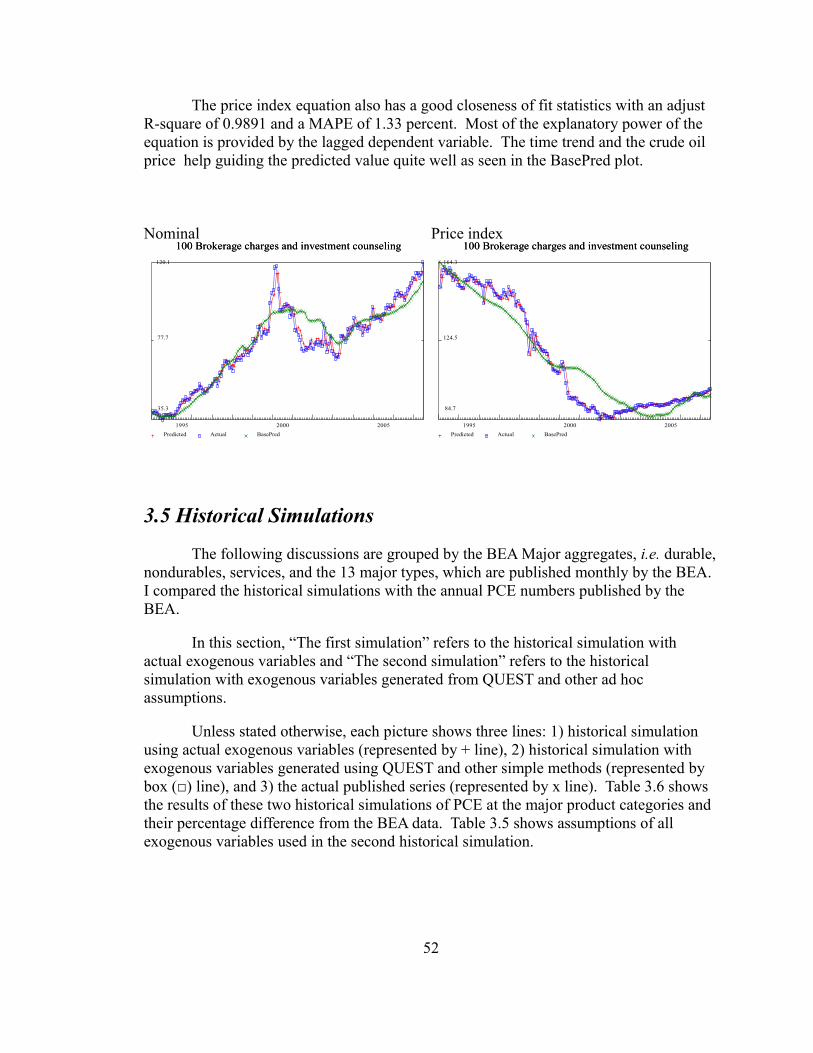
The price index equation also has a good closeness of fit statistics with an adjust R-square of 0.9891 and a MAPE of 1.33 percent. Most of the explanatory power of the equation is provided by the lagged dependent variable. The time trend and the crude oil price help guiding the predicted value quite well as seen in the BasePred plot.
3.5 Historical Simulations
The following discussions are grouped by the BEA Major aggregates, i.e. durable, nondurables, services, and the 13 major types, which are published monthly by the BEA. I compared the historical simulations with the annual PCE numbers published by the BEA.
In this section, “The first simulation” refers to the historical simulation with actual exogenous variables and “The second simulation” refers to the historical simulation with exogenous variables generated from QUEST and other ad hoc assumptions.
Unless stated otherwise, each picture shows three lines: 1) historical simulation using actual exogenous variables (represented by + line), 2) historical simulation with exogenous variables generated using QUEST and other simple methods (represented by box (□) line), and 3) the actual published series (represented by x line). Table 3.6 shows the results of these two historical simulations of PCE at the major product categories and their percentage difference from the BEA data. Table 3.5 shows assumptions of all exogenous variables used in the second historical simulation.
52
Nominal Price index 100 Brokerage charges and investment counseling 100 Brokerage charges and investment counseling
120.1
77.7
35.3
1995 2000 2005 Predicted Actual BasePred
100 Brokerage charges and investment counseling 100 Brokerage charges and investment counseling164.3
124.5
84.7
1995 2000 2005 Predicted Actual BasePred

As shown in Table 3.6, our approach can generate a very reasonable results when given accurate exogenous variables, especially with the forecast of one-year ahead. The errors grow slightly with the two-year ahead forecast. In one-year ahead forecast, we miss the published real total PCE by 0.38% given accurate exogenous variable and by 0.58% using predicted exogenous variables. In general, the approach errors are less than 2%, for the one-year ahead forecast of real PCE, which is very good. Some categories with major shift during the forecast period, such as Gasoline, fuel oil and other energy goods, exhibit higher errors with the second simulation.
It appears that the accuracy of the forecast depends on the quality of the exogenous variables and how further the forecast period from the last known published data.
The rest of this section (3.5) discusses these results in detail with plots of each aggregates. It can be skipped.
53
Table 3.5: Assumptions of exogenous variables used in the Second Historical Simulation
Predetermined explanatory variables used in historical simulation
2005Q1 2005Q2 2005Q3 2005Q4 2006Q1 2006Q2 2006Q3 2006Q4cdmv Nominal PCE of motor vehivcles 474.30 479.94 475.23 461.36 477.78 468.83 483.52 487.92cdfur Nominal PCE of furnitures 369.85 372.61 373.53 382.67 384.42 391.34 393.49 398.22cdoth Nominal PCE of other durables 198.18 200.49 202.42 206.66 206.45 208.71 209.31 211.75cnfood Nominal PCE of food 1,152.76 1,161.61 1,169.64 1,188.96 1,191.88 1,208.31 1,216.47 1,233.24cncloth Nominal PCE of clothing and shoes 333.32 336.74 338.48 343.33 342.94 346.68 348.38 352.78cngas Nominal PCE of gas and oil 270.53 279.80 304.58 323.13 338.87 351.11 359.36 369.08cnoth Nominal PCE of other nondurables 679.62 686.11 692.84 703.81 705.63 714.18 719.66 729.54cshous Nominal PCE of housing 1,267.93 1,276.32 1,280.66 1,301.06 1,300.51 1,317.27 1,323.73 1,339.03csho Nominal PCE of household operations 459.83 463.62 463.66 473.28 476.20 482.49 486.77 492.63cstr Nominal PCE of transportation 314.84 317.35 319.29 324.91 324.18 326.39 326.05 327.44csmc Nominal PCE of medical services 1,448.02 1,466.35 1,484.00 1,511.69 1,522.73 1,542.15 1,558.62 1,582.26csrec Nominal PCE of recreational services 350.36 353.67 353.68 360.39 360.08 366.32 367.02 371.31csoth Nominal PCE of other services 1,189.00 1,201.34 1,204.45 1,225.90 1,225.48 1,245.04 1,248.96 1,264.17ddj djia - djia(-1) 317.97 267.83 231.12 260.29 201.73 227.24 222.18 252.88oildf croil - croil(-1) 5.86 -5.33 1.62 0.45 3.84 3.17 5.13 2.27gdp GDP in Billion dollars 12,126.70 12,241.62 12,328.63 12,494.10 12,591.72 12,727.95 12,844.82 12,995.03djia Dow Jones Industrial Index 10,730.81 10,998.64 11,229.76 11,490.04 11,691.78 11,919.02 12,141.20 12,394.09gdpi GDP deflator (2000Q1 = 1) 1.26 1.27 1.28 1.30 1.31 1.32 1.33 1.35croil Crude Oil Price 34.61 29.28 30.90 31.35 35.19 38.36 43.49 45.75
* all nominal PCE are in Billion dollars
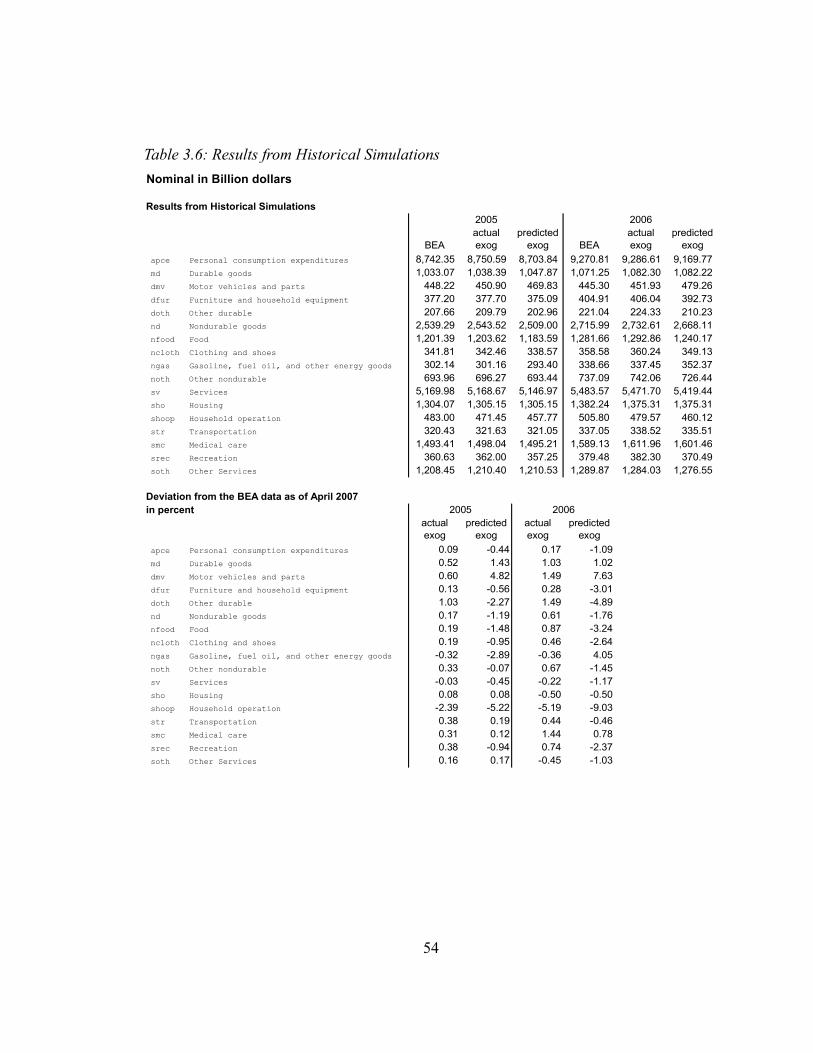
54
Table 3.6: Results from Historical SimulationsNominal in Billion dollars
Results from Historical Simulations
BEAactual exog
predicted exog BEA
actual exog
predicted exog
apce Personal consumption expenditures 8,742.35 8,750.59 8,703.84 9,270.81 9,286.61 9,169.77 md Durable goods 1,033.07 1,038.39 1,047.87 1,071.25 1,082.30 1,082.22 dmv Motor vehicles and parts 448.22 450.90 469.83 445.30 451.93 479.26 dfur Furniture and household equipment 377.20 377.70 375.09 404.91 406.04 392.73 doth Other durable 207.66 209.79 202.96 221.04 224.33 210.23 nd Nondurable goods 2,539.29 2,543.52 2,509.00 2,715.99 2,732.61 2,668.11 nfood Food 1,201.39 1,203.62 1,183.59 1,281.66 1,292.86 1,240.17 ncloth Clothing and shoes 341.81 342.46 338.57 358.58 360.24 349.13 ngas Gasoline, fuel oil, and other energy goods 302.14 301.16 293.40 338.66 337.45 352.37 noth Other nondurable 693.96 696.27 693.44 737.09 742.06 726.44 sv Services 5,169.98 5,168.67 5,146.97 5,483.57 5,471.70 5,419.44 sho Housing 1,304.07 1,305.15 1,305.15 1,382.24 1,375.31 1,375.31 shoop Household operation 483.00 471.45 457.77 505.80 479.57 460.12 str Transportation 320.43 321.63 321.05 337.05 338.52 335.51 smc Medical care 1,493.41 1,498.04 1,495.21 1,589.13 1,611.96 1,601.46 srec Recreation 360.63 362.00 357.25 379.48 382.30 370.49 soth Other Services 1,208.45 1,210.40 1,210.53 1,289.87 1,284.03 1,276.55
Deviation from the BEA data as of April 2007in percent
actual exog
predicted exog
actual exog
predicted exog
apce Personal consumption expenditures 0.09 -0.44 0.17 -1.09 md Durable goods 0.52 1.43 1.03 1.02 dmv Motor vehicles and parts 0.60 4.82 1.49 7.63 dfur Furniture and household equipment 0.13 -0.56 0.28 -3.01 doth Other durable 1.03 -2.27 1.49 -4.89 nd Nondurable goods 0.17 -1.19 0.61 -1.76 nfood Food 0.19 -1.48 0.87 -3.24 ncloth Clothing and shoes 0.19 -0.95 0.46 -2.64 ngas Gasoline, fuel oil, and other energy goods -0.32 -2.89 -0.36 4.05 noth Other nondurable 0.33 -0.07 0.67 -1.45 sv Services -0.03 -0.45 -0.22 -1.17 sho Housing 0.08 0.08 -0.50 -0.50 shoop Household operation -2.39 -5.22 -5.19 -9.03 str Transportation 0.38 0.19 0.44 -0.46 smc Medical care 0.31 0.12 1.44 0.78 srec Recreation 0.38 -0.94 0.74 -2.37 soth Other Services 0.16 0.17 -0.45 -1.03
2005 2006
2005 2006

55
Table 3.6 (cont.)
Chained Real 2000 dollar
Results from Historical Simulations
BEAactual exog
predicted exog BEA
actual exog
predicted exog
apce Personal consumption expenditures 7,841.17 7,871.17 7,886.90 8,092.54 8,123.11 8,167.46 md Durable goods 1,145.34 1,161.62 1,172.78 1,203.99 1,234.71 1,237.08 dmv Motor vehicles and parts 452.90 457.31 477.38 448.01 454.76 482.96 dfur Furniture and household equipment 490.60 499.62 496.25 551.37 570.44 554.11 doth Other durable 212.57 216.14 208.99 224.49 231.84 218.22 nd Nondurable goods 2,276.78 2,286.27 2,275.78 2,363.05 2,391.06 2,370.57 nfood Food 1,065.70 1,068.68 1,049.81 1,111.41 1,123.01 1,075.36 ncloth Clothing and shoes 372.72 378.99 376.70 392.68 405.07 394.75 ngas Gasoline, fuel oil, and other energy goods 199.53 198.78 209.03 197.89 197.67 233.32 noth Other nondurable 643.90 646.18 643.88 671.44 678.13 666.95 sv Services 4,436.65 4,443.60 4,459.80 4,549.55 4,528.90 4,588.10 sho Housing 1,122.60 1,111.55 1,116.35 1,148.68 1,122.75 1,140.53 shoop Household operation 417.98 411.06 409.22 416.21 398.68 409.24 str Transportation 284.41 289.56 289.80 288.41 296.06 295.58 smc Medical care 1,260.92 1,271.88 1,277.03 1,304.32 1,322.40 1,332.79 srec Recreation 313.14 313.09 310.08 319.86 320.09 313.55 soth Other Services 1,036.18 1,045.01 1,055.64 1,070.33 1,067.27 1,094.01
Deviation from the BEA data as of April 2007in percent
actual exog
predicted exog
actual exog
predicted exog
apce Personal consumption expenditures 0.38 0.58 0.38 0.93 md Durable goods 1.42 2.40 2.55 2.75 dmv Motor vehicles and parts 0.97 5.41 1.51 7.80 dfur Furniture and household equipment 1.84 1.15 3.46 0.50 doth Other durable 1.68 -1.69 3.27 -2.79 nd Nondurable goods 0.42 -0.04 1.19 0.32 nfood Food 0.28 -1.49 1.04 -3.24 ncloth Clothing and shoes 1.68 1.07 3.15 0.53 ngas Gasoline, fuel oil, and other energy goods -0.38 4.76 -0.11 17.91 noth Other nondurable 0.35 0.00 1.00 -0.67 sv Services 0.16 0.52 -0.45 0.85 sho Housing -0.98 -0.56 -2.26 -0.71 shoop Household operation -1.66 -2.10 -4.21 -1.67 str Transportation 1.81 1.89 2.65 2.49 smc Medical care 0.87 1.28 1.39 2.18 srec Recreation -0.02 -0.98 0.07 -1.97 soth Other Services 0.85 1.88 -0.29 2.21
2005 2006
2005 2006
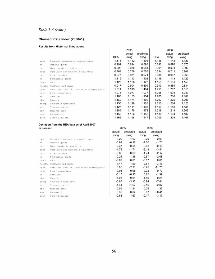
56
Table 3.6 (cont.)
Chained Price Index (2000=1)
Results from Historical Simulations
BEAactual exog
predicted exog BEA
actual exog
predicted exog
apce Personal consumption expenditures 1.115 1.112 1.104 1.146 1.143 1.123 md Durable goods 0.902 0.894 0.893 0.890 0.876 0.875 dmv Motor vehicles and parts 0.990 0.986 0.984 0.994 0.994 0.992 dfur Furniture and household equipment 0.769 0.756 0.755 0.734 0.711 0.708 doth Other durable 0.977 0.971 0.971 0.985 0.967 0.963 nd Nondurable goods 1.115 1.113 1.102 1.149 1.143 1.125 nfood Food 1.127 1.126 1.127 1.153 1.151 1.153 ncloth Clothing and shoes 0.917 0.904 0.899 0.913 0.889 0.884 ngas Gasoline, fuel oil, and other energy goods 1.514 1.515 1.404 1.711 1.707 1.510 noth Other nondurable 1.078 1.077 1.077 1.098 1.094 1.089 sv Services 1.165 1.163 1.154 1.205 1.208 1.181 sho Housing 1.162 1.174 1.169 1.203 1.225 1.206 shoop Household operation 1.156 1.148 1.120 1.215 1.204 1.125 str Transportation 1.127 1.111 1.108 1.169 1.143 1.135 smc Medical care 1.184 1.178 1.171 1.218 1.219 1.202 srec Recreation 1.152 1.156 1.152 1.186 1.194 1.182 soth Other Services 1.166 1.158 1.147 1.205 1.203 1.167
Deviation from the BEA data as of April 2007in percent
actual exog
predicted exog
actual exog
predicted exog
apce Personal consumption expenditures -0.29 -1.02 -0.20 -2.00 md Durable goods -0.92 -0.96 -1.50 -1.70 dmv Motor vehicles and parts -0.37 -0.55 -0.02 -0.16 dfur Furniture and household equipment -1.73 -1.74 -3.13 -3.54 doth Other durable -0.65 -0.60 -1.74 -2.17 nd Nondurable goods -0.25 -1.15 -0.57 -2.08 nfood Food -0.09 0.01 -0.17 0.01 ncloth Clothing and shoes -1.47 -1.99 -2.61 -3.15 ngas Gasoline, fuel oil, and other energy goods 0.05 -7.31 -0.25 -11.75 noth Other nondurable -0.03 -0.08 -0.32 -0.79 sv Services -0.17 -0.95 0.25 -1.99 sho Housing 1.08 0.64 1.80 0.21 shoop Household operation -0.67 -3.12 -0.94 -7.41 str Transportation -1.41 -1.67 -2.16 -2.87 smc Medical care -0.55 -1.14 0.05 -1.37 srec Recreation 0.39 0.04 0.67 -0.41 soth Other Services -0.68 -1.67 -0.17 -3.17
2005 2006
2005 2006
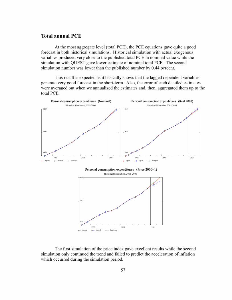
Total annual PCE
At the most aggregate level (total PCE), the PCE equations gave quite a good forecast in both historical simulations. Historical simulation with actual exogenous variables produced very close to the published total PCE in nominal value while the simulation with QUEST gave lower estimate of nominal total PCE. The second simulation number was lower than the published number by 0.44 percent.
This result is expected as it basically shows that the lagged dependent variables generate very good forecast in the short-term. Also, the error of each detailed estimates were averaged out when we annualized the estimates and, then, aggregated them up to the total PCE.
Personal consumption expenditures (Nominal) Personal consumption expenditures (Nominal) Historical Simulation, 2005-2006
9287
6882
4478
1995 2000 2005 napcea napceb beanapce
Personal consumption expenditures (Real 2000) Personal consumption expenditures (Real 2000) Historical Simulation, 2005-2006
8167
6634
5100
1995 2000 2005 apcea apceb beaapce
Personal consumption expenditures (Price,2000=1) Personal consumption expenditures (Price,2000=1) Historical Simulation, 2005-2006
1.15
1.01
0.88
1995 2000 2005 papcea papceb beapapce
The first simulation of the price index gave excellent results while the second simulation only continued the trend and failed to predict the acceleration of inflation which occurred during the simulation period.
57

The comparison of the Chained 2000 real PCE15 compounds the error from both nominal and price equations. Nevertheless, this result is reasonable considering the estimates of nominal values and prices. The first simulation gave a very good estimate of nominal PCE while giving a lower price level. Thus, the real PCE from the first simulation should be higher than the published data. In the same way, the lower estimates of nominal value and price index from the second simulation means that the real PCE estimate should yield a higher value than the published real PCE.
Durable goods
Both the first and the second simulations gave acceptable estimates of nominal PCE of durable goods. As expected. The first simulation provides a better estimate of nominal durable PCE than the second simulation.
BEA published nominal PCE of durable goods of 1,033.1 billion dollars and 1,071.3 billion of dollars in 2005 and 2006, respectively. The estimates from the first simulation are surprisingly close to the published numbers. The second simulation number was higher than the published data by 1.43 percent in 2005 and coming closer to the published number in 2006 with an error of 1.02 percent.
Durable goods (Nominal) Durable goods (Nominal) Historical Simulation, 2005-2006
1082
805
527
1995 2000 2005 nmda nmdb beanmd
Durable goods (Real 2000) Durable goods (Real 2000) Historical Simulation, 2005-2006
1237
863
488
1995 2000 2005 mda mdb beamd
15 All the real values estimated in this chapter are generated from the chained-weighted Fisher index and not from the direct identity [Nominal = price x Real]. As discussed in the previous chapter, since we did not estimate PCEs at the same details as the BEA did, these products (price indexes and real aggregates) from the chain-weighted Fisher index generally will not be equal to the BEA published numbers even when we have no error in all of our estimates.
58

Durable goods (Price,2000=1) Durable goods (Price,2000=1) Historical Simulation, 2005-2006
1.11
0.99
0.87
1995 2000 2005 pmda pmdb beapmd
The chained price of durable PCE estimates from both simulations were very close to each other with the first simulation providing slightly better performance. However, both simulations estimated that the price of durables would fall faster than it did. In August 2007, BEA revised these price index numbers downward in both 2005 and 2006. However, our estimates are still lower than the revised numbers.
It may seem like a big misses from the above graph. However, it should be noted that the actual values show a break in the trend.
As a result of the low estimates of the price index, both simulations gave estimates of chained 2000 real durable PCE higher than the published data. In 2006, the second simulation estimate missed the published real durable PCE by 2.75 percent. The high estimates in real value are the compound effect of over-estimated the nominal value and under-estimated price index.
Motor vehicles and parts
The published nominal PCEs of Motor vehicles and parts in 2005 and 2006 were 448.2 billion dollars and 445.3 billion dollars, respectively. The historical simulation with actual exogenous variables gave pretty good estimates, especially in 2005. The nominal PCE estimates of motor vehicles and parts from the first simulation were higher than the published number by 0.60 percent and 1.49 percent in 2005 and 2006, respectively. On the other hand, the estimates from the second simulation were higher than the published number by 4.82 percent in 2005 and 7.63 percent in 2006.
59

Motor vehicles and parts (Nominal) Motor vehicles and parts (Nominal) Historical Simulation, 2005-2006
479
357
234
1995 2000 2005 ndmva ndmvb beandmv
Motor vehicles and parts (Real 2000) Motor vehicles and parts (Real 2000) Historical Simulation, 2005-2006
483
371
259
1995 2000 2005 dmva dmvb beadmv
Motor vehicles and parts (Price,2000=1) Motor vehicles and parts (Price,2000=1) Historical Simulation, 2005-2006
1.01
0.95
0.90
1995 2000 2005 pdmva pdmvb beapdmv
The difference in performance of the two historical estimations holds for the estimates of chained 2000 real PCE of motor vehicles and parts. On the real side, the second simulation gave an estimate that higher than the published number by 7.80 percent in 2006 while the first simulation missed the published number by 1.51 percent in the same period. The cause of lower accuracy on the real estimates of the second simulation compare to its nominal estimate is evident from observing the estimates of the price index. Both simulations predicted lower price index than the published data with the second simulation provided, relatively, a less accurate one. These underestimations of the price index exacerbate the accuracy of the real numbers.
This result exhibits that the accuracy of the exogenous inputs in the equations is important. We see that, with the accurate exogenous macroeconomic variables, as in the first simulation, we achieve a better forecast than using the less accurate exogenous variables data. This means that, at least for this aggregate, the equation for the nominal estimation performs very well and its performance depends on the quality of its inputs.
60

Furniture and household equipment
In 2005 and 2006, BEA published nominal PCE of furniture and household equipment of 377.2 billion dollars and 404.9 billion dollars, respectively. The results show that our equations estimate the nominal consumption of furniture and equipment very well when given proper exogenous inputs, as in the first simulation. The first simulation provided estimates that were lower than the published nominal numbers by 0.13 percent and 0.28 percent in 2005 and 2006, respectively. While the second simulation gave a pretty comparable performance to the first simulation in 2005 (an error of -0.56 percent), its performance dropped sharply to an error of -3.01 percent in 2006.
Both simulations gave almost identical performance on the estimations of the price indexes. Both missed the published price index by around -3.2 percent with the first simulation having a small advantage (-3.13% vs. -3.54%).
Furniture and household equipment (Nominal) Furniture and household equipment (Nominal) Historical Simulation, 2005-2006
406
300
193
1995 2000 2005 ndfura ndfurb beandfur
Furniture and household equipment (Real 2000) Furniture and household equipment (Real 2000) Historical Simulation, 2005-2006
570
356
141
1995 2000 2005 dfura dfurb beadfur
Furniture and household equipment (Price,2000=1) Furniture and household equipment (Price,2000=1) Historical Simulation, 2005-2006
1.37
1.04
0.71
1995 2000 2005 pdfura pdfurb beapdfur
With the underestimated price indexes, the second simulation, exceptionally, gave a better forecast accuracy than the first simulation in estimating the chain 2000 real PCE of furniture and equipment. The second simulation estimates of the real value were
61

higher than the published numbers by 1.15 percent in 2005 and 0.5 percent in 2006. In the meantime, the first simulation overestimated the real values by 1.84 percent and 3.46 percent in 2005 and 2006, respectively.
The personal consumption of furniture and equipment has become more important in the recent years. In 2005 and 2006, furniture and equipment contributed around 67 percent and 85 percent, respectively, to the change in real PCE of durable goods16. One factor of this increasing contribution is the deceasing trend of the price of furniture and equipment. This declining price is mostly a product of the falling computer price as computers are a component of this category.
As this category has become more important, the good performance from our equations in forecasting both nominal and real values of these products is significant for the accuracy of a economic model.
Other durable goods
The equations’ performance from the historical simulation with actual exogenous inputs is very good in nominal value forecast of other durable PCE. In 2005, the first simulation overestimated the nominal PCE of other durable by 1.03 percent. In the same year, the second simulation underestimated the nominal PCE of other durable by 2.27 percent. In 2006, the first simulation underestimated by 1.49 percent and the second simulation by -4.89 percent. Again, the discrepancy of the performance between the two simulations is coming from the difference in the value of the exogenous inputs.
Other durable (Nominal) Other durable (Nominal) Historical Simulation, 2005-2006
224
162
99
1995 2000 2005 ndotha ndothb beandoth
Other durable (Real 2000) Other durable (Real 2000) Historical Simulation, 2005-2006
232
164
97
1995 2000 2005 dotha dothb beadoth
16 SOURCE: BEA, Survey of Current Business, March 2007: Table 2.3.2 page D-19.
62

Other durable (Price,2000=1) Other durable (Price,2000=1) Historical Simulation, 2005-2006
1.05
1.00
0.96
1995 2000 2005 pdotha pdothb beapdoth
The price index estimations, however, did not fare as well. Both estimations missed the published price index by around one and two percent in 2005 and 2006, respectively. The likely reason for these significant errors is the price is following the decreasing trend of the last decade (1995-2003). In fact, the price of durable PCE reversed its downward trend and showed a positive growth since 2004. As the price equations are heavily depended on the lagged dependent variables, the forecasts’ numbers are to be expected as they follow the past trend of the price level.
For the real value, the first simulation over-estimated by 1.68 percent and 3.27 percent in 2005 and 2006, respectively; and the second simulation under-estimated the real number by 1.69 percent in 2005 and 2.79 percent in 2006.
Nondurable goods
The first historical simulation overestimated nominal PCE of Nondurables by 0.17 percent and 0.61 percent in 2005 and 2006, respectively. The second simulation underestimated the nominal PCE by 1.19 percent and 1.76 percent in 2005 and 2006, respectively. This, again, shows the importance of the exogenous inputs’ quality, especially in the equations used in estimating the nominal consumption.
63

Nondurable goods (Nominal) Nondurable goods (Nominal) Historical Simulation, 2005-2006
2733
2056
1379
1995 2000 2005 nnda nndb beannd
Nondurable goods (Real 2000) Nondurable goods (Real 2000) Historical Simulation, 2005-2006
2391
1970
1550
1995 2000 2005 nda ndb beand
Nondurable goods (Price,2000=1) Nondurable goods (Price,2000=1) Historical Simulation, 2005-2006
1.15
1.02
0.89
1995 2000 2005 pnda pndb beapnd
Both simulations underestimated the price index with better estimates from the first simulation. Both alternatives missed the published price index by around 1 percent in 2005 and 2 percent in 2006.
The Historical simulation with actual exogenous inputs over-estimated the real 2000 consumption by 0.42 percent and 1.19 percent in 2005 and 2006 respectively. The second simulation underestimated the real 2000 PCE by 0.04 percent in 2005 and overestimated it by 0.32 percent in 2006.
64

Food
For the PCE of food, the equations gave good forecasts when the exogenous variables were entered into the model with the actual values. We can observe from the graphs shown below that the movements of all three graphs have the same patterns as we saw in the graphs from the PCE of nondurable goods. This similarity is expected as food PCE accounts for most of nondurable PCE in both nominal value and real value. In 2005 and 2006, BEA estimated the food-consumption contribution to percent change in real PCE of Nondurables at around 60 percent.
Food (Nominal) Food (Nominal) Historical Simulation, 2005-2006
1293
992
692
1995 2000 2005 nnfooda nnfoodb beannfood
Food (Real 2000) Food (Real 2000) Historical Simulation, 2005-2006
1123
963
802
1995 2000 2005 nfooda nfoodb beanfood
Food (Price,2000=1) Food (Price,2000=1) Historical Simulation, 2005-2006
1.15
1.01
0.86
1995 2000 2005 pnfooda pnfoodb beapnfood
In nominal value, the first simulation produced very good forecast of the food PCE with errors of 0.19 percent in 2005 and 0.87 percent in 2006. On the other hand, the second simulation did not fare as well as the first simulation. The second simulation numbers were lower than the published numbers by 1.48 percent and 3.24 percent in 2005 and 2006, respectively.
65
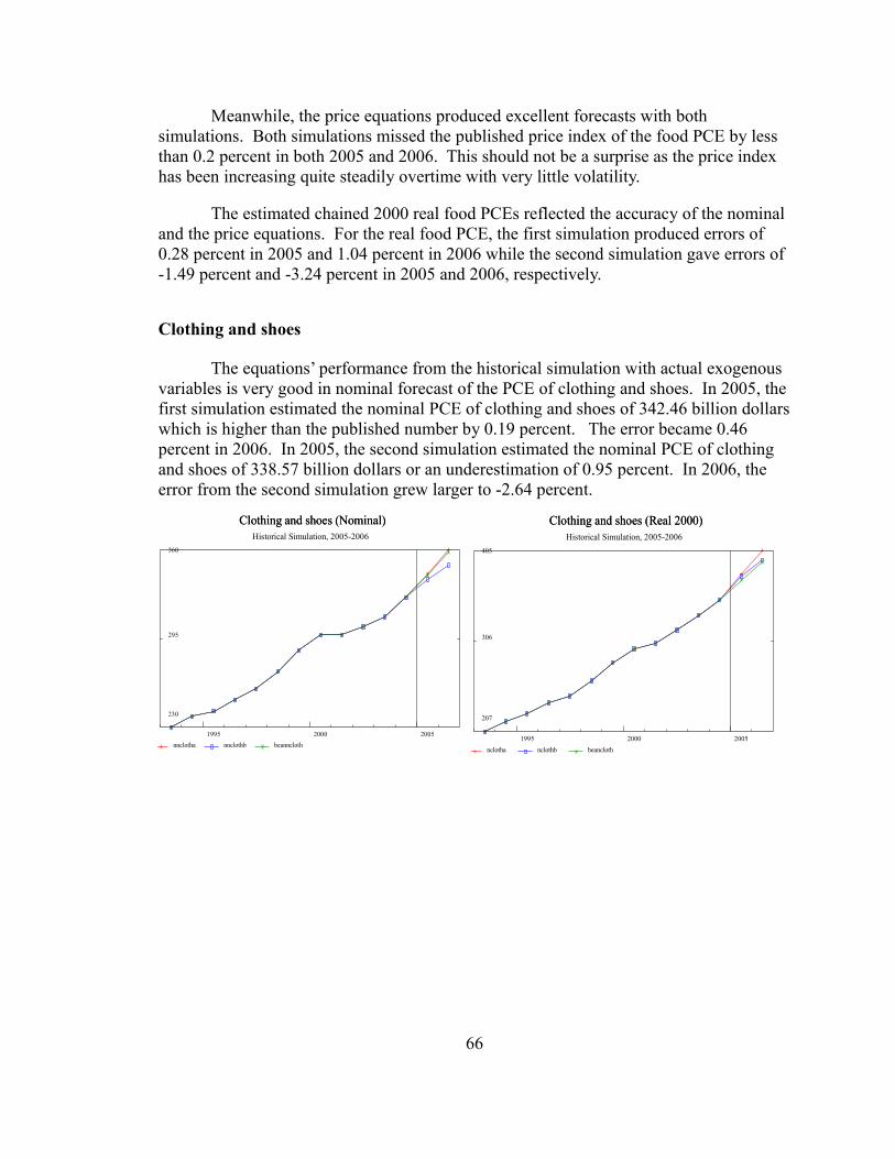
Meanwhile, the price equations produced excellent forecasts with both simulations. Both simulations missed the published price index of the food PCE by less than 0.2 percent in both 2005 and 2006. This should not be a surprise as the price index has been increasing quite steadily overtime with very little volatility.
The estimated chained 2000 real food PCEs reflected the accuracy of the nominal and the price equations. For the real food PCE, the first simulation produced errors of 0.28 percent in 2005 and 1.04 percent in 2006 while the second simulation gave errors of -1.49 percent and -3.24 percent in 2005 and 2006, respectively.
Clothing and shoes
The equations’ performance from the historical simulation with actual exogenous variables is very good in nominal forecast of the PCE of clothing and shoes. In 2005, the first simulation estimated the nominal PCE of clothing and shoes of 342.46 billion dollars which is higher than the published number by 0.19 percent. The error became 0.46 percent in 2006. In 2005, the second simulation estimated the nominal PCE of clothing and shoes of 338.57 billion dollars or an underestimation of 0.95 percent. In 2006, the error from the second simulation grew larger to -2.64 percent.
Clothing and shoes (Nominal) Clothing and shoes (Nominal) Historical Simulation, 2005-2006
360
295
230
1995 2000 2005 nnclotha nnclothb beanncloth
Clothing and shoes (Real 2000) Clothing and shoes (Real 2000) Historical Simulation, 2005-2006
405
306
207
1995 2000 2005 nclotha nclothb beancloth
66

Clothing and shoes (Price,2000=1) Clothing and shoes (Price,2000=1) Historical Simulation, 2005-2006
1.11
1.00
0.88
1995 2000 2005 pnclotha pnclothb beapncloth
On the real side, both historical simulations overestimated the chained 2000 real PCE of clothing and shoes. The first simulation gave estimates that higher than the published real PCE of clothing and shoes by 1.68 percent in 2005 and 3.15 percent in 2006. The second simulation produced numbers that higher than the published values by 1.07 percent and 0.53 percent in 2005 and 2006, respectively. In the graph above, we observe that the second simulation performed better than the first simulation in 2006.
The relatively better performance of the second simulation came from the relative performance between the two simulations in forecasting the price index of the PCE of clothing and shoes in 2005 and 2006. For price index, the second simulation gave additional error of around 0.5 percent more than the first simulation. The first simulation missed the published price index by -1.47 percent in 2005 and -2.61 percent in 2006. The second simulation missed the published price index by -1.99 percent and -3.15 percent in 2005 and 2006, respectively.
Gasoline, fuel oil, and other energy goods
Since 2003, price of gasoline and energy has been rising steadily. This recent trend affects performance of our equation significantly, especially in the price equations, which affect the real value.
67

Gasoline, fuel oil, and other energy goods (Nominal) Gasoline, fuel oil, and other energy goods (Nominal) Historical Simulation, 2005-2006
352
239
127
1995 2000 2005 nngasa nngasb beanngas
Gasoline, fuel oil, and other energy goods (Real 2000) Gasoline, fuel oil, and other energy goods (Real 2000) Historical Simulation, 2005-2006
233.3
200.1
166.9
1995 2000 2005 ngasa ngasb beangas
Gasoline, fuel oil, and other energy goods (Price,2000=1) Gasoline, fuel oil, and other energy goods (Price,2000=1) Historical Simulation, 2005-2006
1.71
1.22
0.72
1995 2000 2005 pngasa pngasb beapngas
The nominal forecasts show decent performance considering the shift in the price movement. Both simulations predicted that the nominal PCE of gasoline, fuel oil, and other energy goods to keep rising, however, at a rate slightly slower than the published data. The first simulation missed the published nominal values by -0.32 percent in 2005 and -0.36 percent in 2006. The second simulation also underestimated the nominal consumption by 2.89 percent and 4.05 percent in 2005 and 2006, respectively.
The second simulation estimated the increasing in price index of the gasoline, fuel oil, and other energy goods but not as fast as the actual growth rate. In fact, the second simulation missed it by a pretty wide margin. In 2005, the first simulation estimated the price index of 151.5 while the second simulation estimated the same price index of 140.4. The second simulation underestimated the price index by 7.31 percent in 2005. This means that, by themselves, the price equations are very accurate when we have better input information.
68

The poor performance of the second simulation in predicting the price index affected the forecasting performance of the chained 2000 real value, especially the 2006 forecast. In 2005, the errors were -0.38 percent with the first simulation and 4.76 percent with the second simulation. However, in 2006, the errors are -0.11 percent and 17.91 percent with the first simulation and the second simulation, respectively.
Other nondurable goods
Other nondurable (Nominal) Other nondurable (Nominal) Historical Simulation, 2005-2006
742
537
331
1995 2000 2005 nnotha nnothb beannoth
Other nondurable (Real 2000) Other nondurable (Real 2000) Historical Simulation, 2005-2006
678
528
379
1995 2000 2005 notha nothb beanoth
Other nondurable (Price,2000=1) Other nondurable (Price,2000=1) Historical Simulation, 2005-2006
1.10
0.99
0.87
1995 2000 2005 pnotha pnothb beapnoth
Both simulations performed very well in forecasting the PCE of other nondurable goods in all three components; i.e. nominal value, real value, and price index. The published nominal PCE of other nondurable goods were 693.96 billion dollars in 2005 and 737.09 billion dollars in 2006. Both simulations provide estimates that have around one percent errors in both 2005 and 2006.
The first simulation overestimated the real PCE of other nondurables by 0.35 percent in 2005 and 1.0 percent in 2006 while the second simulation missed the published real numbers by less than 0.00 percent and -0.67 percent in 2005 and 2006, respectively.
69

The published price indexes of the PCE of other nondurable goods were 107.77 in 2005 and 109.78 in 2006 [2000=100]. Both simulations underestimated the price index by less than 0.8 percent in both 2005 and 2006. The first simulation perform slightly better than the second simulation in forecasting the price index, i.e. the first simulation missed the published number by 0.32 percent, in 2006, compared to 0.79 percent by the second simulation.
Services
Overall, our equations perform very well in forecasting the PCE of services. This excellent performance was due to the good performance in forecasting the three main contributors to the PCE of services: Housing, Medical services, and Other services. This result helped the performance of the equations in producing a good estimate of the total PCE, as discussed earlier, because PCE of services has become the main component of the U.S. PCE. BEA reported that PCE of services contributed to around 50 percent of the real growth rate of the total PCE in 2005 and 2006.
Services (Nominal) Services (Nominal) Historical Simulation, 2005-2006
5484
4028
2572
1995 2000 2005 nsva nsvb beansv
Services (Real 2000) Services (Real 2000) Historical Simulation, 2005-2006
4588
3837
3086
1995 2000 2005 sva svb beasv
Services (Price,2000=1) Services (Price,2000=1) Historical Simulation, 2005-2006
1.21
1.02
0.83
1995 2000 2005 psva psvb beapsv
70

The historical simulation with actual exogenous inputs underestimated the nominal PCE of services by only 0.03 percent in 2005 and 0.22 percent in 2006. The historical simulation with QUEST misses the nominal PCE of services by -0.45 percent and -1.17 percent in 2005 and 2006, respectively.
For the price index, both simulations underestimated the chained 2000 price index of the PCE of services by less than one percent in 2005. The first simulation missed the published figures by -0.17 percent in 2005 and 0.25 percent in 2006. The second simulation provided estimates with errors of -0.95 percent in 2005 and -1.99 percent in 2006.
Housing
PCE of housing is a special aggregate. In this study, this aggregate does not have any sub-category by the definition of PCE, See Appendix 3.2. This means that the nominal value and the price index of this category are estimated by only two equations; one for the nominal value and one for the price index.
As shown below, the equations provided excellent estimates for nominal value of the PCE of housing in both simulations. As stated earlier, this excellent forecast resulted in the better performance at the more aggregate level as PCE of housing contribution to the real growth of the PCE of services were around 25 percent in 2005 and 2006. In fact, it was the second biggest contributor in 2005 and the third biggest contributor in 2006.
Housing (Nominal) Housing (Nominal) Historical Simulation, 2005-2006
1382
1033
684
1995 2000 2005 nshoa nshob beansho
Housing (Real 2000) Housing (Real 2000) Historical Simulation, 2005-2006
1149
995
842
1995 2000 2005 shoa shob beasho
71

Housing (Price,2000=1) Housing (Price,2000=1) Historical Simulation, 2005-2006
1.22
1.02
0.81
1995 2000 2005 pshoa pshob beapsho
The first simulation missed the nominal PCE of housing by 0.08 percent and -0.5 percent in 2005 and 2006, respectively. It underestimated the chained 2000 real PCE of housing by 0.98 percent in 2005 and 2.26 percent in 2006. On the chained 2000 price index, the first simulation missed the published numbers by 1.08 percent and -1.8 percent in 2005 and 2006, respectively.
The second simulation missed the nominal PCE of housing by 0.08 percent and -0.50 percent in 2005 and 2006, respectively. The real 2000 estimates of the second simulation also underestimated the published chained 2000 real PCE of housing by 0.56 percent in 2005 and 0.71 percent in 2006. The second simulation also gave small errors of 0.64 percent in 2005 and 0.21percent in 2006 when estimating the chained 2000 price index of PCE of housing.
Household Operation
Household operation (Nominal) Household operation (Nominal) Historical Simulation, 2005-2006
506
388
270
1995 2000 2005 nshoopa nshoopb beanshoop
Household operation (Real 2000) Household operation (Real 2000) Historical Simulation, 2005-2006
418
355
291
1995 2000 2005 shoopa shoopb beashoop
72

Household operation (Price,2000=1) Household operation (Price,2000=1) Historical Simulation, 2005-2006
1.22
1.07
0.93
1995 2000 2005 pshoopa pshoopb beapshoop
The first simulation underestimated the nominal PCE of household operation by 2.39 percent in 2005 and 5.19 percent in 2006. The second simulation also underestimated the nominal PCE by 5.22 percent and 9.03 percent in 2005 and 2006, respectively.
The first simulation underestimated the chained 2000 price index of PCE of household operation by 0.67 percent in 2005 and 0.94 percent in 2006. The estimates of the price index form the second simulation were lower than the published data by 3.12 percent and 7.41 percent in 2005 and 2006, respectively.
Things look better on the real side, at least with the historical simulation with actual exogenous variables. The first simulation gave the real 2000 PCE of household operation with error of -1.66 percent and -4.21 percent in 2005 and 2006, respectively. On the other hand, the second simulation underestimated the real 2000 PCE of household operation by 2.1 percent in 2005 and 1.67 percent in 2006.
PCE of household operation is the only component of services PCE that our equations did not provide relatively good results, though the actual numbers were not as bad as the above graphs suggested. I believe that the increasing energy price contributes greatly to this result. PCE of electricity and gas contributed around 40 percent of nominal PCE of household operation in 2005 and 2006. The PCE of electricity and gas also contributed more than 50 percent to the real growth rate of PCE of household operation. The rapidly increasing energy price since 2003 means that, by 2005, the utility companies started transfer the increasing cost to the consumer as the price of PCE of electricity and gas increasing sharply in 2005 and 2006. As seen in the previous aggregates, our equations seem to have trouble in providing a good estimate when there is a sudden shift in energy cost and energy price affected the consumption behavior on that category.
However, as the PCE of household operation contributes less than ten percent to the real growth rate of PCE of services. This result had little effect to the performance of our equations in estimating the PCE of services.
73
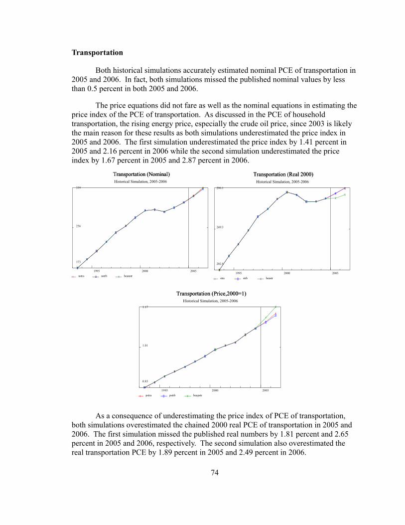
Transportation
Both historical simulations accurately estimated nominal PCE of transportation in 2005 and 2006. In fact, both simulations missed the published nominal values by less than 0.5 percent in both 2005 and 2006.
The price equations did not fare as well as the nominal equations in estimating the price index of the PCE of transportation. As discussed in the PCE of household transportation, the rising energy price, especially the crude oil price, since 2003 is likely the main reason for these results as both simulations underestimated the price index in 2005 and 2006. The first simulation underestimated the price index by 1.41 percent in 2005 and 2.16 percent in 2006 while the second simulation underestimated the price index by 1.67 percent in 2005 and 2.87 percent in 2006.
Transportation (Nominal) Transportation (Nominal) Historical Simulation, 2005-2006
339
256
173
1995 2000 2005 nstra nstrb beanstr
Transportation (Real 2000) Transportation (Real 2000) Historical Simulation, 2005-2006
296.1
249.3
202.5
1995 2000 2005 stra strb beastr
Transportation (Price,2000=1) Transportation (Price,2000=1) Historical Simulation, 2005-2006
1.17
1.01
0.85
1995 2000 2005 pstra pstrb beapstr
As a consequence of underestimating the price index of PCE of transportation, both simulations overestimated the chained 2000 real PCE of transportation in 2005 and 2006. The first simulation missed the published real numbers by 1.81 percent and 2.65 percent in 2005 and 2006, respectively. The second simulation also overestimated the real transportation PCE by 1.89 percent in 2005 and 2.49 percent in 2006.
74

Medical Care
Medical care (Nominal) Medical care (Nominal) Historical Simulation, 2005-2006
1612
1164
715
1995 2000 2005 nsmca nsmcb beansmc
Medical care (Real 2000) Medical care (Real 2000) Historical Simulation, 2005-2006
1333
1105
877
1995 2000 2005 smca smcb beasmc
Medical care (Price,2000=1) Medical care (Price,2000=1) Historical Simulation, 2005-2006
1.22
1.02
0.82
1995 2000 2005 psmca psmcb beapsmc
In the last 3 decades, medical care has been one of the main contributors to the growth of the services PCE. The good performance of both simulations, shown in the above graphs, helps in providing the good estimates of the PCE of services.
The historical simulation with actual exogenous variables overestimated the nominal medical care PCE by 0.31 percent and 1.44 percent in 2005 and 2006, respectively. The second simulation estimated the nominal PCE of medical care with the error of 0.12 percent in 2005 and 0.78 percent in 2006.
Both simulations provided excellent estimates of the price index of medical care PCE. The first simulation missed the published numbers by -0.55 percent and 0.05 percent in 2005 and 2006, respectively. The second simulation also missed the published medical care PCE by -1.14 percent in 2005 and -1.37 percent in 2006.
The first simulation overestimated the published numbers by 0.87 percent in 2005 and 1.39 percent in 2006. The second simulation also overestimated the published numbers by 1.28 percent in 2005 and 2.18 percent in 2006.
75

Recreation
Both simulations performed relatively well in forecasting the PCE of recreation in all three components; i.e. nominal value, real value, and price index. Both simulations provide estimates that have around one percent or less error in both 2005 and 2006, except the 2006 second simulation that gave an error of -2.37 percent.
Recreation (Nominal) Recreation (Nominal) Historical Simulation, 2005-2006
382
271
160
1995 2000 2005 nsreca nsrecb beansrec
Recreation (Real 2000) Recreation (Real 2000) Historical Simulation, 2005-2006
320
258
195
1995 2000 2005 sreca srecb beasrec
Recreation (Price,2000=1) Recreation (Price,2000=1) Historical Simulation, 2005-2006
1.19
1.01
0.82
1995 2000 2005 psreca psrecb beapsrec
The first simulation underestimated the real PCE of recreation by 0.02 percent in 2005 and overestimated it by 0.07 percent in 2006 while the second simulation missed the published real numbers by -0.98 percent and -1.97 percent in 2005 and 2006, respectively.
The published price indexes of the PCE of recreation were 115.17 in 2005 and 118.64 in 2006 [2000=100]. Both simulations underestimated the price index by less than one percent in both 2005 and 2006. The second simulation performed slightly better than the first simulation in forecasting the price index, i.e. the first simulation missed the published number by 0.67 percent, in 2006, compared to -0.41 percent by the second simulation.
76

Other services
As shown below, the equations provided excellent estimates for nominal value of the PCE of housing in both simulations. As stated earlier, this excellent forecast resulted in the better performance at the more aggregate level as PCE of other services contribution to the real growth of the PCE of services were around 20 percent in 2005 and 30 percent in 2006. In fact, it was the third biggest contributor to the real growth of services PCE in 2005 and the second biggest contributor in 2006.
Other Services (Nominal) Other Services (Nominal) Historical Simulation, 2005-2006
1290
930
570
1995 2000 2005 nsotha nsothb beansoth
Other Services (Real 2000) Other Services (Real 2000) Historical Simulation, 2005-2006
1094
887
681
1995 2000 2005 sotha sothb beasoth
Other Services (Price,2000=1) Other Services (Price,2000=1) Historical Simulation, 2005-2006
1.21
1.02
0.84
1995 2000 2005 psotha psothb beapsoth
The first simulation missed the nominal PCE of other services by 0.16 percent and –0.45 percent in 2005 and 2006, respectively. It missed the chained 2000 real PCE of other services by 0.85 percent in 2005 and -0.29 percent in 2006. On the chained 2000 price index, the first simulation missed the published numbers by -0.68 percent and -0.17 percent in 2005 and 2006, respectively.
The second simulation missed the nominal PCE of other services by 0.17 percent and –1.03 percent in 2005 and 2006, respectively. The real 2000 estimates of the second simulation also missed the published chained 2000 real PCE of services by 1.88 percent
77

in 2005 and 2.21 percent in 2006. The second simulation also gave small errors of -1.67 percent in 2005 and -3.17 percent in 2006 when estimating the chained 2000 price index of PCE of other services.
3.6 Short-term forecast of Personal consumption expenditures
In this section, the short-term forecasts of the U.S. Detailed Personal consumption expenditures are estimated using the equations estimated with the approach described earlier in this chapter.
All equations, both nominal PCE and the price indexes, are fitted with data between January 1994 and June 2007. We forecast the detailed PCE from July 2007 to December 2008. The estimation is done at the monthly frequency. Then, the monthly estimated series are annualized and are presented in this discussion. The 116 annualized detailed forecasts, nominal, real and price index, are shown in Appendix 3.4 and Appendix 3.5. The discussion will cover generally at the more aggregate level of PCE which should give a better view of the general consumption.
The values and the plots of the estimated major PCE aggregates are shown in Table 3.8 and Figure 3.2 .
3.6.1 Forecast assumptions
All exogenous variables used in the forecast are generated by QUEST except crude oil price and the Dow Jones Industrial Index. Both the crude oil price and the Dow Jones Industrial Index reflect the author's expectation of these two indicators. The problem in the sub-prime credit market has been included as an exogenous input (through the interest rate) in the QUEST model. All exogenous variable assumptions are shown in Table 3.7.
78

3.6.2 Outlook with plots and aggregates (annual series)
In 2007, the U.S. Economy has experienced rising energy costs which could impact personal consumption expenditures. Total PCE has been increasing with a real growth rate of more than three percent since 2004. This real growth rate is expected to fall to 2.45 percent and 1.65 percent in 2007 and 2008, respectively. Table 3.9 shows the growth rate of the major PCE aggregates. This slower growth in real PCE compared to the nominal PCE is easily seen from the growth rate of the price index. Since 2004, the price index of total PCE is growing at an average rate of 2.5% to 3.0% while it had been growing at around two percent before 2004. In 2007 and 2008, the forecasted price indexes are 1.18 and 1.22, respectively. This means that the price index grows by 3.01% and 3.32% in 2007 and 2008, respectively. We can see that the increasing energy price affects the real consumption as its cut into the disposable income that consumers have left for other purchases (besides Gas and Utilities).
79
Table 3.7: Exogenous variables' assumption between July 2007 and December 2008
Jul Aug Sep Oct Nov Deccdmv 436.19 438.34 440.59 443.43 445.49 447.28cdfur 411.57 410.30 409.54 409.91 409.73 409.61cdoth 221.66 222.45 223.15 223.79 224.34 224.82cnfood 1336.11 1342.21 1347.94 1353.41 1358.32 1362.77cncloth 370.13 370.90 371.57 372.02 372.56 373.09cngas 362.99 358.68 355.11 352.17 350.18 349.03cnoth 766.57 770.97 775.20 779.31 783.14 786.76cshous 1468.72 1476.28 1484.12 1493.17 1500.86 1508.12csho 528.42 531.27 533.95 536.47 538.80 540.94cstr 358.67 360.49 362.30 364.28 365.93 367.44csmc 1697.00 1709.08 1720.95 1733.15 1744.16 1754.54csrec 401.90 403.88 406.06 408.69 411.04 413.38csoth 1388.97 1398.18 1406.89 1415.37 1422.90 1429.75gdp 13865.55 13914.79 13965.36 14018.73 14070.79 14123.08djia 13362.38 13464.63 13592.24 13837.98 13946.58 14010.87ddj -46.24 102.26 127.61 245.74 108.60 64.29crude 65.87 70.19 76.02 89.07 93.63 95.41oildf 0.80 4.32 5.83 13.05 4.56 1.78gdpi 1.45 1.45 1.46 1.46 1.47 1.47
Jan Feb Mar Apr May Jun Jul Aug Sep Oct Nov Deccdmv 448.90 450.03 450.78 449.99 450.88 452.26 454.61 456.66 458.88 461.26 463.80 466.50cdfur 409.70 409.59 409.42 409.10 408.90 408.73 408.59 408.48 408.40 408.36 408.35 408.37cdoth 225.17 225.52 225.83 225.74 226.22 226.92 228.12 229.05 229.98 230.92 231.86 232.80cnfood 1366.59 1370.25 1373.58 1375.13 1378.87 1383.36 1389.42 1394.78 1400.27 1405.89 1411.64 1417.52cncloth 373.73 374.13 374.40 374.10 374.48 375.07 376.13 376.99 377.90 378.84 379.84 380.87cngas 345.13 348.33 355.07 376.94 382.02 381.93 370.90 364.78 357.81 349.99 341.32 331.80cnoth 790.06 793.31 796.43 798.60 802.03 805.93 810.78 815.23 819.79 824.44 829.20 834.04cshous 1515.09 1521.38 1527.15 1530.53 1536.62 1543.55 1552.12 1560.18 1568.51 1577.13 1586.01 1595.17csho 542.83 544.67 546.38 547.40 549.28 551.47 554.29 556.83 559.43 562.08 564.79 567.55cstr 368.79 370.02 371.12 371.62 372.79 374.16 375.96 377.60 379.28 381.02 382.80 384.63csmc 1764.23 1773.39 1781.95 1787.87 1796.79 1806.66 1818.33 1829.45 1840.89 1852.63 1864.69 1877.05csrec 415.85 418.06 420.16 421.69 423.90 426.33 429.19 431.93 434.75 437.64 440.60 443.64csoth 1435.31 1441.22 1446.89 1450.81 1457.12 1464.30 1473.46 1481.58 1489.75 1497.98 1506.27 1514.61gdp 14175.56 14228.21 14281.08 14332.56 14386.98 14442.81 14502.08 14559.09 14615.96 14672.63 14729.14 14785.46djia 13980.67 13994.00 14000.66 13991.78 13991.77 13991.78 13991.78 13991.77 13991.78 13991.78 13991.78 13991.77ddj -30.20 13.32 6.66 -8.88 -0.02 0.02 0.00 -0.02 0.02 -0.01 0.00 -0.01crude 90.49 89.66 89.00 89.02 88.30 87.35 84.86 84.47 84.86 86.02 87.96 90.68oildf -4.92 -0.83 -0.66 0.02 -0.72 -0.94 -2.49 -0.39 0.39 1.16 1.94 2.71gdpi 1.48 1.49 1.49 1.50 1.50 1.51 1.51 1.52 1.53 1.53 1.54 1.54
2007
2008

The forecast shows a decrease in spending in real nondurable goods consumption in 2008. Analysing the component of nondurables goods shows that this decrease in nondurable goods real consumption is largely a result of the rapid decline in real consumption of Gasoline, fuel oil, and other energy goods.
80
Table 3.8: Major aggregates of annual PCE Forecast 2007 and 2008
1995 2000 2005 2006 2007 2008Forecast 2007 and 2008 Nominal apce Personal consumption expenditures 4975.788 6739.376 8707.818 9224.508 9724.809 10223.716 md Durable goods 611.600 863.325 1023.879 1048.921 1077.681 1104.922 dmv Motor vehicles and parts 266.690 386.518 444.932 434.203 444.884 465.527 dfur Furniture and household equipment 228.626 312.907 378.225 404.125 412.966 412.282 doth Other durable 116.285 163.901 200.722 210.593 219.831 227.113 nd Nondurable goods 1485.065 1947.216 2516.179 2688.034 2826.917 2951.951 nfood Food 740.851 925.164 1183.824 1259.279 1336.284 1398.740 ncloth Clothing and shoes 241.722 297.712 341.747 357.232 370.966 377.217 ngas Gasoline, fuel oil, and other energy goods 133.287 191.482 301.832 340.135 351.300 358.961 noth Other nondurable 369.205 532.858 688.776 731.388 768.367 817.034 sv Services 2879.123 3928.836 5167.760 5487.552 5820.209 6166.842 sho Housing 764.386 1006.456 1298.688 1381.341 1465.163 1547.478 shoop Household operation 298.746 390.110 481.019 501.616 523.591 538.327 str Transportation 207.673 291.253 324.242 340.598 356.855 372.245 smc Medical care 797.852 1026.813 1492.622 1587.734 1691.609 1809.859 srec Recreation 187.921 268.265 358.811 380.985 402.980 429.763 soth Other Services 622.546 945.940 1212.379 1295.279 1380.012 1469.170
Forecast 2007 and 2008 Price, [2000=1] apce Personal consumption expenditures 0.92 1.00 1.12 1.15 1.18 1.22 md Durable goods 1.11 1.00 0.90 0.89 0.87 0.85 dmv Motor vehicles and parts 0.98 1.00 0.99 0.99 0.99 0.99 dfur Furniture and household equipment 1.32 1.00 0.77 0.73 0.70 0.66 doth Other durable 1.05 1.00 0.98 0.98 1.00 1.00 nd Nondurable goods 0.91 1.00 1.12 1.15 1.20 1.25 nfood Food 0.90 1.00 1.13 1.15 1.19 1.23 ncloth Clothing and shoes 1.06 1.00 0.92 0.91 0.90 0.91 ngas Gasoline, fuel oil, and other energy goods 0.77 1.00 1.51 1.71 2.07 2.57 noth Other nondurable 0.89 1.00 1.08 1.10 1.11 1.12 sv Services 0.88 1.00 1.17 1.21 1.25 1.30 sho Housing 0.86 1.00 1.16 1.20 1.25 1.29 shoop Household operation 0.96 1.00 1.16 1.22 1.26 1.33 str Transportation 0.90 1.00 1.13 1.17 1.19 1.23 smc Medical care 0.88 1.00 1.19 1.22 1.27 1.31 srec Recreation 0.86 1.00 1.15 1.19 1.21 1.25 soth Other Services 0.88 1.00 1.17 1.21 1.25 1.31
Forecast 2007 and 2008 Real 2000 apce Personal consumption expenditures 5432.392 6739.265 7803.607 8043.521 8240.232 8376.342 md Durable goods 551.933 863.331 1137.756 1180.891 1235.720 1295.207 dmv Motor vehicles and parts 272.249 386.520 451.253 437.305 451.409 469.216 dfur Furniture and household equipment 172.787 312.915 492.589 551.358 589.716 629.163 doth Other durable 111.182 163.897 205.522 213.903 220.779 227.734 nd Nondurable goods 1638.130 1947.129 2255.337 2336.950 2365.485 2358.433 nfood Food 827.063 925.154 1049.892 1091.715 1119.176 1139.516 ncloth Clothing and shoes 227.387 297.727 372.630 391.111 410.166 416.218 ngas Gasoline, fuel oil, and other energy goods 172.956 191.465 199.400 198.552 174.543 139.757 noth Other nondurable 413.699 532.784 638.806 665.647 692.157 729.557 sv Services 3260.278 3928.805 4427.085 4545.299 4665.241 4760.254 sho Housing 887.505 1006.385 1118.238 1148.264 1174.386 1202.516 shoop Household operation 312.829 390.134 416.449 412.862 416.740 404.911 str Transportation 231.763 291.260 287.804 291.197 299.083 302.942 smc Medical care 906.384 1026.744 1258.130 1300.267 1337.132 1380.720 srec Recreation 219.152 268.238 311.551 321.267 333.644 344.179 soth Other Services 704.919 946.043 1033.674 1069.875 1102.748 1123.635

The real consumption of Gasoline, fuel oil, and other energy goods has a growth rate of -12.09% in 2007 and -19.93%in 2008. Typically, the growth rate of the nominal PCE of Gasoline, fuel oil, and other energy goods is very close to the growth rate of its price index. The reason is that this product categories is largely a necessary goods. The price elasticity of this category is very inelastic. The forecast of nominal PCE of Gasoline, fuel oil, and other energy goods also has a positive growth rate (2.18% in 2008) that is much slower than the growth rate of its price index (24.35% in 2008). This discrepancy between the growth rate of nominal PCE and its price index is out of line according to the recent trend. This finding may show a flaw in a set of equations that estimate the nominal PCE of products in this category. These equations do not take the rising price into account and they should be adjusted in the next update of the model.
81
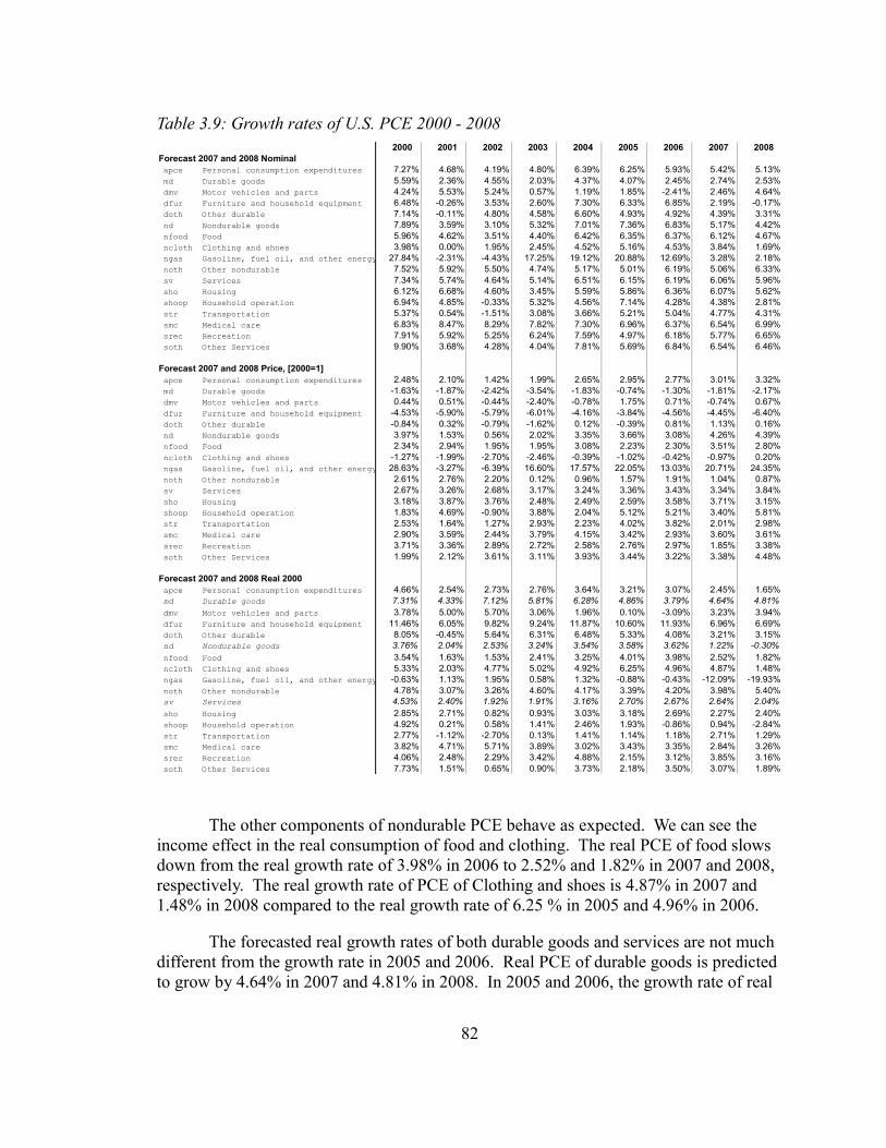
The other components of nondurable PCE behave as expected. We can see the income effect in the real consumption of food and clothing. The real PCE of food slows down from the real growth rate of 3.98% in 2006 to 2.52% and 1.82% in 2007 and 2008, respectively. The real growth rate of PCE of Clothing and shoes is 4.87% in 2007 and 1.48% in 2008 compared to the real growth rate of 6.25 % in 2005 and 4.96% in 2006.
The forecasted real growth rates of both durable goods and services are not much different from the growth rate in 2005 and 2006. Real PCE of durable goods is predicted to grow by 4.64% in 2007 and 4.81% in 2008. In 2005 and 2006, the growth rate of real
82
Table 3.9: Growth rates of U.S. PCE 2000 - 2008 2000 2001 2002 2003 2004 2005 2006 2007 2008
Forecast 2007 and 2008 Nominal apce Personal consumption expenditures 7.27% 4.68% 4.19% 4.80% 6.39% 6.25% 5.93% 5.42% 5.13% md Durable goods 5.59% 2.36% 4.55% 2.03% 4.37% 4.07% 2.45% 2.74% 2.53% dmv Motor vehicles and parts 4.24% 5.53% 5.24% 0.57% 1.19% 1.85% -2.41% 2.46% 4.64% dfur Furniture and household equipment 6.48% -0.26% 3.53% 2.60% 7.30% 6.33% 6.85% 2.19% -0.17% doth Other durable 7.14% -0.11% 4.80% 4.58% 6.60% 4.93% 4.92% 4.39% 3.31% nd Nondurable goods 7.89% 3.59% 3.10% 5.32% 7.01% 7.36% 6.83% 5.17% 4.42% nfood Food 5.96% 4.62% 3.51% 4.40% 6.42% 6.35% 6.37% 6.12% 4.67% ncloth Clothing and shoes 3.98% 0.00% 1.95% 2.45% 4.52% 5.16% 4.53% 3.84% 1.69% ngas Gasoline, fuel oil, and other energy goods 27.84% -2.31% -4.43% 17.25% 19.12% 20.88% 12.69% 3.28% 2.18% noth Other nondurable 7.52% 5.92% 5.50% 4.74% 5.17% 5.01% 6.19% 5.06% 6.33% sv Services 7.34% 5.74% 4.64% 5.14% 6.51% 6.15% 6.19% 6.06% 5.96% sho Housing 6.12% 6.68% 4.60% 3.45% 5.59% 5.86% 6.36% 6.07% 5.62% shoop Household operation 6.94% 4.85% -0.33% 5.32% 4.56% 7.14% 4.28% 4.38% 2.81% str Transportation 5.37% 0.54% -1.51% 3.08% 3.66% 5.21% 5.04% 4.77% 4.31% smc Medical care 6.83% 8.47% 8.29% 7.82% 7.30% 6.96% 6.37% 6.54% 6.99% srec Recreation 7.91% 5.92% 5.25% 6.24% 7.59% 4.97% 6.18% 5.77% 6.65% soth Other Services 9.90% 3.68% 4.28% 4.04% 7.81% 5.69% 6.84% 6.54% 6.46%
Forecast 2007 and 2008 Price, [2000=1] apce Personal consumption expenditures 2.48% 2.10% 1.42% 1.99% 2.65% 2.95% 2.77% 3.01% 3.32% md Durable goods -1.63% -1.87% -2.42% -3.54% -1.83% -0.74% -1.30% -1.81% -2.17% dmv Motor vehicles and parts 0.44% 0.51% -0.44% -2.40% -0.78% 1.75% 0.71% -0.74% 0.67% dfur Furniture and household equipment -4.53% -5.90% -5.79% -6.01% -4.16% -3.84% -4.56% -4.45% -6.40% doth Other durable -0.84% 0.32% -0.79% -1.62% 0.12% -0.39% 0.81% 1.13% 0.16% nd Nondurable goods 3.97% 1.53% 0.56% 2.02% 3.35% 3.66% 3.08% 4.26% 4.39% nfood Food 2.34% 2.94% 1.95% 1.95% 3.08% 2.23% 2.30% 3.51% 2.80% ncloth Clothing and shoes -1.27% -1.99% -2.70% -2.46% -0.39% -1.02% -0.42% -0.97% 0.20% ngas Gasoline, fuel oil, and other energy goods 28.63% -3.27% -6.39% 16.60% 17.57% 22.05% 13.03% 20.71% 24.35% noth Other nondurable 2.61% 2.76% 2.20% 0.12% 0.96% 1.57% 1.91% 1.04% 0.87% sv Services 2.67% 3.26% 2.68% 3.17% 3.24% 3.36% 3.43% 3.34% 3.84% sho Housing 3.18% 3.87% 3.76% 2.48% 2.49% 2.59% 3.58% 3.71% 3.15% shoop Household operation 1.83% 4.69% -0.90% 3.88% 2.04% 5.12% 5.21% 3.40% 5.81% str Transportation 2.53% 1.64% 1.27% 2.93% 2.23% 4.02% 3.82% 2.01% 2.98% smc Medical care 2.90% 3.59% 2.44% 3.79% 4.15% 3.42% 2.93% 3.60% 3.61% srec Recreation 3.71% 3.36% 2.89% 2.72% 2.58% 2.76% 2.97% 1.85% 3.38% soth Other Services 1.99% 2.12% 3.61% 3.11% 3.93% 3.44% 3.22% 3.38% 4.48%
Forecast 2007 and 2008 Real 2000 apce Personal consumption expenditures 4.66% 2.54% 2.73% 2.76% 3.64% 3.21% 3.07% 2.45% 1.65% md Durable goods 7.31% 4.33% 7.12% 5.81% 6.28% 4.86% 3.79% 4.64% 4.81% dmv Motor vehicles and parts 3.78% 5.00% 5.70% 3.06% 1.96% 0.10% -3.09% 3.23% 3.94% dfur Furniture and household equipment 11.46% 6.05% 9.82% 9.24% 11.87% 10.60% 11.93% 6.96% 6.69% doth Other durable 8.05% -0.45% 5.64% 6.31% 6.48% 5.33% 4.08% 3.21% 3.15% nd Nondurable goods 3.76% 2.04% 2.53% 3.24% 3.54% 3.58% 3.62% 1.22% -0.30% nfood Food 3.54% 1.63% 1.53% 2.41% 3.25% 4.01% 3.98% 2.52% 1.82% ncloth Clothing and shoes 5.33% 2.03% 4.77% 5.02% 4.92% 6.25% 4.96% 4.87% 1.48% ngas Gasoline, fuel oil, and other energy goods -0.63% 1.13% 1.95% 0.58% 1.32% -0.88% -0.43% -12.09% -19.93% noth Other nondurable 4.78% 3.07% 3.26% 4.60% 4.17% 3.39% 4.20% 3.98% 5.40% sv Services 4.53% 2.40% 1.92% 1.91% 3.16% 2.70% 2.67% 2.64% 2.04% sho Housing 2.85% 2.71% 0.82% 0.93% 3.03% 3.18% 2.69% 2.27% 2.40% shoop Household operation 4.92% 0.21% 0.58% 1.41% 2.46% 1.93% -0.86% 0.94% -2.84% str Transportation 2.77% -1.12% -2.70% 0.13% 1.41% 1.14% 1.18% 2.71% 1.29% smc Medical care 3.82% 4.71% 5.71% 3.89% 3.02% 3.43% 3.35% 2.84% 3.26% srec Recreation 4.06% 2.48% 2.29% 3.42% 4.88% 2.15% 3.12% 3.85% 3.16% soth Other Services 7.73% 1.51% 0.65% 0.90% 3.73% 2.18% 3.50% 3.07% 1.89%

PCE of durables was 4.86% and 3.89%, respectively. Real PCE of Services is predicted to grow by 2.64% in 2007 and 2.04% in 2008 compared to the growth rate of 2.70% and 2.67% in 2005 and 2006, respectively.
At the more detailed level, we find that the growth in the real PCE of durables is being forecast differently from the trend in the recent years. Since 2004, the real PCE of Furnitures and household equipment was growing at the rapid rate of more than 10 percent each year. The model forecasts the growth rate of real PCE of Furnitures and household equipment at around six percent in 2007 and 2008. Coincidently, 2001, when we had just experienced a brief recession, is the last time we have the growth rate of around 6 percent. On the other hand, the real PCE of Motor vehicles and parts, which grew between 2% and -3 percent between 2004 and 2006, is predicted to grow by 3.23% in 2007 and 3.94% in 2008. This rate of growth is a little lower than the average growth rate of 4.18% between 1994 and 2006 for the real PCE of Motor vehicles and parts. With the computer product as a part of Furnitures and household equipment, it is difficult to analyze the contribution to the real growth rate because of the hedonic price index and the chained index used in calculating the growth rate. However, It is save to say that the model predicts the slower than recent trend in the growth rates for most components of the real PCE of durables.
Forecasts of the growth rates of all the components of real PCE of Services look to be in line with the recent trends.
83
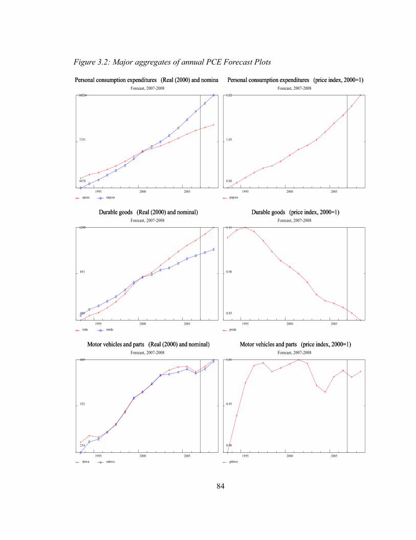
84
Figure 3.2: Major aggregates of annual PCE Forecast Plots
Personal consumption expenditures (Real (2000) and nominal) Personal consumption expenditures (Real (2000) and nominal) Forecast, 2007-2008
10224
7351
4478
1995 2000 2005 apcea napcea
Personal consumption expenditures (price index, 2000=1) Personal consumption expenditures (price index, 2000=1) Forecast, 2007-2008
1.22
1.05
0.88
1995 2000 2005 papcea
Durable goods (Real (2000) and nominal) Durable goods (Real (2000) and nominal) Forecast, 2007-2008
1295
891
488
1995 2000 2005 mda nmda
Durable goods (price index, 2000=1) Durable goods (price index, 2000=1) Forecast, 2007-2008
1.11
0.98
0.85
1995 2000 2005 pmda
Motor vehicles and parts (Real (2000) and nominal) Motor vehicles and parts (Real (2000) and nominal) Forecast, 2007-2008
469
352
234
1995 2000 2005 dmva ndmva
Motor vehicles and parts (price index, 2000=1) Motor vehicles and parts (price index, 2000=1) Forecast, 2007-2008
1.01
0.95
0.90
1995 2000 2005 pdmva
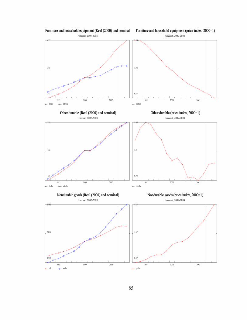
85
Furniture and household equipment (Real (2000) and nominal) Furniture and household equipment (Real (2000) and nominal) Forecast, 2007-2008
629
385
141
1995 2000 2005 dfura ndfura
Furniture and household equipment (price index, 2000=1) Furniture and household equipment (price index, 2000=1) Forecast, 2007-2008
1.38
1.02
0.66
1995 2000 2005 pdfura
Other durable (Real (2000) and nominal) Other durable (Real (2000) and nominal) Forecast, 2007-2008
228
162
97
1995 2000 2005 dotha ndotha
Other durable (price index, 2000=1) Other durable (price index, 2000=1) Forecast, 2007-2008
1.05
1.01
0.98
1995 2000 2005 pdotha
Nondurable goods (Real (2000) and nominal) Nondurable goods (Real (2000) and nominal) Forecast, 2007-2008
2952
2166
1379
1995 2000 2005 nda nnda
Nondurable goods (price index, 2000=1) Nondurable goods (price index, 2000=1) Forecast, 2007-2008
1.25
1.07
0.89
1995 2000 2005 pnda
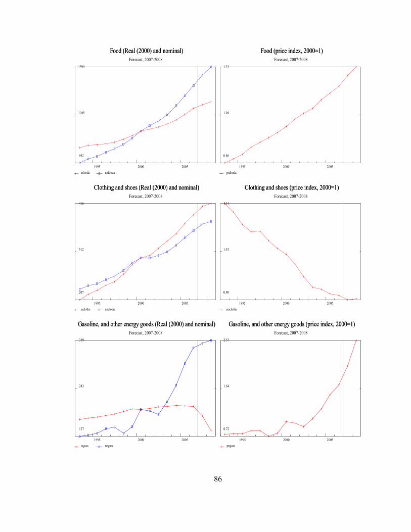
86
Food (Real (2000) and nominal) Food (Real (2000) and nominal) Forecast, 2007-2008
1399
1045
692
1995 2000 2005 nfooda nnfooda
Food (price index, 2000=1) Food (price index, 2000=1) Forecast, 2007-2008
1.23
1.04
0.86
1995 2000 2005 pnfooda
Clothing and shoes (Real (2000) and nominal) Clothing and shoes (Real (2000) and nominal) Forecast, 2007-2008
416
312
207
1995 2000 2005 nclotha nnclotha
Clothing and shoes (price index, 2000=1) Clothing and shoes (price index, 2000=1) Forecast, 2007-2008
1.11
1.01
0.90
1995 2000 2005 pnclotha
Gasoline, and other energy goods (Real (2000) and nominal) Gasoline, and other energy goods (Real (2000) and nominal) Forecast, 2007-2008
359
243
127
1995 2000 2005 ngasa nngasa
Gasoline, and other energy goods (price index, 2000=1) Gasoline, and other energy goods (price index, 2000=1) Forecast, 2007-2008
2.57
1.64
0.72
1995 2000 2005 pngasa

87
Other nondurable (Real (2000) and nominal) Other nondurable (Real (2000) and nominal) Forecast, 2007-2008
817
574
331
1995 2000 2005 notha nnotha
Other nondurable (price index, 2000=1) Other nondurable (price index, 2000=1) Forecast, 2007-2008
1.12
1.00
0.87
1995 2000 2005 pnotha
Services (Real (2000) and nominal) Services (Real (2000) and nominal) Forecast, 2007-2008
6167
4369
2572
1995 2000 2005 sva nsva
Services (price index, 2000=1) Services (price index, 2000=1) Forecast, 2007-2008
1.30
1.06
0.83
1995 2000 2005 psva
Housing (Real (2000) and nominal) Housing (Real (2000) and nominal) Forecast, 2007-2008
1547
1116
684
1995 2000 2005 shoa nshoa
Housing (price index, 2000=1) Housing (price index, 2000=1) Forecast, 2007-2008
1.29
1.05
0.81
1995 2000 2005 pshoa
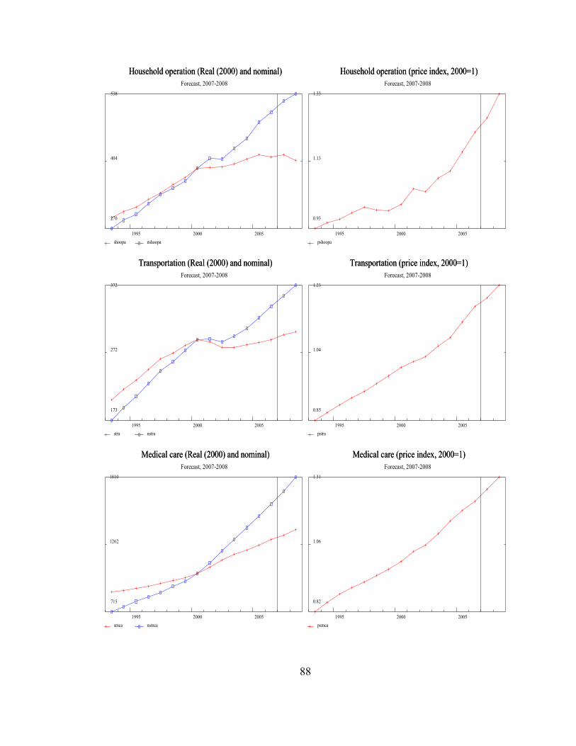
88
Household operation (Real (2000) and nominal) Household operation (Real (2000) and nominal) Forecast, 2007-2008
538
404
270
1995 2000 2005 shoopa nshoopa
Household operation (price index, 2000=1) Household operation (price index, 2000=1) Forecast, 2007-2008
1.33
1.13
0.93
1995 2000 2005 pshoopa
Transportation (Real (2000) and nominal) Transportation (Real (2000) and nominal) Forecast, 2007-2008
372
272
173
1995 2000 2005 stra nstra
Transportation (price index, 2000=1) Transportation (price index, 2000=1) Forecast, 2007-2008
1.23
1.04
0.85
1995 2000 2005 pstra
Medical care (Real (2000) and nominal) Medical care (Real (2000) and nominal) Forecast, 2007-2008
1810
1262
715
1995 2000 2005 smca nsmca
Medical care (price index, 2000=1) Medical care (price index, 2000=1) Forecast, 2007-2008
1.31
1.06
0.82
1995 2000 2005 psmca
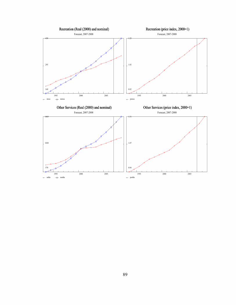
89
Recreation (Real (2000) and nominal) Recreation (Real (2000) and nominal) Forecast, 2007-2008
430
295
160
1995 2000 2005 sreca nsreca
Recreation (price index, 2000=1) Recreation (price index, 2000=1) Forecast, 2007-2008
1.25
1.03
0.82
1995 2000 2005 psreca
Other Services (Real (2000) and nominal) Other Services (Real (2000) and nominal) Forecast, 2007-2008
1469
1020
570
1995 2000 2005 sotha nsotha
Other Services (price index, 2000=1) Other Services (price index, 2000=1) Forecast, 2007-2008
1.31
1.07
0.84
1995 2000 2005 psotha

Chapter 4: Private fixed Investment in Equipment and Software
Investment is the both the engine of growth and the consequence of growth. For an economy to grow, it must have investment, especially in equipment. De Long and Summers found that “the cross nation pattern of equipment prices, quantities, and growth is consistent with the belief that countries with rapid growth have favorable supply conditions for machinery and equipment.” [De Long and Summers, 1991]
Gross private fixed investment in equipment and software accounts for about half of fixed investment. The other half, Investment in structures, has very different data and will be treated in the next chapter. Investment in Equipment and software has fluctuated over the last quarter century from a low of 6.7 percent of GDP in 1992Q1 to a high of 9.4 percent of GDP in 2000Q2. Although the magnitude is small relative to that of PCE, the amplitude of the swings is large. Virtually every recession has had its origin in a fall in a fixed investment. Accurate short-term forecasting of this volatile component of GDP is therefore necessary for getting the the general short-term outlook correct.
4.1 Data for Private Fixed Investment in Equipment and Software
Given this importance for short-term forecasting, the paucity of high-frequency data on equipment is surprising. I have found no monthly data, and the quarterly NIPA give only seven series:
Computers and peripherals
Software (excluding software embedded in machines or bundled in computers)
Other information processing equipment (Communication equipment, Medical instruments, Non-medical equipment and instruments, Photocopy and related equipment, and Office and accounting equipment)
Industrial equipment (Metalworking machinery, Special industrial machinery (i.e. machinery used in specific industries such as paper making machines or textile machines); General industrial machinery (i.e. machines used generally such as pumps, compressors, fans, blowers and material handling equipment); Electrical generation, transmission, and distribution equipment; Engines and turbines; and Fabricated metal products.)
Transportation equipment (Automobiles, trucks, buses, truck trailers, railroad equipment, aircraft, ships and boats)
90

Other equipment (Furniture and fixtures, Agricultural machinery, Construction machinery, Mining and oilfield machinery, Service industry machinery, and other equipment not elsewhere classified.)
Residential equipment: equipment that is owned by landlords and rented to tenants (Washer and dryer, stove and oven, etc.)
Figure 4.1 graphs these series, except software, in constant dollars of the year 2000. To avoid the problematic computer deflator, they have all been deflated by the deflator for food, which adjusts for general inflation without claiming to measure prices for particular types of equipment. Thus, in Figure 4.1, the relative sizes of the different series in any year are the same as those of the series in current prices. The graph presents a very different picture from the PCE graphs, which were mostly extremely smooth. In Equipment investment, ups and downs are common. In the collapse of investment after 2000, investment in Transportation equipment fell some 40 percent; investment in Computers and peripherals took a 30 percent hit; and no component survived unscathed. It is noteworthy that Computers rose rapidly from 1980 to 1985 as the IBM PC caught on
91
Figure 4.1: Components of Equipment Investment

in business, but that from 1985 to 2007 investment in Computers roughly paralleled investment in other capital goods with no growth from 1985 to 1995, then a boom to 2000, and then a bust to 2002. Since 2002, Computers have edged up slightly, while other components have recovered more strongly.
There are several reasons for this volatility of investment. Investment for expansion depends on the changes in the level of output of an industry rather than on its level. For example, if an industry's output went from 100 in year 1 to 103 in year 2 to 109 in year 3, the level of output would have increased rather smoothly, but the change in output in year 3 would be twice what it was in year 2. Besides investment for expansion, there is investment for replacement. But it is deferrable as businesses often can “make do” with existing facilities, especially in periods of slack demand. Waves of optimism and pessimism can lead to substantial additions of capital facilities during expansions, only to be followed by overcapacity and deep cutbacks in investment outlays during recessions, as occurred in the years 2000 to 2002.
In the 1997 comprehensive revision of the NIPA, BEA decided to consider business acquisition of software, whether by purchase or by in-house development, as investment. This decision gave a nice boost to GDP, because expenditures on software had previously been considered an intermediate product and did not count in GDP. Figure 4.2 shows the course of investment in software in comparison to investment in Computers and peripherals and in Other information processing equipment, which includes communication equipment, nonmedical instruments, medical equipment and instruments, photocopy and related equipment, and office and accounting equipment. Clearly, this newcomer to investment was the star performer in the 1990's.
92
Table 4.1: Quarterly Data on Equipment Investment. From NIPA Table 5.3.5 Quarterly
2006 2006 2006 2006 2007 2007 20071 2 3 4 1 2 3
Equipment and software 991.7 991.1 999.1 988.7 991.8 1,004.5 1,016.4 Information processing equipment and software 479.1 479.0 484.9 480.5 497.6 507.7 511.4 Computers and peripheral equipment 91.7 91.7 91.6 90.4 96.6 96.6 95.2 Software \2\ 199.9 202.6 204.9 205.9 210.5 216.1 220.0 Other \3\ 187.5 184.7 188.4 184.3 190.5 195.0 196.2 Industrial equipment 161.5 168.5 169.2 167.5 168.1 176.0 180.4 Transportation equipment 177.6 169.5 172.4 168.0 162.9 153.3 154.0 Other equipment \4\ 173.5 174.0 172.6 172.7 163.2 167.5 170.5

When we turn to annual data, we find much more information. BEA actually produces two sets of it. The first is in the NIPA themselves and is illustrated in Table 4.2. Excluding the addenda at the bottom of the table, there are 36 lines of data, of which 27 are primary and the other are subtotals or totals. Line 1 and line 37 in this table give us Fixed investment in equipment and software as it appears in the NIPA.
93
Figure 4.2: Components of Information Processing Equipment and software
Figure 4.2: Information Processing Equipment & Software Figure 4.2: Information Processing Equipment & Software Constant 2000 food dollars
0
50
100
150
200
1980 1985 1990 1995 2000 2005 computersf softwaref otherinfof

There is, however, a serious problem in the use of these data for models such as LIFT. The models will almost certainly have investment functions for the purchasers of equipment rather than by types of equipment bought. For example, there will be an equation for investment by the automobile industry, not an equation for the purchases of machine tools by all industries. There is, of course, good reason to model investment by purchaser rather than by type of equipment bought, namely, investment decisions are made by the purchaser, not by the seller, of equipment. Models with sectoral detail on output can use the industry's sales in the equation that determines its investment. Investment by type of equipment is then determined by multiplying the vector of investment by purchasing industry by a matrix – called a capital flow coefficient matrix --
94
Table 4.2: Private fixed investment in equipment and software. From NIPA Table 5.5.5Line 2000 2002 2003 2004 2005 2006
1 Private fixed investment in equipment and software 926.2 794.7 808.0 864.7 946.5 1,002.22 Nonresidential equipment and software 918.9 787.1 800.2 856.3 937.5 992.63 Information processing equipment and software 467.6 399.4 406.7 429.6 457.4 480.94 Computers, software, and communication 401.7 329.4 331.0 348.3 369.0 388.55 Computers and peripheral equipment 101.4 77.2 77.8 80.3 89.0 91.36 Software \1\ 176.2 167.6 171.4 183.0 193.8 203.37 Communication equipment \2\ 124.1 84.5 81.8 85.0 86.2 93.98 Medical equipment and instruments 34.4 42.2 46.0 50.7 56.3 59.19 Nonmedical instruments 17.8 18.2 19.0 20.9 22.5 23.810 Photocopy and related equipment 9.6 4.6 4.6 3.6 3.5 3.411 Office and accounting equipment 4.1 4.9 6.0 6.1 6.1 6.012 Industrial equipment 159.2 135.7 140.7 139.7 156.1 166.713 Fabricated metal products 12.4 11.4 11.9 12.5 14.0 14.914 Engines and turbines 7.1 11.6 10.2 4.7 5.5 6.015 Metalworking machinery 30.0 23.1 22.6 23.3 25.7 27.716 Special industry machinery, n.e.c. 36.4 25.8 29.1 28.2 30.3 31.417 General industrial, including materials handling, equipment 48.6 43.6 48.6 51.3 59.4 63.918 Electrical transmission, distribution, and industrial apparatus 24.7 20.2 18.3 19.7 21.1 22.719 Transportation equipment 160.8 126.3 118.3 142.9 159.5 171.920 Trucks, buses, and truck trailers 81.8 61.0 61.9 83.4 99.4 111.021 Light trucks (including utility vehicles) 50.8 37.5 40.8 53.7 63.0 69.622 Other trucks, buses, and truck trailers 31.0 23.6 21.1 29.7 36.3 41.423 Autos 36.5 32.9 29.5 31.2 34.8 39.224 Aircraft 32.6 25.6 19.9 20.3 16.0 13.125 Ships and boats 3.4 3.5 4.0 4.6 4.8 4.126 Railroad equipment 6.5 3.3 3.0 3.4 4.5 4.527 Other equipment 134.6 128.4 137.6 149.6 169.8 180.028 Furniture and fixtures 36.3 30.3 31.8 34.0 38.0 41.329 Agricultural machinery 13.7 17.1 18.4 20.5 22.5 21.730 Construction machinery 23.2 18.4 19.7 23.1 29.7 31.531 Mining and oilfield machinery 5.3 3.8 4.6 5.6 7.8 10.132 Service industry machinery 17.5 16.9 16.5 17.0 18.7 21.333 Electrical equipment, n.e.c. 4.6 5.6 5.8 7.1 6.9 7.834 Other 33.9 36.3 40.7 42.4 46.2 46.535 Less: Sale of equipment scrap, excluding autos 3.4 2.6 3.1 5.7 5.2 6.836 Residential equipment 7.4 7.6 7.9 8.4 9.0 9.6
Addenda:37 Private fixed investment in equipment and software 926.2 794.7 808.0 864.7 946.5 1,002.238 Less: Dealers' margin on used equipment 10.3 10.1 10.0 10.7 11.4 11.639 Net purchases of used equipment from government 0.5 0.5 0.6 0.6 0.6 0.740 Plus: Net sales of used equipment 80.3 77.2 70.9 69.2 71.2 72.641 Net exports of used equipment 0.0 1.9 1.2 1.3 3.2 1.742 Sale of equipment scrap 3.5 2.8 3.2 5.4 5.4 7.043 Equals: Private fixed investment in new equipment and software 999.2 866.0 872.8 929.3 1,014.2 1,071.3

showing the shares of each type of equipment in the spending of each purchaser. The airlines column of this matrix, for example, will show a large share going aircraft and a small share, if any, going to agricultural machinery.
Fortunately, BEA produces another set of accounts known as the Fixed Asset Accounts (FAA) which are separate from but related to the NIPA. The objective of the FAA is to create series on the capital stocks by industry, but on the way to this objective they produce series on equipment purchases by buying industry. In fact, the FAA include a complete equipment capital flow matrix showing the sales of each type of equipment to each industry. The FAA series on equipment investment by purchaser are made by distributing NIPA investment by type to likely buying industries. In making this distribution, BEA may use various sources of information on investment by purchaser such as the Annual Survey of Manufactures and the economic censuses. The results, Equipment and software investment classified by purchasing industry, is shown in Table 4.3 for selected recent years. Of the 78 lines in the table, 63 are primary and the others are subtotals and totals. It also must be noted that the residential equipment investment presented in Table 4.2 is purchased only by the Real estate industry (line 56) in Table 4.3.
Our task in this chapter, put briefly, is to produce up-to-date estimates of these 63 series for the current year and one ahead. These estimates are, as usual, needed in current and constant prices.
The FAA, it may be noted, appear at about the same time as the annual NIPA, that is, in late July or early August of the year following the year which they describe. They include, for each year, the capital flow matrix in current prices17. It can be converted to constant prices using whatever price index one likes on each row and then summing the columns. Because, as the model runs, the capital flow matrix will be used in the other direction, that is, to convert investment classified by purchaser to investment classified by product purchased, we will make the series on constant-price investment by purchaser by simple addition of the components, not by Fisher chained indexes.
A super-attentive reader may have noticed that there are small differences in total equipment investment in the NIPA and in the FAA. There are three conceptual differences and one main source of statistical difference. The conceptual differences are (1) The NIPA total investment includes dealers' margins on used equipment; the FAA do not. (2) The NIPA subtract from total spending the value of scrapped equipment; the FAA do not. (3) There is a difference in the valuation of used cars. The statistical difference is mainly that the makers of the FAA don't always go back and revise their estimates when the makers of the NIPA revise historical data. The FAA give a detailed, product-by-product account of these differences. They are summarized for recent years in Table 4.4.
17 The BEA name of the file is detailedness_inv1.xls. To get to it from the BEA main website, www.bea.gov, click “Fixed Assets”, then under “Fixed assets” to the right of “Interactive tables” click “Fixed assets tables.” Then to the right of “Download a spreadsheet of” click “Detailed fixed assets tables.” On the screen where that brings you look for “ 2. Nonresidential detailed estimates” . Under it find “5. Investment, historical cost” To the far right click on “XLS” and download the file. The last tab, called “Datasets” has all of the series in one sheet.
95

Although the FAA capital flow matrix provides important input for the construction of the capital flow coefficient matrix needed for the interindustry model, it does not yield that matrix by simply dividing each column by its total to get a matrix with columns summing to 1.0. The problem is that the interindustry model needs a matrix in producer prices; the FAA capital flow matrix is in purchaser prices. The margins for transportation and trade must be stripped off the sales of equipment and but into the trade and transportation rows. That step, however, is beyond the scope of this study and will be left for the model builder.
96

97
Table 4.3: Equipment Investment by Purchaser, from the Fixed Assets Accounts
Line 2000 2002 2004 2005 2006
1 Private fixed assets 929.7 794.9 855.3 938.0 994.9
2 Agriculture, forestry, fishing, and hunting 22.4 25.7 29.9 32.1 32.33 Farms \1\ 20.8 23.7 27.3 28.6 28.64 Forestry, fishing, and related activities 1.6 2.0 2.7 3.6 3.6
5 Mining 15.9 11.5 18.6 24.0 26.96 Oil and gas extraction 6.1 3.1 5.9 5.4 5.97 Mining, except oil and gas 5.2 4.5 7.8 10.2 11.48 Support activites for mining 4.6 3.9 4.9 8.4 9.6
9 Utilities 35.0 37.6 30.9 34.5 36.7
10 Construction 31.7 31.1 33.9 38.4 41.3
11 Manufacturing 169.8 142.0 129.2 148.1 157.412 Durable goods 109.5 86.5 76.8 88.2 93.813 Wood products 2.6 2.2 2.3 2.6 2.814 Nonmetallic mineral products 5.1 4.5 4.1 4.6 4.915 Primary metals 5.4 4.7 4.3 4.9 5.216 Fabricated metal products 9.6 8.2 7.3 7.9 8.517 Machinery 18.6 15.4 14.2 16.2 17.218 Computer and electronic products 37.5 21.8 19.2 25.0 26.519 Electrical equipment, appliances, and components 3.9 2.9 2.6 2.2 2.320 Motor vehicles, bodies and trailers, and parts 13.0 11.7 10.7 11.0 11.721 Other transportation equipment 7.9 9.5 6.6 7.9 8.422 Furniture and related products 1.8 1.9 1.4 1.5 1.623 Miscellaneous manufacturing 4.0 3.8 4.1 4.4 4.724 Nondurable goods 60.3 55.4 52.4 60.0 63.725 Food and beverage and tobacco products 11.9 11.4 10.9 12.0 12.826 Textile mills and textile product mills 2.4 1.8 1.2 1.3 1.327 Apparel and leather and allied products 1.3 0.8 0.6 0.7 0.728 Paper products 7.7 6.4 5.5 5.9 6.329 Printing and related support activities 4.8 4.1 4.4 4.7 5.030 Petroleum and coal products 5.2 5.4 7.0 11.1 11.831 Chemical products 18.8 18.3 16.4 17.3 18.432 Plastics and rubber products 8.1 7.3 6.5 6.9 7.4
33 Wholesale trade 56.8 45.5 54.8 70.5 75.5
34 Retail trade 31.7 28.0 35.5 35.2 37.5
35 Transportation and warehousing 64.3 48.9 45.7 48.6 52.736 Air transportation 31.7 24.4 17.2 12.3 13.237 Railroad transportation 1.4 1.0 1.3 1.4 1.538 Water transportation 3.9 4.9 5.3 5.1 5.139 Truck transportation 10.5 8.3 10.3 17.6 19.640 Transit and ground passenger transportation 3.7 1.9 2.9 3.4 3.741 Pipeline transportation 2.8 1.7 2.1 2.4 2.642 Other transportation and support activites \2\ 9.2 4.8 4.5 4.5 4.843 Warehousing and storage 1.1 1.9 2.1 2.1 2.2
44 Information 121.7 63.3 64.2 65.8 70.745 Publishing industries (includes software) 7.4 5.4 6.3 6.0 6.446 Motion picture and sound recording industries 0.7 0.6 0.7 0.9 1.047 Broadcasting and telecommunications 107.4 50.7 49.4 51.3 55.348 Information and data processing services 6.3 6.6 7.7 7.5 7.9
49 Finance and insurance 100.8 80.6 91.9 90.0 93.350 Federal Reserve banks 2.2 1.8 2.2 1.3 1.451 Credit intermediation and related activities 64.7 53.0 57.3 58.9 60.952 Securities, commodity contracts, and investments 13.5 9.2 10.9 10.7 11.253 Insurance carriers and related activities 18.0 15.6 19.5 17.3 18.054 Funds, trusts, and other financial vehicles 2.3 1.0 2.0 1.7 1.7
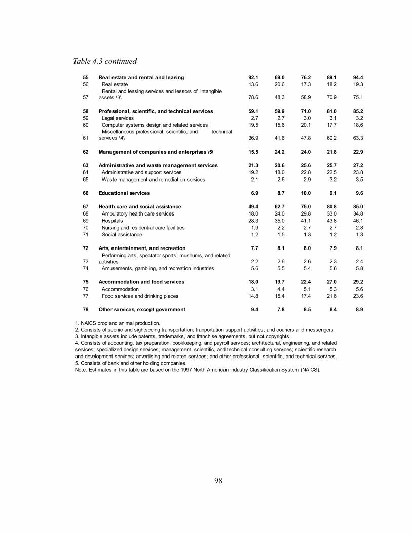
98
Table 4.3 continued
55 Real estate and rental and leasing 92.1 69.0 76.2 89.1 94.456 Real estate 13.6 20.6 17.3 18.2 19.3
57 78.6 48.3 58.9 70.9 75.1
58 Professional, scientific, and technical services 59.1 59.9 71.0 81.0 85.259 Legal services 2.7 2.7 3.0 3.1 3.260 Computer systems design and related services 19.5 15.6 20.1 17.7 18.6
61 36.9 41.6 47.8 60.2 63.3
62 Management of companies and enterprises \5\ 15.5 24.2 24.0 21.8 22.9
63 Administrative and waste management services 21.3 20.6 25.6 25.7 27.264 Administrative and support services 19.2 18.0 22.8 22.5 23.865 Waste management and remediation services 2.1 2.6 2.9 3.2 3.5
66 Educational services 6.9 8.7 10.0 9.1 9.6
67 Health care and social assistance 49.4 62.7 75.0 80.8 85.068 Ambulatory health care services 18.0 24.0 29.8 33.0 34.869 Hospitals 28.3 35.0 41.1 43.8 46.170 Nursing and residential care facilities 1.9 2.2 2.7 2.7 2.871 Social assistance 1.2 1.5 1.3 1.2 1.3
72 Arts, entertainment, and recreation 7.7 8.1 8.0 7.9 8.1
73 2.2 2.6 2.6 2.3 2.474 Amusements, gambling, and recreation industries 5.6 5.5 5.4 5.6 5.8
75 Accommodation and food services 18.0 19.7 22.4 27.0 29.276 Accommodation 3.1 4.4 5.1 5.3 5.677 Food services and drinking places 14.8 15.4 17.4 21.6 23.6
78 Other services, except government 9.4 7.8 8.5 8.4 8.9
1. NAICS crop and animal production. 2. Consists of scenic and sightseeing transportation; tranportation support activities; and couriers and messengers. 3. Intangible assets include patents, trademarks, and franchise agreements, but not copyrights. 4. Consists of accounting, tax preparation, bookkeeping, and payroll services; architectural, engineering, and related services; specialized design services; management, scientific, and technical consulting services; scientific research and development services; advertising and related services; and other professional, scientific, and technical services. 5. Consists of bank and other holding companies. Note. Estimates in this table are based on the 1997 North American Industry Classification System (NAICS).
Rental and leasing services and lessors of intangible assets \3\
Miscellaneous professional, scientific, and technical services \4\
Performing arts, spectator sports, museums, and related activities

4.2 Approach to the problem
As already indicated, our problem is short-range forecasting of the 63 primary series on investment in Table 4.3. We need forecasts for both current-price values and constant price values. Our approach is in seven steps.
Step 1. Make quarterly forecasts of both current price values and the price indexes of the seven series for which we have quarterly data in the NIPA. These forecast will be made with inputs from QUEST in ways already familiar from Chapter 3. They will be in quarterly frequency to make use of the fact that we often have three or even four quarters of a year before the FAA data appear. Convert these quarterly forecasts to annual forecasts.
Step 2. Make preliminary annual forecasts for two years ahead for each of the 63 primary series which are the target of our work. These equations may use as explanatory variables one or more of the seven series forecast in Step 1 or their sum. They may also use their own lagged values.
Step 3. Aggregate the rows of the FAA capital flow matrix to match these seven rows and convert to a capital coefficient matrix. (This step might be done with either the matrix of the most recent year or with a (perhaps weighted) average of the last two or three years.
Step 4. Multiply the coefficients of the matrix made in Step 3 by the forecast of the corresponding investment series made in Step 2.
Step 5. Scale each of the seven rows calculated in Step 4 to sum to the total for the corresponding series forecast in Step 1.
Step 6. Sum the columns of the matrix found in step 6 to give the current price annual forecast for each of the 63 series.
Step 7. Convert each row of the matrix found in Step 5 to constant prices using the price indexes found for each of the seven series in Step 1. Sum the columns to get the forecasts of the 63 industries in constant prices.
99
Table 4.4: Reconciliation of Equipment Investment in NIPA and FAA
Line 2002 2003 2004 2005 20061 NIPA Private fixed investment in equipment and software 794.7 808.0 864.7 946.5 1002.22 Plus: Sale of equipment scrap, excluding autos 2.6 3.1 5.7 5.2 6.84 Less: Dealers' margin on used equipment 10.1 10.0 10.7 11.4 11.65 Plus Intersectoral automobile valuation adjustment -3.5 -5.6 -4.4 -2.2 -2.26 Plus: NIPA revisions since FAA was revised 11.2 7.4 0.0 -0.1 -0.37 FAA Private fixed investment in equipment and software 794.9 802.9 855.3 938.0 994.9

4.3 NIPA Investment in Equipment and Software by Asset Types Equations
In this section, I discuss the equation results estimated in Step 1. These equations (both the nominal values and the price indexes) was estimated during the period from 1970Q1 to 2007Q3. The estimation results of are presented in Table 4.5 and Table 4.6. Figure 4.3 shows the plots of the regressions' predicted values and the historical series.
Before discussing each equation, there is an interesting result from Table 4.5 and Table 4.6. In most of these equations, I use regressors with their current period and their one-period lagged value or with two consecutive lagged values. This is an approximation of using the first difference of the regressors. Thus, we would expect the signs of the coefficients to be different between the two regressors. For example, in Table 4.5, the coefficient of current period nonresidential investment in equipment and software (vfnre) is positive while the coefficient of its lagged value is negative. This result is expected.
Computer and peripheral equipment
The nominal equation of computer and peripheral equipment consists of intercept, one-quarter lagged dependent variable, two-quarter lagged dependent variable, and the current period NIPA nominal private fixed investment of nonresidential equipment and software (vfnre). The equations shows good fit both in test statistics (adjusted R-square and MAPE) and in fitted plot (with BasePred). All regressors except intercept have good Mexvals and reasonable signs within the test period. The intercept is left in this equation as previous estimation with different test period shows that the intercept has explanatory power.
The price index equation is straight forward with two lagged dependent variables (one- and two-quarter lagged) without an intercept. Both regressors have respectable Mexvals. The closeness of fit statistics are good with adjusted R-square of 0.9993 and MAPE of 1.46 percent. The fitted plot is very good in both the predicted value and BasePred.
Software
The nominal equation of Software fixed investment has two regressors and an intercept. The regressors are the one-quarter lagged dependent variable and vfnre. All regressors have good Mexvals and appropriate signs. The adjusted R-square is 0.9993 while the MAPE is 6.94 percent. The fitted plot shows a very good fit with BasePred plot moving within a good proximity of the actual series.
100

The price index equation has two lagged dependent variables as regressors, qvenp2(t-1) and qvenp2(t-1), without an intercept. Both regressors has good Mexvals and providing very good fit as shown by the closeness of fit statistics. However, the fitted plot shows that this equation cannot capture the volatility during the test period as seen in the BasePred plot. This is a problem when using only time-series analysis for forecasting economic indicators. Nevertheless, it should be good for our purpose of short-term forecasting.
Other Information processing equipment and software
The nominal equation for the investment of other information processing equipment and software has the same format as the computer equipment's equation. All regressors, including intercept, have decent Mexvals and appropriate signs. The adjusted R-square is 0.9977 and the MAPE is 3.2 percent. The fitted plot shows that the equation has good fit and should be a good equation for both short-term and long-term forecasts.
The price index equation has two lagged dependent variables, price index of vfnre, and intercept as its regressors. All regressors exhibits good Mexvals and reasonable signs. The closeness of fit statistics are very good. The BasePred plot shows that pvfnre helps explain the movement of the price index quite well.
Industrial equipment
The nominal equation for investment in Industrial equipment has the following regressors: 1) intercept, 2) one-quarter lagged dependent variable, 3) two-quarter lagged dependent variable, and 4) vfnre. All regressors have good Mexvals. The MAPE is 2.05 percent and the adjusted R-square is 0.9972. The predicted value fits well with the historical series (as expected) and the BasePred plot shows a decent fit.
The price index equation consists of three regressors without an intercept. The regressors are one-quarter, two-quarter, and three-quarter lagged dependent variables. All three regressors has respectable Mexvals with most of the explanatory power comes from the first lag. The closeness of fit statistics is very good with MAPE of 0.38 percent. However, the BasePred plot shows that having a short-term forecast rely on the estimation over this test period might not be appropriate. It seems that estimating the equation on the more recent time period might yield a better BasePred plot and a more reliable short-term forecast.
101

Transportation equipment
The nominal equation for investment in transportation equipment has a one-quarter lagged dependent variable, current quarter vfnre, and one-quarter lagged vfnre as its regressors. All three regressors have good Mexvals and expected signs. The adjusted R-square is 0.9934 and the MAPE is 3.49 percent. The fitted plots show very good fit by both the predicted value and the BasePred.
The price index equation has one-quarter lagged dependent variable, current quarter price index of vfnre, and one-quarter lagged price index of vfnre as its regressors. All three regressors contribute to the explanation of the price index over the test period. We have good closeness of fit statistics. The fitted plots show a good fit from predicted value and BasePred. The BasePred plot also shows a tendency of over-predicting the series over the test period.
Other nonresidential equipment
For investment in other nonresidential equipment, its nominal equation has one-quarter lagged dependent variable, current quarter vfnre, and one-quarter lagged vfnre as its regressors. All three regressors have good Mexvals and appropriate signs. The adjusted R-square is 0.9981 and the MAPE is 2.04 percent. The fitted plots show very good fit from both the predicted value and the BasePred.
The price index equation has one-quarter lagged dependent variable, current quarter price index of vfnre, and one-quarter lagged price index of vfnre as regressors. All coefficients have good signs and all regressors have reasonable Mexvals. The closeness of fit statistics are very good with adjusted R-square of 0.9999 and the MAPE of 0.27 percent. The fitted plots also show very good fit.
Residential equipment
The nominal residential equipment investment equation has intercept, one-quarter lagged dependent variable, and the nominal value of private fixed residential investment. The last regressors composes of residential investment in both structures and equipment and software. All three regressors have good Mexvals and appropriate signs. The estimation shows good closeness of fit statistics for the test period with a MAPE of 1.62 percent. The fitted plots are good. The BasePred helps guiding the forecast with the long-term trend.
The price index equation consists of an intercept, one-quarter lagged dependent variable and two-quarter lagged dependent variable. The three regressors have good Mexvals and reasonable signs. The adjusted R-square is 0.9987 and the MAPE is 0.51 percent. The predicted value plot is very good. The BasePred plot cannot capture the exact movement of the actual series but seems to move well along the long-term trend.
102

103
Table 4.5: Estimation Results for Nominal values of Quarterly NIPA Fixed Investment in Equipment and Software
: Nonresidential Computer SEE = 2262.40 RSQ = 0.9953 RHO = 0.03 Obser = 151 from 1970.100 SEE+1 = 2261.83 RBSQ = 0.9952 DurH = 1.28 DoFree = 147 to 2007.300 MAPE = 5.83 Variable name Reg-Coef Mexval Elas NorRes Mean Beta 0 qvenn1 - - - - - - - - - - - - - - - - - 43297.57 - - - 1 intercept -561.84853 0.6 -0.01 212.98 1.00 2 qvenn1[1] 1.15557 54.4 1.14 1.15 42684.86 1.152 3 qvenn1[2] -0.27895 4.2 -0.27 1.08 42062.42 -0.277 4 vfnre 13.79061 3.9 0.14 1.00 454.46 0.123
: Nonresidential software SEE = 1833.01 RSQ = 0.9993 RHO = 0.58 Obser = 151 from 1970.100 SEE+1 = 1491.03 RBSQ = 0.9993 DurH = 7.22 DoFree = 148 to 2007.300 MAPE = 6.94 Variable name Reg-Coef Mexval Elas NorRes Mean Beta 0 qvenn2 - - - - - - - - - - - - - - - - - 67258.89 - - - 1 intercept -1914.04781 6.6 -0.03 1438.86 1.00 2 qvenn2[1] 0.95532 788.7 0.93 1.30 65815.40 0.943 3 vfnre 13.85916 14.2 0.09 1.00 454.46 0.059
: Other Information processing equipment and software SEE = 2729.94 RSQ = 0.9978 RHO = 0.05 Obser = 151 from 1970.100 SEE+1 = 2726.96 RBSQ = 0.9977 DurH = 1.33 DoFree = 147 to 2007.300 MAPE = 3.20 Variable name Reg-Coef Mexval Elas NorRes Mean Beta 0 qvennoit - - - - - - - - - - - - - - - - - 91706.32 - - - 1 intercept 1131.00142 2.4 0.01 448.03 1.00 2 qvennoit[1] 0.93412 36.6 0.92 1.33 90481.58 0.930 3 qvennoit[2] -0.14794 1.4 -0.14 1.28 89261.84 -0.147 4 vfnre 42.37975 13.0 0.21 1.00 454.46 0.216
: Nonresidential industrial equipment SEE = 2453.52 RSQ = 0.9973 RHO = -0.03 Obser = 151 from 1970.100 SEE+1 = 2452.10 RBSQ = 0.9972 DurH = -1.31 DoFree = 147 to 2007.300 MAPE = 2.05 Variable name Reg-Coef Mexval Elas NorRes Mean Beta 0 qvennin - - - - - - - - - - - - - - - - - 90332.58 - - - 1 intercept 1755.34201 2.7 0.02 365.38 1.00 2 qvennin[1] 1.26682 65.2 1.25 1.17 89267.11 1.261 3 qvennin[2] -0.33603 6.2 -0.33 1.05 88230.56 -0.333 4 vfnre 11.30934 2.4 0.06 1.00 454.46 0.071
: Nonresidential Transportation equipment SEE = 3859.05 RSQ = 0.9935 RHO = 0.06 Obser = 151 from 1970.100 SEE+1 = 3852.86 RBSQ = 0.9934 DurH = 0.81 DoFree = 148 to 2007.300 MAPE = 3.49 Variable name Reg-Coef Mexval Elas NorRes Mean Beta 0 qvenntr - - - - - - - - - - - - - - - - - 83589.17 - - - 1 qvenntr[1] 0.87343 135.7 0.86 1.89 82689.14 2 vfnre 334.71098 37.3 1.82 1.83 454.46 2.060 3 vfnre[1] -314.86316 35.4 -1.69 1.00 448.18 -1.925
: Nonresidential other equipment SEE = 2004.77 RSQ = 0.9981 RHO = 0.03 Obser = 151 from 1970.100 SEE+1 = 2004.02 RBSQ = 0.9981 DurH = 0.36 DoFree = 148 to 2007.300 MAPE = 2.04 Variable name Reg-Coef Mexval Elas NorRes Mean Beta 0 qvennot - - - - - - - - - - - - - - - - - 81287.93 - - - 1 qvennot[1] 0.98759 367.3 0.97 1.52 80205.83 2 vfnre 130.64964 23.4 0.73 1.51 454.46 0.843 3 vfnre[1] -128.02004 23.1 -0.71 1.00 448.18 -0.821
: Residential equipment SEE = 85.94 RSQ = 0.9987 RHO = 0.12 Obser = 151 from 1970.100 SEE+1 = 85.37 RBSQ = 0.9987 DurH = 1.44 DoFree = 148 to 2007.300 MAPE = 1.62 Variable name Reg-Coef Mexval Elas NorRes Mean Beta 0 qvennr - - - - - - - - - - - - - - - - - 5168.83 - - - 1 intercept 90.22767 6.7 0.02 762.49 1.00 2 qvennr[1] 0.97497 987.1 0.96 1.11 5111.62 0.973 3 vfr 0.34559 5.1 0.02 1.00 274.64 0.029

104
Table 4.6: Estimation Results for Price indexes of Quarterly NIPA Fixed Investment in Equipment and Software
: Nonresidential Computer SEE = 124.93 RSQ = 0.9993 RHO = 0.30 Obser = 151 from 1970.100 SEE+1 = 122.02 RBSQ = 0.9993 DurH = 5.02 DoFree = 149 to 2007.300 MAPE = 1.46 Variable name Reg-Coef Mexval Elas NorRes Mean Beta 0 qvenp1 - - - - - - - - - - - - - - - - - 3059.84 - - - 1 qvenp1[1] 1.61040 146.7 1.68 1.84 3197.79 2 qvenp1[2] -0.62754 35.7 -0.68 1.00 3338.21 -0.684
: Nonresidential software SEE = 0.71 RSQ = 0.9981 RHO = -0.04 Obser = 151 from 1970.100 SEE+1 = 0.71 RBSQ = 0.9981 DurH = -0.64 DoFree = 149 to 2007.300 MAPE = 0.46 Variable name Reg-Coef Mexval Elas NorRes Mean Beta 0 qvenp2 - - - - - - - - - - - - - - - - - 117.18 - - - 1 qvenp2[1] 1.70314 160.9 1.71 1.99 117.35 2 qvenp2[2] -0.70361 41.2 -0.71 1.00 117.52 -0.696
: Other Information processing equipment and software SEE = 0.43 RSQ = 0.9994 RHO = 0.01 Obser = 151 from 1970.100 SEE+1 = 0.43 RBSQ = 0.9994 DurH = 0.11 DoFree = 147 to 2007.300 MAPE = 0.34 Variable name Reg-Coef Mexval Elas NorRes Mean Beta 0 qvenpoit - - - - - - - - - - - - - - - - - 94.42 - - - 1 intercept 0.74421 4.4 0.01 1734.69 1.00 2 qvenpoit[1] 1.46215 96.4 1.46 2.67 94.18 1.485 3 qvenpoit[2] -0.51683 19.9 -0.51 1.19 93.94 -0.533 4 pvfnre 0.04604 9.0 0.05 1.00 98.17 0.049
: Nonresidential industrial equipment SEE = 0.35 RSQ = 0.9998 RHO = -0.04 Obser = 151 from 1970.100 SEE+1 = 0.35 RBSQ = 0.9998 DurH = -2.30 DoFree = 148 to 2007.300 MAPE = 0.38 Variable name Reg-Coef Mexval Elas NorRes Mean Beta 0 qvenpin - - - - - - - - - - - - - - - - - 73.66 - - - 1 qvenpin[1] 1.55175 89.8 1.54 2.57 73.06 2 qvenpin[2] -0.26571 1.1 -0.26 1.09 72.45 -0.267 3 qvenpin[3] -0.28493 4.2 -0.28 1.00 71.85 -0.287
: Nonresidential Transportation equipment SEE = 0.78 RSQ = 0.9991 RHO = 0.14 Obser = 151 from 1970.100 SEE+1 = 0.77 RBSQ = 0.9991 DurH = 1.78 DoFree = 148 to 2007.300 MAPE = 0.62 Variable name Reg-Coef Mexval Elas NorRes Mean Beta 0 qvenptr - - - - - - - - - - - - - - - - - 77.22 - - - 1 qvenptr[1] 1.00557 1891.6 1.00 1.46 76.68 2 pvfnre 0.58371 14.6 0.74 1.30 98.17 0.434 3 pvfnre[1] -0.58392 14.0 -0.74 1.00 97.91 -0.441
: Nonresidential other equipment SEE = 0.22 RSQ = 0.9999 RHO = 0.47 Obser = 151 from 1970.100 SEE+1 = 0.19 RBSQ = 0.9999 DurH = 5.73 DoFree = 148 to 2007.300 MAPE = 0.27 Variable name Reg-Coef Mexval Elas NorRes Mean Beta 0 qvenpot - - - - - - - - - - - - - - - - - 74.13 - - - 1 qvenpot[1] 1.00576 7775.0 1.00 5.18 73.52 2 pvfnre 0.47393 90.0 0.63 3.50 98.17 0.327 3 pvfnre[1] -0.47326 87.0 -0.63 1.00 97.91 -0.332
: Residential equipment SEE = 0.58 RSQ = 0.9988 RHO = -0.11 Obser = 151 from 1970.100 SEE+1 = 0.58 RBSQ = 0.9987 DurH = -2.79 DoFree = 148 to 2007.300 MAPE = 0.51 Variable name Reg-Coef Mexval Elas NorRes Mean Beta 0 qvenpr - - - - - - - - - - - - - - - - - 88.27 - - - 1 intercept 0.90197 3.6 0.01 806.82 1.00 2 qvenpr[1] 1.44846 91.6 1.44 1.27 87.95 1.467 3 qvenpr[2] -0.45676 12.8 -0.45 1.00 87.63 -0.468

105
Figure 4.3: Plots of NIPA Fixed Investment in Equipment and Software Estimation Results
Nonresidential Computer Nonresidential Computer Nominal (Million dollars)
105013
53642
2272
1970 1975 1980 1985 1990 1995 2000 2005 Predicted Actual BasePred
Nonresidential Computer Nonresidential Computer Price index (2000=100)
20851
10430
9
1970 1975 1980 1985 1990 1995 2000 2005 Predicted Actual BasePred
Nonresidential software Nonresidential software Nominal (Million dollars)
220047
105915
-8217
1970 1975 1980 1985 1990 1995 2000 2005 Predicted Actual BasePred
Nonresidential software Nonresidential software Price index (2000=100)
144.6
118.9
93.2
1970 1975 1980 1985 1990 1995 2000 2005 Predicted Actual BasePred
Other Information processing equipment and software Other Information processing equipment and software Nominal (Million dollars)
201616
106470
11324
1970 1975 1980 1985 1990 1995 2000 2005 Predicted Actual BasePred
Other Information processing equipment and software Other Information processing equipment and software Price index (2000=100)
117.0
86.6
56.2
1970 1975 1980 1985 1990 1995 2000 2005 Predicted Actual BasePred
Nonresidential industrial equipment Nonresidential industrial equipment Nominal (Million dollars)
180431
99778
19126
1970 1975 1980 1985 1990 1995 2000 2005 Predicted Actual BasePred
Nonresidential industrial equipment Nonresidential industrial equipment Price index (2000=100)
116.1
70.0
24.0
1970 1975 1980 1985 1990 1995 2000 2005 Predicted Actual BasePred

4.4 FAA Investment in Equipment and Software by Purchasing Industries Equations
This section discusses the purchasing industries' equation estimated as described in Step 2 for 13 industries selected from the total of 63 industries. All equations were estimated with historical data from 1975 to 2006. All regression results are shown in Appendix 4.1. The fitted plots of all 63 industries are shown in Figure 4.4.
106
Figure 4.3 (cont.) Nonresidential Transportation equipment Nonresidential Transportation equipment
Nominal (Million dollars)177557
96051
14545
1970 1975 1980 1985 1990 1995 2000 2005 Predicted Actual BasePred
Nonresidential Transportation equipment Nonresidential Transportation equipment Price index (2000=100)
118.6
74.6
30.6
1970 1975 1980 1985 1990 1995 2000 2005 Predicted Actual BasePred
Nonresidential other equipment Nonresidential other equipment Nominal (Million dollars)
182401
98711
15020
1970 1975 1980 1985 1990 1995 2000 2005 Predicted Actual BasePred
Nonresidential other equipment Nonresidential other equipment Price index (2000=100)
118.2
71.5
24.8
1970 1975 1980 1985 1990 1995 2000 2005 Predicted Actual BasePred
Residential equipment Residential equipment Nominal (Million dollars)
9908
5492
1076
1970 1975 1980 1985 1990 1995 2000 2005 Predicted Actual BasePred
Residential equipment Residential equipment Price index (2000=100)
103.8
78.4
52.9
1970 1975 1980 1985 1990 1995 2000 2005 Predicted Actual BasePred

Farms
The equation shows a good fit with the adjusted R-square of 0.9213. The MAPE of 10 percent is quite decent as the investment is generally volatile. From experiments, the farms' investment in equipment and software can be explained by the investment in other nonresidential equipment (vennot). The fitted plots show that the equation tracks the general trend over the test period quite well as exhibits by the BasePred. However, the predicted value plot shows observable lagged in movement from the actual series.
Oil and gas extraction
The equation shows decent closeness of fit statistics considering the volatility over the test period. We found that the equipment investment by oil and gas extraction industry related can be explained to some degree by the investment in computer (venn1) and investment in transportation equipment (venntr). The BasePred plot shows that the exogenous regressors can explained the trend of the series but cannot capture the magnitude of the volatility. We also observed an pronounced lagged in predicted value, especially when there were significant volatility.
Construction
107
: Farms SEE = 1716.01 RSQ = 0.9213 RHO = 0.29 Obser = 32 from 1975.000 SEE+1 = 1651.39 RBSQ = 0.9158 DurH = 2.68 DoFree = 29 to 2006.000 MAPE = 10.00 Variable name Reg-Coef Mexval Elas NorRes Mean Beta 0 vein1 - - - - - - - - - - - - - - - - - 16385.84 - - - 1 intercept 1297.25037 3.2 0.08 12.70 1.00 2 vein1[1] 0.67477 34.1 0.65 1.21 15756.44 0.646 3 vennot 0.05031 10.0 0.27 1.00 88589.03 0.331
: Oil and gas extraction SEE = 1285.42 RSQ = 0.5967 RHO = 0.05 Obser = 32 from 1975.000 SEE+1 = 1284.10 RBSQ = 0.5688 DurH = 0.35 DoFree = 29 to 2006.000 MAPE = 21.68 Variable name Reg-Coef Mexval Elas NorRes Mean Beta 0 vein3 - - - - - - - - - - - - - - - - - 4719.94 - - - 1 vein3[1] 0.75240 70.2 0.73 1.27 4565.69 2 venn1 -0.06457 7.8 -0.66 1.22 48312.88 -0.978 3 venntr 0.04787 10.6 0.93 1.00 91518.56 1.032
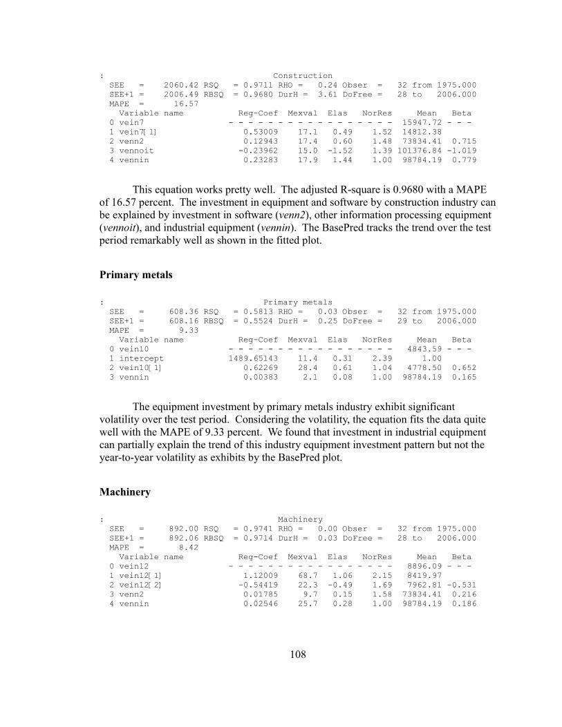
This equation works pretty well. The adjusted R-square is 0.9680 with a MAPE of 16.57 percent. The investment in equipment and software by construction industry can be explained by investment in software (venn2), other information processing equipment (vennoit), and industrial equipment (vennin). The BasePred tracks the trend over the test period remarkably well as shown in the fitted plot.
Primary metals
The equipment investment by primary metals industry exhibit significant volatility over the test period. Considering the volatility, the equation fits the data quite well with the MAPE of 9.33 percent. We found that investment in industrial equipment can partially explain the trend of this industry equipment investment pattern but not the year-to-year volatility as exhibits by the BasePred plot.
Machinery
108
: Construction SEE = 2060.42 RSQ = 0.9711 RHO = 0.24 Obser = 32 from 1975.000 SEE+1 = 2006.49 RBSQ = 0.9680 DurH = 3.61 DoFree = 28 to 2006.000 MAPE = 16.57 Variable name Reg-Coef Mexval Elas NorRes Mean Beta 0 vein7 - - - - - - - - - - - - - - - - - 15947.72 - - - 1 vein7[1] 0.53009 17.1 0.49 1.52 14812.38 2 venn2 0.12943 17.4 0.60 1.48 73834.41 0.715 3 vennoit -0.23962 15.0 -1.52 1.39 101376.84 -1.019 4 vennin 0.23283 17.9 1.44 1.00 98784.19 0.779
: Primary metals SEE = 608.36 RSQ = 0.5813 RHO = 0.03 Obser = 32 from 1975.000 SEE+1 = 608.16 RBSQ = 0.5524 DurH = 0.25 DoFree = 29 to 2006.000 MAPE = 9.33 Variable name Reg-Coef Mexval Elas NorRes Mean Beta 0 vein10 - - - - - - - - - - - - - - - - - 4843.59 - - - 1 intercept 1489.65143 11.4 0.31 2.39 1.00 2 vein10[1] 0.62269 28.4 0.61 1.04 4778.50 0.652 3 vennin 0.00383 2.1 0.08 1.00 98784.19 0.165
: Machinery SEE = 892.00 RSQ = 0.9741 RHO = 0.00 Obser = 32 from 1975.000 SEE+1 = 892.06 RBSQ = 0.9714 DurH = 0.03 DoFree = 28 to 2006.000 MAPE = 8.42 Variable name Reg-Coef Mexval Elas NorRes Mean Beta 0 vein12 - - - - - - - - - - - - - - - - - 8896.09 - - - 1 vein12[1] 1.12009 68.7 1.06 2.15 8419.97 2 vein12[2] -0.54419 22.3 -0.49 1.69 7962.81 -0.531 3 venn2 0.01785 9.7 0.15 1.58 73834.41 0.216 4 vennin 0.02546 25.7 0.28 1.00 98784.19 0.186

The equipment investment by machinery industry can be explained by investment in industrial equipment and software. This shows that, during the test period, the industry not only invested in industrial equipment (as it should) but also rely more heavily on computer controlled processes, both in design and manufacturing processes, as observed by the significant investment in software. The equation has a very good fit as shown by the closeness of fit statistics and the fitted plot. BasePred plots show promising forecasting power of this equation.
Computer and electronics products
With the same pattern as the machinery industry, the investment by computer and electronic products industry can be partially explained by the investment in software and industrial equipment. The manufacturing process of this industry is heavily dependent on the precision tools and machine. We observed a negative sign with the coefficient of the investment in software. I believe the reason behind this negative effect is that, during the test period, the economy has become more information oriented which shows in the needs of better software while the computer industry, which is capital intensive, has been investing at a slower rate. The relative growth is shown here as a negative coefficient.
Overall, the equation performs well over the test period in both the closeness of fit statistics and the fitted plots.
Food, beverage and tobacco products
109
: Computer and electronic products SEE = 2285.66 RSQ = 0.9513 RHO = 0.31 Obser = 32 from 1975.000 SEE+1 = 2190.37 RBSQ = 0.9461 DurH = 2.16 DoFree = 28 to 2006.000 MAPE = 16.69 Variable name Reg-Coef Mexval Elas NorRes Mean Beta 0 vein13 - - - - - - - - - - - - - - - - - 16035.47 - - - 1 intercept -7115.13817 22.2 -0.44 20.54 1.00 2 vein13[1] 0.58715 46.6 0.56 1.94 15296.00 0.591 3 vennin 0.18203 38.3 1.12 1.29 98784.19 0.713 4 venn2 -0.05163 13.4 -0.24 1.00 73834.41 -0.334
: Food, beverage, and tobacco products SEE = 466.24 RSQ = 0.9767 RHO = 0.18 Obser = 32 from 1975.000 SEE+1 = 460.07 RBSQ = 0.9751 DurH = 1.11 DoFree = 29 to 2006.000 MAPE = 4.34 Variable name Reg-Coef Mexval Elas NorRes Mean Beta 0 vein19 - - - - - - - - - - - - - - - - - 8880.84 - - - 1 vein19[1] 0.88258 130.5 0.85 1.53 8557.38 2 vennoit -0.03038 23.0 -0.35 1.45 101376.84 -0.513 3 vennin 0.04452 20.6 0.50 1.00 98784.19 0.591

The equation for investment in equipment and software by food, beverage, and tobacco industry performs very well with an adjusted R-square of 0.9751 and a MAPE of 4.34 percent. The investment in other information processing equipment and industrial equipment helps explains the general movement of the investment very well as shown by the BasePred plot.
Petroleum and coal
The equipment and software investment by petroleum and coal industry can be explained by the investment in industrial equipment and computer and peripheral. The equation fit the data quite well with a MAPE of 11.72 percent. The fitted plot shows that the equation moves the forecast quite well when the movement is small as shown by the BasePred plot. When there was a big year-to-year movement, the predicted value plot exhibits an observable lag.
Air transportation
We found that the equipment investment by air transportation industry can be explained by investment in transportation equipment and other nonresidential equipment. We can observed the effect from the timing of investment decision as the investment in air transportation equipment, i.e. airplanes, is generally a lengthy process. We observed higher coefficient value in the one-year lagged investment in transportation equipment and higher Mexval than the coefficient and Mexval of the current period investment in
110
: Petroleum and coal products SEE = 888.98 RSQ = 0.8402 RHO = 0.13 Obser = 32 from 1975.000 SEE+1 = 883.78 RBSQ = 0.8231 DurH = 1.36 DoFree = 28 to 2006.000 MAPE = 11.72 Variable name Reg-Coef Mexval Elas NorRes Mean Beta 0 vein24 - - - - - - - - - - - - - - - - - 5010.59 - - - 1 intercept -2171.01368 7.6 -0.43 6.26 1.00 2 vein24[1] 0.77371 40.1 0.72 1.24 4694.50 0.672 3 vennin 0.08162 10.9 1.61 1.20 98784.19 1.490 4 venn1 -0.09341 9.7 -0.90 1.00 48312.88 -1.287
: Air transportation SEE = 2200.78 RSQ = 0.9432 RHO = -0.02 Obser = 32 from 1975.000 SEE+1 = 2200.08 RBSQ = 0.9348 DurH = -0.15 DoFree = 27 to 2006.000 MAPE = 20.49 Variable name Reg-Coef Mexval Elas NorRes Mean Beta 0 vein29 - - - - - - - - - - - - - - - - - 11594.88 - - - 1 intercept -612.95837 0.5 -0.05 17.60 1.00 2 vein29[1] 0.56285 43.3 0.55 2.02 11231.75 0.572 3 venntr 0.06378 2.8 0.50 1.81 91518.56 0.301 4 venntr[1] 0.17218 15.1 1.29 1.67 86968.16 0.794 5 vennot -0.16848 29.4 -1.29 1.00 88589.03 -0.735

transportation equipment. Considering the exogenous shock to the industry in the early 2000s, our equation performs remarkably well with adjusted R-square of 0.9348 and well fitted plots of both the predicted value and the BasePred.
Information and data processing services
The equation shows a very good fit with an adjusted R-square of 0.9886. The investment in Software and other information processing equipment are found to be good predictors of this industry's investment in equipment and software. The fitted plot shows that the equation tracks the historical series very well over the test period and should provide a reliable forecast as suggested by the BasePred plot
Real estate
It is no surprise that the investment in residential equipment is the main predictor of equipment investment by real estate industry because, as mentioned earlier, the investment of residential equipment is all counted as a part of equipment investment by real estate industry by the BEA. The equation exhibits good fit in both the closeness of fit statistics and the fitted plot. From the fitted plot, I believe the very high investment by the industry in 2002 was caused by the September 11 2001 terrorist attack.
Educational services
111
: Information and data processing services SEE = 268.32 RSQ = 0.9893 RHO = 0.31 Obser = 32 from 1975.000 SEE+1 = 255.43 RBSQ = 0.9886 DurH = 2.08 DoFree = 29 to 2006.000 MAPE = 12.76 Variable name Reg-Coef Mexval Elas NorRes Mean Beta 0 vein40 - - - - - - - - - - - - - - - - - 2662.88 - - - 1 vein40[1] 0.60085 51.6 0.55 1.91 2420.69 2 venn2 0.01816 25.1 0.50 1.03 73834.41 0.469 3 vennoit -0.00148 1.4 -0.06 1.00 101376.84 -0.029
: Real estate SEE = 1385.17 RSQ = 0.9078 RHO = 0.16 Obser = 32 from 1975.000 SEE+1 = 1367.59 RBSQ = 0.9014 DW = 1.68 DoFree = 29 to 2006.000 MAPE = 8.68 Variable name Reg-Coef Mexval Elas NorRes Mean Beta 0 vein46 - - - - - - - - - - - - - - - - - 10930.16 - - - 1 intercept -1972.04229 8.5 -0.18 10.85 1.00 2 vennr 2.61965 62.0 1.35 1.04 5634.66 1.125 3 vennot -0.02098 2.2 -0.17 1.00 88589.03 -0.185
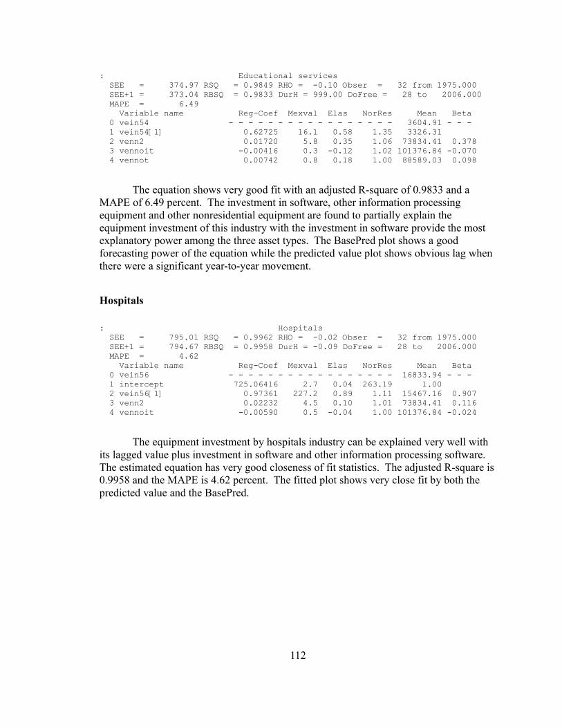
The equation shows very good fit with an adjusted R-square of 0.9833 and a MAPE of 6.49 percent. The investment in software, other information processing equipment and other nonresidential equipment are found to partially explain the equipment investment of this industry with the investment in software provide the most explanatory power among the three asset types. The BasePred plot shows a good forecasting power of the equation while the predicted value plot shows obvious lag when there were a significant year-to-year movement.
Hospitals
The equipment investment by hospitals industry can be explained very well with its lagged value plus investment in software and other information processing software. The estimated equation has very good closeness of fit statistics. The adjusted R-square is 0.9958 and the MAPE is 4.62 percent. The fitted plot shows very close fit by both the predicted value and the BasePred.
112
: Educational services SEE = 374.97 RSQ = 0.9849 RHO = -0.10 Obser = 32 from 1975.000 SEE+1 = 373.04 RBSQ = 0.9833 DurH = 999.00 DoFree = 28 to 2006.000 MAPE = 6.49 Variable name Reg-Coef Mexval Elas NorRes Mean Beta 0 vein54 - - - - - - - - - - - - - - - - - 3604.91 - - - 1 vein54[1] 0.62725 16.1 0.58 1.35 3326.31 2 venn2 0.01720 5.8 0.35 1.06 73834.41 0.378 3 vennoit -0.00416 0.3 -0.12 1.02 101376.84 -0.070 4 vennot 0.00742 0.8 0.18 1.00 88589.03 0.098
: Hospitals SEE = 795.01 RSQ = 0.9962 RHO = -0.02 Obser = 32 from 1975.000 SEE+1 = 794.67 RBSQ = 0.9958 DurH = -0.09 DoFree = 28 to 2006.000 MAPE = 4.62 Variable name Reg-Coef Mexval Elas NorRes Mean Beta 0 vein56 - - - - - - - - - - - - - - - - - 16833.94 - - - 1 intercept 725.06416 2.7 0.04 263.19 1.00 2 vein56[1] 0.97361 227.2 0.89 1.11 15467.16 0.907 3 venn2 0.02232 4.5 0.10 1.01 73834.41 0.116 4 vennoit -0.00590 0.5 -0.04 1.00 101376.84 -0.024

113
Figure 4.4: Plots of FAA by Purchasing Industries Estimation Results
Farms Farms nominal (Million dollars)
29639
19044
8449
1975 1980 1985 1990 1995 2000 2005 Predicted Actual BasePred
Forestry, fishing, and related activities Forestry, fishing, and related activities nominal (Million dollars)
3757
2247
736
1975 1980 1985 1990 1995 2000 2005 Predicted Actual BasePred
Oil and gas extraction Oil and gas extraction nominal (Million dollars)
10811
5964
1117
1975 1980 1985 1990 1995 2000 2005 Predicted Actual BasePred
Mining, except oil and gas Mining, except oil and gas nominal (Million dollars)
11421
6876
2330
1975 1980 1985 1990 1995 2000 2005 Predicted Actual BasePred
Support activites for mining Support activites for mining nominal (Million dollars)
9600
5344
1088
1975 1980 1985 1990 1995 2000 2005 Predicted Actual BasePred
Utilities Utilities nominal (Million dollars)
37619
22000
6380
1975 1980 1985 1990 1995 2000 2005 Predicted Actual BasePred
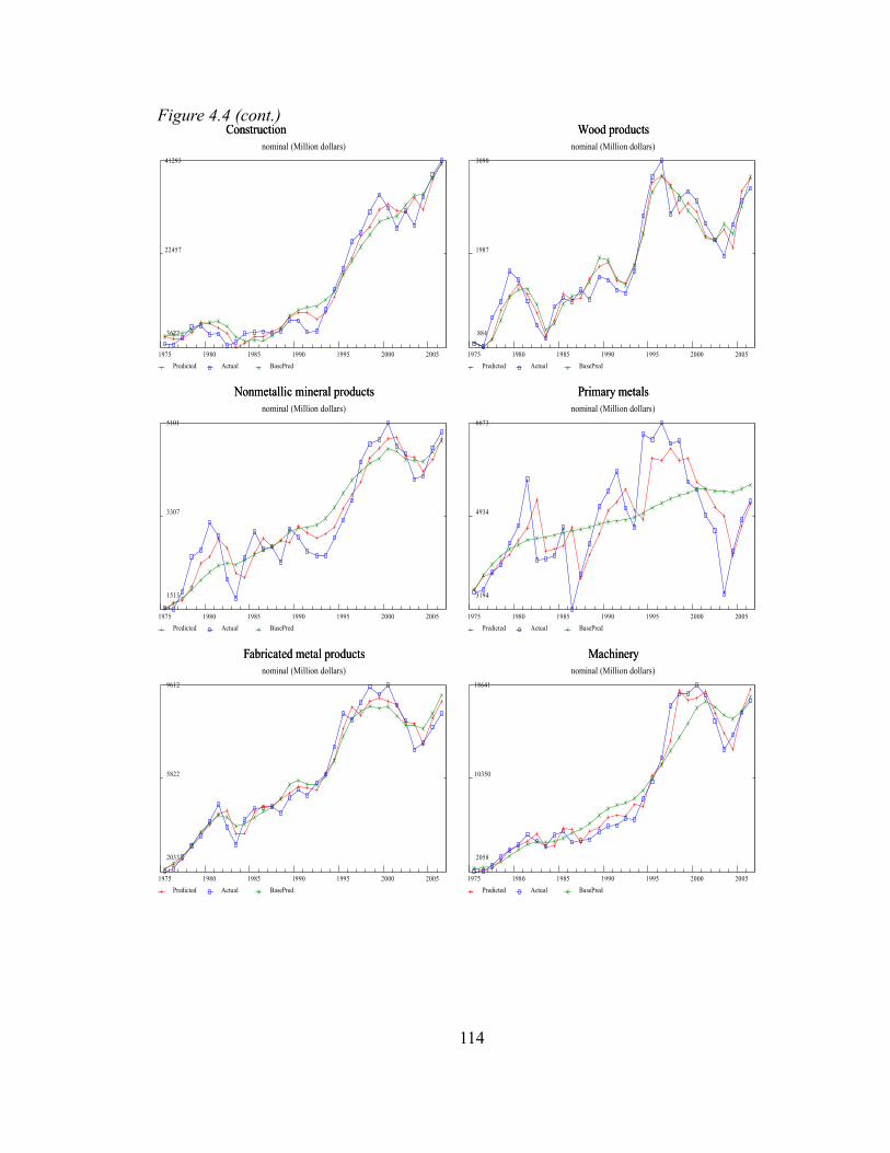
Figure 4.4 (cont.) Construction Construction
nominal (Million dollars)41293
22457
3622
1975 1980 1985 1990 1995 2000 2005 Predicted Actual BasePred
Wood products Wood products nominal (Million dollars)
3090
1987
884
1975 1980 1985 1990 1995 2000 2005 Predicted Actual BasePred
Nonmetallic mineral products Nonmetallic mineral products nominal (Million dollars)
5101
3307
1513
1975 1980 1985 1990 1995 2000 2005 Predicted Actual BasePred
Primary metals Primary metals nominal (Million dollars)
6673
4934
3194
1975 1980 1985 1990 1995 2000 2005 Predicted Actual BasePred
Fabricated metal products Fabricated metal products nominal (Million dollars)
9612
5822
2033
1975 1980 1985 1990 1995 2000 2005 Predicted Actual BasePred
Machinery Machinery nominal (Million dollars)
18641
10350
2058
1975 1980 1985 1990 1995 2000 2005 Predicted Actual BasePred
114

Figure 4.4 (cont.) Computer and electronic products Computer and electronic products
nominal (Million dollars)37494
18156
-1183
1975 1980 1985 1990 1995 2000 2005 Predicted Actual BasePred
Electrical equipment, appliances, and components Electrical equipment, appliances, and components nominal (Million dollars)
4314
2505
695
1975 1980 1985 1990 1995 2000 2005 Predicted Actual BasePred
Motor vehicles, bodies and trailers, and parts Motor vehicles, bodies and trailers, and parts nominal (Million dollars)
16267
8617
967
1975 1980 1985 1990 1995 2000 2005 Predicted Actual BasePred
Other transportation equipment Other transportation equipment nominal (Million dollars)
9798
5304
810
1975 1980 1985 1990 1995 2000 2005 Predicted Actual BasePred
Furniture and related products Furniture and related products nominal (Million dollars)
1907
1009
110
1975 1980 1985 1990 1995 2000 2005 Predicted Actual BasePred
Miscellaneous manufacturing Miscellaneous manufacturing nominal (Million dollars)
4682
2812
941
1975 1980 1985 1990 1995 2000 2005 Predicted Actual BasePred
115

Figure 4.4 (cont.) Food, beverage, and tobacco products Food, beverage, and tobacco products
nominal (Million dollars)12816
7846
2877
1975 1980 1985 1990 1995 2000 2005 Predicted Actual BasePred
Textile mills and textile product mills Textile mills and textile product mills nominal (Million dollars)
3591
2153
714
1975 1980 1985 1990 1995 2000 2005 Predicted Actual
Apparel and leather and allied products Apparel and leather and allied products nominal (Million dollars)
1349
786
223
1975 1980 1985 1990 1995 2000 2005 Predicted Actual BasePred
Paper products Paper products nominal (Million dollars)
10529
6526
2522
1975 1980 1985 1990 1995 2000 2005 Predicted Actual BasePred
Printing and related support activities Printing and related support activities nominal (Million dollars)
4982
2824
665
1975 1980 1985 1990 1995 2000 2005 Predicted Actual BasePred
Petroleum and coal products Petroleum and coal products nominal (Million dollars)
11829
6548
1268
1975 1980 1985 1990 1995 2000 2005 Predicted Actual BasePred
116
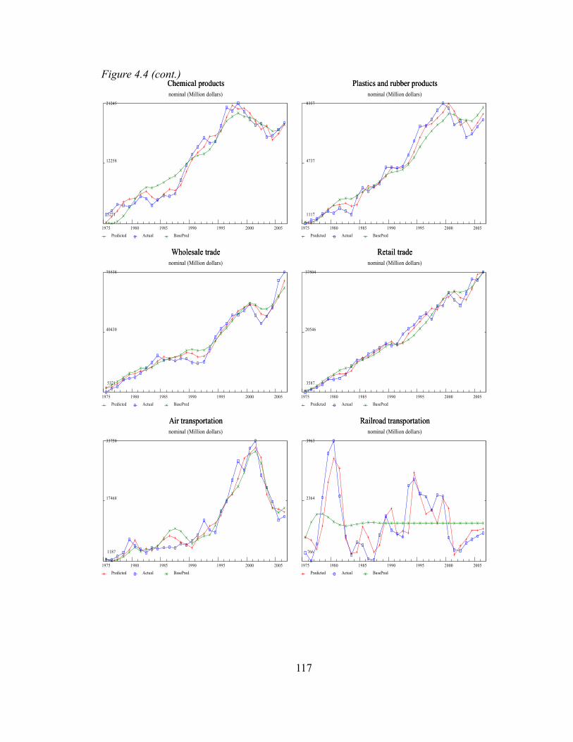
Figure 4.4 (cont.) Chemical products Chemical products nominal (Million dollars)
21245
12258
3271
1975 1980 1985 1990 1995 2000 2005 Predicted Actual BasePred
Plastics and rubber products Plastics and rubber products nominal (Million dollars)
8357
4737
1117
1975 1980 1985 1990 1995 2000 2005 Predicted Actual BasePred
Wholesale trade Wholesale trade nominal (Million dollars)
75538
40430
5321
1975 1980 1985 1990 1995 2000 2005 Predicted Actual BasePred
Retail trade Retail trade nominal (Million dollars)
37504
20546
3587
1975 1980 1985 1990 1995 2000 2005 Predicted Actual BasePred
Air transportation Air transportation nominal (Million dollars)
33750
17468
1187
1975 1980 1985 1990 1995 2000 2005 Predicted Actual BasePred
Railroad transportation Railroad transportation nominal (Million dollars)
3963
2364
766
1975 1980 1985 1990 1995 2000 2005 Predicted Actual BasePred
117

Figure 4.4 (cont.) Water transportation Water transportation
nominal (Million dollars) 5349
3241
1133
1975 1980 1985 1990 1995 2000 2005 Predicted Actual BasePred
Truck transportation Truck transportation nominal (Million dollars)
19647
10653
1659
1975 1980 1985 1990 1995 2000 2005 Predicted Actual BasePred
Transit and ground passenger transportation Transit and ground passenger transportation nominal (Million dollars)
4085
2066
47
1975 1980 1985 1990 1995 2000 2005 Predicted Actual BasePred
Pipeline transportation Pipeline transportation nominal (Million dollars)
2853
1513
173
1975 1980 1985 1990 1995 2000 2005 Predicted Actual BasePred
Other transportation and support activites Other transportation and support activites nominal (Million dollars)
9155
5641
2127
1975 1980 1985 1990 1995 2000 2005 Predicted Actual BasePred
Warehousing and storage Warehousing and storage nominal (Million dollars)
2220
1168
117
1975 1980 1985 1990 1995 2000 2005 Predicted Actual BasePred
118

Figure 4.4 (cont.) Publishing industries (including software) Publishing industries (including software)
nominal (Million dollars) 7655
4133
611
1975 1980 1985 1990 1995 2000 2005 Predicted Actual BasePred
Motion picture and sound recording industries Motion picture and sound recording industries nominal (Million dollars)
2736
1541
347
1975 1980 1985 1990 1995 2000 2005 Predicted Actual BasePred
Broadcasting and telecommunications Broadcasting and telecommunications nominal (Million dollars)
107363
56073
4783
1975 1980 1985 1990 1995 2000 2005 Predicted Actual BasePred
Information and data processing services Information and data processing services nominal (Million dollars)
7984
4069
153
1975 1980 1985 1990 1995 2000 2005 Predicted Actual BasePred
Federal Reserve banks Federal Reserve banks nominal (Million dollars)
2587
1183
-221
1975 1980 1985 1990 1995 2000 2005 Predicted Actual BasePred
Credit intermediation and related activities Credit intermediation and related activities nominal (Million dollars)
70206
37528
4850
1975 1980 1985 1990 1995 2000 2005 Predicted Actual BasePred
119

Figure 4.4 (cont.) Securities, commodity contracts, and investments Securities, commodity contracts, and investments
nominal (Million dollars)13528
7029
529
1975 1980 1985 1990 1995 2000 2005 Predicted Actual BasePred
Insurance carriers and related activities Insurance carriers and related activities nominal (Million dollars)
19836
10509
1183
1975 1980 1985 1990 1995 2000 2005 Predicted Actual BasePred
Funds, trusts, and other financial vehicles Funds, trusts, and other financial vehicles nominal (Million dollars)
2343
1227
110
1975 1980 1985 1990 1995 2000 2005 Predicted Actual BasePred
Real estate Real estate nominal (Million dollars)
20626
11540
2454
1975 1980 1985 1990 1995 2000 2005 Predicted Actual
Rental and leasing services and lessors of intangible assets Rental and leasing services and lessors of intangible assets nominal (Million dollars)
78572
36592
-5389
1975 1980 1985 1990 1995 2000 2005 Predicted Actual BasePred
Legal services Legal services nominal (Million dollars)
3277
1685
94
1975 1980 1985 1990 1995 2000 2005 Predicted Actual BasePred
120

Figure 4.4 (cont.) Computer systems design and related services Computer systems design and related services
nominal (Million dollars)20126
9966
-194
1975 1980 1985 1990 1995 2000 2005 Predicted Actual BasePred
Miscellaneous professional, scientific, and technical services Miscellaneous professional, scientific, and technical services nominal (Million dollars)
63337
32198
1060
1975 1980 1985 1990 1995 2000 2005 Predicted Actual BasePred
Management of companies and enterprises Management of companies and enterprises nominal (Million dollars)
24585
13202
1818
1975 1980 1985 1990 1995 2000 2005 Predicted Actual BasePred
Administrative and support services Administrative and support services nominal (Million dollars)
23994
12152
309
1975 1980 1985 1990 1995 2000 2005 Predicted Actual BasePred
Waste management and remediation services Waste management and remediation services nominal (Million dollars)
3533
1963
394
1975 1980 1985 1990 1995 2000 2005 Predicted Actual BasePred
Educational services Educational services nominal (Million dollars)
10113
5368
623
1975 1980 1985 1990 1995 2000 2005 Predicted Actual BasePred
121
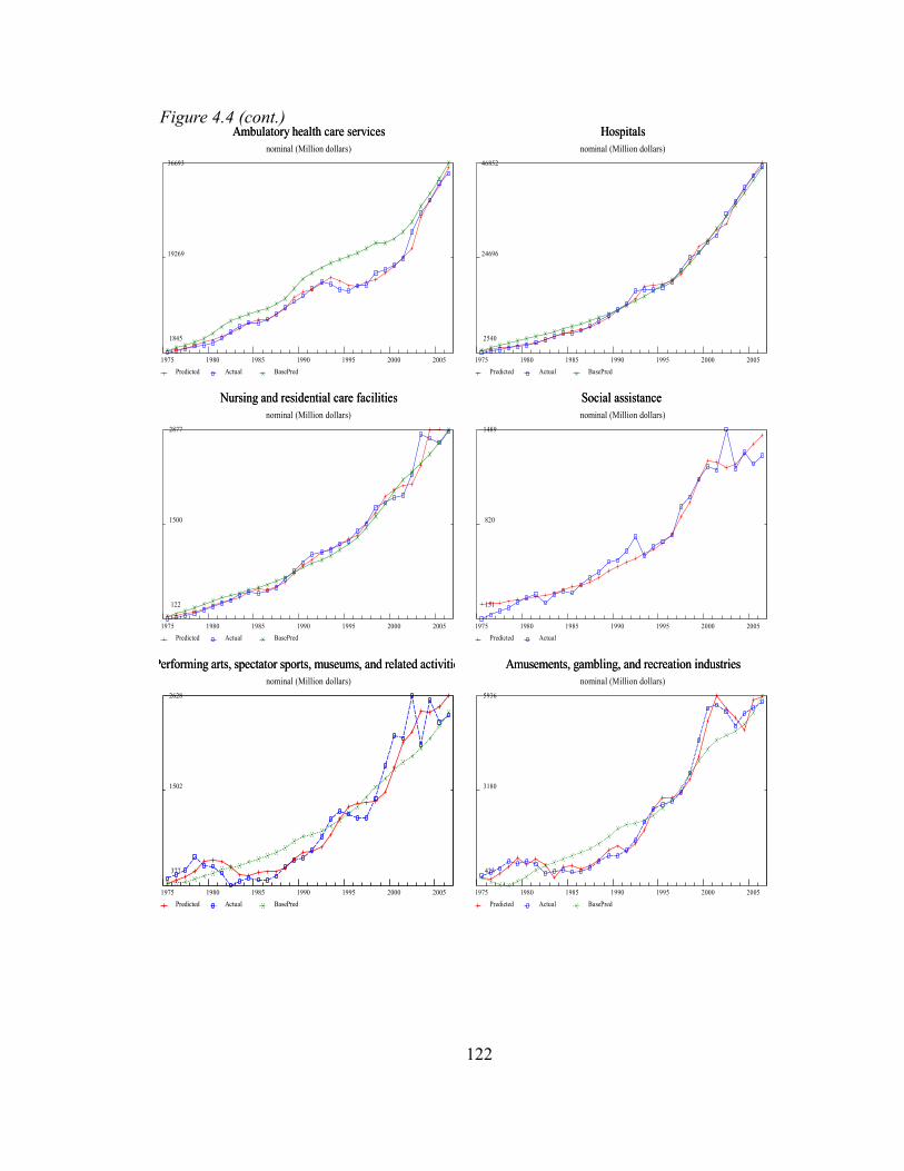
Figure 4.4 (cont.) Ambulatory health care services Ambulatory health care services
nominal (Million dollars)36693
19269
1845
1975 1980 1985 1990 1995 2000 2005 Predicted Actual BasePred
Hospitals Hospitals nominal (Million dollars)
46852
24696
2540
1975 1980 1985 1990 1995 2000 2005 Predicted Actual BasePred
Nursing and residential care facilities Nursing and residential care facilities nominal (Million dollars)
2877
1500
122
1975 1980 1985 1990 1995 2000 2005 Predicted Actual BasePred
Social assistance Social assistance nominal (Million dollars)
1489
820
151
1975 1980 1985 1990 1995 2000 2005 Predicted Actual
Performing arts, spectator sports, museums, and related activities Performing arts, spectator sports, museums, and related activities nominal (Million dollars)
2628
1502
377
1975 1980 1985 1990 1995 2000 2005 Predicted Actual BasePred
Amusements, gambling, and recreation industries Amusements, gambling, and recreation industries nominal (Million dollars)
5936
3180
423
1975 1980 1985 1990 1995 2000 2005 Predicted Actual BasePred
122

Figure 4.4 (cont.) Accommodation Accommodation
nominal (Million dollars) 5682
3070
458
1975 1980 1985 1990 1995 2000 2005 Predicted Actual BasePred
Food services and drinking places Food services and drinking places nominal (Million dollars)
23620
12785
1949
1975 1980 1985 1990 1995 2000 2005 Predicted Actual BasePred
Other services, except government Other services, except government nominal (Million dollars)
9444
5876
2309
1975 1980 1985 1990 1995 2000 2005 Predicted Actual BasePred
4.5 Historical Simulations
Using the earlier described approach, I produced two historical simulations to test the method's performance. Using the same idea as described in Chapter 3, two historical forecasts, one with all actual exogenous variables and one with exogenous variables generated by QUEST, are generated for 2005 and 2006. The assumptions of exogenous variables used in the historical simulation with QUEST (the second simulation) is shown in Table 4.7.
“The first simulation” refers to the historical simulation with actual exogenous variables and “The second simulation” refers to the historical simulation with exogenous variables generated from QUEST and other ad hoc assumptions.
123

We can compare numbers in Table 4.7 with the actual number from the BEA18. First, please note that the price index of nonresidential equipment and software fixed investment inputs are actually the published BEA numbers because QUEST does not provided the price indexes required.
Our assumption for nominal fixed investment in nonresidential equipment is approximately 10% higher than the actual BEA numbers. At the same time, QUEST's numbers for the nominal residential fixed investment are generally lower than the BEA values, especially in 2005. QUEST predicted that the residential fixed investment would expand steadily in both 2005 and 2006. What actually happened is that residential fixed investment expanded rapidly in 2005 and started to slow down in 2006. Historically, only about one to two percent of total residential fixed investment is residential fixed investment in equipment. This underestimation of the residential fixed investment should have minimal effect on the performance of the second simulation.
Table 4.8 and Table 4.9 show the differences between each historical simulation and the published numbers. We can also observe how these differences in exogenous inputs affect the performance of the equations. Figure 4.5 graphically presents these differences by major industry groups.
18 http://www.bea.gov/national/nipaweb/SelectTable.asp
124
Table 4.7: Assumptions of exogenous variables used in the Second Historical Simulation2005Q1 2005Q2 2005Q3 2005Q4
vfnre Nominal value of Nonresidential Equipment and Software fixed investment 1027.41 1027.78 1037.52 1046.97pvfnre Price index of Nonresidential Equipment and Software fixed investment 94.76 94.83 94.24 94.29vfr Nominal value of Residential investment 686.01 700.45 720.79 729.85
2006Q1 2006Q2 2006Q3 2006Q4vfnre Nominal value of Nonresidential Equipment and Software fixed investment 1044.79 1049.36 1058.59 1073.27pvfnre Price index of Nonresidential Equipment and Software fixed investment 94.43 94.38 94.47 94.67vfr Nominal value of Residential investment 732.88 743.59 750.72 761.58
All nominal values are in Billions of dollars
Percentage difference from the actual value 2005Q1 2005Q2 2005Q3 2005Q4
vfnre Nominal value of Nonresidential Equipment and Software fixed investment 12.94% 10.88% 8.88% 9.00%pvfnre Price index of Nonresidential Equipment and Software fixed investment 0.00% 0.00% 0.00% 0.01%vfr Nominal value of Residential investment -5.72% -7.45% -8.26% -9.11%
2006Q1 2006Q2 2006Q3 2006Q4
vfnre Nominal value of Nonresidential Equipment and Software fixed investment 5.35% 5.88% 5.95% 8.55%pvfnre Price index of Nonresidential Equipment and Software fixed investment 0.01% 0.00% 0.00% 0.00%vfr Nominal value of Residential investment -9.45% -5.66% 0.62% 6.47%

From the 63 detailed industries' results shown in Table 4.9, I aggregated the results into 19 industry groups as shown in Table 4.8. I will discuss only the nominal values in this section as BEA does not publish real values or price indexes of Fixed Assets.
125
Table 4.8: Historical Simulations' Results in Major Investment Industries, Nominal
Percentage difference from the published value 2005 2006 2005 2006 Total Private fixed assets 1.47% 1.43% 8.72% 8.04% Agriculture, forestry, fishing, and hunting 4.16% 7.79% 5.98% 6.17% Mining 2.06% 3.44% 11.72% 6.01% Utilities -6.94% -8.65% -5.20% -2.63% Construction 3.46% 2.06% -1.02% -6.46% Manufacturing -1.77% -0.04% -3.53% -0.15% Durable goods -0.34% 2.75% -1.54% 4.15% Nondurable goods -3.87% -4.15% -6.46% -6.47% Wholesale trade -9.46% -9.69% -2.76% -4.48% Retail trade 8.20% 4.99% 10.85% 8.08% Transportation and warehousing 2.83% 2.12% 28.73% 26.92% Information 2.05% 2.09% 28.16% 30.80% Finance and insurance 8.31% 7.01% 22.21% 22.95% Real estate and rental and leasing 1.76% 5.58% 25.16% 18.06% Professional, scientific, and technical services 0.31% -1.82% 1.75% 0.98% Management of companies and enterprises\5\ 11.66% 6.35% 11.33% 8.25% Administrative and waste management services 7.02% 3.65% 8.02% 5.90% Educational services 11.52% 8.12% 11.44% 9.51% Health care and social assistance -0.09% 1.11% -2.70% -0.68% Arts, entertainment, and recreation 10.23% 14.04% 12.21% 14.76% Accommodation and food services 2.13% -0.62% 4.36% -1.65% Other services, except government 8.44% 7.20% 9.14% 9.29%
1st Sim 2nd Sim
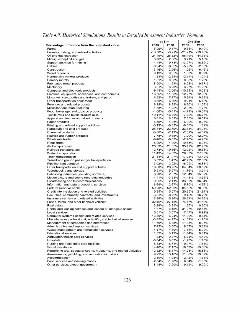
126
Table 4.9: Historical Simulations' Results in Detailed Investment Industries, Nominal
Percentage difference from the published value 2005 2006 2005 2006 Farms 5.99% 9.17% 9.35% 9.40% Forestry, fishing, and related activities -10.58% -3.21% -21.21% -19.46% Oil and gas extraction 24.49% 26.52% 56.49% 44.73% Mining, except oil and gas 3.76% 2.66% 9.21% 5.15% Support activites for mining -14.44% -9.73% -13.97% -16.62% Utilities -6.94% -8.65% -5.20% -2.63% Construction 3.46% 2.06% -1.02% -6.46% Wood products 9.19% 9.85% 1.80% 0.87% Nonmetallic mineral products -1.83% -2.84% -2.14% -1.04% Primary metals 1.61% 0.38% 0.98% 1.23% Fabricated metal products 8.90% 11.24% 6.08% 9.77% Machinery 3.81% 8.70% 3.27% 11.28% Computer and electronic products -9.43% -2.06% -10.23% 0.03% Electrical equipment, appliances, and components 18.75% 11.98% 12.77% 12.90% Motor vehicles, bodies and trailers, and parts 6.82% 7.27% 5.84% 9.38% Other transportation equipment -8.60% -6.60% -9.21% -5.13% Furniture and related products 6.88% 8.99% 6.60% 11.59% Miscellaneous manufacturing -1.68% -4.22% -2.05% -1.75% Food, beverage, and tobacco products -1.66% -5.41% -4.71% -10.04% Textile mills and textile product mills 10.11% 16.55% -7.72% 26.77% Apparel and leather and allied products 6.01% 8.52% 7.35% 16.57% Paper products 6.55% 4.38% 6.99% 9.24% Printing and related support activities -0.13% -0.33% -0.50% 1.82% Petroleum and coal products -28.84% -23.79% -33.71% -34.03% Chemical products -0.06% -2.12% -2.39% -4.67% Plastics and rubber products 7.78% 9.68% 7.29% 12.27% Wholesale trade -9.46% -9.69% -2.76% -4.48% Retail trade 8.20% 4.99% 10.85% 8.08% Air transportation 25.39% 21.35% 35.42% 82.90% Railroad transportation 12.73% 19.16% 12.92% 19.58% Water transportation 11.49% 14.03% 28.63% 27.03% Truck transportation -21.54% -21.47% 17.05% -13.49% Transit and ground passenger transportation 3.39% 1.42% 42.72% 22.63% Pipeline transportation 3.02% 2.22% 16.99% 16.88% Other transportation and support activites 19.80% 26.75% 64.84% 59.52% Warehousing and storage 9.91% 5.57% 11.76% 3.94% Publishing industries (including software) 6.70% 2.07% 12.34% 15.62% Motion picture and sound recording industries -4.41% -3.53% -4.43% -3.92% Broadcasting and telecommunications 0.95% 2.11% 33.89% 36.94% Information and data processing services 6.69% 2.67% 5.70% 4.56% Federal Reserve banks 59.20% 52.30% 84.52% 78.93% Credit intermediation and related activities 5.85% 5.67% 20.35% 21.91% Securities, commodity contracts, and investments -3.81% -8.72% 9.46% 16.76% Insurance carriers and related activities 17.96% 15.96% 26.61% 24.26% Funds, trusts, and other financial vehicles 32.46% 27.13% 74.47% 41.59% Real estate 3.29% 3.31% 1.35% 0.60% Rental and leasing services and lessors of intangible assets 1.37% 6.16% 31.27% 22.54% Legal services 5.51% 3.57% 7.47% 8.99% Computer systems design and related services 13.50% 5.24% 11.90% 9.54% Miscellaneous professional, scientific, and technical services -3.82% -4.17% -1.52% -1.95% Management of companies and enterprises 11.66% 6.35% 11.33% 8.25% Administrative and support services 7.42% 3.50% 8.07% 5.89% Waste management and remediation services 4.17% 4.69% 7.66% 5.92% Educational services 11.52% 8.12% 11.44% 9.51% Ambulatory health care services -1.43% 0.87% -6.34% -4.40% Hospitals -0.04% 0.63% -1.23% 1.16% Nursing and residential care facilities 8.83% 6.71% 9.27% 7.51% Social assistance 14.46% 12.15% 16.57% 15.68% Performing arts, spectator sports, museums, and related activities 12.52% 16.17% 14.23% 16.83% Amusements, gambling, and recreation industries 9.29% 13.16% 11.38% 13.89% Accommodation 2.50% 4.28% -2.42% -1.73% Food services and drinking places 2.04% -1.78% 6.04% -1.63% Other services, except government 8.44% 7.20% 9.14% 9.29%
1st Sim 2nd Sim

Overall, our equations can predict the fixed investment by all private industries very well, at least during the 2005 and 2006 historical simulation period, when we can predict exactly what the exogenous variables will be. The first simulation misses the FAA total by 1.47% in 2005 and 1.43% in 2006. At the same time, the second simulation performs not as good as the first simulation. The second simulation missed the FAA fixed investment by all private industries by 8.72% in 2005 and 8.04% in 2006. This overestimation errors of the second simulation is in line with the overestimation of private fixed investment in nonresidential equipment and software, described earlier.
For equipment investment by Agriculture, forestry, fishing, and hunting, the first simulation missed the BEA numbers by 4.16% and 7.79% in 2005 and 2006, respectively. The second simulation missed the same numbers by 5.98% and 6.17% in 2005 and 2006, respectively. Both simulations show relatively comparable performance in predicting fixed investment in equipment by Agriculture, forestry, fishing, and hunting. However, the detailed results, shown in Table 4.9, tell a different story. The first simulation performs better than the second simulation in predicting the equipment fixed investment by both Farms and Forestry, fishing, and related activities. Both simulations overestimate the investment in Farms and underestimate the investment in Forestry, fishing, and hunting industries.
The first simulation missed the equipment fixed investment by Mining by 2.06% in 2005 and 3.44% in 2006. the second simulation missed the same numbers by 11.72% and 6.01% in 2005 and 2006, respectively. Most of the errors from both simulations come from the oil and gas extraction industry. The second simulation overestimate the expansion by 56.49% in 2005 and 44.73% in 2006.
For fixed investment in equipment by utilities industry, the second simulation provided a better forecast than the first simulation. Out-performing the second simulation, the first simulation performs quite well with errors of -6.94% in 2005 and -8.65% in 2006.
For the investment by construction industry, the first simulation overestimates the published numbers with errors of 3.46% in 2005 and 2.06% in 2006. The second simulation missed the same numbers by -1.02% in 2005 and -6.46% in 2006.
The first simulation performs very well in predicting the equipment investment by Manufacturing. It missed the published numbers by -1.77% in 2005 and -0.04% in 2006. The second simulation performs relatively well with errors of -3.53% in 2005 and -0.15% in 2006. From the detailed industries' forecast, most of the underestimation by both simulations in 2005 comes from nondurable goods manufacturing industries. In 2006, both simulations overestimate the investment by durable goods manufacturing and underestimate the investment by nondurable goods manufacturing. The underestimated forecast of the equipment fixed investment by the computer and electronic products, which contributes around 30% to the durable goods manufacturing investment, is the main contributor to the slightly underestimation of the equipment investment by durable
127

goods manufacturing. For nondurable goods manufacturing equipment investment, the underestimated forecasts of investment by Food, beverage, and tobacco products and investment by petroleum and coal products are the two main sources of errors in the second simulation forecast of nondurable manufacturing equipment investment.
For Wholesale trade equipment investment, the first simulation missed the published numbers by -9.46% and -9.69% in 2005 and 2006, respectively. The second simulation missed the same number by -2.76% in 2005 and -4.48%, respectively.
The equipment investment by Retail trade is overestimated by the first simulation with errors of 8.20% in 2005 and 4.99% in 2006. The second simulation missed the same number by 10.85% in 2005 and 8.08% in 2006.
Overall, the first simulation can predict most of the major components of equipment investment by Service industries. The first simulation forecast of the Finance and insurance industry, the biggest component of nominal fixed investment in equipment by services industries, is not as good as the forecast of other major components such as Real estate and rental and leasing, Professional, scientific, and technical services, and Health care and social services. The first simulation missed the published numbers of Finance and insurance investment by 8.31% in 2005 and 7.01% in 2006. Three industry groups, with the forecast errors by the first simulation over ten percent, are 1) Management of companies and enterprises, 2) Educational services, and 3) Arts, entertainment, and recreation. For these three industry groups, the second simulation generated relative the same magnitude of errors in each industry.
However, the second simulation performs a lot worse than the first simulation in most of the big components of the equipment investment in services industry. Four industry groups have forecast errors by the second simulation bigger than 20% in both 2005 and 2006. These four industries are 1) Transportation and warehousing, 2) Information, 3) Finance and insurance, and 4) Real estate and rental and leasing.
From Table 4.9, the source of the significant errors in these four industry groups is that the second simulation forecast significantly missed the biggest component of each of the four industry groups. For Transportation and warehousing equipment investment, the second simulation missed its biggest component, Air transportation, by 35.42% in 2005 and 82.90% in 2006. For Information industry equipment investment, the second simulation missed the published numbers of equipment investment by Broadcasting and telecommunication industry by 33.89% and 36.94% in 2005 and 2006, respectively. For Finance and insurance industry equipment investment, the second simulation missed the published numbers of equipment investment by Credit intermediation and related activities industry by 20.35% in 2005 and 21.91% in 2006. Lastly, for Real estate and rental and leasing industry, the second simulation missed the published numbers of equipment investment by Rental and leasing services by 31.27% and 22.54% in 2005 and 2006, respectively.
128
With the results from the first and the second simulation, we observe that our approach can forecast the nominal fixed investment by major industry groups quite well when we have accurate exogenous inputs, i.e. the first historical simulation. Specifically, the accuracy of the nonresidential fixed investment in equipment and software directly affects the accuracy of the approach, especially in the forecast of equipment investment by Service industries, as Service industries fixed investment is typically mostly in equipment and software.
129

1 Total Equipment Investment 1 Total Equipment Investment Nominal
1074866
745942
417018
1990 1995 2000 2005 a.veintot b.veintot mveintot
2 Agriculture, forestry, fishing and hunting 2 Agriculture, forestry, fishing and hunting Nominal
34764
24595
14425
1990 1995 2000 2005 a.veinagri b.veinagri mveinagri
3 Mining 3 Mining Nominal
28501
18637
8773
1990 1995 2000 2005 a.veinmin b.veinmin mveinmin
4 Utilities 4 Utilities Nominal
37619
30601
23583
1990 1995 2000 2005 a.veinutil b.veinutil mveinutil
5 Construction 5 Construction Nominal
42143
24415
6687
1990 1995 2000 2005 a.veinconst b.veinconst mveinconst
6 Manufacturing 6 Manufacturing Nominal
171773
135614
99456
1990 1995 2000 2005 a.veinmanu b.veinmanu mveinmanu
130
Figure 4.5: Plots compared BEA numbers with numbers from Historical Simulations

Figure 4.5 (cont.)
7 Durable goods Manufacturing 7 Durable goods Manufacturing Nominal
109545
80177
50809
1990 1995 2000 2005 a.veindmanu b.veindmanu mveindmanu
8 Nondurable goods Manufacturing 8 Nondurable goods Manufacturing Nominal
63914
56280
48647
1990 1995 2000 2005 a.veinnmanu b.veinnmanu mveinnmanu
9 Wholesale 9 Wholesale Nominal
75538
48928
22319
1990 1995 2000 2005 a.veinwhsl b.veinwhsl mveinwhsl
10 Retail 10 Retail Nominal
40535
28606
16677
1990 1995 2000 2005 a.veinrtl b.veinrtl mveinrtl
11 Transportation and warehousing 11 Transportation and warehousing Nominal
66935
44772
22610
1990 1995 2000 2005 a.veintr b.veintr mveintr
12 Information 12 Information Nominal
121749
81201
40653
1990 1995 2000 2005 a.veininfo b.veininfo mveininfo
131
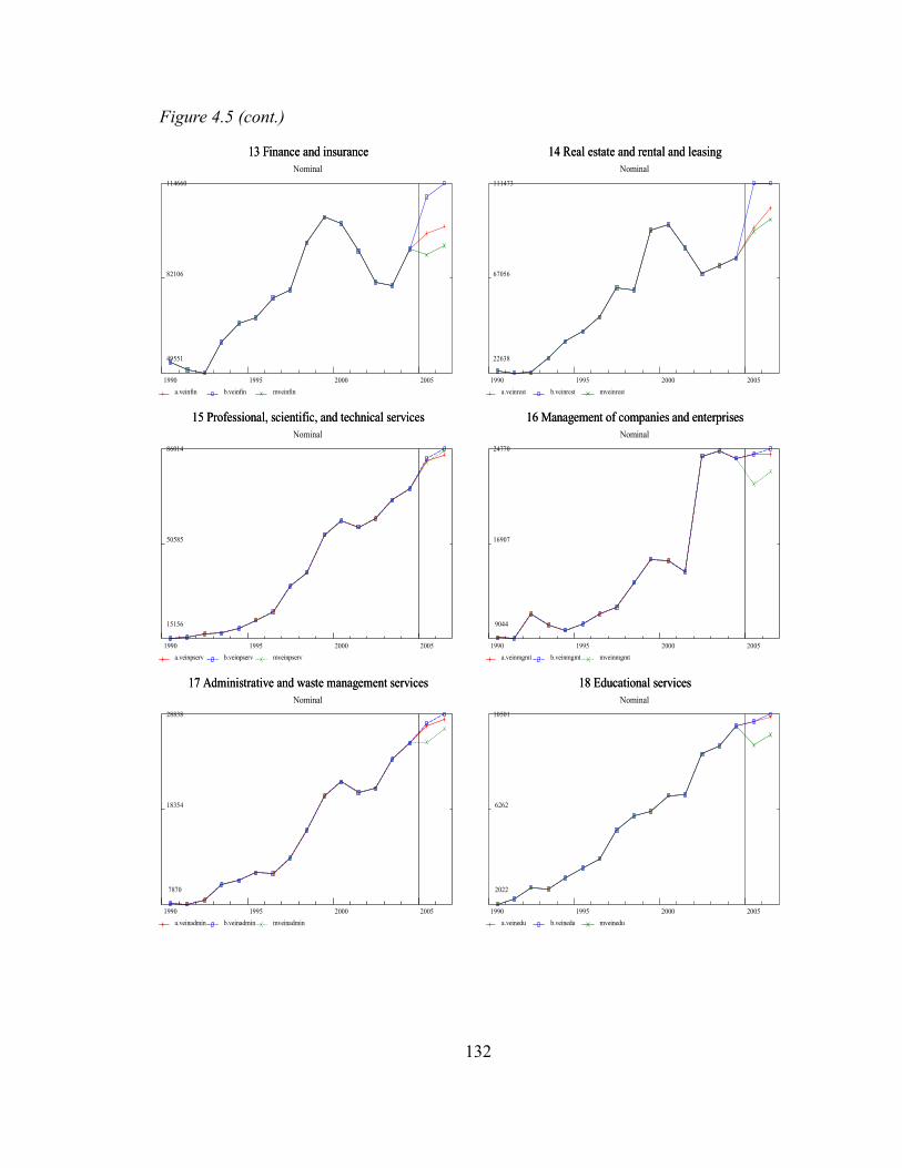
Figure 4.5 (cont.)
13 Finance and insurance 13 Finance and insurance Nominal
114660
82106
49551
1990 1995 2000 2005 a.veinfin b.veinfin mveinfin
14 Real estate and rental and leasing 14 Real estate and rental and leasing Nominal
111473
67056
22638
1990 1995 2000 2005 a.veinrest b.veinrest mveinrest
15 Professional, scientific, and technical services 15 Professional, scientific, and technical services Nominal
86014
50585
15156
1990 1995 2000 2005 a.veinpserv b.veinpserv mveinpserv
16 Management of companies and enterprises 16 Management of companies and enterprises Nominal
24770
16907
9044
1990 1995 2000 2005 a.veinmgmt b.veinmgmt mveinmgmt
17 Administrative and waste management services 17 Administrative and waste management services Nominal
28838
18354
7870
1990 1995 2000 2005 a.veinadmin b.veinadmin mveinadmin
18 Educational services 18 Educational services Nominal
10501
6262
2022
1990 1995 2000 2005 a.veinedu b.veinedu mveinedu
132

Figure 4.5 (cont.)
19 Health care and social assistance 19 Health care and social assistance Nominal
85963
56176
26388
1990 1995 2000 2005 a.veinmc b.veinmc mveinmc
20 Arts, entertainment and recreation 20 Arts, entertainment and recreation Nominal
9346
5656
1966
1990 1995 2000 2005 a.veinrec b.veinrec mveinrec
21 Accommodation and food services 21 Accommodation and food services Nominal
29224
19687
10150
1990 1995 2000 2005 a.veinaccom b.veinaccom mveinaccom
22 Other services, except government 22 Other services, except government Nominal
9749
7583
5418
1990 1995 2000 2005 a.veinsoth b.veinsoth mveinsoth
133

4.6 Forecast of Private Fixed Investment in Equipment and Software through 2008
In this section, I discuss a short-term Outlook of U.S. Private fixed investment in Equipment and software in 2007 and 2008. The forecast is given from the approach described earlier with equations discussed in previous sections.
The outlook is presented by industry groups. The readers can find all detailed forecast estimates and plots of both investment classifications (NIPA by asset types and FAA by purchasing industries) in Appendix 4.2, Appendix 4.3, Appendix 4.4, and Appendix 4.5.
Forecast Assumptions
This approach needs only three exogenous variables which are provided by the QUEST model. Table 4.10 shows all values of the exogenous variables used in this forecast.
The nominal value of residential investment is predicted to be declining in 2008. This is a reasonable estimate as the residential investment (both structures and equipment) is directly affected by the downturn in Real estate market which presents a possible economic recession in the short-term.
The nominal value of nonresidential private fixed investment in equipment and software is predicted to be steadily increasing. However, the growth rates are slower between the last quarter of 2007 and the first half of 2008 while it is predicted to grow faster in the second half of 2008. At the same time, the price index of nonresidential private fixed investment in equipment and software is predicted to be generally stable during the forecast period.
134
Table 4.10: Assumptions of exogenous variables used in fixed investment forecast2007Q4 2008Q1 2008Q2 2008Q3 2008Q4
vfnre Nominal value of Nonresidential Equipment and Software fixed investment 1017.66 1020.93 1021.16 1028.88 1036.08pvfnre Price index of Nonresidential Equipment and Software fixed investment 94.85 94.83 94.82 94.83 94.84vfr Nominal value of Residential investment 638.83 631.77 626.18 627.30 623.69

Outlook of Fixed Investment in Equipment and Software
This discussion contains only the fixed investment by purchasing industries as it is the objective and it can be used in the Inforum model. The 63 industries are grouped into 19 industry groups for discussion. Within the Manufacturing industry group, we show 2 subgroups, Durable goods manufacturing and Nondurable goods manufacturing. Total Private fixed investment in equipment and software is also included.
Table 4.11 shows the historical and forecasted value by industry groups between 1990 and 2008 in both nominal and real 2000. Table 4.12 shows the growth rates between 2001 and 2008. Figure 4.6 shows plots between nominal and real 2000 value of the investment by industry groups.
135

136
Table 4.11: Summary of Forecast by Major Industry Groups
1990 1995 2000 2005 2006 2007 2008 Nominal in Million of dollars Total Equipment Investment 420,324 612,831 929,682 937,976 994,854 1,027,601 1,070,163 Agriculture, forestry, fishing and hunting 17,372 21,260 22,408 32,131 32,253 32,868 34,087 Mining 9,904 16,319 15,897 23,976 26,885 25,673 23,772 Utilities 26,776 26,158 35,022 34,468 36,695 38,175 39,119 Construction 8,982 19,433 31,714 38,395 41,293 44,640 48,145 Manufacturing 99,456 142,511 169,796 148,138 157,435 172,174 185,660 Durable goods Manufacturing 50,809 82,190 109,545 88,165 93,767 103,579 112,862 Nondurable goods Manufacturing 48,647 60,321 60,251 59,973 63,668 68,595 72,799 Wholesale 22,620 42,402 56,839 70,502 75,538 74,850 74,900 Retail 16,677 24,731 31,707 35,246 37,504 38,834 40,521 Transportation and warehousing 22,610 46,004 64,297 48,630 52,738 51,083 48,717 Information 40,653 58,030 121,749 65,764 70,655 72,506 75,686 Finance and insurance 53,129 68,420 100,793 89,964 93,256 95,545 99,561 Real estate and rental and leasing 23,483 42,025 92,126 89,065 94,406 92,211 93,359 Professional, scientific, and technical services 15,156 21,915 59,106 80,977 85,182 86,444 89,956 Management of companies and enterprises 9,088 10,225 15,489 21,807 22,882 24,304 25,813 Administrative and waste management services 7,917 11,317 21,345 25,742 27,232 28,727 30,425 Educational services 2,022 3,648 6,874 9,113 9,589 10,300 11,013 Health care and social assistance 26,388 33,031 49,388 80,788 85,023 91,413 98,992 Arts, entertainment and recreation 1,966 3,988 7,714 7,890 8,144 8,446 8,929 Accommodation and food services 10,707 13,389 17,974 26,973 29,224 29,635 30,972 Other services, except government 5,418 8,025 9,444 8,407 8,920 9,773 10,536
Real 2000 in Million of dollars Total Equipment Investment 399,686 566,897 929,682 1,012,195 1,086,428 1,133,253 1,216,615 Agriculture, forestry, fishing and hunting 20,199 22,195 22,408 29,793 29,270 29,168 29,810 Mining 10,773 16,425 15,897 23,346 25,857 24,376 22,530 Utilities 28,373 25,908 35,022 34,377 36,228 37,223 38,275 Construction 9,477 19,261 31,714 38,165 40,730 43,663 47,301 Manufacturing 102,317 139,159 169,796 150,976 159,594 173,391 189,130 Durable goods Manufacturing 51,572 79,974 109,545 90,393 95,712 105,192 116,145 Nondurable goods Manufacturing 50,858 59,213 60,251 60,565 63,865 68,204 73,022 Wholesale 21,958 39,121 56,839 76,185 83,314 84,025 87,888 Retail 16,396 23,072 31,707 37,796 40,837 42,937 46,667 Transportation and warehousing 21,873 42,957 64,297 51,057 55,641 53,878 52,007 Information 34,414 50,292 121,749 74,926 81,990 85,433 92,126 Finance and insurance 44,706 58,045 100,793 106,610 115,471 123,203 138,441 Real estate and rental and leasing 22,072 37,962 92,126 98,552 107,734 108,122 115,985 Professional, scientific, and technical services 12,029 18,995 59,106 94,428 101,577 105,589 115,520 Management of companies and enterprises 7,259 8,800 15,489 25,748 27,874 30,570 34,573 Administrative and waste management services 7,474 10,446 21,345 27,997 30,004 32,080 35,225 Educational services 1,769 3,256 6,874 10,240 10,975 12,012 13,381 Health care and social assistance 23,097 29,035 49,388 89,884 95,642 103,450 113,772 Arts, entertainment and recreation 2,127 3,949 7,714 7,885 8,122 8,417 9,060 Accommodation and food services 11,994 13,671 17,974 25,865 27,614 27,614 28,809 Other services, except government 5,429 7,690 9,444 8,772 9,357 10,311 11,431

137
Table 4.12: Growth rates of Fixed Investment in Equipment and Software 2001-2008
2001 2002 2003 2004 2005 2006 2007 2008Nominal Total Equipment Investment -7.40% -7.67% 1.01% 6.52% 9.67% 6.06% 3.29% 4.14% Agriculture, forestry, fishing and hunting 4.61% 9.74% 2.52% 13.51% 7.33% 0.38% 1.91% 3.71% Mining 6.50% -31.87% 24.60% 29.35% 28.97% 12.13% -4.51% -7.41% Utilities 7.42% -0.11% -8.35% -10.36% 11.65% 6.46% 4.03% 2.47% Construction -13.10% 12.91% -9.40% 20.30% 13.21% 7.55% 8.11% 7.85% Manufacturing -7.26% -9.85% -8.69% -0.34% 14.68% 6.28% 9.36% 7.83% Durable goods Manufacturing -6.94% -15.11% -10.96% -0.39% 14.87% 6.35% 10.46% 8.96% Nondurable goods Manufacturing -7.83% -0.21% -5.15% -0.26% 14.39% 6.16% 7.74% 6.13% Wholesale -11.71% -9.42% 9.23% 10.41% 28.60% 7.14% -0.91% 0.07% Retail -6.68% -5.23% 11.91% 13.03% -0.64% 6.41% 3.55% 4.34% Transportation and warehousing -7.85% -17.41% -7.16% 0.64% 6.35% 8.45% -3.14% -4.63% Information -15.90% -38.14% -6.19% 8.00% 2.49% 7.44% 2.62% 4.39% Finance and insurance -9.48% -11.68% -1.49% 15.83% -2.15% 3.66% 2.45% 4.20% Real estate and rental and leasing -12.04% -14.89% 5.54% 4.65% 16.92% 6.00% -2.33% 1.25% Professional, scientific, and technical services -4.03% 5.55% 11.56% 6.30% 14.05% 5.19% 1.48% 4.06% Management of companies and enterprises -5.94% 65.85% 1.75% -2.50% -9.03% 4.93% 6.22% 6.21% Administrative and waste management services -5.69% 2.34% 15.99% 7.32% 0.38% 5.79% 5.49% 5.91% Educational services 0.51% 26.02% 4.13% 9.80% -8.47% 5.22% 7.41% 6.92% Health care and social assistance 5.47% 20.44% 10.27% 8.38% 7.76% 5.24% 7.52% 8.29% Arts, entertainment and recreation 0.86% 3.95% -12.34% 12.74% -1.28% 3.22% 3.71% 5.71% Accommodation and food services -3.67% 14.01% 15.55% -1.60% 20.18% 8.35% 1.41% 4.51% Other services, except government -8.09% -10.58% 9.12% 0.26% -1.00% 6.10% 9.56% 7.81%
Real 2000 Total Equipment Investment -5.20% -5.72% 2.53% 7.20% 10.83% 7.33% 4.31% 7.36% Agriculture, forestry, fishing and hunting 4.02% 9.10% 1.22% 10.90% 4.36% -1.76% -0.35% 2.20% Mining 6.77% -31.69% 24.16% 27.70% 27.00% 10.76% -5.73% -7.57% Utilities 7.94% 0.79% -7.98% -11.03% 10.22% 5.38% 2.75% 2.83% Construction -12.64% 13.62% -9.37% 19.32% 12.10% 6.72% 7.20% 8.33% Manufacturing -6.55% -8.68% -7.92% -0.59% 13.84% 5.71% 8.64% 9.08% Durable goods Manufacturing -6.21% -13.92% -10.09% -0.47% 14.22% 5.88% 9.90% 10.41% Nondurable goods Manufacturing -7.18% 0.92% -4.54% -0.77% 13.28% 5.45% 6.79% 7.06% Wholesale -9.22% -7.41% 10.52% 10.43% 30.67% 9.36% 0.85% 4.60% Retail -4.56% -3.27% 13.52% 13.45% 0.26% 8.05% 5.14% 8.69% Transportation and warehousing -5.88% -16.23% -6.57% 0.69% 7.05% 8.98% -3.17% -3.47% Information -13.16% -36.41% -3.70% 10.65% 4.60% 9.43% 4.20% 7.83% Finance and insurance -4.96% -8.07% 1.20% 17.39% 1.90% 8.31% 6.70% 12.37% Real estate and rental and leasing -8.60% -12.73% 6.94% 4.59% 19.91% 9.32% 0.36% 7.27% Professional, scientific, and technical services -1.12% 9.43% 15.37% 9.27% 17.13% 7.57% 3.95% 9.41% Management of companies and enterprises -2.62% 72.45% 5.33% 0.05% -6.07% 8.25% 9.67% 13.09% Administrative and waste management services -3.67% 4.67% 18.17% 8.49% 1.47% 7.17% 6.92% 9.80% Educational services 3.19% 29.53% 6.77% 11.98% -6.79% 7.18% 9.45% 11.40% Health care and social assistance 8.39% 23.03% 12.67% 10.91% 9.21% 6.41% 8.16% 9.98% Arts, entertainment and recreation 1.63% 4.76% -12.12% 11.82% -2.30% 3.01% 3.62% 7.65% Accommodation and food services -3.81% 14.04% 15.00% -3.04% 17.65% 6.76% 0.00% 4.33% Other services, except government -6.80% -9.12% 10.29% 0.29% -0.85% 6.67% 10.20% 10.86%

In general, we expect the economy to rebound in 2008. Toward the end of 2007, we have experienced the problem in the credit markets that not only affected the consumer but also the ability of businesses to acquire necessary capital for investment. We could see the real growth rate of equipment investment of 4.31% in 2007 and 7.36% in 2008. Thus, we should not expect a recession induced by low investment in equipment and software in 2008 unless the problem in the credit markets is becoming worse than expected or there is another economic shock. The continuing depreciation of the U.S. dollar could be factor in the expansion of many industries, especially manufacturing industries.
There is a sign of expansion in the Agriculture, forestry, fishing, and hunting industry group. In 2006, the real growth rate of this industry is -1.76%. We expect the real growth rate to improve to -0.35% in 2007 and 2.20% in 2008. The agriculture industries such as farms would benefit from the depreciation of U.S. dollar as it its price becomes more competitive in the world market. Also, the more expensive imports create higher demand for local goods in the domestic market by the substitution effect.
Mining's investment in equipment and software is expected to decline in 2007 and 2008. The real growth rate is expected to be -5.73% in 2007 and -7.57% in 2008 compared to the real growth rate of more than 25% between 2003 and 2005. Mining, except Oil and gas, has real growth rate of -16.25% in 2008.
I believe this expected decline in investment growth of this industry is a result of massive increase in investment in the past 4 years to update the current infrastructures and building new ones, which was accelerated by the September 11 attack and the rapidly increasing world oil price. This investment has been done and should start paying off in 2007 and 2008. Thus, I think this slow down is plausible.
Utilities show reasonable growth in real investment of equipment of 2.75% in 2007 and 2.83% in 2008.
Surprisingly, the investment in equipment and software by Construction is expected to keep increasing at 7.20% and 8.33% in real terms in 2007 and 2008, respectively. This real growth rates are in the same range as the growth rate in 2006 of 6.72%. Considering the problem in the sub-prime credit market in 2007, this predicted growth rate might be on the high side.
Manufacturing shows strong growth in equipment investment in 2007 and 2008. The growth rates are expected to be 8.64% in 2007 and 9.08% in 2008 in real terms. Expansion in the durable good manufacturing contributes to the majority of this growth rate as Table 4.11 shows that durable good manufacturing contributes to about 60% of real investment in equipment by manufacturing industries. Durable goods manufacturing investment in equipment and software is expected to grow by 9.90% and 10.41% in real terms in 2007 and 2008, respectively. Nondurable goods manufacturing growth rate in real investment in equipment is 6.79% and 7.06% in 2007 and 2008, respectively. As
138

discussed earlier, the depreciation of U.S. dollar might be a factor in the increasing investment by this industry, especially in durable goods manufacturing industries which are more capital intensive than the nondurable goods manufacturing industries.
Wholesale trade exhibits modest real investment growth in equipment and software of 0.85% in 2007. The growth rate of this industry's equipment investment increase to 4.60% in 2008. The higher growth rate in 2008 is a result of predicted lower cost of investment in Wholesale trade in equipment and software as the nominal value of equipment investment by wholesale trade industry is relatively the same size between 2007 and 2008.
Retail trade industry has growth rates of 5.14% in 2007 and 8.69% in 2008 in real terms. From the plots of nominal and real investment in Figure 4.6, this growth rate seems to be in line with its long term trend.
Transportation and warehousing has growth rates of real investment in equipment of -3.17% and -3.47% in 2007 and 2008, respectively. From Appendix 4.3, all detailed industries in this group exhibit the same declining investment pattern except Railroad transportation and Warehousing and storage. Railroad transportation shows a strong real equipment investment growth of 11.90% and 12.78% in 2007 and 2008, respectively. Truck transportation shows as much as a -22.60% decline in real investment in 2007 while Transit and ground passenger transportation shows the decline in real investment growth of -15.07% in 2007.
Information services shows decent equipment investment growth of 4.20% in 2007 and 7.83% in 2008 in real terms. This growth rate shows that this industry continues its expansion after the last recession in 2000 which affected this industry equipment investment well into 2003, as shown in Figure 4.6. Within this industry group, Information and data processing services shows the strongest real investment growth with the rate of 8.80% in 2007 and 10.39% in 2008.
Finance and insurance services shows growth rate of real fixed investment in equipment and software of 6.70% and 12.37% in 2007 and 2008, respectively. Credit intermediation and related activities account for most of this growth as it is the biggest portion and in 2008 grows at the rate of 13.01%. This forecast is likely to be optimistic. As discussed earlier, in 2007, we have seen many banks, big and small, affected by the problem in the sub-prime mortgage market. The outlook into 2008 does not seem to be better for liquidity,so that this industry could slow down its investment in equipment and software in the near future.
Real estate and rental and leasing services investment in equipment and software is 0.36% in 2007 and 7.27% in 2008 in real terms. The real estate services which accounts for about 25% of this industry group's nominal equipment investment has stable growth of 4.82% in 2007 and 5.94% in real terms. This growth rate appears to me to be unlikely to happen in 2008. The reason for this stable growth rate in 2008 comes from the forecast of residential equipment investment in 2008 which has a growth rate of
139

2.18% in 2008 in real terms while accounts for about 90% of all the growth of investment in the real estate services. It is likely that we will see the slowdown in real estate market in 2008 which should slowdown the investment in residential equipment. Thus, the slower growth in equipment investment by real estate industry.
Professional, scientific and technical services shows the equipment investment growth of 3.95% and 9.41% in 2007 and 2008 in real terms. This growth rate shows the continuing expansion of this industry group throughout the last two decades.
Table 4.12 and Figure 4.6 show that most of the services industries are expected to grow at around the average growth rate of the last decade (1990s and early 2000s). However, two industries merit note. Social assistance services continues to grow at a rapid rate which reflects the aging population of the United States, especially the “Baby Boomers” generation. The growth rate of real investment in equipment and software by social assistance services is 15.64% in 2007 and 11.27% in 2008.
The investment in equipment and software by Food services and drinking places shows a decline of -0.94% in 2007 in real terms. The real investment picks up in 2008 with a growth rate of 4.07% in 2008.
140

1 Total Equipment Investment 1 Total Equipment Investment Nominal and Real (2000) in Million dollars
1216615
802300
387986
1990 1995 2000 2005 veintot veirtot
2 Agriculture, forestry, fishing and hunting 2 Agriculture, forestry, fishing and hunting Nominal and Real (2000) in Million dollars
34087
24256
14425
1990 1995 2000 2005 veinagri veiragri
3 Mining 3 Mining Nominal and Real (2000) in Million dollars
26885
17829
8773
1990 1995 2000 2005 veinmin veirmin
4 Utilities 4 Utilities Nominal and Real (2000) in Million dollars
39119
31351
23583
1990 1995 2000 2005 veinutil veirutil
5 Construction 5 Construction Nominal and Real (2000) in Million dollars
48145
27416
6687
1990 1995 2000 2005 veinconst veirconst
6 Manufacturing 6 Manufacturing Nominal and Real (2000) in Million dollars
189130
144293
99456
1990 1995 2000 2005 veinmanu veirmanu
141
Figure 4.6: Plots of Fixed Investment Forecast by Purchasing Industries
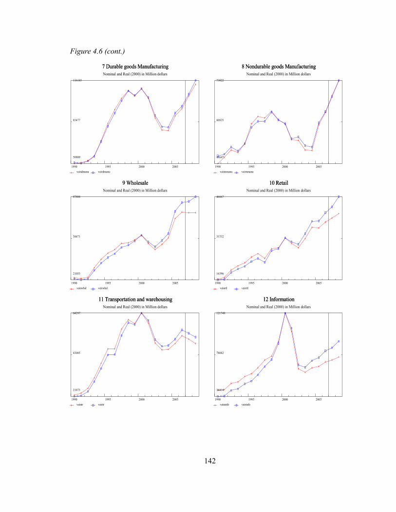
Figure 4.6 (cont.)
7 Durable goods Manufacturing 7 Durable goods Manufacturing Nominal and Real (2000) in Million dollars
116145
83477
50809
1990 1995 2000 2005 veindmanu veirdmanu
8 Nondurable goods Manufacturing 8 Nondurable goods Manufacturing Nominal and Real (2000) in Million dollars
73022
60835
48647
1990 1995 2000 2005 veinnmanu veirnmanu
9 Wholesale 9 Wholesale Nominal and Real (2000) in Million dollars
87888
54471
21055
1990 1995 2000 2005 veinwhsl veirwhsl
10 Retail 10 Retail Nominal and Real (2000) in Million dollars
46667
31532
16396
1990 1995 2000 2005 veinrtl veirrtl
11 Transportation and warehousing 11 Transportation and warehousing Nominal and Real (2000) in Million dollars
64297
43085
21873
1990 1995 2000 2005 veintr veirtr
12 Information 12 Information Nominal and Real (2000) in Million dollars
121749
78082
34414
1990 1995 2000 2005 veininfo veirinfo
142

Figure 4.6 (cont.)
13 Finance and insurance 13 Finance and insurance Nominal and Real (2000) in Million dollars
138441
89883
41325
1990 1995 2000 2005 veinfin veirfin
14 Real estate and rental and leasing 14 Real estate and rental and leasing Nominal and Real (2000) in Million dollars
115985
68350
20714
1990 1995 2000 2005 veinrest veirrest
15 Professional, scientific, and technical services 15 Professional, scientific, and technical services Nominal and Real (2000) in Million dollars
115520
63775
12029
1990 1995 2000 2005 veinpserv veirpserv
16 Management of companies and enterprises 16 Management of companies and enterprises Nominal and Real (2000) in Million dollars
34573
20874
7175
1990 1995 2000 2005 veinmgmt veirmgmt
17 Administrative and waste management services 17 Administrative and waste management services Nominal and Real (2000) in Million dollars
35225
21253
7282
1990 1995 2000 2005 veinadmin veiradmin
18 Educational services 18 Educational services Nominal and Real (2000) in Million dollars
13381
7575
1769
1990 1995 2000 2005 veinedu veiredu
143
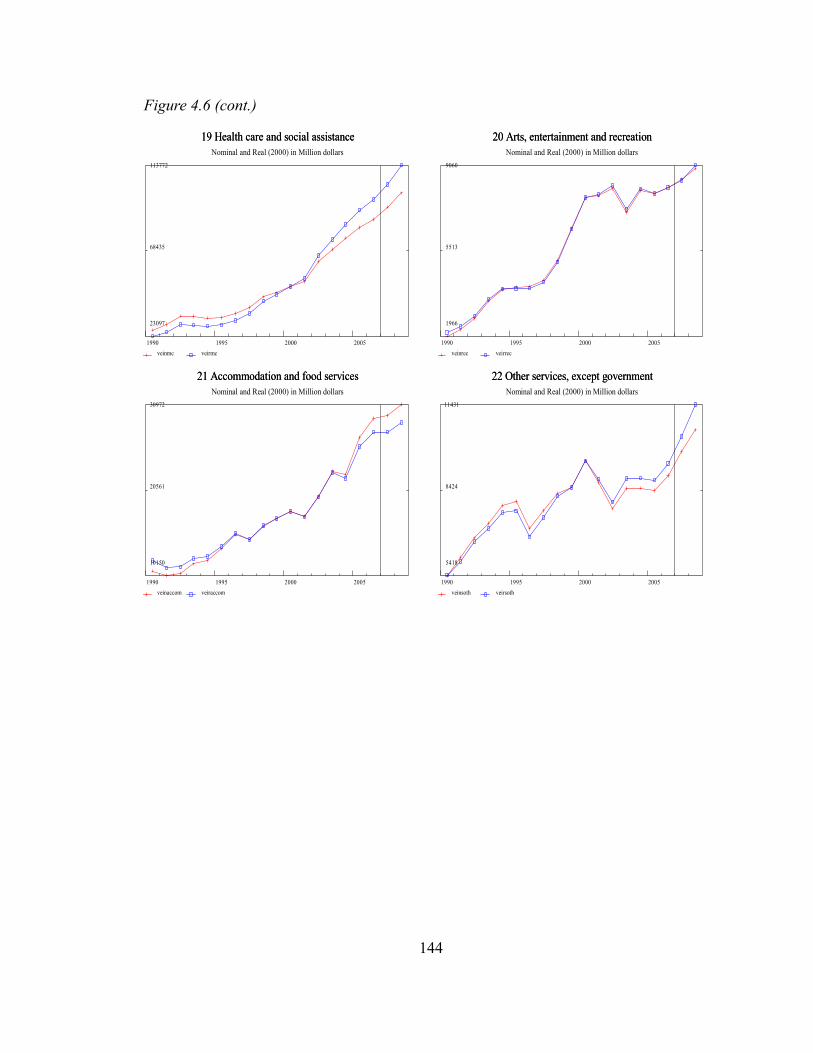
Figure 4.6 (cont.)
19 Health care and social assistance 19 Health care and social assistance Nominal and Real (2000) in Million dollars
113772
68435
23097
1990 1995 2000 2005 veinmc veirmc
20 Arts, entertainment and recreation 20 Arts, entertainment and recreation Nominal and Real (2000) in Million dollars
9060
5513
1966
1990 1995 2000 2005 veinrec veirrec
21 Accommodation and food services 21 Accommodation and food services Nominal and Real (2000) in Million dollars
30972
20561
10150
1990 1995 2000 2005 veinaccom veiraccom
22 Other services, except government 22 Other services, except government Nominal and Real (2000) in Million dollars
11431
8424
5418
1990 1995 2000 2005 veinsoth veirsoth
144
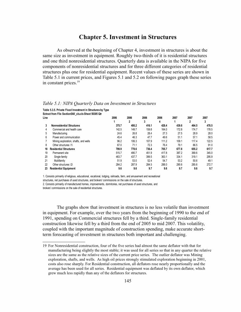
Chapter 5. Investment in Structures
As observed at the beginning of Chapter 4, investment in structures is about the same size as investment in equipment. Roughly two-thirds of it is residential structures and one third nonresidential structures. Quarterly data is available in the NIPA for five components of nonresidential structures and for three different categories of residential structures plus one for residential equipment. Recent values of these series are shown in Table 5.1 in current prices, and Figures 5.1 and 5.2 on following pages graph these series in constant prices.19
The graphs show that investment in structures is no less volatile than investment in equipment. For example, over the two years from the beginning of 1990 to the end of 1991, spending on Commercial structures fell by a third. Single-family residential construction likewise fell by a third from the end of 2005 to mid 2007. This volatility, coupled with the important magnitude of construction spending, make accurate short-term forecasting of investment in structures both important and challenging.
19 For Nonresidential construction, four of the five series had almost the same deflator with that for manufacturing being slightly the most stable; it was used for all series so that in any quarter the relative sizes are the same as the relative sizes of the current price series. The outlier deflator was Mining exploration, shafts, and wells. As high oil prices strongly stimulated exploration beginning in 2001, costs also rose sharply. For Residential construction, all deflators rose nearly proportionally and the average has been used for all series. Residential equipment was deflated by its own deflator, which grew much less rapidly than any of the deflators for structures.
145
Table 5.1: NIPA Quarterly Data on Investment in StructuresTable 5.3.5. Private Fixed Investment in Structures by Type Extract from File Section5All_xls.xls Sheet 50305 QtrLine 2006 2006 2006 2006 2007 2007 2007
1 2 3 4 1 2 33 Nonresidential Structures 375.7 400.2 416.1 428.4 439.6 464.5 478.54 Commercial and health care 142.5 149.7 159.8 164.0 172.8 174.7 178.55 Manufacturing 24.6 26.8 28.4 27.3 27.5 28.9 28.06 Power and communication 45.4 46.3 47.7 49.6 51.1 57.1 58.57 Mining exploration, shafts, and wells 96.2 106.3 107.9 111.2 109.1 117.4 122.58 Other structures \1\ 67.0 71.1 72.3 76.4 79.1 86.5 91.018 Residential Structures 799.9 778.6 736.4 705.7 677.8 655.2 617.719 Permanent site 515.7 490.7 451.9 417.8 387.2 369.6 345.020 Single family 463.7 437.7 399.5 363.1 334.1 319.1 295.921 Multifamily 51.9 53.0 52.4 54.7 53.2 50.6 49.122 Other structures \2\ 284.2 287.9 284.5 288.0 290.6 285.6 272.723 Residential Equipment 9.6 9.6 9.7 9.6 9.7 9.6 9.7
1. Consists primarily of religious, educational, vocational, lodging, railroads, farm, and amusement and recreationalstructures, net purchases of used structures, and brokers' commissions on the sale of structures.2. Consists primarily of manufactured homes, improvements, dormitories, net purchases of used structures, andbrokers' commissions on the sale of residential structures.

5.1 Data and Estimation Approaches for Private Fixed Investment in Structures
Our first question must be the choice of the categories in which we will forecast construction. That choice depends, in the first place, on the categories available in the data sources. We have for construction all the sources we had for equipment plus two more highly important ones. Namely, as in equipment, we have:
NIPA Quarterly (See Table 5.1)
NIPA Annual (See Table 5.2)
FAA Annual (See Table 5.3).
In addition, we have a monthly survey conducted by the Bureau of the Census on the value of construction put in place (VIP) which is the fundamental source for the NIPA and FAA series. It is available both monthly and annually. Thus we have also:
VIP Monthly (See Table 5.4)
146
Figure 5.1: Investment in Nonresidential Structures, NIPA Quarterly Data. All series deflated by the NIPA deflator for Manufacturing construction.

VIP Annual (See Table 5.5).
Finally, it is relevant to know the detail available in the 2002 benchmark input-output table for the inputs into various types of construction. We can certainly have more detail in the types construction we forecast than is shown in the input-output table, but if we do, we will either have to assume that several of the types we distinguish have the same input structure or go to the trouble to split the input structure provided by BEA. In the 2002 benchmark table there are only three types of Nonresidential construction and and two types of Residential, namely:
230101 Nonresidential commercial and health care structures 230102 Nonresidential manufacturing structures 230103 Other nonresidential structures 230201 Residential permanent site single- and multi-family structures 230202 Other residential structures
147
Figure 5.2: NIPA Residential Construction series, all deflated by the average deflator.

148
Table 5.2: NIPA Annual Table 5.4.5B Private Fixed Investment in Structures by Asset Types
Table 5.2: NIPA Annual Table 5.4.5B. Private Fixed Investment in Structures by Type
Line 2002 2003 2004 2005 20061 Private fixed investment in structures 775.5 841.8 965.3 1,093.8 1,160.32 Nonresidential 279.2 277.2 298.2 334.6 405.13 Commercial and health care 116.8 112.2 122.1 132.6 154.04 Office \1\ 40.6 35.1 37.8 42.8 53.15 Health care 25.3 27.3 29.6 32.1 37.46 Hospitals and special care 19.7 20.5 21.0 23.1 29.27 Hospitals 15.8 17.2 18.2 20.6 25.88 Special care 4.0 3.3 2.8 2.5 3.49 Medical buildings 5.5 6.8 8.5 9.0 8.210 Multimerchandise shopping 14.8 14.6 17.9 21.6 27.711 Food and beverage establishments 7.5 7.9 7.8 7.4 7.012 Warehouses 11.3 11.7 11.5 12.2 13.613 Other commercial \2\ 17.3 15.5 17.6 16.5 15.314 Manufacturing 17.8 16.7 18.5 23.3 26.815 Power and communication 49.5 44.2 39.1 40.9 47.316 Power 31.2 32.1 26.2 25.2 29.217 Electric 23.5 24.1 19.2 18.1 20.418 Other power 7.6 8.0 6.9 7.1 8.819 Communication 18.4 12.1 12.9 15.7 18.020 Mining exploration, shafts, and wells 35.6 45.7 55.7 73.7 105.421 Petroleum and natural gas 33.7 44.2 53.3 70.6 101.522 Mining 1.9 1.6 2.4 3.1 3.923 Other structures 59.5 58.4 62.9 64.1 71.724 Religious 8.1 8.3 7.9 7.5 7.525 Educational and vocational 14.6 14.7 13.9 14.2 14.726 Lodging 13.0 12.3 14.8 15.7 21.927 Amusement and recreation 9.0 9.3 10.1 9.0 10.928 Transportation 6.5 6.1 6.7 7.0 7.829 Air 1.4 1.1 1.0 0.9 0.930 Land \3\ 5.1 5.0 5.7 6.1 6.931 Farm 5.6 5.1 5.5 5.9 5.332 Other \4\ 2.6 2.4 3.2 3.6 2.933 Brokers' commissions on sale of structures 2.1 2.1 2.2 2.3 2.734 Net purchases of used structures -1.9 -2.0 -1.4 -1.1 -1.935 Residential 496.3 564.5 667.0 759.2 755.236 Permanent site 298.8 345.7 417.5 480.8 469.037 Single-family structures 265.9 310.6 377.6 433.5 416.038 Multifamily structures 33.0 35.1 39.9 47.3 53.039 Other structures 197.5 218.8 249.5 278.4 286.240 Manufactured homes 8.5 7.1 7.5 9.1 7.441 Dormitories 1.5 1.8 1.7 1.5 2.142 Improvements 121.8 133.2 146.9 160.7 178.543 Brokers' commissions on sale of structures 68.8 80.3 96.1 109.9 101.544 Net purchases of used structures -3.1 -3.5 -2.6 -2.8 -3.4
Addenda:45 Private fixed investment in new structures \5\ 709.7 764.9 871.0 985.5 1,061.346 Nonresidential structures 279.1 277.2 297.5 333.4 404.347 Residential structures 430.7 487.7 573.6 652.1 657.0
1. Consists of office buildings, except those constructed at manufacturing sites and those constructed by power utilities for their own use. Includes all financial buildings. Medical buildings are included in health care.2. Includes buildings and structures used by the retail, wholesale and selected service industries. Consists of auto dealerships, garages, service stations, drug stores, restaurants, mobile structures, and other structures used for commercial purposes. Bus or truck garages are included in transportation.3. Consists primarily of railroads.4. Includes water supply, sewage and waste disposal, public safety, highway and street, and conservation and development.5. Excludes net purchases of used structures and brokers' commissions on the sale of structures.
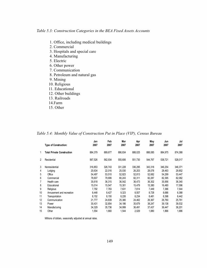
149
Table 5.3: Construction Categories in the BEA Fixed Assets Accounts
1. Office, including medical buildings 2. Commercial 3. Hospitals and special care 4. Manufacturing 5. Electric 6. Other power 7. Communication 8. Petroleum and natural gas 9. Mining10. Religious11. Educational12. Other buildings13. Railroads14.Farm15. Other
Table 5.4: Monthly Value of Construction Put in Place (VIP), Census Bureau
Jan Feb Mar Apr May Jun JulType of Construction: 2007 2007 2007 2007 2007 2007 2007
1 Total Private Construction 884,379 889,677 886,834 888,025 888,085 884,975 874,388
2 Residential 567,526 562,934 555,606 551,730 544,767 538,721 528,017
3 Nonresidential 316,853 326,743 331,228 336,295 343,318 346,254 346,3714 Lodging 20,634 22,016 25,030 26,203 28,078 28,463 29,8525 Office 54,497 53,510 52,823 52,813 52,682 54,299 53,4476 Commercial 78,607 79,906 80,243 82,311 82,287 82,395 82,0827 Health care 35,618 36,315 36,542 36,473 36,302 35,956 36,3408 Educational 15,014 15,547 15,301 15,479 15,380 16,480 17,0969 Religious 7,792 7,783 7,631 7,614 7,449 7,366 7,54410 Amusement and recreation 8,448 8,427 9,323 8,507 8,728 8,686 8,38811 Transportation 8,152 8,150 8,226 8,234 8,481 8,398 8,44212 Communication 21,777 24,839 25,380 24,462 26,367 26,760 25,76113 Power 30,431 32,854 34,186 35,679 38,247 39,138 39,53214 Manufacturing 34,329 35,736 34,999 36,491 37,437 36,447 36,20115 Other 1,554 1,660 1,544 2,029 1,880 1,866 1,686
Millions of dollars, seasonally adjusted at annual rates.

150
Table 5.5: Value of Construction Put in Place (VIP). Annual Data, Bureau of the Census
Type of Construction: 2002 2003 2004 2005 2006
Total Private Construction 659,651 705,276 803,305 897,989 937,047
Residential 421,912 475,941 564,827 641,345 641,332 New single family 265,889 310,575 377,557 433,510 415,997 New multi-family 32,952 35,116 39,944 47,297 53,020 Improvements 123,071 130,250 147,326 160,538 172,315
Nonresidential 237,739 229,335 238,478 256,644 295,715
Lodging 10,467 9,930 11,982 12,666 17,687
Office 35,296 30,579 32,879 37,276 46,194 General 32,356 27,380 28,679 32,962 41,390 Financial 2,857 3,174 4,186 4,285 4,742
Commercial 59,008 57,505 63,195 66,584 72,148 Automotive 5,807 5,039 5,235 5,614 5,463 Sales 2,235 2,099 2,443 2,834 2,306 Service/parts 2,308 1,866 1,978 1,805 2,089 Parking 1,265 1,074 814 975 1,068 Food/beverage 7,914 8,369 8,232 7,795 7,417 Food 4,207 4,234 3,590 3,128 2,773 Dining/drinking 2,916 3,321 3,937 4,078 3,735 Fast food 792 813 705 590 908 Multi-retail 15,581 15,400 18,828 22,750 29,126 General merchandise 6,009 5,341 6,416 6,740 5,849 Shopping center 6,605 6,867 9,256 12,462 18,446 Shopping mall 2,108 2,231 2,138 2,631 3,320 Other commercial 12,083 11,249 13,341 11,744 10,574 Drug store 1,644 1,790 1,427 1,315 1,301 Building supply store 2,471 2,268 2,521 2,416 2,628 Other stores 7,145 6,214 8,229 7,075 5,707 Warehouse 11,908 12,345 12,074 12,827 14,292 General commercial 10,934 11,004 10,830 11,468 13,298 Mini-storage 951 1,326 1,141 1,311 976 Farm 5,611 5,103 5,485 5,854 5,277
Health Care 22,438 24,217 26,272 28,495 33,183 Hospital 13,925 15,234 16,147 18,250 22,860 Medical building 4,924 6,068 7,615 8,031 7,292 Special care 3,538 2,915 2,510 2,213 3,032
Educational 13,109 13,424 12,701 12,788 13,745 Preschool 593 711 674 516 489 Primary/secondary 3,605 3,204 3,202 2,718 3,205 Higher education 6,875 7,259 6,496 6,946 7,561 Instructional 3,619 3,701 3,200 3,556 3,454 Dormitory 1,528 1,761 1,669 1,537 2,085 Sports/recreation 772 677 739 821 854 Other educational 1,651 1,785 1,998 2,294 2,067 Gallery/museum 1,312 1,371 1,335 1,745 1,675
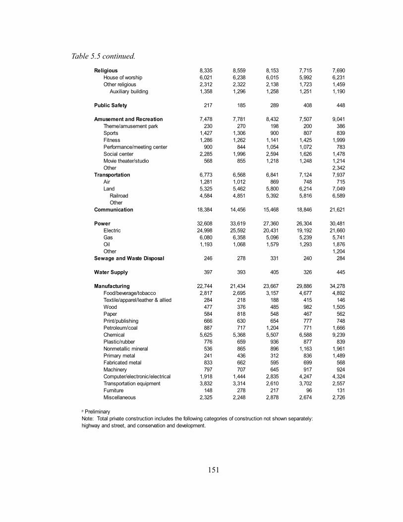
151
Table 5.5 continued.
Religious 8,335 8,559 8,153 7,715 7,690 House of worship 6,021 6,238 6,015 5,992 6,231 Other religious 2,312 2,322 2,138 1,723 1,459 Auxiliary building 1,358 1,296 1,258 1,251 1,190
Public Safety 217 185 289 408 448
Amusement and Recreation 7,478 7,781 8,432 7,507 9,041 Theme/amusement park 230 270 198 200 386 Sports 1,427 1,306 900 807 839 Fitness 1,286 1,262 1,141 1,425 1,999 Performance/meeting center 900 844 1,054 1,072 783 Social center 2,285 1,996 2,594 1,626 1,478 Movie theater/studio 568 855 1,218 1,248 1,214 Other 2,342 Transportation 6,773 6,568 6,841 7,124 7,937 Air 1,281 1,012 869 748 715 Land 5,325 5,462 5,800 6,214 7,049 Railroad 4,584 4,851 5,392 5,816 6,589 Other Communication 18,384 14,456 15,468 18,846 21,621
Power 32,608 33,619 27,360 26,304 30,481 Electric 24,998 25,592 20,431 19,192 21,660 Gas 6,080 6,358 5,096 5,239 5,741 Oil 1,193 1,068 1,579 1,293 1,876 Other 1,204 Sewage and Waste Disposal 246 278 331 240 284
Water Supply 397 393 405 326 445
Manufacturing 22,744 21,434 23,667 29,886 34,278 Food/beverage/tobacco 2,817 2,695 3,157 4,677 4,892 Textile/apparel/leather & allied 284 218 188 415 146 Wood 477 376 485 982 1,505 Paper 584 818 548 467 562 Print/publishing 666 630 654 777 748 Petroleum/coal 887 717 1,204 771 1,666 Chemical 5,625 5,368 5,507 6,588 9,239 Plastic/rubber 776 659 936 877 839 Nonmetallic mineral 536 865 896 1,163 1,961 Primary metal 241 436 312 836 1,489 Fabricated metal 833 662 595 699 568 Machinery 797 707 645 917 924 Computer/electronic/electrical 1,918 1,444 2,835 4,247 4,324 Transportation equipment 3,832 3,314 2,610 3,702 2,557 Furniture 148 278 217 96 131 Miscellaneous 2,325 2,248 2,878 2,674 2,726
Note: Total private construction includes the following categories of construction not shown separately:highway and street, and conservation and development.
p Preliminary

This is the least detail for construction inputs ever given in a benchmark input-output table. The 1997 table, also a NAICS-based table, gave inputs for the following types of construction:
2301 New residential230110 New residential 1-unit structures, nonfarm230120 New multifamily housing structures, nonfarm230130 New residential additions and alterations, nonfarm230140 New farm housing units and additions and alterations2302 New nonresidential construction230210 Manufacturing and industrial buildings230220 Commercial and institutional buildings230230 Highway, street, bridge, and tunnel construction230240 Water, sewer, and pipeline construction230250 Other new construction
Since the 1997 table could be used fairly easily to make a table balanced to the 2002 row and column totals but with the 9 columns of the 1997 table instead of the 5 of the BEA 2002 table. Furthermore, it is not necessarily pointless to distinguish two or more types of construction which use the same input structure. For example, since Offices and Hospitals are built by the same input-output sector, it will not matter for the rest of the economy whether or not we combine them or keep them separate. But it may prove much more natural to formulate scenarios with them separate rather than with them combined. Nonetheless, the limited detail in the input-output table is something of a damper on enthusiasm for forecasting construction in great detail such as is provided by the annual VIP or even the annual NIPA.
We also need to inquire about the content and comparability of NIPA and VIP data. According to Census documentation, VIP includes:
● New buildings and structures ● Additions, alterations, major replacements, etc. to existing buildings and
structures ● Installed mechanical and electrical equipment ● Installed industrial equipment, such as boilers and blast furnaces ● Site preparation and outside construction, such as streets, sidewalks, parking lots,
utility connections ● Cost of labor and materials (including owner supplied) ● Cost of construction equipment rental ● Profit and overhead costs ● Cost of architectural and engineering (A&E) work ● Any miscellaneous costs of the project that appear on the owner's books as capital
assets.
152

This definition is very close to the NIPA definition except that NIPA includes three series not included in VIP, namely (1) Mining exploration, shafts and wells,(2) Brokers' commissions, and (3) Net purchases of used structures. Other than in these three items, the two series are close together, as is to be expected since the VIP are the main source for the other NIPA series. The Brokers' commissions amount to little for Nonresidential structures but are significant part of NIPA Residential construction. I have been unable to find a “reconciliation” of VIP and NIPA on either the BEA or the Census websites, though NIPA documentation makes plain the difference described above. Table 5.6 shows that adjusting the NIPA totals for the three series known not to be in VIP brings the NIPA total down to within one percent of the VIP total for 2001 through 2006.
Manufacturing is higher in VIP than NIPA because it includes offices at manufacturing plants which have been moved to Offices in the NIPA, so Offices are higher in NIPA than in VIP. Since the input-output table will match the NIPA in this respect, our final product also needs to match NIPA.
5.2 Approach to Forecast Investment in Structures
5.2.1 Nonresidential Investment in Structures
We can now pull together what we know of data availability to formulate a plan for short-term forecasting of Nonresidential construction. Table 5.7 shows, for 2006, the relations among the annual values of five NIPA series available quarterly and annual values of the twelve VIP series available monthly. The two largest differences, in Manufacturing and in Offices, are due to the fact that offices built on the site of a manufacturing plant are counted in Manufacturing in VIP and in Offices in NIPA. Otherwise, the agreement is close enough to justify the following five-step procedure for short-term forecasting of the NIPA series which go into the model.
153
Table 5.6: Comparison of NIPA and VIP Total Nonresidential Construction
Line 2001 2002 2003 2004 2005 20061 NIPA Nonresidential construction 322.6 279.2 277.2 298.2 334.6 405.12 Less Mining exploration, shafts, wells 39.2 35.6 45.7 55.7 73.7 105.43 Less Brokers' commissions 2.4 2.1 2.1 2.2 2.3 2.74 Net purchases of used structures 1.6 -1.9 -2 -1.4 -1.1 -1.95 Equals Census definition, NIPA data 279.4 243.4 231.4 241.7 259.7 298.96 Census data 273.9 237.7 229.3 238.5 256.6 295.77 NIPA data – Census data 5.5 5.7 2.1 3.2 3.1 3.28 Percent difference 2.00% 2.38% 0.90% 1.35% 1.19% 1.08%

Step 1. Forecast, using time-series methods, the 12 VIP monthly series three months ahead and extend the series by as many of these months as necessary to round out the current quarter.
Step 2. Convert the monthly series developed in Step 1 to quarterly series.
Step 3. Forecast these 12 quarterly VIP-based series to the end of the following year, relating them to quarterly series from QUEST. Do the same for Mining exploration, for which the quarterly NIPA provide values.
Step 4. Convert these 13 quarterly series to annual series.
Step 5. Use the 13 annual series as regressors to forecast the corresponding annual NIPA series. These should be the series needed by the interindustry model.
154

Brokers' commissions and Net purchases of used structures need to be projected annually exogenously. No specific data is available on them at a higher frequency.
This plan makes no use of the four NIPA quarterly series numbered 1, 2, 3, and 5 in Table 5.7. It is assumed, at least initially, that these do not provide any significant information in addition to the twelve VIP series which compose them.
155
Table 5.7: Integration of VIP with NIPA Nonresidential Structures NIPA Ann VIP Ann NIPA-VIP
2006 2006NIPA Quaterly
VIP Monthly and NIPA annual 405.100 402.115 2.991 Commercial and health care
1 Office 53.100 46.194 6.912 Commercial (incl. farm) 68.900 72.148 -3.253 Health care 37.400 33.183 4.22
2 Manufacturing4 Manufacturing 26.800 34.278 -7.48
3 Power and communication5 Communication 18.000 21.621 -3.626 Power 29.200 30.481 -1.28
4 Mining exploration, shafts, and wells* 105.400 105.400 0
5 Other structures 7 Religious 7.500 7.690 -0.198 Education 14.700 13.745 0.969 Lodging 21.900 17.687 4.2110 Amusement 10.900 9.041 1.8611 Transportation 7.800 7.937 -0.1412 Other 3.800 1.710 2.09
Brokers' commissions* 2.900 2.900 0Net used * -1.900 -1.900 0
Sum of detail 406.400 402.115 4.29Sum without NIPA-only items 300.000 295.715 4.28
Sum of detail may not equal total because of rounding* Item available only in NIPA

5.2.2 Residential Investment in Structures
The plan for Residential construction will be significantly different because the quarterly NIPA give important information not contained in the monthly VIP. Namely, whereas monthly VIP gives only one series for all Residential construction, the quarterly NIPA give three series: (1) Single family, (2) Multifamily, and (3) Other. These are distinctions worth keeping because the 2002 benchmark I-O table has two separate columns, one for the sum of the first two series and one for the third. Moreover, by borrowing information from the 1997 table, it should be possible to split the first of those columns so that we would have three columns matching exactly the three quarterly NIPA series. The following plan makes use of all this data.
Step 1. Forecast with time-series methods the monthly VIP series three months ahead.
Step 2. Convert this series to quarterly frequency. The converted series will not go past the present quarter.
Step 3. Regress each of the three NIPA quarterly series on this one and use to forecast the NIPA series through the current quarter.
Step 4. Forecast these three quarterly series further ahead, through the end of the next year, with exogenous variables from QUEST
Step 5. Convert these three series to annual values for use in the annual multisector model.
5.3 Monthly VIP Equations
This section shows the estimation results from Step 1 in both Nonresidential structures and Residential structures, a total of 13 series. In November 2007, the Census Bureau published the VIP data up through July 2007. Thus, all equations in this section are estimated with data from July 1993 to July 2007.
In this section, all regressors are lagged dependent variables. Many equations do not have intercept as it has little to no explanatory power according to Mexvals. Using only Time-series analysis in these equations should not affect the usefulness of the forecast since the objective of equations in this section are to complete the current quarter of the monthly series which are at most a three months forecast.
Figure 5.3 shows fitted plots of all equations discussed in this section.
In general, most of the equations have very good closeness of fit statistics. The BasePred plots also capture the long-term trend of each series quite well except in some categories, such as Lodging, Manufacturing, and Other Nonresidential structures, that are
156
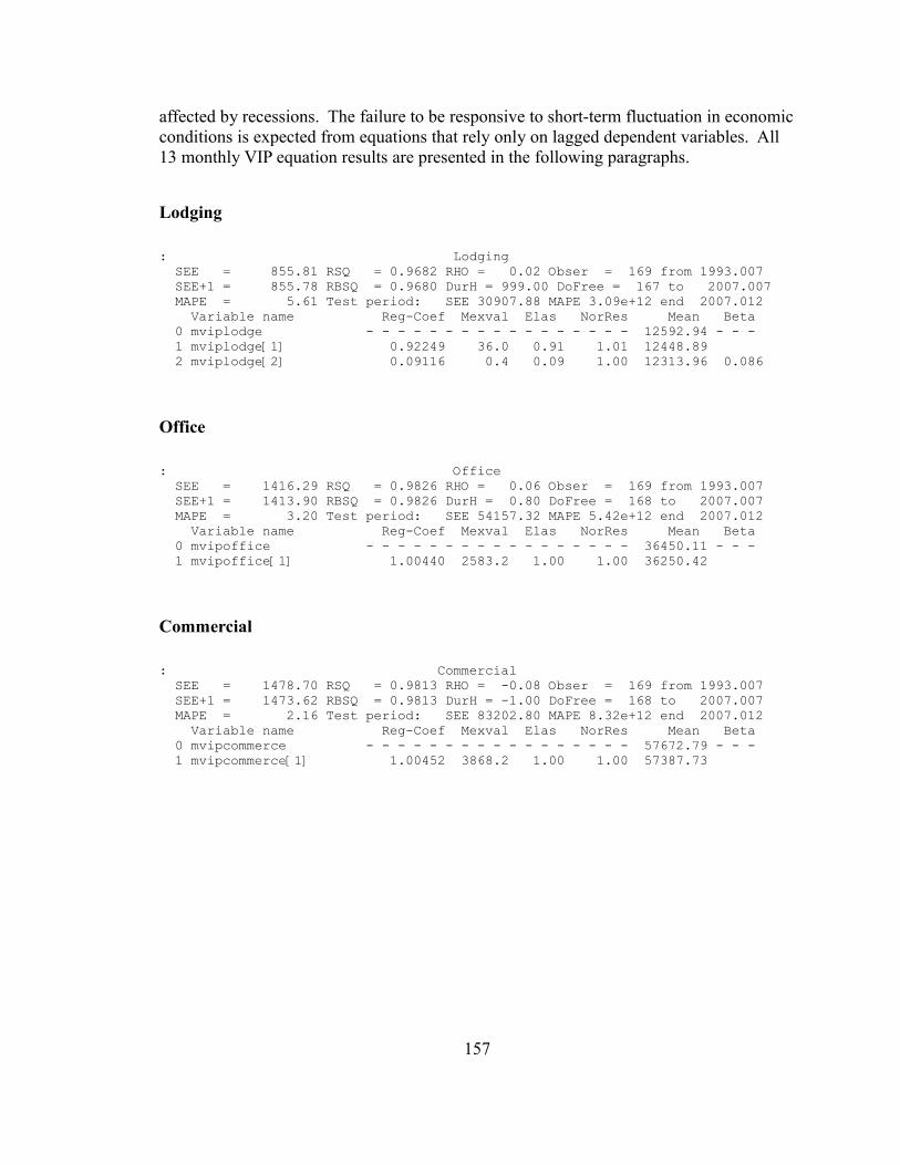
affected by recessions. The failure to be responsive to short-term fluctuation in economic conditions is expected from equations that rely only on lagged dependent variables. All 13 monthly VIP equation results are presented in the following paragraphs.
Lodging
Office
Commercial
157
: Lodging SEE = 855.81 RSQ = 0.9682 RHO = 0.02 Obser = 169 from 1993.007 SEE+1 = 855.78 RBSQ = 0.9680 DurH = 999.00 DoFree = 167 to 2007.007 MAPE = 5.61 Test period: SEE 30907.88 MAPE 3.09e+12 end 2007.012 Variable name Reg-Coef Mexval Elas NorRes Mean Beta 0 mviplodge - - - - - - - - - - - - - - - - - 12592.94 - - - 1 mviplodge[1] 0.92249 36.0 0.91 1.01 12448.89 2 mviplodge[2] 0.09116 0.4 0.09 1.00 12313.96 0.086
: Office SEE = 1416.29 RSQ = 0.9826 RHO = 0.06 Obser = 169 from 1993.007 SEE+1 = 1413.90 RBSQ = 0.9826 DurH = 0.80 DoFree = 168 to 2007.007 MAPE = 3.20 Test period: SEE 54157.32 MAPE 5.42e+12 end 2007.012 Variable name Reg-Coef Mexval Elas NorRes Mean Beta 0 mvipoffice - - - - - - - - - - - - - - - - - 36450.11 - - - 1 mvipoffice[1] 1.00440 2583.2 1.00 1.00 36250.42
: Commercial SEE = 1478.70 RSQ = 0.9813 RHO = -0.08 Obser = 169 from 1993.007 SEE+1 = 1473.62 RBSQ = 0.9813 DurH = -1.00 DoFree = 168 to 2007.007 MAPE = 2.16 Test period: SEE 83202.80 MAPE 8.32e+12 end 2007.012 Variable name Reg-Coef Mexval Elas NorRes Mean Beta 0 mvipcommerce - - - - - - - - - - - - - - - - - 57672.79 - - - 1 mvipcommerce[1] 1.00452 3868.2 1.00 1.00 57387.73

Health Care
Health care structures has shown to be immuned to the recession in 2000-2001. The plot shows that it keeps expanding consistently throughout the test period. This trend is understandable as the demand of health care for the U.S. aging population keeps increasing.
Educational
Education structures also exhibits consistent growth over the test period.
Religious
Amusement and Recreation
158
: Health Care SEE = 604.45 RSQ = 0.9903 RHO = -0.23 Obser = 169 from 1993.007 SEE+1 = 587.57 RBSQ = 0.9903 DurH = -3.05 DoFree = 168 to 2007.007 MAPE = 2.27 Test period: SEE 37021.50 MAPE 3.70e+12 end 2007.012 Variable name Reg-Coef Mexval Elas NorRes Mean Beta 0 mvipmc - - - - - - - - - - - - - - - - - 21451.11 - - - 1 mvipmc[1] 1.00619 3591.3 1.00 1.00 21325.46
: Educational structure SEE = 406.60 RSQ = 0.9842 RHO = 0.00 Obser = 169 from 1993.007 SEE+1 = 406.61 RBSQ = 0.9841 DurH = 0.43 DoFree = 167 to 2007.007 MAPE = 3.35 Test period: SEE 17320.00 MAPE 1.73e+12 end 2007.012 Variable name Reg-Coef Mexval Elas NorRes Mean Beta 0 mvipedu - - - - - - - - - - - - - - - - - 10523.03 - - - 1 mvipedu[1] 0.81134 29.7 0.81 1.04 10452.21 2 mvipedu[2] 0.19586 1.9 0.19 1.00 10382.45 0.195
: Religious SEE = 234.92 RSQ = 0.9805 RHO = 0.00 Obser = 169 from 1993.007 SEE+1 = 234.92 RBSQ = 0.9802 DurH = 0.23 DoFree = 166 to 2007.007 MAPE = 2.96 Test period: SEE 7544.73 MAPE 7.54e+11 end 2007.012 Variable name Reg-Coef Mexval Elas NorRes Mean Beta 0 mviprelig - - - - - - - - - - - - - - - - - 6801.61 - - - 1 intercept 160.67321 1.4 0.02 51.23 1.00 2 mviprelig[1] 0.76168 26.9 0.76 1.05 6778.52 0.769 3 mviprelig[2] 0.21872 2.5 0.22 1.00 6756.99 0.223

Transportation
Communication
Power
159
: Transportation SEE = 349.82 RSQ = 0.8938 RHO = -0.08 Obser = 169 from 1993.007 SEE+1 = 348.74 RBSQ = 0.8932 DurH = -1.39 DoFree = 167 to 2007.007 MAPE = 3.63 Test period: SEE 8499.18 MAPE 8.50e+11 end 2007.012 Variable name Reg-Coef Mexval Elas NorRes Mean Beta 0 mviptr - - - - - - - - - - - - - - - - - 6516.20 - - - 1 mviptr[1] 0.80250 54.8 0.80 1.09 6494.70 2 mviptr[4] 0.20186 4.2 0.20 1.00 6429.31 0.201
: Communication structure SEE = 1037.43 RSQ = 0.9412 RHO = -0.02 Obser = 169 from 1993.007 SEE+1 = 1037.24 RBSQ = 0.9409 DurH = -0.38 DoFree = 167 to 2007.007 MAPE = 4.74 Test period: SEE 26612.39 MAPE 2.66e+12 end 2007.012 Variable name Reg-Coef Mexval Elas NorRes Mean Beta 0 mvipcomm - - - - - - - - - - - - - - - - - 15813.46 - - - 1 mvipcomm[1] 0.70062 35.6 0.70 1.16 15717.28 2 mvipcomm[3] 0.30875 7.6 0.30 1.00 15515.44 0.297
: Power SEE = 2555.48 RSQ = 0.8537 RHO = -0.01 Obser = 169 from 1993.007 SEE+1 = 2555.34 RBSQ = 0.8519 DurH = -0.15 DoFree = 166 to 2007.007 MAPE = 7.12 Test period: SEE 38419.49 MAPE 3.84e+12 end 2007.012 Variable name Reg-Coef Mexval Elas NorRes Mean Beta 0 mvippower - - - - - - - - - - - - - - - - - 25836.60 - - - 1 mvippower[1] 1.03793 45.3 1.03 1.04 25734.06 2 mvippower[2] -0.14210 0.9 -0.14 1.04 25639.60 -0.139 3 mvippower[6] 0.10604 1.9 0.10 1.00 25424.95 0.101
: Amusement and Recreation SEE = 399.42 RSQ = 0.9146 RHO = 0.01 Obser = 169 from 1993.007 SEE+1 = 399.42 RBSQ = 0.9136 DurH = 0.34 DoFree = 166 to 2007.007 MAPE = 4.26 Test period: SEE 8424.95 MAPE 8.42e+11 end 2007.012 Variable name Reg-Coef Mexval Elas NorRes Mean Beta 0 mviprec - - - - - - - - - - - - - - - - - 7745.07 - - - 1 intercept 406.79519 1.6 0.05 11.71 1.00 2 mviprec[1] 0.71617 24.3 0.71 1.06 7725.18 0.724 3 mviprec[2] 0.23451 3.0 0.23 1.00 7699.99 0.241

Manufacturing
Other Nonresidential Structures
Residential construction
160
: Manufacturing SEE = 1536.09 RSQ = 0.9464 RHO = -0.14 Obser = 169 from 1993.007 SEE+1 = 1521.42 RBSQ = 0.9464 DurH = -1.78 DoFree = 168 to 2007.007 MAPE = 3.44 Test period: SEE 36328.22 MAPE 3.63e+12 end 2007.012 Variable name Reg-Coef Mexval Elas NorRes Mean Beta 0 mvipmanu - - - - - - - - - - - - - - - - - 32354.69 - - - 1 mvipmanu[1] 1.00117 2050.1 1.00 1.00 32270.44
: Other NR structure SEE = 202.09 RSQ = 0.5986 RHO = 0.01 Obser = 169 from 1993.007 SEE+1 = 202.07 RBSQ = 0.5888 DurH = 0.31 DoFree = 164 to 2007.007 MAPE = 9.55 Test period: SEE 1692.58 MAPE 1.69e+11 end 2007.012 Variable name Reg-Coef Mexval Elas NorRes Mean Beta 0 mvipoth - - - - - - - - - - - - - - - - - 1596.05 - - - 1 intercept 341.52440 3.8 0.21 2.49 1.00 2 mvipoth[1] 0.50126 12.1 0.50 1.12 1594.17 0.502 3 mvipoth[2] 0.26303 2.9 0.26 1.03 1590.76 0.263 4 mvipoth[3] 0.13697 0.8 0.14 1.02 1587.80 0.137 5 mvipoth[6] -0.11399 1.0 -0.11 1.00 1583.17 -0.114
: Residential structure SEE = 4740.21 RSQ = 0.9988 RHO = -0.00 Obser = 169 from 1993.007 SEE+1 = 4740.17 RBSQ = 0.9988 DurH = -0.02 DoFree = 166 to 2007.007 MAPE = 0.88 Test period: SEE 510353.06 MAPE 5.10e+13 end 2007.012 Variable name Reg-Coef Mexval Elas NorRes Mean Beta 0 mvipr - - - - - - - - - - - - - - - - - 403483.13 - - - 1 mvipr[1] 1.40116 74.7 1.39 1.72 401656.57 2 mvipr[2] -0.29569 3.0 -0.29 1.11 399741.37 -0.297 3 mvipr[6] -0.10543 5.5 -0.10 1.00 391694.49 -0.107

161
Figure 5.3: Plots of Monthly VIP Equations
Lodging Lodging48144
25947
3750
1995 2000 2005 Predicted Actual BasePred
Office Office58458
38390
18322
1995 2000 2005 Predicted Actual BasePred
Commercial Commercial83953
57992
32032
1995 2000 2005 Predicted Actual BasePred
Health Care Health Care44176
28816
13457
1995 2000 2005 Predicted Actual BasePred
Educational structure Educational structure17531
11132
4734
1995 2000 2005 Predicted Actual BasePred
Religious Religious 8801
6212
3622
1995 2000 2005 Predicted Actual BasePred
Amusement and Recreation Amusement and Recreation10532
7445
4358
1995 2000 2005 Predicted Actual BasePred
Transportation Transportation 8546
6466
4386
1995 2000 2005 Predicted Actual BasePred

162
Figure 5.3 (cont.)
Communication structure Communication structure26937
18204
9471
1995 2000 2005 Predicted Actual BasePred
Power Power43150
28571
13991
1995 2000 2005 Predicted Actual BasePred
Manufacturing Manufacturing43275
31436
19598
1995 2000 2005 Predicted Actual BasePred
Other NR structure Other NR structure 2453
1672
892
1995 2000 2005 Predicted Actual BasePred
Residential structure Residential structure703006
462064
221122
1995 2000 2005 Predicted Actual BasePred

5.4 Nonresidential Fixed Investment in Structures Equations
5.4.1 Quarterly Equations for VIP-based Nonresidential Fixed Investment in Structures
This section, corresponding to Step 3 of our nonresidential procedure, develops the equations to forecast the 12 quarterly VIP-based series. All equations are estimated over the period from 1994Q1 to 2007Q3.
Figure 5.4 shows fitted plots of quarterly equations.
Lodging
The equations shows very good fit with an adjusted R-square of 0.9698 and a MAPE of 6.28 percent. All three regressors have good Mexvals and reasonable signs. The fitted plot shows good fit by both predicted value and BasePred. The use of private fixed investment in nonresidential structures and its lagged value as additional regressors helps improve the BasePred.
Office
The equation has good closeness of fit statistics in both adjusted R-square and MAPE. Both plots have quite well to the actual series.
163
: Lodging SEE = 0.96 RSQ = 0.9622 RHO = 0.23 Obser = 55 from 1994.100 SEE+1 = 0.94 RBSQ = 0.9608 DurH = 1.85 DoFree = 52 to 2007.300 MAPE = 6.28 Variable name Reg-Coef Mexval Elas NorRes Mean Beta 0 qviplodge - - - - - - - - - - - - - - - - - 13.09 - - - 1 qviplodge[1] 0.99267 178.9 0.96 1.65 12.62 2 vfnrs 0.08709 28.2 1.94 1.60 291.08 1.200 3 vfnrs[1] -0.08665 26.7 -1.89 1.00 285.69 -1.135
: Office SEE = 1.86 RSQ = 0.9685 RHO = 0.24 Obser = 55 from 1994.100 SEE+1 = 1.81 RBSQ = 0.9672 DurH = 1.91 DoFree = 52 to 2007.300 MAPE = 3.74 Variable name Reg-Coef Mexval Elas NorRes Mean Beta 0 qvipoffice - - - - - - - - - - - - - - - - - 37.28 - - - 1 qvipoffice[1] 0.97591 227.4 0.96 1.61 36.67 2 vfnrs 0.15321 21.9 1.20 1.40 291.08 0.999 3 vfnrs[1] -0.15109 18.2 -1.16 1.00 285.69 -0.936
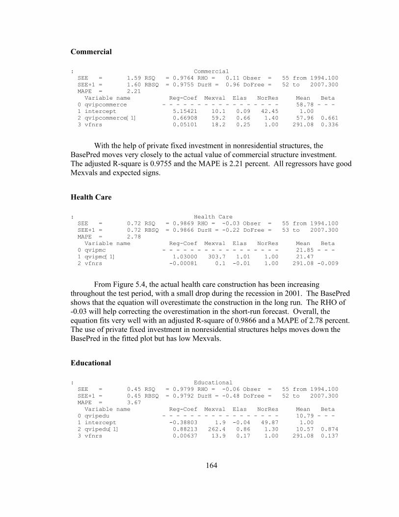
Commercial
With the help of private fixed investment in nonresidential structures, the BasePred moves very closely to the actual value of commercial structure investment. The adjusted R-square is 0.9755 and the MAPE is 2.21 percent. All regressors have good Mexvals and expected signs.
Health Care
From Figure 5.4, the actual health care construction has been increasing throughout the test period, with a small drop during the recession in 2001. The BasePred shows that the equation will overestimate the construction in the long run. The RHO of -0.03 will help correcting the overestimation in the short-run forecast. Overall, the equation fits very well with an adjusted R-square of 0.9866 and a MAPE of 2.78 percent. The use of private fixed investment in nonresidential structures helps moves down the BasePred in the fitted plot but has low Mexvals.
Educational
164
: Commercial SEE = 1.59 RSQ = 0.9764 RHO = 0.11 Obser = 55 from 1994.100 SEE+1 = 1.60 RBSQ = 0.9755 DurH = 0.96 DoFree = 52 to 2007.300 MAPE = 2.21 Variable name Reg-Coef Mexval Elas NorRes Mean Beta 0 qvipcommerce - - - - - - - - - - - - - - - - - 58.78 - - - 1 intercept 5.15421 10.1 0.09 42.45 1.00 2 qvipcommerce[1] 0.66908 59.2 0.66 1.40 57.96 0.661 3 vfnrs 0.05101 18.2 0.25 1.00 291.08 0.336
: Health Care SEE = 0.72 RSQ = 0.9869 RHO = -0.03 Obser = 55 from 1994.100 SEE+1 = 0.72 RBSQ = 0.9866 DurH = -0.22 DoFree = 53 to 2007.300 MAPE = 2.78 Variable name Reg-Coef Mexval Elas NorRes Mean Beta 0 qvipmc - - - - - - - - - - - - - - - - - 21.85 - - - 1 qvipmc[1] 1.03000 303.7 1.01 1.00 21.47 2 vfnrs -0.00081 0.1 -0.01 1.00 291.08 -0.009
: Educational SEE = 0.45 RSQ = 0.9799 RHO = -0.06 Obser = 55 from 1994.100 SEE+1 = 0.45 RBSQ = 0.9792 DurH = -0.48 DoFree = 52 to 2007.300 MAPE = 3.67 Variable name Reg-Coef Mexval Elas NorRes Mean Beta 0 qvipedu - - - - - - - - - - - - - - - - - 10.79 - - - 1 intercept -0.38803 1.9 -0.04 49.87 1.00 2 qvipedu[1] 0.88213 262.4 0.86 1.30 10.57 0.874 3 vfnrs 0.00637 13.9 0.17 1.00 291.08 0.137

All the regressors have good Mexvals and appropriate signs. We have good closeness of fit statistics with an adjusted R-square of 0.9792 and a MAPE of 3.67 percent. The educational construction has very good fit as shown in Figure 5.4. Both predicted value and BasePred track the actual value very well. We should be able to get a reliable forecast from this equation given a good exogenous variable (vfnrs).
Religious
The actual series show that the religious construction has been expanding rapidly during the end of 1990s as the U.S. economy saw a rapid growth rate before the recession in 2001. Although the equation shows good closeness of fit statistics, we can clearly see the lag in movement of predicted value compared to the actual value throughout the test period. As the actual series exhibits a seasonal pattern, the lag from the predicted value should be averaged out when we annualized the predicted value to be used in the annual equations, which will be discussed in the next section.
Amusement and Recreation
The equation has an adjusted R-square of 0.8671 and a MAPE of 4.93 percent. All regressors have good Mexvals and appropriate signs. The plot of predicted value reveal the lag in movement of predicted value as the amusement and recreation construction is quite volatile. The BasePred plot seems to be moving nicely in the middle of the fluctuation which should give a reasonable short-run forecast.
Transportation
165
: Religious SEE = 0.28 RSQ = 0.9696 RHO = 0.18 Obser = 55 from 1994.100 SEE+1 = 0.27 RBSQ = 0.9696 DurH = 1.33 DoFree = 54 to 2007.300 MAPE = 3.08 Variable name Reg-Coef Mexval Elas NorRes Mean Beta 0 qviprelig - - - - - - - - - - - - - - - - - 6.91 - - - 1 qviprelig[1] 1.00667 2443.4 1.00 1.00 6.85
: Amusement and recreation SEE = 0.45 RSQ = 0.8695 RHO = 0.20 Obser = 55 from 1994.100 SEE+1 = 0.45 RBSQ = 0.8671 DurH = 1.58 DoFree = 53 to 2007.300 MAPE = 4.93 Variable name Reg-Coef Mexval Elas NorRes Mean Beta 0 qviprec - - - - - - - - - - - - - - - - - 7.85 - - - 1 intercept 0.84701 4.6 0.11 7.67 1.00 2 qviprec[1] 0.89886 176.9 0.89 1.00 7.79 0.932

The equation for transportation construction performs decently with an adjusted R-square of 0.8583. All regressors have good Mexvals and expected signs. From Figure 5.4, the actual series typically moves without much volatility but each shock had significant magnitude. Overall, the equation fits very well to the series during the test period as shown by both the Predicted value and the BasePred plots.
Communication
The communication construction equation fit the actual series during the test period quite well. An adjusted R-square is 0.9439 and a MAPE is 4.59 percent. Both regressors have good Mexvals and appropriate signs. The fitted plots show the equation doing quite well in both the predicted value and the BasePred.
Power
166
: Transportation SEE = 0.38 RSQ = 0.8635 RHO = -0.07 Obser = 55 from 1994.100 SEE+1 = 0.38 RBSQ = 0.8583 DurH = -0.84 DoFree = 52 to 2007.300 MAPE = 4.76 Variable name Reg-Coef Mexval Elas NorRes Mean Beta 0 qviptr - - - - - - - - - - - - - - - - - 6.60 - - - 1 intercept 0.98441 6.8 0.15 7.33 1.00 2 qviptr[1] 0.65443 32.6 0.65 1.16 6.53 0.653 3 vfnrs 0.00460 7.9 0.20 1.00 291.08 0.304
: Communication SEE = 1.00 RSQ = 0.9450 RHO = 0.14 Obser = 55 from 1994.100 SEE+1 = 0.99 RBSQ = 0.9439 DurH = 1.20 DoFree = 53 to 2007.300 MAPE = 4.59 Variable name Reg-Coef Mexval Elas NorRes Mean Beta 0 qvipcomm - - - - - - - - - - - - - - - - - 16.16 - - - 1 qvipcomm[1] 0.73415 70.4 0.72 1.29 15.86 2 vfnrs 0.01563 13.5 0.28 1.00 291.08 0.250
: Power SEE = 3.18 RSQ = 0.7702 RHO = -0.04 Obser = 55 from 1994.100 SEE+1 = 3.18 RBSQ = 0.7613 DurH = -0.44 DoFree = 52 to 2007.300 MAPE = 9.60 Variable name Reg-Coef Mexval Elas NorRes Mean Beta 0 qvippower - - - - - - - - - - - - - - - - - 26.11 - - - 1 qvippower[1] 0.66446 44.8 0.66 1.30 25.84 2 vfnrs -0.06778 1.4 -0.76 1.05 291.08 -0.697 3 vfnrs[1] 0.10040 2.6 1.10 1.00 285.69 0.981

From Figure 5.4, the power structure construction had been quite volatile with big magnitude of changes. Considering the volatility, the equation performs quite well with an adjusted R-square of 0.7613 and a MAPE of 9.60 percent. All regressors have good Mexvals. The BasePred plot moves along the trend of the actual series very well during the test period. Thus, the short-term forecast from this equation should be reliable.
Manufacturing
Figure 5.4 shows the characteristics of manufacturing construction very well. The manufacturing structure investment typically is affected the most by a downturn in the overall economy. As explained earlier, businesses tend to be conservative in expansion decision, to avoid idle facilities, and they normally keep using the existing facilities until there is a real need for new or additional manufacturing facilities. This characteristics can be observed with the drop in construction in 2001 and the flat investment between 2002 and 2004. Considering this characteristics, the equation works quite well with a decent adjusted R-square and a good MAPE.
Other
The construction of other nonresidential structures is another structure type that is affected by the recession. Ignoring the 2001 recession, Figure 5.4 shows that the construction seems to be slowly increasing during the test period. Overall, the equation is acceptable with decent closeness of fit statistics. The fitted plot shows an observable lag in movement from the actual value.
167
: Manufacturing SEE = 1.99 RSQ = 0.9051 RHO = -0.02 Obser = 55 from 1994.100 SEE+1 = 1.99 RBSQ = 0.9014 DurH = -0.17 DoFree = 52 to 2007.300 MAPE = 4.69 Variable name Reg-Coef Mexval Elas NorRes Mean Beta 0 qvipmanu - - - - - - - - - - - - - - - - - 32.72 - - - 1 intercept 3.32263 5.1 0.10 10.53 1.00 2 qvipmanu[1] 1.14565 120.3 1.14 1.19 32.50 1.160 3 qvipmanu[3] -0.24470 9.0 -0.24 1.00 32.02 -0.256
: Other NR SEE = 0.18 RSQ = 0.6045 RHO = 0.04 Obser = 55 from 1994.100 SEE+1 = 0.18 RBSQ = 0.5812 DurH = 999.00 DoFree = 51 to 2007.300 MAPE = 9.21 Variable name Reg-Coef Mexval Elas NorRes Mean Beta 0 qvipoth - - - - - - - - - - - - - - - - - 1.60 - - - 1 intercept 0.47679 7.6 0.30 2.53 1.00 2 qvipoth[1] 1.00217 41.7 1.00 1.11 1.60 1.001 3 qvipoth[2] -0.38932 3.9 -0.39 1.01 1.59 -0.388 4 qvipoth[3] 0.08935 0.4 0.09 1.00 1.59 0.090

Mining Exploration, Shafts, and Wells
The equation has an adjusted R-square of 0.9904 and a MAPE of 5.73 percent. The BasePred overestimates the increasing trend of the fixed investment in Mining structures, which should not be a problem for the short-term forecast.
168
: Mining (NIPA) SEE = 3.01 RSQ = 0.9904 RHO = 0.31 Obser = 55 from 1994.100 SEE+1 = 2.86 RBSQ = 0.9904 DurH = 2.33 DoFree = 54 to 2007.300 MAPE = 5.73 Variable name Reg-Coef Mexval Elas NorRes Mean Beta 0 qvstnnmin - - - - - - - - - - - - - - - - - 42.50 - - - 1 qvstnnmin[1] 1.05063 1644.5 1.00 1.00 40.60

169
Figure 5.4: Plots of Quarterly Equations for Nonresidential Structures Investment
Lodging Lodging 31.4
17.7
4.0
1995 2000 2005 Predicted Actual BasePred
Office Office 57.1
37.9
18.8
1995 2000 2005 Predicted Actual BasePred
Commercial Commercial 84.6
59.5
34.4
1995 2000 2005 Predicted Actual BasePred
Health Care Health Care 50.5
32.4
14.2
1995 2000 2005 Predicted Actual BasePred
Educational Educational 17.4
11.2
5.0
1995 2000 2005 Predicted Actual BasePred
Religious Religious 8.83
6.33
3.83
1995 2000 2005 Predicted Actual BasePred
Amusement and receration Amusement and receration 9.92
7.32
4.72
1995 2000 2005 Predicted Actual BasePred
Transportation Transportation 8.81
6.70
4.60
1995 2000 2005 Predicted Actual BasePred

170
Figure 5.4 (cont.)
Communication Communication 26.5
18.2
9.9
1995 2000 2005 Predicted Actual BasePred
Power Power 40.6
27.9
15.2
1995 2000 2005 Predicted Actual BasePred
Manufacturing Manufacturing 42.0
31.0
20.0
1995 2000 2005 Predicted Actual BasePred
Other NR Other NR 2.30
1.63
0.96
1995 2000 2005 Predicted Actual BasePred
Mining (NIPA) Mining (NIPA) 275
145
14
1995 2000 2005 Predicted Actual BasePred
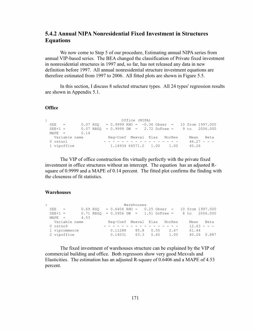
5.4.2 Annual NIPA Nonresidential Fixed Investment in Structures Equations
We now come to Step 5 of our procedure, Estimating annual NIPA series from annual VIP-based series. The BEA changed the classification of Private fixed investment in nonresidential structures in 1997 and, so far, has not released any data in new definition before 1997. All annual nonresidential structure investment equations are therefore estimated from 1997 to 2006. All fitted plots are shown in Figure 5.5.
In this section, I discuss 8 selected structure types. All 24 types' regression results are shown in Appendix 5.1.
Office
The VIP of office construction fits virtually perfectly with the private fixed investment in office structures without an intercept. The equation has an adjusted R-square of 0.9999 and a MAPE of 0.14 percent. The fitted plot confirms the finding with the closeness of fit statistics.
Warehouses
The fixed investment of warehouses structure can be explained by the VIP of commercial building and office. Both regressors show very good Mexvals and Elasticities. The estimation has an adjusted R-square of 0.6406 and a MAPE of 4.53 percent.
171
: Office (NIPA) SEE = 0.07 RSQ = 0.9999 RHO = -0.36 Obser = 10 from 1997.000 SEE+1 = 0.07 RBSQ = 0.9999 DW = 2.72 DoFree = 9 to 2006.000 MAPE = 0.14 Variable name Reg-Coef Mexval Elas NorRes Mean Beta 0 vstnn1 - - - - - - - - - - - - - - - - - 46.27 - - - 1 vipoffice 1.14934 64571.2 1.00 1.00 40.26
: Warehouses SEE = 0.69 RSQ = 0.6406 RHO = 0.25 Obser = 10 from 1997.000 SEE+1 = 0.71 RBSQ = 0.5956 DW = 1.51 DoFree = 8 to 2006.000 MAPE = 4.53 Variable name Reg-Coef Mexval Elas NorRes Mean Beta 0 vstnn9 - - - - - - - - - - - - - - - - - 12.63 - - - 1 vipcommerce 0.11288 85.8 0.55 2.67 61.44 2 vipoffice 0.14031 63.3 0.45 1.00 40.26 0.887

Manufacturing
The VIP of manufacturing structures fits very well to the BEA's fixed investment in manufacturing structures. Plot in Figure 5.5 shows that the predicted value generally moves in the same direction as the actual series. The closeness of fit statistics are good with an adjusted R-square of 0.8768.
Electric power
For fixed investment in electric power structures, we find that it can be explained with only the VIP of power structures. During the estimated period, the equation has an adjusted R-square of 0.9452 and a MAPE of 4.77 percent. The fitted plot shows that the predicted value also moves in the same direction (with slightly different magnitude) as the actual value.
Petroleum and natural gas
Fixed investment in petroleum and natural gas structures is one of the two components of NIPA fixed investment in mining exploration, shafts, and wells structures (the other component is Mining structures). It is also the main contributor to the NIPA
172
: Manufacturing (NIPA) SEE = 2.62 RSQ = 0.8905 RHO = 0.60 Obser = 10 from 1997.000 SEE+1 = 2.36 RBSQ = 0.8768 DW = 0.81 DoFree = 8 to 2006.000 MAPE = 7.52 Variable name Reg-Coef Mexval Elas NorRes Mean Beta 0 vstnnmanu - - - - - - - - - - - - - - - - - 27.51 - - - 1 intercept -7.97617 18.0 -0.29 9.13 1.00 2 vipmanu 1.10648 202.2 1.29 1.00 32.07 0.944
: Electric SEE = 1.00 RSQ = 0.9513 RHO = 0.17 Obser = 10 from 1997.000 SEE+1 = 1.01 RBSQ = 0.9452 DW = 1.66 DoFree = 8 to 2006.000 MAPE = 4.77 Variable name Reg-Coef Mexval Elas NorRes Mean Beta 0 vstnn12 - - - - - - - - - - - - - - - - - 18.94 - - - 1 intercept -3.20768 18.1 -0.17 20.52 1.00 2 vippower 0.81715 353.0 1.17 1.00 27.10 0.975
: Petroleum and natural gas SEE = 0.25 RSQ = 0.9999 RHO = -0.56 Obser = 10 from 1997.000 SEE+1 = 0.20 RBSQ = 0.9999 DW = 3.12 DoFree = 8 to 2006.000 MAPE = 0.64 Variable name Reg-Coef Mexval Elas NorRes Mean Beta 0 vstnn15 - - - - - - - - - - - - - - - - - 43.00 - - - 1 intercept -0.35667 22.4 -0.01 9761.48 1.00 2 vstnnmin 0.96584 9780.0 1.01 1.00 44.89 1.000

fixed investment in Mining exploration, shafts, and wells structures as it covers about 95% of nominal fixed investment in mining exploration, shafts, and wells structures. Thus, it's not surprising to find that fixed investment in mining exploration, shafts, and wells structures fits almost perfectly to the fixed investment in petroleum and natural gas structures with very high closeness of fit statistics and almost perfect fitted plot.
Educational and vocational
The equation for educational and vocational structures has only one regressor, the VIP of educational structures. As to be expected, the equation performs very well throughout the estimation period with very good closeness of fit statistics and fitted plot. The biggest error seen in 2006 might be lower when BEA published its next revised data.
Air transportation
Air transportation is quite difficult to fit well. In this equation, we find that the use of one-period lagged dependent variable and the VIP of transportation structures works best bit still cannot achieve very good closeness of fit statistics, an adjusted R-square of 0.3177. However, the fitted plot gives a good general movement of the investment with pronounced lag which should be alleviated by the use of RHO adjustment in the forecast.
Farm
173
: Educational and vocational SEE = 0.16 RSQ = 0.9922 RHO = 0.27 Obser = 10 from 1997.000 SEE+1 = 0.16 RBSQ = 0.9912 DW = 1.47 DoFree = 8 to 2006.000 MAPE = 0.85 Variable name Reg-Coef Mexval Elas NorRes Mean Beta 0 vstnn18 - - - - - - - - - - - - - - - - - 13.11 - - - 1 intercept 0.80318 23.6 0.06 127.52 1.00 2 vipedu 1.03639 1029.2 0.94 1.00 11.87 0.996
: Air transportation SEE = 0.31 RSQ = 0.4030 RHO = 0.41 Obser = 9 from 1998.000 SEE+1 = 0.29 RBSQ = 0.3177 DurH = 2.16 DoFree = 7 to 2006.000 MAPE = 19.40 Variable name Reg-Coef Mexval Elas NorRes Mean Beta 0 vstnn22 - - - - - - - - - - - - - - - - - 1.31 - - - 1 vstnn22[1] 0.67994 37.4 0.69 1.17 1.32 2 viptr 0.05868 8.2 0.31 1.00 7.02 0.059

This equation works decently in tracking the long-term trend of the fixed investment in farm structures. Both constructions of other nonresidential structures and commercial structures have good Mexvals. Although the adjusted R-square of 0.4414 is not very high, the MAPE of 6.40 percent is quite good. The fitted plot shows that the equations seems to miss the fluctuation in the last decade but generally gives estimated values in that are not far off the actual values.
174
: Farm SEE = 0.43 RSQ = 0.5655 RHO = 0.06 Obser = 10 from 1997.000 SEE+1 = 0.43 RBSQ = 0.4414 DW = 1.88 DoFree = 7 to 2006.000 MAPE = 6.40 Variable name Reg-Coef Mexval Elas NorRes Mean Beta 0 vstnn24 - - - - - - - - - - - - - - - - - 5.17 - - - 1 intercept 1.23534 2.5 0.24 2.30 1.00 2 vipoth -0.83102 10.8 -0.25 2.13 1.58 -0.315 3 vipcommerce 0.08538 45.9 1.01 1.00 61.44 0.702

Office (NIPA) Office (NIPA) 60.2
47.7
35.1
1998 2000 2002 2004 2006 Predicted Actual
Hospitals Hospitals 25.8
18.2
10.6
1998 2000 2002 2004 2006 Predicted Actual
Special Care Special Care 4.70
3.60
2.50
1998 2000 2002 2004 2006 Predicted Actual BasePred
Medical Buildings Medical Buildings 9.00
6.55
4.11
1998 2000 2002 2004 2006 Predicted Actual
Multimerchandise shopping Multimerchandise shopping 27.7
18.9
10.1
1998 2000 2002 2004 2006 Predicted Actual
Food and beverage establishments Food and beverage establishments 8.70
7.85
7.00
1998 2000 2002 2004 2006 Predicted Actual
175
Figure 5.5: Plots of Annual Equations for NIPA Nonresidential Structures Investment

Figure5.5 (cont.)
Warehouses Warehouses14.90
12.75
10.61
1998 2000 2002 2004 2006 Predicted Actual
Other commercial Other commercial18.90
17.10
15.30
2000 2002 2004 2006 Predicted Actual BasePred
Manufacturing (NIPA) Manufacturing (NIPA) 40.5
28.1
15.7
1998 2000 2002 2004 2006 Predicted Actual
Electric Electric 24.3
17.2
10.1
1998 2000 2002 2004 2006 Predicted Actual
Other power Other power 8.80
7.40
6.00
2000 2002 2004 2006 Predicted Actual BasePred
Communication Communication19.86
15.90
11.94
1998 2000 2002 2004 2006 Predicted Actual
176

Figure5.5 (cont.)
Petroleum and natural gas Petroleum and natural gas101.5
60.5
19.5
1998 2000 2002 2004 2006 Predicted Actual
Mining Mining 4.04
2.52
1.00
1998 2000 2002 2004 2006 Predicted Actual BasePred
Religious Religious 8.33
6.96
5.60
1998 2000 2002 2004 2006 Predicted Actual
Educational and vocational Educational and vocational15.08
12.44
9.80
1998 2000 2002 2004 2006 Predicted Actual
Lodging Lodging21.91
17.11
12.30
1998 2000 2002 2004 2006 Predicted Actual
Amusement and recreation Amusement and recreation11.52
10.24
8.96
1998 2000 2002 2004 2006 Predicted Actual
177

Figure5.5 (cont.)
Air transportation Air transportation 2.10
1.50
0.90
1998 2000 2002 2004 2006 Predicted Actual BasePred
Land transportation Land transportation 6.90
5.80
4.69
2000 2002 2004 2006 Predicted Actual BasePred
Farm Farm 6.00
4.90
3.80
1998 2000 2002 2004 2006 Predicted Actual
Other (other) structures Other (other) structures 4.60
3.50
2.40
1998 2000 2002 2004 2006 Predicted Actual
Brokers' commissions Brokers' commissions 2.70
2.35
2.00
1998 2000 2002 2004 2006 Predicted Actual
Used structures Used structures 1.60
-0.50
-2.60
1998 2000 2002 2004 2006 Predicted Actual
178

Figure5.5 (cont.)
Other (other) structures Other (other) structures 4.60
3.50
2.40
1998 2000 2002 2004 2006 Predicted Actual
Brokers' commissions Brokers' commissions 2.70
2.35
2.00
1998 2000 2002 2004 2006 Predicted Actual
Used structures Used structures 1.60
-0.50
-2.60
1998 2000 2002 2004 2006 Predicted Actual
179

5.5 Residential Fixed Investment in Structures Equations
Step 1 of the procedure is discussed earlier in section 5.3. I discuss Step 3 and Step 4 for estimating Residential fixed investment in structures in this section.
5.5.1 Extending NIPA series using VIP-based Residential Construction
First, as indicated, we use a very short-term forecast of the VIP of residential construction estimated from the equation in section 5.2 to complete the current quarter of components of NIPA Fixed investment in residential structures. The following section discusses the regression equations that will be used to complete the current quarter NIPA series, Step 3. Figure 5.6 shows the fitted plots of these three series.
All three series, which are parts of NIPA Fixed investment in residential structures, can be explained very well with combinations of lagged dependent variables and the VIP of residential construction, qvipr, (and its lagged values). All three equations are estimated with data from 1994Q1 to 2007Q2.
The results show that all three equations have very high closeness of fit statistics in both adjusted R-square and MAPE. The plots of predicted value are very good with out showing a lag in movement when the sudden decline in residential investments occurred in the beginning of 2006. The BasePred plots also move along nicely with the actual series. These should provide accurate forecasts if we can get reliable forecasted values of the VIP of residential construction, especially when our objective is to just complete the current quarter.
Single-family structures
180
: Single-family structures SEE = 6.79 RSQ = 0.9947 RHO = 0.69 Obser = 54 from 1994.100 SEE+1 = 5.07 RBSQ = 0.9945 DW = 0.61 DoFree = 51 to 2007.200 MAPE = 2.30 Variable name Reg-Coef Mexval Elas NorRes Mean Beta 0 qvstnnrsing - - - - - - - - - - - - - - - - - 262.06 - - - 1 intercept -21.05345 39.2 -0.08 188.83 1.00 2 qvipr 0.94377 288.9 1.47 2.08 408.98 1.363 3 qvipr[2] -0.25902 44.1 -0.39 1.00 397.16 -0.376

Multifamily structures
Other residential structures
181
: Multifamily structures SEE = 0.91 RSQ = 0.9938 RHO = -0.11 Obser = 54 from 1994.100 SEE+1 = 0.90 RBSQ = 0.9936 DurH = -0.83 DoFree = 52 to 2007.200 MAPE = 2.45 Variable name Reg-Coef Mexval Elas NorRes Mean Beta 0 qvstnnrmul - - - - - - - - - - - - - - - - - 31.11 - - - 1 qvstnnrmul[1] 0.81960 249.7 0.80 1.68 30.38 2 qvipr 0.01526 29.8 0.20 1.00 408.98 0.179
: Other Residential structures SEE = 3.55 RSQ = 0.9960 RHO = 0.14 Obser = 54 from 1994.100 SEE+1 = 3.53 RBSQ = 0.9959 DurH = 1.06 DoFree = 52 to 2007.200 MAPE = 1.25 Variable name Reg-Coef Mexval Elas NorRes Mean Beta 0 qvstnnroth - - - - - - - - - - - - - - - - - 191.04 - - - 1 qvstnnroth[1] 0.92260 245.0 0.91 1.11 187.89 2 qvipr 0.04265 5.5 0.09 1.00 408.98 0.102

182
Figure 5.6: Plots of Regressions of Fixed Residential Investment in Structures (Step 3)
Single-family structures Single-family structures 464
303
142
1995 2000 2005 Predicted Actual
Multifamily structures Multifamily structures 54.7
33.2
11.7
1995 2000 2005 Predicted Actual BasePred
Other Residential structures Other Residential structures 296
207
117
1995 2000 2005 Predicted Actual BasePred

5.5.2 Quarterly Residential Fixed Investment in Structures Equations
All equations in this section are estimated over the period from 1994Q1 to 2007Q2. These equations produce the forecast, which will be annualized, as discussed earlier as the final product of our approach.
Single-family structures
The equation for single-family structures investment has three regressors. The regressors are one-quarter lagged dependent variable, current period NIPA fixed residential investment and one-quarter lagged NIPA fixed residential investment (plus intercept). All regressors have good Mexvals and reasonable signs. The result shows very good closeness of fit statistics. The adjusted R-square is 0.9979 and the MAPE is 0.99 percent. Most of the explanatory power is provided by the NIPA fixed residential investment (investment in single-family structures accounts for 53% of NIPA fixed residential investment on average over the estimation period). Plots of both predicted value and BasePred shows very good tracking ability throughout the estimation period.
Multifamily structures
For the equation of Multifamily structures investment, one-quarter lagged dependent variable and the NIPA fixed residential investment are used as regressors (without intercept). We have very good closeness of fit statistics with an adjusted R-
183
: Single-family structures SEE = 4.18 RSQ = 0.9980 RHO = 0.11 Obser = 54 from 1994.100 SEE+1 = 4.21 RBSQ = 0.9979 DurH = 0.92 DoFree = 50 to 2007.200 MAPE = 0.99 Variable name Reg-Coef Mexval Elas NorRes Mean Beta 0 qvstnnrsing - - - - - - - - - - - - - - - - - 262.45 - - - 1 intercept -6.80430 6.7 -0.03 501.20 1.00 2 qvstnnrsing[1] 0.73232 80.6 0.72 8.50 258.95 0.737 3 vfr 0.81737 187.1 1.53 5.07 491.67 1.403 4 vfr[1] -0.66497 125.1 -1.23 1.00 484.62 -1.146
: Multifamily structures SEE = 0.87 RSQ = 0.9943 RHO = -0.19 Obser = 54 from 1994.100 SEE+1 = 0.85 RBSQ = 0.9942 DurH = -1.45 DoFree = 52 to 2007.200 MAPE = 2.33 Variable name Reg-Coef Mexval Elas NorRes Mean Beta 0 qvstnnrmul - - - - - - - - - - - - - - - - - 31.14 - - - 1 qvstnnrmul[1] 0.82639 252.2 0.81 1.65 30.38 2 vfr 0.01234 28.3 0.19 1.00 491.67 0.172

square of 0.9942 and a MAPE of 2.33 percent. Both regressors have very good Mexvals and positive signs. The plots show a very good fit by both the predicted values and the BasePred.
Other residential structures
Other residential structures investment equation has four regressors plus an intercept. The regressors are 1) one-quarter lagged dependent variable, 2) two-quarter lagged dependent variable, 3) NIPA fixed residential investment, and 4) one-quarter lagged NIPA fixed residential investment. All regressors have good Mexvals and reasonable signs. The closeness of fit statistics are very good with an adjusted R-square of 0.9977 and a MAPE of 0.94 percent. The fitted plots show a very good fit by both the predicted value and the BasePred.
184
: Other Residential structures SEE = 2.63 RSQ = 0.9978 RHO = 0.04 Obser = 54 from 1994.100 SEE+1 = 2.63 RBSQ = 0.9977 DurH = 1.36 DoFree = 49 to 2007.200 MAPE = 0.94 Variable name Reg-Coef Mexval Elas NorRes Mean Beta 0 qvstnnroth - - - - - - - - - - - - - - - - - 191.15 - - - 1 intercept -2.56890 1.9 -0.01 462.33 1.00 2 qvstnnroth[1] 0.72714 28.0 0.71 1.81 187.89 0.717 3 qvstnnroth[2] 0.34476 6.7 0.33 1.79 184.58 0.334 4 vfr 0.19485 32.5 0.50 1.49 491.67 0.554 5 vfr[1] -0.21119 22.0 -0.54 1.00 484.62 -0.603

185
Figure 5.7: Plots of Regression of Fixed Residential Investment in Structures (Step 5)
Single-family structures Single-family structures 464
303
143
1995 2000 2005 Predicted Actual BasePred
Multifamily structures Multifamily structures 54.7
33.2
11.7
1995 2000 2005 Predicted Actual BasePred
Other Residential structures Other Residential structures 292
205
117
1995 2000 2005 Predicted Actual BasePred

5.6 Historical Simulations20
Using the same idea as described in previous chapters, two historical forecasts, one with all actual exogenous variables and one with exogenous variables generated by QUEST, are generated for 2005 and 2006. The assumptions of exogenous variables used in the historical simulation with QUEST (the second simulation) is shown in Table 5.8
As mentioned in Chapter 4, QUEST predicted that the residential fixed investment (vfr) would expand steadily in both 2005 and 2006. This forecast underestimates vfr from 2005Q1 to 2006Q2. Thus, I would expect to find that the second simulation will underestimate residential fixed investment in structures across all types, especially in 2005.
For private fixed investment in nonresidential structures, the numbers from QUEST increase steadily throughout the simulation period. However, the growth rate from QUEST is much slower than what actually happened during 2005 and 2006. This discrepancy results in much lower values of private fixed investment in nonresidential structures that was used in the second simulation. Thus, I would expect the second simulation to underestimate the fixed investment in nonresidential structures across all asset types.
Table 5.9 shows the differences between each historical simulation and the published numbers. Figure 5.8 plots the results in Table 5.9 for easier visual comparison.
20 As in previous Chapters, “The first simulation” refers to the historical simulation with actual exogenous variables and “The second simulation” refers to the historical simulation with exogenous variables generated from QUEST and other ad hoc assumptions.
186
Table 5.8: Assumptions of exogenous variables used in the Second Historical Simulation2005Q1 2005Q2 2005Q3 2005Q4
vfnrs Private Fixed Investment in Nonresidential Structures (nominal) in Billion of dollars 295.94 298.79 311.91 314.95vfr Private Fixed Residential Investment (nominal) in Billion of dollars 686.01 700.45 720.79 729.85
2006Q1 2006Q2 2006Q3 2006Q4vfnrs Private Fixed Investment in Nonresidential Structures (nominal) in Billion of dollars 317.30 316.87 319.28 322.90vfr Private Fixed Residential Investment (nominal) in Billion of dollars 732.88 743.59 750.72 761.58
Percentage difference from the published value 2005Q1 2005Q2 2005Q3 2005Q4
vfnrs Private Fixed Investment in Nonresidential Structures (nominal) in Billion of dollars -8.46% -9.13% -6.67% -10.53%vfr Private Fixed Residential Investment (nominal) in Billion of dollars -5.68% -7.45% -8.26% -9.11%
2006Q1 2006Q2 2006Q3 2006Q4vfnrs Private Fixed Investment in Nonresidential Structures (nominal) in Billion of dollars -15.54% -20.82% -23.27% -24.63%vfr Private Fixed Residential Investment (nominal) in Billion of dollars -9.45% -5.66% 0.62% 6.47%

Overall, the approach, described in this chapter, can predict the private fixed investment in structures very well, especially in the major asset types as seen by the results of the first historical simulation shown in Table 5.9. As expected, as a result of significantly low values of exogenous inputs, the second simulation underestimated the structure investment in most of the asset types. The notable asset types that the second simulation overestimated the investment with significant errors are Air transportation and Manufacturing.
187
Table 5.9: Historical Simulations' Results in Major and Detailed Investment Industries
2005 2006 2005 20061 Private fixed investment in structures -0.03% 0.36% -7.52% -3.69%2 Nonresidential 0.33% 1.02% -3.24% -13.50%3 Commercial and health care -0.37% -0.40% -8.46% -17.32%4 Office \1\ 0.21% -0.04% -13.99% -27.20%5 Health care -0.07% -0.53% -2.39% -8.93%6 Hospitals and special care 2.56% -3.17% -1.15% -14.12%7 Hospitals 0.44% -0.30% -4.15% -14.08%8 Special care 20.10% -24.95% 23.58% -14.41%9 Medical buildings -6.84% 8.90% -5.58% 9.56%10 Multimerchandise shopping -4.90% -10.34% -18.75% -32.98%11 Food and beverage establishments -2.39% 3.98% -0.99% 6.23%12 Warehouses 4.09% 7.39% -5.55% -12.25%13 Other commercial \2\ 1.08% 7.03% 2.03% 9.03%14 Manufacturing 8.53% 11.78% 17.58% 12.15%15 Power and communication -0.29% 0.41% 3.09% -6.89%16 Power -3.00% -2.37% 7.73% -4.18%17 Electric 0.95% 6.68% 13.10% 3.48%18 Other power -13.05% -23.35% -5.96% -21.93%19 Communication 4.06% 5.46% -4.37% -10.76%20 Mining exploration, shafts, and wells 0.02% 0.08% -7.81% -21.43%21 Petroleum and natural gas 0.43% -0.10% -7.41% -21.58%22 Mining -9.27% 4.83% -16.93% -17.56%23 Other structures -0.45% 1.73% 1.21% -7.72%24 Religious 0.14% -0.36% 9.70% 12.60%25 Educational and vocational -1.03% 2.54% -0.56% -1.31%26 Lodging 0.03% 0.03% -0.64% -21.28%27 Amusement and recreation 0.41% -0.58% 14.62% -6.20%28 Transportation -1.10% -2.89% -3.90% -17.45%29 Air 15.03% 27.35% 13.99% 20.67%30 Land \3\ -3.48% -6.83% -6.54% -22.42%31 Farm -3.23% 12.84% -7.78% 1.77%32 Other \4\ -11.68% 23.07% -15.35% 13.46%33 Brokers' commissions on sale of structures 3.66% -3.18% -1.90% -14.28%34 Net purchases of used structures -37.34% 9.92% -22.24% -11.21%35 Residential -0.19% 0.00% -9.40% 1.57%36 Permanent site -0.38% -1.26% -12.53% 0.69%37 Single-family structures -0.29% -1.05% -13.34% 1.60%38 Multifamily structures -1.22% -2.90% -5.09% -6.42%39 Other structures 0.14% 2.06% -4.00% 3.01%
1st Sim 2nd SimPercentage difference from the published value

For the total fixed investment in structures, the first simulation is very accurate during the simulation period with errors of -0.03% in 2005 and 0.36% in 2006. The second simulation missed the same published figures by -7.52% in 2005 and -3.69% in 2006.
The first simulation performs equally well in predicting the investment in nonresidential structures and residential structures. This means that the accuracy we observed for the total structure investment does not come from the averaging effect from residential and nonresidential structure investments.
For residential structures, the first simulation performs very well in predicting all of its components with small tendency to underestimate the permanent site structure investments. The second simulation underestimates all components of residential structure investment in 2005. It underestimates the residential investment in Single-family structures, which is the biggest component of residential structure investment, significantly with errors of -13.34% in 2005. However, in 2006, the second simulation performs relatively well with only slightly more errors than the first simulation.
For nonresidential structure investment, the first simulation missed the published NIPA numbers by 0.33% in 2005 and 1.02% in 2006. The second simulation missed the same numbers by -3.24% in 2005 and -13.50% in 2006.
The commercial and health care structure investment can be predicted pretty well by the first simulation. Considering the described error with the exogenous inputs, the second simulation performs relatively well in this major asset type. From the first simulation, the only asset type with significant errors is Special care structure investment, with errors of 20.10% in 2005 and -24.95% in 2006. This asset type, also, exhibits comparable performance from the second simulation.
The first simulation missed the nominal manufacturing structure investment by 8.53% in 2005 and 11.78% in 2006. The second simulation missed the same numbers by 17.58% and 12.15% in 2005 and 2006, respectively.
For Power and communication structure investment, the first simulation missed the published numbers by only -0.29% in 2005 and 0.41% in 2006. The second simulation missed the same numbers by 3.09% in 2005 and -6.89% in 2006. Other power structure investment is the only component of power and communication structure investment with significant errors from the first simulation. The first simulation missed the published numbers of other power structure investment by -13.05% in 2005 and -23.35% in 2006.
For Mining exploration, shafts, and wells structure investment, the first simulation missed the BEA numbers by only 0.02% in 2005 and 0.08% in 2006. The second simulation missed the same numbers by -7.81% in 2005 and -21.43% in 2006. These errors from both simulations can be traced to the accuracy – or inaccuracy -- of both simulations in predicting Petroleum and natural gas structure investment, the biggest
188

component of Mining exploration, shafts, and wells structure investment. The first simulation missed the official numbers of the Petroleum and natural gas structure investment by 0.43% in 2005 and -0.10% in 2006 while the second simulation missed the same figures by -7.41% and -21.58% in 2005 and 2006, respectively.
Both simulations performed well in predicting the fixed investment in other structures. The first simulation performs very well in most of them except in some minor components such as Air transportation and Other-other structures21. At the same simulation period, the second simulation performs well in predicting the major components of fixed investment in other structures with the exception of Religious structure and Amusement and recreation structure. The second simulation missed the published numbers of investment in religious structure by 9.70% in 2005 and 12.60% in 2006. The second simulation, also, missed the published numbers of investment in Amusement and recreation structure by 14.62% in 2005 and -6.02% in 2006.
Overall, the first simulation shows that, with accurate exogenous inputs, our approach for estimating fixed investment in structures by asset types can produce reasonable and reliable results.
21 Includes water supply, sewage and waste disposal, public safety, highway and street, and conservation and development.
189

1 Private fixed investment in structures 1 Private fixed investment in structures (Million of dollars)
1164
879
593
1998 2000 2002 2004 2006 a.vstnntot b.vstnntot c.vstnntot
2 Nonresidential 2 Nonresidential (Million of dollars)
409
330
250
1998 2000 2002 2004 2006 a.vstnnnr b.vstnnnr c.vstnnnr
3 Commercial and health care 3 Commercial and health care (Million of dollars)
154.0
129.1
104.2
1998 2000 2002 2004 2006 a.vstnncommerce b.vstnncommerce c.vstnncommerce
4 Office 4 Office (Million of dollars)
60.2
47.6
35.1
1998 2000 2002 2004 2006 a.vstnn1 b.vstnn1 c.vstnn1
5 Health care 5 Health care (Million of dollars)
37.4
28.5
19.6
1998 2000 2002 2004 2006 a.vstnn2 b.vstnn2 c.vstnn2
6 Hospitals and special care 6 Hospitals and special care (Million of dollars)
29.2
22.2
15.1
1998 2000 2002 2004 2006 a.vstnn3 b.vstnn3 c.vstnn3
190
Figure 5.8: Plots compared BEA numbers with numbers from Historical Simulations

Figure 5.8 (cont.)
7 Hospitals 7 Hospitals (Million of dollars)
25.8
18.3
10.7
1998 2000 2002 2004 2006 a.vstnn4 b.vstnn4 c.vstnn4
8 Special care 8 Special care (Million of dollars)
4.70
3.60
2.50
1998 2000 2002 2004 2006 a.vstnn5 b.vstnn5 c.vstnn5
9 Medical buildings 9 Medical buildings (Million of dollars)
9.00
6.75
4.50
1998 2000 2002 2004 2006 a.vstnn6 b.vstnn6 c.vstnn6
10 Multimerchandise shopping 10 Multimerchandise shopping (Million of dollars)
27.7
19.6
11.5
1998 2000 2002 2004 2006 a.vstnn7 b.vstnn7 c.vstnn7
11 Food and beverage establishments 11 Food and beverage establishments (Million of dollars)
8.70
7.85
7.00
1998 2000 2002 2004 2006 a.vstnn8 b.vstnn8 c.vstnn8
12 Warehouses 12 Warehouses (Million of dollars)
14.90
13.10
11.30
1998 2000 2002 2004 2006 a.vstnn9 b.vstnn9 c.vstnn9
191
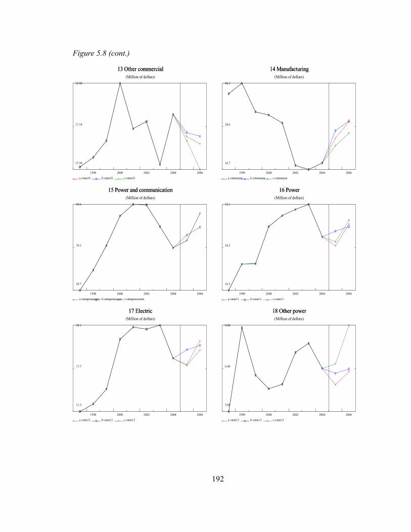
Figure 5.8 (cont.)
13 Other commercial 13 Other commercial (Million of dollars)
18.90
17.10
15.30
1998 2000 2002 2004 2006 a.vstnn10 b.vstnn10 c.vstnn10
14 Manufacturing 14 Manufacturing (Million of dollars)
40.5
28.6
16.7
1998 2000 2002 2004 2006 a.vstnnmanu b.vstnnmanu c.vstnnmanu
15 Power and communication 15 Power and communication (Million of dollars)
49.6
39.2
28.7
1998 2000 2002 2004 2006 a.vstnnpowcomm b.vstnnpowcomm c.vstnnpowcomm
16 Power 16 Power (Million of dollars)
32.1
24.2
16.3
1998 2000 2002 2004 2006 a.vstnn11 b.vstnn11 c.vstnn11
17 Electric 17 Electric (Million of dollars)
24.1
17.7
11.3
1998 2000 2002 2004 2006 a.vstnn12 b.vstnn12 c.vstnn12
18 Other power 18 Other power (Million of dollars)
8.80
6.90
5.00
1998 2000 2002 2004 2006 a.vstnn13 b.vstnn13 c.vstnn13
192

Figure 5.8 (cont.)
19 Communication 19 Communication (Million of dollars)
19.60
15.85
12.10
1998 2000 2002 2004 2006 a.vstnn14 b.vstnn14 c.vstnn14
20 Mining exploration, shafts, and wells 20 Mining exploration, shafts, and wells (Million of dollars)
105.5
63.0
20.6
1998 2000 2002 2004 2006 a.vstnnmin b.vstnnmin c.vstnnmin
21 Petroleum and natural gas 21 Petroleum and natural gas (Million of dollars)
101.5
60.6
19.6
1998 2000 2002 2004 2006 a.vstnn15 b.vstnn15 c.vstnn15
22 Mining 22 Mining (Million of dollars)
4.09
2.54
1.00
1998 2000 2002 2004 2006 a.vstnn16 b.vstnn16 c.vstnn16
23 Other structures 23 Other structures (Million of dollars)
72.9
65.1
57.2
1998 2000 2002 2004 2006 a.vstnnnroth b.vstnnnroth c.vstnnnroth
24 Religious 24 Religious (Million of dollars)
8.45
7.02
5.60
1998 2000 2002 2004 2006 a.vstnn17 b.vstnn17 c.vstnn17
193
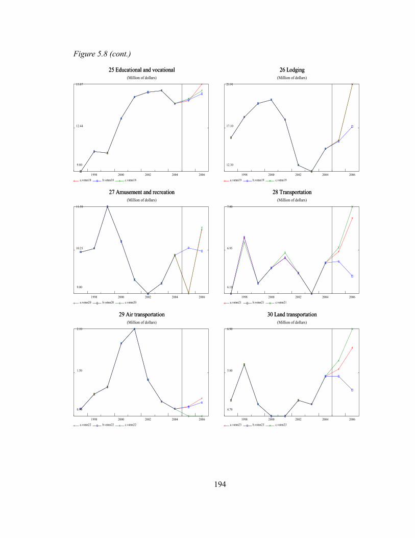
Figure 5.8 (cont.)
25 Educational and vocational 25 Educational and vocational (Million of dollars)
15.07
12.44
9.80
1998 2000 2002 2004 2006 a.vstnn18 b.vstnn18 c.vstnn18
26 Lodging 26 Lodging (Million of dollars)
21.91
17.10
12.30
1998 2000 2002 2004 2006 a.vstnn19 b.vstnn19 c.vstnn19
27 Amusement and recreation 27 Amusement and recreation (Million of dollars)
11.50
10.25
9.00
1998 2000 2002 2004 2006 a.vstnn20 b.vstnn20 c.vstnn20
28 Transportation 28 Transportation (Million of dollars)
7.80
6.95
6.10
1998 2000 2002 2004 2006 a.vstnn21 b.vstnn21 c.vstnn21
29 Air transportation 29 Air transportation (Million of dollars)
2.10
1.50
0.90
1998 2000 2002 2004 2006 a.vstnn22 b.vstnn22 c.vstnn22
30 Land transportation 30 Land transportation (Million of dollars)
6.90
5.80
4.70
1998 2000 2002 2004 2006 a.vstnn23 b.vstnn23 c.vstnn23
194
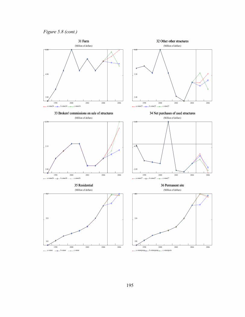
Figure 5.8 (cont.)
31 Farm 31 Farm (Million of dollars)
6.00
4.90
3.80
1998 2000 2002 2004 2006 a.vstnn24 b.vstnn24 c.vstnn24
32 Other other structures 32 Other other structures (Million of dollars)
4.60
3.50
2.40
1998 2000 2002 2004 2006 a.vstnn25 b.vstnn25 c.vstnn25
33 Brokers' commissions on sale of structures 33 Brokers' commissions on sale of structures (Million of dollars)
2.70
2.35
2.00
1998 2000 2002 2004 2006 a.vstnn26 b.vstnn26 c.vstnn26
34 Net purchases of used structures 34 Net purchases of used structures (Million of dollars)
1.60
-0.24
-2.09
1998 2000 2002 2004 2006 a.vstnn27 b.vstnn27 c.vstnn27
35 Residential 35 Residential (Million of dollars)
767
555
343
1998 2000 2002 2004 2006 a.vstnnr b.vstnnr c.vstnnr
36 Permanent site 36 Permanent site (Million of dollars)
481
339
198
1998 2000 2002 2004 2006 a.vstnnrperm b.vstnnrperm c.vstnnrperm
195

Figure 5.8 (cont.)
37 Single-family structures 37 Single-family structures (Million of dollars)
434
304
175
1998 2000 2002 2004 2006 a.vstnnrsing b.vstnnrsing c.vstnnrsing
38 Multifamily structures 38 Multifamily structures (Million of dollars)
53.0
37.9
22.9
1998 2000 2002 2004 2006 a.vstnnrmul b.vstnnrmul c.vstnnrmul
39 Other residential structures 39 Other residential structures (Million of dollars)
295
220
145
1998 2000 2002 2004 2006 a.vstnnroth b.vstnnroth c.vstnnroth
5.7 Forecast of Fixed Investment in Structures between 2007 and 2008
In this section, a short-term outlook of U.S. Private fixed investment in structures in 2007 and 2008 is generated from the described approach. In November 2007, we have monthly VIP data up through July 2007. Thus, after completing the third quarter of 2007 in the VIP monthly series, the forecast for the last quarter of 2007 and all four quarter of 2008 are forecasted.
196

Forecast Assumptions
There are only two exogenous variables used in this approach. Private fixed investment in nonresidential structures and Private fixed residential investment are forecasted though the end of 2008 by QUEST model. Table 5.10 shows the values of these two exogenous variables.
The Private fixed investment in nonresidential structures is forecasted to be increasing until the second quarter of 2008 when it will be stable until the end of 2008. The nominal value of residential investment is predicted to be declining in 2008 as the problem in the sub-prime mortgage market is still affecting the economy.
Outlook of Fixed Investment in Structures by Asset Types in 2007 and 2008
Plots of all fixed investment in structures by asset types are shown in Figure 5.9. Table 5.11 shows nominal value of fixed investment in structures from 1997 to 2008. Table 5.12 shows year-to-year growth rate of nominal Fixed investment in structures by types.
Overall, we expect to see a temporary drop in investment in structures in 2007. The investment will expand again in 2008 with a growth rate of 6.54 percent. With more recent data (up to November 2007), the forecasted growth rate in 2008 seems to be on the high side as many indicators show a sign that the problem in the credit market might persist well into 2008 which will affect the investment, especially residential investment.
Nonresidential
From 2002 to 2006, investment in Nonresidential structures accounts for less than 35% of total private fixed investment in structures on average. Its share is expected to increase in 2007 and 2008 as the problem in credit markets mainly affects the residential structures. However, the slowdown in investment will catch up to the nonresidential structures investment in 2008. We expect the Nonresidential structures investment to keep growing at 17.89% in 2007 and 12.08% in 2008 in nominal terms. This means that its share of the total structures investment will increase from 35% in 2006 to 44% in
197
Table 5.10: Assumptions of exogenous variables used in forecasting fixed investment of structures
2007Q4 2008Q1 2008Q2 2008Q3 2008Q4vfnrs Private Fixed Investment in Nonresidential Structures (nominal) in Billion of dollars 483.50 492.94 501.54 500.17 504.47vfr Private Fixed Residential Investment (nominal) in Billion of dollars 638.83 631.77 626.18 627.30 623.69

2008. Power and communication structures and Mining exploration, shafts, and wells structures are the two asset types that will see the most expansion between 2006 and 2008.
Commercial and Health CareCommercial and Health care structures investment is expected to grow by 15.02%
in 2007 and 5.65% in 2008. Office structures investment will slowdown in 2008 from the growth rate of 15.92% in 2007 to 3.59 percent in 2008. Health care structures will keep expanding at a modest rate of 1.99% in 2007 and 6.91% in 2008. Most of the expansion in Health care structures comes from the construction of Hospitals and Medical building. The medical building structures investment is expected to grow rapidly in 2007 with a growth rate of 34.54% while special care structures will see a slowdown with growth rate of -30.83% in 2007 and -20.06% in 2008; this decreasing trend started in 2001.
Building of Food and beverage establishments is predicted to have a negative growth rate of -3.24 percent in 2007 and follow by growth of 9.08% in 2008. It should be noted that the negative growth rate began in 2001 while the structures investment in Multimerchandise shopping has been increasing at the same time. We expect Investment in Multimerchandise shopping structures to grow by 24.14% in 2007 and 13.86% in 2008.
Investment in Warehouses will grow by 21.7% in 2007 and 7.57% in 2008. Other commercial structures22 investment will grow by 7.66% in 2007 but slowdown in 2008 with a growth rate of -2.77%.
ManufacturingManufacturing structures investment will grow by 12.52% in 2007 and will
decrease by -2.77% in 2008 as the credit problem starts to affect the nonresidential structures investment.
Power and CommunicationPower and communication structures will expand rapidly in 2007 with a growth
rate of 26.49% and will keep expanding in 2008 with a growth rate of 16.66%. Most of this expansion comes from the investment in Electric power structures, which has growth rates of 33.67% in 2007 and 21.42% in 2008. The Communication structures investment will be growing with growth rates of 21.90% in 2007 and 10.78% in 2008.
22 Includes buildings and structures used by the retail, wholesale and selected service industries. Consists of auto dealerships, garages, service stations, drug stores, restaurants, mobile structures, and other structures used for commercial purposes. Bus or truck garages are included in transportation., Source:BEA
198

Mining exploration, Shafts, and WellsMining exploration, shafts, and wells investment is expected to grow at a rate of
13.19% in 2007 and 21.88% in 2008. This higher growth rate in 2008 is unique to this asset type as we observe the smaller growth rate of structures investment in all other nonresidential structures. The Petroleum and natural gas structures investment is the main contributor of this growth as it increase from 101.50 billion dollars in 2006 to 140.12 billion dollars in 2008. I believe this expected expansion is reasonable as the world price of petroleum products keep increasing and the U.S. dollar keep depreciating, which create pressure on the economy to reduce cost by using more domestic petroleum products.
Other Nonresidential StructuresOther nonresidential structures investment will expand with growth rates of
27.29% in 2007 and 12.81% in 2008. Historically, the biggest component of other nonresidential structures investment is investment in Lodging which is expected to have growth rates of 57.33% in 2007 and 16.43% in 2008. Educational and vocational structures investment, which is the second largest component, will keep growing by 21.07% in 2007 and 16.83% in 2008. Investment in amusement and recreation structures will slowdown with negative growth rate of -6.00% in 2007 and -2.01% in 2008.
Transportation structures investment shows decent growth as it will expand by 2.96% in 2007 and 6.30% in 2008. This increase in investment of transportation structures is provided from the increase in both Air transportation structures investment and Land transportation structures investment. Air transportation structures investment increases by 14.87% in 2007 from 0.90 billion dollar in 2006 to 1.03 billion dollar in 2007 while Land transportation structures investment increases from 6.90 billion dollars in 2006 to 7.00 billion dollars in 2007, which equal to a growth rate of 1.41%.
Farm structures investment will grow by 28.33% and 10.83% in 2007 and 2008, respectively.
Residential
Residential structures investment is expected to drop sharply in 2007 from 755.15 billion dollars in 2006 to 669.51 billion dollars in 2007, a 11.34% decrease. The Main contributor to this slowdown is the investment in single-family structures which drop by 86.73 billion dollars from the 416 billion dollars observed in 2006. Our forecast shows that the residential structures investment will stabilize in 2008 with a growth rate of 2.59%. However, this growth is provided mainly from the expansion in other residential structures investment23 which grows by 6.78% in 2008 while the investment in Multifamily structures keeps decreasing further by -6.40% in 2008
23 Consists of Manufactured homes, Dormitories, Improvements, Brokers' commissions on sale of residential structures, and Net purchases of used residential structures
199

As mentioned earlier, the outlook for the residential structures investment in 2008 is not optimistic as the problem in the credit market is expected to persist. Our equations are very likely to overestimate the investment in residential structures in 2008.
200
Table 5.11: Nominal Private Fixed Investment in Structures 2003-2008in Billion dollars
2003 2004 2005 2006 2007 2008Private fixed investment in structures 841.62 965.25 1,093.77 1,160.45 1,147.32 1,222.39 Nonresidential 277.10 298.20 334.60 405.30 477.81 535.55 Commercial and health care 112.10 122.10 132.60 154.10 177.25 187.27 Office \1\ 35.10 37.80 42.80 53.10 61.56 63.77 Health care 27.30 29.50 32.10 37.40 41.51 44.38 Hospitals and special care 20.50 21.00 23.10 29.20 30.48 31.88 Hospitals 17.20 18.20 20.60 25.80 28.13 30.00 Special care 3.30 2.80 2.50 3.40 2.35 1.88 Medical buildings 6.80 8.50 9.00 8.20 11.03 12.50 Multimerchandise shopping 14.60 17.90 21.60 27.70 34.39 39.15 Food and beverage establishments 7.90 7.80 7.40 7.00 6.77 6.16 Warehouses 11.70 11.50 12.20 13.60 16.55 17.80 Other commercial \2\ 15.50 17.60 16.50 15.30 16.47 16.02 Manufacturing 16.70 18.50 23.30 26.80 30.16 30.12 Power and communication 44.20 39.00 40.90 47.20 59.70 69.65 Power 32.10 26.10 25.20 29.20 37.76 45.35 Electric 24.10 19.20 18.10 20.40 27.27 33.11 Other power 8.00 6.90 7.10 8.80 10.49 12.24 Communication 12.10 12.90 15.70 18.00 21.94 24.31 Mining exploration, shafts, and wells 45.80 55.70 73.70 105.40 119.30 145.40 Petroleum and natural gas 44.20 53.30 70.60 101.50 114.89 140.12 Mining 1.60 2.40 3.10 3.90 4.41 5.28 Other structures 58.30 62.90 64.10 71.80 91.40 103.10 Religious 8.30 7.90 7.50 7.50 7.36 7.50 Educational and vocational 14.70 13.90 14.20 14.70 17.80 20.79 Lodging 12.30 14.80 15.70 21.90 34.46 40.12 Amusement and recreation 9.30 10.10 9.00 10.90 10.25 10.04 Transportation 6.10 6.70 7.00 7.80 8.03 8.54 Air 1.10 1.00 0.90 0.90 1.03 1.21 Land \3\ 5.00 5.70 6.10 6.90 7.00 7.32 Farm 5.10 5.50 5.90 5.30 6.80 7.54 Other \4\ 2.40 3.20 3.60 2.90 3.83 3.54 Brokers' commissions on sale of structures 2.10 2.20 2.30 2.70 2.94 3.16 Net purchases of used structures -2.00 -1.40 -1.10 -1.90 -0.07 1.88 Residential 564.52 667.05 759.17 755.15 669.51 686.84 Permanent site 345.67 417.50 480.83 469.00 380.13 377.83 Single-family structures 310.55 377.55 433.52 416.00 329.63 330.56 Multifamily structures 35.13 39.95 47.30 53.00 50.50 47.26 Other structures 218.85 249.55 278.35 286.15 289.38 309.02

201
Table 5.12: Growth Rate of Nominal Private Fixed Investment in Structures
2000-2005 2003-2004 2004-2005 2005-2006 2003-2006 2006-2007 2007-2008Private fixed investment in structures 7.93% 14.69% 13.32% 6.10% 11.37% -1.13% 6.54% Nonresidential 1.74% 7.61% 12.21% 21.13% 13.65% 17.89% 12.08% Commercial and health care -0.38% 8.92% 8.60% 16.21% 11.24% 15.02% 5.65% Office \1\ -5.33% 7.69% 13.23% 24.07% 15.00% 15.93% 3.59% Health care 8.05% 8.06% 8.81% 16.51% 11.13% 10.99% 6.91% Hospitals and special care 7.51% 2.44% 10.00% 26.41% 12.95% 4.37% 4.60% Hospitals 12.52% 5.81% 13.19% 25.24% 14.75% 9.01% 6.66% Special care -11.65% -15.15% -10.71% 36.00% 3.38% -30.83% -20.06% Medical buildings 10.30% 25.00% 5.88% -8.89% 7.33% 34.54% 13.28% Multimerchandise shopping 9.31% 22.60% 20.67% 28.24% 23.84% 24.14% 13.86% Food and beverage establishments -2.14% -1.27% -5.13% -5.41% -3.93% -3.24% -9.08% Warehouses -2.11% -1.71% 6.09% 11.48% 5.28% 21.70% 7.57% Other commercial \2\ -2.28% 13.55% -6.25% -7.27% 0.01% 7.66% -2.77% Manufacturing -3.27% 10.78% 25.95% 15.02% 17.25% 12.52% -0.12% Power and communication -2.36% -11.76% 4.87% 15.40% 2.84% 26.49% 16.66% Power -1.62% -18.69% -3.45% 15.87% -2.09% 29.32% 20.08% Electric -3.32% -20.33% -5.73% 12.71% -4.45% 33.67% 21.42% Other power 4.07% -13.75% 2.90% 23.94% 4.36% 19.25% 16.59% Communication -1.56% 6.61% 21.71% 14.65% 14.32% 21.90% 10.78% Mining exploration, shafts, and wells 23.61% 21.62% 32.32% 43.01% 32.31% 13.19% 21.88% Petroleum and natural gas 24.00% 20.59% 32.46% 43.77% 32.27% 13.20% 21.96% Mining 21.91% 50.00% 29.17% 25.81% 34.99% 13.01% 19.76% Other structures -1.39% 7.89% 1.91% 12.01% 7.27% 27.29% 12.81% Religious -0.70% -4.82% -5.06% 0.00% -3.29% -1.81% 1.79% Educational and vocational 1.90% -5.44% 2.16% 3.52% 0.08% 21.07% 16.83% Lodging -3.53% 20.33% 6.08% 39.49% 21.97% 57.33% 16.43% Amusement and recreation -2.74% 8.60% -10.89% 21.11% 6.27% -6.00% -2.01% Transportation 1.36% 9.84% 4.48% 11.43% 8.58% 2.96% 6.30% Air -12.67% -9.09% -10.00% 0.00% -6.36% 14.87% 17.37% Land \3\ 5.51% 14.00% 7.02% 13.11% 11.38% 1.41% 4.66% Farm 0.20% 7.84% 7.27% -10.17% 1.65% 28.38% 10.83% Other \4\ -2.28% 33.33% 12.50% -19.44% 8.80% 32.10% -7.64% Brokers' commissions on sale of structures -0.64% 4.76% 4.55% 17.39% 8.90% 8.96% 7.31% Net purchases of used structures n/a n/a n/a n/a n/a n/a n/a Residential 11.65% 18.16% 13.81% -0.53% 10.48% -11.34% 2.59% Permanent site 12.80% 20.78% 15.17% -2.46% 11.16% -18.95% -0.60% Single-family structures 13.03% 21.57% 14.83% -4.04% 10.79% -20.76% 0.28% Multifamily structures 10.95% 13.74% 18.40% 12.05% 14.73% -4.72% -6.40% Other structures 9.83% 14.03% 11.54% 2.80% 9.46% 1.13% 6.78%
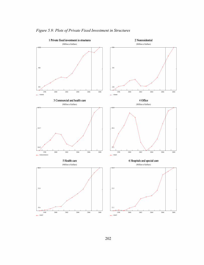
1 Private fixed investment in structures 1 Private fixed investment in structures (Million of dollars)
1222
908
593
1998 2000 2002 2004 2006 2008 vstnntot
2 Nonresidential 2 Nonresidential (Million of dollars)
536
393
250
1998 2000 2002 2004 2006 2008 vstnnnr
3 Commercial and health care 3 Commercial and health care (Million of dollars)
187.3
145.7
104.2
1998 2000 2002 2004 2006 2008 vstnncommerce
4 Office 4 Office (Million of dollars)
63.8
49.4
35.1
1998 2000 2002 2004 2006 2008 vstnn1
5 Health care 5 Health care (Million of dollars)
44.4
32.0
19.6
1998 2000 2002 2004 2006 2008 vstnn2
6 Hospitals and special care 6 Hospitals and special care (Million of dollars)
31.9
23.5
15.1
1998 2000 2002 2004 2006 2008 vstnn3
202
Figure 5.9: Plots of Private Fixed Investment in Structures

Figure 5.9 (cont.)
7 Hospitals 7 Hospitals (Million of dollars)
30.0
20.3
10.7
1998 2000 2002 2004 2006 2008 vstnn4
8 Special care 8 Special care (Million of dollars)
4.70
3.29
1.88
1998 2000 2002 2004 2006 2008 vstnn5
9 Medical buildings 9 Medical buildings (Million of dollars)
12.50
8.50
4.50
1998 2000 2002 2004 2006 2008 vstnn6
10 Multimerchandise shopping 10 Multimerchandise shopping (Million of dollars)
39.2
25.3
11.5
1998 2000 2002 2004 2006 2008 vstnn7
11 Food and beverage establishments 11 Food and beverage establishments (Million of dollars)
8.70
7.43
6.16
1998 2000 2002 2004 2006 2008 vstnn8
12 Warehouses 12 Warehouses (Million of dollars)
17.80
14.55
11.30
1998 2000 2002 2004 2006 2008 vstnn9
203

Figure 5.9 (cont.)
13 Other commercial 13 Other commercial (Million of dollars)
18.90
17.10
15.30
1998 2000 2002 2004 2006 2008 vstnn10
14 Manufacturing 14 Manufacturing (Million of dollars)
40.5
28.6
16.7
1998 2000 2002 2004 2006 2008 vstnnmanu
15 Power and communication 15 Power and communication (Million of dollars)
69.7
49.2
28.7
1998 2000 2002 2004 2006 2008 vstnnpowcomm
16 Power 16 Power (Million of dollars)
45.3
30.8
16.3
1998 2000 2002 2004 2006 2008 vstnn11
17 Electric 17 Electric (Million of dollars)
33.1
22.2
11.3
1998 2000 2002 2004 2006 2008 vstnn12
18 Other power 18 Other power (Million of dollars)
12.24
8.62
5.00
1998 2000 2002 2004 2006 2008 vstnn13
204

Figure 5.9 (cont.)
19 Communication 19 Communication (Million of dollars)
24.3
18.2
12.1
1998 2000 2002 2004 2006 2008 vstnn14
20 Mining exploration, shafts, and wells 20 Mining exploration, shafts, and wells (Million of dollars)
145
83
21
1998 2000 2002 2004 2006 2008 vstnnmin
21 Petroleum and natural gas 21 Petroleum and natural gas (Million of dollars)
140
80
20
1998 2000 2002 2004 2006 2008 vstnn15
22 Mining 22 Mining (Million of dollars)
5.28
3.14
1.00
1998 2000 2002 2004 2006 2008 vstnn16
23 Other structures 23 Other structures (Million of dollars)
103.1
80.2
57.2
1998 2000 2002 2004 2006 2008 vstnnnroth
24 Religious 24 Religious (Million of dollars)
8.30
6.95
5.60
1998 2000 2002 2004 2006 2008 vstnn17
205
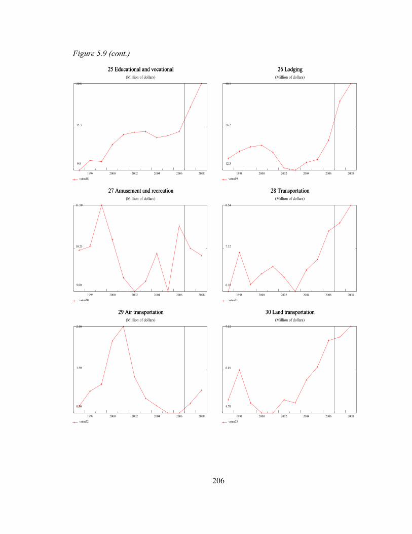
Figure 5.9 (cont.)
25 Educational and vocational 25 Educational and vocational (Million of dollars)
20.8
15.3
9.8
1998 2000 2002 2004 2006 2008 vstnn18
26 Lodging 26 Lodging (Million of dollars)
40.1
26.2
12.3
1998 2000 2002 2004 2006 2008 vstnn19
27 Amusement and recreation 27 Amusement and recreation (Million of dollars)
11.50
10.25
9.00
1998 2000 2002 2004 2006 2008 vstnn20
28 Transportation 28 Transportation (Million of dollars)
8.54
7.32
6.10
1998 2000 2002 2004 2006 2008 vstnn21
29 Air transportation 29 Air transportation (Million of dollars)
2.10
1.50
0.90
1998 2000 2002 2004 2006 2008 vstnn22
30 Land transportation 30 Land transportation (Million of dollars)
7.32
6.01
4.70
1998 2000 2002 2004 2006 2008 vstnn23
206
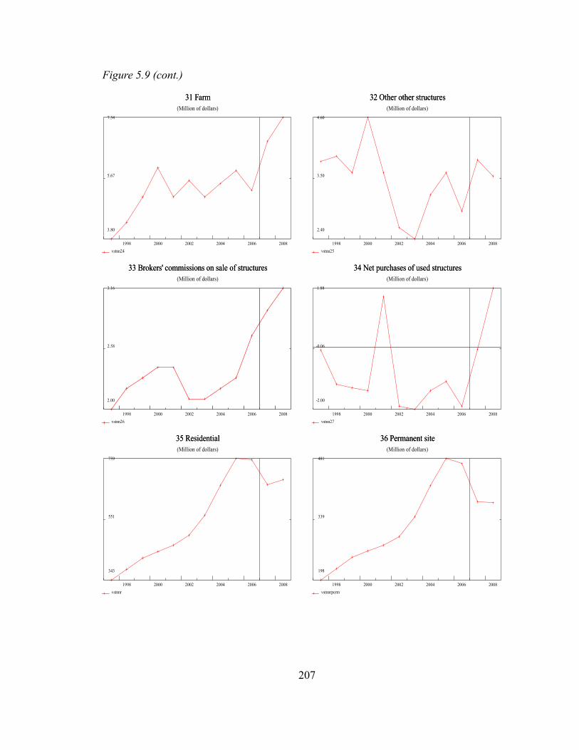
Figure 5.9 (cont.)
31 Farm 31 Farm (Million of dollars)
7.54
5.67
3.80
1998 2000 2002 2004 2006 2008 vstnn24
32 Other other structures 32 Other other structures (Million of dollars)
4.60
3.50
2.40
1998 2000 2002 2004 2006 2008 vstnn25
33 Brokers' commissions on sale of structures 33 Brokers' commissions on sale of structures (Million of dollars)
3.16
2.58
2.00
1998 2000 2002 2004 2006 2008 vstnn26
34 Net purchases of used structures 34 Net purchases of used structures (Million of dollars)
1.88
-0.06
-2.00
1998 2000 2002 2004 2006 2008 vstnn27
35 Residential 35 Residential (Million of dollars)
759
551
343
1998 2000 2002 2004 2006 2008 vstnnr
36 Permanent site 36 Permanent site (Million of dollars)
481
339
198
1998 2000 2002 2004 2006 2008 vstnnrperm
207
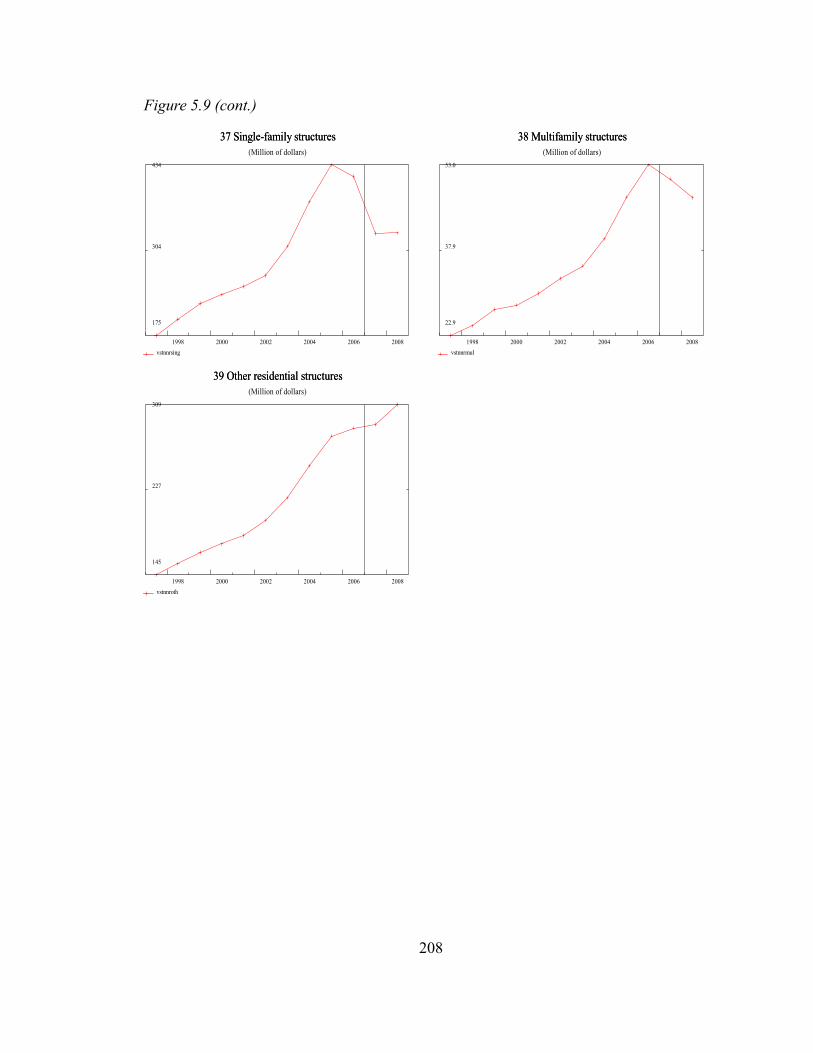
Figure 5.9 (cont.)
37 Single-family structures 37 Single-family structures (Million of dollars)
434
304
175
1998 2000 2002 2004 2006 2008 vstnnrsing
38 Multifamily structures 38 Multifamily structures (Million of dollars)
53.0
37.9
22.9
1998 2000 2002 2004 2006 2008 vstnnrmul
39 Other residential structures 39 Other residential structures (Million of dollars)
309
227
145
1998 2000 2002 2004 2006 2008 vstnnroth
208

Chapter 6: Gross Output by Industry
Gross output of the various industries in the input-output table – roughly speaking, the sales of the industries – is in the center of the computing sequence of interindustry models. They begin with the final demands, some of which we have already studied, and then go through the input-output computations to reach gross output by industry. They then use gross output to compute value added, compensation of employees, capital income, taxes, employment and perhaps other variables by industry. Thus, gross output is the key variable linking final demands to industry-specific variables.
Despite the fact that the gross outputs are well down the chain of calculations, users of the models – especially users who work in private industries – almost invariably look first at the gross output forecasts. Indeed, they look immediately at what the model says about gross output in their industry for the last year, the current year and the next year, precisely the period they know best from their own recent experience -- and the period where, up until now, the model's data base has been the weakest, sometimes two full years out of date. If what they find does not match what they know to be true, they can dismiss the model's results without further examination. Builders of quarterly macromodels do not face this problem, for it is a simple matter to have a model's database always updated with BEA's most recent data.
The strength of interindustry models in forecasting for an industry lies in ensuring consistency among the different industries and in accounting for basic variables, such as demographic changes, and policy variables, such as defense spending. These are long-term considerations and can be easily outweighed in the short terms by inventory or exchange rate fluctuations, overcapacity or undercapacity, or even weather. Yet it is precisely the failure to have up-to-date information on gross output that can readily discredit the model's results for years further in the future. Thus, this final chapter of our study has special importance for the model's credibility and acceptance.
In the U.S. input-output table, gross output of an industry consists of sales, or receipts, and other operating income, plus commodity taxes and changes in inventories. Thus, gross output represents the market value of an industry’s production. Subtracting the industry's cost of purchased materials, energy and services gives value added, which represents the contribution of the industry’s labor and capital to its gross output and to the overall GDP.
Gross output, however, has its limits as a measure of output for large parts of the economy because summing gross output across industries produces a rather meaningless number owing to “double” -- or better, multiple -- counting. The sum of gross outputs in the food producing sector of the economy would include the value of the corn fed to a pig PLUS the value of the pig sold to the slaughter house PLUS the value of the ham sold to a restaurant PLUS the value of meal served by the restaurant. So the corn would have
209

been counted four times. This problem has led to the creation of measures of value added, which are summable. Gross output, however, maintains its importance because it is the industry-level variable which can be computed directly from the final demands and the input-output matrix.
For some purposes, moreover, it is a more appropriate variable than value added. Much of the recent literature on the estimation of production functions adopts this view. Jorgenson and Griliches (1967, 1972) recommend it as the proper measure of production. Hulten (1992) argued that gross output is the correct concept to use in empirical study of structure of production and productivity in contrast to the use of net output (Gross output minus depreciation), as net output requires “a peculiar notion of technological change”. Recently, Meade (2006) has argued cogently against using real value added as a measure of output in productivity studies.
Currently, BEA releases gross output data every year. The data are part of the annual industry accounts and have recently been released in December of the year following the reference year. Thus, data for 2006 was scheduled for release in December of 2007. However, BEA decided to delay the release until January 2008 in order to be able to use the Annual Survey of Manufactures for 2006. Previously, this Survey would not have been used in the first release of the annual industry accounts, but Census has accelerated its production process, and BEA judged the improvement in data quality worth the one-month delay in its release. Each release includes gross output by detailed industry of the previous year and a revision of previous releases.
Thus, the official gross output by industry data can be lagged by up to two years. For example, the data for 2005 is still the most up-to-date gross output data available in December 2007. Meanwhile, other economic indicators, such as Census's Manufacturers' Shipments, Inventories, and Orders, the Federal Reserve Board’s Industrial Production Indexes (IPI) and Census’s wholesale trade survey, have been released monthly or quarterly in a timely manner. We will use these other economic indicators to predict the annual Gross output by industry in the period where the BEA has not released the official information and to forecast the gross output into the near future.
In this chapter, I will discuss (1) sources of data on gross output and indicators that can be used to estimate its recent course, and (2) regression results for estimation of gross output from high-frequency data.
210
6.1 Data on Gross Output and High-Frequency Explanatory Variables
Gross output by industry 1947 – 2005
Since converting the annual industry accounts to North American Industry Classification System (NAICS) in 2002, BEA has also updated GDP by industry information from 1947 to be consistent with the current definition. However, because of the limited historical source data, there are many NAICS categories that cannot be extended back to 1947. Thus, BEA has published historical data in various degrees of aggregation.
There is not, however, any BEA data on gross output with frequency higher than annual. The situation is thus very different from that for PCE for which we have monthly data in full detail. Even for investment, we have monthly data for construction and quarterly data for some aggregate categories of equipment. With gross output, we have nothing until the first annual estimate appears, so our technique will need to be slightly different from what we have used previously. Namely, we will select high-frequency variables which should be good indicators of gross output, convert them to annual series and regress each gross output on the appropriate annualized version of the high-frequency variables. Then we extend the high-frequency series, annualize the extended series, and put it into the estimated regression equation to get predicted values of gross output. The process will be illustrated below. For the moment, it is sufficient to understand that we need data for gross output and the associated price indexes at an annual frequency and data for similar proxy variables at a high frequency.
BEA releases gross output and the associated price indexes at two levels of aggregation. The more aggregate of the two has 65 primary industry categories and a number of subtotal categories. These are the same 65 categories used in the annual input-output tables. These 65 categories are shown in Appendix 6.1. On the BEA website, they are in a file called GDPbyInd_VA_NAICS_1998-2006.xls . (Despite the name, there is no gross output data past 2005.) This same spreadsheet file also contains, for these same industries, series for cost of intermediate inputs, value added, and components of value added added such as wages and salaries, supplements, subsidies, taxes on production and imports, and gross operating surplus. Employment is also available in this classification. Thus, this sectoring is convenient for working with other industry-level data.
On the other hand, the 65-industry aggregation is unfortunately gross in some areas. All construction is in one sector; all utilities – electric, gas, water, and sewer – are in one sector; hospitals and nursing homes are in one sector. However, BEA offers a second set of much more detailed gross product data in 489 primary sectors in a file called GDPbyInd_GO_NAICS_1998-2005.xls . This classification remedies the limitations mentioned, but only gross output in current and constant prices is available, none of the other series.
211

The present work will be limited to the 65-sector classification, but the availability of data in the more detailed classification should be kept in mind for future work. The complete list of the 65 sectors is found in Appendix 6.1.
High-frequency explanatory variables
Industrial production index
The industrial production index (IPI) prepared by the Board of Governors of the Federal Reserve System measures the real output of the goods-producing industries, such as manufacturing, mining, and utilities, as defined by the North American Industry Classification System (NAICS) plus other industries such as logging and publishing that have traditionally been considered as manufacturing industries. The IPI contains more than 300 individual series, classified by market groups and industry groups. It is, however, fairly straight-forward to align the IPI sectors with corresponding sector for gross product. That has been done in the data bank used here, so that IPI series 10 (ips10) corresponds to gross output sector 10, namely, Primary metals. All IPI series used here are seasonally adjusted using CENSUS X-12 ARIMA24.
Industrial production indexes are used in our model to explain most of the goods-producing industries. In this study, we used the IPI published in February 2007 which contains data through January 2007.
In passing, we may note that, in the course of setting monetary policy, the Federal Reserve Board needs very current information on what is happening in the economy. It has therefore been making these indexes since 1938, long before the Commerce Department started preparing gross output by industry or even producing quarterly national accounts.
Producer price index
According to the Bureau of Labor Statistics (BLS), the universe the Producer Price Index (PPI) attempts to cover
consists of the output of all industries in the goods-producing sectors of the American economy—mining, manufacturing, agriculture, fishing, and forestry—as well as gas, electricity, and goods competitive with those made in the producing sectors, such as waste and scrap materials. Imports are no longer included within the PPI universe; however, the BLS International Price Program publishes price indexes for both imports and exports. Domestic production of goods specifically made for the military is included, as are goods shipped between establishments owned by the same company (termed interplant or intracompany transfers). The
24 http://www.census.gov/srd/www/x12a/
212

output of the services sector and other sectors that do not produce physical products is also conceptually within the PPI universe, although, in 2002, actual coverage was approximately half of the service sector’s output. As of January 2002, the PPI program published data for selected industries in the following industry groups: Railroad, water, and air transportation of freight; air passenger transportation; motor freight transportation and warehousing; the U.S. Postal Service; petroleum pipelines; travel agencies; hotels and motels; communications; health services; finance, insurance, and real estate; business services; legal services; electrical power and natural-gas utilities; automotive rental and leasing; retail trade; engineering and architectural services; accounting, auditing, and bookkeeping services; and scrap and waste materials collection.25
The PPI is the major – though not the only – source of data for BEA's calculation of the price indexes for gross output. Not surprisingly, therefore, PPI is a really good indicator of prices of gross output by industry, especially in the goods-producing industries. In this study, we used PPI published in January 2007 which contains data through December 2006.
Employment, hours, and earnings
For the many industries where there is no index of industrial production, we often need to rely on employment as an indicator of output. Each month, the Bureau of Labor Statistics (BLS) publishes widely used measures of employment. First, the Current Employment Statistics survey (CES)26, which is a survey of businesses and government agencies and measures nonfarm payroll employment by industry. Second, the Current Population Survey (CPS)27, measuring civilian employment, is a survey of households in the U.S. The CPS is often referred to as the “household survey” while the CES is called the “establishment survey.”
The CPS is important for determining unemployment and the labor force, while the CES is regarded as the more accurate indicator of which industries provide the jobs. It certainly gives greater detail by industry. In this study, therefore, I use employment data from the CES or establishment survey. According to Kliesen (2007), the CES should be considered a superior time-series measure because the survey is conducted over about a third of all workers or a little more than 45 million workers.
As indicators for gross output by industry, I use three of the 19 measures reported in the CES survey. These three are 1) all employees in each industry, 2) average weekly hours of production workers by industry, and 3) average hourly earnings of production workers. CES data is crucial to most of our equations. It is used as a proxy of either
25 http://www.bls.gov/opub/hom/homch14_b.htm26 http://www.bls.gov/ces/home.htm27 http://www.bls.gov/cps/home.htm
213

production cost (wages per hour) or labor input (employment times hours). In service-producing industries, the CES gives the main explanatory variables used in all the equations, for we have limited information from the IPI or the PPI.
The CES information used in this study was published in January 2007 and includes data up to December 2006.
Personal consumption expenditure
Personal consumption expenditure (PCE) information for this study is taken from PCE by product categories published by the BEA in the National Income and Product Accounts (NIPA). This data, which is both detailed and available at a monthly frequency, was described in detail in Chapter 3. For some industries selling primarily to consumers, PCE is useful in estimating real or nominal gross output. Again, PCE information used in this study was published in August 2007.
Wholesale and retail trade
U.S. Census Bureau publishes both annual and monthly wholesale and retail trade data which are used here for estimating the gross output of wholesale and retail trade, respectively. The annual wholesale trade,28 the annual retail trade,29 the monthly wholesale trade30 and monthly retail trade31 data are each in their separate data files indicated in the footnotes to this sentence. Both monthly surveys were updated to December 2006 for this study.
Annual farm labor expense
For farm related industries, CES does not provide any information. We use Annual farm total labor expense data32 published by the United States Department of Agriculture (USDA). The labor expense data is published as a part of U.S. and State production expenses by expense category, which contains data from 1946. The information used here is updated to 2006.
28 http://www.census.gov/svsd/www/whltable.html29 http://www.census.gov/svsd/www/artstbl.html30 http://www.census.gov/mwts/www/mwts.html31 http://www.census.gov/mrts/www/mrts.html32 http://www.ers.usda.gov/Data/FarmIncome/finfidmuWk4.htm
214

Other indicators
There are two addition indicators used in estimating both level and price index of gross output by industry. There are exchange rate and crude oil price. The monthly crude oil price, and exchange rate are obtained from FRED database33 from the St. Louis Federal Reserve Bank. The FRED databank provides the crude oil price (OILPRICE) in monthly average value from the spot oil price of West Texas Intermediate. The exchange rate is traded weighted exchange index (TWEXBMTH). The information used here was updated to January 2007.
Summary
To summarize, the required data are :
BEA Annual Gross output by industry in current and constant prices FRB monthly Industrial production index, BLS monthly Producer Price indexBLS monthly Current Employment Statistics SurveyBEA National Income and Product AccountsUSDA Annual Farms Labor ExpenseSt. Louis Federal Reserve Bank: monthly crude oil priceSt. Louis Federal Reserve Bank: traded weighted exchange indexU.S. Census Retail Trade surveyU.S. Census Wholesale Trade surveyQUEST: the independent macro economic forecast of exogenous variables
6.2 The Method
As already indicated, there are three steps in the extension of the gross output series and their price indexes.
Step 1. Regress annual gross output on annualized values of monthly series.
Step 2. Extend the monthly series to the end of the following year.
Step 3. Annualize the extended monthly series and use in the equations estimated in Step 1 to forecast the gross output to the end of the following year.
Thus, there are two sets of equations used in the process: 1) quantity and price equations at annual frequency and 2) forecasting equations at monthly frequency for each explanatory variable used in the first set of equations.
33 http://research.stlouisfed.org/fred2/
215
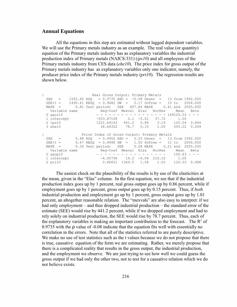
Annual Equations
All the equations in this step are estimated without lagged dependent variables. We will use the Primary metals industry as an example. The real value (or quantity) equation of the Primary metals industry has as explanatory variables the industrial production index of Primary metals (NAICS:331) (ips10) and all employees of the Primary metals industry from CES data (ehe10). The price index for gross output of the Primary metals industry has as explanatory variables only one indicator, namely, the producer price index of the Primary metals industry (pri10). The regression results are shown below.
The easiest check on the plausibility of the results is by use of the elasticities at the mean, given in the “Elas” column. In the first equation, we see that if the industrial production index goes up by 1 percent, real gross output goes up by 0.86 percent, while if employment goes up by 1 percent, gross output goes up by 0.15 percent. Thus, if both industrial production and employment go up by 1 percent, gross output goes up by 1.01 percent, an altogether reasonable relation. The “mexvals” are also easy to interpret: if we had only employment – and thus dropped industrial production – the standard error of the estimate (SEE) would rise by 441.2 percent, while if we dropped employment and had to rely solely on industrial production, the SEE would rise by 78.7 percent. Thus, each of the explanatory variables is making an important contribution to the forecast. The R2 of 0.9735 with the ρ value of -0.08 indicate that the equation fits well with essentially no correlation in the errors. Note that all of the statistics referred to are purely descriptive. We make no use of test statistics such as the t values because we do not propose that there is true, causative equation of the form we are estimating. Rather, we merely propose that there is a complicated reality that results in the gross output, the industrial production, and the employment we observe. We are just trying to see how well we could guess the gross output if we had only the other two, not to test for a causative relation which we do not believe exists.
216
: Real Gross Output: Primary Metals SEE = 1502.60 RSQ = 0.9735 RHO = -0.08 Obser = 13 from 1992.000 SEE+1 = 1490.41 RBSQ = 0.9682 DW = 2.17 DoFree = 10 to 2004.000 MAPE = 0.81 Test period: SEE 607.84 MAPE 0.41 end 2005.000 Variable name Reg-Coef Mexval Elas NorRes Mean Beta 0 agor10 - - - - - - - - - - - - - - - - - 149129.53 - - - 1 intercept -933.87108 0.1 -0.01 37.72 1.00 2 ips10 1221.64143 441.2 0.86 3.19 105.04 0.894 3 ehe10 36.64322 78.7 0.15 1.00 593.22 0.249
: Price Index of Gross Output: Primary Metals SEE = 0.48 RSQ = 0.9952 RHO = 0.25 Obser = 13 from 1992.000 SEE+1 = 0.47 RBSQ = 0.9948 DW = 1.50 DoFree = 11 to 2004.000 MAPE = 0.34 Test period: SEE 0.28 MAPE 0.21 end 2005.000 Variable name Reg-Coef Mexval Elas NorRes Mean Beta 0 agop10 - - - - - - - - - - - - - - - - - 100.43 - - - 1 intercept -4.00796 14.3 -0.04 210.10 1.00 2 pri10 0.86651 1349.5 1.04 1.00 120.53 0.998

In the price equation, we again see a plausible elasticity close to 1, namely 1.04, a good fit with R2 of 0.9952 with the ρ value of 0.25, low enough not to suggest an important missing variable but high enough to make it desirable to use a rho-adjusted forecast.
The explanatory variables ips10, ehe10 and pri10 will be extended into the future by the monthly equations to be described in the next section..
The estimation results for these annual equations for all 65 sectors are given in Appendix 6.3. Please note that, as shown in Appendix 6.3, each sector's gross output price index and level are estimated by separate equations, one for the price index and one for the level of gross output (Real or Nominal). The level equation for each industry will estimate either real value or nominal value. The main reason is simply a better fit between the two. The other reason is that, in some industries, I find a good explanatory value of the price index in explaining both real value and nominal value. Thus, I pick the nominal value equation because having a price index (ppi) as a regressor for real variable is counterintuitive. As we always estimate the price index of each industry, the other level variable will be calculated as an implied value. For example, we estimate the real gross output and the price index for primary metals, as discussed above and the nominal gross output of primary metals will be calculated by identity. Table 6.1 lists how each variable (real, nominal, or price index) is estimated by industries, an R indicates the variable is calculated by regression, while an M means it is implied. Appendix 6.5 shows all variables used in this chapter and their description.
217
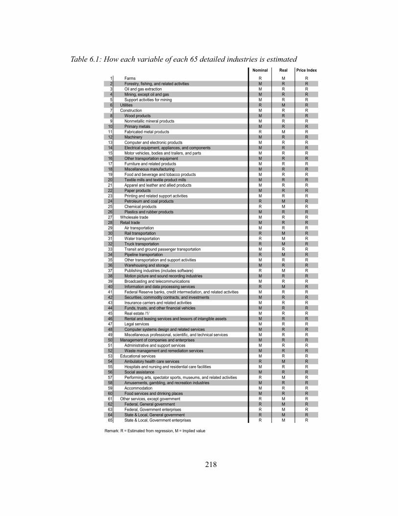
218
Table 6.1: How each variable of each 65 detailed industries is estimatedNominal Real Price Index
1 Farms R M R2 Forestry, fishing, and related activities M R R3 Oil and gas extraction M R R4 Mining, except oil and gas M R R5 Support activities for mining M R R6 Utilities R M R7 Construction M R R8 Wood products M R R9 Nonmetallic mineral products M R R
10 Primary metals M R R11 Fabricated metal products R M R12 Machinery M R R13 Computer and electronic products M R R14 Electrical equipment, appliances, and components M R R15 Motor vehicles, bodies and trailers, and parts M R R16 Other transportation equipment M R R17 Furniture and related products M R R18 Miscellaneous manufacturing M R R19 Food and beverage and tobacco products M R R20 Textile mills and textile product mills M R R21 Apparel and leather and allied products M R R22 Paper products M R R23 Printing and related support activities M R R24 Petroleum and coal products R M R25 Chemical products R M R26 Plastics and rubber products M R R27 Wholesale trade M R R28 Retail trade M R R29 Air transportation M R R30 Rail transportation R M R31 Water transportation R M R32 Truck transportation R M R33 Transit and ground passenger transportation M R R34 Pipeline transportation R M R35 Other transportation and support activities M R R36 Warehousing and storage M R R37 Publishing industries (includes software) R M R38 Motion picture and sound recording industries M R R39 Broadcasting and telecommunications M R R40 Information and data processing services R M R41 Federal Reserve banks, credit intermediation, and related activities M R R42 Securities, commodity contracts, and investments M R R43 Insurance carriers and related activities M R R44 Funds, trusts, and other financial vehicles M R R45 Real estate /1/ M R R46 Rental and leasing services and lessors of intangible assets M R R47 Legal services M R R48 Computer systems design and related services M R R49 Miscellaneous professional, scientific, and technical services M R R50 Management of companies and enterprises M R R51 Administrative and support services M R R52 Waste management and remediation services M R R53 Educational services M R R54 Ambulatory health care services R M R55 Hospitals and nursing and residential care facilities M R R56 Social assistance M R R57 Performing arts, spectator sports, museums, and related activities R M R58 Amusements, gambling, and recreation industries M R R59 Accommodation M R R60 Food services and drinking places M R R61 Other services, except government R M R62 Federal, General government R M R63 Federal, Government enterprises R M R64 State & Local, General government R M R65 State & Local, Government enterprises R M R
Remark: R = Estimated from regression, M = Implied value

Monthly Equations
Time-series analysis is used on all equations with high frequency, as proven useful in generating short-term forecast of economic variables. All equations in this step have the following structure:
Y t = LY t W t t
where Y t = value of dependent variable at time t L = polynomial of lag operators : 1L 2L
2 ... W t = vector of exogenous explanatory variables at time t t = error terms at time t ,1 ,2 , ... , = regression coefficients.
The use of the W variables, additional explanatory variables besides the lagged dependent variables, helps to guide the movement of the forecasts along the long-term trend; without them, a purely autoregressive systems can begin to explode or oscillate. Generally, these exogenous explanatory variables are macroeconomic variables such as GDP and major aggregates of PCE. Table 6.2 shows these W variables and their definitions.
The lagged dependent variables are forecast within the process using time series analysis. Forecasts of other exogenous variables are obtained from (1) QUEST or other macroeconomic model, or (2) simple regression against a time trend or lagged dependent variables, or (3) an ad hoc forecast in the case of variables that are difficult to predict mechanically, such as the oil prices and exchange rate variables.
219
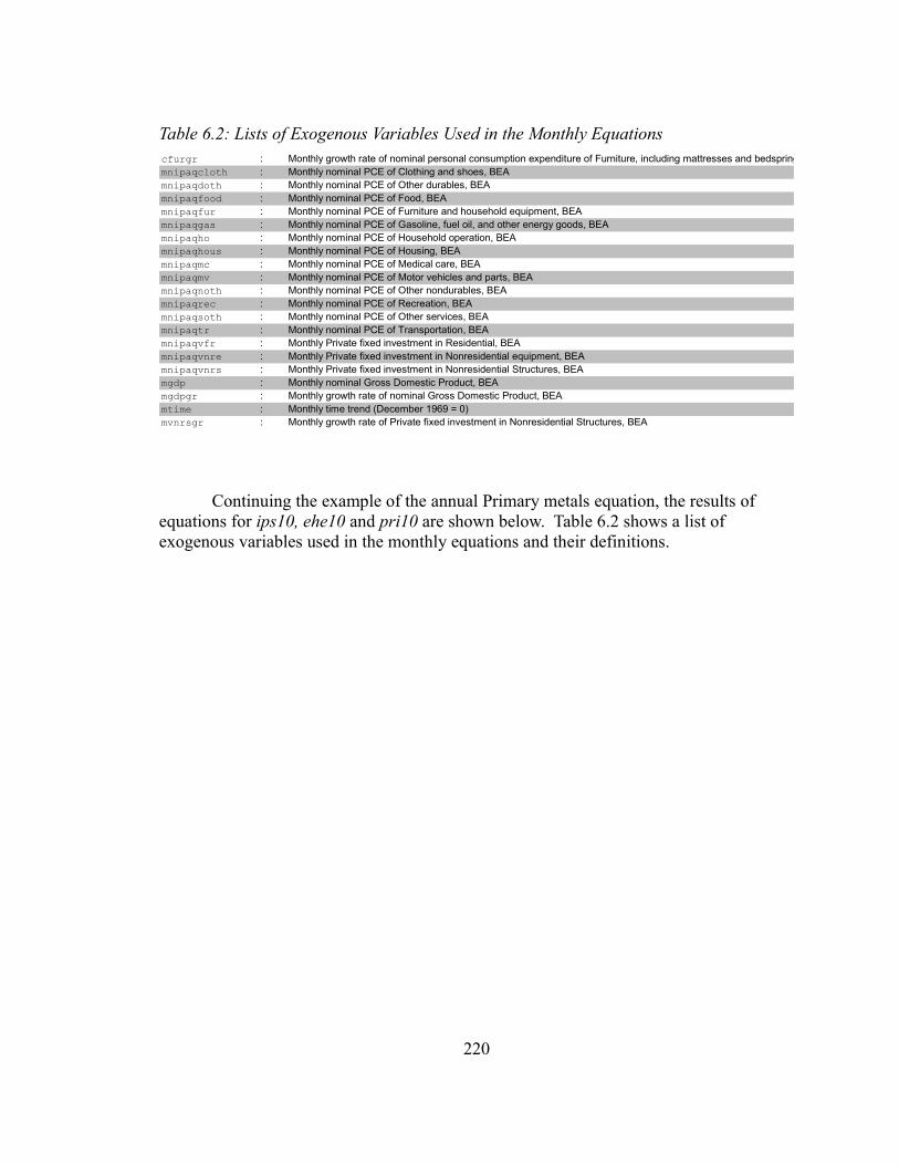
Continuing the example of the annual Primary metals equation, the results of equations for ips10, ehe10 and pri10 are shown below. Table 6.2 shows a list of exogenous variables used in the monthly equations and their definitions.
220
Table 6.2: Lists of Exogenous Variables Used in the Monthly Equationscfurgr : Monthly growth rate of nominal personal consumption expenditure of Furniture, including mattresses and bedsprings, BEAmnipaqcloth : Monthly nominal PCE of Clothing and shoes, BEAmnipaqdoth : Monthly nominal PCE of Other durables, BEAmnipaqfood : Monthly nominal PCE of Food, BEAmnipaqfur : Monthly nominal PCE of Furniture and household equipment, BEAmnipaqgas : Monthly nominal PCE of Gasoline, fuel oil, and other energy goods, BEAmnipaqho : Monthly nominal PCE of Household operation, BEAmnipaqhous : Monthly nominal PCE of Housing, BEAmnipaqmc : Monthly nominal PCE of Medical care, BEAmnipaqmv : Monthly nominal PCE of Motor vehicles and parts, BEAmnipaqnoth : Monthly nominal PCE of Other nondurables, BEAmnipaqrec : Monthly nominal PCE of Recreation, BEAmnipaqsoth : Monthly nominal PCE of Other services, BEAmnipaqtr : Monthly nominal PCE of Transportation, BEAmnipaqvfr : Monthly Private fixed investment in Residential, BEAmnipaqvnre : Monthly Private fixed investment in Nonresidential equipment, BEAmnipaqvnrs : Monthly Private fixed investment in Nonresidential Structures, BEAmgdp : Monthly nominal Gross Domestic Product, BEAmgdpgr : Monthly growth rate of nominal Gross Domestic Product, BEAmtime : Monthly time trend (December 1969 = 0)mvnrsgr : Monthly growth rate of Private fixed investment in Nonresidential Structures, BEA

In the Industrial production index equation (ips10m), we have a plausible elasticity of 1.00 for the lagged dependent variable, a decent fit with adjusted R-Square of 0.8809 and a MAPE of 1.69 percent. The RHO of -0.32 shows that there is unlikely to be an important missing variable but the forecast should be adjusted with the rho-adjustment.
In the employment equation (ehe10m), we have a very good fit with adjusted R-square of 0.9987 and a MAPE of 0.28 percent with the elasticity of 1. There is little correlation in errors with a RHO of -0.13.
The producer price index equation (pri10m) also has a very good fit with an adjusted R-Square of 0.9936 and a MAPE of 0.34 percent. With a very low RHO of -0.07, the equation fits well without significant correlation in the errors. All regressors have appropriate signs and decent Mexvals.
The estimated monthly equations are given in Appendix 6.4. The forecast from these monthly equations are annualized and used in forecasting the annual gross output by detailed industries using the annual equations discussed earlier.
221
#Primary metals: IPI: g331 SEE = 2.24 RSQ = 0.8834 RHO = -0.32 Obser = 144 from 1993.001 SEE+1 = 2.11 RBSQ = 0.8809 DurH = -3.89 DoFree = 140 to 2004.012 MAPE = 1.69 Test period: SEE 7.63 MAPE 5.87 end 2006.012 Variable name Reg-Coef Mexval Elas NorRes Mean Beta 0 ips10m - - - - - - - - - - - - - - - - - 106.10 - - - 1 ips10m[1] 1.00208 900.3 1.00 1.01 105.96 2 mnipaqgas 0.00213 0.0 0.00 1.01 165.14 0.012 3 mnipaqmv -0.01123 0.3 -0.04 1.00 345.86 -0.123 4 mnipaqmv[4] 0.01008 0.2 0.03 1.00 339.61 0.112
: BLS: CES et331 SEE = 2.29 RSQ = 0.9988 RHO = -0.13 Obser = 144 from 1993.001 SEE+1 = 2.27 RBSQ = 0.9987 DurH = -1.67 DoFree = 140 to 2004.012 MAPE = 0.28 Test period: SEE 9.05 MAPE 1.58 end 2006.012 Variable name Reg-Coef Mexval Elas NorRes Mean Beta 0 ehe10m - - - - - - - - - - - - - - - - - 590.11 - - - 1 intercept 0.94029 0.1 0.00 801.68 1.00 2 ehe10m[1] 1.20589 232.0 1.21 1.59 591.18 1.192 3 ehe10m[5] -0.20588 3.9 -0.21 1.00 595.58 -0.193 4 ehe10m[9] -0.00185 0.0 -0.00 1.00 600.17 -0.002
: PPI: u331 SEE = 0.67 RSQ = 0.9937 RHO = -0.07 Obser = 144 from 1993.001 SEE+1 = 0.67 RBSQ = 0.9936 DurH = -1.30 DoFree = 140 to 2004.012 MAPE = 0.34 Test period: SEE 7.08 MAPE 3.72 end 2006.012 Variable name Reg-Coef Mexval Elas NorRes Mean Beta 0 pri10m - - - - - - - - - - - - - - - - - 121.26 - - - 1 intercept 0.46039 0.1 0.00 159.97 1.00 2 pri10m[1] 1.75021 168.1 1.75 2.35 120.95 1.657 3 pri10m[2] -0.75815 44.3 -0.75 1.03 120.65 -0.677 4 mnipaqgas 0.00352 1.4 0.00 1.00 165.14 0.016

6.3 Illustration and Evaluation of the Method
The forecasting accuracy of the method has been evaluated by two tests of the method in forecasting 2003 and 2004 on the basis of equations estimated with data through 2002. The difference between the two tests only is in where they get the exogenous data which, in actual practice, would have to come for QUEST or some other quarterly forecasting model. In the first test, we used the actual values of these variables, as the later proved to be. In the second test, we used the values which QUEST would have produced at the end of 2002 using mechanical projections of its exogenous variables. Thus, the first test shows the error inherent in the methods developed in this study, while the second test compounds these errors with errors in forecasting the variables from the macromodel.
Table 6.3 shows the percentage differences of both simulations from the published real gross output in the 65 detailed industries.
222

223
Table 6.3: 65 detailed Industries Real Gross Output Simulations ResultsPercentage difference from the published value
2003 2004 2003 2004
1 Farms 0.31% 0.70% 0.32% -0.37%2 Forestry, fishing, and related activities -3.23% -3.50% -1.65% -6.25%3 Oil and gas extraction -0.41% -0.23% -0.48% -0.96%4 Mining, except oil and gas -0.01% -0.38% 2.09% 0.01%5 Support activities for mining -6.11% -2.57% 3.53% 16.00%6 Utilities -2.09% 0.55% 2.84% 11.47%7 Construction -0.71% -1.68% -1.39% -7.21%8 Wood products 0.17% 2.00% 0.37% 1.08%9 Nonmetallic mineral products -0.13% 0.84% -0.56% -0.13%10 Primary metals 0.17% 1.13% 0.81% -3.71%11 Fabricated metal products 2.36% -2.97% 4.67% 2.42%12 Machinery -0.60% -0.10% 4.50% 6.76%13 Computer and electronic products -2.95% 0.67% -1.10% -2.38%14 Electrical equipment, appliances, and components -0.23% 1.61% 2.10% 4.47%15 Motor vehicles, bodies and trailers, and parts -0.96% -0.04% -3.06% -2.20%16 Other transportation equipment -1.95% -0.56% 1.08% 14.21%17 Furniture and related products 0.66% -0.67% 4.60% 1.84%18 Miscellaneous manufacturing -0.44% 0.76% -0.46% 2.61%19 Food and beverage and tobacco products -0.02% -0.31% -1.15% 1.81%20 Textile mills and textile product mills -1.11% -1.61% 2.25% 2.91%21 Apparel and leather and allied products 2.59% 2.80% -2.30% -13.54%22 Paper products -0.44% 0.69% -0.19% -6.98%23 Printing and related support activities -0.24% 0.63% -3.15% -13.48%24 Petroleum and coal products 1.82% -0.80% -11.77% -35.47%25 Chemical products 0.99% 0.51% 0.23% -5.71%26 Plastics and rubber products -0.57% 0.63% -1.00% 1.51%27 Wholesale trade -1.70% 3.85% -1.09% -1.23%28 Retail trade -0.95% 1.13% -1.32% -2.55%29 Air transportation 11.35% 5.29% 10.81% 6.14%30 Rail transportation -1.33% -13.08% -2.57% -18.62%31 Water transportation -0.29% -2.76% 3.10% -1.29%32 Truck transportation 1.48% -6.20% 1.41% -11.87%33 Transit and ground passenger transportation -1.83% -2.01% -2.98% -2.77%34 Pipeline transportation 1.24% -0.26% 0.71% 1.42%35 Other transportation and support activities -0.88% -1.08% 1.31% 1.14%36 Warehousing and storage -0.43% 3.61% 0.53% 2.58%37 Publishing industries (includes software) -0.94% -1.31% 0.44% -8.61%38 Motion picture and sound recording industries -2.60% -1.04% -1.36% -1.05%39 Broadcasting and telecommunications 1.14% -1.42% -0.94% -0.34%40 Information and data processing services -4.21% -9.37% -4.43% -11.92%41 Federal Reserve banks, credit intermediation, and 3.63% 7.76% 3.40% 5.84%42 Securities, commodity contracts, and investments -2.36% -5.77% -0.50% -3.05%43 Insurance carriers and related activities 1.56% -1.90% 0.33% -6.10%44 Funds, trusts, and other financial vehicles 1.48% 5.25% -5.35% -12.48%45 Real estate /1/ 0.43% -2.35% -0.04% -5.46%46 Rental and leasing services and lessors of intangi -5.63% -15.67% -10.50% -10.28%47 Legal services -1.96% -0.51% -2.36% -1.68%48 Computer systems design and related services -6.34% -8.13% -5.90% 0.28%49 Miscellaneous professional, scientific, and techni -0.17% 0.05% 3.10% 1.19%50 Management of companies and enterprises -3.54% -6.71% 0.97% -4.80%51 Administrative and support services -4.97% -5.44% -3.79% -2.75%52 Waste management and remediation services -0.52% 0.75% -0.59% -3.02%53 Educational services 0.21% 1.53% 0.23% 1.39%54 Ambulatory health care services -1.88% -0.57% -1.90% -6.42%55 Hospitals and nursing and residential care facilit -0.05% -0.20% -0.33% -0.59%56 Social assistance -2.19% -1.12% -2.15% -3.89%57 Performing arts, spectator sports, museums, and re -4.75% -3.94% -4.27% -1.89%58 Amusements, gambling, and recreation industries -0.41% -0.20% -0.34% -1.33%59 Accommodation -2.71% -2.69% -2.21% -4.81%60 Food services and drinking places 0.45% 2.79% -1.53% -4.36%61 Other services, except government -0.90% -0.91% -1.57% -5.32%62 General government -1.70% -3.39% -3.05% -5.39%63 Government enterprises -0.48% -2.01% -1.38% -3.28%64 General government 0.11% -1.29% -0.05% -0.45%65 Government enterprises 1.41% 3.54% 1.29% 2.73%
1st Sim 2nd Sim

Generally, the first test can predicted most of the real gross output of each industry quite well, especially the important industry such as Construction and Retail trade, in both one-period and two-period ahead forecasts. The second test, generally, shows slightly bigger errors than the first test. These bigger errors emphasize the importance of the accuracy of exogenous variables.
Air transportation is the only important industry that has unusually large errors, between 5% to 11%. These errors are relatively equally large in both tests. Thus, this indicates that our equations for estimating Air transportation does not perform as well as equations for other industries.
For the remainder of this section, I show these results in a more graphical way with more discussion of the more aggregates industries. It can be skipped.
Graphical presentation of the results is certainly more “graphic” than the table and shows the forecast in the context of the historical series. But because the graphs also take a lot of space, I have aggregated the 65 industries into 22 groups for the graphs. All real values are aggregated from the 65-sector level using chain-weighted Fisher indexes. Tabulated numerical results of these 22 industry groups are in Appendix 6.2; the graphs follow here. Unless otherwise noted, each graph shows three lines:
1. a historical simulation using true values of exogenous variables (represented by the red line and marked with plus signs + ),
2. a historical simulation with exogenous variables generated using QUEST and other simple methods such as simple time-series analysis (represented by blue line and marked by the square boxes ), Table 6.4 shows the assumptions of these exogenous variables between 2003 and 2004, and
3. the historical BEA published Gross output by industry group as of April 2007 (represented by green line marked by x's).
All values (shown in Table 6.4), except exchange rate (exrim) and oil price (oilpm), are generated as quarterly series by the QUEST model and converted to monthly data by @qtom command.
224

225
Table 6.4: Assumptions of all exogenous variables used in the Second Historical Simulation
Jan Feb Mar Apr May Jun Jul Aug Sep Oct Nov Decexrim
2003 123.44 123.29 122.81 121.83 117.86 117.22 118.43 119.74 118.40 116.06 115.93 114.362004 112.46 113.01 114.13 114.94 116.81 115.70 114.88 115.05 114.58 112.97 110.11 108.89
oilpm2003 32.94 35.87 33.55 28.25 28.14 30.72 30.76 31.59 28.29 30.33 31.09 32.152004 34.27 34.74 36.76 36.69 40.28 38.02 40.69 44.94 45.95 53.13 48.46 43.33
mnipaqmv2003 409.85 407.32 408.62 418.67 423.92 429.30 442.22 442.29 436.93 410.72 406.04 407.492004 428.02 432.01 432.42 423.96 421.15 418.73 414.15 414.37 416.86 424.91 429.48 433.86
mnipaqfur2003 325.62 327.90 330.32 333.90 335.83 337.14 337.48 337.78 337.69 336.54 336.22 336.052004 335.66 336.04 336.85 338.87 339.91 340.75 341.51 341.89 342.01 340.88 341.18 341.95
mnipaqdoth2003 176.01 177.62 178.93 179.52 180.51 181.48 182.75 183.47 183.95 183.62 184.04 184.662004 185.47 186.45 187.62 189.78 190.71 191.20 190.83 190.79 190.64 190.05 189.95 190.00
mnipaqfood2003 1,017.84 1,018.61 1,018.55 1,017.67 1,015.94 1,013.37 1,008.07 1,005.25 1,003.00 1,001.78 1,000.36 999.182004 997.56 997.39 997.99 999.51 1,001.52 1,004.19 1,008.44 1,011.72 1,014.95 1,016.47 1,020.86 1,026.47
mnipaqcloth2003 305.96 305.75 305.40 304.93 304.26 303.40 301.86 301.05 300.46 300.41 300.01 299.582004 298.82 298.56 298.50 298.70 298.99 299.43 300.21 300.80 301.40 301.52 302.50 303.84
mnipaqgas2003 204.30 210.98 217.86 225.15 232.28 239.45 248.48 254.39 258.98 257.32 262.98 271.022004 285.53 295.26 304.32 316.17 321.26 323.06 316.84 315.62 314.66 315.26 313.86 311.74
mnipaqnoth2003 605.42 605.43 604.74 602.85 601.09 598.98 595.43 593.43 591.90 591.80 590.47 588.882004 585.84 584.61 584.01 584.71 584.84 585.09 585.42 585.91 586.53 586.72 588.05 589.94
mnipaqhous2003 1,137.25 1,137.46 1,136.62 1,135.53 1,132.03 1,126.91 1,117.12 1,111.03 1,105.61 1,099.76 1,096.48 1,094.682004 1,096.95 1,096.16 1,094.90 1,091.89 1,090.67 1,089.94 1,089.41 1,089.91 1,091.15 1,092.56 1,095.67 1,099.94
mnipaqho2003 420.43 421.29 421.54 421.17 420.18 418.56 414.71 413.06 412.00 412.06 411.80 411.742004 412.03 412.28 412.63 412.50 413.50 415.05 418.82 420.21 420.89 419.51 419.80 420.40
mnipaqtr2003 293.09 294.74 296.16 296.91 298.19 299.55 301.29 302.63 303.86 305.00 305.96 306.762004 306.86 307.79 308.99 311.65 312.50 312.72 311.83 311.18 310.27 308.79 307.62 306.43
mnipaqmc2003 1,252.52 1,252.59 1,251.18 1,249.12 1,244.14 1,237.07 1,222.52 1,215.30 1,210.02 1,211.56 1,206.50 1,199.722004 1,186.86 1,179.90 1,174.48 1,171.74 1,168.55 1,166.04 1,164.82 1,163.22 1,161.86 1,159.13 1,159.42 1,161.14
mnipaqrec2003 307.94 308.67 309.49 311.02 311.57 311.75 311.59 311.00 310.02 307.39 306.55 306.272004 307.45 307.55 307.50 306.65 306.79 307.28 309.15 309.55 309.51 307.74 307.81 308.42
mnipaqsoth2003 1,037.19 1,038.74 1,040.36 1,044.15 1,044.30 1,042.91 1,038.77 1,035.25 1,031.12 1,023.67 1,020.36 1,018.492004 1,020.50 1,019.64 1,018.35 1,014.42 1,013.98 1,014.80 1,019.83 1,020.96 1,021.14 1,016.94 1,017.78 1,020.23
mnipaqvnrs2003 268.45 267.48 267.06 267.96 268.05 268.11 268.67 268.25 267.41 263.29 263.70 265.802004 270.84 275.38 280.67 290.10 294.34 296.79 294.38 295.54 297.21 301.08 302.50 303.15
mnipaqvnre2003 782.63 791.58 803.54 822.03 837.39 853.14 876.00 887.48 894.30 889.54 892.26 895.532004 895.04 902.64 914.02 933.68 949.25 965.23 986.85 999.71 1,009.04 1,011.46 1,016.29 1,020.15
mnipaqvfr2003 534.67 542.20 550.27 565.56 569.68 569.33 556.35 553.13 551.54 551.88 553.31 556.122004 560.97 566.09 572.12 581.64 587.57 592.48 597.84 599.61 599.27 591.42 590.88 592.26
mgdp2003 10,640.83 10,668.81 10,701.08 10,754.03 10,782.53 10,803.01 10,814.69 10,819.64 10,817.14 10,783.32 10,783.73 10,794.562004 10,823.52 10,849.32 10,879.73 10,923.03 10,956.37 10,988.09 11,020.77 11,047.22 11,070.10 11,077.57 11,102.07 11,131.80

Table 6.5 shows that there are big errors in the exogenous variables generated by the QUEST models, especially in the PCE of Nondurables and Services. It should be noted that we used the actual values of the exchange rate and the oil price in the second simulation.
226
Table 6.5: Percentage differences of the exogenous variables from the actual valuesJan Feb Mar Apr May Jun Jul Aug Sep Oct Nov Dec
exrim2003 0.00% 0.00% 0.00% 0.00% 0.00% 0.00% 0.00% 0.00% 0.00% 0.00% 0.00% 0.00%2004 0.00% 0.00% 0.00% 0.00% 0.00% 0.00% 0.00% 0.00% 0.00% 0.00% 0.00% 0.00%
oilpm2003 0.00% 0.00% 0.00% 0.00% 0.00% 0.00% 0.00% 0.00% 0.00% 0.00% 0.00% 0.00%2004 0.00% 0.00% 0.00% 0.00% 0.00% 0.00% 0.00% 0.00% 0.00% 0.00% 0.00% 0.00%
mnipaqmv2003 -2.01% -2.68% -2.97% -2.57% -2.32% -1.92% -0.28% -0.41% -1.22% -5.03% -5.54% -4.99%2004 -0.98% -0.14% -0.05% -1.64% -2.37% -3.16% -4.59% -5.03% -5.07% -4.59% -3.97% -3.05%
mnipaqfur2003 1.83% 2.52% 2.91% 3.01% 2.77% 2.22% 0.85% 0.11% -0.55% -1.01% -1.59% -2.17%2004 -2.97% -3.39% -3.66% -3.46% -3.65% -3.91% -4.28% -4.67% -5.10% -5.82% -6.19% -6.44%
mnipaqdoth2003 2.63% 3.39% 3.60% 2.77% 2.27% 1.60% 0.29% -0.29% -0.65% -0.49% -0.69% -0.91%2004 -1.56% -1.56% -1.30% -0.11% 0.17% 0.20% -0.22% -0.52% -0.89% -1.43% -1.90% -2.40%
mnipaqfood2003 -0.50% -0.83% -1.14% -1.11% -1.67% -2.47% -4.07% -4.90% -5.54% -5.61% -6.17% -6.85%2004 -7.98% -8.57% -8.99% -9.10% -9.28% -9.40% -9.24% -9.39% -9.65% -10.41% -10.55% -10.48%
mnipaqcloth2003 1.00% 1.01% 0.67% -0.21% -1.10% -2.18% -4.24% -5.08% -5.52% -4.67% -5.00% -5.61%2004 -7.37% -7.84% -7.94% -6.96% -6.82% -6.83% -7.07% -7.30% -7.61% -8.26% -8.50% -8.63%
mnipaqgas2003 -5.35% -4.08% -0.43% 12.30% 17.50% 20.62% 18.16% 19.48% 21.19% 24.41% 26.27% 27.72%2004 28.86% 29.33% 29.33% 28.44% 27.95% 27.36% 27.71% 26.12% 23.71% 18.44% 16.29% 14.94%
mnipaqnoth2003 -0.54% -0.94% -1.37% -1.47% -2.19% -3.17% -5.07% -6.04% -6.76% -6.94% -7.42% -7.90%2004 -8.38% -8.86% -9.35% -9.90% -10.34% -10.73% -11.06% -11.37% -11.63% -11.92% -12.07% -12.14%
mnipaqhous2003 -0.16% -0.43% -0.77% -1.04% -1.67% -2.50% -3.82% -4.80% -5.75% -6.83% -7.57% -8.16%2004 -8.31% -8.79% -9.31% -10.01% -10.53% -10.99% -11.42% -11.76% -12.04% -12.26% -12.42% -12.51%
mnipaqho2003 -0.40% -0.77% -1.17% -1.62% -2.11% -2.65% -3.36% -3.89% -4.36% -4.66% -5.11% -5.59%2004 -6.28% -6.67% -6.95% -7.09% -7.17% -7.16% -6.70% -6.80% -7.08% -7.90% -8.30% -8.64%
mnipaqtr2003 0.38% 0.58% 0.75% 0.89% 1.00% 1.08% 1.06% 1.13% 1.21% 1.37% 1.44% 1.47%2004 1.37% 1.43% 1.54% 2.04% 1.99% 1.74% 1.17% 0.59% -0.11% -1.09% -1.88% -2.66%
mnipaqmc2003 -0.58% -1.18% -1.88% -2.62% -3.57% -4.65% -6.27% -7.34% -8.24% -8.59% -9.48% -10.52%2004 -12.04% -13.09% -14.03% -14.77% -15.53% -16.23% -16.87% -17.47% -18.02% -18.60% -19.00% -19.32%
mnipaqrec2003 -0.10% -0.27% -0.50% -0.70% -1.09% -1.59% -2.17% -2.90% -3.76% -5.01% -5.91% -6.71%2004 -7.39% -8.06% -8.67% -9.35% -9.78% -10.07% -9.95% -10.21% -10.55% -11.26% -11.56% -11.75%
mnipaqsoth2003 -0.03% -0.17% -0.39% -0.49% -0.96% -1.62% -2.70% -3.55% -4.40% -5.26% -6.13% -7.01%2004 -7.95% -8.76% -9.52% -10.38% -10.93% -11.33% -11.20% -11.59% -12.10% -13.26% -13.63% -13.75%
mnipaqvnrs2003 -0.15% -0.75% -1.58% -3.38% -4.10% -4.51% -4.08% -4.28% -4.58% -5.65% -5.62% -5.18%2004 -3.88% -2.97% -2.00% -0.06% 0.29% 0.02% -1.97% -2.61% -3.02% -2.48% -3.01% -3.87%
mnipaqvnre2003 1.26% 2.35% 3.55% 5.13% 6.30% 7.32% 8.58% 9.07% 9.18% 7.92% 8.03% 8.50%2004 9.92% 10.74% 11.49% 12.06% 12.75% 13.44% 14.74% 15.01% 14.85% 13.60% 13.17% 12.87%
mnipaqvfr2003 0.12% 0.52% 1.07% 3.61% 3.11% 1.44% -3.34% -5.55% -7.31% -8.58% -9.56% -10.20%2004 -9.90% -10.36% -10.95% -11.98% -12.53% -12.96% -12.85% -13.38% -14.12% -15.61% -16.35% -16.89%
mgdp2003 -0.23% -0.34% -0.42% -0.16% -0.41% -0.87% -1.86% -2.44% -2.97% -3.44% -3.87% -4.25%2004 -4.56% -4.87% -5.15% -5.41% -5.64% -5.86% -5.99% -6.22% -6.47% -6.81% -7.07% -7.32%

For each industry or group of industries there are three graphs. The top left is nominal gross output; the top right is real gross output in prices of 2000; and the bottom center is the price index.
Total Gross Output
Total gross output, need it be said, is not equal to Gross domestic product because it includes intermediate consumption. Nonetheless, it provides a useful measure of how the method worked overall. The two preceding years, 2001 and 2002, had been years of stagnation or very slow growth. At this most aggregate level, our method indicated resumed growth and a gave a good forecast from both historical simulations for nominal gross output in 2003 but missed a bit on the low side for 2004. In 2003, the first and the second simulation underestimated the actual value by 1.08 percent and 0.64 percent, respectively. That is, the QUEST-based forecast proved a bit closer than the actual-based forecast. In 2004, the simulations underestimated the later- published value by 1.80 percent and 3.36 percent, respectively.
Total Gross Output (Nominal) Total Gross Output (Nominal) Historical Simulation, 2003-2004
21306874
16279663
11252452
1992 1994 1996 1998 2000 2002 2004 got_t got_q got_b
Total Gross Output (Real 2000) Total Gross Output (Real 2000) Historical Simulation, 2003-2004
19496242
16176094
12855946
1992 1994 1996 1998 2000 2002 2004 gort_t gort_q gort_b
Total Gross Output (Price,2000=100) Total Gross Output (Price,2000=100) Historical Simulation, 2003-2004
109.3
98.4
87.5
1992 1994 1996 1998 2000 2002 2004 gopt_t gopt_q gopt_b
227

Turning to real total gross output, we find the first simulation with the true exogenous variables missing the published figures by -0.51 percent and -0.78 percent in 2003 and 2004, respectively. The second simulation with exogenous values from QUEST missed the BEA numbers by -0.59 percent and -2.72 percent, respectively.
The estimated price indexes are quite accurate. In 2003, the first and the second simulations missed the announced price index by -0.57 percent and -0.06 percent, respectively. The rapid rise of the petroleum price since 2003 caused a slightly worse performance in 2004. The first simulation missed the published number by -1.03 percent in 2004 while the second simulation missed the published number by -0.66 percent in the same year.
Private industries
Gross output of U.S. private industries contributes approximately 90 percent of U.S. total Gross output in nominal value. Thus, the model's performance in estimating Gross output of private industries is unsurprisingly very similar to the performance seen in the total Gross output. The first simulation missed the published number by -0.93 percent in 2003 and -1.49 percent in 2004. The second simulation missed by -0.44 percent in 2003 and -3.20 percent in 2004.
The first simulation missed the chained real 2000 private industries Gross output by –0.54 percent and -0.68 percent in 2003 and 2004, respectively. The second simulation missed by -0.55 percent in 2003 and -2.84 percent in 2004.
Private industries (Nominal) Private industries (Nominal)
Historical Simulation, 2003-200418859316
14378210
9897103
1992 1994 1996 1998 2000 2002 2004 gop_t gop_q gop_b
Private industries (Real 2000) Private industries (Real 2000) Historical Simulation, 2003-2004
17390186
14293178
11196170
1992 1994 1996 1998 2000 2002 2004 gorp_t gorp_q gorp_b
228

Private industries (Price,2000=100) Private industries (Price,2000=100) Historical Simulation, 2003-2004
108.4
98.4
88.4
1992 1994 1996 1998 2000 2002 2004 gopp_t gopp_q gopp_b
The BEA published a price index for private industries’ gross output of 104.48 and 108.45 in 2003 and 2004, respectively. In 2003, the first simulation missed the published figure by -0.40 percent while the second simulation missed it by only 0.11 percent. In 2004, the first and the second simulations missed the published number by -0.82 percent and -0.36 percent, respectively. Given the break from the previous trend, these forecasts look quite accurate.
Agriculture, forestry, fishing, and hunting
Both simulations performed fairly well in predicting real Gross output. The first simulation missed the BEA figures by -0.36 percent and -0.12 percent in 2003 and 2004, respectively while the second simulation missed them by -0.05 percent in 2003 and -1.43 percent in 2006. Agricultural prices soared in 2003 and 2004, and both simulations underestimated the price index.
The first simulation performed fairly well. It missed the published price index by -3.06 percent in 2003 and by -0.04 percent in 2004. The second simulation missed the published numbers by -8.42 percent and -11.82 percent in 2003 and 2004, respectively. Evidently and not surprisingly, QUEST and the time-series methods used for the exogenous variables in this forecast did not provide the basis for anticipating this sudden, unprecedented rise in the farm price index. Specifically, shown in Appendix 6.3 and Appendix 6.4, nominal PCE of Furniture and household equipment is the only exogenous variable used in this industry group. compared the PCE numbers in Table 6.4 with the BEA quarterly NIPA, I find that the assumption match the published numbers quite well until the last quarter of 2003 in which QUEST start to underestimate the PCE of furniture significantly by around nearly 10% each quarter through the end of 2004. Naturally, the nominal gross output forecast will show the combined effect of the real quantity and the price forecasts. The first simulation missed the published number by -3.41 percent in 2003 but by only -0.16 percent in 2004. However, the second simulation did not do as well. It missed the BEA numbers by -8.46 percent and -13.08 percent in 2003 and 2004, respectively. From just looking at the graph, however, this second simulation looks like an altogether plausible guess of where the series was going to go in 2003 and 2004; what really happened looks highly implausible.
229

Agriculture, forestry, fishing, and hunting (Nominal) Agriculture, forestry, fishing, and hunting (Nominal) Historical Simulation, 2003-2004
319541
273166
226792
1992 1994 1996 1998 2000 2002 2004 gopag_t gopag_q gopag_b
Agriculture, forestry, fishing, and hunting (Real 2000) Agriculture, forestry, fishing, and hunting (Real 2000) Historical Simulation, 2003-2004
269783
244789
219795
1992 1994 1996 1998 2000 2002 2004 gorpag_t gorpag_q gorpag_b
Agriculture, forestry, fishing, and hunting (Price,2000=100) Agriculture, forestry, fishing, and hunting (Price,2000=100) Historical Simulation, 2003-2004
118.4
108.1
97.7
1992 1994 1996 1998 2000 2002 2004 goppag_t goppag_q goppag_b
Mining (including petroleum)
The first simulation performed quite well as it missed the published nominal numbers by -2.10 percent and -1.05 percent in 2003 and 2004, respectively. The second simulation overestimated the nominal gross output by 7.79 percent in 2003 and 30.39 percent in 2004. On the other hand, both simulations gave good forecasts for the real gross output of Mining. The first simulation missed the published numbers by -1.62 percent and -1.27 percent in 2003 and 2004, respectively. The second simulation missed the same numbers by 0.72 percent in 2003 and 2.27 percent in 2004.
Mining (Nominal) Mining (Nominal) Historical Simulation, 2003-2004
400395
267817
135238
1992 1994 1996 1998 2000 2002 2004 gopmin_t gopmin_q gopmin_b
Mining (Real 2000) Mining (Real 2000) Historical Simulation, 2003-2004
221334
213024
204714
1992 1994 1996 1998 2000 2002 2004 gorpmin_t gorpmin_q gorpmin_b
230

Mining (Price,2000=100) Mining (Price,2000=100) Historical Simulation, 2003-2004
181
123
65
1992 1994 1996 1998 2000 2002 2004 goppmin_t goppmin_q goppmin_b
As in agriculture, the performance of the second simulation in forecasting the price index helps explaining its poor performance in estimating the nominal gross output. While the first simulation missed the published number by only -0.49 percent in 2003 and 0.23 percent in 2004, the second simulation missed the published numbers by 7.01 percent in 2003 and 27.49 percent in 2004, respectively.
Mining industry includes oil and gas extraction industry, which is responsible for about two-third of the nominal Gross output of Mining industry. The exploding nominal gross output of the industry is to be expected because of the increasing petroleum price. The overestimation of the price index in the second simulation is caused by the overestimated nominal PCE of Gasoline, fuel oil, and other energy goods by QUEST.
Utilities
The first simulation missed the BEA nominal values by -1.96 percent in 2003 and -1.21 percent in 2004 while the second simulation missed the BEA figures by -20.9 percent in 2003 and -1.48 percent in 2004. The difference is evident in estimating the real gross output. The first simulation did fairly well. It missed the published numbers by -20.9 percent and 0.55 percent in 2003 and 2004, respectively. The second simulation overestimated the published number by quite a bit, especially in 2004. It missed the BEA figures by 2.84 percent in 2003 and 11.47 percent in 2004. As in the two previous industry groups, the performance between the two simulations in estimating the price index shows the difference we have seem in the estimation of the chained 2000 real gross output. The first simulation missed the published price index by 0.13 percent in 2003 and -1.75 percent in 2004. The second simulation underestimates the same numbers by -4.80 percent in 2003 and -11.62 percent in 2004.
231
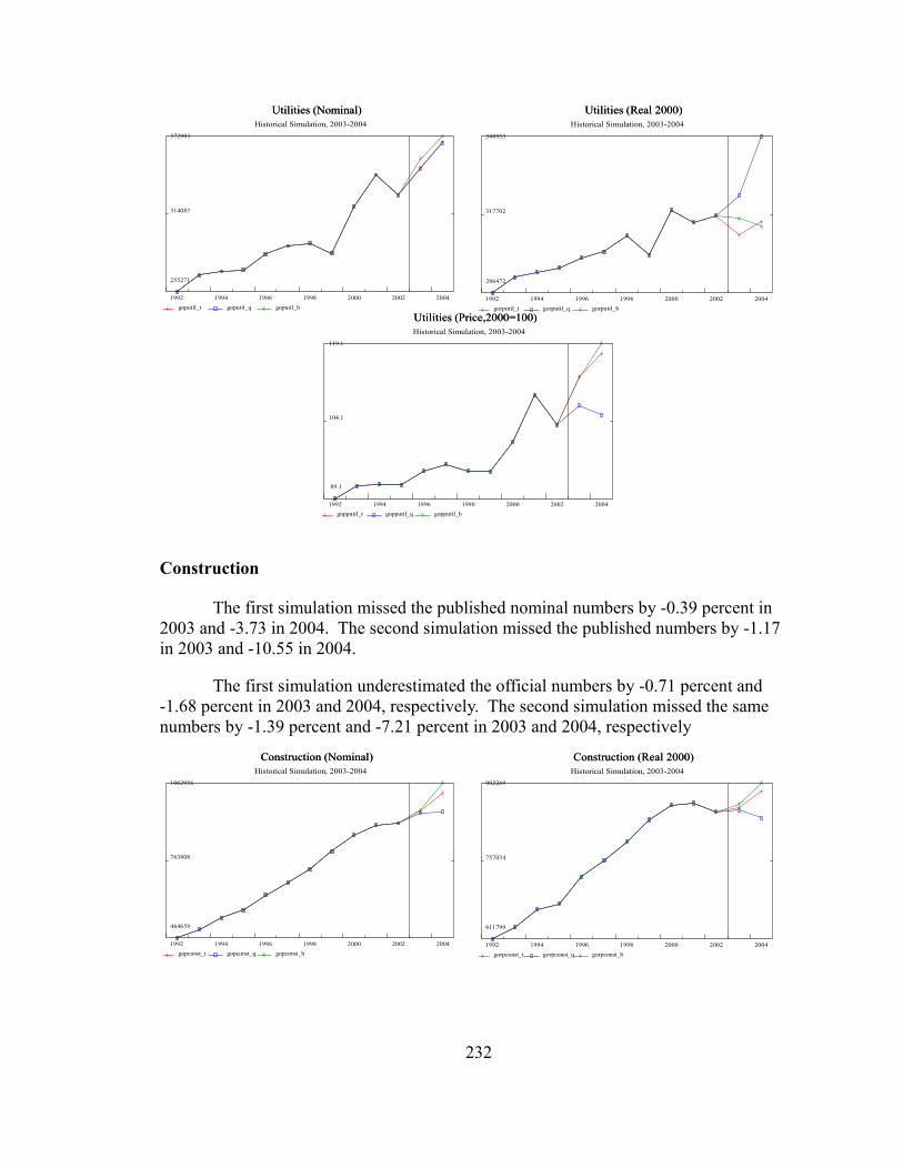
Utilities (Nominal) Utilities (Nominal) Historical Simulation, 2003-2004
372903
314087
255271
1992 1994 1996 1998 2000 2002 2004 goputil_t goputil_q goputil_b
Utilities (Real 2000) Utilities (Real 2000) Historical Simulation, 2003-2004
348933
317702
286472
1992 1994 1996 1998 2000 2002 2004 gorputil_t gorputil_q gorputil_b
Utilities (Price,2000=100) Utilities (Price,2000=100) Historical Simulation, 2003-2004
119.1
104.1
89.1
1992 1994 1996 1998 2000 2002 2004 gopputil_t gopputil_q gopputil_b
Construction
The first simulation missed the published nominal numbers by -0.39 percent in 2003 and -3.73 in 2004. The second simulation missed the published numbers by -1.17 in 2003 and -10.55 in 2004.
The first simulation underestimated the official numbers by -0.71 percent and -1.68 percent in 2003 and 2004, respectively. The second simulation missed the same numbers by -1.39 percent and -7.21 percent in 2003 and 2004, respectively
Construction (Nominal) Construction (Nominal) Historical Simulation, 2003-2004
1062956
763808
464659
1992 1994 1996 1998 2000 2002 2004 gopconst_t gopconst_q gopconst_b
Construction (Real 2000) Construction (Real 2000) Historical Simulation, 2003-2004
902269
757034
611799
1992 1994 1996 1998 2000 2002 2004 gorpconst_t gorpconst_q gorpconst_b
232

Construction (Price,2000=100) Construction (Price,2000=100) Historical Simulation, 2003-2004
117.8
96.9
75.9
1992 1994 1996 1998 2000 2002 2004 goppconst_t goppconst_q goppconst_b
Both simulations estimated the price index quite accurately in 2003 and underestimated the price index slightly in 2004. The first simulation missed the official price index by 0.32 percent in 2003 and -2.08 percent in 2004. The second simulation missed the same price index by 0.22 percent in 2003 and -3.60 percent in 2004.
Both simulations predicted a slowdown in the construction industry in 2004, especially in the price index. This slowdown did not happen until the end of 2005.
Manufacturing
We expect to achieve good estimates from the manufacturing industry as the high frequency data used in the equations of this industry, such as Industrial production index and producer price index, are the main information the BEA used in producing the annual Gross output in these industries. As expected, the model, as seen in the performance of the first simulation, did very well in estimating the Gross output of manufacturing industry in 2003 and 2004.
In 2003, the first simulation missed the BEA nominal gross output by -0.37 percent while the second simulation missed the same number by -0.03 percent. In 2004, the discrepancies are -0.28 percent and -20.7 percent for the first and the second simulation, respectively.
With the chained 2000 real Gross output of manufacturing industry, the first simulation missed the official numbers by -0.19 percent in 2003 and -0.04 percent in 2004. The second simulation missed the same numbers by -0.71 percent and -2.89 percent in 2003 and 2004, respectively.
233

Manufacturing (Nominal) Manufacturing (Nominal) Historical Simulation, 2003-2004
4207105
3538840
2870576
1992 1994 1996 1998 2000 2002 2004 gopmanu_t gopmanu_q gopmanu_b
Manufacturing (Real 2000) Manufacturing (Real 2000) Historical Simulation, 2003-2004
4144489
3531973
2919456
1992 1994 1996 1998 2000 2002 2004 gorpmanu_t gorpmanu_q gorpmanu_b
Manufacturing (Price,2000=100) Manufacturing (Price,2000=100) Historical Simulation, 2003-2004
106.05
101.97
97.89
1992 1994 1996 1998 2000 2002 2004 goppmanu_t goppmanu_q goppmanu_b
The BEA published the price index of gross output of manufacturing industry of 100.35 and 105.16 in 2003 and 2004, respectively. The first simulation missed this numbers by -0.18 percent in 2003 and -0.25 percent in 2004. The second simulation missed the official numbers by 0.69 percent in 2003 and 0.85 percent in 2004.
Durable goods manufacturingThe first simulation missed the published numbers by -0.91 percent and -0.31
percent in 2003 and 2004, respectively. The second simulation missed the same official figures by 1.02 percent in 2003 and 0.71 percent in 2004.
In estimating the chained 2000 real gross output, the first simulation missed the official numbers by -0.68 percent in 2003 and -0.05 percent in 2004 while the second simulation missed the numbers by 0.50 percent and 1.37 percent in 2003 and 2004, respectively.
234

Durable goods manufacturing (Nominal) Durable goods manufacturing (Nominal) Historical Simulation, 2003-2004
2328173
1911094
1494015
1992 1994 1996 1998 2000 2002 2004 gopdur_t gopdur_q gopdur_b
Durable goods manufacturing (Real 2000) Durable goods manufacturing (Real 2000) Historical Simulation, 2003-2004
2328173
1845945
1363716
1992 1994 1996 1998 2000 2002 2004 gorpdur_t gorpdur_q gorpdur_b
Durable goods manufacturing (Price,2000=100) Durable goods manufacturing (Price,2000=100) Historical Simulation, 2003-2004
112.2
104.2
96.2
1992 1994 1996 1998 2000 2002 2004 goppdur_t goppdur_q goppdur_b
The official price index of durable goods manufacturing industry is 96.44 and 99.48 in 2003 and 2004, respectively. The first simulation missed the numbers by -0.23 percent and -0.26 percent in 2003 and 2004, respectively. The second simulation missed the same numbers by 0.51 percent in 2003 and -0.65 percent in 2004.
Nondurable goods manufacturingThe BEA published the nominal gross output of nondurable goods manufacturing
of 1,843 billion dollars and 1,985 billion dollars in 2003 and 2004, respectively. The first simulation with actual inputs missed the official figures by 0.24 percent in 2003 and -0.25 percent in 2004. The second simulation did not do as well. It missed the published numbers by -1.22 percent in 2003 and -5.18 percent in 2004.
235

Nondurable goods manufacturing (Nominal) Nondurable goods manufacturing (Nominal) Historical Simulation, 2003-2004
1985491
1681026
1376561
1992 1994 1996 1998 2000 2002 2004 gopndur_t gopndur_q gopndur_b
Nondurable goods manufacturing (Real 2000) Nondurable goods manufacturing (Real 2000) Historical Simulation, 2003-2004
1816316
1712115
1607914
1992 1994 1996 1998 2000 2002 2004 gorpndur_t gorpndur_q gorpndur_b
Nondurable goods manufacturing (Price,2000=100) Nondurable goods manufacturing (Price,2000=100) Historical Simulation, 2003-2004
115.3
100.5
85.6
1992 1994 1996 1998 2000 2002 2004 goppndur_t goppndur_q goppndur_b
For the estimates of chained 2000 real gross output, the first simulation did very well in both 2003 and 2004. It over estimated the published numbers by less than 0.5 percent in both year. The second simulation did well in 2003 with the error of -2.13 percent. However, in 2004, the second simulation missed the published number by -7.70 percent.
Both simulations did well in estimating the price index. The first simulation estimates the price index of 105.08 in 2003 and 111.97 in 2004. The second simulation estimates the same price index of 106.19 and 115.33 in 2003 and 2004, respectively.
Wholesale trade
The first simulation missed the nominal gross output by -1.77 percent in 2003 and 5.19 percent in 2004. The second simulation missed the same numbers by -0.69 percent and 0.94 percent in 2003 and 2004.
The first simulation missed the published real numbers by -1.70 percent and 3.85 percent in 2003 and 2004, respectively. The second simulation missed the same official figures by -1.09 percent in 2003 and -1.23 percent in 2004.
236

The model did very well in predicting the price index. The first simulation missed the published price index by -0.07 percent in 2003 and 1.29 percent in 2004. The second simulation missed the same price index by 0.41 percent and 2.20 percent in 2003 and 2004, respectively.
Wholesale trade (Nominal) Wholesale trade (Nominal) Historical Simulation, 2003-2004
1046700
792928
539155
1992 1994 1996 1998 2000 2002 2004 gopwhsl_t gopwhsl_q gopwhsl_b
Wholesale trade (Real 2000) Wholesale trade (Real 2000) Historical Simulation, 2003-2004
986698
775267
563836
1992 1994 1996 1998 2000 2002 2004 gorpwhsl_t gorpwhsl_q gorpwhsl_b
Wholesale trade (Price,2000=100) Wholesale trade (Price,2000=100) Historical Simulation, 2003-2004
107.0
101.3
95.6
1992 1994 1996 1998 2000 2002 2004 goppwhsl_t goppwhsl_q goppwhsl_b
Retail trade
BEA published the nominal gross output of retail trade of 1,139 billion dollars in 2003 and 1,223 billion dollars in 2004. The first simulation underestimated the numbers by 1.44 percent in 2003 and 1.46 percent in 2004. The second simulation missed the same official number by -1.54 percent in 2003 and -4.17 percent in 2004.
For the real gross output, the first simulation estimates are 1,115 billion dollars in 2003 and 1,195 billion dollars in 2004 or the first simulation missed the published numbers by -0.95 percent in 2003 and 1.13 percent in 2004. The second simulation missed the same numbers by -1.32 percent and -2.55 percent in 2003 and 2004, respectively.
237

Retail trade (Nominal) Retail trade (Nominal) Historical Simulation, 2003-2004
1223257
921329
619401
1992 1994 1996 1998 2000 2002 2004 goprtl_t goprtl_q goprtl_b
Retail trade (Real 2000) Retail trade (Real 2000) Historical Simulation, 2003-2004
1195019
918669
642320
1992 1994 1996 1998 2000 2002 2004 gorprtl_t gorprtl_q gorprtl_b
Retail trade (Price,2000=100) Retail trade (Price,2000=100) Historical Simulation, 2003-2004
103.52
99.98
96.43
1992 1994 1996 1998 2000 2002 2004 gopprtl_t gopprtl_q gopprtl_b
The first simulation missed the price index of retail trade gross output by -0.49 percent and -2.56 percent in 2003 and 2004, respectively. The second simulation underestimated the published numbers by -0.23 percent in 2003 and -1.66 percent in 2004.
Transportation and warehousing
BEA published the nominal gross output of transportation and warehousing industry of 598 billion dollars in 2003 and 648 billion dollars in 2004. The first simulation gave estimates of 630 billion dollars in 2003 and 655 billion dollars in 2004. These estimates gave errors of 5.21 percent in 2003 and 1.10 percent in 2004. The second simulation missed the published numbers by 6.33 percent and 2.37 percent in 2003 and 2004, respectively.
238

Transportation and warehousing (Nominal) Transportation and warehousing (Nominal) Historical Simulation, 2003-2004
663739
520230
376721
1992 1994 1996 1998 2000 2002 2004 goptran_t goptran_q goptran_b
Transportation and warehousing (Real 2000) Transportation and warehousing (Real 2000) Historical Simulation, 2003-2004
607766
519374
430981
1992 1994 1996 1998 2000 2002 2004 gorptran_t gorptran_q gorptran_b
Transportation and warehousing (Price,2000=100) Transportation and warehousing (Price,2000=100) Historical Simulation, 2003-2004
113.6
100.5
87.4
1992 1994 1996 1998 2000 2002 2004 gopptran_t gopptran_q gopptran_b
The official numbers for chained 2000 real gross output of transportation and warehousing industry are 576 billion dollars in 2003 and 608 billion dollars in 2004. The first simulation missed it by 2.58 percent and -1.94 percent in 2003 and 2004, respectively. The second simulation missed the same numbers by 2.85 percent in 2003 and -3.86 percent in 2004.
The first simulation missed the official price index by -0.49 percent in 2003 and -2.56 percent in 2004. The second simulation missed the same price index by -0.23 percent and -1.66 percent in 2003 and 2004, respectively.
Service industries
BEA's definition of service-producing industries includes Wholesale trade, Retail trade, and Transportation. In this discussion, the Service industries are more narrowly defined to consist of Information and data processing services; Finance, insurance, real estate, rental, and leasing; Professional and business services; Educational services, health care, and social assistance; Arts, entertainment, recreation, accommodation, and food services; and Other services, except government. Thus, the numbers reported here are not to be compared to the BEA’s Gross output of services-producing industries. The values presented as BEA figures in this section are derived from the detailed industries published figures.
239

The method performs well in this service industry, which contributes about 40 percent to total gross output in nominal value in 2000. The trend is that the model underestimated the published numbers in all three measures (nominal value, real value, and price index).
Total Services industries (40-61) (Nominal) Total Services industries (40-61) (Nominal) Historical Simulation, 2003-2004
8741936
6373357
4004778
1992 1994 1996 1998 2000 2002 2004 gopserv_t gopserv_q gopserv_b
Total Services industries (40-61) (Real 2000) Total Services industries (40-61) (Real 2000) Historical Simulation, 2003-2004
7949924
6435833
4921742
1992 1994 1996 1998 2000 2002 2004 gorpserv_t gorpserv_q gorpserv_b
Total Services industries (40-61) (Price,2000=100) Total Services industries (40-61) (Price,2000=100) Historical Simulation, 2003-2004
110.0
95.7
81.4
1992 1994 1996 1998 2000 2002 2004 goppserv_t goppserv_q goppserv_b
The first simulation missed the nominal gross product by -1.52 percent in 2003 and -3.02 percent in 2004. The second simulation missed the same numbers by -0.72 percent and -4.51 percent in 2003 and 2004, respectively.
The first simulation missed the real gross output of the services industries by -0.72 percent in 2003 and -1.51 percent in 2004. The second simulation missed the same real values by -0.64 percent and -3.25 percent in 2003 and 2004, respectively. For the price index, the first simulation underestimated by -0.81 percent in 2003 and -1.53 percent in 2004 while the second simulation missed by -0.09 percent and -1.31 percent in 2003 and 2004, respectively.
240

InformationInformation is one of the industry groups that has increased its share to the total
GDP in the last decade as both information processing services and software publishing industry are included in this group. The model did quite well in estimating the nominal and real gross output of this industry.
The first simulation missed the published nominal gross output of information industry by 0.03 percent in 2003 and -0.54 percent in 2004. The second simulation missed the same nominal values by -1.22 percent and -3.46 percent in 2003 and 2004, respectively.
For the real side, the first simulation missed the real numbers by -0.20 percent in 2003 and -2.19 percent in 2004. The second simulation missed the same numbers by -1.00 percent and -3.60 percent in 2003 and 2004, respectively.
The first simulation missed the price index by 0.23 percent in 2003 and 1.69 percent in 2004. The second simulation missed the same price index by -0.22 percent and 0.15 percent in 2003 and 2004, respectively.
Information (Nominal) Information (Nominal) Historical Simulation, 2003-2004
1094654
762068
429483
1992 1994 1996 1998 2000 2002 2004 gopinfo_t gopinfo_q gopinfo_b
Information (Real 2000) Information (Real 2000) Historical Simulation, 2003-2004
1102996
780372
457747
1992 1994 1996 1998 2000 2002 2004 gorpinfo_t gorpinfo_q gorpinfo_b
Information (Price,2000=100) Information (Price,2000=100) Historical Simulation, 2003-2004
100.92
97.37
93.83
1992 1994 1996 1998 2000 2002 2004 goppinfo_t goppinfo_q goppinfo_b
241
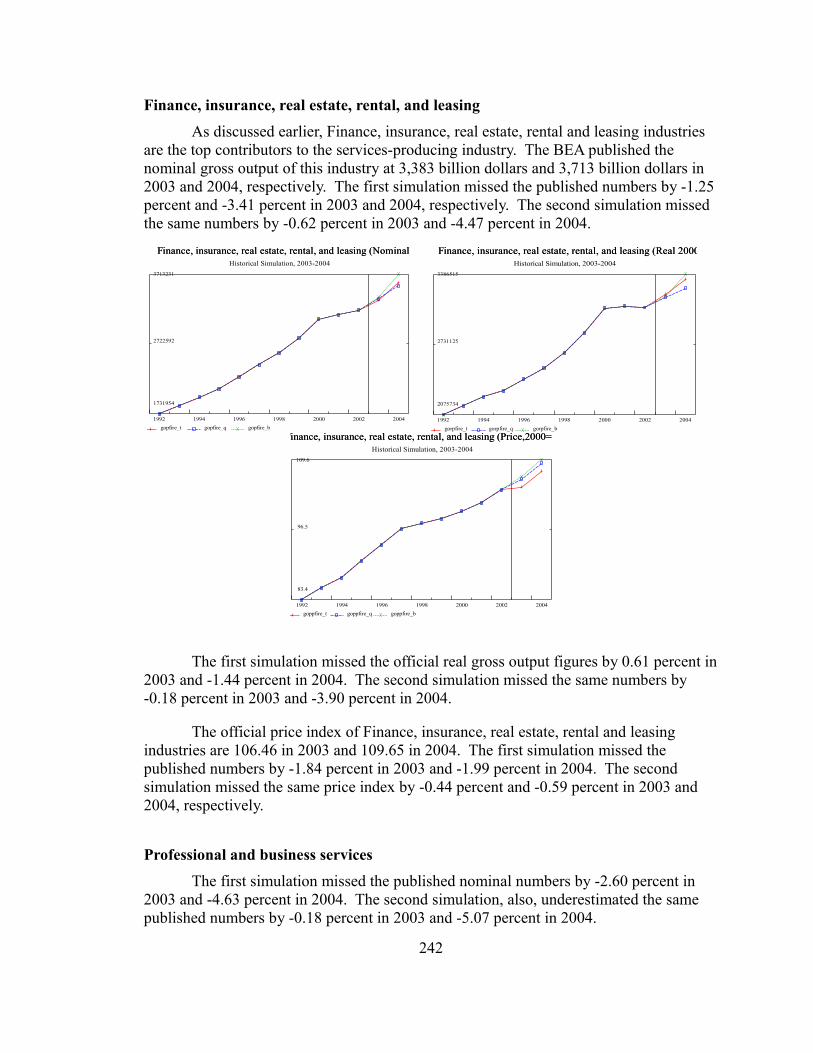
Finance, insurance, real estate, rental, and leasingAs discussed earlier, Finance, insurance, real estate, rental and leasing industries
are the top contributors to the services-producing industry. The BEA published the nominal gross output of this industry at 3,383 billion dollars and 3,713 billion dollars in 2003 and 2004, respectively. The first simulation missed the published numbers by -1.25 percent and -3.41 percent in 2003 and 2004, respectively. The second simulation missed the same numbers by -0.62 percent in 2003 and -4.47 percent in 2004. Finance, insurance, real estate, rental, and leasing (Nominal) Finance, insurance, real estate, rental, and leasing (Nominal)
Historical Simulation, 2003-20043713231
2722592
1731954
1992 1994 1996 1998 2000 2002 2004 gopfire_t gopfire_q gopfire_b
Finance, insurance, real estate, rental, and leasing (Real 2000) Finance, insurance, real estate, rental, and leasing (Real 2000) Historical Simulation, 2003-2004
3386515
2731125
2075734
1992 1994 1996 1998 2000 2002 2004 gorpfire_t gorpfire_q gorpfire_b
Finance, insurance, real estate, rental, and leasing (Price,2000=100) Finance, insurance, real estate, rental, and leasing (Price,2000=100) Historical Simulation, 2003-2004
109.6
96.5
83.4
1992 1994 1996 1998 2000 2002 2004 goppfire_t goppfire_q goppfire_b
The first simulation missed the official real gross output figures by 0.61 percent in 2003 and -1.44 percent in 2004. The second simulation missed the same numbers by -0.18 percent in 2003 and -3.90 percent in 2004.
The official price index of Finance, insurance, real estate, rental and leasing industries are 106.46 in 2003 and 109.65 in 2004. The first simulation missed the published numbers by -1.84 percent in 2003 and -1.99 percent in 2004. The second simulation missed the same price index by -0.44 percent and -0.59 percent in 2003 and 2004, respectively.
Professional and business servicesThe first simulation missed the published nominal numbers by -2.60 percent in
2003 and -4.63 percent in 2004. The second simulation, also, underestimated the same published numbers by -0.18 percent in 2003 and -5.07 percent in 2004.
242

On the real side, the first simulation underestimated the published numbers by -2.51 percent in 2003 and -2.92 percent in 2004. The second simulation missed the same official numbers by -0.27 percent and -1.09 percent in 2003 and 2004, respectively.
Professional and business services (Nominal) Professional and business services (Nominal) Historical Simulation, 2003-2004
2164261
1516609
868957
1992 1994 1996 1998 2000 2002 2004 gopbser_t gopbser_q gopbser_b
Professional and business services (Real 2000) Professional and business services (Real 2000) Historical Simulation, 2003-2004
2013212
1551717
1090222
1992 1994 1996 1998 2000 2002 2004 gorpbser_t gorpbser_q gorpbser_b
Professional and business services (Price,2000=100) Professional and business services (Price,2000=100) Historical Simulation, 2003-2004
107.5
93.6
79.7
1992 1994 1996 1998 2000 2002 2004 goppbser_t goppbser_q goppbser_b
The first simulation missed the chained 2000 price index of this industry by -0.09 percent in 2003 and -1.76 percent in 2004. The second simulation missed the same official price index by 0.09 percent in 2003 and -4.02 percent in 2004.
Educational services, health care, and social assistanceBEA published nominal gross output of Educational services, health care and
social assistance of 1,388 billion dollars in 2003 and 1,475 billion dollars in 2004. The first simulation missed the published numbers by -0.95 percent and -0.81 percent in 2003 and 2004, respectively. The second simulation missed the same official numbers by -0.83 percent in 2003 and -3.06 percent in 2004.
243

Educational services, health care, and social assistance (Nominal) Educational services, health care, and social assistance (Nominal) Historical Simulation, 2003-2004
1474507
1092866
711225
1992 1994 1996 1998 2000 2002 2004 gopedhc_t gopedhc_q gopedhc_b
Educational services, health care, and social assistance (Real 2000) Educational services, health care, and social assistance (Real 2000) Historical Simulation, 2003-2004
1301494
1102584
903674
1992 1994 1996 1998 2000 2002 2004 gorpedhc_t gorpedhc_q gorpedhc_b
Educational services, health care, and social assistance (Price,2000=100) Educational services, health care, and social assistance (Price,2000=100) Historical Simulation, 2003-2004
113.3
96.0
78.7
1992 1994 1996 1998 2000 2002 2004 goppedhc_t goppedhc_q goppedhc_b
The first simulation missed the official chained 2000 real gross output of this industry by -0.94 percent in 2003 and -0.22 percent in 2004. The second simulation missed the same published numbers by -1.05 percent and -3.02 percent in 2003 and 2004, respectively.
The chained 2000 price index of gross output is 109.69 in 2003 and 113.29 in 2004. The first simulation missed the official numbers by -0.02 percent in 2003 and -0.59 percent in 2004. The second simulation missed the same price index by 0.22 percent and -0.04 percent in 2003 and 2004, respectively.
Arts, entertainment, recreation, accommodation, and food servicesThe first simulation missed the published nominal numbers by -0.80 percent and
-0.42 percent in 2003 and 2004, respectively. The second simulation missed the same official numbers by -1.84 percent in 2003 and -4.85 percent in 2004.
The first simulation missed the official chained 2000 real gross output of this industry by -0.86 percent in 2003 and 0.59 percent in 2004. The second simulation missed the same published numbers by -1.81 percent and -3.80 percent in 2003 and 2004, respectively.
244
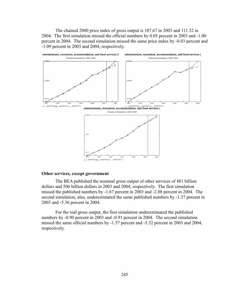
The chained 2000 price index of gross output is 107.67 in 2003 and 111.32 in 2004. The first simulation missed the official numbers by 0.05 percent in 2003 and -1.00 percent in 2004. The second simulation missed the same price index by -0.03 percent and -1.09 percent in 2003 and 2004, respectively.
Arts, entertainment, recreation, accommodation, and food services (Nominal) Arts, entertainment, recreation, accommodation, and food services (Nominal) Historical Simulation, 2003-2004
770884
582000
393117
1992 1994 1996 1998 2000 2002 2004 gopartfood_t gopartfood_q gopartfood_b
Arts, entertainment, recreation, accommodation, and food services (Real 200 Arts, entertainment, recreation, accommodation, and food services (Real 200 Historical Simulation, 2003-2004
696586
586984
477383
1992 1994 1996 1998 2000 2002 2004 gorpartfood_t gorpartfood_q gorpartfood_b
Arts, entertainment, recreation, accommodation, and food services (Price,20 Arts, entertainment, recreation, accommodation, and food services (Price,20 Historical Simulation, 2003-2004
111.3
96.8
82.3
1992 1994 1996 1998 2000 2002 2004 goppartfood_t goppartfood_q goppartfood_b
Other services, except governmentThe BEA published the nominal gross output of other services of 481 billion
dollars and 506 billion dollars in 2003 and 2004, respectively. The first simulation missed the published numbers by -1.67 percent in 2003 and -2.88 percent in 2004. The second simulation, also, underestimated the same published numbers by -1.37 percent in 2003 and -5.36 percent in 2004.
For the real gross output, the first simulation underestimated the published numbers by -0.90 percent in 2003 and -0.91 percent in 2004. The second simulation missed the same official numbers by -1.57 percent and -5.32 percent in 2003 and 2004, respectively.
245

Other services, except government (Nominal) Other services, except government (Nominal) Historical Simulation, 2003-2004
505527
388413
271299
1992 1994 1996 1998 2000 2002 2004 gopothser_t gopothser_q gopothser_b
Other services, except government (Real 2000) Other services, except government (Real 2000) Historical Simulation, 2003-2004
445504
393246
340988
1992 1994 1996 1998 2000 2002 2004 gorpothser_t gorpothser_q gorpothser_b
Other services, except government (Price,2000=100) Other services, except government (Price,2000=100) Historical Simulation, 2003-2004
113.5
96.5
79.6
1992 1994 1996 1998 2000 2002 2004 goppothser_t goppothser_q goppothser_b
The first simulation missed the chained 2000 price index of this industry by -0.78 percent in 2003 and -1.99 percent in 2004. The second simulation missed the same official price index by 0.20 percent in 2003 and -0.04 percent in 2004.
Government
BEA published nominal gross output of Government of 2,300 billion dollars in 2003 and 2,448 billion dollars in 2004. The first simulation missed the published numbers by -2.20 percent and -4.17 percent in 2003 and 2004, respectively. The second simulation missed the same official numbers by -2.14 percent in 2003 and -4.65 percent in 2004.
The first simulation missed the official chained 2000 real gross output of this industry by -0.34 percent in 2003 and -1.58 percent in 2004. The second simulation missed the same published numbers by -0.88 percent and -1.79 percent in 2003 and 2004, respectively.
The chained 2000 price index of gross output is 111.04 in 2003 and 116.17 in 2004. The first simulation missed the official numbers by -1.87 percent in 2003 and -2.63 percent in 2004. The second simulation missed the same price index by -1.27 percent and -2.91 percent in 2003 and 2004, respectively.
246

Government (Nominal) Government (Nominal) Historical Simulation, 2003-2004
2447557
1901453
1355349
1992 1994 1996 1998 2000 2002 2004 gog_t gog_q gog_b
Government (Real 2000) Government (Real 2000) Historical Simulation, 2003-2004
2106862
1892706
1678551
1992 1994 1996 1998 2000 2002 2004 gorg_t gorg_q gorg_b
Government (Price,2000=100) Government (Price,2000=100) Historical Simulation, 2003-2004
116.2
98.5
80.7
1992 1994 1996 1998 2000 2002 2004 gopg_t gopg_q gopg_b
Federal governmentFor the nominal gross output, the first simulation estimates gave errors of -3.51
percent in 2003 and -6.34 percent in 2004. The second simulation missed the published numbers by -4.15 percent and -8.32 percent in 2003 and 2004, respectively.
Federal government (Nominal) Federal government (Nominal) Historical Simulation, 2003-2004
824799
670780
516761
1992 1994 1996 1998 2000 2002 2004 gogf_t gogf_q gogf_b
Federal government (Real 2000) Federal government (Real 2000) Historical Simulation, 2003-2004
703394
638129
572864
1992 1994 1996 1998 2000 2002 2004 gorgf_t gorgf_q gorgf_b
247
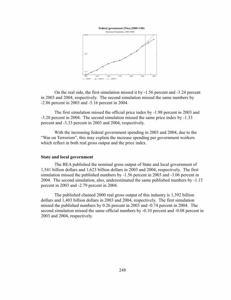
Federal government (Price,2000=100) Federal government (Price,2000=100) Historical Simulation, 2003-2004
117.3
99.5
81.7
1992 1994 1996 1998 2000 2002 2004 gopgf_t gopgf_q gopgf_b
On the real side, the first simulation missed it by -1.56 percent and -3.24 percent in 2003 and 2004, respectively. The second simulation missed the same numbers by -2.86 percent in 2003 and -5.16 percent in 2004.
The first simulation missed the official price index by -1.98 percent in 2003 and -3.20 percent in 2004. The second simulation missed the same price index by -1.33 percent and -3.33 percent in 2003 and 2004, respectively.
With the increasing federal government spending in 2003 and 2004, due to the “War on Terrorism”, this may explain the increase spending per government workers which reflect in both real gross output and the price index.
State and local governmentThe BEA published the nominal gross output of State and local government of
1,541 billion dollars and 1,623 billion dollars in 2003 and 2004, respectively. The first simulation missed the published numbers by -1.56 percent in 2003 and -3.06 percent in 2004. The second simulation, also, underestimated the same published numbers by -1.15 percent in 2003 and -2.79 percent in 2004.
The published chained 2000 real gross output of this industry is 1,392 billion dollars and 1,403 billion dollars in 2003 and 2004, respectively. The first simulation missed the published numbers by 0.26 percent in 2003 and -0.74 percent in 2004. The second simulation missed the same official numbers by -0.10 percent and -0.08 percent in 2003 and 2004, respectively.
248

State and local government (Nominal) State and local government (Nominal) Historical Simulation, 2003-2004
1622758
1229507
836256
1992 1994 1996 1998 2000 2002 2004 gogsl_t gogsl_q gogsl_b
State and local government (Real 2000) State and local government (Real 2000) Historical Simulation, 2003-2004
1402952
1222227
1041501
1992 1994 1996 1998 2000 2002 2004 gorgsl_t gorgsl_q gorgsl_b
State and local government (Price,2000=100) State and local government (Price,2000=100) Historical Simulation, 2003-2004
115.7
98.0
80.3
1992 1994 1996 1998 2000 2002 2004 gopgsl_t gopgsl_q gopgsl_b
The first simulation missed the chained 2000 price index of this industry by -1.81 percent in 2003 and -2.35 percent in 2004. The second simulation missed the same official price index by -1.25 percent in 2003 and -2.71 percent in 2004.
6.4 Forecast of Gross Output between 2006-2008
In this section, I applied the earlier discussed method to forecast the annual gross output by detailed industry from 2006 to 2008. The discussion of the Gross output forecast is presented by Major industry groups, as previously shown in Section 6.3. The detailed forecast is shown in Appendix 6.6.
Forecast assumptions
This approach requires 19 exogenous inputs of monthly variables. All of the exogenous inputs except crude oil price (oilpm) and trade weighted exchange rate index (exrim) are provided by QUEST, where we do not have official numbers (July 2007 to December 2008). oilpm and exrim are generated by ad hoc outlook of the economy from the author's opinion.
Table 6.6 shows all values of the exogenous variables used in this forecast.
249

250
Table 6.6: Assumptions of Exogenous Variables Used in Forecasting Gross OutputJan Feb Mar Apr May Jun Jul Aug Sep Oct Nov Dec
exrim2006 105.03 104.67 104.31 103.96 103.60 103.25 102.90 102.55 102.20 101.86 101.51 101.162007 100.82 100.48 100.14 99.80 99.46 99.12 98.78 98.44 98.11 97.78 97.44 97.112008 96.78 96.45 96.13 95.80 95.47 95.15 94.82 94.50 94.18 93.86 93.54 93.22
oilpm2006 52.75 53.80 54.88 55.97 57.09 58.24 59.40 60.59 61.80 63.04 64.30 65.582007 66.89 68.23 69.60 70.99 72.41 73.86 75.33 76.84 78.38 79.94 81.54 83.172008 84.84 86.53 88.27 90.03 91.83 93.67 95.54 97.45 99.40 101.39 103.42 105.49
mnipaqmv2006 429.57 433.38 435.14 431.11 431.55 432.74 436.94 437.92 437.94 433.88 434.34 436.182007 443.15 444.97 445.38 444.38 441.97 438.15 441.47 443.65 445.93 448.81 450.89 452.702008 454.34 455.48 456.24 455.45 456.34 457.74 460.12 462.19 464.44 466.84 469.42 472.16
mnipaqfur2006 398.01 401.04 402.75 401.09 401.72 402.59 403.91 405.08 406.31 407.51 408.95 410.542007 413.19 414.38 415.03 415.13 414.68 413.69 410.38 409.10 408.35 408.71 408.53 408.412008 408.51 408.40 408.23 407.90 407.71 407.54 407.40 407.29 407.21 407.17 407.16 407.18
mnipaqdoth2006 208.15 209.54 210.21 208.94 209.13 209.54 210.50 211.11 211.70 212.11 212.77 213.512007 214.32 215.26 216.32 217.49 218.76 220.15 220.98 221.76 222.47 223.10 223.65 224.122008 224.47 224.82 225.13 225.04 225.52 226.22 227.42 228.34 229.27 230.20 231.14 232.09
mnipaqfood2006 1,230.81 1,236.89 1,241.51 1,241.58 1,245.61 1,250.51 1,255.77 1,262.78 1,271.04 1,283.39 1,292.00 1,299.722007 1,306.85 1,312.57 1,317.18 1,320.68 1,323.07 1,324.35 1,332.60 1,338.68 1,344.39 1,349.85 1,354.74 1,359.182008 1,363.00 1,366.65 1,369.97 1,371.51 1,375.24 1,379.72 1,385.76 1,391.11 1,396.59 1,402.20 1,407.93 1,413.79
mnipaqcloth2006 350.27 351.27 352.37 353.54 354.86 356.30 358.20 359.64 360.96 361.36 363.04 365.202007 370.02 371.49 371.79 370.92 368.89 365.69 367.49 368.26 368.92 369.37 369.91 370.432008 371.07 371.46 371.73 371.43 371.81 372.40 373.45 374.30 375.20 376.14 377.13 378.16
mnipaqgas2006 312.82 315.89 324.99 353.44 364.62 371.84 381.18 375.94 362.18 316.51 303.29 299.112007 310.23 319.45 333.03 350.96 373.25 399.89 382.89 378.34 374.58 371.47 369.38 368.162008 364.04 367.43 374.53 397.60 402.96 402.87 391.23 384.77 377.42 369.18 360.03 349.99
mnipaqnoth2006 712.21 716.71 720.88 724.73 728.21 731.36 733.79 736.52 739.19 741.26 744.19 747.462007 752.70 755.40 757.20 758.10 758.10 757.20 763.58 767.97 772.18 776.28 780.09 783.702008 786.98 790.22 793.33 795.49 798.91 802.79 807.62 812.06 816.60 821.24 825.97 830.80
mnipaqhous2006 1,340.46 1,347.71 1,355.23 1,363.62 1,371.17 1,378.52 1,385.37 1,392.50 1,399.63 1,406.80 1,413.91 1,421.002007 1,428.17 1,435.13 1,442.00 1,448.77 1,455.43 1,462.00 1,469.15 1,476.72 1,484.56 1,493.61 1,501.30 1,508.562008 1,515.53 1,521.83 1,527.60 1,530.98 1,537.07 1,544.01 1,552.57 1,560.64 1,568.98 1,577.59 1,586.48 1,595.64
mnipaqho2006 497.72 496.62 496.06 495.74 496.45 497.91 501.13 503.31 505.46 506.99 509.56 512.562007 517.34 520.19 522.47 524.17 525.29 525.84 529.52 532.37 535.06 537.58 539.91 542.062008 543.96 545.80 547.51 548.53 550.42 552.61 555.44 557.99 560.59 563.25 565.96 568.73
mnipaqtr2006 333.47 334.70 335.93 337.11 338.39 339.71 341.10 342.49 343.90 345.59 346.86 347.962007 348.33 349.51 350.96 352.66 354.61 356.83 358.66 360.48 362.29 364.27 365.93 367.442008 368.79 370.02 371.11 371.61 372.78 374.16 375.96 377.59 379.28 381.01 382.79 384.63
mnipaqmc2006 1,550.94 1,558.42 1,565.54 1,572.25 1,578.70 1,584.85 1,589.63 1,595.94 1,602.73 1,608.09 1,617.26 1,628.352007 1,646.69 1,657.60 1,666.42 1,673.15 1,677.80 1,680.35 1,695.79 1,707.86 1,719.72 1,731.92 1,742.92 1,753.302008 1,762.98 1,772.12 1,780.68 1,786.60 1,795.51 1,805.37 1,817.03 1,828.15 1,839.58 1,851.32 1,863.36 1,875.71
mnipaqrec2006 369.57 371.10 372.63 373.56 375.55 377.99 381.54 384.41 387.24 390.87 393.02 394.512007 394.41 395.29 396.21 397.17 398.19 399.24 400.86 402.84 405.00 407.63 409.97 412.312008 414.77 416.98 419.07 420.59 422.80 425.23 428.08 430.81 433.62 436.50 439.46 442.49
mnipaqsoth2006 1,253.73 1,261.13 1,269.33 1,281.61 1,288.95 1,294.64 1,293.79 1,299.83 1,307.89 1,322.23 1,331.10 1,338.772007 1,344.24 1,350.25 1,355.81 1,360.91 1,365.55 1,369.74 1,382.12 1,391.27 1,399.94 1,408.39 1,415.88 1,422.692008 1,428.23 1,434.11 1,439.75 1,443.65 1,449.92 1,457.07 1,466.19 1,474.27 1,482.40 1,490.59 1,498.84 1,507.14
mnipaqvnrs2006 367.68 375.67 383.75 393.31 400.52 406.77 411.33 416.23 420.73 424.46 428.44 432.302007 433.70 439.06 446.04 454.64 464.86 476.70 477.19 480.35 483.62 487.25 490.58 493.842008 497.07 500.16 503.17 507.45 509.23 509.89 507.07 507.25 508.07 509.52 511.62 514.35
mnipaqvnre2006 986.01 992.88 996.21 990.03 990.78 992.49 999.16 999.78 998.36 990.17 988.20 987.732007 989.46 991.47 994.46 998.43 1,003.37 1,009.30 1,010.51 1,012.69 1,014.90 1,017.67 1,019.52 1,020.992008 1,022.03 1,022.79 1,023.20 1,021.71 1,022.62 1,024.36 1,028.13 1,030.65 1,033.11 1,035.51 1,037.86 1,040.15
mnipaqvfr2006 811.36 810.42 806.42 798.36 788.97 777.26 758.46 745.68 734.16 725.12 715.19 705.592007 695.76 687.25 679.49 672.49 666.25 660.76 651.66 646.43 642.96 643.93 642.01 639.872008 636.99 634.79 632.75 630.09 628.97 628.60 630.68 630.53 629.85 628.64 626.90 624.64
mgdp2006 12,888.41 12,967.14 13,038.24 13,103.17 13,157.90 13,203.93 13,227.60 13,266.39 13,306.70 13,345.44 13,391.02 13,440.432007 13,489.34 13,549.54 13,616.81 13,691.07 13,772.35 13,860.67 13,896.12 13,945.47 13,996.15 14,049.64 14,101.82 14,154.222008 14,206.81 14,259.58 14,312.56 14,364.16 14,418.70 14,474.66 14,534.06 14,591.19 14,648.18 14,704.98 14,761.61 14,818.06
Outlook of Gross Output by Industries
Table 6.7 shows the forecasted values and their growth rates of Gross output by industry groups from 2006 to 2008 of nominal value, real 2000 value, and price indexes. Figure 6.1 shows plots of these forecasts by industry groups.
Overall, real total Gross output is expected to grow steadily at the average rate of 3.5% annually during 2006-2008. Most of this growth is coming from the growth in Gross output of Private industries which grows at an average rate of 4.41% in real terms between 2006 and 2008. The Gross output of Government is expected to decline significantly in 2007 and 2008 in real terms as the increasing price index crowds out the growth of government nominal gross output. In real terms, the government gross output will decline by -2.8% and -3.41% in 2007 and 2008, respectively.
Among industry groups, the industries that exhibit strong positive growth between 2006 and 2008 are Service industries, Wholesale trade, Retail trade, and Mining industry. Other industry groups grow at a much lower rate, especially in 2007 and 2008.
251

252
Table 6.7: Outlook of Gross output by Industry Groups, 2006-2008Gross output
Forecast real 2000 (Million of Dollars) 2005 2006 2007 2008 05-06 06-07 07-08Total Gross Output 20,058,940 20,900,634 21,639,600 22,368,236 4.20% 3.54% 3.37% Private industries 17,937,770 18,780,048 19,593,794 20,415,080 4.70% 4.33% 4.19% Total Services industries (40-61) 8,266,276 8,593,869 9,041,576 9,516,695 3.96% 5.21% 5.25% Agriculture, forestry, fishing, and hunting 271,988 275,967 278,746 282,101 1.46% 1.01% 1.20% Mining 215,154 234,499 242,825 249,499 8.99% 3.55% 2.75% Utilities 308,632 326,804 325,695 336,083 5.89% -0.34% 3.19% Construction 935,694 974,130 973,468 981,431 4.11% -0.07% 0.82% Manufacturing 4,041,547 4,163,015 4,272,347 4,371,470 3.01% 2.63% 2.32% Durable goods manufacturing 2,320,544 2,474,611 2,530,347 2,587,441 6.64% 2.25% 2.26% Nondurable goods manufacturing 1,731,693 1,715,345 1,767,631 1,809,873 -0.94% 3.05% 2.39% Wholesale trade 972,399 1,085,999 1,182,849 1,284,355 11.68% 8.92% 8.58% Retail trade 1,225,873 1,314,233 1,388,841 1,460,585 7.21% 5.68% 5.17% Transportation and warehousing 633,736 650,313 673,491 695,050 2.62% 3.56% 3.20% Information 1,184,287 1,284,127 1,355,553 1,387,912 8.43% 5.56% 2.39% Finance, insurance, real estate, rental, and leasing 3,549,877 3,723,020 3,944,919 4,173,934 4.88% 5.96% 5.81% Professional and business services 2,100,988 2,188,728 2,298,667 2,418,824 4.18% 5.02% 5.23% Educational services, health care, and social assistance 1,348,384 1,390,250 1,457,779 1,541,394 3.10% 4.86% 5.74% Arts, entertainment, recreation, accommodation, and food services 707,874 738,169 768,446 791,797 4.28% 4.10% 3.04% Other services, except government 444,704 439,733 455,239 473,153 -1.12% 3.53% 3.94% Government 2,125,267 2,132,010 2,072,299 2,001,617 0.32% -2.80% -3.41% Federal government 710,359 715,079 695,107 669,418 0.66% -2.79% -3.70% State and local government 1,414,380 1,416,386 1,376,662 1,331,714 0.14% -2.80% -3.26%
Forecast nominal (Million of dollars) 2005 2006 2007 2008 05-06 06-07 07-08Total Gross Output 22,857,144 24,510,822 26,289,532 28,128,810 7.23% 7.26% 7.00% Private industries 20,256,014 21,811,932 23,489,066 25,227,638 7.68% 7.69% 7.40% Total Services industries (40-61) 9,343,153 9,987,533 10,784,158 11,650,302 6.90% 7.98% 8.03% Agriculture, forestry, fishing, and hunting 312,372 327,810 356,912 364,944 4.94% 8.88% 2.25% Mining 396,278 457,485 515,217 593,814 15.45% 12.62% 15.26% Utilities 409,979 455,648 474,331 529,597 11.14% 4.10% 11.65% Construction 1,174,995 1,252,784 1,360,278 1,501,666 6.62% 8.58% 10.39% Manufacturing 4,501,822 4,786,128 5,067,578 5,302,899 6.32% 5.88% 4.64% Durable goods manufacturing 2,364,127 2,561,733 2,656,236 2,760,741 8.36% 3.69% 3.93% Nondurable goods manufacturing 2,137,695 2,224,395 2,411,341 2,542,159 4.06% 8.40% 5.43% Wholesale trade 1,073,587 1,237,017 1,427,440 1,588,718 15.22% 15.39% 11.30% Retail trade 1,288,716 1,406,178 1,510,383 1,626,061 9.11% 7.41% 7.66% Transportation and warehousing 712,142 777,285 821,052 883,809 9.15% 5.63% 7.64% Information 1,161,134 1,247,692 1,300,356 1,315,753 7.45% 4.22% 1.18% Finance, insurance, real estate, rental, and leasing 3,990,862 4,282,525 4,634,455 5,028,573 7.31% 8.22% 8.50% Professional and business services 2,318,478 2,521,346 2,745,371 2,967,522 8.75% 8.89% 8.09% Educational services, health care, and social assistance 1,578,006 1,667,520 1,801,734 1,961,808 5.67% 8.05% 8.88% Arts, entertainment, recreation, accommodation, and food services 815,391 857,173 900,394 946,595 5.12% 5.04% 5.13% Other services, except government 522,252 535,339 573,564 615,880 2.51% 7.14% 7.38% Government 2,601,131 2,698,891 2,800,466 2,901,174 3.76% 3.76% 3.60% Federal government 872,257 910,285 947,121 980,974 4.36% 4.05% 3.57% State and local government 1,728,874 1,788,606 1,853,345 1,920,199 3.45% 3.62% 3.61%
Forecast price index (2000=100) 2005 2006 2007 2008 05-06 06-07 07-08Total Gross Output 113.95 117.27 121.49 125.75 2.92% 3.59% 3.51% Private industries 112.92 116.14 119.88 123.57 2.85% 3.22% 3.08% Total Services industries (40-61) 113.03 116.22 119.27 122.42 2.82% 2.63% 2.64% Agriculture, forestry, fishing, and hunting 114.85 118.79 128.04 129.37 3.43% 7.79% 1.03% Mining 184.18 195.09 212.18 238.00 5.92% 8.76% 12.17% Utilities 132.84 139.43 145.64 157.58 4.96% 4.45% 8.20% Construction 125.57 128.61 139.74 153.01 2.41% 8.65% 9.50% Manufacturing 111.39 114.97 118.61 121.31 3.21% 3.17% 2.27% Durable goods manufacturing 101.88 103.52 104.98 106.70 1.61% 1.41% 1.64% Nondurable goods manufacturing 123.45 129.68 136.42 140.46 5.05% 5.20% 2.96% Wholesale trade 110.41 113.91 120.68 123.70 3.17% 5.95% 2.50% Retail trade 105.13 107.00 108.75 111.33 1.78% 1.64% 2.37% Transportation and warehousing 112.37 119.52 121.91 127.16 6.37% 2.00% 4.30% Information 98.04 97.16 95.93 94.80 -0.90% -1.27% -1.18% Finance, insurance, real estate, rental, and leasing 112.42 115.03 117.48 120.48 2.32% 2.13% 2.55% Professional and business services 110.35 115.20 119.43 122.68 4.39% 3.68% 2.72% Educational services, health care, and social assistance 117.03 119.94 123.59 127.27 2.49% 3.04% 2.98% Arts, entertainment, recreation, accommodation, and food services 115.19 116.12 117.17 119.55 0.81% 0.90% 2.03% Other services, except government 117.44 121.74 125.99 130.17 3.66% 3.49% 3.31% Government 122.39 126.59 135.14 144.94 3.43% 6.75% 7.25% Federal government 122.79 127.30 136.26 146.54 3.67% 7.04% 7.55% State and local government 122.24 126.28 134.63 144.19 3.31% 6.61% 7.10%

Real Gross output of agriculture, forestry, fishing, and hunting is expected to grow by 1.46%, 1.01%, and 1.20% in 2006, 2007, and 2008, respectively. This growth rate of the real gross output is consistent with its long-term trend as shown in Figure 6.1. In 2007, nominal gross output of this industry will grow significantly by 8.88% as its price index rises by 7.79%.
Real Gross output of Mining industry grows by 8.99%, 3.55%, and 2.75% in 2006, 2007, and 2008, respectively. Surprisingly, Appendix 6.6 shows that the main contributor to this growth is coming from supporting activities for mining industry which has historically been the smallest components of the real gross output of mining industry. The price index of this industries' gross output is expected to rise significantly at rates of 8.76% in 2007 and 12.17% in 2008.
Since 2001, the real gross output of utilities has been slowly decreasing. In 2006, we expect to see a positive growth rate of utilities' real gross output of 5.89%. The real gross output will decline slightly in 2007 by -0.34% and will increase by 3.19% in 2008.
As the problem in sub-prime credit market persists, we expect the real gross output of construction industry will grow at the rate of -0.07% in 2007 and 0.82% in 2008.
Manufacturing industry group contributes on average of 20% to the nominal total gross output. We expect the real gross output of manufacturing industry to grow consistently between 2006 and 2007 at an average rate of 2.65% annually. In 2006, real gross output of durable manufacturing grows significantly by 6.64% while real gross output of nondurable manufacturing decline slightly by -0.94%. Both durable and nondurable manufacturing industries grow steadily in 2007 and 2008 at an average rate of around 2.5% annually. From Appendix 6.6, Computer and electronic products gross output grows by 21.5% in 2006 and will have significantly smaller growth rate in 2007 and 2008 of 11.03% and 3.74%, respectively. Also, the petroleum and coal products, which expected to have its real gross output reduced by -12.47% in 2006, will expand significantly in 2007 and 2008 with growth rates of 13.71% and 17.15%, respectively. Apparel and leather and allied products real gross output is expected to decline significantly in 2008 by -32.82%.
Real gross output of wholesale trade will have growth rates of 11.68%, 8.92%, and 8.58% in 2006, 2007, and 2008, respectively. This growth rate is slightly stronger than its average between 1993 and 2005.
Retail trade will keep growing consistently with its historical trend, as shown in Figure 6.1. The real gross output of this industry will grow at rates of 7.21% in 2006, 5.68% in 2007, and 5.17% in 2008.
253

Overall, the real gross output of service industries will grow by 3.96%, 5.21%, and 5.25% in 2006, 2007, and 2008, respectively. Most of this growth comes from the three biggest contributors to the service industry's nominal gross output; 1) Finance, insurance, real estate, rental, and leasing, 2) Professional and business services, and 3) Educational services, health care, and social assistance.
Finance, insurance, real estate, rental, and leasing is expected to see its real gross output grow by 4.88%, 5.96%, and 5.81% in 2006, 2007, and 2008, respectively. Federal Reserve banks, credit intermediation, and related activities will see significantly smaller growth in 2007 and 2008 of 2.36% and 1.94%, respectively as the problem in credit market persists.
Professional and business services industry's real gross output will grow by an average of 4.81% annually from 2006 to 2008. Among its components, Miscellaneous professional, scientific, and technical services, which is the biggest contributor to Professional and business services industry's real gross output, will grow the most with an average growth rate of 7.73% annually between 2006 and 2008. The real gross output of Management of companies and enterprises will decline slightly by -0.55% in 2006 but will grow rapidly in 2007 and 2008 at rates of 8.01% and 9.14%, respectively.
For Educational services, health care, and social assistance, the real gross output will grow by 3.10%, 4.86%, and 5.74% in 2006, 2007, and 2008, respectively. All of its components show steady positive growth rate consistent with their historical rate since 1993. Between the forecast period, Ambulatory health care services' real gross output has the highest average growth rate of 5.87% annually.
From Appendix 6.6, Performing arts, spectator sports, museums, and related activities' real gross output will be declining throughout the forecast period. This industries' real gross output will decline by -3.23% in 2006, -4.47% in 2007, and -1.16% in 2008.
254

255
Figure 6.1: Plots of Gross output by Industry Groups
Total Gross Output (Nominal and Real 2000) Total Gross Output (Nominal and Real 2000) Forecast, 2006-2008
28128810
19690631
11252452
1995 2000 2005 got_f gort_f
Total Gross Output (Price,2000=100) Total Gross Output (Price,2000=100) Forecast, 2006-2008
125.8
106.6
87.5
1995 2000 2005 gopt_f
Private industries (Nominal and Real 2000) Private industries (Nominal and Real 2000) Forecast, 2006-2008
25227638
17562370
9897103
1995 2000 2005 gop_f gorp_f
Private industries (Price,2000=100) Private industries (Price,2000=100) Forecast, 2006-2008
123.6
106.0
88.4
1995 2000 2005 gopp_f
Total Services industries (40-61) (Nominal and Real 2000) Total Services industries (40-61) (Nominal and Real 2000) Forecast, 2006-2008
11650302
7827540
4004778
1995 2000 2005 gopserv_f gorpserv_f
Total Services industries (40-61) (Price,2000=100) Total Services industries (40-61) (Price,2000=100) Forecast, 2006-2008
122.4
101.9
81.4
1995 2000 2005 goppserv_f

Figure 6.1 (cont.)
Agriculture, forestry, fishing, and hunting (Nominal and Real 2000) Agriculture, forestry, fishing, and hunting (Nominal and Real 2000) Forecast, 2006-2008
364944
292370
219795
1995 2000 2005 gopag_f gorpag_f
Agriculture, forestry, fishing, and hunting (Price,2000=100) Agriculture, forestry, fishing, and hunting (Price,2000=100) Forecast, 2006-2008
129.4
114.2
99.0
1995 2000 2005 goppag_f
Mining (Nominal and Real 2000) Mining (Nominal and Real 2000) Forecast, 2006-2008
593814
364526
135238
1995 2000 2005 gopmin_f gorpmin_f
Mining (Price,2000=100) Mining (Price,2000=100) Forecast, 2006-2008
238
152
65
1995 2000 2005 goppmin_f
Utilities (Nominal and Real 2000) Utilities (Nominal and Real 2000) Forecast, 2006-2008
529597
392434
255271
1995 2000 2005 goputil_f gorputil_f
Utilities (Price,2000=100) Utilities (Price,2000=100) Forecast, 2006-2008
157.6
123.3
89.1
1995 2000 2005 gopputil_f
256

Figure 6.1 (cont.)
Construction (Nominal and Real 2000) Construction (Nominal and Real 2000) Forecast, 2006-2008
1501666
983163
464659
1995 2000 2005 gopconst_f gorpconst_f
Construction (Price,2000=100) Construction (Price,2000=100) Forecast, 2006-2008
153.0
114.5
75.9
1995 2000 2005 goppconst_f
Manufacturing (Nominal and Real 2000) Manufacturing (Nominal and Real 2000) Forecast, 2006-2008
5302899
4086737
2870576
1995 2000 2005 gopmanu_f gorpmanu_f
Manufacturing (Price,2000=100) Manufacturing (Price,2000=100) Forecast, 2006-2008
121.3
109.6
97.9
1995 2000 2005 goppmanu_f
Durable goods manufacturing (Nominal and Real 2000) Durable goods manufacturing (Nominal and Real 2000) Forecast, 2006-2008
2760741
2062229
1363716
1995 2000 2005 gopdur_f gorpdur_f
Durable goods manufacturing (Price,2000=100) Durable goods manufacturing (Price,2000=100) Forecast, 2006-2008
112.2
104.3
96.4
1995 2000 2005 goppdur_f
257

Figure 6.1 (cont.)
Nondurable goods manufacturing (Nominal and Real 2000) Nondurable goods manufacturing (Nominal and Real 2000) Forecast, 2006-2008
2542158
1959360
1376561
1995 2000 2005 gopndur_f gorpndur_f
Nondurable goods manufacturing (Price,2000=100) Nondurable goods manufacturing (Price,2000=100) Forecast, 2006-2008
140.5
113.0
85.6
1995 2000 2005 goppndur_f
Wholesale trade (Nominal and Real 2000) Wholesale trade (Nominal and Real 2000) Forecast, 2006-2008
1588718
1063936
539155
1995 2000 2005 gopwhsl_f gorpwhsl_f
Wholesale trade (Price,2000=100) Wholesale trade (Price,2000=100) Forecast, 2006-2008
123.7
109.7
95.6
1995 2000 2005 goppwhsl_f
Retail trade (Nominal and Real 2000) Retail trade (Nominal and Real 2000) Forecast, 2006-2008
1626061
1122731
619401
1995 2000 2005 goprtl_f gorprtl_f
Retail trade (Price,2000=100) Retail trade (Price,2000=100) Forecast, 2006-2008
111.3
103.9
96.4
1995 2000 2005 gopprtl_f
258

Figure 6.1 (cont.)
Transportation and warehousing (Nominal and Real 2000) Transportation and warehousing (Nominal and Real 2000) Forecast, 2006-2008
883809
630265
376721
1995 2000 2005 goptran_f gorptran_f
Transportation and warehousing (Price,2000=100) Transportation and warehousing (Price,2000=100) Forecast, 2006-2008
127.2
107.3
87.4
1995 2000 2005 gopptran_f
Information (Nominal and Real 2000) Information (Nominal and Real 2000) Forecast, 2006-2008
1387912
908698
429483
1995 2000 2005 gopinfo_f gorpinfo_f
Information (Price,2000=100) Information (Price,2000=100) Forecast, 2006-2008
100.50
97.16
93.83
1995 2000 2005 goppinfo_f
Finance, insurance, real estate, rental, and leasing (Nominal and Real 2000 Finance, insurance, real estate, rental, and leasing (Nominal and Real 2000 Forecast, 2006-2008
5028573
3380264
1731954
1995 2000 2005 gopfire_f gorpfire_f
Finance, insurance, real estate, rental, and leasing (Price,2000=100) Finance, insurance, real estate, rental, and leasing (Price,2000=100) Forecast, 2006-2008
120.5
102.0
83.4
1995 2000 2005 goppfire_f
259

Figure 6.1 (cont.)
Professional and business services (Nominal and Real 2000) Professional and business services (Nominal and Real 2000) Forecast, 2006-2008
2967522
1918240
868957
1995 2000 2005 gopbser_f gorpbser_f
Professional and business services (Price,2000=100) Professional and business services (Price,2000=100) Forecast, 2006-2008
122.7
101.2
79.7
1995 2000 2005 goppbser_f
Educational services, health care, and social assistance (Nominal and Real Educational services, health care, and social assistance (Nominal and Real Forecast, 2006-2008
1961808
1336517
711225
1995 2000 2005 gopedhc_f gorpedhc_f
Educational services, health care, and social assistance (Price,2000=100) Educational services, health care, and social assistance (Price,2000=100) Forecast, 2006-2008
127.3
103.0
78.7
1995 2000 2005 goppedhc_f
Arts, entertainment, recreation, accommodation, and food services (Nominal Arts, entertainment, recreation, accommodation, and food services (Nominal Forecast, 2006-2008
946595
669856
393117
1995 2000 2005 gopartfood_f gorpartfood_f
Arts, entertainment, recreation, accommodation, and food services (Price,20 Arts, entertainment, recreation, accommodation, and food services (Price,20 Forecast, 2006-2008
119.6
100.9
82.3
1995 2000 2005 goppartfood_f
260

Figure 6.1 (cont.)
Other services, except government (Nominal and Real 2000) Other services, except government (Nominal and Real 2000) Forecast, 2006-2008
615880
443590
271299
1995 2000 2005 gopothser_f gorpothser_f
Other services, except government (Price,2000=100) Other services, except government (Price,2000=100) Forecast, 2006-2008
130.2
104.9
79.6
1995 2000 2005 goppothser_f
Government (Nominal and Real 2000) Government (Nominal and Real 2000) Forecast, 2006-2008
2901174
2128261
1355349
1995 2000 2005 gog_f gorg_f
Government (Price,2000=100) Government (Price,2000=100) Forecast, 2006-2008
144.9
112.8
80.7
1995 2000 2005 gopg_f
Federal government (Nominal and Real 2000) Federal government (Nominal and Real 2000) Forecast, 2006-2008
980974
748868
516761
1995 2000 2005 gogf_f gorgf_f
Federal government (Price,2000=100) Federal government (Price,2000=100) Forecast, 2006-2008
146.5
114.1
81.7
1995 2000 2005 gopgf_f
261

Figure 6.1 (cont.)
State and local government (Nominal and Real 2000) State and local government (Nominal and Real 2000) Forecast, 2006-2008
1920199
1378228
836256
1995 2000 2005 gogsl_f gorgsl_f
State and local government (Price,2000=100) State and local government (Price,2000=100) Forecast, 2006-2008
144.2
112.2
80.3
1995 2000 2005 gopgsl_f
262

Chapter 7: Conclusion
The objective of this dissertation is to find a solution to the problem of the “ragged end” of historical data for long-term modeling. Using time-series analysis, this study develops processes to generate values between the last published data and up to two years into the future.
I studied four bodies of data used by a long-term economic model. Personal consumption expenditures, Gross output, Investment in equipment and software, and Investment in structures are estimated in detailed industries or categories.
The processes to estimate the series are generally similar and involve the use of high-frequency data series and time-series analysis. The differences in the methods used for these four bodies of data are due to the differences in the characteristics of the data.
I find that the performance of the forecasts depends heavily on the accuracy of the exogenous variables used in each forecast. The estimated detailed values are consistent with the macroeconomic data, used as regressors in the processes. Thus, generally, the results will be reliable as long as we have a good forecast of macroeconomic variables.
The performance of the first-period forecast also depends on where in the calendar year the last published data is. The closer to the end of the year, the better is the accuracy of the forecast.
Overall, this study met the goal of the dissertation. It established processes to generate detailed economic data which will be used as starting values of a long-term economic model. Nevertheless, there is room for improving these processes. First, the accuracy of the exogenous variables can be improved by improving the macroeconomic model, i.e. QUEST, used in estimating these variables. Then, the processes' performance can be increased by improving some equations that exhibit relatively higher errors than their peers, such as the equation for nominal gross output of Airline transportation.
Although not perfect, I believe this study will help improve the short-term accuracy of a long-term economic model, which is an important concern for many applied economists.
263
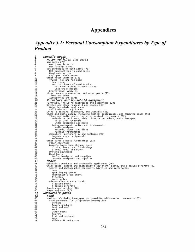
Appendices
Appendix 3.1: Personal Consumption Expenditures by Type of Product1 Durable goods 2 Motor vehicles and parts 3 New autos (70) 4 New domestic autos 5 New foreign autos 6 Net purchases of used autos (71) 7 Net transactions in used autos 8 Used auto margin 9 Employee reimbursement 10 Other motor vehicles (72) 11 Trucks, new and net used 12 New trucks 13 Net purchases of used trucks 14 Net transactions in used trucks 15 Used truck margin 16 Recreational vehicles 17 Tires, tubes, accessories, and other parts (73) 18 Tires and tubes 19 Accessories and parts 20 Furniture and household equipment 21 Furniture, including mattresses and bedsprings (29) 22 Kitchen and other household appliances (30) 23 Major household appliances 24 Small electric appliances 25 China, glassware, tableware, and utensils (31) 26 Video and audio goods, including musical instruments, and computer goods (91) 27 Video and audio goods, including musical instruments (92) 28 Television receivers, video cassette recorders, and videotapes 29 Television receivers 30 Video equipment and media 31 Audio equipment, media, and instruments 32 Audio equipment 33 Records, tapes, and disks 34 Musical instruments 35 Computers, peripherals, and software (93) 36 Computers and peripherals 37 Software 38 Other durable house furnishings (32) 39 Floor coverings 40 Durable house furnishings, n.e.c. 41 Clocks, lamps, and furnishings 42 Blinds, rods, and other 43 Writing equipment 44 Hand tools 45 Tools, hardware, and supplies 46 Outdoor equipment and supplies 47 Other 48 Ophthalmic products and orthopedic appliances (46) 49 Wheel goods, sports and photographic equipment, boats, and pleasure aircraft (90) 50 Sports and photographic equipment, bicycles and motorcycles 51 Guns 52 Sporting equipment 53 Photographic equipment 54 Bicycles 55 Motorcycles 56 Pleasure boats and aircraft 57 Pleasure boats 58 Pleasure aircraft 59 Jewelry and watches (18) 60 Books and maps (87) 61 Nondurable goods 62 Food 63 Food and alcoholic beverages purchased for off-premise consumption (3) 64 Food purchased for off-premise consumption 65 Cereals 66 Bakery products 67 Beef and veal 68 Pork 69 Other meats 70 Poultry 71 Fish and seafood 72 Eggs 73 Fresh milk and cream
264

74 Processed dairy products 75 Fresh fruits 76 Fresh vegetables 77 Processed fruits and vegetables 78 Juices and nonalcoholic drinks 79 Coffee, tea and beverage materials 80 Fats and oils 81 Sugar and sweets 82 Other foods 83 Pet food 84 Alcoholic beverages purchased for off-premise consumption (9) 85 Beer and ale, at home 86 Wine and brandy, at home 87 Distilled spirits, at home 88 Purchased meals and beverages (4) 89 Food in purchased meals 90 Elementary and secondary school lunch 91 Higher education school lunch 92 Other purchased meals 93 Meals at limited service eating places 94 Meals at other eating places 95 Meals at drinking places 96 Alcohol in purchased meals 97 Food furnished to employees (including military) and food produced and consumed on 98 Food furnished to employees (including military) 99 Food supplied civilians 100 Food supplied military 101 Food produced and consumed on farms 102 Clothing and shoes 103 Shoes (12) 104 Women's and children's clothing and accessories except shoes (14) 105 Clothing and sewing for females 106 Clothing for females 107 Clothing for infants 108 Sewing goods for females 109 Luggage for females 110 Men's and boys' clothing and accessories except shoes (15+16) 111 Men's and boys' clothing, sewing goods, and luggage, except military issue 112 Clothing and sewing for males 113 Clothing for males 114 Sewing goods for males 115 Luggage for males 116 Standard clothing issued to military personnel 117 Gasoline, fuel oil, and other energy goods 118 Gasoline and oil (75) 119 Gasoline and other motor fuel 120 Lubricants 121 Fuel oil and coal (40) 122 Fuel oil 123 Liquified petroleum gas and other fuel, and farm fuel 124 Liquified petroleum gas and other fuel 125 Farm fuel 126 Other 127 Tobacco products (7) 128 Toilet articles and preparations (21) 129 Soap 130 Cosmetics and perfumes 131 Other personal hygiene goods 132 Semidurable house furnishings (33) 133 Cleaning and polishing preparations, and miscellaneous household supplies and paper products134 Cleaning preparations 135 Lighting supplies 136 Paper products 137 Drug preparations and sundries (45) 138 Prescription drugs 139 Nonprescription drugs 140 Medical supplies 141 Gynecological goods 142 Nondurable toys and sport supplies (89) 143 Toys, dolls, and games 144 Sport supplies, including ammunition 145 Film and photo supplies 146 Stationery and writing supplies (35) 147 Stationery and school supplies 148 Greeting cards 149 Net foreign remittances (111 less 113) 150 Expenditures abroad by U.S. residents 151 Government expenditures abroad 152 Other private services 153 Less: Personal remittances in kind to nonresidents 154 Magazines, newspapers, and sheet music (88) 155 Magazines and sheet music 156 Newspapers 157 Flowers, seeds, and potted plants (95) 158 Services 159 Housing 160 Owner-occupied nonfarm dwellings--space rent (24) 161 Owner occupied mobile homes
265

162 Owner occupied stationary homes 163 Tenant-occupied nonfarm dwellings--rent (25) 164 Tenant occupied mobile homes 165 Tenant occupied stationary homes 166 Tenant landlord durables 167 Rental value of farm dwellings (26) 168 Other (27) 169 Hotels and motels 170 Clubs and fraternity housing 171 Higher education housing 172 Elementary and secondary education housing 173 Tenant group room and board 174 Tenant group employee lodging 175 Household operation 176 Electricity and gas 177 Electricity (37) 178 Gas (38) 179 Other household operation 180 Water and other sanitary services (39) 181 Water and sewerage maintenance 182 Refuse collection 183 Telephone and telegraph (41) 184 Local and cellular telephone 185 Cellular telephone 186 Local telephone 187 Long distance telephone 188 Intrastate toll calls 189 Interstate toll calls 190 Domestic service (42) 191 Domestic service, cash 192 Domestic service, in kind 193 Other (43) 194 Moving and storage 195 Household insurance 196 Household insurance premiums 197 Less: Household insurance benefits paid 198 Rug and furniture cleaning 199 Electrical repair 200 Reupholstery and furniture repair 201 Postage 202 Household operation services, n.e.c. 203 Transportation 204 User-operated transportation 205 Repair, greasing, washing, parking, storage, rental, and leasing (74) 206 Motor vehicle repair 207 Motor vehicle rental, leasing, and other 208 Motor vehicle rental 209 Motor vehicle leasing 210 Auto leasing 211 Truck leasing 212 Other motor vehicle services 213 Other user-operated transportation (76+77) 214 Bridge, tunnel, ferry, and road tolls 215 Insurance 216 Purchased local transportation 217 Mass transit systems (79) 218 Taxicab (80) 219 Purchased intercity transportation 220 Railway (82) 221 Bus (83) 222 Airline (84) 223 Other (85) 224 Medical care 225 Physicians (47) 226 Dentists (48) 227 Other professional services (49) 228 Home health care 229 Medical laboratories 230 Eye examinations 231 All other professional medical services 232 Hospitals and nursing homes (50) 233 Hospitals 234 Nonprofit 235 Proprietary 236 Government 237 Nursing homes 238 Non-profit nursing homes 239 Proprietary and government nursing homes 240 Health insurance (56) 241 Medical care and hospitalization 242 Income loss 243 Workers' compensation 244 Recreation 245 Admissions to specified spectator amusements (96) 246 Motion picture theaters 247 Legitimate theaters and opera, and entertainments of nonprofit institutions 248 Spectator sports 249 Other (94+100+101+102+103)
266

250 Radio and television repair 251 Clubs and fraternal organizations 252 Commercial participant amusements 253 Sightseeing 254 Private flying 255 Bowling and billiards 256 Casino gambling 257 Other commercial participant amusements 258 Pari-mutual net receipts 259 Other 260 Pets and pets services excluding veterinarians 261 Veterinarians 262 Cable television 263 Film developing 264 Photo studios 265 Sporting and recreational camps 266 High school recreation 267 Lotteries 268 Video cassette rental 269 Commercial amusements n.e.c. 270 Internet service providers 271 Commercial amusements n.e.c. except Internet service providers 272 Other 273 Personal care 274 Cleaning, storage, and repair of clothing and shoes (17) 275 Shoe repair 276 Cleaning, laundering, and garment repair 277 Dry cleaning 278 Laundry and garment repair 279 Barbershops, beauty parlors, and health clubs (22) 280 Beauty shops, including combination 281 Barber shops 282 Other (19) 283 Watch, clock, and jewelry repair 284 Miscellaneous personal services 285 Personal business 286 Brokerage charges and investment counseling (61) 287 Equities commissions including imputed 288 Broker charges on mutual fund sales 289 Trading profits on debt securities 290 Trust services of commercial banks 291 Investment advisory services of brokers 292 Commodities revenue 293 Investment counseling services 294 Bank service charges, trust services, and safe deposit box rental (62) 295 Commercial bank service charges on deposit accounts 296 Commercial bank fees on fiduciary accounts 297 Commercial bank other fee income 298 Charges and fees of other depository institutions
299 Services furnished without payment by financial intermediaries except life insurance 300 Commercial banks 301 Other financial institutions 302 Expense of handling life insurance and pension plans (64) 303 Legal services (65) 304 Funeral and burial expenses (66) 305 Other (67) 306 Labor union expenses 307 Profession association expenses 308 Employment agency fees 309 Money orders 310 Classified ads 311 Tax return preparation services 312 Personal business services, n.e.c. 313 Education and research 314 Higher education (105) 315 Private higher education 316 Public higher education 317 Nursery, elementary, and secondary schools (106) 318 Elementary and secondary schools 319 Nursery schools 320 Other (107) 321 Commercial and vocational schools 322 Foundations and nonprofit research 323 Religious and welfare activities (108) 324 Political organizations 325 Museums and libraries 326 Foundations to religion and welfare 327 Social welfare 328 Child care 329 Social welfare 330 Religion 331 Net foreign travel 332 Foreign travel by U.S. residents (110) 333 Passenger fares for foreign travel 334 U.S. travel outside the U.S. 335 U.S. student expenditures 336 Less: Expenditures in the United States by nonresidents (112) 337 Foreign travel in the U.S.
267

338 Medical expenditures of foreigners 339 Expenditures of foreign students in the U.S. n.e.c. Not elsewhere classified Note. Numbers in parentheses refer to line numbers in NIPA table 2.5.5
published in the Survey of Current Business. Source: BEA
268

Appendix 3.2: PCE categories to be calculated, 116 categoriesNo. Table A1 Definition1 3 New autos (70)2 6 Net purchases of used autos (71)3 10 Other motor vehicles (72)4 13 Tires; tubes; accessories; and other parts (73)5 17 Furniture; including mattresses and bedsprings (29)6 18 Kitchen and other household appliances (30)7 21 China; glassware; tableware; and utensils (31)8 23 Video and audio goods; including musical instruments (92)9 32 Computers and peripherals10 33 Software11 35 Floor coverings12 36 Durable house furnishings; n.e.c.13 39 Writing equipment14 40 Hand tools15 44 Ophthalmic products and orthopedic appliances (46)16 47 Guns17 48 Sporting equipment18 49 Photographic equipment19 50 Bicycles20 51 Motorcycles21 53 Pleasure boats22 54 Pleasure aircraft23 55 Jewelry and watches (18)24 56 Books and maps (87)25 61 Cereals26 62 Bakery products27 63 Beef and veal28 64 Pork29 65 Other meats30 66 Poultry31 67 Fish and seafood32 68 Eggs33 69 Fresh milk and cream34 70 Processed dairy products35 71 Fresh fruits36 72 Fresh vegetables37 73 Processed fruits and vegetables38 74 Juices and nonalcoholic drinks39 75 Coffee; tea and beverage materials40 76 Fats and oils41 77 Sugar and sweets42 78 Other foods43 79 Pet food44 81 Beer and ale; at home45 82 Wine and brandy; at home46 83 Distilled spirits; at home47 84 Purchased meals and beverages (4)48 93 Food furnished to employees (and food produced and consumed on farms (5+6)49 99 Shoes (12)50 100 Women's and children's clothing and accessories except shoes (14)51 106 Men's and boys' clothing and accessories except shoes (15+16)52 114 Gasoline and oil (75)53 117 Fuel oil and coal (40)54 123 Tobacco products (7)55 124 Toilet articles and preparations (21)56 128 Semidurable house furnishings (33)57 129 Cleaning preparations; and miscellaneous household supplies and paper products58 133 Drug preparations and sundries (45)59 139 Toys; dolls; and games60 140 Sport supplies; including ammunition61 141 Film and photo supplies62 142 Stationery and writing supplies (35)63 145 Net foreign remittances (111 less 113)64 150 Magazines; newspapers; and sheet music (88)65 153 Flowers; seeds; and potted plants (95)66 155 Housing67 173 Electricity (37)68 174 Gas (38)69 176 Water and other sanitary services (39)70 181 Cellular telephone71 182 Local telephone72 183 Long distance telephone73 186 Domestic service (42)74 189 Other (43)75 202 Motor vehicle repair76 203 Motor vehicle rental; leasing; and other77 210 Bridge; tunnel; ferry; and road tolls78 211 Insurance79 213 Mass transit systems (79)80 214 Taxicab (80)81 216 Railway (82)82 217 Bus (83)83 218 Airline (84)
269

84 219 Other (85)85 221 Physicians (47)86 222 Dentists (48)87 223 Other professional services (49)88 229 Hospitals89 233 Nursing homes90 236 Health insurance (56)91 241 Admissions to specified spectator amusements (96)92 246 Radio and television repair93 247 Clubs and fraternal organizations94 248 Commercial participant amusements95 254 Pari-mutual net receipts96 255 Other Recreation Services97 270 Cleaning; storage; and repair of clothing and shoes (17)98 275 Barbershops; beauty parlors; and health clubs (22)99 278 Other Personal Care(19)100 282 Brokerage charges and investment counseling (61)101 290 Bank service charges; trust services; and safe deposit box rental (62)102 295 Services furnished without payment by fi except life insurance carriers (63)103 298 Expense of handling life insurance and pension plans (64)104 299 Legal services (65)105 300 Funeral and burial expenses (66)106 301 Other Personal Service(67)107 310 Higher education (105)108 313 Nursery; elementary; and secondary schools (106)109 316 Other Education (107)110 320 Political organizations111 321 Museums and libraries112 322 Foundations to religion and welfare113 323 Social welfare114 326 Religion115 328 Foreign travel by U.S. residents (110)116 332 Less: Expenditures in the United States by nonresidents (112)
270
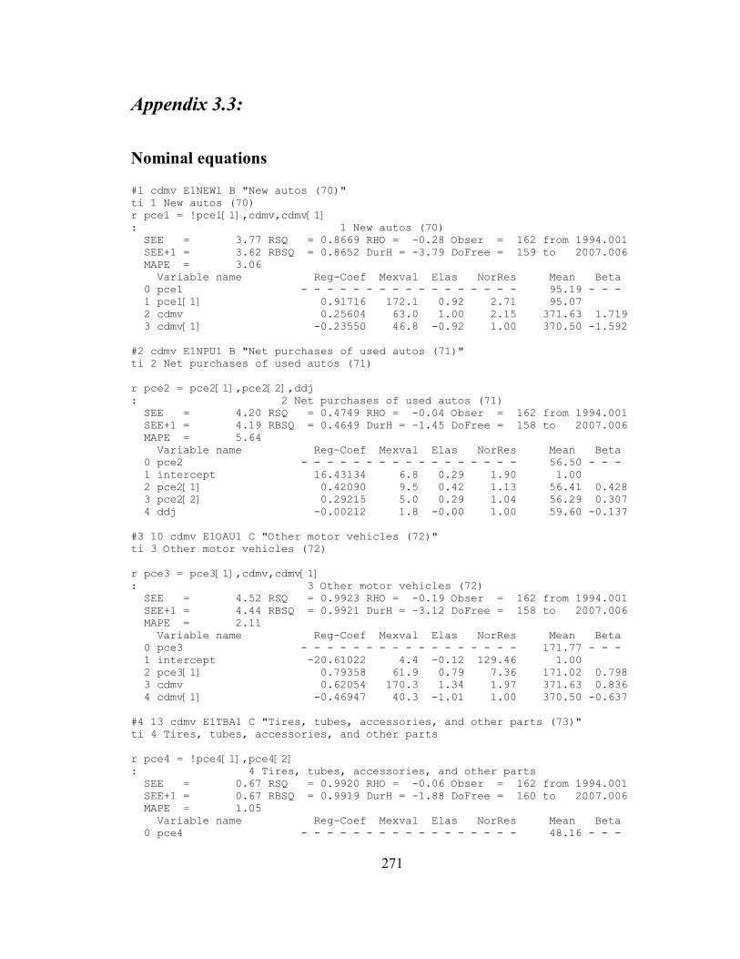
Appendix 3.3:
Nominal equations
#1 cdmv E1NEW1 B "New autos (70)"ti 1 New autos (70)r pce1 = !pce1[1],cdmv,cdmv[1]: 1 New autos (70) SEE = 3.77 RSQ = 0.8669 RHO = -0.28 Obser = 162 from 1994.001 SEE+1 = 3.62 RBSQ = 0.8652 DurH = -3.79 DoFree = 159 to 2007.006 MAPE = 3.06 Variable name Reg-Coef Mexval Elas NorRes Mean Beta 0 pce1 - - - - - - - - - - - - - - - - - 95.19 - - - 1 pce1[1] 0.91716 172.1 0.92 2.71 95.07 2 cdmv 0.25604 63.0 1.00 2.15 371.63 1.719 3 cdmv[1] -0.23550 46.8 -0.92 1.00 370.50 -1.592
#2 cdmv E1NPU1 B "Net purchases of used autos (71)"ti 2 Net purchases of used autos (71)
r pce2 = pce2[1],pce2[2],ddj: 2 Net purchases of used autos (71) SEE = 4.20 RSQ = 0.4749 RHO = -0.04 Obser = 162 from 1994.001 SEE+1 = 4.19 RBSQ = 0.4649 DurH = -1.45 DoFree = 158 to 2007.006 MAPE = 5.64 Variable name Reg-Coef Mexval Elas NorRes Mean Beta 0 pce2 - - - - - - - - - - - - - - - - - 56.50 - - - 1 intercept 16.43134 6.8 0.29 1.90 1.00 2 pce2[1] 0.42090 9.5 0.42 1.13 56.41 0.428 3 pce2[2] 0.29215 5.0 0.29 1.04 56.29 0.307 4 ddj -0.00212 1.8 -0.00 1.00 59.60 -0.137
#3 10 cdmv E1OAU1 C "Other motor vehicles (72)"ti 3 Other motor vehicles (72)
r pce3 = pce3[1],cdmv,cdmv[1]: 3 Other motor vehicles (72) SEE = 4.52 RSQ = 0.9923 RHO = -0.19 Obser = 162 from 1994.001 SEE+1 = 4.44 RBSQ = 0.9921 DurH = -3.12 DoFree = 158 to 2007.006 MAPE = 2.11 Variable name Reg-Coef Mexval Elas NorRes Mean Beta 0 pce3 - - - - - - - - - - - - - - - - - 171.77 - - - 1 intercept -20.61022 4.4 -0.12 129.46 1.00 2 pce3[1] 0.79358 61.9 0.79 7.36 171.02 0.798 3 cdmv 0.62054 170.3 1.34 1.97 371.63 0.836 4 cdmv[1] -0.46947 40.3 -1.01 1.00 370.50 -0.637
#4 13 cdmv E1TBA1 C "Tires, tubes, accessories, and other parts (73)"ti 4 Tires, tubes, accessories, and other parts
r pce4 = !pce4[1],pce4[2]: 4 Tires, tubes, accessories, and other parts SEE = 0.67 RSQ = 0.9920 RHO = -0.06 Obser = 162 from 1994.001 SEE+1 = 0.67 RBSQ = 0.9919 DurH = -1.88 DoFree = 160 to 2007.006 MAPE = 1.05 Variable name Reg-Coef Mexval Elas NorRes Mean Beta 0 pce4 - - - - - - - - - - - - - - - - - 48.16 - - -
271

1 pce4[1] 0.55608 17.6 0.55 1.25 47.99 2 pce4[2] 0.44880 11.7 0.45 1.00 47.82 0.450
#5 17 cdfur E1FNR1 C "Furniture, including mattresses and bedsprings (29)"ti 5 Furniture, including mattresses and bedsprings
r pce5 = pce5[1],cdfur, cdfur[1]: 5 Furniture, including mattresses and bedsprings SEE = 0.58 RSQ = 0.9976 RHO = -0.15 Obser = 162 from 1994.001 SEE+1 = 0.57 RBSQ = 0.9976 DurH = -2.69 DoFree = 158 to 2007.006 MAPE = 0.65 Variable name Reg-Coef Mexval Elas NorRes Mean Beta 0 pce5 - - - - - - - - - - - - - - - - - 65.40 - - - 1 intercept 0.90914 2.8 0.01 420.03 1.00 2 pce5[1] 0.75875 49.9 0.76 2.27 65.14 0.760 3 cdfur 0.22248 45.0 1.04 1.45 306.14 1.095 4 cdfur[1] -0.17402 20.4 -0.81 1.00 304.81 -0.856
#6 18 cdfur E1APP1 C "Kitchen and other household appliances (30)"ti 6 Kitchen and other household appliances
r pce6 = pce6[1],cdfur,cdfur[1]: 6 Kitchen and other household appliances SEE = 0.29 RSQ = 0.9955 RHO = -0.29 Obser = 162 from 1994.001 SEE+1 = 0.27 RBSQ = 0.9955 DurH = -3.96 DoFree = 158 to 2007.006 MAPE = 0.74 Variable name Reg-Coef Mexval Elas NorRes Mean Beta 0 pce6 - - - - - - - - - - - - - - - - - 30.94 - - - 1 intercept 0.55108 1.3 0.02 224.38 1.00 2 pce6[1] 0.92431 195.0 0.92 1.80 30.86 0.919 3 cdfur 0.09084 32.6 0.90 1.64 306.14 1.241 4 cdfur[1] -0.08510 28.0 -0.84 1.00 304.81 -1.162
#7 21 cdfur E1CHN1 C "China, glassware, tableware, and utensils (31)"ti 7 China, glassware, tableware, and utensils
r pce7 = pce7[1],cdfur,cdfur[1]: 7 China, glassware, tableware, and utensils SEE = 0.25 RSQ = 0.9979 RHO = -0.20 Obser = 162 from 1994.001 SEE+1 = 0.24 RBSQ = 0.9979 DurH = -3.57 DoFree = 158 to 2007.006 MAPE = 0.65 Variable name Reg-Coef Mexval Elas NorRes Mean Beta 0 pce7 - - - - - - - - - - - - - - - - - 30.48 - - - 1 intercept 0.29504 1.1 0.01 476.40 1.00 2 pce7[1] 0.80189 55.0 0.80 2.74 30.35 0.798 3 cdfur 0.11347 59.1 1.14 1.65 306.14 1.219 4 cdfur[1] -0.09478 28.5 -0.95 1.00 304.81 -1.018
#8 23 cdfur E1VAM1 C "Video and audio goods, including musical instruments (92)"ti 8 Video and audio goods, including musical instruments
r pce8 = pce8[1],cdfur,cdfur[1]: 8 Video and audio goods, including musical instruments SEE = 0.41 RSQ = 0.9988 RHO = -0.28 Obser = 162 from 1994.001 SEE+1 = 0.40 RBSQ = 0.9987 DurH = -3.73 DoFree = 158 to 2007.006 MAPE = 0.45 Variable name Reg-Coef Mexval Elas NorRes Mean Beta 0 pce8 - - - - - - - - - - - - - - - - - 71.15 - - - 1 intercept 0.59440 1.0 0.01 803.75 1.00 2 pce8[1] 0.94841 199.3 0.95 3.33 70.90 0.949 3 cdfur 0.22551 81.0 0.97 2.66 306.14 1.137
272

4 cdfur[1] -0.21561 63.1 -0.92 1.00 304.81 -1.087
#9 32 cdfur E1CPP1 D "Computers and peripherals"ti 9 Computers and peripherals
r pce9 = !pce9[1],cdfur,cdfur[1]: 9 Computers and peripherals SEE = 0.34 RSQ = 0.9987 RHO = -0.23 Obser = 162 from 1994.001 SEE+1 = 0.33 RBSQ = 0.9987 DurH = -2.91 DoFree = 159 to 2007.006 MAPE = 0.81 Variable name Reg-Coef Mexval Elas NorRes Mean Beta 0 pce9 - - - - - - - - - - - - - - - - - 31.93 - - - 1 pce9[1] 0.98606 855.1 0.98 1.80 31.70 2 cdfur 0.10535 31.7 1.01 1.69 306.14 0.666 3 cdfur[1] -0.10360 30.1 -0.99 1.00 304.81 -0.655
#10 33 cdfur E1CPS1 D "Software"ti 10 Software
r pce10 = pce10[1],cdfur,cdfur[1]: 10 Software SEE = 0.11 RSQ = 0.9987 RHO = -0.19 Obser = 162 from 1994.001 SEE+1 = 0.11 RBSQ = 0.9987 DurH = -2.71 DoFree = 158 to 2007.006 MAPE = 0.86 Variable name Reg-Coef Mexval Elas NorRes Mean Beta 0 pce10 - - - - - - - - - - - - - - - - - 9.74 - - - 1 intercept -0.68115 3.0 -0.07 789.92 1.00 2 pce10[1] 0.88163 117.9 0.88 1.73 9.67 0.881 3 cdfur 0.03262 30.1 1.03 1.37 306.14 0.634 4 cdfur[1] -0.02655 16.9 -0.83 1.00 304.81 -0.516
#11 35 cdfur E1FLR1 D "Floor coverings"ti 11 Floor coverings
r pce11 = pce11[1],cdfur,cdfur[1],crude: 11 Floor coverings SEE = 0.30 RSQ = 0.9921 RHO = -0.27 Obser = 162 from 1994.001 SEE+1 = 0.28 RBSQ = 0.9919 DurH = -5.03 DoFree = 157 to 2007.006 MAPE = 1.40 Variable name Reg-Coef Mexval Elas NorRes Mean Beta 0 pce11 - - - - - - - - - - - - - - - - - 16.49 - - - 1 intercept 0.42137 1.3 0.03 126.71 1.00 2 pce11[1] 0.73318 43.6 0.73 1.24 16.43 0.730 3 cdfur 0.03608 5.5 0.67 1.13 306.14 0.637 4 cdfur[1] -0.02443 2.4 -0.45 1.06 304.81 -0.431 5 crude 0.01518 3.1 0.03 1.00 28.35 0.068
#12 36 cdfur E1DHF1 D "Durable house furnishings, n.e.c."ti 12 Durable house furnishings, n.e.c.
r pce12 = !pce12[1],cdfur,cdfur[1]: 12 Durable house furnishings, n.e.c. SEE = 0.26 RSQ = 0.9986 RHO = -0.28 Obser = 162 from 1994.001 SEE+1 = 0.25 RBSQ = 0.9986 DurH = -3.95 DoFree = 159 to 2007.006 MAPE = 0.58 Variable name Reg-Coef Mexval Elas NorRes Mean Beta 0 pce12 - - - - - - - - - - - - - - - - - 35.92 - - - 1 pce12[1] 0.90812 139.9 0.90 3.05 35.75 2 cdfur 0.13068 70.3 1.11 2.15 306.14 1.091 3 cdfur[1] -0.11991 46.7 -1.02 1.00 304.81 -1.000
273
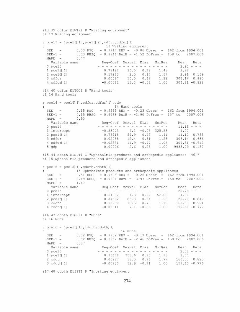
#13 39 cdfur E1WTR1 D "Writing equipment"ti 13 Writing equipment
r pce13 = !pce13[1],pce13[2],cdfur,cdfur[1]: 13 Writing equipment SEE = 0.03 RSQ = 0.9947 RHO = -0.06 Obser = 162 from 1994.001 SEE+1 = 0.03 RBSQ = 0.9946 DurH = -1.52 DoFree = 158 to 2007.006 MAPE = 0.77 Variable name Reg-Coef Mexval Elas NorRes Mean Beta 0 pce13 - - - - - - - - - - - - - - - - - 2.93 - - - 1 pce13[1] 0.79182 35.0 0.79 1.43 2.92 2 pce13[2] 0.17263 2.0 0.17 1.37 2.91 0.169 3 cdfur 0.00597 15.0 0.62 1.28 306.14 0.880 4 cdfur[1] -0.00562 13.3 -0.58 1.00 304.81 -0.828
#14 40 cdfur E1TOO1 D "Hand tools"ti 14 Hand tools
r pce14 = pce14[1],cdfur,cdfur[1],gdp: 14 Hand tools SEE = 0.15 RSQ = 0.9969 RHO = -0.23 Obser = 162 from 1994.001 SEE+1 = 0.15 RBSQ = 0.9968 DurH = -3.90 DoFree = 157 to 2007.006 MAPE = 0.90 Variable name Reg-Coef Mexval Elas NorRes Mean Beta 0 pce14 - - - - - - - - - - - - - - - - - 11.15 - - - 1 intercept -0.53973 4.1 -0.05 325.53 1.00 2 pce14[1] 0.78918 59.9 0.79 1.41 11.10 0.788 3 cdfur 0.02938 12.4 0.81 1.28 306.14 0.636 4 cdfur[1] -0.02831 11.9 -0.77 1.05 304.81 -0.612 5 gdp 0.00026 2.6 0.23 1.00 9935.29 0.187
#15 44 cdoth E1OPT1 C "Ophthalmic products and orthopedic appliances (46)"ti 15 Ophthalmic products and orthopedic appliances
r pce15 = pce15[1],cdoth,cdoth[1]: 15 Ophthalmic products and orthopedic appliances SEE = 0.51 RSQ = 0.9808 RHO = -0.26 Obser = 162 from 1994.001 SEE+1 = 0.49 RBSQ = 0.9804 DurH = -3.97 DoFree = 158 to 2007.006 MAPE = 1.67 Variable name Reg-Coef Mexval Elas NorRes Mean Beta 0 pce15 - - - - - - - - - - - - - - - - - 20.79 - - - 1 intercept 0.51892 1.3 0.02 52.03 1.00 2 pce15[1] 0.84632 83.8 0.84 1.28 20.70 0.842 3 cdoth 0.10290 10.5 0.79 1.15 160.33 0.924 4 cdoth[1] -0.08611 7.1 -0.66 1.00 159.60 -0.772
#16 47 cdoth E1GUN1 D "Guns"ti 16 Guns
r pce16 = !pce16[1],cdoth,cdoth[1]: 16 Guns SEE = 0.02 RSQ = 0.9962 RHO = -0.19 Obser = 162 from 1994.001 SEE+1 = 0.02 RBSQ = 0.9962 DurH = -2.46 DoFree = 159 to 2007.006 MAPE = 0.87 Variable name Reg-Coef Mexval Elas NorRes Mean Beta 0 pce16 - - - - - - - - - - - - - - - - - 2.08 - - - 1 pce16[1] 0.95678 353.6 0.95 1.93 2.07 2 cdoth 0.00987 38.0 0.76 1.77 160.33 0.825 3 cdoth[1] -0.00930 32.9 -0.71 1.00 159.60 -0.776
#17 48 cdoth E1SPT1 D "Sporting equipment
274

ti 17 Sporting equipment
r pce17 = !pce17[1],cdoth,cdoth[1]: 17 Sporting equipment SEE = 0.29 RSQ = 0.9972 RHO = -0.19 Obser = 162 from 1994.001 SEE+1 = 0.29 RBSQ = 0.9971 DurH = -2.70 DoFree = 159 to 2007.006 MAPE = 0.84 Variable name Reg-Coef Mexval Elas NorRes Mean Beta 0 pce17 - - - - - - - - - - - - - - - - - 25.55 - - - 1 pce17[1] 0.92469 134.2 0.92 1.95 25.42 2 cdoth 0.12232 39.2 0.77 1.61 160.33 0.731 3 cdoth[1] -0.11005 27.0 -0.69 1.00 159.60 -0.657
#18 49 cdoth E1CAM1 D "Photographic equipment"ti 18 Photographic equipment
r pce18 = pce18[1],cdoth: 18 Photographic equipment SEE = 0.06 RSQ = 0.9900 RHO = 0.08 Obser = 162 from 1994.001 SEE+1 = 0.06 RBSQ = 0.9899 DurH = 1.40 DoFree = 159 to 2007.006 MAPE = 1.07 Variable name Reg-Coef Mexval Elas NorRes Mean Beta 0 pce18 - - - - - - - - - - - - - - - - - 3.68 - - - 1 intercept 0.34905 13.6 0.09 100.05 1.00 2 pce18[1] 0.58431 30.1 0.58 1.35 3.67 0.584 3 cdoth 0.00742 16.0 0.32 1.00 160.33 0.413
#19 50 cdoth E1BCY1 D "Bicycles"ti 19 Bicycles
r pce19 = !pce19[1],cdoth,cdoth[1]: 19 Bicycles SEE = 0.04 RSQ = 0.9968 RHO = -0.20 Obser = 162 from 1994.001 SEE+1 = 0.04 RBSQ = 0.9968 DurH = -2.65 DoFree = 159 to 2007.006 MAPE = 0.86 Variable name Reg-Coef Mexval Elas NorRes Mean Beta 0 pce19 - - - - - - - - - - - - - - - - - 3.85 - - - 1 pce19[1] 0.94122 199.8 0.94 1.94 3.83 2 cdoth 0.01836 38.8 0.77 1.70 160.33 0.770 3 cdoth[1] -0.01692 30.4 -0.70 1.00 159.60 -0.709
#20 51 cdoth E1MCY1 D "Motorcycles"ti 20 Motorcycles#con 50 0.3 = a3#con 20 0 = a3 + a4#con 50 0.9 = a2r pce20 = pce20[1],cdoth,cdoth[2]: 20 Motorcycles SEE = 0.46 RSQ = 0.9797 RHO = -0.27 Obser = 162 from 1994.001 SEE+1 = 0.44 RBSQ = 0.9793 DurH = -4.25 DoFree = 158 to 2007.006 MAPE = 4.00 Variable name Reg-Coef Mexval Elas NorRes Mean Beta 0 pce20 - - - - - - - - - - - - - - - - - 7.72 - - - 1 intercept -1.48536 4.6 -0.19 49.28 1.00 2 pce20[1] 0.80197 74.1 0.80 1.22 7.67 0.804 3 cdoth 0.07176 6.1 1.49 1.07 160.33 0.731 4 cdoth[2] -0.05319 3.3 -1.09 1.00 158.87 -0.540
#21 53 cdoth E1BOA1 D "Pleasure boats"ti 21 Pleasure boats
275
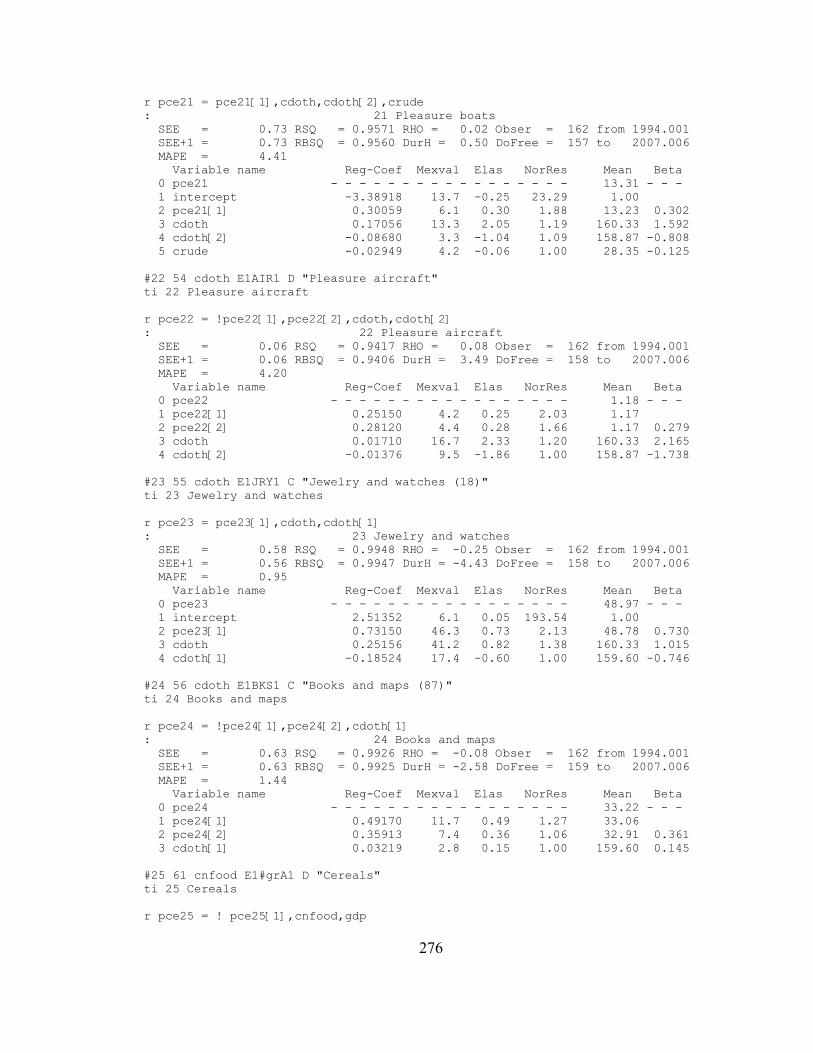
r pce21 = pce21[1],cdoth,cdoth[2],crude: 21 Pleasure boats SEE = 0.73 RSQ = 0.9571 RHO = 0.02 Obser = 162 from 1994.001 SEE+1 = 0.73 RBSQ = 0.9560 DurH = 0.50 DoFree = 157 to 2007.006 MAPE = 4.41 Variable name Reg-Coef Mexval Elas NorRes Mean Beta 0 pce21 - - - - - - - - - - - - - - - - - 13.31 - - - 1 intercept -3.38918 13.7 -0.25 23.29 1.00 2 pce21[1] 0.30059 6.1 0.30 1.88 13.23 0.302 3 cdoth 0.17056 13.3 2.05 1.19 160.33 1.592 4 cdoth[2] -0.08680 3.3 -1.04 1.09 158.87 -0.808 5 crude -0.02949 4.2 -0.06 1.00 28.35 -0.125
#22 54 cdoth E1AIR1 D "Pleasure aircraft"ti 22 Pleasure aircraft
r pce22 = !pce22[1],pce22[2],cdoth,cdoth[2]: 22 Pleasure aircraft SEE = 0.06 RSQ = 0.9417 RHO = 0.08 Obser = 162 from 1994.001 SEE+1 = 0.06 RBSQ = 0.9406 DurH = 3.49 DoFree = 158 to 2007.006 MAPE = 4.20 Variable name Reg-Coef Mexval Elas NorRes Mean Beta 0 pce22 - - - - - - - - - - - - - - - - - 1.18 - - - 1 pce22[1] 0.25150 4.2 0.25 2.03 1.17 2 pce22[2] 0.28120 4.4 0.28 1.66 1.17 0.279 3 cdoth 0.01710 16.7 2.33 1.20 160.33 2.165 4 cdoth[2] -0.01376 9.5 -1.86 1.00 158.87 -1.738
#23 55 cdoth E1JRY1 C "Jewelry and watches (18)"ti 23 Jewelry and watches
r pce23 = pce23[1],cdoth,cdoth[1]: 23 Jewelry and watches SEE = 0.58 RSQ = 0.9948 RHO = -0.25 Obser = 162 from 1994.001 SEE+1 = 0.56 RBSQ = 0.9947 DurH = -4.43 DoFree = 158 to 2007.006 MAPE = 0.95 Variable name Reg-Coef Mexval Elas NorRes Mean Beta 0 pce23 - - - - - - - - - - - - - - - - - 48.97 - - - 1 intercept 2.51352 6.1 0.05 193.54 1.00 2 pce23[1] 0.73150 46.3 0.73 2.13 48.78 0.730 3 cdoth 0.25156 41.2 0.82 1.38 160.33 1.015 4 cdoth[1] -0.18524 17.4 -0.60 1.00 159.60 -0.746
#24 56 cdoth E1BKS1 C "Books and maps (87)"ti 24 Books and maps
r pce24 = !pce24[1],pce24[2],cdoth[1]: 24 Books and maps SEE = 0.63 RSQ = 0.9926 RHO = -0.08 Obser = 162 from 1994.001 SEE+1 = 0.63 RBSQ = 0.9925 DurH = -2.58 DoFree = 159 to 2007.006 MAPE = 1.44 Variable name Reg-Coef Mexval Elas NorRes Mean Beta 0 pce24 - - - - - - - - - - - - - - - - - 33.22 - - - 1 pce24[1] 0.49170 11.7 0.49 1.27 33.06 2 pce24[2] 0.35913 7.4 0.36 1.06 32.91 0.361 3 cdoth[1] 0.03219 2.8 0.15 1.00 159.60 0.145
#25 61 cnfood E1#grA1 D "Cereals"ti 25 Cereals
r pce25 = ! pce25[1],cnfood,gdp
276

: 25 Cereals SEE = 0.23 RSQ = 0.9891 RHO = -0.12 Obser = 162 from 1994.001 SEE+1 = 0.23 RBSQ = 0.9890 DurH = -1.58 DoFree = 159 to 2007.006 MAPE = 0.55 Variable name Reg-Coef Mexval Elas NorRes Mean Beta 0 pce25 - - - - - - - - - - - - - - - - - 27.18 - - - 1 pce25[1] 0.99098 1181.5 0.99 1.05 27.13 2 cnfood 0.00314 2.4 0.11 1.04 954.45 0.258 3 gdp -0.00027 2.2 -0.10 1.00 9935.29 -0.245
#26 62 cnfood E1BAK1 D "Bakery products"ti 26 Bakery products
r pce26 = pce26[1],pce26[2],pce26[3],cnfood: 26 Bakery products SEE = 0.28 RSQ = 0.9979 RHO = 0.03 Obser = 162 from 1994.001 SEE+1 = 0.28 RBSQ = 0.9979 DurH = 0.97 DoFree = 157 to 2007.006 MAPE = 0.46 Variable name Reg-Coef Mexval Elas NorRes Mean Beta 0 pce26 - - - - - - - - - - - - - - - - - 45.49 - - - 1 intercept 1.54810 5.7 0.03 477.39 1.00 2 pce26[1] 0.47427 12.2 0.47 1.41 45.34 0.472 3 pce26[2] 0.13635 0.9 0.14 1.25 45.19 0.135 4 pce26[3] 0.26378 4.2 0.26 1.16 45.05 0.260 5 cnfood 0.00460 7.8 0.10 1.00 954.45 0.133
#27 63 cnfood E1BEE1 D "Beef and veal"ti 27 Beef and veal
r pce27 = !pce27[1],cnfood,cnfood[1]: 27 Beef and veal SEE = 0.17 RSQ = 0.9973 RHO = 0.38 Obser = 162 from 1994.001 SEE+1 = 0.16 RBSQ = 0.9973 DurH = 4.85 DoFree = 159 to 2007.006 MAPE = 0.48 Variable name Reg-Coef Mexval Elas NorRes Mean Beta 0 pce27 - - - - - - - - - - - - - - - - - 26.43 - - - 1 pce27[1] 0.98421 1131.8 0.98 1.95 26.38 2 cnfood 0.02709 36.2 0.98 1.81 954.45 1.458 3 cnfood[1] -0.02671 34.5 -0.96 1.00 950.60 -1.427
#28 64 cnfood E1POR1 D "Pork"ti 28 Pork
r pce28 = ! pce28[1],cnfood,cnfood[1]: 28 Pork SEE = 0.14 RSQ = 0.9980 RHO = 0.28 Obser = 162 from 1994.001 SEE+1 = 0.13 RBSQ = 0.9980 DurH = 3.53 DoFree = 159 to 2007.006 MAPE = 0.44 Variable name Reg-Coef Mexval Elas NorRes Mean Beta 0 pce28 - - - - - - - - - - - - - - - - - 21.83 - - - 1 pce28[1] 1.00469 955.0 1.00 1.94 21.77 2 cnfood 0.02268 39.2 0.99 1.92 954.45 1.329 3 cnfood[1] -0.02282 38.4 -0.99 1.00 950.60 -1.327
#29 65 cnfood E1MEA1 D "Other meats"ti 29 Other meats
r pce29 = pce29[1],cnfood,cnfood[1]: 29 Other meats SEE = 0.08 RSQ = 0.9993 RHO = -0.23 Obser = 162 from 1994.001 SEE+1 = 0.08 RBSQ = 0.9992 DurH = -3.30 DoFree = 158 to 2007.006
277

MAPE = 0.32 Variable name Reg-Coef Mexval Elas NorRes Mean Beta 0 pce29 - - - - - - - - - - - - - - - - - 17.66 - - - 1 intercept 0.19474 2.0 0.01 1350.24 1.00 2 pce29[1] 0.90422 132.9 0.90 2.75 17.60 0.897 3 cnfood 0.01766 63.4 0.95 2.05 954.45 1.075 4 cnfood[1] -0.01609 43.2 -0.87 1.00 950.60 -0.972
#30 66 cnfood E1POU1 D "Poultry"ti 30 Poultry
r pce30 = pce30[1],cnfood,cnfood[1]: 30 Poultry SEE = 0.18 RSQ = 0.9982 RHO = 0.20 Obser = 162 from 1994.001 SEE+1 = 0.17 RBSQ = 0.9982 DurH = 2.58 DoFree = 158 to 2007.006 MAPE = 0.42 Variable name Reg-Coef Mexval Elas NorRes Mean Beta 0 pce30 - - - - - - - - - - - - - - - - - 32.01 - - - 1 intercept 0.41255 2.3 0.01 564.40 1.00 2 pce30[1] 0.97687 507.4 0.97 2.14 31.91 0.977 3 cnfood 0.03186 44.7 0.95 2.02 954.45 1.347 4 cnfood[1] -0.03155 42.3 -0.94 1.00 950.60 -1.323
#31 67 cnfood E1FIS1 D "Fish and seafood"ti 31 Fish and seafood
r pce31 = !pce31[1],cnfood,cnfood[1]: 31 Fish and seafood SEE = 0.07 RSQ = 0.9992 RHO = 0.19 Obser = 162 from 1994.001 SEE+1 = 0.07 RBSQ = 0.9992 DurH = 2.46 DoFree = 159 to 2007.006 MAPE = 0.49 Variable name Reg-Coef Mexval Elas NorRes Mean Beta 0 pce31 - - - - - - - - - - - - - - - - - 10.54 - - - 1 pce31[1] 0.99457 874.5 0.99 1.84 10.50 2 cnfood 0.01046 35.7 0.95 1.83 954.45 0.799 3 cnfood[1] -0.01040 35.1 -0.94 1.00 950.60 -0.788
#32 68 cnfood E1GGS1 D "Eggs"ti 32 Eggs
r pce32 = !pce32[1]: 32 Eggs SEE = 0.07 RSQ = 0.9955 RHO = 0.47 Obser = 162 from 1994.001 SEE+1 = 0.06 RBSQ = 0.9955 DurH = 5.95 DoFree = 161 to 2007.006 MAPE = 0.79 Variable name Reg-Coef Mexval Elas NorRes Mean Beta 0 pce32 - - - - - - - - - - - - - - - - - 5.59 - - - 1 pce32[1] 1.00336 8006.1 1.00 1.00 5.57
#33 69 cnfood E1MIL1 D "Fresh milk and cream"ti 33 Fresh milk and cream#con 50 1 = a2r pce33 = !pce33[1],cnfood: 33 Fresh milk and cream SEE = 0.12 RSQ = 0.9971 RHO = -0.01 Obser = 162 from 1994.001 SEE+1 = 0.12 RBSQ = 0.9970 DurH = -0.16 DoFree = 160 to 2007.006 MAPE = 0.57 Variable name Reg-Coef Mexval Elas NorRes Mean Beta 0 pce33 - - - - - - - - - - - - - - - - - 14.58 - - - 1 pce33[1] 0.96448 832.1 0.96 1.14 14.54 2 cnfood 0.00058 6.6 0.04 1.00 954.45 0.049
278

#34 70 cnfood E1DAI1 D "Processed dairy products"ti 34 Processed dairy products#con 20 -0.3 = a3r pce34 = !pce34[1],cnfood: 34 Processed dairy products SEE = 0.27 RSQ = 0.9982 RHO = -0.06 Obser = 162 from 1994.001 SEE+1 = 0.27 RBSQ = 0.9982 DurH = -0.77 DoFree = 160 to 2007.006 MAPE = 0.55 Variable name Reg-Coef Mexval Elas NorRes Mean Beta 0 pce34 - - - - - - - - - - - - - - - - - 31.72 - - - 1 pce34[1] 0.95497 244.9 0.95 1.03 31.59 2 cnfood 0.00164 1.4 0.05 1.00 954.45 0.047
#35 71 cnfood E1FRU1 D "Fresh fruits"ti 35 Fresh fruits
r pce35 = pce35[1],cnfood: 35 Fresh fruits SEE = 0.15 RSQ = 0.9979 RHO = 0.14 Obser = 162 from 1994.001 SEE+1 = 0.15 RBSQ = 0.9979 DurH = 1.84 DoFree = 159 to 2007.006 MAPE = 0.59 Variable name Reg-Coef Mexval Elas NorRes Mean Beta 0 pce35 - - - - - - - - - - - - - - - - - 17.25 - - - 1 intercept -0.07057 0.4 -0.00 482.70 1.00 2 pce35[1] 0.90603 192.8 0.90 1.09 17.18 0.900 3 cnfood 0.00184 4.5 0.10 1.00 954.45 0.100
#36 72 cnfood E1VEG1 D "Fresh vegetables"ti 36 Fresh vegetables
r pce36 = !pce36[1],cnfood,cnfood[1]: 36 Fresh vegetables SEE = 0.16 RSQ = 0.9992 RHO = 0.10 Obser = 162 from 1994.001 SEE+1 = 0.15 RBSQ = 0.9992 DurH = 1.33 DoFree = 159 to 2007.006 MAPE = 0.42 Variable name Reg-Coef Mexval Elas NorRes Mean Beta 0 pce36 - - - - - - - - - - - - - - - - - 25.49 - - - 1 pce36[1] 0.97941 709.9 0.97 1.83 25.38 2 cnfood 0.02353 34.0 0.88 1.75 954.45 0.765 3 cnfood[1] -0.02296 32.1 -0.86 1.00 950.60 -0.740
#37 73 cnfood E1PFV1 D "Processed fruits and vegetables"ti 37 Processed fruits and vegetables
r pce37 = !pce37[1]: 37 Processed fruits and vegetables SEE = 0.18 RSQ = 0.9957 RHO = 0.01 Obser = 162 from 1994.001 SEE+1 = 0.18 RBSQ = 0.9957 DurH = 0.18 DoFree = 161 to 2007.006 MAPE = 0.61 Variable name Reg-Coef Mexval Elas NorRes Mean Beta 0 pce37 - - - - - - - - - - - - - - - - - 19.13 - - - 1 pce37[1] 1.00314 10888.0 1.00 1.00 19.07
#38 74 cnfood E1JNB1 D "Juices and nonalcoholic drinks"ti 38 Juices and nonalcoholic drinks
r pce38 = pce38[1],cnfood: 38 Juices and nonalcoholic drinks SEE = 0.40 RSQ = 0.9984 RHO = -0.16 Obser = 162 from 1994.001 SEE+1 = 0.40 RBSQ = 0.9984 DurH = -2.11 DoFree = 159 to 2007.006
279

MAPE = 0.52 Variable name Reg-Coef Mexval Elas NorRes Mean Beta 0 pce38 - - - - - - - - - - - - - - - - - 52.92 - - - 1 intercept -0.52460 2.8 -0.01 616.68 1.00 2 pce38[1] 0.96674 452.0 0.96 1.07 52.73 0.954 3 cnfood 0.00259 3.5 0.05 1.00 954.45 0.047
#39 75 cnfood E1CTM1 D "Coffee, tea and beverage materials"ti 39 Coffee, tea and beverage materials
r pce39 = pce39[1],cnfood: 39 Coffee, tea and beverage materials SEE = 0.10 RSQ = 0.9989 RHO = -0.08 Obser = 162 from 1994.001 SEE+1 = 0.09 RBSQ = 0.9989 DurH = -1.03 DoFree = 159 to 2007.006 MAPE = 0.56 Variable name Reg-Coef Mexval Elas NorRes Mean Beta 0 pce39 - - - - - - - - - - - - - - - - - 12.14 - - - 1 intercept -0.18382 2.2 -0.02 932.11 1.00 2 pce39[1] 0.94007 336.1 0.93 1.08 12.07 0.937 3 cnfood 0.00102 4.0 0.08 1.00 954.45 0.063
#40 76 cnfood E1FAT1 D "Fats and oils"ti 40 Fats and oils
r pce40 = ! pce40[1],cnfood,cnfood[1]: 40 Fats and oils SEE = 0.05 RSQ = 0.9978 RHO = -0.01 Obser = 162 from 1994.001 SEE+1 = 0.05 RBSQ = 0.9977 DurH = -0.13 DoFree = 159 to 2007.006 MAPE = 0.37 Variable name Reg-Coef Mexval Elas NorRes Mean Beta 0 pce40 - - - - - - - - - - - - - - - - - 9.86 - - - 1 pce40[1] 0.99205 1293.1 0.99 2.25 9.83 2 cnfood 0.01007 47.9 0.97 2.14 954.45 1.575 3 cnfood[1] -0.01000 46.1 -0.96 1.00 950.60 -1.553
#41 77 cnfood E1SWE1 D "Sugar and sweets"ti 41 Sugar and sweets
r pce41 = pce41[1],cnfood,cnfood[1]: 41 Sugar and sweets SEE = 0.17 RSQ = 0.9986 RHO = -0.06 Obser = 162 from 1994.001 SEE+1 = 0.17 RBSQ = 0.9985 DurH = -0.74 DoFree = 158 to 2007.006 MAPE = 0.37 Variable name Reg-Coef Mexval Elas NorRes Mean Beta 0 pce41 - - - - - - - - - - - - - - - - - 32.44 - - - 1 intercept 0.46669 1.4 0.01 697.87 1.00 2 pce41[1] 0.95627 246.7 0.95 2.23 32.35 0.951 3 cnfood 0.03093 47.6 0.91 2.00 954.45 1.257 4 cnfood[1] -0.02995 41.5 -0.88 1.00 950.60 -1.208
#42 78 cnfood E1OFD1 D "Other foods"ti 42 Other foods
r pce42 = pce42[1],cnfood: 42 Other foods SEE = 0.68 RSQ = 0.9992 RHO = 0.02 Obser = 162 from 1994.001 SEE+1 = 0.68 RBSQ = 0.9991 DurH = 0.25 DoFree = 159 to 2007.006 MAPE = 0.51 Variable name Reg-Coef Mexval Elas NorRes Mean Beta 0 pce42 - - - - - - - - - - - - - - - - - 87.30 - - - 1 intercept -4.19337 5.4 -0.05 1179.60 1.00
280
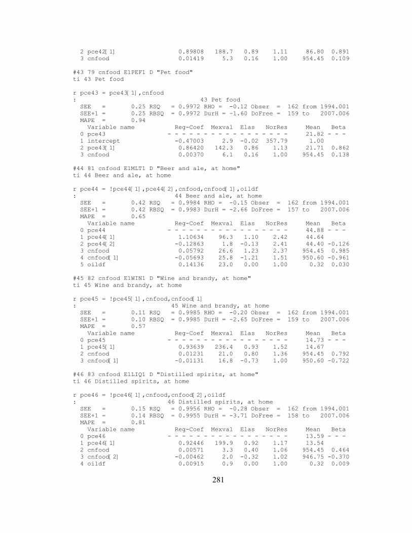
2 pce42[1] 0.89808 188.7 0.89 1.11 86.80 0.891 3 cnfood 0.01419 5.3 0.16 1.00 954.45 0.109
#43 79 cnfood E1PEF1 D "Pet food"ti 43 Pet food
r pce43 = pce43[1],cnfood: 43 Pet food SEE = 0.25 RSQ = 0.9972 RHO = -0.12 Obser = 162 from 1994.001 SEE+1 = 0.25 RBSQ = 0.9972 DurH = -1.60 DoFree = 159 to 2007.006 MAPE = 0.94 Variable name Reg-Coef Mexval Elas NorRes Mean Beta 0 pce43 - - - - - - - - - - - - - - - - - 21.82 - - - 1 intercept -0.47003 2.9 -0.02 357.79 1.00 2 pce43[1] 0.86420 142.3 0.86 1.13 21.71 0.862 3 cnfood 0.00370 6.1 0.16 1.00 954.45 0.138
#44 81 cnfood E1MLT1 D "Beer and ale, at home"ti 44 Beer and ale, at home
r pce44 = !pce44[1],pce44[2],cnfood,cnfood[1],oildf: 44 Beer and ale, at home SEE = 0.42 RSQ = 0.9984 RHO = -0.15 Obser = 162 from 1994.001 SEE+1 = 0.42 RBSQ = 0.9983 DurH = -2.66 DoFree = 157 to 2007.006 MAPE = 0.65 Variable name Reg-Coef Mexval Elas NorRes Mean Beta 0 pce44 - - - - - - - - - - - - - - - - - 44.88 - - - 1 pce44[1] 1.10634 96.3 1.10 2.42 44.64 2 pce44[2] -0.12863 1.8 -0.13 2.41 44.40 -0.126 3 cnfood 0.05792 26.6 1.23 2.37 954.45 0.985 4 cnfood[1] -0.05693 25.8 -1.21 1.51 950.60 -0.961 5 oildf 0.14136 23.0 0.00 1.00 0.32 0.030
#45 82 cnfood E1WIN1 D "Wine and brandy, at home"ti 45 Wine and brandy, at home
r pce45 = !pce45[1],cnfood,cnfood[1]: 45 Wine and brandy, at home SEE = 0.11 RSQ = 0.9985 RHO = -0.20 Obser = 162 from 1994.001 SEE+1 = 0.10 RBSQ = 0.9985 DurH = -2.65 DoFree = 159 to 2007.006 MAPE = 0.57 Variable name Reg-Coef Mexval Elas NorRes Mean Beta 0 pce45 - - - - - - - - - - - - - - - - - 14.73 - - - 1 pce45[1] 0.93639 236.4 0.93 1.52 14.67 2 cnfood 0.01231 21.0 0.80 1.36 954.45 0.792 3 cnfood[1] -0.01131 16.8 -0.73 1.00 950.60 -0.722
#46 83 cnfood E1LIQ1 D "Distilled spirits, at home"ti 46 Distilled spirits, at home
r pce46 = !pce46[1],cnfood,cnfood[2],oildf: 46 Distilled spirits, at home SEE = 0.15 RSQ = 0.9956 RHO = -0.28 Obser = 162 from 1994.001 SEE+1 = 0.14 RBSQ = 0.9955 DurH = -3.71 DoFree = 158 to 2007.006 MAPE = 0.81 Variable name Reg-Coef Mexval Elas NorRes Mean Beta 0 pce46 - - - - - - - - - - - - - - - - - 13.59 - - - 1 pce46[1] 0.92446 199.9 0.92 1.17 13.54 2 cnfood 0.00571 3.3 0.40 1.06 954.45 0.464 3 cnfood[2] -0.00462 2.0 -0.32 1.02 946.75 -0.370 4 oildf 0.00915 0.9 0.00 1.00 0.32 0.009
281

#47 84 cnfood E1PMB1 C "Purchased meals and beverages (4)"ti 47 Purchased meals and beverages
r pce47 = pce47[1],cnfood: 47 Purchased meals and beverages SEE = 2.37 RSQ = 0.9989 RHO = 0.21 Obser = 162 from 1994.001 SEE+1 = 2.33 RBSQ = 0.9989 DurH = 3.73 DoFree = 159 to 2007.006 MAPE = 0.51 Variable name Reg-Coef Mexval Elas NorRes Mean Beta 0 pce47 - - - - - - - - - - - - - - - - - 359.65 - - - 1 intercept -16.65154 30.4 -0.05 920.10 1.00 2 pce47[1] 0.30200 9.0 0.30 2.02 358.13 0.300 3 cnfood 0.28094 42.1 0.75 1.00 954.45 0.700
#48 93 cnfood E1PIF1 C "Food furnished to employees or home grown"ti 48 Food furnished to employees or home grown
r pce48 = !pce48[1],pce48[2]: 48 Food furnished to employees or home grown SEE = 0.04 RSQ = 0.9996 RHO = -0.22 Obser = 162 from 1994.001 SEE+1 = 0.04 RBSQ = 0.9996 DurH = -3.94 DoFree = 160 to 2007.006 MAPE = 0.24 Variable name Reg-Coef Mexval Elas NorRes Mean Beta 0 pce48 - - - - - - - - - - - - - - - - - 10.21 - - - 1 pce48[1] 1.74011 173.4 1.73 2.16 10.17 2 pce48[2] -0.73906 46.9 -0.73 1.00 10.13 -0.722
#49 99 cncloth E1SHU1 C "Shoes (12)"ti 49 Shoes
r pce49 = pce49[1],cncloth,cncloth[1]: 49 Shoes SEE = 0.34 RSQ = 0.9975 RHO = -0.18 Obser = 162 from 1994.001 SEE+1 = 0.33 RBSQ = 0.9975 DurH = -2.84 DoFree = 158 to 2007.006 MAPE = 0.58 Variable name Reg-Coef Mexval Elas NorRes Mean Beta 0 pce49 - - - - - - - - - - - - - - - - - 46.81 - - - 1 intercept -0.71989 1.8 -0.02 401.19 1.00 2 pce49[1] 0.81268 69.3 0.81 4.27 46.67 0.812 3 cncloth 0.16509 105.9 1.04 1.98 293.63 0.941 4 cncloth[1] -0.13276 40.7 -0.83 1.00 292.79 -0.754
#50 100 cncloth E1WCL1 C "Women's and children's clothing and accessories except shoes (14)"ti 50 Women's and children's clothing and accessories except shoes
r pce50 = !pce50[1],cncloth,cncloth[1]: 50 Women's and children's clothing and accessories except shoes SEE = 0.34 RSQ = 0.9997 RHO = -0.29 Obser = 162 from 1994.001 SEE+1 = 0.33 RBSQ = 0.9997 DurH = -3.75 DoFree = 159 to 2007.006 MAPE = 0.17 Variable name Reg-Coef Mexval Elas NorRes Mean Beta 0 pce50 - - - - - - - - - - - - - - - - - 154.72 - - - 1 pce50[1] 0.94225 306.0 0.94 34.29 154.30 2 cncloth 0.52801 483.7 1.00 10.80 293.63 1.032 3 cncloth[1] -0.49765 228.6 -0.94 1.00 292.79 -0.969
#51 106 cncloth E1MMC1 C "Men's and boys' clothing and accessories except shoes (15+16)"ti 51 Men's and boys' clothing and accessories except shoes
282

r pce51 = !pce51[1],cncloth,cncloth[1]: 51 Men's and boys' clothing and accessories except shoes SEE = 0.27 RSQ = 0.9995 RHO = -0.24 Obser = 162 from 1994.001 SEE+1 = 0.26 RBSQ = 0.9995 DurH = -3.12 DoFree = 159 to 2007.006 MAPE = 0.22 Variable name Reg-Coef Mexval Elas NorRes Mean Beta 0 pce51 - - - - - - - - - - - - - - - - - 92.10 - - - 1 pce51[1] 0.94644 273.5 0.94 18.67 91.82 2 cncloth 0.30845 332.0 0.98 8.19 293.63 0.977 3 cncloth[1] -0.29160 186.2 -0.93 1.00 292.79 -0.920
#52 114 cngas E1GAO1 B "Gasoline and oil (75)"ti 52 Gasoline and oil
r pce52 = cngas: 52 Gasoline and oil SEE = 1.38 RSQ = 0.9996 RHO = 0.51 Obser = 162 from 1994.001 SEE+1 = 1.20 RBSQ = 0.9996 DW = 0.99 DoFree = 160 to 2007.006 MAPE = 0.61 Variable name Reg-Coef Mexval Elas NorRes Mean Beta 0 pce52 - - - - - - - - - - - - - - - - - 182.08 - - - 1 intercept -6.29561 84.9 -0.03 2452.52 1.00 2 cngas 0.95223 4852.3 1.03 1.00 197.83 1.000
#53 117 cngas E1FUL1 B "Fuel oil and coal (40)"ti 53 Fuel oil and coal
r pce53 = pce53[1],cngas,oildf: 53 Fuel oil and coal SEE = 1.15 RSQ = 0.9029 RHO = -0.11 Obser = 162 from 1994.001 SEE+1 = 1.14 RBSQ = 0.9011 DurH = -3.15 DoFree = 158 to 2007.006 MAPE = 4.75 Variable name Reg-Coef Mexval Elas NorRes Mean Beta 0 pce53 - - - - - - - - - - - - - - - - - 15.75 - - - 1 intercept 2.67014 8.2 0.17 10.30 1.00 2 pce53[1] 0.58228 19.9 0.58 1.21 15.68 0.577 3 cngas 0.01987 9.3 0.25 1.01 197.83 0.386 4 oildf 0.03981 0.3 0.00 1.00 0.32 0.024
#54 123 cnoth E1TOB1 C "Tobacco products (7)"ti 54 Tobacco products
r pce54 = !pce54[1],pce54[2],cnoth,cnoth[1]: 54 Tobacco products SEE = 1.44 RSQ = 0.9931 RHO = -0.03 Obser = 162 from 1994.001 SEE+1 = 1.44 RBSQ = 0.9930 DurH = -0.94 DoFree = 158 to 2007.006 MAPE = 1.22 Variable name Reg-Coef Mexval Elas NorRes Mean Beta 0 pce54 - - - - - - - - - - - - - - - - - 73.28 - - - 1 pce54[1] 0.61559 20.6 0.61 1.23 72.97 2 pce54[2] 0.36730 7.7 0.36 1.07 72.67 0.369 3 cnoth 0.08196 3.3 0.60 1.06 536.51 0.605 4 cnoth[1] -0.07931 3.1 -0.58 1.00 533.91 -0.584
#55 124 cnoth E1TLG1 C "Toilet articles and preparations (21)"ti 55 Toilet articles and preparations
r pce55 = pce55[1],cnoth,cnoth[1]: 55 Toilet articles and preparations SEE = 0.40 RSQ = 0.9955 RHO = -0.08 Obser = 162 from 1994.001
283

SEE+1 = 0.40 RBSQ = 0.9954 DurH = -0.98 DoFree = 158 to 2007.006 MAPE = 0.55 Variable name Reg-Coef Mexval Elas NorRes Mean Beta 0 pce55 - - - - - - - - - - - - - - - - - 54.25 - - - 1 intercept 0.91110 0.9 0.02 220.48 1.00 2 pce55[1] 0.97078 367.4 0.97 1.71 54.09 0.969 3 cnoth 0.07306 30.2 0.72 1.66 536.51 1.577 4 cnoth[1] -0.07187 29.0 -0.71 1.00 533.91 -1.548
#56 128 cnoth E1SDH1 C "Semidurable house furnishings (33)"ti 56 Semidurable house furnishings
r pce56 = pce56[1],cnoth,cnoth[1]: 56 Semidurable house furnishings SEE = 0.36 RSQ = 0.9956 RHO = -0.25 Obser = 162 from 1994.001 SEE+1 = 0.35 RBSQ = 0.9955 DurH = -3.73 DoFree = 158 to 2007.006 MAPE = 0.73 Variable name Reg-Coef Mexval Elas NorRes Mean Beta 0 pce56 - - - - - - - - - - - - - - - - - 36.33 - - - 1 intercept 1.99449 3.6 0.05 225.25 1.00 2 pce56[1] 0.85533 91.1 0.85 1.25 36.22 0.853 3 cnoth 0.03433 8.9 0.51 1.12 536.51 0.807 4 cnoth[1] -0.02820 5.8 -0.41 1.00 533.91 -0.662
#57 129 cnoth E1CLP1 C "Cleaning, polishing preparations, misc. supplies and paper products"ti 57 Cleaning, polishing, misc. supplies and paper products
r pce57 = !pce57[1],gdp: 57 Cleaning, polishing, misc. supplies and paper products SEE = 0.46 RSQ = 0.9983 RHO = -0.36 Obser = 162 from 1994.001 SEE+1 = 0.43 RBSQ = 0.9983 DurH = -4.81 DoFree = 160 to 2007.006 MAPE = 0.51 Variable name Reg-Coef Mexval Elas NorRes Mean Beta 0 pce57 - - - - - - - - - - - - - - - - - 62.96 - - - 1 pce57[1] 0.95014 209.0 0.95 1.03 62.72 2 gdp 0.00034 1.4 0.05 1.00 9935.29 0.060
#58 133 cnoth E1DRG1 C "Drug preparations and sundries (45)"ti 58 Drug preparations and sundries
r pce58 = pce58[1],cnoth: 58 Drug preparations and sundries SEE = 2.89 RSQ = 0.9983 RHO = -0.10 Obser = 162 from 1994.001 SEE+1 = 2.88 RBSQ = 0.9983 DurH = -1.46 DoFree = 159 to 2007.006 MAPE = 1.21 Variable name Reg-Coef Mexval Elas NorRes Mean Beta 0 pce58 - - - - - - - - - - - - - - - - - 179.71 - - - 1 intercept -30.20938 14.4 -0.17 588.69 1.00 2 pce58[1] 0.73389 87.4 0.73 1.34 178.39 0.732 3 cnoth 0.14725 15.7 0.44 1.00 536.51 0.268
#59 139 cnoth E1DOL1 D "Toys, dolls, and games"ti 59 Toys, dolls, and games
r pce59 = !pce59[1],cnoth,cnoth[1],gdp: 59 Toys, dolls, and games SEE = 0.61 RSQ = 0.9906 RHO = -0.28 Obser = 162 from 1994.001 SEE+1 = 0.59 RBSQ = 0.9904 DurH = -3.84 DoFree = 158 to 2007.006 MAPE = 0.99 Variable name Reg-Coef Mexval Elas NorRes Mean Beta
284
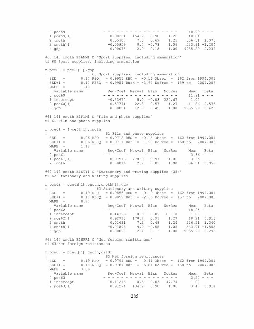
0 pce59 - - - - - - - - - - - - - - - - - 40.99 - - - 1 pce59[1] 0.90261 154.2 0.90 1.26 40.84 2 cnoth 0.05307 7.3 0.69 1.25 536.51 1.075 3 cnoth[1] -0.05959 9.4 -0.78 1.06 533.91 -1.204 4 gdp 0.00075 2.9 0.18 1.00 9935.29 0.234
#60 140 cnoth E1AMM1 D "Sport supplies, including ammunition"ti 60 Sport supplies, including ammunition
r pce60 = pce60[1],gdp: 60 Sport supplies, including ammunition SEE = 0.17 RSQ = 0.9955 RHO = -0.16 Obser = 162 from 1994.001 SEE+1 = 0.17 RBSQ = 0.9954 DurH = -3.67 DoFree = 159 to 2007.006 MAPE = 1.10 Variable name Reg-Coef Mexval Elas NorRes Mean Beta 0 pce60 - - - - - - - - - - - - - - - - - 11.91 - - - 1 intercept -0.33672 5.0 -0.03 220.67 1.00 2 pce60[1] 0.57771 22.3 0.57 1.27 11.86 0.573 3 gdp 0.00054 12.8 0.45 1.00 9935.29 0.425
#61 141 cnoth E1FLM1 D "Film and photo supplies"ti 61 Film and photo supplies
r pce61 = !pce61[1],cnoth: 61 Film and photo supplies SEE = 0.06 RSQ = 0.9712 RHO = -0.15 Obser = 162 from 1994.001 SEE+1 = 0.06 RBSQ = 0.9711 DurH = -1.90 DoFree = 160 to 2007.006 MAPE = 1.18 Variable name Reg-Coef Mexval Elas NorRes Mean Beta 0 pce61 - - - - - - - - - - - - - - - - - 3.36 - - - 1 pce61[1] 0.97516 778.9 0.97 1.06 3.35 2 cnoth 0.00016 2.7 0.03 1.00 536.51 0.058
#62 142 cnoth E1STY1 C "Stationery and writing supplies (35)"ti 62 Stationery and writing supplies
r pce62 = pce62[1],cnoth,cnoth[1],gdp: 62 Stationery and writing supplies SEE = 0.19 RSQ = 0.9855 RHO = -0.19 Obser = 162 from 1994.001 SEE+1 = 0.18 RBSQ = 0.9852 DurH = -2.65 DoFree = 157 to 2007.006 MAPE = 0.77 Variable name Reg-Coef Mexval Elas NorRes Mean Beta 0 pce62 - - - - - - - - - - - - - - - - - 18.25 - - - 1 intercept 0.44326 0.6 0.02 69.18 1.00 2 pce62[1] 0.92715 178.7 0.93 1.27 18.21 0.916 3 cnoth 0.01631 7.2 0.48 1.24 536.51 1.340 4 cnoth[1] -0.01896 9.9 -0.55 1.05 533.91 -1.555 5 gdp 0.00023 2.4 0.13 1.00 9935.29 0.293
#63 145 cnoth E1NFR1 C "Net foreign remittances"ti 63 Net foreign remittances
r pce63 = pce63[1],cnoth,oildf: 63 Net foreign remittances SEE = 0.19 RSQ = 0.9791 RHO = 0.41 Obser = 162 from 1994.001 SEE+1 = 0.18 RBSQ = 0.9787 DurH = 5.81 DoFree = 158 to 2007.006 MAPE = 3.89 Variable name Reg-Coef Mexval Elas NorRes Mean Beta 0 pce63 - - - - - - - - - - - - - - - - - 3.50 - - - 1 intercept -0.11216 0.5 -0.03 47.74 1.00 2 pce63[1] 0.91274 134.2 0.90 1.06 3.47 0.914
285

3 cnoth 0.00082 1.6 0.13 1.02 536.51 0.078 4 oildf 0.01148 0.8 0.00 1.00 0.32 0.019
#64 150 cnoth E1MAG1 C "Magazines, newspapers, and sheet music (88)"ti 64 Magazines, newspapers, and sheet music
r pce64 = pce64[1],pce64[2],pce64[3],gdp,oildf: 64 Magazines, newspapers, and sheet music SEE = 0.38 RSQ = 0.9956 RHO = -0.07 Obser = 162 from 1994.001 SEE+1 = 0.38 RBSQ = 0.9955 DurH = -2.65 DoFree = 156 to 2007.006 MAPE = 0.84 Variable name Reg-Coef Mexval Elas NorRes Mean Beta 0 pce64 - - - - - - - - - - - - - - - - - 34.87 - - - 1 intercept 0.39385 0.7 0.01 228.55 1.00 2 pce64[1] 0.70141 25.1 0.70 1.28 34.72 0.698 3 pce64[2] 0.08318 0.3 0.08 1.21 34.58 0.082 4 pce64[3] 0.15756 1.4 0.16 1.17 34.44 0.155 5 gdp 0.00018 1.0 0.05 1.13 9935.29 0.062 6 oildf 0.06296 6.2 0.00 1.00 0.32 0.024
#65 153 cnoth E1FLO1 C "Flowers, seeds, and potted plants (95)"ti 65 Flowers, seeds, and potted plants
r pce65 = !pce65[1],cnoth,cnoth[1],gdp: 65 Flowers, seeds, and potted plants SEE = 0.25 RSQ = 0.9846 RHO = -0.39 Obser = 162 from 1994.001 SEE+1 = 0.23 RBSQ = 0.9843 DurH = -5.07 DoFree = 158 to 2007.006 MAPE = 1.11 Variable name Reg-Coef Mexval Elas NorRes Mean Beta 0 pce65 - - - - - - - - - - - - - - - - - 17.10 - - - 1 pce65[1] 0.97421 360.8 0.97 1.06 17.06 2 cnoth 0.00967 1.6 0.30 1.06 536.51 0.623 3 cnoth[1] -0.01178 2.3 -0.37 1.02 533.91 -0.757 4 gdp 0.00016 1.1 0.09 1.00 9935.29 0.158
#66 155 cshous E1HOS1 B "Housing"ti 66 Housing
r pce66 = !pce66[1]: 66 Housing SEE = 1.57 RSQ = 0.9999 RHO = 0.20 Obser = 162 from 1994.001 SEE+1 = 1.54 RBSQ = 0.9999 DurH = 2.60 DoFree = 161 to 2007.006 MAPE = 0.11 Variable name Reg-Coef Mexval Elas NorRes Mean Beta 0 pce66 - - - - - - - - - - - - - - - - - 1034.87 - - - 1 pce66[1] 1.00457 67319.6 1.00 1.00 1030.18
stack#67 173 csho E1ELC1 C "Electricity (37)"ti 67 Electricityr pce67 = pce67[1],csho
#68 174 csho E1NGS1 C "Gas (38)"ti 68 Gasr pce68 = pce68[1],csho,gdpdo: 68 Gas SEE = 5.34 RSQ = 0.9249 RHO = 0.06 Obser = 162 from 1994.001 SEE+1 = 5.34 RBSQ = 0.9240 DurH = 1.04 DoFree = 159 to 2007.006 MAPE = 3.69 Variable name Reg-Coef Mexval Elas NorRes Mean Beta
286
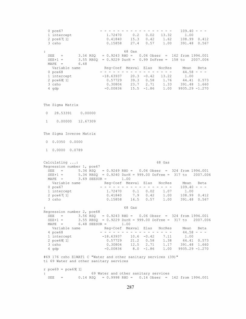
0 pce67 - - - - - - - - - - - - - - - - - 109.40 - - - 1 intercept 1.72470 0.2 0.02 13.32 1.00 2 pce67[1] 0.41840 15.3 0.42 1.62 108.99 0.412 3 csho 0.15858 27.4 0.57 1.00 391.48 0.567
: 68 Gas SEE = 3.56 RSQ = 0.9243 RHO = 0.06 Obser = 162 from 1994.001 SEE+1 = 3.55 RBSQ = 0.9229 DurH = 0.99 DoFree = 158 to 2007.006 MAPE = 6.48 Variable name Reg-Coef Mexval Elas NorRes Mean Beta 0 pce68 - - - - - - - - - - - - - - - - - 44.58 - - - 1 intercept -18.63937 20.3 -0.42 13.22 1.00 2 pce68[1] 0.57729 39.3 0.58 1.76 44.41 0.573 3 csho 0.30804 23.7 2.71 1.33 391.48 1.660 4 gdp -0.00836 15.5 -1.86 1.00 9935.29 -1.270
The Sigma Matrix
0 28.53391 0.00000
1 0.00000 12.67309
The Sigma Inverse Matrix
0 0.0350 0.0000
1 0.0000 0.0789
Calculating ...: 68 GasRegression number 1, pce67 SEE = 5.34 RSQ = 0.9249 RHO = 0.06 Obser = 324 from 1994.001 SEE+1 = 5.34 RBSQ = 0.9240 DurH = 999.00 DoFree = 317 to 2007.006 MAPE = 3.69 SEESUR = 1.00 Variable name Reg-Coef Mexval Elas NorRes Mean Beta 0 pce67 - - - - - - - - - - - - - - - - - 109.40 - - - 1 intercept 1.72470 0.1 0.02 1.07 1.00 2 pce67[1] 0.41840 7.9 0.42 1.00 108.99 0.412 3 csho 0.15858 14.5 0.57 1.00 391.48 0.567
: 68 GasRegression number 2, pce68 SEE = 3.56 RSQ = 0.9243 RHO = 0.06 Obser = 324 from 1994.001 SEE+1 = 3.55 RBSQ = 0.9229 DurH = 999.00 DoFree = 317 to 2007.006 MAPE = 6.48 SEESUR = 1.00 Variable name Reg-Coef Mexval Elas NorRes Mean Beta 4 pce68 - - - - - - - - - - - - - - - - - 44.58 - - - 1 intercept -18.63937 10.6 -0.42 7.11 1.00 2 pce68[1] 0.57729 21.2 0.58 1.38 44.41 0.573 3 csho 0.30804 12.5 2.71 1.17 391.48 1.660 4 gdp -0.00836 8.0 -1.86 1.00 9935.29 -1.270
#69 176 csho E1WAT1 C "Water and other sanitary services (39)"ti 69 Water and other sanitary services
r pce69 = pce69[1]: 69 Water and other sanitary services SEE = 0.14 RSQ = 0.9998 RHO = 0.16 Obser = 162 from 1994.001
287
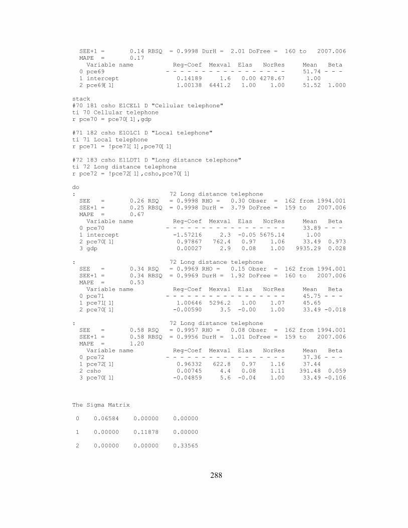
SEE+1 = 0.14 RBSQ = 0.9998 DurH = 2.01 DoFree = 160 to 2007.006 MAPE = 0.17 Variable name Reg-Coef Mexval Elas NorRes Mean Beta 0 pce69 - - - - - - - - - - - - - - - - - 51.74 - - - 1 intercept 0.14189 1.6 0.00 4278.67 1.00 2 pce69[1] 1.00138 6441.2 1.00 1.00 51.52 1.000
stack#70 181 csho E1CEL1 D "Cellular telephone"ti 70 Cellular telephoner pce70 = pce70[1],gdp
#71 182 csho E1OLC1 D "Local telephone"ti 71 Local telephoner pce71 = !pce71[1],pce70[1]
#72 183 csho E1LDT1 D "Long distance telephone"ti 72 Long distance telephoner pce72 = !pce72[1],csho,pce70[1]
do: 72 Long distance telephone SEE = 0.26 RSQ = 0.9998 RHO = 0.30 Obser = 162 from 1994.001 SEE+1 = 0.25 RBSQ = 0.9998 DurH = 3.79 DoFree = 159 to 2007.006 MAPE = 0.67 Variable name Reg-Coef Mexval Elas NorRes Mean Beta 0 pce70 - - - - - - - - - - - - - - - - - 33.89 - - - 1 intercept -1.57216 2.3 -0.05 5675.14 1.00 2 pce70[1] 0.97867 762.4 0.97 1.06 33.49 0.973 3 gdp 0.00027 2.9 0.08 1.00 9935.29 0.028
: 72 Long distance telephone SEE = 0.34 RSQ = 0.9969 RHO = 0.15 Obser = 162 from 1994.001 SEE+1 = 0.34 RBSQ = 0.9969 DurH = 1.92 DoFree = 160 to 2007.006 MAPE = 0.53 Variable name Reg-Coef Mexval Elas NorRes Mean Beta 0 pce71 - - - - - - - - - - - - - - - - - 45.75 - - - 1 pce71[1] 1.00646 5296.2 1.00 1.07 45.65 2 pce70[1] -0.00590 3.5 -0.00 1.00 33.49 -0.018
: 72 Long distance telephone SEE = 0.58 RSQ = 0.9957 RHO = 0.08 Obser = 162 from 1994.001 SEE+1 = 0.58 RBSQ = 0.9956 DurH = 1.01 DoFree = 159 to 2007.006 MAPE = 1.20 Variable name Reg-Coef Mexval Elas NorRes Mean Beta 0 pce72 - - - - - - - - - - - - - - - - - 37.36 - - - 1 pce72[1] 0.96332 622.8 0.97 1.16 37.44 2 csho 0.00745 4.4 0.08 1.11 391.48 0.059 3 pce70[1] -0.04859 5.6 -0.04 1.00 33.49 -0.106
The Sigma Matrix
0 0.06584 0.00000 0.00000
1 0.00000 0.11878 0.00000
2 0.00000 0.00000 0.33565
288

The Sigma Inverse Matrix
0 15.1892 0.0000 0.0000
1 0.0000 8.4188 0.0000
2 0.0000 0.0000 2.9793
Calculating ...: 72 Long distance telephoneRegression number 1, pce70 SEE = 0.26 RSQ = 0.9998 RHO = 0.30 Obser = 486 from 1994.001 SEE+1 = 0.25 RBSQ = 0.9998 DurH = 3.77 DoFree = 478 to 2007.006 MAPE = 0.67 SEESUR = 1.00 Variable name Reg-Coef Mexval Elas NorRes Mean Beta 0 pce70 - - - - - - - - - - - - - - - - - 33.89 - - - 1 intercept -1.57216 0.8 -0.05 1.25 1.00 2 pce70[1] 0.97867 404.5 0.97 1.00 33.49 0.973 3 gdp 0.00027 1.0 0.08 1.00 9935.29 0.028
: 72 Long distance telephoneRegression number 2, pce71 SEE = 0.34 RSQ = 0.9969 RHO = 0.15 Obser = 486 from 1994.001 SEE+1 = 0.34 RBSQ = 0.9969 DurH = 1.92 DoFree = 478 to 2007.006 MAPE = 0.53 SEESUR = 1.00 Variable name Reg-Coef Mexval Elas NorRes Mean Beta 4 pce71 - - - - - - - - - - - - - - - - - 45.75 - - - 1 pce71[1] 1.00646 3016.6 1.00 1.00 45.65 2 pce70[1] -0.00590 1.2 -0.00 1.00 33.49 -0.018
: 72 Long distance telephoneRegression number 3, pce72 SEE = 0.58 RSQ = 0.9957 RHO = 0.08 Obser = 486 from 1994.001 SEE+1 = 0.58 RBSQ = 0.9956 DurH = 1.01 DoFree = 478 to 2007.006 MAPE = 1.20 SEESUR = 1.00 Variable name Reg-Coef Mexval Elas NorRes Mean Beta 7 pce72 - - - - - - - - - - - - - - - - - 37.36 - - - 1 pce72[1] 0.96332 325.2 0.97 1.05 37.44 2 csho 0.00745 1.5 0.08 1.04 391.48 0.059 3 pce70[1] -0.04859 1.9 -0.04 1.00 33.49 -0.106
#73 186 csho E1DMS1 C "Domestic service (42)"ti 73 Domestic service
r pce73 = pce73[1],csho,csho[1]: 73 Domestic service SEE = 0.15 RSQ = 0.9964 RHO = 0.55 Obser = 162 from 1994.001 SEE+1 = 0.13 RBSQ = 0.9964 DurH = 7.23 DoFree = 158 to 2007.006 MAPE = 0.61 Variable name Reg-Coef Mexval Elas NorRes Mean Beta 0 pce73 - - - - - - - - - - - - - - - - - 16.92 - - - 1 intercept 0.11043 0.5 0.01 280.56 1.00 2 pce73[1] 0.98043 356.6 0.98 1.01 16.86 0.980 3 csho -0.00075 0.1 -0.02 1.01 391.48 -0.021 4 csho[1] 0.00146 0.4 0.03 1.00 389.99 0.040
#74 189 csho E1OPO1 C "Other (43)"ti 74 Other Household Services
r pce74 = pce74[1],pce74[2],pce74[3],csho,csho[1]: 74 Other Household Services
289

SEE = 0.20 RSQ = 0.9996 RHO = 0.00 Obser = 162 from 1994.001 SEE+1 = 0.20 RBSQ = 0.9996 DurH = 999.00 DoFree = 156 to 2007.006 MAPE = 0.29 Variable name Reg-Coef Mexval Elas NorRes Mean Beta 0 pce74 - - - - - - - - - - - - - - - - - 51.85 - - - 1 intercept 0.21395 1.2 0.00 2391.71 1.00 2 pce74[1] 1.25851 61.5 1.25 1.12 51.63 1.262 3 pce74[2] -0.14343 0.4 -0.14 1.02 51.40 -0.144 4 pce74[3] -0.12012 0.7 -0.12 1.01 51.18 -0.121 5 csho 0.00254 0.6 0.02 1.01 391.48 0.018 6 csho[1] -0.00208 0.4 -0.02 1.00 389.99 -0.014
#75 202 cstr E1ARP1 D "Motor vehicle repair"ti 75 Motor vehicle repair
r pce75 = !pce75[1],cstr: 75 Motor vehicle repair SEE = 0.27 RSQ = 0.9998 RHO = 0.16 Obser = 162 from 1994.001 SEE+1 = 0.27 RBSQ = 0.9998 DurH = 2.10 DoFree = 160 to 2007.006 MAPE = 0.18 Variable name Reg-Coef Mexval Elas NorRes Mean Beta 0 pce75 - - - - - - - - - - - - - - - - - 118.60 - - - 1 pce75[1] 0.98423 1491.6 0.98 1.10 118.11 2 cstr 0.00850 5.0 0.02 1.00 275.95 0.018
#76 203 cstr E1RLO1 D "Motor vehicle rental, leasing, and other"ti 76 Motor vehicle rental, leasing, and other
r pce76 = pce76[1],oildf: 76 Motor vehicle rental, leasing, and other SEE = 0.60 RSQ = 0.9963 RHO = 0.19 Obser = 162 from 1994.001 SEE+1 = 0.59 RBSQ = 0.9962 DurH = 2.36 DoFree = 159 to 2007.006 MAPE = 0.88 Variable name Reg-Coef Mexval Elas NorRes Mean Beta 0 pce76 - - - - - - - - - - - - - - - - - 52.78 - - - 1 intercept 1.24298 7.2 0.02 268.35 1.00 2 pce76[1] 0.98054 1538.1 0.98 1.01 52.55 0.998 3 oildf 0.01963 0.3 0.00 1.00 0.32 0.004
#77 210 cstr E1TOL1 C "Bridge, tunnel, ferry, and road tolls"ti 77 Bridge, tunnel, ferry, and road tolls
r pce77 = !pce77[1]: 77 Bridge, tunnel, ferry, and road tolls SEE = 0.06 RSQ = 0.9972 RHO = -0.05 Obser = 162 from 1994.001 SEE+1 = 0.06 RBSQ = 0.9972 DurH = -0.62 DoFree = 161 to 2007.006 MAPE = 0.86 Variable name Reg-Coef Mexval Elas NorRes Mean Beta 0 pce77 - - - - - - - - - - - - - - - - - 5.08 - - - 1 pce77[1] 1.00473 8991.6 1.00 1.00 5.06
#78 211 cstr E1AIN1 C "Insurance"ti 78 Insurance (Automobiles)
r pce78 = pce78[1],cstr,gdp: 78 Insurance (Automobiles) SEE = 0.26 RSQ = 0.9991 RHO = 0.15 Obser = 162 from 1994.001 SEE+1 = 0.25 RBSQ = 0.9991 DurH = 2.02 DoFree = 158 to 2007.006 MAPE = 0.49 Variable name Reg-Coef Mexval Elas NorRes Mean Beta 0 pce78 - - - - - - - - - - - - - - - - - 45.19 - - -
290

1 intercept 0.19525 0.5 0.00 1161.13 1.00 2 pce78[1] 0.99968 296.3 1.00 1.01 45.02 0.997 3 cstr -0.00225 0.4 -0.01 1.00 275.95 -0.012 4 gdp 0.00006 0.1 0.01 1.00 9935.29 0.014
#79 213 cstr E1IMT1 C "Mass transit systems (79)"ti 79 Mass transit systems (79)
r pce79 = !pce79[1],gdp: 79 Mass transit systems (79) SEE = 0.15 RSQ = 0.9882 RHO = -0.30 Obser = 162 from 1994.001 SEE+1 = 0.14 RBSQ = 0.9881 DurH = -4.02 DoFree = 160 to 2007.006 MAPE = 1.30 Variable name Reg-Coef Mexval Elas NorRes Mean Beta 0 pce79 - - - - - - - - - - - - - - - - - 9.03 - - - 1 pce79[1] 0.93549 198.9 0.93 1.04 9.00 2 gdp 0.00006 2.1 0.07 1.00 9935.29 0.086
#80 214 cstr E1TAX1 C "Taxicab (80)"ti 80 Taxicab
r pce80 = !pce80[1],pce80[2],gdp,cstr[1]: 80 Taxicab SEE = 0.04 RSQ = 0.9911 RHO = -0.00 Obser = 162 from 1994.001 SEE+1 = 0.04 RBSQ = 0.9909 DurH = 999.00 DoFree = 158 to 2007.006 MAPE = 0.55 Variable name Reg-Coef Mexval Elas NorRes Mean Beta 0 pce80 - - - - - - - - - - - - - - - - - 3.42 - - - 1 pce80[1] 1.09614 48.8 1.09 1.03 3.41 2 pce80[2] -0.09385 0.4 -0.09 1.02 3.40 -0.093 3 gdp 0.00001 1.0 0.03 1.01 9935.29 0.047 4 cstr[1] -0.00034 0.7 -0.03 1.00 274.86 -0.039
#81 216 cstr E1IRR1 C "Railway (82)"ti 81 Railway
r pce81 = !pce81[1],cstr,oildf: 81 Railway SEE = 0.01 RSQ = 0.9749 RHO = -0.22 Obser = 162 from 1994.001 SEE+1 = 0.01 RBSQ = 0.9746 DurH = -2.99 DoFree = 159 to 2007.006 MAPE = 1.97 Variable name Reg-Coef Mexval Elas NorRes Mean Beta 0 pce81 - - - - - - - - - - - - - - - - - 0.51 - - - 1 pce81[1] 0.91936 179.8 0.92 1.06 0.51 2 cstr 0.00016 2.8 0.08 1.00 275.95 0.082 3 oildf 0.00023 0.1 0.00 1.00 0.32 0.006
#82 217 cstr E1IBU1 C "Bus (83)"ti 82 Bus
r pce82 = pce82[1]: 82 Bus SEE = 0.09 RSQ = 0.8233 RHO = -0.37 Obser = 162 from 1994.001 SEE+1 = 0.09 RBSQ = 0.8222 DurH = -5.17 DoFree = 160 to 2007.006 MAPE = 2.96 Variable name Reg-Coef Mexval Elas NorRes Mean Beta 0 pce82 - - - - - - - - - - - - - - - - - 2.16 - - - 1 intercept 0.22763 3.1 0.11 5.66 1.00 2 pce82[1] 0.89560 137.9 0.89 1.00 2.16 0.907
#83 218 cstr E1IAI1 C "Airline (84)"
291
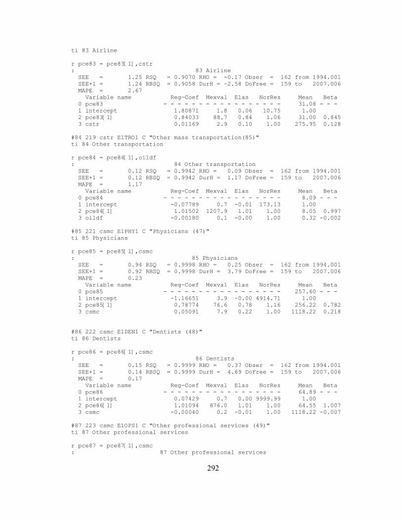
ti 83 Airline
r pce83 = pce83[1],cstr: 83 Airline SEE = 1.25 RSQ = 0.9070 RHO = -0.17 Obser = 162 from 1994.001 SEE+1 = 1.24 RBSQ = 0.9058 DurH = -2.58 DoFree = 159 to 2007.006 MAPE = 2.67 Variable name Reg-Coef Mexval Elas NorRes Mean Beta 0 pce83 - - - - - - - - - - - - - - - - - 31.08 - - - 1 intercept 1.80871 1.8 0.06 10.75 1.00 2 pce83[1] 0.84033 88.7 0.84 1.06 31.00 0.845 3 cstr 0.01169 2.9 0.10 1.00 275.95 0.128
#84 219 cstr E1TRO1 C "Other mass transportation(85)"ti 84 Other transportation
r pce84 = pce84[1],oildf: 84 Other transportation SEE = 0.12 RSQ = 0.9942 RHO = 0.09 Obser = 162 from 1994.001 SEE+1 = 0.12 RBSQ = 0.9942 DurH = 1.17 DoFree = 159 to 2007.006 MAPE = 1.17 Variable name Reg-Coef Mexval Elas NorRes Mean Beta 0 pce84 - - - - - - - - - - - - - - - - - 8.09 - - - 1 intercept -0.07789 0.7 -0.01 173.13 1.00 2 pce84[1] 1.01502 1207.9 1.01 1.00 8.05 0.997 3 oildf -0.00180 0.1 -0.00 1.00 0.32 -0.002
#85 221 csmc E1PHY1 C "Physicians (47)"ti 85 Physicians
r pce85 = pce85[1],csmc: 85 Physicians SEE = 0.94 RSQ = 0.9998 RHO = 0.25 Obser = 162 from 1994.001 SEE+1 = 0.92 RBSQ = 0.9998 DurH = 3.79 DoFree = 159 to 2007.006 MAPE = 0.23 Variable name Reg-Coef Mexval Elas NorRes Mean Beta 0 pce85 - - - - - - - - - - - - - - - - - 257.60 - - - 1 intercept -1.16651 3.9 -0.00 4914.71 1.00 2 pce85[1] 0.78774 76.6 0.78 1.16 256.22 0.782 3 csmc 0.05091 7.9 0.22 1.00 1118.22 0.218
#86 222 csmc E1DEN1 C "Dentists (48)"ti 86 Dentists
r pce86 = pce86[1],csmc: 86 Dentists SEE = 0.15 RSQ = 0.9999 RHO = 0.37 Obser = 162 from 1994.001 SEE+1 = 0.14 RBSQ = 0.9999 DurH = 4.69 DoFree = 159 to 2007.006 MAPE = 0.17 Variable name Reg-Coef Mexval Elas NorRes Mean Beta 0 pce86 - - - - - - - - - - - - - - - - - 64.89 - - - 1 intercept 0.07429 0.7 0.00 9999.99 1.00 2 pce86[1] 1.01094 876.0 1.01 1.00 64.55 1.007 3 csmc -0.00040 0.2 -0.01 1.00 1118.22 -0.007
#87 223 csmc E1OPS1 C "Other professional services (49)"ti 87 Other professional services
r pce87 = pce87[1],csmc: 87 Other professional services
292

SEE = 0.47 RSQ = 0.9999 RHO = 0.34 Obser = 162 from 1994.001 SEE+1 = 0.44 RBSQ = 0.9999 DurH = 4.48 DoFree = 159 to 2007.006 MAPE = 0.20 Variable name Reg-Coef Mexval Elas NorRes Mean Beta 0 pce87 - - - - - - - - - - - - - - - - - 175.65 - - - 1 intercept 0.66587 3.4 0.00 8253.35 1.00 2 pce87[1] 0.92531 373.1 0.92 1.16 174.73 0.921 3 csmc 0.01190 7.7 0.08 1.00 1118.22 0.079
#88 229 csmc E1HSP1 C "Hospitals"ti 88 Hospitals
r pce88 = !pce88[1],csmc: 88 Hospitals SEE = 1.91 RSQ = 0.9997 RHO = -0.15 Obser = 162 from 1994.001 SEE+1 = 1.89 RBSQ = 0.9997 DurH = -2.21 DoFree = 160 to 2007.006 MAPE = 0.37 Variable name Reg-Coef Mexval Elas NorRes Mean Beta 0 pce88 - - - - - - - - - - - - - - - - - 435.95 - - - 1 pce88[1] 0.82141 104.2 0.82 1.16 433.73 2 csmc 0.07126 7.6 0.18 1.00 1118.22 0.184
#89 233 csmc E1NRS1 C "Nursing homes"ti 89 Nursing homes
r pce89 = pce89[1],csmc: 89 Nursing homes SEE = 0.26 RSQ = 0.9998 RHO = 0.60 Obser = 162 from 1994.001 SEE+1 = 0.21 RBSQ = 0.9998 DurH = 7.63 DoFree = 159 to 2007.006 MAPE = 0.22 Variable name Reg-Coef Mexval Elas NorRes Mean Beta 0 pce89 - - - - - - - - - - - - - - - - - 89.70 - - - 1 intercept 0.64368 5.3 0.01 4702.34 1.00 2 pce89[1] 0.98086 1124.3 0.98 1.07 89.30 0.979 3 csmc 0.00131 3.4 0.02 1.00 1118.22 0.021
#90 236 csmc E1HIN1 C "Health insurance (56)"ti 90 Health insurance
r pce90 = pce90[1],csmc,csmc[1]: 90 Health insurance SEE = 0.35 RSQ = 0.9999 RHO = 0.80 Obser = 162 from 1994.001 SEE+1 = 0.22 RBSQ = 0.9999 DurH = 10.21 DoFree = 158 to 2007.006 MAPE = 0.28 Variable name Reg-Coef Mexval Elas NorRes Mean Beta 0 pce90 - - - - - - - - - - - - - - - - - 94.43 - - - 1 intercept -1.08819 4.9 -0.01 8209.40 1.00 2 pce90[1] 0.97680 906.7 0.97 1.19 93.81 0.969 3 csmc 0.03343 3.0 0.40 1.05 1118.22 0.295 4 csmc[1] -0.03011 2.4 -0.35 1.00 1112.34 -0.264
#91 241 csrec E1SSA1 C "Admissions to specified spectator amusements (96)"ti 91 Admissions to specified spectator amusements
r pce91 = pce91[1],csrec,csrec[1],oildf: 91 Admissions to specified spectator amusements SEE = 0.78 RSQ = 0.9870 RHO = -0.15 Obser = 162 from 1994.001 SEE+1 = 0.77 RBSQ = 0.9866 DurH = -2.79 DoFree = 157 to 2007.006 MAPE = 1.95 Variable name Reg-Coef Mexval Elas NorRes Mean Beta 0 pce91 - - - - - - - - - - - - - - - - - 30.69 - - -
293

1 intercept 0.97615 2.8 0.03 76.73 1.00 2 pce91[1] 0.70533 40.6 0.70 1.84 30.55 0.708 3 csrec 0.31648 24.0 2.83 1.42 274.40 3.147 4 csrec[1] -0.28819 18.7 -2.56 1.02 272.95 -2.858 5 oildf -0.05468 1.1 -0.00 1.00 0.32 -0.017
#92 246 csrec E1RTV1 C "Radio and television repair"ti 92 Radio and television repair
r pce92 = pce92[1],pce92[2],csrec: 92 Radio and television repair SEE = 0.02 RSQ = 0.9987 RHO = -0.14 Obser = 162 from 1994.001 SEE+1 = 0.02 RBSQ = 0.9987 DurH = -2.91 DoFree = 158 to 2007.006 MAPE = 0.36 Variable name Reg-Coef Mexval Elas NorRes Mean Beta 0 pce92 - - - - - - - - - - - - - - - - - 4.18 - - - 1 intercept 0.02132 0.5 0.01 767.74 1.00 2 pce92[1] 1.61556 129.5 1.61 1.64 4.17 1.604 3 pce92[2] -0.62562 27.8 -0.62 1.01 4.15 -0.617 4 csrec 0.00009 0.7 0.01 1.00 274.40 0.011
#93 247 csrec E1CLU1 C "Clubs and fraternal organizations"ti 93 Clubs and fraternal organizations
r pce93 = !pce93[1],gdp: 93 Clubs and fraternal organizations SEE = 0.16 RSQ = 0.9967 RHO = 0.28 Obser = 162 from 1994.001 SEE+1 = 0.15 RBSQ = 0.9967 DurH = 3.61 DoFree = 160 to 2007.006 MAPE = 0.54 Variable name Reg-Coef Mexval Elas NorRes Mean Beta 0 pce93 - - - - - - - - - - - - - - - - - 19.83 - - - 1 pce93[1] 0.98631 888.1 0.98 1.03 19.78 2 gdp 0.00003 1.3 0.02 1.00 9935.29 0.023
#94 248 csrec E1COM1 C "Commercial participant amusements"ti 94 Commercial participant amusements
r pce94 = pce94[1],csrec,csrec[1]: 94 Commercial participant amusements SEE = 0.83 RSQ = 0.9987 RHO = -0.14 Obser = 162 from 1994.001 SEE+1 = 0.82 RBSQ = 0.9987 DurH = -2.20 DoFree = 158 to 2007.006 MAPE = 0.86 Variable name Reg-Coef Mexval Elas NorRes Mean Beta 0 pce94 - - - - - - - - - - - - - - - - - 77.78 - - - 1 intercept -3.03012 4.8 -0.04 772.36 1.00 2 pce94[1] 0.80843 67.4 0.80 3.17 77.28 0.807 3 csrec 0.61391 66.2 2.17 2.01 274.40 1.811 4 csrec[1] -0.55001 41.8 -1.93 1.00 272.95 -1.618
#95 254 csrec E1PAR1 C "Pari-mutual net receipts"ti 95 Pari-mutual net receipts
r pce95 = pce95[1],pce95[2],csrec,gdp: 95 Pari-mutual net receipts SEE = 0.02 RSQ = 0.9994 RHO = -0.05 Obser = 162 from 1994.001 SEE+1 = 0.02 RBSQ = 0.9994 DurH = -1.43 DoFree = 157 to 2007.006 MAPE = 0.30 Variable name Reg-Coef Mexval Elas NorRes Mean Beta 0 pce95 - - - - - - - - - - - - - - - - - 4.95 - - - 1 intercept -0.05623 1.1 -0.01 1611.57 1.00 2 pce95[1] 1.33692 76.6 1.33 1.32 4.92 1.331
294

3 pce95[2] -0.39265 9.3 -0.39 1.09 4.90 -0.389 4 csrec -0.00086 1.4 -0.05 1.06 274.40 -0.061 5 gdp 0.00006 3.2 0.12 1.00 9935.29 0.119
#96 255 csrec E1REO1 C "Other Recreation Services"ti 96 Other Recreation Services
r pce96 = pce96[1],csrec: 96 Other Recreation Services SEE = 0.48 RSQ = 0.9998 RHO = 0.09 Obser = 162 from 1994.001 SEE+1 = 0.47 RBSQ = 0.9998 DurH = 1.34 DoFree = 159 to 2007.006 MAPE = 0.24 Variable name Reg-Coef Mexval Elas NorRes Mean Beta 0 pce96 - - - - - - - - - - - - - - - - - 136.98 - - - 1 intercept 0.08001 0.1 0.00 5211.73 1.00 2 pce96[1] 0.90540 129.9 0.90 1.05 136.24 0.902 3 csrec 0.04935 2.5 0.10 1.00 274.40 0.098
#97 270 csoth E1CRC1 C "Cleaning, storage, and repair of clothing and shoes (17)"ti 97 Cleaning, storage, and repair of clothing and shoes
r pce97 = !pce97[1],pce97[2]: 97 Cleaning, storage, and repair of clothing and shoes SEE = 0.05 RSQ = 0.9992 RHO = -0.13 Obser = 162 from 1994.001 SEE+1 = 0.04 RBSQ = 0.9992 DurH = -2.59 DoFree = 160 to 2007.006 MAPE = 0.22 Variable name Reg-Coef Mexval Elas NorRes Mean Beta 0 pce97 - - - - - - - - - - - - - - - - - 14.75 - - - 1 pce97[1] 1.64907 136.9 1.65 1.71 14.71 2 pce97[2] -0.64832 30.8 -0.65 1.00 14.68 -0.656
#98 275 csoth E1BBB1 C "Barbershops, beauty parlors, and health clubs (22)"ti 98 Barbershops, beauty parlors, and health clubs
r pce98 = pce98[1],gdp: 98 Barbershops, beauty parlors, and health clubs SEE = 0.13 RSQ = 0.9998 RHO = 0.34 Obser = 162 from 1994.001 SEE+1 = 0.12 RBSQ = 0.9998 DurH = 4.40 DoFree = 159 to 2007.006 MAPE = 0.25 Variable name Reg-Coef Mexval Elas NorRes Mean Beta 0 pce98 - - - - - - - - - - - - - - - - - 38.77 - - - 1 intercept 0.22554 2.0 0.01 5034.09 1.00 2 pce98[1] 1.01177 689.6 1.01 1.01 38.59 1.011 3 gdp -0.00005 0.4 -0.01 1.00 9935.29 -0.011
#99 278 csoth E1COT1 C "Other Personal Care(19)"ti 99 Other Personal Care
r pce99 = !pce99[1],pce99[2]: 99 Other Personal Care SEE = 0.16 RSQ = 0.9998 RHO = -0.07 Obser = 162 from 1994.001 SEE+1 = 0.16 RBSQ = 0.9998 DurH = -2.35 DoFree = 160 to 2007.006 MAPE = 0.34 Variable name Reg-Coef Mexval Elas NorRes Mean Beta 0 pce99 - - - - - - - - - - - - - - - - - 34.69 - - - 1 pce99[1] 1.44993 88.9 1.44 1.24 34.45 2 pce99[2] -0.44588 11.3 -0.44 1.00 34.20 -0.438
#100 282 csoth E1BRO1 C "Brokerage charges and investment counseling (61)"ti 100 Brokerage charges and investment counseling
295

r pce100 = pce100[1],djia: 100 Brokerage charges and investment counseling SEE = 3.51 RSQ = 0.9736 RHO = 0.06 Obser = 162 from 1994.001 SEE+1 = 3.50 RBSQ = 0.9733 DurH = 0.89 DoFree = 159 to 2007.006 MAPE = 3.29 Variable name Reg-Coef Mexval Elas NorRes Mean Beta 0 pce100 - - - - - - - - - - - - - - - - - 75.55 - - - 1 intercept 0.78405 0.2 0.01 37.86 1.00 2 pce100[1] 0.83978 90.8 0.83 1.09 75.05 0.836 3 djia 0.00134 4.6 0.16 1.00 8771.94 0.157
#101 290 csoth E1BNK1 C "Bank service charges, trust services, and safe deposit box rental"ti 101 Bank, trust services, and safe deposit box rental
r pce101 = !pce101[1],csoth,csoth[1]: 101 Bank, trust services, and safe deposit box rental SEE = 0.61 RSQ = 0.9994 RHO = 0.17 Obser = 162 from 1994.001 SEE+1 = 0.60 RBSQ = 0.9994 DurH = 2.21 DoFree = 159 to 2007.006 MAPE = 0.66 Variable name Reg-Coef Mexval Elas NorRes Mean Beta 0 pce101 - - - - - - - - - - - - - - - - - 67.36 - - - 1 pce101[1] 1.00687 1215.9 1.00 1.06 66.85 2 csoth 0.02306 3.0 0.32 1.06 933.88 0.217 3 csoth[1] -0.02312 3.0 -0.32 1.00 928.97 -0.217
#102 295 csoth E1IMP1 C "Services furnished w/out payment by intermediaries except life ins. carriers"ti 102 Services furnished w/out payment by intermediaries except life ins. carriers
r pce102 = pce102[1],csoth,djia 102 Services furnished w/out payment by intermediaries except life ins. carrier SEE = 1.01 RSQ = 0.9991 RHO = 0.69 Obser = 162 from 1994.001 SEE+1 = 0.75 RBSQ = 0.9991 DurH = 8.89 DoFree = 158 to 2007.006 MAPE = 0.47 Variable name Reg-Coef Mexval Elas NorRes Mean Beta 0 pce102 - - - - - - - - - - - - - - - - - 164.08 - - - 1 intercept 2.00803 4.2 0.01 1125.32 1.00 2 pce102[1] 0.94777 410.8 0.94 1.15 163.38 0.947 3 csoth 0.00510 1.8 0.03 1.12 933.88 0.035 4 djia 0.00028 5.6 0.01 1.00 8771.94 0.021
#103 298 csoth E1LIF1 C "Expense of handling life insurance and pension plans (64)"ti 103 Expense of handling life insurance and pension plans
r pce103 = pce103[1],csmc,gdp,oildf[6],oildf[9]: 103 Expense of handling life insurance and pension plans SEE = 3.58 RSQ = 0.9387 RHO = -0.21 Obser = 162 from 1994.001 SEE+1 = 3.50 RBSQ = 0.9368 DurH = -3.94 DoFree = 156 to 2007.006 MAPE = 1.97 Variable name Reg-Coef Mexval Elas NorRes Mean Beta 0 pce103 - - - - - - - - - - - - - - - - - 89.41 - - - 1 intercept 0.85311 0.0 0.01 16.32 1.00 2 pce103[1] 0.67094 37.2 0.67 1.22 89.13 0.664 3 csmc -0.02157 2.0 -0.27 1.12 1118.22 -0.422 4 gdp 0.00531 4.3 0.59 1.04 9935.29 0.722 5 oildf[6] 0.12589 0.3 0.00 1.03 0.24 0.018 6 oildf[9] 0.31839 1.6 0.00 1.00 0.25 0.046
296

#104 299 csoth E1GAL1 C "Legal services (65)"ti 104 Legal services
r pce104 = !pce104[1],pce104[2],csoth: 104 Legal services SEE = 0.30 RSQ = 0.9996 RHO = -0.04 Obser = 162 from 1994.001 SEE+1 = 0.30 RBSQ = 0.9996 DurH = -1.37 DoFree = 159 to 2007.006 MAPE = 0.30 Variable name Reg-Coef Mexval Elas NorRes Mean Beta 0 pce104 - - - - - - - - - - - - - - - - - 67.21 - - - 1 pce104[1] 1.37063 78.1 1.36 1.21 66.89 2 pce104[2] -0.39001 8.5 -0.39 1.03 66.57 -0.384 3 csoth 0.00159 1.6 0.02 1.00 933.88 0.024
#105 300 csoth E1FUN1 C "Funeral and burial expenses (66)"ti 105 Funeral and burial expenses
r pce105 = pce105[1],pce105[2],oildf,gdp: 105 Funeral and burial expenses SEE = 0.38 RSQ = 0.9481 RHO = -0.02 Obser = 162 from 1994.001 SEE+1 = 0.38 RBSQ = 0.9468 DurH = 999.00 DoFree = 157 to 2007.006 MAPE = 2.00 Variable name Reg-Coef Mexval Elas NorRes Mean Beta 0 pce105 - - - - - - - - - - - - - - - - - 14.39 - - - 1 intercept 2.33271 7.1 0.16 19.27 1.00 2 pce105[1] 0.53690 13.5 0.54 1.27 14.35 0.534 3 pce105[2] 0.09041 0.4 0.09 1.17 14.31 0.090 4 oildf -0.01633 0.4 -0.00 1.17 0.32 -0.022 5 gdp 0.00031 8.0 0.21 1.00 9935.29 0.364
#106 301 csoth E1PBO1 C "Other Personal Service(67)"ti 106 Other Personal Service(67)
r pce106 = pce106[1]: 106 Other Personal Service(67) SEE = 0.13 RSQ = 0.9998 RHO = 0.32 Obser = 162 from 1994.001 SEE+1 = 0.13 RBSQ = 0.9998 DurH = 4.09 DoFree = 160 to 2007.006 MAPE = 0.28 Variable name Reg-Coef Mexval Elas NorRes Mean Beta 0 pce106 - - - - - - - - - - - - - - - - - 34.18 - - - 1 intercept 0.13000 2.8 0.00 4167.40 1.00 2 pce106[1] 1.00118 6355.5 1.00 1.00 34.01 1.000
#107 310 csoth E1HED1 C "Higher education (105)"ti 107 Higher education
r pce107 = pce107[1],csoth: 107 Higher education SEE = 0.26 RSQ = 0.9999 RHO = 0.57 Obser = 162 from 1994.001 SEE+1 = 0.22 RBSQ = 0.9999 DurH = 7.29 DoFree = 159 to 2007.006 MAPE = 0.21 Variable name Reg-Coef Mexval Elas NorRes Mean Beta 0 pce107 - - - - - - - - - - - - - - - - - 93.36 - - - 1 intercept -0.09998 0.3 -0.00 9546.32 1.00 2 pce107[1] 0.99047 1348.9 0.98 1.05 92.84 0.986 3 csoth 0.00161 2.3 0.02 1.00 933.88 0.015
#108 313 csoth E1EED1 C "Nursery, elementary, and secondary schools (106)"ti 108 Nursery, elementary, and secondary schools
297

r pce108 = pce108[1],csoth: 108 Nursery, elementary, and secondary schools SEE = 0.07 RSQ = 0.9999 RHO = 0.35 Obser = 162 from 1994.001 SEE+1 = 0.07 RBSQ = 0.9999 DurH = 4.48 DoFree = 159 to 2007.006 MAPE = 0.15 Variable name Reg-Coef Mexval Elas NorRes Mean Beta 0 pce108 - - - - - - - - - - - - - - - - - 35.62 - - - 1 intercept 0.17186 1.7 0.00 8596.67 1.00 2 pce108[1] 0.98681 789.0 0.98 1.02 35.47 0.984 3 csoth 0.00047 1.0 0.01 1.00 933.88 0.016
#109 316 csoth E1OED1 C "Other Education (107)"ti 109 Other Education
r pce109 = !pce109[1],pce109[2],csoth: 109 Other Education SEE = 0.27 RSQ = 0.9995 RHO = -0.00 Obser = 162 from 1994.001 SEE+1 = 0.27 RBSQ = 0.9995 DurH = -0.09 DoFree = 159 to 2007.006 MAPE = 0.40 Variable name Reg-Coef Mexval Elas NorRes Mean Beta 0 pce109 - - - - - - - - - - - - - - - - - 41.68 - - - 1 pce109[1] 1.36701 78.0 1.36 1.22 41.41 2 pce109[2] -0.38281 8.3 -0.38 1.03 41.14 -0.379 3 csoth 0.00089 1.5 0.02 1.00 933.88 0.017
#110 320 csoth E1POL1 D "Political organizations"ti 110 Political organizations
r pce110 = !pce110[8],pce110[4],csoth: 110 Political organizations SEE = 1.21 RSQ = 0.5307 RHO = 0.81 Obser = 162 from 1994.001 SEE+1 = 0.72 RBSQ = 0.5248 DurH = 16.22 DoFree = 159 to 2007.006 MAPE = 96.24 Variable name Reg-Coef Mexval Elas NorRes Mean Beta 0 pce110 - - - - - - - - - - - - - - - - - 2.27 - - - 1 pce110[8] -0.69327 34.5 -0.66 4.39 2.17 2 pce110[4] 0.64745 31.0 0.64 2.07 2.25 0.652 3 csoth 0.00242 43.8 1.00 1.00 933.88 0.317
#111 321 csoth E1MUS1 D "Museums and libraries"ti 111 Museums and libraries
r pce111 = !pce111[1],pce111[2],csoth[1]: 111 Museums and libraries SEE = 0.04 RSQ = 0.9996 RHO = -0.06 Obser = 162 from 1994.001 SEE+1 = 0.04 RBSQ = 0.9995 DurH = -1.13 DoFree = 159 to 2007.006 MAPE = 0.39 Variable name Reg-Coef Mexval Elas NorRes Mean Beta 0 pce111 - - - - - - - - - - - - - - - - - 7.58 - - - 1 pce111[1] 1.61217 132.4 1.60 1.75 7.54 2 pce111[2] -0.63850 30.5 -0.63 1.05 7.50 -0.635 3 csoth[1] 0.00023 2.4 0.03 1.00 928.97 0.029
#112 322 csoth E1FOU1 D "Foundations to religion and welfare"ti 112 Foundations to religion and welfare
r pce112 = ! pce112[1],csoth: 112 Foundations to religion and welfare SEE = 0.08 RSQ = 0.9991 RHO = 0.54 Obser = 162 from 1994.001 SEE+1 = 0.07 RBSQ = 0.9991 DurH = 6.92 DoFree = 160 to 2007.006 MAPE = 0.60
298
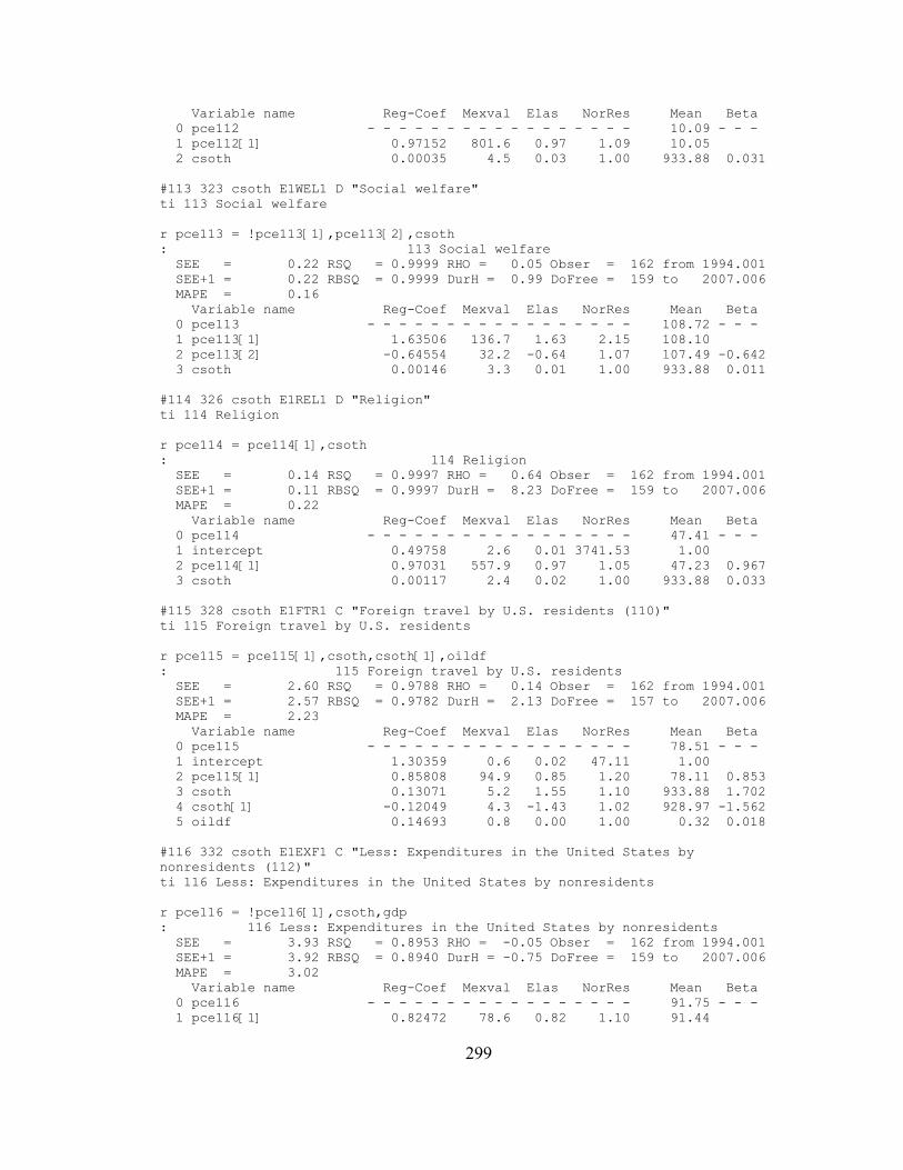
Variable name Reg-Coef Mexval Elas NorRes Mean Beta 0 pce112 - - - - - - - - - - - - - - - - - 10.09 - - - 1 pce112[1] 0.97152 801.6 0.97 1.09 10.05 2 csoth 0.00035 4.5 0.03 1.00 933.88 0.031
#113 323 csoth E1WEL1 D "Social welfare"ti 113 Social welfare
r pce113 = !pce113[1],pce113[2],csoth: 113 Social welfare SEE = 0.22 RSQ = 0.9999 RHO = 0.05 Obser = 162 from 1994.001 SEE+1 = 0.22 RBSQ = 0.9999 DurH = 0.99 DoFree = 159 to 2007.006 MAPE = 0.16 Variable name Reg-Coef Mexval Elas NorRes Mean Beta 0 pce113 - - - - - - - - - - - - - - - - - 108.72 - - - 1 pce113[1] 1.63506 136.7 1.63 2.15 108.10 2 pce113[2] -0.64554 32.2 -0.64 1.07 107.49 -0.642 3 csoth 0.00146 3.3 0.01 1.00 933.88 0.011
#114 326 csoth E1REL1 D "Religion"ti 114 Religion
r pce114 = pce114[1],csoth: 114 Religion SEE = 0.14 RSQ = 0.9997 RHO = 0.64 Obser = 162 from 1994.001 SEE+1 = 0.11 RBSQ = 0.9997 DurH = 8.23 DoFree = 159 to 2007.006 MAPE = 0.22 Variable name Reg-Coef Mexval Elas NorRes Mean Beta 0 pce114 - - - - - - - - - - - - - - - - - 47.41 - - - 1 intercept 0.49758 2.6 0.01 3741.53 1.00 2 pce114[1] 0.97031 557.9 0.97 1.05 47.23 0.967 3 csoth 0.00117 2.4 0.02 1.00 933.88 0.033
#115 328 csoth E1FTR1 C "Foreign travel by U.S. residents (110)"ti 115 Foreign travel by U.S. residents
r pce115 = pce115[1],csoth,csoth[1],oildf: 115 Foreign travel by U.S. residents SEE = 2.60 RSQ = 0.9788 RHO = 0.14 Obser = 162 from 1994.001 SEE+1 = 2.57 RBSQ = 0.9782 DurH = 2.13 DoFree = 157 to 2007.006 MAPE = 2.23 Variable name Reg-Coef Mexval Elas NorRes Mean Beta 0 pce115 - - - - - - - - - - - - - - - - - 78.51 - - - 1 intercept 1.30359 0.6 0.02 47.11 1.00 2 pce115[1] 0.85808 94.9 0.85 1.20 78.11 0.853 3 csoth 0.13071 5.2 1.55 1.10 933.88 1.702 4 csoth[1] -0.12049 4.3 -1.43 1.02 928.97 -1.562 5 oildf 0.14693 0.8 0.00 1.00 0.32 0.018
#116 332 csoth E1EXF1 C "Less: Expenditures in the United States by nonresidents (112)"ti 116 Less: Expenditures in the United States by nonresidents
r pce116 = !pce116[1],csoth,gdp: 116 Less: Expenditures in the United States by nonresidents SEE = 3.93 RSQ = 0.8953 RHO = -0.05 Obser = 162 from 1994.001 SEE+1 = 3.92 RBSQ = 0.8940 DurH = -0.75 DoFree = 159 to 2007.006 MAPE = 3.02 Variable name Reg-Coef Mexval Elas NorRes Mean Beta 0 pce116 - - - - - - - - - - - - - - - - - 91.75 - - - 1 pce116[1] 0.82472 78.6 0.82 1.10 91.44
299

2 csoth -0.02918 2.7 -0.30 1.08 933.88 -0.557 3 gdp 0.00439 3.7 0.48 1.00 9935.29 0.710
Price index equations
#1 3 cdmv E1NEW1 B "New autos (70)"ti 1 New autos (70)
r cqp1 = cqp1[1],time,gdpi: 1 New autos (70) SEE = 0.22 RSQ = 0.9856 RHO = 0.21 Obser = 162 from 1994.001 SEE+1 = 0.22 RBSQ = 0.9854 DurH = 2.75 DoFree = 158 to 2007.006 MAPE = 0.17 Variable name Reg-Coef Mexval Elas NorRes Mean Beta 0 cqp1 - - - - - - - - - - - - - - - - - 98.89 - - - 1 intercept 3.06750 1.5 0.03 69.58 1.00 2 cqp1[1] 0.95401 518.0 0.95 1.21 98.89 0.958 3 time -0.16709 5.3 -0.01 1.08 7.79 -0.347 4 gdpi 2.68918 3.8 0.03 1.00 1.04 0.295
#2 6 cdmv E1NPU1 B "Net purchases of used autos (71)"ti 2 Net purchases of used autos (71)
r cqp2 = cqp2[1],crude,crude[1]: 2 Net purchases of used autos (71) SEE = 0.89 RSQ = 0.9547 RHO = 0.05 Obser = 162 from 1994.001 SEE+1 = 0.89 RBSQ = 0.9539 DurH = 0.71 DoFree = 158 to 2007.006 MAPE = 0.62 Variable name Reg-Coef Mexval Elas NorRes Mean Beta 0 cqp2 - - - - - - - - - - - - - - - - - 98.59 - - - 1 intercept 6.38240 4.2 0.06 22.08 1.00 2 cqp2[1] 0.93508 321.6 0.93 1.01 98.49 0.971 3 crude 0.02427 0.2 0.01 1.00 28.35 0.087 4 crude[1] -0.02049 0.1 -0.01 1.00 28.03 -0.072
#3 10 cdmv E1OAU1 C "Other motor vehicles (72)"ti 3 Other motor vehicles (72)
r cqp3 = cqp3[1],time,oildf: 3 Other motor vehicles (72) SEE = 0.32 RSQ = 0.9803 RHO = 0.10 Obser = 162 from 1994.001 SEE+1 = 0.31 RBSQ = 0.9800 DurH = 1.33 DoFree = 158 to 2007.006 MAPE = 0.26 Variable name Reg-Coef Mexval Elas NorRes Mean Beta 0 cqp3 - - - - - - - - - - - - - - - - - 97.47 - - - 1 intercept 3.83319 4.0 0.04 50.83 1.00 2 cqp3[1] 0.96306 608.7 0.96 1.13 97.44 0.987 3 time -0.02585 4.9 -0.00 1.02 7.79 -0.045 4 oildf -0.01932 0.9 -0.00 1.00 0.32 -0.019
#4 13 cdmv E1TBA1 C "Tires, tubes, accessories, and other parts (73)"ti 4 Tires, tubes, accessories, and other parts
r cqp4 = cqp4[1],crude: 4 Tires, tubes, accessories, and other parts SEE = 0.28 RSQ = 0.9957 RHO = -0.11 Obser = 162 from 1994.001 SEE+1 = 0.28 RBSQ = 0.9956 DurH = -1.44 DoFree = 159 to 2007.006 MAPE = 0.20
300

Variable name Reg-Coef Mexval Elas NorRes Mean Beta 0 cqp4 - - - - - - - - - - - - - - - - - 103.84 - - - 1 intercept 1.77061 0.7 0.02 231.10 1.00 2 cqp4[1] 0.98026 540.8 0.98 1.09 103.75 0.956 3 crude 0.01289 4.5 0.00 1.00 28.35 0.046
#5 17 cdfur E1FNR1 C "Furniture, including mattresses and bedsprings (29)"ti 5 Furniture, including mattresses and bedsprings
r cqp5 = cqp5[1],oildf: 5 Furniture, including mattresses and bedsprings SEE = 0.54 RSQ = 0.9611 RHO = 0.02 Obser = 162 from 1994.001 SEE+1 = 0.54 RBSQ = 0.9606 DurH = 0.25 DoFree = 159 to 2007.006 MAPE = 0.43 Variable name Reg-Coef Mexval Elas NorRes Mean Beta 0 cqp5 - - - - - - - - - - - - - - - - - 97.82 - - - 1 intercept 1.28593 0.2 0.01 25.68 1.00 2 cqp5[1] 0.98663 403.5 0.99 1.00 97.84 0.982 3 oildf 0.01644 0.2 0.00 1.00 0.32 0.013
#6 18 cdfur E1APP1 C "Kitchen and other household appliances (30)"ti 6 Kitchen and other household appliances
r cqp6 = cqp6[1],gdpi: 6 Kitchen and other household appliances SEE = 0.53 RSQ = 0.9872 RHO = 0.10 Obser = 162 from 1994.001 SEE+1 = 0.53 RBSQ = 0.9871 DurH = 1.36 DoFree = 159 to 2007.006 MAPE = 0.42 Variable name Reg-Coef Mexval Elas NorRes Mean Beta 0 cqp6 - - - - - - - - - - - - - - - - - 99.93 - - - 1 intercept -1.05275 0.1 -0.01 78.28 1.00 2 cqp6[1] 1.00590 345.4 1.01 1.01 99.97 1.009 3 gdpi 0.41180 0.3 0.00 1.00 1.04 0.018
#7 21 cdfur E1CHN1 C "China, glassware, tableware, and utensils (31)"ti 7 China, glassware, tableware, and utensils
r cqp7 = !cqp7[1],cqp7[2]: 7 China, glassware, tableware, and utensils SEE = 1.09 RSQ = 0.9751 RHO = -0.04 Obser = 162 from 1994.001 SEE+1 = 1.09 RBSQ = 0.9749 DurH = -5.45 DoFree = 160 to 2007.006 MAPE = 0.88 Variable name Reg-Coef Mexval Elas NorRes Mean Beta 0 cqp7 - - - - - - - - - - - - - - - - - 96.82 - - - 1 cqp7[1] 0.86441 32.8 0.87 1.02 96.95 2 cqp7[2] 0.13406 0.9 0.13 1.00 97.09 0.133
#8 23 cdfur E1VAM1 C "Video and audio goods, including musical instruments (92)"ti 8 Video and audio goods, including musical instruments
r cqp8 = !cqp8[1],time: 8 Video and audio goods, including musical instruments SEE = 0.64 RSQ = 0.9990 RHO = -0.12 Obser = 162 from 1994.001 SEE+1 = 0.64 RBSQ = 0.9990 DurH = -1.48 DoFree = 160 to 2007.006 MAPE = 0.39 Variable name Reg-Coef Mexval Elas NorRes Mean Beta 0 cqp8 - - - - - - - - - - - - - - - - - 97.91 - - - 1 cqp8[1] 0.99773 9596.3 1.00 1.05 98.34 2 time -0.02670 2.5 -0.00 1.00 7.79 -0.005
#9 32 cdfur E1CPP1 D "Computers and peripherals"
301

ti 9 Computers and peripherals
r cqp9 = !cqp9[1],cqp9[2]: 9 Computers and peripherals SEE = 4.94 RSQ = 0.9996 RHO = -0.04 Obser = 162 from 1994.001 SEE+1 = 4.93 RBSQ = 0.9996 DurH = -1.44 DoFree = 160 to 2007.006 MAPE = 1.06 Variable name Reg-Coef Mexval Elas NorRes Mean Beta 0 cqp9 - - - - - - - - - - - - - - - - - 209.02 - - - 1 cqp9[1] 1.31230 72.7 1.34 1.13 213.87 2 cqp9[2] -0.32579 6.2 -0.34 1.00 218.76 -0.337
#10 33 cdfur E1CPS1 D "Software"ti 10 Software
r cqp10 = !cqp10[1],cqp10[2]: 10 Software SEE = 2.49 RSQ = 0.9993 RHO = -0.05 Obser = 162 from 1994.001 SEE+1 = 2.48 RBSQ = 0.9992 DurH = -1.68 DoFree = 160 to 2007.006 MAPE = 1.10 Variable name Reg-Coef Mexval Elas NorRes Mean Beta 0 cqp10 - - - - - - - - - - - - - - - - - 134.75 - - - 1 cqp10[1] 1.33541 74.8 1.36 1.14 136.73 2 cqp10[2] -0.34628 6.9 -0.36 1.00 138.74 -0.361
#11 35 cdfur E1FLR1 D "Floor coverings"ti 11 Floor coverings
r cqp11 = cqp11[1],gdpi: 11 Floor coverings SEE = 0.81 RSQ = 0.9841 RHO = 0.11 Obser = 162 from 1994.001 SEE+1 = 0.81 RBSQ = 0.9839 DurH = 1.63 DoFree = 159 to 2007.006 MAPE = 0.61 Variable name Reg-Coef Mexval Elas NorRes Mean Beta 0 cqp11 - - - - - - - - - - - - - - - - - 100.51 - - - 1 intercept 9.09872 3.7 0.09 62.78 1.00 2 cqp11[1] 0.86782 107.5 0.87 1.08 100.36 0.864 3 gdpi 4.15998 3.8 0.04 1.00 1.04 0.132
#12 36 cdfur E1DHF1 D "Durable house furnishings, n.e.c."ti 12 Durable house furnishings, n.e.c.
r cqp12 = !cqp12[1],time: 12 Durable house furnishings, n.e.c. SEE = 0.97 RSQ = 0.9943 RHO = -0.16 Obser = 162 from 1994.001 SEE+1 = 0.96 RBSQ = 0.9943 DurH = -2.07 DoFree = 160 to 2007.006 MAPE = 0.74 Variable name Reg-Coef Mexval Elas NorRes Mean Beta 0 cqp12 - - - - - - - - - - - - - - - - - 95.27 - - - 1 cqp12[1] 0.99979 5439.1 1.00 1.02 95.52 2 time -0.03081 1.2 -0.00 1.00 7.79 -0.009
#13 39 cdfur E1WTR1 D "Writing equipment"ti 13 Writing equipment
r cqp13 = !cqp13[1]: 13 Writing equipment SEE = 0.82 RSQ = 0.9986 RHO = -0.07 Obser = 162 from 1994.001 SEE+1 = 0.82 RBSQ = 0.9986 DurH = -0.84 DoFree = 161 to 2007.006 MAPE = 0.38 Variable name Reg-Coef Mexval Elas NorRes Mean Beta
302
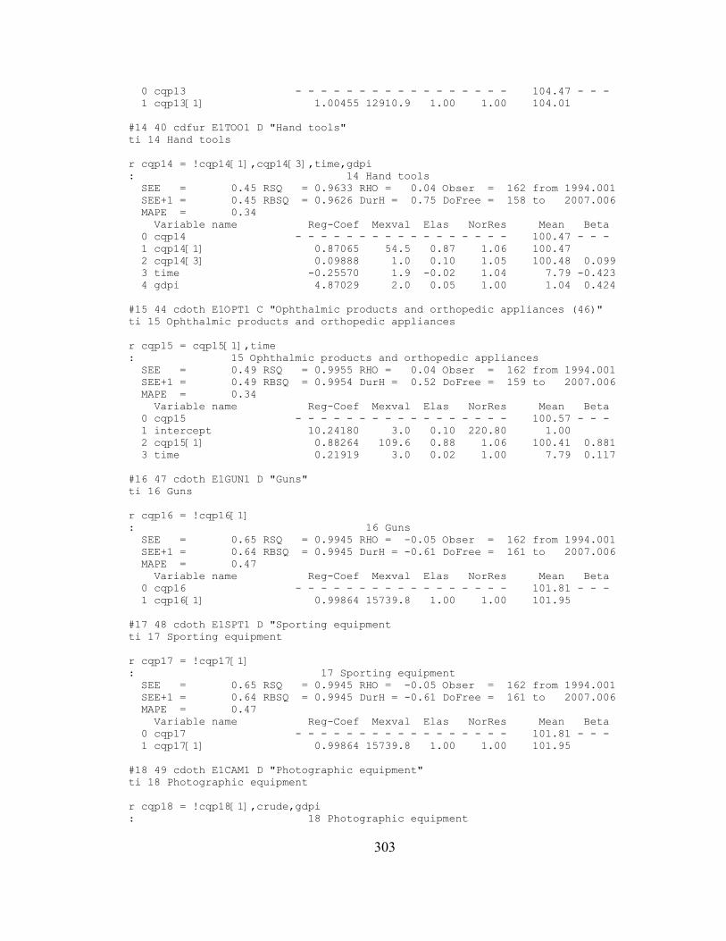
0 cqp13 - - - - - - - - - - - - - - - - - 104.47 - - - 1 cqp13[1] 1.00455 12910.9 1.00 1.00 104.01
#14 40 cdfur E1TOO1 D "Hand tools"ti 14 Hand tools
r cqp14 = !cqp14[1],cqp14[3],time,gdpi: 14 Hand tools SEE = 0.45 RSQ = 0.9633 RHO = 0.04 Obser = 162 from 1994.001 SEE+1 = 0.45 RBSQ = 0.9626 DurH = 0.75 DoFree = 158 to 2007.006 MAPE = 0.34 Variable name Reg-Coef Mexval Elas NorRes Mean Beta 0 cqp14 - - - - - - - - - - - - - - - - - 100.47 - - - 1 cqp14[1] 0.87065 54.5 0.87 1.06 100.47 2 cqp14[3] 0.09888 1.0 0.10 1.05 100.48 0.099 3 time -0.25570 1.9 -0.02 1.04 7.79 -0.423 4 gdpi 4.87029 2.0 0.05 1.00 1.04 0.424
#15 44 cdoth E1OPT1 C "Ophthalmic products and orthopedic appliances (46)"ti 15 Ophthalmic products and orthopedic appliances
r cqp15 = cqp15[1],time: 15 Ophthalmic products and orthopedic appliances SEE = 0.49 RSQ = 0.9955 RHO = 0.04 Obser = 162 from 1994.001 SEE+1 = 0.49 RBSQ = 0.9954 DurH = 0.52 DoFree = 159 to 2007.006 MAPE = 0.34 Variable name Reg-Coef Mexval Elas NorRes Mean Beta 0 cqp15 - - - - - - - - - - - - - - - - - 100.57 - - - 1 intercept 10.24180 3.0 0.10 220.80 1.00 2 cqp15[1] 0.88264 109.6 0.88 1.06 100.41 0.881 3 time 0.21919 3.0 0.02 1.00 7.79 0.117
#16 47 cdoth E1GUN1 D "Guns"ti 16 Guns
r cqp16 = !cqp16[1]: 16 Guns SEE = 0.65 RSQ = 0.9945 RHO = -0.05 Obser = 162 from 1994.001 SEE+1 = 0.64 RBSQ = 0.9945 DurH = -0.61 DoFree = 161 to 2007.006 MAPE = 0.47 Variable name Reg-Coef Mexval Elas NorRes Mean Beta 0 cqp16 - - - - - - - - - - - - - - - - - 101.81 - - - 1 cqp16[1] 0.99864 15739.8 1.00 1.00 101.95
#17 48 cdoth E1SPT1 D "Sporting equipmentti 17 Sporting equipment
r cqp17 = !cqp17[1]: 17 Sporting equipment SEE = 0.65 RSQ = 0.9945 RHO = -0.05 Obser = 162 from 1994.001 SEE+1 = 0.64 RBSQ = 0.9945 DurH = -0.61 DoFree = 161 to 2007.006 MAPE = 0.47 Variable name Reg-Coef Mexval Elas NorRes Mean Beta 0 cqp17 - - - - - - - - - - - - - - - - - 101.81 - - - 1 cqp17[1] 0.99864 15739.8 1.00 1.00 101.95
#18 49 cdoth E1CAM1 D "Photographic equipment"ti 18 Photographic equipment
r cqp18 = !cqp18[1],crude,gdpi: 18 Photographic equipment
303
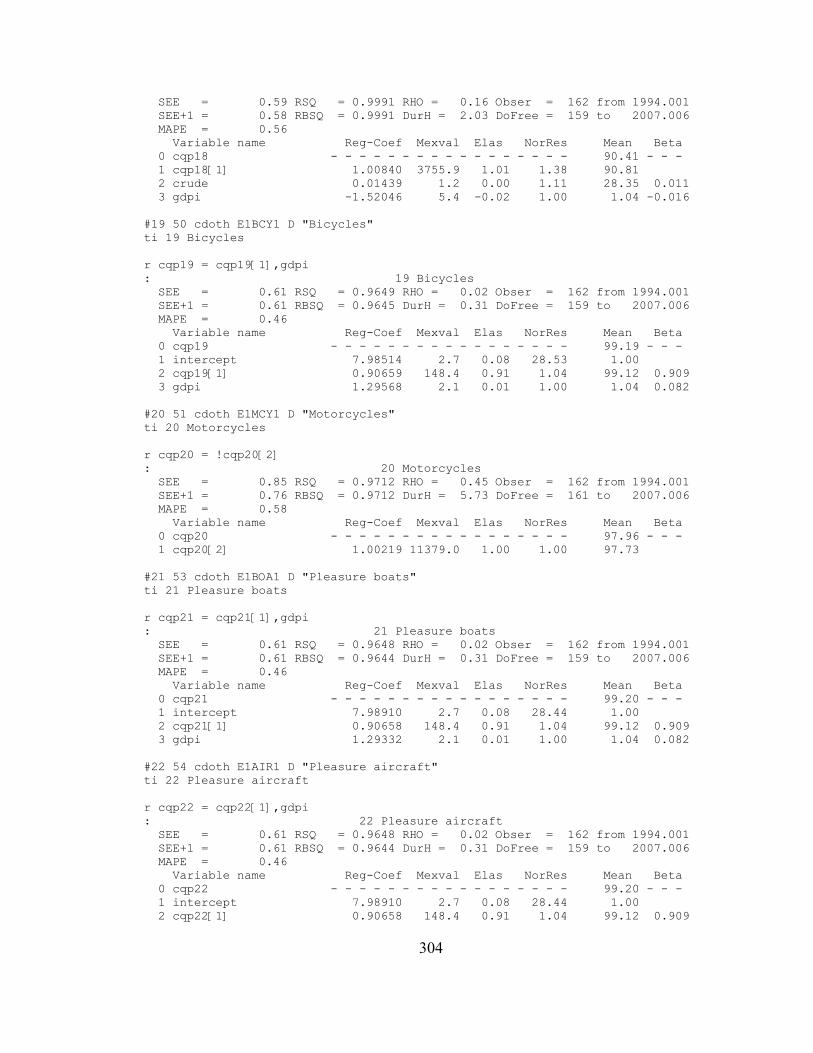
SEE = 0.59 RSQ = 0.9991 RHO = 0.16 Obser = 162 from 1994.001 SEE+1 = 0.58 RBSQ = 0.9991 DurH = 2.03 DoFree = 159 to 2007.006 MAPE = 0.56 Variable name Reg-Coef Mexval Elas NorRes Mean Beta 0 cqp18 - - - - - - - - - - - - - - - - - 90.41 - - - 1 cqp18[1] 1.00840 3755.9 1.01 1.38 90.81 2 crude 0.01439 1.2 0.00 1.11 28.35 0.011 3 gdpi -1.52046 5.4 -0.02 1.00 1.04 -0.016
#19 50 cdoth E1BCY1 D "Bicycles"ti 19 Bicycles
r cqp19 = cqp19[1],gdpi: 19 Bicycles SEE = 0.61 RSQ = 0.9649 RHO = 0.02 Obser = 162 from 1994.001 SEE+1 = 0.61 RBSQ = 0.9645 DurH = 0.31 DoFree = 159 to 2007.006 MAPE = 0.46 Variable name Reg-Coef Mexval Elas NorRes Mean Beta 0 cqp19 - - - - - - - - - - - - - - - - - 99.19 - - - 1 intercept 7.98514 2.7 0.08 28.53 1.00 2 cqp19[1] 0.90659 148.4 0.91 1.04 99.12 0.909 3 gdpi 1.29568 2.1 0.01 1.00 1.04 0.082
#20 51 cdoth E1MCY1 D "Motorcycles"ti 20 Motorcycles
r cqp20 = !cqp20[2]: 20 Motorcycles SEE = 0.85 RSQ = 0.9712 RHO = 0.45 Obser = 162 from 1994.001 SEE+1 = 0.76 RBSQ = 0.9712 DurH = 5.73 DoFree = 161 to 2007.006 MAPE = 0.58 Variable name Reg-Coef Mexval Elas NorRes Mean Beta 0 cqp20 - - - - - - - - - - - - - - - - - 97.96 - - - 1 cqp20[2] 1.00219 11379.0 1.00 1.00 97.73
#21 53 cdoth E1BOA1 D "Pleasure boats"ti 21 Pleasure boats
r cqp21 = cqp21[1],gdpi: 21 Pleasure boats SEE = 0.61 RSQ = 0.9648 RHO = 0.02 Obser = 162 from 1994.001 SEE+1 = 0.61 RBSQ = 0.9644 DurH = 0.31 DoFree = 159 to 2007.006 MAPE = 0.46 Variable name Reg-Coef Mexval Elas NorRes Mean Beta 0 cqp21 - - - - - - - - - - - - - - - - - 99.20 - - - 1 intercept 7.98910 2.7 0.08 28.44 1.00 2 cqp21[1] 0.90658 148.4 0.91 1.04 99.12 0.909 3 gdpi 1.29332 2.1 0.01 1.00 1.04 0.082
#22 54 cdoth E1AIR1 D "Pleasure aircraft"ti 22 Pleasure aircraft
r cqp22 = cqp22[1],gdpi: 22 Pleasure aircraft SEE = 0.61 RSQ = 0.9648 RHO = 0.02 Obser = 162 from 1994.001 SEE+1 = 0.61 RBSQ = 0.9644 DurH = 0.31 DoFree = 159 to 2007.006 MAPE = 0.46 Variable name Reg-Coef Mexval Elas NorRes Mean Beta 0 cqp22 - - - - - - - - - - - - - - - - - 99.20 - - - 1 intercept 7.98910 2.7 0.08 28.44 1.00 2 cqp22[1] 0.90658 148.4 0.91 1.04 99.12 0.909
304

3 gdpi 1.29332 2.1 0.01 1.00 1.04 0.082
#23 55 cdoth E1JRY1 C "Jewelry and watches (18)"ti 23 Jewelry and watches
r cqp23 = !cqp23[1],gdpi: 23 Jewelry and watches SEE = 1.25 RSQ = 0.9797 RHO = -0.22 Obser = 162 from 1994.001 SEE+1 = 1.21 RBSQ = 0.9796 DurH = -2.75 DoFree = 160 to 2007.006 MAPE = 0.92 Variable name Reg-Coef Mexval Elas NorRes Mean Beta 0 cqp23 - - - - - - - - - - - - - - - - - 103.14 - - - 1 cqp23[1] 0.99370 2133.7 0.99 1.01 103.23 2 gdpi 0.53439 0.7 0.01 1.00 1.04 0.013
#24 56 cdoth E1BKS1 C "Books and maps (87)"ti 24 Books and maps
r cqp24 = !cqp24[1],time: 24 Books and maps SEE = 0.63 RSQ = 0.9660 RHO = -0.06 Obser = 162 from 1994.001 SEE+1 = 0.63 RBSQ = 0.9658 DurH = -0.80 DoFree = 160 to 2007.006 MAPE = 0.45 Variable name Reg-Coef Mexval Elas NorRes Mean Beta 0 cqp24 - - - - - - - - - - - - - - - - - 100.46 - - - 1 cqp24[1] 1.00183 6663.5 1.00 1.01 100.39 2 time -0.01465 0.4 -0.00 1.00 7.79 -0.017
#25 61 cnfood E1GRA1 D "Cereals"ti 25 Cereals
r cqp25 = !cqp25[1],cqp25[2]: 25 Cereals SEE = 0.50 RSQ = 0.9870 RHO = 0.02 Obser = 162 from 1994.001 SEE+1 = 0.50 RBSQ = 0.9869 DurH = 0.84 DoFree = 160 to 2007.006 MAPE = 0.38 Variable name Reg-Coef Mexval Elas NorRes Mean Beta 0 cqp25 - - - - - - - - - - - - - - - - - 101.09 - - - 1 cqp25[1] 0.72677 25.3 0.73 1.08 100.98 2 cqp25[2] 0.27462 4.0 0.27 1.00 100.87 0.273
#26 62 cnfood E1BAK1 D "Bakery products"ti 26 Bakery products
r cqp26 = !cqp26[1],cqp26[2]: 26 Bakery products SEE = 0.40 RSQ = 0.9985 RHO = -0.04 Obser = 162 from 1994.001 SEE+1 = 0.40 RBSQ = 0.9985 DurH = -3.33 DoFree = 160 to 2007.006 MAPE = 0.29 Variable name Reg-Coef Mexval Elas NorRes Mean Beta 0 cqp26 - - - - - - - - - - - - - - - - - 101.56 - - - 1 cqp26[1] 0.75409 26.3 0.75 1.06 101.32 2 cqp26[2] 0.24885 3.2 0.25 1.00 101.08 0.248
#27 63 cnfood E1BEE1 D "Beef and veal"ti 27 Beef and veal
r cqp27 = !cqp27[1],gdpi: 27 Beef and veal SEE = 1.17 RSQ = 0.9958 RHO = 0.39 Obser = 162 from 1994.001 SEE+1 = 1.07 RBSQ = 0.9958 DurH = 5.04 DoFree = 160 to 2007.006
305

MAPE = 0.63 Variable name Reg-Coef Mexval Elas NorRes Mean Beta 0 cqp27 - - - - - - - - - - - - - - - - - 108.39 - - - 1 cqp27[1] 0.96950 522.8 0.97 1.05 108.08 2 gdpi 3.47808 2.2 0.03 1.00 1.04 0.039
#28 64 cnfood E1POR1 D "Pork"ti 28 Pork
r cqp28 = !cqp28[1],cqp28[2]: 28 Pork SEE = 0.82 RSQ = 0.9915 RHO = -0.02 Obser = 162 from 1994.001 SEE+1 = 0.82 RBSQ = 0.9915 DurH = 999.00 DoFree = 160 to 2007.006 MAPE = 0.61 Variable name Reg-Coef Mexval Elas NorRes Mean Beta 0 cqp28 - - - - - - - - - - - - - - - - - 101.41 - - - 1 cqp28[1] 1.06482 46.2 1.06 1.00 101.23 2 cqp28[2] -0.06312 0.2 -0.06 1.00 101.05 -0.063
#29 65 cnfood E1MEA1 D "Other meats"ti 29 Other meats
r cqp29 = !cqp29[1],gdpi: 29 Other meats SEE = 1.03 RSQ = 0.9881 RHO = -0.39 Obser = 162 from 1994.001 SEE+1 = 0.95 RBSQ = 0.9880 DurH = -5.01 DoFree = 160 to 2007.006 MAPE = 0.74 Variable name Reg-Coef Mexval Elas NorRes Mean Beta 0 cqp29 - - - - - - - - - - - - - - - - - 103.74 - - - 1 cqp29[1] 0.99362 997.3 0.99 1.01 103.55 2 gdpi 0.80866 0.4 0.01 1.00 1.04 0.018
#30 66 cnfood E1POU1 D "Poultry"ti 30 Poultry
r cqp30 = !cqp30[1],cqp30[2]: 30 Poultry SEE = 0.95 RSQ = 0.9873 RHO = 0.07 Obser = 162 from 1994.001 SEE+1 = 0.95 RBSQ = 0.9872 DurH = 8.30 DoFree = 160 to 2007.006 MAPE = 0.73 Variable name Reg-Coef Mexval Elas NorRes Mean Beta 0 cqp30 - - - - - - - - - - - - - - - - - 102.84 - - - 1 cqp30[1] 0.75577 26.0 0.75 1.06 102.65 2 cqp30[2] 0.24657 3.1 0.25 1.00 102.47 0.243
#31 67 cnfood E1FIS1 D "Fish and seafood"ti 31 Fish and seafood
r cqp31 = cqp31[1],gdpi: 31 Fish and seafood SEE = 0.76 RSQ = 0.9855 RHO = -0.19 Obser = 162 from 1994.001 SEE+1 = 0.75 RBSQ = 0.9853 DurH = -2.76 DoFree = 159 to 2007.006 MAPE = 0.60 Variable name Reg-Coef Mexval Elas NorRes Mean Beta 0 cqp31 - - - - - - - - - - - - - - - - - 98.80 - - - 1 intercept 6.01194 1.8 0.06 68.85 1.00 2 cqp31[1] 0.90922 123.0 0.91 1.05 98.62 0.898 3 gdpi 3.01316 2.3 0.03 1.00 1.04 0.098
#32 68 cnfood E1GGS1 D "Eggs"ti 32 Eggs
306

r cqp32 = !cqp32[1],cqp32[2],cqp32[3]: 32 Eggs SEE = 3.27 RSQ = 0.9359 RHO = -0.04 Obser = 162 from 1994.001 SEE+1 = 3.27 RBSQ = 0.9351 DurH = 999.00 DoFree = 159 to 2007.006 MAPE = 2.33 Variable name Reg-Coef Mexval Elas NorRes Mean Beta 0 cqp32 - - - - - - - - - - - - - - - - - 106.58 - - - 1 cqp32[1] 0.79854 28.7 0.80 1.08 106.24 2 cqp32[2] 0.36391 4.1 0.36 1.02 105.89 0.352 3 cqp32[3] -0.15929 1.2 -0.16 1.00 105.62 -0.153
#33 69 cnfood E1MIL1 D "Fresh milk and cream"ti 33 Fresh milk and cream
r cqp33 = cqp33[1]: 33 Fresh milk and cream SEE = 1.96 RSQ = 0.9725 RHO = 0.31 Obser = 162 from 1994.001 SEE+1 = 1.87 RBSQ = 0.9723 DurH = 4.03 DoFree = 160 to 2007.006 MAPE = 1.04 Variable name Reg-Coef Mexval Elas NorRes Mean Beta 0 cqp33 - - - - - - - - - - - - - - - - - 101.25 - - - 1 intercept 0.73778 0.1 0.01 36.36 1.00 2 cqp33[1] 0.99540 503.0 0.99 1.00 100.97 0.986
#34 70 cnfood E1DAI1 D "Processed dairy products"ti 34 Processed dairy products
r cqp34 = cqp34[1],time,crude: 34 Processed dairy products SEE = 0.68 RSQ = 0.9954 RHO = 0.05 Obser = 162 from 1994.001 SEE+1 = 0.68 RBSQ = 0.9953 DurH = 0.65 DoFree = 158 to 2007.006 MAPE = 0.52 Variable name Reg-Coef Mexval Elas NorRes Mean Beta 0 cqp34 - - - - - - - - - - - - - - - - - 99.32 - - - 1 intercept 7.34185 3.0 0.07 216.36 1.00 2 cqp34[1] 0.91179 165.4 0.91 1.06 99.12 0.914 3 time 0.27442 2.8 0.02 1.04 7.79 0.107 4 crude -0.01879 1.8 -0.01 1.00 28.35 -0.028
#35 71 cnfood E1FRU1 D "Fresh fruits"ti 35 Fresh fruits
r cqp35 = cqp35[1],gdpi: 35 Fresh fruits SEE = 1.67 RSQ = 0.9777 RHO = 0.08 Obser = 162 from 1994.001 SEE+1 = 1.66 RBSQ = 0.9774 DurH = 1.24 DoFree = 159 to 2007.006 MAPE = 1.19 Variable name Reg-Coef Mexval Elas NorRes Mean Beta 0 cqp35 - - - - - - - - - - - - - - - - - 103.01 - - - 1 intercept 8.72200 4.2 0.08 44.77 1.00 2 cqp35[1] 0.81899 71.3 0.82 1.09 102.74 0.814 3 gdpi 9.77841 4.6 0.10 1.00 1.04 0.180
#36 72 cnfood E1VEG1 D "Fresh vegetables"ti 36 Fresh vegetables
r cqp36 = cqp36[1],gdpi: 36 Fresh vegetables SEE = 3.17 RSQ = 0.9612 RHO = 0.11 Obser = 162 from 1994.001 SEE+1 = 3.15 RBSQ = 0.9607 DurH = 2.21 DoFree = 159 to 2007.006
307

MAPE = 2.18 Variable name Reg-Coef Mexval Elas NorRes Mean Beta 0 cqp36 - - - - - - - - - - - - - - - - - 104.43 - - - 1 intercept 8.88688 5.9 0.09 25.78 1.00 2 cqp36[1] 0.65931 33.0 0.66 1.19 104.13 0.657 3 gdpi 25.93037 9.3 0.26 1.00 1.04 0.331
#37 73 cnfood E1PFV1 D "Processed fruits and vegetables"ti 37 Processed fruits and vegetables
r cqp37 = cqp37[1],cqp37[2],gdpi: 37 Processed fruits and vegetables SEE = 0.57 RSQ = 0.9962 RHO = -0.10 Obser = 162 from 1994.001 SEE+1 = 0.56 RBSQ = 0.9961 DurH = -3.20 DoFree = 158 to 2007.006 MAPE = 0.41 Variable name Reg-Coef Mexval Elas NorRes Mean Beta 0 cqp37 - - - - - - - - - - - - - - - - - 102.05 - - - 1 intercept 4.37025 1.3 0.04 261.34 1.00 2 cqp37[1] 0.48236 13.2 0.48 1.33 101.85 0.480 3 cqp37[2] 0.43972 11.0 0.44 1.03 101.65 0.436 4 gdpi 3.71884 1.5 0.04 1.00 1.04 0.083
#38 74 cnfood E1JNB1 D "Juices and nonalcoholic drinks"ti 38 Juices and nonalcoholic drinks
r cqp38 = cqp38[1],gdpi: 38 Juices and nonalcoholic drinks SEE = 0.66 RSQ = 0.9778 RHO = -0.25 Obser = 162 from 1994.001 SEE+1 = 0.63 RBSQ = 0.9776 DurH = -3.59 DoFree = 159 to 2007.006 MAPE = 0.49 Variable name Reg-Coef Mexval Elas NorRes Mean Beta 0 cqp38 - - - - - - - - - - - - - - - - - 100.10 - - - 1 intercept 7.80945 2.3 0.08 45.13 1.00 2 cqp38[1] 0.89788 122.1 0.90 1.06 100.00 0.882 3 gdpi 2.41324 3.1 0.03 1.00 1.04 0.112
#39 75 cnfood E1CTM1 D "Coffee, tea and beverage materials"ti 39 Coffee, tea and beverage materials#lim 2000.001 2007.001 2006.012r cqp39 = cqp39[1],cqp39[2],gdpi: 39 Coffee, tea and beverage materials SEE = 1.64 RSQ = 0.9544 RHO = 0.06 Obser = 162 from 1994.001 SEE+1 = 1.63 RBSQ = 0.9535 DurH = 1.33 DoFree = 158 to 2007.006 MAPE = 0.85 Variable name Reg-Coef Mexval Elas NorRes Mean Beta 0 cqp39 - - - - - - - - - - - - - - - - - 98.99 - - - 1 intercept 7.73683 6.8 0.08 21.92 1.00 2 cqp39[1] 1.45147 103.5 1.45 1.50 98.73 1.513 3 cqp39[2] -0.54702 21.8 -0.54 1.03 98.46 -0.594 4 gdpi 1.75147 1.6 0.02 1.00 1.04 0.047
#40 76 cnfood E1FAT1 D "Fats and oils"ti 40 Fats and oils
r cqp40 = !cqp40[1]: 40 Fats and oils SEE = 0.90 RSQ = 0.9859 RHO = 0.02 Obser = 162 from 1994.001 SEE+1 = 0.90 RBSQ = 0.9859 DurH = 0.29 DoFree = 161 to 2007.006 MAPE = 0.61 Variable name Reg-Coef Mexval Elas NorRes Mean Beta 0 cqp40 - - - - - - - - - - - - - - - - - 103.57 - - -
308

1 cqp40[1] 1.00153 11493.6 1.00 1.00 103.41
#41 77 cnfood E1SWE1 D "Sugar and sweets"ti 41 Sugar and sweets
r cqp41 = cqp41[1],gdpi: 41 Sugar and sweets SEE = 0.52 RSQ = 0.9942 RHO = -0.39 Obser = 162 from 1994.001 SEE+1 = 0.48 RBSQ = 0.9941 DurH = -5.53 DoFree = 159 to 2007.006 MAPE = 0.36 Variable name Reg-Coef Mexval Elas NorRes Mean Beta 0 cqp41 - - - - - - - - - - - - - - - - - 100.51 - - - 1 intercept 6.31980 2.5 0.06 172.40 1.00 2 cqp41[1] 0.90528 137.9 0.90 1.05 100.35 0.902 3 gdpi 3.22647 2.6 0.03 1.00 1.04 0.097
#42 78 cnfood E1OFD1 D "Other foods"ti 42 Other foods
r cqp42 = !cqp42[1],oildf,oildf[1]: 42 Other foods SEE = 0.46 RSQ = 0.9953 RHO = -0.41 Obser = 162 from 1994.001 SEE+1 = 0.42 RBSQ = 0.9952 DurH = -5.22 DoFree = 159 to 2007.006 MAPE = 0.35 Variable name Reg-Coef Mexval Elas NorRes Mean Beta 0 cqp42 - - - - - - - - - - - - - - - - - 98.94 - - - 1 cqp42[1] 1.00136 21172.7 1.00 1.05 98.79 2 oildf 0.04707 2.4 0.00 1.00 0.32 0.015 3 oildf[1] -0.01417 0.2 -0.00 1.00 0.29 -0.005
#43 79 cnfood E1PEF1 D "Pet food"ti 43 Pet food
r cqp43 = !cqp43[1]: 43 Pet food SEE = 0.55 RSQ = 0.9927 RHO = -0.03 Obser = 162 from 1994.001 SEE+1 = 0.55 RBSQ = 0.9927 DurH = -0.32 DoFree = 161 to 2007.006 MAPE = 0.44 Variable name Reg-Coef Mexval Elas NorRes Mean Beta 0 cqp43 - - - - - - - - - - - - - - - - - 101.75 - - - 1 cqp43[1] 1.00151 18498.0 1.00 1.00 101.60
#44 81 cnfood E1MLT1 D "Beer and ale, at home"ti 44 Beer and ale, at home
r cqp44 = !cqp44[1],gdpi: 44 Beer and ale, at home SEE = 0.35 RSQ = 0.9982 RHO = -0.07 Obser = 162 from 1994.001 SEE+1 = 0.35 RBSQ = 0.9981 DurH = -0.89 DoFree = 160 to 2007.006 MAPE = 0.26 Variable name Reg-Coef Mexval Elas NorRes Mean Beta 0 cqp44 - - - - - - - - - - - - - - - - - 101.79 - - - 1 cqp44[1] 0.99620 3350.9 0.99 1.04 101.63 2 gdpi 0.52605 1.8 0.01 1.00 1.04 0.013
#45 82 cnfood E1WIN1 D "Wine and brandy, at home"ti 45 Wine and brandy, at home
r cqp45 = cqp45[1]: 45 Wine and brandy, at home SEE = 0.37 RSQ = 0.9948 RHO = -0.11 Obser = 162 from 1994.001
309

SEE+1 = 0.37 RBSQ = 0.9947 DurH = -1.46 DoFree = 160 to 2007.006 MAPE = 0.29 Variable name Reg-Coef Mexval Elas NorRes Mean Beta 0 cqp45 - - - - - - - - - - - - - - - - - 98.33 - - - 1 intercept 0.41204 0.2 0.00 191.59 1.00 2 cqp45[1] 0.99686 1284.2 1.00 1.00 98.23 0.997
#46 83 cnfood E1LIQ1 D "Distilled spirits, at home"ti 46 Distilled spirits, at home
r cqp46 = !cqp46[1]: 46 Distilled spirits, at home SEE = 0.28 RSQ = 0.9987 RHO = -0.09 Obser = 162 from 1994.001 SEE+1 = 0.28 RBSQ = 0.9987 DurH = -1.16 DoFree = 161 to 2007.006 MAPE = 0.20 Variable name Reg-Coef Mexval Elas NorRes Mean Beta 0 cqp46 - - - - - - - - - - - - - - - - - 100.21 - - - 1 cqp46[1] 1.00144 35948.6 1.00 1.00 100.07
#47 84 cnfood E1PMB1 C "Purchased meals and beverages (4)"ti 47 Purchased meals and beverages
r cqp47 = cqp47[1],gdpi: 47 Purchased meals and beverages SEE = 0.08 RSQ = 0.9999 RHO = -0.04 Obser = 162 from 1994.001 SEE+1 = 0.08 RBSQ = 0.9999 DurH = -0.54 DoFree = 159 to 2007.006 MAPE = 0.06 Variable name Reg-Coef Mexval Elas NorRes Mean Beta 0 cqp47 - - - - - - - - - - - - - - - - - 101.73 - - - 1 intercept 1.11047 1.7 0.01 9999.99 1.00 2 cqp47[1] 0.97620 704.1 0.97 1.06 101.51 0.971 3 gdpi 1.47978 2.7 0.02 1.00 1.04 0.029
#48 93 cnfood E1PIF1 C "Food furnished to employees or home #grown"ti 48 Food furnished to employees or home #grown
r cqp48 = !cqp48[1],crude: 48 Food furnished to employees or home #grown SEE = 0.27 RSQ = 0.9992 RHO = 0.11 Obser = 162 from 1994.001 SEE+1 = 0.27 RBSQ = 0.9992 DurH = 1.35 DoFree = 160 to 2007.006 MAPE = 0.19 Variable name Reg-Coef Mexval Elas NorRes Mean Beta 0 cqp48 - - - - - - - - - - - - - - - - - 101.92 - - - 1 cqp48[1] 1.00098 14713.3 1.00 1.03 101.72 2 crude 0.00374 1.5 0.00 1.00 28.35 0.006
#49 99 cncloth E1SHU1 C "Shoes (12)"ti 49 Shoes
r cqp49 = !cqp49[1],crude,crude[11]: 49 Shoes SEE = 0.72 RSQ = 0.9632 RHO = -0.06 Obser = 162 from 1994.001 SEE+1 = 0.72 RBSQ = 0.9627 DurH = -0.73 DoFree = 159 to 2007.006 MAPE = 0.56 Variable name Reg-Coef Mexval Elas NorRes Mean Beta 0 cqp49 - - - - - - - - - - - - - - - - - 101.41 - - - 1 cqp49[1] 0.99869 6410.7 1.00 1.01 101.48 2 crude 0.01197 0.6 0.00 1.01 28.35 0.048 3 crude[11] -0.01082 0.4 -0.00 1.00 25.51 -0.037
310

#50 100 cncloth E1WCL1 C "Women's and children's clothing and accessories except shoes (14)"ti 50 Women's and children's clothing and accessories except shoes
r cqp50 = !cqp50[1],crude,crude[11]: 50 Women's and children's clothing and accessories except shoes SEE = 0.70 RSQ = 0.9903 RHO = -0.11 Obser = 162 from 1994.001 SEE+1 = 0.69 RBSQ = 0.9902 DurH = -1.43 DoFree = 159 to 2007.006 MAPE = 0.53 Variable name Reg-Coef Mexval Elas NorRes Mean Beta 0 cqp50 - - - - - - - - - - - - - - - - - 99.77 - - - 1 cqp50[1] 0.99784 6966.3 1.00 1.01 99.93 2 crude 0.01123 0.6 0.00 1.01 28.35 0.024 3 crude[11] -0.01038 0.4 -0.00 1.00 25.51 -0.019
#51 106 cncloth E1MMC1 C "Men's and boys' clothing and accessories except shoes (15+16)"ti 51 Men's and boys' clothing and accessories except shoes
r cqp51 = !cqp51[1]: 51 Men's and boys' clothing and accessories except shoes SEE = 0.55 RSQ = 0.9907 RHO = -0.09 Obser = 162 from 1994.001 SEE+1 = 0.55 RBSQ = 0.9907 DurH = -1.13 DoFree = 161 to 2007.006 MAPE = 0.45 Variable name Reg-Coef Mexval Elas NorRes Mean Beta 0 cqp51 - - - - - - - - - - - - - - - - - 96.67 - - - 1 cqp51[1] 0.99887 17374.4 1.00 1.00 96.78
#52 114 cngas E1GAO1 B "Gasoline and oil (75)"ti 52 Gasoline and oil
r cqp52 = !cqp52[1],oildf,oildf[1]: 52 Gasoline and oil SEE = 4.12 RSQ = 0.9848 RHO = 0.07 Obser = 162 from 1994.001 SEE+1 = 4.11 RBSQ = 0.9846 DurH = 0.83 DoFree = 159 to 2007.006 MAPE = 2.60 Variable name Reg-Coef Mexval Elas NorRes Mean Beta 0 cqp52 - - - - - - - - - - - - - - - - - 103.34 - - - 1 cqp52[1] 0.99859 2467.8 0.99 2.36 102.59 2 oildf 1.51676 27.4 0.00 1.42 0.32 0.100 3 oildf[1] 1.25764 19.2 0.00 1.00 0.29 0.083
#53 117 cngas E1FUL1 B "Fuel oil and coal (40)"ti 53 Fuel oil and coal
r cqp53 = !cqp53[1],cqp53[2],oildf,oildf[1]: 53 Fuel oil and coal SEE = 2.94 RSQ = 0.9938 RHO = -0.05 Obser = 162 from 1994.001 SEE+1 = 2.94 RBSQ = 0.9936 DurH = -1.77 DoFree = 158 to 2007.006 MAPE = 1.60 Variable name Reg-Coef Mexval Elas NorRes Mean Beta 0 cqp53 - - - - - - - - - - - - - - - - - 103.70 - - - 1 cqp53[1] 1.10510 57.6 1.10 1.66 102.97 2 cqp53[2] -0.10250 0.6 -0.10 1.56 102.26 -0.100 3 oildf 0.70990 12.0 0.00 1.14 0.32 0.042 4 oildf[1] 0.59923 6.7 0.00 1.00 0.29 0.035
#54 123 cnoth E1TOB1 C "Tobacco products (7)"ti 54 Tobacco products
r cqp54 = cqp54[1]
311
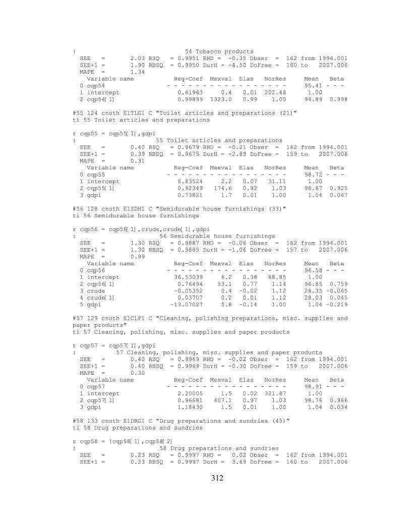
: 54 Tobacco products SEE = 2.03 RSQ = 0.9951 RHO = -0.35 Obser = 162 from 1994.001 SEE+1 = 1.90 RBSQ = 0.9950 DurH = -4.50 DoFree = 160 to 2007.006 MAPE = 1.34 Variable name Reg-Coef Mexval Elas NorRes Mean Beta 0 cqp54 - - - - - - - - - - - - - - - - - 95.41 - - - 1 intercept 0.61963 0.4 0.01 202.48 1.00 2 cqp54[1] 0.99899 1323.0 0.99 1.00 94.89 0.998
#55 124 cnoth E1TLG1 C "Toilet articles and preparations (21)"ti 55 Toilet articles and preparations
r cqp55 = cqp55[1],gdpi: 55 Toilet articles and preparations SEE = 0.40 RSQ = 0.9679 RHO = -0.21 Obser = 162 from 1994.001 SEE+1 = 0.39 RBSQ = 0.9675 DurH = -2.89 DoFree = 159 to 2007.006 MAPE = 0.31 Variable name Reg-Coef Mexval Elas NorRes Mean Beta 0 cqp55 - - - - - - - - - - - - - - - - - 98.72 - - - 1 intercept 6.83524 2.2 0.07 31.11 1.00 2 cqp55[1] 0.92349 174.6 0.92 1.03 98.67 0.925 3 gdpi 0.73821 1.7 0.01 1.00 1.04 0.067
#56 128 cnoth E1SDH1 C "Semidurable house furnishings (33)"ti 56 Semidurable house furnishings
r cqp56 = cqp56[1],crude,crude[1],gdpi: 56 Semidurable house furnishings SEE = 1.30 RSQ = 0.9887 RHO = -0.06 Obser = 162 from 1994.001 SEE+1 = 1.30 RBSQ = 0.9885 DurH = -1.06 DoFree = 157 to 2007.006 MAPE = 0.99 Variable name Reg-Coef Mexval Elas NorRes Mean Beta 0 cqp56 - - - - - - - - - - - - - - - - - 96.58 - - - 1 intercept 36.53039 6.2 0.38 88.85 1.00 2 cqp56[1] 0.76494 53.1 0.77 1.14 96.85 0.759 3 crude -0.05352 0.4 -0.02 1.12 28.35 -0.065 4 crude[1] 0.03707 0.2 0.01 1.12 28.03 0.045 5 gdpi -13.07027 5.8 -0.14 1.00 1.04 -0.219
#57 129 cnoth E1CLP1 C "Cleaning, polishing preparations, misc. supplies and paper products"ti 57 Cleaning, polishing, misc. supplies and paper products
r cqp57 = cqp57[1],gdpi: 57 Cleaning, polishing, misc. supplies and paper products SEE = 0.40 RSQ = 0.9969 RHO = -0.02 Obser = 162 from 1994.001 SEE+1 = 0.40 RBSQ = 0.9969 DurH = -0.30 DoFree = 159 to 2007.006 MAPE = 0.30 Variable name Reg-Coef Mexval Elas NorRes Mean Beta 0 cqp57 - - - - - - - - - - - - - - - - - 98.91 - - - 1 intercept 2.20005 1.5 0.02 321.87 1.00 2 cqp57[1] 0.96681 407.1 0.97 1.03 98.76 0.966 3 gdpi 1.18430 1.5 0.01 1.00 1.04 0.034
#58 133 cnoth E1DRG1 C "Drug preparations and sundries (45)"ti 58 Drug preparations and sundries
r cqp58 = !cqp58[1],cqp58[2]: 58 Drug preparations and sundries SEE = 0.23 RSQ = 0.9997 RHO = 0.02 Obser = 162 from 1994.001 SEE+1 = 0.23 RBSQ = 0.9997 DurH = 3.69 DoFree = 160 to 2007.006
312

MAPE = 0.16 Variable name Reg-Coef Mexval Elas NorRes Mean Beta 0 cqp58 - - - - - - - - - - - - - - - - - 102.75 - - - 1 cqp58[1] 1.22069 58.7 1.22 1.05 102.51 2 cqp58[2] -0.21888 2.4 -0.22 1.00 102.27 -0.217
#59 139 cnoth E1DOL1 D "Toys, dolls, and games"ti 59 Toys, dolls, and games
r cqp59 = cqp59[1]: 59 Toys, dolls, and games SEE = 0.68 RSQ = 0.9988 RHO = -0.02 Obser = 162 from 1994.001 SEE+1 = 0.68 RBSQ = 0.9988 DurH = -0.20 DoFree = 160 to 2007.006 MAPE = 0.50 Variable name Reg-Coef Mexval Elas NorRes Mean Beta 0 cqp59 - - - - - - - - - - - - - - - - - 98.61 - - - 1 intercept -0.61275 1.5 -0.01 819.23 1.00 2 cqp59[1] 1.00268 2762.2 1.01 1.00 98.95 0.999
#60 140 cnoth E1AMM1 D "Sport supplies, including ammunition"ti 60 Sport supplies, including ammunition
r cqp60 = !cqp60[1],oildf[1]: 60 Sport supplies, including ammunition SEE = 0.64 RSQ = 0.9945 RHO = -0.05 Obser = 162 from 1994.001 SEE+1 = 0.64 RBSQ = 0.9945 DurH = -0.57 DoFree = 160 to 2007.006 MAPE = 0.46 Variable name Reg-Coef Mexval Elas NorRes Mean Beta 0 cqp60 - - - - - - - - - - - - - - - - - 101.81 - - - 1 cqp60[1] 0.99859 15655.8 1.00 1.00 101.95 2 oildf[1] 0.02040 0.2 0.00 1.00 0.29 0.005
#61 141 cnoth E1FLM1 D "Film and photo supplies"ti 61 Film and photo supplies
r cqp61 = !cqp61[1],oildf,oildf[1]: 61 Film and photo supplies SEE = 0.71 RSQ = 0.9888 RHO = 0.01 Obser = 162 from 1994.001 SEE+1 = 0.71 RBSQ = 0.9887 DurH = 0.13 DoFree = 159 to 2007.006 MAPE = 0.54 Variable name Reg-Coef Mexval Elas NorRes Mean Beta 0 cqp61 - - - - - - - - - - - - - - - - - 99.07 - - - 1 cqp61[1] 0.99861 13764.6 1.00 1.02 99.19 2 oildf 0.01878 0.2 0.00 1.01 0.32 0.006 3 oildf[1] 0.03971 0.7 0.00 1.00 0.29 0.013
#62 142 cnoth E1STY1 C "Stationery and writing supplies (35)"ti 62 Stationery and writing supplies
r cqp62 = cqp62[1]: 62 Stationery and writing supplies SEE = 0.55 RSQ = 0.9826 RHO = -0.02 Obser = 162 from 1994.001 SEE+1 = 0.55 RBSQ = 0.9825 DurH = -0.32 DoFree = 160 to 2007.006 MAPE = 0.45 Variable name Reg-Coef Mexval Elas NorRes Mean Beta 0 cqp62 - - - - - - - - - - - - - - - - - 97.21 - - - 1 intercept 2.65021 2.2 0.03 57.47 1.00 2 cqp62[1] 0.97343 658.1 0.97 1.00 97.14 0.991
#63 145 cnoth E1NFR1 C "Net foreign remittances (111 less 113)"ti 63 Net foreign remittances
313
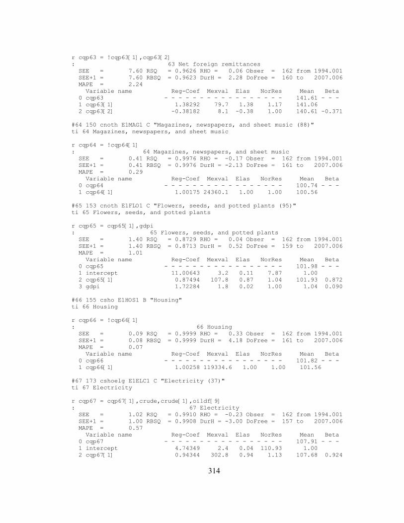
r cqp63 = !cqp63[1],cqp63[2]: 63 Net foreign remittances SEE = 7.60 RSQ = 0.9626 RHO = 0.06 Obser = 162 from 1994.001 SEE+1 = 7.60 RBSQ = 0.9623 DurH = 2.28 DoFree = 160 to 2007.006 MAPE = 2.24 Variable name Reg-Coef Mexval Elas NorRes Mean Beta 0 cqp63 - - - - - - - - - - - - - - - - - 141.61 - - - 1 cqp63[1] 1.38292 79.7 1.38 1.17 141.06 2 cqp63[2] -0.38182 8.1 -0.38 1.00 140.61 -0.371
#64 150 cnoth E1MAG1 C "Magazines, newspapers, and sheet music (88)"ti 64 Magazines, newspapers, and sheet music
r cqp64 = !cqp64[1]: 64 Magazines, newspapers, and sheet music SEE = 0.41 RSQ = 0.9976 RHO = -0.17 Obser = 162 from 1994.001 SEE+1 = 0.41 RBSQ = 0.9976 DurH = -2.13 DoFree = 161 to 2007.006 MAPE = 0.29 Variable name Reg-Coef Mexval Elas NorRes Mean Beta 0 cqp64 - - - - - - - - - - - - - - - - - 100.74 - - - 1 cqp64[1] 1.00175 24360.1 1.00 1.00 100.56
#65 153 cnoth E1FLO1 C "Flowers, seeds, and potted plants (95)"ti 65 Flowers, seeds, and potted plants
r cqp65 = cqp65[1],gdpi: 65 Flowers, seeds, and potted plants SEE = 1.40 RSQ = 0.8729 RHO = 0.04 Obser = 162 from 1994.001 SEE+1 = 1.40 RBSQ = 0.8713 DurH = 0.52 DoFree = 159 to 2007.006 MAPE = 1.01 Variable name Reg-Coef Mexval Elas NorRes Mean Beta 0 cqp65 - - - - - - - - - - - - - - - - - 101.98 - - - 1 intercept 11.00643 3.2 0.11 7.87 1.00 2 cqp65[1] 0.87494 107.8 0.87 1.04 101.93 0.872 3 gdpi 1.72284 1.8 0.02 1.00 1.04 0.090
#66 155 csho E1HOS1 B "Housing"ti 66 Housing
r cqp66 = !cqp66[1]: 66 Housing SEE = 0.09 RSQ = 0.9999 RHO = 0.33 Obser = 162 from 1994.001 SEE+1 = 0.08 RBSQ = 0.9999 DurH = 4.18 DoFree = 161 to 2007.006 MAPE = 0.07 Variable name Reg-Coef Mexval Elas NorRes Mean Beta 0 cqp66 - - - - - - - - - - - - - - - - - 101.82 - - - 1 cqp66[1] 1.00258 119334.6 1.00 1.00 101.56
#67 173 cshoelg E1ELC1 C "Electricity (37)"ti 67 Electricity
r cqp67 = cqp67[1],crude,crude[1],oildf[9]: 67 Electricity SEE = 1.02 RSQ = 0.9910 RHO = -0.23 Obser = 162 from 1994.001 SEE+1 = 1.00 RBSQ = 0.9908 DurH = -3.00 DoFree = 157 to 2007.006 MAPE = 0.57 Variable name Reg-Coef Mexval Elas NorRes Mean Beta 0 cqp67 - - - - - - - - - - - - - - - - - 107.91 - - - 1 intercept 4.74349 2.4 0.04 110.93 1.00 2 cqp67[1] 0.94344 302.8 0.94 1.13 107.68 0.924
314

3 crude -0.04279 0.4 -0.01 1.05 28.35 -0.059 4 crude[1] 0.09951 2.1 0.03 1.00 28.03 0.136 5 oildf[9] 0.02240 0.1 0.00 1.00 0.25 0.004
#68 174 cshoelg E1NGS1 C "Gas (38)"ti 68 Gas
r cqp68 = !cqp68[1],cqp68[2],oildf[1]: 68 Gas SEE = 4.16 RSQ = 0.9829 RHO = 0.01 Obser = 162 from 1994.001 SEE+1 = 4.16 RBSQ = 0.9826 DurH = 0.64 DoFree = 159 to 2007.006 MAPE = 2.00 Variable name Reg-Coef Mexval Elas NorRes Mean Beta 0 cqp68 - - - - - - - - - - - - - - - - - 109.61 - - - 1 cqp68[1] 1.27830 68.4 1.27 1.12 109.09 2 cqp68[2] -0.27667 4.2 -0.27 1.04 108.56 -0.272 3 oildf[1] 0.37714 2.0 0.00 1.00 0.29 0.026
#69 176 cshoelg E1WAT1 C "Water and other sanitary services (39)"ti 69 Water and other sanitary services
r cqp69 = cqp69[1],cqp69[2]: 69 Water and other sanitary services SEE = 0.27 RSQ = 0.9997 RHO = 0.01 Obser = 162 from 1994.001 SEE+1 = 0.27 RBSQ = 0.9996 DurH = 999.00 DoFree = 159 to 2007.006 MAPE = 0.15 Variable name Reg-Coef Mexval Elas NorRes Mean Beta 0 cqp69 - - - - - - - - - - - - - - - - - 103.90 - - - 1 intercept -0.39190 1.8 -0.00 2875.53 1.00 2 cqp69[1] 1.11479 49.9 1.11 1.01 103.58 1.106 3 cqp69[2] -0.10821 0.6 -0.11 1.00 103.25 -0.107
#70 181 cshoelg E1CEL1 D "Cellular telephone"ti 70 Cellular telephone
r cqp70 = cqp70[1],cqp70[2],gdpi: 70 Cellular telephone SEE = 0.57 RSQ = 0.9996 RHO = -0.03 Obser = 162 from 1994.001 SEE+1 = 0.57 RBSQ = 0.9995 DurH = -0.82 DoFree = 158 to 2007.006 MAPE = 0.39 Variable name Reg-Coef Mexval Elas NorRes Mean Beta 0 cqp70 - - - - - - - - - - - - - - - - - 111.06 - - - 1 intercept -0.72664 0.2 -0.01 2254.50 1.00 2 cqp70[1] 1.54662 110.0 1.55 1.49 111.52 1.558 3 cqp70[2] -0.54687 19.2 -0.55 1.01 111.99 -0.555 4 gdpi 0.52499 0.3 0.00 1.00 1.04 0.004
#71 182 cshoelg E1OLC1 D "Local telephone"ti 71 Local telephone
r cqp71 = !cqp71[1]: 71 Local telephone SEE = 0.55 RSQ = 0.9979 RHO = -0.10 Obser = 162 from 1994.001 SEE+1 = 0.55 RBSQ = 0.9979 DurH = -1.26 DoFree = 161 to 2007.006 MAPE = 0.33 Variable name Reg-Coef Mexval Elas NorRes Mean Beta 0 cqp71 - - - - - - - - - - - - - - - - - 104.11 - - - 1 cqp71[1] 1.00221 19024.3 1.00 1.00 103.88
#72 183 cshoelg E1LDT1 D "Long distance telephone"ti 72 Long distance telephone
315
r cqp72 = !cqp72[1],cqp72[2],cqp72[3]: 72 Long distance telephone SEE = 1.08 RSQ = 0.9945 RHO = -0.01 Obser = 162 from 1994.001 SEE+1 = 1.08 RBSQ = 0.9944 DurH = -1.89 DoFree = 159 to 2007.006 MAPE = 0.81 Variable name Reg-Coef Mexval Elas NorRes Mean Beta 0 cqp72 - - - - - - - - - - - - - - - - - 95.26 - - - 1 cqp72[1] 0.90901 36.5 0.91 1.05 95.43 2 cqp72[2] 0.28984 2.4 0.29 1.04 95.60 0.288 3 cqp72[3] -0.20043 2.0 -0.20 1.00 95.78 -0.198
#73 186 cshoelg E1DMS1 C "Domestic service (42)"ti 73 Domestic service
r cqp73 = cqp73[1],gdpi: 73 Domestic service SEE = 0.37 RSQ = 0.9991 RHO = -0.02 Obser = 162 from 1994.001 SEE+1 = 0.37 RBSQ = 0.9991 DurH = -0.22 DoFree = 159 to 2007.006 MAPE = 0.22 Variable name Reg-Coef Mexval Elas NorRes Mean Beta 0 cqp73 - - - - - - - - - - - - - - - - - 101.53 - - - 1 intercept 1.94178 1.7 0.02 1167.37 1.00 2 cqp73[1] 0.94960 262.1 0.95 1.04 101.27 0.946 3 gdpi 3.30563 2.0 0.03 1.00 1.04 0.054
#74 189 cshooth E1OPO1 C "Other (43)"ti 74 Other Household Services
r cqp74 = cqp74[1],time,crude: 74 Other Household Services SEE = 0.40 RSQ = 0.9993 RHO = 0.01 Obser = 162 from 1994.001 SEE+1 = 0.40 RBSQ = 0.9992 DurH = 0.14 DoFree = 158 to 2007.006 MAPE = 0.21 Variable name Reg-Coef Mexval Elas NorRes Mean Beta 0 cqp74 - - - - - - - - - - - - - - - - - 103.64 - - - 1 intercept 3.27657 1.2 0.03 1346.86 1.00 2 cqp74[1] 0.95870 255.7 0.96 1.03 103.34 0.956 3 time 0.15403 1.3 0.01 1.00 7.79 0.041 4 crude 0.00319 0.1 0.00 1.00 28.35 0.003
#75 202 cstr E1ARP1 D "Motor vehicle repair"ti 75 Motor vehicle repair
r cqp75 = cqp75[1],cqp75[2],time,crude: 75 Motor vehicle repair SEE = 0.16 RSQ = 0.9998 RHO = -0.02 Obser = 162 from 1994.001 SEE+1 = 0.16 RBSQ = 0.9998 DurH = -1.56 DoFree = 157 to 2007.006 MAPE = 0.11 Variable name Reg-Coef Mexval Elas NorRes Mean Beta 0 cqp75 - - - - - - - - - - - - - - - - - 102.27 - - - 1 intercept 2.23202 1.4 0.02 5403.16 1.00 2 cqp75[1] 0.82356 30.5 0.82 1.07 102.02 0.819 3 cqp75[2] 0.14977 1.2 0.15 1.05 101.77 0.148 4 time 0.07894 1.4 0.01 1.05 7.79 0.026 5 crude 0.00587 2.3 0.00 1.00 28.35 0.007
#76 203 cstr E1RLO1 D "Motor vehicle rental, leasing, and other"ti 76 Motor vehicle rental, leasing, and other
r cqp76 = !cqp76[1],cqp76[2],oildf[1],oildf[2]
316

: 76 Motor vehicle rental, leasing, and other SEE = 0.65 RSQ = 0.9730 RHO = 0.01 Obser = 162 from 1994.001 SEE+1 = 0.65 RBSQ = 0.9725 DurH = 999.00 DoFree = 158 to 2007.006 MAPE = 0.48 Variable name Reg-Coef Mexval Elas NorRes Mean Beta 0 cqp76 - - - - - - - - - - - - - - - - - 100.27 - - - 1 cqp76[1] 1.03160 44.5 1.03 1.01 100.17 2 cqp76[2] -0.03057 0.0 -0.03 1.01 100.08 -0.031 3 oildf[1] -0.01837 0.2 -0.00 1.00 0.29 -0.010 4 oildf[2] -0.01534 0.1 -0.00 1.00 0.28 -0.009
#77 210 cstr E1TOL1 C "Bridge, tunnel, ferry, and road tolls"ti 77 Bridge, tunnel, ferry, and road tolls
r cqp77 = cqp77[1],gdpi: 77 Bridge, tunnel, ferry, and road tolls SEE = 1.07 RSQ = 0.9956 RHO = -0.02 Obser = 162 from 1994.001 SEE+1 = 1.07 RBSQ = 0.9955 DurH = -0.39 DoFree = 159 to 2007.006 MAPE = 0.76 Variable name Reg-Coef Mexval Elas NorRes Mean Beta 0 cqp77 - - - - - - - - - - - - - - - - - 102.70 - - - 1 intercept 5.08496 5.5 0.05 226.08 1.00 2 cqp77[1] 0.76930 55.4 0.77 1.13 102.36 0.767 3 gdpi 18.19516 6.3 0.18 1.00 1.04 0.232
#78 211 cstr E1AIN1 C "Insurance"ti 78 Automobile Insurance
r cqp78 = !cqp78[1],cqp78[2]: 78 Automobile Insurance SEE = 0.61 RSQ = 0.9987 RHO = 0.00 Obser = 162 from 1994.001 SEE+1 = 0.61 RBSQ = 0.9987 DurH = 0.45 DoFree = 160 to 2007.006 MAPE = 0.48 Variable name Reg-Coef Mexval Elas NorRes Mean Beta 0 cqp78 - - - - - - - - - - - - - - - - - 105.31 - - - 1 cqp78[1] 1.13473 52.3 1.13 1.02 104.97 2 cqp78[2] -0.13191 0.9 -0.13 1.00 104.63 -0.131
#79 213 cstr E1IMT1 C "Mass transit systems (79)"ti 79 Mass transit systems (79)
r cqp79 = !cqp79[1],gdpi: 79 Mass transit systems (79) SEE = 0.84 RSQ = 0.9957 RHO = 0.05 Obser = 162 from 1994.001 SEE+1 = 0.84 RBSQ = 0.9956 DurH = 0.61 DoFree = 160 to 2007.006 MAPE = 0.34 Variable name Reg-Coef Mexval Elas NorRes Mean Beta 0 cqp79 - - - - - - - - - - - - - - - - - 106.57 - - - 1 cqp79[1] 0.99623 1023.7 0.99 1.01 106.30 2 gdpi 0.64364 0.3 0.01 1.00 1.04 0.010
#80 214 cstr E1TAX1 C "Taxicab (80)"ti 80 Taxicab
r cqp80 = !cqp80[1],gdpi: 80 Taxicab SEE = 1.06 RSQ = 0.9935 RHO = 0.02 Obser = 162 from 1994.001 SEE+1 = 1.06 RBSQ = 0.9935 DurH = 0.24 DoFree = 160 to 2007.006 MAPE = 0.37 Variable name Reg-Coef Mexval Elas NorRes Mean Beta 0 cqp80 - - - - - - - - - - - - - - - - - 106.31 - - -
317

1 cqp80[1] 0.99503 758.0 0.99 1.00 106.02 2 gdpi 0.77194 0.2 0.01 1.00 1.04 0.012
#81 216 cstr E1IRR1 C "Railway (82)"ti 81 Railway
r cqp81 = cqp81[1],cqp81[2]: 81 Railway SEE = 2.56 RSQ = 0.9186 RHO = 0.20 Obser = 162 from 1994.001 SEE+1 = 2.53 RBSQ = 0.9176 DurH = 13.68 DoFree = 159 to 2007.006 MAPE = 1.40 Variable name Reg-Coef Mexval Elas NorRes Mean Beta 0 cqp81 - - - - - - - - - - - - - - - - - 97.80 - - - 1 intercept 6.23471 2.4 0.06 12.28 1.00 2 cqp81[1] 1.29357 65.3 1.29 1.13 97.62 1.298 3 cqp81[2] -0.35597 6.5 -0.35 1.00 97.49 -0.361
#82 217 cstr E1IBU1 C "Bus (83)"ti 82 Bus
r cqp82 = cqp82[1],gdpi: 82 Bus SEE = 1.11 RSQ = 0.9932 RHO = 0.26 Obser = 162 from 1994.001 SEE+1 = 1.08 RBSQ = 0.9931 DurH = 3.66 DoFree = 159 to 2007.006 MAPE = 0.73 Variable name Reg-Coef Mexval Elas NorRes Mean Beta 0 cqp82 - - - - - - - - - - - - - - - - - 102.78 - - - 1 intercept 3.09271 1.9 0.03 147.79 1.00 2 cqp82[1] 0.91401 146.5 0.91 1.05 102.51 0.911 3 gdpi 5.77051 2.3 0.06 1.00 1.04 0.088
#83 218 cstr E1IAI1 C "Airline (84)"ti 83 Airline
r cqp83 = cqp83[1],cqp83[2]: 83 Airline SEE = 2.03 RSQ = 0.8733 RHO = 0.02 Obser = 162 from 1994.001 SEE+1 = 2.03 RBSQ = 0.8717 DurH = 4.03 DoFree = 159 to 2007.006 MAPE = 1.70 Variable name Reg-Coef Mexval Elas NorRes Mean Beta 0 cqp83 - - - - - - - - - - - - - - - - - 90.33 - - - 1 intercept 6.59431 2.0 0.07 7.90 1.00 2 cqp83[1] 1.02277 43.6 1.02 1.01 90.35 1.024 3 cqp83[2] -0.09587 0.5 -0.10 1.00 90.40 -0.096
#84 219 cstr E1TRO1 C "Other mass transportation(85)"ti 84 Other transportation
r cqp84 = cqp84[1],gdpi: 84 Other transportation SEE = 1.15 RSQ = 0.9742 RHO = 0.09 Obser = 162 from 1994.001 SEE+1 = 1.15 RBSQ = 0.9739 DurH = 1.36 DoFree = 159 to 2007.006 MAPE = 0.93 Variable name Reg-Coef Mexval Elas NorRes Mean Beta 0 cqp84 - - - - - - - - - - - - - - - - - 96.37 - - - 1 intercept 8.55763 3.8 0.09 38.75 1.00 2 cqp84[1] 0.86071 102.8 0.86 1.08 96.24 0.856 3 gdpi 4.79595 3.9 0.05 1.00 1.04 0.137
#85 221 csmc E1PHY1 C "Physicians (47)"ti 85 Physicians
318

r cqp85 = !cqp85[1],cqp85[2]: 85 Physicians SEE = 0.33 RSQ = 0.9976 RHO = 0.02 Obser = 162 from 1994.001 SEE+1 = 0.33 RBSQ = 0.9976 DurH = 4.21 DoFree = 160 to 2007.006 MAPE = 0.16 Variable name Reg-Coef Mexval Elas NorRes Mean Beta 0 cqp85 - - - - - - - - - - - - - - - - - 100.27 - - - 1 cqp85[1] 1.14132 52.6 1.14 1.02 100.10 2 cqp85[2] -0.13989 1.0 -0.14 1.00 99.93 -0.140
#86 222 csmc E1DEN1 C "Dentists (48)"ti 86 Dentists
r cqp86 = !cqp86[1]: 86 Dentists SEE = 0.17 RSQ = 0.9999 RHO = -0.06 Obser = 162 from 1994.001 SEE+1 = 0.17 RBSQ = 0.9999 DurH = -0.80 DoFree = 161 to 2007.006 MAPE = 0.11 Variable name Reg-Coef Mexval Elas NorRes Mean Beta 0 cqp86 - - - - - - - - - - - - - - - - - 102.59 - - - 1 cqp86[1] 1.00385 62566.7 1.00 1.00 102.19
#87 223 csmc E1OPS1 C "Other professional services (49)"ti 87 Other professional services
r cqp87 = cqp87[1],time: 87 Other professional services SEE = 0.21 RSQ = 0.9995 RHO = 0.00 Obser = 162 from 1994.001 SEE+1 = 0.21 RBSQ = 0.9995 DurH = 0.02 DoFree = 159 to 2007.006 MAPE = 0.15 Variable name Reg-Coef Mexval Elas NorRes Mean Beta 0 cqp87 - - - - - - - - - - - - - - - - - 101.35 - - - 1 intercept 6.62244 2.1 0.07 2025.09 1.00 2 cqp87[1] 0.92208 156.2 0.92 1.04 101.15 0.922 3 time 0.18750 2.0 0.01 1.00 7.79 0.078
#88 229 csmc E1HSP1 C "Hospitals"ti 88 Hospitals
r cqp88 = !cqp88[1],crude: 88 Hospitals SEE = 0.18 RSQ = 0.9998 RHO = -0.09 Obser = 162 from 1994.001 SEE+1 = 0.18 RBSQ = 0.9998 DurH = -1.10 DoFree = 160 to 2007.006 MAPE = 0.14 Variable name Reg-Coef Mexval Elas NorRes Mean Beta 0 cqp88 - - - - - - - - - - - - - - - - - 104.29 - - - 1 cqp88[1] 1.00182 21306.2 1.00 1.06 104.00 2 crude 0.00361 2.7 0.00 1.00 28.35 0.004
#89 233 csmc E1NRS1 C "Nursing homes"ti 89 Nursing homes
r cqp89 = cqp89[1],cqp89[2],time,crude: 89 Nursing homes SEE = 0.18 RSQ = 0.9999 RHO = 0.01 Obser = 162 from 1994.001 SEE+1 = 0.18 RBSQ = 0.9999 DurH = 31.87 DoFree = 157 to 2007.006 MAPE = 0.14 Variable name Reg-Coef Mexval Elas NorRes Mean Beta 0 cqp89 - - - - - - - - - - - - - - - - - 102.29 - - - 1 intercept 2.95081 1.7 0.03 7342.94 1.00
319

2 cqp89[1] 0.88556 33.7 0.88 1.04 101.96 0.885 3 cqp89[2] 0.07707 0.3 0.08 1.03 101.64 0.077 4 time 0.15172 1.5 0.01 1.00 7.79 0.038 5 crude 0.00088 0.1 0.00 1.00 28.35 0.001
#90 236 csmc E1HIN1 C "Health insurance (56)"ti 90 Health insurance
r cqp90 = !cqp90[1],cqp90[2],gdpi: 90 Health insurance SEE = 0.24 RSQ = 0.9998 RHO = -0.25 Obser = 162 from 1994.001 SEE+1 = 0.23 RBSQ = 0.9998 DurH = -4.36 DoFree = 159 to 2007.006 MAPE = 0.16 Variable name Reg-Coef Mexval Elas NorRes Mean Beta 0 cqp90 - - - - - - - - - - - - - - - - - 105.40 - - - 1 cqp90[1] 1.76739 187.7 1.76 2.37 104.97 2 cqp90[2] -0.76974 52.6 -0.76 1.00 104.55 -0.766 3 gdpi 0.33077 0.2 0.00 1.00 1.04 0.004
#91 241 csrec E1SSA1 C "Admissions to specified spectator amusements (96)"ti 91 Admissions to specified spectator amusements
r cqp91 = cqp91[1],time,crude: 91 Admissions to specified spectator amusements SEE = 0.56 RSQ = 0.9988 RHO = -0.01 Obser = 162 from 1994.001 SEE+1 = 0.56 RBSQ = 0.9988 DurH = -0.13 DoFree = 158 to 2007.006 MAPE = 0.41 Variable name Reg-Coef Mexval Elas NorRes Mean Beta 0 cqp91 - - - - - - - - - - - - - - - - - 101.41 - - - 1 intercept 7.17389 2.8 0.07 842.86 1.00 2 cqp91[1] 0.89833 127.4 0.90 1.06 101.07 0.896 3 time 0.40178 2.9 0.03 1.01 7.79 0.096 4 crude 0.01091 0.7 0.00 1.00 28.35 0.010
#92 246 csrec E1RTV1 C "Radio and television repair"ti 92 Radio and television repair
r cqp92 = cqp92[1]: 92 Radio and television repair SEE = 0.31 RSQ = 0.9931 RHO = -0.00 Obser = 162 from 1994.001 SEE+1 = 0.31 RBSQ = 0.9930 DurH = -0.03 DoFree = 160 to 2007.006 MAPE = 0.21 Variable name Reg-Coef Mexval Elas NorRes Mean Beta 0 cqp92 - - - - - - - - - - - - - - - - - 99.68 - - - 1 intercept 2.07626 3.2 0.02 144.42 1.00 2 cqp92[1] 0.97988 1101.7 0.98 1.00 99.61 0.997
#93 247 csrec E1CLU1 C "Clubs and fraternal organizations"ti 93 Clubs and fraternal organizations
r cqp93 = !cqp93[1],cqp93[2]: 93 Clubs and fraternal organizations SEE = 0.30 RSQ = 0.9989 RHO = -0.00 Obser = 162 from 1994.001 SEE+1 = 0.30 RBSQ = 0.9989 DurH = 999.00 DoFree = 160 to 2007.006 MAPE = 0.21 Variable name Reg-Coef Mexval Elas NorRes Mean Beta 0 cqp93 - - - - - - - - - - - - - - - - - 99.30 - - - 1 cqp93[1] 1.05649 45.6 1.05 1.00 99.11 2 cqp93[2] -0.05461 0.1 -0.05 1.00 98.91 -0.054
#94 248 csrec E1COM1 C "Commercial participant amusements"
320

ti 94 Commercial participant amusements
r cqp94 = cqp94[1],time,crude: 94 Commercial participant amusements SEE = 0.18 RSQ = 0.9997 RHO = 0.17 Obser = 162 from 1994.001 SEE+1 = 0.18 RBSQ = 0.9997 DurH = 2.26 DoFree = 158 to 2007.006 MAPE = 0.13 Variable name Reg-Coef Mexval Elas NorRes Mean Beta 0 cqp94 - - - - - - - - - - - - - - - - - 101.13 - - - 1 intercept 12.05457 10.4 0.12 3441.37 1.00 2 cqp94[1] 0.84998 180.2 0.85 1.28 100.90 0.846 3 time 0.35725 9.7 0.03 1.27 7.79 0.131 4 crude 0.01867 12.6 0.01 1.00 28.35 0.026
#95 254 csrec E1PAR1 C "Pari-mutual net receipts"ti 95 Pari-mutual net receipts
r cqp95 = !cqp95[1],oildf,oildf[1]: 95 Pari-mutual net receipts SEE = 0.18 RSQ = 0.9996 RHO = 0.14 Obser = 162 from 1994.001 SEE+1 = 0.18 RBSQ = 0.9996 DurH = 1.79 DoFree = 159 to 2007.006 MAPE = 0.13 Variable name Reg-Coef Mexval Elas NorRes Mean Beta 0 cqp95 - - - - - - - - - - - - - - - - - 101.14 - - - 1 cqp95[1] 1.00183 54199.4 1.00 1.85 100.93 2 oildf 0.05072 16.1 0.00 1.31 0.32 0.012 3 oildf[1] 0.04781 14.3 0.00 1.00 0.29 0.011
#96 255 csrec E1REO1 C "Other Recreation Services"ti 96 Other Recreation Services
r cqp96 = cqp96[1],time,oildf,oildf[1]: 96 Other Recreation Services SEE = 0.22 RSQ = 0.9996 RHO = 0.30 Obser = 162 from 1994.001 SEE+1 = 0.21 RBSQ = 0.9996 DurH = 4.01 DoFree = 157 to 2007.006 MAPE = 0.16 Variable name Reg-Coef Mexval Elas NorRes Mean Beta 0 cqp96 - - - - - - - - - - - - - - - - - 101.20 - - - 1 intercept 3.10360 1.1 0.03 2689.52 1.00 2 cqp96[1] 0.96293 273.0 0.96 1.10 100.98 0.963 3 time 0.10861 0.9 0.01 1.07 7.79 0.036 4 oildf 0.02065 1.9 0.00 1.02 0.32 0.004 5 oildf[1] 0.01364 0.8 0.00 1.00 0.29 0.003
#97 270 csoth E1CRC1 C "Cleaning, storage, and repair of clothing and shoes (17)"ti 97 Cleaning, storage, and repair of clothing and shoes
r cqp97 = cqp97[1],gdpi: 97 Cleaning, storage, and repair of clothing and shoes SEE = 0.22 RSQ = 0.9996 RHO = -0.04 Obser = 162 from 1994.001 SEE+1 = 0.22 RBSQ = 0.9996 DurH = -0.47 DoFree = 159 to 2007.006 MAPE = 0.15 Variable name Reg-Coef Mexval Elas NorRes Mean Beta 0 cqp97 - - - - - - - - - - - - - - - - - 103.11 - - - 1 intercept 1.03040 0.6 0.01 2275.57 1.00 2 cqp97[1] 0.97578 445.8 0.97 1.03 102.88 0.969 3 gdpi 1.62840 1.5 0.02 1.00 1.04 0.031
#98 275 csoth E1BBB1 C "Barbershops, beauty parlors, and health clubs (22)"ti 98 Barbershops, beauty parlors, and health clubs
321

r cqp98 = cqp98[1],time,crude: 98 Barbershops, beauty parlors, and health clubs SEE = 0.22 RSQ = 0.9996 RHO = 0.04 Obser = 162 from 1994.001 SEE+1 = 0.22 RBSQ = 0.9996 DurH = 0.58 DoFree = 158 to 2007.006 MAPE = 0.16 Variable name Reg-Coef Mexval Elas NorRes Mean Beta 0 cqp98 - - - - - - - - - - - - - - - - - 100.75 - - - 1 intercept 7.09851 3.2 0.07 2600.42 1.00 2 cqp98[1] 0.91119 173.8 0.91 1.07 100.52 0.909 3 time 0.25262 3.2 0.02 1.01 7.79 0.088 4 crude 0.00336 0.6 0.00 1.00 28.35 0.004
#99 278 csoth E1COT1 C "Other Personal Care(19)"ti 99 Other Personal Care
r cqp99 = cqp99[1],crude,gdpi: 99 Other Personal Care SEE = 0.31 RSQ = 0.9993 RHO = 0.01 Obser = 162 from 1994.001 SEE+1 = 0.31 RBSQ = 0.9993 DurH = 0.14 DoFree = 158 to 2007.006 MAPE = 0.20 Variable name Reg-Coef Mexval Elas NorRes Mean Beta 0 cqp99 - - - - - - - - - - - - - - - - - 103.55 - - - 1 intercept 1.84569 1.4 0.02 1387.87 1.00 2 cqp99[1] 0.95892 348.6 0.96 1.05 103.30 0.950 3 crude 0.00680 0.9 0.00 1.04 28.35 0.009 4 gdpi 2.36655 2.2 0.02 1.00 1.04 0.042
#100 282 csoth E1BRO1 C "Brokerage charges and investment counseling (61)"ti 100 Brokerage charges and investment counseling
r cqp100 = cqp100[1],time,crude: 100 Brokerage charges and investment counseling SEE = 2.79 RSQ = 0.9893 RHO = -0.16 Obser = 162 from 1994.001 SEE+1 = 2.73 RBSQ = 0.9891 DurH = -2.15 DoFree = 158 to 2007.006 MAPE = 1.33 Variable name Reg-Coef Mexval Elas NorRes Mean Beta 0 cqp100 - - - - - - - - - - - - - - - - - 114.96 - - - 1 intercept 6.25085 0.8 0.05 93.48 1.00 2 cqp100[1] 0.95325 234.1 0.96 1.03 115.37 0.962 3 time -0.44230 1.0 -0.03 1.03 7.79 -0.064 4 crude 0.07707 1.4 0.02 1.00 28.35 0.043
#101 290 csoth E1BNK1 C "Bank service charges, trust services, and safe deposit box rental"ti 101 Bank, trust services, and safe deposit box rental
r cqp101 = cqp101[1],cqp101[2]: 101 Bank, trust services, and safe deposit box rental SEE = 0.65 RSQ = 0.9979 RHO = 0.03 Obser = 162 from 1994.001 SEE+1 = 0.65 RBSQ = 0.9978 DurH = 999.00 DoFree = 159 to 2007.006 MAPE = 0.43 Variable name Reg-Coef Mexval Elas NorRes Mean Beta 0 cqp101 - - - - - - - - - - - - - - - - - 97.80 - - - 1 intercept 0.71114 1.2 0.01 465.92 1.00 2 cqp101[1] 1.09569 48.6 1.09 1.01 97.48 1.100 3 cqp101[2] -0.10003 0.5 -0.10 1.00 97.17 -0.101
#102 295 csoth E1IMP1 C "Services furnished w/out payment by intermediaries except life ins. carriers"
322

ti 102 Services furnished w/out payment by intermediaries except life ins. carriers
r cqp102 = cqp102[1],gdpi 102 Services furnished w/out payment by intermediaries except life ins. carrier SEE = 0.68 RSQ = 0.9943 RHO = 0.56 Obser = 162 from 1994.001 SEE+1 = 0.56 RBSQ = 0.9942 DurH = 7.46 DoFree = 159 to 2007.006 MAPE = 0.46 Variable name Reg-Coef Mexval Elas NorRes Mean Beta 0 cqp102 - - - - - - - - - - - - - - - - - 100.15 - - - 1 intercept 2.37422 1.2 0.02 175.54 1.00 2 cqp102[1] 0.96756 273.0 0.97 1.01 99.96 0.975 3 gdpi 1.01557 0.4 0.01 1.00 1.04 0.023
#103 298 csoth E1LIF1 C "Expense of handling life insurance and pension plans (64)"ti 103 Expense of handling life insurance and pension plans
r cqp103 = gdpi: 103 Expense of handling life insurance and pension plans SEE = 3.55 RSQ = 0.9583 RHO = 0.25 Obser = 162 from 1994.001 SEE+1 = 3.44 RBSQ = 0.9581 DW = 1.50 DoFree = 160 to 2007.006 MAPE = 2.18 Variable name Reg-Coef Mexval Elas NorRes Mean Beta 0 cqp103 - - - - - - - - - - - - - - - - - 99.02 - - - 1 intercept 12.93481 22.5 0.13 24.01 1.00 2 gdpi 83.00659 390.0 0.87 1.00 1.04 0.979
#104 299 csoth E1GAL1 C "Legal services (65)"ti 104 Legal services
r cqp104 = !cqp104[1],gdpi: 104 Legal services SEE = 0.33 RSQ = 0.9997 RHO = 0.01 Obser = 162 from 1994.001 SEE+1 = 0.33 RBSQ = 0.9997 DurH = 0.07 DoFree = 160 to 2007.006 MAPE = 0.24 Variable name Reg-Coef Mexval Elas NorRes Mean Beta 0 cqp104 - - - - - - - - - - - - - - - - - 103.43 - - - 1 cqp104[1] 0.99248 803.6 0.99 1.01 103.06 2 gdpi 1.10367 0.5 0.01 1.00 1.04 0.012
#105 300 csoth E1FUN1 C "Funeral and burial expenses (66)"ti 105 Funeral and burial expenses
r cqp105 = !cqp105[1],cqp105[2]: 105 Funeral and burial expenses SEE = 0.21 RSQ = 0.9998 RHO = 0.01 Obser = 162 from 1994.001 SEE+1 = 0.21 RBSQ = 0.9998 DurH = 999.00 DoFree = 160 to 2007.006 MAPE = 0.15 Variable name Reg-Coef Mexval Elas NorRes Mean Beta 0 cqp105 - - - - - - - - - - - - - - - - - 102.77 - - - 1 cqp105[1] 1.14374 52.7 1.14 1.02 102.41 2 cqp105[2] -0.14072 1.0 -0.14 1.00 102.04 -0.140
#106 301 csoth E1PBO1 C "Other Personal Service(67)"ti 106 Other Personal Service(67)
r cqp106 = cqp106[1],time,crude: 106 Other Personal Service(67) SEE = 0.24 RSQ = 0.9997 RHO = -0.14 Obser = 162 from 1994.001 SEE+1 = 0.23 RBSQ = 0.9997 DurH = -1.97 DoFree = 158 to 2007.006
323
MAPE = 0.16 Variable name Reg-Coef Mexval Elas NorRes Mean Beta 0 cqp106 - - - - - - - - - - - - - - - - - 101.65 - - - 1 intercept 5.99394 2.6 0.06 3637.55 1.00 2 cqp106[1] 0.92106 174.1 0.92 1.06 101.34 0.920 3 time 0.27739 2.3 0.02 1.03 7.79 0.076 4 crude 0.00535 1.4 0.00 1.00 28.35 0.006
#107 310 csoth E1HED1 C "Higher education (105)"ti 107 Higher education
r cqp107 = !cqp107[1],cqp107[2],oildf,oildf[1]: 107 Higher education SEE = 0.13 RSQ = 1.0000 RHO = -0.06 Obser = 162 from 1994.001 SEE+1 = 0.13 RBSQ = 1.0000 DurH = -2.92 DoFree = 158 to 2007.006 MAPE = 0.09 Variable name Reg-Coef Mexval Elas NorRes Mean Beta 0 cqp107 - - - - - - - - - - - - - - - - - 105.82 - - - 1 cqp107[1] 1.32370 71.1 1.32 1.17 105.40 2 cqp107[2] -0.32101 5.5 -0.32 1.06 104.99 -0.317 3 oildf 0.01567 3.1 0.00 1.00 0.32 0.002 4 oildf[1] -0.00209 0.1 -0.00 1.00 0.29 -0.000
#108 313 csoth E1EED1 C "Nursery, elementary, and secondary schools (106)"ti 108 Nursery, elementary, and secondary schools
r cqp108 = cqp108[1],time,crude: 108 Nursery, elementary, and secondary schools SEE = 0.13 RSQ = 0.9999 RHO = 0.12 Obser = 162 from 1994.001 SEE+1 = 0.13 RBSQ = 0.9999 DurH = 1.61 DoFree = 158 to 2007.006 MAPE = 0.10 Variable name Reg-Coef Mexval Elas NorRes Mean Beta 0 cqp108 - - - - - - - - - - - - - - - - - 101.86 - - - 1 intercept 4.02898 4.5 0.04 9999.99 1.00 2 cqp108[1] 0.94878 440.7 0.95 1.09 101.58 0.946 3 time 0.17125 4.3 0.01 1.04 7.79 0.050 4 crude 0.00409 2.0 0.00 1.00 28.35 0.005
#109 316 csoth E1OED1 C "Other Education (107)"ti 109 Other Education
r cqp109 = !cqp109[1],gdpi,crude: 109 Other Education SEE = 0.43 RSQ = 0.9995 RHO = -0.02 Obser = 162 from 1994.001 SEE+1 = 0.43 RBSQ = 0.9995 DurH = -0.24 DoFree = 159 to 2007.006 MAPE = 0.28 Variable name Reg-Coef Mexval Elas NorRes Mean Beta 0 cqp109 - - - - - - - - - - - - - - - - - 104.05 - - - 1 cqp109[1] 0.97216 351.7 0.97 1.02 103.64 2 gdpi 3.13519 1.0 0.03 1.00 1.04 0.032 3 crude 0.00176 0.1 0.00 1.00 28.35 0.001
#110 320 csoth E1POL1 D "Political organizations"ti 110 Political organizations
r cqp110 = !cqp110[1],cqp110[2],oildf,oildf[1]: 110 Political organizations SEE = 0.19 RSQ = 0.9996 RHO = -0.10 Obser = 162 from 1994.001 SEE+1 = 0.19 RBSQ = 0.9996 DurH = -2.98 DoFree = 158 to 2007.006 MAPE = 0.15 Variable name Reg-Coef Mexval Elas NorRes Mean Beta
324

0 cqp110 - - - - - - - - - - - - - - - - - 100.14 - - - 1 cqp110[1] 1.46874 93.9 1.47 1.32 99.93 2 cqp110[2] -0.46764 13.1 -0.47 1.05 99.71 -0.466 3 oildf 0.02010 2.5 0.00 1.00 0.32 0.004 4 oildf[1] -0.00501 0.2 -0.00 1.00 0.29 -0.001
#111 321 csoth E1MUS1 D "Museums and libraries"ti 111 Museums and libraries
r cqp111 = cqp111[1],time: 111 Museums and libraries SEE = 0.38 RSQ = 0.9987 RHO = -0.08 Obser = 162 from 1994.001 SEE+1 = 0.38 RBSQ = 0.9986 DurH = -1.04 DoFree = 159 to 2007.006 MAPE = 0.29 Variable name Reg-Coef Mexval Elas NorRes Mean Beta 0 cqp111 - - - - - - - - - - - - - - - - - 99.23 - - - 1 intercept 4.33280 1.4 0.04 744.84 1.00 2 cqp111[1] 0.94673 199.9 0.94 1.03 99.01 0.944 3 time 0.14997 1.4 0.01 1.00 7.79 0.056
#112 322 csoth E1FOU1 D "Foundations to religion and welfare"ti 112 Foundations to religion and welfare
r cqp112 = !cqp112[1],cqp112[2]: 112 Foundations to religion and welfare SEE = 0.41 RSQ = 0.9992 RHO = -0.00 Obser = 162 from 1994.001 SEE+1 = 0.41 RBSQ = 0.9992 DurH = 999.00 DoFree = 160 to 2007.006 MAPE = 0.24 Variable name Reg-Coef Mexval Elas NorRes Mean Beta 0 cqp112 - - - - - - - - - - - - - - - - - 101.22 - - - 1 cqp112[1] 1.01835 42.7 1.02 1.00 100.94 2 cqp112[2] -0.01561 0.0 -0.02 1.00 100.66 -0.016
#113 323 csoth E1WEL1 D "Social welfare"ti 113 Social welfare
r cqp113 = cqp113[1],time,crude: 113 Social welfare SEE = 0.15 RSQ = 0.9998 RHO = -0.08 Obser = 162 from 1994.001 SEE+1 = 0.15 RBSQ = 0.9998 DurH = -1.05 DoFree = 158 to 2007.006 MAPE = 0.11 Variable name Reg-Coef Mexval Elas NorRes Mean Beta 0 cqp113 - - - - - - - - - - - - - - - - - 100.74 - - - 1 intercept 5.35417 3.8 0.05 6615.15 1.00 2 cqp113[1] 0.93198 283.7 0.93 1.10 100.48 0.929 3 time 0.19294 3.7 0.01 1.09 7.79 0.062 4 crude 0.00829 4.3 0.00 1.00 28.35 0.010
#114 326 csoth E1REL1 D "Religion"ti 114 Religion
r cqp114 = !cqp114[1],gdpi: 114 Religion SEE = 0.17 RSQ = 0.9999 RHO = 0.38 Obser = 162 from 1994.001 SEE+1 = 0.15 RBSQ = 0.9999 DurH = 4.83 DoFree = 160 to 2007.006 MAPE = 0.13 Variable name Reg-Coef Mexval Elas NorRes Mean Beta 0 cqp114 - - - - - - - - - - - - - - - - - 101.32 - - - 1 cqp114[1] 0.99998 3161.5 1.00 1.01 101.01 2 gdpi 0.29792 0.5 0.00 1.00 1.04 0.004
325

#115 328 csoth E1FTR1 C "Foreign travel by U.S. residents (110)"ti 115 Foreign travel by U.S. residents
r cqp115 = !cqp115[1],oildf,oildf[1],oildf[2]: 115 Foreign travel by U.S. residents SEE = 0.60 RSQ = 0.9976 RHO = 0.57 Obser = 162 from 1994.001 SEE+1 = 0.49 RBSQ = 0.9976 DurH = 7.22 DoFree = 158 to 2007.006 MAPE = 0.42 Variable name Reg-Coef Mexval Elas NorRes Mean Beta 0 cqp115 - - - - - - - - - - - - - - - - - 106.35 - - - 1 cqp115[1] 1.00202 17373.5 1.00 1.16 106.09 2 oildf 0.07265 3.2 0.00 1.07 0.32 0.013 3 oildf[1] 0.05375 1.7 0.00 1.02 0.29 0.010 4 oildf[2] 0.03879 0.9 0.00 1.00 0.28 0.007
#116 332 csoth E1EXF1 C "Less: Expenditures in the United States by nonresidents (112)"ti 116 Less: Expenditures in the United States by nonresidents
r cqp116 = cqp116[1],time,crude: 116 Less: Expenditures in the United States by nonresidents SEE = 0.41 RSQ = 0.9985 RHO = 0.23 Obser = 162 from 1994.001 SEE+1 = 0.40 RBSQ = 0.9985 DurH = 3.22 DoFree = 158 to 2007.006 MAPE = 0.30 Variable name Reg-Coef Mexval Elas NorRes Mean Beta 0 cqp116 - - - - - - - - - - - - - - - - - 100.18 - - - 1 intercept 14.55249 10.7 0.15 666.22 1.00 2 cqp116[1] 0.81495 132.5 0.81 1.29 99.95 0.806 3 time 0.33698 9.4 0.03 1.29 7.79 0.124 4 crude 0.05490 13.6 0.02 1.00 28.35 0.078
326

Appendix 3.4: Plots of Detailed Annual PCE Forecast 2007-2008
1 New autos (70) 1 New autos (70) Forecast 2007-2008
114.9
97.7
80.6
1995 2000 2005 anca1 arca1
2 Net purchases of used autos (71) 2 Net purchases of used autos (71) Forecast 2007-2008
61.7
50.0
38.4
1995 2000 2005 anca2 arca2
3 Other motor vehicles (72) 3 Other motor vehicles (72) Forecast 2007-2008
247
164
81
1995 2000 2005 anca3 arca3
4 Tires, tubes, accessories, and other 4 Tires, tubes, accessories, and other Forecast 2007-2008
63.9
48.0
32.2
1995 2000 2005 anca4 arca4
5 Furniture, including mattresses and b 5 Furniture, including mattresses and b Forecast 2007-2008
91.1
66.6
42.0
1995 2000 2005 anca5 arca5
6 Kitchen and other household appliance 6 Kitchen and other household appliance Forecast 2007-2008
40.2
32.1
23.9
1995 2000 2005 anca6 arca6
327

Appendix 3.4 (cont.)
7 China, glassware, tableware, and uten 7 China, glassware, tableware, and uten Forecast 2007-2008
48.5
34.1
19.8
1995 2000 2005 anca7 arca7
8 Video and audio goods, including musi 8 Video and audio goods, including musi Forecast 2007-2008
167
102
37
1995 2000 2005 anca8 arca8
9 Computers and peripherals 9 Computers and peripherals Forecast 2007-2008
272
137
1
1995 2000 2005 anca9 arca9
10 Software 10 Software Forecast 2007-2008
30.1
15.5
0.9
1995 2000 2005 anca10 arca10
11 Floor coverings 11 Floor coverings Forecast 2007-2008
24.4
18.0
11.7
1995 2000 2005 anca11 arca11
12 Durable house furnishings, n.e.c. 12 Durable house furnishings, n.e.c. Forecast 2007-2008
76.7
47.9
19.1
1995 2000 2005 anca12 arca12
328

Appendix 3.4 (cont.)
13 Writing equipment 13 Writing equipment Forecast 2007-2008
3.84
3.12
2.40
1995 2000 2005 anca13 arca13
14 Hand tools 14 Hand tools Forecast 2007-2008
17.0
11.7
6.3
1995 2000 2005 anca14 arca14
15 Ophthalmic products and orthopedic ap 15 Ophthalmic products and orthopedic ap Forecast 2007-2008
28.5
20.9
13.4
1995 2000 2005 anca15 arca15
16 Guns 16 Guns Forecast 2007-2008
3.41
2.41
1.42
1995 2000 2005 anca16 arca16
17 Sporting equipment 17 Sporting equipment Forecast 2007-2008
42.3
28.3
14.4
1995 2000 2005 anca17 arca17
18 Photographic equipment 18 Photographic equipment Forecast 2007-2008
13.6
7.9
2.3
1995 2000 2005 anca18 arca18
329

Appendix 3.4 (cont.)
19 Bicycles 19 Bicycles Forecast 2007-2008
5.63
4.14
2.65
1995 2000 2005 anca19 arca19
20 Motorcycles 20 Motorcycles Forecast 2007-2008
13.9
8.4
2.9
1995 2000 2005 anca20 arca20
21 Pleasure boats 21 Pleasure boats Forecast 2007-2008
18.9
12.7
6.4
1995 2000 2005 anca21 arca21
22 Pleasure aircraft 22 Pleasure aircraft Forecast 2007-2008
1.66
1.22
0.79
1995 2000 2005 anca22 arca22
23 Jewelry and watches (18) 23 Jewelry and watches (18) Forecast 2007-2008
65.8
47.2
28.7
1995 2000 2005 anca23 arca23
24 Books and maps (87) 24 Books and maps (87) Forecast 2007-2008
47.5
33.2
18.8
1995 2000 2005 anca24 arca24
330
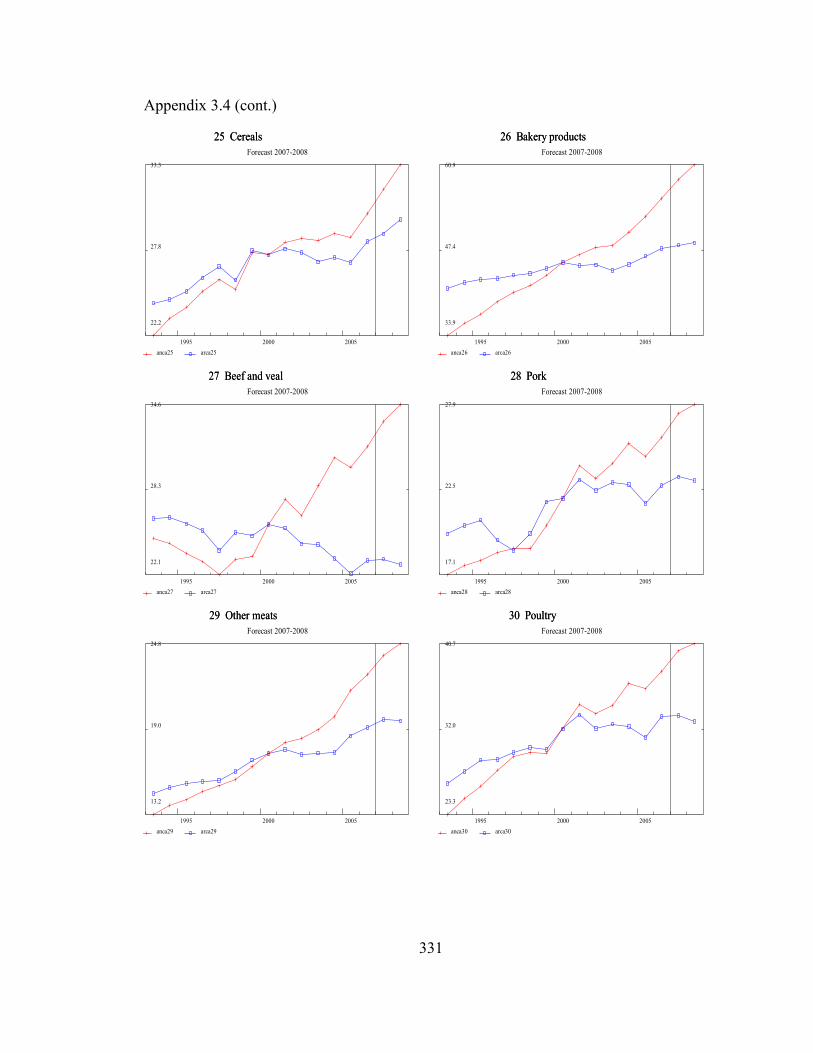
Appendix 3.4 (cont.)
25 Cereals 25 Cereals Forecast 2007-2008
33.3
27.8
22.2
1995 2000 2005 anca25 arca25
26 Bakery products 26 Bakery products Forecast 2007-2008
60.9
47.4
33.9
1995 2000 2005 anca26 arca26
27 Beef and veal 27 Beef and veal Forecast 2007-2008
34.6
28.3
22.1
1995 2000 2005 anca27 arca27
28 Pork 28 Pork Forecast 2007-2008
27.9
22.5
17.1
1995 2000 2005 anca28 arca28
29 Other meats 29 Other meats Forecast 2007-2008
24.8
19.0
13.2
1995 2000 2005 anca29 arca29
30 Poultry 30 Poultry Forecast 2007-2008
40.7
32.0
23.3
1995 2000 2005 anca30 arca30
331

Appendix 3.4 (cont.)
31 Fish and seafood 31 Fish and seafood Forecast 2007-2008
15.22
11.31
7.40
1995 2000 2005 anca31 arca31
32 Eggs 32 Eggs Forecast 2007-2008
7.40
5.34
3.28
1995 2000 2005 anca32 arca32
33 Fresh milk and cream 33 Fresh milk and cream Forecast 2007-2008
20.59
16.49
12.39
1995 2000 2005 anca33 arca33
34 Processed dairy products 34 Processed dairy products Forecast 2007-2008
47.3
35.4
23.5
1995 2000 2005 anca34 arca34
35 Fresh fruits 35 Fresh fruits Forecast 2007-2008
25.3
18.9
12.4
1995 2000 2005 anca35 arca35
36 Fresh vegetables 36 Fresh vegetables Forecast 2007-2008
37.2
26.4
15.6
1995 2000 2005 anca36 arca36
332

Appendix 3.4 (cont.)
37 Processed fruits and vegetables 37 Processed fruits and vegetables Forecast 2007-2008
25.9
20.5
15.2
1995 2000 2005 anca37 arca37
38 Juices and nonalcoholic drinks 38 Juices and nonalcoholic drinks Forecast 2007-2008
80.6
62.1
43.7
1995 2000 2005 anca38 arca38
39 Coffee, tea and beverage materials 39 Coffee, tea and beverage materials Forecast 2007-2008
19.2
12.9
6.6
1995 2000 2005 anca39 arca39
40 Fats and oils 40 Fats and oils Forecast 2007-2008
12.75
10.61
8.47
1995 2000 2005 anca40 arca40
41 Sugar and sweets 41 Sugar and sweets Forecast 2007-2008
42.6
33.9
25.2
1995 2000 2005 anca41 arca41
42 Other foods 42 Other foods Forecast 2007-2008
145.9
99.6
53.3
1995 2000 2005 anca42 arca42
333
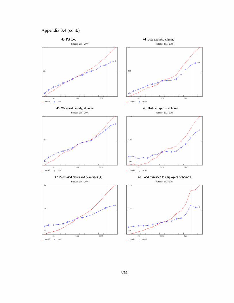
Appendix 3.4 (cont.)
43 Pet food 43 Pet food Forecast 2007-2008
33.5
23.1
12.8
1995 2000 2005 anca43 arca43
44 Beer and ale, at home 44 Beer and ale, at home Forecast 2007-2008
72.2
50.8
29.3
1995 2000 2005 anca44 arca44
45 Wine and brandy, at home 45 Wine and brandy, at home Forecast 2007-2008
21.7
15.7
9.7
1995 2000 2005 anca45 arca45
46 Distilled spirits, at home 46 Distilled spirits, at home Forecast 2007-2008
19.79
15.38
10.97
1995 2000 2005 anca46 arca46
47 Purchased meals and beverages (4) 47 Purchased meals and beverages (4) Forecast 2007-2008
534
396
258
1995 2000 2005 anca47 arca47
48 Food furnished to employees or home g 48 Food furnished to employees or home g Forecast 2007-2008
15.18
11.53
7.89
1995 2000 2005 anca48 arca48
334

Appendix 3.4 (cont.)
49 Shoes (12) 49 Shoes (12) Forecast 2007-2008
61.0
46.2
31.5
1995 2000 2005 anca49 arca49
50 Women's and children's clothing and a 50 Women's and children's clothing and a Forecast 2007-2008
218
164
110
1995 2000 2005 anca50 arca50
51 Men's and boys' clothing and accessor 51 Men's and boys' clothing and accessor Forecast 2007-2008
138.7
102.2
65.7
1995 2000 2005 anca51 arca51
52 Gasoline and oil (75) 52 Gasoline and oil (75) Forecast 2007-2008
335
225
114
1995 2000 2005 anca52 arca52
53 Fuel oil and coal (40) 53 Fuel oil and coal (40) Forecast 2007-2008
24.0
17.1
10.1
1995 2000 2005 anca53 arca53
54 Tobacco products (7) 54 Tobacco products (7) Forecast 2007-2008
101.9
74.6
47.3
1995 2000 2005 anca54 arca54
335

Appendix 3.4 (cont.)
55 Toilet articles and preparations (21) 55 Toilet articles and preparations (21) Forecast 2007-2008
69.0
54.6
40.3
1995 2000 2005 anca55 arca55
56 Semidurable house furnishings (33) 56 Semidurable house furnishings (33) Forecast 2007-2008
72.5
48.1
23.8
1995 2000 2005 anca56 arca56
57 Cleaning, polishing preparations, mis 57 Cleaning, polishing preparations, mis Forecast 2007-2008
90.0
66.7
43.4
1995 2000 2005 anca57 arca57
58 Drug preparations and sundries (45) 58 Drug preparations and sundries (45) Forecast 2007-2008
329
205
81
1995 2000 2005 anca58 arca58
59 Toys, dolls, and games 59 Toys, dolls, and games Forecast 2007-2008
93.3
58.0
22.6
1995 2000 2005 anca59 arca59
60 Sport supplies, including ammunition 60 Sport supplies, including ammunition Forecast 2007-2008
19.9
13.4
6.9
1995 2000 2005 anca60 arca60
336

Appendix 3.4 (cont.)
61 Film and photo supplies 61 Film and photo supplies Forecast 2007-2008
4.93
3.77
2.60
1995 2000 2005 anca61 arca61
62 Stationery and writing supplies (35) 62 Stationery and writing supplies (35) Forecast 2007-2008
23.23
19.30
15.37
1995 2000 2005 anca62 arca62
63 Net foreign remittances (111 less 113 63 Net foreign remittances (111 less 113 Forecast 2007-2008
6.17
3.46
0.74
1995 2000 2005 anca63 arca63
64 Magazines, newspapers, and sheet musi 64 Magazines, newspapers, and sheet musi Forecast 2007-2008
49.8
36.6
23.4
1995 2000 2005 anca64 arca64
65 Flowers, seeds, and potted plants (95 65 Flowers, seeds, and potted plants (95 Forecast 2007-2008
21.16
16.87
12.59
1995 2000 2005 anca65 arca65
66 Housing 66 Housing Forecast 2007-2008
1547
1116
684
1995 2000 2005 anca66 arca66
337

Appendix 3.4 (cont.)
67 Electricity (37) 67 Electricity (37) Forecast 2007-2008
153.6
119.6
85.7
1995 2000 2005 anca67 arca67
68 Gas (38) 68 Gas (38) Forecast 2007-2008
72.7
52.0
31.2
1995 2000 2005 anca68 arca68
69 Water and other sanitary services (39 69 Water and other sanitary services (39 Forecast 2007-2008
72.5
53.0
33.5
1995 2000 2005 anca69 arca69
70 Cellular telephone 70 Cellular telephone Forecast 2007-2008
93.1
48.5
4.0
1995 2000 2005 anca70 arca70
71 Local telephone 71 Local telephone Forecast 2007-2008
52.4
42.7
33.1
1995 2000 2005 anca71 arca71
72 Long distance telephone 72 Long distance telephone Forecast 2007-2008
48.9
33.3
17.6
1995 2000 2005 anca72 arca72
338

Appendix 3.4 (cont.)
73 Domestic service (42) 73 Domestic service (42) Forecast 2007-2008
22.5
17.3
12.1
1995 2000 2005 anca73 arca73
74 Other (43) 74 Other (43) Forecast 2007-2008
71.0
51.2
31.3
1995 2000 2005 anca74 arca74
75 Motor vehicle repair 75 Motor vehicle repair Forecast 2007-2008
164.9
119.8
74.8
1995 2000 2005 anca75 arca75
76 Motor vehicle rental, leasing, and ot 76 Motor vehicle rental, leasing, and ot Forecast 2007-2008
64.2
44.4
24.7
1995 2000 2005 anca76 arca76
77 Bridge, tunnel, ferry, and road tolls 77 Bridge, tunnel, ferry, and road tolls Forecast 2007-2008
7.65
5.39
3.14
1995 2000 2005 anca77 arca77
78 Insurance 78 Insurance Forecast 2007-2008
63.6
47.0
30.4
1995 2000 2005 anca78 arca78
339

Appendix 3.4 (cont.)
79 Mass transit systems (79) 79 Mass transit systems (79) Forecast 2007-2008
12.72
9.70
6.67
1995 2000 2005 anca79 arca79
80 Taxicab (80) 80 Taxicab (80) Forecast 2007-2008
4.50
3.61
2.71
1995 2000 2005 anca80 arca80
81 Railway (82) 81 Railway (82) Forecast 2007-2008
0.71
0.56
0.41
1995 2000 2005 anca81 arca81
82 Bus (83) 82 Bus (83) Forecast 2007-2008
2.51
2.05
1.60
1995 2000 2005 anca82 arca82
83 Airline (84) 83 Airline (84) Forecast 2007-2008
42.1
32.5
22.9
1995 2000 2005 anca83 arca83
84 Other (85) 84 Other (85) Forecast 2007-2008
14.03
9.65
5.26
1995 2000 2005 anca84 arca84
340
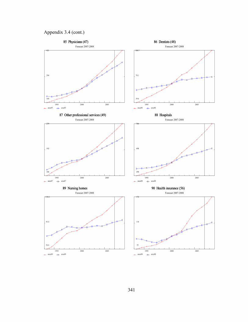
Appendix 3.4 (cont.)
85 Physicians (47) 85 Physicians (47) Forecast 2007-2008
421
294
168
1995 2000 2005 anca85 arca85
86 Dentists (48) 86 Dentists (48) Forecast 2007-2008
100.7
70.1
39.6
1995 2000 2005 anca86 arca86
87 Other professional services (49) 87 Other professional services (49) Forecast 2007-2008
279
192
106
1995 2000 2005 anca87 arca87
88 Hospitals 88 Hospitals Forecast 2007-2008
706
498
290
1995 2000 2005 anca88 arca88
89 Nursing homes 89 Nursing homes Forecast 2007-2008
130.2
93.4
56.6
1995 2000 2005 anca89 arca89
90 Health insurance (56) 90 Health insurance (56) Forecast 2007-2008
172
114
55
1995 2000 2005 anca90 arca90
341

Appendix 3.4 (cont.)
91 Admissions to specified spectator amu 91 Admissions to specified spectator amu Forecast 2007-2008
46.2
32.3
18.5
1995 2000 2005 anca91 arca91
92 Radio and television repair 92 Radio and television repair Forecast 2007-2008
5.57
4.40
3.23
1995 2000 2005 anca92 arca92
93 Clubs and fraternal organizations 93 Clubs and fraternal organizations Forecast 2007-2008
26.05
21.18
16.30
1995 2000 2005 anca93 arca93
94 Commercial participant amusements 94 Commercial participant amusements Forecast 2007-2008
130.5
83.3
36.1
1995 2000 2005 anca94 arca94
95 Pari-mutuel net receipts 95 Pari-mutuel net receipts Forecast 2007-2008
7.22
5.28
3.35
1995 2000 2005 anca95 arca95
96 Other Recreation Services 96 Other Recreation Services Forecast 2007-2008
214
148
82
1995 2000 2005 anca96 arca96
342

Appendix 3.4 (cont.)
97 Cleaning, storage, and repair of clot 97 Cleaning, storage, and repair of clot Forecast 2007-2008
17.33
14.37
11.41
1995 2000 2005 anca97 arca97
98 Barbershops, beauty parlors, and heal 98 Barbershops, beauty parlors, and heal Forecast 2007-2008
56.0
40.1
24.1
1995 2000 2005 anca98 arca98
99 Other Personal Care(19) 99 Other Personal Care(19) Forecast 2007-2008
64.4
41.2
18.1
1995 2000 2005 anca99 arca99
100 Brokerage charges and investment coun 100 Brokerage charges and investment coun Forecast 2007-2008
121.2
71.3
21.4
1995 2000 2005 anca100 arca100
101 Bank service charges, trust services, 101 Bank service charges, trust services, Forecast 2007-2008
130.7
82.3
34.0
1995 2000 2005 anca101 arca101
102 Services furnished w/out payment by i 102 Services furnished w/out payment by i Forecast 2007-2008
237
173
109
1995 2000 2005 anca102 arca102
343
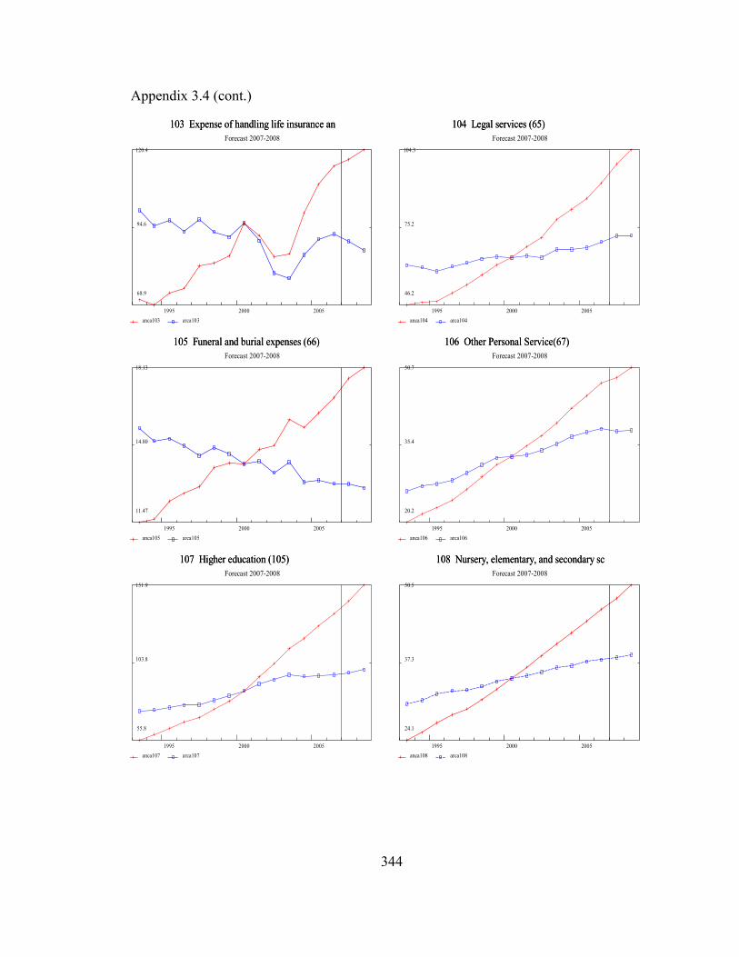
Appendix 3.4 (cont.)
103 Expense of handling life insurance an 103 Expense of handling life insurance an Forecast 2007-2008
120.4
94.6
68.9
1995 2000 2005 anca103 arca103
104 Legal services (65) 104 Legal services (65) Forecast 2007-2008
104.3
75.2
46.2
1995 2000 2005 anca104 arca104
105 Funeral and burial expenses (66) 105 Funeral and burial expenses (66) Forecast 2007-2008
18.13
14.80
11.47
1995 2000 2005 anca105 arca105
106 Other Personal Service(67) 106 Other Personal Service(67) Forecast 2007-2008
50.7
35.4
20.2
1995 2000 2005 anca106 arca106
107 Higher education (105) 107 Higher education (105) Forecast 2007-2008
151.9
103.8
55.8
1995 2000 2005 anca107 arca107
108 Nursery, elementary, and secondary sc 108 Nursery, elementary, and secondary sc Forecast 2007-2008
50.5
37.3
24.1
1995 2000 2005 anca108 arca108
344

Appendix 3.4 (cont.)
109 Other Education (107) 109 Other Education (107) Forecast 2007-2008
71.0
46.3
21.6
1995 2000 2005 anca109 arca109
110 Political organizations 110 Political organizations Forecast 2007-2008
4.62
2.53
0.44
1995 2000 2005 anca110 arca110
111 Museums and libraries 111 Museums and libraries Forecast 2007-2008
11.91
8.00
4.08
1995 2000 2005 anca111 arca111
112 Foundations to religion and welfare 112 Foundations to religion and welfare Forecast 2007-2008
15.46
11.03
6.60
1995 2000 2005 anca112 arca112
113 Social welfare 113 Social welfare Forecast 2007-2008
175
118
62
1995 2000 2005 anca113 arca113
114 Religion 114 Religion Forecast 2007-2008
66.4
49.4
32.4
1995 2000 2005 anca114 arca114
345

Appendix 3.4 (cont.)
115 Foreign travel by U.S. residents (110 115 Foreign travel by U.S. residents (110 Forecast 2007-2008
119.7
84.2
48.8
1995 2000 2005 anca115 arca115
116 Less: Expenditures in the United Stat 116 Less: Expenditures in the United Stat Forecast 2007-2008
118.9
94.7
70.5
1995 2000 2005 anca116 arca116
346

Appendix 3.5: Results
347
Nominal in Billion dollars1995 2000 2005 2006 2007 2008
1 New autos (70) 82.129 103.582 104.007 107.060 107.028 112.3992 Net purchases of used autos (71) 50.505 60.650 57.553 58.044 56.308 57.0193 Other motor vehicles (72) 96.231 173.248 225.431 209.255 219.981 232.2044 Tires, tubes, accessories, and other parts (73) 37.826 49.037 57.941 59.844 61.566 63.9055 Furniture, including mattresses and bedsprings (29) 48.525 67.596 79.871 84.478 86.185 85.8006 Kitchen and other household appliances (30) 26.465 30.410 36.830 38.623 38.889 38.3517 China, glassware, tableware, and utensils (31) 23.371 30.993 36.613 39.768 40.988 40.1378 Video and audio goods, including musical instruments (92) 57.199 72.764 85.776 90.094 90.653 89.8129 Computers and peripherals 18.801 33.514 43.062 46.899 49.330 49.58410 Software 5.501 10.319 13.421 14.521 15.250 15.24311 Floor coverings 12.683 16.483 20.823 23.025 23.085 24.35312 Durable house furnishings, n.e.c. 25.969 36.934 43.652 47.184 48.732 48.15413 Writing equipment 2.496 3.061 3.403 3.619 3.782 3.84014 Hand tools 7.617 10.830 14.776 15.914 16.072 17.00915 Ophthalmic products and orthopedic appliances (46) 14.979 22.116 24.312 26.134 28.352 28.47616 Guns 1.674 2.023 2.587 2.795 2.923 3.01917 Sporting equipment 18.748 25.352 32.415 35.014 36.541 37.42418 Photographic equipment 2.856 3.808 4.336 4.576 4.747 4.89919 Bicycles 2.941 3.789 4.845 5.233 5.469 5.62620 Motorcycles 3.850 7.182 12.501 12.312 12.125 13.85421 Pleasure boats 8.701 14.187 18.003 17.476 18.722 18.89922 Pleasure aircraft 0.902 1.220 1.549 1.503 1.624 1.65823 Jewelry and watches (18) 38.421 50.568 58.366 62.155 64.439 65.75624 Books and maps (87) 23.212 33.655 41.808 43.394 44.891 47.50225 Cereals 24.018 27.448 28.615 30.150 31.747 33.33426 Bakery products 37.275 45.467 52.771 55.603 58.660 60.92827 Beef and veal 23.617 25.770 30.001 31.509 33.363 34.63728 Pork 18.024 21.923 24.567 25.799 27.282 27.87329 Other meats 14.153 17.297 21.632 22.718 24.005 24.82530 Poultry 26.173 32.013 36.102 37.916 39.998 40.73031 Fish and seafood 7.550 10.401 13.019 13.675 14.601 15.21832 Eggs 4.066 5.705 6.157 6.488 6.933 7.20633 Fresh milk and cream 13.096 13.916 17.656 18.603 19.660 20.59334 Processed dairy products 24.807 29.712 40.710 42.895 45.473 47.26635 Fresh fruits 13.289 16.789 21.310 22.454 23.941 25.34136 Fresh vegetables 18.037 25.146 31.574 33.268 35.504 37.17537 Processed fruits and vegetables 15.857 19.179 22.533 23.742 24.958 25.89038 Juices and nonalcoholic drinks 43.969 48.932 67.819 71.459 75.857 80.57939 Coffee, tea and beverage materials 8.394 11.647 16.142 17.008 18.126 19.20540 Fats and oils 8.664 9.519 11.106 11.702 12.348 12.75241 Sugar and sweets 26.949 32.153 37.189 39.185 41.434 42.60042 Other foods 60.596 81.186 121.125 128.056 137.033 145.86443 Pet food 15.517 21.315 27.688 29.408 31.489 33.47744 Beer and ale, at home 32.629 43.053 59.354 64.099 69.106 72.20145 Wine and brandy, at home 10.966 14.763 17.981 19.336 20.765 21.68546 Distilled spirits, at home 10.966 13.363 16.198 17.525 18.929 19.79147 Purchased meals and beverages (4) 273.969 348.809 450.221 482.364 510.549 534.39448 Food furnished to employees or home grown 8.271 9.659 12.356 14.315 14.523 15.17549 Shoes (12) 37.582 47.026 55.092 58.153 59.431 61.02650 Women's and children's clothing and accessories except shoes (14) 129.484 156.692 179.757 187.730 195.526 198.27351 Men's and boys' clothing and accessories except shoes (15+16) 74.656 93.993 106.898 111.350 116.008 117.91852 Gasoline and oil (75) 120.213 175.656 280.688 318.570 327.261 335.46053 Fuel oil and coal (40) 13.074 15.826 21.144 21.565 24.039 23.50054 Tobacco products (7) 49.205 78.543 89.693 92.362 96.201 101.89155 Toilet articles and preparations (21) 45.934 55.016 61.097 63.804 67.216 68.97356 Semidurable house furnishings (33) 29.410 36.465 43.216 45.401 46.651 47.99457 Cleaning, polishing preparations, misc. supplies and paper products 48.794 61.587 77.087 81.255 85.017 89.97658 Drug preparations and sundries (45) 92.133 169.412 265.213 285.979 302.269 328.67459 Toys, dolls, and games 32.298 41.510 47.685 51.110 54.019 57.35760 Sport supplies, including ammunition 8.867 11.793 15.078 16.287 16.956 17.75661 Film and photo supplies 3.186 3.308 3.766 3.975 4.129 4.38062 Stationery and writing supplies (35) 16.330 18.982 19.629 20.959 22.307 22.90763 Net foreign remittances (111 less 113) 1.554 3.220 5.025 5.308 5.529 6.17164 Magazines, newspapers, and sheet music (88) 27.525 35.048 42.132 45.043 47.908 49.79165 Flowers, seeds, and potted plants (95) 13.970 17.974 19.154 19.903 20.165 21.16366 Housing 764.386 1006.456 1298.688 1381.341 1465.163 1547.47867 Electricity (37) 90.958 102.348 133.409 146.341 152.657 153.56868 Gas (38) 31.245 40.953 65.334 63.494 67.245 72.74569 Water and other sanitary services (39) 39.337 50.816 63.295 66.397 69.559 72.49570 Cellular telephone 11.274 30.187 58.052 65.121 72.530 79.70871 Local telephone 35.988 48.893 50.771 49.639 49.665 48.63672 Long distance telephone 37.765 45.988 25.505 22.818 21.504 17.62873 Domestic service (42) 13.767 17.350 19.854 20.696 21.685 22.50274 Other (43) 38.413 53.576 64.799 67.111 68.747 71.04475 Motor vehicle repair 89.030 119.334 143.124 149.346 157.610 164.86176 Motor vehicle rental, leasing, and other 36.444 64.160 55.247 59.074 62.765 63.77377 Bridge, tunnel, ferry, and road tolls 3.663 5.076 6.513 6.910 7.233 7.64878 Insurance 34.495 43.033 57.803 60.131 61.209 63.61779 Mass transit systems (79) 7.148 9.087 10.679 11.507 12.030 12.72380 Taxicab (80) 2.989 3.139 3.947 4.156 4.311 4.502

348
Nominal in Billion dollars (cont.)1995 2000 2005 2006 2007 2008
81 Railway (82) 0.410 0.518 0.578 0.639 0.698 0.71282 Bus (83) 1.826 2.376 2.175 2.170 2.043 2.13683 Airline (84) 25.278 36.724 34.374 35.624 36.246 38.24384 Other (85) 6.390 7.807 9.803 11.040 12.710 14.03085 Physicians (47) 184.635 236.836 344.570 366.337 394.594 421.26686 Dentists (48) 45.389 61.827 85.186 90.303 95.419 100.68287 Other professional services (49) 126.596 161.577 230.928 246.131 260.973 278.80188 Hospitals 314.344 395.998 579.725 618.012 658.959 706.46889 Nursing homes 66.171 86.599 110.936 117.800 123.638 130.20990 Health insurance (56) 60.716 83.975 141.277 149.150 158.026 172.43391 Admissions to specified spectator amusements (96) 21.099 30.400 38.704 39.877 41.959 46.16092 Radio and television repair 3.553 4.172 4.782 5.353 5.424 5.56693 Clubs and fraternal organizations 17.394 19.026 23.714 23.907 24.803 26.05294 Commercial participant amusements 48.815 75.812 106.759 115.302 121.539 130.54695 Pari-mutuel net receipts 3.702 4.986 6.164 6.580 6.882 7.21896 Other Recreation Services 93.357 133.868 178.687 189.966 202.372 214.22197 Cleaning, storage, and repair of clothing and shoes (17) 12.297 15.737 16.057 16.919 17.032 17.33098 Barbershops, beauty parlors, and health clubs (22) 26.847 38.356 50.812 51.875 54.130 56.02299 Other Personal Care(19) 22.053 32.936 47.945 54.815 59.371 64.374100 Brokerage charges and investment counseling (61) 43.464 100.582 92.712 104.177 117.008 121.192101 Bank service charges, trust services, and safe deposit box rental 37.190 64.244 99.244 108.034 118.532 130.668102 Services furnished w/out payment by intermediaries except life ins. carriers 113.260 167.223 203.446 208.512 222.873 237.366103 Expense of handling life insurance and pension plans (64) 72.890 96.078 108.867 114.923 117.127 120.373104 Legal services (65) 47.354 63.854 85.985 91.832 98.980 104.323105 Funeral and burial expenses (66) 12.377 13.977 16.174 16.847 17.646 18.135106 Other Personal Service(67) 23.026 33.140 45.048 47.583 48.640 50.650107 Higher education (105) 62.906 86.358 126.422 134.117 142.089 151.866108 Nursery, elementary, and secondary schools (106) 26.995 34.618 44.360 46.382 48.179 50.497109 Other Education (107) 24.445 42.795 55.095 59.141 66.359 70.978110 Political organizations 0.615 4.290 0.873 3.982 1.770 4.344111 Museums and libraries 5.103 7.533 9.398 10.094 11.178 11.909112 Foundations to religion and welfare 7.324 9.334 13.088 13.976 14.463 15.458113 Social welfare 70.862 105.218 144.267 152.281 163.544 175.053114 Religion 36.453 45.909 57.485 61.001 63.533 66.364115 Foreign travel by U.S. residents (110) 54.711 84.415 99.985 108.650 116.469 119.671116 Less: Expenditures in the United States by nonresidents (112) 77.626 100.658 104.883 109.862 118.911 117.404

349
Chained Real 2000 in Billion dollars 1995 2000 2005 2006 2007 2008
1 New autos (70) 82.165 103.583 107.508 109.673 109.917 114.9132 Net purchases of used autos (71) 52.814 60.638 56.976 56.494 56.104 55.8273 Other motor vehicles (72) 99.823 173.261 233.248 217.693 232.805 247.4664 Tires, tubes, accessories, and other parts (73) 37.157 49.038 53.553 53.174 52.918 52.2555 Furniture, including mattresses and bedsprings (29) 48.735 67.595 85.238 89.408 91.146 90.3456 Kitchen and other household appliances (30) 25.105 30.413 39.226 40.196 39.198 37.9877 China, glassware, tableware, and utensils (31) 22.534 30.992 41.058 46.299 48.451 47.9298 Video and audio goods, including musical instruments (92) 45.924 72.771 117.976 134.646 151.117 167.2959 Computers and peripherals 3.065 33.504 138.431 178.353 213.081 272.40210 Software 1.890 10.319 19.460 22.413 25.062 30.05411 Floor coverings 13.746 16.483 19.422 20.577 20.293 21.10812 Durable house furnishings, n.e.c. 23.868 36.947 54.919 64.632 71.299 76.72913 Writing equipment 3.223 3.061 2.605 2.605 2.537 2.43814 Hand tools 7.497 10.830 14.778 15.741 15.753 16.34715 Ophthalmic products and orthopedic appliances (46) 16.350 22.116 22.302 23.279 24.756 24.68416 Guns 1.475 2.023 2.802 3.065 3.241 3.41017 Sporting equipment 16.525 25.352 35.108 38.404 40.504 42.26818 Photographic equipment 2.631 3.808 6.825 8.276 10.782 13.59319 Bicycles 3.042 3.789 4.761 4.965 5.211 5.32720 Motorcycles 4.247 7.182 12.103 11.980 12.049 13.61321 Pleasure boats 8.999 14.187 17.703 16.574 17.840 17.89522 Pleasure aircraft 0.933 1.220 1.523 1.426 1.547 1.57023 Jewelry and watches (18) 32.571 50.565 62.683 65.162 64.034 63.75624 Books and maps (87) 24.547 33.654 40.529 42.338 43.446 46.01425 Cereals 25.050 27.448 26.963 28.316 28.814 29.75526 Bakery products 42.782 45.467 46.448 47.680 48.218 48.56427 Beef and veal 25.799 25.770 22.166 23.093 23.220 22.82128 Pork 20.578 21.923 21.630 22.772 23.292 23.09329 Other meats 15.287 17.297 18.528 19.113 19.613 19.54630 Poultry 28.811 32.011 31.145 33.297 33.422 32.77931 Fish and seafood 8.188 10.401 12.384 12.421 12.696 13.14332 Eggs 4.458 5.704 5.638 5.664 4.974 4.92233 Fresh milk and cream 15.546 13.915 14.979 15.979 15.629 15.64934 Processed dairy products 29.705 29.712 36.654 38.730 40.135 41.85835 Fresh fruits 14.802 16.786 18.512 18.401 18.785 19.69036 Fresh vegetables 20.312 25.139 25.511 25.678 26.367 26.51737 Processed fruits and vegetables 17.790 19.179 19.921 20.405 20.795 20.96838 Juices and nonalcoholic drinks 45.381 48.933 64.768 66.699 68.369 72.20039 Coffee, tea and beverage materials 8.531 11.647 15.434 16.006 16.512 17.70340 Fats and oils 9.155 9.519 9.762 10.269 10.602 10.71541 Sugar and sweets 29.922 32.154 34.668 35.185 36.248 36.57542 Other foods 68.453 81.187 114.315 119.248 124.757 129.79543 Pet food 16.832 21.315 25.591 26.051 27.181 27.81844 Beer and ale, at home 35.504 43.053 52.778 56.436 58.633 59.08045 Wine and brandy, at home 12.324 14.763 17.448 18.351 19.403 19.82546 Distilled spirits, at home 12.194 13.363 14.815 15.829 16.889 17.33047 Purchased meals and beverages (4) 310.774 348.812 391.544 406.654 416.042 421.57748 Food furnished to employees or home grown 9.150 9.659 10.831 12.166 11.913 11.94449 Shoes (12) 35.372 47.026 55.623 58.282 60.303 60.57250 Women's and children's clothing and accessories except shoes (14) 118.690 156.695 197.672 206.523 215.672 217.54951 Men's and boys' clothing and accessories except shoes (15+16) 73.314 94.006 119.530 126.546 134.596 138.69152 Gasoline and oil (75) 154.454 175.666 186.188 186.762 162.342 129.78053 Fuel oil and coal (40) 18.700 15.799 13.306 11.958 12.342 10.10854 Tobacco products (7) 85.453 78.543 70.452 70.164 68.609 69.90255 Toilet articles and preparations (21) 47.933 55.016 61.051 63.203 65.460 66.76256 Semidurable house furnishings (33) 26.484 36.461 52.891 59.640 65.994 72.45757 Cleaning, polishing preparations, misc. supplies and paper products 54.505 61.594 73.230 74.090 76.107 78.89058 Drug preparations and sundries (45) 105.602 169.342 223.810 232.195 242.796 257.71559 Toys, dolls, and games 26.733 41.509 64.874 72.842 80.932 93.25560 Sport supplies, including ammunition 7.815 11.793 16.331 17.864 18.757 19.89761 Film and photo supplies 2.992 3.308 4.137 4.493 4.669 4.93262 Stationery and writing supplies (35) 17.838 18.982 20.595 21.712 22.775 23.23163 Net foreign remittances (111 less 113) 0.908 3.219 2.907 2.750 2.277 2.55164 Magazines, newspapers, and sheet music (88) 30.791 35.047 37.689 39.663 41.828 42.68965 Flowers, seeds, and potted plants (95) 13.541 17.970 18.080 18.635 18.750 19.56066 Housing 887.505 1006.385 1118.238 1148.264 1174.386 1202.51667 Electricity (37) 90.172 102.338 112.998 110.563 110.616 100.52568 Gas (38) 40.394 40.987 40.802 38.700 39.529 39.24869 Water and other sanitary services (39) 45.153 50.815 51.430 51.417 51.391 51.03970 Cellular telephone 7.228 30.180 67.629 76.327 85.181 93.09471 Local telephone 39.397 48.892 42.537 40.747 39.376 37.49272 Long distance telephone 35.480 45.991 35.211 31.044 27.797 22.90473 Domestic service (42) 16.049 17.352 17.024 17.133 17.232 17.27974 Other (43) 44.285 53.578 53.097 52.975 52.856 52.64775 Motor vehicle repair 101.722 119.334 122.712 122.878 125.266 125.83676 Motor vehicle rental, leasing, and other 37.784 64.161 52.987 55.699 58.946 59.69077 Bridge, tunnel, ferry, and road tolls 4.404 5.076 5.207 5.367 5.416 5.47778 Insurance 40.213 43.034 44.152 44.268 44.620 44.81679 Mass transit systems (79) 7.865 9.087 8.545 8.906 9.085 9.24680 Taxicab (80) 3.372 3.139 3.158 3.217 3.255 3.262

350
Chained Real 2000 in Billion dollars 1995 2000 2005 2006 2007 2008
81 Railway (82) 0.478 0.518 0.582 0.592 0.637 0.66782 Bus (83) 2.109 2.376 1.829 1.702 1.598 1.61483 Airline (84) 27.182 36.730 40.502 39.696 40.393 42.11384 Other (85) 7.352 7.806 9.471 10.229 11.652 12.51985 Physicians (47) 200.126 236.837 317.668 334.740 346.453 363.35886 Dentists (48) 56.689 61.828 67.975 68.492 69.142 69.74287 Other professional services (49) 142.259 161.565 204.402 213.694 221.403 232.12388 Hospitals 353.295 395.951 473.488 484.599 497.875 508.68189 Nursing homes 80.733 86.598 91.009 93.782 95.548 97.32990 Health insurance (56) 73.734 83.966 105.829 108.441 110.857 115.03591 Admissions to specified spectator amusements (96) 26.150 30.397 31.732 31.566 31.758 33.58792 Radio and television repair 3.818 4.172 4.638 5.173 5.312 5.43293 Clubs and fraternal organizations 19.972 19.026 21.871 21.374 21.427 21.95894 Commercial participant amusements 55.677 75.799 93.484 97.719 99.800 103.11495 Pari-mutuel net receipts 4.172 4.986 5.443 5.629 5.688 5.74296 Other Recreation Services 109.400 133.858 154.562 160.048 169.972 174.56097 Cleaning, storage, and repair of clothing and shoes (17) 13.583 15.738 13.765 13.993 13.603 13.37798 Barbershops, beauty parlors, and health clubs (22) 31.331 38.354 44.404 44.080 44.565 44.93299 Other Personal Care(19) 24.434 32.934 40.399 44.252 46.058 47.703100 Brokerage charges and investment counseling (61) 28.088 100.571 99.483 108.466 115.896 106.274101 Bank service charges, trust services, and safe deposit box rental 48.732 64.239 88.009 93.184 98.038 105.442102 Services furnished w/out payment by intermediaries except life ins. carriers 129.716 167.396 183.064 185.743 198.836 208.161103 Expense of handling life insurance and pension plans (64) 96.991 96.078 90.701 92.476 89.971 87.012104 Legal services (65) 58.807 63.854 67.626 69.821 71.975 72.206105 Funeral and burial expenses (66) 15.068 13.977 13.275 13.149 13.139 12.948106 Other Personal Service(67) 27.784 33.139 37.925 38.594 38.097 38.296107 Higher education (105) 75.962 86.350 95.743 96.307 97.525 99.308108 Nursery, elementary, and secondary schools (106) 31.930 34.616 37.500 37.811 38.205 38.647109 Other Education (107) 30.380 42.782 41.867 42.780 46.189 46.770110 Political organizations 0.710 4.291 0.782 3.444 1.490 3.572111 Museums and libraries 5.960 7.533 8.421 8.745 9.399 9.811112 Foundations to religion and welfare 8.886 9.334 11.017 11.270 11.523 11.895113 Social welfare 82.865 105.197 125.059 127.220 132.100 136.234114 Religion 44.130 45.909 48.387 48.799 49.264 49.552115 Foreign travel by U.S. residents (110) 57.545 84.418 79.617 84.784 87.170 85.119116 Less: Expenditures in the United States by nonresidents (112) 88.903 100.667 92.200 92.339 95.811 89.214

351
Chained 2000 Price index [2000=100] 1995 2000 2005 2006 2007 2008
1 New autos (70) 99.95 100.00 96.75 97.62 97.37 97.812 Net purchases of used autos (71) 95.64 100.00 101.04 102.75 100.37 102.133 Other motor vehicles (72) 96.38 100.00 96.64 96.13 94.49 93.834 Tires, tubes, accessories, and other parts (73) 101.80 100.00 108.19 112.56 116.35 122.305 Furniture, including mattresses and bedsprings (29) 99.56 100.00 93.71 94.49 94.56 94.976 Kitchen and other household appliances (30) 105.42 100.00 93.89 96.09 99.22 100.967 China, glassware, tableware, and utensils (31) 103.74 100.00 89.21 85.91 84.60 83.748 Video and audio goods, including musical instruments (92) 124.62 100.00 72.76 66.97 60.02 53.749 Computers and peripherals 621.82 100.00 31.23 26.36 23.24 18.2910 Software 295.02 100.00 69.00 64.84 60.93 50.8811 Floor coverings 92.27 100.00 107.19 111.93 113.75 115.3712 Durable house furnishings, n.e.c. 108.79 100.00 79.56 73.04 68.38 62.8013 Writing equipment 77.43 100.00 130.62 138.93 149.11 157.5514 Hand tools 101.59 100.00 99.98 101.10 102.03 104.0415 Ophthalmic products and orthopedic appliances (46) 91.62 100.00 109.00 112.27 114.53 115.3616 Guns 113.47 100.00 92.33 91.18 90.22 88.5417 Sporting equipment 113.47 100.00 92.33 91.18 90.22 88.5418 Photographic equipment 108.56 100.00 63.58 55.51 44.16 36.2319 Bicycles 96.69 100.00 101.76 105.42 104.96 105.6020 Motorcycles 90.65 100.00 103.30 102.77 100.62 101.7621 Pleasure boats 96.70 100.00 101.76 105.42 104.96 105.6022 Pleasure aircraft 96.70 100.00 101.76 105.42 104.96 105.6023 Jewelry and watches (18) 117.97 100.00 93.12 95.40 100.64 103.1324 Books and maps (87) 94.56 100.00 103.16 102.49 103.32 103.2425 Cereals 95.88 100.00 106.13 106.47 110.18 112.0226 Bakery products 87.13 100.00 113.61 116.61 121.66 125.4627 Beef and veal 91.54 100.00 135.36 136.45 143.71 151.7828 Pork 87.61 100.00 113.59 113.29 117.14 120.7029 Other meats 92.59 100.00 116.74 118.86 122.39 127.0130 Poultry 90.84 100.00 115.92 113.87 119.73 124.2631 Fish and seafood 92.22 100.00 105.13 110.08 115.01 115.7932 Eggs 91.47 100.00 109.32 114.55 139.44 146.4133 Fresh milk and cream 84.24 100.00 117.87 116.45 125.92 131.5934 Processed dairy products 83.51 100.00 111.06 110.76 113.30 112.9235 Fresh fruits 89.82 100.00 115.12 122.03 127.46 128.6936 Fresh vegetables 88.91 100.00 123.86 129.56 134.65 140.1937 Processed fruits and vegetables 89.13 100.00 113.08 116.35 120.02 123.4738 Juices and nonalcoholic drinks 96.89 100.00 104.69 107.13 110.95 111.6039 Coffee, tea and beverage materials 98.54 100.00 104.57 106.25 109.78 108.4840 Fats and oils 94.65 100.00 113.76 113.96 116.47 119.0041 Sugar and sweets 90.07 100.00 107.28 111.36 114.31 116.4742 Other foods 88.52 100.00 105.94 107.39 109.83 112.3743 Pet food 92.19 100.00 108.19 112.88 115.84 120.3444 Beer and ale, at home 91.90 100.00 112.46 113.58 117.83 122.2245 Wine and brandy, at home 88.98 100.00 103.04 105.36 107.01 109.3846 Distilled spirits, at home 89.93 100.00 109.33 110.71 112.06 114.2047 Purchased meals and beverages (4) 88.16 100.00 114.98 118.61 122.71 126.7648 Food furnished to employees or home grown 90.40 100.00 114.06 117.64 121.91 127.0549 Shoes (12) 106.25 100.00 99.04 99.78 98.56 100.7550 Women's and children's clothing and accessories except shoes (14) 109.10 100.00 90.95 90.90 90.67 91.1451 Men's and boys' clothing and accessories except shoes (15+16) 101.83 100.00 89.45 87.99 86.19 85.0352 Gasoline and oil (75) 77.83 100.00 150.84 170.50 207.26 258.6853 Fuel oil and coal (40) 69.90 100.00 159.61 180.35 196.95 232.5454 Tobacco products (7) 57.58 100.00 127.31 131.64 140.21 145.7555 Toilet articles and preparations (21) 95.83 100.00 100.07 100.95 102.68 103.3156 Semidurable house furnishings (33) 111.05 100.00 81.77 76.17 70.74 66.2657 Cleaning, polishing preparations, misc. supplies and paper products 89.52 100.00 105.26 109.67 111.70 114.0558 Drug preparations and sundries (45) 87.24 100.00 118.50 123.15 124.49 127.5259 Toys, dolls, and games 120.83 100.00 73.53 70.18 66.80 61.5760 Sport supplies, including ammunition 113.47 100.00 92.33 91.18 90.40 89.2561 Film and photo supplies 106.48 100.00 91.04 88.49 88.43 88.8262 Stationery and writing supplies (35) 91.55 100.00 95.31 96.52 97.95 98.6063 Net foreign remittances (111 less 113) 173.90 100.00 173.35 196.79 247.52 241.8964 Magazines, newspapers, and sheet music (88) 89.39 100.00 111.78 113.56 114.53 116.6365 Flowers, seeds, and potted plants (95) 103.17 100.00 105.93 106.80 107.55 108.1966 Housing 86.12 100.00 116.13 120.29 124.75 128.6867 Electricity (37) 100.86 100.00 118.02 132.35 138.06 152.8268 Gas (38) 77.40 100.00 160.34 164.48 170.20 185.3469 Water and other sanitary services (39) 87.12 100.00 123.07 129.14 135.35 142.0470 Cellular telephone 156.31 100.00 85.85 85.32 85.15 85.6171 Local telephone 91.35 100.00 119.37 121.82 126.14 129.7472 Long distance telephone 106.44 100.00 72.42 73.53 77.39 76.9473 Domestic service (42) 85.78 100.00 116.63 120.80 125.84 130.2374 Other (43) 86.74 100.00 122.03 126.69 130.07 134.9575 Motor vehicle repair 87.51 100.00 116.64 121.53 125.82 131.0176 Motor vehicle rental, leasing, and other 96.45 100.00 104.25 106.06 106.49 106.8477 Bridge, tunnel, ferry, and road tolls 83.17 100.00 125.06 128.73 133.54 139.6478 Insurance 85.78 100.00 130.92 135.83 137.18 141.9579 Mass transit systems (79) 90.89 100.00 124.96 129.19 132.41 137.6080 Taxicab (80) 88.66 100.00 124.96 129.20 132.47 137.98

352
Chained 2000 Price index [2000=100] 1995 2000 2005 2006 2007 2008
81 Railway (82) 85.83 100.00 99.76 108.03 109.91 106.8582 Bus (83) 86.56 100.00 118.93 127.57 127.86 132.3583 Airline (84) 92.99 100.00 84.89 89.75 89.72 90.8184 Other (85) 86.91 100.00 103.49 107.94 109.06 112.0585 Physicians (47) 92.26 100.00 108.46 109.43 113.89 115.9386 Dentists (48) 80.07 100.00 125.32 131.84 138.00 144.3687 Other professional services (49) 88.99 100.00 112.97 115.17 117.87 120.1088 Hospitals 88.97 100.00 122.42 127.53 132.35 138.8789 Nursing homes 81.95 100.00 121.88 125.61 129.39 133.7890 Health insurance (56) 82.37 100.00 133.48 137.54 142.53 149.8791 Admissions to specified spectator amusements (96) 80.65 100.00 121.97 126.34 132.11 137.4292 Radio and television repair 93.02 100.00 103.11 103.49 102.10 102.4693 Clubs and fraternal organizations 87.10 100.00 108.42 111.85 115.75 118.6494 Commercial participant amusements 87.66 100.00 114.19 117.98 121.78 126.5995 Pari-mutuel net receipts 88.75 100.00 113.23 116.89 121.00 125.7196 Other Recreation Services 85.33 100.00 115.60 118.69 119.05 122.7197 Cleaning, storage, and repair of clothing and shoes (17) 90.53 100.00 116.65 120.91 125.22 129.5698 Barbershops, beauty parlors, and health clubs (22) 85.68 100.00 114.43 117.69 121.46 124.6899 Other Personal Care(19) 90.25 100.00 118.66 123.83 128.90 134.93100 Brokerage charges and investment counseling (61) 154.64 100.00 93.18 96.04 100.98 114.08101 Bank service charges, trust services, and safe deposit box rental 76.31 100.00 112.76 115.93 120.87 123.91102 Services furnished w/out payment by intermediaries except life ins. carriers 87.31 100.00 111.14 112.25 112.09 114.02103 Expense of handling life insurance and pension plans (64) 75.15 100.00 119.99 124.28 130.32 138.36104 Legal services (65) 80.52 100.00 127.15 131.50 137.53 144.47105 Funeral and burial expenses (66) 82.14 100.00 121.85 128.11 134.32 140.06106 Other Personal Service(67) 82.87 100.00 118.77 123.29 127.68 132.25107 Higher education (105) 82.81 100.00 132.04 139.25 145.69 152.91108 Nursery, elementary, and secondary schools (106) 84.54 100.00 118.29 122.66 126.10 130.66109 Other Education (107) 80.46 100.00 131.60 138.22 143.64 151.76110 Political organizations 86.81 100.00 112.10 115.30 118.39 121.75111 Museums and libraries 85.60 100.00 111.60 115.40 118.92 121.37112 Foundations to religion and welfare 82.43 100.00 118.80 124.00 125.51 129.94113 Social welfare 85.51 100.00 115.35 119.69 123.79 128.49114 Religion 82.60 100.00 118.80 125.00 128.96 133.93115 Foreign travel by U.S. residents (110) 95.09 100.00 125.59 128.14 133.62 140.59116 Less: Expenditures in the United States by nonresidents (112) 87.29 100.00 113.77 118.97 124.15 131.60

Appendix 4.1: Estimation Results for Nominal Value of annual Fixed Asset Accounts by Purchasing Industries
: Farms SEE = 1716.01 RSQ = 0.9213 RHO = 0.29 Obser = 32 from 1975.000 SEE+1 = 1651.39 RBSQ = 0.9158 DurH = 2.68 DoFree = 29 to 2006.000 MAPE = 10.00 Variable name Reg-Coef Mexval Elas NorRes Mean Beta 0 vein1 - - - - - - - - - - - - - - - - - 16385.84 - - - 1 intercept 1297.25037 3.2 0.08 12.70 1.00 2 vein1[1] 0.67477 34.1 0.65 1.21 15756.44 0.646 3 vennot 0.05031 10.0 0.27 1.00 88589.03 0.331
: Forestry, fishing, and related activities SEE = 232.05 RSQ = 0.8695 RHO = -0.24 Obser = 32 from 1975.000 SEE+1 = 224.55 RBSQ = 0.8555 DurH = -1.54 DoFree = 28 to 2006.000 MAPE = 9.76 Variable name Reg-Coef Mexval Elas NorRes Mean Beta 0 vein2 - - - - - - - - - - - - - - - - - 1984.97 - - - 1 intercept 241.97384 4.8 0.12 7.66 1.00 2 vein2[1] 0.78192 99.0 0.75 1.66 1891.81 0.749 3 vennot 0.01774 28.3 0.79 1.53 88589.03 1.113 4 venntr -0.01429 23.9 -0.66 1.00 91518.56 -0.971
: Oil and gas extraction SEE = 1285.42 RSQ = 0.5967 RHO = 0.05 Obser = 32 from 1975.000 SEE+1 = 1284.10 RBSQ = 0.5688 DurH = 0.35 DoFree = 29 to 2006.000 MAPE = 21.68 Variable name Reg-Coef Mexval Elas NorRes Mean Beta 0 vein3 - - - - - - - - - - - - - - - - - 4719.94 - - - 1 vein3[1] 0.75240 70.2 0.73 1.27 4565.69 2 venn1 -0.06457 7.8 -0.66 1.22 48312.88 -0.978 3 venntr 0.04787 10.6 0.93 1.00 91518.56 1.032
: Mining, except oil and gas SEE = 696.75 RSQ = 0.8776 RHO = 0.03 Obser = 32 from 1975.000 SEE+1 = 696.44 RBSQ = 0.8595 DurH = 999.00 DoFree = 27 to 2006.000 MAPE = 11.88 Variable name Reg-Coef Mexval Elas NorRes Mean Beta 0 vein4 - - - - - - - - - - - - - - - - - 4973.12 - - - 1 vein4[1] 1.02771 56.1 0.97 1.99 4675.16 2 vein4[2] -0.59061 18.4 -0.52 1.71 4398.78 -0.437 3 vennot 0.06979 20.5 1.24 1.29 88589.03 1.412 4 vennin -0.02242 4.9 -0.45 1.25 98784.19 -0.457 5 venn2 -0.01643 11.6 -0.24 1.00 73834.41 -0.552
: Support activities for mining SEE = 713.61 RSQ = 0.8448 RHO = 0.02 Obser = 32 from 1975.000 SEE+1 = 713.60 RBSQ = 0.8341 DurH = 0.14 DoFree = 29 to 2006.000 MAPE = 16.94 Variable name Reg-Coef Mexval Elas NorRes Mean Beta 0 vein5 - - - - - - - - - - - - - - - - - 3842.72 - - - 1 vein5[1] 0.65554 51.1 0.61 1.88 3570.94 2 vennoit -0.03850 21.9 -1.02 1.75 101376.84 -1.096 3 vennot 0.06154 32.1 1.42 1.00 88589.03 1.369
: Utilities SEE = 2122.46 RSQ = 0.9396 RHO = 0.03 Obser = 32 from 1975.000
353

SEE+1 = 2122.62 RBSQ = 0.9306 DurH = 0.35 DoFree = 27 to 2006.000 MAPE = 7.92 Variable name Reg-Coef Mexval Elas NorRes Mean Beta 0 vein6 - - - - - - - - - - - - - - - - - 24278.19 - - - 1 intercept 1945.04855 2.9 0.08 16.54 1.00 2 vein6[1] 0.98572 48.2 0.95 1.41 23352.25 1.009 3 vein6[2] -0.29552 6.1 -0.27 1.33 22471.12 -0.311 4 venn2 -0.02275 1.8 -0.07 1.17 73834.41 -0.177 5 vennoit 0.07531 7.9 0.31 1.00 101376.84 0.450
: Construction SEE = 2060.42 RSQ = 0.9711 RHO = 0.24 Obser = 32 from 1975.000 SEE+1 = 2006.49 RBSQ = 0.9680 DurH = 3.61 DoFree = 28 to 2006.000 MAPE = 16.57 Variable name Reg-Coef Mexval Elas NorRes Mean Beta 0 vein7 - - - - - - - - - - - - - - - - - 15947.72 - - - 1 vein7[1] 0.53009 17.1 0.49 1.52 14812.38 2 venn2 0.12943 17.4 0.60 1.48 73834.41 0.715 3 vennoit -0.23962 15.0 -1.52 1.39 101376.84 -1.019 4 vennin 0.23283 17.9 1.44 1.00 98784.19 0.779
: Wood products SEE = 164.76 RSQ = 0.9285 RHO = -0.00 Obser = 32 from 1975.000 SEE+1 = 164.76 RBSQ = 0.9208 DurH = -0.04 DoFree = 28 to 2006.000 MAPE = 7.49 Variable name Reg-Coef Mexval Elas NorRes Mean Beta 0 vein8 - - - - - - - - - - - - - - - - - 1875.53 - - - 1 vein8[1] 0.44638 11.0 0.43 2.62 1819.00 2 vein8[2] -0.34171 12.4 -0.32 2.44 1759.47 -0.348 3 vennoit -0.01874 35.6 -1.01 2.23 101376.84 -1.569 4 vennin 0.03605 49.5 1.90 1.00 98784.19 2.375
: Nonmetallic mineral products SEE = 320.30 RSQ = 0.9054 RHO = 0.31 Obser = 32 from 1975.000 SEE+1 = 305.04 RBSQ = 0.8989 DurH = 2.43 DoFree = 29 to 2006.000 MAPE = 9.74 Variable name Reg-Coef Mexval Elas NorRes Mean Beta 0 vein9 - - - - - - - - - - - - - - - - - 3199.81 - - - 1 intercept 426.04007 8.5 0.13 10.57 1.00 2 vein9[1] 0.52221 27.1 0.50 1.47 3089.38 0.522 3 vennin 0.01175 21.4 0.36 1.00 98784.19 0.458
: Primary metals SEE = 608.36 RSQ = 0.5813 RHO = 0.03 Obser = 32 from 1975.000 SEE+1 = 608.16 RBSQ = 0.5524 DurH = 0.25 DoFree = 29 to 2006.000 MAPE = 9.33 Variable name Reg-Coef Mexval Elas NorRes Mean Beta 0 vein10 - - - - - - - - - - - - - - - - - 4843.59 - - - 1 intercept 1489.65143 11.4 0.31 2.39 1.00 2 vein10[1] 0.62269 28.4 0.61 1.04 4778.50 0.652 3 vennin 0.00383 2.1 0.08 1.00 98784.19 0.165
: Fabricated metal products SEE = 409.87 RSQ = 0.9683 RHO = 0.05 Obser = 32 from 1975.000 SEE+1 = 409.76 RBSQ = 0.9649 DurH = 0.56 DoFree = 28 to 2006.000 MAPE = 5.74 Variable name Reg-Coef Mexval Elas NorRes Mean Beta 0 vein11 - - - - - - - - - - - - - - - - - 5847.19 - - - 1 vein11[1] 0.59278 19.2 0.57 2.26 5639.84 2 vein11[2] -0.14732 1.7 -0.14 2.15 5442.59 -0.155 3 vennoit -0.01800 9.4 -0.31 1.93 101376.84 -0.403
354

4 vennin 0.05207 38.9 0.88 1.00 98784.19 0.919
: Machinery SEE = 892.00 RSQ = 0.9741 RHO = 0.00 Obser = 32 from 1975.000 SEE+1 = 892.06 RBSQ = 0.9714 DurH = 0.03 DoFree = 28 to 2006.000 MAPE = 8.42 Variable name Reg-Coef Mexval Elas NorRes Mean Beta 0 vein12 - - - - - - - - - - - - - - - - - 8896.09 - - - 1 vein12[1] 1.12009 68.7 1.06 2.15 8419.97 2 vein12[2] -0.54419 22.3 -0.49 1.69 7962.81 -0.531 3 venn2 0.01785 9.7 0.15 1.58 73834.41 0.216 4 vennin 0.02546 25.7 0.28 1.00 98784.19 0.186
: Computer and electronic products SEE = 2285.66 RSQ = 0.9513 RHO = 0.31 Obser = 32 from 1975.000 SEE+1 = 2190.37 RBSQ = 0.9461 DurH = 2.16 DoFree = 28 to 2006.000 MAPE = 16.69 Variable name Reg-Coef Mexval Elas NorRes Mean Beta 0 vein13 - - - - - - - - - - - - - - - - - 16035.47 - - - 1 intercept -7115.13817 22.2 -0.44 20.54 1.00 2 vein13[1] 0.58715 46.6 0.56 1.94 15296.00 0.591 3 vennin 0.18203 38.3 1.12 1.29 98784.19 0.713 4 venn2 -0.05163 13.4 -0.24 1.00 73834.41 -0.334
: Electrical equipment, appliances, and components SEE = 275.75 RSQ = 0.9058 RHO = 0.19 Obser = 32 from 1975.000 SEE+1 = 271.55 RBSQ = 0.8919 DurH = 2.30 DoFree = 27 to 2006.000 MAPE = 8.58 Variable name Reg-Coef Mexval Elas NorRes Mean Beta 0 vein14 - - - - - - - - - - - - - - - - - 2596.91 - - - 1 vein14[1] 0.71244 28.1 0.70 1.99 2551.22 2 vein14[2] -0.28170 5.9 -0.27 1.90 2506.12 -0.312 3 vennin 0.03482 25.8 1.32 1.79 98784.19 1.573 4 venn2 -0.00657 18.3 -0.19 1.18 73834.41 -0.490 5 vennot -0.01662 8.8 -0.57 1.00 88589.03 -0.745
: Motor vehicles, bodies and trailers, and parts SEE = 1196.08 RSQ = 0.9208 RHO = 0.17 Obser = 32 from 1975.000 SEE+1 = 1179.03 RBSQ = 0.9124 DurH = 1.50 DoFree = 28 to 2006.000 MAPE = 17.66 Variable name Reg-Coef Mexval Elas NorRes Mean Beta 0 vein15 - - - - - - - - - - - - - - - - - 8180.03 - - - 1 intercept -2459.86585 10.2 -0.30 12.63 1.00 2 vein15[1] 0.54037 26.0 0.52 1.56 7882.06 0.550 3 venn2 -0.02688 13.4 -0.24 1.56 73834.41 -0.424 4 vennin 0.08468 24.7 1.02 1.00 98784.19 0.809
: Other transportation equipment SEE = 737.50 RSQ = 0.9236 RHO = 0.18 Obser = 32 from 1975.000 SEE+1 = 725.05 RBSQ = 0.9210 DurH = 1.36 DoFree = 30 to 2006.000 MAPE = 12.74 Variable name Reg-Coef Mexval Elas NorRes Mean Beta 0 vein16 - - - - - - - - - - - - - - - - - 4765.72 - - - 1 vein16[1] 0.63680 43.6 0.60 1.42 4524.75 2 vennin 0.01964 19.0 0.41 1.00 98784.19 0.299
: Furniture and related products SEE = 99.99 RSQ = 0.9699 RHO = 0.05 Obser = 32 from 1975.000 SEE+1 = 99.88 RBSQ = 0.9678 DurH = 0.38 DoFree = 29 to 2006.000 MAPE = 9.27 Variable name Reg-Coef Mexval Elas NorRes Mean Beta
355
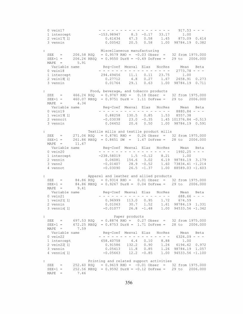
0 vein17 - - - - - - - - - - - - - - - - - 917.53 - - - 1 intercept -153.98947 8.3 -0.17 33.17 1.00 2 vein17[1] 0.61434 47.3 0.58 1.45 873.09 0.614 3 vennin 0.00542 20.5 0.58 1.00 98784.19 0.382
: Miscellaneous manufacturing SEE = 206.58 RSQ = 0.9579 RHO = -0.03 Obser = 32 from 1975.000 SEE+1 = 206.26 RBSQ = 0.9550 DurH = -0.49 DoFree = 29 to 2006.000 MAPE = 5.91 Variable name Reg-Coef Mexval Elas NorRes Mean Beta 0 vein18 - - - - - - - - - - - - - - - - - 2773.78 - - - 1 intercept 294.49456 11.1 0.11 23.75 1.00 2 vein18[1] 0.27712 4.8 0.27 1.67 2658.91 0.273 3 vennin 0.01764 29.1 0.63 1.00 98784.19 0.711
: Food, beverage, and tobacco products SEE = 466.24 RSQ = 0.9767 RHO = 0.18 Obser = 32 from 1975.000 SEE+1 = 460.07 RBSQ = 0.9751 DurH = 1.11 DoFree = 29 to 2006.000 MAPE = 4.34 Variable name Reg-Coef Mexval Elas NorRes Mean Beta 0 vein19 - - - - - - - - - - - - - - - - - 8880.84 - - - 1 vein19[1] 0.88258 130.5 0.85 1.53 8557.38 2 vennoit -0.03038 23.0 -0.35 1.45 101376.84 -0.513 3 vennin 0.04452 20.6 0.50 1.00 98784.19 0.591
: Textile mills and textile product mills SEE = 271.06 RSQ = 0.8781 RHO = 0.26 Obser = 32 from 1975.000 SEE+1 = 261.86 RBSQ = 0.8651 DW = 1.47 DoFree = 28 to 2006.000 MAPE = 11.67 Variable name Reg-Coef Mexval Elas NorRes Mean Beta 0 vein20 - - - - - - - - - - - - - - - - - 1992.25 - - - 1 intercept -238.58019 1.5 -0.12 8.21 1.00 2 vennin 0.06081 154.6 3.02 6.19 98784.19 3.179 3 venn2 -0.01407 28.9 -0.52 1.60 73834.41 -1.214 4 vennot -0.03090 26.5 -1.37 1.00 88589.03 -1.603
: Apparel and leather and allied products SEE = 84.86 RSQ = 0.9314 RHO = 0.01 Obser = 32 from 1975.000 SEE+1 = 84.86 RBSQ = 0.9267 DurH = 0.04 DoFree = 29 to 2006.000 MAPE = 9.41 Variable name Reg-Coef Mexval Elas NorRes Mean Beta 0 vein21 - - - - - - - - - - - - - - - - - 688.66 - - - 1 vein21[1] 0.96999 113.0 0.95 1.72 674.59 2 vennin 0.01063 30.7 1.52 1.61 98784.19 1.331 3 vennin[1] -0.01077 26.8 -1.48 1.00 94533.56 -1.342
: Paper products SEE = 697.53 RSQ = 0.8874 RHO = 0.27 Obser = 32 from 1975.000 SEE+1 = 672.25 RBSQ = 0.8753 DurH = 1.71 DoFree = 28 to 2006.000 MAPE = 7.59 Variable name Reg-Coef Mexval Elas NorRes Mean Beta 0 vein22 - - - - - - - - - - - - - - - - - 6326.09 - - - 1 intercept 658.40758 4.4 0.10 8.88 1.00 2 vein22[1] 0.91586 132.2 0.90 1.26 6194.62 0.972 3 vennin 0.05413 11.8 0.85 1.26 98784.19 1.057 4 vennin[1] -0.05663 12.2 -0.85 1.00 94533.56 -1.100
: Printing and related support activities SEE = 252.60 RSQ = 0.9619 RHO = -0.01 Obser = 32 from 1975.000 SEE+1 = 252.56 RBSQ = 0.9592 DurH = -0.12 DoFree = 29 to 2006.000 MAPE = 7.46
356

Variable name Reg-Coef Mexval Elas NorRes Mean Beta 0 vein23 - - - - - - - - - - - - - - - - - 2890.72 - - - 1 vein23[1] 0.43562 13.7 0.42 1.69 2756.00 2 vennin 0.01248 5.4 0.43 1.01 98784.19 0.392 3 vennin[1] 0.00490 0.6 0.16 1.00 94533.56 0.153
: Petroleum and coal products SEE = 888.98 RSQ = 0.8402 RHO = 0.13 Obser = 32 from 1975.000 SEE+1 = 883.78 RBSQ = 0.8231 DurH = 1.36 DoFree = 28 to 2006.000 MAPE = 11.72 Variable name Reg-Coef Mexval Elas NorRes Mean Beta 0 vein24 - - - - - - - - - - - - - - - - - 5010.59 - - - 1 intercept -2171.01368 7.6 -0.43 6.26 1.00 2 vein24[1] 0.77371 40.1 0.72 1.24 4694.50 0.672 3 vennin 0.08162 10.9 1.61 1.20 98784.19 1.490 4 venn1 -0.09341 9.7 -0.90 1.00 48312.88 -1.287
: Chemical products SEE = 900.91 RSQ = 0.9742 RHO = 0.19 Obser = 32 from 1975.000 SEE+1 = 889.75 RBSQ = 0.9704 DurH = 1.27 DoFree = 27 to 2006.000 MAPE = 8.37 Variable name Reg-Coef Mexval Elas NorRes Mean Beta 0 vein25 - - - - - - - - - - - - - - - - - 12605.88 - - - 1 intercept -2044.85088 6.4 -0.16 38.80 1.00 2 vein25[1] 0.82267 92.9 0.79 1.45 12149.59 0.838 3 vennin 0.08259 13.7 0.65 1.38 98784.19 0.597 4 venn1 -0.04223 2.3 -0.16 1.25 48312.88 -0.231 5 venn2 -0.01982 11.9 -0.12 1.00 73834.41 -0.237
: Plastics and rubber products SEE = 404.38 RSQ = 0.9714 RHO = 0.26 Obser = 32 from 1975.000 SEE+1 = 391.87 RBSQ = 0.9694 DurH = 2.21 DoFree = 29 to 2006.000 MAPE = 8.69 Variable name Reg-Coef Mexval Elas NorRes Mean Beta 0 vein26 - - - - - - - - - - - - - - - - - 4597.03 - - - 1 intercept -342.71910 2.9 -0.07 34.95 1.00 2 vennin 0.02411 14.9 0.52 1.65 98784.19 0.409 3 vein26[1] 0.58014 28.4 0.56 1.00 4409.28 0.583
: Wholesale trade SEE = 3206.28 RSQ = 0.9694 RHO = 0.56 Obser = 32 from 1975.000 SEE+1 = 2717.86 RBSQ = 0.9661 DurH = 999.00 DoFree = 28 to 2006.000 MAPE = 10.03 Variable name Reg-Coef Mexval Elas NorRes Mean Beta 0 vein27 - - - - - - - - - - - - - - - - - 32799.66 - - - 1 vein27[1] 0.47805 11.5 0.45 1.47 30624.47 2 venntr 0.04832 0.9 0.13 1.14 91518.56 0.115 3 venn1 0.06767 1.0 0.10 1.14 48312.88 0.113 4 vennot 0.12330 6.9 0.33 1.00 88589.03 0.271
: Retail trade SEE = 1353.32 RSQ = 0.9818 RHO = -0.00 Obser = 32 from 1975.000 SEE+1 = 1353.32 RBSQ = 0.9806 DurH = -0.00 DoFree = 29 to 2006.000 MAPE = 6.11 Variable name Reg-Coef Mexval Elas NorRes Mean Beta 0 vein28 - - - - - - - - - - - - - - - - - 18927.47 - - - 1 vein28[1] 0.66357 33.8 0.63 1.29 17857.44 2 vennot 0.05680 12.1 0.27 1.06 88589.03 0.228 3 venn1 0.04170 3.2 0.11 1.00 48312.88 0.127
: Air transportation
357

SEE = 2200.78 RSQ = 0.9432 RHO = -0.02 Obser = 32 from 1975.000 SEE+1 = 2200.08 RBSQ = 0.9348 DurH = -0.15 DoFree = 27 to 2006.000 MAPE = 20.49 Variable name Reg-Coef Mexval Elas NorRes Mean Beta 0 vein29 - - - - - - - - - - - - - - - - - 11594.88 - - - 1 intercept -612.95837 0.5 -0.05 17.60 1.00 2 vein29[1] 0.56285 43.3 0.55 2.02 11231.75 0.572 3 venntr 0.06378 2.8 0.50 1.81 91518.56 0.301 4 venntr[1] 0.17218 15.1 1.29 1.67 86968.16 0.794 5 vennot -0.16848 29.4 -1.29 1.00 88589.03 -0.735
: Railroad transportation SEE = 458.26 RSQ = 0.6855 RHO = 0.08 Obser = 32 from 1975.000 SEE+1 = 457.19 RBSQ = 0.6638 DurH = 0.88 DoFree = 29 to 2006.000 MAPE = 21.47 Variable name Reg-Coef Mexval Elas NorRes Mean Beta 0 vein30 - - - - - - - - - - - - - - - - - 1768.09 - - - 1 intercept 740.62910 19.8 0.42 3.18 1.00 2 vein30[1] 1.14203 71.5 1.13 1.49 1751.28 1.157 3 vein30[2] -0.56150 21.9 -0.55 1.00 1732.06 -0.579
: Water transportation SEE = 481.15 RSQ = 0.8687 RHO = 0.16 Obser = 32 from 1975.000 SEE+1 = 476.61 RBSQ = 0.8596 DurH = 1.38 DoFree = 29 to 2006.000 MAPE = 14.61 Variable name Reg-Coef Mexval Elas NorRes Mean Beta 0 vein31 - - - - - - - - - - - - - - - - - 2870.16 - - - 1 vein31[1] 0.70956 40.2 0.68 1.23 2747.78 2 venntr 0.01922 6.2 0.61 1.04 91518.56 0.632 3 vennoit -0.00854 2.0 -0.30 1.00 101376.84 -0.332
: Truck transportation SEE = 1543.55 RSQ = 0.8586 RHO = 0.13 Obser = 32 from 1975.000 SEE+1 = 1537.20 RBSQ = 0.8434 DurH = 2.33 DoFree = 28 to 2006.000 MAPE = 14.47 Variable name Reg-Coef Mexval Elas NorRes Mean Beta 0 vein32 - - - - - - - - - - - - - - - - - 7788.06 - - - 1 vein32[1] 0.59443 20.4 0.55 1.80 7252.69 2 venntr 0.13829 28.8 1.63 1.44 91518.56 1.470 3 venntr[1] -0.10802 20.1 -1.21 1.00 86968.16 -1.121 4 venptr 2.89262 0.1 0.03 1.00 83.21 0.014
: Transit and ground passenger transportation SEE = 345.39 RSQ = 0.9121 RHO = -0.19 Obser = 32 from 1975.000 SEE+1 = 338.55 RBSQ = 0.9027 DurH = -1.73 DoFree = 28 to 2006.000 MAPE = 21.82 Variable name Reg-Coef Mexval Elas NorRes Mean Beta 0 vein33 - - - - - - - - - - - - - - - - - 1529.88 - - - 1 intercept -422.19874 6.9 -0.28 11.37 1.00 2 vein33[1] 0.27483 6.7 0.26 2.03 1422.84 0.263 3 vennin -0.01064 3.2 -0.69 1.42 98784.19 -0.371 4 venntr 0.02855 19.3 1.71 1.00 91518.56 1.069
: Pipeline transportation SEE = 284.84 RSQ = 0.8719 RHO = 0.40 Obser = 32 from 1975.000 SEE+1 = 261.52 RBSQ = 0.8631 DurH = 3.00 DoFree = 29 to 2006.000 MAPE = 22.34 Variable name Reg-Coef Mexval Elas NorRes Mean Beta 0 vein34 - - - - - - - - - - - - - - - - - 1660.66 - - - 1 vein34[1] 0.66723 47.0 0.64 1.38 1587.22 2 venntr 0.00942 16.9 0.52 1.15 91518.56 0.516
358
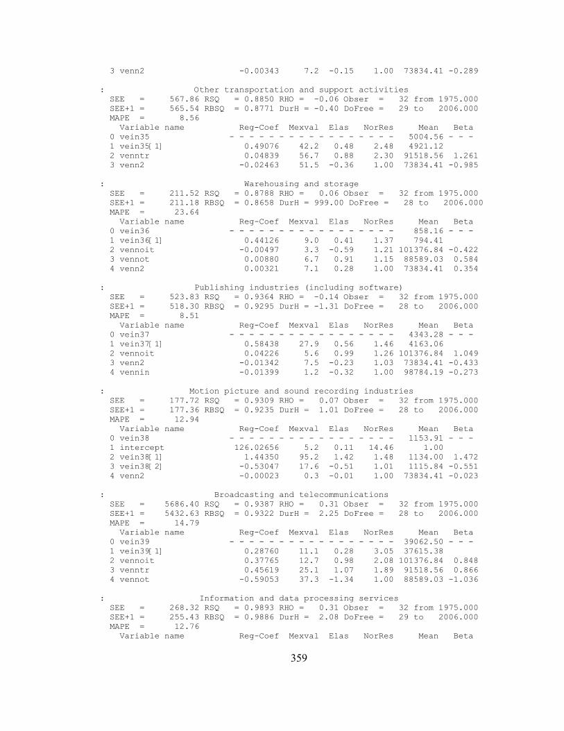
3 venn2 -0.00343 7.2 -0.15 1.00 73834.41 -0.289
: Other transportation and support activities SEE = 567.86 RSQ = 0.8850 RHO = -0.06 Obser = 32 from 1975.000 SEE+1 = 565.54 RBSQ = 0.8771 DurH = -0.40 DoFree = 29 to 2006.000 MAPE = 8.56 Variable name Reg-Coef Mexval Elas NorRes Mean Beta 0 vein35 - - - - - - - - - - - - - - - - - 5004.56 - - - 1 vein35[1] 0.49076 42.2 0.48 2.48 4921.12 2 venntr 0.04839 56.7 0.88 2.30 91518.56 1.261 3 venn2 -0.02463 51.5 -0.36 1.00 73834.41 -0.985
: Warehousing and storage SEE = 211.52 RSQ = 0.8788 RHO = 0.06 Obser = 32 from 1975.000 SEE+1 = 211.18 RBSQ = 0.8658 DurH = 999.00 DoFree = 28 to 2006.000 MAPE = 23.64 Variable name Reg-Coef Mexval Elas NorRes Mean Beta 0 vein36 - - - - - - - - - - - - - - - - - 858.16 - - - 1 vein36[1] 0.44126 9.0 0.41 1.37 794.41 2 vennoit -0.00497 3.3 -0.59 1.21 101376.84 -0.422 3 vennot 0.00880 6.7 0.91 1.15 88589.03 0.584 4 venn2 0.00321 7.1 0.28 1.00 73834.41 0.354
: Publishing industries (including software) SEE = 523.83 RSQ = 0.9364 RHO = -0.14 Obser = 32 from 1975.000 SEE+1 = 518.30 RBSQ = 0.9295 DurH = -1.31 DoFree = 28 to 2006.000 MAPE = 8.51 Variable name Reg-Coef Mexval Elas NorRes Mean Beta 0 vein37 - - - - - - - - - - - - - - - - - 4343.28 - - - 1 vein37[1] 0.58438 27.9 0.56 1.46 4163.06 2 vennoit 0.04226 5.6 0.99 1.26 101376.84 1.049 3 venn2 -0.01342 7.5 -0.23 1.03 73834.41 -0.433 4 vennin -0.01399 1.2 -0.32 1.00 98784.19 -0.273
: Motion picture and sound recording industries SEE = 177.72 RSQ = 0.9309 RHO = 0.07 Obser = 32 from 1975.000 SEE+1 = 177.36 RBSQ = 0.9235 DurH = 1.01 DoFree = 28 to 2006.000 MAPE = 12.94 Variable name Reg-Coef Mexval Elas NorRes Mean Beta 0 vein38 - - - - - - - - - - - - - - - - - 1153.91 - - - 1 intercept 126.02656 5.2 0.11 14.46 1.00 2 vein38[1] 1.44350 95.2 1.42 1.48 1134.00 1.472 3 vein38[2] -0.53047 17.6 -0.51 1.01 1115.84 -0.551 4 venn2 -0.00023 0.3 -0.01 1.00 73834.41 -0.023
: Broadcasting and telecommunications SEE = 5686.40 RSQ = 0.9387 RHO = 0.31 Obser = 32 from 1975.000 SEE+1 = 5432.63 RBSQ = 0.9322 DurH = 2.25 DoFree = 28 to 2006.000 MAPE = 14.79 Variable name Reg-Coef Mexval Elas NorRes Mean Beta 0 vein39 - - - - - - - - - - - - - - - - - 39062.50 - - - 1 vein39[1] 0.28760 11.1 0.28 3.05 37615.38 2 vennoit 0.37765 12.7 0.98 2.08 101376.84 0.848 3 venntr 0.45619 25.1 1.07 1.89 91518.56 0.866 4 vennot -0.59053 37.3 -1.34 1.00 88589.03 -1.036
: Information and data processing services SEE = 268.32 RSQ = 0.9893 RHO = 0.31 Obser = 32 from 1975.000 SEE+1 = 255.43 RBSQ = 0.9886 DurH = 2.08 DoFree = 29 to 2006.000 MAPE = 12.76 Variable name Reg-Coef Mexval Elas NorRes Mean Beta
359

0 vein40 - - - - - - - - - - - - - - - - - 2662.88 - - - 1 vein40[1] 0.60085 51.6 0.55 1.91 2420.69 2 venn2 0.01816 25.1 0.50 1.03 73834.41 0.469 3 vennoit -0.00148 1.4 -0.06 1.00 101376.84 -0.029
: Federal Reserve banks SEE = 225.92 RSQ = 0.9241 RHO = -0.07 Obser = 32 from 1975.000 SEE+1 = 225.01 RBSQ = 0.9129 DurH = -1.21 DoFree = 27 to 2006.000 MAPE = 70.11 Variable name Reg-Coef Mexval Elas NorRes Mean Beta 0 vein41 - - - - - - - - - - - - - - - - - 771.62 - - - 1 intercept -325.25690 5.8 -0.42 13.18 1.00 2 vein41[1] 0.70451 29.1 0.67 1.33 729.28 0.707 3 venn1 0.00314 0.3 0.20 1.08 48312.88 0.117 4 venn2 -0.00254 2.1 -0.24 1.05 73834.41 -0.207 5 venntr 0.00676 2.7 0.80 1.00 91518.56 0.360
: Credit intermediation and related activities SEE = 2712.35 RSQ = 0.9818 RHO = -0.10 Obser = 32 from 1975.000 SEE+1 = 2698.75 RBSQ = 0.9799 DurH = -0.93 DoFree = 28 to 2006.000 MAPE = 6.44 Variable name Reg-Coef Mexval Elas NorRes Mean Beta 0 vein42 - - - - - - - - - - - - - - - - - 35409.19 - - - 1 vein42[1] 0.29087 7.2 0.28 2.54 33647.16 2 venn1 0.45569 24.1 0.62 1.73 48312.88 0.694 3 venn2 -0.05888 15.0 -0.12 1.22 73834.41 -0.196 4 venntr 0.08725 10.4 0.23 1.00 91518.56 0.189
: Securities, commodity contracts, and investment SEE = 1530.12 RSQ = 0.8354 RHO = -0.06 Obser = 32 from 1975.000 SEE+1 = 1526.66 RBSQ = 0.8177 DurH = -0.57 DoFree = 28 to 2006.000 MAPE = 17.66 Variable name Reg-Coef Mexval Elas NorRes Mean Beta 0 vein43 - - - - - - - - - - - - - - - - - 7038.31 - - - 1 vein43[1] 0.49347 20.8 0.47 1.55 6708.88 2 venn2 -0.04057 9.0 -0.43 1.47 73834.41 -0.721 3 vennoit 0.14546 9.5 2.10 1.10 101376.84 1.989 4 vennin -0.08153 5.1 -1.14 1.00 98784.19 -0.878
: Insurance carriers and related activities SEE = 1553.99 RSQ = 0.9395 RHO = -0.03 Obser = 32 from 1975.000 SEE+1 = 1553.17 RBSQ = 0.9353 DurH = -0.41 DoFree = 29 to 2006.000 MAPE = 14.79 Variable name Reg-Coef Mexval Elas NorRes Mean Beta 0 vein44 - - - - - - - - - - - - - - - - - 9497.50 - - - 1 vein44[1] 0.66258 25.2 0.63 1.22 8963.34 2 venn2 0.01088 1.3 0.08 1.21 73834.41 0.115 3 venntr 0.03007 9.8 0.29 1.00 91518.56 0.208
: Funds, trusts, and other financial vehicles SEE = 254.53 RSQ = 0.8383 RHO = 0.08 Obser = 32 from 1975.000 SEE+1 = 253.89 RBSQ = 0.8210 DurH = 999.00 DoFree = 28 to 2006.000 MAPE = 25.79 Variable name Reg-Coef Mexval Elas NorRes Mean Beta 0 vein45 - - - - - - - - - - - - - - - - - 882.81 - - - 1 intercept -174.13124 3.8 -0.20 6.18 1.00 2 vein45[1] 0.53439 14.4 0.51 1.78 836.34 0.526 3 venntr 0.01483 12.2 1.54 1.05 91518.56 1.022 4 venntr[1] -0.00859 2.7 -0.85 1.00 86968.16 -0.578
: Real estate
360

SEE = 1385.17 RSQ = 0.9078 RHO = 0.16 Obser = 32 from 1975.000 SEE+1 = 1367.59 RBSQ = 0.9014 DW = 1.68 DoFree = 29 to 2006.000 MAPE = 8.68 Variable name Reg-Coef Mexval Elas NorRes Mean Beta 0 vein46 - - - - - - - - - - - - - - - - - 10930.16 - - - 1 intercept -1972.04229 8.5 -0.18 10.85 1.00 2 vennr 2.61965 62.0 1.35 1.04 5634.66 1.125 3 vennot -0.02098 2.2 -0.17 1.00 88589.03 -0.185
: Rental and leasing services and lessors of intangible assets SEE = 4586.91 RSQ = 0.9684 RHO = 0.03 Obser = 32 from 1975.000 SEE+1 = 4589.98 RBSQ = 0.9638 DurH = 0.23 DoFree = 27 to 2006.000 MAPE = 30.41 Variable name Reg-Coef Mexval Elas NorRes Mean Beta 0 vein47 - - - - - - - - - - - - - - - - - 27668.12 - - - 1 intercept -16200.26275 30.8 -0.59 31.68 1.00 2 vein47[1] 0.36690 8.2 0.34 2.42 25414.69 0.351 3 vein47[2] 0.13435 1.8 0.11 2.40 23307.72 0.123 4 venn1 -0.15444 1.8 -0.27 1.48 48312.88 -0.183 5 venntr 0.42477 21.6 1.41 1.00 91518.56 0.718
: Legal services SEE = 130.07 RSQ = 0.9832 RHO = 0.08 Obser = 32 from 1975.000 SEE+1 = 129.63 RBSQ = 0.9814 DurH = 0.65 DoFree = 28 to 2006.000 MAPE = 7.89 Variable name Reg-Coef Mexval Elas NorRes Mean Beta 0 vein48 - - - - - - - - - - - - - - - - - 1468.56 - - - 1 intercept -172.33111 5.6 -0.12 59.39 1.00 2 vein48[1] 0.57230 34.7 0.53 1.51 1371.38 0.558 3 vennot 0.00612 9.1 0.37 1.18 88589.03 0.246 4 venn1 0.00649 8.5 0.21 1.00 48312.88 0.198
: Computer systems design and related services SEE = 1076.98 RSQ = 0.9761 RHO = 0.03 Obser = 32 from 1975.000 SEE+1 = 1076.59 RBSQ = 0.9726 DurH = 0.37 DoFree = 27 to 2006.000 MAPE = 38.60 Variable name Reg-Coef Mexval Elas NorRes Mean Beta 0 vein49 - - - - - - - - - - - - - - - - - 6714.06 - - - 1 intercept 1494.47182 3.6 0.22 41.90 1.00 2 vein49[1] 0.41973 12.6 0.38 2.18 6136.84 0.405 3 venn1 0.12617 11.5 0.91 1.40 48312.88 0.555 4 venn2 0.07018 15.6 0.77 1.20 73834.41 0.674 5 vennoit -0.08516 9.6 -1.29 1.00 101376.84 -0.630
: Miscellaneous professional, scientific, and technical services SEE = 1873.54 RSQ = 0.9889 RHO = -0.29 Obser = 32 from 1975.000 SEE+1 = 1789.79 RBSQ = 0.9877 DurH = -3.93 DoFree = 28 to 2006.000 MAPE = 17.04 Variable name Reg-Coef Mexval Elas NorRes Mean Beta 0 vein50 - - - - - - - - - - - - - - - - - 18171.09 - - - 1 vein50[1] 0.38666 9.8 0.35 1.74 16227.47 2 venn2 0.13074 27.2 0.53 1.47 73834.41 0.494 3 vennin -0.23171 21.2 -1.26 1.47 98784.19 -0.530 4 vennot 0.28477 21.0 1.39 1.00 88589.03 0.647
: Management of companies and enterprises SEE = 1632.77 RSQ = 0.9402 RHO = -0.04 Obser = 32 from 1975.000 SEE+1 = 1630.94 RBSQ = 0.9360 DurH = -0.37 DoFree = 29 to 2006.000 MAPE = 10.38 Variable name Reg-Coef Mexval Elas NorRes Mean Beta 0 vein51 - - - - - - - - - - - - - - - - - 10585.94 - - -
361

1 intercept 1476.15129 9.2 0.14 16.71 1.00 2 vein51[1] 0.67218 37.0 0.63 1.23 9920.88 0.652 3 venn2 0.03306 10.8 0.23 1.00 73834.41 0.332
: Administrative and support services SEE = 601.57 RSQ = 0.9939 RHO = 0.22 Obser = 32 from 1975.000 SEE+1 = 586.99 RBSQ = 0.9930 DurH = 5.78 DoFree = 27 to 2006.000 MAPE = 12.42 Variable name Reg-Coef Mexval Elas NorRes Mean Beta 0 vein52 - - - - - - - - - - - - - - - - - 8430.50 - - - 1 vein52[1] 0.33758 6.9 0.31 2.58 7699.44 2 venn1 0.05245 8.3 0.30 1.77 48312.88 0.209 3 venn2 0.07205 19.0 0.63 1.29 73834.41 0.627 4 vennoit -0.04870 13.2 -0.59 1.26 101376.84 -0.326 5 vennot 0.03292 12.1 0.35 1.00 88589.03 0.172
: Waste management and remediation services SEE = 289.19 RSQ = 0.8891 RHO = 0.04 Obser = 32 from 1975.000 SEE+1 = 289.19 RBSQ = 0.8772 DurH = 0.26 DoFree = 28 to 2006.000 MAPE = 14.16 Variable name Reg-Coef Mexval Elas NorRes Mean Beta 0 vein53 - - - - - - - - - - - - - - - - - 2054.06 - - - 1 intercept 260.08264 4.9 0.13 9.02 1.00 2 vein53[1] 0.90762 128.1 0.87 1.16 1960.56 0.910 3 vennin -0.00969 5.6 -0.47 1.16 98784.19 -0.453 4 vennot 0.01097 7.5 0.47 1.00 88589.03 0.509
: Educational services SEE = 374.97 RSQ = 0.9849 RHO = -0.10 Obser = 32 from 1975.000 SEE+1 = 373.04 RBSQ = 0.9833 DurH = 999.00 DoFree = 28 to 2006.000 MAPE = 6.49 Variable name Reg-Coef Mexval Elas NorRes Mean Beta 0 vein54 - - - - - - - - - - - - - - - - - 3604.91 - - - 1 vein54[1] 0.62725 16.1 0.58 1.35 3326.31 2 venn2 0.01720 5.8 0.35 1.06 73834.41 0.378 3 vennoit -0.00416 0.3 -0.12 1.02 101376.84 -0.070 4 vennot 0.00742 0.8 0.18 1.00 88589.03 0.098
: Ambulatory health care services SEE = 814.34 RSQ = 0.9915 RHO = 0.24 Obser = 32 from 1975.000 SEE+1 = 796.23 RBSQ = 0.9910 DurH = 1.40 DoFree = 29 to 2006.000 MAPE = 5.61 Variable name Reg-Coef Mexval Elas NorRes Mean Beta 0 vein55 - - - - - - - - - - - - - - - - - 12994.56 - - - 1 vein55[1] 0.99562 275.1 0.92 1.39 11959.88 2 vennot 0.05982 17.0 0.41 1.38 88589.03 0.272 3 venntr -0.04524 17.6 -0.32 1.00 91518.56 -0.223
: Hospitals SEE = 795.01 RSQ = 0.9962 RHO = -0.02 Obser = 32 from 1975.000 SEE+1 = 794.67 RBSQ = 0.9958 DurH = -0.09 DoFree = 28 to 2006.000 MAPE = 4.62 Variable name Reg-Coef Mexval Elas NorRes Mean Beta 0 vein56 - - - - - - - - - - - - - - - - - 16833.94 - - - 1 intercept 725.06416 2.7 0.04 263.19 1.00 2 vein56[1] 0.97361 227.2 0.89 1.11 15467.16 0.907 3 venn2 0.02232 4.5 0.10 1.01 73834.41 0.116 4 vennoit -0.00590 0.5 -0.04 1.00 101376.84 -0.024
: Nursing and residential care facilities SEE = 106.30 RSQ = 0.9842 RHO = 0.12 Obser = 32 from 1975.000
362

SEE+1 = 105.58 RBSQ = 0.9825 DurH = 1.05 DoFree = 28 to 2006.000 MAPE = 6.77 Variable name Reg-Coef Mexval Elas NorRes Mean Beta 0 vein57 - - - - - - - - - - - - - - - - - 1132.09 - - - 1 vein57[1] 0.82134 52.0 0.76 1.15 1047.09 2 venn2 0.00179 2.7 0.12 1.12 73834.41 0.142 3 vennoit -0.00041 0.1 -0.04 1.03 101376.84 -0.025 4 vennot 0.00204 1.6 0.16 1.00 88589.03 0.097
: Social assistance SEE = 77.72 RSQ = 0.9627 RHO = 0.24 Obser = 32 from 1975.000 SEE+1 = 76.69 RBSQ = 0.9601 DW = 1.52 DoFree = 29 to 2006.000 MAPE = 11.20 Variable name Reg-Coef Mexval Elas NorRes Mean Beta 0 vein58 - - - - - - - - - - - - - - - - - 671.69 - - - 1 intercept 216.29035 14.3 0.32 26.80 1.00 2 venn2 0.00563 51.6 0.62 1.00 73834.41 0.937 3 vennot 0.00045 0.1 0.06 1.00 88589.03 0.045
: Performing arts, spectator sports, museums, and related activities SEE = 175.45 RSQ = 0.9411 RHO = 0.15 Obser = 32 from 1975.000 SEE+1 = 174.16 RBSQ = 0.9348 DurH = 5.26 DoFree = 28 to 2006.000 MAPE = 13.63 Variable name Reg-Coef Mexval Elas NorRes Mean Beta 0 vein59 - - - - - - - - - - - - - - - - - 1114.25 - - - 1 intercept -60.42053 0.8 -0.05 16.99 1.00 2 vein59[1] 0.44746 11.0 0.42 1.38 1053.69 0.429 3 vein59[2] 0.40487 9.2 0.36 1.09 993.78 0.372 4 vennot 0.00340 4.4 0.27 1.00 88589.03 0.189
: Amusements, gambling, and recreation industries SEE = 207.82 RSQ = 0.9874 RHO = 0.10 Obser = 32 from 1975.000 SEE+1 = 207.05 RBSQ = 0.9861 DurH = 0.99 DoFree = 28 to 2006.000 MAPE = 10.10 Variable name Reg-Coef Mexval Elas NorRes Mean Beta 0 vein60 - - - - - - - - - - - - - - - - - 2467.91 - - - 1 intercept -231.40660 6.0 -0.09 79.55 1.00 2 vein60[1] 1.38015 96.9 1.29 1.80 2309.97 1.326 3 vein60[2] -0.54197 21.8 -0.47 1.29 2153.19 -0.499 4 vennot 0.00766 13.6 0.27 1.00 88589.03 0.166
: Accommodation SEE = 352.54 RSQ = 0.9283 RHO = -0.24 Obser = 32 from 1975.000 SEE+1 = 340.58 RBSQ = 0.9234 DurH = -2.52 DoFree = 29 to 2006.000 MAPE = 15.32 Variable name Reg-Coef Mexval Elas NorRes Mean Beta 0 vein61 - - - - - - - - - - - - - - - - - 2618.84 - - - 1 vein61[1] 0.40619 12.1 0.38 1.70 2462.72 2 vennot 0.03263 24.3 1.10 1.20 88589.03 0.999 3 venntr -0.01377 9.6 -0.48 1.00 91518.56 -0.456
: Food services and drinking places SEE = 756.59 RSQ = 0.9818 RHO = -0.03 Obser = 32 from 1975.000 SEE+1 = 755.76 RBSQ = 0.9791 DurH = 999.00 DoFree = 27 to 2006.000 MAPE = 6.89 Variable name Reg-Coef Mexval Elas NorRes Mean Beta 0 vein62 - - - - - - - - - - - - - - - - - 9363.22 - - - 1 intercept -909.97689 4.4 -0.10 54.89 1.00 2 vein62[1] 0.31514 4.9 0.29 1.63 8686.31 0.288 3 vein62[2] 0.33602 5.5 0.29 1.26 8072.28 0.282 4 vennin -0.03048 7.5 -0.32 1.25 98784.19 -0.221
363

5 vennot 0.08844 11.9 0.84 1.00 88589.03 0.636
: Other services, except government SEE = 403.51 RSQ = 0.9629 RHO = 0.18 Obser = 32 from 1975.000 SEE+1 = 398.62 RBSQ = 0.9589 DurH = 7.09 DoFree = 28 to 2006.000 MAPE = 6.07 Variable name Reg-Coef Mexval Elas NorRes Mean Beta 0 vein63 - - - - - - - - - - - - - - - - - 6080.91 - - - 1 intercept 730.22234 14.4 0.12 26.96 1.00 2 vein63[1] 0.65936 19.6 0.64 1.41 5886.84 0.664 3 vein63[2] -0.28685 4.7 -0.27 1.41 5706.78 -0.292 4 vennin 0.03144 18.6 0.51 1.00 98784.19 0.609
364
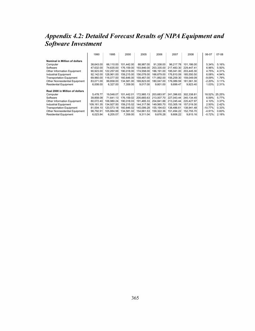
Appendix 4.2: Detailed Forecast Results of NIPA Equipment and Software Investment
365
1990 1995 2000 2005 2006 2007 2008 06-07 07-08
Nominal in Million of dollars Computer 38,643.00 66,110.00 101,442.00 88,987.00 91,338.00 96,217.78 101,186.00 5.34% 5.16% Software 47,632.00 74,635.00 176,159.00 193,846.00 203,335.00 217,483.30 229,447.41 6.96% 5.50% Other Information Equipment 90,923.00 122,257.00 190,018.00 174,558.00 186,191.00 195,041.00 203,445.30 4.75% 4.31% Industrial Equipment 92,142.00 128,961.00 159,215.00 156,078.00 166,679.00 176,810.09 185,550.50 6.08% 4.94% Transportation Equipment 69,960.00 116,077.00 160,846.00 159,467.00 171,892.00 156,259.30 159,049.09 -9.09% 1.79% Other Nonresidential Equipment 83,071.00 99,858.00 134,581.00 169,823.00 180,047.00 176,089.59 181,561.30 -2.20% 3.11% Residential Equipment 6,008.00 6,327.00 7,359.00 9,017.00 9,601.00 9,699.47 9,923.40 1.03% 2.31%
Real 2000 in Million of dollars Computer 5,478.77 19,548.07 101,442.01 172,985.13 203,683.97 241,396.63 302,338.81 18.52% 25.25% Software 39,858.08 71,641.13 176,159.02 205,665.63 213,007.70 227,043.44 240,134.45 6.59% 5.77% Other Information Equipment 80,072.40 106,980.24 190,018.03 191,485.33 204,841.88 213,245.44 220,427.97 4.10% 3.37% Industrial Equipment 109,161.35 134,927.50 159,215.02 144,317.56 149,565.70 153,305.19 157,019.30 2.50% 2.42% Transportation Equipment 81,004.10 120,573.18 160,846.02 145,099.28 155,194.63 138,486.61 138,941.48 -10.77% 0.33% Other Nonresidential Equipment 98,792.91 105,884.98 134,581.02 154,661.53 159,322.36 151,494.22 152,755.70 -4.91% 0.83% Residential Equipment 6,023.84 6,205.07 7,359.00 9,311.04 9,676.28 9,606.22 9,815.16 -0.72% 2.18%

Appendix 4.3: Detailed Forecast Results of FAA by Purchasing Industries
366
1990 1995 2000 2005 2006 2007 2008 06-07 07-08Nominal in Million of dollars Farms 14,714.00 19,104.00 20,781.00 28,579.00 28,644.00 28,911.59 29,811.27 0.93% 3.11% Forestry, fishing, and related activities 2,658.00 2,156.00 1,627.00 3,552.00 3,609.00 3,956.47 4,275.79 9.63% 8.07% Oil and gas extraction 3,711.00 4,508.00 6,070.00 5,371.00 5,864.00 5,638.71 5,345.37 -3.84% -5.20% Mining, except oil and gas 3,517.00 7,776.00 5,201.00 10,243.00 11,421.00 10,431.08 8,757.44 -8.67% -16.04% Support activites for mining 2,676.00 4,035.00 4,626.00 8,362.00 9,600.00 9,603.70 9,668.70 0.04% 0.68% Utilities 26,776.00 26,158.00 35,022.00 34,468.00 36,695.00 38,174.90 39,119.02 4.03% 2.47% Construction 8,982.00 19,433.00 31,714.00 38,395.00 41,293.00 44,639.81 48,145.30 8.11% 7.85% Wood products 1,673.00 2,898.00 2,612.00 2,609.00 2,762.00 3,094.05 3,353.80 12.02% 8.40% Nonmetallic mineral products 2,901.00 3,227.00 5,101.00 4,618.00 4,922.00 5,174.76 5,386.89 5.14% 4.10% Primary metals 5,403.00 6,355.00 5,425.00 4,862.00 5,208.00 5,483.13 5,682.15 5.28% 3.63% Fabricated metal products 5,354.00 8,447.00 9,612.00 7,891.00 8,454.00 9,654.01 10,618.64 14.19% 9.99% Machinery 6,084.00 10,019.00 18,641.00 16,159.00 17,204.00 19,125.61 21,063.38 11.17% 10.13% Computer and electronic products 12,421.00 24,289.00 37,494.00 25,034.00 26,460.00 29,493.71 32,542.95 11.47% 10.34% Electrical equipment, appliances, and components 2,939.00 4,030.00 3,899.00 2,191.00 2,339.00 2,892.78 3,382.14 23.68% 16.92% Motor vehicles, bodies and trailers, and parts 6,370.00 13,882.00 12,951.00 10,964.00 11,735.00 13,134.61 14,383.83 11.93% 9.51% Other transportation equipment 4,231.00 4,584.00 7,942.00 7,931.00 8,394.00 8,951.40 9,488.22 6.64% 6.00% Furniture and related products 697.00 1,222.00 1,831.00 1,511.00 1,607.00 1,811.03 1,987.62 12.70% 9.75% Miscellaneous manufacturing 2,736.00 3,237.00 4,037.00 4,395.00 4,682.00 4,763.77 4,971.97 1.75% 4.37% Food, beverage, and tobacco products 9,799.00 12,158.00 11,906.00 12,007.00 12,816.00 13,485.06 14,110.89 5.22% 4.64% Textile mills and textile product mills 2,482.00 3,271.00 2,430.00 1,252.00 1,317.00 1,998.15 2,238.63 51.72% 12.04% Apparel and leather and allied products 646.00 1,215.00 1,273.00 695.00 736.00 807.28 856.95 9.68% 6.15% Paper products 10,529.00 8,472.00 7,692.00 5,941.00 6,286.00 6,636.50 6,820.93 5.58% 2.78% Printing and related support activities 3,125.00 3,127.00 4,825.00 4,714.00 4,963.00 5,249.85 5,547.99 5.78% 5.68% Petroleum and coal products 3,966.00 7,234.00 5,217.00 11,115.00 11,829.00 12,627.20 13,436.57 6.75% 6.41% Chemical products 13,602.00 17,874.00 18,834.00 17,309.00 18,358.00 19,567.48 20,795.05 6.59% 6.27% Plastics and rubber products 4,498.00 6,970.00 8,074.00 6,940.00 7,363.00 8,223.65 8,991.50 11.69% 9.34% Wholesale trade 22,620.00 42,402.00 56,839.00 70,502.00 75,538.00 74,849.70 74,900.40 -0.91% 0.07% Retail trade 16,677.00 24,731.00 31,707.00 35,246.00 37,504.00 38,834.28 40,520.97 3.55% 4.34% Air transportation 6,569.00 14,668.00 31,713.00 12,268.00 13,248.00 16,752.79 15,366.78 26.46% -8.27% Railroad transportation 1,580.00 2,552.00 1,380.00 1,423.00 1,509.00 1,667.40 1,810.73 10.50% 8.60% Water transportation 1,749.00 2,828.00 3,918.00 5,086.00 5,073.00 4,876.66 4,792.28 -3.87% -1.73% Truck transportation 5,126.00 13,121.00 10,476.00 17,569.00 19,647.00 15,306.81 14,654.93 -22.09% -4.26% Transit and ground passenger transportation 747.00 1,467.00 3,730.00 3,364.00 3,730.00 3,161.37 3,033.60 -15.24% -4.04% Pipeline transportation 1,480.00 2,641.00 2,823.00 2,373.00 2,557.00 2,454.73 2,373.54 -4.00% -3.31% Other transportation and support activites 4,792.00 7,409.00 9,155.00 4,487.00 4,762.00 4,602.39 4,345.19 -3.35% -5.59% Warehousing and storage 567.00 1,318.00 1,102.00 2,060.00 2,212.00 2,260.76 2,339.76 2.20% 3.49% Publishing industries (including software) 5,640.00 4,892.00 7,369.00 6,045.00 6,387.00 6,662.94 6,935.12 4.32% 4.08% Motion picture and sound recording industries 1,869.00 2,418.00 737.00 936.00 997.00 1,017.11 1,018.73 2.02% 0.16% Broadcasting and telecommunications 31,606.00 48,614.00 107,363.00 51,312.00 55,344.00 56,310.89 58,610.60 1.75% 4.08% Information and data processing services 1,538.00 2,106.00 6,280.00 7,471.00 7,927.00 8,514.87 9,121.06 7.42% 7.12% Federal Reserve banks 179.00 1,328.00 2,155.00 1,331.00 1,377.00 1,469.24 1,539.68 6.70% 4.79% Credit intermediation and related activities 34,118.00 42,440.00 64,750.00 58,900.00 60,858.00 62,589.82 65,429.16 2.85% 4.54% Securities, commodity contracts, and investments 10,174.00 6,540.00 13,528.00 10,728.00 11,238.00 10,709.18 10,615.11 -4.71% -0.88% Insurance carriers and related activities 7,912.00 17,416.00 18,017.00 17,344.00 18,040.00 19,182.28 20,262.78 6.33% 5.63% Funds, trusts, and other financial vehicles 746.00 696.00 2,343.00 1,661.00 1,743.00 1,594.04 1,714.38 -8.55% 7.55% Real estate 12,734.00 10,360.00 13,554.00 18,186.00 19,293.00 20,122.36 20,684.19 4.30% 2.79% Rental and leasing services and lessors of intangible assets 10,749.00 31,665.00 78,572.00 70,879.00 75,113.00 72,088.55 72,675.03 -4.03% 0.81% Legal services 1,490.00 1,548.00 2,725.00 3,064.00 3,228.00 3,392.10 3,586.56 5.08% 5.73% Computer systems design and related services 3,024.00 5,340.00 19,530.00 17,679.00 18,617.00 20,346.99 22,033.81 9.29% 8.29% Miscellaneous professional, scientific, and technical services 10,642.00 15,027.00 36,851.00 60,234.00 63,337.00 62,704.93 64,335.31 -1.00% 2.60% Management of companies and enterprises 9,088.00 10,225.00 15,489.00 21,807.00 22,882.00 24,304.40 25,813.18 6.22% 6.21% Administrative and support services 5,227.00 8,773.00 19,202.00 22,533.00 23,752.00 25,070.61 26,625.23 5.55% 6.20% Waste management and remediation services 2,690.00 2,544.00 2,143.00 3,209.00 3,480.00 3,656.01 3,800.18 5.06% 3.94% Educational services 2,022.00 3,648.00 6,874.00 9,113.00 9,589.00 10,299.61 11,012.74 7.41% 6.92% Ambulatory health care services 12,265.00 13,240.00 17,952.00 33,018.00 34,768.00 37,717.64 41,377.16 8.48% 9.70% Hospitals 12,625.00 17,850.00 28,331.00 43,844.00 46,106.00 49,209.30 52,842.67 6.73% 7.38% Nursing and residential care facilities 936.00 1,245.00 1,879.00 2,682.00 2,843.00 2,997.25 3,177.21 5.43% 6.00% Social assistance 562.00 696.00 1,226.00 1,244.00 1,306.00 1,488.71 1,595.35 13.99% 7.16% Performing arts, spectator sports, museums, and related activities 698.00 1,218.00 2,152.00 2,310.00 2,394.00 2,492.69 2,638.06 4.12% 5.83% Amusements, gambling, and recreation industries 1,268.00 2,770.00 5,562.00 5,580.00 5,750.00 5,953.67 6,290.87 3.54% 5.66% Accommodation 3,453.00 2,737.00 3,134.00 5,349.00 5,604.00 5,860.34 6,116.40 4.57% 4.37% Food services and drinking places 7,254.00 10,652.00 14,840.00 21,624.00 23,620.00 23,774.82 24,855.29 0.66% 4.54% Other services, except government 5,418.00 8,025.00 9,444.00 8,407.00 8,920.00 9,772.92 10,535.95 9.56% 7.81%

Appendix 4.3 (cont.)
367
1990 1995 2000 2005 2006 2007 2008 06-07 07-08Real 2000 in Million of dollars Farms 17,139.23 19,966.21 20,781.00 26,461.42 25,941.64 25,592.04 25,989.11 -1.35% 1.55% Forestry, fishing, and related activities 3,033.36 2,218.75 1,627.00 3,346.54 3,343.53 3,597.28 3,848.10 7.59% 6.97% Oil and gas extraction 3,981.47 4,500.97 6,070.00 5,266.79 5,709.51 5,441.95 5,171.80 -4.69% -4.96% Mining, except oil and gas 3,862.57 7,869.07 5,201.00 9,919.30 10,912.54 9,828.75 8,231.56 -9.93% -16.25% Support activites for mining 2,915.65 4,071.20 4,626.00 8,134.89 9,206.37 9,081.30 9,110.03 -1.36% 0.32% Utilities 28,373.41 25,908.07 35,022.00 34,377.43 36,227.71 37,222.75 38,274.77 2.75% 2.83% Construction 9,476.82 19,260.53 31,714.00 38,164.91 40,729.93 43,662.50 47,301.26 7.20% 8.33% Wood products 1,846.41 2,919.30 2,612.00 2,543.47 2,654.82 2,923.69 3,164.15 10.13% 8.22% Nonmetallic mineral products 3,112.90 3,210.33 5,101.00 4,579.08 4,826.95 5,007.15 5,226.05 3.73% 4.37% Primary metals 5,793.19 6,336.89 5,425.00 4,810.77 5,090.40 5,282.94 5,480.78 3.78% 3.74% Fabricated metal products 5,654.58 8,330.71 9,612.00 7,934.38 8,438.60 9,547.56 10,605.63 13.14% 11.08% Machinery 5,901.90 9,572.95 18,641.00 16,956.80 18,060.68 20,090.05 22,583.94 11.24% 12.41% Computer and electronic products 12,182.60 23,372.62 37,494.00 26,037.34 27,469.44 30,567.38 34,306.44 11.28% 12.23% Electrical equipment, appliances, and components 3,017.47 3,920.86 3,899.00 2,240.30 2,382.86 2,931.37 3,476.39 23.02% 18.59% Motor vehicles, bodies and trailers, and parts 6,715.27 13,779.74 12,951.00 10,941.09 11,581.53 12,804.51 14,077.05 10.56% 9.94% Other transportation equipment 4,006.89 4,357.19 7,942.00 8,372.03 8,865.02 9,466.26 10,229.14 6.78% 8.06% Furniture and related products 753.55 1,215.44 1,831.00 1,501.42 1,582.56 1,763.09 1,949.95 11.41% 10.60% Miscellaneous manufacturing 2,765.94 3,124.98 4,037.00 4,539.10 4,829.65 4,901.34 5,207.33 1.48% 6.24% Food, beverage, and tobacco products 10,439.03 12,045.56 11,906.00 11,984.13 12,682.56 13,206.47 13,916.97 4.13% 5.38% Textile mills and textile product mills 2,761.58 3,319.72 2,430.00 1,208.99 1,250.10 1,858.98 2,070.21 48.71% 11.36% Apparel and leather and allied products 688.32 1,200.03 1,273.00 696.50 732.69 796.32 854.05 8.68% 7.25% Paper products 11,548.22 8,532.30 7,692.00 5,802.58 6,050.39 6,279.55 6,443.47 3.79% 2.61% Printing and related support activities 3,264.81 3,044.05 4,825.00 4,817.89 5,066.61 5,340.61 5,754.21 5.41% 7.74% Petroleum and coal products 4,158.78 7,118.98 5,217.00 11,173.19 11,793.53 12,456.83 13,335.14 5.62% 7.05% Chemical products 13,216.34 16,950.63 18,834.00 18,249.63 19,407.03 20,721.34 22,508.60 6.77% 8.63% Plastics and rubber products 5,058.88 7,100.80 8,074.00 6,661.93 6,929.96 7,562.67 8,187.71 9.13% 8.26% Wholesale trade 21,957.55 39,120.70 56,839.01 76,185.30 83,313.67 84,025.37 87,888.38 0.85% 4.60% Retail trade 16,395.92 23,071.84 31,707.01 37,796.11 40,837.34 42,937.18 46,667.35 5.14% 8.69% Air transportation 5,979.96 13,215.18 31,713.01 13,322.46 14,501.37 18,380.60 17,056.79 26.75% -7.20% Railroad transportation 1,511.26 2,366.95 1,380.00 1,537.03 1,652.89 1,849.57 2,085.93 11.90% 12.78% Water transportation 1,752.28 2,683.26 3,918.00 5,188.71 5,179.41 4,943.67 4,846.20 -4.55% -1.97% Truck transportation 5,543.43 13,022.40 10,476.00 17,147.15 19,180.85 14,846.06 14,286.80 -22.60% -3.77% Transit and ground passenger transportation 761.44 1,407.05 3,730.00 3,438.18 3,839.82 3,261.32 3,184.90 -15.07% -2.34% Pipeline transportation 1,309.14 2,357.98 2,823.00 2,611.09 2,838.98 2,738.29 2,687.61 -3.55% -1.85% Other transportation and support activites 4,626.75 6,990.30 9,155.00 4,731.34 5,076.17 4,952.47 4,812.22 -2.44% -2.83% Warehousing and storage 567.86 1,249.97 1,102.00 2,161.75 2,341.26 2,408.97 2,566.78 2.89% 6.55% Publishing industries (including software) 4,848.38 4,440.34 7,369.00 6,742.64 7,220.60 7,647.59 8,265.90 5.91% 8.08% Motion picture and sound recording industries 1,750.88 2,235.83 737.00 1,011.66 1,090.00 1,124.99 1,163.01 3.21% 3.38% Broadcasting and telecommunications 26,678.04 41,800.10 107,363.01 58,692.44 64,586.98 66,756.99 71,762.65 3.36% 7.50% Information and data processing services 1,282.10 1,888.63 6,280.00 8,380.61 8,994.45 9,786.31 10,803.10 8.80% 10.39% Federal Reserve banks 140.73 1,063.33 2,155.00 1,662.78 1,822.01 2,049.37 2,357.73 12.48% 15.05% Credit intermediation and related activities 29,341.85 36,041.80 64,750.00 69,506.78 75,210.88 80,670.63 91,168.87 7.26% 13.01% Securities, commodity contracts, and investments 7,184.58 5,003.21 13,528.00 14,008.65 15,591.69 15,732.23 17,221.43 0.90% 9.47% Insurance carriers and related activities 6,876.08 15,533.64 18,017.00 19,651.90 20,996.73 22,933.04 25,603.29 9.22% 11.64% Funds, trusts, and other financial vehicles 697.97 643.11 2,343.00 1,801.72 1,933.43 1,805.40 2,034.71 -6.62% 12.70% Real estate 12,076.61 9,667.56 13,554.00 19,710.57 20,970.82 21,980.63 23,286.61 4.82% 5.94% Rental and leasing services and lessors of intangible assets 10,297.90 28,405.24 78,572.02 78,644.17 86,571.19 85,878.72 92,448.59 -0.80% 7.65% Legal services 1,137.38 1,248.27 2,725.00 3,832.00 4,241.57 4,677.86 5,395.07 10.29% 15.33% Computer systems design and related services 2,222.99 4,413.13 19,530.00 21,613.09 23,594.04 26,713.87 30,910.88 13.22% 15.71% Miscellaneous professional, scientific, and technical services 8,728.85 13,403.32 36,851.00 68,578.50 73,345.70 74,026.25 79,259.89 0.93% 7.07% Management of companies and enterprises 7,259.04 8,800.08 15,489.00 25,748.47 27,873.76 30,570.45 34,572.79 9.67% 13.09% Administrative and support services 4,822.58 8,029.43 19,202.00 24,740.34 26,479.67 28,406.44 31,395.46 7.28% 10.52% Waste management and remediation services 2,774.19 2,480.73 2,143.00 3,246.23 3,510.54 3,668.30 3,849.78 4.49% 4.95% Educational services 1,769.29 3,255.90 6,874.00 10,239.70 10,974.88 12,012.21 13,381.24 9.45% 11.40% Ambulatory health care services 10,703.51 11,599.66 17,952.00 36,809.50 39,208.30 42,799.77 47,691.78 9.16% 11.43% Hospitals 10,959.00 15,619.51 28,331.00 48,914.43 51,997.65 55,806.55 60,780.61 7.33% 8.91% Nursing and residential care facilities 900.12 1,159.39 1,879.00 2,860.53 3,055.28 3,243.34 3,521.52 6.16% 8.58% Social assistance 536.53 652.64 1,226.00 1,335.33 1,418.30 1,640.12 1,824.90 15.64% 11.27% Performing arts, spectator sports, museums, and related activities 694.07 1,133.01 2,152.00 2,484.38 2,620.27 2,778.48 3,076.02 6.04% 10.71% Amusements, gambling, and recreation industries 1,420.98 2,810.33 5,562.00 5,404.76 5,513.28 5,658.39 6,019.78 2.63% 6.39% Accommodation 3,730.70 2,735.23 3,134.00 5,286.10 5,497.70 5,715.85 6,023.91 3.97% 5.39% Food services and drinking places 8,211.07 10,937.45 14,840.00 20,581.08 22,111.77 21,904.69 22,795.98 -0.94% 4.07% Other services, except government 5,429.19 7,689.55 9,444.00 8,771.80 9,356.68 10,311.14 11,430.64 10.20% 10.86%

Appendix 4.4: Plots of NIPA Equipment and Software Fixed Investment Forecast
368
Computer Computer Nominal and Real (2000) in Million dollars
302339
153909
5479
1990 1995 2000 2005 venncomp venrcomp
Software Software Nominal and Real (2000) in Million dollars
240134
139996
39858
1990 1995 2000 2005 vennsw venrsw
Other Information Processing Equipment Other Information Processing Equipment Nominal and Real (2000) in Million dollars
220428
150006
79584
1990 1995 2000 2005 vennoit venroit
Industrial Equipment Industrial Equipment Nominal and Real (2000) in Million dollars
185550
137432
89313
1990 1995 2000 2005 vennin venrin
Transportation Equipment Transportation Equipment Nominal and Real (2000) in Million dollars
171892
120926
69960
1990 1995 2000 2005 venntr venrtr
Other Nonresidential Equipment Other Nonresidential Equipment Nominal and Real (2000) in Million dollars
181561
127244
72926
1990 1995 2000 2005 vennot venrot
Residential Equipment Residential Equipment Nominal and Real (2000) in Million dollars
9923
7836
5748
1990 1995 2000 2005 vennr venrr

Appendix 4.5: Plots of FAA by Purchasing Industries Forecast
1 Farms 1 Farms Nominal and Real (2000) in Million dollars
29811
20672
11533
1990 1995 2000 2005 vein1 veir1
2 Forestry, fishing, and related activities 2 Forestry, fishing, and related activities Nominal and Real (2000) in Million dollars
4276
2825
1374
1990 1995 2000 2005 vein2 veir2
3 Oil and gas extraction 3 Oil and gas extraction Nominal and Real (2000) in Million dollars
6606
4837
3069
1990 1995 2000 2005 vein3 veir3
4 Mining, except oil and gas 4 Mining, except oil and gas Nominal and Real (2000) in Million dollars
11421
7419
3417
1990 1995 2000 2005 vein4 veir4
5 Support activites for mining 5 Support activites for mining Nominal and Real (2000) in Million dollars
9669
5978
2287
1990 1995 2000 2005 vein5 veir5
6 Utilities 6 Utilities Nominal and Real (2000) in Million dollars
39119
31351
23583
1990 1995 2000 2005 vein6 veir6
369

Appendix 4.5 (cont.)
7 Construction 7 Construction Nominal and Real (2000) in Million dollars
48145
27416
6687
1990 1995 2000 2005 vein7 veir7
8 Wood products 8 Wood products Nominal and Real (2000) in Million dollars
3354
2437
1520
1990 1995 2000 2005 vein8 veir8
9 Nonmetallic mineral products 9 Nonmetallic mineral products Nominal and Real (2000) in Million dollars
5387
3966
2545
1990 1995 2000 2005 vein9 veir9
10 Primary metals 10 Primary metals Nominal and Real (2000) in Million dollars
6673
5077
3481
1990 1995 2000 2005 vein10 veir10
11 Fabricated metal products 11 Fabricated metal products Nominal and Real (2000) in Million dollars
10619
7866
5113
1990 1995 2000 2005 vein11 veir11
12 Machinery 12 Machinery Nominal and Real (2000) in Million dollars
22584
14210
5835
1990 1995 2000 2005 vein12 veir12
370

Appendix 4.5 (cont.)
13 Computer and electronic products 13 Computer and electronic products Nominal and Real (2000) in Million dollars
37494
24838
12183
1990 1995 2000 2005 vein13 veir13
14 Electrical equipment, appliances, and components 14 Electrical equipment, appliances, and components Nominal and Real (2000) in Million dollars
4268
3230
2191
1990 1995 2000 2005 vein14 veir14
15 Motor vehicles, bodies and trailers, and parts 15 Motor vehicles, bodies and trailers, and parts Nominal and Real (2000) in Million dollars
16335
11268
6201
1990 1995 2000 2005 vein15 veir15
16 Other transportation equipment 16 Other transportation equipment Nominal and Real (2000) in Million dollars
10229
6954
3678
1990 1995 2000 2005 vein16 veir16
17 Furniture and related products 17 Furniture and related products Nominal and Real (2000) in Million dollars
1988
1294
600
1990 1995 2000 2005 vein17 veir17
18 Miscellaneous manufacturing 18 Miscellaneous manufacturing Nominal and Real (2000) in Million dollars
5207
3938
2668
1990 1995 2000 2005 vein18 veir18
371

Appendix 4.5 (cont.)
19 Food, beverage, and tobacco products 19 Food, beverage, and tobacco products Nominal and Real (2000) in Million dollars
14111
11955
9799
1990 1995 2000 2005 vein19 veir19
20 Textile mills and textile product mills 20 Textile mills and textile product mills Nominal and Real (2000) in Million dollars
3623
2408
1194
1990 1995 2000 2005 vein20 veir20
21 Apparel and leather and allied products 21 Apparel and leather and allied products Nominal and Real (2000) in Million dollars
1280
925
571
1990 1995 2000 2005 vein21 veir21
22 Paper products 22 Paper products Nominal and Real (2000) in Million dollars
11548
8492
5435
1990 1995 2000 2005 vein22 veir22
23 Printing and related support activities 23 Printing and related support activities Nominal and Real (2000) in Million dollars
5754
4162
2570
1990 1995 2000 2005 vein23 veir23
24 Petroleum and coal products 24 Petroleum and coal products Nominal and Real (2000) in Million dollars
13437
8701
3966
1990 1995 2000 2005 vein24 veir24
372

Appendix 4.5 (cont.)
25 Chemical products 25 Chemical products Nominal and Real (2000) in Million dollars
22509
17862
13216
1990 1995 2000 2005 vein25 veir25
26 Plastics and rubber products 26 Plastics and rubber products Nominal and Real (2000) in Million dollars
8992
6732
4472
1990 1995 2000 2005 vein26 veir26
27 Wholesale trade 27 Wholesale trade Nominal and Real (2000) in Million dollars
87888
54471
21055
1990 1995 2000 2005 vein27 veir27
28 Retail trade 28 Retail trade Nominal and Real (2000) in Million dollars
46667
31532
16396
1990 1995 2000 2005 vein28 veir28
29 Air transportation 29 Air transportation Nominal and Real (2000) in Million dollars
34572
20276
5980
1990 1995 2000 2005 vein29 veir29
30 Railroad transportation 30 Railroad transportation Nominal and Real (2000) in Million dollars
2938
1989
1040
1990 1995 2000 2005 vein30 veir30
373

Appendix 4.5 (cont.)
31 Water transportation 31 Water transportation Nominal and Real (2000) in Million dollars
5407
3289
1171
1990 1995 2000 2005 vein31 veir31
32 Truck transportation 32 Truck transportation Nominal and Real (2000) in Million dollars
19647
11872
4097
1990 1995 2000 2005 vein32 veir32
33 Transit and ground passenger transportation 33 Transit and ground passenger transportation Nominal and Real (2000) in Million dollars
4085
2351
618
1990 1995 2000 2005 vein33 veir33
34 Pipeline transportation 34 Pipeline transportation Nominal and Real (2000) in Million dollars
2853
2071
1289
1990 1995 2000 2005 vein34 veir34
35 Other transportation and support activites 35 Other transportation and support activites Nominal and Real (2000) in Million dollars
9155
6283
3411
1990 1995 2000 2005 vein35 veir35
36 Warehousing and storage 36 Warehousing and storage Nominal and Real (2000) in Million dollars
2567
1512
457
1990 1995 2000 2005 vein36 veir36
374

Appendix 4.5 (cont.)
37 Publishing industries (including software) 37 Publishing industries (including software) Nominal and Real (2000) in Million dollars
8266
6258
4251
1990 1995 2000 2005 vein37 veir37
38 Motion picture and sound recording industries 38 Motion picture and sound recording industries Nominal and Real (2000) in Million dollars
2715
1627
539
1990 1995 2000 2005 vein38 veir38
39 Broadcasting and telecommunications 39 Broadcasting and telecommunications Nominal and Real (2000) in Million dollars
107363
67021
26678
1990 1995 2000 2005 vein39 veir39
40 Information and data processing services 40 Information and data processing services Nominal and Real (2000) in Million dollars
10803
6035
1266
1990 1995 2000 2005 vein40 veir40
41 Federal Reserve banks 41 Federal Reserve banks Nominal and Real (2000) in Million dollars
2587
1364
141
1990 1995 2000 2005 vein41 veir41
42 Credit intermediation and related activities 42 Credit intermediation and related activities Nominal and Real (2000) in Million dollars
91169
58272
25375
1990 1995 2000 2005 vein42 veir42
375
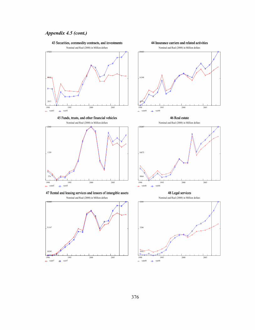
Appendix 4.5 (cont.)
43 Securities, commodity contracts, and investments 43 Securities, commodity contracts, and investments Nominal and Real (2000) in Million dollars
17221
9918
2615
1990 1995 2000 2005 vein43 veir43
44 Insurance carriers and related activities 44 Insurance carriers and related activities Nominal and Real (2000) in Million dollars
25603
16240
6876
1990 1995 2000 2005 vein44 veir44
45 Funds, trusts, and other financial vehicles 45 Funds, trusts, and other financial vehicles Nominal and Real (2000) in Million dollars
2343
1359
376
1990 1995 2000 2005 vein45 veir45
46 Real estate 46 Real estate Nominal and Real (2000) in Million dollars
23287
16075
8864
1990 1995 2000 2005 vein46 veir46
47 Rental and leasing services and lessors of intangible assets 47 Rental and leasing services and lessors of intangible assets Nominal and Real (2000) in Million dollars
92449
51347
10245
1990 1995 2000 2005 vein47 veir47
48 Legal services 48 Legal services Nominal and Real (2000) in Million dollars
5395
3206
1016
1990 1995 2000 2005 vein48 veir48
376

Appendix 4.5 (cont.)
49 Computer systems design and related services 49 Computer systems design and related services Nominal and Real (2000) in Million dollars
30911
16443
1976
1990 1995 2000 2005 vein49 veir49
50 Miscellaneous professional, scientific, and technical services 50 Miscellaneous professional, scientific, and technical services Nominal and Real (2000) in Million dollars
79260
43994
8729
1990 1995 2000 2005 vein50 veir50
51 Management of companies and enterprises 51 Management of companies and enterprises Nominal and Real (2000) in Million dollars
34573
20874
7175
1990 1995 2000 2005 vein51 veir51
52 Administrative and support services 52 Administrative and support services Nominal and Real (2000) in Million dollars
31395
18109
4823
1990 1995 2000 2005 vein52 veir52
53 Waste management and remediation services 53 Waste management and remediation services Nominal and Real (2000) in Million dollars
3850
2636
1422
1990 1995 2000 2005 vein53 veir53
54 Educational services 54 Educational services Nominal and Real (2000) in Million dollars
13381
7575
1769
1990 1995 2000 2005 vein54 veir54
377

Appendix 4.5 (cont.)
55 Ambulatory health care services 55 Ambulatory health care services Nominal and Real (2000) in Million dollars
47692
29198
10704
1990 1995 2000 2005 vein55 veir55
56 Hospitals 56 Hospitals Nominal and Real (2000) in Million dollars
60781
35870
10959
1990 1995 2000 2005 vein56 veir56
57 Nursing and residential care facilities 57 Nursing and residential care facilities Nominal and Real (2000) in Million dollars
3522
2211
900
1990 1995 2000 2005 vein57 veir57
58 Social assistance 58 Social assistance Nominal and Real (2000) in Million dollars
1825
1181
537
1990 1995 2000 2005 vein58 veir58
59 Performing arts, spectator sports, museums, and related activities 59 Performing arts, spectator sports, museums, and related activities Nominal and Real (2000) in Million dollars
3076
1885
694
1990 1995 2000 2005 vein59 veir59
60 Amusements, gambling, and recreation industries 60 Amusements, gambling, and recreation industries Nominal and Real (2000) in Million dollars
6291
3779
1268
1990 1995 2000 2005 vein60 veir60
378

Appendix 4.5 (cont.)
61 Accommodation 61 Accommodation Nominal and Real (2000) in Million dollars
6116
4270
2424
1990 1995 2000 2005 vein61 veir61
62 Food services and drinking places 62 Food services and drinking places Nominal and Real (2000) in Million dollars
24855
16046
7236
1990 1995 2000 2005 vein62 veir62
63 Other services, except government 63 Other services, except government Nominal and Real (2000) in Million dollars
11431
8424
5418
1990 1995 2000 2005 vein63 veir63
379

Appendix 5.1: Regressions' Results of Annual Fixed Investment in Nonresidential Structures
: Office (NIPA) SEE = 0.07 RSQ = 0.9999 RHO = -0.36 Obser = 10 from 1997.000 SEE+1 = 0.07 RBSQ = 0.9999 DW = 2.72 DoFree = 9 to 2006.000 MAPE = 0.14 Variable name Reg-Coef Mexval Elas NorRes Mean Beta 0 vstnn1 - - - - - - - - - - - - - - - - - 46.27 - - - 1 vipoffice 1.14934 64571.2 1.00 1.00 40.26
: Hospitals SEE = 0.46 RSQ = 0.9909 RHO = -0.09 Obser = 10 from 1997.000 SEE+1 = 0.46 RBSQ = 0.9882 DW = 2.17 DoFree = 7 to 2006.000 MAPE = 2.85 Variable name Reg-Coef Mexval Elas NorRes Mean Beta 0 vstnn4 - - - - - - - - - - - - - - - - - 15.45 - - - 1 intercept -4.98382 104.5 -0.32 109.36 1.00 2 vipmc 1.27634 180.8 1.88 1.46 22.70 1.329 3 vipmc[1] -0.40812 20.7 -0.55 1.00 20.93 -0.342
: Special Care SEE = 0.47 RSQ = 0.6281 RHO = 0.19 Obser = 9 from 1998.000 SEE+1 = 0.47 RBSQ = 0.5042 DurH = 999.00 DoFree = 6 to 2006.000 MAPE = 12.17 Variable name Reg-Coef Mexval Elas NorRes Mean Beta 0 vstnn5 - - - - - - - - - - - - - - - - - 3.77 - - - 1 intercept 6.34659 15.8 1.68 2.69 1.00 2 vstnn5[1] 0.04094 0.0 0.04 1.26 3.82 0.040 3 vipmc -0.11749 12.2 -0.73 1.00 23.29 -0.756
: Medical Buildings SEE = 0.54 RSQ = 0.8829 RHO = -0.03 Obser = 10 from 1997.000 SEE+1 = 0.54 RBSQ = 0.8495 DW = 2.06 DoFree = 7 to 2006.000 MAPE = 7.53 Variable name Reg-Coef Mexval Elas NorRes Mean Beta 0 vstnn6 - - - - - - - - - - - - - - - - - 6.35 - - - 1 intercept -1.76966 13.5 -0.28 8.54 1.00 2 vipmc -0.15372 3.5 -0.55 1.61 22.70 -0.486 3 vipmc[1] 0.55478 26.8 1.83 1.00 20.93 1.413
: Multimerchandise shopping SEE = 1.99 RSQ = 0.8116 RHO = 0.58 Obser = 10 from 1997.000 SEE+1 = 1.72 RBSQ = 0.7881 DW = 0.85 DoFree = 8 to 2006.000 MAPE = 9.33 Variable name Reg-Coef Mexval Elas NorRes Mean Beta 0 vstnn7 - - - - - - - - - - - - - - - - - 16.49 - - - 1 intercept -31.29721 68.4 -1.90 5.31 1.00 2 vipcommerce 0.77776 130.4 2.90 1.00 61.44 0.901
: Food and beverage establishments SEE = 0.26 RSQ = 0.7059 RHO = -0.33 Obser = 10 from 1997.000 SEE+1 = 0.23 RBSQ = 0.6219 DW = 2.66 DoFree = 7 to 2006.000 MAPE = 2.92 Variable name Reg-Coef Mexval Elas NorRes Mean Beta 0 vstnn8 - - - - - - - - - - - - - - - - - 7.89 - - - 1 intercept 11.37066 295.5 1.44 3.40 1.00 2 vipoffice 0.04114 43.0 0.21 3.29 40.26 0.635
380

3 vipcommerce -0.08361 81.5 -0.65 1.00 61.44 -0.941
: Warehouses SEE = 0.69 RSQ = 0.6406 RHO = 0.25 Obser = 10 from 1997.000 SEE+1 = 0.71 RBSQ = 0.5956 DW = 1.51 DoFree = 8 to 2006.000 MAPE = 4.53 Variable name Reg-Coef Mexval Elas NorRes Mean Beta 0 vstnn9 - - - - - - - - - - - - - - - - - 12.63 - - - 1 vipcommerce 0.11288 85.8 0.55 2.67 61.44 2 vipoffice 0.14031 63.3 0.45 1.00 40.26 0.887
: Other commercial SEE = 1.05 RSQ = 0.0704 RHO = -0.13 Obser = 8 from 1999.000 SEE+1 = 1.02 RBSQ = -0.6268 DurH = 999.00 DoFree = 4 to 2006.000 MAPE = 5.44 Variable name Reg-Coef Mexval Elas NorRes Mean Beta 0 vstnn10 - - - - - - - - - - - - - - - - - 16.83 - - - 1 intercept 24.63346 32.1 1.46 1.08 1.00 2 vstnn10[1] -0.16023 1.2 -0.16 1.05 16.89 -0.149 3 vstnn10[2] -0.14946 1.3 -0.15 1.03 16.75 -0.154 4 vipcommerce -0.04112 1.5 -0.15 1.00 63.20 -0.167
: Manufacturing (NIPA) SEE = 2.62 RSQ = 0.8905 RHO = 0.60 Obser = 10 from 1997.000 SEE+1 = 2.36 RBSQ = 0.8768 DW = 0.81 DoFree = 8 to 2006.000 MAPE = 7.52 Variable name Reg-Coef Mexval Elas NorRes Mean Beta 0 vstnnmanu - - - - - - - - - - - - - - - - - 27.51 - - - 1 intercept -7.97617 18.0 -0.29 9.13 1.00 2 vipmanu 1.10648 202.2 1.29 1.00 32.07 0.944
: Electric SEE = 1.00 RSQ = 0.9513 RHO = 0.17 Obser = 10 from 1997.000 SEE+1 = 1.01 RBSQ = 0.9452 DW = 1.66 DoFree = 8 to 2006.000 MAPE = 4.77 Variable name Reg-Coef Mexval Elas NorRes Mean Beta 0 vstnn12 - - - - - - - - - - - - - - - - - 18.94 - - - 1 intercept -3.20768 18.1 -0.17 20.52 1.00 2 vippower 0.81715 353.0 1.17 1.00 27.10 0.975
: Other power SEE = 0.70 RSQ = 0.3736 RHO = 0.63 Obser = 8 from 1999.000 SEE+1 = 0.60 RBSQ = -0.0962 DurH = 8.25 DoFree = 4 to 2006.000 MAPE = 8.15 Variable name Reg-Coef Mexval Elas NorRes Mean Beta 0 vstnn13 - - - - - - - - - - - - - - - - - 7.15 - - - 1 intercept -1.62310 0.5 -0.23 1.60 1.00 2 vstnn13[1] 0.54424 10.4 0.54 1.58 7.14 0.530 3 vstnn13[2] -0.08370 0.7 -0.08 1.50 6.88 -0.106 4 vippower 0.18702 22.3 0.76 1.00 29.22 0.747
: Communication SEE = 1.42 RSQ = 0.7663 RHO = 0.76 Obser = 10 from 1997.000 SEE+1 = 0.96 RBSQ = 0.7371 DW = 0.47 DoFree = 8 to 2006.000 MAPE = 8.49 Variable name Reg-Coef Mexval Elas NorRes Mean Beta 0 vstnn14 - - - - - - - - - - - - - - - - - 15.88 - - - 1 intercept 1.24004 1.1 0.08 4.28 1.00 2 vipcomm 0.86040 106.9 0.92 1.00 17.02 0.875
: Petroleum and natural gas
381

SEE = 0.25 RSQ = 0.9999 RHO = -0.56 Obser = 10 from 1997.000 SEE+1 = 0.20 RBSQ = 0.9999 DW = 3.12 DoFree = 8 to 2006.000 MAPE = 0.64 Variable name Reg-Coef Mexval Elas NorRes Mean Beta 0 vstnn15 - - - - - - - - - - - - - - - - - 43.00 - - - 1 intercept -0.35667 22.4 -0.01 9761.48 1.00 2 vstnnmin 0.96584 9780.0 1.01 1.00 44.89 1.000
: Mining SEE = 0.21 RSQ = 0.9479 RHO = -0.56 Obser = 9 from 1998.000 SEE+1 = 0.17 RBSQ = 0.9305 DurH = 999.00 DoFree = 6 to 2006.000 MAPE = 9.32 Variable name Reg-Coef Mexval Elas NorRes Mean Beta 0 vstnn16 - - - - - - - - - - - - - - - - - 1.96 - - - 1 intercept 0.42963 14.8 0.22 19.18 1.00 2 vstnn16[1] -0.26083 2.7 -0.22 3.18 1.68 -0.180 3 vstnnmin 0.04143 78.5 1.00 1.00 47.39 1.144
: Religious SEE = 0.02 RSQ = 0.9991 RHO = -0.16 Obser = 10 from 1997.000 SEE+1 = 0.02 RBSQ = 0.9990 DW = 2.32 DoFree = 8 to 2006.000 MAPE = 0.27 Variable name Reg-Coef Mexval Elas NorRes Mean Beta 0 vstnn17 - - - - - - - - - - - - - - - - - 7.45 - - - 1 intercept -0.04507 1.9 -0.01 1092.95 1.00 2 viprelig 0.97779 3206.0 1.01 1.00 7.67 1.000
: Educational and vocational SEE = 0.16 RSQ = 0.9922 RHO = 0.27 Obser = 10 from 1997.000 SEE+1 = 0.16 RBSQ = 0.9912 DW = 1.47 DoFree = 8 to 2006.000 MAPE = 0.85 Variable name Reg-Coef Mexval Elas NorRes Mean Beta 0 vstnn18 - - - - - - - - - - - - - - - - - 13.11 - - - 1 intercept 0.80318 23.6 0.06 127.52 1.00 2 vipedu 1.03639 1029.2 0.94 1.00 11.87 0.996
: Lodging SEE = 0.03 RSQ = 0.9999 RHO = -0.34 Obser = 10 from 1997.000 SEE+1 = 0.03 RBSQ = 0.9999 DW = 2.67 DoFree = 9 to 2006.000 MAPE = 0.14 Variable name Reg-Coef Mexval Elas NorRes Mean Beta 0 vstnn19 - - - - - - - - - - - - - - - - - 17.00 - - - 1 viplodge 1.23880 60149.0 1.00 1.00 13.72
: Amusement and recreation SEE = 0.03 RSQ = 0.9985 RHO = -0.08 Obser = 10 from 1997.000 SEE+1 = 0.03 RBSQ = 0.9983 DW = 2.17 DoFree = 8 to 2006.000 MAPE = 0.26 Variable name Reg-Coef Mexval Elas NorRes Mean Beta 0 vstnn20 - - - - - - - - - - - - - - - - - 10.02 - - - 1 intercept -0.10770 3.7 -0.01 662.95 1.00 2 viprec 1.21266 2474.8 1.01 1.00 8.35 0.999
: Air transportation SEE = 0.31 RSQ = 0.4030 RHO = 0.41 Obser = 9 from 1998.000 SEE+1 = 0.29 RBSQ = 0.3177 DurH = 2.16 DoFree = 7 to 2006.000 MAPE = 19.40 Variable name Reg-Coef Mexval Elas NorRes Mean Beta 0 vstnn22 - - - - - - - - - - - - - - - - - 1.31 - - - 1 vstnn22[1] 0.67994 37.4 0.69 1.17 1.32 2 viptr 0.05868 8.2 0.31 1.00 7.02 0.059
382
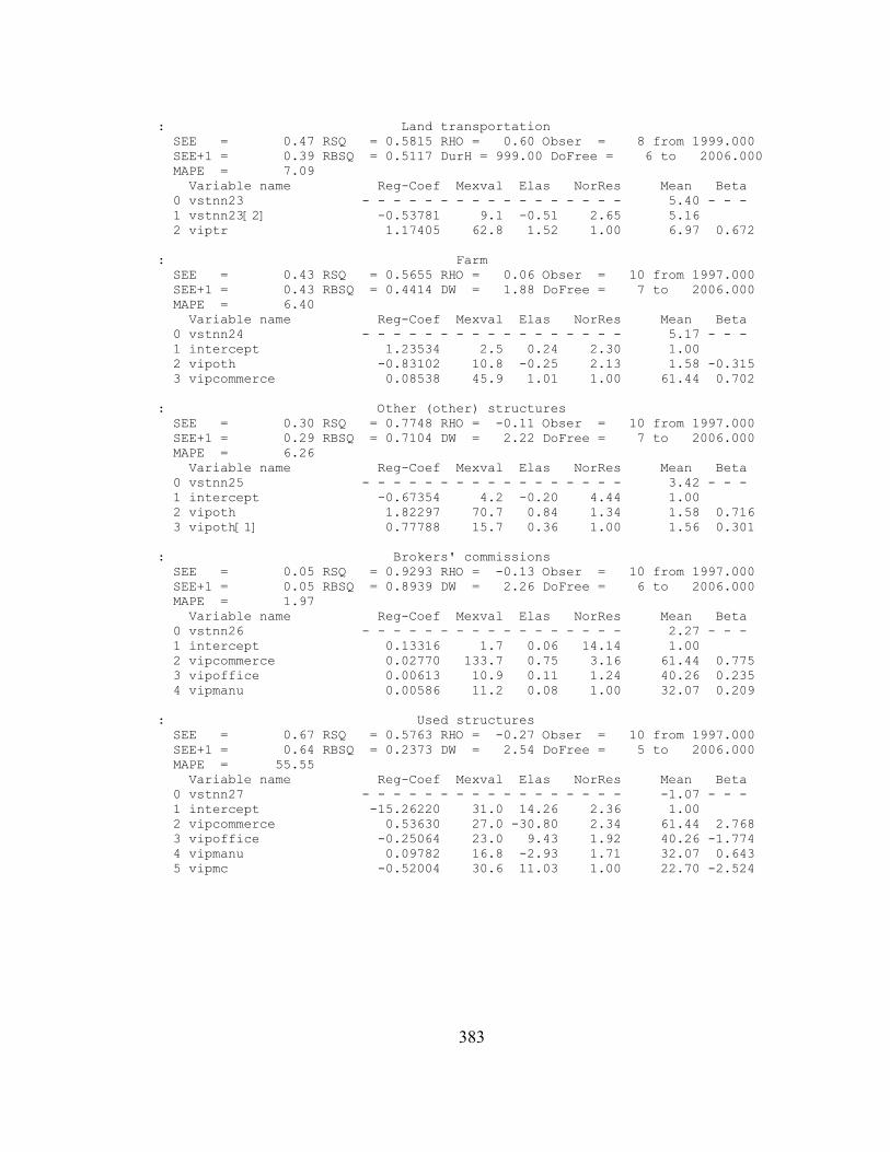
: Land transportation SEE = 0.47 RSQ = 0.5815 RHO = 0.60 Obser = 8 from 1999.000 SEE+1 = 0.39 RBSQ = 0.5117 DurH = 999.00 DoFree = 6 to 2006.000 MAPE = 7.09 Variable name Reg-Coef Mexval Elas NorRes Mean Beta 0 vstnn23 - - - - - - - - - - - - - - - - - 5.40 - - - 1 vstnn23[2] -0.53781 9.1 -0.51 2.65 5.16 2 viptr 1.17405 62.8 1.52 1.00 6.97 0.672
: Farm SEE = 0.43 RSQ = 0.5655 RHO = 0.06 Obser = 10 from 1997.000 SEE+1 = 0.43 RBSQ = 0.4414 DW = 1.88 DoFree = 7 to 2006.000 MAPE = 6.40 Variable name Reg-Coef Mexval Elas NorRes Mean Beta 0 vstnn24 - - - - - - - - - - - - - - - - - 5.17 - - - 1 intercept 1.23534 2.5 0.24 2.30 1.00 2 vipoth -0.83102 10.8 -0.25 2.13 1.58 -0.315 3 vipcommerce 0.08538 45.9 1.01 1.00 61.44 0.702
: Other (other) structures SEE = 0.30 RSQ = 0.7748 RHO = -0.11 Obser = 10 from 1997.000 SEE+1 = 0.29 RBSQ = 0.7104 DW = 2.22 DoFree = 7 to 2006.000 MAPE = 6.26 Variable name Reg-Coef Mexval Elas NorRes Mean Beta 0 vstnn25 - - - - - - - - - - - - - - - - - 3.42 - - - 1 intercept -0.67354 4.2 -0.20 4.44 1.00 2 vipoth 1.82297 70.7 0.84 1.34 1.58 0.716 3 vipoth[1] 0.77788 15.7 0.36 1.00 1.56 0.301
: Brokers' commissions SEE = 0.05 RSQ = 0.9293 RHO = -0.13 Obser = 10 from 1997.000 SEE+1 = 0.05 RBSQ = 0.8939 DW = 2.26 DoFree = 6 to 2006.000 MAPE = 1.97 Variable name Reg-Coef Mexval Elas NorRes Mean Beta 0 vstnn26 - - - - - - - - - - - - - - - - - 2.27 - - - 1 intercept 0.13316 1.7 0.06 14.14 1.00 2 vipcommerce 0.02770 133.7 0.75 3.16 61.44 0.775 3 vipoffice 0.00613 10.9 0.11 1.24 40.26 0.235 4 vipmanu 0.00586 11.2 0.08 1.00 32.07 0.209
: Used structures SEE = 0.67 RSQ = 0.5763 RHO = -0.27 Obser = 10 from 1997.000 SEE+1 = 0.64 RBSQ = 0.2373 DW = 2.54 DoFree = 5 to 2006.000 MAPE = 55.55 Variable name Reg-Coef Mexval Elas NorRes Mean Beta 0 vstnn27 - - - - - - - - - - - - - - - - - -1.07 - - - 1 intercept -15.26220 31.0 14.26 2.36 1.00 2 vipcommerce 0.53630 27.0 -30.80 2.34 61.44 2.768 3 vipoffice -0.25064 23.0 9.43 1.92 40.26 -1.774 4 vipmanu 0.09782 16.8 -2.93 1.71 32.07 0.643 5 vipmc -0.52004 30.6 11.03 1.00 22.70 -2.524
383

Appendix 6.1: Gross Domestic Product by Industry Categories, BEA
BEADetailed Industry
1 Gross domestic product2 Private industries3 Agriculture, forestry, fishing, and hunting4 1 Farms5 2 Forestry, fishing, and related activities6 Mining7 3 Oil and gas extraction8 4 Mining, except oil and gas9 5 Support activities for mining10 6 Utilities11 7 Construction12 Manufacturing13 Durable goods14 8 Wood products15 9 Nonmetallic mineral products16 10 Primary metals17 11 Fabricated metal products18 12 Machinery19 13 Computer and electronic products20 14 Electrical equipment, appliances, and components21 15 Motor vehicles, bodies and trailers, and parts22 16 Other transportation equipment23 17 Furniture and related products24 18 Miscellaneous manufacturing25 Nondurable goods26 19 Food and beverage and tobacco products27 20 Textile mills and textile product mills28 21 Apparel and leather and allied products29 22 Paper products30 23 Printing and related support activities31 24 Petroleum and coal products32 25 Chemical products33 26 Plastics and rubber products34 27 Wholesale trade35 28 Retail trade36 Transportation and warehousing37 29 Air transportation38 30 Rail transportation39 31 Water transportation
384
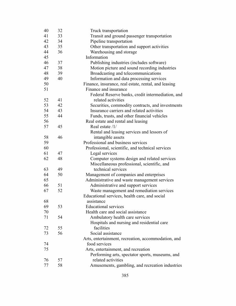
40 32 Truck transportation41 33 Transit and ground passenger transportation42 34 Pipeline transportation43 35 Other transportation and support activities44 36 Warehousing and storage45 Information46 37 Publishing industries (includes software)47 38 Motion picture and sound recording industries48 39 Broadcasting and telecommunications49 40 Information and data processing services50 Finance, insurance, real estate, rental, and leasing51 Finance and insurance
52 41 Federal Reserve banks, credit intermediation, and related activities
53 42 Securities, commodity contracts, and investments54 43 Insurance carriers and related activities55 44 Funds, trusts, and other financial vehicles56 Real estate and rental and leasing57 45 Real estate /1/
58 46 Rental and leasing services and lessors of intangible assets
59 Professional and business services60 Professional, scientific, and technical services61 47 Legal services62 48 Computer systems design and related services
63 49 Miscellaneous professional, scientific, and technical services
64 50 Management of companies and enterprises65 Administrative and waste management services66 51 Administrative and support services67 52 Waste management and remediation services
68 Educational services, health care, and social assistance
69 53 Educational services70 Health care and social assistance71 54 Ambulatory health care services
72 55 Hospitals and nursing and residential care facilities
73 56 Social assistance
74 Arts, entertainment, recreation, accommodation, and food services
75 Arts, entertainment, and recreation
76 57 Performing arts, spectator sports, museums, and related activities
77 58 Amusements, gambling, and recreation industries
385
78 Accommodation and food services79 59 Accommodation80 60 Food services and drinking places81 61 Other services, except government82 Government83 Federal84 62 General government85 63 Government enterprises86 State and local87 64 General government88 65 Government enterprises89 Private goods-producing industries90 Private services-producing industries
91 Information-communications-technology-producing industries
386

Appendix 6.2: Results from Historical SimulationsNominal in Billion dollars
Results from Historical simulations BEAactual exog
predicted exog BEA
actual exog
predicted exog
Total Gross Output 19,757.5 19,544.2 19,630.9 21,306.9 20,923.8 20,590.4 Private industries 17,457.3 17,294.6 17,379.9 18,859.3 18,578.2 18,256.7 Total Services industries (40-61) 8,078.4 7,955.5 8,020.1 8,741.9 8,478.0 8,347.8 Agriculture, forestry, fishing, and hunting 279.6 270.1 256.0 319.5 319.0 277.7 Mining 259.9 254.5 280.2 307.1 303.9 400.4 Utilities 355.7 348.7 348.3 372.9 368.4 367.4 Construction 956.8 953.1 945.5 1,063.0 1,023.3 950.8 Manufacturing 3,957.6 3,942.8 3,956.6 4,207.1 4,195.2 4,120.0 Durable goods manufacturing 2,114.9 2,095.6 2,136.5 2,221.6 2,214.7 2,237.3 Nondurable goods manufacturing 1,842.7 1,847.2 1,820.1 1,985.5 1,980.5 1,882.6 Wholesale trade 902.3 886.4 896.1 995.1 1,046.7 1,004.4 Retail trade 1,138.9 1,122.5 1,121.4 1,223.3 1,205.5 1,172.3 Transportation and warehousing 598.5 629.7 636.4 648.4 655.5 663.7 Information 1,031.5 1,031.8 1,019.0 1,094.7 1,088.7 1,056.8 Finance, insurance, real estate, rental, and leasing 3,382.4 3,340.2 3,361.3 3,713.2 3,586.8 3,547.3 Professional and business services 2,004.5 1,952.4 2,000.9 2,164.3 2,064.1 2,054.5 Educational services, health care, and social assistance 1,387.6 1,374.3 1,376.0 1,474.5 1,462.6 1,429.4 Arts, entertainment, recreation, accommodation, and food services 721.3 715.5 708.0 770.9 767.7 733.5 Other services, except government 480.7 472.7 474.2 505.5 491.0 478.4 Government 2,300.2 2,249.5 2,251.0 2,447.6 2,345.5 2,333.7 Federal government 758.9 732.2 727.4 824.8 772.5 756.2 State and local government 1,541.3 1,517.3 1,523.6 1,622.8 1,573.1 1,577.5
Percentage Deviation from the BEA data as of December 2006
actual exog
predicted exog
actual exog
predicted exog
Total Gross Output -1.08% -0.64% -1.80% -3.36% Private industries -0.93% -0.44% -1.49% -3.20% Total Services industries (40-61) -1.52% -0.72% -3.02% -4.51% Agriculture, forestry, fishing, and hunting -3.41% -8.46% -0.16% -13.08% Mining -2.10% 7.79% -1.05% 30.39% Utilities -1.96% -2.09% -1.21% -1.48% Construction -0.39% -1.17% -3.73% -10.55% Manufacturing -0.37% -0.03% -0.28% -2.07% Durable goods manufacturing -0.91% 1.02% -0.31% 0.71% Nondurable goods manufacturing 0.24% -1.22% -0.25% -5.18% Wholesale trade -1.77% -0.69% 5.19% 0.94% Retail trade -1.44% -1.54% -1.46% -4.17% Transportation and warehousing 5.21% 6.33% 1.10% 2.37% Information 0.03% -1.22% -0.54% -3.46% Finance, insurance, real estate, rental, and leasing -1.25% -0.62% -3.41% -4.47% Professional and business services -2.60% -0.18% -4.63% -5.07% Educational services, health care, and social assistance -0.95% -0.83% -0.81% -3.06% Arts, entertainment, recreation, accommodation, and food services -0.80% -1.84% -0.42% -4.85% Other services, except government -1.67% -1.37% -2.88% -5.36% Government -2.20% -2.14% -4.17% -4.65% Federal government -3.51% -4.15% -6.34% -8.32% State and local government -1.56% -1.15% -3.06% -2.79%
2003 2004
2003 2004
387

Chained 2000 dollars in Billion dollars
Results from Historical simulations BEAactual exog
predicted exog BEA
actual exog
predicted exog
Total Gross Output 18,782.6 18,686.1 18,672.6 19,496.2 19,344.6 18,965.7 Private industries 16,709.1 16,619.5 16,617.5 17,390.2 17,271.9 16,895.6 Total Services industries (40-61) 7,559.2 7,504.7 7,511.1 7,949.9 7,830.1 7,691.9 Agriculture, forestry, fishing, and hunting 262.0 261.0 261.9 269.8 269.5 265.9 Mining 211.4 208.0 213.0 216.4 213.7 221.3 Utilities 316.1 309.5 325.1 313.0 314.8 348.9 Construction 863.0 856.9 851.0 902.3 887.1 837.2 Manufacturing 3,943.8 3,936.1 3,915.8 4,000.6 3,999.1 3,884.9 Durable goods manufacturing 2,193.1 2,178.1 2,204.1 2,233.3 2,232.1 2,263.9 Nondurable goods manufacturing 1,751.2 1,757.9 1,714.0 1,768.7 1,768.8 1,632.4 Wholesale trade 911.8 896.3 901.9 950.1 986.7 938.4 Retail trade 1,125.8 1,115.1 1,111.0 1,181.6 1,195.0 1,151.6 Transportation and warehousing 575.7 590.6 592.1 607.8 596.0 584.3 Information 1,033.2 1,031.2 1,022.9 1,103.0 1,078.8 1,063.3 Finance, insurance, real estate, rental, and leasing 3,177.1 3,196.4 3,171.3 3,386.5 3,337.7 3,254.4 Professional and business services 1,909.7 1,861.8 1,904.5 2,013.2 1,954.4 1,991.2 Educational services, health care, and social assistance 1,265.0 1,253.2 1,251.7 1,301.5 1,298.7 1,262.2 Arts, entertainment, recreation, accommodation, and food services 669.9 664.1 657.7 692.5 696.6 666.2 Other services, except government 437.5 433.6 430.6 445.5 441.5 421.8 Government 2,071.5 2,064.4 2,053.4 2,106.9 2,073.5 2,069.1 Federal government 678.9 668.3 659.5 703.4 680.6 667.1 State and local government 1,392.3 1,395.9 1,393.7 1,403.0 1,392.6 1,401.8
Percentage Deviation from the BEA data as of December 2006
actual exog
predicted exog
actual exog
predicted exog
Total Gross Output -0.51% -0.59% -0.78% -2.72% Private industries -0.54% -0.55% -0.68% -2.84% Total Services industries (40-61) -0.72% -0.64% -1.51% -3.25% Agriculture, forestry, fishing, and hunting -0.36% -0.05% -0.12% -1.43% Mining -1.62% 0.72% -1.27% 2.27% Utilities -2.09% 2.84% 0.55% 11.47% Construction -0.71% -1.39% -1.68% -7.21% Manufacturing -0.19% -0.71% -0.04% -2.89% Durable goods manufacturing -0.68% 0.50% -0.05% 1.37% Nondurable goods manufacturing 0.38% -2.13% 0.01% -7.70% Wholesale trade -1.70% -1.09% 3.85% -1.23% Retail trade -0.95% -1.32% 1.13% -2.55% Transportation and warehousing 2.58% 2.85% -1.94% -3.86% Information -0.20% -1.00% -2.19% -3.60% Finance, insurance, real estate, rental, and leasing 0.61% -0.18% -1.44% -3.90% Professional and business services -2.51% -0.27% -2.92% -1.09% Educational services, health care, and social assistance -0.94% -1.05% -0.22% -3.02% Arts, entertainment, recreation, accommodation, and food services -0.86% -1.81% 0.59% -3.80% Other services, except government -0.90% -1.57% -0.91% -5.32% Government -0.34% -0.88% -1.58% -1.79% Federal government -1.56% -2.86% -3.24% -5.16% State and local government 0.26% 0.10% -0.74% -0.08%
2003 2004
2003 2004
388

Chained Price Index (2000=100)
Results from Historical simulations BEAactual exog
predicted exog BEA
actual exog
predicted exog
Total Gross Output 105.2 104.6 105.1 109.3 108.2 108.6 Private industries 104.5 104.1 104.6 108.4 107.6 108.1 Total Services industries (40-61) 106.9 106.0 106.8 110.0 108.3 108.5 Agriculture, forestry, fishing, and hunting 106.7 103.5 97.7 118.4 118.4 104.4 Mining 122.9 122.3 131.6 141.9 142.2 180.9 Utilities 112.5 112.7 107.1 119.1 117.0 105.3 Construction 110.9 111.2 111.1 117.8 115.4 113.6 Manufacturing 100.4 100.2 101.0 105.2 104.9 106.1 Durable goods manufacturing 96.4 96.2 96.9 99.5 99.2 98.8 Nondurable goods manufacturing 105.2 105.1 106.2 112.3 112.0 115.3 Wholesale trade 99.0 98.9 99.4 104.7 106.1 107.0 Retail trade 101.2 100.7 100.9 103.5 100.9 101.8 Transportation and warehousing 104.0 106.6 107.5 106.7 110.0 113.6 Information 99.8 100.1 99.6 99.2 100.9 99.4 Finance, insurance, real estate, rental, and leasing 106.5 104.5 106.0 109.6 107.5 109.0 Professional and business services 105.0 104.9 105.1 107.5 105.6 103.2 Educational services, health care, and social assistance 109.7 109.7 109.9 113.3 112.6 113.2 Arts, entertainment, recreation, accommodation, and food services 107.7 107.7 107.6 111.3 110.2 110.1 Other services, except government 109.9 109.0 110.1 113.5 111.2 113.4 Government 111.0 109.0 109.6 116.2 113.1 112.8 Federal government 111.8 109.6 110.3 117.3 113.5 113.4 State and local government 110.7 108.7 109.3 115.7 113.0 112.5
Percentage Deviation from the BEA data as of December 2006
actual exog
predicted exog
actual exog
predicted exog
Total Gross Output -0.57% -0.06% -1.03% -0.66% Private industries -0.40% 0.11% -0.82% -0.36% Total Services industries (40-61) -0.81% -0.09% -1.53% -1.31% Agriculture, forestry, fishing, and hunting -3.06% -8.42% -0.04% -11.82% Mining -0.49% 7.01% 0.23% 27.49% Utilities 0.13% -4.80% -1.75% -11.62% Construction 0.32% 0.22% -2.08% -3.60% Manufacturing -0.18% 0.69% -0.25% 0.85% Durable goods manufacturing -0.23% 0.51% -0.26% -0.65% Nondurable goods manufacturing -0.14% 0.92% -0.26% 2.73% Wholesale trade -0.07% 0.41% 1.29% 2.20% Retail trade -0.49% -0.23% -2.56% -1.66% Transportation and warehousing 2.57% 3.39% 3.10% 6.48% Information 0.23% -0.22% 1.69% 0.15% Finance, insurance, real estate, rental, and leasing -1.84% -0.44% -1.99% -0.59% Professional and business services -0.09% 0.09% -1.76% -4.02% Educational services, health care, and social assistance -0.02% 0.22% -0.59% -0.04% Arts, entertainment, recreation, accommodation, and food services 0.05% -0.03% -1.00% -1.09% Other services, except government -0.78% 0.20% -1.99% -0.04% Government -1.87% -1.27% -2.63% -2.91% Federal government -1.98% -1.33% -3.20% -3.33% State and local government -1.81% -1.25% -2.35% -2.71%
2003 2004
2003 2004
389
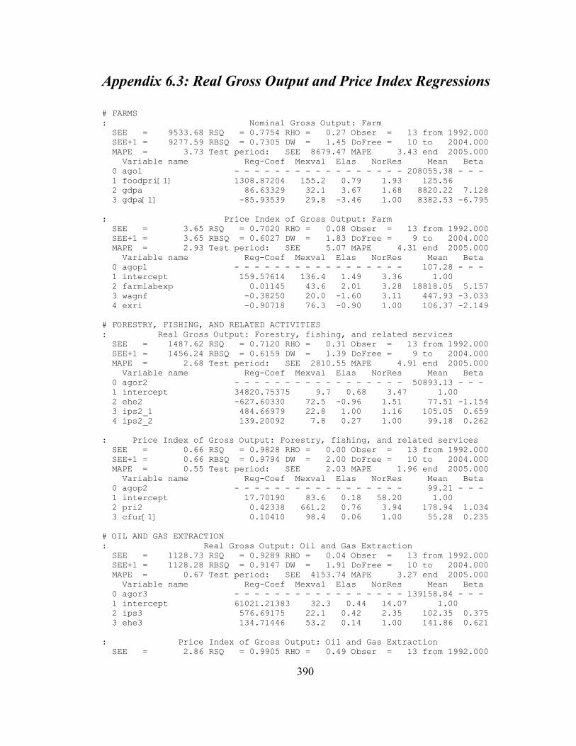
Appendix 6.3: Real Gross Output and Price Index Regressions
# FARMS: Nominal Gross Output: Farm SEE = 9533.68 RSQ = 0.7754 RHO = 0.27 Obser = 13 from 1992.000 SEE+1 = 9277.59 RBSQ = 0.7305 DW = 1.45 DoFree = 10 to 2004.000 MAPE = 3.73 Test period: SEE 8679.47 MAPE 3.43 end 2005.000 Variable name Reg-Coef Mexval Elas NorRes Mean Beta 0 ago1 - - - - - - - - - - - - - - - - - 208055.38 - - - 1 foodpri[1] 1308.87204 155.2 0.79 1.93 125.56 2 gdpa 86.63329 32.1 3.67 1.68 8820.22 7.128 3 gdpa[1] -85.93539 29.8 -3.46 1.00 8382.53 -6.795
: Price Index of Gross Output: Farm SEE = 3.65 RSQ = 0.7020 RHO = 0.08 Obser = 13 from 1992.000 SEE+1 = 3.65 RBSQ = 0.6027 DW = 1.83 DoFree = 9 to 2004.000 MAPE = 2.93 Test period: SEE 5.07 MAPE 4.31 end 2005.000 Variable name Reg-Coef Mexval Elas NorRes Mean Beta 0 agop1 - - - - - - - - - - - - - - - - - 107.28 - - - 1 intercept 159.57614 136.4 1.49 3.36 1.00 2 farmlabexp 0.01145 43.6 2.01 3.28 18818.05 5.157 3 wagnf -0.38250 20.0 -1.60 3.11 447.93 -3.033 4 exri -0.90718 76.3 -0.90 1.00 106.37 -2.149
# FORESTRY, FISHING, AND RELATED ACTIVITIES: Real Gross Output: Forestry, fishing, and related services SEE = 1487.62 RSQ = 0.7120 RHO = 0.31 Obser = 13 from 1992.000 SEE+1 = 1456.24 RBSQ = 0.6159 DW = 1.39 DoFree = 9 to 2004.000 MAPE = 2.68 Test period: SEE 2810.55 MAPE 4.91 end 2005.000 Variable name Reg-Coef Mexval Elas NorRes Mean Beta 0 agor2 - - - - - - - - - - - - - - - - - 50893.13 - - - 1 intercept 34820.75375 9.7 0.68 3.47 1.00 2 ehe2 -627.60330 72.5 -0.96 1.51 77.51 -1.154 3 ips2_1 484.66979 22.8 1.00 1.16 105.05 0.659 4 ips2_2 139.20092 7.8 0.27 1.00 99.18 0.262
: Price Index of Gross Output: Forestry, fishing, and related services SEE = 0.66 RSQ = 0.9828 RHO = 0.00 Obser = 13 from 1992.000 SEE+1 = 0.66 RBSQ = 0.9794 DW = 2.00 DoFree = 10 to 2004.000 MAPE = 0.55 Test period: SEE 2.03 MAPE 1.96 end 2005.000 Variable name Reg-Coef Mexval Elas NorRes Mean Beta 0 agop2 - - - - - - - - - - - - - - - - - 99.21 - - - 1 intercept 17.70190 83.6 0.18 58.20 1.00 2 pri2 0.42338 661.2 0.76 3.94 178.94 1.034 3 cfur[1] 0.10410 98.4 0.06 1.00 55.28 0.235
# OIL AND GAS EXTRACTION: Real Gross Output: Oil and Gas Extraction SEE = 1128.73 RSQ = 0.9289 RHO = 0.04 Obser = 13 from 1992.000 SEE+1 = 1128.28 RBSQ = 0.9147 DW = 1.91 DoFree = 10 to 2004.000 MAPE = 0.67 Test period: SEE 4153.74 MAPE 3.27 end 2005.000 Variable name Reg-Coef Mexval Elas NorRes Mean Beta 0 agor3 - - - - - - - - - - - - - - - - - 139158.84 - - - 1 intercept 61021.21383 32.3 0.44 14.07 1.00 2 ips3 576.69175 22.1 0.42 2.35 102.35 0.375 3 ehe3 134.71446 53.2 0.14 1.00 141.86 0.621
: Price Index of Gross Output: Oil and Gas Extraction SEE = 2.86 RSQ = 0.9905 RHO = 0.49 Obser = 13 from 1992.000
390

SEE+1 = 2.66 RBSQ = 0.9896 DW = 1.01 DoFree = 11 to 2004.000 MAPE = 3.63 Test period: SEE 3.47 MAPE 1.78 end 2005.000 Variable name Reg-Coef Mexval Elas NorRes Mean Beta 0 agop3 - - - - - - - - - - - - - - - - - 75.26 - - - 1 intercept -3.25044 7.6 -0.04 105.23 1.00 2 pri3 0.77110 925.8 1.04 1.00 101.82 0.995
# MINING, EXCEPT OIL AND GAS: Real Gross Output: Mining, except Oil and Gas SEE = 268.42 RSQ = 0.9759 RHO = -0.35 Obser = 13 from 1992.000 SEE+1 = 246.17 RBSQ = 0.9711 DW = 2.69 DoFree = 10 to 2004.000 MAPE = 0.50 Test period: SEE 718.89 MAPE 1.48 end 2005.000 Variable name Reg-Coef Mexval Elas NorRes Mean Beta 0 agor4 - - - - - - - - - - - - - - - - - 46503.42 - - - 1 intercept 3269.51085 7.1 0.07 41.53 1.00 2 ips4 398.58727 519.6 0.86 2.01 100.05 1.049 3 ehe4 14.21965 41.8 0.07 1.00 236.03 0.172
: Price Index of Gross Output: Mining, except Oil and Gas SEE = 1.96 RSQ = 0.8649 RHO = 0.04 Obser = 13 from 1992.000 SEE+1 = 1.96 RBSQ = 0.8379 DW = 1.92 DoFree = 10 to 2004.000 MAPE = 1.52 Test period: SEE 2.95 MAPE 2.23 end 2005.000 Variable name Reg-Coef Mexval Elas NorRes Mean Beta 0 agop4 - - - - - - - - - - - - - - - - - 108.25 - - - 1 intercept 14.55680 5.7 0.13 7.40 1.00 2 pri4 1.16599 170.6 1.00 1.68 92.38 0.947 3 wagnf -0.03130 29.6 -0.13 1.00 447.93 -0.311
# SUPPORT ACTIVITIES FOR MINING: Real Gross Output: Support activities for Mining SEE = 2249.93 RSQ = 0.7902 RHO = 0.08 Obser = 13 from 1992.000 SEE+1 = 2249.08 RBSQ = 0.7483 DW = 1.85 DoFree = 10 to 2004.000 MAPE = 6.89 Test period: SEE 4863.64 MAPE 12.53 end 2005.000 Variable name Reg-Coef Mexval Elas NorRes Mean Beta 0 agor5 - - - - - - - - - - - - - - - - - 26792.74 - - - 1 intercept -27109.95120 32.0 -1.01 4.77 1.00 2 ips5 -6.48249 0.1 -0.03 4.53 118.24 -0.017 3 ehe5 320.54506 112.9 2.04 1.00 170.55 0.893
: Price Index of for Gross Output: Support activities for Mining SEE = 11.89 RSQ = 0.8843 RHO = 0.30 Obser = 13 from 1992.000 SEE+1 = 11.54 RBSQ = 0.8612 DW = 1.40 DoFree = 10 to 2004.000 MAPE = 6.08 Test period: SEE 3.13 MAPE 1.46 end 2005.000 Variable name Reg-Coef Mexval Elas NorRes Mean Beta 0 agop5 - - - - - - - - - - - - - - - - - 102.71 - - - 1 intercept -296.14561 32.9 -2.88 8.65 1.00 2 pri5_2 2.15780 157.5 2.51 1.15 119.42 0.876 3 pri5_4 1.23157 7.2 1.37 1.00 114.63 0.143
# UTILITIES: Nominal Gross Output: Utilities SEE = 5741.58 RSQ = 0.9744 RHO = -0.03 Obser = 13 from 1992.000 SEE+1 = 5734.57 RBSQ = 0.9692 DW = 2.05 DoFree = 10 to 2004.000 MAPE = 1.52 Test period: SEE 3410.53 MAPE 0.83 end 2005.000 Variable name Reg-Coef Mexval Elas NorRes Mean Beta 0 ago6 - - - - - - - - - - - - - - - - - 302719.77 - - - 1 intercept -82307.46187 47.8 -0.27 39.02 1.00 2 ips6 3459.21138 272.5 1.05 5.27 92.26 0.700 3 oilp[1] 2994.81199 129.6 0.22 1.00 22.00 0.403
: Price Index of for Gross Output: Utilities
391

SEE = 0.81 RSQ = 0.9918 RHO = 0.41 Obser = 13 from 1992.000 SEE+1 = 0.78 RBSQ = 0.9878 DW = 1.19 DoFree = 8 to 2004.000 MAPE = 0.57 Test period: SEE 4.55 MAPE 3.42 end 2005.000 Variable name Reg-Coef Mexval Elas NorRes Mean Beta 0 agop6 - - - - - - - - - - - - - - - - - 99.02 - - - 1 intercept 3.30311 0.2 0.03 122.61 1.00 2 wag6 0.47508 15.7 0.10 21.80 21.35 0.138 3 pri6_1 0.31257 9.7 0.37 9.28 116.31 0.165 4 pri6_2 0.28283 9.5 0.32 4.21 113.00 0.169 5 pri6_3 0.13710 105.3 0.17 1.00 125.88 0.556
# CONSTRUCTION: Real Gross output: Construction SEE = 6962.39 RSQ = 0.9947 RHO = 0.29 Obser = 13 from 1992.000 SEE+1 = 6909.06 RBSQ = 0.9942 DW = 1.42 DoFree = 11 to 2004.000 MAPE = 0.72 Test period: SEE 5697.81 MAPE 0.61 end 2005.000 Variable name Reg-Coef Mexval Elas NorRes Mean Beta 0 agor7 - - - - - - - - - - - - - - - - - 772214.43 - - - 1 intercept 71600.83992 71.1 0.09 188.93 1.00 2 ehe7 117.01271 1274.5 0.91 1.00 5987.50 0.997
: Price Index of for Gross Output: Construction SEE = 1.26 RSQ = 0.9899 RHO = 0.35 Obser = 13 from 1992.000 SEE+1 = 1.26 RBSQ = 0.9879 DW = 1.29 DoFree = 10 to 2004.000 MAPE = 1.06 Test period: SEE 5.43 MAPE 4.32 end 2005.000 Variable name Reg-Coef Mexval Elas NorRes Mean Beta 0 agop7 - - - - - - - - - - - - - - - - - 94.14 - - - 1 intercept -10.88908 29.3 -0.12 99.48 1.00 2 wag7 6.10102 472.9 1.06 1.61 16.37 0.896 3 oilp 0.22008 26.8 0.06 1.00 23.53 0.124
# MANUFACTURING: WOOD PRODUCTS: Real Gross Output: Wood Products SEE = 747.75 RSQ = 0.9885 RHO = 0.43 Obser = 13 from 1992.000 SEE+1 = 720.59 RBSQ = 0.9862 DW = 1.13 DoFree = 10 to 2004.000 MAPE = 0.75 Test period: SEE 5920.60 MAPE 6.41 end 2005.000 Variable name Reg-Coef Mexval Elas NorRes Mean Beta 0 agor8 - - - - - - - - - - - - - - - - - 85926.15 - - - 1 intercept -13876.12016 48.4 -0.16 86.87 1.00 2 ips8 862.41172 530.2 0.97 2.00 96.44 0.893 3 ehe8 29.23253 41.5 0.19 1.00 569.02 0.144
: Price Index of Gross Output: Wood Products SEE = 1.21 RSQ = 0.9648 RHO = 0.17 Obser = 13 from 1992.000 SEE+1 = 1.20 RBSQ = 0.9578 DW = 1.67 DoFree = 10 to 2004.000 MAPE = 0.92 Test period: SEE 1.42 MAPE 1.25 end 2005.000 Variable name Reg-Coef Mexval Elas NorRes Mean Beta 0 agop8 - - - - - - - - - - - - - - - - - 98.71 - - - 1 intercept -5.51910 3.5 -0.06 28.43 1.00 2 wagnf 0.09036 308.4 0.41 14.25 447.93 0.744 3 pri8_1 0.42354 277.4 0.65 1.00 150.53 0.684
# NONMETALLIC MINERAL PRODUCTS: Real Gross Output: Nonmetallic mineral products SEE = 439.40 RSQ = 0.9969 RHO = 0.52 Obser = 13 from 1992.000 SEE+1 = 387.62 RBSQ = 0.9963 DW = 0.97 DoFree = 10 to 2004.000 MAPE = 0.43 Test period: SEE 1560.54 MAPE 1.58 end 2005.000 Variable name Reg-Coef Mexval Elas NorRes Mean Beta 0 agor9 - - - - - - - - - - - - - - - - - 88241.95 - - - 1 intercept -2379.83058 2.1 -0.03 325.43 1.00 2 ips9 979.04120 1224.1 1.07 1.05 96.17 1.011
392

3 ehe9 -6.81513 2.6 -0.04 1.00 517.76 -0.018
: Price Index of Gross Output: Nonmetallic mineral products SEE = 0.19 RSQ = 0.9991 RHO = 0.53 Obser = 13 from 1992.000 SEE+1 = 0.17 RBSQ = 0.9990 DW = 0.95 DoFree = 11 to 2004.000 MAPE = 0.17 Test period: SEE 0.61 MAPE 0.54 end 2005.000 Variable name Reg-Coef Mexval Elas NorRes Mean Beta 0 agop9 - - - - - - - - - - - - - - - - - 95.62 - - - 1 intercept -0.48434 1.4 -0.01 1135.42 1.00 2 pri9 0.74563 3269.6 1.01 1.00 128.89 1.000
# PRIMARY METALS: Real Gross Output: Primary Metals SEE = 1502.60 RSQ = 0.9735 RHO = -0.08 Obser = 13 from 1992.000 SEE+1 = 1490.41 RBSQ = 0.9682 DW = 2.17 DoFree = 10 to 2004.000 MAPE = 0.81 Test period: SEE 607.84 MAPE 0.41 end 2005.000 Variable name Reg-Coef Mexval Elas NorRes Mean Beta 0 agor10 - - - - - - - - - - - - - - - - - 149129.53 - - - 1 intercept -933.87108 0.1 -0.01 37.72 1.00 2 ips10 1221.64143 441.2 0.86 3.19 105.04 0.894 3 ehe10 36.64322 78.7 0.15 1.00 593.22 0.249
: Price Index of Gross Output: Primary Metals SEE = 0.48 RSQ = 0.9952 RHO = 0.25 Obser = 13 from 1992.000 SEE+1 = 0.47 RBSQ = 0.9948 DW = 1.50 DoFree = 11 to 2004.000 MAPE = 0.34 Test period: SEE 0.28 MAPE 0.21 end 2005.000 Variable name Reg-Coef Mexval Elas NorRes Mean Beta 0 agop10 - - - - - - - - - - - - - - - - - 100.43 - - - 1 intercept -4.00796 14.3 -0.04 210.10 1.00 2 pri10 0.86651 1349.5 1.04 1.00 120.53 0.998
# FABRICATED METAL PRODUCTS: Nominal Gross Output: Fabricated metal products SEE = 3742.47 RSQ = 0.9832 RHO = -0.09 Obser = 13 from 1992.000 SEE+1 = 3659.06 RBSQ = 0.9799 DW = 2.18 DoFree = 10 to 2004.000 MAPE = 1.30 Test period: SEE 11766.19 MAPE 4.34 end 2005.000 Variable name Reg-Coef Mexval Elas NorRes Mean Beta 0 ago11 - - - - - - - - - - - - - - - - - 228872.62 - - - 1 intercept 11529.19165 1.7 0.05 59.59 1.00 2 ips11 3922.51035 540.2 1.68 4.25 97.94 1.222 3 ehe11 -103.47916 106.1 -0.73 1.00 1612.32 -0.348
: Price Index of Gross Output:Fabricated metal products SEE = 0.15 RSQ = 0.9991 RHO = 0.55 Obser = 13 from 1992.000 SEE+1 = 0.13 RBSQ = 0.9990 DW = 0.91 DoFree = 11 to 2004.000 MAPE = 0.13 Test period: SEE 0.27 MAPE 0.24 end 2005.000 Variable name Reg-Coef Mexval Elas NorRes Mean Beta 0 agop11 - - - - - - - - - - - - - - - - - 97.66 - - - 1 intercept -4.54239 78.6 -0.05 1113.06 1.00 2 pri11 0.80065 3236.3 1.05 1.00 127.65 1.000
# MACHINERY: Real Gross Output: Machinery SEE = 1594.67 RSQ = 0.9954 RHO = -0.31 Obser = 13 from 1992.000 SEE+1 = 1510.81 RBSQ = 0.9945 DW = 2.63 DoFree = 10 to 2004.000 MAPE = 0.46 Test period: SEE 1203.97 MAPE 0.45 end 2005.000 Variable name Reg-Coef Mexval Elas NorRes Mean Beta 0 agor12 - - - - - - - - - - - - - - - - - 246831.01 - - - 1 intercept 6040.15572 4.5 0.02 218.73 1.00 2 ips12 2335.44648 1178.0 0.97 1.00 102.72 0.996 3 ehe12 0.65746 0.1 0.00 1.00 1364.78 0.003
393

: Price Index of Gross Output: Machinery SEE = 0.93 RSQ = 0.9553 RHO = 0.84 Obser = 13 from 1992.000 SEE+1 = 0.67 RBSQ = 0.9512 DW = 0.31 DoFree = 11 to 2004.000 MAPE = 0.83 Test period: SEE 1.11 MAPE 1.02 end 2005.000 Variable name Reg-Coef Mexval Elas NorRes Mean Beta 0 agop12 - - - - - - - - - - - - - - - - - 97.48 - - - 1 intercept 36.34052 191.7 0.37 22.36 1.00 2 pri12 0.40426 372.8 0.63 1.00 151.25 0.977
# COMPUTER AND ELECTRONIC PRODUCTS: Real Gross Output: Computer and electronics products SEE = 12249.96 RSQ = 0.9923 RHO = 0.52 Obser = 13 from 1992.000 SEE+1 = 11750.77 RBSQ = 0.9907 DW = 0.96 DoFree = 10 to 2004.000 MAPE = 4.74 Test period: SEE 11539.94 MAPE 2.20 end 2005.000 Variable name Reg-Coef Mexval Elas NorRes Mean Beta 0 agor13 - - - - - - - - - - - - - - - - - 317952.52 - - - 1 intercept -316197.46716 125.5 -0.99 129.67 1.00 2 ips13 3862.44804 1000.5 0.77 8.32 63.34 1.098 3 ehe13 234.22982 188.4 1.23 1.00 1662.96 0.271
: Price Index of Gross Output: Computer and electronics products SEE = 5.21 RSQ = 0.9922 RHO = 0.44 Obser = 13 from 1992.000 SEE+1 = 5.13 RBSQ = 0.9914 DW = 1.11 DoFree = 11 to 2004.000 MAPE = 2.96 Test period: SEE 2.68 MAPE 3.69 end 2005.000 Variable name Reg-Coef Mexval Elas NorRes Mean Beta 0 agop13 - - - - - - - - - - - - - - - - - 144.54 - - - 1 intercept 41.93604 311.5 0.29 127.44 1.00 2 pri13 0.30289 1028.9 0.71 1.00 338.76 0.996
#ELECTRICAL EQUIPMENT, APPLIANCES, AND COMPONENTS: Real Gross Output: Electrical equipment, appliances, and components SEE = 668.61 RSQ = 0.9948 RHO = 0.22 Obser = 13 from 1992.000 SEE+1 = 678.19 RBSQ = 0.9938 DW = 1.56 DoFree = 10 to 2004.000 MAPE = 0.44 Test period: SEE 40.77 MAPE 0.04 end 2005.000 Variable name Reg-Coef Mexval Elas NorRes Mean Beta 0 agor14 - - - - - - - - - - - - - - - - - 104574.79 - - - 1 intercept 4479.81442 12.1 0.04 194.08 1.00 2 ips14 1022.00022 1207.6 1.03 1.88 105.24 1.025 3 ehe14 -13.38465 37.1 -0.07 1.00 557.12 -0.074
: Price Index of Gross Output: Electrical equipment, appliances, and components SEE = 0.61 RSQ = 0.9316 RHO = 0.50 Obser = 13 from 1992.000 SEE+1 = 0.56 RBSQ = 0.9179 DW = 1.01 DoFree = 10 to 2004.000 MAPE = 0.52 Test period: SEE 2.94 MAPE 2.73 end 2005.000 Variable name Reg-Coef Mexval Elas NorRes Mean Beta 0 agop14 - - - - - - - - - - - - - - - - - 98.49 - - - 1 pri14 0.85274 133.4 1.19 4.22 137.99 2 hr14 -0.11206 0.8 -0.05 1.53 41.51 -0.044 3 wagnf -0.03243 23.6 -0.15 1.00 447.93 -0.739
# MOTOR VEHICLE, BODIES AND TRAILERS, AND PARTS: Real Gross Output: Motor vehicle, bodies and trailers, and parts SEE = 6587.17 RSQ = 0.9896 RHO = 0.11 Obser = 13 from 1992.000 SEE+1 = 6551.72 RBSQ = 0.9875 DW = 1.78 DoFree = 10 to 2004.000 MAPE = 1.08 Test period: SEE 7045.25 MAPE 1.45 end 2005.000 Variable name Reg-Coef Mexval Elas NorRes Mean Beta 0 agor15 - - - - - - - - - - - - - - - - - 418208.43 - - - 1 intercept -15243.21608 1.3 -0.04 96.12 1.00 2 ips15 4656.20085 786.9 0.97 1.07 87.38 0.983 3 ehe15 22.24281 3.3 0.06 1.00 1194.64 0.029
394

: Price Index of Gross Output: Motor vehicle, bodies and trailers, and parts SEE = 0.26 RSQ = 0.9736 RHO = 0.40 Obser = 13 from 1992.000 SEE+1 = 0.24 RBSQ = 0.9683 DW = 1.20 DoFree = 10 to 2004.000 MAPE = 0.21 Test period: SEE 1.04 MAPE 1.05 end 2005.000 Variable name Reg-Coef Mexval Elas NorRes Mean Beta 0 agop15 - - - - - - - - - - - - - - - - - 98.98 - - - 1 intercept 23.16113 109.5 0.23 37.91 1.00 2 wagnf 0.00520 43.9 0.02 34.64 447.93 0.170 3 pri15 0.54020 488.6 0.74 1.00 136.03 0.950
# OTHER TRANSPORTATION EQUIPMENT: Real Gross Output: Other transportation equipment SEE = 1679.29 RSQ = 0.9865 RHO = 0.36 Obser = 13 from 1992.000 SEE+1 = 1603.24 RBSQ = 0.9838 DW = 1.27 DoFree = 10 to 2004.000 MAPE = 0.86 Test period: SEE 112.48 MAPE 0.07 end 2005.000 Variable name Reg-Coef Mexval Elas NorRes Mean Beta 0 agor16 - - - - - - - - - - - - - - - - - 158718.64 - - - 1 intercept 16856.22084 12.6 0.11 73.97 1.00 2 ips16 1756.78339 697.4 1.12 1.93 100.78 1.048 3 ehe16 -18.05430 38.8 -0.22 1.00 1948.58 -0.127
: Price Index of Gross Output: Other transportation equipment SEE = 0.49 RSQ = 0.9941 RHO = 0.62 Obser = 13 from 1992.000 SEE+1 = 0.46 RBSQ = 0.9936 DW = 0.75 DoFree = 11 to 2004.000 MAPE = 0.40 Test period: SEE 0.20 MAPE 0.18 end 2005.000 Variable name Reg-Coef Mexval Elas NorRes Mean Beta 0 agop16 - - - - - - - - - - - - - - - - - 97.62 - - - 1 intercept 43.65025 951.7 0.45 170.88 1.00 2 pri16 0.35000 1207.2 0.55 1.00 154.21 0.997
# FURNITURE AND RELATED PRODUCTS: Real Gross Output: Furniture and related products SEE = 262.31 RSQ = 0.9988 RHO = -0.08 Obser = 13 from 1992.000 SEE+1 = 258.28 RBSQ = 0.9985 DW = 2.16 DoFree = 10 to 2004.000 MAPE = 0.32 Test period: SEE 1749.62 MAPE 2.23 end 2005.000 Variable name Reg-Coef Mexval Elas NorRes Mean Beta 0 agor17 - - - - - - - - - - - - - - - - - 65794.11 - - - 1 intercept -1254.35144 3.8 -0.02 825.13 1.00 2 ips17 771.48286 2356.8 1.07 1.33 90.92 1.012 3 ehe17 -5.06565 15.5 -0.05 1.00 611.03 -0.024
: Price Index of Gross Output: Furniture and related products SEE = 0.26 RSQ = 0.9981 RHO = 0.09 Obser = 13 from 1992.000 SEE+1 = 0.26 RBSQ = 0.9979 DW = 1.83 DoFree = 11 to 2004.000 MAPE = 0.19 Test period: SEE 1.16 MAPE 1.07 end 2005.000 Variable name Reg-Coef Mexval Elas NorRes Mean Beta 0 agop17 - - - - - - - - - - - - - - - - - 96.58 - - - 1 intercept -0.78951 1.7 -0.01 523.75 1.00 2 pri17 0.70308 2188.6 1.01 1.00 138.49 0.999
# MISCELLANEOUS MANUFACTURING: Real Gross Output: Miscellaneous manufacturing SEE = 532.13 RSQ = 0.9985 RHO = -0.08 Obser = 13 from 1992.000 SEE+1 = 524.28 RBSQ = 0.9982 DW = 2.17 DoFree = 10 to 2004.000 MAPE = 0.35 Test period: SEE 3943.20 MAPE 2.93 end 2005.000 Variable name Reg-Coef Mexval Elas NorRes Mean Beta 0 agor18 - - - - - - - - - - - - - - - - - 107540.05 - - - 1 intercept 4643.52755 2.8 0.04 664.31 1.00 2 ips18 1272.60670 2251.1 1.04 1.30 88.20 0.990 3 ehe18 -13.22931 14.0 -0.09 1.00 706.37 -0.023
395

: Price Index of Gross Output: Miscellaneous manufacturing SEE = 0.47 RSQ = 0.9875 RHO = 0.63 Obser = 13 from 1992.000 SEE+1 = 0.41 RBSQ = 0.9864 DW = 0.73 DoFree = 11 to 2004.000 MAPE = 0.41 Test period: SEE 0.59 MAPE 0.55 end 2005.000 Variable name Reg-Coef Mexval Elas NorRes Mean Beta 0 agop18 - - - - - - - - - - - - - - - - - 98.35 - - - 1 intercept 51.57055 881.9 0.52 80.13 1.00 2 pri18 0.38306 795.1 0.48 1.00 122.11 0.994
# FOOD AND BEVERAGE AND TOBACCO PRODUCTS: Real Gross Output: Food and beverage and tobacco products SEE = 3910.32 RSQ = 0.9695 RHO = 0.09 Obser = 13 from 1992.000 SEE+1 = 3896.56 RBSQ = 0.9635 DW = 1.82 DoFree = 10 to 2004.000 MAPE = 0.65 Test period: SEE 13889.44 MAPE 2.47 end 2005.000 Variable name Reg-Coef Mexval Elas NorRes Mean Beta 0 agor19 - - - - - - - - - - - - - - - - - 533591.75 - - - 1 intercept -186350.60597 22.0 -0.35 32.84 1.00 2 ips19 6287.36558 457.4 1.16 1.24 98.35 1.010 3 ehe19 494.99965 11.2 0.19 1.00 205.26 0.090
: Price Index of Gross Output: Food and beverage and tobacco products SEE = 1.03 RSQ = 0.9773 RHO = 0.70 Obser = 13 from 1992.000 SEE+1 = 0.81 RBSQ = 0.9752 DW = 0.60 DoFree = 11 to 2004.000 MAPE = 0.97 Test period: SEE 1.45 MAPE 1.24 end 2005.000 Variable name Reg-Coef Mexval Elas NorRes Mean Beta 0 agop19 - - - - - - - - - - - - - - - - - 98.71 - - - 1 intercept -17.94846 42.0 -0.18 44.04 1.00 2 pri19 0.91361 563.6 1.18 1.00 127.69 0.989
# TEXTILE MILLS AND TEXTILE PRODUCT MILLS: Real Gross Output: Textile mills and textile product mills SEE = 1191.64 RSQ = 0.9611 RHO = 0.42 Obser = 13 from 1992.000 SEE+1 = 1094.44 RBSQ = 0.9533 DW = 1.15 DoFree = 10 to 2004.000 MAPE = 1.19 Test period: SEE 3873.01 MAPE 5.65 end 2005.000 Variable name Reg-Coef Mexval Elas NorRes Mean Beta 0 ago20 - - - - - - - - - - - - - - - - - 81150.54 - - - 1 intercept -9951.41544 10.5 -0.12 25.69 1.00 2 ips20 874.55915 263.2 1.16 1.12 107.56 1.056 3 ehe20_1 -7.54932 5.7 -0.04 1.00 392.72 -0.103
: Price Index of Gross Output: Textile mills and textile product mills SEE = 1.16 RSQ = 0.4818 RHO = 0.79 Obser = 13 from 1992.000 SEE+1 = 0.91 RBSQ = 0.3782 DW = 0.41 DoFree = 10 to 2004.000 MAPE = 0.96 Test period: SEE 0.58 MAPE 0.56 end 2005.000 Variable name Reg-Coef Mexval Elas NorRes Mean Beta 0 agop20 - - - - - - - - - - - - - - - - - 99.87 - - - 1 intercept 66.00412 109.4 0.66 1.93 1.00 2 pri20 0.29608 38.6 0.32 1.19 107.53 0.821 3 oilp 0.08634 9.3 0.02 1.00 23.53 0.378
# APPAREL AND LEATHER AND ALLIED PRODUCTS: Real Gross Output: Apparel and leather and allied products SEE = 972.72 RSQ = 0.9960 RHO = -0.18 Obser = 13 from 1992.000 SEE+1 = 946.74 RBSQ = 0.9952 DW = 2.36 DoFree = 10 to 2004.000 MAPE = 1.33 Test period: SEE 534.81 MAPE 1.50 end 2005.000 Variable name Reg-Coef Mexval Elas NorRes Mean Beta 0 agor21 - - - - - - - - - - - - - - - - - 65639.27 - - - 1 intercept -487.33603 0.4 -0.01 248.46 1.00 2 ips21 454.95837 502.4 1.04 1.07 149.90 1.042 3 ehe21_1 -3.37668 3.6 -0.03 1.00 613.64 -0.047
396

: Price Index of Gross Output: Apparel and leather and allied products SEE = 0.68 RSQ = 0.8931 RHO = 0.75 Obser = 13 from 1992.000 SEE+1 = 0.49 RBSQ = 0.8834 DW = 0.50 DoFree = 11 to 2004.000 MAPE = 0.62 Test period: SEE 0.78 MAPE 0.78 end 2005.000 Variable name Reg-Coef Mexval Elas NorRes Mean Beta 0 agop21 - - - - - - - - - - - - - - - - - 98.31 - - - 1 intercept 45.34015 166.7 0.46 9.35 1.00 2 pri21 0.38844 205.8 0.54 1.00 136.38 0.945
# PAPER PRODUCTS: Real Gross Output: Paper products SEE = 701.65 RSQ = 0.9861 RHO = -0.33 Obser = 13 from 1992.000 SEE+1 = 638.59 RBSQ = 0.9833 DW = 2.66 DoFree = 10 to 2004.000 MAPE = 0.36 Test period: SEE 3619.94 MAPE 2.47 end 2005.000 Variable name Reg-Coef Mexval Elas NorRes Mean Beta 0 agor22 - - - - - - - - - - - - - - - - - 159469.06 - - - 1 intercept 1813.43291 0.3 0.01 71.77 1.00 2 ips22 1337.05973 382.1 0.86 3.79 102.66 0.780 3 ehe22 33.97987 94.8 0.13 1.00 600.15 0.276
: Price Index of Gross Output: Paper products SEE = 3.39 RSQ = 0.7959 RHO = 0.84 Obser = 13 from 1992.000 SEE+1 = 1.96 RBSQ = 0.7773 DW = 0.33 DoFree = 11 to 2004.000 MAPE = 3.29 Test period: SEE 1.95 MAPE 1.84 end 2005.000 Variable name Reg-Coef Mexval Elas NorRes Mean Beta 0 agop22 - - - - - - - - - - - - - - - - - 93.10 - - - 1 intercept 2.84726 0.2 0.03 4.90 1.00 2 pri22 0.62850 121.3 0.97 1.00 143.60 0.892
# PRINTING AND RELATED SUPPORT ACTIVITIES: Real Gross Output: Printing and related support activities SEE = 375.51 RSQ = 0.9926 RHO = -0.01 Obser = 13 from 1992.000 SEE+1 = 375.30 RBSQ = 0.9911 DW = 2.01 DoFree = 10 to 2004.000 MAPE = 0.32 Test period: SEE 7101.57 MAPE 8.30 end 2005.000 Variable name Reg-Coef Mexval Elas NorRes Mean Beta 0 agor23 - - - - - - - - - - - - - - - - - 97610.61 - - - 1 intercept 7691.93353 35.0 0.08 135.25 1.00 2 ips23 942.03718 434.1 1.02 1.52 105.90 1.139 3 ehe23 -12.67857 23.5 -0.10 1.00 776.04 -0.157
: Price Index of Gross Output: Printing and related support activities SEE = 0.69 RSQ = 0.9878 RHO = 0.73 Obser = 13 from 1992.000 SEE+1 = 0.49 RBSQ = 0.9867 DW = 0.53 DoFree = 11 to 2004.000 MAPE = 0.56 Test period: SEE 0.57 MAPE 0.54 end 2005.000 Variable name Reg-Coef Mexval Elas NorRes Mean Beta 0 agop23 - - - - - - - - - - - - - - - - - 95.71 - - - 1 intercept -5.05089 9.7 -0.05 82.18 1.00 2 pri23 0.67543 806.6 1.05 1.00 149.18 0.994
# PETROLEUM AND COAL PRODUCTS: Nominal Gross Output: Petroleum and coal products SEE = 4261.57 RSQ = 0.9928 RHO = -0.13 Obser = 13 from 1992.000 SEE+1 = 4212.68 RBSQ = 0.9913 DW = 2.26 DoFree = 10 to 2004.000 MAPE = 1.93 Test period: SEE 7906.41 MAPE 1.99 end 2005.000 Variable name Reg-Coef Mexval Elas NorRes Mean Beta 0 ago24 - - - - - - - - - - - - - - - - - 186606.38 - - - 1 intercept 188312.36126 128.9 1.01 138.16 1.00 2 ehe24 -1013.13136 109.2 -0.71 34.19 131.27 -0.251 3 oilp 5578.87223 484.8 0.70 1.00 23.53 0.788
397

: Price Index of Gross Output: Petroleum and coal products SEE = 0.42 RSQ = 0.9995 RHO = -0.11 Obser = 13 from 1992.000 SEE+1 = 0.42 RBSQ = 0.9995 DW = 2.21 DoFree = 11 to 2004.000 MAPE = 0.41 Test period: SEE 0.93 MAPE 0.53 end 2005.000 Variable name Reg-Coef Mexval Elas NorRes Mean Beta 0 agop24 - - - - - - - - - - - - - - - - - 82.97 - - - 1 intercept 1.66240 36.5 0.02 2188.71 1.00 2 pri24 0.87006 4578.4 0.98 1.00 93.45 1.000
# CHEMICAL PRODUCTS: Nominal Gross Output: Chemical products SEE = 9585.19 RSQ = 0.9705 RHO = 0.18 Obser = 13 from 1992.000 SEE+1 = 9528.21 RBSQ = 0.9646 DW = 1.63 DoFree = 10 to 2004.000 MAPE = 2.02 Test period: SEE 14800.69 MAPE 2.74 end 2005.000 Variable name Reg-Coef Mexval Elas NorRes Mean Beta 0 ago25 - - - - - - - - - - - - - - - - - 403904.46 - - - 1 intercept 118247.43730 0.9 0.29 33.89 1.00 2 ehe25 -233.55794 7.1 -0.56 4.34 973.29 -0.172 3 ips25 5646.89122 108.3 1.27 1.00 90.84 0.824
: Price Index of Gross Output: Chemical products SEE = 1.23 RSQ = 0.9741 RHO = 0.66 Obser = 13 from 1992.000 SEE+1 = 0.98 RBSQ = 0.9718 DW = 0.69 DoFree = 11 to 2004.000 MAPE = 1.01 Test period: SEE 5.54 MAPE 4.50 end 2005.000 Variable name Reg-Coef Mexval Elas NorRes Mean Beta 0 agop25 - - - - - - - - - - - - - - - - - 95.97 - - - 1 intercept 14.44395 47.4 0.15 38.68 1.00 2 pri25 0.54987 521.9 0.85 1.00 148.27 0.987
# PLASTICS AND RUBBER PRODUCTS: Real Gross Output: Plastics and rubber products SEE = 645.65 RSQ = 0.9984 RHO = -0.36 Obser = 13 from 1992.000 SEE+1 = 558.49 RBSQ = 0.9981 DW = 2.73 DoFree = 10 to 2004.000 MAPE = 0.31 Test period: SEE 1641.39 MAPE 0.96 end 2005.000 Variable name Reg-Coef Mexval Elas NorRes Mean Beta 0 agor26 - - - - - - - - - - - - - - - - - 156981.26 - - - 1 intercept 996.69926 0.4 0.01 617.95 1.00 2 ips26 1617.56635 2281.1 0.95 1.30 92.51 0.993 3 ehe26 7.14380 14.2 0.04 1.00 887.43 0.023
: Price Index of Gross Output: Plastics and rubber products SEE = 0.17 RSQ = 0.9981 RHO = 0.14 Obser = 13 from 1992.000 SEE+1 = 0.16 RBSQ = 0.9979 DW = 1.72 DoFree = 11 to 2004.000 MAPE = 0.14 Test period: SEE 0.09 MAPE 0.08 end 2005.000 Variable name Reg-Coef Mexval Elas NorRes Mean Beta 0 agop26 - - - - - - - - - - - - - - - - - 98.36 - - - 1 intercept 1.01182 2.8 0.01 518.39 1.00 2 pri26 0.79269 2176.8 0.99 1.00 122.80 0.999
# WHOLESALE TRADE: Real Gross Output: Wholesale trade SEE = 19678.46 RSQ = 0.9755 RHO = 0.31 Obser = 13 from 1992.000 SEE+1 = 19018.05 RBSQ = 0.9706 DW = 1.37 DoFree = 10 to 2004.000 MAPE = 2.23 Test period: SEE 83629.12 MAPE 8.60 end 2005.000 Variable name Reg-Coef Mexval Elas NorRes Mean Beta 0 agor27 - - - - - - - - - - - - - - - - - 771270.77 - - - 1 intercept -311850.50078 16.8 -0.40 40.87 1.00 2 whilst 0.24246 263.6 0.78 1.58 2479824.85 0.842 3 ehe27 86.53847 25.5 0.62 1.00 5568.31 0.183
: Price Index of Gross Output: Wholesale trade
398

SEE = 1.33 RSQ = 0.8082 RHO = 0.32 Obser = 13 from 1992.000 SEE+1 = 1.30 RBSQ = 0.7443 DW = 1.36 DoFree = 9 to 2004.000 MAPE = 0.98 Test period: SEE 4.81 MAPE 4.36 end 2005.000 Variable name Reg-Coef Mexval Elas NorRes Mean Beta 0 agop27 - - - - - - - - - - - - - - - - - 99.76 - - - 1 intercept 13.59763 0.2 0.14 5.21 1.00 2 pri27 0.10819 128.3 0.16 1.43 147.64 0.952 3 hr27 1.90054 5.5 0.73 1.04 38.46 0.209 4 wag27 -0.19366 1.8 -0.03 1.00 15.00 -0.118
# RETAIL TRADE: Real Gross Output: Retail trade SEE = 6449.49 RSQ = 0.9986 RHO = 0.20 Obser = 13 from 1992.000 SEE+1 = 6489.33 RBSQ = 0.9983 DW = 1.60 DoFree = 10 to 2004.000 MAPE = 0.66 Test period: SEE 39827.75 MAPE 3.25 end 2005.000 Variable name Reg-Coef Mexval Elas NorRes Mean Beta 0 agor28 - - - - - - - - - - - - - - - - - 901639.02 - - - 1 intercept 197968.92002 33.4 0.22 700.72 1.00 2 retl 0.35838 980.4 1.05 1.63 2635187.54 1.072 3 ehe28 -16.74711 27.7 -0.27 1.00 14373.85 -0.079
: Price Index of Gross Output: Retail trade SEE = 1.14 RSQ = 0.5196 RHO = 0.61 Obser = 13 from 1992.000 SEE+1 = 0.95 RBSQ = 0.3594 DW = 0.79 DoFree = 9 to 2004.000 MAPE = 1.00 Test period: SEE 2.13 MAPE 2.02 end 2005.000 Variable name Reg-Coef Mexval Elas NorRes Mean Beta 0 agop28 - - - - - - - - - - - - - - - - - 99.69 - - - 1 intercept -20.30247 0.1 -0.20 2.08 1.00 2 hr28 4.23553 4.3 1.31 2.08 30.78 0.227 3 wag28 -4.90742 16.9 -0.50 1.48 10.08 -3.997 4 rtptot 0.00002 21.5 0.39 1.00 1918479.15 4.548
# AIR TRANSPORTATION: Real Gross Output: Air transportation SEE = 1352.76 RSQ = 0.9895 RHO = 0.16 Obser = 9 from 1992.000 SEE+1 = 1344.76 RBSQ = 0.9860 DW = 1.67 DoFree = 6 to 2000.000 MAPE = 1.22 Variable name Reg-Coef Mexval Elas NorRes Mean Beta 0 agor29 - - - - - - - - - - - - - - - - - 101325.91 - - - 1 intercept -31651.38329 64.8 -0.31 94.92 1.00 2 ehe29 -92.45774 32.3 -0.50 19.69 543.24 -0.244 3 wagnf 436.68858 343.7 1.81 1.00 419.53 1.218
: Price Index of Gross Output: Air transportation SEE = 1.20 RSQ = 0.6386 RHO = -0.18 Obser = 9 from 1992.000 SEE+1 = 1.17 RBSQ = 0.5869 DW = 2.35 DoFree = 7 to 2000.000 MAPE = 0.88 Variable name Reg-Coef Mexval Elas NorRes Mean Beta 0 agop29 - - - - - - - - - - - - - - - - - 95.76 - - - 1 intercept 83.45588 799.7 0.87 2.77 1.00 2 pri29 0.08601 66.3 0.13 1.00 143.06 0.799
# RAIL TRANSPORTATION: Nominal Gross Output: Rail transportation SEE = 1536.81 RSQ = 0.8273 RHO = 0.51 Obser = 13 from 1992.000 SEE+1 = 1435.03 RBSQ = 0.7927 DW = 0.98 DoFree = 10 to 2004.000 MAPE = 2.60 Test period: SEE 9808.21 MAPE 17.03 end 2005.000 Variable name Reg-Coef Mexval Elas NorRes Mean Beta 0 ago30 - - - - - - - - - - - - - - - - - 42469.31 - - - 1 intercept 34280.29024 9.5 0.81 5.79 1.00 2 ehe30 -70.82674 3.5 -0.38 2.58 229.00 -0.165
399
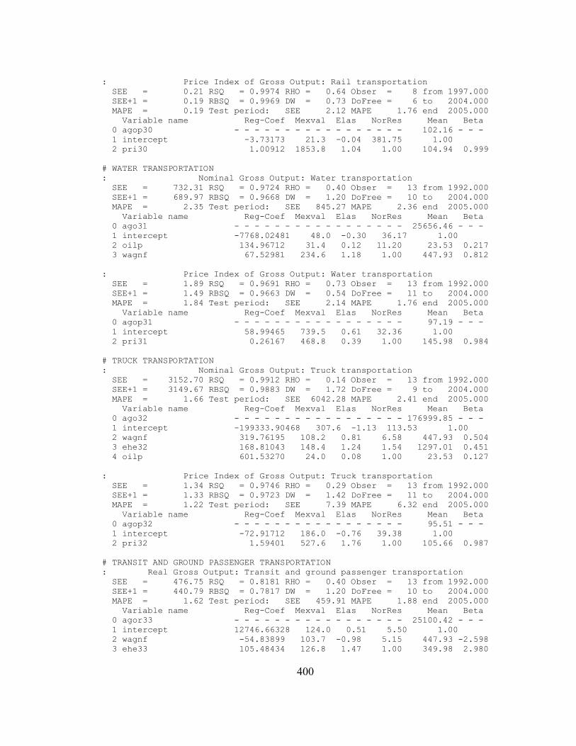
: Price Index of Gross Output: Rail transportation SEE = 0.21 RSQ = 0.9974 RHO = 0.64 Obser = 8 from 1997.000 SEE+1 = 0.19 RBSQ = 0.9969 DW = 0.73 DoFree = 6 to 2004.000 MAPE = 0.19 Test period: SEE 2.12 MAPE 1.76 end 2005.000 Variable name Reg-Coef Mexval Elas NorRes Mean Beta 0 agop30 - - - - - - - - - - - - - - - - - 102.16 - - - 1 intercept -3.73173 21.3 -0.04 381.75 1.00 2 pri30 1.00912 1853.8 1.04 1.00 104.94 0.999
# WATER TRANSPORTATION: Nominal Gross Output: Water transportation SEE = 732.31 RSQ = 0.9724 RHO = 0.40 Obser = 13 from 1992.000 SEE+1 = 689.97 RBSQ = 0.9668 DW = 1.20 DoFree = 10 to 2004.000 MAPE = 2.35 Test period: SEE 845.27 MAPE 2.36 end 2005.000 Variable name Reg-Coef Mexval Elas NorRes Mean Beta 0 ago31 - - - - - - - - - - - - - - - - - 25656.46 - - - 1 intercept -7768.02481 48.0 -0.30 36.17 1.00 2 oilp 134.96712 31.4 0.12 11.20 23.53 0.217 3 wagnf 67.52981 234.6 1.18 1.00 447.93 0.812
: Price Index of Gross Output: Water transportation SEE = 1.89 RSQ = 0.9691 RHO = 0.73 Obser = 13 from 1992.000 SEE+1 = 1.49 RBSQ = 0.9663 DW = 0.54 DoFree = 11 to 2004.000 MAPE = 1.84 Test period: SEE 2.14 MAPE 1.76 end 2005.000 Variable name Reg-Coef Mexval Elas NorRes Mean Beta 0 agop31 - - - - - - - - - - - - - - - - - 97.19 - - - 1 intercept 58.99465 739.5 0.61 32.36 1.00 2 pri31 0.26167 468.8 0.39 1.00 145.98 0.984
# TRUCK TRANSPORTATION: Nominal Gross Output: Truck transportation SEE = 3152.70 RSQ = 0.9912 RHO = 0.14 Obser = 13 from 1992.000 SEE+1 = 3149.67 RBSQ = 0.9883 DW = 1.72 DoFree = 9 to 2004.000 MAPE = 1.66 Test period: SEE 6042.28 MAPE 2.41 end 2005.000 Variable name Reg-Coef Mexval Elas NorRes Mean Beta 0 ago32 - - - - - - - - - - - - - - - - - 176999.85 - - - 1 intercept -199333.90468 307.6 -1.13 113.53 1.00 2 wagnf 319.76195 108.2 0.81 6.58 447.93 0.504 3 ehe32 168.81043 148.4 1.24 1.54 1297.01 0.451 4 oilp 601.53270 24.0 0.08 1.00 23.53 0.127
: Price Index of Gross Output: Truck transportation SEE = 1.34 RSQ = 0.9746 RHO = 0.29 Obser = 13 from 1992.000 SEE+1 = 1.33 RBSQ = 0.9723 DW = 1.42 DoFree = 11 to 2004.000 MAPE = 1.22 Test period: SEE 7.39 MAPE 6.32 end 2005.000 Variable name Reg-Coef Mexval Elas NorRes Mean Beta 0 agop32 - - - - - - - - - - - - - - - - - 95.51 - - - 1 intercept -72.91712 186.0 -0.76 39.38 1.00 2 pri32 1.59401 527.6 1.76 1.00 105.66 0.987
# TRANSIT AND GROUND PASSENGER TRANSPORTATION: Real Gross Output: Transit and ground passenger transportation SEE = 476.75 RSQ = 0.8181 RHO = 0.40 Obser = 13 from 1992.000 SEE+1 = 440.79 RBSQ = 0.7817 DW = 1.20 DoFree = 10 to 2004.000 MAPE = 1.62 Test period: SEE 459.91 MAPE 1.88 end 2005.000 Variable name Reg-Coef Mexval Elas NorRes Mean Beta 0 agor33 - - - - - - - - - - - - - - - - - 25100.42 - - - 1 intercept 12746.66328 124.0 0.51 5.50 1.00 2 wagnf -54.83899 103.7 -0.98 5.15 447.93 -2.598 3 ehe33 105.48434 126.8 1.47 1.00 349.98 2.980
400

: Price Index of Gross Output: Transit and ground passenger transportation SEE = 0.89 RSQ = 0.9882 RHO = 0.08 Obser = 13 from 1992.000 SEE+1 = 0.89 RBSQ = 0.9843 DW = 1.84 DoFree = 9 to 2004.000 MAPE = 0.77 Test period: SEE 0.63 MAPE 0.54 end 2005.000 Variable name Reg-Coef Mexval Elas NorRes Mean Beta 0 agop33 - - - - - - - - - - - - - - - - - 96.74 - - - 1 intercept -20.92750 4.8 -0.22 84.78 1.00 2 hr33 0.80804 15.3 0.32 38.15 38.05 0.101 3 wag33 5.68601 315.9 0.84 2.15 14.33 0.903 4 oilp 0.23101 46.6 0.06 1.00 23.53 0.200
# PIPELINE TRANSPORTATION: Nominal Gross Output: Pipeline transportation SEE = 881.58 RSQ = 0.9126 RHO = 0.07 Obser = 13 from 1992.000 SEE+1 = 879.64 RBSQ = 0.8951 DW = 1.87 DoFree = 10 to 2004.000 MAPE = 2.46 Test period: SEE 7088.85 MAPE 18.15 end 2005.000 Variable name Reg-Coef Mexval Elas NorRes Mean Beta 0 ago34 - - - - - - - - - - - - - - - - - 27359.77 - - - 1 intercept 64421.44870 28.1 2.35 11.44 1.00 2 wagnf -19.50436 2.0 -0.32 1.57 447.93 -0.346 3 ehe34 -578.02697 25.3 -1.04 1.00 49.00 -1.295
: Price Index of Gross Output: Pipeline transportation SEE = 3.85 RSQ = 0.7093 RHO = 0.47 Obser = 13 from 1992.000 SEE+1 = 3.73 RBSQ = 0.6512 DW = 1.07 DoFree = 10 to 2004.000 MAPE = 3.18 Test period: SEE 4.60 MAPE 3.78 end 2005.000 Variable name Reg-Coef Mexval Elas NorRes Mean Beta 0 agop34 - - - - - - - - - - - - - - - - - 98.56 - - - 1 intercept 66.60433 51.4 0.68 3.44 1.00 2 pri34 0.13718 2.2 0.14 2.18 103.80 0.145 3 oilp 0.75277 47.6 0.18 1.00 23.53 0.744
# OTHER TRANSPORTATION AND SUPPORT ACTIVITIES: Real Gross Output: Other transportation and support activities SEE = 968.63 RSQ = 0.9861 RHO = 0.05 Obser = 13 from 1992.000 SEE+1 = 968.46 RBSQ = 0.9833 DW = 1.90 DoFree = 10 to 2004.000 MAPE = 0.86 Test period: SEE 702.55 MAPE 0.70 end 2005.000 Variable name Reg-Coef Mexval Elas NorRes Mean Beta 0 agor35 - - - - - - - - - - - - - - - - - 91210.09 - - - 1 intercept 27717.52928 250.5 0.30 71.74 1.00 2 wagnf -29.95013 14.0 -0.15 12.01 447.93 -0.193 3 ehe35 161.83338 246.5 0.84 1.00 475.23 1.173
: Price Index of Gross Output: Other transportation and support activities SEE = 1.18 RSQ = 0.9815 RHO = 0.42 Obser = 13 from 1992.000 SEE+1 = 1.16 RBSQ = 0.9779 DW = 1.16 DoFree = 10 to 2004.000 MAPE = 1.00 Test period: SEE 5.70 MAPE 4.71 end 2005.000 Variable name Reg-Coef Mexval Elas NorRes Mean Beta 0 agop35 - - - - - - - - - - - - - - - - - 95.42 - - - 1 intercept 29.56344 180.9 0.31 54.18 1.00 2 pri35 0.53695 312.3 0.67 1.12 118.33 0.925 3 oilp 0.09831 5.9 0.02 1.00 23.53 0.080
# WAREHOUSING AND STORAGE: Real Gross Output: Warehousing and storage SEE = 966.99 RSQ = 0.9713 RHO = 0.63 Obser = 13 from 1992.000 SEE+1 = 798.60 RBSQ = 0.9655 DW = 0.75 DoFree = 10 to 2004.000 MAPE = 2.91 Test period: SEE 788.93 MAPE 1.93 end 2005.000 Variable name Reg-Coef Mexval Elas NorRes Mean Beta 0 agor36 - - - - - - - - - - - - - - - - - 29494.19 - - -
401

1 intercept -18988.10743 53.9 -0.64 34.83 1.00 2 wagnf 98.07608 26.6 1.49 1.00 447.93 0.910 3 ehe36 9.53155 0.2 0.15 1.00 477.52 0.076
: Price Index of Gross Output: Warehousing and storage SEE = 1.04 RSQ = 0.9615 RHO = 0.44 Obser = 11 from 1994.000 SEE+1 = 0.97 RBSQ = 0.9519 DW = 1.11 DoFree = 8 to 2004.000 MAPE = 0.91 Test period: SEE 0.75 MAPE 0.70 end 2005.000 Variable name Reg-Coef Mexval Elas NorRes Mean Beta 0 agop36 - - - - - - - - - - - - - - - - - 98.45 - - - 1 intercept -104.51001 80.5 -1.06 25.97 1.00 2 pri36 1.93645 189.5 2.07 1.01 105.06 1.005 3 oilp -0.02029 0.3 -0.01 1.00 24.26 -0.028
#PUBLISHING INDUSTRIES (INCLUDING SOFTWARE): Nominal Gross Output: Publishing industries (including software) SEE = 5709.92 RSQ = 0.9848 RHO = 0.47 Obser = 12 from 1993.000 SEE+1 = 5228.90 RBSQ = 0.9815 DW = 1.06 DoFree = 9 to 2004.000 MAPE = 2.38 Test period: SEE 11175.06 MAPE 4.17 end 2005.000 Variable name Reg-Coef Mexval Elas NorRes Mean Beta 0 ago37 - - - - - - - - - - - - - - - - - 200453.67 - - - 1 intercept -39397.64188 8.1 -0.20 65.97 1.00 2 ips37 1095.41097 38.9 0.54 28.00 98.04 0.162 3 apce37 3715.60164 429.1 0.66 1.00 35.65 0.875
: Price Index of Gross Output: Publishing industries (including software) SEE = 1.06 RSQ = 0.7567 RHO = 0.50 Obser = 12 from 1993.000 SEE+1 = 0.94 RBSQ = 0.6655 DW = 0.99 DoFree = 8 to 2004.000 MAPE = 0.86 Test period: SEE 1.56 MAPE 1.56 end 2005.000 Variable name Reg-Coef Mexval Elas NorRes Mean Beta 0 agop37 - - - - - - - - - - - - - - - - - 98.44 - - - 1 intercept 93.34451 129.1 0.95 4.11 1.00 2 nipa37p -0.00477 4.0 -0.01 1.10 260.90 -0.529 3 oilp 0.01766 0.1 0.00 1.02 23.78 0.060 4 pri37 0.03255 0.8 0.06 1.00 181.79 0.312
# MOTION PICTURE AND SOUND RECORDING INDUSTRIES: Real Gross Output: Motion picture and sound recording industries SEE = 1423.02 RSQ = 0.9549 RHO = 0.60 Obser = 12 from 1993.000 SEE+1 = 1157.08 RBSQ = 0.9504 DW = 0.79 DoFree = 10 to 2004.000 MAPE = 1.54 Test period: SEE 1861.03 MAPE 2.38 end 2005.000 Variable name Reg-Coef Mexval Elas NorRes Mean Beta 0 agor38 - - - - - - - - - - - - - - - - - 71972.28 - - - 1 intercept 17921.49742 81.5 0.25 22.19 1.00 2 ehe38 154.52064 371.1 0.75 1.00 349.80 0.977
: Price Index of Gross Output: Motion picture and sound recording industries SEE = 1.09 RSQ = 0.9901 RHO = 0.24 Obser = 12 from 1993.000 SEE+1 = 1.07 RBSQ = 0.9891 DW = 1.52 DoFree = 10 to 2004.000 MAPE = 1.00 Test period: SEE 2.41 MAPE 2.17 end 2005.000 Variable name Reg-Coef Mexval Elas NorRes Mean Beta 0 agop38 - - - - - - - - - - - - - - - - - 93.62 - - - 1 intercept 2.42708 3.4 0.03 101.08 1.00 2 wag38 5.04690 905.4 0.97 1.00 18.07 0.995
# BROADCASTING AND TELECOMMUNICATIONS: Real Gross Output: Broadcasting and telecommunications SEE = 29307.52 RSQ = 0.9562 RHO = 0.33 Obser = 12 from 1993.000 SEE+1 = 27803.79 RBSQ = 0.9464 DW = 1.34 DoFree = 9 to 2004.000 MAPE = 4.82 Test period: SEE 18534.81 MAPE 2.56 end 2005.000 Variable name Reg-Coef Mexval Elas NorRes Mean Beta
402

0 agor39 - - - - - - - - - - - - - - - - - 455850.28 - - - 1 intercept 1290150.84809 35.3 2.83 22.81 1.00 2 ips39 6720.76413 139.0 1.16 1.69 78.81 1.513 3 ehe39 -4289.67355 29.9 -2.99 1.00 317.97 -0.578
: Price Index of Gross Output: Broadcasting and telecommunications SEE = 1.03 RSQ = 0.7932 RHO = 0.29 Obser = 12 from 1993.000 SEE+1 = 1.02 RBSQ = 0.7472 DW = 1.42 DoFree = 9 to 2004.000 MAPE = 0.84 Test period: SEE 2.22 MAPE 2.34 end 2005.000 Variable name Reg-Coef Mexval Elas NorRes Mean Beta 0 agop39 - - - - - - - - - - - - - - - - - 100.81 - - - 1 intercept 122.83895 945.0 1.22 4.83 1.00 2 wag39 -3.09879 53.3 -0.56 1.74 18.07 -2.966
# INFORMATION AND DATA PROCESSING SERVICES: Nominal Gross Output: Information and data processing services SEE = 9172.66 RSQ = 0.8918 RHO = 0.82 Obser = 12 from 1993.000 SEE+1 = 6383.22 RBSQ = 0.8677 DW = 0.36 DoFree = 9 to 2004.000 MAPE = 15.65 Test period: SEE 13560.19 MAPE 11.48 end 2005.000 Variable name Reg-Coef Mexval Elas NorRes Mean Beta 0 ago40 - - - - - - - - - - - - - - - - - 67553.75 - - - 1 intercept -72381.26250 18.2 -1.07 9.24 1.00 2 ips40 311.06129 7.4 0.36 1.46 78.81 0.352 3 ehe40 2747.67946 20.8 1.71 1.00 42.01 0.608
: Price Index of Gross Output: Information and data processing services SEE = 2.90 RSQ = 0.8466 RHO = 0.71 Obser = 12 from 1993.000 SEE+1 = 2.36 RBSQ = 0.8313 DW = 0.58 DoFree = 10 to 2004.000 MAPE = 2.51 Test period: SEE 2.22 MAPE 2.19 end 2005.000 Variable name Reg-Coef Mexval Elas NorRes Mean Beta 0 agop40 - - - - - - - - - - - - - - - - - 95.89 - - - 1 intercept -74.65722 43.4 -0.78 6.52 1.00 2 wag40 15.91629 155.3 1.78 1.00 10.72 0.920
# FEDERAL RESERVE BANKS, CREDIT INTERMIDIATION, AND RELATED ACTIVITIES: Real Gross Output: 41 SEE = 18774.13 RSQ = 0.9107 RHO = 0.69 Obser = 12 from 1993.000 SEE+1 = 15504.54 RBSQ = 0.8909 DW = 0.63 DoFree = 9 to 2004.000 MAPE = 3.37 Test period: SEE 24637.00 MAPE 4.15 end 2005.000 Variable name Reg-Coef Mexval Elas NorRes Mean Beta 0 agor41 - - - - - - - - - - - - - - - - - 490324.79 - - - 1 intercept -484281.85192 82.7 -0.99 11.20 1.00 2 ehe41_2 216.92518 15.0 1.12 1.17 2534.67 0.562 3 ehe41_2[1] 170.38489 7.9 0.87 1.00 2493.02 0.403
: Price Index of Gross Output: 41 SEE = 0.63 RSQ = 0.9972 RHO = 0.06 Obser = 12 from 1993.000 SEE+1 = 0.63 RBSQ = 0.9961 DW = 1.88 DoFree = 8 to 2004.000 MAPE = 0.55 Test period: SEE 3.48 MAPE 3.02 end 2005.000 Variable name Reg-Coef Mexval Elas NorRes Mean Beta 0 agop41 - - - - - - - - - - - - - - - - - 93.96 - - - 1 intercept -184.48893 54.8 -1.96 353.19 1.00 2 wag41 -4.09420 13.3 -0.37 16.46 8.45 -0.170 3 hr41 5.64787 66.2 2.14 13.72 35.66 0.073 4 atime 3.91704 270.5 1.19 1.00 28.50 1.147
# SECURITIES, COMMODITY CONTRACRS, AND INVESTMENTS: Real Gross Output: 42 SEE = 17329.18 RSQ = 0.9697 RHO = 0.20 Obser = 12 from 1993.000 SEE+1 = 17291.19 RBSQ = 0.9583 DW = 1.61 DoFree = 8 to 2004.000 MAPE = 11.38 Test period: SEE 63221.00 MAPE 17.36 end 2005.000
403

Variable name Reg-Coef Mexval Elas NorRes Mean Beta 0 agor42 - - - - - - - - - - - - - - - - - 198847.58 - - - 1 intercept -432759.86129 275.2 -2.18 32.99 1.00 2 ehe42 1267.38103 100.1 4.37 1.76 685.57 1.357 3 ehe42[1] -910.38413 26.7 -3.03 1.76 661.35 -1.079 4 ehe42[2] 573.45515 32.6 1.83 1.00 636.17 0.730
: Price Index of Gross Output: 42 SEE = 8.11 RSQ = 0.9233 RHO = 0.58 Obser = 12 from 1993.000 SEE+1 = 6.71 RBSQ = 0.9062 DW = 0.85 DoFree = 9 to 2004.000 MAPE = 6.39 Test period: SEE 6.39 MAPE 7.25 end 2005.000 Variable name Reg-Coef Mexval Elas NorRes Mean Beta 0 agop42 - - - - - - - - - - - - - - - - - 122.77 - - - 1 intercept 1011.48831 12.9 8.24 13.03 1.00 2 wag42 -56.40244 247.7 -3.88 1.04 8.45 -0.946 3 hr42 -11.56314 2.2 -3.36 1.00 35.66 -0.060
# INSURANCE CARRIERS AND RELATED ACTIVITIES: Real Gross Output: 43 SEE = 9041.56 RSQ = 0.9157 RHO = 0.27 Obser = 12 from 1993.000 SEE+1 = 8810.89 RBSQ = 0.8675 DW = 1.47 DoFree = 7 to 2004.000 MAPE = 1.97 Test period: SEE 21815.03 MAPE 4.41 end 2005.000 Variable name Reg-Coef Mexval Elas NorRes Mean Beta 0 agor43 - - - - - - - - - - - - - - - - - 414833.71 - - - 1 intercept -619614.57658 20.8 -1.49 11.86 1.00 2 ehe43 414.60404 29.4 2.18 4.37 2184.81 0.857 3 ehe43[1] 109.46693 1.8 0.57 3.45 2166.58 0.252 4 oilp 1936.49033 25.6 0.11 1.47 23.78 0.454 5 exri -1420.63821 21.4 -0.37 1.00 108.83 -0.634
: Price Index of Gross Output: 43 SEE = 1.63 RSQ = 0.9818 RHO = 0.66 Obser = 12 from 1993.000 SEE+1 = 1.28 RBSQ = 0.9778 DW = 0.67 DoFree = 9 to 2004.000 MAPE = 1.46 Test period: SEE 0.47 MAPE 0.39 end 2005.000 Variable name Reg-Coef Mexval Elas NorRes Mean Beta 0 agop43 - - - - - - - - - - - - - - - - - 95.77 - - - 1 intercept 19.65477 2.4 0.21 54.94 1.00 2 wag43 -5.05675 3.2 -0.45 3.16 8.45 -0.206 3 atime 4.16947 77.8 1.24 1.00 28.50 1.193
# FUNDS, TRUSTS, AND OTHER FINANCIAL VEHICLES: Real Gross Output: 44 SEE = 2463.92 RSQ = 0.9744 RHO = -0.47 Obser = 12 from 1993.000 SEE+1 = 2135.90 RBSQ = 0.9598 DW = 2.94 DoFree = 7 to 2004.000 MAPE = 3.06 Test period: SEE 5775.77 MAPE 6.09 end 2005.000 Variable name Reg-Coef Mexval Elas NorRes Mean Beta 0 agor44 - - - - - - - - - - - - - - - - - 64193.23 - - - 1 intercept -45850.56481 150.2 -0.71 39.07 1.00 2 ehe44 2794.93844 104.7 3.30 3.37 75.85 1.790 3 ehe44[1] -1199.82880 44.5 -1.38 2.98 73.60 -0.816 4 oilp 554.69077 24.7 0.21 1.06 23.78 0.263 5 exri -246.45658 3.2 -0.42 1.00 108.83 -0.222
: Price Index of Gross Output: 44 SEE = 1.46 RSQ = 0.6527 RHO = 0.08 Obser = 12 from 1993.000 SEE+1 = 1.47 RBSQ = 0.5225 DW = 1.84 DoFree = 8 to 2004.000 MAPE = 1.13 Test period: SEE 2.15 MAPE 2.18 end 2005.000 Variable name Reg-Coef Mexval Elas NorRes Mean Beta 0 agop44 - - - - - - - - - - - - - - - - - 98.62 - - - 1 intercept -146.56918 8.2 -1.49 2.88 1.00 2 wag44 0.61604 0.1 0.05 1.39 8.45 0.122
404
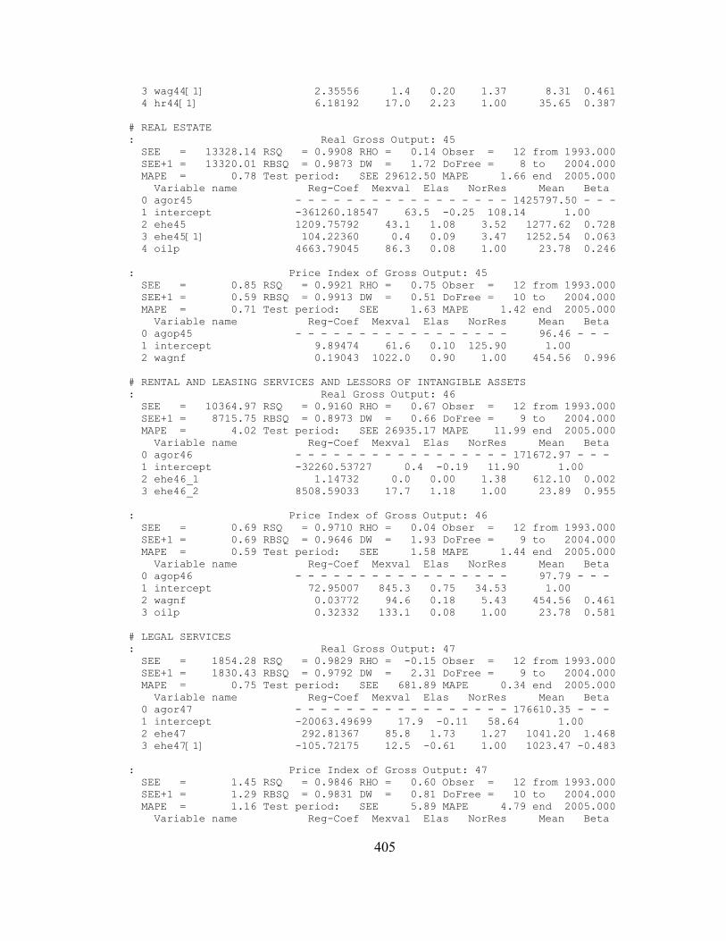
3 wag44[1] 2.35556 1.4 0.20 1.37 8.31 0.461 4 hr44[1] 6.18192 17.0 2.23 1.00 35.65 0.387
# REAL ESTATE: Real Gross Output: 45 SEE = 13328.14 RSQ = 0.9908 RHO = 0.14 Obser = 12 from 1993.000 SEE+1 = 13320.01 RBSQ = 0.9873 DW = 1.72 DoFree = 8 to 2004.000 MAPE = 0.78 Test period: SEE 29612.50 MAPE 1.66 end 2005.000 Variable name Reg-Coef Mexval Elas NorRes Mean Beta 0 agor45 - - - - - - - - - - - - - - - - - 1425797.50 - - - 1 intercept -361260.18547 63.5 -0.25 108.14 1.00 2 ehe45 1209.75792 43.1 1.08 3.52 1277.62 0.728 3 ehe45[1] 104.22360 0.4 0.09 3.47 1252.54 0.063 4 oilp 4663.79045 86.3 0.08 1.00 23.78 0.246
: Price Index of Gross Output: 45 SEE = 0.85 RSQ = 0.9921 RHO = 0.75 Obser = 12 from 1993.000 SEE+1 = 0.59 RBSQ = 0.9913 DW = 0.51 DoFree = 10 to 2004.000 MAPE = 0.71 Test period: SEE 1.63 MAPE 1.42 end 2005.000 Variable name Reg-Coef Mexval Elas NorRes Mean Beta 0 agop45 - - - - - - - - - - - - - - - - - 96.46 - - - 1 intercept 9.89474 61.6 0.10 125.90 1.00 2 wagnf 0.19043 1022.0 0.90 1.00 454.56 0.996
# RENTAL AND LEASING SERVICES AND LESSORS OF INTANGIBLE ASSETS: Real Gross Output: 46 SEE = 10364.97 RSQ = 0.9160 RHO = 0.67 Obser = 12 from 1993.000 SEE+1 = 8715.75 RBSQ = 0.8973 DW = 0.66 DoFree = 9 to 2004.000 MAPE = 4.02 Test period: SEE 26935.17 MAPE 11.99 end 2005.000 Variable name Reg-Coef Mexval Elas NorRes Mean Beta 0 agor46 - - - - - - - - - - - - - - - - - 171672.97 - - - 1 intercept -32260.53727 0.4 -0.19 11.90 1.00 2 ehe46_1 1.14732 0.0 0.00 1.38 612.10 0.002 3 ehe46_2 8508.59033 17.7 1.18 1.00 23.89 0.955
: Price Index of Gross Output: 46 SEE = 0.69 RSQ = 0.9710 RHO = 0.04 Obser = 12 from 1993.000 SEE+1 = 0.69 RBSQ = 0.9646 DW = 1.93 DoFree = 9 to 2004.000 MAPE = 0.59 Test period: SEE 1.58 MAPE 1.44 end 2005.000 Variable name Reg-Coef Mexval Elas NorRes Mean Beta 0 agop46 - - - - - - - - - - - - - - - - - 97.79 - - - 1 intercept 72.95007 845.3 0.75 34.53 1.00 2 wagnf 0.03772 94.6 0.18 5.43 454.56 0.461 3 oilp 0.32332 133.1 0.08 1.00 23.78 0.581
# LEGAL SERVICES: Real Gross Output: 47 SEE = 1854.28 RSQ = 0.9829 RHO = -0.15 Obser = 12 from 1993.000 SEE+1 = 1830.43 RBSQ = 0.9792 DW = 2.31 DoFree = 9 to 2004.000 MAPE = 0.75 Test period: SEE 681.89 MAPE 0.34 end 2005.000 Variable name Reg-Coef Mexval Elas NorRes Mean Beta 0 agor47 - - - - - - - - - - - - - - - - - 176610.35 - - - 1 intercept -20063.49699 17.9 -0.11 58.64 1.00 2 ehe47 292.81367 85.8 1.73 1.27 1041.20 1.468 3 ehe47[1] -105.72175 12.5 -0.61 1.00 1023.47 -0.483
: Price Index of Gross Output: 47 SEE = 1.45 RSQ = 0.9846 RHO = 0.60 Obser = 12 from 1993.000 SEE+1 = 1.29 RBSQ = 0.9831 DW = 0.81 DoFree = 10 to 2004.000 MAPE = 1.16 Test period: SEE 5.89 MAPE 4.79 end 2005.000 Variable name Reg-Coef Mexval Elas NorRes Mean Beta
405

0 agop47 - - - - - - - - - - - - - - - - - 96.37 - - - 1 intercept 8.59686 26.6 0.09 64.91 1.00 2 wag47 5.99527 705.7 0.91 1.00 14.64 0.992
# COMPUTER SYSTEMS DESIGN AND RELATED SERVICES: Real Gross Output: 48 SEE = 6165.88 RSQ = 0.9809 RHO = 0.50 Obser = 12 from 1993.000 SEE+1 = 5604.58 RBSQ = 0.9767 DW = 0.99 DoFree = 9 to 2004.000 MAPE = 3.56 Test period: SEE 18353.12 MAPE 9.83 end 2005.000 Variable name Reg-Coef Mexval Elas NorRes Mean Beta 0 agor48 - - - - - - - - - - - - - - - - - 127329.91 - - - 1 intercept -16556.45737 23.6 -0.13 52.44 1.00 2 ehe48 116.20137 72.9 0.85 1.27 936.01 0.727 3 ehe48[1] 40.02856 12.9 0.28 1.00 877.39 0.270
: Price Index of Gross Output: 48 SEE = 1.50 RSQ = 0.8913 RHO = 0.07 Obser = 12 from 1993.000 SEE+1 = 1.50 RBSQ = 0.8672 DW = 1.86 DoFree = 9 to 2004.000 MAPE = 1.33 Test period: SEE 0.86 MAPE 0.89 end 2005.000 Variable name Reg-Coef Mexval Elas NorRes Mean Beta 0 agop48 - - - - - - - - - - - - - - - - - 95.18 - - - 1 intercept 61.41592 419.2 0.65 9.20 1.00 2 wag48 0.00635 0.0 0.00 2.78 14.64 0.003 3 exri 0.30936 66.7 0.35 1.00 108.83 0.942
# MISCELLANEOUS PROFESSIONAL, SCIENTIFIC, AND TECHNICAL SERVICES: Real Gross Output: 49 SEE = 21149.97 RSQ = 0.9793 RHO = 0.68 Obser = 12 from 1993.000 SEE+1 = 17732.51 RBSQ = 0.9747 DW = 0.63 DoFree = 9 to 2004.000 MAPE = 3.52 Test period: SEE 10247.88 MAPE 1.17 end 2005.000 Variable name Reg-Coef Mexval Elas NorRes Mean Beta 0 agor49 - - - - - - - - - - - - - - - - - 590592.18 - - - 1 intercept 269175.72239 23.9 0.46 48.36 1.00 2 ehe49 1441.17097 273.5 1.49 1.94 612.47 1.301 3 ehe49_2 -719.27815 39.2 -0.95 1.00 780.31 -0.350
: Price Index of Gross Output: 49 SEE = 1.42 RSQ = 0.9440 RHO = 0.48 Obser = 12 from 1993.000 SEE+1 = 1.35 RBSQ = 0.9316 DW = 1.05 DoFree = 9 to 2004.000 MAPE = 1.18 Test period: SEE 1.40 MAPE 1.31 end 2005.000 Variable name Reg-Coef Mexval Elas NorRes Mean Beta 0 agop49 - - - - - - - - - - - - - - - - - 97.63 - - - 1 intercept 54.39001 410.7 0.56 17.87 1.00 2 wag49 8.79549 52.2 1.32 1.58 14.64 2.830 3 wag49[1] -6.03823 25.8 -0.88 1.00 14.16 -1.884
# MANAGEMENT OF COMPANIES AND ENTERPRISES: Real Gross Output: 50 SEE = 5963.07 RSQ = 0.9072 RHO = 0.48 Obser = 12 from 1993.000 SEE+1 = 5597.93 RBSQ = 0.8724 DW = 1.05 DoFree = 8 to 2004.000 MAPE = 2.00 Test period: SEE 10109.47 MAPE 3.09 end 2005.000 Variable name Reg-Coef Mexval Elas NorRes Mean Beta 0 agor50 - - - - - - - - - - - - - - - - - 282490.78 - - - 1 intercept -2001764.63590 38.8 -7.09 10.78 1.00 2 hr50 65961.11440 44.1 7.61 10.48 32.58 0.471 3 exri 805.86160 88.0 0.31 3.15 108.83 0.572 4 oilp 1995.82152 77.6 0.17 1.00 23.78 0.745
: Price Index of Gross Output: 50 SEE = 1.61 RSQ = 0.9770 RHO = 0.21 Obser = 12 from 1993.000 SEE+1 = 1.59 RBSQ = 0.9719 DW = 1.59 DoFree = 9 to 2004.000
406

MAPE = 1.46 Test period: SEE 2.45 MAPE 2.18 end 2005.000 Variable name Reg-Coef Mexval Elas NorRes Mean Beta 0 agop50 - - - - - - - - - - - - - - - - - 91.34 - - - 1 intercept 12.15857 40.7 0.13 43.50 1.00 2 wag50 7.79691 34.5 1.25 1.08 14.64 1.422 3 wag50[1] -2.46918 3.7 -0.38 1.00 14.16 -0.437
# ADMINISTRATIVE AND SUPPORT SERVICES: Real Gross Output: 51 SEE = 12141.25 RSQ = 0.9712 RHO = 0.65 Obser = 12 from 1993.000 SEE+1 = 9854.77 RBSQ = 0.9649 DW = 0.69 DoFree = 9 to 2004.000 MAPE = 2.56 Test period: SEE 19524.22 MAPE 4.25 end 2005.000 Variable name Reg-Coef Mexval Elas NorRes Mean Beta 0 agor51 - - - - - - - - - - - - - - - - - 363328.94 - - - 1 intercept -113521.19830 45.4 -0.31 34.78 1.00 2 ehe51 40.38731 20.4 0.75 1.37 6744.55 0.520 3 ehe51[1] 31.49987 17.0 0.56 1.00 6490.69 0.471
: Price Index of Of Gross Output: 51 SEE = 0.55 RSQ = 0.9968 RHO = -0.19 Obser = 12 from 1993.000 SEE+1 = 0.53 RBSQ = 0.9956 DW = 2.39 DoFree = 8 to 2004.000 MAPE = 0.48 Test period: SEE 1.43 MAPE 1.25 end 2005.000 Variable name Reg-Coef Mexval Elas NorRes Mean Beta 0 agop51 - - - - - - - - - - - - - - - - - 94.69 - - - 1 intercept 24.63383 379.5 0.26 312.94 1.00 2 wag51 6.06696 102.4 0.94 2.33 14.64 1.204 3 wag51[1] -1.61281 8.5 -0.24 2.24 14.16 -0.310 4 oilp 0.17119 49.5 0.04 1.00 23.78 0.128
# WASTE MANAGEMENT AND REMEDIATION SERVICES: Real Gross Output: 52 SEE = 711.00 RSQ = 0.9690 RHO = 0.26 Obser = 12 from 1993.000 SEE+1 = 691.16 RBSQ = 0.9574 DW = 1.49 DoFree = 8 to 2004.000 MAPE = 1.10 Test period: SEE 1186.32 MAPE 2.19 end 2005.000 Variable name Reg-Coef Mexval Elas NorRes Mean Beta 0 agor52 - - - - - - - - - - - - - - - - - 46700.05 - - - 1 intercept -132257.50696 23.3 -2.83 32.25 1.00 2 ehe52 212.03223 18.6 1.35 1.58 297.05 1.305 3 ehe52[1] -40.68929 0.9 -0.25 1.49 289.40 -0.282 4 hr52 3920.95011 22.2 2.74 1.00 32.58 0.136
: Price Index of Of Gross Output: 52 SEE = 1.80 RSQ = 0.9703 RHO = 0.67 Obser = 14 from 1991.000 SEE+1 = 1.49 RBSQ = 0.9649 DW = 0.65 DoFree = 11 to 2004.000 MAPE = 1.64 Test period: SEE 1.62 MAPE 1.33 end 2005.000 Variable name Reg-Coef Mexval Elas NorRes Mean Beta 0 agop52 - - - - - - - - - - - - - - - - - 95.78 - - - 1 intercept 25.23230 105.9 0.26 33.70 1.00 2 wag52 5.20010 253.3 0.68 1.36 12.51 0.866 3 oilp 0.23442 16.7 0.06 1.00 23.39 0.154
# EDUCATIONAL SERVICES: Real Gross Output: 53 SEE = 1433.59 RSQ = 0.9893 RHO = 0.41 Obser = 12 from 1993.000 SEE+1 = 1342.64 RBSQ = 0.9852 DW = 1.18 DoFree = 8 to 2004.000 MAPE = 0.84 Test period: SEE 2871.33 MAPE 1.86 end 2005.000 Variable name Reg-Coef Mexval Elas NorRes Mean Beta 0 agor53 - - - - - - - - - - - - - - - - - 132741.07 - - - 1 intercept -1361.39192 0.0 -0.01 93.04 1.00 2 ehe53 17.49507 6.6 0.30 1.32 2287.38 0.394 3 ehe53[1] 26.07349 14.7 0.43 1.00 2199.97 0.590
407
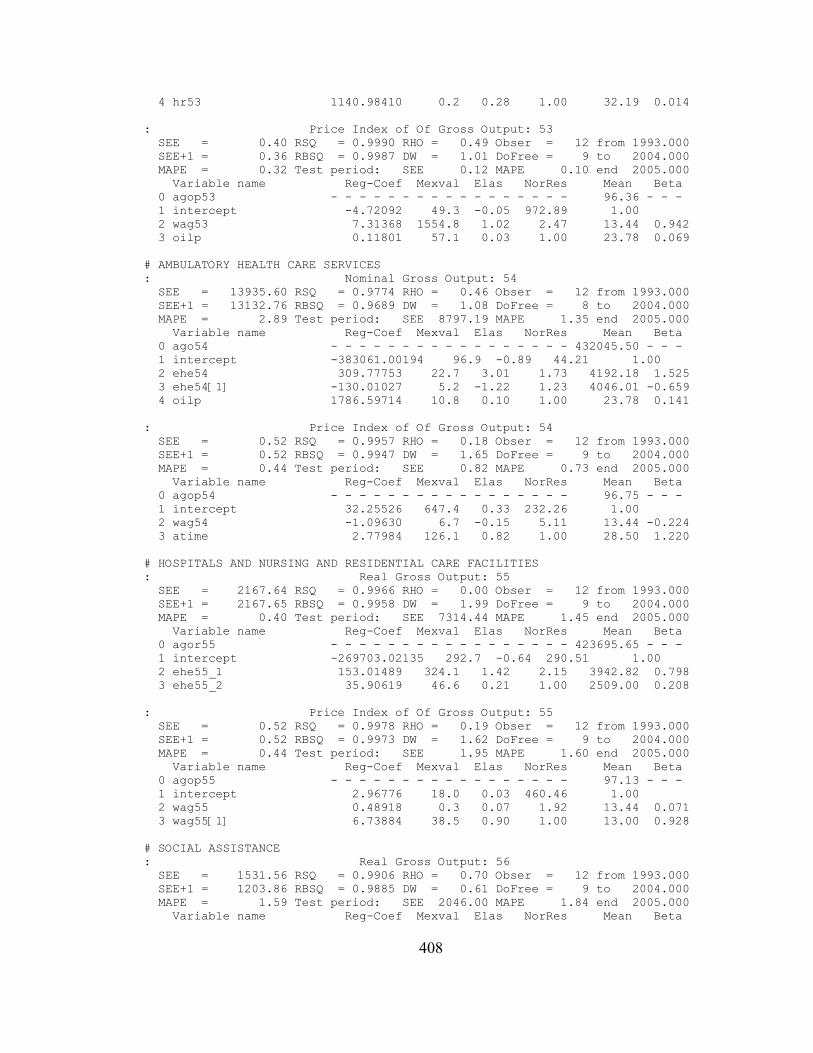
4 hr53 1140.98410 0.2 0.28 1.00 32.19 0.014
: Price Index of Of Gross Output: 53 SEE = 0.40 RSQ = 0.9990 RHO = 0.49 Obser = 12 from 1993.000 SEE+1 = 0.36 RBSQ = 0.9987 DW = 1.01 DoFree = 9 to 2004.000 MAPE = 0.32 Test period: SEE 0.12 MAPE 0.10 end 2005.000 Variable name Reg-Coef Mexval Elas NorRes Mean Beta 0 agop53 - - - - - - - - - - - - - - - - - 96.36 - - - 1 intercept -4.72092 49.3 -0.05 972.89 1.00 2 wag53 7.31368 1554.8 1.02 2.47 13.44 0.942 3 oilp 0.11801 57.1 0.03 1.00 23.78 0.069
# AMBULATORY HEALTH CARE SERVICES: Nominal Gross Output: 54 SEE = 13935.60 RSQ = 0.9774 RHO = 0.46 Obser = 12 from 1993.000 SEE+1 = 13132.76 RBSQ = 0.9689 DW = 1.08 DoFree = 8 to 2004.000 MAPE = 2.89 Test period: SEE 8797.19 MAPE 1.35 end 2005.000 Variable name Reg-Coef Mexval Elas NorRes Mean Beta 0 ago54 - - - - - - - - - - - - - - - - - 432045.50 - - - 1 intercept -383061.00194 96.9 -0.89 44.21 1.00 2 ehe54 309.77753 22.7 3.01 1.73 4192.18 1.525 3 ehe54[1] -130.01027 5.2 -1.22 1.23 4046.01 -0.659 4 oilp 1786.59714 10.8 0.10 1.00 23.78 0.141
: Price Index of Of Gross Output: 54 SEE = 0.52 RSQ = 0.9957 RHO = 0.18 Obser = 12 from 1993.000 SEE+1 = 0.52 RBSQ = 0.9947 DW = 1.65 DoFree = 9 to 2004.000 MAPE = 0.44 Test period: SEE 0.82 MAPE 0.73 end 2005.000 Variable name Reg-Coef Mexval Elas NorRes Mean Beta 0 agop54 - - - - - - - - - - - - - - - - - 96.75 - - - 1 intercept 32.25526 647.4 0.33 232.26 1.00 2 wag54 -1.09630 6.7 -0.15 5.11 13.44 -0.224 3 atime 2.77984 126.1 0.82 1.00 28.50 1.220
# HOSPITALS AND NURSING AND RESIDENTIAL CARE FACILITIES: Real Gross Output: 55 SEE = 2167.64 RSQ = 0.9966 RHO = 0.00 Obser = 12 from 1993.000 SEE+1 = 2167.65 RBSQ = 0.9958 DW = 1.99 DoFree = 9 to 2004.000 MAPE = 0.40 Test period: SEE 7314.44 MAPE 1.45 end 2005.000 Variable name Reg-Coef Mexval Elas NorRes Mean Beta 0 agor55 - - - - - - - - - - - - - - - - - 423695.65 - - - 1 intercept -269703.02135 292.7 -0.64 290.51 1.00 2 ehe55_1 153.01489 324.1 1.42 2.15 3942.82 0.798 3 ehe55_2 35.90619 46.6 0.21 1.00 2509.00 0.208
: Price Index of Of Gross Output: 55 SEE = 0.52 RSQ = 0.9978 RHO = 0.19 Obser = 12 from 1993.000 SEE+1 = 0.52 RBSQ = 0.9973 DW = 1.62 DoFree = 9 to 2004.000 MAPE = 0.44 Test period: SEE 1.95 MAPE 1.60 end 2005.000 Variable name Reg-Coef Mexval Elas NorRes Mean Beta 0 agop55 - - - - - - - - - - - - - - - - - 97.13 - - - 1 intercept 2.96776 18.0 0.03 460.46 1.00 2 wag55 0.48918 0.3 0.07 1.92 13.44 0.071 3 wag55[1] 6.73884 38.5 0.90 1.00 13.00 0.928
# SOCIAL ASSISTANCE: Real Gross Output: 56 SEE = 1531.56 RSQ = 0.9906 RHO = 0.70 Obser = 12 from 1993.000 SEE+1 = 1203.86 RBSQ = 0.9885 DW = 0.61 DoFree = 9 to 2004.000 MAPE = 1.59 Test period: SEE 2046.00 MAPE 1.84 end 2005.000 Variable name Reg-Coef Mexval Elas NorRes Mean Beta
408

0 agor56 - - - - - - - - - - - - - - - - - 82755.07 - - - 1 intercept -457768.80566 24.5 -5.53 106.38 1.00 2 ehe56 49.95541 321.9 1.04 1.51 1727.12 0.860 3 hr56 14113.07057 22.9 5.49 1.00 32.19 0.150
: Price Index of Of Gross Output: 56 SEE = 1.39 RSQ = 0.9761 RHO = 0.76 Obser = 12 from 1993.000 SEE+1 = 1.02 RBSQ = 0.9737 DW = 0.48 DoFree = 10 to 2004.000 MAPE = 1.17 Test period: SEE 3.64 MAPE 3.34 end 2005.000 Variable name Reg-Coef Mexval Elas NorRes Mean Beta 0 agop56 - - - - - - - - - - - - - - - - - 94.44 - - - 1 intercept 20.06176 98.3 0.21 41.87 1.00 2 wag56 5.53546 547.1 0.79 1.00 13.44 0.988
# PERFORMING ARTS, SPECTATOR SPORTS, MUSEUMS, AND RELATED ACTIVITIES: Nominal Gross Output: 57 SEE = 1937.87 RSQ = 0.9785 RHO = 0.54 Obser = 12 from 1993.000 SEE+1 = 1708.88 RBSQ = 0.9737 DW = 0.92 DoFree = 9 to 2004.000 MAPE = 2.67 Test period: SEE 882.19 MAPE 1.08 end 2005.000 Variable name Reg-Coef Mexval Elas NorRes Mean Beta 0 ago57 - - - - - - - - - - - - - - - - - 60817.08 - - - 1 intercept -27947.14056 112.8 -0.46 46.53 1.00 2 ehe57_2 98.03047 0.5 0.16 1.81 99.96 0.103 3 ehe57_2[1] 819.58460 34.4 1.30 1.00 96.35 0.887
: Price Index of Of Gross Output: 57 SEE = 0.78 RSQ = 0.9959 RHO = 0.30 Obser = 12 from 1993.000 SEE+1 = 0.77 RBSQ = 0.9950 DW = 1.40 DoFree = 9 to 2004.000 MAPE = 0.72 Test period: SEE 1.29 MAPE 1.08 end 2005.000 Variable name Reg-Coef Mexval Elas NorRes Mean Beta 0 agop57 - - - - - - - - - - - - - - - - - 94.40 - - - 1 intercept -8.03012 56.5 -0.09 246.32 1.00 2 wag57 15.46610 726.1 1.28 2.80 7.81 1.164 3 exri -0.16828 67.3 -0.19 1.00 108.83 -0.190
# AMUSEMENTS, GAMBLING, AND RECREATION INDUSTRIES: Real Gross Output: 58 SEE = 1042.74 RSQ = 0.9871 RHO = 0.38 Obser = 12 from 1993.000 SEE+1 = 966.74 RBSQ = 0.9823 DW = 1.24 DoFree = 8 to 2004.000 MAPE = 0.97 Test period: SEE 3698.47 MAPE 4.17 end 2005.000 Variable name Reg-Coef Mexval Elas NorRes Mean Beta 0 agor58 - - - - - - - - - - - - - - - - - 75374.03 - - - 1 intercept -703.73793 0.1 -0.01 77.78 1.00 2 ehe58 53.27452 29.2 0.84 1.83 1193.11 0.784 3 ehe58[1] 31.25417 11.2 0.48 1.82 1152.14 0.513 4 exri -215.88569 34.9 -0.31 1.00 108.83 -0.326
: Price Index of Of Gross Output: 58 SEE = 0.60 RSQ = 0.9956 RHO = 0.30 Obser = 12 from 1993.000 SEE+1 = 0.59 RBSQ = 0.9940 DW = 1.41 DoFree = 8 to 2004.000 MAPE = 0.56 Test period: SEE 1.01 MAPE 0.89 end 2005.000 Variable name Reg-Coef Mexval Elas NorRes Mean Beta 0 agop58 - - - - - - - - - - - - - - - - - 96.27 - - - 1 intercept 18.71496 241.3 0.19 229.61 1.00 2 wag58 9.53560 31.8 0.77 2.00 7.81 0.973 3 wag58[1] -7.81491 6.1 -0.61 1.43 7.57 -0.782 4 wag58[2] 8.48680 19.6 0.65 1.00 7.34 0.812
# ACCOMMODATION: Real Gross Output: 59 SEE = 2901.85 RSQ = 0.9304 RHO = 0.31 Obser = 12 from 1993.000
409

SEE+1 = 2847.72 RBSQ = 0.8906 DW = 1.39 DoFree = 7 to 2004.000 MAPE = 1.81 Test period: SEE 9152.78 MAPE 6.12 end 2005.000 Variable name Reg-Coef Mexval Elas NorRes Mean Beta 0 agor59 - - - - - - - - - - - - - - - - - 125238.67 - - - 1 intercept -37793.77577 0.1 -0.30 14.36 1.00 2 ehe59 79.57757 14.5 1.11 4.39 1747.02 0.654 3 ehe59[1] -12.63804 0.6 -0.17 4.27 1727.97 -0.118 4 hr59 963.33240 0.0 0.20 2.26 25.90 0.015 5 oilp 878.86775 50.2 0.17 1.00 23.78 0.584
: Price Index of Of Gross Output: 59 SEE = 1.12 RSQ = 0.9864 RHO = 0.33 Obser = 12 from 1993.000 SEE+1 = 1.07 RBSQ = 0.9834 DW = 1.34 DoFree = 9 to 2004.000 MAPE = 1.04 Test period: SEE 3.46 MAPE 3.03 end 2005.000 Variable name Reg-Coef Mexval Elas NorRes Mean Beta 0 agop59 - - - - - - - - - - - - - - - - - 94.08 - - - 1 intercept 13.99267 75.9 0.15 73.49 1.00 2 wag59 7.87806 18.8 0.65 1.04 7.81 0.759 3 atime 0.65211 1.9 0.20 1.00 28.50 0.235
# FOOD SERVICES AND DRINKING PLACES: Real Gross Output: 60 SEE = 3750.19 RSQ = 0.9881 RHO = 0.60 Obser = 12 from 1993.000 SEE+1 = 3058.61 RBSQ = 0.9855 DW = 0.80 DoFree = 9 to 2004.000 MAPE = 0.95 Test period: SEE 7173.12 MAPE 1.79 end 2005.000 Variable name Reg-Coef Mexval Elas NorRes Mean Beta 0 agor60 - - - - - - - - - - - - - - - - - 333534.53 - - - 1 intercept 72392.00722 9.7 0.22 84.07 1.00 2 ehe60 13.95118 7.7 0.33 2.64 7901.43 0.238 3 rtfood 0.53101 62.4 0.45 1.00 284189.75 0.759
: Price Index of Of Gross Output: 60 SEE = 0.64 RSQ = 0.9923 RHO = -0.03 Obser = 12 from 1993.000 SEE+1 = 0.64 RBSQ = 0.9894 DW = 2.06 DoFree = 8 to 2004.000 MAPE = 0.47 Test period: SEE 2.19 MAPE 1.91 end 2005.000 Variable name Reg-Coef Mexval Elas NorRes Mean Beta 0 agop60 - - - - - - - - - - - - - - - - - 98.21 - - - 1 intercept 39.21065 609.0 0.40 130.11 1.00 2 wag60 -11.55420 51.2 -0.92 4.82 7.81 -1.451 3 wag60[1] 8.85818 46.6 0.68 3.28 7.57 1.092 4 atime 2.88086 81.0 0.84 1.00 28.50 1.352
# OTHER SERVICES, EXCEPT GOVERNMENT: Nominal Gross Output: 61 SEE = 7005.37 RSQ = 0.9901 RHO = 0.07 Obser = 12 from 1993.000 SEE+1 = 6999.65 RBSQ = 0.9879 DW = 1.85 DoFree = 9 to 2004.000 MAPE = 1.57 Test period: SEE 8297.38 MAPE 1.59 end 2005.000 Variable name Reg-Coef Mexval Elas NorRes Mean Beta 0 ago61 - - - - - - - - - - - - - - - - - 390858.58 - - - 1 intercept -441392.09928 295.1 -1.13 100.85 1.00 2 ehe61 157.24330 479.8 2.00 3.52 4961.44 0.819 3 oilp 2190.80386 87.6 0.13 1.00 23.78 0.227
: Price Index of Of Gross Output: 61 SEE = 1.12 RSQ = 0.9877 RHO = 0.73 Obser = 12 from 1993.000 SEE+1 = 0.83 RBSQ = 0.9865 DW = 0.53 DoFree = 10 to 2004.000 MAPE = 0.95 Test period: SEE 2.91 MAPE 2.48 end 2005.000 Variable name Reg-Coef Mexval Elas NorRes Mean Beta 0 agop61 - - - - - - - - - - - - - - - - - 96.38 - - - 1 intercept 4.26249 8.2 0.04 81.28 1.00 2 wagnf 0.20265 801.6 0.96 1.00 454.56 0.994
410

# FEDERAL GOVERNMENT: GENERAL: Nominal Gross Output: 62 SEE = 19052.56 RSQ = 0.9569 RHO = 0.50 Obser = 12 from 1993.000 SEE+1 = 16953.83 RBSQ = 0.9408 DW = 1.00 DoFree = 8 to 2004.000 MAPE = 2.77 Test period: SEE 32736.94 MAPE 4.19 end 2005.000 Variable name Reg-Coef Mexval Elas NorRes Mean Beta 0 ago62 - - - - - - - - - - - - - - - - - 524062.33 - - - 1 intercept -1656730.68889 141.9 -3.16 23.23 1.00 2 ehe62 203.30124 12.0 0.78 19.74 1998.73 0.267 3 ehe62[1] 314.56938 26.4 1.22 16.16 2028.99 0.502
: Price Index of Of Gross Output: 62 SEE = 1.54 RSQ = 0.9781 RHO = 0.52 Obser = 12 from 1993.000 SEE+1 = 1.34 RBSQ = 0.9732 DW = 0.96 DoFree = 9 to 2004.000 MAPE = 1.15 Test period: SEE 0.32 MAPE 0.26 end 2005.000 Variable name Reg-Coef Mexval Elas NorRes Mean Beta 0 agop62 - - - - - - - - - - - - - - - - - 97.27 - - - 1 intercept 15.86664 36.0 0.16 45.58 1.00 2 wagnf 0.15896 232.4 0.74 2.27 454.56 0.761 3 oilp 0.38467 50.8 0.09 1.00 23.78 0.271
# FEDERAL GOVERNMENT: ENTERPRISES: Nominal Gross Output: 63 SEE = 1057.25 RSQ = 0.9809 RHO = 0.18 Obser = 12 from 1993.000 SEE+1 = 1055.37 RBSQ = 0.9766 DW = 1.64 DoFree = 9 to 2004.000 MAPE = 1.12 Test period: SEE 7.67 MAPE 0.01 end 2005.000 Variable name Reg-Coef Mexval Elas NorRes Mean Beta 0 ago63 - - - - - - - - - - - - - - - - - 77426.67 - - - 1 intercept -1271.23549 0.1 -0.02 52.31 1.00 2 ehe63 19.00818 18.3 0.21 52.27 845.64 0.087 3 atime 2197.32942 623.0 0.81 1.00 28.50 0.992
: Price Index of Of Gross Output: 63 SEE = 2.27 RSQ = 0.9027 RHO = 0.24 Obser = 12 from 1993.000 SEE+1 = 2.21 RBSQ = 0.8810 DW = 1.53 DoFree = 9 to 2004.000 MAPE = 1.75 Test period: SEE 2.58 MAPE 2.25 end 2005.000 Variable name Reg-Coef Mexval Elas NorRes Mean Beta 0 agop63 - - - - - - - - - - - - - - - - - 100.75 - - - 1 intercept 43.31577 97.6 0.43 10.27 1.00 2 wagnf 0.11677 86.8 0.53 1.13 454.56 0.798 3 oilp 0.18335 6.4 0.04 1.00 23.78 0.184
# STATE AND LOCAL GOVERNMENT: GENERAL: Nominal Gross Output: 64 SEE = 23954.35 RSQ = 0.9870 RHO = 0.85 Obser = 12 from 1993.000 SEE+1 = 17202.61 RBSQ = 0.9841 DW = 0.30 DoFree = 9 to 2004.000 MAPE = 2.08 Test period: SEE 64377.00 MAPE 4.20 end 2005.000 Variable name Reg-Coef Mexval Elas NorRes Mean Beta 0 ago64 - - - - - - - - - - - - - - - - - 1076137.83 - - - 1 intercept -985233.45583 8.6 -0.92 77.03 1.00 2 ehe64 137.56510 1.1 0.35 28.16 2723.05 0.027 3 atime 59185.08520 430.6 1.57 1.00 28.50 0.972
: Price Index of Of Gross Output: 64 SEE = 1.22 RSQ = 0.9854 RHO = 0.39 Obser = 12 from 1993.000 SEE+1 = 1.13 RBSQ = 0.9822 DW = 1.21 DoFree = 9 to 2004.000 MAPE = 0.93 Test period: SEE 0.28 MAPE 0.23 end 2005.000 Variable name Reg-Coef Mexval Elas NorRes Mean Beta 0 agop64 - - - - - - - - - - - - - - - - - 96.73 - - - 1 intercept 16.78179 58.6 0.17 68.72 1.00
411
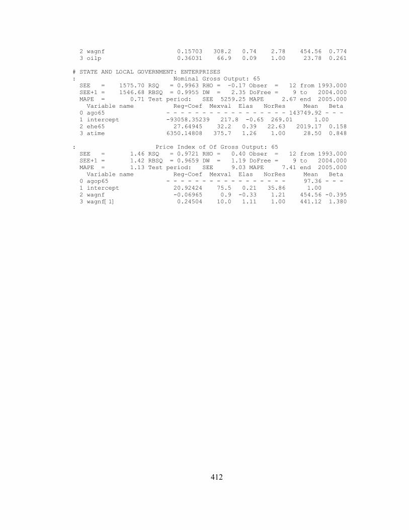
2 wagnf 0.15703 308.2 0.74 2.78 454.56 0.774 3 oilp 0.36031 66.9 0.09 1.00 23.78 0.261
# STATE AND LOCAL GOVERNMENT: ENTERPRISES: Nominal Gross Output: 65 SEE = 1575.70 RSQ = 0.9963 RHO = -0.17 Obser = 12 from 1993.000 SEE+1 = 1546.68 RBSQ = 0.9955 DW = 2.35 DoFree = 9 to 2004.000 MAPE = 0.71 Test period: SEE 5259.25 MAPE 2.67 end 2005.000 Variable name Reg-Coef Mexval Elas NorRes Mean Beta 0 ago65 - - - - - - - - - - - - - - - - - 143749.92 - - - 1 intercept -93058.35239 217.8 -0.65 269.01 1.00 2 ehe65 27.64945 32.2 0.39 22.63 2019.17 0.158 3 atime 6350.14808 375.7 1.26 1.00 28.50 0.848
: Price Index of Of Gross Output: 65 SEE = 1.46 RSQ = 0.9721 RHO = 0.40 Obser = 12 from 1993.000 SEE+1 = 1.42 RBSQ = 0.9659 DW = 1.19 DoFree = 9 to 2004.000 MAPE = 1.13 Test period: SEE 9.03 MAPE 7.41 end 2005.000 Variable name Reg-Coef Mexval Elas NorRes Mean Beta 0 agop65 - - - - - - - - - - - - - - - - - 97.36 - - - 1 intercept 20.92424 75.5 0.21 35.86 1.00 2 wagnf -0.06965 0.9 -0.33 1.21 454.56 -0.395 3 wagnf[1] 0.24504 10.0 1.11 1.00 441.12 1.380
412

Appendix 6.4: Regression Results for Monthly Equations
# Farms: PPI: u311 SEE = 0.94 RSQ = 0.9829 RHO = 0.01 Obser = 144 from 1993.001 SEE+1 = 0.94 RBSQ = 0.9824 DurH = 999.00 DoFree = 139 to 2004.012 MAPE = 0.45 Test period: SEE 1.61 MAPE 0.90 end 2006.012 Variable name Reg-Coef Mexval Elas NorRes Mean Beta 0 foodprim - - - - - - - - - - - - - - - - - 128.60 - - - 1 intercept 6.95262 2.3 0.05 58.36 1.00 2 foodprim[1] 1.09027 48.0 1.09 1.08 128.41 1.081 3 foodprim[2] -0.09934 0.2 -0.10 1.05 128.22 -0.098 4 foodprim[3] -0.07479 0.3 -0.07 1.05 128.04 -0.073 5 mnipaqfood 0.00453 2.6 0.03 1.00 872.92 0.084
: USDA: Farm Labor Expense SEE = 54.21 RSQ = 0.9996 RHO = 0.46 Obser = 144 from 1993.001 SEE+1 = 49.24 RBSQ = 0.9996 DurH = 5.73 DoFree = 140 to 2004.012 MAPE = 0.16 Test period: SEE 193.68 MAPE 0.74 end 2006.012 Variable name Reg-Coef Mexval Elas NorRes Mean Beta 0 mfarmlexp - - - - - - - - - - - - - - - - - 19228.17 - - - 1 intercept 50.54923 0.8 0.00 2608.42 1.00 2 mfarmlexp[1] 1.21112 255.4 1.21 1.44 19162.00 1.213 3 mfarmlexp[4] -0.21526 7.7 -0.21 1.00 18959.15 -0.216 4 mfarmlexp[8] 0.00275 0.0 0.00 1.00 18689.69 0.003
: BEA Farm employment SEE = 2.17 RSQ = 0.9979 RHO = -0.09 Obser = 72 from 1999.001 SEE+1 = 2.16 RBSQ = 0.9979 DurH = -0.94 DoFree = 68 to 2004.012 MAPE = 0.07 Test period: SEE 1007.01 MAPE 7.12e+10 end 2006.012 Variable name Reg-Coef Mexval Elas NorRes Mean Beta 0 mempprod1 - - - - - - - - - - - - - - - - - 1586.50 - - - 1 intercept 13.16412 1.6 0.01 487.67 1.00 2 mempprod1[1] 1.85858 273.1 1.86 5.29 1586.69 1.850 3 mempprod1[2] -0.86357 91.2 -0.86 1.02 1586.83 -0.857 4 mnipaqfood -0.00539 1.2 -0.00 1.00 987.86 -0.009
# Forestry, fishing, and related: BLS: CES et1133 SEE = 0.86 RSQ = 0.9746 RHO = -0.07 Obser = 144 from 1993.001 SEE+1 = 0.86 RBSQ = 0.9742 DurH = -0.88 DoFree = 141 to 2004.012 MAPE = 0.89 Test period: SEE 1.66 MAPE 2.18 end 2006.012 Variable name Reg-Coef Mexval Elas NorRes Mean Beta 0 ehe2m - - - - - - - - - - - - - - - - - 77.42 - - - 1 intercept 5.85130 2.1 0.08 39.38 1.00 2 ehe2m[1] 0.94777 258.4 0.95 1.05 77.50 0.936 3 mnipaqfur -0.00678 2.6 -0.02 1.00 278.07 -0.062
: IPI: n1133 SEE = 2.53 RSQ = 0.6208 RHO = 0.02 Obser = 144 from 1993.001 SEE+1 = 2.53 RBSQ = 0.6126 DurH = 999.00 DoFree = 140 to 2004.012 MAPE = 1.88 Test period: SEE 3.41 MAPE 2.75 end 2006.012 Variable name Reg-Coef Mexval Elas NorRes Mean Beta 0 ips2_1m - - - - - - - - - - - - - - - - - 104.42 - - - 1 intercept 40.92302 6.7 0.39 2.64 1.00 2 ips2_1m[1] 0.51323 12.5 0.51 1.11 104.44 0.516 3 ips2_1m[2] 0.14052 1.0 0.14 1.06 104.48 0.142 4 mnipaqfur -0.01723 2.8 -0.05 1.00 278.07 -0.208
413
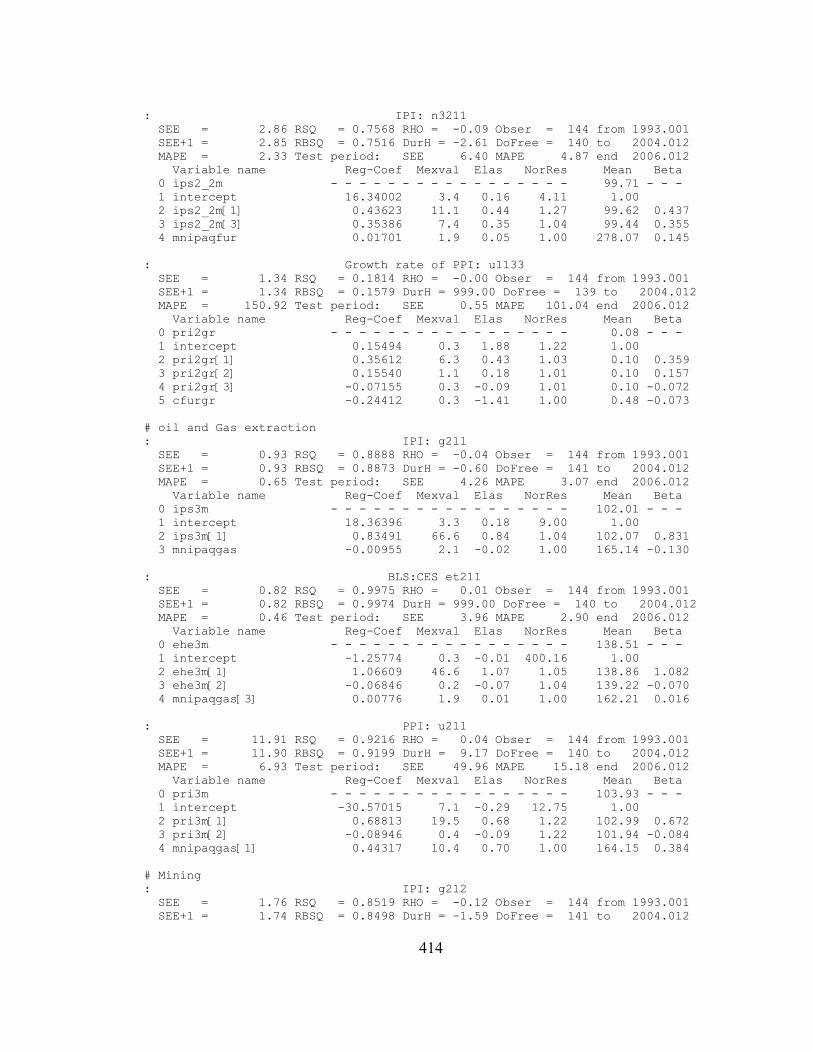
: IPI: n3211 SEE = 2.86 RSQ = 0.7568 RHO = -0.09 Obser = 144 from 1993.001 SEE+1 = 2.85 RBSQ = 0.7516 DurH = -2.61 DoFree = 140 to 2004.012 MAPE = 2.33 Test period: SEE 6.40 MAPE 4.87 end 2006.012 Variable name Reg-Coef Mexval Elas NorRes Mean Beta 0 ips2_2m - - - - - - - - - - - - - - - - - 99.71 - - - 1 intercept 16.34002 3.4 0.16 4.11 1.00 2 ips2_2m[1] 0.43623 11.1 0.44 1.27 99.62 0.437 3 ips2_2m[3] 0.35386 7.4 0.35 1.04 99.44 0.355 4 mnipaqfur 0.01701 1.9 0.05 1.00 278.07 0.145
: Growth rate of PPI: u1133 SEE = 1.34 RSQ = 0.1814 RHO = -0.00 Obser = 144 from 1993.001 SEE+1 = 1.34 RBSQ = 0.1579 DurH = 999.00 DoFree = 139 to 2004.012 MAPE = 150.92 Test period: SEE 0.55 MAPE 101.04 end 2006.012 Variable name Reg-Coef Mexval Elas NorRes Mean Beta 0 pri2gr - - - - - - - - - - - - - - - - - 0.08 - - - 1 intercept 0.15494 0.3 1.88 1.22 1.00 2 pri2gr[1] 0.35612 6.3 0.43 1.03 0.10 0.359 3 pri2gr[2] 0.15540 1.1 0.18 1.01 0.10 0.157 4 pri2gr[3] -0.07155 0.3 -0.09 1.01 0.10 -0.072 5 cfurgr -0.24412 0.3 -1.41 1.00 0.48 -0.073
# oil and Gas extraction: IPI: g211 SEE = 0.93 RSQ = 0.8888 RHO = -0.04 Obser = 144 from 1993.001 SEE+1 = 0.93 RBSQ = 0.8873 DurH = -0.60 DoFree = 141 to 2004.012 MAPE = 0.65 Test period: SEE 4.26 MAPE 3.07 end 2006.012 Variable name Reg-Coef Mexval Elas NorRes Mean Beta 0 ips3m - - - - - - - - - - - - - - - - - 102.01 - - - 1 intercept 18.36396 3.3 0.18 9.00 1.00 2 ips3m[1] 0.83491 66.6 0.84 1.04 102.07 0.831 3 mnipaqgas -0.00955 2.1 -0.02 1.00 165.14 -0.130
: BLS:CES et211 SEE = 0.82 RSQ = 0.9975 RHO = 0.01 Obser = 144 from 1993.001 SEE+1 = 0.82 RBSQ = 0.9974 DurH = 999.00 DoFree = 140 to 2004.012 MAPE = 0.46 Test period: SEE 3.96 MAPE 2.90 end 2006.012 Variable name Reg-Coef Mexval Elas NorRes Mean Beta 0 ehe3m - - - - - - - - - - - - - - - - - 138.51 - - - 1 intercept -1.25774 0.3 -0.01 400.16 1.00 2 ehe3m[1] 1.06609 46.6 1.07 1.05 138.86 1.082 3 ehe3m[2] -0.06846 0.2 -0.07 1.04 139.22 -0.070 4 mnipaqgas[3] 0.00776 1.9 0.01 1.00 162.21 0.016
: PPI: u211 SEE = 11.91 RSQ = 0.9216 RHO = 0.04 Obser = 144 from 1993.001 SEE+1 = 11.90 RBSQ = 0.9199 DurH = 9.17 DoFree = 140 to 2004.012 MAPE = 6.93 Test period: SEE 49.96 MAPE 15.18 end 2006.012 Variable name Reg-Coef Mexval Elas NorRes Mean Beta 0 pri3m - - - - - - - - - - - - - - - - - 103.93 - - - 1 intercept -30.57015 7.1 -0.29 12.75 1.00 2 pri3m[1] 0.68813 19.5 0.68 1.22 102.99 0.672 3 pri3m[2] -0.08946 0.4 -0.09 1.22 101.94 -0.084 4 mnipaqgas[1] 0.44317 10.4 0.70 1.00 164.15 0.384
# Mining: IPI: g212 SEE = 1.76 RSQ = 0.8519 RHO = -0.12 Obser = 144 from 1993.001 SEE+1 = 1.74 RBSQ = 0.8498 DurH = -1.59 DoFree = 141 to 2004.012
414

MAPE = 1.37 Test period: SEE 2.46 MAPE 1.90 end 2006.012 Variable name Reg-Coef Mexval Elas NorRes Mean Beta 0 ips4m - - - - - - - - - - - - - - - - - 100.65 - - - 1 intercept 9.62637 2.9 0.10 6.75 1.00 2 ips4m[1] 0.89596 130.4 0.90 1.01 100.57 0.906 3 mgdp 0.00010 0.3 0.01 1.00 9027.08 0.035
: BLS: CES et212 SEE = 0.89 RSQ = 0.7915 RHO = -0.02 Obser = 144 from 1993.001 SEE+1 = 0.00 RBSQ = 0.7870 DurH = 999.00 DoFree = 140 to 2004.012 MAPE = 506.90 Test period: SEE 0.28 MAPE 101.57 end 2006.012 Variable name Reg-Coef Mexval Elas NorRes Mean Beta 0 ehe4gr - - - - - - - - - - - - - - - - - -0.63 - - - 1 intercept -0.21495 0.1 1.27 4.95 3.71 2 ehe4gr[1] 0.79458 27.5 0.87 4.83 -0.68 0.575 3 mgdpgr 0.43307 1.8 -1.09 3.80 1.58 0.105 4 ehe4gr_mu[1] -0.73580 82.2 -0.05 1.00 -0.04 -1.055
: PPI: u2121 SEE = 1.54 RSQ = 0.8934 RHO = -0.32 Obser = 144 from 1993.001 SEE+1 = 1.45 RBSQ = 0.8918 DurH = -4.15 DoFree = 141 to 2004.012 MAPE = 1.17 Test period: SEE 15.03 MAPE 11.72 end 2006.012 Variable name Reg-Coef Mexval Elas NorRes Mean Beta 0 pri4m - - - - - - - - - - - - - - - - - 92.25 - - - 1 intercept 2.20092 0.2 0.02 9.38 1.00 2 pri4m[1] 0.96076 188.9 0.96 1.03 92.16 0.927 3 mgdp 0.00017 1.3 0.02 1.00 9027.08 0.055
# Mining supports: IPI: g213 SEE = 2.77 RSQ = 0.9602 RHO = 0.42 Obser = 144 from 1993.001 SEE+1 = 2.52 RBSQ = 0.9596 DurH = 5.10 DoFree = 141 to 2004.012 MAPE = 1.75 Test period: SEE 2.29 MAPE 1.22 end 2006.012 Variable name Reg-Coef Mexval Elas NorRes Mean Beta 0 ips5m - - - - - - - - - - - - - - - - - 119.72 - - - 1 intercept 0.97230 0.1 0.01 25.11 1.00 2 ips5m[1] 0.98024 400.5 0.98 1.01 119.60 0.981 3 mnipaqgas[2] 0.00925 0.7 0.01 1.00 163.17 0.024
: BLS: CES et213 SEE = 1.85 RSQ = 0.9834 RHO = 0.52 Obser = 144 from 1993.001 SEE+1 = 1.59 RBSQ = 0.9832 DurH = 6.31 DoFree = 141 to 2004.012 MAPE = 0.81 Test period: SEE 14.47 MAPE 5.34 end 2006.012 Variable name Reg-Coef Mexval Elas NorRes Mean Beta 0 ehe5m - - - - - - - - - - - - - - - - - 171.77 - - - 1 intercept 4.18414 1.4 0.02 60.31 1.00 2 ehe5m[1] 0.94823 432.1 0.95 1.18 171.44 0.937 3 mnipaqgas[2] 0.03073 8.7 0.03 1.00 163.17 0.077
: PPI: u213112 SEE = 1.99 RSQ = 0.9807 RHO = -0.01 Obser = 144 from 1993.001 SEE+1 = 1.99 RBSQ = 0.9803 DurH = -0.42 DoFree = 140 to 2004.012 MAPE = 0.85 Test period: SEE 3.88 MAPE 1.85 end 2006.012 Variable name Reg-Coef Mexval Elas NorRes Mean Beta 0 pri5_2m - - - - - - - - - - - - - - - - - 120.73 - - - 1 intercept 4.22903 2.3 0.04 51.81 1.00 2 pri5_2m[1] 0.96876 39.6 0.97 1.12 120.42 0.962 3 pri5_2m[2] -0.04929 0.1 -0.05 1.11 120.11 -0.049 4 mnipaqgas[2] 0.03530 5.4 0.05 1.00 163.17 0.088
: PPI: u213114
415

SEE = 1.43 RSQ = 0.8765 RHO = 0.03 Obser = 144 from 1993.001 SEE+1 = 1.43 RBSQ = 0.8747 DurH = 0.34 DoFree = 141 to 2004.012 MAPE = 0.50 Test period: SEE 11.03 MAPE 7.97 end 2006.012 Variable name Reg-Coef Mexval Elas NorRes Mean Beta 0 pri5_4m - - - - - - - - - - - - - - - - - 115.11 - - - 1 intercept 7.58897 1.7 0.07 8.09 1.00 2 pri5_4m[1] 0.92952 181.0 0.93 1.01 115.03 0.931 3 mnipaqgas[2] 0.00366 0.4 0.01 1.00 163.17 0.032
# Utilities: IPI: g2211a2 SEE = 1.53 RSQ = 0.9490 RHO = 0.03 Obser = 144 from 1993.001 SEE+1 = 1.53 RBSQ = 0.9483 DurH = 0.76 DoFree = 141 to 2004.012 MAPE = 1.27 Test period: SEE 2.53 MAPE 1.83 end 2006.012 Variable name Reg-Coef Mexval Elas NorRes Mean Beta 0 ips6m - - - - - - - - - - - - - - - - - 93.30 - - - 1 intercept 17.32578 11.8 0.19 19.61 1.00 2 ips6m[1] 0.55161 19.9 0.55 1.27 93.15 0.550 3 mtime 0.84691 12.8 0.26 1.00 29.04 0.433
: BLS: CES wp22 SEE = 0.12 RSQ = 0.9977 RHO = -0.13 Obser = 144 from 1993.001 SEE+1 = 0.11 RBSQ = 0.9977 DurH = -3.04 DoFree = 140 to 2004.012 MAPE = 0.41 Test period: SEE 0.26 MAPE 0.80 end 2006.012 Variable name Reg-Coef Mexval Elas NorRes Mean Beta 0 wag6m - - - - - - - - - - - - - - - - - 21.70 - - - 1 intercept 2.15393 6.8 0.10 435.52 1.00 2 wag6m[1] 0.51212 16.7 0.51 1.33 21.64 0.512 3 mgdp 0.00034 3.7 0.14 1.10 9027.08 0.221 4 mtime 0.18530 4.7 0.25 1.00 29.04 0.267
: PPI: u22112242 SEE = 2.04 RSQ = 0.8977 RHO = 0.57 Obser = 144 from 1993.001 SEE+1 = 1.68 RBSQ = 0.8940 DurH = 8.80 DoFree = 138 to 2004.012 MAPE = 1.33 Test period: SEE 10.11 MAPE 6.34 end 2006.012 Variable name Reg-Coef Mexval Elas NorRes Mean Beta 0 pri6_1m - - - - - - - - - - - - - - - - - 116.93 - - - 1 intercept 14.61397 1.3 0.12 9.78 1.00 2 pri6_1m[1] 0.41816 20.6 0.42 2.40 116.79 0.421 3 pri6_1m[4] -0.10329 2.5 -0.10 2.16 116.45 -0.103 4 pri6_1m[8] -0.00826 0.0 -0.01 2.05 116.07 -0.008 5 pri6_1m[12] 0.54021 33.8 0.53 1.03 115.58 0.538 6 mgdp 0.00045 1.5 0.03 1.00 9027.08 0.109
: PPI: u22112243 SEE = 1.90 RSQ = 0.9131 RHO = 0.37 Obser = 144 from 1993.001 SEE+1 = 1.77 RBSQ = 0.9100 DurH = 5.85 DoFree = 138 to 2004.012 MAPE = 1.21 Test period: SEE 11.93 MAPE 6.95 end 2006.012 Variable name Reg-Coef Mexval Elas NorRes Mean Beta 0 pri6_2m - - - - - - - - - - - - - - - - - 113.33 - - - 1 intercept 3.14902 0.1 0.03 11.51 1.00 2 pri6_2m[1] 0.67631 40.7 0.68 1.58 113.22 0.674 3 pri6_2m[4] -0.13001 3.5 -0.13 1.50 112.92 -0.125 4 pri6_2m[8] 0.06790 1.1 0.07 1.32 112.51 0.061 5 pri6_2m[12] 0.32885 12.3 0.33 1.04 112.10 0.291 6 mgdp 0.00042 2.1 0.03 1.00 9027.08 0.102
: PPI: u221210114 SEE = 9.11 RSQ = 0.9480 RHO = 0.20 Obser = 144 from 1993.001 SEE+1 = 8.94 RBSQ = 0.9465 DurH = 2.84 DoFree = 139 to 2004.012 MAPE = 3.55 Test period: SEE 50.51 MAPE 17.46 end 2006.012
416

Variable name Reg-Coef Mexval Elas NorRes Mean Beta 0 pri6_3m - - - - - - - - - - - - - - - - - 128.52 - - - 1 intercept 49.05714 0.9 0.38 19.24 1.00 2 pri6_3m[1] 0.96048 100.6 0.95 1.10 127.69 0.943 3 pri6_3m[4] -0.08729 1.3 -0.09 1.09 125.45 -0.082 4 mgdp 0.01757 1.7 1.23 1.03 9027.08 0.686 5 mtime -6.57083 1.3 -1.48 1.00 29.04 -0.570
# Construction: BLS: CES etct SEE = 23.29 RSQ = 0.9990 RHO = -0.15 Obser = 144 from 1993.001 SEE+1 = 23.01 RBSQ = 0.9990 DurH = -1.86 DoFree = 139 to 2004.012 MAPE = 0.29 Test period: SEE 141.18 MAPE 1.64 end 2006.012 Variable name Reg-Coef Mexval Elas NorRes Mean Beta 0 ehe7m - - - - - - - - - - - - - - - - - 6102.69 - - - 1 intercept 50.26997 2.0 0.01 1022.04 1.00 2 mgdp[1] 0.11233 3.6 0.17 88.12 8988.88 0.234 3 mgdp[6] -0.05593 0.3 -0.08 86.34 8800.77 -0.115 4 mgdp[12] -0.06062 1.2 -0.09 85.75 8581.40 -0.122 5 ehe7m[1] 0.99503 826.0 0.99 1.00 6085.32 1.002
: BLS: CES wpct SEE = 0.05 RSQ = 0.9992 RHO = -0.03 Obser = 144 from 1993.001 SEE+1 = 0.05 RBSQ = 0.9992 DurH = -1.17 DoFree = 140 to 2004.012 MAPE = 0.22 Test period: SEE 0.14 MAPE 0.64 end 2006.012 Variable name Reg-Coef Mexval Elas NorRes Mean Beta 0 wag7m - - - - - - - - - - - - - - - - - 16.58 - - - 1 intercept 0.10239 1.9 0.01 1268.06 1.00 2 wag7m[1] 0.61649 19.8 0.62 1.19 16.54 0.616 3 wag7m[2] 0.37332 7.8 0.37 1.05 16.50 0.373 4 mnipaqvnrs 0.00046 2.5 0.01 1.00 257.85 0.012
# Wood products: IPI: g321 SEE = 1.30 RSQ = 0.9619 RHO = 0.01 Obser = 144 from 1993.001 SEE+1 = 1.30 RBSQ = 0.9605 DurH = 999.00 DoFree = 138 to 2004.012 MAPE = 1.05 Test period: SEE 5.28 MAPE 4.10 end 2006.012 Variable name Reg-Coef Mexval Elas NorRes Mean Beta 0 ips8m - - - - - - - - - - - - - - - - - 97.54 - - - 1 intercept 3.58622 0.9 0.04 26.23 1.00 2 ips8m[1] 0.78975 27.5 0.79 1.04 97.39 0.796 3 ips8m[2] 0.11880 0.4 0.12 1.02 97.24 0.121 4 ips8m[3] 0.04828 0.1 0.05 1.01 97.09 0.049 5 mnipaqfur 0.00772 0.7 0.02 1.01 278.07 0.058 6 mnipaqvnrs[1] -0.00525 0.3 -0.01 1.00 256.88 -0.037
: BLS: CES et321 SEE = 2.06 RSQ = 0.9953 RHO = -0.08 Obser = 144 from 1993.001 SEE+1 = 2.06 RBSQ = 0.9951 DurH = -1.07 DoFree = 139 to 2004.012 MAPE = 0.27 Test period: SEE 8.40 MAPE 1.11 end 2006.012 Variable name Reg-Coef Mexval Elas NorRes Mean Beta 0 ehe8m - - - - - - - - - - - - - - - - - 574.62 - - - 1 intercept 11.15367 3.3 0.02 211.39 1.00 2 ehe8m[1] 1.06609 168.2 1.07 1.53 574.30 1.081 3 ehe8m[6] -0.08250 2.1 -0.08 1.04 572.61 -0.090 4 mnipaqfur 0.06769 1.2 0.03 1.03 278.07 0.112 5 mnipaqfur[12] -0.07738 1.5 -0.04 1.00 263.31 -0.130
: PPI: u321113 SEE = 3.19 RSQ = 0.8987 RHO = 0.00 Obser = 144 from 1993.001 SEE+1 = 3.19 RBSQ = 0.8958 DurH = 0.12 DoFree = 139 to 2004.012
417

MAPE = 1.61 Test period: SEE 9.11 MAPE 4.97 end 2006.012 Variable name Reg-Coef Mexval Elas NorRes Mean Beta 0 pri8_1m - - - - - - - - - - - - - - - - - 152.42 - - - 1 intercept 26.95731 7.6 0.18 9.87 1.00 2 pri8_1m[1] 1.25610 72.0 1.25 1.30 152.28 1.266 3 pri8_1m[2] -0.42281 11.4 -0.42 1.07 152.10 -0.433 4 mnipaqfur 0.11078 2.3 0.20 1.05 278.07 0.546 5 mnipaqfur[12] -0.12271 2.7 -0.21 1.00 263.31 -0.618
#Nonmetallic mineral products: IPI: g327 SEE = 0.98 RSQ = 0.1094 RHO = 0.03 Obser = 144 from 1993.001 SEE+1 = 0.98 RBSQ = 0.0903 DurH = 2.33 DoFree = 140 to 2004.012 MAPE = 166.05 Test period: SEE 1.29 MAPE 161.14 end 2006.012 Variable name Reg-Coef Mexval Elas NorRes Mean Beta 0 ips9gr - - - - - - - - - - - - - - - - - 0.19 - - - 1 intercept 0.18003 1.4 0.93 1.12 1.00 2 ips9gr[1] -0.29148 4.6 -0.27 1.03 0.18 -0.289 3 ips9gr[12] 0.05491 0.2 0.05 1.03 0.18 0.054 4 mvnrsgr 0.14037 1.3 0.30 1.00 0.41 0.156
: BLS: CES et327 SEE = 1.97 RSQ = 0.9901 RHO = -0.21 Obser = 144 from 1993.001 SEE+1 = 1.93 RBSQ = 0.9899 DurH = -3.76 DoFree = 140 to 2004.012 MAPE = 0.28 Test period: SEE 6.18 MAPE 1.03 end 2006.012 Variable name Reg-Coef Mexval Elas NorRes Mean Beta 0 ehe9m - - - - - - - - - - - - - - - - - 520.27 - - - 1 intercept 7.91146 1.2 0.02 101.20 1.00 2 ehe9m[1] 1.14661 135.3 1.15 1.22 520.13 1.155 3 ehe9m[4] -0.07731 0.2 -0.08 1.01 519.64 -0.080 4 ehe9m[6] -0.08445 0.7 -0.08 1.00 519.34 -0.088
: PPI: u327 SEE = 0.27 RSQ = 0.9988 RHO = 0.12 Obser = 144 from 1993.001 SEE+1 = 0.27 RBSQ = 0.9987 DurH = 1.48 DoFree = 138 to 2004.012 MAPE = 0.17 Test period: SEE 8.26 MAPE 4.53 end 2006.012 Variable name Reg-Coef Mexval Elas NorRes Mean Beta 0 pri9m - - - - - - - - - - - - - - - - - 130.23 - - - 1 intercept 4.73636 4.5 0.04 806.88 1.00 2 pri9m[1] 1.01037 182.9 1.01 1.21 130.01 1.013 3 pri9m[6] -0.02198 0.1 -0.02 1.12 128.91 -0.022 4 pri9m[12] -0.04319 0.8 -0.04 1.12 127.74 -0.045 5 mgdp 0.00066 2.9 0.05 1.02 9027.08 0.132 6 mgdp[12] -0.00040 1.0 -0.03 1.00 8581.40 -0.077
#Primary metals: IPI: g331 SEE = 2.24 RSQ = 0.8834 RHO = -0.32 Obser = 144 from 1993.001 SEE+1 = 2.11 RBSQ = 0.8809 DurH = -3.89 DoFree = 140 to 2004.012 MAPE = 1.69 Test period: SEE 7.63 MAPE 5.87 end 2006.012 Variable name Reg-Coef Mexval Elas NorRes Mean Beta 0 ips10m - - - - - - - - - - - - - - - - - 106.10 - - - 1 ips10m[1] 1.00208 900.3 1.00 1.01 105.96 2 mnipaqgas 0.00213 0.0 0.00 1.01 165.14 0.012 3 mnipaqmv -0.01123 0.3 -0.04 1.00 345.86 -0.123 4 mnipaqmv[4] 0.01008 0.2 0.03 1.00 339.61 0.112
: BLS: CES et331 SEE = 2.29 RSQ = 0.9988 RHO = -0.13 Obser = 144 from 1993.001 SEE+1 = 2.27 RBSQ = 0.9987 DurH = -1.67 DoFree = 140 to 2004.012 MAPE = 0.28 Test period: SEE 9.05 MAPE 1.58 end 2006.012
418

Variable name Reg-Coef Mexval Elas NorRes Mean Beta 0 ehe10m - - - - - - - - - - - - - - - - - 590.11 - - - 1 intercept 0.94029 0.1 0.00 801.68 1.00 2 ehe10m[1] 1.20589 232.0 1.21 1.59 591.18 1.192 3 ehe10m[5] -0.20588 3.9 -0.21 1.00 595.58 -0.193 4 ehe10m[9] -0.00185 0.0 -0.00 1.00 600.17 -0.002
: PPI: u331 SEE = 0.67 RSQ = 0.9937 RHO = -0.07 Obser = 144 from 1993.001 SEE+1 = 0.67 RBSQ = 0.9936 DurH = -1.30 DoFree = 140 to 2004.012 MAPE = 0.34 Test period: SEE 7.08 MAPE 3.72 end 2006.012 Variable name Reg-Coef Mexval Elas NorRes Mean Beta 0 pri10m - - - - - - - - - - - - - - - - - 121.26 - - - 1 intercept 0.46039 0.1 0.00 159.97 1.00 2 pri10m[1] 1.75021 168.1 1.75 2.35 120.95 1.657 3 pri10m[2] -0.75815 44.3 -0.75 1.03 120.65 -0.677 4 mnipaqgas 0.00352 1.4 0.00 1.00 165.14 0.016
# 11 Fabricated metal product: IPI: g332 SEE = 0.63 RSQ = 0.9933 RHO = -0.01 Obser = 144 from 1993.001 SEE+1 = 0.63 RBSQ = 0.9931 DurH = -0.13 DoFree = 139 to 2004.012 MAPE = 0.50 Test period: SEE 4.95 MAPE 3.85 end 2006.012 Variable name Reg-Coef Mexval Elas NorRes Mean Beta 0 ips11m - - - - - - - - - - - - - - - - - 99.49 - - - 1 intercept 2.09444 3.2 0.02 149.10 1.00 2 ips11m[1] 1.03716 435.1 1.04 1.13 99.35 1.059 3 ips11m[12] -0.06108 4.2 -0.06 1.01 97.85 -0.075 4 mnipaqmv 0.00490 0.6 0.02 1.01 345.86 0.046 5 mnipaqmv[6] -0.00407 0.5 -0.01 1.00 336.53 -0.039
: BLS: CES et332 SEE = 4.52 RSQ = 0.9978 RHO = 0.61 Obser = 144 from 1993.001 SEE+1 = 3.58 RBSQ = 0.9978 DurH = 7.38 DoFree = 140 to 2004.012 MAPE = 0.21 Test period: SEE 16.71 MAPE 1.02 end 2006.012 Variable name Reg-Coef Mexval Elas NorRes Mean Beta 0 ehe11m - - - - - - - - - - - - - - - - - 1621.91 - - - 1 intercept 30.97760 7.2 0.02 463.30 1.00 2 ehe11m[1] 1.05689 950.7 1.06 2.00 1621.80 1.058 3 ehe11m[12] -0.07433 21.8 -0.07 1.01 1621.96 -0.074 4 mnipaqmv -0.00744 0.4 -0.00 1.00 345.86 -0.006
: PPI: u332 SEE = 0.18 RSQ = 0.9992 RHO = -0.13 Obser = 156 from 1992.001 SEE+1 = 0.18 RBSQ = 0.9992 DurH = -2.26 DoFree = 152 to 2004.012 MAPE = 0.11 Test period: SEE 1.20 MAPE 0.71 end 2006.012 Variable name Reg-Coef Mexval Elas NorRes Mean Beta 0 pri11m - - - - - - - - - - - - - - - - - 127.65 - - - 1 intercept 0.75134 0.7 0.01 1228.51 1.00 2 pri11m[1] 1.73983 176.8 1.74 2.56 127.46 1.711 3 pri11m[2] -0.74785 50.2 -0.75 1.04 127.28 -0.723 4 mnipaqgas 0.00197 1.8 0.00 1.00 162.02 0.012
# Machinery: IPI: g333 SEE = 1.28 RSQ = 0.9780 RHO = -0.19 Obser = 144 from 1993.001 SEE+1 = 1.26 RBSQ = 0.9773 DurH = -2.57 DoFree = 139 to 2004.012 MAPE = 0.94 Test period: SEE 7.12 MAPE 5.27 end 2006.012 Variable name Reg-Coef Mexval Elas NorRes Mean Beta 0 ips12m - - - - - - - - - - - - - - - - - 104.51 - - - 1 intercept 3.83455 2.8 0.04 45.39 1.00
419

2 ips12m[1] 0.99307 133.7 0.99 1.11 104.36 1.015 3 ips12m[6] -0.03080 0.2 -0.03 1.05 103.55 -0.035 4 mnipaqvnre 0.01650 2.3 0.12 1.05 737.62 0.253 5 mnipaqvnre[4] -0.01646 2.4 -0.11 1.00 725.53 -0.262
: BLS: CES et333 SEE = 3.48 RSQ = 0.9992 RHO = 0.23 Obser = 144 from 1993.001 SEE+1 = 3.39 RBSQ = 0.9992 DurH = 2.83 DoFree = 140 to 2004.012 MAPE = 0.19 Test period: SEE 51.35 MAPE 3.60 end 2006.012 Variable name Reg-Coef Mexval Elas NorRes Mean Beta 0 ehe12m - - - - - - - - - - - - - - - - - 1369.38 - - - 1 intercept 10.82490 2.9 0.01 1330.20 1.00 2 ehe12m[1] 1.16863 710.2 1.17 3.15 1370.54 1.157 3 ehe12m[6] -0.17358 51.5 -0.17 1.04 1376.12 -0.163 4 mnipaqvnre[2] -0.00579 1.8 -0.00 1.00 731.52 -0.006
: PPI: u333131 SEE = 0.43 RSQ = 0.9982 RHO = 0.06 Obser = 144 from 1993.001 SEE+1 = 0.43 RBSQ = 0.9981 DurH = 0.75 DoFree = 141 to 2004.012 MAPE = 0.20 Test period: SEE 3.56 MAPE 1.74 end 2006.012 Variable name Reg-Coef Mexval Elas NorRes Mean Beta 0 pri12m - - - - - - - - - - - - - - - - - 152.60 - - - 1 intercept 0.49648 0.1 0.00 542.48 1.00 2 pri12m[1] 0.99445 899.6 0.99 1.02 152.33 0.987 3 mnipaqgas[1] 0.00378 1.0 0.00 1.00 164.15 0.014
# Computer and electronic products: IPI: g334 SEE = 0.90 RSQ = 0.9995 RHO = 0.63 Obser = 144 from 1993.001 SEE+1 = 0.70 RBSQ = 0.9995 DurH = 7.65 DoFree = 141 to 2004.012 MAPE = 1.09 Test period: SEE 9.11 MAPE 4.24 end 2006.012 Variable name Reg-Coef Mexval Elas NorRes Mean Beta 0 ips13m - - - - - - - - - - - - - - - - - 67.44 - - - 1 intercept -7.63222 9.4 -0.11 1853.28 1.00 2 ips13m[1] 0.94903 746.6 0.94 1.23 66.64 0.946 3 mnipaqfur 0.04252 11.1 0.18 1.00 278.07 0.054
: BLS: CES et334 SEE = 4.16 RSQ = 0.9994 RHO = -0.19 Obser = 144 from 1993.001 SEE+1 = 4.09 RBSQ = 0.9994 DurH = -2.57 DoFree = 140 to 2004.012 MAPE = 0.18 Test period: SEE 43.97 MAPE 2.75 end 2006.012 Variable name Reg-Coef Mexval Elas NorRes Mean Beta 0 ehe13m - - - - - - - - - - - - - - - - - 1659.26 - - - 1 intercept 8.72423 1.0 0.01 1684.09 1.00 2 ehe13m[1] 1.89106 323.8 1.89 5.13 1661.79 1.864 3 ehe13m[2] -0.89434 117.6 -0.90 1.02 1664.33 -0.869 4 mnipaqfur -0.01269 0.9 -0.00 1.00 278.07 -0.004
: PPI: u334111 SEE = 3.26 RSQ = 0.9996 RHO = 0.02 Obser = 144 from 1993.001 SEE+1 = 3.26 RBSQ = 0.9996 DurH = 0.21 DoFree = 141 to 2004.012 MAPE = 0.80 Test period: SEE 7.04 MAPE 7.19 end 2006.012 Variable name Reg-Coef Mexval Elas NorRes Mean Beta 0 pri13m - - - - - - - - - - - - - - - - - 308.81 - - - 1 intercept -20.42022 1.0 -0.07 2738.91 1.00 2 pri13m[1] 1.00142 1135.9 1.01 1.02 312.71 1.011 3 mtime 0.55365 0.9 0.05 1.00 29.04 0.011
# Electrical equipment, appliances, and components: IPI: g335 SEE = 1.10 RSQ = 0.9839 RHO = -0.22 Obser = 144 from 1993.001
420

SEE+1 = 1.07 RBSQ = 0.9836 DurH = -2.66 DoFree = 140 to 2004.012 MAPE = 0.81 Test period: SEE 2.31 MAPE 1.94 end 2006.012 Variable name Reg-Coef Mexval Elas NorRes Mean Beta 0 ips14m - - - - - - - - - - - - - - - - - 106.60 - - - 1 intercept 2.59078 1.7 0.02 62.12 1.00 2 ips14m[1] 1.03749 386.4 1.04 1.12 106.54 1.046 3 ips14m[12] -0.06050 3.8 -0.06 1.00 105.74 -0.068 4 mnipaqfur -0.00048 0.0 -0.00 1.00 278.07 -0.003
: BLS: CES et335 SEE = 1.86 RSQ = 0.9988 RHO = -0.08 Obser = 144 from 1993.001 SEE+1 = 1.85 RBSQ = 0.9988 DurH = -1.04 DoFree = 140 to 2004.012 MAPE = 0.26 Test period: SEE 10.78 MAPE 1.87 end 2006.012 Variable name Reg-Coef Mexval Elas NorRes Mean Beta 0 ehe14m - - - - - - - - - - - - - - - - - 555.26 - - - 1 intercept 7.00572 1.6 0.01 827.97 1.00 2 ehe14m[1] 1.15497 449.2 1.16 1.70 556.16 1.137 3 ehe14m[6] -0.16289 24.4 -0.16 1.03 560.70 -0.147 4 mnipaqfur -0.00995 1.7 -0.00 1.00 278.07 -0.009
: PPI: u335121p SEE = 0.45 RSQ = 0.9852 RHO = -0.02 Obser = 144 from 1993.001 SEE+1 = 0.45 RBSQ = 0.9848 DurH = -0.28 DoFree = 140 to 2004.012 MAPE = 0.22 Test period: SEE 1.30 MAPE 0.71 end 2006.012 Variable name Reg-Coef Mexval Elas NorRes Mean Beta 0 pri14m - - - - - - - - - - - - - - - - - 138.74 - - - 1 intercept 5.42791 2.1 0.04 67.37 1.00 2 pri14m[1] 0.95641 369.9 0.96 1.07 138.62 0.953 3 mnipaqgas 0.01715 1.3 0.02 1.01 165.14 0.176 4 mnipaqgas[1] -0.01279 0.7 -0.02 1.00 164.15 -0.128
: BLS: CES hp335 SEE = 0.35 RSQ = 0.8815 RHO = -0.11 Obser = 144 from 1993.001 SEE+1 = 0.34 RBSQ = 0.8781 DurH = -1.62 DoFree = 139 to 2004.012 MAPE = 0.60 Test period: SEE 0.65 MAPE 1.43 end 2006.012 Variable name Reg-Coef Mexval Elas NorRes Mean Beta 0 hr14m - - - - - - - - - - - - - - - - - 41.48 - - - 1 intercept 17.75018 11.4 0.43 8.44 1.00 2 hr14m[1] 0.61319 28.2 0.61 1.24 41.49 0.610 3 hr14m[12] -0.00910 0.0 -0.01 1.23 41.57 -0.009 4 mnipaqfur 0.01880 4.8 0.13 1.14 278.07 0.924 5 mnipaqfur[12] -0.02492 7.0 -0.16 1.00 263.31 -1.250
# Motor Vehicles, bodies and trailers, and parts: IPI: g3361t3 SEE = 3.03 RSQ = 0.9377 RHO = -0.14 Obser = 144 from 1993.001 SEE+1 = 3.00 RBSQ = 0.9364 DurH = -2.12 DoFree = 140 to 2004.012 MAPE = 2.21 Test period: SEE 2.54 MAPE 1.97 end 2006.012 Variable name Reg-Coef Mexval Elas NorRes Mean Beta 0 ips15m - - - - - - - - - - - - - - - - - 89.63 - - - 1 intercept 8.04873 4.5 0.09 16.06 1.00 2 ips15m[1] 0.78771 68.8 0.79 1.11 89.35 0.795 3 mnipaqmv 0.03978 2.4 0.15 1.00 345.86 0.235 4 mnipaqmv[12] -0.00782 0.1 -0.03 1.00 327.21 -0.048
: BLS: CES et336001 SEE = 17.58 RSQ = 0.9487 RHO = -0.26 Obser = 144 from 1993.001 SEE+1 = 16.96 RBSQ = 0.9476 DurH = -4.24 DoFree = 140 to 2004.012 MAPE = 0.72 Test period: SEE 16.13 MAPE 1.09 end 2006.012 Variable name Reg-Coef Mexval Elas NorRes Mean Beta 0 ehe15m - - - - - - - - - - - - - - - - - 1206.88 - - -
421

1 intercept 59.13825 2.1 0.05 19.49 1.00 2 ehe15m[1] 0.85156 60.4 0.85 1.06 1206.54 0.857 3 ehe15m[6] 0.11814 1.6 0.12 1.05 1204.37 0.124 4 mnipaqmv -0.06352 2.6 -0.02 1.00 345.86 -0.059
: PPI: u336110p SEE = 1.71 RSQ = 0.7003 RHO = 0.41 Obser = 144 from 1993.001 SEE+1 = 1.56 RBSQ = 0.6895 DurH = 6.43 DoFree = 138 to 2004.012 MAPE = 0.98 Test period: SEE 3.97 MAPE 2.38 end 2006.012 Variable name Reg-Coef Mexval Elas NorRes Mean Beta 0 pri15m - - - - - - - - - - - - - - - - - 136.64 - - - 1 intercept 40.66377 9.3 0.30 3.34 1.00 2 pri15m[1] 0.29422 9.0 0.29 1.91 136.59 0.297 3 pri15m[6] -0.06913 0.7 -0.07 1.90 136.36 -0.076 4 pri15m[9] -0.06541 0.6 -0.07 1.84 136.22 -0.076 5 pri15m[12] 0.57156 34.5 0.57 1.17 136.06 0.691 6 mnipaqmv -0.01053 8.2 -0.03 1.00 345.86 -0.243
#Other Transportation equipment: IPI: g3364t9 SEE = 1.08 RSQ = 0.9857 RHO = 0.17 Obser = 144 from 1993.001 SEE+1 = 1.06 RBSQ = 0.9852 DurH = 2.01 DoFree = 138 to 2004.012 MAPE = 0.78 Test period: SEE 4.01 MAPE 2.40 end 2006.012 Variable name Reg-Coef Mexval Elas NorRes Mean Beta 0 ips16m - - - - - - - - - - - - - - - - - 100.02 - - - 1 intercept 2.49373 1.0 0.02 69.91 1.00 2 ips16m[1] 1.02117 521.3 1.02 1.45 100.10 1.024 3 ips16m[12] -0.06428 8.4 -0.07 1.11 101.30 -0.066 4 mnipaqmv -0.01690 4.1 -0.06 1.10 345.86 -0.135 5 mnipaqtr 0.02677 4.1 0.07 1.01 254.75 0.131 6 mnipaqgas[4] 0.00526 0.3 0.01 1.00 161.33 0.020
: BLS:CES et336 SEE = 17.57 RSQ = 0.9735 RHO = -0.22 Obser = 144 from 1993.001 SEE+1 = 17.12 RBSQ = 0.9728 DurH = -3.03 DoFree = 139 to 2004.012 MAPE = 0.46 Test period: SEE 25.12 MAPE 1.17 end 2006.012 Variable name Reg-Coef Mexval Elas NorRes Mean Beta 0 ehe16m - - - - - - - - - - - - - - - - - 1946.15 - - - 1 intercept 73.93615 1.5 0.04 37.78 1.00 2 ehe16m[1] 0.79173 47.0 0.79 1.13 1947.37 0.785 3 ehe16m[4] 0.28556 4.9 0.29 1.10 1951.06 0.275 4 ehe16m[12] -0.10841 2.9 -0.11 1.02 1963.82 -0.094 5 mnipaqmv[6] -0.04108 1.1 -0.01 1.00 336.53 -0.028
: PPI: u3364113 SEE = 0.71 RSQ = 0.9983 RHO = 0.16 Obser = 144 from 1993.001 SEE+1 = 0.70 RBSQ = 0.9983 DurH = 2.03 DoFree = 141 to 2004.012 MAPE = 0.30 Test period: SEE 4.90 MAPE 2.08 end 2006.012 Variable name Reg-Coef Mexval Elas NorRes Mean Beta 0 pri16m - - - - - - - - - - - - - - - - - 156.34 - - - 1 intercept -0.80811 0.6 -0.01 590.54 1.00 2 pri16m[1] 1.03878 333.9 1.04 1.01 155.86 1.027 3 pri16m[12] -0.03148 0.7 -0.03 1.00 151.20 -0.028
# furniture and related products
: IPI: g337 SEE = 0.95 RSQ = 0.9893 RHO = 0.08 Obser = 144 from 1993.001 SEE+1 = 0.94 RBSQ = 0.9891 DurH = 1.00 DoFree = 141 to 2004.012 MAPE = 0.80 Test period: SEE 3.30 MAPE 2.57 end 2006.012 Variable name Reg-Coef Mexval Elas NorRes Mean Beta
422
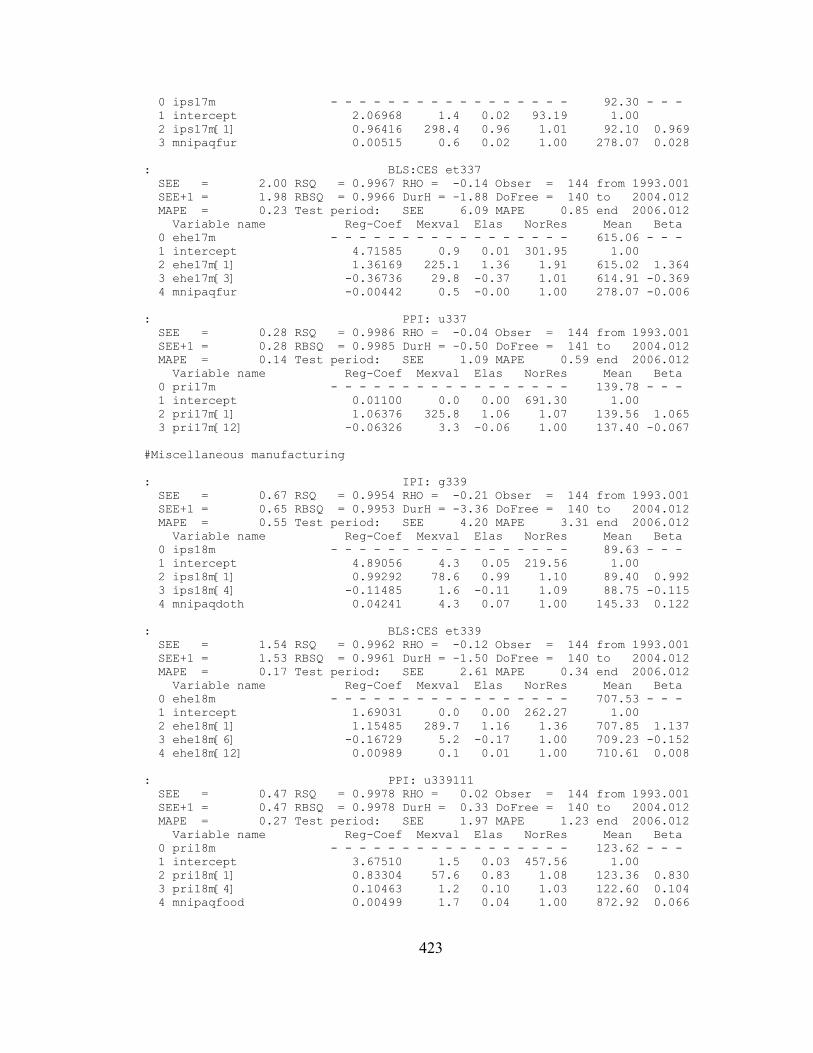
0 ips17m - - - - - - - - - - - - - - - - - 92.30 - - - 1 intercept 2.06968 1.4 0.02 93.19 1.00 2 ips17m[1] 0.96416 298.4 0.96 1.01 92.10 0.969 3 mnipaqfur 0.00515 0.6 0.02 1.00 278.07 0.028
: BLS:CES et337 SEE = 2.00 RSQ = 0.9967 RHO = -0.14 Obser = 144 from 1993.001 SEE+1 = 1.98 RBSQ = 0.9966 DurH = -1.88 DoFree = 140 to 2004.012 MAPE = 0.23 Test period: SEE 6.09 MAPE 0.85 end 2006.012 Variable name Reg-Coef Mexval Elas NorRes Mean Beta 0 ehe17m - - - - - - - - - - - - - - - - - 615.06 - - - 1 intercept 4.71585 0.9 0.01 301.95 1.00 2 ehe17m[1] 1.36169 225.1 1.36 1.91 615.02 1.364 3 ehe17m[3] -0.36736 29.8 -0.37 1.01 614.91 -0.369 4 mnipaqfur -0.00442 0.5 -0.00 1.00 278.07 -0.006
: PPI: u337 SEE = 0.28 RSQ = 0.9986 RHO = -0.04 Obser = 144 from 1993.001 SEE+1 = 0.28 RBSQ = 0.9985 DurH = -0.50 DoFree = 141 to 2004.012 MAPE = 0.14 Test period: SEE 1.09 MAPE 0.59 end 2006.012 Variable name Reg-Coef Mexval Elas NorRes Mean Beta 0 pri17m - - - - - - - - - - - - - - - - - 139.78 - - - 1 intercept 0.01100 0.0 0.00 691.30 1.00 2 pri17m[1] 1.06376 325.8 1.06 1.07 139.56 1.065 3 pri17m[12] -0.06326 3.3 -0.06 1.00 137.40 -0.067
#Miscellaneous manufacturing
: IPI: g339 SEE = 0.67 RSQ = 0.9954 RHO = -0.21 Obser = 144 from 1993.001 SEE+1 = 0.65 RBSQ = 0.9953 DurH = -3.36 DoFree = 140 to 2004.012 MAPE = 0.55 Test period: SEE 4.20 MAPE 3.31 end 2006.012 Variable name Reg-Coef Mexval Elas NorRes Mean Beta 0 ips18m - - - - - - - - - - - - - - - - - 89.63 - - - 1 intercept 4.89056 4.3 0.05 219.56 1.00 2 ips18m[1] 0.99292 78.6 0.99 1.10 89.40 0.992 3 ips18m[4] -0.11485 1.6 -0.11 1.09 88.75 -0.115 4 mnipaqdoth 0.04241 4.3 0.07 1.00 145.33 0.122
: BLS:CES et339 SEE = 1.54 RSQ = 0.9962 RHO = -0.12 Obser = 144 from 1993.001 SEE+1 = 1.53 RBSQ = 0.9961 DurH = -1.50 DoFree = 140 to 2004.012 MAPE = 0.17 Test period: SEE 2.61 MAPE 0.34 end 2006.012 Variable name Reg-Coef Mexval Elas NorRes Mean Beta 0 ehe18m - - - - - - - - - - - - - - - - - 707.53 - - - 1 intercept 1.69031 0.0 0.00 262.27 1.00 2 ehe18m[1] 1.15485 289.7 1.16 1.36 707.85 1.137 3 ehe18m[6] -0.16729 5.2 -0.17 1.00 709.23 -0.152 4 ehe18m[12] 0.00989 0.1 0.01 1.00 710.61 0.008
: PPI: u339111 SEE = 0.47 RSQ = 0.9978 RHO = 0.02 Obser = 144 from 1993.001 SEE+1 = 0.47 RBSQ = 0.9978 DurH = 0.33 DoFree = 140 to 2004.012 MAPE = 0.27 Test period: SEE 1.97 MAPE 1.23 end 2006.012 Variable name Reg-Coef Mexval Elas NorRes Mean Beta 0 pri18m - - - - - - - - - - - - - - - - - 123.62 - - - 1 intercept 3.67510 1.5 0.03 457.56 1.00 2 pri18m[1] 0.83304 57.6 0.83 1.08 123.36 0.830 3 pri18m[4] 0.10463 1.2 0.10 1.03 122.60 0.104 4 mnipaqfood 0.00499 1.7 0.04 1.00 872.92 0.066
423

# Food,beverage, tobacco: IPI: g331a2 SEE = 0.87 RSQ = 0.9317 RHO = -0.13 Obser = 144 from 1993.001 SEE+1 = 0.87 RBSQ = 0.9297 DurH = -1.91 DoFree = 139 to 2004.012 MAPE = 0.71 Test period: SEE 4.85 MAPE 4.01 end 2006.012 Variable name Reg-Coef Mexval Elas NorRes Mean Beta 0 ips19m - - - - - - - - - - - - - - - - - 98.89 - - - 1 intercept 29.98874 7.2 0.30 14.64 1.00 2 ips19m[1] 0.75600 60.1 0.76 1.14 98.81 0.766 3 ips19m[12] -0.08122 1.0 -0.08 1.12 97.99 -0.089 4 mnipaqfood[4] -0.02546 4.1 -0.22 1.10 860.21 -0.977 5 mgdp 0.00267 4.9 0.24 1.00 9027.08 1.244
: BLS:CES et312 SEE = 1.00 RSQ = 0.9465 RHO = -0.07 Obser = 144 from 1993.001 SEE+1 = 1.00 RBSQ = 0.9449 DurH = -0.98 DoFree = 139 to 2004.012 MAPE = 0.37 Test period: SEE 3.23 MAPE 1.56 end 2006.012 Variable name Reg-Coef Mexval Elas NorRes Mean Beta 0 ehe19m - - - - - - - - - - - - - - - - - 204.98 - - - 1 intercept 11.12297 1.2 0.05 18.68 1.00 2 ehe19m[1] 0.91128 72.9 0.91 1.05 205.08 0.893 3 ehe19m[4] 0.12151 1.2 0.12 1.05 205.33 0.112 4 ehe19m[12] -0.08297 1.4 -0.08 1.01 206.14 -0.060 5 mnipaqfood[4] -0.00101 0.7 -0.00 1.00 860.21 -0.030
: PPI: u311 SEE = 0.94 RSQ = 0.9826 RHO = 0.14 Obser = 144 from 1993.001 SEE+1 = 0.94 RBSQ = 0.9821 DurH = 1.98 DoFree = 139 to 2004.012 MAPE = 0.46 Test period: SEE 1.64 MAPE 0.91 end 2006.012 Variable name Reg-Coef Mexval Elas NorRes Mean Beta 0 pri19m - - - - - - - - - - - - - - - - - 128.60 - - - 1 intercept 9.29319 2.4 0.07 57.31 1.00 2 pri19m[1] 0.95715 102.1 0.96 1.06 128.41 0.949 3 pri19m[4] -0.00891 0.0 -0.01 1.06 127.85 -0.009 4 pri19m[12] -0.05731 0.7 -0.06 1.06 126.31 -0.048 5 mnipaqfood[1] 0.00549 2.8 0.04 1.00 869.71 0.101
# Textile, mills: IPI: g313a4 SEE = 1.45 RSQ = 0.9654 RHO = -0.20 Obser = 144 from 1993.001 SEE+1 = 1.42 RBSQ = 0.9644 DurH = -3.40 DoFree = 139 to 2004.012 MAPE = 1.12 Test period: SEE 3.97 MAPE 3.87 end 2006.012 Variable name Reg-Coef Mexval Elas NorRes Mean Beta 0 ips20m - - - - - - - - - - - - - - - - - 107.88 - - - 1 intercept 9.51544 2.7 0.09 28.88 1.00 2 ips20m[1] 0.99094 70.1 0.99 1.07 107.96 0.980 3 ips20m[4] -0.04150 0.2 -0.04 1.06 108.17 -0.040 4 mnipaqcloth[6] -0.00302 0.0 -0.01 1.00 271.60 -0.012 5 mnipaqcloth[12] -0.01236 0.1 -0.03 1.00 267.24 -0.048
: BLS:CES et313 SEE = 1.69 RSQ = 0.9995 RHO = -0.03 Obser = 120 from 1995.001 SEE+1 = 1.69 RBSQ = 0.9995 DurH = -0.32 DoFree = 116 to 2004.012 MAPE = 0.32 Test period: SEE 8.15 MAPE 3.45 end 2006.012 Variable name Reg-Coef Mexval Elas NorRes Mean Beta 0 ehe20_1m - - - - - - - - - - - - - - - - - 367.00 - - - 1 ehe20_1m[1] 1.07093 49.5 1.08 1.54 369.09 2 ehe20_1m[2] 0.26411 1.8 0.27 1.32 371.16 0.262 3 ehe20_1m[4] -0.34504 10.0 -0.35 1.00 375.25 -0.338 4 ehe20_1m[12] 0.00822 0.1 0.01 1.00 391.09 0.007
424
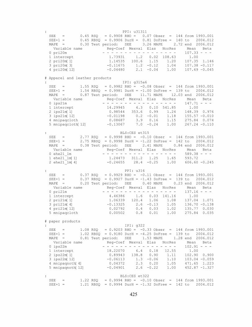
: PPI: u31311 SEE = 0.45 RSQ = 0.9908 RHO = 0.07 Obser = 144 from 1993.001 SEE+1 = 0.45 RBSQ = 0.9906 DurH = 0.81 DoFree = 140 to 2004.012 MAPE = 0.30 Test period: SEE 3.26 MAPE 2.72 end 2006.012 Variable name Reg-Coef Mexval Elas NorRes Mean Beta 0 pri20m - - - - - - - - - - - - - - - - - 107.33 - - - 1 intercept 1.73931 1.2 0.02 108.63 1.00 2 pri20m[1] 1.14535 100.6 1.15 1.20 107.35 1.146 3 pri20m[3] -0.11675 1.2 -0.12 1.04 107.38 -0.117 4 pri20m[12] -0.04480 2.1 -0.04 1.00 107.69 -0.045
# Apparel and leather products: IPI: g315a6 SEE = 1.55 RSQ = 0.9982 RHO = -0.08 Obser = 144 from 1993.001 SEE+1 = 1.54 RBSQ = 0.9981 DurH = -1.00 DoFree = 139 to 2004.012 MAPE = 0.87 Test period: SEE 11.71 MAPE 12.03 end 2006.012 Variable name Reg-Coef Mexval Elas NorRes Mean Beta 0 ips21m - - - - - - - - - - - - - - - - - 147.71 - - - 1 intercept 14.29945 4.3 0.10 541.85 1.00 2 ips21m[1] 0.98544 353.6 0.99 1.24 148.39 0.976 3 ips21m[12] -0.01198 0.2 -0.01 1.18 155.57 -0.010 4 mnipaqcloth 0.08687 3.9 0.16 1.15 275.84 0.074 5 mnipaqcloth[12] -0.13067 7.0 -0.24 1.00 267.24 -0.110
: BLS:CES et315 SEE = 2.77 RSQ = 0.9998 RHO = -0.10 Obser = 144 from 1993.001 SEE+1 = 2.75 RBSQ = 0.9998 DurH = -1.22 DoFree = 142 to 2004.012 MAPE = 0.38 Test period: SEE 2.41 MAPE 0.84 end 2006.012 Variable name Reg-Coef Mexval Elas NorRes Mean Beta 0 ehe21_1m - - - - - - - - - - - - - - - - - 589.38 - - - 1 ehe21_1m[1] 1.24473 311.2 1.25 1.65 593.72 2 ehe21_1m[4] -0.24655 28.4 -0.25 1.00 606.60 -0.245
: PPI: u316 SEE = 0.37 RSQ = 0.9929 RHO = -0.11 Obser = 144 from 1993.001 SEE+1 = 0.37 RBSQ = 0.9927 DurH = -1.43 DoFree = 139 to 2004.012 MAPE = 0.20 Test period: SEE 0.40 MAPE 0.23 end 2006.012 Variable name Reg-Coef Mexval Elas NorRes Mean Beta 0 pri21m - - - - - - - - - - - - - - - - - 137.16 - - - 1 intercept 4.46386 1.6 0.03 141.16 1.00 2 pri21m[1] 1.06339 120.4 1.06 1.08 137.04 1.071 3 pri21m[4] -0.13325 2.6 -0.13 1.05 136.70 -0.138 4 pri21m[12] 0.02792 0.4 0.03 1.02 135.77 0.030 5 mnipaqcloth 0.00502 0.8 0.01 1.00 275.84 0.035
# paper products: IPI: g322 SEE = 1.08 RSQ = 0.9203 RHO = -0.33 Obser = 144 from 1993.001 SEE+1 = 1.02 RBSQ = 0.9180 DurH = -4.25 DoFree = 139 to 2004.012 MAPE = 0.81 Test period: SEE 1.53 MAPE 1.28 end 2006.012 Variable name Reg-Coef Mexval Elas NorRes Mean Beta 0 ips22m - - - - - - - - - - - - - - - - - 102.91 - - - 1 intercept 18.22070 6.4 0.18 12.55 1.00 2 ips22m[1] 0.89943 138.8 0.90 1.11 102.90 0.900 3 ips22m[12] -0.06113 1.3 -0.06 1.10 103.04 -0.059 4 mnipaqnoth[4] 0.04372 2.3 0.20 1.05 471.65 1.223 5 mnipaqnoth[12] -0.04901 2.6 -0.22 1.00 452.87 -1.327
: BLS:CES et322 SEE = 1.22 RSQ = 0.9994 RHO = -0.10 Obser = 144 from 1993.001 SEE+1 = 1.21 RBSQ = 0.9994 DurH = -1.32 DoFree = 142 to 2004.012
425

MAPE = 0.16 Test period: SEE 3.22 MAPE 0.54 end 2006.012 Variable name Reg-Coef Mexval Elas NorRes Mean Beta 0 ehe22m - - - - - - - - - - - - - - - - - 596.85 - - - 1 ehe22m[1] 1.33404 201.2 1.34 1.51 597.90 2 ehe22m[3] -0.33461 22.9 -0.34 1.00 599.98 -0.321
: PPI: u32212 SEE = 0.90 RSQ = 0.9932 RHO = 0.10 Obser = 144 from 1993.001 SEE+1 = 0.89 RBSQ = 0.9930 DurH = 1.50 DoFree = 139 to 2004.012 MAPE = 0.48 Test period: SEE 5.04 MAPE 2.69 end 2006.012 Variable name Reg-Coef Mexval Elas NorRes Mean Beta 0 pri22m - - - - - - - - - - - - - - - - - 145.01 - - - 1 intercept 4.76259 5.9 0.03 146.29 1.00 2 pri22m[1] 1.29204 244.7 1.29 3.25 144.80 1.301 3 pri22m[4] -0.38164 9.4 -0.38 1.03 144.21 -0.391 4 pri22m[6] 0.05322 0.5 0.05 1.02 143.86 0.055 5 mnipaqgas 0.00327 0.8 0.00 1.00 165.14 0.011
# Printing: IPI: g323 SEE = 0.67 RSQ = 0.9920 RHO = -0.18 Obser = 144 from 1993.001 SEE+1 = 0.00 RBSQ = 0.9916 DurH = -2.30 DoFree = 137 to 2004.012 MAPE = 0.51 Test period: SEE 1.26 MAPE 0.92 end 2006.012 Variable name Reg-Coef Mexval Elas NorRes Mean Beta 0 ips23m - - - - - - - - - - - - - - - - - 134.60 - - - 1 intercept 6.44430 5.1 0.06 118.47 1.27 2 ips23m[1] 0.98287 229.9 0.98 1.21 134.66 0.979 3 ips23m[12] -0.03809 0.9 -0.04 1.14 135.37 -0.035 4 mnipaqnoth 0.03161 5.1 0.14 1.13 610.43 0.583 5 mnipaqnoth[12] -0.03641 5.0 -0.16 1.07 574.35 -0.641 6 mnipaqgas 0.00399 0.4 0.01 1.05 209.35 0.025 7 ips23m_mu[1] -0.21360 2.1 0.00 1.00 -0.01 -0.021
: BLS:CES et323 SEE = 1.72 RSQ = 0.9991 RHO = -0.06 Obser = 144 from 1993.001 SEE+1 = 1.71 RBSQ = 0.9991 DurH = -0.69 DoFree = 142 to 2004.012 MAPE = 0.17 Test period: SEE 3.91 MAPE 0.57 end 2006.012 Variable name Reg-Coef Mexval Elas NorRes Mean Beta 0 ehe23m - - - - - - - - - - - - - - - - - 775.70 - - - 1 ehe23m[1] 1.27549 396.5 1.28 2.11 776.57 2 ehe23m[4] -0.27571 45.3 -0.28 1.00 779.12 -0.258
: PPI: u323110 SEE = 0.44 RSQ = 0.9969 RHO = 0.03 Obser = 144 from 1993.001 SEE+1 = 0.44 RBSQ = 0.9967 DurH = 0.56 DoFree = 138 to 2004.012 MAPE = 0.19 Test period: SEE 0.39 MAPE 0.19 end 2006.012 Variable name Reg-Coef Mexval Elas NorRes Mean Beta 0 pri23m - - - - - - - - - - - - - - - - - 150.71 - - - 1 intercept 1.43382 0.2 0.01 318.72 1.00 2 pri23m[1] 1.11139 135.1 1.11 1.09 150.52 1.127 3 pri23m[4] -0.11048 0.7 -0.11 1.01 149.92 -0.117 4 pri23m[6] -0.01547 0.0 -0.02 1.01 149.53 -0.017 5 mnipaqnoth -0.00257 0.1 -0.01 1.00 481.30 -0.036 6 mnipaqfood 0.00241 0.2 0.01 1.00 872.92 0.041
# Petroleum and Coal: BLS:CES et324 SEE = 0.74 RSQ = 0.9958 RHO = -0.01 Obser = 144 from 1993.001 SEE+1 = 0.74 RBSQ = 0.9957 DurH = 999.00 DoFree = 139 to 2004.012 MAPE = 0.41 Test period: SEE 3.16 MAPE 2.33 end 2006.012 Variable name Reg-Coef Mexval Elas NorRes Mean Beta
426

0 ehe24m - - - - - - - - - - - - - - - - - 129.52 - - - 1 intercept -3.82499 0.9 -0.03 238.24 1.00 2 ehe24m[1] 0.79955 29.3 0.80 1.06 129.78 0.800 3 ehe24m[2] 0.21844 2.4 0.22 1.02 130.03 0.219 4 mnipaqgas 0.00283 0.1 0.00 1.00 165.14 0.009 5 mnipaqgas[4] 0.00442 0.2 0.01 1.00 161.33 0.013
: PPI: u324 SEE = 5.44 RSQ = 0.9520 RHO = 0.29 Obser = 144 from 1993.001 SEE+1 = 5.26 RBSQ = 0.9510 DurH = 4.24 DoFree = 140 to 2004.012 MAPE = 4.46 Test period: SEE 28.04 MAPE 10.01 end 2006.012 Variable name Reg-Coef Mexval Elas NorRes Mean Beta 0 pri24m - - - - - - - - - - - - - - - - - 94.54 - - - 1 intercept -5.64312 2.4 -0.06 20.83 1.00 2 pri24m[1] 0.56444 24.8 0.56 1.40 94.04 0.555 3 pri24m[4] 0.00280 0.0 0.00 1.38 92.27 0.002 4 mnipaqgas 0.28368 17.4 0.50 1.00 165.14 0.431
# Chemical products: IPI: g325 SEE = 0.77 RSQ = 0.9903 RHO = -0.03 Obser = 144 from 1993.001 SEE+1 = 0.77 RBSQ = 0.9901 DurH = -0.39 DoFree = 140 to 2004.012 MAPE = 0.66 Test period: SEE 8.69 MAPE 6.82 end 2006.012 Variable name Reg-Coef Mexval Elas NorRes Mean Beta 0 ips25m - - - - - - - - - - - - - - - - - 91.82 - - - 1 intercept 0.79258 0.2 0.01 103.09 1.00 2 ips25m[1] 0.98040 352.5 0.98 1.03 91.61 0.971 3 mnipaqgas 0.00003 0.0 0.00 1.02 165.14 0.000 4 mnipaqgas[12] 0.00778 1.2 0.01 1.00 154.72 0.029
: BLS:CES et325 SEE = 1.62 RSQ = 0.9983 RHO = -0.15 Obser = 144 from 1993.001 SEE+1 = 1.60 RBSQ = 0.9983 DurH = -2.02 DoFree = 142 to 2004.012 MAPE = 0.13 Test period: SEE 6.67 MAPE 0.50 end 2006.012 Variable name Reg-Coef Mexval Elas NorRes Mean Beta 0 ehe25m - - - - - - - - - - - - - - - - - 968.64 - - - 1 ehe25m[1] 1.19327 202.1 1.19 1.22 969.66 2 ehe25m[4] -0.19372 10.2 -0.19 1.00 972.67 -0.186
: PPI: u325 SEE = 0.68 RSQ = 0.9971 RHO = 0.22 Obser = 144 from 1993.001 SEE+1 = 0.67 RBSQ = 0.9971 DurH = 2.83 DoFree = 140 to 2004.012 MAPE = 0.33 Test period: SEE 8.41 MAPE 3.25 end 2006.012 Variable name Reg-Coef Mexval Elas NorRes Mean Beta 0 pri25m - - - - - - - - - - - - - - - - - 150.14 - - - 1 intercept 2.89256 2.7 0.02 348.39 1.00 2 pri25m[1] 1.14572 195.1 1.14 1.40 149.76 1.136 3 pri25m[4] -0.17733 10.3 -0.18 1.09 148.71 -0.173 4 mnipaqgas 0.01229 4.4 0.01 1.00 165.14 0.036
# Plastic and rubbers: IPI: g326 SEE = 0.71 RSQ = 0.9927 RHO = -0.22 Obser = 144 from 1993.001 SEE+1 = 0.69 RBSQ = 0.9924 DurH = -2.83 DoFree = 137 to 2004.012 MAPE = 0.60 Test period: SEE 1.25 MAPE 1.02 end 2006.012 Variable name Reg-Coef Mexval Elas NorRes Mean Beta 0 ips26m - - - - - - - - - - - - - - - - - 94.22 - - - 1 intercept -1.57653 0.1 -0.02 136.70 1.00 2 ips26m[1] 1.04981 91.0 1.05 1.09 94.03 1.068 3 ips26m[4] -0.08102 0.6 -0.08 1.05 93.45 -0.087 4 ips26m[12] -0.02191 0.2 -0.02 1.05 91.78 -0.026
427

5 mnipaqnoth 0.02107 0.8 0.11 1.05 481.30 0.274 6 mnipaqnoth[4] -0.03102 1.7 -0.16 1.02 471.65 -0.397 7 mtime 0.38398 1.1 0.12 1.00 29.04 0.160
: BLS:CES et326 SEE = 2.44 RSQ = 0.9977 RHO = -0.08 Obser = 144 from 1993.001 SEE+1 = 2.43 RBSQ = 0.9977 DurH = -0.98 DoFree = 142 to 2004.012 MAPE = 0.21 Test period: SEE 7.53 MAPE 0.85 end 2006.012 Variable name Reg-Coef Mexval Elas NorRes Mean Beta 0 ehe26m - - - - - - - - - - - - - - - - - 893.12 - - - 1 ehe26m[1] 1.27175 363.1 1.27 1.94 893.31 2 ehe26m[4] -0.27184 39.1 -0.27 1.00 893.74 -0.267
: PPI: u326 SEE = 0.30 RSQ = 0.9951 RHO = 0.11 Obser = 144 from 1993.001 SEE+1 = 0.30 RBSQ = 0.9949 DurH = 1.39 DoFree = 139 to 2004.012 MAPE = 0.19 Test period: SEE 3.09 MAPE 1.80 end 2006.012 Variable name Reg-Coef Mexval Elas NorRes Mean Beta 0 pri26m - - - - - - - - - - - - - - - - - 123.52 - - - 1 intercept 3.53429 2.5 0.03 202.42 1.00 2 pri26m[1] 1.13061 200.9 1.13 1.54 123.37 1.113 3 pri26m[4] -0.16461 9.2 -0.16 1.18 122.96 -0.157 4 mnipaqgas 0.00965 7.7 0.01 1.04 165.14 0.084 5 mnipaqgas[6] -0.00534 1.8 -0.01 1.00 159.62 -0.040
# Wholesale Trade: BLS:CES et42 SEE = 6.08 RSQ = 0.9994 RHO = -0.01 Obser = 144 from 1993.001 SEE+1 = 6.08 RBSQ = 0.9993 DurH = -0.10 DoFree = 137 to 2004.012 MAPE = 0.09 Test period: SEE 108.26 MAPE 1.43 end 2006.012 Variable name Reg-Coef Mexval Elas NorRes Mean Beta 0 ehe27m - - - - - - - - - - - - - - - - - 5606.48 - - - 1 intercept 138.93537 2.1 0.02 1586.07 1.00 2 ehe27m[1] 1.18221 177.1 1.18 2.81 5602.05 1.201 3 ehe27m[4] -0.19095 6.2 -0.19 1.10 5589.29 -0.202 4 ehe27m[12] -0.01397 0.4 -0.01 1.10 5560.48 -0.016 5 mgdp 0.03953 4.5 0.06 1.09 9027.08 0.254 6 mgdp[6] -0.02175 1.4 -0.03 1.02 8800.77 -0.137 7 mnipaqfood[1] -0.20200 1.0 -0.03 1.00 869.71 -0.109
: PPI: u429930 SEE = 5.82 RSQ = 0.9591 RHO = 0.48 Obser = 144 from 1993.001 SEE+1 = 5.15 RBSQ = 0.9582 DurH = 5.96 DoFree = 140 to 2004.012 MAPE = 2.69 Test period: SEE 45.38 MAPE 17.47 end 2006.012 Variable name Reg-Coef Mexval Elas NorRes Mean Beta 0 pri27m - - - - - - - - - - - - - - - - - 149.90 - - - 1 intercept 1.70158 0.0 0.01 24.43 1.00 2 pri27m[1] 0.97468 259.8 0.97 1.03 149.10 0.948 3 mnipaqgas 0.06502 1.0 0.07 1.01 165.14 0.085 4 mgdp[4] -0.00089 0.4 -0.05 1.00 8875.59 -0.047
: BLS:CES hp42 SEE = 0.11 RSQ = 0.9066 RHO = -0.28 Obser = 144 from 1993.001 SEE+1 = 0.11 RBSQ = 0.9032 DurH = -4.92 DoFree = 138 to 2004.012 MAPE = 0.23 Test period: SEE 0.48 MAPE 1.01 end 2006.012 Variable name Reg-Coef Mexval Elas NorRes Mean Beta 0 hr27m - - - - - - - - - - - - - - - - - 38.45 - - - 1 intercept 10.60211 4.5 0.28 10.71 1.00 2 hr27m[1] 0.64970 33.3 0.65 1.24 38.46 0.640 3 hr27m[12] 0.09670 0.9 0.10 1.21 38.51 0.083 4 mgdp 0.00074 4.5 0.17 1.15 9027.08 3.181
428

5 mgdp[4] -0.00051 1.9 -0.12 1.07 8875.59 -2.164 6 mnipaqfood[1] -0.00346 3.3 -0.08 1.00 869.71 -1.247
: BLS:CES wp42 SEE = 0.04 RSQ = 0.9995 RHO = -0.05 Obser = 144 from 1993.001 SEE+1 = 0.04 RBSQ = 0.9995 DurH = -3.58 DoFree = 140 to 2004.012 MAPE = 0.19 Test period: SEE 0.35 MAPE 1.56 end 2006.012 Variable name Reg-Coef Mexval Elas NorRes Mean Beta 0 wag27m - - - - - - - - - - - - - - - - - 15.23 - - - 1 intercept 0.08155 0.4 0.01 2178.63 1.00 2 wag27m[1] 0.73851 25.9 0.74 1.07 15.19 0.740 3 wag27m[2] 0.25932 3.5 0.26 1.00 15.16 0.260 4 mgdp[1] -0.00000 0.0 -0.00 1.00 8988.88 -0.000
: CENSUS: wholesale trade SEE = 1976.95 RSQ = 0.9967 RHO = -0.00 Obser = 144 from 1993.001 SEE+1 = 1976.94 RBSQ = 0.9966 DurH = 999.00 DoFree = 139 to 2004.012 MAPE = 0.72 Test period: SEE 12274.08 MAPE 3.08 end 2006.012 Variable name Reg-Coef Mexval Elas NorRes Mean Beta 0 mwh42 - - - - - - - - - - - - - - - - - 210734.99 - - - 1 intercept 31.06328 0.0 0.00 301.49 1.00 2 mwh42[1] 0.92106 36.7 0.92 1.03 209773.40 0.915 3 mwh42[2] 0.11798 0.4 0.12 1.02 208838.80 0.117 4 mwh42[3] 0.10790 0.3 0.11 1.02 207931.52 0.106 5 mwh42[4] -0.14290 1.0 -0.14 1.00 207045.91 -0.140
# Retail Trade: BLS:CES etrt SEE = 22.13 RSQ = 0.9990 RHO = -0.06 Obser = 144 from 1993.001 SEE+1 = 22.08 RBSQ = 0.9990 DurH = -0.78 DoFree = 137 to 2004.012 MAPE = 0.11 Test period: SEE 123.60 MAPE 0.73 end 2006.012 Variable name Reg-Coef Mexval Elas NorRes Mean Beta 0 ehe28m - - - - - - - - - - - - - - - - - 14502.62 - - - 1 intercept 220.84009 2.5 0.02 1016.44 1.00 2 ehe28m[1] 1.01381 100.2 1.01 1.34 14486.73 1.030 3 ehe28m[4] 0.02575 0.1 0.03 1.15 14439.17 0.027 4 ehe28m[12] -0.05703 2.2 -0.06 1.12 14316.79 -0.066 5 mgdp 0.12136 4.3 0.08 1.10 9027.08 0.268 6 mgdp[6] -0.11538 3.4 -0.07 1.02 8800.77 -0.249 7 mnipaqgas -0.24549 0.9 -0.00 1.00 165.14 -0.013
: BLS:CES hprt SEE = 0.09 RSQ = 0.4328 RHO = -0.02 Obser = 144 from 1993.001 SEE+1 = 0.09 RBSQ = 0.4123 DurH = -0.40 DoFree = 138 to 2004.012 MAPE = 0.23 Test period: SEE 0.23 MAPE 0.68 end 2006.012 Variable name Reg-Coef Mexval Elas NorRes Mean Beta 0 hr28m - - - - - - - - - - - - - - - - - 30.78 - - - 1 intercept 8.76052 3.8 0.28 1.76 1.00 2 hr28m[1] 0.50873 15.4 0.51 1.10 30.78 0.510 3 hr28m[3] 0.27548 4.2 0.28 1.02 30.78 0.274 4 hr28m[6] -0.06828 0.3 -0.07 1.01 30.79 -0.072 5 mnipaqgas -0.00069 0.5 -0.00 1.01 165.14 -0.210 6 mnipaqgas[6] 0.00061 0.3 0.00 1.00 159.62 0.160
: BLS:CES wprt SEE = 0.03 RSQ = 0.9996 RHO = -0.08 Obser = 144 from 1993.001 SEE+1 = 0.03 RBSQ = 0.9996 DurH = -1.32 DoFree = 139 to 2004.012 MAPE = 0.19 Test period: SEE 0.11 MAPE 0.75 end 2006.012 Variable name Reg-Coef Mexval Elas NorRes Mean Beta 0 wag28m - - - - - - - - - - - - - - - - - 10.24 - - - 1 intercept 0.02598 0.5 0.00 2427.90 1.00
429

2 wag28m[1] 0.70688 25.0 0.70 1.13 10.22 0.707 3 wag28m[2] 0.37005 5.9 0.37 1.02 10.19 0.370 4 wag28m[6] -0.07612 0.7 -0.07 1.00 10.08 -0.076 5 mnipaqgas -0.00004 0.0 -0.00 1.00 165.14 -0.001
: CENSUS: Retail sales, total SEE = 5017.39 RSQ = 0.9999 RHO = 0.82 Obser = 144 from 1993.001 SEE+1 = 2912.26 RBSQ = 0.9999 DurH = 9.93 DoFree = 141 to 2004.012 MAPE = 0.14 Test period: SEE 16275.45 MAPE 0.40 end 2005.012 Variable name Reg-Coef Mexval Elas NorRes Mean Beta 0 retlm - - - - - - - - - - - - - - - - - 2703476.57 - - - 1 intercept 6011.66046 2.0 0.00 8888.50 1.00 2 retlm[1] 0.94457 504.7 0.94 1.13 2691628.10 0.943 3 mgdp 17.17409 6.2 0.06 1.00 9027.08 0.057
: CENSUS: Retail Purchases, total SEE = 4167.33 RSQ = 0.9999 RHO = 0.81 Obser = 144 from 1993.001 SEE+1 = 2468.73 RBSQ = 0.9998 DurH = 9.79 DoFree = 141 to 2004.012 MAPE = 0.15 Test period: SEE 13815.62 MAPE 0.46 end 2005.012 Variable name Reg-Coef Mexval Elas NorRes Mean Beta 0 rtptotm - - - - - - - - - - - - - - - - - 1968248.18 - - - 1 intercept 6867.58752 3.9 0.00 6667.20 1.00 2 rtptotm[1] 0.95136 585.5 0.95 1.12 1959774.94 0.951 3 mgdp 10.73723 6.0 0.05 1.00 9027.08 0.049
# Air transportation: BLS:CES et481 SEE = 4.05 RSQ = 0.9889 RHO = 0.66 Obser = 144 from 1993.001 SEE+1 = 3.05 RBSQ = 0.9887 DurH = 7.99 DoFree = 141 to 2004.012 MAPE = 0.43 Test period: SEE 7.26 MAPE 1.15 end 2006.012 Variable name Reg-Coef Mexval Elas NorRes Mean Beta 0 ehe29m - - - - - - - - - - - - - - - - - 549.27 - - - 1 intercept 1.48159 0.0 0.00 89.77 1.00 2 ehe29m[1] 1.00285 687.4 1.00 1.01 549.30 1.002 3 mnipaqtr -0.01207 0.6 -0.01 1.00 254.75 -0.014
: PPI: u4811 SEE = 1.70 RSQ = 0.9960 RHO = 0.00 Obser = 144 from 1993.001 SEE+1 = 1.70 RBSQ = 0.9959 DurH = 0.01 DoFree = 140 to 2004.012 MAPE = 0.67 Test period: SEE 12.16 MAPE 4.98 end 2006.012 Variable name Reg-Coef Mexval Elas NorRes Mean Beta 0 pri29m - - - - - - - - - - - - - - - - - 163.06 - - - 1 intercept 1.38845 0.4 0.01 251.07 1.00 2 pri29m[1] 0.96777 407.2 0.96 1.03 162.51 0.972 3 mnipaqtr 0.01595 0.0 0.02 1.00 254.75 0.026 4 mnipaqtr[4] 0.00135 0.0 0.00 1.00 250.59 0.002
# Rail Transportation: BLS:CES et482 SEE = 1.37 RSQ = 0.9643 RHO = -0.20 Obser = 144 from 1993.001 SEE+1 = 1.34 RBSQ = 0.9633 DurH = -2.54 DoFree = 139 to 2004.012 MAPE = 0.45 Test period: SEE 0.64 MAPE 0.21 end 2006.012 Variable name Reg-Coef Mexval Elas NorRes Mean Beta 0 ehe30m - - - - - - - - - - - - - - - - - 227.40 - - - 1 intercept 18.40754 3.2 0.08 28.00 1.00 2 ehe30m[1] 0.99616 233.8 1.00 1.06 227.53 1.020 3 ehe30m[12] -0.07027 2.9 -0.07 1.02 229.27 -0.089 4 mnipaqtr[12] -0.00821 0.9 -0.01 1.00 242.20 -0.055 5 mnipaqgas 0.00262 0.1 0.00 1.00 165.14 0.014
: PPI: u482
430
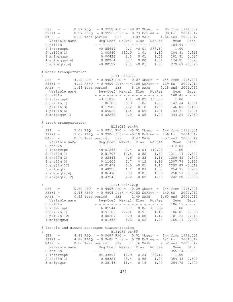
SEE = 0.27 RSQ = 0.9958 RHO = -0.07 Obser = 95 from 1997.002 SEE+1 = 0.27 RBSQ = 0.9956 DurH = -0.73 DoFree = 90 to 2004.012 MAPE = 0.18 Test period: SEE 3.03 MAPE 1.64 end 2006.012 Variable name Reg-Coef Mexval Elas NorRes Mean Beta 0 pri30m - - - - - - - - - - - - - - - - - 104.99 - - - 1 intercept -0.55699 0.1 -0.01 238.17 1.00 2 pri30m[1] 1.00940 580.0 1.01 1.10 104.81 0.968 3 mnipaqgas 0.00426 2.3 0.01 1.05 181.31 0.037 4 mnipaqgas[6] 0.00264 0.7 0.00 1.04 174.21 0.020 5 mnipaqtr[4] -0.00527 2.1 -0.01 1.00 279.67 -0.025
# Water transportation: PPI: u483111 SEE = 4.12 RSQ = 0.9903 RHO = -0.07 Obser = 144 from 1993.001 SEE+1 = 4.11 RBSQ = 0.9900 DurH = -1.06 DoFree = 139 to 2004.012 MAPE = 1.48 Test period: SEE 8.18 MAPE 3.18 end 2006.012 Variable name Reg-Coef Mexval Elas NorRes Mean Beta 0 pri31m - - - - - - - - - - - - - - - - - 148.45 - - - 1 intercept -3.11896 1.1 -0.02 103.05 1.00 2 pri31m[1] 1.06306 85.3 1.06 1.08 147.64 1.051 3 pri31m[3] -0.17903 2.2 -0.18 1.07 146.05 -0.173 4 pri31m[6] 0.09026 1.4 0.09 1.04 143.71 0.084 5 mnipaqmv[1] 0.02262 2.0 0.05 1.00 344.29 0.039
# Truck transportation: BLS:CES et484 SEE = 7.09 RSQ = 0.9911 RHO = -0.01 Obser = 144 from 1993.001 SEE+1 = 7.09 RBSQ = 0.9906 DurH = -0.10 DoFree = 136 to 2004.012 MAPE = 0.32 Test period: SEE 8.47 MAPE 0.57 end 2006.012 Variable name Reg-Coef Mexval Elas NorRes Mean Beta 0 ehe32m - - - - - - - - - - - - - - - - - 1312.83 - - - 1 intercept 48.01253 2.4 0.04 112.23 1.00 2 ehe32m[1] 0.51707 12.8 0.52 1.30 1311.14 0.527 3 ehe32m[2] 0.32844 4.6 0.33 1.16 1309.45 0.342 4 ehe32m[3] 0.11605 0.7 0.12 1.16 1307.73 0.123 5 ehe32m[12] -0.01458 0.0 -0.01 1.10 1292.47 -0.018 6 mnipaqtr 0.48211 1.1 0.09 1.08 254.75 0.283 7 mnipaqtr[4] 0.06470 0.0 0.01 1.05 250.59 0.039 8 mnipaqtr[12] -0.47541 2.2 -0.09 1.00 242.20 -0.306
: PPI: u484121p SEE = 0.50 RSQ = 0.9906 RHO = -0.29 Obser = 144 from 1993.001 SEE+1 = 0.48 RBSQ = 0.9904 DurH = -3.53 DoFree = 140 to 2004.012 MAPE = 0.32 Test period: SEE 2.49 MAPE 1.63 end 2006.012 Variable name Reg-Coef Mexval Elas NorRes Mean Beta 0 pri32m - - - - - - - - - - - - - - - - - 106.15 - - - 1 intercept 6.85544 3.7 0.06 106.59 1.00 2 pri32m[1] 0.91186 222.4 0.91 1.13 106.01 0.896 3 pri32m[12] 0.00387 0.9 0.00 1.12 101.25 0.015 4 mnipaqgas 0.01353 5.8 0.02 1.00 165.14 0.098
# Transit and ground passenger transportation: BLS:CES et485 SEE = 4.88 RSQ = 0.9689 RHO = 0.01 Obser = 144 from 1993.001 SEE+1 = 4.88 RBSQ = 0.9685 DurH = 0.28 DoFree = 141 to 2004.012 MAPE = 0.80 Test period: SEE 11.16 MAPE 2.52 end 2006.012 Variable name Reg-Coef Mexval Elas NorRes Mean Beta 0 ehe33m - - - - - - - - - - - - - - - - - 355.14 - - - 1 intercept 84.33597 12.9 0.24 32.17 1.00 2 ehe33m[1] 0.58324 23.4 0.58 1.24 354.48 0.590 3 mnipaqtr 0.25148 11.4 0.18 1.00 254.75 0.400
431

: BLS:CES hptr SEE = 0.22 RSQ = 0.9604 RHO = -0.14 Obser = 144 from 1993.001 SEE+1 = 0.21 RBSQ = 0.9595 DurH = -1.79 DoFree = 140 to 2004.012 MAPE = 0.40 Test period: SEE 0.24 MAPE 0.57 end 2006.012 Variable name Reg-Coef Mexval Elas NorRes Mean Beta 0 hr33m - - - - - - - - - - - - - - - - - 38.09 - - - 1 intercept 5.23460 5.0 0.14 25.24 1.00 2 hr33m[1] 0.87674 146.6 0.88 1.09 38.10 0.876 3 mnipaqtr 0.01683 1.0 0.11 1.02 254.75 0.684 4 mnipaqtr[3] -0.01919 1.2 -0.13 1.00 251.63 -0.799
: BLS:CES wptr SEE = 0.05 RSQ = 0.9986 RHO = -0.11 Obser = 144 from 1993.001 SEE+1 = 0.05 RBSQ = 0.9986 DurH = -2.31 DoFree = 140 to 2004.012 MAPE = 0.25 Test period: SEE 0.12 MAPE 0.60 end 2006.012 Variable name Reg-Coef Mexval Elas NorRes Mean Beta 0 wag33m - - - - - - - - - - - - - - - - - 14.46 - - - 1 intercept 0.13149 1.2 0.01 739.29 1.00 2 wag33m[1] 0.77178 37.7 0.77 1.10 14.44 0.769 3 wag33m[3] 0.20875 3.4 0.21 1.05 14.38 0.206 4 mnipaqtr 0.00073 2.7 0.01 1.00 254.75 0.025
# Pipeline transportation: BLS:CES et486 SEE = 0.25 RSQ = 0.9983 RHO = -0.00 Obser = 144 from 1993.001 SEE+1 = 0.25 RBSQ = 0.9983 DurH = -0.00 DoFree = 140 to 2004.012 MAPE = 0.33 Test period: SEE 1.08 MAPE 2.20 end 2006.012 Variable name Reg-Coef Mexval Elas NorRes Mean Beta 0 ehe34m - - - - - - - - - - - - - - - - - 48.08 - - - 1 intercept -0.45959 0.3 -0.01 592.76 1.00 2 ehe34m[1] 1.01250 166.9 1.02 1.01 48.23 1.014 3 ehe34m[6] -0.00963 0.0 -0.01 1.01 48.98 -0.010 4 mnipaqgas 0.00108 0.3 0.00 1.00 165.14 0.007
: PPI: u486110 SEE = 1.51 RSQ = 0.9609 RHO = -0.00 Obser = 144 from 1993.001 SEE+1 = 1.51 RBSQ = 0.9598 DurH = -0.03 DoFree = 139 to 2004.012 MAPE = 0.65 Test period: SEE 5.06 MAPE 3.75 end 2006.012 Variable name Reg-Coef Mexval Elas NorRes Mean Beta 0 pri34m - - - - - - - - - - - - - - - - - 104.55 - - - 1 intercept 3.63295 1.2 0.03 25.58 1.00 2 pri34m[1] 1.00160 74.2 1.00 1.03 104.40 0.998 3 pri34m[3] -0.04201 0.2 -0.04 1.02 104.10 -0.042 4 mnipaqgas 0.01062 0.9 0.02 1.00 165.14 0.052 5 mnipaqtr[1] -0.00406 0.2 -0.01 1.00 253.71 -0.024
# Other transportation: BLS:CES et488 SEE = 2.13 RSQ = 0.9984 RHO = -0.09 Obser = 144 from 1993.001 SEE+1 = 2.12 RBSQ = 0.9984 DurH = -1.10 DoFree = 140 to 2004.012 MAPE = 0.35 Test period: SEE 11.35 MAPE 1.80 end 2006.012 Variable name Reg-Coef Mexval Elas NorRes Mean Beta 0 ehe35m - - - - - - - - - - - - - - - - - 484.01 - - - 1 intercept 8.47458 1.5 0.02 632.78 1.00 2 ehe35m[1] 0.94990 289.1 0.95 1.19 482.81 0.959 3 mnipaqtr 0.18502 8.3 0.10 1.14 254.75 0.152 4 mnipaqtr[12] -0.12477 7.0 -0.06 1.00 242.20 -0.112
: PPI: u488119p SEE = 2.00 RSQ = 0.9814 RHO = -0.09 Obser = 144 from 1993.001
432

SEE+1 = 1.99 RBSQ = 0.9807 DurH = -2.13 DoFree = 138 to 2004.012 MAPE = 1.21 Test period: SEE 4.07 MAPE 1.84 end 2006.012 Variable name Reg-Coef Mexval Elas NorRes Mean Beta 0 pri35m - - - - - - - - - - - - - - - - - 119.88 - - - 1 intercept 5.46898 1.8 0.05 53.63 1.00 2 pri35m[1] 0.66072 26.2 0.66 1.19 119.56 0.659 3 pri35m[4] 0.02136 0.0 0.02 1.12 118.63 0.021 4 pri35m[6] 0.18002 2.3 0.18 1.06 118.03 0.176 5 mnipaqtr 0.03406 2.8 0.07 1.02 254.75 0.102 6 mnipaqgas 0.01789 0.9 0.02 1.00 165.14 0.046
# warehousing and storage: BLS:CES et493 SEE = 2.01 RSQ = 0.9978 RHO = -0.10 Obser = 144 from 1993.001 SEE+1 = 2.00 RBSQ = 0.9977 DurH = -1.28 DoFree = 139 to 2004.012 MAPE = 0.26 Test period: SEE 22.41 MAPE 3.12 end 2006.012 Variable name Reg-Coef Mexval Elas NorRes Mean Beta 0 ehe36m - - - - - - - - - - - - - - - - - 483.49 - - - 1 intercept 25.75244 4.5 0.05 450.86 1.00 2 ehe36m[1] 0.88969 169.4 0.89 1.23 482.36 0.886 3 mgdp 0.00408 0.1 0.08 1.17 9027.08 0.149 4 mgdp[1] 0.00696 0.1 0.13 1.15 8988.88 0.253 5 mgdp[12] -0.00826 7.0 -0.15 1.00 8581.40 -0.290
: PPI: u4931101 SEE = 0.32 RSQ = 0.9868 RHO = -0.03 Obser = 132 from 1994.001 SEE+1 = 0.32 RBSQ = 0.9866 DurH = -0.36 DoFree = 129 to 2004.012 MAPE = 0.17 Test period: SEE 0.75 MAPE 0.62 end 2006.012 Variable name Reg-Coef Mexval Elas NorRes Mean Beta 0 pri36m - - - - - - - - - - - - - - - - - 105.06 - - - 1 intercept 7.29283 2.2 0.07 75.60 1.00 2 pri36m[1] 0.91641 154.3 0.92 1.05 105.00 0.911 3 mgdp 0.00017 2.4 0.01 1.00 9242.51 0.086
# publishing: IPI: g5111 SEE = 0.86 RSQ = 0.9851 RHO = -0.03 Obser = 144 from 1993.001 SEE+1 = 0.86 RBSQ = 0.9847 DurH = -0.37 DoFree = 139 to 2004.012 MAPE = 0.66 Test period: SEE 3.41 MAPE 2.81 end 2006.012 Variable name Reg-Coef Mexval Elas NorRes Mean Beta 0 ips37m - - - - - - - - - - - - - - - - - 98.04 - - - 1 intercept 3.88732 2.6 0.04 67.15 1.00 2 ips37m[1] 1.00410 276.2 1.00 1.08 97.97 1.009 3 ips37m[12] -0.05086 2.0 -0.05 1.03 97.38 -0.054 4 mnipaqnoth 0.02698 1.5 0.13 1.03 481.30 0.415 5 mnipaqnoth[12] -0.02706 1.5 -0.13 1.00 452.87 -0.397
: PPI: u51113 SEE = 1.01 RSQ = 0.9976 RHO = -0.17 Obser = 144 from 1993.001 SEE+1 = 1.00 RBSQ = 0.9975 DurH = -2.15 DoFree = 140 to 2004.012 MAPE = 0.43 Test period: SEE 2.64 MAPE 1.02 end 2006.012 Variable name Reg-Coef Mexval Elas NorRes Mean Beta 0 pri37m - - - - - - - - - - - - - - - - - 181.79 - - - 1 intercept 4.82487 1.3 0.03 415.11 1.00 2 pri37m[1] 0.95042 213.3 0.95 1.03 181.28 0.949 3 mnipaqnoth 0.00945 0.2 0.03 1.00 481.30 0.049 4 mnipaqnoth[12] 0.00027 0.0 0.00 1.00 452.87 0.001
: NIPA: Nominal PCE of Computer and software SEE = 1.53 RSQ = 0.9806 RHO = 0.99 Obser = 144 from 1993.001 SEE+1 = 0.28 RBSQ = 0.9804 DW = 0.02 DoFree = 141 to 2004.012
433

MAPE = 4.43 Test period: SEE 1.57 MAPE 2.44 end 2006.012 Variable name Reg-Coef Mexval Elas NorRes Mean Beta 0 mcomppce - - - - - - - - - - - - - - - - - 35.65 - - - 1 intercept -25.20839 199.8 -0.71 51.63 1.00 2 mnipaqfur 0.13030 0.5 1.02 1.00 278.07 0.588 3 mnipaqfur[1] 0.08896 0.2 0.69 1.00 276.82 0.402
: NIPA: Price index of PCE of Computer and software SEE = 55.67 RSQ = 0.9458 RHO = 0.95 Obser = 144 from 1993.001 SEE+1 = 18.66 RBSQ = 0.9447 DW = 0.11 DoFree = 140 to 2004.012 MAPE = 35.25 Test period: SEE 85.66 MAPE 199.93 end 2006.012 Variable name Reg-Coef Mexval Elas NorRes Mean Beta 0 mcomppceq - - - - - - - - - - - - - - - - - 260.90 - - - 1 intercept 1565.04570 385.6 6.00 18.46 1.00 2 mnipaqfur 8.48463 1.6 9.04 2.13 278.07 1.756 3 mnipaqfur[1] -15.12943 5.0 -16.05 2.09 276.82 -3.135 4 mnipaqgas 3.17660 44.6 2.01 1.00 165.14 0.501
#Motion pictures and sound recording: BLS:CES et512 SEE = 4.09 RSQ = 0.9909 RHO = -0.06 Obser = 144 from 1993.001 SEE+1 = 4.08 RBSQ = 0.9907 DurH = -0.95 DoFree = 140 to 2004.012 MAPE = 0.87 Test period: SEE 10.60 MAPE 2.51 end 2006.012 Variable name Reg-Coef Mexval Elas NorRes Mean Beta 0 ehe38m - - - - - - - - - - - - - - - - - 349.80 - - - 1 intercept 6.51582 1.5 0.02 109.44 1.00 2 ehe38m[1] 0.93222 97.0 0.93 1.02 349.00 0.945 3 ehe38m[6] 0.06303 0.6 0.06 1.01 344.50 0.068 4 mnipaqnoth -0.00784 0.5 -0.01 1.00 481.30 -0.020
: BLS:CES wpin SEE = 0.07 RSQ = 0.9988 RHO = -0.20 Obser = 144 from 1993.001 SEE+1 = 0.07 RBSQ = 0.9988 DurH = -2.37 DoFree = 141 to 2004.012 MAPE = 0.30 Test period: SEE 0.23 MAPE 0.82 end 2006.012 Variable name Reg-Coef Mexval Elas NorRes Mean Beta 0 wag38m - - - - - - - - - - - - - - - - - 18.07 - - - 1 intercept 0.06170 0.3 0.00 852.96 1.00 2 wag38m[1] 0.99751 1248.1 0.99 1.00 18.02 0.996 3 mnipaqgas 0.00019 0.1 0.00 1.00 165.14 0.003
# Broadcasting and telecommunication: IPI: b52120 SEE = 0.90 RSQ = 0.9992 RHO = 0.50 Obser = 144 from 1993.001 SEE+1 = 0.79 RBSQ = 0.9992 DurH = 6.07 DoFree = 140 to 2004.012 MAPE = 0.92 Test period: SEE 2.56 MAPE 1.52 end 2006.012 Variable name Reg-Coef Mexval Elas NorRes Mean Beta 0 ips39m - - - - - - - - - - - - - - - - - 78.81 - - - 1 intercept -9.46846 17.0 -0.12 1237.49 1.00 2 ips39m[1] 0.89288 450.2 0.89 1.64 78.22 0.896 3 mnipaqnoth 0.00591 2.7 0.04 1.61 481.30 0.020 4 mnipaqvnre 0.02115 26.8 0.20 1.00 737.62 0.088
: BLS:CES et515 SEE = 0.90 RSQ = 0.9978 RHO = -0.04 Obser = 144 from 1993.001 SEE+1 = 0.90 RBSQ = 0.9977 DurH = -0.48 DoFree = 140 to 2004.012 MAPE = 0.22 Test period: SEE 6.37 MAPE 1.75 end 2006.012 Variable name Reg-Coef Mexval Elas NorRes Mean Beta 0 ehe39m - - - - - - - - - - - - - - - - - 317.97 - - - 1 intercept 15.45412 10.7 0.05 444.94 1.00 2 ehe39m[1] 0.93238 536.9 0.93 1.40 317.65 0.943 3 mnipaqvnre 0.01284 15.2 0.03 1.19 737.62 0.090
434

4 mnipaqnoth -0.00650 9.0 -0.01 1.00 481.30 -0.037
: PPI: u515112 SEE = 2.19 RSQ = 0.9909 RHO = 0.19 Obser = 144 from 1993.001 SEE+1 = 2.15 RBSQ = 0.9907 DurH = 2.86 DoFree = 140 to 2004.012 MAPE = 1.05 Test period: SEE 4.65 MAPE 2.04 end 2006.012 Variable name Reg-Coef Mexval Elas NorRes Mean Beta 0 pri39m - - - - - - - - - - - - - - - - - 154.19 - - - 1 intercept 2.22124 1.1 0.01 109.87 1.00 2 pri39m[1] 0.81409 74.5 0.81 1.11 153.65 0.816 3 pri39m[6] 0.05836 0.4 0.06 1.04 150.91 0.058 4 pri39m[12] 0.12221 2.1 0.12 1.00 147.88 0.124
#Information and data processing: BLS:CES et519 SEE = 0.34 RSQ = 0.9971 RHO = 0.06 Obser = 144 from 1993.001 SEE+1 = 0.34 RBSQ = 0.9970 DurH = 0.70 DoFree = 139 to 2004.012 MAPE = 0.61 Test period: SEE 0.69 MAPE 1.04 end 2006.012 Variable name Reg-Coef Mexval Elas NorRes Mean Beta 0 ehe40m - - - - - - - - - - - - - - - - - 42.01 - - - 1 intercept 0.47362 2.0 0.01 341.97 1.00 2 ehe40m[1] 1.09164 94.1 1.09 1.08 41.86 1.098 3 ehe40m[3] -0.06489 0.3 -0.06 1.03 41.58 -0.066 4 ehe40m[6] -0.00441 0.0 -0.00 1.01 41.17 -0.004 5 ehe40m[12] -0.03177 0.5 -0.03 1.00 40.46 -0.031
: BLS:CES w$in SEE = 0.05 RSQ = 0.9872 RHO = 0.02 Obser = 144 from 1993.001 SEE+1 = 0.00 RBSQ = 0.9868 DurH = 999.00 DoFree = 139 to 2004.012 MAPE = 0.33 Test period: SEE 0.01 MAPE 0.72 end 2006.012 Variable name Reg-Coef Mexval Elas NorRes Mean Beta 0 wag40m - - - - - - - - - - - - - - - - - 10.18 - - - 1 intercept 0.08344 0.3 0.01 78.07 0.95 2 wag40m[1] 0.77097 21.1 0.77 1.07 10.17 0.772 3 wag40m[3] 0.25349 2.2 0.25 1.00 10.16 0.255 4 wag40m[4] -0.03124 0.0 -0.03 1.00 10.15 -0.031 5 wag40m_mu[1] 0.05312 0.1 -0.00 1.00 -0.00 0.006
# Federal reserve banks, credit intermediation, etc.: BLS:CES et522 SEE = 4.13 RSQ = 0.9994 RHO = 0.22 Obser = 144 from 1993.001 SEE+1 = 4.04 RBSQ = 0.9993 DurH = 3.28 DoFree = 139 to 2004.012 MAPE = 0.12 Test period: SEE 10.80 MAPE 0.31 end 2006.012 Variable name Reg-Coef Mexval Elas NorRes Mean Beta 0 ehe41_2m - - - - - - - - - - - - - - - - - 2534.67 - - - 1 intercept 42.57581 2.6 0.02 1579.81 1.00 2 ehe41_2m[1] 1.29367 248.9 1.29 2.34 2531.15 1.285 3 ehe41_2m[4] -0.37847 9.2 -0.38 1.11 2520.75 -0.369 4 ehe41_2m[6] 0.06141 0.6 0.06 1.06 2513.73 0.059 5 mnipaqsoth 0.02075 3.0 0.01 1.00 832.56 0.024
: BLS:CES hpfi SEE = 0.10 RSQ = 0.6722 RHO = -0.10 Obser = 144 from 1993.001 SEE+1 = 0.10 RBSQ = 0.6652 DurH = -2.06 DoFree = 140 to 2004.012 MAPE = 0.21 Test period: SEE 0.27 MAPE 0.63 end 2006.012 Variable name Reg-Coef Mexval Elas NorRes Mean Beta 0 hr41m - - - - - - - - - - - - - - - - - 35.66 - - - 1 intercept 3.65307 1.2 0.10 3.05 1.00 2 hr41m[1] 0.57348 24.4 0.57 1.18 35.66 0.574 3 hr41m[6] 0.31212 6.2 0.31 1.00 35.65 0.313 4 hr41m[12] 0.01199 0.0 0.01 1.00 35.65 0.012
435

: BLS:CES w$fi SEE = 0.03 RSQ = 0.9963 RHO = 0.08 Obser = 144 from 1993.001 SEE+1 = 0.03 RBSQ = 0.9962 DurH = 1.12 DoFree = 139 to 2004.012 MAPE = 0.26 Test period: SEE 0.13 MAPE 1.11 end 2006.012 Variable name Reg-Coef Mexval Elas NorRes Mean Beta 0 wag41m - - - - - - - - - - - - - - - - - 8.45 - - - 1 intercept 0.34299 1.6 0.04 270.97 1.00 2 wag41m[1] 0.99636 101.8 1.00 1.05 8.44 0.998 3 wag41m[4] -0.05067 0.4 -0.05 1.05 8.40 -0.051 4 mnipaqmv 0.00033 1.2 0.01 1.00 345.86 0.048 5 mnipaqsoth[6] 0.00001 0.0 0.00 1.00 806.70 0.005
# securities, commodity contracts and investment: BLS:CES et523 SEE = 2.18 RSQ = 0.9996 RHO = -0.22 Obser = 144 from 1993.001 SEE+1 = 2.13 RBSQ = 0.9996 DurH = -2.92 DoFree = 138 to 2004.012 MAPE = 0.20 Test period: SEE 24.58 MAPE 2.74 end 2006.012 Variable name Reg-Coef Mexval Elas NorRes Mean Beta 0 ehe42m - - - - - - - - - - - - - - - - - 685.57 - - - 1 intercept 5.09952 4.1 0.01 2415.39 1.00 2 ehe42m[1] 1.17302 184.7 1.17 2.53 683.54 1.184 3 ehe42m[4] -0.19987 11.3 -0.20 1.12 677.46 -0.207 4 mnipaqsoth 0.01546 0.4 0.02 1.10 832.56 0.027 5 mnipaqsoth[12] -0.01573 0.3 -0.02 1.05 781.60 -0.027 6 mnipaqvnre 0.01829 2.7 0.02 1.00 737.62 0.023
# Insurance: BLS:CES et524 SEE = 2.59 RSQ = 0.9984 RHO = -0.10 Obser = 144 from 1993.001 SEE+1 = 2.57 RBSQ = 0.9984 DurH = -1.25 DoFree = 139 to 2004.012 MAPE = 0.09 Test period: SEE 26.03 MAPE 0.93 end 2006.012 Variable name Reg-Coef Mexval Elas NorRes Mean Beta 0 ehe43m - - - - - - - - - - - - - - - - - 2184.81 - - - 1 intercept 60.94188 3.3 0.03 633.83 1.00 2 ehe43m[1] 1.23958 304.6 1.24 1.68 2183.38 1.252 3 ehe43m[4] -0.27131 29.0 -0.27 1.05 2178.92 -0.282 4 mgdp 0.00013 0.0 0.00 1.01 9027.08 0.003 5 mnipaqmv[6] 0.02188 0.7 0.00 1.00 336.53 0.025
# Funds, Trusts, etc.: BLS:CES et525 SEE = 0.35 RSQ = 0.9988 RHO = -0.06 Obser = 144 from 1993.001 SEE+1 = 0.34 RBSQ = 0.9988 DurH = -0.68 DoFree = 140 to 2004.012 MAPE = 0.31 Test period: SEE 4.58 MAPE 4.13 end 2006.012 Variable name Reg-Coef Mexval Elas NorRes Mean Beta 0 ehe44m - - - - - - - - - - - - - - - - - 75.85 - - - 1 intercept 0.35863 0.9 0.00 827.09 1.00 2 ehe44m[1] 1.18397 165.6 1.18 1.29 75.66 1.191 3 ehe44m[4] -0.17259 3.9 -0.17 1.01 75.12 -0.177 4 ehe44m[12] -0.01537 0.3 -0.01 1.00 73.60 -0.016
# Real estate: BLS:CES et531 SEE = 3.27 RSQ = 0.9985 RHO = -0.00 Obser = 144 from 1993.001 SEE+1 = 3.27 RBSQ = 0.9984 DurH = 999.00 DoFree = 140 to 2004.012 MAPE = 0.20 Test period: SEE 11.87 MAPE 0.68 end 2006.012 Variable name Reg-Coef Mexval Elas NorRes Mean Beta 0 ehe45m - - - - - - - - - - - - - - - - - 1277.62 - - - 1 intercept 62.33624 2.0 0.05 658.01 1.00 2 ehe45m[1] 0.96571 39.0 0.96 1.04 1275.48 0.965
436

3 ehe45m[2] -0.04220 0.1 -0.04 1.04 1273.33 -0.042 4 mgdp 0.00413 1.9 0.03 1.00 9027.08 0.077
# Rental and leasing: BLS:CES et532 SEE = 2.26 RSQ = 0.9981 RHO = 0.04 Obser = 144 from 1993.001 SEE+1 = 2.26 RBSQ = 0.9980 DurH = 0.51 DoFree = 139 to 2004.012 MAPE = 0.26 Test period: SEE 4.23 MAPE 0.56 end 2006.012 Variable name Reg-Coef Mexval Elas NorRes Mean Beta 0 ehe46_1m - - - - - - - - - - - - - - - - - 612.10 - - - 1 intercept 5.89633 1.2 0.01 525.79 1.00 2 ehe46_1m[1] 1.00053 165.9 1.00 1.12 611.12 1.014 3 ehe46_1m[6] 0.08402 1.0 0.08 1.08 606.16 0.091 4 ehe46_1m[12] -0.09393 2.8 -0.09 1.00 600.03 -0.109 5 mnipaqmv[6] 0.00057 0.0 0.00 1.00 336.53 0.001
: BLS:CES et533 SEE = 0.27 RSQ = 0.9956 RHO = -0.01 Obser = 144 from 1993.001 SEE+1 = 0.27 RBSQ = 0.9955 DurH = -0.18 DoFree = 140 to 2004.012 MAPE = 0.77 Test period: SEE 2.02 MAPE 5.93 end 2006.012 Variable name Reg-Coef Mexval Elas NorRes Mean Beta 0 ehe46_2m - - - - - - - - - - - - - - - - - 23.89 - - - 1 intercept 0.37125 2.4 0.02 227.57 1.00 2 ehe46_2m[1] 1.11575 93.0 1.11 1.04 23.81 1.131 3 ehe46_2m[3] -0.13818 1.1 -0.14 1.00 23.68 -0.144 4 ehe46_2m[6] 0.00915 0.0 0.01 1.00 23.46 0.010
# Legal services: BLS:CES et5411 SEE = 1.96 RSQ = 0.9992 RHO = 0.02 Obser = 144 from 1993.001 SEE+1 = 1.96 RBSQ = 0.9992 DurH = 0.20 DoFree = 138 to 2004.012 MAPE = 0.14 Test period: SEE 3.84 MAPE 0.28 end 2006.012 Variable name Reg-Coef Mexval Elas NorRes Mean Beta 0 ehe47m - - - - - - - - - - - - - - - - - 1041.20 - - - 1 intercept 11.16727 1.1 0.01 1332.53 1.00 2 ehe47m[1] 1.05718 81.2 1.06 1.11 1039.73 1.051 3 ehe47m[3] -0.02291 0.0 -0.02 1.07 1036.73 -0.022 4 ehe47m[12] -0.04978 1.7 -0.05 1.03 1023.47 -0.045 5 mnipaqmv 0.00210 0.0 0.00 1.01 345.86 0.002 6 mnipaqmv[3] 0.01414 0.5 0.00 1.00 341.15 0.014
: BLS:CES wppb SEE = 0.04 RSQ = 0.9996 RHO = -0.23 Obser = 144 from 1993.001 SEE+1 = 0.04 RBSQ = 0.9996 DurH = -3.97 DoFree = 139 to 2004.012 MAPE = 0.18 Test period: SEE 0.09 MAPE 0.41 end 2006.012 Variable name Reg-Coef Mexval Elas NorRes Mean Beta 0 wag47m - - - - - - - - - - - - - - - - - 14.64 - - - 1 intercept 0.27625 2.6 0.02 2714.01 1.00 2 wag47m[1] 0.95153 86.7 0.95 1.18 14.60 0.950 3 wag47m[4] 0.27045 3.4 0.27 1.17 14.48 0.268 4 wag47m[6] -0.26425 6.6 -0.26 1.05 14.40 -0.261 5 mnipaqsoth 0.00043 2.4 0.02 1.00 832.56 0.043
# computer systems design: BLS:CES et5415 SEE = 3.62 RSQ = 0.9998 RHO = 0.18 Obser = 144 from 1993.001 SEE+1 = 3.57 RBSQ = 0.9998 DurH = 2.23 DoFree = 140 to 2004.012 MAPE = 0.27 Test period: SEE 105.27 MAPE 7.70 end 2006.012 Variable name Reg-Coef Mexval Elas NorRes Mean Beta 0 ehe48m - - - - - - - - - - - - - - - - - 936.01 - - - 1 intercept -20.85032 9.3 -0.02 6019.41 1.00
437
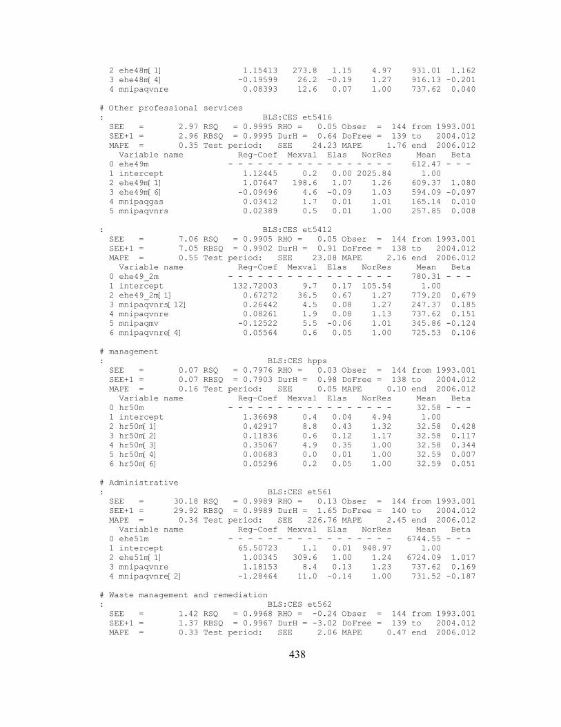
2 ehe48m[1] 1.15413 273.8 1.15 4.97 931.01 1.162 3 ehe48m[4] -0.19599 26.2 -0.19 1.27 916.13 -0.201 4 mnipaqvnre 0.08393 12.6 0.07 1.00 737.62 0.040
# Other professional services: BLS:CES et5416 SEE = 2.97 RSQ = 0.9995 RHO = 0.05 Obser = 144 from 1993.001 SEE+1 = 2.96 RBSQ = 0.9995 DurH = 0.64 DoFree = 139 to 2004.012 MAPE = 0.35 Test period: SEE 24.23 MAPE 1.76 end 2006.012 Variable name Reg-Coef Mexval Elas NorRes Mean Beta 0 ehe49m - - - - - - - - - - - - - - - - - 612.47 - - - 1 intercept 1.12445 0.2 0.00 2025.84 1.00 2 ehe49m[1] 1.07647 198.6 1.07 1.26 609.37 1.080 3 ehe49m[6] -0.09496 4.6 -0.09 1.03 594.09 -0.097 4 mnipaqgas 0.03412 1.7 0.01 1.01 165.14 0.010 5 mnipaqvnrs 0.02389 0.5 0.01 1.00 257.85 0.008
: BLS:CES et5412 SEE = 7.06 RSQ = 0.9905 RHO = 0.05 Obser = 144 from 1993.001 SEE+1 = 7.05 RBSQ = 0.9902 DurH = 0.91 DoFree = 138 to 2004.012 MAPE = 0.55 Test period: SEE 23.08 MAPE 2.16 end 2006.012 Variable name Reg-Coef Mexval Elas NorRes Mean Beta 0 ehe49_2m - - - - - - - - - - - - - - - - - 780.31 - - - 1 intercept 132.72003 9.7 0.17 105.54 1.00 2 ehe49_2m[1] 0.67272 36.5 0.67 1.27 779.20 0.679 3 mnipaqvnrs[12] 0.26442 4.5 0.08 1.27 247.37 0.185 4 mnipaqvnre 0.08261 1.9 0.08 1.13 737.62 0.151 5 mnipaqmv -0.12522 5.5 -0.06 1.01 345.86 -0.124 6 mnipaqvnre[4] 0.05564 0.6 0.05 1.00 725.53 0.106
# management: BLS:CES hpps SEE = 0.07 RSQ = 0.7976 RHO = 0.03 Obser = 144 from 1993.001 SEE+1 = 0.07 RBSQ = 0.7903 DurH = 0.98 DoFree = 138 to 2004.012 MAPE = 0.16 Test period: SEE 0.05 MAPE 0.10 end 2006.012 Variable name Reg-Coef Mexval Elas NorRes Mean Beta 0 hr50m - - - - - - - - - - - - - - - - - 32.58 - - - 1 intercept 1.36698 0.4 0.04 4.94 1.00 2 hr50m[1] 0.42917 8.8 0.43 1.32 32.58 0.428 3 hr50m[2] 0.11836 0.6 0.12 1.17 32.58 0.117 4 hr50m[3] 0.35067 4.9 0.35 1.00 32.58 0.344 5 hr50m[4] 0.00683 0.0 0.01 1.00 32.59 0.007 6 hr50m[6] 0.05296 0.2 0.05 1.00 32.59 0.051
# Administrative : BLS:CES et561 SEE = 30.18 RSQ = 0.9989 RHO = 0.13 Obser = 144 from 1993.001 SEE+1 = 29.92 RBSQ = 0.9989 DurH = 1.65 DoFree = 140 to 2004.012 MAPE = 0.34 Test period: SEE 226.76 MAPE 2.45 end 2006.012 Variable name Reg-Coef Mexval Elas NorRes Mean Beta 0 ehe51m - - - - - - - - - - - - - - - - - 6744.55 - - - 1 intercept 65.50723 1.1 0.01 948.97 1.00 2 ehe51m[1] 1.00345 309.6 1.00 1.24 6724.09 1.017 3 mnipaqvnre 1.18153 8.4 0.13 1.23 737.62 0.169 4 mnipaqvnre[2] -1.28464 11.0 -0.14 1.00 731.52 -0.187
# Waste management and remediation: BLS:CES et562 SEE = 1.42 RSQ = 0.9968 RHO = -0.24 Obser = 144 from 1993.001 SEE+1 = 1.37 RBSQ = 0.9967 DurH = -3.02 DoFree = 139 to 2004.012 MAPE = 0.33 Test period: SEE 2.06 MAPE 0.47 end 2006.012
438

Variable name Reg-Coef Mexval Elas NorRes Mean Beta 0 ehe52m - - - - - - - - - - - - - - - - - 297.05 - - - 1 intercept 8.40465 2.5 0.03 311.66 1.00 2 ehe52m[1] 0.94982 308.5 0.95 1.03 296.40 0.959 3 mnipaqho 0.02414 0.7 0.03 1.01 359.22 0.055 4 mnipaqsoth 0.00697 0.3 0.02 1.01 832.56 0.053 5 mnipaqsoth[12] -0.00942 0.6 -0.02 1.00 781.60 -0.068
: BLS:CES wpps SEE = 0.02 RSQ = 0.9999 RHO = -0.12 Obser = 144 from 1993.001 SEE+1 = 0.02 RBSQ = 0.9998 DurH = -1.48 DoFree = 141 to 2004.012 MAPE = 0.11 Test period: SEE 0.09 MAPE 0.42 end 2006.012 Variable name Reg-Coef Mexval Elas NorRes Mean Beta 0 wag52m - - - - - - - - - - - - - - - - - 12.90 - - - 1 intercept 0.11959 0.9 0.01 6758.85 1.00 2 wag52m[1] 0.98430 584.5 0.98 1.01 12.86 0.983 3 mnipaqsoth 0.00014 0.7 0.01 1.00 832.56 0.017
# Educational services: BLS:CES et61 SEE = 10.00 RSQ = 0.9990 RHO = -0.04 Obser = 144 from 1993.001 SEE+1 = 9.99 RBSQ = 0.9990 DurH = -0.52 DoFree = 141 to 2004.012 MAPE = 0.30 Test period: SEE 12.19 MAPE 0.36 end 2006.012 Variable name Reg-Coef Mexval Elas NorRes Mean Beta 0 ehe53m - - - - - - - - - - - - - - - - - 2287.38 - - - 1 intercept 15.18050 2.1 0.01 976.51 1.00 2 ehe53m[1] 0.99283 1587.7 0.99 1.01 2279.76 0.995 3 mnipaqvnrs 0.03404 0.4 0.00 1.00 257.85 0.005
: BLS:CES hpeh SEE = 0.07 RSQ = 0.8565 RHO = 0.14 Obser = 144 from 1993.001 SEE+1 = 0.07 RBSQ = 0.8524 DurH = 2.26 DoFree = 139 to 2004.012 MAPE = 0.16 Test period: SEE 0.15 MAPE 0.44 end 2006.012 Variable name Reg-Coef Mexval Elas NorRes Mean Beta 0 hr53m - - - - - - - - - - - - - - - - - 32.19 - - - 1 intercept 15.95915 10.3 0.50 4.96 1.00 2 hr53m[1] 0.37029 5.2 0.37 1.41 32.18 0.368 3 hr53m[3] 0.38178 5.1 0.38 1.25 32.18 0.375 4 hr53m[12] -0.26061 4.4 -0.26 1.25 32.15 -0.245 5 mnipaqmv 0.00117 11.6 0.01 1.00 345.86 0.464
: BLS:CES wpeh SEE = 0.03 RSQ = 0.9998 RHO = -0.16 Obser = 144 from 1993.001 SEE+1 = 0.03 RBSQ = 0.9997 DurH = -1.96 DoFree = 142 to 2004.012 MAPE = 0.11 Test period: SEE 0.03 MAPE 0.14 end 2006.012 Variable name Reg-Coef Mexval Elas NorRes Mean Beta 0 wag53m - - - - - - - - - - - - - - - - - 13.44 - - - 1 intercept -0.02005 0.4 -0.00 4014.14 1.00 2 wag53m[1] 1.00426 6235.7 1.00 1.00 13.40 1.000
# Ambulatory health care services: BLS:CES et621 SEE = 4.82 RSQ = 0.9999 RHO = 0.04 Obser = 144 from 1993.001 SEE+1 = 4.81 RBSQ = 0.9999 DurH = 0.71 DoFree = 139 to 2004.012 MAPE = 0.09 Test period: SEE 7.98 MAPE 0.13 end 2006.012 Variable name Reg-Coef Mexval Elas NorRes Mean Beta 0 ehe54m - - - - - - - - - - - - - - - - - 4192.18 - - - 1 intercept 33.95366 4.4 0.01 9051.14 1.00 2 ehe54m[1] 1.09920 95.6 1.10 1.41 4180.03 1.101 3 ehe54m[3] -0.11149 1.5 -0.11 1.15 4155.63 -0.112 4 mnipaqvnre -0.03204 6.2 -0.01 1.07 737.62 -0.009
439
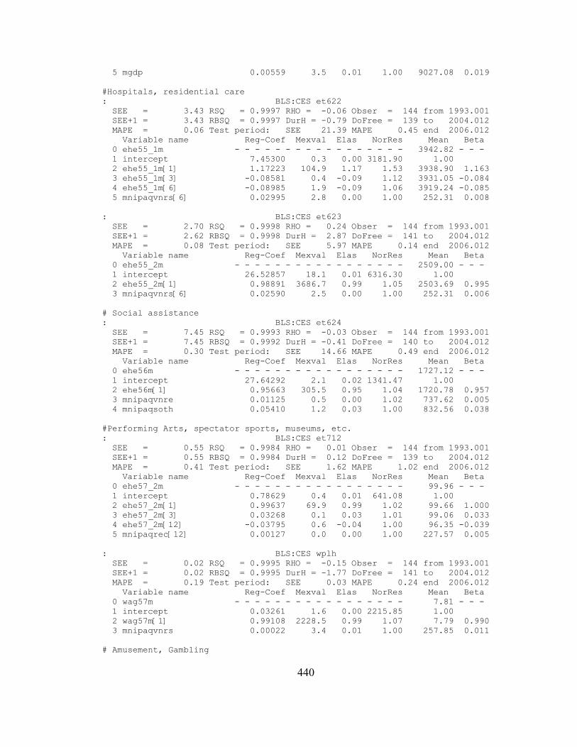
5 mgdp 0.00559 3.5 0.01 1.00 9027.08 0.019
#Hospitals, residential care: BLS:CES et622 SEE = 3.43 RSQ = 0.9997 RHO = -0.06 Obser = 144 from 1993.001 SEE+1 = 3.43 RBSQ = 0.9997 DurH = -0.79 DoFree = 139 to 2004.012 MAPE = 0.06 Test period: SEE 21.39 MAPE 0.45 end 2006.012 Variable name Reg-Coef Mexval Elas NorRes Mean Beta 0 ehe55_1m - - - - - - - - - - - - - - - - - 3942.82 - - - 1 intercept 7.45300 0.3 0.00 3181.90 1.00 2 ehe55_1m[1] 1.17223 104.9 1.17 1.53 3938.90 1.163 3 ehe55_1m[3] -0.08581 0.4 -0.09 1.12 3931.05 -0.084 4 ehe55_1m[6] -0.08985 1.9 -0.09 1.06 3919.24 -0.085 5 mnipaqvnrs[6] 0.02995 2.8 0.00 1.00 252.31 0.008
: BLS:CES et623 SEE = 2.70 RSQ = 0.9998 RHO = 0.24 Obser = 144 from 1993.001 SEE+1 = 2.62 RBSQ = 0.9998 DurH = 2.87 DoFree = 141 to 2004.012 MAPE = 0.08 Test period: SEE 5.97 MAPE 0.14 end 2006.012 Variable name Reg-Coef Mexval Elas NorRes Mean Beta 0 ehe55_2m - - - - - - - - - - - - - - - - - 2509.00 - - - 1 intercept 26.52857 18.1 0.01 6316.30 1.00 2 ehe55_2m[1] 0.98891 3686.7 0.99 1.05 2503.69 0.995 3 mnipaqvnrs[6] 0.02590 2.5 0.00 1.00 252.31 0.006
# Social assistance: BLS:CES et624 SEE = 7.45 RSQ = 0.9993 RHO = -0.03 Obser = 144 from 1993.001 SEE+1 = 7.45 RBSQ = 0.9992 DurH = -0.41 DoFree = 140 to 2004.012 MAPE = 0.30 Test period: SEE 14.66 MAPE 0.49 end 2006.012 Variable name Reg-Coef Mexval Elas NorRes Mean Beta 0 ehe56m - - - - - - - - - - - - - - - - - 1727.12 - - - 1 intercept 27.64292 2.1 0.02 1341.47 1.00 2 ehe56m[1] 0.95663 305.5 0.95 1.04 1720.78 0.957 3 mnipaqvnre 0.01125 0.5 0.00 1.02 737.62 0.005 4 mnipaqsoth 0.05410 1.2 0.03 1.00 832.56 0.038
#Performing Arts, spectator sports, museums, etc.: BLS:CES et712 SEE = 0.55 RSQ = 0.9984 RHO = 0.01 Obser = 144 from 1993.001 SEE+1 = 0.55 RBSQ = 0.9984 DurH = 0.12 DoFree = 139 to 2004.012 MAPE = 0.41 Test period: SEE 1.62 MAPE 1.02 end 2006.012 Variable name Reg-Coef Mexval Elas NorRes Mean Beta 0 ehe57_2m - - - - - - - - - - - - - - - - - 99.96 - - - 1 intercept 0.78629 0.4 0.01 641.08 1.00 2 ehe57_2m[1] 0.99637 69.9 0.99 1.02 99.66 1.000 3 ehe57_2m[3] 0.03268 0.1 0.03 1.01 99.06 0.033 4 ehe57_2m[12] -0.03795 0.6 -0.04 1.00 96.35 -0.039 5 mnipaqrec[12] 0.00127 0.0 0.00 1.00 227.57 0.005
: BLS:CES wplh SEE = 0.02 RSQ = 0.9995 RHO = -0.15 Obser = 144 from 1993.001 SEE+1 = 0.02 RBSQ = 0.9995 DurH = -1.77 DoFree = 141 to 2004.012 MAPE = 0.19 Test period: SEE 0.03 MAPE 0.24 end 2006.012 Variable name Reg-Coef Mexval Elas NorRes Mean Beta 0 wag57m - - - - - - - - - - - - - - - - - 7.81 - - - 1 intercept 0.03261 1.6 0.00 2215.85 1.00 2 wag57m[1] 0.99108 2228.5 0.99 1.07 7.79 0.990 3 mnipaqvnrs 0.00022 3.4 0.01 1.00 257.85 0.011
# Amusement, Gambling
440

: BLS:CES et713 SEE = 7.89 RSQ = 0.9966 RHO = 0.01 Obser = 144 from 1993.001 SEE+1 = 7.89 RBSQ = 0.9966 DurH = 0.11 DoFree = 141 to 2004.012 MAPE = 0.53 Test period: SEE 11.38 MAPE 0.65 end 2006.012 Variable name Reg-Coef Mexval Elas NorRes Mean Beta 0 ehe58m - - - - - - - - - - - - - - - - - 1193.11 - - - 1 intercept 24.84941 1.8 0.02 297.35 1.00 2 ehe58m[1] 0.97584 398.5 0.97 1.00 1189.82 0.986 3 mnipaqrec[12] 0.03161 0.2 0.01 1.00 227.57 0.013
# accommodation: BLS:CES et721 SEE = 7.51 RSQ = 0.9934 RHO = 0.26 Obser = 144 from 1993.001 SEE+1 = 7.25 RBSQ = 0.9931 DurH = 4.21 DoFree = 138 to 2004.012 MAPE = 0.30 Test period: SEE 25.57 MAPE 1.22 end 2006.012 Variable name Reg-Coef Mexval Elas NorRes Mean Beta 0 ehe59m - - - - - - - - - - - - - - - - - 1747.02 - - - 1 intercept 101.20397 0.6 0.06 150.63 1.00 2 ehe59m[1] 1.05935 117.2 1.06 1.08 1745.34 1.072 3 ehe59m[4] -0.13272 2.0 -0.13 1.01 1740.55 -0.139 4 mnipaqrec[12] -0.01251 0.1 -0.00 1.01 227.57 -0.007 5 mnipaqvnrs[12] -0.06008 0.6 -0.01 1.01 247.37 -0.033 6 mnipaqvnre[7] 0.06364 0.5 0.03 1.00 716.85 0.098
: BLS:CES hplh SEE = 0.14 RSQ = 0.5661 RHO = 0.35 Obser = 144 from 1993.001 SEE+1 = 0.13 RBSQ = 0.5537 DurH = 999.00 DoFree = 139 to 2004.012 MAPE = 0.41 Test period: SEE 0.16 MAPE 0.53 end 2006.012 Variable name Reg-Coef Mexval Elas NorRes Mean Beta 0 hr59m - - - - - - - - - - - - - - - - - 25.90 - - - 1 intercept 4.36864 2.5 0.17 2.30 1.00 2 hr59m[2] 0.38330 6.4 0.38 1.16 25.90 0.383 3 hr59m[3] 0.31949 3.7 0.32 1.01 25.90 0.319 4 hr59m[4] 0.04687 0.1 0.05 1.01 25.90 0.047 5 hr59m[6] 0.08162 0.3 0.08 1.00 25.90 0.081
# Food services: BLS:CES et722 SEE = 18.74 RSQ = 0.9990 RHO = -0.22 Obser = 144 from 1993.001 SEE+1 = 18.29 RBSQ = 0.9990 DurH = -2.64 DoFree = 141 to 2004.012 MAPE = 0.17 Test period: SEE 25.64 MAPE 0.22 end 2006.012 Variable name Reg-Coef Mexval Elas NorRes Mean Beta 0 ehe60m - - - - - - - - - - - - - - - - - 7901.43 - - - 1 intercept 172.05646 3.5 0.02 986.97 1.00 2 ehe60m[1] 0.96242 524.6 0.96 1.05 7885.82 0.964 3 mnipaqfood 0.16026 2.6 0.02 1.00 872.92 0.036
: CENSUS: Retail sales of Food services and drinking places SEE = 2568.78 RSQ = 0.9974 RHO = 0.94 Obser = 144 from 1993.001 SEE+1 = 843.95 RBSQ = 0.9974 DW = 0.11 DoFree = 142 to 2004.012 MAPE = 0.72 Test period: SEE 3710.18 MAPE 0.83 end 2005.012 Variable name Reg-Coef Mexval Elas NorRes Mean Beta 0 mrt722 - - - - - - - - - - - - - - - - - 284920.89 - - - 1 intercept -48958.73717 202.5 -0.17 388.69 1.00 2 mnipaqfood 382.48385 1871.5 1.17 1.00 872.92 0.999
# other services: BLS:CES etos SEE = 6.36 RSQ = 0.9997 RHO = 0.20 Obser = 144 from 1993.001 SEE+1 = 6.27 RBSQ = 0.9997 DurH = 2.39 DoFree = 139 to 2004.012 MAPE = 0.10 Test period: SEE 108.93 MAPE 1.55 end 2006.012
441
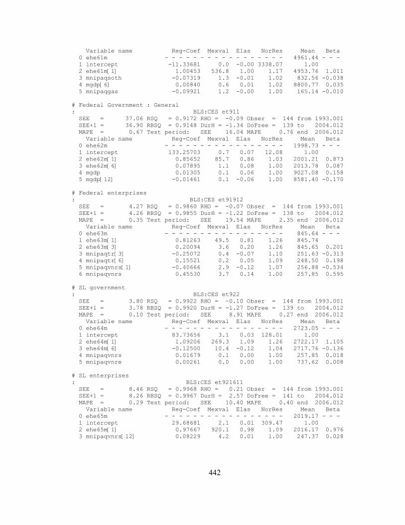
Variable name Reg-Coef Mexval Elas NorRes Mean Beta 0 ehe61m - - - - - - - - - - - - - - - - - 4961.44 - - - 1 intercept -11.33681 0.0 -0.00 3338.07 1.00 2 ehe61m[1] 1.00453 536.8 1.00 1.17 4953.76 1.011 3 mnipaqsoth -0.07319 1.3 -0.01 1.02 832.56 -0.038 4 mgdp[6] 0.00840 0.6 0.01 1.02 8800.77 0.035 5 mnipaqgas -0.09921 1.2 -0.00 1.00 165.14 -0.010
# Federal Government : General: BLS:CES et911 SEE = 37.06 RSQ = 0.9172 RHO = -0.09 Obser = 144 from 1993.001 SEE+1 = 36.90 RBSQ = 0.9148 DurH = -1.34 DoFree = 139 to 2004.012 MAPE = 0.67 Test period: SEE 16.04 MAPE 0.76 end 2006.012 Variable name Reg-Coef Mexval Elas NorRes Mean Beta 0 ehe62m - - - - - - - - - - - - - - - - - 1998.73 - - - 1 intercept 133.25703 0.7 0.07 12.08 1.00 2 ehe62m[1] 0.85652 85.7 0.86 1.03 2001.21 0.873 3 ehe62m[6] 0.07895 1.1 0.08 1.00 2013.78 0.087 4 mgdp 0.01305 0.1 0.06 1.00 9027.08 0.158 5 mgdp[12] -0.01461 0.1 -0.06 1.00 8581.40 -0.170
# Federal enterprises: BLS:CES et91912 SEE = 4.27 RSQ = 0.9860 RHO = -0.07 Obser = 144 from 1993.001 SEE+1 = 4.26 RBSQ = 0.9855 DurH = -1.22 DoFree = 138 to 2004.012 MAPE = 0.35 Test period: SEE 19.54 MAPE 2.35 end 2006.012 Variable name Reg-Coef Mexval Elas NorRes Mean Beta 0 ehe63m - - - - - - - - - - - - - - - - - 845.64 - - - 1 ehe63m[1] 0.81263 49.5 0.81 1.26 845.74 2 ehe63m[3] 0.20094 3.6 0.20 1.26 845.65 0.201 3 mnipaqtr[3] -0.25072 0.4 -0.07 1.10 251.63 -0.313 4 mnipaqtr[6] 0.15521 0.2 0.05 1.09 248.50 0.198 5 mnipaqvnrs[1] -0.40666 2.9 -0.12 1.07 256.88 -0.534 6 mnipaqvnrs 0.45530 3.7 0.14 1.00 257.85 0.595
# SL government: BLS:CES et922 SEE = 3.80 RSQ = 0.9922 RHO = -0.10 Obser = 144 from 1993.001 SEE+1 = 3.78 RBSQ = 0.9920 DurH = -1.27 DoFree = 139 to 2004.012 MAPE = 0.10 Test period: SEE 8.91 MAPE 0.27 end 2006.012 Variable name Reg-Coef Mexval Elas NorRes Mean Beta 0 ehe64m - - - - - - - - - - - - - - - - - 2723.05 - - - 1 intercept 83.73656 3.1 0.03 128.01 1.00 2 ehe64m[1] 1.09206 269.3 1.09 1.26 2722.17 1.105 3 ehe64m[6] -0.12500 10.4 -0.12 1.04 2717.76 -0.136 4 mnipaqvnrs 0.01679 0.1 0.00 1.00 257.85 0.018 5 mnipaqvnre 0.00261 0.0 0.00 1.00 737.62 0.008
# SL enterprises: BLS:CES et921611 SEE = 8.46 RSQ = 0.9968 RHO = 0.21 Obser = 144 from 1993.001 SEE+1 = 8.26 RBSQ = 0.9967 DurH = 2.57 DoFree = 141 to 2004.012 MAPE = 0.29 Test period: SEE 10.40 MAPE 0.40 end 2006.012 Variable name Reg-Coef Mexval Elas NorRes Mean Beta 0 ehe65m - - - - - - - - - - - - - - - - - 2019.17 - - - 1 intercept 29.68681 2.1 0.01 309.47 1.00 2 ehe65m[1] 0.97667 920.1 0.98 1.09 2016.17 0.976 3 mnipaqvnrs[12] 0.08229 4.2 0.01 1.00 247.37 0.028
442
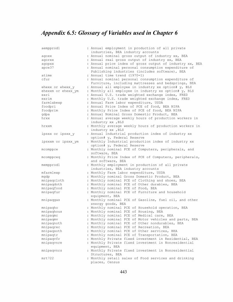
Appendix 6.5: Glossary of Variables used in Chapter 6
aempprod1 : Annual employment in production of all private industries, BEA industry accounts
agoxx : Annual nominal gross output of industry xx, BEAagorxx : Annual real gross output of industry xx, BEAagopxx : Annual price index of gross output of industry xx, BEAapce37 : Annual nominal personal consumption expenditure of
Publishing industries (includes software), BEAatime : Annual time trend (1970=1)cfur : Annual nominal personal consumption expenditure of
Furniture, including mattresses and bedsprings, BEAehexx or ehexx_y : Annual all employee in industry xx option# y, BLSehexxm or ehexx_ym : Monthly all employee in industry xx option# y, BLSexri : Annual U.S. trade weighted exchange index, FREDexrim : Monthly U.S. trade weighted exchange index, FREDfarmlabexp : Annual Farm labor expenditure, USDAfoodpri : Annual Price Index of PCE of food, BEA NIPAfoodprim : Monthly Price Index of PCE of food, BEA NIPAgdpa : Annual Nominal Gross Domestic Product, BEAhrxx : Annual average weekly hours of production workers in
industry xx ,BLShrxxm : Monthly average weekly hours of production workers in
industry xx ,BLSipsxx or ipsxx_y : Annual Industrial production index of industry xx
option# y, Federal Reserveipsxxm or ipsxx_ym : Monthly Industrial production index of industry xx
option# y, Federal Reservemcomppce : Monthly nominal PCE of Computers, peripherals, and
software, BEAmcomppceq : Monthly Price Index of PCE of Computers, peripherals,
and software, BEAmempprod1 : Monthly employment in production of all private
industries, BEA industry accountsmfarmlexp : Monthly Farm labor expenditure, USDAmgdp : Monthly nominal Gross Domestic Product, BEAmnipaqcloth : Monthly nominal PCE of Clothing and shoes, BEAmnipaqdoth : Monthly nominal PCE of Other durables, BEAmnipaqfood : Monthly nominal PCE of Food, BEAmnipaqfur : Monthly nominal PCE of Furniture and household
equipment, BEAmnipaqgas : Monthly nominal PCE of Gasoline, fuel oil, and other
energy goods, BEAmnipaqho : Monthly nominal PCE of Household operation, BEAmnipaqhous : Monthly nominal PCE of Housing, BEAmnipaqmc : Monthly nominal PCE of Medical care, BEAmnipaqmv : Monthly nominal PCE of Motor vehicles and parts, BEAmnipaqnoth : Monthly nominal PCE of Other nondurables, BEAmnipaqrec : Monthly nominal PCE of Recreation, BEAmnipaqsoth : Monthly nominal PCE of Other services, BEAmnipaqtr : Monthly nominal PCE of Transportation, BEAmnipaqvfr : Monthly Private fixed investment in Residential, BEAmnipaqvnre : Monthly Private fixed investment in Nonresidential
equipment, BEAmnipaqvnrs : Monthly Private fixed investment in Nonresidential
Structures, BEAmrt722 : Monthly retail sales of Food services and drinking
places, Census
443

Appendix 6.5 (cont.)
mtime : Monthly time trend (December 1969 = 0)mwh42 : Monthly total wholesale sales, Censusnipa37p : Annual Price Index of PCE of Computers, peripherals,
and software, BEAoilp : Annual Crude Oil Price, FREDoilpm : Monthly Crude oil price, FREDprixx or prixx_y : Annual Producer price index of industry xx option# y,
BLSprixxm or prixx_ym : Annual Producer price index of industry xx option# y,
BLSretl : Annual Retail Sales, Total, Censusretlm : Monthly Retail Sales, Total, Censusrtfood : Annual retail sales of Food services and drinking
places, Censusrtptot : Annual Retail purchase, Total, Censusrtptotm : Monthly Retail purchase, Total, Censuswagxx or wagxx_y : Annual average hourly earnings of production workers in
industry xx option# y, BLSwagxxm or wagxx_ym : Monthly average hourly earnings of production workers
in industry xx option# y, BLSwagnf : Annual average hourly earnings of production workers,
Total Nonfarm, BLSwagnfm : Monthly average hourly earnings of production workers,
Total Nonfarm, BLSwhsl : Annual total wholesale sales, Census
444
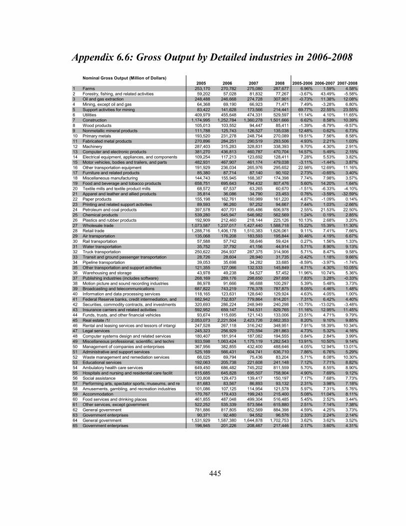
Appendix 6.6: Gross Output by Detailed industries in 2006-2008
445
Nominal Gross Output (Million of Dollars) 2005 2006 2007 2008 2005-2006 2006-2007 2007-2008
1 Farms 253,170 270,782 275,080 287,677 6.96% 1.59% 4.58%2 Forestry, fishing, and related activities 59,202 57,028 81,832 77,267 -3.67% 43.49% -5.58%3 Oil and gas extraction 248,488 246,668 274,728 307,901 -0.73% 11.38% 12.08%4 Mining, except oil and gas 64,368 69,190 66,923 71,471 7.49% -3.28% 6.80%5 Support activities for mining 83,422 141,628 173,566 214,441 69.77% 22.55% 23.55%6 Utilities 409,979 455,648 474,331 529,597 11.14% 4.10% 11.65%7 Construction 1,174,995 1,252,784 1,360,278 1,501,666 6.62% 8.58% 10.39%8 Wood products 105,013 103,552 94,447 85,411 -1.39% -8.79% -9.57%9 Nonmetallic mineral products 111,788 125,743 126,527 135,038 12.48% 0.62% 6.73%10 Primary metals 193,520 231,278 248,754 270,089 19.51% 7.56% 8.58%11 Fabricated metal products 270,896 284,251 290,519 293,506 4.93% 2.21% 1.03%12 Machinery 287,403 315,283 328,831 338,393 9.70% 4.30% 2.91%13 Computer and electronic products 381,270 436,813 460,787 470,704 14.57% 5.49% 2.15%14 Electrical equipment, appliances, and components 109,254 117,213 123,692 128,411 7.28% 5.53% 3.82%15 Motor vehicles, bodies and trailers, and parts 482,931 467,907 461,174 479,038 -3.11% -1.44% 3.87%16 Other transportation equipment 191,929 236,034 265,976 295,652 22.98% 12.69% 11.16%17 Furniture and related products 85,380 87,714 87,140 90,102 2.73% -0.65% 3.40%18 Miscellaneous manufacturing 144,743 155,945 168,387 174,398 7.74% 7.98% 3.57%19 Food and beverage and tobacco products 658,751 695,643 794,432 807,476 5.60% 14.20% 1.64%20 Textile mills and textile product mills 68,572 67,537 63,265 60,670 -1.51% -6.33% -4.10%21 Apparel and leather and allied products 35,814 36,086 34,790 23,453 0.76% -3.59% -32.59%22 Paper products 155,198 162,761 160,989 161,220 4.87% -1.09% 0.14%23 Printing and related support activities 89,593 96,260 97,252 94,667 7.44% 1.03% -2.66%24 Petroleum and coal products 397,578 407,701 495,486 606,978 2.55% 21.53% 22.50%25 Chemical products 539,280 545,947 546,982 562,569 1.24% 0.19% 2.85%26 Plastics and rubber products 192,909 212,460 218,144 225,126 10.13% 2.68% 3.20%27 Wholesale trade 1,073,587 1,237,017 1,427,440 1,588,718 15.22% 15.39% 11.30%28 Retail trade 1,288,716 1,406,178 1,510,383 1,626,061 9.11% 7.41% 7.66%29 Air transportation 135,068 176,208 183,593 195,844 30.46% 4.19% 6.67%30 Rail transportation 57,588 57,742 58,646 59,424 0.27% 1.56% 1.33%31 Water transportation 35,752 37,792 41,156 44,914 5.71% 8.90% 9.13%32 Truck transportation 250,622 264,937 287,375 314,906 5.71% 8.47% 9.58%33 Transit and ground passenger transportation 28,726 28,604 28,940 31,735 -0.42% 1.18% 9.66%34 Pipeline transportation 39,053 35,698 34,282 33,685 -8.59% -3.97% -1.74%35 Other transportation and support activities 121,355 127,066 132,533 145,849 4.71% 4.30% 10.05%36 Warehousing and storage 43,978 49,238 54,527 57,452 11.96% 10.74% 5.36%37 Publishing industries (includes software) 268,169 289,176 298,650 297,658 7.83% 3.28% -0.33%38 Motion picture and sound recording industries 86,978 91,666 96,688 100,297 5.39% 5.48% 3.73%39 Broadcasting and telecommunications 687,822 743,219 776,378 787,875 8.05% 4.46% 1.48%40 Information and data processing services 118,165 123,631 128,640 129,924 4.63% 4.05% 1.00%41 Federal Reserve banks, credit intermediation, and 682,942 732,837 779,864 814,201 7.31% 6.42% 4.40%42 Securities, commodity contracts, and investments 320,693 286,224 248,949 240,298 -10.75% -13.02% -3.48%43 Insurance carriers and related activities 592,952 659,147 744,531 829,765 11.16% 12.95% 11.45%44 Funds, trusts, and other financial vehicles 93,674 115,695 121,143 133,006 23.51% 4.71% 9.79%45 Real estate /1/ 2,053,073 2,221,504 2,423,726 2,662,353 8.20% 9.10% 9.85%46 Rental and leasing services and lessors of intangi 247,528 267,118 316,242 348,951 7.91% 18.39% 10.34%47 Legal services 245,323 256,929 270,594 281,863 4.73% 5.32% 4.16%48 Computer systems design and related services 180,407 181,914 187,082 194,555 0.84% 2.84% 3.99%49 Miscellaneous professional, scientific, and techni 933,598 1,063,424 1,175,119 1,282,543 13.91% 10.50% 9.14%50 Management of companies and enterprises 367,956 382,855 432,400 488,646 4.05% 12.94% 13.01%51 Administrative and support services 525,169 566,431 604,741 636,710 7.86% 6.76% 5.29%52 Waste management and remediation services 66,025 69,794 75,436 83,204 5.71% 8.08% 10.30%53 Educational services 192,063 205,738 221,608 241,148 7.12% 7.71% 8.82%54 Ambulatory health care services 649,450 686,482 745,202 811,559 5.70% 8.55% 8.90%55 Hospitals and nursing and residential care facilit 615,685 645,828 695,507 758,904 4.90% 7.69% 9.12%56 Social assistance 120,808 129,473 139,417 150,197 7.17% 7.68% 7.73%57 Performing arts, spectator sports, museums, and re 81,683 83,567 86,893 93,132 2.31% 3.98% 7.18%58 Amusements, gambling, and recreation industries 101,086 107,125 114,954 121,578 5.97% 7.31% 5.76%59 Accommodation 170,767 179,433 199,243 215,400 5.08% 11.04% 8.11%60 Food services and drinking places 461,855 487,048 499,304 516,485 5.45% 2.52% 3.44%61 Other services, except government 522,252 535,339 573,564 615,880 2.51% 7.14% 7.38%62 General government 781,886 817,805 852,569 884,398 4.59% 4.25% 3.73%63 Government enterprises 90,371 92,480 94,552 96,576 2.33% 2.24% 2.14%64 General government 1,531,929 1,587,380 1,644,878 1,702,753 3.62% 3.62% 3.52%65 Government enterprises 196,945 201,226 208,467 217,446 2.17% 3.60% 4.31%

Appendix 6.6 (cont.)
446
Real 2000 Gross Output (Million of Dollars) 2005 2006 2007 2008 2005-2006 2006-2007 2007-2008
1 Farms 215,052 220,011 221,079 229,290 2.31% 0.49% 3.71%2 Forestry, fishing, and related activities 57,272 55,985 57,721 53,567 -2.25% 3.10% -7.20%3 Oil and gas extraction 127,206 130,655 132,380 129,324 2.71% 1.32% -2.31%4 Mining, except oil and gas 48,610 48,782 46,090 47,424 0.35% -5.52% 2.89%5 Support activities for mining 38,803 50,879 56,842 62,990 31.12% 11.72% 10.81%6 Utilities 308,632 326,804 325,695 336,083 5.89% -0.34% 3.19%7 Construction 935,694 974,130 973,468 981,431 4.11% -0.07% 0.82%8 Wood products 92,357 91,336 84,267 79,865 -1.11% -7.74% -5.22%9 Nonmetallic mineral products 98,513 103,171 101,423 107,480 4.73% -1.69% 5.97%10 Primary metals 147,582 153,104 151,179 153,675 3.74% -1.26% 1.65%11 Fabricated metal products 235,857 237,165 231,001 223,859 0.55% -2.60% -3.09%12 Machinery 264,962 280,041 281,194 278,562 5.69% 0.41% -0.94%13 Computer and electronic products 525,050 637,953 708,315 734,782 21.50% 11.03% 3.74%14 Electrical equipment, appliances, and components 101,601 106,874 110,016 111,759 5.19% 2.94% 1.58%15 Motor vehicles, bodies and trailers, and parts 485,024 481,758 477,700 497,025 -0.67% -0.84% 4.05%16 Other transportation equipment 168,100 200,456 221,457 240,605 19.25% 10.48% 8.65%17 Furniture and related products 78,323 77,912 75,719 77,054 -0.52% -2.82% 1.76%18 Miscellaneous manufacturing 134,385 142,423 150,096 152,931 5.98% 5.39% 1.89%19 Food and beverage and tobacco products 563,183 593,495 619,657 620,626 5.38% 4.41% 0.16%20 Textile mills and textile product mills 66,151 64,574 59,177 55,555 -2.38% -8.36% -6.12%21 Apparel and leather and allied products 35,572 35,522 33,871 22,755 -0.14% -4.65% -32.82%22 Paper products 146,427 147,552 143,998 141,672 0.77% -2.41% -1.62%23 Printing and related support activities 85,531 90,120 90,432 87,189 5.37% 0.35% -3.59%24 Petroleum and coal products 224,720 196,702 223,667 262,016 -12.47% 13.71% 17.15%25 Chemical products 438,657 426,927 416,269 408,578 -2.67% -2.50% -1.85%26 Plastics and rubber products 170,619 177,371 181,109 182,881 3.96% 2.11% 0.98%27 Wholesale trade 972,399 1,085,999 1,182,849 1,284,355 11.68% 8.92% 8.58%28 Retail trade 1,225,873 1,314,233 1,388,841 1,460,585 7.21% 5.68% 5.17%29 Air transportation 147,957 169,019 179,681 189,415 14.23% 6.31% 5.42%30 Rail transportation 47,794 44,188 43,952 42,771 -7.54% -0.53% -2.69%31 Water transportation 29,347 31,028 34,222 36,965 5.73% 10.29% 8.01%32 Truck transportation 214,465 214,541 225,916 234,689 0.04% 5.30% 3.88%33 Transit and ground passenger transportation 24,424 23,603 22,656 23,480 -3.36% -4.01% 3.64%34 Pipeline transportation 32,080 28,429 25,117 22,322 -11.38% -11.65% -11.13%35 Other transportation and support activities 100,113 102,879 104,476 107,498 2.76% 1.55% 2.89%36 Warehousing and storage 40,833 43,681 46,002 48,221 6.97% 5.31% 4.82%37 Publishing industries (includes software) 268,429 287,733 297,254 297,002 7.19% 3.31% -0.08%38 Motion picture and sound recording industries 78,072 77,536 78,774 78,536 -0.69% 1.60% -0.30%39 Broadcasting and telecommunications 723,188 806,274 866,162 900,777 11.49% 7.43% 4.00%40 Information and data processing services 116,550 117,465 120,739 121,454 0.79% 2.79% 0.59%41 Federal Reserve banks, credit intermediation, and 593,519 620,387 635,042 647,377 4.53% 2.36% 1.94%42 Securities, commodity contracts, and investments 364,161 354,161 362,861 381,029 -2.75% 2.46% 5.01%43 Insurance carriers and related activities 494,138 534,059 587,780 636,674 8.08% 10.06% 8.32%44 Funds, trusts, and other financial vehicles 94,909 112,711 119,476 128,793 18.76% 6.00% 7.80%45 Real estate /1/ 1,782,986 1,862,015 1,964,428 2,090,476 4.43% 5.50% 6.42%46 Rental and leasing services and lessors of intangi 224,722 238,085 268,937 281,179 5.95% 12.96% 4.55%47 Legal services 199,537 200,341 201,929 202,778 0.40% 0.79% 0.42%48 Computer systems design and related services 186,670 193,150 200,992 211,391 3.47% 4.06% 5.17%49 Miscellaneous professional, scientific, and techni 876,800 947,711 1,018,006 1,096,161 8.09% 7.42% 7.68%50 Management of companies and enterprises 327,183 325,385 351,451 383,579 -0.55% 8.01% 9.14%51 Administrative and support services 459,005 471,529 477,045 477,790 2.73% 1.17% 0.16%52 Waste management and remediation services 54,153 55,445 56,495 58,421 2.39% 1.89% 3.41%53 Educational services 154,539 158,954 163,190 168,347 2.86% 2.67% 3.16%54 Ambulatory health care services 579,629 603,263 643,008 687,723 4.08% 6.59% 6.95%55 Hospitals and nursing and residential care facilit 504,922 515,545 535,316 565,149 2.10% 3.83% 5.57%56 Social assistance 110,909 114,683 119,687 124,740 3.40% 4.36% 4.22%57 Performing arts, spectator sports, museums, and re 68,246 66,039 63,086 62,356 -3.23% -4.47% -1.16%58 Amusements, gambling, and recreation industries 88,618 91,817 94,135 96,540 3.61% 2.52% 2.56%59 Accommodation 149,578 154,329 165,531 172,512 3.18% 7.26% 4.22%60 Food services and drinking places 401,774 426,737 447,293 462,650 6.21% 4.82% 3.43%61 Other services, except government 444,704 439,733 455,239 473,153 -1.12% 3.53% 3.94%62 General government 631,773 637,044 618,422 594,289 0.83% -2.92% -3.90%63 Government enterprises 78,843 78,205 76,937 75,554 -0.81% -1.62% -1.80%64 General government 1,252,665 1,251,825 1,210,575 1,163,748 -0.07% -3.30% -3.87%65 Government enterprises 161,670 164,568 166,466 169,144 1.79% 1.15% 1.61%

Appendix 6.6 (cont.)
447
Price Index (2000=100) 2005 2006 2007 2008 2005-2006 2006-2007 2007-2008
1 Farms 117.72 123.08 124.43 125.46 4.55% 1.10% 0.83%2 Forestry, fishing, and related activities 103.37 101.86 141.77 144.25 -1.46% 39.18% 1.75%3 Oil and gas extraction 195.34 188.79 207.53 238.09 -3.35% 9.92% 14.72%4 Mining, except oil and gas 132.42 141.83 145.20 150.71 7.11% 2.37% 3.79%5 Support activities for mining 214.99 278.36 305.35 340.44 29.48% 9.69% 11.49%6 Utilities 132.84 139.43 145.64 157.58 4.96% 4.45% 8.20%7 Construction 125.57 128.61 139.74 153.01 2.41% 8.65% 9.50%8 Wood products 113.70 113.37 112.08 106.94 -0.29% -1.14% -4.58%9 Nonmetallic mineral products 113.47 121.88 124.75 125.64 7.41% 2.36% 0.71%10 Primary metals 131.13 151.06 164.54 175.75 15.20% 8.93% 6.81%11 Fabricated metal products 114.86 119.85 125.77 131.11 4.35% 4.93% 4.25%12 Machinery 108.47 112.58 116.94 121.48 3.79% 3.87% 3.88%13 Computer and electronic products 72.62 68.47 65.05 64.06 -5.71% -4.99% -1.53%14 Electrical equipment, appliances, and components 107.53 109.67 112.43 114.90 1.99% 2.51% 2.20%15 Motor vehicles, bodies and trailers, and parts 99.57 97.12 96.54 96.38 -2.45% -0.60% -0.17%16 Other transportation equipment 114.18 117.75 120.10 122.88 3.13% 2.00% 2.31%17 Furniture and related products 109.01 112.58 115.08 116.93 3.28% 2.22% 1.61%18 Miscellaneous manufacturing 107.71 109.50 112.19 114.04 1.66% 2.46% 1.65%19 Food and beverage and tobacco products 116.97 117.21 128.21 130.11 0.21% 9.38% 1.48%20 Textile mills and textile product mills 103.66 104.59 106.91 109.21 0.90% 2.22% 2.15%21 Apparel and leather and allied products 100.68 101.59 102.72 103.07 0.90% 1.11% 0.34%22 Paper products 105.99 110.31 111.80 113.80 4.07% 1.35% 1.79%23 Printing and related support activities 104.75 106.81 107.54 108.58 1.97% 0.68% 0.96%24 Petroleum and coal products 176.92 207.27 221.53 231.66 17.15% 6.88% 4.57%25 Chemical products 122.94 127.88 131.40 137.69 4.02% 2.76% 4.79%26 Plastics and rubber products 113.06 119.78 120.45 123.10 5.94% 0.56% 2.20%27 Wholesale trade 110.41 113.91 120.68 123.70 3.17% 5.95% 2.50%28 Retail trade 105.13 107.00 108.75 111.33 1.78% 1.64% 2.37%29 Air transportation 91.29 104.25 102.18 103.39 14.20% -1.99% 1.19%30 Rail transportation 120.49 130.67 133.43 138.94 8.45% 2.11% 4.13%31 Water transportation 121.82 121.80 120.26 121.50 -0.02% -1.26% 1.03%32 Truck transportation 116.86 123.49 127.20 134.18 5.67% 3.01% 5.48%33 Transit and ground passenger transportation 117.61 121.19 127.74 135.16 3.04% 5.40% 5.81%34 Pipeline transportation 121.74 125.57 136.48 150.90 3.15% 8.70% 10.56%35 Other transportation and support activities 121.22 123.51 126.86 135.68 1.89% 2.71% 6.95%36 Warehousing and storage 107.70 112.72 118.53 119.14 4.66% 5.15% 0.52%37 Publishing industries (includes software) 99.90 100.50 100.47 100.22 0.60% -0.03% -0.25%38 Motion picture and sound recording industries 111.41 118.22 122.74 127.71 6.12% 3.82% 4.05%39 Broadcasting and telecommunications 95.11 92.18 89.63 87.47 -3.08% -2.76% -2.42%40 Information and data processing services 101.39 105.25 106.54 106.97 3.81% 1.23% 0.40%41 Federal Reserve banks, credit intermediation, and 115.07 118.13 122.81 125.77 2.66% 3.96% 2.41%42 Securities, commodity contracts, and investments 88.06 80.82 68.61 63.07 -8.23% -15.11% -8.08%43 Insurance carriers and related activities 120.00 123.42 126.67 130.33 2.85% 2.63% 2.89%44 Funds, trusts, and other financial vehicles 98.70 102.65 101.40 103.27 4.00% -1.22% 1.85%45 Real estate /1/ 115.15 119.31 123.38 127.36 3.61% 3.41% 3.22%46 Rental and leasing services and lessors of intangi 110.15 112.19 117.59 124.10 1.86% 4.81% 5.54%47 Legal services 122.95 128.25 134.00 139.00 4.31% 4.49% 3.73%48 Computer systems design and related services 96.64 94.18 93.08 92.04 -2.55% -1.17% -1.12%49 Miscellaneous professional, scientific, and techni 106.48 112.21 115.43 117.00 5.38% 2.87% 1.36%50 Management of companies and enterprises 112.46 117.66 123.03 127.39 4.62% 4.56% 3.54%51 Administrative and support services 114.41 120.13 126.77 133.26 4.99% 5.53% 5.12%52 Waste management and remediation services 121.92 125.88 133.53 142.42 3.25% 6.08% 6.66%53 Educational services 124.28 129.43 135.80 143.24 4.14% 4.92% 5.48%54 Ambulatory health care services 112.05 113.79 115.89 118.01 1.56% 1.84% 1.82%55 Hospitals and nursing and residential care facilit 121.94 125.27 129.92 134.28 2.73% 3.71% 3.36%56 Social assistance 108.93 112.90 116.48 120.41 3.65% 3.18% 3.37%57 Performing arts, spectator sports, museums, and re 119.69 126.54 137.74 149.36 5.72% 8.85% 8.43%58 Amusements, gambling, and recreation industries 114.07 116.67 122.12 125.94 2.28% 4.67% 3.13%59 Accommodation 114.17 116.27 120.37 124.86 1.84% 3.53% 3.73%60 Food services and drinking places 114.95 114.13 111.63 111.64 -0.71% -2.19% 0.01%61 Other services, except government 117.44 121.74 125.99 130.17 3.66% 3.49% 3.31%62 General government 123.76 128.38 137.86 148.82 3.73% 7.39% 7.95%63 Government enterprises 114.62 118.25 122.90 127.82 3.17% 3.93% 4.01%64 General government 122.29 126.81 135.88 146.32 3.69% 7.15% 7.68%65 Government enterprises 121.82 122.28 125.23 128.56 0.37% 2.42% 2.66%

Bibliography
Clopper Almon, “Thoughts on Input-Output Models in National Accounting Systems
with “Superlative” and Chain-Weighted Indexes”, personal notes, March 2005
H. N. Barnum and Lyn squire, “Predicting Agricultural Output Response”, Oxford
Economic Papers, New Series, Vol. 32, No. 2 (July 1980), 284-295
V.R. Berlinguette, “Measurement of Real Output”, The Canadian Journal of Economics
and Political Science/Revue canadienne d’Economique et de Science politique,
Vol. 20, No. 1 (February 1954) 59-75Bureau of Economic Analysis, “A guide to
the National Income and Product Accounts of the United States”
Bureau of Economic Analysis, “An Introduction to National Economic Accounting,
Methodology Papers: U.S. National Income and Product Accounts”, March 1985
Bureau of Economic analysis, “Personal Consumption Expenditures, Methodology
Papers: U.S. National Income and Product Accounts”,June 1990
Bureau of Economic Analysis, “Updated Summary of NIPA Methodologies”, Survey of
Current Business, November 2006, page 10-27
Leo Breiman, “Bagging Predictors”, Machine Learning, 36, 105-139, 1996.
John Y. Campbell and N. Gregory Mankiw, “Are Output Fluctuations Transitory?”, The
Quarterly Journal of Economic, Vol. 102, No. 4 (November 1987), 857-880
448

Lawrence J. Christiano, “P*: Not the Inflation Forecaster's Holy Grail”, Federal Reserve
Bank of Minneapolis Quarterly Review 13 (1989), 3-18.
Rosanne Cole, Y.C. Chen, Joan A. Barquin-Stolleman, Ellen Dulberger, Nurhan
Helvacian, and James H. Hodge, “Quality-Adjusted Price Indexes for Computer
Processors and Selected Peripheral Equipment”, Survey of Current Business,
January 1986, pp 41-50.
Rosanne Cole, “Data Errors and Forecasting Accuracy”, Chapter 2 in Jacob Mincer (ed.),
Economic Forecasts and Expectations: Analysis of Forecasting Behavior and
Performance, National Bureau of Economic Research, 1969.
Carol A. Corrado and Mark N. Greene, “Reducing uncertainty in Short-Term Projections:
Linkage of monthly and quarterly models”, Journal of Forecasting 7 (1988).
Carol A. Corrado and Jane Haltmaier, “The Use of High-Frequency Data in Model Based
Forecasting at the Federal Reserve Board”, Finance and Economics Discussion
Series 24 (1988), Division of Research and Statistics, Board of Governors of the
Federal Reserve System.
Carol A. Corrado and Reifschneider, “A Monthly Forecasting Model of the United States
Economy”, Board of Governors of the Federal Reserve System (1986).
Dean Croushore and Tom Stark, “A Real-Time Data Set for Macroeconomists”, Journal
of Econometrics 105 (2001), 111-130.
449

Dean Croushore, “Forecasting with Real-Time Macroeconomic Data”, University of
Richmond, June 2005.
Francis X. Diebold and Glenn D. Rudebusch, “Forecasting Output with the Composite
Leading Index: A Real Time Analysis”, Journal of the American Statistical
Association (1991), 603-610.
W.E. Diewert, “Exact and Superlative Index Numbers”, Journal of Econometrics 4(2),
1976, pp. 115–145.
W.E. Diewert, “Superlative Index Numbers and Consistency in Aggregation”,
Econometrica 46(4), 1978, pp 883-900.
Eugene F. Fama, “Inflation, Output, and Money”, The Journal of Business, Vol. 55, No.
2. (April 1982), 201-231
John F. Foschen and Herschel I. Grossman, “Tests of Equilibrium Macroeconomics
Using Contemporaneous Monetary Data”’ Journal of Monetary Economics 10
(1982), 309-333.
Scott Freeman and Finn E. Kydland, “Monetary Aggregates and Output”, The American
Economic Review, Vol. 90, No. 5. (December 2000), 1125-1135
Norman Frumkin, “Tracking America’s Economy”, Second Edition, M.E. Sharpe, Inc.,
1992
450
Jeffrey C. Fuhrer and Jane Haltmaier, “Minimum Variance Pooling of Forecasts at
Different Levels of Aggregation”, Journal of Forecasting 7 (1988).
Robert E. Hall and Charles I. Jones, “Why Do Some Countries Produce So Much More
Output Per Worker Than Others?”, The Quarterly Journal of Economic, Vol. 114,
No. 1 (February 1999), 83-116
Thomas F. Howells III and Kevin B. Barefoot, “Annual Industry Accounts: Advance
Estimate for 2006”, Survey of Current Business, BEA, May 2007, 12-25
Thomas F. Howells III, Kevin B. Barefoot, and Brian M. Lindberg, “Annual Industry
Accounts: Revised Estimates for 2003-2005”, Survey of Current Business, BEA,
December 2006, 45-55
Philip E. Howrey, Saul H. Hymans, and Michael R. Donihue, “Merging Monthly and
Quarterly Forecasts: Experience with MQEM”, Journal of Forecasting 10 (1991).
Atsushi Inoue and Lutz Kilian, “Bagging Time Series Models”, Preliminary paper, 2003
Timotej Jagric, “Forecasting with Leading Economic Indicators---A Neural Network
Approach”, Business Economics, October 2003.
Konstantin A. Kholodilin and Wenxiong Vincent Yao, “Business Cycle Turning Points:
Mixed-Frequency Data with Structural Breaks”, IRES, September 2004.
John Kitchen and Ralph Monaco, “Real-Time Forecasting in Practice”, Business
Economics, October 2003.
451

Kevin L. Kliesen, “How Well Does Employment Predict Output?”, Federal Reserve
Bank of St. Louis Review, (2007),Volume 89, Number 5, 433-446
J. Steven Landefeld and Bruce T. Grimm, “A Note on the Impact of Hedonics and
Computers on Real GDP”, Survey of Current Business, December 2000, pp 17-22.
Robert B. Litterman, “Above-Average National Growth in 1985 and 1986”, Federal
Reserve Bank of Minneapolis Quarterly Review 8 (1984), 3-7.
Roberto S. Mariano and Hisashi Tanizaki, “Prediction of Final Data with Use of
Preliminary and/or Revised Data”, Journal of Forecasting (1994).
Roberto Mariano and Yasutomo Murasawa, “A New Coincident Index of Business Cycles
based on Monthly and Quarterly data”, Journal of Applied Econometrics, 18,
427-443, 2003.
Margaret M. McConnell and Gabriel Perez-Quiros, “Output Fluctuations in the United
States: What Has Changed Since the Early 1980’s?”, The American Economic
Review, Vol. 90, No.5. (December 2000), 1464-1476
Douglas S. Meade, “Why Real Value Added Is Not My Favorite Concept”, Working
paper, 2006
Preston J. Miller and Daniel M. Chin, “Using Monthly Data to Improve Quarterly Model
Forecasts”, Federal Reserve Bank of Minneapolis Quarterly Review (1996).
452

Larry R. Moran and Clinton P. McCully, “Trends in Consumer Spending 1959-2000”,
Survey of Current Business, March 2001, page 15-21
Marc Nerlove, “Hedonic price functions and the measurement of preferences: The case of
Swedish wine consumers”, European Economic Review (39), 1995, pp
1697-1716.
K. D. Patterson, “An Integrated Model of the Data Measurement and Data Generation
Process with an Application to Consumers' Expenditure”, The Economic Journal,
Volume 105, Issue 428, 1995, 54-76.
George L. Perry, Michael L. Wachter, Otto Eckstein, and Peter K. Clark, “Potential
Output and Productivity”, Brookings Papers on Economic Activity, Vol. 1997, No.
1. (1977), 11-60
Peter Rathjens and Russell P. Robins, “Forecasting Quarterly Data Using Monthly
Information”, Journal of Forecasting 12 (1993).
T.W. Schultz, “Output-Input Relationships Revisited”, Journal of Farm Economic, Vol.
40, No. 4 (November 1958), 924-932
Eugene P. Seskin and Daniel Larkins, “Improved Estimates of the National Income and
Product Accounts for 1929-2002”, Survey of Current Business, February 2004,
page 7-29
453
George M. Smith, Mathew J. Gruenberg, Tameka R.L. Harris, and Erich H. Strassner,
“Annual Industry Accounts: Revised Estimates for 2001-2003”, Survey of Current
Business, BEA, January 2005, 9-43
James H. Stock and Mark W. Watson, “Forecasting Output and Inflation: the Role of
Asset Prices”, Journal of Economic Literature, Vol. 41, NO. 3 (September 2003),
788-829
Norman R. Swanson and Halbert White, “A Model Selection Approach to Assessing the
Information in the terms Structure Using Linear Models and Artificial Neural
Networks”, Journal of Business and Economic Statistics 13 (1995), 265-275.
Jack E. Triplett, “The Economic Interpretation of Hedonic Methods”, Survey of Current
Business, January 1986, pp 36-40.
Ugo Trivellato and Enrico Rettore, “Preliminary Data Errors and Their Impact on the
Forecast Error of Simultaneous-Equations Models”, Journal of Business and
Economic Statistics 4 (1986), 445-453.
Robert E. Yuskavage and Yvon H. Pho, “Gross Domestic Product by Industry for
1987-2000: New Estimate on the North American Industry Classification
System”, Survey of Current Business, BEA, November 2004, 33-53
Robert E. Yuskavage and Mahnaz Fahim-Nader, “Gross Domestic Product by Industry
for 1947-86: New Estimates Based on the North American Industry Classification
System”, Survey of Current Business, BEA, December 2005, 70-84
454
Peter Zadrozny, “Estimating a Multivariate ARMA Model with Mixed Frequency Data:
an Application to Forecasting U.S. GNP at Monthly Intervals”, Center for
Economic Studies Discussion Paper 90-5 (1990), Bureau of Census, U.S.
Department of Commerce.
455
Related Documents