ABSTRACT Title of Dissertation / Thesis: FAILURE PREDICTION OF WIRE BONDS DUE TO FLEXURE Karumbu Nathan Meyyappan, Ph.D., 2004 Dissertation / Thesis Directed By: Associate Professor Patrick McCluskey, Department of Mechanical Engineering Solid state power modules are subjected to harsh environmental and operational loads. Identifying the potential design weakness and dominant failure mechanisms associated with the application is very critical to designing such power modules. Failure of the wedge-bonded wires is one of the most commonly identified causes of failures in power modules. This can occur when wires flex in response to a thermal cycling load. Since the heel of the wire is already weakened due to the ultrasonic bonding process, the flexing motion is enough to initiate a crack in the heel of the wire. Owing to the prevalence of this failure mechanism in power modules, a generalized first-order physics- of-failure based model has been developed to quantify these flexural/bending stresses. A variational calculus approach has been employed to determine the minimum energy wire profiles. The difference in curvatures corresponding to the wire profiles before and after thermal cycling provide the flexural stresses. The stresses/strains determined from the load transformation model are then used in a damage model to determine the cycles to failure. The model has been validated against temperature cycling test results. The effects

Welcome message from author
This document is posted to help you gain knowledge. Please leave a comment to let me know what you think about it! Share it to your friends and learn new things together.
Transcript
ABSTRACT Title of Dissertation / Thesis: FAILURE PREDICTION OF WIRE BONDS
DUE TO FLEXURE Karumbu Nathan Meyyappan, Ph.D., 2004 Dissertation / Thesis Directed By: Associate Professor Patrick McCluskey,
Department of Mechanical Engineering
Solid state power modules are subjected to harsh environmental and operational
loads. Identifying the potential design weakness and dominant failure mechanisms
associated with the application is very critical to designing such power modules. Failure
of the wedge-bonded wires is one of the most commonly identified causes of failures in
power modules. This can occur when wires flex in response to a thermal cycling load.
Since the heel of the wire is already weakened due to the ultrasonic bonding process, the
flexing motion is enough to initiate a crack in the heel of the wire. Owing to the
prevalence of this failure mechanism in power modules, a generalized first-order physics-
of-failure based model has been developed to quantify these flexural/bending stresses. A
variational calculus approach has been employed to determine the minimum energy wire
profiles. The difference in curvatures corresponding to the wire profiles before and after
thermal cycling provide the flexural stresses. The stresses/strains determined from the
load transformation model are then used in a damage model to determine the cycles to
failure. The model has been validated against temperature cycling test results. The effects
of residual stresses, that are introduced during the loop formation, (on the thermal cycling
life) of these wires also has been studied.
It is believed that the ultrasonic wirebonding process renders the wires weaker at
the heel. Efforts have been made to simulate the wirebonding mechanism using Finite
element analysis. The key parameters that influence the wirebonding process are
identified. Flexural stresses are determined for various heel cross-sectional profiles that
correspond to different bond forces.
Additional design constraints may prevent some of the wedge-bonded wires from
being aligned parallel to the bond pads. The influence of having the bond pads with a
non-zero width offset has been studied through finite element simulations. The 3D
minimum energy wire profiles used in the modeling has been obtained through a new
energy minimization based model.
FAILURE PREDICTION OF WIRE BONDS DUE TO FLEXURE
By
Karumbu Nathan Meyyappan
Thesis or Dissertation submitted to the Faculty of the Graduate School of the University of Maryland, College Park, in partial fulfillment
of the requirements for the degree of Doctor of Philosophy
2004 Advisory Committee: Associate Professor Patrick McCluskey, Chair Prof. Michael Pecht Prof. Sung Lee Associate Professor Bongtae Han Assistant Professor Donald Robbins

© Copyright by Karumbu Nathan Meyyappan
2004

Dedication
To my
Wife and my Parents
ii
Acknowledgements
First and foremost I would like to thank my advisor, mentor and well wisher, Dr.
Patrick McCluskey. Without his able support, advice and encouragement this research
might have not materialized. I deeply appreciate his efforts to take time off his busy
schedule to set me on the right path. I am also deeply indebted to Dr. Don Robbins for his
invaluable suggestions and guidance. I would also like to thank my other committee
members, Dr. Bongtae Han, Prof. Sung Lee and Prof. Michael Pecht for evaluating my
work and also providing invaluable suggestions. In addition, I would also like to thank
Prof. Abhijit Dasgupta for some of the lively discussions and the invaluable suggestions
in refining the work.
I would also like to thank the over 30 members of the CALCE Electronic
Products and Systems Consortium for their support of this research and particularly
Grundfos Management A/S for its technical and financial leadership. Special thanks to
Peter Hansen at Grundfos A/S for providing continuous feedback and suggestions in this
research. I would also like to express my gratitude to Mr. Zeke Topolosky and Mr.
Witaly Zeiler for their assistance with some of the validation testing.
Special thanks to all my friends and colleagues, Manikandan Ramasamy,
Ragunath Sankaranarayanan, Kaushik Ghosh, Seungmin Cho, Ron DiSabatino, Yunqi
Zheng, Vidyasagar Shetty, Sudhir Kumar, Shirish Gupta, Anshul Shrivastava, Casey
O’Connor, Arvind Chandrasekharan, Keith Rogers, Sanjay Tikku etc. etc. for all their
help and support during my stay here. Another person who deserves special
acknowledgement is my late friend, Swaminathan Gowrisankaran, who has been very
iii

instrumental in the work. I still remember those wonderful days when we used to have
inspiring discussions related to the thesis.
Most of all I specially wish to thank my wife, Nagalaxmi, and my parents for
supporting me all through these years and also giving me able support and comfort when
I needed them most.
iv
Table of Contents
Dedication ........................................................................................................................... ii
Acknowledgements............................................................................................................ iii
Table of Contents................................................................................................................ v
List of Tables ................................................................................................................... viii
List of Figures .................................................................................................................... ix
Chapter 1: Introduction and Literature Review............................................................ 1 1.1 Background......................................................................................................... 1 1.2 Wirebonding in Microelectronics ....................................................................... 4 1.3 Wire Material ...................................................................................................... 7 1.4 Ultrasonic Wedge Bonding of Aluminum Wires................................................ 8 1.5 Failure Mechanism............................................................................................ 12 1.6 Virtual Qualification ......................................................................................... 15 1.7 Scope of the Current Thesis.............................................................................. 17 1.8 Nomenclature and Terminology used............................................................... 18
Chapter 2: Wire Flexure Failure and Life Prediction Models .................................... 23 2.1 Review of existing Fatigue Models and Limitations ........................................ 24 2.2 Load Transformation Model ............................................................................. 25
2.2.1 Wire Loop Profile ..................................................................................... 28 2.2.2 Hermite Polynomial to represent the Wire Profile ................................... 29 2.2.3 Cubic Spline to represent the Wire Loop Profile...................................... 31
2.3 Residual Stresses during Loop Formation ........................................................ 36 2.3.1 Inelastic Bending of Curved Beams ......................................................... 36 2.3.2 Residual Stresses in a Curved Beam......................................................... 40 2.3.3 Residual Stresses for a Sample Wire Profile ............................................ 42
2.4 Damage Model.................................................................................................. 46 2.4.1 Effect of Residual Stresses on the Fatigue Life ........................................ 46 2.4.2 Stress Based Life Approach...................................................................... 47 2.4.3 Strain Based Approach to Total Life ........................................................ 49
Chapter 3: Assumptions and Validation Studies ........................................................ 53 3.1 Introduction....................................................................................................... 53 3.2 FE Validation of the Energy Based Approach.................................................. 53 3.3 Thermal Cycling Tests...................................................................................... 55
3.3.1 Comparison with the Analytical Model.................................................... 57 3.4 Sensitivity Analysis .......................................................................................... 58
v
3.4.1 Effect of Wire Length on the Wire Life.................................................... 59 3.4.2 Effect of Bond Pad Height........................................................................ 61 3.4.3 Effect of Wire Span .................................................................................. 63 3.4.4 Effect of Wire Thickness .......................................................................... 64 3.4.5 Effect of Thermal Load............................................................................. 65
3.5 Significance of Frame Displacement ................................................................ 66 3.5.1 Effect of Frame Displacements on the Flexural Stresses.......................... 69 3.5.2 Effect of CTE on the Heel Stresses in the Wire........................................ 70
3.6 Model Assumptions .......................................................................................... 76 3.6.1 Further Limitations, if using the Hermite Interpolation Scheme.............. 78 3.6.2 Disadvantages of the CUBIC Interpolation Scheme ................................ 80
Chapter 4: Ultrasonic Bonding and its Effect on Wire Flexural Failure .................... 81 4.1 Introduction....................................................................................................... 81 4.2 Ultrasonic Bonding Mechanism ....................................................................... 82 4.3 Bond Formation Patterns .................................................................................. 86 4.4 Wire Bond Process Parameters......................................................................... 88 4.5 Wire Properties when subjected to Ultrasonic Energy ..................................... 90 4.6 Effect of Tool Shape on Wedge Bonding ......................................................... 93 4.7 Wire Deformation and its Effect on Flexural Stresses...................................... 98 4.8 Effect of Wire Deformation on the Wire Fatigue Model................................ 108
Chapter 5: Effect of Wire Twisting .......................................................................... 111 5.1 Loop Profile .................................................................................................... 112
5.1.1 Minimization of Strain Energy of the Cubic Spline ............................... 116 5.2 Case Study ...................................................................................................... 120
Chapter 6: Contributions and Suggestions for Future Work .................................... 135 6.1 Major Accomplishments................................................................................. 135 6.2 Suggestions for Future Work .......................................................................... 138
6.2.1 Effect of Wire Heating............................................................................ 138 6.2.2 Effect of Silicone Gel Encapsulant ......................................................... 138 6.2.3 Plastic Deformation of the Wire ............................................................. 139 6.2.4 Wire Twisting with no Constraints in the Three Dimensional Plane ..... 140 6.2.5 Determination of Optimum Wirebonding Process Parameters............... 140 6.2.6 Characterization of Wire Material Properties for Low Cycle Fatigue.... 141
Appendix A..................................................................................................................... 142 A.1 Frame Displacement Model ................................................................................. 142
Appendix B ..................................................................................................................... 146 B.1 Derivation of Wire Loop Profile using a Cubic Spline........................................ 146
Appendix C ..................................................................................................................... 150 C.1 Simple Cubic Spline Model ................................................................................. 150
C.1.1 Location of Reference Point in Wire Geometry............................................ 150
vi
Appendix D..................................................................................................................... 154 D.1 Modeling a Reliable Wirebonded Interconnection .............................................. 154
D.1.1 Imposed Constraints...................................................................................... 154 D.1.1 Wire Flexural Stresses .................................................................................. 155
References....................................................................................................................... 158
vii

List of Tables
Table 4-1 Tool dimensions ............................................................................................... 90
Table D-1Upper and lower bounds of geometric parameters......................................... 155
viii
List of Figures
Figure 1-1 Hybrid power modules...................................................................................... 2
Figure 1-2 Schematics of power module ............................................................................ 3
Figure 1-3 Critical failure sites in a typical power module ................................................ 4
Figure 1-4 Wires bonded in different years ........................................................................ 5
Figure 1-5 Ball bond ........................................................................................................... 6
Figure 1-6 Wedge bond ...................................................................................................... 6
Figure 1-7 Wire selection chart........................................................................................... 8
Figure 1-8 Ultrasonic bonding process ............................................................................... 9
Figure 1-9 Ultrasonic wedge tool ..................................................................................... 10
Figure 1-10 Unidirectional wire bonds in a hybrid power module................................... 10
Figure 1-11 Wires bonded with twist in hybrid power modules ...................................... 11
Figure 1-12 View of the wire bond near the heel ............................................................. 11
Figure 1-13 IC failures...................................................................................................... 12
Figure 1-14 Wire heel crack ............................................................................................. 14
Figure 1-15 Failure of wire near the heel for a twisted wire ............................................ 15
Figure 1-16 Terminology used.......................................................................................... 22
Figure 2-1 Typical power module..................................................................................... 23
Figure 2-2 Wire label definitions...................................................................................... 27
Figure 2-3 Rectangular beam in bending.......................................................................... 37
Figure 2-4 Finite element simulation of deformation ....................................................... 39
Figure 2-5 Stress distribution across fibers....................................................................... 40
Figure 2-6 Curved bar in pure bending............................................................................. 41
ix
Figure 2-7 Wire profile ..................................................................................................... 43
Figure 2-8 Curvature plot.................................................................................................. 44
Figure 2-9 Shift of neutral axis ......................................................................................... 44
Figure 2-10 Residual stress plot in the wire...................................................................... 45
Figure 2-11 S-N curve for a 15 mil wire........................................................................... 48
Figure 2-12 Strain amplitude vs. cycles to failure ............................................................ 51
Figure 2-13 Flowchart of model ....................................................................................... 52
Figure 3-1 Deformed wire profile from energy-based model and FE .............................. 54
Figure 3-2 Module with the bond # shown....................................................................... 55
Figure 3-3 Thermal cycling load profile........................................................................... 56
Figure 3-4 Heel crack failure in wire #9 after 1125 cycle ................................................ 56
Figure 3-5 Comparison of output from model and experiment ........................................ 58
Figure 3-6 Effect of wire length on wire life (H=3.5 mm) ............................................... 59
Figure 3-7 Cycles to failure for various wire lengths (lower bond pad)........................... 60
Figure 3-8 Cycles to failure for various wire Lengths (upper bond pad) ......................... 61
Figure 3-9 Wire profiles for varying bond pad height offset............................................ 62
Figure 3-10 Cycles to failure at the upper bond pad......................................................... 63
Figure 3-11 Effect of wire span on wire life (upper bond pad) ........................................ 64
Figure 3-12 Effect of wire thickness................................................................................. 65
Figure 3-13 Effect of stepwise increase in temperature.................................................... 66
Figure 3-14 Finite element mesh ...................................................................................... 67
Figure 3-15 Displacement contour.................................................................................... 68
Figure 3-16 Frame displacements at the various lead numbers........................................ 69
x
Figure 3-17 Frame displacement model ........................................................................... 71
Figure 3-18 Heel stresses .................................................................................................. 71
Figure 3-19 Wire heel stresses at the upper bond pad for various frame CTE’s. ............. 74
Figure 3-20 Bending stresses at the wire heel for various frame CTE’s .......................... 75
Figure 3-21 Variation in model output due to variation of top point definition ............... 79
Figure 3-22 Life of wire dependent on wire span length.................................................. 79
Figure 4-1 Ultrasonic transducer ...................................................................................... 82
Figure 4-2 Stress vs. elongation for aluminum crystals.................................................... 84
Figure 4-3 Bond pad lift-off pattern for non-optimized process parameters .................... 87
Figure 4-4 Bond wedge profile ......................................................................................... 89
Figure 4-5 Wedge groove profile for large bonding wires ............................................... 89
Figure 4-6 Stress-strain curves at room and high temperature ......................................... 92
Figure 4-7 Modulus at various temperatures .................................................................... 92
Figure 4-8 Finite element simulation of contact between wire and pad ........................... 93
Figure 4-9 Displacement contour for the 60 V-groove tool ............................................. 95
Figure 4-10 60° groove angle ........................................................................................... 96
Figure 4-11 50° groove Angle ......................................................................................... 96
Figure 4-12 70° Groove angle ......................................................................................... 97
Figure 4-13 90° Groove angle .......................................................................................... 97
Figure 4-14 Wedge bonding for fine pitch applications ................................................... 98
Figure 4-15 Front view of the cross-sectioned wire ......................................................... 99
Figure 4-16 Top view of the cross-sectioned wire.......................................................... 100
Figure 4-17 3D Finite element model of the tool-wire-pad............................................ 101
xi
Figure 4-18 Deformed wire profile................................................................................. 103
Figure 4-19 Bending stress distribution in the wire........................................................ 105
Figure 4-20 Bending stresses near the upper bond pad .................................................. 105
Figure 4-21 Wire deformation for various tool displacements....................................... 107
Figure 4-22 B/2r for various tool displacements ............................................................ 107
Figure 4-23 Flexural stress for various B/2r ................................................................... 108
Figure 4-24 Thermal cycling results revalidated ............................................................ 110
Figure 5-1 Twisted wires ................................................................................................ 111
Figure 5-2 Critical regions in a twisted wire .................................................................. 112
Figure 5-3 Wire profile with parameters ........................................................................ 114
Figure 5-4 Wire profile for D=20, H=10 and W=2 ........................................................ 119
Figure 5-5 Wire loop profile on the two dimensional plane........................................... 122
Figure 5-6 Three dimensional wire loop profile ............................................................. 122
Figure 5-7 Deformed wire profile with boundary conditions......................................... 124
Figure 5-8 Maximum stresses near the heel for a wire with zero width offset............... 125
Figure 5-9 Maximum bending stresses at the heel.......................................................... 126
Figure 5-10 Curvature at the heel of the wire ................................................................. 127
Figure 5-11 Sections of wire where stresses are plotted................................................. 128
Figure 5-12 Stresses at cross section of wire away from the heel .................................. 129
Figure 5-13 Location of neutral plane for width offset 0 mm ........................................ 130
Figure 5-14 Location of neutral plane for width offset 8 mm ........................................ 131
Figure 5-15 Stresses at nodes on the top side of wire..................................................... 131
Figure 5-16 Stresses at nodes on the bottom side of wire............................................... 132
xii
Figure 5-17 Stresses at nodes on the left side of the wire............................................... 133
Figure 5-18 Stresses at nodes on the right side of the wire ............................................ 133
Figure 6-1 Cycles to failure with/without gel ................................................................. 139
Figure A- 1 Frame geometry parameters ........................................................................ 142
Figure A-2 Bowing of frame........................................................................................... 143
Figure B-1 Wire loop profile parameters........................................................................ 146
Figure C-1 Location of reference point for varying wire lengths................................... 152
Figure C-2 Location of reference point for varying bond height offsets ........................ 152
Figure D-1 Flexural stress for height offset of 3 mm ..................................................... 156
Figure D-2 Flexural stresses for various height offsets .................................................. 157
xiii
Chapter 1: Introduction and Literature Review
1.1 Background
Solid-state power modules are incorporated in a variety of electronic products
where they are typically used for power control/adjustment. Understanding and
controlling the reliability of such power modules under harsh environments, is one of the
challenges facing designers. Such knowledge is essential for maximizing performance
and minimizing life cycle cost.
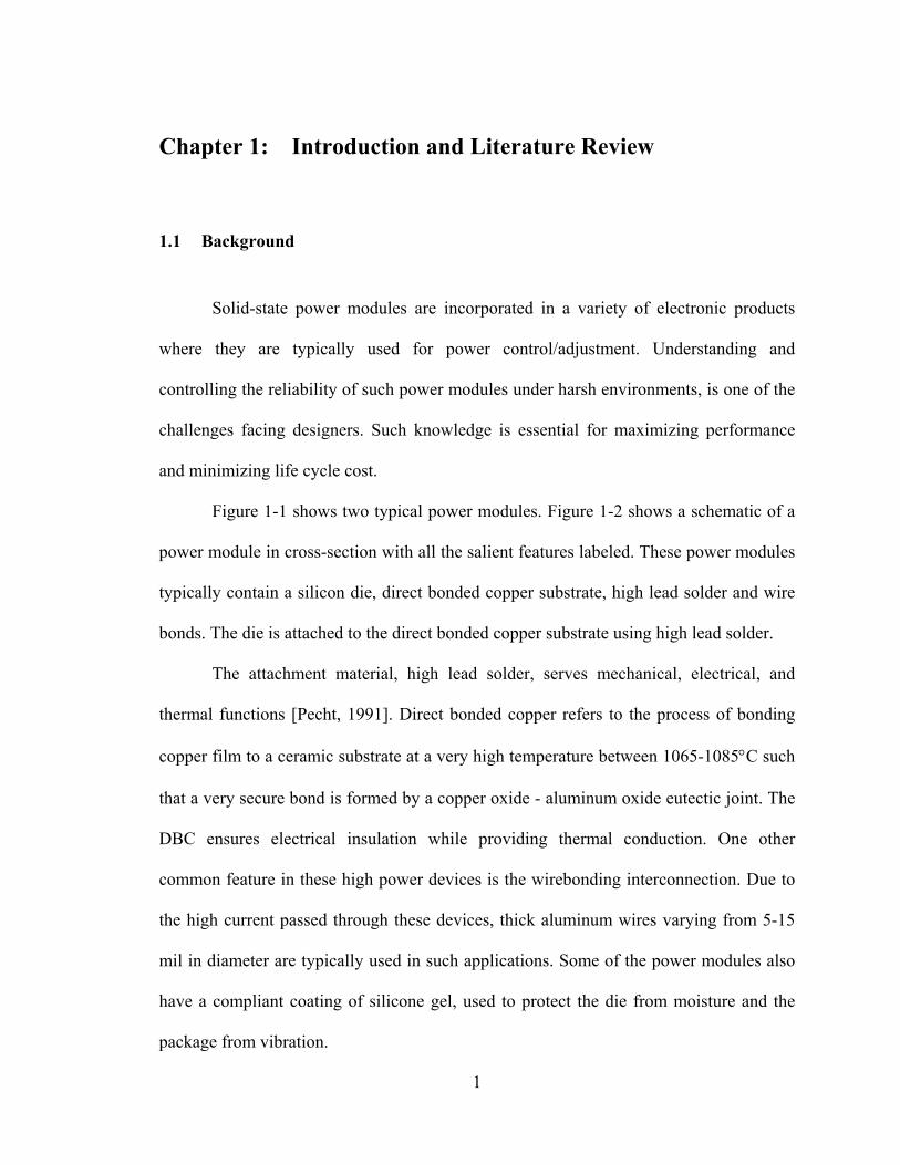
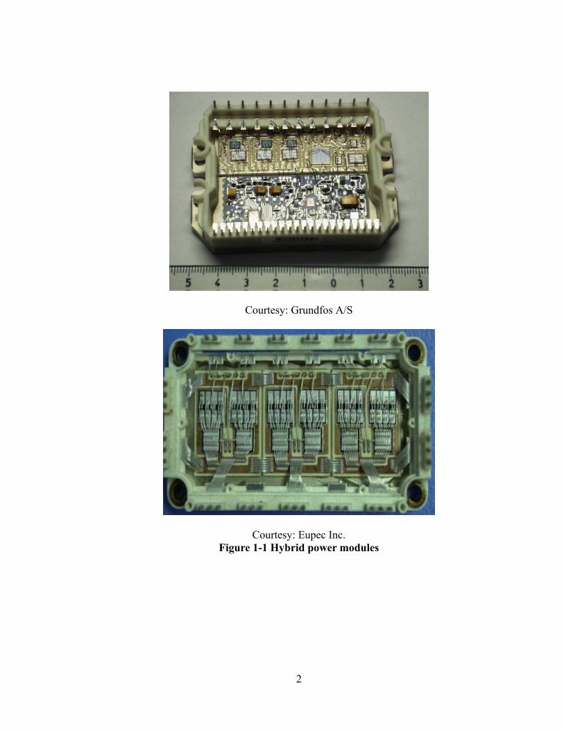
Figure 1-1 shows two typical power modules. Figure 1-2 shows a schematic of a
power module in cross-section with all the salient features labeled. These power modules
typically contain a silicon die, direct bonded copper substrate, high lead solder and wire
bonds. The die is attached to the direct bonded copper substrate using high lead solder.
The attachment material, high lead solder, serves mechanical, electrical, and
thermal functions [Pecht, 1991]. Direct bonded copper refers to the process of bonding
copper film to a ceramic substrate at a very high temperature between 1065-1085°C such
that a very secure bond is formed by a copper oxide - aluminum oxide eutectic joint. The
DBC ensures electrical insulation while providing thermal conduction. One other
common feature in these high power devices is the wirebonding interconnection. Due to
the high current passed through these devices, thick aluminum wires varying from 5-15
mil in diameter are typically used in such applications. Some of the power modules also
have a compliant coating of silicone gel, used to protect the die from moisture and the
package from vibration.
1
Courtesy: Grundfos A/S
Courtesy: Eupec Inc. Figure 1-1 Hybrid power modules
2
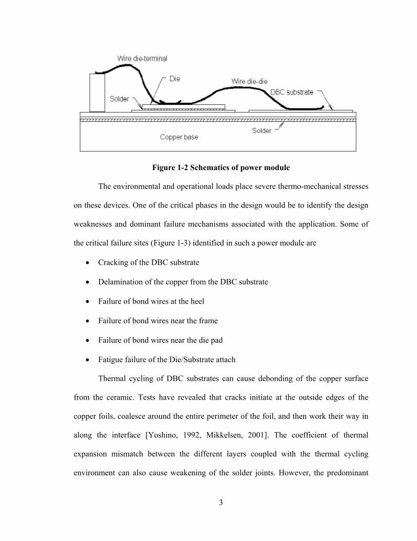
Figure 1-2 Schematics of power module
The environmental and operational loads place severe thermo-mechanical stresses
on these devices. One of the critical phases in the design would be to identify the design
weaknesses and dominant failure mechanisms associated with the application. Some of
the critical failure sites (Figure 1-3) identified in such a power module are
• Cracking of the DBC substrate
• Delamination of the copper from the DBC substrate
• Failure of bond wires at the heel
• Failure of bond wires near the frame
• Failure of bond wires near the die pad
• Fatigue failure of the Die/Substrate attach
Thermal cycling of DBC substrates can cause debonding of the copper surface
from the ceramic. Tests have revealed that cracks initiate at the outside edges of the
copper foils, coalesce around the entire perimeter of the foil, and then work their way in
along the interface [Yoshino, 1992, Mikkelsen, 2001]. The coefficient of thermal
expansion mismatch between the different layers coupled with the thermal cycling
environment can also cause weakening of the solder joints. However, the predominant
3
failure site observed in these power modules is the fatigue failure of the bond wires [Hu
et al., 1991]. Also, thermal cycling of field samples revealed wire bond failures as the
dominant failure mechanism.
Figure 1-3 Critical failure sites in a typical power module
1.2 Wirebonding in Microelectronics
Wire bonding today is used throughout the microelectronics industry as a means
of interconnecting bond pads on the die to the internal lands of package leadframes or
bond pads on a substrate using thin wire and a combination of heat, pressure and/or
ultrasonic energy. Wire bonding continues to be the dominant bonding technologies in
industry. It was estimated in 1996 that about 4 ×10¹² wires were bonded per year
4
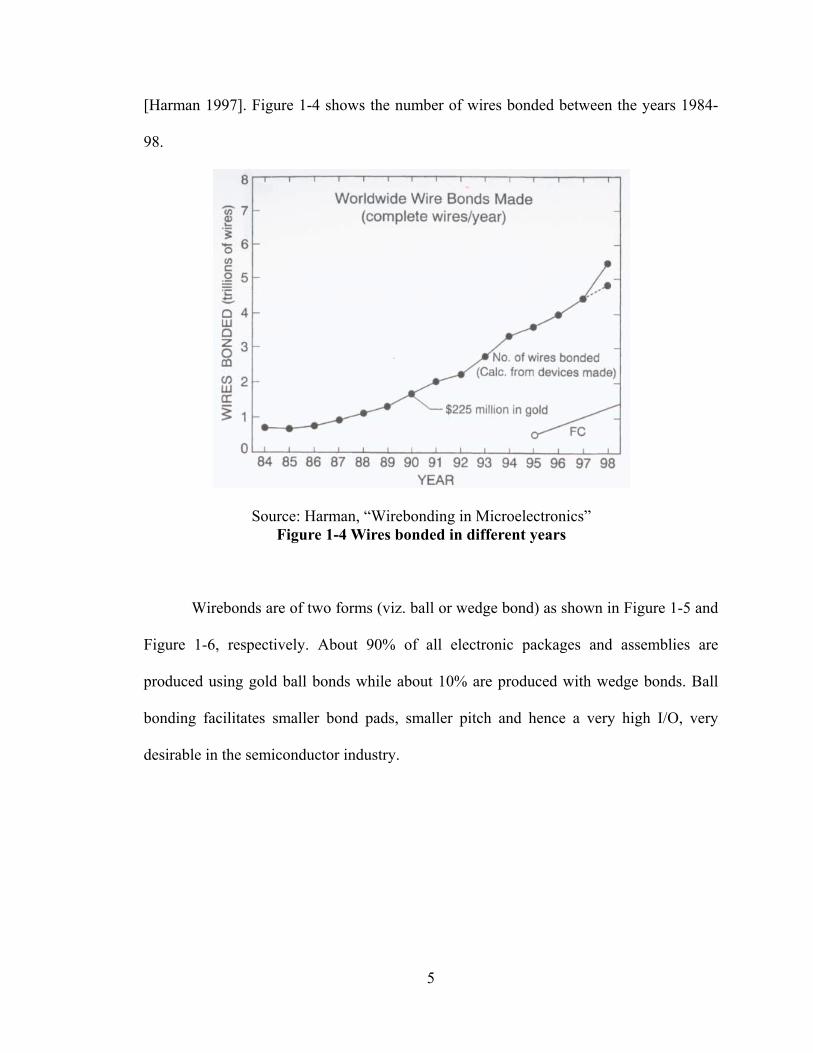
[Harman 1997]. Figure 1-4 shows the number of wires bonded between the years 1984-
98.
Source: Harman, “Wirebonding in Microelectronics” Figure 1-4 Wires bonded in different years
Wirebonds are of two forms (viz. ball or wedge bond) as shown in Figure 1-5 and
Figure 1-6, respectively. About 90% of all electronic packages and assemblies are
produced using gold ball bonds while about 10% are produced with wedge bonds. Ball
bonding facilitates smaller bond pads, smaller pitch and hence a very high I/O, very
desirable in the semiconductor industry.
5
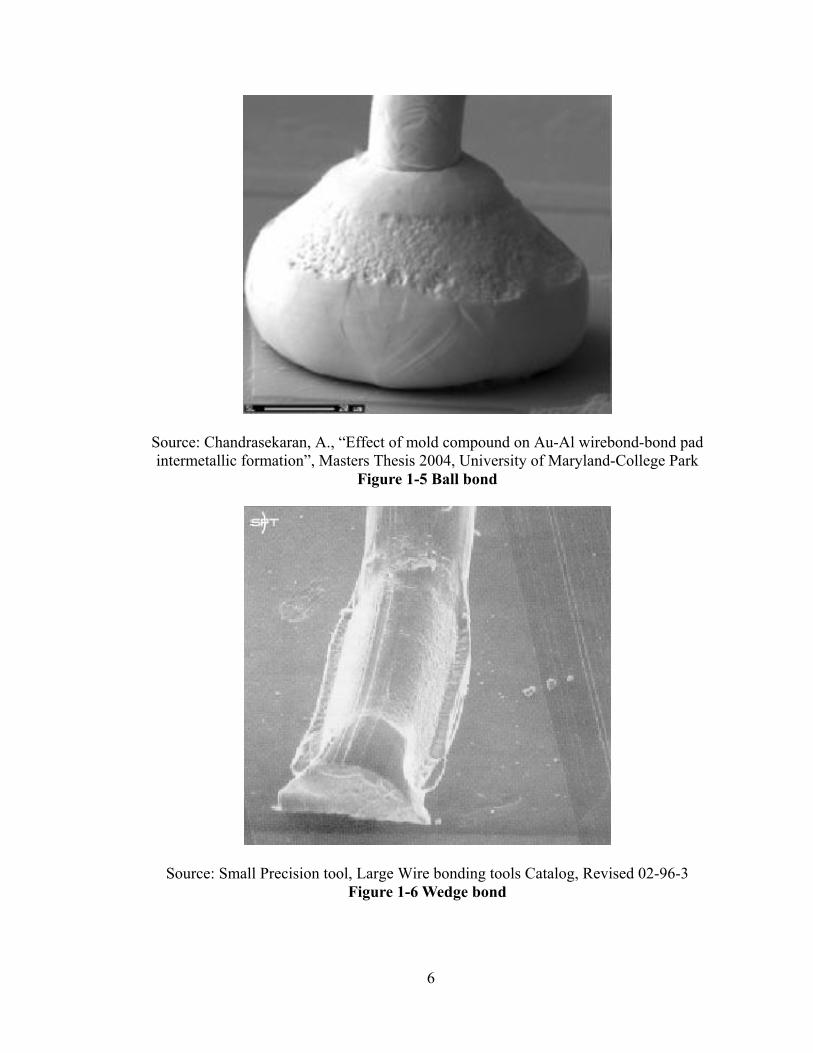
Source: Chandrasekaran, A., “Effect of mold compound on Au-Al wirebond-bond pad intermetallic formation”, Masters Thesis 2004, University of Maryland-College Park
Figure 1-5 Ball bond
Source: Small Precision tool, Large Wire bonding tools Catalog, Revised 02-96-3 Figure 1-6 Wedge bond
6
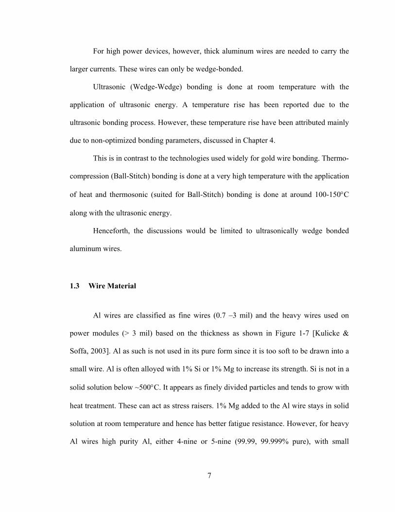
For high power devices, however, thick aluminum wires are needed to carry the
larger currents. These wires can only be wedge-bonded.
Ultrasonic (Wedge-Wedge) bonding is done at room temperature with the
application of ultrasonic energy. A temperature rise has been reported due to the
ultrasonic bonding process. However, these temperature rise have been attributed mainly
due to non-optimized bonding parameters, discussed in Chapter 4.
This is in contrast to the technologies used widely for gold wire bonding. Thermo-
compression (Ball-Stitch) bonding is done at a very high temperature with the application
of heat and thermosonic (suited for Ball-Stitch) bonding is done at around 100-150°C
along with the ultrasonic energy.
Henceforth, the discussions would be limited to ultrasonically wedge bonded
aluminum wires.
1.3 Wire Material
Al wires are classified as fine wires (0.7 –3 mil) and the heavy wires used on
power modules (> 3 mil) based on the thickness as shown in Figure 1-7 [Kulicke &
Soffa, 2003]. Al as such is not used in its pure form since it is too soft to be drawn into a
small wire. Al is often alloyed with 1% Si or 1% Mg to increase its strength. Si is not in a
solid solution below ~500°C. It appears as finely divided particles and tends to grow with
heat treatment. These can act as stress raisers. 1% Mg added to the Al wire stays in solid
solution at room temperature and hence has better fatigue resistance. However, for heavy
Al wires high purity Al, either 4-nine or 5-nine (99.99, 99.999% pure), with small
7
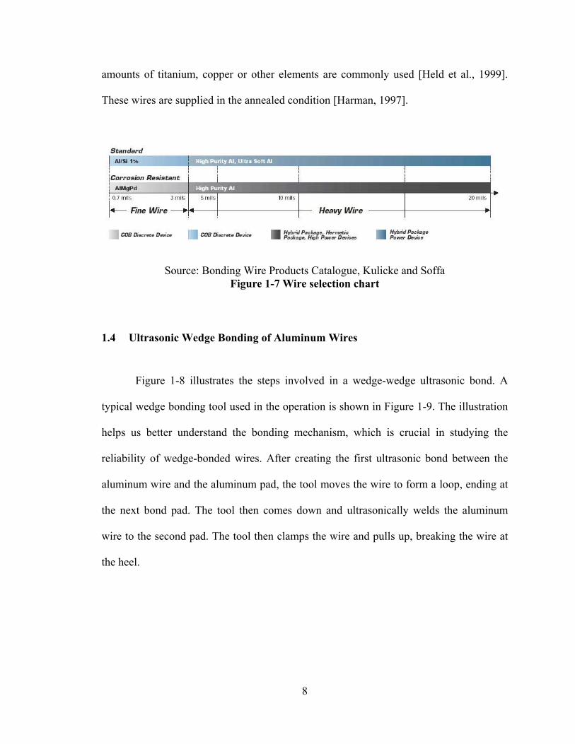
amounts of titanium, copper or other elements are commonly used [Held et al., 1999].
These wires are supplied in the annealed condition [Harman, 1997].
Source: Bonding Wire Products Catalogue, Kulicke and Soffa Figure 1-7 Wire selection chart
1.4 Ultrasonic Wedge Bonding of Aluminum Wires
Figure 1-8 illustrates the steps involved in a wedge-wedge ultrasonic bond. A
typical wedge bonding tool used in the operation is shown in Figure 1-9. The illustration
helps us better understand the bonding mechanism, which is crucial in studying the
reliability of wedge-bonded wires. After creating the first ultrasonic bond between the
aluminum wire and the aluminum pad, the tool moves the wire to form a loop, ending at
the next bond pad. The tool then comes down and ultrasonically welds the aluminum
wire to the second pad. The tool then clamps the wire and pulls up, breaking the wire at
the heel.
8
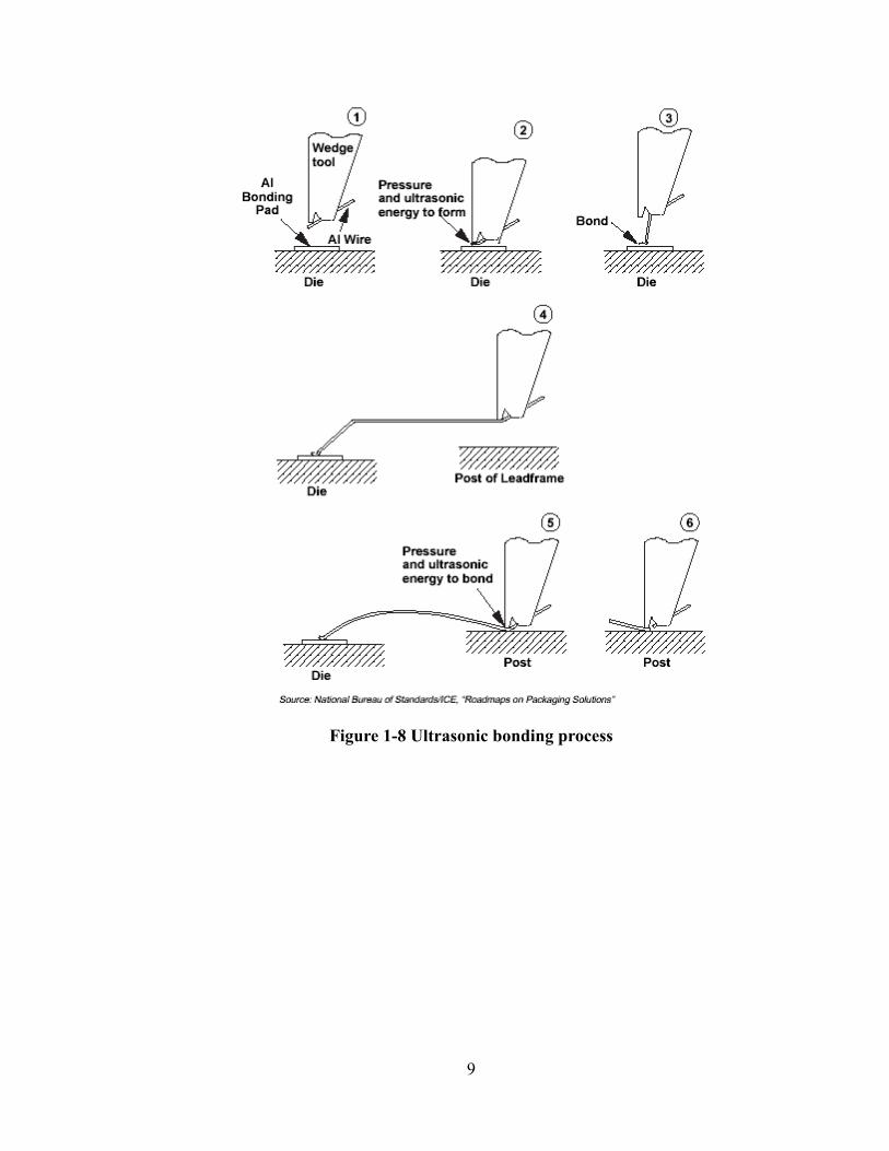
Figure 1-8 Ultrasonic bonding process
9
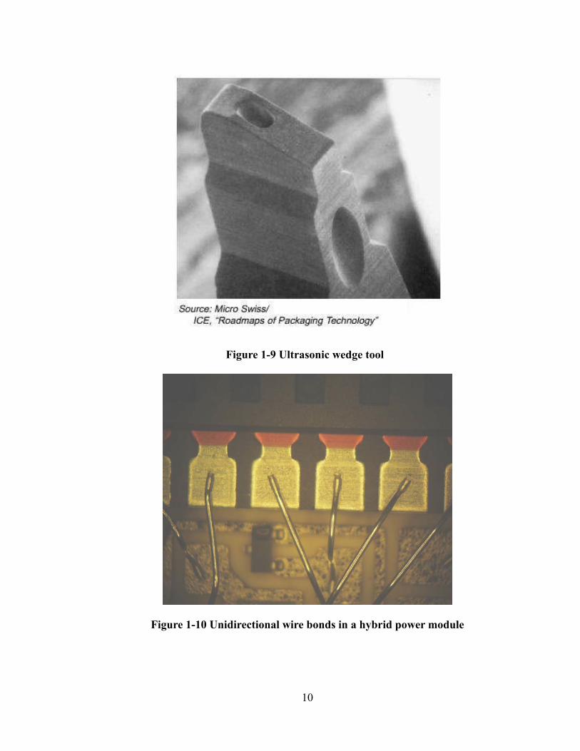
Figure 1-9 Ultrasonic wedge tool
Figure 1-10 Unidirectional wire bonds in a hybrid power module
10
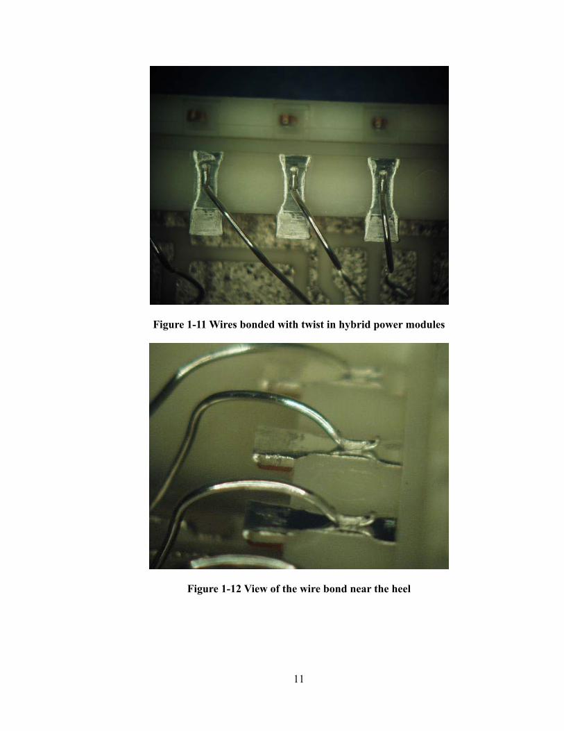
Figure 1-11 Wires bonded with twist in hybrid power modules
Figure 1-12 View of the wire bond near the heel
11
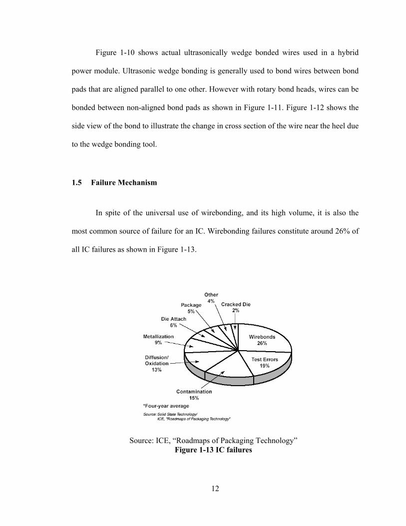
Figure 1-10 shows actual ultrasonically wedge bonded wires used in a hybrid
power module. Ultrasonic wedge bonding is generally used to bond wires between bond
pads that are aligned parallel to one other. However with rotary bond heads, wires can be
bonded between non-aligned bond pads as shown in Figure 1-11. Figure 1-12 shows the
side view of the bond to illustrate the change in cross section of the wire near the heel due
to the wedge bonding tool.
1.5 Failure Mechanism
In spite of the universal use of wirebonding, and its high volume, it is also the
most common source of failure for an IC. Wirebonding failures constitute around 26% of
all IC failures as shown in Figure 1-13.
Source: ICE, “Roadmaps of Packaging Technology” Figure 1-13 IC failures
12
In the past the number of failures due to wirebonds were numerous and the
number of failure mechanisms identified were limited. Currently around a dozen failure
mechanisms have been identified for Al-Al bonds [Harman, 1997]. These failure
mechanisms include: corrosion, wire flexure, wire bond lift-off, cratering, dendritic
growth and electrical leakage.
Corrosion of passive and active microelectronic devices by ionic contaminants
can result in problems ranging from a loss in strength to a change in thermal properties.
Pecht [Pecht, 1990] provides a foundation to which prior and future corrosion models can
be compared.
Thermal cycling can cause wires to lift-off due to shear stresses generated
between the bond pad-wire interface and between bond pad–substrate interface. This can
be reduced if the coefficient of thermal expansion (CTE) mismatch between the materials
at the interface is reduced. Ramminger [Ramminger et al., 2003] and Hu [Hu et al., 1991]
have developed physics-of-failure based models to study wire lift-off failures.
The thermal cycling environment can also cause the wires to flex in response to
the rise in temperature. The flexing motion of the wire when exposed to a power cycling
environment was captured by Ravi [Ravi et al. 1972]. The flexing motion produces stress
reversals in the heel of the bond wire thus causing cracks to appear at this location. The
heel of the wire is already weakened due to the ultrasonic bonding and the flexing motion
is enough to initiate a crack in the heel of the wire. Cracks in the heel of the wire can also
arise due to: a sharp-heeled bonding tool, by operator motion, bonding machine vibration
or due to the wire loop formation. It is very important to decide and produce an optimum
loop profile since a sub optimal loop profile can cause unnecessary flexing of the wire.
13
Also, an asymmetrically bonded wire (wires bonded with a height offset) promotes
cracking more than a wire bonded without any height offset [Harman, 1997]. The bond
pull strength should be indicative enough of the weakening of the wire at the heel of the
wire due to cracking.
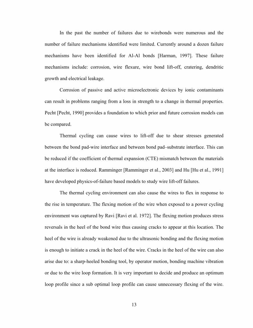
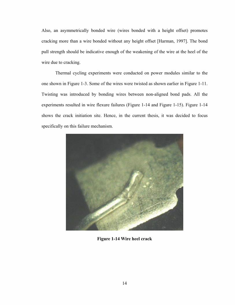
Thermal cycling experiments were conducted on power modules similar to the
one shown in Figure 1-3. Some of the wires were twisted as shown earlier in Figure 1-11.
Twisting was introduced by bonding wires between non-aligned bond pads. All the
experiments resulted in wire flexure failures (Figure 1-14 and Figure 1-15). Figure 1-14
shows the crack initiation site. Hence, in the current thesis, it was decided to focus
specifically on this failure mechanism.
Figure 1-14 Wire heel crack
14
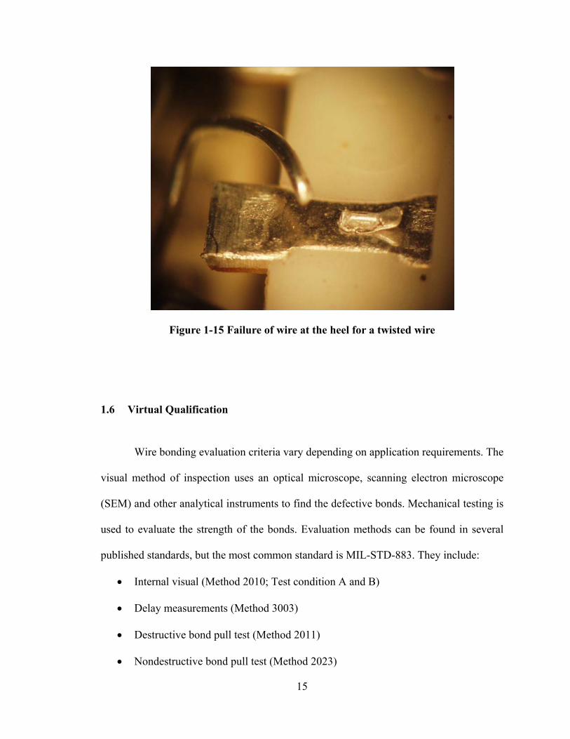
Figure 1-15 Failure of wire at the heel for a twisted wire
1.6 Virtual Qualification
Wire bonding evaluation criteria vary depending on application requirements. The
visual method of inspection uses an optical microscope, scanning electron microscope
(SEM) and other analytical instruments to find the defective bonds. Mechanical testing is
used to evaluate the strength of the bonds. Evaluation methods can be found in several
published standards, but the most common standard is MIL-STD-883. They include:
• Internal visual (Method 2010; Test condition A and B)
• Delay measurements (Method 3003)
• Destructive bond pull test (Method 2011)
• Nondestructive bond pull test (Method 2023)
15
• Ball bond shear test
• Temperature cycling test (Method 0101, Test Condition C)
• Constant acceleration (Method 2001; Test condition E)
• Random vibration (Method 2026)
• Mechanical shock (Method 2002)
• Stabilization bake (Method 1008)
• Moisture resistance (Method 1004)
The temperature cycling tests subject the wirebond interconnects to alternatively
changing temperatures. The failure mechanisms addressed by the temperature cycling test
include flexure failure of the wire at the heel, bond pad-substrate shear failure, wire-
substrate shear failure.
This thesis focuses primarily on the flexural fatigue failures of wedge bonded
wires commonly seen in power devices. The approach explained in this thesis to study
the flexural fatigue failure is generic and can be extended to cover any semiconductor
device with wedge-bonded wire interconnections.
A typical power module has traditionally been required to sustain 1000 thermal
cycles between –40°C and +125°C in order to be qualified for use. This procedure is
meant to detect modules that are likely to fail by wire flexure fatigue in operational life
when the assembly is subjected to cyclic strain as a result of thermal (i.e., temperature
and power) cycling.
While this traditional procedure is well accepted, it has two major shortcomings.
First, the selection of the temperature cycle magnitude and duration is arbitrary and they
do not correspond to a particular field life. Second, the procedure is costly and time
16
consuming and is therefore undesirable in today’s product development environment of
shortened design cycles and quick time-to-market. It is no longer acceptable to make a
prototype, subject it to a series of standardized tests, analyze the failures, fix the design,
and test again. Instead, a fundamental model is needed to assess the susceptibility of
module designs to wire flexure fatigue without conducting such extensive qualification
tests. Such a model should be based on a fundamental understanding of the thermo-
mechanical mechanism that causes wire flexure failure in electronic systems. The use of
such models to qualify assemblies for field use is known as virtual qualification.
1.7 Scope of the Current Thesis
Focus on this thesis would be limited to flexure-induced failure of wedge-bonded
interconnections. The outcome of this research is a model which can be used to produce
guidelines for reliable wirebonded interconnections. In addition to identifying the prime
factors affecting the reliability of the wirebonds, this research also identified the optimum
values of design parameters based on the available constraints. The models are energy-
based since every physical system would prefer to take up a configuration where it would
store minimum potential energy. Identifying the most stable configuration can help
decide the best loop profile. This information can be fed to the wirebonder; to produce
reliable wire bonded interconnections.
Chapter 2 describes a first order physics-of-failure (PoF) based wire flexure
model. The chapter describes a load transformation model and a damage model. The load
transformation model determines the cyclic strain at the heel of the wire during
17
temperature cycling. The damage model calculates the life based on the strain cycle
magnitude and the elastic-plastic fatigue response of the wire.
The validation of the analytical model, sensitivity analysis and model limitations
are explained in Chapter 3.
Chapter 4 deals exclusively with one of the limitations explained in Chapter 3, the
effect of ultrasonic bonding of wires on the flexural stresses, which has not been modeled
in the first order PoF model, but has been addressed using an FEM model of the
ultrasonic bonding of wires. The critical bonding parameters that could influence the wire
flexural stresses are identified.
Chapter 5 deals with another possible factor that could influence the flexural
stresses, the effect of wire twisting. A new, energy-based, approach has been developed
for determining the minimum energy profile in a Euclidean three-space, R3. The heel
stresses are determined for such geometries using FEA.
The thesis is concluded in Chapter 6 with the list of contributions and suggestions
for future work.
1.8 Nomenclature and Terminology used
ε = Strain at the wire heel due to wire flexure
εlow= Bending strains at lower bond pad
εhigh= Bending strains at upper bond pad
σ = Stress at the wire heel due to wire flexure
σlow= Bending stresses at lower bond pad
18

σhigh= Bending stresses at upper bond pad
e= offset of neutral axis from centroidal axis
FT= Resultant reaction force on top section of wire
FB= Resultant reaction force on bottom section of wire
Mult= Ultimate resisting moment
σf′= Fatigue strength coefficient
b= Fatigue strength exponent
εf′= Fatigue ductility coefficient
c= Fatigue ductility exponent
σys= Yield stress
σ0= Mean stresses
yR= Distance of outermost fiber from neutral axis
R = Radius of curvature from the neutral axis
r = Radius of wire
r = Radius of curvature from centroidal axis
π= Potential energy
λ= Lagrange parameter
ρI = Radius of curvature before heating
ρf = Radius of curvature after heating
ψi = Take off angle before heating
ψf = Take off angle after heating
κi = The curvature at the heel of the wire before heating
19
κf = The curvature at the heel of the wire after heating
α(u) = Differentiable curve parameterized by u
β(v) = Differentiable curve parameterized by v
di = The x co-ordinate of the reference point, defining the loop height, before
heating
hi = The y co-ordinate of the reference point, defining the loop height, before
heating
Di = The span of the wire before heating
Hi = The bond pad height offset of the wire before heating
df = The x co-ordinate of the reference point, defining the loop height, after
heating
hf = The y co-ordinate of the reference point, defining the loop height, after
heating
Df = The span of the wire after heating
Hf = The bond pad height offset of the wire after heating
αsub = Thermal expansion coefficient of the heat spreader
αglue = Thermal expansion coefficient of the glue
αply = Thermal expansion coefficient of the plastic frame
αdbc = Thermal expansion coefficient of the DBC layer
E = Modulus of elasticity of Al wire
∆T = Temperature load cycle applied
FL= Tool flat length
20

BF= Bond Flat
B= Wire deformation due to bonding
d = The x co-ordinate of the reference point
h = The y co-ordinate of the reference point
D = The span of the wire
H = The bond pad height offset of the wire
w= The z co-ordinate of the reference point
W= Width offset of Bond pad
I= Moment of Inertia of Wire
L= Length of wire
L1= Length of first curve
L2= Length of second curve
Figure 1-16 shows a cross sectional view of a typical power module with some of
the commonly used terminology seen throughout the text of the report.
21
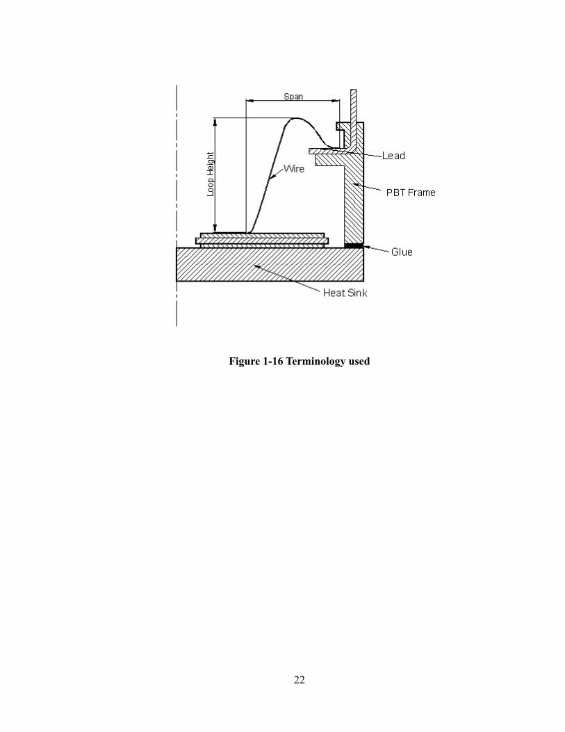
Figure 1-16 Terminology used
22
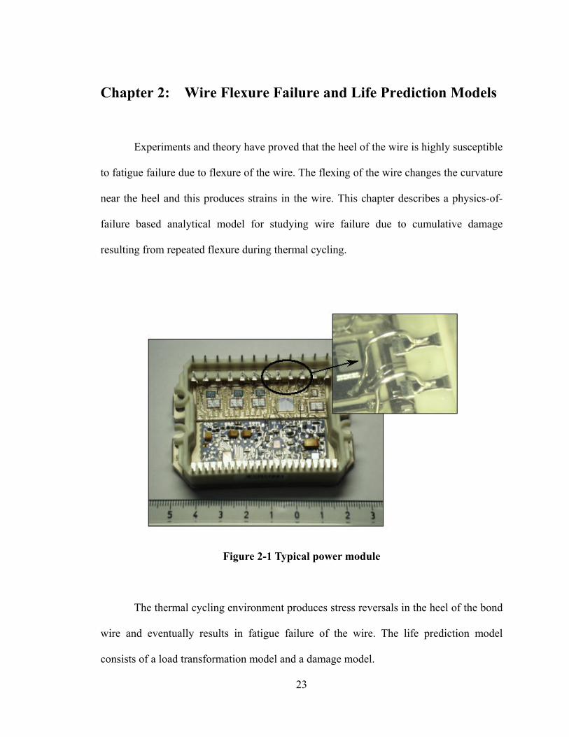
Chapter 2: Wire Flexure Failure and Life Prediction Models
Experiments and theory have proved that the heel of the wire is highly susceptible
to fatigue failure due to flexure of the wire. The flexing of the wire changes the curvature
near the heel and this produces strains in the wire. This chapter describes a physics-of-
failure based analytical model for studying wire failure due to cumulative damage
resulting from repeated flexure during thermal cycling.
Figure 2-1 Typical power module
The thermal cycling environment produces stress reversals in the heel of the bond
wire and eventually results in fatigue failure of the wire. The life prediction model
consists of a load transformation model and a damage model.
23
The load transformation model computes the stresses and the strains from the
change in curvature of the wire near the heel. The change in curvature is more dominant
in the heel of the wire near the upper bond pad, for a wire that is bonded with a bond pad
height offset [Harman, 1997].
2.1 Review of existing Fatigue Models and Limitations
The first failure prediction model for wire bonds was explained in 1989 [Pecht et
al., 1989]. The strains were a function of the change in take-off angles of the wire near
the heel. The impracticality in measuring the take-off angles [Pecht et al., 1989] near the
heel of the wire necessitated further efforts in this direction. In 1991, a new energy based
model [Hu et al., 1991], was proposed to predict strains for wires bonded without any
height offset. The theory of curved beams was used to predict strains near the heel of the
wire. However, in wires bonded with a height offset, the wire is more strained near the
heel of the elevated bond bad. Also, procedures for determination of wire loop profiles
are limited in literature. They are mostly based on mapping of wire loop profiles in
existing power modules. These loop profiles are very essential for use in analytical tools
like finite element.
Based on the limitations mentioned, it is also necessary for the new first-order
wire flexure model to incorporate the following,
• A well defined procedure to determine the wire loop profiles
• To account for the height offset between the bond pads
• To eliminate the need to measure take-off angles
24
2.2 Load Transformation Model
The load transformation model is essentially used to predict the bending
strains/stresses in the wire. These strains are derived based on the theory of curved
beams. Pure bending strains, at any section offset from the neutral axis, would be equal to
the ratio of change in length to the original length of the curved section, given by,
ii
R dyψρ
ψ=ε 2-1
where, yR is the distance of the outermost fiber from the neutral axis, dψ is the change in
angle subtended by the curved beam and ρi is the curvature of the section at the surface of
the beam before deformation (note: - the suffixes i and f are used to denote the variables
described before and after deformation of the wire). Hence, ρiψi would indicate the
original length of curved beam. The strains in the upper surface of the wire, given in Eq.
2-1, can be rewritten in terms of the new curvature after deformation, ρf and the radius of
curvature of the neutral axis, R, by,
( )ii
fi
ii
f
ii
f rd)r(d)R(ψρ
ψ−ψ=
ψρψρ−
≈ψρ
ψρ−=ε
2-2
where, r is the radius of curvature of the wire from the centroidal axes (Figure 2-2) and r
is the radius of the cross-section of the wire.
The curvature in the beam results in an offset of the neutral axis of the wire from
its centroidal axis. The location of the neutral axis follows from the condition that the
summation of the forces perpendicular to the section must be zero. The location of the
neutral axis for a curved beam with a circular cross-section is,
25
2rrrR
22−+
= 2-3
However, for all practical purposes R can be equated to r as done in Eq. 2-2, since the
wire has a high radius of curvature when compared to the wire radius near the heel.
Assuming no appreciable change in a small curved length of the wire, δs, before
and after deformation, the radii of curvatures and the take off angles can be related by the
expression,
δs = ρiψi ≈ ρfψf 2-4
From Eq. 2-2 and Eq. 2-4 the expressions for the strains can be rewritten as,
)(rρρ
)ρr(ρfi
fi
if κ−κ=−
=ε 2-5
where κi and κf are the curvatures of the wire and they are inversely proportional to the
radius of curvature. It is evident from Eq. 2-5 that the strains are a function of the change
in curvature. This dependence of heel crack failures on the loop geometry has also been
shown experimentally [Ramminger et al., 2000]. Hence, one of the most important
aspects in the model would be the accurate prediction of the geometry.
26
Figure 2-2 Wire label definitions
27
2.2.1 Wire Loop Profile
The wedge-bonded wires currently studied are all ultrasonically bonded. A non-
zero bond foot length (length of the base of the ultrasonic wedge tool that presses the
wire) ensures a zero vertical displacement at all ends that are pressed. It is easy to
understand that this would force the conditions of zero slopes and zero displacements at
ends where the wire is bonded. Also, the length of the wire is always provided as a
constraint (this requirement would become clearer in the later sections). Therefore, any
suitable wire geometry that is obtained should satisfy the admissibility conditions i.e. the
boundary conditions and the length constraint.
For representing the wire profile, a single polynomial of a very high order would
be an obvious choice. These curves are smooth in the sense of being maximally
differentiable and represented through the Lagrange interpolating polynomial. However
with all the constraints provided, the curve will have more stationary points. The
oscillation of the interpolating polynomial can be reduced by using piecewise
interpolating curves. However, the first derivatives in the interpolating points are
discontinuous and hence more interpolating points are needed to represent the wire
geometry. Hence, one of the possible solutions would be to represent the wire geometry
using a piecewise interpolating polynomial of third order which is differentiable at least
to the first order, at the interpolating points.
A Hermite polynomial [Meyyappan et al., 2003] was initially used and the wire
was represented using two curves as shown in Figure 2-2. The bond point locations are
given by points, 1(0, 0) and 3(D, H). Point 2 is chosen to be arbitrary with co-ordinates
(d, h). Hereafter, the notations point 1, point 2 (sometimes also referred as the reference
28
point defining the loop height) and point 3 are reserved and cross-referenced to the Figure
2-2 throughout the text.
A Hermite interpolation polynomial satisfies a C1 continuity (continuity of y and
y’). Due to the lower order continuity requirement, the solution process is much easier but
more interpolation points would be needed for representing the wire geometry more
accurately.
A cubic spline satisfies a y ′′ continuity in addition to the y and y′ continuity
provided by the Hermite Interpolation polynomial. Therefore, it would be sufficient to
use much fewer interpolation points in between the bond point locations. Also, it can be
proved that the cubic spline is the smoothest possible curve through a set of points and it
would always minimize the strain energy [Spath 1974, de Boor 2001]. Hence, one can
now combine all these features with a cubic spline: i.e. weaker oscillations, a C2
continuity, and minimum the strain energy for the chosen interpolating point (point 2).
However, for the sake of completeness both the approaches, Hermite polynomial
and the Cubic spline approach [Meyyappan et al., 2003] have been explained.
2.2.2 Hermite Polynomial to represent the Wire Profile
The wire loop geometry is fitted through a Hermite interpolation polynomial. For
simplicity, the model described is not energy-based and hence is less accurate. This
approach requires the reference point, point 2, to be provided by the user. The curves
α(u) and β(v) are used to map the parameters u and v to the curves 1-2 and 2-3
respectively shown in Figure 2-2.
29
Let α,β:I→R2 be differentiable curves parameterized by u and v respectively such
that,
α(u) = (ud, h(3u2-2u3)) 2-6
β(v) = (v(D-d)+d, h+3(H-h)v2-2(H-h)v3) 2-7
Eq. 2-6 and Eq. 2-7 have been derived based on the boundary conditions (slopes
and co-ordinates of the data points that define the Hermite Polynomial). The detailed
derivations have been omitted for the sake of simplicity. For a regular parameterized
curve, the curvature κ(u) is given by,
κ(u) = 3'
"'
α(u)
α(u)α(u) ∧ , κ(v) =
3'
"'
(v)
(v)(v)
β
β∧β
2-8
Substituting u=0 in Eq. 2-8 provides the curvature of the wire at point 1 while v=1
provides the curvature of the wire at point 3. Simplifying the equations for the curvature,
κlow_0 (curvature at u=0) and κhigh_0 (curvature at v=1) can be written as,
κlow_0 = 2dh6 , κhigh_0 = 2)dD(
)Hh(6−− 2-9
The “low_0” and “high_0” suffixes are used to represent the terms at lower and
elevated bond pad for a wire bonded with a height offset before heating. Similarly, κlow_1
and κhigh_1, is determined after thermal cycling the wire. The strains are then expressed as
a function of the change in curvatures as shown in Eq. 2-5.
After simplification, the strains in the lower and upper bond pads are given by,
30
εlow =
− 2
f
f2
i
i
dh
dh
r6 , εhigh = ( ) ( )
−−
−−−
2ff
ff2
ii
ii
dDHh
dDHh
r6 2-10
The displacement of the bond pads on the package frame due to thermal cycling
(explained in Appendix A) is embedded in the variables Df, Hf. For a wire bonded
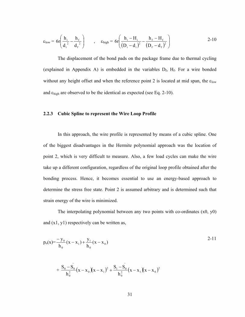
without any height offset and when the reference point 2 is located at mid span, the εlow
and εhigh are observed to be the identical as expected (see Eq. 2-10).
2.2.3 Cubic Spline to represent the Wire Loop Profile
In this approach, the wire profile is represented by means of a cubic spline. One
of the biggest disadvantages in the Hermite polynomial approach was the location of
point 2, which is very difficult to measure. Also, a few load cycles can make the wire
take up a different configuration, regardless of the original loop profile obtained after the
bonding process. Hence, it becomes essential to use an energy-based approach to
determine the stress free state. Point 2 is assumed arbitrary and is determined such that
strain energy of the wire is minimized.
The interpolating polynomial between any two points with co-ordinates (x0, y0)
and (x1, y1) respectively can be written as,
po(x)= )xx(hy)xx(
hy
00
11
0
0 −+−−
+ ( )( ) ( )( 2012
0
012102
0
00 xxxxh
SSxxxx
hSS
−−−
+−−− )
~~
2-11
31
where, S0 and S1 represent the slopes at the two end points. S represents the gradient of
a straight line passing through the two points. The representation of the polynomial using
Lagrange parameter automatically ensures a C1 continuity (continuity of y and y′). This
procedure is very much similar to how the C1 continuous beam elements with
displacement and slope continuity are derived in the finite element method. The point 2
acts as a common point lying on the boundary of the curves 1 & 2 (see Figure 2-2). By
equating the second order derivative of Eq. 2-11 at point 2 from the two curves (1 & 2) a
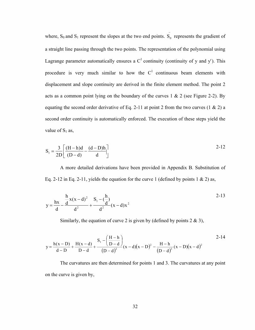
second order continuity is automatically enforced. The execution of these steps yield the
value of S1 as,
~
0
−−
−−
=d
h)Dd()dD(d)hH(
D23S1
2-12
A more detailed derivations have been provided in Appendix B. Substitution of
Eq. 2-12 in Eq. 2-11, yields the equation for the curve 1 (defined by points 1 & 2) as,
22
1
2
2
x)dx(d
)dh(S
d
)dx(xdh
dhxy −
−+
−−=
2-13
Similarly, the equation of curve 2 is given by (defined by points 2 & 3),
( )( )
( )( )2
32
2
1
dx)Dx(dDhHDx)dx(
dDdDhHS
dD)dx(H
Dd)Dx(hy −−
−−
−−−−
−−
−+
−−
+−−
=
2-14
The curvatures are then determined for points 1 and 3. The curvatures at any point
on the curve is given by,
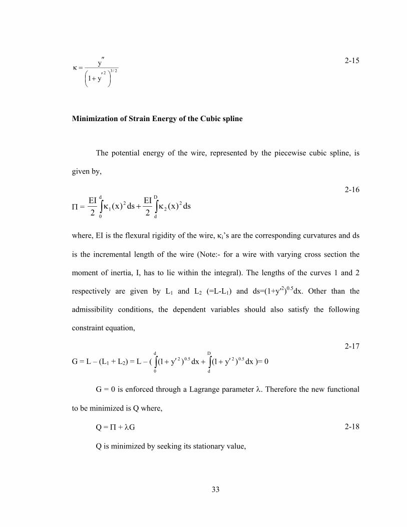
32
2/32y1
y
′+
″=κ 2-15
Minimization of Strain Energy of the Cubic spline
The potential energy of the wire, represented by the piecewise cubic spline, is
given by,
Π = ∫∫ κ+κD
d
22
d
0
21 ds)x(
2EIds)x(
2EI
2-16
where, EI is the flexural rigidity of the wire, κi’s are the corresponding curvatures and ds
is the incremental length of the wire (Note:- for a wire with varying cross section the
moment of inertia, I, has to lie within the integral). The lengths of the curves 1 and 2
respectively are given by L1 and L2 (=L-L1) and ds=(1+y′2)0.5dx. Other than the
admissibility conditions, the dependent variables should also satisfy the following
constraint equation,
G = L – (L1 + L2) = L – ( )= 0 ∫∫ ′++′+D
d
5.02d
0
5.02 dx)y1(dx)y1(
2-17
G = 0 is enforced through a Lagrange parameter λ. Therefore the new functional
to be minimized is Q where,
Q = Π + λG 2-18
Q is minimized by seeking its stationary value,
33

δQ = 0 2-19
0dQ
=δδ 0
hQ
=δδ 0Q
=δλδ
2-20
The above set of non-linear equations are solved iteratively using the Levenberg-
Marquardt algorithm to provide the location of the second point (d, h) which seeks to
minimize the potential energy and also satisfies the length constraint. Substitution of d
and h into Eq. 2-13 provides the wire geometry. However, the energy minimization could
also be performed using the ‘fmincon’ function, found in the optimization toolbox, in
Matlab. Both the approaches require the input of a guess value. These guess values are
very critical to the model, since the curve could have several local minima and it is the
objective of the program to choose the point that determines the global minima of the
curve.
Wire Stresses at the Heel
The radii of curvatures of the curves 1 and 2 are calculated at x=0 and x=D using
Eq. 2-13 as,
ρlow_0 = ( )yy1 5.12
′′′+ at x=0
2-21
ρhigh_0 = ( )yy1 5.12
′′′+ at x=D
2-22
When the wire elongates due to heating, the wire would occupy a new
configuration. Also, the frame can expand/contract in the linear direction and
34
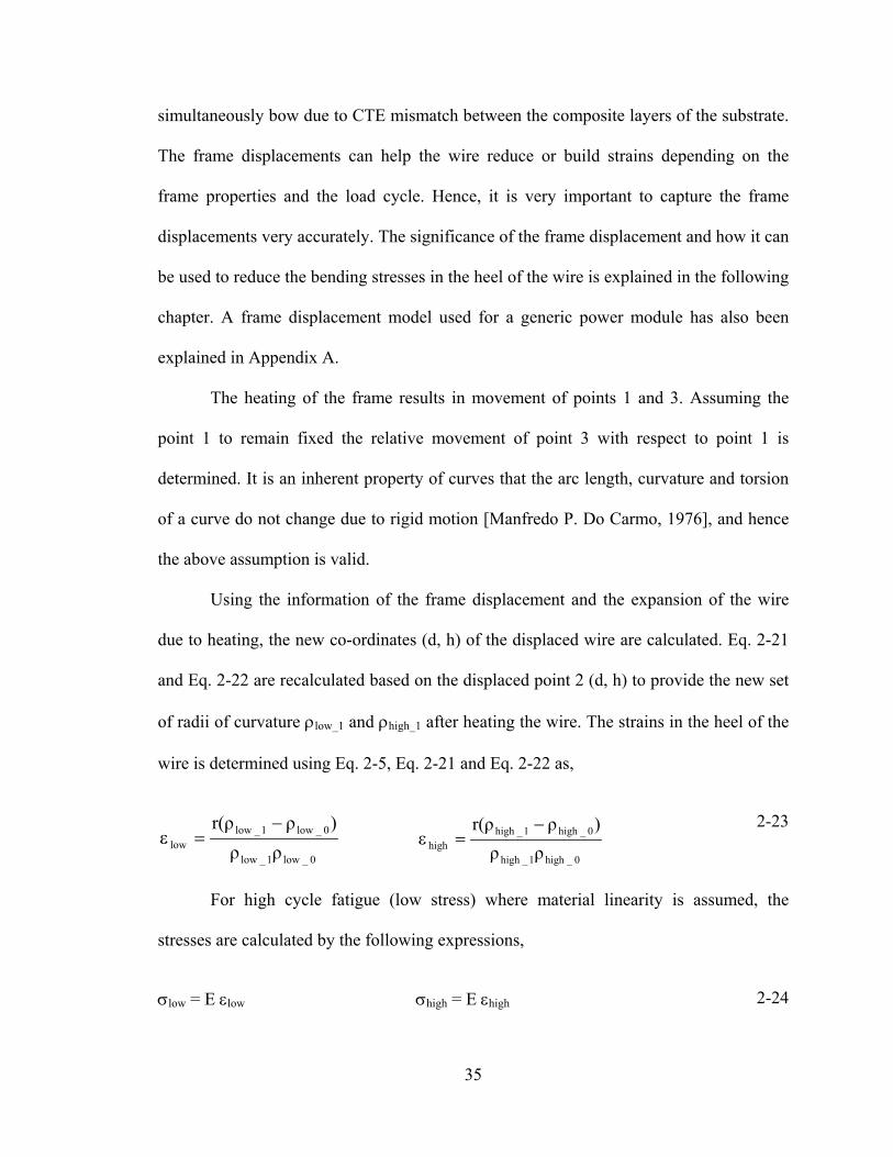
simultaneously bow due to CTE mismatch between the composite layers of the substrate.
The frame displacements can help the wire reduce or build strains depending on the
frame properties and the load cycle. Hence, it is very important to capture the frame
displacements very accurately. The significance of the frame displacement and how it can
be used to reduce the bending stresses in the heel of the wire is explained in the following
chapter. A frame displacement model used for a generic power module has also been
explained in Appendix A.
The heating of the frame results in movement of points 1 and 3. Assuming the
point 1 to remain fixed the relative movement of point 3 with respect to point 1 is
determined. It is an inherent property of curves that the arc length, curvature and torsion
of a curve do not change due to rigid motion [Manfredo P. Do Carmo, 1976], and hence
the above assumption is valid.
Using the information of the frame displacement and the expansion of the wire
due to heating, the new co-ordinates (d, h) of the displaced wire are calculated. Eq. 2-21
and Eq. 2-22 are recalculated based on the displaced point 2 (d, h) to provide the new set
of radii of curvature ρlow_1 and ρhigh_1 after heating the wire. The strains in the heel of the
wire is determined using Eq. 2-5, Eq. 2-21 and Eq. 2-22 as,
0_low1_low
0_low1_lowlow ρρ
)ρr(ρ −=ε
0_high1_high
0_high1_highhigh ρρ
)ρr(ρ −=ε
2-23
For high cycle fatigue (low stress) where material linearity is assumed, the
stresses are calculated by the following expressions,
σlow = E εlow σhigh = E εhigh 2-24
35
2.3 Residual Stresses during Loop Formation
On removing the constraints, the wire should retain its original profile if it had
deformed elastically. However, clipping a set of bonded wires showed that the wires had
a permanent deformation and they retained their current shape. For an elastic, perfectly
plastic material, some fibers of the wire away from the neutral axis would have deformed
plastically while the fibers near the neutral axis would have deformed elastically. On
unloading, the elastic sections of the wire would try to retain their original shape whereas
the plastically deformed section would prefer staying in the permanent set configuration.
This would introduce residual stresses in the wire.
The residual stresses when superimposed on the applied fatigue loads alter the
mean stresses of fatigue cycling. It is necessary to quantify the magnitude of these
residual stresses, as they could be critical to the damage prediction model. This section
describes an approach to determine the residual stresses in a curved beam that is
deformed inelastically and then unloaded.
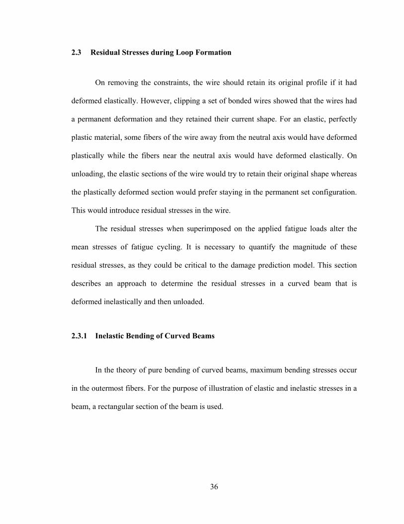
2.3.1 Inelastic Bending of Curved Beams
In the theory of pure bending of curved beams, maximum bending stresses occur
in the outermost fibers. For the purpose of illustration of elastic and inelastic stresses in a
beam, a rectangular section of the beam is used.
36
Figure 2-3 Rectangular beam in bending
σ1 and σ2 in Figure 2-3 represent the elastic and inelastic stresses on applying a
bending moment to the beam. However, for a curved beam, the elastic stress distribution
σ1 shown in the figure would be a curve due to the offset of the neutral axis from the
centroidal axis. The worst case of loading the beam, with elastic-perfectly plastic material
properties, would result in having uniform compressive and tensile stresses (σys) on either
sides of the neutral axis. In order to prove the existence of the inelastic stress distribution
and permanent deformation during the loop formation, a finite element analysis was
performed.
It is very difficult to determine the stresses by simulating the formation of the
loop using non-linear finite element method. However, the reverse procedure of
unloading a deformed wire with zero offset is feasible. The wire in its minimum energy
state, with a span of 20 mm, was assumed to be the unstressed configuration and it was
given a horizontal displacement of 0.5 and 1.1 mm. The resultant bending stresses across
the wire cross-section was then observed. Figure 2-4 shows the finite element model with
37
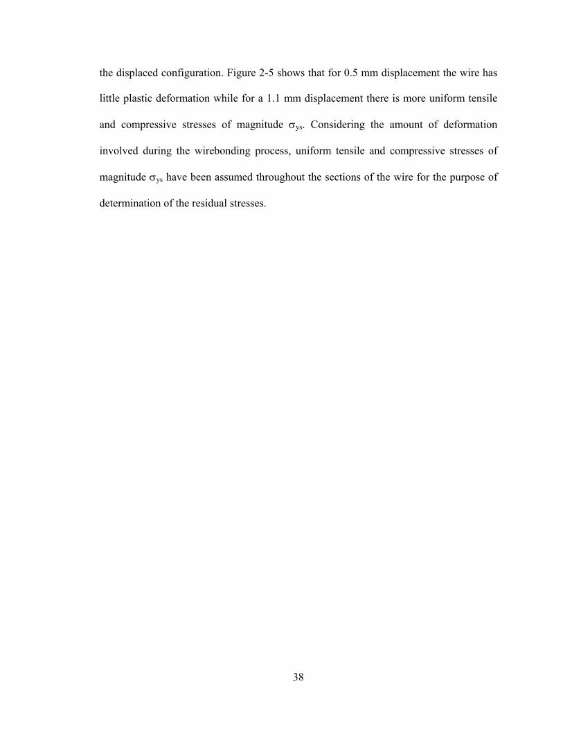
the displaced configuration. Figure 2-5 shows that for 0.5 mm displacement the wire has
little plastic deformation while for a 1.1 mm displacement there is more uniform tensile
and compressive stresses of magnitude σys. Considering the amount of deformation
involved during the wirebonding process, uniform tensile and compressive stresses of
magnitude σys have been assumed throughout the sections of the wire for the purpose of
determination of the residual stresses.
38
Figure 2-4 Finite element simulation of deformation
39
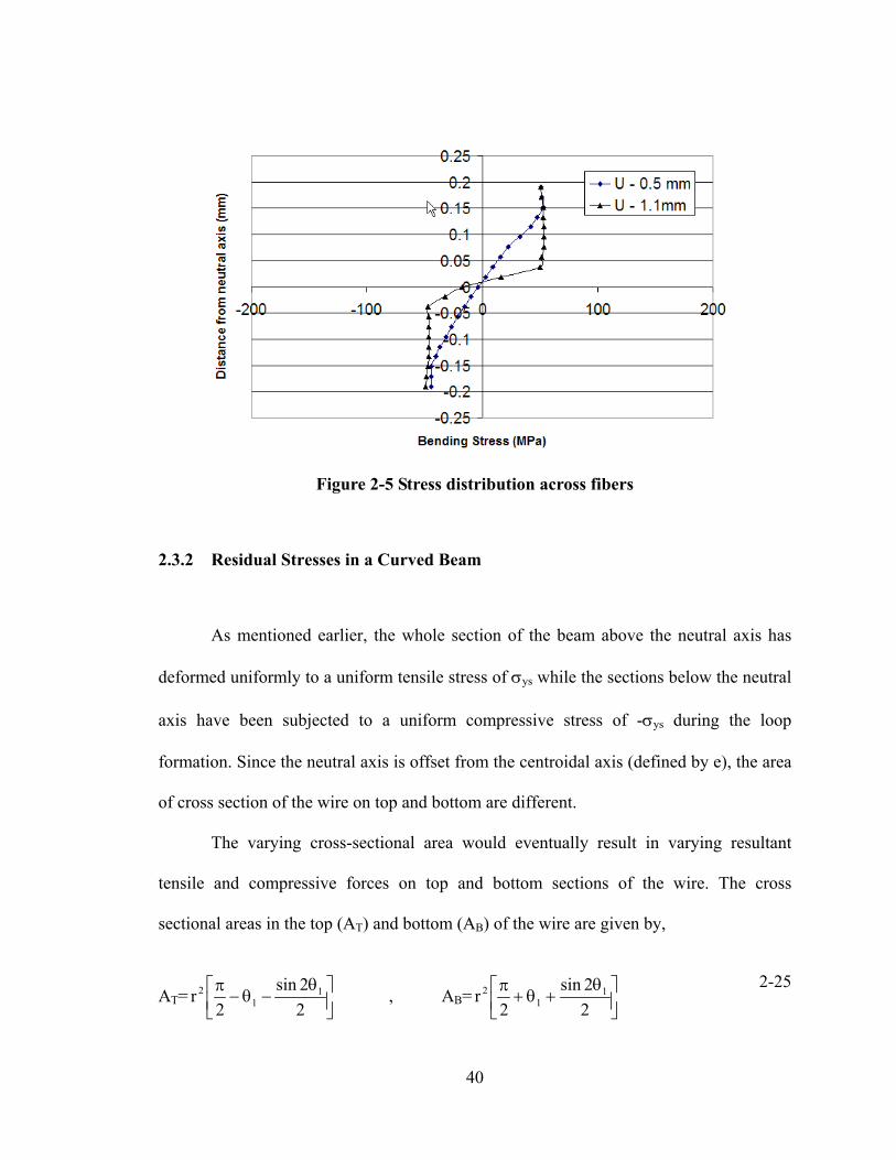
Figure 2-5 Stress distribution across fibers
2.3.2 Residual Stresses in a Curved Beam
As mentioned earlier, the whole section of the beam above the neutral axis has
deformed uniformly to a uniform tensile stress of σys while the sections below the neutral
axis have been subjected to a uniform compressive stress of -σys during the loop
formation. Since the neutral axis is offset from the centroidal axis (defined by e), the area
of cross section of the wire on top and bottom are different.
The varying cross-sectional area would eventually result in varying resultant
tensile and compressive forces on top and bottom sections of the wire. The cross
sectional areas in the top (AT) and bottom (AB) of the wire are given by,
AT=
θ
−θ−π
22sin
2r 1
12 , AB=
θ
+θ+π
22sin
21
12r
2-25
40
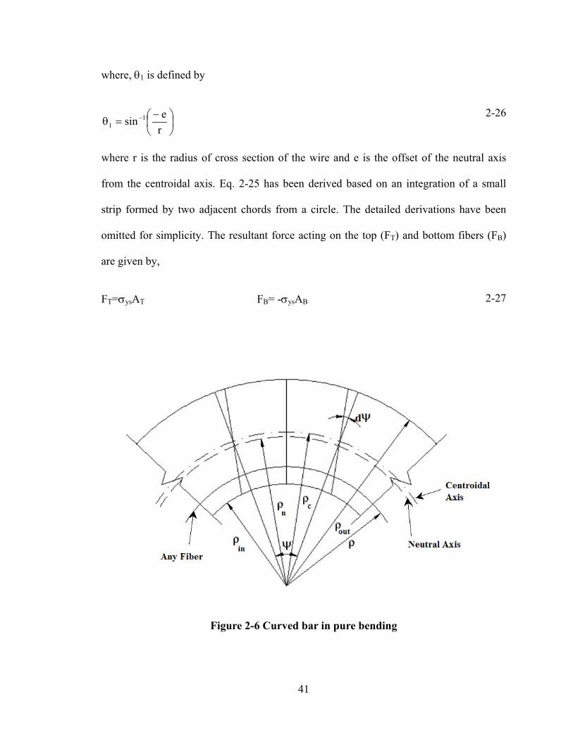
where, θ1 is defined by
−
=θ −
resin 1
1 2-26
where r is the radius of cross section of the wire and e is the offset of the neutral axis
from the centroidal axis. Eq. 2-25 has been derived based on an integration of a small
strip formed by two adjacent chords from a circle. The detailed derivations have been
omitted for simplicity. The resultant force acting on the top (FT) and bottom fibers (FB)
are given by,
FT=σysAT FB= -σysAB 2-27
Figure 2-6 Curved bar in pure bending
41
Hence, the total plastic or ultimate resisting moment (Mult), of the beam is given
by the product of the resultant forces and the length of bending arm.
−
+
+
=2
erF2
reFM BTult 2-28
If the beam were allowed to rebound elastically from the ultimate resisting
moment, Mult, the stress distribution would be given by,
( )eAcc.M
n
ult
−ρ=σ 2-29
where c is the distance of any fiber from the neutral axis. Superimposing the initial
stresses (σys) on the elastically rebounded stresses, given in Eq. 2-29, the residual stresses
are obtained.
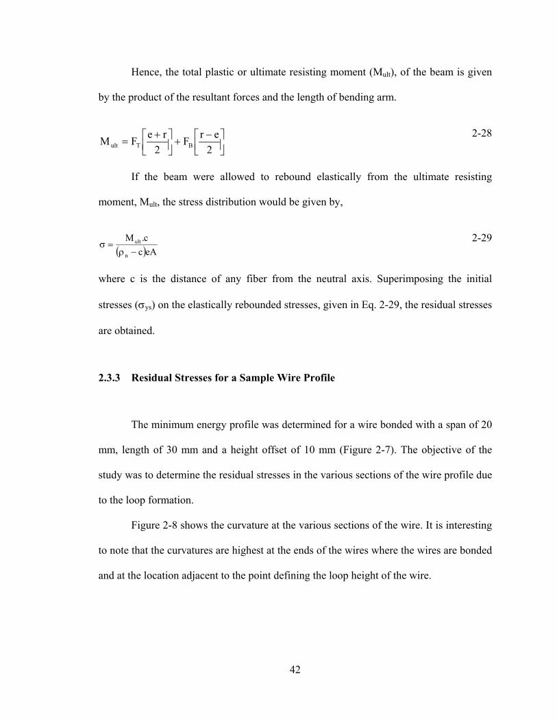
2.3.3 Residual Stresses for a Sample Wire Profile
The minimum energy profile was determined for a wire bonded with a span of 20
mm, length of 30 mm and a height offset of 10 mm (Figure 2-7). The objective of the
study was to determine the residual stresses in the various sections of the wire profile due
to the loop formation.
Figure 2-8 shows the curvature at the various sections of the wire. It is interesting
to note that the curvatures are highest at the ends of the wires where the wires are bonded
and at the location adjacent to the point defining the loop height of the wire.
42
Figure 2-7 Wire profile
The shift in the signs of the curvature suggests that the stresses switch from
tensile to compressive near the point defining the loop height and then back to tensile
stresses near the opposite edge. The offset of the neutral axis from the centroidal axis has
also been determined and is shown in Figure 2-9. The figure shows the shift of the neutral
axis is very small when compared to the radius of the wire. This is largely due to the high
curvature of the wire in comparison to the radius of cross-section. Hence, it would be
prudent to assume coincidental neutral and centroidal axis.
43
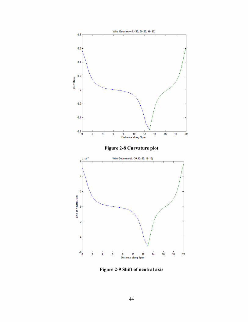
Figure 2-8 Curvature plot
Figure 2-9 Shift of neutral axis
44
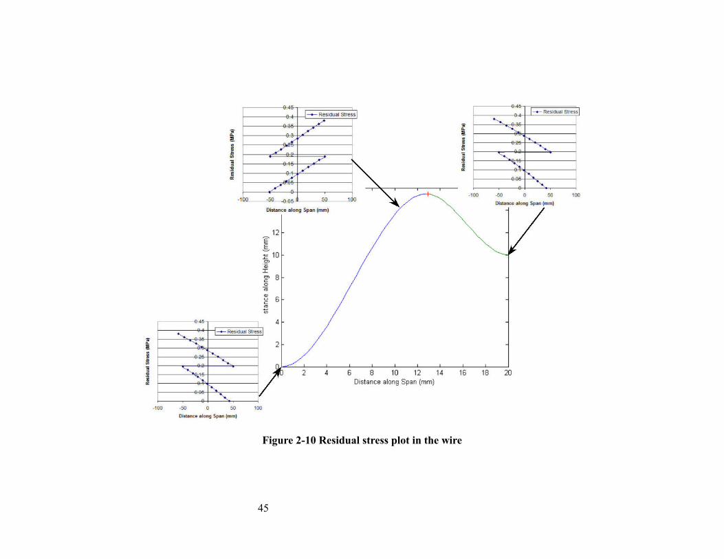
Figure 2-10 Residual stress plot in the wire
45
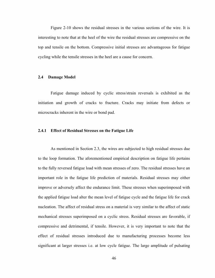
Figure 2-10 shows the residual stresses in the various sections of the wire. It is
interesting to note that at the heel of the wire the residual stresses are compressive on the
top and tensile on the bottom. Compressive initial stresses are advantageous for fatigue
cycling while the tensile stresses in the heel are a cause for concern.
2.4 Damage Model
Fatigue damage induced by cyclic stress/strain reversals is exhibited as the
initiation and growth of cracks to fracture. Cracks may initiate from defects or
microcracks inherent in the wire or bond pad.
2.4.1 Effect of Residual Stresses on the Fatigue Life
As mentioned in Section 2.3, the wires are subjected to high residual stresses due
to the loop formation. The aforementioned empirical description on fatigue life pertains
to the fully reversed fatigue load with mean stresses of zero. The residual stresses have an
important role in the fatigue life prediction of materials. Residual stresses may either
improve or adversely affect the endurance limit. These stresses when superimposed with
the applied fatigue load alter the mean level of fatigue cycle and the fatigue life for crack
nucleation. The affect of residual stress on a material is very similar to the affect of static
mechanical stresses superimposed on a cyclic stress. Residual stresses are favorable, if
compressive and detrimental, if tensile. However, it is very important to note that the
effect of residual stresses introduced due to manufacturing processes become less
significant at larger stresses i.e. at low cycle fatigue. The large amplitude of pulsating
46
stress easily relaxes the residual stresses [Suresh, 1992, Rowland, 1968 and Fox, 1981].
However, for a high cycle fatigue problem, the effects of mean stresses have to be
included in the model.
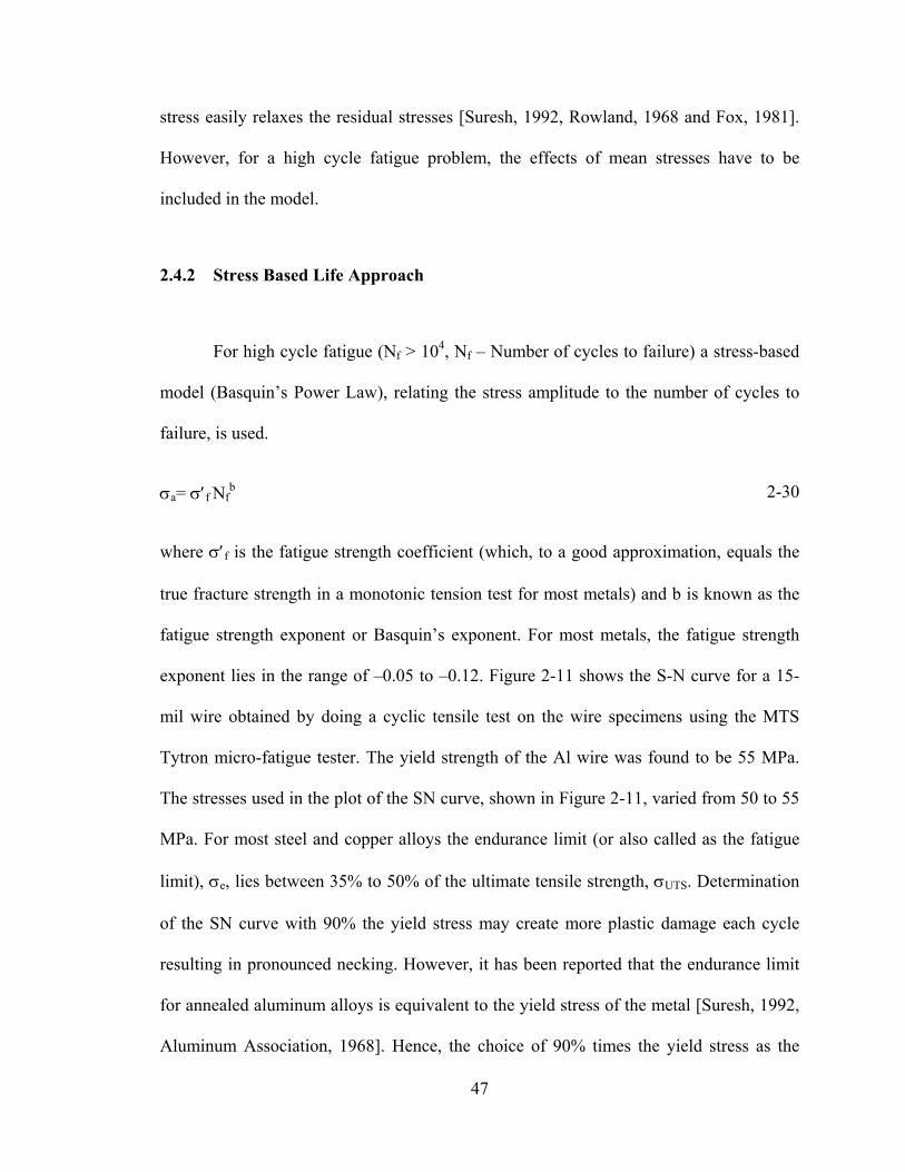
2.4.2 Stress Based Life Approach
For high cycle fatigue (Nf > 104, Nf – Number of cycles to failure) a stress-based
model (Basquin’s Power Law), relating the stress amplitude to the number of cycles to
failure, is used.
σa= σ′f Nfb 2-30
where σ′f is the fatigue strength coefficient (which, to a good approximation, equals the
true fracture strength in a monotonic tension test for most metals) and b is known as the
fatigue strength exponent or Basquin’s exponent. For most metals, the fatigue strength
exponent lies in the range of –0.05 to –0.12. Figure 2-11 shows the S-N curve for a 15-
mil wire obtained by doing a cyclic tensile test on the wire specimens using the MTS
Tytron micro-fatigue tester. The yield strength of the Al wire was found to be 55 MPa.
The stresses used in the plot of the SN curve, shown in Figure 2-11, varied from 50 to 55
MPa. For most steel and copper alloys the endurance limit (or also called as the fatigue
limit), σe, lies between 35% to 50% of the ultimate tensile strength, σUTS. Determination
of the SN curve with 90% the yield stress may create more plastic damage each cycle
resulting in pronounced necking. However, it has been reported that the endurance limit
for annealed aluminum alloys is equivalent to the yield stress of the metal [Suresh, 1992,
Aluminum Association, 1968]. Hence, the choice of 90% times the yield stress as the
47
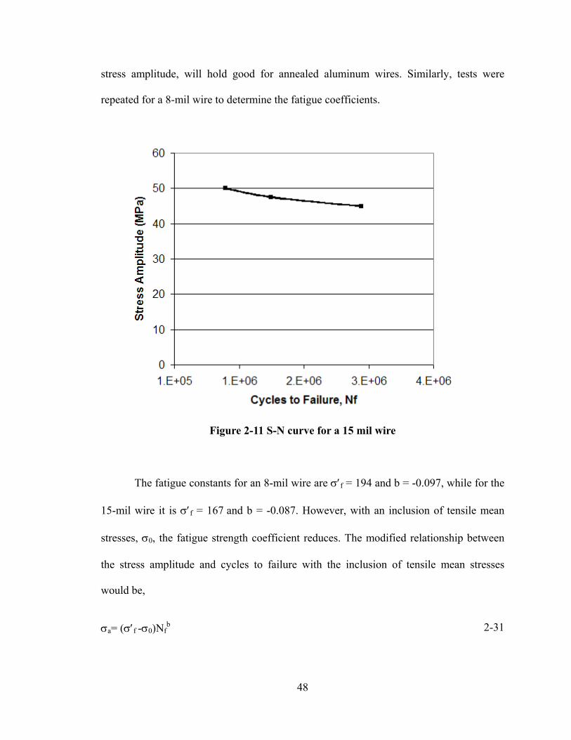
stress amplitude, will hold good for annealed aluminum wires. Similarly, tests were
repeated for a 8-mil wire to determine the fatigue coefficients.
Figure 2-11 S-N curve for a 15 mil wire
The fatigue constants for an 8-mil wire are σ′f = 194 and b = -0.097, while for the
15-mil wire it is σ′f = 167 and b = -0.087. However, with an inclusion of tensile mean
stresses, σ0, the fatigue strength coefficient reduces. The modified relationship between
the stress amplitude and cycles to failure with the inclusion of tensile mean stresses
would be,
σa= (σ′f -σ0)Nfb 2-31
48
2.4.3 Strain Based Approach to Total Life
The actual testing of the power modules provide cycles to failure <3000 cycles,
which makes the assumption of high cycle fatigue invalid. Hence, a strain range based
approach should be used for such problems that face huge stress amplitudes.
Coffin [Coffin, 1954] and Manson [Manson, 1954] working independently on
thermal fatigue problems proposed a model to characterize the fatigue life based on the
plastic strain amplitude. The plastic strain range is related to the cycles to failure by the
following relation,
2pε∆ = ε′f Nf
c 2-32
where ε′f is the fatigue ductility coefficient (which is experimentally found to be
approximately equal to the true fracture ductility in monotonic tension) and c is the
fatigue ductility exponent (which is in the range of –0.5 to –0.7 for most metals).
The fatigue constants for low cycle fatigue for the aluminum wire are determined
from literature as ε′f = 1.8 and c = -0.69 [Suresh, 1992 and Deyhim et al., 1996].
The strain life based approach to fatigue design has the elastic and plastic
components. The total strain amplitude in a constant strain amplitude test, ∆ε/2, can be
written in terms of the elastic and plastic strain amplitudes, ∆εe/2 and ∆εp/2 respectively,
as,
2ε∆ =
2eε∆ +
2pε∆ 2-33
49
Combining Eq. 2-31, 2-32 and 2-33, the total strain amplitude can be expressed in
terms of the cycles to failure as,
2ε∆ = ( )b
f0f N
E)( σ−′σ +ε′f Nf
c 2-34
Eq. 2-34 is essentially a superposition of the elastic and plastic strain amplitudes.
For an aluminum wire whose modulus was determined to be 41 GPa with yield strength
of 55 MPa, the strain amplitudes vs. cycles to failure were plotted. Figure 3-22 shows the
cycles to failure for various strain amplitudes derived from a pure stress-based, strain-
based and a method based on the superposition of the elastic and plastic strain
amplitudes. The figure also has the effect of mean stresses (55 MPa), represented through
dotted lines. The mean stresses are critical to the Basquin’s relation, which is used to
estimate the high cycle fatigue to failure. However, for low cycle fatigue problems (Nf <
104), the effect of residual stresses is insignificant. This study serves as a good validation
to exclude the effect of mean stresses for the low cycle fatigue problems.
50
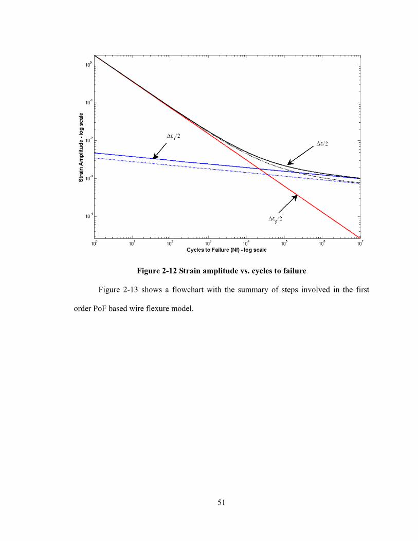
Figure 2-12 Strain amplitude vs. cycles to failure
Figure 2-13 shows a flowchart with the summary of steps involved in the first
order PoF based wire flexure model.
51
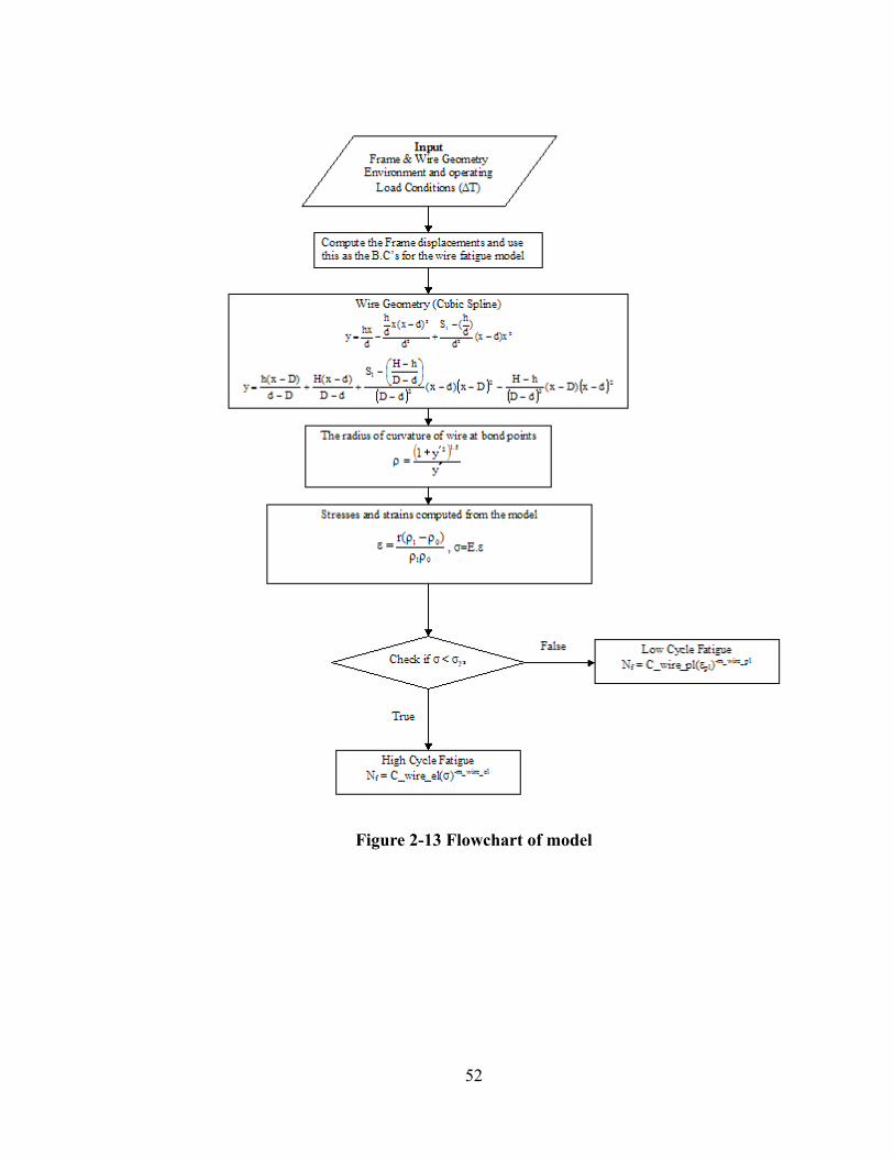
Figure 2-13 Flowchart of model
52
Chapter 3: Assumptions and Validation Studies
3.1 Introduction
This chapter has been mainly dedicated to explore more into the analytical model,
its validation, its shortcomings and possible improvements. Sensitivity analysis has been
performed by modifying some of the key parameters used in the design of wirebonded
interconnections. The key parameters described this chapter include, length, span, height
offset of wire and frame properties that control the frame displacements. The overall
objective is to design the best possible wirebonded interconnection based on the imposed
constraints.
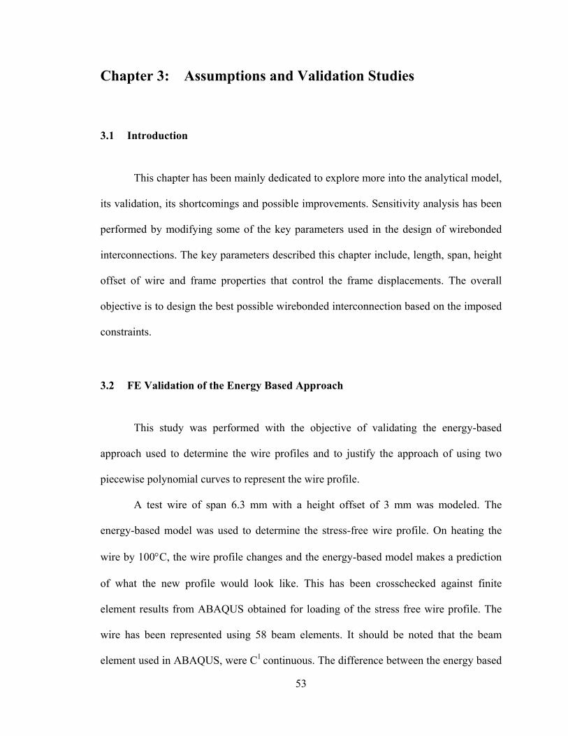
3.2 FE Validation of the Energy Based Approach
This study was performed with the objective of validating the energy-based
approach used to determine the wire profiles and to justify the approach of using two
piecewise polynomial curves to represent the wire profile.
A test wire of span 6.3 mm with a height offset of 3 mm was modeled. The
energy-based model was used to determine the stress-free wire profile. On heating the
wire by 100°C, the wire profile changes and the energy-based model makes a prediction
of what the new profile would look like. This has been crosschecked against finite
element results from ABAQUS obtained for loading of the stress free wire profile. The
wire has been represented using 58 beam elements. It should be noted that the beam
element used in ABAQUS, were C1 continuous. The difference between the energy based
53
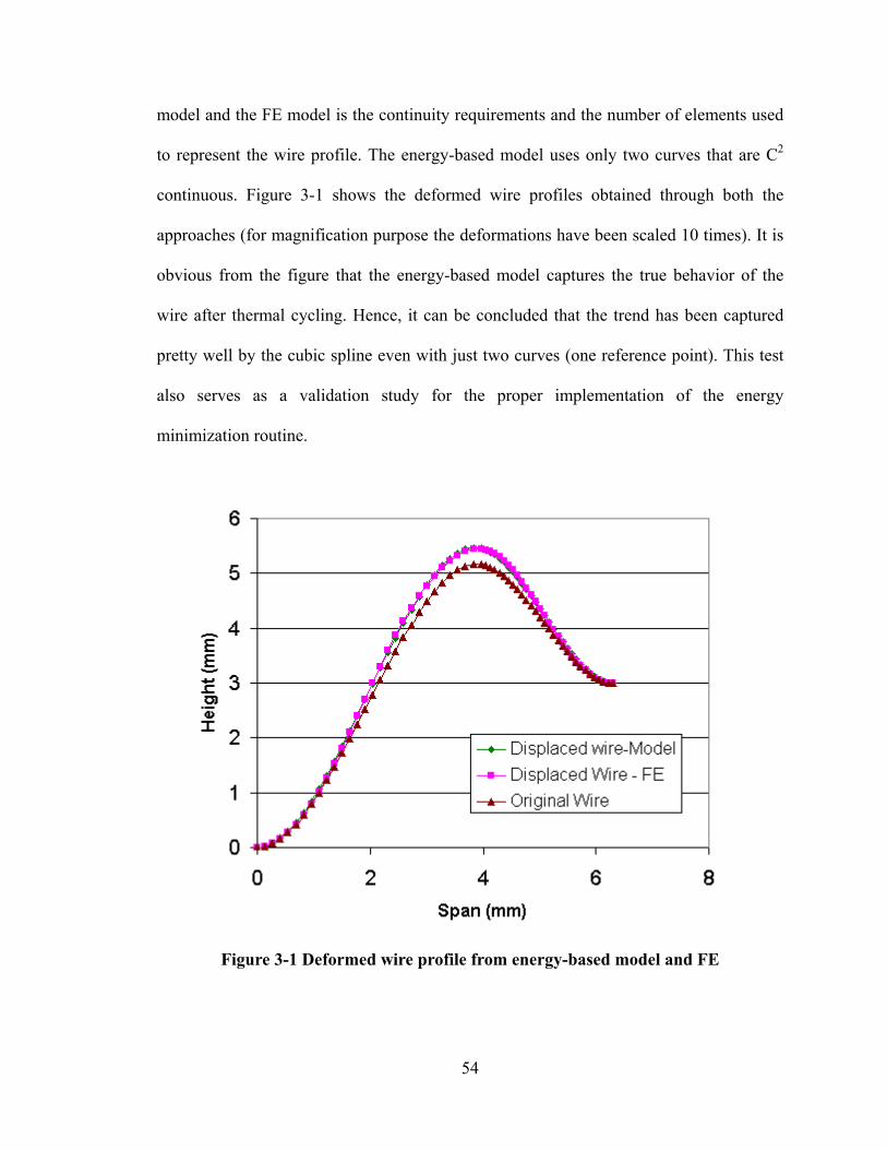
model and the FE model is the continuity requirements and the number of elements used
to represent the wire profile. The energy-based model uses only two curves that are C2
continuous. Figure 3-1 shows the deformed wire profiles obtained through both the
approaches (for magnification purpose the deformations have been scaled 10 times). It is
obvious from the figure that the energy-based model captures the true behavior of the
wire after thermal cycling. Hence, it can be concluded that the trend has been captured
pretty well by the cubic spline even with just two curves (one reference point). This test
also serves as a validation study for the proper implementation of the energy
minimization routine.
Figure 3-1 Deformed wire profile from energy-based model and FE
54
3.3 Thermal Cycling Tests
Thermal cycling experiments were conducted by means of a liquid-to-liquid
thermal shock chamber. Five modules similar to the ones shown in Figure 2-1 were
placed in a Thermal Shock Chamber to be cycled from –40° C to 125° C. The wire bonds
were assigned values 1-12 counting from left to right shown below in Figure 3-2.
Figure 3-2 Module with the bond # shown
One thermal cycle consisted of placing the modules in the cold bath for 3 minutes
to bring the module temperature to –40° C, and then transiting to the hot bath for 3
minutes to bring the modules temperature up to 125° C. The transition time between
baths was approximately 5 seconds through ambient air conditions of 25° C. The
temperature profile is shown in Figure 3-3.
55
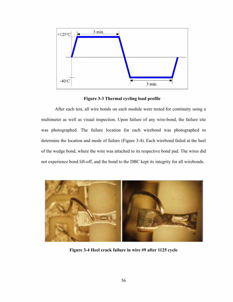
Figure 3-3 Thermal cycling load profile
After each test, all wire bonds on each module were tested for continuity using a
multimeter as well as visual inspection. Upon failure of any wire-bond, the failure site
was photographed. The failure location for each wirebond was photographed to
determine the location and mode of failure (Figure 3-4). Each wirebond failed at the heel
of the wedge bond, where the wire was attached to its respective bond pad. The wires did
not experience bond lift-off, and the bond to the DBC kept its integrity for all wirebonds.
Figure 3-4 Heel crack failure in wire #9 after 1125 cycle
56
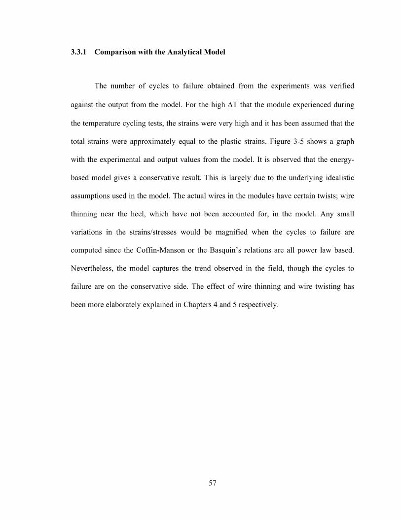
3.3.1 Comparison with the Analytical Model
The number of cycles to failure obtained from the experiments was verified
against the output from the model. For the high ∆T that the module experienced during
the temperature cycling tests, the strains were very high and it has been assumed that the
total strains were approximately equal to the plastic strains. Figure 3-5 shows a graph
with the experimental and output values from the model. It is observed that the energy-
based model gives a conservative result. This is largely due to the underlying idealistic
assumptions used in the model. The actual wires in the modules have certain twists; wire
thinning near the heel, which have not been accounted for, in the model. Any small
variations in the strains/stresses would be magnified when the cycles to failure are
computed since the Coffin-Manson or the Basquin’s relations are all power law based.
Nevertheless, the model captures the trend observed in the field, though the cycles to
failure are on the conservative side. The effect of wire thinning and wire twisting has
been more elaborately explained in Chapters 4 and 5 respectively.
57
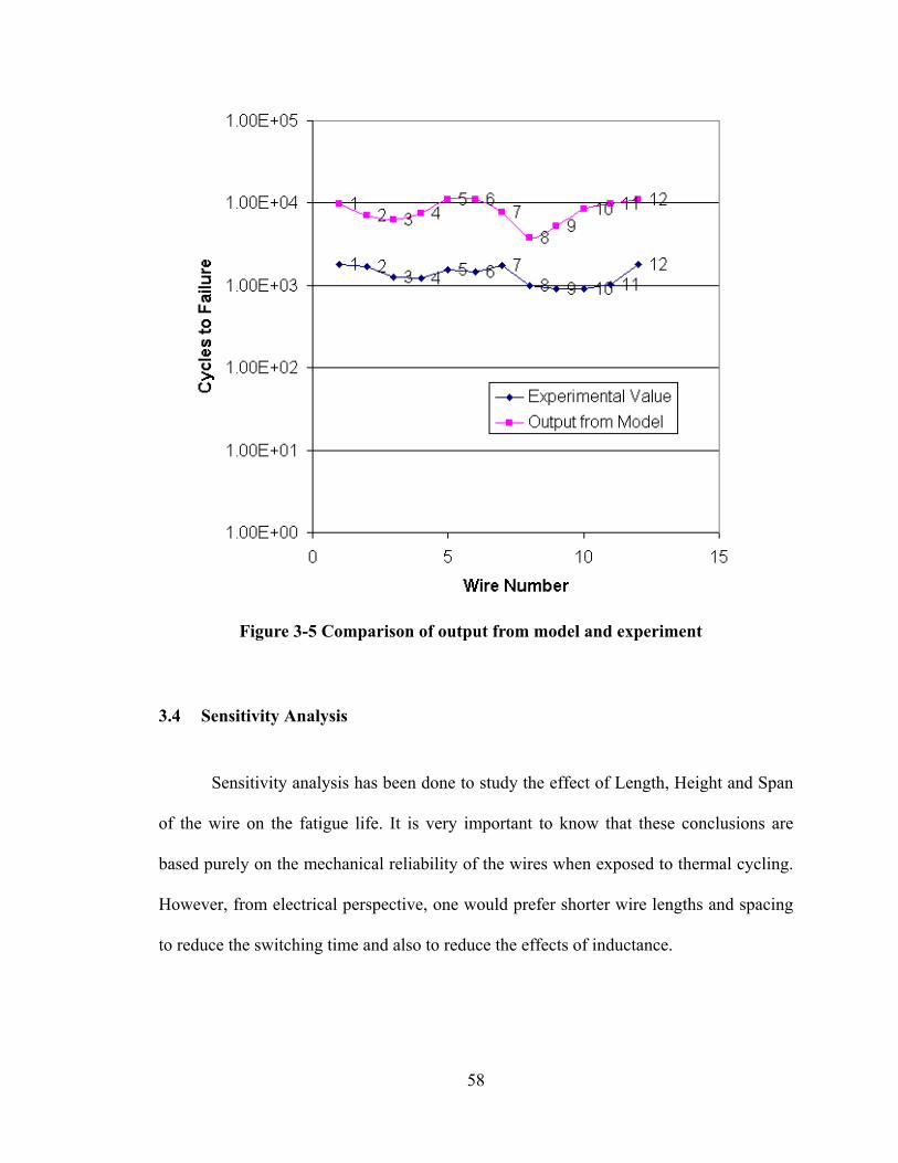
Figure 3-5 Comparison of output from model and experiment
3.4 Sensitivity Analysis
Sensitivity analysis has been done to study the effect of Length, Height and Span
of the wire on the fatigue life. It is very important to know that these conclusions are
based purely on the mechanical reliability of the wires when exposed to thermal cycling.
However, from electrical perspective, one would prefer shorter wire lengths and spacing
to reduce the switching time and also to reduce the effects of inductance.
58
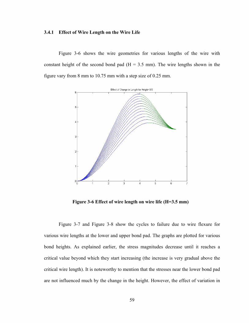
3.4.1 Effect of Wire Length on the Wire Life
Figure 3-6 shows the wire geometries for various lengths of the wire with
constant height of the second bond pad (H = 3.5 mm). The wire lengths shown in the
figure vary from 8 mm to 10.75 mm with a step size of 0.25 mm.
Figure 3-6 Effect of wire length on wire life (H=3.5 mm)
Figure 3-7 and Figure 3-8 show the cycles to failure due to wire flexure for
various wire lengths at the lower and upper bond pad. The graphs are plotted for various
bond heights. As explained earlier, the stress magnitudes decrease until it reaches a
critical value beyond which they start increasing (the increase is very gradual above the
critical wire length). It is noteworthy to mention that the stresses near the lower bond pad
are not influenced much by the change in the height. However, the effect of variation in
59
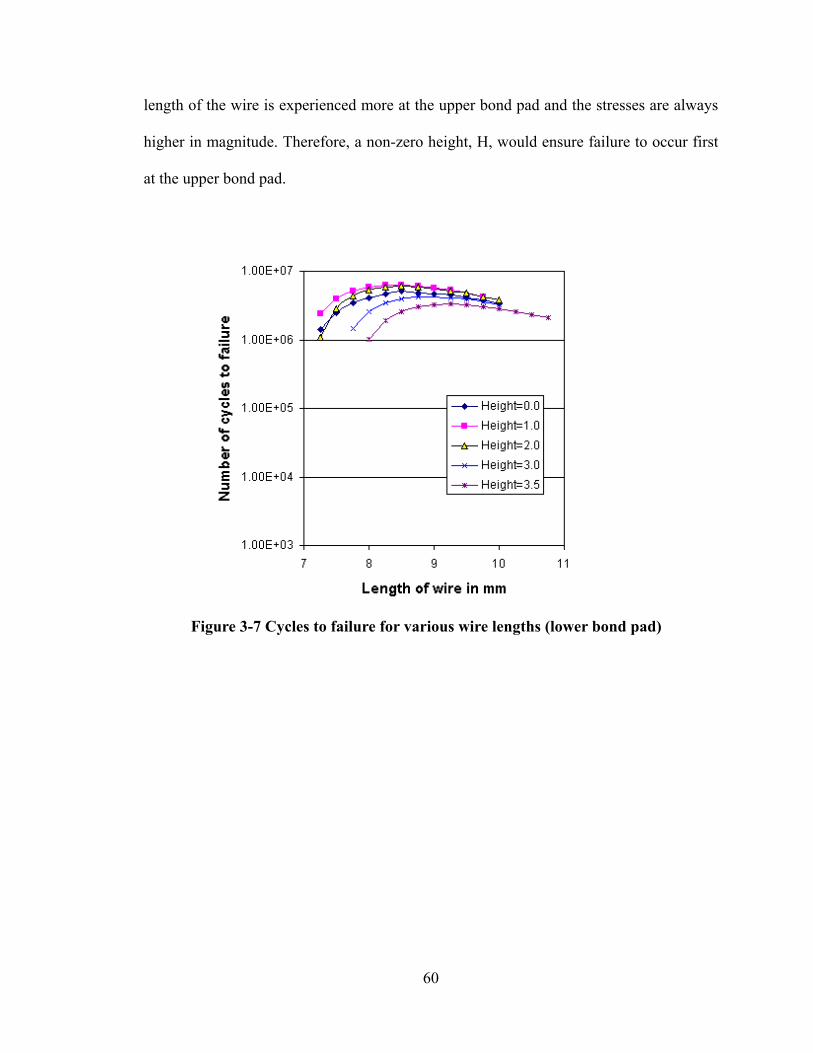
length of the wire is experienced more at the upper bond pad and the stresses are always
higher in magnitude. Therefore, a non-zero height, H, would ensure failure to occur first
at the upper bond pad.
Figure 3-7 Cycles to failure for various wire lengths (lower bond pad)
60
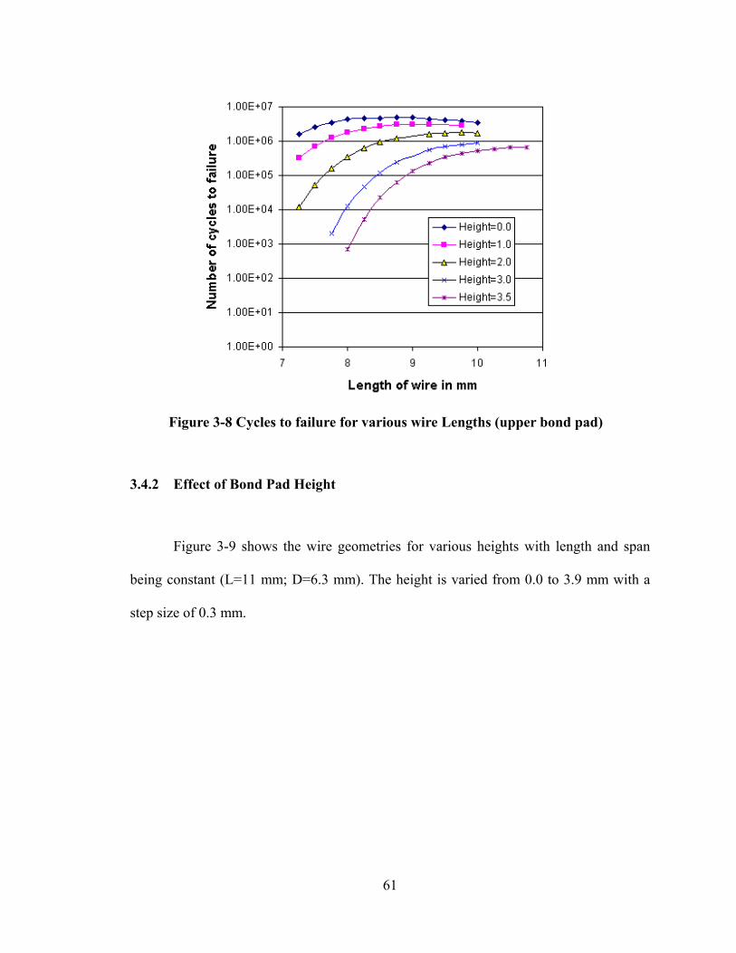
Figure 3-8 Cycles to failure for various wire Lengths (upper bond pad)
3.4.2 Effect of Bond Pad Height
Figure 3-9 shows the wire geometries for various heights with length and span
being constant (L=11 mm; D=6.3 mm). The height is varied from 0.0 to 3.9 mm with a
step size of 0.3 mm.
61
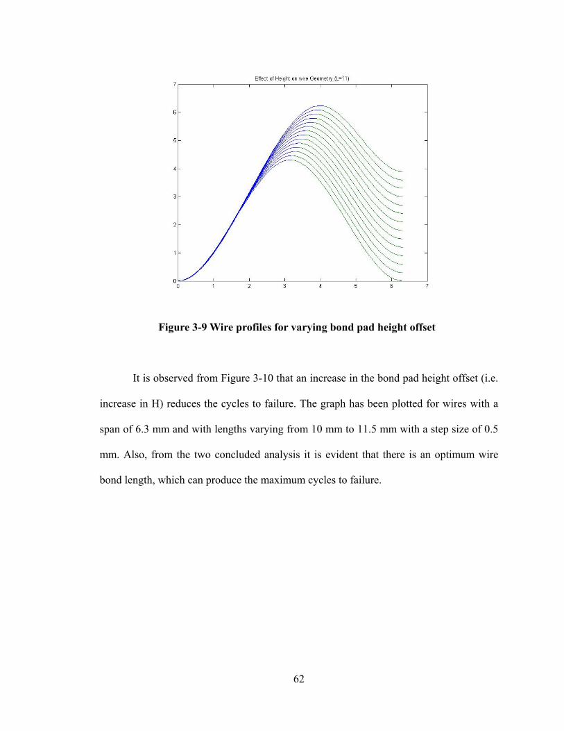
Figure 3-9 Wire profiles for varying bond pad height offset
It is observed from Figure 3-10 that an increase in the bond pad height offset (i.e.
increase in H) reduces the cycles to failure. The graph has been plotted for wires with a
span of 6.3 mm and with lengths varying from 10 mm to 11.5 mm with a step size of 0.5
mm. Also, from the two concluded analysis it is evident that there is an optimum wire
bond length, which can produce the maximum cycles to failure.
62
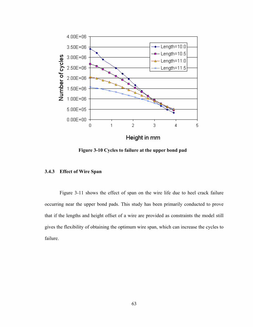
Figure 3-10 Cycles to failure at the upper bond pad
3.4.3 Effect of Wire Span
Figure 3-11 shows the effect of span on the wire life due to heel crack failure
occurring near the upper bond pads. This study has been primarily conducted to prove
that if the lengths and height offset of a wire are provided as constraints the model still
gives the flexibility of obtaining the optimum wire span, which can increase the cycles to
failure.
63
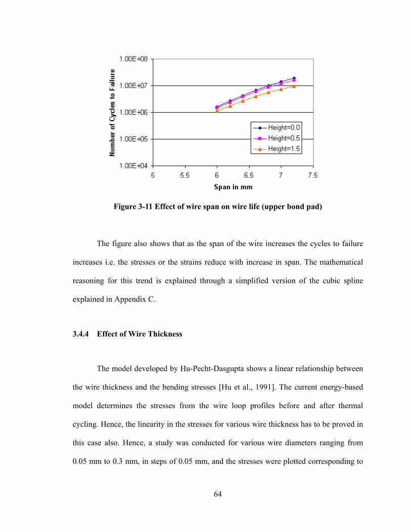
Figure 3-11 Effect of wire span on wire life (upper bond pad)
The figure also shows that as the span of the wire increases the cycles to failure
increases i.e. the stresses or the strains reduce with increase in span. The mathematical
reasoning for this trend is explained through a simplified version of the cubic spline
explained in Appendix C.
3.4.4 Effect of Wire Thickness
The model developed by Hu-Pecht-Dasgupta shows a linear relationship between
the wire thickness and the bending stresses [Hu et al., 1991]. The current energy-based
model determines the stresses from the wire loop profiles before and after thermal
cycling. Hence, the linearity in the stresses for various wire thickness has to be proved in
this case also. Hence, a study was conducted for various wire diameters ranging from
0.05 mm to 0.3 mm, in steps of 0.05 mm, and the stresses were plotted corresponding to
64
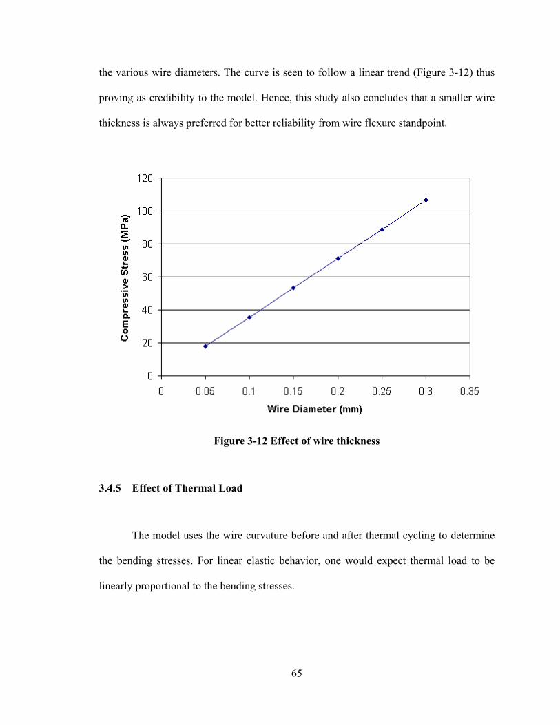
the various wire diameters. The curve is seen to follow a linear trend (Figure 3-12) thus
proving as credibility to the model. Hence, this study also concludes that a smaller wire
thickness is always preferred for better reliability from wire flexure standpoint.
Figure 3-12 Effect of wire thickness
3.4.5 Effect of Thermal Load
The model uses the wire curvature before and after thermal cycling to determine
the bending stresses. For linear elastic behavior, one would expect thermal load to be
linearly proportional to the bending stresses.
65
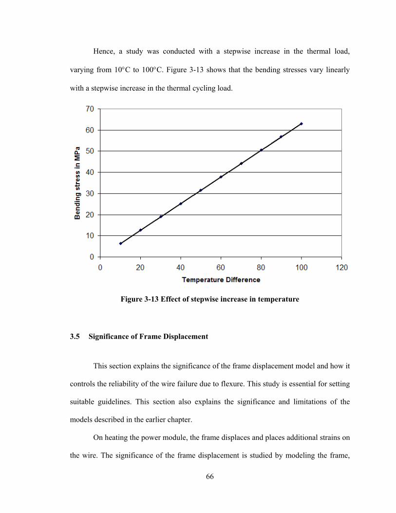
Hence, a study was conducted with a stepwise increase in the thermal load,
varying from 10°C to 100°C. Figure 3-13 shows that the bending stresses vary linearly
with a stepwise increase in the thermal cycling load.
Figure 3-13 Effect of stepwise increase in temperature
3.5 Significance of Frame Displacement
This section explains the significance of the frame displacement model and how it
controls the reliability of the wire failure due to flexure. This study is essential for setting
suitable guidelines. This section also explains the significance and limitations of the
models described in the earlier chapter.
On heating the power module, the frame displaces and places additional strains on
the wire. The significance of the frame displacement is studied by modeling the frame,
66
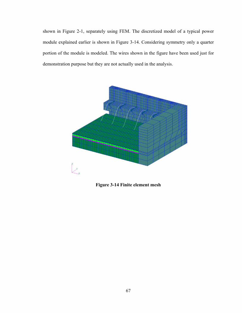
shown in Figure 2-1, separately using FEM. The discretized model of a typical power
module explained earlier is shown in Figure 3-14. Considering symmetry only a quarter
portion of the module is modeled. The wires shown in the figure have been used just for
demonstration purpose but they are not actually used in the analysis.
Figure 3-14 Finite element mesh
67
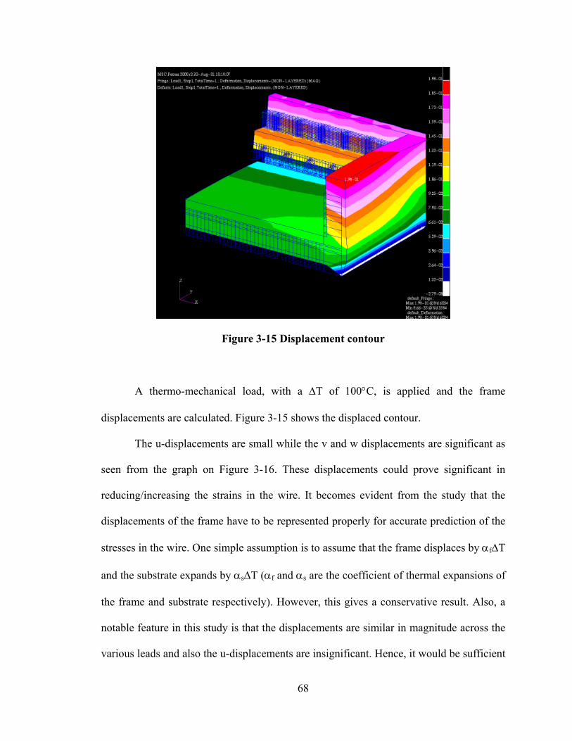
Figure 3-15 Displacement contour
A thermo-mechanical load, with a ∆T of 100°C, is applied and the frame
displacements are calculated. Figure 3-15 shows the displaced contour.
The u-displacements are small while the v and w displacements are significant as
seen from the graph on Figure 3-16. These displacements could prove significant in
reducing/increasing the strains in the wire. It becomes evident from the study that the
displacements of the frame have to be represented properly for accurate prediction of the
stresses in the wire. One simple assumption is to assume that the frame displaces by αf∆T
and the substrate expands by αs∆T (αf and αs are the coefficient of thermal expansions of
the frame and substrate respectively). However, this gives a conservative result. Also, a
notable feature in this study is that the displacements are similar in magnitude across the
various leads and also the u-displacements are insignificant. Hence, it would be sufficient
68
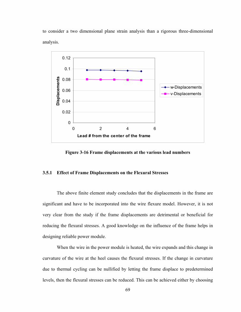
to consider a two dimensional plane strain analysis than a rigorous three-dimensional
analysis.
0
0.02
0.04
0.06
0.08
0.1
0.12
0 2 4 6
Lead # from the center of the frame
Dis
plac
emen
ts
w-Displacementsv-Displacements
Figure 3-16 Frame displacements at the various lead numbers
3.5.1 Effect of Frame Displacements on the Flexural Stresses
The above finite element study concludes that the displacements in the frame are
significant and have to be incorporated into the wire flexure model. However, it is not
very clear from the study if the frame displacements are detrimental or beneficial for
reducing the flexural stresses. A good knowledge on the influence of the frame helps in
designing reliable power module.
When the wire in the power module is heated, the wire expands and this change in
curvature of the wire at the heel causes the flexural stresses. If the change in curvature
due to thermal cycling can be nullified by letting the frame displace to predetermined
levels, then the flexural stresses can be reduced. This can be achieved either by choosing
69
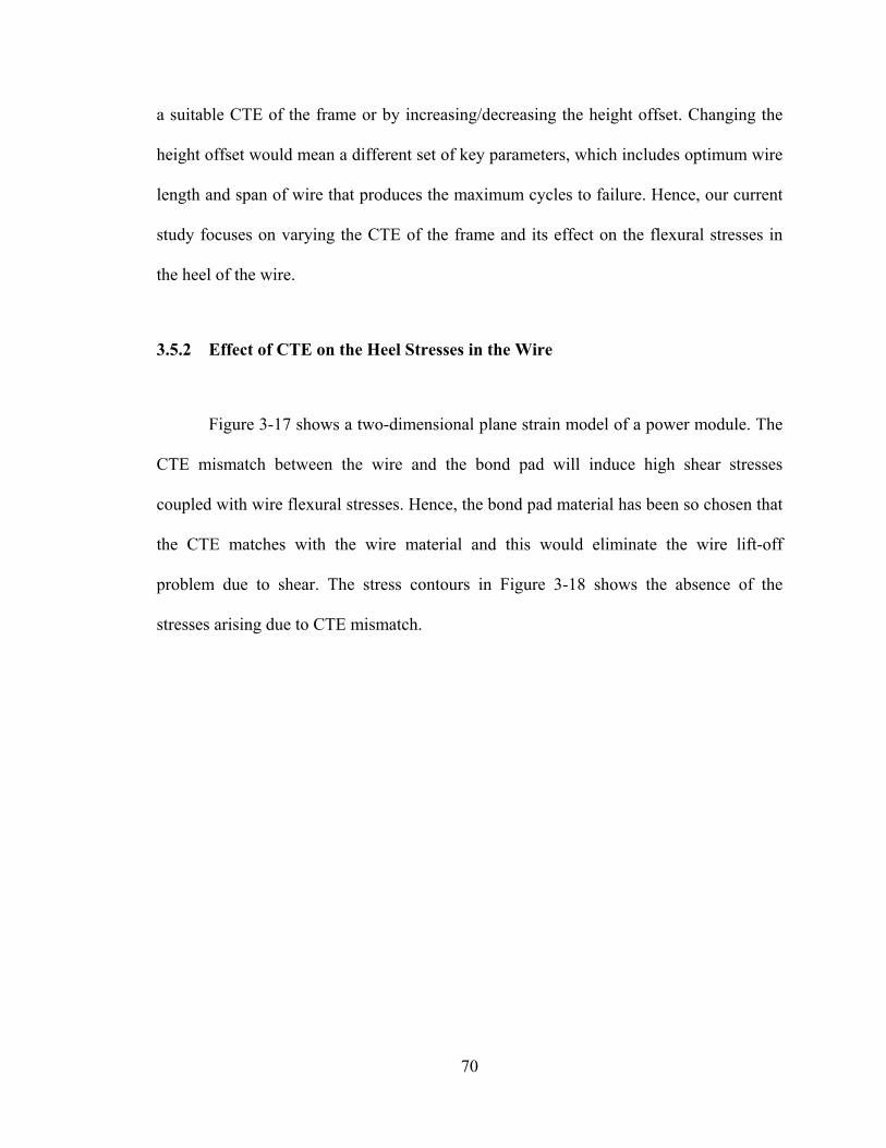
a suitable CTE of the frame or by increasing/decreasing the height offset. Changing the
height offset would mean a different set of key parameters, which includes optimum wire
length and span of wire that produces the maximum cycles to failure. Hence, our current
study focuses on varying the CTE of the frame and its effect on the flexural stresses in
the heel of the wire.
3.5.2 Effect of CTE on the Heel Stresses in the Wire
Figure 3-17 shows a two-dimensional plane strain model of a power module. The
CTE mismatch between the wire and the bond pad will induce high shear stresses
coupled with wire flexural stresses. Hence, the bond pad material has been so chosen that
the CTE matches with the wire material and this would eliminate the wire lift-off
problem due to shear. The stress contours in Figure 3-18 shows the absence of the
stresses arising due to CTE mismatch.
70
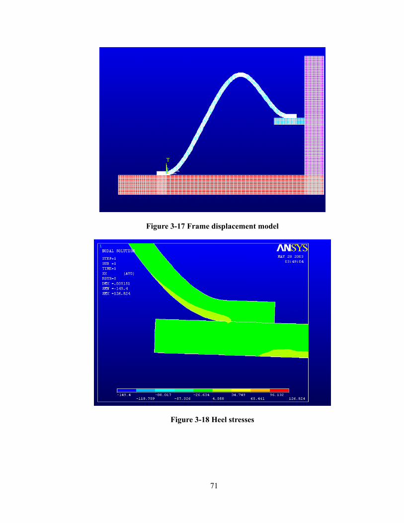
Figure 3-17 Frame displacement model
Figure 3-18 Heel stresses
71
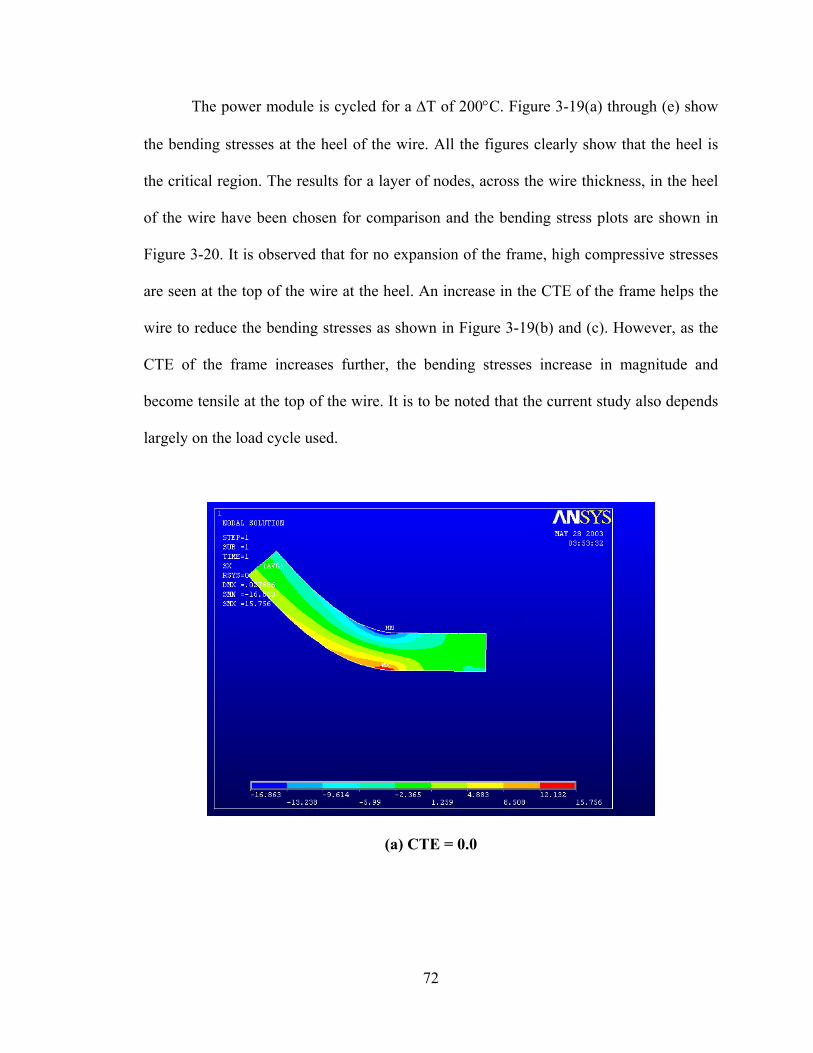
The power module is cycled for a ∆T of 200°C. Figure 3-19(a) through (e) show
the bending stresses at the heel of the wire. All the figures clearly show that the heel is
the critical region. The results for a layer of nodes, across the wire thickness, in the heel
of the wire have been chosen for comparison and the bending stress plots are shown in
Figure 3-20. It is observed that for no expansion of the frame, high compressive stresses
are seen at the top of the wire at the heel. An increase in the CTE of the frame helps the
wire to reduce the bending stresses as shown in Figure 3-19(b) and (c). However, as the
CTE of the frame increases further, the bending stresses increase in magnitude and
become tensile at the top of the wire. It is to be noted that the current study also depends
largely on the load cycle used.
(a) CTE = 0.0
72
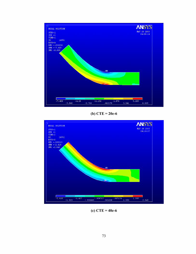
(b) CTE = 20e-6
(c) CTE = 40e-6
73
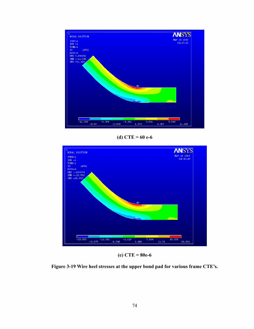
(d) CTE = 60 e-6
(e) CTE = 80e-6
Figure 3-19 Wire heel stresses at the upper bond pad for various frame CTE’s.
74
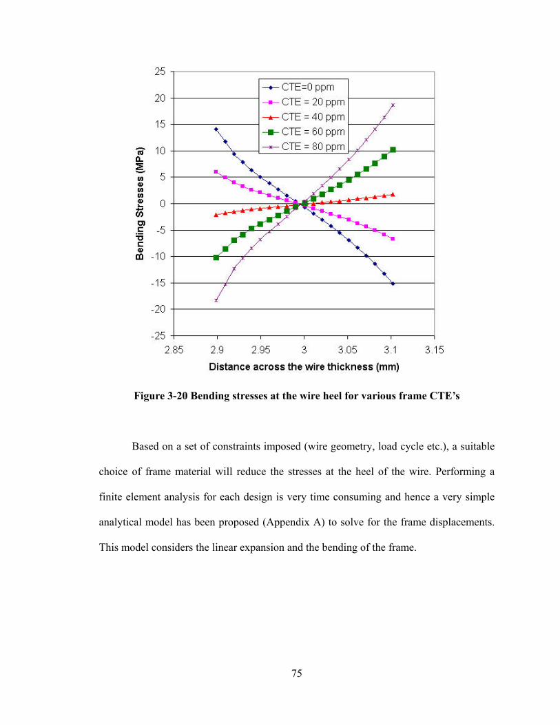
Figure 3-20 Bending stresses at the wire heel for various frame CTE’s
Based on a set of constraints imposed (wire geometry, load cycle etc.), a suitable
choice of frame material will reduce the stresses at the heel of the wire. Performing a
finite element analysis for each design is very time consuming and hence a very simple
analytical model has been proposed (Appendix A) to solve for the frame displacements.
This model considers the linear expansion and the bending of the frame.
75
3.6 Model Assumptions
The model assumes that the manufacturing process is perfect and no additional
stresses are placed due to the manufacturing process. The manufacturing errors include
the cracking caused at the heel of the wire due to the tool motion and bonding machine
vibration. Residual stresses induced during the bond formation will not be critical for low
cycle fatigue problems (less than 104 cycles) for the aluminum wire chosen in the study.
However, if other materials are chosen, the SN curve should be re-plotted to study the
effects of residual stresses on fatigue cycling.
The model determines the most stable configuration that a wire would prefer to
occupy before and after the load cycle. Based on the change in curvature during these two
states before and after thermal cycling the strains are obtained. However, not all the wires
are bonded with the minimum energy wire profile and these are sometimes governed by
the applications and limitations of the geometry of the power modules. However,
pronounced thermal cycling will result in the wire trying to attain a stable configuration
after sufficient number of thermal cycles.
The model is very accurate for an idealistically bonded wire and when it is loaded
elastically. However, for plastic deformation of the wire, the loading has to be applied
gradually and the strains have to be decoupled into elastic and plastic strains. All the
wires in the power modules considered in the study failed in less than 3000 cycles.
Hence, the bending strains, which hold good even for plastic deformation, have been
assumed to be equal to the total strains. The life cycle prediction has been based on these
assumption of strains.
76
During the loop formation in wedge bonding, the movement of the axis of the
bonding wedge feed hole is usually aligned with the center line of the first bond, so that
the wire can be fed freely through the hole in the wedge. The width offset between the
bond places additional strains in the wire. In addition, the model assumes there is no wire
thinning near the bonding locations. The strains have been calculated based on the theory
of pure bending of curved beams. The Euler-Bernoulli equations derived in Chapter 2 are
valid only for the local model and cease to exist near the reduced cross section of the wire
(caused by wire thinning). There is an additional moment/shear force acting in the
reduced cross section of the wire. This influence can be introduced by means of a stress
concentration parameter, Ks. Ks accounts for the effects of wire thinning and twisting.
The determination of Ks for the wires used in the study is explained in Chapter 4.
The minimum energy wire profiles determined by the model could be used by
commercial finite element codes to solve for the bending stresses. Also, these finite
element codes add the additional flexibility of including the effects of wire thinning near
the heel by suitable modification of the geometry. The solution time for an elastic loading
of a thermomechanical load for a discretized two dimensional model is very small,
depending on the number of nodes and degrees of freedom. However, sufficient time is
involved in modeling and meshing these complicated geometries. To avoid the huge
modeling time, an automated program has been written to generate the ANSYS log files.
This approach has been implemented to generate 3D wire profiles in Chapters 4 and 5.
The analytical model is preferred over the analytical model for checking reliability of
existing designs, since it can more accurately model the wire thinning effects. However,
77
the pure first order physics of failure based model is preferable to derive suitable
guidelines and also to determine the optimum geometric parameters.
3.6.1 Further Limitations, if using the Hermite Interpolation Scheme
As explained earlier, the hermite interpolation model explained in the previous
chapter, has a C1 continuity and hence lesser accuracy. For better accuracy with a hermite
interpolation scheme, more reference points are needed, which increases the
computational time. Also, the hermite interpolation model is based on the user providing
the details about the point that defines the loop height (point 2 shown in Figure 2-2).
Most of the time, it is very difficult to obtain these details from the actual power module.
In addition, thermal cycling can always result in the wire profile taking a new
configuration after a few load cycles. Hence, a study was conducted to observe the
sensitivity of the model to small variations in the location of the reference point 2. This
dependence on the outputs is seen in Figure 3-21. From a design point of view, the model
seems appropriate when the point is defined within +/-0.5 mm. However, this is problem
dependent i.e. depends on the wire length, span, height and load applied.
Figure 3-22 shows the life as a function of wire span. The effect of variation in
the reference point (point 2 shown in Figure 2-2) to the life has also been plotted in
Figure 3-22. Considering these drawbacks, the hermite interpolation scheme in spite of its
simplicity was not preferred, unless the user had accurate loop height information.
78
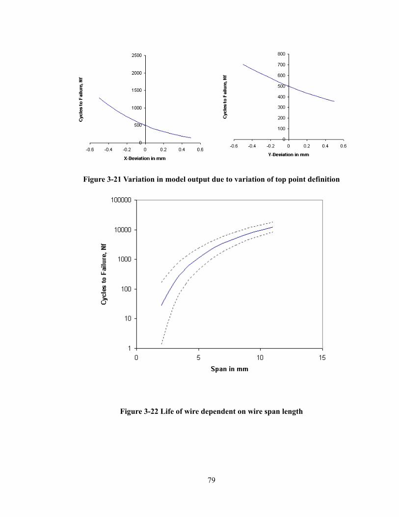
Figure 3-21 Variation in model output due to variation of top point definition
Figure 3-22 Life of wire dependent on wire span length
79

3.6.2 Disadvantages of the CUBIC Interpolation Scheme
The cubic interpolation scheme was found to be much more accurate in
comparison to the Hermite interpolation scheme. The model is certainly useful in
providing guidelines about the important parameters that influence the reliability of the
wirebonded connections. The main disadvantage with the energy-based cubic spline is
the computation time involved in trying to minimize the strain energy. The solution
process involves numerical differentiation, integration and a numerical solver
(Levenberg-Marquardt Algorithm) for solving a set of non-linear equations. This process
has to be repeated for the configuration of the wire before and after heating. Appendix C
provides a much simpler and quicker version of the model.
80
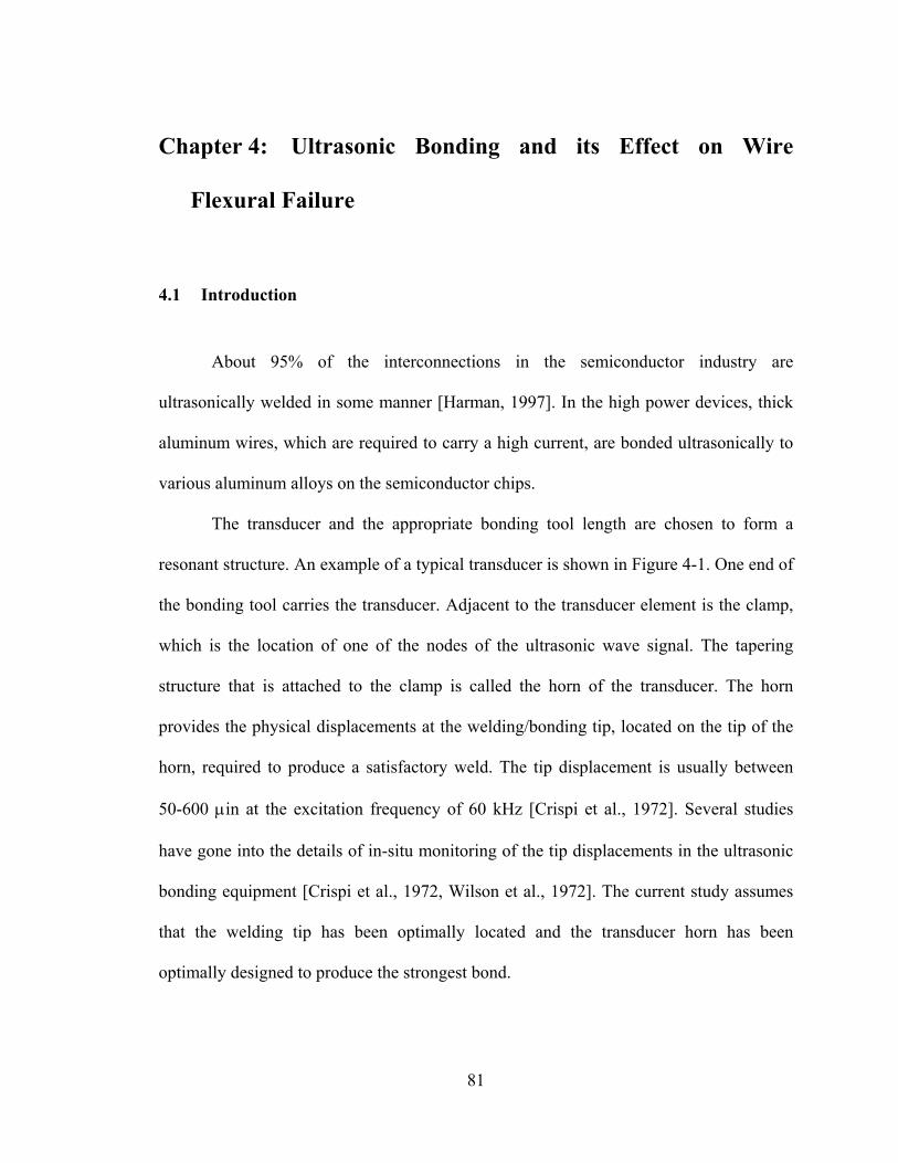
Chapter 4: Ultrasonic Bonding and its Effect on Wire
Flexural Failure
4.1 Introduction
About 95% of the interconnections in the semiconductor industry are
ultrasonically welded in some manner [Harman, 1997]. In the high power devices, thick
aluminum wires, which are required to carry a high current, are bonded ultrasonically to
various aluminum alloys on the semiconductor chips.
The transducer and the appropriate bonding tool length are chosen to form a
resonant structure. An example of a typical transducer is shown in Figure 4-1. One end of
the bonding tool carries the transducer. Adjacent to the transducer element is the clamp,
which is the location of one of the nodes of the ultrasonic wave signal. The tapering
structure that is attached to the clamp is called the horn of the transducer. The horn
provides the physical displacements at the welding/bonding tip, located on the tip of the
horn, required to produce a satisfactory weld. The tip displacement is usually between
50-600 µin at the excitation frequency of 60 kHz [Crispi et al., 1972]. Several studies
have gone into the details of in-situ monitoring of the tip displacements in the ultrasonic
bonding equipment [Crispi et al., 1972, Wilson et al., 1972]. The current study assumes
that the welding tip has been optimally located and the transducer horn has been
optimally designed to produce the strongest bond.
81
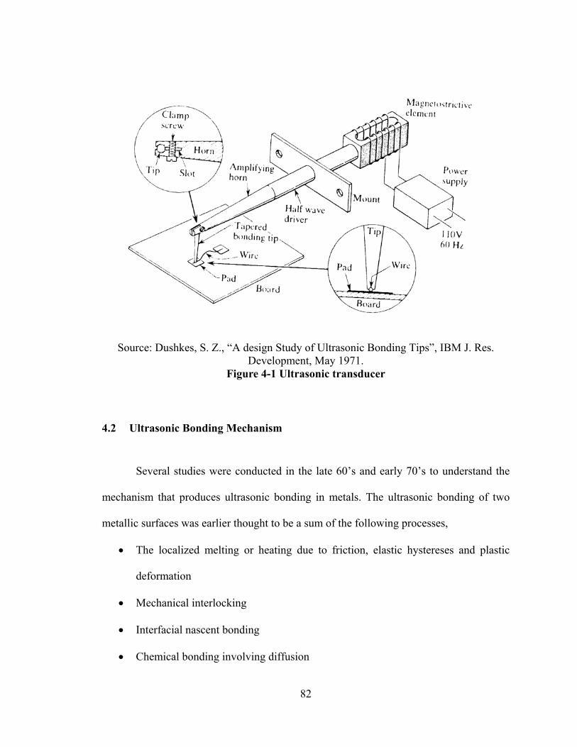
Source: Dushkes, S. Z., “A design Study of Ultrasonic Bonding Tips”, IBM J. Res. Development, May 1971.
Figure 4-1 Ultrasonic transducer
4.2 Ultrasonic Bonding Mechanism
Several studies were conducted in the late 60’s and early 70’s to understand the
mechanism that produces ultrasonic bonding in metals. The ultrasonic bonding of two
metallic surfaces was earlier thought to be a sum of the following processes,
• The localized melting or heating due to friction, elastic hystereses and plastic
deformation
• Mechanical interlocking
• Interfacial nascent bonding
• Chemical bonding involving diffusion
82
The role of heat in ultrasonic bond formation raised several controversies. It was
earlier thought that high temperature was necessary for the ultrasonic welds; however, it
was proved that the heat associated with rubbing was due to non-optimum bonding
parameters [Joshi, 1971 and Harman et al., 1972]. A low clamping force would
eventually result in interfacial sliding thus causing a rise in temperature. Joshi had
observed that the temperature readings during the bonding process were less than 70°C,
based on readings from a thermocouple. The absence of heat-affected zones and
intermetallic compounds in the study also suggested that there was no significant heating.
Also, Harman and Leedy [Harman et al., 1972] had successfully made strong bonds in a
atmosphere of liquid nitrogen.
In order to study the relative motion between the tool, wire and substrate, Joshi
[Joshi, 1971] used a specifically designed laser interferometer. He found that the
amplitude of motion of the tool tip, wire and substrate quickly attain a value and remain
constant during the entire bonding process. Hence, his study concluded that there was no
relative motion between the wire and the substrate.
Ultrasonic stress waves force dislocations to oscillate with amplitudes comparable
to distances between their equilibrium positions when no ultrasonic field is applied.
[Langenecker, 1966]. Pronounced plasticity is seen to occur in metals. Large scale
forming process and strengthening of materials occur as a result of ultrasonic treatment.
The following non-linear effects can be observed in a metal exposed to ultrasonic
irradiation,
• Acoustic softening
• Acoustic hardening
83
The acoustic irradiation reduces the apparent static stress necessary for plastic
deformation. Hardening occurs after ultrasonic irradiation. Langenecker had shown the
similarity between stress elongation curves in aluminum resulting from ultrasonic
irradiation at constant temperature to equivalent elongations arising due to the application
of heat (Figure 4-2). In his study, high purity aluminum crystals were exposed to
ultrasonic irradiation at 20 kHz at various power levels at 18°C.
Source: Langenecker, “Effects of Ultrasound on Deformation Characteristics of Metals”, IEEE Transactions on Sonics and Ultrasonics
Figure 4-2 Stress vs. elongation for aluminum crystals
This softening mechanism was observed in several other metals like, Cd, Fe, Ti
and W. It was concluded that the acoustic softening takes place when the metal is
subjected to ultrasonic irradiation.
The stress vs. elongation was essentially equivalent to deformation under a
compressive load. It was concluded from the study that either heat or ultrasound would
produce equivalent deformation. However, apart from the similarity in displacements,
84
there are several differences between the processes. The ultrasonic energy density
required to produce deformation in aluminum with no applied stress is 107 eV/cm3 times
lesser in magnitude in comparison to a sample subjected to thermal energy producing
equivalent deformation.
Acoustic energy was assumed to be absorbed at those regions in the metal lattice,
which are known to carry out mechanisms of plastic deformation (e.g. grain boundary
and dislocations). Ultrasound is presumably propagated through the metal by phonons, a
quantized mode of vibration occurring in a rigid crystal lattice. These phonons give up
most of their energy to crystallographic defects. In contrast, the thermal energy
distributes rather homogenously among all atoms of the crystal including those that do
not participate in the plastic deformation. Hence, deformation through plastic
deformation by thermal energy is less efficient in comparison with ultrasonic irradiation.
It is to be noted that Langenecker’s studied only the softening of metals and metal
forming when exposed to ultrasonic irradiation and not the ultrasonic bonding or welding
process.
Joshi [Joshi, 1971] conducted further studies to develop an understanding on how
metal-to-metal ultrasonic bonds were made. He observed that localized deformation
occurs on favorably oriented grains on both sides of the interface and joining occurs on
certain matching areas. In Al-Al bonds, the interface disappears completely leaving
behind a structural pattern that indicates a gross flow of metals. The features of the
interface are characterized by lack of work hardening and diffusion. Bonding in
dissimilar materials occurs by extensive mechanical interlocking and deformation. The
softer material flows around the topography of the harder material. Hence, the ultrasonic
85
bonding process can be summarized as seizure through atomic attraction, and sometimes
by mechanical interlocking once intimate contact is developed due to softening on both
sides of the interface. Also, ultrasonic bonding is a process where deformation and
recrystallization proceed concomitantly [Joshi, 1971]. The high energy densities during
bonding results in strains being annealed continually thus leaving a strain free interface.
This theory was also supported by the fact that intense acoustic oscillations caused a large
increase in recrystallization kinetics of copper [Hayes et al., 1969]. Evidence of
concomitant deformation and recrystallization during bonding process was also supported
by studies by Krzanowski [Krzanowski, 1990]. In that study, transmission electron
microscopy (TEM) was used to examine ultrasonic bonding of aluminum wire to various
metal substrates. The growth process of aluminum crystals due to thermal cycling was
later studied by Ohga [Ohga, 1991]. He observed that crystal growth was not found near
the bonding points of the aluminum wire suggesting less damage was done during the
wire bonding process. However, the reduced cross-section with the constraint would
result in the heel section acting like a stress-raiser.
4.3 Bond Formation Patterns
The footprints that remain after the bond is lifted off were studied to better
understand the contact mechanism. The lift-off patterns represent the best method of
studying the early stages of the bond formation. The wire-to-bond pad micro-welds were
formed at points near the perimeter [Harman et al., 1972, Harman 1997, Ramminger et
al., 2003, Wu et al., 1995]. The weld formation always begins around the perimeter and
as the welding time increases the welded area grows inwards. Krzanowski [Krzanowski,
86
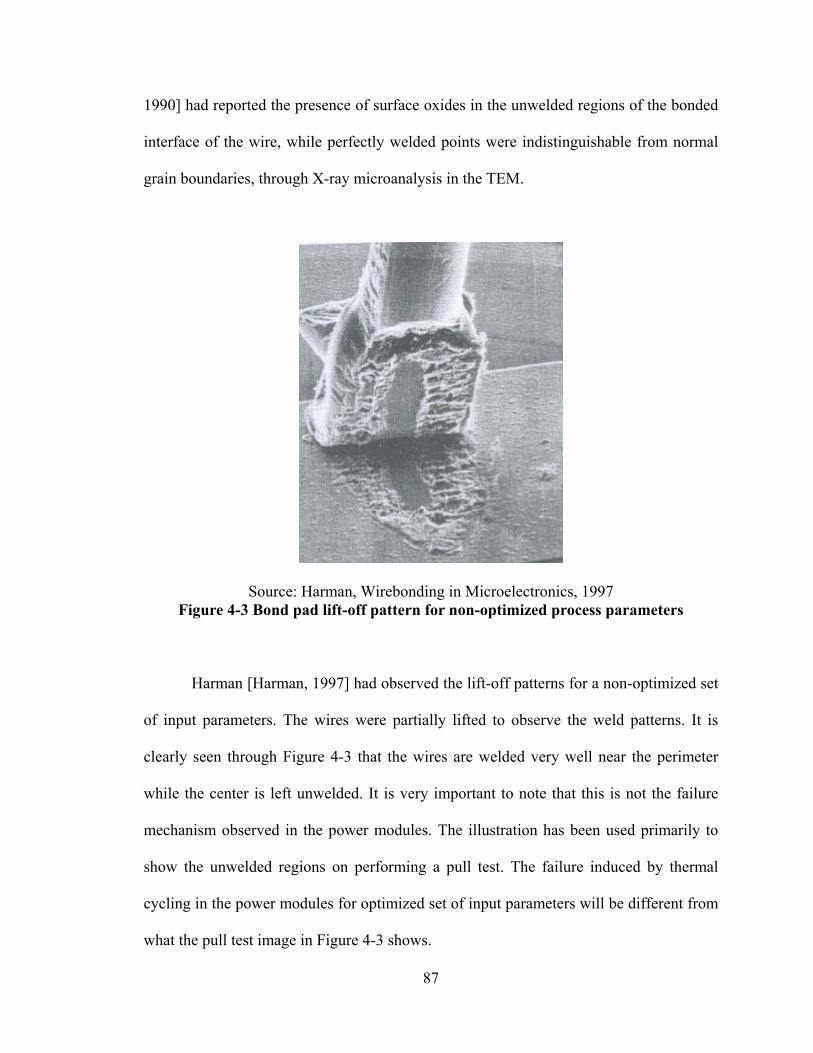
1990] had reported the presence of surface oxides in the unwelded regions of the bonded
interface of the wire, while perfectly welded points were indistinguishable from normal
grain boundaries, through X-ray microanalysis in the TEM.
Source: Harman, Wirebonding in Microelectronics, 1997 Figure 4-3 Bond pad lift-off pattern for non-optimized process parameters
Harman [Harman, 1997] had observed the lift-off patterns for a non-optimized set
of input parameters. The wires were partially lifted to observe the weld patterns. It is
clearly seen through Figure 4-3 that the wires are welded very well near the perimeter
while the center is left unwelded. It is very important to note that this is not the failure
mechanism observed in the power modules. The illustration has been used primarily to
show the unwelded regions on performing a pull test. The failure induced by thermal
cycling in the power modules for optimized set of input parameters will be different from
what the pull test image in Figure 4-3 shows.
87
One of the explanations for this perimeter bonding is the fact that the softening
effect plays an important role in dispersing the surface oxide film and contaminant from
the perimeter. The removal of surface oxides is very essential for a strong bond. In the
initial phase of the wirebonding process, the wire is pressed onto the substrate and the
surface oxide layer is broken up effectively at the points of high plastic deformation.
Little deformation takes place in the center, leaving the surface oxides and eventually
leaving this area unwelded. The perimeter welding in well-made microelectronic bonds
seem to be related to the bonding machine, tool shape and the bonding schedule [Harman
et al., 1977].
4.4 Wire Bond Process Parameters
The wire bonding process depends on many parameters, of which the critical ones
are shape of the bonding head, ultrasonic power, bonding force and the bonding time.
Heat is an additional factor for ball bonding.
The wire is positioned under the bond foot of the wedge via the hole (Figure 4-4),
and the tool comes down on top of the wire with a pre-determined force. Ultrasonic
energy is transmitted to the wire through the tool, as soon as contact is established. As
explained earlier, the intensity of the ultrasonic power governs the softening of the wires.
For a good bond to be created, the tool must be effective in transmitting the ultrasonic
energy down through the wire. There are several profiles of the groove edges commonly
used for large bonding wires [SPT catalogue, 1996], which include concave, inline
groove, “V” groove and Deep “V” groove designs (Figure 4-5). The V-Groove is the
more prevalent design in the large bonding wires. Hence, in this thesis the tool profiles
88
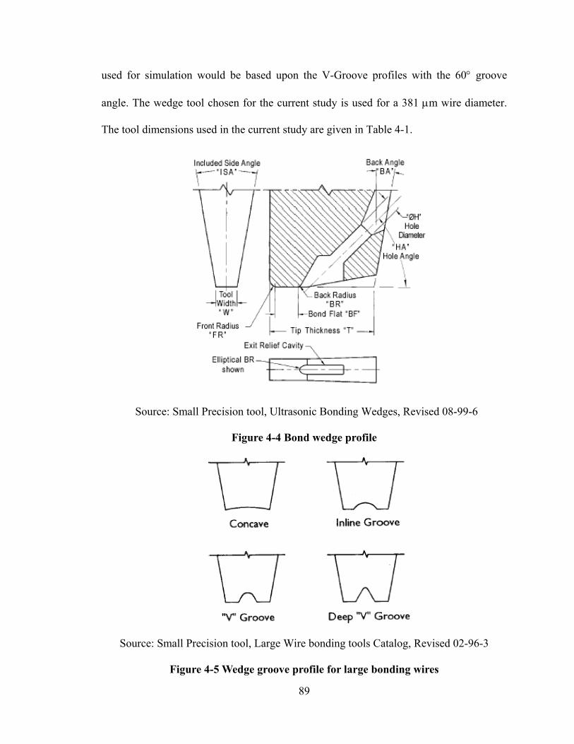
used for simulation would be based upon the V-Groove profiles with the 60° groove
angle. The wedge tool chosen for the current study is used for a 381 µm wire diameter.
The tool dimensions used in the current study are given in Table 4-1.
Source: Small Precision tool, Ultrasonic Bonding Wedges, Revised 08-99-6
Figure 4-4 Bond wedge profile
Source: Small Precision tool, Large Wire bonding tools Catalog, Revised 02-96-3
Figure 4-5 Wedge groove profile for large bonding wires
89
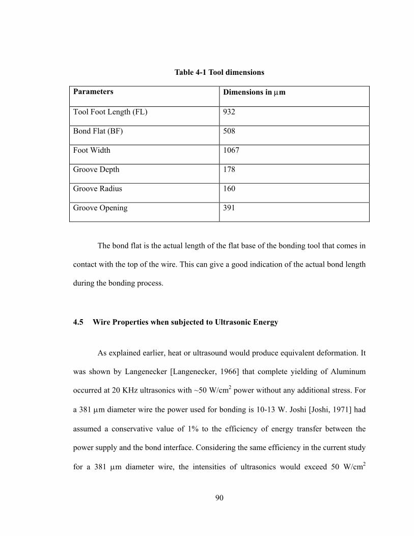
Table 4-1 Tool dimensions
Parameters Dimensions in µm
Tool Foot Length (FL) 932
Bond Flat (BF) 508
Foot Width 1067
Groove Depth 178
Groove Radius 160
Groove Opening 391
The bond flat is the actual length of the flat base of the bonding tool that comes in
contact with the top of the wire. This can give a good indication of the actual bond length
during the bonding process.
4.5 Wire Properties when subjected to Ultrasonic Energy
As explained earlier, heat or ultrasound would produce equivalent deformation. It
was shown by Langenecker [Langenecker, 1966] that complete yielding of Aluminum
occurred at 20 KHz ultrasonics with ~50 W/cm2 power without any additional stress. For
a 381 µm diameter wire the power used for bonding is 10-13 W. Joshi [Joshi, 1971] had
assumed a conservative value of 1% to the efficiency of energy transfer between the
power supply and the bond interface. Considering the same efficiency in the current study
for a 381 µm diameter wire, the intensities of ultrasonics would exceed 50 W/cm2
90
(assuming the area of contact to be a product of wire diameter x bond flat). Since it was
impractical to simulate the real ultrasonic bonding process considering all the
complications explained earlier, heat that would produce an equivalent effect was used
instead. For this purpose, the material properties of the wire were determined at 500°C.
At this high temperature, the stress elongation behavior of the material would be
equivalent to the properties of the wire when exposed to ultrasonic power of 10 W.
Figure 4-6 shows the stress-strain curves of the aluminum wire measured at room
and high temperatures. It is observed that at 500°C extreme softening of the metal occurs.
Figure 4-7 shows the modulus of the wire at various temperatures. It is observed that until
about 200°C the modulus remains almost a constant beyond which it starts to reduce. All
these properties were measured using the Rheometrics Solids Analyzer, RSA 2, which
has a capability to measure the mechanical properties in the temperature range -150°C to
600°C.
91
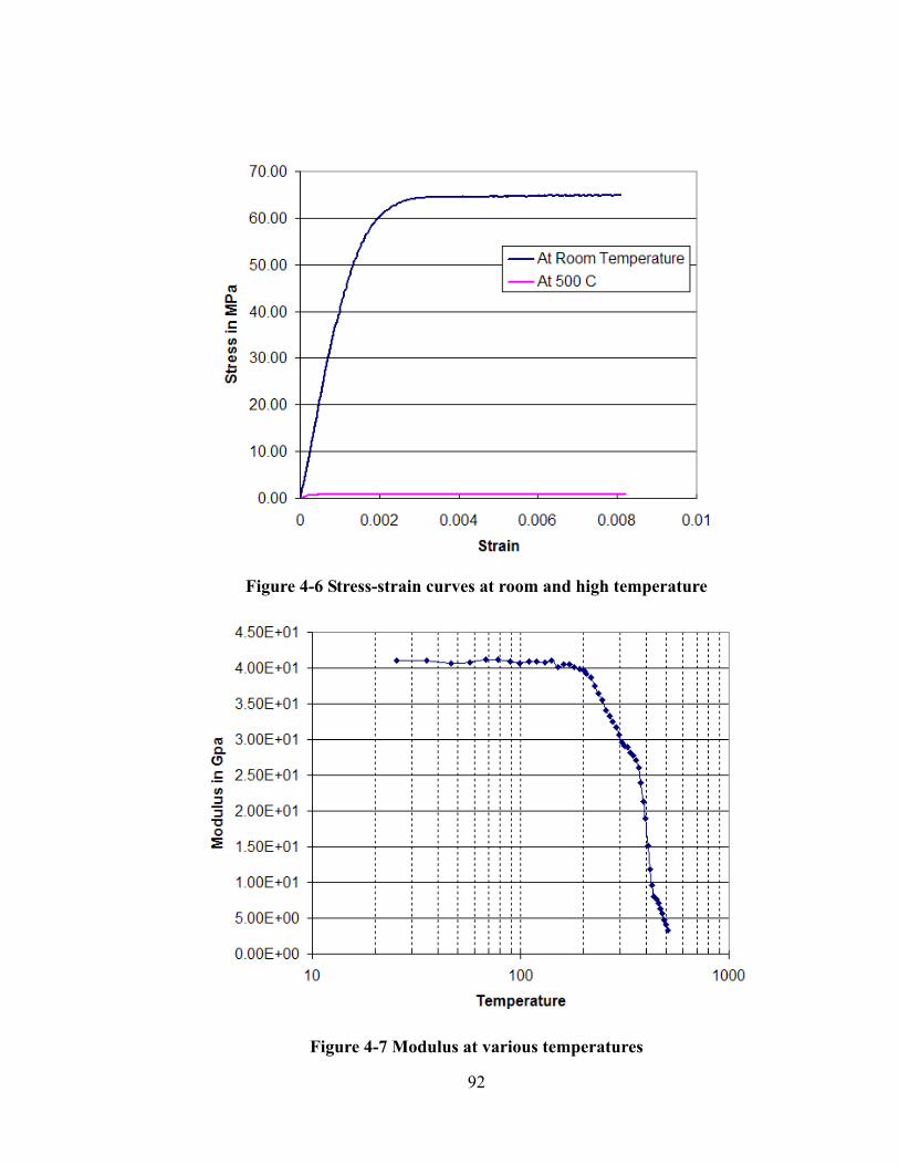
Figure 4-6 Stress-strain curves at room and high temperature
Figure 4-7 Modulus at various temperatures
92
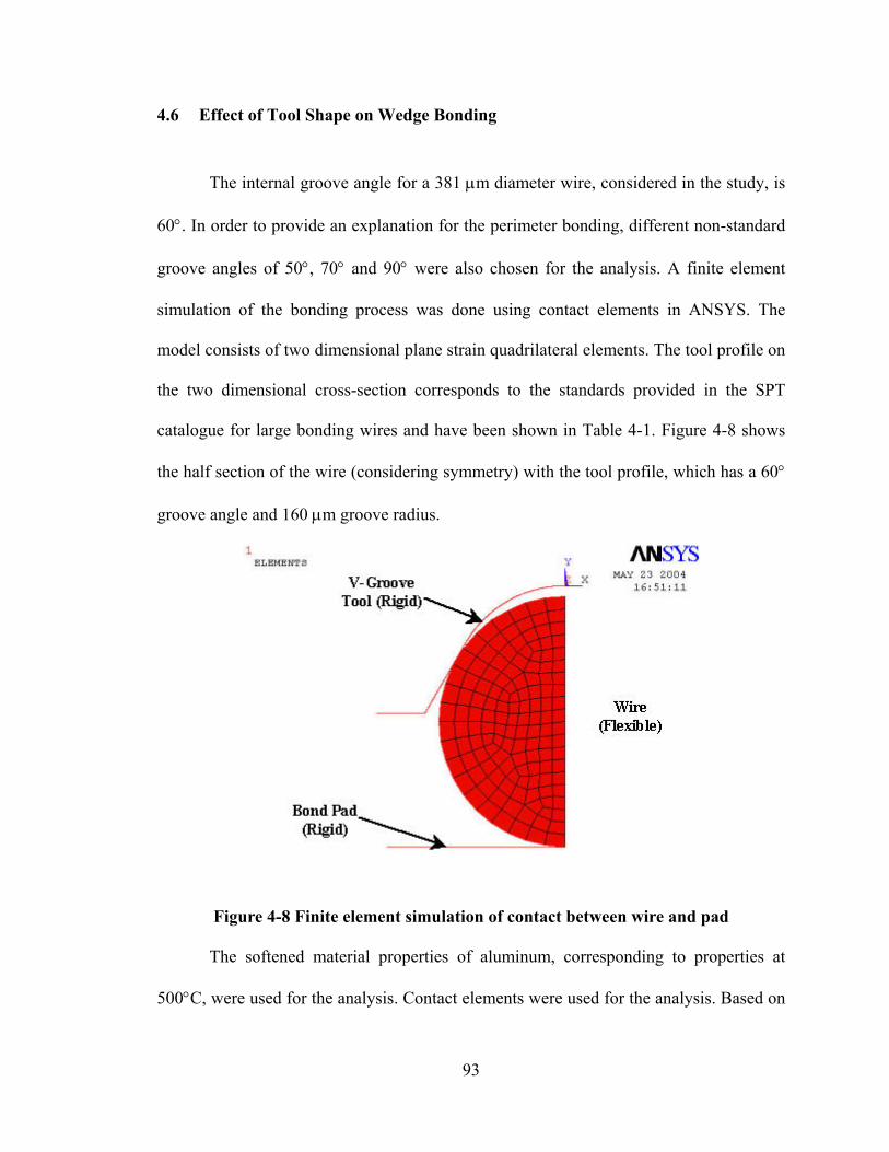
4.6 Effect of Tool Shape on Wedge Bonding
The internal groove angle for a 381 µm diameter wire, considered in the study, is
60°. In order to provide an explanation for the perimeter bonding, different non-standard
groove angles of 50°, 70° and 90° were also chosen for the analysis. A finite element
simulation of the bonding process was done using contact elements in ANSYS. The
model consists of two dimensional plane strain quadrilateral elements. The tool profile on
the two dimensional cross-section corresponds to the standards provided in the SPT
catalogue for large bonding wires and have been shown in Table 4-1. Figure 4-8 shows
the half section of the wire (considering symmetry) with the tool profile, which has a 60°
groove angle and 160 µm groove radius.
Figure 4-8 Finite element simulation of contact between wire and pad
The softened material properties of aluminum, corresponding to properties at
500°C, were used for the analysis. Contact elements were used for the analysis. Based on
93
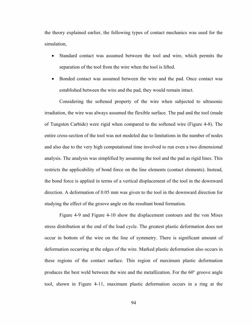
the theory explained earlier, the following types of contact mechanics was used for the
simulation,
• Standard contact was assumed between the tool and wire, which permits the
separation of the tool from the wire when the tool is lifted.
• Bonded contact was assumed between the wire and the pad. Once contact was
established between the wire and the pad, they would remain intact.
Considering the softened property of the wire when subjected to ultrasonic
irradiation, the wire was always assumed the flexible surface. The pad and the tool (made
of Tungsten Carbide) were rigid when compared to the softened wire (Figure 4-8). The
entire cross-section of the tool was not modeled due to limitations in the number of nodes
and also due to the very high computational time involved to run even a two dimensional
analysis. The analysis was simplified by assuming the tool and the pad as rigid lines. This
restricts the applicability of bond force on the line elements (contact elements). Instead,
the bond force is applied in terms of a vertical displacement of the tool in the downward
direction. A deformation of 0.05 mm was given to the tool in the downward direction for
studying the effect of the groove angle on the resultant bond formation.
Figure 4-9 and Figure 4-10 show the displacement contours and the von Mises
stress distribution at the end of the load cycle. The greatest plastic deformation does not
occur in bottom of the wire on the line of symmetry. There is significant amount of
deformation occurring at the edges of the wire. Marked plastic deformation also occurs in
these regions of the contact surface. This region of maximum plastic deformation
produces the best weld between the wire and the metallization. For the 60° groove angle
tool, shown in Figure 4-11, maximum plastic deformation occurs in a ring at the
94
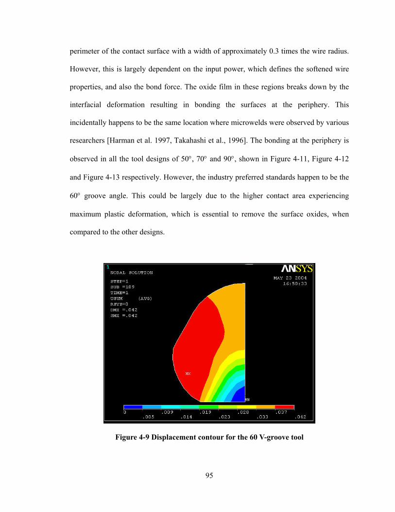
perimeter of the contact surface with a width of approximately 0.3 times the wire radius.
However, this is largely dependent on the input power, which defines the softened wire
properties, and also the bond force. The oxide film in these regions breaks down by the
interfacial deformation resulting in bonding the surfaces at the periphery. This
incidentally happens to be the same location where microwelds were observed by various
researchers [Harman et al. 1997, Takahashi et al., 1996]. The bonding at the periphery is
observed in all the tool designs of 50°, 70° and 90°, shown in Figure 4-11, Figure 4-12
and Figure 4-13 respectively. However, the industry preferred standards happen to be the
60° groove angle. This could be largely due to the higher contact area experiencing
maximum plastic deformation, which is essential to remove the surface oxides, when
compared to the other designs.
Figure 4-9 Displacement contour for the 60 V-groove tool
95
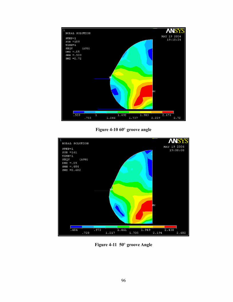
Figure 4-10 60° groove angle
Figure 4-11 50° groove Angle
96
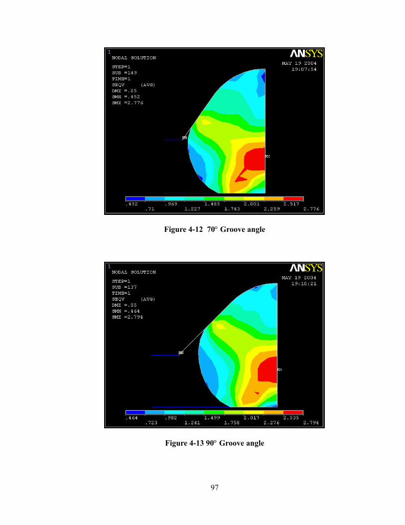
Figure 4-12 70° Groove angle
Figure 4-13 90° Groove angle
97
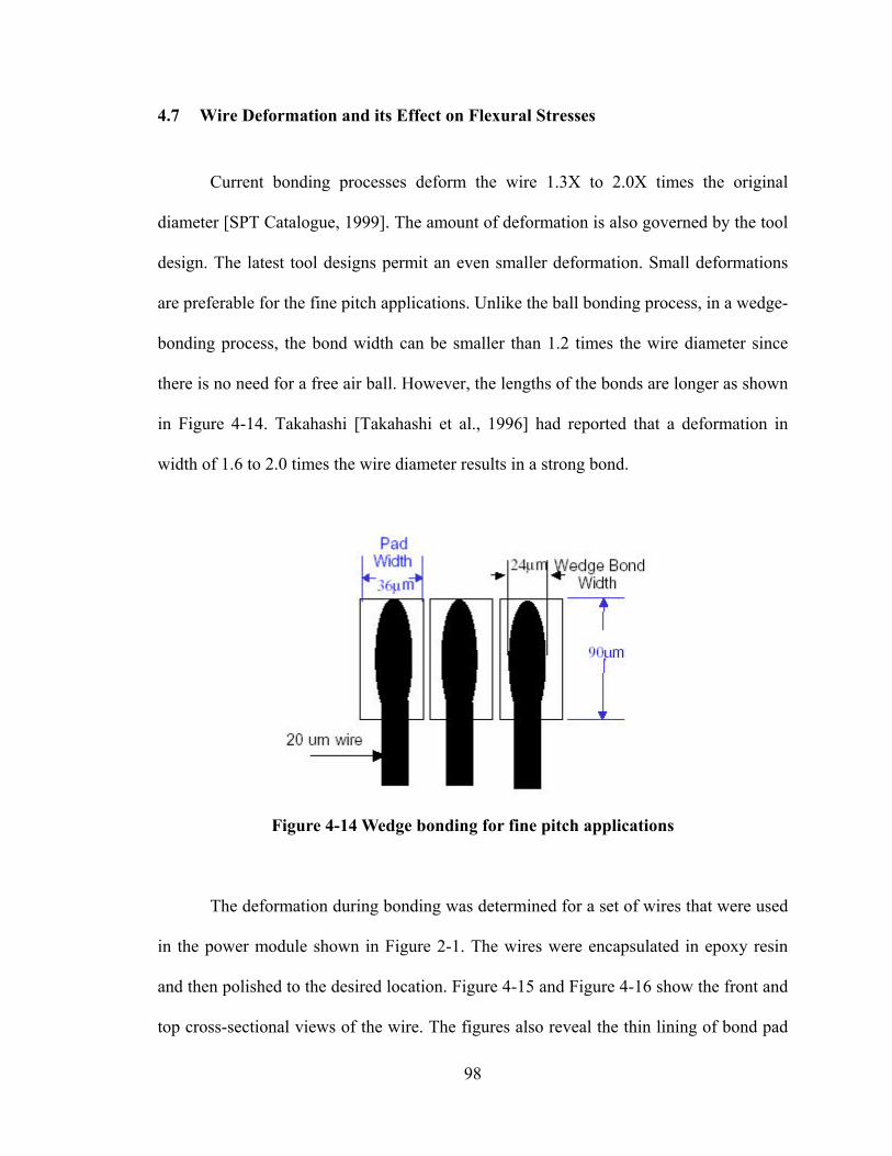
4.7 Wire Deformation and its Effect on Flexural Stresses
Current bonding processes deform the wire 1.3X to 2.0X times the original
diameter [SPT Catalogue, 1999]. The amount of deformation is also governed by the tool
design. The latest tool designs permit an even smaller deformation. Small deformations
are preferable for the fine pitch applications. Unlike the ball bonding process, in a wedge-
bonding process, the bond width can be smaller than 1.2 times the wire diameter since
there is no need for a free air ball. However, the lengths of the bonds are longer as shown
in Figure 4-14. Takahashi [Takahashi et al., 1996] had reported that a deformation in
width of 1.6 to 2.0 times the wire diameter results in a strong bond.
Figure 4-14 Wedge bonding for fine pitch applications
The deformation during bonding was determined for a set of wires that were used
in the power module shown in Figure 2-1. The wires were encapsulated in epoxy resin
and then polished to the desired location. Figure 4-15 and Figure 4-16 show the front and
top cross-sectional views of the wire. The figures also reveal the thin lining of bond pad
98
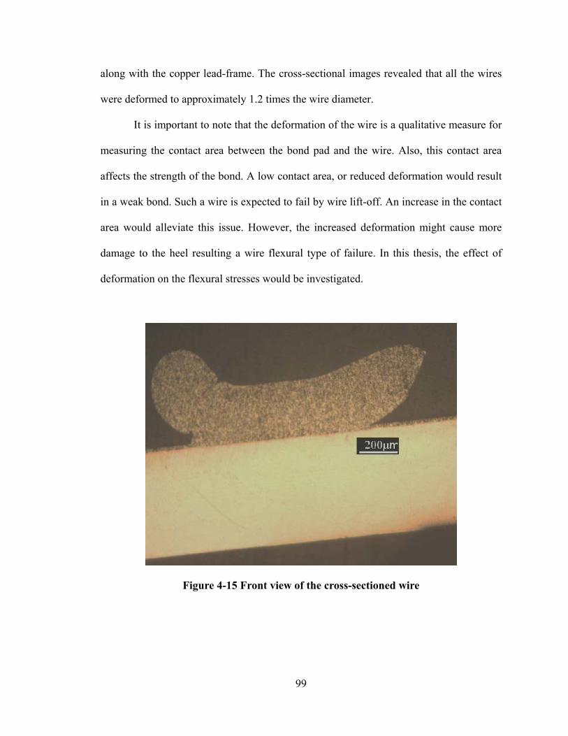
along with the copper lead-frame. The cross-sectional images revealed that all the wires
were deformed to approximately 1.2 times the wire diameter.
It is important to note that the deformation of the wire is a qualitative measure for
measuring the contact area between the bond pad and the wire. Also, this contact area
affects the strength of the bond. A low contact area, or reduced deformation would result
in a weak bond. Such a wire is expected to fail by wire lift-off. An increase in the contact
area would alleviate this issue. However, the increased deformation might cause more
damage to the heel resulting a wire flexural type of failure. In this thesis, the effect of
deformation on the flexural stresses would be investigated.
Figure 4-15 Front view of the cross-sectioned wire
99
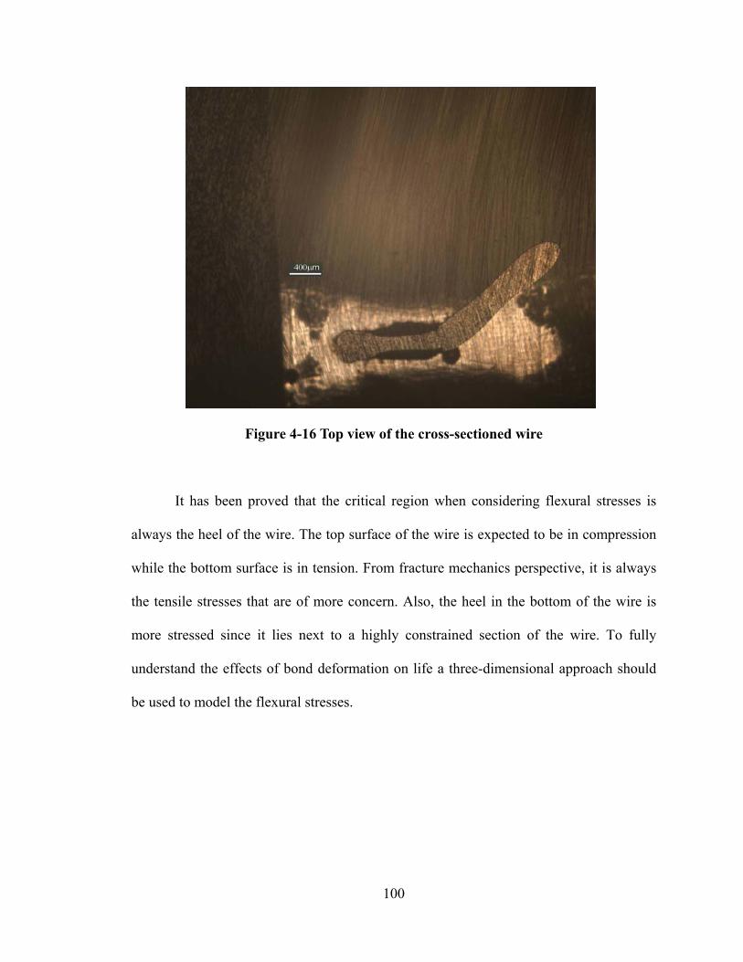
Figure 4-16 Top view of the cross-sectioned wire
It has been proved that the critical region when considering flexural stresses is
always the heel of the wire. The top surface of the wire is expected to be in compression
while the bottom surface is in tension. From fracture mechanics perspective, it is always
the tensile stresses that are of more concern. Also, the heel in the bottom of the wire is
more stressed since it lies next to a highly constrained section of the wire. To fully
understand the effects of bond deformation on life a three-dimensional approach should
be used to model the flexural stresses.
100
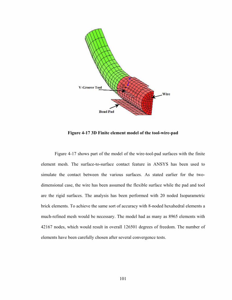
Figure 4-17 3D Finite element model of the tool-wire-pad
Figure 4-17 shows part of the model of the wire-tool-pad surfaces with the finite
element mesh. The surface-to-surface contact feature in ANSYS has been used to
simulate the contact between the various surfaces. As stated earlier for the two-
dimensional case, the wire has been assumed the flexible surface while the pad and tool
are the rigid surfaces. The analysis has been performed with 20 noded Isoparametric
brick elements. To achieve the same sort of accuracy with 8-noded hexahedral elements a
much-refined mesh would be necessary. The model had as many as 8965 elements with
42167 nodes, which would result in overall 126501 degrees of freedom. The number of
elements have been carefully chosen after several convergence tests.
101
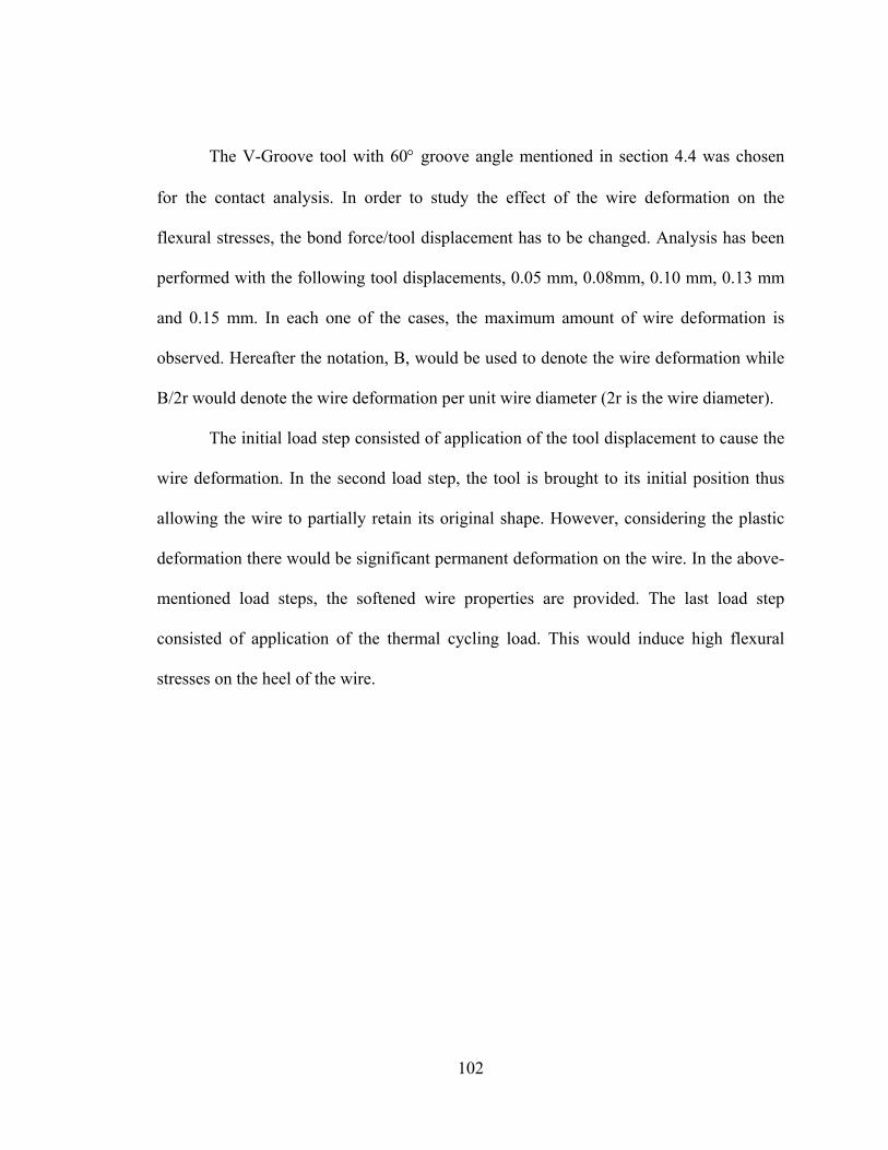
The V-Groove tool with 60° groove angle mentioned in section 4.4 was chosen
for the contact analysis. In order to study the effect of the wire deformation on the
flexural stresses, the bond force/tool displacement has to be changed. Analysis has been
performed with the following tool displacements, 0.05 mm, 0.08mm, 0.10 mm, 0.13 mm
and 0.15 mm. In each one of the cases, the maximum amount of wire deformation is
observed. Hereafter the notation, B, would be used to denote the wire deformation while
B/2r would denote the wire deformation per unit wire diameter (2r is the wire diameter).
The initial load step consisted of application of the tool displacement to cause the
wire deformation. In the second load step, the tool is brought to its initial position thus
allowing the wire to partially retain its original shape. However, considering the plastic
deformation there would be significant permanent deformation on the wire. In the above-
mentioned load steps, the softened wire properties are provided. The last load step
consisted of application of the thermal cycling load. This would induce high flexural
stresses on the heel of the wire.
102
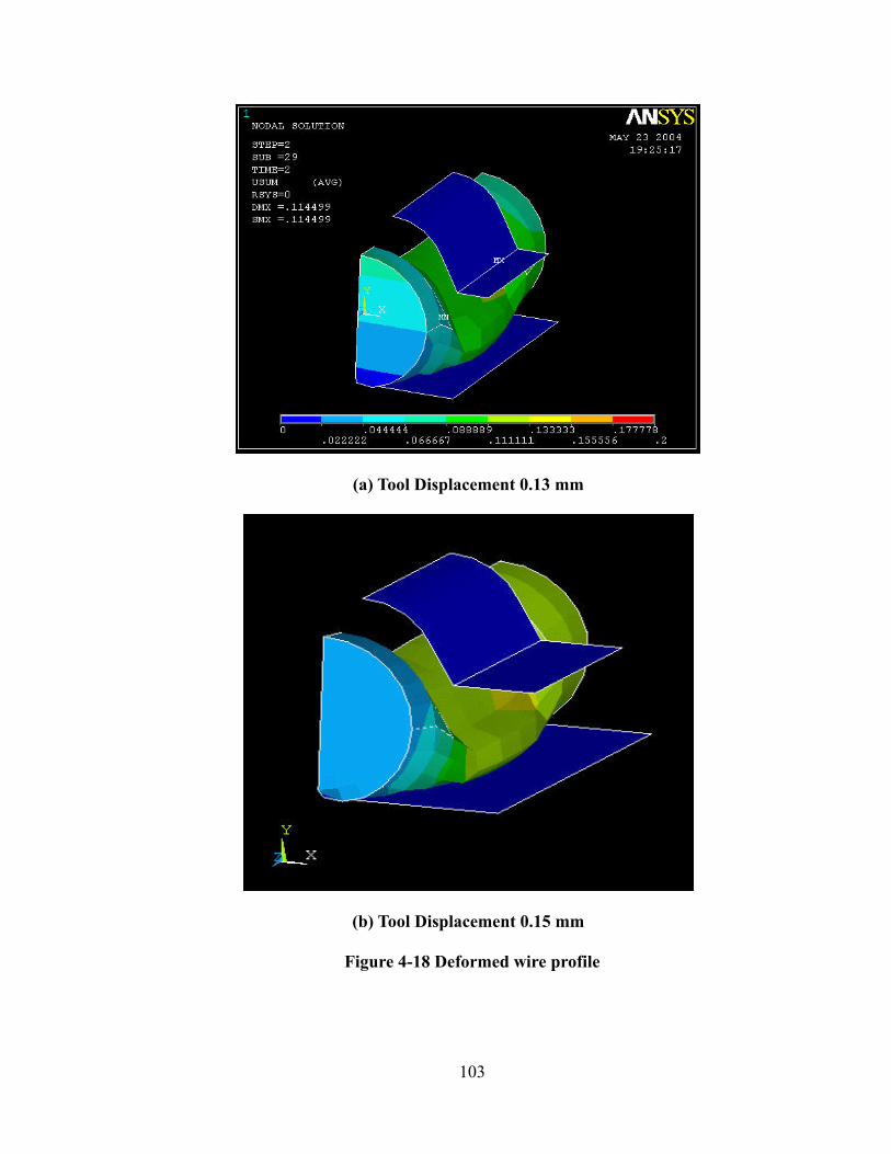
(a) Tool Displacement 0.13 mm
(b) Tool Displacement 0.15 mm
Figure 4-18 Deformed wire profile
103
Figure 4-18 (a) and (b) show the deformed wire profiles for a 0.13 mm and 0.15
mm displacement of the tool. The bending stresses have been plotted for a 0.15 mm tool
displacement in Figure 4-19. Figure 4-20 shows a blowup of the wire profile near the
upper bond pad. It is clearly seen from the figures that maximum bending stresses occur
in the heel of the wire near the upper bond pad. As one would expect, the tensile bending
stresses are higher than the compressive bending stresses due to the proximity of the
lower section of the heel to the location of the constraints. This location in the heel of the
wire is approximately 0.15 times the wire diameter, from the point of constraint. The
bending stresses are maximum tensile at the lower section of the wire near the heel. The
magnitude switches to compressive near the loop height and then switches back to tensile
near the lower heel of the wire at the other end. A very similar trend is seen for the other
tool displacements of 0.05, 0.08, 0.10, 0.13 and 0.15 mm. However, the results have been
plotted only for the tool displacement of 0.15 mm.
104
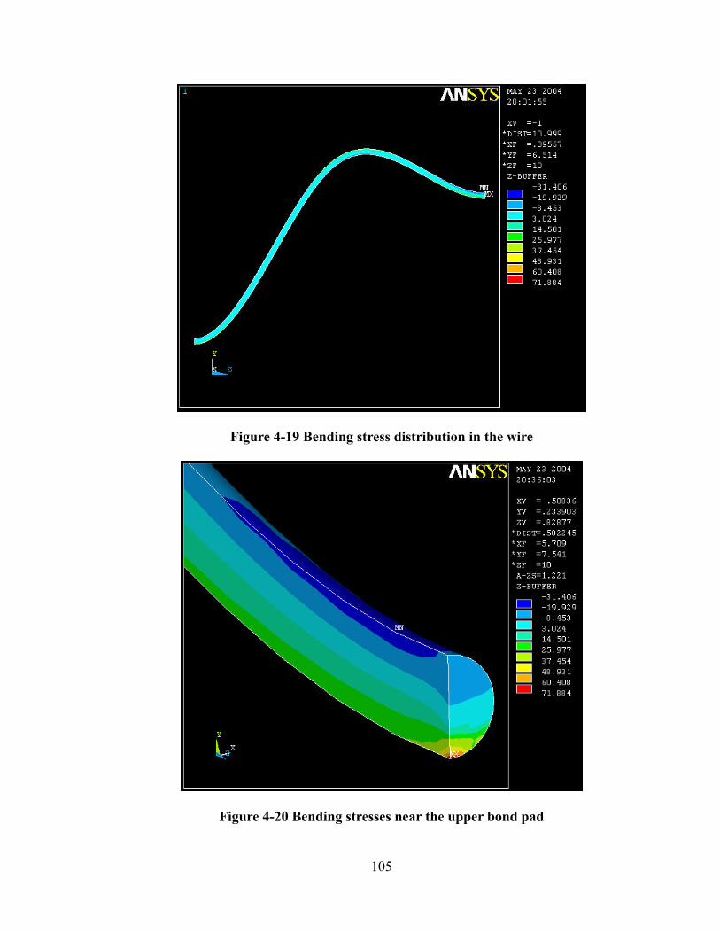
Figure 4-19 Bending stress distribution in the wire
Figure 4-20 Bending stresses near the upper bond pad
105
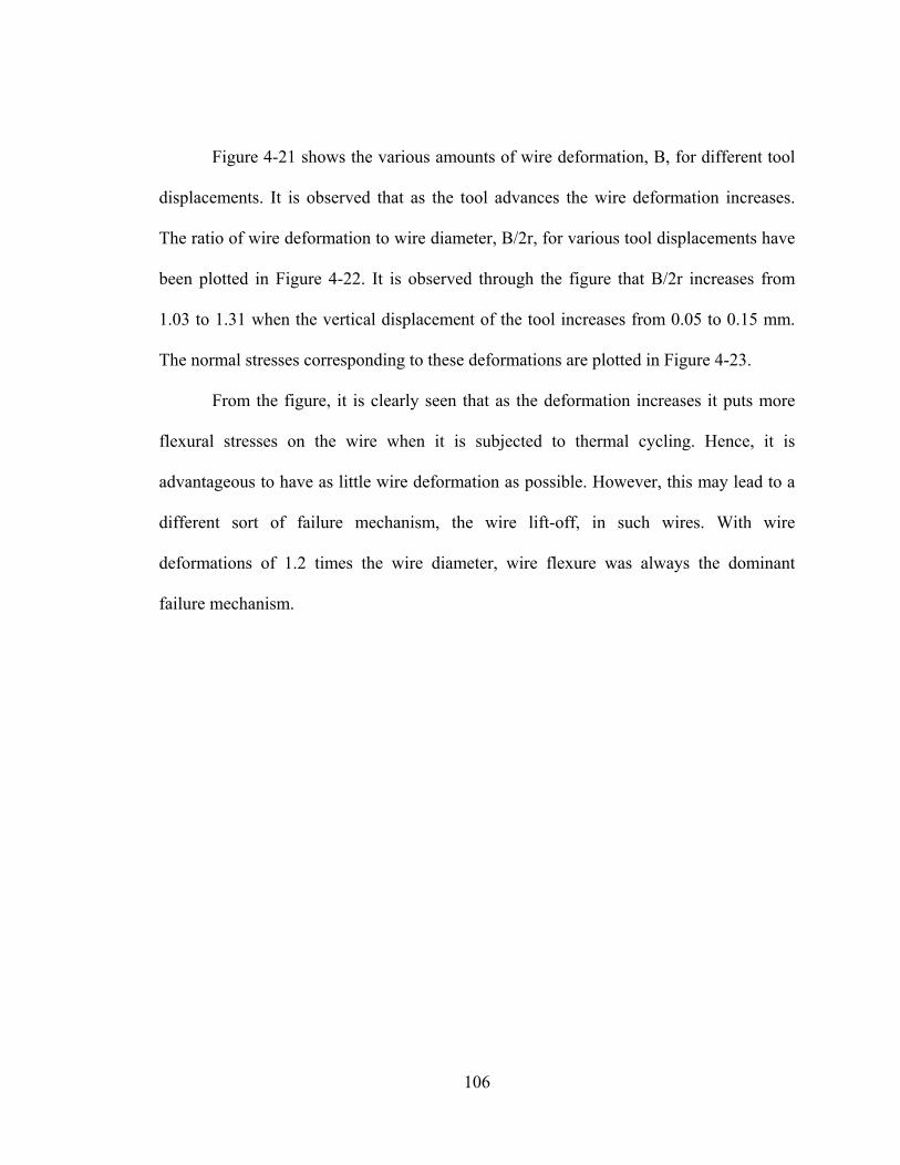
Figure 4-21 shows the various amounts of wire deformation, B, for different tool
displacements. It is observed that as the tool advances the wire deformation increases.
The ratio of wire deformation to wire diameter, B/2r, for various tool displacements have
been plotted in Figure 4-22. It is observed through the figure that B/2r increases from
1.03 to 1.31 when the vertical displacement of the tool increases from 0.05 to 0.15 mm.
The normal stresses corresponding to these deformations are plotted in Figure 4-23.
From the figure, it is clearly seen that as the deformation increases it puts more
flexural stresses on the wire when it is subjected to thermal cycling. Hence, it is
advantageous to have as little wire deformation as possible. However, this may lead to a
different sort of failure mechanism, the wire lift-off, in such wires. With wire
deformations of 1.2 times the wire diameter, wire flexure was always the dominant
failure mechanism.
106
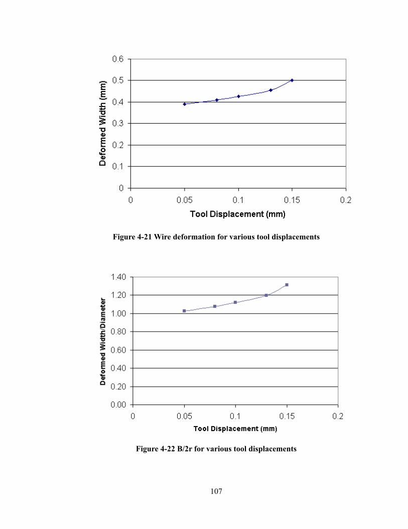
Figure 4-21 Wire deformation for various tool displacements
Figure 4-22 B/2r for various tool displacements
107
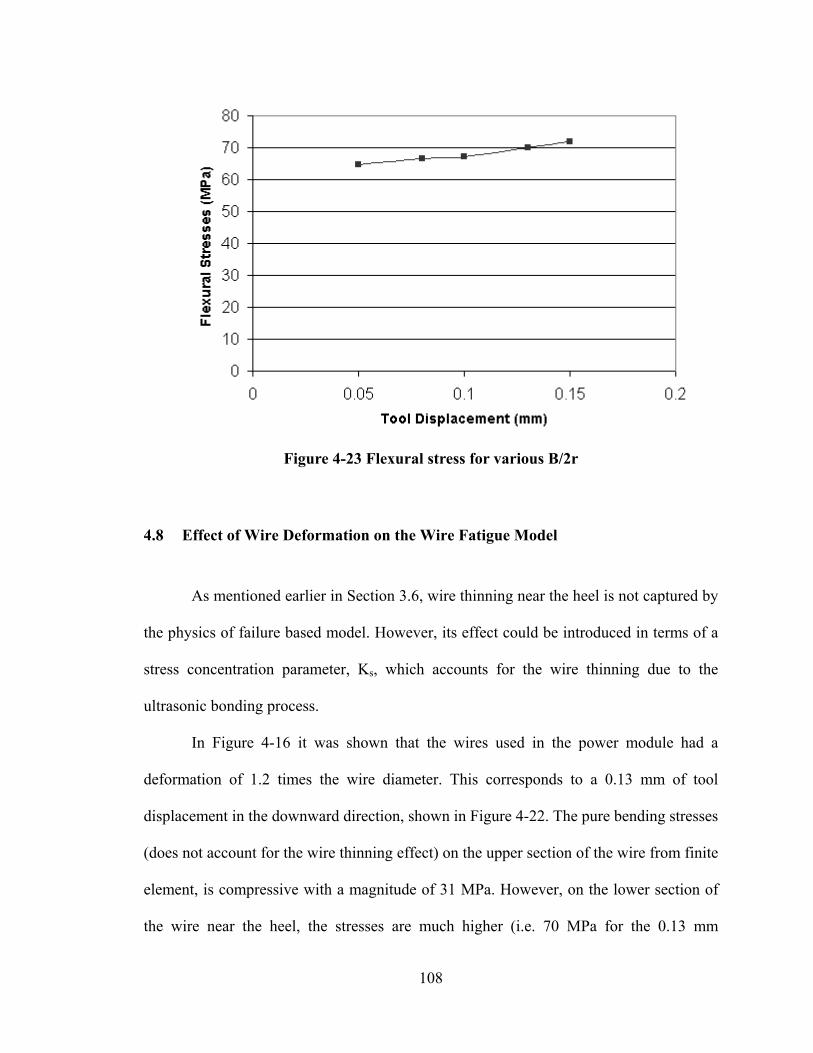
Figure 4-23 Flexural stress for various B/2r
4.8 Effect of Wire Deformation on the Wire Fatigue Model
As mentioned earlier in Section 3.6, wire thinning near the heel is not captured by
the physics of failure based model. However, its effect could be introduced in terms of a
stress concentration parameter, Ks, which accounts for the wire thinning due to the
ultrasonic bonding process.
In Figure 4-16 it was shown that the wires used in the power module had a
deformation of 1.2 times the wire diameter. This corresponds to a 0.13 mm of tool
displacement in the downward direction, shown in Figure 4-22. The pure bending stresses
(does not account for the wire thinning effect) on the upper section of the wire from finite
element, is compressive with a magnitude of 31 MPa. However, on the lower section of
the wire near the heel, the stresses are much higher (i.e. 70 MPa for the 0.13 mm
108
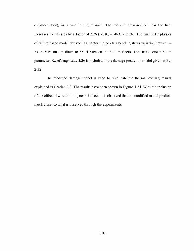
displaced tool), as shown in Figure 4-23. The reduced cross-section near the heel
increases the stresses by a factor of 2.26 (i.e. Ks = 70/31 ≈ 2.26). The first order physics
of failure based model derived in Chapter 2 predicts a bending stress variation between –
35.14 MPa on top fibers to 35.14 MPa on the bottom fibers. The stress concentration
parameter, Ks, of magnitude 2.26 is included in the damage prediction model given in Eq.
2-32.
The modified damage model is used to revalidate the thermal cycling results
explained in Section 3.3. The results have been shown in Figure 4-24. With the inclusion
of the effect of wire thinning near the heel, it is observed that the modified model predicts
much closer to what is observed through the experiments.
109
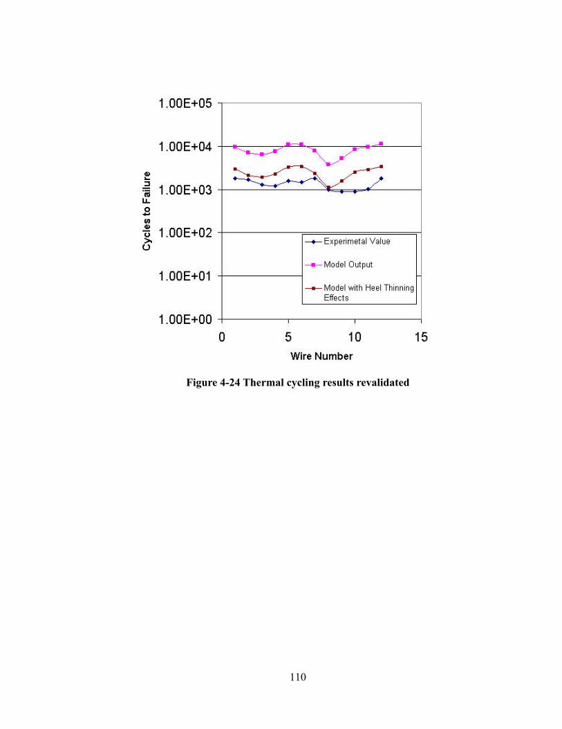
Figure 4-24 Thermal cycling results revalidated
110
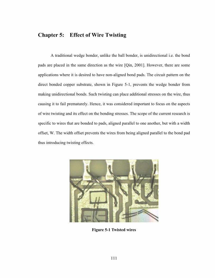
Chapter 5: Effect of Wire Twisting
A traditional wedge bonder, unlike the ball bonder, is unidirectional i.e. the bond
pads are placed in the same direction as the wire [Qin, 2001]. However, there are some
applications where it is desired to have non-aligned bond pads. The circuit pattern on the
direct bonded copper substrate, shown in Figure 5-1, prevents the wedge bonder from
making unidirectional bonds. Such twisting can place additional stresses on the wire, thus
causing it to fail prematurely. Hence, it was considered important to focus on the aspects
of wire twisting and its effect on the bending stresses. The scope of the current research is
specific to wires that are bonded to pads, aligned parallel to one another, but with a width
offset, W. The width offset prevents the wires from being aligned parallel to the bond pad
thus introducing twisting effects.
Figure 5-1 Twisted wires
111
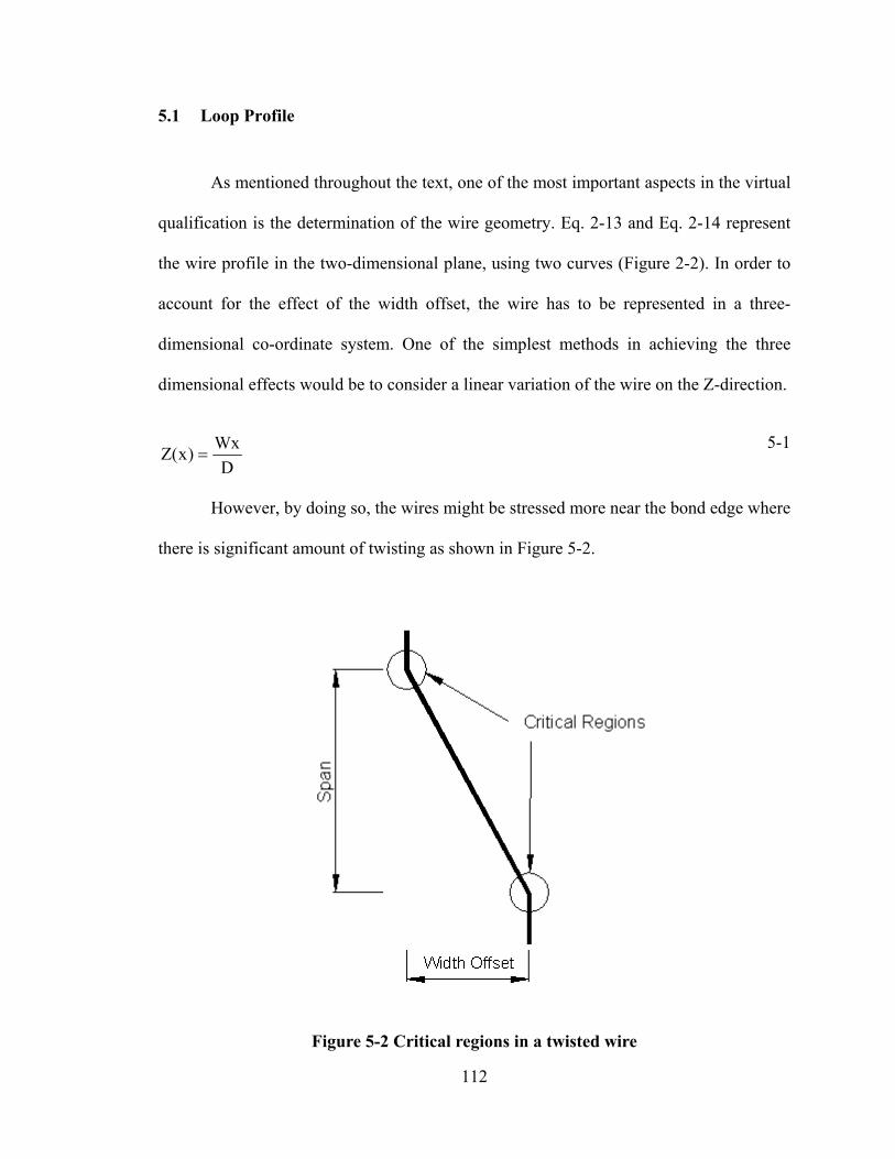
5.1 Loop Profile
As mentioned throughout the text, one of the most important aspects in the virtual
qualification is the determination of the wire geometry. Eq. 2-13 and Eq. 2-14 represent
the wire profile in the two-dimensional plane, using two curves (Figure 2-2). In order to
account for the effect of the width offset, the wire has to be represented in a three-
dimensional co-ordinate system. One of the simplest methods in achieving the three
dimensional effects would be to consider a linear variation of the wire on the Z-direction.
DWx)x(Z =
5-1
However, by doing so, the wires might be stressed more near the bond edge where
there is significant amount of twisting as shown in Figure 5-2.
Figure 5-2 Critical regions in a twisted wire
112
Also, the wire may not prefer to stay in such a highly stressed state after a few
fatigue cycles. Hence, it would be more appropriate and accurate, to determine the
minimum energy configuration that the wire would prefer to occupy. The energy
minimization explained earlier in Section 2.2.3 for a wire represented in a two-
dimensional plane, has to be repeated for the wire profile represented in the Euclidean
three space, R3. However, unlike the earlier procedure, a parametric approach is used to
represent the three dimensional wire profiles. The following section briefly explains the
energy based minimization routine used to determine the three-dimensional wire profiles.
A piecewise parameterized cubic polynomial is used to represent the curves 1 and
2 of the wire profile (Figure 5-3).
113
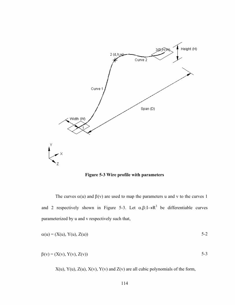
Figure 5-3 Wire profile with parameters
The curves α(u) and β(v) are used to map the parameters u and v to the curves 1
and 2 respectively shown in Figure 5-3. Let α,β:I→R3 be differentiable curves
parameterized by u and v respectively such that,
α(u) = (X(u), Y(u), Z(u)) 5-2
β(v) = (X(v), Y(v), Z(v)) 5-3
X(u), Y(u), Z(u), X(v), Y(v) and Z(v) are all cubic polynomials of the form,
114
X(u)=A0 + A1u + A2u2 + A3u3
Y(u)=B0 + B1u + B2u2 + B3u3
Z(u)=C0 + C1u + C2u2 + C3u3
5-4
where, Ai’s, Bi’s and Ci’s are the coefficients of the cubic polynomial. Also, the wires
should satisfy the length constraint. Therefore, any suitable wire geometry that is
obtained should satisfy these admissibility conditions i.e. the boundary conditions and the
length constraint. The bond point locations are given by points, 1(0, 0, 0) and 3(D, H, W).
Point 2 is chosen to be arbitrary with co-ordinates (d, h, w). On imposing the boundary
conditions a C1 continuous curve representing the wire profile is obtained. A C2
continuity is enforced by equating the slopes of curves 1 and 2 at point 2 (Figure 5-3).
The coefficients are determined based on the boundary conditions, location and slopes of
the curve at the bond pad. As mentioned earlier, the bond pads are aligned parallel to one
another, but with a width offset. The zero slopes at the bond pads, i.e. 0dXdZ ,
dXdY
= , are
enforced by making Yu (or dY/du) and Zu (or dZ/du) zero while Xu (or dX/du) remains
arbitrary. The arbitrary non-zero value is chosen to be a variable q. On application of the
boundary conditions to Eq. 2-6, Eq. 2-7 and Eq. 5-4, the coefficients Ai’s, Bi’s and Ci’s of
the cubic polynomials are determined in terms of the unknown parameters d, h, w and q
as,
115
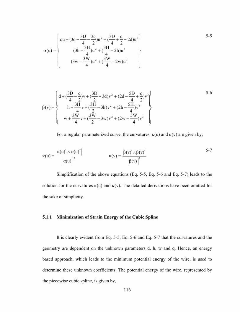
α(u) =
−+−
−+−
−++−−+
32
32
32
u)w24W3(u)
4W3w3(
u)h24H3(u)
4H3h3(
u)d22q
4D3(u)
2q3
4D3d3(qu
5-5
β(v) =
−+−++
−+−++
+−+−+−+
32
32
32
v)4W5w2(v)w3
2W3(v
4W3w
v)4H5h2(v)h3
2H3(v
4H3h
v)2q
4D5d2(v)d3
2D3(v)
2q
4D3(d
5-6
For a regular parameterized curve, the curvatures κ(u) and κ(v) are given by,
κ(u) = 3'
"'
α(u)
α(u)α(u) ∧ κ(v) =
3'
"'
(v)
(v)(v)
β
β∧β
5-7
Simplification of the above equations (Eq. 5-5, Eq. 5-6 and Eq. 5-7) leads to the
solution for the curvatures κ(u) and κ(v). The detailed derivations have been omitted for
the sake of simplicity.
5.1.1 Minimization of Strain Energy of the Cubic Spline
It is clearly evident from Eq. 5-5, Eq. 5-6 and Eq. 5-7 that the curvatures and the
geometry are dependent on the unknown parameters d, h, w and q. Hence, an energy
based approach, which leads to the minimum potential energy of the wire, is used to
determine these unknown coefficients. The potential energy of the wire, represented by
the piecewise cubic spline, is given by,
116
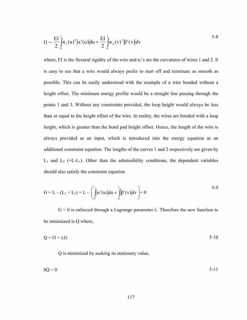
Π = ∫∫ βκ+ακ1
0
22
1
0
21 dv)v(')v(
2EIdu)u(')u(
2EI
5-8
where, EI is the flexural rigidity of the wire and κi’s are the curvatures of wires 1 and 2. It
is easy to see that a wire would always prefer to start off and terminate as smooth as
possible. This can be easily understood with the example of a wire bonded without a
height offset. The minimum energy profile would be a straight line passing through the
points 1 and 3. Without any constraints provided, the loop height would always be less
than or equal to the height offset of the wire. In reality, the wires are bonded with a loop
height, which is greater than the bond pad height offset. Hence, the length of the wire is
always provided as an input, which is introduced into the energy equation as an
additional constraint equation. The lengths of the curves 1 and 2 respectively are given by
L1 and L2 (=L-L1). Other than the admissibility conditions, the dependent variables
should also satisfy the constraint equation
G = L – (L1 + L2) = L –
β+α ∫∫
1
d
1
0
dv)v('du)u( 0 ' =5-9
G = 0 is enforced through a Lagrange parameter λ. Therefore the new function to
be minimized is Q where,
Q = Π + λG 5-10
Q is minimized by seeking its stationary value,
δQ = 0 5-11
117

0dQ
=δδ 0
hQ
=δδ 0
wQ
=δδ 0
=δδ 0Q
=δλδ
5-12
The above set of non-linear equations are solved iteratively using the Levenberg-
Marquardt algorithm to provide the location of the second point (d, h, w) which seeks to
minimize the potential energy and also satisfies the length constraint. (Note:
Alternatively, the energy minimization could also be solved using the optimization
toolbox in Matlab). Substitution of d, h, w and q into Eq. 5-5 and Eq. 5-6 provides the
wire geometry.
Considering the vast number of possibilities of locating the reference point 2, on a
three-dimensional space, it is very essential to assign the proper upper and lower bounds
for each one of the parameters. The program always tries to locate the point 2(d, h, w)
such that the strain energy is minimum. Figure 5-4 represents one of the wire profiles
determined for a span of 20 mm and width offset of 2 mm. Even though the curve is
smooth, the program has located the point 2 outside the bounds (0, W). The reason for
such a behavior is presence of several local minima. However, it is the objective of the
program to determine the global minima. Enforcing the limits 0 to W for point 2 might
still not resolve the problem of preventing the curve entering the –Z axis. However, it can
be noted that the slope has to be positive in the interval (0<x<D), i.e. 0dXdZ
> .
118
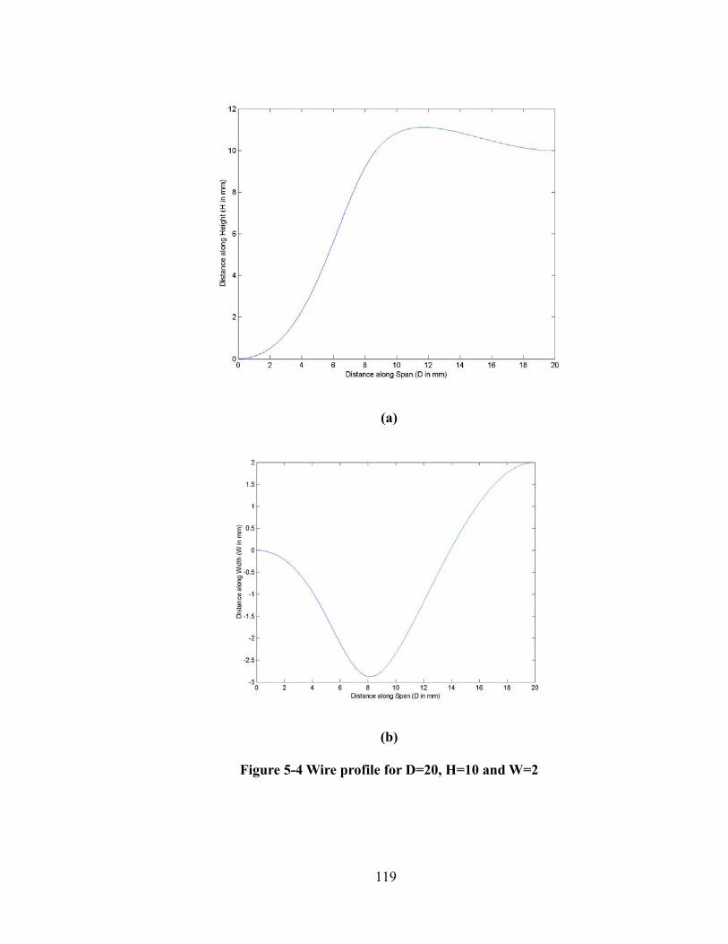
(a)
(b)
Figure 5-4 Wire profile for D=20, H=10 and W=2
119
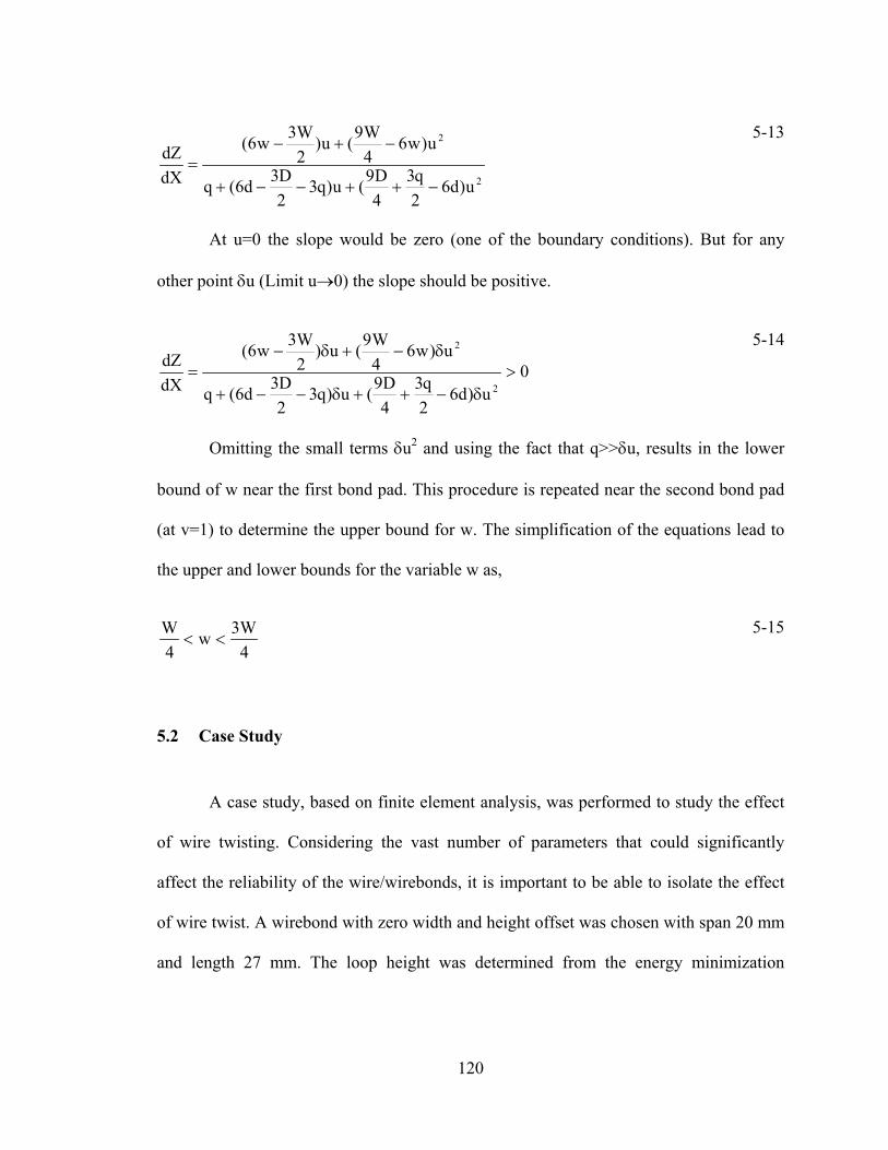
2
2
u)d62q3
4D9(u)q3
2D3d6(q
u)w64W9(u)
2W3w6(
dXdZ
−++−−+
−+−=
5-13
At u=0 the slope would be zero (one of the boundary conditions). But for any
other point δu (Limit u→0) the slope should be positive.
0u)d6
2q3
4D9(u)q3
2D3d6(q
u)w64W9(u)
2W3w6(
dXdZ
2
2
>δ−++δ−−+
δ−+δ−=
5-14
Omitting the small terms δu2 and using the fact that q>>δu, results in the lower
bound of w near the first bond pad. This procedure is repeated near the second bond pad
(at v=1) to determine the upper bound for w. The simplification of the equations lead to
the upper and lower bounds for the variable w as,
4W3w
4W
<< 5-15
5.2 Case Study
A case study, based on finite element analysis, was performed to study the effect
of wire twisting. Considering the vast number of parameters that could significantly
affect the reliability of the wire/wirebonds, it is important to be able to isolate the effect
of wire twist. A wirebond with zero width and height offset was chosen with span 20 mm
and length 27 mm. The loop height was determined from the energy minimization
120
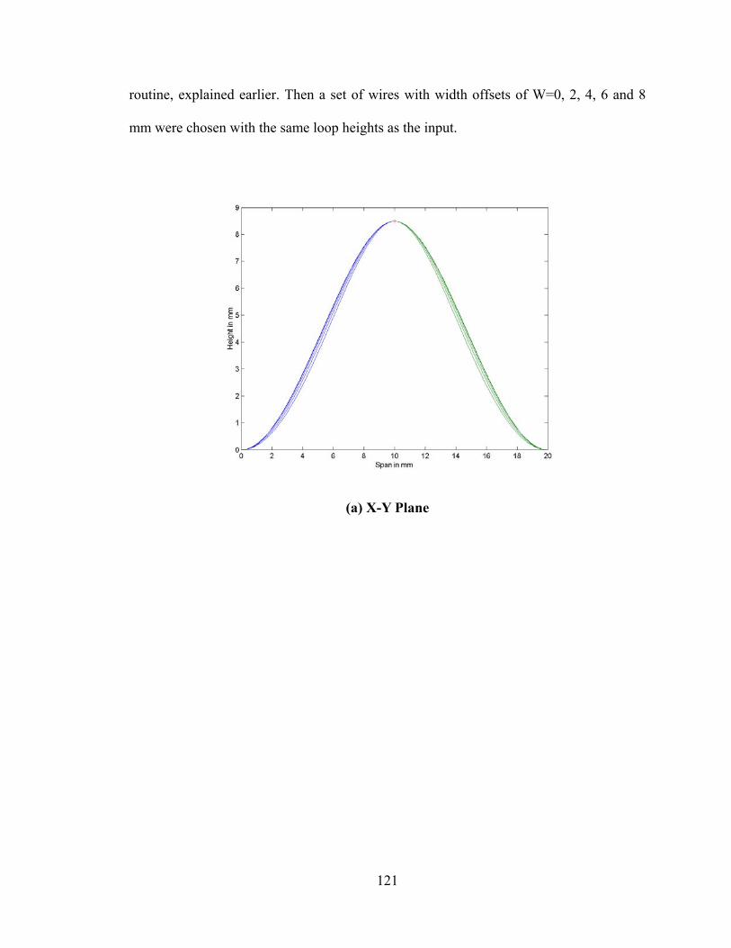
routine, explained earlier. Then a set of wires with width offsets of W=0, 2, 4, 6 and 8
mm were chosen with the same loop heights as the input.
(a) X-Y Plane
121
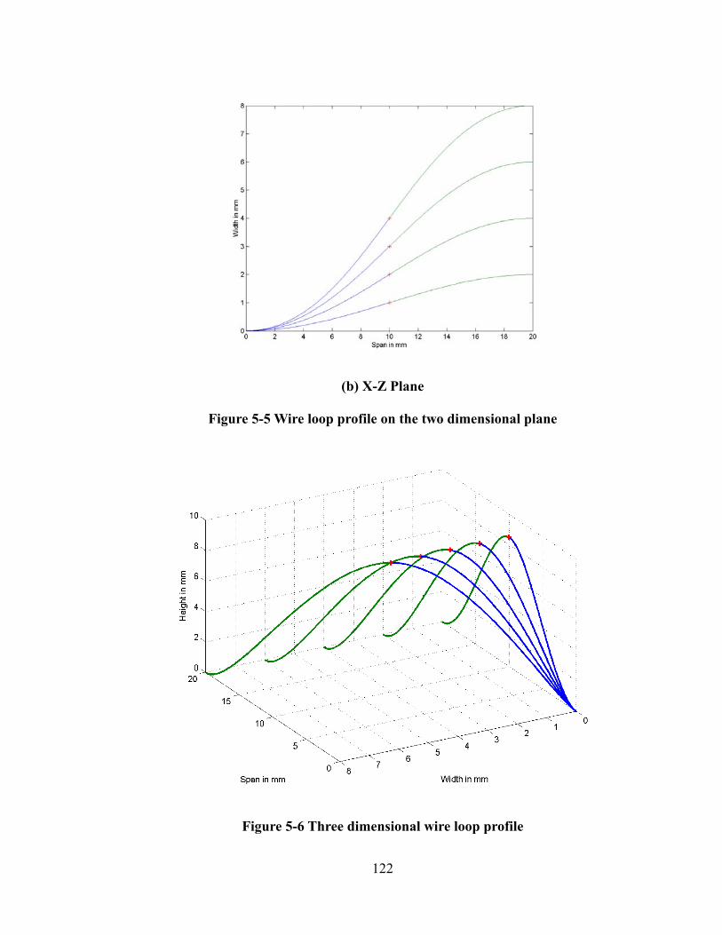
(b) X-Z Plane
Figure 5-5 Wire loop profile on the two dimensional plane
Figure 5-6 Three dimensional wire loop profile
122
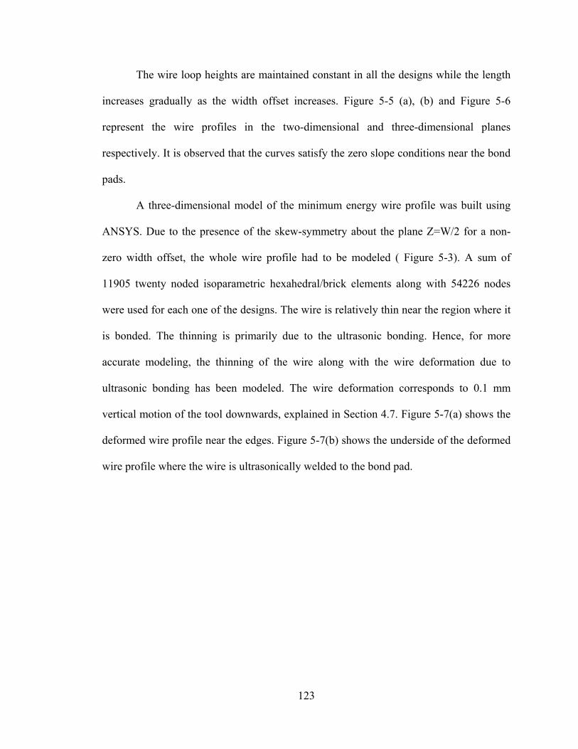
The wire loop heights are maintained constant in all the designs while the length
increases gradually as the width offset increases. Figure 5-5 (a), (b) and Figure 5-6
represent the wire profiles in the two-dimensional and three-dimensional planes
respectively. It is observed that the curves satisfy the zero slope conditions near the bond
pads.
A three-dimensional model of the minimum energy wire profile was built using
ANSYS. Due to the presence of the skew-symmetry about the plane Z=W/2 for a non-
zero width offset, the whole wire profile had to be modeled ( Figure 5-3). A sum of
11905 twenty noded isoparametric hexahedral/brick elements along with 54226 nodes
were used for each one of the designs. The wire is relatively thin near the region where it
is bonded. The thinning is primarily due to the ultrasonic bonding. Hence, for more
accurate modeling, the thinning of the wire along with the wire deformation due to
ultrasonic bonding has been modeled. The wire deformation corresponds to 0.1 mm
vertical motion of the tool downwards, explained in Section 4.7. Figure 5-7(a) shows the
deformed wire profile near the edges. Figure 5-7(b) shows the underside of the deformed
wire profile where the wire is ultrasonically welded to the bond pad.
123
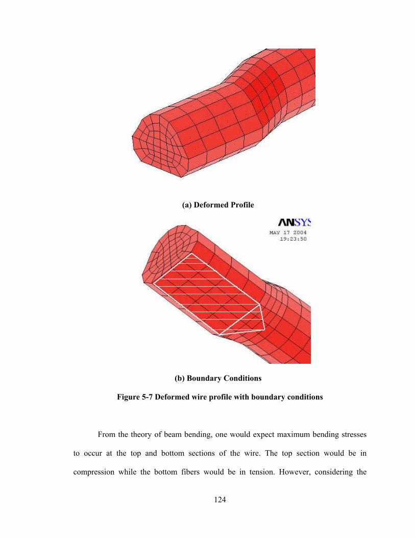
(a) Deformed Profile
(b) Boundary Conditions
Figure 5-7 Deformed wire profile with boundary conditions
From the theory of beam bending, one would expect maximum bending stresses
to occur at the top and bottom sections of the wire. The top section would be in
compression while the bottom fibers would be in tension. However, considering the
124
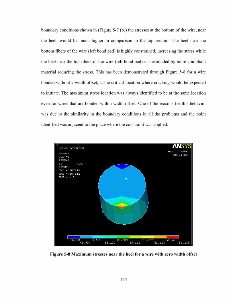
boundary conditions shown in (Figure 5-7 (b)) the stresses at the bottom of the wire, near
the heel, would be much higher in comparison to the top section. The heel near the
bottom fibers of the wire (left bond pad) is highly constrained, increasing the stress while
the heel near the top fibers of the wire (left bond pad) is surrounded by more compliant
material reducing the stress. This has been demonstrated through Figure 5-8 for a wire
bonded without a width offset, at the critical location where cracking would be expected
to initiate. The maximum stress location was always identified to be at the same location
even for wires that are bonded with a width offset. One of the reasons for this behavior
was due to the similarity in the boundary conditions in all the problems and the point
identified was adjacent to the place where the constraint was applied.
Figure 5-8 Maximum stresses near the heel for a wire with zero width offset
125
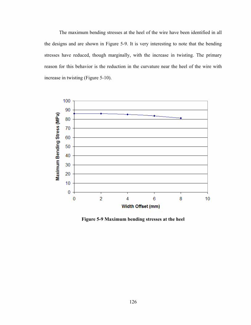
The maximum bending stresses at the heel of the wire have been identified in all
the designs and are shown in Figure 5-9. It is very interesting to note that the bending
stresses have reduced, though marginally, with the increase in twisting. The primary
reason for this behavior is the reduction in the curvature near the heel of the wire with
increase in twisting (Figure 5-10).
Figure 5-9 Maximum bending stresses at the heel
126
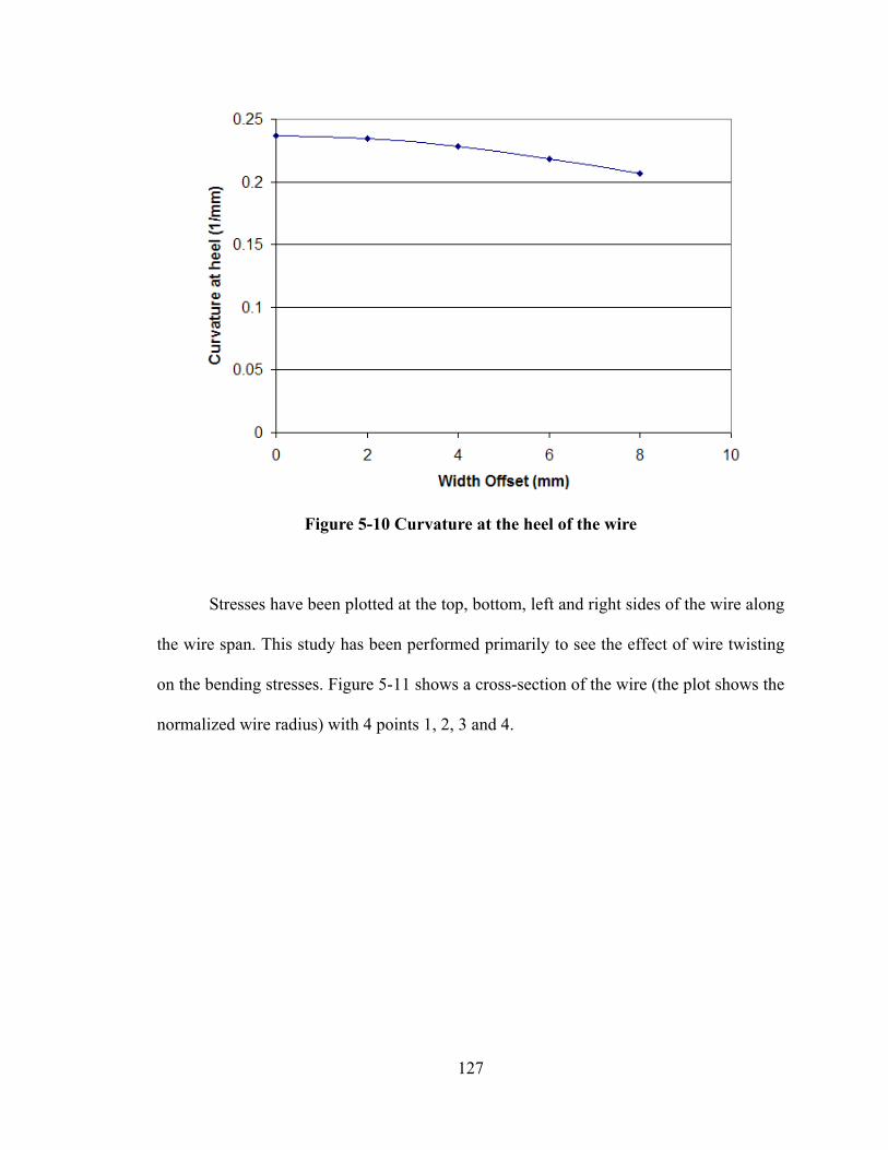
Figure 5-10 Curvature at the heel of the wire
Stresses have been plotted at the top, bottom, left and right sides of the wire along
the wire span. This study has been performed primarily to see the effect of wire twisting
on the bending stresses. Figure 5-11 shows a cross-section of the wire (the plot shows the
normalized wire radius) with 4 points 1, 2, 3 and 4.
127
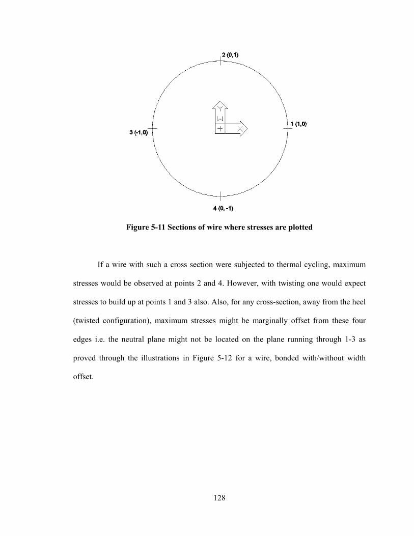
Figure 5-11 Sections of wire where stresses are plotted
If a wire with such a cross section were subjected to thermal cycling, maximum
stresses would be observed at points 2 and 4. However, with twisting one would expect
stresses to build up at points 1 and 3 also. Also, for any cross-section, away from the heel
(twisted configuration), maximum stresses might be marginally offset from these four
edges i.e. the neutral plane might not be located on the plane running through 1-3 as
proved through the illustrations in Figure 5-12 for a wire, bonded with/without width
offset.
128
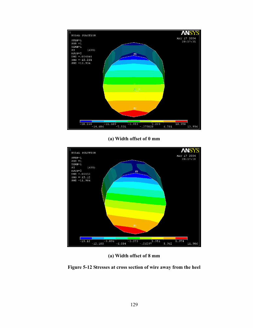
(a) Width offset of 0 mm
(a) Width offset of 8 mm
Figure 5-12 Stresses at cross section of wire away from the heel
129
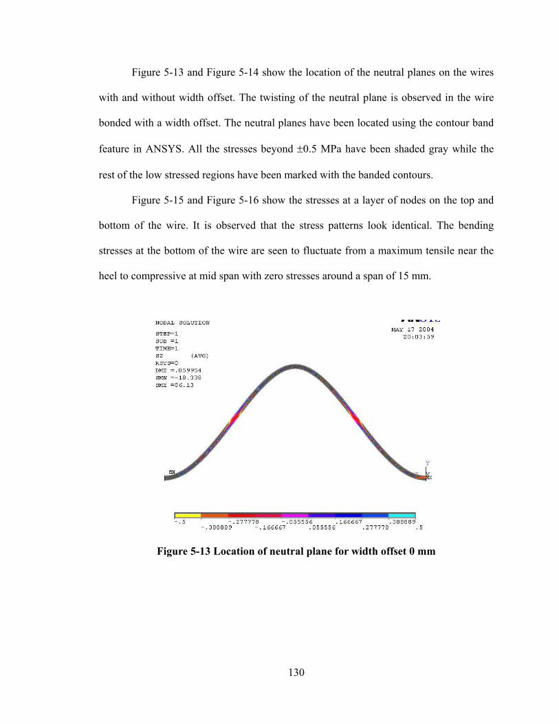
Figure 5-13 and Figure 5-14 show the location of the neutral planes on the wires
with and without width offset. The twisting of the neutral plane is observed in the wire
bonded with a width offset. The neutral planes have been located using the contour band
feature in ANSYS. All the stresses beyond ±0.5 MPa have been shaded gray while the
rest of the low stressed regions have been marked with the banded contours.
Figure 5-15 and Figure 5-16 show the stresses at a layer of nodes on the top and
bottom of the wire. It is observed that the stress patterns look identical. The bending
stresses at the bottom of the wire are seen to fluctuate from a maximum tensile near the
heel to compressive at mid span with zero stresses around a span of 15 mm.
Figure 5-13 Location of neutral plane for width offset 0 mm
130
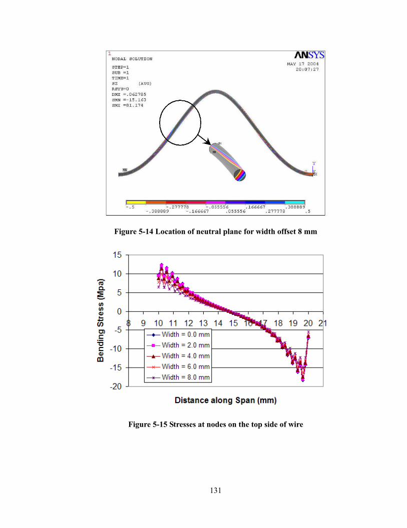
Figure 5-14 Location of neutral plane for width offset 8 mm
Figure 5-15 Stresses at nodes on the top side of wire
131
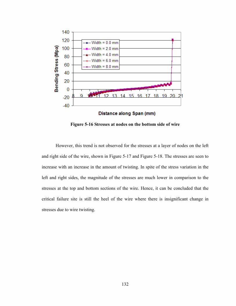
Figure 5-16 Stresses at nodes on the bottom side of wire
However, this trend is not observed for the stresses at a layer of nodes on the left
and right side of the wire, shown in Figure 5-17 and Figure 5-18. The stresses are seen to
increase with an increase in the amount of twisting. In spite of the stress variation in the
left and right sides, the magnitude of the stresses are much lower in comparison to the
stresses at the top and bottom sections of the wire. Hence, it can be concluded that the
critical failure site is still the heel of the wire where there is insignificant change in
stresses due to wire twisting.
132
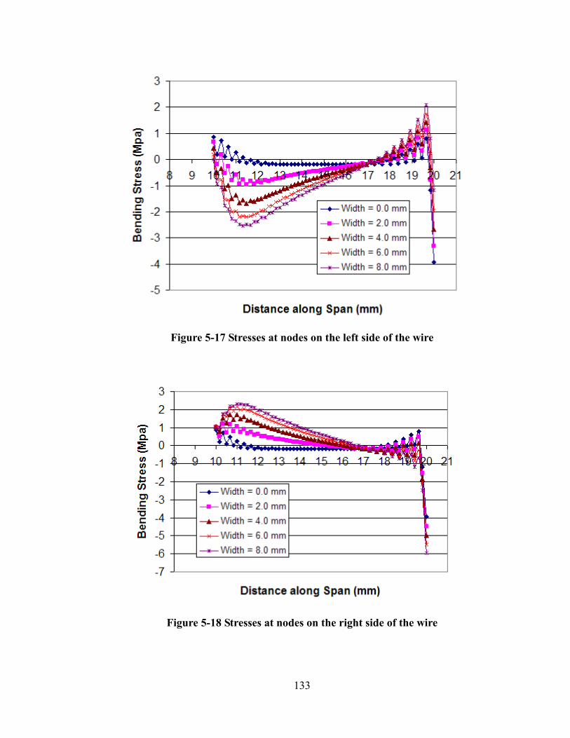
Figure 5-17 Stresses at nodes on the left side of the wire
Figure 5-18 Stresses at nodes on the right side of the wire
133
This study is valid for wires that are bonded to pads that are aligned parallel, but
with a width offset. The study reveals that wires, if properly bonded, will not be highly
stressed by twisting effects near the heel. However, this model can be made more
comprehensive by not imposing the constraint of parallel bond pads. Though one might
not experience a drastic reduction in the stresses near the heel, there might be a reduction
in stresses in the center of the wire where there is more twisting.
The model provides an approach to determine stresses in wires that are bonded
with some width and height offset. The minimum energy wire geometry can be fed into
the wirebonder to design reliable wirebonded interconnections regardless of the
constraints.
134
Chapter 6: Contributions and Suggestions for Future Work
The major accomplishments and contributions of this dissertation are summarized
in this chapter, along with suggestions for future work.
6.1 Major Accomplishments
The major contributions of this dissertation are listed below,
• The determination of minimum energy profiles for wires. The model predicts the
minimum energy profile based on any type of constraints provided. This has been
performed for a two dimensional case and a three dimensional case. The
determination of the wire loop profile is critical to both finite element modeling as
well as for the physics of failure based models. Also, these minimum energy
profiles could be fed into the wirebonder for producing reliable wire
interconnections.
• Development of a first order physics of failure based model to predict cycles to
failure for asymmetrically bonded wires subjected to wire flexural fatigue. The
model essentially consists of a load transformation model and a damage model.
The load transformation model also includes a frame displacement model that is
critical to wire flexural fatigue. The effect of wire thinning near the heel, which is
not modeled in the Euler-Bernoulli beam equations are introduced in terms of a
stress concentration parameter, Ks. The model developed can be used to assess the
135
reliability of an existing design i.e. as a good design evaluation tool. In addition,
the model can also be used to design reliable wirebonded interconnection.
• A finite element investigation was used to prove the theory of perimeter bonding
commonly observed in experiments. Wire deformation due to the wirebonding
process was reproduced using finite element simulations. The process parameters
that are critical for the wirebonding process are identified. In addition, the effect
of wire thinning on the flexural stresses was determined by means of the finite
element simulations.
• The effect of wire twisting is high only on regions away from the heel where high
stresses are not seen in comparison to the heel stresses. Hence, it was concluded
that wire twisting is not critical to the reliability of the wires.
The first order model employs an energy based method approach, using cubic
splines, to fit the minimum energy wire profile with wire span, wire length, wire diameter
and bond pad height offset as input parameters. The model combines both changes in the
wire geometry and changes in frame geometry as a function of temperature cycling to
calculate strains in the heel of the wire. The strains are converted to time to failure using
elastic and plastic damage models. The damage model has an additional parameter, which
accounts for the wire thinning. This stress concentration parameter, has been determined
through finite element simulations.
The model can be used in evaluating the reliability for existing designs or also in
designing new wirebonded interconnections. As mentioned in the contributions these
136
minimum energy profiles can be fed into the wire bonder for producing reliable
wirebonded interconnections.
Some of the interesting conclusions of the parametric studies for designing
reliable wirebonded interconnections are,
• Flexural stresses are low when the wire is thin. This is easily seen through Eq.
2-5. However, from electrical perspective thinner wires will have more resistance
and hence more joule heating.
• Increase in height offset of wirebonds would always result in failure happening at
the heel of the wire near the upper bond pad, provided the wire is bonded without
any manufacturing defect. Hence, the height offset should be minimized as much
as possible to circumvent this problem.
• There is an optimum wire length of wire, which can increase the mechanical
reliability of the interconnection. The model helps one determine these optimum
values. Also, for a wire designed with an optimum wire length, an increase in
wire span helps reduce the heel stresses or strains.
• The frame displacements are critical to the wire flexure. Suitable frame properties
can help alleviate the issue of high heel stresses.
• Wire deformation, due to wirebonding should be as small as possible in order to
reduce the flexural stresses. However, this could lead to a shift in the failure
mechanism from wire flexure to wire lift-off.
137
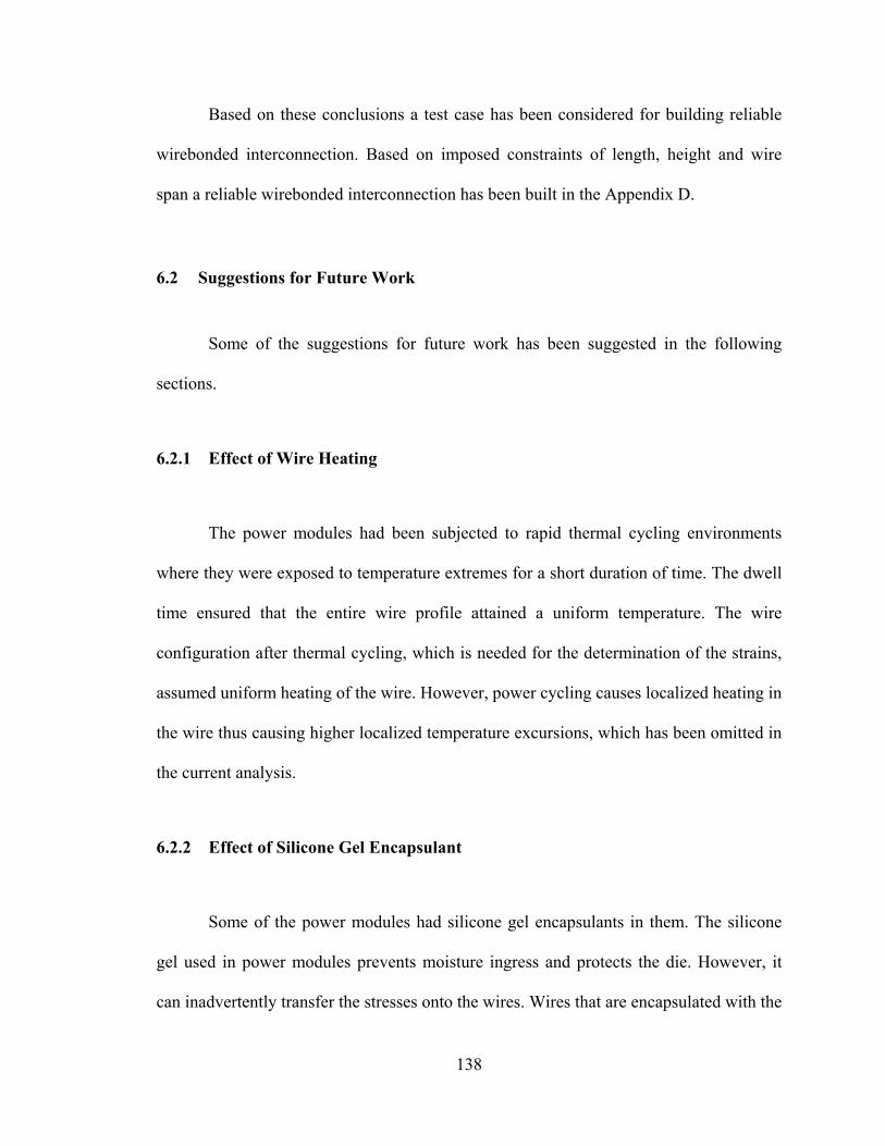
Based on these conclusions a test case has been considered for building reliable
wirebonded interconnection. Based on imposed constraints of length, height and wire
span a reliable wirebonded interconnection has been built in the Appendix D.
6.2 Suggestions for Future Work
Some of the suggestions for future work has been suggested in the following
sections.
6.2.1 Effect of Wire Heating
The power modules had been subjected to rapid thermal cycling environments
where they were exposed to temperature extremes for a short duration of time. The dwell
time ensured that the entire wire profile attained a uniform temperature. The wire
configuration after thermal cycling, which is needed for the determination of the strains,
assumed uniform heating of the wire. However, power cycling causes localized heating in
the wire thus causing higher localized temperature excursions, which has been omitted in
the current analysis.
6.2.2 Effect of Silicone Gel Encapsulant
Some of the power modules had silicone gel encapsulants in them. The silicone
gel used in power modules prevents moisture ingress and protects the die. However, it
can inadvertently transfer the stresses onto the wires. Wires that are encapsulated with the
138
silicone gel are seen to fail much earlier than wires that are free to expand. This was
observed through a study done on one of the power modules used in the study (Figure
6-1).
Hence, the model should be modified to include the effect of silicone gel
encapsulant.
Figure 6-1 Cycles to failure with/without gel
6.2.3 Plastic Deformation of the Wire
For very high thermal cycling load, the wires would experience more plastic
deformation and hence it was assumed that the total plastic strains used in the low cycle
fatigue model would be approximately equal to the total strains. However, for more
accurate modeling, the loading has to be applied in steps, which allows the strains to be
decoupled into elastic and plastic strains.
139
6.2.4 Wire Twisting with no Constraints in the Three Dimensional Plane
The model assumes that the wire profiles are all two dimensional. Any three-
dimensional wire profiles are all mapped onto a two dimensional plane. However, several
wires are bonded with wire twisting due to constraints imposed on the design. An effort
has been made to account for wire twisting in the model.
The model assumes the bond pads are aligned parallel but placed at an offset from
one another. This model can be made more comprehensive by not imposing the constraint
of parallel bond pads. As proved through the study in Chapter 5, with smooth wire
profiles one might not see a drastic reduction in the heel stresses. However, this could
prove to be the desired tool for a wirebonder to produce wires that are not improperly
stressed at the heel.
6.2.5 Determination of Optimum Wirebonding Process Parameters
The optimum wire bonding process parameters were identified in Chapter 4 as,
bonding force, geometry of bonding head, ultrasonic power, and the bonding time. Finite
element simulations were performed to better understand the bonding process and also to
see the effect of wire thinning on the heel stresses. The process parameters that were
considered were, bonding force and the geometry of the bonding head. Future efforts
could be directed in quantifying the contact area through the ultrasonic power and
bonding time.
140
6.2.6 Characterization of Wire Material Properties for Low Cycle Fatigue
The fatigue constants are very critical to the damage model. The Basquin’s, or the
high cycle fatigue constants were determined for the 8-mil and 15-mil wires. However,
the experiment could not be conducted for the low-cycle fatigue region since the wires
could not be compressed (reduced cross-section). The Basquin’s constant were close to
the values reported in literature [Suresh, 1992] for annealed aluminum. Hence, the plastic
constants used in the model are based on the properties reported in the literature for
annealed aluminum [Suresh, 1992]. Considering the fact that the lifetime is based on a
power law, it might be more prudent to develop a test setup where the wires can be
cyclically loaded plastically in the tensile and compressive regions.
141
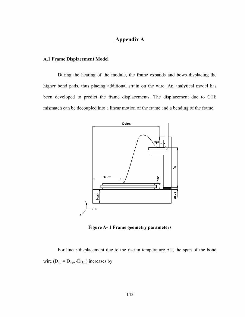
Appendix A
A.1 Frame Displacement Model
During the heating of the module, the frame expands and bows displacing the
higher bond pads, thus placing additional strain on the wire. An analytical model has
been developed to predict the frame displacements. The displacement due to CTE
mismatch can be decoupled into a linear motion of the frame and a bending of the frame.
Figure A- 1 Frame geometry parameters
For linear displacement due to the rise in temperature ∆T, the span of the bond
wire (Dx0 = Dclpx-Dclcx) increases by:
142
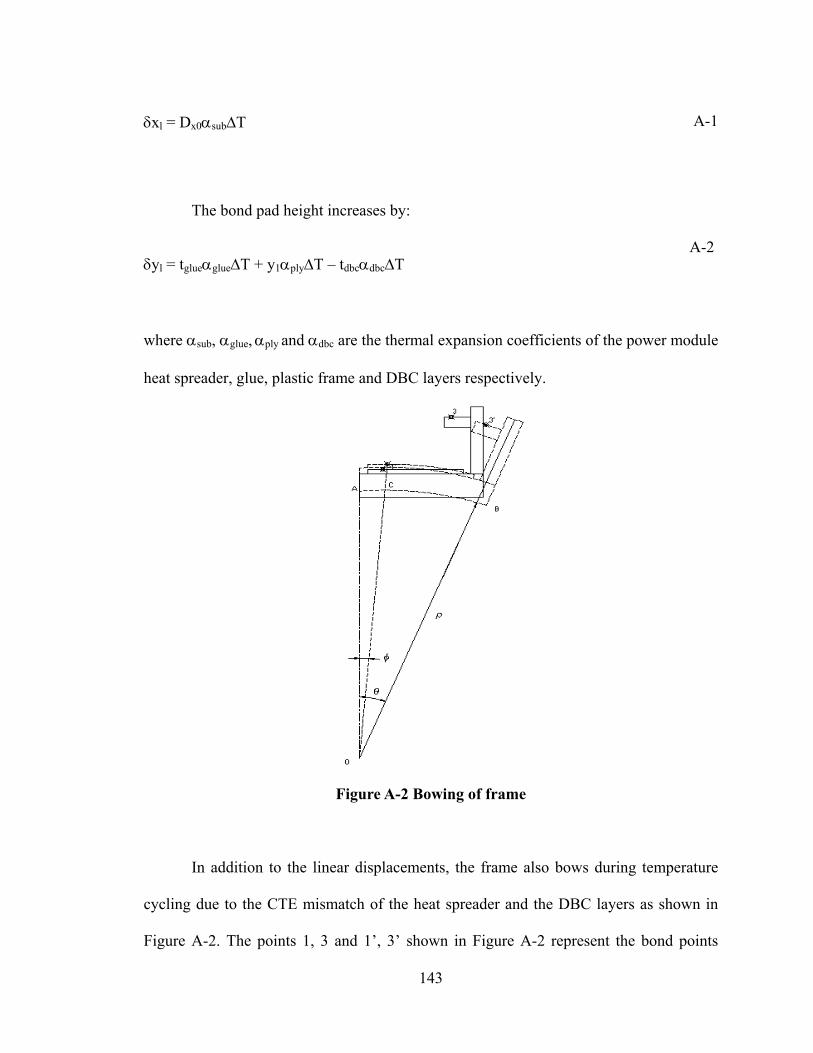
δxl = Dx0αsub∆T A-1
The bond pad height increases by:
δyl = tglueαglue∆T + y1αply∆T – tdbcαdbc∆T A-2
where αsub, αglue, αply and αdbc are the thermal expansion coefficients of the power module
heat spreader, glue, plastic frame and DBC layers respectively.
Figure A-2 Bowing of frame
In addition to the linear displacements, the frame also bows during temperature
cycling due to the CTE mismatch of the heat spreader and the DBC layers as shown in
Figure A-2. The points 1, 3 and 1’, 3’ shown in Figure A-2 represent the bond points
143
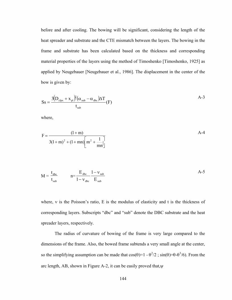
before and after cooling. The bowing will be significant, considering the length of the
heat spreader and substrate and the CTE mismatch between the layers. The bowing in the
frame and substrate has been calculated based on the thickness and corresponding
material properties of the layers using the method of Timoshenko [Timoshenko, 1925] as
applied by Neugebauer [Neugebauer et al., 1986]. The displacement in the center of the
bow is given by:
( ) ( ))F(
tTxD3
Sssub
dbcsub2
plclpx ∆α−α+=
A-3
where,
++++
+=
mn1m)mn1()m1(3
)m1(F22
A-4
M = sub
dbc
tt
n=sub
sub
dbc
dbc
Eν1
ν1E −−
A-5
where, ν is the Poisson’s ratio, E is the modulus of elasticity and t is the thickness of
corresponding layers. Subscripts “dbc” and “sub” denote the DBC substrate and the heat
spreader layers, respectively.
The radius of curvature of bowing of the frame is very large compared to the
dimensions of the frame. Also, the bowed frame subtends a very small angle at the center,
so the simplifying assumption can be made that cos(θ)=1 - θ2/2 ; sin(θ)=θ-θ3/6). From the
arc length, AB, shown in Figure A-2, it can be easily proved that,ψ
144
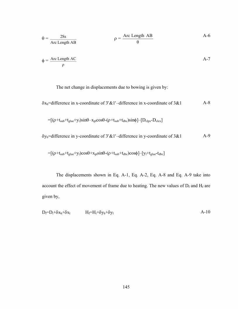
θ = AB Length Arc
Ss2 ρ = θ
ABLength Arc A-6
φ = ρ
ACLength Arc A-7
The net change in displacements due to bowing is given by:
δxb=difference in x-coordinate of 3′&1′–difference in x-coordinate of 3&1
=[(ρ+tsub+tglue+yl)sinθ–xplcosθ-(ρ+tsub+tdbc)sinφ]–[Dclpx-Dclcx]
A-8
δyb=difference in y-coordinate of 3′&1′–difference in y-coordinate of 3&1
=[(ρ+tsub+tglue+yl)cosθ+xplsinθ-(ρ+tsub+tdbc)cosφ]–[yl+tglue-tdbc]
A-9
The displacements shown in Eq. A-1, Eq. A-2, Eq. A-8 and Eq. A-9 take into
account the effect of movement of frame due to heating. The new values of Df and Hf are
given by,
Df=Di+δxb+δxl Hf=Hi+δyb+δyl A-10
145
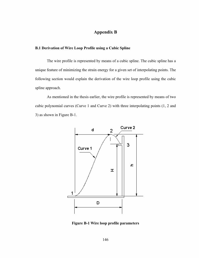
Appendix B
B.1 Derivation of Wire Loop Profile using a Cubic Spline
The wire profile is represented by means of a cubic spline. The cubic spline has a
unique feature of minimizing the strain energy for a given set of interpolating points. The
following section would explain the derivation of the wire loop profile using the cubic
spline approach.
As mentioned in the thesis earlier, the wire profile is represented by means of two
cubic polynomial curves (Curve 1 and Curve 2) with three interpolating points (1, 2 and
3) as shown in Figure B-1.
Figure B-1 Wire loop profile parameters
146
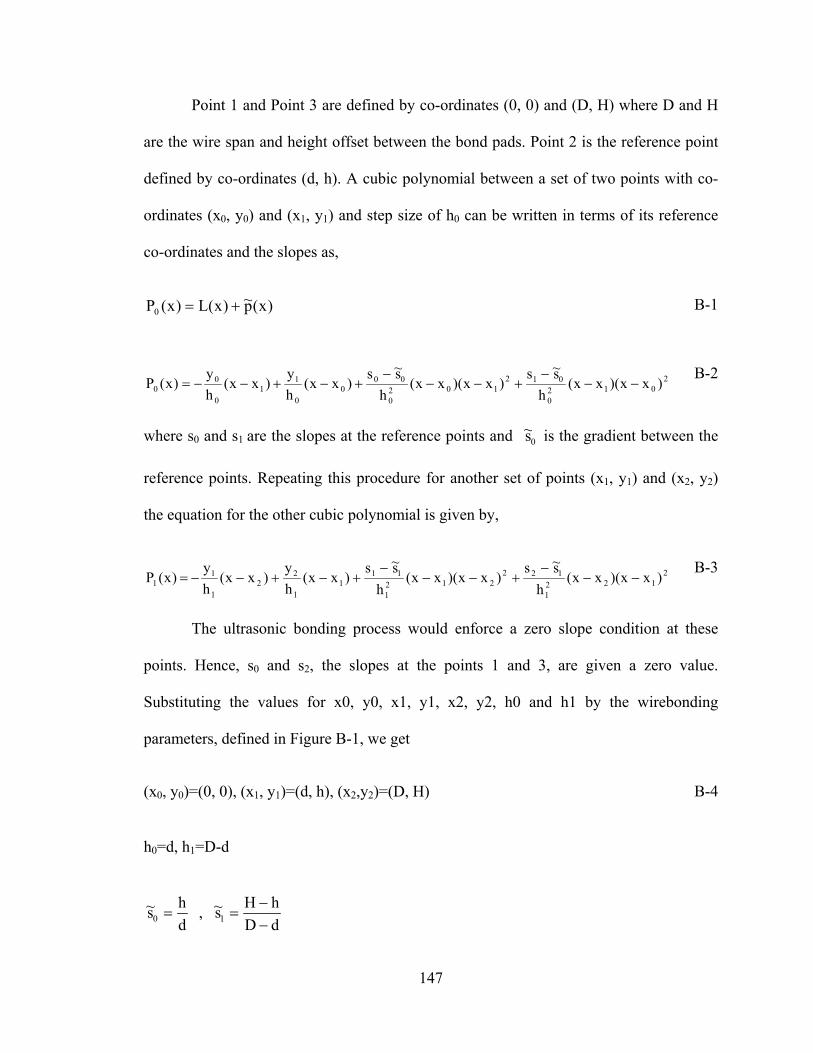
Point 1 and Point 3 are defined by co-ordinates (0, 0) and (D, H) where D and H
are the wire span and height offset between the bond pads. Point 2 is the reference point
defined by co-ordinates (d, h). A cubic polynomial between a set of two points with co-
ordinates (x0, y0) and (x1, y1) and step size of h0 can be written in terms of its reference
co-ordinates and the slopes as,
)x(p~)x(L)x(P0 += B-1
2012
0
012102
0
000
0
11
0
00 )xx)(xx(
hs~s
)xx)(xx(h
s~s)xx(
hy
)xx(hy
)x(P −−−
+−−−
+−+−−=B-2
where s0 and s1 are the slopes at the reference points and 0s~ is the gradient between the
reference points. Repeating this procedure for another set of points (x1, y1) and (x2, y2)
the equation for the other cubic polynomial is given by,
2122
1
122212
1
111
1
22
1
11 )xx)(xx(
hs~s
)xx)(xx(h
s~s)xx(
hy
)xx(hy
)x(P −−−
+−−−
+−+−−=B-3
The ultrasonic bonding process would enforce a zero slope condition at these
points. Hence, s0 and s2, the slopes at the points 1 and 3, are given a zero value.
Substituting the values for x0, y0, x1, y1, x2, y2, h0 and h1 by the wirebonding
parameters, defined in Figure B-1, we get
(x0, y0)=(0, 0), (x1, y1)=(d, h), (x2,y2)=(D, H)
h0=d, h1=D-d
dDs~ ,
ds~ 10 −
==hHh −
B-4
147

The point and slope continuity at points 1, 2 and 3 provides C1 continuity. A C2
continuity is enforced by equating the second order derivatives at point 2 through the
equation,
P0″(x) = P1″(x) at x=x1 B-5
The simplification of Eq. B-5 provides the solution to the unknown slope at point
2, i.e. the value of s1 as,
( )( )
( )
−−
−−
=dD
hDddDDdhH
23s1
B-6
Applying the boundary conditions, the equations of the two curves defining the
wire profile are given by,
22
1
2
2
0 x)dx(d
)dh(S
d
)dx(xdh
dhx)x(P −
−+
−−=
B-7
( )( )
( )( )2
32
2
1
1 dx)Dx(dDhHDx)dx(
dDdDhHS
dD)dx(H
Dd)Dx(h)x(P −−
−−
−−−−
−−
−+
−−
+−−
=
B-8
The curvatures at any point on the curve, defined by y=f(x), is given by,
2/32y1
y
′+
″=κ B-9
Considering the fact that the slope, y′is zero at the reference points 1 and 3, the
equation for the curvature at the reference points is given by,
148
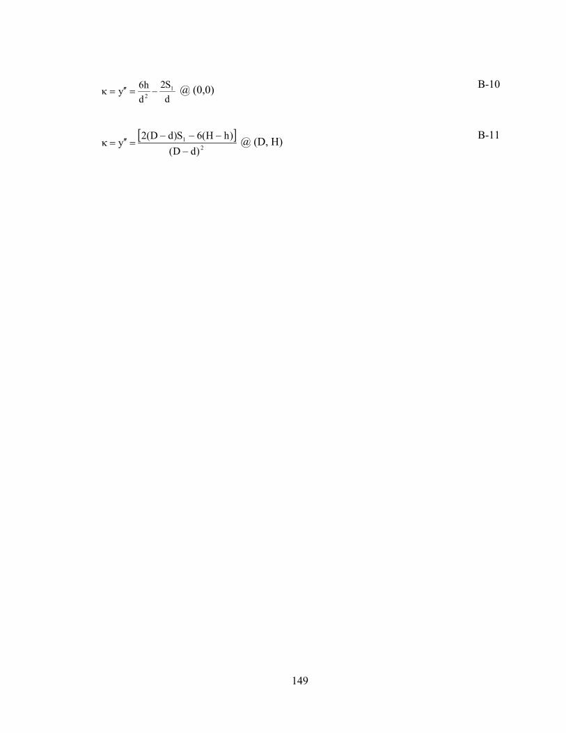
dS2
dh6y 12 −=′′=κ @ (0,0) B-10
[ ]2
1
)dD()hH(6S)dD(2
y−
−−−=′′=κ @ (D, H) B-11
149

Appendix C
C.1 Simple Cubic Spline Model
The energy-based cubic spline model is an iterative solver, which runs on the
Levenberg-Marquardt algorithm for solving a set of non-linear equations. In addition, the
solver also makes use of numerical differentiation and integration. These steps help us
obtain the best location of reference point 2 where the wire would store minimum
potential energy. The main purpose for using a simple analytical model is lost if the
computation time is very high. Hence, a series of tests were performed to study the
patterns of reference point 2, based on various input bond parameters.
C.1.1 Location of Reference Point in Wire Geometry
The cubic spline would plot the best wire shape with minimum energy for a given
reference point 2. The energy-based model goes a step further in locating the best
reference point 2 on the domain, which would further reduce the energy of the curve.
There are several minima’s in the domain chosen and it is important to choose a good
guess value for the solver for a quicker convergence. For a wire bonded without any
height offset the reference point is always located in the middle of the wire span. Figure
C-1 and Figure C-2 show the reference point locations for varying wire lengths and
varying bond height offsets respectively. When the wire lengths are varied it is observed
that the reference point tries to shift towards the mid-span whereas for a higher bond
offset the point shifts towards the right bond pad. It is difficult to capture the trend in
150
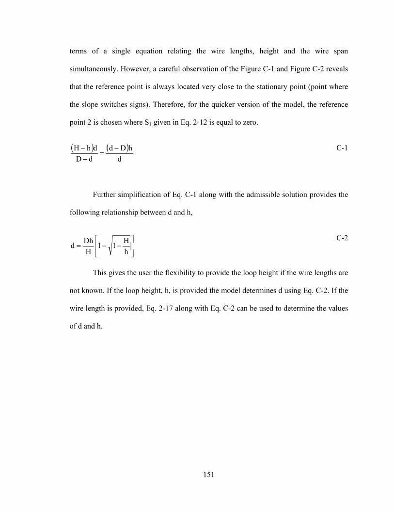
terms of a single equation relating the wire lengths, height and the wire span
simultaneously. However, a careful observation of the Figure C-1 and Figure C-2 reveals
that the reference point is always located very close to the stationary point (point where
the slope switches signs). Therefore, for the quicker version of the model, the reference
point 2 is chosen where S1 given in Eq. 2-12 is equal to zero.
( ) ( )d
hDddD
dhH −=
−−
C-1
Further simplification of Eq. C-1 along with the admissible solution provides the
following relationship between d and h,
−−=
hH11
HDhd
C-2
This gives the user the flexibility to provide the loop height if the wire lengths are
not known. If the loop height, h, is provided the model determines d using Eq. C-2. If the
wire length is provided, Eq. 2-17 along with Eq. C-2 can be used to determine the values
of d and h.
151
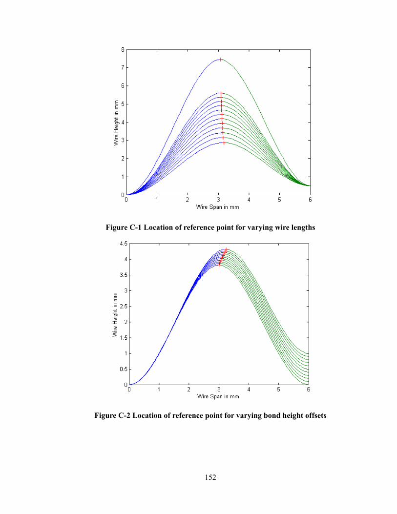
Figure C-1 Location of reference point for varying wire lengths
Figure C-2 Location of reference point for varying bond height offsets
152
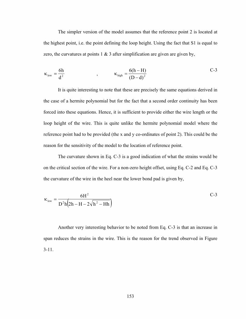
The simpler version of the model assumes that the reference point 2 is located at
the highest point, i.e. the point defining the loop height. Using the fact that S1 is equal to
zero, the curvatures at points 1 & 3 after simplification are given are given by,
2low dh6
=κ , 2high )dD()Hh(6
−−
=κ C-3
It is quite interesting to note that these are precisely the same equations derived in
the case of a hermite polynomial but for the fact that a second order continuity has been
forced into these equations. Hence, it is sufficient to provide either the wire length or the
loop height of the wire. This is quite unlike the hermite polynomial model where the
reference point had to be provided (the x and y co-ordinates of point 2). This could be the
reason for the sensitivity of the model to the location of reference point.
The curvature shown in Eq. C-3 is a good indication of what the strains would be
on the critical section of the wire. For a non-zero height offset, using Eq. C-2 and Eq. C-3
the curvature of the wire in the heel near the lower bond pad is given by,
( )Hhh2Hh2hDH6
22
2
low−−−
=κ C-3
Another very interesting behavior to be noted from Eq. C-3 is that an increase in
span reduces the strains in the wire. This is the reason for the trend observed in Figure
3-11.
153
Appendix D
D.1 Modeling a Reliable Wirebonded Interconnection
This section explains the utility of the model as a design tool in developing
reliable wirebonded interconnection. The objective of the current study would be to
determine the optimum set of input parameters that can produce reliable wirebonds.
Effects of wire twisting and wire thinning near the heel would be ignored. It is assumed
that the optimum bond force, power and bonding time have been used to produce very
strong bonds. The critical parameters that are considered for the study are,
• Wire Length
• Height Offset of bond pads
• Wire Span
• Wire Diameter
D.1.1 Imposed Constraints
As mentioned in the conclusion section of the dissertation, the wire diameter
should be as small as possible to minimize the wire flexure problem. However,
considering the applications and power ratings the wire diameter has been chosen to be15
mil (or 381 µm). The design of the power module prevents a zero height offset of the
wirebonds. However, there is a maximum and minimum bound for each parameter, listed
in Table D-1.
154
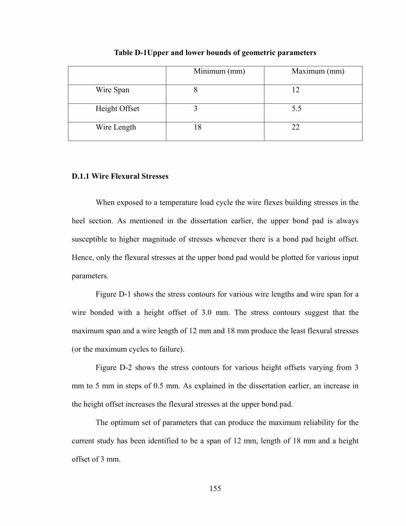
Table D-1Upper and lower bounds of geometric parameters
Minimum (mm) Maximum (mm)
Wire Span 8 12
Height Offset 3 5.5
Wire Length 18 22
D.1.1 Wire Flexural Stresses
When exposed to a temperature load cycle the wire flexes building stresses in the
heel section. As mentioned in the dissertation earlier, the upper bond pad is always
susceptible to higher magnitude of stresses whenever there is a bond pad height offset.
Hence, only the flexural stresses at the upper bond pad would be plotted for various input
parameters.
Figure D-1 shows the stress contours for various wire lengths and wire span for a
wire bonded with a height offset of 3.0 mm. The stress contours suggest that the
maximum span and a wire length of 12 mm and 18 mm produce the least flexural stresses
(or the maximum cycles to failure).
Figure D-2 shows the stress contours for various height offsets varying from 3
mm to 5 mm in steps of 0.5 mm. As explained in the dissertation earlier, an increase in
the height offset increases the flexural stresses at the upper bond pad.
The optimum set of parameters that can produce the maximum reliability for the
current study has been identified to be a span of 12 mm, length of 18 mm and a height
offset of 3 mm.
155
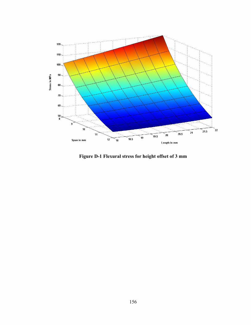
Figure D-1 Flexural stress for height offset of 3 mm
156
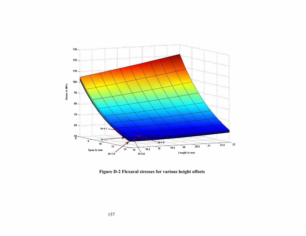
Figure D-2 Flexural stresses for various height offsets
157
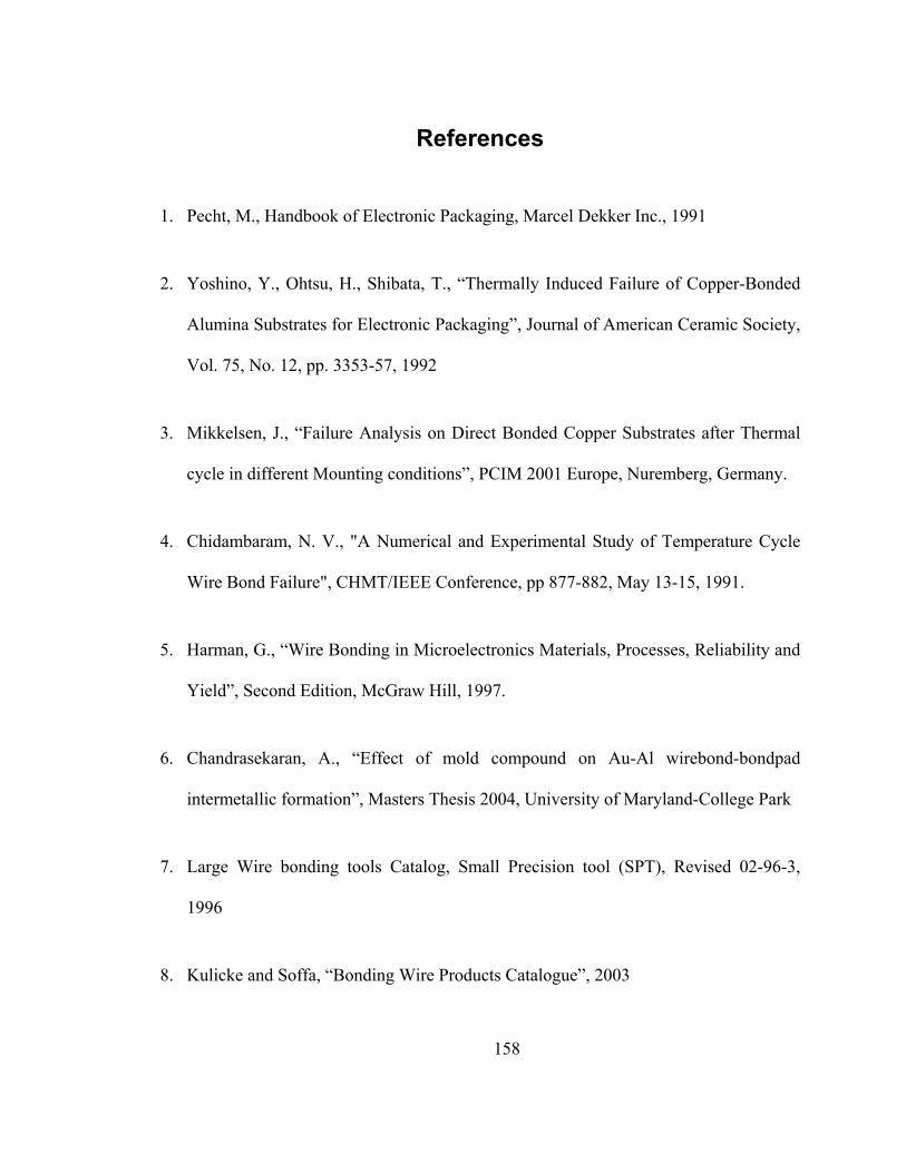
References
1. Pecht, M., Handbook of Electronic Packaging, Marcel Dekker Inc., 1991
2. Yoshino, Y., Ohtsu, H., Shibata, T., “Thermally Induced Failure of Copper-Bonded
Alumina Substrates for Electronic Packaging”, Journal of American Ceramic Society,
Vol. 75, No. 12, pp. 3353-57, 1992
3. Mikkelsen, J., “Failure Analysis on Direct Bonded Copper Substrates after Thermal
cycle in different Mounting conditions”, PCIM 2001 Europe, Nuremberg, Germany.
4. Chidambaram, N. V., "A Numerical and Experimental Study of Temperature Cycle
Wire Bond Failure", CHMT/IEEE Conference, pp 877-882, May 13-15, 1991.
5. Harman, G., “Wire Bonding in Microelectronics Materials, Processes, Reliability and
Yield”, Second Edition, McGraw Hill, 1997.
6. Chandrasekaran, A., “Effect of mold compound on Au-Al wirebond-bondpad
intermetallic formation”, Masters Thesis 2004, University of Maryland-College Park
7. Large Wire bonding tools Catalog, Small Precision tool (SPT), Revised 02-96-3,
1996
8. Kulicke and Soffa, “Bonding Wire Products Catalogue”, 2003
158
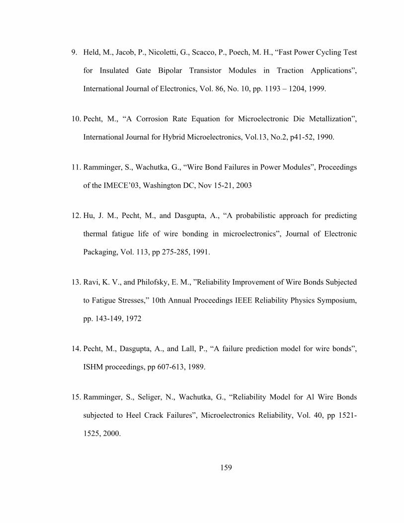
9. Held, M., Jacob, P., Nicoletti, G., Scacco, P., Poech, M. H., “Fast Power Cycling Test
for Insulated Gate Bipolar Transistor Modules in Traction Applications”,
International Journal of Electronics, Vol. 86, No. 10, pp. 1193 – 1204, 1999.
10. Pecht, M., “A Corrosion Rate Equation for Microelectronic Die Metallization”,
International Journal for Hybrid Microelectronics, Vol.13, No.2, p41-52, 1990.
11. Ramminger, S., Wachutka, G., “Wire Bond Failures in Power Modules”, Proceedings
of the IMECE’03, Washington DC, Nov 15-21, 2003
12. Hu, J. M., Pecht, M., and Dasgupta, A., “A probabilistic approach for predicting
thermal fatigue life of wire bonding in microelectronics”, Journal of Electronic
Packaging, Vol. 113, pp 275-285, 1991.
13. Ravi, K. V., and Philofsky, E. M., ”Reliability Improvement of Wire Bonds Subjected
to Fatigue Stresses,” 10th Annual Proceedings IEEE Reliability Physics Symposium,
pp. 143-149, 1972
14. Pecht, M., Dasgupta, A., and Lall, P., “A failure prediction model for wire bonds”,
ISHM proceedings, pp 607-613, 1989.
15. Ramminger, S., Seliger, N., Wachutka, G., “Reliability Model for Al Wire Bonds
subjected to Heel Crack Failures”, Microelectronics Reliability, Vol. 40, pp 1521-
1525, 2000.
159
16. Meyyappan, K., McCluskey, P., Hansen, P., “Wire Flexure Fatigue Model for
Asymmetric Bond Height”, InterPACK’03, Jul 6-11, 2003.
17. Spath, H., “Spline Algorithms for Curves and Surfaces”, Utilitas Mathematica
Publishing Inc, 1974.
18. Carl de Boor, “A Practical Guide to Splines- Revised Edition”, Springer, 2001.
19. Meyyappan, K., McCluskey, P., Hansen, P., “Wire Fatigue Models for Power
Electronic Modules”, IMECE 2003, Washington DC, Nov 15-21, 2003
20. Manfredo P. Do Carmo, “Differential geometry of curves and surfaces”, Prentice
Hall, 1976
21. Suresh, S., “Fatigue of Materials”, Cambridge University Press, 1992
22. Rowland, E. S., “Effect of Residual Stress on Fatigue”, Proceedings of the 10th
Sagamore Army Materials Research Conference, New York, pp. 229-244, Aug 13-16,
1963
23. Fox, A., “Effect of Temperature on Stress Relaxation of Several Metallic Materials”,
Proceedings of the 28th Sagamore Army Materials Research Conference, New York,
pp. 181-203, Jul 13-17, 1981
24. The Aluminum Association, “Aluminum Standards and Data”, New York, 1968
160
25. Coffin, L. F., “A study of the effects of cyclic thermal stresses on a ductile metal”,
Transaction of the ASME, Vol. 76, pp 931-950, 1954
26. Manson, S. S., “Behavior of materials under conditions of thermal stress”, National
Advisory Commission on Aeronautics: Report 1170, Cleveland: Lewis Flight
Propulsion Laboratory, 1954
27. Deyhim, A., Yost, B., Lii, M. J., Li, C. Y., “Characterization of the fatigue properties
of bonding wires”, Electronic Components and Technology Conference, pp 836-841,
1991
28. Crispi, F. J., Mailing, G. C., Rzant, A. W., “Monitoring Microinch Displacements in
Ultrasonic Welding Equipment”, IBM Journal of Research and Development, 1972,
pp 307-312.
29. Wilson, A. D., Martin, B. D., Strope, D. H., “Holographic Interferometry Applied to
Motion Studies of Ultrasonic Bonders”, IEEE Transactions on Sonics and
Ultrasonics, Vol. SU-19, No. 4, pp. 453-461, Oct 1972
30. Dushkes, S.Z., “A design Study of Ultrasonic Bonding Tips”, IBM Journal of
Research and Development, Vol. 13, No. 3, pp. 230-235, May 1971
31. Joshi, K. C., “The Formation of Ultrasonic Bonds Between Metals”, IBM Journal of
Research and Development, Welding Journal, pp 840-848, Dec 1971
161
32. Harman, G., Leedy, K. O., “An experimental model of the microelectronic ultrasonic
wire bonding mechanism”, 10th Annual proceedings Reliability Physics Symposium,
pp. 72-77, 1972
33. Langenecker, B., “Effects of Ultrasound on Deformation Characteristics of Metals”,
IEEE Transactions on Sonics and Ultrasonics, Vol. SU-13, No. 1, Mar 1966
34. Hayes, G. A., Shyne, J. C., “The influence of Ultrasonic Energy on Kinetic Processes
in Solids”, IEEE Transactions on Sonics and Ultrasonics, Vol. SU-16, No. 2, pp. 68-
75, Apr 1969
35. Krzanowski, J. E., “A Transmission Electron Microscopy Study of Ultrasonic Wire
Bonding”, IEEE Transactions on Components, Hybrids and Manufacturing
Technology, Vol. 13, No. 1, Mar 1990
36. Ohga, K., “Failure Analysis of Bonding Wires in Power Transistor Modules”, 17th
International Symposium for testing & Failure Analysis, Los Angeles, CA, pp. 237-
247, 11-15 Nov, 1991.
37. Wu, W., Held, M., Jacob, P., Scacco, P., Birolini, A., “Investigation on the Long
Term reliability of Power IGBT Modules”, Proceedings of the 7th International
Symposium on Power Semiconductor Devices and ICs, Yokohama, pp. 443-448, May
23-25, 1995.
162
38. Harman, G., Albers, J., “The Ultrasonic Welding Mechanism as Applied to
Aluminum and Gold Wire Bonding in Microelectronics”, IEEE Transactions on Parts,
Hybrids and Packaging, Vol. PHP-13, No. 4, Dec 1977
39. Ultrasonic Bonding Wedges Catalogue, Small Precision tool (SPT), Revised 08-99-6,
1999
40. Takahashi, Y., Shibamoto, S., Inoue, K., “Numerical Analysis of the Interfacial
Contact Process in Wire Thermocompression Bonding”, IEEE Transaction on
Components, Hybrids and Manufacturing Technology, Part A, Vol. 19, No. 2, Jun
1996
41. Qin, I. W., Bereznycky, P., Doerr, D., "Wedge Bonding for Ultra Fine Pitch
Applications," Proc. Advanced Packaging Technologies Seminar, SEMICON
Singapore 2001
42. Timoshenko, S., “Analysis of Bi-Metal Thermostats”, Journal of Optical Society of
America, Vol. 23, pp. 233-55, 1925
43. Neugebauer, C. A., Yerman, A. F., Carlson, R. O., Burgess, J. F., Webster, H. F., and
Glascock, H. H., “The Packaging of Power Semiconductor Devices”, Gordon and
Breach Science Publishers, Vol. 7, 1986
163
164
44. Jeon, I., Chung, Q., Hong, J., Byun, K., “The Effect of Ultrasonic Power on Bonding
Pad and IMD Layers in Ultrasonic Wire Bonding”, IEEE International Symposium on
Electronic Materials and Packaging, pp 235-242, 2001
45. Popov, E. P., “Engineering Mechanics of Solids”, Prentice-Hall Inc., 1998
Related Documents


