ABSTRACT INTERACTION OF INTENSE LASER PULSES …ireap.umd.edu/sites/default/files/documents/Johnson-Lu… ·  · 2015-01-08THZ GENERATION AND REMOTE MAG-NETOMETRY Luke A. Johnson,

ABSTRACT

Title of dissertation: INTERACTION OF INTENSE LASERPULSES WITH GAS FOR TWO-COLORTHZ GENERATION AND REMOTE MAG-NETOMETRY

Luke A. Johnson, Doctor of Philosophy, 2014

Dissertation directed by: Professor Thomas AntonsenDepartments of Physics and Electrical & Com-puter EngineeringProfessor Phillip SprangleDepartments of Physics and Electrical & Com-puter Engineering

The interaction of intense laser pulses with atmospheric gases is studied in

two contexts: (i) the generation of broadband terahertz radiation via two-color

photoionization currents in nitrogen, and (ii) the generation of an electromagnetic

wakefield by the induced magnetization currents of oxygen.

(i) A laser pulse propagation simulation code was developed to investigate

the radiation patterns from two-color THz generation in nitrogen. Understanding

the mechanism for conical, two-color THz furthers the development of broadband

THz sources. Two-color photoionization produces a cycle-averaged current driving

broadband, conically emitted THz radiation. The THz emission angle is found to

be determined by an optical Cherenkov effect, occurring when the front velocity of

the ionization induced current source is greater than the THz phase velocity.

(ii) A laser pulse propagating in the atmosphere is capable of exciting a mag-

netic dipole transition in molecular oxygen. The resulting transient current creates

a co-propagating electromagnetic field behind the laser pulse, i.e. the wakefield,

which has a rotated polarization that depends on the background magnetic field.

This effect is analyzed to determine it’s suitability for remote atmospheric magne-

tometry for the detection of underwater and underground objects. In the proposed

approach, Kerr self-focusing is used to bring a polarized, high-intensity, laser pulse

to focus at a remote detection site where the laser pulse induces a ringing in the oxy-

gen magnetization.The detection signature for underwater and underground objects

is the change in the wakefield polarization between different measurement locations.

The magnetic dipole transition line that is considered is the b1Σ+g −X3Σ−

g transition

band of oxygen near 762 nm.

INTERACTION OF INTENSE LASER PULSES WITH GAS FOR

TWO-COLOR THZ GENERATION AND REMOTEMAGNETOMETRY

by

Luke A. Johnson

Dissertation submitted to the Faculty of the Graduate School of theUniversity of Maryland, College Park in partial fulfillment

of the requirements for the degree ofDoctor of Philosophy

2014

Advisory Committee:Professor Thomas Antonsen, Chair/AdvisorProfessor Phillip SprangleProfessor Ki-yong KimProfessor Adil HassamProfessor Edward Ott

c© Copyright by

Luke A. Johnson2014

Table of Contents

List of Figures iv

1 Introduction 11.1 Two-Color THz generation . . . . . . . . . . . . . . . . . . . . . . . . 21.2 Electromagnetic Wakefields from Oxygen Magnetization . . . . . . . 7

2 Two-color THz Generation 112.1 Overview . . . . . . . . . . . . . . . . . . . . . . . . . . . . . . . . . . 112.2 Model . . . . . . . . . . . . . . . . . . . . . . . . . . . . . . . . . . . 15

2.2.1 Unidirectional Pulse Propagation Model . . . . . . . . . . . . 152.2.2 Material Response of Molecular Nitrogen . . . . . . . . . . . . 16

2.3 Conical THz Radiation . . . . . . . . . . . . . . . . . . . . . . . . . . 212.3.1 Cherenkov Model . . . . . . . . . . . . . . . . . . . . . . . . . 222.3.2 Angular Dependence of THz on Refractive Index . . . . . . . 292.3.3 Cherenkov Radiation from Four-Wave Mixing . . . . . . . . . 322.3.4 Experimental Comparison . . . . . . . . . . . . . . . . . . . . 32

2.4 Directing THz Using Tilted-Intensity Fronts . . . . . . . . . . . . . . 342.5 Conclusion . . . . . . . . . . . . . . . . . . . . . . . . . . . . . . . . . 362.A Hybrid Ionization Rate . . . . . . . . . . . . . . . . . . . . . . . . . . 382.B Derivation of THz Spectrum . . . . . . . . . . . . . . . . . . . . . . . 41

2.B.1 Spectrum of Cherenkov Emission . . . . . . . . . . . . . . . . 432.B.2 Spectrum from Tilted Intensity Fronts . . . . . . . . . . . . . 45

3 Remote Atmospheric Magnetometry 503.1 Introduction . . . . . . . . . . . . . . . . . . . . . . . . . . . . . . . . 503.2 Focusing & Compression of Intense Laser Pulses . . . . . . . . . . . . 533.3 Optical Magnetometry Model . . . . . . . . . . . . . . . . . . . . . . 573.4 Faraday Rotation of Wakefields Driven by Intense Laser Pulses . . . . 603.5 Discussion and Concluding Remarks . . . . . . . . . . . . . . . . . . 663.A Transitions in Oxygen Molecule . . . . . . . . . . . . . . . . . . . . . 673.B Density Matrix Equations . . . . . . . . . . . . . . . . . . . . . . . . 693.C Resonant Fluorescent Excitation (Hanle effect) . . . . . . . . . . . . 72

ii

Bibliography 75

iii

List of Figures

1.1 Two-color THz mechanism . . . . . . . . . . . . . . . . . . . . . . . . 61.2 Conical THz from experiment and simulation . . . . . . . . . . . . . 8

2.1 Schematic of the experimental setup being modeled . . . . . . . . . . 122.2 Example of conical THz radiation . . . . . . . . . . . . . . . . . . . . 232.3 Schematic of optical Cherenkov mechanism . . . . . . . . . . . . . . . 242.4 Terahertz source current . . . . . . . . . . . . . . . . . . . . . . . . . 262.5 Terahertz energy . . . . . . . . . . . . . . . . . . . . . . . . . . . . . 272.6 Conical THz for different refractive index . . . . . . . . . . . . . . . . 302.7 Dependence of THz angle on refractive index . . . . . . . . . . . . . . 312.8 Conical THz from four-wave mixing . . . . . . . . . . . . . . . . . . . 332.9 Laser pulse with tilted intensity fronts . . . . . . . . . . . . . . . . . 352.10 Terahertz from tilted intensity fronts . . . . . . . . . . . . . . . . . . 362.11 Terahertz angle dependence on tilt . . . . . . . . . . . . . . . . . . . 372.12 Ionization rates . . . . . . . . . . . . . . . . . . . . . . . . . . . . . . 39

3.1 Remote magnetometry configuration . . . . . . . . . . . . . . . . . . 513.2 Schematic of nonlinear laser propagation . . . . . . . . . . . . . . . . 543.3 Example of laser propagation with self-focusing . . . . . . . . . . . . 563.4 Molecular oxygen’s energy levels . . . . . . . . . . . . . . . . . . . . . 583.5 Schematic of laser pulse train and electromagnetic wakefield . . . . . 623.6 Wakefield response functions . . . . . . . . . . . . . . . . . . . . . . . 643.7 Fractional change in wakefield intensity . . . . . . . . . . . . . . . . . 653.8 Electron occupancy energy levels of oxygen . . . . . . . . . . . . . . . 69

iv

Chapter 1: Introduction

The propagation of intense laser pulses through gases and plasma is of sig-

nificant scientific and practical interest. Applications include; compact sources for

1GeV electrons from laser wakefield acceleration [1], generation of ultraviolet and

x-ray radiation via high harmonic generation [2], laser generated plasma columns

for directing electrostatic discharges [3], and remote sensing via laser induced break-

down spectroscopy [4]. But each application requires understanding the interplay

of many physical processes, such as the nonlinear response to the gas specie’s po-

larization in the presence of the laser electric field. For a single gas specie, such as

molecular nitrogen, the nonlinear response can be divided into a number of separate

effects such as the instantaneous response of the bound electron cloud, the delayed

rotational response of the molecule, and the production of plasma via photoion-

ization. Each process can couple back to the fields and modify the laser pulse as

it propagates, generate new frequencies of electromagnetic radiation, or accelerate

charged particles. Consequently, intense laser-gas interactions have proved to be an

interesting and fruitful area of research.

This thesis will explore two phenomena associated with laser-gas interaction:

the generation of broadband terahertz radiation via two-color photoionization cur-

1

rents in nitrogen, and the generation of an electromagnetic wakefield by the induced

magnetization currents of oxygen.

1.1 Two-Color THz generation

Electromagnetic THz radiation has a flexible definition in the literature. The

name alone suggests that it should refer to frequencies of electromagnetic radiation

on the order of 1 THz. But the “THz gap,” the range of frequencies in the electro-

magnetic spectrum that lacks sources and detectors, is often referred to as covering

from 0.3 to 20 THz [5]. The use of THz as a descriptor is relaxed further when

discussing broadband THz radiation where the pulse bandwidth can reach 75 THz

which is well into the mid-infrared [5, 6]. In this work, THz radiation will typically

refer to broadband THz pulses.

A number of different mechanisms can be responsible for the generation of

THz radiation. However, the mechanisms share a common feature: charged particles

(typically electrons) oscillating at THz frequencies. For example, in an accelerator,

coherent synchrotron radiation will produce single-cycle THz pulses from electron

bunches with sub-picosecond density modulations. At Brookhaven Lab, a ∼ 100 µJ

single cycle THz pulses with peak fields of ∼ 3 MV/cm was generated [5]. A second

example involves electro-optic crystals, such as LiTaO3 or LiNbO3, which produce

a nonlinear polarization that depends on the electric field squared. This allows for

rectification of femtosecond laser pulses generating THz radiation [7, 8]. Another

mechanism for THz generation uses the electrostatic fields of a laser-accelerated,

2

sub-picosecond electron bunch to drive transition radiation at a plasma-vacuum

interface [9].

Hamster et al. [10] made the first observation of THz radiation from a laser

generated plasma. An intense laser pulse (1018 to 1019 W/cm2) was focused on gas

targets. Field ionization generated a plasma and then, on the timescale of the laser

pulse (100 fs), the electrons were driven away from the ions via the pondermotive

force. This pondermotive current drove the THz radiation. The emitted radiation

had an energy of ∼ 0.1 nJ and was centered at a few THz.

The first observation of THz generation due to an intense laser pulse com-

posed of a fundamental frequency and its harmonic, a “two-color pulse,” was made

by Cook et al. [11]. Cook et al. observed ∼ 5 pJ THz pulses with peak fields of

∼ 2 kV/cm which was comparable to optical rectification in electro-optic crystals.

The THz generation mechanism was attributed to an unknown four-wave mixing

process. Interestingly, several possible THz generation mechanisms were discussed

in Ref. [11]. The first being the nonlinear response of the bound electrons. But,

the THz energy scaling did not match the expected dependence on the intensities

of the two colors. The second possibility proposed by Cook et al. was that a field-

ionization process was occurring, but they lacked the ability to scan a large enough

range of laser intensities to investigate this effect. Another unexplored possibility

was that excited or Rydberg states where being created and they were contributing

to an enhanced nonlinear susceptibility. Later experimental work also observed that

the THz yields were two orders of magnitude larger than what would be expected

based on the nonlinear susceptibility of air [12]. Additionally, these works found

3

that the THz energy scaling was observed to follow UTHz ∝ I2I21 (where I1 is the

fundamental intensity and I2 is the second harmonic intensity) which is suggestive

of an four-wave mixing process, but this scaling only occurred when the laser inten-

sity was sufficiently high to field ionize the gas [12–14]. This firmly connected the

THz generation with plasma formation, but the mechanism remained unknown and

continued to be described in the context of four-wave mixing.

It was proposed that the THz generation mechanism involves the generation

of a current, called a photocurrent, on the timescale of the laser pulse by electrons

that are field ionized [15]. The previously observed sinusoidal dependence of the

THz yield with propagation distance is consistent with both the photocurrent [15]

and four-wave mixing models [11, 12]. But in Ref. [15], the oscillating behavior in

the THz yield was shown to indicate that the THz yield is minimal when the field

peaks of the two colors are coincident. This result is inconsistent with the four-

wave mixing model. Additionally, a preformed plasma was shown to reduce the

THz yield [15]. This bolstered the argument that THz generation is not due to a

nonlinear susceptibility, but rather, due to ionizing the gas. Later work provided the

theoretical underpinning for the two-color photocurrent model and is the basis of the

current understanding of the fundamental mechanism for two-color THz generation

[6].

Understanding the mechanism of two-color THz, as explained by Kim et al.

[15], is important for understanding why the THz is emitted with a conical radiation

profile. A typical experimental setup is as follows [15]. A femtosecond laser pulse

with millijoule energies is focused into a nitrogen gas cell. As the fundamental

4

pulse propagates, it passes through a beta barium borate (BBO) crystal, and a

copropagating second-harmonic (400 nm) pulse is generated. The fundamental and

second-harmonic pulses will be referred to as the “pump pulses.” The pump pulses

largely overlap both spatially and temporally as they approach their common focal

point. When they reach sufficient intensity, they weakly ionize the gas and generate

THz radiation.

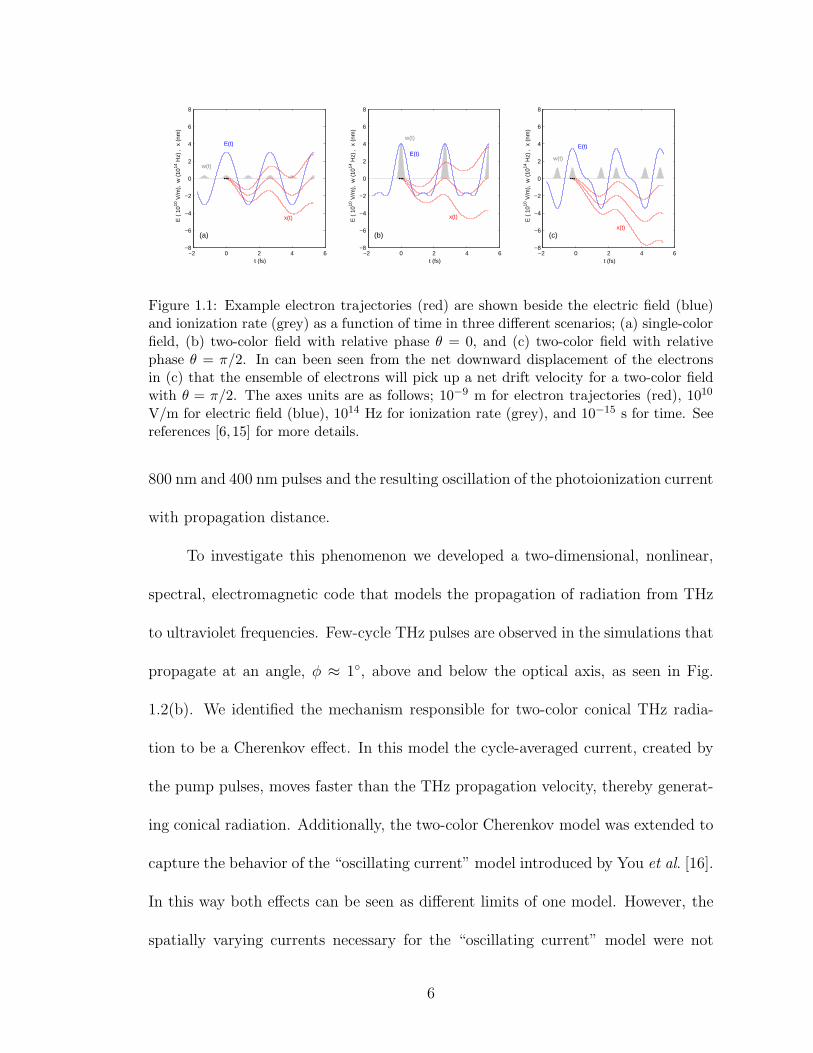
The THz radiation is generated when electrons, produced by ionization, create

a cycle-averaged current on the time scale of the pump-pulses’ envelope (25 fs).

Atoms are preferentially ionized at temporal peaks in the laser field and the resulting

electrons are born with essentially zero velocity. This is illustrated by the location

of the peak ionization rate and the initial slope of the electron trajectories in Fig.

1.1. In a single-color pulse, as shown in Fig.1.1(a), electrons ionized on either

side of the peak field acquire drift velocities in opposite directions. The ensemble

average drift velocity of the resulting electrons is zero, and therefore no macroscopic,

cycle-averaged current is produced. However, when two colors are present with the

appropriate relative phase, for example in Fig. 1.1(c), they interfere, and electrons

acquire a macroscopic, cycle-averaged current. The cycle-averaged current builds

up on the time scale of the pump-pulses’ duration and drives the THz fields.

Experimentally, the THz radiation is observed to have a conical radiation

profile relative to the laser pulse axis [16]. An example of a slice of the conical THz

profile is seen in Fig. 1.2(a) [17]. The conical THz was previously explained by off-

axis phase matching from a line source of periodic THz emitters [16]. It was proposed

that the THz line source was created by the phase-velocity mismatch between the

5

−2 0 2 4 6−8

−6

−4

−2

0

2

4

6

8

t (fs)

E

( 1

010 V

/m),

w (

1014

Hz)

, x

(nm

)

E(t)

w(t)

x(t)

(a)

−2 0 2 4 6−8

−6

−4

−2

0

2

4

6

8

t (fs)

E

( 1

010 V

/m),

w (

1014

Hz)

, x

(nm

)

E(t)

w(t)

x(t)

(b)

−2 0 2 4 6−8

−6

−4

−2

0

2

4

6

8

t (fs)

E

( 1

010 V

/m),

w (

1014

Hz)

, x

(nm

)

E(t)

w(t)

x(t)(c)

Figure 1.1: Example electron trajectories (red) are shown beside the electric field (blue)and ionization rate (grey) as a function of time in three different scenarios; (a) single-colorfield, (b) two-color field with relative phase θ = 0, and (c) two-color field with relativephase θ = π/2. In can been seen from the net downward displacement of the electronsin (c) that the ensemble of electrons will pick up a net drift velocity for a two-color fieldwith θ = π/2. The axes units are as follows; 10−9 m for electron trajectories (red), 1010

V/m for electric field (blue), 1014 Hz for ionization rate (grey), and 10−15 s for time. Seereferences [6, 15] for more details.

800 nm and 400 nm pulses and the resulting oscillation of the photoionization current

with propagation distance.

To investigate this phenomenon we developed a two-dimensional, nonlinear,

spectral, electromagnetic code that models the propagation of radiation from THz

to ultraviolet frequencies. Few-cycle THz pulses are observed in the simulations that

propagate at an angle, φ ≈ 1, above and below the optical axis, as seen in Fig.

1.2(b). We identified the mechanism responsible for two-color conical THz radia-

tion to be a Cherenkov effect. In this model the cycle-averaged current, created by

the pump pulses, moves faster than the THz propagation velocity, thereby generat-

ing conical radiation. Additionally, the two-color Cherenkov model was extended to

capture the behavior of the “oscillating current” model introduced by You et al. [16].

In this way both effects can be seen as different limits of one model. However, the

spatially varying currents necessary for the “oscillating current” model were not

6

observed in simulations implying that the optical Cherenkov mechanism is domi-

nant. [18]. It is noted that optical Cherenkov is a common mechanism to achieve

the necessary phase matching for the generation of THz radiation in electro-optic

crystals by the nonlinear optics community [7].

There are two THz generation mechanisms that appear similar to that in this

work but are in fact different. The first is that of D’Amico et al. [19, 20], observed

conical THz radiation and interpreted it as a form of the Cherenkov effect. How-

ever, D’Amico et al. used a single-color laser pulse to drive a collisionally-damped,

few-cycle plasma oscillation via the pondermotive force. Whereas, the two-color

Cherenkov mechanism requires a two-color laser pulse to drive photocurrents and

operates at intensities for which the pondermotive force is negligible. The second

was proposed by Penano et al. [21] and involves the four-wave mixing of a two-color

laser pulse in a collisional, preionized plasma. While this mechanism does require a

two-color laser pulse, it does not produce conical THz via a Cherenkov process. Ad-

ditionally, it relies on the pondermotive force which is not significant for intensities

considered in our work.

1.2 Electromagnetic Wakefields from Oxygen Magnetization

A high-intensity pump laser pulse can be employed to drive a magnetization

current in molecular oxygen. This is possible because oxygen’s ground state has a

total spin 1 and therefore an oscillating magnetic field can drive an oscillation in

oxygen’s magnetic moment. After the intense laser pulse has passed, the magne-

7

(a)

τ (fs)

x (m

m)

−50 0 50

−1

0

1

(MV

/cm

)

−20

0

20

φ

(b)

Figure 1.2: (a) Experimental and (b) simulation examples of conical few-cycle THz pulses.The experimental figure shows a snapshot of the spatial profile of THz pulse inside a ZnTecrystal. The simulation shows the THz pulse directly after its creation as a function oftransverse space and time in the light frame. There is a direct correspondence betweenthe temporal axis and the optical axis.

tization current from the oxygen will be left ringing at approximately the pump

frequency and will slowly damp away due to collisions with atmospheric molecules.

This forms an electromagnetic wakefield that trails behind the laser pulse. In the

presence of a static background magnetic field, the Zeeman effect causes a splitting

in the ground state energy levels. This energy level splitting means that polarization

of the magnetization wakefield will rotate around the optical access in proportion

to the magnetic field strength.

This mechanism can, in principle, provide a means to remotely measure vari-

ations in the earth’s magnetic field in atmospheric conditions. For a number of

magnetic anomaly detection (MAD) applications, such as detection of nuclear sub-

marines, 10µG magnetic field variations must be detected at standoff distances of

8

approximately one kilometer from the sensor [22]. Other applications include detec-

tion of unexploded ordinance and underwater mines.

The propagation of the high-intensity pump laser pulse to remote detection

sites is considered. We show that high laser intensities (below 1012W/cm2 to avoid

photoionization processes) can be propagated to remote locations due to the self

focusing optical Kerr effect. We consider the magnetization currents that are left

ringing behind the pump pulse and the resulting co-propagating electromagnetic

field. This field is referred to as the wakefield and it undergoes polarization rotation

due to the Zeeman splitting of oxygen’s ground state. The magnetic field variation

is detected by measuring the wakefield’s polarization.

Molecular oxygen’s paramagnetic response is due to two unpaired valance elec-

trons. The ground state of oxygen X3Σ−g , commonly referred to as “triplet oxygen,”

has total angular momentum J = 1, total spin S = 1, and three degenerate sub-

levels. The excited upper state being considered is denoted by b1Σ+g . It has J = 0

and is a spin singlet state S = 0 with only one sublevel. The upper state can

undergo three radiative transitions, b1Σ+g →X3Σ−

g (m = ±1), b1Σ+g →X3Σ−

g (m = 0),

but the latter is insignificant because it is an electric quadruple transition. The

O2 transition line being considered is the b1Σ+g −X3Σ−

g transition band of oxygen

near 762 nm. In the low intensity, long laser pulse, regime, this transition has been

investigated theoretically [23,24] and experimentally [25] and is a prominent feature

of air glow.

A major challenge for this, as well as any remote atmospheric optical magne-

tometry concept, is collisional dephasing (elastic collisions) of the transitions. The

9

elastic molecular collision frequency, at standard temperature and pressure (STP),

is γc = Nairσvth = 3.5 × 109 s−1, where σ is the molecular cross section and vth

is the thermal velocity [25]. The Larmor frequency in the earth’s magnetic field

is Ω0 = qB0/(2mc) ≈ 4.5 × 106 rad/s (~Ω0 = 3 × 10−9 eV), where m and q are

the electron mass and charge and c is the speed of light, is much smaller than the

collision frequency. Since the dephasing frequency is far greater than the Larmor

frequency, the parameters are somewhat restrictive for remote atmospheric magne-

tometry. However, rotational magnetometry experiments based on molecular oxy-

gen at STP and magnetic fields of ∼ 10G have shown measurable linear Faraday

rotational effects [25].

Previous theoretical work [24] revealed major issues with atmospheric mag-

netic field measurements using oxygen, these include: (1) extremely low photon

absorption cross sections, (2) a broad magnetic resonance linewidth due to colli-

sions, and (3) quenching of excited-state fluorescence. These issues largely stem

from oxygen’s small magnetic dipole moment and large collision rate. In our work,

however, the wakefield’s polarization rotation is the magnetic signature and the laser

pulse intensities are approximately six orders of magnitude larger.

10

Chapter 2: Two-color THz Generation

2.1 Overview

Ultrashort, ultraintense laser pulses propagating through and ionizing gases

have produced intense pulses of THz radiation. The large electric and magnetic

fields of these pulses are potentially useful for a variety of applications [5]. For

example, intense magnetic fields (≈ 1 T) with subpicosecond duration can be used

for coherent control of the spin degree of freedom, in spintronic systems, exciting

and deexciting spin waves [26]. In molecular spectroscopy, the high electric fields

(≈ 1 MV/cm) of THz pulses can be used to orient molecules for transient birefrin-

gence and free induction decay measurements [27]. Using ultrashort laser pulses to

generate THz via air breakdown may provide a scalable, compact source of few-cycle

THz pulses when compared to modern accelerators [5]. Scaling to higher energies is

possible because field-induced breakdown of the medium is a feature, not a limita-

tion. In addition, the compact nature of these sources and their ability to use air as

a generation medium potentially allows for standoff capabilities [28]. Generating the

THz close to its target decreases the distance over which the THz must propagate,

limiting atmospheric absorption [29]. Developing such a THz source will require an

understanding of the competing nonlinear interactions in atmospheric gases.

11

Figure 2.1: This is a schematic of the experimental setup that is being simulated. Thesimulation domain includes everything to the left of the BBO crystal. As the two-colorpulse (red and blue) approaches focus, it ionizes the gas and generates a plasma. The THzradiation (gray) exits the other side of the plasma as a cone [16].

Cook et al. [11] reported using an ultrashort laser pulse consisting of two

colors, a fundamental (800 nm) and its second harmonic (400 nm), to produce ap-

proximately 5 pJ of THz radiation between 0 and 5THz. Recent experiments have

been able to reach 7 µJ for frequencies below 10THz [30]. The generation mecha-

nism was originally explained as optical rectification via an unspecified third-order

nonlinearity. In 2007, Kim et al. [6,15] described the process as tunneling ionization

that induces transverse currents on the time scale of the laser pulse envelope (50 fs).

Recent three-dimensional simulations by Berge et al. [31] have shown that the bulk

of the THz generation in argon, which has a similar ionization potential to N2, can

be explained by this mechanism. One feature in recent experiments [16] is that the

THz radiation is observed to emerge in the forward direction (parallel to the axis of

the two laser pulses) in a cone with angle roughly 4 to 7 with respect to the optical

axis. In this chapter we will explore the mechanism contributing to this effect.

We are interested in modeling an experimental setup similar to that of You et

al. [16], as shown in Fig. 2.1. In our setup, an ultrashort pulse with a wavelength

12

of 800 nm, duration of 25 fs, and energy of 0.8 mJ is focused into a nitrogen gas

cell. As the fundamental pulse propagates, it passes through a beta barium borate

(BBO) crystal, and a copropagating second-harmonic (400 nm) pulse is generated.

The fundamental and second-harmonic pulses will be referred to together as the

“pump pulses.” The pump pulses largely overlap both spatially and temporally as

they approach their common focal point. When they reach sufficient intensity, they

weakly ionize the gas and generate THz radiation.

The THz radiation is generated when the electrons produced by ionization

create a cycle-averaged current on the time scale of the pump-pulses’ envelope.

Atoms are preferentially ionized at temporal peaks in the laser field and the result-

ing electrons are born with essentially zero velocity. In a single-color pulse, electrons

ionized on either side of the peak field acquire drift velocities in opposite directions.

The resulting electrons have no ensemble-averaged drift velocity, and therefore no

macroscopic, cycle-averaged current. However, when two colors are present with

the appropriate relative phase, they interfere, and electrons acquire a macroscopic,

cycle-averaged current. The cycle-averaged current builds up on the time scale of

the pump-pulses’ duration and drives the THz fields. This two-color THz genera-

tion mechanism is sometimes couched as a four-wave mixing process, but, strictly

speaking, it is not due to a third-order nonlinearity.

There are other mechanisms which can modify the two-color, cycle-averaged

current or even produce a cycle-averaged current in the absence of the second color.

The envelope in few-cycle, single-color laser pulses varies fast enough that a cycle-

averaged current on the time scale of the envelope can be created [32]. This cur-

13

rent can drive broadband THz radiation similar to the two-color mechanism. For

laser pulses intense enough to deplete the neutral gas, a cycle-averaged current can

be formed. This occurs because, during a half cycle, there are more neutral gas

molecules to ionize on the rise to the peak field than on the decent. The optimal

phase for THz generation in intense, two-color pulses can be modified by this ef-

fect [33]. Both effects are included in our model, but are not significant for the

parameters we consider. A third effect related to the time variation of the envelope

of an elliptically polarized laser pulse is not included in our study, which focuses on

linearly polarized fields.

We observe in simulations few-cycle THz pulses that propagate at an angle,

φ ≈ 1, above and below the optical axis. This can be explained with an optical

Cherenkov model, where the cycle-averaged current, created by the pump pulses,

moves faster than the THz propagation velocity. Optical Cherenkov is a common

mechanism for generating THz radiation in electro-optic crystals by the nonlinear

optics community [7]. We will also discuss a unification of our Cherenkov model

with the “oscillating current” model introduced by You et al. [16]. In this way both

effects can be seen as different limits of one model. D’Amico et al. [20] observed

conical THz and it was interpreted as a transition-Cherenkov effect, i.e., a single-

color optical pulse drives a collisional-damped, few-cycle plasma oscillation via the

pondermotive force. The plasma wake following the drive laser emits THz radiation

as if it were a dipole aligned with the optical axis, traveling at the speed of the optical

pulse. This differs from our mechanism in two ways: The cycle-averaged current is

transverse to the direction of propagation and is not driven by the pondermotive

14

force.

The organization of this chapter is as follows: First we will describe the compo-

nents of our propagation and material response models. During this we will discuss

the necessity of including each physical phenomena in our model for studying THz

generation. Finally, we will describe the Cherenkov model, its connection to the

oscillating current model, and analyze our simulation results.

2.2 Model

2.2.1 Unidirectional Pulse Propagation Model

The optical and THz pulses of interest propagate predominately in the forward

direction [34], justifying the use of the unidirectional pulse propagation equation

(UPPE) [35], where the main assumption is that the backward propagating fields

do not contribute to the nonlinear response of the medium. The UPPE is amenable

to pseudospectral methods which reduce the electromagnetic propagation equation

to a set of coupled ordinary differential equations for the field’s spectral components.

Since the fields are propagated in the spectral domain, the UPPE captures linear

dispersion to all orders, allowing treatment of broadband, multicolor pulses.

The electric field’s spectral components E = E(kx, z, ω) are propagated along

z according to

∂zE = −i[kz −

ω

vw

]E +

S

−2ikz, (2.1)

15

where

S(kx, z, ω) = −µ0ω2P (NL,gas) + µ0

∂J

∂τ+ iµ0ωJloss. (2.2)

The variables ω and kx are Fourier conjugates to the time coordinate in a window

moving with velocity vw, τ = t−z/vw, and the transverse dimension, x, respectively.

The medium’s nonlinear response to the field, S(x, z, τ), is calculated in the (x, τ)

domain and then transformed to the spectral domain, S = S(kx, z, ω), to drive

the fields. The z component of the wave number, kz = kz(kx, ω), depends on the

frequency and transverse wave number, and includes the linear response of the gas

through the refractive index, n(ω). Specifically, kz(kx, ω) =√ω2n(ω)2/c2 − k2x. The

propagation constant in Eq. (2.1), kz−ω/vw, reflects the shift in the z component of

the wave number due to the moving window. The nonlinear response of the medium

can be decomposed into a bound nonlinear response of the neutral gas P (NL,gas), the

free electron response ∂τJ , and an effective current to deplete the field energy during

ionization, Jloss.

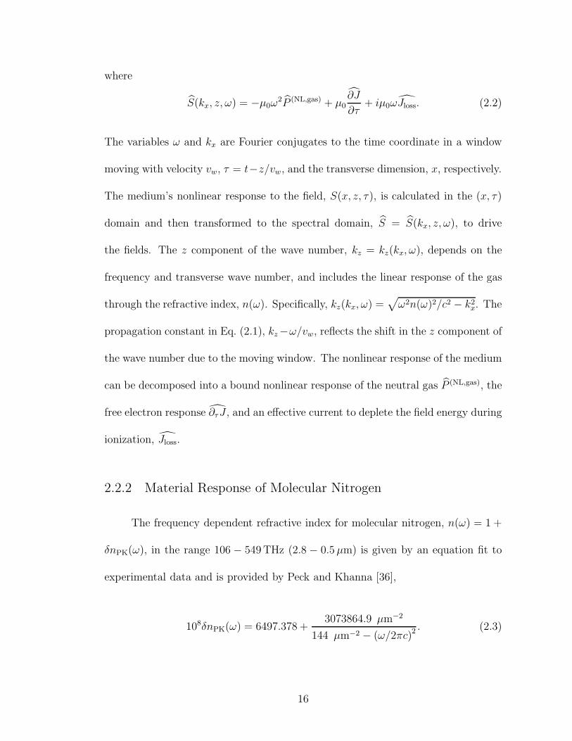
2.2.2 Material Response of Molecular Nitrogen

The frequency dependent refractive index for molecular nitrogen, n(ω) = 1 +

δnPK(ω), in the range 106 − 549THz (2.8 − 0.5µm) is given by an equation fit to

experimental data and is provided by Peck and Khanna [36],

108δnPK(ω) = 6497.378 +3073864.9 µm−2

144 µm−2 − (ω/2πc)2. (2.3)

16

For frequencies below 106THz, the index is found by extrapolating Eq. (2.3). Recent

experiments in air [37] have indicated nair − 1 ≈ 1.7 × 10−4 at THz frequencies,

which is similar to the zero frequency limit of Eq. (2.3), n(0) − 1 = 2.78 × 10−4.

By extrapolating Eq. (2.3), the detailed structure in the refractive index due to

vibrational and rotational excitations of N2 is not included.

The nonlinear bound response of neutral N2 is captured in the nonlinear po-

larization density, P (NL,gas), and is calculated in the (x, τ) domain using

P (NL,gas) =4

3cǫ20n

(inst)2 E3 + ǫ0n0∆αQE. (2.4)

Here, two third-order nonlinear processes contribute to the polarization density:

an instantaneous electronic response and a delayed rotational response, the first

and second terms of Eq. (2.4), respectively. In a classical picture of the instan-

taneous nonlinear bound response, the laser field strongly drives bound electrons

and they experience the anharmonicity of the binding potential. Because gases are

isotropic on macroscopic scales, the lowest-order nonlinear polarization to man-

ifest itself at macroscopic scales is proportional to E3, instead of E2. We use

n(inst)2 = 7.4 × 10−20 cm2/W at a N2 density of n0 = 2.5 × 1019 cm−3 [38]. The

delayed response arises because the laser field applies a torque to the N2 molecules

due to the anisotropy in their linear polarizability, ∆α = α‖−α⊥ = 6.7×10−25 cm3,

where α‖,⊥ are the linear polarizabilities parallel and perpendicular to the molec-

ular axis, respectively. A simple model for the molecular alignment of the gas,

17

Q = Q(x, z, τ), is to treat it as a driven, damped, harmonic oscillator:

∂2Q

∂τ 2+ 2ν

∂Q

∂τ+ Ω2Q = 2Ω2n

(align)2 ǫ0cE(τ)

2. (2.5)

The oscillator parameters ν = 9.6THz, Ω = 18THz, n(align)2 = 1.35× 10−15 cm2/W

are chosen to best match density matrix calculations [39] where the laser pulse du-

ration, ≈ 25 fs, is much shorter than the thermal rotational time scale, 2π/Ω. These

two nonlinear processes result in propagation effects such as spectral broadening,

harmonic generation, and self-focusing.

During propagation of high power, ultrashort laser pulses, field ionization is

the primary mechanism for free electron generation. This can be modeled with a

rate equation for the electron density, ne = ne(x, z, τ), where

∂ne∂τ

= w (n0 − ne) . (2.6)

The rate of electron generation is the ionization rate of a single molecule, w =

w[E(x, z, τ)], times the number density of neutral molecules, nn = n0 − ne, where

n0 is the initial density of the neutral gas. Here we neglect electron transport,

recombination, and attachment; the time scales for these processes are much longer

than the pump-pulses’ duration [40].

We use a two-color hybrid ionization rate, w[E], which is a fit to a Perelomov,

Popov, and Terent’ev (PPT) ionization rate [41] when w[E] is cycle averaged. The

ionization rate includes multiphoton ionization (MPI) for the two pump-pulse fre-

18

quencies and tunneling ionization (TI). MPI is an Nth-order perturbative process in

the intensity, where a bound electron escapes from its binding potential by absorb-

ing N photons with energy ~ω and frequency ω. The energy in the N photons must

be greater than or equal to the binding energy Ui; N~ω ≥ Ui. Tunneling ionization

occurs when the instantaneous electric field deforms the binding potential enough

to create a classically allowed region outside the atomic or molecular core. With

some probability, an electron can tunnel through the barrier between the classically

bound and classically free regions, resulting in a free electron. Further details of

the two-color hybrid rate and how it was fit to the limiting cases are given in the

Appendix.

The free electron current J = J(x, z, τ) is determined by the electron momen-

tum balance equation,

∂J

∂τ=

e2

meneE − νenJ. (2.7)

It is through this current that the THz will be generated. In Eq. (2.7), the electron

density is time dependent due to ionization. There is no momentum source term

accompanying the ionization because we assume that new free electrons are born at

rest. It can be shown that the solution of this equation for the macroscopic current

is equivalent to the single particle picture of Kim et al. [6, 42]. We include a fixed

collision frequency, νne = 5THz, to account for electron-neutral collisions which

dominate electron-ion collisions in a weakly ionized gas. The collision frequency of

5 THz is found by approximating the neutral N2 density as atmospheric density and

assuming that the electron’s temperature is approximately the quiver energy at field

19

intensities of 1013 − 1014W/cm2 [40].

The second source term for the electromagnetic fields [see Eq. (2.2)] is the

Fourier transform of the time derivative of the current, ∂τJ . Care must be exercised

in its numerical evaluation. If J is solved for in the time domain and then Fourier

transformed, the moving window must extend several collision times, ν−1ne , so that

the currents decay to zero. If the domain is too short, the current is finite at the

window boundary and its frequency spectrum has an unphysical ω−1 dependence.

To circumvent this, we Fourier transform neE, which tends to zero outside of the

temporal range of the pump pulses’, and compute the Fourier transform of ∂τJ via

∂J

∂τ=

e2

me

neE

1− iνen/ω. (2.8)

During ionization, the electric field must perform work equal to the ionization

potential Ui to liberate each electron. Ionization energy depletion is included by

adding an effective current, Jloss = Jloss(x, z, τ), that accounts for the rate of energy

loss: EJloss = w[E]nnUi [43] ,

Jloss =w[E]nnUi

E. (2.9)

To avoid issues when dividing the cycle-averaged contributions of Eq. (2.14) by

the instantaneous electric field, the loss current is only evaluated when |E(t)| >

27 MV/cm. Below these field strengths, the ionization rate is too small to signifi-

cantly deplete the pump pulses.

20

2.3 Conical THz Radiation

We now describe simulation results based on the numerical solution of the

model equations introduced in the previous section. The incident electric field is

composed of two pulses with central wavelengths λ = 800 and 400 nm, respectively.

The 800 nm pulse has a total energy of 0.7 mJ, a full-width half-maximum duration

of 25 fs, and a vacuum spot size of w0 = 15.3µm. The 400 nm pulse is created

experimentally by second-harmonic generation in a BBO crystal. This motivates the

400 nm pulse having a total energy that is 10% of the fundamental pulse, 0.07 mJ, a

full-width half-maximum duration that is a factor√2 shorter than the fundamental,

18 fs, and a vacuum spot size that is√2 smaller than the fundamental, w0 = 11µm.

The pulses are assumed to overlap spatially and temporally with the peak of each

pulse colocated 8 cm before the vacuum focus. This is where the BBO crystal ends

and the simulation begins. Both colors are initialized with a phase front curvature

that is consistent with passing through a lens with focal length and diameter of 15

and 0.5 cm, respectively. The polarization of the pump pulses are assumed to be

collinear.

The simulation domain is 6 mm in the transverse spatial dimension, x, and

1 ps in the time domain, τ , with 29 and 215 grid points, respectively. The trans-

verse spatial resolution is ∆x = 12µm. This resolution is sufficient because plasma

refraction keeps the pulse from reaching its vacuum spot size. For example, the

pump-pulses’ time-averaged rms radii is always larger than 100µm. At the front of

the pulse, where the intensity is lower, the rms radius reaches a minimum of 40µm.

21

The transverse spatial resolutions also resolve the transverse phase variation associ-

ated with focusing sufficiently well for the vacuum focal point to remain unchanged.

Simulations with double the spatial resolution, ∆x = 6µm, show convergence of the

THz energy and fields. The temporal domain is chosen so as to capture low frequency

behavior, ∆f = 1 THz, while having sufficiently small time steps, ∆τ = 0.03 fs,

to resolve ionization bursts and harmonic generation. The pulses propagate 12 cm,

with a uniform step size of ∆z = 10µm. The window velocity, vw = 0.99972c, is

comoving with the group velocity of 800 nm in N2. The background N2 density is

ngas = 2.5× 1019 cm−3. The UPPE model, Eq. (2.1), is solved using a second-order

predictor-corrector scheme for the nonlinear term, S.

The simulation predicts off-axis, broadband, THz radiation as seen in Fig. 2.2.

The figure displays the THz electric field as a function of x and τ after propagating

to 2 cm before the vacuum focus. To calculate the THz electric field, E has been

filtered to remove frequency components with f > 100THz and transformed to the

space and time domain. The THz field is a few-cycle pulse that has been created near

the axis and is propagating at approximately 1 above and below the propagation

axis of the pump pulses. This can be seen from the nulls in the phase (white in the

figure) where the fields will propagate perpendicular to the phase front.

2.3.1 Cherenkov Model

The angle of the THz pulse shown in Fig. 2.2 can be explained by an optical

Cherenkov effect. As the pump pulses approach focus, their fronts of constant

22

τ (fs)

x (

mm

)

−50 0 50

−1

0

1

(MV

/cm

)

−20

0

20

φ

Figure 2.2: The electric field from 0 to 100THz is shown in the transverse spatial dimen-sion, x, versus a time window that is comoving with the 800 nm pulse, τ . The pulse ispropagating from right to left with an off-axis angle φ. The electric field at 2 cm beforevacuum focus was chosen because most of final THz energy is already in the pulse.

intensity and, through ionization, fronts of constant plasma density move axially

faster than the pump-pulses’ group velocities. The resulting current drives the THz

radiation and travels faster than the THz phase velocity in the medium. This results

in a “Cherenkov cone” in which the emitted THz field interferes constructively at

the Cherenkov angle φ given by cos φ = vTHz(ω)/vf , where vf is the velocity of the

plasma current front and vTHz(ω) = c/n(ω) is the THz phase velocity. A schematic

of this is shown in Fig. 2.3. The duration of the current approximates the time scale

of the pump-pulses’ envelope, providing the few-cycle THz phase front observed in

Fig. 2.2.

A simple model illustrates this phenomenon. Equations (2.1) and (2.2) can

be solved analytically to find the THz field spectrum resulting from a prespecified

THz current. We model the current driven by the pump pulses as a localized, on-

23

t=t3

φ

t=t2

t=t1

vf v

THz

Figure 2.3: The broadband THz frequency current (red) is traveling faster from right toleft than the phase velocity of the THz fields (lines of constant phase are shown in gray).Constructive interference can be seen along the front (black dashed) above and below thepropagation axis.

axis source with velocity, vf , Jp(x, z, t) = I0δ(x)θ(t − z/vf ) where I0 is the current

amplitude (A m−1 in two dimensions). After the current pulse has propagated a

distance, L, the THz spectrum is given by

∣∣∣ETHz(kx, z, ω)∣∣∣2

=I20µ

20

4k2zsinc2

[(ω

vf− kz

)L

2

]L2, (2.10)

where kz =√(ωn/c)2 − k2x. The peaks in the power spectrum occur approximately

where the argument of the sinc is zero, reproducing the expression for the Cherenkov

angle:

cos φ = vTHz(ω)/vf . (2.11)

We note that the THz angle is related to the vector components of the wave number

via kz = (ωn/c) cosφ.

24

This model can be extended to capture a current source with transverse spatial

extent or a current source that oscillates along the propagation distance. The latter

extension captures the effect on the two-color THz current of phase slippage between

the pump pulses due to their phase-velocity difference. This phase slippage was

considered in a previous model of off-axis THz emission [16]. You et al. [16] treat

the THz driving current as a dipole radiator traveling with the laser pulse. The

phase of the dipole’s oscillation, and hence the emitted radiation, varies along the

propagation axis with the relative phase between the pump pulses. In You’s model,

the group velocity of the laser pulses, the velocity of the driving current, vf , and

the THz phase velocity, vTHz, are all set to c. While the model predicts off-axis

radiation, the equality of THz and drive velocities precludes Cherenkov radiation.

Our model can capture this oscillating current effect if we impose a second spatial

variation on the current density, Jp(x, z, t) = I0δ(x) cos(kdz)θ(t−z/vf ). In this case

the THz spectrum is peaked at angles given by

cosφ = vTHz/vf ± kdvTHz/ω, (2.12)

where ω is the THz frequency of interest, kd = π/Lπ is the dephasing wavenumber,

and Lπ is the distance over which the two colors will phase slip by π.

The dephasing length is inversely proportional to the phase-velocity difference

and can be estimated as Lπ = (λ0/4) |n(ω0)− n(2ω0)|−1 [44]. The refractive index

is given by n(ω) = 1 + δngas(ω) + δnplasma(ω) + · · · , where ω could be for either

the fundamental, ω0, or second harmonic, 2ω0. The quantity λ0 is the wavelength

25

τ (fs)

z (

cm

)

−50 0 50−6

−4

−2

0

2

(arb

. u

nit

s)

−1

0

1

Figure 2.4: The on-axis ∂τJ after a low-pass filter with cutoff frequency of 200THz hasbeen applied.

of the fundamental. From N2 dispersion alone Lπ = 2.7 cm, but with a plasma

density in the range of 1016 − 1017 cm−3, the dephasing length would be 2.1 −

0.7 cm, respectively. These plasma densities are typical for the region where THz is

generated.

Figure 2.4 displays the time derivative of the current density on axis, low-

pass filtered to frequencies below 200THz as a function of z and τ . Most of the

THz energy is generated between z = −4 and −1 cm, as can be seen in Fig. 2.5.

Over this distance, the THz current source has the form of a temporally oscillating

signal that moves forward in the frame of the simulation. For comparison, an object

moving at the group velocity of 800 nm would trace out a vertical path in (z, τ)

domain, while objects moving faster, or slower, follow paths to the left, or right, of

vertical respectively. It is the overall forward motion of the THz ∂τJ that drives the

Cherenkov radiation. The forward motion of the THz current density profile can

26

−8 −6 −4 −2 0 2 40

1

2

3

4

z (cm)

10

−3 T

Hz

Co

nv

ersi

on

Eff

icie

ncy

Figure 2.5: The solid line is the energy in the THz from 10 to 100THz relative to the totalinitial energy in the pump pulses. The dashed line is for the same simulation parameters,but only the nonlinear gas response was allowed to drive THz radiation.

be attributed to the fact that the pump pulses are converging towards focus. As

the pulses converge, their intensity rises, and the time in the pulse envelope when

ionization becomes significant moves forward in the plane of Fig. 2.4.

The spatiotemporal form of the current density waveform implied by Fig. 2.4

is that of a few-cycle pulse. The temporal (≈ 10 fs) variations in ∂τJ at fixed z are

due to a combination of the temporal variation in the pump-pulses’ relative phase

during the pulse and the frequency upshift of the THz field due to the rising electron

density. We note the variations become more rapid with propagation distance. As

the pump pulses propagate their relative phase becomes a time varying function due

to the rise in electron density during the pulses. The sign of the two-color driven

THz current then varies with this relative phase. This variation becomes more rapid

with propagation distance. A second contribution to the increase in frequency of the

27

on-axis ∂τJ as a function of propagation distance is the direct spectral blueshifting

(up to approximately 150THz) of the THz fields in the region of increasing free

electron density.

The signal in Fig. 2.4 was low-pass filtered at 200THz (as opposed to the

100THz filter applied in Fig. 2.2) to include the peak frequency of the on-axis,

blue-shifted THz field (around 150THz at z = −2 cm). While the peak frequency is

larger on axis, most of the THz field energy is distributed off axis where the average

frequency is lower (≈ 50THz).

The front velocity is extracted from Fig. 2.4 by measuring the slope of the

null lines of ∂τJ . We find that the front velocity is approximately vf = 0.999 95c.

For comparison, the 800 nm group velocity is vg,800 nm = 0.999 72c. With this

front velocity and the refractive index model discussed above, the Cherenkov model

predicts an off-axis angle of φ ≈ 1.2 [according to Eq. (2.11)], which is similar to

0.9, the value seen in Fig. 2.2.

Finally, we note the space-time dependence of the time derivative of the current

density is not of the form required to produce Eq. (2.12) (except when kd ≈ 0).

There is variation of the waveform with z, in addition to translation at vf . The

amplitude of ∂τJ grows and the frequency increases over a distance of 3 cm. However

the behavior is not a periodic oscillation with a clearly identifiable wave number kd.

28

2.3.2 Angular Dependence of THz on Refractive Index

To test the model giving rise to Eq. (2.11) we attempt to vary vTHz. Competing

propagation effects in the simulation make control of the current front velocity

challenging. The THz phase velocity, on the other hand, can be directly manipulated

by modifying the refractive index at THz frequencies. The resulting change in the

simulated THz emission angle can then be compared to predictions of the Cherenkov

model. Specifically, we use the following modified refractive index model;

δn(ω) =

δn0, ω/2π < 190THz

δnPK(ω), otherwise,

(2.13)

where n(ω) = 1 + δn(ω) and δPK(ω) is defined in Eq. (2.3). While the modified

refractive index has no frequency dependence below 190THz, the relative change

in the actual refractive index of N2 is only 0.2% between 0 and 190THz [36]. In

all cases, the group velocity at low frequencies in N2 is not significantly different

than the phase velocity. Experimentally, the dispersion at low frequencies could be

modified by the selection and relative percentage of gas species in the medium.

Figure 2.6 shows the extracted THz electric field for δn0 = 0, 2.78×10−4, and

1.1 × 10−3. The propagation angle of the THz radiation can be seen to increase

with increasing δn0, as anticipated by Eq. (2.11). The variations of δn0 leave the

pump pulses and current front velocity largely unchanged. The pump pulses drive

the current source and indirectly control the front velocity. Changes to the pump-

29

τ (fs)

x (

mm

)

0 50 100

−1

0

1

−20

20

τ (fs)

0 50 100

−1

0

1

−20

20

τ (fs)

0 50 100

−1

0

1

(MV

/cm

)

−10

10(a) (b) (c)

Figure 2.6: Shows the electric field at 1 cm before vacuum focus from 0 to 100THz forthree different THz dispersion models; δn0 = 0, 2.78 × 10−4, and 1.1 × 10−3 for (a), (b),and (c) respectively. Most of the THz have been generated at this point.

pulses’ propagation, due to changes in the THz refractive index, should only occur

via nonlinear interactions with the THz frequencies, e.g. non-degenerate four-wave

mixing. These interactions tend to be smaller than the nonlinear processes involving

the pump pulses alone.

The dependence of the THz propagation angle, φ, on δn0 is shown in Fig.

2.7. For each δn0, the THz angle is extracted from images such as those in Fig.

2.6 after most of the THz radiation has been generated, z = −1 cm. The simu-

lation results are bounded by the Cherenkov model, Eq. (2.11), evaluated with vf

equal to the group velocity of 800 nm (0.999 72c) and the extracted front velocity,

vf = 0.999 95, from the simulations. This shows reasonable agreement between the

predicted Cherenkov model and our simulations. The blue dotted curves in Fig. 2.7

show the predicted angle for the positive (lower curve) and negative (upper curve)

solutions of Eq. (2.12). We substitute kd = π/Lπ with Lπ = 3 cm which is roughly

the distance over which the THz current waveform varies. In this way Eq. (2.12)

can be used to indicate the degree of uncertainty in the prediction of Eq. (2.11).

30

0 0.5 10

1

2

10−3

δn0

φ (

deg

rees

)

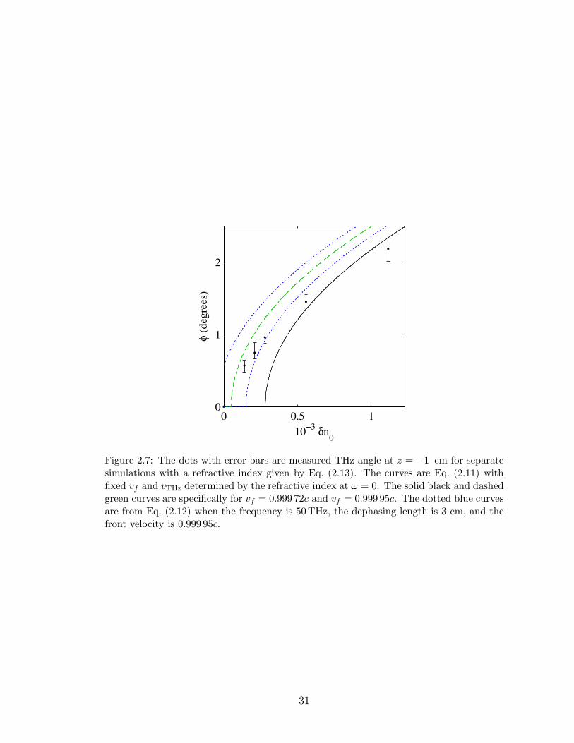
Figure 2.7: The dots with error bars are measured THz angle at z = −1 cm for separatesimulations with a refractive index given by Eq. (2.13). The curves are Eq. (2.11) withfixed vf and vTHz determined by the refractive index at ω = 0. The solid black and dashedgreen curves are specifically for vf = 0.999 72c and vf = 0.999 95c. The dotted blue curvesare from Eq. (2.12) when the frequency is 50THz, the dephasing length is 3 cm, and thefront velocity is 0.999 95c.

31

2.3.3 Cherenkov Radiation from Four-Wave Mixing

In simulations, the free electron current is the dominant mechanism for gen-

eration of THz radiation [31]. When the current source, ∂τJ , and the effective loss

current are removed from Eq. (2.2) using a high-pass filter, the third-order nonlin-

earities [the first term in Eq. (2.2)] still generate THz radiation as seen by the dashed

curve in Fig. 2.5. But in this scenario, the conversion efficiency from pump-pulses’

energy to THz is a factor of ≈ 40 times smaller than the photocurrent model. This

is similar to results reported in [31]. Interestingly, the THz generated via four-wave

mixing is also conical, suggesting that the optical Cherenkov mechanism is still at

play. Figure 2.8 shows the THz field that is generated from four-wave interaction

alone. The THz angle is the same as that of Fig. 2.2. This is expected since the

bound nonlinear polarization current, which drives the THz, will follow the super-

luminal intensity fronts of the pump pulses.

2.3.4 Experimental Comparison

While the simulations seem to predict a THz propagation angle of ≈ 1, You

et al. observe THz radiation at angles of ≈ 4 [16]. In the experiment, the focus was

on frequencies below 10 THz as opposed to the broadband radiation below 100THz

that we have investigated. Blank et al. [45] observed a THz intensity spectrum

that extends up to 100THz with an off-axis angle of 3.2. Their experiments are

performed in air with similar parameters to ours: a pump-pulse energy of 0.42 mJ,

fundamental wavelength of 775 nm, pump-pulse duration below 20 fs, and a focal

32

τ (fs)

x (

mm

)

−50 0 50

−1

0

1

(MV

/cm

)

−3

0

3

Figure 2.8: The electric field from 0 to 100THz is shown in the transverse spatial dimen-sion, x, versus a time window that is co-moving with the 800 nm pulse, τ . This THzelectric field comparable to that of Fig. 2.2, except that this one was generated exclusivelyby a four-wave rectification process.

length of 20 cm. We find, if we further filter the THz signal, the average off-axis

angle from the electric field power spectrum for frequencies between 5 and 10THz

to be 2.1 ± 1.0. This is closer to the experimentally measured values. Differences

still remain between the conditions in our simulations and the experiments. The

simulated medium is N2 as opposed to air. The index of refraction of air in the

10THz range may have a frequency dependence not contained in our simulations.

Also, the presence of oxygen, with a lower ionization potential than N2, could lead to

more free electrons and a different THz current source speed. Finally, the simulations

are two dimensional. The superluminal front velocity is due to the focusing of the

pump pulses. This speed can then be altered in going from two to three dimensions.

33

2.4 Directing THz Using Tilted-Intensity Fronts

The few cycle THz pulses that are created by the two-color mechanism can

have a conical radiation patten. Experimentally, the THz pulses are observed at

angles of 4 to 7 [16] and, in two-dimensional simulations, at angles of 1 to 2 [18].

By using a two-color pump pulse with fronts of constant intensity that are tilted with

respect to the laser’s phase fronts, the resulting THz is emitted directionally, instead

of conically, and the THz angle can be controlled. This provides a mechanism for

creating better collimated few cycle THz pulses.

A simple example of a tilted intensity front laser pulse is a Gaussian envelope

with a transverse spatial chirp, or in other words, a transverse wavenumber kx. The

resulting single-color laser field is given by E ∝ exp [−τ 2/(2T 2)] exp [−x2/(2R2)]

exp [ikzz + ikxx− iωt], where the time in the group velocity frame is τ = t− z/vg,

the pulse duration is T , and the spot size is R. Lines of constant laser intensity

would form concentric ellipses with the axes parallel and perpendicular to the x

and τ axes, but the phase fronts of the electric field would be tilted by an angle

θt = tan−1(kx/kz). While this is a tilted intensity front pulse, it is an inconve-

nient representation for laser propagation simulations because the laser pulse would

propagate off of the z axis and out of the simulation domain. A more practical

representation is when the Gaussian profile is rotated with respect to the z axis

instead of the wavenumber. The electric field of a Gaussian laser pulse with tilted

intensity fronts can be specified by using coordinates that have been rotated by

the tilt angle θt; E ∝ exp [−τ 2/(2T 2)] exp [−x2/(2R2) exp [−iωτ ]], where the tilted

34

Figure 2.9: The laser electric field is shown in the transverse spatial dimension, x, versusa time window that is co-moving with the 800 nm pulse, τ . The intensity fronts of thispulse have been tilted by 1.5.

time coordinate is τ = τ cos θt + (x/c) sin θt, and the tilted transverse coordinate

is x = −cτ sin θt + x cos θt. For example, a two-color laser pulse with a 1.5 tilt is

shown in Fig. 2.9.

Tilted intensity front pulses can be created by reflecting a laser pulse off of

a diffraction grating to impart the necessary transverse wavenumber [46]. For a

two-color laser pulse, each color could be tilted independently and then recombined

as was done in earlier two-color THz work [14].

For a two-color, tilted intensity front pulse, such as that in Fig. 2.9, the result-

ing THz pulse can be seen in Fig. 2.10. The laser and gas parameters are similar

to those of Section 2.3 except for a θt = 1.5 tilt in the laser pulse. The resulting

THz radiation in Fig. 2.10 is preferentially propagating in one direction. This is

different than the Cherenkov emissions which occur in two directions as seen in Fig.

35

Figure 2.10: The electric field from 0 to 100 THz is shown in the transverse spatialdimension, x, versus a time window that is co-moving with the 800 nm pulse, τ .

2.2. Additionally, the THz emission angle can be controlled by changing the tilt

angle, as in Fig. 2.11.

The theoretical model for the two-color Cherenkov mechanism can be ex-

panded upon to capture the behavior of the THz emission from tilted intensity

fronts. See Appendix 2.B.2 for details. For the Cherenkov emission, the THz cur-

rent source was modeled as a spatially (transverse) localized source, but for two-color

laser pulses with tilted intensity fronts a transverse profile is key.

2.5 Conclusion

We have developed a two-dimensional, unidirectional, electromagnetic propa-

gation code to examine two-color THz generation in N2. The model includes linear

dispersion to all orders, the instantaneous and delayed-rotational nonlinear bound

36

0 0.5 1 1.5 2 2.50

0.5

1

1.5

2

2.5

Tilt Angle (deg)

TH

z A

ngle

(de

g)

Figure 2.11: The angle of the THz pulse is shown as a function of the laser pulse tilt angle.

response, free electron generation via multiphoton and tunneling ionization, plasma

response including collisional momentum damping, and ionization energy depletion.

We have found that the off-axis, THz generation predicted by the simulations can

be explained as an optical Cherenkov process. The angle of THz emission depends

sensitively on the low frequency refractive index and current front velocity. Using

our best estimate of the frequency dependent refractive index produces reasonable

agreement with the experiment. Although the THz radiation is generated predom-

inately by the photocurrent mechanism, the Cherenkov process also determines the

emission angle of THz radiation generated by two-color, four-wave interaction in the

nonlinear molecular polarizability. By using laser pulses with tilted intensity fronts,

the THz radiation can be directed into one direction and the emission angle can be

controlled.

37

2.A Hybrid Ionization Rate

MPI and TI are distinct limiting cases of a more general nonlinear photoion-

ization theory such as that of Keldysh [47, 48] or later refinements by PPT and

others [41,49]. These limiting cases are roughly delineated by the Keldysh parame-

ter γ = ω√2meUi/(eE), where me and e are the electron mass and charge, while E is

the electric field amplitude. For ease of calculation, the Keldysh parameter can be

expressed as γ = 6.4 × 1012√Ui [eV]/(λ [nm] E [V/m]), where λ is the wavelength.

For example, γ ≫ 1 implies the multiphoton regime, while γ ≪ 1 implies the tun-

neling regime. Typical parameters of the pump pulse during THz generation are

λ = 800 nm and E ≈ 4 × 1010 V/m. The resulting Keldysh parameter is γ ≈ 0.8

which is at the boundary between multiphoton and tunneling ionization.

As the pump pulses focus, the field strength will transition from the multipho-

ton to the tunneling regime. In the multiphoton regime, the TI rate underestimates

free electron generation. Therefore, the decreased refractive index associated with

the multiphoton generated free electrons can defocus the pump pulses and modify

subsequent propagation more than expected from a TI rate. Unfortunately, the PPT

ionization rate, which covers both regimes, is for a single color and dependent on

the intensity, not on the instantaneous electric field. Therefore, it does not generate

THz radiation according to the mechanism of interest.

The motivation for the hybrid ionization rate is to capture both the instanta-

neous nature of the tunneling ionization rate when in the tunneling regime, while not

significantly underestimating free electron generation and defocusing effects when

38

1013

1014

1015

10−10

10−5

100

Intensity ( W/cm2 )

Ioniz

atio

n R

ate

( T

Hz

)

wADK

wPPT

wPPT

wMPI,1

wMPI,2

Figure 2.12: The solid red and blue curves represent PPT ionization rates for λ =800nm, 400 nm respectively. The solid black curve indicates a cycle-averaged tunnel-ing rate which approaches the PPT rate at high intensities. The dashed-dotted red andblue curves show the MPI rates for λ = 800nm, 400 nm respectively. Notice that a singlecolor MPI rate plus the tunneling rate is a reasonable approximation of the associatedPPT rate.

in the multiphoton regime.

Conventional MPI rates depend on the intensity to a large power [50]. This

poses a problem when attempting to approximate the PPT ionization rate by in-

terpolating from the multiphoton to the tunneling regime, e.g., by summing the

MPI and TI rates. The problem arises because the MPI rate is orders of magni-

tude larger than the TI rate when evaluated in either the multiphoton or tunneling

regimes. Therefore, the sum of the individual rates is always dominated by MPI.

This is beneficial in the multiphoton limit but not in the tunneling limit where the

tunneling rate should be a reasonable approximation. We adapt the MPI rate to

drop exponentially with increasing intensity, as shown by the dashed-dotted red and

blue curves of Fig. 2.12. The modified MPI rate is then summed with the tunneling

39

ionization rate to yield our single-color hybrid ionization rate. The cutoff intensity

used in the exponential decay, Icutoff, becomes a free parameter that is used to match

wMPI,i +wADK, after cycle averaging, to the PPT ionization rate for each color [41].

We then extend this hybrid ionization rate for two-color pulses. In the tunnel-

ing limit, the ionization rate should depend on the instantaneous field and therefore

the Ammosov-Delone-Krainov (ADK) model should capture the two-color ionization

dynamics [51, 52]. But in the multiphoton regime, the rate is strongly dependent

on the frequency. In general, a nonlinear process like ionization is not additive in

the individual rates. It is possible that mixed-photon ionization channels, like those

involving N 800 nm photons and M 400 nm photons, would have important con-

tributions to the total ionization rate. But summing the 800 nm and 400 nm MPI

rates provides a better lower bound on the free electron generation in the multi-

photon regime than neglecting either or both. Additionally, it provides a rate that

can be fit to the accepted PPT rates in the limits of a laser pulse of either color.

The absence of computationally efficient, quantum mechanical, atomic or molecular

response models necessitates approximation. To this end, we treat the total MPI

rate as the sum of the rates for the individual harmonics.

The full two-color hybrid ionization rate is given by

w[E] = wMPI,1(I1) + wMPI,2(I2) + wADK(E), (2.14)

where I1 and I2 are the enveloped intensities of the fundamental- and second-

harmonic pulses, respectively. The individual MPI rates are given by wMPI,i =

40

σiINi

i exp (−Ii/Icutoff,i), where σ1 = 4.47×10−140 cm22W−11 s−1 , N1 = 11, Icutoff,1 =

8.46 × 1012 W/cm2, σ2 = 2.46 × 10−72 cm12W−6 s−1 , N2 = 6, and Icutoff,2 =

5.29 × 1013 W/cm2. The tunneling rate used is outlined in [51] with an ionization

potential of Ui = 15.576 eV and effective Coulomb barrier Zeff = 0.9 [52].

In the tunneling regime, Eq. (2.14) approximates the instantaneous ADK tun-

neling rate [51]. In the limit of a single color, either 800 or 400 nm, Eq. (2.14) after

cycle averaging approaches the PPT rate for that color [41]. This implies that in

the multiphoton limit and in the limit of a single color, Eq. (2.14) also matches the

MPI rate.

As a result of enveloping, I1 and I2 do not depend on their respective carrier

or carrier-envelope phases. This is consistent with traditional MPI models, which

depend on the cycle-averaged field [50]. There has been recent theoretical work on

the phase dependence of two-color MPI [53], but it does not lend itself to efficient

numerical implementation in an electromagnetic propagation code. There has been

work on computationally efficient ionization models [54] but work remains before

implementation in a propagation code.

2.B Derivation of THz Spectrum

This appendix will derive the THz spectrum that results from the two-color

Cherenkov process with and without tilted intensity fronts. Ideally, it would be

possible to assert the initial two-color laser pulse and self consistently solve for the

THz frequency currents and resulting fields, but this is not the case. The propagation

41

of the two-color pump pulse will be ignored and THz frequency source current it

drives will be asserted. The assumed form of the THz frequency source current is

based on observations of numerical simulations. The spectrum of the THz frequency

electric fields, those that are driven by the source current, will be derived for three

spatial dimensions. The limit to two spatial dimensions will be taken at the end.

The unidirectional pulse propagation equation with the free electron current

as the driving term is

[∂z − ikz(kx, ky, ω)] E(kx, ky, z, ω) = − µ0

2ikz(kx, ky, ω)∂tJ(kx, ky, z, ω), (2.15)

where the z component of the wavenumber is specified by the x and y components

and the frequency using kz(kx, ky, ω) = [ω2n(ω)2/c2 − k2x − k2y ]1/2. The linear re-

fractive index of the gas is frequency dependent and given by n(ω). The spectrum

of the electric field at each z position is specified by E(kx, ky, z, ω) using the trans-

formation E(kx, ky, z, ω) =∫∞

−∞E(x, y, z, t) exp[−i(kxx + kyy − ωt)] dx dy dt. The

spectrum of the current source ∂tJ(kx, ky, ω, t) is similarly defined. Issues with the

zero frequency limit of Eq. (2.15) can be corrected by including collisional damping

to the current model, as was done in the simulations.

In simulations, the current at THz frequencies is driven dominantly by the

two-color pump pulse and the two-color pump is largely unaffected by the THz.

Therefore, a fixed pump pulse will be assumed and for the UPPE, Eq. (2.15), it is

only nessecary to consider how the THz electric fields develop with z. The resulting

UPPE equation with functional dependences dropped would be [∂z − ikz] ETHz =

42

−[µ0/(2ikz)]∂tJpump.

The THz spectrum of the electric field can be solved for in general as an

integral of the two-color pump pulse’s source current over the propagation distance

ETHz(kx, ky, z, ω) = − µ0

2ikz(kx, ky, ω)

∫ z

0

dz′∂tJpump(kx, ky, z′, ω)eikz(kx,ky,ω)(z−z

′),

(2.16)

with the initial condition that ETHz(kx, ky, 0, ω) = 0.

2.B.1 Spectrum of Cherenkov Emission

An idealized current source must be constructed to approximate the key fea-

tures of what is observed in simulations. For simplicity, the current source ∂tJpump

is treated as localized on the optical axis by using delta functions in the transverse

dimensions. Additionally, the front of the current source is treated as a step function

that moves at a speed vf ≈ c. A resulting free electron current is

Jpump(x, y, z, t) = I0 cos(kdz + θ0)δ(x)δ(y)θ(t− z/vf ), (2.17)

where I0 is the current with units of amperes. The cos(kdz+θ0) is included to model

the effect of the sign of the current oscillating over a distance of 2Lπ = 2π/kd,

where Lπ is the dephasing distance. The sign of the current at z = 0 is set by

the initial phase θ0. The oscillating of the currents sign could be caused by phase

velocity mismatch between the two colors in the pump pulse and is the mechanism

for conical THz radiation in Ref. [16]. The oscillating currents can be neglected by

43

taking kd → 0 and θ0 = 0.

Before using Eq. (2.16) a time derivative must be taken of Eq. (2.17), yielding

∂tJpump(x, y, z, t) = I0 cos(kdz+ θ0)δ(x)δ(y)δ(t− z/vf ). This highlights the need for

an assumed source current model with a differential time-dependence.

The final form of the electric field’s THz spectrum is given by using Eqs. (2.16)

and (2.17) to get

∣∣∣ETHz(kx, kx, z, ω)∣∣∣2

=µ20I

20

16k2z(kx, ky, ω)|f(kx, ky, z, ω)|2 z2, (2.18)

where k± = ω/vf ± kd − kz(kx, ky, ω) and,

|f(kx, ky, z, ω)|2 =[sinc2(k+z/2) + sinc2(k−z/2)

+2 cos(kdz + 2θ0)sinc(k+z/2)sinc(k−z/2)] .

(2.19)

The angle of the THz radiation off of the z axis, φ, is given by kz = k cosφ, where

k = ω/vTHz, and vTHz is the THz phase velocity. The sinc functions will be largest

when k± = 0, which provides a way to estimate the angle of the THz radiation.

For example, there are two possible angles φ± when k± = 0 and they are given by

cosφ± = vTHz/vf ± [λ/(2Lπ)](vTHz/c). If the sign of the THz current doesn’t slowly

oscillate with propagation distance, i.e. kd = 0, then k+ = k− and then the electric

field spectrum will go like |f(kx, ky, z, ω)|2 = 4sinc2 [(ω/vf − (ω/vTHz) cosφ) z/2].

To achieve more realistic source currents, other spatio-temporal profiles can

be created. Tractable solutions have been found for cylindrical or Gaussian trans-

verse spatial profiles and for smooth ramps, such as the error function, for the time

44

dependence of the current. Additionally, the current source can be given a cen-

tral frequency at which it drives THz. Unfortunately, using the more complicated

current model does not yield greatly improved predictive ability because, with the

more realistic appearing source currents, there are an increasing number of free

parameters.

The result for two-dimensional planar geometry is given below. In this situa-

tion, the previous results can be used in the limit that ky → 0 and the current I0

becomes the current per unit length

∣∣∣E2DTHz(kx, z, ω)

∣∣∣2

=µ20I

20

16k2z|f(kx, 0, z, ω)|2 z2, (2.20)

where kz =√ω2n2/c2 − k2x.

2.B.2 Spectrum from Tilted Intensity Fronts

The derivation for the two-color Cherenkov spectrum can be extended to cap-

ture the effect of a pump pulse with tilted intensity fronts. The time rate of change

of the current, i.e. , the current source ∂τJpump, will be assumed to have a transverse

length scale σx and temporal duration σt. These scales are smaller than those of

the two-color laser pulse, but are still the same order of magnitude. The main as-

sumption is that the current source has the same tilted intensity front profile as the

electric field. The current source is Gaussian along the coordinates x and t. These

coordinates are rotated by θt with respect to x and τ . A positive rotation of θt > 0

corresponds to a pulse with a positive average 〈kx〉 > 0 such that 〈kx〉 / 〈kz〉 = tan θt.

45

In the rotated coordinates (x, y, t) the laser field and the resulting current source

have the form of a Gaussian

|∂tJpump(x, y, z, t)| ∝ e−x2/(2σx)2e−y

2/(2σx)2e−τ2/(2σt)2 . (2.21)

where τ = t− z/vg is time in the frame moving with the group velocity. We expect

that a rotation will relate (x, y, τ) and (x, y, τ).

x = x cos θt − τc sin θt

y = y

τ =x

csin θt + τ cos θt

(2.22)

The current source expressed in We choose the rate of change of the current to have

a the same tilted front profile as the laser pulse except instead of moving at the

group velocity the current source as allowed to move at the front velocity vf , so

τ = t− z/vf and

∂tJpump =I0

8√πσt(πσxσy)

e−(x cos θt−(t−z/vf )c sin θt)2

/(2σx)2e−y2/(2σy)2

× e−((x/c) sin θt+(t−z/vf ) cos θt)2

/(2σt)2 .

(2.23)

The prefactor for the ∂tJpump is such that πσxσy is the cross-sectional area of the

current source, σt is the temporal duration, and I0 is the total current. This source

current will limit to that of the Cherenkov model when σx, σy, σt → 0. In Eq. (2.16),

46

the THz field depends on the source current in the spectral domain

∂tJpump =I0

8√πσt(πσxσy)

∫dxdydte−ikxx−ikyy+iωt

× e−(x cos θt−(t−z/vf )c sin θt)2

/(2σx)2e−y2/(2σy)2

× e−((x/c) sin θt+(t−z/vf ) cos θt)2

/(2σt)2 .

(2.24)

The transform becomes a three dimensional Gaussian if a change of variables is

made from (x, y, t) to (x, y, τ )

∂tJpump =I0e

iωz/vf

8√πσt(πσxσy)

∫dxdydτe−x

2/(2σx)2e−y2/(2σy)2e−τ

2/(2σt)2

× e−ikx(x cos θt+τc sin θt)−iky y+iω(−xcsin θt+τ cos θt).

(2.25)

The wavenumber components and frequency can be redefined so as to simplify

Fourier transforms. This will correspond to a rotation in (kx, ky, ω)-space

kx = kx cos θt +ω

csin θt, (2.26)

ky = ky, (2.27)

ω = −kxc sin θt + ω cos θt. (2.28)

The resulting spectrum of the source current in the rotated spectral coordinates is

∂tJpump = I0eiωz/vf e−k

2xσ

2xe−k

2yσ

2ye−ω

2σ2t . (2.29)

47

After using Eq. (2.29) with Eq. (2.16) the electric field amplitude is

ATHz(z) = −µ0I02ikz

e−k2xσ

2xe−k

2yσ

2ye−ω

2σ2t e−i 1

2(kz−

ωvf

)zsinc

[(kz −

ω

vf

)z

2

]z. (2.30)

The magnitude of the THz spectrum in the (kx, ky, ω) domain is

∣∣∣ATHz(z)∣∣∣2

=

(µ0I02kz

)2

e−2g(kx,ky,ω)sinc2[1

2

(kz −

ω

vf

)z

]z2 (2.31)

with

g(kx, ky, ω) = (kx cos θt +ω

csin θt)

2σ2x + k2yσ

2y + (−kx sin θt +

ω

ccos θt)

2c2σ2t . (2.32)

The function g(kx, ky, ω) is nonnegative and captures the part of the THz spectrum

that is due to the finite bandwidth of the source current. The THz spectrum is

largest where g is smallest. The minima of g can be found by separately minimizing

in kx and ω. This sets the axes of an ellipse

axis (a): +k(a)x cos θt +ω

csin θt = 0, (2.33)

axis (b): −k(b)x sin θt +ω

ccos θt = 0. (2.34)

where the transverse wavenumber for principle axis (a) and (b) are given by k(a)x =

−(ω/c) tan θt and k(b)x = (ω/c) cot θt respectively. Typically in ultrashort laser pulses

the longitudinal (or temporal) dimension of the laser pulse is much smaller than the

transverse dimension, i.e. , cσt ≪ σx. As a result, σx is the dominant contribution

48

to g(kx, ky, ω) and axis (a) is the major axis of g(kx, ky, ω). For small tilt angles and

in the absence of a Cherenkov effect, this is suggestive of the THz spectrum being

biased to propagate off-axis at θt because kx/(ω/c) ≈ tan θt ≈ θt.

49

Chapter 3: Remote Atmospheric Magnetometry

3.1 Introduction

Optical magnetometry is a highly sensitive method for measuring small varia-

tions in magnetic fields [55–57]. The development of a remote optical magnetometry

system would have important applications for the detection of underwater and un-

derground objects that perturb the local ambient magnetic field. In our remote

atmospheric optical magnetometry model, a high-intensity pump laser pulse is em-

ployed to drive wakefields which have a rotated polarization due to the earth’s

magnetic field. This can, in principle, provide a means to measure variations in

the earth’s magnetic field. For a number of magnetic anomaly detection (MAD)

applications, 10µG magnetic field variations must be detected at standoff distances

of approximately one kilometer from the sensor [22].

In this chapter, we consider molecular oxygen at atmospheric conditions as the

paramagnetic species in a remote optical magnetometry configuration depicted in

Fig. 3.1. The propagation of the high-intensity pump laser pulse to remote detection

sites is considered. We show that high laser intensities (below 1012W/cm2 to avoid

photoionization processes) can be propagated to remote locations due to the self

focusing of the optical Ker effect. Using a linearly polarized, high-intensity laser

50

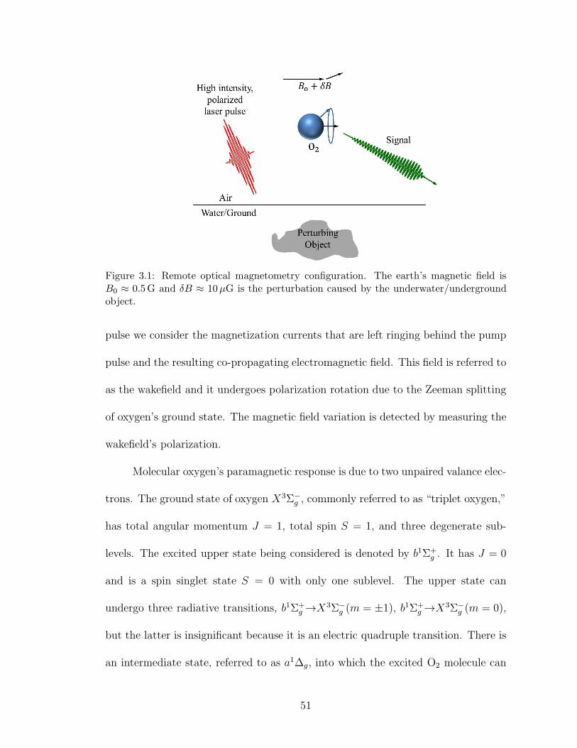
Figure 3.1: Remote optical magnetometry configuration. The earth’s magnetic field isB0 ≈ 0.5G and δB ≈ 10µG is the perturbation caused by the underwater/undergroundobject.

pulse we consider the magnetization currents that are left ringing behind the pump

pulse and the resulting co-propagating electromagnetic field. This field is referred to

as the wakefield and it undergoes polarization rotation due to the Zeeman splitting

of oxygen’s ground state. The magnetic field variation is detected by measuring the

wakefield’s polarization.

Molecular oxygen’s paramagnetic response is due to two unpaired valance elec-

trons. The ground state of oxygen X3Σ−g , commonly referred to as “triplet oxygen,”

has total angular momentum J = 1, total spin S = 1, and three degenerate sub-

levels. The excited upper state being considered is denoted by b1Σ+g . It has J = 0

and is a spin singlet state S = 0 with only one sublevel. The upper state can

undergo three radiative transitions, b1Σ+g →X3Σ−

g (m = ±1), b1Σ+g →X3Σ−

g (m = 0),

but the latter is insignificant because it is an electric quadruple transition. There is

an intermediate state, referred to as a1∆g, into which the excited O2 molecule can

51

decay and is discussed in Appendix 3.A. The O2 transition line being considered

is the b1Σ+g −X3Σ−

g transition band of oxygen near 762 nm. In the low intensity,

long laser pulse, regime, this transition has been investigated theoretically [23, 24]

and experimentally [25] and is a prominent feature of air glow. A high intensity,

polarized titanium-doped sapphire laser is considered for the pump laser. These

lasers have an extremely large tuning range from 660 nm to 1180 nm, and can have

linewidths that are transform limited.

A major challenge for this, as well as any remote atmospheric optical magne-

tometry concept, is collisional dephasing (elastic collisions) of the transitions. The

elastic molecular collision frequency, at standard temperature and pressure (STP),

is γc = Nairσvth = 3.5 × 109 s−1, where σ is the molecular cross section and vth is

the thermal velocity [25]. On the other hand, the Larmor frequency in the earth’s

magnetic field is Ω0 = qB0/(2mc) ≈ 4.5 × 106 rad/s (~Ω0 = 3 × 10−9 eV), where

m and q are the electron mass and charge and c is the speed of light. Since the

dephasing frequency is far greater than the Larmor frequency, the parameters are

somewhat restrictive for remote atmospheric magnetometry. However, rotational

magnetometry experiments based on molecular oxygen at STP and magnetic fields

of ∼ 10G have shown measurable linear Faraday rotational effects [25].

Previous theoretical work [24] revealed major issues with atmospheric mag-

netic field measurements using oxygen, these include: (1) extremely low photon

absorption cross sections, (2) a broad magnetic resonance linewidth due to colli-

sions, and (3) quenching of excited-state fluorescence. These issues largely stem

from oxygen’s small magnetic dipole moment and large collision rate. In our work,

52

however, the wakefield’s polarization rotation is the magnetic signature and the laser

pulse intensities are approximately six orders of magnitude larger.

3.2 Focusing & Compression of Intense Laser Pulses

The magnetometry concept considered here relies on propagation of intense

laser beams in the atmosphere. This propagation is strongly affected by various

interrelated linear and nonlinear processes [43]. These include diffraction, Kerr

self-focusing, group velocity dispersion, spectral broadening, and self-phase modu-

lation. In general, a laser pulse propagating in air can be longitudinally and trans-

versely focused simultaneously at remote distances (∼ km) to reach high intensities

(∼ 1012W/cm2), as indicated in Fig. 3.2. Due to group velocity dispersion, pulse

compression can be achieved by introducing a frequency chirp on the pulse; how-

ever, for the parameters under consideration, pulse compression is not significant.

Nonlinear transverse focusing is caused by the optical Kerr effect.

Here, we present the model describing longitudinal and transverse compression

of a chirped laser pulses in air [43]. The laser electric field is given by E(r, η, τ) =

(1/2)E(r, η, τ)e−iωτ ex+c.c., where E is the complex amplitude, ω is the frequency, r

is the radial coordinate, τ = t− z/c and η = z are the transformed coordinates, and

the propagation distance z and time t are in the laboratory frame. Substituting this

field representation into the wave equation results in an extension of the paraxial

53

Figure 3.2: Simultaneous transverse focusing and longitudinal compression of a chirpedultrashort laser pulse in air due to nonlinear self-focusing and group velocity dispersion.For the 100 ps pulses that are optimal for magnetometry, longitudinal compression isnegligible, but transverse self-focusing can compensate.

wave equation for E(r, η, τ) [43],

[∇2

⊥ + 2ik∂

∂η− c2kβ2

∂2

∂c2τ 2+ω2nK4πc

∣∣∣E(r, η, τ)∣∣∣2]E(r, η, τ) = 0, (3.1)

where the wavenumber is k = ω/c. For air at STP and λ = 2π/k ≈ 762 nm, the

group velocity dispersion is β2 = 2.2 × 10−31 s2/cm, the Kerr nonlinear index is

nK = 3× 10−19 cm2/W, and 1 + nKI is the refractive index of air.

Equation (3.1) can be solved by assuming the pulse is described by a form that

depends on certain spatially dependent parameters. With this assumption, a set of

simplified coupled equations can be derived for the evolution of the spot size, pulse

duration, amplitude, and phase of the laser field. Taking the laser pulse to have

a Gaussian shape in both the transverse and longitudinal directions, the complex

54

amplitude can be written as

E(r, η, τ) = E0(η)eiθ(η)e−(1+iα(η))r2/R2(η)e−(1+iβ(η))τ2/T 2(η), (3.2)

where E0(η) is the field amplitude, θ(η) is the phase, R(η) is the spot size, α(η) is

related to the curvature of the wavefront, T (η) is the laser pulse duration, and β(η)

is the chirp parameter. The E0, θ, T , R, α, β are real functions of the propaga-

tion distance η. The instantaneous frequency spread along the pulse, i.e., chirp, is

δω(η, τ) = 2β(η)τ/T 2(η), where β(η) = T (η)/ (2β2) ∂T (η)/∂η. A negative (positive)

frequency chirp, β(η) < 0 (β(η) > 0), results in decreasing (increasing) frequencies

towards the back of the pulse.

Substituting Eq. (3.2) into Eq. (3.1) and equating like powers of r and τ , the

following coupled equations for R and T are obtained,

∂2R

∂η2=

4

k2R3

(1− E0

PNL

1

T

), (3.3a)

∂2T

∂η2=

4β2k

E0PNL

1

R2T 2+

4β22

T 3, (3.3b)

where E0 = P (0)T (0) is proportional to the laser pulse energy and is independent of

η, P (η) = πR2(η)I(η)/2 is the laser power, I(η) = cE20(η)/(8π) = I(0)R2(0)T (0)/

(R2(η)T (η)) is the peak intensity, and PNL = λ2/(2πnK) is the self-focusing or criti-

cal power. In Eq. (3.3) the initial conditions are given by α(0) = −(kR(0)/2)∂R(0)/∂η

and β(0) = T (0)/(2β2)∂T (0)/∂η = 0. The first term on the right hand side of Eq.

(3.3a) describes vacuum diffraction while the second term describes nonlinear self-

55

Figure 3.3: Evolution of (a) laser spot size and (b) normalized peak laser intensity asfunctions of propagation distance for different initial laser energies and spot sizes. Thelaser energy and initial spot size for the solid, dashed, and dotted lines are E0 = 100, 150,and 190mJ and R(0) = 4.7, 6.7, and 8.2 cm, respectively. By tuning laser parameters, theremote detection region can be moved.

focusing, i.e., due to nK . Nonlinear self-focusing dominates diffraction resulting in

filamentation when P > PNL ≈ 3GW [43,50].

In the limit that the pulse length does not change appreciably, the laser

spot size is given by R(η) = R(0)[1− 2α(0)η/ZR0 + (1− P/PNL + α2(0))η2/Z2R0]

1/2,

where ZR0 = kR2(0)/2 is the Rayleigh length. The spot size reaches a focus in a

distance η/ZR0 = α(0)/ (1− P/PNL + α2(0)) as long as P < (1 + α2(0))PNL.

Figures 3.3(a) and 3.3(b) show the evolution of the laser spot size and the

intensity as a function of propagation distance for λ = 762 nm. At focus, the laser

intensity Ifocus = 6 × 1010W/cm2 and spot size Rfocus = 1.3mm are held constant

by choosing appropriate initial conditions: wavefront curvature α(0) = 37, pulse

duration T (0) = 100 ps, and chirp β(0) = 0. By changing the laser energy and

the initial spot size, the nonlinear self-focusing effect changes the focal point from

0.25 km to 0.75 km (see Fig. 3.3). Nonlinear laser pulse propagation allows for

moving of the detection site location.

56

To achieve high focal intensities at ranges from 0.25 km to 0.5 km without

relying on atmospheric nonlinearities, i.e., Kerr index, would require focusing optics

with diameters from 22 cm to 66 cm.

3.3 Optical Magnetometry Model

The four levels of O2 being considered in the magnetometry model are shown

in Fig. 3.4. The ground state is split by the Zeeman effect into three levels |1〉, |2〉,

and |3〉 and the excited state is denoted by |4〉. The transition frequency with no

Zeeman splitting corresponds to ~ωA = 1.63 eV (762 nm). The magnetic quantum

number m associated with the various levels is indicated in Fig. 3.4. The excited

state, level |4〉, can be populated by left hand polarized (LHP) light from level |3〉 or

by right hand polarized (RHP) light from level |1〉. Here, the quantization axis and

the direction of the static magnetic field are taken to be along the direction of laser

propagation, the z-axis. Circularly polarized radiation carries angular momentum

±~, which is directed along the propagation direction. The selection rule for allowed

transitions is ∆m = ±1 which will conserve angular momentum [58]. It should be

noted that this transition is strictly magnetic dipole and spin forbidden, but spin-

orbit coupling between the b1Σ+g and X3Σ−

g (m = 0) states leads to a transition with

a magnetic dipole-like nature and a larger than expected dipole moment [23,24,59].

A high-intensity pump pulse generates a magnetization current density JM =

c∇ × M, where M is the magnetization field. The current density in turn gen-

erates a response electric field and can also modify the pump pulse. The re-

57

Figure 3.4: Energy levels associated with the ground and excited state of O2. The tran-sition frequency corresponds to ~ωA = 1.63 eV (762 nm). The Zeeman splitting of theground state is caused by the ambient magnetic field.

sponse electric field E is given by (∇2 − (1/c2) ∂2/∂t2)E = (4π/c2) ∂JM/∂t =

(4π/c) ∂ (∇×M) /∂t (Gaussian units). The magnetization is represented by a

sum of LHP and RHP components M(z, t) = ML(z, t)eL + MR(z, t)eR + c.c.,

where ML(z, t) = Nµmρ43(z, t), MR(z, t) = Nµmρ41(z, t), N is the density of

the oxygen molecules, µm is the effective magnetic dipole moment associated with

the transitions, ρ43 and ρ41 are the off-diagonal coherence of the allowed den-

sity matrix elements (see Fig. 3.4) and eL,R = (ex ± iey) /2 are vectors denoting

the polarization direction. The magnetization current density can be written as

JM = −ic∂ML(z, t)/∂zeL + ic∂MR(z, t)/∂zeR + c.c. In terms of the x and y com-

ponents, JM = −i(c/2)∂ (ML −MR) /∂zex + (c/2)∂ (ML +MR) /∂zey + c.c.

The density matrix equation is given by ∂ρnm/∂t = −iωnmρnm+i∑

l(Ωnlρlm−

Ωlmρnl) + relaxation terms, where ωnm = ωn − ωm, Ωnm denotes the interaction fre-

quency, the phenomenological relaxation terms are due to elastic and inelastic colli-

sions, and spontaneous transitions and the magnetic dipole interaction Hamiltonian

58

is −µm ·B (Appendix 3.B) [58, 60, 61]. The off-diagonal coherence elements of the

density matrix for the relevant transitions, |1〉 → |4〉 and |3〉 → |4〉, are given by

∂ρ41/∂t = −γcρ41 − iω41ρ41 + iΩ41 (ρ11 − ρ44) + iΩ43ρ31, (3.4a)

∂ρ43/∂t = −γcρ43 − iω43ρ43 + iΩ43 (ρ33 − ρ44) + iΩ41ρ13, (3.4b)

where γc is the elastic collision frequency (not population transferring), the full set

of density matrix equations are given in Appendix 3.B.

The pump laser field, which induces the magnetization field, is expressed

as a sum of LHP and RHP fields Bpump(z, t) = BL(z, t)eL + BR(z, t)eR + c.c.,

where BL,R(z, t) = BL,R(z, t)eiψ(z,t) and ψ(z, t) = kz − ωt. The interaction fre-

quencies associated with the allowed transitions are Ω43(z, t) = ΩL(z, t)eiψ(z,t) and

Ω41(z, t) = ΩR(z, t)eiψ(z,t), where ΩL,R(z, t) = µmBL,R(z, t)/~ is half the Rabi fre-

quency associated with the LHP and RHP components of the pump. Note that the

Rabi frequency is defined with respect to the peak field.

Although we are considering a magnetic dipole transition, it is convenient to

express the Rabi frequency normalized to an electric dipole moment. The magnitude

of the Rabi frequency can be written as ΩRabi = µmBpeak/~ = (µm/µe)(µeEpeak/~) =

(µm/µe)(µe/~) (8πI/c)1/2, where I = cE2

peak/(8π) is the pump laser intensity and

Epeak is the peak electric field. Taking the normalizing electric dipole moment to be

µe = qrB = 2.5×10−18 statC-cm, where rB is the Bohr radius, the magnitude of the

Rabi frequency is ΩRabi [rad/s] = 2.5× 108(µm/µe)√I [W/cm2]. As an example, for

I = 1011W/cm2 and µm/µe = 10−4, the Rabi frequency is ΩRabi = 8× 109 rad/s.

59

3.4 Faraday Rotation of Wakefields Driven by Intense Laser Pulses

The incident pump field is taken to be polarized in the x-direction E =

E0(z, t)ei(kz−ωt)(eL + eR) + c.c., where ω is the carrier laser frequency and the com-

plex pulse amplitude E0(z, t) can be modulated. Employing the variables τ = t−z/c

and η = z, E = E0(τ)e−iωτei∆kη (eL + eR) + c.c., the corresponding magnetic field

in the y-direction is B = −iE0(τ)e−iωτei∆kη (eL − eR) + c.c., where ∆k = k − ω/c

is the wavenumber mismatch. The imaginary part of the wavenumber mismatch

Im[∆k] = ΓD = (2πkNµ2mρ11γc/~)((ω − ωA)

2 + γ2c )−1 is obtained from the linear

dispersion relation and accounts for absorption. The characteristic wavenumber mis-

match for λ = 762 nm at atmospheric molecular oxygen density N = 5.7×1018 cm−3

and an equilibrium population of ρ11 = 1/3 is ΓD = 1.7×10−2 cm−1 (1/ΓD ≈ 60 cm).

To circumvent this short absorption length, the laser frequency can be moved off-

resonance. For example, if we detune the laser by 30γc, which corresponds to a

wavelength shift of 0.03 nm, then the absorption length is 1/ΓD ≈ 500m.

As the pulse propagates through the atmosphere, it induces a magnetization

current, which generates a field polarized in both the x- and y-directions. The wave

equation for the forward propagating, y-component of the complex field amplitude

is (∂/∂η + i∆k) Ey(η, τ) = −iπNµmk (ρ43(τ) + ρ41(τ)), where the Faraday rotated

field is Ey(η, τ)e−iωτei∆kηey+c.c. The magnetization current is a function of the off-

diagonal coherence terms of the density matrix elements ρ43(η, τ) = ρ43(τ)e−iωτei∆kη

and ρ41(η, τ) = ρ41(τ)e−iωτei∆kη. The slowly varying quantities ρ43(τ) and ρ41(τ)

are given by reduced density matrix equations (∂/∂τ − i∆ω43) ρ43(τ) = iΩ43(τ)ρ0

60

and (∂/∂τ − i∆ω41) ρ41(τ) = iΩ41(τ)ρ0, where Ω43(τ) = ΩL(τ) = −iµmE0(τ)/~,

Ω41(τ) = ΩR(τ) = iµmE0(τ)/~, ρ0 = ρ11 = ρ22 = ρ33 = 1/3, ρ44 = 0, ∆ωnm =

ω − ωnm + iγc, ω43 = ωA − Ω0, ω41 = ωA + Ω0 and it has been assumed that

c |∆k| /ω ≪ 1.

In the case of conventional Faraday rotation within a long pump duration,

∂/∂τ = 0, the spatial change in the Faraday rotated field is given by (∂/∂η +

i∆k)Ey(η, τ) = 2πkNµ2m(E0/~)ρ0Ω0/γ

2c . After propagating a distance L, the ra-

tio between the Faraday rotated and incident intensities is Iy/I0 = |Ey|2/|E0|2 =

(2π)4(L/λ)2(Nµ2mρ0/~)

2(Ω0/γ

2c )

2.

In the present model, the pump pulse consists of a pulse train, as shown in Fig.

3.5, in which the duration of the individual pulses, denoted by τp, can be comparable

or longer than the damping time 1/γc. However, the time separation between the

pulses T is taken to be long compared to a damping time. With this ordering

of timescales, the individual pump pulses excite the density matrix elements ρ43

and ρ41, which generate a magnetization current that decays behind the individual

pump pulses (Fig. 3.5). The magnetization current is oscillating at the transition

frequencies, which are shifted from 762 nm by the Larmor frequency. The frequency

shifts lead to a polarization rotation of the magnetization current. This generates

a Faraday rotated electric wakefield, co-propagating with and behind each pump

pulse.

The general form of the off-diagonal coherence elements is (∂/∂τ − i∆ωnm)

ρnm(τ) = iΩnm(τ)ρ0 with solution ρnm(τ) = iρ0∫ τ0dτ ′Ωnm(τ

′) exp(−i∆ωnm(τ ′ −

τ)) within the pump pulse. The solution behind the pump pulse is ρ43(τ) =

61

Figure 3.5: Pump pulse train and induced polarization rotated wakefields. The envelopesof both a train of x-polarized laser pulses and the x-component of the induced electricwakefield are shown with dashed-red and solid-green lines, respectively. The wakefield’s y-component, the rotated signal, and the magnetization current are not shown for simplicity.The wakefield and magnetization current have a similar polarization and temporal form.

ρ43(τp) exp(i∆ω43(τ − τp)) and ρ41(τ) = ρ41(τp) exp(i∆ω41(τ − τp)). The reduced

wave equations for the x- and y-components of the wakefields are

(∂/∂η + i∆k) Ex(η, τ) = − (2π/c) JMx(τ) (3.5a)

= −C0kρ0Wx(τ)E0, (3.5b)

(∂/∂η + i∆k) Ey(η, τ) = − (2π/c) JMy(τ) (3.5c)

= −iC0kρ0Wy(τ)E0, (3.5d)

where k = ω/c, ω ≫ |∂/∂τ |, c |∆k| and C0 = 2π(Nµ2m/~)/γc ≈ 6×10−7 is a unitless

parameter. In estimating C0 we have taken the magnetic dipole moment to equal

µm = µe×10−4 = 2.5×10−22 statC-cm, the collision frequency to be γc = 3.5×109s−1

62

and the O2 density to be N = 5.7× 1018 cm−3. The current densities are JMx(τ) =

(Nµmω/2) (ρ43(τ)− ρ41(τ)) and JMy(τ) = i(Nµmω/2) (ρ43(τ) + ρ41(τ)). When the

collision rate is much larger than the Larmor frequency or detuning γc ≫ Ω0, ω−ωA,

the current densities behind the pulse (τ ≥ τp) are given by

JMx(τ) ≈ −Nµ2mE0ρ0~

ω

γcWx(τ), (3.6a)

JMy(τ) ≈Nµ2

mE0ρ0~

ω

γcWy(τ), (3.6b)

where the time dependence of the wakefield is captured by

Wx(τ) = e−γc(τ−τp) [cos (Ω0(τ − τp))− e−γcτp cos (Ω0τ)

− (Ω0/γc) (sin (Ω0(τ − τp))− e−γcτp sin (Ω0τ))] ,

(3.7a)

Wy(τ) = e−γc(τ−τp) [sin (Ω0(τ − τp))− e−γcτp sin (Ω0τ)

+ (Ω0/γc) (cos (Ω0(τ − τp))− e−γcτp cos (Ω0τ))] .

(3.7b)

When the laser detuning is larger than the collision rate ω − ωA ≫ γc, there is a

phase shift from Eqs. (3.6), but, more importantly, the magnitude of the current is

suppressed by a factor of γc/(ω − ωA).

Figure 3.6 shows the wakefield time dependence, Eqs. (3.7), for pump pulse

durations of τp = 0.1, 0.5, and 1 ns, pump pulse energy of 100mJ, and spot size of

1mm. These choices in pulse duration, for a fixed pulse energy, result in a range of

pump intensities from 6× 109W/cm2 to 6× 1010W/cm2. Equations (3.5) indicates

that Ex,y/E0 is proportional to Wx,y(τ), if ∆k is neglected. For the parameters in

63

Figure 3.6: (a) x-component and (b) y-components of the wakefield response functionsWx,y(τ), as defined in Eqs. (3.7), behind the pulse for Ω0 = 4.5 × 106 rad/s. The pulsedurations for the solid, dashed, and dotted lines are τp = 0.1 ns, 0.5 ns, 1 ns, respectively.

Fig. 3.6, the normalized peak wakefield amplitudes are |Ex/E0| ≈ 0.5, 1.5, and 1.6

and |Ey/E0| ≈ 1 × 10−4, 1.2 × 10−3, and 2 × 10−3. There is a tradeoff between

driving the wakefields with a higher intensity pump (E0 ∼ τ−1/2p ) versus driving it

for a longer duration (Wx,y ∼ τp). As a result, for τp > 3/γc, the wakefield amplitude

begins monotonically decreasing.

For remote magnetic anomaly detection, small spatial differences in the mag-

netic field must be measured. Here, we consider measuring the differences in wake-

field intensities at two nearby locations (∼ 1m). The locations are referred to as

(1) and (2) and have local magnetic fields B0 and B0 + δB. The intensity of the

wakefield’s y-component at location (1) and (2) is I1 and I2, respectively. The frac-

tional change in its intensity of the y-polarized wakefield is |I1 − I2| /I1 = |δI| /I1 ≈

64

Figure 3.7: Fractional difference in the wakefield intensity for various fractional differencesin the magnetic field δB/B0. The pump pulse has duration τp = 0.5 ns, spot size 1mm,and energy 100mJ. The differences in magnetic field and corresponding intensities arefrom two nearby locations.

2∣∣∣δEy/E1y

∣∣∣, where E1y is the y-component of the wakefield amplitude and δEy is

the difference in the wakefield amplitudes between the two locations. Figure 3.7

shows the fractional wakefield intensities for various values of δB. For the values

shown, |δI| /I1 ∼ 10−3.

The pump pulse energy is I(π/2)R2τp, where R is the spot size. For a pulse

of duration τp = 0.5 ns ≈ 2/γc, R = 1mm and intensity I = 1010W/cm2, the pump

pulse energy is 80mJ/pulse. For a pulse train, rep-rated at fp = 1 kHz, the average

pump laser power is 〈P 〉 = fpI(π/2)R2τp = 80W.

It is worth noting that at sufficiently high intensities, the upper level, level |4〉,

can be populated resulting in a laser induced florescence signal to lower energy levels,

i.e. levels |1〉 and |3〉. This process is known as the Hanle effect and is briefly dis-

cussed in Appendix 3.C. The magnetization current resulting from the induced flo-

rescence of an x-polarized pump laser is JM ∝ e−γcτ cos(ωAτ) [cos(Ω0τ)ex − sin(Ω0τ)ey]

[58]. Using polarization filters, the intensity on a detector due to the x- and y-

65

components of the current density can be measured separately. Taking the ratio of

the intensities from the x- and y-components of JM gives Ix/Iy ∝ cot2 (Ω0τ). Note

that the ratio is independent of the collision rate as long as the individual intensities

are greater than the inherent intensity fluctuations.

3.5 Discussion and Concluding Remarks

Remote magnetometry has important applications, such as detection of under-

water and underground objects. Detection of the spatial magnetic field fluctuations

caused by such an object is important to the US Navy’s missions. In the laboratory,

under a controlled environment, conventional magnetometry techniques can be used

to measure extremely small magnetic field perturbations (pT) [56]. Limitations on

remote detection include effects from the laser propagation such as slight variations

in the focal intensity due to air turbulence.

Polarized laser light propagating through atmospheric turbulence will develop

small fluctuations in polarization. The ratio of the depolarized light intensity to

the polarized light intensity is [62] 〈∆I/I〉 = π−3/2〈δn2〉(L/ℓ0)(λ/ℓ0)2 where 〈 〉

denotes an ensemble average, ∆I is the depolarized intensity, 〈δn2〉 is the mean

square refractive index fluctuation due to turbulence, L is the propagation range,

and ℓ0 is the inner characteristic scale length associated with the turbulence. As an

example, we consider the typical parameters λ = 762 nm, ℓ0 = 1mm, L = 1 km and

〈δn2〉1/2 = 10−6. For these parameters, 〈∆I/I〉 ≈ 10−13 and depolarization due to

turbulence is negligible compared to the polarization rotation of the wakefields.

66

The paramagnetic species considered here is the oxygen molecule which has an

effective magnetic dipole transition (b1Σ+g −X3Σ−

g ) near 762 nm. We considered an

intense pump laser to induce a polarization rotation of the wakefield. This transition

is resonantly driven by a linearly-polarized pump laser pulse. Our examples suggest

that the intensity of the rotated component of the wakefield can be measured.

Numerous issues remain to be considered, these include signal detection config-

uration, i.e. monostatic or bistatic, signal-to-noise ratio limitations, magnetic field

orientation relative to the optical axis, and pump laser absorption in the atmo-

sphere.

3.A Transitions in Oxygen Molecule

Oxygen’s abundance in the earth’s atmosphere, approximately 21% (N =

5.7×1018 cm−3), and its paramagnetic response make it a possible candidate species

for a remote optical magnetometer [22–25]. Molecular oxygen O2 has two unpaired

electrons in the upper level of the ground state, giving it a paramagnetic response.

The ground state of oxygen X3Σ−g , commonly referred to as“triplet oxygen,” has

total spin S = 1 and three degenerate sublevels (see Fig. 3.4). In atmospheric

conditions near the surface of the earth (pressure P = 1 atm, total number density

Nair = 2.7 × 1019 cm−3, and temperature T = 23.5meV), the ground state is fully

populated because the next excited electronic state’s energy, Ea = 0.98 eV is much

greater than the thermal energy.

The electronic configuration of molecular oxygen is shown in Fig. 3.8. As seen

67

in Fig. 3.4, the first excited electronic state of oxygen, a1∆g, is referred to as “singlet

oxygen” and only has one spin state (S,m) = (0, 0). This state has an energy of

Ea−X = 0.98 eV, a1∆g can undergo spontaneous emission via a magnetic dipole

transition to the ground state O2(a1∆g−X3Σ−

g ) or a−X. The a−X transition has

a wavelength of 1.27µm. This transition is dominantly due to the orbital angular

momentum and has spontaneous emission rate of Aa−X = 2× 10−4 s−1 [63].

The second excited state of oxygen b1Σ+g (see Fig. 3.4) will be referred to as the

upper state. It is also a spin singlet state with only one sublevel. The upper state can

undergo three radiative transitions; b1Σ+g −X3Σ−

g (m = ±1), b1Σ+g −X3Σ−

g (m = 0),

and b1Σ+g −a1∆g, where the first and second transitions are between the different

magnetic sublevels of the ground state and are referred to as the A band [59]. The

transitions will be referred to as b − X, 1, b − X, 0, and b − a, respectively. The

b−X transitions have an energy of Eb−X = 1.63 eV, wavelength λb−X = 762 nm, and

frequency ωb−X = 2.5×1015 rad/s. The calculated spontaneous emission rates of the

b−X, 1 and b−X, 0 transitions are Ab−X,1 = 0.087 s−1 and Ab−X,0 = 1.6×10−7 s−1,

respectively [63]. The radiation from the b−X, 1 transition can be seen in air-glow,

night-glow and aurorae [63]. The b − X, 1 transition is magnetic dipole- and spin-

forbidden and it is dominant over the b−a and b−X, 0 transitions, which are electric

quadrupole transitions [59]. This can be explained by a large spin-orbit coupling

between the b1Σ+g state and the X3Σ−

g (m = 0) state. The spin-orbit coupling results

in a mixing of the levels and the b − X, 1. The b − a transition has an energy of

Eb−a = 0.65 eV, wavelength λb−a = 1.9µm, frequency ωb−a = 9.9 × 1014 rad/s and

spontaneous emission rate of Ab−a = 1.4× 10−4 s−1 [14].

68

Figure 3.8: Electron occupancy energy levels of O2 as two oxygen molecules are broughttogether.

3.B Density Matrix Equations

Interaction of an oxygen molecule with radiation is governed by Schrodinger’s

equation i~∂ |ψ〉 /∂t = H |ψ〉, where H = H0 − µm · B(t) is the full Hamiltonian,

H0 is the electronic Hamiltonian after Zeeman splitting, and −µm · B(t) is the

magnetic dipole interaction energy. The state |ψ(t)〉 =∑n

Cn(t) |n〉 can be decom-

posed into the orthogonal energy eigenstates of O2, |n〉. The probability amplitudes

Cn(t) are related to the density matrix elements ρnm(t) = Cn(t)C∗m(t). The macro-

scopic electromagnetic fields are driven by a statistical ensemble of molecules, not

a single molecule, and therefore it is necessary to use the density matrix equations

and to introduce phenomenological relaxations terms, i.e., ∂ρnm/∂t = −iωnmρnm +

i∑

l (Ωnlρlm − Ωlmρnl) + relaxation terms. The interaction frequency is given by

~Ωnl = 〈n |µm ·B(t)| l〉.

In our model, molecular oxygen is treated as a closed four level atom composed

of the ground state O2(X3Σ−

g ) and the upper level O2(b1Σ+

g ). The ground state has

69

three spin sublevels m = −1, 0, +1 which are referred to as states |1〉, |2〉, and |3〉

respectively. The excited upper level is referred to as state |4〉. The complete set

of coupled equations for the density matrix elements, assuming a closed system, are

given by

∂ρ11/∂t = −(Γ12 + Γ13)ρ11 + Γ21ρ22 + Γ31ρ33 + Γ41ρ44

+i (Ω14ρ41 − Ω41ρ14) ,

(3.8a)

∂ρ22/∂t = Γ12ρ11 − (Γ21 + Γ23)ρ22 + Γ32ρ33 + Γ42ρ44, (3.8b)

∂ρ33/∂t = Γ13ρ11 + Γ23ρ22 − (Γ31 + Γ32)ρ33 + Γ43ρ44

+i (Ω34ρ43 − Ω43ρ34) ,

(3.8c)

∂ρ44/∂t = −(Γ41 + Γ42 + Γ43)ρ44

+i (Ω41ρ14 − Ω14ρ41) + i (Ω43ρ34 − Ω34ρ43) ,

(3.8d)

∂ρ41/∂t = −γ41ρ41 − iω41ρ41

+iΩ41(ρ11 − ρ44) + iΩ43ρ31,

(3.8e)

∂ρ43/∂t = −γ43ρ43 − iω43ρ43

+iΩ43(ρ33 − ρ44) + iΩ41ρ13,

(3.8f)

∂ρ13/∂t = −γ13ρ13 − iω13ρ13 + iΩ14ρ43 − iΩ43ρ14, (3.8g)

The population level of state |n〉 is given by ρnn while the coherence between the

states are given by ρnm = ρ∗mn. The transition frequencies are defined as ωmn =

ωm − ωn, where ~ωn is energy of the nth state. For example, the state frequencies

are ω1 = −Ω0, ω2 = 0, ω3 = Ω0, and ω4 = ωA, and the transition frequencies are

70

ω41 = ωA + Ω0, ω13 = −2Ω0, and ω43 = ωA − Ω0, where ωA is O2(b1Σ+

g −X3Σ−g )

transition frequency in the absence of a magnetic field. The Larmor frequency is

given by Ω0 = qB0/(2mc), where q is the electric charge, B0 is the static background

magnetic field, and m is the electron’s mass. Equations (3.8) imply conservation of

population levels, i.e., ∂(ρ11+ρ22+ρ33+ρ44)/∂t = 0 (closed system). The populations

are additionally normalized unity, i.e., Tr(ρ) = 1. The interaction frequency between

states m and state n is Ωmn = Ω∗nm. Specifically, Ω43(z, t) = µmBL(z, t)/~ and

Ω41(z, t) = µmBR(z, t)/~, where µm is the effective magnetic dipole moment between

triplet oxygen and the upper state and BL,R corresponds to is the left (right) handed

polarization of the pump field. The rate equation for ρ42 is not considered since it

does not couple to the those in Eqs. (3.8).

The rates γ41 and γ43 consist of contributions from (i) elastic collisions (soft,

dephasing collisions with no population transfers), (ii) inelastic collisions (population

transferring) and spontaneous emission. The elastic collision rate is taken to be the

dominate rate and we set γ41 = γ43 = γ31 = γc. In the absence of the pump field

and at equilibrium, we have ρ11 = ρ22 = ρ33 = ρ0 and ρ44 = 0. This implies that

Γ21 = Γ12, Γ31 = Γ13, and Γ23 = Γ32 and we take these rates, which include inelastic

collisions and spontaneous emission, to equal Γ0. In addition, the rates Γ41, Γ42, and

Γ43 consist of inelastic collisions and spontaneous emission and we take these rates

to be equal to ΓU . Taking the inelastic collision rates to be equal, i.e., Γ0 = ΓU , the

71

density matrix equations become

∂ρ11/∂t = −γ0(ρ11 − ρeq11) + i (Ω14ρ41 − Ω41ρ14) , (3.9a)

∂ρ22/∂t = −γ0(ρ22 − ρeq22), (3.9b)

∂ρ33/∂t = −γ0(ρ33 − ρeq33) + i (Ω34ρ43 − Ω43ρ34) , (3.9c)

∂ρ44/∂t = −γ0(ρ44 − ρeq44) + i (Ω41ρ14 − Ω14ρ41) + i (Ω43ρ34 − Ω34ρ43) , (3.9d)

∂ρ41/∂t = −γcρ41 − iω41ρ41 + iΩ41(ρ11 − ρ44) + iΩ43ρ31, (3.9e)

∂ρ43/∂t = −γcρ43 − iω43ρ43 + iΩ43(ρ33 − ρ44) + iΩ41ρ13, (3.9f)

∂ρ13/∂t = −γcρ13 − iω13ρ13 + iΩ14ρ43 − iΩ43ρ14. (3.9g)

The phenomenological inelastic damping rate is given by γ0 = 3Γ0 = 3ΓU ≈ 108 s−1

[24]. The equilibrium populations for the ground state are ρeq11 = ρeq22 = ρeq33 = 1/3

and for the upper state ρeq44 = 0.

3.C Resonant Fluorescent Excitation (Hanle effect)

At sufficiently high intensities, laser induced fluorescence, i.e., Hanle effect,

can be considered. The Hanle effect refers to the depolarization of resonant flu-

orescence lines by an external magnetic field [55, 56, 58]. It provides a sensitive

experimental technique for a number of measurements, including remote measure-

ment of planetary magnetic fields [64] and spontaneous emission rates [58], and spin

depolarization rates [65]. It is also the basis of one of the most sensitive methods for

72

measuring the lifetime of excited levels of atoms and molecules [66]. In the presence

of a magnetic field, the Zeeman sublevels of the ground state are split, resulting

in a difference in the resonance frequencies for LHP and RHP light. The resulting

phase difference between LHP and RHP light, which is dependent on the ambient

magnetic field, alters the polarization of fluorescing radiation.

To discuss this mechanism in more detail, we consider a short intense laser

pulse polarized in the x-direction Epump = E0(τ)e−iωAτ (eL + eR) + c.c. This is just

one of many orientations and configurations of the pump polarization and magnetic

field direction in which the Hanle effect can occur.

The pump pulse is intense enough to excite level |4〉 at the expense of levels |1〉

and |3〉. The pump pulse duration τp is short compared to the collision time which

in turn is short compared to a Larmor period. As the short duration, high-intensity

polarized pump pulse sweeps by it leaves behind an excited state, which fluoresces

with polarization components different then that of the pump. The fluorescence

from the excited state ρ44 to states ρ11 and ρ33 is described by the off-diagonal

coherence of the molecular density matrix elements ρ43 = −iΩLτpρ44e−i(ω43−iγc)τ

and ρ41 = −iΩRτpρ44e−i(ω41−iγc)τ , where ΩL = −iµmE0/~, ΩR = iµmE0/~, ω43 =

ωA − Ω0, and ω41 = ωA + Ω0. The magnetization left behind the pump pulse is

M = −M0e−γcτ (e−iω43τ eL − e−iω41τ eR) + c.c. where M0 = Nµ2

m(E0/~)τpρ44. The

associated current density is JM = −M0e−γcτ [ω43 cos (ω43τ)− i sin (ω43τ) eL +

ω41 cos (ω41τ)− i sin (ω41τ) eR] + c.c., where ω43, ω41 ≫ γc. The current density

73

has components in the x and y directions [58] which, for ωA ≫ Ω0, are given by

JM = −2M0e−γcτωA cos(ωAτ) [cos(Ω0τ)ex − sin(Ω0τ)ey] . (3.10)

By using polarizer filters, the time average intensity on a detector due to the x- and

y-components of the current density can be measured separately. Taking the ratio

of the intensities from the x- and y-components of JM gives Ix/Iy ∝ cot2(Ω0τ). The

ratio is independent of the collision rate as long as the individual intensities are

greater than the inherent intensity fluctuations.

74

Bibliography

[1] P. Sprangle, E. Esarey, A. Ting, and G. Joyce. Laser wakefield acceleration andrelativistic optical guiding. Applied Physics Letters, 53(22), 1988.

[2] Ivan P. Christov, Margaret M. Murnane, and Henry C. Kapteyn. High-harmonic generation of attosecond pulses in the “single-cycle” regime. Phys.

Rev. Lett., 78:1251–1254, Feb 1997.

[3] S. Tzortzakis, B. Prade, M. Franco, A. Mysyrowicz, S. Huller, and P. Mora.Femtosecond laser-guided electric discharge in air. Phys. Rev. E, 64:057401,Oct 2001.

[4] K. Stelmaszczyk, P. Rohwetter, Guillaume Mejean, Jin Yu, E. Salmon, JeromeKasparian, Roland Ackermann, J.-P. Wolf, and Ludger Woste. Long-distanceremote laser-induced breakdown spectroscopy using filamentation in air. Ap-

plied Physics Letters, 85(18):3977–3979, Nov 2004.

[5] MS Sherwin, CA Schmuttenmaer, and PH Bucksbaum. Opportunities in THzScience. 2004.

[6] K. Y. Kim. Generation of coherent terahertz radiation in ultrafast laser-gasinteractions. Phys. Plasmas, 16(5):056706, 2009.

[7] D. H. Auston, K. P. Cheung, J. A. Valdmanis, and D. A. Kleinman. Cherenkovradiation from femtosecond optical pulses in electro-optic media. Phys. Rev.

Lett., 53(16):1555–1558, 1984.

[8] L. Xu, X.-C. Zhang, and D. H. Auston. Terahertz beam generation by fem-tosecond optical pulses in electro-optic materials. Applied Physics Letters,61(15):1784, 1992.

[9] W. Leemans, C. Geddes, J. Faure, Cs. Toth, J. van Tilborg, C. Schroeder,E. Esarey, G. Fubiani, D. Auerbach, B. Marcelis, M. Carnahan, R. Kaindl,J. Byrd, and M. Martin. Observation of Terahertz Emission from a Laser-Plasma Accelerated Electron Bunch Crossing a Plasma-Vacuum Boundary.Physical Review Letters, 91(7):074802, August 2003.

75

[10] H. Hamster, A. Sullivan, S. Gordon, W. White, and R. Falcone. Subpicosecond,electromagnetic pulses from intense laser-plasma interaction. Phys. Rev. Lett.,71(17):2725–2728, 1993.

[11] D. J. Cook and R. M. Hochstrasser. Intense terahertz pulses by four-waverectification in air. Opt. Lett., 25(16):1210, 2000.

[12] Markus Kress, Torsten Loffler, Susanne Eden, Mark Thomson, and Hart-mut G Roskos. Terahertz-pulse generation by photoionization of air with laserpulses composed of both fundamental and second-harmonic waves. Opt. Lett.,29(10):1120, 2004.

[13] T Bartel, P Gaal, K Reimann, M Woerner, and T Elsaesser. Generationof single-cycle THz transients with high electric-field amplitudes. Opt. Lett.,30(20):2805, 2005.

[14] Xu Xie, Jianming Dai, and X.-C. Zhang. Coherent Control of THz WaveGeneration in Ambient Air. Phys. Rev. Lett., 96(7):1–4, 2006.

[15] K. Y. Kim, James H. Glownia, Antoinette J. Taylor, and George Rodriguez.Terahertz emission from ultrafast ionizing air in symmetry-broken laser fields.Opt. Express, 15(8):4577, 2007.

[16] Y. S. You, T. I. Oh, and K. Y. Kim. Off-Axis Phase-Matched TerahertzEmission from Two-Color Laser-Induced Plasma Filaments. Phys. Rev. Lett.,109(18):183902, 2012.

[17] Y. S. You, L. A. Johnson, and K. Y. Kim. Conical THz Radiation by CherenkovEmission in Plasma.

[18] L. A. Johnson, J. P. Palastro, T. M. Antonsen, and K. Y. Kim. THz generationby optical cherenkov emission from ionizing two-color laser pulses. Phys. Rev.

A, 88:063804, Dec 2013.

[19] C. DAmico, a. Houard, M. Franco, B. Prade, A. Mysyrowicz, a. Couairon, andV. Tikhonchuk. Conical Forward THz Emission from Femtosecond-Laser-BeamFilamentation in Air. Phys. Rev. Lett., 98(23):8–11, 2007.

[20] C D’Amico, A Houard, S Akturk, Y Liu, J Le Bloas, M Franco, B Prade,A Couairon, V T Tikhonchuk, and A Mysyrowicz. Forward THz radiationemission by femtosecond filamentation in gases: theory and experiment. New

J. Phys., 10(1):013015, 2008.

[21] Joseph Penano, Phillip Sprangle, Bahman Hafizi, Daniel Gordon, and PhilipSerafim. Terahertz generation in plasmas using two-color laser pulses. Phys.

Rev. E, 81(2), 2010.

76

[22] J.P. Davis, M.B. Rankin, L.C. Bobb, C. Giranda, and M.J. Squicciarini. RE-MAS Source Book. Technical report, Mission and Avionics Tech. Dept., NavalAir Development Center, 1989.

[23] R J Brecha, L M Pedrotti, and D Krause. Magnetic rotation spectroscopy ofmolecular oxygen with a diode laser. J. Opt. Soc. Am. B, 14(8):1921, August1997.

[24] W. Happer and A.C. Tam. Remote Laser Pumping of Molecular Oxygen InThe Atmosphere for Magnetic Field Measurements. Technical report, ColumbiaRadiation Laboratory, 1977.

[25] Robert J. Brecha. Noninvasive Magnetometry Based on Magnetic RotationSpectroscopy of Oxygen. Appl. Opt., 37(21):4834, July 1998.

[26] Tobias Kampfrath, Alexander Sell, Gregor Klatt, Alexej Pashkin, SebastianMahrlein, Thomas Dekorsy, Martin Wolf, Manfred Fiebig, Alfred Leitenstorfer,and Rupert Huber. Coherent terahertz control of antiferromagnetic spin waves.Nat. Photonics, 5(1):31–34, 2010.

[27] Sharly Fleischer, Yan Zhou, Robert W. Field, and Keith A. Nelson. MolecularOrientation and Alignment by Intense Single-Cycle THz Pulses. Phys. Rev.

Lett., 107(16):163603, 2011.

[28] J. F. Daigle, F Theberge, M Henriksson, T. J. Wang, S Yuan, M Chateauneuf,J Dubois, M Piche, and S. L. Chin. Remote THz generation from two-colorfilamentation: long distance dependence. Opt. Express, 20(6):6825, 2012.

[29] Meihong Lu, Jingling Shen, Ning Li, Yan Zhang, Cunlin Zhang, Laishun Liang,and Xiaoyu Xu. Detection and identification of illicit drugs using terahertzimaging. J. Appl. Phys., 100(10):103104, 2006.

[30] T. I. Oh, Y. S. You, N. Jhajj, E. W. Rosenthal, H. M. Milchberg, and K. Y.Kim. Scaling and saturation of high-power terahertz radiation generation intwo-color laser filamentation. Appl. Phys. Lett., 102(20):201113, 2013.

[31] Luc Berge, Stefan Skupin, Christian Kohler, Ihar Babushkin, and JoachimHerrmann. 3D Numerical Simulations of THz Generation by Two-Color LaserFilaments. Phys. Rev. Lett., 110(7):073901, 2013.

[32] Rongjie Xu, Ya Bai, Liwei Song, Peng Liu, Ruxin Li, and Zhizhan Xu. Initialcarrier-envelope phase of few-cycle pulses determined by terahertz emissionfrom air plasma. Appl. Phys. Lett., 103(6):061111, 2013.

[33] Houmei Dai and Jinsong Liu. Phase dependence of the generation of terahertzwaves from two-color laser-induced gas plasma. J. Opt., 13(5):055201, 2011.

77

[34] C Kohler, E. Cabrera-Granado, I Babushkin, L Berge, J Herrmann, andS Skupin. Directionality of terahertz emission from photoinduced gas plasmas.Opt. Lett., 36(16):3166, 2011.

[35] M. Kolesik and J. V. Moloney. Nonlinear optical pulse propagation simulation:From Maxwells to unidirectional equations. Phys. Rev. E, 70(3):036604, 2004.

[36] E. R. Peck and B. N. Khanna. Dispersion of nitrogen. J. Opt. Soc. Am.,56(August):1059, 1966.

[37] Xiaofei Lu and X.-C. Zhang. Generation of Elliptically Polarized TerahertzWaves from Laser-Induced Plasma with Double Helix Electrodes. Phys. Rev.

Lett., 108(12):123903, 2012.

[38] J. Wahlstrand, Y.-H. Cheng, and H. M. Milchberg. Absolute measurementof the transient optical nonlinearity in N2, O2, N2O, and Ar. Phys. Rev. A,85(4):043820, 2012.

[39] J. P. Palastro, T. M. Antonsen, and H. M. Milchberg. Compression, spectralbroadening, and collimation in multiple, femtosecond pulse filamentation inatmosphere. Phys. Rev. A, 86(3):033834, 2012.

[40] P. Sprangle, J. Penano, B. Hafizi, and C. Kapetanakos. Ultrashort laser pulsesand electromagnetic pulse generation in air and on dielectric surfaces. Phys.

Rev. E, 69(6):066415, 2004.

[41] S. Popruzhenko, V. Mur, V. Popov, and D. Bauer. Strong Field IonizationRate for Arbitrary Laser Frequencies. Phys. Rev. Lett., 101(19):93003, 2008.

[42] I. Babushkin, W. Kuehn, C. Kohler, S. Skupin, L. Berge, K. Reimann, M. Wo-erner, J. Herrmann, and T. Elsaesser. Ultrafast Spatiotemporal Dynamicsof Terahertz Generation by Ionizing Two-Color Femtosecond Pulses in Gases.Phys. Rev. Lett., 105(5):053903, 2010.

[43] P. Sprangle, J. Penano, and B. Hafizi. Propagation of intense short laser pulsesin the atmosphere. Phys. Rev. E, 66(4):046418, 2002.

[44] George Rodriguez and Georgi L Dakovski. Scaling behavior of ultrafast two-color terahertz generation in plasma gas targets: energy and pressure depen-dence. Opt. Express, 18(14):15130–43, 2010.

[45] V Blank, M D Thomson, and H G Roskos. Spatio-spectral characteristics ofultra-broadband THz emission from two-colour photoexcited gas plasmas andtheir impact for nonlinear spectroscopy. New J. Phys., 15(7):075023, 2013.

[46] Janos Hebling, Gabor Almasi, Ida Kozma, and Jurgen Kuhl. Velocity match-ing by pulse front tilting for large area THz-pulse generation. Opt. Express,10(21):1161, October 2002.

78

[47] L V Keldysh. Ionization in the field of a strong electromagnetic wave. Sov.

Phys. JETP, 20(5):1307–1314, 1965.

[48] Vladimir S Popov. Tunnel and multiphoton ionization of atoms and ions in astrong laser field (Keldysh theory). Physics-Uspekhi, 47(9):855–885, 2004.

[49] A M Perelomov, V S Popov, and M V Terentev. Ionization of atoms in analternating electric field. Sov. Phys. JETP, 23(5):924–934, 1966.

[50] A. Couairon and A. Mysyrowicz. Femtosecond filamentation in transparentmedia. Physics Reports, 441(2-4):47–189, 2007.

[51] S F J Larochelle, A Talebpour, and S L Chin. Coulomb effect in multiphotonionization of rare-gas atoms. J. Phys. B, 31:1215, 1998.

[52] A Talebpour. Semi-empirical model for the rate of tunnel ionization of N2 andO2 molecule in an intense Ti:sapphire laser pulse. Opt. Commun., 163(1-3):29–32, 1999.

[53] I. A. Kotelnikov, A. V. Borodin, and A. P. Shkurinov. Multiphoton ionizationof atoms by a two-color laser pulse. Sov. Phys. JEPT, 112(6):946–951, 2011.

[54] T. C. Rensink, T. M. Antonsen, J. P. Palastro, and D. F. Gordon. Modelfor atomic dielectric response in strong, time-dependent laser fields. Physical

Review A, 89(3):033418, March 2014.

[55] D Budker, W. Gawlik, D.F. Kimball, S.M. Rochester, V.V. Yashchuk, andA Weis. Resonant nonlinear magneto-optical effects in atoms. Rev. of Mod.

Phys., 74(4):1153–1201, November 2002.

[56] Dmitry Budker and Derek F. Jackson Kimball. Optical Magnetometry. Cam-bridge University Press, Cambridge, UK, 2013.

[57] G. Bison, R. Wynands, and A. Weis. A laser-pumped magnetometer for themapping of human cardiomagnetic fields. Appl. Phys. B: Lasers and Opt.,76(3):325–328, March 2003.

[58] Peter W. Milonni and Joseph H. Eberly. Laser Physics. John Wiley & Sons,Inc., Hoboken, NJ, USA, March 2010.

[59] Boris Minaev, Olav Vahtras, and Hans Agren. Magnetic phosphorescence ofmolecular oxygen. A study of the b1Σg+-X3Σg transition probability usingmulticonfiguration response theory. Chem. Phys., 208(3):299–311, August 1996.

[60] R.W. Boyd. Nonlinear Optics. Elsevier, Burlington MA, 3rd ed. edition, 2008.

[61] Marlan Scully and Suhail Zubairy. Quantum optics. Cambridge UniversityPress, Cambridge, 6. printin edition, 2008.

79

[62] J. W. Strohbehn and S. F. Clifford. IEEE Trans. Antennas Propagation,15(3):416, 1967.

[63] Boris F. Minaev and Hans A gren. Collision-induced b1Σg+a1 ∆g, b1Σg+X3Σg- and a1∆gX3Σg - transition probabilities in molecular oxygen. J. Chem.

Soc., Faraday Transactions, 93(13):2231–2239, 1997.

[64] CK Kumar, L Klein, and M Giraud. Remote measurement of planetary mag-netic fields by the Hanle effect. In J. Appleby, editor, Workshop on Advanced

Technologies for Planetary Instruments, page 14, Fairfax, Virginia, 1993. Lunarand Planetary Institute.

[65] S. Curry, W. Happer, A. Tam, and T. Yabuzaki. Spin Polarization in Flamesby Optical Pumping. Phys. Rev. Lett., 40(1):67–70, January 1978.

[66] Alan Corney. Atomic and Laser Spectroscopy. Oxford Univ. Press, Oxford,2006.

80