
Welcome message from author
This document is posted to help you gain knowledge. Please leave a comment to let me know what you think about it! Share it to your friends and learn new things together.
Transcript


Abstract
The paper presents a comparative study of potential cost functions for the adaptive non-
linear model predictive control based on probabilistic black-box model. We investigate
the time-domain properties of closed-loop control with different cost functions. Model
predictive control requires a model of the controlled system. We identify a NARX
Gaussian process (GP) model using measurements of inputs and outputs. The model
prediction itself is a normally distributed random variable. The information from a nor-
mally distributed prediction is used for implementation of probabilistic model predictive
control. Our goal is to illustrate the effects on the controlled system performance. By
examining the empirical results under the specified requirements, we can infer that the
prediction variance of an incomplete model does not have a noticeable impact on the
stability of the controlled system.
Key words: Adaptive model predictive control, Gaussian process model.

Contents
1 Introduction 1
2 Model predictive control 2
3 Adaptive MPC 3
4 Model identification 5
4.1 GP model . . . . . . . . . . . . . . . . . . . . . . . . . . . . . . . . . . . 5
4.2 Evolving GP model . . . . . . . . . . . . . . . . . . . . . . . . . . . . . . 8
5 Optimization of control input 10
5.1 Cost functions . . . . . . . . . . . . . . . . . . . . . . . . . . . . . . . . 10
5.1.1 Quadratic cost . . . . . . . . . . . . . . . . . . . . . . . . . . . . 10
5.1.2 Saturating cost . . . . . . . . . . . . . . . . . . . . . . . . . . . . 12
5.2 Optimization method . . . . . . . . . . . . . . . . . . . . . . . . . . . . . 13
6 Case studies 13
6.1 Bioreactor . . . . . . . . . . . . . . . . . . . . . . . . . . . . . . . . . . . 14
6.2 Unstable system . . . . . . . . . . . . . . . . . . . . . . . . . . . . . . . 16
7 Conclusion 18
iii

iv Contents

1 Introduction
Control systems are what makes the system, in the broadest sense of the term, to
function as desired. Control systems are most often based on the principle of feedback,
whereby the signal to be controlled is compared to a desired reference signal and the
discrepancy used to compute corrective control action [1]. The term named closed-loop
control is very common in control theory. Its name comes from the information path in
the system: process inputs (e.g., voltage applied to an electric motor) have an effect on
the process outputs (e.g., speed or torque of the motor), which is measured with sensors
and processed by the controller to form a control signal [1]. This signal is “fed back”
as input to the process, closing the loop. A broad range controllers were developed in
the past century. One branch of control theory is optimal control theory, an extension
of the calculus of variations. Optimal control is a mathematical optimization method
for deriving control policies and it requires a mathematical model of the controlled
process. The drawback is that in some cases the exact solution cannot be found if
the mathematical model is not simple enough. Methods such model predictive control
(MPC) were developed to solve such control system issues to perform as close as possible
to optimal control. The idea of MPC is that a control performance test is measured
on a model by finding the optimal future input signal. The control performance relies
on a criterion to be minimized which is called a cost function. When optimal control
performance is found according to the cost function, a part of future input signal is
applied to the real process.
The main problem of this study is which variable in cost function inside the MPC
algorithm is important to the performance of controlled system. We will focus specially
on the variance obtained from the probabilistic model in Section 5.1.
The structure of this text is following, starting with the definition of the problem
in Chapter 1. The overview of research includes Chapters from 2 to 5, starting with
a brief explanation about the basic concept of MPC in Chapter 2. We will explain how
MPC uses a model of the controlled process and after that we advance to the concept
of adaptive control in Chapter 3, by extending the MPC method. The model for MPC
is chosen to be a probabilistic, black-box model (Chapter 4) which is applied to the
evolving concept (Section 4.2). The criterion of MPC optimization will be presented as
a cost function and its impact on control performance will be examined by modifying
1

it in Chapter 5. The critical judgement will base on two case studies in Chapter 6: a
non-linear bioreactor and a toy linear unstable process. Finally, results will be discussed
and concluded with further suggestions for upgrading the existing condition
in Chapter 7.
2 Model predictive control
MPC control was originally developed to meet the specialized control needs of power
plants and petroleum refineries since the 1880s because it handles non-linear or multi-
variable control problems naturally.[2] A drawback of MPC is computational cost but
this was not a problem since some processes are enough slow to solve the computation
in time. MPC technology can now be found in a wide variety of application areas
including chemicals, food processing, automotive, and aerospace applications [2].
Model predictive control (MPC) is an intuitive and advanced approach for control
systems. It requires a model of the controlled process and this model can be as simple as
step response in time-domain or first-principle model, described with partial differential
equations. More specifically, the model is used by an optimization algorithm which
simulates the future process output to find a suitable future control input. The devotion
to output response optimality is expressed in terms of cost function minimization but it
always depend on the model accuracy. A cost function can take the following arguments:
the reference point where the process is wanted to be driven, the simulated output
from the model with corresponding future input. The design of cost function will be
explained in Section 5.1.
The usual way of computer-aided control design restricts the process output sam-
pling and input control action to be taken at discrete-time intervals.1 In a similar way
we are dealing with the discrete model. We can present the values of a simulated out-
put signal for a given input as discrete-time values for a finite number of discrete-time
steps as shown in Figure 2.1. MPC control is called also receding horizon control [3, 4]
because the optimal control input is recalculated by each new discrete-time instant.
The predictive horizon Hp is the number of total time steps we take into account for
predicting future signal. A future input signal must be defined in order to simulate the
corresponding output signal. We set a parameter for each step till the end of control
horizon Hu is reached and the latter input signal is set to a constant value till the end
of prediction horizon.
1We omit the discretization problem of continuous systems
2

output y
input u
(past) (future)
k k +Hp
reference trajectory
model output
model input
k +Hc
Control horizon Hc
Predictive horizon Hp
Figure 2.1: Illustrative example of input optimization within the receding horizon con-text.
The concept of receding horizon is using predictive horizon as a moving frame of
future signals as input values to optimize the simulated (model) response. We apply a
feedback from the process state to the model and form a closed-loop control by matching
the current state of process with the model. The closed-loop concept is implemented
as the persistent observation of the system output is fed back to the regulator part.
The MPC has become an increasingly popular in industry by using linear models[5].
Qin and Badgwell summarized more than 4600 applications spanning a wide range from
chemicals to aerospace industries through 1999 [2]. At the other hand every system is
inherently non-linear in nature [4]. Some surveys into non-linear MPC are included in
[4, 6].
3 Adaptive MPC
The following chapter is partially adapted from [7]. Adaptive controller is the controller
that continuously adapts to some changing process. Adaptive controllers emerged in
early sixties of the previous century. At the beginning these controllers were mainly
adapting themselves based on linear models with changing parameters. Since then,
several authors have proposed the use of non-linear models as a base to build non-
linear adaptive controllers. These are meant for the control of time-varying non-linear
systems or for time-invariant non-linear systems that are modeled as parameter-varying
simplified non-linear models.
3

A subset of adaptive systems are dual-adaptive systems [8, 9] where the optimisation
of the information collection and the control action are pursued at the same time.
The control signal should ensure that the system output cautiously tracks the desired
reference value and at the same time excites the plant sufficiently to accelerate the
buildup of model [10, 11], known as the identification process. The solution to the
dual control problem is based on dynamic programming and the resulting functional
equation is often the Bellman equation. More information about dynamic programming
and the bellman equation is available in [12] and [13].
Many adaptive controllers in general are based on the separation principle [9] that
implies separate estimation of system model, i.e., system parameters, and the appli-
cation of this model for control design. When the identified model used for control
design and adaptation is presumed to be the same as the true system then the adaptive
controller of this kind is said to be based on certainty equivalence principle and such
adaptive control is named non-dual adaptive control. The control actions in non-dual
adaptive control do not take any active actions that will influence the uncertainty. Our
adaptive control algorithm is basing on non-dual adaptive control.
The designed scheme used for adaptive MPC is shown in Figure 3.1. The optimizer
uses a model to simulate and searches the desired response by finding a suitable input
which will be then partially applied to the plant. The control algorithm is altered to
an adaptive one which repeatedly updates the model on-line. This additional structure
is presented as model identification block. The data for identification is collected by
taking the process input u and output y. The problem is when such control system
starts without any identification data to build a model. We override this by giving an
initial model.
r y
u
u
y
Model
Optimizer
−Plant
identificationModel
Figure 3.1: A sheme of adaptive MPC control.
4
5
4 Model identification
The MPC control algorithm requires a model of the controlled system. We consider
a stochastic black-box dynamic model in the NARX representation [7][14], where the
output at time step k depends on the delayed outputs y and the exogeneous control
inputs u:
yk+1 = f(yk, . . . , yk−L, uk, . . . , uk−L) + ε(k), (4.1)
where f denotes a function, ε is white noise and the output y(k) depends on the state
vector x(k) = [yk, . . . , yk−L, uk, . . . , uk−L] [7]. Assuming the signal is known up to k,
we wish to predict the output of the system l steps ahead, i.e., we need to find the
predictive distribution of y(k + l) corresponding to x(k + l), if a probabilistic model
is taken into account. Multi-step-ahead predictions of a system modelled by (4.1) is
achieved by iteratively repeating one-step-ahead prediction, up to the desired horizon
[7]. One of possible implementations of a NARX model is the Gaussian process model
which will be presented in Section 4.1.
4.1 GP model
One should form the model of dynamical system in a probabilistic way when dealing
with control under unexpected disturbances [15]. If the variance of stochastic output
is reduced, the control can be more accurate [15]. With such motivation a probabilistic
model is favourable, giving some information about uncertainty of the modeled process
for various operating regions [16–18]. The Gaussian process (GP) model is a proba-
bilistic, non-parametric model and can be used for modeling dynamical systems very
similar to other black-box models, for example, neural network models. More litera-
ture about GP models is available from [16, 17, 19–27]. It is probabilistic because its
prediction is normally distributed and it is non-parametric because it has no structural
evidence of a modeled system[17, 20, 28]. This kind of modeling method is classified as
supervised learning and depends on a learning set. In our case, the learning set can be
percieved as a part of the model itself. The learning set D is composed from delayed
input and output signal measurements of the process. This kind of data is followed
from the NARX model form. Each element of {xi, yi} ∈ D can be splitted into a state
vector xi and its following predictive target yi:
{xi, yi} ∈ D, (4.2)
for i = 1, . . . , N where N is the size of learning set D. The output values yi are assumed
to be noisy measurements of an underlying function f(xi) with a conditional probability
distribution p(yi|fi) = N (fi, σ2). Let f = [f(x1), . . . , f(xN )]T and y = [y1, . . . , yN ]T ,

6 Model identification
then the learning set D is used to form a joined Gaussian distribution of function values
f [29]. This is a Gaussian process and it is defined as a collection of random variables
with joined Gaussian distribution:
p(y|D) = N (0,K), (4.3)
where K is a (semi-positive definite) covariance matrix which inherits the input part
of the learning set D by mapping its paired inputs xi,xj with a covariance function
k(xi,xj):
K =
k(x1,x1) k(x1,x2) . . . k(x1,xN )
k(x2,x1) k(x2,x2) . . . k(x2,xN )...
.... . .
...
k(xN ,x1) k(xN ,x2) . . . k(xN ,xN )
. (4.4)
The covariance function k returns a scalar value, representing how two state vectors
from D are related to each other. For now, we keep in mind just what covariance
function does, but not how it is made. A common aim in Gaussian process regression
is to predict the output y∗ from a new state vector x∗ given the learning set D and a
known covariance function k(xi,xj). The posterior predictive distribution is obtained
by altering the joint Gaussian distribution (4.3) into:
p
([y
y∗
]x∗,D
)= N
(0,
[K k∗
k∗T k(x∗,x∗)
]). (4.5)
It can be shown that the single posterior distribution p(y∗|D,x∗) can be analytically
solved [29], hence we get the form of GP model prediction:
p(y∗|x∗,D) = N(y∗|k∗TK−1y, k(x∗,x∗)− k∗TK−1k∗
), (4.6)
where k∗ is the vector of covariance function values between the inputs xi ∈ D, i =
1, . . . , N and the prediction input x∗:
k∗ = [k(x1,x∗), k(x2,x
∗), . . . , k(xN ,x∗)]T (4.7)
The covariance function design was omitted but it is essentialy the main part of
GP model structure along the learning set D. Inference in GP firstly involves finding
the form of covariance function k(xi, xj) to provide a Bayesian interpretation of kernel
methods2[28]. Its value expresses the correlation between the individual outputs yi and
2The theory of kernel methods will not be discussed here. For more information, some surveys intokernel methods are provided (Pilonetto et al. [30]; Campbell [31]).
4.1 GP model 7
yj with respect to inputs xi and xj [28]. Usually, the covariance function is used along
with some parameters named hyperparameters. We tend to optimize the covariance
function hyperparameters instead of finding a more general covariance function w.r.t.
the learning set D. The use of hyperparameters can highlight or neglect individual
regressors from an input vector xi. Assuming stationary data is contaminated with
white noise, most commonly used covariance function is a composition of the square
exponential (SE) covariance function with “automatic relevance determination” (ARD)
hyperparameters [21] and an additional term δij for the white noise assumption [28]:
k(xi,xj) = v0 exp
(−1
2
D∑
d=1
θd(xid − xjd)2
)+ v1δij , (4.8)
where θd are the automatic relevance determination hyperparameters, v1 and v0 are
hyperparameters of the covariance function, D is the number of regressors, and δij is the
kronecker operator. The method of setting the hiperparameters Θ = [v1, v0, θ1, . . . , θd]
will not be discussed here, but can be further provided in [27, 28].
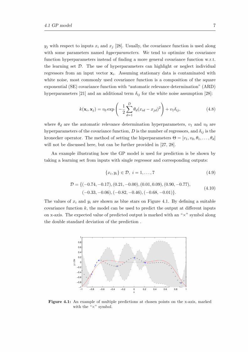
An example illustrating how the GP model is used for prediction is be shown by
taking a learning set from inputs with single regressor and corresponding outputs:
{xi, yi} ∈ D, i = 1, . . . , 7 (4.9)
D = {(−0.74,−0.17), (0.21,−0.00), (0.01, 0.09), (0.90,−0.77),
(−0.33,−0.06), (−0.82,−0.46), (−0.68,−0.01)}.(4.10)
The values of xi and yi are shown as blue stars on Figure 4.1. By defining a suitable
covariance function k, the model can be used to predict the output at different inputs
on x-axis. The expected value of predicted output is marked with an “×” symbol along
the double standard deviation of the prediction .
−1 −0.8 −0.6 −0.4 −0.2 0 0.2 0.4 0.6 0.8 1−1
−0.8
−0.6
−0.4
−0.2
0
0.2
0.4
0.6
0.8
1
y ±
2σ
x
Figure 4.1: An example of multiple predictions at chosen points on the x-axis, markedwith the “×” symbol.
8 Model identification
In our case we are interested in the applications of Non-linear MPC (NMPC) princi-
ple with a GP model [7]. Stochastic NMPC problems are formulated in the applications
where the system to be controlled is described by a stochastic model such as the GP
model [32]. Stochastic problems like state estimation are studied for long time, but,
in our case, we explore only stochastic NMPC problem. Nevertheless, most known
stochastic MPC approaches are based on parametric probabilistic models. Alterna-
tively, the stochastic systems can be modeled with nonparametric models which can
offer a significant advantage compared to the parametric models [7]. This is related
to the fact that the nonparametric probabilistic models, like GP models, provide in-
formation about prediction uncertainties which are difficult to evaluate appropriately
with the parametric models. Other relevant literature of MPC with GP models can be
found also in [7, 32–36].
The GP model used for adaptive control is identified on-line [32]. It is sensible that
advantages of GP models are considered in the control design, which relates the GP
model-based adaptive control at least to suboptimal dual adaptive control principles.
The uncertainty of model predictions obtained with the GP model prediction are de-
pendent, among others, on local learning-data density, and the model complexity is
automatically related to the amount and the distribution of the available data – more
complex models need more evidence to make them likely [37]. Both aspects are very
useful in sparsely-populated transient regimes. Moreover, since weaker prior assump-
tions are typically applied in a nonparametric model, the bias is typically lower than
in parametric models. The related
4.2 Evolving GP model
This section is summarized from [28]. The Evolving GP model (EGP) is inspired
by Evolving systems [38], which are self-developing systems, adapting on-line both,
structure and parameter values of the model from incoming data [38]. We use the term
Evolving GP models in sense of sequential adapting of both, the “structure” of GP
model and hyperparameter values.
This enables fast and efficient GP model adaptation to the time-varying system.
The concept of EGP proposed in [32] and further developed in [39] considers adaptation
of four main parts of GP model: a learning set, hyperparameter values, covariance
function and regressors. In comparison with the learning set D of a GP model, the
learning set of an EGP model DA is said to be an active set with the property:
DA ⊆ D (4.11)
where only a subset of entire learning dataset is used for modeling with EGP. We

t[s]
y ± 2σ
t[s]
y ± 2σnon-adaptive GP model
adaptive GP model
Predicted variance increasesin unknown operating region
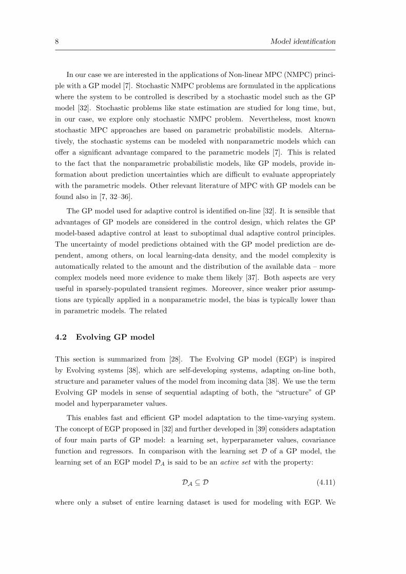
Figure 4.2: An example showing the difference between an adaptive and non-adaptiveGP model.
decided to use fixed squared exponential (SE) covariance function with ARD (4.8) be-
cause its functionality is able to find influential regressors [39]. With the optimization of
the hyperparameter values, uninfluential regressors have smaller influence in covariance
function and as a consequence have smaller influence to the result. Therefore is not
necessary to remove uninfluential regressors manually. In general the proposed method
consists of three main steps to adapt the GP model sequentially. In the first step new
data is processed in sense of including the incoming data to the active set D. Secondly,
hyperparameter values Θ are optimized while in the third step the covariance matrix
K and its inversion are updated according to the changes from the first two steps.
In our specific case we have an EGP of NARX form whose incoming data consists
from an input vector xi of delayed inputs and outputs and its target value yi of the
current output. For every new incoming data, the novelty of the data according to the
current GP model is verified. This is simply done by predicting the output mean value
E[y∗i ] of the incoming input vector xi and calculating the error:
e = E[y∗i ]− yi (4.12)
If the error e is greater than a pre-set threshold ζEGP , the element {xi, yi} ∈ D is
added to the active set DA. A method for excluding elements must be used if the
active learning set has to be limited to a maximum size. This methodology will not be
9
10 Optimization of control input
disscused here but more information is available from [28, 32, 39].
5 Optimization of control input
The optimization part of MPC algorithm can be shown in Figure 3.1. It mainly depends
on the:
• structure of cost function,
• optimization method used,
• construction of the future input signal.
5.1 Cost functions
The cost function is used to value the short-hand closed-loop simulations using a model
with varying the input signal to the model. The task of designing a cost function
strongly depends on how is the notion “control system performance” interpreted. A
cost function should project the control system performance to a scalar value accurately.
5.1.1 Quadratic cost
The quadratic cost for stochastic control can be expressed as the expected value of eu-
clidean distance between the reference and predicted process output with an additional
weighing term of control input signal:
J = E[(r(k + 1)− y∗(k + 1))2] + λuu(k)2, (5.1)
using the fact that var[y∗(k + 1)] = E[y∗(k + 1)] − E[y∗(k + 1)]2, we modify (5.1) into
[40]:
J = (r(k)− E[y∗(k + 1)])2 + var[y∗(k + 1)] + λuu(k)2, . (5.2)
We can imply from (5.2) that the quadratic cost for stochastic control leads to variance
minimization. The origin of predicted variance from a GP model can have more possible
sources. If the GP model is used to acquire the properties of a stochastic process, the
noise source is modeled within the GP model. Another reason of GP model variance
is the model uncertainty. The control strategy with cost function (5.2) is “to avoid”

5.1 Cost functions 11
going into regions with greater variance [7]. In the case that controller is not “cautious”
enough, a “quick-and-dirty” option is that the variance term can be weighted with
a constant λvar to enable shaping of the closed-loop response according to variance
information [7]:
J = (r(k + 1)− E[y∗(k + 1)])2 + λvarvar[y∗(k + 1)] + λuu(k)2, . (5.3)
The cost function from (5.3) can be further modified that fits to the receding horizon
concept. Instead of using just one-step prediction, we can extend the cost with sum of
multi-step prediction, including a weighted control input [7]:
J =
Hp∑
i=1
λe,i(r(k + i)− E[y∗(k + i)])2 + λvar,ivar[y∗(k + i)] + λu,iu(k + i)2, (5.4)
where each term has its weight λe,i, λvar,i and λu,i.
For practical reasons, the cost term of control input can be modified being propor-
tional to the euclidean distance (u(k + i)− us)2 where us is the value of control input
at steady-state of the modeled process [4, 41, 42]. The value of steady-state control
input is calculated using a NARX model by finding the solution of an implicit algebraic
equation:
yk = f(yk−1, . . . , yk−L, uk−1, . . . , uk−L), (5.5)
under the conditions:
rs = yk = yk−1 = . . . = yk−L, (5.6)
us = uk−1 = . . . = uk−L, (5.7)
where rs is the desired setpoint of the controlled system. In practical, the calculation of
steady-state target us is done numerically with a gradient optimization method. The
form of quadratic cost function with steady-state target is following:
J =
Hp∑
i=1
λe,i(r(k+ i)−E[y∗(k + i)])2 + λvar,ivar[y∗(k + i)] + λu,i(u(k+ i)− us)2, (5.8)
In our case, the weights from (5.8) will be reduced to two parameters λvar and λu in

12 Optimization of control input
order to simplify the cost function design:
λe,i = 1 · Hp − i+ 1
Hp, (5.9)
λvar,i = λvarHp − i+ 1
Hp, (5.10)
λu,i = λuHp − i+ 1
Hp. (5.11)
The weight values are defined in a linear descending form along the prediction horizon
Hp. Each another prediction inside of a multi-step prediction is more inaccurate than
previous one and this is a reasonable approach to shift the sensivity of cost funciton at
the beginning part of multi-step model prediction. This kind of cost function will be
also used for two case studies.
5.1.2 Saturating cost
The saturating cost function is proposed in [43, 44]
Ji = E
{1− exp
(− 1
2a2(y∗(i)− r(i))2
)}, (5.12)
that is a locally quadratic but which saturates at unity for large deviations between
the desired process output r and the model prediction y∗. The saturating cost from
(5.12) is an unnormalized Gaussian function3 with mean r and variance parameter a2.
The expected value of (5.12) can be solved analytically and we get:
Ji = 1−(
a2
a2 + var[y∗(i)]
) 12
exp
(− (r(i)− y∗(i))2a2 + var[y∗(i)]
). (5.13)
In comparison with cost function from (5.8), it involves neither weights nor control
input term but a single parameter a. In order to form a saturating cost from a receding
horizon, we need to sum up each step of prediction horizon:
J =
k+Hp∑
i=k+1
Ji. (5.14)
3The term “Gaussian function” should not be confused with “Gaussian probability distribution”which has the same form as normalized Gaussian function

5.2 Optimization method
One of main reasons why MPC method was developed is that it can be used for uncon-
strained control problems. In our case, the control input limits are the only constraints
we will be dealing with and these can be overriden by saturating the control input if the
limit is exceeded. The Quasi-Newton method is chosen for uncostrained optimization
of the cost function. It is designed to find a local optimum and it works good with a
convex shaped cost function which is usual in uncostrained linear MPC. One should be
careful with non-linear (or constrained) control because the convexity property of cost
function is not guaranteed.
6 Case studies
The adaptive MPC-GP method and the theories will be judged expermientally on two
processes defined with recurrence equations: a process named bioreactor and a toy
system, further called as the “unstable system”. The main properties for both systems
are given in Table 61.
System Bioreactor Unstable
Open-loop stability yes no
Linearity non-linear linear
Order 2 3
Number of inputs 1 1
Number of outputs 1 1
Input constraint 0 ≤ u ≤ 0.7 −0.5 ≤ u ≤ 0.5
Table 61: Main properties of the system
Eight experiments of closed-loop control were executed with four different cost func-
tions per two prediction horizons Hp under same circumstances, including the same
noise signal ε of the process output. Three cost functions belong to a quadratic form,
the fourth is a saturating one. Each cost function will be additionaly named by its
properties:
• controlled system which belongs to (B-bioreactor,U-unstable),
• quadratic or saturating form,
• weighing parameters λU , λV AR.
13

14 Case studies
Cost name JB,Quad,E JB,Quad,ES JB,Quad,EV JB,Sat
Form quadratic quadratic quadratic saturating
Parameter λU 0 0.07 0 /
Parameter λV 0 0 0.14 /
Parameter a / / / 1
Table 62: Four cost functions with different parameter settings. λU forces the controlinput to be closer to the steady-state input, λV increases the predicted varianceterm of the quadratic cost, a sets the margin between a local quadratic andthe saturated shape of the saturating cost function, relative to the predictedvariance
6.1 Bioreactor
This dynamical system is a highly simplified version of a real bioreactor process [45].
It is an open-loop stable, non-linear and second order system, desribed with recurrence
equation (6.1) and (6.2):
x1(k + 1) = x1(k) +1
2
x1(k)x2(k)
x1(k) + x2(k)− 1
2u(k)x1(k), (6.1)
x2(k + 1) = x2(k)− 1
2
x1(k)x2(k)
x1(k) + x2(k)− 1
2u(k)x2(k) +
1
20u(k), (6.2)
y(k) = x1(k) + ε(k), (6.3)
where u is system input, limited to [0, 0.7], x1 and x2 are system states, and the output
y is contaminated with a normally distributed noise ε with p(ε) = N (0, 0.001). The
adaptive MPC-EGP algorithm requres an initial GP model to perform effectively. A
simple proportional (P) regulator was used to train a GP model in closed-loop in the
first 0 ≤ k ≤ 30 time steps. At k > 30 the adaptive MPC-EGP regulator was activated
and replaced the proportional one. The error threshold for EGP model update is set
to ζEGP = 0.0021 and we restricted the EGP active learning set to a maximum of 15
learning points. Such small active learning set would probably be too risky for control of
real systems. In our case, a smaller dataset can influence higher prediction uncertainty
(and also inaccuracy). This is interesting since we want to somehow implement the cost
function involving prediction variance, partially derived from the model uncertainty.
Just a representative segment of the closed-loop performance is shown in Figure 6.1
for two different prediction horizons Hp and four different cost functions as shown in
Table 62.
The algorithm performed relatively good for all configurations (Figure 6.1). We
can notice that the control using cost JU,Quad,ES performed with a smoother control
signal and a slower closed-loop response (for both horizons Hp = 1 and Hp = 8) as

6.1 Bioreactor 15
290 300 310 320 330 340 350 3600
0.2
0.4
0.6
u(t
)
k
0.04
0.06
0.08
0.1
y(t
) ± 2
σ
(a) JU,Quad,E cost function, Hp = 1
290 300 310 320 330 340 350 3600
0.2
0.4
0.6
u(t
)
k
0.04
0.06
0.08
0.1
y(t
) ± 2
σ
(b) JU,Quad,E cost function, Hp = 8
290 300 310 320 330 340 350 3600
0.2
0.4
0.6
u(t
)
k
0.04
0.06
0.08
0.1
y(t
) ± 2
σ
(c) JU,Quad,ES cost function, Hp = 1
290 300 310 320 330 340 350 3600
0.2
0.4
0.6
u(t
)
k
0.04
0.06
0.08
0.1
y(t
) ± 2
σ
(d) JU,Quad,ES cost function, Hp = 8
290 300 310 320 330 340 350 3600
0.2
0.4
0.6
u(t
)
k
0.04
0.06
0.08
0.1
y(t
) ± 2
σ
(e) JU,Quad,EV cost function, Hp = 1
290 300 310 320 330 340 350 3600
0.2
0.4
0.6
u(t
)
k
0.04
0.06
0.08
0.1
y(t
) ± 2
σ
(f) JU,Quad,EV cost function, Hp = 8
290 300 310 320 330 340 350 3600
0.2
0.4
0.6
u(t
)
k
0.04
0.06
0.08
0.1
y(t
) ± 2
σ
(g) JU,Sat cost function, Hp = 1
290 300 310 320 330 340 350 3600
0.2
0.4
0.6
u(t
)
k
0.04
0.06
0.08
0.1
y(t
) ± 2
σ
(h) JU,Sat cost function, Hp = 8
Figure 6.1: Closed-loop control of bioreactor. The upper window contains a reference signal(blue), process output (red) and one-step prediction mean with double std. devia-tion (black with gray gap). The lower window is control input.

16 Case studies
Cost name JU,Quad,E JU,Quad,ES JU,Quad,EV JU,Sat
Form quadratic quadratic quadratic saturating
Parameter λU 0 8 · 10−4 0 /
Parameter λV 0 0 2 /
Parameter a / / / 1
Table 63: Four cost functions with different parameter settings. λU forces the controlinput to be closer to the steady-state input, λV increases the predicted varianceterm of the quadratic cost, a sets the margin between a local quadratic andthe saturated shape of the saturating cost function, relative to the predictedvariance
expected. Using the cost JU,Quad,EV or JU,Sat does not improve the control performance
significantly, compared to a simpler cost term JU,Quad,E . We should expect that the
prediction variance would influence a slower closed-loop performance because the cost
should increase when predicting in a less known operating region.
6.2 Unstable system
Another case study of control performance is based on an artificially created linear
unstable system, described with difference equation:
y(k) =2.12y(k − 1)− 1.25y(k − 2) + 0.09y(k − 3)
+0.006u(k − 1) + 0.016u(k − 2) + 0.002u(k − 3)
+0.001ε(k),
(6.4)
where system input u is limited to [−0.5, 0.5] and y is the system output, contaminated
with a normally distributed noise ε with p(ε) = N (0, 0.001)4. The adaptive MPC-
EGP algorithm requres an initial GP model to perform effectively. A MPC regulator
with fixed parametric model (6.4) was used for closed-loop identification in the first
0 ≤ k ≤ 263 time steps. At k > 30 the adaptive MPC-EGP regulator was activated
and replaced with the proportional one. The error threshold for EGP model update is
ζEGP = 0.004 and the upper size limit of EGP active set is set to 40 elements.
Just a representative segment of the closed-loop performance is shown in Figure 6.2
for two different prediction horizons Hp and four different cost functions as shown in
Table 63;
The algorithm performed relatively slow but smoother using a larger horizon of
Hp = 8 (Figure 6.2). We can point out that using a larger predictive horizon gives a
more insensitive control performance w.r.t. the cost function chosen. While instead
4One should note that the noise signal ε is the same for bioreactor and the unstable system, but theunstable system operating region is two times larger than bioreactor

6.2 Unstable system 17
520 540 560 580 600 620 640 660 680 700 720−0.5
0
0.5
u(t
)
k
−0.1
−0.05
0
0.05
0.1
(a) JU,Quad,E cost function, Hp = 1
520 540 560 580 600 620 640 660 680 700 720−0.5
0
0.5
u(t
)
k
−0.1
−0.05
0
0.05
0.1
y(t
) ± 2
σ
(b) JU,Quad,E cost function, Hp = 8
520 540 560 580 600 620 640 660 680 700 720−0.5
0
0.5
u(t
)
k
−0.1
−0.05
0
0.05
0.1
y(t
) ± 2
σ
(c) JU,Quad,ES cost function, Hp = 1
520 540 560 580 600 620 640 660 680 700 720−0.5
0
0.5
u(t
)
k
−0.1
−0.05
0
0.05
0.1
y(t
) ± 2
σ
(d) JU,Quad,ES cost function, Hp = 8
520 540 560 580 600 620 640 660 680 700 720−0.5
0
0.5
u(t
)
k
−0.1
−0.05
0
0.05
0.1
y(t
) ± 2
σ
(e) JU,Quad,EV cost function, Hp = 1
520 540 560 580 600 620 640 660 680 700 720−0.5
0
0.5
u(t
)
k
−0.1
−0.05
0
0.05
0.1
y(t
) ± 2
σ
(f) JU,Quad,EV cost function, Hp = 8
520 540 560 580 600 620 640 660 680 700 720−0.5
0
0.5
u(t
)
k
−0.1
−0.05
0
0.05
0.1
y(t
) ± 2
σ
(g) JU,Sat cost function, Hp = 1
520 540 560 580 600 620 640 660 680 700 720−0.5
0
0.5
u(t
)
k
−0.1
−0.05
0
0.05
0.1
y(t
) ± 2
σ
(h) JU,Sat cost function, Hp = 8
Figure 6.2: Closed-loop control of the “unstable” system. The upper window contains a refer-ence signal (blue), process output (red) and one-step prediction mean with doublestd. deviation (black with gray gap). The lower window is control input.
using a predictive horizon Hp = 1, we can notice that the control was feasible and
smother using cost JU,Quad,ES and JU,Quad,EV compared to JU,Quad,E and JU,Sat. At
the other hand, the performance using Hp = 1 is very sensitive to the cost function
parameters chosen and it would prevert to an unstable closed-loop performance if they
would enough increased.
7 Conclusion
Our goal was to experimentally evaluate the effects of various cost functions on the
controlled system performance. The results from the bioreactor control and unstable
system control (figure 6.2) show that the performance using a larger horizon is accept-
able and less sensitive to parameters, compared to Hp = 1. The effect of weighing a
control input signal inside the quadratic cost from (5.8) does provide a smoother control
input signal and might improve the control performance (Figure 6.2c). The observed
effect of weighing a prediction variance inside quadratic cost might affect smoother
control input signal (figure 6.2e). No notable difference can be concluded between the
saturating JSat and a quadratic JQuad,E cost function for the given parameter a = 1.
Some practical issues were noticed. Firstly, the developed identification and control
algorithm are both computationally demanding but this is not a problem when real
controlled systems have longer time constant. Secondly, thinking about cost function
optimization, uncertain model might cause a non-convex form of the cost function which
is non-trivial to minimize.
The current issues in EGP methodology are many. One should note that we im-
plemented an adaptive control algorithm which adapts the GP model on-line and its
prediction infers a much smaller uncertainty compared to an offline GP model. Small
prediction variance cannot leave a bigger impact on control. A big increase of crite-
rion weights λi,V AR could solve the use of prediction uncertainty but might lead to
unwanted results. Another problem is the validation of an EGP model in specific time
instant: we can validate the overall performance of EGP model during system control
but another question is how to measure the accuracy of the EGP model in a specific
moment during the control if the model is time-varying.
The control design based on EGP is known for stable systems. More focus is
needed on control of unstable systems. GP models are good for interpolation between
two known regions, but another question is if GP models can be used for extrapolation
of unknown regions of a dynamical system during closed-loop control. Such issue could
18

lead to the study of local and global stability of a closed-loop system. More properties
of dynamical GP models should be further investigated in order to understand and
improve closed-loop control of unstable systems. Yet another question is how to reach
convergence of closed-loop performance starting with an initial model as simple as
possible. The former is closely related to dual adaptive control.
Robust control is a branch of control theory that explicitly deals with uncertainty
in its approach to controller design but is non-adaptive. GP modeling framework gives
an opportunity to work with models where unertainty is handled by nature. Robust
control based on GP model is another aspect that can be further studied and developed
for industry needs.
Bibliography
[1] J. Doyle, B. Francis, and A. Tannenbaum, Feedback Control Theory. Macmillan
Publishing Co., 1990.
[2] S. J. Qin and T. A. Badgwell, “A survey of industrial model predictive control
technology,” Control Engineering Practice, vol. 11, p. 733–764, 2003.
[3] S. Qin and T. Badgwell, “An overview of nonlinear model predictive control appli-
cations,” in Nonlinear Model Predictive Control (F. Allgower and A. Zheng, eds.),
vol. 26 of Progress in Systems and Control Theory, pp. 369–392, Birkhauser Basel,
2000.
[4] J. B. Rawlings, “Tutorial overview of model predictive control,” IEEE Control
Systems Magazine, vol. 20, pp. 38–52, 2000.
[5] F. Allgower, R. Findeisen, and Z. K. Nagy, “Nonlinear model predictive control:
From theory to application,” Journal of the Chinese Institute of Chemical Engi-
neers, vol. 35, pp. 299–315, 2004.
[6] C. E. Garcıa, D. M. Prett, and M. Morari, “Model Predictive Control: Theory
and Practice - a Survey,” Automatica, vol. 25, pp. 335–348, 1989.
[7] J. Kocijan, “Control Algorithms Based on Gaussian Process Models: A State-of-
the-Art Survey,” in Special International Conference on Complex systems: synergy
of control communications and computing, September 16-20, 2011, Ohrid, Republic
of Macedonia. Proceedings of COSY 2011 papers, 2011.
19

20 BIBLIOGRAPHY
[8] N. Filatov and H. Unbehauen, “Survey of adaptive dual control methods,” IEE
Proceedings - Control Theory and Applications, vol. 147, pp. 118–128, 2000.
[9] B. Wittenmark, “Adaptive dual control,” in Control Systems, Robotics and Au-
tomation, Encyclopedia of Life Support Systems (EOLSS), Developed under the
auspices of the UNESCO, Oxford, UK: Eolss Publishers, Jan. 2002.
[10] J. Alster and P. Belanger, “A Technique for Dual Adaptive Control,” Automatica,
vol. 10, pp. 627–634, 1974.
[11] S. Fabri and V. Kadirkamanathantn, “Dual Adaptive Control of Nonlinear
Stochastic Systems using Neural Networks,” Automatica, vol. 34, pp. 245–253,
1998.
[12] D. P. Bertsekas, “Dynamic programming and suboptimal control: A survey from
adp to mpc,” European Journal of Control, vol. 11, pp. 310–334, 2005.
[13] K. Astrom, “Theory and applications of adaptive control—a survey,” Automatica,
vol. 19, no. 5, pp. 471 – 486, 1983.
[14] R. Sa lat, M. Awtoniuk, and K. Korpysz, “Black-Box system identification by
means of Support Vector Regression and Imperialist Competitive Algorithm,” in
Przeglad Elektrotechniczny, 2013.
[15] H. Arellano-Garcia, M. Wendt, T. Barz, and G. Wozny, “Close-loop stochastic dy-
namic optimization under probabilistic output-constraints,” in Assessment and Fu-
ture Directions of Nonlinear Model Predictive Control (R. Findeisen, F. Allgower,
and L. Biegler, eds.), vol. 358 of Lecture Notes in Control and Information Sci-
ences, pp. 305–315, Springer Berlin Heidelberg, 2007.
[16] J. Kocijan, “Dynamic GP Models: An Overview and Recent Developments,” in
Proceedings of the 6th International Conference on Applied Mathematics, Simu-
lation, Modelling, ASM’12, (Stevens Point, Wisconsin, USA), pp. 38–43, World
Scientific and Engineering Academy and Society (WSEAS), 2012.
[17] K. Azman and J. Kocijan, “Dynamical Systems Identification Using Gaussian Pro-
cess Models with Incorporated Local Models,” Journal of Engineering Applications
of Artificial Intelligence, vol. 24, pp. 398–408, Mar. 2011.
[18] D. Petelin and J. Kocijan, “Application of on-line Gaussian process models for
pressure signal,” in 11th International PhD Workshop on Systems and Control,
2010.
[19] F. Perez-Cruz, S. Van Vaerenbergh, J. Murillo-Fuentes, M. Lazaro-Gredilla, and
I. Santamaria, “Gaussian processes for nonlinear signal processing: An overview
BIBLIOGRAPHY 21
of recent advances,” Signal Processing Magazine, IEEE, vol. 30, pp. 40–50, July
2013.
[20] J. Kocijan, A. Girard, B. Banko, and R. Murray-Smith, “Dynamic systems identi-
fication with Gaussian processes,” Mathematical and Computer Modelling of Dy-
namical Systems, vol. 11, pp. 411–424, 2005.
[21] C. K. I. Williams and C. E. Rasmussen, “Gaussian processes for regression,” Ad-
vances in Neural Information Processing Systems, vol. 8, pp. 514–520, 1996.
[22] G. Gregorcic and G. Lightbody, “Gaussian processes for modelling of dynamic
non-linear systems,” in Proceedings of the Irish Signals and Systems Conference,
(Cork, Ireland), pp. 141–147, 2002.
[23] J. Quinoneiro-Candela and C. Rasmussen, “A Unifying View of Sparse Approxi-
mate Gaussian Process Regression,” Journal of Machine Learning Research, vol. 6,
pp. 1939–1959, 2005.
[24] M. Lazaro-Gredilla, J. Quinonero-Candela, C. E. Rasmussen, and A. R. Figueiras-
Vidal, “Sparse Spectrum Gaussian Process Regression,” Journal of Machine
Learning Research, vol. 11, pp. 1865–1881, 2010.
[25] R. Turner, M. P. Deisenroth, and C. E. Rasmussen, “State-space inference and
learning with Gaussian processes,” in Proceedings of 13th International Conference
on Artificial Intelligence and Statistics, vol. 9, (Sardinia, Italy), pp. 868–875, 2010.
[26] D. Nguyen-Tuong, M. Seeger, and J. Peters, “Computed torque control with non-
parametric regression models,” in Proceedings of the American Control Conference
(ACC), pp. 212–217, 2008.
[27] R. Neal, “Regression and classification using gaussian process priors,” Bayesian
Statistics, vol. 6, pp. 475–501, 1998.
[28] D. Petelin and J. Kocijan, “Evolving Gaussian process models for predicting
chaotic time-series,” in IEEE Conference on Evolving and Adaptive Intelligent
Systems (EAIS), 2014. Accepted for publication.
[29] H. Nickisch and C. Rasmussen, “Approximations for binary gaussian process clas-
sification,” Journal of Machine Learning Research, vol. 9, pp. 2035–2078, 2008.
[30] G. Pillonetto, F. Dinuzzo, T. Chen, G. D. Nicolao, and L. Ljung, “Kernel methods
in system identification, machine learning and function estimation: A survey,”
Automatica, vol. 50, no. 3, pp. 657–682, 2014.

22 BIBLIOGRAPHY
[31] C. Campbell, “Kernel methods: a survey of current techniques,” Neurocomputing,
vol. 48, pp. 63–84, 2002.
[32] D. Petelin and J. Kocijan, “Control system with evolving Gaussian process mod-
els,” in Evolving and Adaptive Intelligent Systems (EAIS), 2011 IEEE Workshop
on, pp. 178–184, 2011.
[33] G. Shen and Y. Cao, “A Gaussian Process Based Model Predictive Controller for
Nonlinear Systems with Uncertain Input-output Delay,” Applied Mechanics and
Materials, vol. 433-435, pp. 1015–1020, 2013.
[34] J. M. Macijeowski and X. Yang, “Fault tolerant control using Gaussian processes
and model predictive control,” in Conference on Control and Fault-Tolerant Sys-
tems (SysTol), Nice, France., October 2013.
[35] J. Kocijan, R. Murray-Smith, C. Rasmussen, and B. Likar, “Predictive control
with gaussian process models,” in EUROCON 2003. Computer as a Tool. The
IEEE Region 8, vol. 1, pp. 352–356 vol.1, Sept 2003.
[36] R. Murray-Smith, D. Sbarbaro, C. E. Rasmussen, and A. Girard, “Adaptive, cau-
tious, predictive control with Gaussian process priors,” in Proceedings of 13th IFAC
Symposium on System Identification, (Rotterdam, Netherlands), 2003.
[37] R. Murray-Smith and A. Girard, “Gaussian Process priors with ARMA noise mod-
els,” in Irish Signals and Systems Conference, Maynooth, Ireland, (Maynooth,
Ireland), pp. 147–152, 2001.
[38] P. Angelov, D. P. Filev, and N. Kasabov, “Evolving intelligent systems: Methodol-
ogy and applications,” in IEEE Press Series on Computational Intelligence, Wiley
IEEE Press, April 2010.
[39] D. Petelin, A. Grancharova, and J. Kocijan, “Evolving Gaussian process models
for prediction of ozone concentration in the air,” Simulation Modelling Practice
and Theory, vol. 33, no. 0, pp. 68 – 80, 2013.
[40] R. Murray-Smith and D. Sbarbaro, “Nonlinear adaptive control using nonparamet-
ric Gaussian process prior models,” in Proceedings of IFAC 15th World Congress,
(Barcelona, Spain), 2002.
[41] C. V. Rao and J. B. Rawlings, “Steady states and constraints in model predictive
control,” AIChE Journal, vol. 45, pp. 1266–1279, 1999.
[42] K. R. Muske, “Steady-state target optimization in linear model predictive control,”
in Proceedings of the American Control Conference, 1997.

BIBLIOGRAPHY 23
[43] M. P. Deisenroth and C. E. Rasmussen, “Pilco: A model-based and data-efficient
approach to policy search,” in In Proceedings of the International Conference on
Machine Learning, 2011.
[44] M. P. Deisenroth and C. E. Rasmussen, “Efficient reinforcement learning for motor
control,” in Proceedings of the 10th International PhD Workshop on Systems and
Control, a Young Generation Viewpoint, (Hluboka nad Vltavou, Czech Republic),
2009.
[45] K. Azman and J. Kocijan, “Application of Gaussian processes for black-box mod-
elling of biosystems,” ISA Transactions, vol. 46, no. 4, pp. 443 – 457, 2007.
Related Documents


