1 Abstract The first part of the thesis consists in a literature review on Organic Rankine Cycles (ORCs). After a brief introduction on the role of ORCs in the frame of nowadays global energy context, the potential heat sources for this technology are described: low and medium enthalpy geothermal, solar radiation, biomass and waste heat from internal combustion engines and industrial processes. Then, the main cycle configurations are presented with regard to the conditions that make each of them preferable over the others. A part from the basic subcritical cycle, also the regenerative subcritical cycle and the basic supercritical cycle are analyzed. A section is spent on the possibility to superheat the fluid before the expansion. Then, two thermal processes that compete with ORCs are presented: the transcritical cycle and the proprietary Kalina® cycle. Afterward, we will discuss the “state-of-the-art” about the expansion machines (both dynamic and volumetric). Indeed, the choice of the expander represents a crucial moment in the design of an ORC system. The fifth Chapter introduces the problem of working fluid selection, by presenting advantages, disadvantages and characteristics of a wide variety of organic fluids, with concern to “technical” as well as environmental and safety issues. The classical works about this problem, which is fundamental in the process of ORC design, is synthetically presented. The second part consists in a series of simulations performed with the software EES, that aim at providing useful indications in choosing the working fluid and the cycle layout in low to medium temperature applications. The heat source has been modeled as 10 kg/s of sub-cooled water available at three different temperatures: 120, 150 and 180°C, while three cycle configurations have been considered: basic subcritical, regenerative subcritical (both without superheating) and the basic supercritical cycle. The temperature difference between the heat source at the evaporator inlet and the critical point of the considered working fluid has been utilized to characterize the behavior of each fluid with respect to its cycle efficiency and to the amount of heat recovered from the source. This approach simplifies the problem, otherwise subject to many variables due to differences in fluid properties. If the aforementioned temperature difference is treated as a decision variable of the problem, standing for the corresponding working fluid, it shows a maximum in power output that comes from the trade-off between high cycle efficiency and high heat recovery effectiveness. Working fluids with highly tilted vapor saturation line seem to be interesting in the regenerative cycle when the outlet temperature of the heat source is constrained by a lower limit, as it occurs in many applications. Finally, under the same assumptions it has been observed that also for supercritical cycles, the maximum power output is achieved through a compromise between high cycle efficiency and good heat recovery. Moreover, a “thermodynamically” optimal region has been found as function of maximum cycle temperature and evaporating pressure.

Abstract - Benvenuti su Padua@Thesis - [email protected]/45717/1/TESI_VIVIAN_printed.pdf · Abstract The first part of the thesis consists in a literature review on Organic
Jul 10, 2020
Welcome message from author
This document is posted to help you gain knowledge. Please leave a comment to let me know what you think about it! Share it to your friends and learn new things together.
Transcript
1
Abstract
The first part of the thesis consists in a literature review on Organic Rankine Cycles (ORCs). After a
brief introduction on the role of ORCs in the frame of nowadays global energy context, the
potential heat sources for this technology are described: low and medium enthalpy geothermal,
solar radiation, biomass and waste heat from internal combustion engines and industrial
processes. Then, the main cycle configurations are presented with regard to the conditions that
make each of them preferable over the others. A part from the basic subcritical cycle, also the
regenerative subcritical cycle and the basic supercritical cycle are analyzed. A section is spent on
the possibility to superheat the fluid before the expansion. Then, two thermal processes that
compete with ORCs are presented: the transcritical cycle and the proprietary Kalina® cycle.
Afterward, we will discuss the “state-of-the-art” about the expansion machines (both dynamic and
volumetric). Indeed, the choice of the expander represents a crucial moment in the design of an
ORC system. The fifth Chapter introduces the problem of working fluid selection, by presenting
advantages, disadvantages and characteristics of a wide variety of organic fluids, with concern to
“technical” as well as environmental and safety issues. The classical works about this problem,
which is fundamental in the process of ORC design, is synthetically presented.
The second part consists in a series of simulations performed with the software EES, that aim at
providing useful indications in choosing the working fluid and the cycle layout in low to medium
temperature applications. The heat source has been modeled as 10 kg/s of sub-cooled water
available at three different temperatures: 120, 150 and 180°C, while three cycle configurations
have been considered: basic subcritical, regenerative subcritical (both without superheating) and
the basic supercritical cycle. The temperature difference between the heat source at the
evaporator inlet and the critical point of the considered working fluid has been utilized to
characterize the behavior of each fluid with respect to its cycle efficiency and to the amount of
heat recovered from the source. This approach simplifies the problem, otherwise subject to many
variables due to differences in fluid properties. If the aforementioned temperature difference is
treated as a decision variable of the problem, standing for the corresponding working fluid, it
shows a maximum in power output that comes from the trade-off between high cycle efficiency
and high heat recovery effectiveness. Working fluids with highly tilted vapor saturation line seem
to be interesting in the regenerative cycle when the outlet temperature of the heat source is
constrained by a lower limit, as it occurs in many applications. Finally, under the same
assumptions it has been observed that also for supercritical cycles, the maximum power output is
achieved through a compromise between high cycle efficiency and good heat recovery. Moreover,
a “thermodynamically” optimal region has been found as function of maximum cycle temperature
and evaporating pressure.

2
In conclusion, the cost functions of the components have been introduced to verify whether a shift
occurs while passing from the thermodynamic to the thermoeconomic optimum. It has been
possible to utilize again the aforementioned temperature difference as criterion for fluid selection.
Indeed, a shift of the optimum actually occurs and it can be related to this parameter. From the
observation of the results, it has been concluded that cycle efficiency is more relevant than heat
recovery effectiveness in the determination of the thermoeconomic optimum, both for subcritical
and for supercritical cycles. As a consequence, in subcritical cycles, working fluids with small or
negative temperature difference between heat source and critical point become relevant under an
economic perspective, whereas they were excluded from the thermodynamic optimization. In
supercritical cycles, the optimum shifts clearly from a region of high power output to a region of
high cycle efficiency.

3
Riassunto
La prima parte della tesi consiste in una revisione di letteratura sui cicli Rankine a fluido organico
(ORC). Dopo una breve introduzione in cui si inquadra il ruolo dei cicli ORC nel contesto energetico
globale in cui ci troviamo, vengono analizzate le potenziali fonti termiche per questi tipi di
impianti: il geotermico a bassa e media entalpia, gli impianti cogenerativi a biomassa, la radiazione
solare e il calore in eccesso (o di scarto) di motori a combustione interna e di processi industriali.
Vengono successivamente presentate le principali configurazioni di ciclo, mettendo in evidenza
per ognuna di queste le condizioni che la rendono più conveniente rispetto alla configurazione
base. Oltre al ciclo base subcritico, vengono analizzati il ciclo rigenerativo subcritico e quello base
supercritico, oltre alla possibilità di surriscaldare il fluido prima di espanderlo. Inoltre, vengono
presentati due processi termici che possono competer con gli ORC nelle applicazioni di cui sopra: il
ciclo a transcritica e il ciclo Kalina®. Viene poi presentato lo stato dell’arte sugli espansori (sia
dinamici che volumetrici, con particolare attenzione alle macchine scroll), la cui scelta determina
un momento fondamentale nella progettazione di un sistema ORC. Il quinto capitolo introduce il
problema della scelta del fluido operativo, presentando caratteristiche, vantaggi e svantaggi di
un’ampia gamma di fluidi organici, sia da un punto di vista “tecnico” che da un punto di vista
ambientale e di sicurezza per l’uomo. Viene presentata in modo sintetico la letteratura di
riferimento concernente questo problema, anch’esso cruciale nel processo di design di questi
sistemi.
La seconda parte consiste in una serie di simulazioni eseguite col software EES con cui si vuole
dare delle indicazioni utili per la scelta del fluido di lavoro e della configurazione di ciclo in
applicazioni a bassa e media temperatura. In particolare, la fonte termica è stata assunta pari a 10
kg/s di acqua pressurizzata a 120, 150 e 180°C; sono state considerate solamente tre
configurazioni di ciclo: subcritico base e subcritico rigenerativo senza surriscaldamento, e
supercritico base. La differenza di temperatura tra ingresso della sorgente e temperatura critica
del fluido analizzato (indipendente dai parametri del ciclo) è stata utilizzata per caratterizzare il
comportamento di ogni fluido rispetto all’efficienza del ciclo e alla quantità di calore recuperato
dalla sorgente stessa. Questo approccio ha permesso di semplificare il problema, altrimenti
soggetto a molte variabili a causa delle diverse proprietà dei fluidi. L’analisi ha mostrato che esiste
un valore della suddetta differenza di temperatura (che viene trattata come variabile di decisione
del problema) attorno al quale è massima la potenza prodotta dal sistema, frutto del
compromesso tra calore recuperato e efficienza del ciclo ORC a valle di tale recupero termico. Per
quanto riguarda il ciclo rigenerativo, esso può diventare interessante per la fonte termica
considerata nel caso in cui ci sia un vincolo inferiore al raffreddamento della fonte termica, come
avviene in molte realtà applicative (ad esempio nel geotermico) per fluidi di lavoro che mostrano
una elevata pendenza della linea di vapor saturo nel diagramma T-s. Infine, è stato riscontrato che
anche per i cicli supercritici, nelle nostre ipotesi, la massima potenza viene raggiunta dal

4
compromesso tra efficienza del recupero termico ed efficienza del ciclo. Inoltre, è stata trovata
una regione “ottimale” dal punto di vista termodinamico, cioè ad elevata produzione di potenza,
in funzione della pressione di evaporazione e della temperatura massima di ciclo.
Nell’ultimo capitolo, sono state introdotte delle funzioni di costo dei componenti per verificare
l’eventuale spostamento delle condizioni operative ottimali passando da un’ottimizzazione
termodinamica ad una termoeconomica. È stato possibile utilizzare nuovamente la differenza di
temperatura tra ingresso della sorgente e punto critico del fluido come criterio per la scelta dello
stesso. Si è visto infatti che anche il suddetto spostamento dell’ottimo può essere messo in
relazione a tale parametro. Dall’osservazione dei risultati, si è evinto come l’efficienza del ciclo
abbia un peso specifico maggiore dell’efficienza di recupero termico nella determinazione
dell’ottimo termoeconomico, sia per cicli subcritici sia per cicli supercritici. Come conseguenza di
ciò, nei cicli subcritici i fluidi operativi con temperatura critica leggermente inferiore o superiore a
quella di ingresso della sorgente diventano interessanti da un punto di vista economico, mentre
erano stati esclusi dalla procedura di selezione prettamente termodinamica. Nei cicli supercritici,
l’ottimo si sposta chiaramente da una regione ad alta potenza ad una regione ad alta efficienza di
ciclo.

5
Acknowledgments
I am grateful to those people who first had the idea of promoting
the European Students Exchange Programs, as a mean of
integration, collaboration and strengthening of the communitarian
feeling.
Indeed, this work was carried out for the most part in the
Technische Universität Berlin within the Erasmus Program, under
the supervision of Prof. Tatjana Morozyuk, whom I would like to
thank.
Furthermore, the final version of the thesis would not have been
possible without the effort of Prof. Andrea Lazzaretto and Ing.
Giovanni Manente. They helped me crucially both on the side of
contents and on the side of structuring the work with an ordered
pattern.
Last but not least, I want to thank my family and friends for their
continuous support throughout my studies.

6

7
Table of contents
Abstract ................................................................................................................................................ 1
Riassunto .............................................................................................................................................. 3
Acknowledgments ............................................................................................................................... 5
Table of contents ................................................................................................................................. 7
Chapter I. Introduction ...................................................................................................................... 11
Chapter II. Applications of Organic Rankine Cycles ......................................................................... 13
2.1 Medium and low-temperature geothermal heat .................................................................... 13
2.1.1 Minimum rejection temperature and other constraints ................................................................ 14
2.1.2 Availability of low-temperature geothermal resources in Italy ..................................................... 15
2.1.3 Availability of low-enthalpy geothermal resources in Germany .................................................... 16
2.2 Biomass CHP ............................................................................................................................. 18
2.3 Solar radiation .......................................................................................................................... 19
2.3.1 Examples of prototypes and operating plants ............................................................................... 21
2.4 Waste heat recovery from ICE exhaust gases .......................................................................... 22
2.5 Waste heat recovery from industrial processes ...................................................................... 23
2.5.1 Introduction to heat recovery ........................................................................................................ 24
2.5.2 Recuperators and heat exchangers for internal heat recovery ...................................................... 25
2.5.3 Glass manufacturing ....................................................................................................................... 26
2.5.4 Cement manufacturing ................................................................................................................... 27
2.5.5 Iron and steel production ............................................................................................................... 28
2.5.6 Aluminum production .................................................................................................................... 31
2.5.7 Metal casting .................................................................................................................................. 31
2.5.8 Ethylene furnaces ........................................................................................................................... 32
2.5.9 Industrial boilers in other manufacturing sectors .......................................................................... 32
2.5.10 Potential of heat recovery from energy intensive industries in Italy ........................................... 32
Chapter III. Cycle configuration ................................................................................................................ 34
3.1 Basic cycle ................................................................................................................................. 34
3.2 Regenerative cycle ................................................................................................................... 37
3.3 Supercritical cycle ..................................................................................................................... 39
3.4 Superheating ............................................................................................................................ 44

8
3.5 General guidelines for the choice of cycle configuration ........................................................ 45
3.6 Transcritical CO₂ cycle .............................................................................................................. 46
3.7 Kalina cycle ............................................................................................................................... 49
3.7.1 Description of the Kalina process ................................................................................................... 49
3.7.2 Phase change of a non-azeotropic solution ................................................................................... 50
3.7.3 Insights on cycle optimization ........................................................................................................ 51
3.7.4 Kalina Cycle versus ORC .................................................................................................................. 53
3.7.5 Conclusions ..................................................................................................................................... 54
Chapter IV. Expanders ................................................................................................................................. 55
4.1 Turbines .................................................................................................................................... 55
4.1.1 Fundamentals of turbomachines: the similitude theory ................................................................ 56
4.1.2 Size effect on turbine efficiency ..................................................................................................... 58
4.1.3 Effects of compressibility on turbine efficiency ............................................................................. 61
4.1.4 Other constraints ............................................................................................................................ 64
4.1.5 The choice of the turbine in the ORC design .................................................................................. 64
4.2 Volumetric expanders .............................................................................................................. 68
4.2.1 Scroll expanders ............................................................................................................................. 68
4.2.2 Screw expanders ............................................................................................................................. 74
4.2.3 Reciprocating piston ....................................................................................................................... 74
4.2.4 Constraints of volumetric expanders in the ORC design ................................................................ 75
4.3 Comparison between dynamic and volumetric expanders ..................................................... 77
Chapter V. Organic fluids ........................................................................................................................... 79
5.1 Fluids characteristics ................................................................................................................ 79
5.1.1 Thermodynamic properties ............................................................................................................ 79
5.1.2 Safety level: toxicity and flammability............................................................................................ 82
5.1.3 Environmental impact and international standards....................................................................... 82
5.2 Working fluid selection............................................................................................................. 84
5.1.1 Classical works on working fluid selection ..................................................................................... 84
5.2.2 Comparison between Organic and conventional Rankine Cycle .................................................... 88
5.2.3 Zeotropic mixtures.......................................................................................................................... 89
Chapter VI. Thermodynamic optimization .............................................................................................. 92
6.1 Assumptions and system modeling .......................................................................................... 92
6.1.1 Candidate working fluids ................................................................................................................ 92
6.1.2 System modeling ............................................................................................................................ 93
9
6.2 Basic subcritical cycle ............................................................................................................... 94
6.2.1 Cycle optimization .......................................................................................................................... 94
6.2.2 Matching of heat source and ORC: system optimization ............................................................... 96
6.3 Regenerative subcritical cycle ................................................................................................ 102
6.3.1 System optimization ..................................................................................................................... 103
6.4 Basic supercritical cycle .......................................................................................................... 105
6.4.1 System optimization ..................................................................................................................... 106
6.4.2 Working fluid selection for supercritical cycles ............................................................................ 107
6.5 Conclusions ............................................................................................................................. 109
Chapter VII. Thermoeconomic optimization ......................................................................................... 111
7.1 Assumptions and system modeling ........................................................................................ 111
7.1.1 Evaluation of equipment capital cost ........................................................................................... 111
7.1.2 Thermodynamic assumptions ...................................................................................................... 113
7.1.3 Objective function for thermoeconomic optimization ................................................................. 115
7.2 Basic subcritical cycle ............................................................................................................. 116
7.2.1 Results .......................................................................................................................................... 116
7.2.2 Deviation of the thermoeconomic SOET from the thermodynamic SOET ................................... 119
7.3 Regenerative cycle ................................................................................................................. 122
7.3.1 Effect of the constraint of the hot stream outlet temperature on the basic cycle ...................... 122
7.4 Basic supercritical cycle .......................................................................................................... 124
7.4.1 Results of thermo-economic optimization and comparison with the subcritical cycle ............... 124
7.4.2 Deviation of the thermo-economic optimum from the thermodynamic optimum ..................... 126
7.5 Conclusions ............................................................................................................................. 128
Bibliography ................................................................................................................................................ 130

10

11
Chapter I. Introduction
Although there’s not a general consensus of the scientific community about the humans
responsibility in the average temperature rise of the Earth’s climate system recorded in the last
decades –also known as Global Warming-, the International Panel on Climate Change (IPCC)
reported that scientists were more than 90% certain that most of global warming was being
caused by increasing concentrations of greenhouse gases produced by human activities [1]. In
2010 that finding was recognized by the national science academies of all major industrialized
nations. Affirming these findings in 2013, the IPCC stated that the largest driver of global warming
is carbon dioxide (CO2) emissions from fossil fuel combustion, cement production, and land
use changes such as deforestation [1].
The global environmental crisis is the primary reason for the need to generate carbon-free
electricity. Nonetheless, this necessity stems also from other reasons, such as the need of
accessing to electrical power by a large part of humanity. In 2009, almost 1,4 billion people
worldwide did not have access to electricity [2]. Most of these electricity-deprived live in sub-
Saharan Africa and south Asia. Usually, these populations live in remote areas far from the
centralized electricity grid with very low income and extending the electricity grid is not seen as
economically feasible for electricity companies which prefer to concentrate their activities in
urban areas. The development of solutions for localized energy generation seems therefore the
only sustainable way to support the socio-economic growth of the mentioned areas.
Another reason is to reduce the geopolitical stresses related to the possession of fossil reservoirs,
that has been responsible of many conflicts. The propriety of finite fossil resources is strictly
related to macro-economic phenomena, as the oil crisis of 1973 demonstrated. That was the first
alarm signal on a global scale. By now, a great political and technical effort must be done to face
the transition from the centralized power production of big fossil-fuelled power plants to the
distributed generation. From an economic point of view, this process has been facilitated by liberal
policies such as deregulation and privatization of the electrical generation sector, that have
promoted the exploitation of renewable and local energy sources and increased the market
potential of small sized power plants.
In this framework, the heat that can be earned from solar radiation, from geothermal reservoirs,
from biomass combustion and the waste heat that can be recovered from industrial processes or
engines is an interesting source, both for direct use as well as for conversion into electricity.
Nonetheless, such heat can’t be converted into electricity through big power plants operating at
high temperature either because of its inherently low enthalpy level or because of its low energy
intensity. Thus, the technologies dedicated to the exploitation of low-medium temperature heat
sources have been strongly developing and widely increasing in the last years. The Organic
Rankine Cycle (ORC) is commonly considered one of the most promising technologies for the

12
conversion of low grade heat into power. The Organic Rankine Cycle is a simple Rankine cycle that
uses an organic medium instead of steam as working fluid, thus reducing many problems related
to the operation of small sized power plants.
The first part of the work consists in a literature review on Organic Rankine Cycles. In particular,
Chapter II focuses on the various applications suitable to these systems, while the following
Chapters present different aspects related to the system design. In particular, Chapter III describes
the main cycle configurations and includes also some general insights on the concurrent
technologies; Chapter IV deals with expanders, as they are a crucial component in the system
design. Finally, Chapter V provides an overview on the organic fluids that concur to be the working
fluid of the process. Fluid selection plays a key role in the system design. Moreover, the choice of
the working fluid affects the sustainability of the plant both in terms of environmental impact and
safety.
The second part of the work aims at providing general criteria for the choice of working fluid and
cycle configuration for ORC systems supplied by low-to-medium temperature heat sources (120-
180°C without intermediate heat carrier) such as geothermal heat and waste heat from industrial
processes, both from a thermodynamic (Chapter VI) and from an economic point of view (Chapter
VII).
13
Chapter II. Applications of Organic Rankine Cycles
ORCs are Rankine cycles operated by organic working fluids, whose properties make them
attractive for the conversion of low grade heat into power. The aim of the present chapter is the
individuation of the exploitable heat sources and the description of their general characteristics.
2.1 Medium and low-temperature geothermal heat
Geothermal heat sources vary in temperature from 50 to 350 °C, and can either be dry, mainly
steam, a mixture of steam and water, or just liquid water. Geothermal reservoirs can be found in
nature in regions with aquifers filling pores or faults and cracks, or can be produced by man, in
regions formed by dry rocks having high temperatures (HDR) [3]. In these cases, water must be
sent from the surface to the reservoir and, once heated by the rock, return again to the surface to
be used [3]. This method is sometimes used in conventional reservoirs when the water supply is
less than the amount of water or steam withdrawn from the reservoir [3]. The temperature of the
resource is a major determinant of the type of technologies required to extract the heat and of its
possible utilization [4].
Generally, the high-temperature reservoirs ( > 220 °C) are the most suitable ones for commercial
production of electricity. Dry steam and flash steam systems are widely used to produce electricity
from high-temperature resources [4].
- Dry steam systems use steam from geothermal reservoirs as it comes from the wells, and
route it directly through turbine/generator units to produce electricity [4].
- Flash steam plants are the most common type of geothermal power generation plants in
operation today. In flash steam plants, hot water under very high pressure is suddenly
released to a chamber at low pressure, allowing some of the water to be converted into
steam, which is then used to drive a turbine [4].
Medium-temperature geothermal resources, where temperatures are typically in the range of
100 - 220 °C, are by far the most commonly available resource [4]. Binary cycle power plants are
the most common technology to generate electricity using such resources. There are many
different technical variations of binary plants including those known as Organic Rankine cycles
(ORC) and proprietary systems known as Kalina cycles [4]. Binary cycle geothermal power
generation plants differ from dry steam and flash steam systems in that the water or the steam
from the geothermal reservoir never comes in contact with the turbine/generator units. In binary
systems, the water from the geothermal reservoir is used to heat up a secondary fluid which is
vaporized and used to turn the turbine/generator units. The geothermal water and the working
fluid are each confined in separate circulating systems and never come in contact with each other.

14
Although binary power plants are generally more expensive to build than steam-driven plants,
they have several advantages. Pressure being equal, the working fluid boils and flashes to a vapor
at a lower temperature than does water, so electricity can be generated from reservoirs with
lower temperatures. This increases the number of geothermal reservoirs in the world with
electricity-generating potential. Since the geothermal water and working fluid travel through
entirely closed systems, binary power plants have virtually no emissions into the atmosphere [4].
Currently, the potential of electricity generation using low-temperature geothermal resources
(especially in the range of 70 - 100 °C) has been overlooked. Extension of binary power cycle
technology to utilize low-temperature geothermal resources has received much attention. Since
the available temperature difference is less, the cycle efficiency (i.e., approximately 5–9%) is much
lower than that of thermal power generation using medium temperature geothermal resources
(i.e., approximately 10 – 15%) [4]. Furthermore, in low-temperature systems, large heat exchanger
areas are required to extract the same amount of energy compared to medium-temperature
systems [4]. These factors impose limits on exploiting low-temperature geothermal resources and
emphasize the necessity of an optimum, cost-effective design of binary power cycles [4].
2.1.1 Minimum rejection temperature and other constraints
According to Franco and Villani [5] the geothermal brine can’t be cooled below 70÷80°C in order to
avoid problems of silica oversaturation. The latter could lead to silica scaling, serious fouling
problems in recovery heat exchangers and in mineral deposition in pipes and valves [5]. The
fundamental variables that must be considered in the optimization of geothermal binary power
plants are the temperature, pressure and chemical composition of the geothermal fluid, the
rejection temperature, the ambient temperature and the maximum rate of energy extraction that
can be sustained without a significant decrease of the water temperature in the reservoir [5]. A
correct approach to the problem would be therefore the selection of the rejection temperature
based on the brine chemical composition. In any case, according to the aforementioned authors, it
seems difficult to decrease the rejection temperature below 70°C [5].
This constraint influences the determination of the objective function, as the maximum heat that
can be extracted from the geothermal resource must refer to the minimum rejection temperature
which does not coincide with the ambient temperature. As an example, the objective function in
the optimization carried out by Toffolo et al. [6] has been the so-called exergy recovery efficiency,
( )
where the numerator is the net power output and the denominator is the difference between the
exergy associated with the geofluid at inlet conditions and the exergy of the same stream at the
minimum rejection temperature, here set to 70°C.

15
Another parameter of crucial importance for these plants is the specific brine consumption β,
which is the ratio of the extracted brine mass flow rate to the produced net power. Of course the
lower it is, the lower are the costs associated with brine pumping.
The specific brine consumption must be limited within certain values in order to assure the
economic feasibility of the plant [5]. In the aforementioned work of Franco and Villani, they
pointed out that its value is affected by the temperature difference between inlet and outlet of
the geofluid stream and by the condensing temperature of the fluid [5]. Indicatively, a
temperature difference of 90°C (from 160°C to the rejection temperature of 70°C) with the
condensing pressure at 30°C result in a specific brine consumption included between 20 and 24
kg/MJ, depending on the working fluid. For a temperature difference of 60°C (130° to 70°C) and a
condensing temperature of 40°C, 40÷50 kg/s of brine are consumed for each MW of electric
power produced. For further reductions of the temperature difference the specific brine
consumption could be too high and make the heat source unattractive [5].
2.1.2 Availability of low-temperature geothermal resources in Italy
The plant of Larderello (Italy), operating since 1911, is the first geothermal power plant in the
world. During the first half of the twentieth century, no other location has been used for power
production since energy could be produced more easily and cheaply through conventional fossil
fuels. The second large-scale geothermal power plant was built in New Zealand in 1958 [7]. The
crisis of the early seventies shocked the energy market through the raise of oil prices and the
Italian government supported an intensive investigative research on the potential of geothermal
sources under the Italian soil. Such study became obsolete as the oil price dropped down again but
acquires nowadays great importance in the perspective of a sustainable energy supply due to the
high dependence on foreign fuels providers, high energy prices for final consumers and
international regulation in the matter of Global Warming power generation. The results have been
mapped and are now publicly available in GIS format online [8]. In Figure 2.1 a map has been
extracted from the above website, showing the isothermal curves at a depth of 3000 m.
The whole Pianura Padana is interested by a low temperature level ranging from 70 to 100°C, with
a few exception taking place in Liguria and in the Euganian hills (110 ÷ 125°C). Central Italy is
roughly divided into two zones by the Apennines: the Tyrrhenian coast, with great activity in
Tuscany (120÷150°C) with the high temperature hot spot in the operating area of Larderello
(about 350°C) and Lazio (100÷150°C) with a relatively extended area at which medium to high
temperatures are available (200÷300°C). On the other side of the mountain chain, geothermal
heat ranges from 70 to 90°C. In almost the whole Southern Italy temperatures range from 50 to
90°C, whilst medium to high temperatures are achieved in the area of Naples and the Phlegraean
Fields (from 200 to 300÷350°C). Sicily ranges between 70 and 100°C under the whole territory. If
we consider a depth of 2 km instead of 3, these values are about 20°C lower. The potential of
exploiting low and medium temperature geothermal sources for power generation with

16
unconventional cycles such as ORCs, together with the abundance of such resources in almost the
whole territory, could boost new research and industrial opportunities towards the directions of
sustainability and lower dependence on foreign countries.
Figure 2.1 Isotherms at 3000 m depth [8].
In September 2013, the installed capacity of geothermal power plants in Italy amounted to 901
MWe [9], all of them being concentrated in Tuscany [10]. Italy is nowadays the world’s fifth
producer in terms of installed capacity after USA, Philippines, Indonesia and Mexico and the top
leader in Europe [9].
2.1.3 Availability of low-enthalpy geothermal resources in Germany
Unlike Italy, Germany has no industrial background in the field of power production from
geothermal sources. Nonetheless, the absence of high temperature resources has boosted

17
German companies in the study of technical and economic feasibility of low temperature
geothermal power plants before other countries. The first pioneering plant was built in Neustadt-
Glewe in 1994.
Aquifers are present in southern as well as in northern Länder, as shown in Figure 2.2. In Southern
Germany geothermal resources are located in the southern part of Bayern and Baden-
Württemberg and in a narrow strip of land confining with France in the region of Baden-
Württemberg which also includes the south-eastern part of Rheinland-Pfalz and a part of Hessen
up to Frankfurt am Main. The whole Northern Germany lies on a warm basin (Norddeutsches
Becken) and has therefore great potential. The involved Länder are Schleswig-Holstein,
Niedersachsen, Sachsen-Anhalt, Mecklenburg-Vorpommern and Brandenburg. In particular, the
warmest region (T>100°C) within the basin takes place on the axis West-East and interests great
part of Niedersachsen, Sachsen-Anhalt, the northern part of Brandenburg and the eastern part of
Mecklenburg-Vorpommern.
Figure 2.2 German regions with deep aquifers. In orange where temperatures are above 60°C, in red where they are above 100°C [11].
The aforementioned plant of Neustadt-Glewe is located in the south-western part of
Mecklenburg-Vorpommern. Heat is supplied by hot water at 98°C extracted from a depth of 2250
m. The extracted heat serves on one side a small district heating network and on the other side
feeds the evaporator of an ORC which uses n-perfluorpentane ( , also known as FC87) as
working fluid.
Among the 23 geothermal plants that began operation between 1984 and 2012, only 5 produce
electric power (a part from Neustadt-Glewe the others have been constructed after 2007)
achieving a total 12.5 MWe of installed capacity; 15 plants are currently under construction,

18
among which 9 for power production (1 in Baden- Württemberg and 8 in Bayern), for an estimated
total installed capacity of at least 47.6 MWe. 43 other plants in the project phase [12].
2.2 Biomass CHP The use of the ORC process for CHP production from biomass combustion has been discussed a lot
during the last decade.
The ORC technology in cogenerative systems has reached a level of full maturity in biomass
applications; already in 2010, there were over 120 plants in operation in Europe with sizes
between 0.2 and 2.5 MWe [13]. The main reason why the construction of new ORC plants is
increasing is that the latter is the only proven technology for decentralized applications for the
production of power up to 1 MWe from solid fuels like biomass [14,15]. The decentralization is a
key factor because of the low specific energy content of the biomasses relative to conventional
fossil fuels, the supply of biomass must take place on a local dimension in order to contain the
transportation costs [16]. This reason makes these plants particularly suitable to the cases of off-
grid or unreliable grid connection [16].
A part from the presence of government incentives, another aspect is crucial in the economic
feasibility of these plants: the presence of a heat demand in order to let the rejected heat of the
ORC become remunerative. The heat demand can be either provided by a district heating system
or by a specific need of an industrial process. Trigeneration systems with absorption chillers are a
mature technical solution that allows to use heat instead of electricity to produce cold water for
space cooling. So they give the possibility to add an important heat user during the “non-peak”
season, achieving a much better distribution of the yearly heat load. From a strategic point of view
these plants are particularly interesting because they substitute a valuable electric energy
consumption, due to compressor chillers, with an easily available thermal energy consumption
required by the absorption chiller [13].
With the continual rise in gas and electricity prices and the advances in the development of
biomass technologies and biomass fuel supply infrastructure, small-scale (<100 kWe) and micro-
scale (a few kWe) biomass-fuelled CHP systems will become more economically competitive in
those places where biomass is available [17]. In developing countries, small-scale and micro-scale
biomass-fuelled CHP systems have a particular strong relevance in the life quality improvement,
especially in remote villages and rural communities [17].
Other interesting applications are those tied to biomass production such as sawmills, MDF or
pellet production [13]. All these processes present contemporarily the availability of wooden
biomass and a heat demand (belt dryers, drying chambers..) that can be met by replacing the
traditional hot water boiler (fed by natural gas or biomass) with a biomass boiler heating thermal
oil in order to feed an ORC unit [13]. Hot water will be available downstream the ORC condenser
instead than directly downstream the boiler, while electricity is produced.
19
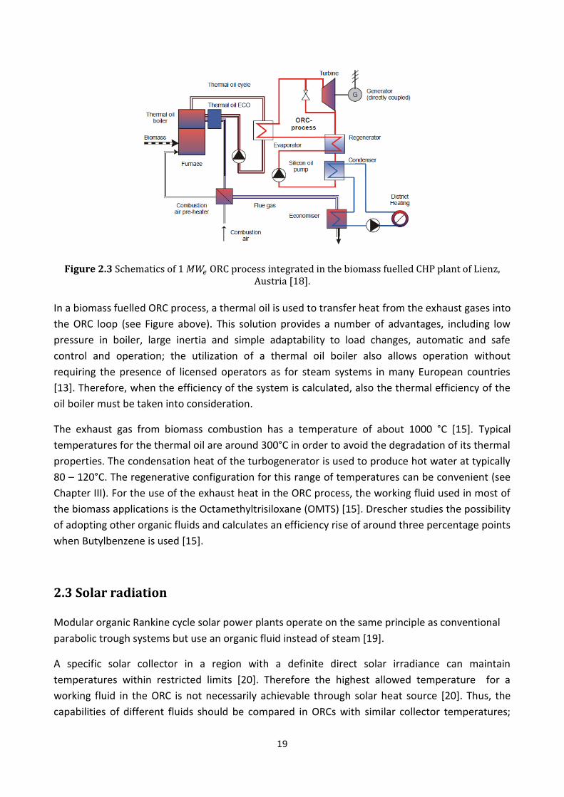
Figure 2.3 Schematics of 1 ORC process integrated in the biomass fuelled CHP plant of Lienz, Austria [18].
In a biomass fuelled ORC process, a thermal oil is used to transfer heat from the exhaust gases into
the ORC loop (see Figure above). This solution provides a number of advantages, including low
pressure in boiler, large inertia and simple adaptability to load changes, automatic and safe
control and operation; the utilization of a thermal oil boiler also allows operation without
requiring the presence of licensed operators as for steam systems in many European countries
[13]. Therefore, when the efficiency of the system is calculated, also the thermal efficiency of the
oil boiler must be taken into consideration.
The exhaust gas from biomass combustion has a temperature of about 1000 °C [15]. Typical
temperatures for the thermal oil are around 300°C in order to avoid the degradation of its thermal
properties. The condensation heat of the turbogenerator is used to produce hot water at typically
80 – 120°C. The regenerative configuration for this range of temperatures can be convenient (see
Chapter III). For the use of the exhaust heat in the ORC process, the working fluid used in most of
the biomass applications is the Octamethyltrisiloxane (OMTS) [15]. Drescher studies the possibility
of adopting other organic fluids and calculates an efficiency rise of around three percentage points
when Butylbenzene is used [15].
2.3 Solar radiation
Modular organic Rankine cycle solar power plants operate on the same principle as conventional
parabolic trough systems but use an organic fluid instead of steam [19].
A specific solar collector in a region with a definite direct solar irradiance can maintain
temperatures within restricted limits [20]. Therefore the highest allowed temperature for a
working fluid in the ORC is not necessarily achievable through solar heat source [20]. Thus, the
capabilities of different fluids should be compared in ORCs with similar collector temperatures;

20
solar collectors can be categorized according to the temperature level they can maintain [20].
Generally there are three solar collectors based on their temperature level [20]:
- Low temperature solar collectors: with the output temperature below 85°C. Flat plate
collectors are in this category.
- Medium temperature solar collectors: with the output temperature below 130÷150°C. Most
evacuated tube collectors are in this category.
- High temperature solar collectors: with the output temperature higher than 150°C. Parabolic
trough collectors belong to this category.
Since the Sun can be modeled as a punctual heat source at an apparent temperature of about
5000 K, the higher the mean temperature at which heat is transferred to the cycle, the higher the
thermal efficiency of the cycle, and so the power output. As a general trend, since the higher
temperature limit for subcritical cycles is set by the critical temperature, the higher is the latter,
the higher will be the cycle efficiency [20]. Because of their relatively high critical temperature,
hydrocarbons can usually reach higher thermal efficiencies and therefore higher power output in
comparison with refrigerants in solar ORC applications [20]. Increasing evaporation temperature
improves cycle efficiency but on the other hand the collector heat losses increase. The main
variants of solar collectors have been listed in Table 2.1.
Technology Temperature [°C] Concentration ratio Tracking
Air collector Pool collector Reflector collector Solar pond Solar chimney Flat plate collector Advanced flat plate collector Combined heat and power solar collector (CHAPS) Evacuated tube collector Compound Parabolic CPC Fresnel reflector technology Parabolic through Heliostat field + central receiver Dish concentrator
<50 <50
50÷90 70÷90 20÷80
30÷100 80÷150
80÷150 90÷200 70÷240
100÷400 70÷400
500÷800 500÷1200
1 1 - 1 1 1 1
8÷80 1
1÷5 8÷80 8÷80
600÷1000 800÷8000
- - - - - - -
One-axis - -
One-axis One-axis Two-axis Two-axis
Table 2.1 Solar thermal collectors [19].
Tchanche highlighted the importance of the heat recovery process in the design of a solar ORC
system, as it determines the size of the collector array and the volume of the heat store, that
constitute major part of system cost [21]. The authors mentioned that for an efficient plant, low
flow rates (10÷15 l/m²h) are preferable in the collector loop [21]. The consequences of considering
the system heat input on the working fluid selection has been discussed in Section 5.2.1.

21
2.3.1 Examples of prototypes and operating plants
Nguyen et al. [22] built and tested a prototype of low temperature ORC system. It used n-Pentane
as working fluid, and encompassed: a 60 kW propane boiler, compact brazed heat exchangers, a
compressed air diaphragm pump, and a radial flow turbine (65000 rpm) coupled to a high speed
alternator. With hot water inlet temperature 93°C, evaporating temperature 81°C, condensing
temperature 38°C and a working fluid mass flow rate of 0.10 kg/s, the power output obtained was
1.44 kWe and the efficiency 4.3%. The cost of the unit was estimated at £21,560. The turbine-
generator accounted for more than 37% of the system cost. Authors concluded that the system
could be cost-effective in remote areas where good solar radiation is available provided the
efficiency of the expander is improved (>50%) and the unit produced in mass.
Medium temperature collectors coupled with ORC modules could efficiently work in cogeneration
application producing hot water and clean electricity. On-site tests carried out in Lesotho by Solar
Turbine Group International prove that micro-solar ORC based on HVAC components is cost-
effective in off-grid areas of developing countries, where billions of people live without access to
electricity [23].
Figure 2.4 Schematic of the solar ORC tested in Lesotho [23].
A 1 MW solar ORC power plant owned by Arizona Public Service (APS) is in operation since 2006 at
Red Rock in Arizona, USA [19]. LS-2 collectors provided by Solargenix are coupled to an ORMAT
ORC module filled with n-Pentane. The ORC and solar to electricity efficiency are 20.7% and 12.1%,
respectively.
From an economic point of view, large photovoltaic plants can now produce power at rates up to
52 percent cheaper than concentrating solar power (CSP) plants, according to Bloomberg data
[24].

22
2.4 Waste heat recovery from ICE exhaust gases A typical example of ORC powered waste heat recovery units comes from internal combustion
engines (ICE). Nowadays, internal combustion engines for stationary power production are not an
interesting solution because of their low efficiency compared to gas turbines and their high
environmental impact. Nonetheless, the bottoming of an ORC to an operating plant can be a
profitable option to raise power production without any raise in fuel consumption. Moreover,
some different and more innovative applications are currently available or under study.
Examples of ICE application are biomass digestion plants, where biogas coming out from the
biomass digester is burned in an internal combustion engine. The waste heat from this engine
serves the ORC cycle, as shown in Figure 2.5. Depending on the size of the digestion plant and the
standard of the insulation of the plant, the thermal need is between 20÷25% of the waste heat of
the motor [14]. According to the low temperature level, the digester can be heated with the
cooling water of the motor and the turbocharger. The heat of the exhaust gas can be used for
driving the ORC.
Figure 2.5 Schematics of an ORC served by the exhaust gases of a biogas-fuelled ICE [14].
There are also ORC prototypes for on-road-vehicle applications, where the condition for waste
heat is variable [15,80].
23
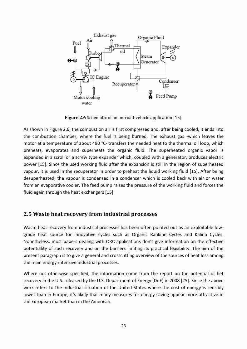
Figure 2.6 Schematic of an on-road-vehicle application [15].
As shown in Figure 2.6, the combustion air is first compressed and, after being cooled, it ends into
the combustion chamber, where the fuel is being burned. The exhaust gas -which leaves the
motor at a temperature of about 490 °C- transfers the needed heat to the thermal oil loop, which
preheats, evaporates and superheats the organic fluid. The superheated organic vapor is
expanded in a scroll or a screw type expander which, coupled with a generator, produces electric
power [15]. Since the used working fluid after the expansion is still in the region of superheated
vapour, it is used in the recuperator in order to preheat the liquid working fluid [15]. After being
desuperheated, the vapour is condensed in a condenser which is cooled back with air or water
from an evaporative cooler. The feed pump raises the pressure of the working fluid and forces the
fluid again through the heat exchangers [15].
2.5 Waste heat recovery from industrial processes Waste heat recovery from industrial processes has been often pointed out as an exploitable low-
grade heat source for innovative cycles such as Organic Rankine Cycles and Kalina Cycles.
Nonetheless, most papers dealing with ORC applications don’t give information on the effective
potentiality of such recovery and on the barriers limiting its practical feasibility. The aim of the
present paragraph is to give a general and crosscutting overview of the sources of heat loss among
the main energy-intensive industrial processes.
Where not otherwise specified, the information come from the report on the potential of het
recovery in the U.S. released by the U.S. Department of Energy (DoE) in 2008 [25]. Since the above
work refers to the industrial situation of the United States where the cost of energy is sensibly
lower than in Europe, it’s likely that many measures for energy saving appear more attractive in
the European market than in the American.
24
2.5.1 Introduction to heat recovery
The most common barriers to the economic and practical feasibility of waste heat recovery
measures are listed and explained here.
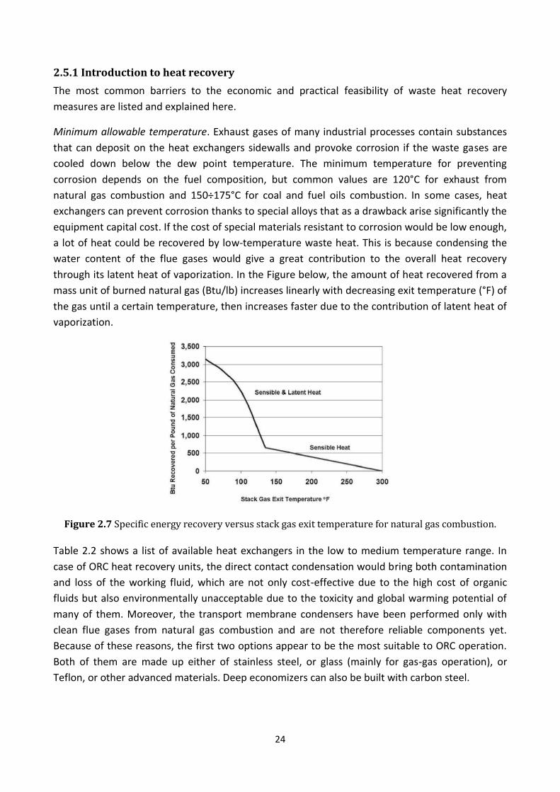
Minimum allowable temperature. Exhaust gases of many industrial processes contain substances
that can deposit on the heat exchangers sidewalls and provoke corrosion if the waste gases are
cooled down below the dew point temperature. The minimum temperature for preventing
corrosion depends on the fuel composition, but common values are 120°C for exhaust from
natural gas combustion and 150÷175°C for coal and fuel oils combustion. In some cases, heat
exchangers can prevent corrosion thanks to special alloys that as a drawback arise significantly the
equipment capital cost. If the cost of special materials resistant to corrosion would be low enough,
a lot of heat could be recovered by low-temperature waste heat. This is because condensing the
water content of the flue gases would give a great contribution to the overall heat recovery
through its latent heat of vaporization. In the Figure below, the amount of heat recovered from a
mass unit of burned natural gas (Btu/lb) increases linearly with decreasing exit temperature (°F) of
the gas until a certain temperature, then increases faster due to the contribution of latent heat of
vaporization.
Figure 2.7 Specific energy recovery versus stack gas exit temperature for natural gas combustion. Table 2.2 shows a list of available heat exchangers in the low to medium temperature range. In
case of ORC heat recovery units, the direct contact condensation would bring both contamination
and loss of the working fluid, which are not only cost-effective due to the high cost of organic
fluids but also environmentally unacceptable due to the toxicity and global warming potential of
many of them. Moreover, the transport membrane condensers have been performed only with
clean flue gases from natural gas combustion and are not therefore reliable components yet.
Because of these reasons, the first two options appear to be the most suitable to ORC operation.
Both of them are made up either of stainless steel, or glass (mainly for gas-gas operation), or
Teflon, or other advanced materials. Deep economizers can also be built with carbon steel.
25
Minimum exhaust temperature can also be constrained by process-related chemicals in the
exhaust stream; for example, sulfates in the exhaust stream of glass melting furnaces will deposit
on the heat exchanger surface at temperature below about 270°C.
Type Min. allowable temperature [°C]
Characteristics
Deep economizer 65 - 71 Tolerates acidic condensate deposits
Indirect contact condensation recovery (shell & tube HE)
38 - 43 Water vapor can condense almost completely
Direct contact condensation recovery (direct mixing of process and cooling fluid)
38 - 43 Avoids the problem of big heat transfer areas; Problem of cooling fluid contamination.
Transport Membrane Condenser
/ Capillary condensation; Membrane should be enhanced to work with dirty flue gas streams.
Table 2.2 Heat exchangers for low-temperature heat recovery.
Economies of scale. Due to their high payback time, waste heat recovery measures are in general
more attractive for big sized plants rather than for small-scale plants.
Physical constraints. It’s not always possible to reach the desired heat source stream because of
the blockage opposed by already present equipment arrangements.
Transportability of the hot stream. While with gaseous and liquid streams the heat can be easily
“transported”, for hot solid streams (such as cement clinkers, molten slags..) the energy content is
not easily accessible or transportable to recovery equipment.
Furthermore, the report indicates also end-use and matching between heat source and load as a
possible constraint for an effective use of the recovered energy. In our case, this constraint is
reduced because of the possibility to consume the desired amount of produced power and to sell
the exceeding amount in the electrical market. Another constraint is the large areas required for
heat transfer in the case of low-temperature heat recovery, since high temperature gradients
between two fluid streams are not allowed.
2.5.2 Recuperators and heat exchangers for internal heat recovery
The aforementioned report describes the main energy-intensive industrial processes and their
possibility to increase efficiency. Often the efficiency improvement is achieved through an internal
heat transfer that uses a regenerative or a recuperative exchanger to preheat inlet air or the
process load. In such cases, energy is saved without introducing an external cooling medium.
Nonetheless, knowing where recuperative or regenerative processes can be expected provides
useful information for the particular purposes of the present work, since temperature of the hot
stream exiting the process is reduced to a level at which ORCs can be a competitive solution.

26
A furnace regenerator consists in two brick checkerwork chambers through which hot and cold
airflow alternate. As combustion gases pass through one chamber, the bricks absorb heat and
increase in temperature. The flow of air is adjusted so that it is heated up before entering the
furnace, thus reducing the fuel consumption to keep the furnace at high temperature. Every 20
minutes the direction of the air flow is changed, so that the ‘cooled’ chamber is heated up again
by the exhaust gases while the other one releases heat to the inlet air. This measure is typically
applied to glass furnaces and coke ovens, where the exhaust gases are relatively dirty.
In the rotative recuperator -also known as hot wheel- the ducts of exhaust gases and of inlet air
are parallel to each other, with a rotating wheel made up of a porous material that, driven by an
external motor, “moves” heat from the first to the latter. Disadvantages of this solution are the
deformations of metal ducts when temperature gradients are too high and cross contamination
between the two gas streams. The advantage is that the wheel can be designed to recover
moisture as well as heat from clean gas streams (hygroscopic wheel).
Passive air preheaters are heat exchangers designed for gas to gas heat recovery of low to medium
temperature applications, such as ovens, steam boilers, gas turbine exhaust, secondary recovery
from furnaces and recovery from conditioned air. They can be of two types: plate heat exchangers
or heat pipes.
Finned tube heat exchangers are used to recover heat from low to medium temperature exhaust
gases for heating liquid. A typical case is the so called economizer, a setup in which boiler exhaust
gases are used to preheat feedwater before it is evaporated.
Other solutions for energy saving are load preheating, such as solid materials heated up before
entering the furnace, waste heat boilers (medium to high exhaust gases recirculated to generate
steam) and regenerative burners, in which the fuel is heated before feeding the
furnace/combustion chamber. Burners that incorporate regenerative systems are commercially
available.
2.5.3 Glass manufacturing
Some sources estimate that as much as 70% of the energy consumption of this industrial sector is
devoted to glass melting and refining processes in high temperature furnaces. Glass melting
includes different types of furnaces (regenerative, oxyfuel..), each of them having its own
efficiency. In the following Table, an average exhaust gas temperature is assumed for each type of
furnace. Recuperative furnaces are less efficient than regenerative and are used for small scale
operation. In oxyfuel furnaces pure oxygen or oxygen-enriched air is used instead of air.
Regeneration is removed but the efficiency is increased because less nitrogen, which is inert in the
combustion process, is heated up.

27
Type of furnace Assumed average exhaust temperature [°C]
Regenerative Recuperative Oxyfuel Electric boost Direct melter
430 (320÷540) 980
1430 430
1320
Table 2.3 Assumed average exhaust gas temperature in glass manufacturing.
Moreover, in European plants batches are often collected in special silos to be preheated before
entering the furnace, which also contributes to reduce fuel consumption.
2.5.4 Cement manufacturing
The major process steps in cement production are mining and quarrying raw materials (mostly
limestone and chalk), crushing and grinding, clinker production and cooling, cement milling. Even
if the most commonly used fuel is coal, some kilns use natural gas, oil and various waste fuels. Raw
meal (limestone and other materials) enters at the top of the kiln and passes through increasingly
hot zones toward the flame, which is located at the bottom of the kiln. The solid nodular material
exiting the kiln is called clinker.
Raw materials are mostly limestone and chalk, while clinker is the solid nodular material exiting
kilns and used for the cement production. Kilns can either be wet or dry. Wet kilns are no longer
constructed since they need a lot of energy to evaporate the moisture contained in the raw
material (approximately 30-40%). In dry kilns, if meal is not preheated, exhaust gases of coal
combustion are approximately at a temperature of 450°C.
Meal preheating is the first option to recover heat from the exhaust gases. It commonly occurs
through a 4-stage preheater. The gases are released at an average temperature of 340°C. If 5-6
stages are used, exhaust temperatures can drop to 200-300°C, thus increasing the complexity of
the system. Exhaust gases could be also used to preheat the grinded raw materials. An
opportunity for increasing kiln efficiency is optimizing waste heat recovery in the clinker cooler. In
fact, after being discharged by the kiln at high temperature (about 1200°C), clinker is cooled down
to approximately 100°C. Typically, the hot air exiting the clinker cooler is used to heat secondary
air in the kiln combustion or tertiary air for the precalciner.
Type of furnace Assumed average exhaust temperature [°C]
Wet kiln 340
Dry kiln - No preheater - Only preheater - Preheater + precalciner
450 340 340
Table 2.4 Assumed average exhaust gas temperature in cement manufacturing.

28
2.5.5 Iron and steel production
The integrated steel mill is composed by the following units:
- Coke Oven: where coke, which is an essential fuel for blast furnace operation, is produced
through the heating of coal in an oxygen-limited environment;
- Blast Furnace: it’s the major unit. Here the iron ore (iron oxide, FeO) is converted into pig iron
(Fe);
- Basic Oxygen Furnace (BOF): oxygen is here utilized to oxidize impurities in the iron such as
carbon, silicon, phosphorus, sulfur and manganese.
Furthermore, the steel industry has experienced significant growth in manufacture from recycled
scrap via electric smelting.
Electric Arc Furnaces (EAF) are used to melt ferrous scraps derived from cutoffs from steelworks
and product manufacturers as well as from post-consumer scrap.
The above processes and their opportunities to recover waste heat will be briefly described and
summarized in Table 2.7.
Coke oven. There are two types of oven for producing coke:
- by-product process: chemical by-products (such as tar, ammonia and light oils) are recovered,
while the remaining coke oven gas (RCOG) is cleaned and recycled within the steel plant.
- non-recovery process: all the coke oven gas is burned in the process.
The by-product process has two sites of sensible heat loss: RCOG cooled in the gas cleaning
process and waste coke oven gas exiting the coke oven (about 650-980°C). A typical RCOG
composition is shown in Table 2.5. The presence of hydrogen, carbon monoxide, methane and
other hydrocarbons make this gas flammable and reusable within the process, which is the reason
why it is recycled.
Compound Volume [%]
39-65 32-42
3.0-8.5 4.0-6.5
3-4 23-30
Nd 6-8 2-3
Table 2.5 Typical RCOG composition.
The coke oven is made up of several chambers separated by heating flues, often fueled with
internal gases such as the RCOG (calorific value approximately 18,8÷26,4 MJ/sm3) and the blast
furnace gas. In such way, only the chemical energy of the RCOG is recovered while its sensible heat
is wasted during the cleaning/cooling process (cooled down with ammonia spray). Some
applications in Japan are able to recover approximately 1/3 of such sensible heat by means of a
low-pressure heat transfer medium that cools down the RCOG to 450°C. Finally, waste heat gases

29
from the RCOG combustion are used in a regenerator to preheat the inlet air but still leave it at an
average temperature of about 200°C, being therefore an interesting source for ORC power
production. Nevertheless, due to environmental considerations, the industry will probably move
towards the non-recovery process. In such process, all the COG is burned and the waste gases are
recovered through a waste heat boiler which generates steam.
Blast Furnace. In the blast furnace raw materials including iron-ore, additives and coke are
charged from the top while hot air and supplemental fuels are injected from the bottom. The hot
air entering the furnace is provided by several auxiliary hot blast stoves, in which fuels as COG and
blast furnace gas (BFG) are combusted. Old blast furnaces have outlet temperatures of about
400°C, while newer recover BFG as fuel for blast air heating, coke oven heating, reheating
furnaces, steam generation or power production. Due to the low calorific value of BFG (3,0-3,4
MJ/m3), the latter is often mixed with COG or natural gas. As with RCOG, the BFG must be cleaned
before being burned. An opportunity of sensible heat recovery is therefore provided by the BFG
cleaning process, but it is rarely done. Instead, when blast furnace operates with sufficiently high
pressure (around 2,5 atm), the static energy of the cleaned BFG is recovered through so called top
pressure recovery turbines (TRT). The recovered power depends on the type of cleaning: with wet
cleaning the sensible heat content is wasted, while with dry cleaning the temperature entering the
TRT can be around 120°C. Another opportunity is offered by the hot exhaust leaving the hot blast
stoves at a temperature of about 250°C. Because of the cleaner nature of such gases, this practice
is quite common. The sensible heat is commonly used for the preheating of combustion air or fuel
gases.
Basic Oxygen Furnace. The operation is semi-continuous: hot metal and scrap are charged to the
furnace, oxygen is injected, fluxes are added to control erosion and then metal is sampled and
tapped. The exothermic oxidation reaction supplies the heat required to melt the metal. The off-
gases of the BOF are at high temperature and due to its composition (which is shown in Table 2.6)
both chemical and sensible thermal energy can be recovered. The dirty substances contained in
the BOF off-gases (iron oxides, heavy metals, Sox, NOx, fuorides) make the recovery of sensible
heat difficult.
Compound Volume [%] Range Average
55-80 72.5
2-10 3.3
10-18 16.2
8-26 8
Table 2.6 Typical BOF exhaust gas composition.
The two main methods for heat recovery are open combustion, through which air is introduced in
the BOF gas duct to burn CO and suppressed combustion, through which a skirt is added to the
coverter mouth to reduce air infiltration and inhibit combustion of the CO. The gas is cleaned,
collected and used as a fuel. As already mentioned, a part from the integrated steel mill, a lot of
electric arc furnaces have been constructed in order to recycle metal scrap.

30
Electric arc furnace. The furnace is refractory lined with a retractable roof, from which two
electrodes are lowered to an inch above the scrap material. Fluxes and alloying materials are
added to control the quality of the material. During furnace operation, several gases and
particulate emissions are released, including CO, SOx, NOx, metal oxides, VOCs and other
pollutants. The losses in the exhaust gases are half chemical energy and half sensible heat. There
are different possibilities to recover such energy: scrap preheating, scrap preheating through
Consteel process (which exploits not only the sensible heat of the gases but introduces air to burn
their CO content) or the Fuchs shaft system. The benefit of scrap preheating depends on specific
operation: when tap to tap times decrease the energy savings are sensibly reduced. A summary of
the gaseous heat sources connected with iron and steel manufacturing is presented in the
following table.
Source Assumed average exhaust temperature [°C]
Coke oven Coke oven gas Coke oven waste gas
980 200
Blast furnace Blast furnace gas Blast stove exhaust - no recovery - with recovery
430
250 130
Basic oxygen furnace 1700
Electric arc furnace - no recovery - with recovery
1200 200
Table 2.7 Assumed average exhaust gas temperature in iron and steel production industry.
Moreover, liquid and solid streams are also available and could potentially be sources of further
energy recovery. Coke dry quenching (CDQ), as an alternative to wet dry quenching, involves
catching incandescent coke in a special designed bucket which is discharged in a vessel where an
inert gas (nitrogen) passes and recovers sensible heat. Other ways of saving energy are the use of
radiant heat boilers (RHB), which are currently used for cast steel, and hot charging, in which hot
slabs are charged into a reheating furnace while still hot. An opportunity at lower temperature is
given by the hot rolled steel, which can be cooled through water, the latter being discharged at
about 80°C.
Source Assumed maximum temperature [°C]
Sensible heat [kJ/t]
Recovery technology
Hot coke BF slag BOF slag Cast steel Hot rolled steel
1100 1300 1500 1600 900
0.22 0.35 0.02 1.25 4.94
DCQ RHB (unsuccessful) RHB (unsuccessful) RHB, hot charging
Water spraying
Table 2.8 Maximum temperature of solid hot streams in iron and steel production.

31
2.5.6 Aluminum production
Aluminum manufacturing is divided into two different production phases:
- Primary production: alumina and bauxite are refined in electrolytic cells to get aluminum.
- Secondary production: Recycled scrap are melt in high temperature furnaces to get bare
aluminum from used products. The secondary production has seen a great improvement due
to the lower energy-intensive process relative to primary production.
Primary aluminum production. It is carried on in Hall-Hèroult cells where alumina is electrolyzed
in a molten bath of fluoride compounds known as cryolite. Furnace operates typically at 960°C.
The sources of heat loss are off-gases and sidewall heat losses. Indeed, a frozen ledge of cryolite
shall be maintained on the cathode lining. This requires high heat transfer away from the furnace
(about 45% of the energy input is lost via conduction, convection and radiation from the sidewalls,
against only 1% of the off-gases).
Secondary aluminum production. The energy needed for producing a mass unit of secondary
aluminum equals one sixth of that used for the production of primary aluminum. The scrap is melt
in a furnace, whose exhaust gases range from 1100 to 1200°C, reaching as much as 60% of the
energy input of the furnace. Heat recovery has faced problems such as chloride and fluoride
release, secondary combustion of volatile in the recuperator and overheating.
Source Assumed average exhaust temperature [°C]
Hall-Hèroult cells 700
Secondary melting - No recovery - With recovery
1150 540
Table 2.9 Assumed average exhaust gas temperature in aluminum production processes.
2.5.7 Metal casting
Metal casting involves pouring molten metal into molds to produce consumer goods. It relies on a
variety of melting metals and high temperature furnaces. Among them the most common are
reverberatory furnaces for aluminum casting and cupola, electric arc and induction furnaces for
iron casting. The major barrier to heat recovery in metal casting is economic rather than technical,
since the industry is dominated by small operations that don’t allow the required payback periods.
The most common uses of waste gases exiting the furnaces are preheating of charge material, of
combustion air, or space heating.

32
Source Assumed average exhaust temperature [°C]
Aluminum casting - Reverb furnace - Stack melter
1150 120
Iron cupola - No recovery - With recovery
900 200
Table 2.10 Assumed average exhaust gas temperature in iron and aluminum casting.
2.5.8 Ethylene furnaces
Ethylene is a petrochemical product whose worldwide production exceeds that of any other
organic compound. A key component of the production process is the pyrolysis furnace, where
hydrocarbon feedstocks are cracked at temperatures around 760-870°C. The heat necessary to the
pyrolysis reaction is provided to the furnace both through a radiant section -that contains reactor
tubes where the pyrolysis occurs- and a convective part, where heat is exchanged between flue
gases and process fluids. As a result, the exhaust temperature is relatively low, accounting to
about 150°C.
2.5.9 Industrial boilers in other manufacturing sectors
Steam is critical to several manufacturing sectors, such as chemicals, refining, food, paper and
primary metal industries. Most of industrial boilers for steam generation are fuelled with natural
gas and by-product fuels. The temperature of the latter depends on the pressure of the steam
required for a given industrial process. According to the aforementioned report, in the U.S. most
boilers with thermal capacities greater than 7 MW include economizers.
2.5.10 Potential of heat recovery from energy intensive industries in Italy
The European top-leader company in ORC plants, Turboden, has conducted a research project co-
financed by the European Commission’s Life+ Programme with other four scientific, technical and
administrative partners on the potential of power production (through ORC generators sized from
0,5 to 5 MW) from waste Heat Recovered by Energy Intensive Industries (HREII) in Italy [26]. The
project activities were carried out from January 2010 to December 2012. The activities carried out
within the project were manifold, among which:
- Establishment of a Monitoring Centre on the potential of heat recovery as measure for energy
efficiency and environmental compatibility of industrial processes, involving not only the
project partners but also other stakeholders from industry, university and local government;
- Definition and identification of the “energy intensive industries” and drawing-up of a list of
energy intensive companies;
- Development and testing of the model built for energy audits;
- Estimate of the potential of the various sectors studied, extending the singular results (both
measured and estimated through the model) to the corresponding industry sector;

33
- Promotion of heat recovery at the regulatory and policy level with the aim of bringing
uniformity to a still unclear regulatory scenario.
The results are summarized in the so-called Layman Report [26]. To each company of the list
mentioned in the second point above, a compatibility rating has been assigned in order to
“measure” the feasibility of a heat recovery system considering parameters such as: presence of
heat recovery in internal processes, process annual operating hours, technical parameters and
quality of the heat source. The project established that the most promising industrial sectors
identified for installation of heat recovery systems are:
- Steel production;
- Glass manufacturing;
- Cement manufacturing;
- Non-ferrous metals;
- Oil&Gas
Excluding the latter, these sectors are exactly those described above with the help of the
aforementioned document. The maximum estimated potential for the sectors studied, which for
the authors is an underestimate, reaches about 2 TWh of electricity produced annually for Italy,
corresponding to about 800 kton of avoidable per annum. Figure 2.11 shows the potential
energy saving and emission avoidance distributed by sector in two scenarios of operating
hours.
Figure 2.11 Estimate of potential energy saving and CO2 emission avoidance in Italy in the four main
energy intensive industrial sectors in two scenarios: 5000 (a) and 8000 (b) operating h/y [26].

34
Chapter III. Cycle configuration The choice of cycle configuration, as well as the working fluid selection, is a key aspect in the
design of best performing ORCs. There’s a limited number of cycle layouts that compete to
improve the thermodynamic performance given by the basic ORC configuration. This chapter aims
at describing the most used cycle configurations, which besides the basic are essentially the
regenerative and the supercritical cycles. Moreover, superheating will be hereafter discussed,
while turbine bleeding and reheating do not seem to be attractive solutions for ORC plants [16].
Finally, two alternative cycles that appear as possible competitors against ORCs are described: the
transcritical CO₂ cycle and the Kalina cycle.
3.1 Basic cycle An Organic Rankine Cycle is simply a Rankine cycle that uses an organic fluid instead of steam as
working medium. The basic ORC configuration is made up of four components. The fluid is heated
up by the hot source in the evaporator (23), then it is expanded in the turbine or in a volumetric
expander (34) until the condensing pressure, and then it is cooled down (41) in the first
section of the condenser until the condensing temperature, at which is finally condensed and
pumped (41) back to the evaporator. The evaporator, in the general case, is made up of three
consequent processes: preheating, isothermal vaporization and eventually superheating.
According to Quoilin [16], these processes can be performed by a single heat exchanger and with
no need of a water-steam drum. Nonetheless, especially in high temperature applications where a
limit on the working fluid maximum temperature occurs, splitting the heat transfer into three
separate heat exchangers allows a better control of the turbine inlet temperature and is therefore
desirable.
Figure 3.1 Schematics of ORC basic cycle. The aim of the process is to recover heat and convert it into power. Therefore, two parameters are
needed to assess both how much heat is recovered and how efficient is the Organic Rankine Cycle
itself. Therefore, cycle efficiency is generally not sufficient to evaluate the overall process [27].

35
Such evaluation occurs, for example, when different working fluids or different cycle layouts must
be compared in order to find the best thermodynamic or the most profitable solution for given
heat source and sink.
The ratio between the heat flow that actually supplies the ORC and the highest recoverable heat
flow is called heat recovery effectiveness (or heat recovery factor, or heat availability [27,16]); for
sensible heat sources the latter is obtained by cooling down the heat medium to the lowest
achievable temperature, which is the reference temperature of the environment.
The cycle efficiency is the ratio between the net power output and the heat flow that supplies the
evaporator of the ORC
The system overall efficiency (or total heat recovery efficiency [27,16]) accounts for the
performance of the overall process, i.e. how much power is produced with respect to the amount
of heat that can be ideally extracted from the considered heat source.
Thus, the maximization of system overall efficiency is equal to the maximization of the net power
output produced by the process from the considered heat source. Further information and
references are given in Section 5.2.1.
In general, the maximum of cycle efficiency does not coincide with the maximum of system overall
efficiency.
However, it is useful to understand when the performance can be assessed in terms of cycle
efficiency, i.e. regardless of the heat recovery. According to Quoilin [16], heat sources are divided
into two fictitious categories: sensible and latent heat sources.
As already mentioned, the full potential of a sensible heat source is exploited when the heat
source stream is brought to the lowest achievable temperature [16]. Examples are geothermal
brines, ICE exhaust gases and the large category of waste heat, that includes hot gases and process
steam available at different temperatures within many industrial processes, as already illustrated
in the previous Chapter. If on one side cooling down the hot stream is required to recover a fair
amount of heat, on the other side this brings to a drop in the evaporation pressure and in turn in
cycle efficiency due to the pinch point in the evaporator. The maximum in system overall
efficiency (i.e. net power output) comes therefore from the best trade-off between cycle efficiency
and heat recovery effectiveness.

36
On the contrary, heat sources are latent if heat can be extracted without influencing their
temperature level [16]. The most typical example of latent heat source is the Sun, that can be
considered as a black body radiating at the constant apparent temperature of 5000 K. Thus, for
solar ORCs the maximization of power output comes from the maximization of cycle efficiency1.
Biomass can be considered as a latent heat source, although the flue gases must be cooled down
to recover the sensible heat released by its combustion. In fact, in most cases the thermal cycle is
coupled to the flue gas by a thermal oil that leads to have two pinch points: one at the beginning
of vaporization -similar to low grade heat applications- and another between thermal oil and flue
gas [28]. These pinch points are the reason why thermal efficiency and total heat recovery do not
strongly correlate [28]. In fact, increasing the evaporation temperature does not bring directly to a
decrease in the heat recovered, since in comparison to low grade heat applications, the thermal
oil mass flow can be adjusted to a certain extent [28]. Furthermore, heat can be transferred by
more than one thermal oil cycle [28], thus enabling the thermal cycle to increase efficiency
without any influence on the outlet temperature of the exhaust gas.
The above considerations are summarized in the following table: the third column indicates the
objective function that maximizes the power output.
Heat source type Application Objective function
Sensible Waste heat recovery ICE exhaust Geothermal brine
Latent Solar thermal power Biomass combustion
Table 3.1 Objective function for the maximization of net power output in different applications.
According to the second law of Thermodynamics, every real process generates irreversibility.
Sources of irreversibility are friction and heat transfer occurring with finite temperature
difference. Such irreversibility destroys part of the exergy associated with the heat source stream.
A part from exergy destruction, exergy can be lost by the system, depending on the control
boundaries that the analyst selects to evaluate the thermodynamic system. Exergy efficiency (or
second-law efficiency) is the index that allows to assess how much exergy is lost and destructed
(and therefore not exploited) from the initial amount of exergy associated with the fuel. According
to the classical work of Bejan et al. [29], “exergy efficiency shows the percentage of the fuel exergy
provided to a system that is found in the product exergy”. The definition assumes the knowledge
of fuel and product.
The fuel exergy depends on the application; when a hot stream supplies heat to the working fluid
in the evaporator, the fuel exergy is the difference between the exergy associated with that
stream at the inlet and the outlet of the evaporator. In other cases, such as for example the
combustion of biomass supplying heat to a boiler, the fuel is the chemical exergy associated with
1 In the reality, a too high temperature of the heat transfer medium turns into excessive losses of the solar collectors,
thus reducing the overall efficiency of the system.

37
the burning fuel. The product exergy of a normal ORC for power generation is the net power
output provided by the system. For applications with cogeneration, an additional term accounting
for the heat provided by the cycle should also be included.
From the above definitions, it’s clear that exergy efficiency does not only assess the performance
of the cycle, as thermal efficiency does, but also evaluates the “quality” of the heat recovery as
part of the overall process. Various authors choose exergy efficiency as objective function in the
system optimization [20,30,31]. Moreover, an exergy analysis of the system reveals which
components are responsible of the generated irreversibility, therefore pointing out where the
system can be improved.
3.2 Regenerative cycle The regenerative cycle has an additional heat exchanger after the expansion process that is used
to pre-heat the working fluid before it enters the evaporator. Cycle efficiency therefore rises, since
less heat is needed by the preheater to reach the same evaporating temperature. Equivalently, the
rise in cycle efficiency can be justified by the fact that heat is supplied to the working fluid at a
higher mean temperature.
Figure 3.2 Schematics of the ORC regenerative cycle [32].
Figure 3.3 Regenerative cycle in the T-s diagram [32].

38
On the other hand, the increase in temperature at the evaporator inlet (from T2 to T2a in Figure
3.3) involves cooling down the heat source stream to a higher temperature, thereby recovering a
lower amount of heat. If the heat source is “sensible”, the system overall efficiency won’t be
significantly increased by the introduction of the regenerator because the higher efficiency is
obtained at the cost of a worse heat recovery. Hence, the net power output remains more or less
constant and the higher cost for the additional heat exchanger is not justified [16].
Conversely, for latent heat sources increasing the thermal efficiency involves the increasing the
net power output. The regenerative cycle is therefore an interesting solution.
Figure 3.4 Thermal efficiency, exergy efficiency and exergy losses versus evaporating pressure for
basic and regenerative ORC [33]. In the study of Mago, hot gases with fixed inlet and outlet temperature -1000 K and 450 K
respectively- serving a basic ORC that works with R113 –critical temperature 487 K- at a
condensing temperature of 298 K, both cycle efficiency and exergy efficiency increase with
evaporating pressure [33]. This is due to the fact that when the evaporating pressure is increased,
the difference between the evaporating temperature and the temperature of the hot gas stream
entering the evaporator is reduced [33]. Note that, with such a high temperature difference
between heat source and working fluid, an increment of the evaporation pressure does not
influence the temperature profile of the hot stream, which in fact is kept constant.
It can also be noticed that not only the thermal efficiency but also the exergy efficiency is higher
in the regenerative cycle than that of the basic one in all the considered evaporating pressure
range [33]. Now the question is: how much can the internal heat recovery improve the system
performance? Rayegan and Tao [20] investigated the effect of regeneration on the exergy
efficiency of a solar ORC (latent heat source), and found it to be fluid dependent; thus, they tried
to correlate this effect with a thermodynamic property of the fluid called molecular complexity
( ) (
)

39
where is the critical temperature, R the gas constant, and the second term is inverse of the
slope of the vapor saturation line in the T-s diagram at the reduced temperature of 0,7. The
correlation is not straightforward but it was observed that, as a general trend, the regeneration
has a greater impact on the exergy efficiency of fluids with higher molecular complexity than it has
for fluids with a lower one [20]. This means in turn that high critical temperature and highly tilted
vapor saturation line are desirable characteristics of working fluids that are supposed to operate in
regenerative cycles. Although they have high molecular complexity, the effect shown by cyclo-
hydrocarbons is not that strong, therefore they seem to be an exception to this general trend [20].
This result could be an important prompt to sense the opportunity to design a regenerative cycle
instead of a basic one.
Heat source type Suitability of IHE
Sensible Not convenient unless the heat recovery and cycle efficiency do not depend on each other.
Latent Better to fluids with high molecular complexity (high critical temperature and dry vapor saturation curve).
Table 3.2 Suitability of regenerative cycle.
The regeneration efficiency accounts for the heat transferred with respect to the heat that could
be ideally transferred by bringing the turbine exhaust to the pump outlet temperature. Since the
heat capacity of a gaseous stream is much lower than that of the same mass flow rate of liquid
stream, and heat is transferred from the turbine exhaust gas to the liquid stream, the pinch point
must take place at the cold stream inlet. Therefore
3.3 Supercritical cycle Supercritical ORCs are not yet a commercially diffused technology. The main studies on the
potential of supercritical ORCs have been carried out by A. Schuster and S. Karellas [34,35,15].
In the supercritical cycle, the working fluid does not undergo the phase change as in the subcritical
case. Therefore, the whole evaporating process relies on one heat exchanger only. Since the
critical point of organic fluids is reached at lower pressures and temperatures compared with
water, supercritical fluid parameters are more easily realized in ORCs than in conventional Rankine
cycles [34].
Let’s qualitatively compare with the help of Figure 3.5 the performances of a subcritical and of a
supercritical cycle with same condensing pressure and the same maximum temperature. The
supercritical cycle has higher efficiency than the subcritical, since the average temperature at
which the heat flow is supplied to the working fluid is higher in the supercritical case. From

40
another point of view, the additional work released by the expander of the supercritical cycle is
sensibly higher than the additional work supplied to the pump to reach the supercritical pressure
p2’ from the evaporating pressure of the subcritical cycle p2 [34].
Figure 3.5 Subcritical and supercritical ORC. Example for R245fa [34].
Moreover, the benefit of supercritical conditions on system performance can be explained
through an exergy analysis, which accounts for the irreversibility generated in the evaporator.
Schuster and Karellas [34] provide two T-q diagrams in which irreversibility and exergy losses
occurring in the evaporators of a subcritical and a supercritical cycle are compared. Initial
temperature and heat capacity of the heat source are equal, as well as the pinch point
temperature of the evaporator. The working fluid maximum temperature has also been set equal
in the two cases.
Figure 3.6 Exergy destruction and loss in subcritical (a) and supercritical (b) ORC cycle [34].
By comparing the two diagrams, it can be seen that the working fluid in the supercritical cycle
suites better the temperature profile of the heat source than the subcritical. This occurs because
of the non-isothermal evaporation process occurring in the supercritical cycle. In the subcritical
case, in fact, the pinch point takes place necessarily at the vaporizer or at the pre-heater inlet,

41
while with supercritical vaporization a good matching between the heat source temperature
profile and the heating process can lead to a different position of the latter. This is illustrated in
Figure 3.6, where it can be observed that the better matching of temperature profiles in the
supercritical cycle allows the hot stream to exit the evaporator at a lower temperature, thus
reducing the exergy loss –i.e. recovering a bigger amount of heat-.
Schuster and Karellas [34] compared the thermodynamic performance of a supercritical cycle for
different working fluids with a subcritical cycle run by the same fluids while keeping the same
condensing temperature (20°C), the same isentropic efficiency of both pump (0.85) and turbine
(0.80), and the same pinch point temperatures in the heat exchangers (10 K). The initial heat
source temperature has been set to 210°C and a minimum vapor quality of 90% at the end of the
expansion was set as a boundary condition to prevent blades erosion. The working conditions in
the two cases are:
- supercritical conditions: p = 1.03 and a live vapor temperatures of T > 0.985 ;
- subcritical conditions: constant superheating of 2 K for live vapor temperatures of T < 0.965
.
Figure 3.7 (a) shows the thermal efficiency of the considered working fluids calculated with the
specified subcritical conditions. Water and cyclohexane show the best performances, while R134a
appears to be the worst from a first-principle point of view. The trends of these fluids are a
reference for the performance evaluation of the selected fluids in supercritical cycles, that are
shown in Figure 3.7 (b).
Figure 3.7 Thermal efficiency versus live vapor temperature for different working fluids (a=subcritical, b=supercritical) [34].
It’s evident that supercritical cycles, with the aforementioned assumptions, have a lower thermal
efficiency compared to subcritical ones. For latent heat sources, since the maximization of work
output corresponds to that of thermal efficiency, supercritical cycles do not seem to be an
interesting solution. Nonetheless, considering the higher heat recovery efficiency allowed by the
lower exergy loss in the supercritical case, system efficiency maxima for some fluids are higher in
supercritical cycles than in the subcritical ones [34].

42
Figure 3.8 System overall efficiency versus live vapor temperature for different working fluids
(a=subcritical, b=supercritical) [34].
Moreover, it can be seen from the comparison of subcritical thermal and system efficiency (Fig.
3.7 (a) and 3.8 (a)) that at high live vapor temperatures the fluids with favorable thermal efficiency
(like cyclohexane, isohexane..) have moderate system efficiency. The reason may be that those
fluids, due to a higher critical temperature, evaporate at a lower reduced temperature fixed by the
pinch point of the evaporator. Therefore they receive great part of the heat at constant
temperature. On one hand, this allows them to receive heat at a higher average temperature than
other fluids, but on the other hand this occurs at expense of a poor heat recovery efficiency, that
is reflected by the low value of system efficiency. This involves the presence of a distinguishable
maximum in system efficiency, being the best compromise solution between high thermal
efficiency and high heat recovery effectiveness. This behavior can also be seen for supercritical
conditions in combination with the same heat source (Figures 3.7 (b) and 3.8 (b)), but the maxima
are not so evident as in the previous case because of the nearly linear shape of the organic fluid’s
curve in the T-q diagram. However, the maximum system overall efficiency reached by R365mfc
operating in a supercritical cycle is 14.4%, against the 13.3% reached by R245fa in the subcritical
cycle; this is a non-negligible improvement of 8%. The primary drawback of supercritical cycles is
the higher heat transfer capacity needed in order to receive the same heat flow with a lower mean
temperature difference. An example is provided for fluid R134a in Figure 3.9: the evaporation
takes place in subcritical and supercritical conditions in both case reaching a superheated
temperature of 140 °C thanks to the same heat source .
Figure 3.9 Subcritical (p=30 bar) and supercritical (p=50 bar) evaporation with R134a [35].
The average temperature difference is lower in the supercritical case, allowing lower exergy
destruction at the cost of a higher heat transfer capacity (since the same heat flux is transferred

43
from the heat source to the working fluid). Therefore, there’s great interest in the understanding
of the heat transfer mechanism in order to quantify the needed heat exchange area, which is
directly linked to the system cost [30].
Karellas and Schuster [35] studied the heat transfer of plate heat exchangers operating in
supercritical conditions through the following steps:
- division of the heat exchanger (HE) into n parts and calculation of the heat capacity of
each part from and ;
- calculation of the Nusselt number with the Jackson correlation (Dittus-Boelter classical
correlation cannot be used due to the significant change in thermo-physical properties that
the fluid undergoes in the pseudo-critical region2²);
- calculation of the heat transfer coefficient using the calculated Nu;
- calculation of global heat exchange coefficient ;
- calculation of the needed area for every part of the HE and sum the n values to find the
total heat exchange area .
With this procedure, they calculated the mean overall heat transfer coefficient U for three fluids
(R134a, R227ea, R245fa) maintaining a constant pinch point of 10 K while varying the evaporating
pressure. It was found that the mean overall heat transfer coefficient decreases with increasing
pressure, as shown in Figure 3.10. The corresponding increase of heat exchange area follows in
Figure 3.11.
Figure 3.10 Mean overall heat coefficient U versus pressure for different fluids reaching different superheated temperatures [35].
Figure 3.11 Needed heat exchanger area A versus pressure for different fluids reaching different
superheated temperatures [35].
2 The region about the pseudo-critical temperature, which is defined as the temperature at which Prandtl number (Pr)
and specific heat capacity (cp) rise to a peak and then fall steeply.

44
Finally, the effectiveness of the supercritical heat exchanger is calculated for increasing pressure.
Figure 3.12 shows that there’s a range of pressures where efficiency slightly drops and then
increases again.
Figure 3.12 Heat exchanger effectiveness versus pressure for constant heat exchange area [35].
The authors concluded that the application of supercritical fluid parameters in ORCs seems to raise
the system overall efficiency without disproportioned rise of installation costs [35]. Moreover, it is
very important to further investigate the heat transfer mechanisms in partial loads and transient
procedures with subsequent verification by experiments and tests in actual ORC installations.
Furthermore, Lazzaretto et al. [36] found that the exergy recovery efficiency (see Section 2.1.1) in
supercritical cycles decreases only slightly for large variations of cycle maximum pressure from its
optimal value. Since increasing pressure involves higher costs of the machinery, suboptimal
thermodynamic solutions (at lower maximum pressure than the optimal) could be economically
convenient with no significant influence on the thermodynamic performance of the system.
3.4 Superheating Superheating is commonly used in normal Rankine cycles to absorb heat at a higher mean
temperature and therefore work with a higher thermal efficiency.
Yamamoto et al. [37] tested the improvement potential for fluid R123 in an experimental
apparatus which evaporated the working fluid by means of an electric heater. By changing the
electrical power dissipated in the latter, the turbine inlet temperature was varied. It was found
that, contrary to water, for R123 the maximum work output was reached by evaporating the vapor
directly from saturated conditions. The authors concluded that for fluids with low latent heat of
vaporization, saturated vapor at turbine inlet gives the best operating condition.
Saleh et al. [38] divided the organic fluids into two types, according to the slope of their vapor
saturation line: b-fluids, i.e. those with a bell shape in the T-s diagram and o-fluids, i.e. those with
overhanging saturation line. In their study, they generalized the results of Yamamoto confirming
that for o-fluids (such as R123) the greatest thermal efficiency is reached without superheating,

45
while for b-fluids the increase in thermal efficiency is small in the case of basic cycle, but increases
when a regenerator is introduced.
Working fluid type
Convenience of the superheating
Tips
Dry No In terms of cycle efficiency, the optimal solution is without superheating at the turbine inlet.
Wet Yes Superheating is necessary to avoid droplets erosion in the turbine blades; A performance increase occurs from saturated to superheated expansion, in particular in the regenerative cycle.
Table 3.3 Suitability of superheating.
Furthermore, it must be considered that the use of a superheater determines a significant
increment of system capital costs, since its heat exchange area is generally large, because of the
low value of the heat transfer coefficient (U = 5÷15 W/m²K) [39]. Therefore, the selection of the
superheater and its exchange area is a typical thermo-economic problem in which the optimal
value of the superheating degree must be selected balancing the possible increase in system
overall efficiency and the corresponding increase in equipment cost [39]. This means that even
though a little performance enhancement could be achieved in the mentioned conditions, the
higher investment cost provoked by the additional heat exchanger turns into a further barrier to
superheating. Moreover, a few degrees of superheating can be useful to control the degree of
superheating at the expander outlet in the real plant operation [16].
3.5 General guidelines for the choice of cycle configuration The basic cycle is by definition the standard solution, but the opportunity to enhance the system
performance with a regenerative or with a supercritical cycle must be taken into account. From a
thermodynamic point of view, such performance improvement is usually assessed in terms of
system overall efficiency (or equivalently power output), cycle or exergy efficiency. If such increase
is significant, the increase in capital cost shall be evaluated in order to estimate the potential
increase in the system profitability.
The regenerative cycle allows to work with higher cycle efficiency because part of the heat that in
the basic cycle would be rejected to the environment, can be recovered by preheating the working
fluid before it enters the evaporator. It’s straightforward that the introduction of the internal heat
exchanger (IHE) is thermodynamically feasible only if the temperature difference between turbine
exhaust and pump outlet is wide enough to allow the heat transfer according to the pinch point
constraints and if the improvement in cycle efficiency does not negatively affect the heat recovery.
In general, for sensible heat sources, the internal heat regeneration is not convenient because the
gain in thermal efficiency implies a worse heat recovery. Furthermore, fluids with high molecular

46
complexity tend to gain more from the introduction of the IHE compared to fluids with low
molecular complexity, cyclic hydrocarbons being an exception to this general trend.
Theoretically, supercritical cycles are attractive because both cycle efficiency and heat recovery
effectiveness can be improved by supercritical conditions. In fact, supercritical evaporation with
respect to the subcritical one allows to recover heat from the source at a higher mean
temperature and with a lower temperature difference between working fluid and hot stream
temperature profiles. This occurs because of the non-isothermal evaporation process, that implies
lower irreversibility to be generated in the heat transfer while still recovering a fair amount of heat
from the source. Schuster demonstrated that the improvement potential of some fluids recovering
heat from sensible heat sources at medium temperature is non-negligible. Nevertheless, the heat
transfer capacity (UA) required by the supercritical evaporator is higher than in subcritical
conditions, thereby leading to a higher heat exchange area which could turn into an economical
barrier while evaluating the convenience of this solution compared to the subcritical one. The
supercritical cycle allows the possibility of internal regeneration due to the high degree of
superheating expected at the turbine outlet.
Superheating is needed by wet fluids in order to avoid blade erosion in the final portion of the
expansion. For this class of fluids, the increase in power output is more sensitive in the
regenerative than in the basic cycle.
Hereafter the main competitors of the ORCs will be presented, in order to provide a complete
view on the possible configurations that could be adopted to exploit low grade heat.
3.6 Transcritical CO₂ cycle Due to low critical temperature of (31.1°C), part of the power cycle takes place in
supercritical region, therefore it is known as transcritical cycle. However, two different
characteristics distinguish it from a supercritical ORC [40]:
- It runs instead of an organic fluid ( is not an organic fluid since its molecule does not
contain hydrogen);
- It operates closer to the triple point than organic fluids in supercritical ORCs, as it can be
noticed with the help of the phase diagram shown in Figure 3.13.
Carbon dioxide as a non-toxic and non-combustible natural refrigerant has attracted more and
more interests in refrigeration applications [41]. Other characteristics that make this fluid
interesting as a working fluid for power cycles are the relative inertness (for the temperature
range of interest) and sufficient knowledge of its thermodynamic properties; further, it is
inexpensive, non-explosive, abundant in the nature and environmentally friendly [40,41].
Working close to the triple point should decrease the amount of work required to compress the
fluid in comparison with supercritical ORCs [40].
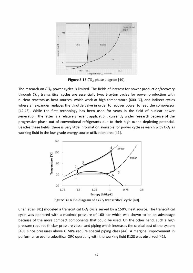
47
Figure 3.13 phase diagram [40].
The research on power cycles is limited. The fields of interest for power production/recovery
through transcritical cycles are essentially two: Brayton cycles for power production with
nuclear reactors as heat sources, which work at high temperature (600 °C), and indirect cycles
where an expander replaces the throttle valve in order to recover power to feed the compressor
[42,43]. While the first technology has been used for years in the field of nuclear power
generation, the latter is a relatively recent application, currently under research because of the
progressive phase out of conventional refrigerants due to their high ozone depleting potential.
Besides these fields, there is very little information available for power cycle research with as
working fluid in the low-grade energy source utilization area [41].
Figure 3.14 T-s diagram of a transcritical cycle [40].
Chen et al. [41] modeled a transcritical cycle served by a 150°C heat source. The transcritical
cycle was operated with a maximal pressure of 160 bar which was shown to be an advantage
because of the more compact components that could be used. On the other hand, such a high
pressure requires thicker pressure vessel and piping which increases the capital cost of the system
[40], since pressures above 6 MPa require special piping class [44]. A marginal improvement in
performance over a subcritical ORC operating with the working fluid R123 was observed [41].

48
Guo et al. [45] modeled a regenerative transcritical cycle with a geothermal heat source
varying from 80 to 120°C, and compared its performance with a subcritical regenerative ORC
running R245fa. The two cycles are assumed to work with the same pump and expansion
isentropic efficiencies and regenerator efficiency. Depending on the heat source initial
temperature, thermal efficiencies of the subcritical ORC were from 18 to 27% higher than that of
the transcritical cycle, while the net power output was slightly higher in the transcritical
cycle (the improvement was found in the range from 3 to 7%). The reason of this improvement
from thermal efficiency to net power output is that non-isothermal vaporization allows more heat
to be recovered as already explained for supercritical ORCs. Moreover, the volume flow rate at
turbine inlet and the volume expansion ratio of the -based transcritical system present a
reduction of 84% and 47% respectively, compared with those of the subcritical ORC system, which
turns into a smaller turbine. However, larger total heat transfer areas and special materials are
required for the transcritical Rankine cycle.
Small scale plants and high operating pressures suggest piston expanders to be the best solution
for this type of cycles. Pistons have low performance due to the high friction losses [40].
Volumetric expanders are more deeply treated in the next Chapter. Zhang et al. [42] studied a
double-acting free piston expander that offered an isentropic efficiency of 62%. Tian et al. [43]
designed and manufactured a rolling piston expander that reached an efficiency of 45%.
Moreover, the low critical temperature also comes with a disadvantage due to the limited
condensing temperature (< 25÷30°C) needed to condensate .
In conclusion, a Table with the main advantages and disadvantages of this cycle is presented.
Pro Contro
CO2 safety and environmental characteristics³: - Non-toxic; - Non-flammable; non-explosive; - Environmentally friendly (GWP=1, ODP=0); - Inertness (in the temperature range of
interest).
CO2 availability³: - Relatively inexpensive; - Abundant in nature;
Good knowledge of CO2 properties³;
Slightly higher power output than subcritical ORCs when fed by an equal low/medium-grade sensible heat source.
Compact dimensions due to high pressure operation;
Limited pressure ratios (around 3) in optimal conditions.
Special materials required by high pressure operation;
Poor information on: - Expanders performance in supercritical
region; - System cost;
Part of the compression occurs in the supercritical region;
Low condensing temperature;
Table 3.4 Advantages and disadvantages of the transcritical power cycle (³ compared to the
organic fluids used in ORCs).

49
3.7 Kalina cycle
In comparison with the previous one, this cycle differs from an ORC not only because of the
properties (and working conditions) of the working fluid, but also for the cycle layout itself: the
Kalina cycle is an absorption power cycle that works with a zeotropic solution, usually a mixture of
water and ammonia. In the upcoming Section the process will be described, then the attention will
be shifted on the phase change process of non-azeotropic mixtures such as the solutions used by
Kalina cycles. Note that different authors [49..] proposed to operate ORCs with zeotropic
solutions. The advantages of this solution will be discussed in Section 5.2.3. Then, some insights
will be given on cycle optimization. Finally, the performance of the Kalina cycle will be compared
to that of ORCs.
3.7.1 Description of the Kalina process
Nowadays, heat recovery from high temperature gases is monopolized by the steam Rankine
cycles and application of the Kalina cycle is restricted to medium-low temperatures heat sources
(typical maximum temperatures of 300–400°C in the case of heat recovery, and 100-120°C in the
binary geothermal plants) and to small power conversion systems, and it is specifically in the
sector of heat recovery that the Kalina cycle is in competition with the ORC cycle [46].
In Figure 3.15, the simplest layout of the Kalina cycle is illustrated. The mixture of ammonia-water
(usually 70%-30%) is evaporated (34) and then sent to the separator, where ammonia-rich
vapor flows up to the expander (5) while the heavier ammonia-poor liquid mixture falls down to
the regenerator (6), in order to pre-heat the mixture before it enters the evaporator (23). After
the expansion (59) the ammonia-poor liquid is throttled in a valve to reach the low pressure of
the ammonia-rich vapor exiting the expander; the two flows are then mixed together in the
absorber; the initial mixture is then sent to the condenser and finally pumped back to the
regenerator, where it is pre-heated by the ammonia-poor liquid solution.
Figure 3.15 Schematics of the basic Kalina cycle [40].

50
There are several variations of this cycle with the inclusion of additional regenerators, condensers,
separators and pumps (see for example Figure 3.18, which is also the actual configuration of the
Kalina power plant of Husavik (Iceland), one of the few Kalina power plants in operation, or Figure
3.19). These variations do not necessarily lead to improved performance.
3.7.2 Phase change of a non-azeotropic solution
As already stated, in addition to the different cycle configuration, the Kalina cycle differs from
ORCs also for the working fluid properties. Indeed, the ammonia-water mixture is a non-
azeotropic mixture. This implies that the compound does not behave like a pure fluid, i.e. it does
not evaporate nor condensate at constant temperature, as pure fluids do. This behavior occurs
when the components of the mixture have different boiling points; in our case, pure ammonia’s
boiling point is -33°C while that of pure water lies at 100°C. The thermophysical properties of the
mixture can therefore be altered by changing ammonia’s concentration.
Figure 3.16 shows the equilibrium of the mixture for a total pressure of 550 kPa. The upper line
represents the saturated vapor, which means that the mixture is completely under vapor form and
condensation begins as soon as the mixture is cooled down. The lower line represents instead the
saturated liquid, which occurs when the mixture is completely condensed and the vaporization
begins as soon as heat is provided to the solution.
Figure 3.16 Equilibrium temperature-concentration curve (phase diagram) for water-ammonia solution at constant pressure [47].
Let’s assume that the mixture approaching the recuperator is made up of 70% ammonia and 30%
water at 25°C; the diagram tells us that the mixture is in saturated liquid phase, as point 3 lies on
the saturated liquid curve. As it is heated up to 70°C (point 4), the concentration of ammonia in
the remaining liquid is more or less 36%, while the concentration of ammonia in the vaporized
mixture is close to 100%. This means that ammonia is much more volatile than water, as can be
also noticed by comparing temperatures of point 1 and point 2: the first corresponds to pure

51
water, which boiling temperature (above 150°C at the aforementioned total pressure) is much
higher than that of pure ammonia (slightly higher than 0°C). This means that when the mixture, in
its liquid or biphase form, is heated up, ammonia will evaporate much faster than water. The same
is saying that when the mixture, in its vapor or biphase form, is cooled down, water will
condensate much faster than ammonia. Back to Figure 3.16, in order to reach the equilibrium in
the saturated vapor phase the mixture should be heated up to approximately 115°C (temperature
of point 7), where ammonia’s concentration falls down to the initial value of 70%, according with
the mass conservation law. Moreover, if we had a solution with very low content of ammonia
(close to point 1), evaporation and condensation would be nearly isothermal processes, and for a
given pressure (in this case 550 kPa) they would occur at a higher temperature than that of the
considered mixture (70% ammonia).
Now it should be clear that having a non-azeotropic solution as working fluid allows the control of
the temperature both during evaporation and condensation, and this is a big advantage due to the
possibility to match the working fluid temperature profile with that of the available heat source
and sink. In particular, the advantage is once again the reduction of thermal irreversibility
obtained by reducing the logarithmic mean temperature difference between the heat source (and
sink) and the working fluid stream, the pinch points difference being fixed (see Figure below).
Figure 3.17 Evaporation of 70%-30% ammonia-water solution in the T-q diagram [47].
The heat transfer coefficient of pure boiling ammonia is similar to that of the pure boiling water
and is 10-20 times as high as those of ordinary refrigerants [46]. In the ammonia-water mixture,
however, the boiling heat coefficient decreases by a third, at least in pool boiling [46]. In any case,
in gas heat exchangers of both Kalina and ORC power plants, the global heat transfer coefficient is
dominated by the gas-side thermal resistance [46].
3.7.3 Insights on cycle optimization
Rodriguez et al. [47] performed an analysis for a 1 kg/s low-enthalpy geothermal stream at a
temperature ranging between 90°C and 140°C, with a cycle made up of two recuperators (one at
hot temperature and one at low temperature) and two separators (one before the expander and
one before the condenser), as shown in Figure 3.18. Before entering the condenser a second
separator is installed separating the phases and the water is pumped through inlet nozzles into the

52
condenser where the ammonia vapor is condensed. The characteristics of the heat source stream
being given, the cycle is optimized through the evaporation pressure and the ammonia
concentration of the working fluid. Since every total pressure value has its own phase diagram, the
two variables depend on each other.
Figure 3.18 Kalina power cycle with two recuperators [47].
The condensation pressure can be decreased by reducing the concentration of ammonia in the
solution. However, in the mentioned study the condensation temperature is set to 36°C due to
environmental constraints (the ambient temperature is assumed to be 25°C). This means that
condensing pressure decreases depending on ammonia concentration, which together with
evaporation temperature is one of the two control variables that have been varied in order to
maximize the power output for a certain ammonia concentration in the solution. The authors tried
three different ammonia concentrations (65, 75 and 84%) and found that the maximum power
output was achieved with 84% of ammonia mass fraction. Increasing the percentage of ammonia
mass fraction in the composition of the working fluid reduces the mass flow rate and at the same
time increases the ammonia mass fraction that can be evaporated. This results in lower size of the
heat exchangers and in higher power output. The authors stated that the break-point in this
improving trend is 90% of ammonia mass fraction, beyond which the efficiency drops sharply.
An explanation for this parabolic trend emerges from the results obtained by Nag and Gupta [48],
who investigated the effects of key parameters of a cycle similar to that shown in Figure 3.19 on
system performance both from an energetic and from an exergetic point of view. They
individuated three key parameters affecting cycle performance: turbine inlet conditions
(temperature and gas composition) and separator temperature. They found the second law
efficiency increasing with ammonia concentration until a maximum and then decreasing (see
Figure 3.20). At low values of ammonia mass concentration (at the turbine inlet) turbine exergy
loss is high and decreases with increasing ammonia concentration, maybe because of the high
entropy generation in the expansion process. In this region the effect of the turbine is primary,
therefore exergy efficiency increases with increasing ammonia concentration. At higher ammonia
concentration rates HRSG irreversibility increases and becomes more important in comparison
with the turbine irreversibility. Therefore, after a certain value exergy efficiency falls due to the

53
HRSG irreversibility. The increasing irreversibility of the HRSG may be due to the increasing mean
distance between the temperature profile of the flue gas and the working fluid during boiling, thus
resulting in higher thermodynamic irreversibility for high values of ammonia concentration. The
optimum ammonia concentration rate depends on the turbine inlet temperature.
Figure 3.19 Kalina layout adopted in [46].
Figure 3.20 Second law efficiency versus ammonia concentration [48].
3.7.4 Kalina Cycle versus ORC
Bombarda et al. [46] studied the possibility to recover heat from high temperature exhaust gases
of two large size Diesel engines -available at a temperature of 346°C- by means of a Kalina cycle
and of an ORC. The limited power level of the considered application did not justify an excessive
plant complication; thus, the simple configuration shown in Figure 3.19 was adopted. With this
layout, the separator pressure is not equal to the evaporator pressure and a third recuperator is
added. The selected fluid for ORC is the siloxane HMDS; as will be shown in a later section,
siloxanes suite good to ORCs with high temperature sources. The comparison investigates the
suitability of Kalina cycles in recovering heat at medium/high temperature (the exhaust gases exit
the engine at 346°C). Due to this temperature, the evaporation pressure achieved through the
54
optimization should be higher than 100 bar. Nonetheless, the authors set it to 50 and 100 bar due
to the excessive cost of materials needed to bear the optimum pressure. The better heat recovery
allowed by the non-isothermal evaporation of the Kalina cycle is overcome by other kinds of losses
that in the ORC are lower: the high number of heat exchangers leads to higher heat losses (both in
internal heat transfers and in the condensation), the performance of the expander in the ORC is
better than that in the Kalina cycle and the mixing processes turn into a further loss, absent in
ORCs. The 100 bar-Kalina process is only slightly better than the ORC for low mean logarithmic
temperature difference, at the expense of a higher system cost, due to higher number of
components and longer piping, to a higher cost for the components (because of the presence of
ammonia and, for evaporator, because of the higher maximum pressure) and finally to a higher
cost of the turbine, since a multistage expander is needed. For these reasons, the adoption of
Kalina cycles does not seem to be a reasonable solution for the considered heat source.
DiPippo [50], as response to the articles published by H.M. Liebowitz and H.A. Mlcak [51,52] that
claimed for a marked superiority (15–50% more power output for the same heat input) of Kalina
cycles over ORCs, demonstrated that under simulated identical conditions of ambient
temperature and cooling systems, the calculated difference in performance is about 3% in favor of
a Kalina cycle, while it is uncertain whether the difference in inlet brine exergy favoring the Kalina
cycle in this study may have played a role in the efficiency advantage of the Kalina over the ORC.
Furthermore, he pointed out that while ORC geothermal technology is mature, with hundreds of
megawatts of various kinds of cycles installed throughout the world, the Húsavık plant is the only
commercial Kalina cycle in operation so far.
3.7.5 Conclusions
- Kalina cycles have different cycle layouts; with increasing complexity of the plant the cost rises
without resulting necessarily in a system performance improvement.
- The binary solution operating in the Kalina cycle introduces a further degree of freedom,
therefore not only the evaporation pressure but also the ammonia concentration shall be
found in order to optimize the system.
- The non-isothermal evaporation process of non-azeotropic mixtures such as the ammonia-
water solution of the classic Kalina cycle results in less irreversibility generated in the heat
transfer with hot source and cold sink with respect to ORC subcritical cycles. The heat
temperature profiles can be controlled by variating the ammonia concentration in the
mixture.
- Exergy efficiency is mainly affected by the irreversibility generated in the evaporator and in
the turbine. Their conflicting trends give rise to a maximum in exergy efficiency that takes
place at a certain ammonia concentration rate, which in turn depends on turbine inlet
temperature.
- The improvement obtained by the Kalina cycle over the ORC is overwhelmed by other sources
of loss; the higher complexity of Kalina cycles results therefore in an unjustifiable increase of
capital cost compared to ORCs.

55
Chapter IV. Expanders
The expander is a critical component in an ORC plant because of different reasons:
- turbine efficiency has a great impact on the system performance because of the inherently
low efficiency of systems (such as ORCs) served by a low grade heat source [53];
- the matching between fluid and expander is one of the main issues in the plant design [54];
- practical expander operation sets several constraints, both from a technical and from an
economic point of view, that must be encountered when analyzing the results of a preliminary
system optimization [55].
- turbine cost is one of the main cost items in the economic balance of the system [36,54];
Although these points have been listed separately, it will be shown that they are closely related to
one another. A literature survey has been conducted on the performance of dynamic and
volumetric machines and on the constraints that must be observed in order to design a realistic
machine. With regard to volumetric expanders, most attention has been paid to the scroll
expanders rather than to other machines.
4.1 Turbines
Turbines can be classified into two categories: radial and axial turbines. Among machines of the
first category, inward flow radial (IFR) or simply radial inflow turbines are the most suitable
turbines for ORC power plants, as they are used as expanders in the cryogenic industry, they are
rugged in design and suitable for small power installations [44]. In addition, manufacturers have
recently developed a new concept radial outflow turbine specifically designed for high-
temperature ORC applications [54].
Radial inflow turbines. These turbines are similar to radial compressors, but with centripetal flow
instead of centrifugal. Instead of having diffuser vanes they have nozzle vanes, often adjustable.
From a high pressure barrel housing the gas expands through guide vane or nozzles arrangement
located in the circumference of the wheel [56]. The gas is accelerated in the guide vanes and
enters the turbine wheel. It converts the kinetic portion of energy contained in the gas by means
of deflection into mechanical energy [56]. The gas leaves the wheel axially at the low pressure
level and subsequently passes through the discharge diffuser where kinetic energy of the gas
stream is converted into static energy thus reducing its velocity to normal pipeline velocities [56].
They are rugged in design and, particularly when fitted in turbochargers, may rotate at speeds
over 100000 rpm. Their flexibility in terms of flow range and power range control is much less than
the axial turbine designs, so they tend only to be used for small power installations [57].

56
Figure 4.1 Radial-inflow turbine [57].
Radial outflow turbines. The outward flow machine is less common, but has been used to some
effect with steam as the large increase in specific volume is more easily allowed for [57]. The
possibility to expand heavy organic fluids through small enthalpy drops with good efficiency, as
explained in the upcoming Section, has driven Exergy S.r.l., one of the main ORC manufacturers, to
design and patent this technology [58]. The turbine itself will be briefly described in Section 4.1.4,
where its advantages over axial turbines will be explained.
Axial turbines. The stream flow is mono-dimensional, as it enters the machine axially and it is
discharged in the same direction. In the impulse turbine, the gases expand in the nozzle and pass
over to the moving blades [59]. The latter convert kinetic energy into mechanical energy and
direct the gas flow to the next stage (multi-stage turbine) or to the exit (single-stage turbine) [59].
In the reaction turbine, the pressure drop of expansion takes place both in the stator and in the
rotor blades; the blade passage area varies continuously to allow for the continued expansion of
the gas stream over the rotor blades [59].
4.1.1 Fundamentals of turbomachines: the similitude theory
The classical concepts of turbomachines design are summarized in order to understand on which
parameters does the turbine efficiency depend. The reader is referred to Dixon [60] and Turton
[57] for a deeper and more complete analysis on the turbomachines theory. The similitude theory
allows to predict the performance of a turbomachine prototype from tests conducted on a scale
model. Such prediction can be done for an incompressible fluid by knowing three kinds of
independent variables:
- Control variables: ω, ;
- Fluid properties: ρ, μ;
- Geometric variables: D, , .. , .
The so called control variables are the rotational speed of the machine and the volumetric flow
rate; the fluid properties are density and viscosity; finally, the geometric variables are all the
characteristic lengths of the machine. Head (specific work), efficiency and power are then

57
functions of the mentioned variables. The dimensional analysis makes it possible to reduce the
number of independent variables of the system by combining them in adimensional groups. The
adimensional group for the specific work is the so called pressure number
The adimensional volume flow rate is called flow coefficient and is expressed as
while both the fluid properties are included in the Reynolds number
And all the geometrical lengths and diameters of the machine are referred to a reference
diameter, assuming thereby the form
,
,
,
.
This means that each of the three performance parameters can be expressed as function of the
flow coefficient, of the Reynolds number and of the geometrical variables, as follows:
,
,
,
,
,
,
The same is valid for power, expressed in its non-dimensional form. The similitude theory then
states that in a family of geometrically similar machines, the geometrical variables are almost
constant. They can be therefore eliminated from the previous relations. Moreover, since in the
turbomachines the flow is fully turbulent, the dependence of performance on the Reynolds
number is very weak and can be ignored. Thus, we obtain that for similar machines
For each family of machines, we have a curve for every position of the blade. The
envelope of such curves, that passes through all the maxima, provides the operating map of that
kind of machine. The maximum of such map is the best condition for that kind of machine, which
can be therefore characterized by three values: and . Every ‘family’ of machines is
characterized by the same specific number (or specific speed), found simply by eliminating the
dependence of the ratio between on the diameter
High specific speeds correspond to machines operating high flow rates and low head loads, vice
versa for low . Every machine is characterized by a specific number , each corresponding to a
set of three optimal operational parameters ( and ).

58
4.1.2 Size effect on turbine efficiency
So far, it has been assumed that the geometrical similarity among machines of different size is
assured if they have the same specific speed. Nonetheless, small machines running at high speed
can achieve the same specific speed of slower machines that use larger mass flow rates to
exchange the same amount of energy [61]. Therefore, small turbines do not have the same
relative thicknesses, clearances etc. of larger machines. When a machine is small relative to the
amount of energy that operates, the ratio between viscous forces and inertial forces of the fluid
decreases, thus bringing to a decrease of turbine efficiency. The parameter that accounts for the
actual dimensions of the machine is the specific diameter [61], defined as
The rotor diameter is therefore obtained by multiplying the specific diameter to the inverse of the
term on the right, called size parameter
Machines with the same specific speed and specific diameter (or size parameter) can be therefore
considered similar. Balje [61] provides charts where concentric areas of constant
isentropic efficiency account for the maximum efficiency achievable by a specific type of turbine.
Figure 4.2 shows a diagram for turbines operating with compressible fluid.
Figure 4.2 diagram for turbines operating with compressible fluids [61].
Due to the elongated shape of the iso-efficiency curves, high efficiency operation can be described
by a line connecting the top left-hand corner of an iso-efficiency curve to its bottom right-hand

59
corner. Such line is known as Cordier line: going away from it orthogonally turns into a sharp
efficiency decrease, while working on it assures a good performance for the type of machine
considered. Radial turbines work at high performance with higher specific diameters than axial
turbines, as can be seen from Figure 4.3.
Figure 4.3 Cordier line [61].
This diagram provides a useful initial tool for the determination of rotor diameter since the latter
can be estimated by the knowledge of the sole thermodynamic parameters of the cycle and
rotating speed of the turbine.
By observing Figure 4.2 and 4.3, it’s straightforward that every point on the Cordier line
corresponds to a different efficiency. In fact, for every couple of , the latter depends on
different variables, that have already been discussed for incompressible fluids and that will be
better analyzed for operation with compressible fluids. By now, it is sufficient to know that the
load is no more indicated as column of water but as isentropic enthalpy drop .
In Figure 4.4, it can be seen that for radial turbines with = 90° (which is the most common
configuration), a maximum in efficiency occurs at a specific speed around 0,7. For axial machines
the optimum specific speed is slightly higher and the decrease in efficiency while going away from
such condition is more moderate.

60
Figure 4.4 Maximum efficiency versus specific number for different turbines [61].
We can conclude that, at least for radial-inflow turbines, the specific speed is constrained within
an upper and a lower limit in order to have an acceptable efficiency. Hereafter a Table is
presented with different boundaries on specific speed for optimal working conditions of radial-
inflow turbines proposed by different authors.
Author
Japikse, Baines [62] 0.2 0.6
Dixon [60] 0.5 0.9
Wood [63] 0.2 1.1
Table 4.1 Boundaries for the specific speed in radial-inflow turbines.
As it can be seen, the optimal range is not clearly defined but it’s a region roughly comprised
between 0.2 and 1.1. These boundaries of good-performing region are very useful in order to
sense the practical feasibility of the optimized ORC system. An example of such sensitivity analysis
is provided by the work of Clemente et al. [64], that used the parameters of the optimized cycle
for six different fluids to find the specific speed for different values of rotating speed (from 20 000
up to 100 000 rpm). The results are shown in Figure 4.5, where it can be seen that the specific
speeds range between 0.1 and 10. For MDM and D4, radial-inflow turbines are not feasible in the
considered range of rotating speed. However, the mentioned fluids are siloxanes, whose critical
temperatures are high and therefore the adoption of a multi-stage axial turbine appears to be
reasonable even from an economic point of view, according to the conclusions of Congedo et al.
[65] that will be reported later.

61
Figure 4.5 Specific speed for different fluids operated from 20000 up to 100000 rpm, the cross being
the specific speed referred to a rotating speed of 70000 rpm [64].
Hereafter, a manufacturer relation is provided by Quoilin [55]. Setting 84% as minimum wheel
efficiency, the specific speed optimal range falls between 0.3 and 0.9, that is in good agreement
with the aforementioned boundaries.
Figure 4.6 Manufacturer’s relation between turbine efficiency and specific speed [55].
4.1.3 Effects of compressibility on turbine efficiency
In order to understand how the compressibility can be expressed from the fluid properties, we
must consider that large changes in flow velocity occur within the pressure drop inside the turbine
[60]. The energy of the flow in each point of the machine can be expressed as a sum of its enthalpy
and its kinetic energy. The sum is called stagnation enthalpy and is constant in an open
thermodynamic system that doesn’t involve work and heat transfer (such as the turbine stator)
[60]. With the hypothesis of an ideal gas operating an adiabatic process, the compressibility can be
easily expressed as
[
]
Where γ is the ratio between the specific heat at constant pressure and that at constant volume,
respectively. With the above assumption, the speed of sound assumes the form

62
√
Where M is the molecular mass of the fluid, R the Boltzmann constant, T the temperature and γ
the specific heat ratio. Thus, the compressibility effects depend both on operating conditions and
on fluid properties. If the effects of Re are neglected again, the parameters of similar machines,
i.e. turbines with the same specific number and specific diameter, become therefore
.
The isentropic efficiency of the machine does not only depend on but also on the
thermodynamic parameters of the cycle (since blade Mach number depends on the pressure ratio)
and on the type of fluid. Thus, as highlighted by Macchi [54], there is a strong relationship
between the working fluid properties and the turbine architecture (speed of revolution, number of
stages, dimensions) and performance (isentropic efficiency) [54].
As it will be shown in Chapter VI, optimized ORC systems often operate with relatively high
pressure ratios. This involves that a supersonic flow occurs if the usual rotational speed of 3000
rpm is adopted [65]. The points where the flow can reach supersonic conditions are the nozzle and
the rotor exhaust. In both of them the Mach number must be limited in order to avoid any local
choking of the flow. Quoilin et al. [55] suggested 0.85 as a generally recommended limit to Mach
number. Conversely, many manufacturers allow the flow to be supersonic in the nozzle; however,
even in supersonic conditions the Mach number should not reach too high values as
compressibility effects (shock-wave effects) could negatively affect turbine efficiency [55].
According to Macchi [54], supersonic flow in ORC turbines in generally mandatory. In turbines, the
flow near the trailing edges of nozzles is of particular importance. If expansion ratios are selected
that give rise to shock conditions, the flow is deflected by a Prandtl-Meyer expansion, the
misdirection caused being several degrees [57]. With such deviation, a substantial correction is
needed in design calculations.
Figure 4.7 Characteristic curve (pressure ratio versus corrected mass flow rate) for a turbine. The almost vertical line represents choking conditions in the nozzle [60].

63
Sauret and Rowlands [44] stated that for radial-inflow turbines operated by high density fluids, a
pressure ratio approximately below 4 involves a simple design due to low Mach numbers, that
until 8 a more complex design is needed in order to cope with choking conditions and that above
this pressure ratio multi-staging or high-expansion machines are needed. The last solution is
normally avoided due to excessive costs related with both design and production. Summarizing:
- 1 < PR < 4 simple design;
- 4 < PR < 8 more complex design due to choked conditions;
- 8 < PR < 120 multi-stage (or high-expansion) machines.
For high pressure ratios (the values above give general ranges), supersonic conditions can be
reached and the Mach number can, in general, overrate the maximum limits indicated above.
According to Congedo et al. [65], the designer has two solutions to cope with such problem:
1. Adopt radial-inflow turbine and drive the rotor at very high rotational velocity (in the order of
25000 rpm);
2. Split the pressure jump into more stages. For multi-staging, axial turbines are preferred
because of the easier manufacturing.
The first solution is the most common due to its lower cost and technical simplicity. However, this
solution implies having poor efficiencies (60÷80%), higher mechanical constraints on rotor and
bearings due to high rotational speed and unbalanced axial loads, and finally requires reduction
gears or sophisticated electrical generators and power conditioning units [65]. The rotating speed
is also limited: Quoilin et al. [55] indicated an upper limit of 50000 rpm. Sauret and Rowlands [44]
stated that 24000 rpm is a reasonable value, since inverter-rectifier systems at this frequency have
been widely used for decades in military and aircraft electrical systems. Furthermore, with this
technology there’s no need of a gearbox between turbine and alternator to obtain grid frequency
[44]. With the second solution higher efficiencies would be achieved (up to 85% depending on the
application) and there would be no need of special cautions for grid connection. These advantages
would be paid at the price of a bigger, more complex and more expensive equipment and
installation [65]. According to the economies of scale, Congedo et al. [65] affirmed that multiple
staging becomes attractive for heat sources at medium to high temperatures (> 250°C).
Both the Mach constraint on the pressure ratio and the efficiency constraint on the specific speed
must be taken into account while analyzing the results of optimization of an ORC, in order to verify
whether the parameters correspond to a practically feasible turbine design. The operating maps
provided by Quoilin et al. [55] emphasize such constraint for radial-inflow turbines run by different
working fluids and are shown here in Figure 4.8, where the upper line represents the critical
temperature, the left curve stands for the stronger constraint between Mach number and
minimum specific speed, and the right curve represents the constraint on the maximum specific
speed.

64
Figure 4.8 Operating maps for radial-inflow turbines [55].
In the aforementioned work of Congedo, the authors want to see if the Theory of non-classical gas
dynamics developed by Bethe (1942), Zeldovich (1946) and Thompson (1972) implies positive
effects on the expansion of dense gases such as some of the candidate working fluids of ORCs.
These fluids (called BZT fluids from the initials of the three pioneers who developed it) are
characterized by a low fundamental derivative of Gasdynamics, Γ.
(
)
where ρ is the fluid density and a the speed of sound. Among them, there are heavy
hydrocarbons, PCFs and siloxanes, that are all candidate fluids for ORC applications as will be
discussed in Chapter V. For these fluids, due to a different behavior of the shock waves, the
turbine could theoretically work with higher Mach numbers, therefore allowing higher pressure
ratios for a given rotating speed [65]. So far, no experimental studies have confirmed such
behavior in real turbines.
4.1.4 Other constraints
A mechanical constraint that should be considered in the preliminary design of a turbine is the tip
speed, limited by the strength of the available materials; in general the maximum does not
depend on the turbine size [55]. The boundary value is commonly set at 370 m/s [55].
Regarding other constraints, it emerged that for Kalina cycles a rigorous selection of materials is
needed to avoid corrosion due to the presence of ammonia: copper and aluminum being
prohibited, the expander wheel should be made of titanium [66]. For ORC cycles, similar
considerations shall be made on each candidate working fluid considered.
4.1.5 The choice of the turbine in the ORC design
The choice of turbine between axial and radial type depends on the application. Some indication
have been already given in the previous Section. In general, one-stage axial machines are
commonly used in systems with high flow rates and low pressure ratios, whereas one-stage radial-
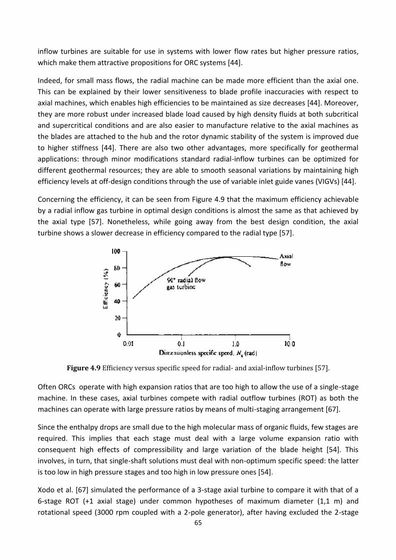
65
inflow turbines are suitable for use in systems with lower flow rates but higher pressure ratios,
which make them attractive propositions for ORC systems [44].
Indeed, for small mass flows, the radial machine can be made more efficient than the axial one.
This can be explained by their lower sensitiveness to blade profile inaccuracies with respect to
axial machines, which enables high efficiencies to be maintained as size decreases [44]. Moreover,
they are more robust under increased blade load caused by high density fluids at both subcritical
and supercritical conditions and are also easier to manufacture relative to the axial machines as
the blades are attached to the hub and the rotor dynamic stability of the system is improved due
to higher stiffness [44]. There are also two other advantages, more specifically for geothermal
applications: through minor modifications standard radial-inflow turbines can be optimized for
different geothermal resources; they are able to smooth seasonal variations by maintaining high
efficiency levels at off-design conditions through the use of variable inlet guide vanes (VIGVs) [44].
Concerning the efficiency, it can be seen from Figure 4.9 that the maximum efficiency achievable
by a radial inflow gas turbine in optimal design conditions is almost the same as that achieved by
the axial type [57]. Nonetheless, while going away from the best design condition, the axial
turbine shows a slower decrease in efficiency compared to the radial type [57].
Figure 4.9 Efficiency versus specific speed for radial- and axial-inflow turbines [57].
Often ORCs operate with high expansion ratios that are too high to allow the use of a single-stage
machine. In these cases, axial turbines compete with radial outflow turbines (ROT) as both the
machines can operate with large pressure ratios by means of multi-staging arrangement [67].
Since the enthalpy drops are small due to the high molecular mass of organic fluids, few stages are
required. This implies that each stage must deal with a large volume expansion ratio with
consequent high effects of compressibility and large variation of the blade height [54]. This
involves, in turn, that single-shaft solutions must deal with non-optimum specific speed: the latter
is too low in high pressure stages and too high in low pressure ones [54].
Xodo et al. [67] simulated the performance of a 3-stage axial turbine to compare it with that of a
6-stage ROT (+1 axial stage) under common hypotheses of maximum diameter (1,1 m) and
rotational speed (3000 rpm coupled with a 2-pole generator), after having excluded the 2-stage

66
IFR turbine from the candidate machines due to the excess of cost and complication related to its
arrangement. The case is a 3 MWe cyclopentane unit fed by oil at 300-150°C (medium-high
enthalpy heat recovery). They found that for the axial machine the inlet pressure must be lowered
as a compromise between cycle efficiency and turbine efficiency, whereas the ROT could work
with high efficiency even with the cycle optimal evaporation pressure, i.e. with high pressure ratio.
The trade-off resulted in approximately 5% more power output of the cycle using the ROT
compared to that using the axial turbine.
Figure 4.10 Axial turbine (left) vs. ROT (right) [67].
The above example clarifies the essential role played by the turbine design in the overall ORC
system design, as it was pointed out by Macchi [54]. The latter suggested the possibility to design
the turbine at optimum conditions and to obtain a proper SP value by selecting appropriate
working fluid properties. The map shown in Figure 4.11 illustrates exactly the dependence of
turbine efficiency on SP and VER for given optimal conditions. The correlation used to draw
this map can be therefore adopted in the preliminary system design to account for the effects of
compressibility and dimensions on turbine efficiency.
Figure 4.11 Efficiency prediction map (optimum conditions) [54].
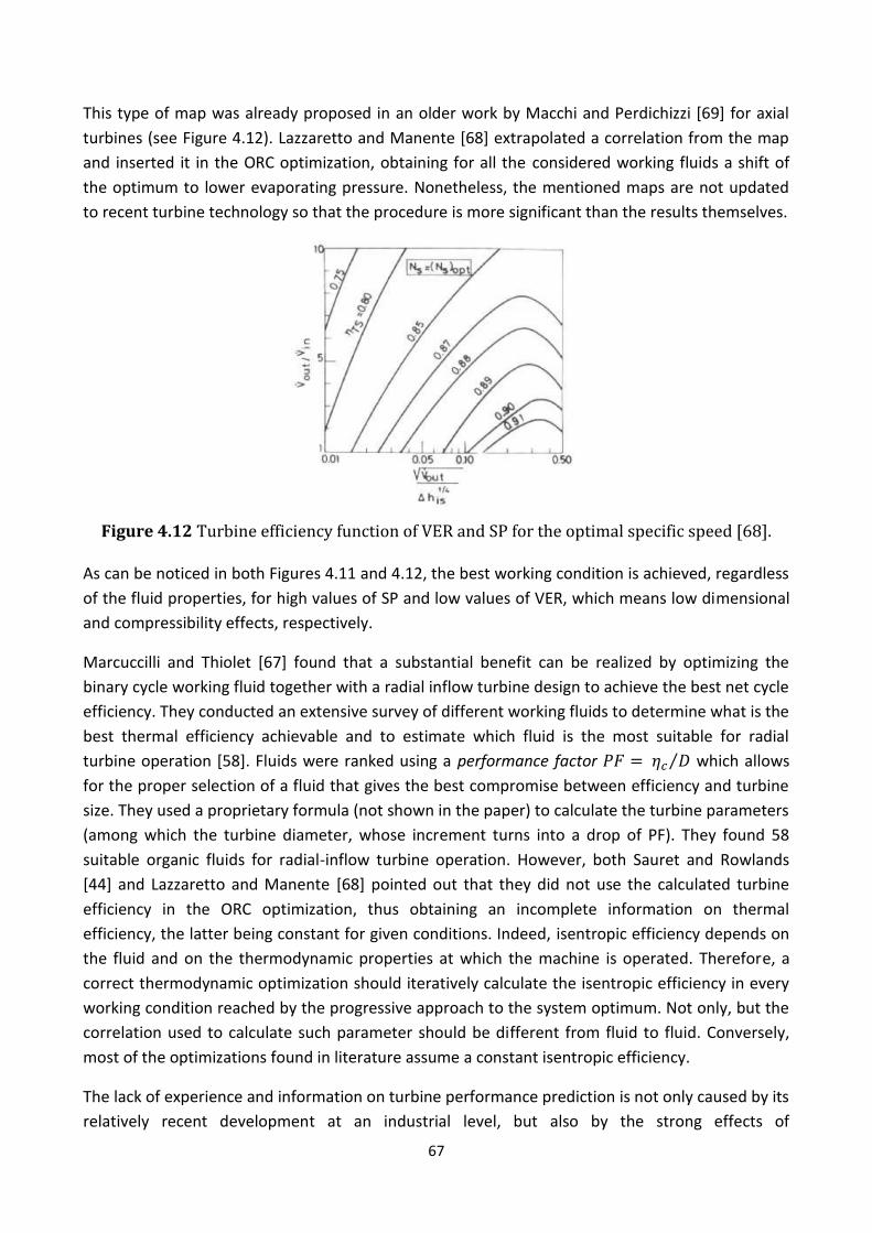
67
This type of map was already proposed in an older work by Macchi and Perdichizzi [69] for axial
turbines (see Figure 4.12). Lazzaretto and Manente [68] extrapolated a correlation from the map
and inserted it in the ORC optimization, obtaining for all the considered working fluids a shift of
the optimum to lower evaporating pressure. Nonetheless, the mentioned maps are not updated
to recent turbine technology so that the procedure is more significant than the results themselves.
Figure 4.12 Turbine efficiency function of VER and SP for the optimal specific speed [68]. As can be noticed in both Figures 4.11 and 4.12, the best working condition is achieved, regardless
of the fluid properties, for high values of SP and low values of VER, which means low dimensional
and compressibility effects, respectively.
Marcuccilli and Thiolet [67] found that a substantial benefit can be realized by optimizing the
binary cycle working fluid together with a radial inflow turbine design to achieve the best net cycle
efficiency. They conducted an extensive survey of different working fluids to determine what is the
best thermal efficiency achievable and to estimate which fluid is the most suitable for radial
turbine operation [58]. Fluids were ranked using a performance factor ⁄ which allows
for the proper selection of a fluid that gives the best compromise between efficiency and turbine
size. They used a proprietary formula (not shown in the paper) to calculate the turbine parameters
(among which the turbine diameter, whose increment turns into a drop of PF). They found 58
suitable organic fluids for radial-inflow turbine operation. However, both Sauret and Rowlands
[44] and Lazzaretto and Manente [68] pointed out that they did not use the calculated turbine
efficiency in the ORC optimization, thus obtaining an incomplete information on thermal
efficiency, the latter being constant for given conditions. Indeed, isentropic efficiency depends on
the fluid and on the thermodynamic properties at which the machine is operated. Therefore, a
correct thermodynamic optimization should iteratively calculate the isentropic efficiency in every
working condition reached by the progressive approach to the system optimum. Not only, but the
correlation used to calculate such parameter should be different from fluid to fluid. Conversely,
most of the optimizations found in literature assume a constant isentropic efficiency.
The lack of experience and information on turbine performance prediction is not only caused by its
relatively recent development at an industrial level, but also by the strong effects of

68
compressibility that affect the machine performance due to the large volume expansion ratios,
thus requiring nonstandard turbomachinery design [70]. Therefore, Pasquale et al. [70] suggested
intensive CFD simulations to cope with this problem and investigate a wide range of possible
configurations.
4.2 Volumetric expanders
All volumetric expanders are positive-displacement machines with a fixed displacement and a
fixed volume expansion ratio [71]. The latter is therefore an inherent characteristic of this type of
machines. Three types of volumetric expanders are considered here: scroll and screw expanders
and reciprocating pistons. The operation and performance of the first will be analyzed through
some works found in recent literature. Many authors recently focused their attention on scroll
expanders due to the possibility of converting them from compressor to expander mode, thus
reducing the cost of the expander for low sized ORC plants. Screw and reciprocating expanders will
be only roughly described for sake of briefness.
4.2.1 Scroll expanders
Scroll compressors can be turned into expanders with some easy devices [72], so it is interesting to
investigate the performance of scroll machines operating in the expander mode and its
improvement potential. Many works have focused on this topics.
Machine operation
One working cycle includes three processes: suction, expansion and discharge [73]. During the
suction process, the suction chamber communicates with the suction line and the fluid flows into
the chamber [73]. The expansion process is initiated when the suction chamber ceases to be in
communication with the suction line [73]. The working principle of the expansion within the scrolls
is illustrated in Figure 4.13: the available volume that the gas finds by means of the orbiting scroll
revolution about the axe of the stationary scroll progressively increases from suction to discharge
chamber [73]. The pressure exerted by the gas on the mobile scroll allows the motion of the scroll
itself, whose mechanical energy is then converted into electrical power through an electrical
generator [73] . The discharge process begins when the discharge chambers enter in
communication with the discharge line [73].
Figure 4.13 Working principle of the scroll expander [73].
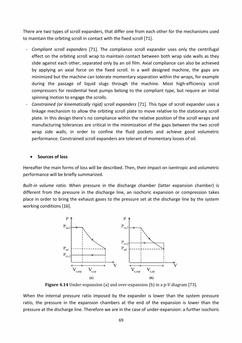
69
There are two types of scroll expanders, that differ one from each other for the mechanisms used
to maintain the orbiting scroll in contact with the fixed scroll [71].
- Compliant scroll expanders [71]. The compliance scroll expander uses only the centrifugal
effect on the orbiting scroll wrap to maintain contact between both wrap side walls as they
slide against each other, separated only by an oil film. Axial compliance can also be achieved
by applying an axial force on the fixed scroll. In a well designed machine, the gaps are
minimized but the machine can tolerate momentary separation within the wraps, for example
during the passage of liquid slugs through the machine. Most high-efficiency scroll
compressors for residential heat pumps belong to the compliant type, but require an initial
spinning motion to engage the scrolls.
- Constrained (or kinematically rigid) scroll expanders [71]. This type of scroll expander uses a
linkage mechanism to allow the orbiting scroll plate to move relative to the stationary scroll
plate. In this design there’s no compliance within the relative position of the scroll wraps and
manufacturing tolerances are critical in the minimization of the gaps between the two scroll
wrap side walls, in order to confine the fluid pockets and achieve good volumetric
performance. Constrained scroll expanders are tolerant of momentary losses of oil.
Sources of loss
Hereafter the main forms of loss will be described. Then, their impact on isentropic and volumetric
performance will be briefly summarized.
Built-in volume ratio. When pressure in the discharge chamber (latter expansion chamber) is
different from the pressure in the discharge line, an isochoric expansion or compression takes
place in order to bring the exhaust gases to the pressure set at the discharge line by the system
working conditions [16].
Figure 4.14 Under-expansion (a) and over-expansion (b) in a p-V diagram [73].
When the internal pressure ratio imposed by the expander is lower than the system pressure
ratio, the pressure in the expansion chambers at the end of the expansion is lower than the
pressure at the discharge line. Therefore we are in the case of under-expansion: a further isochoric
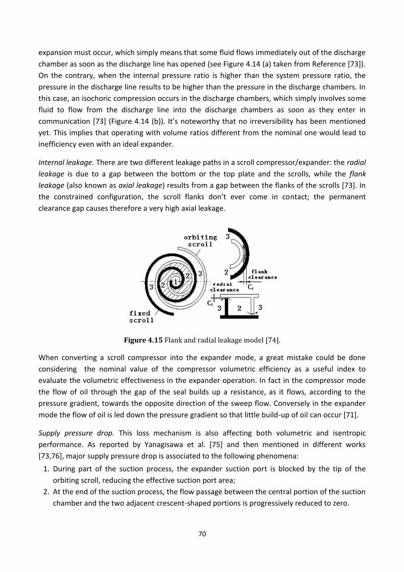
70
expansion must occur, which simply means that some fluid flows immediately out of the discharge
chamber as soon as the discharge line has opened (see Figure 4.14 (a) taken from Reference [73]).
On the contrary, when the internal pressure ratio is higher than the system pressure ratio, the
pressure in the discharge line results to be higher than the pressure in the discharge chambers. In
this case, an isochoric compression occurs in the discharge chambers, which simply involves some
fluid to flow from the discharge line into the discharge chambers as soon as they enter in
communication [73] (Figure 4.14 (b)). It’s noteworthy that no irreversibility has been mentioned
yet. This implies that operating with volume ratios different from the nominal one would lead to
inefficiency even with an ideal expander.
Internal leakage. There are two different leakage paths in a scroll compressor/expander: the radial
leakage is due to a gap between the bottom or the top plate and the scrolls, while the flank
leakage (also known as axial leakage) results from a gap between the flanks of the scrolls [73]. In
the constrained configuration, the scroll flanks don’t ever come in contact; the permanent
clearance gap causes therefore a very high axial leakage.
Figure 4.15 Flank and radial leakage model [74].
When converting a scroll compressor into the expander mode, a great mistake could be done
considering the nominal value of the compressor volumetric efficiency as a useful index to
evaluate the volumetric effectiveness in the expander operation. In fact in the compressor mode
the flow of oil through the gap of the seal builds up a resistance, as it flows, according to the
pressure gradient, towards the opposite direction of the sweep flow. Conversely in the expander
mode the flow of oil is led down the pressure gradient so that little build-up of oil can occur [71].
Supply pressure drop. This loss mechanism is also affecting both volumetric and isentropic
performance. As reported by Yanagisawa et al. [75] and then mentioned in different works
[73,76], major supply pressure drop is associated to the following phenomena:
1. During part of the suction process, the expander suction port is blocked by the tip of the
orbiting scroll, reducing the effective suction port area;
2. At the end of the suction process, the flow passage between the central portion of the suction
chamber and the two adjacent crescent-shaped portions is progressively reduced to zero.

71
These two mechanisms cannot be eliminated since they are inherent to the scroll expander
operation. By means of a simple energy balance, Lemort and Quoilin [76] expressed the relative
supply pressure drop as function of supply pressure, specific volume at expander supply, volume
flow rate and inlet port area.
Then, they calculated it for the organic fluid R123 and for water steam at different rotational
speeds. They found it to increase with rotational speed and to be much higher for R123 than for
water steam, probably because of the larger specific volume that steam has at the end of the
expansion (pressure and temperature being equal) with respect to organic fluids.
Mechanical losses. The mechanical losses are due to the friction between the scrolls and the losses
in the bearings [73]. In the kinematically rigid machine the scrolls flanks don’t ever come in direct
contact, since a small clearance is maintained between them.
Heat losses and oil management. This type of losses is also non negligible: for a kinematically
constrained expander they are estimated as the 5÷10% of boiler heat input, the cycle maximum
temperature being 175°C [71]. Assuming that approximately half of this amount is lost in the high
temperature section ahead the expander, this means losing from 2.5 to 5 percentage points of the
system output capacity [71].
They also state that the oil management in this type of scroll expander could play an important
role in reducing such losses, since having a separate oil separator, trap, and oil pump makes the
system bulky and seems to exacerbate heat loss (and by the way also pressure drops) due to
longer runs of tubing and more volume to insulate. Approaches towards mitigating this problem
could involve using oil entrained in the working fluid and permanently circulating in the cycle [71].
Lemort encountered also the heat losses to the ambient, finding them in the range between 15
and 40% of the output power [77].
Isentropic efficiency
The effects of the described loss mechanisms on isentropic efficiency of compliant and
constrained scroll expanders have been calculated by means of semi-empirical correlations by
Lemort [73,77]. The isentropic efficiency of both configurations has been reported as function of
the pressure ratio in Figures 4.16 and 4.17, respectively.
The built-in volume ratio, that determines the internal pressure ratio, is the main cause of loss
when the pressure ratio of the system goes significantly away from the internal pressure ratio,
since under- and over-expansion occur. Both electro-mechanical losses and internal leakage
significantly contribute to the reduction of isentropic efficiency.

72
Figure 4.16 Isentropic efficiency versus pressure ratio in a compliant scroll expander operated by
R245fa, expander supply temperature 110°C [77].
Figure 4.17 Isentropic efficiency versus pressure ratio in a constrained scroll expander, operated by
R123, expander supply temperature 142°C [73].
In the constrained expander, internal leakage is responsible of an efficiency drop of roughly 20%
against the approximately 10% of the compliant case, as it can be noticed from Figure 4.17. As
already stated above, this is explained by the presence of a permanent clearance gap between the
scroll flanks, that make the axial leakages increase dramatically with respect to the compliant
configuration [77].
Electro-mechanical losses have a large impact on the expander efficiency, in particular concerning
the constrained configuration, in which friction occurs also in the bearings of the linkage
mechanism. Lemort indicated the choice of a better adapted induction motor as one of the
potential improvements that can be done in order to raise the overall efficiency [77].
The supply pressure drop becomes relevant in regime of over-expansion. For slight under-
expansions, the relative pressure drop decreases, as well as its influence on the isentropic
efficiency. This may justify the shift of the global isentropic efficiency maximum from the pressure

73
ratio associated with the built-in volume ratio to a slightly higher value (for both configurations, as
shown in Figures 4.16 and 4.17). Therefore, small under-expansions are not only acceptable but
sometimes even desirable. In general, it is well known that for volumetric expanders re-
compression at the machine’s discharge is more penalizing than under-expansion, where part of
the pressure ratio is simply unexploited [53].
Other factors affecting the expander performance heat losses and the oil fraction in the working
fluid and the rotational speed. Lemort [77] found that increasing oil mass fraction reduces the
isentropic efficiency; although no specific investigation is conducted, raise of supply pressure and
viscous losses are pointed as possible main causes for this behavior.
Volumetric performance
The most common index used to assess the volumetric performance of a scroll expander is the
filling factor, i.e. the ratio between the measured mass flow rate and the mass flow rate
theoretically displaced by the expander [76]. The ‘theoretical’ mass flow rate depends on the
control volume of the displacement (inherent characteristic of the machine) and on the rotating
speed.
The definition is equal to that of the volumetric efficiency of the machine operating in the
compressor mode [78]. The volumetric efficiency of the machine in the expander mode is exactly
the inverse of the filling factor, its definition being the ratio between the theoretical and the
practical delivery [74].
For Xiaojun [74] there are two primary factors affecting the volumetric efficiency of a scroll
expander: the leakage and the porting effects that cause the supply pressure drop. Both the loss
mechanisms have been already described above. Their effects are clearly conflicting: while the
supply pressure drop reduces the delivered volume flow rate compared to the design value, the
internal leakages are responsible for a higher delivery due to the additional fluid that is led down
the pressure gradient without expanding in the appropriate chambers (thus, without contributing
to power production). According to Woodland at el. [78], below unity suggests that the
expansion chamber is not being completely filled with each revolution. On the contrary, in the
expander mode, filling factor is often greater than unity [77,78]. This suggests leakage as a result
of the pump delivering more flow than the expander is able to receive in the expander chamber
with each revolution [78].
Summarizing, two primary and conflicting effects influence the volumetric performance of a scroll
compressor/expander: supply pressure drop and internal leakage. In the expander mode, fill factor
(inverse of the volumetric efficiency) is often greater than unity, which means that the
delivered flow is greater than the flow theoretically displaced by the machine, according to the
dimensions of its chambers. Since internal leakage tends to increase (contrary to porting
effects), it’s reasonable to think that this is the dominant effect and that for constrained

74
expanders would be greater than that of a similar compliant machine, as confirmed by the
aforementioned work of Lemort et al. [77].
4.2.2 Screw expanders
Screw expanders are displacement machines without clearance volume, whose working chambers
are formed by the tooth gaps of two helically toothed gears, the rotors [79]. When a tooth of the
female rotor on the high-pressure side unscrews from the tooth space of the male rotor, a working
chamber arises [79]. With progressing rotation of the rotor, the volume of this working chamber
increases up to a maximum before it is reduced again by a repeated tooth engagement or by the
low-pressure side at the front edge, until the working chamber disappears [79].
Figure 4.18 Screw compressor [83].
4.2.3 Reciprocating piston
The ideal cycle of a single-stage single-acting reciprocating expander is reported on the (p,V)
diagram in Figure 4.19: during the “mechanical admission” (12), the inlet valve is open and the
high-pressure fluid enters the cylinder as the piston moves towards the bottom dead center (BDC);
at a defined crank angle (2), often called “cut-off”, the inlet valve is closed and the isentropic
expansion (23) takes place; when the piston reaches the BDC, the exhaust valve is opened and
the fluid is “thermodynamically” discharged (34); then the piston begins to move towards the
upper dead center (UDC) and drives the fluid out of the cylinder through the exhaust valve, during
the “mechanical discharge” phase (45); finally, at the UDC the exhaust valve is closed and the
inlet one is open, so the fluid instantaneously enters the expander chamber, until it reaches the
upstream pressure (“thermodynamic admission”, 51) [53].

75
Figure 4.19 Ideal cycle of a reciprocating expander in a p-V diagram [53].
Clemente et al. [53] compared performances of scroll and reciprocating expanders using already
validated numerical models. The calculated maximum efficiencies corresponding to three values of
volumetric expansion ratio (respectively lower, equal and higher than the built-in one) are always
equal or very close to 0.70, that is to say they are practically constant with volumetric expansion
ratio [53]. They are similar to values obtained by scroll expanders [53]. If volumetric expansion
ratio is lower than the built-in volumetric ratio, efficiency decreases rather quickly, while for
higher values it keeps high up to expansion ratios of several points higher than the optimal one
[53]. Under-expansions are tolerated, and the machine can work with high pressure ratios without
disproportioned decrease in efficiency. ORC efficiency versus pressure ratio is illustrated in Figure
4.20 for both scroll expander and reciprocating piston [53].
Figure 4.20 ORC efficiency without (a) and with (b) regeneration for a reciprocating piston and a
‘’short’’ scroll expander [53].
4.2.4 Constraints of volumetric expanders in the ORC design
As well as it happens for turbo-expanders, also the operation of volumetric machines involves
constraints that shall be considered in the design of an ORC.
First, the above listed losses should be limited in order to have a sufficiently high isentropic
efficiency. The most important issue to achieve this goal is the matching between the internal and
the system pressure ratios. The built-in volume ratio is limited in order to avoid unacceptable

76
bending stresses. In case of a scroll expander the number of spiral revolutions and in case of screw
expanders the length of the rotor impose a maximum value of approximately 4 and 5, respectively
[55]. As already stated above, small under-expansions are allowed; in other words the machine
can be chosen with an pressure ratio slightly lower than the desired pressure ratio of the cycle
(from optimization). The tolerance in the difference between the external and the internal
pressure ratio can be evaluated through the internal expansion isentropic efficiency, defined as
where is the enthalpy drop of the isentropic expansion corresponding to the
internal (built-in) volume ratio, is the work produced by the isochoric
expansion occurring during the discharge phase (i.e. without contributing to power production),
and the enthalpy drop of the isentropic expansion corresponding to the actual (external)
pressure ratio. Quoilin et al. [55] suggested a lower limit of 90% for this parameter.
The swept volume is linked to the maximum rotor diameter in the case of screw expanders (about
40 cm) or to the maximum spiral height and diameter in the case of a scroll expander. The volume
flow rate is therefore limited; from a screening of the available scroll and screw compressors in
the refrigeration market, Quoilin found a range of 1.1 ÷ 49 l/s for scroll compressors and of 25 ÷
1100 l/s for screw compressors [55].
Finally, Quoilin introduced a further constraint considering that volumetric machines can absorb a
limited volume flow rate; it is therefore not advisable to run them with too low vapor density, in
order to contain machine dimensions with respect to the delivered power. The volume constant
VC, defined as follows, must be therefore limited.
A screening of scroll compressors for refrigeration and heat pumps applications revealed that this
parameter is supposed to be roughly comprised between 0.25 and 0.6 m³/MJ [55].
Machine VER [-]
[-]
VC
[
[l/s]
Scroll <4 >0.9 0.25÷0.6 1.1÷49
Screw <5 >0.9 0.25÷0.6 25÷1100
Table 4.2 Summary of the constraints to scroll and screw expanders.
Quoilin turned all the constraints summarized Table 4.2 into graphical form for both scroll and
screw expanders (Figures 4.21 (a) and (b) respectively), as well as it was done for radial-inflow
turbines (see Figure 4.8) [55]. The operating maps of screw expanders are wider than those of
scroll expanders, due to the higher pressure ratio allowed [55]. The upper-left curve represents
the under-expansion losses limit, whilst the down-right curve is defined by the limitation on the
volume coefficient [55]. The upper line is given by the constraint on the critical temperature, since

77
in [55] only subcritical cycles are considered. No constraints have been considered for the distance
between the critical point and the evaporation temperature. The maximum pressure ratio is
represented by the top-right corner.
Figure 4.21 Operating maps for scroll (a) and screw (b) expanders [55].
By comparing these maps with the working points of five different applications (low enthalpy
geothermy, low temperature solar and waste heat recovery, high temperature waste heat
recovery and high temperature solar power/biomass combined heat and power), it can be seen
that volumetric expanders can only be suitable for low temperature applications, whilst radial-
inflow turbines can also fulfill the requirements of medium-to-high temperature applications [55].
4.3 Comparison between dynamic and volumetric expanders
Turbo-machines present divers advantages over volumetric expanders. First of all, the high
efficiency they can achieve has made them the most common solution for power production
applications. Another reason is the possibility to deflect the gas stream at the turbine inlet with
variable guide vanes in order to work close to the design point also during partial load operation
[28]. However, the power range of ORC process applications can vary from a few kWs up to 1 MW
[15]. The most commonly used turbines which are available in the market cover a range above 50
kW [15]. Therefore, volumetric expanders can be competitive against turbomachines for small-
scale power plants [15].
Unlike for turbines, there’s not a developed market for scroll machines operated in the expander
mode yet. Nonetheless, scroll machines have a very developed market as compressors in the fields
of air conditioning and refrigeration [64]. Since the conversion from compressor to expander is
quite simple [72] and since scroll machines can operate with high efficiency even with imposed
pressure ratios slightly different from the built-in one, it would not be necessary to design new
units, as they can be derived from commercial compressors, allowing for a significant reduction of
costs [64]. This could make the lower isentropic efficiencies acceptable in comparison with the
turbo-machines [64], in particular in the small-to-medium range of electric power [72]. In addition,

78
the reduced number of parts, the ability to cope with two phase working fluids and the inherent
reliability proven in compressor mode are major reasons for its wider use in energy recovery [72].
The suitable ranges of power covered by the different expanders have been summarized by
Quoilin for three different applications [55] (see Figure 4.22).
Figure 4.22 Suitable range of power for radial-inflow turbines, scroll and screw expanders in different ORC applications [55].
Among volumetric expanders, reciprocating expanders could also be taken into account as a
suitable solution. This choice may be justified by the simplicity and the wide diffusion of this
technology, since it is the standard for internal combustion engines [53]; moreover, due to the
advances in materials and engine control systems carried out by the automotive sector, this
technology could become more attractive in the next future [53]. Finally, these machines are more
robust than scroll expanders according to Glavatskaya et al. [80]. However, nowadays the
efficiency of these machines lays approximately in the range of that of scroll expanders (for
example the isentropic efficiency achieves a value of 0.65 in a 25 kWe WHR application [64]) while
their cost is sensibly higher as they cannot be derived from cheap commercial units as it is often
possible in the case of scroll expanders [64].
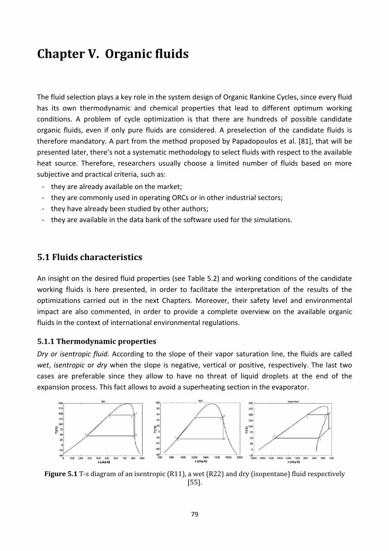
79
Chapter V. Organic fluids The fluid selection plays a key role in the system design of Organic Rankine Cycles, since every fluid
has its own thermodynamic and chemical properties that lead to different optimum working
conditions. A problem of cycle optimization is that there are hundreds of possible candidate
organic fluids, even if only pure fluids are considered. A preselection of the candidate fluids is
therefore mandatory. A part from the method proposed by Papadopoulos et al. [81], that will be
presented later, there’s not a systematic methodology to select fluids with respect to the available
heat source. Therefore, researchers usually choose a limited number of fluids based on more
subjective and practical criteria, such as:
- they are already available on the market;
- they are commonly used in operating ORCs or in other industrial sectors;
- they have already been studied by other authors;
- they are available in the data bank of the software used for the simulations.
5.1 Fluids characteristics An insight on the desired fluid properties (see Table 5.2) and working conditions of the candidate
working fluids is here presented, in order to facilitate the interpretation of the results of the
optimizations carried out in the next Chapters. Moreover, their safety level and environmental
impact are also commented, in order to provide a complete overview on the available organic
fluids in the context of international environmental regulations.
5.1.1 Thermodynamic properties
Dry or isentropic fluid. According to the slope of their vapor saturation line, the fluids are called
wet, isentropic or dry when the slope is negative, vertical or positive, respectively. The last two
cases are preferable since they allow to have no threat of liquid droplets at the end of the
expansion process. This fact allows to avoid a superheating section in the evaporator.
Figure 5.1 T-s diagram of an isentropic (R11), a wet (R22) and dry (isopentane) fluid respectively [55].
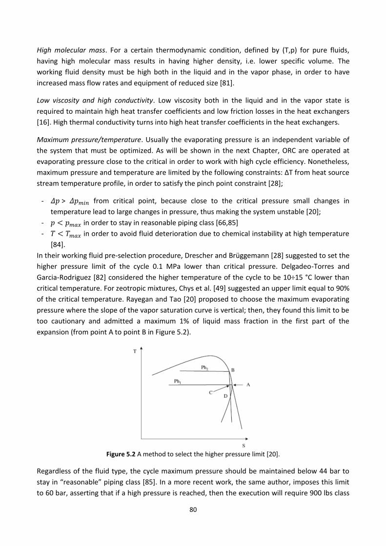
80
High molecular mass. For a certain thermodynamic condition, defined by (T,p) for pure fluids,
having high molecular mass results in having higher density, i.e. lower specific volume. The
working fluid density must be high both in the liquid and in the vapor phase, in order to have
increased mass flow rates and equipment of reduced size [81].
Low viscosity and high conductivity. Low viscosity both in the liquid and in the vapor state is
required to maintain high heat transfer coefficients and low friction losses in the heat exchangers
[16]. High thermal conductivity turns into high heat transfer coefficients in the heat exchangers.
Maximum pressure/temperature. Usually the evaporating pressure is an independent variable of
the system that must be optimized. As will be shown in the next Chapter, ORC are operated at
evaporating pressure close to the critical in order to work with high cycle efficiency. Nonetheless,
maximum pressure and temperature are limited by the following constraints: ΔT from heat source
stream temperature profile, in order to satisfy the pinch point constraint [28];
- > from critical point, because close to the critical pressure small changes in
temperature lead to large changes in pressure, thus making the system unstable [20];
- in order to stay in reasonable piping class [66,85]
- in order to avoid fluid deterioration due to chemical instability at high temperature
[84].
In their working fluid pre-selection procedure, Drescher and Brüggemann [28] suggested to set the
higher pressure limit of the cycle 0.1 MPa lower than critical pressure. Delgadeo-Torres and
Garcia-Rodriguez [82] considered the higher temperature of the cycle to be 10÷15 °C lower than
critical temperature. For zeotropic mixtures, Chys et al. [49] suggested an upper limit equal to 90%
of the critical temperature. Rayegan and Tao [20] proposed to choose the maximum evaporating
pressure where the slope of the vapor saturation curve is vertical; then, they found this limit to be
too cautionary and admitted a maximum 1% of liquid mass fraction in the first part of the
expansion (from point A to point B in Figure 5.2).
Figure 5.2 A method to select the higher pressure limit [20].
Regardless of the fluid type, the cycle maximum pressure should be maintained below 44 bar to
stay in “reasonable” piping class [85]. In a more recent work, the same author, imposes this limit
to 60 bar, asserting that if a high pressure is reached, then the execution will require 900 lbs class

81
flanges which is not realistic for power plant design [66]. This will help to limit the piping cost.
Higher pressure involves the adoption of more expensive pipes and more complex sealing
systems. In the aforementioned work of Drescher [28], the maximum process pressure was limited
to 2 MPa to reduce safety measures and material expenses, as suggested in a previous study by
Lee et al. [86].
In most cases the working fluid expands from saturated conditions. However, superheating can
also be a viable option, especially for high temperature applications. In this case, as well as in
supercritical cycles, maximum process temperature is higher than the evaporating temperature
and a further limit occurs. Unlike water, indeed, organic fluids usually suffer chemical
deterioration and decomposition at high temperatures [16]. For zeotropic mixtures, every single
component must be chemically stable [49].
Minimum condensing pressure. Many authors set the condensing temperature to a fixed value (for
example 35°C) regardless of the corresponding condensing pressure [21,81..]. Nonetheless, there
are fluids with normal boiling point higher than 35°C, that would therefore have the minimum
pressure below the atmospheric value. According to Sauret and Rowlands [44], condensing
pressure should possibly lie above the atmospheric pressure in order to avoid air or water
infiltrations. In this way special sealing for vacuum can be avoided and there’s no threat of fluid
deterioration caused by water and air contamination [44]. Many fluids, and especially those with
high critical temperature, have normal boiling temperature far above the atmospheric value. For
this reason, some authors imposed a minimum pressure in the condenser. Both Drescher [28] and
Rayegan [20] chose to set a lower limit of 5000 Pa to the condensing pressure.
Melting point above the lowest achievable ambient temperature. This measure is aimed at
preventing working fluid freezing during the cold season.
Latent heat of vaporization. Maizza and Maizza [87] indicated high latent heat of vaporization as a
desirable characteristic so that most of the heat is added during phase change without the need to
introduce a regenerator to realize high efficiency. The same concept is presented by Papadopoulos
[81], who asserted that high latent heat of vaporization enables the heat to be recovered at a
higher mean temperature, therefore leading to high cycle efficiency and, again, no need of
internal regeneration. Furthermore, he asserted that high latent heat of vaporization is often
associated with a nearly vertical vapor saturation line, thus resulting in an expansion between the
wet and the superheated region [81]. Other researchers, as reported in the same work, prefer to
select fluids with low latent heat of vaporization in order to avoid the formation of liquid droplets
during the expansion. According to Bo Tau et al. [27], for instance, large vaporizing enthalpy is
regarded as inappropriate for ORC systems. Chapter VI will provide further information on this
apparently contradictory aspect.
Low liquid heat capacity. It must be as low as possible to have a nearly vertical liquid saturation
line [81].

82
5.1.2 Safety level: toxicity and flammability
The ASHRAE Standard 34 [88] classifies refrigerants in groups with different safety levels,
encountering both the toxicity (A=high toxicity, B=low toxicity) the flammability (1=no flame
propagation, 2=lower flammability, 3=higher flammability). The toxicity level takes into account
mortality, cardiac sensitization, anesthetic or central nervous system effects and other eventual
escape-impairing effects. In Table 5.1 the extrapolated data of the mentioned standard have been
reported. In the last lines safety level of ammonia, water and CO2 have been also inserted.
Moreover, the European Standard EN 378 [89] recommends an upper refrigerant concentration
limit (RCL) in refrigeration and air conditioning applications of 8 g/m³ for any system with a charge
size of more than 0.15 kg. The aforementioned American standard provides an RCL for each of the
considered fluids. For some of them, such as ammonia and some hydrocarbons, the indicated limit
is lower than 8 g/m³. In such cases, the RCL suggested by the ASHRAE Standard 34 has been
reported in brackets (in g/m³).
5.1.3 Environmental impact and international standards
The protection of the ozone layer and the emission reduction of greenhouse gases caused various
regulations on international, European and national level.
Low Ozone Depletion Potential (ODP). The most important international agreement in the fight
against the ozone layer depletion is the Montreal Protocol [90], that sanctioned the progressive
phase-out of gases that have been found to be responsible of such depletion, such as
chlorofluorocarbons (CFCs) and hydrochlorofluorocarbons (HCFCs). At European level, the
regulation 2037/2000 is the legal binding implementation of the protocol [14]. It prohibits the
marketing of ozone depleting substances depending on their ozone depletion potential (ODP)
directly or with transition periods. The phase-out of CFCs has occurred from 1991 to 1996, whilst
that of HCFCs is still occurring (2013-2015). HCFCs were transitional CFCs replacements, with lower
ODP (0.01-0.5 in comparison with 0.6-1 of CFCs) and lower GWP (76-2270 in comparison with
4680-10720 of CFCs). Nowadays HFCs replace HCFCs and CFCs.
HFCs pose no harm to the ozone layer because, unlike CFCs and HCFCs, they do not contain
chlorine that contributes to the ozone layer depletion. But it has been established that HFCs are
not innocuous either. They are super-greenhouse gases with an extremely high GWP as they trap
enormous amounts of infrared radiations in the atmosphere, thus causing a greenhouse effect
thousands times stronger than carbon dioxide. Some countries want to extend the Montreal
Protocol to these gases, but other countries are apprehensive about the high cost of transition
from HFCs to a safer option and still oppose resistance [90].
Low Global Warming Potential (GWP). Since one of the main targets of ORC technology is the
reduction of greenhouse gas emissions by exploiting sustainable sources, it would be self-
defeating to adopt fluids with a high Global Warming Potential (GWP). However, there’s still no
legislation that imposes a maximum GWP level for power applications. As shown in Table 5.1, the
fluorinated carbons HFCs and PCFs (which are the current substitutes of the refrigerants phased
out by the Montreal Protocol) have high GWP. The Kyoto Protocol mentions both HFCs and PCFs

83
as greenhouse gases, but it gives no specific aim of reduction for these chemicals [14]. The
Regulation 842/2006 of European Parliament and Council regulates the marketing and handling of
fluorinated gases [14]. The reduction of the emission of fluorinated gases will not be reached with
a decrement of their utilization but with a reduction of leakage, obligation of recycling and
education of operators. Due to this reason, the adoption of such fluids in Countries without a
strong environmental legislation could be counterproductive. According to the Directive 2006/40,
replacement of HFCs/PFCs with substances with low GWP is only required for mobile air-
conditioning [14].
Refrigerant No. Name Cathegory Safety level
R32 HFC A2 675
R41 fluoromethane HFC - 92
R50 methane HC A3 25
R116 PFC A1 12200
R125 HFC A1 3500
R134a HFC A1 1430
R143a HFC A2 4470
R152a HFC A2 124
R170 ethane HC A3 Lower alpha
RE134 HFC - Lower alpha
RE170 dimethyl ether HC A3 Lower alpha
R218 PFC A1 8830
R227ea HFC A1 3220
R236ea HFC - 1370
R236fa HFC A1 9810
R245ca HFC - 693
R245fa HFC B1 1030
R290 propane HC A3 0
RC318 PFC - 10300
R365mfc HFC - 794
R407c HFC A1 1774
R600 butane HC A3 (2.4) 0
R600a isobutane HC A3 0
R601 pentane HC - 0
R601a isopentane HC A3 (2.9) 0
R610 diethyl ether HC - 0
R611 methyl formate HC B2 0
R717 ammonia Inorg. comp. B2 (0.22) 0
R718 water Inorg. comp. A1 0.2
R744 carbon dioxide Inorg. comp. A1 1
Table 5.1 Safety and environmental properties of some refrigerants.
There are also organic fluids that do not belong to the class of refrigerants, which are not listed in
the above Table and for which the same considerations could be done. Among them we find
acetone, many hydrocarbons (benzene, butane, transbutene, n-pentane, cisbutene, cyclohexane,
toluene..), syloxanes (HMDS, OMTS..) etc. The latter are particularly suitable for heat recovery at
high temperatures because of the combination of low critical pressure and high critical
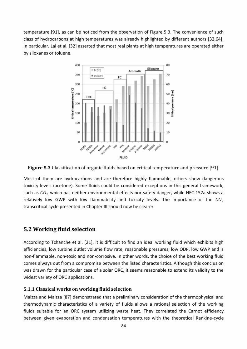
84
temperature [91], as can be noticed from the observation of Figure 5.3. The convenience of such
class of hydrocarbons at high temperatures was already highlighted by different authors [32,64].
In particular, Lai et al. [32] asserted that most real plants at high temperatures are operated either
by siloxanes or toluene.
Figure 5.3 Classification of organic fluids based on critical temperature and pressure [91].
Most of them are hydrocarbons and are therefore highly flammable, others show dangerous
toxicity levels (acetone). Some fluids could be considered exceptions in this general framework,
such as which has neither environmental effects nor safety danger, while HFC 152a shows a
relatively low GWP with low flammability and toxicity levels. The importance of the
transcritical cycle presented in Chapter III should now be clearer.
5.2 Working fluid selection
According to Tchanche et al. [21], it is difficult to find an ideal working fluid which exhibits high
efficiencies, low turbine outlet volume flow rate, reasonable pressures, low ODP, low GWP and is
non-flammable, non-toxic and non-corrosive. In other words, the choice of the best working fluid
comes always out from a compromise between the listed characteristics. Although this conclusion
was drawn for the particular case of a solar ORC, it seems reasonable to extend its validity to the
widest variety of ORC applications.
5.1.1 Classical works on working fluid selection
Maizza and Maizza [87] demonstrated that a preliminary consideration of the thermophysical and
thermodynamic characteristics of a variety of fluids allows a rational selection of the working
fluids suitable for an ORC system utilizing waste heat. They correlated the Carnot efficiency
between given evaporation and condensation temperatures with the theoretical Rankine-cycle
85
efficiency achieved by different organic fluids operating between the same temperatures [87]. As
the difference between the two calculated efficiencies depends only on thermodynamic
properties of the considered fluid (such as critical point location, shape of liquid and vapor
saturation lines etc.), it was indicated as a measure of working fluid behavior in the specific
application, thus being a useful guide for working fluid selection in the preliminary design of an
ORC system utilizing waste heat [87]. Maizza indicated high latent heat of vaporization (see
Section 5.1.1), low liquid specific heat (that implies a nearly vertical saturated liquid line), almost
vertical saturated vapor line and moderate vapor pressures among the desired characteristics of
the candidate working fluid [87].
Liu et al. [27] demonstrated the thermal efficiency to be a weak function of the critical
temperature. This fact was already known but his demonstration did not come out from the mere
observation that thermal efficiency of fluids with low critical temperature is lower, but it was
obtained analytically. Moreover, this work clarifies the need to consider total heat recovery
efficiency instead of thermal efficiency in order to collect a high amount of heat in waste heat
recovery applications [27]. Finally, the presence of hydrogen bond in certain molecules such as
water results in wet fluids due to larger vaporizing enthalpy and is regarded as inappropriate for
ORC systems, as already reported above.
Saleh et al. [38] divided organic fluids into two categories: b-fluids, i.e. those having bell-shaped
vapor saturation line in the T-s diagram, and o-fluids, i.e. those with overhanging saturation line.
This study classifies the possible cycle configurations according to the fluid type (one of the two
defined above, indicated with the letter b or o), to the type of evaporation (subcritical or
supercritical, the latter being regarded with the letter s) and to the presence of superheating
and/or regeneration [38]. The heat transfer from the heat carrier fluid to the working fluid is
considered by a pinch analysis for four representative cycles. The thermodynamic optimization,
that utilizes the BACKONE Equation of State to maximize thermal efficiency to 31 candidate
working fluids, is therefore clearly organized and the results easy to read. In the results, the
authors highlighted that the maximization of thermal efficiency can be misleading since the
processing of the heat carrier fluid should be also included. The optimization results report also
parameters related to turbine operation, i.e. volume flow rate and volume expansion ratio (see
Chapter IV). Finally, a significant result concerning superheating has been reported in Section 3.4.
As already mentioned in the introduction of the present Chapter, Papadopoulos developed a
systematic method to select organic fluids with the so called Computer-Aided Molecular Design
(CAMD): a few molecular function groups generate thousands of possible molecular structures
based on chemical constraints [81]. Then, a set of thermodynamic properties (see the first column
of Table 5.2) concur to select a limited number of the generated molecules through a multi-
objective optimization [81].

86
Thermodynamic Environmental Safety Process-related
1. Density 2. Latent heat of
vaporization 3. Liquid heat capacity 4. Viscosity 5. Thermal conductivity 6. Melting point
temperature 7. Critical temperature
8. Ozone Depleting Potential (ODP)
9. Global Warming Potential (GWP)
10. Toxicity 11. Flammability
12. Efficiency 13. Maximum operating
pressure 14. Mass flow rate 15. Critical pressure
Table 5.2 Properties considered in the CAMD methodology proposed in [81].
At this point, fluids are grouped according to their safety and process-related parameters and
finally a thermo-economic objective function is used to pursue the optimum working fluid [81].
The procedure is illustrated in Figure 5.4, where it is compared to the standard procedure for fluid
selection. The procedure is more complicated than a standard fluid selection. Nonetheless, it
brings the remarkable advantage of including all the possible organic fluids among the candidates
for the specific application, which is interesting to address the problem of fluid selection with a
scientific, systematic approach.
Figure 5.4 Comparison between the simplified schemes of standard optimization procedure and
multi-objective CAMD optimization procedure proposed by Papadopoulos [81].
Another interesting work in the field of fluid selection for ORC systems was carried out by
Hettiarachchi et al. [4]. He compared the behavior of ammonia with that of three organic fluids
with low heat of vaporization and overhanging vapor saturation line in the exploitation of low
temperature geothermal heat (see Figure 5.5). Ammonia results to be the best performing fluid
with respect to ratio of the total heat exchange area on the net power output, that is assumed to
be indicative for the system total cost. This result is obtained thanks to the large heat transfer
coefficient of evaporation, that allows to recover a big part of the available heat with small
working fluid mass flow rate. The relatively better performance of ammonia with respect to the

87
concurrent working fluids is highly influenced by the selected objective function, which utilization
is questionable in the light of the economic evaluation carried out by Lazzaretto et al. [36] on a
real geothermal power plant similar to the one simulated here. Moreover, Hettiarachchi justifies
the scarce value of cycle efficiency as a compromise to reach the economic optimum. This seems
to be only partially true, since even without considering the heat exchange area, the maximum
power output (which is the denominator in the objective function) would be inherently limited by
the high latent heat of vaporization, that does not allow a large heat recovery.
Figure 5.5 T-s diagram of 4 candidate working fluids in Hettiarachchi’s optimization [4].
Another comprehensive optimization in the field of low temperature Organic Rankine Cycles was
carried out by Tchanche et al. [21]. The study, as already mentioned in the second Chapter,
underlines the importance of designing a system that requires a small heat input in order to
contain the collectors array area and the volume of the heat storage, and so the system cost.
Figure 5.6 Temperature profiles of the heat transfer in the evaporator for fluids with high (methanol)
and low (R134a) latent heat of vaporization [21].
Fluids with high latent heat of vaporization –such as water, ethanol, methanol and ammonia-
operate with high efficiency, thus requiring lower heat rates than other fluids [21]. Moreover, the
heat input decreases with increasing evaporating pressure [21]. This suggests that in the design of

88
a solar ORC, depending on the application, one could choose between system with large collector
area-low temperature and a system with small collector area-high operating temperature [21].
5.2.2 Comparison between Organic and conventional Rankine Cycle
Saleh et al. [38] indicated the high value of the volume expansion ratio between turbine outlet
and inlet as the main cause of unsuitability of water as working fluid for low grade heat power
cycles, since organic fluids achieve ratios of an order of magnitude lower than that of water, thus
allowing the use of simpler and cheaper turbines.
Dai et al. [31] used a genetic algorithm to optimize an ORC fed by medium temperature waste
heat available both with and without the internal heat regeneration. Here we report a Table with
the results obtained for water and for two organic fluids, one from the family of refrigerants
(R141b) and one from that of hydrocarbons (isobutane).
R141b Isobutane
type m
[bar] [°C] [bar] [°C] [°C] [kJ/kg] [kg/s] [m³/kg]
wet 220.6 374.0 0.46 79.2
135.0 2310 0.43
41.23
dry 42.5
204.2 4.4
81.7 81.7
195.4 7.47
0.270
dry 36.4
134.7 15.5 87.1 87.1
238.9 3.61
0.118
Table 5.3 Results of Dai’s optimization [31].
In the mentioned optimization, the turbine inlet temperature is not constrained on the vapor
saturation line. Note that while for organic fluids the maximum temperature is equal to the
optimized evaporation temperature, for water it is not: the optimum takes place at the highest
possible turbine inlet temperature. The same behavior was found for ammonia, as it can be seen
in Figure 5.7 [31].
Figure 5.7 Net power output versus turbine inlet temperature [31].

89
According to Dai [31], for a fixed evaporating pressure the optimal turbine inlet temperature is:
- as high as possible below the heat source temperature profile for water and ammonia;
- as low as possible above the boiling temperature for organic fluids.
This fact turns into a significant advantage for isentropic and dry organic fluids, for which the
absence of a superheating section is allowed by the slope of their vapor saturation line. Thus,
superheating shall be avoided because the increased system capital cost of a superheating section
is not justified by a thermodynamic performance improvement. Conversely, wet fluids need
superheating to avoid the presence of droplets at the end of the expansion and to enhance the
system performance at the same time. From Figure 5.4 it can be noticed that even though
superheated, water does not reach the maximum power output of organic fluids expanded from
saturated conditions [31], as it was already observed by Yamamoto et al. [37].
In addition, the very low pressure at which steam condensates into water at about 30°C makes the
specific volume at turbine outlet huge. Organic fluids instead condense at pressures closed to the
atmospheric, which results in two advantages: the gauge pressure is often positive and the specific
volume at the turbine outlet is not excessively high. Gas density is also proportional to the
molecular mass, the latter being much higher for organic fluids than for water (18 kg/kmol).
Moreover, as already mentioned in the previous Chapter, in small scaled plants organic fluids are
preferred against water as their fluid mechanics leads to high turbine efficiency also in partial load
operation [28]. Another disadvantage of water is that it needs high pressure to work with good
efficiency, thus requiring safety measures that are not feasible in small sized plants [28].
5.2.3 Zeotropic mixtures
The advantage of zeotropic mixtures against pure substances has been already clarified in Section
3.6.2 where the behavior of the ammonia-water solution in Kalina cycles has been descripted. For
equal pinch point and inlet temperature of the heat source in the evaporator, the generated
irreversibility decreases due to non-isothermal evaporation, as illustrated in Figure 5.9.
Figure 5.9 T-s diagrams for (a) 0.5/0.5 pentane-hexane mixture and (b) pure pentane as working
fluids with the heat source temperature profiles [49].

90
Angelino and Colonna [92] stated that advantages in utilizing zeotropic mixtures are predictable
whenever the heat sources and sinks exhibit marked temperature differences. Moreover,
extensive thermodynamic computations showed that the internal efficiencies of multi-component
conversion cycles are similar to those obtained with pure fluids, i.e. no thermodynamic penalty is
associated with the replacement of the usual isothermal vaporization by variable temperature
processes [92]. Nonetheless, the apparent heat transfer capacity in the vaporization and
condensation processes is a complex function of the mixture chemical characteristics. Therefore,
an analytical effort is required to find compositions exhibiting nearly linear temperature profiles
which are the best for practical use [92].
Chys et al. [49] studied the improvement potential gained by zeotropic mixtures with respect to
pure substances as working fluids for ORCs. In order to establish the suitable components, they
used the guidelines available for cryogenic refrigerants. One requirement is the appearance of a
volatile component at 1-1.5 bar, so that low temperatures can be reached after the expansion
without the need to work with pressure below the atmospheric one; the boiling point of the
second component needs to exceed both the desired average condensation temperature and the
boiling point of the first component. In order to assure mixability they considered hydrocarbon
and siloxane-based fluids. The most volatile component is the one with the lowest boiling
temperature. A higher concentration of the latter gives rise to higher condensation and
evaporation pressures [49]. Again, the convenience of adopting zeotropic mixtures instead of pure
fluids lies in the possibility to have a better temperature profile matching both in the evaporator
and in the condenser. As a general indication, the higher s the temperature glide, the better is the
temperature profile matching [49]. However, this statement is not necessarily true and should be
evaluated case by case. Another general trend is that the higher is the difference of the boiling
point temperatures between the two components, the higher results the glide [49]. Too big glides
could be inappropriate for a certain heat source (sink) stream, thus requiring a decrease (increase)
in evaporating (condensing) pressure [49]. Furthermore, big glides can lead to a problem known as
fractioning, that occurs when in the evaporator or in the condenser one component is largely in
the vapor state, while the other is for the most part in the liquid phase [49,93]. In presence of
leakage, this leads to a dramatic change in mixture composition; mixtures that fractionate
substantially should therefore be excluded [49]. To prevent this problem, only mixtures with
vaporization and condensation glides lower than heat source and sink gradients and with a
maximum difference in the boiling point temperatures of 45°C are to be considered [49]. After
these preliminary considerations, the authors studied the influence of the heat source
temperature profile on the system performance.
In the first part of the analysis, they fixed both inlet (two cases: 150°C and 250°C) and outlet
temperatures of the heat source and its mass flow rate, and calculated the cycle efficiency relative
increase over its best component. They found an improvement could be obtained, especially for
the lowest temperature case. Thus, in the second part they introduced a degree of freedom by
releasing the outlet temperature of the heat source. Here it was found that the performance
improvement of mixtures over single component working fluids is higher at low temperatures and
with increasing temperature gradient of the heat source, except for very dry fluids such as

91
siloxanes [49]. Moreover, they compared this improvement in terms of work output. In the case of
150°C, +15% of delivered electric power was registered for 0.88-0.12 isopentane-cyclohexane
mixture over the single isobutene. They are the best working fluids for a 2- and for a single-
component working fluid, respectively. Three-components mixtures achieve only a slight further
improvement (of approximately 2%) with respect to two-components mixtures [49].
Nonetheless, it is known that zeotropic refrigerant mixtures have smaller heat exchange
coefficients than those found by a linear interpolation of the heat coefficients of the constitutive
pure fluids. Therefore, the advantage of the improved performance of zeotropic mixtures over
pure fluids could be overwhelmed by the higher heat exchange area needed by the heat
exchangers as well as by the higher technical issues caused by the working fluid leakage [49].
The use of zeotropic mixtures as ORC working fluids for geothermal applications was investigated
by Heberle et al. [93] by optimizing the cycle with respect to the second law efficiency of
isobutane/isopentane and R227ea/R245fa. The results showed that the non-isothermal phase
change of mixtures leads to an efficiency increase in comparison to pure fluids. This is caused by a
better glide matching of the temperature profiles in the heat exchanger equipment, with
particular decrease of the irreversibility in the condenser [93]. Moreover, a case study showed
that important parameters concerning turbine design and costs, like outlet/inlet volume flow ratio
is lower for suitable fluid mixtures compared to pure working fluids. For heat source temperatures
below 120°C, the second law efficiency increases in the range of 4.3% and 15% for mixtures
compared to the most efficient pure component [93]. Pure fluids are suitable, if the pinch point
shifts from the inlet of the evaporator to the inlet of the preheater. Using a mixture the shift and
the resulting efficiency increase can be adjusted to higher temperatures with rising mole fraction
of the less volatile component [93].
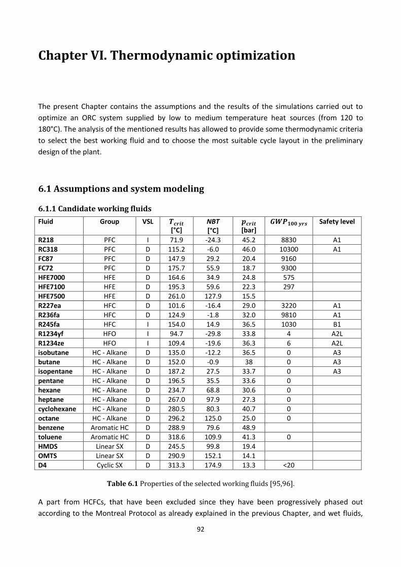
92
Chapter VI. Thermodynamic optimization
The present Chapter contains the assumptions and the results of the simulations carried out to
optimize an ORC system supplied by low to medium temperature heat sources (from 120 to
180°C). The analysis of the mentioned results has allowed to provide some thermodynamic criteria
to select the best working fluid and to choose the most suitable cycle layout in the preliminary
design of the plant.
6.1 Assumptions and system modeling
6.1.1 Candidate working fluids
Fluid
Group VSL [°C]
NBT [°C]
[bar]
Safety level
R218 PFC I 71.9 -24.3 45.2 8830 A1
RC318 PFC D 115.2 -6.0 46.0 10300 A1
FC87 PFC D 147.9 29.2 20.4 9160
FC72 PFC D 175.7 55.9 18.7 9300
HFE7000 HFE D 164.6 34.9 24.8 575
HFE7100 HFE D 195.3 59.6 22.3 297
HFE7500 HFE D 261.0 127.9 15.5
R227ea HFC D 101.6 -16.4 29.0 3220 A1
R236fa HFC D 124.9 -1.8 32.0 9810 A1
R245fa HFC I 154.0 14.9 36.5 1030 B1
R1234yf HFO I 94.7 -29.8 33.8 4 A2L
R1234ze HFO I 109.4 -19.6 36.3 6 A2L
isobutane HC - Alkane D 135.0 -12.2 36.5 0 A3
butane HC - Alkane D 152.0 -0.9 38 0 A3
isopentane HC - Alkane D 187.2 27.5 33.7 0 A3
pentane HC - Alkane D 196.5 35.5 33.6 0
hexane HC - Alkane D 234.7 68.8 30.6 0
heptane HC - Alkane D 267.0 97.9 27.3 0
cyclohexane HC - Alkane D 280.5 80.3 40.7 0
octane HC - Alkane D 296.2 125.0 25.0 0
benzene Aromatic HC D 288.9 79.6 48.9
toluene Aromatic HC D 318.6 109.9 41.3 0
HMDS Linear SX D 245.5 99.8 19.4
OMTS Linear SX D 290.9 152.1 14.1
D4 Cyclic SX D 313.3 174.9 13.3 <20
Table 6.1 Properties of the selected working fluids [95,96].
A part from HCFCs, that have been excluded since they have been progressively phased out
according to the Montreal Protocol as already explained in the previous Chapter, and wet fluids,
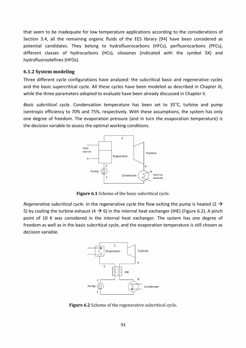
93
that seem to be inadequate for low temperature applications according to the considerations of
Section 3.4, all the remaining organic fluids of the EES library [94] have been considered as
potential candidates. They belong to hydrofluorocarbons (HFCs), perfluorocarbons (PFCs),
different classes of hydrocarbons (HCs), siloxanes (indicated with the symbol SX) and
hydrofluoroolefines (HFOs).
6.1.2 System modeling
Three different cycle configurations have analyzed: the subcritical basic and regenerative cycles
and the basic supercritical cycle. All these cycles have been modeled as described in Chapter III,
while the three parameters adopted to evaluate have been already discussed in Chapter II.
Basic subcritical cycle. Condensation temperature has been set to 35°C, turbine and pump
isentropic efficiency to 70% and 75%, respectively. With these assumptions, the system has only
one degree of freedom. The evaporation pressure (and in turn the evaporation temperature) is
the decision variable to assess the optimal working conditions.
Figure 6.1 Scheme of the basic subcritical cycle.
Regenerative subcritical cycle. In the regenerative cycle the flow exiting the pump is heated (2
5) by cooling the turbine exhaust (4 6) in the internal heat exchanger (IHE) (Figure 6.2). A pinch
point of 10 K was considered in the internal heat exchanger. The system has one degree of
freedom as well as in the basic subcritical cycle, and the evaporation temperature is still chosen as
decision variable.
Figure 6.2 Scheme of the regenerative subcritical cycle.

94
Basic supercritical cycle. Two main differences arise in the modeling of the basic supercritical cycle
compared to the basic subcritical one:
1. Due to the absence of the isothermal part of evaporation, a discretization of the temperature
profile is required to determine the position of the pinch point in the supercritical evaporator.
2. Assuming the same independent variables of the subcritical case (turbine and pump isentropic
efficiencies, pinch point in the evaporator and condensation temperature), the system has
two degrees of freedom; two decision variables are therefore required to optimize the
system. In this work, evaporation pressure and maximum cycle temperature have been
selected as decision variables.
Figure 6.3 Discretization of the temperature profiles of heat source (inlet temperature 150°C) and
working fluid (R1234yf) in the evaporator.
The discretization of the heat transfer in the evaporator has been performed using eight
temperature intervals on the working fluid temperature profile. The corresponding intervals on
the temperature profile of the heat source have been determined by the heat flow transferred
through each temperature interval.
6.2 Basic subcritical cycle
6.2.1 Cycle optimization
Drescher and Brüggemann [28] suggested an upper limit to the evaporation pressure of 1 bar
below the critical point. Nonetheless, due to the curvature of the VSL close to the critical point, a
significant portion of the expansion occurs under the vapor dome for some of these fluids (in
particular for isentropic fluids). With such limit, a maximum in cycle efficiency appears for o-fluids
expanded from saturated conditions. This may explain the existence of a maximum in cycle
efficiency: increasing the evaporation pressure on one hand turns into an increase of the
maximum temperature at which heat is provided to the cycle, but on the other hand it decreases
the portion of heat recovered at that temperature, since latent heat of vaporization decreases.
The combined effect causes a parabolic trend of the mean temperature of evaporation and

95
therefore of cycle efficiency, as shown in Figure 6.4. Other criteria for this assumption have been
mentioned in Section 5.1.1.
In this work, the maximum evaporation temperature is kept 10 K below the critical point,
which agrees with the limit suggested in [82]. 25 fluids out of 27 have the cycle optimal
evaporation temperature (COET) between this value ( ) and the critical temperature. As it
can be observed in Table 6.2, the only exceptions are isobutane and HFE7500, whilst for all the
other fluids COET coincides with the maximum allowed evaporation temperature. Thus, the
constraint has a negative effect on maximum cycle efficiency. Nonetheless, this limit has been
imposed because a less cautionary constraint such as that suggested by Drescher [28] would bring
some of the considered fluids (especially the isentropic ones) to expand completely under the
vapor dome (i.e. in the two-phase region), due to the flat shape of their vapor saturation line close
to the critical point.
Figure 6.4 Maxima of cycle efficiency and specific work output lie above the upper limit on evaporation temperature for R1234yf.
As fluids with high critical temperature generally show high normal boiling temperature, a fixed
condensation temperature (here 35°C) turns into low condensation pressure and thus into high
pressure ratio, which may exclude the utilization of single stage turbines, and that could be
reduced by increasing the condensation temperature with consequent reduction of cycle
efficiency.
Finally, it can be noticed that the value of the maximum efficiency increases with the critical
temperature for almost all the considered fluids. PFCs, HFEs and siloxanes deviate from such
behavior as they show lower efficiencies than expected. This may be explained by the low latent
heat of vaporization with respect to other fluids, such as alkanes. In fact, recovering a low amount
of heat at the highest cycle temperature decreases the mean temperature in the evaporator and
consequently cycle efficiency. The advantages of using the working fluids with high latent heat at
evaporation temperature were already discussed by Papadopoulos et al. [81].

96
Fluid
[°C]
Type [°C]
COET [°C]
VER [-]
[kJ/kg]
[%]
[kJ/kg]
R218 71.9 I 11.3 61.9 2.45 41.4 3.79 2.90
R1234yf 94.7 I 8.95 84.7 4.26 68.2 6.73 9.97
propane* 96.7 I 12.2 86.7 3.52 155.3 7.24 25.3
R134a* 101.1 I 8.87 91.1 4.61 79.0 7.85 14.6
R227ea 102.8 D 6.09 92.8 6.28 46.4 7.38 9.21
R1234ze 109.4 I 6.68 99.4 6.48 70.7 8.36 14.6
RC318 115.2 D 4.25 105.2 8.40 43.2 8.42 11.2
R236fa 124.9 D 3.75 114.9 10.7 57.9 9.78 16.8
isobutane 135.0 D 4.64 124.7 10.0 128.9 10.7 42.2
FC87 147.9 D 1.24 137.9 22.3 38.1 9.01 15.1
butane 152.0 D 3.29 142.0 15.0 135.6 12.2 55.8
R245fa 154.0 D 2.11 144.0 21.7 70.1 12.4 29.8
HFE7000 164.6 D 1.00 154.6 34.5 53.0 11.7 25.7
FC72 175.7 D 0.46 165.7 53.7 41.2 10.5 19.6
isopentane 187.2 D 1.29 177.2 37.8 115.1 14.2 74.6
HFE7100 195.3 D 0.42 185.2 73.7 49.1 12.3 29.8
pentane 196.5 D 0.98 186.5 50.6 117.8 14.9 83.1
hexane 234.7 D 0.31 224.7 150 99.1 16.5 106.6
HMDS 245.5 D 0.094 235.5 320 67.0 14.2 73.4
HFE7500 261.0 D 0.020 236.1 740 44.6 12.5 37.7
heptane 267.0 D 0.098 257.0 450 96.5 17.1 126.2
cyclohexane 280.5 D 0.20 270.5 330 93.1 19.3 136.1
benzene 288.9 D 0.20 278.9 340 117.5 21.3 143.6
OMTS 290.9 D 0.009 280.9 2380 54.1 13.9 81.3
octane 296.2 D 0.020 286.2 1260 93.3 17.6 143.9
D4 313.3 D 0.003 303.3 8130 44.3 14.7 79.3
toluene 318.6 D 0.060 308.6 1020 101.2 21.9 160.6
Table 6.2 Maximization of cycle efficiency (*5 K superheating).
6.2.2 Matching of heat source and ORC: system optimization
In the previous Section the focus was only on the thermal cycle. Here the matching of heat source
and ORC is considered to search for the optimum evaporation temperature of the overall system
(ORC plus heat recovery). As shown in the previous section, a maximum in cycle efficiency and
specific work output exists close to the critical temperature, for the so called o-fluids, i.e. for dry
and isentropic fluids. Nonetheless, this region of high performance cannot be achieved for most of
the considered fluids since a constraint on maximum evaporation temperature has been set. Cycle
optimal evaporation temperature (COET) is therefore limited to the maximum allowed
evaporation temperature (10 K below the critical temperature).
However, the utilization of low grade heat sources (geothermal heat, waste heat from engines or
industrial processes, etc.), which are most commonly used to feed ORC systems, requires the
maximization of power output to properly exploit the heat content of these sources while
rejecting the minimum amount of heat to the environment.

97
It is already known from Chapter II that for the so-called latent heat sources, the maximization of
power output coincides with that of thermal efficiency, whilst for sensible heat sources maximum
power output comes from a trade-off between high thermal efficiency and high heat recovery
effectiveness. The latter assesses the amount of heat recovered with respect to the maximum
available heat that is obtained by cooling down the hot stream to the lowest temperature, i.e. to
the temperature of the environment. Therefore, power output can be assessed through the
product between thermal efficiency and heat recovery effectiveness, i.e. the already defined
system overall efficiency (also known as total heat-recovery efficiency) .
In this work, the heat source has been modeled as a 10 kg/s stream of subcooled water available
at three different temperatures: 120°C, 150°C and 180°C. The temperature of the environment has
been set to 15°C.
In this first step, the basic subcritical configuration with fixed condensation temperature (35°C)
and pinch point of 10 K in the evaporator has been analyzed. is the decision variable. Its
optimal value (that corresponds to maximum power output) has been called system optimal
evaporation temperature (SOET). The temperature difference
= COET – SOET
measures the distance between the evaporation temperatures that maximize cycle efficiency and
system (cycle plus heat recovery) efficiency. In other words, measures the effect of on
the system optimum. Candidate working fluids have been ordered with increasing critical
temperature as in Table 6.2.
In a subcritical cycle the pinch point (PP) in the evaporator takes place either at the beginning of
the preheating process (PH in Fig. 5) or at the beginning of the isothermal evaporation (EV in
Figure 6.5) on the working fluid side. As shown in the following, the pinch point shifts between
these two positions depending on the distance between critical temperature of the working fluid
and inlet heat source temperature. This distance is called here
= – .
Figure 6.5 Pinch point position in the evaporator for working fluids with different .

98
is an important parameter in the evaluation of fluid suitability to sensible heat sources, as
already pointed out by Invernizzi [97].
Figure 6.6 shows the trend of SOET and of the difference versus for 17 candidate
working fluids. At heat source inlet temperatures ( ) sufficiently higher than the critical
temperature (i.e., > 35°C) the optimal system evaporation temperature (SOET) coincides
with the optimal cycle evaporation temperature (COET), i.e. = 0. When the heat source inlet
temperature approaches the fluid critical temperature ( ) the SOET gradually departs from the
COET towards lower values. At ≈ the SOET is about 45°C lower than the COET. At
lower than the difference increases linearly with being COET strictly linked to
.
Figure 6.7 shows the variation with of thermodynamic cycle efficiency and system efficiency
calculated at the system optimal evaporation temperature. The system efficiency shows a distinct
maximum at between 35°C and 40°C. At lower , SOET starts decreasing with respect
to COET, and the system efficiency decreases because of the worse heat recovery effectiveness
caused by the higher latent heat of vaporization owned by fluids with high critical temperature. At
higher the system efficiency decreases due to the low thermal efficiency resulting from the
low evaporation temperatures (see Figure 6.6). Although Figures 6.6 and 6.7 refer to the particular
case of = 150°C, similar trends have been found for the other two values of (120 and
180°C), as confirmed by Tables 6.3a, 6.3b and 6.3c, and by Figure 6.8.
The trend of SOET over the whole range of critical temperatures has been shown in Figure 6.8 as
difference between and SOET versus . At the point of maximum system efficiency
(around = 35°C) this temperature difference reaches a minimum which corresponds to a
good thermal matching between heat source and ORC, which is obtained thanks to the shift of the
pinch point from PH to EV (see Figure 6.5). It is interesting to note that the difference between
and SOET is almost constant for <0 regardless of the working fluid as it was found by
Invernizzi [97]. for application at higher . Although not physically meaningful, in Figures 6.6,
6.7 and 6.8 a dotted line has been used to connect points (each one representing a different fluid)
in order to highlight the trend of the represented parameters.

99
Figure 6.6 and SOET versus for 17 candidate fluids with = 150°C.
Figure 6.7 , and versus for 17 candidate fluids with = 150°C.
Figure 6.8 - versus at three different temperature levels.

100
Fluid [°C]
[°C]
SOET [°C]
[%]
[%]
[%]
PP ⁄
[%]
R218 71.9 48.1 61.9 3.79 70.2 2.66 PH 100.0
R1234yf Propane3 R134a³ R227ea R1234ze
94.7 96.7
101.1 102.8 109.4
25.3 23.3 18.9 17.2 10.6
84.7 73.0 70.0 80.0 76.4
6.73 6.20 6.04 6.58 6.61
52.5 60.8 63.1 52.9 49.3
3.53 3.77 3.81 3.48 3.26
EV EV EV EV EV
100.0 85.6 76.9 89.2 79.0
RC318 R236fa Isobutane FC87 Butane R245fa HFE7000 FC72 Isopentane HFE7100
115.2 124.9 135.0 147.9 152.0 154.0 164.6 175.7 187.2 195.3
4.8 -4.9
-15.0 -27.9 -32.0 -34.0 -44.6 -55.7 -67.2 -75.3
76.6 75.1 74.4 74.9 73.7 73.7 73.5 73.5 73.2 73.3
6.36 6.62 6.57 6.09 6.75 6.80 6.55 5.94 6.76 6.37
52.9 48.9 47.3 54.0 46.0 46.2 47.6 54.3 45.7 49.3
3.36 3.24 3.11 3.29 3.11 3.14 3.12 3.23 3.09 3.14
EV EV EV EV EV EV EV EV EV EV
75.4 67.7 61.4 67.6 55.3 54.8 56.0 56.6 47.6 51.8
Table 6.3 (a) Results of system optimization for different fluids with = 120°C.
Fluid
[°C]
[°C]
SOET [°C]
[%]
[%]
[%]
PP ⁄
[%]
R218 R1234yf R227ea R1234ze RC318
71.9 94.7
102.8 109.4 115.2
78.1 55.3 47.2 40.6 34.8
61.9 84.7 92.8 99.4
105.2
3.79 6.73 7.38 8.37 8.44
76.8 76.8 76.8 76.8 76.8
2.91 5.17 5.67 6.43 6.48
PH PH PH PH PH
100.0 100.0 100.0 100.0 100.0
R236fa Isobutane FC87
124.9 135.0 147.9
25.1 15.0 2.1
101.6 95.0 94.3
9.08 8.84 7.60
60.6 58.0 71.0
5.50 5.13 5.40
EV EV EV
92.8 82.6 84.4
Butane R245fa HFE7000 FC72 Isopentane HFE7100 pentane hexane HMDS
152.0 154.0 164.6 175.7 187.2 195.3 196.5 234.7 245.5
-2.0 -4.0
-14.6 -25.7 -37.2 -45.3 -46.5 -84.7 -95.5
91.9 91.9 90.9 89.7 90.0 89.5 89.6 88.6 89.8
8.87 8.94 8.43 7.36 8.81 8.06 8.81 8.79 8.17
55.5 55.9 58.2 68.7 54.7 60.6 53.9 53.5 57.8
4.92 5.00 4.91 5.06 4.82 4.88 4.75 4.70 4.72
EV EV EV EV EV EV EV EV EV
72.7 72.1 72.1 70.1 62.0 65.5 59.1 53.3 57.5
Table 6.3 (b) Results of system optimization for different fluids with = 150°C.
3 5 K superheating before the expansion to reduce moisture formation.

101
Fluid
[°C]
[°C]
SOET [°C]
[%]
[%]
[%]
PP ⁄
[%]
R1234yf R227ea R1234ze RC318 R236fa Isobutane
94.7 102.8 109.4 115.2 124.9 135.0
85.3 77.2 70.6 64.8 55.1 45.0
84.7 92.8 99.4
105.2 114.9 125.0
6.73 7.38 8.37 8.44 9.80
10.72
80.7 80.7 80.7 80.7 80.7 80.7
5.43 5.96 6.75 6.81 7.91 8.65
PH PH PH PH PH PH
100.0 100.0 100.0 100.0 100.0 100.0
FC87 Butane R245fa HFE7000
147.9 152.0 154.0 164.6
32.1 28.0 26.0 15.4
137.9 119.6 117.3 112.4
9.02 11.16 11.10 10.14
80.7 65.0 66.0 69.3
7.28 7.25 7.33 7.03
PH,EV EV EV EV
100.0 91.5 89.5 86.7
FC72 Isopentane HFE7100 pentane hexane HMDS
175.7 187.2 195.3 196.5 234.7 245.5
4.3 -7.2
-15.3 -16.5 -54.7 -65.5
109.1 109.3 106.9 108.2 105.4 107.0
8.62 10.66 9.46
10.67 10.56 9.67
80.7 63.7 71.9 62.3 61.4 68.0
6.96 6.79 6.80 6.65 6.48 6.58
EV EV EV EV EV EV
82.1 75.1 76.9 71.6 64.0 68.1
Table 6.3 (c) Results of system optimization for different fluids with = 180°C.
Tables 6.3 supply an additional insight on the key role played by in fixing the position of the
pinch point:
- Working fluids having low critical temperature, i.e. high , show the pinch point in PH
(see Figure 6.5) and equal to zero. This means that the heat recovery subprocess does
not affect the system optimum. Moreover, the condition of maximum power output coincides
with that of maximum cycle efficiency. Since the latter increases approximately with
increasing , the same occurs for power output.
- Working fluids having lower show a shift of the pinch point from PH to EV (see Figure
6.5) and the exploitation of the heat source stream turns dependent on the working fluid
evaporation pressure. This means that the maximum power output results from the trade-off
between high cycle efficiency and high heat recovery. The compromise implies the decrease
of SOET with respect to COET: increases proportionally to the decrease of , even
for negative values of the latter, as it appears from Figure 6.6. Increasing means that
the fluid cannot operate simultaneously with high cycle efficiency (with respect to its own
maximum efficiency) and good heat recovery. SOET first diminishes and then remains almost
constant although increases. For these fluids, a high latent heat of vaporization turns
into a high maximum thermal efficiency since a big portion of heat is recovered at maximum
cycle temperature, but it involves also having a flat temperature profile of the heat source
stream, thus reducing the amount of recovered heat. On the other hand, fluids having small
latent heat of vaporization recover more heat because of both the better matching of the
temperature profiles and the lower irreversibility generated in the heat transfer due to the
small temperature difference between streams. This explains why the local drops of cycle

102
efficiency (red squared dots) in Figure 6.7 do not involve corresponding drops in the overall
efficiency (blue diamond dots).
Summarizing, three categories of fluid have been individuated:
- Working fluids having too high must be excluded from the working fluid selection due
to the low thermal efficiency that in any case results in low power output.
- Working fluids having negative are penalized by a scarce heat recovery factor resulting
from the bad matching of the temperature profiles in the evaporator.
- Best performing fluids (those resulting in the highest power output) may have the pinch point
either in PH or in EV (see Figure 6.5), provided that their , where
is the distance between heat source temperature and working fluid critical temperature at
which the pinch point shifts from the preheater to the vaporizer inlet, on the working fluid
side of the evaporator. This value, which is approximately 35 K under the assumptions
considered here, does not seem to vary with the inlet heat source temperature.
6.3 Regenerative subcritical cycle
Although many studies conclude that cycle efficiency is increased by the introduction of
regeneration processes, in waste heat to power applications this is not the main goal, which is
instead the power output maximization [31]. Indeed, the introduction of an internal heat
exchanger (IHE) turns into an increase in cycle efficiency as heat is recovered from the hot source
at a higher mean temperature. However, such increase can lead to a decrease of the recovered
heat as the hot stream cannot be cooled to low temperatures as in the basic cycle.
There are applications where the hot stream cannot be cooled down to the lowest achievable
temperature because of practical constraints. For example, in geothermal applications the brine
must be usually reinjected into the ground at a temperature of at least 70°C. This implies that the
basic cycle works with scarce heat recovery effectiveness at low heat source temperatures as the
brine flow cannot be cooled down to the temperature of maximum power output. In this case,
introducing internal heat regeneration could be interesting since the higher cycle efficiency
achieved by the regenerative configuration would not further penalize the heat recovery
effectiveness in comparison with the basic cycle. A constraint on the minimum heat source
temperature has therefore been set at 70°C.
The regeneration can be evaluated through the regeneration efficiency that accounts for the heat
transferred with respect to the heat that could be ideally transferred by bringing the turbine
exhaust to the pump outlet temperature. Since the heat capacity of a gaseous stream is much
lower than that of the same mass flow rate of liquid stream, and heat is transferred from the
turbine exhaust gas to the liquid stream, the pinch point must take place at the cold stream inlet,

103
.
The regenerator effectiveness can be simplified as follows
to highlight the dependence on the temperature difference
=
which corresponds to the maximum cooling of the superheated vapor exiting the turbine that can
be achieved by an ideal regenerator. Thus, can be expressed as a function of and
as
.
By fixing a minimum regeneration effectiveness of 50%, this equation gives a minimum of
20 K if is fixed at 10 K. Accordingly, only fluids having higher than 20 K have been
considered in regenerative cycles.
6.3.1 System optimization
A significant number of preselected working fluids with positive has been found only at
=180°C. The convenience of introducing the internal heat exchanger has been evaluated
using the ratio , that quantifies the heat that is recovered internally by means of the
regenerator out of the total heat supplied to the cycle by the heat source. Assuming that
does not change significantly from basic to regenerative cycle, has been plotted in
Figure 6.9a as function of that was calculated in the optimized basic subcritical cycle. It
can be observed that is approximately proportional to .
On the other hand, fluids having high are those with high slope of the vapor saturation
line. In fact, fluids having the same critical temperature show a higher turbine outlet temperature
( ) if their vapor saturation line is more tilted (at fixed condensation and evaporation
temperatures). This may explain why molecular complexity, which accounts for the slope of the
vapor saturation line, can be used as parameter to evaluate the beneficial effect of regeneration
on cycle efficiency, as suggested by Invernizzi et al. [97] and Rayegan and Tao [20]. This parameter
is based exclusively on fluid properties. It depends on working fluid critical temperature, molecular
weight and on the slope of the vapor saturation line, evaluated at a reduced temperature (the
ratio ⁄ evaluated in K) of 0.7.
(
)
Thus, a correlation is searched here between the molecular complexity and the temperature drop
available at turbine outlet for regeneration ( ). Figure 6.9 (b) shows the strong correlation

104
between and which suggests the use of as additional performance predictor
for regenerative layouts.
Figure 6.9 (a) versus for the preselected working fluids at = 180°C;
(b) correlation between (calculated in the optimized basic cycle with = 180°C) and
molecular complexity.
Cycle Basic Regenerative
Fluid [K]
[K]
[%]
[%]
[%]
⁄
[%]
[%]
[%]
[kJ/kg]
[%]
RC318 FC87 Butane R245fa HFE7000 FC72 Isopentane HFE7100 Pentane Hexane
64.8 32.1 28.0 26.0 15.4 4.3 -7.2
-15.3 -16.5 -54.7
25.8 68.7 26.7 25.6 47.6 66.4 35.4 54.3 35.4 38.3
8.44 9.02
11.16 11.10 10.49 9.51
10.66 10.04 10.67 10.56
66.7 66.7 65.0 66.0 66.7 66.7 63.7 66.7 62.3 61.4
5.63 6.02 7.25 7.33 7.00 6.34 6.79 6.70 6.65 6.48
10.4 38.0 7.0 6.6
19.5 32.0 11.5 24.1 10.9 12.2
9.30 12.19 11.95 11.82 12.11 11.19 11.87 11.73 11.82 11.84
66.7 66.7 60.7 62.0 57.9 62.7 57.2 57.8 56.2 54.7
43.5 38.1
214.2 114.9 98.2 69.3
261.5 96.7
286.6 301.0
6.20 8.13 7.26 7.33 7.02 7.02 6.78 6.78 6.64 6.47
Table 6.4 Optimized parameters of subcritical basic and regenerative cycles for different working
fluids with a lower limit of 70°C on the heat source outlet temperature, and with = 180°C.
Figure 6.10 Cycle and system efficiency for basic and regenerative cycle with = 180°C.

105
Table 6.4 and Figure 6.10 show that the cycle efficiency decreases with (red squared dots
in Figure 6.10) unless a regenerative cycle is used (shown with blue marks). Regeneration provides
value in increasing thermal efficiency without compromising the heat recovery effectiveness (i.e.,
it increases the system efficiency and power output) only at the highest (i.e. for fluids
having high molecular complexity) provided that they have positive and a low latent heat of
vaporization. Instead, it does not seem advantageous for all the other fluids (see the overlapping
of orange and green dots) because it does not allow the whole exploitation of the external heat
source. In particular, in Section 6.2.2 it has been shown that high allows high heat recovery
effectiveness as the heat source can be cooled down to the minimum allowed temperature. In
these cases regeneration provides an additional heat source at low temperature that can be
usefully exploited by the ORC. On the other hand, fluids with lower or negative are not able
to recover all the heat available from the heat source, especially when using the regenerative
cycle. The heat source stream leaves the evaporator at a temperature higher than 70°C, which
results in < 0.67. Such decrease of is particularly marked for fluids that have high latent
heat of vaporization, which would worsen the matching of the temperature profiles in the
evaporator.
From Table 6.4, it can be noted that the best fluid in the regenerative configuration (FC87) leads to
an improvement of approximately 9% in power output against the best fluid of the basic cycle
(R245fa). FC87 yields both a higher thermal efficiency (12.2 versus 11.0%) and a slightly higher
heat recovery effectiveness (66.7 vs. 66.0%).
In conclusion, regeneration improves the system efficiency only using fluids that combine a highly
tilted vapor saturation line, which allows a big portion of heat to be regenerated, a positive ,
and a low latent heat of vaporization that make such improvement possible without an excessive
decrease of the amount of recovered heat.
Moreover, the temperature difference calculated in the optimized basic cycle was found
to give a reliable indication on the beneficial effect in terms of cycle efficiency of the regenerative
configuration compared to the basic one.
6.4 Basic supercritical cycle
The differences in modeling the supercritical cycle configuration with respect to the subcritical
ones have been discussed in Section 6.1.2. The domain of the decision variables ( ) has been
set by the following constraints:
1. must be higher than a fixed Δp (=0.03 in order to avoid unstable
temperature in the supercritical evaporator ;
2. must be higher than a minimum ΔT ( ), and must be
higher than a fixed ΔT (5 K) to avoid unstable temperature; thus, the critical temperature of
each candidate working fluid must lie at least 15 K below ;

106
3. must be positive in order to assure that the expansion process does not cross the
saturated liquid line.
6.4.1 System optimization
Results of system optimization show that at each maximum cycle temperature there is an
evaporation pressure above which the third constraint (see above) is not fulfilled. In Figures 6.11,
6.12 and 6.13 cycle efficiency, heat recovery effectiveness and system efficiency are plotted for
R227ea, respectively, in the plane of the decision variables evaporation pressure – maximum cycle
temperature (with reference to = 150°C). The evaporation pressure is represented as
reduced evaporation pressure ⁄ (i.e., the ratio between maximum evaporation
pressure and critical pressure). The grey area corresponds to working points that do not fulfill the
third constraint indicated above.
As it was expected, for each evaporation pressure, the cycle efficiency increases with because
increasing the latter results in higher mean temperature of the heat supplied to the thermal cycle.
Moreover, for a fixed value of , the thermal efficiency decreases with the increase of . This
means that the optimal region of cycle efficiency takes place at high and low reduced
evaporation pressures.
Figure 6.11 Isometric curves of (%) as function of and for R227ea with =150°C.
Figure 6.12 Isometric curves of (-) as function of and for R227ea with =150°C.

107
Instead, the heat recovery effectiveness shows the lowest values in the region of maximum cycle
efficiency, whereas it grows for intermediate to low values of and .
For sensible heat sources, a trade-off between high efficiency and high heat recovery is therefore
needed to maximize the power output, exactly as in the subcritical cycles. The compromise gives
rise to a region of high power output, as that shown in Figure 6.13 for R227ea at = 150°C,
which is obtained with a relatively low (centered on 1.2), almost independently of
because of the similar magnitude of the counteracting effects of thermal efficiency and heat
recovery effectiveness. Similar findings were obtained in [6] in spite of the different contributions
of these two performance indexes to power output.
Figure 6.13 Isometric curves of power output [kW] as function of and for R227ea with
=150°C.
Note that the optimum ( ) lies in suboptimal regions of both thermal
efficiency (Figure 6.11) and heat recovery effectiveness (Figure 6.12). This further demonstrates
that power output maximization derives from the best compromise between these two metrics.
6.4.2 Working fluid selection for supercritical cycles
In subcritical saturated cycles, the pinch point can be found either at the preheater or at the
vaporizer inlet, the position depending on (Section 6.2.2). In supercritical cycles there are
not only two possible positions of the pinch point, but as many as the number of points into which
the evaporation has been discretized (9 in our case). Moreover, since is not constrained by the
critical temperature as in subcritical cycles, it is more difficult to find a correlation between
and (Figure 6.8). Optimization results are summarized in Tables 6.5. For
comparison, the last column reports the system overall efficiency of each fluid in the subcritical
cycle.

108
Fluid [°C]
[bar]
[°C]
[%]
[%]
[%]
[K]
[K]
PP [%]
R218 71.9 1.47 98.5 5.62 66.1 3.71 48.1 21.5 4;5 2.66
R1234yf 94.7 1.14 102.7 6.89 44.2 3.05 25.3 17.3 1 3.53
propane 96.7 1.12 103.1 6.76 47.6 3.22 23.3 16.9 1 3.774
R227ea 102.8 1.09 107.8 7.34 40.7 2.99 17.2 12.2 1 3.48
Table 6.5 (a) Optimal parameters of working fluids in the supercritical cycle at = 120°C.
Fluid [°C]
[bar]
[°C]
[%]
[%]
[%]
[K]
[K]
PP [%]
R1234yf 94.7 1.36 116.8 8.02 72.3 5.80 55.3 33.2 3;4 5.17
propane 96.7 1.26 117.5 8.39 68.5 5.75 53.3 32.5 3 5.26⁴
R134a 101.1 1.34 124.5 9.06 65.4 5.93 48.9 25.5 2 5.71⁴
R227ea 102.8 1.34 122.0 8.33 73.8 6.15 47.2 28.0 4;5 5.67
R1234ze 109.4 1.20 122.0 9.01 67.3 6.06 40.6 28.0 2 6.43
RC318 115.2 1.15 122.6 8.64 74.7 6.45 34.8 27.4 4;5 6.48
R236fa 124.9 1.15 132.1 9.55 62.0 5.92 25.1 17.9 1 5.50
Table 6.5 (b) Optimal parameters of working fluids in the supercritical cycle at = 150°C.
Fluid [°C]
[bar]
[°C]
[%]
[%]
[%]
[K]
[K]
PP [%]
R1234yf 94.7 1.89 149.9 9.68 76.5 7.41 85.3 30.1 4;5 5.43
propane 96.7 1.68 149.9 10.15 74.5 7.56 83.3 30.1 4;5 /
R134a 101.1 1.74 151.6 10.55 74.8 7.89 78.9 28.4 4 /
R227ea 102.8 1.93 153.5 9.52 78.0 7.43 77.2 26.5 5;6 5.96
R1234ze 109.4 1.66 148.9 10.41 76.9 8.01 70.6 31.1 4;5 6.75
RC318 115.2 1.71 151.8 9.71 78.8 7.65 64.8 28.2 5;6 6.81
R236fa 124.9 1.42 147.7 10.68 78.1 8.34 55.1 32.3 4;5 7.91
isobutane 135.0 1.16 144.9 10.91 76.2 8.31 45.0 35.1 3 8.65
butane 152.0 1.13 157.0 11.30 74.3 8.40 28.0 23.0 3 7.25
R245fa 154.0 1.19 162.8 12.00 64.5 7.74 26.0 17.2 1 7.33
Table 6.5 (c) Optimal parameters of working fluids in the supercritical cycle at = 180°C.
The following conclusions can be drawn from the Tables above:
- The highest increase in power output (up to 40%) has been achieved by working fluids with
very high (>> 30 K), which are not among the best ones in the subcritical cycle. Such
improvement is associated with the increase in cycle efficiency, the latter being no more
constrained by the critical temperature as in the subcritical configuration.
- Fluids that were among the best performing ones in the subcritical cycle show a limited gain in
power output when used in the supercritical configuration. The increase in power output may
be justified by the higher cycle efficiency and the improved heat recovery deriving by the good
4 5 K superheating to reduce moisture formation.

109
matching of the temperature profiles in the evaporator, which results in a lower exergy
destruction in the heat recovery process.
- Fluids having low (approximately < 25÷30 K) are penalized by a scarce heat recovery, as
the pinch point shifts from medium towards high temperatures of the working fluid
temperature profile (point 1 in Figure 6.3).
6.5 Conclusions
A comprehensive list of organic working fluids has been analyzed to find the most suitable ones for
the exploitation of hot water available at three different temperatures (120, 150 and 180°C) using
three possible ORC configurations: basic subcritical, regenerative subcritical and basic
supercritical.
1. A systematic classification of working fluids operating in subcritical cycles has been proposed
on the basis of their critical temperature. The distance between the heat source inlet
temperature and the critical temperature, i.e. = – , has been found to be
crucial in determining system performance. Table 6.6 provides summarizing indications of the
performance parameters trends versus . High implies having the pinch point at
the beginning of the preheating process, which allows a complete recovery of the available
heat at the expense of a relatively low cycle efficiency (being the latter roughly proportional
to the critical temperature). When falls below , which is approximately 35 K
under the assumptions considered here (and appears independent of ), the pinch point
shifts to the beginning of the vaporization process and the maximum power output results
from the trade-off between high cycle efficiency and high heat recovery effectiveness.
Working fluids having close to 35°C enable a good matching between heat source and
working fluid temperature profiles, with a minimum between the two profiles that is
approximately the same at the beginning of the preheating and evaporation processes (PH
and EV in Figure 6.5).
PP ⁄ ⁄
> 35 K PH low 1 1 low
35 K PH, EV high 1 1 high
< 0 K EV very high <<1 << 1 low
Table 6.6 Trends of optimized performance parameters for fluids at different .
2. In general, the regenerative configuration is not attractive for sensible heat sources due to the
decrease of the amount of heat recovered by the heat source that is not compensated by the
heat recovered internally. Nonetheless, with the introduction of a lower limit on the heat
source outlet temperature, regeneration turns to be interesting. Indeed, regeneration can
lead to an improvement in power output against the basic configuration for fluids that
combine a highly tilted vapor saturation line in the T-s diagram, which allows a big portion of

110
heat to be regenerated, and on the other hand a positive and a low latent heat of
vaporization, which allow such improvement to occur without excessive decrease of the heat
recovery effectiveness. The temperature difference between turbine outlet and pump outlet
calculated in the optimized basic cycle was found to give a reliable
indication on the improvement in cycle efficiency obtained by the regenerative cycle with
respect to the basic one. A comparison between the basic and the regenerative subcritical
cycle for = 180°C with a lower limit of 70°C to the heat source outlet temperature has
shown that the best fluid of the regenerative cycle can improve the power output of about 9%
with respect to the best fluid of the basic cycle. At lower temperatures, regenerative cycles
can be hardly operated without superheating due to the low temperature difference that
would drive the internal heat transfer.
3. Finally, the supercritical cycle has been optimized to find the optimal maximum cycle
temperature ( and reduced evaporation pressure ( ):
- A region of high power output in the diagram ( has been found. As in the
subcritical cycle, this is the result of a trade-off between high heat recovery effectiveness
and high cycle efficiency.
- Compared to subcritical cycles, the highest improvement in power output has been found
for fluids with very high , i.e. fluids that were penalized in the subcritical cycles by the
scarce cycle efficiency due to the low critical temperature.
- Fluids that were among the best performing ones in the subcritical cycle show a limited
gain in power output when used in the supercritical configuration. The convenience of
using a supercritical configuration must therefore be evaluated case by case.

111
Chapter VII. Thermoeconomic optimization
A thermoeconomic optimization has been carried out in order to test the convenience of the
results of thermodynamic optimizations (choice of cycle configuration, fluid selection and
determination of optimal working conditions) conducted in the previous Chapter. Different
objective functions can be chosen while optimizing the system economic performance. In
particular, two indexes are important and considered in most of the works found in literature:
- Capital cost of the system per unit of produced power (SIC, Specific Investment Cost);
- Levelized cost of energy (LCOE) or levelized energy cost (LEC).
Whilst the SIC can be simply obtained by dividing the total capital cost of the plant on its net
power output, the LCOE involves the estimation of the operating life of the plant in terms of
lifetime, working hours per year and the efficiency at which the system works in real operation,
i.e. at partial load. Moreover, the capital cost of the plant must be first evaluated and then
discounted with a certain interest rate over the lifetime of the plant.
7.1 Assumptions and system modeling
7.1.1 Evaluation of equipment capital cost
The Module Costing Technique proposed by Turton [98] has been extensively used for preliminary
cost estimates of chemical plants. It relates all direct and indirect costs to the purchased cost of
equipment evaluated for some “base conditions” [98]. The relationship between the equipment
cost and its ‘attribute’ (for example the size, or the material..) is expressed through an equation of
the following type:
(
)
Where C and A represent respectively the cost and the attribute parameter in the condition
indicated by the subscript. Turning the equation into logarithms, we obtain:
Where
By fitting the data related to the cost of the equipment in its different attributes (for example the
costs of the equipment for different sizes) both the exponent n and the parameter k can be
calculated.
A base condition for the equipment is fixed by the material (carbon steel) and the pressure (close
to the atmospheric value). This condition is indicated in [98] by the apex 0.

112
Moreover, in [98] the cost of the equipment in its base conditions is given in an equation of higher
degree, as follows:
Deviations from the base conditions are accounted by means of multiplying factors, and ,
that depend on the operating pressure in the considered component and on its material of
construction. The pressure factor is provided by the following general formula:
where p is the pressure and , and are coefficients peculiar to each component and type.
Also the indirect costs (such as those required for installation, labor, engineering design, taxes
etc.) related to the considered equipment can be allocated to each component through a
parameter, called bare module factor .
is function of and through two coefficients, and -which are also peculiar to each
component type- as indicated in the following equation.
Through the bare module factor we obtain the bare module cost
Every component has its own . The additional costs due to contingency and fees must be
considered, as well as those for the site development and the auxiliary facilities. The final
grassroots cost is expressed in the following form:
∑
∑
Since all these coefficients are referred to the equipment cost in 2001, when this technique was
developed, the effect of time must be also considered.
The most used index to account for such effect is the so called CEPCI (Chemical Engineering Plant
Cost Index), which is yearly updated.
Lazzaretto et al. [36] applied the Module Costing Technique to evaluate the cost of an ORC fed by
geothermal brine ranging between 130 and 180°C and verified the validity of such evaluation with
the cost data of a real ORC plant.
It’s noteworthy that the material factors for both expander and ACC fans have been induced from
the real cost data. As highlighted in [36], the very high used for the turbine is justified by its
special material of construction. The application of this technique provided accurate estimates for
the purchased cost of the equipment and the overall cost, which includes all the direct and
indirect costs and the costs for the site development [36].

113
Table 7.1 Coefficients used for the evaluation of the capital costs of binary cycle plants according to
the Module Costing Technique suggested in [98].
7.1.2 Thermodynamic assumptions
The Specific Investment Cost, i.e. the capital cost of the plant per unit of power output, has been
chosen as objective function of the system. When the power output is a fixed variable of the
problem, the minimization of the SIC is exactly the same as the minimization of the capital cost of
the plant. In our model, instead, the mass flow rate of the brine is a given data and the power
output is a dependent variable. This approach allows to recognize how the system capital cost and
the power output are affected by a variation (positive or negative) of the decision variables.
Whilst the thermodynamic optimization with our assumptions allowed only one independent
variable to be determined, the thermo-economic optimization defines more parameters. In our
model, a part from the evaporating temperature, three other variables have been determined by
means of the thermo-economic optimization: the condensing temperature and the pinch point in
both heat exchangers (condenser and evaporator).
Increasing the pinch points allows to reduce the required heat exchange area but, on the other
side, implies producing less work for equal temperature of the hot source and of the cold sink.
Concerning the condensing temperature, a lower value involves more work output but, for a given
pinch point in the condenser, it also means that more cooling medium is required to remove heat
from the cycle. This means, of course, a higher size of the condenser and therefore a higher cost.
The mean temperature of the environment has been set to 15°C. This will be therefore also the
temperature of the cooling air suctioned by the condenser.

114
The optimum for the evaporating temperature can be explained, at least at a first glance, as for
the thermodynamic optimization: increasing it for a given pinch point implies working with high
thermal efficiency but, at least if the pinch point takes place at the vaporizer inlet, recovering less
heat. Actually, this criterion is valid for the thermodynamic optimization but it’s not enough to
understand the position of the thermo-economic optimal evaporating temperature, since nothing
has been said about its influence on the equipment cost. Recovering more heat does not only
involve evaporating more working fluid and thereby producing more power, but also having bigger
components, which obviously involves higher cost of the equipment. The relationship between
capital cost of the equipment and recovered heat has been shown in Figure 7.1, where each point
represents a different working fluid in its thermo-economic optimal condition (minimum SIC).
Each diagram shows two clouds of fluids: one at low , with limited capital cost, and one at high
, with higher capital cost.
Figure 7.1 Capital cost of the equipment versus for different working fluids in optimal thermo-
economic conditions with heat source at 150°C (left) and 180°C (right).
This is trivial but also useful to emphasize the difference between the thermodynamic and the
thermo-economic optimization: whilst in the thermodynamic optimization no advantage could be
gained by recovering less heat, in the thermo-economic one less heat means lower capital cost of
the equipment.
The turbine efficiency has been set to 70%, including the electrical efficiency of the generator.
Such value is realistic according to the preliminary design conducted by Sauret and Rowlands [44]
that found an average isentropic efficiency of about 77% for five organic fluids expanded in radial
inflow turbines. The pump isentropic efficiency has been set to 75%.
The global heat transfer coefficients have been simply assumed, based on the ranges suggested
by Kakac [99], which are 300 - 1000 W/(m²K) for the evaporators of refrigeration and 10 -
50 W/(m²K) for the category of gas boilers. It has been assumed a coefficient of 400 W/(m²K) in
the preheater and of 700 W/(m²K) in the vaporizer. In the air cooled condenser, a global heat
transfer coefficient of 30 W/(m²K) has been assumed. The number of fans has been set to 9, which
corresponds to a volumetric air flow rate per fan lower than 65 m³/s. The latter was the
volumetric flow rate per fan used by Lazzaretto et al. in [36]. As of the cost correlations, the MCT
has been used. The same coefficients of the cost evaluation of Lazzaretto et al. [36] reported in

115
Table 7.1 have been adopted. The cost of the working fluid charge has not been considered,
although its influence is not negligible in the overall economic balance of the plant. According to
Sauret and Rawlands [44], turbines with pressure ratios higher than 4 are likely to operate in
choked conditions, therefore requiring more design work. Since the basic cycle with isobutane
served by brine at 180°C works with a pressure ratio higher than 4 according to our results,
probably part of the should be assigned to the additional design work due to the choked flow
occurring both in the rotor and in the nozzle. This involves that the adopted regardless of the
pressure ratio in the turbine could be incorrect.
7.1.3 Objective function for thermoeconomic optimization
The chosen objective function is Specific Investment Cost (SIC) which is the ratio between total
cost of the equipment and net power output. Due to the scarce information on cost correlations
for ORC power plants, both Shengjun et al. [30] and Hettiarachchi et al. [4] approximated the cost
of the whole plant as the total capital cost of the heat exchangers. In fact, they assumed that in a
low-temperature geothermal application, the heat exchangers are responsible of 80÷90% of the
system capital cost. Since the cost of the heat exchanger is roughly proportional to its heat
transfer area, the profitability of the plant has been evaluated through the objective function
APR = / [m²/kW], which has been minimized to achieve the optimal conditions.
Nonetheless, in the cost evaluation carried out by Lazzaretto et al. [36], the Module Costing
Technique has been applied and validated with the data of a real plant fed by 150°C geothermal
brine. The estimated costs, that were found to agree with those of the real plant [36], are
summarized in Table 7.2, where it can be seen that the sum of the purchased costs of the heat
exchangers rather reaches the 50% of the total cost of the equipment. Therefore, the assumption
ofthat the mentioned authors [4,30] do in order to skip the cost evaluation of the components and
to economically optimize the system by means of the APR minimization is not verified, or at least
not in this case.
The levelized energy cost (LEC) is the cost associated with each unity of produced electrical energy.
The latter (also known as levelized cost of energy, LCOE) is an interesting index, since it can be
compared to the market price of electrical energy. However, a correct evaluation of this
parameter can be achieved, especially for air cooled cycles, by knowing the evolution of the
environment temperature during the year. This would go beyond the scope of this work.
Component [$] [$] / [%] / [%]
Expander-generator Air cooled condenser Preheaters and vaporizers Feed pumps
18 892 900 14 112 300 5 620 900 2 650 500
39 056 300 27 765 100 17 222 100 4 942 900
45.6 34.3 13.6 6.4
43.7 31.1 19.3 5.5
Total 41 276 600 89 297 700 100 99.6
Table 7.2 Estimated purchased and bare module costs of the equipment with the MCT [36].

116
7.2 Basic subcritical cycle
7.2.1 Results
The optimization has been carried out only for heat source temperatures of 150 and 180°C, since
almost all fluids at 120°C operate with lower PR and could probably be characterized by different
bare module factors. Common mechanisms in the determination of the optimal conditions have
been found out for both temperature levels. The results have been shown in Tables 7.3 (a) and (b).
Fluid [°C]
[°C]
[°C]
[°C]
[%]
[%]
[kW]
SIC [$/kW]
R134a R227ea R1234ze
36.7 36.1 37.5
7.5 8.0 8.5
94.2 95.5
101.3
6.9 5.6 8.3
6.62 6.55 7.30
77.1 78.9 74.9
291 292 314
11438 11309 10424
RC318 R236fa
35.5 38.5
8.3 9.6
110.7 123.2
7.1 5.5
7.84 8.70
78.4 72.1
347 370
9727 9118
isobutane FC87 butane R245fa HFE7000 isopentane R141b
39.0 36.8 39.6 39.9 38.0 40.0 40.9
10.2 8.9
10.8 11.0 9.4
11.3 11.4
112.0 111.5 109.5 109.6 109.1 109.2 107.9
5.0* 5.0* 5.0* 5.0* 5.0* 5.0* 5.0*
8.90 7.69 9.18 9.20 8.94 9.34 9.63
53.3 65.8 47.8 48.0 50.0 44.6 40.9
269 287 249 250 254 237 224
9452 9382 9273 9103 9101 8998 9079
Fluid [°C]
[°C]
[°C]
[°C]
[%]
[%]
[kW]
SIC [$/kW]
RC318 R236fa isobutane FC87
38.3 39.5 39.6 38.5
9.7 10.1 10.2 10.8
110.0 117.7 127.7 132.1
5.1 6.5 8.3 9.7
7.59 8.67 9.58 8.12
819 802 78.7 78.9
432 484 525 447
8625 7850 7446 7698
butane R245fa
39.3 40.9
10.5 11.0
147.9 152.7
5.3 8.0
11.16 11.15
74.7 75.9
581 590
6819 6651
HFE7000 isopentane R141b
40.5 41.6 42.8
11.8 12.3 11.8
132.3 130.2 126.3
5.0* 5.0* 5.0*
10.05 10.82 11.22
63.9 55.0 49.6
450 418 390
6965 6873
7015
Table 7.3 Results of thermo-economic optimization for different fluids with heat source at 150°C (a)
and at 180°C (b).
1. Working fluids with low critical temperature (relative to the inlet heat source temperature)
have, as in the thermodynamic optimum, the pinch point at the preheater inlet (on the
working fluid side). In the thermodynamic optimization, this fact means that the SOET
coincides with the COET, which in turn involves that a good heat recovery can be performed
even in the region of maximum thermal efficiency of the cycle. The latter occurs normally at
high reduced pressure for basic subcritical cycles with saturated expansion. Nonetheless, the
advantage of working with both high thermal efficiency and high heat recovery effectiveness
is overwhelmed by the low maximal efficiency caused by the low critical temperature.
Operating with high heat recovery effectiveness, as it can be seen in Figure 7.1, means having
high capital cost for the equipment because a high mass flow rate of working fluid is
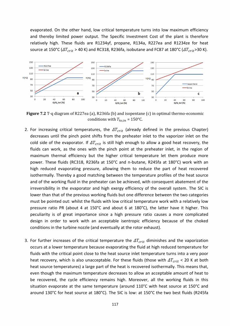
117
evaporated. On the other hand, low critical temperature turns into low maximum efficiency
and thereby limited power output. The Specific Investment Cost of the plant is therefore
relatively high. These fluids are R1234yf, propane, R134a, R227ea and R1234ze for heat
source at 150°C ( > 40 K) and RC318, R236fa, isobutane and FC87 at 180°C ( >30 K).
Figure 7.2 T-q diagram of R227ea (a), R236fa (b) and isopentane (c) in optimal thermo-economic
conditions with = 150°C.
2. For increasing critical temperatures, the (already defined in the previous Chapter)
decreases until the pinch point shifts from the preheater inlet to the vaporizer inlet on the
cold side of the evaporator. If is still high enough to allow a good heat recovery, the
fluids can work, as the ones with the pinch point at the preheater inlet, in the region of
maximum thermal efficiency but the higher critical temperature let them produce more
power. These fluids (RC318, R236fa at 150°C and n-butane, R245fa at 180°C) work with an
high reduced evaporating pressure, allowing them to reduce the part of heat recovered
isothermally. Thereby a good matching between the temperature profiles of the heat source
and of the working fluid in the preheater can be achieved, with consequent abatement of the
irreversibility in the evaporator and high exergy efficiency of the overall system. The SIC is
lower than that of the previous working fluids but one difference between the two categories
must be pointed out: whilst the fluids with low critical temperature work with a relatively low
pressure ratio PR (about 4 at 150°C and about 6 at 180°C), the latter have it higher. This
peculiarity is of great importance since a high pressure ratio causes a more complicated
design in order to work with an acceptable isentropic efficiency because of the choked
conditions in the turbine nozzle (and eventually at the rotor exhaust).
3. For further increases of the critical temperature the diminishes and the vaporization
occurs at a lower temperature because evaporating the fluid at high reduced temperature for
fluids with the critical point close to the heat source inlet temperature turns into a very poor
heat recovery, which is also unacceptable. For these fluids (those with < 20 K at both
heat source temperatures) a large part of the heat is recovered isothermally. This means that,
even though the maximum temperature decreases to allow an acceptable amount of heat to
be recovered, the cycle efficiency remains high. Moreover, all the working fluids in this
situation evaporate at the same temperature (around 110°C with heat source at 150°C and
around 130°C for heat source at 180°C). The SIC is low: at 150°C the two best fluids (R245fa

118
and HFE7000) belong to this category of fluids and even at 180°C a low SIC can be noticed,
and isopentane ranks third among the fluids considered.
This behavior of working fluids with decreasing is similar to that of the thermodynamic
optimization. The latter finds good agreement with the results of Invernizzi et al. [97] (see Figure
6.8) as already pointed out in Section 6.2. However, also admitting that the same behavior occurs
in the thermodynamic optimization, an interesting difference between thermodynamic and
thermoeconomic optima can be underlined: whilst in the thermodynamic optimization the fluids
with low SOET don’t seem to be attractive due to the low power output compared to those with
both good heat recovery and high evaporating temperature, the same fluids become competitive
from an economical viewpoint. This may happen because of two reasons:
- A low heat recovery effectiveness means lower capital cost of the equipment;
- A low evaporating temperature means big latent heat of vaporization, which means that a
significant portion of the heat is recovered at maximum temperature, therefore allowing the
cycle to operate with a relatively high efficiency.
In each of the three categories of fluids individuated, the evaporating temperature plays a key role
in the determination of the cycle efficiency. Their behavior can be summarized as follows:
1. Fluids with high (> 35 K) have an inherently limited cycle efficiency due to the low
critical temperature and the SIC of the plant is high.
2. Fluids with intermediate work with high evaporating temperature and high heat
recovery effectiveness, so that they can sensibly reduce the irreversibility generated in the
evaporator and at the same time work with high cycle efficiency. The SIC is low due to the
high power output.
3. Fluids with small or negative (< 25 K) work with low reduced evaporating temperature
in order to allow an acceptable portion of heat to be recovered. Whilst in the thermodynamic
optimization these fluids are unattractive due to the low power output, in the thermo-
economic they compete with those of the previous category because of the combination of
low capital cost for the equipment (due to the limited heat recovery) and good cycle efficiency
(due to the large part of heat recovered isothermally).
Moreover, what emerges from Tables 7.3 (a) and (b) is that for fluids with high critical
temperature, the pinch point in the evaporator tends to be very little because of the scarce heat
recovery. This means that when the hot stream is not cooled down to a low temperature, the
additional power produced by decreasing the pinch point is more convenient than reducing the
cost of the evaporator by increasing it. Also intuitively, when the heat recovery is scarce, the
recovered heat becomes ‘precious’ and the maximum power must be gained from it. For this
reason a minimum pinch point of 5 K has been set, in order to avoid too low values, that could be
insufficient to transfer heat from the hot fluid to the cold one.
The condensing temperature and the pinch point in the condenser are clearly linked together
since a high pinch point turns into a high condensing temperature, for constant outlet air
temperature. Both of them slightly increase with the critical temperature. In particular, the

119
optimal condensing temperature has been found to range from 36 to 41°C for the first case and
from 38 to 43°C for the latter. The pinch point in the condenser, that plays also an important role
in the minimization of the SIC due to the high cost of the ACC in the overall economic balance of
the plant, ranges from 8 to 12 K. The ACC and the turbine together account for approximately 90%
of the total cost of the equipment (see Table 7.4). This result is in good agreement with the cost
evaluation of Lazzaretto et al. [36].
Component Relative cost [%]
150°C 180°C
Turbine + Generator 42.6 ÷ 49.4 47.0 ÷ 54.2
ACC + Fans + Motors 40.9 ÷ 46.5 36.4 ÷ 43.2
Evaporator 8.0 ÷ 10.0 7.2 ÷ 9.5
Pumps + Motors 0.9 ÷ 2.7 1.1 ÷ 2.7
Table 7.4 Relative cost of the components at 150 and at 180°C.
7.2.2 Deviation of the thermoeconomic SOET from the thermodynamic SOET
The different assumptions made in the thermodynamic models with respect to the thermo-
economic one makes it difficult to compare their results. In particular, three decision variables of
the thermo-economic optimization were constant values or dependent variables in the
thermodynamic one. They are summarized in Table 7.5.
Independent variable Thermodynamic model Thermo-economic model
Assumed 35°C (or equal to NBT for those fluids with NBT higher than 35°C).
From optimization ( being 15°C).
Not calculated. From optimization (lower limit 5 K).
Assumed 10 K. From optimization (lower limit 5 K).
Table 7.5 Different assumptions between thermodynamic and thermo-economic optimizations.
In order to make the results comparable, the three mentioned decision variables were set to the
values resulting from the thermo-economic optimization and then the evaporating temperature
was varied to reach the thermodynamic optimum in the new conditions. From Tables 7.6 (a) and
(b) it emerges that:
1. for fluids with high (approximately > 25 K) the evaporating temperature is
close to the critical point and the thermo-economic SOET ( ) is slightly lower than
the thermodynamic SOET ( );
2. for fluids with small or negative , the reduced evaporating temperature is low and
is sensibly higher (almost a dozen degrees) than .
In the following lines, two fluids have been studied, each standing for one of the two mentioned
categories (R227ea standing for the first and isopentane for the latter).

120
Fluid [°C]
[°C]
[°C]
[°C]
[$/kW]
[kW]
[°C]
[kW]
[$/kW]
R134a R227ea R1234ze
36.8 36.1 37.5
7.5 8.0 8.2
6.8 5.6 8.2
94.2 95.5
102.2
11438 11309 10418
291 294 317
95.7 97.8
103.2
292 294 317
11459 11340 10426
RC318 R236fa
35.5 38.5
8.3 9.6
7.1 5.5
110.6 121.0
9711 9117
336 358
111.9 122.1
336 383
9719 9243
isobutane FC87 butane R245fa HFE7000 isopentane R141b
39.0 36.8 39.6 39.9 38.0 40.0 40.9
10.2 8.9
10.8 11.0 9.4
11.3 11.4
5.05 5.0⁵ 5.0⁵ 5.0⁵ 5.0⁵ 5.0⁵ 5.0⁵
111.9 111.7 109.5 109.6 109.1 109.2 107.9
9452 9371 9273 9103 9101 8998 9079
269 280 249 250 254 237 224
103.5 111.5 99.4 99.2 97.4 97.4 96.4
274 280 258 260 267 250 236
9565 9371 9464 9301 9348 9259 9339
Table 7.6 (a) Thermo-economic and thermodynamic optimal conditions with = 150°C.
Fluid [°C]
[°C]
[°C]
[°C]
[$/kW]
[kW]
[°C]
[kW]
[$/kW]
RC318 R236fa isobutane FC87
38.4 39.4 39.6 38.2
9.7 10.0 10.3 10.5
5.0 6.5 8.3 9.7
110.0 117.7 127.7 132.2
8625 7850 7446 7698
431 484 525 449
112.0 119.6 129.2 137.7
432 486 525 451
8646 7862 7452 7726
butane R245fa
40.5 40.7
10.9 11.1
7.7 7.6
149.6 152.6
6813 6651
581 591
149.8 152.7
600 607
6840 6666
HFE7000 isopentane R141b
40.2 41.8 42.9
11.6 12.4 12.6
5.0⁵ 5.0⁵ 5.0⁵
132.3 130.2 126.4
6966 6873 7013
452 417 386
121.4 117.7 114.6
461 431 399
7057 7004 7139
Table 7.6 (b) Thermo-economic and thermodynamic optimal conditions with = 150°C.
slightly lower than
R227ea belongs to the first class of fluids, i.e. those with high and pinch point at the
preheater inlet. However, the same behavior occurs to fluids with pinch point at the vaporizer
inlet and intermediate , which allows them to have good heat recovery and high cycle
efficiency thanks to the high reduced evaporating temperature.
According to Table 7.6 (a), when the inlet heat source temperature is 150°C the is 95.5°C
and the is 97.8°C. For these fluids, an increment of the evaporating temperature raises
the capital cost of the equipment; in particular the costs of turbine and generator, pump and
motor increase due to the bigger size of those components. The blue line in Figure 7.3 (a) shows
the increasing trend of the equipment capital cost with increasing evaporating temperature. This
clearly moves the minimum SIC to a lower SOET than that of maximum power output, as shown in
Figure 7.3 (b).
5 Constrained by the lower limit, assumed 5 K.

121
Figure 7.3 R227ea with = 150°C: (a) capital cost of the equipment and power output versus
[K]; (b) SIC and net power output versus [K].
higher than
Isopentane represents the other class of fluids: those with small or negative , which means
that the optimal evaporating temperature comes both in the thermodynamic and in the thermo-
economic optimization from the balance between good heat recovery and good cycle efficiency: in
this case the SOET is lower than the COET. The maximum power output occurs at 97.4°C (370.5 K).
For these fluids, in the interval about the SOET, the capital cost has opposite trend compared to
that of the first class of fluids: it decreases with increasing evaporating temperature. In fact, due to
the proximity between critical point of the fluid and inlet heat source temperature, the
evaporating temperature has a strong influence on the heat recovery effectiveness: increasing
evaporating temperature means less heat recovered, which in turn means lower capital cost of the
equipment, as shown in Figure 7.4 (a). Therefore, the thermo-economic SOET is higher than the
thermodynamic. From Figure 7.4 (a), it can be seen that the drop in capital cost is steep: almost
10% in the first 10 K above the thermodynamic SOET, whilst the fall of power output is slower.
Figure 7.4 Isopentane with = 150°C: (a) capital cost of the equipment [$] and net power output
[kW] versus [K]; (b) SIC [$/kW] and net power output [kW] versus [K].
This unbalance turns into a sensible distance between and , as can be seen in
Figure 7.4 (b). Although the heat recovery is scarce, these fluids still maintain a power output that
makes them competitive with the best ones of the first category. This can be explained by their

122
high latent heat of vaporization, that lets the cycle extract a big portion of the heat from the
source at maximum working fluid temperature.
7.3 Regenerative cycle
7.3.1 Effect of the constraint of the hot stream outlet temperature on the basic cycle
We already know from the previous Chapter that a lower limit on the temperature of the hot
stream exiting the evaporator could make it convenient to replace the basic
configuration with the regenerative one from a thermodynamic point of view. It seems therefore
interesting, as a first step, to understand how much the same limit affects the profitability of the
plant (in terms of SIC) so that in a later section the economic convenience of the regenerative
configuration over the basic one will be investigated. It seems superfluous to run the optimization
to those fluids that in the basic subcritical cycle due to their low critical temperature have already
shown high SIC even with a good heat recovery, because the mentioned constraint would worsen
their heat recovery without any other thermodynamic gain.
Fluid [°C]
[°C]
[°C]
[°C]
[%]
[%]
[kW]
SIC [$/kW]
[°C]
RC318 R236fa
40.1 40.9
10.8 11.0
109.6 117.0
70.06 70.0⁶
7.33 8.44
59.2⁶ 59.2⁶
248 286
10269 9373
20.1 11.9
isobutane FC87 butane R245fa HFE7000 isopentane R141b
39.0 39.3 39.6 39.9 38.0 40.0 40.9
10.2 11.2 10.8 11.0 9.4
11.3 11.4
112.0 116.6 109.5 109.6 109.1 109.2 107.9
78.0 70.0⁶ 85.5 85.2 82.5 89.8 94.8
8.90 7.60 9.18 9.20 8.94 9.34 9.63
53.3 59.2⁶ 47.8 48.0 50.0 44.6 40.9
269 257 249 250 254 237 224
9452 9435 9273 9103 9101 8998 9079
17.2 51.7 21.8 21.3 40.2 32.5 19.1
Table 7.7 (a) Results of thermo-economic optimization for different fluids with = 150°C.
Fluid
[°C]
[°C]
[°C]
[°C]
[%]
[%]
[kW]
SIC [$/kW]
[°C]
butane R245fa
39.5 41.4
10.7 11.7
130.9 149.0
70.0⁶ 70.0⁶
10.5 11.1
66.6⁶ 66.6⁶
495 522
7025 6749
24.5 19.0
HFE7000 isopentane R141b
40.5 41.6 42.8
11.8 12.3 11.8
132.3 130.2 126.3
74.5 89.2 98.2
10.0 10.8 11.2
63.9 55.0 49.6
450 418 390
6965 6873 7015
50.6 41.6 23.6
Table 7.7 (b) Results of thermo-economic optimization for different fluids with = 180°C.
A lower limit of 70°C has been set to . For all the fluids considered, in optimal
conditions lies exactly on the above limit. As forecasted, the fluids with high evaporating
temperature lose the advantage they had against the other fluids (good matching of the streams
temperature profiles), with consequent increase of the SIC. Among the fluids with high critical
6 Constrained by the minimum heat source outlet temperature, assumed 70°C.
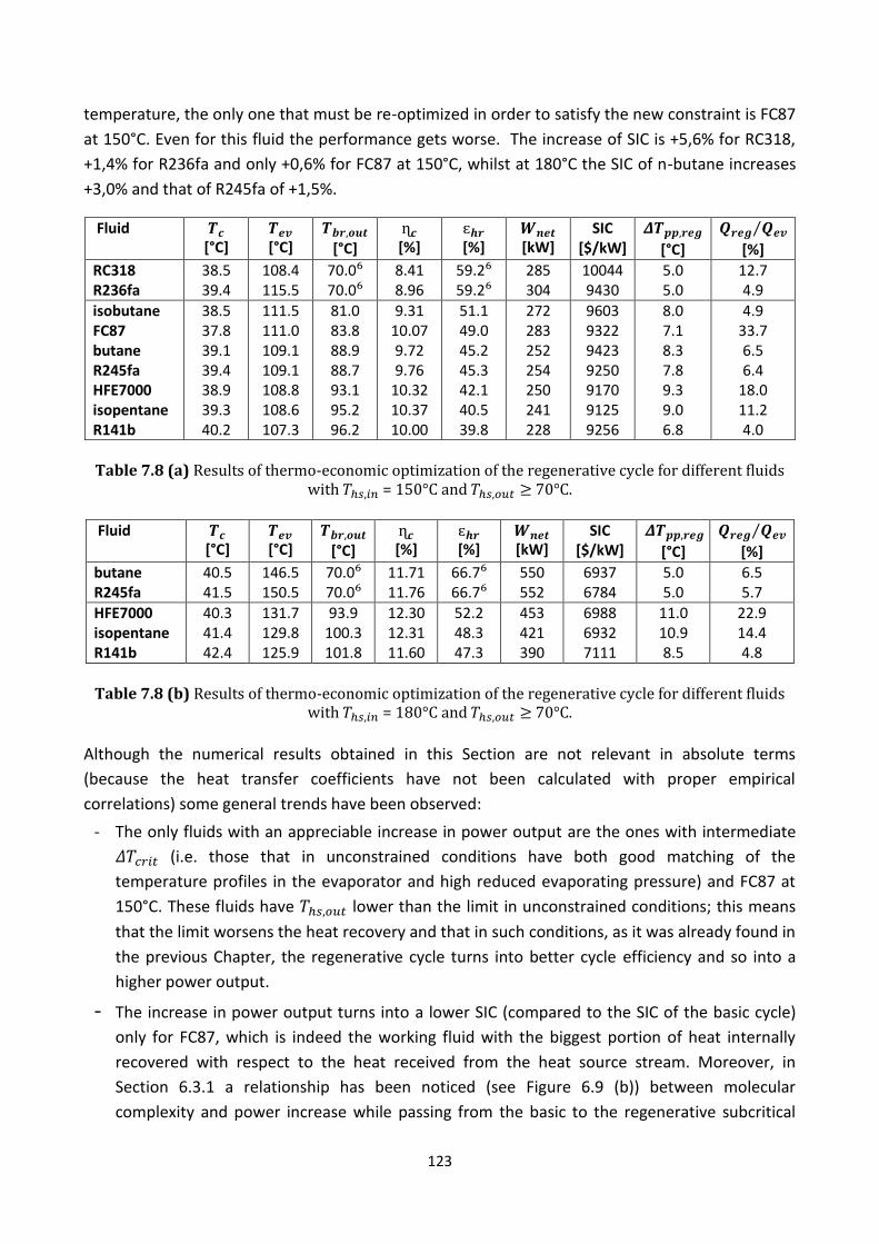
123
temperature, the only one that must be re-optimized in order to satisfy the new constraint is FC87
at 150°C. Even for this fluid the performance gets worse. The increase of SIC is +5,6% for RC318,
+1,4% for R236fa and only +0,6% for FC87 at 150°C, whilst at 180°C the SIC of n-butane increases
+3,0% and that of R245fa of +1,5%.
Fluid [°C]
[°C]
[°C] [%]
[%]
[kW]
SIC [$/kW]
[°C]
⁄
[%]
RC318 R236fa
38.5 39.4
108.4 115.5
70.0⁶ 70.0⁶
8.41 8.96
59.2⁶ 59.2⁶
285 304
10044 9430
5.0 5.0
12.7 4.9
isobutane FC87 butane R245fa HFE7000 isopentane R141b
38.5 37.8 39.1 39.4 38.9 39.3 40.2
111.5 111.0 109.1 109.1 108.8 108.6 107.3
81.0 83.8 88.9 88.7 93.1 95.2 96.2
9.31 10.07 9.72 9.76
10.32 10.37 10.00
51.1 49.0 45.2 45.3 42.1 40.5 39.8
272 283 252 254 250 241 228
9603 9322 9423 9250 9170 9125 9256
8.0 7.1 8.3 7.8 9.3 9.0 6.8
4.9 33.7 6.5 6.4
18.0 11.2 4.0
Table 7.8 (a) Results of thermo-economic optimization of the regenerative cycle for different fluids
with = 150°C and 70°C.
Fluid [°C]
[°C]
[°C]
[%]
[%]
[kW]
SIC [$/kW]
[°C]
⁄
[%]
butane R245fa
40.5 41.5
146.5 150.5
70.0⁶ 70.0⁶
11.71 11.76
66.7⁶ 66.7⁶
550 552
6937 6784
5.0 5.0
6.5 5.7
HFE7000 isopentane R141b
40.3 41.4 42.4
131.7 129.8 125.9
93.9 100.3 101.8
12.30 12.31 11.60
52.2 48.3 47.3
453 421 390
6988 6932 7111
11.0 10.9 8.5
22.9 14.4 4.8
Table 7.8 (b) Results of thermo-economic optimization of the regenerative cycle for different fluids
with = 180°C and 70°C.
Although the numerical results obtained in this Section are not relevant in absolute terms
(because the heat transfer coefficients have not been calculated with proper empirical
correlations) some general trends have been observed:
- The only fluids with an appreciable increase in power output are the ones with intermediate
(i.e. those that in unconstrained conditions have both good matching of the
temperature profiles in the evaporator and high reduced evaporating pressure) and FC87 at
150°C. These fluids have lower than the limit in unconstrained conditions; this means
that the limit worsens the heat recovery and that in such conditions, as it was already found in
the previous Chapter, the regenerative cycle turns into better cycle efficiency and so into a
higher power output.
- The increase in power output turns into a lower SIC (compared to the SIC of the basic cycle)
only for FC87, which is indeed the working fluid with the biggest portion of heat internally
recovered with respect to the heat received from the heat source stream. Moreover, in
Section 6.3.1 a relationship has been noticed (see Figure 6.9 (b)) between molecular
complexity and power increase while passing from the basic to the regenerative subcritical

124
cycle. FC87 was exactly the fluid with the biggest increase due to the high value of the
mentioned parameter.
7.4 Basic supercritical cycle
The aim of the present Chapter is to set realistic values to variables (the pinch points in the heat
exchangers and the condensing pressure) that were assumed a priori in the thermodynamic
optimization through a thermo-economic optimization and to see whether the thermo-economic
optimum moves away from the thermodynamic one. As already stated in Chapter VI, the model of
the supercritical cycle has one degree of freedom more than the subcritical, since the evaporating
pressure is not enough to define the thermodynamic conditions at the turbine inlet: the maximum
temperature must be also determined. The latter must lie above the critical temperature and
obviously below the inlet heat source temperature. The evaporating pressure must lie above the
critical pressure and below a certain maximum pressure (approximately 60 bar [66]) in order to
avoid expensive piping class.
With the usual assumptions (constant isentropic efficiency of the pump and the turbine, negligible
pressure drops and given temperature and mass flow rate of the heat source), the system has five
independent variables that shall be found through the thermo-economic optimization. As for the
subcritical cycle, the objective is to understand how the decision variables move from the
thermodynamic to the thermo-economic optimization. The pinch points and the condensing
pressure will be set again through the thermo-economic optimization, then the evaporating
pressure and the maximum temperature will be compared, from the condition of maximum power
output to that of minimum SIC.
7.4.1 Results of thermo-economic optimization and comparison with the subcritical cycle
The results of the thermo-economic optimization are shown in Tables 7.9 (a) and (b) for inlet heat
source temperature of 150 and 180°C, respectively.
The global heat transfer coefficient has been assumed equal to 0.500 kW/(m²K), that is higher
than the coefficient of the preheater but lower than that of the vaporizer of the subcritical cycle.
This is a very rough assumption. Nonetheless, this work does not aim at finding the correct results,
but rather at understanding how the thermodynamic variables interact in the optimization process
and how the same parameters move after having introduced the cost of the equipment and
minimized the thermo-economic objective function.

125
Fluid PR SIC
R134a 37.2 9.6 145 5 1.09 68.2 4.68 8.81 60.6 305 9028
R227ea 36.1 9.3 145 5 1.24 67.0 5.91 8.17 61.4 287 9406
R1234ze 37.2 9.7 145 5 1.14 75.9 5.82 9.23 54.9 290 9016
RC318 37.2 9.7 145 5 1.09 73.1 6.65 8.32 57.0 271 9158
R236fa 38.4 10.5 139.1 5 1.03 83.7 7.91 9.55 49.1 269 8909
isobutane 38.7 10.5 139.7 5 1.03 99.9 7.31 10.0 37.1 213 9766
Table 7.9 (a) Optimized parameters of supercritical cycle after SIC minimization for = 150°C.
Fluid PR SIC
RC318 37.3 10.3 171.1 5 1.44 63.2 8.75 8.95 70.8 445 7455
R236fa 38.8 10.8 169.7 5 1.24 74.1 9.43 10.3 64.2 465 6951
Isobutane 39.3 11.2 169.2 5 1.04 82.2 7.27 10.7 59.2 447 6915
Butane 40.5 11.9 169.4 5 1.03 98.8 10.18 11.8 49.2 412 6890
R245fa 41 12.3 171.6 5 1.03 101.1 14.57 12.0 47.9 406 6777
Table 7.9 (b) Optimized parameters of supercritical cycle after SIC minimization for = 180°C.
The pinch point in the supercritical evaporator lies on the lower limit that was fixed in order to
grant the heat transfer from the hot fluid to the working fluid (5 K); this means that the advantage
of well matching temperature profiles compensates the disadvantage of large heat exchange
areas. The working fluid maximum temperature is very close to the inlet heat source temperature
and the evaporating pressure of working fluids with low critical temperature is higher than that of
fluids with critical point close to the inlet heat source temperature. This may be due to the need of
cooling down the hot source stream to a sufficiently low temperature.
Cycle Subcritical Supercritical
Fluid [%]
[%]
[kW]
SIC [$/kW]
[%]
[%]
[kW]
SIC [$/kW]
R134a R227ea R1234ze RC318 R236fa isobutane
6.62 6.55 7.30 7.84 8.70 8.90
77.1 78.9 74.9 78.4 72.1 53.3
291 292 314 347 370 269
11438 11309 10424 9727 9118 9452
8.81 8.17 9.23 8.32 9.55 10.0
60.6 61.4 54.9 57.0 49.1 37.1
305 287 290 271 269 213
9028 9406 9016 9158 8909 9766
Table 7.10 (a) Cycle efficiency, heat recovery effectiveness, net power output and SIC after thermo-
economic optimization for = 150°C in subcritical and supercritical conditions.

126
Cycle Subcritical Supercritical
Fluid [%]
[%]
[kW]
SIC [$/kW]
[%]
[%]
[kW]
SIC [$/kW]
RC318 R236fa isobutane FC87 butane R245fa
7.59 8.67 9.58 8.12 11.2 11.1
81.9 80.2 78.7 78.9 74.7 75.9
431 484 525 449 581 591
8625 7850 7446 7698 6813 6651
8.95 10.3 10.7
- 11.8 12.0
70.8 64.2 59.2
- 49.2 47.9
445 465 447
- 412 406
7455 6951 6915
- 6890 6777
Table 7.10 (b) Cycle efficiency, heat recovery effectiveness, net power output and SIC after thermo-
economic optimization for = 180°C in subcritical and supercritical conditions (bold).
7.4.2 Deviation of the thermo-economic optimum from the thermodynamic optimum
The objective of this section is the same as that of section 7.2.2: understanding where the optimal
thermo-economic conditions tend to with respect to the thermodynamic optimum. We chose
again the working fluid R227ea with . The condensing temperature has been fixed
to 37°C and the pinch points in the evaporator and in the condenser have been set to 5 and 10 K,
respectively. The diagram of Figure 7.5 pictures the same trend of power output found in the
previous Chapter. We already know that, according to the constraint on the entropy at turbine
inlet ( ), only the upper left-hand part of the graph is really meaningful in order to avoid
partial condensation in the expander.
Figure 7.5 Level curves of power output versus and for R227ea with = 150°C.
Now that the trend of power output has been defined within the borders of the selected
independent variables, we aim at investigating how the cost relations of the equipment move the
sub-optimal region (red area in Figure 7.5) while passing from thermodynamic to thermo-
economic optimum. As already stated, the couple turbine-generator and the equipment
associated with the air cooled condenser (condenser itself, fans and electrical motors) are the
main cost items in the plant economic balance. Therefore, their capital cost has been plotted as
function of and .
1 1,2 1,4 1,6 1,8 2 2,2110
115
120
125
130
135
140
145
326,7
314,9
303,5
291,7
280
268,5
256,8
245
233,3
221,8
210,1
pev;red
T3

127
The capital cost for the equipment shows strong dependence on the evaporating pressure. The
interpretation of this dependence could be misleading. It could be intended, indeed, that since the
condensing pressure is assumed, the turbine power output increases due to the higher enthalpy
drop in the expander ( ) caused by the higher pressure ratio. The results, instead, show that
decreases with increasing evaporating pressure for a given . Thus, something else must
justify the low cost of the turbine at low evaporating pressures. For constant , the increase in
evaporating pressure provokes a decrease in (see isenthalpic lines in the T-s diagram of a pure
substance in Figure 7.8) which overwhelms the increase of due to the higher pressure ratio.
This means that an increase of evaporating pressure causes a decrement of the enthalpy received
by the working fluid in the evaporation, . In a supercritical cycle, for fluids with a high
as for example R227ea at 150°C, the increase in evaporating pressure does not modify
substantially the heat recovered by the heat source stream. This involves that the mass flow rate
of the working fluid must increase, and so the cost of equipment.
Figure 7.6 T-s diagram of a pure substance. At constant temperature, in the supercritical region an increase of pressure provokes a drop in enthalpy.
Furthermore, the minimum of occurs at high , as can be seen in Figure 7.9. For a given
evaporating pressure, higher means higher and, in turn, higher . Even if the heat flow
rate absorbed by the cycle were constant, higher would imply a lower working fluid mass
flow rate. Nonetheless, it has been observed that for a certain , increasing leads, after a
certain temperature, to a drop in the heat recovery effectiveness. The combination of increasing
and decreasing turns into a fall of the working fluid mass flow rate and in turn of the
equipment cost.

128
Figure 7.7 Level curves of capital cost of the equipment versus and for R227ea
with = 150°C.
From the comparison between Figures 7.5 and 7.7, it emerges that the zone of minimum capital
cost (blue area in Figure 7.7) corresponds to a zone of medium power output, for the reasons
already explained within the above lines. Therefore, the minimum SIC shifts from the
thermodynamic sub-optimal region towards the top left-hand corner of the diagram, where cycle
efficiency is high (as shown in Figure 6.11). The specific investment cost increases when moving
towards lower temperatures and higher pressure ratios, as illustrated in Figure 7.8.
Figure 7.8 Level curves of SIC versus and for R227ea with = 150°C.
7.5 Conclusions
Because of the simple models used in the present Chapter, the latter was not meant to provide
precise indications on component costs and sizing. Instead, the aim is to analyze some general
trends that could be expected in the working fluid selection while passing from a purely
1 1,2 1,4 1,6 1,8 2 2,2110
115
120
125
130
135
140
145
3,638E+06
3,540E+06
3,442E+06
3,343E+06
3,245E+06
3,147E+06
3,049E+06
2,954E+06
2,856E+06
2,758E+06
pev;red
T3
1 1,2 1,4 1,6 1,8 2 2,2110
115
120
125
130
135
140
145
15899
15247
14611
13959
13307
12656
12020
11368
10716
10064
9428
pev;red
T3
129
thermodynamic optimization to a thermoeconomic preliminary design of an ORC system. The heat
source is still a 10 kg/s mass flow rate of subcooled water at 150°C and 180°C. The objective of the
optimization was the minimization of the Specific Investment Cost (SIC) of the plant, later defined.
It has already been concluded that whereas the thermodynamic optimum (maximum power
output) is obtained by maximizing the system overall efficiency , regardless of the
relative contribution of each factor to the product, in the thermoeconomic optimization achieving
a certain with high rather than with high seems to be a favorable condition. Indeed,
increasing leads to bigger components and so to a higher capital cost of the equipment. This
fact has been noticed both in the subcritical and in the supercritical cycle, in fact:
- In the basic subcritical cycle, fluids with small or negative , that were excluded by the
thermodynamic selection, become competitive with the introduction of the economic
objective function. Indeed, thanks to their high latent heat of vaporization and critical
temperature, these fluids have relatively high and low with respect to the
“thermodynamically” optimal working fluids.
- In the basic supercritical cycle, the thermoeconomic optimal region corresponds to a region of
high cycle efficiency, i.e. with high maximum temperature and low evaporating pressure. In the subcritical regenerative cycle, the best fluid is still FC87, i.e. the one that showed the best
performance even from a thermodynamic point of view. This means that, with the assumed heat
transfer coefficients and cost correlations, the increase in power output is more relevant than the
increase in capital cost caused by the additional heat exchanger. Moreover, the constraint on
is still a necessary condition in order to make the regenerative configuration interesting.

130
Bibliography
[1] <http://en.wikipedia.org/wiki/Global_warming> [accessed 8.4.2014]
[2] <http://www.worldenergyoutlook.org/resources/energydevelopment/accesstoelectricity/>
[accessed 8.4.2014]
[3] Duque MR. Geothermal reservoirs: from vapour dominated to conductive systems. In:
International Conference on Renewable Energies and Power Quality (ICREPQ’13) Bilbao
(Spain), 20th to 22th March, 2013.
[4] Hettiarachchi MHD, Golubovic M, Worek WM, Ikegami Y. Optimum design criteria for an
Organic Rankine cycle using low-temperature geothermal heat sources. Energy 32 (2007)
1698–1706.
[5] Franco A, Villani M. Optimal design of binary cycle power plants for water-dominated, medium
temperature geothermal fields. Geothermics 38, 379–391.
[6] Toffolo A, Lazzaretto A, Manente G, Rossi N. Synthesis/Design Optimization of Organic Rankine
Cycles for Low Temperature Geothermal Sources with the HEATSEP Method. In: Proceedings
of ECOS 2010, Lausanne (Switzerland), June 14-17, 2010.
[7] <http://en.wikipedia.org/wiki/Geothermal_power_in_New_Zealand> [accessed 8.4.2014]
[8] <http://geothopica.igg.cnr.it/> [accessed 8.4.2014]
[9] Antics M, Bertani R, Sanner B. Summary of ECG 2013 Country Update Reports on Geothermal
Energy in Europe. Available at:
<http://www.gpc-france.com/archives/EGC2013_Keynote%201.pdf> [accessed 8.4.2014]
[10] Matek B. 2013 Geothermal Power: International Market Overview. Geothermal Energy
Association. Available at [accessed 8.4.2014]:
http://geo-energy.org/events/2013%20International%20Report%20Final.pdf
[11] Schellschmidt R, Sanner B, Pester S, Schulz R. Geothermal energy use in Germany. In:
Proceedings World Geothermal Congress 2010 Bali, Indonesia, 25-29 April 2010.
[12] <www.geothermie.de> [accessed 8.4.2014].
[13] Bini R, Di Prima M, Guercio A. Organic Rankine Cycle (ORC) in biomass plants: an overview on
different applications. Available at: <http://www.turboden.eu/it/public/downloads/>
[accessed 8.4.2014].

131
[14] Schuster A, Karellas S, Kakaras E, Spliethoff H. Energetic and economic investigation of
Organic Rankine Cycle applications. Applied Thermal Engineering 29 (2009) 1809–1817.
[15] Karellas S, Schuster A. Supercritical fluid parameters in Organic Rankine Cycle applications. Int.
J. of Thermodynamics Vol. 11 (No. 3), pp. 101-108, September 2008.
[16] Quoilin S. Sustainable energy conversion through the use of Organic Rankine Cycles for waste
heat recovery and solar applications (Abstract from PhD Thesis, Creative Commons licensed,
available at: <http://bictel.ulg.ac.be/ETD-db/collection/available/ULgetd-10032011-
002906/unrestricted/PhD_Thesis_Dissertation.pdf> [accessed 8.4.2014]).
[17] Dong L, Liu H, Riffat S. Development of small-scale and micro-scale biomass-fuelled CHP
systems - A literature review. Applied Thermal Engineering 29 (2009) 2119–2126.
[18] Obernberger I, Thonhofer P, Reisenhofer E. Description and evaluation of the new 1000 kWel
Organic Rankine Cycle process integrated in the biomass CHP plant in Lienz, Austria.
Euroheat & Power, Volume 10/2002.
[19] Tchanche BF, Lambrinos G, Frangoudakis A, Papadakis G. Low-grade heat conversion into
power using organic Rankine cycles – A review of various applications. Renewable and
Sustainable Energy Reviews 15 (2011) 3963–3979.
[20] Rayegan R, Tao YX. A procedure to select working fluids for Solar Organic Rankine Cycles
(ORCs). Renewable Energy 36 (2011) 659-670.
[21] Tchanche BF, Papadakis G, Lambrinos G, Frangoudakis A. Fluid selection for a low-
temperature solar organic Rankine cycle. Applied Thermal Engineering 29 (2009) 2468-2476.
[22] Nguyen VM, Doherty PS, Riffat SB. Development of a prototype low temperature Rankine
cycle electricity generation system. Applied Thermal Engineering 2001; 21:169–81.
[23] Orosz M. Small scale solar ORC system for distributed power in Lesotho. Johannesburg, South
Africa: Solar World Congress; 2009.
[24] <http://www.businessweek.com/articles/2013-11-14/2014-outlook-solar-energy-shakeout-
concentrating-vs-dot-photovoltaic> [accessed 8.4.2014].
[25] Waste heat recovery: technology and opportunity in the U.S. industry. (Prepared by BCS, Inc.
for the U.S. Department of Energy). Available at:
<https://www1.eere.energy.gov/manufacturing/intensiveprocesses/pdfs/waste_heat_recov
ery.pdf> [accessed 8.4.2014].
[26] <http://www.hreii.eu/it/index.php> [accessed 8.4.2014].
[27] Liu BT, Chien KH, Wang CC. Effect of working fluids on organic Rankine cycle for waste heat
recovery. Energy 2004; 29: 1207–17.

132
[28] Drescher U, Brüggemann D. Fluid selection for the Organic Rankine Cycle (ORC) in biomass
power and heat plants. Applied Thermal Engineering 27 (2007) 223–228.
[29] Bejan A, Tsatsaronis G, Moran M. Thermal design and optimization. Wiley Interscience, John
Wiley Sons Inc., New York (1996).
[30] Shengjun Z, Huaixin W, Tao G. Performance comparison and parametric optimization of
subcritical Organic Rankine Cycle (ORC) and transcritical power cycle system for low
temperature geothermal power generation. Applied Energy 2011; 88:2740–54.
[31] Dai Y, Wang J, Gao L. Parametric optimization and comparative study of organic Rankine cycle
(ORC) for low grade waste heat recovery. Energy Conversion and Management 2009;
50:576–82.
[32] Lai NA, Wendland M, Fischer J. Working fluids for high-temperature organic Rankine cycles.
Energy 36 (2011) 199-211.
[33] Mago PJ, Srinivasan KK, Chamra LM, Somayaji C. An examination of exergy destruction in
organic Rankine cycles. International Journal of Energy Research, 2008; 32:926–938.
[34] Schuster A, Karellas S, Aumann R. Efficiency optimization potential in supercritical Organic
Rankine Cycles. Energy 35 (2010) 1033–1039.
[35] Karellas S, Schuster A, Leontaritis AD. Influence of supercritical ORC parameters on plate heat
exchanger design. Applied Thermal Engineering 33-34 (2012) 70-76.
[36] Lazzaretto A, Toffolo A, Manente G, Rossi N, Paci M. Cost evaluation of organic Rankine cycles
for low temperature geothermal sources. In: Proceedings of ECOS 2011, Novi Sad (Serbia).
[37] Yamamoto T, Furuhata T, Arai N, Mori K. Design and testing of the Organic Rankine Cycle.
Energy 2001; 26: 239–251.
[38] Saleh B, Koglbauer G, Wendland M, Fischer J. Working fluids for low-temperature organic
Rankine cycles. Energy 2007; 32: 1210–21.
[39] Calise F, Capuozzo C, Vanoli L. Design and parametric optimization of an Organic Rankine
Cycle powered by solar energy. American Journal of Engineering and Applied Sciences, 6 (2):
178-204, 2013.
[40] Harada KJ. Development of a small scale scroll expander. (Abstract from MSc Thesis,
available at:
<http://ir.library.oregonstate.edu/xmlui/bitstream/handle/1957/18837/HaradaKevinJ2011.p
df> [accessed 8.4.2014]).
[41] Chen Y, Lundqvist P, Johansson A, Platell P. A comparative study of the carbon dioxide
transcritical power cycle compared with an organic rankine cycle with R123 as working fluid
in waste heat recovery. Applied Thermal Engineering 26 (2006) 2142–2147.
133
[42] Zhang B, Peng X, He Z, Xing Z, Shu P. Development of a double acting free piston expander for
power recovery in transcritical CO2 cycle. Applied Thermal Engineering 27 (2007) 1629-1636.
[43] Tian H, Ma Y, Li M, Wang W. Study on expansion power recovery in CO2 trans-critical cycle.
Energy Conversion and Management 51 (2010) 2516–2522.
[44] Sauret E, Rowlands AS. Candidate radial-inflow turbines and high-density working fluids for
geothermal power systems. Energy 36 (2011) 4460-4467.
[45] Guo T, Wang HX, Zhang SJ. Comparative analysis of CO2-based transcritical Rankine cycle and
HFC245fa-based subcritical organic Rankine cycle using low-temperature geothermal source.
Science China – Tech. Science, 2010, 53: 1638−1646.
[46] Bombarda P, Invernizzi C, Pietra C. Heat recovery from Diesel engines: a thermodynamic
comparison between Kalina and ORC cycles. Applied Thermal Engineering 30, 2-3 (2009) 212.
[47] Rodriguez CEC, Palacio JCE, Sotomonte CR, Leme M, Venturini OJ, Lora EES, Cobas VM, dos
Santos DM, Lofrano Dotto FR, Gialluca V. Exergetic and economic analysis of Kalina cycle for
low temperature geothermal sources in Brazil. In: Proceedings of ECOS 2012, Perugia (Italy).
[48] Nag PK, Gupta A. Exergy analysis of the Kalina Cycle. Applied Thermal Engineering Vol. 18, No.
6, pp. 427±439, 1998.
[49] Chys M, Van Den Broek M, Vanslambrouck B, De Paepe M. Potential of zeotropic mixtures as
working fluids in organic Rankine cycles. Energy 44 (2012) 623-632.
[50] DiPippo R. Second Law assessment of binary plants generating power from low-temperature
geothermal fluids. Geothermics 33 (2004) 565–586.
[51] Liebowitz HM, Mlcak HA. Design of a 2 MW Kalina cycle® binary module for installation in
Húsavık, Iceland. Geothermal Res. Council Trans. (1999) 23, 75–80.
[52] Mlcak HA. Kalina cycle® concepts for low temperature geothermal. Geothermal Res. Council
Trans. (2002) 26, 707–713.
[53] Clemente S, Micheli D, Reini M, Taccani R. Performance analysis and modeling of different
volumetric expanders for small-scale organic rankine cycles. In: Proceedings of the ASME
2011, Washington DC, USA.
[54] Macchi E. The choice of working fluid: the most important step for a successful Organic
Rankine Cycle (and an efficient turbine). In: ASME ORC 2013, Rotterdam. Available at:
<http://www.asme-orc2013.nl/content/presentations> [accessed 8.4.2014].
[55] Quoilin S, Declaye S, Legros A, Guillaume L, Lemort V. Working fluid selection and operating
maps for Organic Rankine Cycle expansion machines. International Compressor Engineering
Conference, July 16-19, 2012, Purdue, USA.

134
[56] Bambang Teguh P. Design of n-Butane Radial Inflow Turbine for 100 kW binary cycle power
plant. International Journal of Engineering & Technology IJET-IJENS Vol: 11 No: 06.
[57] Turton RK. Principles of Turbomachinery. London: E. & F.N. Spon, 1995.
[58] <http://exergy-orc.com/radial-outflow-turbine> [accessed 8.4.2014]
[59] Rama Gorla SR, Khan AA. Turbomachinery: design and theory. Marcel Dekker Inc., New York,
2003.
[60] Dixon SL, Hall CA. Fluid Mechanics and Thermodynamics of Turbomachinery. Butterworth
Heinemann, Sixth edition, 2010.
[61] Balje O. Turbomachines: a guide to selection and theory. Wiley (New York), 1981.
[62] Japikse D, Baines NC. Introduction to turbomachinery. Norwich (VT), Concepts ETI, Oxford,
1994.
[63] Wood HJ. Current technology of radial-inflow turbines for compressible fluids. Journal of
Engineering for GT and Power. Transactions of the ASME 1963;85:72–83.
[64] Clemente S, Micheli D, Reini M, Taccani R. Bottoming organic Rankine cycle for a small scale
gas turbine: a comparison of different solutions. Applied Energy 106 (2013) 355–364.
[65] Congedo PM, Corre C, Cinnella P. Numerical investigation of dense-gas effects in
turbomachinery. Computers & Fluids 49 (2011) 290–301.
[66] Marcuccilli F, Thiolet D. Optimizing Binary Cycles in Radial Inflow Turbines, GRC Transactions,
2009.
[67] Xodo LG, Spadacini C, Astolfi M, Macchi E. Comparison of axial and radial outflow turbines in a
medium-high enthalpy heat recovery ORC application. In: ASME ORC 2013, Rotterdam.
Available at: <http://www.asme-orc2013.nl/content/presentations> [accessed 8.4.2014].
[68] Lazzaretto A, Manente G. A criterion to optimize ORC design performance taking into account
real turbine efficiencies. In: Proceedings of ECOS 2013, Guilin, China.
[69] Macchi E, Perdichizzi A. Efficiency prediction for axial-flow turbines operating with
nonconventional fluids. Journal of Engineering for Power, October 1981, Vol. 103, 718- 724.
[70] Pasquale D, Ghidoni A, Rebay S. Shape optimization of an Organic Rankine Cycle radial turbine
nozzle. Journal of Engineering for Gas Turbines and Power 135(4), 2013.
[71] Peterson RB, Wang H, Herron T. Performance of a small-scale regenerative Rankine power
cycle employing a scroll expander. In: Proceedings of the IMechE, Part A: Journal of Power
and Energy, 2008, 222: 271.

135
[72] Zanelli R, Favrat D. Experimental Investigation of a Hermetic Scroll Expander-Generator.
(1994). International Compressor Engineering Conference. Paper 1021.
[73] Lemort V, Quoilin S, Cuevas C, Lebrun J. Testing and modeling a scroll expander integrated
into an Organic Rankine Cycle. Applied Thermal Engineering 29 (2009) 3094–3102.
[74] Xiaojun G, Liansheng L, Yuanyang Z, Pengcheng S. Research on a scroll expander used for
recovering work in a fuel cell. Internaltional Journal of Thermodynamics. Vol. 7, No. 1, pp. 1-
8, March, 2004.
[75] Yanagisawa T, Fukuta M, Ogi Y, Hikichi T. Performance of an oil-free scroll-type air expander.
In: Proceedings of the IMechE Conference on Compressors and their Systems, 2001, 167-
174.
[76] Lemort V, Quoilin S. Designing scroll expanders for use in heat recovery Rankine cycles.
IMechE, 2009.
[77] Lemort V, Declaye S, Quoilin S. Experimental characterization of a hermetic scroll expander
for use in a micro-scale Rankine cycle. In: Proceedings of the IMechE, Part A: Journal of
Power and Energy 2012 226: 126.
[78] Woodland BJ, Braun JE, Groll EA, Horton WT. Experimental testing of an Organic Rankine
Cycle with scroll-type expander. (2012). Publications of the Ray W. Herrick Laboratories.
Paper 52. Available at: <http://docs.lib.purdue.edu/herrick/52> [accessed 8.4.2014].
[79] Brümmer A. Energy efficiency – waste heat utilization with screw expanders. Pumps,
Compressors and Process Components 2012, pp. 120-126.
[80] Glavatskaya Y, Podevin P, Lemort V, Shonda O, Descombes G. Reciprocating expander for an
exhaust heat recovery Rankine Cycle for a passenger car application. Energies 2012, 5, 1751-
1765.
[81] Papadopoulos AI, Stijepovic M, Linke P. On the systematic design and selection of optimal
working fluids for Organic Rankine Cycles. Applied Thermal Engineering 2010; 30:760–69.
[82] Delgadeo-Torres AM, Garcia-Rodriguez L. Preliminary assessment of solar organic Rankine
cycles for driving a desalination system. Desalination 2007; 216:252-75.
[83] Tang Y. Screw Compressors with a Novel Flexible Discharge Port Design. In: International
Compressor Engineering Conference at Purdue 2012.
[84] Andersen WC, Bruno TJ. Rapid screening of fluids for chemical stability in organic rankine
cycle applications. Industrial and Engineering Chemistry 44 (2005) 5560–5566.
[85] Marcuccilli F, Zouaghi S. Radial Inflow Turbines for Kalina and Organic Rankine Cycles. In:
Proceedings European Geothermal Congress 2007, Unterhaching (Germany).
136
[86] Lee MJ, Tien DL, Shao CT. Thermophysical capability of ozonesafe working fluids for an organic
Rankine cycle system. Heat Recovery Systems & CHP 13 (5) (1993) 409–418.
[87] Maizza V, Maizza A. Unconventional working fluids in organic Rankine-cycles for waste energy
recovery systems, Applied Thermal Engineering 21 (2001) 381–390.
[88] ASHRAE Standard 34. Available at:
<https://www.ashrae.org/File%20Library/docLib/Public/20080807_34m_thru_34v_final.pdf
> [accessed 8.4.2014].
[89] <http://www.nedo.go.jp/content/100080128.pdf> [accessed 8.4.2014].
[90] <http://en.wikipedia.org/wiki/Montreal_Protocol> [accessed 8.4.2014].
[91] Branchini L, De Pascale A, Peretto A. Systematic comparison of ORC configurations by means
of comprehensive performance indexes. Applied Thermal Engineering 61 (2013) 129-140.
[92] Angelino G, Colonna di Paliano P. Multicomponent working fluids for Organic Rankine Cycles
(ORCs). Energy, Vol. 23, No. 6, pp. 449–463, 1998.
[93] Heberle F, Preissinger C, Brüggemann D. Zeotropic mixtures as working fluids in Organic
Rankine Cycles for low-enthalpy geothermal resources. Renewable Energy 37 (2012) 364-
370.
[94] Klein SA. Engineering Equation Solver (EES), Academic Professional Version. F-Chart Software,
Middleton, WI, 2012.
[95] Listing of GWP Values as per Report IPCC WG1 AR4. Available at:
<http://www.fmv.se/Global/Dokument/Engelska%20webben/Our%20activities/Enviroment
al%20work/Environmental%20criteria%20documents/121023/12FMV1533%202%201%20G
WP%20eng.pdf> [accessed 8.4.2014].
[96] Available at:
<http://www.epa.gov/ozone/snap/refrigerants/Notice25SubstituteRefrigerants.pdf>
[accessed 12.9.2013].
[97] Invernizzi C, Iora P, Silva P. Bottoming micro-Rankine cycles for micro-gas turbines. Applied
Thermal Engineering 2007; 27: 100–110.
[98] Turton R, Bailie RC, Whiting WB. Analysis, synthesis, and design of chemical processes. 3rd
edition, Prentice Hall, 2009.
[99] Kakac S. Boilers, evaporators and condensers. Wiley, 1991.
Related Documents