ABSTRACT Title: ANALYSIS OF ROUTING STRATEGIES IN AIR TRANSPORTATION NETWORKS FOR EXPRESS PACKAGE DELIVERY SERVICES Subrat Mahapatra, M.S., 2005 Directed By: Professor Ali Haghani, Department of Civil and Environmental Engineering The package delivery industry plays a dominant role in our economy by providing consistent and reliable delivery of a wide range of goods. Shipment Service Providers (SSP) offer a wide range of service levels characterized by varying time windows and modes of operation and follow different network configurations and strategies for their operations. SSP operate vast systems of aircraft, trucks, sorting facilities, equipment and personnel to move packages between customer locations. Due to the high values of the assets involved in terms of aircraft and huge operational cost implications, any small percentage savings could result in the order of savings of millions of dollars for the company. The current research focuses on the Express Package Delivery Problem and the optimization of the air transportation network. SSP must determine which routes to fly, which fleets to assign to those routes and how to assign packages to those aircraft, all in response to demand projections and operational restrictions. The objective is to find the cost minimizing movement of packages from their origins to their destinations given the very tight service windows, and limited aircraft capacity.

Welcome message from author
This document is posted to help you gain knowledge. Please leave a comment to let me know what you think about it! Share it to your friends and learn new things together.
Transcript

ABSTRACT
Title: ANALYSIS OF ROUTING STRATEGIES IN AIR TRANSPORTATION NETWORKS FOR EXPRESS PACKAGE DELIVERY SERVICES
Subrat Mahapatra, M.S., 2005
Directed By: Professor Ali Haghani,
Department of Civil and Environmental Engineering
The package delivery industry plays a dominant role in our economy by providing consistent
and reliable delivery of a wide range of goods. Shipment Service Providers (SSP) offer a wide
range of service levels characterized by varying time windows and modes of operation and
follow different network configurations and strategies for their operations. SSP operate vast
systems of aircraft, trucks, sorting facilities, equipment and personnel to move packages
between customer locations. Due to the high values of the assets involved in terms of aircraft
and huge operational cost implications, any small percentage savings could result in the order
of savings of millions of dollars for the company. The current research focuses on the
Express Package Delivery Problem and the optimization of the air transportation network.
SSP must determine which routes to fly, which fleets to assign to those routes and how to
assign packages to those aircraft, all in response to demand projections and operational
restrictions. The objective is to find the cost minimizing movement of packages from their
origins to their destinations given the very tight service windows, and limited aircraft
capacity.

In the current research, we formulate the air transportation network as a mixed integer
program which minimizes the total operating costs subject to the demand, capacity, time,
aircraft and airport constraints. We use this model to study of various operational strategies
and their potential cost implications. We consider two main operational strategies: one
involving no intermediate stops on pick-up and delivery sides and the other involving one
intermediate stop between origin and hub on pick-up side and between hub and destination on
delivery side. Under each strategy, we analyze the cost implications under a single hub
network configuration and regional hub network configuration. We study the impact of
various routing scenarios, various variants and logical combinations of these scenarios which
gives a clear understanding of the network structure. We perform an extensive sensitivity
analysis to understand the implications of variation in demand, fixed cost of operation,
variable cost of operation and bounds on the number of aircraft taking off and landing in the
airports.
ANALYSIS OF ROUTING STRATEGIES IN AIR
TRANSPORTATION NETWORKS FOR EXPRESS PACKAGE
DELIVERY SERVICES
By
Subrat Mahapatra
Thesis submitted to the Faculty of the Graduate School of the University of Maryland, College Park, in partial fulfillment
of the requirements for the degree of Master of Science
2005 Advisory Committee: Professor Ali Haghani, Chair Professor Paul Schonfeld Professor G.L. Chang

© Copyright by Subrat Mahapatra
2005
Dedication
To Baba, Bou, Bapa, Maa, Meghana, Kity and Litu
- ii -

Acknowledgements
First and foremost, I would like to thank my advisor Dr. Ali Haghani for his valuable
guidance and patience all these years. This thesis was a learning experience and offered me an
insight about research. I had always been interested in bridging the gap between academic
research and real world industrial applications. I believe that academic research should not be
confined to be a theoretical pursuit of ‘unknown waters’; it should also be oriented towards
subjectivity and real world applicability. A research should shed light on aspects hidden to the
obvious both in the philosophic and practical level. And this research has been a honest
endeavor along these lines. It aims to answers certain questions that come up in a rational
mind. Some of the results may sound obvious at sight; nevertheless, they offer deeper insights
about the system. It would be a great reward if this work aids in some minuscule way towards
some real world implementation.
I would like to take this opportunity to thank my parents, grandparents, brother, sister, family,
friends and relatives who have believed in me and stood by my side all these years. It has not
been an easy journey, but with all the blessings and good wishes, I have come through a long
way. Thanks to Meghana for being such a great emotional support. It would be unfair if I did
not mention how much my brother Siddhartha and sister Sushree cared about my pursuits. I
would also like to thank Dr. Schonfeld and Dr. Chang for being in my committee. Last but not
the least, I am grateful to Dr. Mahmassani and my friends in the Transportation group for
their comments and suggestions for this work.
- iii -

List of Contents
Chapter 1: INTRODUCTION
1.1 Background 1
1.2 Literature Review 5
1.3 Scope of Research 8
1.4 Organization of Thesis 10
Chapter 2: SYSTEM OVERVIEW: CONCEPTS AND DEFINTIONS
2.1 Introduction 11
2.1.1 Direct Flight Delivery Networks 14
2.1.2 Hub and Spoke Networks 14
2.2 Time Windows 16
2.3 Effect of Time Zones 18
2.4 Arc, Path and Route Incidence Matrices 20
Chapter 3: SYSTEM DESIGN AND FORMULATIONS
3.1 Introduction 23
3.2 Assumptions 24
3.3 Terminology 25
3.4 Problem Formulation 27
Chapter 4: DATASETS
4.1 Test Problem Data 29
Chapter 5: NO INTERMEDIATE STOPS ON PICK-UP & DELIVERY ROUTES
5.1 Introduction 37
5.2 Scenario 1: Only one Origin-Hub and only one Hub-Destination pair 39
allowed on pick-up and delivery sides respectively
5.2.1 Case A: Single Hub 39
(i) Pick-up Side 39
- iv -

LIST OF CONTENTS
(ii) Delivery Side 40
5.2.2 Case B: Demands routed through Regional Hubs 41
(i) Pick-up Side 42
(ii) Delivery Side 43
(iii) Interhub Component 44
5.2.3 Case C: Demands routed through origin regional hub and directly 45
dispatched to destination
(i) Pick-up Side 45
(ii) Delivery Side 45
5.2.4 Case D: Demands routed through destination regional hub 45
5.3 Scenario 2: Demands routed from Origin through multiple hubs on pick-up
side and multiple hubs to Destination on delivery side 48
5.3.1 Case A: Demands routed either through Origin Regional Hub 49
or directly to main hub on pickup side and routed either through
destination regional hub or directly to destination on delivery side
(i) Pick-up Side 49
(ii) Delivery Side 50
5.3.2 Case B: Combining Scenario 1 results with Scenario 2 results 52
5.4 Scenario 3:No main hubs; Demands routed through Regional Hubs only 54
5.4.1 Case A: Demands routed either through Origin Regional Hub or 54
directly to Destination Regional Hub on pickup side
5.4.2 Case B: Demands routed either through Destination Regional 56
Hub or directly to destination on delivery side
Chapter 6: INTERMEDIATE STOPS ON PICK-UP & DELIVERY ROUTES
6.1 Introduction 59
6.2 Scenario 1: Presence of One Intermediate Stop on Pick-up and Delivery 61
Routes – Single Hub Case
(i) Pick-up Side 62
(ii) Delivery Side 62
6.3 Scenario 2: Presence of One Intermediate Stop on Pick-up and Delivery 64
Routes – Regional Hubs Present
- v -

LIST OF CONTENTS
(i) Pick-up Side 64
(ii) Delivery Side 65
6.4 Scenario 3: Presence of One Intermediate Stop on Pick-up and Delivery 67
Routes – Demands directly dispatched to Destination Regional Hubs
Case A: One Stop Routes from Origins to Destination Regional Hubs 67
Case B: One Stop Routes from Origin Regional Hubs to Destinations 68
Scenario 4: Demands routed from Origin either through One Stop routes 70
to Destination Regional Hubs or through No Stop Routes through
Origin Regional Hubs on Pickup and Demands routed from Origin
Regional Hubs either through One Stop routes to Destination or
through No Stop routes through Destination Regional Hubs
Chapter 7: SENSITIVITY ANALYSIS
7.1 Introduction 73
7.2 Demand Sensitivity 75
7.2.1 No Intermediate Hub Scenarios 75
7.2.1.1 Scenario 1: Only one Origin-Hub and only one 75
Hub-Destination pair
(i) Single Hub Case 75
(ii) Regional Hubs Present 76
7.2.1.2 Scenario 2: No Intermediate Stops with demands routed 80
through multiple hubs
7.2.1.3 Scenario 3:
7.2.1.3.1 Scenario 3A: Demands routed either through 83
Origin Regional Hub or Destination Regional
Hub on pickup side
7.2.1.3.2 Scenario 3B: Demands routed from Origin 85
Regional Hub to Destination or Destination
Regional Hub on delivery side
7.2.2 One Intermediate Hub Scenarios 87
7.2.2.1 Single Hub Case 87
- vi -

LIST OF CONTENTS
7.2.2.2 All demands routed through origin regional hub 88
7.2.2.3 .1 Scenario 3A 91
7.2.2.3.2 Scenario 3B 92
7.3 Fixed Cost Sensitivity 93
7.3.1 No Intermediate Hub Scenarios 94
7.3.1.1 Scenario 1: Only one Origin-Hub and only one 94
Hub-Destination pair allowed on pick-up and delivery sides
(i) Single Hub Case 94
(ii) Regional Hubs Present 95
7.3.1.2 Scenario 2: No Intermediate Stops with demands routed 99
through multiple hubs
7.3.1.3 Scenario 3:
7.3.1.3.1 Scenario 3A: Demands routed either through 102
Origin Regional Hub or Destination Regional Hub
7.3.1.3.2 Scenario 3B: Demands routed from Origin 105
Regional Hub to Destination or Destination Regional
Hub
7.3.2 One Intermediate Hub Scenarios 108
7.3.2.1 Single Hub Case 108
7.3.2.2 All demands routed through origin regional hub 109
7.3.2.3 .1 Scenario 3A 112
7.2.2.3.2 Scenario 3B 113
7.4 Variable Cost Sensitivity 114
7.4.1 No Intermediate Hub Scenarios 115
7.4.1.1 Scenario 1: Only one Origin-Hub and only one Hub- 115
Destination pair allowed on pick-up and delivery sides
(i) Single Hub Case 115
(ii) Regional Hubs Present 116
7.4.1.2 Scenario 2: No Intermediate Stops with demands routed 120
through multiple hubs
7.4.1.3 Scenario 3:
- vii -

LIST OF CONTENTS
7.4.1.3.1 Scenario 3A: Demands routed either through 123
Origin Regional Hub or Destination Regional
Hub on pickup side
7.4.1.3.2 Scenario 3B: Demands routed from Origin 125
Regional Hub to Destination or Destination
Regional Hub on delivery side
7.4.2 One Intermediate Hub Scenarios 127
7.4.2.1 Single Hub Case 127
7.4.2.2 All demands routed through origin regional hub 128
7.4.2.3 .1 Scenario 3A 131
7.4.2.3.2 Scenario 3B 132
7.5 Bounds on Fights Sensitivity 133
7.5.1 No Intermediate Hub Scenario 133
7.5.1.1 Scenario-1 No intermediate stops with demands routed 133
through multiple hubs
(i) Pickup Side 133
(ii) Delivery Side 135
Chapter 8: CONCLUSION & FUTURE SCOPE OF RESEARCH
8.1 Conclusions 137
8.2 Summary of Results 138
8.2.1 Total Cost Implications of Demand 140
8.2.2 Total Cost Implications of Fixed Cost 142
8.2.3 Total Cost Implications of Variable Cost 143
8.3 Computation Times 146
8.4 Future Scope 147
List of References
Appendices
Appendix 1: Sample Calculation showing the effect of time zones
Appendix 2A: List of Cities and Codes in the sample Air Network
Appendix 2B: Regional Hubs and Connected Cities in the sample Air Network
- viii -
LIST OF FIGURES
List of Figures
Figure 2.1: Express Package Delivery Process
Figure 2.2: Express Package Delivery Network
Figure 2.3: Express Package Delivery Process Flow Figure
Figure 2.4: Direct Flight Delivery Network
Figure 2.5: Hub and Spoke Networks
Figure 2.6: Time Windows
Figure 2.7: Summary Representation of Time Windows
Figure 2.8: Time Zone Map of USA
Figure 2.9: Arcs, Routes and Paths in Air Transportation Network
Figure 4.1: Map showing Cities in Sample Air Network
Figure 4.2: Map showing Location of Hubs in Sample Air Network
Figure 4.3: Package Market Volume Distribution 2001
Figure 4.4a: Regression Analysis for Type-A (B727-100) aircraft travel time
Figure 4.4b: Regression Analysis for Type-B (B757-200) aircraft travel time
Figure 5.1: No Intermediate Stops- Single Hub Case (Pick-up Side)
Figure 5.2: No Intermediate Stops- Single Hub Case (Delivery Side)
Figure 5.3: No Intermediate Stops- Regional Hubs Case (Pick-up Side)
Figure 5.4: No Intermediate Stops- Regional Hubs Case (Delivery Side)
Figure 5.5: Demands routed through Origin Regional Hubs and directly dispatched to Destination
Figure 5.6a: Demands routed through Origin Regional Hub or directly to main hub (Pick-up)
Figure 5.6b: Demands routed through Origin Regional Hub or directly to main hub (Pick-up)
Figure 5.7: Demands routed destination regional hub or directly to destination (Delivery)
Figure 5.8a: Demands routed through Origin Regional Hub or directly to Destination Regional Hub
- ix -

LIST OF FIGURES
Figure 5.8b: Demands routed through Origin Regional Hub or directly to Destination Regional Hub
Figure 5.9: Demands routed through Destination Regional Hub or directly to destination (Delivery)
Figure 6.1: One Stop Routes on Pick-up and Delivery Sides
Figure 6.2: One Stop Routes for Single Hub Case (Pick-up)
Figure 6.3: One Stop Routes for Single Hub Case (Delivery)
Figure 6.4: One Stop Cases with Regional Hubs Present (Pickup Side)
Figure 6.5: One Stop Cases with Regional Hubs Present (Delivery Side)
Figure 6.6: One Stop Routes from Origin Cities to Destination Regional Hubs
Figure 6.7: One Stop Routes From Origin Regional Hubs To Destination Cities
Figure 6.8: Demands routed from Origin either through One Stop routes to Destination Regional
Hubs or through No Stop routes through Original Regional Hubs on Pick-up
Figure 6.9: Demands routed from Origin Regional Hubs either through One Stop routes to
Destinations or through No Stop routes through Destination Regional Hubs on Delivery
Figure 7.1: Demand Sensitivity- No Stop Scenario1- Single Hub Case
Figure-7.2a: Demand Sensitivity- No Stop Scenario1- Regional Hubs Case (Pickup)
Figure 7.2b: Demand Sensitivity- No Stop Scenario1- Regional Hubs Case (Delivery)
Figure 7.3: Demand Sensitivity of Total Cost for Scenario 1 Regional Hub Case
Figure 7.4a: No Stop- Scenario 2 Demand Sensitivity (Pickup)
Figure 7.4b: No Stop- Scenario 2 Demand Sensitivity (Delivery)
Figure 7.5: No Stop- Scenario 2 Demand Sensitivity (Total Cost Variation)
Figure 7.6a: No Stop- Scenario 3A Demand Sensitivity of Regional Hubs
Figure 7.6b: No Stop- Scenario 3A Demand Sensitivity (Total Cost)
Figure 7.7a: No Stop- Scenario 3A Demand Sensitivity of Regional Hubs
Figure-7.7b: No Stop Scenario 3A Total Cost versus Demand
- x -

LIST OF FIGURES
Figure 7.8: One Stop- Single Hub Case Demand Sensitivity Results
Figure 7.9a: One Stop- Scenario 1 Regional Hubs Case Demand Sensitivity (Pickup)
Figure 7.9b: One Stop- Scenario 1 Regional Hubs Case Demand Sensitivity (Delivery)
Figure 7.10: One Stop- Scenario 1 Regional Hubs Case Demand Sensitivity (Total Cost)
Figure 7.11: One Stop- Scenario 3A Demand Sensitivity (Total Cost)
Figure 7.12: One Stop- Scenario 3B Demand Sensitivity (Total Cost)
Figure7.13: Fixed Cost Sensitivity- No Stop Scenario1- Single Hub Case
Figure 7.14a: Fixed Cost Sensitivity- No Stop Scenario1- Regional Hubs Case (Pickup)
Figure 7.14b: Fixed Cost Sensitivity- No Stop Scenario1- Regional Hubs Case (Delivery)
Figure 7.15: Sensitivity of Total Cost for Scenario 1 Regional Hub Case
Figure-7.16a: No Stop- Scenario 2 Fixed Cost Sensitivity (Pickup)
Figure-7.16b: No Stop- Scenario 2 Fixed Cost Sensitivity (Delivery)
Figure 7.17: No Stop- Scenario 2 Demand Sensitivity (Total Cost Variation)
Figure 7.18a: No Stop- Scenario 3A Fixed Cost Sensitivity of Regional Hubs
Figure7.18b: No Stop- Scenario 3A Fixed Cost Sensitivity (Total Cost)
Figure 7.19a: No Stop- Scenario 3A Fixed Cost Sensitivity of Regional Hubs
Figure 7.19b: No Stop- Scenario 3A Fixed Cost Sensitivity (Total Cost)
Figure7.20: One Stop- Single Hub Case Fixed Cost Sensitivity Results
Figure 7.21a: One Stop- Scenario 1 Regional Hubs Case Fixed Cost Sensitivity (Pickup)
Figure 7.21b: One Stop- Scenario 1 Regional Hubs Case Fixed Cost Sensitivity (Delivery)
Figure7.22: One Stop- Scenario 1 Regional Hubs Case Fixed Cost Sensitivity (Total Cost)
Figure 7.23: One Stop- Scenario 3A Fixed Cost Sensitivity (Total Cost)
Figure 7.24: One Stop- Scenario 3B Demand Sensitivity (Total Cost)
Figure 7.25: Variable Cost Sensitivity- No Stop Scenario1- Single Hub Case
- xi -

LIST OF FIGURES
Figure 7.26a: Variable Cost Sensitivity- No Stop Scenario1- Regional Hubs Case (Pickup)
Figure 7.26b: Variable Cost Sensitivity- No Stop Scenario1- Regional Hubs Case (Delivery)
Figure 7.27: Variable Cost Sensitivity of Total Cost for Scenario 1 Regional Hub Case
Figure-7.28a: No Stop- Scenario 2 Variable Cost Sensitivity (Pickup)
Figure-7.28b: No Stop- Scenario 2 Fixed Cost Sensitivity (Delivery)
Figure 7.29: No Stop- Scenario 2 Demand Sensitivity (Total Cost Variation)
Figure 7.30a: No Stop- Scenario 3A Fixed Cost Sensitivity of Regional Hubs
Figure7.30b: No Stop- Scenario 3A Fixed Cost Sensitivity (Total Cost)
Figure 7.31a: No Stop- Scenario 3A Variable Cost Sensitivity of Regional Hubs
Figure 7.31b: No Stop- Scenario 3A Variable Cost Sensitivity (Total Cost)
Figure7.32: One Stop- Single Hub Case Variable Cost Sensitivity Results
Figure 7.33a: One Stop- Scenario 1 Regional Hubs Case Variable Cost Sensitivity (Pickup)
Figure 7.33b: One Stop- Scenario 1 Regional Hubs Case Variable Cost Sensitivity (Delivery)
Figure7.34: One Stop- Scenario 1 Regional Hubs Case Fixed Cost Sensitivity (Total Cost)
Figure 7.35: One Stop- Scenario 3A Variable Cost Sensitivity (Total Cost)
Figure 7.36: One Stop- Scenario 3B Sensitivity (Total Cost)
Figure 7.37a: Effect of Bounds on Pickup Side
Figure 7.37b: Effect of Bounds on Delivery Side
Figure 8.1: Scenario Descriptions
Figure 8.2: Total Cost Variation versus Demand
Figure 8.3 Total Cost Variations versus Fixed Cost
Figure 8.4 Total Cost Variations versus Variable Cost
- xii -

LIST OF TABLES
List of Tables
Table 2.1: Path-Route Incidence Matrix Ipr
Table 2.2: Path-Airport Incidence Matrix Ipw
Table 2.3: Route –Aircraft Type Incidence Matrix Irk
Table 4.1: Market Share of Major Players in Courier Industry
Table 4.2: Aircraft Characteristics
Table 4.3: Travel Time Equations
Table 5.1: Results for No Intermediate Stops- Single Hub Case
Table 5.2: Results for No Intermediate Stops- Regional Hubs Case (Pick-up Side)
Table 5.3: Results for No Intermediate Stops- Regional Hubs Case (Delivery Side)
Table 5.4: Results for No Intermediate Stops- Regional Hubs Case (Total Cost)
Table 5.5: Results for Scenario 1 Case C
Table 5.6: Summary of Results for Scenario 1
Table 5.7a: Results of Scenario 2 Pick-up Side
Table 5.7b: Results of Scenario 2 Delivery Side
Table 5.8: Results of Scenario 2 (Total Cost)
Table 5.9a: Scenario 1 Case A Pick-up with Scenario2 Case A Delivery
Table 5.9b: Scenario 2 Case A Pick-up with Scenario1 Case A Delivery Table 5.10: Results of Scenario 3 Case A (Pick-up) Table 5.11: Results of Scenario 3 Case B (Delivery)
Table 5.12: Summary of No Stop Scenarios
Table 6.1: Results of One Stop Scenario for Single Hub Case
Table 6.2: Comparison of Pick-up Costs for Regional Hubs Case
Table 6.3: Comparison of Delivery Costs for Regional Hubs Case
- xiii -

LIST OF TABLES
Table 6.4: Results of Scenario 3 - One Stop Case A
Table 6.5: Results of Scenario 3 - One Stop Case B
Table 6.6: Results of Scenario 4
Table 6.7: Summary of One Stop Scenarios
Table 7.1: No Stop Scenario 1- Single Hub Case Demand Sensitivity Results
Table 7.2: No Stop Scenario 1- Regional Hub Case Demand Sensitivity Results
Table 7.3: Interhub Transportation Costs
Table 7.4: Demand Sensitivity of Total Cost for Scenario 1 Regional Hub Case
Table 7.5: No Stop- Scenario 2 Demand Sensitivity Results
Table-7.6a: No Stop- Scenario 3A Demand Sensitivity
Table-7.6b: No Stop- Scenario 3B Demand Sensitivity
Table-7.7: One Stop- Single Hub Case Demand Sensitivity Results
Table 7.8: One Stop- Scenario 1 Regional Hubs Case Demand Sensitivity Results
Table-7.9: One Stop- Scenario 1 Regional Hubs Case Demand Sensitivity (Total Cost)
Table 7.10: One Stop- Scenario 3A Demand Sensitivity (Total Cost) Table 7.11: One Stop- Scenario 3B Demand Sensitivity (Total Cost)
Table 7.12: No Stop Scenario 1- Single Hub Case Fixed Cost Sensitivity Results
Table-7.13: No Stop Scenario 1 Regional Hub Case - Fixed Cost Sensitivity Results
Table 7.14: Interhub Transportation Costs
Table 7.15: Fixed Cost Sensitivity of Total Cost for Scenario 1 Regional Hub Case
Table-7.16: No Stop- Scenario 2 Fixed Cost Sensitivity Results
Table7.17: No Stop- Scenario 3A Fixed Cost Sensitivity
Table 7.18: No Stop- Scenario 3B Fixed Cost Sensitivity
Table7.19: One Stop- Single Hub Case Fixed Cost Sensitivity Results
- xiv -
LIST OF TABLES
Table7.20: One Stop- Scenario 1 Regional Hubs Case Fixed Cost Sensitivity Results
Table7.21 One Stop- Scenario 1 Regional Hubs Case Fixed Cost Sensitivity (Total Cost)
Table 7.22 One Stop- Scenario 3A Fixed Cost Sensitivity (Total Cost) Table 7.24: One Stop- Scenario 3B Demand Sensitivity (Total Cost) Table 7.24: No Stop Scenario 1- Single Hub Case Variable Cost Sensitivity Results
Table 7.25: No Stop Scenario 1 Regional Hub Case - Variable Cost Sensitivity Results
Table 7.26: Interhub Transportation Costs
Table 7.27: Variable Cost Sensitivity of Total Cost for Scenario 1 Regional Hub Case
Table 7.28: No Stop- Scenario 2 Variable Cost Sensitivity Results
Table 7.30: No Stop- Scenario 3A Variable Cost Sensitivity
Table 7.31: No Stop- Scenario 3B Fixed Cost Sensitivity
Table7.32: One Stop- Single Hub Case Variable Cost Sensitivity Results
Table 7.33: One Stop- Scenario 1 Regional Hubs Case Variable Cost Sensitivity Results
Table7.34: One Stop- Scenario 1 Regional Hubs Case Fixed Cost Sensitivity (Total Cost)
Table 7.35: One Stop- Scenario 3A Variable Cost Sensitivity (Total Cost) Table 7.36: One Stop- Scenario 3B Sensitivity (Total Cost)
Table 7.37a: Effect of Bounds on Take-Offs and Landings (Pickup Side)
Table 7.37b: Effect of Bounds on Take-Offs and Landings (Delivery Side)
Table 8.1 Summary of Demand Sensitivity Analysis
Table 8.2 Summary of Fixed Cost Sensitivity Analysis
Table 8.3 Percentage Comparison of Total Cost with respect to Fixed Cost across all Scenarios
Table 8.4 Summary of Variable Cost Sensitivity Analysis
Table 8.5 Percentage Comparison of Total Cost with respect to Fixed Cost across all Scenarios
Table 8.6 Computation Times
- xv -

CHAPTER 1. INTRODUCTION
Chapter 1
Introduction
1.1 Background The package delivery industry plays a dominant role in our economy by providing consistent
and reliable delivery of a wide range of goods. In the last decade, radical changes have
occurred in the goods transported, the geographic scale of the marketplace, customer needs,
and the transportation and communications technologies involved. This translates into a
highly competitive environment for shipment service providers (SSP). SSP have to rapidly
adjust to changing economic and regulatory conditions, offer reliable high quality, low cost
services to their customers and simultaneously aim to maximize their profit margin. To
capture a larger portion of the market share, SSP offer a wide range of service levels
characterized by varying time windows and modes of operation.
- 1 -
CHAPTER 1. INTRODUCTION
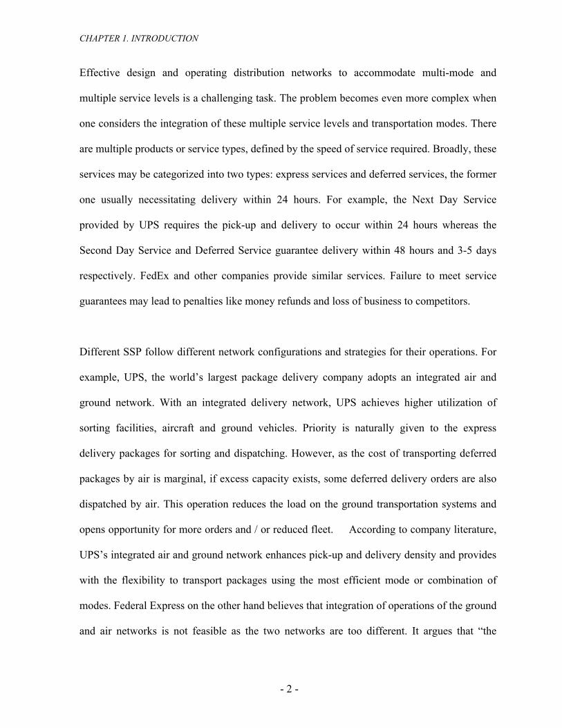
Effective design and operating distribution networks to accommodate multi-mode and
multiple service levels is a challenging task. The problem becomes even more complex when
one considers the integration of these multiple service levels and transportation modes. There
are multiple products or service types, defined by the speed of service required. Broadly, these
services may be categorized into two types: express services and deferred services, the former
one usually necessitating delivery within 24 hours. For example, the Next Day Service
provided by UPS requires the pick-up and delivery to occur within 24 hours whereas the
Second Day Service and Deferred Service guarantee delivery within 48 hours and 3-5 days
respectively. FedEx and other companies provide similar services. Failure to meet service
guarantees may lead to penalties like money refunds and loss of business to competitors.
Different SSP follow different network configurations and strategies for their operations. For
example, UPS, the world’s largest package delivery company adopts an integrated air and
ground network. With an integrated delivery network, UPS achieves higher utilization of
sorting facilities, aircraft and ground vehicles. Priority is naturally given to the express
delivery packages for sorting and dispatching. However, as the cost of transporting deferred
packages by air is marginal, if excess capacity exists, some deferred delivery orders are also
dispatched by air. This operation reduces the load on the ground transportation systems and
opens opportunity for more orders and / or reduced fleet. According to company literature,
UPS’s integrated air and ground network enhances pick-up and delivery density and provides
with the flexibility to transport packages using the most efficient mode or combination of
modes. Federal Express on the other hand believes that integration of operations of the ground
and air networks is not feasible as the two networks are too different. It argues that “the
- 2 -

CHAPTER 1. INTRODUCTION
optimal way to serve very distinct market segments, such as express and ground is to operate
highly efficient, independent networks.”
SSP operate vast systems of aircraft, trucks, sorting facilities, equipment and personnel to
move packages between customer locations. The SSP must determine which routes to fly,
which fleets to assign to those routes and how to assign packages to those aircraft, all in
response to demand projections and operational restrictions [Armacost et al. (2002)]. The
objective is to find the cost minimizing movement of packages from their origins to their
destinations, given the very tight service windows, limited package sort capacity and a finite
number of ground vehicles and aircraft [Kim et al. (1999)]. The problem faced by a SSP is
combinatorial in nature and involves the simultaneous solution of the capacitated network
flow problem with strict time windows, aircraft routing, fleet scheduling and package
allocation problem.
The shipment service process begins with a request from a customer with specifications of
location of origin and destination, type of service required (Next Day Service / Second Day
Service / Deferred Service), size and weight of the package (s) and a time window for the
pick-up. A fleet of ground vehicles responds to these requests and consolidates all the
packages to the sorting facility in the nearest airport. This calls for the optimization of the
vehicle routing problem associated with the ground transportation from various pick-up points
in a zone to the nearest airport. As there are strict time windows associated with the Next Day
Delivery Services and the package sizes are relatively small compared to the truck sizes, this
routing problem basically becomes a less than truck (LTL) routing problem with strict time
windows.
- 3 -

CHAPTER 1. INTRODUCTION
The packages are sorted by their destinations and service type. Since, air transport is
expensive; there is an attempt to deliver packages to some destinations by ground
transportation if possible. But due to the strict time constraints and associated penalties for not
meeting service guarantees in case of Express Services, ground transportation can cater only
to the destinations which are in geographic proximity to the origin. The Deferred Services are
usually catered by ground transportation as the time constraints are relaxed. Some companies
like UPS do use the air route for some Deferred Service orders, if excess capacity exists in the
aircraft after satisfying the capacity required for express services. The packages are assigned
to aircraft destined to concerned airports. The air service may be dedicated or commercial; the
former being performed using company’s fleet of aircraft, while the latter involves the use of
commercial airlines. Express shipment services stick to a direct flight delivery strategy or a
hub-and-spoke network arrangement or a combination of both for shipping the packages from
origin airport to the destination airport. In the direct flight delivery option, the shipments are
directly shipped from the origin airport to the destination airport. The destination airports may
be more than one if it satisfies the temporal constraints. The hub and spoke network
arrangement necessitates that all the shipments are consolidated at a central facility (hub),
sorted and dispatched to the destination airports. Each of the above operational strategies has
their advantages and disadvantages depending on the demands. Direct delivery flights may
lead to the usage of comparatively more number of flights and each running less than
capacity. The hub and spoke arrangement leads to loss of time as it involves a sorting at the
hub and the packages reach the destination in a rather roundabout fashion. However, a mixed
network can be envisaged as a combination of the direct delivery and hub-and-spoke network
configuration, which incorporates the advantages of both. On reaching the destination airport,
- 4 -

CHAPTER 1. INTRODUCTION
the packages are assigned to different ground vehicle routes so that it reaches the destination
on / before time. There may be a time-window specified in the request with which the carrier
should comply.
Conventional network design and routing models cannot sufficiently capture the complexity
of multimode, multi-service networks. Network designs and routing decisions must comply
with the various time constraints for each service level. Unlike passenger networks, shipments
in freight networks can be routed in more circuitous ways to achieve economies of scale and
density, provided time constraints are not violated. For deferred service shipments, these cost
efficient routings are more likely to occur as the time constraints are more relaxed. However,
with the increased number of routing options and service levels, finding an optimum network
design and distribution strategy becomes more difficult.
1.2 Literature Review
Express shipment service is an instance of the transportation service network design
application. Transportation service network design problems are a variation of the well-
studied and well-documented network design problems.
Conventional network design formulations generally involve two types of decision variables:
those for the routing decisions and those for the package flow decisions; however these can be
applied only to problems of limited size [Armacost et al. (2002)]. Comprehensive surveys of
network design research are presented by [Ahuja et al. (1993)], [Minoux (1989)] and
[Padberg et al. (1985)]. Research on uncapacitated and capacitated network design is
- 5 -

CHAPTER 1. INTRODUCTION
presented by [Balakrishnan (1989)], [Balakrishnan (1994 a], [Balakrishnan (1994 b] and
[Bienstock and Gunluk (1995)].
Recent research on network design problems has primarily focused on strengthening the LP
relaxation [Padberg et al. (1985)] and [Van Roy and Wolsey (1985)]. Network loading
problems have been studied by [Goeman and Bertsimas (1993)], [Magnanti and Mirchandani
(1993)] and [Pochet and Wolsey (1995)]. [Goeman and Bertsimas (1993)] and [Balakrishnan
et al. (1989)] developed approximation algorithms for network design.
However, there are two major difficulties in applying conventional network design problems
and approaches to the transportation service network design problem [Kim et al. (1999)].
First, the interactions among the decision variables in transportation applications are more
complicated. Second, the state-of-the-art network design methods are not suitable for
transportation networks which are very huge in size because of their ‘spatio-temporal’
ingredients.
For express shipment service network design, [Kuby and Gray (1993)] develop models for
the case of Federal Express. [Hall (1989)] studies the effects of time zones and overnight
service requirements on the configuration of an overnight package network, but the paper
does not address the problems of routing and scheduling. [Barnhart and Schneur (1996)]
develop models for the express package service network design problem and present a column
generation approach for its solution. The algorithm finds near optimal air service designs for a
fixed aircraft fleet or for a fleet of unspecified size and make-up. However, the problem is
simplified as the model assumes only one hub, one ground vehicle feeder service and no
- 6 -

CHAPTER 1. INTRODUCTION
transfer of shipments between aircraft at gateways. [Grunert and Sebastian (2000] identify
planning tasks faced by postal and express shipment companies and define corresponding
optimization models. [Budenbender et al. (2000)] develop a hybrid tabu search / branch and
bound-and-bound solution methodology for direct flight postal delivery. [Kim et al. (1999)]
develop a model for large scale transportation service network design problems with time
windows. Column and row generation optimization techniques and heuristics are
implemented to generate solutions to an express package delivery application. Complex cost
structures, regulations and policies are taken care of by the use of route-based decision
variables. The problem size is greatly reduced by exploiting the problem structure using a
specialized network representation and applying a series of problem reduction methods.
[Armacost et al. (2002)] develop a robust solution methodology for solving the express
shipment service network design problem. The conventional formulations are transformed to
composite variables and its linear programming relaxation is shown to provide stronger lower
bounds than conventional approaches. By removing the flow decisions as explicit decisions,
this extended formulation is cast purely in terms of the design elements.
[Grunert and Sebastian (2000)] have not considered the existence of intermediate airports
explicitly in their formulations. The aircraft starts from the origin and reaches the hub directly
on the pick-up side and similarly, on the delivery side, the aircraft starts from the hub and
reaches the destination without making any intermediate stops. [Armacost et al. (2002)],
[Barnhart and Schneur (1996)] and [Kim et al. (1999)] have considered a maximum of one
intermediate stop on the pick-up and delivery routes. [Smilowitz (2001)] discusses routing in
air networks and asymmetric routing strategies. It is quite possible that an aircraft can make
two intermediate stops on its pick-up route or two intermediate stops on its delivery route
- 7 -

CHAPTER 1. INTRODUCTION
depending on both the temporal and capacity constraints. [Smilowitz (2001)] discusses the
aspects of 2:2, 2:1,1:2 and 1:1 zoning and minimum pair-wise matching of 2:1 to 1:2 zoning
to reduce the fleet size. However, the formulations are not of mixed integer type.
1.3 Scope of Research
The current study focuses on the air transportation network design for the shipment service
providers (SSP). We formulate this network as a mixed integer problem. In our study, we
assume that ground vehicles respond to the pick-up orders on time and all the packages are
consolidated at the sorting facility. Packages are sorted by destination and service type.
Optimizing the ground transportation for pick-up is out of the present scope of this research.
We study various formulations under the scenarios described below.
As has been extensively studied and practiced successfully in the industry, hub and spoke
networks have a significant advantage over “point to point” or directly connected networks.
Researchers have analyzed the air transportation network splitting it into two parts: the pick-
up side and the delivery side. The inferences drawn from the study of either side is equally
applicable to the other side. In the current study, we focus on the various aspects of the air
transportation network typically faced by a shipment service provider particularly in
geographic areas the size of the continental USA. However, the inferences drawn are equally
applicable to small areas of interest as well. One of the major factors when we are dealing
with countries like the size of USA is the time zones, which severely restrict the available
options and aggravate the already strict time window conditions.
- 8 -

CHAPTER 1. INTRODUCTION
In the current study, we focus on a combination of various operational strategies and their
potential cost implications. We start our analysis with the assumption of a single hub and
spoke network configuration for the air network with the location of the hub known a priori.
In this case, all origin airports are connected to the hub by (a) flight(s) with no intermediate
stops. Similarly, all destination airports are connected to the hub by (a) flight(s) with no
intermediate stops. We further our analysis assuming a regional hub and spoke configuration
i.e pick-up from origin airports are consolidated at their regional hubs, dispatched to the
destination regional hub from where it is transported to the destination airport. Again, the
regional hub locations are assumed to be known a priori. In the next analysis, we study the
cost effects if we assume a strategy in which the demands could either be routed directly from
the origin city to the main hub or through the regional hub. The strategy implications are
further analyzed when the demands from origins are routed either directly to the regional
destination hub or through the regional origin hub (i.e there is no main hub). Another logical
extension is to study the implications of a strategy in which demands are routed from the
origin city to the destination hub. Assuming similar strategies on the delivery side, we analyze
the various combinations of strategies and their cost impacts.
All the above studies are based on the fact that there is no intermediate stop of the demands
from the origin city until it reaches a hub (either the main hub / regional hub). Subject to the
temporal and capacity constraints, it is possible to make intermediate stops at airports on pick-
up / delivery routes. Earlier researchers [Barnhart and Schneur (1996)], [Kim et al.(1999)],
[Armacost et al. (2002)] have considered the presence of one intermediate stop on the pick-up
and delivery routes in their formulations. We formulate the above problems as mixed integer
- 9 -

CHAPTER 1. INTRODUCTION
programs which optimize the total operating costs subject to the demand, capacity, time,
aircraft and airport constraints.
1.4 Organization of Thesis
Chapter 2 gives a system overview and discusses the various concepts and definitions
involved in the design of air networks for shipment service companies. In Chapter 3, we
develop mixed integer formulations for studying the implications of various feasible strategies
as described in the previous section. Chapter 4 describes the methodology used to create the
various datasets that we have used for evaluation of the models. In Chapter 5, we analyze
various scenarios of model performance where we allow no intermediate stops on the pick-up
and delivery routes. We extend our research to study implications of scenarios where pick-up
and delivery routes have one intermediate stops in Chapter 6. Chapter 5 and Chapter 6 results
are based on one sample dataset. In Chapter 7, we conduct a sensitivity analysis of various
parameters like demand, fixed and variable costs on the total cost of operation under various
scenarios. We summarize our findings of this research and discuss future scope of study in
Chapter 8.
- 10 -

CHAPTER 2. SYSTEM OVERVIEW: CONCEPTS & DEFINITIONS
Chapter 2
System Overview: Concepts and Definitions
2.1 Introduction
Express Shipment Service problems come under the class of transportation service network
design problems. The network design calls for combinatorial optimization at all stages of the
process starting from the call for service to the delivery of the package at the destination. The
objective is to find the cost minimizing movement of packages from their origins to their
destinations, given the very tight service windows, limited package sort capacity and a finite
number of ground vehicles and aircraft.
11

CHAPTER 2. SYSTEM OVERVIEW: CONCEPTS & DEFINITIONS
An aircraft route beginning at an airport, typically visits a set of delivery stops followed by an
idle period, and then visits a set of pick-up stops before returning to the origin airport. Associated
with each airport are earliest pick-up times (EPTO) and latest delivery times (LDTD). EPTO
denote the times at which packages will be available for pick-up at an airport. The EPTO of each
airport is scheduled as late as possible to allow customers sufficient time to prepare their
shipments. LDTD denote the times by which all packages must be delivered to satisfy delivery
standards.
The Express Package Delivery Process
Pick-up Phase
SortingPhase
Delivery Phase
[Figure 2.1: Express Package Delivery Process]
The airports are associated with time windows designating the start and end sort times. An
aircraft route can be decomposed into two distinct components – a pick-up route and a
delivery route. A pick-up route typically starts from an airport in the early evening, covers
a set of airports before ending at a destination airport (in case of direct flight network) or
hub (in case of a hub-and-spoke network). A delivery route begins at any airport (in case of
direct flight network) or hub (in case of hub-and-spoke network) typically in the early
12

CHAPTER 2. SYSTEM OVERVIEW: CONCEPTS & DEFINITIONS
morning and delivers packages at some destination airports. The aircraft may be ferried to
some other airport if it optimizes the pick-up process.
[Figure 2.2: Express Package Delivery Network]
Figures 2.1and 2.2 show a typical network with a few pick-up, delivery and ferrying routes for
instances of direct flight delivery and the hub-and-spoke configuration. Figure 2.3 shows the
flow diagram of package delivery services.
Order for Pickup Received with Package Details
Truck Routes Constructed for Pickups
Packages sorted for Hubs & Assigned to Flights
Packages dispatched to Hubs
Packages sorted at Hub & Assigned to Flights
Packages dispatched to Destination Airports
Truck Routes Constructed for Deliveries
Packages Delivered at Destination
13

CHAPTER 2. SYSTEM OVERVIEW: CONCEPTS & DEFINITIONS
[Figure 2.3: Express Package Delivery Process Flow Figure]
2.1.1 Direct Flight Delivery Networks
We need to find a cost-minimizing flight schedule and an assignment of requests to the flights
subject to the temporal and capacity constraints so that all the shipments are transported from
origins to their destinations. Figure 2.4 shows a typical direct network.
[Figure 2.4: Direct Flight Delivery Network]
2.1.2 Hub and Spoke Networks
The problem is to find a cost-minimizing flight schedule from a number of airports to one or
several hubs and back again a ose flights. The flights must
tisfy temporal constraints, the capacity constraints taking care of the sort times at the hub(s)
nd an assignment of requests to th
sa
and other operational considerations. Figure 2.5 shows a typical one single hub and spoke
network.
14

CHAPTER 2. SYSTEM OVERVIEW: CONCEPTS & DEFINITIONS
[Figure 2.5: Hub and Spoke Networks]
The airside problems faced by the express shipment services differ greatly from the groundside
problem. These differences primarily arise from federal requirements mandating that air routes
and schedules be set in advance. Hence, while the schedules may experience changes (due to
weather, air traffic control failures etc.), the established air routes may not be updated in real
time. Thus, this becomes a problem of strategic routing and scheduling of air fleet and allocation
of packages to different routes.
15

CHAPTER 2. SYSTEM OVERVIEW: CONCEPTS & DEFINITIONS
2.2 Time Windows
The shipment service process begins with a request from a customer with specifications of origin
and destination locations, type of service required (next day service / 48 hour service / deferred
service), size and weight of the package (s) and generally a time window for the pick-up. A fleet
of ground vehicles responds to these requests and consolidates all the packages at the sorting
facility in the nearest airport. The following information emerges as a result of user
specifications (see Figure 2.6):
[Figure 2.6: Time Windows]
Earliest Pick-up Time at Origin Location [Epo ], Latest Pick-up Time at Origin Location [Lpo] and
the Latest Delivery Time at the destination location [Ldd]. Alternatively speaking, [Epo , Lpo] is
the time window in which the package needs to be collected by the ground transportation unit
from the customer requesting pick-up. Depending on the ground travel time for transporting the
package from the origin location to the sorting facility at the airport and the package sort time,
we can associate an Earliest Pick-up Time for the package [EPTO] at the origin airport. [EPTO]
is calculated by adding the package sorting times and the ground travel time from the pick-up
tDd
16

CHAPTER 2. SYSTEM OVERVIEW: CONCEPTS & DEFINITIONS
location to the origin airport [toO] to the user-specified earliest pick-up time [Epo]. The latest
pick-up time at the origin airport [LPTO] is specified by the latest plane departure (specified by
an exogenously established flight schedule) such that a direct delivery from the destination
airport (D) to the destination location (d) does not exceed the user-specified latest delivery time
at the destination location [Ldd]. The Latest Start Time at origin airport [LPTO] could be derived
by deducting the sum of air travel time from origin airport [O] to the destination airport [D] and
the package sorting time at the destination airport from the Latest Delivery Time [LDTD].
[LDTD] could be derived by deducting the travel time from destination airport [D] to the
destination location [d] from the user specified latest delivery time [Ldd]. We assume that the
loading, unloading and package handling times are incorporated in the ground transportation
travel times. Similarly, we can associate an earliest delivery time with the destination airport
[EDTD], which could be obtained by summing up the earliest pick-up time [EPTO] at the origin
airport, the air travel time from origin airport [O] to the destination airport [D] and the package
sorting time at destination airport [D]. Similarly, we could associate an Earlier Delivery Time at
the destination location [Edd] as the sum of the [EDTD] and the ground travel time from
destination airport to the destination location [tDd]. Figure 2.7 gives the summarized
representation of the above.
[Figure 2.7: Summary Representation of Time Windows]
17

CHAPTER 2. SYSTEM OVERVIEW: CONCEPTS & DEFINITIONS
2.3 Effect of Time Zones
A lower bound on the time window is defined as the maximum time between any city pair,
accounting for all time zone changes. A flight satisfying this lower bound condition is most
likely supposed to originate on the western end of a service region (for example the United
States) and terminate on the eastern end [Hall (1989)]. Let us assume that the city pairs are
distributed between two ends of a line segment oriented west to east, over which Z numbers of
time zones are crossed. In the northern hemisphere, east bound wind velocity is 100 mph larger
than the west bound velocity.
Let us base all our calculations with the easternmost end as our reference. We assume that the
cut-off time is same in all cities and represent the identical time that aircraft departs the
originating city in the local time zone. Let t =0 be the cut-off time for planes that depart from the
easternmost time zone, t =1 be the cutoff time for the second most eastern time zone and t = Z-1
be the cutoff time for the western most time zone. The last plane to arrive at the hub depends on
the hub location, but usually, it would arrive from one of the ends of the region. The latest arrival
time at the hub is the maximum of western and eastern arrival times and is represented by t(x)
where x is the location of the hub.
No plane can depart the hub for delivery until every pick-up plane has arrived and requests
be the one which has the m
sorted. The earliest time that a plane can arrive at a destination is t(x) plus the flight time from
hub to the destination, adjusted to the local time at the destination. Eastbound shipments from the
hub to the destination cities are time critical. So, ideally, the first shipments from the hub should
aximum flight time to the eastbound destination. If max is the te
18

CHAPTER 2. SYSTEM OVERVIEW: CONCEPTS & DEFINITIONS
maximum flight time for an eastbound destination from the hub, LAD is the latest arrival time at
the destination (local time) and the hub is n time zones behind the destination, then the shipment
should be dispatched from the hub no later than [LAD - temax - n] (local time at hub) i.e [LAD -
temax ] eastern time. Similarly, if the farthest west bound shipment from the hub is (Z-n) time
zones behind the time zone at the hub and the flight tim , the latest arrival time at the
e), then the shipment should be dispatched from the hub no later
than [LAD - + (Z- n)] i.e [LAD - + (Z- n) + Z] eastern time. Figure 2.8 shows the
various time zones in US. Appendix- 1 shows a sample calculation for time windows with
reference to a service region comp
e is twmax
destination is LAD (local tim
twmax tw
max
arable to US.
[Figure 2.8: Time Zone Map of USA]
19

CHAPTER 2. SYSTEM OVERVIEW: CONCEPTS & DEFINITIONS
2.4 Arc, Path and Route Incidence Matrices
We define the terminology for arc, path and route [Kuby and Gray (1993)] below and
subsequently develop three incidence matrices for our problem formulation. An arc is a single
airport to airport connection using a particular aircraft type. There may be a restriction on the
type of aircraft that can be flown to and from an airport. Also volume of requests may only
require smaller aircraft. In the network shown in Figure 2.9, AC0, CE1, EH2, EH3 etc. are
instances of arcs; 0,1,2,3 representing the type of aircraft available. Path is a sequence of arcs
used to deliver packages from an origin airport to a destination airport. Each path that is routed
through the hub is basically a union of two disjoint paths viz: path from the origin airport to the
hub and path from hub to the destination airport. In Fig-2.9, AC0CE1EH2, BC0CEH2,
BD0DF2H3, CE2H3, DF2H3 etc. are instances of paths from an origin airport to the hub.
Similar paths can be developed for the delivery side, i.e from the hub to the destination airport.
Route is a sequence of arcs used to deliver packages from the origin airport to the destination
airport by the same aircraft. CE2, CEH3, DFH2 are instances of routes in the network shown in
Figure 2.9.
[Figure 2.9: Arcs, Routes and Paths in Air Transportation Network]
20

CHAPTER 2. SYSTEM OVERVIEW: CONCEPTS & DEFINITIONS
We develop three incide atrices define t tial rela between origin and
destination airports, aircraft, arc, path and route variab s. The path ute incidence matrix (Ipr)
relates each path to all routes r in that path. We define the path-route variable Ipr as follows:
1, if route r is in path p Ipr
0, otherwise
Table 2.1 shows a sample of the path-route incidence matrix for the network shown in Figure
CEH2 EH3 CH3
nce m that he spa tion the
le -ro
p
=
2.9. AC0 CE1
AC0CE1EH2 1 1 0 0 0
AC0CEH2 1 0 1 0 0
AC0CH3 1 0 0 0 1
[Table 2.1: Path-Route Incidence Matrix Ipr]
The path-ai atrix (Ipw) shows the linkage between a path and the airports that are
covered in that path. We define the path-airport riable as follows:
airport w in pa Ipw
0, otherwise
A B C D E F H
rport incidence m
va
1, if is th p=
Table 2.2 shows a sample of the path-airport incidence matrix for the network shown in Figure
2.9.
A 0C 2 C E1EH 1 0 1 0 1 0 1
BC0CEH2 0 1 1 0 1 0 1
BD0DFH2 0 1 0 1 0 1 1
[Table 2.2: Path-Airport Incidence Matrix I ]
pw
21

CHAPTER 2. SYSTEM OVERVIEW: CONCEPTS & DEFINITIONS
We define the route-aircraft incidence matrix ) that captures the use of a particular aircraft
type k in a route r. We define the route-aircraft v le as follows:
I
0, otherwise
Table 2.3 shows a samp
2.9. Aircraft Type -0 Aircraft Type -1 Aircraft Type -2 Aircraft Type -3
(Irk
ariab
1, if aircraft type k is used in path p rk =
le of the path-airport incidence matrix for the network shown in Figure
AC0 1 0 0 0
CE1 0 1 0 0
CEH2 0 0 1 0
CH3 0 0 0 1
DF2 1 0 1 0
[Table 2.3: Route –Aircraft Type Incidence Matrix Irk]
The above incidence matrices are instrumental in our model formulations in Chapter 3.
22

CHAPTER 3. SYSTEM DESIGN AND FORMULATIONS
Chapter 3
System Design and Formulations
3.1 Introduction
In this chapter, we formulate the air transportation network design problem as a mixed integer
problem. In our study, we assume that ground vehicles respond to the pick-up orders on time
and all the packages are consolidated at the sorting facility. Packages are sorted by destination
and service type. Optimizing the ground transportation for pick-up is beyond the present
scope of this research. We develop formulations for the following scenarios. As described in
Section 1.3, we start our analysis with the assumption of a single hub and spoke network
configuration for the air network with the location of the hub known a priori. We further our
analysis assuming a regional hub and spoke configuration. Subject to the temporal and
23

CHAPTER 3. SYSTEM DESIGN AND FORMULATIONS
capacity constraints, it is possible to cover one / more airports on pick-up / delivery routes.
Due to time zone differences, flights that have flexibility on the pick-up route may not have
the flexibility on the delivery route (and vice versa). We formulate the above problems as
mixed integer programs which optimize the total operating costs subject to the demand,
capacity, time, aircraft and airport constraints. The following model is utilized for analysis of
different scenarios in the subsequent chapters of this research.
3.2 Assumptions
We consider that the locations of hub(s) are known a priori. Generally, the requests are
routed through the hub as it facilitates better consolidation of the requests by destination,
thereby increasing use of capacity. However, some direct flights may also be needed
depending on the volume of requests, time constraints and economy.
We have deterministic requests for service with known volumes between each Origin-
Destination (OD) airport pairs.
The latest pick-up time and latest delivery time is the same at all cities.
Aircraft routings and schedules are assumed not to vary on a day-to-day basis.
Line haul costs are assumed not to be a function of the volume of requests.
We assume that there are no transfers, i.e if there is a flight from an airport to a hub on
the pick-up route and requests (packages) are loaded on that flight, they stay on it until it
reaches the hub. However, if the flight terminates before the hub on one of the
intermediate airports owing to capacity / temporal restrictions, the packages may be
transferred.
There are no intermediate stops between hub to hub flights wherever it is applicable.
24

CHAPTER 3. SYSTEM DESIGN AND FORMULATIONS
3.3 Terminology
We define the following terms for our problem formulation. X : set of all requests XH
: set of requests that are routed through hubs
leX D
C arly,
: set of requests that are routed to destinations by direct flights
XXX DH ∪=
W : set of all airports, Ww∈
: set of all origin airports, Oo ∈ , WO ⊆ ODd ∈ , WD⊆ D : set of all destination airports,
H : set of hubs, Hh∈
P : set of all feasible paths from origin airport to destin tion airport via hua bs,
aths)
estination airport, (delivery paths)
of all inter-hub feas le paths,
C
to destination airport
Pp∈
: set of all feasible paths from origin airport to hub, Pp pp (pick-up pP p ∈
Pd : set of all feasible paths from hub to d Pp dd∈
Ph : set ib Pp hh∈
learly, PPPP hdp ∪∪=
qodo d : amount of request from origin airport
Kk∈ K : set of all aircraft types,
Q apacity of aircraft type Kk ∈ k: c
C : set of commercial aircraft, Cc∈
*ckp p
: cost of flight from origin to hub along path using aircraft type
hh ji using aircraft type
using aircraft type
cal m
[*
o hi ppk
* k : cost of flight from hub to hub k c hi hj
*c : cost of flight from hub hj to destination d to along path p
d dkp k
c : unit cost of transportation per nauti ile by a commercial aircraft
uc
: cost incl des the sum of fixed and variable costs for the flight] : number of aircraft of type Kk∈ nk
25

CHAPTER 3. SYSTEM DESIGN AND FORMULATIONS
z pkw : maximum num ircraft of type Kkber of a ∈ that are permitted in airport on
p pp∈
: maximum number of aircraft of type
Owi∈,
ick-up paths p P
zdkw Kk∈ that are permitted in airport on
= 1, if airport is present along pick-up path
0, otherwise
d
Decision Variables
: Number of flights from origin to hub along path using aircraft type
l
: Amount of request that is transported from hub to destination along path
: Amount of request transported from origin to hub by commercial aircraft
Dwi∈,
delivery paths Pdd∈ p
Ipw
p
Owi∈, Pp pp
∈
Ipw= 1, if airport Owi
∈, is present along delivery path Pp dd∈
0, otherwise
I kpoh
p
i
o hi ppk
Ikpdh
d
j
: Number of flights from hub h to destination d a ong path pdusing aircraft type
jk
Ikhh ji
: Number of aircraft of type k from hub hi to hubhj
, Hhji∈, h
: Amount of request that is transported from origin o to hub along path pp x p
oh
p
ihi
jd pd
xpdh
d
ih
xcoh i
o hiCc∈
xcdhi
: Amount of request transported from hub to destination by commercial aircraft
: Amount of request that is transported from hub to hub
: Amount of request transported from hub to hub , commercial aircraft
hjd
Cc∈
x hh jihi hj
, Hhh ji∈,
xchh ji
hi hjCc∈
26

CHAPTER 3. SYSTEM DESIGN AND FORMULATIONS
3.4 Problem Formulation The mixed integer program can be formulated as follows:
cIcIcI khh
Hh Hh
khhDd Hh Pp
kpkpdhOo Hh Pp
kpkpohMinimize
ji
i j
ji
jdd
dd
j
ipp
pp
i∑ ∑∑ ∑ ∑∑ ∑ ∑∈ ∈∈ ∈∈ ∈ ∈
+∈
+, ,,,
)(, ,,,∑ ∑∑ ∑∑ ∑∈ ∈∈∈
+∈
+∈
+Hh Hh
chh
Hh Dd
cdhiHh Oo
coh
c
i j
ji
ii
ixxxc (0)
∈ ∈ ∈−+ ,
,0 (1)
xx ji
Hh Hh
chh
cdh
coh
Dd Ppdh
O Pp Hhhh
poh
i i
jiiidd
d
j
ipp
j
ji
p
i∈−−−−− ∀≤∑ ∑ ∑∑
∈ ∈ ∈∈ ∈∈ ∈ ∈∀
,0, , ,,, ,
(3)
w
pw
ppp
∈∈− ∀≤∑
OoqxxHh Pp Hh Dd
coh
poh
ipp
i
i
p
i od ∈∀∑ ∑ ∑ ∑ ≥∈,
DdqxxHh Pp Hh Oo
cdh
pdh
jdd
j oj
d
j od ∈∀∑ ∑ ∑ ∑ ≥∈ ∈ ∈ ∈
−+ ,, ,
0 (2)
xp∑∑ ∑ ∑ Hhhxxxo Hhj
KkPpQIxI ppkkpoh
poh
Oii
i∈
,,0 (4)
∈− ≤∑∈
,,0,
+Pp Hh Hh
hhohppi j
jiiknII k
,, ,
Pdd j (7)
∈≤ ∀∑∈
,,
Pp
pd
∈
)
tosubject
,
KkPpQIxI ddkkpdh
pdh
Dw
pw
d
j
d
i
i
d
∈∀ (5)
∑ ∀≤∑ ∑∈ ∈ ∈
kkp p
∈K (6)
∑ ∀≤ ∈kpdh
d
KknI k , p ∈
kOwzI i
pkw
Pp
pwpp
p
K∈ (8)
KkDwzI ikwwdd
∈∈≤ ∀∑ ,, (9
d
27

CHAPTER 3. SYSTEM DESIGN AND FORMULATIONS
int,, 0 andkkpkp IIIji
d
j
p
i≥ (1
0,,,, ≥xxxxx chhhh
coh
pdh
poh jijii
(
The objective function is to minimize the total cost of operation for requests for service. The
first three terms in equation (0) represent the cost components on the pick-up, delivery and
inter-hub paths respectively by use of company owned aircraft in the operations. These cost
components capture the fixed and variable cost for each origin-hub hub-destination and hub-
hub pair for each aircraft type. Fixed costs are attributed to the aircraft, crew, airport take-
off and landing fees etc. and the variable cost being the fuel cost The fourth, fifth and sixth
terms in the objective function reflect the cost components attributed to the use of
commercial aircraft in the pick-up, delivery and inter-hub paths respectively. Constraints
(1) and (2) show that all requests are satisfied for the pick-up and delivery sides
respectively. Constraint (3) ensures that the hubs are transshipment points and the amount of
requests entering a hub is same as the amount leaving. Constraints (4) and (5) are the
aircraft capacity constraints or the bundle constraints on the pick-up and delivery side
respectively which capture the fact that amount of request that can flow along a path cannot
hhdhoh 0)
11)
exceed the capacity of the aircraft. Constraints (6) and (7) are the aircraft availability
constraints i.e the number of aircraft of a certain type used in the pick-up and delivery
phases cannot exceed the numbers available. Constraints (8) and (9) represent the bounds on
the number of flights of a certain type of aircraft that are allowed in the pick-up and delivery
phases respectively. Constraint (10) ensures the integrality and non-negativity of the flights
and Constraint (11) represents the non-negativity constraints of the other variables.
d
i
p
i
28

CHAPTER 4.DATASETS
Chapter 4
Datasets
4.1 Test Problem Data
We use the continental USA as our area of study. We create an air network in line with the
United Parcel Service (UPS) network with 90 cities as shown in Figure 4.1. Appendix 2A lists
the airports that we have considered in our sample air network. We assume that Louisville is
the main hub and Ontario, Rockford, Dallas, Louisville, Philadelphia and Columbia are the
regional hubs when and where applicable as shown in Figure 4.2. Appendix 2B shows the
assignment of airports to the nearest regional hubs. When we are dealing with multiple hub
scenarios, we define the hub nearest to the origin and destinations as “Origin-Regional Hub”
and “Destination Regional Hub” respectively.
29

CHAPTER 4.DATASETS
30
[Figure 4.1: Map showing Cities in Sample Air Network]
[Figure 4.2: Map showing Location of Hubs in Sample Air Network]
For demand data, we use the 1997 Commodity Flow Survey (CFS) data of courier flows
originating /destined from / to the Metropolitan Statistical Areas (MSA) and other states.

CHAPTER 4.DATASETS
Chan and Ponder (1979) list service industries and hi-tech dominated light industries as the
major users of express package shipping. O’hUallachain and Reid (1990) link businesses and
professional services with technological development and information access. In order to
calculate the express package volumes from various MSAs, we adopt an approach similar to
[Kuby and Gray (1993)] to estimate the air package supply volumes. Census 2000 population
data for all states and Metropolitan Statistical Area (MSA) is used for our calculations.
at would be
e (air).
the 2001 Metro
em (NAICS). We have
Besides population, there are other economic factors like employment type th
expected to affect the volume of packages shipped from / to a city through express mod
In an effort to more accurately estimate volumes, we have considered
Business Patterns as per North American Industry Classification Syst
assumed that employment in the Information (NAICS Code 51), Insurance and Finance
(NAICS Code 52), Technical, Professional and Scientific Services (NAICS Code 54) and
Management of Companies and Enterprises (NAICS Code 55) sectors are a good indicator of
express package volumes. We define a Location Quotient measuring regional variation in
employment in the above sectors as follows:
Location Quotient (LQ): [(e 2001 / E 2001) / (n 2001 / N 2001)]
Where e2001: 2001 MSA or, CMSA employment under NAICS 51, 52, 54 & 55
E2001:2001 MSA or, CMSA total employment in US (NAICS 11 through 99)
n2001:2001 total employment in US under NAICS 51, 52, 54 & 55
N2001: 2001 total employment in US (NAICS 11 through 99)
From the CFS data, we take the volume of packages routed by Parcel, USPS or, Courier from
the MSAs to all other MSAs and states. We derive the package volume per capita per day for
31

CHAPTER 4.DATASETS
all the MSAs and states. For our sample network, we take the airports under the UPS Cargo
Network. Next, we try to allocate different airports to population (markets). Allocating an
airport for a city / geographical area is by itself a combinatorial problem and not the present
focus ands
genera ate to
the airports present in the state. Even though, a portion of the demand could be better served
by allocatin For states
which do not have any airport in the network, we divide the demands generated to the nearest
airport(s) in neighboring state(s). By undergoing the above exercise, we obtain the population
served by all the airports in our network. We calculate the total courier volume generated for
all the airports based on this population and the demand/capita/day obtained before. Basically,
the total volume of courier generated in an airport can be found out by the following
expression:
Total Courier Volume Out = C* LQ*[MSA Volume/ Capita/Day]*[MSA Population] +
∑[Geographical Area ‘g’ Volume / Capita / Day]*[Geographical Area ‘g’ Population]
of our research. It’s reasonable to assume that an airport would serve the dem
ted in the nearest city. For simplicity, we allocate the demands generated in a st
g it to an airport of another state, we have not focused on this aspect.
Source: The Colography Group Inc., Package Market Trend Analysis, Dec 28, 2001
[ 4.3: Packa rk lume Distribution 20
where ‘g’ is the set of geographical areas to the port factor (0≤C≤1)
corresponding to the fraction of total courier volumes which are to be served by aircraft. We
Figure ge Ma et Vo 01]
allotted air . C is a
32

CHAPTER 4.DATASETS
have taken C as 0 Q is the location
uotient of the airport city under consideration. This is incorporated in the formula to capture
.25 as an upper bound of 16% as shown in Figure 4.3. L
q
the fact that a city with a high LQ is supposed to generate higher demands for the air network.
Table 4.1 shows the market share of the major players in the Courier industry.
Company Overnight 2/3 Day Ground Parcel
( ’000) % ( ’000) % ( ’000) %
USPS 66.4 5 1117.8 59 1538.8 18
FedEx 558.2 43 330.1 17 1457.9 18
UPS 393.8 30 330.3 17 4644.9 57
Airborne 236.3 18 103.8 6 345.7 4
Others 46.2 4 5.4 1 212.7 3
Total 1300.9 16 1887.4 23 8200.0 61
[Table 4.1: Market Share of Major Players in Courier Industry]
The courier demand is a fluctuating vari ith respe d .We created our
demand file for one such realization. Origin-Destination matrix generation for courier flows is
a subject of research by itself, which is beyond the current scope. The above process was
aimed to obtain a practical Origin-Destination demand set that we could utilize to run our
model.
because of their widespread use in the express package delivery industry. Company literature
able w ct to time an space
In our model, we assume that we operate two kinds of aircraft Type-A and Type-B. These
aircraft are in line with the Boeing 727-100 and Boeing 757-200 specifications and are chosen
33

CHAPTER 4.DATASETS
shows that these two aircraft types are dominant in air cargo delivery operations. For aircraft
related data like cost and maximum payload data, we refer to the Annual Reports (SEC 1OK
Form) of FedEx and UPS. For our analysis, we would consider that the Shipment Service
Provider (SSP) operates only aircraft of the following types as shown in Table 4.2.
Sl.No. Air Craft Type Maximum
(lbs)
Avg. Fixed
(in dollars)
Fuel usage per
(kg) Payload Cost nautical mile
1 Type-A (Boeing 727 -100) 46,000 5000* 9.0*
2 Type- B (Boeing 757 -200) 88,000 7500* 12.50*
*Approximate Values (actual values may vary)
s assumed are approximate values as the actual fixed costs incurred
would vary on an aircraft to aircraft basis and would depend on factors like age of aircraft,
miles flown etc. Similarly, the fuel usage per nautical mile is also an average value. Actual fuel
usage would depend on many factors like origin-destination, wind direction, percent full etc.
These approximations are practical and could easily provide sufficient insight to the problem
context from a planning perspective. And these approximate values could easily be replaced by
actual data or functions if it’s available. For calculation of travel time incurred by a particular
aircraft from one city to another, we performed a regression analysis. The two major factors
determining the travel time between two cities is the distance and speed. Great Ci le Distances
for each origin-des e calculated
the mean travel times (ramp to ramp) from airline data available from BTS Aviation databases
and Air Carrier Statistics. We plotted the mean travel times against the distances for all the
[Table 4.2: Aircraft Characteristics]
The average fixed cost
rc
tination pair of cities based on their latitudes and longitudes. W
34

CHAPTER 4.DATASETS
flights using a particular aircraft to find the line of best-fit. The best fit graphs are shown in
Figures 4.4a and 4.4b.
B 727-100 y = 0.1165x + 30.021R2 = 0.9297
200
250
300
Tim
ein
)
Series1
0
50
100
150
0 500 1000 1500 2000 2500
(m
Linear (Series1)
Distance (miles)
[Figure 4.4a: Regression Analysis raft travel tfor Type-A (B727-100) airc ime]
B 757-200 y = 0.1172x + 27.825R2 = 0.9503
0
50
100
150
200
250
me
(min
)
300
350
400
0 500 1000 1500 2000 2500 3000
Distance (miles)
Ti
Series1Linear (Series1)
[Figure 4.4b: Regression Analysis for Type-B (B757-200) aircraft travel time ]
The accuracy of the travel time equations for all the aircraft are shown by the high coefficients
of determination (R-Squared > 0.9). The regression equations for the two types of aircraft are
35

CHAPTER 4.DATASETS
shown in Table 4.3, with T denoting the travel time (in minutes) and D denoting the distance (in
nautical miles). The constant in the equation accounts for the taxi-in and taxi-out times and the
added times the aircraft takes to ascend to cruising altitude and attain cruising speed and then
descend to land. The coefficient of the distance variable is the time in minutes that an aircraft
takes to travel one mile at cruising speed and altitude. Travel times for each origin-destination
city pair are derived for each of the above aircraft.
l.No. Air Craft Type Travel Time Equation R-Squared S
1 Type-A (Boeing 727 -100) T = 0.1165D + 30.021 0.9297
2 Type-B (Boeing 757 -200) T = 0.1172D + 27.825 0.9503
[Table 4.3: Travel Time Equations]
or
We make use of the air network, demand data, aircraft data described in this chapter f
analysis of various operational scenarios in the following chapters.
36

CHAPTER 5. NO INTERMEDIATE STOPS ON PICK-UP & DELIVERY ROUTES
Chapter 5
o Intermediate Stops on Pick-up & Delivery Routes
5.1 Introduction
ixed integer formulations described in Chapter 3 to the datasets of Chapter 4 and
obtain various scenarios. These scenarios are developed both on the pick-up and delivery
sides of the problem and all logical combinations of pick-up and delivery strategies are
evaluated.
We start our analysis with the assumption of a single hub and spoke network configuration for
the air network. In this case, all origin airports are connected to the hub by flight(s) with no
N
In this chapter, we evaluate the model performance under various operational strategies. We
apply the m
37

CHAPTER 5. NO INTERMEDIATE STOPS ON PICK-UP & DELIVERY ROUTES
intermediate stops. Similarly, all destination airports are connected to the hub by flight(s) with
dispatched to the destination regional hub from where it is transported to the destination
airport. In the next analysis, we study the cost effects if we assume a strategy in which the
demands could either be routed directly from the origin city to the main hub or through the
regional hub. The strategy implications are further analyzed when the demands from origins
are routed either directly to the regional destination hub or through the regional origin hub (i.e
there is no main hub). Another logical extension is to study the implications of a strategy in
which demands are routed from the origin city to the destination hub. Assuming similar
strategies on the delivery side, we analyze the various combinations of strategies and their
cost impacts.
All the above studies are based on the fact that there is no intermediate stop of the demands
from the origin city until it reaches a hub (either the main hub / regional hub). Subject to the
temporal and capacity constraints, it is possible to cover one or more airports on pick-up /
delivery routes. The following sections describe the results obtained for various operational
strategies:
no intermediate stops. We further extend our analysis assuming a regional hub and spoke
configuration i.e pick-up from origin airports are consolidated at their regional hubs,
38

CHAPTER 5. NO INTERMEDIATE STOPS ON PICK-UP & DELIVERY ROUTES
5.2 Scenario-1:
No Intermediate Stops with only one Origin-Hub pair allowed on pick-up
and only one Hub-Destination pair allowed on delivery side
In this case, we assume that on the pick-up route, there is no intermediate stop between the
origin cities to the hub. And the demands are routed from origin to destination such that there
is only one Origin-Hub pair on the pick-up side and only one Hub-Destination pair on the
delivery side. Similarly, there is no intermediate stop between the hub and the destination
cities on the delivery route. In other words, demands are restricted on certain flight legs and
we assume that there is only one flight leg from origin to hub and hub to delivery. The hub
may be a single main hub or a regional hub, the location of which is known a priori.
Depending on the number of hubs and operational strategies, we come up with the following
cases:
5.2.1 Case-A: Single Hub
(i) Pick-up Side
[Figure 5.1: No Intermediate Stops- Single Hub Case (Pick-up Side) ]
39

CHAPTER 5. NO INTERMEDIATE STOPS ON PICK-UP & DELIVERY ROUTES
In this case, we as only one hub in the network and demands are routed from
the origin cities through this hub (see Figure 5.1). In our dataset, we have conducted our
analysis taking Louisville as our single hub. We assume that demands can be routed to the
ub by three means viz: Boeing 727 -100, Boeing 757 -200 or a commercial / third party
ft when the demands to be routed are very small
nd it’s not cost effective to assign a single aircraft for that operation. We have assumed in
es the actual cost incurred by
a company owned aircraft. Appendix 2A gives the list of cities and codes assigned for the
MIP formulation. Time windows are not a factor here in this formulation as this is the base
case and unless we go for a direct delivery option from origin to destination, we cannot do
any better. Since we are dealing with flights with no intermediate stops, we have not put
(ii) Delivery Side
sume that there is
h
aircraft. These are referred to as Type-A, Type-B and Type-C aircraft in our analysis.
Naturally, we expect to use commercial aircra
a
our cost structure that a commercial aircraft would charge 3 tim
bounds on the number of aircraft originating from an origin to the hub.
[[Figure 5.2: No Intermediate Stops- Single Hub Case (Delivery Side) ]
40

CHAPTER 5. NO INTERMEDIATE STOPS ON PICK-UP & DELIVERY ROUTES
We analyze the delivery side along the same lines assuming that there is only one hub in the
network and demands are routed from this hub to destination city with no intermediate stops
(see Figure 5.2). Table 5.1 summarizes the results for the single hub case.
Single Hub at Louisville Cost $(000) Pick-up Cost
4800 Delivery Cost
4953
GRAND TOTAL 9753
[Table 5.1: Results for No Intermediate Stops- Single Hub Case]
We refer to this scenario as our base scenario through the subsequent sections and compare
results of other scenarios with respect to this.
5.2.2 Case-B: Demands routed through Regional Hubs
arest regional hubs. The
90 cities taken in our dataset have been assigned to six regional hubs at Ontario, Rockford,
Louisville, Dallas/ Fort Worth, Philadelphia and Columbia depending on their proximity.
These hub-city assignments are shown in Appendix-2B. Pick-up are consolidated at
the origin regional hub (the regional hub nearest to the origin cit rted and dispatched to
the destination regional hubs (the regional hub nearest to the destination city). These demands
are subse ed to the destinations.
In this strategy, we assume that all demands are routed through the ne
demands
y), so
quently rout
41
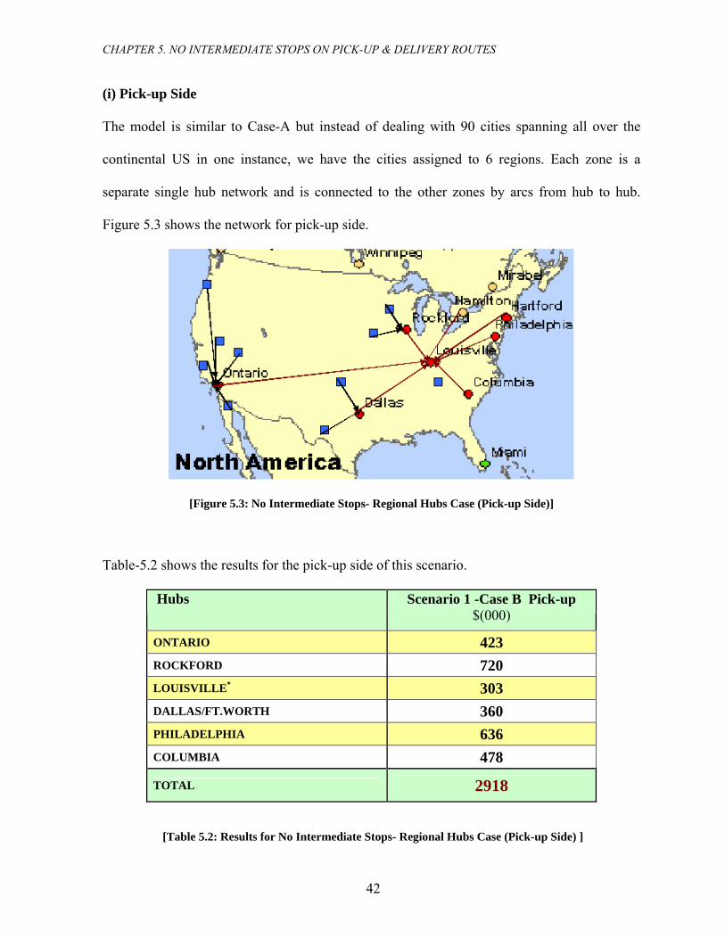
CHAPTER 5. NO INTERMEDIATE STOPS ON PICK-UP & DELIVERY ROUTES
(i) Pick-up Side
The model is similar to Case-A but instead of dealing with 90 cities spanning all over the
continental US in one instance, we have the cities assigned to 6 regions. Each zone is a
separate single hub network and is connected to the other zones by arcs from hub to hub.
Figure 5.3 shows the network for pick-up side.
[Figure 5.3: No Intermediate Stops- Regional Hubs Cas
Table-5.2
e (Pick-up Side)]
shows the results for the pick-up side of this scenario.
Hubs Scenario 1 -Case B Pick-up $(000)
ONTARIO 423 ROCKFORD 720 LOUISVILLE* 303 DALLAS/FT.WORTH 360 PHILADELPHIA 636 COLUMBIA 478
TOTAL 2918
[Table 5.2: Results for No Intermediate Stops- Regional Hubs Case (Pick-up Side) ]
42

CHAPTER 5. NO INTERMEDIATE STOPS ON PICK-UP & DELIVERY ROUTES
(ii) Delivery Side
The delivery side analysis is similar to the single hub network. Figure 5.4 shows the delivery
network.
[Figure 5.4: No Inter te Stops- Regional Hubs Case (Delivery Si
Table 5.3 shows the results for the delivery side of th
media de)]
is scenario.
Hubs Scenario 1 -Case B Delivery $(000)
ONTARIO 572 ROCKFORD 484 LOUISVILLE* 295 DALLAS/FT.WORTH 428 PHILADELPHIA 662 COLUMBIA 488
TOTAL 2929
[Table 5.3: Results for No Intermediate Stops- Regional Hubs Case (Delivery Side) ]
43

CHAPTER 5. NO INTERMEDIATE STOPS ON PICK-UP & DELIVERY ROUTES
(iii) Interhub Component
The third cost component is the major one and it deals with the inter hub flights between the
six regional hubs.
Table 5.4 shows the summary of results obtained from above MIP runs.
Hubs Pick-up $(000)
Interhub
$(000)
Delivery
$(000)
ONTARIO 423 572 ROCKFORD 720 484 LOUISVILLE 303 295 *
DALLAS/FT.WORTH 360 428 PHILADELPHIA 636 662 COLUMBIA 478
4915
488 TOTAL 2918 4915 2929 GRAND TOTAL 10762
[Table 5.4: Results for No Intermediate Stops- Regional Hubs Case (Total Cost)]
]
We find that the total cost of this scenario is 10.3% more than the base case. This is probably
du al
hubs on the pick-up and delivery sides respectively. If there is a demand comparable to a full
airport and destination regional hub, it is practical to dispatch
routing it through the origin
plications of these kinds of strategies in our subsequent
sections.
e to the fact that all demands are forced to go through the origin and destination region
flight load between an origin
the demands directly to the destination regional hubs (instead of
regional hub). We analyze the im
44

CHAPTER 5. NO INTERMEDIATE STOPS ON PICK-UP & DELIVERY ROUTES
5.2.3 Case C: Demands routed through Origin Regional Hub and directly
dispatched to destination
Since the cost of routing from a regional hub to other regional hubs is a big proportion of the
total cost and there is already a consolidation at the regional hubs, we analyzed the scenario
wh i onal hub would be and consolidated
with respect to their destination cities (inste sorting them with respect to destination
regional hub as we did in 5.2.2. Case B). By this strategy, we undo the costs incurred for pick-
up and delivery between regional hubs and delivery from the destination regional hub to the
destinati
ere the demands after reaching the orig n regi sorted
ad of
on cities.
[Figure 5.5: Demands routed through Origin Regional Hubs and directly dispatched to Destination]
(i) Pick-up Side
Pick-up is the same as Scenario 1 Case-B (Table 5.2).
(ii) Delivery Side
This would be the cost of dispatching the demands from origin regional hubs to destinations
by direct flights.
45

CHAPTER 5. NO INTERMEDIATE STOPS ON PICK-UP & DELIVERY ROUTES
Table 5.5 summarizes the results of this analysis.
Hubs
Pick-up Cost $(000)
Delivery Cost $(000)
ONTARIO 423 1872
ROCKFORD 720 1590
LOUISVILLE* 303 1009
DALLAS/FT.WORTH 360 1320
PHILADELPHIA 636 1771
COLUMBIA 478 1325
Total 2918 8887
GRAND TOTAL 11805
[Table 5.5: Results for Scenario 1 Case C]
Clearly, this strategy is not a good one as the cost implications are 21% higher than the base
s, it essentially means less than capacity flights
ying much longer distances.
case (Scenario 1 Case A).
5.2.4 Case D: Demands routed to destination regional hub
This scenario was not pursued further as the strategy itself by its structure has huge cost
implications. Instead of a consolidation at the early stages (i.e at origin regional hubs), if the
demands are carried directly to destination hub
fl
46
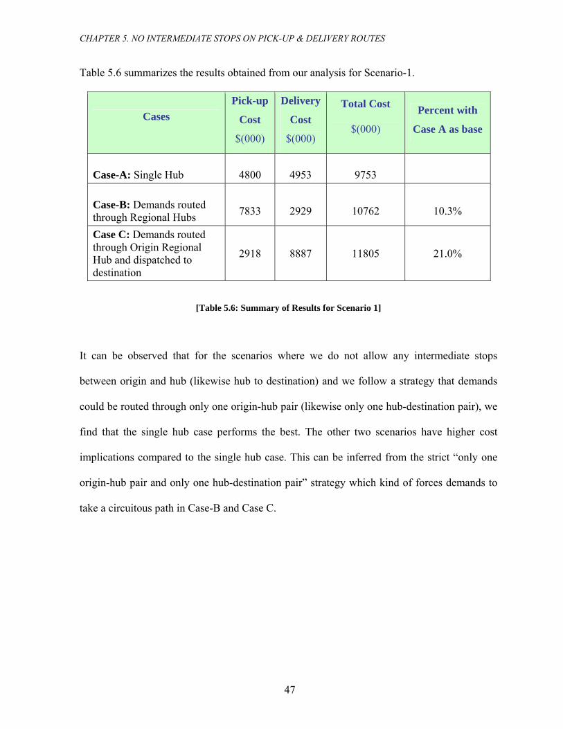
CHAPTER 5. NO INTERMEDIATE STOPS ON PICK-UP & DELIVERY ROUTES
Table 5.6 summarizes the results obtained from our analysis for Scenario-1.
Cases Pick-up
Cost
$(000)
Delivery
Cost
$(000)
Total Cost
$(000)
Percent with
Case A as base
Case-A: Single Hub 4800 4953 9753 Case-B: Demands routed through Regional Hubs 7833 2929 10762 10.3%
Case C: Demands routed through Origin Regional Hub and dispatched to destination
2918 8887 11805 21.0%
[Table 5.6: Summary of Results for Scenario 1]
It can be observed that for the scenarios where we do not allow any intermediate stops
between origin and hub (likewise hub to destination) and we follow a strategy that demands
could be routed through only one origin-hub pair (likewise only one hub-destination pair), we
implications compared to the single hub case. This can be inferred from the strict “only one
take a circuitous path in
find that the single hub case performs the best. The other two scenarios have higher cost
origin-hub pair and only one hub-destination pair” strategy which kind of forces demands to
Case-B and Case C.
47

CHAPTER 5. NO INTERMEDIATE STOPS ON PICK-UP & DELIVERY ROUTES
5.3 Scenario-2:
No Intermediate Stops with demands routed from Origin through multiple
delivery side, we routed the demands from only
nation. This restriction naturally led to inefficient use of capacity, thereby
e study the implications of the strategy when the
rough more than one hub on both pick-up and
re there are regional hubs, on the pick-up side,
e route going from the origin to the destination
cuitous way from origin to origin regional hub
upon the idea that if there is a demand from
lightly more than an aircraft capacity, then it
destination regional hub and route the balance
ere is a likelihood that it gets consolidated
with demands from other origins to the same destination hub. This strategy promises with its
structure to m e no
We start with a case where there are regional hubs and on hub. All the demands are
routed th , the demands could be routed directly to the
main hub origin regional hub to the main hub. Similarly, on the delivery side,
hubs on pick-up and multiple hubs to Destination on delivery
In Scenario-1, we studied instances where the demand was routed between only one origin-
hub pair on pick-up side. Similarly, on the
one hub to a desti
increasing cost. Under the present scenario, w
demands could be routed to the destination th
delivery sides. For example, for the case whe
the demands could be split into two routes: on
regional hub and the second going in a more cir
to destination regional hub. This split builds
origin to destination regional hub which is s
makes sense to send an aircraft from origin to
demand through the local regional hub; where th
ake better use of aircraft capacity and available fleet. As before, we assum
intermediate stops.
e main
rough the main hub. On the pick-up side
or through the
48
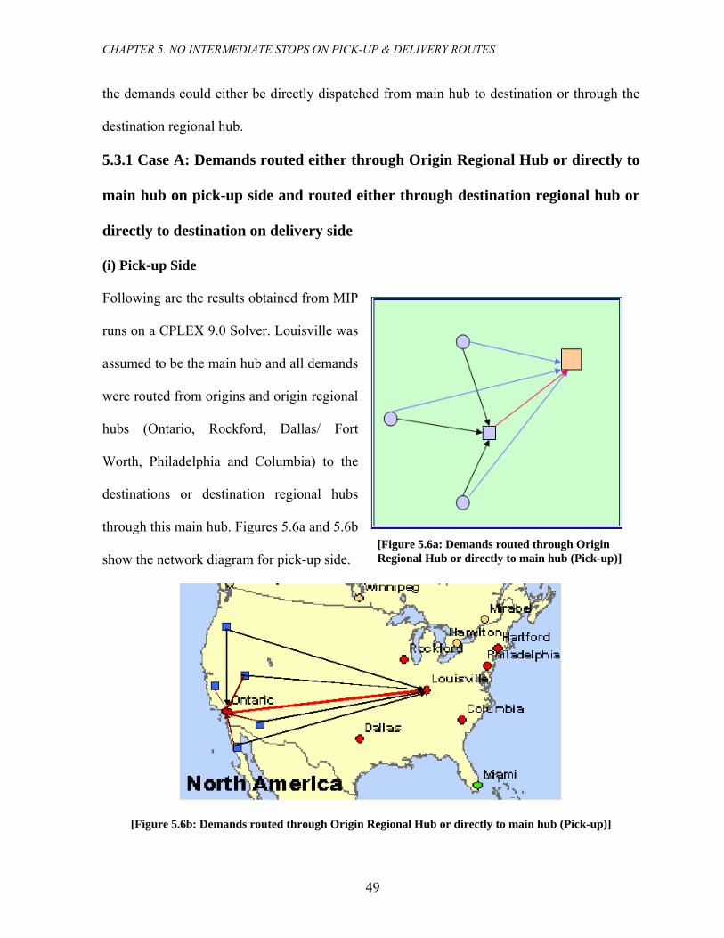
CHAPTER 5. NO INTERMEDIATE STOPS ON PICK-UP & DELIVERY ROUTES
the dema ly dispatched from main hub to destination or through the
destinatio
5.3.1 Ca s routed either through Origin ional Hub or directly to
main hub on pick-up side and routed either through destination regional hub or
directly to destination on delivery side
) Pick-up Side
sults obtained from MIP
nds
ere routed from origins and origin regional
ubs (Ontario, Rockford, Dallas/ Fort
orth, Philadelphia and Columbia) to the
estinations or destination regional hubs
through this main hub. Figures 5.6a and 5.6b
how the network diagram for pick-up side.
nds could either be direct
n regional hub.
se A: Demand Reg
(i
Following are the re
runs on a CPLEX 9.0 Solver. Louisville was
assumed to be the main hub and all dema
w
h
[Figure 5.6a: Demands routed through Origin Regional Hub or directly to main hub (Pick-up)]
W
d
s
[Figure 5 Origin Regional Hub or ain hub (Pick-up)]
.6b: Demands routed through directly to m
49

CHAPTER 5. NO INTERMEDIATE STOPS ON PICK-UP & DELIVERY ROUTES
The results are shown in Table 5.7a.
REGIONAL HUBS COST $(000)
ONTARIO 1011
ROCKFORD 848
LOUISVILLE * 303
DALLAS/FT.WORTH 671
PHILADELPHIA 969
COLUMBIA 604
TOTAL 4405 * In case of Louisville, there won o hubs as the main nd the regional hu ame.
[Table 5.7 ults of Scenario 2 p Side]
ide
a similar methodology f delivery side ( ures 5.7) and p with the
followi
[Figure 5.7: Demands routed destination regional hub or directly to destination (Delivery)]
't be tw hub a b are s
a: Res Pick-u
(ii) Delivery S
We adopt or the see Fig come u
ng costs as shown in Table 5.7b.
50

CHAPTER 5. NO INTERMEDIATE STOPS ON PICK-UP & DELIVERY ROUTES
REGIONAL HUBS Cost $(000)
ONTARIO 1433
ROCKFORD 566
LOUISVILLE* 295
DALLAS/FT.WORTH 740
PHILADELPHIA 1021
COLUMBIA 606
TOTAL 4661 * In case of Louisville, there won't be two hubs a ain hub and the region re same.
[Table 5.7b: Results of Sc ivery Side]
s the m al hub a
enario 2 Del
REGI Pick-up Cost Delivery Cost TotalONAL HUBS Cost $(000) $(000) $(000)
ONTARIO 1011 1433 2444
ROCKFORD 848 566 1414
LOUISVILLE* 303 295 598
DALLAS/FT.WORTH 671 740 1411
PHILADELPHIA 969 1021 1990
COLUMBIA 604 606 1210
TOTAL 4405 4661 9066 * In case of Louisville, there won't be two hubs as the main hub and the regional hub are same.
[Table 5.8: Results of Scenario 2 (Total Cost)]
Comparing this value with Scenario 1 Case A, we find that there is a significant saving of
7.0% by opting for this strategy.
51

CHAPTER 5. NO INTERMEDIATE STOPS ON PICK-UP & DELIVERY ROUTES
5.3.2 Case B: Combining Scenario 1 results with Scenario 2 results
We further our analysis to see the impl lts obt io 1. It
makes sense to see the effects of a strategy if w ine the delivery sid enario 1 Case
A to the pick-up side of Scenario 2 Case A. Alo same lines, we could combine the pick-
up side of Scenario 1 Case A to delivery side of Scenario 2 Case A. The results are shown in
Tables 5.9a and 5.9b respectively.
ications of the resu ained under Scenar
e comb e of Sc
ng the
REGIONAL HUBS
Scenario 2 Case A
(Delivery)
Scenario1 Case A (Pick-up)
$000 $000
ONTARIO 1433
ROCKFORD 566
LOUISVILLE* 295
DALLAS/FT.WORTH 740
PHILADELPHIA 1021
COLUMBIA 606
4800
TOTAL 9461
* In case of Louisville, there won't be two hubs as the main hub and the regional hub are same.
[Table 5.9a: Scenario 1 Case A Pick-up with Scenario2 Case A Delivery]
52

CHAPTER 5. NO INTERMEDIATE STOPS ON PICK-UP & DELIVERY ROUTES
* In case of Louisville, there won't be two hubs as the main hub and the regional hub are same.
[Table 5.9b: Scenario 2 Case A Pick-up with Scenario1 Case A Delivery]
We see that “Scenario 2 Case A Delivery with Scenario 1 Case A Pick-up” and “Scenario 2
Case A Pick-up with Scenario 1 Case A Delivery” lead to savings of 3.0% and 4.1%
respectively compared to the base case. Thus, we can conclude that even if we do not allow
intermediate stops, simply opting for a strategy in which demands could be routed through
either hub as applicable, we end up saving in the order of 7.0%.
REGIONAL HUBS Scenario 2
Case A (Pick-up) Scenario1 Case A
(Delivery) $000 $000
ONTARIO 1011
ROCKFORD 848
LOUISVILLE* 303
DALLAS/FT.WORTH 671
PHILADELPHIA 9
4953
69
COLUMBIA 604
TOTAL 9358
53

CHAPTER 5. NO INTERMEDIATE STOPS ON PICK-UP & DELIVERY ROUTES
5
No Main Hubs, Demands routed through Regional Hubs only
In this analysis conducted, we exclude the presence of main hub and assume that there are
only regi ands are routed through them only.
5.4.1 Ca s routed either th Origin Regio ub or directly to
Destina ub on pick-up sid
On the ds would outed either dire from the origin to
destination regional hub or through the origin regional hub (see Figures 8a and 8b).
[Figure 5.8a: Demands routed through Origin Regional Hub or directly to Destination Regional Hub]
The delivery side naturally becomes a case where the demands need to be routed from the
delivery destination hub to the destination (as studied in Scenario1 Case B).
.4 Scenario 3:
onal hubs and the dem
se A: Demand rough nal H
tion Regional H e
pick-up side, the deman be r ctly
54

CHAPTER 5. NO INTERMEDIATE STOPS ON PICK-UP & DELIVERY ROUTES
[Figure 5.8b: Demands routed through Origin Regional Hub or directly to Destination Regional Hub] ]
The results of the MIP runs are shown in Table 5.10.
REGIONAL HUBS Pick-up Delivery $(000) $(000)
ONTARIO 849 572
ROCKFORD 1158 484
LOUISVILLE* 726 295
DALLAS/FT.WORTH 763 428
PHILADELPHIA 1160 662
COLUMBIA 752 488
TOTAL 5408 2929
GRAND TOTAL 8337
[Table 5.10: Results of Scenario 3 Ca ck-up)] se A (Pi
55
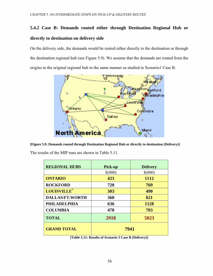
CHAPTER 5. NO INTERMEDIATE STOPS ON PICK-UP & DELIVERY ROUTES
5.4.2 Case B: Demands routed either through Destination Regional Hub or
directly to destination on delivery side
On the delivery side, the demands would be routed either directly to the destination or through
the destination regional hub (see Figure 5.9). We assume that the demands are routed from the
rigins to the original regional hub in the same manner as studied in Scenario1 Case B. o
[Figure 5.9: Demands routed through Destination Regional Hub or directly to destination (Delivery)]
The results of the MIP runs are shown in Table 5.11.
REGIONAL HUBS Pick-up Delivery $(000) $(000) ONTARIO 423 1112 ROCKFORD 720 769 LOUISVILLE* 303 490 DALLAS/FT.WORTH 360 821 PHILADELPHIA 636 1128 COLUMBIA 478 703
TOTAL 2918 5023
GRAND TOTAL 7941 [Table 5.11: Results of Scenario 3 Case B (Delivery)]
56

CHAPTER 5. NO INTERMEDIATE STOPS ON PICK-UP & DELIVERY ROUTES
57
d ough origin regional hub or directly to destination regional hub
on pick-up side has 5.0% more cost implications than the strategy in which demands are
routed either through destination regional hub or directly to destination on delivery side.
All the above analysis conducted
are no intermediate stops from the origin to the hub to
the destination on the delivery rout e summarize out results in Table 5.12. And we see that
‘Sce i bs, Demands routed through Regional Hubs only Case-B’ appears to be the
best strategy as o s gs e o of 14.5% and 18.7% on the pick-up (Case A) and
delivery side (Ca ) tegies respe
may vary if there are major changes in demands. Nev eless, this analy gives a
“comparative feel” of the various scenarios. We undertake a more in-depth sensitivity analysis
in Chapter 7 to make generalized inferences of .
From the results shown in Table 5.10 and Tabl
emands are routed either thr
e 5.11, we find that for the strategy in which
in Scenario 1 through 3 are based on the strategy that there
e. W
in th
ctively.
the hub on the pick-up route and from
nar o 3 No Main Hu
we
se B
btain
stra
avin rder
However, it may be noted that the inferences drawn
erth sis
impacts of various strategies on our problem
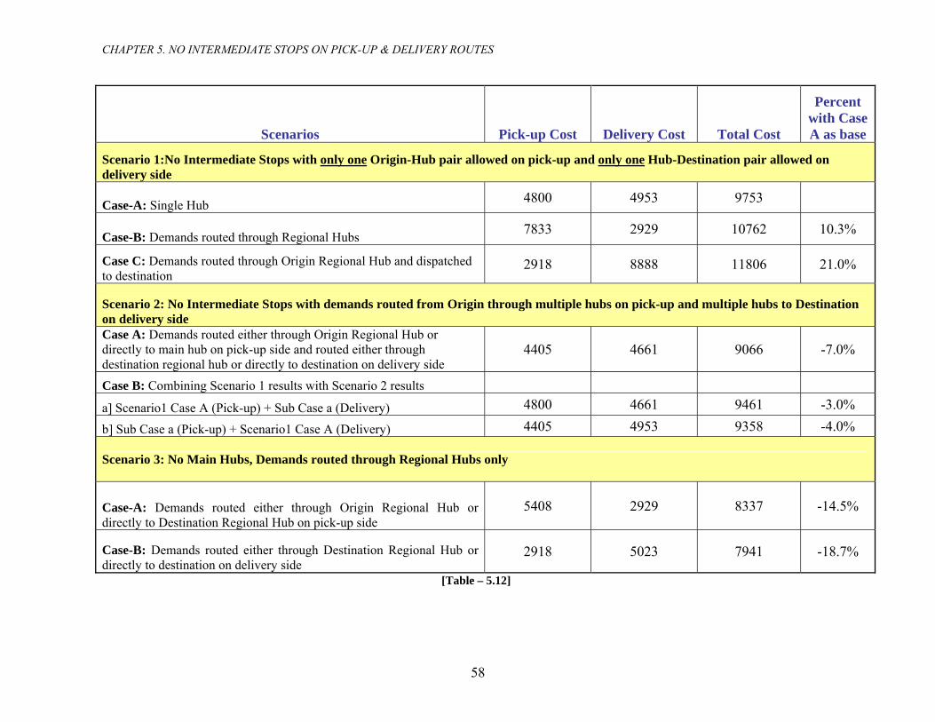
CHAPTER 5. NO INTERMEDIATE STOPS ON PICK-UP & DELIVERY ROUTES
58
Delivery Cost Total Cost
Percent with Case A as base Scenarios Pick-up Cost
Sc ri o r ia to it lyena o 1:N Inte med te S ps w h on one Origin-Hub pai ed o -up and only oner allow n pick Hub-Destination pair allowed on delivery side
Case-A: Sin e Hu gl b 4800 4953 9753
Case-B: Dem nds uted hrou h Region a ro t g al Hubs 7833 2929 10762 10.3%
Case C: Dem nds uted hrou h Origin Re onala ro t g gi Hub and dispatchto destination
2918 8888 11806 21.0% ed
Scenario 2: No Intermediate Stops with demands routed from O hrough multiple hubs on pick-up and multiple hubs to Destination rigin ton iv i del ery s de Case A: Dem nds uted Ori n Redirectly to m n hu on pi k-up de a d rou d eitdestination regional hub o directly to estin ion o
a ro either through gi gional Hub or ai b c si n te her through
r d at n delivery side 4405 4661 9066 -7.0%
Case B: Com inin Scen io 1 sultsb g ar re with Scenario 2 results
a] A (Pick-up) + Sub Case a ( ery) 4800 4661 9461 -3.0% Scenario1 Case Delivb] Sub Case a (Pick-up) + Scenario1 Ca very) 4405 4953 9358 -4.0% se A (Deli
Scenario 3: No Main Hubs, Demands routed through Regional Hubs only
Case-A: De ands rout eit r th ough Origidirectly to D tinat n Re ional Hub pick up si
m ed he r n Regional Hubes io g on - de
5408 2929 8337 -14.5% or
Case-B: Demands routed either throdirectly to destination on delivery side
ugh Destination Regional Hu
2918 5023 7941 -18.7% b or
[Table – 5.12]

CHAPTER 6.INTERMEDIATE STOPS ON PICK-UP & DELIVERY ROUTES
Chapter 6
Intermediate Stops on Pick-up & Delivery Routes
6.1 Introduction
All analysis conducted in Chapter 5 by Scenarios 1 through 3 are based on the model that
there are no intermediate stops from the origin to the hub on the pick-up route and from the
hub to the destination on the delivery route. This strategy by its structure leads to less than
capacity flight legs. Subject to the temporal and capacity constraints, it is possible to cover
one / more airports on pick-up / delivery routes. Introducing intermediate stops leads to
reduced fleet size required for the operations thereby opening the opportunity to reduce total
costs of operation. Again, there may be several strategies one could envisage to dispatch the
demands on pick-up and delivery routes. In this chapter, we introduce the concept of
59

CHAPTER 6.INTERMEDIATE STOPS ON PICK-UP & DELIVERY ROUTES
intermediate stops and study the implications of a strategy in which we allow one
intermediate stop on the pick-up route and similarly, one intermediate stop on the delivery
route (see Figure 6.1).
[Figure 6.1: One Stop Routes on Pick-up and Delivery Sides]
In the subsequent sections, we study various possible configurations, logical combinations
and their extensions for the one intermediate stop case.
60

CHAPTER 6.INTERMEDIATE STOPS ON PICK-UP & DELIVERY ROUTES
6.2 Scenario 1: Presence of One Intermediate Stop on Pick-up and Delivery
Routes – Single Hub Case
We make use of the travel time matrices that we derived from the statistical analysis of the
two aircraft types. As described in Chapter 3, we build a set of feasible paths on the city
network on both the pick-up and delivery sides with an intermediate stop on each path.
raft type, we have total travel time from
h is equal to the sum of the actual air travel
analysis performed on the aircraft travel
times as shown in Chapter 4. We assume that the loading time at the intermediate stop on a
pick-up route and the unloading time at an intermediate stop on a delivery route are 45
minutes each. We assume a constant cut-off time at all cities by which all the demands reach
the origin airports. Similarly, we assume a constant cut-off time by which all the demands
should reach the hub. The effect of time zones and the time windows are described in Chapter
2. Based on the above cut-off times, we eliminate the one stop paths obtained above that do
not satisfy the temporal constraints. This prescreening helps in reducing the num er of path
variables that we the problem size.
add the paths corresponding to the direct flights from the origins to the
hs are envisaged to be
sed by the optimal solution if there are no one-stop paths from an origin to hub (hub to
destination) that satisfies the temporal constr nts. These paths may also be used in the
optimal solution if t n aircraft capacity.
Corresponding to each path and depending on the airc
an origin to the hub (or, hub to destination) whic
time and take-off and landing times and loading time at the intermediate stop. These travel
times are further adjusted by taking the time zones into account. The take-off and landing
times of an aircraft are the constants of the regression
b
pass on to the MIP formulation, thereby reducing
Obviously, we still
hub (hub to the destinations) on pick-up (delivery) routes. These pat
u
ai
he demand from an origin (to a destination) is more tha
61
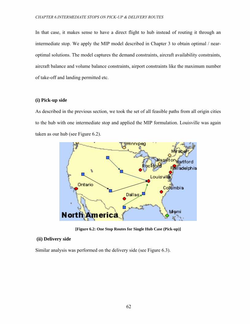
CHAPTER 6.INTERMEDIATE STOPS ON PICK-UP & DELIVERY ROUTES
In that case, it makes sense to have a direct flight to hub instead of routing it through an
3 to obtain optimal / near-
o . The model captures the demand constraints, aircraft availability constraints,
aircraft balance and volume bala ints, airpor ts like th m number
of take g permitted e
(i) Pick-up side
As described in the previous section, we took the set of all feasible paths from all origin cities
to the hub with one uisville was again
ken as our hub (see Figure 6.2).
intermediate stop. We apply the MIP model described in Chapter
ptimal solutions
nce constra t constrain e maximu
-off and landin tc.
intermediate stop and applied the MIP formulation. Lo
ta
[Figure 6.2: One Stop Routes for Single Hub Case (Pick-up)]
(ii) Delivery side
Similar analysis was performed on the delivery side (see Figure 6.3).
62

CHAPTER 6.INTERMEDIATE STOPS ON PICK-UP & DELIVERY ROUTES
[Figure 6.3: One Stop Routes for Single Hub Case (Delivery)]
Table 6.1 summarizes the results obtained from the CPLEX runs.
Single Hub at Louisville One Stop No Stop Savings $000 $000 %
Pick-up Side 4556 4800 5.4%
Delivery Side 4781 4953 3.6%
GRAND TOTAL 9337 9753 4.5%
[Table 6.1: Results of One Stop Scenario for Single Hub Case]
Thus, with the introduction of one intermediate stop on the pick-up and delivery routes in the
single hub case leads to a total savings of 4.5%.
63

CHAPTER 6.INTERMEDIATE STOPS ON PICK-UP & DELIVERY ROUTES
6.3 Scenario 2: Presence of One Intermediate Stop on Pick-up and Delivery
Routes – Regional Hubs Present
the scenario where we have six regional hubs in
o, Rockford, Louisville, Dallas / Ft. Wo
In this section, we further our analysis with
our network; the hubs being located at Ontari rth,
Philadelphia and Columbia. The origin airports ed to the hub which is at a minimum
distance; so we have six zones with each zone having a regi d so For
e -up side, we construct paths from each origin to the regional hub having
o stop. Similarly, we construct paths from the hub to the destination with one
i e eliminate paths the set of paths obtained above depending on the
t tain a set asible paths for th work. We apply the MIP
formulation to each regional hub on both the pick-up and delivery sides. As described in
Chapter 5, we assume that the dem d be flown from
regional hubs by direct flights.
(i) Pick-up side
e pick-up side under this strategy.
are assign
onal hub an me airports.
ach zone, on the pick
ne intermediate
ntermediate stop. W from
emporal constraints to ob of fe e net
ands woul the regional hubs to other
Figure 6.4 shows a sample network on th
[Figure 6.4: One Stop Cases with Regional Hubs Present (Pickup Side)]
64

CHAPTER 6.INTERMEDIATE STOPS ON PICK-UP & DELIVERY ROUTES
Table 6.2 shows the results obtained from the model runs for the pick-up side for one
inte nd its comparison to the no intermediate s se. From the results,
we find that the cost implications in the one-intermediate stop case are about 4.4 % lesser
than the no intermediate hub case. This may be attributed to the effective use of capacity.
rmediate stop case a top ca
REGIONAL HUBS Pick-up
One Intermediate
S No Intermediate
Stop % Savitop ngs $(000) $(000)
ONTARIO 391 42 7.5%3
ROCKFORD 715 720 0.7%
LOUISVILLE * 293 303 3.5%
DALLAS/FT.WORTH 325 360 9.6%
PHILADELPHIA 606 636 4.8%
COLUMBIA 459 478 3.9% TOTAL 2789 2918 4.4%
[Table 6.2: Comparison of Pick-up Costs for Regional Hubs Case]
(ii) Delivery side
Fig-6.5 shows a sample network on the delivery side under this strategy.
[Figure 6.5: One Stop Cases with Regional Hubs Present (Delivery Side)]
65

CHAPTER 6.INTERMEDIATE STOPS ON PICK-UP & DELIVERY ROUTES
Similarly, on the delivery side, we show the results obtained in the one intermediate stop and
compare with the fleet size requirements for the no intermediate stop case. As shown in Table
6.3, we find that there is a savings of 3.9 % in total cost.
REGIONAL HUBS Delivery One Intermediate Stop No Intermediate Stop % Savings $(000) $(000)
ONTARIO 554 572 3.1%
ROCKFORD 481 484 0.6%
LOUISVILLE 283 295 4.0%
DALLAS/FT.WORTH 405 428 5.4%
PHILADELPHIA 632 662 4.5%
COLUMBIA 459 488 5.9%
TOTAL 2814 2929 3.9%
[Table 6.3: Comparison of Delivery Costs for Regional Hubs Case]
Total cost incurred would be 10518 [$(000)] the sum of the pick-up side, delivery side and
interhub transportation costs. This total cost is 2.3% lower and 12.6% higher compared to the
Single Hub-No Stop (Section 5.2) and Single Hub-One Stop (Section 6.2) respectively. We
see that even when there are savings of around 4% in both the pick-up and delivery phases,
the total cost is higher. This is because of the high interhub transportation cost component.
We have assumed that there won’t be any intermediate stops on the flights from to hub to hub.
This is a realistic assumption owing to the fact that there is considerable consolidation at
hubs. And we don’t have much leeway as we are dealing with tight time windows.
66

CHAPTER 6.INTERMEDIATE STOPS ON PICK-UP & DELIVERY ROUTES
6.4 Scenario 3: Presence of One Intermediate Stop on Pick-up and Delivery
Routes when demands directly dispatched to Destination Regional Hubs
Interhub transportation cost is a big component as we have seen in previous sections (Sections
5.2.2 and 6.3) in which demands were consolidat on tched to
destination regional hubs by interh hts. In this on, we study trategy where
de tly dispatched to estination regional hubs on the pick-up side and
dis in regional hub he destinations on the delivery side. As before, we
generate one stop flights on both pick-up and delivery routes subject to al constraints.
In flight would rom an orig y, make a stop in an intermediate
city and finally reach the destination regional hub. On the delivery side, ht would start
fro in regional hub, make an intermediate sto inally reach tination city.
gy.
ed at origin regi al hubs and dispa
ub flig secti the s
mands are direc the d
patched from orig s to t
tempor
the pick-up case, the start f in cit
the flig
m the orig p and f the des
Case-A: One Stop Routes From Origin Cities to Destination Regional Hubs
Figure 6.6 shows a sample network on the pick-up side under this strate
[Figure 6.6: One St utes from Origin to Destination Re bs] op Ro Cities gional Hu
67

CHAPTER 6.INTERMEDIATE STOPS ON PICK-UP & DELIVERY ROUTES
As shown in Figure 6.6, on the pic side, demands are routed from the o city to the
destination regional hubs. These are subsequently delivered to the destinations by one stop
p tion regional h able 6.4 show sults of the MI
k-up rigin
aths from the destina ub. T s the re P runs.
REGIONAL HUBS
Pick-up Cost
Delivery Cost $(
TOTAL COST $(00000) 0) $(000)
ONTARIO 1576 554 2130
ROCKFORD 1073 481 1554
LOUISVILLE 750 283 1033
DALLAS/FT.WORTH 1016 405 1421
PHILADELPHIA 1787 632 2419
COLUMBIA 1077 459 1536
TOTAL 7279 2814 10093
The total cost under this strategy is 3.5% and 8.1% higher compared to the Single Hub-No
[Table 6.4: Results of Scenario 3 - One Stop Case A]
Stop (Section 5.2) and Single Hub-One Stop (Section 6.2) respectively.
Case-B: One Stop Routes From Origin Regional Hubs To Destination Cities
As shown in Figure 6.7, on the delivery side, demands are routed from the origin regional hub
to the destination city. Table 6.5 shows the result of the MIP runs.
68

CHAPTER 6.INTERMEDIATE STOPS ON PICK-UP & DELIVERY ROUTES
[Figure 6.7: One Stop Routes From Origin Regional Hubs To Destination Cities]
REGIONAL HUBS
Pick-up Cost $(000)
Delivery Cost $(000)
TOTAL COST $(000)
ONTARIO 391 1117 1508
ROCKFORD 715 1485 2200 LOUISVILLE 293 870 1163 DALLAS/FT.WORTH 325 1727 2052 PHILADELPHIA 606 1729 2335 COLUMBIA 459 1122 1581
TOTAL 2789 8050 10839 [Table 6.5: Results of Scenario 3 - One Stop Case B]
The total cost under this strategy is 11.1% and 16.1% higher compared to the Single Hub-No
Stop (Section 5.2) and Single Hub-One Stop (Section 6.2) respectively. One of the reasons
that the total cost under the above scenarios is higher than the single hub cases (either with no
intermediate stops / one stop) could be attributed to the fact that there is not sufficient amount
of consolidation. This results in less than capacity flights. Under Case-A, most likely, it
happens that the one stop paths from origin cities to destination regional hub fly less than
payload capacity. Similarly, under Case-B, there is not sufficient amount of consolidation
which results in less than flight loads from origin regional hub to destination.
69

CHAPTER 6.INTERMEDIATE STOPS ON PICK-UP & DELIVERY ROUTES
6.5 Scenario 4: Demands routed from Origin either through One Stop
routes to Destination Regional Hubs
riginal Regional Hubs on Pick-up
Demands routed from Origin Regional Hubs either through One Stop
r utes to Destinations or throu
Regional Hubs on Delivery
O outed he origin either through one-stop routes to the
destination regional hubs or through no stop routes through the origin regional hub (see
F ecomes the case where we allow one-stop routes to the
d y side, demands are routed from origin regional hubs
e na or through no stop routes through destination
regional hub on delivery (see Figure 6.9). The pick-up side is the case where we allow one-
stop routes from origin to origin regional hub..
or through No Stop routes through
O
and
o gh No Stop routes through Destination
n the pick-up side, demands are r from t
igure 6.8). The delivery side b
estination. Similarly on the deliver
ither through one-stop routes to desti tions
[Figure 6.8: Demands routed from Origin either through One Stop routes to Destination Regional Hubs or
through No Stop routes through Original Regional Hubs on Pick-up ]
70

CHAPTER 6.INTERMEDIATE STOPS ON PICK-UP & DELIVERY ROUTES
[Figure 6.9: Demands routed from Origin Regional H
or through No Stop routes throug
u through One Stop to Desti
h Destination Regional Hubs on Delivery]
rio.
bs either routes nations
Table 6.6 shows the results of the MIP runs for this scena
Pick-up Side Delivery Side TOTAL $000 $000 $000Demands routed from Origin either through One Stop routes to Destination Regional Hubs or through No Stop routes through Original Regional Hubs on Pick-up
4210 2814 7024
Demands routed from Origin Regional Hubs either through One Stop routes to Destinations or through No Stop routes through Destination Regional Hubs on Delivery
2789 4025 6814
[Table 6.6: Resu s of Scenario 4] lt
71

CHAPTER 6.INTERMEDIATE STOPS ON PICK-UP & DELIVERY ROUTES
Table 6.7 summarizes the results of all one-stop scenarios.
6.7: Summary of One Stop Scenarios]
hat the scenario where demands routed from Origin either through
SCENARIOS
Pick-up Cost
$(000)
Delivery Cost
$(000)
TOTAL COST $(000)
Savings compared
to (1) $(000) $(000)
(1) Single Hub Case 4556 4781 9337
(2)Demand routed through origin regional hubs 7704 2815 10519 -13%
(3)Demand routed from origins to destination regional hubs 7279 2814 10093 -8%
(4)Demand routed from origin regional hubs to ations 2789 8050 10839 -16% destin
(5)a Demands routed from Origin either through One Stop routes to Destination Regional Hubs or through No Stop routes through Original Regional Hubs on Pick-up
4210 2814 7024 25%
(5)b Demands routed from Origin Regional Hubs either through One Stop routes to Destinations or through No Stop routes through Destination Regional Hubs on D
2789 4025 6814 27%
elivery
[Table
From the analysis, we find t
One Stop routes to Destination Regional Hubs or through No Stop routes through Original
Regional Hubs on Pick-up or, demands routed from Origin Regional Hubs either through One
Stop routes to Destinations or through No Stop routes through Destination Regional Hubs on
Delivery performs the best operational cost wise with average savings of 26%. Clearly, this
strategy stands out to be the best of all the scenarios we have discussed in Chapters 5 and 6.
72

CHAPTER 7.SENSITIVITY ANALYSIS
Chapter 7
Sensitivity Analysis
7.1 Introduction
In the previous two chapters, we studied the cost impact of various operational scenarios and
we made comparisons of cost savings. It may be noted that the costs obtained from the MIP
runs for all the cases in Chapter 5 and 6 are based on one deterministic set of origin-
destination demands. Similarly, the unit cost incurred by an aircraft per nautical mile reflects
a preset fuel price and fixed cost of the aircraft. Naturally, the observations made in the
previous chapter cannot be generalized for all feasible demands and unit cost of
transportation. An ideal way of finding the cost savings under various scenarios would be
obtaining real demand and cost data from the industry and running the model scenarios.
73

CHAPTER 7.SENSITIVITY ANALYSIS
However, with the absence of real data, we could run some sensitivity analysis and figure out
50% and 200% of the original demand taken. We run the same scenarios and
arly, on the unit cost of transportation side, we
of operations. In addition, to the above two components, we conduct some sensitivity analysis
on the implications of airport constraints on the model. Chapter 5 and 6 assumed that there
was no limitation on the number of flights between a pair of airports. Realistically, there is a
restrictio r of take-of landings at a particular airport that depends on
factors like gateway availability etc. nalyze t implic by prov ounds
on the n ts of a particular type of ai between of citie could
easily incorporate other airport constraints and study the implicat
the trends in operational costs across various scenarios. Since demand and unit cost of
transportation are the most important factors in the problem, we perform a sensitivity analysis
for these two components. For the demand analysis, we take three sets of deterministic
demands in addition to the earlier demand taken for the model run. These three demand sets
reflect 50%, 1
analyze the cost implications of demand. Simil
run some sensitivity analysis to study the effect of fixed costs and fuel price on the total cost
n on the numbe fs and
We a the cos ations iding b
umber of fligh rcraft a pair s. One
ions.
74

CHAPTER 7.SENSITIVITY ANALYSIS
7.2 Demand Sensitivity
As discussed in the introduction, for the demand analysis, we take three sets of deterministic
demands in addition to the earlier demand taken for the model run. These three demand sets
reflect 50%, 150% and 200% of the original demand taken. Cost components remain the same
as before. We run the scenarios described in Chapters 5 and 6 and analyze the cost
implications.
7.2.1 No Intermediate Stop Scenarios
.2.1.1 Scenario-1: Only one7 Origin-Hub pair and only one Hub-Destination pair
1 and Figure 7.1 show the results of the MIP runs.
(i) Single Hub Case
Table 7.
SINGLE HUB AT LOUISVILLE 50% Base 150% 200% $('000) $('000) $('000) $('000)
PICK-UP 2660 4800 6872 7237
DELIVERY 2854 4953 9051 9478
TOTAL 5514 15923 9753 16715
% Change from Base -43% 63% 71%
[Table 7.1 top S io 1 H De Sen Res: No S cenar - Single ub Case mand sitivity ults]
75

CHAPTER 7.SENSITIVITY ANALYSIS
2660 2854
4800 4953
6872 9051
7237 9478
0 5000 10000 15000 20000
$(000)
50%
Base
150%
200%
Demand Sensitivity - Single Hub CaseScenario-1
PickupDelivery
It appears that ec
200%.
i) Regional H
are routed throug
(i
Pick-up and Del
Table 7.2 and Fig
REGIONAL H
ONTARIO
ROCKFORD
LOUISVILLE*
DALLAS/FT.W
PHILADELPH
COLUMBIA
TOTAL
[Figure 7.1: Demand Sensitivity- No Stop Scenario1- Single Hub Case]76
onomies of scales are achieved when the demand increases from 150% to
ubs Present
b show the results of MIP runs for the case when demands
h origin regional hubs only.
ivery Costs
ures 7.2a and 7.2
Pick-up Side Delivery Side UBS 50% Base 150% 200% 50% Base 150% 200%
('000) ('000) ('000) ('000) ('000) ('000) ('000) ('000)
247 423 593 771 315 572 829 1098
378 720 1055 1403 256 484 724 949
164 303 442 577 164 295 421 558
ORTH 205 359 493 656 238 428 647 831
IA 337 636 906 1216 358 662 964 1259
265 478 691 906 271 488 698 919
1596 2918 4180 5529 1602 2929 4283 5615
[Table 7.2: No Stop Scenario 1- Regional Hub Case Demand Sensitivity Results]
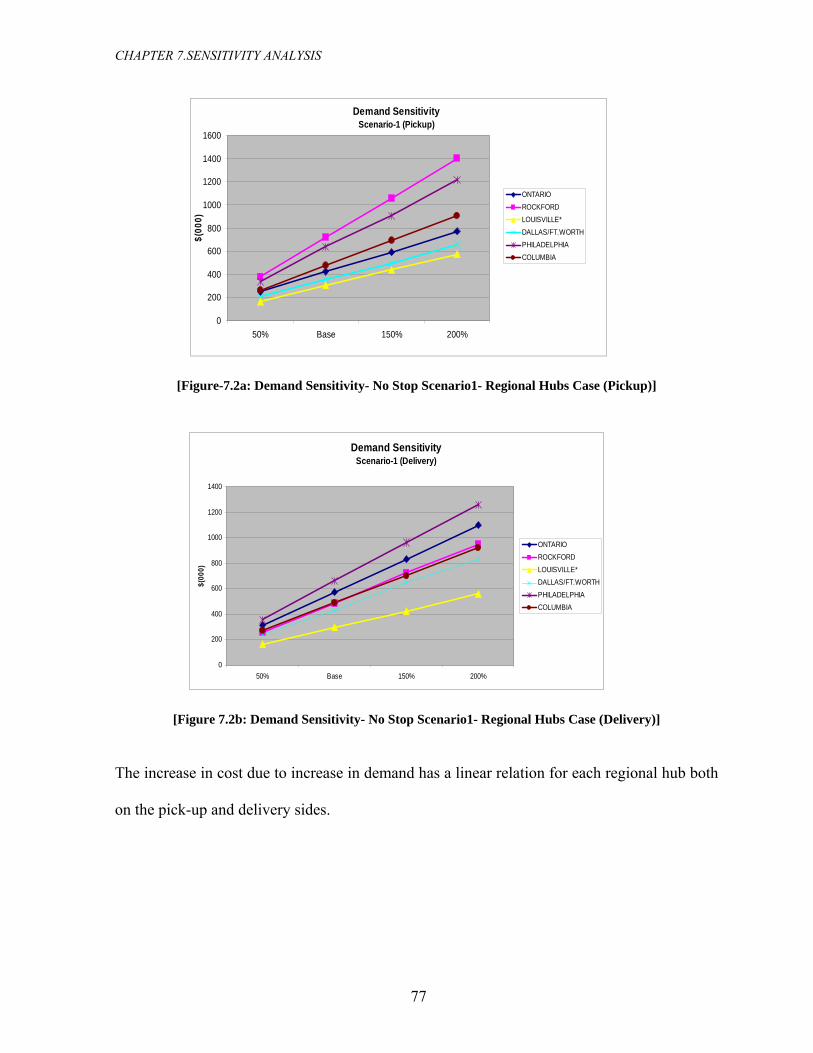
CHAPTER 7.SENSITIVITY ANALYSIS
Demand Sensitivity Scenario-1 (Pickup)
0
200
400
600
800
1000
1200
1400
1600
$(00
0)ONTARIO ROCKFORD LOUISVILLE*DALLAS/FT.WORTH
50% Base 150% 200%
PHILADELPHIA COLUMBIA
[Figure-7.2a: Demand Sensitivity- No Stop Scenario1- Regional Hubs Case (Pickup)]
Demand SensitivityScenario-1 (Delivery)
0
200
400
0
1000
1200
50% B 150% %
00
600$(
80
0)
1400
ase 200
ONTARIO ROCKFORD LOUISVILLE*DALLA ORTHS/FT.WPHI LADELPHIACOLUMBIA
[Figure 7.2b: Demand Sensitivity- No Stop Scenario1- Regional Hubs Case (Delivery)]
se in cost due to increa emand ha r relation h regiona th
ery sides.
The increa se in d s a linea for eac l hub bo
on the pick-up and deliv
77

CHAPTER 7.SENSITIVITY ANALYSIS
Interhub Transportation Costs
Table 7.3 shows the interhub transportation costs for different demand levels.
Base 50% 150% 200% ('000) ('000) ('000) ('000)
4915 2549 7314 9681
[Table 7.3: Interhub Transportation Costs]
Total Cost
This is the sum of the pick-up side cost, delivery side cost and the interhub transportation
costs. Table 7.4 and Figure 7.3 show the results.
TOTAL COST
REGIONAL HUBS 50% Base 150% 200% ('000) ('000) ('000) ('000)
ONTARIO 562 995 1422 1869
ROCKFORD 634 1204 1778 2352
LOUISVILLE* 328 598 864 1135
DALLAS/FT.WORTH 443 787 1140 1487
PHILADELPHIA 695 1298 1869 2475
COLUMBIA 536 966 1389 1825
INTERHUB 2549 4915 7314 9681
TOTAL 5747 10762 15777 20824
% Change from Base 47% 47% 93%
[Table 7.4: Demand Sensitivity of Total Cost for Scenario 1 Regional Hub Case]
78

CHAPTER 7.SENSITIVITY ANALYSIS
79
Demand Sensitivity - Regional Hubs PresentScenario-1
1596
2918
4180
1602
2929
5615
25
4915
7314
9681
10000 15000 20000 25000
1
2
3
$(000)
5529
4283
49
0 5000
4
PICKUP
DELIVERY
INTERHUB
and Sensi y of Total Cost for Scenario 1 Regional Hub Case] [Figure 7.3: Dem tivit

CHAPTER 7. SENSITIVITY ANALYSIS
7.2.1.2 Scenario-2: No Intermediate Stops with demands routed through multiple
hubs
In this case, demands are routed either through Origin Regional Hub or directly to main hub on
the pick-up side. On the delivery side, demands are routed either through destination regional
hub or to destination Table 7.5 shows the result of MIP runs. Figures 7.4a and 7.4b show the cost
impact of the variation in demand on pick-up and delivery sides respectively.
80

CHAPTER 7. SENSITIVITY ANALYSIS
81
Demand Sensitiv cenario-2 (Pick
0
200
400
600
800
1000
1200
1400
1600
1800
2000
50% Base 150% 200
$(00
0)
ity S up)
%
ONTARIO
ROCKFORD
LOUISVILLE*
DALLAS/FT.WORTH
PHIL PHIA ADEL
COLUMBIA
d Sensitiv Scena 2 (Deli ry)
150% 00%
ity rio- ve
0
1000
20
50% 2
500
1$(
000)
500
00
5002
3000
ONTARIO
ROCKFORD
LOUISVILLE*
DALLAS/FT.WORTH
PHILADELPHIA
COLUMBIA
50% Base 150% 200% Pick-up Delivery Pick-up Delivery Pic eliv ery Pick-up Deliv y erScenario-2 $(000) $(000) $(000) $(000) $(0 $(000) $( 0) 00 $(00 0)
ONTARIO 585 804 1011 1433 14 2064 1853 269 5ROCKFORD 6 12 8 8447 311 848 56 17 1649 107 LOUISVILLE* 164 164 303 295 4 421 577 558 DALLAS/FT.WORTH 394 419 671 740 9 1 1035 1245 136 PHILADELPHIA 523 554 969 1021 14 1502 1877 198 5COLUMBIA 43 604 6 8 8 43 344 60 59 1114 111 TO L 5051 9066 5 0TA 171 6 % Increase from Base % -44% 89
[Table 7.5: No Sto tivit s ]
p- Scenario 2
Demand Sensi
[Figure 7.4a: No Stop- Scenario 2 D nsitivity (Pickup)] [F .4b: - S ri Dema tiv Delivery)] cena o 2 nd Sensi ity (igure 7nd Seema
Base
No Stop
Deman
k-up D00) 30 52
43 53 27 43
130444%
y Result

CHAPTER 7. SENSITIVITY ANALYSIS
As shown in Figure 7.4a and Figure 7.4b, the cost increases linearly for both pick-up and
delivery sides with the increase in demand. Figure 7.5 shows the graphic of total cost.
Demand Sensitivity - Scenario 2
245
259
00
5 4405 63
67 8315
6 4661
6698
8791
5051
9066
13065
17106
0
10
2000
3000
4000
5000
6000
7000
8000
9000
10000
50% Base 150% 200%
$(00
0)
0
2000
400
6000
8000
10000
12000
14000
16000
18000
$(00
0)
0
Pickup Delivery Total
[Figure 7.5: No Stop- Scenario 2 Demand Sensitivity (Total Cost Variation)]
It appears that total cost increases with a slope of nearly one; i.e. total costs increases by
almost the same percentage as the increase in demand.
82

CHAPTER 7. SENSITIVITY ANALYSIS
7.2.1.3.1 Scenario 3A: Demands routed either through Origin Regional Hub or
Destination Regional Hub on pick-up side
P runs. Figure 7.6a and Figure 7.6b shows the variation of total costs with
spect to demand.
In this analysis conducted, we exclude the presence of main hub and assume that there are
only regional hubs and the demands are routed through them only. On the pick-up side,
demands are routed either through Origin Regional Hub or directly to Destination Regional
Hub. On the delivery side, demands are routed directly to the destination. Table 7.6a shows
the results of the MI
re
50% Base 150% 200% Pick-up Delivery Pick-up Delivery Pick-up Delivery Pick-up Delivery
Scenario- 3A $(000) $(000) $(000) $(000) $(000) $(000) $(000) $(000)
ONTARIO 5 3 84 57 11 82 13 10954 15 9 2 18 9 95 8 ROCKFORD 711 256 1158 484 1686 724 2207 949 LOUISVILLE 3 1 72 29 72 42 90 5523 64 6 5 8 1 3 8 DALLAS/FT.WORTH 588 238 763 428 1033 647 1315 831 PHILADELPHIA 6 3 11 66 16 96 212 12565 58 60 2 60 4 7 9 COLUMBIA 271 752 488 1029 698 1305 919 452 TOTAL 3293 1602 5408 2929 7254 9252 4283 5614 GRAND TOTAL 4 833 11 148895 7 537 66
% Increase from Base -41% 38% 78%
[Table 7.6a: No Stop- Scenario 3A Demand Sensitivity]
83
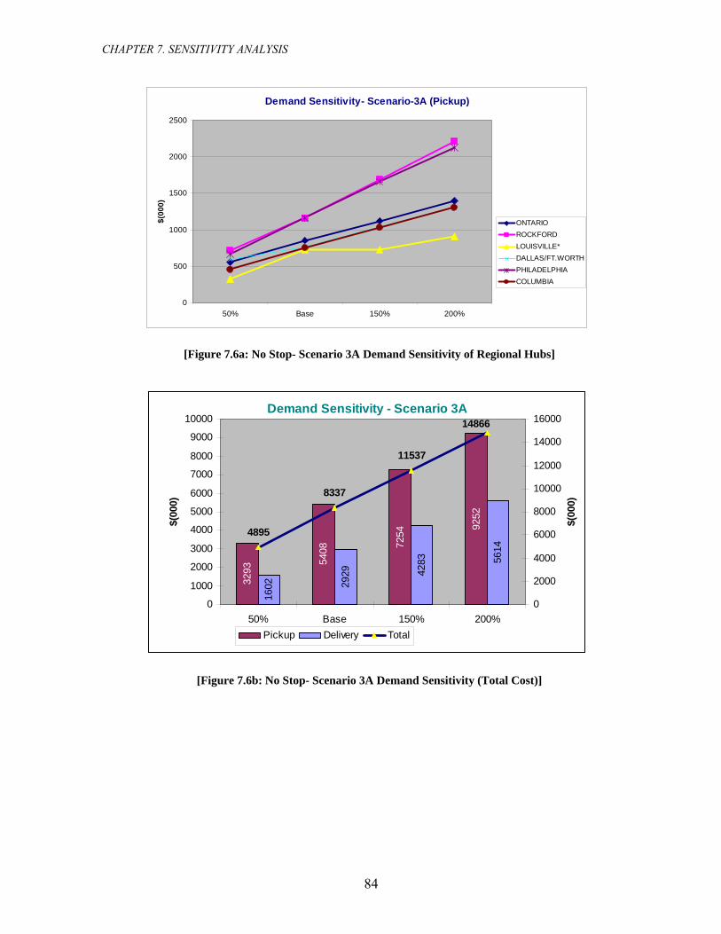
CHAPTER 7. SENSITIVITY ANALYSIS
Demand Sensitivity- Scenario-3A (Pickup)
0
500
1000
1500
2000
2500
50% Base 150% 200%
$(00
0)
ONTARIO ROCKFORD LOUISVILLE*DALLAS/FT.WORTHPHILADELPHIA COLUMBIA
[Figure 7.6a: No Stop- Scenario 3A Demand Sensitivity of Regional Hubs]
Demand Sensitivity - Scenario 3A
3293
5408 72
54
9252
1602 29
29 4283 56
14
4895
8337
11537
14866
0
1000
2000
3000
4000
5000
6000
7000
8000
9000
10000
50% Base 150% 200%
$(00
0)
0
2000
4000
6000
8000
10000
12000
14000
16000
$(00
0)
Pickup Delivery Total
[Figure 7.6b: No Stop- Scenario 3A Demand Sensitivity (Total Cost)]
84

CHAPTER 7. SENSITIVITY ANALYSIS
7.2.1.3.2 Scenario 3B: Demands routed from Origin Regional Hubs to destination
irectly to the
destination. Table 7.6b shows the results of the MIP runs. Figure 7.7a shows the variation of
delivery cost with respect to dem ure s t cost with
respec .
or Destination Regional Hub
On the pick-up side, demands are routed through the Origin Regional Hub. On the delivery
side, demands are routed either through destination regional hub or to d
and. Fig 7.7b show he variation of total
t to demand
50% Base 150% 200% Pick-up Delivery Pick-up Delivery Pick-up Delivery Pick-up Delivery
Scenario- 3B $(000) $(000) $(000) $(000) $(000) $(000) $(000) $(000)
ONTARIO 247 708 423 1112 593 1472 771 1876 ROCKFORD 378 451 720 769 1055 1088 1403 1403 LOUISVILLE 164 306 303 490 442 645 577 796 DALLAS/FT.WORTH 205 524 359 821 493 1166 656 1345 PHILADELPHIA 337 680 636 1128 906 1593 1216 2068 COLUMBIA 8 906 1208 265 435 478 703 691 94TOTAL 1596 3104 2919 5023 4180 6912 5529 8696 GRAND TOTAL 4700 7942 11092 14225 % Increase from Base -41% 40% 79%
[Table 7.6b: No Stop- Scenario 3B Demand Sensitivity]
85

CHAPTER 7. SENSITIVITY ANALYSIS
Demand Sensitivity- Scenario-3B (Delivery)
14
0
200
600
1000
1200
00
50% % 2
$(00
0
ONTARIO ROCKFORD LOUISVILLE*800)
DALLAS/FT.WORTHPHILADELPHIA COLUMBIA
400
Base 150 00%
.7a top- rio 3A and ivity gion s] [Figure 7
: No S Scena Dem Sensit of Re al Hub
Demand Sensitivity - Scenario 3B
1596 29
19 4180 55
29
3104 50
23 6912 86
96
4700
7942
110927000
800012000
14225
0
1000
2000
3000
4000
5000
6000
9000
10000
50% Base 150% 200%
$(00
0)
0
2000
4000
6000
8000
10000
14000
0
$(00
0)
160 0
Pickup Delivery Total
[Figure-7.7b: No Stop Scenario 3A Total Cost versus Demand]
86

CHAPTER 7. SENSITIVITY ANALYSIS
7.2.2 One Intermediate Stop Scenarios
7.2.2.1
ies of scale is observed when the demand
doub ost increases with a slope one with respect to demand.
Scenario 1: Single Hub Case
As shown in Table 7.7 and Figure 7.8, some econom
les, but mostly it c
SINGLE HUB AT LOUISVILLE 50% B 150ase % 200% $('000) $('0 $('00 $('000) 00) 0)
PICK-UP 2 45 6679380 56 6997
DELIVERY 2 47 7031 9294 460 81
TOTAL 4840 9337 13710 16290
% Change from Base -48% 47% 74%
[Table 7.7: One Stop- Hub Case Dema vitySingle nd Sensiti Results]
Demand Sens Single Hub One Stop e
2380
4556
6679
6997
2460
4781
7031
9337
4840
16290
0
1000
2000
3000
4000
6000
7000
10000
50% Base 150% 200%
Pick
up /
Del
ios
t $(0
00)
0
2000
4000
6000
8000
0
12000
14000
18000
Tota
l Cos
t $(0
00)
itivity - Cas
137108000
9000 16000
92945000ve
ry C 1000
PICK-UP DELIVERY TOTAL
[Figure 7.8: One Stop- Single Hub Case Demand Sensitivity Results]
87

CHAPTER 7. SENSITIVITY ANALYSIS
7.2.2.2 Scenario 2: Regional Hubs Present-All demands dispatched through origin
regional hubs
Results for the pick-up and delivery sides are shown in Table 7.8. Figure 7.9a and 7.9b show the
variation of cost with respect to demand.
Pick-up Side Delivery Side REGIONAL HUBS 50% Base 150% 200% 50% Base 150% 200%
$('000) $('000) $('000) $('000) $('000) $('000) $('000) $('000)
ONTARIO 185 391 570 760 289 554 830 1105
ROCKFORD 369 715 1078 1438 247 481 724 965
LOUISVILLE* 152 293 440 583 147 283 422 563
DALLAS/FT.WORTH 178 325 486 643 222 405 636 839
PHILADELPHIA 294 606 917 1211 323 632 958 1274
COLUMBIA 237 459 688 916 238 461 688 917
TOTAL 1415 2789 4179 5551 1468 2817 4258 5664
[Table 7.8: One Stop- Scenario 1 Regional Hubs Case Demand Sensitivity Results]
Demand Sensitivity One Stop Scenario- Regional Hubs Case (Pickup)
0
200
400
600
800
1000
1200
1400
1600
50% Base 150% 200%
$(00
0)
ONTARIO ROCKFORD LOUISVILLE*DALLAS/FT.WORTHPHILADELPHIA COLUMBIA
[Figure 7.9a: One Stop- Scenario 1 Regional Hubs Case Demand Sensitivity (Pickup)]
88

CHAPTER 7. SENSITIVITY ANALYSIS
Demand Sensitivity One Stop Scenario- Regional Hubs Case (Delivery)
1200
0
600
1400
200
400
800
1000
$(00
0)
ONTARIO ROCKFORD LOUISVILLE*DALLAS/FT.WORTHPHILADELPHIA COLUMBIA 50% Base 150% 200%
[F b: One Stop- egion Case Dem itivity (D
Total Cost ations is sh Table 7.9
igure 7.9 Scenario 1 R al Hubs and Sens elivery)]
of oper own in .
TOTAL COST REGIONAL HUBS 50% Base 150% 200% $('000) $('000) $('000) $('000)
ONTARIO 475 946 1400 1865
ROCKFORD 616 1196 1803 2403
LOUISVILLE* 300 576 862 1146
DALLAS/FT.WORTH 401 730 1122 1482
PHILADELPHIA 617 1238 1875 2485
COLUMBIA 475 921 1376 1832
INTERHUB 2549 4915 7314 9681
TOTAL 5432 10521 15751 20896
% Change from Base -48% 50% 99%
[Table 7.9: One Stop- Scenario 1 Regional Hubs Case Demand Sensitivity (Total Cost)]
89

CHAPTER 7. SENSITIVITY ANALYSIS
Fig re 7.10 shows the variati st with respect to varia n the demand. u on of total co tion i
141514682549
2789
2817
4915
4179
4258
7314
5551
5664
9681
0
5000
10000
1 0
20000
$(00
0)
50% 150% 200%
De ensitivity - al Hubs Ce Interm top
mandSOn
Regionediate S
ase
25000
500
Base
Interhub
Delivery
Pick-up
[Figure 7.10: One Stop- Scenario 1 Regional Hubs Case Demand Sensitivity (Total Cost)]
90
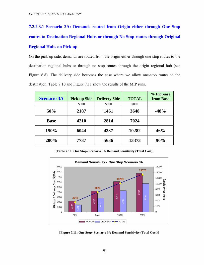
CHAPTER 7. SENSITIVITY ANALYSIS
7.2.2.3.1 Scenario 3A: Demands routed from Origin either through One Stop
routes to Destination Regional Hubs or through No Stop routes through Original
Regional Hubs on Pick-up
On the pick-up side, demands are routed from the origin either through one-stop routes to the
destination regional hubs or through no stop routes through the origin regional hub (see
Figure 6.8). The delivery side becomes the case where we allow one-stop routes to the
destination. Table 7.10 and Figure 7.11 show the results of the MIP runs.
Scenario 3A Pick-up Side Delivery Side TOTAL % Increase from Base
$000 $000 $000
50% 2187 1461 3648 -48%
Base 4210 2814 7024
150% 6044 4237 10282 46%
200% 7737 5636 13373 90%
[Table 7.10: One Stop- Scenario 3A Demand Sensitivity (Total Cost)]
Demand Sensitivity - One Stop Scenario 3A
2187
4210
6044
7737
1461 28
14 4237 56
36
10281
7024
3648
13373
0
1000
2000
3000
4000
5000
6000
7000
8000
9000
50% Base 150% 200%
Pick
up /
Deliv
ery
Cost
$(0
00)
0
2000
4000
6000
8000
10000
12000
14000
16000To
tal C
ost $
(000
)
PICK-UP DELIVERY TOTAL
[Figure 7.11: One Stop- Scenario 3A Demand Sensitivity (Total Cost)]
91

CHAPTER 7. SENSITIVITY ANALYSIS
7.2.2.3.2 Scenario 3B: Demands routed from Origin Regional Hubs either
Hubs on Delivery
from origin to origin regional
hub. On the delivery side, demands are routed from origin regional hubs either through one-
s p routes to destinations ugh p ro roug natio nal
delivery. Table 7.11 and Figure 7.12 show the results of the MIP runs.
through One Stop routes to Destinations or through No Stop routes through
Destination Regional
The pick-up side is the case where we allow one-stop routes
to or thro no sto utes th h desti n regio hub on
Scenario 3B Pick-up Side Delivery Side TOTAL % Increase from Base
$000 $000 $000
50% 1408 2102 3511 -48%
Base 2789 4025 6814
150% 4158 5868 10027 47%
200% 5524 7711 13235 94%
[Table 7.11: One Stop- Scenario 3B Demand Sensitivity (Total Cost)]
Demand Sensitivity - One Stop Scenario 3B
1408 27
89 4158 55
24
2102
4025
5868
7711
10026
6814
3510
13235
0
1000
2000
3000
4000
5000
6000
7000
8000
9000
50% Base 150% 200%
Pick
up /
Del
iver
y Co
st $
(000
)
0
2000
4000
6000
8000
10000
12000
14000
Tota
l Cos
t $(0
00)
PICK-UP DELIVERY TOTAL
[Figure 7.12: One Stop- Scenario 3B Demand Sensitivity (Total Cost)]
92

CHAPTER 7. SENSITIVITY ANALYSIS
7.3 Fixed Cost Sensitivity
ixed cost of owning or leasing, maintaining the aircraft,
personnel, airport fees etc. come under the fixed category. The operational cost component is
broadly dependent on the unit cost of fuel, type of aircraft used and nautical distance between
the origin and destination. As we can see, the unit cost of transportation between an origin-
destination pair could be easily affected by any of the above factors e.g fuel price. In the
following sections, we have conducted sensitivity analysis of cost with regard to the fixed cost
of operations. In this analysis, we increased the fixed component of the flights to 125%,
150%, 200%, 300% and 500% of the fixed cost assumed in Chapter-5 and Chapter-6. The
variable cost component was kept same as before. MIP runs were conducted for the same
scenarios as discussed in Chapter 5 and Chapter 6.
Unit cost of transportation is the most important factor from the revenue standpoint of the
operations. Cost of transportation between an origin-destination pair has two broad
components: fixed and operational. F
93

CHAPTER 7. SENSITIVITY ANALYSIS
94
7 S arios
7.
.3.1 No Intermediate Stop cen
3.1.1 Scenario-1: Only one Origin-Hub pair and only one Hub-Destination pair
(i) Single Hub Case
the results of the MIP runs. Table-7.12 and Figure-7.13 show
SINGLE HUB AT LOUISVILLE Base 125% 150% 200% 300% 500% ('000) ('000) ('000) ('000) ('000) ('000)
P P ICK-U 4800 5342 5875 6930 8971 12629
D RY 4953 5488 6016 7051 9056 12790 ELIVE
TOTAL 9753 10830 11891 13981 18027 25419
% Increase from Base 11% 22% 43% 85% 160%
[Table 7.12: No Stop Scenario Single Hub Case Fixed Cost Sensitivity Results]
4800
4953
5342
1-
5488
5875
6016
6930
7051
8971
9056
1262
912
790
0
5000
15000
25000
10000
20000
30000
Ba 125% 150% 200% 300% 500%
o ns ivity - Single Hub Caseenario-1
se
Fixed C st Se itSc
DELIVERYPICKUP
st Sensitivity- No Stop Scenario1- Single Hub Case][Figure7.13: Fixed Co

CHAPTER 7. SENSITIVITY ANALYSIS
(ii) Regional Hubs Present
Table 7.13 shows the results of the MIP runs for the case when demands are routed through origin
regional hubs only. Figures 7.14a and 7.14b show the with respect to the
variation in fixed cost.
variation of total cost
95

CHAPTER 7. SENSITIVITY ANALYSIS
96
Fixed Cost Sensitivity - Scenario 1 (Pickup)
0
500
1000
1500
2000
2500
3000
0 100 200 300 400 500 600
%
$(00
0)
ONTARIO ROCKFORD LOUISVILLE*DALLAS/FT.WORTHPHILADELPHIA COLUM BIA
Fixed Cost nsitivity - Scenario 1 (Delivery)
0
500
1000
1500
2000
2500
3000
0 100 20
$(00
0)
ONTARIO
Pick-up Side Delivery Side
REGIONAL HUBS Base 125% 150% 200% 300% 500% Base 12 150% 200% 300% 500% $('000) $('000) $('000) $('000) $('000) $('000) $('000) $( 0) $('000) $('000) $('000) $('000)
ONTARIO 423 461 496 562 690 925 572 6 686 788 980 1316
ROCKFORD 720 822 908 1074 1391 1814 484 5 605 712 914 1192
LOUISVILLE* 303 354 402 488 613 707 295 3 393 470 584 707
DALLAS/FT.WORTH 360 410 459 556 736 958 428 4 565 703 960 1241
PHILADELPHIA 636 759 882 1128 1621 2603 662 7 921 1178 1693 2723
COLUMBIA 478 555 627 758 1013 1245 488 5 635 762 997 1226
TOTAL 2919 3361 3773 4567 6064 8251 2929 3 7 3806 4614 6129 8406
[Table 7.13: No Stop Scenario 1 Regional Hub Case ed Cost Sens ity Results]
[Figure 7.14a: Fixed Cost Sensitivity- No Stop Scenario1- Regional Hubs Case (Pickup)]
[Figure 7.14b: Fixed
- Fix
Se
5%'00
29
49
48
97
91
63
37
itiv
0 300 400 500 600
%
ROCKFORD LOUISVILLE*DALLAS/FT.WORTHPHILADELPHIA COLUM BIA
Cost Sensitivity- No Stop Scenario1- Regional Hubs Case (Delivery)]

CHAPTER 7. SENSITIVITY ANALYSIS
Interhub Cost
Table 7.14 shows the interhub transportation cost for variation in fixed cost.
Base 125% 150% 200% 300% 500% ('000) ('000) ('000) ('000) ('000) ('000)
4915 5353 5789 6660 8400 11855
Total Cost
This is sum of the pick-up side cost, delivery side cost and the interhub transportation cost and
is shown in Table 7.15 and Figure 7.15.
[Table 7.15: Fixed Cost Sensitivity of Total Cost for Scenario 1 Regional Hub Case]
[Table 7.14: Interhub Transportation Costs]
TOTAL COST
REGIONAL HUBS Base 125% 150% 200% 300% 500% ('000) ('000) ('000) ('000) ('000) ('000) ONTARIO 995 1090 1182 1351 1671 2241 ROCKFORD 1204 1372 1513 1787 2305 3006 LOUISVILLE* 598 701 795 958 1197 1415 DALLAS/FT.WORTH 788 907 1025 1259 1696 2199 PHILADELPHIA 1298 1550 1803 2307 3314 5326 COLUMBIA 966 1118 1262 1520 2010 2471 INTERHUB 4915 5353 5789 6660 8400 11855
TOTAL 10763 12091 13369 15841 20593 28513
% Increase from Base 12% 24% 47% 91% 165%
97

C PTER 7. SENSITIVITY ANALYSIS
98
HA
Fixed Cost Sensitivity nario-1 (Regional Hubs Present)
2919 4567 6064825129
46146129
8406
53535789
6660
8400
11855
000
20000
000
125% 200% 300% 500%
29
1549
0
5
10
000
15000
25000
30
Base
$(00
0)Sce
3361
3377
3773
3806
150%
InterhubDeliveryPick-up
Sensitivity of l Cost for Scenario 1 Regional Hub Case] [Figure 7.15: Tota

CHAPTER 7. SENSITIVITY ANALYSIS
7.3.1.2 Scenario-2: No Intermediate Stops with demands routed through multiple
hubs
In this case, demands are routed either through Origin Regional Hub or directly to main hub on
the pick-up side. On the delivery side, demands are routed either through destination regional
hub or to destination Table 7.16 shows the result of MIP runs. Figures 7.16 a and 7.16b show the
cost impact of the variation in fixed cost on pick-up and delivery sides respectively.
99

CHAPTER 7. SENSITIVITY ANALYSIS
100
Fixe S nsit ity Sce rio
0
e iv - na 2 liv
0
500
1000
1500
2000
2500
3000
3500
0 1
$(00
0)
(De ery)
ONTARIO
Fixed Cost Sensitivity - Scenario 2 (Pickup)
0
500
1000
1500
2000
2500
3000
0 100 200 300 400 500 600
%
$(00
0)
ONTARIO ROCKFORD LOUISVILLE*DALLAS/FT.WORTHPHILADELPHIA COLUM BIA
Base 125% 150% 300% 500% Pick-up Delivery Pick-up Delivery Pick-up Delivery Pick- li ery v Pick- up Deliv y er Pick-up Delivery Scenario-2 $(000) $(000) $(000) $(000) $(000) $(000) $ 0(0 (0 0) 0 $(00 0) $( 000) $( 0) 00 $(000)
ONTARIO 1011 1433 1085 1533 1093 1539 1 03 819 1566 2190 2076 2922 ROCKFORD 848 566 974 653 1100 906 134 226 1829 1535 2642 1743 LOUISVILLE* 303 295 354 348 402 393 48 470 613 584 707 707 DALLAS/FT.WORTH 671 740 745 824 820 908 9 8 1 78 2004 6 072 124 396 1 5 PHILADELPHIA 969 1021 1095 1155 1219 1288 1 54 548 1900 2044 2736 2950 COLUMBIA 604 606 684 686 762 766 9 26 1 1 74 1739 1 9 120 211 1 5 TOTAL 9066 10136 11197 1 8 56 731 237% Increase from Base 12% 24% 9 % 1% 162
[Table 7.16: No Stop- Scenario 2 Fixed Cost Sensitiv
[Figure-7.16
it s]
[Figure-7.16a: No Stop- Scenario 2 Fixed Cost Sensitivity (Pickup)]
d ostC
200%up De0) $0 18 18 7 16 1 613536
94 %
esy R ult
0 3 0 400 500 0 600
%
ROCKFORD LOUISVILLE*DALLAS/FT.WORTHPHILADELPHIA COLUM BIA
F d Co ensitivity ivery)] (Delop- Scenario 2 ixe st S
0 20
Nob: St
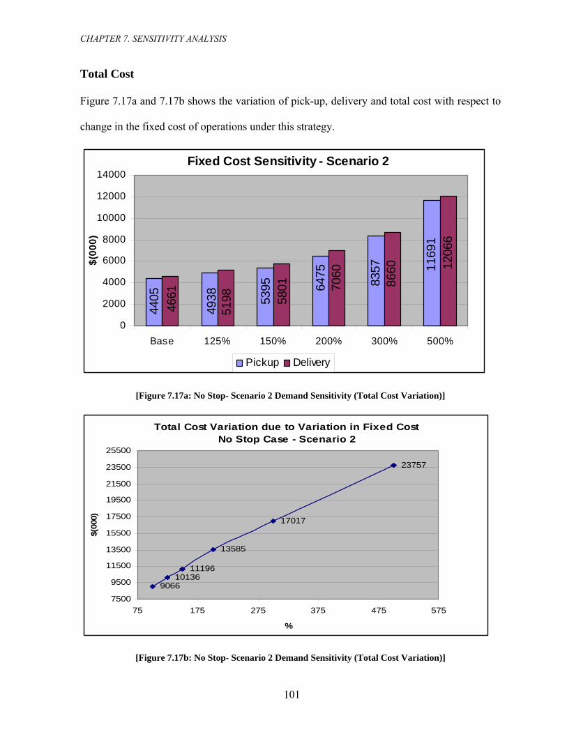
CHAPTER 7. SENSITIVITY ANALYSIS
101
Total Cost
Figure 7.17a and 7.17b shows the va pick-up, delivery and total cost with respect to
chan the fixed cost of operations under egy.
To Cost Va ion to Variatio Fixed CostNo Stop Case - Scena
9010136
11196
85
17017
23757
75
95
115
13500
15500
175
19
00
255
75 475 575
$(00
0)riation of
ge in this strat
Fixed Cos itivity - Scenario 240
5
4938 53
6475
8357 11
691
7060
8660 12
066
5198
4661
0
40
6000
80
10 0
120
1400
Base 125% 150% 200% 300% 500%
$(00
0)
t Sens4
95 801
5
0
200
00
00
00
00
0
Pickup Deliv yer
[Figure 7.17a: No Stop- Scenario 2 D (Total Cost Variation)]
tal riat due
emand Sensit
n inrio 2
66
135
00
00
00
75
00
500
215
23500
00
175 275 3
%
[Figure 7.17b: No Stop- Scenario 2 Demand Sensitivity (Total Cost Variation)]
ivity

CHAPTER 7. SENSITIVITY ANALYSIS
7.3.1.3.1 Scenario 3A: Demands routed either through Origin Regional Hub or
Destination Regional Hub on pick-up side
In this analysis conducted, we exclude the presence of main hub and assume that there are only
regional hubs and the demands are routed through them only. On the pick-up side, demands are
routed either through Origin Regional Hub or directly to Destination Regional Hub. On the
delivery side, demands are routed directly to the destination. Table 7.17 shows the results of
the MIP runs. Figures 7.18a shows the variation of pick-up cost with respect to change in fixed
costs. Figure 7.18b shows the variation of pick-up, delivery and total costs with respect to
variation in fixed cost.
102

CHAPTER 7. SENSITIVITY ANALYSIS
103
[Table 7.17: No Stop- Scenario 3A Fixed Cost Sensitivity
]
Base 150% 200% 300% 500% Pick-up Delivery Pick-up Delivery Pick-up Delivery Pick-up D ryelive P k-up ic Deli ry ve
Scenario- 3A $(000) $(000) $(000) $(000) $(000) $(000) $(00 0) $(000) $ 000) ( $(0 0) 0
ONTARIO 849 572 995 686 1143 788 1452 980 2008 1316
ROCKFORD 1158 484 1426 605 1684 71 30 1192 2 2188 914 94
LOUISVILLE 726 295 964 393 1035 470 1365 584 1926 707
DALLAS/FT.WORTH 763 428 915 565 1084 70 20 1243 1365 960 33 1
PHILADELPHIA 1160 662 1388 921 1636 1178 2116 1693 3138 2723
COLUMBIA 752 488 896 635 1077 762 19 1221386 997 21 6
TOTAL 5408 2929 6584 3805 7659 4613 9872 6128 1 120 4 8405 GRAND TOTAL 8337 10389 12272 16000 22525 % Increase from Base 25% 47% 0%92% 17

CHAPTER 7. SENSITIVITY ANALYSIS
104
Fixed Cost nsitivity - Scenario 3A (Pickup)
0
1000
2000
3000
300 5
0
Se
500
1500
2500
3500
0 100 200 400 00 600
%
$(00
)ONTARIO ROCKFORD LOUISVILLE*DALLAS/FT.WORTHPHILADELPHIA COLUM BIA
7 a nario 3A Fixe ost Sensitivity of Regional Hubs]
[Figure .18 : No Stop- Sce d C
Total Cost Variation due to riation in Fixed CostNo S - S nario 3A
833
10389
12272
16000
22525
7500
9500
11500
15500
19500
23500
375 475 575
%
0
top Case
7
13500
17500
21500
75 175 275
$(0
0)
Vace
rio 3A Fixed Cost Sensitivity (Total Cost)]
[Figure 7.18b: No Stop- Scena

CHAPTER 7. SENSITIVITY ANALYSIS
7.3.1.3.2 Scenario 3B: Demands routed from Origin Regional Hubs to destination or
Destination Regional Hub
In this analysis conducted, we exclude the presence of main hub and assume that there are only
regional hubs and the demands are routed through them only. On the pick-up side, demands are
routed to the Origin Regional Hub directly. On the delivery side, demands are routed directly to
the destination. Table 7.18 shows the results of the MIP runs. Figures 7.19a show the variation of
pick-up cost with respect to change in fixed costs. 7.19b shows the variation of total costs with
respect to variation in fixed cost.
105

CHAPTER 7. SENSITIVITY ANALYSIS
106
Base 150% 200% 300% 500% Pick-up Delivery Pick-up Delivery Pick-up D y eliver Pick-up Delivery Pick-up Delivery
Scenario- 3B $(000) $(000) $(000) $(000) $(000) $ (000) $(000) $(000) $(000) $(000)
ONTARIO 423 1112 496 1301 562 1523 690 1914 925 2659
ROCKFORD 720 769 908 945 1074 3 6 1814 2218 1153 1 91 148
LOUISVILLE 303 490 402 535 488 676 613 703 707 887
DALLAS/FT.WORTH 360 821 459 978 556 736 7 958 221184 147 08
PHILADELPHIA 636 1128 882 1389 1128 1686 1621 2165 2603 3203
COLUMBIA 478 703 627 848 758 1013 2 1245 191004 130 57
TOTAL 2920 5023 3774 5996 4566 7226 6064 9047 8252 13132 GRAND TOTAL 7943 9770 11792 15111 21384 % Increase from Base 23% 48% 90% 169%
[Table 7.18: No Stop- Scenario 3B Fixed Cost S vi
ensiti ty]

CHAPTER 7. SENSITIVITY ANALYSIS
107
Fixed Cost Sensitivity - Scenario 3B (Delivery)
00
00
00
0 100 200 400 500
%
0
0
500
10
1500
20
2500
30
3500
300 600
$(0
0)ONTARIO ROCKFORD LOUISVILLE*DALLAS/FT.WORTHPHILADELPHIA COLUM BIA
3A Fixed Cost Sensitivity of Regional Hubs]
[Figure 7.19a: No Stop- Scenario
Total Cost Variat to Variation in Fixed CostNo St ase - Scenario 3A
79
11792
15111
21384
7500
0
0
0
75 75 275 375 475 575
%
$(00
0)
43
977095
1150
00
1
1
35
550
00
1
1
75
950
00
2
2
150
350
0
0
1
ion dueop C
rio 3A Fixed Cost Sensitivity (Total Cost)] [Figure 7.19b: No Stop- Scena

CHAPTER 7. SENSITIVITY ANALYSIS
7.3.2 One Intermediate Stop Scenarios
7.3 : Single Hub Case
Ta 0 show su M
.2.1 Scenario 1
ble 7.19 and Figure 7.2 the re lt of the IP runs.
SINGLE HUB AT LOUISVILLE Base 125% 150% 200% 300% 500% ('0 ( 0) 00) ('000) 00) '000) ('000) ('00 ('0
P 45 5101 5603 6676 8551 ICK-UP 56 12460
DELIVERY 4781 5263 5788 6675 8816 12563
T 93 10364 11391 13352 17367 25023 37 OTAL
% Base Increase from 11% 22% 43% 86% 168%
[Table 7.19: One Sto Single se F st S y Rep- Hub Ca ixed Co ensitivit sults]
Total Cost Variation due to Variation in Fixed CostOne Stop Case - Scenario 1
933710364
11391
13351
17367
25023
7500
9500
11500
13500
15500
17500
19500
21500
23500
25500
27500
75 175 275 375 475 575
%
$(00
0)
[Figure7.20: One Stop- Single Hub Case Fixed Cost Sensitivity Results]
108

CHAPTER 7. SENSITIVITY ANALYSIS
7.3.2.2 Scenario 2: Regional Hubs Present-All demands dispatched through origin
regional hubs
Results for the pick-up and delivery cases are shown in Table 7.20. Figures 7.21a and 7.22b
show the variation of total cost with respect to fixed cost.
109

CHAPTER 7. SENSITIVITY ANALYSIS
110
Fi ed C st Swit
0200400600800000200400600800000
0 0 200
x o ensitivit Regional Hub Cases h One (Pickup)
111112
10 300 00 500 600
%
$(00
0)
y - Stop
4
ONTARIO ROCKFORD LOUISVILLE*DALLAS/FT.WORTHPHILADELPHIA COLUM BIA
Fixed st Sensitivity - Regional Huy)
b Cawith One Stop (Deliver
0
200
400
600
800
1000
1200
1400
1600
100
$(00
0)
ses
0
O O NTARI
Pick-up Side Delivery Side R O LEGI NA HUBS Base 125% 150% 200% 300% 500% Base 125% 150% 200% 300% 500% $ $('000) $('000) $('000) $('000) $('000) $('000) $('000) $('000) $('00 $('0 $ 00) ('000) 0) 00) ('0O RNTA IO 391 426 459 526 658 907 554 609 663 759 947 1293 R F 715 820 908 1083 1416 1868 4 71 9 22 OCK ORD 81 548 604 4 22 12L V EOUIS ILL * 293 346 396 485 617 728 283 334 380 462 588 705 D A . T 369 414 505 677 954 405 468 530 65 9 28 ALL S/FT WOR H 325 4 01 12P D HHILA ELP IA 606 719 811 938 1182 1382 632 754 858 989 1214 1399 COLUMBIA 459 533 603 734 986 1235 459 536 608 74 9 47
[Figure 7.21
94 12 1 T AOT L 2789 3213 3591 4271 5536 7075 2814 3248 3643 4319 5566 7093
able 7.20: One Stop- Scenario 1 Regional Hubs Case ed Cost nsitivity Results] Fix
[ gure 21a: ne SFi 7. O top- Scenario 1 Regional Hubs Case Fixed Cost Sensitivity (Pickup)]
[T
CoSe
200 300 400 50 000 6
%
R RD OCKFOLOUISVILLE*D FT.WORTHALLAS/P LPHIA HILADEC IA OLUM B
b: One Stop- Scenario 1 Regi bs Case F Cost Sensitivity (Delivery)]
ixedonal Hu

CHAPTER 7. SENSITIVITY ANALYSIS
Total Cost of operations is shown in Table 7.21
TOTAL COST
REGIONAL HUBS Base 125% 150% 200% 300% 500% ('000) ('000) ('000) ('000) ('000) ('000) ONTARIO 946 1035 1123 1285 1605 2200
ROCKFORD 1196 1368 1512 1796 2338 3090
LOUISVILLE* 576 680 776 948 1205 1433
DALLAS/FT.WORTH 730 836 945 1159 1578 2182
PHILADELPHIA 1238 1473 1669 1927 2397 2781
COLUMBIA 918 1068 1210 1475 1980 2482
INTERHUB 4915 5353 5789 6660 8400 11855
TOTAL 10519 11813 13023 15250 19502 26023
% Increase from Base 12% 24% 45% 85% 147%
[Table 7.21 One Stop- Scenario 1 Regional Hubs Case Fixed Cost Sensitivity (Total Cost) ]
Figure 7.22 shows the variation of total cost with respect to changes in the demand.
Fixed Cost Semsitivity Scenario-1 (Regional Hubs Present)
2789 3213 3591 4271 5536 70742814 3249 36434319
5566
7094
49155353
57896660
8400
11855
0
5000
10000
15000
20000
25000
30000
Base 125% 150% 175% 200% 300%
$(00
0)
InterhubDeliveryPick-up
[Figure 7.22: One Stop- Scenario 1 Regional Hubs Case Fixed Cost Sensitivity (Total Cost)]
111

CHAPTER 7. SENSITIVITY ANALYSIS
7.3.2.3.1 Scenario 3A: Demands routed from Origin either through One Stop
k-up
ough one-stop routes to the
destination regional hubs or through no stop routes through the origin regional hub (see
F delivery s come ase we ne-s tes
destination. Table 7.22 and Figure 7.23 show the results of the MIP runs.
routes to Destination Regional Hubs or through No Stop routes through Original
Regional Hubs on Pic
On the pick-up side, demands are routed from the origin either thr
igure 6.8). The ide be s the c where allow o top rou to the
Scenario 3A Pick-up Side Delivery
Side TOTAL % Increase from Base
$000 $000 $000
Base 4 024210 281 7 4
125% 47 9 8007 14% 5 3248
150% 5067 3643 8710 24%
200% 6287 4319 10606 51%
300% 8342 5566 13908 98%
500% 12434 7093 19527 178%
[Table 7.22 One Stop- Scenario 3A Fixed Cost Sensitivity (Total Cost)]
Total Cost Variation due to Variation in Fixed CostOne Stop Case - Scenario 3A
80078710
10606
13908
19527
7500
9500
11500
13500
15500
17500
19500
21500
75 175 275 375 475 575
%
$(00
0)
[Figure 7.23: One Stop- Scenario 3A Fixed Cost Sensitivity (Total Cost)]
112

CHAPTER 7. SENSITIVITY ANALYSIS
7.3.2.3.2 Scenario 3B: Demands routed from Origin Regional Hubs either
through One Stop routes to Destinations or through No Stop routes through
e allow one-stop routes from origin to origin regional
hub. On the delivery side, demands are routed from origin regional hubs either through one-
stop routes to destinations or through no stop routes through destination regional hub on
delivery. Table 7.23 and Figure 7.24 show the results of the MIP runs.
Destination Regional Hubs on Delivery
The pick-up side is the case where w
Scenario 3B Pick-up Side Delivery Side TOTAL % Increase from Base
$000 $000 $000
Base 2789 4025 6814
125% 3213 4555 7768 14%
150% 3591 5063 8654 27%
200% 4271 6154 10425 53%
300% 5536 8160 13696 101%
500% 7075 12277 19352 184%
[Table 7.24: One Stop- Scenario 3B Demand Sensitivity (Total Cost)]
Total Cost Variation due to Variation in Fixed CostOne Stop Case - Scenario 3B
77688654
10425
13696
19352
7500
9500
11500
13500
15500
17500
19500
21500
75 175 275 375 475 575
%
$(00
0)
[Figure 7.24: One Stop- Scenario 3B Demand Sensitivity (Total Cost)]
113

CHAPTER 7
114
7.4
In this section, we vary the variable cost component of the problem and analyze it’s
arily varies with the fuel usage. Usage of fuel may vary
epending on the type of aircraft flown, payload of the aircraft, percent full etc. Fuel price
ar s and this affects our problem context. In this section, we
stu ich cts the variable cost component. Keeping the fixed
cos onent constant, we the
stu
. SENSITIVITY ANALYSIS
Variable Cost Sensitivity
sensitivity. The variable cost prim
d
v ies due to various uncertaintie
dy t
t co
he
mp
effect of fuel prices wh
vary
affe
fuel price by 125%, 150%, 175%, 200% and 300% and
dy its impacts on the cost function.

CHAPTER 7. SENSITIVITY ANALYSIS
7.4.1 Scenario-1: No Intermediate Stop Scenarios
7.4.1.1 Scenario-1: Only one Origin-Hub pair and only one Hub-Destination pair
(i) Single Hub Ca
Results of the MIP runs are shown in Table-7.24 and Figure-7.25.
se
SINGLE HUB AT LOUISVILLE Base 125% 150% 175% 200% 300% 00) $('000) $('000) $('000) $('000) $('000) $('0
PICK-UP 4800 5430 6053 6673 7282 9690
DELIVERY 4953 5623 6293 6957 7619 10232
TOTAL 9753 11053 12346 13630 14901 19922
% Increase from Base 13% 27% 40% 53% 104%
[Table 7.24: No Stop Scen - Singl Case V le Cos ivity Results] ario 1 e Hub ariab t Sensit
4800
4953
5430
5623
6053
6293
6673
6957
7282
7619
9690
1023
2
02000
800010000
12000
40006000
1400016000
1800020000
Base 125% 150% 200% 300% 500%
Variabl st Sen ity - S Hub S io-1
e Co sitiv ingle Casecenar
DELIVERYPICKUP
[Figure 7.25: Variable Cost Sensitivity- No Stop Scenario1- Single Hub Case ]
115

CHAPTER 7. SENSITIVITY ANALYSIS
(ii) Regional Hubs Present
Table 7.25 shows the results of the MIP runs for the case when demands are routed through
origin regional hubs only. Figures 7.26a and 7.26b show the variation of total cost with
respect to variation in the variable cost.
116

CHAPTER 7. SENSITIVITY ANALYSIS
117
Variable Cost Sensitivity - Regional Hub Cases No Stop Scenario 1 (Pickup)
0
200
400
600
800
1000
1200
75 125 175 225 275 325
%
$(00
0)
ONTARIO ROCKFORD LOUISVILLE*DALLAS/FT.WORTHPHILADELPHIA COLUM BIA
`
Variab e Cost Se sitiv y - R gionStop Scen rio 1 Deli
n it e al Hub s No a ( very)
0
200
400
600
800
1000
1200
75 1
$(00
0)
Case
ONTARIO
Pick-up Side D e deliv ry Si e REGIONAL HUBS Base 125% 150% 175% 200% 300% Bas 125% 1 0% 5 175% 200% 300% $('000) $('000) $('000) $('000) $('000) $('000) $('00 $ ) (' '00 ) $('000) ) ('000 $ 000) $( 0) $('000ONTARIO 423 463 501 539 576 724 572 628 683 728 739 1015 ROCKFORD 720 762 766 845 887 1053 484 512 512 566 593 700 LOUISVILLE* 303 320 337 354 371 439 295 314 332 350 368 436 DALLAS/FT.WORTH 360 395 430 465 500 635 428 465 503 540 618 727 PHILADELPHIA 636 671 706 741 776 916 662 697 733 769 805 947 COLUMBIA 478 518 557 596 636 790 488 528 569 609 647 802
TOTAL 2920 3129 3297 3540 3746 4557 292 3144 3332 3562 3770 4627
[Table 7.25: No Stop Scenario 1 Regional Hub Case - Variable Cost S sitivit Results]
[Figure 7.26b:
y
[Figure 7.26a: Variable Cost Sensitivity- No Stop Scenario1- Regional Hubs Case (Pickup)]
l
e0
9
en
175 5 275
%
25 22 325
ROCKFORD LOUISVILLE*DALLAS/FT.WORTHPHILADELPHIA COLUM BIA
`
Variab st nsitiv - p Scena Region b se v
rio1-le Co Se ity No Stoal Hu s Ca (Deli ery)]

CHAPTER 7. SENSITIVITY ANALYSIS
118
ariable costs are shown in Table 7.26.
I
I
nterhub Cost
nterhub costs for the change in v
Base 125% 150% 175% 200% 300% ('000) ('000) ('000) ('000) ('000) ('000)
4915 5704 6492 7277 8063 11194
[Table 7.26: Interhub Transportation Costs]
his is sum of the pick-up side cost ery side cost and the interhub transportation cost.
[Table Variable C ensitivity of Total Cost for Scenario 1 Regional Hub Case]
The results are shown in Table 7.27 and Figure 7.27.
7.27: ost S
TOTAL COST
REGIONAL HUBS Base
Total Cost
T , deliv
125% 150% 175% 200% 300% ('000) ('000) ('000) ('000) ('000) ('000) ONTARIO 995 1091 1184 1267 1315 1739
R CKFORD 1204 1274 1278 1411 1480 1753 O
LOUISVILLE* 598 634 669 704 739 875
DALLAS/FT.WORTH 933 1005 1118 1362 788 860
PHILADELPHIA 1298 1368 1439 1510 1581 1863
COLUMBIA 966 1046 1126 1205 1283 1592
INTERHUB 4915 5704 6492 7277 8063 11194
TOTAL 10764 11977 13121 14379 15579 20378
% Increase from Base 11% 22% 33% 43% 89%
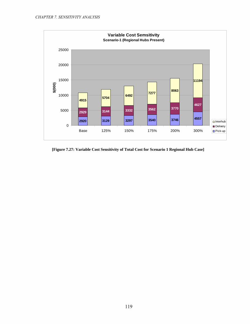
CHAPTER 7. SENSITIVITY ANALYSIS
Variable Cost Semsitivity Scenario-1 (Regional Hubs Present)
2920 3129 3297 3540 3746 4557
2929 3144 3332 3562 37704627
49155704 6492
72778063
11194
0
5000
10000
15000
20000
25000
Base 125% 150% 175% 200% 300%
$(00
0)
InterhubDeliveryPick-up
[Figure 7.27: Variable Cost Sensitivity of Total Cost for Scenario 1 Regional Hub Case]
119

CHAPTER 7. SENSITIVITY ANALYSIS
7.4.1.2 Scenario-2: No Intermediate Stops with demands routed from Origin
through multiple hubs
In this case, demands are routed either through Origin Regional Hub or directly to main hub
on the pick-up side. On the delivery side, demands are routed either through destination
regional hub or to destination Table 7.28 shows the result of MIP runs. Figures 7.28a and
7.28b show the cost impact of the variation in variable cost on pick-up and delivery sides
respectively.
120

CHAPTER 7. SENSITIVITY ANALYSIS
121
Variable ensitivity - No Stop Scenario 2A (Delivery)
0
00
00
00
00
00
00
00
75
5
10
15
20
25
30
35
125 225 275 325
%
$(00
0)
ONTARIO ROCKFORD LOUISVILLE*DALLAS/FT.WORTHPHILADELPHIA COLUM BIA
`
Variab Cos Sen itivitle t s y - No(Pic p)
12 175 22
S Sc io A ku
0
500
1000
1500
2000
2500
75 5 5 275
%
$(00
0)
top enar
325
2
ONTARIO ROCKFORD LOUISVILLE*DALLAS/FT.WORTHPHILADELPHIA COLUM BIA
`
Base 125% 150% 200% 300% Pick-up Delivery Pick-up Delivery Pick-up Delivery Pick-u ivery Pick-up Delivery Pick-up Delivery Scenario-2 $ (000) $(000) $(000) $(000) $(000) $(000) $(000 00) $(000) $(000) $(000) $(000)
ONTARIO 1011 1433 1144 1643 1292 1862 1440 77 1584 2291 2149 3145 ROCKFOR 607 993 654 1068 01 1143 748 1442 932 D 848 566 917LOUISVILLE* 303 295 320 314 337 332 354 50 371 368 439 436 DALLAS/F 671 740 715 799 796 887 876 75 956 1062 1264 1405 T.WORTH PHILADEL IPH A 969 1021 1042 1097 1145 1202 1248 07 1351 1411 1758 1824 COLUMBI 1108 1122 A 604 606 666 670 731 737 794 04 858 869 TOTAL 90 9934 10968 1 13012 17024 67 % 10% 21% 44% 88% Increase from Base
bl 8: No Stop- Scena Va st Sensitiv lts]
[Figure-7.28b: N Scenario 2 Fixed Cost Sensitivity (Delivery)]
riable Corio 2
[Figure-7.28a S Sc st Sen ity (Pickup)]
[Ta e 7.2
sitiv: No top- enario 2 Variable Co
175
o Stop-
Cost S
175% p Del) $(0 20 7 3 9 13
81994
32%
ity Resu

CHAPTER 7. SENSITIVITY ANALYSIS
T
Figure 7.29 shows the variation of total cost with respect to variable cost.
otal Cost
Total Cost V tion due to iation in V ble Cost S s e
90679934
096811994
024
7500
9500
75 125 175 225 275 325
%
$(00
0)
ariaN
Var - S
ariao top Ca e c nario 2
1
13012
17
11500
13500
15500
17500
19500
[Figure 7.29: No Stop- Scenario 2 Demand Sensitivity (Total Cost Variation)]
122
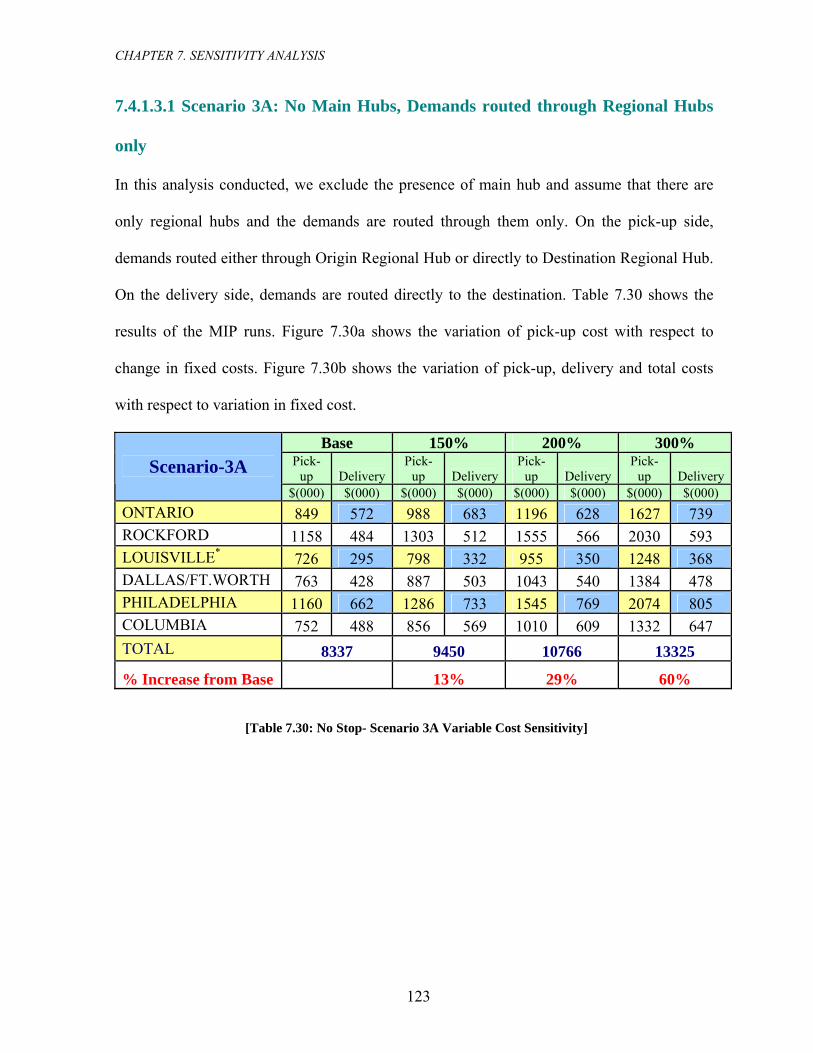
CHAPTER 7. SENSITIVITY ANALYSIS
7.4.1.3.1 Sc onal Hubs
only
In this analysis conducted, we exclude the presence of main hub and assume that there are
only regional hubs and the demands are routed through them only. On the pick-up side,
demands routed either through Origin Regional Hub or directly to Destination Regional Hub.
On the delivery side, demands are routed directly to the destination. Table 7.30 shows the
results of the MIP runs. Figure 7.30a shows the variation of pick-up cost with respect to
change in fixed costs. Figure 7.30b shows the variation of pick-up, delivery and total costs
with respect to variation in fixed cost.
enario 3A: No Main Hubs, Demands routed through Regi
Base 150% 200% 300% Pick-
up Delivery Pick-
up DeliveryPick-
up Delivery Pick-
up DeliveryScenario-3A $(000) $(000) $(000) $(000) $(000) $(000) $(000) $(000)
ONTARIO 849 572 988 683 1196 628 1627 739 ROCKFORD 1158 484 1303 512 1555 566 2030 593 LOUISVILLE* 726 295 798 332 955 350 1248 368 DALLAS/FT.WORTH 763 428 887 503 1043 540 1384 478 PHILADELPHIA 1160 662 1286 733 1545 769 2074 805 COLUMBIA 752 488 856 569 1010 609 1332 647 TOTAL 8337 9450 10766 13325
% Increase from Base 13% 29% 60%
[Table 7.30: No Stop- Scenario 3A Variable Cost Sensitivity]
123

CHAPTER 7. SENSITIVITY ANALYSIS
Variable Cost Sensitivity - No Stop Scenario 3A (Pickup)
0
1000
5 175
%
$(2500
ONTARIO ROCKFORD LOUISVILLE*DALLAS/FT.WORTH
2000
500
1500
000) PHILADELPHIA
COLUM BIA
75 12 225 275 325
`
[Figure 7.30a: No Stop- Scenario 3A Variable Cost Sensitivity of Regional Hubs]
Total Cost Variation due to Variation in Variable CostNo Stop Case - Scenario 3A
8337
9450
10766
13325
7500
8500
9500
10500
11500
12500
13500
14500
75 125 175 225 275 325
%
$(00
0)
[Figure 7.30b: No Stop- Scenario 3A Variable Cost Sensitivity (Total Cost)]]
124

CHAPTER 7. SENSITIVITY ANALYSIS
7.4.1.3.2 Scenario 3B: No Main Hubs, Demands routed from Origin Regiona
Hubs to destinati
l
on or Destination Regional Hub
only. On the pick-up side,
demands are routed to the Origin Regional Hub directly. On the delivery side, demands are
routed directly to the destination. Table 7.31 shows the results of the MIP runs. Figure
7.31a shows the variation of pick-up cost with respect to change in variable costs. Figure
7.31b shows the variation of pick-up, delivery and total costs with respect to variation in
variable cost.
In this analysis conducted, we exclude the presence of main hub and assume that there are
only regional hubs and the demands are routed through them
Base 150% 200% 300% Pick-
up DeliveryPick-
up DeliveryPick-
up Delivery Pick-
up DeliveryScenario-3B $(000) $(000) $(000) $(000) $(000) $(000) $(000) $(000)
ONTARIO 423 1112 501 1288 539 1562 576 2148 ROCKFORD 720 769 766 862 845 1006 887 1318 LOUISVILLE* 303 490 337 545 354 623 371 821 DALLAS/FT.WORTH 360 821 430 914 465 1103 500 1445 PHILADELPHIA 636 1128 706 1234 741 1475 776 1984 COLUMBIA 478 703 557 785 596 924 636 1238 TOTAL 2920 5023 3297 5628 % Increase from Base 12% 29% 60%
[Table 7.31: No Stop- Scenario 3B Variable Cost Sensitivity]
125

CHAPTER 7. SENSITIVITY ANALYSIS
126
Variable Cost Sensitivity - No Stop Scenario 3B (Delivery)
500
2000
00
75 125 175 225 275
%
00
0
1000
1500
25
325
$(0)
ONTARIO ROCKFORD LOUISVILLE*DALLAS/FT.WORTHPHILADELPHIA COLUM BIA
`
nari Variable Cost Sensitivity of Regional Hubs]
[Figure 7.31a: No Stop- Sce o 3B
Total Cost VariaNo
tion due to Variation in Variable Cost St ase - Scenario 3B
8925
10233
12700
7500
10500
13500
75 125 175 225 275 325
%
$(00
0)
op C
7943
8500
9500
11500
12500
rio 3A Variable Cost Sensitivity (Total Cost)] [Figure 7.31b: No Stop- Scena

CHAPTER 7. SENSITIVITY ANALYSIS
7.4.2 One Intermediate Stop Scenarios
7.4 : Single Hub Case
Table-7.32 and Figure-7.32 show ult MI
.2.1 Scenario 1
the res s of the P runs.
SINGLE HUB AT LOUISVILLE Base 125% 150% 175 200 30 % % 0% ('000 '000 ('000) ('000) ('000) ('000) ) ( ) P 4556 5176 5757 631 694 93ICK-UP 6 1 38
D 4781 5374 6008 6662 7345 9897 ELIVERY
T 9337 10551 11765 129 142 1978 86 234 OTAL
% Base 13% 26% 39% 53 10 % Increase from 6%
[Table 7.32: One Sto H ar S ep- Single ub Case V iable Cost ensitivity R sults]
Total Cost Variat n due riat r ost
550
13500
17500
75 125 175 225 275 325
io to Va ion in Va iable COne Stop Case - Scenario 1
21500
933710
1176512978
14286
9500
11500
$(00
0)
1923519500
7500
%
15500
[Figure 7.32: One Stop- Single Hub Case Variable Cost Sensitivity Results]
127

CHAPTER 7. SENSITIVITY ANALYSIS
7.4.2.2 Scenario 2: Region bs Present-All demands dispatched hrough
origin regional hubs
Results for the pick-up and delivery sides are shown in Table-7.33. Figures 33a and 33b
show the var l cost w ost.
al Hu t
iation of tota ith respect to variable c
128

CHAPTER 7. SENSITIVITY ANALYSIS
129
Varia le C st Se sitiv y - O e St p Ca e cen io 2 Pick p)
125 17 25 275 3 5
%
b o n it n o sS ar ( u
0
200
400
600
800
1000
1200
75 5 2 2
$(00
0)
ONTARIO RO RDCKFO LO LLE*UISVIDA FT.LLAS/ WORTHPH PHILADEL IA CO IA LUM B
`
Variable Sensitivity - One Stop Case enario 2(Delivery)
0
00
00
00
00
00
00
75 125
stc
2
4
6
8
10
12
$(00
0)
ONTARIO ROCKFORD LOUISVILLE*DALLAS/FT.WORTH
Pick-up Side Delivery Side REG AION L HUBS Base 125% 150% 175% 200% 300% Base 12 150% 175% 200% 300% 0 0) ( '0 $ 00 ) '000) $('0 ) $('000) $('000) $('000) $('000) $('0 0) $('00 $ '000) $( 00) ('0 ) $('000 $(
ONTARIO 391 431 470 5 1 1 55 3 709 554 6 664 719 773 989 ROCKFOR 5 4 3 8D 71 759 804 8 9 89 106 481 5 539 569 595 707 LOUISVILLE* 293 311 330 3 8 4 36 7 439 283 3 320 340 358 431 DALLAS/FT R 5 3 9 405 4 480 516 554 702 .WO TH 32 363 397 4 3 46 608 PHILADELPHIA 606 622 649 6 4 7 70 0 799 632 6 720 750 779 890 COLUMB 9 1 8 4 5 541 617 623 780 IA 45 500 538 6 4 61 767 59TOTAL 2789 2985 3187 3428 3600 4390 2817 30 3264 3510 3682 4498
[ e O to o gio H a Cost S ivity Results]
Tabl 7.33: ne S p- Scenari 1 Re nal ubs C se Variable it
[Figure a S - Sc ri e l V lvity (Pickup)]
7.33 : One top ena o 1 R giona Hubs Case ariab e Cost Sensiti
[Figure 7.33b: One Sto
CoS
5%00
10 10 03 39 92 0 255
ens
175 225
%
275 325
PHILADELPHIA COLUM BIA
`
p- Scenario 1 Regional Hubs Case Variable Cost Sensitivity (Delivery)]
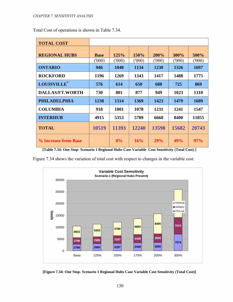
CHAPTER 7. SENSITIVITY ANALYSIS
Total Cost of operations is shown in Table 7.34.
TOTAL COST
REGIONAL HUBS Base 125% 150% 200% 300% 500% ('000) ('000) ('000) ('000) ('000) ('000) ONTARIO 946 1040 1134 1230 1326 1697
ROCKFORD 1196 1269 1343 1417 1488 1775
LOUISVILLE* 576 614 650 688 725 869
DALLAS/FT.WORTH 730 801 877 949 1023 1310
PHILADELPHIA 1238 1314 1369 1423 1479 1689
COLUMBIA 918 1001 1078 1231 1241 1547
INTERHUB 4915 5353 5789 6660 8400 11855
TOTAL 10519 11393 12240 13598 15682 20743
% Increase from Base 8% 16% 29% 49% 97%
[Table 7.34: One Stop- Scenario 1 Regional Hubs Case Variable Cost Sensitivity (Total Cost) ]
Figure 7.34 shows the variation of total cost with respect to changes in the variable cost.
Variable Cost Semsitivity Scenario-1 (Regional Hubs Present)
25000
30000
27890
2 3187 3428 3600
2789 2 3187 3428
4915 5 57896660
11855
15000
20000
Base 125% 150% 175% 200% 300%
00
9857074
9853600
7074353
8400
5000
10000
$(0)
InterhubDeliveryPick-up
[Figure 7.34: One Stop- Scenario 1 Regional Hubs Case Variable Cost Sensitivity (Total Cost)]
130

CHAPTER 7. SENSITIVITY ANALYSIS
7 rio 3A: Dema routed from Origin either through One Stop
routes to Destination Region s or th No Sto es through Original
Regional Hubs on Pick-up
On the pick-up side, demands are routed from e origin either through one-stop routes to the
.4.2.3.1 Scena nds
al Hub rough p rout
th
destination regional hubs or through no stop routes through the origin regional hub (see
Figure 6.8). The delivery side becomes the case where we allow one-stop routes to the
destination. Table 7.35 and Figure 7.35 show the results of the MIP runs.
Scenario 3A Pick-up Side Delivery
Side TOTAL % Increase from Base
$000 $000 $000
Base 4210 2814 7024
125% 4549 3248 7797 11%
150% 4856 3643 8499 21%
175% 4953 4319 9272 32%
200% 4408 5566 9974 42%
300% 5831 7093 12924 84%
[Table 7.35: One Stop- Scenario 3A Variable Cost Sensitivity (Total Cost)]
Total Cost Variation due to Variation in Variable CostOne Stop Case - Scenario 3A
7024
77978499
92729974
12924
6000
7000
8000
9000
10000
11000
12000
13000
14000
75 125 175 225 275 325
%
$(00
0)
[Figure 7.35: One Stop- Scenario 3A Variable Cost Sensitivity (Total Cost)]
131

CHAPTER 7. SENSITIVITY ANALYSIS
7.4.2.3.2 Scenario 3B: Demands routed from Origin Regional Hubs either
through One Stop routes to Destinations or through No Stop routes through
The pick-up side is the case wh w o rigin to origin regional
hub. On the delivery side, demands are routed igin hu either through one-
stop routes to destinations or through no stop routes through destination regional hub on
deliv nd Figure 7.36 the res f the M ns.
Destination Regional Hubs on Delivery
ere we allo one-stop r utes from o
from or regional bs
ery. Table 7.36 a show ults o IP ru
Scenario 3B Delivery
SPick-up S TOTAL ide ide % Increase from Base
$000 $000 $000
Base 2789 4025 6814
125% 3213 4 7495 10282 %
150% 3591 4654 8245 21%
175% 4271 4792 9063 33%
200% 5536 4072 9608 41%
300% 7075 5190 12265 80%
[Table 7.36: One Stop- Scenario 3B Sensitivity (Total Cost)]
Total Cost Variation due to Variation in Variable CostOne Stop Case - Scenario 3B
12000
13000
6814
7495
8245
12265
6000
7000
8000
9000
10000
11000
75 125 175 225 275 325
%
$(00
0)
90639608
[Figure 7.36: One Stop- Scenario 3B Sensitivity (Total Cost)]
132

CHAPTER 7. SENSITIVITY ANALYSIS
7.5 Bounds on Flights Sensitivity
In this section, we analyze the effect of imposing bounds on the number of aircraft between
origin-hub and hub-destination pair. This constraint has real world significance owing to
e fact that FAA and Airport Authorities often impose restrictions on the number of flights
een an origin-destination pair. Due to the restrictions on gate availability and numerous
other factors, there may be bounds on the number of aircraft of certain kind that can take-off
d land at an airport. We study the effects by comparing the “no bound” case (unlimited
ke-off and landing) to cases where the maximum take-offs and landings are for each aircraft
pe are bounded. These constraints are kind of generalized but the model has the capability
se real world airport constraints. New airport constraints could be easily
ated within the model for example constraints on the total number of gates available
aircraft that a SSP may fly
e study the effect of bounds for the following
7.5.1 No Intermediate Stop Scenario
an
th
betw
an
ta
ty
of handling the
incorpor
for a company, which would be a restriction on the number of
between a origin-hub or hub-destination pair. W
scenarios.
7.5.1.1 Scenario-1 No Intermediate Stops with demands routed through multiple
hubs
(i) Pick-up Side: Demands routed either through Origin Regional Hub or directly
to main hub
Following are the results obtained from MIP runs on a CPLEX 9.0 Solver. Louisville was
assumed to be the main hub and all demands were routed from origins and origin regional
hubs (Ontario, Rockford, Dallas/ Fort Worth, Philadelphia and Columbia) to the destinations
133

CHAPTER 7. SENSITIVITY ANALYSIS
or destination regional hubs through this main hub. As explained before, we have assumed
three sub cases in each regional hub: Sub Case (a): no limits on number of aircraft that can fly
between an origin-hub / regional hub-hub pair; Sub Case (b): maximum number of aircraft of
a certain type that can fly between a origin-hub pair is 2 and maximum number of regional
hub-hub pair is 5; Sub Case (c): the maximum number of aircraft of a certain type that can fly
between a origin-hub pair and maximum number of regional hub-hub pair are 5 and 10
respectively. The results are shown in Table 7.37a.
REGIONAL HUBS Sub Case a Sub Case b Sub Case c b vs a c vs a $(000) $(000) $(000) ONTARIO 1011 2497 1082 147% 7%
ROCKFORD 848 2018 992 138% 17%
LOUISVILLE * 303 391 303 29% 0%
DALLAS/FT.WORTH 671 1234 677 84% 1%
PHILADELPHIA 969 2035 989 110% 2%
COLUMBIA 604 972 658 61% 9%
TOTAL 4405 9119 4714 107% 7% * In case of Louisville, there won't be two hubs as the main hub and the regional hub are same.
[Table 7.37a: Effect of Bounds on Take-Offs and Landings (Pickup Side)]
learly, the effects of bounds cannot be overstated. SSP have to incur a significant lot more
ost to deliver p ckages. The bounds in Sub Case b have the largest impact in the Ontario hub
gion and most of the cost can be attributed to the demand arising from Los Angeles.
imilarly, the second highest impacted hub is Rockford which is again due to the high
emand from Chicago. As the number of take-offs from these cities are restricted to 2 by the
constraint, it implies that the shipping is
C
c a
re
S
d
done by commercial airlines where the cost is
134

CHAPTER 7. SENSITIVITY ANALYSIS
assumed to be around 3 times. The bounds in Sub Case c are kind of weak as most of the
demands would be routed adhering to the bounds. The increase of 7% is only due to cities
with very high demands. Figure 7.37a shows these effects more elaborately.
Effect of Bounds
1000
1500
2500
3000
0
500
2000
$(00
0)
No BoundsOrigin-Hub <= 2, Hub-Hub <=5Origin-Hub <= 5, Hub-Hub <=10
[Figure 7.37a: Effect of Bounds on Pickup Side]
(ii) Delivery Side: Demands routed either through destination regional hub or
directly to destination on delivery side
e adopt a similar methodology for the delivery side. The costs are shown in Table 7.35b. W
REGIONAL HUBS Sub Case
a Sub Case
b Sub Case
c b vs a c vs a $(000) $(000) $(000) ONTARIO 1433 3740 1863 161% 30%
ROCKFORD 566 837 600 48% 6%
LOUISVILLE* 295 375 295 27% 0%
DALLAS/FT.WORTH 740 799 740 8% 0%
PHILADELPHIA 1021 2135 1072 109% 5%
COLUMBIA 606 782 618 29% 2%
TOTAL 4661 9042 5174 94% 11%* In case of Louisville, there won't be two hubs as the main hub and the regional hub are same.
[Table 7.37b: Effect of Bounds on Take-Offs and Landings (Delivery Side)]
135
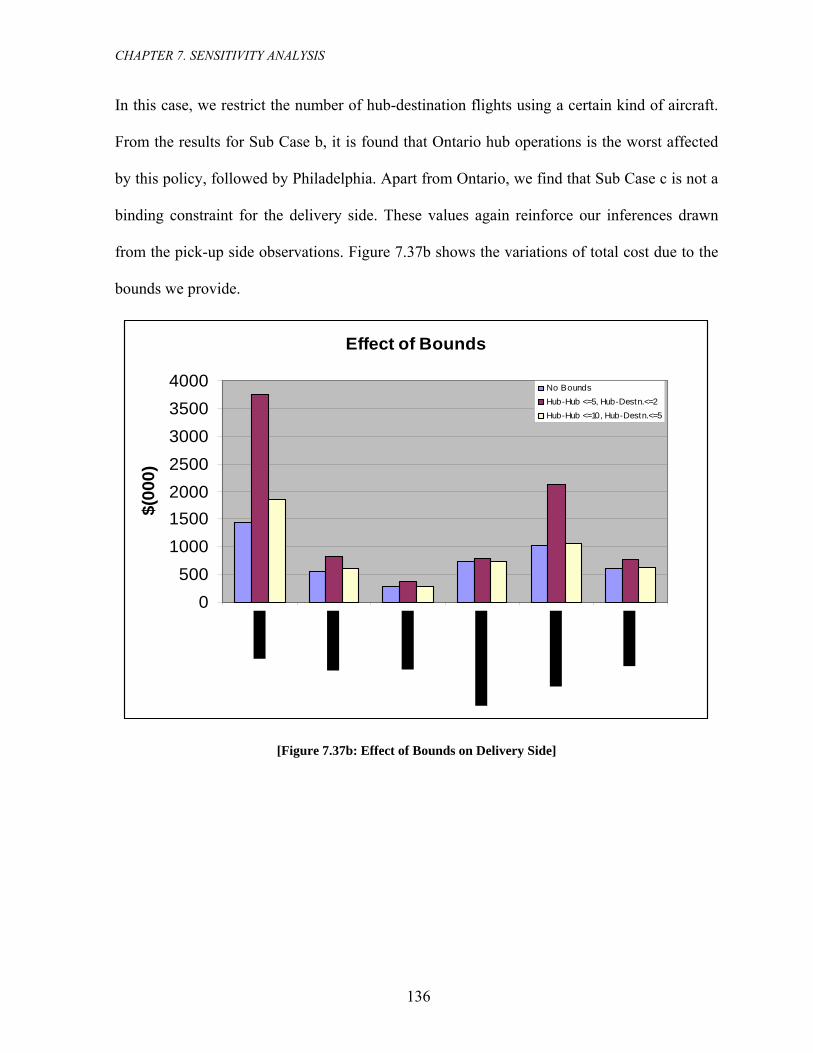
CHAPTER 7. SENSITIVITY ANALYSIS
In this case, we restrict the number of hub-destination flights using a certain kind of aircraft.
From the results for Sub Case b, it is found that Ontario hub operations is the worst affected
by this policy, followed by Philadelphia. Apart from Ontario, we find that Sub Case c is not a
binding constraint for the delivery side. These values again reinforce our inferences drawn
from the pick-up side observations. Figure 7.37b shows the variations of total cost due to the
bounds we provide.
Effect of Bounds
0
20002500
4000
50010001500
30003500
$(00
0)
No BoundsHub-Hub <=5, Hub-Destn.<=2Hub-Hub <=10, Hub-Destn.<=5
[Figure 7.37b: Effect of Bounds on Delivery Side]
136

CHAPTER 8. CONCLUSIONS
C
Conclusion & Future Scope of Research
8.1 Conclusions
This chapter summarizes our observations, findings from our analysis and future scope of
research in this area. Air transportation is a crucial component of the Express Package
Delivery Services from and operational as well as cost standpoint. Due to the high values of
the assets involved in terms of aircraft and huge operational cost implications, any small
percentage savings could result in the order of savings of millions of dollars for the company.
In the previous chapters, we analyzed the cost implications of various strategies that a
company may think of implementing. We considered two main operational strategies: one
involving no intermediate stops on pick-up and delivery sides and the other involving one
intermediate stop betwee hub and destination on
hapter 8
n origin and hub on pick-up side and between
137

CHAPTER 8. CONCLUSIONS
delivery side. Under each strategy, we analyzed the cost implications under a single hub
nsitivity
analysis to understand the implications of variation in dem
va o also a d a fe ances the im tions o ds
on rcraf g off ing irpor
8.2 Summary of Re
In umm results from the sensitivity analysis. Figure 8.1 gives the brief
description of the scenarios analyzed in Chapters 5 through 7.
[Figure 8.1: Scenario Descriptions]
network configuration and regional hub network configuration. In Chapters 5 and 6, we
studied various variants and logical combinations of these scenarios which gave a clear
understanding of the network structure. In Chapter 7, we carried an extensive se
and, fixed cost of operation and
riable cost of operati n. We nalyze w inst to test plica f boun
the number of ai t takin and land in the a ts.
sults
this section, we s arize
No Stop Scenarios Scenario-1(A): Single Hub Case Scenario-1(B): Demands routed through Origin Regional Hubs on pick-up side Demands routed through Destination Regional Hubs on delivery side Scenario-2: Demands routed either through Origin Regional Hub or directly to Main Hub
on pick-up Demands routed either through Destination Regional Hub or directly to Destination on delivery
Scenario-3(A): Demands routed either through Origin Regional Hub or directly to Destination Regional Hub
Scenario-3(B): Demands routed from Origin Regional Hubs to destination or Destination Regional Hub One Stop Scenarios Scenario-1: Single Hub Case Scenario-2: Demands routed through Origin Regional Hubs on pick-up side Demands routed through Destination Regional Hubs on delivery side Scenario-3(A): Scenario-3(B): Demands consolidated at Origin Regional Hubs and are routed from there either through
One Stop routes to Destinations or through No Stop routes through Destination Regional Hubs on delivery side
138

CHAPTER 8. CONCLUSIONS
From the results of our analysis in Chapters 5 through 7, we find out that One Intermediate
Stop Scenario 3 strategy has the least total cost of operations. We consistently observe that
w from Origin Regional Hubs either through One Stop routes to
Destinations or through No Stop routes through Destination Regional Hubs on delivery side,
we obtain the least cost of operation. The pickup side is the case where demands from the
origins are consolidated at the Origin Regional Hub by means of one stop routes from
Origins to the Origin Regional Hub. This strategy stands out as the best strategy across all
demand ranges, fixed cost and variable cost ranges.
Total costs incurred for opting for a similar strategy, when demands are routed from Origin
either through One Stop routes to Destination Regional Hubs or through No Stop routes
through Original Regional Hubs on pick-up side and from dispatched to the destination by
one stop routes from Destination Regional Hub, we get the second minimal total cost of
operations.
From our sensitivity analysis, we find a clear understanding of the cost implications of
various strategies. Our results show relative performances of various strategies and we have
sufficient evidence to accept or reject a strategy. We can also find out how much better or
worse we could perform by opting a certain strategy against another. For example, we can
find out that Single Hub Case with one intermediate stop on pick-up and delivery has a
certain percentage of less cost implications than the Single Hub Case with no intermediate
stops on pick-up or delivery routes.
hen demands are routed
139

CHAPTER 8. CONCLUSIONS
In the following sections, we summarize our findings of our research with respect to
variation in demand, fixed and variable costs of operation. The data obtained give valuable
information about the network structure. Based on the results obtained, we have developed
equations relating the total costs with demand, fixed costs and variable costs. We find simple
patterns in the network structure. These equations could be used with reasonable accuracy to
study the network from a planning stand point. Needless to say, the model could also be used
from a tactical or operational standpoint. With the proper data inputs, the model could serve
for operational management decision inputs. With very few modifications, one can study
implications of a plethora of strategies using this model. One could easily incorporate
constraints to the problem.
8.2.1 Total Cost Implications of Demand
Table 8.1 summarizes the results of the demand sensitivity. We find that the total cost of
operation under a strategy increases linearly with increase in demand. Scenario 3B under the
one stop scenario has the least total cost of operations. We see that total cost varies linearly
with demand and different strategies have different rates of increase of total cost (see Figure
8.2). We also show the percentage comparison of total cost with respect to demand across all
scenarios.
140

CHAPTER 8. CONCLUSIONS
50% Base 150% 200% Scenarios $(000) % $(000) % $(000) % $(000) %
No Stop Scenario-1(A): 5514 157% 9753 143% 15923 159% 16715 126%
No Stop Scenario-1(B): 5747 164% 10762 158% 15777 157% 20824 157%
No Stop Scenario-2: 5051 144% 9066 133% 13045 130% 17106 129%
No Stop Scenario-3(A): 4895 139% 8337 122% 11537 115% 14866 112%
No Stop Scenario-3(B): 4700 134% 7942 117% 11092 111% 14225 107%
One Stop Scenario-1(A): 4840 138% 9337 137% 13710 137% 16290 123%
One Stop Scenario-2: 5432 155% 10521 154% 15751 157% 20896 158%
One Stop Scenario-3(A): 3648 104% 7024 103% 10282 103% 13373 101%
One Stop Scenario-3(B): 3511 100% 6814 100% 10027 100% 13235 100%
[Table 8.1: Summary of Demand Sensitivity Analysis]
Demand Sensitivity Trends
0
5000
10000
15000
20000
25000
50% Base 150% 200%
Tota
l Cos
t $(0
00)
No Stop Scenario-1(A): No Stop Scenario-1(B): No Stop Scenario-2:
No Stop Scenario-3(A): No Stop Scenario-3(B): One Stop Scenario-1(A):
One Stop Scenario-2: One Stop Scenario-3(A): One Stop Scenario-3(B):
[Figure 8.2: Total Cost Variation versus Demand]
141

CHAPTER 8. CONCLUSIONS
142
8.2.2 Total Cost Implications of Fixed Cost
Table 8.2 summarizes the results of the fixed cost sensitivity. Figure 8.3 shows the total cost
trends with respect to fixed costs. We see a polynomial variation with the slope of the lines
increasing as we move from lower fixed cost intervals to higher fixed cost intervals.
Base 125% 150% 200% 300% 500%
$(000) $(000) $(000) $(000) $(000) $(000)
No Stop Scenarios Scenario-1(A): 9753 10830 11891 13981 18027 25419
Scenario-1(B): 10763 12091 13369 15841 20593 28513
Scenario-2: 9066 10136 11196 13585 17017 23757
Scenario-3(A): 8337 10389 12272 16000 22525
Scenario-3(B): 7943 9770 11792 15111 21384 One Stop Scenarios Scenario-1(A): 9337 10364 11391 13352 17367 25023
Scenario-2: 10519 11813 13023 15250 19502 26023
Scenario-3(A): 7024 8007 8710 10606 13908 19527
Scenario-3(B): 6814 7768 8654 10425 13696 19352 [Table 8.2: Summary of Fixed Cost Sensitivity Analysis]
Total Cost Implications of Fixed Cost
0
5000
10000
15000
20000
25000
30000
0% 100% 200% 300% 400% 500% 600%
$(00
0)
No Stop Scenario-1(A):No Stop Scenario-1(B):No Stop Scenario-2:No Stop Scenario-3(A):No Stop Scenario-3(B):One Stop Scenario-1(A):One Stop Scenario-2:One Stop Scenario-3(A):One Stop Scenario-3(B):
[Figure 8.3: Total Cost Variation versus Fixed Cost Variation]

CHAPTER 8. CONCLUSIONS
Table 8.3 shows the percentage comparison of total cost with respect to fixed cost
Scenarios Base 125% 150% 200% 300% 500%
No Stop Scenario-1(A): 143% 139% 137% 134% 132% 131%
No Stop Scenario-1(B): 158% 156% 154% 152% 150% 147%
No Stop Scenario-2: 133% 130% 129% 130% 124% 123%
No Stop Scenario-3(A): 122% 120% 118% 117% 116%
No Stop Scenario-3(B): 117% 113% 113% 110% 111%
One Stop Scenario-1(A): 137% 133% 132% 128% 127% 129%
One Stop Scenario-2: 154% 152% 150% 146% 142% 134%
One Stop Scenario-3(A): 103% 103% 101% 102% 102% 101%
One Stop Scenario-3(B): 100% 100% 100% 100% 100% 100%
[Table 8.3: Percentage Comparison of Total Cost with respect to Fixed Cost across all Scenarios]
8.2.3 Total Cost Implications of Variable Cost
Table 8.4 summarizes the results of the variable cost sensitivity. Figure 8.4 shows the total
cost trends with respect to variable costs. We see that the slope of the lines remains constant
till the variable cost increases by 200%.
143
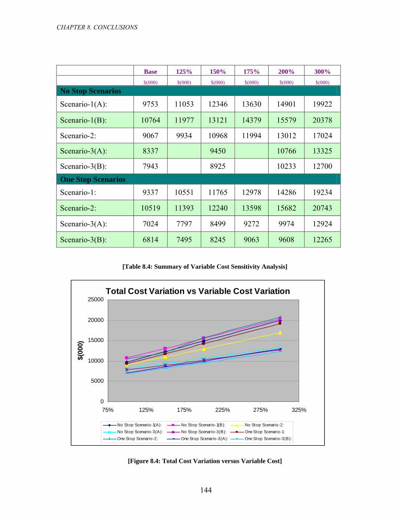
CHAPTER 8. CONCLUSIONS
Base 125% 150% 175% 200% 300% $(000) $(000) $(000) $(000) $(000) $(000)
No Stop Scenarios
Scenario-1(A): 9753 11053 12346 13630 14901 19922
Scenario-1(B): 10764 11977 13121 14379 15579 20378
Scenario-2: 9067 9934 10968 11994 13012 17024
Scenario-3(A): 8337 9450 10766 13325
Scenario-3(B): 7943 8925 10233 12700
One Stop Scenarios
Scenario-1: 9337 10551 11765 12978 14286 19234
Scenario-2: 10519 11393 12240 13598 15682 20743
Scenario-3(A): 7024 7797 8499 9272 9974 12924
Scenario-3(B): 6814 7495 8245 9063 9608 12265
[Table 8.4: Summary of Variable Cost Sensitivity Analysis]
Total Cost Variation vs Variable Cost Variation
0
5000
10000
15000
20000
25000
75% 125% 175% 225% 275% 325%
$(00
0)
No Stop Scenario-1(A): No Stop Scenario-1(B): No Stop Scenario-2:No Stop Scenario-3(A): No Stop Scenario-3(B): One Stop Scenario-1:One Stop Scenario-2: One Stop Scenario-3(A): One Stop Scenario-3(B):
[Figure 8.4: Total Cost Variation versus Variable Cost]
144

CHAPTER 8. CONCLUSIONS
Table 8.5 shows the percentage comparison of total cost with respect to variable cost across
all scenarios.
Scenarios Base 125% 150% 175% 200% 300%
No Stop Scenario-1(A): 143% 147% 150% 150% 155% 162%
No Stop Scenario-1(B): 158% 160% 159% 159% 162% 166%
No Stop Scenario-2: 133% 133% 133% 132% 135% 139%
No Stop Scenario-3(A): 122% 115% 112% 109%
No Stop Scenario-3(B): 117% 108% 107% 104%
One Stop Scenario-1(A): 137% 141% 143% 143% 149% 157%
One Stop Scenario-2: 154% 152% 148% 150% 163% 169%
One Stop Scenario-3(A): 103% 104% 103% 102% 104% 105%
One Stop Scenario-3(B): 100% 100% 100% 100% 100% 100%
[Table 8.5 Percentage Comparison of Total Cost with respect to Variable Cost across all Scenarios]
145

CHAPTER 8. CONCLUSIONS
8.3 Computation Times
All the models were run using a CPLEX 9.0 MIP Solver on a 512MB Pentium IV processor.
Th ation t with respect to the modeled. Table
8.6 gives the order of average computational time observed for various scenarios. Scenario 1
cases with no intermediate stops were the fastest to reach optimality followed by Regional
Hub Cases and Single Hub case with one stop routes and Scenario 2 with no stops. Scenario 3
with no stops was computationally the most demanding. Some of the cases ran for more than
18 hours. In our analysis, in some cases, whenever there was a problem of convergence i.e it
took a really long time for optimal solutions, we stopped the solver when it reached 1.0% or
1.5% of optimality. These convergence problems were only encountered in some of Scenario
3 no stop cases. Scenario 3A and Scenario 3B by their structure resulted in huge MIP
programs and the problem read and presolve time were comparatively high (in the order of 3-
5 seconds). The time for a single iteration took an average of 12-15 minutes, but the models
converged to less than 1.5% of optimality in less than 30-40 minutes most of the cases. Due to
time constraints, some of the Scenario 3A and Scenario 3B cases were not solved to
optimality and the solver was terminated once we reached 0.5% optimality.
e comput ime varied problem size and scenario
Scenarios Average Computation Time Order No Stop Scenario-1(A): 101 (usually ~ 30 seconds) No Stop Scenario-1(B): 10-1 (usually ~ 10 seconds) No Stop Scenario-2: 101 (usually ~ 45 seconds) No Stop Scenario-3(A): 103 (usually ~ 7200 seconds) No Stop Scenario-3(B): 103 (usually ~ 7200 seconds) One Stop Scenario-1(A): 101 (usually ~ 7200 seconds) One Stop Scenario-2: 10-1 (usually ~ 1800 seconds) One Stop Scenario-3(A): 103 (usually ~ 7200 seconds) One Stop Scenario-3(B): 103 (usually ~ 7200 seconds)
[Table 8.6: Computation Times]
146

CHAPTER 8. CONCLUSIONS
8.4 Future Scope
The MIP models used in the analysis could easily be updated to study other strategies that a
shipment service provider wishes to employ. Constraints could easily be incorporated in the
model to reflect more real life situations. The dataset used in our analysis was created from
the Commodity Flow Survey and NAICS data. We only considered two kinds of aircraft in
our analysis. The models could easily be run with real data and more aircraft types. One of the
areas where the model could be updated is running it on a time horizon. With these trial runs
with actual data, one could come up with recurrent patterns of flights selected, demand
allocations to the flights. There could be potentially two main lines of research: one would be
to come up with more innovative operational strategies and the other is to optimize the model
performance. Reliability of the paths chosen by the model and introduction of penalty terms to
reflect more decision scenarios would be a logical step in this direction. Air transportation
network design for express package delivery problems comes under the difficult class of
multi-commodity flow problems. There is enormous potential in this area of application from
a research as well as industry stand point.
147

APPENDICES
148
Appendix 1: Sample calculation showing the effect of time-zones.
Figure-A1 shows a sample calculation for time windows with reference to a service region
comparable to US. Let segment length, L = 3200 miles and hub is located at x = 1400 miles
from east end on time zone 1.
[Fig – A1]
Number of time zones, Z = 4
West bound aircraft cruise velocity, vw = 500 mph
East bound aircraft cruise velocity, ve = 600 mph
Latest Departure Time at airport (local time) = 18:00 hours
Take-off / Landing time, f = 30 min.
Arrival time at hub (local time) from western end of segment Tw(x) = 18:00 +f + (Zo- Zh) + x/ ve
= 18:00 + (0.5 + 3 – 1 + 1800/600) = 23:30 hours
Arrival time at hub (local time) from eastern end of segment Tw(x) = f - (Zo- Zh) + (L-x)/ vw
= 18:00 + (0.5 – (0 – 1) + 1400/500) = 22:20 hours
Maximum Arrival Time at hub = 23:30 hours
If 7:00 hours is the latest delivery time at the destination, then latest delivery time from the hub for
East bound destination = 7:00 + (Zd- Zh) – x/ vw – f
= 7:00 + (3-1) – 1800/500 – 0.5 = 5:00 hours
West bound destination = 7:00 + (Zd- Zh) – (L-x)/ ve – f
= 7:00 + (0-1) – 1400/600 – 0.5 = 3:10 hours
Z=3 Z =2 Z=1 Z=0
(L-x) = 1800 miles x = 1400 miles

APPENDICES
So, the east bound shipment is critical and should be dispatched prior to the westbound
shipment.
Appendix 2A: List of Cities and Codes in the sample Air Network
1 SEATTLE 31 BIRMINGHAM 61 NEWARK
2 BILLINGS 32 NASHVILLE 62 WASHINGTON-DULLES
3 BOISE 33 CLEVELAND 63 NEW YORK
4 BURBANK 34 CINCINNATI 64 HARRISBURG
5 FRESNO 35 DAYTON 65 NORFOLK
6 SPOKANE 36 FORT WAYNE 66 PITTSBURGH
7 LAS VEGAS 37 HUNTSVILLE 67 RICHMOND
8 LOS ANGELES 38 INDIANAPOLIS 68 ALBANY(NY)
9 LONG BEACH 39 COLUMBUS 69 HARTFORD
10 SACRAMENTO 40 MEMPHIS 70 BOSTON
11 OAKLAND 41 KNOXVILLE 71 MANCHESTER
12 PORTLAND 42 ALBUQUERQUE 72 PROVIDENCE
13 PHOENIX 43 AUSTIN 73 NEWBURGH
14 RENO 44 DENVER 74 SYRACUSE
15 SAN DIEGO 45 HOUSTON 75 PHILADELPHIA
16 SAN JOSE 46 EL PASO 76 ALBANY(GA)
17 SALT LAKE CITY 47 HOUSTON 77 ATLANTA
18 CEDAR RAPIDS 48 WICHITA 78 MOBILE
19 DECATUR 49 JACKSON 79 CHARLOTTE
20 DES MOINES 50 LAFAYETTE 80 GREENSBORO
21 DETROIT 51 LITTLE ROCK 81 GREENVILLE
22 SIOUX FALLS 52 NEW ORLEANS 82 JACKSONVILLE
23 LANSING 53 OKLAHOMA CITY 83 RALEIGH
24 KANSAS CITY 54 SAN ANTONIO 84 ROANOKE
25 MILWAUKEE 55 SPRINGFIELD 85 FT. LAUDERDALE
26 MINNEAPOLIS 56 SHREVEPORT 86 ORLANDO
27 OMAHA 57 TULSA 87 MIAMI
28 CHICAGO 58 DALLAS / FT. WORTH 88 PALM BEACH
29 SOUTH BEND 59 BUFFALO 89 ST. PETERSBURG
30 ST. LOUIS 60 BALTIMORE 90 FORT MYERS [Table – A2A]
149

APPENDICES
150
Appendix 2B: Regional Hubs and Connected Cities in the sample Air Network
Regional Hub -1 Regional Hub -2 Regional Hub -3 Regional Hub -4 Regional Hub -5 Regional Hub-6
ONTARIO DALLAS /
FT. WORTH ROCKFORD LOUISVILLE PHILADELPHIA COLUMBIA SEATTLE ALBUQUERQUE CEDAR RAPIDS BIRMINGHAM BUFFALO ALBANY(GA)
BILLINGS AUSTIN DECATUR NASHVILLE BALTIMORE ATLANTA
BOISE DENVER DES MOINES CLEVELAND NEWARK MOBILE
BURBANK HOUSTON DETROIT CINCINNATI WASHINGTON-
DULLES CHARLOTTE
FRESNO EL PASO SIOUX FALLS DAYTON NEW YORK GREENSBORO
SPOKANE HOUSTON LANSING FORT WAYNE HARRISBURG GREENVILLE
LAS VEGAS WICHITA KANSAS CITY HUNTSVILLE NORFOLK JACKSONVILLE
LOS ANGELES JACKSON MILWAUKEE INDIANAPOLIS PITTSBURGH RALEIGH
LONG BEACH LAFAYETTE MINNEAPOLIS COLUMBUS RICHMOND ROANOKE
SACRAMENTO LITTLE ROCK OMAHA MEMPHIS ALBANY(NY) FT.
LAUDERDALE
OAKLAND NEW ORLEANS CHICAGO KNOXVILLE HARTFORD ORLANDO
PORTLAND OKLAHOMA
CITY SOUTH BEND BOSTON MIAMI
PHOENIX SAN ANTONIO ST. LOUIS MANCHESTER PALM BEACH
RENO SPRINGFIELD PROVIDENCE ST.
PETERSBURG
SAN DIEGO SHREVEPORT NEWBURGH FORT MYERS
SAN JOSE TULSA SYRACUSE
SALT LAKE CITY
[Table – A2B]

LIST OF REFERENCES
- 151 -
List of References
1. A .P. ARMACOST, C. BARNHART, K. A. WARE. “Composite Variable Formulations for Express Shipment Service Network Design”, Transportation Science, Vol.36, No.1, February 2002, pp. 1-20. 2. A. BALAKRISHNAN, T. L. MAGNANTI, R. WONG. “A Dual-Ascent Procedure for Large-Scale Uncapacitated Network Design”, Operations Research, Vol. 37, 1989, pp. 716-740. 3. A. BALAKRISHNAN, T. L. MAGNANTI, P. MIRCHANDANI. “A Dual- Based Algorithm for Multilevel Network Design”, Management Science, Vol.40, No.__, 1994a, pp. 567-581 4. A. BALAKRISHNAN, T. L. MAGNANTI, P. MIRCHANDANI. “Modeling and Heuristic Worst-Case Performance Analysis of the Two-Level Network Design Problem”, Management Science, Vol.40, No.__ , 1994b, pp. 846-867 5. R.K. AHUJA, T.L. MAGNANTI, J.B. ORLIN. “Network Flows : Theory, Algorithms, and Applications” Prentice Hall, 1993 6. C. BARNHART, RINA R. SCHNEUR.. “Air Network Design for Express Shipment Service”, Operations Research, Vol.44, Issue 6, Nov-Dec 1996, pp. 852-863. 7. D. BERTSIMAS, C. P. TEO. “From valid inequalities to heuristics: A unified view of primal-dual approximation algorithms in covering problems. Operations Research, Vol. 46, 1998 pp. 503–514. 8. D. BIENSTOCK, O. GÜNLÜK. “Computational experience with a difficult mixed-integer multicommodity flow problem.” Math. Programming, Vol. 68, 1995, pp. 213–237. 9. K. BÜDENBENDER, T. GRÜNERT, H.J. SEBASTIAN. “A hybrid tabu search/branch-and-bound algorithm for the direct flight network design problem” Transportation Sci. Vol. 34 , 2000, pp.364–380. 10. M.S. DASKIN “Network and Discrete Location: Models, Algorithms and Applications”, Wiley Interscience Series in Discrete Mathematics and Optimization, 1995. 11. D. KIM, C. BARNHART, K.A. WARE, G. REINHARDT. “ Multi-modal Express Delivery: A Service Network Design Application”, Transportation Science, Vol.33, No.4, November 1999, pp.391-407. 12. M. X. GOEMAN, D. J. BERTSIMAS. “Survivable networks, linear programming relaxations and the parsimonious property.”, Math. Programming , Vol.60, 1993, pp.143-166. 13. T. GRÜNERT, H. J. SEBASTIAN. “Planning models for long-haul operations of postal and express shipment companies.”, Eur. J. Oper. Res., Vol. 122, 2000, pp.289–309.

LIST OF REFERENCES
- 152 -
14. R.W. HALL “Configuration of an Overnight Package Air Network”. Trans. Res. A, 23A, 2, 1999, pp.139-149. 15. K.L. JONES, I.J. LUSTIG, J.M. FARVOLDEN, W.N. POWELL. “Multicommodity Network Flows ; The Impact of Formulation on Decomposition”, Math Prog. 62, 1993, pp. 95-117. 16. M. KUBY, R. GRAY. “ The hub network design problem with stopovers and feeders: The case of Federal Express”, Transportation Res. A: Policy and Practice 27A, 1993, pp. 1–12. 17. F.J. LUDDERS. “Mixed Integer Programming Models for Integrated Vehicle Routing and Flight Assignment in the Intermodal Package Industry” Thesis, The University of Texas at Austin, Dec’ 18. T.L. MAGNANTI, P.MIRCHANDANI. “ Shortest paths, single origin destination network design and associated polyhedra”, Networks, Vol. 23, 1993, pp. 103–121. 19. T. L. MAGNANTI, R. T. WONG. “Network Design and Transportation Planning: Models and Algorithms”, Transportation Science, Vol.18, No.1, 1984, pp.1-55. 20. M. MINOUX. “Network Synthesis and Optimum Network Design Problems: Models, Solution Methods and Applications”, Networks, Vol.19, 1989, pp.313-360 21. M. W. PADBERG, T. J. VAN ROY, L. A. WOLSEY. “Valid linear inequalities for fixed charge problems” Oper. Res. 33, 1985, pp. 842–861. 22. Y. POCHET, L.A. WOLSEY. “Integer knapsack and .ow covers with divisible coefficients: Polyhedra, optimization, and separation.” Discrete Appl. Math., Vol. 59 1995, pp.57–74. 23. K.R. SMILOWITZ “Design and Operation of Multimode, Multiservice Logistics Systems" Doctoral Dissertation,UCB, 2001, (http://www.uctc.net/papers/dissalpha.html) 24. T. J. VAN ROY, L. A. WOLSEY. “Valid inequalities and separation for uncapacitated fixed charge networks”, Oper. Res. Letters 4, 1985, pp.105–112. 25. L. A. WOLSEY. “Faces of linear inequalities in 0-1 variables” Math. Programming, Vol.8, 1975 pp. 165–178.

LIST OF REFERENCES
- 153 -
Web References :
TUhttps://www.aerocom-int.com/UT TUhttp://www.census.govUT TUhttp://www.census.gov/econ/wwwUT TUhttp://www.census.gov/population/www/estimates/metroarea.htmlUT TUhttp://www.fedex.comUT TUhttp://ilog.cplex.comUT TUhttp://www.transtats.bts.gov/UT TUhttp://www.ups.comUT TUhttp://www.usps.comUT
Related Documents