Absorber Tuto

Gas Absorption ColumnTutorial

HYSYS Tutorial for the Steady State Behavior of the Gas Absorption Column in the Unit Operation Laboratory

AbstractA tutorial has been prepared to show how HYSYS can be used to model a continuous gas absorption process in a packed column. In the absorption process, air and CO2 are mixed before they enter the packed column where the CO2 is removed from the air by water. The equipment used for the absorption can be represented in a HYSYS process flow diagram. Information about the streams can be entered from a program created in HYSYS. This program also uses HYSYS transport properties to calculate the linear approximation of the number of transfer units and height per transfer units.

TutorialThe purpose of this tutorial is to introduce the use of HYSYS as a modeling tool for the gas absorption column in the Unit Operations Laboratory of the chemical engineering program. This tutorial shows how to:

build an HYSYS case for the process program in HYSYS , and use HYSYS transport properties to calculate height and

transfer units.

In this tutorial, carbon dioxide (CO2) is removed form air by water in a packed column. The packed column contains ¼ inch Ceramic Interlock Saddles.

What is HYSYS?

HYSYS is a simulation software designed by Hyprotech. In this tutorial, HYSYS Plant 2.2.2, (released August 2000) isused. Some of the procedure described within may not apply to other versions of HYSYS.

Getting Started in HYSYS

Two versions of HYSYS are install on computers in the BieryRoom of the Chemical Engineering Building. Care should be taken to ensure that the correct version is used.

After logging onto the Windows NT workstations, either of the following can be used to access HYSYS 2.2.2.

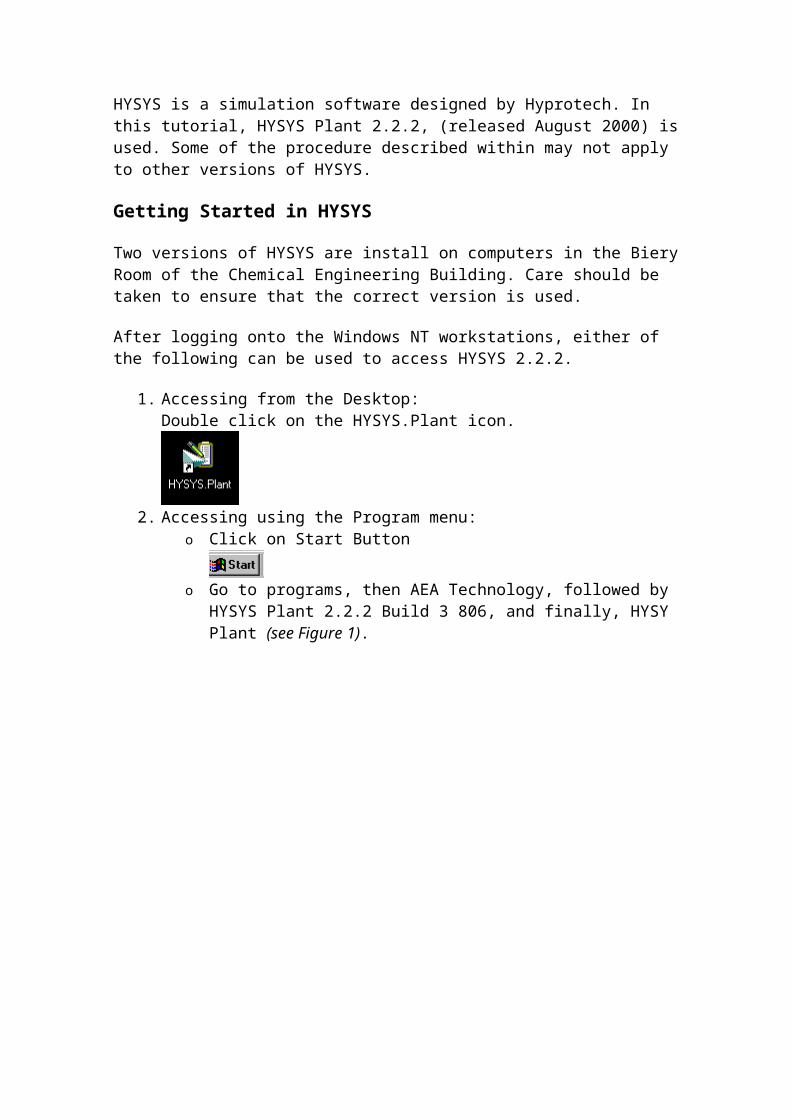
1. Accessing from the Desktop:Double click on the HYSYS.Plant icon.

2. Accessing using the Program menu:o Click on Start Button

o Go to programs, then AEA Technology, followed by HYSYS Plant 2.2.2 Build 3 806, and finally, HYSY Plant (see Figure 1).

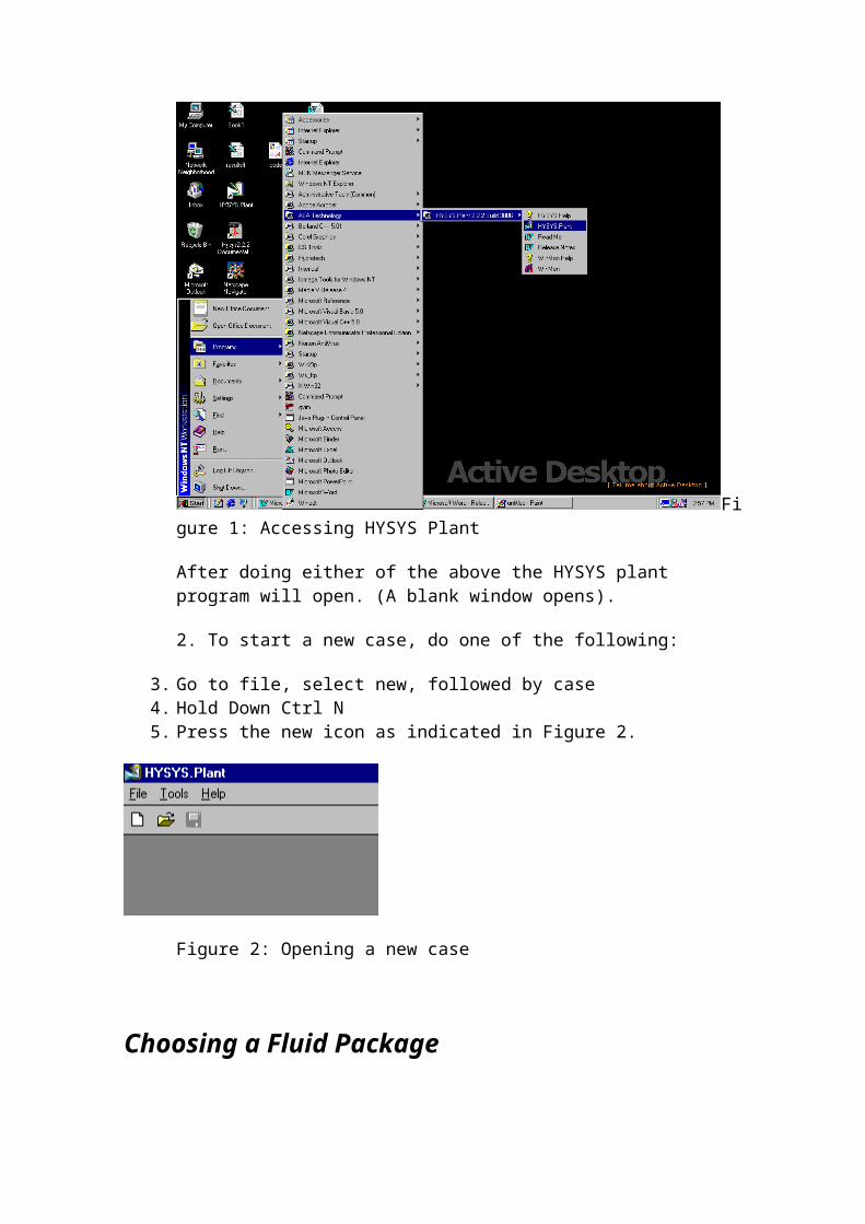
Figure 1: Accessing HYSYS Plant

After doing either of the above the HYSYS plant program will open. (A blank window opens).

2. To start a new case, do one of the following:

3. Go to file, select new, followed by case4. Hold Down Ctrl N5. Press the new icon as indicated in Figure 2.

Figure 2: Opening a new case

Choosing a Fluid Package

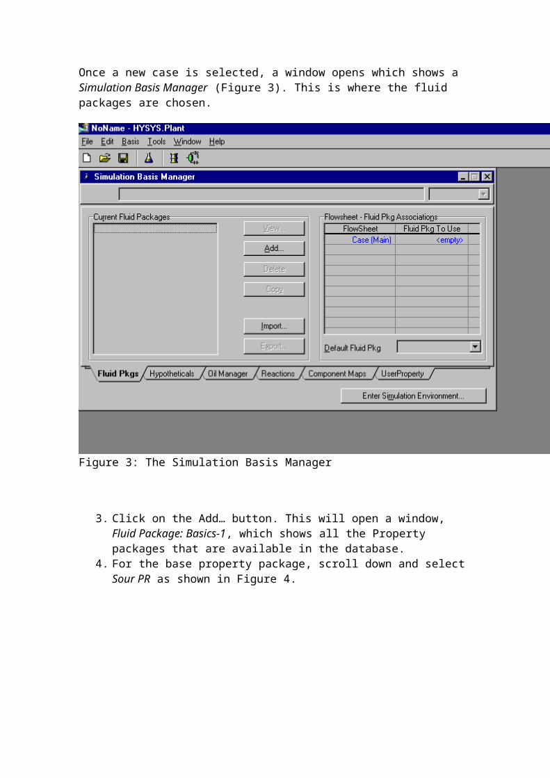
Once a new case is selected, a window opens which shows a Simulation Basis Manager (Figure 3). This is where the fluid packages are chosen.

Figure 3: The Simulation Basis Manager

3. Click on the Add… button. This will open a window, Fluid Package: Basics-1, which shows all the Property packages that are available in the database.

4. For the base property package, scroll down and select Sour PR as shown in Figure 4.

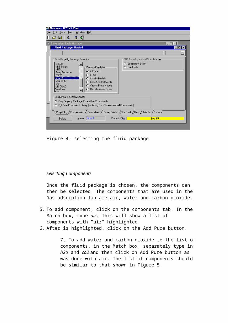
Figure 4: selecting the fluid package

Selecting Components

Once the fluid package is chosen, the components can then be selected. The components that are used in the Gas adsorption lab are air, water and carbon dioxide.

5. To add component, click on the components tab. In the Match box, type air. This will show a list of components with "air" highlighted.

6. After is highlighted, click on the Add Pure button.

7. To add water and carbon dioxide to the list ofcomponents, in the Match box, separately type in h2o and co2 and then click on Add Pure button as was done with air. The list of components should be similar to that shown in Figure 5.

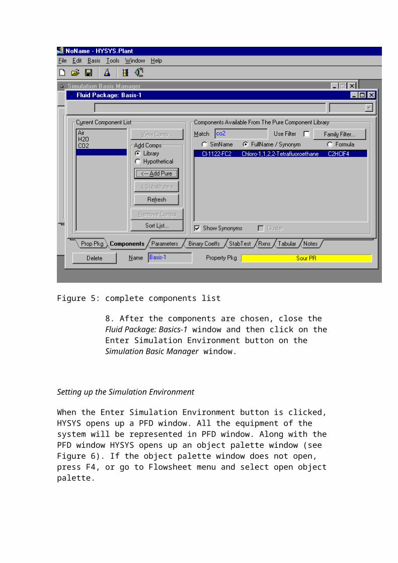
Figure 5: complete components list

8. After the components are chosen, close the Fluid Package: Basics-1 window and then click on the Enter Simulation Environment button on the Simulation Basic Manager window.

Setting up the Simulation Environment

When the Enter Simulation Environment button is clicked, HYSYS opens up a PFD window. All the equipment of the system will be represented in PFD window. Along with the PFD window HYSYS opens up an object palette window (see Figure 6). If the object palette window does not open, press F4, or go to Flowsheet menu and select open object palette.

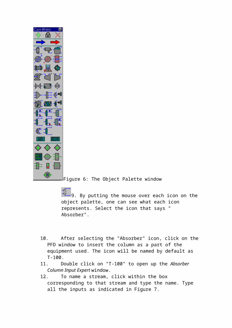
Figure 6: The Object Palette window

9. By putting the mouse over each icon on theobject palette, one can see what each icon represents. Select the icon that says " Absorber".

10. After selecting the "Absorber" icon, click on thePFD window to insert the column as a part of the equipment used. The icon will be named by default as T-100.

11. Double click on "T-100" to open up the Absorber Column Input Expert window.

12. To name a stream, click within the box corresponding to that stream and type the name. Type all the inputs as indicated in Figure 7.

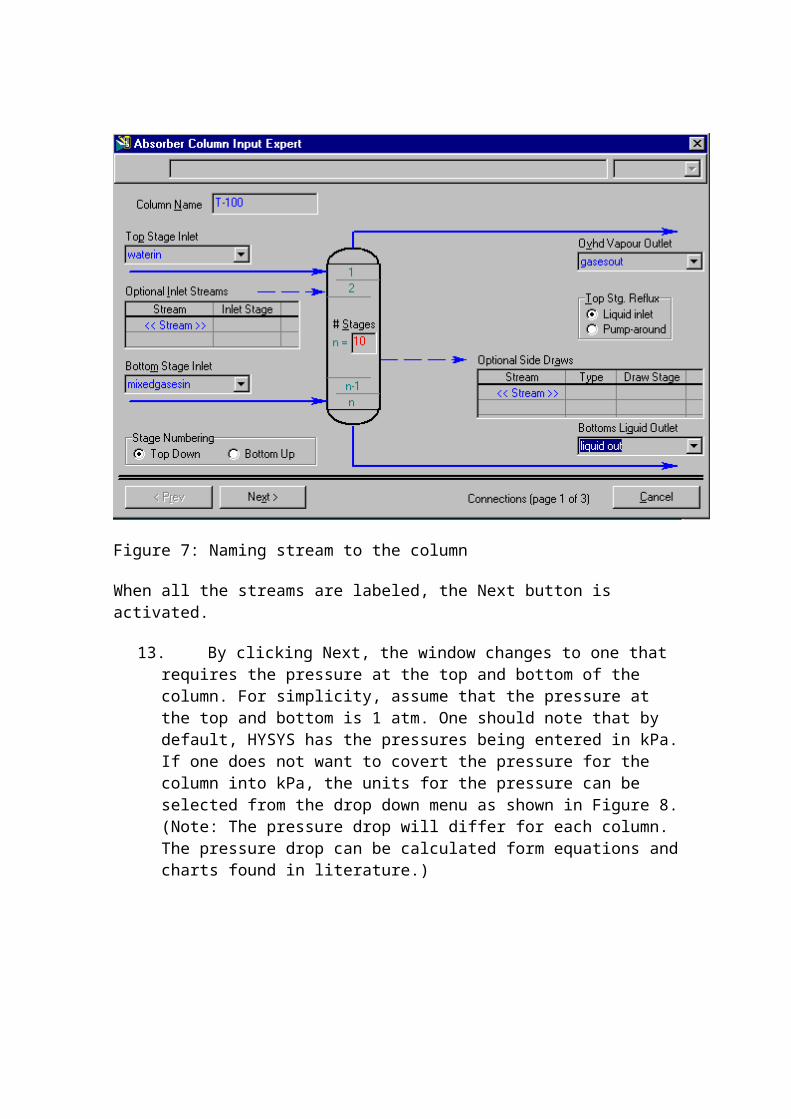
Figure 7: Naming stream to the column

When all the streams are labeled, the Next button is activated.

13. By clicking Next, the window changes to one that requires the pressure at the top and bottom of the column. For simplicity, assume that the pressure at the top and bottom is 1 atm. One should note that by default, HYSYS has the pressures being entered in kPa.If one does not want to covert the pressure for the column into kPa, the units for the pressure can be selected from the drop down menu as shown in Figure 8.(Note: The pressure drop will differ for each column. The pressure drop can be calculated form equations andcharts found in literature.)

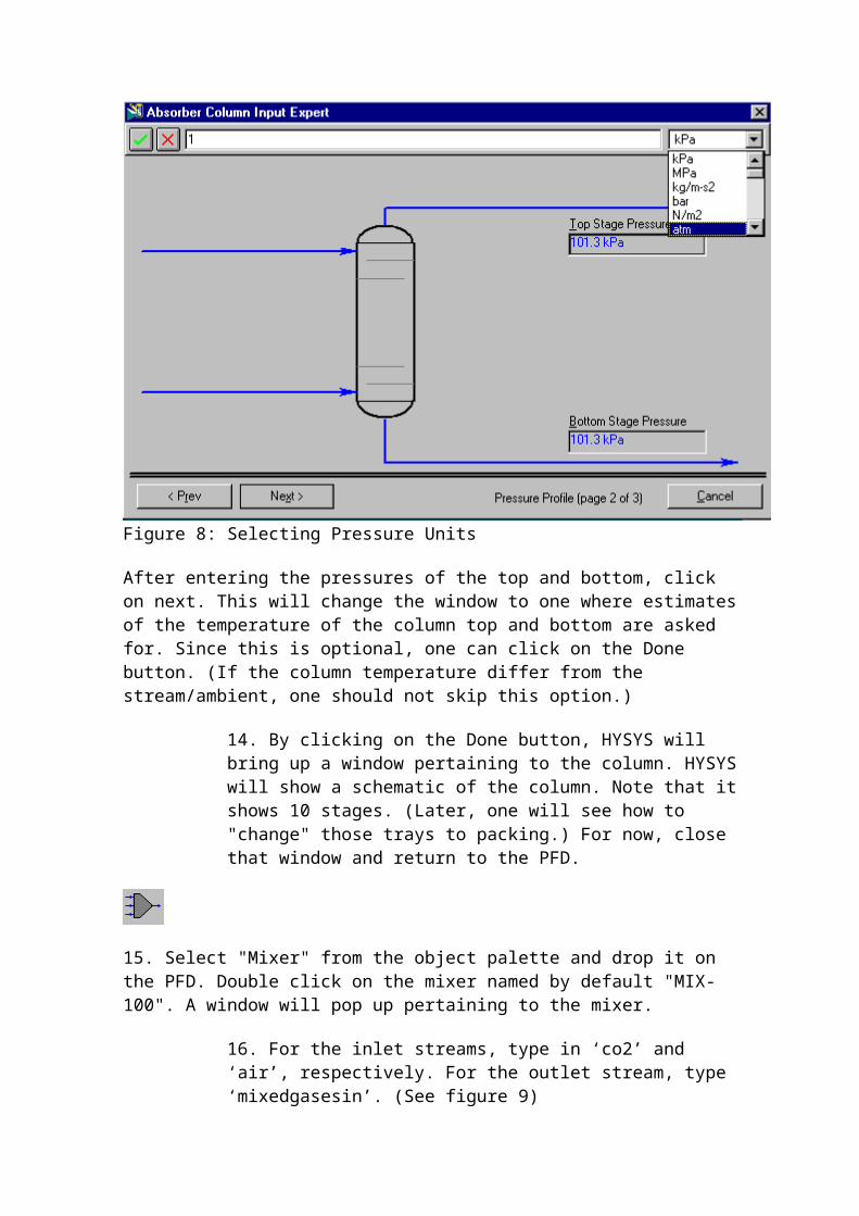
Figure 8: Selecting Pressure Units

After entering the pressures of the top and bottom, click on next. This will change the window to one where estimatesof the temperature of the column top and bottom are asked for. Since this is optional, one can click on the Done button. (If the column temperature differ from the stream/ambient, one should not skip this option.)

14. By clicking on the Done button, HYSYS will bring up a window pertaining to the column. HYSYSwill show a schematic of the column. Note that itshows 10 stages. (Later, one will see how to "change" those trays to packing.) For now, close that window and return to the PFD.

15. Select "Mixer" from the object palette and drop it on the PFD. Double click on the mixer named by default "MIX-100". A window will pop up pertaining to the mixer.

16. For the inlet streams, type in ‘co2’ and ‘air’, respectively. For the outlet stream, type ‘mixedgasesin’. (See figure 9)

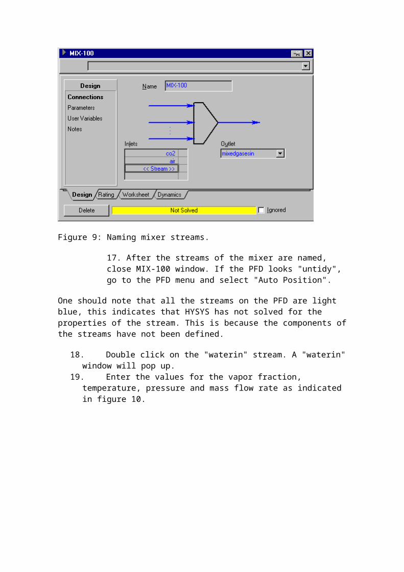
Figure 9: Naming mixer streams.

17. After the streams of the mixer are named, close MIX-100 window. If the PFD looks "untidy", go to the PFD menu and select "Auto Position".

One should note that all the streams on the PFD are light blue, this indicates that HYSYS has not solved for the properties of the stream. This is because the components ofthe streams have not been defined.

18. Double click on the "waterin" stream. A "waterin"window will pop up.

19. Enter the values for the vapor fraction, temperature, pressure and mass flow rate as indicated in figure 10.

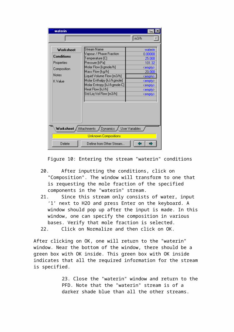
Figure 10: Entering the stream "waterin" conditions

20. After inputting the conditions, click on "Composition". The window will transform to one that is requesting the mole fraction of the specified components in the "waterin" stream.

21. Since this stream only consists of water, input ‘1’ next to H2O and press Enter on the keyboard. A window should pop up after the input is made. In this window, one can specify the composition in various bases. Verify that mole fraction is selected.

22. Click on Normalize and then click on OK.

After clicking on OK, one will return to the "waterin" window. Near the bottom of the window, there should be a green box with OK inside. This green box with OK inside indicates that all the required information for the stream is specified.

23. Close the "waterin" window and return to the PFD. Note that the "waterin" stream is of a darker shade blue than all the other streams.

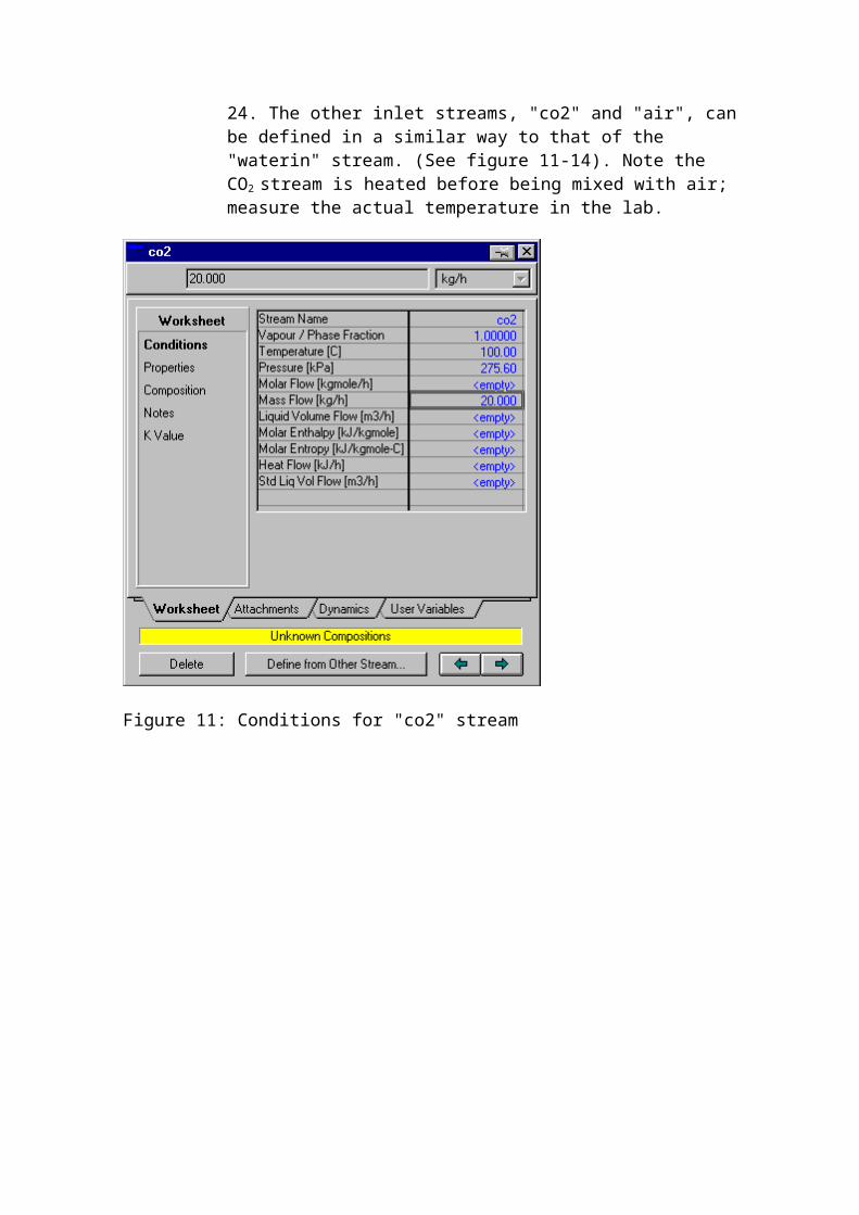
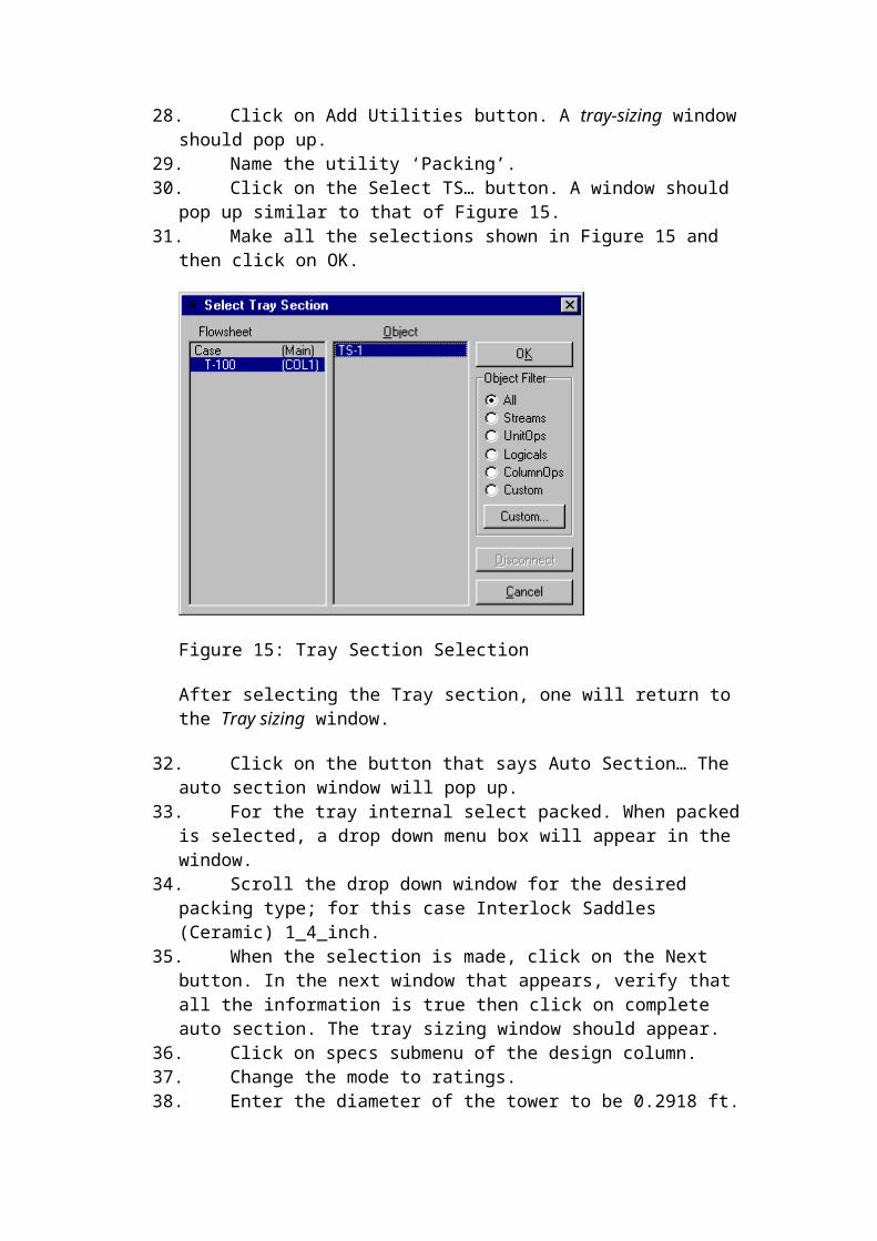
24. The other inlet streams, "co2" and "air", canbe defined in a similar way to that of the "waterin" stream. (See figure 11-14). Note the CO2 stream is heated before being mixed with air;measure the actual temperature in the lab.

Figure 11: Conditions for "co2" stream

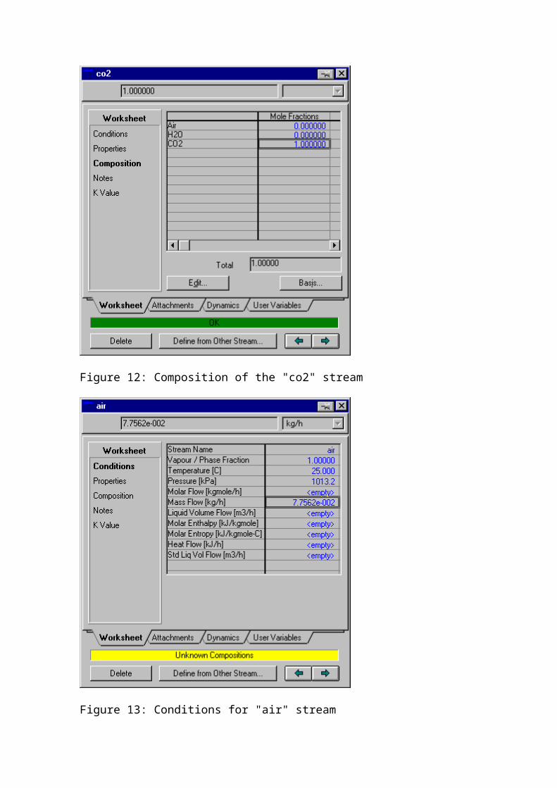
Figure 12: Composition of the "co2" stream

Figure 13: Conditions for "air" stream

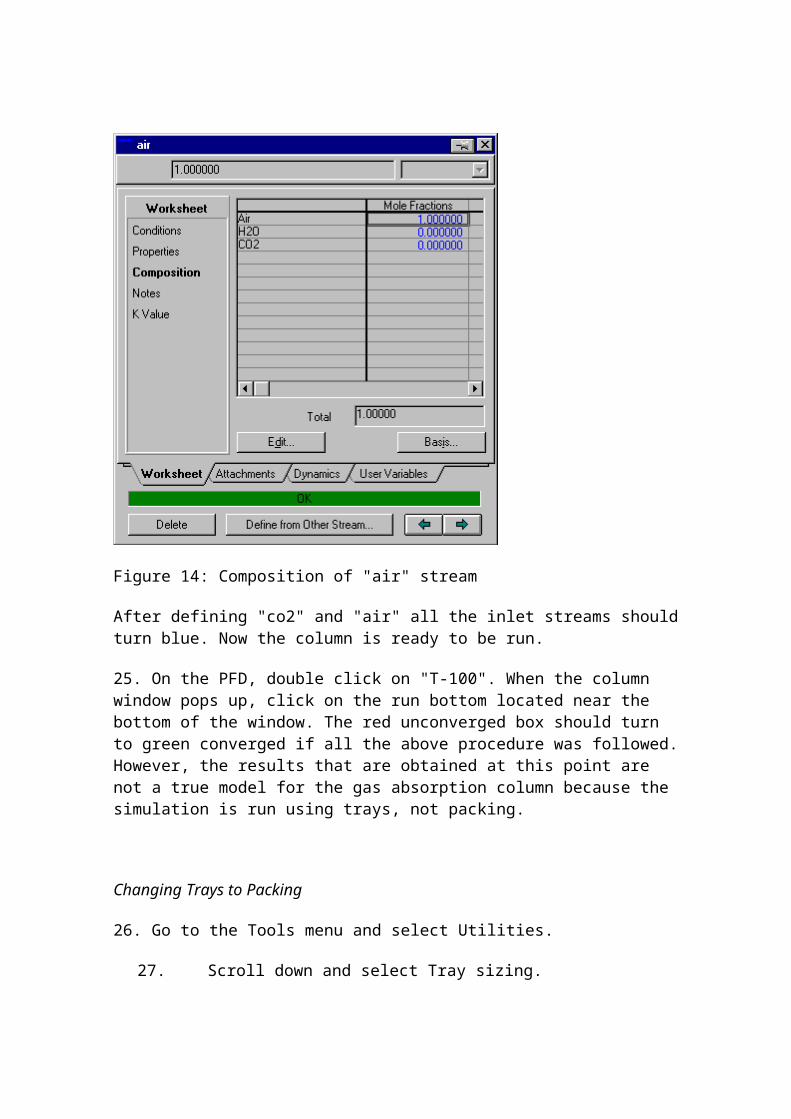
Figure 14: Composition of "air" stream

After defining "co2" and "air" all the inlet streams shouldturn blue. Now the column is ready to be run.

25. On the PFD, double click on "T-100". When the column window pops up, click on the run bottom located near the bottom of the window. The red unconverged box should turn to green converged if all the above procedure was followed.However, the results that are obtained at this point are not a true model for the gas absorption column because the simulation is run using trays, not packing.

Changing Trays to Packing

26. Go to the Tools menu and select Utilities.

27. Scroll down and select Tray sizing.

28. Click on Add Utilities button. A tray-sizing window should pop up.

29. Name the utility ‘Packing’. 30. Click on the Select TS… button. A window should

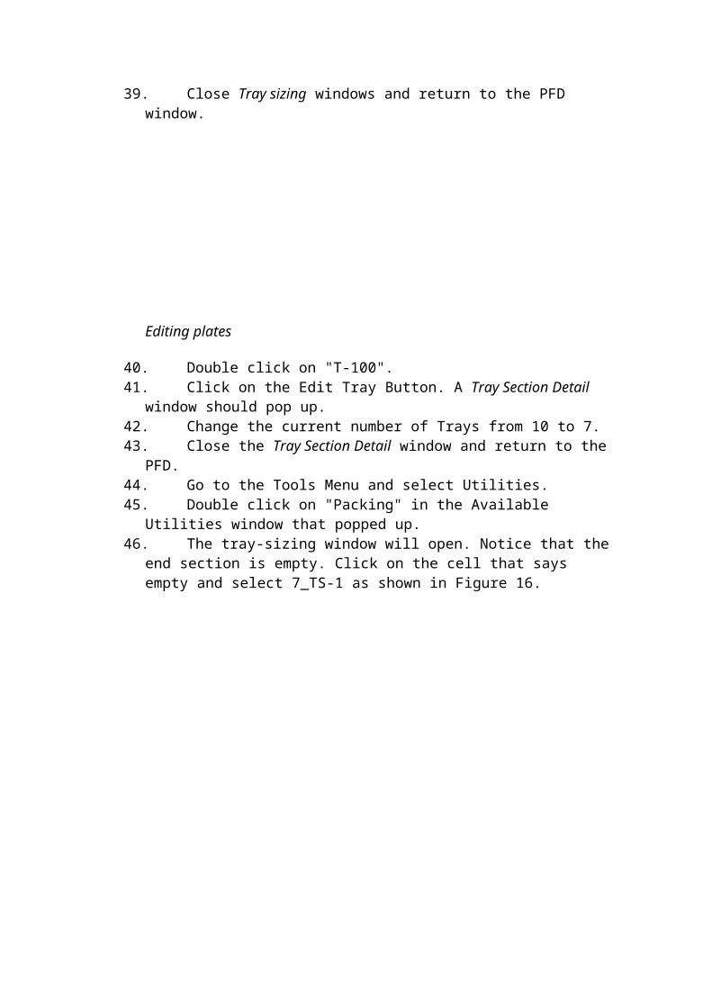
pop up similar to that of Figure 15. 31. Make all the selections shown in Figure 15 and

then click on OK.

Figure 15: Tray Section Selection

After selecting the Tray section, one will return to the Tray sizing window.

32. Click on the button that says Auto Section… The auto section window will pop up.

33. For the tray internal select packed. When packed is selected, a drop down menu box will appear in the window.

34. Scroll the drop down window for the desired packing type; for this case Interlock Saddles (Ceramic) 1_4_inch.

35. When the selection is made, click on the Next button. In the next window that appears, verify that all the information is true then click on complete auto section. The tray sizing window should appear.

36. Click on specs submenu of the design column.37. Change the mode to ratings.38. Enter the diameter of the tower to be 0.2918 ft.

39. Close Tray sizing windows and return to the PFD window.

Editing plates

40. Double click on "T-100".41. Click on the Edit Tray Button. A Tray Section Detail

window should pop up.42. Change the current number of Trays from 10 to 7.43. Close the Tray Section Detail window and return to the

PFD.44. Go to the Tools Menu and select Utilities.45. Double click on "Packing" in the Available

Utilities window that popped up.46. The tray-sizing window will open. Notice that the

end section is empty. Click on the cell that says empty and select 7_TS-1 as shown in Figure 16.

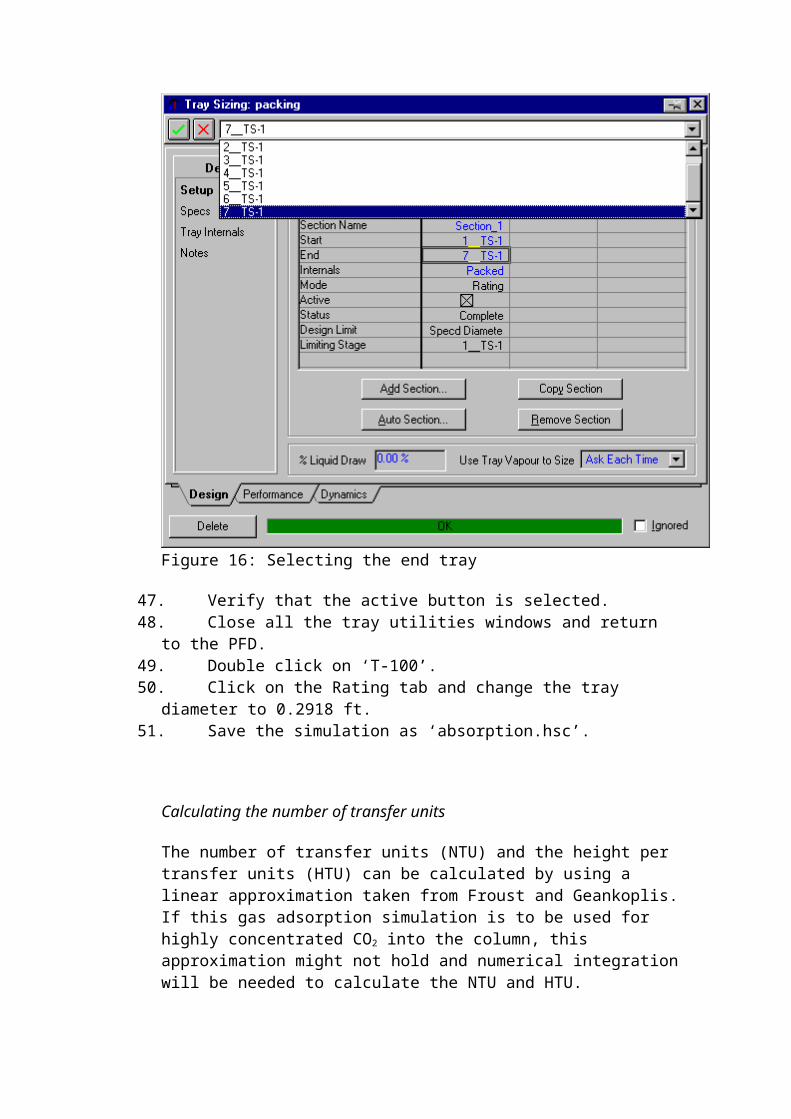
Figure 16: Selecting the end tray

47. Verify that the active button is selected.48. Close all the tray utilities windows and return

to the PFD.49. Double click on ‘T-100’.50. Click on the Rating tab and change the tray

diameter to 0.2918 ft.51. Save the simulation as ‘absorption.hsc’.

Calculating the number of transfer units

The number of transfer units (NTU) and the height per transfer units (HTU) can be calculated by using a linear approximation taken from Froust and Geankoplis.If this gas adsorption simulation is to be used for highly concentrated CO2 into the column, this approximation might not hold and numerical integrationwill be needed to calculate the NTU and HTU.

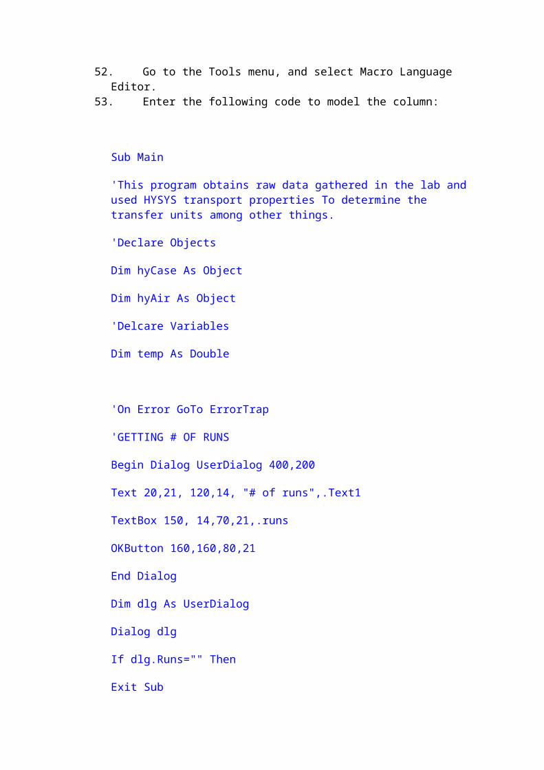
52. Go to the Tools menu, and select Macro Language Editor.

53. Enter the following code to model the column:

Sub Main

'This program obtains raw data gathered in the lab andused HYSYS transport properties To determine the transfer units among other things.

'Declare Objects

Dim hyCase As Object

Dim hyAir As Object

'Delcare Variables

Dim temp As Double

'On Error GoTo ErrorTrap

'GETTING # OF RUNS

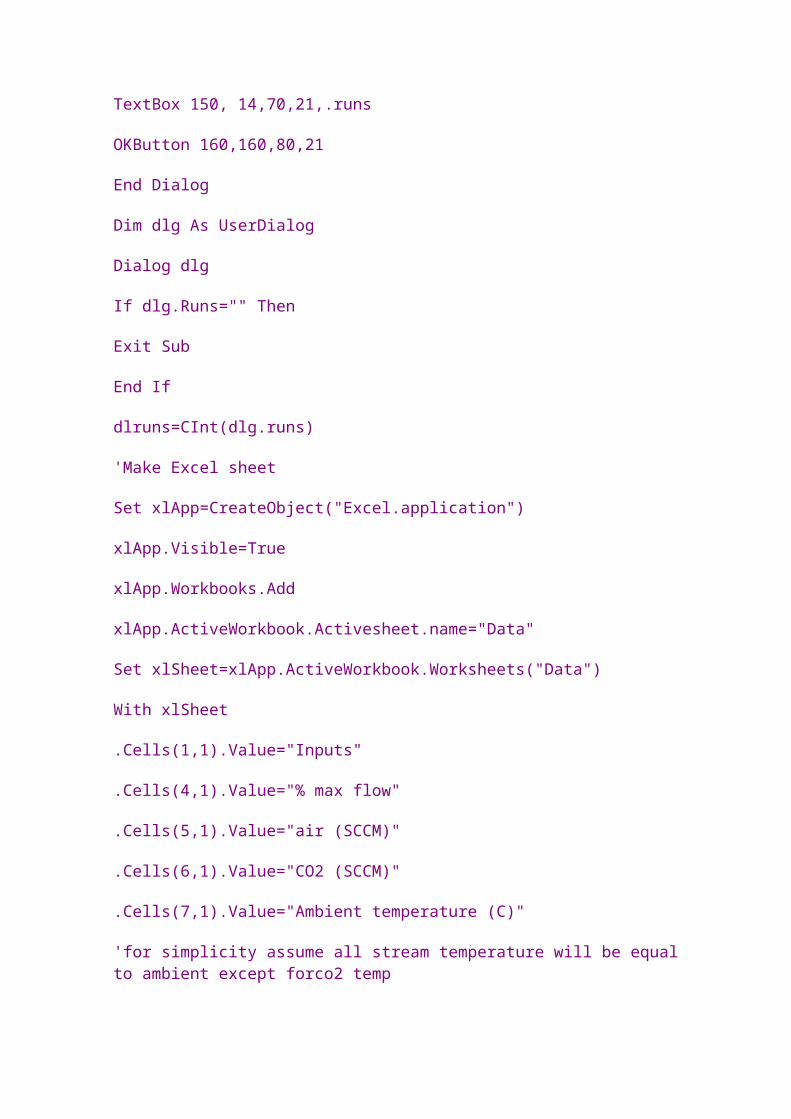
Begin Dialog UserDialog 400,200

Text 20,21, 120,14, "# of runs",.Text1

TextBox 150, 14,70,21,.runs

OKButton 160,160,80,21

End Dialog

Dim dlg As UserDialog

Dialog dlg

If dlg.Runs="" Then

Exit Sub

End If

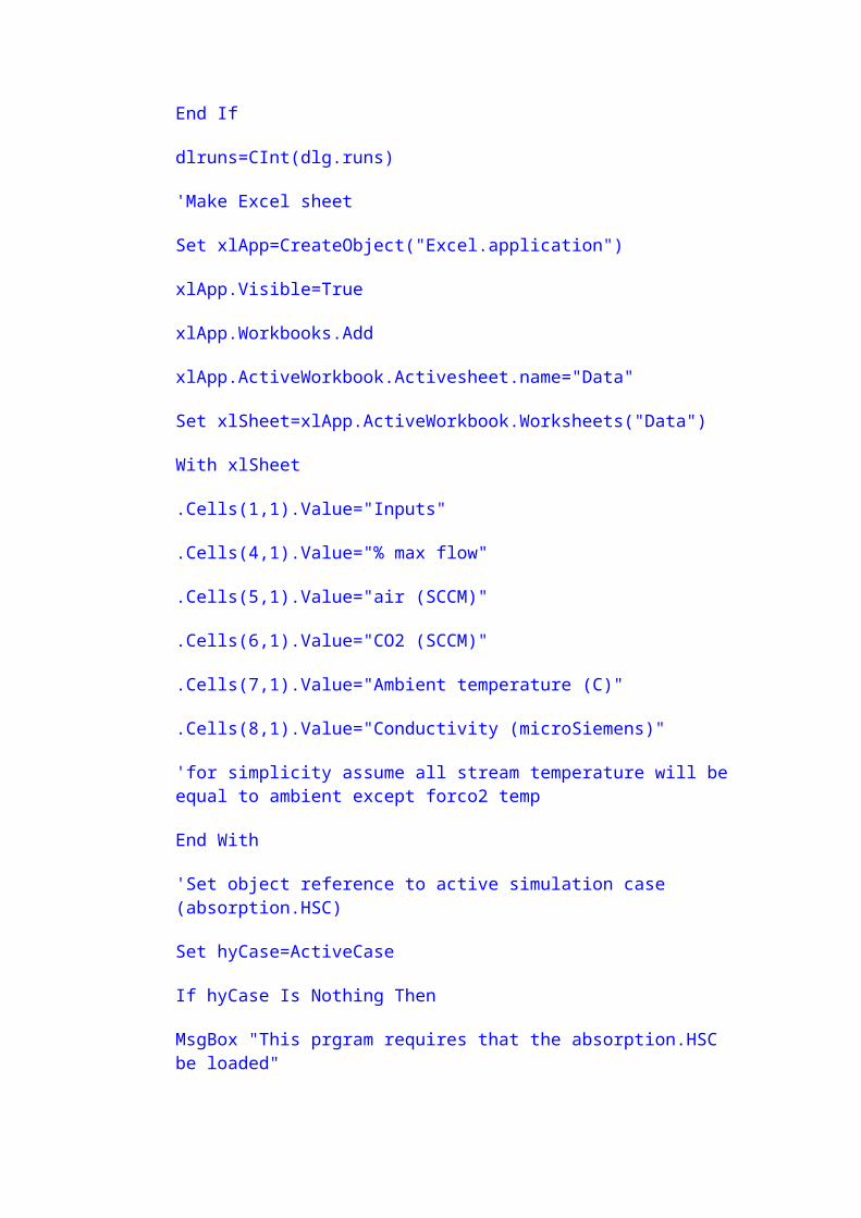
dlruns=CInt(dlg.runs)

'Make Excel sheet

Set xlApp=CreateObject("Excel.application")

xlApp.Visible=True

xlApp.Workbooks.Add

xlApp.ActiveWorkbook.Activesheet.name="Data"

Set xlSheet=xlApp.ActiveWorkbook.Worksheets("Data")

With xlSheet

.Cells(1,1).Value="Inputs"

.Cells(4,1).Value="% max flow"

.Cells(5,1).Value="air (SCCM)"

.Cells(6,1).Value="CO2 (SCCM)"

.Cells(7,1).Value="Ambient temperature (C)"

.Cells(8,1).Value="Conductivity (microSiemens)"

'for simplicity assume all stream temperature will be equal to ambient except forco2 temp

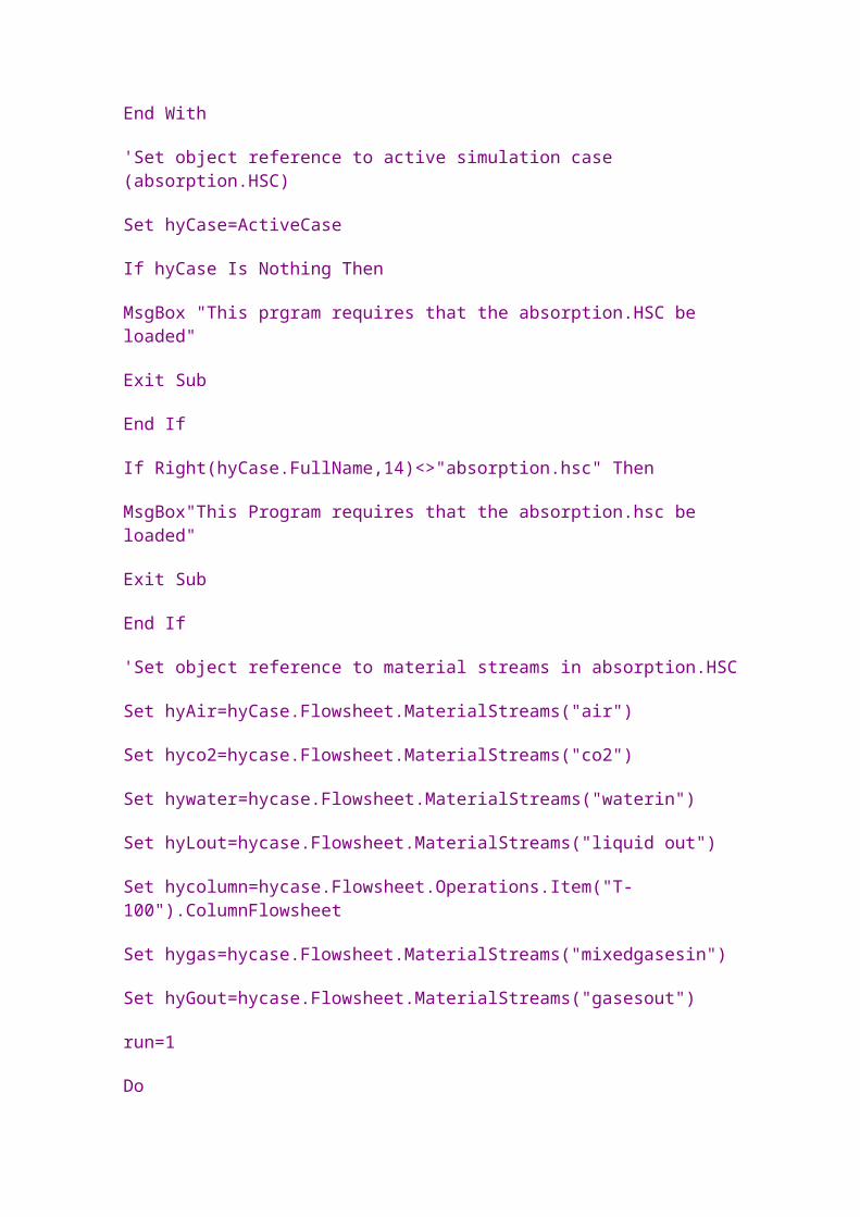
End With

'Set object reference to active simulation case (absorption.HSC)

Set hyCase=ActiveCase

If hyCase Is Nothing Then

MsgBox "This prgram requires that the absorption.HSC be loaded"

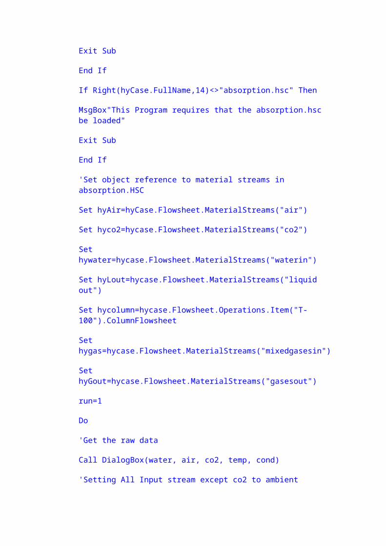
Exit Sub

End If

If Right(hyCase.FullName,14)<>"absorption.hsc" Then

MsgBox"This Program requires that the absorption.hsc be loaded"

Exit Sub

End If

'Set object reference to material streams in absorption.HSC

Set hyAir=hyCase.Flowsheet.MaterialStreams("air")

Set hyco2=hycase.Flowsheet.MaterialStreams("co2")

Set hywater=hycase.Flowsheet.MaterialStreams("waterin")

Set hyLout=hycase.Flowsheet.MaterialStreams("liquid out")

Set hycolumn=hycase.Flowsheet.Operations.Item("T-100").ColumnFlowsheet

Set hygas=hycase.Flowsheet.MaterialStreams("mixedgasesin")

Set hyGout=hycase.Flowsheet.MaterialStreams("gasesout")

run=1

Do

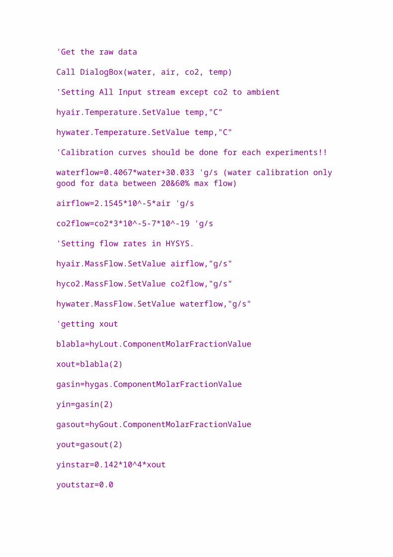
'Get the raw data

Call DialogBox(water, air, co2, temp, cond)

'Setting All Input stream except co2 to ambient

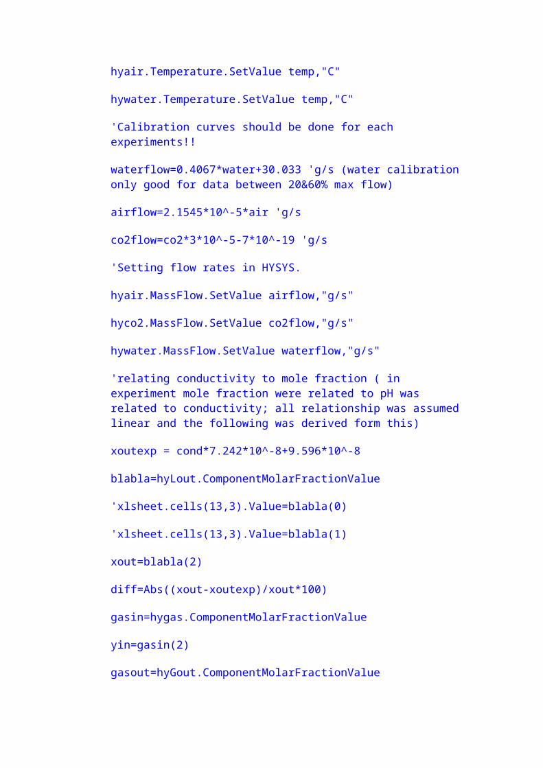
hyair.Temperature.SetValue temp,"C"

hywater.Temperature.SetValue temp,"C"

'Calibration curves should be done for each experiments!!

waterflow=0.4067*water+30.033 'g/s (water calibration only good for data between 20&60% max flow)

airflow=2.1545*10^-5*air 'g/s

co2flow=co2*3*10^-5-7*10^-19 'g/s

'Setting flow rates in HYSYS.

hyair.MassFlow.SetValue airflow,"g/s"

hyco2.MassFlow.SetValue co2flow,"g/s"

hywater.MassFlow.SetValue waterflow,"g/s"

'relating conductivity to mole fraction ( in experiment mole fraction were related to pH was related to conductivity; all relationship was assumed linear and the following was derived form this)

xoutexp = cond*7.242*10^-8+9.596*10^-8

blabla=hyLout.ComponentMolarFractionValue

'xlsheet.cells(13,3).Value=blabla(0)

'xlsheet.cells(13,3).Value=blabla(1)

xout=blabla(2)

diff=Abs((xout-xoutexp)/xout*100)

gasin=hygas.ComponentMolarFractionValue

yin=gasin(2)

gasout=hyGout.ComponentMolarFractionValue

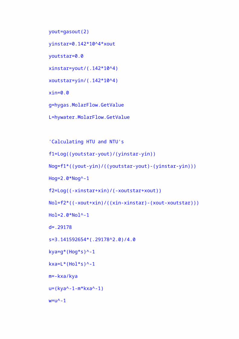
yout=gasout(2)

yinstar=0.142*10^4*xout

youtstar=0.0

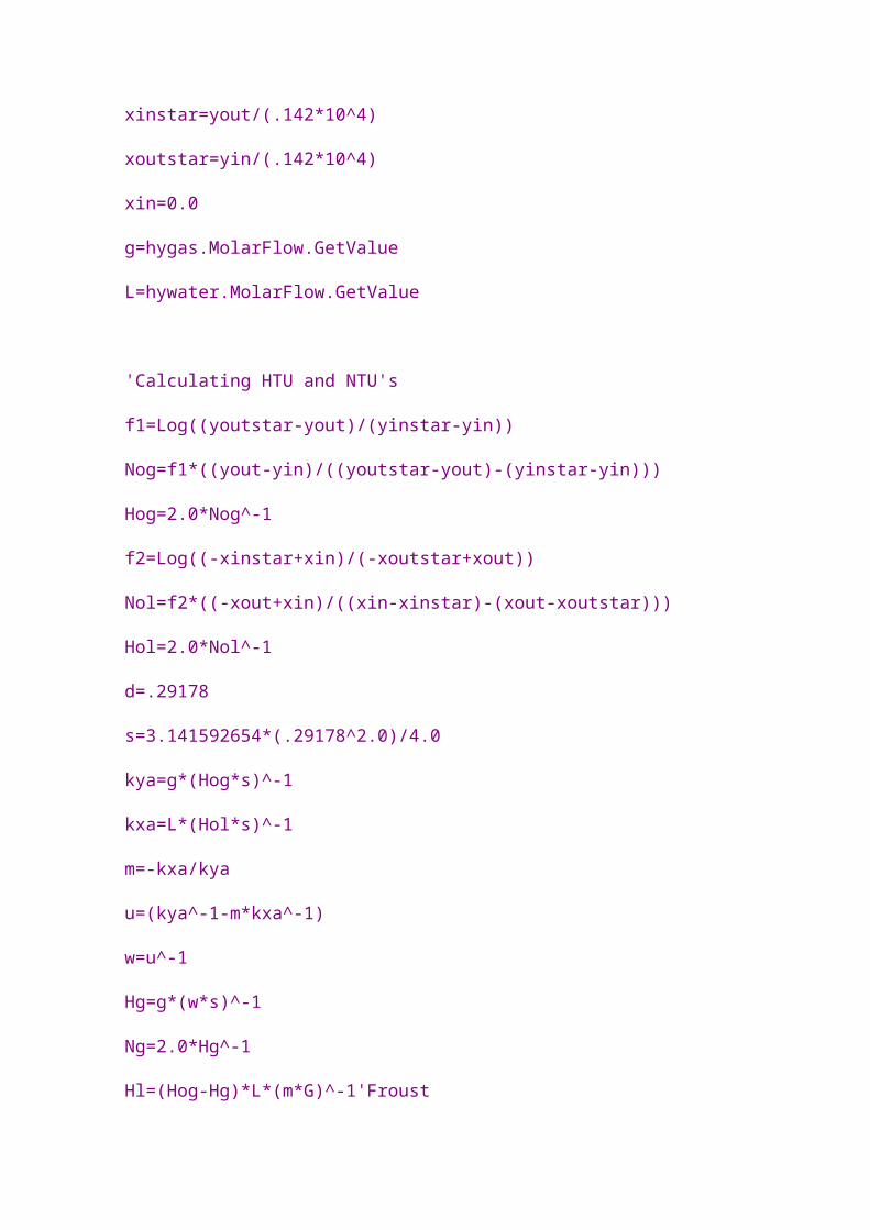
xinstar=yout/(.142*10^4)

xoutstar=yin/(.142*10^4)

xin=0.0

g=hygas.MolarFlow.GetValue

L=hywater.MolarFlow.GetValue

'Calculating HTU and NTU's

f1=Log((youtstar-yout)/(yinstar-yin))

Nog=f1*((yout-yin)/((youtstar-yout)-(yinstar-yin)))

Hog=2.0*Nog^-1

f2=Log((-xinstar+xin)/(-xoutstar+xout))

Nol=f2*((-xout+xin)/((xin-xinstar)-(xout-xoutstar)))

Hol=2.0*Nol^-1

d=.29178

s=3.141592654*(.29178^2.0)/4.0

kya=g*(Hog*s)^-1

kxa=L*(Hol*s)^-1

m=-kxa/kya

u=(kya^-1-m*kxa^-1)

w=u^-1

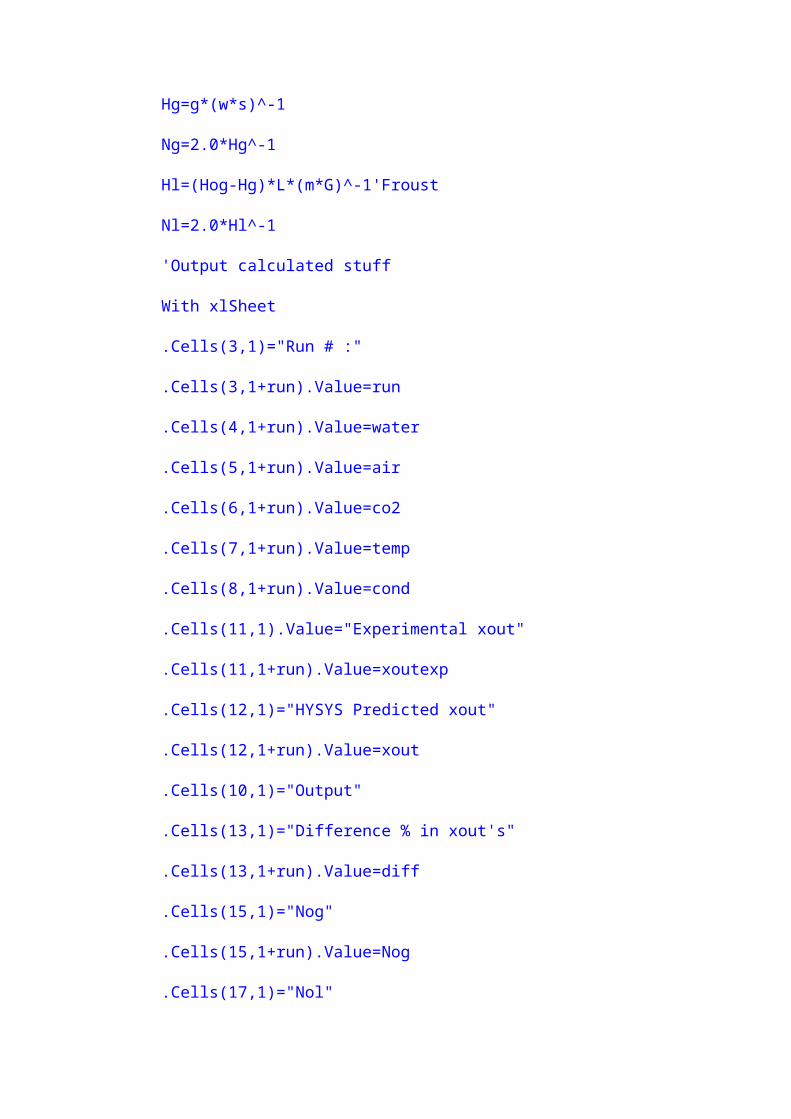
Hg=g*(w*s)^-1

Ng=2.0*Hg^-1

Hl=(Hog-Hg)*L*(m*G)^-1'Froust

Nl=2.0*Hl^-1

'Output calculated stuff

With xlSheet

.Cells(3,1)="Run # :"

.Cells(3,1+run).Value=run

.Cells(4,1+run).Value=water

.Cells(5,1+run).Value=air

.Cells(6,1+run).Value=co2

.Cells(7,1+run).Value=temp

.Cells(8,1+run).Value=cond

.Cells(11,1).Value="Experimental xout"

.Cells(11,1+run).Value=xoutexp

.Cells(12,1)="HYSYS Predicted xout"

.Cells(12,1+run).Value=xout

.Cells(10,1)="Output"

.Cells(13,1)="Difference % in xout's"

.Cells(13,1+run).Value=diff

.Cells(15,1)="Nog"

.Cells(15,1+run).Value=Nog

.Cells(17,1)="Nol"

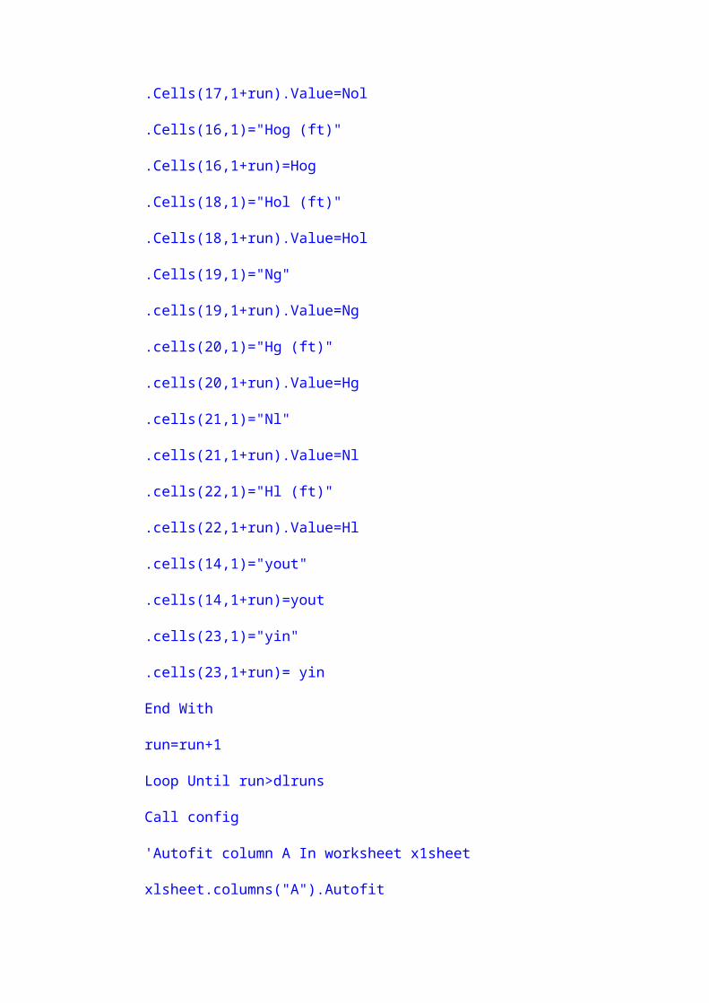
.Cells(17,1+run).Value=Nol

.Cells(16,1)="Hog (ft)"

.Cells(16,1+run)=Hog

.Cells(18,1)="Hol (ft)"

.Cells(18,1+run).Value=Hol

.Cells(19,1)="Ng"

.cells(19,1+run).Value=Ng

.cells(20,1)="Hg (ft)"

.cells(20,1+run).Value=Hg

.cells(21,1)="Nl"

.cells(21,1+run).Value=Nl

.cells(22,1)="Hl (ft)"

.cells(22,1+run).Value=Hl

.cells(14,1)="yout"

.cells(14,1+run)=yout

.cells(23,1)="yin"

.cells(23,1+run)= yin

End With

run=run+1

Loop Until run>dlruns

Call config

'Autofit column A In worksheet x1sheet

xlsheet.columns("A").Autofit

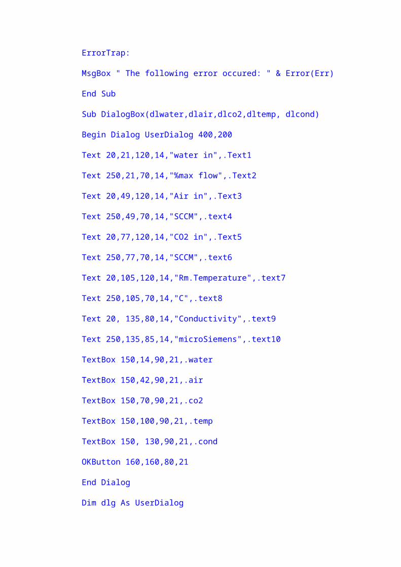
ErrorTrap:

MsgBox " The following error occured: " & Error(Err)

End Sub

Sub DialogBox(dlwater,dlair,dlco2,dltemp, dlcond)

Begin Dialog UserDialog 400,200

Text 20,21,120,14,"water in",.Text1

Text 250,21,70,14,"%max flow",.Text2

Text 20,49,120,14,"Air in",.Text3

Text 250,49,70,14,"SCCM",.text4

Text 20,77,120,14,"CO2 in",.Text5

Text 250,77,70,14,"SCCM",.text6

Text 20,105,120,14,"Rm.Temperature",.text7

Text 250,105,70,14,"C",.text8

Text 20, 135,80,14,"Conductivity",.text9

Text 250,135,85,14,"microSiemens",.text10

TextBox 150,14,90,21,.water

TextBox 150,42,90,21,.air

TextBox 150,70,90,21,.co2

TextBox 150,100,90,21,.temp

TextBox 150, 130,90,21,.cond

OKButton 160,160,80,21

End Dialog

Dim dlg As UserDialog

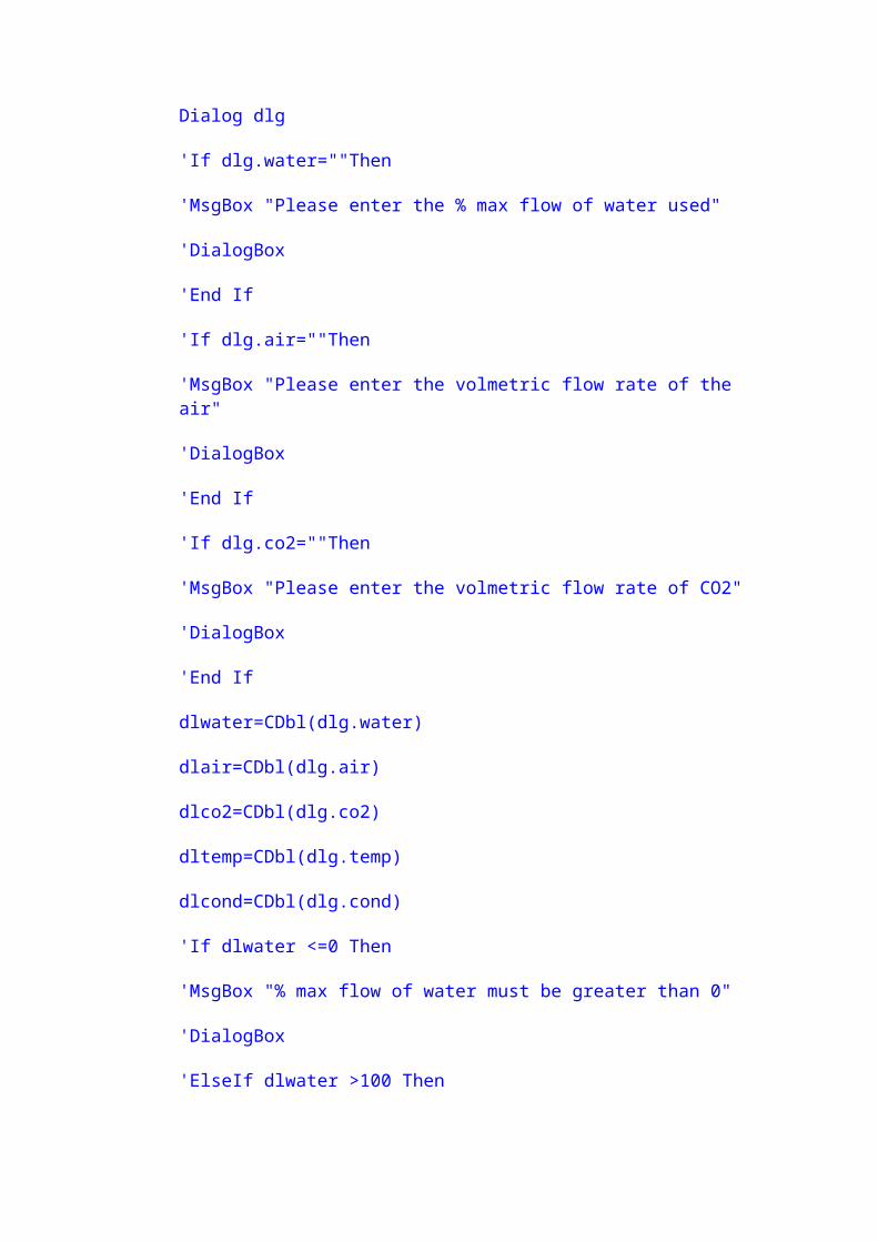
Dialog dlg

'If dlg.water=""Then

'MsgBox "Please enter the % max flow of water used"

'DialogBox

'End If

'If dlg.air=""Then

'MsgBox "Please enter the volmetric flow rate of the air"

'DialogBox

'End If

'If dlg.co2=""Then

'MsgBox "Please enter the volmetric flow rate of CO2"

'DialogBox

'End If

dlwater=CDbl(dlg.water)

dlair=CDbl(dlg.air)

dlco2=CDbl(dlg.co2)

dltemp=CDbl(dlg.temp)

dlcond=CDbl(dlg.cond)

'If dlwater <=0 Then

'MsgBox "% max flow of water must be greater than 0"

'DialogBox

'ElseIf dlwater >100 Then

'MsgBox "% max flow of water must be less than 100"

'DialogBox

'End If

'If dlair <0 Then

'MsgBox "air flow must be greater than 0"

'DialogBox

'End If

'If dlco2 <0 Then

'MsgBox "CO2 flow must be greater than 0"

'DialogBox

'End If

End Sub

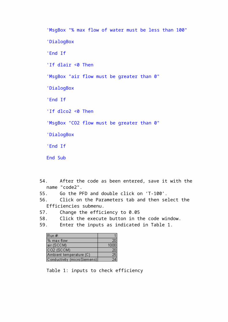
54. After the code as been entered, save it with the name "code2".

55. Go the PFD and double click on ‘T-100’.56. Click on the Parameters tab and then select the

Efficiencies submenu.57. Change the efficiency to 0.0558. Click the execute button in the code window.59. Enter the inputs as indicated in Table 1.

Table 1: inputs to check efficiency

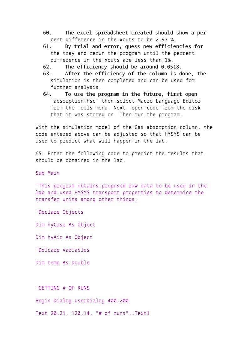
60. The excel spreadsheet created should show a per cent difference in the xouts to be 2.97 %.

61. By trial and error, guess new efficiencies for the tray and rerun the program until the percent difference in the xouts are less than 1%.

62. The efficiency should be around 0.0518.63. After the efficiency of the column is done, the

simulation is then completed and can be used for further analysis.

64. To use the program in the future, first open ‘absorption.hsc’ then select Macro Language Editor from the Tools menu. Next, open code from the disk that it was stored on. Then run the program.

With the simulation model of the Gas absorption column, thecode entered above can be adjusted so that HYSYS can be used to predict what will happen in the lab.

65. Enter the following code to predict the results that should be obtained in the lab.

Sub Main

'This program obtains proposed raw data to be used in the lab and used HYSYS transport properties to determine the transfer units among other things.

'Declare Objects

Dim hyCase As Object

Dim hyAir As Object

'Delcare Variables

Dim temp As Double

'GETTING # OF RUNS

Begin Dialog UserDialog 400,200

Text 20,21, 120,14, "# of runs",.Text1

TextBox 150, 14,70,21,.runs

OKButton 160,160,80,21

End Dialog

Dim dlg As UserDialog

Dialog dlg

If dlg.Runs="" Then

Exit Sub

End If

dlruns=CInt(dlg.runs)

'Make Excel sheet

Set xlApp=CreateObject("Excel.application")

xlApp.Visible=True

xlApp.Workbooks.Add

xlApp.ActiveWorkbook.Activesheet.name="Data"

Set xlSheet=xlApp.ActiveWorkbook.Worksheets("Data")

With xlSheet

.Cells(1,1).Value="Inputs"

.Cells(4,1).Value="% max flow"

.Cells(5,1).Value="air (SCCM)"

.Cells(6,1).Value="CO2 (SCCM)"

.Cells(7,1).Value="Ambient temperature (C)"

'for simplicity assume all stream temperature will be equalto ambient except forco2 temp

End With

'Set object reference to active simulation case (absorption.HSC)

Set hyCase=ActiveCase

If hyCase Is Nothing Then

MsgBox "This prgram requires that the absorption.HSC be loaded"

Exit Sub

End If

If Right(hyCase.FullName,14)<>"absorption.hsc" Then

MsgBox"This Program requires that the absorption.hsc be loaded"

Exit Sub

End If

'Set object reference to material streams in absorption.HSC

Set hyAir=hyCase.Flowsheet.MaterialStreams("air")

Set hyco2=hycase.Flowsheet.MaterialStreams("co2")

Set hywater=hycase.Flowsheet.MaterialStreams("waterin")

Set hyLout=hycase.Flowsheet.MaterialStreams("liquid out")

Set hycolumn=hycase.Flowsheet.Operations.Item("T-100").ColumnFlowsheet

Set hygas=hycase.Flowsheet.MaterialStreams("mixedgasesin")

Set hyGout=hycase.Flowsheet.MaterialStreams("gasesout")

run=1

Do

'Get the raw data

Call DialogBox(water, air, co2, temp)

'Setting All Input stream except co2 to ambient

hyair.Temperature.SetValue temp,"C"

hywater.Temperature.SetValue temp,"C"

'Calibration curves should be done for each experiments!!

waterflow=0.4067*water+30.033 'g/s (water calibration only good for data between 20&60% max flow)

airflow=2.1545*10^-5*air 'g/s

co2flow=co2*3*10^-5-7*10^-19 'g/s

'Setting flow rates in HYSYS.

hyair.MassFlow.SetValue airflow,"g/s"

hyco2.MassFlow.SetValue co2flow,"g/s"

hywater.MassFlow.SetValue waterflow,"g/s"

'getting xout

blabla=hyLout.ComponentMolarFractionValue

xout=blabla(2)

gasin=hygas.ComponentMolarFractionValue

yin=gasin(2)

gasout=hyGout.ComponentMolarFractionValue

yout=gasout(2)

yinstar=0.142*10^4*xout

youtstar=0.0

xinstar=yout/(.142*10^4)

xoutstar=yin/(.142*10^4)

xin=0.0

g=hygas.MolarFlow.GetValue

L=hywater.MolarFlow.GetValue

'Calculating HTU and NTU's

f1=Log((youtstar-yout)/(yinstar-yin))

Nog=f1*((yout-yin)/((youtstar-yout)-(yinstar-yin)))

Hog=2.0*Nog^-1

f2=Log((-xinstar+xin)/(-xoutstar+xout))

Nol=f2*((-xout+xin)/((xin-xinstar)-(xout-xoutstar)))

Hol=2.0*Nol^-1

d=.29178

s=3.141592654*(.29178^2.0)/4.0

kya=g*(Hog*s)^-1

kxa=L*(Hol*s)^-1

m=-kxa/kya

u=(kya^-1-m*kxa^-1)

w=u^-1

Hg=g*(w*s)^-1

Ng=2.0*Hg^-1

Hl=(Hog-Hg)*L*(m*G)^-1'Froust

Nl=2.0*Hl^-1

'Output calculated stuff

With xlSheet

.Cells(3,1)="Run # :"

.Cells(3,1+run).Value=run

.Cells(4,1+run).Value=water

.Cells(5,1+run).Value=air

.Cells(6,1+run).Value=co2

.Cells(7,1+run).Value=temp

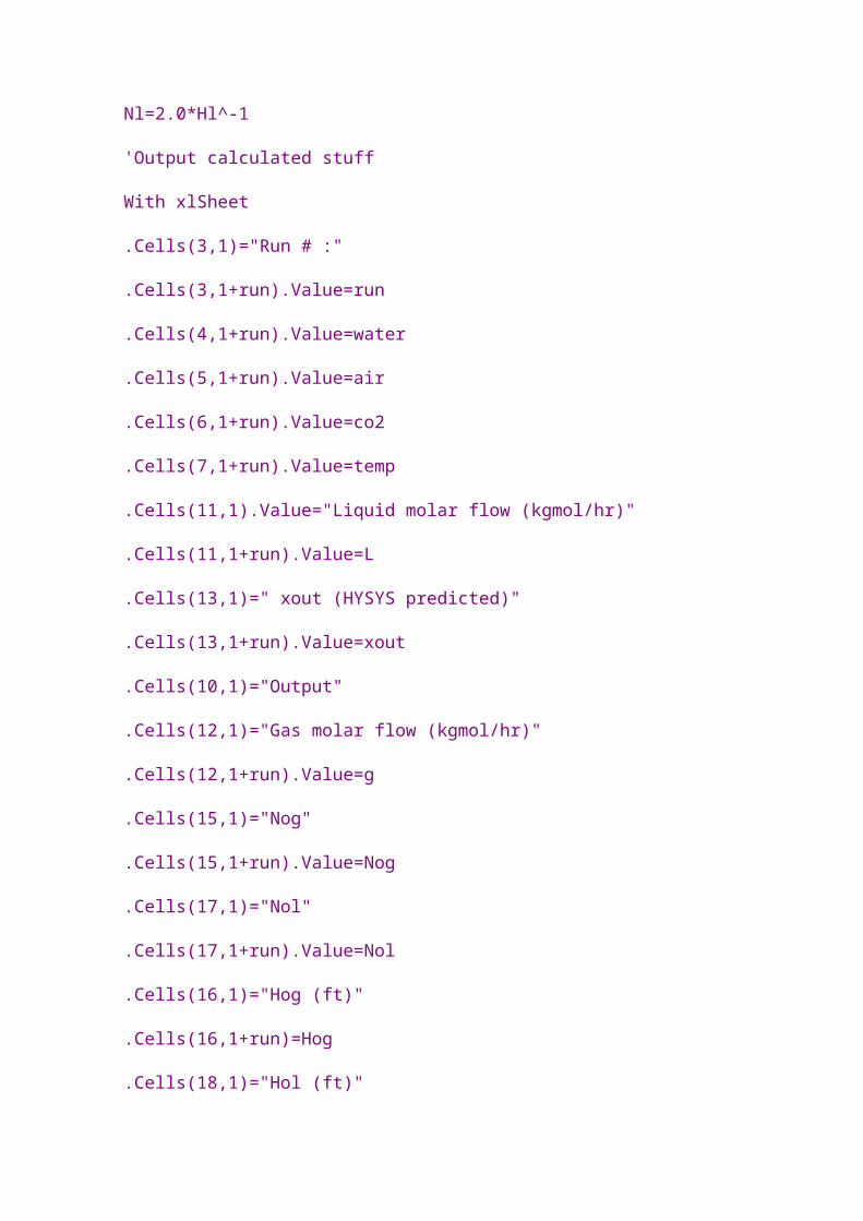
.Cells(11,1).Value="Liquid molar flow (kgmol/hr)"

.Cells(11,1+run).Value=L

.Cells(13,1)=" xout (HYSYS predicted)"

.Cells(13,1+run).Value=xout

.Cells(10,1)="Output"

.Cells(12,1)="Gas molar flow (kgmol/hr)"

.Cells(12,1+run).Value=g

.Cells(15,1)="Nog"

.Cells(15,1+run).Value=Nog

.Cells(17,1)="Nol"

.Cells(17,1+run).Value=Nol

.Cells(16,1)="Hog (ft)"

.Cells(16,1+run)=Hog

.Cells(18,1)="Hol (ft)"

.Cells(18,1+run).Value=Hol

.Cells(19,1)="Ng"

.cells(19,1+run).Value=Ng

.cells(20,1)="Hg (ft)"

.cells(20,1+run).Value=Hg

.cells(21,1)="Nl"

.cells(21,1+run).Value=Nl

.cells(22,1)="Hl (ft)"

.cells(22,1+run).Value=Hl

.cells(14,1)="yout"

.cells(14,1+run)=yout

.cells(23,1)="yin"

.cells(23,1+run)= yin

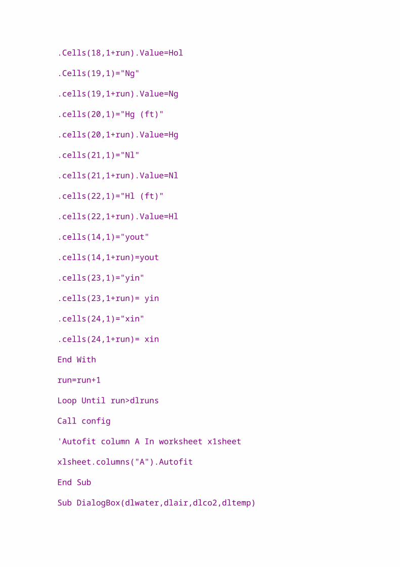
.cells(24,1)="xin"

.cells(24,1+run)= xin

End With

run=run+1

Loop Until run>dlruns

Call config

'Autofit column A In worksheet x1sheet

xlsheet.columns("A").Autofit

End Sub

Sub DialogBox(dlwater,dlair,dlco2,dltemp)

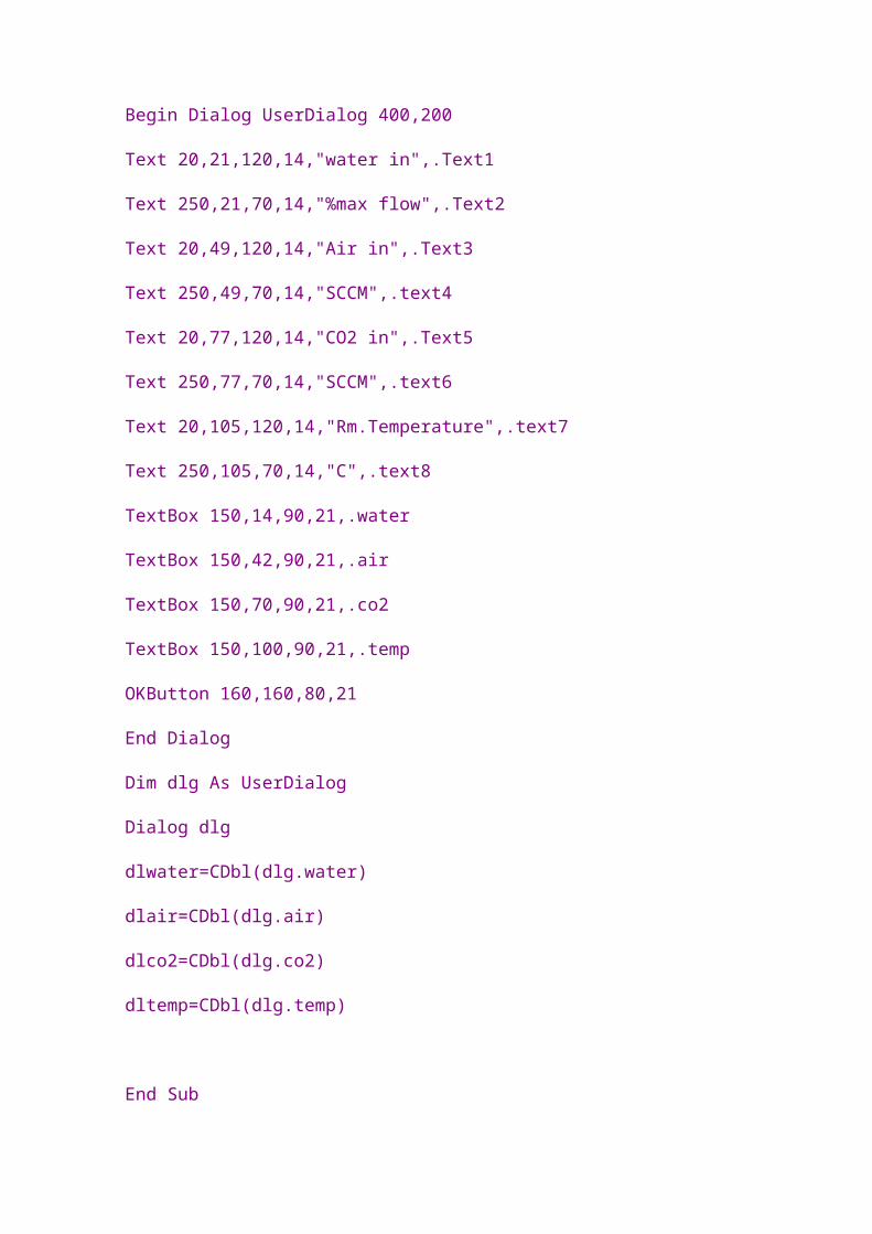
Begin Dialog UserDialog 400,200

Text 20,21,120,14,"water in",.Text1

Text 250,21,70,14,"%max flow",.Text2

Text 20,49,120,14,"Air in",.Text3

Text 250,49,70,14,"SCCM",.text4

Text 20,77,120,14,"CO2 in",.Text5

Text 250,77,70,14,"SCCM",.text6

Text 20,105,120,14,"Rm.Temperature",.text7

Text 250,105,70,14,"C",.text8

TextBox 150,14,90,21,.water

TextBox 150,42,90,21,.air

TextBox 150,70,90,21,.co2

TextBox 150,100,90,21,.temp

OKButton 160,160,80,21

End Dialog

Dim dlg As UserDialog

Dialog dlg

dlwater=CDbl(dlg.water)

dlair=CDbl(dlg.air)

dlco2=CDbl(dlg.co2)

dltemp=CDbl(dlg.temp)

End Sub

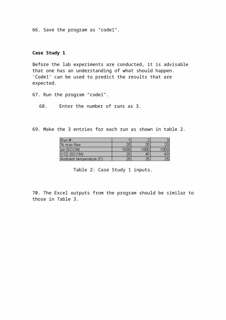
66. Save the program as "code1".

Case Study 1

Before the lab experiments are conducted, it is advisable that one has an understanding of what should happen. ‘Code1’ can be used to predict the results that are expected.

67. Run the program "code1".

68. Enter the number of runs as 3.

69. Make the 3 entries for each run as shown in table 2.

Table 2: Case Study 1 inputs.

70. The Excel outputs from the program should be similar tothose in Table 3.

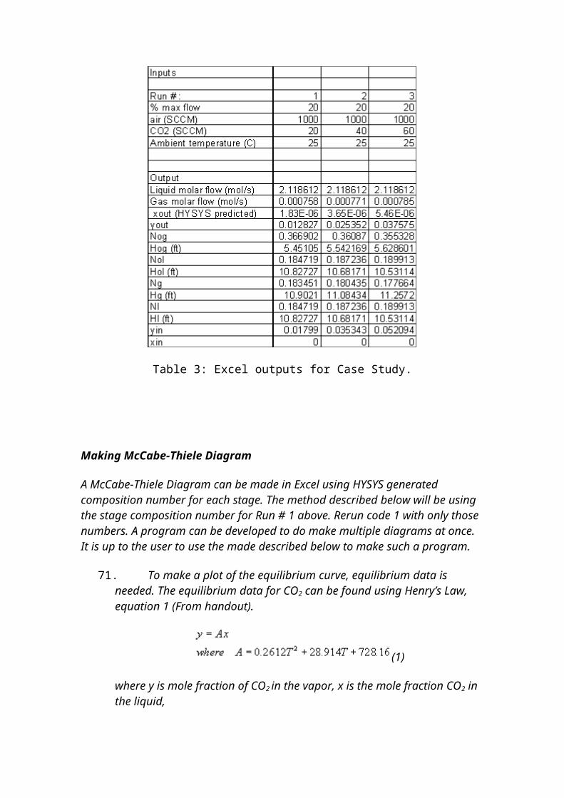
Table 3: Excel outputs for Case Study.

Making McCabe-Thiele Diagram

A McCabe-Thiele Diagram can be made in Excel using HYSYS generated composition number for each stage. The method described below will be using the stage composition number for Run # 1 above. Rerun code 1 with only those numbers. A program can be developed to do make multiple diagrams at once. It is up to the user to use the made described below to make such a program.

71. To make a plot of the equilibrium curve, equilibrium data is needed. The equilibrium data for CO2 can be found using Henry’s Law, equation 1 (From handout).

(1)

where y is mole fraction of CO2 in the vapor, x is the mole fraction CO2 in the liquid,

and T is the temperature in C.

Since the temperature was assumed to be 25 C, A = 1614.51.

From this the line can be generated; use values for x = 0, and x = 0.00001.

72. For the operating line data, the values that are needed are those of the inlet and outlet streams. The coordinate pairs are (xin,yout) and (xout, yin). From sheet 1, xin=0, yin=0.01799, xout=1.83E-06, yout = 0.0128.

73. In HYSYS, on the PFD, double click on T-100.74. Click on the Performance tab.75. Click on the Result on the Performance tab.76. Click on the table button.77. When the Profile Table window open, click on the Properties button.78. A new window should open. In this new, for the basis, ensure that Molar

is selected: for the phase, select Vapour and Light Liquid: for the Comp Basis, select fraction; and for the components, select only CO2.

79. Close the property view window and return to the Profile table window.80. In the table, select the stages and liquid and vapour composition

columns.81. Hold down ‘Crtl’ and ‘C’ on the key broad to copy these values.82. On sheet 2 of the excel spreadsheet generated above, right click in a cell

and select paste special from the menu. If you select paste, these value will change every time that absorption.hsc is ran and the excel file is open since a regular pasting will create a link.

83. In the window that pops up, select to paste as a text. The numbers should be pasted as this time. Check to make sure they are correct.

84. Label the columns accordingly.85. Set up a matrix in which the steps can be drawn (see Table 4).

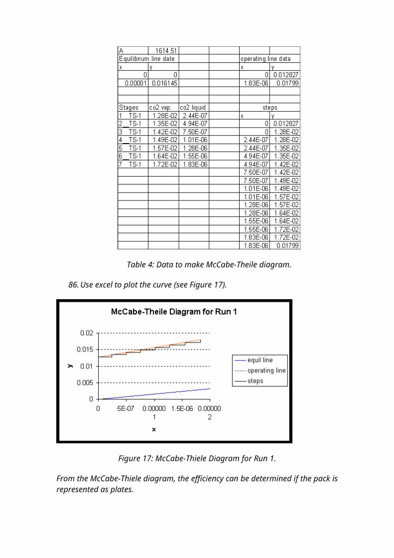
Table 4: Data to make McCabe-Theile diagram.

86. Use excel to plot the curve (see Figure 17).

Figure 17: McCabe-Thiele Diagram for Run 1.

From the McCabe-Thiele diagram, the efficiency can be determined if the pack isrepresented as plates.

Case Study 2

After the lab is conducted, the results obtained from the lab can be compared to those obtained in HYSYS. In this case study, the flow rate of the CO2 is varied (20,40, 60 SCCM), while the water and air flow rates are kept constant at 20 % max flow and 1000 SCCM, respectively.

87. Run the program "code2".88. Enter the number of runs as 3.89. Make the 3 entries for each run as shown in table 5.

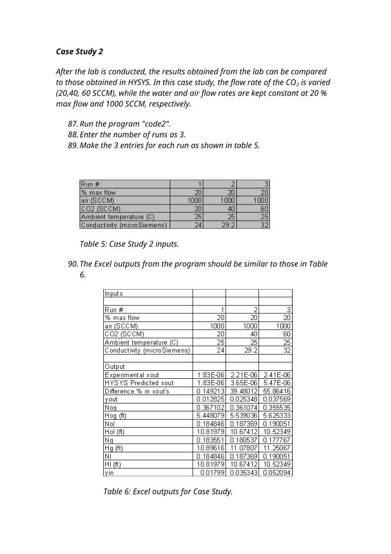
Table 5: Case Study 2 inputs.

90. The Excel outputs from the program should be similar to those in Table 6.

Table 6: Excel outputs for Case Study.

One should note that the % difference in the xouts (CO2 in liquid out) increase as the CO2 concentration into the increases. This was expected because the efficiency for the column was determined from using a low value for the feed of CO2. Changing the efficiency of column for each feed flow can rectify this problem; however, this is not very time effective. So it is recommended that efficiency for the low flow rate be kept because the NTU are calculated based onapproximation for low concentrations.

Since the gas feed to the column is relatively dilute, the liquid film will be controlling the absorption, and Hol and Nol are the preferred transfer units to determine the separation effectiveness of the column. In Table 4, it is shown that for a lowest CO2 in (yin) the Nol is largest which indicates a relatively better separation. Other case studies can be done by varying the water and/or air flowrate(s).

References

Foust, A. S. et al., Principles of Unit Operations. John Wiley and Sons, New York, 1980.

Geankopolis, C. J., Transport Processes and Unit Operations 3rd ed., Prentice Hall,

Englewood Cliffs, NJ, 1993.