Abrupt rise in atmospheric CO at the onset of the Bølling ... · Abrupt rise in atmospheric CO2 at the onset of the Bølling/Allerød: in-situ ice core data versus true atmospheric

Clim. Past, 7, 473–486, 2011www.clim-past.net/7/473/2011/doi:10.5194/cp-7-473-2011© Author(s) 2011. CC Attribution 3.0 License.

Climateof the Past

Abrupt rise in atmospheric CO2 at the onset of the Bølling/Allerød:in-situ ice core data versus true atmospheric signals

P. Kohler1, G. Knorr 1,2, D. Buiron3, A. Lourantou3,*, and J. Chappellaz3

1Alfred Wegener Institute for Polar and Marine Research (AWI), P.O. Box 120161, 27515 Bremerhaven, Germany2School of Earth and Ocean Sciences, Cardiff University, Cardiff, Wales, UK3Laboratoire de Glaciologie et Geophysique de l’Environnement, (LGGE, CNRS, Universite Joseph Fourier-Grenoble),54b rue Moliere, Domaine Universitaire BP 96, 38402 St. Martin d’Heres, France* now at: Laboratoire d’Oceanographie et du Climat (LOCEAN), Institut Pierre Simon Laplace, Universite P. et M. Curie(UPMC), Paris, France

Received: 24 June 2010 – Published in Clim. Past Discuss.: 11 August 2010Revised: 15 March 2011 – Accepted: 24 March 2011 – Published: 4 May 2011

Abstract. During the last glacial/interglacial transition theEarth’s climate underwent abrupt changes around 14.6 kyrago. Temperature proxies from ice cores revealed the onsetof the Bølling/Allerød (B/A) warm period in the north andthe start of the Antarctic Cold Reversal in the south. Further-more, the B/A was accompanied by a rapid sea level rise ofabout 20 m during meltwater pulse (MWP) 1A, whose exacttiming is a matter of current debate. In-situ measured CO2 inthe EPICA Dome C (EDC) ice core also revealed a remark-able jump of 10±1 ppmv in 230 yr at the same time. Allow-ing for the modelled age distribution of CO2 in firn, we showthat atmospheric CO2 could have jumped by 20–35 ppmv inless than 200 yr, which is a factor of 2–3.5 greater than theCO2 signal recorded in-situ in EDC. This rate of change in at-mospheric CO2 corresponds to 29–50% of the anthropogenicsignal during the last 50 yr and is connected with a radiativeforcing of 0.59–0.75 W m−2. Using a model-based airbornefraction of 0.17 of atmospheric CO2, we infer that 125 Pgof carbon need to be released into the atmosphere to pro-duce such a peak. If the abrupt rise in CO2 at the onset ofthe B/A is unique with respect to other Dansgaard/Oeschger(D/O) events of the last 60 kyr (which seems plausible if notunequivocal based on current observations), then the mecha-nism responsible for it may also have been unique. Availableδ13CO2 data are neutral, whether the source of the carbonis of marine or terrestrial origin. We therefore hypothesisethat most of the carbon might have been activated as a conse-

Correspondence to:P. Kohler([email protected])

quence of continental shelf flooding during MWP-1A. Thispotential impact of rapid sea level rise on atmospheric CO2might define the point of no return during the last deglacia-tion.

1 Introduction

Measurements of CO2 over Termination I (20–10 kyr BP)from the EPICA Dome C (EDC) ice core (Monnin et al.,2001; Lourantou et al., 2010) (Fig. 1b) are temporally higherresolved and more precise than CO2 records from other icecores (Smith et al., 1999; Ahn et al., 2004). They have anuncertainty(1σ) of 1 ppmv or less (Monnin et al., 2001;Lourantou et al., 2010). In these in-situ measured data inEDC, CO2 abruptly rose by 10±1 ppmv between 14.74 and14.51 kyr BP on the most recent ice core age scale (Lemieux-Dudon et al., 2010). This abrupt CO2 rise is therefore syn-chronous with the onset of the Bølling/Allerød (B/A) warmperiod in the North (Steffensen et al., 2008), the start of theAntarctic Cold Reversal in the South (Stenni et al., 2001), aswell as abrupt rises in the two other greenhouse gases CH4(Spahni et al., 2005) and N2O (Schilt et al., 2010). Further-more, the B/A is accompanied by a rapid sea level rise ofabout 20 m during meltwater pulse (MWP) 1A (Peltier andFairbanks, 2007), whose exact timing is matter of current de-bate (e.g.Hanebuth et al., 2000; Kienast et al., 2003; Stanfordet al., 2006; Deschamps et al., 2009).

However, atmospheric gases trapped in ice cores arenot precisely recording one point in time but averageover decades to centuries, mainly depending on their

Published by Copernicus Publications on behalf of the European Geosciences Union.

474 P. Kohler et al.: Abrupt rise in CO2 at the onset of the Bølling/Allerød

-140-120-100

-80-60

-140-120-100

-80-60

sea

leve

l(m

)

180

200

220

240

260

280

300

N2O

(ppb

v)

190

200

210

220

230

240

250

260

270

190

200

210

220

230

240

250

260

270

CO

2(p

pmv)

300

400

500

600

700

800

CH

4(p

pbv)

-42.5

-40.0

-37.5

-35.0

18O

(o / oo)

60 50 40 30 20

Age (kyr BP)

-42.5

-40.0

-37.5

-35.0

-32.5

18O

(o / oo)

A

-140-120-100

-80-60

-140-120-100

-80-60

sea

leve

l(m

)

180

200

220

240

260

280

300

N2O

(ppb

v)

190

200

210

220

230

240

250

260

270

190

200

210

220

230

240

250

260

270

CO

2(p

pmv)

300

400

500

600

700

800

CH

4(p

pbv)

-45

-42

-39

-36

-33

-30

18O

(o / oo)

-460

-440

-420

-400

-380

D(o / o

o)

20 18 16 14 12 10

QSR2010 age (kyr BP)

B

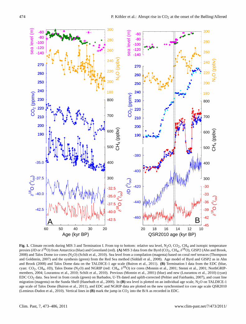
Fig. 1. Climate records during MIS 3 and Termination I. From top to bottom: relative sea level, N2O, CO2, CH4 and isotopic temperatureproxies (δD or δ18O) from Antarctica (blue) and Greenland (red).(A) MIS 3 data from the Byrd (CO2, CH4, δ18O), GISP2 (Ahn and Brook,2008) and Talos Dome ice cores (N2O) (Schilt et al., 2010). Sea level from a compilation (magenta) based on coral reef terraces (Thompsonand Goldstein, 2007) and the synthesis (green) from the Red Sea method (Siddall et al., 2008). Age model of Byrd and GISP2 as inAhnand Brook(2008) and Talos Dome data on the TALDICE-1 age scale (Buiron et al., 2011). (B) Termination I data from the EDC (blue,cyan: CO2, CH4, δD), Talos Dome (N2O) and NGRIP (red: CH4, δ18O) ice cores (Monnin et al., 2001; Stenni et al., 2001; NorthGRIP-members, 2004; Lourantou et al., 2010; Schilt et al., 2010). Previous (Monnin et al., 2001) (blue) and new (Lourantou et al., 2010) (cyan)EDC CO2 data. Sea level in from corals (green) on Barbados, U-Th dated and uplift-corrected (Peltier and Fairbanks, 2007), and coast linemigration (magenta) on the Sunda Shelf (Hanebuth et al., 2000). In (B) sea level is plotted on an individual age scale, N2O on TALDICE-1age scale of Talos Dome (Buiron et al., 2011), and EDC and NGRIP data are plotted on the new synchronised ice core age scale QSR2010(Lemieux-Dudon et al., 2010). Vertical lines in(B) mark the jump in CO2 into the B/A as recorded in EDC.

Clim. Past, 7, 473–486, 2011 www.clim-past.net/7/473/2011/

P. Kohler et al.: Abrupt rise in CO2 at the onset of the Bølling/Allerød 475

0 500 1000 1500 2000Time since last exchange with atmosphere (yr)

0

1

2

3

4

5

6P

roba

bilit

y(o / o

o) EPRE=213yr

EB/A=400yr

ELGM=590yr

LGM CO2 firn modelLGM lognormal

B/A lognormal

PRE CO2 firn modelPRE lognormal

Fig. 2. Age distribution PDF of CO2 as a function of climate state,here pre-industrial (PRE), Bølling/Allerød (B/A) and LGM condi-tions. Calculation with a firn densification model (Joos and Spahni,2008) (solid lines, for PRE and LGM) and approximations of allthree climate states by a log-normal function (broken lines). For allfunctions the expected mean values, or widthE, are also given.

accumulation rate because of the movement of gases in thefirn above the close-off depth and before its enclosure in gasbubbles in the ice. To infer the transfer signature of the trueatmospheric CO2 signal out of in-situ ice core CO2 measure-ments, the latter has to be deconvoluted with the ice-core-specific age distribution probability density function (PDF).Based on a firn densification model (Joos and Spahni, 2008),this age distribution PDF describing the elapsed time sincethe last exchange of the CO2 molecules with the atmosphere(Fig. 2) reveals for EDC a width of approximately 200 and600 yr for climate conditions of pre-industrial times (PRE)and the Last Glacial Maximum (LGM), respectively. Thesewide age distributions implicate that the CO2 measured in-situ, especially in ice cores with low accumulation rates (suchas EDC), differs from the true atmospheric signal when CO2changes abruptly.

In the following we will deconvolve the atmospheric CO2signal connected with this abrupt rise in CO2 measured in-situ in the EDC ice core, allowing for the age distributionPDF during the onset of the B/A. We furthermore use sim-ulations of a global carbon cycle box model to develop andtest a hypotheses which might explain the abrupt rise in at-mospheric CO2.

2 Methods

2.1 Age distribution PDF of CO2

The age distributions PDF of CO2 or CH4 are functions ofthe climate state and the local site conditions of the ice core.

In Fig. 2, the age distributions PDF of CO2 in the EDC icecore for pre-industrial (PRE) and LGM conditions based oncalculations with a firn densification model (Joos and Spahni,2008) are shown. The resulting age distribution PDF for CO2can be approximated with reasonable accuracy (r2

= 90–94%) by a log-normal function (Kohler et al., 2010b):

y =1

x ·σ ·√

2π·e

−0.5(

ln(x)−µσ

)2

(1)

with x (yr) as the time elapsed since the last exchange withthe atmosphere. This equation has two free parametersµ andσ . For simplcity, we have chosenσ = 1, which leads to anexpected value (mean) Eof the PDF of

E = eµ+0.5 . (2)

Theexpected value Eis described aswidth of the PDF inthe terminology of gas physics, a terminology which we willalso use in the following.E should not be confused with themost likely valuedefined by the location of the maximum ofthe PDF.

Our choice to use a log-normal function (Eq.1) for theage distribution PDF was motivated by the good represen-tation of firn densification model output (r2

≥ 90%) and itsdependency on only one free parameter, which can be ob-tained from models. Other approaches using, for example, aGreen’s function are also possible (seeTrudinger et al., 2002,and references therein).

In the case of the CO2 jump at 14.6 kyr BP, one has to con-sider that the atmospheric records are much younger than thesurrounding ice matrix; indeed, the CO2 jump is embeddedbetween 473 and 480 m in glacial ice (Monnin et al., 2001;Lourantou et al., 2010) with low temperatures and low accu-mulation rates. However, from a model of firn densificationwhich includes heat diffusion, it is known that the close-offof the gas bubbles in the ice matrix is not a simple func-tion of the temperature of the surrounding ice (Goujon et al.,2003). Heat from the surface diffuses down to the close-offregion in a few centuries, depending on site-specific condi-tions. This implies that atmospheric gases during the onset ofthe B/A were not trapped by conditions of either the LGM orthe Antarctic Cold Reversal, but by some intermediate state.New calculations with this firn densification model (Goujonet al., 2003) give a width of the age distribution PDFEB/Aof about 400 yr with a relative uncertainty (1σ ) of 14% at theonset of the B/A (Fig.3). The widthE itself varies duringthe jump into the B/A between 380 and 420 yr; we thereforeconservatively estimateEB/A to lie between 320 to 480 yrwith our best-guess estimate ofEB/A = 400 yr in-between.

The performance of the applied gas age distribution PDF(Eq.1) is tested with ice core CH4 data for the time windowof interest (Appendix A, Supplement). In summary, this teststrongly suggests that the log-normal age distribution PDFdoes not introduce a systematic bias in the shape of the signalif applied onto a hypothetical atmospheric CO2 record. It is

www.clim-past.net/7/473/2011/ Clim. Past, 7, 473–486, 2011

476 P. Kohler et al.: Abrupt rise in CO2 at the onset of the Bølling/Allerød

190

200

210

220

230

240

250

260

270

280

290C

O2

(ppm

v)

700

600

500

400

300

200

100

0

wid

thE

ofag

edi

strib

utio

nP

DF

(yr)

20181614 12 10 8 6 4 2 0

QSR2010 age (kyr BP)

-440

-420

-400

-380

-360

D(o / o

o)

Fig. 3. Evolution of the widthE of the age distribution PDF (±1σ )during the last 20 kyr (red squares) calculated with a firn densifi-cation model including heat diffusion (Goujon et al., 2003). Greendiamonds represent the results for the LGM and pre-industrial cli-mate with another firn densification model (Joos and Spahni, 2008).Please note reverse y-axis. Top: EDC CO2 (Monnin et al., 2001;Lourantou et al., 2010). Bottom: EDCδD data (Stenni et al., 2001).All records are on the new age scale QSR2010 (Lemieux-Dudonet al., 2010).

therefore justified to apply Eq. (1) to convolve the CO2 signalwhich might be recorded in the EDC ice core.

2.2 Carbon cycle modelling

In order to determine how fast carbon injected into the atmo-sphere is taken up by the ocean, we used the carbon cycle boxmodel BICYCLE (Kohler and Fischer, 2004; Kohler et al.,2005a, 2010b). The model version used here and its forcingover Termination I are described in detail inLourantou et al.

(2010). Furthermore, we tried to determine of which origin(terrestrial or marine) the carbon might have been by com-paring the simulated and measured atmosphericδ13CO2 fin-gerprint during the carbon release event. Similar approaches(identifying processes based on theirδ13C signature) wereapplied earlier for the discussion of the atmosphericδ13CO2record over the whole Termination I (Lourantou et al., 2010)and longer timescales (Kohler et al., 2010b). Here, we re-strict the analysis to the question of whether the observedsignal might be generated by terrestrial or marine processesonly.

Briefly, BICYCLE consists of modules of the ocean (10boxes distinguishing surface, intermediate and deep oceanin the Atlantic, Southern Ocean and Indo-Pacific), a glob-ally averaged terrestrial biosphere (7 boxes), a homoge-neously mixed one-box atmosphere, and a relaxation ap-proach to account for carbonate compensation in the deepocean (sediment-ocean interaction). The model calculatesthe temporal development of its prognostic variables overtime as functions of changing boundary conditions, repre-senting the climate forcing. These prognostic variables are(a) carbon (as dissolved inorganic carbon DIC in the ocean),(b) the carbon isotopesδ13C, 114C, and (c) additionally inthe ocean total alkalinity, oxygen and phosphate. The terres-trial module accounts for different photosynthetic pathways(C3 or C4), which is relevant for the temporal developmentof the13C cycle.

Here, the model is equilibrated for 4000 yr for climateconditions typical before the onset of the B/A. The At-lantic meridional overturning circulation (AMOC) is in anoff mode. Simulations with the AMOC in an on mode leadto a different background state of the carbon cycle (atmo-sphericpCO2 is then 255 ppmv versus 223 ppmv in the offmode), but the amplitudes in the atmospheric CO2 rise dif-fer by less than 3 ppmv between both settings. Scenarios inwhich the AMOC amplifies precisely at the onset of the B/Awarm period are not explicitly considered here, but are im-plicitly covered in the marine scenario. An amplification ofthe AMOC would lead to stadial/interstadial variations typ-ical for the bipolar seesaw. Such behaviour was found forthe onset of other D/O events in MIS 3 (Barker et al., 2010)during which CO2 started to fall and not to rise as observedfor the B/A. Based on this analogy, our working hypothe-sis is that the main processes connected with changes in theAMOC play a minor role for the abrupt rise in atmosphericCO2 around 14.6 kyr BP (see Sect.3.2for details).

The simulated jump of CO2 is generated by the injec-tion of a certain amount of carbon into the atmosphere,while all other processes (ocean overturning, temperature,sea level, sea ice cover, marine productivity, terrestrial bio-sphere) are kept constant. The size of the injection is deducedfrom considerations on the airborne fraction and model sim-ulations (see Sect.3.1). The carbon is then brought witha constant injection flux in a time window of a differentlength (over either 50, 100, 150, 200, 250 or 300 yr) into the

Clim. Past, 7, 473–486, 2011 www.clim-past.net/7/473/2011/

P. Kohler et al.: Abrupt rise in CO2 at the onset of the Bølling/Allerød 477

atmosphere. Our best guess injection amplitude of 125 PgCcorresponds to constant injection fluxes of 2.5 Pg C yr−1 (in50 yr) to 0.42 Pg C yr−1 (in 300 yr) over the whole release pe-riod. The fastest injection (in 50 yr) with the largest annualflux has been motivated by the abruptness in the climate sig-nals recorded in the NGRIP ice core (Steffensen et al., 2008).It is furthermore assumed that the injected carbon is either ofterrestrial or marine origin. These two scenarios differ onlyin their carbon isotopic signature:

Terrestrial scenario:theδ13C signature is based on a studywith a global dynamical vegetation model (Scholze et al.,2003), which calculates a mean global isotopic fractionationof the terrestrial biosphere of 17.7‰ for the present day. Wehave to consider a larger fraction of C4 plants during colderclimates and lower atmosphericpCO2 (Collatz et al., 1998),as found at the onset of the B/A. This implies that about 20and 30% of the terrestrial carbon is of C4 origin for presentday and LGM, respectively (Kohler and Fischer, 2004). Thesignificantly smaller isotopic fractionation during C4 photo-synthesis (about 5‰) in comparison to C3 photosynthesis(about 20‰) (Lloyd and Farquhar, 1994) therefore reducesthe global mean terrestrial fractionation to 16‰. With an at-mosphericδ13CO2 signature of about−6.5‰, the terrestrialbiosphere has a meanδ13C signature of−22.5‰.

Marine scenario:in this scenario we assume that old car-bon from the deep ocean heavily depleted inδ13C mightupwell and outgas into the atmosphere. Today’s values ofoceanicδ13C in the deep Pacific are about 0.0‰ (Kroopnick,1985). From reconstructions (Oliver et al., 2010), it is knownthat during the LGM deep oceanδ13C was on average about0.5‰ smaller, thusδ13CLGM=−0.5‰. During out-gassing,mainly in high latitudes, we consider a net isotopic fraction-ation of 8‰ (Siegenthaler and Munnich, 1981). This wouldlead toδ13C=−8.5‰ in the carbon injected into the atmo-sphere if it were of marine origin.

The signals of simulated atmospheric CO2 and δ13CO2plotted in the figures are derived by subtracting simulatedCO2 andδ13CO2 of a reference run without carbon injectionsfrom our scenarios. The anomalies1(CO2) and1(δ13CO2)

are then added to the starting point of the CO2 jump (δ13CO2drop) into the B/A, which we define as 228 ppmv (−6.76‰)at 14.8 kyr BP. In doing so, existing equilibration trends(which will exist even for longer equilibration periods dueto the sediment-ocean interaction) are eliminated. The simu-lated atmospheric CO2 (δ13CO2) at the end of the equilibra-tion period was 223 ppmv (−6.54‰). Our modelling exer-cise is therefore only valid for an interpretation of the abruptCO2 rise of 10 ppmv in the in-situ data of EDC. The mis-match in CO2 and δ13CO2 between simulations and EDCdata before 15 kyr BP and after 14.2 kyr BP, is therefore ex-pected (Figs.4b, 4d, 5b, 5d, 7).

3 Results and discussions

3.1 Assessing the size of the carbon injection

We first estimate roughly the amount of carbon necessary tobe injected as CO2 into the atmosphere to produce a long-term jump of 10 ppmv using the airborne fractionf . Thelong-term (centuries to millennia) airborne fractionf of CO2can be approximated from the buffer or Revelle factor (RF)of the ocean on atmosphericpCO2 rise. The present daymean surface ocean Revelle factor (Sabine et al., 2004a) isabout 10. With

RF=1pCO2/pCO2

1DIC/DIC(3)

and the content of C at the beginning of the B/A in theatmosphere (CA = 500 Pg C≈ 235 ppmv) and in the ocean(CO = 37 500 Pg C= 75· CA) it is

f =1pCO2

1pCO2+1DIC=

1

1+75RF

= 0.118. (4)

Thus, the lower end of the range of the airborne fractionf

is about 0.12 (given by Eq.4), while the upper end of therange might be derived from modern anthropogenic fossilfuel emissions to about 0.45 (Le Quere et al., 2009). Pleasenote thatf estimated with Eq. (4) assumes a passive (con-stant) terrestrial biosphere, while in the estimate off fromfossil fuel emissions (Le Quere et al., 2009), the terrestrialcarbon cycle is assumed to take up about a third of the an-thropogenic C emissions. We take the range off between0.12 and 0.45 as a first order approximation and assumef

during the B/A to lie in-between. This implies that a long-term rise in atmospheric CO2 of 10 ppmv (equivalent to a risein the atmospheric C reservoir by 21.2 Pg C) can be generatedby the injection of 47 to 180 Pg C into the atmosphere.

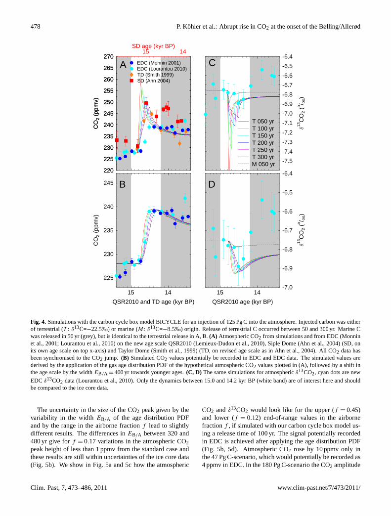
We further refine this amplitude to 125 Pg C (equivalent tof = 0.17) by using the global carbon cycle box model BICY-CLE. The model then generates atmospheric CO2 peaks of20–35 ppmv, depending on the abruptness of the C injection(Fig. 4a). All scenarios with release times of 50–200 yr fulfilthe EDC ice core data requirements after the application ofthe age distribution PDF (Fig.4b). The acceptable scenariosimply rates of change in atmospheric CO2 of 13–70 ppmv percentury, a factor of 3–16 higher than in the EDC data. Ourfastest scenario (release time of 50 yr) has a rate of change inatmospheric CO2, which is still a factor of two smaller thanthe anthropogenic CO2 rise of 70 ppmv during the last 50 yr(Keeling et al., 2009). For comparison, in the less preciseCO2 data points taken from the Taylor Dome (Smith et al.,1999) and Siple Dome (Ahn et al., 2004) ice cores, the abruptrise in CO2 at the onset of the B/A is recorded with 15±2 and19±4 ppmv, respectively (Fig.4a), with changing rates in icecore CO2 of ∼4–6 ppmv per century. This already indicatesthat at 14.6 kyr BP, CO2 measured in-situ in EDC differedmarkedly from the true atmospheric CO2.

www.clim-past.net/7/473/2011/ Clim. Past, 7, 473–486, 2011

478 P. Kohler et al.: Abrupt rise in CO2 at the onset of the Bølling/Allerød

220

225

230

235

240

245

250

255

260

265

270

CO

2(p

pmv)

SD (Ahn 2004)TD (Smith 1999)EDC (Lourantou 2010)EDC (Monnin 2001)A

220

225

230

235

240

245

250

255

260

265

270

CO

2(p

pmv)

15 14SD age (kyr BP)

15 14

QSR2010 and TD age (kyr BP)

225

230

235

240

245

CO

2(p

pmv)

B

-7.5

-7.4

-7.3

-7.2

-7.1

-7.0

-6.9

-6.8

-6.7

-6.6

-6.5

-6.4

13C

O2

(o / oo)

M 050 yrT 300 yrT 250 yrT 200 yrT 150 yrT 100 yrT 050 yr

C

15 14

QSR2010 age (kyr BP)

-7.0

-6.9

-6.8

-6.7

-6.6

-6.5

-6.4

13C

O2

(o / oo)

D

Fig. 4. Simulations with the carbon cycle box model BICYCLE for an injection of 125 Pg C into the atmosphere. Injected carbon was eitherof terrestrial (T : δ13C=−22.5‰) or marine (M: δ13C=−8.5‰) origin. Release of terrestrial C occurred between 50 and 300 yr. Marine Cwas released in 50 yr (grey), but is identical to the terrestrial release in A, B.(A) Atmospheric CO2 from simulations and from EDC (Monninet al., 2001; Lourantou et al., 2010) on the new age scale QSR2010 (Lemieux-Dudon et al., 2010), Siple Dome (Ahn et al., 2004) (SD, onits own age scale on top x-axis) and Taylor Dome (Smith et al., 1999) (TD, on revised age scale as inAhn et al., 2004). All CO2 data hasbeen synchronised to the CO2 jump. (B) Simulated CO2 values potentially be recorded in EDC and EDC data. The simulated values arederived by the application of the gas age distribution PDF of the hypothetical atmospheric CO2 values plotted in (A), followed by a shift inthe age scale by the widthEB/A = 400 yr towards younger ages.(C, D) The same simulations for atmosphericδ13CO2, cyan dots are new

EDC δ13CO2 data (Lourantou et al., 2010). Only the dynamics between 15.0 and 14.2 kyr BP (white band) are of interest here and shouldbe compared to the ice core data.

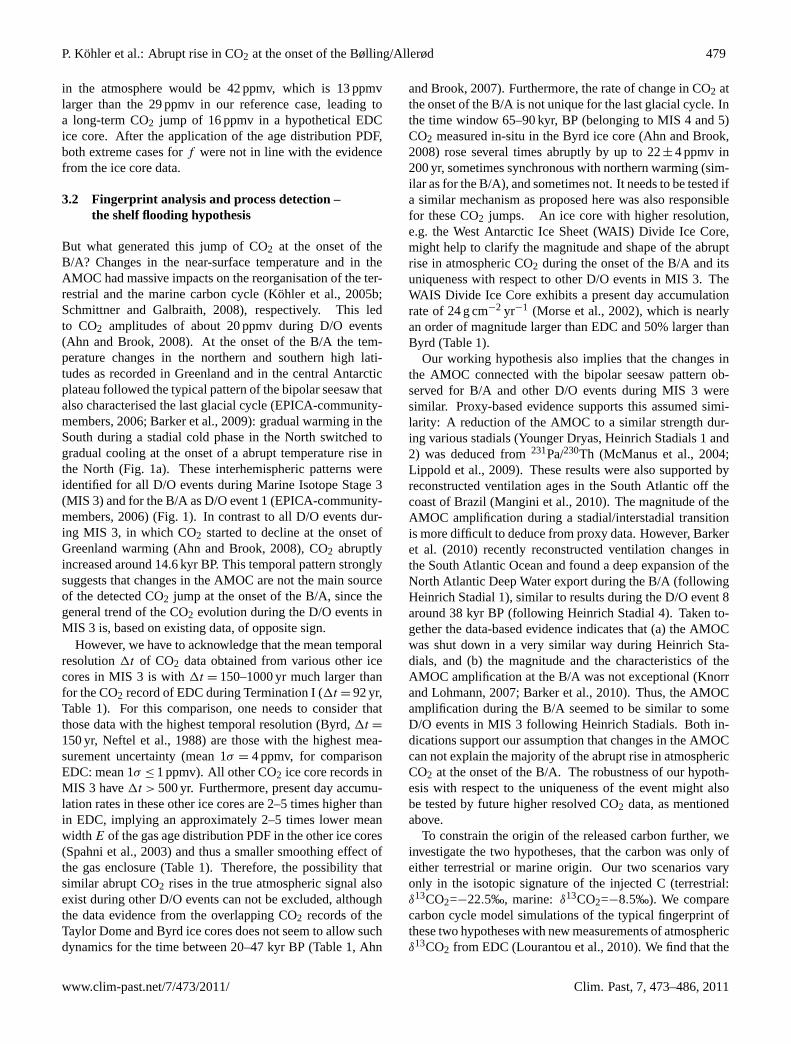
The uncertainty in the size of the CO2 peak given by thevariability in the widthEB/A of the age distribution PDFand by the range in the airborne fractionf lead to slightlydifferent results. The differences inEB/A between 320 and480 yr give forf = 0.17 variations in the atmospheric CO2peak height of less than 1 ppmv from the standard case andthese results are still within uncertainties of the ice core data(Fig. 5b). We show in Fig.5a and5c how the atmospheric

CO2 andδ13CO2 would look like for the upper (f = 0.45)and lower (f = 0.12) end-of-range values in the airbornefractionf , if simulated with our carbon cycle box model us-ing a release time of 100 yr. The signal potentially recordedin EDC is achieved after applying the age distribution PDF(Fig. 5b, 5d). Atmospheric CO2 rose by 10 ppmv only inthe 47 Pg C-scenario, which would potentially be recorded as4 ppmv in EDC. In the 180 Pg C-scenario the CO2 amplitude

Clim. Past, 7, 473–486, 2011 www.clim-past.net/7/473/2011/

P. Kohler et al.: Abrupt rise in CO2 at the onset of the Bølling/Allerød 479

in the atmosphere would be 42 ppmv, which is 13 ppmvlarger than the 29 ppmv in our reference case, leading toa long-term CO2 jump of 16 ppmv in a hypothetical EDCice core. After the application of the age distribution PDF,both extreme cases forf were not in line with the evidencefrom the ice core data.

3.2 Fingerprint analysis and process detection –the shelf flooding hypothesis

But what generated this jump of CO2 at the onset of theB/A? Changes in the near-surface temperature and in theAMOC had massive impacts on the reorganisation of the ter-restrial and the marine carbon cycle (Kohler et al., 2005b;Schmittner and Galbraith, 2008), respectively. This ledto CO2 amplitudes of about 20 ppmv during D/O events(Ahn and Brook, 2008). At the onset of the B/A the tem-perature changes in the northern and southern high lati-tudes as recorded in Greenland and in the central Antarcticplateau followed the typical pattern of the bipolar seesaw thatalso characterised the last glacial cycle (EPICA-community-members, 2006; Barker et al., 2009): gradual warming in theSouth during a stadial cold phase in the North switched togradual cooling at the onset of a abrupt temperature rise inthe North (Fig.1a). These interhemispheric patterns wereidentified for all D/O events during Marine Isotope Stage 3(MIS 3) and for the B/A as D/O event 1 (EPICA-community-members, 2006) (Fig. 1). In contrast to all D/O events dur-ing MIS 3, in which CO2 started to decline at the onset ofGreenland warming (Ahn and Brook, 2008), CO2 abruptlyincreased around 14.6 kyr BP. This temporal pattern stronglysuggests that changes in the AMOC are not the main sourceof the detected CO2 jump at the onset of the B/A, since thegeneral trend of the CO2 evolution during the D/O events inMIS 3 is, based on existing data, of opposite sign.

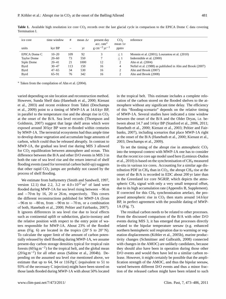
However, we have to acknowledge that the mean temporalresolution1t of CO2 data obtained from various other icecores in MIS 3 is with1t = 150–1000 yr much larger thanfor the CO2 record of EDC during Termination I (1t = 92 yr,Table 1). For this comparison, one needs to consider thatthose data with the highest temporal resolution (Byrd,1t =

150 yr, Neftel et al., 1988) are those with the highest mea-surement uncertainty (mean 1σ = 4 ppmv, for comparisonEDC: mean 1σ ≤ 1 ppmv). All other CO2 ice core records inMIS 3 have1t > 500 yr. Furthermore, present day accumu-lation rates in these other ice cores are 2–5 times higher thanin EDC, implying an approximately 2–5 times lower meanwidth E of the gas age distribution PDF in the other ice cores(Spahni et al., 2003) and thus a smaller smoothing effect ofthe gas enclosure (Table1). Therefore, the possibility thatsimilar abrupt CO2 rises in the true atmospheric signal alsoexist during other D/O events can not be excluded, althoughthe data evidence from the overlapping CO2 records of theTaylor Dome and Byrd ice cores does not seem to allow suchdynamics for the time between 20–47 kyr BP (Table1, Ahn

and Brook, 2007). Furthermore, the rate of change in CO2 atthe onset of the B/A is not unique for the last glacial cycle. Inthe time window 65–90 kyr, BP (belonging to MIS 4 and 5)CO2 measured in-situ in the Byrd ice core (Ahn and Brook,2008) rose several times abruptly by up to 22± 4 ppmv in200 yr, sometimes synchronous with northern warming (sim-ilar as for the B/A), and sometimes not. It needs to be tested ifa similar mechanism as proposed here was also responsiblefor these CO2 jumps. An ice core with higher resolution,e.g. the West Antarctic Ice Sheet (WAIS) Divide Ice Core,might help to clarify the magnitude and shape of the abruptrise in atmospheric CO2 during the onset of the B/A and itsuniqueness with respect to other D/O events in MIS 3. TheWAIS Divide Ice Core exhibits a present day accumulationrate of 24 g cm−2 yr−1 (Morse et al., 2002), which is nearlyan order of magnitude larger than EDC and 50% larger thanByrd (Table1).

Our working hypothesis also implies that the changes inthe AMOC connected with the bipolar seesaw pattern ob-served for B/A and other D/O events during MIS 3 weresimilar. Proxy-based evidence supports this assumed simi-larity: A reduction of the AMOC to a similar strength dur-ing various stadials (Younger Dryas, Heinrich Stadials 1 and2) was deduced from231Pa/230Th (McManus et al., 2004;Lippold et al., 2009). These results were also supported byreconstructed ventilation ages in the South Atlantic off thecoast of Brazil (Mangini et al., 2010). The magnitude of theAMOC amplification during a stadial/interstadial transitionis more difficult to deduce from proxy data. However,Barkeret al. (2010) recently reconstructed ventilation changes inthe South Atlantic Ocean and found a deep expansion of theNorth Atlantic Deep Water export during the B/A (followingHeinrich Stadial 1), similar to results during the D/O event 8around 38 kyr BP (following Heinrich Stadial 4). Taken to-gether the data-based evidence indicates that (a) the AMOCwas shut down in a very similar way during Heinrich Sta-dials, and (b) the magnitude and the characteristics of theAMOC amplification at the B/A was not exceptional (Knorrand Lohmann, 2007; Barker et al., 2010). Thus, the AMOCamplification during the B/A seemed to be similar to someD/O events in MIS 3 following Heinrich Stadials. Both in-dications support our assumption that changes in the AMOCcan not explain the majority of the abrupt rise in atmosphericCO2 at the onset of the B/A. The robustness of our hypoth-esis with respect to the uniqueness of the event might alsobe tested by future higher resolved CO2 data, as mentionedabove.

To constrain the origin of the released carbon further, weinvestigate the two hypotheses, that the carbon was only ofeither terrestrial or marine origin. Our two scenarios varyonly in the isotopic signature of the injected C (terrestrial:δ13CO2=−22.5‰, marine: δ13CO2=−8.5‰). We comparecarbon cycle model simulations of the typical fingerprint ofthese two hypotheses with new measurements of atmosphericδ13CO2 from EDC (Lourantou et al., 2010). We find that the

www.clim-past.net/7/473/2011/ Clim. Past, 7, 473–486, 2011

480 P. Kohler et al.: Abrupt rise in CO2 at the onset of the Bølling/Allerød

220

225

230

235

240

245

250

255

260

265

270

CO

2(p

pmv)

047 PgC125 PgC180 PgC

A

15 14

QSR2010 age (kyr BP)

225

230

235

240

245

CO

2(p

pmv)

E = 480 yrE = 400 yrE = 320 yr

B

-7.5

-7.4

-7.3

-7.2

-7.1

-7.0

-6.9

-6.8

-6.7

-6.6

-6.5

-6.4

13C

O2

(o / oo)

C

15 14

QSR2010 age (kyr BP)

-7.0

-6.9

-6.8

-6.7

-6.6

-6.5

-6.4

13C

O2

(o / oo)

D

Fig. 5. Influence of (i) the amount of carbon injected in the atmosphere and of (ii) the details of the gas age distribution on both theatmospheric signal and that potentially recorded in EDC. The amount of carbon injected in the atmosphere(A, C) covers the range derivedfrom an airborne fractionf between 12 and 45% from 47 to 180 Pg C with our reference scenario of 125 Pg C in bold. Injections occurredin 100 yr with terrestrialδ13C signature. In the filter function of the gas age distribution(B, D) the widthE varies from 320 yr to 480 yr,our best-estimated gas age widthE at the onset of the B/A of 400 yr in the solid line, representing the range given by the firn densificationmodel including heat diffusion (Goujon et al., 2003), as plotted in Fig.3. Only the dynamics between 15.0 and 14.2 kyr BP (white band) areof interest here and should be compared with the ice core data.

small dip of−0.14±0.14‰ in δ13CO2 measured in-situ inEDC might be generated by terrestrial C released in less thanthree centuries (Fig.4c, 4d). The marine scenario leads tochanges inδ13CO2 of less than−0.03‰ (Fig. 4d). Withinthe uncertainty in so-far-published ice coreδ13CO2 of 0.10‰(1σ ), this marine scenario seems less likely than the terres-trial one, but it can not be excluded. All together, thisδ13CO2fingerprint analysis shows that all terrestrial or marine sce-narios seemed to be possible, but a further constraint is, basedon the given data so far, not possible. New measured, but upto now unpublishedδ13CO2 data does not seem to lead todifferent conclusions (Fischer et al., 2010).

Besides the similarity in the typical patterns of the bipolarseesaw, the B/A and the other D/O events differ significantlyin the rate of sea level rise. While the amplitudes of sea levelvariations are with about 20 m during MIS 3 and B/A compa-rable (Peltier and Fairbanks, 2007; Siddall et al., 2008), therates of change are not. It took one to several millennia forthe sea level to change during MIS 3 (rate of change of 1–2 m per century,Siddall et al., 2008), but during MWP-1Athe sea level rose by more than 5 m per century accumulat-ing 16 to 20 m of sea level rise within centuries (Peltier andFairbanks, 2007; Hanebuth et al., 2000). The exact magni-tude but also the timing of the sea level rise during MWP-1A

Clim. Past, 7, 473–486, 2011 www.clim-past.net/7/473/2011/

P. Kohler et al.: Abrupt rise in CO2 at the onset of the Bølling/Allerød 481

Table 1. Available high resolution ice core CO2 records over the last glacial cycle in comparison to the EPICA Dome C data coveringTermination I.

ice core time window # mean1t present day CO2 referenceacc. rate∗ mean 1σ

units kyr BP – yr g cm−2 yr−1 ppmv

EPICA Dome C 10–20 109 92 3 ≤ 1 Monnin et al.(2001); Lourantou et al.(2010)Taylor Dome 20–60 73 550 7 ≤ 1 Indermuhle et al.(2000)Siple Dome 20–41 21 1000 12 2 Ahn et al.(2004)Byrd 30–47 113 150 16 4 Neftel et al.(1988) as published inAhn and Brook(2007)Byrd 47–65 34 530 16 2 Ahn and Brook(2007)Byrd 65–91 76 342 16 2 Ahn and Brook(2008)

∗ Taken from the compilation ofAhn et al.(2004).

varied depending on site location and reconstruction method.However, Sunda Shelf data (Hanebuth et al., 2000; Kienastet al., 2003) and recent evidence from Tahiti (Deschampset al., 2009) point to a timing of MWP-1A at 14.6 kyr BP,in parallel to the temperature rise and the abrupt rise in CO2at the onset of the B/A. Sea level records (Thompson andGoldstein, 2007) suggest that large shelf areas which wereexposed around 30 kyr BP were re-flooded within centuriesby MWP-1A. The terrestrial ecosystems had thus ample timeto develop dense vegetation and accumulate huge amounts ofcarbon, which could thus be released abruptly. In contrast toMWP-1A, the gradual sea level rise during MIS 3 allowedfor CO2 equilibration between atmosphere and ocean. Thisdifference between the B/A and other D/O events in MIS 3 inboth the rate of sea level rise and the return interval of shelfflooding events (used for terrestrial carbon build-up) suggeststhat other rapid CO2 jumps are probably not caused by theprocess of shelf flooding.

We estimate from bathymetry (Smith and Sandwell, 1997,version 12.1) that 2.2, 3.2 or 4.0×1012 m2 of land wereflooded during MWP-1A for sea level rising between−96 mand −70 m by 16, 20 or 26 m, respectively. This coversthe different reconstructions published for MWP-1A (from−96 m to−80 m, from−90 m to−70 m, or a combinationof both,Hanebuth et al., 2000; Peltier and Fairbanks, 2007).It ignores differences in sea level rise due to local effectssuch as continental uplift or subduction, glacio-isostasy andthe relative position with respect to the entry point of wa-ters responsible for MWP-1A. About 23% of the floodedareas (Fig.6) are located in the tropics (20◦ S to 20◦ N).To calculate the upper limit of the amount of carbon poten-tially released by shelf flooding during MWP-1A, we assumepresent-day carbon storage densities typical for tropical rainforests (60 kg m−2) for the tropical belt, and the global mean(20 kg m−2) for all other areas (Sabine et al., 2004b). De-pending on the assumed sea level rise mentioned above, weestimate that up to 64, 94 or 116 Pg C (equivalent to 51 to93% of the necessary C injection) might have been stored onthose lands flooded during MWP-1A with about 50% located

in the tropical belt. This estimate includes a complete relo-cation of the carbon stored on the flooded shelves to the at-mosphere without any significant time delay. The efficiencyof this “flooding-scenario” depends on the relative timingof MWP-1A. Several studies have indicated a time windowbetween the onset of the B/A and the Older Dryas, i.e. be-tween about 14.7 and 14 kyr BP (Stanford et al., 2006, 2011;Hanebuth et al., 2000; Kienast et al., 2003; Peltier and Fair-banks, 2007), including scenarios that place MWP-1A rightat the onset of the B/A (Hanebuth et al., 2000; Kienast et al.,2003; Deschamps et al., 2009).

To set the timing of the abrupt rise in atmospheric CO2into the temporal context with MWP-1A one has to considerthat the recent ice core age model used here (Lemieux-Dudonet al., 2010) is based on the synchronisation of CH4 measuredin-situ in various ice cores. Accounting for a similar age dis-tribution PDF in CH4 than in CO2, the abrupt CH4 rise at theonset of the B/A is recorded in EDC about 200 yr later thanin the Greenland ice core NGRIP, which depicts the atmo-spheric CH4 signal with only a very small temporal offset,due to its high accumulation rate (Appendix B, Supplement).If corrected for this CH4 synchronisation artefact, the pro-posed atmospheric rise in CO2 then starts around 14.6 kyrBP, in perfect agreement with the possible dating of MWP-1A (Fig. 7).

The residual carbon needs to be related to other processes.From the discussed comparison of the B/A with other D/Oevents during MIS 3, it has emerged that processes directlyrelated to the bipolar temperature seesaw (e.g. enhancednorthern hemispheric soil respiration due to warming or veg-etation displacements (Kohler et al., 2005b), marine produc-tivity changes (Schmittner and Galbraith, 2008) connectedwith changes in the AMOC) are unlikely candidates, becausethey should also have been in operation during those otherD/O events and would then have led to a similar carbon re-lease. However, it might certainly be possible that the ampli-fication strength of the AMOC, and thus the bipolar seesaw,varied between different D/O events and thus a minor frac-tion of the released carbon might have been related to such

www.clim-past.net/7/473/2011/ Clim. Past, 7, 473–486, 2011

482 P. Kohler et al.: Abrupt rise in CO2 at the onset of the Bølling/Allerød

Fig. 6. Areas flooded during MWP-1A. Changes in relative sea level from−96 m to−70 m are plotted from the most recent update (version12.1) of a global bathymetry (Smith and Sandwell, 1997) with 1 min spatial resolution ranging from 81◦ S to 81◦ N.

processes. The origin of the water masses responsible forMWP-1A is debated (Peltier, 2005). If a main fraction ofthe waters was of northern origin and released during a re-treat (not a thinning) of northern hemispheric ice sheets, thenthe release of carbon potentially buried underneath ice sheetsfollowing the glacial burial hypothesis (Zeng, 2007) mightalso be considered. This might, however, be counteracted byenhanced carbon sequestration on new land areas available atthe southern edge of the retreating ice sheets. Both processesare irrelevant for the retreating ice sheets in Antarctica. Thegeneration of new wetlands at the onset of the B/A, as corrob-orated by the isotopic signature ofδ13CH4 points to a uniqueredistribution of the land carbon cycle during that time (Fis-cher et al., 2008). Furthermore, a potential contribution fromthe ocean might also be necessary. However, a quantificationof these processes is not in the scope of this study.

3.3 The impact of shelf flooding on the carbon cycle

Shelf flooding might have had an impact on the marine exportproduction. According toRippeth et al.(2008), the floodingof continental shelves would have increased the marine bi-ological carbon pump. This hypothesis is based on recentobservations that shelf areas are sinks for atmospheric CO2(e.g.Thomas et al., 2005a,b). Thus, increasing the area offlooded shelves by sea level rise would according toRippethet al.(2008) increase the marine net primary production andmight lead to enhanced export production and reduced atmo-spheric CO2. The impact of shelf flooding on the marine ex-

port production might therefore have increased the amplitudeof the atmospheric CO2 rise, which needs to be explained byother processes.

To our knowledge, so far no study considers how car-bon stored on land would be released in detail by floodingevents. Our first order approximation given here is there-fore based on the assumption that all carbon stored on land isreleased into the atmosphere within the given time windowof the carbon injection (50 to 200 yr). Our understanding ofshelf flooding is as follows: a rise in sea level with a rate ofmore than 5 m per century typical for MWP-1A would be su-perimposed on sea level variability with higher frequencies(e.g. tides). Short sea level high stands (e.g. spring tides)successively threaten plants so far established on the floodedland. Salt-intolerant species would be the first to suffer andbecome locally extinct after sufficient exposure to salt-waterconditions, even after a temporal water retreat following sealevel high stands. Finally, all previously established plantsrelying on freshwater conditions would die and decay. Thedecay of foliage is abrupt (less than a 1 yr), while that ofhard wood might takes considerably longer (up to 10 yr inrecent Amazonian rain forest plots,Chao et al., 2009). Het-erotrophic respired carbon of this dead vegetation is domi-nantly partitioned to the detritus and partially to the atmo-sphere and soil pools. Detritus itself has a turn over times ofa few years only. Most soil carbon pools have a turnovertime of less than one century. We therefore assume thatafter the collapse of the vegetation, implying a stop to the

Clim. Past, 7, 473–486, 2011 www.clim-past.net/7/473/2011/

P. Kohler et al.: Abrupt rise in CO2 at the onset of the Bølling/Allerød 483

220

225

230

235

240

245

250

255

26015.0 14.5 14.0 13.5

corrected age (kyr BP)

14.6

15.0 14.5 14.0 13.5

QSR2010 age (kyr BP)

220

225

230

235

240

245

250

255

260C

O2

(ppm

v)

potential EDCatm @ gas age filteratmosphere

Lourantou 2010Monnin 2001

EB/A

14.8

Fig. 7. Influence of the gas age distribution PDF on the CO2 signal.The original atmospheric signal (blue) leads to a time series (red)with similar characteristics (e.g., mean values) after filtering withthe gas age distribution PDF with the widthEB/A = 400 yr. To ac-count for the use of the width of the gas age PDF in the gas chronol-ogy (R. Spahni, personal communication, 2010) the resulting curvehas to be shifted byEB/A towards younger ages to a time seriespotentially recorded in EDC (black). This leads to a synchronousstart in the CO2 rise in the atmosphere (blue) and in EDC (black)around 14.8 kyr BP on the ice core age scale QSR2010 (lower x-axis) (Lemieux-Dudon et al., 2010). Due to a similar gas age dis-tribution PDF of CH4 the synchronisation of ice core data containsa dating artefact which is for EDC at the onset of the B/A around200 yr (Appendix B, Supplement). On the age scale corrected forthe synchronisation artefact (upperx-axis), the onset in atmosphericCO2 falls together with the earliest timing of MWP-1A (grey band)(Hanebuth et al., 2000; Kienast et al., 2003).

input of carbon into the soil carbon pools, most soil carbonis released into the atmosphere in less than a century. Ourestimate that 50% of the released carbon had originated inthe tropics would allow for an even faster release of terres-trial carbon into the atmosphere, because respiration ratesare temperature dependent and much faster (turnover timesmuch smaller) in the warm and humid tropics than in bo-real regions. The soil carbon release is affected by rising sealevel and thus salt water conditions and depends on the tem-poral offset between the vegetation collapse and the start ofthe long-term influence of salty water on the soil. Followingthe spring tide idea above, this temporal offset might havebeen substantial, e.g. some decades. All together, the carbonreleased from flooded shelves might include nearly the com-plete standing stocks and should not be delayed by more thana century.

180

200

220

240

260

N2O

(ppb

v)

Talos Dome

180

190

200

210

220

230

240

250

260

270

180

190

200

210

220

230

240

250

260

270

CO

2(p

pmv)

CO2 jump 050yCO2 jump 200y

EDC

300

400

500

600

700

800

CH

4(p

pbv)

Greenland

-2.2-2.0-1.8-1.6-1.4-1.2-1.0-0.8-0.6-0.4-0.20.0

Rof

CO

2,C

H4,

N2O

(Wm

-2)

RN2O

RCH4

RCO2

-3.0-2.8-2.6-2.4-2.2-2.0-1.8-1.6-1.4-1.2-1.0-0.8-0.6-0.4-0.20.0

Rof

GH

G(W

m-2

)

20 18 16 14 12 10

QSR2010 age (kyr BP)

RGHG

Fig. 8. Greenhouse gas records (Talos Dome N2O, EDC CO2,Greenland composite CH4) and their radiative forcing1R duringTermination I. See Captions to Fig.1b for details. EDC CO2 andGreenland composite CH4 are plotted on the QSR2010 age scale,thus without considering a potential dating artefact in EDC CO2due to CH4 synchronisation, Talos Dome N2O is shown on theTALDICE-1 age scale. Black lines are running means over 290 yr(to reduce sampling noise) of resamplings with 10 yr equidistantspacing. Talos Dome and Greenland gas records are temporallyhigher resolved than EDC and should contain a much smaller effectof the age distribution PDF proposed for CO2 in EDC. The two CO2jump scenarios are the minimum and maximum injection scenar-ios from our BICYCLE simulations which are still in line with thein-situ CO2 data in EDC. The 50-yr and 200-yr injection scenariocontains a constant injection flux of either 2.5 and 0.625 Pg C yr−1,respectively, over the given time window. The calculated radiativeforcing1R uses equations summarised inKohler et al.(2010a) in-cluding a 40% enhancement of the effect of methane (Hansen et al.,2008).

www.clim-past.net/7/473/2011/ Clim. Past, 7, 473–486, 2011

484 P. Kohler et al.: Abrupt rise in CO2 at the onset of the Bølling/Allerød

4 Conclusions

Our analysis provides evidence that changes in the true atmo-spheric CO2 at the onset of the B/A include the possibility ofan abrupt rise by 20–35 ppmv within less than two centuries.This result depends in its details on the applied model andthe assumed carbon injection scenarios and needs further in-vestigations into sophisticated carbon cycle-climate models,because the radiative forcing of this CO2 jump alone is 0.59–0.75 W m−2 in 50–200 yr (Fig.8). The Planck feedback ofthis forcing causes a global temperature rise of 0.18–0.23 K,which other feedbacks would amplify substantially (Kohleret al., 2010a). Based on the dynamical linkage between thetemperature rise, the changes in the AMOC and the timingof MWP-1A we have provided a shelf flooding hypothesiswhich might explain the CO2 jump at the onset of the B/A.In the light of existing CO2 data, this dynamic is distinctfrom the CO2 signature during other D/O events in MIS 3and might potentially define the point of no return during thelast deglaciation. A new CO2 record from the WAIS Divideice core has the potential to clarify whether this abrupt risein atmospheric CO2 during the B/A is unique with respectto other D/O events during the last 60 kyr, thus also testingthe robustness of our hypothesis. The mechanism of conti-nental shelf flooding might also be relevant for future climatechange, given the range of sea level projections in responseto rising global temperature and potential instabilities of theGreenland and the West Antarctic ice sheets (Lenton et al.,2008). In analogy to the identified deglacial sequence, suchan instability might amplify the anthropogenic CO2 rise.

Supplementary material related to thisarticle is available online at:http://www.clim-past.net/7/473/2011/cp-7-473-2011-supplement.pdf.

Acknowledgements.We thank Hubertus Fischer for discussionsand for pointing us at the question of strong terrestrial carbonchanges during abrupt CO2 jumps. Johannes Freitag providedus with insights to gases in firn and related difficulties in dat-ing ice core gas records. Renato Spahni provided the gas agedistribution calculated with a firn densification model plottedin Fig. 2 and in-depth details on gas chronologies. We thankLuke Skinner, Mark Siddall and an anonymous reviewer for theirconstructive comments. Work done at LGGE was partly funded bythe LEFE programme of Institut National des Sciences de l’Univers.

Edited by: L. Skinner

References

Ahn, J. and Brook, E. J.: Atmospheric CO2 and climate from65 to 30 ka B.P., Geophysical Research Letters, 34, L10703,doi:10.1029/2007GL029551, 2007.

Ahn, J. and Brook, E. J.: Atmospheric CO2 and climate on mil-lennial time scales during the last glacial period, Science, 322,83–85,doi:10.1126/science.1160832, 2008.

Ahn, J., Wahlen, M., Deck, B. L., Brook, E. J., Mayewski,P. A., Taylor, K. C., and White, J. W. C.: A record of at-mospheric CO2 during the last 40,000 years from the SipleDome, Antarctica ice core, J. Geophys. Res., 109, D13305,doi:10.1029/2003JD004415, 2004.

Barker, S., Diz, P., Vantravers, M. J., Pike, J., Knorr, G., Hall,I. R., and Broecker, W. S.: Interhemispheric Atlantic seesawresponse during the last deglaciation, Nature, 457, 1007–1102,doi:10.1038/nature07770, 2009.

Barker, S., Knorr, G., Vautravers, M. J., Diz, P., and Skin-ner, L. C.: Extreme deepening of the Atlantic overturning cir-culation during deglaciation, Nature Geoscience, 3, 567–571,doi:10.1038/ngeo921, 2010.

Buiron, D., Chappellaz, J., Stenni, B., Frezzotti, M., Baumgart-ner, M., Capron, E., Landais, A., Lemieux-Dudon, B., Masson-Delmotte, V., Montagnat, M., Parrenin, F., and Schilt, A.:TALDICE-1 age scale of the Talos Dome deep ice core, EastAntarctica, Clim. Past, 7, 1–16,doi:10.5194/cp-7-1-2011, 2011.

Chao, K.-J., Phillips, O. L., Baker, T. R., Peacock, J., Lopez-Gonzalez, G., Vasquez Martınez, R., Monteagudo, A., andTorres-Lezama, A.: After trees die: quantities and determinantsof necromass across Amazonia, Biogeosciences, 6, 1615–1626,doi:10.5194/bg-6-1615-2009, 2009.

Collatz, G. J., Berry, J. A., and Clark, J. S.: Effects of climate andatmospheric CO2 partial pressure on the global distribution ofC4 grasses: present, past and future, Oecologia, 114, 441–454,1998.

Deschamps, P., Durand, N., Bard, E., Hamelin, B., Camoin, G.,Thomas, A., Henderson, G., and Yokoyama, Y.: Synchroneity ofMeltwater Pulse 1A and the Bolling onset: New evidence fromthe IODP Tahiti Sea-Level Expedition, Geophysical ResearchAbstracts, 11, EGU22 009–10 233, 2009.

EPICA-community-members: One-to-one coupling of glacial cli-mate variability in Greenland and Antarctica, Nature, 444, 195–198,doi:10.1038/nature05301, 2006.

Fischer, H., Behrens, M., Bock, M., Richter, U., Schmitt, J., Louler-gue, L., Chappellaz, J., Spahni, R., Blunier, T., Leuenberger, M.,and Stocker, T. F.: Changing boreal methane sources and con-stant biomass burning during the last termination, Nature, 452,864–867,doi:10.1038/nature06825, 2008.

Fischer, H., Schmitt, J., Schneider, R., Elsig, J., Lourantou, A.,Leuenberger, M., Stocker, T. F., Kohler, P., Lavric, J., Ray-naud, D., and Chappellaz, J.: New ice core records on theglacial/interglacial change in atmosphericδ13CO2, AGU, FallMeet. Suppl., Abstract C23D-06,13–17 December 2010, SanFrancisco, USA, 2010.

Goujon, C., Barnola, J.-M., and Ritz, C.: Modeling the den-sification of polar firn including heat diffusion: Applicationto close-off characteristics and gas isotopic fractionation forAntarctica and Greenland sites, J. Geophys. Res., 108, 4792,doi:10.1029/2002JD003319, 2003.

Hanebuth, T., Stattegger, K., and Grootes, P. M.: Rapid Flooding

Clim. Past, 7, 473–486, 2011 www.clim-past.net/7/473/2011/

P. Kohler et al.: Abrupt rise in CO2 at the onset of the Bølling/Allerød 485

of the Sunda Shelf: A Late-Glacial Sea-Level Record, Science,288, 1033–1035,doi:10.1126/science.288.5468.1033, 2000.

Hansen, J., Sato, M., Kharecha, P., Beerling, D., Berner, R.,Masson-Delmotte, V., Pagani, M., Raymo, M., Royer, D. L., andZachos, J. C.: Target atmospheric CO2: Where should human-ity aim?, The Open Atmospheric Science Journal, 2, 217–231,doi:10.2174/1874282300802010217, 2008.

Indermuhle, A., Monnin, E., Stauffer, B., and Stocker, T. F.: Atmo-spheric CO2 concentration from 60 to 20 kyr BP from the TaylorDome ice core, Antarctica, Geophys. Res. Lett., 27, 735–738,2000.

Joos, F. and Spahni, R.: Rates of change in natural andanthropogenic radiative forcing over the past 20,000years, P. Natl. Acad. Sci. USA, 105, 1425–1430,doi:10.1073/pnas.0707386105, 2008.

Keeling, R. F., Piper, S., Bollenbacher, A., and Walker, J.: Atmo-spheric CO2 records from sites in the SIO air sampling network,in: Trends: A Compendium of Data on Global Change., Car-bon Dioxide Information Analysis Center, Oak Ridge NationalLaboratory, US Department of Energy, Oak Ridge, Tenn., USA,2009.

Kienast, M., Hanebuth, T., Pelejero, C., and Steinke, S.: Syn-chroneity of meltwater pulse 1a and the Bølling warming:New evidence from the South China Sea, Geology, 31, 67–70,doi:10.1130/0091-7613(2003)031<0067:SOMPAT>2.0.CO;2,2003.

Knorr, G. and Lohmann, G.: Rapid transitions in the Atlantic ther-mohaline circulation triggered by global warming and meltwa-ter during the last deglaciation, Geochem. Geophy. Geosy., 8,Q12006,doi:10.1029/2007GC001604, 2007.

Kohler, P. and Fischer, H.: Simulating changes in theterrestrial biosphere during the last glacial/interglacialtransition, Global and Planetary Change, 43, 33–55,doi:10.1016/j.gloplacha.2004.02.005, 2004.

Kohler, P., Fischer, H., Munhoven, G., and Zeebe, R. E.: Quan-titative interpretation of atmospheric carbon records over thelast glacial termination, Global Biogeochem. Cy., 19, GB4020,doi:10.1029/2004GB002345, 2005a.

Kohler, P., Joos, F., Gerber, S., and Knutti, R.: Simulated changesin vegetation distribution, land carbon storage, and atmosphericCO2 in response to a collapse of the North Atlantic thermohalinecirculation, Clim. Dynam., 25, 689–708,doi:10.1007/s00382-005-0058-8, 2005b.

Kohler, P., Bintanja, R., Fischer, H., Joos, F., Knutti, R.,Lohmann, G., and Masson-Delmotte, V.: What causedEarth’s temperature variations during the last 800,000 years?Data-based evidences on radiative forcing and constraintson climate sensitivity, Quaternary Sci. Rev., 29, 129–145,doi:10.1016/j.quascirev.2009.09.026, 2010a.

Kohler, P., Fischer, H., and Schmitt, J.: Atmosphericδ13CO2and its relation to pCO2 and deep oceanδ13C dur-ing the late Pleistocene, Paleoceanography, 25, PA1213,doi:10.1029/2008PA001703, 2010b.

Kroopnick, P. M.: The distribution of13C of∑

CO2 in the worldoceans, Deep-Sea Res. A, 32, 57–84, 1985.

Le Quere, C., Raupach, M. R., Canadell, J. G., Marland, G., Bopp,L., Ciais, P., Conway, T. J., Doney, S. C., Feely, R. A., Foster,P., Friedlingstein, P., Gurney, K., Houghton, R. A., House, J. I.,Huntingford, C., Levy, P. E., Lomas, M. R., Majku, J., Metz, N.,

Ometto, J. P., Peters, G. P., Prentice, I. C., Randerson, J. T., Run-ning, S. W., Sarmiento, J. L., Schuster, U., Sitch, S., Takahashi,T., Viovy, N., van der Werf, G. R., and Woodward, F. I.: Trendsin the sources and sinks of carbon dioxide, Nature Geoscience,2, 831–836,doi:10.1038/ngeo689, 2009.

Lemieux-Dudon, B., Blayo, E., Petit, J.-R., Waelbroeck, C., Svens-son, A., Ritz, C., Barnola, J.-M., Narcisi, B. M., and Parrenin, F.:Consistent dating for Antarctic and Greenland ice cores, Quater-nary Sci. Rev., 29, 8–20,doi:10.1016/j.quascirev.2009.11.010,2010.

Lenton, T. M., Held, H., Kriegler, E., Hall, J. W., Lucht, W.,Rahmstorf, S., and Schellnhuber, H. J.: Tipping elements in theEarth’s climate system, P. Natl. Acad. Sci. USA, 105, 1786–1793,doi:10.1073/pnas.0705414105, 2008.

Lippold, J., Gratzner, J., Winter, D., Lahaye, Y., Mangini, A., andChristl, M.: Does sedimentary231Pa/230Th from the BermudaRise monitor past Atlantic Meridional Overturning Circulation?,Geophys. Res. Lett., 36, L12601,doi:10.1029/2009GL038068,2009.

Lloyd, J. and Farquhar, G. D.:13C discrimination during CO2 as-similation by the terrestrial biosphere, Oecologia, 99, 201–215,1994.

Lourantou, A., Lavric, J. V., Kohler, P., Barnola, J.-M., Michel, E.,Paillard, D., Raynaud, D., and Chappellaz, J.: Constraint of theCO2 rise by new atmospheric carbon isotopic measurements dur-ing the last deglaciation, Global Biogeochem. Cy., 24, GB2015,doi:10.1029/2009GB003545, 2010.

Mangini, A., Godoy, J., Godoy, M., Kowsmann, R., Santos, G.,Ruckelshausen, M., Schroeder-Ritzrau, A., and Wacker, L.:Deep sea corals off Brazil verify a poorly ventilated Southern Pa-cific Ocean during H2, H1 and the Younger Dryas, Earth Planet.Sci. Lett., 293, 269–276,doi:10.1016/j.epsl.2010.02.041, 2010.

McManus, J. F., Francois, R., Gheradi, J.-M., Keigwin, L. D., andBrown-Leger, S.: Collapse and rapid resumption of Atlanticmeridional circulation linked to deglacial climate changes, Na-ture, 428, 834–837, 2004.

Monnin, E., Indermuhle, A., Dallenbach, A., Fluckiger, J., Stauffer,B., Stocker, T. F., Raynaud, D., and Barnola, J.-M.: AtmosphericCO2 concentrations over the last glacial termination, Science,291, 112–114, 2001.

Morse, D., Blankenship, D., Waddington, E., and Neumann, T.: Asite for deep ice coring in West Antarctica: Results from aerogeo-physical surveys and thermal-kinematic modeling, Ann. Glaciol.,35, 36–44, 2002.

Neftel, A., Oeschger, H., Staffelbach, T., and Stauffer, B.: CO2record in the Byrd ice core 50000–5000 years BP, Nature, 331,609–611, 1988.

NorthGRIP-members: High-resolution record of Northern Hemi-sphere climate extending into the last interglacial period, Nature,431, 147–151, 2004.

Oliver, K. I. C., Hoogakker, B. A. A., Crowhurst, S., Henderson,G. M., Rickaby, R. E. M., Edwards, N. R., and Elderfield, H.: Asynthesis of marine sediment coreδ13C data over the last 150 000years, Clim. Past, 6, 645–673,doi:10.5194/cp-6-645-2010, 2010.

Peltier, W. R.: On the hemispheric origin of meltwater pulse 1a,Quaternary Sci. Rev., 24, 1655–1671, 2005.

Peltier, W. R. and Fairbanks, R. G.: Global glacial ice volumeand Last Glacial Maximum duration from an extended Bar-bados sea level record, Quaternary Sci. Rev., 25, 3322–3337,

www.clim-past.net/7/473/2011/ Clim. Past, 7, 473–486, 2011

486 P. Kohler et al.: Abrupt rise in CO2 at the onset of the Bølling/Allerød

doi:10.1016/j.quascirev.2006.04.010, 2007.Rippeth, T. P., Scourse, J. D., Uehara, K., and McKeown, S.: Im-

pact of sea-level rise over the last deglacial transition on thestrength of the continental shelf CO2 pump, Geophys. Res. Lett.,35, L24604,doi:10.1029/2008GL035880, 2008.

Sabine, C. L., Feely, R. A., Gruber, N., Key, R. M., Lee, K., Bullis-ter, J. L., Wanninkhof, R., Wong, C. S., Wallace, D. W. R.,Tilbrook, B., Millero, F. J., Peng, T.-H., Kozyr, A., Ono, T., andRios, A. F.: The oceanic sink for anthropogenic CO2, Science,305, 367–371, 2004a.

Sabine, C. L., Heimann, M., Artaxo, P., Bakker, D. C. E., Arthur,C.-T., Field, C. B., Gruber, N., Le Quere, C., Prinn, R. G.,Richey, J. E., Lankao, P. R., Sathaye, J. A., and Valentini, R.:Current status and past trends of the global carbon cycle, in: Theglobal carbon cycle: integrating humans, climate, and the naturalworld, edited by: Field, C. B. and Raupach, M. R., pp. 17–44,Island Press, Washington, Covelo, London, 2004b.

Schilt, A., Baumgartner, M., Schwander, J., Buiron, D., Capron,E., Chappellaz, J., Loulergue, L., Schupbach, S., Spahni, R.,Fischer, H., and Stocker, T. F.: Atmospheric nitrous oxide dur-ing the last 140,000 years, Earth Planet. Sci. Lett., 300, 33–43,doi:10.1016/j.epsl.2010.09.027, 2010.

Schmittner, A. and Galbraith, E. D.: Glacial greenhouse-gas fluc-tuations controlled by ocean circulation changes, Nature, 456,373–376,doi:10.1038/nature07531, 2008.

Scholze, M., Kaplan, J. O., Knorr, W., and Heimann,M.: Climate and interannual variability of the atmosphere-biosphere 13CO2 flux, Geophys. Res. Lett., 30, 1097,doi:10.1029/2002GL015631, 2003.

Siddall, M., Rohling, E. J., Thompson, W. G., and Wael-broeck, C.: Marine isotope stage 3 sea level fluctuations:data synthesis and new outlook, Rev. Geophys., 46, RG4003,doi:10.1029/2007RG000226, 2008.

Siegenthaler, U. and Munnich, K. O.:13C/12C fractionation duringCO2 transfer from air to sea, in: Carbon cycle modelling, editedby Bolin, B., vol. 16 ofSCOPE, pp. 249–257, Wiley and Sons,Chichester, NY, 1981.

Smith, H. J., Fischer, H., Wahlen, M., Mastroianni, D., and Deck,B.: Dual modes of the carbon cycle since the Last Glacial Maxi-mum, Nature, 400, 248–250, 1999.

Smith, W. H. and Sandwell, D. T.: Global Sea Floor Topographyfrom Satellite Altimetry and Ship Depth Soundings, Science,277, 1956–1962,doi:10.1126/science.277.5334.1956, 1997.

Spahni, R., Schwander, J., Fluckiger, J., Stauffer, B., Chappellaz,J., and Raynaud, D.: The attenuation of fast atmospheric CH4variations recorded in polar ice cores, Geophys. Res. Lett., 30,1571,doi:10.1029/2003GL017093, 2003.

Spahni, R., Chappellaz, J., Stocker, T. F., Loulergue, L., Hausam-mann, G., Kawamura, K., Fluckiger, J., Schwander, J., Raynaud,D., Masson-Delmotte, V., and Jouzel, J.: Atmospheric methaneand nitrous oxide of the late Pleistocene from Antarctic ice cores,Science, 310, 1317–1321,doi:10.1126/science.1120132, 2005.

Stanford, J., Hemingway, R., Rohling, E., Challenor, P., Medina-Elizalde, M., and Lester, A.: Sea-level probability for the lastdeglaciation: A statistical analysis of far-field records, GlobalPlanet. Change,doi:10.1016/j.gloplacha.2010.11.002, in press,2011.

Stanford, J. D., Rohling, E. J., Hunter, S. E., Roberts, A. P.,Rasmussen, S. O., Bard, E., McManus, J., and Fairbanks,R. G.: Timing of meltwater pulse 1a and climate re-sponses to meltwater injections, Paleoceanography, 21, PA4103,doi:10.1029/2006PA001340, 2006.

Steffensen, J. P., Andersen, K. K., Bigler, M., Clausen, H. B.,Dahl-Jensen, D., Fischer, H., Goto-Azuma, K., Hansson, M.,Johnsen, S. J., Jouzel, J., Masson-Delmotte, V., Popp, T., Ras-mussen, S. O., Rothlisberger, R., Ruth, U., Stauffer, B., Siggaard-Andersen, M.-L., Sveinbjornsdottir, A. E., Svensson, A., andWhite, J. W. C.: High-resolution Greenland ice core data showabrupt climate change happens in few years, Science, 321, 680–684,doi:10.1126/science.1157707, 2008.

Stenni, B., Masson-Delmotte, V., Johnsen, S., Jouzel, J., Longinelli,A., Monnin, E., Rothlisberger, R., and Selmo, E.: An oceaniccold reversal during the last deglaciation, Science, 293, 2074–2077, 2001.

Thomas, H., Bozec, Y., de Baar, H. J. W., Elkalay, K., Frankig-noulle, M., Schiettecatte, L.-S., Kattner, G., and Borges, A. V.:The carbon budget of the North Sea, Biogeosciences, 2, 87–96,doi:10.5194/bg-2-87-2005, 2005a.

Thomas, H., Bozec, Y., Elkalay, K., de Baar, H. J. W., Borges, A.V., and Schiettecatte, L.-S.: Controls of the surface water partialpressure of CO2 in the North Sea, Biogeosciences, 2, 323–334,doi:10.5194/bg-2-323-2005, 2005b.

Thompson, W. G. and Goldstein, S. L.: A radiometric calibration ofthe SPECMAP timescale, Quaternary Sci. Rev., 25, 3207–3206,doi:10.1016/j.quascirev.2006.02.007, 2007.

Trudinger, C. M., Etheridge, D. M., Rayner, P. J., Enting, I. G.,Sturrock, G. A., and Langenfelds, R. L.: Reconstructing atmo-spheric histories from measurements of air composition in firn,J. Geophys. Res., 107, 4780,doi:10.1029/2001JD002545, 2002.

Zeng, N.: Quasi-100 ky glacial-interglacial cycles triggered bysubglacial burial carbon release, Clim. Past, 3, 135–153,doi:10.5194/cp-3-135-2007, 2007.

Clim. Past, 7, 473–486, 2011 www.clim-past.net/7/473/2011/