About the HELM Project - Queen's University Belfastqub.ac.uk/helm/HELM_2008/pages/combined_workbooks/... · About the HELM Project ... We show that a circle has a constant value for

About the HELM ProjectHELM (Helping Engineers Learn Mathematics) materials were the outcome of a three-year curriculumdevelopment project undertaken by a consortium of five English universities led by Loughborough University,funded by the Higher Education Funding Council for England under the Fund for the Development ofTeaching and Learning for the period October 2002 September 2005.HELM aims to enhance the mathematical education of engineering undergraduates through a range offlexible learning resources in the form of Workbooks and web-delivered interactive segments.HELM supports two CAA regimes: an integrated web-delivered implementation and a CD-based version.HELM learning resources have been produced primarily by teams of writers at six universities:Hull, Loughborough, Manchester, Newcastle, Reading, Sunderland.HELM gratefully acknowledges the valuable support of colleagues at the following universities and col-leges involved in the critical reading, trialling, enhancement and revision of the learning materials: Aston,Bournemouth & Poole College, Cambridge, City, Glamorgan, Glasgow, Glasgow Caledonian, Glenrothes In-stitute of Applied Technology, Harper Adams University College, Hertfordshire, Leicester, Liverpool, LondonMetropolitan, Moray College, Northumbria, Nottingham, Nottingham Trent, Oxford Brookes, Plymouth,Portsmouth, Queens Belfast, Robert Gordon, Royal Forest of Dean College, Salford, Sligo Institute of Tech-nology, Southampton, Southampton Institute, Surrey, Teesside, Ulster, University of Wales Institute Cardiff,West Kingsway College (London), West Notts College.

HELM Contacts:

Post: HELM, Mathematics Education Centre, Loughborough University, Loughborough, LE11 3TU.Email: [email protected] Web: http://helm.lboro.ac.uk

HELM Workbooks List

1 Basic Algebra 26 Functions of a Complex Variable2 Basic Functions 27 Multiple Integration3 Equations, Inequalities & Partial Fractions 28 Differential Vector Calculus4 Trigonometry 29 Integral Vector Calculus5 Functions and Modelling 30 Introduction to Numerical Methods6 Exponential and Logarithmic Functions 31 Numerical Methods of Approximation7 Matrices 32 Numerical Initial Value Problems8 Matrix Solution of Equations 33 Numerical Boundary Value Problems9 Vectors 34 Modelling Motion10 Complex Numbers 35 Sets and Probability11 Differentiation 36 Descriptive Statistics12 Applications of Differentiation 37 Discrete Probability Distributions13 Integration 38 Continuous Probability Distributions14 Applications of Integration 1 39 The Normal Distribution15 Applications of Integration 2 40 Sampling Distributions and Estimation16 Sequences and Series 41 Hypothesis Testing17 Conics and Polar Coordinates 42 Goodness of Fit and Contingency Tables18 Functions of Several Variables 43 Regression and Correlation19 Differential Equations 44 Analysis of Variance20 Laplace Transforms 45 Non-parametric Statistics21 z-Transforms 46 Reliability and Quality Control22 Eigenvalues and Eigenvectors 47 Mathematics and Physics Miscellany23 Fourier Series 48 Engineering Case Studies24 Fourier Transforms 49 Student’s Guide25 Partial Differential Equations 50 Tutor’s Guide

Copyright Loughborough University, 2006

ContentsContents !"!"

Differentiation Applications of

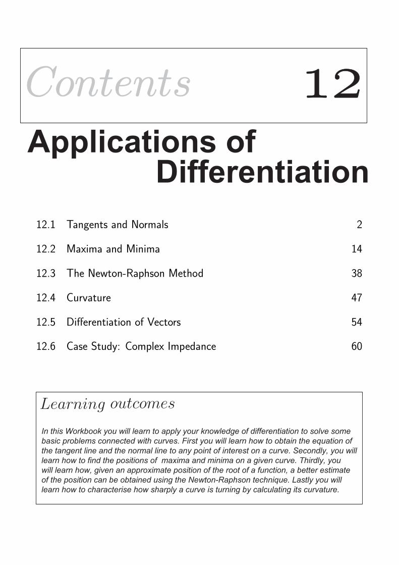
12.1 Tangents and Normals 2

12.2 Maxima and Minima 14

12.3 The Newton-Raphson Method 38

12.4 Curvature 47

12.5 Differentiation of Vectors 54

12.6 Case Study: Complex Impedance 60

Learning

In this Workbook you will learn to apply your knowledge of differentiation to solve some basic problems connected with curves. First you will learn how to obtain the equation ofthe tangent line and the normal line to any point of interest on a curve. Secondly, you willlearn how to find the positions of maxima and minima on a given curve. Thirdly, youwill learn how, given an approximate position of the root of a function, a better estimateof the position can be obtained using the Newton-Raphson technique. Lastly you willlearn how to characterise how sharply a curve is turning by calculating its curvature.

outcomes

Maxima and Minima

12.2

Introduction

In this Section we analyse curves in the ‘local neighbourhood’ of a stationary point and, from thisanalysis, deduce necessary conditions satisfied by local maxima and local minima. Locating the max-ima and minima of a function is an important task which arises often in applications of mathematicsto problems in engineering and science. It is a task which can often be carried out using only aknowledge of the derivatives of the function concerned. The problem breaks into two parts

• finding the stationary points of the given functions

• distinguishing whether these stationary points are maxima, minima or, exceptionally, points ofinflection.

This Section ends with maximum and minimum problems from engineering contexts.

Prerequisites

Before starting this Section you should . . .

• be able to obtain first and second derivativesof simple functions

• be able to find the roots of simple equations

Learning Outcomes

On completion you should be able to . . .

• explain the difference between local andglobal maxima and minima

• describe how a tangent line changes near amaximum or a minimum

• locate the position of stationary points

• use knowledge of the second derivative todistinguish between maxima and minima

14 HELM (2008):

Workbook 12: Applications of Differentiation

®

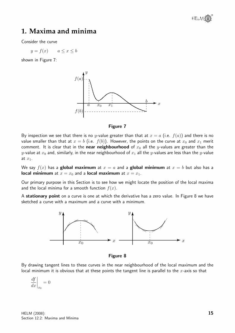
1. Maxima and minima

Consider the curve

y = f(x) a ≤ x ≤ b

shown in Figure 7:

x

y

f(a)

f(b)a

bx0 x1

Figure 7

By inspection we see that there is no y-value greater than that at x = a (i.e. f(a)) and there is novalue smaller than that at x = b (i.e. f(b)). However, the points on the curve at x0 and x1 meritcomment. It is clear that in the near neighbourhood of x0 all the y-values are greater than they-value at x0 and, similarly, in the near neighbourhood of x1 all the y-values are less than the y-valueat x1.

We say f(x) has a global maximum at x = a and a global minimum at x = b but also has alocal minimum at x = x0 and a local maximum at x = x1.

Our primary purpose in this Section is to see how we might locate the position of the local maximaand the local minima for a smooth function f(x).

A stationary point on a curve is one at which the derivative has a zero value. In Figure 8 we havesketched a curve with a maximum and a curve with a minimum.

x

y

x0x

y

x0

Figure 8

By drawing tangent lines to these curves in the near neighbourhood of the local maximum and thelocal minimum it is obvious that at these points the tangent line is parallel to the x-axis so that

df

dx

x0

= 0

HELM (2008):

Section 12.2: Maxima and Minima

15

The Newton-Raphson

Method

12.3

Introduction

This Section is concerned with the problem of “root location”; i.e. finding those values of x whichsatisfy an equation of the form f(x) = 0. An initial estimate of the root is found (for example bydrawing a graph of the function). This estimate is then improved using a technique known as theNewton-Raphson method, which is based upon a knowledge of the tangent to the curve near theroot. It is an “iterative” method in that it can be used repeatedly to continually improve the accuracyof the root.

Prerequisites


• be able to differentiate simple functions

• be able to sketch graphs

Learning Outcomes


• distinguish between simple and multiple roots

• estimate the root of an equation by drawinga graph

• employ the Newton-Raphson method toimprove the accuracy of a root

38 HELM (2008):


®

Curvature

12.4

Introduction

Curvature is a measure of how sharply a curve is turning. At a particular point along the curve atangent line can be drawn; this tangent line making an angle ψ with the positive x-axis. Curvatureis then defined as the magnitude of the rate of change of ψ with respect to the measure of lengthon the curve - the arc length s. That is

Curvature =

dψ

ds

In this Section we examine the concept of curvature and, from its definition, obtain more usefulexpressions for curvature when the equation of the curve is expressed either in Cartesian form y = f(x)or in parametric form x = x(t) y = y(t). We show that a circle has a constant value for thecurvature, which is to be expected, as the tangent line to a circle turns equally quickly irrespectiveof the position on the circle. For all curves, except circles, other than a circle, the curvature willdepend upon position, changing its value as the curve twists and turns.

Prerequisites


• understand the geometrical interpretation ofthe derivative

• be able to differentiate standard functions

• be able to use the parametric description of acurve

Learning Outcomes


• understand the concept of curvature

• calculate curvature when the curve is definedin Cartesian form or in parametric form

HELM (2008):

Section 12.4: Curvature

47

1. Curvature

Curvature is a measure of how quickly a tangent line turns as the contact point moves along a curve.For example, consider a simple parabola, with equation y = x2. Its graph is shown in Figure 27.

x

y

P Q

R

Figure 27

It is obvious, geometrically, that the tangent lines to this curve turn ‘more quickly’ between P andQ than between Q and R. It is the purpose of this Section to give, a quantitative measure of thisrate of ‘turning’.

If we change from a parabola to a circle, (centred on the origin, of radius 1), we can again considerhow quickly the tangent lines turn as we move along the curve. See Figure 28. It is immediatelyclear that the tangent lines to a circle turn equally quickly no matter where located on the circle.

x

y

Figure 28

However, if we consider two circles with the same centre but different radii, as in Figure 29, it isagain obvious that the smaller circle ‘bends’ more tightly than the larger circle and we say it has alarger curvature. Athletes who run the 200 metres find it easier to run in the outside lanes (wherethe curve turns less sharply) than in the inside lanes.

x

y

!P

QP !

Q!

!

Figure 29

On the two circle diagram (Figure 29) we have drawn tangent lines at P and P ; both lines makean angle ψ (greek letter psi) with the positive x-axis. We need to measure how quickly the angle

48 HELM (2008):


Differentiation of

Vectors

12.5

Introduction

The area of mathematics known as vector calculus is used to model mathematically a vast range of

engineering phenomena including electrostatics, electromagnetic fields, air flow around aircraft and

heat flow in nuclear reactors. In this Section we introduce briefly the differential calculus of vectors.

Prerequisites


• have a knowledge of vectors, in Cartesian

form

• be able to calculate the scalar and vector

products of two vectors

• be able to differentiate and integrate scalar

functions

Learning Outcomes


• differentiate vectors

54 HELM (2008):


Case Study:Complex Impedance

12.6

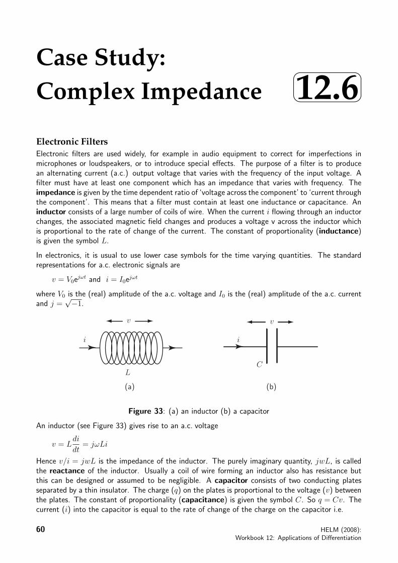
Electronic FiltersElectronic filters are used widely, for example in audio equipment to correct for imperfections inmicrophones or loudspeakers, or to introduce special effects. The purpose of a filter is to producean alternating current (a.c.) output voltage that varies with the frequency of the input voltage. Afilter must have at least one component which has an impedance that varies with frequency. Theimpedance is given by the time dependent ratio of ‘voltage across the component’ to ‘current throughthe component’. This means that a filter must contain at least one inductance or capacitance. Aninductor consists of a large number of coils of wire. When the current i flowing through an inductorchanges, the associated magnetic field changes and produces a voltage v across the inductor whichis proportional to the rate of change of the current. The constant of proportionality (inductance)is given the symbol L.

In electronics, it is usual to use lower case symbols for the time varying quantities. The standardrepresentations for a.c. electronic signals are

v = V0ejωt and i = I0ejωt

where V0 is the (real) amplitude of the a.c. voltage and I0 is the (real) amplitude of the a.c. currentand j =

√−1.

L

i

C

i

v v

(a) (b)

Figure 33: (a) an inductor (b) a capacitor

An inductor (see Figure 33) gives rise to an a.c. voltage

v = Ldi

dt= jωLi

Hence v/i = jwL is the impedance of the inductor. The purely imaginary quantity, jwL, is calledthe reactance of the inductor. Usually a coil of wire forming an inductor also has resistance butthis can be designed or assumed to be negligible. A capacitor consists of two conducting platesseparated by a thin insulator. The charge (q) on the plates is proportional to the voltage (v) betweenthe plates. The constant of proportionality (capacitance) is given the symbol C. So q = Cv. Thecurrent (i) into the capacitor is equal to the rate of change of the charge on the capacitor i.e.

60 HELM (2008):


®

i =dq

dt= C

dv

dt= jωCv.

Hence, for a capacitor, the impedance Zc = v/i = 1/jwC. This purely imaginary quantity is also areactance. Because of Ohm’s law (v = iR), a resistance R provides a constant (real) contributionof R to the impedance of a circuit. If two resistors R1 and R2 are in series the same current passesthrough both of them and the combined resistance is R1 + R2. In the circuit shown in Figure 34(consider the left-hand representation of this circuit first but note that the right-hand version isequivalent), the input voltage across both resistors and the output voltage across R2 are related by

vin = i(R1 + R2) and vout = iR2 sovout

vin=

R2

R1 + R2.

Such a circuit is called a potential divider.

R1

R2vin

vout

vout

R2

R1

vin

Figure 34: Two representations of a potential divider circuit

Now consider this circuit with the resistor R2 replaced by a capacitor C as in Figure 35.

vout

R

vinC

Figure 35: Low pass filter circuit containing a resistor and a capacitor

If R1 is replaced by R and R2 by ZC = 1/jwC, in the relevant expression for the potential dividercircuit, then

vout

vin=

1/jωC

R + 1/jωC=

1

1 + jωRC

The square of the magnitude of the voltage ratio is given by multiplying the existing complex expres-sion by its complex conjugate, i.e.

vout

vin

2

=1

(1 + jωRC)(1− jωRC)=

1

(1 + ω2R2C2)

HELM (2008):

Section 12.6: Case Study: Complex Impedance

61

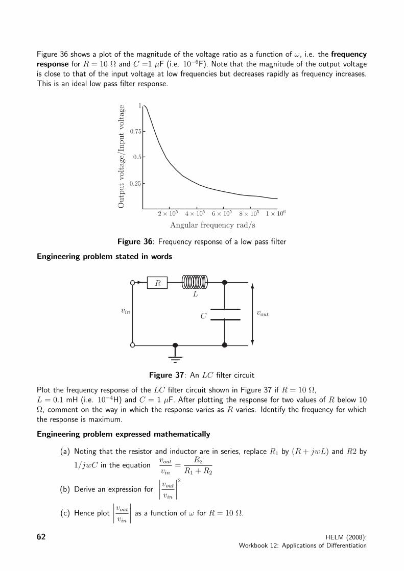
Figure 36 shows a plot of the magnitude of the voltage ratio as a function of ω, i.e. the frequencyresponse for R = 10 Ω and C =1 µF (i.e. 10−6F). Note that the magnitude of the output voltageis close to that of the input voltage at low frequencies but decreases rapidly as frequency increases.This is an ideal low pass filter response.

0.25

0.5

0.75

1

2 ! 105 4 ! 105 6 ! 105 8 ! 105 1 ! 106

Outp

ut

voltag

e/In

put

voltag

e

Angular frequency rad/s

Figure 36: Frequency response of a low pass filter

Engineering problem stated in words

vinC

RL

vout

Figure 37: An LC filter circuit

Plot the frequency response of the LC filter circuit shown in Figure 37 if R = 10 Ω,L = 0.1 mH (i.e. 10−4H) and C = 1 µF. After plotting the response for two values of R below 10Ω, comment on the way in which the response varies as R varies. Identify the frequency for whichthe response is maximum.

Engineering problem expressed mathematically

(a) Noting that the resistor and inductor are in series, replace R1 by (R + jwL) and R2 by

1/jwC in the equationvout

vin=

R2

R1 + R2

(b) Derive an expression for

vout

vin

2

(c) Hence plot

vout

vin

as a function of ω for R = 10 Ω.

62 HELM (2008):


®

(d) Plot

vout

vin

for two further values of R < 10 Ω (e.g. 5 Ω and 2 Ω).

(e) Find an expression for the value of ω = ωres at which

vout

vin

is maximum.

Mathematical analysis

(a) The substitutions R1 → (R + jwL) and R2 → 1/jwC in the equation

vout

vin=

R2

R1 + R2yield

vout

vin=

1/jωC

R + jωL + 1/jωC=

1

(1− ω2LC + jωRC)

(b) Multiplying by the complex conjugate of the denominatorvout

vin

2

=1

(1− ω2LC + jωRC)(1− ω2LC − jωRC)=

1

(1− ω2LC)2 + ω2R2C2

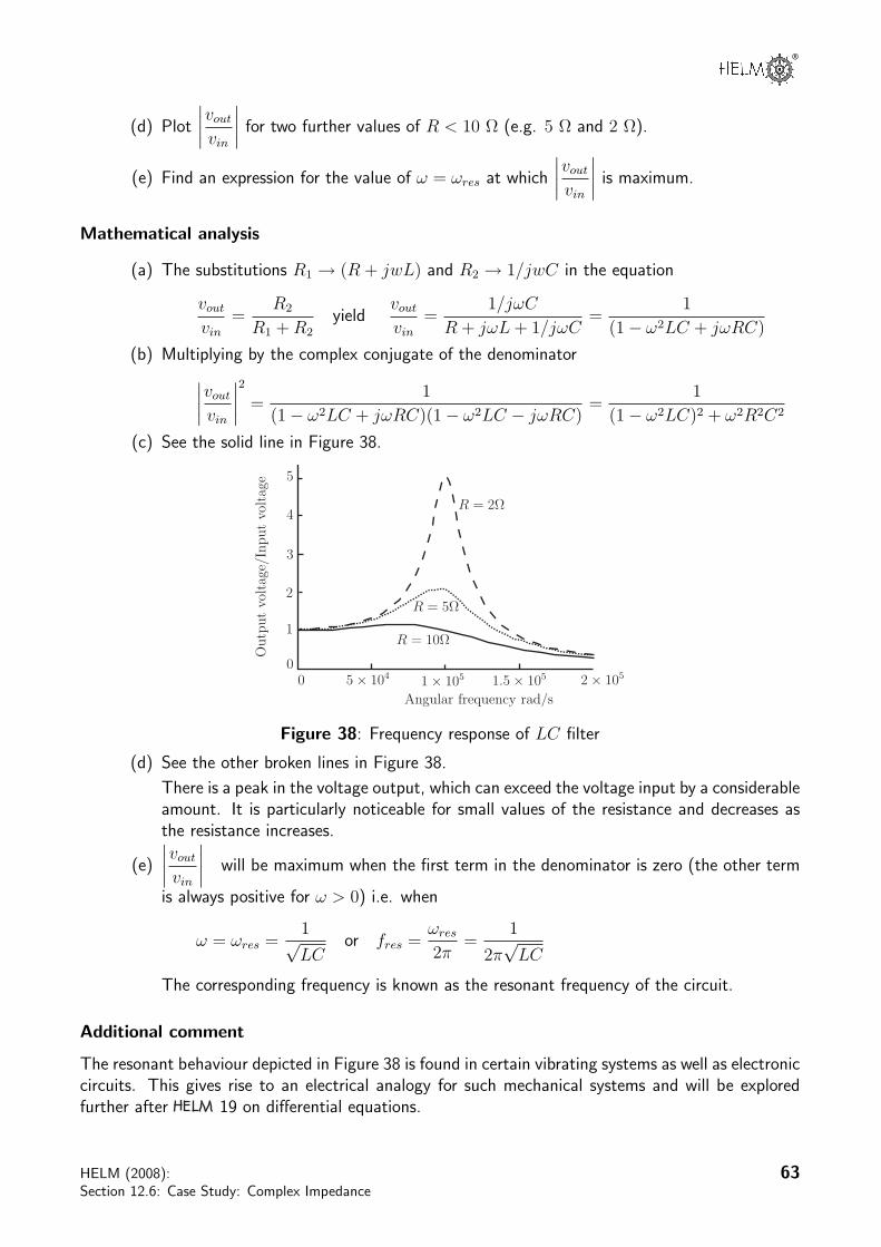
(c) See the solid line in Figure 38.

R = 5!

R = 10!

5 ! 104 1 ! 105 1.5 ! 105 2 ! 105

R = 2!

Outp

ut

voltag

e/In

put

voltag

e

Angular frequency rad/s

1

2

3

4

5

00

Figure 38: Frequency response of LC filter

(d) See the other broken lines in Figure 38.

There is a peak in the voltage output, which can exceed the voltage input by a considerableamount. It is particularly noticeable for small values of the resistance and decreases asthe resistance increases.

(e)

vout

vin

will be maximum when the first term in the denominator is zero (the other term

is always positive for ω > 0) i.e. when

ω = ωres =1√LC

or fres =ωres

2π=

1

2π√

LC

The corresponding frequency is known as the resonant frequency of the circuit.

Additional comment

The resonant behaviour depicted in Figure 38 is found in certain vibrating systems as well as electroniccircuits. This gives rise to an electrical analogy for such mechanical systems and will be exploredfurther after 19 on differential equations.

HELM (2008):

Section 12.6: Case Study: Complex Impedance

63

®

1. Differentiation of vectors

Consider Figure 31.

P

Cr

x

y

Figure 31

If r represents the position vector of an object which is moving along a curve C, then the position

vector will be dependent upon the time, t. We write r = r(t) to show the dependence upon time.

Suppose that the object is at the point P , with position vector r at time t and at the point Q, with

position vector r(t + δt), at the later time t + δt, as shown in Figure 32.

P

x

y

Qr(t)

r(t + !t)

!"PQ

Figure 32

Then−→PQ represents the displacement vector of the object during the interval of time δt. The length

of the displacement vector represents the distance travelled, and its direction gives the direction of

motion. The average velocity during the time from t to t + δt is defined as the displacement vector

divided by the time interval δt, that is,

average velocity =

−→PQ

δt=

r(t + δt)− r(t)

δt

If we now take the limit as the interval of time δt tends to zero then the expression on the right

hand side is the derivative of r with respect to t. Not surprisingly we refer to this derivative as

the instantaneous velocity, v. By its very construction we see that the velocity vector is always

tangential to the curve as the object moves along it. We have:

v = limδt→0

r(t + δt)− r(t)

δt=

dr

dt

HELM (2008):

Section 12.5: Differentiation of Vectors

55

Now, since the x and y coordinates of the object depend upon time, we can write the position vector

r in Cartesian coordinates as:

r(t) = x(t)i + y(t)j

Therefore,

r(t + δt) = x(t + δt)i + y(t + δt)j

so that,

v(t) = limδt→0

x(t + δt)i + y(t + δt)j − x(t)i− y(t)j

δt

= limδt→0

x(t + δt)− x(t)

δti +

y(t + δt)− y(t)

δtj

=dx

dti +

dy

dtj

This is often abbreviated to v = r = xi + yj, using notation for derivatives with respect to time.

So we see that the velocity vector is the derivative of the position vector with respect to time. This

result generalizes in an obvious way to three dimensions as summarized in the following Key Point.

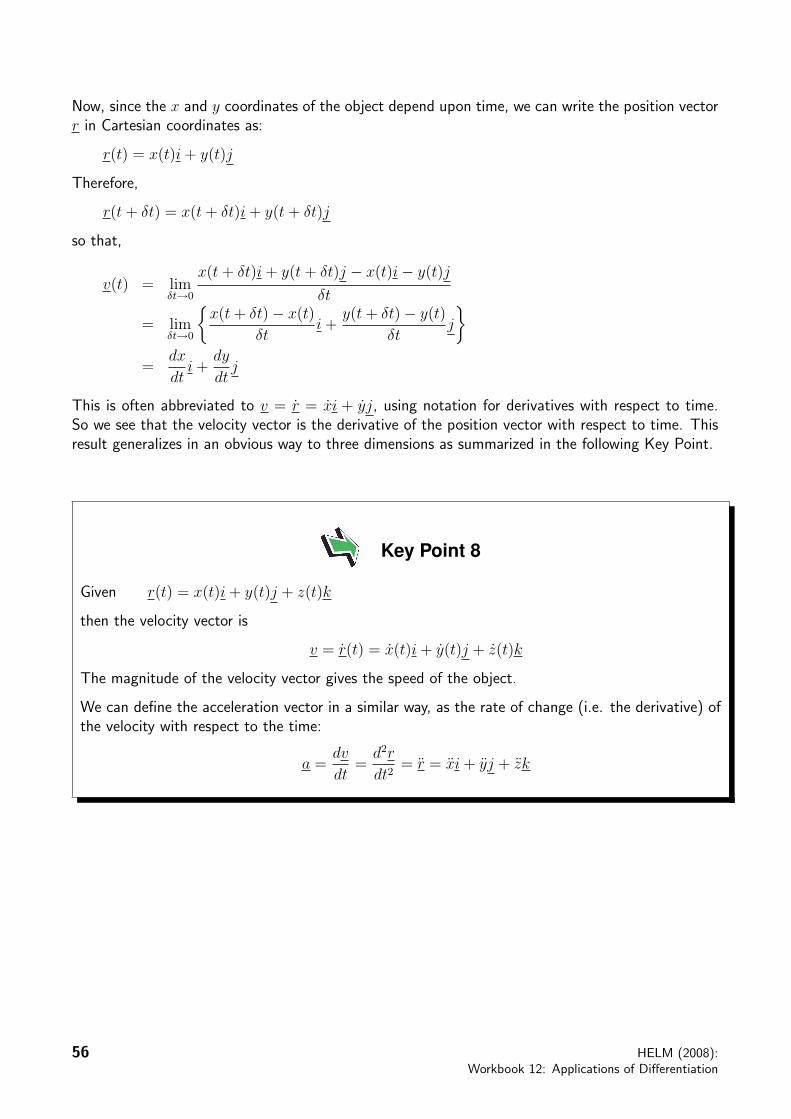
Key Point 8

Given r(t) = x(t)i + y(t)j + z(t)k

then the velocity vector is

v = r(t) = x(t)i + y(t)j + z(t)k

The magnitude of the velocity vector gives the speed of the object.

We can define the acceleration vector in a similar way, as the rate of change (i.e. the derivative) of

the velocity with respect to the time:

a =dv

dt=

d2r

dt2= r = xi + yj + zk

56 HELM (2008):


®

Example 6

If w = 3t2i + cos 2tj, find

(a)dw

dt(b)

dw

dt

(c)d2w

dt2

Solution

(a) If w = 3t2i + cos 2tj, then differentiation with respect to t yields:dw

dt= 6ti− 2 sin 2tj

(b)

dw

dt

=

(6t)2 + (−2 sin 2t)2 =

36t2 + 4 sin2 2t

(c)d2w

dt2= 6i− 4 cos 2tj

It is possible to differentiate more complicated expressions involving vectors provided certain rules

are adhered to as summarized in the following Key Point.

Key Point 9If w and z are vectors and c is a scalar, all these being functions of time t, then:

d

dt(w + z) =

dw

dt+

dz

dtd

dt(cw) = c

dw

dt+

dc

dtw

d

dt(w · z) = w · dz

dt+

dw

dt· z

d

dt(w × z) = w × dz

dt+

dw

dt× z

HELM (2008):


57

Example 7

If w = 3ti− t2j and z = 2t2i + 3j, verify the result

d

dt(w · z) = w · dz

dt+

dw

dt· z

Solution

w · z = (3ti− t2j) · (2t2i + 3j) = 6t3 − 3t2.

Therefored

dt(w · z) = 18t2 − 6t (1)

Alsodw

dt= 3i− 2tj and

dz

dt= 4ti

so w · dz

dt+ z · dw

dt= (3ti− t2j) · (4ti) + (2t2i + 3j) · (3i− 2tj)

= 12t2 + 6t2 − 6t

= 18t2 − 6t (2)

We have verifiedd

dt(w · z) = w · dz

dt+

dw

dt· z since (1) is the same as (2).

Example 8

If w = 3ti− t2j and z = 2t2i + 3j, verify the result

d

dt(w × z) = w × dz

dt+

dw

dt× z

Solution

w × z =

i j k3t −t2 02t2 3 0

= (9t + 2t4)k implying

d

dt(w × z) = (9 + 8t3)k (1)

w × dz

dt=

i j k3t −t2 04t 0 0

= 4t3k (2)

dw

dt× z =

i j k3 −2t 0

2t2 3 0

= (9 + 4t3)k (3)

We can see that (1) is the same as (2) + (3) as required.

58 HELM (2008):


®

Exercises

1. If r = 3ti + 2t2j + t3k, find (a)dr

dt(b)

d2r

dt2

2. Given B = te−t i + cos t j find (a)dB

dt(b)

d2B

dt2

3. If r = 4t2i + 2tj − 7k evaluate r anddr

dtwhen t = 1.

4. If w = t3i− 7tk and z = (2 + t)i + t2j − 2k

(a) find w · z, (b) finddw

dt, (c) find

dz

dt, (d) show that

d

dt(w · z) = w · dz

dt+

dw

dt· z

5. Given r = sin t i + cos t j

(a) find r, (b) find r, (c) find |r|

(d) Show that the position vector r and velocity vector r are perpendicular.

Answers

1. (a) 3i + 4tj + 3t2k (b) 4j + 6tk

2. (a) (−te−t + e−t)i− sin tj (b) e−t(t− 2)i− cos tj

3. 4i + 2j − 7k, 8i + 2j

4. (a) t(t3 + 2t2 + 14) (b) 3t2i− 7k (c) i + 2tj

5. (a) cos ti− sin tj (b) − sin ti− cos tj (c) 1 (d) Follows by showing r · r = 0.

HELM (2008):


59

®

ψ changes as we move along the curve. As we move from P to Q (inner circle), or from P to Q

(outer circle), the angle ψ changes by the same amount. However, the distance traversed on theinner circle is less than the distance traversed on the outer circle. This suggests that a measure ofcurvature is:

curvature is the magnitude of the rate of change of ψ

with respect to the distance moved along the curve.

We shall denote the curvature by the Greek letter κ (kappa).So

κ =

dψ

ds

where s is the measure of arc-length along a curve. This rather odd-looking derivative needs con-verting to involve the variable x if the equation of the curve is given in the usual form y = f(x). Asa preliminary we note that

dψ

ds=

dψ

dx

ds

dx

We now obtain expressions for the derivativesdψ

dxand

ds

dxin terms of the derivatives of f(x).

Consider Figure 30 below.

x

y

!

x

y"x

"y"s

Figure 30

Small increments in the x- and y-directions have been denoted by δx and δy respectively. Thehypotenuse on this ‘small triangle’ is δs which is the change in arc-length along the curve.From Pythagoras’ theorem:

δs2 = δx2 + δy2

so

δs

δx

2

= 1 +

δy

δx

2

so thatδs

δx=

1 +

δy

δx

2

In the limit as the increments get smaller and smaller, we write this relation in derivative form:

ds

dx=

1 +

dy

dx

2

HELM (2008):


49

However, as y = f(x) is the equation of the curve we obtain

ds

dx=

1 +

df

dx

2

= (1 + [f (x)]2)1/2

We also know the relation between the angle ψ and the derivativedf

dx:

df

dx= tan ψ

so differentiating again:

d2f

dx2= sec2 ψ

dψ

dx= (1 + tan2 ψ)

dψ

dx

= (1 + [f (x)]2)dψ

dx

Inverting this relation:

dψ

dx=

f (x)

(1 + [f (x)]2)

and so, finally, the curvature is given by

κ =

dψ

ds

=

dψ

dx

ds

dx

=

f (x)

(1 + [f (x)]2)3/2

Key Point 6Curvature

At each point on a curve, with equation y = f(x), the tangent line turns at a certain rate.

A measure of this rate of turning is the curvature κ defined by

κ =

f (x)

(1 + [f (x)]2)3/2

50 HELM (2008):


®

Task

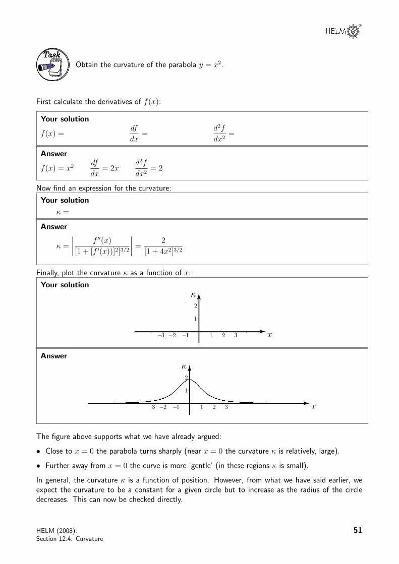
Obtain the curvature of the parabola y = x2.

First calculate the derivatives of f(x):

Your solution

f(x) =df

dx=

d2f

dx2=

Answer

f(x) = x2 df

dx= 2x

d2f

dx2= 2

Now find an expression for the curvature:

Your solution

κ =

Answer

κ =

f (x)

[1 + [f (x))]2]3/2

=2

[1 + 4x2]3/2

Finally, plot the curvature κ as a function of x:

Your solution

x!3 !2 !1

1

2

31 2

!

Answer

x!3 !2 !1

1

2

31 2

!

The figure above supports what we have already argued:

• Close to x = 0 the parabola turns sharply (near x = 0 the curvature κ is relatively, large).

• Further away from x = 0 the curve is more ‘gentle’ (in these regions κ is small).

In general, the curvature κ is a function of position. However, from what we have said earlier, weexpect the curvature to be a constant for a given circle but to increase as the radius of the circledecreases. This can now be checked directly.

HELM (2008):


51

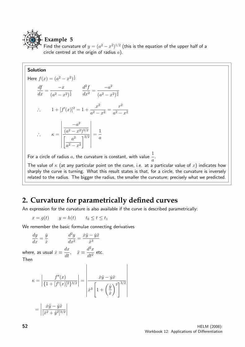
Example 5

Find the curvature of y = (a2 − x2)1/2 (this is the equation of the upper half of acircle centred at the origin of radius a).

Solution

Here f(x) = (a2 − x2)12

df

dx=

−x

(a2 − x2)12

d2f

dx2=

−a2

(a2 − x2)32

∴ 1 + [f (x)]2 = 1 +x2

a2 − x2=

r2

a2 − x2

∴ κ =

−a2

(a2 − x2)3/2

a2

a2 − x2

3/2

=1

a

For a circle of radius a, the curvature is constant, with value1

a.

The value of κ (at any particular point on the curve, i.e. at a particular value of x) indicates howsharply the curve is turning. What this result states is that, for a circle, the curvature is inverselyrelated to the radius. The bigger the radius, the smaller the curvature; precisely what we predicted.

2. Curvature for parametrically defined curves

An expression for the curvature is also available if the curve is described parametrically:

x = g(t) y = h(t) t0 ≤ t ≤ t1

We remember the basic formulae connecting derivatives

dy

dx=

y

x

d2y

dx2=

xy − yx

x3

where, as usual x ≡ dx

dt, x ≡ d2x

dt2etc.

Then

κ =

f (x)

1 + [f (x)]23/2

=

xy − yx

x3

1 +

y

x

23/2

=

xy − yx

[x2 + y2]3/2

52 HELM (2008):


®

Key Point 7

The formula for curvature in parametric form is κ =

xy − yx

[x2 + y2]3/2

Task

An ellipse is described parametrically by the equations

x = 2 cos t y = sin t 0 ≤ t ≤ 2π

Obtain an expression for the curvature κ and find where the curvature is a maxi-mum or a minimum.

First find x, y, x, y:

Your solution

x = y = x = y =

Answer

x = −2 sin t y = cos t x = −2 cos t y = − sin t

Now find κ:Your solution

κ =

Answer

κ =

xy − yx

[x2 + y2]3/2

=

2 sin2 t + 2 cos2 t

[4 sin2 t + cos2 t]3/2

=2

[1 + 3 sin2 t]3/2

Find maximum and minimum values of κ by inspection of the expression for κ:

Your solution

max κ = min κ =

AnswerDenominator is max when t = π/2. This gives minimum value of κ = 1/4,Denominator is min when t = 0. This gives maximum value of κ = 2.

x!2

!1

1

2

minimum value of !

maximum value of !

y

HELM (2008):


53

®

1. The Newton-Raphson method

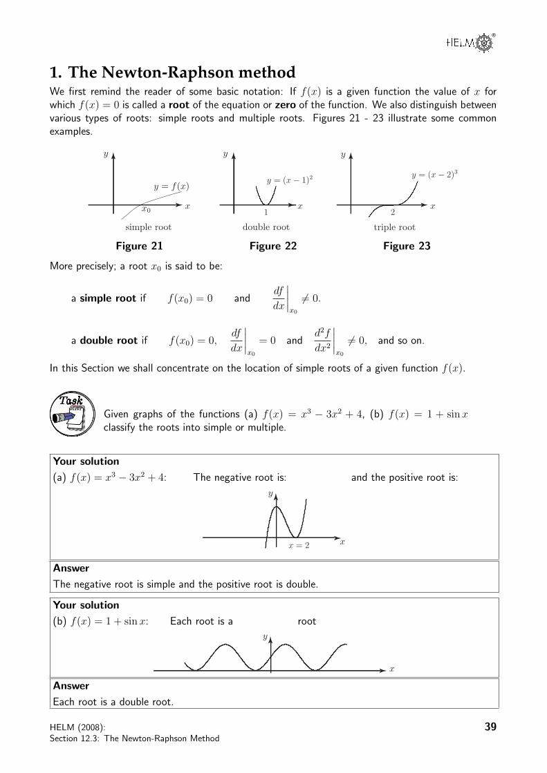
We first remind the reader of some basic notation: If f(x) is a given function the value of x forwhich f(x) = 0 is called a root of the equation or zero of the function. We also distinguish betweenvarious types of roots: simple roots and multiple roots. Figures 21 - 23 illustrate some commonexamples.

xxxx0

simple root double root triple root

y = f(x)

yyy

y = (x ! 1)2 y = (x ! 2)3

1 2

Figure 21 Figure 22 Figure 23

More precisely; a root x0 is said to be:

a simple root if f(x0) = 0 anddf

dx

x0

= 0.

a double root if f(x0) = 0,df

dx

x0

= 0 andd2f

dx2

x0

= 0, and so on.

In this Section we shall concentrate on the location of simple roots of a given function f(x).

Task

Given graphs of the functions (a) f(x) = x3 − 3x2 + 4, (b) f(x) = 1 + sin xclassify the roots into simple or multiple.

Your solution

(a) f(x) = x3 − 3x2 + 4: The negative root is: and the positive root is:

x

y

x = 2

Answer

The negative root is simple and the positive root is double.

Your solution

(b) f(x) = 1 + sin x: Each root is a root

x

y

Answer

Each root is a double root.

HELM (2008):

Section 12.3: The Newton-Raphson Method

39

2. Finding roots of the equation fff(((xxx))) === 000A first investigation into the roots of f(x) might be graphical. Such an analysis will supply informationas to the approximate location of the roots.

Task

Sketch the function

f(x) = x− 2 + ln x x > 0

and estimate the value of the root.

Your solution

x

y

1 2

An estimate of the root is:

Answer

x

y

1 2

A simple root is located near 1.5

One method of obtaining a better approximation is to halve the interval 1 ≤ x ≤ 2 into 1 ≤ x ≤ 1.5and 1.5 ≤ x ≤ 2 and test the sign of the function at the end-points of these new regions. We find

x f(x)1 < 01.5 < 02 > 0

so a root must lie between x = 1.5 and x = 2 because the sign of f(x) changes between thesevalues and f(x) is a continuous curve. We can repeat this procedure and divide the interval (1.5, 2)into the two new intervals (1.5, 1.75) and (1.75, 2) and test again. This time we find

x f(x)1.5 < 01.75 > 02.0 > 0

40 HELM (2008):


®

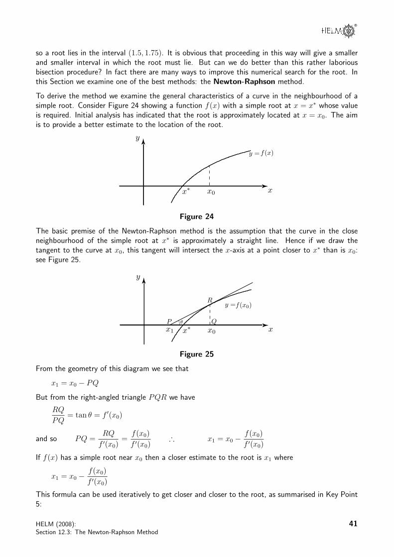
so a root lies in the interval (1.5, 1.75). It is obvious that proceeding in this way will give a smallerand smaller interval in which the root must lie. But can we do better than this rather laboriousbisection procedure? In fact there are many ways to improve this numerical search for the root. Inthis Section we examine one of the best methods: the Newton-Raphson method.

To derive the method we examine the general characteristics of a curve in the neighbourhood of asimple root. Consider Figure 24 showing a function f(x) with a simple root at x = x∗ whose valueis required. Initial analysis has indicated that the root is approximately located at x = x0. The aimis to provide a better estimate to the location of the root.

x

y

x!

y =f(x)

x0

Figure 24

The basic premise of the Newton-Raphson method is the assumption that the curve in the closeneighbourhood of the simple root at x∗ is approximately a straight line. Hence if we draw thetangent to the curve at x0, this tangent will intersect the x-axis at a point closer to x∗ than is x0:see Figure 25.

x

y

x!x1

P Q

Rf(x0)y =

x0

!

Figure 25

From the geometry of this diagram we see that

x1 = x0 − PQ

But from the right-angled triangle PQR we have

RQ

PQ= tan θ = f (x0)

and so PQ =RQ

f (x0)=

f(x0)

f (x0)∴ x1 = x0 −

f(x0)

f (x0)

If f(x) has a simple root near x0 then a closer estimate to the root is x1 where

x1 = x0 −f(x0)

f (x0)

This formula can be used iteratively to get closer and closer to the root, as summarised in Key Point5:

HELM (2008):


41

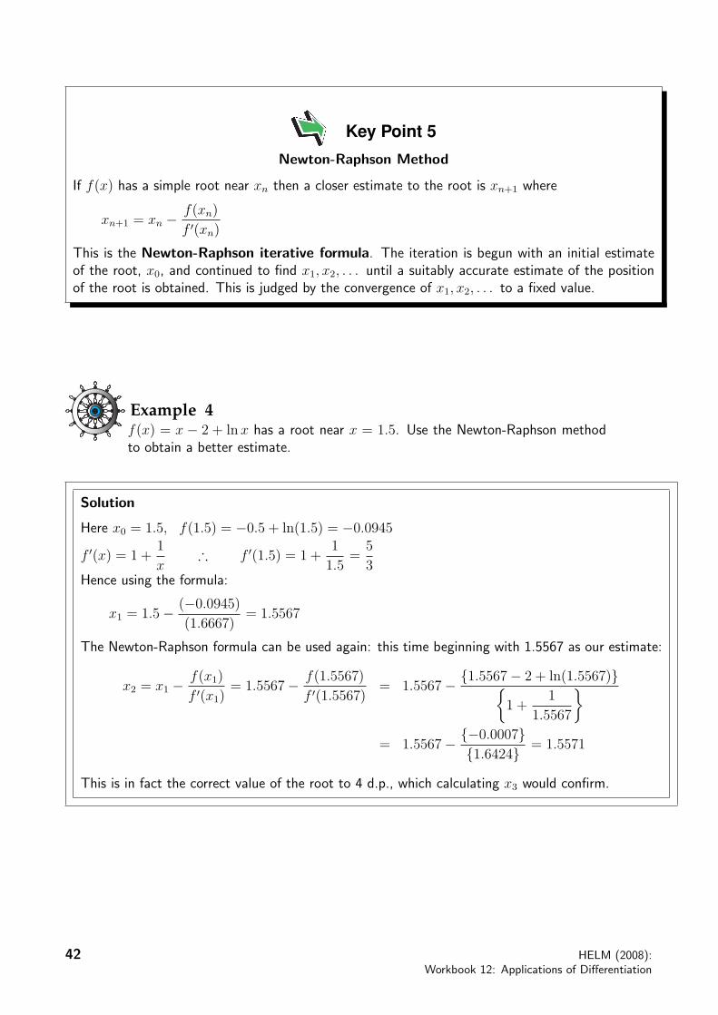
Key Point 5Newton-Raphson Method

If f(x) has a simple root near xn then a closer estimate to the root is xn+1 where

xn+1 = xn −f(xn)

f (xn)

This is the Newton-Raphson iterative formula. The iteration is begun with an initial estimateof the root, x0, and continued to find x1, x2, . . . until a suitably accurate estimate of the positionof the root is obtained. This is judged by the convergence of x1, x2, . . . to a fixed value.

Example 4

f(x) = x − 2 + ln x has a root near x = 1.5. Use the Newton-Raphson methodto obtain a better estimate.

Solution

Here x0 = 1.5, f(1.5) = −0.5 + ln(1.5) = −0.0945

f (x) = 1 +1

x∴ f (1.5) = 1 +

1

1.5=

5

3Hence using the formula:

x1 = 1.5− (−0.0945)

(1.6667)= 1.5567

The Newton-Raphson formula can be used again: this time beginning with 1.5567 as our estimate:

x2 = x1 −f(x1)

f (x1)= 1.5567− f(1.5567)

f (1.5567)= 1.5567− 1.5567− 2 + ln(1.5567)

1 +1

1.5567

= 1.5567− −0.00071.6424 = 1.5571

This is in fact the correct value of the root to 4 d.p., which calculating x3 would confirm.

42 HELM (2008):


®

Task

The function f(x) = x− tan x has a simple root near x = 4.5. Use one iterationof the Newton-Raphson method to find a more accurate value for the root.

First finddf

dx:

Your solutiondf

dx=

Answerdf

dx= 1− sec2 x = − tan2 x

Now use the formula x1 = x0 − f(x0)/f (x0) with x0 = 4.5 to obtain x1:

Your solution

f(4.5) = 4.5− tan(4.5) =

f (4.5) = 1− sec2(4.5) = − tan2(4.5) =

x1 = 4.5− f(4.5)

f (4.5)=

Answerf(4.5) = −0.1373, f (4.5) = −21.5048

∴ x1 = 4.5− 0.1373

21.5048= 4.4936.

As the value of x1 has changed little from x0 = 4.5 we can expect the root to be 4.49 to 3 d.p.

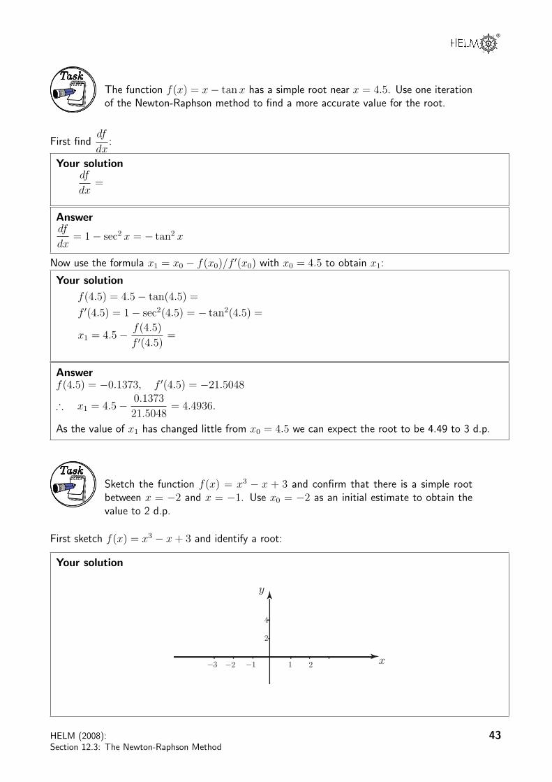
Task

Sketch the function f(x) = x3 − x + 3 and confirm that there is a simple rootbetween x = −2 and x = −1. Use x0 = −2 as an initial estimate to obtain thevalue to 2 d.p.

First sketch f(x) = x3 − x + 3 and identify a root:

Your solution

x

y

4

!3

2

21!2 !1

HELM (2008):


43

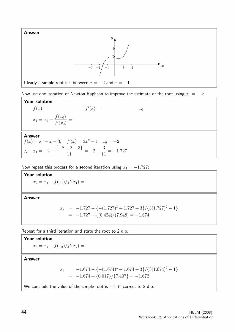
Answer

x!3 21!2 !1

y

4

2

Clearly a simple root lies between x = −2 and x = −1.

Now use one iteration of Newton-Raphson to improve the estimate of the root using x0 = −2:

Your solution

f(x) = f (x) = x0 =

x1 = x0 −f(x0)

f (x0)=

Answerf(x) = x3 − x + 3, f (x) = 3x2 − 1 x0 = −2

∴ x1 = −2− −8 + 2 + 311

= −2 +3

11= −1.727

Now repeat this process for a second iteration using x1 = −1.727:

Your solution

x2 = x1 − f(x1)/f (x1) =

Answer

x2 = −1.727− −(1.727)3 + 1.727 + 3/3(1.727)2 − 1= −1.727 + (0.424)/(7.948) = −1.674

Repeat for a third iteration and state the root to 2 d.p.:

Your solution

x3 = x2 − f(x2)/f (x2) =

Answer

x3 = −1.674− −(1.674)3 + 1.674 + 3/3(1.674)2 − 1= −1.674 + 0.017/7.407 = −1.672

We conclude the value of the simple root is −1.67 correct to 2 d.p.

44 HELM (2008):


®

Engineering Example 5

Buckling of a strut

The equation governing the buckling load P of a strut with one end fixed and the other end simply

supported is given by tan µL = µL where µ =

P

EI, L is the length of the strut and EI is the

flexural rigidity of the strut. For safe design it is important that the load applied to the strut is lessthan the lowest buckling load. This equation has no exact solution and we must therefore use themethod described in this Workbook to find the lowest buckling loadP .

deflected shape

PL

P

Figure 26

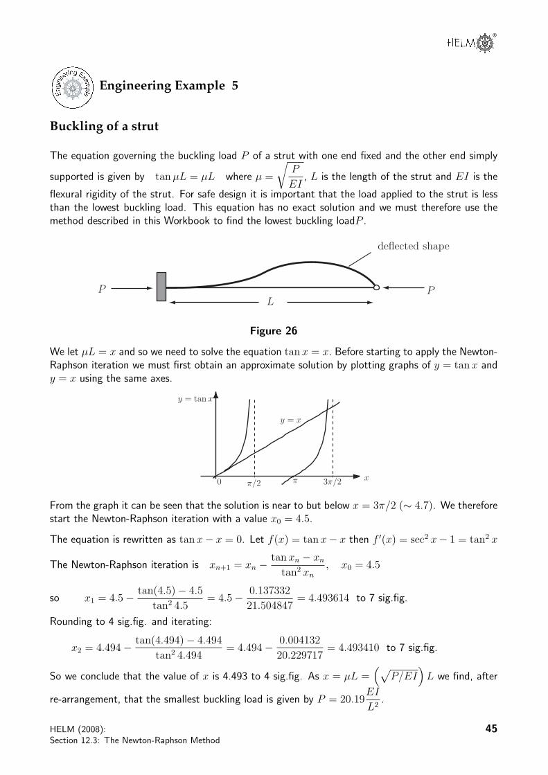
We let µL = x and so we need to solve the equation tan x = x. Before starting to apply the Newton-Raphson iteration we must first obtain an approximate solution by plotting graphs of y = tan x andy = x using the same axes.

y = x

y = tan x

0 !/2 ! 3!/2 x

From the graph it can be seen that the solution is near to but below x = 3π/2 (∼ 4.7). We thereforestart the Newton-Raphson iteration with a value x0 = 4.5.

The equation is rewritten as tan x− x = 0. Let f(x) = tan x− x then f (x) = sec2 x− 1 = tan2 x

The Newton-Raphson iteration is xn+1 = xn −tan xn − xn

tan2 xn, x0 = 4.5

so x1 = 4.5− tan(4.5)− 4.5

tan2 4.5= 4.5− 0.137332

21.504847= 4.493614 to 7 sig.fig.

Rounding to 4 sig.fig. and iterating:

x2 = 4.494− tan(4.494)− 4.494

tan2 4.494= 4.494− 0.004132

20.229717= 4.493410 to 7 sig.fig.

So we conclude that the value of x is 4.493 to 4 sig.fig. As x = µL =

P/EI

L we find, after

re-arrangement, that the smallest buckling load is given by P = 20.19EI

L2.

HELM (2008):


45

Exercises

1. By sketching the function f(x) = x − 1 − sin x show that there is a simple root near x = 2.Use two iterations of the Newton-Raphson method to obtain a better estimate of the root.

2. Obtain an estimation accurate to 2 d.p. of the point of intersection of the curves y = x − 1and y = cos x.

Answers

1. x0 = 2, x1 = 1.936, x2 = 1.935

2. The curves intersect when x− 1− cos x = 0. Solve this using the Newton-Raphson methodwith initial estimate (say) x0 = 1.2.

The point of intersection is (1.28342, 0.283437) to 6 significant figures.

46 HELM (2008):


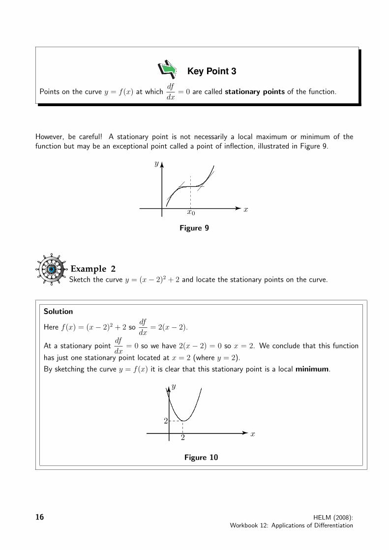
Key Point 3

Points on the curve y = f(x) at whichdf

dx= 0 are called stationary points of the function.

However, be careful! A stationary point is not necessarily a local maximum or minimum of thefunction but may be an exceptional point called a point of inflection, illustrated in Figure 9.

x

y

x0

Figure 9

Example 2

Sketch the curve y = (x− 2)2 + 2 and locate the stationary points on the curve.

Solution

Here f(x) = (x− 2)2 + 2 sodf

dx= 2(x− 2).

At a stationary pointdf

dx= 0 so we have 2(x − 2) = 0 so x = 2. We conclude that this function

has just one stationary point located at x = 2 (where y = 2).

By sketching the curve y = f(x) it is clear that this stationary point is a local minimum.

x

y

2

2

Figure 10

16 HELM (2008):


®

Task

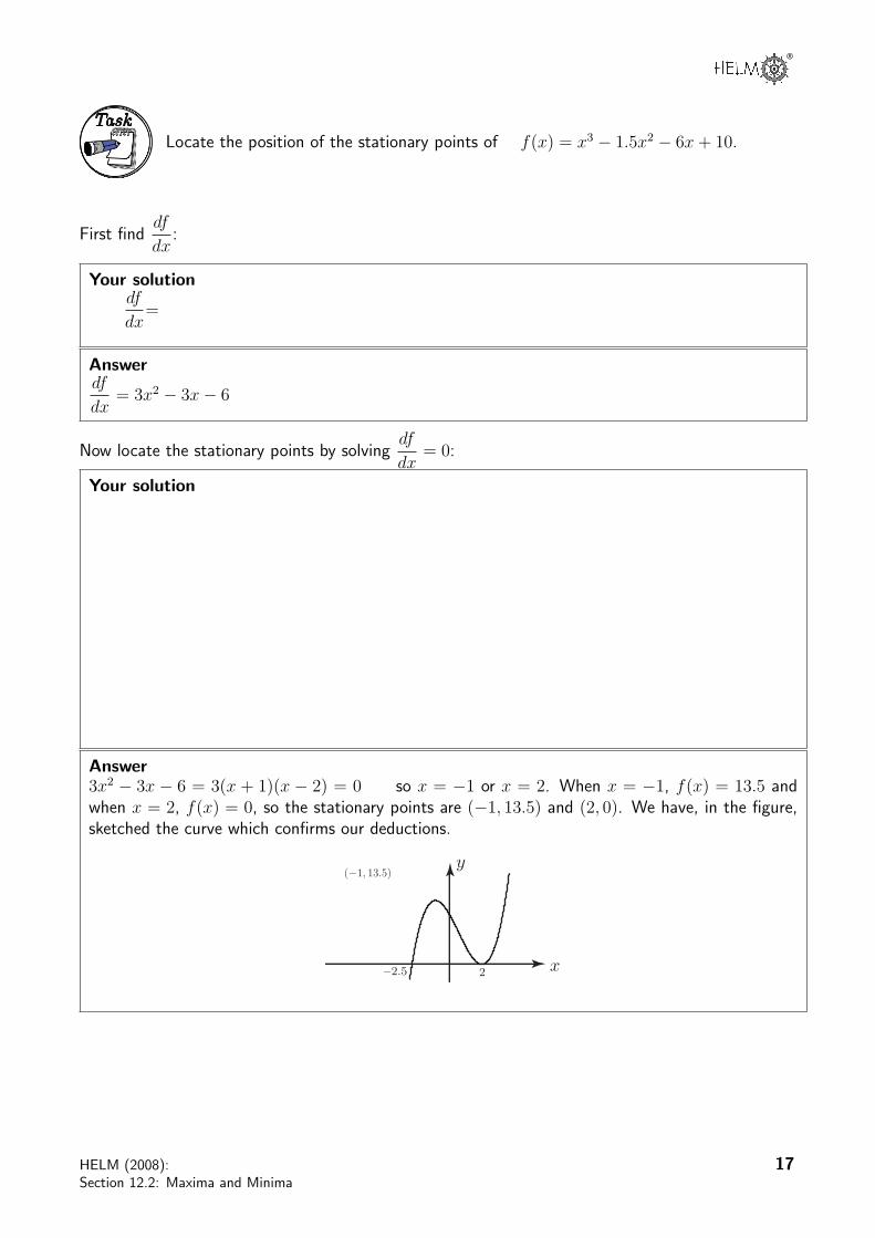
Locate the position of the stationary points of f(x) = x3 − 1.5x2 − 6x + 10.

First finddf

dx:

Your solutiondf

dx=

Answerdf

dx= 3x2 − 3x− 6

Now locate the stationary points by solvingdf

dx= 0:

Your solution

Answer3x2 − 3x − 6 = 3(x + 1)(x − 2) = 0 so x = −1 or x = 2. When x = −1, f(x) = 13.5 andwhen x = 2, f(x) = 0, so the stationary points are (−1, 13.5) and (2, 0). We have, in the figure,sketched the curve which confirms our deductions.

x

y

2!2.5

(!1, 13.5)

HELM (2008):


17

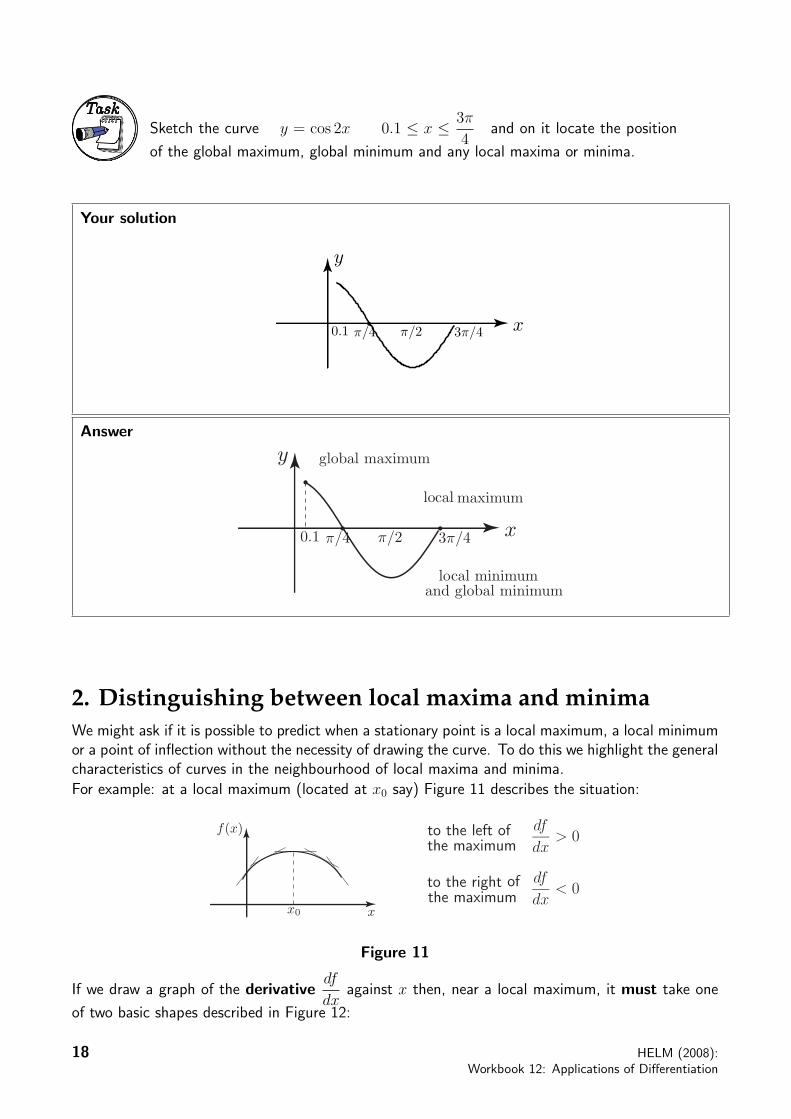
Task

Sketch the curve y = cos 2x 0.1 ≤ x ≤ 3π

4and on it locate the position

of the global maximum, global minimum and any local maxima or minima.

Your solution

x

y

0.1 !/4 !/2 3!/4

Answer

x

y global maximum

0.1 !/4 !/2 3!/4

local minimumand global minimum

local maximum

2. Distinguishing between local maxima and minima

We might ask if it is possible to predict when a stationary point is a local maximum, a local minimumor a point of inflection without the necessity of drawing the curve. To do this we highlight the generalcharacteristics of curves in the neighbourhood of local maxima and minima.For example: at a local maximum (located at x0 say) Figure 11 describes the situation:

xx0

f(x) to the left ofthe maximum

to the right ofthe maximum

df

dx> 0

df

dx< 0

Figure 11

If we draw a graph of the derivativedf

dxagainst x then, near a local maximum, it must take one

of two basic shapes described in Figure 12:

18 HELM (2008):


®

xx0xx0

!

or

(a) (b)

df

dx

df

dx

! = 180!

Figure 12

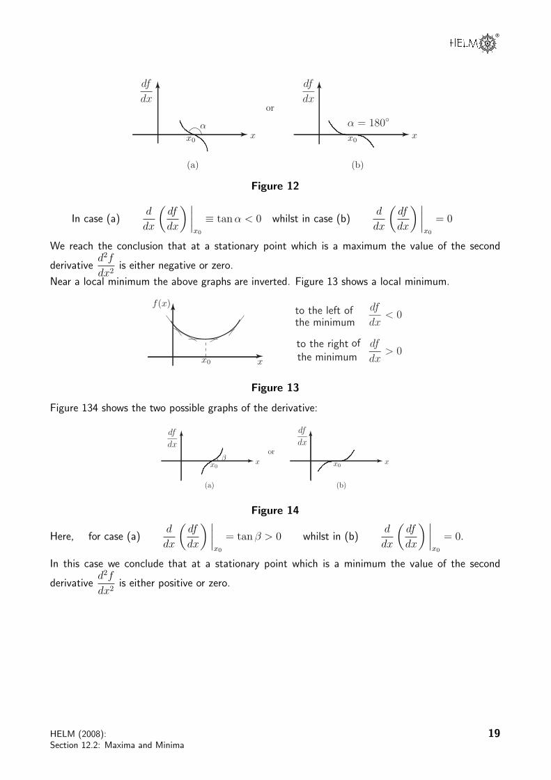
In case (a)d

dx

df

dx

x0

≡ tan α < 0 whilst in case (b)d

dx

df

dx

x0

= 0

We reach the conclusion that at a stationary point which is a maximum the value of the second

derivatived2f

dx2is either negative or zero.

Near a local minimum the above graphs are inverted. Figure 13 shows a local minimum.

xx0

f(x)to the left of

to the right

the minimum

ofthe minimum

df

dx> 0

df

dx< 0

Figure 13

Figure 134 shows the two possible graphs of the derivative:

xx0xx0

or

(a) (b)

!

df

dx

df

dx

Figure 14

Here, for case (a)d

dx

df

dx

x0

= tan β > 0 whilst in (b)d

dx

df

dx

x0

= 0.

In this case we conclude that at a stationary point which is a minimum the value of the second

derivatived2f

dx2is either positive or zero.

HELM (2008):


19

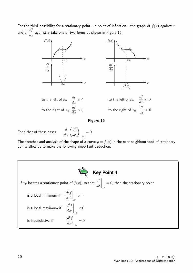
For the third possibility for a stationary point - a point of inflection - the graph of f(x) against x

and ofdf

dxagainst x take one of two forms as shown in Figure 15.

xx0

xx0

f(x)

xx0

xx0

f(x)

to the left of x0

to the right of x0

df

dx> 0

df

dx< 0

df

dx> 0

to the left of x0

to the right of x0df

dx< 0

df

dx

df

dx

Figure 15

For either of these casesd

dx

df

dx

x0

= 0

The sketches and analysis of the shape of a curve y = f(x) in the near neighbourhood of stationarypoints allow us to make the following important deduction:

Key Point 4

If x0 locates a stationary point of f(x), so thatdf

dx

x0

= 0, then the stationary point

is a local minimum ifd2f

dx2

x0

> 0

is a local maximum ifd2f

dx2

x0

< 0

is inconclusive ifd2f

dx2

x0

= 0

20 HELM (2008):


®

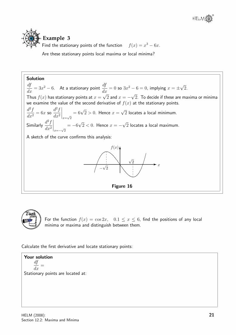
Example 3

Find the stationary points of the function f(x) = x3 − 6x.

Are these stationary points local maxima or local minima?

Solutiondf

dx= 3x2 − 6. At a stationary point

df

dx= 0 so 3x2 − 6 = 0, implying x = ±

√2.

Thus f(x) has stationary points at x =√

2 and x = −√

2. To decide if these are maxima or minimawe examine the value of the second derivative of f(x) at the stationary points.

d2f

dx2= 6x so

d2f

dx2

x=√

2

= 6√

2 > 0. Hence x =√

2 locates a local minimum.

Similarlyd2f

dx2

x=−

√2

= −6√

2 < 0. Hence x = −√

2 locates a local maximum.

A sketch of the curve confirms this analysis:

x

f(x)

!"

2

"2

Figure 16

Task

For the function f(x) = cos 2x, 0.1 ≤ x ≤ 6, find the positions of any localminima or maxima and distinguish between them.

Calculate the first derivative and locate stationary points:

Your solutiondf

dx=

Stationary points are located at:

HELM (2008):


21

Answerdf

dx= −2 sin 2x.

Hence stationary points are at values of x in the range specified for which sin 2x = 0 i.e. at 2x = π

or 2x = 2π or 2x = 3π (making sure x is within the range 0.1 ≤ x ≤ 6)

∴ Stationary points at x =π

2, x = π, x =

3π

2

Now calculate the second derivative:

Your solutiond2f

dx2=

Answerd2f

dx2= −4 cos 2x

Finally: evaluate the second derivative at each stationary points and draw appropriate conclusions:

Your solutiond2f

dx2

x=π

2

=

d2f

dx2

x=π

=

d2f

dx2

x= 3π

2

=

Answerd2f

dx2

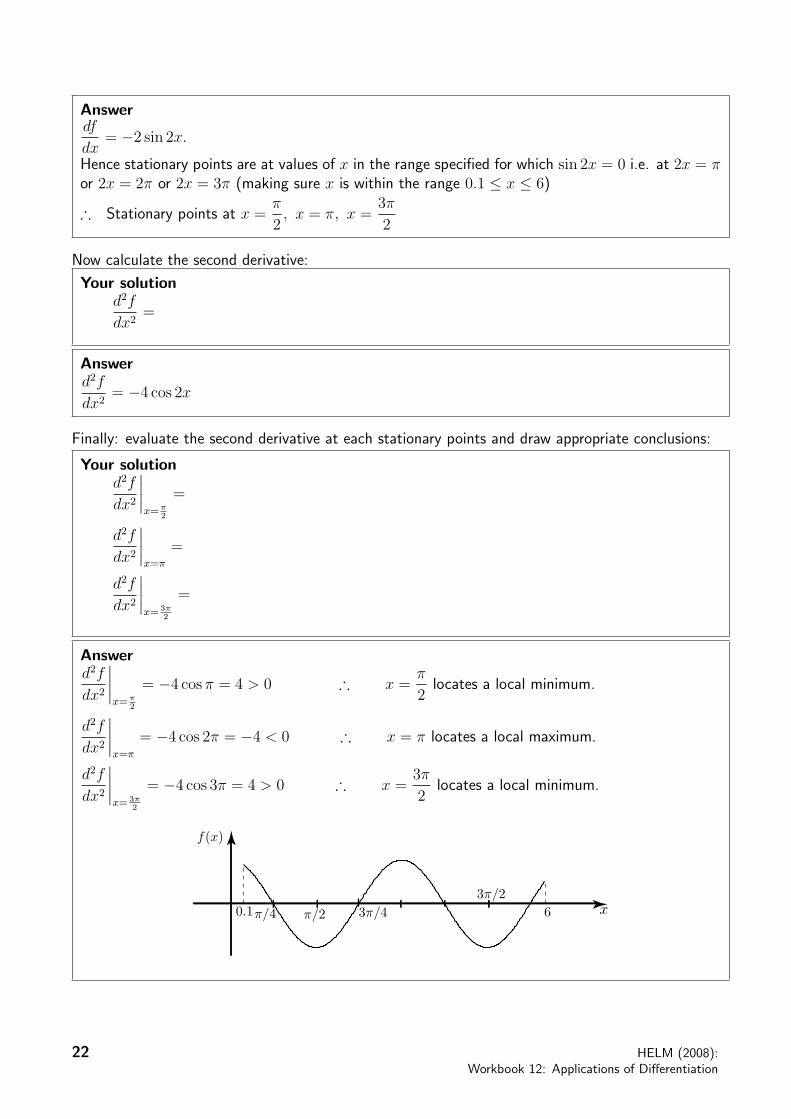
x=π

2

= −4 cos π = 4 > 0 ∴ x =π

2locates a local minimum.

d2f

dx2

x=π

= −4 cos 2π = −4 < 0 ∴ x = π locates a local maximum.

d2f

dx2

x= 3π

2

= −4 cos 3π = 4 > 0 ∴ x =3π


x0.1!/4 !/2 3!/43!/2

6

f(x)

22 HELM (2008):


®

Task

Determine the local maxima and/or minima of the function y = x4 − 1

3x

3

First obtain the positions of the stationary points:

Your solution

f(x) = x4 − 1

3x3 df

dx=

Thusdf

dx= 0 when:

Answerdf

dx= 4x3 − x2 = x2(4x− 1)

df

dx= 0 when x = 0 or when x = 1/4

Now obtain the value of the second derivatives at the stationary points:

Your solutiond2f

dx2= ∴ d2f

dx2

x=0

=

d2f

dx2

x=1/4

=

Answerd2f

dx2= 12x2 − 2x

d2f

dx2

x=0

= 0, which is inconclusive.

d2f

dx2

x=1/4

=12

16− 1

2=

1

4> 0 Hence x =

1


Using this analysis we cannot decide whether the stationary point at x = 0 is a local maximum,

minimum or a point of inflection. However, just to the left of x = 0 the value ofdf

dx(which equals

x2(4x − 1)) is negative whilst just to the right of x = 0 the value ofdf

dxis negative again. Hence

the stationary point at x = 0 is a point of inflection. This is confirmed by sketching the curve asin Figure 17.

x

f(x)

1/4

! 0.0013

Figure 17

HELM (2008):


23

Task

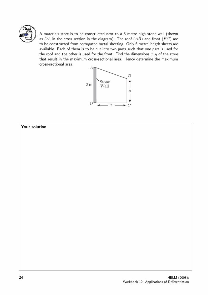
A materials store is to be constructed next to a 3 metre high stone wall (shownas OA in the cross section in the diagram). The roof (AB) and front (BC) areto be constructed from corrugated metal sheeting. Only 6 metre length sheets areavailable. Each of them is to be cut into two parts such that one part is used forthe roof and the other is used for the front. Find the dimensions x, y of the storethat result in the maximum cross-sectional area. Hence determine the maximumcross-sectional area.

xO

B

A

Stone3 m Wall

y

C

Your solution

24 HELM (2008):


®

AnswerNote that the store has the shape of a trapezium. So the cross-sectional area (A) of the store isgiven by the formula: Area = average length of parallel sides × distance between parallel sides:

A =1

2(y + 3)x (1)

The lengths x and y are related through the fact that AB + BC = 6, where BC = y andAB =

x2 + (3− y)2. Hence

x2 + (3− y)2 + y = 6. This equation can be rearranged in the

following way:

x2 + (3− y)2 = 6− y ⇔ x2 + (3− y)2 = (6− y)2 i.e. x2 + 9− 6y + y2 = 36− 12y + y2

which implies that x2 + 6y = 27 (2)

It is necessary to eliminate either x or y from (1) and (2) to obtain an equation in a single variable.Using y instead of x as the variable will avoid having square roots appearing in the expression forthe cross-sectional area. Hence from Equation (2)

y =27− x2

6(3)

Substituting for y from Equation (3) into Equation (1) gives

A =1

2

27− x2

6+ 3

x =

1

2

27− x2 + 18

6

x =

1

12

45x− x

3

(4)

To find turning points, we evaluatedA

dxfrom Equation (4) to get

dA

dx=

1

12(45− 3x2) (5)

Solving the equationdA

dx= 0 gives

1

12(45− 3x2) = 0⇒ 45− 3x2 = 0

Hence x = ±√

15 = ± 3.8730. Only x > 0 is of interest, so

x =√

15 = 3.87306 (6)

gives the required turning point.

Check: Differentiating Equation (5) and using the positive x solution (6) gives

d2A

dx2= −6x

12= −x

2= −3.8730

2< 0

Since the second derivative is negative then the cross-sectional area is a maximum. This is the onlyturning point identified for A > 0 and it is identified as a maximum. To find the corresponding

value of y, substitute x = 3.8730 into Equation (3) to get y =27− 3.87302

6= 2.0000

So the values of x and y that yield the maximum cross-sectional area are 3.8730 m and 2.00000m respectively. To find the maximum cross-sectional area, substitute for x = 3.8730 into Equation(5) to get

A =1

2(45× 3.8730− 3.87303) = 9.6825

So the maximum cross-sectional area of the store is 9.68 m2 to 2 d.p.

HELM (2008):


25

Task

Equivalent resistance in an electrical circuit

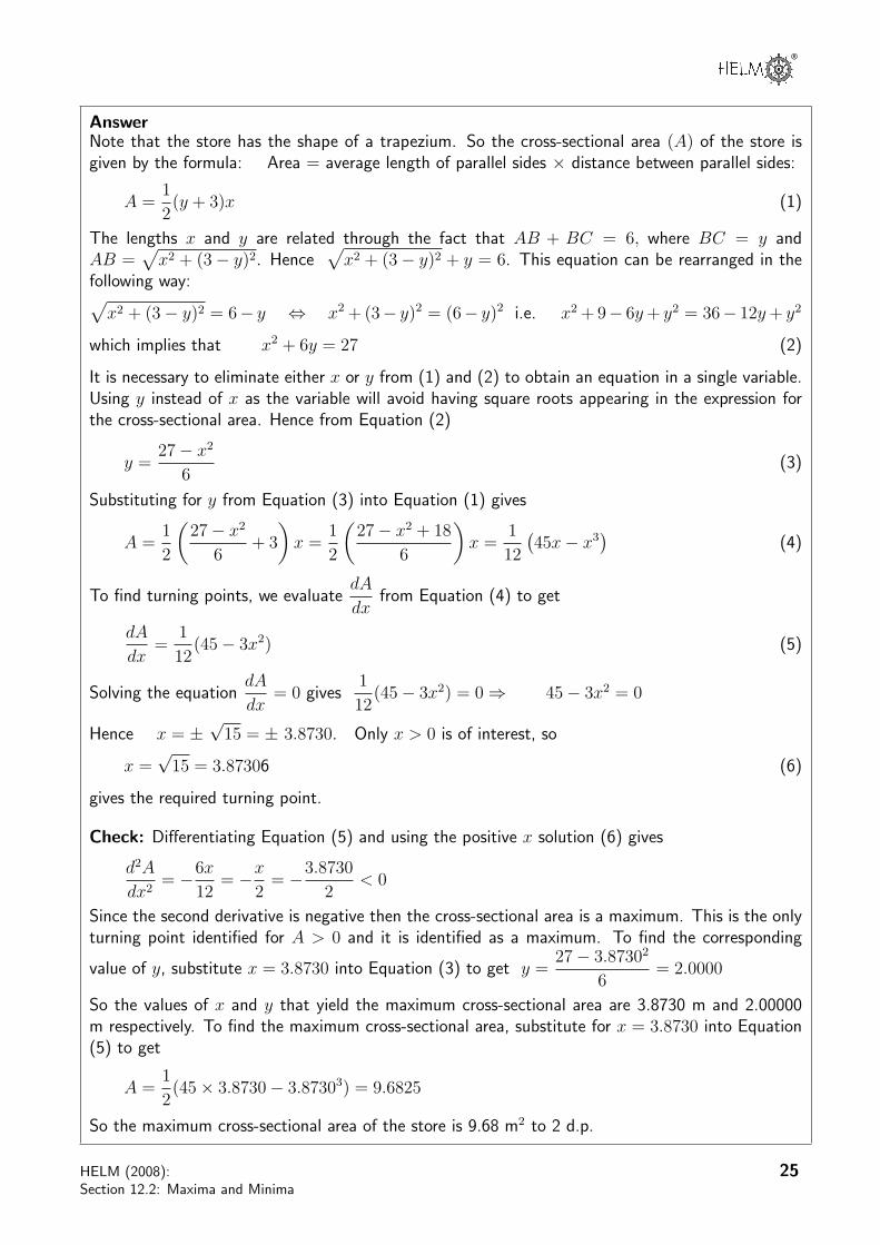
Current distributes itself in the wires of an electrical circuit so as to minimise the total powerconsumption i.e. the rate at which heat is produced. The power (p) dissipated in an electrical circuitis given by the product of voltage (v) and current (i) flowing in the circuit, i.e. p = vi. The voltageacross a resistor is the product of current and resistance (r). This means that the power dissipatedin a resistor is given by p = i2r.

Suppose that an electrical circuit contains three resistors r1, r2, r3 and i1 represents the currentflowing through both r1 and r2, and that (i − i1) represents the current flowing through r3 (seediagram):

R1 R2

R3i1

i

i!i1

(a) Write down an expression for the power dissipated in the circuit:

Your solution

Answer

p = i21r1 + i21r2 + (i− i1)2r3

(b) Show that the power dissipated is a minimum when i1 =r3

r1 + r2 + r3i :

Your solution

26 HELM (2008):


®

AnswerDifferentiate result (a) with respect to i1:

dp

di1= 2i1r1 + 2i1r2 + 2(i− i1)(−1)r3

= 2i1(r1 + r2 + r3)− 2ir3

This is zero when

i1 =r3

r1 + r2 + r3i.

To check if this represents a minimum, differentiate again:

d2p

di21

= 2(r1 + r2 + r3)

This is positive, so the previous result represents a minimum.

(c) If R is the equivalent resistance of the circuit, i.e. of r1, r2 and r3, for minimum power dissipationand the corresponding voltage V across the circuit is given by V = iR = i1(r1 + r2), show that

R =(r1 + r2)r3

r1 + r2 + r3.

Your solution

AnswerSubstituting for i1 in iR = i1(r1 + r2) gives

iR =r3(r1 + r2)

r1 + r2 + r3i.

So

R =(r1 + r2)r3

r1 + r2 + r3.

Note In this problem R1 and R2 could be replaced by a single resistor. However, treating them asseparate allows the possibility of considering more general situations (variable resistors or temperaturedependent resistors).

HELM (2008):


27


Water wheel efficiency

Introduction

A water wheel is constructed with symmetrical curved vanes of angle of curvature θ. Assuming thatfriction can be taken as negligible, the efficiency, η, i.e. the ratio of output power to input power, iscalculated as

η =2(V − v)(1 + cos θ)v

V 2

where V is the velocity of the jet of water as it strikes the vane, v is the velocity of the vane in thedirection of the jet and θ is constant. Find the ratio, v/V , which gives maximum efficiency and findthe maximum efficiency.

Mathematical statement of the problem

We need to express the efficiency in terms of a single variable so that we can find the maximumvalue.

Efficiency =2(V − v)(1 + cos θ)v

V 2= 2

1− v

V

v

V(1 + cos θ).

Let η = Efficiency and x =v

Vthen η = 2x(1− x)(1 + cos θ).

We must find the value of x which maximises η and we must find the maximum value of η. To do

this we differentiate η with respect to x and solvedη

dx= 0 in order to find the stationary points.

Mathematical analysis

Now η = 2x(1− x)(1 + cos θ) = (2x− 2x2)(1 + cos θ)

Sodη

dx= (2− 4x)(1 + cos θ)

Nowdη

dx= 0⇒ 2− 4x = 0⇒ x =

1

2and the value of η when x =

1

2is

η = 2

1

2

1− 1

2

(1 + cos θ) =

1

2(1 + cos θ).

This is clearly a maximum not a minimum, but to check we calculated2η

dx2= −4(1 + cos θ) which is

negative which provides confirmation.

Interpretation

Maximum efficiency occurs whenv

V=

1

2and the maximum efficiency is given by

η =1

2(1 + cos θ).

28 HELM (2008):


®


Refraction

The problem

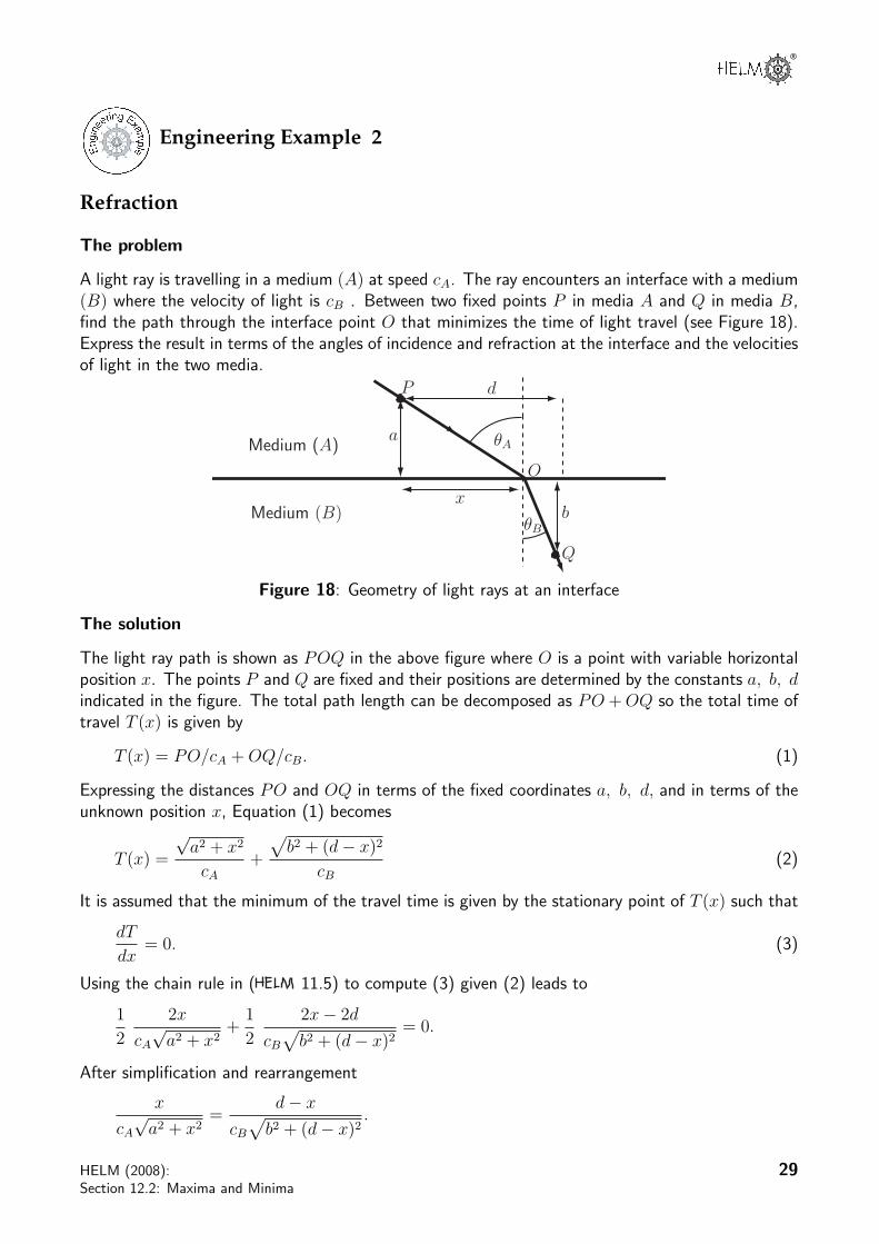
A light ray is travelling in a medium (A) at speed cA. The ray encounters an interface with a medium(B) where the velocity of light is cB . Between two fixed points P in media A and Q in media B,find the path through the interface point O that minimizes the time of light travel (see Figure 18).Express the result in terms of the angles of incidence and refraction at the interface and the velocitiesof light in the two media.

a

d

!A

O

xb

!B

Q

P

Medium (A)

Medium (B)

Figure 18: Geometry of light rays at an interface

The solution

The light ray path is shown as POQ in the above figure where O is a point with variable horizontalposition x. The points P and Q are fixed and their positions are determined by the constants a, b, d

indicated in the figure. The total path length can be decomposed as PO + OQ so the total time oftravel T (x) is given by

T (x) = PO/cA + OQ/cB. (1)

Expressing the distances PO and OQ in terms of the fixed coordinates a, b, d, and in terms of theunknown position x, Equation (1) becomes

T (x) =

√a2 + x2

cA+

b2 + (d− x)2

cB(2)

It is assumed that the minimum of the travel time is given by the stationary point of T (x) such that

dT

dx= 0. (3)

Using the chain rule in ( 11.5) to compute (3) given (2) leads to

1

2

2x

cA

√a2 + x2

+1

2

2x− 2d

cB

b2 + (d− x)2

= 0.

After simplification and rearrangement

x

cA

√a2 + x2

=d− x

cB

b2 + (d− x)2

.

HELM (2008):


29

Using the definitions sin θA =x√

a2 + x2and sin θB =

d− xb2 + (d− x)2

this can be written as

sin θA

cA=

sin θB

cB. (4)

Note that θA andθB are the incidence angles measured from the interface normal as shown in thefigure. Equation (4) can be expressed as

sin θA

sin θB=

cA

cB

which is the well-known law of refraction for geometrical optics and applies to many other kinds

of waves. The ratiocA

cBis a constant called the refractive index of medium (B) with respect to

medium (A).

30 HELM (2008):


®


Fluid power transmission

Introduction

Power transmitted through fluid-filled pipes is the basis of hydraulic braking systems and otherhydraulic control systems. Suppose that power associated with a piston motion at one end of apipeline is transmitted by a fluid of density ρ moving with positive velocity V along a cylindricalpipeline of constant cross-sectional area A. Assuming that the loss of power is mainly attributable tofriction and that the friction coefficient f can be taken to be a constant, then the power transmitted,P is given by

P = ρgA(hV − cV3),

where g is the acceleration due to gravity and h is the head which is the height of the fluid above

some reference level (= the potential energy per unit weight of the fluid). The constant c =4fl

2gd

where l is the length of the pipe and d is the diameter of the pipe. The power transmission efficiencyis the ratio of power output to power input.

Problem in words

Assuming that the head of the fluid, h, is a constant find the value of the fluid velocity, V , whichgives a maximum value for the output power P . Given that the input power is Pi = ρgAV h, findthe maximum power transmission efficiency obtainable.

Mathematical statement of the problemWe are given that P = ρgA(hV −cV 3) and we want to find its maximum value and hence maximumefficiency.

To find stationary points for P we solvedP

dV= 0.

To classify the stationary points we can differentiate again to find the value ofd2P

dV 2at each stationary

point and if this is negative then we have found a local maximum point. The maximum efficiencyis given by the ratio P/Pi at this value of V and where Pi = ρgAV h. Finally we should check thatthis is the only maximum in the range of P that is of interest.

Mathematical analysisP = ρgA(hV − cV 3)

dP

dV= ρgA(h− 3cV 2)

dP

dV= 0 gives ρgA(h− 3cV 2) = 0

⇒ V 2 =h

3c⇒ V = ±

h

3cand as V is positive ⇒ V =

h

3c.

HELM (2008):


31

To show this is a maximum we differentiatedP

dVagain giving

d2P

dV 2= ρgA(−6cV ). Clearly this is

negative, or zero if V = 0. Thus V =

h

3cgives a local maximum value for P .

We note that P = 0 when E = ρgA(hV − cV 3) = 0, i.e. when hV − cV 3 = 0, so V = 0 or

V =

h

C. So the maximum at V =

h

3Cis the only max in this range between 0 and V =

h

C.

The efficiency E, is given by (input power/output power), so here

E =ρgA(hV − cV 3)

ρgAV h= 1− cV 2

h

At V =

h

3cthen V 2 =

h

3cand therefore E = 1−

ch

3cc

= 1− 1

3=

2

3or 662

3%.

Interpretation

Maximum power transmitted through the fluid when the velocity V =

h

3cand the maximum

efficiency is 6623%. Note that this result is independent of the friction and the maximum efficiency

is independent of the velocity and (static) pressure in the pipe.

420 3

2.215

1.81 h = 3

P (V )

h = 2

1

4

2

3

1

m

m

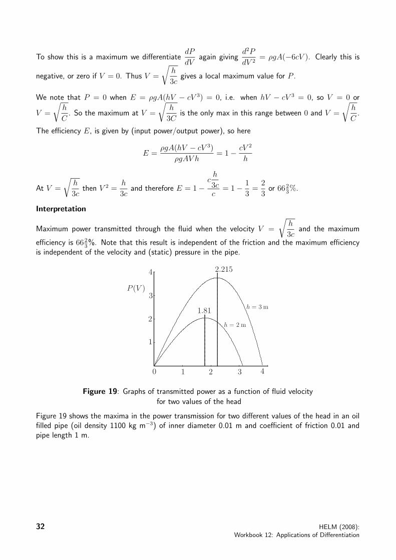
Figure 19: Graphs of transmitted power as a function of fluid velocityfor two values of the head

Figure 19 shows the maxima in the power transmission for two different values of the head in an oilfilled pipe (oil density 1100 kg m−3) of inner diameter 0.01 m and coefficient of friction 0.01 andpipe length 1 m.

32 HELM (2008):


®


Crank used to drive a piston

Introduction

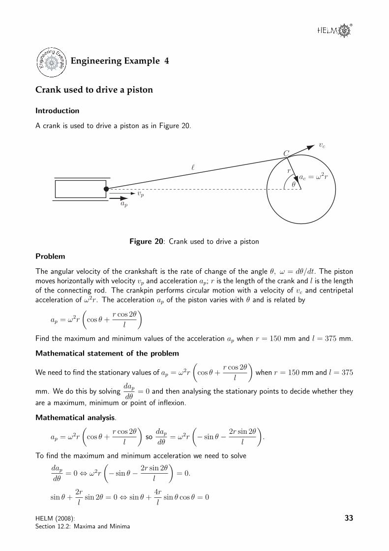
A crank is used to drive a piston as in Figure 20.

ap

vp

vc

! r

"

C

ac = #2r

Figure 20: Crank used to drive a piston

Problem

The angular velocity of the crankshaft is the rate of change of the angle θ, ω = dθ/dt. The pistonmoves horizontally with velocity vp and acceleration ap; r is the length of the crank and l is the lengthof the connecting rod. The crankpin performs circular motion with a velocity of vc and centripetalacceleration of ω2r. The acceleration ap of the piston varies with θ and is related by

ap = ω2r

cos θ +

r cos 2θ

l

Find the maximum and minimum values of the acceleration ap when r = 150 mm and l = 375 mm.

Mathematical statement of the problem

We need to find the stationary values of ap = ω2r

cos θ +

r cos 2θ

l

when r = 150 mm and l = 375

mm. We do this by solvingdap

dθ= 0 and then analysing the stationary points to decide whether they

are a maximum, minimum or point of inflexion.

Mathematical analysis.

ap = ω2r

cos θ +

r cos 2θ

l

so

dap

dθ= ω2r

− sin θ − 2r sin 2θ

l

.

To find the maximum and minimum acceleration we need to solve

dap

dθ= 0⇔ ω2r

− sin θ − 2r sin 2θ

l

= 0.

sin θ +2r

lsin 2θ = 0⇔ sin θ +

4r

lsin θ cos θ = 0

HELM (2008):


33

⇔ sin θ

1 +

4r

lcos θ

= 0

⇔ sin θ = 0 or cos θ = − l

4rand as r = 150 mm and l = 375 mm

⇔ sin θ = 0 or cos θ = −5

8

CASE 1: sinsinsin θθθ === 000

If sin θ = 0 then θ = 0 or θ = π. If θ = 0 then cos θ = cos 2θ = 1

so ap = ω2r

cos θ +

r cos 2θ

l

= ω2r

1 +

r

l

= ω2r

1 +

2

5

=

7

5ω2r

If θ = π then cos θ = −1, cos 2θ = 1 so

ap = ω2r

cos θ +

r cos 2θ

l

= ω2r

−1 +

r

l

= ω2r

−1 +

2

5

= −3

5ω2r

In order to classify the stationary points, we differentiatedap

dθwith respect to θ to find the second

derivative:

d2ap

dθ2= ω2r

− cos θ − 4r cos 2θ

l

= −ω2r

cos θ +

4r cos 2θ

l

At θ = 0 we getd2ap

dθ2= −ω2r

1 +

4r

l

which is negative.

So θ = 0 gives a maximum value and ap =7

5ω2r is the value at the maximum.

At θ = π we getd2ap

dθ2= −ω2r

−1 +

4

l

= −ω2r

3

5

which is negative.

So θ = π gives a maximum value and ap = −3

5ω2r

CASE 2: coscoscos θθθ ===−−−555

888

If cos θ = −5

8then cos 2θ = 2 cos2 θ − 1 = 2

5

8

2

− 1 so cos 2θ = − 7

32.

ap = ω2r

cos θ +

r cos 2θ

l

= ω2r

−5

8+− 7

32× 2

5

=

57

80ω2r.

At cos θ = −5

8we get

d2ap

dθ2= ω2r

− cos θ − 4r cos 2θ

l

= ω2r

5

8+

4r

l

7

32

which is positive.

So cos θ = −5

8gives a minimum value and ap = −57

80ω2r

Thus the values of ap at the stationary points are:-

7

5ω2r (maximum), −3

5ω2r (maximum) and −57

80ω2r (minimum).

34 HELM (2008):


®

So the overall maximum value is 1.4ω2r = 0.21ω2 and the minimum value is−0.7125ω2r = −0.106875ω2 where we have substituted r = 150 mm (= 0.15 m) and l = 375 mm(= 0.375 m).

Interpretation

The maximum acceleration occurs when θ = 0 and ap = 0.21ω2.

The minimum acceleration occurs when cos θ = −5

8and ap = −0.106875ω2.

Exercises

1. Locate the stationary points of the following functions and distinguish among them as maxima,minima and points of inflection.

(a) f(x) = x− ln |x|. [Rememberd

dx(ln |x|) =

1

x]

(b) f(x) = x3

(c) f(x) =(x− 1)

(x + 1)(x− 2)− 1 < x < 2

2. A perturbation in the temperature of a stream leaving a chemical reactor follows a decayingsinusoidal variation, according to

T (t) = 5exp(−at) sin(ωt)

where a and ω are positive constants.

(a) Sketch the variation of temperature with time.

(b) By examining the behaviour ofdT

dt, show that the maximum temperatures occur at times

oftan−1(

ω

a) + 2πn

/ω.

HELM (2008):


35

Answers

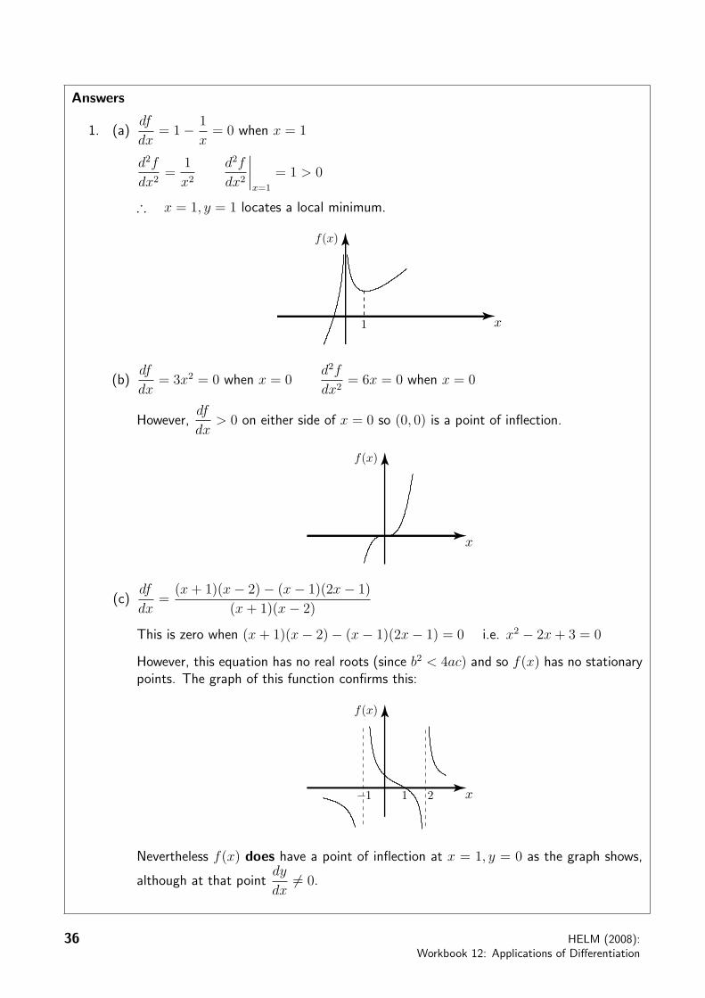
1. (a)df

dx= 1− 1

x= 0 when x = 1

d2f

dx2=

1

x2

d2f

dx2

x=1

= 1 > 0

∴ x = 1, y = 1 locates a local minimum.

x

f(x)

1

(b)df

dx= 3x2 = 0 when x = 0

d2f

dx2= 6x = 0 when x = 0

However,df

dx> 0 on either side of x = 0 so (0, 0) is a point of inflection.

x

f(x)

(c)df

dx=

(x + 1)(x− 2)− (x− 1)(2x− 1)

(x + 1)(x− 2)

This is zero when (x + 1)(x− 2)− (x− 1)(2x− 1) = 0 i.e. x2 − 2x + 3 = 0

However, this equation has no real roots (since b2 < 4ac) and so f(x) has no stationarypoints. The graph of this function confirms this:

x

f(x)

!1 1 2

Nevertheless f(x) does have a point of inflection at x = 1, y = 0 as the graph shows,

although at that pointdy

dx= 0.

36 HELM (2008):


®

Answer

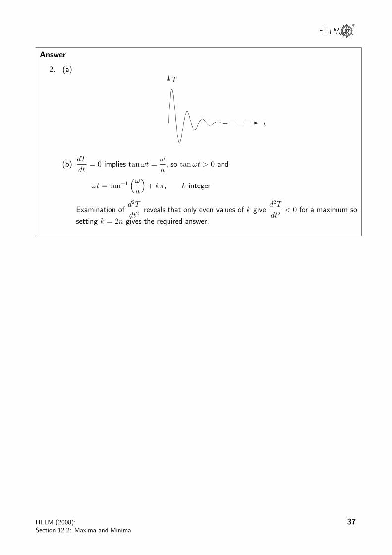
2. (a)T

t

(b)dT

dt= 0 implies tan ωt =

ω

a, so tan ωt > 0 and

ωt = tan−1

ω

a

+ kπ, k integer

Examination ofd2T

dt2reveals that only even values of k give

d2T

dt2< 0 for a maximum so

setting k = 2n gives the required answer.

HELM (2008):


37

Tangents and Normals

12.1

Introduction

In this Section we see how the equations of the tangent line and the normal line at a particular pointon the curve y = f(x) can be obtained. The equations of tangent and normal lines are often writtenas

y = mx + c, y = nx + d

respectively. We shall show that the product of their gradients m and n is such that mn is −1 whichis the condition for perpendicularity.

Prerequisites


• be able to differentiate standard functions

• understand the geometrical interpretation ofa derivative

• know the trigonometric expansions ofsin(A + B), cos(A + B)

Learning Outcomes


• obtain the condition that two given lines areperpendicular

• obtain the equation of the tangent line to acurve

• obtain the equation of the normal line to acurve

2 HELM (2008):


®

1. Perpendicular lines

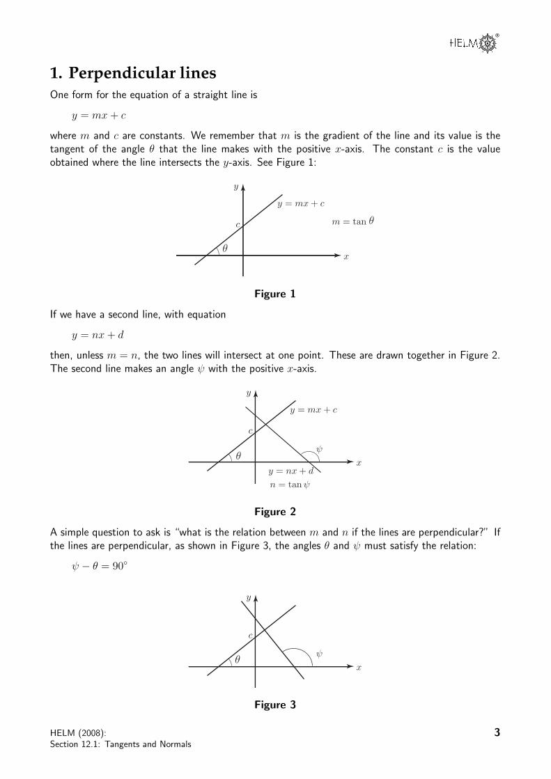
One form for the equation of a straight line is

y = mx + c

where m and c are constants. We remember that m is the gradient of the line and its value is thetangent of the angle θ that the line makes with the positive x-axis. The constant c is the valueobtained where the line intersects the y-axis. See Figure 1:

y = mx + c

m = tan

x

y

c

!

!

Figure 1

If we have a second line, with equation

y = nx + d

then, unless m = n, the two lines will intersect at one point. These are drawn together in Figure 2.The second line makes an angle ψ with the positive x-axis.

y = mx + c

x

y

c

y = nx + d

n = tan !

!!

Figure 2

A simple question to ask is “what is the relation between m and n if the lines are perpendicular?” Ifthe lines are perpendicular, as shown in Figure 3, the angles θ and ψ must satisfy the relation:

ψ − θ = 90

x

y

c

!!

Figure 3

HELM (2008):

Section 12.1: Tangents and Normals

3

This is true since the angles in a triangle add up to 180. According to the figure the three anglesare 90, θ and 180 − ψ. Therefore

180 = 90 + θ + (180 − ψ) implying ψ − θ = 90

In this special case that the lines are perpendicular or normal to each other the relation betweenthe gradients m and n is easily obtained. In this deduction we use the following basic trigonometricrelations and identities:

sin(A−B) ≡ sin A cos B − cos A sin B cos(A−B) ≡ cos A cos B + sin A sin B

tan A ≡ sin A

cos Asin 90 = 1 cos 90 = 0

Now

m = tan θ

= tan(ψ − 90o) (see Figure 3)

=sin(ψ − 90o)

cos(ψ − 90o)

=− cos ψ

sin ψ= − 1

tan ψ= − 1

nSo mn = −1

Key Point 1Two straight lines y = mx + c, y = nx + d are perpendicular if

m = − 1

nor equivalently mn = −1

This result assumes that neither of the lines are parallel to the x-axis or to the y-axis, as in suchcases one gradient will be zero and the other infinite.

Exercise

Which of the following pairs of lines are perpendicular?

(a) y = −x + 1, y = x + 1

(b) y + x− 1 = 0, y + x− 2 = 0

(c) 2y = 8x + 3, y = −0.25x− 1

Answer

(a) perpendicular (b) not perpendicular (c) perpendicular

4 HELM (2008):


®

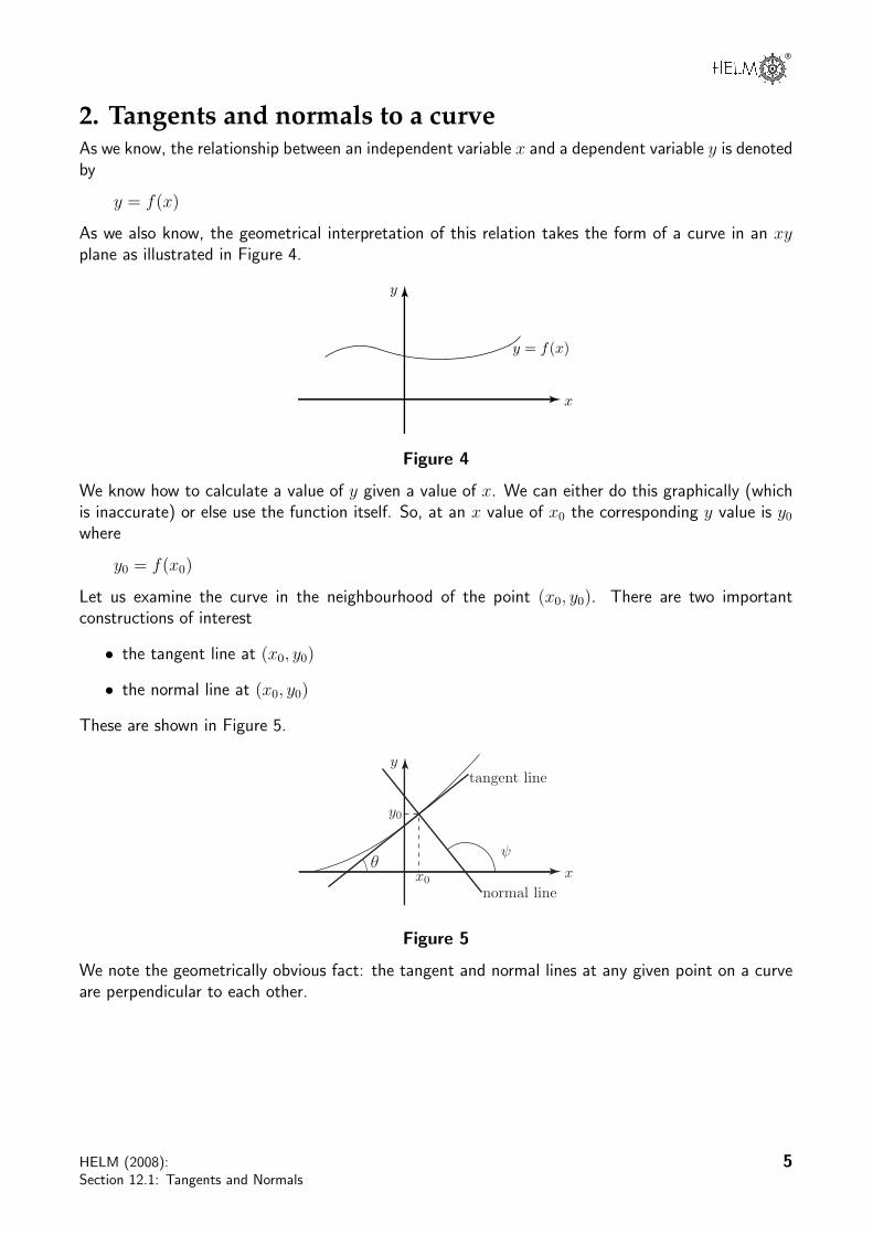
2. Tangents and normals to a curve

As we know, the relationship between an independent variable x and a dependent variable y is denotedby

y = f(x)

As we also know, the geometrical interpretation of this relation takes the form of a curve in an xyplane as illustrated in Figure 4.

x

y

y = f(x)

Figure 4

We know how to calculate a value of y given a value of x. We can either do this graphically (whichis inaccurate) or else use the function itself. So, at an x value of x0 the corresponding y value is y0

where

y0 = f(x0)

Let us examine the curve in the neighbourhood of the point (x0, y0). There are two importantconstructions of interest

• the tangent line at (x0, y0)

• the normal line at (x0, y0)

These are shown in Figure 5.

x

y

!

tangent line

normal linex0

y0

!

Figure 5

We note the geometrically obvious fact: the tangent and normal lines at any given point on a curveare perpendicular to each other.

HELM (2008):


5

Task

The curve y = x2 is drawn below. On this graph draw the tangent line and thenormal line at the point (x0 = 1, y0 = 1):

Your solution

x

y

1

1

Answer

x

y

!

tangent line normal line1

1 !

From your graph, estimate the values of θ and ψ in degrees. (You will need a protractor.)

Your solution

θ ψ

Answer

θ ≈ 63.4o ψ ≈ 153.4o

Returning to the curve y = f(x) : we know, from the geometrical interpretation of the derivativethat

df

dx

x0

= tan θ

(the notationdf

dx

x0

means evaluatedf

dxat the value x = x0)

Here θ is the angle the tangent line to the curve y = f(x) makes with the positive x-axis. This ishighlighted in Figure 6:

x

y

x0

y = f(x)

!

df

dx

!!!!x0

= tan !

Figure 6

6 HELM (2008):


®

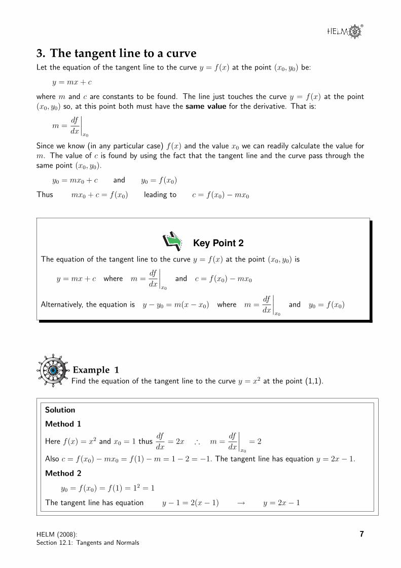
3. The tangent line to a curve

Let the equation of the tangent line to the curve y = f(x) at the point (x0, y0) be:

y = mx + c

where m and c are constants to be found. The line just touches the curve y = f(x) at the point(x0, y0) so, at this point both must have the same value for the derivative. That is:

m =df

dx

x0

Since we know (in any particular case) f(x) and the value x0 we can readily calculate the value form. The value of c is found by using the fact that the tangent line and the curve pass through thesame point (x0, y0).

y0 = mx0 + c and y0 = f(x0)

Thus mx0 + c = f(x0) leading to c = f(x0)−mx0

Key Point 2The equation of the tangent line to the curve y = f(x) at the point (x0, y0) is

y = mx + c where m =df

dx

x0

and c = f(x0)−mx0

Alternatively, the equation is y − y0 = m(x− x0) where m =df

dx

x0

and y0 = f(x0)

Example 1

Find the equation of the tangent line to the curve y = x2 at the point (1,1).

Solution

Method 1

Here f(x) = x2 and x0 = 1 thusdf

dx= 2x ∴ m =

df

dx

x0

= 2

Also c = f(x0)−mx0 = f(1)−m = 1− 2 = −1. The tangent line has equation y = 2x− 1.

Method 2

y0 = f(x0) = f(1) = 12 = 1

The tangent line has equation y − 1 = 2(x− 1) → y = 2x− 1

HELM (2008):


7

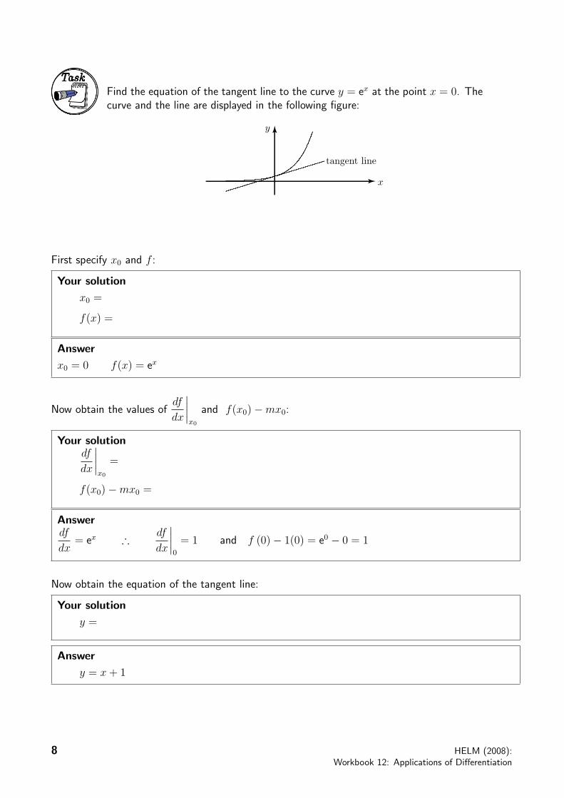
Task

Find the equation of the tangent line to the curve y = ex at the point x = 0. Thecurve and the line are displayed in the following figure:

x

y

tangent line

First specify x0 and f :

Your solution

x0 =

f(x) =

Answer

x0 = 0 f(x) = ex

Now obtain the values ofdf

dx

x0

and f(x0)−mx0:

Your solutiondf

dx

x0

=

f(x0)−mx0 =

Answerdf

dx= ex ∴ df

dx

0

= 1 and f (0)− 1(0) = e0 − 0 = 1

Now obtain the equation of the tangent line:

Your solution

y =

Answer

y = x + 1

8 HELM (2008):


®

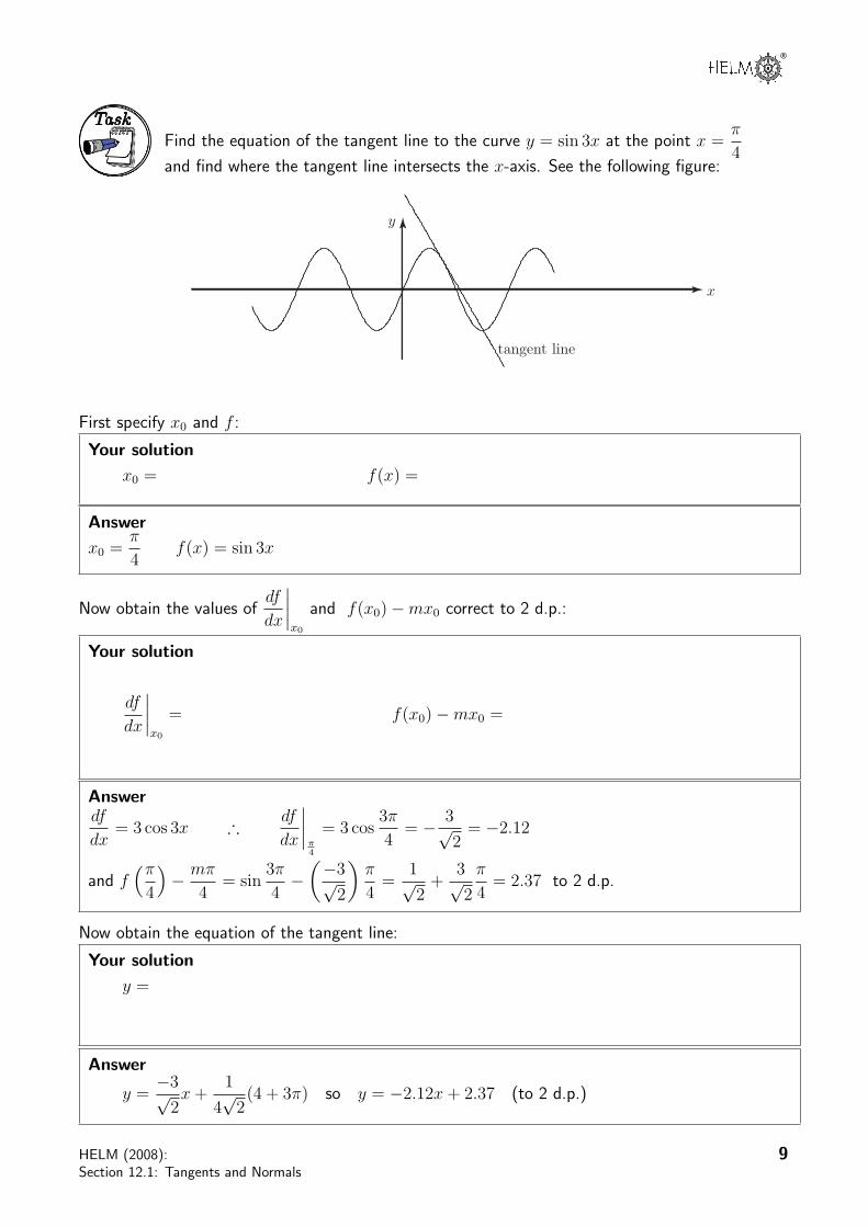
Task

Find the equation of the tangent line to the curve y = sin 3x at the point x =π

4and find where the tangent line intersects the x-axis. See the following figure:

x

y

tangent line

First specify x0 and f :

Your solution

x0 = f(x) =

Answer

x0 =π

4f(x) = sin 3x

Now obtain the values ofdf

dx

x0

and f(x0)−mx0 correct to 2 d.p.:

Your solution

df

dx

x0

= f(x0)−mx0 =

Answerdf

dx= 3 cos 3x ∴ df

dx

π4

= 3 cos3π

4= − 3√

2= −2.12

and fπ

4

− mπ

4= sin

3π

4−

−3√

2

π

4=

1√2

+3√2

π

4= 2.37 to 2 d.p.

Now obtain the equation of the tangent line:

Your solution

y =

Answer

y =−3√

2x +

1

4√

2(4 + 3π) so y = −2.12x + 2.37 (to 2 d.p.)

HELM (2008):


9

Where does the line intersect the x-axis?

Your solution

x =

Answer

When y = 0 ∴ −2.12x + 2.37 = 0 ∴ x = 1.12 to 2 d.p.

4. The normal line to a curve

We have already noted that, at any point (x0, y0) on a curve y = f(x), the tangent and normal linesare perpendicular. Thus if the equations of the tangent and normal lines are, respectively

y = mx + c y = nx + d

then m = − 1

nor, equivalently n = − 1

m.

We have also noted, for the tangent line

m =df

dx

x0

so n can easily be obtained. To find d, we again use the fact that the normal line y = nx + d andthe curve have a point in common:

y0 = nx0 + d and y0 = f(x0)

so nx0 + d = f(x0) leading to d = f(x0)− nx0.

Task

Find the equation of the normal line to curve y = sin 3x at the point x =π

4.

[The equation of the tangent line was found in the previous Task.]

First find the value of m:

Your solution

m =df

dx

π4

=

Answer

m =−3√

2

Hence find the value of n:

Your solution

n =

Answer

nm = −1 ∴ n =

√2

3

10 HELM (2008):


®

The equation of the normal line is y =

√2

3x + d. Now find the value of d to 2 d.p.. (Remember the

normal line must pass through the curve at the point x =π

4.)

Your solution

Answer√2

3

π

4

+ d = sin

π

4∴ d =

1√2−√

2

3

π

4 0.34

Now obtain the equation of the normal line to 2 d.p.:

Your solution

y =

Answery = 0.47x + 0.34. The curve and the normal line are shown in the following figure:

x

y normal line

Task

Find the equation of the normal line to the curve y = x3 at x = 1.

First find f(x), x0,df

dx

x0

, m, n:

Your solution

Answer

f(x) = x3, x0 = 1,df

dx

1

= 3x2

1

= 3 ∴ m = 3 and n = −1

3

HELM (2008):


11

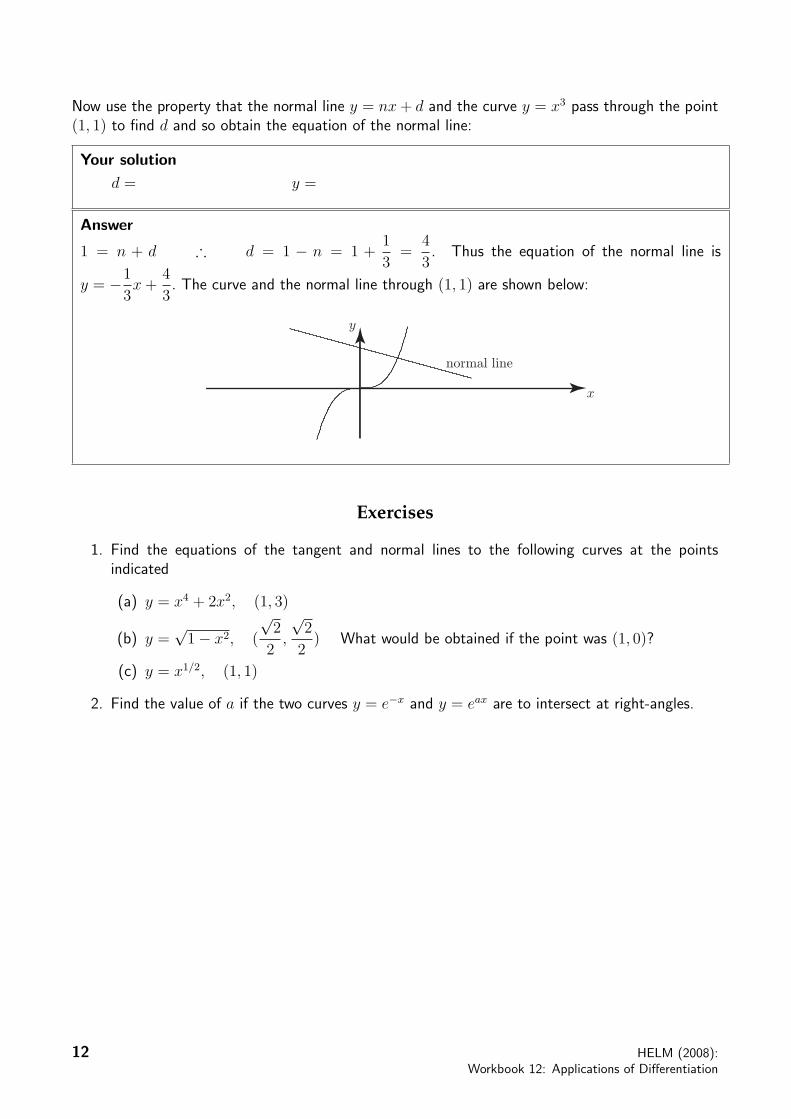
Now use the property that the normal line y = nx + d and the curve y = x3 pass through the point(1, 1) to find d and so obtain the equation of the normal line:

Your solution

d = y =

Answer

1 = n + d ∴ d = 1 − n = 1 +1

3=

4

3. Thus the equation of the normal line is

y = −1

3x +

4

3. The curve and the normal line through (1, 1) are shown below:

x

y

normal line

Exercises

1. Find the equations of the tangent and normal lines to the following curves at the pointsindicated

(a) y = x4 + 2x2, (1, 3)

(b) y =√

1− x2, (

√2

2,

√2

2) What would be obtained if the point was (1, 0)?

(c) y = x1/2, (1, 1)

2. Find the value of a if the two curves y = e−x and y = eax are to intersect at right-angles.

12 HELM (2008):


®

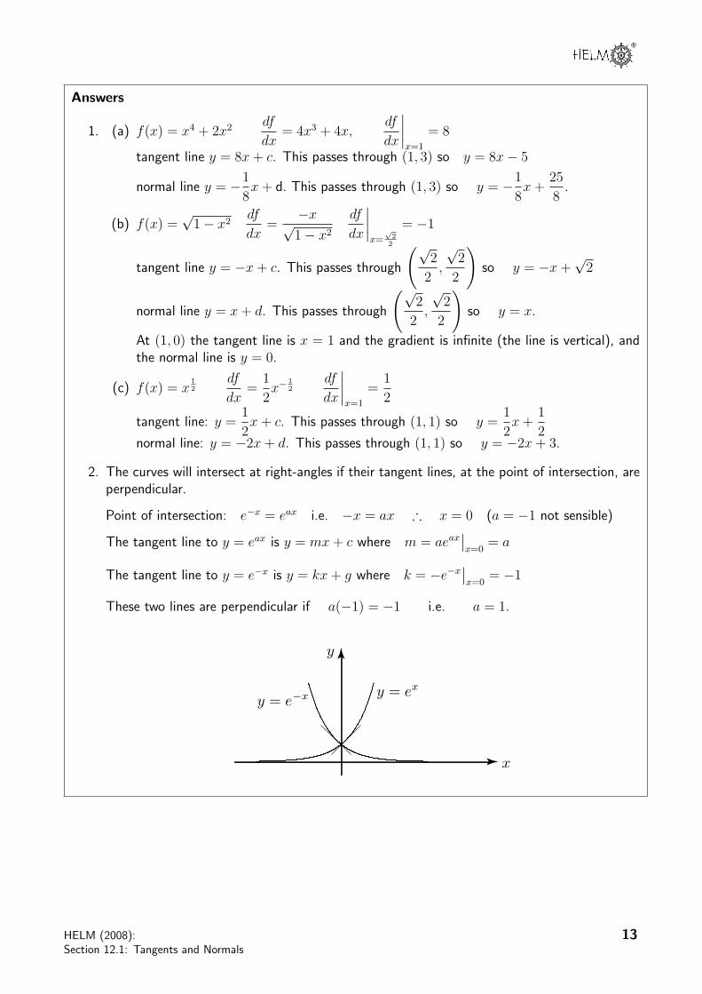
Answers

1. (a) f(x) = x4 + 2x2 df

dx= 4x3 + 4x,

df

dx

x=1

= 8

tangent line y = 8x + c. This passes through (1, 3) so y = 8x− 5

normal line y = −1

8x + d. This passes through (1, 3) so y = −1

8x +

25

8.

(b) f(x) =√

1− x2df

dx=

−x√1− x2

df

dx

x=

√2

2

= −1

tangent line y = −x + c. This passes through

√2

2,

√2

2

so y = −x +

√2

normal line y = x + d. This passes through

√2

2,

√2

2

so y = x.

At (1, 0) the tangent line is x = 1 and the gradient is infinite (the line is vertical), andthe normal line is y = 0.

(c) f(x) = x12

df

dx=

1

2x−

12

df

dx

x=1

=1

2

tangent line: y =1

2x + c. This passes through (1, 1) so y =

1

2x +

1

2normal line: y = −2x + d. This passes through (1, 1) so y = −2x + 3.

2. The curves will intersect at right-angles if their tangent lines, at the point of intersection, areperpendicular.

Point of intersection: e−x = eax i.e. −x = ax ∴ x = 0 (a = −1 not sensible)

The tangent line to y = eax is y = mx + c where m = aeaxx=0

= a

The tangent line to y = e−x is y = kx + g where k = −e−xx=0

= −1

These two lines are perpendicular if a(−1) = −1 i.e. a = 1.

x

y

y = ex

y = e!x

HELM (2008):


13

Index for Workbook 12

Acceleration vector 56

Angular velocity 33

Buckling load 45

Centripetal acceleration 33

Circle 48, 52

Complex independence 60-63

Crank 33

Curvature 47-53

Efficiency 28

Electric circuit 26

Electronic filters 2, 60

Ellipse 53

Fluid power transmission 31

Global maximum 15

Hydraulic brakes 31

Impedance 60-63

Inflection 23

Instantaneous velocity 55

Iterative formula 42

Light rays 29

Local maximum 15

Materials store 24

Maxima and minima 14-37

Multiple roots 39

Newton-Raphson method 38-46

Normal to curve 4, 10-12

Parabola 48, 51

Perpendicularity 4

Piston 33

Power 28, 31

Power dissipation 26

Pythagoras’ theorem 49

Refraction 29

Resistance 26

Root location 38-46

Solving equations 40

Stationary point 15-16

Straight line 3

Strut 45

Target to curve 5-9

Vector differentiation 54-59

Velocity vector 56

Water wheel 28

Zero 39

EXERCISES

4, 12, 35, 46, 59

ENGINEERING EXAMPLES

1 Water wheel efficiency 28

2 Refraction 29

3 Fluid power transmission 31

4 Crank used to drive a piston 33

5 Buckling of a strut 44

About the HELM Project - Queen's University Belfastqub.ac.uk/helm/HELM_2008/pages/combined_workbooks/... · About the HELM Project ... We show that a circle has a constant value for

Documents