About the generalized LM-inverse and the weighted Moore–Penrose inverse

arX

iv:1

104.

1698

v1 [

cs.S

C]

9 A

pr 2

011

About the generalized LM-inverse and

the Weighted Moore-Penrose inverse

Milan B. Tasic∗, Predrag S. Stanimirovic, Selver H. Pepic

University of Nis, Faculty of Sciences and Mathematics,

Visegradska 33, 18000 Nis, Serbia†

E-mail: [email protected], [email protected], p [email protected]

Abstract

The recursive method for computing the generalized LM - inverse of a constant rectangular ma-trix augmented by a column vector is proposed in [16, 17]. The corresponding algorithm for thesequential determination of the generalized LM -inverse is established in the present paper. Weprove that the introduced algorithm for computing the generalized LM inverse and the algorithmfor the computation of the weighted Moore-Penrose inverse developed by Wang in [23] are equiv-alent algorithms. Both of the algorithms are implemented in the present paper using the packageMATHEMATICA. Several rational test matrices and randomly generated constant matrices are testedand the CPU time is compared and discussed.

AMS Subj. Class.: 15A09, 68W30.

Key words: Generalized inverses, LM-inverse, Weighted Moore-Penrose inverse, rational matrices,MATHEMATICA, Partitioning method.

1 Introduction

As usual, let C be the set of complex numbers, Cm×n be the set of m × n complex matrices, andCm×n

r ={X ∈ Cm×n : rank(X)=r}. For any matrix A ∈ Cm×n and positive definite matrices M andN of the orders m and n respectively, consider the following equations in X , where ∗ denotes conjugateand transpose:

(1) AXA = A (2) XAX=X(3M) (MAX)∗ = MAX (4N) (NXA)∗=NXA.

The matrix X satisfying equations (1), (2), (3M) and (4N) is called the weighted Moore-Penrose

inverse of A, and it is denoted by X = A†M,N . Especially, in the case M = Im and N = In, the matrix

X = A†M,N becomes the Moore-Penrose inverse of A, and it is denoted by X = A†.

Various methods for computing the Moore-Penrose inverse of a matrix are known. The main methodsare based on the Cayley-Hamilton theorem, the full-rank factorization and the singular value decom-position (see the example [1]). The Greville’s partitioning method , introduced in [4], is one of the mostefficient algorithms for computing the Moore-Penrose inverse. Two different proofs for the Greville’smethod were presented in [2, 24]. Udwadia and Kalaba gave an alternative and a simple constructive

∗Corresponding author†The authors gratefully acknowledge support from the research project 144011 of the Serbian Ministry of Science.

1

http://arxiv.org/abs/1104.1698v1

2 M.B. Tasic, P.S. Stanimirovic, S.H. Pepic

proof of Greville’s formula in [19]. In [3] Fan and Kalaba determined the Moore-Penrose inverse ofmatrices using dynamic programming and the Belman’s principle of optimality. Sivakumar in [12] used

the Greville’s formula for A†k = [Ak−1 |ak]

† and just verified that it satisfies the four Penrose equations.This provides a proof of the Greville’s method by the verification.

The Greville’s algorithm is used in various computations, where its dominance is verified over variousdirect methods for the pseudoinverse computation. The computational experience presented in [7]is: ”When applied to a square, fully populated, non-symmetric case, with independent columns, theGreville’s algorithm was found that the approach can be up to 8 times faster than the conventionalapproach of using the SVD; rectangular cases are shown to yield similar levels of speed increase”. TheGreville’s method has been used as a benchmark for the calculation of the pseudo-inverse.

Due to its computational dominance, this method has been extensively applied in many mathemat-ical areas, such as statistical inference, filtering theory, linear estimation theory, optimization and morerecently analytical dynamics [20] (see also [6]). An application in a direct approach for computing thegradient of the pseudo-inverse is presented in [7]. It has also found wide applications in database andthe neural network computation [8]. In the paper [5], the sequential determination of the Moore-Penroseinverse by dynamic programming is applied to the diagnostic classification of electromyography signals.

There is a lot of extensions of the partitioning method. Wang in [23] generalized Greville’s methodto the weighted Moore-Penrose inverse. Also, the results in [23] are proved by using a new technique.Udwadia and Kalaba developed the recursive relations for the different types of generalized inverses[21, 22]. Finally, the Greville’s recursive principle is generalized to various subsets of outer inverses andextended to the set of the one-variable rational and polynomial matrices in [15].

The algorithm for the computation of the Moore-Penrose inverse of the one-variable polynomialand/or rational matrix, based on the Greville’s partitioning algorithm, was introduced in [13]. Theextension of results from [13] to the set of the two-variable rational and polynomial matrices is introducedin the paper [10].

The Wang’s partitioning method from [23], aimed in the computation of the weighted Moore-Penroseinverse, is extended to the set of the one-variable rational and polynomial matrices in the paper [14].Also the efficient algorithm for computing the weighted Moore-Penrose inverse, appropriate for thepolynomial matrices where only a few polynomial coefficients are nonzero, is established in [9].

In the paper [6] the authors derived a formula for the computation of the Moore-Penrose inverse ofM∗M and obtained sufficient conditions for its nonnegativity, where M = [A | a].

On the other side, there are a few articles which are interested in with computation of the generalizedLM -inverse. The definition of the LM -inverse and the recursive algorithm of the Greville’s type (for amatrix augmented by a column vector) are given in [16, 17]. The recursive relations in [16, 17] are provedby direct verification of the four conditions of the generalized LM -inverse. Also, these formulae areparticularized to obtain recursive relations for the generalized L-inverse of a general matrix augmentedby a column [17]. The recursive relations for the determination of the generalized Moore-PenroseM -inverse are derived in [18]. Separate relations for the situations when the rectangular matrix isaugmented by a row vector and when such a matrix is augmented by a column vector are consideredin [18]. The alternative proof for the determination of the generalized Moore-Penrose M -inverse ofa matrix through the direct verification of the four properties of the Moore-Penrose M -inverse arepresented in [11].

It is not difficult to verify that the conditions which characterize the generalized LM -inverse areequivalent with the corresponding equations characterizing the weighted Moore-Penrose inverse. More-over, the matrix norms minimization used in (3) and (4) in the article [16] also characterizes the weightedMoore-Penrose inverse. Therefore, the generalized LM -inverse and the weighted Moore-Penrose inverse

About the generalized LM -inverse and the Weighted Moore-Penrose inverse 3

are identical. In the present paper we compare the corresponding algorithms. It is realistic to predictthat algorithm for computing the weighted Moore-Penrose inverse from [23] and the algorithm for thecomputation of the generalized LM -inverse, introduced in the present paper and based on the resultsfrom [16, 17] are the same. Verification of this prediction is the main result of the present paper.Therefore, the present paper is continuation of the papers [9, 13, 14, 16, 17].

The structure of the present paper is as follows. In the second section we restate the representationof the generalized LM -inverse from [16, 17] as well as the representation and algorithm for computingthe weighted Moore-Penrose from [23]. We also introduce an effective algorithm for construction of thegeneralized LM -inverse directly using its representation proposed in [16, 17]. In the third section weprovide a proof that two algorithms from the second section are equivalent. Implementation of bothalgorithms and a few illustrative examples are presented.

2 Preliminaries and motivation

The recursive determination of the weighted Moore-Penrose inverse A†M,N is established in [23].

Let A ∈ Cm×n and Ak be the submatrix of A consisting of its first k columns. For k = 2, . . . , n the

matrix Ak is partitioned asAk = [Ak−1 | ak] , (2.1)

where ak is the k-th column of A.

Theorem 2.1 (G.R. Wang, Y.L. Chen [23]). Let A ∈ Cm×n and Ak be the submatrix of A consisting ofits first k columns. For k = 2, . . . , n the matrix Ak is partitioned as in (2.1), and the matrix Nk ∈ Ck×k

is the leading principal submatrix of N , and Nk is partitioned as

Nk =

[Nk−1 lkl∗k nkk

]. (2.2)

Let the matrices Xk−1 and Xk be defined by

Xk−1 = (Ak−1)†M,Nk−1

, Xk = (Ak)†M,Nk

, (2.3)

the vectors dk, ck be defined by

dk = Xk−1ak (2.4)

ck = ak −Ak−1dk = (I −Ak−1Xk−1) ak. (2.5)

Then

Xk=

[Xk−1−(dk + (I −Xk−1Ak−1)N

−1k−1lk)b

∗k

b∗k

], (2.6)

where

b∗k =

(c∗kMck)−1

c∗kM, ck 6= 0

δ−1k (d∗kNk−1 − l∗k)Xk−1, ck = 0,

(2.7)

and δk = nkk + d∗kNk−1dk − (d∗klk + l∗kdk(s))− l∗k (I −Xk−1Ak−1)N−1k−1lk.

According to the above theorem the next Algorithm 2.1 is introduced in [23].


Algorithm 2.1 Computing the weighted M-P inverse A†M,N using algorithm from [23].

Require: Let A ∈ Cm×n, M and N be p.d. matrices of the order m and n respectively.1: A1 = a1.2: if a1 = 0, then3: X1 = (a∗1Ma1)

−1a∗1M ;4: else

5: X1 = 0.6: end if

7: for k = 2 to n do

8: dk=Xk−1ak,9: ck = ak −Ak−1dk,

10: if ck 6= 0, then11: b∗k = (c∗kMck)

−1c∗kM, goto Step 16,12: else

13: δk = nkk + d∗kNk−1dk − (d∗klk + l∗kdk)− l∗k(I −Xk−1Ak−1)N−1k−1lk,

14: b∗k = δ−1k (d∗kNk−1 − l∗k)Xk−1,

15: end if

16: Xk =

[Xk−1 − (dk + (I −Xk−1Ak−1)N

−1k−1lk)b

∗k

b∗k

].

17: end for

18: return A†MN = Xn.

Also, the next auxiliary Algorithm 2.2, required in Algorithm 2.1 is stated in [23].

Algorithm 2.2 Computing the inverse matrix N−1.

Require: Let Nk =

[Nk−1 lkl∗k nkk

]∈ Ck×k be the leading principal submatrix of p.d. matrix N .

1: N−11 = n−1

11 .2: for k = 2 to n do

3: gkk=(nkk − l∗kN−1k−1lk)

−1,

4: fk = −gkkN−1k−1lk,

5: Ek−1 = N−1k−1 + g−1

kk fkf∗k ,

6: N−1k =

[Ek−1 fkf∗k gkk

].

7: end for

8: return N−1 = N−1n .

The definition of the generalized LM -inverse is given in [16], and it is based on the usage of thelinear equation Ax = b, where A is an m×n matrix, b is an m-vector and x is an n-vector. The matrixA†

LM is such that the vector x, uniquely given by x = A†LMb, minimizes both of the following two vector

norms (conditions (3) and (4) from [16])

G =‖ L1/2(Ax− b) ‖2=‖ Ax− b ‖2L,

H =‖ M1/2x ‖2=‖ x ‖2M ,

where L is an m×m symmetric positive-definite matrix and M is an n× n symmetric positive-definitematrix.


The recursive formulae for determining the generalized LM -inverse A†L,M of any given matrix A are

introduced in [16, 17], and they are restated here for the sake of completeness.

Theorem 2.2 (F.E. Udwadia, P. Phohomsiri [16, 17]). The generalized LM -inverse of any given matrixB = [A | a] ∈ Cm×n is determined using the following recursive relations:

B†L,M = [A | a]†L,M =

[A†

L,M −A†L,M a d†L − p d†Ld†L

], d =

(I − AA†

L,M

)a 6= 0;

[A†

L,M −A†L,M ah− p h

h

], d =

(I − AA†

L,M

)a = 0,

(2.8)

where A is an m× (n− 1) matrix, a is a column vector of m components,

d†L =dTL

dTLd, h =

qTMU

qTMq,

U =

[A†

L,M

01×m

], q =

[v + p−1

], v = A†

L,M a

andp =

(I −A†

L,M A)M−1m.

Note that L is a symmetric positive definite m×m matrix, and

M =

M m

mT m

, (2.9)

where M is a symmetric positive-definite n×n matrix, M is a symmetric positive-definite (n−1)×(n−1)matrix, m is a column vector of n− 1 components, and m is a scalar.

Theorem 2.2 assumes in B = [A | a] that the matrix B is obtained augmenting the matrix A byan appropriate column vector a. In the rest of the paper we assume that B = [A | a] is just thepartitioning (2.1): B = Ak, A = Ak−1, a = ak. Moreover, it is clear that the following notationsimmediately follows from Algorithm 2.1:

B†L,M = Xk, A† = Xk−1.

Also, we use the following denotation for the matrix M defined in (2.9):

M =

Mk−1 mk

mTk mk,k

, (2.10)

Finally, the vector d corresponding to the first k columns of A is denoted by dk.

According to the above Theorem 2.2 we introduce the next algorithm.


Algorithm 2.3 Computing the LM -inverse A†LM using the representation from [16].

Require: Let A ∈ Cm×n, L and M be p.d. matrices of order m and n respectively.1: A1 = a1.2: if a1 = 0 then

3: X1 = (a∗1La1)−1a∗1L

4: else

5: X1 = 0.6: end if

7: for k = 2 to n do

8: dk = (I −Ak−1Xk−1) ak,9: p = (I −Xk−1Ak−1)M

−1k−1mk,

10: if dk 6= 0 then

11: b∗k =d∗kL

d∗kLdk

goto Step 17

12: else

13: q =

[Xk−1ak + p

−1

],

14: U =

[Xk−1

0

],

15: b∗k = q∗

q∗MkqMkU ,

16: end if

17: Xk =

[Xk−1 −Xk−1akb

∗k − p b∗k

b∗k

].

18: end for

19: return A†L,M = Xn.

It is clear from restated definitions that the generalized LM -inverse is just the weighted Moore-Penrose inverse. Therefore, Algorithm 2.3 and algorithms 2.1, 2.2 together produce identical result -the weighted Moore-Penrose inverse of the given m × n matrix. In the next section we compare thedescribed algorithms.

3 Comparison of algorithms

Theorem 3.1. Algorithm 2.3 is equivalent to algorithms 2.1 and 2.2.

Proof. In order to ensure unambiguous, during the proof we assume that the symbol W in a superscriptdenotes terms from the Wang’s algorithm; similarly we use the convention that U , as a superscript,denotes terms from the Udwadia’s algorithm, elsewhere it is necessary. Since the LM -inverse is just theweighted Moore-Penrose inverse, we conclude that the matrix M in Algorithm 2.1 is just the matrix Lin Algorithm 2.3 and the matrix N in Algorithm 2.1 is analogous with the matrix M in Algorithm 2.3.Therefore, it is not necessarily to mark the matrices L,M,N and A by appropriate superscript.

We prove the theorem by verifying the equivalence of the outputs from the corresponding algorithmicsteps of mentioned algorithms. The proof proceeds by the mathematical induction.

The proof for the case k = 1 in view of Step 3 in both algorithms is trivial. Assume that thestatement is valid for the first k − 1 columns, i.e.

XUk−1 = XW

k−1 = (Ak−1)†M,Nk−1

= A†LM . (3.11)


Now we verify the inductive step. Wang used the matrix Xk in the form

XWk =

[XW

k−1−(dWk + (I −XW

k−1Ak−1

)N−1

k−1lk)(b∗k)

W

(b∗k)W

], (3.12)

while Udwadia observed two cases, as in (2.8).

If we denote with

(b∗k)U=

{d†L, dUk 6= 0h, dUk = 0,

(3.13)

then the equalities in (2.8) become

XUk =

[XU

k−1−XUk−1ak(b

∗k)

U − p (b∗k)U

(b∗k)U

]. (3.14)

Let us show that the output of Step 9 from Algorithm 2.1 is the same as the output of Step 8 fromAlgorithm 2.3:

cWk ≡ ak −Ak−1dWk = ak −Ak−1X

Wk−1ak =

(I −Ak−1X

Wk−1

)ak ≡ dUk .

Now we show that Step 11 from Algorithm 2.1 and Step 11 from Algorithm 2.3 are equivalent. As it isstated above cWk = dUk , so that in the case cWk 6= 0 we have

(b∗k)W = ((c∗k)

WMcWk )−1(c∗k)WM = ((d∗k)

ULdUk )−1(d∗k)

UL = (b∗k)U .

In a similar way it can be verified that Step 14 from Algorithm 2.1 is equivalent to Step 15 fromAlgorithm 2.3. In the case cWk = 0 we can start from the statement in Step 15 from Algorithm 2.3.

(b∗k)U = (q∗MkU)/(q∗Mkq).

From Step 9 of Algorithm 2.3 and the inductive hypothesis the following holds

p =(I −XU

k−1Ak−1

)N−1

k−1lk =(I −XW

k−1Ak−1

)N−1

k−1lk,

so that we derive the following:

qTMkU =[(XU

k−1ak + p)∗ | − 1] [ Nk−1 lk

l∗k nkk

] [XU

k−1

0

]

=[(XU

k−1ak + p)∗Nk−1 − l∗k | (XUk−1ak + p)∗lk − nkk

] [ XUk−1

0

]

= (XUk−1ak + p)∗Nk−1X

Uk−1 − l∗kX

Uk−1 {since XU

k−1ak = XWk−1ak = dWk }

= (d∗k)WNk−1X

Wk−1 − l∗kX

Wk−1 + p∗Nk−1X

Wk−1

=((d∗k)

WNk−1 − l∗k)XW

k−1 +((I −XW

k−1Ak−1

)N−1

k−1lk)∗

Nk−1XWk−1

=((d∗k)


k−1 +(l∗kN

−1k−1

(I −XW

k−1Ak−1

)∗)Nk−1X

Wk−1

=((d∗k)


k−1 + l∗kXWk−1 − l∗kN

−1k−1

(XW

k−1Ak−1

)∗Nk−1X

Wk−1.

Since Nk−1 is the symmetric positive definite applying equality (4N) together with (3.11) the followingholds (

XWk−1Ak−1

)∗Nk−1 =

(Nk−1X

Wk−1Ak−1

)∗= Nk−1X

Wk−1Ak−1,


and later

qTMkU =((d∗k)


k−1 + l∗kXWk−1 − l∗kN

−1k−1Nk−1X

Wk−1Ak−1X

Wk−1

=((d∗k)


k−1 + l∗k(XW

k−1 −XWk−1Ak−1X

Wk−1

)

=((d∗k)


k−1 + l∗k(XW

k−1 −XWk−1

)

=((d∗k)


k−1.

Moreover, we have

qTMkq =[(XU

k−1ak + p)∗ | − 1] [ Nk−1 lk

l∗k nkk

] [XU

k−1ak + p−1

]

=[(XU

k−1ak + p)∗Nk−1 − l∗k | (XUk−1ak + p)∗lk − nkk

] [ XUk−1ak + p

−1

]

= ((XUk−1ak + p)∗Nk−1 − l∗k)(X

Uk−1ak + p)− (XU

k−1ak + p)∗lk + nkk

= (XUk−1ak + p)∗Nk−1(X

Uk−1ak + p)− l∗k(X

Uk−1ak + p)− (XU

k−1ak + p)∗lk + nkk

(since {XUk−1ak = XW

k−1ak = dWk })

= (dWk + p)∗Nk−1(dWk + p)− l∗k(d

Wk + p)− (dWk + p)∗lk + nkk

= (d∗k)WNk−1d

Wk − l∗kd

Wk − (d∗k)

W lk + nkk − l∗kp

+ p∗Nk−1dWk + (d∗k)

WNk−1p+ p∗Nk−1p− p∗lk.

Furthermore

p∗Nk−1dWk + (d∗k)

WNk−1p+ p∗Nk−1p− p∗lk = 0. (3.15)

First we show that p∗Nk−1dWk = 0, as follows

p∗Nk−1dWk =

((I −XW

k−1Ak−1

)N−1

k−1lk)∗

Nk−1XWk−1ak

= l∗kN−1k−1

(I −XW

k−1Ak−1

)∗Nk−1X

Wk−1ak

= l∗kN−1k−1

(Nk−1 −

(XW

k−1Ak−1

)∗Nk−1

)XW

k−1ak

= l∗kN−1k−1

(Nk−1 −Nk−1X

Wk−1Ak−1

)XW

k−1ak

= l∗kN−1k−1Nk−1

(I −XW

k−1Ak−1

)XW

k−1ak

= l∗k(I −XW

k−1Ak−1

)XW

k−1ak

= l∗k(XW

k−1 −XWk−1Ak−1X

Wk−1

)ak

= l∗k(XW

k−1 −XWk−1

)ak = 0.

Also, from the above equality, we have

(d∗k)WNk−1p = (p∗Nk−1d

Wk )∗ = 0.

Finally, the last term of the sum in the left hand side of (3.15), is equal to p∗Nk−1p − p∗lk, and it is


also equal to zero:

p∗Nk−1p− p∗lk = p∗(Nk−1

(I −XW

k−1Ak−1

)N−1

k−1lk − lk)

= p∗(−Nk−1XWk−1Ak−1N

−1k−1 lk)

= p∗(−(XW

k−1Ak−1)∗ lk

)

=((I −XW

k−1Ak−1

)N−1

k−1lk)∗

(−A∗k−1(X

∗k−1)

W lk)

= −l∗kN−1k−1A

∗k−1(X

∗k−1)

W lk + l∗kN−1k−1A

∗k−1(X

∗k−1)

WA∗k−1(X

∗k−1)

W lk

= −l∗kN−1k−1A

∗k−1(X

∗k−1)

W lk + l∗kN−1k−1A

∗k−1(X

∗k−1)

W lk = 0.

Continuing the transformation for qTMkq we have

qTMkq = (d∗k)WNk−1d

Wk − l∗kd

Wk − (d∗k)

W lk + nkk − l∗k(I −XW

k−1Ak−1

)N−1

k−1lk

= δk.

Now we are able to continue the rest of our proof. According to the equality

(b∗k)U = (q∗MkU)/(q∗Mkq),

Step 15 from Algorithm 2.3 produces the result

(b∗k)U = δ−1

k (d∗kNk−1 − l∗k)XWk−1,

which is identical to the output (b∗k)W , derived in Step 14 from Algorithm 2.1.

According to Step 16 of Algorithm 2.1 and Step 17 of Algorithm 2.3, the generalized LM -inverseand the weighted Moore-Penrose inverse of the first k columns of A are identical:

XUk =

[XU

k−1−(XU

k−1ak + p)(b∗k)

U

(b∗k)U

]

=

[XW

k−1−(dWk +

(I −XW

k−1Ak−1

)N−1

k−1lk)(b∗k)

W

(b∗k)W

]

= XWk .

(3.16)

Finally, for the case k = n, it immediately follows that A†L,M = A†

M,N , which means that the outputsfrom both algorithms are identical.

4 Examples

In order to compare the algorithms from the second section it is necessary to use the precise imple-mentation of the corresponding algorithms. Details concerning the implementation of the partitioningalgorithm corresponding to the weighted Moore-Penrose inverse can be found in [14]. In order to com-pare the mentioned algorithms we developed a MATHEMATICA code for the implementation of Algorithm2.3. We later tested results on different types of matrices. Since the language MATHEMATICA admitssymbolic manipulation with data, developed implementations are immediately applicable to the rationaland polynomial matrices.


Example 4.1. Consider the test matrix A11×10 from [25], in the case a = 1

A =

1 2 3 4 1 1 3 4 6 2

1 3 4 6 2 2 3 4 5 3

2 3 4 5 3 3 4 5 6 4

3 4 5 6 4 4 5 6 7 6

4 5 6 7 6 6 6 7 7 8

6 6 7 7 8 1 2 3 4 1

3 4 1 1 3 4 6 2 1 2

4 6 2 2 3 4 5 3 1 3

4 5 3 3 4 5 6 4 2 3

5 6 4 4 5 6 7 6 3 4

6 7 6 6 6 7 7 8 4 5

11×10

and randomly generated symmetric positive definite matrices L10×10 and M11×11:

L =

280 −5 −133 −27 −12 −93 −133 −42 84 52

−5 216 −93 −23 141 −2 −108 −48 21 165

−133 −93 336 1 0 0 9 −5 91 81

−27 −23 1 260 −62 −42 −40 6 85 −8

−12 141 0 −62 278 −63 −19 −135 9 99

−93 −2 0 −42 −63 238 68 −27 −80 −34

−133 −108 9 −40 −19 68 290 12 −233 −244

−42 −48 −5 6 −135 −27 12 209 −15 −87

84 21 91 85 9 −80 −233 −15 332 145

52 165 81 −8 99 −34 −244 −87 145 402

10×10

,

M=

452 91 −186 −97 −161 68 28 16 151 41 −65

91 413 −74 −119 −317 −41 −12 67 180 −53 54

−186 −74 497 −136 78 −208 −175 −120 9 −99 6

−97 −119 −136 371 157 154 129 29 −102 −16 −96

−161 −317 78 157 444 28 −39 −201 −165 3 43

68 −41 −208 154 28 509 52 55 90 179 −81

28 −12 −175 129 −39 52 454 −38 −157 145 22

16 67 −120 29 −201 55 −38 408 −9 −16 −100

151 180 9 −102 −165 90 −157 −9 257 −32 14

41 −53 −99 −16 3 179 145 −16 −32 376 −15

−65 54 6 −96 43 −81 22 −100 14 −15 339

11×11

.

The generalized LM -inverse A†L,M from [16, 17] and the weighted Moore-Penrose inverse A†

M,N from[23] are both equal to

0.755 −0.156 −1.917 0.823 0.143 0.033 0.383 −0.33 0.213 −0.802 0.67−0.542 −0.078 1.683 −0.544 −0.27 0.003 −0.432 0.673 0.075 0.087 −0.3470.346 −0.194 −0.881 0.751 −0.187 0.002 0.32 −0.149 0.711 −1.749 1.003

−0.049 0.558 −0.724 0.145 0.065 0.007 0.128 −0.258 −0.245 0.481 −0.141−0.454 −0.013 1.181 −0.79 0.188 0.109 −0.3 0.057 −0.563 1.498 −0.907−1.188 −0.468 2.87 −0.203 −0.792 −0.107 0.233 0.19 1.258 −2.561 1.0830.701 0.364 −2.009 0.492 0.282 0.009 0.395 −0.407 −0.481 0.786 −0.1920.472 0.156 −0.533 −0.675 0.507 −0.02 −0.62 −0.008 −0.822 2.174 −0.848

−0.415 −0.481 1.824 −0.22 −0.377 0.002 0.013 0.247 0.615 −1.143 0.2570.328 0.156 −1.388 0.469 0.362 −0.02 0.028 −0.008 −0.47 0.526 −0.2

.

The Moore-Penrose inverse can be generated in the case L = M = αI, M = N = βI [16], and it isequal to

A†=

0.294 −0.169 −1.511 1.415 −0.391 0.041 −0.04 −0.26 0.454 −0.264 0.23−0.067 −0.074 1.227 −1.064 0.23 0.001 −0.192 0.649 −0.103 −0.191 −0.1020.227 −0.179 −0.692 0.705 −0.214 −0.009 −0.254 −0.238 1.514 −1.319 0.449

−0.165 0.547 −0.657 0.376 −0.116 0.015 0.179 −0.196 −0.456 0.531 −0.104−0.297 −0.01 1.035 −0.972 0.359 0.108 0.238 0.044 −1.065 0.938 −0.366−0.008 −0.474 1.663 −1.319 0.352 −0.103 −0.428 0.224 1.83 −1.844 0.4140.062 0.368 −1.349 1.081 −0.33 0.006 0.426 −0.434 −0.442 0.712 −0.156

−0.081 0.158 0.029 −0.144 −0.034 −0.021 0.087 −0.019 −1.499 1.448 −0.1380.195 −0.484 1.198 −0.791 0.211 0.005 −0.19 0.268 0.765 −0.906 0.049

−0.081 0.158 −0.971 0.856 −0.034 −0.021 0.087 −0.019 −0.499 0.448 −0.138

.


Example 4.2. Consider the one variable test matrix

A =

x 1 0 0 0 0 0 0 0 0 0 0x2 x 1 0 0 0 0 0 0 0 0 0x3 x2 x 1 0 0 0 0 0 0 0 0x4 x3 x2 x 1 0 0 0 0 0 0 0x5 x4 x3 x2 x 1 0 0 0 0 0 0x6 x5 x4 x3 x2 x 1 0 0 0 0 0x7 x6 x5 x4 x3 x2 x 1 0 0 0 0x8 x7 x6 x5 x4 x3 x2 x 1 0 0 0x9 x8 x7 x6 x5 x4 x3 x2 x 1 0 0x10 x9 x8 x7 x6 x5 x4 x3 x2 x 1 0x11 x10 x9 x8 x7 x6 x5 x4 x3 x2 x 1x12 x11 x10 x9 x8 x7 x6 x5 x4 x3 x2 x

proposed in [25] and L (resp. M) and M (resp. N) as the identity matrices of the appropriatedimensions. Both of the considered algorithms produce the following Moore-Penrose inverse:

A† =

x

x2+1

0 0 0 0 0 0 0 0 0 0 01

x2+1

0 0 0 0 0 0 0 0 0 0 0

−x 1 0 0 0 0 0 0 0 0 0 00 −x 1 0 0 0 0 0 0 0 0 00 0 −x 1 0 0 0 0 0 0 0 00 0 0 −x 1 0 0 0 0 0 0 00 0 0 0 −x 1 0 0 0 0 0 00 0 0 0 0 −x 1 0 0 0 0 00 0 0 0 0 0 −x 1 0 0 0 00 0 0 0 0 0 0 −x 1 0 0 00 0 0 0 0 0 0 0 −x 1 0 00 0 0 0 0 0 0 0 0 −x

1

x2+1

x

x2+1

.

Example 4.3. The CPU time needed for the computation of the generalized LM -inverse and theweighted Moore-Penrose inverse (according to Algorithm 2.3 and the algorithms 2.1, 2.2, respectively)is compared in the next table. The testing is done on the local machine with the following performances:Windows edition: Windows Home Edition; Processor: Intel(R) Celeron(R) M CPU @ 1.6GHz; Memory(RAM): 512 MB; System type: 32-bit Operating System; Software: MATHEMATICA 5.2. Also, in the tablethere are arranged results obtained on the set of randomly generated test matrices Am×n and randomlygenerated symmetric positive definite matrices Lm×m (resp. Mm×m) and Mn×n (resp. Nn×n):

m × n degreeAlgorithm 2.1

A†

MN

Algorithm 2.3

A†

LM

5x6 1 2.265 Seconds 2.235 Seconds

5x6 2 4.078 4.063

6x4 5 9.969 9.625

6x4 10 23.328 21.11

10x11 1 104.109 103.484

10x11 2 192.734 186.297

11x10 1 133.469 130.125

11x10 2 261.359 227.047

Table 1. The comparison in the efficiency on the set of randomly generated test matrices

According to the above Table 1 results it is evident that Algorithm 2.3 produces negligibly betterperformances with respect to Algorithm 2.1 for all test cases. This fact is in accordance with the verifiedequivalence between the algorithms.


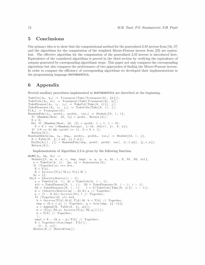
5 Conclusions

Our primary idea is to show that the computational method for the generalized LM -inverse from [16, 17]and the algorithms for the computation of the weighted Moore-Penrose inverse from [23] are equiva-lent. The effective algorithm for the computation of the generalized LM -inverse is introduced here.Equivalence of the considered algorithms is proved in the third section by verifying the equivalence ofoutputs generated by corresponding algorithmic steps. This paper not only compares the correspondingalgorithms but also compares the performance of two approaches of finding the Moore-Penrose inverse.In order to compare the efficiency of corresponding algorithms we developed their implementations inthe programming language MATHEMATICA.

6 Appendix

Several auxiliary procedures implemented in MATHEMATICA are described at the beginning.

TakeCol [ A , k ] := Transpose [ Take [ Transpose [A] , {k } ] ] ;TakeCols [ A , k ] := Transpose [ Take [ Transpose [A] , k ] ] ;TakeElement [ A , i , j ] := TakeCol [ Take [A, { i } ] , j ] ;TakeElements [ A , i , j ] := TakeCols [ Take [A, i ] , j ] ;T[ A ] := Transpose [A ] ;RandomPoly [ n , prob1 , prob2 , var ] := Module [{S , i , l } ,

I f [Random [ Real , {0 , 1} ] > prob1 , Return [ 0 ] ] ;S = 0 ;Do [ I f [Random [ Real , {0 , 1} ] < prob2 , l = 1 , l = 0 ] ;

S = S + var ˆ i ∗Random [ Integer , {−10, 10} ]∗ l , { i , 0 , n } ] ;I f [ ( S == 0) && ( prob1 >= 1) , S = S + 1 ] ;Return [ S ] ] ;

RandomMatrix [m , n , deg , prob1 , prob2 , var ] := Module [{A, i , j } ,A = Table [ 0 , { i , 1 ,m} , { j , 1 , n } ] ;Do [Do [A [ [ i , j ] ] = RandomPoly [ deg , prob1 , prob2 , var ] , { i , 1 ,m} ] , { j , 1 , n } ] ;Return [A ] ] ;

Implementation of Algorithm 2.3 is given by the following function.

ALMW[A , M , N ] :=Module [{ I , m, n , d , c , tmp , tmp1 , u , q , p , a , A1 , l , X, N1 , N2 , n11 } ,a = TakeCol [A, 1 ] ; {m, n} = Dimensions [A ] ;I f [ Together [ a ] === 0∗a ,X = T[ a ] ,X = Inve r s e [T[ a ] .M. a ] .T[ a ] .M ] ;

A1 = {} ;Do [ I = Ident i tyMatr i x [ i − 1 ] ;

a = TakeCol [A, i ] ; A1 = TakeCols [A, i − 1 ] ;n11 = TakeElement [N, i , i ] ; N1 = TakeElements [N, i − 1 , i − 1 ] ;N2 = TakeElements [N, i , i ] ; l = T[ TakeCols [ Take [N, { i } ] , i − 1 ] ] ;d = ( Ident i tyMatr i x [m] − A1 .X) . a // Together ;p = ( I − X.A1 ) . Inve r s e [N1 ] . l // Together ;I f [ Together [ d ] =!= 0∗d ,b = Inve r s e [T[ d ] .M. d ] .T[ d ] .M; b = T[ b ] // Together ,tmp = (X. a + p) // Together ; q = Join [ tmp , {{ −1}} ] ;u = Append [X, Table [ 0 , { j , m} ] ] ;b = (T[ q ] . N2 . u) Inve r s e [T[ q ] . N2 . q ] [ [ 1 ] ] ;b = T[ b ] // Together ;] ;

tmp1 = X − (X. a − p ) .T[ b ] // Together ;X = Together [ Join [ tmp1 , T[ b ] ] ] ;, { i , 2 , n } ] ;

Return [X // MatrixForm ] ] ;


Implementation of Algorithm 2.1 is obtained by slightly adopting the MATHEMATICA code describedin [14].

AWang[ A , M , N ] :=Module [{ I , m, n , d , c , a , A1 , l , del , X, tmp , tmp1 , N1 , n11 } ,

a = TakeCol [A, 1 ] ;{m, n} = Dimensions [A ] ;I f [ Together [ a ] === 0∗a ,

X = T[ a ] ,X = Inve r s e [T[ a ] .M. a ] .T[ a ] .M ] ; A1 = {} ;

Do [ I = Ident i tyMatr i x [ i − 1 ] ;a = TakeCol [A, i ] ; A1 = TakeCols [A, i − 1 ] ;d = X. a ; c = Together [ a − A1 . d ] ;n11 = TakeElement [N, i , i ] ;N1 = TakeElements [N, i − 1 , i − 1 ] ;l = T[ TakeCols [ Take [N, { i } ] , i − 1 ] ] ;tmp = T[ d ] . N1 − T[ l ] ;tmp1 = ( I − X.A1 ) . Inve r s e [N1 ] . l // Together ;I f [ Together [ c ] =!= 0∗c ,

b = Inve r s e [T[ c ] .M. c ] .T[ c ] .M;b = T[ b ] // Together ,de l = n11 + T[ d ] . N1 . d − (T[ d ] . l + T[ l ] . d ) − T[ l ] . tmp1 // Together ;b = T[ Inve r s e [ de l ] . tmp .X] // Together ;] ;X = Together [ Join [X − (d + tmp1 ) .T[ b ] , T[ b ] ] ] ;, { i , 2 , n } ] ;

Return [X ] ] ;

References

[1] A. Ben-Israel and T.N.E. Greville, Generalized inverses: theory and applications, Second Ed.,Springer, 2003.

[2] S.L. Campbell and C.D. Meyer, Jr., Generalized inverses of linear transformations, London, Pit-man, 1979.

[3] Y. Fan a and R. Kalaba, Dynamic programming and pseudo-inverses, Appl. Math. Comput. 139(2003), 323-342.

[4] T.N.E. Greville, Some applications of the pseudo-inverse of matrix SIAM Rev. 3 (1960), 15–22.

[5] C. Itiki, Dynamic programming and diagnostic classification, J. Optim. Theory Appl. 127 (2005),579-586.

[6] T. Kurmayya and K.C. Sivakumar, Moore-Penrose inverse of a Gram matrix and its nonnegativity,J. Optim. Theory Appl. 139 (2008), 201-207.

[7] J.B. Layton, Efficient direct computation of the pseudo-inverse and its gradient, Internat. J. Numer.Methods Engrg. 40 (1997), 4211–4223.

[8] S. Mohideen and V. Cherkassky, On recursive calculation of the generalized inverse of a matrix,ACM Trans. Math. Software 17 (1991), 130-147.

[9] M.D. Petkovic, P.S. Stanimirovic and M.B. Tasic, Effective partitioning method for computingweighted MoorePenrose inverse, Comput. Math. Appl. 55 (2008), 1720-1734.


[10] M.D. Petkovic and P.S. Stanimirovic, Symbolic computation of the Moore-Penrose inverse usingpartitioning method, Int. J. Comput. Math. 82 (2005), 355–367.

[11] P. Phohomsiri, B. Han, An alternative proof for the recursive formulae for computing the MoorePen-rose M-inverse of a matrix, Appl. Math. Comput. 174 (2006), 81-97.

[12] K. C. Sivakumar, Proof by verification of the Greville/Udwadia/Kalaba formula for the Moore-Penrose inverse of a matrix, J. Optim. Theory Appl. 131 (2006), 307-311.

[13] P.S. Stanimirovic and M.B. Tasic, Partitioning method for rational and polynomial matrices, Appl.Math. Comput. 155 (2004), 137–163.

[14] M.B. Tasic, P.S. Stanimirovic, M.D. Petkovic, Symbolic computation of weighted Moore-Penroseinverse using partitioning method, Appl. Math. Comput. 189 (2007), 615–640.

[15] M.B. Tasic, P.S. Stanimirovic, Symbolic and recursive computation of different types of generalizedinverses, Appl. Math. Comput. 199 (2008), 349–367.

[16] F.E. Udwadia and P.Phohomsiri, Generalized LM -inverse of a matrix augmented by a columnvector, Appl. Math. Comput. 190 (2007), 999–1006.

[17] F.E. Udwadia and P.Phohomsiri, Recursive Formulas for Generalized LM-Inverse of a Matrix, J.Optim. Theory Appl. 131 (2007), 1–16.

[18] F. E. Udwadia and P. Phohomsiri, Recursive Determination of the Generalized MoorePenrose M-Inverse of a Matrix, J. Optim. Theory Appl. 127 (2005), 639-663.

[19] F.E. Udwadia and R.E. Kalaba, An Alternative Proof for Greville’s Formula, J. Optim. TheoryAppl. 94 (1997), 23-28.

[20] F.E. Udwadia and R.E. Kalaba, Analytical Dynamics: A New Approach, Cambridge UniversityPress, Cambridge, England, 1996.

[21] F.E. Udwadia and R.E. Kalaba, A Unified Approach for the Recursive Determination of GeneralizedInverses, Comput. Math. Appl. 37 (1999), 125-130.

[22] F.E. Udwadia and R.E. Kalaba, General forms for the Recursive Determination of GeneralizedInverses: Unified approach, J. Optim. Theory Appl. 101 (1999), 509–521.

[23] G.R. Wang and Y.L.Chen, A recursive algorithm for computing the weighted Moore-Penrose inverse

A†MN , J. Comput. Math. 4 (1986), 74–85.

[24] G.R. Wang, A new proof of Greville’s method for computing the weighted M-P inverse, J. ShangaiTeach. Univ., Nat. Sci. Ed. 3 (1985), 32–38.

[25] G. Zielke, Report on test matrices for generalized inverses, Computing 36 (1986), 105–162.

About the generalized LM-inverse and the weighted Moore–Penrose inverse

Documents