About barcodes and Calabi invariant for Hamiltonian ...

HAL Id: tel-03465434https://tel.archives-ouvertes.fr/tel-03465434

Submitted on 3 Dec 2021

HAL is a multi-disciplinary open accessarchive for the deposit and dissemination of sci-entific research documents, whether they are pub-lished or not. The documents may come fromteaching and research institutions in France orabroad, or from public or private research centers.

L’archive ouverte pluridisciplinaire HAL, estdestinée au dépôt et à la diffusion de documentsscientifiques de niveau recherche, publiés ou non,émanant des établissements d’enseignement et derecherche français ou étrangers, des laboratoirespublics ou privés.

About barcodes and Calabi invariant for Hamiltonianhomeomorphisms of surfaces

Benoît Joly

To cite this version:Benoît Joly. About barcodes and Calabi invariant for Hamiltonian homeomorphisms of surfaces.Dynamical Systems [math.DS]. Sorbonne Université, 2021. English. NNT : 2021SORUS196. tel-03465434

Sorbonne Université

École doctorale de sciences mathématiques de Paris centre

Thèse de doctoratDiscipline : Mathématiques

présentée par

Benoît JOLY

About Barcodes and Calabi invariant forHamiltonian homeomorphisms of surfaces

dirigée par Patrice Le Calvez et Frédéric Le Roux

Soutenue le 15 Octobre 2021 devant le jury composé de :

M. Barney Bramham Ruhr-Universität RapporteurM. Vincent Colin Université de Nantes ExaminateurM. Patrice Le Calvez Sorbonne Université DirecteurM. Frédéric Le Roux Sorbonne Université Co-DirecteurM. Rémi Leclercq Université Paris-Saclay RapporteurMme Ana Rechtman Université de Strasbourg Examinatrice

1

Institut de mathématiques de Jussieu-Paris Rive gauche. UMR 7586.Boîte courrier 2474 place Jussieu75 252 Paris Cedex 05

Sorbonne Université, Campus Pierre etMarie Curie.École doctorale de sciencesmathématiques de Paris centre.Boîte courrier 2904 place Jussieu75 252 Paris Cedex 05

2

Remerciements

Il est enfin l’heure des remerciements, la soutenance va surement bientôt commencer.Comme toute personne participant à une soutenance vous êtes sur le point de lire cesquelques lignes remplies de noms pour la plupart inconnus.

En premier lieu, je tiens à remercier chaleureusement mes directeurs Patrice Le Calvezet Frédéric Le Roux. Vous m’avez accompagné, soutenu avec intérêts et bienveillance toutau long de ces années de thèse. Merci pour vos précieux conseils, remarques, discussionset relectures. Je vous suis particulièrement reconnaissant pour votre patience face à moninefficacité, merci infiniment de m’avoir accordé de votre temps, conscient que je ne suispas toujours facile à suivre.

Je souhaite remercier les membres du jury, et en particulier les rapporteurs RémiLeclercq et Barney Bramham pour leur relecture attentive et leurs retours bienveillants.Je suis également reconnaissant envers Ana Retchman et Vincent Colin qui ont acceptéd’être mes examinateurs. C’est un honneur pour moi de soutenir devant un tel jury.

Je remercie le laboratoire de l’IMJ qui m’a permis d’élaborer ma thèse dans des con-ditions idylliques. Merci pour toutes les rencontres, les voyages, les séminaires qui m’ontaussi beaucoup aidé.

Je tiens à remercier mes chers parents qui depuis toujours me soutiennent, m’encouragent,s’inquiètent pour moi et me font confiance. Une douce pensée à mes grands parents qui nesont plus parmi nous et qui étaient si bienveillants envers moi.

Je remercie infiniment Lucie, nos années de colocation ont su nourrir une amitié àtoute épreuve. Tu as toujours été présente et je tiens à t’exprimer toute ma gratitude.Ensemble, nous avons bu, dansé, ri, pleuré. . . Grace à toi j’ai rencontré le Qwirkleclub quim’a accompagné ces dernières années ! Je remercie amoureusement Daniel, Elise, Justineet Maxime qui m’apportent une telle joie de vivre. Ecumer les bars à petits prix de Parisavec vous est un véritable plaisir et toutes nos soirées resteront gravées à jamais dans mamémoire.

Je tiens à remercier Gauthier et Alexandre qui m’accompagnent depuis les années prépa.J’ai vécu avec vous tant de moments exceptionnels. Comment oublier toutes nos heuresde travail, nos road trip dans le van, nos voyages à Montréal avec Elodie et Nazia quej’embrasse fort, etc. . . Je remercie également Théodor, Alex et Jeanne que j’ai rencontrégrâce à vous.

3

Je remercie Florestan, notre colocation pleine de "shlaguitude", les séminaires que l’ona fait ensemble, nos vacances, nos soirées, les morsures de Pistou, nos siestes dans les cafésde Montréal, ont su instaurer un quotidien à notre image. Tu m’auras aussi permis pleinde belles rencontres, je tiens à remercier Alais, Eugénie, Sarah, Claire, Gwenn, ainsi quetous les autres membres de cette famille Marseillaise !

Je remercie Idriss, Ziad et Florent que j’ai rencontré à l’ENS. Que ce soit à Paris ouailleurs en France nous avons su rester proches ! Vous savez égailler nos soirées et mathèse aurait été bien triste sans vous, des blagues douteuses aux discussions passionnéesje ne me lasserai jamais de vous. Promis je reviendrai pour notre rendez-vous annuel aufestival Court Métrage de Clermont. Je remercie également Lisa, Simon, Marie, Romainet Bernard que j’ai eu la joie de rencontrer grâce à vous.

Il est temps de remercier tous ceux qui ont subi le même sort que moi dans ce couloirdu 5ème étage 15-16. Alexandre, ce fut un plaisir de partager ces années avec toi, que cesoit au labo, à discuter de maths, en conférence, à la salle d’escalade, dans un bar ou pourune partie de hanabi. Je tiens à remercier tous les Thomas qui ont croisé mon chemindans ce couloir, j’ai beaucoup ri avec vous, surtout ne changez rien ! Jean-Michel pour tesconseils avisés en matière de tikz et de LATEX, Hugo sans qui les ICM n’aurait pas eula même saveur, Christina pour tes remarques si gentilles, Thibaut, Anna, Mahya, Grâce,Jacques, Raphael, Sylvain, Matthieu (les deux), Vadim, Ilias, Léo, Amiel , Justin, Louis,Nicolina, Xavier, Arnaud, Christophe et tous ceux que j’ai omis de citer. Merci à touspour cette chaleureuse ambiance que vous avez su créer.

Une pensée pour mes autres amis qui m’ont accompagné ces années : Camille, à quij’aurai toujours des histoires à raconter, Volodia, que j’ai eu la joie de rencontrer au CRRd’Aubervilliers, Côme, Maïlys et Noémie que j’ai eu le plaisir de croiser en conférences.

Je remercie tous les membres de la compagnie La Roulotte : Maxime, Christophe,Coralie, Baptiste, Marion, Pauline pour m’avoir embarqué dans l’incroyable aventure deJules et Roméo. Vous êtes des artistes et acteur·rice·s incroyables ! Je ne me lasseraijamais de jouer avec vous.

Je remercie également Léa pour m’avoir accompagné lors de la dernière ligne droite.

Il n’est pas coutume, mais je reconnais que ma capacité de procrastination et mon inca-pacité d’ordonner mes idées m’ont valu bien des frustrations! Votre aide m’a été d’autantplus précieuse, tout simplement merci à vous tous.

Je m’excuse pour tous ceux que j’ai pu oublier dans cette liste déjà si longue.

Je finirai en remerciant les courageux qui oseront lire ma thèse, ou simplement la feuil-leter par curiosité.

4

Résumé

Nous cherchons à expliciter certains liens entre la topologie symplectique et l’étude dessystèmes dynamiques à travers la notion de code barres d’homéomorphismes hamiltoniensde surfaces et de l’invariant de Calabi de difféomorphismes hamiltoniens du disque unité.Ces deux objets représentent de puissants invariants en topologie symplectique. Plus pré-cisément, nous visons à mettre en avant une interprétation dynamique de ces objets.

Cette thèse se divise en deux parties.

Dans une première partie nous étudierons les codes barres de Floer d’un point de vue dy-namique. Notre motivation provient en particulier de l’utilisation récente des codes barresen topologie symplectique permettant d’obtenir des résultats purement dynamiques. Ainsi,nous expliciterons des constructions de codes barres pour certains homéomorphismes hamil-toniens de surfaces à l’aide de la théorie des feuilletages transverses de Le Calvez. Notrestratégie consistera à calquer la construction de l’homologie de Floer et de l’homologie deMorse à l’aide d’outils de systèmes dynamiques tels que des feuilletages. Nous prouveronsen particulier que dans les cas les plus simples, nos constructions correspondent aux codesbarres de Floer.

Dans une seconde partie nous nous intéresserons à l’invariant de Calabi pour les dif-féomorphismes hamiltoniens du disque unité. Usuellement, l’invariant de Calabi est biendéfini sur l’ensemble des difféomorphismes hamiltoniens à support compact du disque unité.Inspirés par l’interprétation dynamique de cet object donné par Fathi dans sa thèse, nousétendrons la définition de ce dernier au groupe des C1 difféomorphismes hamiltoniens dudisque. En particulier, cela nous permettra de calculer l’invariant de Calabi de certainespseudo-rotations irrationnelles du disque.

5

6

Abstract

The goal of this thesis is to give some links between sympletic topology and the studyof dynamical systems through the notion of barcodes of Hamiltonian homeomorphisms ofsurfaces and the Calabi invariant of Hamiltonian diffeomorphisms of the unit disk. Thesetwo objects represent powerful invariants in symplectic topology. More precisely, we aimat giving a dynamical interpretation of these objects.

This thesis is divided into two parts.

In a first part we will study the Floer Homology barcodes from a dynamical point ofview. Our motivation comes from recent results in symplectic topology using barcodes toobtain dynamical results. We will give some constructions of barcodes of some Hamiltonianhomeomorphisms of surfaces using Le Calvez’s transverse foliation theory. The strategyconsists in copying the construction of the Floer and Morse Homologies using dynamicaltools like Le Calvez’s foliations. In particular, we will prove that for the simplest cases,our constructions coincide with the Floer Homology barcodes.

In a second part we will deal with the Calabi invariant of the Hamiltonian diffeomor-phisms of the unit disk. Inspired by the dynamical interpretation of this object developedby Fathi in his thesis, we will extend it to the group of C1 Hamiltonian diffeomorphisms ofthe disk. In particular, we will be able to compute the Calabi invariant of some irrationalpseudo-rotations of the disk.

7

8

Contents

I Barcodes for Hamiltonian homeomorphisms of surfaces 13

1 Introduction 151.1 Goals and motivations . . . . . . . . . . . . . . . . . . . . . . . . . . . . . . 151.2 Results . . . . . . . . . . . . . . . . . . . . . . . . . . . . . . . . . . . . . . . 18

2 Preliminaries 212.1 Morse Homology . . . . . . . . . . . . . . . . . . . . . . . . . . . . . . . . . 212.2 Symplectic geometry . . . . . . . . . . . . . . . . . . . . . . . . . . . . . . . 24

2.2.1 Hamiltonian diffeomorphisms . . . . . . . . . . . . . . . . . . . . . . 242.2.2 Hamiltonian Action . . . . . . . . . . . . . . . . . . . . . . . . . . . 252.2.3 Floer Homology . . . . . . . . . . . . . . . . . . . . . . . . . . . . . . 252.2.4 Filtered Floer Homology . . . . . . . . . . . . . . . . . . . . . . . . . 282.2.5 Conley-Zehnder index and Maslov index . . . . . . . . . . . . . . . . 29

2.3 Dynamical systems . . . . . . . . . . . . . . . . . . . . . . . . . . . . . . . . 312.3.1 Isotopies and maximal Isotopies . . . . . . . . . . . . . . . . . . . . . 312.3.2 Lefschetz index . . . . . . . . . . . . . . . . . . . . . . . . . . . . . . 322.3.3 Linking number . . . . . . . . . . . . . . . . . . . . . . . . . . . . . . 322.3.4 Rotation vectors . . . . . . . . . . . . . . . . . . . . . . . . . . . . . 332.3.5 Local isotopies and local rotation set . . . . . . . . . . . . . . . . . . 332.3.6 The blow-up at a fixed point . . . . . . . . . . . . . . . . . . . . . . 352.3.7 Positively transverse foliations . . . . . . . . . . . . . . . . . . . . . . 362.3.8 Generalized Isotopies . . . . . . . . . . . . . . . . . . . . . . . . . . . 382.3.9 Intersection number . . . . . . . . . . . . . . . . . . . . . . . . . . . 402.3.10 Action function of a Hamiltonian homeomorphism . . . . . . . . . . 40

3 Introduction to barcodes and persistence modules 45

4 The simplest case of barcode for Hamiltonian homeomorphisms 49

5 First step into the non generic case, construction of the map B 57

6 The barcode of a gradient-like foliation 616.1 Geometric properties of a gradient-like foliation . . . . . . . . . . . . . . . . 616.2 Some properties of the Barcode BpGpFq, A, indpF , ¨qq . . . . . . . . . . . . . 71

7 A barcode with an order on a maximal unlinked set of fixed points 83

9

8 Equalities of the previous constructions and independence of the foliation 898.1 Equality between the barcode βF and the barcode βą . . . . . . . . . . . . 898.2 Equality between the barcode βF and the barcode Bgenpf,Fq in the generic

case . . . . . . . . . . . . . . . . . . . . . . . . . . . . . . . . . . . . . . . . 93

9 Perspectives 99

II Calabi invariant for Hamiltonian diffeomorphism of the unit disk101

1 Introduction 103

2 Preliminaries 111

3 Three extensions 1153.1 Action function . . . . . . . . . . . . . . . . . . . . . . . . . . . . . . . . . . 1153.2 Angle function . . . . . . . . . . . . . . . . . . . . . . . . . . . . . . . . . . 1173.3 Hamiltonian function . . . . . . . . . . . . . . . . . . . . . . . . . . . . . . . 120

4 Proof of Theorem 1.0.7 1234.1 Equality between ĄCal2 and ĄCal3. . . . . . . . . . . . . . . . . . . . . . . . . 1234.2 Continuity of ĄCal. . . . . . . . . . . . . . . . . . . . . . . . . . . . . . . . . 128

5 Computation of Cal1 in some rigid cases 1335.1 A simple case of C1-rigidity . . . . . . . . . . . . . . . . . . . . . . . . . . . 1335.2 C0-rigidity . . . . . . . . . . . . . . . . . . . . . . . . . . . . . . . . . . . . . 134

6 Examples 1396.1 An example of C0-rigidity, the super Liouville type . . . . . . . . . . . . . . 1396.2 An example of C1-rigidity, the non Bruno type . . . . . . . . . . . . . . . . 141

Bibliography 143

10

Context

Let us begin with some basic definitions of symplectic geometry.

Let us consider pM2n, ωq a symplectic manifold, meaning thatM is an even dimensionalmanifold equipped with a closed non-degenerate differential 2-form ω called the symplecticform. In particular, if M is a symplectic surface, the symplectic form is an area form.

Let us consider a time-dependent vector field pXtqtPR defined by the equation

dHt “ ωpXt, ¨q,

where H : RˆM Ñ R is a smooth function 1-periodic in t, meaning that Ht`1 “ Ht forevery t P R. The function H is called a Hamiltonian function. If the vector field pXtqtPRis complete, it induces a Hamiltonian flow which is a family pftqtPR of diffeomorphisms ofM preserving ω and satisfying the equation

B

Btftpzq “ Xtpftpzqq.

The time one map f1 of the isotopy pftqtPr0,1s is called a Hamiltonian diffeomorphism. Inparticular, a Hamiltonian diffeomorphism on a surface preserves the area.

The case of autonomous Hamiltonian diffeomorphisms can be kept in mind. Con-sidering a C1 function H on a surface, the previous hamiltonian formalism provides aHamiltonian flow which follows the level sets of H such that the flux passing through anyloop is zero. The time-one map of such a Hamiltonian flow will be called an autonomousHamiltonian diffeomorphism.

Birkhoff proved [10] a celebrated result, conjectured and proved in some cases byPoincaré [65], known as the Poincaré-Birkhoff theorem, that asserts that an area-preservinghomeomorphism of a closed annulus that satisfies some "twist conditions" admits atleast two fixed points. Further generalizations have been obtained by Franks [31], usingBrouwer’s lemma on translation arcs, and other authors.

In one hand, the Poincaré-Birkhoff theorem led to many questions of symplectic geom-etry such as the Arnold conjecture [2] and the developement of the Floer Homology theory[26, 27, 28, 29, 30]. Floer introduced the Floer Homology by combining the variationalapproach of Conley and Zehnder, the elliptic techniques of Gromov and the Morse-Smale-Witten complex in order to answer the Arnold conjecture stated as follows.

11

Conjecture 0.0.1. A Hamiltonian diffeomorphism of a symplectic manifold M must haveat least as many fixed points as the minimal number of critical points of a smooth functionon M .

On the other hand, the Poincaré-Birkhoff theorem led to the study of periodic pointsof homeomorphisms of surfaces and more generally to the study of the dynamics of suchhomeomorphisms.

The main goal of this thesis is to study some links between the symplectic geometryand the dynamical systems of surfaces. In a first part we will study barcodes for Hamilto-nian homeomorphisms on surfaces. In a second part we will study the Calabi invariant forHamiltonian diffeomorphisms of the unit disk.

Both parts of the thesis contain their own introduction and preliminaries chapters.They are independant.

12

Part I

Barcodes for Hamiltonian homeomorphismsof surfaces

13

Chapter 1

Introduction

1.1 Goals and motivations

Main question

In the first part of this thesis, we will think about the following question.

Question 1.1.1. Can we construct barcodes for Hamiltonian homeomorphisms of surfaces,equal to the Floer homology barcodes, using dynamical objects as Le Calvez’s transversefoliations?

Barcodes

Given a Hamiltonian function pHtqtPr0,1s on a symplectic manifold pM,ωq, we definethe action function AH on the space of contractible loops of M by

AHpγq “ ´

ż

Du˚ω `

ż 1

0Htpγptqqdt,

where u is an extension to the disk of the contractible loop γ : S1 Ñ M , that is, a mapu : D “ tz P C||z| ď 1u Ñ M such that upe2iπtq “ γptq. If we suppose that π2pMq “ 0,the function AH does not depend on the choice of u and it will always be the case in thisthesis. We will see in the preliminaries that for a Hamiltonian diffeomorphism f , the actionfunction AH does not depend on the choice of the Hamiltonian function H which inducesf , hence it defines an action function Af asociated to f .

For example, on surfaces, the difference of action between two points x and y fixed bya Hamiltonian flow can be interpreted as the flux of this flow through any oriented path γjoining x and y.

An important fact is that the critical points of an action function Af are the trajecto-ries of the contractible fixed points of f . The study of the critical values of Af will play akey role in this thesis.

The barcode of a Hamiltonian diffeomorphism f is a countable collection of intervals,called bars whose extremities are the critical values of its action function Af . In the par-ticular case of a generic hamiltonian diffeomorphism, each critical value of Af is the end

15

of one and only one bar.

The construction of these barcodes, recalled in Chapter 3, is based on the Floer Ho-mology theory.

Let us begin with a simple example. We consider a Hamiltonian flow pftqtPr0,1s inducedby an autonomous Hamiltonian function H. In this case, for t small enough, the barcode ofthe Hamiltonian diffeomorphism ft is equal to the filtered Morse Homology pHMt

˚pHqqtPRof H.To give more details about this example we explain how the filtered homology of H canbe interpreted as a collection of bars. In general, the bars of a barcode are of the formIj “ paj , bjs, aj P R, bj P R Y t`8u and satisfy certain finiteness assumptions. The endsof these bars are in correspondence with the critical points of H and can be classified asfollows.

• There are the death points which are the critical points x of H ending some homology,meaning that the dimension of the vector spaces pHMt

˚pHqqtPR decreases at Hpxq.

• There are the birth points which are the critical points x of H generating homologyin HM˚HpxqpHq, meaning that the dimension of the vector spaces pHMt

˚pHqqtPRincreases at Hpxq. The value Hpxq of a birth point x will be the begining of a bar.

The bars of a barcode can be described by the following classification of the birth points.

• A birth point can be "homological" and associated to the semi-infinite bar pHpsq,`8qin the barcode if the homology it generates in HM

Hpxq˚ persists in the vector spaces

pHMt˚qtěHpsq.

• A birth point can be "bound to die" and associated to a death point y and a finitebar pHpxq, Hpyqs in the barcode if the homology it generates in HM

Hpxq˚ disapears in

HMHpyq˚ .

The previous filtered homology is an example of a persistence module. In fact, we willsee that barcodes use to classify persistence modules up to isomorphisms. Roughly speak-ing, it is equivalent to consider a barcode as a set of bars or as a filtered homology.

Following this idea, we associate, canonically, a barcode Bpfq to every Hamiltoniandiffeomorphism f by considering the filtered Floer Homology of f where the filtration isgiven by the action function Af .

The barcode Bpfq gives information about the structure of the set of fixed points andthe spectral invariants of f . The spectral invariants have been introduced by Viterbo [73].They have been used in numerous deep applications and their theory has been developpedin many contexts, we can cite for example the work of Schwarz [?] and Oh [?]. They arepowerful tools which took an important place in the development of symplectic topology.

16

The notion of Barcode provides, in some topology, a continuous invariant of conjugacyon the set of smooth Hamiltonian diffeomorphisms of symplectic manifolds.

Hamiltonian homeomorphisms

In symplectic geometry, we can define the notion of Hamiltonian homeomorphism ofa surface Σ by taking the closure of the Hamiltonian diffeomorphisms of Σ. This defini-tion comes from the Gromov-Eliashberg theorem [19] which states that if a sequence ofsymplectomorphisms of a symplectic manifold pM,ωq converges in the C0 topology to adiffeomorphism then this diffeomorphism is a symplectomorphism as well.

For a Hamiltonian homeomorphism of a surface, we are not able to consider directly itsFloer Homology as the construction requires at least a C2 setting. Howeover, on surfaces,the barcode Bpfq depends continuously, in the uniform topology, on f and moreover, ex-tends to Hamiltonian homeomorphisms, see [61] for more details.

The barcode of a Hamiltonian homeomorphism f is defined by a limiting process andit is natural to wonder if it is possible to describe a direct construction.

Moreover, the notion of Hamiltonian homeomorphism of surfaces is well-known in dy-namical systems and has a dynamical interpretation thanks to the notion of rotation vec-tors. On a symplectic surface pΣ, ωq, ω is an area form which induces a Borel probabilitymeasure µ. We will say that a homeomorphism f of an oriented compact surface is Hamil-tonian if it is isotopic to the identity and preserves a Borel probability measure µ whosesupport is the whole surface and whose rotation vector ρpµq is zero.

Le Calvez’s transverse foliations

A key motivation for this thesis is to bring a dynamical interpretation of the barcodesfor Hamiltonian homeomorphisms of surfaces. Taking this direction, we will give someconstructions of barcodes, inspired by the Floer homology constructions, using Le Calvez’sfoliation theory.

Le Calvez’s foliations theory has many applications in the study of dynamical systemsof surfaces. For example in the study of prime ends by Koropecki, Le Calvez and Nassiri[48], the study of homoclinic orbits for area preserving diffeomorphisms by Sambarino andLe Calvez [52] or the results about the forcing theory of Le Calvez and Tal [53, 54].

Nowadays, Le Calvez’s foliations theory [49] represents one of the most importantdynamical tool in the study of the dynamics of homeomorphisms of surfaces. This the-ory already found applications to Barcodes of Hamiltonian homeomorphisms of surfaces.For example, for a homeomorphism f which preserves the area, Le Roux, Seyfaddini andViterbo in [61] used Le Calvez’s foliations theory to extract dynamical informations of thebarcode of f without Kislev-Shelukhin’s result [47].

Here are some details about transverse foliations. Let us consider a homeomorphismf on a surface. There are sets X of fixed points of f , called maximal unlinked sets, such

17

that there exists an isotopy, called maximal isotopy, from id to f fixing all points of X andwhich are maximal for the inclusion.

Le Calvez proved that given a maximal unlinked set X of fixed points of f and an iso-topy I fixing all the fixed points of X, there exist oriented foliations F positively transverseto the isotopy I. Roughly speaking, this means that, given a point in the complement ofX, its trajectory along the isotopy I is homotopic in ΣzX to a path transverse to F .

Moreover, if we suppose that f is area-preserving, we will see in 2.3.7 that those fo-liations are gradient-like. To keep it simple, this means that we can see such a foliationas the gradient lines of a function defined on the surface. In particular, every leaf of agradient-like foliation is an injective path, called a connexion, between two singularities ofF and there is no cycle of connexions.In the particular case where f has finitely many fixed points, by a result of Wang [74], thenotion of action function can be extended. A key point is that, for every leaf φ of F theaction function Af of f satifsies Af pαpφqq ą Af pωpφqq.

To give an example, we can consider again a Hamiltonian diffeomorphism f inducedby an autonomous Hamiltonian function H on a surface. The induced Hamiltonian flow isa maximal isotopy I of f and the gradient flow of H is a gradient-like foliation positivelytransverse to I. In this case, the only maximal unlinked set of fixed points fixed by I isthe set of critical points of H.

1.2 Results

We describe briefly the results of the first part of this thesis. We provide distinct construc-tions of barcodes for Hamiltonian homeomorphisms of surfaces.

First construction

We will describe a first construction in Chapter 4 under some generic hypothesis whichis inspired from the Morse and Floer homology constructions. We will consider a Hamil-tonian homeomorphism f of an oriented compact surface Σ with a finite number of fixedpoints which are, in a sense, non degenerate and such that the set of fixed points is unlinked,meaning that there exists an isotopy I “ pftqtPr0,1s from id to f fixing all the fixed pointsof f . By Le Calvez’s theorem we can consider a gradient-like foliation F transverse to I.We will suppose that F satisfies some "generic" hypothesis which allows us to construct achain complex inducing a filtered homology and then a barcode denoted BgenpFq.

We have the following theorem proved in Chapter 8.

Theorem 1.2.1. The Barcode BgenpFq does not depend on the choice of the foliationF P FgenpIq.

In the case of a Hamiltonian diffeomorphism close enough of the identity and generatedby an autonomous hamiltonian function we will obtain the following result.

18

Theorem 1.2.2. If we consider a Hamiltonian diffeomorphism f with a finite number offixed points which is C2-close to the identity and generated by an autonomous Hamiltonianfunction then the barcode BgenpFq is equal to the Floer homology barcode of f .

Let us give the idea of the construction. Since f is area-preserving, we will see thatthere are three kinds of singularities for the foliation F : sinks, sources and saddle points.We will suppose that F is in the set FgenpIq of "generic" foliations positively transverseto I, meaning that there are finitely many leaves between sources and saddle points andbetween sinks and saddle points. In the Morse Homology theory, the chain complex isdefined by counting modulo 2 the number of trajectories between the critical points of aMorse function f . Following the same ideas we will be able to define a chain complexassociated to F by counting modulo 2 the number of leaves between singularities of F andmore precisely the number of leaves between sinks and saddle points and between sourcesand saddle points.

A natural question appears.

Question 1.2.3. Can we generalize the construction to barcodes for every Hamiltonianhomeomorphisms of surfaces?

Second construction

In general there is no natural way to construct a chain complex from a positively trans-verse foliation. The difficulties come from geometrical limitations of the foliations.

Nevertheless, given a Hamiltonian homeomorphism f , we will construct barcodes asso-ciated to maximal unlinked sets of fixed points of F .

Let us consider a maximal unlinked set X of fixed points of f , a maximal isotopyI “ pftqtPr0,1s fixing all the fixed points of X, and a gradient-like foliation F , positivelytransverse to I. We will begin by associating a graph GpFq to the foliation F whose setof vertices is equal to X and for every couple px, yq of vertices there is an edge from x toy if there is a leaf φ of F starting at x and ending at y.

In Chapter 5 we will construct an application β which associates a barcode to tripletspG,A, iq where G is an oriented graph on the set of verticesX equipped with an action func-tion A defined on X, meaning that for every edge e of G from x to y we have Apxq ą Apyq,and an index function i : X Ñ Z.

In Chapter 6, we will consider the barcode βpGpFq, Af , indpF , ¨qq, denoted βF , whereAf is the action function of f and indpF , ¨q the index function induced by F and provesome useful properties.

We will prove in Chapter 8 the following result.

Theorem 1.2.4. The barcode βF does not depend on the choice of F and only dependson the maximal unlinked set of fixed points X.

Third construction

19

To prove Theorem 1.2.4 we will construct another barcode associated to X as follows.

In Chapter 7, we will introduce an order on the fixed points of X. For two fixed pointsx, y P X we will say that x ą y if there exists an oriented path γ from x to y of whichany lift rγ on the universal cover D2 of ΣzX is a Brouwer line for the natural lift rf of f ,meaning that rγ is the boundary of an attractor of rf . In the same ideas, we associate tothis order a graph Gpąq whose set of vertices is equal to X and for every couple of verticesx and y there is an edge from x to y if x ą y.

We will consider the barcode βą “ pGpąq, Af , indpI, ¨qq which depends only on X andwe will prove the following result in Chapter 8.

Theorem 1.2.5. For every foliation F positively transverse to the isotopy I we have

βą “ βF .

In the same chapter, we will prove the following result which enlighten the link betweenthe barcode associated to a maximal set of fixed points and the first construction in a moregeneric case.

Theorem 1.2.6. Let us consider a Hamiltonian homeomorphism f on a compact surfaceΣ whose set of fixed points is finite, unlinked, and such that each fixed point x P Fixpfq isnot degenerate.We consider a maximal isotopy I such that SingpIq “ Fixpfq then for a foliation F P

FgenpIq we haveBgenpFq “ βF .

In fact, Theorems 1.0.3, ?? and 1.0.4 will be consequences of the two previous theorems.

20

Chapter 2

Preliminaries

2.1 Morse Homology

We give a quick presentation of Morse homology, largely inspired by the presentation ofM. Audin and M. Damian in [3].

We fix a n-dimensional compact smooth manifold M . For a function F : M Ñ R, apoint x is said to be a critical point if dFx “ 0. The function F is said to be a Morsefunction if each critical point x of F is non degenerate, i.e. D2Fx is non degenerate.

The local theory of critical points of Morse functions is well understood and we havethe following lemma.

Lemma 2.1.1. Let x P M a critical point of a Morse function F : M Ñ R. There existsa neighborhood U of x and a diffeomorphism ψ : pU, xq Ñ pRn, 0q, called a Morse chart,such that

F ˝ ψ´1px1, ..., xnq “ F pxq ´iÿ

j“1

x2j `

nÿ

j“i`1

x2j .

The integer i is called the Morse index, denoted indpF, xq, of the critical point x anddoes not depend on the choice of the diffeomorphism ψ. We denote by CritipF q the set ofcritical points of F of index i.

Let us consider a Morse function F : M Ñ R. A pseudo gradient vector field adaptedto F is a vector field X on M such that for all x PM we have dFxpXxq ď 0 with equalityif and only if x is a critical point of F and for a Morse chart near a critical point of F , thevector field X is equal to the opposite of the gradient vector of F for the canonical metricon Rn. That is to say that, in local coordinates, we have

X “

iÿ

j“1

2xjB

Bxj´

nÿ

j“i`1

2xjB

Bxj.

Notice that such a vector field always exists. If we denote by φs the flow of X, for x acritical point of F we define its stable manifold to be

W spxq “

"

y PM | limsÑ`8

φspyq “ x

*

21

and its unstable manifold to be

W upxq “

"

y PM | limsÑ´8

φspyq “ x

*

.

Those manifolds satisfy dimpW upxqq “ codimpW spxqq “ indpF, xq.Let us consider a pseudo gradient vector field X adapted to a Morse function F : M Ñ

R. We say that X satisfies the Smale condition if all stable and unstable manifolds of itscritical points meet transversely.

Moreover Smale’s Theorem assures that we can find a vector field Y on M C1-close toX which satisfies the Smale condition.

Let us describe the Morse chain complex C˚pF q of a Morse function F : M Ñ R anda pseudo gradient X of F on M which satisfy the Smale condition. The ith group of thechain complex Cipfq is given by

Cipfq “

$

&

%

ÿ

yPCritipfq

λy ¨ y, λy P Z2Z

,

.

-

.

We define the differential map BX : Cipfq Ñ Ci´1pfq as follows. For two critical pointsx` and x´ of F we define the set

Mpx´, x`;F,Xq “

"

x PM | limtÑ˘8

φtpxq “ x˘

*

.

We have that Mpx´, x`;F,Xq – W upx´q XW spx`q, so the transversality conditionassures that dimpMpx´, x`;F,Xqq “ indpF, x´q ´ indpF, x`q.

For all c P R, if x is in Mpx´, x`;F,Xq then we have limtÑ˘8 φt`cpxq “ x˘. So it

gives a free and proper action of R on Mpx´, x`;F,Xq. Thus we can define the quo-tient xMpx´, x`;F,Xq ofMpx´, x`;F,Xq by this action. The dimension of the manifoldxMpx´, x`;F,Xq is equal to indpF, x´q ´ indpF, x`q ´ 1.

For all critical points x´ of F of index i we define

BXpx´q “ÿ

x`PCriti´1

npx´, x`;F,Xq ¨ x`,

where npx´, x`;F,Xq denotes the cardinal of xMpx´, x`;F,Xq modulo 2.

Thus we have to verify that BX ˝ BX “ 0. First, for x P Criti`2pF q we compute

BX ˝ BXpxq “ÿ

zPCritipF q

ÿ

yPCriti`1pF q

pnpx, y;F,Xq ˆ npy, z;F,Xqq ¨ z

To prove that the previous sum is zero it suffices to prove that given two critical points,x of index i` 2 and z of index i the sum

ÿ

yPCriti`1pF q

npx, y;F,Xq ˆ npy, z;F,Xq (2.1)

22

is zero. This number equals the cardinal of the unionď

yPCriti`1pF q

xMpx, y;F,Xqq ˆ xMpy, z;F,Xqq.

This union is a set of points and the idea is to prove that it is the boundary of a manifoldof dimension 1 which is an even number of points. We introduce the concept of brokengradient trajectories.

Definition 2.1.2. A broken gradient trajectory between two critical points x´ and x` is afamily px1, ..., xpq of points such that there exists a sequence py1, ..., yp`1q of critical pointsof F satisfying

1. for all i, xi P xMpyi, yi`1;F,Xq

2. y1 “ x´ and yp`1 “ x`.

For two critical points x and z we denote Ě

yMpx, z;F,Xq the space of broken gradienttrajectories from x to z. We have the following two theorems.

Theorem 2.1.3. The space Ě

yMpx, z;F,Xq is compact for all critical points x and z.

The topology on Ě

yMpx, z;F,Xq is induced by the topology onM . It admits a countablefundamental system of open neighborhoods and the compactness is proved using sequences.We refer to [3] for more details.

Theorem 2.1.4. Let us consider px, y, zq P Criti`1pF q ˆ CritipF q ˆ Criti´1pF q, x1 PxMpx, y;F,Xq and x2 P xMpy, z;F,Xq. There is a continuous embedding ψ, differentiableon the interior of its definition domain, from an interval r0, δq, δ ą 0 to a neighborhood ofpx1, x2q in Ě

yMpx, z;F,Xqq such that

1. ψp0q “ px1, x2q PĚyMpx, z;F,Xq,

2. ψpsq P xMpx, z;F,Xq for all s ‰ 0.

Moreover, for any sequence pxnqnPN in xMpx, z;F,Xq converging to px1, x2q and for n largeenough, xn lies in the image of ψ.

With some properties about the index, we obtain that

ď

yPCritipF q

xMpx, y;F,Xq ˆ xMpy, z;F,Xq “ BĚyMpx, z;F,Xqq,

where px, y, zq is defined as in the above theorem. Moreover, ĚyMpx´, x`;F,Xqq is a onedimensional manifold with boundary. His boundary is an even number of points and hencewe obtain that B2

X “ 0.The Morse homolgy of a Morse function F will be denoted HM˚pF q and HMt

˚pF q willrefer to the naturally filtered Morse homology induced.

23

Remark 2.1.5. There is an important fact that we will use in the construction of barcodesand persistence modules: given a Morse function F : M Ñ R and a pseudo gradient vectorfield adapted to F , the value of F decreases along the flow of a point. Which means that,for every non critical point x we have

F p limsÑ´8

φspxqq ě F p limsÑ`8

φspxqq.

If we consider a Morse function F of a surface Σ then there are three categories ofcritical points of F , the critical points of index 0 called the sinks, corresponding to thelocal minimum, those of index 1 called the saddle points and those of index 2 called thesources, corresponding to the maximum local.

2.2 Symplectic geometry

For the remainder of this section, we consider a connected symplectic surface pΣ, ωq suchthat π2pMq “ 0 and where ω is a 2-form which is closed and nondegenerate. A symplecticdiffeomorphism is a diffeomorphism f : Σ Ñ Σ such that f˚ω “ ω.

2.2.1 Hamiltonian diffeomorphisms

A Hamiltonian function on M is a time dependent function

H : S1 ˆM Ñ R.

The Hamiltonian function generates a Hamiltonian vector field XH defined by the equation

dHt “ ωpXH , ¨q,

where we denote Htpxq “ Hpt, xq. The flow pftqtPr0,1s of this vector field is called theHamiltonian isotopy generated by H. A Hamiltonian diffeomorphism is a symplectomor-phism that can be written as the time 1 map of a Hamiltonian isotopy.

We consider two Hamiltonian diffeomorphisms f and g on a symplectic manifold pM,ωq.We denote H : S1 ˆM Ñ R and G : S1 ˆM Ñ R two Hamiltonian functions such thatf and g are the time-one map of the induced Hamiltonian flows pftqtPr0,1s and pgtqtPr0,1s.Then the Hamiltonian K : S1 ˆM Ñ R given by

Ktpzq “ Ht `Gt ˝ f´1t pzq,

induces a Hamiltonian flow such that f ˝g is its time-one map. Moreover, the HamiltonianH : S1 ˆM Ñ R defined by

Htpzq “ ´Htpftpzqq,

induces a Hamiltonian flow such that f´1 is its time-one map.

Hence the set of Hamiltonian diffeomorphisms of a symplectic manifold is a group thatwe denote HampM,ωq.

24

2.2.2 Hamiltonian Action

Let us consider pM,ωq a symplectic manifold and H : RˆM Ñ R a Hamiltonian functionwhich is periodic in t and satisfies Ht`1 “ Ht for all t P R. We denote pφtqtPR the Hamil-tonian flow defined by H.

We consider a contractible loop γ “ pγptqqtPS1 in M and we denote by Ω the set ofloops in M . We can consider the expression

AHpγq “ ´

ż

Du˚ω `

ż 1

0Htpγptqqdt,

where u is an extension of γ : S1 Ñ M to the disk, that is, a map u : D “ tz P C||z| ď1u ÑM such that upe2iπtq “ γptq.

The integral does not depend on the choice of the extension u. Indeed if we consideranother extension v then

ż

Du˚ω ´

ż

Dv˚ω “

ż

S2w˚ω,

where w is defined by gluing the two disks along their common boundary. Since we assumethat π2pMq “ 0 we have that the previous equation is equal to zero.

The function AH will be called the action function and satisfies the following property.

Proposition 2.2.1. A loop is a critical point of AH if and only if t ÞÑ γptq is a 1 periodicsolution of the Hamiltonian system 9γptq “ Xtpγptqq.

Let us sketch the proof. For a loop γ P Ω, the tangent space TγΩ at γ consists ofthe smooth vector fields ξ P C8pγ˚TMq along γ satisfying ξpt ` 1q “ ξptq. Then thecomputation of the action function at γ in the direction of ξ gives

dAHpγqξ “

ż 1

0tωp 9γ, ξq ` dHtpγptqqrξsudt,

which vanishes for every ξ P TγΩ if and only if the loop γ is a solution of the Hamiltoniansystem

9γptq “ Xtpγptqq.

The periodic solutions of the flow induced by H will be denoted PH .

2.2.3 Floer Homology

We sketch the construction of the Floer homology in this section. There are many difficul-ties in making this construction and the purpurse of this section is only to give ideas of howFloer homology works. Thus, we may ignore some of these difficulties to set an understand-able and short introduction to Floer homology. The section is inspired by Audin-Damian[3] and Hofer-Zehnder [40] presentations.

25

Let us consider a symplectic manifold pM,ωq and let us choose an almost complexstructure J on M compatible with ω. The almost complex structure J is a smooth endo-morphism of TM , such that for all x PM , Jx P LpTxM,TxMq satisfies J2

x “ ´1 and suchthat

gpξ, ηq “ ωpξ, Jxηq, η, ξ P TxM

defines a Riemannian metric g onM . We denote ∇H the gradient of H onM with respectto the x-variable in the metric g. Note that we have ∇H “ ´JXH .

The crucial objects are the solutions u : R ˆ S1 Ñ M of the gradient flow equation(also called the Floer equation)

Bu

Bs` Jpuq

Bu

Bt`∇Hpt, uq “ 0. (2.2)

We denote by M the set of "bounded solutions" of equation 2.2. This set is definedas the set of smooth solutions u : Rˆ S1 ÑM of equation 2.2 which are contractible, andhave finite energy, i.e. such that the number

Epuq “1

2

ż `8

´8

ż 1

0

#

ˇ

ˇ

ˇ

ˇ

Bu

Bs

ˇ

ˇ

ˇ

ˇ

2

`

ˇ

ˇ

ˇ

ˇ

Bu

Bt´XHpt, uq

ˇ

ˇ

ˇ

ˇ

2+

dsdt (2.3)

is finite. Floer proved in [29] that the spaceM has a structure similar to the set of brokentrajectories defined in section 2.1. The group R acts naturally onM by shifting ups, tq inthe s direction which defines a continuous flow onM. Moreover, for every bounded orbitu PM there exists a pair x, y P PH such that u is a connecting orbit from y to x, i.e.,

limsÑ´8

ups, tq “ yptq, limsÑ`8

ups, tq “ xptq, (2.4)

the convergence being uniform in t as |s| Ñ 8 and BuBs converging to zero again uniformly

in t. Given two periodic solutions x, y P PH we denoteMpy, xq the set of solutions u PMsatisfying the asymptotic boundary conditions 2.4. Thus we have

M “ď

y,xPPH

Mpy, xq.

For two critical points y, x, the set Mpy, xq is an invariant subspace. The compactnesscan be formulated analogously to the finite dimensional Morse theory that we developedin section 2.1. We have the following proposition of Schwarz book [?].

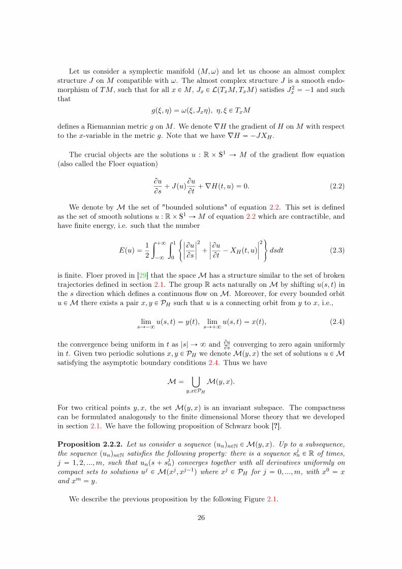
Proposition 2.2.2. Let us consider a sequence punqnPN PMpy, xq. Up to a subsequence,the sequence punqnPN satisfies the following property: there is a sequence sjn P R of times,j “ 1, 2, ...,m, such that unps ` sjnq converges together with all derivatives uniformly oncompact sets to solutions uj P Mpxj , xj´1q where xj P PH for j “ 0, ...,m, with x0 “ xand xm “ y.

We describe the previous proposition by the following Figure 2.1.

26

x

y

unxj

xj´1

uj

‚

‚

‚

‚

Figure 2.1: illustration of proposition 2.2.2

One may prove using Fredholm theory in the appropriate functional analytic settingthat for a "generic" choice of the pair pH,Jq the sets Mpy, xq are smooth and finite di-mensional manifolds such that the dimension of a set Mpy, xq is equal to the differenceindCZpyq ´ indCZpxq, where indCZpxq is the Conley-Zehnder index of x whose definitionwill be recalled in section 2.2.5.

Then we can define the homology groups associated to a pair pH,Jq on pM,ωq. Thegrading of the chain complex pCkqkPZ is given by the Conley-Zenhder index that we definelater in section 2.2.5 and for all k P Z we have

Ck “à

tZ2Z ¨ x|x P PH & indCZpxq “ ku,

where PH is the set of non degenerate contractible periodic orbits of H.

If we consider a pair y, x P PH such that indCZpyq´indCZpxq “ 1 thenMpy, xq is a one-dimensional manifold and more precisely has finitely many components, each componentconsists of a connecting orbit together with all its translates by the time s shift. We cannow define the differential map Bk : Ck Ñ Ck´1 for y P PH of index k as follows.

Bky “ÿ

xPPH |indCZpxq“k´1

npy, xqx,

where npy, xq is the number of connected components ofMpy, xq counted modulo 2.

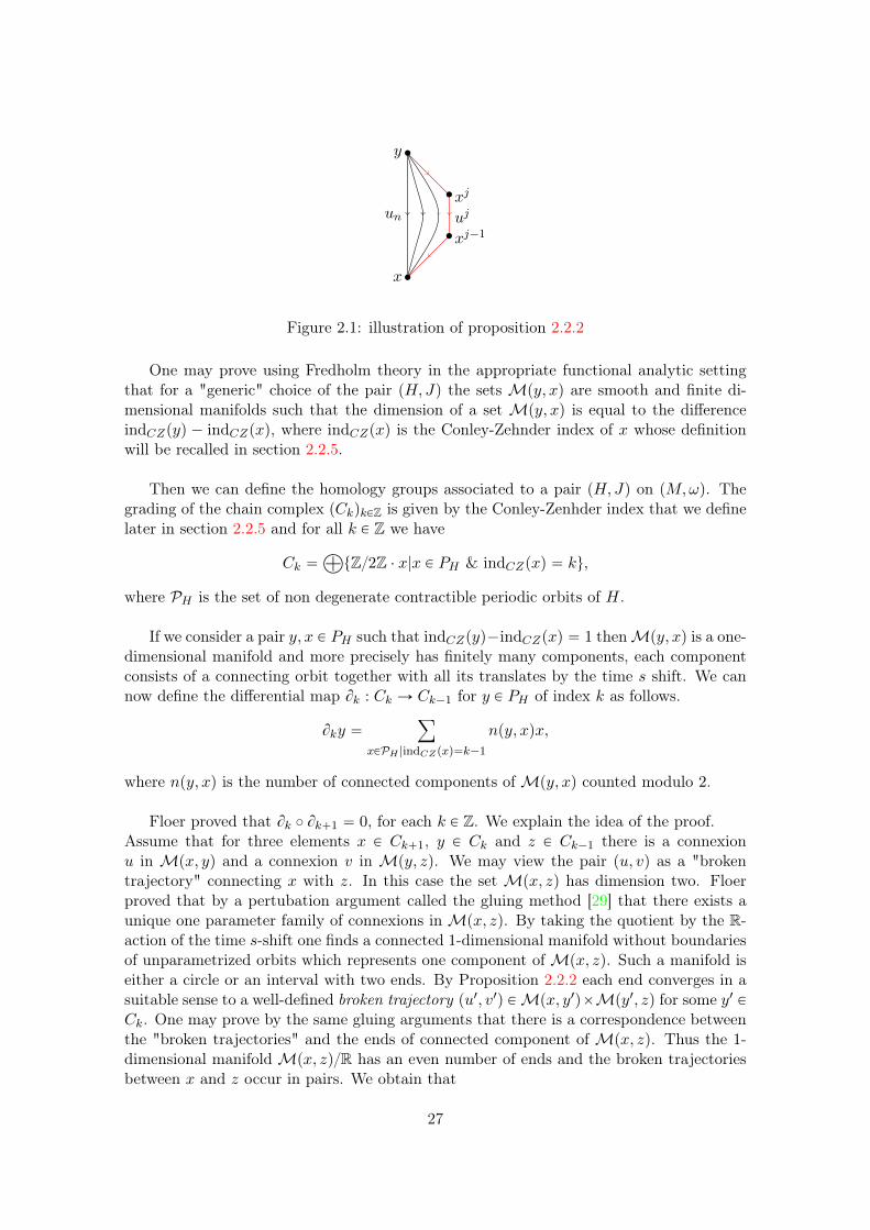
Floer proved that Bk ˝ Bk`1 “ 0, for each k P Z. We explain the idea of the proof.Assume that for three elements x P Ck`1, y P Ck and z P Ck´1 there is a connexionu in Mpx, yq and a connexion v in Mpy, zq. We may view the pair pu, vq as a "brokentrajectory" connecting x with z. In this case the set Mpx, zq has dimension two. Floerproved that by a pertubation argument called the gluing method [29] that there exists aunique one parameter family of connexions inMpx, zq. By taking the quotient by the R-action of the time s-shift one finds a connected 1-dimensional manifold without boundariesof unparametrized orbits which represents one component ofMpx, zq. Such a manifold iseither a circle or an interval with two ends. By Proposition 2.2.2 each end converges in asuitable sense to a well-defined broken trajectory pu1, v1q PMpx, y1qˆMpy1, zq for some y1 PCk. One may prove by the same gluing arguments that there is a correspondence betweenthe "broken trajectories" and the ends of connected component of Mpx, zq. Thus the 1-dimensional manifoldMpx, zqR has an even number of ends and the broken trajectoriesbetween x and z occur in pairs. We obtain that

27

Bk ˝ Bk`1pxq “ÿ

indCZpzq“k´1

¨

˝

ÿ

indCZpyq“k

npx, yqnpy, zq

˛

‚z

is equal to 0 modulo 2.

z

x

yy1

u

v

u1

v1

‚

‚

‚‚

Figure 2.2

We can define the Floer homology groups pHFkpM,H, JqqkPZ by

HFkpM,H, Jq “ KerpBkqImBk`1.

Remark 2.2.3. Notice that the energy of a solution u PMpy, xq is equal to Epuq “ AHpyq´AHpxq and is positive. We deduce that the action function AH decreases along the solutionu. We can compare this result to Remark 2.1.5 where a Morse funtion F onM is decreasingalong the solutions of a pseudo gradient vector field.

2.2.4 Filtered Floer Homology

Let us consider a non-degenerate Hamiltonian function H on a symplectic manifold pM,ωqwhich satisfies the hypothesis of the previous section 2.2.3 and let us fix J an almostcomplex structure on M . We use the same notation as in Section 2.2.3 to define thefiltered Floer homology of H from the Floer homology of H.

We consider the natural filtered chain complex pCtkqkPZ,tPR where Ctk “À

tZ2Z ¨x|x P PH , indCZpH,xq “ k, AHpxq ă tu and the natural filtered differential applicationBtk : Ctk Ñ Ctk´1 defined as the restriction of Bk on Ctk.

The filtered chain complex pCtk, BtkqkPZ,tPR induces an homology denoted pHFt˚qtPR. This

homology is referred to as the filtered Floer homology of the Hamiltonian H. One mayprove that the filtered Floer homology of H does not depend on the choice of the almostcomplex structure J on M , see [3] for example.

We have the following property.

Proposition 2.2.4. We consider two Hamiltonian flows pφtH0qtPr0,1s and pφtH1

qtPr0,1s oftwo Hamiltonian functions H0 and H1 on S1 ˆM . Let us suppose that pφtH0

qtPr0,1s andpφtH1

qtPr0,1s are homotopic relative to the endpoints in HampM,ωq. Then there exists aconstant c P R such that

HFt˚pH0q “ HFt`c˚ pH1, 1q,@t P R.

28

2.2.5 Conley-Zehnder index and Maslov index

The Conley-Zehnder index is an important tool in the definition of Barcodes and we willdiscuss some properties of this index in our constructions. We give a short version of thedefinition although we will not use it directly.

Given a Hamiltonian function H of a symplectic manifold pM2n, ωq we want to definethe Conley-Zehnder index of any contractible 1-periodic solution xptq of 9xptq “ Xtpxq.

We consider the symplectic manifold pR2n, ω0q where ω0 is the standard symplecticform on R2n written in the coordinates z “ px1, ..., xn, y1, ..., ynq P R2n as follows

ω0 “

nÿ

i“1

dxi ^ dyi.

We denote J0 the 2nˆ 2n matrix

J0 “

ˆ

0 ´1n1n 0

˙

,

which represents a rotation by π2 and satisfies J20 “ ´12n. We denote the group of

symplectic matrices by

Sppnq “ tM P R2n ˆ R2n|MTJ0M “ J0u,

where MT is the transpose matrix of M . We also denote SPpnq the set of paths γ in Sppnqfrom id to a matrix A which do not have eigenvalue 1.

Let us consider a non degenerate orbit x. There are two steps to compute the index ofthe critical point x. We associate to the orbit a path ψ : t ÞÑ Aptq of matrices in Spp2nq.Then to a path ψ we associate an integer which is the Conley-Zenhder index of x.

First step

We fix the orbit xptq “ φtpxp0qq then we can choose a family of symplectic bases, see[3] for example, Zptq “ pZ1ptq, ..., Z2nptqq of TxptqM that depends smoothly on t. For everyt P R, we can consider the matrix Aptq of the linear map Txp0qφ

t in the bases Zp0q andZptq and we obtain a path ψ : tÑ Aptq such that Ap0q “ id and such that Ap1q does nothave eigenvalue 1 because the orbit is supposed to be nondegenerate.

Second step

Definition 2.2.5. Let ρ : Sppnq Ñ S1 be the continuous map defined as follows. GivenA P Sppnq, we consider its positive eigenvalues tλiu. For an eigenvalue λ “ eiφ P S1zt˘1u,let m`pλq be the number of positive eigenvalues of the symmetric non degenerate 2-formQ defined on the generalized eigenspace Eλ by

Q : Eλ ˆ Eλ Ñ R : pz, z1q Ñ ωpz, z1q.

Hence we haveρpAq “ p´1q

12m´

ź

λPS1zt˘1u

λ12m`pλq, (2.5)

29

where m´ is the sum of the algebraic multiplicities mλ “ dimCEλ of the real negativeeigenvalues.

Theorem 2.2.6. The map ρ : Sppnq Ñ S1 satisfies the following properties:

1. determinant: if A P Upnq “ Sppnq XOp2nq, then

ρpAq “ detCpX ` iY q, where A “ˆ

X ´YY X

˙

.

2. invariance: ρ is invariant under conjugation, i.e. for all B P Sppnq we have ρpBAB´1q “

ρpAq;

3. normalisation: ρpAq “ ˘1 for matrices which have no eigenvalue on the unit circle;

4. multiplication: ρ behaves multiplicatively with respect to direct sums e.g if we considerA P Sppmq and B P Sppnq then we have

ρp

ˆ

A 00 B

˙

q “ ρpAqρpBq.

Moreover, the set Sp˚pnq “ tA P Sppnq|detpA ´ idq ‰ 0u has two connected compo-nents. There are the connected component Sp´pnq “ tA P Sppnq|detpA ´ idq ă 0u whichcontains the matrix ´id, denoted W´, and the connected component Sp`pnq “ tA P

Sppnq|detpA ´ idq ą 0u which contains the matrix diagp2, 12,´1, ...,´1q, denoted W`.Notice that any loop in Sp˚pnq is contractible in Sppnq.

Then any path ψ : r0, 1s Ñ Sppnq in SPpnq such that ψp1q is in Sp˚pnq can be extendedto a path ψ : r0, 2s Ñ Sppnq such that

1. rψptq “ ψptq for t ď 1;

2. rψptq is in Sp˚pnq for any t ě 1;

3. rψp2q P tW˘u.

Since pρpidqq2 “ 1 and pρpW˘qq2 “ 1 we have that ρ2 ˝ rψ : r0, 2s Ñ S1 is a loop in S1.Moreover one may prove that its degree does not depend on the extension rψ of ψ.

Definition 2.2.7. The Maslov index of an element ψ of Sppnq is defined by:

µM : Sppnq Ñ Z | ψ ÞÑ degpρ2 ˝ ψq, (2.6)

where ψ is an extension of ψ as above.

Then we define the Conley-Zendher index of a critical point x of H as the Maslov indexof the path of symplectic matrices associated to x in the first step.

Remark 2.2.8. If we suppose that the Hamiltonian diffeomorphism f is given by the 1-timemap flow of an autonomous Hamiltonian function H : M Ñ R which is C2-close to theidentity then the Conley-Zehnder index of a fixed point x of f is equal to the Morse indexof x where H is seen as a Morse function on M . One may refer to [68] for more details.

30

2.3 Dynamical systems

From now we consider a connected, compact and oriented surface Σ without boundary. LetHomeopΣq be the space of homeomorphisms of Σ equipped with the topology of uniformconvergence on Σ. For f P HomeopΣq, Fixpfq represents the set of fixed points of f .

2.3.1 Isotopies and maximal Isotopies

An isotopy is a continuous path t ÞÑ ft from r0, 1s to HomeopΣq. We say that f P HomeopΣqis isotopic to the identity if there exists an isotopy I “ pftqtPr0,1s such that f0 “ id andf1 “ f . We denote by Homeo0pΣq the set of those homeomorphisms.

Given an isotopy I “ pftqtPr0,1s from id to f , we can extend it to an isotopy defined onR by the periodic relation ft`1 “ ft ˝ f1. We define the set of singularities SingpIq of I asfollows.

SingpIq “ tx P Σ| @t P r0, 1s, ftpxq “ xu.

The complement of SingpIq in Σ is called the domain of I and denoted DompIq.

For a point z P Σ, the arc γ : r0, 1s Ñ Σ where for each tP r0, 1s, γptq “ ftpzq iscalled the trajectory of z along the isotopy I. For every n ě 0, we denote by γnpzq theconcatenation of the trajectories of z, fpzq, ..., fn´1pzq.

We fix a homeomorphism f P Homeo0pΣq. A set X Ă Fixpfq is say to be unlinked ifthere exists an isotopy I “ pftqtPr0,1s from id to f such that X is included in the set ofsingularities of I.We denote by Ipfq the set of couples pX, Iq such that I is an isotopy from id to f andX Ă SingpIq. The set Ipfq is naturally equipped with a pre-order ď, where

pX, Iq ď pX 1, I 1q,

if X Ă X 1 and for each z P ΣzX, its trajectory along I 1 and I are homotopic in ΣzX.The couple pX 1, Iq is called an extension of pX, Iq. An isotopy I P I is called a maximalisotopy in I if the couple pSingpIq, Iq is a maximal element of pI,ďq.

A recent result by F. Béguin, S. Crovisier and F. Le Roux [8] asserts that for a home-omorphism f P Homeo0pΣq isotopic to the identity there always exists a maximal isotopy(a weaker result was previously proved by O. Jaulent [44]). We will often use Corollary1.3 of [8] which we write as the following theorem:

Theorem 2.3.1. Let us consider f P Homeo0pΣq. For each element pX, Iq P Ipfq there isa maximal element pX 1, I 1q P Ipfq such that pX 1, I 1q is an extension of pX, Iq.

In the case of the 2-sphere S2 we have the following result, which can be found in [50],about the homotopy classes of isotopies of an orientation preserving homeomorphism f ofthe sphere S2. We consider the isotopy R8 “ prtqtPr0,1s where rt is the rotation of angle2πt i.e rtpr, θq “ pr, θ ` 2πtq in radial coordinates. The isotopy extends into an isotopyR2 \ t8u on the sphere. For z P S2, we choose an orientation preserving homeomor-phism hz : R2 Ñ S2ztzu and we define the isotopy Rz “ hz ˝ R8 ˝ h

´1z . If we consider

31

two points z and z1 of the sphere we choose an orientation preserving homeomorphismhz,z1 : R2 Ñ S2ztzu such that hz,z1p0q “ z1 and we define the isotopy Rz,z1 “ hz,z1˝R8˝h

´1z,z1

which fixes the points z and z1.

Proposition 2.3.2. Let us consider an orientation preserving homeomorphism f of thesphere S2.

1. For each fixed point z P Fixpfq, the set of isotopies from id to f which fix z is notempty. For two such isotopies I and I 1, there exists a unique integer k P Z such thatI 1 is homotopic to RkzI relatively to tzu.

2. If f has at least two fixed points, then for each couple pz, z1q of distinct fixed points theset of isotopies from id to f which fix z and z1 is not empty. For two such isotopies,there exists a unique integer k P Z such that I 1 is homotopic to Rkz,z1I relatively totz, z1u.

3. If f has at least three fixed points, then for each triplet pz, z1, z2q of distinct fixedpoints the set of isotopies from id to f which fix z, z1 and z2 is not empty. All thoseisotopies are homotopic relatively to tz, z1, z2u.

2.3.2 Lefschetz index

For a homeomorphism f P HomeopΣq and an isolated fixed point x of f , we define theLefschetz index indpf, xq of x as follows. let U be a chart centered at x and we denote byΓ a small oriented circle in U around x. For Γ sufficiently small, the map

z ÞÑfpzq ´ z

||fpzq ´ z||,

is well defined on Γ and we denote by indpf, xq the degree of this map.

2.3.3 Linking number

Let us consider an orientation preserving homeomorphism f of the plane isotopic to theidentity and I “ pftqtPr0,1s an isotopy from id to f . Let us suppose that there exists aperiodic point z˚ of f of period q ě 1. If z is a fixed point of f , the quotient of the map

t ÞÑftpz

˚q ´ ftpzq

||ftpz˚q ´ ftpzq||,

defines a continuous function of the circle RqZ to S1. The degree of this applicationis called the real linking number of z˚ and is denoted by lI,z˚pzq. It depends only onthe homotopy class of the isotopy I. For another isotopy I 1 of f there exists k P Zsuch that I 1 is homotopic to RkzI, where Rkz was defined in section 2.3.1. We verify thatlI 1,z˚pzq “ lI,z˚pzq ´ kq. Then the linking number Lf,z˚pzq “ lI,z˚pzq ` qZ P ZqZ isindependent on the choice of the isotopy.

32

2.3.4 Rotation vectors

Let f P Homeo0pΣq be the time one map of an isotopy I “ pftqtPr0,1s from the identity tof . Among the many ways to define the rotation vector, we restrict ourselves to positivelyrecurrent points. A point z P Σ is a positively recurrent point of f if for each neighborhoodU Ă Σ of z there exists an integer n P N such that fnpzq P U . The integer n ą 0 whichis minimal for the previous property is called the first return time and is denoted by τpzq.The set of positively recurrent points is denoted by Rec`pfq.

Let z P Σ be a positively recurrent point. Fix a 2-ball U Ă Σ containing z and letpfnkpzqqkě0 be a subsequence of the positive orbit of z obtained by keeping the iteratesof z by f that are in U . For any k ě 0, choose an arc γk in U from fnkpzq to z. Thehomology class rΓks P H1pΣ,Zq where Γk is the concatenation of γnk´1pzq and γk do notdepend on the choice of γk. We say that z has a rotation vector ρpzq P H1pΣ,Rq if

limlÑ`8

1

nklrΓkls “ ρpzq,

for any subsequence pfnkl pzqqlě0 which converges to z. Notice that the linking number ofa periodic point z˚ of an orientation preserving homeomorphism of the plane is equal tothe rotation number of z˚ in R2ztzu.

In the case where f preserves a Borel probability measure µ, one applies Birkhoff’sergodic theorem to the first return map in U and proves that µ-a.e. point z is positivelyrecurrent and has a rotation vector ρpzq. Moreover, the measurable map ρ is bounded,and one may define the rotation vector of the measure

ρpµq “

ż

Σρ dµ P H1pΣ,Rq.

We say that f P Homeo0pΣq is a Hamiltonian homeomorphism if it preserves a Borelprobability measure whose support is the whole surface and rotation vector is zero. Wedenote by HampΣq the set of Hamiltonians on Σ.

2.3.5 Local isotopies and local rotation set

Let Σ be a connected oriented surface. We write f : pW, z0q Ñ pW 1, z0q for an orientationpreserving homeomorphism between two neighborhoods W and W 1 of z0 P Σ such thatfpz0q “ z0. Such a local homeomorphism f is called an orientation preserving local homeo-morphism at z0. We recall the definition of local isotopies of Le Calvez [50]: a local isotopyI “ pftqtPr0,1s from id to f is a continuous family of local homeomorphisms pftqtPr0,1s fixingz0 such that

- each ft is a homeomorphism of a neigborhood Vt ĂW of z into a neighborhood V 1t ĂW 1

of z ;

- the sets tpz, tq P Σˆr0, 1s|z P Vtu and tpz, tq P Σˆr0, 1s | z P V 1t u are open in Σˆr0, 1s ;

- the map pz, tq ÞÑ ftpzq is continuous on tpz, tq P Σˆ r0, 1s | z P Vtu ;

33

- the map pz, tq ÞÑ f´1t pzq is continuous on tpz, tq P Σˆ r0, 1s | z P V 1t u ;

- we have f0 “ idV0 and f1 “ f |V1 ;

- for all t P r0, 1s, we have ftpz0q “ z0.

Let us consider a local orientation preserving homeomorphism f : pW, z0q Ñ pW 1, z0q

and I “ pftqtPr0,1s a local isotopy from id to f . We want to define the local rotation set ofthe isotopy I at z0. Given two neighborhoods V Ă U of z0 included in W and an integern ě 1 we define

EpU, V, nq “ tz P U | z R V, fnpzq R V, f ipzq P U for all 1 ď i ď nu.

We define the rotation set of I relative to U and V by

ρU,V pIq “č

mě1

ď

něm

tρnpzq | z P EpU, V, nqu Ă r´8,8s,

where ρnpzq is the average change of angular coordinate along the trajectory of z duringn iterates. We define the local rotation set of I to be

ρspI, z0q “č

U

ď

V

ρU,V pIq Ă r´8,8s,

where V Ă U ĂW are neighborhoods of z0.

The local rotation set is an invariant of local conjugacy in the following sense: let us saythat an isotopy I 1 “ pf 1tqtPr0,1s is locally conjugated to I if there exists a homeomorphismφ : W ÑW 2 between two neighborhood of z0 which preserves the orientation and fixes z0

such that for each t P r0, 1s we have f 1t “ φ ˝ ft ˝ φ´1. For each neighborhoods V and U of

z0 such that V Ă U ĂW we have

ρU,V pIq “ ρφpUq,φpV qpφIφ´1q.

In particular we deduce thatρspIq “ ρspφIφ

´1q.

Let us consider a homeomorphism of the plane f isotopic to the identity which preservesthe orientation and fixes the origin and an isotopy I “ pftqtPr0,1s from id to f which fixesthe origin. Recall that R “ pRtqtPr0,1s is the isotopy of the rotation of angle 2π such thatRtpzq “ ze2iπt for each z P R2 and t P r0, 1s. We have the following result about the localrotation set.

Lemma 2.3.3. For each p P Z and q P Z we have

ρspRpIqq “ qρspIq ` p.

We say that f satisfies the local intersection property at z0 if we have:

For each non contractible loop γ of W ztz0u we have fpγq X γ ‰ H. (P2.6)

34

Example 2.3.4. Let us consider a fiber rotation hα : pr, θq Ñ pr, θ`αprqq on the plane whereα : p0,8q Ñ R is continuous and an isotopy I “ phtqtPr0,1s such that htpr, θq “ pr, θ`tαprqqfor t P r0, 1s. The local rotation set ρspIq of I at the origin is equal to the set of accumulationpoints of α at 0.

F. Le Roux proved [56, 59] that a homeomorphism of the plane which preserves theorientation and which fixes the origin has an empty local rotation set at 0 if and only if itis locally conjugated to the following maps:

- the contraction z ÞÑ z2 ,

- the expansion z ÞÑ 2z,

- a holomorphic function z ÞÑ e2iπ p

q zp1` zqrq where q, r P N` and p P Z.

Remark 2.3.5. In particular, in the case where f is area-preserving, Gambaudo and Pécout[34] proved that none of those above cases occurs, then the local rotation set is not empty.Moreover, if we suppose that Fixpfq is finite, 0 is not accumulated by fixed points thenif the local rotation set is not empty it does not contain an integer in its interior. Noticethat the result holds if we suppose that f satisfies the local intersection property, meaningthat for each non contractible loop γ of W ztz0u we have fpγq X γ ‰ H.

The rotation number classify the homotopy classes of the isotopies at z0. Let us con-sider a local orientation preserving homeomorphism f : pW, z0q Ñ pW 1, z0q of a surface Σsuch that fpz0q “ z0 and I “ pftqtPr0,1s a local isotopy from id to f which fix z0. Let usconsider a closed disk D Ă Σ containing z0 in its interior. For every point z P Dztz0u closeenough to z0, the trajectory of z0 along I is a loop included in Dztz0u. There exists aninteger k P Z such that this trajectory is freely homotopic in Dztz0u to pBDqk. The integerk depends only on the choice of the isotopy I, it is the rotation number k “ ρpI, z0q ofI at z0. We consider the isotopy R8 defined in the previous section 2.3.1. The isotopyR8 extends into an isotopy on the sphere R2 \ t8u and we have ρpR8,8q “ 1 whileρpR8, 0q “ ´1. We refer to [50] for more details.

2.3.6 The blow-up at a fixed point

Let us consider f : pW, z0q Ñ pW 1, z0q an orientation preserving homeomorphism. We saythat f can be blown-up at z0, if we can "replace" z0 by a unit circle S1 and extend f |W ztz0ucontinuously to a homeomorphism betweenW ztz0u\S

1 andW ztz0u\S1, see [59] for more

details. In particular, when f is a diffeomorphism, the extension can be induced by themap

v ÞÑDfpz0qv

||Dfpz0qv||

on the space of unit tangent vectors.

Let us suppose that f can be blown-up at z0, is isotopic to the identity and is notconjugate to a contraction or an expansion. We denote by h the extension of f on S1 andby I “ pftqtPr0,1s a local isotopy of f . We choose a small disk D which contains z0 and weconsider the universal cover π : rD Ñ Dztz0u. We consider the isotopy p rftqtPr0,1s from id torf obtain by lifting I and we consider rh the lift of h to R which is a continuous extension

35

of rf1. We define the blown-up rotation number ρpI, z0q P R to be the rotation numberof rh. J.-M. Gambaudo,P. Le-Calvez and E. Pécou [33] proved that the blown-up rotationnumbers does not depend on the choice of h.

Naturally we have the following property [59].

Proposition 2.3.6. Let us consider an isotopy I “ pftqtPr0,1s from id to a homeomorphismof the plane f which preserves the orientation, fixes the origin and can be blown-up at 0.If the local rotation set ρspIq is not empty then it is equal to the singleton tρpI, z0qu.

2.3.7 Positively transverse foliations

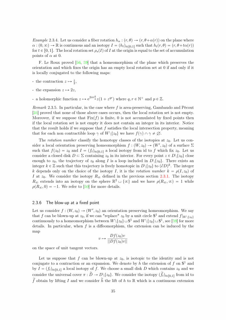
Let us consider an oriented topological foliation F on the complement of a compact setX of a surface Σ. The set X will be called the set of singularities of F . An open flowbox of F is a couple pV, hq, where V is an open set of Σ and h : V Ñ p´1, 1q2 is anorientation-preserving homeomorphism that sends the foliation F |V on the vertical folia-tion oriented with y decreasing. Writing p1 : R2 Ñ R for the first projection, we say thatan arc γ : I Ñ Σ is positively transverse to the foliation F if for every t0 P I, there existsan open flow-box pV, hq such that γpt0q P V and the map t ÞÑ p1phpγptqqq defined in aneighborhood of t0 is strictly increasing.

γ

Figure 2.3: An example of a flow box

For z P Σ, we write φz the leaf passing through z and φ`z for the positive half-leaffrom z. We consider an isolated singularity x of the foliation F , we can define the indexindpF , xq of x for the foliation F as follows. We consider a sufficiently small open chart Ucontaining x and an orientation preserving homeomorphism h : U Ñ Dzt0u which sendsx to 0. We denote Fh the image of the foliation F |U by h and we consider a simple loopΓ : S1 Ñ Dztxu, one may cover Γ by a finite family pViqiPJ of flow-boxes of the foliationFh included in Dzt0u. We denote by φ`Vi,z the positive half-leaf from z of the restrictedfoliation Fh|Vi . We can find a continuous map ψ defined from the loop Γ to D1ztxu suchthat ψpzq P φ`Vi,z for every i P J and any z P Vi. The map

θ ÑψpΓpθqq ´ Γpθq

||ψpΓpθqq ´ Γpθq||,

is well defined on Γ and indpF , xq is the degree of this map.

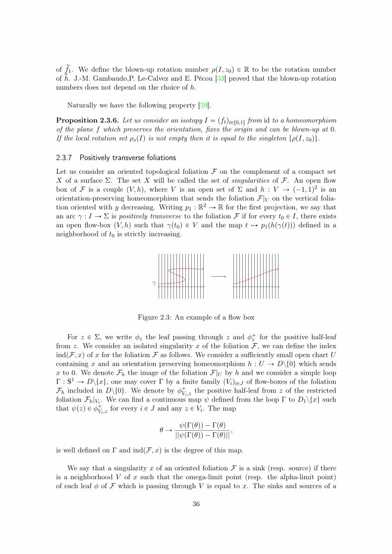
We say that a singularity x of an oriented foliation F is a sink (resp. source) if thereis a neighborhood V of x such that the omega-limit point (resp. the alpha-limit point)of each leaf φ of F which is passing through V is equal to x. The sinks and sources of a

36

foliation F have an index equal to 1. Let us draw an example of the neighborhood of asink on the left and a neighborhood of a source on the right of the following figure.

Figure 2.4: An example of a sink and a source of a foliation

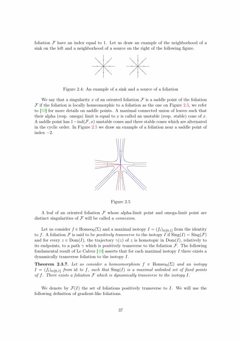
We say that a singularity x of an oriented foliation F is a saddle point of the foliationF if the foliation is locally homeomorphic to a foliation as the one on Figure 2.5, we referto [59] for more details on saddle points. A maximal connected union of leaves such thattheir alpha (resp. omega) limit is equal to x is called an unstable (resp. stable) cone of x.A saddle point has 1´ indpF , xq unstable cones and three stable cones which are alternatedin the cyclic order. In Figure 2.5 we draw an example of a foliation near a saddle point ofindex ´2.

Figure 2.5

A leaf of an oriented foliation F whose alpha-limit point and omega-limit point aredistinct singularities of F will be called a connexion.

Let us consider f P Homeo0pΣq and a maximal isotopy I “ pftqtPr0,1s from the identityto f . A foliation F is said to be positively transverse to the isotopy I if SingpIq “ SingpFqand for every z P DompIq, the trajectory γpzq of z is homotopic in DompIq, relatively toits endpoints, to a path γ which is positively transverse to the foliation F . The followingfondamental result of Le Calvez [49] asserts that for each maximal isotopy I there exists adynamically transverse foliation to the isotopy I.

Theorem 2.3.7. Let us consider a homeomorphism f P Homeo0pΣq and an isotopyI “ pftqtPr0,1s from id to f , such that SingpIq is a maximal unlinked set of fixed pointsof f . There exists a foliation F which is dynamically transverse to the isotopy I.

We denote by FpIq the set of foliations positively transverse to I. We will use thefollowing definition of gradient-like foliations.

37

Definition 2.3.8. A foliation F is said to be gradient-like if

• The number of singularities is finite.

• Every leaf defines a connexion.

• There is no closed leaf.

• There is no family pφiqiPZkZ, k ě 1 of leaves such that ωpφiq “ αpφi`1q, i P ZkZ.

For the remaining of the thesis, most of the transverse foliations we will meet will begradient-like foliations. The notion of connexion will be generalized in chapter 7, but untilthis chapter, a connexion will always refer to a leaf of a gradient-like foliation.

We refer to [49] for the proof of the following important properties.

Proposition 2.3.9. Consider a Hamiltonian homeomorphism of a surface Σ with a finitenumber of fixed points then for each maximal isotopy I from id to f , a foliation F positivelytransverse to I is gradient-like. Moreover we have

• indpF , xq ď 1 for every point x P SingpIq.

• indpF , xq “ 1 for every sink or source x P SingpIq

• indpF , xq “ indpf, xq for every saddle point x P SingpIq, where indpf, ¨q is the Lef-schetz index.

• For every leaf φ P F , the action function Af , defined later, of f satisfies Af pαpφqq ąAf pωpφqq.

For the remaining, we can keep in mind that, for a gradient-like foliation, there arethree kinds of singularities: sinks, sources and saddle points.

Remark 2.3.10. For a maximal isotopy I of a Hamiltonian homeomorphism f of a surfaceΣ and a foliation F P FpIq, if Σ is not the sphere, then the index function indpF , ¨q definedon SingpIq does not depend on the choice of F P FpIq and can be denoted indpI, ¨q.

Let us consider a gradient-like foliation F of a surface Σ and a leaf φ of F . By definition,the omega-limit set (resp. the alpha-limit set) of φ exists and is equal to a singleton txu.To simplify the notations, x will be called the omega-limit point also denoted ωpφq (resp.the alpha-limit point also denoted αpφq) of φ.

2.3.8 Generalized Isotopies

In this section, we consider a Hamiltonian homeomorphism f of a compact surface Σ suchthat Fixpfq is finite.

We consider the compactification Σ “ rΣY t8u of rΣ into a 2-sphere.

Let us consider a maximal isotopy I of f on Σ and its natural lift rI on rΣ. The isotopyrI has an infinite number of singularities but for a non zero integer k P Z˚ and a fixedpoint rx of rf , Rk

rxrI has a finite number of singularities and can be extended to an isotopy

38

I of a homeomorphism f on Σ which has a finite number of fixed points. The point atinfinity in Σ becomes a fixed point of such a homeomorphism f and its rotation numberfor I satisfies:

ρIp8q “ ´k.

An isotopy I from id to f which is homotopic to Rkrx,8

rI relatively to Σztrx,8u such thatthe rotation number of 8 is equal to ´k is called a generalized isotopy of f . We denoteby Ik the set of couples pX, Iq where I is a generalized isotopy of f such that ρIp8q “ ´kand X Ă SingpIq. To simplify notations, we can consider I P Ik which refers to the couplepSingpIq, Iq.

The set Ik is naturally equipped with a pre-order ď, where pX, Iq ď pX 1, I 1q if 8 P

X Ă X 1 are unlinked sets of fixed points and for each z P ΣzX, its trajectory along I 1 andI are homotopic in ΣzX. The couple pX 1, Iq is called an extension of pX, Iq. An isotopyI P Ik is called a maximal generalized isotopy in Ik if the couple pSingpIq, Iq is a maximalelement of pIk,ďq.

Lemma 2.3.11. Let us consider a generalized isotopy I P Ik of f with k P Z˚,

#SingpIq ď #Fixpfq ` 1,

and for each z P Fixpfq we have

#pSingpIq X π´1pzqq ď 1.

Proof. By contradiction we prove the second inequality, the first one will follow.

Let us consider a generalized isotopy I P I such that there exists x P Fixpfq satisfying#pSingpIq X π´1pxqq ą 1 or #SingpIq ě Fixpfq ` 2. We consider rI the isotopy from idto f whose compactification is the isotopy I. There exists two singularities rx and rx1 of Iwhich are in π´1ptxuq. The linking number between rx and rx1 for the isotopy rI is equal tozero.

We consider I 1 a maximal isotopy from id to f which fixes x and we denote rI 1 theisotopy obtained by lifting I 1 on rΣ. We have that rI 1 is homotopic to R´k

rxrI relatively to

Σztx,8u, see Proposition 2.3.2 for more details, and we have π´1ptxuq Ă SingprI 1q. So, thelinking number between rx and rx1 for the isotopy rI 1 is equal to zero but the linking numberbetween rx and rx1 for the isotopy R´k

rxrI is equal to ´k. Hence we obtain our contradiction.

We deduce the inequality #SingpIq ď #Fixpfq ` 1.

Lemma 2.3.12. Let us consider a maximal generalized isotopy I P Ik of f where k P Z˚.There exists a foliation F on the 2-sphere such that F is positively transverse to I andevery foliation which is positively transverse to I is gradient-like.

Remark 2.3.13. i. For such a foliation F of a maximal generalized isotopy I, the actionfunction is decreasing along the leaves of F .

ii. The fixed point 8 is a source of F if k ă 0 and a sink of F if k ą 0.

39

2.3.9 Intersection number

Let Γ and Γ1 be two oriented, transverse and simple closed curves on an oriented surfaceΣ. The algebraic intersection number Γ ^ Γ1 is defined as the sum of the indices of theintersection points of Γ and Γ1, where an index of an intersection point is `1 if the orien-tation of the intersection agrees with the orientation of Σ and ´1 otherwise.

We keep the same notation Γ^ γ for the algebraic intersection number between a loopΓ and a path γ when it is defined, for example, when γ is proper or when γ is a compactpath whose extremities are not in Γ. Similarly, we write γ^γ1 for the algebraic intersectionnumber of two path γ and γ1 when it is defined, for example, when γ and γ1 are compactpaths and the ends of γ (resp. γ1) are not on γ1 (resp. γ).

2.3.10 Action function of a Hamiltonian homeomorphism

In this section we define dynamically the action function of a Hamiltonian homeomorphismf of a compact surface Σ with a finite number of fixed points. Notice that this definition ex-tends the notion of action function defined in section 2.2.2 for Hamiltonian diffeomprhisms.

Let us consider two unlinked fixed points x, y P Fixpfq of f and an isotopy I “ pftqtPr0,1sfrom id to f such that x, y P SingpIq. Let γ be a simple path from x to y and define themap ρf,γ on Σ by ρf,γpzq “ γ ^ γpzq where γpzq is the trajectory of z under the isotopy Iand γ ^ γpzq is the intersection number between γ and γpzq. We define the difference ofaction between y and x by

Af pxq ´Af pyq “

ż

Σρf,γpzqdz, (2.7)

which does not depend on the choice of γ. Notice that in general for a homeomorphism f ,the map ρf,γ is not integrable. In our case, f admits a finite number of fixed points andone may prove that the previous integral exists, see [49].

Unfortunately, if we consider two fixed points x, y P Fixpfq they may not be unlinked.The previous arguments fail and to define the action difference between y and x we haveto consider the universal cover of Σ. We denote by rΣ the universal cover of Σ, π : rΣ Ñ Σthe covering map and for a homeomorphism f we set G˚ the group of automorphisms ofΣ which commute with the lift rf of f on Σ.

The following definition comes from a more general work of Wang [74]. The construc-tion is more difficult, first we have to extend the linking number used in equation 2.7then thanks to the work of Wang if the number of fixed points of f is finite then this link-ing number exists and we can define the action function by integrating this linking number.

Extension of the linking number for a positively recurrent point

Let us consider f the time one map of an isotopy I “ pftqtPr0,1s on Σ and rf the time1-map of the lifted identity isotopy rI “ p rftqtPr0,1s to the universal cover rΣ of Σ. For everydistinct fixed points rx and ry of rf there exists a non-equivariant isotopy rI1 from id to rf

40

that fixes rx and ry.

Recall that the set of positively recurrent points is denoted by Rec`pfq.

We consider z P Rec`pfqzπptrx, ryuq and an open disk U Ă Σzπptrx, ryuq which containsz. For each couple pz1, z2q P U2, we choose an oriented simple path γz1,z2 in U from z1 toz2. We define the function rΦ by:

rΦ : π´1pRec`pfqq X π´1pUq Ñ π´1pRec`pfqq X π´1pUq

rz ÞÑ rf τpzqprzq,

where z “ πprzq and τpzq is the first return map in U . rΦ is the lifted function of the firstreturn map Φ define on the recurrent points of U by Φpzq “ f τpzqpzq where z P Rec`pfqXU .

For any rz P π´1pUq, write rUrz the connected component of π´1pUq that contains rz. For

every j ě 1, recall that τjpzq “řj´1i“0 τpΦ

ipzqq. For every n ě 1, consider the followingcurve in rΣ:

rΓnrI1,rz

“ rIτnpzq1 przqrγ

rΦnprzq,rzn,

where rzn P π´1ptzuq X rU

rΦnprzq, and rγ

rΦnprzq,rznis the lift of γΦnpzq,z which is contained in

rUrΦnprzq

. We can define the infinite product

rΓnrI1,z

“ź

πprzq“z

rΓnrI1,rz.

In the annulus Arx,ry we can see rΓn

rI1,zas a multi-loop with finite homology. So, if we

consider rγ an oriented path in rΣ from rx to ry, the intersection number rγ ^ rΓnrI1,z

is well

defined and does not depend on rγ nor the isotopy rI1 but depends on the open set U . Wehave:

rγ ^ rΓnrI1,z

“ rγ ^ź

πprzq“z

rΓnrI1,rz

“

n´1ÿ

j“0

rγ ^ rΓjrI1,rz.

For n ě 1 we define the functions

Ln : ppFixp rfq ˆ Fixp rfqqzr∆q ˆ pRec`pfq X Uq Ñ Z,

by

Lnp rf ; rx, ry, zq “ rγ ^ rΓnrI1,z

“

n´1ÿ

j“0

L1p rf ; rx, ry,Φjpzqq,

where U Ă Σzπptrx, ryuq. Again, the function Ln depends on U but not on the choice ofγΦnpzq,z.

Action function

Definition 2.3.14. Let us consider z P Rec`pfqzπptrx, ryu. We say that the linking numberip rf ; rx, ry, zq P R is defined if

limkÑ8

Lnkprf ; rx, ry, zq

τnkpzq“ ip rf ; rx, ry, zq

41

for any subsequence tΦnkpzqukě1 of tΦnpzquně1 which converges to z.

J. Wang proved that the linking number ip rf ; rx, ry, zq does not depend on U .

Let us consider µ P Mpfq such that µ is ergodic or the support of µ is the wholesurface Σ. In our particular case where I has a finite number of fixed points, the functionip rf ; rx, ry, zq is µ-integrable and we define a function iµp rf ; rx, ryq as follows.

iµp rf ; rx, ryq “

ż

Σzπptrx,ryuip rf ; rx, ry, zqdµ.

Proposition 2.3.15. For any distinct fixed points rx, ry and rz of rf , we have

iµp rf ; rx, ryq ` iµp rf ; ry, rzq ` iµp rf ; rz, rxq “ 0.

So there exists a function lµ : Fixp rfq Ñ R defined up to an additive constant, such that

iµp rf ; rx, ryq “ lµp rf, ryq ´ lµp rf, rxq.

If f is a Hamiltonian homeomorphism then ρΣ,IpLebq “ 0 for each isotopy I from idto f on Σ and we have the following result.

Proposition 2.3.16. If we suppose that ρΣ,Ipµq “ 0, iµp rf ; rx, T prxqq “ 0 for every rx P

Fixp rfq and every automorphism T P G˚ then there exists a function Lµp rf, ¨q defined onFixp rfq such that for every two distinct fixed points rx and ry of rf we have

iµp rf ; rx, ryq “ Lµp rf, πpryqq ´ Lµp rf, πprxqq.

The function Lµp rf, ¨q is called the action function defined on Fixpfq for the measureµ. If µ “ Leb then the function Lµp rf, ¨q will be denoted Af .

Proposition 2.3.17. Let us consider a smooth diffeomorphism f of a surface Σ. Theaction function Af is equal to the action function of section 2.2.2.

Action function along a leaf of a transverse foliation

In particular, if we consider a maximal isotopy I “ pftqtPr0,1s from id to f and a foliationF positively transverse to I we can give a short proof of the last point of Proposition 2.3.9stated as the following lemma.

Lemma 2.3.18. For every leaf φ P F we have Af pαpφqq ą Af pωpφqq.

Proof. We set x “ αpφq and y “ ωpφq. We give the ideas of the proof using Wang’s work.

Let us consider a small open disk U Ă ΣzX. For almost every point z P U we can defineτpzq the first return map. Meaning that τpzq is the first integer n ą 0 such that fnpzq P U .We consider the loop Γpzq “ Iτpzq´1pzqγpzq where γpxq Ă U is a path which joins f τpzqpzqto z. The algebraic intersection of Γpzq and φ does not depend on the choice of γ and iswell defined. We will denote δpzq “ Γpzq^φ the algebraic intersection number defined on U .

42

There is a finite number of fixed points, so Wang proved that δτ is bounded and thenintegrable. We can define the limit of Birkhoff’s average functions δ˚ and τ˚ of δ and τ .One may prove that the function η “ δ˚τ˚ is defined almost everywhere on U and doesnot depend on the choice of U . So we obtain a function defined almost everywhere onΣzX such that, by the construction of Wang, its integral is equal to the action differencebetween x and y. Thus, it is enough to prove that δpzq is positive and not zero to obtainthe result.

We consider the universal cover ĆΣzX of ΣzX, which can be identify as the open diskD.

We fix a lift rφ of φ on D, hence δpzq is equal to the finite sum of the algebraic intersectionnumbers of rφ and the lifts of Γpzq. Let us consider a lift rΓpzq of Γpzq whose algebraicintersection number with rφ is not zero. Roughly speaking, rΓpzq is an oriented path goingfrom one side of Dzrφ to another. Moreover, rφ is a Brouwer line for rf , so rΓ is going from theright hand side of rφ to the left hand side of rφ. Hence the intersection number rΓpzq^ rφ ą 0and then we have δpzq ą 0.

43

44

Chapter 3

Introduction to barcodes and persistencemodules

The notion of barcodes and persistence modules was used in topological data analysis, seefor example G. Carlsson in [15] or R. Ghrist in [35]. Barannikov already noticed the exis-tence of a filtration of the Morse homology in [6] and we can find the notion of persistencemodules in Usher’s work [70, 71] but the barcodes have been introduced in symplectictopology by Polterovich and Shelukhin [67]. The same year, without the terminology ofthe barcodes Usher and Zang published some results about the persistent homology in [72].Recently, the notion of barcodes appears as a great tool to study C0 symplectic geometry,let us cite for example the work of Buhovski-Humilière-Seyfaddini [14], Jannaud [?] andLe Roux-Viterbo-Seyfaddini [61].

Most of the following definitions and results are coming from [61]. One can also referto Chazal, De Silva, Glisse and Outdot’s book [16] or to [18].

Barcodes

Let us consider a special family of intervals B of the form ppaj , bjsqjPt1,...,nu, with ´8 ďaj ď bj ď `8, where we allow trivial intervals of the form pa, as. We say that two familiesare equivalent if removing all intervals of the form pa, as from them yields the same family.

Definition 3.0.1. A barcode B is an equivalence class of family of intervals B.

By convenience, we will often identify a list of intervals with the corresponding barcode.

Let a ď b, c ď d be four elements of RY˘t8. We set dppa, bs, pc, dsq “ maxt|c´a|, |d´b|u, with convention that dp8,8q “ 0. Note that if c “ d “ a`b

2 , then dppa, bs, pc, dsq “ b´a2 .

Definition 3.0.2. Let B1, B2 be barcodes and take representatives B1 “ pI1j qjPJ , B2 “

pI2kqkPK . The bottleneck distance between B1, B2, denoted by dbotpB1, B2q, is the infimum

of the set of ε such that there is a bijection σ between two subsets J 1,K 1 of J,K with theproperty that for every j P J 1, dpI1

j , I2σpjqq ď ε and all the remaining intervals I1

j , I2k for

j P JzJ 1, k P KzK 1 have length less than 2ε.

45

We will denote Barcode the set of barcodes in the next sections.

Persistence module

Definition 3.0.3. A persistence module V is a family pVtqtPR of vector spaces equippedwith morphisms is,t : Vs Ñ Vt, for s ď t, satisfying:

1. For all t P R we have it,t “ id and for every s ď t ď u we have it,u ˝ is,t “ is,u,

2. There exists a finite subset F Ă R, often referred to the spectrum of V , such that is,tis an isomorphism whenever s, t belong to the same connected component of RzF ,

3. For all t P R, limsÑt,săt

Vs “ Vt ; equivalently, for fixed t, is,t is an isomorphism for

s ă t sufficiently close to t.

Let us consider a persitence module pVtqtPR equipped with the morphisms pis,tqsďt. Forany t P R, there exists ε such that is,u : Vs Ñ Vu is an isomorphism if s, u P pt´ ε, ts or ifs, u P pt, t` εq. Choose t´ P pt´ ε, ts and t` P pt, t` εq and let jptq “ dimpKerpit´,t`qq `codimpImpit´,t`qq. Notice that jptq is zero except for t in the spectrum of V. We say thatV is generic if jptq ď 1 for all t P R.

Functorial relations between the barcodes and the persistence modules

To establish the link between the previous objects we consider two functors as follows.

(i) Consider an interval I of the form pa, bs and define QtpIq “ Z2Z, if t P I, andQspIq “ t0u, if s R I. QspIq is a persistence module, with is,t equal to id if s, t P Iand 0 otherwise. For a set of intervals I for each t P R we define

QtpIq “à

IPIQtpIq.

(ii) We define a functor β from the set of generic persistence modules into the set ofbarcodes which associate to a generic persistence module V “ pVsqsPR a barcode.We denote pis,tqsďt the family of morphisms equipped with V. Let us consider theset of t in the spectrum of V such that dimpKerpit´,t`qq “ 1 and label its elementsb1, ..., bn. For each bj , there exists a unique aj P R with the following property: Letx P Vb´j

represents a non-zero element in Kerpit´,t`q, the element x is in the imageof ia`j ,b´j but x is not in the image of ia´j ,b´j . We label the remaining elements ofthe spectrum of V by tc1, ..., cmu. The barcode βpVq consists of the list of intervals:ppaj , bjs, pck,`8qq, where 1 ď j ď n and 1 ď k ď m.One may prove that the functor β extends to the set of persistence modules, we referto r61s for more details.

The following theorem holds.

Theorem 3.0.4. The functors defined above satisfy the following properties.

46

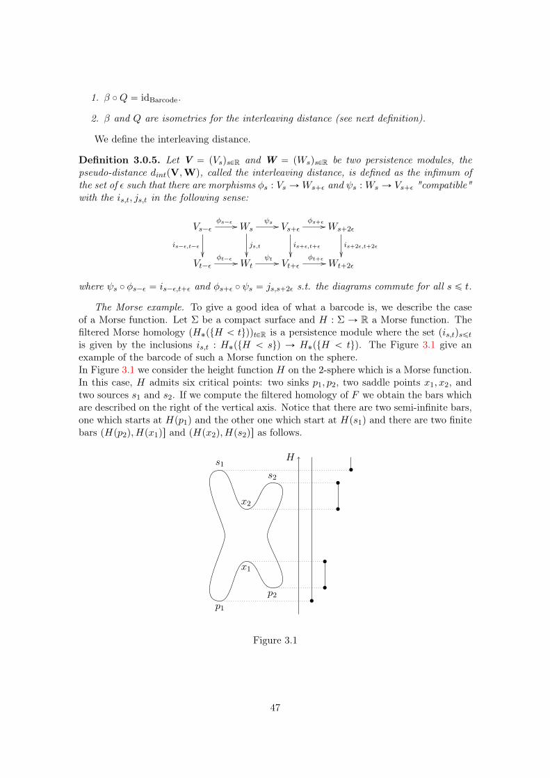
1. β ˝Q “ idBarcode.

2. β and Q are isometries for the interleaving distance (see next definition).

We define the interleaving distance.

Definition 3.0.5. Let V “ pVsqsPR and W “ pWsqsPR be two persistence modules, thepseudo-distance dintpV,Wq, called the interleaving distance, is defined as the infimum ofthe set of ε such that there are morphisms φs : Vs ÑWs`ε and ψs : Ws Ñ Vs`ε "compatible"with the is,t, js,t in the following sense:

Vs´εφs´ε //

is´ε,t´ε

Wsψs //

js,t

Vs`εφs`ε //

is`ε,t`ε

Ws`2ε

is`2ε,t`2ε

Vt´ε

φt´ε //Wtψt // Vt`ε

φt`ε //Wt`2ε

where ψs ˝ φs´ε “ is´ε,t`ε and φs`ε ˝ ψs “ js,s`2ε s.t. the diagrams commute for all s ď t.

The Morse example. To give a good idea of what a barcode is, we describe the caseof a Morse function. Let Σ be a compact surface and H : Σ Ñ R a Morse function. Thefiltered Morse homology pH˚ptH ă tuqqtPR is a persistence module where the set pis,tqsďtis given by the inclusions is,t : H˚ptH ă suq Ñ H˚ptH ă tuq. The Figure 3.1 give anexample of the barcode of such a Morse function on the sphere.In Figure 3.1 we consider the height function H on the 2-sphere which is a Morse function.In this case, H admits six critical points: two sinks p1, p2, two saddle points x1, x2, andtwo sources s1 and s2. If we compute the filtered homology of F we obtain the bars whichare described on the right of the vertical axis. Notice that there are two semi-infinite bars,one which starts at Hpp1q and the other one which start at Hps1q and there are two finitebars pHpp2q, Hpx1qs and pHpx2q, Hps2qs as follows.

H

p1

x1

p2

s1

x2

s2

‚

‚

‚

‚

‚

‚

Figure 3.1

47

48

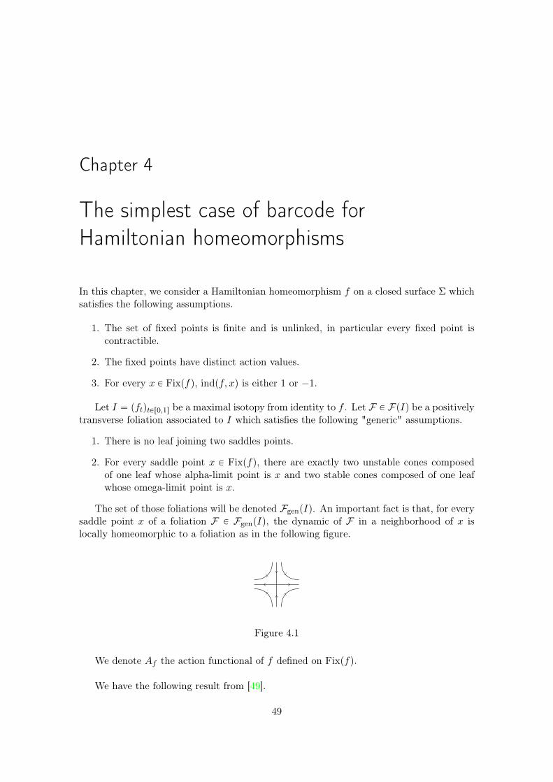
Chapter 4

The simplest case of barcode forHamiltonian homeomorphisms

In this chapter, we consider a Hamiltonian homeomorphism f on a closed surface Σ whichsatisfies the following assumptions.

1. The set of fixed points is finite and is unlinked, in particular every fixed point iscontractible.

2. The fixed points have distinct action values.

3. For every x P Fixpfq, indpf, xq is either 1 or ´1.

Let I “ pftqtPr0,1s be a maximal isotopy from identity to f . Let F P FpIq be a positivelytransverse foliation associated to I which satisfies the following "generic" assumptions.

1. There is no leaf joining two saddles points.

2. For every saddle point x P Fixpfq, there are exactly two unstable cones composedof one leaf whose alpha-limit point is x and two stable cones composed of one leafwhose omega-limit point is x.

The set of those foliations will be denoted FgenpIq. An important fact is that, for everysaddle point x of a foliation F P FgenpIq, the dynamic of F in a neighborhood of x islocally homeomorphic to a foliation as in the following figure.

Figure 4.1

We denote Af the action functional of f defined on Fixpfq.

We have the following result from [49].

49

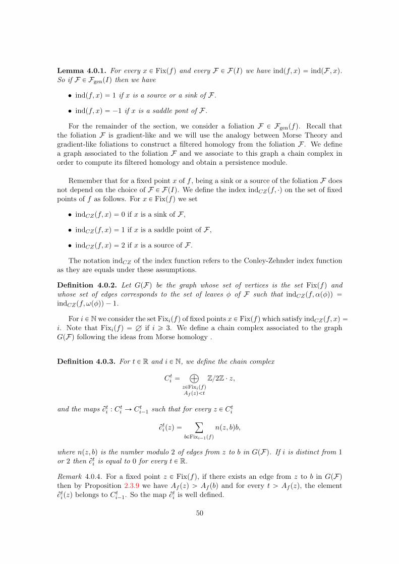
Lemma 4.0.1. For every x P Fixpfq and every F P FpIq we have indpf, xq “ indpF , xq.So if F P FgenpIq then we have

• indpf, xq “ 1 if x is a source or a sink of F .

• indpf, xq “ ´1 if x is a saddle pont of F .

For the remainder of the section, we consider a foliation F P Fgenpfq. Recall thatthe foliation F is gradient-like and we will use the analogy between Morse Theory andgradient-like foliations to construct a filtered homology from the foliation F . We definea graph associated to the foliation F and we associate to this graph a chain complex inorder to compute its filtered homology and obtain a persistence module.

Remember that for a fixed point x of f , being a sink or a source of the foliation F doesnot depend on the choice of F P FpIq. We define the index indCZpf, ¨q on the set of fixedpoints of f as follows. For x P Fixpfq we set

• indCZpf, xq “ 0 if x is a sink of F ,

• indCZpf, xq “ 1 if x is a saddle point of F ,

• indCZpf, xq “ 2 if x is a source of F .

The notation indCZ of the index function refers to the Conley-Zehnder index functionas they are equals under these assumptions.

Definition 4.0.2. Let GpFq be the graph whose set of vertices is the set Fixpfq andwhose set of edges corresponds to the set of leaves φ of F such that indCZpf, αpφqq “indCZpf, ωpφqq ´ 1.

For i P N we consider the set Fixipfq of fixed points x P Fixpfq which satisfy indCZpf, xq “i. Note that Fixipfq “ H if i ě 3. We define a chain complex associated to the graphGpFq following the ideas from Morse homology .

Definition 4.0.3. For t P R and i P N, we define the chain complex

Cti “à

zPFixipfqAf pzqăt

Z2Z ¨ z,

and the maps Bti : Cti Ñ Cti´1 such that for every z P Cti

Btipzq “ÿ

bPFixi´1pfq

npz, bqb,

where npz, bq is the number modulo 2 of edges from z to b in GpFq. If i is distinct from 1or 2 then Bti is equal to 0 for every t P R.

Remark 4.0.4. For a fixed point z P Fixpfq, if there exists an edge from z to b in GpFqthen by Proposition 2.3.9 we have Af pzq ą Af pbq and for every t ą Af pzq, the elementBtipzq belongs to C

ti´1. So the map Bti is well defined.

50

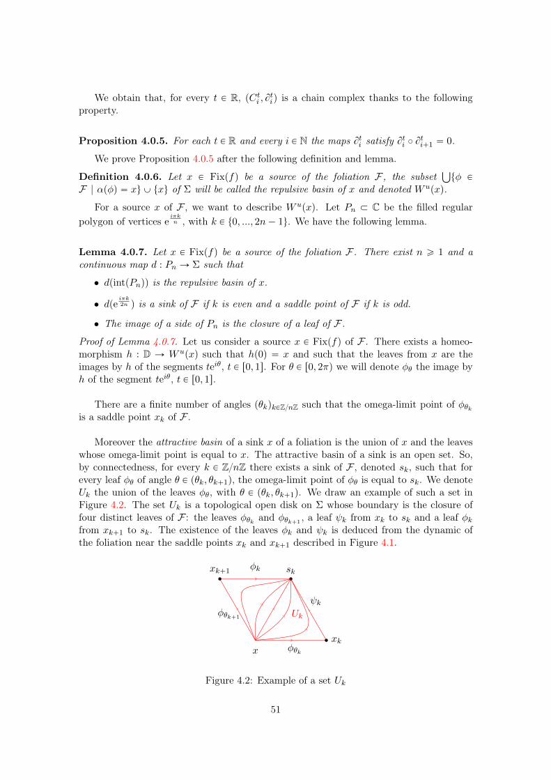
We obtain that, for every t P R, pCti , Btiq is a chain complex thanks to the followingproperty.

Proposition 4.0.5. For each t P R and every i P N the maps Bti satisfy Bti ˝ B

ti`1 “ 0.

We prove Proposition 4.0.5 after the following definition and lemma.

Definition 4.0.6. Let x P Fixpfq be a source of the foliation F , the subsetŤ

tφ P

F | αpφq “ xu Y txu of Σ will be called the repulsive basin of x and denoted W upxq.

For a source x of F , we want to describe W upxq. Let Pn Ă C be the filled regularpolygon of vertices e

iπkn , with k P t0, ..., 2n´ 1u. We have the following lemma.

Lemma 4.0.7. Let x P Fixpfq be a source of the foliation F . There exist n ě 1 and acontinuous map d : Pn Ñ Σ such that

• dpintpPnqq is the repulsive basin of x.

• dpeiπk2n q is a sink of F if k is even and a saddle point of F if k is odd.

• The image of a side of Pn is the closure of a leaf of F .

Proof of Lemma 4.0.7. Let us consider a source x P Fixpfq of F . There exists a homeo-morphism h : D Ñ W upxq such that hp0q “ x and such that the leaves from x are theimages by h of the segments teiθ, t P r0, 1s. For θ P r0, 2πq we will denote φθ the image byh of the segment teiθ, t P r0, 1s.

There are a finite number of angles pθkqkPZnZ such that the omega-limit point of φθkis a saddle point xk of F .

Moreover the attractive basin of a sink x of a foliation is the union of x and the leaveswhose omega-limit point is equal to x. The attractive basin of a sink is an open set. So,by connectedness, for every k P ZnZ there exists a sink of F , denoted sk, such that forevery leaf φθ of angle θ P pθk, θk`1q, the omega-limit point of φθ is equal to sk. We denoteUk the union of the leaves φθ, with θ P pθk, θk`1q. We draw an example of such a set inFigure 4.2. The set Uk is a topological open disk on Σ whose boundary is the closure offour distinct leaves of F : the leaves φθk and φθk`1

, a leaf ψk from xk to sk and a leaf φkfrom xk`1 to sk. The existence of the leaves φk and ψk is deduced from the dynamic ofthe foliation near the saddle points xk and xk`1 described in Figure 4.1.

Uk

x

φk

ψk

φθk

φθk`1

skxk`1

xk

Figure 4.2: Example of a set Uk

51

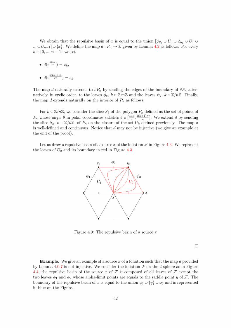
We obtain that the repulsive basin of x is equal to the union rφθ0 Y U0 Y φθ1 Y U1 Y

...YUn´1sYtxu. We define the map d : Pn Ñ Σ given by Lemma 4.2 as follows. For everyk P t0, ..., n´ 1u we set

• dpei2kπ2n q “ xk,

• dpeip2k`1qπ

2n q “ sk.

The map d naturally extends to BPn by sending the edges of the boundary of BPn alter-natively, in cyclic order, to the leaves φk, k P ZnZ and the leaves ψk, k P ZnZ. Finally,the map d extends naturally on the interior of Pn as follows.

For k P ZnZ, we consider the slice Sk of the polygon Pn defined as the set of points ofPn whose angle θ in polar coordinates satisfies θ P r ikπn ,

ipk`1qπn s. We extend d by sending

the slice Sk, k P ZnZ, of Pn on the closure of the set Uk defined previously. The map dis well-defined and continuous. Notice that d may not be injective (we give an example atthe end of the proof).

Let us draw a repulsive basin of a source x of the foliation F in Figure 4.3. We representthe leaves of U0 and its boundary in red in Figure 4.3.

U1 U0

x

φ0

ψ0ψ1

s0x1

x0

Figure 4.3: The repulsive basin of a source x

Example. We give an example of a source x of a foliation such that the map d providedby Lemma 4.0.7 is not injective. We consider the foliation F on the 2-sphere as in Figure4.4, the repulsive basin of the source x of F is composed of all leaves of F except thetwo leaves φ1 and φ2 whose alpha-limit points are equals to the saddle point y of F . Theboundary of the repulsive basin of x is equal to the union φ1YtyuYφ2 and is representedin blue on the Figure.

52

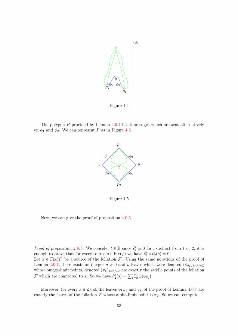
A

x

p1

y

p2φ1φ2

Figure 4.4

The polygon P provided by Lemma 4.0.7 has four edges which are sent alternativelyon φ1 and φ2. We can represent P as in Figure 4.5.

p2

p1

y y

φ1

φ2

φ1

φ2

x

Figure 4.5

Now, we can give the proof of proposition 4.0.5.

Proof of proposition 4.0.5. We consider t P R since Bti is 0 for i distinct from 1 or 2, it isenough to prove that for every source s P Fixpfq we have Bt1 ˝ Bt2psq “ 0.Let x P Fixpfq be a source of the foliation F . Using the same notations of the proof ofLemma 4.0.7, there exists an integer n ą 0 and n leaves which were denoted pφθkqkPZnZwhose omega-limit points, denoted pxkqkPZnZ are exactly the saddle points of the foliationF which are connected to x. So we have Bt2psq “

řn´1k“0 ωpφθkq.

Moreover, for every k P ZnZ the leaves φk´1 and ψk of the proof of Lemma 4.0.7 areexactly the leaves of the foliation F whose alpha-limit point is xk. So we can compute

53

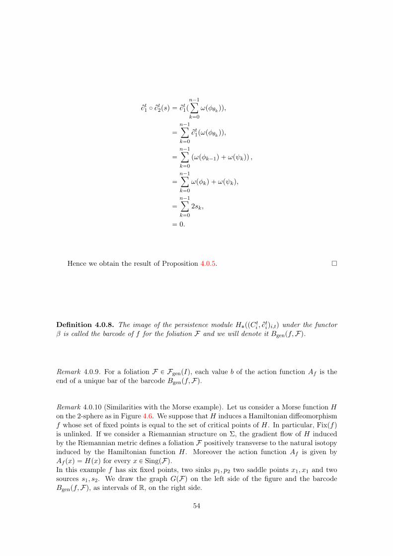
Bt1 ˝ Bt2psq “ B

t1p

n´1ÿ

k“0

ωpφθkqq,

“

n´1ÿ

k“0

Bt1pωpφθkqq,

“

n´1ÿ

k“0

pωpφk´1q ` ωpψkqq ,

“

n´1ÿ

k“0

ωpφkq ` ωpψkq,

“

n´1ÿ

k“0

2sk,

“ 0.

Hence we obtain the result of Proposition 4.0.5.

Definition 4.0.8. The image of the persistence module H˚ppCti , Btiqi,tq under the functor

β is called the barcode of f for the foliation F and we will denote it Bgenpf,Fq.

Remark 4.0.9. For a foliation F P FgenpIq, each value b of the action function Af is theend of a unique bar of the barcode Bgenpf,Fq.

Remark 4.0.10 (Similarities with the Morse example). Let us consider a Morse function Hon the 2-sphere as in Figure 4.6. We suppose thatH induces a Hamiltonian diffeomorphismf whose set of fixed points is equal to the set of critical points of H. In particular, Fixpfqis unlinked. If we consider a Riemannian structure on Σ, the gradient flow of H inducedby the Riemannian metric defines a foliation F positively transverse to the natural isotopyinduced by the Hamiltonian function H. Moreover the action function Af is given byAf pxq “ Hpxq for every x P SingpFq.In this example f has six fixed points, two sinks p1, p2 two saddle points x1, x1 and twosources s1, s2. We draw the graph GpFq on the left side of the figure and the barcodeBgenpf,Fq, as intervals of R, on the right side.

54

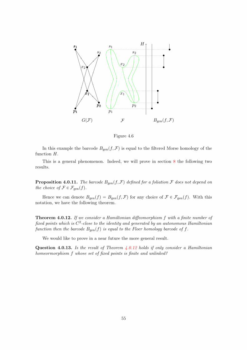
H

p1

x1

p2

s1

x2

s2

F Bgenpf,Fq

‚

‚

‚

‚

‚

‚

GpFq

p1

x1

p2

s1

x2

s2

p1

x1

p2

s1

‚

‚

‚

‚

‚

‚

‚

‚

‚

‚

‚

‚

Figure 4.6

In this example the barcode Bgenpf,Fq is equal to the filtered Morse homology of thefunction H.

This is a general phenomenon. Indeed, we will prove in section 8 the following tworesults.

Proposition 4.0.11. The barcode Bgenpf,Fq defined for a foliation F does not depend onthe choice of F P Fgenpfq.

Hence we can denote Bgenpfq “ Bgenpf,Fq for any choice of F P Fgenpfq. With thisnotation, we have the following theorem.

Theorem 4.0.12. If we consider a Hamiltonian diffeomorphism f with a finite number offixed points which is C2-close to the identity and generated by an autonomous Hamiltonianfunction then the barcode Bgenpfq is equal to the Floer homology barcode of f .

We would like to prove in a near future the more general result.

Question 4.0.13. Is the result of Theorem 4.0.12 holds if only consider a Hamiltonianhomeormorphism f whose set of fixed points is finite and unlinked?

55

56

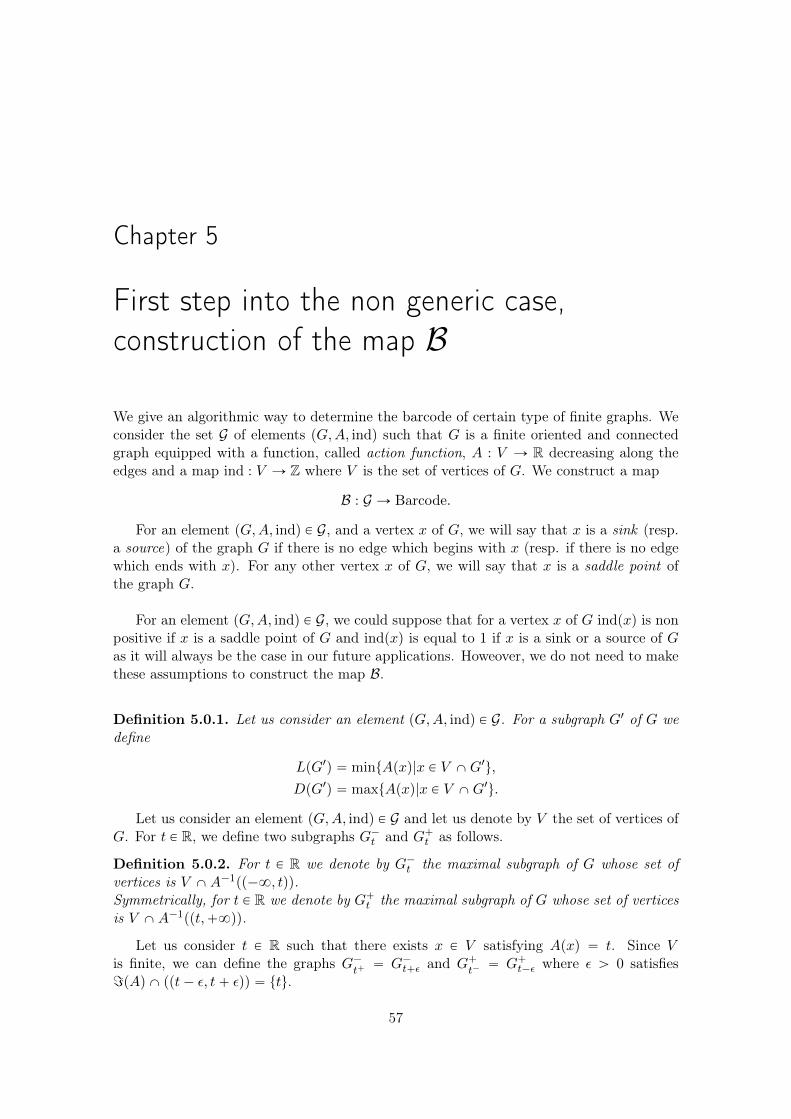
Chapter 5

First step into the non generic case,construction of the map B

We give an algorithmic way to determine the barcode of certain type of finite graphs. Weconsider the set G of elements pG,A, indq such that G is a finite oriented and connectedgraph equipped with a function, called action function, A : V Ñ R decreasing along theedges and a map ind : V Ñ Z where V is the set of vertices of G. We construct a map

B : G Ñ Barcode.

For an element pG,A, indq P G, and a vertex x of G, we will say that x is a sink (resp.a source) of the graph G if there is no edge which begins with x (resp. if there is no edgewhich ends with x). For any other vertex x of G, we will say that x is a saddle point ofthe graph G.

For an element pG,A, indq P G, we could suppose that for a vertex x of G indpxq is nonpositive if x is a saddle point of G and indpxq is equal to 1 if x is a sink or a source of Gas it will always be the case in our future applications. Howeover, we do not need to makethese assumptions to construct the map B.

Definition 5.0.1. Let us consider an element pG,A, indq P G. For a subgraph G1 of G wedefine

LpG1q “ mintApxq|x P V XG1u,

DpG1q “ maxtApxq|x P V XG1u.

Let us consider an element pG,A, indq P G and let us denote by V the set of vertices ofG. For t P R, we define two subgraphs G´t and G`t as follows.

Definition 5.0.2. For t P R we denote by G´t the maximal subgraph of G whose set ofvertices is V XA´1pp´8, tqq.Symmetrically, for t P R we denote by G`t the maximal subgraph of G whose set of verticesis V XA´1ppt,`8qq.

Let us consider t P R such that there exists x P V satisfying Apxq “ t. Since Vis finite, we can define the graphs G´

t`“ G´t`ε and G`

t´“ G`t´ε where ε ą 0 satisfies

=pAq X ppt´ ε, t` εqq “ ttu.

57

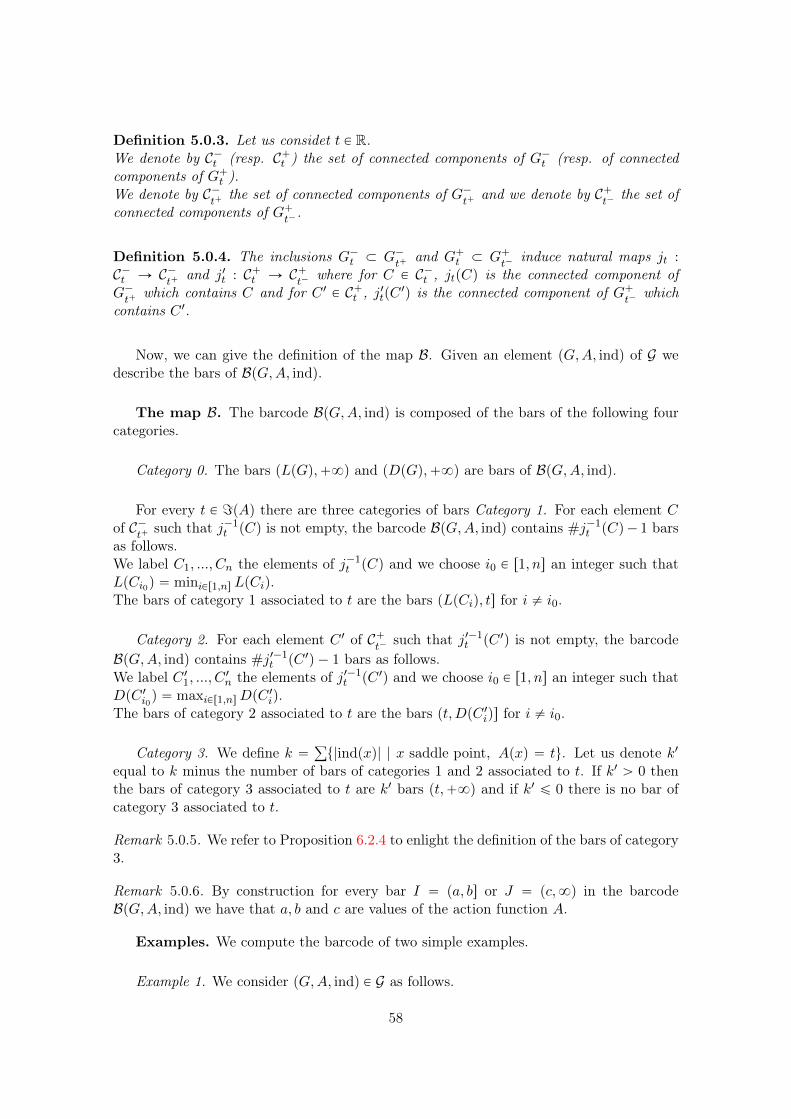
Definition 5.0.3. Let us considet t P R.We denote by C´t (resp. C`t ) the set of connected components of G´t (resp. of connectedcomponents of G`t ).We denote by C´

t`the set of connected components of G´

t`and we denote by C`

t´the set of

connected components of G`t´.

Definition 5.0.4. The inclusions G´t Ă G´t`

and G`t Ă G`t´

induce natural maps jt :C´t Ñ C´

t`and j1t : C`t Ñ C`

t´where for C P C´t , jtpCq is the connected component of

G´t`

which contains C and for C 1 P C`t , j1tpC 1q is the connected component of G`t´

whichcontains C 1.

Now, we can give the definition of the map B. Given an element pG,A, indq of G wedescribe the bars of BpG,A, indq.

The map B. The barcode BpG,A, indq is composed of the bars of the following fourcategories.

Category 0. The bars pLpGq,`8q and pDpGq,`8q are bars of BpG,A, indq.

For every t P =pAq there are three categories of bars Category 1. For each element Cof C´

t`such that j´1

t pCq is not empty, the barcode BpG,A, indq contains #j´1t pCq´ 1 bars

as follows.We label C1, ..., Cn the elements of j´1

t pCq and we choose i0 P r1, ns an integer such thatLpCi0q “ miniPr1,ns LpCiq.The bars of category 1 associated to t are the bars pLpCiq, ts for i ‰ i0.

Category 2. For each element C 1 of C`t´

such that j1´1t pC 1q is not empty, the barcode

BpG,A, indq contains #j1´1t pC 1q ´ 1 bars as follows.

We label C 11, ..., C 1n the elements of j1´1t pC 1q and we choose i0 P r1, ns an integer such that

DpC 1i0q “ maxiPr1,nsDpC1iq.

The bars of category 2 associated to t are the bars pt,DpC 1iqs for i ‰ i0.

Category 3. We define k “ř

t|indpxq| | x saddle point, Apxq “ tu. Let us denote k1

equal to k minus the number of bars of categories 1 and 2 associated to t. If k1 ą 0 thenthe bars of category 3 associated to t are k1 bars pt,`8q and if k1 ď 0 there is no bar ofcategory 3 associated to t.

Remark 5.0.5. We refer to Proposition 6.2.4 to enlight the definition of the bars of category3.

Remark 5.0.6. By construction for every bar I “ pa, bs or J “ pc,8q in the barcodeBpG,A, indq we have that a, b and c are values of the action function A.

Examples. We compute the barcode of two simple examples.

Example 1. We consider pG,A, indq P G as follows.

58

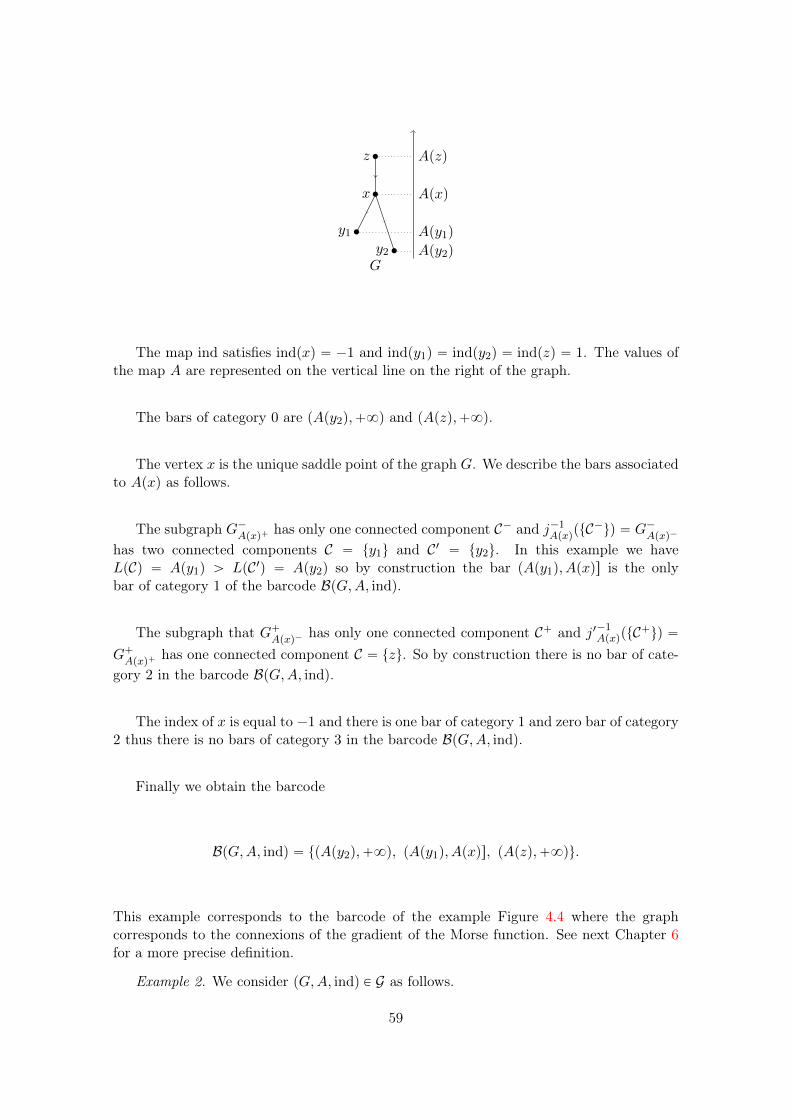
‚x

‚z

‚y2

‚y1

Apy2q

Apy1q

Apxq

Apzq

G

The map ind satisfies indpxq “ ´1 and indpy1q “ indpy2q “ indpzq “ 1. The values ofthe map A are represented on the vertical line on the right of the graph.

The bars of category 0 are pApy2q,`8q and pApzq,`8q.

The vertex x is the unique saddle point of the graph G. We describe the bars associatedto Apxq as follows.

The subgraph G´Apxq`

has only one connected component C´ and j´1ApxqptC

´uq “ G´Apxq´

has two connected components C “ ty1u and C1 “ ty2u. In this example we haveLpCq “ Apy1q ą LpC1q “ Apy2q so by construction the bar pApy1q, Apxqs is the onlybar of category 1 of the barcode BpG,A, indq.

The subgraph that G`Apxq´

has only one connected component C` and j1´1ApxqptC`uq “

G`Apxq`

has one connected component C “ tzu. So by construction there is no bar of cate-gory 2 in the barcode BpG,A, indq.

The index of x is equal to ´1 and there is one bar of category 1 and zero bar of category2 thus there is no bars of category 3 in the barcode BpG,A, indq.

Finally we obtain the barcode

BpG,A, indq “ tpApy2q,`8q, pApy1q, Apxqs, pApzq,`8qu.

This example corresponds to the barcode of the example Figure 4.4 where the graphcorresponds to the connexions of the gradient of the Morse function. See next Chapter 6for a more precise definition.

Example 2. We consider pG,A, indq P G as follows.

59

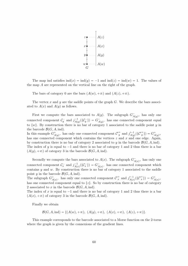
‚x

‚z

‚y

‚w

Apyq

Apxq

Apzq

ApwqG

The map ind satisfies indpxq “ indpyq “ ´1 and indpzq “ indpwq “ 1. The values ofthe map A are represented on the vertical line on the right of the graph.

The bars of category 0 are the bars pApwq,`8q and pApzq,`8q.

The vertex x and y are the saddle points of the graph G. We describe the bars associ-ated to Apxq and Apyq as follows.

First we compute the bars associated to Apyq. The subgraph G´Apyq`

has only oneconnected component C´y and j´1

ApyqptC´y uq “ G´

Apyq´has one connected component equal

to twu. By construction there is no bar of category 1 associated to the saddle point y inthe barcode BpG,A, indq.In this example G`

Apyq´has only one connected component C1`y and j1´1

ApyqptC1`y uq “ G`

Apyq`

has one connected component which contains the vertices z and x and one edge. Again,by construction there is no bar of category 2 associated to y in the barcode BpG,A, indq.The index of y is equal to ´1 and there is no bar of category 1 and 2 thus there is a barpApyq,`8q of category 3 in the barcode BpG,A, indq.

Secondly we compute the bars associated to Apxq. The subgraph G´Apxq`

has only oneconnected component C´x and j´1

ApxqptC´x uq “ G´

Apxq´has one connected component which

contains y and w. By construction there is no bar of category 1 associated to the saddlepoint y in the barcode BpG,A, indq.The subgraph G`

Apxq´has only one connected component C1`x and j1´1

ApxqptC1`x uq “ G`

Apxq`

has one connected component equal to tzu. So by construction there is no bar of category2 associated to x in the barcode BpG,A, indq.The index of x is equal to ´1 and there is no bar of category 1 and 2 thus there is a barpApxq,`8q of category 3 in the barcode BpG,A, indq.

Finally we obtain

BpG,A, indq “ tpApwq,`8q, pApyq,`8q, pApxq,`8q, pApzq,`8qu.

This example corresponds to the barcode associated to a Morse function on the 2-toruswhere the graph is given by the connexions of the gradient lines.

60

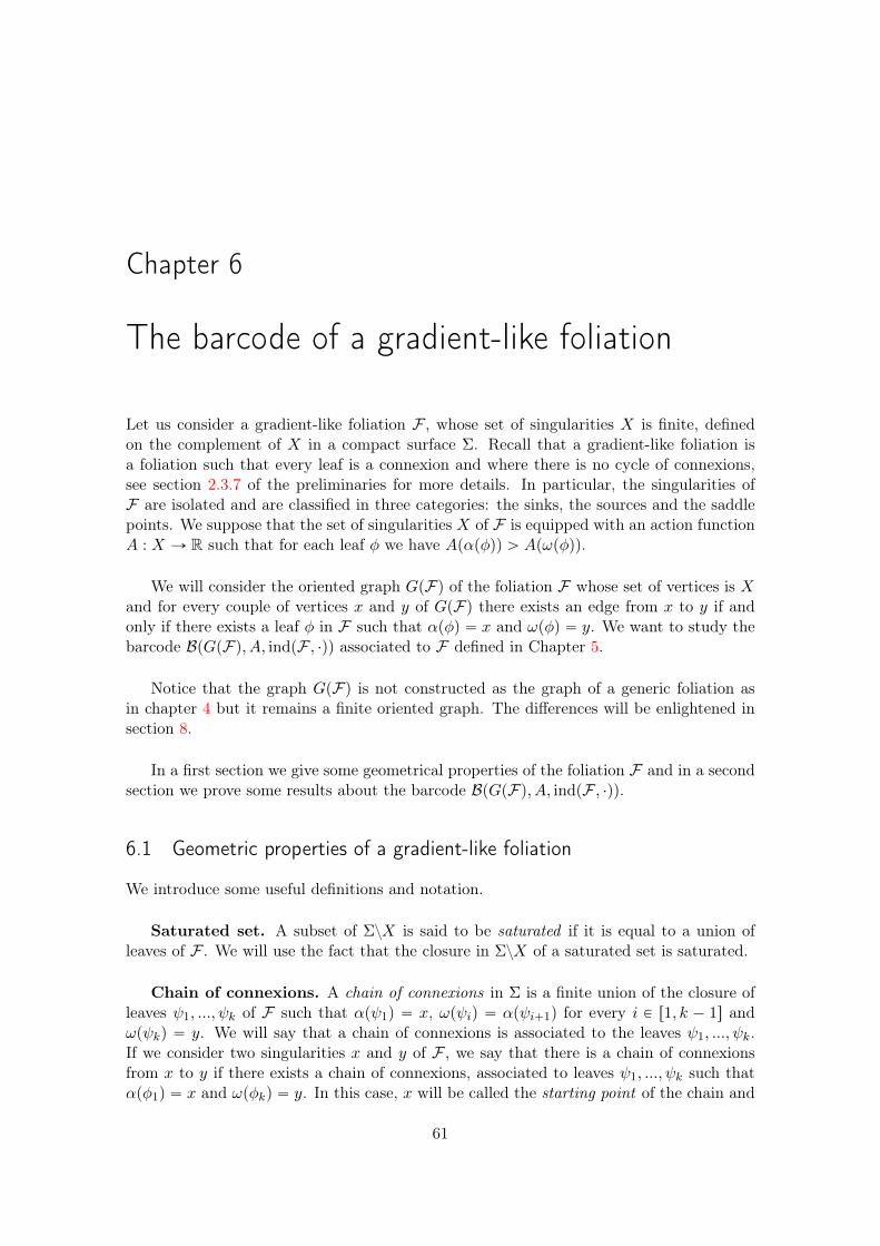
Chapter 6

The barcode of a gradient-like foliation

Let us consider a gradient-like foliation F , whose set of singularities X is finite, definedon the complement of X in a compact surface Σ. Recall that a gradient-like foliation isa foliation such that every leaf is a connexion and where there is no cycle of connexions,see section 2.3.7 of the preliminaries for more details. In particular, the singularities ofF are isolated and are classified in three categories: the sinks, the sources and the saddlepoints. We suppose that the set of singularities X of F is equipped with an action functionA : X Ñ R such that for each leaf φ we have Apαpφqq ą Apωpφqq.

We will consider the oriented graph GpFq of the foliation F whose set of vertices is Xand for every couple of vertices x and y of GpFq there exists an edge from x to y if andonly if there exists a leaf φ in F such that αpφq “ x and ωpφq “ y. We want to study thebarcode BpGpFq, A, indpF , ¨qq associated to F defined in Chapter 5.

Notice that the graph GpFq is not constructed as the graph of a generic foliation asin chapter 4 but it remains a finite oriented graph. The differences will be enlightened insection 8.

In a first section we give some geometrical properties of the foliation F and in a secondsection we prove some results about the barcode BpGpFq, A, indpF , ¨qq.

6.1 Geometric properties of a gradient-like foliation

We introduce some useful definitions and notation.

Saturated set. A subset of ΣzX is said to be saturated if it is equal to a union ofleaves of F . We will use the fact that the closure in ΣzX of a saturated set is saturated.

Chain of connexions. A chain of connexions in Σ is a finite union of the closure ofleaves ψ1, ..., ψk of F such that αpψ1q “ x, ωpψiq “ αpψi`1q for every i P r1, k ´ 1s andωpψkq “ y. We will say that a chain of connexions is associated to the leaves ψ1, ..., ψk.If we consider two singularities x and y of F , we say that there is a chain of connexionsfrom x to y if there exists a chain of connexions, associated to leaves ψ1, ..., ψk such thatαpφ1q “ x and ωpφkq “ y. In this case, x will be called the starting point of the chain and

61

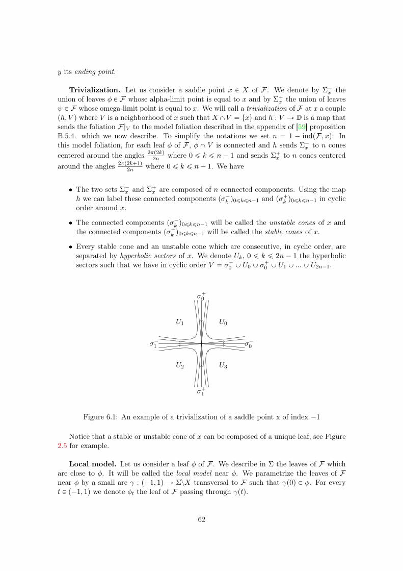
y its ending point.

Trivialization. Let us consider a saddle point x P X of F . We denote by Σ´x theunion of leaves φ P F whose alpha-limit point is equal to x and by Σ`x the union of leavesψ P F whose omega-limit point is equal to x. We will call a trivialization of F at x a coupleph, V q where V is a neighborhood of x such that XXV “ txu and h : V Ñ D is a map thatsends the foliation F |V to the model foliation described in the appendix of [59] propositionB.5.4. which we now describe. To simplify the notations we set n “ 1 ´ indpF , xq. Inthis model foliation, for each leaf φ of F , φ X V is connected and h sends Σ´x to n conescentered around the angles 2πp2kq

2n where 0 ď k ď n´ 1 and sends Σ`x to n cones centeredaround the angles 2πp2k`1q

2n where 0 ď k ď n´ 1. We have

• The two sets Σ´x and Σ`x are composed of n connected components. Using the maph we can label these connected components pσ´k q0ďkďn´1 and pσ`k q0ďkďn´1 in cyclicorder around x.

• The connected components pσ´k q0ďkďn´1 will be called the unstable cones of x andthe connected components pσ`k q0ďkďn´1 will be called the stable cones of x.

• Every stable cone and an unstable cone which are consecutive, in cyclic order, areseparated by hyperbolic sectors of x. We denote Uk, 0 ď k ď 2n ´ 1 the hyperbolicsectors such that we have in cyclic order V “ σ´0 Y U0 Y σ

`0 Y U1 Y ...Y U2n´1.

σ`1

σ`0

σ´1 σ´0

U0U1

U2 U3

Figure 6.1: An example of a trivialization of a saddle point x of index ´1

Notice that a stable or unstable cone of x can be composed of a unique leaf, see Figure2.5 for example.

Local model. Let us consider a leaf φ of F . We describe in Σ the leaves of F whichare close to φ. It will be called the local model near φ. We parametrize the leaves of Fnear φ by a small arc γ : p´1, 1q Ñ ΣzX transversal to F such that γp0q P φ. For everyt P p´1, 1q we denote φt the leaf of F passing through γptq.

62

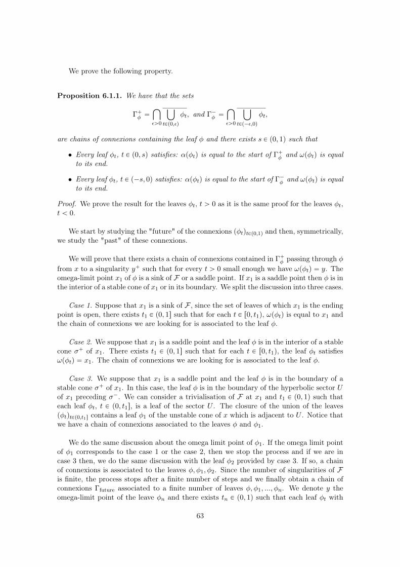
We prove the following property.

Proposition 6.1.1. We have that the sets

Γ`φ “č

εą0

ď

tPp0,εq

φt, and Γ´φ “č

εą0

ď

tPp´ε,0q

φt,

are chains of connexions containing the leaf φ and there exists s P p0, 1q such that

• Every leaf φt, t P p0, sq satisfies: αpφtq is equal to the start of Γ`φ and ωpφtq is equalto its end.

• Every leaf φt, t P p´s, 0q satisfies: αpφtq is equal to the start of Γ´φ and ωpφtq is equalto its end.

Proof. We prove the result for the leaves φt, t ą 0 as it is the same proof for the leaves φt,t ă 0.

We start by studying the "future" of the connexions pφtqtPp0,1q and then, symmetrically,we study the "past" of these connexions.

We will prove that there exists a chain of connexions contained in Γ`φ passing through φfrom x to a singularity y` such that for every t ą 0 small enough we have ωpφtq “ y. Theomega-limit point x1 of φ is a sink of F or a saddle point. If x1 is a saddle point then φ is inthe interior of a stable cone of x1 or in its boundary. We split the discussion into three cases.

Case 1. Suppose that x1 is a sink of F , since the set of leaves of which x1 is the endingpoint is open, there exists t1 P p0, 1s such that for each t P r0, t1q, ωpφtq is equal to x1 andthe chain of connexions we are looking for is associated to the leaf φ.

Case 2. We suppose that x1 is a saddle point and the leaf φ is in the interior of a stablecone σ` of x1. There exists t1 P p0, 1s such that for each t P r0, t1q, the leaf φt satisfiesωpφtq “ x1. The chain of connexions we are looking for is associated to the leaf φ.

Case 3. We suppose that x1 is a saddle point and the leaf φ is in the boundary of astable cone σ` of x1. In this case, the leaf φ is in the boundary of the hyperbolic sector Uof x1 preceding σ´. We can consider a trivialisation of F at x1 and t1 P p0, 1q such thateach leaf φt, t P p0, t1s, is a leaf of the sector U . The closure of the union of the leavespφtqtPp0,t1s contains a leaf φ1 of the unstable cone of x which is adjacent to U . Notice thatwe have a chain of connexions associated to the leaves φ and φ1.

We do the same discussion about the omega limit point of φ1. If the omega limit pointof φ1 corresponds to the case 1 or the case 2, then we stop the process and if we are incase 3 then, we do the same discussion with the leaf φ2 provided by case 3. If so, a chainof connexions is associated to the leaves φ, φ1, φ2. Since the number of singularities of Fis finite, the process stops after a finite number of steps and we finally obtain a chain ofconnexions Γfuture associated to a finite number of leaves φ, φ1, ..., φn. We denote y theomega-limit point of the leave φn and there exists tn P p0, 1q such that each leaf φt with

63

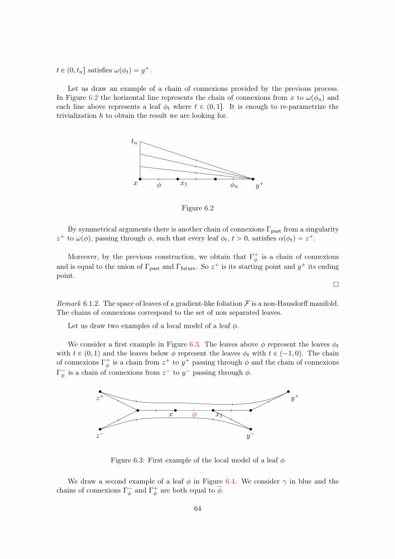
t P p0, tns satisfies ωpφtq “ y`.

Let us draw an example of a chain of connexions provided by the previous process.In Figure 6.2 the horizontal line represents the chain of connexions from x to ωpφnq andeach line above represents a leaf φt where t P p0, 1s. It is enough to re-parametrize thetrivialization h to obtain the result we are looking for.

‚x φ

‚y`φn

tn

‚x1

‚

Figure 6.2

By symmetrical arguments there is another chain of connexions Γpast from a singularityz` to ωpφq, passing through φ, such that every leaf φt, t ą 0, satisfies αpφtq “ z`.

Moreover, by the previous construction, we obtain that Γ`φ is a chain of connexionsand is equal to the union of Γpast and Γfuture. So z` is its starting point and y` its endingpoint.

Remark 6.1.2. The space of leaves of a gradient-like foliation F is a non-Hausdorff manifold.The chains of connexions correspond to the set of non separated leaves.

Let us draw two examples of a local model of a leaf φ.

We consider a first example in Figure 6.3. The leaves above φ represent the leaves φtwith t P p0, 1q and the leaves below φ represent the leaves φt with t P p´1, 0q. The chainof connexions Γ`φ is a chain from z` to y` passing through φ and the chain of connexionsΓ´φ is a chain of connexions from z´ to y´ passing through φ.

‚x φ

‚y`

‚x1

‚‚

‚z`

‚z´

‚y´

Figure 6.3: First example of the local model of a leaf φ

We draw a second example of a leaf φ in Figure 6.4. We consider γ in blue and thechains of connexions Γ´φ and Γ`φ are both equal to φ.

64

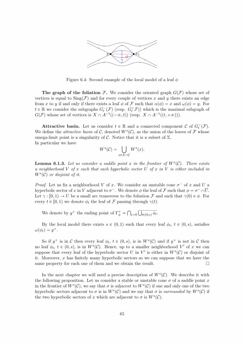
γ

‚xφ

‚x1

Figure 6.4: Second example of the local model of a leaf φ

The graph of the foliation F . We consider the oriented graph GpFq whose set ofvertices is equal to SingpFq and for every couple of vertices x and y there exists an edgefrom x to y if and only if there exists a leaf φ of F such that αpφq “ x and ωpφq “ y. Fort P R we consider the subgraphs G´t pFq (resp. G`t Fq) which is the maximal subgraph ofGpFq whose set of vertices is X XA´1pp´8, tqq (resp. X XA´1ppt,`8qq).

Attractive basin. Let us consider t P R and a connected component C of G´t pFq.We define the attractive basin of C, denoted W spCq, as the union of the leaves of F whoseomega-limit point is a singularity of C. Notice that it is a subset of Σ.In particular we have

W spCq “ď

xPXXCW spxq.

Lemma 6.1.3. Let us consider a saddle point x in the frontier of W spCq. There existsa neighborhood V of x such that each hyperbolic sector U of x in V is either included inW spCq or disjoint of it.

Proof. Let us fix a neighborhood V of x. We consider an unstable cone σ´ of x and U ahyperbolic sector of x in V adjacent to σ´. We denote φ the leaf of F such that φ “ σ´XU .Let γ : r0, 1q Ñ U be a small arc transverse to the foliation F and such that γp0q P φ. Forevery t P r0, 1q we denote φt the leaf of F passing through γptq.

We denote by y` the ending point of Γ`φ “Ş

εą0

Ť

tPp0,εq φt.

By the local model there exists s P p0, 1q such that every leaf φt, t P p0, sq, satisfiesωpφtq “ y`.

So if y` is in C then every leaf φt, t P p0, sq, is in W spCq and if y` is not in C thenno leaf φt, t P p0, sq, is in W spCq. Hence, up to a smaller neighborhood V 1 of x we cansuppose that every leaf of the hyperbolic sector U in V 1 is either in W spCq or disjoint ofit. Moreover, x has finitely many hyperbolic sectors so we can suppose that we have thesame property for each one of them and we obtain the result.

In the next chapter we will need a precise description of W spCq. We describe it withthe following proposition. Let us consider a stable or unstable cone σ of a saddle point xin the frontier of W spCq, we say that σ is adjacent to W spCq if one and only one of the twohyperbolic sectors adjacent to σ is in W spCq and we say that σ is surrounded by W spCq ifthe two hyperbolic sectors of x which are adjacent to σ is W spCq.

65

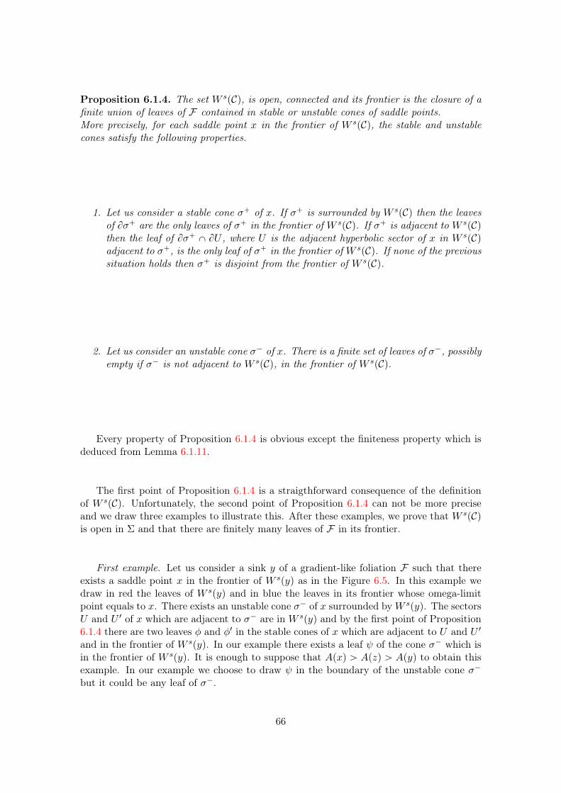
Proposition 6.1.4. The set W spCq, is open, connected and its frontier is the closure of afinite union of leaves of F contained in stable or unstable cones of saddle points.More precisely, for each saddle point x in the frontier of W spCq, the stable and unstablecones satisfy the following properties.

1. Let us consider a stable cone σ` of x. If σ` is surrounded by W spCq then the leavesof Bσ` are the only leaves of σ` in the frontier of W spCq. If σ` is adjacent to W spCqthen the leaf of Bσ` X BU , where U is the adjacent hyperbolic sector of x in W spCqadjacent to σ`, is the only leaf of σ` in the frontier of W spCq. If none of the previoussituation holds then σ` is disjoint from the frontier of W spCq.

2. Let us consider an unstable cone σ´ of x. There is a finite set of leaves of σ´, possiblyempty if σ´ is not adjacent to W spCq, in the frontier of W spCq.

Every property of Proposition 6.1.4 is obvious except the finiteness property which isdeduced from Lemma 6.1.11.

The first point of Proposition 6.1.4 is a straigthforward consequence of the definitionof W spCq. Unfortunately, the second point of Proposition 6.1.4 can not be more preciseand we draw three examples to illustrate this. After these examples, we prove that W spCqis open in Σ and that there are finitely many leaves of F in its frontier.

First example. Let us consider a sink y of a gradient-like foliation F such that thereexists a saddle point x in the frontier of W spyq as in the Figure 6.5. In this example wedraw in red the leaves of W spyq and in blue the leaves in its frontier whose omega-limitpoint equals to x. There exists an unstable cone σ´ of x surrounded byW spyq. The sectorsU and U 1 of x which are adjacent to σ´ are in W spyq and by the first point of Proposition6.1.4 there are two leaves φ and φ1 in the stable cones of x which are adjacent to U and U 1

and in the frontier of W spyq. In our example there exists a leaf ψ of the cone σ´ which isin the frontier of W spyq. It is enough to suppose that Apxq ą Apzq ą Apyq to obtain thisexample. In our example we choose to draw ψ in the boundary of the unstable cone σ´

but it could be any leaf of σ´.

66

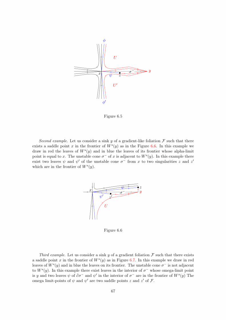
x

φ1

φ

σ´ y

U

U 1

ψ‚z

Figure 6.5

Second example. Let us consider a sink y of a gradient-like foliation F such that thereexists a saddle point x in the frontier of W spyq as in the Figure 6.6. In this example wedraw in red the leaves of W spyq and in blue the leaves of its frontier whose alpha-limitpoint is equal to x. The unstable cone σ´ of x is adjacent to W spyq. In this example thereexist two leaves ψ and ψ1 of the unstable cone σ´ from x to two singularities z and z1

which are in the frontier of W spyq.

x¨ σ´

ψ1‚z1

ψ

U

y‚z

Figure 6.6

Third example. Let us consider a sink y of a gradient foliation F such that there existsa saddle point x in the frontier of W spyq as in Figure 6.7. In this example we draw in redleaves ofW spyq and in blue the leaves on its frontier. The unstable cone σ´ is not adjacentto W spyq. In this example there exist leaves in the interior of σ´ whose omega-limit pointis y and two leaves ψ of Bσ´ and ψ1 in the interior of σ´ are in the frontier of W spyq Theomega limit-points of ψ and ψ1 are two saddle points z and z1 of F .

67

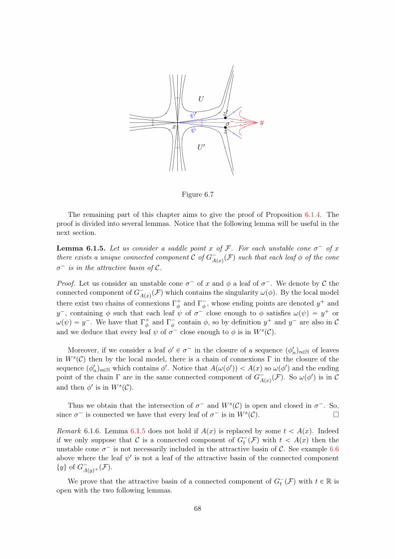
x σ´ y

U

U 1

ψ ‚z

ψ1 ‚z1

Figure 6.7

The remaining part of this chapter aims to give the proof of Proposition 6.1.4. Theproof is divided into several lemmas. Notice that the following lemma will be useful in thenext section.

Lemma 6.1.5. Let us consider a saddle point x of F . For each unstable cone σ´ of xthere exists a unique connected component C of G´ApxqpFq such that each leaf φ of the coneσ´ is in the attractive basin of C.

Proof. Let us consider an unstable cone σ´ of x and φ a leaf of σ´. We denote by C theconnected component of G´ApxqpFq which contains the singularity ωpφq. By the local modelthere exist two chains of connexions Γ`φ and Γ´φ , whose ending points are denoted y` andy´, containing φ such that each leaf ψ of σ´ close enough to φ satisfies ωpψq “ y` orωpψq “ y´. We have that Γ`φ and Γ´φ contain φ, so by definition y` and y´ are also in Cand we deduce that every leaf ψ of σ´ close enough to φ is in W spCq.

Moreover, if we consider a leaf φ1 P σ´ in the closure of a sequence pφ1nqnPN of leavesin W spCq then by the local model, there is a chain of connexions Γ in the closure of thesequence pφ1nqnPN which contains φ1. Notice that Apωpφ1qq ă Apxq so ωpφ1q and the endingpoint of the chain Γ are in the same connected component of G´ApxqpFq. So ωpφ1q is in Cand then φ1 is in W spCq.

Thus we obtain that the intersection of σ´ and W spCq is open and closed in σ´. So,since σ´ is connected we have that every leaf of σ´ is in W spCq.

Remark 6.1.6. Lemma 6.1.5 does not hold if Apxq is replaced by some t ă Apxq. Indeedif we only suppose that C is a connected component of G´t pFq with t ă Apxq then theunstable cone σ´ is not necessarily included in the attractive basin of C. See example 6.6above where the leaf ψ1 is not a leaf of the attractive basin of the connected componenttyu of G´

Apyq`pFq.

We prove that the attractive basin of a connected component of G´t pFq with t P R isopen with the two following lemmas.

68

Lemma 6.1.7. Let us consider t P R and C a connected component of G´t pFq. Eachsingularity x of C is in the interior of W spCq.

Proof. Let us consider a singularity x of F in C. It is either a sink, a source or saddle. Weseparate those three cases.

1. If x is a sink, then each leaf in a neighborhood of x is in W spCq.

2. If x is a source, then each leaf φ in a neighborhood of x satisfies Apωpφqq ă Apxqand is in W spCq.

3. If x is a saddle point, we consider a trivialization ph, V q of F at x on a neighborhoodV given by Lemma 6.1.3. By definition of W spCq, each leaf of Σ´x and Σ`x is in W spCq.Moreover, let us consider a leaf φ in the boundary of an unstable cone σ´ of x and U thehyperbolic sector adjacent to φ, by the local model there exists a chain of connexions fromx to a singularity y such that every leaf of the hyperbolic sector U admits y as its omegalimit. By definition, the singularity y is in C hence the leaves of the hyperbolic sector Uare in W spCq. Since it holds for each hyperbolic sector of x we obtain the result.

Let us consider t P R and C a connected component of G´t pFq. We describe theattractive basin of C and its frontier.

Lemma 6.1.8. The intersection of W spCq and ΣzX is open.

Proof. We consider a leaf φ inW spCq, by the local model there exists a small neighborhoodV of φ and two chains of connexions φ1, ..., φk and φ11, ..., φ1k1 of F which contain φ such thateach leaf ψ passing through V satisfies ωpψq “ ωpφkq or ωpψq “ ωpφ1k1q. By constructionωpφkq and ωpφ1k1q are in the same connected component of G´t pFq and so every leaf passingthrough V is in W spCq.

The following corollary is a consequence of Lemmas 6.1.7 and 6.1.8.

Corollary 6.1.9. The attractive basin of C is an open surface in Σ.

We deduce the following lemma.

Lemma 6.1.10. The attractive basin of C is connected.

Proof. For every x P XXC, W sp§q is connected as it is arc-connected. Let us consider twosingularities x and y of C such that there exists an edge from x to y. So there is a leaf φsuch that αpφq “ x and ωpφq “ y. The point x is in the frontier of W spyq and is either asaddle point or a source. Since we proved previously that x is in the interior of W spCq wededuce that φ ĂW spxq YW spyq.We deduce easily that W spCq “

Ť

xPXXCWspxq is connected.

We prove a last result which concludes the proof of Proposition 6.1.4.

Lemma 6.1.11. The number of leaves included in the frontier of the attractive basin of Cis finite.

69

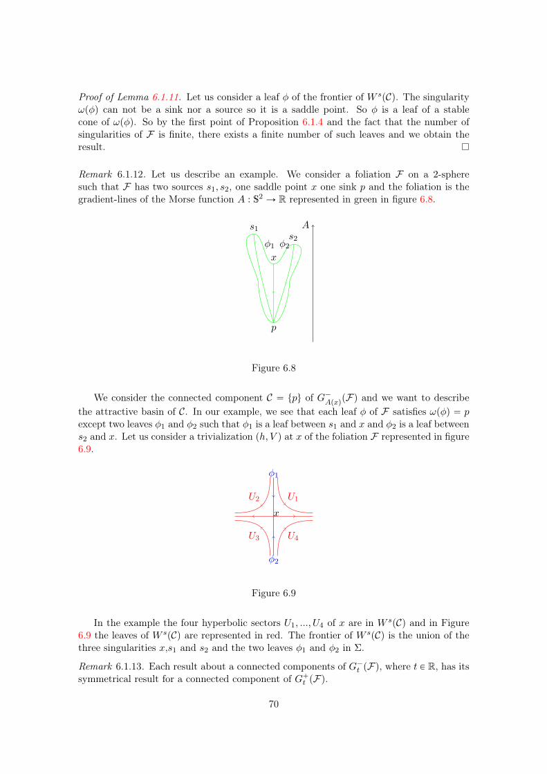
Proof of Lemma 6.1.11. Let us consider a leaf φ of the frontier of W spCq. The singularityωpφq can not be a sink nor a source so it is a saddle point. So φ is a leaf of a stablecone of ωpφq. So by the first point of Proposition 6.1.4 and the fact that the number ofsingularities of F is finite, there exists a finite number of such leaves and we obtain theresult.

Remark 6.1.12. Let us describe an example. We consider a foliation F on a 2-spheresuch that F has two sources s1, s2, one saddle point x one sink p and the foliation is thegradient-lines of the Morse function A : S2 Ñ R represented in green in figure 6.8.

A

p

s1

x

s2φ1 φ2

Figure 6.8

We consider the connected component C “ tpu of G´ApxqpFq and we want to describethe attractive basin of C. In our example, we see that each leaf φ of F satisfies ωpφq “ pexcept two leaves φ1 and φ2 such that φ1 is a leaf between s1 and x and φ2 is a leaf betweens2 and x. Let us consider a trivialization ph, V q at x of the foliation F represented in figure6.9.

φ1

φ2

x

U1

U4

U2

U3

Figure 6.9

In the example the four hyperbolic sectors U1, ..., U4 of x are in W spCq and in Figure6.9 the leaves of W spCq are represented in red. The frontier of W spCq is the union of thethree singularities x,s1 and s2 and the two leaves φ1 and φ2 in Σ.

Remark 6.1.13. Each result about a connected components of G´t pFq, where t P R, has itssymmetrical result for a connected component of G`t pFq.

70

6.2 Some properties of the Barcode BpGpFq, A, indpF , ¨qqLet us consider a gradient-like foliation F defined on the complement of a finite set X ofa compact surface Σ. We suppose that X is equipped with an action function A : X Ñ Rsuch that for each leaf φ we have Apαpφqq ą Apωpφqq. We prove some properties aboutthe Barcode BpGpFq, A, indpF , ¨qq, which will be denoted βF .

We set Am the minimum value of the action function A on X and AM its maximumvalue.

Notice that, by construction of the map B, for every singularity z of F of index zerothere is no bar in BpGpFq, A, indpF , ¨qq one end of whose is equal to Apzq. Indeed, the pointz does not connect distinct connected components of the graphs G´Af pzqpFq and G

`

Af pzpFq

so if we follow the construction in Chapter 5, there is no bar of category 1 or 2 induced byz. So, since indpF , zq “ 0 there is no bar of category 3 induced by z neither.

We consider the graph GpFq associated to F and the subgraphs pG´t pFqqtPR andpG`t pFqqtPR. We will use some notations from Chapter 5. For t P R we denote C´t and C`tthe set of connected components of G´t pFq and G`t pFq.We set the maps jt : C´t Ñ C´

t`and j1t : C`t Ñ C`

t´where for C P C´t , jtpCq is the

connected component of G´t`

which contains C and for C 1 P C`t j1tpC1q is the connected

component of G`t´

which contains C 1. For a connected component C of G´t pFq we considerLpCq “ mintApyq | y vertex of Cu.

Lemma 6.2.1. For each sink y of F satisfying Am ă Apyq there exists at least one saddlepoint x of F such that the barcode βF contains a bar b “ pApyq, Apxqs.For each source y of F satisfying Apyq ă AM there exists at least one saddle point x of Fsuch that the barcode βF contains a bar b “ pApxq, Apyqs.

In the situation of Lemma 6.2.1 we say that the pair px, yq is associated to the finitebar b of βF .

Proof. Let us fix a value t ą Am of the action function A. We label y1, ..., yn the sinks ofX whose action value is t. We prove that for every i P t1, ..., nu there exists a saddle pointxi of F such that the barcode βF contains a bar pApyiq, Apxiqs.

For i P r1, ns there is a map ci : s ÞÑ Csi defined for s ą t where Csi is the connectedcomponent of the graph G´s pFq which contains yi.

For a value s ą t such that A´1ppt, sqq “ H, the connected components Cs1, ..., Csn aredistinct.

For s ą t close to t, the elements cipsq, i P r1, ns, are distincts and for s ą AM , we havethat cipsq “ GpFq for every i P r1, ns, hence we have Lpcipsqq “ t for s ą 0 close to t andLpcipsqq “ Am for t ą AM .

Thus, for every i P r1, ns, there exists an action value, denoted si, such that Apyiq “Lpcipsiqq and t ą Lpjspcipsiqqq. In other words, there exists a saddle point xi of F of actionsi such that

71

• Lpcipsiqq “ t “ Apyiq

• xi connects the connected component cipsiq and another connected component C ofG´s pFq such that LpCq ă t.

By construction of the barcode βF there exists a bar pApyiq, sis of category 1 (see Chapter5).

Notice that the points xi, i P t1, ..., nu are not sources. Indeed, by contradiction wesuppose that a source z of action s connects two distinct connected components C1 andC2 of the graph G´s pFq. Thus, by hypothesis, there exist two singularities x1 P C1 andx2 P C2 in the frontier of W upzq. By Proposition 6.1.4, there exists a path of connexions Γbetween x1 and x2 such that every singularity y in Γ satisfies Apyq ă s, so x1 and x2 arein the same connected component of G´s pFq and we have a contradiction.

We obtain the symmetrical results for sources of F by considering bars of category2.

Remark 6.2.2. For a singularity y of F of index 1, there may exist two saddle points x andx1 with Apxq “ Apx1q such that the couples px, yq and px1, yq are associated to the samebar b.

Lemma 6.2.3. We label y1, ..., yn the sinks of F of action Am. There exist n ´ 1 finitebars J1, ..., Jn´1 whose lower bound is equal to Am and upper bound is the action value ofa saddle point of F and one semi-infinite bar pAm,8q in the barcode βF .

Proof. For s ą Am such that A´1ppAm, sqq “ H, we denote Csi the connected componentof G´s pFq which contains the singularity yi.

For i P r1, ns there is a map ci : s ÞÑ Csi defined for s ą t where Csi is the connectedcomponent of the graph G´s pFq which contains yi.

For s ą Am close to Am, we have Csi “ tyiu, i P r1, ns.

Let us consider s ą Am, such that there exists a subset K of t1, ..., nu of cardinal atleast two such that the connected components cipsq, i P K are distinct but the connectedcomponent jspcipsqq, i P K, are equal. We have Lpcipsqq “ Am for i P K so, by construc-tion, it induces the existence of #K ´ 1 bars pAm, ss in the barcode βF .

Moreover, for each i ‰ j in t1, ..., nu there exists s ą Am such that jspcipsqq “ jspcjpsqqand cipsq ‰ cjpsq. Hence we obtain n ´ 1 finite bars such that Am is the lower bound ofthe bar.

The existence of a semi-infinite bar pAm,8q in the barcode BpGpFq, A, indpF , ¨qq isprovided by the construction of B : it is a bar of category 0.

Let us consider a sink ym of the foliation F such that Apymq “ Am and a source yMof the foliation F such that ApyM q “ AM . We denote Xă0 Ă X the set of negative indexsingularities of F and X1 Ă X the set of singularities of index 1.

72

By Lemmas 6.2.1 and 6.2.3 there exists a map, which may be not unique,

ι : X1ztym, yMu Ñ Xă0, (6.1)

where ιpyq “ x is a saddle point x of the foliation F given by Lemmas 6.2.1 and 6.2.3 suchthat the couple px, yq is associated to a finite bar of βF .

In particular, if A is injective and each singularity x of Xă0 has an index equal to ´1then, every bar pa, bs of the barcode is naturally associated to a unique couple x, y P Xby Lemma 6.2.1. In this case, ι is unique and an injection. Indeed, by construction, forevery saddle point x of Xă0 there exists a unique bar one end of which is equal to Apxq.notice that this bar is either a finite interval whose infimum is Apxq, maximum is Apxq ora semi-infinite interval whose infimum is Apxq.

We have the following result.

Proposition 6.2.4. Let x be a saddle point of F of action value t P R such that A´1ptq “txu. We have

#j´1t pCxq `#j1´1

t pC1xq ď |indpF , xq| ` 2,

where Cx (resp. C1x) is the connected component of G´t`pFq (resp. G`

t´pFq) which contains

x.

In general, Proposition 6.2.4 certifies that for a saddle point x of F such that A´1ptq “txu, there are |indpf, xq| bars of which t is an end. We can link this result to Proposition 28of [61] which asserts that for a Hamiltonian function H on a manifold the number of barsof which t P R is an ending value is given by the dimension of the local Floer Homology att.

Proof of Proposition 6.2.4. We set t “ Apxq and i “ indpF , xq. We label Σ´x the set of theunstable cones of x and Σ`x the set of the stable cones of x. Both Σ´x and Σ`x are equippedwith a cyclic order and a natural cyclic transformation τx : Σ´x Y Σ`x Ñ Σ´x Y Σ`x whichsends Σ´x into Σ`x and Σ`x into Σ´x such that every element σ´ P Σ´x (resp. σ` P Σ`x ) issent to the element of Σ`x (resp. Σ´x ) right after it in cyclic order.

By Lemma 6.1.5, for every σ´ P Σ´x there is a connected component C´of G´t pFq suchthat ωpφq is a vertex of C´ for every leaf φ P σ´. So we can define a map ω : Σ´x Ñ C´t pFqgiven by ωpσ´q “ C´.

Symmetrically, for every σ` P Σ`x there is a connected component C`of G`t pFq suchthat αpφq is a vertex of C` for every leaf φ P σ`. So we can define a map α : Σ`x Ñ C`t pFqgiven by αpσ`q “ C`.

We will denote by Impαq and Impωq the image sets of α and ω and the result consistsin establishing the inequality

#Impαq `#Impωq ď i` 2. (6.2)

We introduce a combinatorial context to facilitate the proof.

73

Let us consider two sets E` and E´ and a couple of maps α : Σ` Ñ E` and ωΣ´ Ñ E´

defined on sets Σ` Ă Σ`x , Σ´ Ă Σ´x such that there is, in cyclic order, alternatively anelement of Σ` and an element of Σ´ in Σ´x YΣ`x . In particular, Σ` and Σ´ have the samecardinal and are naturally equipped with a cyclic transformation τ . We define some usefulnotation.

Let c be in the image of ω. We set J “ ω´1pcq and we will say that

• An element σ` P Σ` is adjacent to J in Σ` if one and only one of the two elementsτpσ`q and τ´1pσ`q is in J . More precisely we will say that an element σ` P Σ` isadjacent and before J in Σ` if τpσ`q is in J and τ´1pσ`q is not. Symmetrically wewill say that an element σ` P Σ` is adjacent and after J in Σ` if τ´1pσ`q is in Jand τpσ`q is not.

• An element σ` P Σ` is surrounded by J in Σ` if the two elements τpσ`q and τ´1pσ`qare in J .

A maximal set of consecutive elements of J in Σ´ will be called a maximal interval of J .

We prove the following lemma about the maps α and ω.

Lemma 6.2.5. Suppose that for every c P Impωq and every σ` P Σ` adjacent to ω´1pcqin Σ`, there exists σ1` P Σ`ztσ`u adjacent to ω´1pcq in Σ` such that αpσ1`q “ αpσ`q.Then we have

#Impαq `#Impωq ď i` 2,

where i` 1 is the cardinal of the sets Σ` and Σ´.

Proof. Let i “ 0, for a couple pα, ωq defined on sets Σ` and Σ´ of cardinal equal to 1, theinequality is trivial.

Let i ě 1, we suppose by induction that couples defined on sets of cardinal less than isatisfying the hypothesis of Lemma 6.2.5 satisfy the result.

We consider a couple pα, ωq defined on sets Σ` and Σ´ of cardinal equals to i ` 1satisfying the hypothesis of Lemma 6.2.5. We prove that #Impαq `#Impωq ď i` 2.

We divide the proof of the inequality into three cases.

Case 1. Suppose that ω is constant. In this case we have by definition #Impωq “ 1and #Impαq ď i` 1 so the result is trivial.

Case 2. Suppose that for each c P Impωq we have #ω´1pcq “ 1. By hypothesis, weobtain that α is constant on Σ`. So we compute

#Impαq `#Impωq “ 1` pi` 1q,

and we obtain the result.

Case 3. Suppose that there exists c P Impωq such that i ` 1 ą #ω´1pcq ą 1. We willmodify the couple pα, ωq into another couple pα1, ω1q defined on subsets of Σ` and Σ´ and

74

we prove that the couple pα1, ω1q satisfies the hypothesis of Lemma 6.2.5.

We denote J “ ω´1pcq and we define new maps on Σ´1 “ Σ´zJ and Σ`1 “ Σ`zτpJq.We set ω1 : Σ´1 Ñ E´ztcu, defined as the restriction of ω.We define α1 : Σ`1 Ñ E`αpτpJq∆τ´1pJqq, where we have

• τpJq∆τ´1pJq is the symmetric difference of τpJq and τ´1pJq.

• E`αpτpJq∆τ´1pJqq is the set obtained by identifiyng the elements of αpτpJq∆τ´1pJqq.

• α1 is the natural map induced by α.

Notice that the set τpJq∆τ´1pJq is composed of the elements of Σ` which are adjacent toJ . Moreover, the sets Σ´1 and Σ`1 are not empty.

We prove that pα1, ω1q satisfies the hypothesis of Lemma 6.2.5.

Let us consider c1 P Impω1q. We set J1 “ ω´11 pc1q and we consider σ`1 P Σ`1 adjacent

to J1 in Σ`1 . Our goal is to find an element of Σ`1 distinct from σ`1 and adjacent to J1 inΣ`1 whose α1 value is equal to the α1 value of σ`1 .The element σ`1 may not be adjacent to J1 in Σ`. There are two possibilities.1) σ`1 is adjacent to J1 in Σ`.2) σ`1 is adjacent and before a maximal interval K of J in Σ` and there exists σ1`1 P Jwhich is adjacent and after the interval K of J in Σ` and adjacent and before J1 in Σ`.

We separate these two cases.

In case 1), by hypothesis, there exists σ`2 P Σ`ztσ`1 u adjacent to J1 in Σ` such thatαpσ`1 q “ αpσ`2 q. Again, there are two possibilities.

i) If σ`2 R τpJq then σ`2 is adjacent to J1 in Σ`1 and α1pσ`1 q “ α1pσ

`2 q by definition.

We obtain the result.

ii) If σ`2 P τpJq then σ`2 is adjacent and after a maximal interval K2 of J in Σ`. So σ`2

is before an interval K1 of J1 in Σ` and after the interval K2 of J in Σ`. We consider σ1`2in Σ` just before the interval K2 in Σ`. We have that σ1`2 R τpJq and σ1

`2 ‰ σ`1 . Indeed,

if we supposed that σ`1 “ σ1`2 then since σ`1 is adjacent to J1 in Σ` it is after an intervalK 1

1 of J1 in Σ` and just before the interval K2 of J in Σ`. Hence in the cyclic order wehave in Σ`

K 11, σ

`1 “ σ1

`

2 ,K2, σ`2 ,K1.

So in Σ`1 we obtain in the cyclic order

K 11, σ

`1 ,K1.

Meaning that σ`1 is surrounded by J1 in Σ`1 and so it contradicts the fact that σ`1 isadjacent to J1 in Σ`1 .Moreover, by hyothesis, αpσ`1 q “ αpσ`2 q P αpτpJq∆τ

´1pJqq so by construction α1pσ`1 q “

α1pσ1`2 q and we obtain the result.

75

In case 2), σ1`1 is just before a maximal interval K 11 of J1 in Σ`. Moreover, by hypoth-

esis, there exists σ`2 P Σ`ztσ1`1 u adjacent to J1 in Σ` such that αpσ1`1 q “ αpσ`2 q. Again,there are two possibilities.

i) If σ`2 R τpJq then σ`2 is adjacent to J1 in Σ`1 and distinct from σ`1 . Indeed, if wesuppose that σ`2 “ σ`1 then σ`1 is before the maximal interval K of J in Σ` and after amaximal interval K1 of J1 in Σ`. Hence, in Σ`, we have and in the cyclic order

K1, σ`1 “ σ`2 ,K, σ

1`

1 ,K11.

So in Σ`1 we obtain in the cyclic order

K1, σ`1 ,K

11.

Meaning that σ`1 is surrounded by J1 in Σ`1 and it contradicts the fact that σ`1 is adjacentto J1 in Σ`1 .Moreover, by hypothesis, αpσ1`1 q “ αpσ`2 q P αpτpJq∆τ

´1pJqq and by definition αpσ`1 q PαpτpJq∆τ´1pJqq. So, by construction, we have α1pσ

`1 q “ α1pσ

`2 q and we obtain the result.

ii) If σ`2 P τpJq then σ`2 is adjacent and after a maximal interval K2 of J in Σ`. We

consider σ1`2 in Σ` just before the interval K2 in Σ`. We have K ‰ K2 then σ1`2 ‰ σ`1and αpσ1`2 q “ αpσ`1 q. Indeed, if we suppose that K2 “ K then it contradicts the fact thatσ`2 ‰ σ1`2 and we obtain the result.

Now, we prove that #Impαq `#Impωq ď i` 2.

The image of ω is the union of the image of ω1 and the singleton tcu. So we have#Impωq “ #Impω1q ` 1.

Let us consider the natural projection p : E` Ñ E`αpτpJq∆τ´1pJqq, we have thefollowing diagram

Σ`1α //

α1

''

E`

p

E`αpτpJq∆τ´1pJqq

We denote e P E`αpτpJq∆τ´1pJqq such that ppαpσqq “ e, for every ppcq P τpJq∆τ´1pJq.

The image of α satisfies

Impαq “ αpτpJq Y τ´1pJqq Y αpΣ`ztτpJq Y τ´1pJquq.

By definition, we have

τpJq Y τ´1pJq “ pτpJq∆τ´1pJqq Y pτpJq X τ´1pJqq.

So, we deduce

αpτpJq Y τ´1pJqq “ αpτpJq∆τ´1pJqq Y αpτpJq X τ´1pJqq.

76

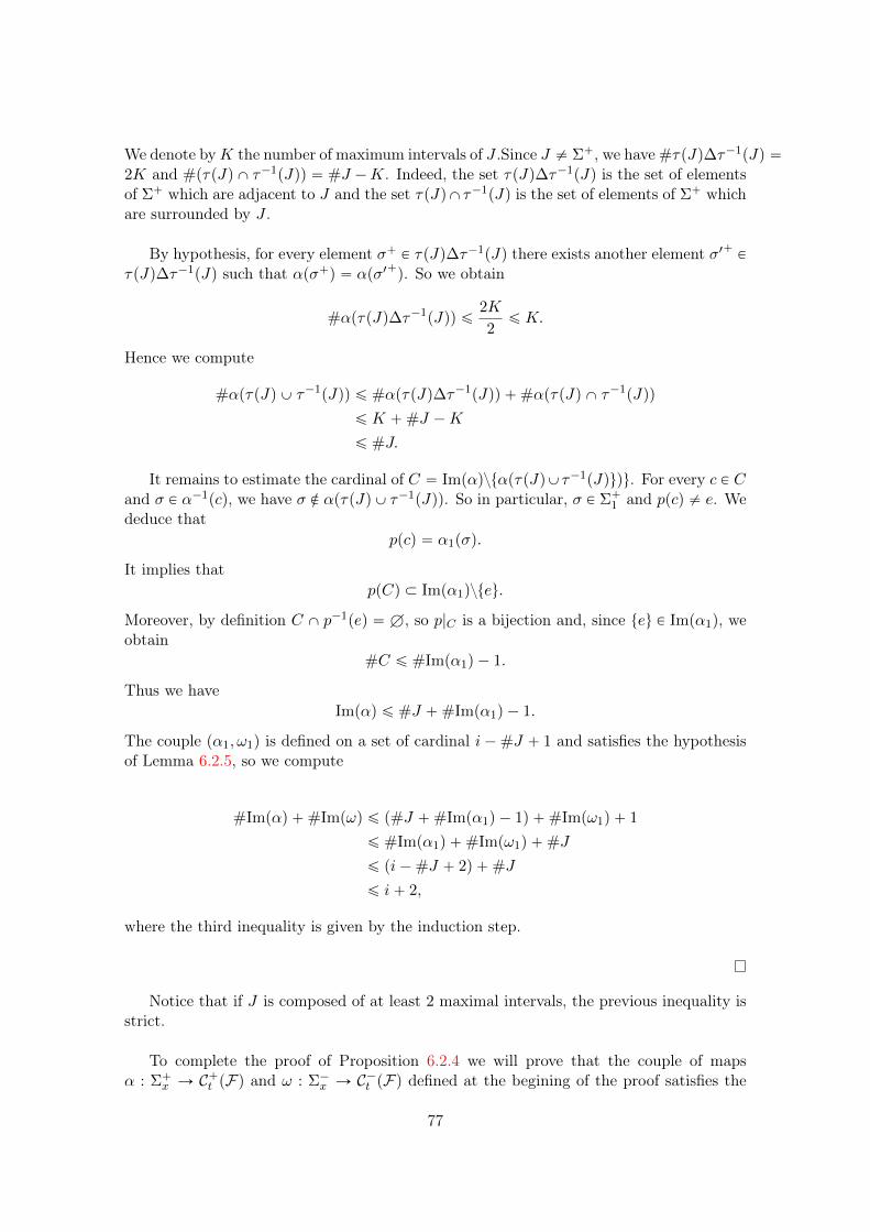
We denote byK the number of maximum intervals of J .Since J ‰ Σ`, we have #τpJq∆τ´1pJq “2K and #pτpJq X τ´1pJqq “ #J ´K. Indeed, the set τpJq∆τ´1pJq is the set of elementsof Σ` which are adjacent to J and the set τpJqXτ´1pJq is the set of elements of Σ` whichare surrounded by J .

By hypothesis, for every element σ` P τpJq∆τ´1pJq there exists another element σ1` PτpJq∆τ´1pJq such that αpσ`q “ αpσ1`q. So we obtain

#αpτpJq∆τ´1pJqq ď2K

2ď K.

Hence we compute

#αpτpJq Y τ´1pJqq ď #αpτpJq∆τ´1pJqq `#αpτpJq X τ´1pJqq

ď K `#J ´K

ď #J.

It remains to estimate the cardinal of C “ ImpαqztαpτpJqYτ´1pJququ. For every c P Cand σ P α´1pcq, we have σ R αpτpJq Y τ´1pJqq. So in particular, σ P Σ`1 and ppcq ‰ e. Wededuce that

ppcq “ α1pσq.

It implies thatppCq Ă Impα1qzteu.

Moreover, by definition C X p´1peq “ H, so p|C is a bijection and, since teu P Impα1q, weobtain

#C ď #Impα1q ´ 1.

Thus we haveImpαq ď #J `#Impα1q ´ 1.

The couple pα1, ω1q is defined on a set of cardinal i´#J ` 1 and satisfies the hypothesisof Lemma 6.2.5, so we compute

#Impαq `#Impωq ď p#J `#Impα1q ´ 1q `#Impω1q ` 1

ď #Impα1q `#Impω1q `#J

ď pi´#J ` 2q `#J

ď i` 2,

where the third inequality is given by the induction step.

Notice that if J is composed of at least 2 maximal intervals, the previous inequality isstrict.

To complete the proof of Proposition 6.2.4 we will prove that the couple of mapsα : Σ`x Ñ C`t pFq and ω : Σ´x Ñ C´t pFq defined at the begining of the proof satisfies the

77

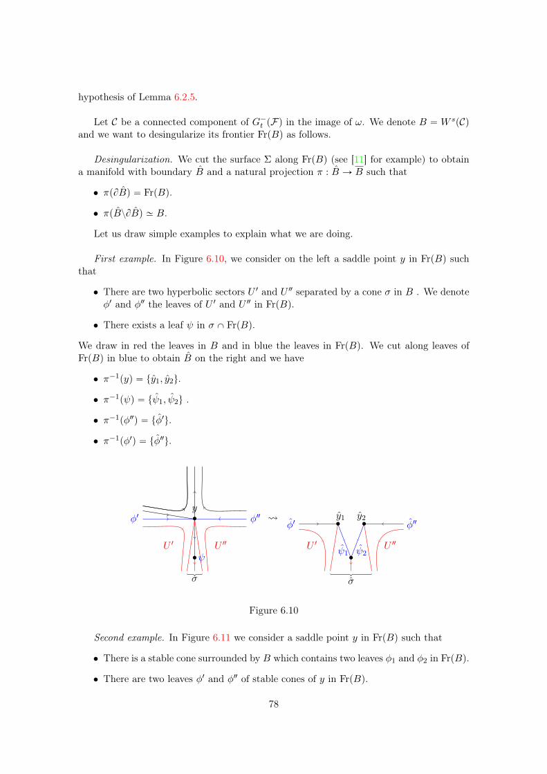
hypothesis of Lemma 6.2.5.

Let C be a connected component of G´t pFq in the image of ω. We denote B “ W spCqand we want to desingularize its frontier FrpBq as follows.

Desingularization. We cut the surface Σ along FrpBq (see [11] for example) to obtaina manifold with boundary B and a natural projection π : B Ñ B such that

• πpBBq “ FrpBq.

• πpBzBBq » B.

Let us draw simple examples to explain what we are doing.

First example. In Figure 6.10, we consider on the left a saddle point y in FrpBq suchthat

• There are two hyperbolic sectors U 1 and U2 separated by a cone σ in B . We denoteφ1 and φ2 the leaves of U 1 and U2 in FrpBq.

• There exists a leaf ψ in σ X FrpBq.

We draw in red the leaves in B and in blue the leaves in FrpBq. We cut along leaves ofFrpBq in blue to obtain B on the right and we have

• π´1pyq “ ty1, y2u.

• π´1pψq “ tψ1, ψ2u .

• π´1pφ2q “ tφ1u.

• π´1pφ1q “ tφ2u.

σ

‚ψ

‚y

U 1 U2

φ1 φ2

σ

‚

‚ ‚φ1 φ2

ψ2ψ1

y1 y2

U 1 U2

Figure 6.10

Second example. In Figure 6.11 we consider a saddle point y in FrpBq such that

• There is a stable cone surrounded by B which contains two leaves φ1 and φ2 in FrpBq.

• There are two leaves φ1 and φ2 of stable cones of y in FrpBq.

78

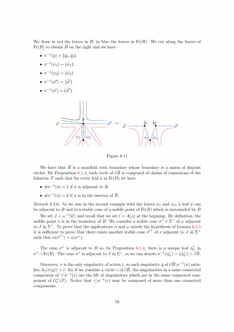
We draw in red the leaves in B, in blue the leaves in FrpBq. We cut along the leaves ofFrpBq to obtain B on the right and we have

• π´1pyq “ ty1, y2u.

• π´1pψ1q “ tψ1u.

• π´1pψ2q “ tψ2u

• π´1pφ2q “ tφ1u.

• π´1pφ1q “ tφ2u.

‚ψ2ψ1

‚y

φ1 φ2

‚

‚ ‚φ1 φ2

ψ2ψ1

y1 y2

Figure 6.11

We have that B is a manifold with boundary whose boundary is a union of disjointcircles. By Proposition 6.1.4, each circle of BB is composed of chains of connexions of thefoliation F such that for every leaf φ in FrpBq we have

• #π´1pφq “ 1 if φ is adjacent to B.

• #π´1pφq “ 2 if φ is in the interior of B.

Remark 6.2.6. As we saw in the second example with the leaves ψ1 and ψ2, a leaf φ canbe adjacent to B and in a stable cone of a saddle point of FrpBq which is surrounded by B

We set J “ ω´1pCq and recall that we set t “ Apxq at the begining. By definition, thesaddle point x is in the boundary of B. We consider a stable cone σ` P Σ` of x adjacentto J in Σ`. To prove that the applications α and ω satisfy the hypothesis of Lemma 6.2.5it is sufficient to prove that there exists another stable cone σ1` of x adjacent to J in Σ`

such that αpσ1`q “ αpσ`q.

The cone σ` is adjacent to B so, by Proposition 6.1.4, there is a unique leaf φ`0 inσ`XFrpBq. The cone σ` is adjacent to J in Σ`, so we can denote π´1pφ`0 q “ tφ

`0 u Ă BB.

Moreover, x is the only singularity of action t, so each singularity y of BBzπ´1pxq satis-fies Af pπpyqq ą t. So, if we consider a circle γ of BB, the singularities in a same connectedcomponent of γzπ´1pxq are the lift of singularities which are in the same connected com-ponent of G`t pFq. Notice that γzπ´1pxq may be composed of more than one connectedcomponents.

79

We consider the circle γ0 of BB containing φ`0 . The connected component of γ0zπ´1pxq

containing φ`0 contains a leaf φ1`

0 distinct from φ`0 such that ωpπpφ10qq “ x. There are twocases.

1) If πpφ10q is in a stable cone of x adjacent to J in Σ` then we obtain the result.

2) Suppose that πpφ10q is in a stable cone σ`1 of x surrounded by J in Σ`. By con-struction, there exists another leaf φ`1 P BB distinct from φ1

`

0 such that πpφ`1 q, which maybe equal to πpφ1

`

0 q, is in σ`1 .

By Lemma 6.1.5, we have that αpπpφ`1 qq “ αpπpφ1`

0 qq. So we apply the same argu-ments to φ`1 and then there exists a leaf φ1

`

1 Ă BB such that φ1`

1 and φ`1 are in the sameconnected component of γ1ztπ

´1pxqu and ωpπpφ1`

1 qq “ x . If φ1`1 is in a stable cone of xadjacent to J in Σ` we stop the process and if not we do the same discussion for φ1`1 aswe did for φ1`0 in case 2).

Since x has finitely many stable cones, the process stops after a finite number of timesand we obtain a leaf φ1` in the frontier of the attractive basin of C distinct from φ` whichis in a stable cone σ1` of x adjacent to J in Σ` such that αpσ1`q “ αpσ`q and this endsthe proof of Proposition 6.2.4.

By construction of B, we deduce the following corollary.

Corollary 6.2.7. Let us suppose that the singularities of F have distinct action valuesand consider a saddle point x of F . There exist exactly ´indpf, xq bars J1, ..., J´indpf,xq ofwhich Apxq is an end point.Moreover, for each source or sink y of X there exists exactly one bar J of which Apyq isan end point.

Proof. Let us consider a saddle point x of F of action t. We denote Cx (resp. C1x theconnected component of G´

t`pFq (resp. G`

t´pFq) which contains x. By construction, there

are #j´1t pCxq bars of category 1 such that Apxq is the maximum and #j1´1

t pC1xq bars ofcategory 2 such that Apxq is the infimum. Finally, by Proposition 6.2.4 we have k “|indpF , xq| ´#j´1

t pCxq ´#j1´1t pC1xq ě 0 so there exists k bars pAf pxq,`8q of category 3.

Thus there are exactly ´indpF , xq bars of which Af pxq is an end.

Recall that Xă is the set of singularities of X of negative index and X1 the set of sin-gularities of X of index 1. We set Să0 “ ApXă0q and we consider a sink ym of the foliationF such that Apymq “ Am and a source yM of the foliation F such that ApyM q “ AM andan application ι : Xztym, yMu Ñ Xă0 given by 6.1. We will prove the following resultabout the semi-infinite bars of βF .

Lemma 6.2.8. There exist exactly 2g ` 2 semi-infinite bars in βF , where g is the genusof Σ.

Proof. By Lemma 6.2.1 for each value t P Să0 the number of finite bars of which one end

80

is the action value of t is equal to¨

˚

˝

ÿ

CPC´t`

p#j´1t ptCuq ´ 1q `

ÿ

C1PC`t´

p#j1´1t ptC

1uq ´ 1q

˛

‹

‚

.

Moreover, the existence of the application ι asserts that the total number of finite barsis equal to the number of singularities of index 1 minus two. So we compute

ÿ

yPX1

1 “ 2`ÿ

yPX1ztym,yM u

indpF , yq

“ 2`ÿ

tPSă0

¨

˚

˝

ÿ

CPC´t`

p#j´1t ptCuq ´ 1q `

ÿ

CPC`t´

p#j1´1t ptC

1uq ´ 1q

˛

‹

‚

.

(6.3)

Moreover, we have

2´ 2g “ÿ

xPX

indpF , xq

“ 2`ÿ

xPXztym,yM u

indpF , xq.

“ 2`ÿ

xPXă0

indpF , xq `ÿ

yPX1ztym,yM u

indpF , yq.

Where the last equality is given by separating the fixed points of negative index and thefixed points of index 1.

For t P Să0 we definekt “ ´

ÿ

xPXă0Apxq“t

indpF , xq.

By equation 6.3, we get

2´ 2g “ 2`ÿ

tPSă0

¨

˚

˚

˝

ÿ

xPXă0Apxq“t

indpF , xq

˛

‹

‹

‚

`ÿ

tPSă0

¨

˚

˝

ÿ

CPC´t`

p#j´1t ptCuq ´ 1q `

ÿ

C1PC`t´

p#j1´1t ptC

1uq ´ 1q

˛

‹

‚

“ 2´ÿ

tPSă0

¨

˚

˝

kt ´ÿ

CPC´t`

p#j´1t ptCuq ´ 1q ´

ÿ

C1PC`t´

p#pj1´1t ptC

1uq ´ 1q

˛

‹

‚

“ 2´ p#tsemi-infinite barsu ´ 2q.

The last equation is given by the construction of the bars of category 3 in the constructionof B. Indeed, for action value t, the number of bars pt,`8q in the barcode is equal, by

81

definition, to kt ´ř

CPC´t`p#j´1

t ptCuq ´ 1q ´ř

C1PC`t´p#pj1´1

t ptC1uq ´ 1q. The ´2 comes

from the two semi-infinite bars pAm,`8q and pAM ,`8q. So the number of semi-infinitebars is equal to 2g ` 2.

Remark 6.2.9. Let us suppose that for each value t in the image of A, the set A´1pttuq isa singleton and each singularity x of Xă0 has index ´1. In this case the proof is simplerto understand because ι is an injection.

The number of semi-infinite bars is equal to #pXă0zImpιqq ` 2 and we compute

2´ 2g “ÿ

xPX

indpF , xq

“ 2`ÿ

yPX1ztym,yM u

indpF , yq `ÿ

xPXă0

indpF , xq

“ 2`ÿ

yPX1ztym,yM u

1´ÿ

xPImpιq

1´ p#tsemi-infinite barsu ´ 2q

“ 4´#tsemi-infinite barsu.

We obtain the result.

82

Chapter 7

A barcode with an order on a maximalunlinked set of fixed points

We consider a homeomorphism f of a compact surface Σ with a finite number of fixedpoints. We fix a maximal unlinked set of fixed points X of f . We denote by D the unitdisk.

For a set U Ă D we will denote by AdhDpUq its closure in D and by AdhR2U its closurein R2. A line γ will be a proper oriented topological embedding of the interval p0, 1q. If anoriented line γ : p0, 1q Ñ D separates D in two connected components, we will consider itsleft hand side, denoted Lprγq, and its right-hand side, denoted Rprφq.

Let us consider a maximal isotopy I from id to f such that SingpIq “ X. We equippedΣzX with a hyperbolic metric m such that the universal cover ĆΣzX of ΣzX with the pullback metric is isomorphic to D.

We consider a singularity x P X and a path γ : r0, 1s Ñ Σ such that limtÑ1 γptq “ xand γpp0, 1sq Ă ΣzX. We fix a lift rγ : p0, 1q Ñ D of γ|p0,1q. We consider a horosphericalneighborhood V of x in pΣzX,mq. Meaning that π´1pV q is a disjoint union of horodiskswhere a horodisk is a disk internally tangent to the unit circle. Notice that V Y txu is atopological neighborhood of x in Σ.

Moreover, rγpp0, εsq is connected so there exists a unique horoball rV Ă π´1pV q whichcontains rγpp0, εsq. By definition, the closure of a horoball intersects the boundary S1 of Din exactly one point and we set rx “ AdhR2pV q X S1. Since the alpha-limit point of rγ is apoint of S1 we obtain that limtÑ0 rγptq “ rx.

Thus, if we consider a path γ : r0, 1s Ñ Σ such that αpγq “ x P X, ωpγq “ y P X andγpp0, 1qq Ă ΣzX, then for every lift rγ of γ is line in D such that there are two points rx andry of S1 which satisfy

limtÑ0

rγptq “ rx, and limtÑ1

rγptq “ ry.

The point rx (resp. ry) will be denoted αprγq (resp. ωprφq). We refer to Ratcliffe’s book [?],chapter 9.8 for more details.

83

For two distinct points rx and ry of S1, we define rrx, rys Ă S1 the arc joining rx to ry forthe usual orientation. We set prx, ryq “ rrx, rysztrx, ryu.

Let us consider two proper paths φ : r0, 1s Ñ ΣzX and φ1 : r0, 1s Ñ ΣzX whose al-pha and omega limit points are in X and satisfy φpp0, 1qq Ă ΣzX and φ1pp0, 1qq Ă ΣzX.We say that φ and φ1 strongly intersect if there exist two lifts rφ and rφ1 of φ and φ1 as follows.

If we denote

• αprφq “ rx,

• ωprφq “ ry,

• αprφ1q “ rx1,

• ωprφ1q “ ry1,

then we have

• rx, ry, rx1, ry1 are distinct,

•"

rx1 P prx, ryqry1 P pry, rxq

or"

rx1 P pry, rxqry1 P prx, ryq

.

The homeomorphism rf can be extended on the closed unit disk AdhR2pDq. A lineγ Ă D is said to be a Brouwer line of rf if it separates D in two connected components suchthat the one on the left-hand side, denoted Lpγq, contains rfpγq and the one on the right-hand side, denoted Rpγq, contains rf´1pγq. In particular, we have rfpAdhDpLpγqqq Ă Lpγq.We have the following definition.

Definition 7.0.1. For a couple x, y P X, an oriented path γ : r0, 1s Ñ Σ such thatαpγq “ x P X, ωpγq “ y P X and γpp0, 1qq Ă ΣzX is called a connexion from x to y ifevery lift rγ of γ is an oriented Brouwer line of rf .

Remark 7.0.2. If we consider a maximal isotopy I “ pftqtPr0,1s from id to f and a foliationF positively transverse to I then each leaf φ of F is a connexion in the previous sense.Indeed, if we consider a leaf φ of F , then a lift rφ of φ is an oriented line which separates Din two connected components Lprφq and Rprφq such that rfprφq Ă Lprφq and we deduce thatrfpAdhDpLprφqqq Ă Lprφqq.

We will prove the following lemma which will be useful in Chapter 8.

Lemma 7.0.3. Let us consider x, x1, y, y1 P X fixed points of f such that there exist aconnexion φ from x to y and a connexion φ1 from x1 to y1. If φ and φ1 strongly intersectthen there exists a connexion from x to y1 and a connexion from x1 to y.

Remark 7.0.4. The result stands for non area-preserving homeomorphisms isotopic tothe identity and no foliations are involved in the statement. Moreover, the fixed pointsx, y, x1, y1 do not have to be distincts to obtain the result. Nevertheless, if we suppose thatf is a Hamiltonian homeomorphism, then for every connexion φ between two fixed points

84

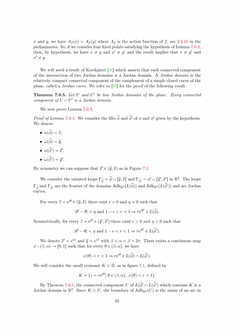
x and y, we have Af pxq ą Af pyq where Af is the action function of f , see 2.3.18 in thepreliminaries. So, if we consider four fixed points satisfying the hypothesis of Lemma 7.0.3,then, by hypothesis, we have x ‰ y and x1 ‰ y1 and the result implies that x ‰ y1 andx1 ‰ y.

We will need a result of Kerékjártó [46] which asserts that each connected componentof the intersection of two Jordan domains is a Jordan domain. A Jordan domain is therelatively compact connected component of the complement of a simple closed curve of theplane, called a Jordan curve. We refer to [55] for the proof of the following result.

Theorem 7.0.5. Let U and U 1 be two Jordan domains of the plane. Every connectedcomponent of U X U 1 is a Jordan domain.

We now prove Lemma 7.0.3.

Proof of Lemma 7.0.3. We consider the lifts rφ and rφ1 of φ and φ1 given by the hypothesis.We denote

• αprφq “ rx,

• ωprφq “ ry,

• αprφ1q “ rx1,

• ωprφ1q “ ry1.

By symmetry we can suppose that rx1 P pry, rxq as in Figure 7.1.

We consider the oriented loops Γrφ“ rφY rry, rxs and Γ

rφ1“ φ1 Y rry1, rx1s in R2. The loops

Γrφand Γ

rφ1are the frontier of the domains AdhR2pLprφqq and AdhR2pLprφ1qq and are Jordan

curves.

For every rz “ eiθ P pry, rxq there exist ε ą 0 and η ą 0 such that

|θ1 ´ θ| ă η and 1´ ε ă r ă 1 ñ reiθ1

P Lprφq.

Symmetrically, for every rz “ eiθ P pry1, rx1q there exist ε ą 0 and η ą 0 such that

|θ1 ´ θ| ă η and 1´ ε ă r ă 1 ñ reiθ1

P Lprφ1q.

We denote rx1 “ eiα and ry “ eiβ with β ă α ă β ` 2π. There exists a continuous mapψ : pβ, αq Ñ r0, 1s such that for every θ P pβ, αq, we have

ψpθq ă r ă 1 ñ reiθ P Lprφq X Lprφ1q.

We will consider the small croissant K Ă D, as in figure 7.1, defined by

K “ tz “ reiθ| θ P pβ, αq, ψpθq ă r ă 1u.

By Theorem 7.0.5, the connected component U of Lprφ1 X Lprφ1q which contains K is aJordan domain in R2. Since K Ă U , the boundary of AdhR2pUq is the union of an arc in

85

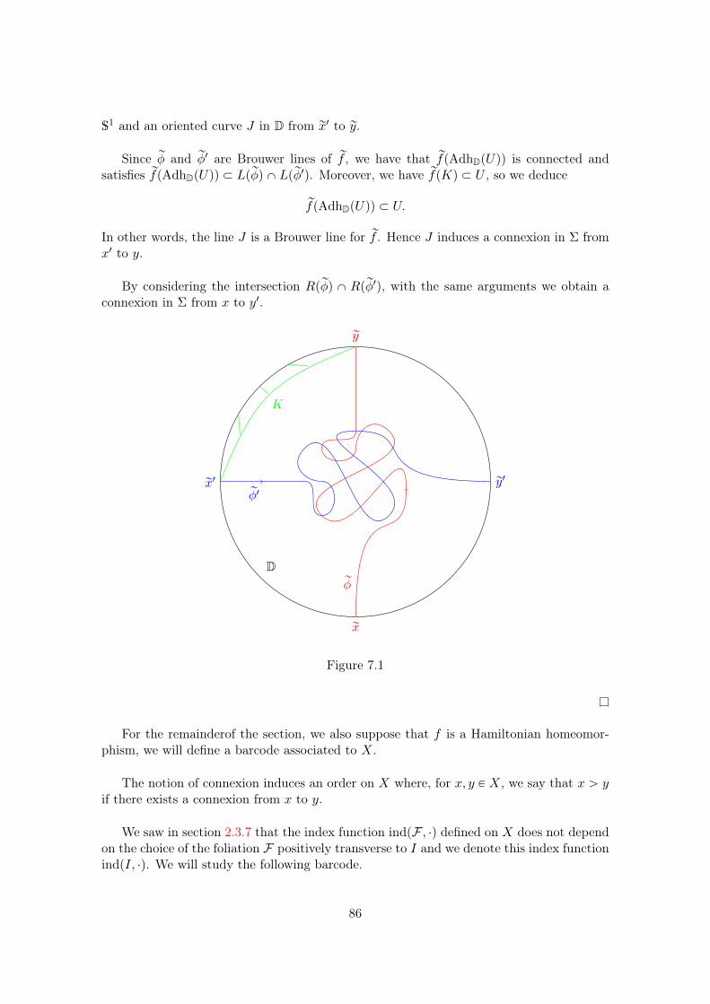
S1 and an oriented curve J in D from rx1 to ry.

Since rφ and rφ1 are Brouwer lines of rf , we have that rfpAdhDpUqq is connected andsatisfies rfpAdhDpUqq Ă Lprφq X Lprφ1q. Moreover, we have rfpKq Ă U , so we deduce

rfpAdhDpUqq Ă U.

In other words, the line J is a Brouwer line for rf . Hence J induces a connexion in Σ fromx1 to y.

By considering the intersection Rprφq X Rprφ1q, with the same arguments we obtain aconnexion in Σ from x to y1.

D

K

rφ

rφ1rx1 ry1

rx

ry

Figure 7.1

For the remainderof the section, we also suppose that f is a Hamiltonian homeomor-phism, we will define a barcode associated to X.

The notion of connexion induces an order on X where, for x, y P X, we say that x ą yif there exists a connexion from x to y.

We saw in section 2.3.7 that the index function indpF , ¨q defined on X does not dependon the choice of the foliation F positively transverse to I and we denote this index functionindpI, ¨q. We will study the following barcode.

86

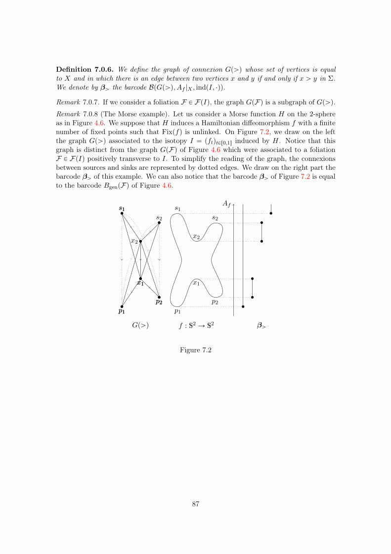
Definition 7.0.6. We define the graph of connexion Gpąq whose set of vertices is equalto X and in which there is an edge between two vertices x and y if and only if x ą y in Σ.We denote by βą the barcode BpGpąq, Af |X , indpI, ¨qq.

Remark 7.0.7. If we consider a foliation F P FpIq, the graph GpFq is a subgraph of Gpąq.

Remark 7.0.8 (The Morse example). Let us consider a Morse function H on the 2-sphereas in Figure 4.6. We suppose that H induces a Hamiltonian diffeomorphism f with a finitenumber of fixed points such that Fixpfq is unlinked. On Figure 7.2, we draw on the leftthe graph Gpąq associated to the isotopy I “ pftqtPr0,1s induced by H. Notice that thisgraph is distinct from the graph GpFq of Figure 4.6 which were associated to a foliationF P FpIq positively transverse to I. To simplify the reading of the graph, the connexionsbetween sources and sinks are represented by dotted edges. We draw on the right part thebarcode βą of this example. We can also notice that the barcode βą of Figure 7.2 is equalto the barcode BgenpFq of Figure 4.6.

f : S2 Ñ S2

Af

p1

x1

p2

s1

x2

s2

βą

‚

‚

‚

‚

‚

‚

Gpąq

p1

x1

p2

s1

x2

s2

p1

x1

p2

s1

‚

‚

‚

‚

‚

‚

‚

‚

‚

‚

‚

‚

Figure 7.2

87

88

Chapter 8

Equalities of the previous constructions andindependence of the foliation

In this chapter, we fix a Hamiltonian homeomorphism f of a closed and oriented surfaceΣ with a finite number of fixed points. Let X Ă Fixpfq be a maximal unlinked set offixed points and I “ pftqtPr0,1s an isotopy from id to f such that SingpIq “ X. The actionfunctional of f will be denoted Af .For a foliation F positively transverse to the isotopy I, we denote by GpFq the graph, de-fined in Chapter 6, whose set of vertices is the set X such that for every couple of verticesx and y of GpFq there exists an edge from x to y if and only if there exists a leaf in Ffrom x to y. We will also consider the subgraphs pG´t pFqqtPR and pG`t pFqqtPR given bythe natural filtration of GpFq by Af .

We will use some notation of Chapter 5. For t P R we denote C´t and C`t the sets ofconnected components of G´t pFq and G`t pFq and for a connected component C of G´t pFqwe define LpCq “ mintAf pyq | y vertex of Cu.

We consider the graph of connexion Gpąq, defined in Chapter 7, whose set of verticesis equal to X such that there is an edge between two vertices x and y if and only if thereexists a connexion between x and y in Σ.

We will consider the barcode BpGpFq, Af |X , indpF , ¨qq, denoted βF , constructed inChapter 6 and associated to the foliation F . Recall that the index function indpF , ¨q de-fined on X does not depend on the choice of F P FpIq and we denote this index functionindpI, ¨q. We will consider the barcode BpGpąq, Af |X , indpI, ¨qq, denoted βą, defined inChapter 7.

In the first section, we compare these two barcodes and in the second section we comparethe barcode βF with the barcode constructed in Chapter 4 in the generic case.

8.1 Equality between the barcode βF and the barcode βą

In this section, we prove the following theorem.

89

Theorem 8.1.1. The barcode βF does not depend on the choice of F P FpIq and satisfiesβF “ βą.

For the proof, we fix a foliation F P FpIq positively transverse to the isotopy I. Wewill need the following lemma.

Lemma 8.1.2 (Fundamental). For each t P R, the set of connected components of G´t pFqdefines the same partition of X X A´1

f pp´8, tqq than the set of connected components ofG´t pąq.

If we suppose Lemma 8.1.2 true, the proof of Theorem 8.1.1 is straigthforward since theaction functions and the index functions are equals and the constructions of the barcodesβą and βF in Chapter 5 depend only on the connected components of the graphs GpFqand Gpąq and the action and index values of the singularities of X.

Proof of Lemma 8.1.2. For t P R and for each fixed points x, y P X of action less than t,we want to prove the equivalence of the following two properties.

(i) The elements x, y are in the same connected component Cą of G´t pąq,

(ii) The elements x, y are in the same connected component CF of G´t pFq.

(ii) ñ (i). Since x and y are in the same connected component C of G´t pąq, thereexists a family pxiq0ďiďk of singularities of X such that

• x0 “ x and xk “ y.

• Af pxiq ă t for every i P t0, ..., ku

• For every i P t1, ..., ku there exists a leaf φi of F either from xi to xi´1 or from xi´1

to xi

Moreover, each leaf of the foliation F is by definition a connexion, so pφiq0ďiďk is afamily of connexions and then the singularities xi, i P t0, ..., ku, are in the same connectedcomponent of G´t pąq and we obtain the result.

(i) ñ (ii). We will prove the following lemma.

Lemma 8.1.3. Let us consider F P FpIq and px, yq P X2. If x ą y then x and y are inthe same connected component of G´t pFq for every t ą Af pxq.

Let us assume that Lemma 8.1.3 is true and consider x, y P X and t ą Af pxq such thatpiq is satisfied, we prove that piiq holds.

Since x and y are in the same connected component C of G´t pąq, there exists a familypxiq0ďiďk of singularities of X such that

• x0 “ x and xk “ y.

• Af pxiq ă t for every i P t0, ..., ku

• For every i P t1, ..., ku there exists a connexion φi either from xi to xi´1 or from xi´1

to xi

90

Moreover, by Lemma 8.1.3 xi´1 and xi are in the same connected component of G´t pFqfor every i P t1, ..., ku so x and y are also in the same connected component of G´t pFq.

To complete the proof of Lemma 8.1.2, it remains to prove Lemma 8.1.3.

Proof of Lemma 8.1.3. We consider two fixed points x, y P X such that x ą y. Everyattractive or repulsive basin in this proof will be defined relatively to the foliation F . Wewill divide the proof in three cases, in the first one x will be a sink of F , in the second onex will be a saddle and in the last one x will be a source of F .

First case. We suppose that x is a sink. We will prove that there is no connexion fromx to another singularity of F .

We say that the orbit of a q-periodic point z of f is contractible if the concatenation ofthe trajectories of the points fkpzq, k P t0, ..., q ´ 1u, along the isotopy I is a contractibleloop , denoted γz, in Σ. The loop γz is called the trajectory of the periodic orbit of z.We say that a contractible q-periodic orbit has type pp, qq associated to I at x P Fixpfqif its trajectory along I is homotopic to pΓ in ΣzSingpIq, where Γ is the boundary of asufficiently small Jordan domain containing x.

We will use the following version of a result of Yan and we refer to [75], Theorem 1.1,for a proof.

Theorem 8.1.4. Let us consider a fixed point z of f of Lefschetz index equal to 1 fixedby the isotopy I, and such that the rotation set ρspI, zq is reduced to t0u. The point z isaccumulated by periodic points. More precisely, the following property holds: there existsε ą 0, such that, for every neighborhood of z, either for every irreducible pq P p0, εq, or forevery irreducible pq P p´ε, 0q, there exists a contractible periodic orbit Opq of type pp, qq.

Let us prove that there is no connexion from x to another singularity of F . We supposethat there exists a connexion φ from x to another singularity y of F , we want to find acontradiction.

The singularity x is a sink of the foliation F which is positively transverse to the isotopyI, so the local rotation set ρs,Ipxq of x, introduced in section 2.3.5, is included in p´8, 0s.Moreover, it is not difficult to prove that the existence of the connexion φ implies that therotation set ρs,Ipxq of x is included in r0,`8q. Indeed, locally, a connexion whose alpha-limit is x is a positive arc, which means that in polar coordinates where γ corresponds tothe semi-line tθ “ 0u, for every point z close enough to x, the variation of θ along thetrajectory is positive. We refer to Theorem 3.2.4 and section 2.4 of [59] for more details.So the local rotation set of x for the isotopy I is reduced to the integer t0u.

If the Lefschetz index of x is not equal to 1, by a result of Le Roux, see [59] Theorem4.1.1, the foliation F and the homeomorphism f have the same index at x for the isotopyI. But, by hypothesis, x is a sink of the foliation F so indpF , xq “ 1 and we obtain acontradiction.

91

If the Lefschetz index of x is equal to 1 then we can apply Theorem 8.1.4. More pre-cisely, the singularity x is a sink of F so there exists ε ą 0 such that x is accumumated byperiodic orbits Opq of type pp, qq where pq P p0, εq. So the rotation number ρs,Ipxq is notreduced to t0u and we obtain a contradiction.

Second case. We suppose that x is a saddle point. We prove the result by contradiction.

We suppose that there exists a connexion γ : r0, 1s Ñ Σ from x to some y and that x andy are not in the same connected component of G´

Af pxq`pFq. We denote byW spC´x q Ă Σ the

attractive basin of C´x , where C´x is the connected component of G´Af pxq`

pFq which containsx. By Lemma 6.1.7, the fixed point x is in the interior of W spC´x q and every singularity zof F in the frontier of W spC´x q satisfies Af pzq ą Af pxq. The existence of the connexion γimplies that Af pxq ą Af pyq so the fixed point y is not in the frontier of W spC´x q and is inΣzW spC´x q.We consider the universal cover ĆΣzX of ΣzX which is identified to the unit disk D andπ : DÑ ΣzX the universal covering map. Let U be a connected component of π´1pC´x zXqand rγ a lift of the connexion γ such that there exists ε ą 0 such that rγpp0, εqq Ă U . Byhypothesis on y, there exists ε1 ą 0 such that rγpp1´ ε1, 1qq R U .Recall that π naturally extends to S1. Moreover, we saw that limtÑ0 rγptq and limtÑ1 rγptqare well-defined on S1 and will be denoted rx and ry.

The set U is an open connected set of D whose frontier is a union of lifted leaves. Thenthere exists a lifted leaf rψ of FrpUq which separates D such that U is on one side and ry isin the other. By hypothesis, the points ωp rψq and αp rψq are distinct from rx and ry, indeed,x is in the interior of W spC´x q and y R FrpW spC´x qq. Since rψ is the lift of a connexion,we obtain that ψ and γ are two connections which intersect strongly, hence by Lemma7.0.3 there exists a connexion from x to ωpψq which is impossible because by definitionωpψq P FrpW spC´x qq and then Af pωpψqq ą Af pxq.

Third case. Suppose that x is a source of F . The point y is either in the frontier of therepulsive basin W upxq of x or in the complement of W upxq. We separate these two cases.

1) We suppose that y is in the frontier of W upxq. There exists a chain of connexionsfrom x to y and so we deduce the result. Indeed, by definition, the singularity y is ac-cumulated by leaves pφjqjPJ of W upxq whose alpha-limit point is x. By the local modeldescribed in Chapter 6.1, the closure of these leaves contains a chain of connexions whichstarts at x and also contains y.

2) We suppose that y is in the complement of W upxq. We consider U a connected com-ponent of π´1pW upxqztxuq where π : D Ñ ΣzX the covering map defined in the secondcase. We can consider a lift rγ of the connexion γ such that there exists ε ą 0 such thatrγpp0, εqq Ă U . By hypothesis on y, there exists ε1 ą 0 such that rγpp1 ´ ε1, 1qq R U . Thelimits limtÑ0 rγptq and limtÑ1 rγptq are well-defined on S1 and will be denoted rx and ry.

We apply similar arguments as in the second case. The set U is an open connectedset of D whose boundary is a union of lifted leaves. Then there exists a lifted leaf rψ of

92

FrpUq separating D such that U is on one side and ry is on the other. By hypothesis, thepoints ωp rψq and αp rψq are distinct from rx and ry, indeed, x is in the interior of W spC´x qand y R FrpW spC´x qq. Since rψ is the lift of a connexion, we obtain that ψ and γ are twoconnections which intersect strongly, hence by Lemma 7.0.3 there exists a connexion fromαpψq to y. The singularity αpψq can not be a source nor a sink so it is a saddle pointof F , hence we apply the result of the second case which asserts that the existence of aconnexion from αpψq to y implies that αpψq and y are in the same connected component ofG´Af pαpψqq`

pFq. Moreover, by hypothesis, αpψq and x are in the same connected componentof G´

Af pxq`pFq thus we deduce that x and y are also in the same connected component of

G´Af pxq`

pFq.

8.2 Equality between the barcode βF and the barcode Bgenpf,Fq in thegeneric case

We consider a Hamiltonian homeomorphism f of a closed and oriented surface Σ with afinite number of fixed points. We suppose that Fixpfq is finite and unlinked, each fixedpoint x P Fixpfq satisfies indpf, xq P t´1, 1u and that the action function Af : Fixpfq Ñ Ris injective. Let I “ pftqtPr0,1s be a maximal isotopy from id to f fixing all fixed points off . We denote Af the action functional of f .

Recall that a foliation F P FgenpIq does not have connexions between saddle points,and the stable and unstable cones of a saddle point x of F are both composed of a uniqueleaf which will be referred to as the stable and unstable leaves of x.

Let us consider the graph GgenpFq given by Definition 4.0.2. Remember that GgenpFqis the graph whose set of vertices is the set Fixpfq and whose edges correspond to leavesφ of F such that indCZpf, αpφqq “ indCZpf, ωpφqq ´ 1, where indCZpf, ¨q is the Conley-Zehnder index, defined in Chapter 4, equals to 1 on sources and sinks and equals to ´1 onsaddle points. Notice that Ggen is distinct from the graph GpFq given in the introductionof this chapter.

In this section we want to compare the barcode BgenpFq to the barcode

BpGpFq, Af |X , indpF , ¨qq,

denoted βF , constructed in Chapter 6. We will prove the following result.

Theorem 8.2.1. Let us consider a Hamiltonian homeomorphism f on a compact surfaceΣ. We suppose that Fixpfq is finite and unlinked, each fixed point x P Fixpfq satisfiesindpf, xq P t´1, 1u and the action function is injective. We consider a maximal isotopy Isuch that SingpIq “ Fixpfq then for a foliation F P FgenpIq we have

BgenpFq “ βF .

We recall the definition of the functor β. Let V “ pVsqsPR be a persistence module. Letus consider the set of t P R in the spectrum of V such that dimpKerpit´,t`qq is equal to 1and label its elements b1, ..., bn. For each bj , there exists a unique aj P R with the following

93

property: Let x P Vb´j represents a non-zero element in Kerpit´,t`q “ 1, the element x is inthe image of ia`j ,b´j but x is not in the image of ia´j ,b´j ; if we label the remaining elementsof the spectrum of V by tc1, ..., cmu then the barcode βpVq consists of the list of intervalspaj , bjs and pck,`8q, where 1 ď j ď n and 1 ď k ď m.

We will consider G´gen,tpFq, G`gen,tpFq the associated filtered graphs and we denote bypHt

˚qtPR the persistence module of the chain complex pCti qiPt0,1,2u,tPR of Definition 4.0.3.Finally, we denote by BgenpFq the barcode βppHt

˚qtPRq where β is the functor defined inChapter 3.

To avoid any confusion, we will always refer to the chain complex by Cti where i Pt0, 1, 2u and t P R. We will refer to connected components of the graph GpFq by C or C1and to a connected component of the graph GgenpFq by Cgen. For t P R and a connectedcomponent C of G´t pFq we denote LpCq the minimum of the action function on the sinksof C and for t P R and a connected component C1 of G`t pFq we denote DpCq the maximumof the action function on the sources of C1. Moreover, to simplify the notation, we providethe filtered chain complex pCitqiPt0,1,2u,tPR with a natural scalar product x.|.y associated tothe canonical basis. Meaning that we consider the bilinear function x.|.y on the space Citsuch that for every couple of fixed points x and y of f in Cit , we have xx, yy “ 1 if and onlyif x “ y and xx, yy “ 0 otherwise.

Theorem 8.2.1 allows us to prove Property 4.0.11 of Chapter 4 which states that thebarcode Bgenpf,Fq does not depend on the choice of F P FgenpIq. We recall that assump-tions of Theorem 8.2.1 are satisfies in this particular case.

Proof of Proposition 4.0.11. By Theorem 8.2.1, for each foliation F P FgenpIq we have thatBgenpFq “ βF . Moreover, by Theorem 8.1.1, the barcode βF does not depend on thechoice of the foliation F P FgenpIq. So we obtain that Bgenpf,Fq does not depend on thechoice of F P FgenpIq which is the result.

We fix a foliation F P Fgen for the remaining of the section.

Proof of Theorem 8.2.1. By Remark 4.0.9, each action value of Af is the end of a uniquebar of the barcode BgenpFq and by Corollary 6.2.7, we have the same result for the barcodeβF so it is enough to prove the inclusion βF Ă BgenpFq to prove that these barcodes areequal.

Moreover, Corollary 6.2.7 states that exactly one end point of every bar of the barcodeβF , except the bars pminAf ,`8q and pmaxAf ,`8q, is the action value of a saddle pointof F . So it is enough to prove that finite bars of the barcode βF are also bars of the bar-code Bgen to prove the inclusion βF Ă BgenpFq. Indeed, the remaining bars of the barcodewould be the same semi-infinite bars as they would be associated to the same saddle points.

We will prove that for every saddle point x of f , if the bar J of βF , of which Af pxq is anend, is a finite bar, then it is also a bar of the barcode BgenpFq. Notice that, by construc-

94

tion, the bars pminAf ,`8q and pmaxAf ,`8q of βF are also bars of the barcode BgenpFq.

For the remainder of the proof, we consider a saddle point x of f , we denote by t itsaction value and by Cx the connected component of G´

t`pFq which contains x. By Lemma

6.2.4 the set of connected components of G´t pFq which are included in Cx, which werelabeled j´1

t pCxq in Chapter 5, has one or two elements. We separate those two cases.

Case 1. The set j´1t pCxq consists of two connected components of G´t pFq denoted C and

C1. By symmetry, we can suppose that LpCq ą LpC1q and, by the construction describedin Chapter 5, there is a bar pLpCq, ts in the barcode βF . Let us prove that this bar is alsoa bar of the barcode BgenpFq. It means that there is an element of Kerpit´,t`q which is inthe image of iLpCq`,t´ but not in the image of iLpCq´,t´ .

By hypothesis, the omega-limit points of the unstable leaves of x are distinct sinks yand y1 of F where y P C and y1 P C1. We have Bt`1 pxq “ y ` y1 so the element y ` y1 P Ct`0satisfies ry ` y1s P Kerpit´,t`q. It remains to prove that ry ` y1s is in the image of iLpCq`,t´and not in the image of iLpCq´,t´ . For that, we will consider another cycle in Ct`0 repre-senting ry ` y1s in homology.

We will use some geometric lemmas.

We will call a path of leaves a path Γ in Σ which is the concatenation of leaves of F .The singularities of a path of leaves will refer to the alpha-limit points and omega-limitpoints of those leaves.

Lemma 8.2.2. Let us consider s P R, and two sinks y1 and y2 of F in the same connectedcomponent Cs of G´s pFq. There exists a path of leaves from y1 to y2 whose singularitiesare alternatively sinks and saddle points of Cs.

Proof of Lemma 8.2.2. By definition of the connected component Cs of G´s , there exists apath of leaves Γ from y1 to y2 in Σ. The path Γ may contain sources. For a source z in Γwe will modify Γ into a path which does not contain z.

If there is a source z in Γ, there exist two leaves φ1 Ă Γ and φ2 Ă Γ whose alpha-limitpoints are equal to z and omega-limit points are either saddle points or sinks of F that wedenote x1 and x2. The singularities x1 and x2 are in the repulsive basin of z for F so, byLemma 4.0.7, there exists a path γ of leaves of G´s pFq from x1 to x2 whose singularitiesare alternatively saddle points and sinks of F .We cut the union φ1 Y tzu Y φ2 from the path Γ and replace this portion by the path γgiven by Lemma 4.0.7. We obtain a new path Γ1 from y to y1 such that the source z is notin Γ1.

We do the same process for every source of Γ and we finally obtain a path from y to y1

as wanted.

We prove the following lemma.

95

Lemma 8.2.3. For every s P R and every couple of sinks y1 and y2 of F in the sameconnected component Cs of G´s pFq we have ry1s “ ry2s in Hs

0 .

Proof of Lemma 8.2.3. Let us consider s P R, and two sinks y1 and y2 of F in the sameconnected component Cs of G´s pFq. By Lemma 8.2.2 there exists a path of leaves in Σfrom y1 to y2 whose singularities are alternatively sinks and saddle points of Cs. We denoteby pxiq0ďiďns the saddle points of the path Γ and by a simple computation we obtain

Bs1

˜

nÿ

i“0

xi

¸

“ y1 ` y2.

So, by definition, ry1s “ ry2s in Hs0 .

Let us come back to the first case of the proof of Theorem 8.2.1. By Lemma 8.2.3 eachsink z P C of F (resp. each sink z1 P C1 of F) satisfies rzs “ rys (resp. rz1s “ ry1s) inHt

0. So for every couple of sinks z P C and z P C1 of F , the element z ` z1 P Ct`

0 satisfiesrz ` z1s “ ry ` y1s P Kerpit´,t`q. We denote by zC and zC1 the sinks of C and C1 such thatAf pzCq “ LpCq, Af pzC1q “ LpC1q.We supposed that Af pzCq “ LpCq ą Af pzC1q “ LpC1q so the sink zC is not a cycle in CLpCq

´

0

so the element rzC ` zC1s is not in the image of iLpCq´,t´ . Moreover, the sinks zC and zC1are not in the same connected component of Gt´pFq and so we deduce that rzC ` zC1s isin the image of iLpCq`,t´ .

So, by construction, there exists a bar pLpCq, ts in the barcode BgenpFq.

Case 2. The set j´1t pCxq is a unique element. We will consider the connected compo-

nents of the subgraphs pG`t qtPR instead of connected components of the subgraphs pG´t qtPR.We consider the connected component C1x of G`

t´pFq which contains x. By Lemma 6.2.4

the set of connected components of G`t pFq included in C1x, which were labeled j1´1t pC´x q in

Chapter 5, is composed of 1 or 2 elements. We separate those two cases.

1) Suppose that j1´1t pC1xq is composed of one connected component, then, by construc-

tion, there is no finite bar J in the barcode βF of which t is an end point. We have nothingto prove in this case.

2) Now we suppose that j1´1t pC1xq is composed of two connected components of the

graph G`t`pFq denoted C and C1. By symmetry we can suppose that DpCq ă DpC1q and by

construction there is a bar pt,DpCqs in the barcode βF . Let us prove that this bar is also abar of the barcode BgenpFq. It means that there is an element in KerpiDpCq´,DpCq`q whichis in the image of it`,DpCq´ but not in the image of it´,DpCq´ . We will need the followinglemma about the repulsive basin W spCq of C.

Lemma 8.2.4. We label x1, ..., xn the saddle points in the frontier of W spCq. Then, forevery T ą DpCq, the element Y “

ř

yPCy source

y of CT2 satisfies

BT2 pY q “nÿ

i“1

xi.

96

Proof. For each source y of C, by definition, BT2 pyq is equal to the sum of the saddle pointsin the frontier of the repulsive basin of y. These saddle points have either one or both oftheir stable leaves in W spCq. We separate those cases.

Firstly, we label x1, ..., xn the saddle points of F of which only one stable leaf have itsalpha-limit point in C. For every i P r0, ns we have xBT2 pY q|xiy “ 1 for every i P r0, ns.Moreover, the action values of these saddle points is less then or equal to t and it is simpleto see that this belong to the frontier of W spCq.

Secondly, we label x11, ..., x1m the saddle points such that both stable leaves have theiralpha-limit points in C. For every i P r0,ms we have xBT2 pY q|x1iy “ 2. Those saddle pointsare nondegenerate saddle points of F so that they are in the interior W spCq and not in itsfrontier. Indeed, both stable cones of a saddle point x whose action satisfies Af pxq ą t areleaves of F whose alpha-limit points are in the same connected component of G`t pFq.

Finally, we compute BT2 pY q as follows.

BT2 pY q “ÿ

yPC,y source

BT2 pyq

“

nÿ

i“1

xi `mÿ

i“1

2x1i

“

nÿ

i“1

xi.

And we obtain the result.

Let us denote c “ DpCq, we will consider the element Y “ř

yPCy source

y in Cc`

2 . By

Lemma 8.2.4, Y satisfies

Bc`

2 pY q “nÿ

i“1

xi,

where x1, ..., xn are the saddle points of the frontier of W spCq. So we have rřni“1 xis P

Kerpic´,c`q.

By hypothesis, the saddle point x is one of the saddle points pxiqiPr1,ns and each xi sat-isfies Apxiq ď Apxq since C is a connected component of G`t pFq. So we have that r

řni“1 xis

is in the image of it`,c´ .

Moreover, the singularity x is not homologous in Cc´1 to a chain of singularities of Ct´1 .Indeed, if it was the case then, by definition, it would exist X 1 P Ct´1 and Y 1 P Cc´2 suchthat x “ X 1 ` Bc

´

2 pY1q.

We set yx P C and y1x P C1 the only two sources of F such that x is in the frontier of thesets W upyxq and W upy1xq. The equality x “ X 1 ` Bc

´

2 pY1q would imply that xY 1|yxy “ 1

97

or xY 1|y1xy “ 1, which is impossible because, by hypothesis, Af py1xq ą Af pyxq “ c. In-deed, if we have Bc´2 pY 1q “ x ´X 1 then, there exists a source y such that xY |yy “ 1 andxBc

´

2 pyq|xy “ 1 , which means that x is in the frontier of W upyq. So y is either equal to yxor y1x.

So, we have the same result forřni“1 xi and so r

řni“1 xis R Impit´,c´q.

Thus, by construction, there exists a bar pApxq, DpCqs in the barcode BgenpFq.

Now we can prove Theorem 4.0.12 from Chapter 4 stated as follows.

Theorem 8.2.5. If we consider a Hamiltonian diffeomorphism f with a finite number offixed points which is C2-close to the identity and generated by an autonomous Hamiltonianfunction then the barcode BgenpFq is equal to the Floer homology barcode of f .

Proof. If we suppose that the autonomous Hamiltonian function H is C2 close to a con-stant then the Floer homology of H is equal to the Morse homology of H, we refer to [3]for a proof. We deduce that the Morse Homology barcode βpHMt

˚pHqqtPRq of H is equalto the Floer Homology barcode βpHFt˚pHqqtPRq of H, where β is the functor defined inChapter 3 which associate a persistence module to its barcode.

The time one map f1 “ f of the Hamiltonian flow is C1 close the the identity and itsset of fixed points is unlinked.

Moreover, the gradient-lines of H provides a C1 foliation F positively transverse tothe natural Hamiltonian isotopy induces by H. This isotopy is maximal and so fixes everyfixed points of f . The foliation F is gradient-like and there is no cone of leaves at thesaddle points of F .

Moreover, the construction of the map B in Chapter 5 follows the ideas of the Morse ho-mology theory then we can assert that the barcode βF is equal to the barcode βpHMt

˚pHqqtPR,

Thus, by Theorem 8.2.1 we have

Bgenpfq “ βF “ βpHMt˚pHqqtPR “ βpHFt˚pHqqtPR.

So we obtain the result.

98

Chapter 9

Perspectives

Let us consider a Hamiltonian homeomorphism f of a surface with a finite number of fixedpoints. In the previous chapter, every construction of barcodes depends on the choice of amaximal unlinked set of fixed points X of f . A natural question remains.

Question 9.0.1. Can we construct a barcode associated to f which is equal to the FloerHomology barcode in the case of a generic diffeomorphism?

We have some ideas to study this question. In this short chapter we explain the diffi-culties to generalize our constructions and the objects we may use in a near future.

Conley-Zehnder index

The first problem we will have to deal with is the Conley-Zehnder index. The FloerHomology is indexed by the Conley-Zehnder index, denoted indCZp¨q, which is well-definedfor C1 diffeomorphisms.

Nevertheless, the Conley-Zehnder index can be extended for Hamiltonian homeomor-phisms at isolated fixed points. We found an interesting way to describe this extensionusing generalized isotopies, defined in the preliminaries. Let us recall a quick definition.If we consider a Hamiltonian homeomorphism f on Σ, we denote rΣ the universal cover ofΣ and we can consider its compactification into a 2-sphere S2 by adding a point 8, thena lift rf of f can be compactified into a homeomorphism f of S2. An isotopy from id tof on S1 which fixes 8 is called a generalized isotopy. In the next section we will see whyconsidering generalized isotopies can be useful in our studies.

Moreover, let us consider the Floer homology barcode of a Hamiltonian diffeomorphismf . We denote Af the action function of f . For every finite bar J “ pAf pxq, Af pyqs wherex, y P Fixcpfq, we have indCZpyq ´ indCZpxq “ 1. We refer to the construction of FloerHomology for more details [3].

Now, let us consider a Hamiltonian homeomorphism f with a finite number of fixedpoints, a maximal unlinked set of fixed points X of f and an isotopy I from id to f whichfixes X and a foliation F positively transverse to I. We denote indCZp¨q the extension ofthe Conley-Zehnder index defined on Fixcpfq. For every fixed point x P X one may provethat we have

• if indCZpxq “ 1, then x is a saddle point for F ,99

• if indCZpxq ‰ 1, then x is either a sink or a source for F .

So, the barcode βF defined in Chapter 6 may have finite bars J “ pAf pxq, Af pyqs suchthat indCZpyq ´ indCZpxq ‰ 1. Indeed, it can be the case if Fixcpfq is not unlinked. Thusit is not enough to work only with maximal isotopies of f .

Torsion-low isotopies

Let us consider of a Hamiltonian homeomorphism f on a surface Σ. Yan [76] introducedthe notion of torsion-low isotopies. Roughly speaking, an isotopy I from id to f is said tobe torsion-low at x P SingpIq if ρspI, xq Ă r´1, 1s, where ρspI, xq is the local rotation setof x for I, defined in the preliminaries.

Now, we consider a maximal generalized isotopy I of a Hamiltonian homeomorphismf on Σ. Every fixed point rx of I is a lift of a fixed point x of f . The isotopy I is saidto be a maximal torsion-low generalized isotopy if I is torsion-low at every fixed point ofSingpIq except at 8 and I is a maximal isotopy.

A result of Yan [76] asserts the existence of maximal torsion-low generalized isotopies.

Moreover, for a maximal torsion-low generalized isotopy I of f , the Conley-Zehnderindices of the points of SingpIqzt8u is linked to the rotation number of the point 8.Indeed, one may prove that if the rotation number of 8 for the isotopy I is equal to ´k,then it holds that:

• every saddle point rx of I is the lift of a fixed point x of f such that indCZpxq “ 2k`1,

• every sink rx of I is the lift of a fixed point x of f such that indCZpxq “ 2k,

• every source rx of I is the lift of a fixed point x of f such that indCZpxq “ 2k ` 2.

We can consider a gradient-like foliation F positively transverse to the maximal torsion-low generalized isotopy I. Moreover, F is equipped with the action function Af of f andan index function indpF , ¨q.

Thus, we can consider the barcode βF associated to F as defined in Chapter 6. Wecan prove that for every finite bar J of βF , there exist x, y P Fixcpfq and lifts rx, ry of x andy fixed by I such that J “ pAf pxq, Af pyqs and indCZpyq ´ indCZpxq “ 1.

In a near future, we hope to define a Barcode using the barcodes associated to maximaltorsion-low generalized isotopies but two important questions remain.

Question 9.0.2. We consider a Hamiltonian diffeomorphism f and a bar J of its Floerhomology barcode. Does there exist a torsion-low generalized isotopy of f such that for apositively transverse foliation F , J is a bar of βF?

If we consider every torsion-low generalized isotopy of a Hamiltonian diffeomorphismf and every bar of their associated barcodes, then we may have too many bars to obtaina barcode equal to the Floer homology barcode of f .

Question 9.0.3. Is there a natural way to select the "good" bars to keep?

100

Part II

Calabi invariant for Hamiltoniandiffeomorphism of the unit disk

101

Chapter 1

Introduction

In this second part of the thesis, we study the Calabi invariant on the unit disk usuallydefined on compactly supported Hamiltonian diffeomorphisms of the open disk. In partic-ular we extend the Calabi invariant to the group of C1 diffeomorphisms of the closed diskwhich preserves the standard symplectic form. We also compute the Calabi invariant forsome diffeomorphisms of the disk which satisfy some rigidity hypothesis.

Let us begin with some basic definitions of symplectic geometry.

Let us consider pM2n, ωq a symplectic manifold, meaning thatM is an even dimensionalmanifold equipped with a closed non-degenerate differential 2-form ω called the symplecticform. We suppose that π2pMq “ 0 and that ω is exact, meaning that there exists a 1-formλ, called a Liouville form, which satisfies dλ “ ω.

Let us consider a time-dependent vector field pXtqtPR defined by the equation

dHt “ ωpXt, .q, (1.1)

where

H : RˆM Ñ Rpt, xq ÞÑ Htpxq

is a smooth function 1-periodic on t, meaning that Ht`1 “ Ht for every t P R. The functionH is called a Hamiltonian function. If the vector field pXtqtPR is complete, it induces afamily pftqtPR of diffeomorphisms of M that preserve ω, also called symplectomorphismsor symplectic diffeomorphisms, satisfying the equation

f0 “ id andB

Btftpzq “ Xtpftpzqq.

In particular the family I “ pftqtPr0,1s defines an isotopy from id to f1. The map f1 iscalled a Hamiltonian diffeomorphism. It is well known that the set of Hamiltonian diffeo-morphisms of a symplectic manifold M is a group which we denote HampM,ωq, we referto [62] for more details.

Let us consider pM,ωq a symplectic manifold which is boundaryless, π2pMq “ 0 andsuch that ω is exact. We say that H is a compactly supported Hamiltonian function if

103

there exists a compact set K Ă M such that Ht vanishes outside K for every t P R.A compactly supported Hamiltonian function induces a compactly supported Hamiltoniandiffeomorphism f . Such a map is equal to the identity outside a compact subset of M .Let us consider a compactly supported Hamiltonian diffeomorphism f and λ a Liouvilleform on M . The form f˚λ ´ λ is closed because f is symplectic but we have more, it isexact. More precisely there exists a unique compactly supported function Af : M Ñ R,also called action function, such that

dAf “ f˚λ´ λ.

In the literature the Calabi invariant Calpfq of f is defined as the mean of the functionAf and we have

Calpfq “

ż

MAfω

n, (1.2)

where ωn “ ω^ ...^ω is the volume form induced by ω, see [62] for more details. We willprove later that the number Calpfq does not depend on the choice of λ.

Let us give another equivalent definition of the Calabi invariant for a compactly sup-ported Hamiltonian diffeomorphism f . We note H a compactly supported Hamiltonianfunction defining f . The Calabi invariant of f can also be defined by the equation

Calpfq “ pn` 1q

ż 1

0

ż

MHtω

ndt. (1.3)

To prove thatş

M Afωn does not depend on the choice of the Liouville form λ, one may

use the fact that the action function Af satisfies

Af pzq “

ż 1

0pιpXsqλ`Hsq ˝ fspzqds, (1.4)

where pXsqsPR is the time dependent vector field induced by H by equation (1.1) andpfsqsPR is the isotopy induced by the vector field pXsqsPR. Moreover,

ş10

ş

M Htωndt does

not depend on the compactly supported Hamiltonian function H defining f .

The function Cal defines a real valued morphism on the group of compactly supportedHamiltonian diffeomorphisms ofM and thus it is a conjugacy invariant. It is an importanttool in the study of difficult problems such as the description of the algebraic structure ofthe groups HampM,ωq: A.Banyaga proved in [5] that the kernel of the Calabi invariant isalways simple, which means that it does not contain nontrivial normal subgroups.

In this article, we study the case of the dimension two and more precisely the case of theclosed unit disk which is a surface with boundary. We denote by ||.|| the usual Euclidiannorm on R2, by D the closed unit disk and by S1 its boundary. The group of C1 orientationpreserving diffeomorphisms of D will be denoted by Diff1

`pDq. We consider Diff1ωpDq the

group of C1 symplectomorphisms of D which preserve the normalized standard symplecticform ω “ 1

πdu ^ dv, written in cartesian coordinates pu, vq. In the case of the disk, thegroup Diff1

ωpDq is contractible, see [39] for a proof, and coincides with the group of Hamil-tonian diffeomorphisms of D. Moreover, the 2-form ω induces the Lebesgue probabilitymeasure denoted by Leb and the symplectic diffeomorphisms are the C1 diffeomorphisms

104

of D which preserve the Lebesgue measure and the orientation.

Let us begin by the case of the unit open disk D. The open disk is boundaryless hencewe already have two equivalent definitions of the Calabi invariant given by equations 1.2and 1.3 on the set of compactly supported symplectic diffeomorphisms of D. Let us give athird one. A. Fathi in his thesis [22] gave a dynamical definition which is also described byJ.-M. Gambaudo and É. Ghys in [32]: if we consider an isotopy I “ pftqtPr0,1s from id to f ,there exists an angle function AngI : Dˆ Dz∆ Ñ R where ∆ is the diagonal of Dˆ D suchthat for each px, yq P Dˆ Dz∆, the quantity 2πAngIpx, yq is the variation of angle of thevector ftpyq ´ ftpxq between t “ 0 and t “ 1. If f is a compactly supported C1 symplecticdiffeomorphism then this angle function is integrable (see section 3) and it holds that

Calpfq “

ż

DˆDz∆AngIpx, yqdLebpxqdLebpyq, (1.5)

where the integral does not depend on the choice of the isotopy.

In this article we will give an answer to the following question.

Question 1.0.1. How to define an extension of the Calabi invariant to the group Diff1ωpDq?

M. Hutchings [43] extended the definition given by equation 1.3 to the C1 symplecticdiffeomorphisms which are equal to a rotation near the boundary. In another point ofview, V. Humilière [42] extended the definition given by equation 1.3 to certain group ofcompactly supported symplectic homeomorphisms of an exact symplectic manifold pM,ωqwhere a compactly supported symplectic homeomorphism f of M is a C0 limit of a se-quence of Hamiltonian diffeomorphisms of M supported on a common compact subset ofM .

In the case of the open disk, for a compactly supported symplectomorphism f , thechoice of the isotopy class of f is natural. But if f is a symplectic diffeomorphism of theclosed disk such that its restriction to the open disk is not compactly supported then thereis no such natural choice of an isotopy from id to f .

The rotation number is a well-known dynamical tool introduced by Poincaré in [66]on the group Homeo`pS

1q of homeomorphisms of S1 which preserve the orientation. Letus consider the set of homeomorphisms rg : R Ñ R such that rgpx ` 1q “ rgpxq, denotedČHomeo`pS

1q. One may prove that there exists a unique rρ P R such that for each z P R andn P Z we have |rgnpzq ´ z´ nrρ| ă 1. The number rρ “ rρprgq is called the rotation number ofrg. Let us consider g P Homeo`pS

1q and two lifts rg and rg1 of g in ČHomeo`pS1q, there exists

k P Z such that rg “ rg1 ` k and so rρprgq “ rρprg1q ` k. Consequently we can define a mapρ : Homeo`pS

1q Ñ T1 such that ρpgq “ rρprgq `Z where rg is a lift of g. The number ρpgq iscalled the rotation number of g. We give further details about the rotation number in thenext section.

We now state the results of this article. The following proposition allows us to considera natural choice of an action function of a symplectomorphism of the closed disk.

105

Proposition 1.0.2. Let us consider f P Diff1ωpDq, Af : D Ñ R a C1 function such that

dAf “ f˚λ´ λ and µ an f invariant Borel probability measure supported on S1. Then thenumber

ş

S1Afdµ does not depend on the choice of µ and λ.

The first theorem follows.

Theorem 1.0.3. For each f P Diff1ωpDq there exists a unique function Af : D Ñ R such

that dAf “ f˚λ ´ λ andş

S1Afdµ “ 0 where λ is a Liouville form and µ a f -invariant

probability measure on S1. The map Cal1 : Diff1ωpDq Ñ R defined by

Cal1pfq “

ż

DAf pzqωpzq

does not depend on the choice of λ and µ. Moreover the map Cal1 is a homogeneousquasi-morphism that extends the Calabi invariant.

In another direction, the definition given by equation 1.3 and the definition given byequation 1.5 are based on isotopies. Then we consider the universal cover ĄDiff

1

ωpDq ofDiff1

ωpDq which is composed of couples rf “ pf, rIsq where f P Diff1ωpDq and rIs is an

homotopy class of isotopies from id to f . We will prove that for f P Diff1ωpDq and I an

isotopy from id to f , the angle function AngI does not depend on the choice of I P rIs.Hence, for rf “ pf, rIsq P ĄDiff

1

ωpDq we can denote Angrf“ AngI for I P rIs.

Moreover, for a diffeomorphism f P Diff1pDq two isotopies I “ pftqtPr0,1s and I 1 “ pf 1tqtPr0,1sfrom id to f are homotopic if and only if their restriction I|S1 and I 1|S1 to S1 are homotopicand so define the same lift Ąf |S1 of f |S1 on the universal cover of S1. Hence it is equivalentto consider ĄDiff

1

ωpDq as the set of couples rf “ pf, rφq where f P Diff1ωpDq and rφ a lift of

f |S1 to the universal cover of S1.

Theorem 1.0.4. Let us consider an element rf of ĄDiff1

ωpDq. The number

ĄCal2p rfq “

ż

D2z∆Ang

rfpx, yqωpxqωpyq,

defines a morphism ĄCal2 : ĄDiff1

ωpDq Ñ R which induces a morphism Cal2 : Diff1ωpDq Ñ T1

defined for every f P Diff1ωpDq by

Cal2pfq “ĄCal2p rfq ` Z,

where rf is a lift of f to ĄDiff1

ωpDq.

Along the same lines, we have the following result.

Theorem 1.0.5. Let us consider an element pf, rφq of ĄDiff1

ωpDq. There exists a Hamiltonianfunction H : T1 ˆM Ñ R such that Ht is equal to 0 on S1 for every t P R which inducesan isotopy pφtqtPr0,1s from id to f where the lifted isotopy prφtqtPr0,1s satisfies rφ1 “ rφ . Thenumber

ĄCal3pf, rφq “

ż 1

0

ż

DHtpzqωpzqdt,

does not depend on the choice of such a Hamiltonian function H. Moreover the mapĄCal3 : ĄDiff

1

ωpDq Ñ R is a morphism and induces a morphism Cal3 : Diff1ωpDq Ñ T1 defined

byCal3pfq “ĄCal3pf, rφq ` Z.

106

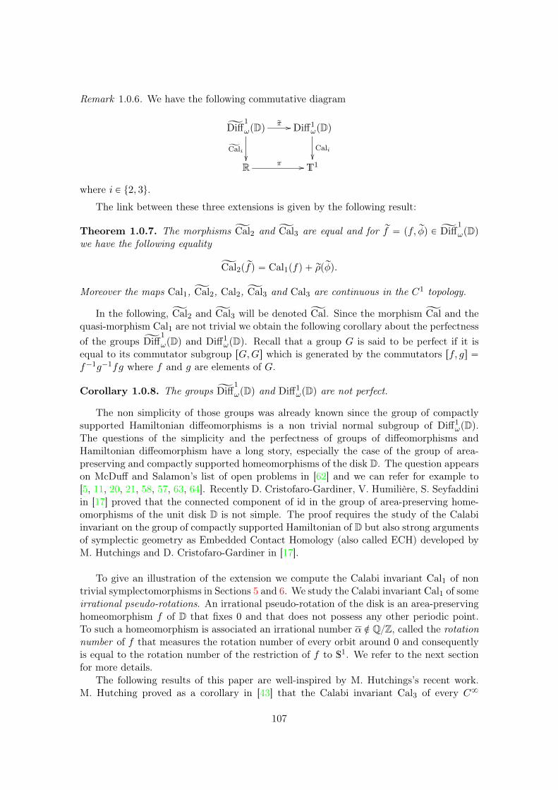
Remark 1.0.6. We have the following commutative diagram

ĄDiff1

ωpDqrπ //

ĄCali

Diff1ωpDq

Cali

R π // T1

where i P t2, 3u.

The link between these three extensions is given by the following result:

Theorem 1.0.7. The morphisms ĄCal2 and ĄCal3 are equal and for rf “ pf, rφq P ĄDiff1

ωpDqwe have the following equality

ĄCal2p rfq “ Cal1pfq ` rρprφq.

Moreover the maps Cal1, ĄCal2, Cal2, ĄCal3 and Cal3 are continuous in the C1 topology.

In the following, ĄCal2 and ĄCal3 will be denoted ĄCal. Since the morphism ĄCal and thequasi-morphism Cal1 are not trivial we obtain the following corollary about the perfectnessof the groups ĄDiff

1

ωpDq and Diff1ωpDq. Recall that a group G is said to be perfect if it is

equal to its commutator subgroup rG,Gs which is generated by the commutators rf, gs “f´1g´1fg where f and g are elements of G.

Corollary 1.0.8. The groups ĄDiff1

ωpDq and Diff1ωpDq are not perfect.

The non simplicity of those groups was already known since the group of compactlysupported Hamiltonian diffeomorphisms is a non trivial normal subgroup of Diff1

ωpDq.The questions of the simplicity and the perfectness of groups of diffeomorphisms andHamiltonian diffeomorphism have a long story, especially the case of the group of area-preserving and compactly supported homeomorphisms of the disk D. The question appearson McDuff and Salamon’s list of open problems in [62] and we can refer for example to[5, 11, 20, 21, 58, 57, 63, 64]. Recently D. Cristofaro-Gardiner, V. Humilière, S. Seyfaddiniin [17] proved that the connected component of id in the group of area-preserving home-omorphisms of the unit disk D is not simple. The proof requires the study of the Calabiinvariant on the group of compactly supported Hamiltonian of D but also strong argumentsof symplectic geometry as Embedded Contact Homology (also called ECH) developed byM. Hutchings and D. Cristofaro-Gardiner in [17].

To give an illustration of the extension we compute the Calabi invariant Cal1 of nontrivial symplectomorphisms in Sections 5 and 6. We study the Calabi invariant Cal1 of someirrational pseudo-rotations. An irrational pseudo-rotation of the disk is an area-preservinghomeomorphism f of D that fixes 0 and that does not possess any other periodic point.To such a homeomorphism is associated an irrational number α R QZ, called the rotationnumber of f that measures the rotation number of every orbit around 0 and consequentlyis equal to the rotation number of the restriction of f to S1. We refer to the next sectionfor more details.

The following results of this paper are well-inspired by M. Hutchings’s recent work.M. Hutching proved as a corollary in [43] that the Calabi invariant Cal3 of every C8

107

irrational pseudo-rotation f of the closed unit disk D such that f is equal to a rotationnear the boundary is equal to the rotation number of f . This means that for an irrationalpseudo-rotation f which is equal to a rotation near the boundary, Cal1pfq is equal to 0.The proof uses strong arguments of symplectic geometry such as the notion of open-booksintroduced by Giroux (see [37] for example) and the Embedded Contact Homology theory.We want to adopt a more dynamical point of view and we partially answer the followingquestion.

Question 1.0.9. Is the Calabi invariant Cal1pfq equal to 0 for every C1 irrational pseudo-rotation f of D?

With the continuity of ĄCal in the C1 topology, we can deduce the first result of C1-rigidity as the following result.

Theorem 1.0.10. Let f be a C1 irrational pseudo-rotation of D. If there exists a sequencepgnqnPN in Diff1

ωpDq of C1 diffeomorphisms of finite order which converges to f for the C1

topology, thenCal1pfq “ 0.

Corollary 1.0.11. Let f be a C1 irrational pseudo-rotation of D. If there exists a sequencepnkqkPN such that fnk converges to the identity in the C1 topology, then we have

Cal1pfq “ 0.

The morphisms ĄCal and Cal are not continuous in the C0 topology, see proposition4.2.5. Nevertheless, by a more precise study of the definition of Cal we obtain a C0-rigidityresult as follows.

Theorem 1.0.12. Let f be a C1 irrational pseudo-rotation of D. If there exists a sequencepnkqkPN of integers such that pfnkqkPN converges to the identity in the C0 topology, thenwe have

Cal1pfq “ 0.

There are already general results of C0-rigidity of pseudo-rotations. Bramham proved[12] that every C8 irrational pseudo-rotation f is the limit, for the C0 topology, of a se-quence of periodic C8 diffeomorphisms. Bramham [13] also proved that if we consider anirrational pseudo-rotation f whose rotation number is super Liouville (we will recall whatit means later) then f is C0-rigid. That is, there exists a sequence of iterates fnj thatconverges to the identity in the C0-topology as nj Ñ 8. Le Calvez [51] proved similarresults for C1 irrational pseudo-rotation f whose restriction to S1 is C1 conjugate to arotation.

Then for f a C1 pseudo-rotation of the disk D the results of Bramham and Le Calvezprovide a sequence of periodic diffeomorphisms pgnqnPN which converges to f , the diffeo-morphism gn may not be area-preserving but let us hope to completely answer question1.0.9.

In the last section we give examples where the rotation number of a pseudo-rotationsatisfies some algebraic properties and where the hypothesis of Theorem 1.0.12 and Corol-lary 1.0.11 are satisfied.

108

Organization

We begin to give some additional preliminaries in chapter 1. In a second chapter wegive the formal definitions of the Calabi invariant of equations 1.2, 1.3 and 1.5 and theirnatural extensions given by Theorems 1.0.3, 1.0.4 and 1.0.5. In chapter 3 we give the proofof the link between these extensions given by Theorem 1.0.7. The last chapter concernsthe results about the computation of the Calabi invariant for pseudo-rotations.

109

110

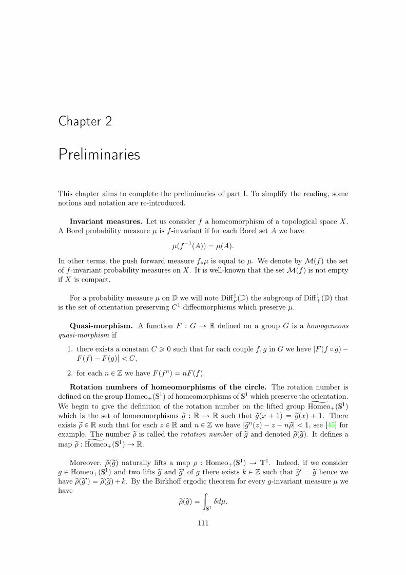
Chapter 2

Preliminaries

This chapter aims to complete the preliminaries of part I. To simplify the reading, somenotions and notation are re-introduced.

Invariant measures. Let us consider f a homeomorphism of a topological space X.A Borel probability measure µ is f -invariant if for each Borel set A we have

µpf´1pAqq “ µpAq.

In other terms, the push forward measure f˚µ is equal to µ. We denote byMpfq the setof f -invariant probability measures on X. It is well-known that the setMpfq is not emptyif X is compact.

For a probability measure µ on D we will note Diff1µpDq the subgroup of Diff1

`pDq thatis the set of orientation preserving C1 diffeomorphisms which preserve µ.

Quasi-morphism. A function F : G Ñ R defined on a group G is a homogeneousquasi-morphism if

1. there exists a constant C ě 0 such that for each couple f, g in G we have |F pf ˝ gq´F pfq ´ F pgq| ă C,

2. for each n P Z we have F pfnq “ nF pfq.

Rotation numbers of homeomorphisms of the circle. The rotation number isdefined on the group Homeo`pS

1q of homeomorphisms of S1 which preserve the orientation.We begin to give the definition of the rotation number on the lifted group ČHomeo`pS

1q

which is the set of homeomorphisms rg : R Ñ R such that rgpx ` 1q “ rgpxq ` 1. Thereexists rρ P R such that for each z P R and n P Z we have |rgnpzq ´ z ´ nrρ| ă 1, see [45] forexample. The number rρ is called the rotation number of rg and denoted rρprgq. It defines amap rρ : ČHomeo`pS

1q Ñ R.

Moreover, rρprgq naturally lifts a map ρ : Homeo`pS1q Ñ T1. Indeed, if we consider

g P Homeo`pS1q and two lifts rg and rg1 of g there exists k P Z such that rg1 “ rg hence we

have rρprg1q “ rρprgq`k. By the Birkhoff ergodic theorem for every g-invariant measure µ wehave

rρprgq “

ż

S1δdµ.

111

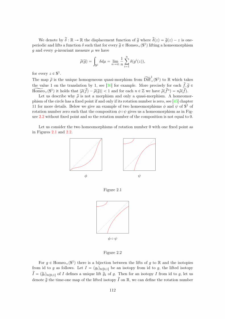
We denote by rδ : RÑ R the displacement function of rg where rδpzq “ rgpzq ´ z is one-periodic and lifts a function δ such that for every rg P Homeo`pS

1q lifting a homeomorphismg and every g-invariant measure µ we have

rρprgq “

ż

S1δdµ “ lim

nÑ8

1

n

nÿ

i“1

δpgipzqq,

for every z P S1.The map rρ is the unique homogeneous quasi-morphism from ĄDiff

1

`pS1q to R which takes

the value 1 on the translation by 1, see [36] for example. More precisely for each rf, rg PČHomeo`pS

1q it holds that |rρp rfq ´ rρprgq| ă 1 and for each n P Z we have rρp rfnq “ nrρp rfq.Let us describe why rρ is not a morphism and only a quasi-morphism. A homeomor-

phism of the circle has a fixed point if and only if its rotation number is zero, see [45] chapter11 for more details. Below we give an example of two homeomorphisms φ and ψ of S1 ofrotation number zero such that the composition φ˝ψ gives us a homeomorphism as in Fig-ure 2.2 without fixed point and so the rotation number of the composition is not equal to 0.

Let us consider the two homeomorphisms of rotation number 0 with one fixed point asin Figures 2.1 and 2.2.

φ ψ

Figure 2.1

φ ˝ ψ

Figure 2.2

For g P Homeo`pS1q there is a bijection between the lifts of g to R and the isotopies

from id to g as follows. Let I “ pgtqtPr0,1s be an isotopy from id to g, the lifted isotopyrI “ prgtqtPr0,1s of I defines a unique lift rg1 of g. Then for an isotopy I from id to g, let usdenote rg the time-one map of the lifted isotopy rI on R, we can define the rotation number

112

rρpIq P R of I to be the rotation number rρprgq of rg. If we consider f a homeomorphism of thedisk isotopic to the identity and I “ pftqtPr0,1s an isotopy from id to f then we will denoterρpI|S1q P R the rotation number of the restriction of the isotopy I to S1. If we consideranother isotopy I 1 from id to g one may prove that there exists an integer k P Z such thatI 1 is homotopic to RkI where the isotopy R “ pRtqtPr0,1s satisfies Rtpzq “ ze2πit for everyz P S1 and every t P r0, 1s. We consider rI the lifted isotopy of I 1 and we denote rg1 its time-one map. Hence rg and rg1 are two lifts of g such that rg1 “ rg ` k and rρprg1q “ rρprgq ` k andso the number rρpIq does not depend on the choice of the isotopy in the homotopy class of I.

Irrational pseudo-rotation. An irrational pseudo-rotation is an area-preservinghomeomorphism f of D that fixes 0 and that does not possess any other periodic point.To such a homeomorphism is associated an irrational number α P RZzQZ, called therotation number of f , characterized by the following : every point admits α as a rotationnumber around the origin. To be more precise, choose a lift rf of f |Dzt0u to the universalcovering space rD “ R ˆ p0, 1s. There exists rα P R such that rα ` Z “ α and for everycompact set K Ă Dzt0u and every ε ą 0, one can find N ě 1 such that

@n ě N, rz P π´1pKq X rf´npπ´1pKqq ñ |p2p rf

nprzqq ´ p2przq

n´ rα| ď ε,

where π : pr, θq ÞÑ pr cosp2πθq, r sinp2πθqq is the covering projection and p2 : pr, θq ÞÑ θ theprojection on the second coordinate. If moreover f is a Ck diffeomorphism 1 ď k ď `8we will call f a Ck irrational pseudo-rotation.

Notice that the rotation number α of an irrational pseudo-rotation f is equal to ρpf |S1q.

One can construct irrational pseudo-rotations with the method of fast periodic ap-proximations, presented by Anosov and Katok [1]. One may see [23, 24, 25, 38, 60] forfurther developments about this method and see [9, 7] for other results on irrational pseudo-rotations.

113

114

Chapter 3

Three extensions

In this section we will explain why the functions Cal1, ĄCal2 and ĄCal3 are well-defined andwe will establish the relations between them. The full statement like the continuity or thequasi-morphism property will be proved in the next section.

3.1 Action function

Let us consider f P Diff1ωpDq and λ a Liouville 1-form such that dλ “ ω. The fact that

H1pD,Rq “ 0 implies that the closed 1-form f˚λ ´ λ is exact. More precisely its integralalong each loop γ Ă D is zero. Consequently the map z ÞÑ

ş

γzf˚λ´ λ is a C1 primitive of

f˚λ ´ λ, equal to 0 at the origin, where for every z P D the path γz : r0, 1s Ñ D is suchthat γzptq “ tz.

If we suppose that f is compactly supported on D then it is natural to consider theunique C1 function A : DÑ R that is zero near the boundary of D and that satisfies

dA “ f˚λ´ λ. (3.1)

Without the compact support hypothesis we have the following proposition.

Proposition 3.1.1. If we consider a C1 function A : DÑ R such that dA “ f˚λ´λ thenthe number

ż

S1A|BDdµ

does not depend on the choice of µ inMpf |S1q.

Proof. To prove the independence over µ there are two cases to consider.

‚ If there exists only one f |S1-invariant probability measure on S1 the result is obvious.In this case f |S1 is said to be uniquely ergodic.

‚ If f |S1 is not uniquely ergodic then by Poincaré’s theory ρpf |S1q “pq ` Z is rational

with p^ q “ 1. The ergodic decomposition theorem, see [45] for example, tells us that anf |S1-invariant measure is the barycenter of ergodic f |S1-invariant measures. Moreover, each

115

ergodic measure of f |S1 is supported on a q-periodic orbit as follows. For z a q-periodicpoint of f |S1 , we define the probability measure µz supported on the orbit of z by

µz “1

q

q´1ÿ

k“0

δfkpzq,

where δz is the Dirac measure on the point z P S1. Hence it is sufficient to prove thatş

DApf, λ, µzqω does not depend on the choice of a periodic point z P S1.

Let us consider two periodic points z and w of f |S1 . We consider an oriented pathγ Ă S1 from z to w. We compute

ż

S1Adµz ´

ż

S1Adµw “

1

q

q´1ÿ

k“0

Apfkpzqq ´Apfkpwqq

“1

q

q´1ÿ

k“0

ż

fkpγqdA

“1

q

q´1ÿ

k“0

ż

fkpγqf˚pλq ´ λ

“1

qp

ż

fqpγqλ´

ż

γλq

“ 0

where the last equality is due to the fact that f qpγq is a reparametrization of the pathγ.

Proposition 3.1.1 allows us to make a natural choice of the action function to define anextension of the Calabi invariant as follows.

Theorem 3.1.2. For each f P Diff1ωpDq we consider the unique C1 function Af of f such

that dAf “ f˚λ´λ andş

S1Afdµ “ 0 where λ is a Liouville form of ω and µ an f -invariant

probability measure on S1. The number

Cal1pfq “

ż

DAf pzqωpzq

does not depend on the choice of λ or µ.

Proof. The independence on the measure µ comes from Proposition 3.1.1 and it remainsto prove the independence on λ.Let us consider another primitive λ1 of ω. We denote A and A1 the two functions suchthat dA “ f˚λ ´ λ and dA1 “ f˚λ1 ´ λ1 and such that for each µ P Mpf |S1q we haveş

S1Adµ “

ş

S1A1dµ “ 0.

The 1-form λ ´ λ1 is closed because dλ ´ dλ1 “ ω ´ ω “ 0. So there exists a smoothfunction u : DÑ R such that λ1 “ λ` du. We compute

dA1 “ f˚pλ` duq ´ pλ` duq

“ f˚λ´ λ` dpu ˝ f ´ uq

“ dA` dpu ˝ f ´ uq.

116

Thus there exists a constant c such that

A1 “ A` u ˝ f ´ u` c.

For a measure µ PMpf |S1q the conditionş

S1A1dµ “ 0 “

ş

S1Adµ implies that

ż

S1A1dµ “

ż

S1Adµ`

ż

S1pu ˝ f |S1 ´ uqdµ` c “

ż

S1Adµ,

Howeoverş

S1pu ˝ f |S1 ´ uqdµ “ 0 since f |S1 preserves µ we have

c “ 0.

Finally f preserves ω henceş

Dpu ˝ f ´ uqω “ 0 and we can conclude thatż

DA1ω “

ż

DAω.

We show that the extension Cal1 vanishes on rotations of the disk.

Proposition 3.1.3. For θ P R the rotation Rθ of angle θ satisfies

Cal1pRθq “ 0.

Proof. For the Liouville form λ “ r2

2πdθ of ω we have R˚θλ´λ “ 0 thus the action functionA is constant. So it is equal to 0 and we obtain the result.

3.2 Angle function

The following interpretation is due to Fathi in his thesis [22] in the case of compactly sup-ported symplectic diffeomorphisms of the unit disk. This interpretation is also developpedby Ghys and Gambaudo in [32].

Let us consider f P Diff1`pDq and I “ pftqtPr0,1s an isotopy from id to f . For x, y P D

distinct we can consider the vector vt from ftpxq to ftpyq and we denote by AngIpx, yq theangle variation of the vector vt for t P r0, 1s defined as follows.

We have the polar coordinates pr, θq and a differential form

dθ “udv ´ vdu

u2 ` v2,

where pu, vq are the cartesian coordinates. For every couple px, yq P D2z∆ we define

AngIpx, yq “1

2π

ż

γdθ, (3.2)

where γ : t ÞÑ ftpxq ´ ftpyq.

117

The function AngI is continuous on the complement of the diagonal of D ˆ D. More-over, if f is at least C1 then the function AngI can be extended on the diagonal into abounded function on D ˆ D. Indeed, we consider K the compact set of triplets px, y, dqwhere px, yq P DˆD and d a half line in R2 containing x and y and oriented by the vectorjoining x to y if x ‰ y. If x and y are distinct, the half line d is uniquely determined andDˆ Dz∆ can be embedded in K as a dense and open set. We define AngIpx, x, dq as thevariation of angle of the half lines dftpdq for t P r0, 1s. This number is well-defined andextends AngI into a continuous function on K.

For rf “ pf, rφq P ĄDiff1

ωpDq and two Hamiltonian isotopies I “ pftqtPr0,1s and I 1 “

pf 1tqtPr0,1s from id to f associated to rφ. The isotopies I 1 and I are homotopic so for everycouple px, yq P D2z∆ we have

ż

γdθ “

ż

γ1dθ,

where γ : t ÞÑ ftpxq ´ ftpyq and γ1 : t ÞÑ f 1tpxq ´ f 1tpyq. Hence, we can define the anglefunction Ang

rfof rf by

Angrf“ AngI .

We have the following lemma.

Lemma 3.2.1. Let us consider rf “ pf, rφq P ĄDiff1

ωpDq. For every px, yq P D2z∆ the numberAng

rfpx, yq ´ rρprφq only depends on f .

Proof. Let us consider I 1 another isotopy from id to f .

There exists k P Z such that I 1 is homotopic to Rk2πI and by definition of Angh givenby equation 4.1 we have AngRk2πI

“ AngI ` k. Moreover I 1 is in the same homotopyclass of Rk2πI and we obtain AngI 1 “ AngI ` k. Since the rotation number also satisfiesrρpI 1|S1q “ rρpI|S1q ` k, the result follows.

Lemma 3.2.1 allows us to extend the Calabi invariant on the lifted group ĄDiff1

ωpDq asfollows.

Theorem 3.2.2. Let us consider rf “ p rf, rφq P ĄDiff1

ωpDq. The number

ĄCal2p rfq “

ż

D2z∆Ang

rfpx, yqωpxqωpyq,

defines a morphism ĄCal2 : ĄDiff1

ωpDq Ñ R and induces a morphism on Diff1ωpDq defined by

Cal2pfq “ĄCal2p rfq ` Z,

where rf P ĄDiff1

ωpDq is a lift of f .

Proof. First, ĄCal is well-defined since the angle function Angrfis integrable on D2z∆.

Let us consider rf “ pf, rφq and rg “ pg, rφ1q two elements of ĄDiff1

ωpDq and two isotopiesI “ pftqtPr0,1s P rIs from id to f associated to rφ and I 1 “ pgtqtPr0,1s from id to g associatedto rφ1. We consider the concatenation I ¨ I 1 of the isotopy I and I 1 which gives an isotopy

118

from id to f ˝g associated to rφ˝rφ1 and we define the element rf ˝rg “ pf ˝g, rφ˝rφ1q P ĄDiff1

ωpDq.For each px, yq P D2z∆ we have

AngI¨I 1px, yq “ AngI 1px, yq `AngIpgpxq, gpyqq.

Hence we obtainAng

rf˝rgpx, yq “ Ang

rgpx, yq `Angrfpgpxq, gpyqq.

We integrate the previous equality and since g preserves ω we deduce that ĄCal2 is a mor-phism from ĄDiff

1

ωpDq to R.

Moreover, Lemma 3.2.1 assures that ĄCal2 induces the morphism Cal2 from Diff1ωpDq to

T1.

Notice that the morphisms ĄCal2 and Cal2 satisfy the following commutative diagram

ĄDiff1

ωpDq //

ĄCal2

Diff1ωpDq

Cal2

R // T1

where the horizontal arrows are the covering maps.

This interpretation allows us to generalize the definition to other invariant measures ofthe disk. Let us consider rf “ pf, rφq P ĄDiff

1pDq and an isotopy I from id to f associated

to rφ. We consider a probability measure µ on D without atom which is f -invariant. Wedefine the number rCµpIq by

rCµp rfq “ż ż

D2z∆Ang

rfpx, yqdµpxqdµpyq.

By Lemma 3.2.1 we obtain the following corollary.

Corollary 3.2.3. Let us consider rf “ pf, rφq P ĄDiff1

ωpDq. For every px, yq P D2z∆ thenumber rCµp rfq ´ rρprφq only depends on f .

Birkhoff ergodic theorem gives another way to compute rCµp rfq for rf “ pf, rφq P ĄDiff1pDq.

Let us consider an isotopy I “ pftqtPr0,1s from id to f associated to rφ. For px, yq P DˆDz∆we have

AngInpx, yq “ AngIpx, yq `AngIpfpxq, fpyqq ` ...`AngIpfn´1pxq, fn´1pxqq. (3.3)

The function AngI is bounded so the function

yAngIpx, yq “ limnÑ8

1

nAngInpx, yq,

is defined µ ˆ µ almost everywhere and depends only on the homotopy class of I. Hencewe can define yAng

rf“ yAngI . Thus we obtain the following equality

rCµp rfq “ż ż

DˆDyAng

rfpx, yqdµpxqdµpyq. (3.4)

We state the proposition of topological invariance, see [32].

119

Proposition 3.2.4. Let us consider two probability measures µ1 and µ2 of D withoutatom and two compactly supported elements of Diff1

µ1pDq and Diff1µ2pDq denoted φ1 and φ2

such that there exists a homeomorphism h P Diff0`pDq satisfying φ2 “ h ˝ φ1 ˝ h

´1 andh˚pµ1q “ µ2. We have that

Cµ1pφ1q “ Cµ2pφ2q.

For a probability measure µ of the disk, there is the equivalent result to extend theinvariant Cµ.

Theorem 3.2.5. Let us consider an element rf P ĄDiff1

µpDq. The number

rCµp rfq “ż

D2z∆Ang

rfpx, yqdµpxqdµpyq,

defines a morphism rCµ : ĄDiff1

µpDq Ñ R which induces a morphism Cµ : Diff1µpDq Ñ T1

defined for every f P Diff1µpDq by

Cµpfq “ rCµp rfq ` Z,

where rf P ĄDiff1

µpDq is a lift of f .

The proof of the previous theorem is basically the same as Theorem 3.2.2 and if weconsider the Lesbegue measure Leb then we have

rCLeb “ĄCal2.

We have the following computation in the case of the rotations.

Lemma 3.2.6. For θ P R we consider rRθ “ pRθ, rrq P ĄDiff1

ωpDq where Rθ is the rotationDÑ D of angle θ. We have

ĄCal2p rRq “ rρprrq.

Proof. Let us consider R “ pRtqtPr0,1s the isotopy from id to Rθ given in section 2. For acouple px, yq P DˆDz∆ we consider the complex z “ x´ y and we have for each t P r0, 1sRtpzq “ zeitθ and we can compute AngRpx, yq “ θ. By integration on DˆDz∆ we obtain

ĄCal2p rRθq “ θ “ rρprrq.

3.3 Hamiltonian function

In this section, the goal is to detail the construction of the Calabi invariant given by equa-tion 1.3 in the case of compactly supported diffeomorphisms of the disk. This constructionleads to Theorem 1.0.5 and we explain the definition of ĄCal3 given by this theorem but werefer to the next section for the proofs of certain results.

Let us consider f P Diff1ωpDq and a Hamiltonian isotopy I “ pftqtPr0,1s from id to f . We

consider the Hamiltonian function pHtqtPR which induces the isotopy I. We denote pXtqtPRthe associated vector field. We have that for every t P R, Xt is tangent to S1. So each Ht

is constant on S1 and we can consider pHtqtPR the associated Hamiltonian function suchthat

Ht|S1 “ 0.

We have the following lemma.

120

Lemma 3.3.1. The integral

2

ż

zPD

ż 1

0Htpzqωpzqdt´ rρpI|S1q,

depends only on f .

Proof. The result will be a corollary of Theorem 1.0.7.

Theorem 3.3.2. Let us consider an element rf “ pf, rφq P ĄDiff1

ωpDq and a Hamiltonianfunction H : S1 ˆ D Ñ R of f which induces the flow pφtqtPr0,1s such that the lift of φ1|S1

is equal to rφ and such that Ht is equal to 0 on S1 for every t P R. The number

ĄCal3p rfq “ 2

ż 1

0

ż

DHtpzqωpzqdt,

does not depend on the choice of H. Moreover the map ĄCal3 : ĄDiff1

ωpDq Ñ R is a morphismand ĄCalp rfq ` Z depends only on f . It induces a morphism

Cal3pfq “ 2

ż 1

0

ż

DHtpzqωpzqdt` Z,

defined on Diff1ωpDq.

The proof comes from the equality between ĄCal2 and ĄCal3 which will be proven in thenext section. Moreover, the definition of Cal3 comes from Lemma 3.3.1 and we obtainthe following commutative diagram where the horizontal arrows are the universal coveringmaps.

ĄDiff1

ωpDq //

ĄCal3

Diff1ωpDq

Cal3

R // T1

121

122

Chapter 4

Proof of Theorem 1.0.7

In this section, we prove Theorem 1.0.7.

Theorem 4.0.1. The morphisms ĄCal2 and ĄCal3 are equal. For rf “ pf, rφq P ĄDiff1

ωpDq wehave the following equality

ĄCal2p rfq “ Cal1pfq ` rρprφq.

Moreover Cal1, ĄCal2 and ĄCal3 are continuous in the C1 topology.

We separate the proof into two subsections, in the first one we establish the linksbetween the previous definitions then we prove the continuity of ĄCal2 and ĄCal3.

4.1 Equality between ĄCal2 and ĄCal3.

Proposition 4.1.1. The morphisms ĄCal2 and ĄCal3 are equal.

Proof. The proof is essentially the same as in [69], the only difference is that our sym-plectic form is normalized and the Hamiltonian diffeomorphisms that we consider is notcompactly supported in the open unit disk. Nevertheless, we verify that the proof is stillrelevant in our case.

Let us consider rf “ pf, rφq P ĄDiff1

ωpDq and a Hamiltonian isotopy I “ pftqtPr0,1s from id

to f associated to rφ. For the proof we will give a definition of the angle function AngI incomplex coordinates as follows. We define a 1-form α by

α “1

2π

dpz1 ´ z2q

z1 ´ z2.

The imaginary part satisfiesdθ “ 2πImpαq,

where θ is the angle coordinate in radial coordinates. For an element Z “ pz1, z2q P D2z∆we consider the curve IZ Ă Dˆ Dz∆ defined by

t ÞÑ IZptq “ pftpz1q, ftpz2qq,

for each t P r0, 1s and that for every element Z “ pz1, z2q P Dˆ Dz∆ we have

AngIpz1, z2q “1

2π

ż

IZ

dθ. (4.1)

123

Let us consider the Hamiltonian pHtqtPr0,1s which induces the flow of the isotopy I andwhich is equal to 0 on the boundary of D. We consider the symplectic form ω “ i

2πdz^ dzwritten in complex coordinates on D. We define ξt “ dzpXtq and then it satisfies

iXt

ˆ

i

2πdz ^ dz

˙

“i

2πξtdz ´

i

2πξtdz.

By definition

dHt “ ´BHt

Bzdz ´

BHt

Bzdz,

so we haveξt “ ´2iπ

BHt

Bz. (4.2)

We compute the integral of the angle functionż

DˆDz∆AngIpz1, z2qωpz1qωpz2q “

ż

DˆDz∆

ż

Ipz1,z2q

1

2πdθ ωpz1qωpz2q

“ Im

˜

ż

DˆDz∆

ż

Ipz1,z2q

α ωpz1qωpz2q

¸

.

The following computation is well-inspired by the proof in [69].ż

DˆDz∆

ż

Ipz1,z2q

α ωpz1qωpz2q “1

2π

ż

DˆDz∆

ż

Ipz1,z2q

dpz1 ´ z2q

z1 ´ z2ωpz1qωpz2q

“1

2π

ż

DˆDz∆

ż 1

t“0

ξtpftpz1qq ´ ξtpftpz2qq

ftpz1q ´ ftpz2qdtωpz1qωpz2q,

“1

2π

ż 1

t“0

ż

DˆDz∆

ξtpftpz1qq ´ ξtpftpz2qq

ftpz1q ´ ftpz2qωpz1qωpz2qdt,

“ 2ˆ1

2π

ż 1

t“0

ż

z2PD

ż

z1PDztz2u

ξtpz1q

z1 ´ z2ωpz1qωpz2qdt

“1

π

ż 1

0

ż

D

ż

Dztz2u´2iπ

BHt

Bz

i

2π

dz1 ^ dz1

z1 ´ z2ωpz2qdt

“ 2i

ż 1

0

ż

D

ż

Dztz2u

1

2iπ

BHt

Bz

dz1 ^ dz1

z1 ´ z2ωpz2qdt.

The third equality is obtained by Fubini because the integral is absolutely integrable,see Lemma 4.1.2 below. The fourth equality is due to the absolute integrability of bothterms. We established the penultimate with equation 4.2 and the definition of ω.

We use the Cauchy formula for smooth functions (see [41]). For any C1-function g :DÑ C, we have

gpwq “1

2iπ

ż

S1

gpzq

z ´ wdz `

1

2iπ

ż

D

Bf

Bz

dz ^ dz

z ´ w.

Moreover Ht is equal to zero on the boundary S1 and we haveż

DˆDz∆

ż

Ipz1,z2q

α ωpz1qωpz2q “ 2i

ż 1

0

ż

DHtpz2qωpz2qdt.

124

It leads toż

DˆDz∆AngIpz1, z2qωpz1qωpz2q “ 2

ż 1

0

ż

DHtpzqωpzqdt.

To obtain the result it remains to prove the absolute integrability we used in the compu-tation.

Lemma 4.1.2. We have the following inequalityż

DˆDz∆

ż 1

t“0

ˇ

ˇ

ˇ

ˇ

ξtpftpz1qq ´ ξtpftpz2qq

ftpz1q ´ ftpz2q

ˇ

ˇ

ˇ

ˇ

ωpz1qωpz2qdt ă 8.

Proof. The total measure of DˆDz∆ for ω and r0, 1s for the Lebesgue measure is finite soby Tonnelli’s theorem it is sufficient to have the following inequalitiesż 1

t“0

ż

DˆDz∆

ˇ

ˇ

ˇ

ˇ

ξtpftpz1qq ´ ξtpftpz2qq

ftpz1q ´ ftpz2q

ˇ

ˇ

ˇ

ˇ

ωpz1qωpz2qdt “

ż 1

t“0

ż

DˆDz∆

ˇ

ˇ

ˇ

ˇ

ξtpz1q ´ ξtpz2q

z1 ´ z2

ˇ

ˇ

ˇ

ˇ

ωpz1qωpz2qdt

ď 2

ż 1

t“0

ż

z1PD|ξtpz1q|

ż

z2PDztz1u

1

|z1 ´ z2|ωpz1qωpz2qdt

ď 8π

ż 1

t“0

ż

z1PD|ξtpz1q|ωpz1qdt

ă 8.

To prove the second last inequality one may prove thatż

z2PDztz1u

1

|z1 ´ z2|ωpz2q ď 4π.

Remark 4.1.3. The number ĄCal2pf, rφq does not depend on the choice of the isotopy in thehomotopy class of I, we obtain the same result for the construction of ĄCal3pf, rφq whichcompletes the proof of Lemma 3.3.1.

Proposition 4.1.4. For each element rf “ pf, rφq P ĄDiff1

ωpDq we have

ĄCal3p rfq “ Cal1pfq ` rρprφq.

Proof. Let us consider an element rf “ pf, rφq P ĄDiff1

ωpDq and a Hamiltonian isotopyI “ pftqtPr0,1s from id to f associated to rφ. There exists a unique Hamiltonian func-tion pHtqtPR which induces the isotopy I and such that Ht is zero on the boundary S1 ofD for each t P R.

We know that Cal1 does not depend on the choice of the primitive of ω. We considerthe Liouville 1-form λ “ r2

2πdθ in radial coordinates. We consider a probability measureµ PMpf |S1q.

125

We describe the link between the action function of the first definition and the Hamil-tonian of the third definition. We consider a C1 family of functions pAtqtPr0,1s, whereAt : DÑ R satisfies for each t P r0, 1s

dAt “ f˚t λ´ λ,

and such that the map A1 is equal to Apf, λ, µq. So the isotopy pAtqtPr0,1s satisfies

d 9At “d

dtpf˚t λq

“ f˚t LXt“ f˚t piXtpdλq ` dpλpXtqqq

“ dpHt ˝ ft ` λpXtq ˝ ftq.

Then, for every t P r0, 1s, there exists a constant ct such that

9At “ Ht ˝ ft ` λpXtq ˝ ft ` ct,

and the map A : DÑ R satisfies for each z P D

A1pzq “

ż 1

0pHt ` iXtλqpftpzqqdt`

ż 1

0ctdt.

We denote by C the constantş10 ctdt. Since the restriction of λ to S1 is equal to 1

2πdθ thenfor every z P S1 we have

ż 1

0iXtλpftpzqqdt “

1

2π

ż 1

0dθp

B

Btftpzqqdt.

Notice that the last integral is equal to the displacement function δ : RÑ R of rφ.

Moreover, the rotation number rρprφq of the isotopy I satisfies for each z P S1

rρprφq “ limnÑ8

1

n

n´1ÿ

k“0

δprφkpzqq.

The map z ÞÑ δpzq is µ integrable and the Birkhoff ergodic theorem gives usż

S1rρprφqdµpzq “

ż

S1δpzqdµpzq.

We obtainż

S1

ż 1

0iXtλpftpzqqdtdµpzq “

ż

S1rρprφqdµpzq “ rρpI|S1q.

Moreover, the Hamiltonian Ht is equal to zero on S1. So if z P S1 it holds that A1pzq “δpzq ` C and consequently

ż

S1A1pzqdµpzq “ C ` rρprφq.

126

So the condition on A implies that

C “ ´rρprφq.

Thusż

DApzqωpzq “

ż

D

ż 1

0pHt ` iXtλqpftpzqqdtωpzq ´ rρprφq

“

ż

D

ż 1

0Htpftpzqqdtωpzq `

ż

D

ż 1

0iXtpλqpftpzqqdtωpzq ´ rρprφq.

We computeş

Dş10 iXtpλqpftpzqqdtωpzq. Each 3-form is zero on the disk so we have

0 “ iXtpλ^ ωq

“ iXtpλqω ´ λ^ iXtpωq

“ iXtpλqω ´ λ^ dHt

“ iXtpλqω ` dHt ^ λ

“ iXtpλqω ` dpHtλq ´Htω.

We deduce thatż

D

ż 1

0iXtpλqpftpzqqdtωpzq “

ż

D

ż 1

0pHtω ´ dpHtλqqdt

“

ż

D

ż 1

0Htωdt´

ż 1

0

ż

S1Htλdt

“

ż

D

ż 1

0Htωdt,

where the first equality is due to the fact that ft preserves ω. Moreover Ht is equal to zeroon the boundary S1. We obtain

ż

DApzqωpzq “ 2

ż

D

ż 1

0Htpzqωpzqdt´ rρprφq.

We know that rρ is a homogeneous quasi-morphism, it gives us the following corollary.

Corollary 4.1.5. The map Cal1 : Diff1ωpDq Ñ R is a homogeneous quasi-morphism.

Proof. The result is straightforward because Cal1 is equal to the sum of a morphism anda homogeneous quasi-morphism.

Notice that Lemma 3.2.6 ensures that the morphisms ĄCal (resp. Cal) is not zero, thenits kernel is a normal non trivial subgroup of ĄDiff

1

ωpDq (resp. Diff1ωpDqq and we obtain the

following corollary.

Corollary 4.1.6. The groups ĄDiff1

ωpDq and Diff1ωpDq are not perfect.

127

4.2 Continuity of ĄCal.

For every continuous map f from D to C we set ||f ||8 “ maxxPD |fpxq|.We denote d0 the distance between two maps f and g of Diff0pDq defined by

d0pf, gq “ maxp||f ´ g||8, ||f´1 ´ g´1||8q.

We denote d1 the distance between two maps f and g of Diff1pDq defined by

d1pf, gq “ maxpd0pf, gq, ||Df ´Dg||8, ||Df´1 ´Dg´1||8q,

where for every C1 diffeomorphism f of D, ||Df ||8 “ maxxPD ||Dxf ||.

The distances d0 and d1 define naturally two distances, denoted rd0 and rd1, on ĄDiff1

ωpDqdefined as follows. Let us consider rf “ pf, rφq and rg “ pg, rψq in ĄDiff

1

ωpDq, we haverd0p rf, rgq “ maxpd0pf, gq, ||rφ´ rψ||8, ||rφ

´1 ´ rψ´1||8q,

rd1p rf, rgq “ maxpd1pf, gq, ||rφ´ rψ||8, ||rφ´1 ´ rψ´1||8q.

We denote rid “ pidD, idRq P ĄDiff1

ωpDq. In this section we prove the following result.

Theorem 4.2.1. The map ĄCal : ĄDiff1

ωpDq Ñ R is continuous in C1 topology.

We need some results about the angle function.

Lemma 4.2.2. Let us consider rf “ pf, rφq P Diff1`pDq such that rd1p rf, ridq ď ε ď 12, then

for every px, yq P D2z∆, it holds that

| cosp2πAngrfpx, yqq ´ 1| ď 2ε.

Proof of Lemma 4.2.2. The proof is a simple computation. Let us consider x, y P D suchthat x ‰ y. One can write f “ id ` h where ||h||8 ď ε and ||Dh||8 ď ε. By the meantheorem we have

ˇ

ˇ

ˇ

ˇ

hpyq ´ hpxq

y ´ x

ˇ

ˇ

ˇ

ˇ

ď ε. (4.3)

We havecosp2πAng

rfpx, yqq “

B

fpyq ´ fpxq

|fpyq ´ fpxq|

ˇ

ˇ

y ´ x

|y ´ x|

F

,

where x.|.y is the canonical scalar product on R2. We compute

| cosp2πAngrfpx, yqq ´ 1| “

ˇ

ˇ

ˇ

ˇ

B

fpyq ´ fpxq

|fpyq ´ fpxq|´

y ´ x

|y ´ x|

ˇ

ˇ

y ´ x

|y ´ x|

Fˇ

ˇ

ˇ

ˇ

ď

ˇ

ˇ

ˇ

ˇ

fpyq ´ fpxq

|fpyq ´ fpxq|´

y ´ x

|y ´ x|

ˇ

ˇ

ˇ

ˇ

.

We computeˇ

ˇ

ˇ

ˇ

fpyq ´ fpxq

|fpyq ´ fpxq|´

y ´ x

|y ´ x|

ˇ

ˇ

ˇ

ˇ

ď

ˇ

ˇ

ˇ

ˇ

fpyq ´ fpxq ´ py ´ xq

|y ´ x|

ˇ

ˇ

ˇ

ˇ

` |fpyq ´ fpxq|

ˇ

ˇ

ˇ

ˇ

1

|fpyq ´ fpxq|´

1

|y ´ x|

ˇ

ˇ

ˇ

ˇ

ď

ˇ

ˇ

ˇ

ˇ

hpyq ´ hpxq

|y ´ x|

ˇ

ˇ

ˇ

ˇ

`

ˇ

ˇ

ˇ

ˇ

|y ´ x| ´ |fpyq ´ fpxq|

|y ´ x|

ˇ

ˇ

ˇ

ˇ

ď 2

ˇ

ˇ

ˇ

ˇ

hpyq ´ hpxq

y ´ x

ˇ

ˇ

ˇ

ˇ

ď 2ε.

128

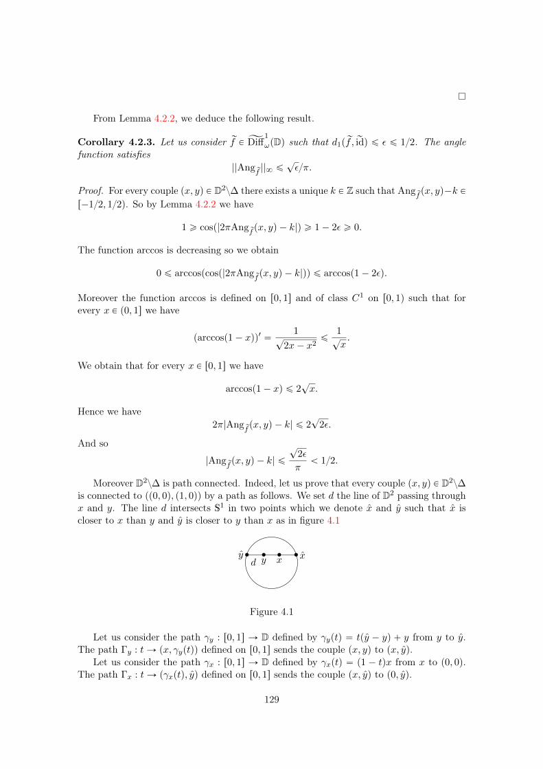
From Lemma 4.2.2, we deduce the following result.

Corollary 4.2.3. Let us consider rf P ĄDiff1

ωpDq such that d1p rf, ridq ď ε ď 12. The anglefunction satisfies

||Angrf||8 ď

?επ.

Proof. For every couple px, yq P D2z∆ there exists a unique k P Z such that Angrfpx, yq´k P

r´12, 12q. So by Lemma 4.2.2 we have

1 ě cosp|2πAngrfpx, yq ´ k|q ě 1´ 2ε ě 0.

The function arccos is decreasing so we obtain

0 ď arccospcosp|2πAngrfpx, yq ´ k|qq ď arccosp1´ 2εq.

Moreover the function arccos is defined on r0, 1s and of class C1 on r0, 1q such that forevery x P p0, 1s we have

parccosp1´ xqq1 “1

?2x´ x2

ď1?x.

We obtain that for every x P r0, 1s we have

arccosp1´ xq ď 2?x.

Hence we have2π|Ang

rfpx, yq ´ k| ď 2

?2ε.

And so

|Angrfpx, yq ´ k| ď

?2ε

πă 12.

Moreover D2z∆ is path connected. Indeed, let us prove that every couple px, yq P D2z∆is connected to pp0, 0q, p1, 0qq by a path as follows. We set d the line of D2 passing throughx and y. The line d intersects S1 in two points which we denote x and y such that x iscloser to x than y and y is closer to y than x as in figure 4.1

‚x

‚y

‚ x‚yd

Figure 4.1

Let us consider the path γy : r0, 1s Ñ D defined by γyptq “ tpy ´ yq ` y from y to y.The path Γy : tÑ px, γyptqq defined on r0, 1s sends the couple px, yq to px, yq.

Let us consider the path γx : r0, 1s Ñ D defined by γxptq “ p1 ´ tqx from x to p0, 0q.The path Γx : tÑ pγxptq, yq defined on r0, 1s sends the couple px, yq to p0, yq.

129

Now we consider Rα the rotation of D of angle α “ argpyq. The rotation R´1α sends y

to p1, 0q. We denote pRtqtPr0,1s the isotopy from id to Rα such that for every t P r0, 1s Rtis the rotation of angle tα.

Hence the composition of the path Γy, Γx and t Ñ pp0, 0q, R´1t pyqq sends px, yq to

pp0, 0q, p0, 1qq.

Moreover Angrfis continuous on D2z∆ we deduce from the last inequality that k does

not depend on the choice of px, yq. The fact that rd1p rf, ridq ď ε ď 12 implies that k “ 0and we obtain that for every px, yq P D2z∆

|Angrfpx, yq| ď

?επ.

We now prove the continuity of Cal1 in C1 topology.

Proof of theorem 4.2.1. By Theorem 3.2.2 we know that ĄCal is a group morphism. So itis sufficient to prove the continuity at the identity. Let us consider rf “ pf, rφq P ĄDiff

1

ωpDqsuch that rd1p rf, ridq ď ε ď 12. By Corollary 4.2.3 we have for every couple px, yq P D2z∆

|Angrfpx, yq| ď

?επ.

By integration on D2z∆ we obtain that

|ĄCalp rfq| ď

?2ε

π.

Hence ĄCal is continuous at the identity.

Moreover, it is well-known that the rotation number rρ : ČHomeo`pS1q Ñ R is continuous

and we deduce from Theorem 4.0.1 the following corollary.

Corollary 4.2.4. The map Cal1 : Diff1ωpDq Ñ R is continuous in C1 topology.

Let us prove that the Calabi invariant is not continuous in C0 topology.

Proposition 4.2.5. The morphism ĄCal is not continuous in C0 topology.

We give a counterexample which also prove that the Calabi invariant defined in theintroduction is also not continuous in the C0 topology, this counterexample can be foundin [32]

Proof. Let us consider a sequence phnqně1 of smooth functions hn : r0, 1s Ñ R such that

1. hn is constant near the origin,

2. hnprq is zero for r ą 1n,

3.ş10 hnprq2πrdr “ 1.

We consider the Hamiltonian functions Hn : DÑ R by Hnpzq “ hnp|z|q. Each functionHn defines a time independent vector field Xn, whose induced flow is denoted φtn. We havethe following property [32] about the computation of the Calabi invariant for compactlysupported and autonomous Hamiltonian functions

130

Proposition 4.2.6. Let us consider H : D Ñ R a Hamiltonian function with compactsupport. We denote φt the induced Hamiltonian flow and we have

Calpφtq “ ´2πt

ż

DHpzqωpzq,

where Cal is the Calabi invariant defined by equation 1.3.

This result allows us to compute the Calabi invariant for φ1n and we obtain for each

n ě 1Calpφ1

nq “ ´2π.

For each n ě 1 we consider pφ1n, idq P

ĄDiff1

ωpDq and we have

ĄCal2ppφ1n, idqq “ ´2π.

Moreover, φ1n converges to the identity in C0 topology and we obtain the result.

131

132

Chapter 5

Computation of Cal1 in some rigid cases

In this section, we prove several results about the Calabi invariant of irrational pseudo-rotations.

5.1 A simple case of C1-rigidity

Let us begin by the simple computation of the Calabi invariant for periodic symplecticmaps.

Lemma 5.1.1. If f P Diff1ωpDq has a finite order, then we have

Cal1pfq “ 0.

Proof. By assumption there exists p ě 1 such that fp “ id and so Cal1pfpq “ p Cal1pidq “

0.

We deduce the following properties

Proposition 5.1.2. Let us consider f P Diff1ωpDq. If there exists a sequence of periodic

diffeomorphisms pgkqkPN in Diff1ωpDq which converges to f fin C1 topology, then we have

Cal1pfq “ 0.

Proof. By Lemma 5.1.1 for each n P N we have Cal1pgnq “ 0 and we obtain the result bythe continuity of the map Cal1 in C1 topology.

Proposition 5.1.3. Let us consider f P Diff1ωpDq. If there exists a sequence pqkqkPN such

that f qk converges to the identity in C1 topology then we have

Cal1pfq “ 0.

Proof. We have Cal1pfqkq “ qkCal1pfq and Cal1pf

qkq converges to Cal1pidq “ 0 so Cal1pfq “0.

133

5.2 C0-rigidity

The following theorem is a stronger version of Corollary 5.1.3.

Theorem 5.2.1. Let us consider f P Diff1ωpDq. If there exists a sequence pqkqkPN of

integers such that pf qkqkPN converges to the identity in C0 topology then we have

Cal1pfq “ 0.

To prove the previous statement we will give an estimation of the angle function of f qnfor a given isotopy I from id to f . For that we will consider two cases, the first one if x isclose to y and the other if x is not close to y. The following lemma gives us an evaluationof what close means.

Lemma 5.2.2. Let us consider f a C1 diffeomorphism of the unit disc D, I an isotopyfrom id to f . If d0pf, idq ď ε ď 14 then for every couple px, yq P D ˆ D which satisfies|x´ y| ě

?ε, we have

| cosp2πAngIpx, yqq ´ 1| ď 4?ε.

Proof. Let px, yq P D ˆ D be a couple such that |x ´ y| ě?ε. One can write f “ id ` h

where h : DÑ R2 satisfies ||h||8 ď ε and we haveˇ

ˇ

ˇ

ˇ

hpyq ´ hpxq

y ´ x

ˇ

ˇ

ˇ

ˇ

ď 2ε?ε“ 2

?ε. (5.1)

We use the equation

cosp2πAngIpx, yqq “xfpyq ´ fpxq, y ´ xy

|fpyq ´ fpxq| |y ´ x|(5.2)

Moreover, if we write 1 “ x y´x|y´x| ,

y´x|y´x|y we obtain

cospAngIpx, yqq ´ 1 “ xfpyq ´ fpxq

|fpyq ´ fpxq|´

y ´ x

|y ´ x|,y ´ x

|y ´ x|y (5.3)

Equation 5.3 becomes

ˇ

ˇ

ˇ

ˇ

fpyq ´ fpxq

|fpyq ´ fpxq|´

y ´ x

|y ´ x|

ˇ

ˇ

ˇ

ˇ

ď |fpyq ´ fpxq|

ˇ

ˇ

ˇ

ˇ

1

|fpyq ´ fpxq|´

1

|y ´ x|

ˇ

ˇ

ˇ

ˇ

`

ˇ

ˇ

ˇ

ˇ

fpyq ´ fpxq ´ py ´ xq

|y ´ x|

ˇ

ˇ

ˇ

ˇ

“

ˇ

ˇ

ˇ

ˇ

|y ´ x| ´ |fpyq ´ fpxq|

|y ´ x|

ˇ

ˇ

ˇ

ˇ

`

ˇ

ˇ

ˇ

ˇ

hpyq ´ hpxq

|y ´ x|

ˇ

ˇ

ˇ

ˇ

ď 2

ˇ

ˇ

ˇ

ˇ

hpyq ´ hpxq

y ´ x

ˇ

ˇ

ˇ

ˇ

ď 4?ε.

We obtain the following lemma.

Lemma 5.2.3. Under the same hypothesis, there exists an integer k P Z, uniquely defined,such that for every couple px, yq P Dˆ D such that |x´ y| ě

?ε, we have

|AngIpx, yq ´ k| ď 2 4?επ ă 12. (5.4)

134

Proof. We consider ε P p0, 116q and a couple px, yq P D such that |y ´ x| ě?ε. By

definition of the floor function there exists a unique k P Z such that 2πAngIpx, yq ´ 2πk Pr´π, πq and we have

1 ě cosp|2πAngIpx, yq ´ 2πk|q ě 1´ 4?ε ě 0.

The function arccos is decreasing so we obtain

0 ď arccospcosp|2πAngIpx, yq ´ 2πk|qq ď arccosp1´ 4?εq.

The function arccos is defined on r0, 1s and of class C1 on r0, 1q. Moreover we have forevery x P r0, 1q

parccosp1´ xqq1 “1

?2x´ x2

ď1?x.

We obtain that for every x P r0, 1s

arccosp1´ xq ď 2?x.

Hence we have

|2πAngIpx, yq ´ 2πk| ď arccosp1´ 4?εq

ď 4 4?ε.

Thus we have|AngIpx, yq ´ k| ď 2 4

?επ ă 12.

Now we prove that k does not depend of px, yq. Indeed the set of couples px, yq P D2 suchthat |x´y| ě

?ε is connected in D2. Indeed for a couple px, yq P D2 such that |x´y| ě

?ε,

let us construct a path from px, yq to pp´1, 0q, p1, 0qq.We set d the line of D2 passing through x and y. The line d intersects S1 in two pointswhich we denote x and y such that x is closer to x than y and y is closer to y than x as inthe previous figure 4.1.

Let us consider the path γx : r0, 1s Ñ D defined by γxptq “ tpx ´ xq ` x from xto x and the path γy : r0, 1s defines by γyptq “ tpy ´ yq ` y from y to y. So the pathΓ : t ÞÑ pγxptq, γyptqq defined on r0, 1s sends the couple px, yq to px, yq.

We consider a path Γ1 : tÑ px, γptqq which fixes x and send y on x along the arc of S1

such that γptq P S1ztxu.

Now we consider Rα the rotation of D of angle α “ argpxq. Notice that the rotationR´1α sends x to p1, 0q. We denote pRtqtPr0,1s the isotopy from id to Rα such that for every

t P r0, 1s Rt is the rotation of angle tα.

Hence the composition of the path Γ, Gamma1 and the path t ÞÑ pR´1t pxq, R

´1t pyqq

sends px, yq to pp1, 0q, p´1, 0qq.

Moreover, 2 4?επ ă 12 so k does not depend on the choice of px, yq P D such that

|x´ y| ą?ε.

135

With these two lemmas we can give a proof of Theorem 5.2.1.

Proof of Theorem 5.2.1. We can consider I “ pftqtPr0,1s an isotopy from id to f which fixesa point of D. Up to conjugacy we can suppose that I fixes the origin and we denote I|S1the restriction of I on S1. We lift I|S1 to an isotopy prφtqtPr0,1s on the universal coveringspace R of S1 such that rφ0 “ id and set rφ “ rφ1. We will prove that ĄCal2pf, rφq “ rρprφq andfrom Theorem 4.0.1 we will obtain

ĄCal2pf, rφq ´ rρprφq “ Cal1pfq “ 0.

For q P N we define the isotopy Iq from id to f q as follows. We write Iq “ pf qt qtPr0,1sand for every z P D and t P rk´1

q , kq s we set

f qt pzq “ fqt´k`1 ˝ pf ˝ ... ˝ fqlooooomooooon

k´1 times

.

We will denote εn “ d0pfqn , idq. For every k P Z we can separate the difference between

the integral of the angle function of f qn and k into two parts as follows

ş ş

DˆD AngIqn px, yqωpyqωpxq ´ k “ş

D

´

ş

B?εn pxqAngIqn px, yqωpyq ´ k

¯

ωpxq

`ş

D

ˆ

ş

Bc?εnpxqAngIqn px, yqωpyq ´ k

˙

ωpxq,(5.5)

where Bc?εnpxq is the complementary of B?εnpxq in D.

We can suppose that εn ă 116 and by Lemma 5.2.3, there exists a unique kn P Z suchthat for each couple px, yq P Dˆ D such that |y ´ x| ě

?εn we have

|AngIqn px, yq ´ kn| ď 2 4?εnπ. (5.6)

Moreover, by definition of the rotation number there exists a sequence pξnqnPN of 1-periodicfunctions ξn : RÑ R such that ||ξn||8 ď 1 for every n P N and such that for every y P S1

and every lift ry P R of y we have

AngIqn p0, yq “rφqnpryq ´ ry “ qnrρprφq ` ξnpryq.

So, for every y P S1 we have

|AngIqn p0, yq ´ kn| “ |qnrρprφq ` ξnpryq ´ kn| ď 2 4

?εnπ,

where ry is a lift of y. Hence we obtain

|qnrρprφq ´ kn| ď 2 4?εnπ ` 1.

Thus we haverρprφq “ lim

nÑ8

knqn.

By equation 5.6 we obtainˇ

ˇ

ˇ

ˇ

ˇ

ż

D

˜

ż

Bc?εnpxqpAngIqn px, yq ´ knqωpyq

¸

ωpxq

ˇ

ˇ

ˇ

ˇ

ˇ

ď 2 4?εnπ. (5.7)

136

We know that for every couple px, yq P D2z∆ and for every n P N we have

AngIqn px, yq “ AngIpx, yq `AngIpfpxq, fpyqq ` ...`AngIpfqn´1pxq, f qn´1pyqq. (5.8)

Hence for every n P N the angle function satisfies

||AngIqn ||8 ď qn||AngI ||8. (5.9)

We can estimate the first integral of equation 5.5 as followsˇ

ˇ

ˇ

ˇ

ˇ

ż

D

˜

ż

B?εn pxqpAngIqn px, yq ´ knqωpyq

¸

ωpxq

ˇ

ˇ

ˇ

ˇ

ˇ

ď εnpqn||AngI ||8 ` |kn|q. (5.10)

So we can deduce from the previous equations a new estimation of the Calabi invariant

ˇ

ˇ

ˇ

ˇ

ż ż

DˆDAngIqn px, yqωpyqωpxq ´ kn

ˇ

ˇ

ˇ

ˇ

ď 2 4?εnπ ` εnpqn||Angf ||8 ` |kn|q. (5.11)

By definition we obtainˇ

ˇ

ˇ

ˇ

ĄCal2pf, rφq ´knqn

ˇ

ˇ

ˇ

ˇ

ď2 4?εn

qnπ` εn||Angf ||8 ` εn

|kn|

qn. (5.12)

Hence we have

ˇ

ˇ

ˇ

ĄCal2pf, rφq ´ rρprφqˇ

ˇ

ˇď

ˇ

ˇ

ˇ

ˇ

ĄCalpf, rφq ´knqn

ˇ

ˇ

ˇ

ˇ

`

ˇ

ˇ

ˇ

ˇ

rρprφq ´knqn

ˇ

ˇ

ˇ

ˇ

ď4 4?εn

qnπ` εn||Angf ||8 `

1

qn` εn

|kn|

qn.

By taking the limit on n P N, we conclude that

ĄCal2pf, rφq “ rρprφq.

Remark 5.2.4. If we consider a sequence prgn “ pgn, rφnqqnPN P ĄDiff1

ωpDq which converges torf “ pf, rφq P ĄDiff

1

ωpDq in C0 topology where for each n P N, gn is a periodic diffeomorphismof the disk and f is an irrational pseudo-rotation, then the previous method fails to provethat ĄCal2pgn, rφnq converges to ĄCal2pf, rφq. It is easy to see that Ang

rfis close to Ang

rgn but

if we compute the difference ĄCalpgn, rφnq ´ĄCalpf, rφq, as we did in equation 5.5, we do nothave a control of ||Ang

rgn ||8 so we cannot estimate properly the integralż

x

ż

yPB?εnpxq

Angrgnpx, yqωpxqωpyq,

where εn “ ||gn ´ f ||8.

137

138

Chapter 6

Examples

In this section, we will be interested in irrational pseudo-rotations with specific rotationnumbers.

Best approximation: Any irrational number α P RzQ can be written as a continuedfraction where paiqiě1 is a sequence of integers ě 1 and a0 “ tαu. Conversely, any sequencepaiqiPN corresponds to a unique number α. We define two sequences ppnqnPN and pqnqnPNas follows

pn “ anpn´1 ` pn2 for n ě 2, p0 “ a0, p1 “ a0a1 ` 1

qn “ anqn´1 ` qn´2 for n ě 2, q0 “ 1, q1 “ a1.

The sequence ppnqnqnPN is called the best approximation of α and for every n ě 1 wehave

tqn´1αu ď tkαu, @k ă qn

where txu is the fractional part of x P R. And for every n P N we have

1

qnpqn ` qn`1qď p´1qnpα´ pnqn, q ď

1

qnqn`1. (6.1)

The numbers qn are called the approximation denominators of α.

6.1 An example of C0-rigidity, the super Liouville type

In this section, we show that a C1 irrational pseudo-rotation with a super Liouville rotationnumber satisfies the assumptions of Theorem 5.2.1.

Super Liouville. A real number α P RzQ is called super Liouville if the sequence pqnqnPNof the approximation denominators of α satisfies

lim supn

q´1n logpqn`1q “ `8. (6.2)

If we consider a real α P R which has super Liouville type then for each k P Z thereal α` k is also super Liouville and to simplify the notations we will say that an element

139

rα P T1 is super Liouville.

Bramham already showed in [13] that any C8 irrational pseudo-rotation f of the diskwith super Liouville rotation number is C0 rigid, meaning that f is the C0-limit of asequence of periodic diffeomorphisms. More recently Le Calvez [51] proved that any C1

irrational pseudo-rotation which is C1 conjugated to a rotation on the boundary is C0

rigid. These results go as follows.

Theorem 6.1.1. Let us consider either a C8 irrational pseudo-rotation or a C1 irrationalpseudo-rotation f which is C1 conjugated to a rotation on the boundary.We consider α P Rsuch that α ` Z is equal to the rotation number of f . For a sequence of rationals ppnqn qnPNwhich converges to α there exists a sequence pgnqnPN : DÑ D of qn-periodic diffeomorphimsof the unit disk which converges to f for the C0 topology.Moreover there exists a constant C depending on f such that for every n P N we have

d0pf, gnq ă Cpqnα´ pnq12 .

We deduce the following corollary.

Corollary 6.1.2. Let us consider either a C8 irrational pseudo-rotation or a C1 irrationalpseudo-rotation f which is C1 conjugated to a rotation on the boundary. If the rotationnumber of f is super Liouville then we have

Cal1pfq “ 0.

Proof of Corollary 6.1.2. Let us consider f which is either a C8 irrational pseudo-rotationor a C1 irrational pseudo-rotation. We consider α P R such that α ` Z is equal to therotation number of f . We will prove that f satisfies the hypothesis of Theorem 5.2.1. Weconsider α P R such that α ` Z is equal to the rotation number of f and we considerthe sequence of rationals ppnqnqnPN, defined above, which converges to α such that qnsatisfies equation 6.1. Let pgnqnPN be the sequence of qn periodic diffeomorphisms given byTheorem 6.1.1 associated to f and the sequence ppnqnqnPN. We denote by K the C1 normof f and we set εn “ Cpqnα´ pnq

12 where C is the constant given by Theorem 6.1.1.

For all k P N and each n P N the following inequality holds

d0pfk, gknq ă Kkεn. (6.3)

By equation 6.1 we can majorate εn by C

pqn`1q12to obtain for k “ qn the inequality

dpf qn , idq ă Kqn C

pqn`1q12

. (6.4)

Equation 6.2 assures that

lim supn

Kqn

pqn`1q12“ 0.

Thus we obtain thatlim sup

nd0pf

qn , idq “ 0.

140

Hence up to a subsequence we can suppose that

d0pfqn , idq Ñ 0.

So f satisfies the hypothesis of Theorem 5.2.1 and we conclude

Cal1pfq “ 0.

6.2 An example of C1-rigidity, the non Bruno type

Bruno type. A number α P RzQ will be said to be Bruno type if the sequence pqnqnPN ofthe approximation denominators of α satisfies

8ÿ

n“0

logpqn`1q

qnă `8.

If we consider α P R which is not Bruno type then for each k P Z the real α` k is alsonot Bruno type and to simplify the notation we will say that an element rα P T1 is nonBruno type.

Avila, Fayad, Le Calvez, Xu and Zhang proved in [4] that if we consider a numberα P RzQ which is not Bruno type, for H ą 1 there exists a subsequence qnk of thesequence of the approximation denominators of α such that for every n P N qnj`1 ě Hqnj

and there exists an infinite set J Ă N such that for every j P J we have

tqnjαu ă e´qnj

j2 . (6.5)

We can also find the following result in the same paper.

Proposition 6.2.1. Let us consider a C2 irrational pseudo-rotation f P Diff1ωpDq. Suppose

that ρpf |S1q is not Bruno type, then the sequence qnj satisfies

d1pfqnj , Idq Ñ 0.

Hence a C2 irrational pseudo-rotation f P Diff1ωpDq satisfies the hypothesis of Corollary

5.1.3 and we obtain the following corollary.

Corollary 6.2.2. Let us consider a C2 irrational pseudo-rotation f P Diff1ωpDq. Suppose

that ρpfq is not Bruno type, then we have

Cal1pfq “ 0.

141

142

Bibliography

[1] D. V. Anosov and A. B. Katok. New examples in smooth ergodic theory. Ergodicdiffeomorphisms. Trudy Moskov. Mat. Obšč., 23:3–36, 1970.

[2] V. I. Arnol d. The first steps of symplectic topology. Uspekhi Mat. Nauk, 41(6(252)):3–18, 229, 1986.

[3] M. Audin, M. Damian, and R. Erné. Morse Theory and Floer Homology. Universitext.Springer London, 2013.

[4] A. Avila, B. Fayad, P. Le Calvez, D. Xu, and Z. Zhang. On mixing diffeomorphismsof the disc. Invent. Math., 220(3):673–714, 2020.

[5] A. Banyaga. Sur la structure du groupe des difféomorphismes qui préservent uneforme symplectique. Comment. Math. Helv., 53(2):174–227, 1978.

[6] S. A. Barannikov. The framed Morse complex and its invariants. In Singularitiesand bifurcations, volume 21 of Adv. Soviet Math., pages 93–115. Amer. Math. Soc.,Providence, RI, 1994.

[7] F. Béguin, S. Crovisier, and F. Le Roux. Pseudo-rotations of the open annulus. Bull.Braz. Math. Soc. (N.S.), 37(2):275–306, 2006.

[8] F. Béguin, S. Crovisier, and F. Le Roux. Fixed point sets of isotopies on surfaces,2016.

[9] F. Béguin, S. Crovisier, F. Le Roux, and A. Patou. Pseudo-rotations of the closedannulus: variation on a theorem of J. Kwapisz. Nonlinearity, 17(4):1427–1453, 2004.

[10] G. Birkhoff. Proof of poincaré’s geometric theorem. Transactions of the AmericanMathematical Society, 14:14–22.

[11] A. Bounemoura. Simplicité des groupes de transformations de surfaces, volume 14 ofEnsaios Matemáticos [Mathematical Surveys]. Sociedade Brasileira de Matemática,Rio de Janeiro, 2008.

[12] B. Bramham. Periodic approximations of irrational pseudo-rotations using pseudo-holomorphic curves. Ann. of Math. (2), 181(3):1033–1086, 2015.

[13] B. Bramham. Pseudo-rotations with sufficiently Liouvillean rotation number are C0-rigid. Invent. Math., 199(2):561–580, 2015.

[14] L. Buhovsky and E. Opshtein. Some quantitative results in CalC0 symplectic geom-etry. Invent. Math., 205(1):1–56, 2016.

143

[15] G. Carlsson, A. Zomorodian, A. Collins, and L. Guibas. Persistence barcodes forshapes. In SGP ’04, 2004.

[16] F. Chazal, V. de Silva, M. Glisse, and S. Oudot. The structure and stability of persis-tence modules. SpringerBriefs in Mathematics. Springer, [Cham], 2016.

[17] D. Cristofaro-Gardiner, V. Humilière, and S. Seyfaddini. Proof of the simplicity con-jecture, 2020.

[18] H. Edelsbrunner, D. Letscher, and A. Zomorodian. Topological persistence and sim-plification. volume 28, pages 511–533. 2002. Discrete and computational geometryand graph drawing (Columbia, SC, 2001).

[19] Ya. M. Eliashberg. A theorem on the structure of wave fronts and its application insymplectic topology. Funktsional. Anal. i Prilozhen., 21(3):65–72, 96, 1987.

[20] M. Entov, L. Polterovich, and P. Py. On continuity of quasimorphisms for symplecticmaps. In Perspectives in analysis, geometry, and topology, volume 296 of Progr. Math.,pages 169–197. Birkhäuser/Springer, New York, 2012. With an appendix by MichaelKhanevsky.

[21] A. Fathi. Structure of the group of homeomorphisms preserving a good measure on acompact manifold. Ann. Sci. École Norm. Sup. (4), 13(1):45–93, 1980.

[22] A. Fathi. Transformations et homeomorphismes préservant la mesure. systèmes dy-namiques minimaux. Thèse Orsay, 1980.

[23] A. Fathi and M. R. Herman. Existence de difféomorphismes minimaux. In Systèmedynamique I - Varsovie, number 49 in Astérisque, pages 37–59. Société mathématiquede France, 1977.

[24] B. Fayad and A. Katok. Constructions in elliptic dynamics. Ergodic Theory Dynam.Systems, 24(5):1477–1520, 2004.

[25] B. Fayad and M. Saprykina. Weak mixing disc and annulus diffeomorphisms witharbitrary Liouville rotation number on the boundary. Ann. Sci. École Norm. Sup.(4), 38(3):339–364, 2005.

[26] A. Floer. Morse theory for fixed points of symplectic diffeomorphisms. Bull. Amer.Math. Soc. (N.S.), 16(2):279–281, 1987.

[27] A. Floer. Morse theory for Lagrangian intersections. J. Differential Geom., 28(3):513–547, 1988.

[28] A. Floer. A relative Morse index for the symplectic action. Comm. Pure Appl. Math.,41(4):393–407, 1988.

[29] A. Floer. The unregularized gradient flow of the symplectic action. Comm. Pure Appl.Math., 41(6):775–813, 1988.

[30] A. Floer. Witten’s complex and infinite-dimensional Morse theory. J. DifferentialGeom., 30(1):207–221, 1989.

144

[31] J. Franks. Generalizations of the Poincaré-Birkhoff theorem. Ann. of Math. (2),128(1):139–151, 1988.

[32] J.-M. Gambaudo and É. Ghys. Enlacements asymptotiques. Topology, 36(6):1355–1379, 1997.

[33] J.-M. Gambaudo, P. Le Calvez, and É. Pécou. Une généralisation d’un théorème deNaishul. C. R. Acad. Sci. Paris Sér. I Math., 323(4):397–402, 1996.

[34] J.-M. Gambaudo and E. Pécou. A topological invariant for volume preserving diffeo-morphisms. Ergodic Theory Dynam. Systems, 15(3):535–541, 1995.

[35] R. Ghrist. Barcodes: the persistent topology of data. Bull. Amer. Math. Soc. (N.S.),45(1):61–75, 2008.

[36] É. Ghys. Groups acting on the circle, volume 6 of Monografías del Instituto deMatemática y Ciencias Afines [Monographs of the Institute of Mathematics and Re-lated Sciences]. Instituto de Matemática y Ciencias Afines, IMCA, Lima, 1999. Apaper from the 12th Escuela Latinoamericana de Matemáticas (XII-ELAM) held inLima, June 28-July 3, 1999.

[37] E. Giroux. Géométrie de contact: de la dimension trois vers les dimensions supérieures.In Proceedings of the International Congress of Mathematicians, Vol. II (Beijing,2002), pages 405–414. Higher Ed. Press, Beijing, 2002.

[38] M. Handel. A pathological area preserving C8 diffeomorphism of the plane. Proc.Amer. Math. Soc., 86(1):163–168, 1982.

[39] M. W. Hirsch. Differential topology, volume 33 of Graduate Texts in Mathematics.Springer-Verlag, New York, 1994. Corrected reprint of the 1976 original.

[40] H. Hofer. On the topological properties of symplectic maps. Proceedings of the RoyalSociety of Edinburgh: Section A Mathematics, 115(1-2):25?38, 1990.

[41] L. Hörmander. An introduction to complex analysis in several variables. D. VanNostrand Co., Inc., Princeton, N.J.-Toronto, Ont.-London, 1966.

[42] V. Humilière. The Calabi invariant for some groups of homeomorphisms. J. SymplecticGeom., 9(1):107–117, 2011.

[43] M. Hutchings. Mean action and the Calabi invariant. J. Mod. Dyn., 10:511–539, 2016.

[44] O. Jaulent. Existence d’un feuilletage positivement transverse homorphisme de sur-face, 2012.

[45] A. Katok and B. Hasselblatt. Introduction to the modern theory of dynamical systems,volume 54 of Encyclopedia of Mathematics and its Applications. Cambridge UniversityPress, Cambridge, 1995. With a supplementary chapter by Katok and LeonardoMendoza.

[46] B. Kerekjarto. Vorlesungen ueber topologie. 1925.

[47] A. Kislev and E. Shelukhin. Bounds on spectral norms and barcodes, 2018.

145

[48] A. Koropecki, P. Le Calvez, and M. Nassiri. Prime ends rotation numbers and periodicpoints. Duke Mathematical Journal, 164(3):403?472, Feb 2015.

[49] P. Le Calvez. Une version feuilletée équivariante du théorème de translation deBrouwer. Publ. Math. Inst. Hautes Études Sci., (102):1–98, 2005.

[50] P. Le Calvez. Pourquoi les points périodiques des homéomorphismes du plan tournent-ils autour de certains points fixes ? Annales scientifiques de l’École NormaleSupérieure, 4e série, 41(1):141–176, 2008.

[51] P. Le Calvez. A finite dimensional approach to Bramham’s approximation theorem.Ann. Inst. Fourier (Grenoble), 66(5):2169–2202, 2016.

[52] P Le Calvez and M Sambarino. Homoclinic orbits for area preserving diffeomorphisms,2019.

[53] P. Le Calvez and F. A. Tal. Forcing theory for transverse trajectories of surfacehomeomorphisms, 2015.

[54] P. Le Calvez and F. A. Tal. Topological horseshoes for surface homeomorphisms, 2018.

[55] P. Le Calvez and J.-C. Yoccoz. Un theoreme d’indice pour les homeomorphismes duplan au voisinage d’un point fixe. Annals of Mathematics, 146(2):241–293, 1997.

[56] F. Le Roux. A topological characterization of holomorphic parabolic germs in theplane. Fund. Math., 198(1):77–94, 2008.

[57] F. Le Roux. Simplicity of HomeopD2, BD2,Areaq and fragmentation of symplecticdiffeomorphisms. J. Symplectic Geom., 8(1):73–93, 2010.

[58] F. Le Roux. Six questions, a proposition and two pictures on Hofer distance for Hamil-tonian diffeomorphisms on surfaces. In Symplectic topology and measure preservingdynamical systems, volume 512 of Contemp. Math., pages 33–40. Amer. Math. Soc.,Providence, RI, 2010.

[59] F. Le Roux. L’ensemble de rotation autour d’un point fixe. Astérisque, (350):x+109,2013.

[60] F Le Roux and S. Seyfaddini. The anosov-katok method and pseudo-rotations insymplectic dynamics, 2020.

[61] F. Le Roux, S. Seyfaddini, and C. Viterbo. Barcodes and area-preserving homeomor-phisms, 2018.

[62] D. McDuff and D. Salamon. Introduction to symplectic topology. Oxford GraduateTexts in Mathematics. Oxford University Press, Oxford, third edition, 2017.

[63] Y.-G. Oh. The group of Hamiltonian homeomorphisms and continuous Hamiltonianflows. In Symplectic topology and measure preserving dynamical systems, volume 512of Contemp. Math., pages 149–177. Amer. Math. Soc., Providence, RI, 2010.

[64] Y.-G. Oh and S. Müller. The group of Hamiltonian homeomorphisms and C0-symplectic topology. J. Symplectic Geom., 5(2):167–219, 2007.

146

[65] H. Poincaré. Sur un théorème de géométrie. Rendiconti del Circolo Matematico diPalermo (1884-1940), 33(1):375–407, 1912.

[66] H. Poincaré. Mémoire sur les courbes définies par une équation différentielle. ÉditionsJacques Gabay, Sceaux, 1993. Reprints of the originals from 1856 through 1921.

[67] L. Polterovich and E. Shelukhin. Autonomous Hamiltonian flows, Hofer’s geometryand persistence modules. Selecta Math. (N.S.), 22(1):227–296, 2016.

[68] S. Seyfaddini. Spectral killers and poisson bracket invariants, 2014.

[69] E. Shelukhin. “Enlacements asymptotiques” revisited. Ann. Math. Qué., 39(2):205–208, 2015.

[70] M. Usher. Boundary depth in Floer theory and its applications to Hamiltonian dy-namics and coisotropic submanifolds. Israel J. Math., 184:1–57, 2011.

[71] M. Usher. Hofer’s metrics and boundary depth. Ann. Sci. Éc. Norm. Supér. (4),46(1):57–128 (2013), 2013.

[72] M. Usher and J. Zhang. Persistent homology and Floer-Novikov theory. Geom. Topol.,20(6):3333–3430, 2016.

[73] C. Viterbo. Symplectic topology as the geometry of generating functions. Mathema-tische Annalen, 292(1):685–710, 1992.

[74] J. Wang. A generalization of classical action of hamiltonian diffeomorphisms to hamil-tonian homeomorphisms on fixed points, 2011.

[75] J. Yan. Existence of periodic points near an isolated fixed point with Lefschetz indexone and zero rotation for area preserving surface homeomorphisms. Ergodic TheoryDynam. Systems, 36(7):2293–2333, 2016.

[76] J. Yan. Existence of torsion-low maximal isotopies for area preserving surface home-omorphisms. Discrete Contin. Dyn. Syst., 38(9):4571–4602, 2018.

147