Abortion and Crime in Canada: A Test of the BMDL Hypothesis

Western University Western University

Scholarship@Western Scholarship@Western

Electronic Thesis and Dissertation Repository

5-21-2013 12:00 AM

Abortion and Crime in Canada: A Test of the BMDL Hypothesis Abortion and Crime in Canada: A Test of the BMDL Hypothesis

Timothy Kang, The University of Western Ontario

Supervisor: Dr. Paul-Philippe Paré, The University of Western Ontario

A thesis submitted in partial fulfillment of the requirements for the Master of Arts degree in

Sociology

© Timothy Kang 2013

Follow this and additional works at: https://ir.lib.uwo.ca/etd

Part of the Criminology Commons, Econometrics Commons, and the Social Control, Law, Crime, and

Deviance Commons

Recommended Citation Recommended Citation Kang, Timothy, "Abortion and Crime in Canada: A Test of the BMDL Hypothesis" (2013). Electronic Thesis and Dissertation Repository. 1289. https://ir.lib.uwo.ca/etd/1289

This Dissertation/Thesis is brought to you for free and open access by Scholarship@Western. It has been accepted for inclusion in Electronic Thesis and Dissertation Repository by an authorized administrator of Scholarship@Western. For more information, please contact [email protected].

Abortion and Crime in Canada: A Test of the BMDL Hypothesis

(Thesis format: Monograph)

by

Timothy Kang

Graduate Program in Sociology

A thesis submitted in partial fulfillment

of the requirements for the degree of

Master of Arts

The School of Graduate and Postdoctoral Studies

The University of Western Ontario

London, Ontario, Canada

© Timothy Kang 2013

ii

Abstract

Donohue and Levitt (2001) argued that the legalization of abortion in the US during the

1970s contributed to 50 percent of the dramatic decline in crime that occurred in the

1990s. Although a lengthy debate in the literature has proliferated and remains

inconclusive, this controversial theory has been popularized by the Freakonomics (2005)

franchise. The liberalization of abortion services that occurred in Canada in 1988 offers

an improved focal intervention to perform an empirical test of this theory. The methods

that have emerged from the debate are reviewed. The most promising strategies, namely

time-series plots of crime, “effective abortion rate” analyses, and age-specific crime rate

analyses, are employed. Using data from the UCR2 and the TAS, this study finds no

consistent relationship between abortion and crime rates in Canada. The theory that an

increase in abortion rates is associated with declines in crime, therefore, must be regarded

with serious skepticism.

Keywords: Canada, Freakonomics, hypothesis testing, legalized abortion, R v

Morgentaler, youth

iii

Acknowledgements

I would like to take this opportunity to acknowledge the individuals that have, without

question, made the completion of this thesis possible.

Firstly, I would like to thank Prof. Paul C. Whitehead for introducing me to the

“Morgentaler hypothesis,” for his guidance in the development of this thesis, and for

serving on the examination committee. I would also like to thank Prof. Paul-Philippe Paré

for his counsel and assistance in the preparation and completion of this thesis as well as

the thesis examination.

Second, I would like to thank Prof. Michael Gardiner for presiding as the chair of

the thesis examination. I would also like to thank Prof. William R. Avison and Prof.

Salvador Navarro for serving on the examination committee and for their insightful

comments.

Third, I would like to acknowledge Chris Houle at the Canadian Centre for Justice

Statistics for compiling and providing the required custom tabulations as well as the

administrators of the Graduate Thesis Research Fund for providing the funding to obtain

these data.

Finally, I would like to thank my friends and family that have encouraged and

supported me during the completion of this thesis as well as the throughout all of the

steps that have led me to pursue graduate studies. Indeed, without these people in my life,

none of my accomplishments would be possible.

To all of these individuals, I would like to extend my sincerest thanks,

acknowledgement and gratitude.

iv

Table of Contents

Abstract ......................................................................................................................... ii

Acknowledgements ...................................................................................................... iii

Table of Contents ......................................................................................................... iv

List of Tables ............................................................................................................... vi

List of Figures ............................................................................................................. vii

List of Appendices ..................................................................................................... viii

1 Introduction ..............................................................................................................1

1.1 The BMDL Hypothesis ........................................................................................1

2 Literature Review .....................................................................................................6

2.1 The Econometric Debate ......................................................................................6

2.1.1 The Donohue and Levitt (2001) Study .......................................................6

2.1.2 Joyce’s (2004) Criticisms and Donohue and Levitt’s (2004) Responses ....8

2.1.3 Foote and Goetz’s (2008) Critique and Donohue and Levitt’s (2008)

Response ................................................................................................ 14

2.1.4 Joyce’s (2009) Response to Donohue and Levitt (2008) .......................... 15

2.1.5 Lott and Whitley’s (2007) Critique ......................................................... 16

2.2 Abortion and Crime in Canada ........................................................................... 18

2.2.1 Abortion in Canada ................................................................................ 19

2.2.2 Crime in Canada .................................................................................... 23

2.3 Designing an Empirical Test .............................................................................. 25

2.4 The Current Study .............................................................................................. 34

3 Methods ................................................................................................................... 37

3.1 Data ................................................................................................................... 37

3.2 Analytic Strategy ............................................................................................... 40

v

4 Results ..................................................................................................................... 48

4.1 Time Series Plots ............................................................................................... 48

4.1.1 Plots of Aggregate Crime Rate ............................................................... 48

4.1.2 Plots of Age-Specific Crime Rate ............................................................ 51

4.2 Descriptive Statistics .......................................................................................... 55

4.3 Effective Abortion Rate (EAR) Analyses ........................................................... 60

4.4 Age-Specific Crime Rate Analyses .................................................................... 61

5 Discussion and Conclusion ..................................................................................... 65

5.1 Discussion.......................................................................................................... 65

5.1.1 Time Series Plots .................................................................................... 66

5.1.2 Effective Abortion Rate (EAR) Analyses.................................................. 68

5.1.3 Age-Specific Crime Rate Analyses .......................................................... 69

5.2 Limitations ......................................................................................................... 73

5.2.1 Sample Size, Methodological Constraints, and Modifications ................. 73

5.2.2 Migration ............................................................................................... 75

5.2.3 Issues related to Aggregate Measures of Abortion and Crime ................. 78

5.3 Conclusion ......................................................................................................... 83

References .................................................................................................................... 84

Appendices ................................................................................................................... 90

Curriculum Vitae....................................................................................................... 109

vi

List of Tables

Table 4.1: Descriptive Statistics for Effective Abortion Rate Analyses .......................... 56

Table 4.2: Descriptive Statistics for National Age-Specific Crime Rate Analyses .......... 57

Table 4.3: Descriptive Statistics for Provincial Age-Specific Crime Rate Analyses ........ 59

Table 4.4: Analyses of the Relationship Between the Effective Abortion Rate and Youth

Crime Rates in Canada, 1998-2011 .............................................................. 61

Table 4.5: Analyses of the Relationship Between Lagged Abortion Rates and Age-

Specific Crime Rates of Individuals Aged 12-31 in Canada, 2006-2011 ...... 62

Table 5.1: Average Interprovincial Migration, Canadian Provinces, 1988-2011 ............. 77

vii

List of Figures

Figure 1.1: Violent Crime Rate, United States, 1960-2010 ...............................................2

Figure 2.1: Ratio of Induced Abortions per 100 Live Births, .......................................... 20

Figure 2.2: Ratio of Induced Abortions per 100 Live Births, Canada and Focal Provinces,

1970-2006 ................................................................................................... 22

Figure 2.3: Total Selected Violent Crime Rate per 100 000 Population, ......................... 24

Figure 2.4: Total Selected Property Crime Rate per 100 000 Population, ....................... 25

Figure 2.5: Violent and Property Criminal Code Violations, Rate per 100 000 Population,

Youth and Adult, Canada, 1998-2011 .......................................................... 33

Figure 4.1: Youth Crime Rate per 100 000 Population, Age 12-17 Years, ...................... 49

Figure 4.2: Youth Crime Rate per 100 000 Population, Age 12-17 Years, ...................... 51

Figure 4.3: Violent Crime Rate per 100 000 Population, Age 17-23 by Single Year,

Canada, 2006-2011 ...................................................................................... 52

Figure 4.4: Property Crime Rate per 100 000 Population, Age 17-23 by Single Year,

Canada, 2006-2011 ...................................................................................... 53

Figure 4.5: Violent Crime Rate per 100 000 Population, Age 16-25 Grouped, BC AB ON

QC, 2006-2011 ............................................................................................ 54

Figure 4.6: Property Crime Rate per 100 000 Population, Age 16-25 Grouped, BC AB

ON QC, 2006-2011 ..................................................................................... 55

Figure 5.1: Population by Single Year of Age, Canada, 2011 ......................................... 81

viii

List of Appendices

Appendix A: Trend Graphs of Abortions and Abortion Ratios, Canada and Provinces,

1970-2006 ................................................................................................... 90

Appendix B: Uniform Crime Reporting Incident-based Survey (UCR2) categories

included in the EAR and age-specific analyses ............................................ 96

Appendix C: Complete model outputs for the EAR and age-specific analyses ................ 99

Appendix D: EAR Analysis Robustness Checks .......................................................... 105

1

Chapter 1

1 INTRODUCTION

Levitt and Dubner’s book, Freakonomics (2005), has been enormously popular since its

first publication in 2005. The focus of this thesis is one of their more controversial

claims, which will be referred to as the Bouza-Morgentaler-Donohue-Levitt (BMDL)

Hypothesis.1 This hypothesis states that the legalization of abortion in the United States

in the early 1970s contributed to nearly 50 percent of the enormous decline in crime in

the 1990s. Levitt and Dubner (2005) explain that

the women most likely to seek an abortion – poor, single, black or teenage

mothers – were the very women whose children, if born, have been shown

most likely to become criminals. But since those children weren’t

[emphasis as in original] born, crime began to decrease during the years

they would have entered their criminal prime (218).

Although Freakonomics (2005) has presented this theory as fact, its original formulation

in Donohue and Levitt’s (2001) study has been met with much criticism and the validity

of the theory remains unproven. Given the popularity of the Freakonomics franchise and

the potentially far-reaching policy and legislative implications this theory could have, it is

crucial that the claim be subjected to the scrutiny of further empirical testing. Not to do

so, as Joyce (2010) notes, would border on “social science negligence” (453).

1.1 The BMDL Hypothesis

In the 1990s, the United States experienced the most extensive and prolonged decline in

crime in recent American history (Figure 1.1). This decline in crime was particularly

fascinating for several reasons. First, it was the longest decline in recorded history,

spanning nearly a decade from its start in 1991 (Zimring 2007). It was a large decline; the

overall crime rate declined 43 percent, the violent crime rate declined 33.5 percent, and

the property crime rate declined 28.8 percent between 1991 and 2001. The decline in

rates of crime was broad; declines were found in every major category of crime. The

1 The “Bouza-Morgentaler-Donohue-Levitt Hypothesis” was originally coined by Lott and Whitley (2007: 305).

2

decline in crime also spanned the entire United States (Zimring 2007). What made this

decline in crime even more remarkable was the inability of experts to predict it. To the

contrary, leading criminologists and scholars had forecast that crime would rise to

“epidemic” proportions (Levitt 2004). Even in the mid-1990s, when crime rates had

already began to fall, scholars continued to predict rises in crime rates to be seen well

into the 2000s (Zimring 2007). Many of the “excessively punitive” criminal charging

practices characteristic of mid-1990s America were fueled by these pessimistic

predictions (Zimring 2007; Zimring, Hawkins, and Kamin 2001).

Figure 1.1: Violent Crime Rate, United States, 1960-2010

Source: FBI, Uniform Crime Reports, prepared by the National Archive of Criminal Justice

As the decline in crime became more apparent, criminologists, scholars, and

policy makers provided an assortment of explanations. Levitt (2004) found that the most

commonly cited explanations during the 1991-2001 period were changes in gun control

laws, innovative policing strategies, increased numbers of police officers, increased

reliance on prisons, increased use of capital punishment, changes in crack-cocaine

markets, changing demographics, and a strong economy. Levitt (2004) argued that only

three of these could explain an appreciable part of the 1990s decline in crime: increases

in the number of police (accounting for 10-20 percent of the decline in crime), the rising

prison population (accounting for 33 percent of the decline in crime), and the waning of

the crack-cocaine epidemic (accounting for 10-15 percent of the decline in crime).

0

100

200

300

400

500

600

700

800

1960

1962

1964

1966

1968

1970

1972

1974

1976

1978

1980

1982

1984

1986

1988

1990

1992

1994

1996

1998

2000

2002

2004

2006

2008

2010

Vio

len

t C

rim

e R

ate

per

100,0

00 P

op

ula

tion

Year

3

Against these competing theories, Donohue and Levitt (2001) proposed a novel

explanation. In 1973, abortion was legalized nationally with the US Supreme Court ruling

in Roe v. Wade. Donohue and Levitt (2001) argued that this exogenous change in

abortion legislation explained nearly 50 percent of the 1990s decline in crime. Two main

mechanisms were argued to be at work simultaneously: cohort and selection effects.2 The

legalization of abortion reduced total fertility, which in turn reduced the number of

people born in each subsequent cohort leaving fewer people available to be both

criminals and victims, and consequently less crime. Access to legal abortions also

afforded women the ability to choose, or select, the outcome of “unwanted” pregnancies.

The national legalization of abortion lowered the overall costs of abortion, financially as

well as socially, allowing greater access to and use of abortion services. The women who

were most likely to give birth to children who would engage in criminal activity,

specifically poor, black, teenage, and unmarried women, were also the women who were

most likely to seek abortions. These “at risk” women sought abortions at higher rates

after the legalization of abortion made the procedure more accessible. The selective

abortion of “unwanted” children reduced the likelihood that children would be born into

adverse family environments including poverty, maternal rejection, neglect, drug and

alcohol abuse, and various other unfavorable parental behaviours. Donohue and Levitt

(2001) cited evidence that children born into such adverse environments were

disproportionately more likely to be involved in criminal activity in adulthood.

Accordingly, they argued that fifteen to twenty years after Roe v. Wade, when the

children born after the national legalization of abortion in 1973 were reaching their

“high-crime” years, rates of crime declined because “unwanted” children were absent.

Women were better able to time births and fewer children were born into socioeconomic

risk. If “unwanted” children had been born, they would have grown up in more abusive,

neglectful, and socioeconomically disadvantaged environments. There were, therefore,

fewer children “at risk” of being criminals and consequently less crime.

2 For clarity, this paper defines cohort effects as those that affect the size of birth cohorts. The reduction in number of children born in a given year due to increases in abortion, in other words, will be referred to as “cohort effects.”

Selection effects will refer to the changes in the relative composition of cohorts born after the legalization of abortion. According to the BMDL Hypothesis, the legalization of abortion afforded women the ability to select whether or not to take pregnancies to term. Children who would have been more likely to be criminal were therefore selected out of birth cohorts.

4

Although this was presented as a novel explanation, the idea had been expressed

earlier. In 1970, President Nixon formed the Commission on Population Growth and the

American Future. The Commission argued for stable population growth through state-

funded, on-demand abortions, with the “admonition that abortion not be considered a

primary means of fertility control” (1972:178). They cited a Swedish study (Forssman

and Thuwe 1966) that found that the children of women who sought but were denied

abortions had worse health, behavioural, and economic outcomes. The costs of the

“unwanted” birth also extended to society in the form of health care costs, social

assistance burdens, and criminality (US Commission on Population Growth and the

American Future 1972). In 1990, Anthony V. Bouza, the former police chief of

Minneapolis, wrote that abortion was “arguably the only effective crime-prevention

device adopted [in the US] since the late 1960s” (275). Henry Morgentaler (1999: 40),

the leading Canadian advocate of abortion services, wrote that “one of the most important

consequences [of abortion] is the declining violent crime rate…. To prevent the birth of

unwanted children through family planning, birth control, and abortion is preventative

medicine, preventative psychiatry, and prevention of violent crime.” Donohue and

Levitt’s (2001) study took these ideas a step further and conducted the first empirical

examination of the claim, hence Lott and Whitley’s (2007) coining of the Bouza-

Morgentaler-Donohue-Levitt (BMDL) Hypothesis.

The theory gained attention as it was incorporated into the controversial debate

surrounding abortion legislation. It was more recently popularized in the NY Times

Bestseller Freakonomics (2005) by Levitt and Dubner and the media coverage that

accompanied it. It has sold over 4 million copies world-wide and has spurred a franchise

including a revision and thirty five translations, another book titled SuperFreakonomics

(2009), a television focus on the book in 2006 by ABC’s 20/20, a documentary film titled

Freakonomics: The Movie in 2010, a popular blog, a podcast radio show, and an

enormous amount of media attention for both the authors and their work (Freakonomics

2011). Although this franchise is by no means hinged on the BMDL Hypothesis, it is

undoubtedly one of the more controversial topics and has received recurring attention. It

is of concern that this theory has the potential to be considered valid in the general

population when it remains contentious and unproven among social scientists.

5

The present study, therefore, aims to submit the BMDL Hypothesis to further

scrutiny by testing it on the case of Canada. Although abortion was decriminalized in

1969, access to abortion services in Canada was greatly increased in 1988 following the

Supreme Court decision in R v. Morgentaler. By taking advantage of this exogenous

intervention in abortion legislation and by investigating its impact on Canadian crime

rates, the credibility of the BMDL Hypothesis will be tested and verified. If the increase

in access to abortion services are found to be associated with a decline in Canadian crime

rates, the case of Canada would provide further support for the BMDL Hypothesis. If

supportive evidence is not found, however, the continued public dissemination of the

BMDL Hypothesis may require amendment and retraction.

6

Chapter 2

2 LITERATURE REVIEW

2.1 The Econometric Debate

Donohue and Levitt’s (2001) study sparked an enormous academic debate that has lasted

over a decade. This debate remains, however, primarily within the field of econometrics

by virtue of its original formulation. Joyce (2010), who has been heavily involved in the

debate, reviewed the major econometric arguments in a summary chapter far better than

could be attempted here.3 From the perspective of a non-econometrician, reviewing the

debate has demonstrated the importance of critically and thoughtfully analyzing the

BMDL hypothesis. Above all else, however, the literature has demonstrated how

sensitive the econometric methods used thus far have been to small variations in

specification. Depending on the way researchers have specified their models, what

variables they have included, and how they have designed their analyses, studies have

found supporting evidence in some cases, null effects in others, and inverse effects in still

other cases. Overall, the validity of the original theoretical link has been left obscure.

Important elements required for the accurate investigation of the BMDL Hypothesis that

have emerged during the debate will be emphasized in section 2.3 as an improved

empirical test is designed. It is important, however, to review the state of the academic

debate to appreciate the level of consensus established on the BMDL Hypothesis thus far.

2.1.1 The Donohue and Levitt (2001) Study

Donohue and Levitt’s (2001) study deserves attention and explication to situate the

debate. The empirical strategy they employed involves two main parts: national time

series and regression analyses. In the first strategy, three main pieces of evidence are

presented. When looking at the time series of crime rates from the 1990s, the break in the

national crime trend from its peak in 1991 fits temporally with the legalization of

abortion in 1973. By 1991, children born after the legalization of abortion would have

3 Please refer to Joyce, Theodore J. 2010. “Abortion and Crime: A Review.” Pp. 452-487 in Handbook on the Economics of Crime, edited by Bruce L. Benson and Paul R. Zimmerman. Northampton, MA: Edward Elgar.

7

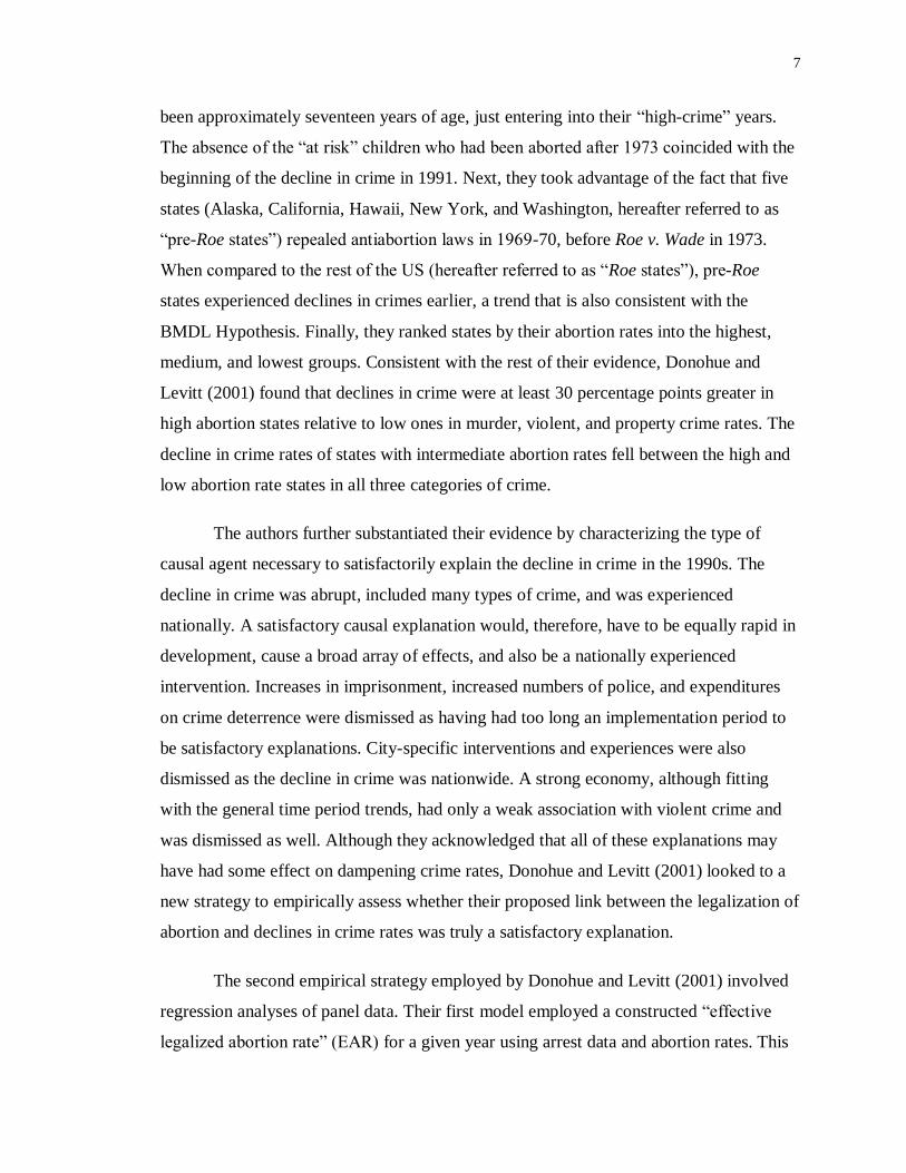
been approximately seventeen years of age, just entering into their “high-crime” years.

The absence of the “at risk” children who had been aborted after 1973 coincided with the

beginning of the decline in crime in 1991. Next, they took advantage of the fact that five

states (Alaska, California, Hawaii, New York, and Washington, hereafter referred to as

“pre-Roe states”) repealed antiabortion laws in 1969-70, before Roe v. Wade in 1973.

When compared to the rest of the US (hereafter referred to as “Roe states”), pre-Roe

states experienced declines in crimes earlier, a trend that is also consistent with the

BMDL Hypothesis. Finally, they ranked states by their abortion rates into the highest,

medium, and lowest groups. Consistent with the rest of their evidence, Donohue and

Levitt (2001) found that declines in crime were at least 30 percentage points greater in

high abortion states relative to low ones in murder, violent, and property crime rates. The

decline in crime rates of states with intermediate abortion rates fell between the high and

low abortion rate states in all three categories of crime.

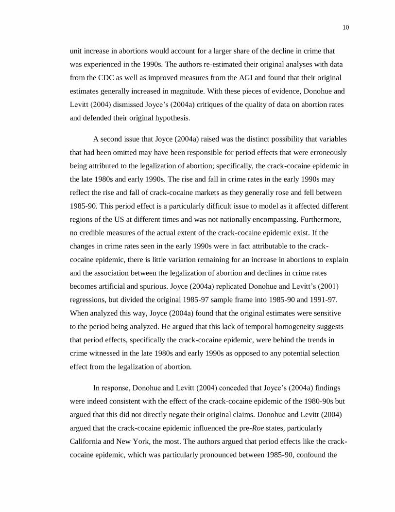
The authors further substantiated their evidence by characterizing the type of

causal agent necessary to satisfactorily explain the decline in crime in the 1990s. The

decline in crime was abrupt, included many types of crime, and was experienced

nationally. A satisfactory causal explanation would, therefore, have to be equally rapid in

development, cause a broad array of effects, and also be a nationally experienced

intervention. Increases in imprisonment, increased numbers of police, and expenditures

on crime deterrence were dismissed as having had too long an implementation period to

be satisfactory explanations. City-specific interventions and experiences were also

dismissed as the decline in crime was nationwide. A strong economy, although fitting

with the general time period trends, had only a weak association with violent crime and

was dismissed as well. Although they acknowledged that all of these explanations may

have had some effect on dampening crime rates, Donohue and Levitt (2001) looked to a

new strategy to empirically assess whether their proposed link between the legalization of

abortion and declines in crime rates was truly a satisfactory explanation.

The second empirical strategy employed by Donohue and Levitt (2001) involved

regression analyses of panel data. Their first model employed a constructed “effective

legalized abortion rate” (EAR) for a given year using arrest data and abortion rates. This

8

term sums the product of the ratio of arrests for a given cohort and the abortion rate for

the year prior to that cohort’s birth (i.e., approximately when the cohort was in utero).

This term was intended to isolate the influence of abortions on criminal arrests in a given

year by taking into account the fraction of arrests committed by individuals born after

abortion legalization. They regressed the rates of annual state-level crime on the

constructed EAR term and found that increases in the EAR were associated with declines

in aggregate crime rates.

Next, they drew a more direct link between abortion and crime rates by regressing

age-specific arrest data, which were available by single year of age of the arrestee, on the

abortion rate of the year prior to each cohort’s birth. Again, the abortion rate of the year

prior to a cohort’s birth was used as a proxy for the likelihood of abortion that cohorts

experienced while in utero. After performing their analyses, they concluded that an

increase of 100 abortions per 1000 live births reduced a cohort’s crime by approximately

10 percent. Their calculation of the effective abortion rate for 1997 suggested that crime

rates were approximately 15-25 percent lower in 1997 because of the legalization of

abortion. Since homicide, violent, and property crime rates fell more than 30 percent in

the 1990s, Donohue and Levitt (2001) argued that the legalization of abortion could

account for at least 50 percent of the total decline in crime between 1991 and 1997 (i.e.,

the 15-25 percent decline explained by the legalization of abortion accounts for at least

half of the total 30 percent decline in crime).

2.1.2 Joyce’s (2004) Criticisms and Donohue and Levitt’s (2004) Responses

Their study was met with swift criticism from many sources, but the three critiques that

were potentially the most relevant and damaging came from economists. Theodore Joyce

has been one of the most involved critics and has engaged with Donohue and Levitt at

length on multiple occasions.4 In Joyce’s (2004a) first rebuttal, he argued that Donohue

and Levitt (2001) erroneously assumed that no abortions took place before legalization,

and therefore their use of a zero abortion ratio for cohorts born before 1973 flawed their

4 After the first appearance of Donohue and Levitt’s work in the Chicago Tribune (1999), they have been in a lengthy back-and-forth with Joyce for over a decade of working manuscripts and publications (Donohue and Levitt 2000, 2001, 2003, 2004, 2006, 2008; Joyce 2001, 2004a, 2004b, 2006, 2009, 2010; Joyce et al 2012)

9

equations. Joyce (2004a) argued instead that nearly two-thirds of legal abortions post-Roe

v Wade simply replaced illegal ones that occurred before legalization. Citing data from

the Centers for Disease Control (CDC), Joyce (2004a) further argued that those states that

had the highest rates of abortion after legalization in 1973 also had the highest rates of

abortion before legalization in 1972. If so, there would have been no dramatic change in

abortion rate, negating any of the causal force that the legalization of abortion could have

had. Further, the abortion rate data from the Alan Guttmacher Institute (AGI) that

Donohue and Levitt (2001) used was inaccurate as it measured abortion rates by the state

of occurrence as opposed to the state of residence of the woman. These data were,

therefore, susceptible to misrepresenting the magnitude of influence that an increase in

abortion rates in a given state could have had on that state’s future crime rates if non-

trivial numbers of women had crossed state borders to obtain abortions. This would have

artificially inflated abortion rates in some states while artificially lowering the abortion

rate in others.

In response, Donohue and Levitt (2004) first argued that Joyce (2004a) was

mistaken and abortions did increase substantially after legalization in 1973. The financial

costs dropped significantly from $400-500 to as little as $80 after legalization, making

abortions more easily accessible. The increasing trend in abortion rates also took seven

years after legalization to stabilize, suggesting that the observed change in rates of legal

abortion was a genuine change as opposed to simply a replacement of illegal abortions.

The number of children being put up for adoption also declined after abortion legalization

from nine percent of premarital births to just four percent. The authors argued with these

pieces of evidence that the change in abortion rates that occurred as a result of the

legalization of abortion in 1973 were real and did not represent the simple replacement of

illegal abortions.

Further, Donohue and Levitt (2004) asserted that even if Joyce (2004a) was

correct, his claim did not reduce the influence of legalizing abortion on rates of crime and

instead made their original estimates more conservative. They argued that if, in reality,

there was a smaller increase in abortions than had originally been assumed, the

magnitude of the association between abortion and crime would be even greater as each

10

unit increase in abortions would account for a larger share of the decline in crime that

was experienced in the 1990s. The authors re-estimated their original analyses with data

from the CDC as well as improved measures from the AGI and found that their original

estimates generally increased in magnitude. With these pieces of evidence, Donohue and

Levitt (2004) dismissed Joyce’s (2004a) critiques of the quality of data on abortion rates

and defended their original hypothesis.

A second issue that Joyce (2004a) raised was the distinct possibility that variables

that had been omitted may have been responsible for period effects that were erroneously

being attributed to the legalization of abortion; specifically, the crack-cocaine epidemic in

the late 1980s and early 1990s. The rise and fall in crime rates in the early 1990s may

reflect the rise and fall of crack-cocaine markets as they generally rose and fell between

1985-90. This period effect is a particularly difficult issue to model as it affected different

regions of the US at different times and was not nationally encompassing. Furthermore,

no credible measures of the actual extent of the crack-cocaine epidemic exist. If the

changes in crime rates seen in the early 1990s were in fact attributable to the crack-

cocaine epidemic, there is little variation remaining for an increase in abortions to explain

and the association between the legalization of abortion and declines in crime rates

becomes artificial and spurious. Joyce (2004a) replicated Donohue and Levitt’s (2001)

regressions, but divided the original 1985-97 sample frame into 1985-90 and 1991-97.

When analyzed this way, Joyce (2004a) found that the original estimates were sensitive

to the period being analyzed. He argued that this lack of temporal homogeneity suggests

that period effects, specifically the crack-cocaine epidemic, were behind the trends in

crime witnessed in the late 1980s and early 1990s as opposed to any potential selection

effect from the legalization of abortion.

In response, Donohue and Levitt (2004) conceded that Joyce’s (2004a) findings

were indeed consistent with the effect of the crack-cocaine epidemic of the 1980-90s but

argued that this did not directly negate their original claims. Donohue and Levitt (2004)

argued that the crack-cocaine epidemic influenced the pre-Roe states, particularly

California and New York, the most. The authors argued that period effects like the crack-

cocaine epidemic, which was particularly pronounced between 1985-90, confound the

11

time period and make it difficult to investigate causal claims. Failing to satisfactorily

control for the crack-cocaine epidemic would bias regression estimates against finding an

association between abortion legalization and declines in crime rates. The narrow focus

of Joyce (2004a) on the time frames of 1985-90 and 1991-97, therefore, biased his

regression analyses against finding an association between abortion legalization and

crime trends. Donohue and Levitt (2004) argued that to adequately control for the crack-

cocaine epidemic, it is necessary to study a longer time period so that crime trends before

and after the crack-cocaine epidemic could be taken into account. They argued, therefore,

that the use of their original time frame of 1985-97 was necessary for credible analyses.

Further, they argued that the potential impact of the legalization of abortion during 1985-

90 would have been very small because individuals born after 1973 would still comprise

a small proportion of the total population. Joyce’s (2004a) focus on 1985-90 to

investigate abortion and crime associations was, therefore, dismissed as flawed because

of the failure to control for and contextualize the crack-cocaine epidemic and because

regression analyses were biased against finding an association between abortion and

crime by design.

Joyce (2004a) also conducted several difference-in-difference (DD) analyses to

address the issues he raised with Donohue and Levitt (2001). The DD technique is a

quasi-experimental strategy that attempts to measure a treatment effect by differencing

the outcomes of a control group from the outcomes of a treatment group.5 In the first,

Joyce (2004a) constructs a comparison group of states that legalized abortion in 1973, but

were more similar to the pre-Roe states in their histories of crack-cocaine markets.6 The

use of these states offers an improved estimate of the counterfactual of the period effects

experienced by the pre-Roe states7 as opposed to including all of the remaining American

states. Joyce (2004a) divided the study sample again between 1985-90 and 1991-96 and

5 Please refer to Joyce (2009) for a more thorough elaboration on the DD and DDD strategy employed by Joyce (2004a; 2009). 6 Based on Grogger and Willis (2000), Joyce (2004a) constructed a comparison group consisting of Colorado, Florida, Georgia, Illinois, Indiana, Louisiana, Maryland, Massachusetts, Michigan, Missouri, New Jersey, Ohio, Pennsylvania,

Texas, and Virginia as these states experienced crack-cocaine use in their major cities between 1984 to 1989. These states also have urban centres with large African-American populations, which were argued to improve the estimate of the counterfactual of the pre-Roe states that include California and New York. 7 Unlike Donohue and Levitt (2001), Joyce (2004a) included the District of Columbia into the pre-Roe states.

12

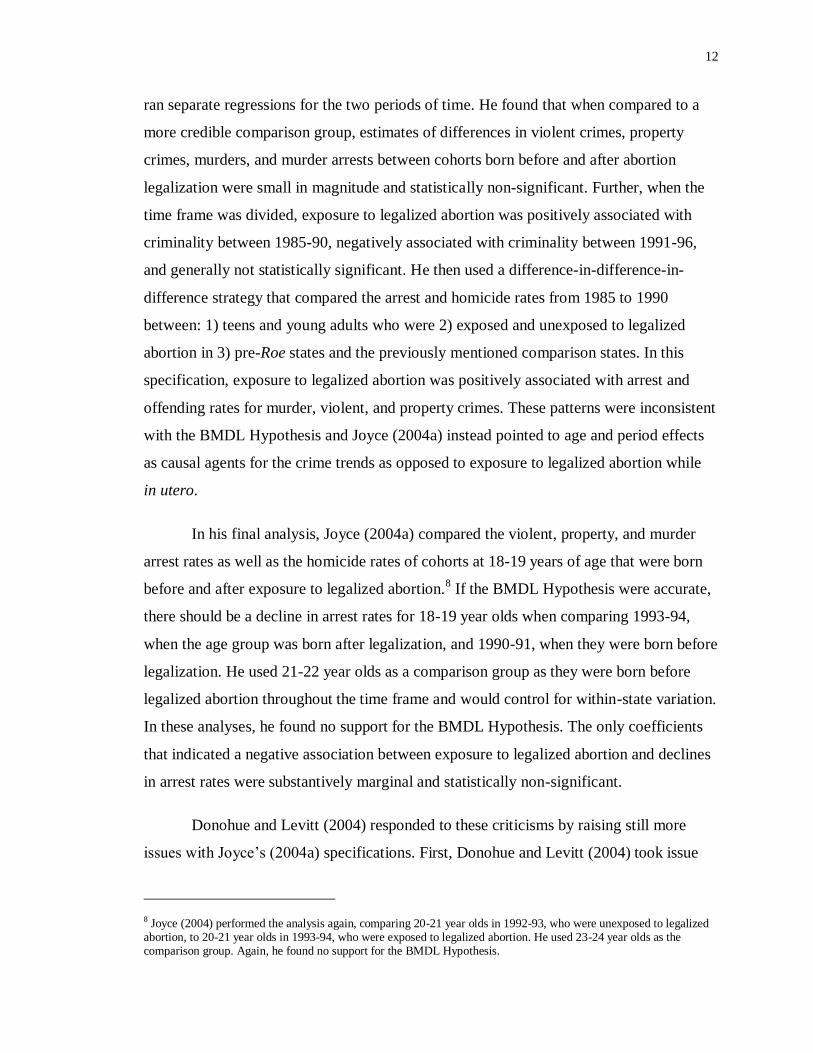
ran separate regressions for the two periods of time. He found that when compared to a

more credible comparison group, estimates of differences in violent crimes, property

crimes, murders, and murder arrests between cohorts born before and after abortion

legalization were small in magnitude and statistically non-significant. Further, when the

time frame was divided, exposure to legalized abortion was positively associated with

criminality between 1985-90, negatively associated with criminality between 1991-96,

and generally not statistically significant. He then used a difference-in-difference-in-

difference strategy that compared the arrest and homicide rates from 1985 to 1990

between: 1) teens and young adults who were 2) exposed and unexposed to legalized

abortion in 3) pre-Roe states and the previously mentioned comparison states. In this

specification, exposure to legalized abortion was positively associated with arrest and

offending rates for murder, violent, and property crimes. These patterns were inconsistent

with the BMDL Hypothesis and Joyce (2004a) instead pointed to age and period effects

as causal agents for the crime trends as opposed to exposure to legalized abortion while

in utero.

In his final analysis, Joyce (2004a) compared the violent, property, and murder

arrest rates as well as the homicide rates of cohorts at 18-19 years of age that were born

before and after exposure to legalized abortion.8 If the BMDL Hypothesis were accurate,

there should be a decline in arrest rates for 18-19 year olds when comparing 1993-94,

when the age group was born after legalization, and 1990-91, when they were born before

legalization. He used 21-22 year olds as a comparison group as they were born before

legalized abortion throughout the time frame and would control for within-state variation.

In these analyses, he found no support for the BMDL Hypothesis. The only coefficients

that indicated a negative association between exposure to legalized abortion and declines

in arrest rates were substantively marginal and statistically non-significant.

Donohue and Levitt (2004) responded to these criticisms by raising still more

issues with Joyce’s (2004a) specifications. First, Donohue and Levitt (2004) took issue

8 Joyce (2004) performed the analysis again, comparing 20-21 year olds in 1992-93, who were unexposed to legalized abortion, to 20-21 year olds in 1993-94, who were exposed to legalized abortion. He used 23-24 year olds as the comparison group. Again, he found no support for the BMDL Hypothesis.

13

with the inclusion of the District of Columbia (D.C.) by Joyce (2004a) as an “early

legalizer” state (see footnote 10 of Donohue and Levitt 2004). Joyce (2004a) included

D.C. citing evidence that their abortion facilities had 20 000 patients in 1971 and the

state’s resident abortion ratio was double that of California or New York in 1972.

Donohue and Levitt (2004) argued that although the D.C. Supreme Court decision in U.S.

v. Vuitch in 1969 repealed anti-abortion laws, the decision was quickly overturned in

1971 by the U.S. Supreme Court and therefore abortion services were not legal in D.C.

until 1973 with the rest of the nation. Even though Joyce’s (2004a) results were not

sensitive to the inclusion of D.C. as a pre-Roe state, Donohue and Levitt (2004) took

issue with Joyce’s (2004a) decision and devoted a substantial footnote to the topic.

More importantly, Donohue and Levitt (2004) argued that Joyce’s (2004a) focus

on the time frame of 1985-90 only allowed for the examination of the criminal outcomes

of cohorts during a very specific, “well chosen” period of time during the crack-cocaine

epidemic, which primarily influenced younger individuals, and therefore concluded that

there was no association between abortion legalization and crime (42). As discussed

earlier, failure to account for the crack-cocaine epidemic could bias estimates,

particularly when focusing on the years 1985-90. Further, the authors argued that

ignoring the lifetime criminal involvement of exposed cohorts who were born in the areas

most affected by the crack-cocaine epidemic and focusing on the crimes they committed

between 1985-90 biased estimates towards finding no association between the exposure

to legalized abortion and crime. When Donohue and Levitt (2004) re-estimated their

analyses with a longer time frame to cover more of the lifetime criminal involvement of

exposed cohorts, they found that exposed cohorts committed fewer crimes both before

and after the crack-cocaine epidemic. The authors argued that this was even more

compelling evidence for their hypothesis as Joyce’s (2004a) analyses were unable to

definitively distinguish between “exposed” and “unexposed” cohorts or between states

where abortions were relatively easy or difficult to obtain because he only used a

dichotomous indicator for the legal status of abortions. Donohue and Levitt (2004)

concluded that Joyce’s (2004a) study was generally biased by design to find no

association between the in utero exposure to legalized abortion and later criminality.

14

2.1.3 Foote and Goetz’s (2008) Critique and Donohue and Levitt’s (2008) Response

A second econometric critique of note came from Foote and Goetz (2008). The first, and

most crippling point they raised, was a flaw in the final regression of Donohue and

Levitt’s (2001) paper, arguably their most convincing piece of evidence. To review, their

final analysis involved directly linking the arrest rates of cohorts to the abortion rates they

experienced while in utero. Foote and Goetz (2008), however, pointed out that Donohue

and Levitt (2001) did not include important regressors in their equation, namely a state-

year interaction term that absorbs the influence of various unobserved differences

between states over time that are difficult to explicitly measure. Its omission meant that

their regression estimates were biased by attributing the variation that would have been

absorbed by the state-year interaction term to the other terms in the regression, including

the term for the effect of abortion.

A second flaw in the final regression that Foote and Goetz (2008) identified was

the use of the total number of arrests of a cohort as opposed to arrests per capita of a

cohort. Donohue and Levitt (2001) used this measure because they felt that there was no

credible measure of cohort size per year by state to calculate a cohort rate. Foote and

Goetz (2008), however, found that these data were available from 1980 on. When they

corrected for these issues and re-estimated the regressions, Foote and Goetz (2008) found

that the coefficients for the effect of abortion on property and violent crime arrest rates

decline to essentially zero (Table 1, Column 4, p.412).

A third issue raised by Foote and Goetz (2008) was the likelihood that variables

that were omitted were biasing the association between abortion and crime rates. They

noted that states that had high levels of abortion also had high levels of crime before

1985, when the legalization of abortion could not have influenced crime. When

regressed, there was a large and significant positive association between abortion and

crime rates between 1970-1984, suggesting that both abortion and crime rates were being

driven by common, state-specific factors. Declines in crime rates after 1985 that were

driven by other factors may, therefore, be erroneously attributed to abortion rates. Thus,

like Joyce (2004a), the authors argued that some other omitted variable, most likely a

within-state period effect, must be driving the association.

15

In response, Donohue and Levitt (2008) acknowledged the omission of the state-

year interaction term in their original (2001) analysis. They noted, however, that although

the magnitude of their estimates decline after adding the state-year interaction term, the

sign and statistical significance of their estimates remained the same. Although Foote and

Goetz (2008) demonstrated that after correction, the violent crime coefficient declined

and the property crime coefficient actually changed signs, Donohue and Levitt (2008)

argued that even more corrections were necessary. Namely, the cross-state mobility of

both the women who sought abortions as well as the children who were exposed to

legalized abortion needed to be controlled. Donohue and Levitt (2008) also attempted to

more accurately model the exposure to legalized abortion that cohorts experienced while

in utero. When the data on rates of abortion were improved and more directly linked to

crime rates, the new coefficient estimates increased to be far greater than the original

estimates. Finally, when Donohue and Levitt (2008) re-estimated Foote and Goetz’s

(2008) analysis using several more adjustments (e.g., division-year interactions, the

inclusion of D.C., the functional form of interaction terms, etc.), the new coefficients

remained as strong or stronger than their original estimates, providing support yet again

for the BMDL Hypothesis.

2.1.4 Joyce’s (2009) Response to Donohue and Levitt (2008)

Joyce (2009) countered Donohue and Levitt (2008) by raising some of the recurring

issues again and performing modified replications. He concluded that “the association

between legalized abortion and crime rates is weak and inconsequential” (113).

Specifically, Joyce (2009) argued that Donohue and Levitt (2008) underestimated

standard errors in their abortion rates, their results remained inconsistent with age-

specific time series plots, and their improved abortion data suffered from measurement

errors. Joyce (2009) replicated Donohue and Levitt’s (2008) analysis while adjusting the

standard errors for within-state serial correlation and limited the sample to cohorts born

between 1974-81 when abortion data were available. His results provided no support for

an association between abortion rates and age-specific crime rates.

Joyce (2009) then performed analyses using two models. The first used a

difference-in-difference-in-difference (DDD) estimator that compared the crime rates of

16

cohorts born before 1974 (i.e. 1972-73), and therefore unexposed to legalized abortion,

with cohorts born after (i.e. 1974-75) between 1985-2001 in the 45 states that legalized

abortion with Roe v. Wade. This sample had the added benefit of representing cohorts

born during the largest three-year increase in abortion rates, variation that Joyce (2009)

argued was based on changes in the price of abortions and was thus a better test of the

BMDL Hypothesis. The DDD estimator also compared the crime rates of cohorts born in

states with above median changes in abortion rates to the crime rates of cohorts born in

states at or below median abortion rates. The results of this model generally had positive

coefficients and were not statistically significant, which provided no support for the

BMDL Hypothesis. The second model that Joyce (2009) used was similar to Donohue

and Levitt’s (2004, 2008) strategy where crime rates by single year of age were regressed

on lagged abortion rates. Unlike Donohue and Levitt (2008), however, Joyce (2009) used

cohorts born between 1972-75 for the reasons cited above. These regressions similarly

provided no evidence for the BMDL Hypothesis. The majority of the coefficients were

positive and the negative coefficients were small in magnitude and never statistically

significant. Joyce (2009) therefore concluded that “there is little evidence that legalized

abortion lowers crime through a selection effect” (121).

2.1.5 Lott and Whitley’s (2007) Critique

A third major econometric critique came from Lott and Whitley (2007). Joyce (2010) has

noted that their regression analyses were unconvincing and their motives for critiquing

Donohue and Levitt (2001) have also been questioned (Zimring 2007).9 Although their

regressions were weak, Lott and Whitley (2007) made other arguments worth noting.

They presented data collected by the CDC between 1969 and 1972 comparing abortion

rates between the pre-Roe states and those of states that allowed abortions when the

health or life of a woman was in danger. They showed that several states in the latter

category had abortion rates higher than pre-Roe states between 1969 and 1972. The crux

of Donohue and Levitt’s (2001) theory, however, argued that it was likely only wealthier

women who were able to obtain abortions before legalization. It was the change in access

9 Zimring (2007) noted that Lott and Donohue have been involved in a dispute over prior studies on the impact of the liberalization of permit-to-carry legislation on crime rates.

17

to abortions for “at risk” women that occurred after legalization that Donohue and Levitt

(2001) argued was the driving force behind their theory. To investigate this, Lott and

Whitley (2007) compared the racial composition of women who obtained abortions

before legalization as a proxy for their wealth. Although the reliability and validity of

such a proxy is debatable, they found that in Roe states, “Blacks and other women” made

up 24 percent of live births, but 30 percent of abortions. In pre-Roe states, however,

“Blacks and other women” made up 33 percent of live births but only 21 percent of

abortions. With these data, Lott and Whitley (2007) argued that poorer “at risk” women

made up a larger proportion of abortions in Roe states than in pre-Roe states.

Lott and Whitley (2007) also produced a series of time series plots to investigate

changes in crimes rates. Based on the magnitude of Donohue and Levitt’s (2001) original

estimates, Lott and Whitley (2007) argued that if the legalization of abortion explained

such a large proportion of the decline in crime in the 1990s, patterns should be visually

apparent in basic time series plots.10

Specifically, if the selection effect of the legalization

of abortion was an important causal agent, declines in crime should be evident in younger

age groups and then in successively older age groups over time. Declines in crime should

also be evident in the pre-Roe states approximately three years before declines in crime in

the Roe states. Lott and Whitley (2007) also presented time series graphs that plotted the

teen and adult crime rates for the cohorts born immediately before and after the

legalization of abortion in both the pre-Roe and Roe states to look for diverging patterns

based on their exposure to legalized abortion. Although definitive conclusions cannot be

drawn from these graphs, the crime trends do not provide any support for the BMDL

Hypothesis. Careful examination of these graphs suggests that crime trends were heavily

influenced by period effects that influenced younger individuals particularly around the

early 1990s. These trends provide more support for the argument that the crack-cocaine

epidemic was a major driving force behind the rise and fall in crime rates during the late

1980s and the early 1990s.

10 The inconsistency of Donohue and Levitt’s (2001) theory and basic time series has been argued by several other scholars as well, but was done most extensively by Lott and Whitley (2007) (Joyce 2010).

18

For individuals who have not been thoroughly immersed in this econometric

debate or are not an expert in econometric techniques, the debate seems “to end in a ‘he

said, she said’ stalemate” leaving the validity of the BMDL Hypothesis uncertain (Joyce

2010:471). Of the major controversies, three stand out as particularly difficult to manage

through econometric controls and methods. Although estimates exist, it is difficult to

determine the credibility of data on illegal abortion rates before 1970-73. Depending on

the source and preparation of abortion data, researchers have produced convincing

evidence both supporting and refuting the BMDL Hypothesis. The crack-cocaine

epidemic in the US has also been cited as an important driving force behind crime rates in

the late 1980s and early 1990s. There are no sources of credible data, however, on the

proportion of crimes that were directly related to crack-cocaine markets (Joyce 2010).

Econometric methods have been used in an attempt to control for the influence of the

crack-cocaine epidemic, but given its magnitude, it is difficult to reliably account for this

period effect. Slight differences in model specifications have produced contradictory

results and Levitt (2004) has conceded that its influence during the late 1980s was quite

large. The crack-cocaine epidemic has also obscured basic time series plots of crime rates

in the 1980-90s, but again, its exact impact is difficult to specify. The inconsistency of

the BMDL Hypothesis with these time series plots has been evidence enough for many

criminologists to dismiss the theory (Joyce 2010). Based on the causal magnitude of

abortion legalization purported by Donohue and Levitt (2001), patterns supporting the

BMDL Hypothesis should be evident in basic plots before such complicated and heavily

specified methods are used to search for associations. What is needed for a test of the

BMDL Hypothesis is an improved source of data rather than a new and potentially more

complicated econometric method.

2.2 Abortion and Crime in Canada

The changes in Canadian abortion legislation offers a new intervention to test the BMDL

Hypothesis prospectively. Thus far, researchers have looked to the past for causes to

explain the decline in crime during the 1990s in America. Proponents of the BMDL

Hypothesis have argued a causal link between the legalization of abortion and the decline

in crime. They have then used the declines in crime of the 1990s to provide evidence for

19

their claims. This circular logic, although potentially valid, is difficult to substantiate

(Zimring 2007). Zimring (2007:76) wrote, “[t]esting a theory only against the history that

provoked it is a specially constrained empirical inquiry. The chances of coincidental

timing are inescapably greater.” An improved test of the BMDL Hypothesis must,

therefore, use a new change in abortion legislation as the focal intervention and then look

at future crime rates for evidence of a causal link.

2.2.1 Abortion in Canada

In Canada, abortion legislation changed in a two-step process. Abortion was partially

decriminalized in 1969 with the passage of the Omnibus Bill C-150, which amended

Section 251 of the Criminal Code. The revision specified that abortions required the

approval of Therapeutic Abortion Committees (TAC), which were to be voluntarily

established by hospitals, that were to consist of at minimum three doctors. Approval for

abortion procedures was reserved for situations where the woman’s health was in serious

jeopardy due to a pregnancy. If approved by the TAC, abortions could only be performed

in “accredited or approved” hospitals; most hospitals at the time were not accredited or

approved and many of those that were did not perform abortions (Browne and Sullivan

2005). Although legal, abortion procedures were highly controlled and relatively

inaccessible, particularly to the “at risk” groups of women that Donohue and Levitt

(2001) identified. After the 1969 legalization of abortion in Canada, an increase in

abortions was evident, but not to the extent that it was in the US (Figure 2.1). The change

in the legal status of abortion in Canada was not nearly as permissive as in the US after

Roe v. Wade (Zimring 2007). What is most important for the BMDL Hypothesis is that

this change in legislation did not constitute the improvement in access to abortion

services for “at risk” women that was necessary to influence crime rates through a

“selection” effect.

Abortion legislation was liberalized in Canada in 1988 with amendments to the

Canada Health Act after the Supreme Court decision in Regina v. Morgentaler. The

existing Criminal Code legislation that covered abortion was found to be unconstitutional

and struck down. Specifically, Section 251 of the Criminal Code violated Section 7 of the

Canadian Charter of Rights because they interfered with women’s rights, liberty, and

20

freedom of choice (Browne and Sullivan 2005). Attempts to re-enact legislation have

been unsuccessful and there remains no unique abortion restrictions under the Canadian

Criminal Code (Erdman 2007). Legislation only stipulates that a qualified medical

practitioner is required to perform an abortion. After 1988, therefore, obtaining an

abortion no longer required an approval process and became a pregnant woman’s choice.

Theoretically, the 1988 liberalization of abortion is an intervention that is more in

accordance with the BMDL Hypothesis as “at risk” women were able to “select”

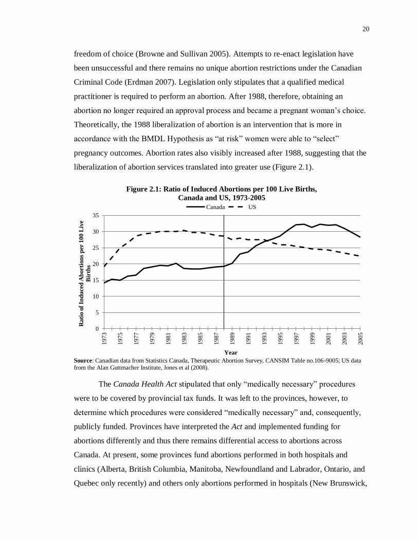
pregnancy outcomes. Abortion rates also visibly increased after 1988, suggesting that the

liberalization of abortion services translated into greater use (Figure 2.1).

Figure 2.1: Ratio of Induced Abortions per 100 Live Births,

Canada and US, 1973-2005

Source: Canadian data from Statistics Canada, Therapeutic Abortion Survey, CANSIM Table no.106-9005; US data from the Alan Guttmacher Institute, Jones et al (2008).

The Canada Health Act stipulated that only “medically necessary” procedures

were to be covered by provincial tax funds. It was left to the provinces, however, to

determine which procedures were considered “medically necessary” and, consequently,

publicly funded. Provinces have interpreted the Act and implemented funding for

abortions differently and thus there remains differential access to abortions across

Canada. At present, some provinces fund abortions performed in both hospitals and

clinics (Alberta, British Columbia, Manitoba, Newfoundland and Labrador, Ontario, and

Quebec only recently) and others only abortions performed in hospitals (New Brunswick,

0

5

10

15

20

25

30

35

1973

1975

1977

1979

1981

1983

1985

1987

1989

1991

1993

1995

1997

1999

2001

2003

2005

Rati

o o

f In

du

ced

Ab

ort

ion

s p

er 1

00 L

ive

Bir

ths

Year

Canada US

21

Northwest Territories, Nova Scotia, Nunavut, Saskatchewan, Yukon). No abortions are

performed in Prince Edward Island; women must leave the province and the procedure

will only be covered if the abortion is considered “medically necessary.” Territorial

health plans cover hospital abortions and travel expenses to the nearest facility.11

Considering the costs of abortion (approximately $500 in clinics, over $1000 in

hospitals), “at risk” women are also the ones who would have the most difficulty

accessing abortion services (AbortionInCanada.ca 2012). Further, clinic and hospital

availability varies substantially by province. British Columbia, Ontario, and Quebec host

the most facilities (23, 36, and 54 respectively) while the rest of the provinces and

territories range from zero to five (Canadians for Choice n.d.). The gestational limits for

abortion procedures also fluctuate widely by province from ten to over twenty-three

weeks (National Abortion Federation 2010).

To perform an effective test of the BMDL Hypothesis, access to abortion services

must be available to “at risk” women and rates of abortion must also be amenable to

statistical analyses. That is, the sample size must be large enough and the change after

intervention great enough to allow for statistical verification of the theory. Four provinces

fit this description: British Columbia (BC), Alberta (AB), Ontario (ON), and Quebec

(QC).12

These four provinces also constitute the largest provinces by population (86.1

percent of the Canadian population),13

by incidents of crime (78.5 percent of all Canadian

incidents of crime),14

as well as by number of abortions (88.7 percent of all Canadian

abortions).15

These provinces are not only the largest by population, but theoretically

demonstrate the requirements for an appropriate tests of the hypothesis. They

demonstrate increases in abortions after both the 1969 and 1988 interventions; the first

requirement for abortions to be a causal agent (Figure 2.2). Between 1983 and 1993, the

ratio of abortions per 100 live births by area of residence increased 15 percent in British

11 Yukon and Northwest Territories will cover travel expenses only after 12 and 14 weeks when their in-territory facilities will not perform abortions (National Abortion Federation 2010) 12 Please refer to Appendix A for trend graphs of provincial abortion rates. 13 Estimates based on 2011 figures taken from Statistics Canada, CANSIM table no. 051-0001. 14 Estimates based on 2011 figures taken from Statistics Canada, CANSIM table no. 252-0051. 15 Estimates based on 2011 figures taken from the Canadian Institute for Health Information, Induced Abortions Reported in Canada in 2011.

22

Columbia, 56 percent in Alberta, 36 percent in Ontario, and 86 percent in Quebec. Since

these provinces experienced the largest increases in abortion rates following the

liberalization of 1988, the BMDL Hypothesis predicts that they should also exhibit the

largest declines in crime rates. The 1988 liberalization of abortion access was, however, a

national legislative change and national abortion rates increased accordingly as well.

Between 1983 and 1993, the national ratio of abortions per 100 live births increased 45

percent. Testing the impact on abortion liberalization on crime should, therefore, examine

national crime rates as well. Recognizing the differential access to and use of abortion by

province, however, may eliminate noise in the data and provide a potentially more direct

test of the BMDL Hypothesis. Investigating the impact of the increased use of abortion

services on the rates of crime in the four aforementioned provinces (i.e., BC, AB, ON,

and QC, hereafter referred to as the “focal provinces”) will provide for an improved test

of the BMDL Hypothesis. Examining the focal provinces will, moreover, increase the

sample size available for analysis and also provide more variation in both the

independent and dependent variables, allowing analyses to produce more robust estimates

and results.

Figure 2.2: Ratio of Induced Abortions per 100 Live Births,

Canada and Focal Provinces, 1970-2006

Source: Statistics Canada, Therapeutic Abortion Survey, CANSIM Table no.106-9005.

0

5

10

15

20

25

30

35

40

45

50

1970

1972

1974

1976

1978

1980

1982

1984

1986

1988

1990

1992

1994

1996

1998

2000

2002

2004

2006

Ind

uce

d A

bort

ion

s p

er 1

00 L

ive

Bir

ths

Year

CANADA BC ON AB QC

23

2.2.2 Crime in Canada

The similarity of trends in Canadian and American crime during the 1980-90s make

Canadian data a relevant source for testing the BMDL Hypothesis as well. The 1990s

decline in American crime was a unique experience in comparison to many other

similarly developed nations including France, Italy, Japan, and the UK (Zimring 2007).

Canada, on the other hand, experienced relatively similar crime trends to the US (Figure

2.3 and 2.4). Between 1990 and 2000, the US experienced an average decline of 33

percent in all seven of the FBI index crimes: homicide, rape, serious assault, robbery,

burglary, index larceny, and auto theft. In Canada, the declines in crime were similarly

broad and substantial with an average decline of 33 percent in six of the seven index

crimes16

(Zimring 2007). These similarities are especially striking as the two nations

followed very different crime policy and policing approaches. For instance, between

1980 and 2000, rates of incarceration were highly divergent between the two nations,

increasing 57 percent in the US while declining 6 percent in Canada. In the 1990s, the

employment of police per 100 000 population increased 14 percent in the US while it

declined 10 percent in Canada (Zimring 2007).

Zimring (2007) argued that “joint causes” must be identified to reasonably

explain the similarity in crime trends and dissimilarity in crime policy. That is, factors

that were similar in timing, abruptness, and magnitude that were experienced in both the

US and Canada were the only reasonable causal agents to explain the parallel crime

trends of the 1990s. He therefore argued that the legalization of abortion was not an

attractive explanation because the American and Canadian experiences differed in both

legislation and timing. Canadian abortion legislation followed a “two-step” process of

which only the first was relevant for explaining the decline in crime in the 1990s. The

1969 legalization of abortion in Canada was less permissive than the 1973 legalization in

the US and the rates of abortion in Canada also increased more modestly than in the US.

16 Auto theft was the only index crime in Canada that did not decline between 1990 and 2000 and instead increase of

26%. When compared to available insurance data, however, a decline in auto theft remains plausible (Zimring 2007). Based on partial data from Ontario, Alberta, the Atlantic provinces, Yukon, Nunavut, the Northwest Territories, and Quebec, Zimring (2007) found that auto theft declined 32% between 1990 and 2000; a finding very close to the 37% decline in auto theft in the US during the same time frame.

24

Consistent with the BMDL Hypothesis, however, the relative decline in violent crime

rates in the 1990 was also less dramatic in Canada (Figure 2.3). The legalization of

abortion as an explanation for the 1990s decline in crime, therefore, remains plausible; its

magnitude of influence, however, remains to be specified and validated.

Figure 2.3: Total Selected Violent Crime Rate per 100 000 Population,

Canada and US, 1983-2011

Source: Canadian data from Canadian Centre for Justice Statistics, Uniform Crime Reporting Survey; US data from

FBI, Uniform Crime Reports as prepared by the National Archive of Criminal Justice Data. Canadian crime rates were calculated based on the population estimates from CANSIM table no. 051-0001. Note: Canada and the US employ different definitions of violent crimes. Based on Gannon (2001), only comparable violent crimes have been included in Figure 2.3. These are homicide, aggravated assault, and robbery for the US, and homicide, aggravated assault, assault with a weapon, attempted murder, and robbery for Canada. Figure 2.3 presents data from 1983 on due to a change in the classification of Canadian assault categories that occurred in 1983.

0

100

200

300

400

500

600

700

800

0

50

100

150

200

250

300

1983

1984

1985

1986

1987

1988

1989

1990

1991

1992

1993

1994

1995

1996

1997

1998

1999

2000

2001

2002

2003

2004

2005

2006

2007

2008

2009

2010

2011

US

Vio

len

t C

rim

e R

ate

per

100 0

00

Pop

ula

tion

Can

ad

a V

iole

nt

Cri

me

Rate

per

100 0

00

Pop

ula

tion

Year

Canada US

25

Figure 2.4: Total Selected Property Crime Rate per 100 000 Population,

Canada and US, 1983-2011

Source: Canadian data from Canadian Centre for Justice Statistics, Uniform Crime Reporting Survey; US data from FBI, Uniform Crime Reports as prepared by the National Archive of Criminal Justice Data. Canadian crime rates were calculated based on the population estimates from CANSIM table no. 051-0001. Note: Canada and the US employ different definitions of property crimes. Based on Gannon (2001), only comparable property crimes have been included in Figure 2.4. These are burglary, larceny-theft, and motor vehicle theft for the US, and break and enter, total theft, and motor vehicle theft for Canada. Figure 2.4 presents data from 1983 on to maintain

consistency with Figure 2.3.

2.3 Designing an Empirical Test

The dramatic decline in crime in the 1990s was the phenomenon that generated the

BMDL Hypothesis. The econometric debate has, in turn, relied on 1990s crime data from

the US to provide the evidence to support or refute the BMDL Hypothesis. This

methodological handicap suggests that an improved empirical test should look to

different sources of data (Zimring 2007). Canada offers such an opportunity because of

the 1988 liberalization of abortion. Using this intervention will allow for an improved test

of causality as different, but relevant, crime data are used.

Two of the major issues that prior American studies have been confounded by are

the lack of reliable data on abortions before legalization and the crack-cocaine epidemic.

Previous studies have used various adjustments and controls to manage these issues, but

none have been completely reliable. The issue with American abortion data arises due to

the unreliability of measures and sources of data before abortion legalization in 1973. The

controversy surrounding the credibility of data from the AGI and/or the CDC (the two

0

1,000

2,000

3,000

4,000

5,000

6,000

1983

1984

1985

1986

1987

1988

1989

1990

1991

1992

1993

1994

1995

1996

1997

1998

1999

2000

2001

2002

2003

2004

2005

2006

2007

2008

2009

2010

2011

Pro

per

ty C

rim

e R

ate

per

100 0

00

Pop

ula

tion

Year

Canada US

26

main sources for US Abortion statistics) also complicate analyses. In Canada, focusing on

the liberalization of abortion in 1988 allows for the use of more reliable abortion data

from both before and after the year of intervention because abortions were legal in

Canada since 1969 and reporting was mandatory. Further, Canada was not as influenced

by the guns, gangs, and crack-cocaine epidemics of the 1980s and 1990s (Joyce 2010;

Zimring 2007). Not only was the crack-cocaine epidemic not as severe in Canada, but the

crime rates of interest in this study begin in the late 1990s and 2000s; a decade after the

waning of the epidemic. Prior research has found the crack-cocaine epidemic a difficult

period effect to manage using reliable post-hoc controls. Using Canadian data from a

time period when the crack-cocaine epidemic was not a prevalent influence may,

therefore, allow for an improved empirical test by predominantly avoiding these issues

rather than relying on post-hoc controls.

Canadian data have been used in analyses conducted by Sen (2007), which have

been cited in Freakonomics as international evidence supporting the BMDL

Hypothesis.17

Sen (2007) attempted to replicate the regression from Donohue and Levitt’s

(2001) seminal study that used the “effective abortion rate” to predict changes in

aggregate crime rates. Sen (2007) also added teen and general fertility rates to the model

in an attempt to model the “unwantedness” of pregnancies. Specifically, he argued that “a

significant correlation between higher abortion rates and lower crime is plausible if the

decline in crime can also be associated with lower fertility rates” (2007:3). He found a

significant correlation between abortion and violent crime, but not property crime.

Further, he found that over a quarter of the 1990s decline in crime was attributable to

increases in teen abortion rates and over half to the decline in teen fertility rates overall in

the 1970s and 1980s (Sen 2007).

17 Internationally, Sen (2007), along with Pop-Eleches (2006) on Romania, Kahane et al (2008) on the UK, and Leigh and Wolfers (2000) on Australia, have analysed the impact of changes to abortion legislation on later crime. The Romanian study looked at criminal outcomes of cohorts born after abortions was banned in 1967 and found some

evidence to support the BMDL Hypothesis. The UK study found little support for the BMDL Hypothesis and instead found evidence more congruent with Lott and Whitley (2007) in that the criminal outcomes of UK cohorts born after the legalization of abortion increased. The Australian “study” was not an empirical analysis at all, and instead was based on “speculation” as data were unavailable.

27

Important issues exist, however, in this study’s justifications and execution. The

study was an attempt to replicate a weaker portion of Donohue and Levitt’s (2001)

analysis using Canadian data relying on using the “effective abortion ratio.” As noted

earlier, this was an innovative method for incorporating abortion data with aggregate

crime data, but does not directly link the actual abortion rates experienced by cohorts

while in utero. In Donohue and Levitt’s (2001) final analysis, they used crime data that

were age-specific, which allowed them to more directly link each cohorts in utero

experience to their crime outcomes. Sen (2007), unfortunately, did not have age-specific

arrest rates and therefore could not perform the age-specific crime rate analyses. Further,

Sen (2007) used the 1969 change in abortion legislation as the focal year of intervention

and thus examined crime data from 1983 to 1998. He argued that although the degree of

legalization of abortion in Canada in 1969 was not as extensive as in the US in 1973, the

difficulty of obtaining an abortion was nonetheless quite low. This argument directly

contradicted the findings of the 1977 Badgley Report. The committee that produced the

Badgley Report was established by the Canadian federal government in 1975 to assess

the operation of the abortion law. They concluded that the procedures set out in the

Criminal Code for obtaining an abortion were not operating equitably across Canada and

access to abortion services were “illusionary” for many women (Committee on the

Operation of the Abortion Law 1977).

Sen (2007) had abortion data, moreover, only from 1970 onward and therefore

assumed zero abortions prior to 1970, in the same fashion as Donohue and Levitt (2001).

As argued earlier, it is impossible to substantiate the number of abortions prior to

legalization. Sen (2007) argued that his abortion data were an improvement to Donohue

and Levitt’s (2001) as additional years were available for analysis. The benefits of having

three more years of abortion data, particularly when both sets are post-legalization, seem

trivial. An improved empirical test should, therefore avoid such controversies altogether

and rely more heavily on credible data. Instead of constructing an “effective abortion

ratio” that theoretically weighs the influence of abortion rates in lagged years, empirical

analysis should rely on directly linking the actual in utero abortion experience of cohorts

with their age-specific criminality. In his review, Joyce (2010) noted other issues with

Sen’s (2007) study, criticizing it as a “step backwards in the debate” (475). For Joyce

28

(2010), the preferred strategy for investigating the BMDL Hypothesis is the DDD

estimator, discussed above. Joyce (2010) noted, however, that since Canada has only

thirteen provinces and territories to America’s fifty, there is less variation in Canada than

in the US. Unfortunately, the DDD strategy would also be inappropriate in Canada as

there is simply not enough variation for this strategy. The most damaging of Joyce’s

(2010) critiques, however, is Sen’s (2007) lack of age-specific data on crime rates. He is,

therefore, unable to link the crime rates of cohorts directly with the abortion rates they

experienced in utero. This is the most direct link and therefore the best test of the BMDL

Hypothesis.

Berk et al. (2003), although not featured prominently in the debate, made

profound arguments about the econometric debate from a non-economic perspective.

They conducted a time-series analysis examining a more proximal test of the BMDL

hypothesis, namely, the impact of legalized abortion on youth homicides. They raised

many methodological concerns that were quite damaging for much of the econometric

debate that they cited (e.g., Donohue and Levitt 2001; Joyce 2004a; Lott and Whitley

2007). The econometric literature’s reliance on regression analyses posed many problems

including issues of missing data, measurement error, untestable assumptions, overfitting,

and multicollinearity. For instance, Berk et al (2003) argued that the differing results of

the debate have been due to the selection of different control parameters, a point that has

been emphasized by Moody and Marvell (2010). Prior studies have used a variety of

different socio-demographic, economic, policing, and other social service variables in

each of their models. Berk et al (2003) argued that this has produced complex results that

have been difficult to interpret and has made meaningful conclusions difficult to draw.

The authors also highlighted the issue surrounding abortion data. As there is no definitive

measure of abortions before legalization, regression-based associations that employ

unreliable data can be misleading.

To address the issues of previous econometric studies, Berk et al. (2003) proposed

the use of time series analyses. This approach was an attractive method as it avoided

many of the pitfalls of previous regression analyses. The authors claimed that previous

studies have “asked too much of the data and of the causal modeling approach”

29

(2003:48). Alternatively, Berk et al (2003) employed a quasi-experimental perspective

with an interrupted time series design to look for a relatively discrete change in homicide

rates of 15-24 year olds between 1970 and 1998 in the US. The timing of the

intervention’s impact was set at 1988, 15 years after the 1973 Roe v. Wade decision. The

authors conducted analyses on 40 time series (ten ages by two race categories by two

sexes) and overall found evidence supporting the BMDL Hypothesis.

Given the ability of Berk et al. (2003) to so sharply identify the shortcomings of

previous studies, their solutions seem insufficient, particularly for the case of Canada.

Firstly, they employed national measures of abortion and crime. The rationale for this

decision rested on the use of the US as a whole as their unit of analysis in an attempt to

control for inter-state migration (i.e., when women obtain an abortion in a different state

than their state of residence or when they move to a different state after giving birth) by

design. The authors stated that they were looking to characterize the impact of a federal

decision, and therefore used the US as a whole for their analysis. Prior research, however,

has identified that the availability of abortion services has differed substantially by state

(e.g., Donohue and Levitt 2001). Berk et al’s (2003) use of a simple binary variable (i.e.,

0 = before 1973, 1 = after 1973) to characterize the intervention of legalized abortion also

does not seem to have been an optimal solution. Many studies (e.g., Joyce 2004; Lott and

Whitley 2007) have demonstrated that abortions were taking place at high levels before

legalization. The credibility of different estimates for rates of abortion prior to

legalization remains debatable. The fact remains, however, that abortions were taking

place at non-negligible levels before 1973. That five states were allowing abortions

before 1973 and that other studies (namely Donohue & Levitt’s paper that sparked this

literature) used this very source of variation for quasi-experimental designs suggests that

using 1973 as the year of intervention is untenable. Using a dichotomous indicator of

abortion legislative status to represent changes in abortion rates is, therefore, an

inappropriate proxy (Donohue and Levitt 2004). Time-series analyses that characterize

abortion legislation changes in this manner are, therefore, not an appropriate method for

testing the BMDL Hypothesis. Instead, abortion rates should be incorporated to directly

capture the selection effect that the BMDL Hypothesis purports (Donohue and Levitt

2004).

30

Furthermore, it is reasonable to assume that abortions were not extensively

available immediately after legalization and required a period of time for implementation.

American abortion rates confirm that it took around seven years for abortion rates to

stabilize (Figure 2.1). This variation in abortion around 1973 suggests that using a binary

variable to categorize abortion legalization, while being appropriate for a legal impact

study, is not a good test of the BMDL Hypothesis. This is the case particularly for a

Canadian test as abortion rates increased in a much less dramatic and discrete manner

after 1988 than in the US following 1973. Instead, the strategy employed to test the

BMDL Hypothesis should incorporate actual abortion rates in order to be sensitive to

gradual and progressive changes.

Secondly, Berk et al. (2003) used the number of homicides each year as their

outcome variable to investigate the link between abortion legalization and crime. It was

erroneous to use incidents rather than a rate as there is no control for potential cohort size

changes. This was an odd oversight as they repeatedly emphasized the cohort size

explanation of the BMDL Hypothesis (i.e., fewer potential victims and offenders). As

Joyce (2010: 471) emphasized, the “outcome should be a rate of crime and not a level.”

Finally, the use of homicides as the outcome variable of interest was argued

thoroughly by Berk et al (2003), but not convincingly. Homicides were argued to be the

most reliably recorded crime measure and thus a good variable to use for testing the

BMDL Hypothesis. They used homicides by year of age of the victim, not the accused,

based on the assumption that “people tend to kill others like themselves” (Berk et al.

2003:50). They wrote “[t]his assumption follows from the kinds of activities engaged in

(e.g., gangs) and more generally, social and economic forces that tend to foster

interaction among people who are alike. One key instance is the ways in which income

often produces class and racial homogeneity within neighborhoods” (Berk et al.

2003:50). As consistent with past research this assumption may be, it was inappropriate

to test the BMDL Hypothesis by using measures of the victims of crime, individuals who

may or may not have been part of the treatment group at all, and therefore theoretically

irrelevant. A more appropriate test of the hypothesis would have been to isolate and

analyze the behaviours of those individuals who were and were not in the “treatment”

31

group. That is, the criminality of individuals born after the legalization of abortion in

comparison to those born before.

Joyce (2010) has noted that this literature has resulted in more confusion than

consensus. He therefore summarized eight features of an empirical test of the BMDL

hypothesis on which all parties may be able to agree (Joyce 2010:471-472):

1. The crime measure must be age-specific in order to identify cohorts.

2. The outcome should be a rate of crime and not a level.

3. The hypothesis should be consistent with the timing of abortion legalization and

should be evident or not contradicted by basic time series plots.

4. The abortion rate should be measured by state of residence.

5. The abortion rate should be inversely related to fertility rates.18

6. Regressions of age-state-year crime rates should include state-year fixed effects.

7. The number of observations with no measure of abortion should be minimized.

8. Statistical tests should take account of the autocorrelation in crime rate residuals.

With these features in mind, this study proposes an improved empirical test of the BMDL

Hypothesis by including critical developments and avoiding major controversies by

design rather than through statistical controls.

The major improvement that this study proposes is to take advantage of the 1988

liberalization of abortion in Canada as the focal intervention for three reasons. First, the

reliability of abortion data before and after this intervention is far superior to the data

available before the 1969 legalization in Canada and the 1970-73 legalization in the US.

Canadian abortion data are available from 1970 onward and report the province of

residence of the woman. Second, the use of Canadian data avoids the biases created by

the crack-cocaine epidemic that has plagued the American studies as this history effect

was not a major factor in Canada (Joyce 2010). Finally, to properly test the BMDL

Hypothesis and to avoid the circular reasoning of previous studies, selecting a different,

yet theoretically parallel, intervention and then examining its impact on future crime rates

18 Several scholars (e.g. Sen 2007; Joyce 2010) have argued that increases in abortions must be associated with declines in fertility for the BMDL Hypothesis to have plausibly had an impact on unwanted births. Fertility rates, however, are not theoretically critical to the BMDL Hypothesis. Donohue and Levitt (2004:33) asserted that “[a]s long as the number

of unwanted births falls [evidenced by increases in abortions], even if total births do not decline at all, one would expect to see better life outcomes on average for the resulting cohorts.” This is the core assumption of the BMDL Hypothesis’ logic of the selection effect. Tests of the BMDL Hypothesis must, therefore, focus on the impact of increases in abortions irrespective of changes in total or teen fertility rates.

32

is a far more attractive and tenable method. In accordance with Joyce’s (2010)

suggestions, Canadian crime data will be used that measure crime as a rate. Donohue and

Levitt (2004) argued that linking the crime rate of cohorts with the abortion rate that they

experienced in utero is a better proxy for unwantedness than a binary legalization

indicator. In order to investigate the selection effect of the BMDL Hypothesis, therefore,

regressions must use crime rates and not a number crimes (Joyce 2009).

Since this study will focus on the 1988 liberalization of abortion, the crime rates

from the late 1990s to 2011 will be examined. The focus will, therefore, remain on the

criminality of relatively younger cohorts. In Canada, however, an important potential

threat to internal validity must be addressed. The Juvenile Delinquents Act was the

legislation governing youth crime in Canada until 1984 when the Young Offenders Act

(YOA) came into effect. The YOA had a profound influence on the practices of charging

young people, creating a substantial increase in the youth crime rate and a substantial

decrease in the use of extrajudicial measures to manage young offenders (Carrington &

Schulenberg 2005). The use of custody and courts in Canada under the YOA was much

higher than other comparable western nations (Bala, Carrington & Roberts 2009). The

large and immediate increase in the rate of youth being charged for crimes without a

similar pattern in adult rates indicates that the changes in the youth crime rate following

1984 were the effect of the YOA and not of changing rates of youth crime.

The Youth Criminal Justice Act (YCJA) came into effect on April 1, 2003. The

intent of this legislation was to encourage the use of extrajudicial measures instead of

heavily relying on the formal judicial system for managing youth crime and to more

effectively respond to the relatively small number of serious crimes of violence. The

YCJA has been successful in reducing the use of the formal court system for less serious

crimes, while maintaining similar rates for more serious offences. Further, the use of

extrajudicial measures has increased in complement to the decline in the charging of

youth, indicating that charging practices have changed, not youth crime (Carrington &

Schulenberg 2005; Bala, Carrington & Roberts 2009).

33

Figure 2.5 illustrates the outcomes of criminal incidents involving youth

compared to adults over time. The distinct decline in 2003 of incidents that resulted in

youth being charged was supplanted by a complementary increase in incidents where

youth were not charged (i.e., dealt with using extrajudicial measures). The rate of total

chargeable youth offences (i.e., the sum of youth who were charged and youth who were

not charged) and the adult rate show little variation around 2003. These results suggest

that changes in legislation have had significant effects on the charging practices of police,

but have not gone so far as to significantly affect incidents of youth crime itself. This

study will, therefore, use rates of youth accused of crime rather than rates of youth

charged with crime to measure youth offending. Young offenders in this study were born

before and after the liberalization of abortion in 1988 and were therefore equally affected

by the YOA and YCJA. Significant differences in crime rates between affected and non-

affected cohorts can, therefore, be attributed to other causal agents like the liberalization

of abortion in 1988 and not to changes in the legislation governing youth charging

practices.

Figure 2.5: Violent and Property Criminal Code Violations, Rate per 100 000 Population,

Youth and Adult, Canada, 1998-2011

Source: Statistics Canada, Criminal Justice Statistics, Uniform Crime Reporting Survey

Note: Youth are ages 12-17, adults are 18 and over

0

1000

2000

3000

4000

5000

6000

7000

8000

1998

1999

2000

2001

2002

2003

2004

2005

2006

2007

2008

2009

2010

2011

Rate

Ch

arg

ed p

er 1

00,0

00 P

op

ula

tion

of

Sam

e A

ge

Gro

up

Year

Youth, sum Youth, charged Youth, not charged Adult, charged

YCJA

34

2.4 The Current Study

The current study aims to contribute to the literature by testing the BMDL Hypothesis on

the liberalization of abortion in Canada that occurred in 1988. As discussed previously,

this intervention offers an improved source of data by avoiding the issues surrounding

measures of illegal abortions and the crack-cocaine epidemic. Taking the elements

outlined by Joyce (2010) into consideration, this study will also employ abortion rates by

area of residence of the women and age-specific crime rates. The time series of relevant

crime rates will also be plotted to assess the plausibility of the BMDL Hypothesis. Many

of the elements outlined by Joyce (2010) are relatively simple and largely accomplished

by using the 1988 liberalization of abortion as the focal intervention. The selection of a

credible and tenable analytic strategy is a more difficult task.

Four main analytic strategies have emerged from the econometric debate that has

surrounded the BMDL Hypothesis. The DDD strategy (i.e., Joyce 2009) and time series

analyses (i.e., Berk et al 2003) both relied on the use of dichotomous characterizations of

the legal status of abortion. In essence, they were similar to a legal impact study,

examining the impact of a change in legislation by characterizing it using a pre/post

intervention strategy. These strategies, therefore, assumed that the legalization of

abortion had an impact immediately after changes in legislation had been made. Further,

these strategies did not incorporate the extent or rate of change in abortion rates that

occurred after the legalization of abortion. That is, if abortion rates substantially

increased immediately following the legalization of abortion and maintained a uniform

rate hence, they would be modelled appropriately using a dichotomous categorization. If,

however, abortion rates deviated from this ideal situation (e.g., if abortion rates were

relatively similar in magnitude before and after the legalization of abortion), the two time

periods would be attributed with an inappropriately dichotomous distinction. In

opposition to this ideal situation, the rates of abortion that followed 1988 increased

gradually (Figure 2.1 and 2.2). To test the BMDL Hypothesis, therefore, models must

take into account actual changes in abortion rates to accurately identify associations

between increases in abortions rates and declines in crime rates.

35

The construction of an “effective abortion rate” (EAR) (i.e., Sen 2007) and the

use of age-specific crime rates (i.e., Donohue and Levitt 2001) were the other two

strategies that were featured prominently in the debate. These two strategies incorporated

data on rates of abortion into their models, allowing for more sensitivity and accuracy in

estimating the association between changing abortion rates and crime rates. Unlike the

DDD and the time series analysis strategies that investigated the impact of a change in

legislation, the EAR and age-specific crime rate strategies examined the impact of a

change in the rate of abortions. The EAR strategy was first employed by Donohue and

Levitt (2001) and also by Sen (2007) in the sole Canadian analysis of the BMDL

Hypothesis. The EAR strategy regresses the average weighted influence of abortion

exposure that individuals experienced in utero on the aggregate youth crime rates of a

given year. The second strategy regressed age-specific crime rates on the abortion rates of

the year prior to a cohort’s birth to approximate the exposure to abortion these cohorts

experienced while in utero. As argued previously, the latter method was superior as it

directly linked the in utero exposure to abortion that cohorts experienced with their crime

outcomes while the EAR strategy relied on regressing aggregate crime rates on weighted

and aggregated abortion rates. Although the EAR strategy relied on stronger assumptions

regarding the influence of abortion rates on cohorts, it will be attempted again using the

1988 liberalization of abortion as a new exogenous source of abortion variation to test the

plausibility of the BMDL Hypothesis. The age-specific strategy will also be used as it

theoretically constitutes a more direct test of the BMDL Hypothesis. These two strategies

have also been successfully used to find support for the BMDL Hypothesis in prior

research. The EAR and age-specific strategies will, therefore, be employed to perform

improved investigations of the BMDL Hypothesis. The current study will, therefore,

investigate the impact of an increase in the abortion rate as opposed to a change in

abortion legislation.

Contrary to prior studies, the current study will not include the various economic,

socio-demographic, policing, and other control variables that have been common in order

to examine the link between abortion and crime as clearly as possible and to avoid the

36

issues of complexity and heavy parameterization (Berk et al 2003).19

Furthermore,

national analyses will be conducted to test the plausibility of the BMDL Hypothesis in

Canada. These will benefit from avoiding the issue of interprovincial migration (Berk et

al 2003). Due to differences in the provincial variation in the availability of abortion, the

abortion and crime rates of the four focal provinces (i.e., BC, AB, ON, and QC) will also

be analysed in a single model. These provincial data will constitute an improved analysis

to supplement the national analyses by providing a larger sample size, more variation in

the dependant and independent variables, and a more theoretically direct test of the

BMDL Hypothesis.

19 Please refer to footnote 27 and Appendix D for a discussion concerning covariates from prior research and their employment in the present study for robustness checks.

37

Chapter 3

3 METHODS

This study estimates two sets of fixed-effects models that resemble the design used by

Sen (2007) and Donohue and Levitt (2001), in which crime rates were regressed on

lagged abortion rates. The details of these two strategies will be further elaborated on in

Section 3.2.

3.1 Data

The number of induced abortions per 100 live births in both hospitals and clinics is the

focal independent variable used in this analysis, following the convention established in

past research. The ratio of abortions per live births was the metric used as the explanatory

variable when the EAR and age-specific crime rate strategies were employed in the past

(i.e., Donohue and Levitt 2001; Sen 2007). This metric is theoretically important for the

BMDL Hypothesis because it measures abortions as a proportion of completed

pregnancies. It is, therefore, more parsimonious than other possible metrics, such as a

measure of abortions per females of childbearing age while controlling for fertility. The

ratio of abortions per 100 live births was, therefore, selected as it captures the proportion

of pregnancies that were terminated versus the proportion that were brought to term.

Statistics Canada reported this measure from 1970 to 2006 by the province of residence

of the patient. This study employs Canadian abortion data from the Therapeutic Abortion

Survey (TAS), CANSIM Table 106-9013, which was collected by Statistics Canada from

1969 to 1994 and by the Canadian Institute for Health Information from 1995 on. The

TAS is a cross-sectional census conducted on an annual basis per calendar year. The

province of residence for Canadian women who obtained abortions in the US was

reported as well. Data for 1991 were not available provincially and were imputed by

averaging the values for 1990 and 1992.

Some issues should be noted with the TAS data. The abortion legislation that

decriminalized abortion services from 1969 to 1988 also included a clause that required

the mandatory reporting of all induced abortions that were performed in Canada to the

38

Dominion Bureau of Statistics and later, to Statistics Canada. The coverage of the TAS

was, therefore, considered to be 100 percent of all induced abortions from 1970 to 1987

(Statistics Canada 2009). The liberalization of abortion in 1988, however, also removed

the clause for the mandatory reporting of all induced abortions to Statistics Canada. The

reporting of induced abortion statistics is now voluntary, but the Canadian Institute of

Health Information maintains that the TAS represents 90 percent of all induced abortions

performed in Canada (Canadian Institute for Health Information 2003).20

Despite its

limitations, the present study uses the TAS as it is the only source for abortion statistics

in Canada.

The violent and property crime rates per 100 000 population are the dependent

variables of interest in this study. Canadian crime data were taken from the Uniform

Crime Reporting Incident-based Survey (UCR2), which has been conducted by the

Canadian Centre for Justice Statistics (CCJS) since 1988. The UCR2 is also a cross-

sectional census conducted on an annual basis per calendar year. The first affected cohort

(i.e., those born in 1989) had only reached 22 years of age by the end of the study time

frame (i.e., 2011) because the liberalization of abortion in 1988 was selected as the focal

year of intervention. An examination of youth crime rates, as opposed to total crime

rates, was therefore attempted as a more proximal replication of Donohue and Levitt’s

(2001) strategy. The EAR analyses examined youth crime rates (i.e., 12-17 year old)

between 1998-2011 for all ten Canadian provinces, which encompassed cohorts born

between 1973 and 1999. Unlike prior studies, abortion rates were available for all years

of birth included in this analysis. The present study analyzed rates of youth violent and

property crime were separately using two sets of panel data.

This study, as with the prior research surrounding the BMDL Hypothesis, relied

on official police statistics to capture incidents of crime. It is well recognized that biases

are inherent in official crime statistics due to the under-reporting of incidents of crime to

20 Please refer to “Data Quality in the Therapeutic Abortion Survey” and “History of the Therapeutic Abortion Survey” for more detailed accounts of the methodological issues in the Therapeutic Abortion Survey. Available in the Documentation section of the Definitions, data sources, and methods of the Therapeutic Abortion Survey, available at http://www23.statcan.gc.ca/imdb/p2SV.pl?Function=getSurvey&lang=en&db=imdb&adm=8&dis=2&SDDS=3209#a3

39

the police, as well as justice officials’ discretion used in the handling of incidents of

crime reported to them (Gabor 1999). The biases involved in youth crime rates are of

particular concern because they are the focus of the analyses of the present study.

Specifically, it may be more likely that the criminality of younger aged youth (i.e., 12-15

year olds) is more easily “forgiven,” than for slightly older youth (i.e., 16-17 year olds),

who may be treated more harshly (Gabor 1999). Youth crime rate statistics in the UCR2,

moreover, combine the rates of all youth incidents of crime that have been charged as

well as those that were managed using extrajudicial measures. The proportion of

“chargeable” youth who were not charged suffers from the bias of individual

interpretation as it is under the discretion of individual police officers to decide whether

or not to lay a charge for incidents of crime and, if not laying a charge, decide whether or

not to record the incident at all (Carrington and Schulenberg 2005). These biases caused

by the variation between individual officers as well as between police services in the

reporting of criminal incidents involving youth who are not charged are stable enough

over time to conduct time series analyses when the data are aggregated to the provincial

level (Carrington and Schulenberg 2005). The present study, therefore, utilized crime

data that were, at minimum, aggregated at the provincial level to overcome these

potential limitations.

To obtain age-specific data for the age-specific crime rate analyses custom

tabulations were ordered directly from the CCJS. Unfortunately, reliable measures for the

age of accused could only be obtained from 2006 to 2011.21

This study used national

crime rates by single year of age of accused, and provincial crime rates in two-year age

groupings due to censorship demands. Crime data were received as incident counts

rather than rates and were subsequently converted to rates per 100 000 population using

population estimates by single year of age from Statistics Canada, CANSIM Table 051-

0001. The influence of legislative changes that created discontinuity in offence

21 Please refer to Summary of changes over time – Uniform Crime Reporting Survey in the “Definitions, data sources and methods” section of the Uniform Crime Reporting Survey for changes in coverage of the survey, available at http://www23.statcan.gc.ca/imdb/p2SV.pl?Function=getMainChange&SurvId=3302&SurvVer=0&InstaId=15093&SDDS=3302&lang=en&db=imdb&adm=8&dis=2.

40

classification and recording in the UCR2 was counteracted thorough data management.22

Crime categories that were removed, added, or dramatically altered between 2006-11

were removed from analyses to maintain internal consistency.23

Youth violent and property crime rates from 1998 to 2011 were analysed

separately using the EAR strategy. The annual violent and property crime rates of youth

were linked with the “effective abortion rate” calculated for each year, which required

abortion data from 1980 to 1998. Abortion data were available for all of these years,

unlike prior application of the EAR strategy.

The age-specific analyses use four data sets consisting of age-specific crime

rates of individuals aged 12-31. These individuals were born between 1973 and 1999.

Abortion rate data were also available for all of these years. The first two data sets linked

the national violent and property crime rates by single year of age with the national

abortion rate of the year prior to each cohorts birth. The second data set included only

British Columbia, Alberta, Ontario, and Quebec as they were the largest provinces by

population and experienced large increases in abortion rates after 1988. As mentioned

previously, the provincial crime data were obtained in two-year age groupings and so the

abortion rates that corresponded to the years prior to the birth of these two-year cohorts

were averaged. For instance, in 2004, the crime rates of sixteen and seventeen year olds

were reported together. Since these individuals would have been born in 1987 and 1988,

the abortion rates for 1986 and 1987 were averaged together to produce the abortion rate

these cohorts experienced while in utero.

3.2 Analytic Strategy

Descriptive time-series plots of crime rates were produced to examine broad patterns and

trends. Time-series plots should be consistent with, or at least not contradict, the BMDL

Hypothesis, but they are not a conclusive test on their own. These plots will evidence the

type of forces that were predominantly driving crime trends as period and selection

22 Please refer to Legislative Influences (2011) in the “Documentation, data sources and methods” section of the Uniform Crime Reporting Survey, available at http://www23.statcan.gc.ca/imdb-bmdi/document/3306_D6_T9_V6-eng.htm. 23 Please refer to the Appendix B for a complete list of violent and property crimes included in this analysis.

41

effects present in characteristic and distinct patterns (Joyce 2010). That is, the BMDL

Hypothesis predicts declines in crime that should follow patterns consistent with

selection effects. Declines in crime should be evident in younger cohorts followed by

declines in successively older cohorts over time in an ordered manner to indicate the

presence of selection effects. Period effects driving changes in crime rates rather than the

selection effects proposed by the BMDL Hypothesis would be indicated by the crime

rates of different cohorts changing in unison. Prior analyses that have attempted such

time series plots have been biased by profound confounders, namely the crack-cocaine

epidemic of the late 1980s and early 1990s. The time-series plots produced in this study

have the benefit of avoiding such confounding period effects as they focus on the 1998-

2011 and 2006-11 time frames. This should allow the selection effects of the BMDL

Hypothesis to be more visually apparent.

The first statistical analysis involved regressing the constructed “effective

abortion rate” (EAR) on annual youth crime rates based on the strategy used by Donohue

and Levitt (2001). This strategy was employed here to assess the plausibility of the

BMDL Hypothesis because it has been used in the past to produce supportive evidence

(i.e., Donohue and Levitt 2001), particularly in the sole Canadian empirical investigation

(Sen 2007). This analysis focused on the crime rates of youth that were 12-17 years of

age because only 23 years have elapsed from 1988 to 2011. The EAR term was

constructed following the method outlined by Sen (2007), but the weighting procedure

was modified to be more theoretically parallel with Donohue and Levitt’s (2001) original

EAR weighting procedure. The EAR equation used in this study was

(1)

,

where the EAR in year t equals the sum of the weighted abortion rate of each age group,

a. ABORTION is the ratio of induced abortions per 100 live births in the year prior to the

birth of each age group. The weight in parentheses is the number of individuals of age

group a in year t divided by the total number of individuals 12-17 years of age in year t,

or the ratio of the 12-17 year old population that is in age group a in year t. To explain

42

how Equation 1 was derived, it may be beneficial to review Donohue and Levitt’s (2001)

original calculation. Their equation was as follows,

(2)

,

where the weight in parentheses was the arrests in year t committed by age group a

divided by the total arrests of year t, or the ratio of crimes committed by age group a in

year t. Both Sen (2007) and the present study lacked age-specific arrest data and therefore

were not able to perfectly replicate Donohue and Levitt’s (2001) strategy. Sen (2007)

used population composition ratios to weight abortion rates to overcome this limitation as

follows,

(3)

,

where the weight in parentheses was the proportion of the total population that were

males 15-24 years of age. This weighting procedure was constructed under the

assumption that the legalization of abortion reduced the cohort sizes of males who

commit the majority of crime. Sen (2007) elected to use the ratio of the total population

constituted by males 15-24 years of age in a given year as a proxy for the ratio of crimes

committed by age group a in year t. It is unclear why Sen (2007) included females in the

denominator but not the numerator in Equation 3. The population of males in cohort a

divided by the total male population in year t is the theoretically driven weighting

procedure that should have been used under Sen’s (2007) assumptions. This procedure

would still use the population of males as a proxy for the population of arrestees, but

would include only males in the denominator of the weight. This would be more

consistent with Donohue and Levitt’s (2001) weighting procedure to capture the ratio of

crimes committed by age group a in year t if males are assumed to be more

representative of arrestees. The present study did not elect to make such assumptions

about the gender differences in criminality because it is not an accurately measured

control and the legalization of abortion should have influenced the cohort sizes of both

43

sexes indiscriminately. This study therefore used the proportion of the population that

was represented by cohort a in year t as the weight to calculate the EAR.24

This study offered the use of 1988 as the focal year of intervention as a second

improvement. Donohue and Levitt’s (2001) and Sen’s (2007) lack of data on abortion

rates prior to the legalization of abortion was a major criticism of both studies. This

meant that Donohue and Levitt’s (2001) EAR terms included zeros for abortion rates

prior to 1973 and Sen’s (2007) EAR terms included zeros for abortion rates prior to 1970.

Prior EAR analyses conducted on American data attempted to overcome this limitation

by using combined estimates from various sources (i.e., the AGI and CDC). The lack of

reliability that is inherent in estimates of illegal behaviours were, however, unavoidable.

The present study avoided this issue altogether by focussing on the crime rates of 12-17

year olds between 1998-2011. These cohorts were born in 1981 at the earliest. Actual

abortion rates were therefore available for every cohort included in the EAR analyses.

The EAR regression equation estimated in this study was

(4) ,

where CRIME referred to the natural logarithm25

of either violent or property crime rates

per 100 000 population, EAR was the effective abortion rate, γ was the province fixed

effect, λ was the year fixed effect, ϵ was the error term, and i and t indexed the province

and year, respectively. The fixed effects are dichotomous dummy variables that were

added for each province and year. These terms were included to control for persistent

differences in crime between provinces and to control for time trends that were

experienced by all provinces in a given year.

24 Sen (2007) argued that his weighting procedure was a valid method based on a Pearson correlation coefficient of 0.67. The Pearson coefficient between this study’s weighting procedure and Sen’s (2007) weights was 0.97. The Pearson coefficient between this study’s weighting procedure and the theoretically more parallel method described above (i.e. male population in cohort a in year t / total male population in year t) was 0.98. Based on this evidence, the use of any of the three weighting procedures would be appropriate. Sen’s (2007) weights, however, were not theoretically parallel to Donohue and Levitt’s (2001) method, assuming male over-representation in criminality. This

study did not elect to make such assumptions and instead based EAR weights on population proportions that included both sexes as crime and abortion rates also included men and women. 25 The models used the natural logarithm of crime rates to maintain consistency with the prior research central to the econometric debate.

44

Ideally, the EAR analyses should only be conducted on theoretically relevant

provinces. That is, the only provinces that should be included in the analyses are those

that experienced improved access to abortion service after 1988 as this is a necessary

precondition for the BMDL Hypothesis. Unfortunately, there were insufficient

observations to analyse provinces separately. This limitation of insufficient observations

is not a major set-back since the EAR analyses were conducted to test the plausibility of

the BMDL Hypothesis in Canada. Prior studies that have used the EAR strategy and have

found support for the BMDL Hypothesis based on analyses of the US or Canada as a

whole without the selection of only theoretically relevant states or provinces (Donohue

and Levitt 2001, 2008; Sen 2007). This study, therefore, conducted the EAR analyses on

all ten Canadian provinces.

The second set of analyses in this study were based on regressing age-specific

crime rates on lagged abortion rates. Two sources of data were used: national age-specific

crime rates and provincial age-specific crime rates. These data were directly linked with

national and provincial abortion ratios (i.e., abortions per 100 live births), respectively.

As with the EAR analyses, these age-specific analyses also benefitted from focusing on

the 1988 change in abortion legislation. The analysis included 12-31 year olds in all

available years of age-specific data (i.e., from 2006-11). These individuals were born in

1975 at the earliest. Actual abortion data were therefore available for all included

individuals.

To perform a more direct test of the BMDL Hypothesis, four focal provinces were

selected that demonstrated the largest increases in access to abortion services as well as

the largest increases in abortions shortly after 1988. These provinces were British

Columbia, Alberta, Ontario and Quebec. Equation 5 was estimated using only these four

provinces to remove the suppressing effects that theoretically inappropriate provinces

could add. According to the BMDL Hypothesis, provinces that did not experience large

increases in abortions after 1988 could not be expected to also experience a decline in

future crime rates from the influence of abortion. Their inclusion would dampen the

impact an increase in abortions could have had on crime rates, which could potentially

lead to false null findings. The four provinces were, therefore, aggregated together to

45

perform the age-specific analyses on an improved, more theoretically informed, set of

observations to supplement the national age-specific analyses. An additional advantage of

analysing the four focal provinces was that more observations were included in the

sample. The national rates included only one observation per age per year. The provincial

data, however, included one observation per two-year age group per year per province.

This increased the sample size, which assisted in detecting statistical patterns using more

robust analyses.

Three models were estimated for age-specific crime rates for the national and

provincial data sets. The equations for the first model included age and year fixed effects

in the national analysis (5a) and also included a province fixed effect in the provincial

analysis (5b) as follows,

(5a) ,

(5b) ,

where CRIME referred to the natural logarithm of either violent or property crime rates

per 100 000 population of age group a in year t. ABORT was the abortion rate in the year

prior to the birth of age group a. γ was the age fixed effect, λ was the year fixed effect, θ

was the province fixed effect, and ϵ was the error term. a, t, and i indexed age group,

year, and province respectively.

A one-year lagged dependant variable was added in the second model to correct

for serial correlation in the crime data (Vieraitis, Kovandzic, and Marvell 2007). The

equations for the national (6a) and provincial (6b) models were,

(6a) ,

(6b) ,

where CRIME referred to the natural logarithm of either violent or property crime rates

per 100 000 population of age group a in year t. ABORT was the abortion rate in the year

prior to the birth of age group a. γ was the age fixed effect, λ was the year fixed effect, θ

was the province fixed effect, and ϵ was the error term. a, t, and i, indexed age group,

year, and province, respectively. The lagged dependant variable term (i.e., lnCRIMEat-1)

improved the ability of the ABORT coefficient to estimate the specific impact of abortion

46

rates on crime rates by removing the correlation between the crime rate of each year with

the crime rate of the previous year. The age-specific national violent and property crime

rates as well as the provincial violent and property crime rates exhibited high auto-

correlation with their one-year lags.26

The ABORT coefficient of Equation 6, therefore,

offered an improved estimate of the association between abortion and crime rates in

comparison to the ABORT coefficient estimates of Equation 5.

The effect of abortion liberalization was expected to affect different age groups in

different years because the crime rates were age-specific. An age-year interaction term

was added to Equation 6, following Donohue and Levitt (2001), to control for changes in

age-specific trends in crime over time. This control allowed the ABORT coefficient to

estimate the association between exposure to legalized abortion while in utero and

criminality regardless of the age or year of observation by allowing the slopes of age-

specific trends to vary individually over time. The year fixed effect dummy variables in

Equation 6 were replaced with a single continuous year variable. This was necessary to

prevent over-identification of the model as the national and provincial data sets included

only 100 and 200 observations, respectively. The equations for the final national and

provincial models were,

(7a)

,

(7b)

,

where CRIME referred to the natural logarithm of either violent or property crime rates

per 100 000 population of age group a in year t. ABORT was the abortion rate in the year

prior to the birth of age group a. CRIMEat-1 was the lagged dependant variable term for

each age group a in year t. YEAR was a linear year trend term that replaced the year fixed

effect in Equation 6 (i.e., λ). γ*YEAR was the age-year interaction term. γ was the age

fixed effect, θ was the province fixed effect, and ϵ was the error term. a, t, and i, indexed

age group, year, and province, respectively.

26 The Pearson correlation coefficients were 0.94, 0.98, 0.85, and 0.90, respectively.

47

Serial correlation and heteroskedasticity were expected to be issues in all of the

data sets. The Durbin-Watson test statistic and the Breusch-Pagan test for

heteroskedasticity revealed that first-order serial correlation and heteroskedasticity were

indeed present. White robust standard errors were calculated for each model to correct for

heteroskedasticity following Sen (2007). A one-year lagged dependant variable (i.e.

lnCRIMEit-1) was added to each model as an independent variable to correct for serial

correlation (Vieraitis, Kovandzic, and Marvell 2007). The models that included lagged

dependant variables were estimated to examine if the abortion coefficients (i.e. β1) would

change in response to this correction. Coefficient estimates from models with and without

lagged dependant variables will be reported.

Other covariates were not added to the model for several reasons. Prior studies

have not maintained a consistent set of control parameters and have, at times, used

inappropriate proxies and measures (Moody and Marvell 2010). For instance, both Sen

(2007) and Donohue and Levitt (2001) included beer consumption per capita in their

models. The logic was never specified and presumably rested on the assumption that the

presence of alcoholism in the home was a detrimental influence for children. There was

no method for linking aggregate beer consumption per capita with the childhood

environments of the cohorts included in the analyses, however, in either the construction

of the beer consumption measure or in the specification of the model. The heavily

controlled and parameterized models that have been characteristic of previous

econometric analyses have also made regression models extremely burdened and

complicated to interpret (Berk et al. 2003). This study did not include other covariates in

any of the models to avoid these issues and to conduct a more direct test of the BMDL

Hypothesis.27

27 Other covariates that have been found to be statistically significant when included in similar analyses in prior research were added to the analyses conducted in the present study to check the robustness of the abortion coefficient

estimates. When included, the abortion coefficient estimates did not change in direction and only slightly in magnitude. The results and substantive conclusions of the present study, therefore, remain robust to the inclusion or exclusion of other covariates. Please refer to Appendix D for a description of the covariates, a discussion of their derivation, and tables of complete results.

48

Chapter 4

4 RESULTS

4.1 Time Series Plots

The consistency of the predictions of the BMDL Hypothesis with basic time series plots

is an important prerequisite for the credibility of the BMDL Hypothesis (Joyce 2010).

The first portion of this analysis, therefore, investigated the plausibility of the BMDL

Hypothesis by plotting two types of crime rate measures: aggregate and age-specific

crime rates.

4.1.1 Plots of Aggregate Crime Rate

Aggregate crime statistics are plotted first to assess the plausibility of the BMDL

Hypothesis. These plots are similar to those used by Donohue and Levitt (2001, Figure II)

to establish that the timing of the large declines in crime in the 1990s were consistent

with the legalization of abortion in the early 1970s. In the US, crime rates began to

decline in 1991, when the first cohort born after Roe v. Wade in 1973 would have been

approximately 17 years of age. As affected cohorts (i.e., those born after 1973)

progressed into their “high-crime” years, aggregate crime rates declined further. Since the

1988 liberalization of abortion in Canada, the first affected individuals would have only

turned 23 years of age by 2011. The first set of time series plots will, therefore, present

only youth crime rates (i.e., the crime rate of 12-17 year olds) to look for evidence for the

BMDL Hypothesis. Although Donohue and Levitt (2001) focused on the crime rates of

all ages, it is reasonable to assume that the reduced criminality of “wanted” children

predicted by the BMDL Hypothesis should be evident first at younger ages.

Figure 4.1 presents the national violent and property crime rates of youth from

1998 to 2011 in Canada. These are the crime rates of individuals who were 12-17 years

of age at the time the crime they were accused of was committed. The figures are shaded

to represent the time periods when the 1988 liberalization of abortion could be expected

to have an impact. Individuals who were 12-17 years of age between 1998 to 2000 (time

period “A”) were born between 1981-88 and, therefore, unaffected by the 1988 change in

49

abortion legislation. Between 2001 and 2005, 12-17 year olds were born both before and

after 1988, representing a “transition” period where exposure to liberalized abortion in

utero was mixed in the 12-17 year old population (time period “B”). From 2006 on, 12-

17 year olds were all born in 1989 or later, therefore having been exposed to liberalized

abortion while in utero (time period “C”).

Figure 4.1: Youth Crime Rate per 100 000 Population, Age 12-17 Years,

Canada, 1998-2011

Source: Statistics Canada, Criminal Justice Statistics, Uniform Crime Reporting Survey

In theory, this time series plot would provide ideal evidence for the BMDL

Hypothesis if crime rates were high in time period “A”, declined in “B”, and maintained

a lower rate of crime in “C”. The national violent crime rates of youth did not change

dramatically between the three time periods, increasing 0.8 percent in time period “B”

(i.e., from 2000 to 2006) and declining 10.4 percent in time period “C” (i.e., from 2006 to

2011). The national property crime rates of youth did, however, decline 7.6 percent in

time period “B” and declined 24.3 percent in time period “C”. Although youth property

crime rates declined between 1998 and 2011, the start of major declines are slower than

predicted by the BMDL Hypothesis. This pattern may, however, reflect lags in the

implementation of the amendments to the Canada Health Act in 1988. It may have taken

some time before abortion services were made available to women in medical facilities or

for women to learn of the changes in the funding of abortions. Furthermore, abortion

0

500

1000

1500

2000

2500

3000

3500

4000

4500

0

200

400

600

800

1000

1200

1400

1600

1800

2000

2200

1998 1999 2000 2001 2002 2003 2004 2005 2006 2007 2008 2009 2010 2011

Pro

per

ty C

rim

e R

ate

per

100 0

00 P

op

ula

tion

Vio

len

t C

rim

e R

ate

per

100 0

00 P

op

ula

tion

Year

Violent Crime Rate Property Crime Rate

A B C

50

services were not equally accessible nationally. To investigate this possibility further, the

crime rates of only those provinces that did experience large increases in abortions after

1988 are examined in Figure 4.2. Patterns should be clearer after removing the crime

rates of provinces that did not experience large increases in abortions and are therefore

not predicted by the BMDL Hypothesis to experience large declines in crime.

Figure 4.2 presents data similar to Figure 4.1, but for the four focal provinces of

British Columbia (BC), Alberta (AB), Ontario (ON), and Quebec (QC) only. The

increase in abortion rates around the 1988 liberalization of abortion were particularly

pronounced in these four provinces (Figure 2.2) and are therefore expected to exhibit the

largest declines in crime.

According to the BMDL Hypothesis, declines in youth crime rates should be

more clearly evident in these focal provinces than for Canada as a whole. In these four

provinces, however, trends in crime rates do not differ substantially from the declines in

Figure 4.1. Property crime rates declined 13 percent in time period “B” and 24 percent in

time period “C”. Violent crime rates declined 5.6 percent in time period “B” and 10.1

percent in time period “C”. Although declines in crime rates in the focal provinces are

evident, they also begin later and are more gradually than the BMDL Hypothesis

predicts. Barring minor fluctuations, the declines in crime rates in Figure 4.2 appear to be

part of a larger trend of decline as opposed to a more sudden decline as predicted by the

BMDL Hypothesis (Donohue 2008). Although these plots do not provide strong evidence

to support the BMDL Hypothesis, they also do not conclusively contradict the theory.

51

Figure 4.2: Youth Crime Rate per 100 000 Population, Age 12-17 Years,

BC AB ON QC, 1998-2011

Source: Statistics Canada, Criminal Justice Statistics, Uniform Crime Reporting Survey

4.1.2 Plots of Age-Specific Crime Rate

To investigate the BMDL Hypothesis more effectively using time-series plots, crime

rates by the age of the accused were plotted so that period and selection effects could be

distinguished. The mechanism of influence purported by the BMDL Hypothesis predicts

that declines in crime rates should occur in a very characteristic pattern. Declines in

crime should be distinctly evident first in young age groups before they occur in

successively older age groups to provide evidence of selection effects. This is because the

exposure to legalized abortion while in utero follows affected cohorts as they age. The

first affected cohort was born in 1989. Declines in crime should, therefore, be evident for

15 year olds in 2004, 16 year olds in 2005, 17 year olds in 2006, and so on. As the rates

of abortion continued to increase after 1988, the crime rates of the aforementioned age

groups should continue to decline as time passes. For instance, the crime rate of 15 year

olds should be lower in 2005 than in 2004, the crime rate of 16 year olds should be lower

in 2006 than in 2005, and so on. Investigating crime rates by age allows for the

identification of the primary driving force behind changes in crime rates. That is, whether

the trends in age-specific crime rates were experienced simultaneously by all age groups

0

500

1000

1500

2000

2500

3000

3500

4000

4500

0

200

400

600

800

1000

1200

1400

1600

1800

2000

1998 1999 2000 2001 2002 2003 2004 2005 2006 2007 2008 2009 2010 2011

Pro

per

ty C

rim

e R

ate

per

100 0

00 P

op

ula

tion

Vio

len

t C

rim

e R

ate

per

100 0

00 P

op

ula

tion

Year

Violent Crime Rate Property Crime Rate

A B C

52

(i.e., period effects) or for particular age groups in a successive pattern (i.e., selection

effects).

National age-specific crime rates (Figures 4.3 & 4.4) as well as the provincial

crime rates in two-year age groupings for the focal provinces BC, AB, ON, and QC

(Figures 4.5 & 4.6) are plotted. As discussed earlier, reliable age-specific data could only

be obtained from 2006-11. Although this time frame is shorter than ideal, selection

effects of the magnitude described by Donohue and Levitt (2001; 2008) should

nonetheless be clearly evident in these time series plots.

Figure 4.3: Violent Crime Rate per 100 000 Population, Age 17-23 by Single Year, Canada,

2006-2011

Source: Statistics Canada, Criminal Justice Statistics, Uniform Crime Reporting Survey, Custom Tabulation

In Figures 4.3 and 4.4, the crime rates of 17 and 23 year olds were included as

comparison years of age to identify general period trends in crime. Between 2006-11, 23

year olds were not exposed to the 1988 liberalization of abortion while 17 year olds were

exposed in all six years. Variation in the crime rates of 17 and 23 year olds are therefore

not attributable to their in utero exposure to abortion. According to the BMDL

Hypothesis, the crime rate of 18 year olds (i.e. born in 1989) should begin to decline in

2007, the crime rate of 19 year olds should begin to decline in 2008, the crime rate of 20

year olds should begin to decline in 2009, and so on. In both Figures 4.3 and 4.4, the age-

specific crime rates do not deviate significantly from one another. Instead, the annual

0

500

1000

1500

2000

2500

3000

2006 2007 2008 2009 2010 2011

Vio

len

t C

rim

e R

ate

per

100 0

00 P

op

ula

tion

Year

17 18 19 20 21 22 23

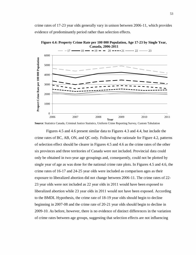
53

crime rates of 17-23 year olds generally vary in unison between 2006-11, which provides

evidence of predominantly period rather than selection effects.

Figure 4.4: Property Crime Rate per 100 000 Population, Age 17-23 by Single Year,

Canada, 2006-2011

Source: Statistics Canada, Criminal Justice Statistics, Uniform Crime Reporting Survey, Custom Tabulation

Figures 4.5 and 4.6 present similar data to Figures 4.3 and 4.4, but include the

crime rates of BC, AB, ON, and QC only. Following the rationale for Figure 4.2, patterns

of selection effect should be clearer in Figures 4.5 and 4.6 as the crime rates of the other

six provinces and three territories of Canada were not included. Provincial data could

only be obtained in two-year age groupings and, consequently, could not be plotted by

single year of age as was done for the national crime rate plots. In Figures 4.5 and 4.6, the

crime rates of 16-17 and 24-25 year olds were included as comparison ages as their

exposure to liberalized abortion did not change between 2006-11. The crime rates of 22-

23 year olds were not included as 22 year olds in 2011 would have been exposed to

liberalized abortion while 23 year olds in 2011 would not have been exposed. According

to the BMDL Hypothesis, the crime rate of 18-19 year olds should begin to decline

beginning in 2007-08 and the crime rate of 20-21 year olds should begin to decline in

2009-10. As before, however, there is no evidence of distinct differences in the variation

of crime rates between age groups, suggesting that selection effects are not influencing

0

1000

2000

3000

4000

5000

6000

2006 2007 2008 2009 2010 2011

Pro

per

t C

rim

e R

ate

per

100 0

00 P

op

ula

tion

Year

17 18 19 20 21 22 23

54

these crime rates. Instead, the year-to-year variation exhibits trends more consistent with

period effects.

Figure 4.5: Violent Crime Rate per 100 000 Population, Age 16-25 Grouped, BC AB ON

QC, 2006-2011

Source: Statistics Canada, Criminal Justice Statistics, Uniform Crime Reporting Survey, Custom Tabulation

Altogether, these time series plots do not provide compelling evidence for the

BMDL Hypothesis. The trends in the plots of both aggregate and age-specific crime rates

are more gradual than are predicted by the BMDL Hypothesis and instead appear to be

driven primarily by period effects. Time series plots are not, however, conclusive tests by

themselves. More sophisticated statistical analyses that are capable of directly linking

crime rates to lagged abortion rates are therefore required for a more rigorous test of the

BMDL Hypothesis.

0

500

1000

1500

2000

2500

3000

3500

4000

4500

5000

2006 2007 2008 2009 2010 2011

Vio

len

t C

rim

e R

ate

per

100 0

00 P

op

ula

tion

Year

16-17 18-19 20-21 24-25

55

Figure 4.6: Property Crime Rate per 100 000 Population, Age 16-25 Grouped, BC AB ON

QC, 2006-2011

Source: Statistics Canada, Criminal Justice Statistics, Uniform Crime Reporting Survey, Custom Tabulation

4.2 Descriptive Statistics

Table 4.1 reports the means and standard deviations for the violent crime rates, property

crime rates, and effective abortion rates employed in EAR analyses. The crime rates are

reported in their original, unlogged units (i.e., rates per 100 000 population). The

provincial values are the average of observations from each province across 14 years (i.e.,

1998-2011). The yearly values are the average of observations from each year across all

ten provinces. The overall means and standard deviations of violent crime rates, property

crime rates, and effective abortion rates are reported in the final row of Table 4.1.

It is important to highlight the trends of the mean effective abortion rates in Table

4.1. In accordance with the reasons argued previously, the mean effective abortion rates

for the four focal provinces are the highest values of all provinces. This provides further

support for the use of BC, AB, ON, and QC to provide the most favorable source of data

for testing the BMDL Hypothesis appropriately. A second trend worth noting is the

increase of mean effective abortion rates of each year over time. As the proportion of 12-

17 year olds who were born after the liberalization of abortion in 1988 increase, the EAR

should also increase accordingly. By virtue of its construction (i.e., Equation 1), the EAR

term should increase each year beginning in the year 2000. The values of the mean EAR

0

500

1000

1500

2000

2500

3000

3500

4000

4500

5000

2006 2007 2008 2009 2010 2011

Pro

per

ty C

rim

e R

ate

per

100 0

00 P

op

ula

tion

Year

16-17 18-19 20-21 24-25

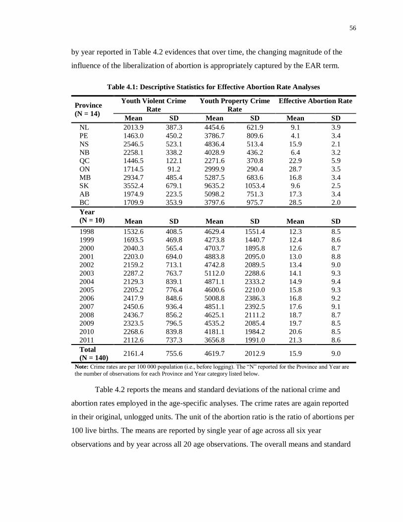
56

by year reported in Table 4.2 evidences that over time, the changing magnitude of the

influence of the liberalization of abortion is appropriately captured by the EAR term.

Table 4.1: Descriptive Statistics for Effective Abortion Rate Analyses

Province

(N = 14)

Youth Violent Crime

Rate

Youth Property Crime

Rate

Effective Abortion Rate

Mean SD Mean SD Mean SD

NL 2013.9 387.3 4454.6 621.9 9.1 3.9

PE 1463.0 450.2 3786.7 809.6 4.1 3.4

NS 2546.5 523.1 4836.4 513.4 15.9 2.1

NB 2258.1 338.2 4028.9 436.2 6.4 3.2 QC 1446.5 122.1 2271.6 370.8 22.9 5.9

ON 1714.5 91.2 2999.9 290.4 28.7 3.5

MB 2934.7 485.4 5287.5 683.6 16.8 3.4 SK 3552.4 679.1 9635.2 1053.4 9.6 2.5

AB 1974.9 223.5 5098.2 751.3 17.3 3.4

BC 1709.9 353.9 3797.6 975.7 28.5 2.0

Year

(N = 10)

Mean SD Mean SD Mean SD

1998 1532.6 408.5 4629.4 1551.4 12.3 8.5 1999 1693.5 469.8 4273.8 1440.7 12.4 8.6

2000 2040.3 565.4 4703.7 1895.8 12.6 8.7

2001 2203.0 694.0 4883.8 2095.0 13.0 8.8 2002 2159.2 713.1 4742.8 2089.5 13.4 9.0

2003 2287.2 763.7 5112.0 2288.6 14.1 9.3

2004 2129.3 839.1 4871.1 2333.2 14.9 9.4 2005 2205.2 776.4 4600.6 2210.0 15.8 9.3

2006 2417.9 848.6 5008.8 2386.3 16.8 9.2

2007 2450.6 936.4 4851.1 2392.5 17.6 9.1

2008 2436.7 856.2 4625.1 2111.2 18.7 8.7 2009 2323.5 796.5 4535.2 2085.4 19.7 8.5

2010 2268.6 839.8 4181.1 1984.2 20.6 8.5

2011 2112.6 737.3 3656.8 1991.0 21.3 8.6

Total

(N = 140) 2161.4 755.6 4619.7 2012.9 15.9 9.0

Note: Crime rates are per 100 000 population (i.e., before logging). The “N” reported for the Province and Year are

the number of observations for each Province and Year category listed below.

Table 4.2 reports the means and standard deviations of the national crime and

abortion rates employed in the age-specific analyses. The crime rates are again reported

in their original, unlogged units. The unit of the abortion ratio is the ratio of abortions per

100 live births. The means are reported by single year of age across all six year

observations and by year across all 20 age observations. The overall means and standard

57

deviations of violent crime rates, property crime rates, and abortion ratios for the entire

sample are reported in the final row of Table 4.2.

Table 4.2: Descriptive Statistics for National Age-Specific Crime Rate Analyses

Age

(N = 6)

Violent Crime Rate Property Crime Rate Abortion Ratio

Mean SD Mean SD Mean SD

12 728.2 48.3 1234.1 162.3 29.6 2.3 13 1224.0 67.6 2219.8 241.5 28.5 2.4

14 1714.6 79.8 2626.8 321.5 27.1 2.4

15 2159.6 77.5 4384.4 367.8 25.9 2.2

16 2368.5 102.5 4740.0 345.0 24.5 2.8 17 2445.0 79.0 4548.4 252.8 23.1 3.0

18 2268.8 100.2 3986.7 235.6 21.8 2.7

19 2109.6 106.2 3238.5 176.3 20.6 2.1 20 2043.7 69.5 2742.3 153.2 19.8 1.7

21 1900.5 89.3 2408.9 96.5 19.0 .7

22 1818.1 80.0 2155.5 92.5 18.7 .3 23 1727.4 88.6 1999.6 98.3 18.9 .6

24 1656.4 66.2 1890.1 99.7 18.9 .7

25 1653.5 82.4 1862.2 68.1 19.1 .7

26 1538.3 81.5 1754.5 55.8 19.2 .6 27 1506.7 78.0 1667.0 42.7 19.2 .6

28 1446.5 65.5 1611.1 46.6 18.9 1.3

29 1398.9 57.9 1514.2 42.1 18.2 1.5 30 1433.9 82.2 1540.1 80.5 17.5 1.8

31 1316.7 57.2 1376.5 54.3 16.8 1.7

Year

(N = 20)

Mean SD Mean SD Mean SD

2006 1762.6 445.6 2641.3 1193.3 19.6 3.1 2007 1616.7 410.4 2437.3 1113.4 20.2 3.4

2008 1756.6 439.8 2584.9 1209.7 20.9 3.7

2009 1795.0 445.4 2644.1 1247.8 21.6 4.1

2010 1708.7 421.6 2469.7 1123.3 22.4 4.5 2011 1698.0 417.0 2345.6 972.8 23.0 4.9

Total

(N = 120) 1722.9 425.1 2520.5 1128.1 21.3 4.1

Note: Crime rates are per 100 000 population (i.e., before logging). Abortion ratios are per 100 live births. The “N” reported for the Age and Year are the number of observations for each Age or Year category that is listed below.

The mean abortion ratio of the year prior to the year of birth of each year of age is

highest for 12 year olds and generally declines for each older year of age. Mean age-

specific violent crime rates increase from 12 year olds to a maximum for 17 year olds,

declining in each subsequent year of age until 31 year olds. Mean age-specific property

crime rates are highest for 16 year olds, declining in both younger and older ages. Prior

studies have maintained that the “high crime” years are between ages 15-25 (e.g.,

58

Donohue and Levitt 2001). These data suggest, however, that the highest mean crime

rates are more tightly clustered around younger ages, specifically around ages 16-17.

Although there is some evidence of yearly variation in crime rates, reaching a

high-point in 2009, they are relatively stable across all six years. The abortion ratio,

however, steadily increases over time as expected as more of the individuals included in

the sample are exposed to liberalized abortion over time.

Table 4.3 reports the means and standard deviations of crime and abortion rates

from the provinces BC, AB, ON, and QC, which were employed in the provincial age-

specific analyses. As in Table 4.2, the crime rates are reported in their original, unlogged

units. The unit of the abortion ratio is the ratio of induced abortions per 100 live births.

Means are reported by two-year age group across all six year observations and across all

four provinces. The means of each year are also reported by year across all ten age group

observations and across all four provinces. The means of each province are also reported

across all ten age group observations across all six years. The overall means and standard

deviations of violent crime rates, property crime rates, and abortion ratios are reported in

the final row of Table 4.3.

The trends in Table 4.3 are very similar to the trends reviewed in Table 4.2. As in

Table 4.2, the abortion ratio is highest in the youngest age group (i.e., 12-13 year olds)

and generally declines for older age groups. Also, the mean violent and property crime

rates peak in the 16-17 age group and decline in both younger and older ages as they did

in Table 4.2. The yearly mean crime rates in Table 4.3 also reach a maximum in 2009,

but again demonstrate relative stability across the six years. The abortion ratio also

steadily increased from 2006 to 2011. It is important to note, however, the differences

between Table 4.3 and Table 4.2 in abortion ratios. All of the mean abortion ratios

reported in Table 4.3 are larger in magnitude than their corresponding values in Table

4.2. As argued previously, these four provinces were selected based on the increase in

access to abortion services that they experienced after 1988. This is a critical

improvement for the proper testing of the BMDL Hypothesis. Table 4.3 provides

evidence that the use of the four focal provinces, namely BC, AB, ON, and QC,

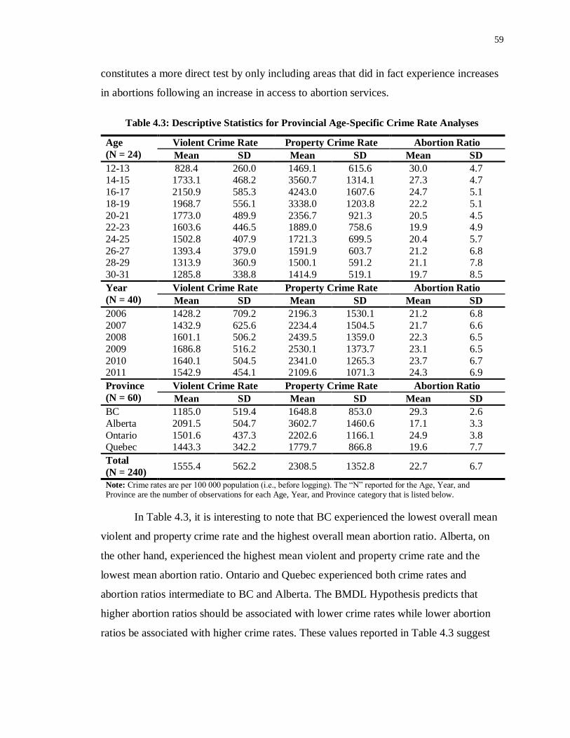
59

constitutes a more direct test by only including areas that did in fact experience increases

in abortions following an increase in access to abortion services.

Table 4.3: Descriptive Statistics for Provincial Age-Specific Crime Rate Analyses

Age

(N = 24)

Violent Crime Rate Property Crime Rate Abortion Ratio

Mean SD Mean SD Mean SD

12-13 828.4 260.0 1469.1 615.6 30.0 4.7 14-15 1733.1 468.2 3560.7 1314.1 27.3 4.7

16-17 2150.9 585.3 4243.0 1607.6 24.7 5.1

18-19 1968.7 556.1 3338.0 1203.8 22.2 5.1

20-21 1773.0 489.9 2356.7 921.3 20.5 4.5 22-23 1603.6 446.5 1889.0 758.6 19.9 4.9

24-25 1502.8 407.9 1721.3 699.5 20.4 5.7

26-27 1393.4 379.0 1591.9 603.7 21.2 6.8 28-29 1313.9 360.9 1500.1 591.2 21.1 7.8

30-31 1285.8 338.8 1414.9 519.1 19.7 8.5

Year

(N = 40)

Violent Crime Rate Property Crime Rate Abortion Ratio

Mean SD Mean SD Mean SD

2006 1428.2 709.2 2196.3 1530.1 21.2 6.8

2007 1432.9 625.6 2234.4 1504.5 21.7 6.6 2008 1601.1 506.2 2439.5 1359.0 22.3 6.5

2009 1686.8 516.2 2530.1 1373.7 23.1 6.5

2010 1640.1 504.5 2341.0 1265.3 23.7 6.7 2011 1542.9 454.1 2109.6 1071.3 24.3 6.9

Province

(N = 60)

Violent Crime Rate Property Crime Rate Abortion Ratio

Mean SD Mean SD Mean SD

BC 1185.0 519.4 1648.8 853.0 29.3 2.6

Alberta 2091.5 504.7 3602.7 1460.6 17.1 3.3

Ontario 1501.6 437.3 2202.6 1166.1 24.9 3.8 Quebec 1443.3 342.2 1779.7 866.8 19.6 7.7

Total

(N = 240) 1555.4 562.2 2308.5 1352.8 22.7 6.7

Note: Crime rates are per 100 000 population (i.e., before logging). The “N” reported for the Age, Year, and Province are the number of observations for each Age, Year, and Province category that is listed below.

In Table 4.3, it is interesting to note that BC experienced the lowest overall mean

violent and property crime rate and the highest overall mean abortion ratio. Alberta, on

the other hand, experienced the highest mean violent and property crime rate and the

lowest mean abortion ratio. Ontario and Quebec experienced both crime rates and

abortion ratios intermediate to BC and Alberta. The BMDL Hypothesis predicts that

higher abortion ratios should be associated with lower crime rates while lower abortion

ratios be associated with higher crime rates. These values reported in Table 4.3 suggest

60

the plausibility of the BMDL Hypothesis in these four provinces. Further statistical

analyses are, however, required to investigate this preliminary pattern.

4.3 Effective Abortion Rate (EAR) Analyses

The next two sections report the results of the statistical analyses that were conducted to

investigate changes in crime rates while incorporating changes in abortion rates. These

analyses constitute an improvement to the time-series plots presented above as the

variation in abortion rates is used to predict the variation in crime rates.

Table 4.4 reports the estimates of the coefficient of the EAR term (i.e., β1) in

Equation 4. The model is estimated for the annual violent and property crime rates of

youth offenders (i.e., 12-17 years of age) from all ten Canadian provinces. A one-year

lagged dependant variable term (i.e., lnCRIMEit-1) is added to the model to correct for

serial correlation and the adjusted coefficient of the EAR term (i.e., β1) is reported

beneath the original EAR coefficients. Robust standard errors are reported in parentheses

beneath coefficient estimates.

To review, these EAR analyses focus on annual youth crime rates and construct

an “effective abortion rate” for each year of crime. The EAR is the average exposure to

abortion that 12-17 year olds experienced in each year. This average is calculated by

weighting the abortion rate that each cohort experienced while in utero by the proportion

of the 12-17 year old population that each age cohort constitutes for each year.

The results of the EAR analyses provide little support for the BMDL Hypothesis.

To provide evidence for the hypothesis, all of the EAR coefficient estimates in Table 4.4

should be negative. This would suggest that an increase in the effective abortion rate

would be associated with a decline in crime rate. The EAR analyses, however, estimate

EAR coefficients that are generally not of the expected negative sign. The sole coefficient

that was negative (i.e., the property crime model without a lagged dependant variable)

was not statistically significant at the p ≤ 0.05 level. The only EAR coefficient that is

statistically significant at the p ≤ 0.05 level is from the violent crime model after a lagged

dependant variable was added. This coefficient estimates that an increase in the EAR of

61

one abortion per 100 live births is associated with a 1.4 percent increase in the youth

crime rate, which directly contradicts the BMDL Hypothesis.

Table 4.4: Analyses of the Relationship Between the Effective Abortion Rate and Youth

Crime Rates in Canada, 1998-2011

ln Violent Crime ln Property Crime

EAR (N = 140)

.014

(.012)

-.003

(.010)

EAR + lagDV

(N = 130)

.014*

(.006)

.008

(.004)

* p ≤ .05; ** p ≤ .01; *** p ≤ .001 Note: Robust standard errors are reported in parentheses beneath their respective coefficients. Please refer to Appendix C for a complete set of model outputs.

Although the results Table 4.4 provide little support for the BMDL Hypothesis,

the strategy relies on strong assumptions of the influence of abortion rates on cohorts due

to the construction of the EAR term. The EAR strategy, therefore, lacks the ability to

directly link the actual abortion rates experienced by cohorts with their crime rates

because it relies on aggregate crime rates and averaged abortion rates. To perform a more

direct test of the BMDL Hypothesis, age-specific crime rates are used to directly identify

cohorts and link their criminality with the abortion rates that they experienced while in

utero.

4.4 Age-Specific Crime Rate Analyses

Table 4.5 reports the regressions of lagged abortion rates on age-specific crime rates. The

results of the three age-specific national and provincial crime rate models discussed in

section 3.2 are reported in the six rows. Only the estimates of the coefficient of the

ABORT term (i.e., β1) from Equations 5-7 are reported. The ABORT coefficient estimates

from the national models are reported in Panel A while the estimates from the provincial

models that included only BC, AB, ON, and QC are reported in Panel B. Robust standard

errors are reported in parentheses beneath their respective coefficients.

To review, Equation 5 linked the crime rate of cohorts with the abortion rate of

the year prior to the birth of that cohort. Age, year, and provincial fixed effects were

included to control for time invariant sources of heterogeneity. To improve the model

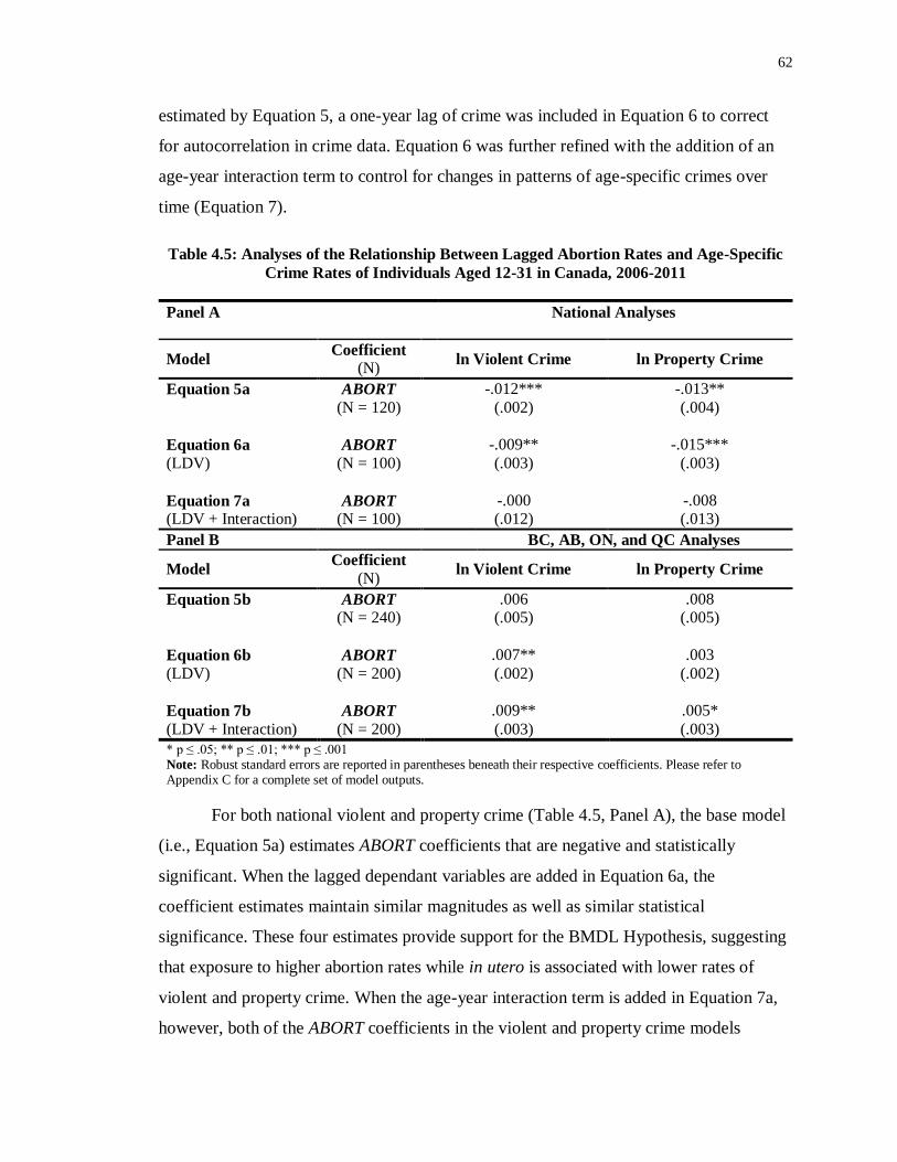
62

estimated by Equation 5, a one-year lag of crime was included in Equation 6 to correct

for autocorrelation in crime data. Equation 6 was further refined with the addition of an

age-year interaction term to control for changes in patterns of age-specific crimes over

time (Equation 7).

Table 4.5: Analyses of the Relationship Between Lagged Abortion Rates and Age-Specific

Crime Rates of Individuals Aged 12-31 in Canada, 2006-2011

Panel A National Analyses

Model Coefficient

(N) ln Violent Crime ln Property Crime

Equation 5a ABORT

(N = 120)

-.012***

(.002)

-.013**

(.004)

Equation 6a

(LDV) ABORT

(N = 100)

-.009**

(.003)

-.015***

(.003)

Equation 7a (LDV + Interaction)

ABORT (N = 100)

-.000 (.012)

-.008 (.013)

Panel B BC, AB, ON, and QC Analyses

Model Coefficient

(N) ln Violent Crime ln Property Crime

Equation 5b ABORT (N = 240)

.006 (.005)

.008 (.005)

Equation 6b

(LDV) ABORT

(N = 200)

.007**

(.002)

.003

(.002)

Equation 7b

(LDV + Interaction) ABORT

(N = 200)

.009**

(.003)

.005*

(.003)

* p ≤ .05; ** p ≤ .01; *** p ≤ .001 Note: Robust standard errors are reported in parentheses beneath their respective coefficients. Please refer to Appendix C for a complete set of model outputs.

For both national violent and property crime (Table 4.5, Panel A), the base model

(i.e., Equation 5a) estimates ABORT coefficients that are negative and statistically

significant. When the lagged dependant variables are added in Equation 6a, the

coefficient estimates maintain similar magnitudes as well as similar statistical

significance. These four estimates provide support for the BMDL Hypothesis, suggesting

that exposure to higher abortion rates while in utero is associated with lower rates of

violent and property crime. When the age-year interaction term is added in Equation 7a,

however, both of the ABORT coefficients in the violent and property crime models

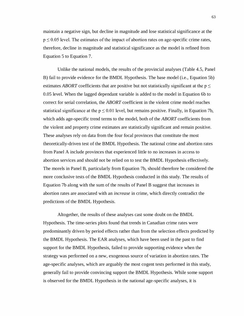
63

maintain a negative sign, but decline in magnitude and lose statistical significance at the

p ≤ 0.05 level. The estimates of the impact of abortion rates on age-specific crime rates,

therefore, decline in magnitude and statistical significance as the model is refined from

Equation 5 to Equation 7.

Unlike the national models, the results of the provincial analyses (Table 4.5, Panel

B) fail to provide evidence for the BMDL Hypothesis. The base model (i.e., Equation 5b)

estimates ABORT coefficients that are positive but not statistically significant at the p ≤

0.05 level. When the lagged dependant variable is added to the model in Equation 6b to

correct for serial correlation, the ABORT coefficient in the violent crime model reaches

statistical significance at the p ≤ 0.01 level, but remains positive. Finally, in Equation 7b,

which adds age-specific trend terms to the model, both of the ABORT coefficients from

the violent and property crime estimates are statistically significant and remain positive.

These analyses rely on data from the four focal provinces that constitute the most

theoretically-driven test of the BMDL Hypothesis. The national crime and abortion rates

from Panel A include provinces that experienced little to no increases in access to

abortion services and should not be relied on to test the BMDL Hypothesis effectively.

The morels in Panel B, particularly from Equation 7b, should therefore be considered the

more conclusive tests of the BMDL Hypothesis conducted in this study. The results of

Equation 7b along with the sum of the results of Panel B suggest that increases in

abortion rates are associated with an increase in crime, which directly contradict the

predictions of the BMDL Hypothesis.

Altogether, the results of these analyses cast some doubt on the BMDL

Hypothesis. The time-series plots found that trends in Canadian crime rates were

predominantly driven by period effects rather than from the selection effects predicted by

the BMDL Hypothesis. The EAR analyses, which have been used in the past to find

support for the BMDL Hypothesis, failed to provide supporting evidence when the

strategy was performed on a new, exogenous source of variation in abortion rates. The

age-specific analyses, which are arguably the most cogent tests performed in this study,

generally fail to provide convincing support the BMDL Hypothesis. While some support

is observed for the BMDL Hypothesis in the national age-specific analyses, it is

64

surprising that the provincial analyses, which benefitted from more theoretically direct

data, a larger sample size, and greater variation in both the dependant and independent

variables, failed to provide support for the BMDL Hypothesis. Although limitations in

the execution of this study do exist, the findings overall provide little support for the

BMDL Hypothesis and lead one to be skeptical of its validity. The increase in abortion

rates that occurred after the 1988 liberalization of abortion in Canada does not, therefore,

appear to be associated with a decline in either rates of violent or property crime.

65

Chapter 5

5 DISCUSSION AND CONCLUSION

5.1 Discussion

The purpose of this study was to test the BMDL Hypothesis on a new source of data by

taking advantage of the liberalization of abortion that occurred in Canada in 1988. Thus

far, the American literature that has surrounded the BMDL Hypothesis has been

hampered by issues of circular logic. The BMDL Hypothesis was generated to explain

the dramatic decline in crime that occurred in the US in 1990s and, therefore, should not

be tested by investigating the same crime rates of the 1990s that motivated the

development of the BMDL Hypothesis (Zimring 2007). The primary improvement that

this study offered to the literature was to focus on a new intervention in abortion

legislation, namely the 1988 liberalization of abortion services in Canada, and to then

look for evidence of an impact in a different set of crime rates.

To situate the results of this analysis, it would be beneficial to review the main

tenets of the BMDL Hypothesis. The BMDL Hypothesis argues that the legalization of

abortion increases access to abortion services by lowering the social and financial costs

of obtaining an abortion. This change in access is particularly important for women who

are socioeconomically disadvantaged, allowing them the ability to more easily abort

unwanted pregnancies. Had these unwanted pregnancies come to term, unwanted children

would have been born into adverse environments influenced by both socioeconomic

disadvantage and the effects of being an unwanted child. Children born into such

environments are disproportionately more likely to be involved in criminal activity. The

BMDL Hypothesis predicts, therefore, that individuals born after the legalization of

abortion, or more accurately, after an increase in the availability of abortion services, will

exhibit lower rates of criminality. More explicitly, the BMDL Hypothesis predicts that

birth cohorts that experienced higher rates of abortions while in utero (i.e., the year prior

to their birth), should be involved in less criminal activity, particularly during their high-

crime years between 15-25 years of age. According to the BMDL Hypothesis, then, the

increase in abortion rates that followed the liberalization of abortion services in Canada

66

in 1988 should have caused a decline in crime rates in the 1990s and 2000s for those

cohorts born after 1988. To investigate the plausibility of the BMDL Hypothesis, three of

the best strategies that have emerged in the literature were selected and employed in this

study: time series plots of crime rates, “effective abortion rate” analyses, and age-specific

crime rate analyses.

5.1.1 Time Series Plots

Many critics have been skeptical of the credibility of the BMDL Hypothesis because it

has been found to be inconsistent with time series plots of American crime rates (e.g.,

Lott and Whitley 2007; Zimring 2007; Joyce 2010). Donohue and Levitt (2004), on the

other hand, have argued that the crack-cocaine epidemic that occurred during the late

1980s and early 1990s had a such a dramatic impact on crime trends that the time series

patterns predicted by the BMDL Hypothesis have been hidden and obscured in simple

plots of crime rates. Time series plots of crime rates from this period were, therefore,

argued by Donohue and Levitt (2004) to be ineffective for visually investigating the

BMDL Hypothesis.

To avoid this issue, this study examined youth crime rates from 1998 to 2011; a

time frame that was not influenced by the crack-cocaine epidemic. Furthermore, the four

provinces (BC, AB, ON, and QC) that experienced the largest increases in the availability

of abortion services after 1988 were investigated separately. According to the BMDL

Hypothesis, time series plots of youth crime rates including only these four provinces

should display patterns that are consistent with the BMDL Hypothesis more clearly. The

time series plots of aggregated Canadian youth crime rates (Figures 4.1 and 4.2) revealed

declines in both violent and property crime rates. These trends were, however, slower and

more gradual than predicted by the BMDL Hypothesis, even when the youth crime rates

of only the four focal provinces were examined. Instead, the declines in Canadian youth

crime rates appear to be part of a larger trend of decline that was not associated with a

particular “shock” as predicted by the BMDL Hypothesis (Donohue 2008).

Time series plots of age-specific crime rates have also been critical in the

academic debate surrounding the BMDL Hypothesis because it predicts a selection effect

67

that presents in a very characteristic, cascading pattern in time series plots of age-specific

crime rates (Joyce 2010). That is, the crime rates of age groups are predicted to decline in

succession as each age group includes individuals born after 1988. The time series plots

produced in this study (Figures 4.3 to 4.6) do not, however, provide evidence of such

selection effects. The trend lines of age-specific crime rates in Figures 4.3 to 4.6 vary in

unison, providing evidence of period effects rather than selection effects.

The results of the time series plots of Canadian crime rates produced in this study

were similar to time series plots from prior American research (e.g., Lott and Whitley

2007; Joyce 2010) in that period effects seemed to be the predominant driving force

behind trends in crime. In the US, these period influences have been identified as changes

in policing and incarceration practices, demographics, the economy, and the decline of

the crack-cocaine epidemic, with varying degrees of influence and contribution (Levitt

2004; Zimring 2007). Excluding the relatively acute influence of the crack-cocaine

epidemic, these explanations were more gradual, long-term processes that influenced

American crime trends in the 1990s (Donohue 2008). In Canada, similarly gradual

explanations have been posited to influence crime rates, including the economy, alcohol

consumption, policing legislation, and changing demographics (Bunge, Johnson, and

Balde 2005). The aggregate time series plots suggested that the recent declines in crime

have been part of a larger pattern of decline. The age-specific time series plots also

suggest that more gradual period effects, rather than abrupt selection effects, have been

predominantly influencing crime trends. The time series plots produced in this study

generally support the explanation that broader and more gradual demographic,

socioeconomic, and policing-related period effects have been predominantly influencing

crime trends.

The time series plots produced in this study, combined with previous time series

plots from past research, fail to provide convincing evidence to support the BMDL

Hypothesis. To supplement the time series plots, statistical analyses were conducted to

take into account the changing rate of abortions that occurred in Canada after 1988.

68

5.1.2 Effective Abortion Rate (EAR) Analyses

To review, the “effective abortion rate” (EAR) was a constructed variable that captured

the average exposure to abortion rates that was experienced by each youth cohort for each

year of crime data. As only 23 years had elapsed from 1988 to 2011, the EAR analyses

focused on annual youth crime rates. This strategy was originally devised by Donohue

and Levitt (2001) and was used by Sen (2007) in the sole Canadian examination of the

BMDL Hypothesis. In both studies, the EAR strategy produced results in support the

BMDL Hypothesis. The EAR strategy was, therefore, replicated to test the plausibility of

the BMDL Hypothesis using the 1988 liberalization of abortion services in Canada as a

new focal intervention. Although this study only examined youth crime rates while prior

applications of the EAR strategy examined total population crime rates, differences in the

criminality of those born before and after 1988 should still be evident in this younger age

sample.

The results of the EAR analyses unanimously failed to support the BMDL

Hypothesis. Only one of four estimated coefficient was found to be statistically

significant, but was in the opposite direction from that predicted by the BMDL

Hypothesis. This result suggests that increases in the effective abortion rate are associated

with an increase in the youth violent crime rate. It is important to note that the

modifications of the EAR term used in this study still produced values that increased from

1998 to 2011 (Table 4.1), which provides evidence that the construction of the EAR term

correctly took into account the increase in abortion rates that followed the 1988

liberalization of abortion services. The lack of a negative association, therefore, should

not be attributed to the modified construction of the EAR term.

The EAR strategy has been employed in prior research to find support for the

BMDL Hypothesis in the US and Canada (e.g., Donohue and Levitt 2001; Sen 2007).

Contrary to prior applications of this strategy, however, the results of the EAR analyses

performed in the present study failed to provide support for the BMDL Hypothesis. The

strong assumptions involved in the construction of the EAR term, however, make the

EAR strategy as whole a weaker and less direct method for testing the BMDL

69

Hypothesis. Nevertheless, the effective abortion rate was not found to be negatively

associated with crime rates.

5.1.3 Age-Specific Crime Rate Analyses

The second statistical strategy employed in this study was regression analyses of age-

specific crime rates and lagged abortion rates. This strategy has been important in the

literature as it was the main strategy that Donohue and Levitt (2001; 2008) relied on to

find evidence to support the BMDL Hypothesis. To review, the crime rate of a cohort

was linked with the abortion rate of the year prior to the birth of that cohort. Regression

analyses were conducted on national crime and abortion rates and on provincial crime

and abortion rates of the four focal provinces (BC, AB, ON, and QC). To provide

evidence to support the BMDL Hypothesis, these analyses should have estimated

negative and statistically significant coefficients.

Four of the six coefficient estimates of the national age-specific analyses were

found to be both negative and statistically significant providing evidence in support of the

BMDL Hypothesis. That is, exposure to higher abortion rates while in utero was

associated with lower rates of both violent and property crime. In Equation 7a of the

national age-specific analyses, however, an age-year interaction term was added to the

model to control for changes in patterns of age-specific crimes over time. When this

interaction term was added, the coefficient estimates for both violent and property crime

lost statistical significance and declined in magnitude. It is interesting to note that as the

model was progressively improved from Equation 5a to 7a, the coefficient estimates

declined in magnitude and lost statistical significance.

Unlike the results of the national analyses, the coefficient estimates of the

provincial age-specific analyses contradicted the predictions of the BMDL Hypothesis.

Three of the six coefficient estimates from the provincial age-specific crime rate analyses

were found to be statistically significant, but none were negative. These results suggested

that exposure to higher abortion rates while in utero was associated with increases in both

violent and property crime rates. The coefficient estimates also increased in statistical

significance from Equation 5b to 7b, which was the opposite trend found in the national

70

analyses. That is, as the provincial models were refined with the addition of a lagged

dependant variable and an age-year interaction term, the coefficient estimates generally

increased in positive magnitude and gained statistical significance. As the provincial

analyses also benefitted from more theoretically direct data, a larger sample size, and

greater variation in both the dependant and independent variables, it is surprising that

these results directly contradicted the results of the national analyses and the BMDL

Hypothesis.

To interpret these conflicting results, it is important to take stock of the theoretical

rationale that motivated the age-specific crime rate analyses. The national measures of

abortion and crime rates were highly aggregated and included data from all thirteen

Canadian provinces and territories, most of which did not experience a large increase in

access to abortion services after 1988. To improve the theoretical precision of the age-

specific crime rate analyses, the models were refined (i.e., from Equation 5 to 7) and the

provinces and territories that did not experience increases in access to abortion services

or large increases in abortion rates following 1988 were removed. Four focal provinces

were, therefore, selected on the basis that they constituted the most theoretically direct set

of data to test the BMDL Hypothesis. The BMDL Hypothesis predicts that the coefficient

estimates of the provincial analyses should be larger in magnitude than the estimates of

the national analyses and that all coefficient estimates should be negative.

The results of the age-specific analyses contradict this theoretical rationale; the

coefficient estimates from the national analyses were negative and the coefficients from

the provincial analyses were positive. Under the theoretical assumption that the modeling

procedure was improved from Equation 5 to 7 and from national to provincial analyses,

one interpretation of these conflicting results is that increases in abortion rates were

actually associated with increases in crime rates. The national analyses included all

Canadian provinces, including those that did not experience an increase in access to

abortion services. Since the availability of abortion services did not increase in provinces

other than BC, AB, ON, and QC, their influence may have dampened the overall positive

association between abortion and crime. Consequently, the national analyses may have

falsely estimated negative coefficients due to this “contamination” of the data. The

71

provincial analyses, which included only provinces that experienced increases in access

to abortion services, estimated coefficients that were generally positive. Since these

analyses constituted a more direct test of the impact of abortion on crime, they were able

to reveal the “true” positive association between abortion and crime. Contrary to the

predictions of the BMDL Hypothesis, therefore, the results of these age-specific analyses

suggest that increases in access to abortion services are associated with increases in crime

rates.

This interpretation is consistent with the findings of Lott and Whitley (2007), in

which increases in abortion rates were associated with increases in murder rates. Based

on Akerlof et al (1996), Lott and Whitley (2007) argued that the legalization of abortion

in the US increased out-of-wedlock childbearing due to a decline in “shotgun marriages.”

Joyce (2010:470) explains that, “The availability of safe, legal abortion allows men to

insist that women terminate a pregnancy instead of offering marriage. Women unwilling

to terminate their pregnancies are more likely to raise the child alone. The

impoverishment of women reduces investment in their children’s human capital, which

leads to later increases in crime.” If this theory is true, it may constitute the mechanism

through which an increase in the availability of abortion services is associated with

increases in crime rates.

Kahane et al (2008) replicated Donohue and Levitt’s (2001) study in the UK and

found evidence contrary to the predictions of the BMDL Hypothesis as well. Kahane et al

(2008) performed EAR analyses that found that increases in the abortion rate were

associated with declines in property crime rates, but positively associated with violent

crime rates. They also performed age-specific crime rate analyses and found that

increases in the abortion rate were positively associated with total crime rates. They

rationalized their results using two possible explanations. First, they hypothesized that the

legalization of abortion in the UK did, in fact, reduce crime rates, but that other

unmeasured factors were obscuring their results. This would primarily be due to the

difficulties of asserting a causal link between abortion rates and crime rates that occurred

approximately 20 years apart with many other socioeconomic changes occurring

concomitantly.

72

Second, they hypothesized that the legalization of abortion was not associated

with crime rates at all, and the results of Donohue and Levitt’s (2001) were spurious and

attributable to omitted variable bias. For instance, they cited evidence from Finer and

Henshaw (2006) that in 2001, the abortion ratio for women in poverty and for women

with less than a high school education (or “at risk” women) were lower than for women

with higher incomes and college degrees in the US. Income and education may have

influenced both the propensity of women to terminate an unwanted pregnancy and the

likelihood of their children to engage in criminal activity. The authors argued that other

measures like income and education that influenced the variation in both abortion and

crime rates must be identified and explored to satisfactorily investigate the BMDL

Hypothesis.

Overall, however, Kahane et al (2008) concluded that the mixed results of their

analyses highlighted the difficulties of testing a causal link between abortion rates and

crime rates that occurred 15 to 25 years apart. They argued that to conclusively

substantiate the BMDL Hypothesis, it would be necessary to identify omitted variables

and to more closely examine the mechanisms of change that linked abortion and crime

rates within changing macro-social contexts. The myriad of social factors that influenced

both abortion and crime rates between the late 1960s to the early 2000s has made the

BMDL Hypothesis both difficult to study and substantiate. Although the limitations in

this line of research were identified, Kahane et al (2008) concluded that based on their

mixed and conflicting results, there was no consistent relationship between abortion and

crime in the UK.

The present study employed methods similar to Kahane et al (2008) and also

found mixed results concerning the BMDL Hypothesis. The, arguably, most direct test of

the BMDL Hypothesis (i.e., the provincial age-specific crime rate analyses) found a

positive relationship between the liberalization of abortion in 1988 and crime rates in the

2000s. It would be irresponsible, however, to focus solely on this single result and claim

that increasing abortion rates are conclusively associated with increasing crime rates.

Taking into consideration the results of the time series plots, the EAR analyses, and the

73

age-specific crime rate analyses together, this study instead concludes that there is no

consistent support for the BMDL Hypothesis in Canada.

5.2 Limitations

The results of the analyses conducted in this study generally do not find convincing

support for the BMDL Hypothesis. Limitations do exist, however, that must be noted and

discussed.

5.2.1 Sample Size, Methodological Constraints, and Modifications

Prior research has focused on the legalization of abortion in the US, Canada, and the UK

that occurred in the late 1960s and early 1970s and examined crime rates, in some cases,

as recent as 2003. The length of time that has elapsed between the legalization of abortion

and the crime rates of interest has allowed researchers to examine a large number of

observations by year. This study, on the other hand, focused on the liberalization of

abortion that occurred in Canada in 1988 and crime rates up to 2011. This shorter length

of time allowed for substantially fewer observations of crime rates to be included in

analyses. The US in particular affords even more variation as there are 50 states as

opposed to only 13 Canadian provinces and territories. The American population is also

substantially larger than that of Canada and, therefore, provides far more variation in

abortions and crime to investigate.

The primary practical consequence of these differences was a smaller sample size

available for analysis in this study. The EAR analyses were, therefore, restricted to

investigating only youth crime rates from 1998 to 2011. Prior American analyses that

used the EAR strategy had sample sizes of over 900 observations (e.g., Foote and Goetz

2008). As there are far fewer Canadian provinces than there are American states, both the

present study as well as Sen’s (2007) analysis included only 130 to 144 observations. The

data used in the age-specific crime rate analyses were limited even further as reliable age-

specific crime rate data were only available from 2006 on, leaving only six year of

observations for analysis. Again, prior American analyses that have used this age-specific

strategy included, in some cases, nearly 6000 observations while this study included a

maximum of 240 observations. Although concerns about the robustness of findings based

74

on these smaller samples may exist, the only way to improve this would be to allow more

time to elapse.

The present study also required modified versions of the EAR and age-specific

crime rate strategies due to various constraints. As discussed in Section 3.2, the

construction of the EAR term was based on population proportions as opposed to

Donohue and Levitt’s (2001) original construction using age-specific arrest rates because

such data were not available for Canada. Although this was a different procedure, it was

similar to the method used by Sen (2007), who was able to find evidence to support the

BMDL Hypothesis. The procedure employed in this study to construct the EAR term was,

however, arguably more parallel to Donohue and Levitt’s (2001) method and relied on

fewer assumptions than Sen’s (2007) procedure. The EAR term was also found to

correctly capture the increases in abortion rates and, therefore, should be considered a

valid implementation of the EAR strategy.

The age-specific analyses also required modifications, departing from the original

strategy used by Donohue and Levitt (2001; 2008). While national age-specific crime

rates were obtained by single year of age, provincial age-specific crime rates were

obtained in two-year age groupings, reducing the ability to isolate single age cohorts.

Furthermore, samples in prior age-specific analyses were large enough to include

complete sets of age, year, and state fixed effects along with age-year, age-state, and

state-year interaction terms in estimation models. This study, however, could only

include age, year, and province fixed effect terms due to small sample sizes. The age-year

interaction term in Equations 7a and 7b were the only interaction terms included in

models and required the use of a linear time variable to avoid issues of over-

identification. Although this study was not able to faithfully replicate prior analyses, the

full range of interaction terms could only be included if the number of observations was

substantially larger. Unfortunately, the only way to accomplish this would be to allow

more time to elapse.

75

5.2.2 Migration

International and interstate/interprovincial migration pose an issue that has not received

much attention in this study or in prior research. The threat that migration poses is the

possibility that the measures of aggregate abortion rates and aggregate crime rates do not

represent the same individuals. That is, individuals may be represented in the crime rates

of a geography while not having experienced the abortion rate of that same geography.

For instance, if an immigrant was born after 1988 in a country where access to abortion

was highly restrictive and then subsequently moved to Canada and committed a crime,

they would be represented in Canadian crime rates but would not have experienced

Canadian abortion rates while in utero. International migration may, therefore, pose a

threat to the internal validity of both this and prior studies. Research on immigrant

criminality in the US suggests, however, that immigrant crime rates tend to be

substantially lower than those of the native-born in most categories of crime (Martinez

and Lee 2000). Research on major Canadian cities, moreover has found that at the

neighbourhood level, higher concentrations of recent immigrants were either not

associated or inversely associated with crime rates (Charron 2009). If international

immigrants are not heavily represented in crime rates, then the issue of international

immigration may be of little concern for this study.

Interstate and interprovincial migration, however, poses a potentially more serious

concern. Similar to the issue of international migration, interstate and interprovincial

migration threatens the ability of the aggregated abortion and crime rates of a geography

to represent the same individuals. That is, the crime rates of a geographic area must also

represent individuals who were born there and, therefore, experienced the abortion rates

of that geographic area while in utero. This assumption is threatened if high levels of

interstate or interprovincial migration occurred in the time between the measures of crime

and abortion. Prior research has attempted to manage the issue of interstate migration in

several ways. For instance, the literature has stressed the need to use measures of abortion

by the state of residence of the women who obtained the abortion rather than by the state

of occurrence of abortions to maintain the continuity between abortion and crime rates.

Berk et al (2003) attempted to manage interstate migration by analyzing the US as a

76

whole. Donohue and Levitt (2008) used a complex weighting procedure to calculate an

abortion rate that accounted for the proportion of a state’s population that was born in a

different state. The national age-specific crime rate analyses employed in this study

avoided the issue of interprovincial migration in the same way that Berk et al (2003)

managed interstate migration by examining national measures. Since these measures

were aggregated at the national level, interprovincial migration was a non-issue. The

EAR analyses and the provincial age-specific analyses, however, employed abortion and

crime rates aggregated at the provincial level. These analyses were susceptible to the

threat of interprovincial migration. It may, therefore, be beneficial to investigate the level

of interprovincial migration that occurred between 1988 and 2011 to assess how great of

a threat it may have posed.

Table 5.1 reports average annual levels of interprovincial migration between 1988

to 2011. The average number of annual in- and out-migrants for each province and the

percentage of the provincial population constituted by interprovincial migration was

calculated. The number of interprovincial migrants under age 25 were calculated

separately because this was the demographic primarily influenced by the liberalization of

abortion in 1988. The calculations in Table 5.1 suggest that interprovincial migration has

not comprised a large proportion of average annual provincial populations, constituting

0.9 percent of provincial populations. Interprovincial migrants under age 25 constituted

an even smaller proportion, averaging 0.4 percent of annual provincial populations.

Furthermore, average interprovincial migration was relatively low in the four focal

provinces (BC, AB, ON, and QC). This suggests that interprovincial migration may not

have posed a large threat to the abortion and crime measures used in this study.

Although these percentages were low, they suggest that on average, nearly 300

000 individuals were migrating within Canada every year and over 40 percent were under

age 25. During the 23 years between 1988 and 2011, this translates to nearly seven

million interprovincial migrants; a potentially non-trivial quantity of individuals. The

impact of interprovincial migration on crime rates remains unclear, but is unfortunately

beyond the scope of this study. Interprovincial migration does, however, speak to the

issues of investigating aggregated variables separated by long periods of time. Many

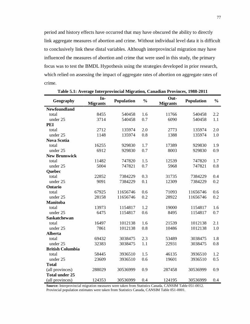
77

period and history effects have occurred that may have obscured the ability to directly

link aggregate measures of abortion and crime. Without individual level data it is difficult

to conclusively link these distal variables. Although interprovincial migration may have

influenced the measures of abortion and crime that were used in this study, the primary

focus was to test the BMDL Hypothesis using the strategies developed in prior research,

which relied on assessing the impact of aggregate rates of abortion on aggregate rates of

crime.

Table 5.1: Average Interprovincial Migration, Canadian Provinces, 1988-2011

Geography In-

Migrants Population %

Out-

Migrants Population %

Newfoundland

total 8455 540458 1.6 11766 540458 2.2

under 25 3714 540458 0.7 6090 540458 1.1

PEI

total 2712 135974 2.0 2773 135974 2.0

under 25 1148 135974 0.8 1388 135974 1.0

Nova Scotia total 16255 929830 1.7 17389 929830 1.9

under 25 6912 929830 0.7 8003 929830 0.9

New Brunswick total 11482 747820 1.5 12539 747820 1.7

under 25 5004 747821 0.7 5968 747821 0.8

Quebec total 22852 7384229 0.3 31735 7384229 0.4

under 25 9091 7384229 0.1 12309 7384229 0.2

Ontario

total 67925 11656746 0.6 71093 11656746 0.6 under 25 28158 11656746 0.2 28922 11656746 0.2

Manitoba

total 13973 1154817 1.2 19000 1154817 1.6 under 25 6475 1154817 0.6 8495 1154817 0.7

Saskatchewan

total 16497 1012138 1.6 21539 1012138 2.1

under 25 7861 1012138 0.8 10486 1012138 1.0

Alberta

total 69432 3038475 2.3 53489 3038475 1.8

under 25 32383 3038475 1.1 22931 3038475 0.8

British Columbia

total 58445 3936510 1.5 46135 3936510 1.2

under 25 23609 3936510 0.6 19601 3936510 0.5

Total

(all provinces) 288029 30536999 0.9 287458 30536999 0.9

Total under 25

(all provinces) 124353 30536999 0.4 124195 30536999 0.4

Source: Interprovincial migration measures were taken from Statistics Canada, CANSIM Table 051-0012. Provincial population estimates were taken from Statistics Canada, CANSIM Table 051-0001.

78

5.2.3 Issues related to Aggregate Measures of Abortion and Crime

This study, as well as prior research, has focused on examining aggregate abortion and

crime rates that occurred decades apart without investigating the actual causal link

between these two distal variables. This line of analysis has posed two main problems:

the difficulty of reliably linking abortion and crime rates and the lack of investigation into

the mechanisms of change. Just as with the issue of migration discussed above, prior

research has found it difficult to reliably link crime rates with the appropriate abortion

rate that was experienced by cohorts while in utero. By convention, the abortion rate of

the year prior to a cohort’s birth has been linked with the crime rates of that cohort.

Terms of pregnancy, however, generally last for nine months. This discrepancy leads to

the distinct possibility that the abortion rate of the year prior to a cohort’s birth does not

accurately capture the exposure to abortion while in utero. Individuals born late in a year,

for instance, may have been conceived in that same year. Linking their crime rates with

the abortion rate of the prior year would, therefore, not be accurate. Overall, it is very

difficult to reliably link individual exposure to abortion with rates of criminality when

employing aggregate and distal measures of abortion and crime.

The possibility of committing an ecological fallacy is always present when

examining aggregate data to make conclusions about individual behaviour and becomes

greater when aggregate measures are separated by long periods of time (Babbie 2004). In

terms of the BMDL Hypothesis, it is possible that such a fallacy may be committed

because the measure used as a proxy for the “wantedness” of cohorts has been rates of

abortions and the outcome measure has been incidents of crime aggregated, at minimum,

at the provincial level. For instance, “at risk” women may not have been obtaining

abortions at high rates and instead, non-“at risk” women may have been predominantly

driving the increase in abortion rates shortly after 1988. Evidence suggests that older

women, women with higher education, and women with higher incomes may have been

the ones more likely to take advantage of the increase in access to abortion services

(Finer and Henshaw 2006; Goldin and Katz 2002). An ecological fallacy may be

committed, therefore, if “at risk” women were producing more criminal children while

non-“at risk” women were increasing the rates of abortion.

79

The underlying assumptions for the use of abortion rates as a proxy for the

“wantedness” of cohorts are also limitations of this and prior studies. The use of this

proxy was based on the assumption that all pregnant women consider aborting an

unwanted pregnancy a real possibility. Considering the controversies over abortion,

however, this assumption is not entirely tenable. It was also assumed that after

legalization, all pregnant women had access to abortion services to the extent that they

could easily elect to abort unwanted pregnancies. The prior discussion concerning the

differential access to abortion services that women faced based on geography, however,

also demonstrates that this is a faulty assumption. Finally, it is assumed that the decline in

cost of abortion services did not affect the overall likelihood of conception. It is a real

possibility, however, that an increase in the availability of abortion services may have

influenced the likelihood of women to engage in risky sexual behaviour, consequently

increasing both pregnancy and abortion rates. Joyce (2010) has stressed that abortion is

endogenous with many other factors influencing fertility, including contraception, mores

of sexual activity, marriage, and labour supply. He argued that the factors that influence

the likelihood of unintended or unwanted pregnancy and childbearing represent a

complicated structural model.

Other critically important changes that were occurring around the same time as

the legalization of abortion may, therefore, have heavily influenced fertility. For instance,

the increase in the availability of birth control pills has been found to have decreased the

cost of investment into careers for women and increased the age at marriage for women

in the 1970s by providing greater certainty regarding the pregnancy outcomes of sexual

activity (Goldin and Katz 2002). Changes in the 1970s regarding the costs and attitudes

toward sexual activity, marriage, labour force participation, and childbearing coupled

with changes in the costs of contraception and abortion may have influenced the

likelihood of unintended pregnancy. If any of these aforementioned factors changed the

likelihood of sexual behaviour resulting in pregnancy, this may have also artificially

changed rates of abortion. In economic terms, this would represent an increase in the

demand curve of abortions while the BMDL Hypothesis argues primarily for a change in

the supply curve. Instead, Joyce (2010) argues that models that attempt to link abortion

and crime must find a method for identifying changes in abortion rates that are induced

80

only by changes in the supply curve of abortion services and not by changes in the

incidence of unwanted pregnancies. These aforementioned alternative influences may

have had dramatic effects of the likelihood of unwanted pregnancies, while the effect of

abortion primarily concerns the prevention of unwanted births. To return to the use of

abortion rates as a proxy for “unwantedness,” incorporating other endogenous factors

(e.g., levels of sexual activity or use of contraceptives) may be a more appropriate way to

investigate the BMDL Hypothesis by isolating the impact of abortion in preventing

unwanted births from the prevention of unwanted pregnancies through contraceptives.

In addition to these issues surrounding the use of abortion rates, crime rates have

also been influenced by a myriad of other socioeconomic and demographic factors.

Demographic changes, particularly the effects of relative cohort size, may represent a

potentially important influence on crime for this study. Easterlin (1987) has hypothesized

that relatively larger cohorts exhibit higher crime propensities as sources of socialization

and social control, which come primarily from older age groups, are spread thinner and

become strained. This line of research has generally attributed the rise in crime rates of

the 1960-70s to the increase in relative size of the “baby-boom” generation (South and

Messner 2000). Furthermore, as the relative size of cohorts began to decline after the

“baby-boomers,” cohort-specific delinquency rates also began to decline (Maxim 1985).

In the context of the present study, the “baby-boom” generation (i.e., born 1947-

1966) were the parents of the focal group of study, namely the “baby-boom echo”

generation, who were born between 1980-95. In 2011, the “baby-boomers” were 45-65

years of age while the “echo” was 15-30 (Figure 5.1). Following the Easterlin hypothesis,

the “echo” generation should have evidenced a lower rate of criminality because they

were relatively smaller in size. It is important to note that the cohort that was in their

“high crime” years (15-25) during the late 1980s and early 1990s, when crime rates

reached an upper maximum, were born just after the “baby-boomers” and were

approximately 35-45 years old in 2011. This cohort, or the “baby bust” generation (born

in 1967-1979), is relatively smaller than the “boomers” and relatively similar in size to

the “echo” cohort. The smaller relative size of these cohorts in comparison to the

“boomers” should, therefore, predict declines in crime rates, at least at the national level

81

of aggregation. The results of the national age-specific analyses conducted in this study

may, therefore, have been a spurious relationship that could be better explained by the

effect of relative cohort size on crime prevalence.

Figure 5.1: Population by Single Year of Age, Canada, 2011

Source: Statistics Canada, CANSIM Table 051-0001

The results of the provincial age-specific analyses, however, were of the opposite,

positive direction. Given the increases in abortion rates that occurred around 1988 and the

predictions of the Easterlin hypothesis, declines in crime should have been evident in the

provincial analyses as well. A cohort explanation may, however, also be able to make

sense of these results. The “baby-boomers” may have experienced fewer agents of social

control due to the relatively smaller size of the cohorts that preceded them. The “baby-

boom echo” cohort, however, was preceded by the larger “boomer” and “bust” cohorts.

Although this may have afforded the “echo” cohort with more agents of social control,

and consequently lower rates of crime, they were also entering a labour force saturated

with the “baby-boomers” and the “baby bust” cohorts (Foot and Stoffman 1996). The

lack of labour opportunities and the more volatile economy that the “echo” cohort faced

may have increased their likelihood of criminality. This cohort effect may explain why a

positive association between abortion and crime was found in the provincial age-specific

crime rate analyses. The lack of economic opportunity that the “echo” cohort faced may

0

100

200

300

400

500

600

0 5 10 15 20 25 30 35 40 45 50 55 60 65 70 75 80 85 90 95

Pop

ula

tion

(in

th

ou

san

ds)

Age (in years)

BOOM BUST ECHO

82

have increased their criminality and the positive association between abortion and crime

found in the provincial age-specific analyses may have been a spurious association.

This discussion on the demographic influences on crime is meant to highlight a

larger limitation with both this and the prior analyses that have engaged with the BMDL

Hypothesis. The social realities that have surrounded both abortion and crime rates at

larger, macro-levels may have had profound influences on these measures. The social,

economic, and demographic influences discussed here emphasize just some of the factors

that have influenced both abortion and crime between 1988 and 2011. Analyses that aim

to investigate the link between abortion and crime should, therefore, take these larger

factors into consideration.

Finally, the actual causal mechanism purported by the BMDL Hypothesis has

received little attention in both this and prior studies. Although no consistent relationship

between abortion and crime was found in this study, confounding period effects or

inaccuracies in linking abortion and crime rates may have diluted the effect. To

satisfactorily dismiss the BMDL Hypothesis, the theoretical links between increases in

access to abortion, increases in the “wantedness” of cohorts, and declines in crime rates

should be investigated while accounting for the myriad of external influences described

above. According to the BMDL Hypothesis, the legalization of abortion reduced the

number of “unwanted” children born into environments of socioeconomic disadvantage,

abuse, and neglect, which consequently reduced the criminality of these children.

Children who experience environments characterized by abuse, neglect, and

socioeconomic disadvantage have been repeatedly shown to have poorer cognitive,

social, behavioural, and criminal outcomes (Currie and Tekin 2012; Hildyard and Wolfe

2002; Widom 1989). The “unwantedness” of children may indeed have criminogenic

effects. Although the BMDL Hypothesis argues that less of these “unwanted” children

have been born since the legalization of abortion, the use of rates of induced abortions as

the primary explanatory variable may not be an accurate proxy for the “unwantedness” of

cohorts. The association between unwanted pregnancies and unwanted children is a

related, but theoretically separate empirical question. Future research should, therefore,

follow the theoretical links more closely and look for declines in the rates of “unwanted”

83

children born into adverse environments and declines in the likelihood of criminality for

children born into “wanted” environments in direct response to increases in access to

abortion services. This type of longitudinal investigation would require individual level

data. The lack of support for the BMDL Hypothesis at the aggregate level, however,

suggests that there is not much justification for investigating the link between abortion

and crime further.

5.3 Conclusion

The aim of this study was to test the BMDL Hypothesis using the 1988 liberalization of

abortion services in Canada. Based on a review of the literature, three main strategies

were selected that were sensitive to the increases in abortion rates that followed the 1988

liberalization of abortion services. These were time series plots of crime rates, “effective

abortion rate” analyses, and age-specific crime rate analyses. The time series plots

suggested that period effects, rather than the selection effects purported by the BMDL

Hypothesis, were the primary forces driving crime rates. The EAR analyses found no

association between the effective abortion rate and annual youth crime rates. Finally, the

age-specific crime rate analyses found mixed results that generally failed to support the

BMDL Hypothesis. The results of these analyses taken together do not provide consistent

support for the BMDL Hypothesis. Limitations of this study do exist, but are common to

this line of research and speak to the difficulties of investigating the BMDL Hypothesis

using these methods. Future research may benefit from either elucidating the causal links

between abortion and crime or using a more encompassing proxy for the latent

“unwantedness” variable. The methods and results of this study are not powerful enough

to conclusively settle the current academic debate. Nevertheless, the sheer quantity of

research that has failed to find evidence to support the BMDL Hypothesis leads one to be

highly skeptical of an association between the legalization or liberalization of abortion

and crime. Considering the controversy in the academic literature in the US, the lack of

support from the UK, and the results of the present study, the BMDL Hypothesis cannot

continue to be publically disseminated as an important influence on declines in crime

rates.

84

References

AbortionInCanada.ca. 2012. “Tax-Funded Abortions.” Retrieved January 21, 2013

(http://www.abortionincanada.ca/funding/index.html).

Akerlof, George A., Janet L. Yellen, and Michael L. Katz. 1996. “An analysis of out-of-

wedlock childbearing in the United States.” The Quarterly Journal of Economics

111(2):277-317.

Babbie, Earl. 2004. The Practice of Social Research. 10th ed. Belmont, CA:

Wadsworth/Thomson Learning.

Bala, Nicholas, Peter J. Carrington, and Julian V. Roberts. 2009. "Evaluating the Youth

Criminal Justice Act after Five Years: A Qualified Success." Canadian Journal of

Criminology and Criminal Justice 51(2):131-167.

Berk, Richard A., Susan B. Sorenson, Douglas J. Wiebe, and Dawn M. Upchurch. 2003.

“The Legalization of Abortion and Subsequent Youth Homicide: A Time Series

Analysis.” Analyses of Social Issues and Public Policy 3(1):45-64.

Bouza, Anthony V. 1990. The Police Mystique: An Insider's Look at Cops, Crime, and

the Criminal Justice System. New York: Plenum Press.

Brandon, Karen. 1999. “Abortion, Reduced Crime Linked.” The Chicago Tribune,

August 08, pp. 1.

Browne, Alister and Bill Sullivan. 2005. “Abortion in Canada.” Cambridge Quarterly of

Healthcare Ethics 14:287-291.

Bunge, Valerie P., Holly Johnson, and Thierno A. Balde. 2005. “Exploring crime patterns

in Canada.” Canadian Centre for Justice Statistics and Time Series Research and

Analysis Centre, Statistics Canada.

Canadian Institute for Health Information. 2003. “Privacy Impact Assessment of the

Therapeutic Abortions Database.”.

Canadians for Choice. n.d. “Access at a Glance: Abortion Services in Canada.” Retrieved

January 21, 2013

(http://www.canadiansforchoice.ca/Access%20at%20a%20Glance%20-

%20Abortion%20Services%20in%20Canada.pdf).

85

Carrington, Peter J. and Jennifer L. Schulenberg. 2005. “The Impact of the Youth

Criminal Justice Act on Police Charging Practices with Young Persons: A

Preliminary Statistical Assessment.” Department of Justice Canada.

Charron, Mathieu 2009. “Neighbourhood Characteristics and the Distribution of Police-

reported Crime in the City of Toronto.” in Crime and Justice Research Paper

Series. Statistics Canada Catalogue no. 85-561-M, no. 18.

Committee on the Operation of the Abortion Law. 1977. “Report of the Committee on the

Operation of the Abortion Law.” Supply and Services Canada, Ottawa.

Currie, Janet and Erdal Tekin. 2012. “Understanding the Cycle: Childhood Maltreatment

and Future Crime.” Journal of Human Resources 2(509-549):47.

Donohue, John J. 2008. “Book Review: The Great American Crime Decline, Franklin E.

Zimring.” Punishment & Society 10(3):333-337.

Donohue, John J. and Steven D. Levitt. 2000. “The Impact of Legalized Abortion on

Crime.” NBER Working Paper Series No. 8004.

Donohue, John J. and Steven D. Levitt. 2001. “The impact of legalized abortion on

crime.” The Quarterly Journal of Economics 116(2):379-420.

Donohue, John J. and Steven D. Levitt. 2003. “Further Evidence that Legalized Abortion

Lowered Crime: A Reply to Joyce.” NBER Working Paper Series No. 9532.

Donohue, John J. and Steven D. Levitt. 2004. “Further Evidence that Legalized Abortion

Lowered Crime: A Reply to Joyce.” The Journal of Human Resources 39(1):29-49.

Donohue, John J. and Steven D. Levitt. 2006. “Measurement Error, Legalized Abortion,

and the Decline in Crime: A Response to Foote and Goetz (2005).” NBER Working

Paper Series No. 11987.

Donohue, John J. and Steven D. Levitt. 2008. “Measurement Error, Legalized Abortion,

and the Decline in Crime: A Response to Foote and Goetz.” The Quarterly Journal

of Economics 123(1):425-440.

Easterlin, Richard A. 1987. Birth and Fortune: The Impact of Numbers on Personal

Welfare. 2nd

ed. Chicago: University of Chicago Press.

Erdman, Joanna N. 2007. “In the back alleys of health care: abortion, equality, and

community in Canada.” Emory Law Journal 56:1093-1156.

86

Finer, Lawrence B. and Stanley K. Henshaw. 2006. “Disparities in Rates of Unintended

Pregnancy in the United States, 1994 and 2001.” Perspectives on Sexual and

Reproductive Health 38(2):90-96.

Fitzgerald, Robin, Michael Wisener, and Josee Savoie 2004. “Neighbourhood

characteristics and the distribution of crime in Winnipeg.” in Crime and Justice

Research Paper Series. Ottawa: Statistics Canada Catalogue no. 85-561-

MIE2004004.

Foote, Christopher L. and Christopher F. Goetz. 2008. “The Impact of Legalized

Abortion on Crime: Comment.” The Quarterly Journal of Economics 123(1):407-

423.

Foot, David K. and Daniel Stoffman. 1996. Boom Bust and Echo: How to Profit from the

Coming Demographic Shift. Toronto, ON: Macfarlane Walter & Ross.

Forssman, Hans and Inga Thuwe. 1966. “One Hundred and Twenty Children Born After

Application for Therapeutic Abortion Refused: Their mental health, social

adjustment and educational level up to the age of 21.” Acta psychiatrica

Scandinavica 42(1):71-88.

Freakonomics, LLC. 2011. “Freakonomics: The Hidden Side of Everything.” Retrieved

December 15, 2012 (www.freakonomics.com).

Gabor, Thomas. 1999. “Trends in youth crime: Some evidence pointing to increases in

the severity and volume of violence on the part of young people.” Canadian

Journal of Criminology 41:385-392.

Gannon, Marie and Canadian Centre for Justice Statistics. 2001. Feasibility Study on

Crime Comparisons between Canada and the United States. Ottawa: Canadian

Centre for Justice Statistics.

Goldin, Claudia and Lawrence F. Katz. 2002. “The Power of the Pill: Oral

Contraceptives and Women's Career and Marriage Decisions.” Journal of Political

Economy 110(4):730-770.

Grogger, Jeff and Michael Willis. 2000. "The Emergence of Crack Cocaine and the Rise

of Urban Crime Rates." The Review of Economics and Statistics 82(4):519-529.

Hildyard, Kathryn L. and David A. Wolfe. 2002. “Child neglect: developmental issues

and outcomes.” Child Abuse & Neglect 26:679-695.

87

Jones, Rachel K., Mia R. S. Zolana, Stanley K. Henshaw, and Lawrence B. Finer. 2008.

“Abortion in the United States: Incidence and Access to Services, 2005.”

Perspectives on Sexual and Reproductive Health 40(1):6-16.

Joyce, Theodore J. 2001. “Did Legalized Abortion Lower Crime?” NBER Working Paper

Series No. 8319.

Joyce, Theodore J. 2004a. “Did Legalized Abortion Lower Crime?” The Journal of

Human Resources 39(1):1-28.

Joyce, Theodore J. 2004b. “Further Tests of Abortion and Crime.” NBER Working Paper

Series No. 10564.

Joyce, Theodore J. 2006. “Further Tests of Abortion and Crime: A Response to Donohue

and Levitt (2001, 2004, 2006).” NBER Working Paper Series No. 12607.

Joyce, Theodore J. 2009. “A Simple Test of Abortion and Crime.” The Review of

Economics and Statistics 91(1):112-123.

Joyce, Theodore J. 2010. “Abortion and crime: a review.” Pp. 452-487 in Handbook on

the Economics of Crime, edited by Bruce L. Benson and Paul R. Zimmerman.

Northampton, MA: Edward Elgar.

Joyce, Theodore J., Ruoding Tan, and Yuxiu Zhang. 2012. “Back to the Future? Abortion

Before & After Roe.” NBER Working Paper Series No. 18338.

Kahane, Leo H., David Paton, and Rob Simmons. 2008. “The Abortion-Crime Link:

Evidence from England and Wales.” Economica 75(297):1-21.

Leigh, Andrew and Justin Wolfers. 2000. “Abortion and Crime.” Australian Quarterly

72(4):28-30.

Levitt, Steven D. 2004. “Understanding Why Crime Fell in the 1990s: Four Factors that

Explain the Decline and Six that Do Not.” Journal of Economic Perspectives

18(1):163-190.

Levitt, Steven D. and Stephen J. Dubner. 2005. Freakonomics: A Rogue Economist

Explores the Hidden Side of Everything. 1st ed. New York: William Morrow.

Lott, John R. and John Whitley. 2007. “Abortion and crime: unwanted children and out-

of-wedlock births.” Economic Inquiry 45(2):304-324.

Martinez, Ramiro and Matthew T. Lee. 2000. “On Immigration and Crime.” Criminal

Justice 1(1):486-524.

88

Maxim, Paul S. 1985. “Cohort Size and Juvenile Delinquency: A Test of the Easterlin

Hypothesis.” Social Forces 63(3):661-681.

Moody, Carlisle E. and Thomas B. Marvell. 2010. “On the Choice of Control Variables

in the Crime Equation.” Oxford Bulletin of Economics and Statistics 72(5):696-715.

Morgentaler, Henry. 1999. “Abortion and Violence.” The Humanist 59(2):40.

National Abortion Federation. 2010. “Abortion Coverage by Region.” Retrieved January

21, 2013 (http://www.prochoice.org/canada/regional.html).

O'Brien, Robert M., Jean Stockard, and Lynne Isaacson. 1999. “The Enduring Effects of

Cohort Characteristics on Age-Specific Homicide Rates, 1960-95.” American

Journal of Sociology 104(4):1061-1095.

Pop-Eleches, Cristian. 2006. “The Impact of an Abortion Ban on Socioeconomic

Outcomes of Children: Evidence from Romania.” Journal of Political Economy

114(4):744-773.

Rossi, Alice S. and Peter H. Rossi. 1990. Of Human Bonding: Parent-Child Relations

Across the Life Course. Hawthorne, New York: Aldine de Gruyter.

Sen, Anindya. 2007. “Does Increased Abortion Lead to Lower Crime? Evaluating the

Relationship between Crime, Abortion, and Fertility.” The B.E. Journal of

Economic Analysis & Policy 7(1):1-36.

South, Scott J. and Steven F. Messner. 2000. “Crime and Demography: Multiple

Linkages, Reciprocal Relations.” Annual Review of Sociology 26:83-106.

Statistics Canada. 2006. Induced abortions in hospitals and clinics, by area of report and

type of facility performing the abortion, Canada, provinces and territories, annual

(number), 1970-2006, CANSIM Table no. 106-9005.

Statistics Canada. 2006. Induced abortions in hospitals and clinics, by area of residence

of patient, Canada, provinces and territories, 1970-2006, CANSIM Table no. 106-

9013.

Statistics Canada. 2009. “Data Accuracy.” Definitions, data sources and methods,

Therapeutic Abortion Survey. Retrieved March 24, 2013

(http://www23.statcan.gc.ca/imdb/p2SV.pl?Function=getSurvey&lang=en&db=im

db&adm=8&dis=2&SDDS=3209#a3).

89

Statistics Canada. 2012. Estimates of population by sex and age group for July 1, Canada,

provinces and territories, annual (persons), CANSIM Table no. 051-0001.

Statistics Canada. 2012. Government transfers and income tax, by economic family type

and after-tax income quintiles, 2010 constant dollars, annual, CANSIM Table no.

202-0704.

Statistics Canada. 2012. Incident-based crime statistics, by detailed violations, annual

(number), CANSIM Table no. 252-0051.

Statistics Canada. 2012. Persons in low income families, annual, CANSIM Table no.

202-0802.

Statistics Canada. 2013. Labour force survey estimates (LFS), by sex and detailed age

group, annual, CANSIM Table no. 282-0002.

Statistics Canada. 2013. Sales of alcoholic beverages by volume, value per capita 15

years and over, fiscal years ended March 31, annual, CANSIM Table no. 183-0006.

Statistics Canada. 2013. Youth correctional services, average counts of young persons in

provincial and territorial correctional services, annual, CANSIM Table no. 251-

0008.

US Commission on Population Growth and the American Future. 1972. Population and

the American Future. Washington, DC: US Government Printing Office.

Vieraitis, Lynne M., Tomislav V. Kovandzic, and Thomas B. Marvell. 2007. “The

criminogenic effects of improsonment: evidence from state panel data, 1974-2002.”

Crriminology & Public Policy 6(3):589-622.

Widom, Cathy S. 1989. “Child Abuse, Neglect, and Violent Criminal Behaviour.”

Criminology 27(2):251-271.

Wooldridge, Jeffrey M. 2006. Introductory Econometrics: A Modern Approach. 3rd

ed.

Mason, Ohio: Thomson Higher Education.

Zimring, Franklin E. 2007. The Great American Crime Decline. New York: Oxford

University Press.

Zimring, Franklin E., Gordon Hawkins, and Sam Kamin. 2001. Punishment and

Democracy: Three Strikes and You're Out in California. New York: Oxford

University Press.

90

Appendices

Appendix A: Trend Graphs of Abortions and Abortion Ratios, Canada and

Provinces, 1970-2006

0

20000

40000

60000

80000

100000

120000

0

5

10

15

20

25

30

35

1970

1972

1974

1976

1978

1980

1982

1984

1986

1988

1990

1992

1994

1996

1998

2000

2002

2004

2006

Nu

mb

er o

f In

du

ced

Ab

ort

ion

s

Rati

o o

f In

du

ced

Ab

ort

ion

s p

er 1

00 L

ive

Bir

ths

Year

Canada

Ratio Number

0

200

400

600

800

1000

1200

0

5

10

15

20

25

1970

1972

1974

1976

1978

1980

1982

1984

1986

1988

1990

1992

1994

1996

1998

2000

2002

2004

2006

Nu

mb

er o

f In

du

ced

Ab

ort

ion

s

Rati

o o

f In

du

ced

Ab

ort

ion

s p

er 1

00 L

ive

Bir

ths

Year

Newfoundland and Labrador

Ratio Number

91

0

20

40

60

80

100

120

140

160

180

200

0

2

4

6

8

10

12

14

1970

1972

1974

1976

1978

1980

1982

1984

1986

1988

1990

1992

1994

1996

1998

2000

2002

2004

2006

Nu

mb

er o

f In

du

ced

Ab

ort

ion

s

Rati

o o

f In

du

ced

Ab

ort

ion

s p

er 1

00 L

ive

Bir

ths

Year

Prince Edward Island

Ratio Number

0

500

1000

1500

2000

2500

0

5

10

15

20

25

1970

1972

1974

1976

1978

1980

1982

1984

1986

1988

1990

1992

1994

1996

1998

2000

2002

2004

2006

Nu

mb

er o

f In

du

ced

Ab

ort

ion

s

Rati

o o

f In

du

ced

Ab

ort

ion

s p

er 1

00 L

ive

Bir

ths

Year

Nova Scotia

Ratio Number

92

0

200

400

600

800

1000

1200

0

2

4

6

8

10

12

14

16

1970

1972

1974

1976

1978

1980

1982

1984

1986

1988

1990

1992

1994

1996

1998

2000

2002

2004

2006

Nu

mb

er o

f In

du

ced

Ab

ort

ion

s

Rati

o o

f In

du

ced

Ab

ort

ion

s p

er 1

00 L

ive

Bir

ths

Year

New Brunswick

Ratio Number

0

5000

10000

15000

20000

25000

30000

35000

0

5

10

15

20

25

30

35

40

45

50

1970

1972

1974

1976

1978

1980

1982

1984

1986

1988

1990

1992

1994

1996

1998

2000

2002

2004

2006

Nu

mb

er o

f In

du

ced

Ab

ort

ion

s

Rati

o o

f In

du

ced

Ab

ort

ion

s p

er 1

00 L

ive

Bir

ths

Year

Quebec

Ratio Number

93

0

5000

10000

15000

20000

25000

30000

35000

40000

45000

50000

0

5

10

15

20

25

30

35

40

1970

1972

1974

1976

1978

1980

1982

1984

1986

1988

1990

1992

1994

1996

1998

2000

2002

2004

2006

Nu

mb

er o

f In

du

ced

Ab

ort

ion

s

Rati

o o

f In

du

ced

Ab

ort

ion

s p

er 1

00 L

ive

Bir

ths

Year

Ontario

Ratio Number

0

500

1000

1500

2000

2500

3000

3500

4000

0

5

10

15

20

25

30

1970

1972

1974

1976

1978

1980

1982

1984

1986

1988

1990

1992

1994

1996

1998

2000

2002

2004

2006

Nu

mb

er o

f In

du

ced

Ab

ort

ion

s

Rati

o o

f In

du

ced

Ab

ort

ion

s p

er 1

00 L

ive

Bir

ths

Year

Manitoba

Ratio Number

94

0

500

1000

1500

2000

2500

0

2

4

6

8

10

12

14

16

18

1970

1972

1974

1976

1978

1980

1982

1984

1986

1988

1990

1992

1994

1996

1998

2000

2002

2004

2006

Nu

mb

er o

f In

du

ced

Ab

ort

ion

s

Ra

tio o

f In

du

ced

Ab

ort

ion

s p

er 1

00 L

ive

Bir

ths

Year

Saskatchewan

Ratio Number

0

2000

4000

6000

8000

10000

12000

14000

0

5

10

15

20

25

30

1970

1972

1974

1976

1978

1980

1982

1984

1986

1988

1990

1992

1994

1996

1998

2000

2002

2004

2006

Nu

mb

er o

f In

du

ced

Ab

ort

ion

s

Rati

o o

f In

du

ced

Ab

ort

ion

s p

er 1

00 L

ive

Bir

ths

Year

Alberta

Ratio Number

95

Source: Statistics Canada, Therapeutic Abortion Survey, CANSIM Table no. 106-9005

Note: Nunavut officially separated from the Northwest Territories in 1999, creating discontinuity

in the abortion data and, therefore, were not included in this set of graphs.

0

2000

4000

6000

8000

10000

12000

14000

16000

18000

0

5

10

15

20

25

30

35

40

45

1970

1972

1974

1976

1978

1980

1982

1984

1986

1988

1990

1992

1994

1996

1998

2000

2002

2004

2006

Nu

mb

er o

f In

du

ced

Ab

ort

ion

s

Ra

tio o

f In

du

ced

Ab

ort

ion

s p

er 1

00 L

ive

Bir

ths

Year

British Columbia

Ratio Number

0

20

40

60

80

100

120

140

160

180

200

0

5

10

15

20

25

30

35

40

45

50

1970

1972

1974

1976

1978

1980

1982

1984

1986

1988

1990

1992

1994

1996

1998

2000

2002

2004

2006

Nu

mb

er o

f In

du

ced

Ab

ort

ion

s

Rati

o o

f In

du

ced

Ab

ort

ion

s p

er 1

00 L

ive

Bir

ths

Year

Yukon

Ratio Number

96

Appendix B: Uniform Crime Reporting Incident-based Survey (UCR2) categories

included in the EAR and age-specific analyses

Categories included in the violent crime rate

Homicide

- Murder, first degree

- Murder, second degree

- Manslaughter

- Infanticide

Other violations causing death

- Criminal negligence causing death

- Other related violations causing death

Attempted murder

Sexual assault, level 3, aggravated

Sexual assault, level 2, weapon or bodily harm

Sexual assault, level 1

Sexual violations against children

- Sexual interference

- Invitation to sexual touching

- Sexual exploitation

- Luring a child via a computer

Assault, level 3, aggravated

Assault, level 2, weapon or bodily harm

Assault, level 1

Assaults against a peace officer

Other assaults

- Unlawfully causing bodily harm

- Criminal negligence causing bodily harm

- Other assaults

Firearms; use of, discharge, pointing

- Discharge firearm with intent

- Using firearm in commission of offence

- Pointing a firearm

Robbery

- Robbery

- Robbery to steal a firearm

Forcible confinement or kidnapping

- Forcible confinement

- Kidnapping

Abduction

- Abduction under the age 14, not parent or guardian

- Abduction under the age 16

- Removal of children from Canada

- Abduction under the age 14 contravening a custody order

- Abduction under the age 14, by parent or guardian

97

Extortion

Criminal harassment

Uttering threats

Threatening or harassing phone calls

Other violent violations

- Conspire to commit murder

- Other sexual violations

- Sexual exploitation of a person with a disability

- Incest

- Corrupting morals of a child

- Anal intercourse

- Bestiality, commit or compel person

- Voyeurism

- Trap likely to or causing bodily harm

- Hostage-taking

- Trafficking in persons

- Intimidation of a justice system participant or a journalist

- Intimidation of a non-justice participant

- Explosives causing death or bodily harm

- Arson, disregard for human life

- Other violent violations

Categories included in the property crime rate

Breaking and entering

- Breaking and entering

- Breaking and entering to steal a firearm

- Break and enter to steal a firearm from a motor vehicle

Possession of stolen property

- Possess stolen property

- Possession of stolen goods over $5000

- Possession of stolen goods $5000 or under

Trafficking in stolen goods

- Traffic stolen goods over $5000 (including intent)

- Traffic stolen goods under $5000 (including intent)

Theft of motor vehicle

- Theft of motor vehicle over $5000

- Theft of motor vehicle $5000 or under

- Motor vehicle theft

Theft over $5000 (non-motor vehicle)

- Theft over $5000

- Theft over $5000 from a motor vehicle

- Shoplifting over $5000

Theft under $5000 (non-motor vehicle)

- Theft $5000 or under

- Theft $5000 or under from a motor vehicle

- Shoplifting $5000 or under

98

Fraud

Identity theft

Identity fraud

Mischief

- Mischief

- Mischief to religious property motivated by hate

Arson

Altering/removing/destroying vehicle identification number (VIN)

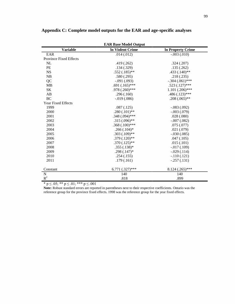
99

Appendix C: Complete model outputs for the EAR and age-specific analyses

EAR Base Model Output

Variable ln Violent Crime ln Property Crime

EAR .014 (.012) -.003 (.010)

Province Fixed Effects

NL .419 (.262) .324 (.207)

PE .134 (.329) .135 (.262)

NS .552 (.185)** .433 (.140)**

NB .580 (.295) .218 (.235)

QC -.091 (.093) -.304 (.061)***

MB .691 (.165)*** .523 (.127)***

SK .978 (.260)*** 1.101 (.206)***

AB .296 (.160) .486 (.123)***

BC -.019 (.086) .208 (.065)**

Year Fixed Effects 1999 .087 (.125) -.083 (.092)

2000 .280 (.101)** -.003 (.079)

2001 .348 (.094)*** .028 (.080)

2002 .315 (.096)** -.007 (.082)

2003 .368 (.100)*** .075 (.077)

2004 .266 (.104)* .021 (.079)

2005 .303 (.109)** -.030 (.085)

2006 .379 (.120)** .047 (.105)

2007 .370 (.125)** .015 (.101)

2008 .355 (.138)* -.017 (.109)

2009 .298 (.147)* -.029 (.114) 2010 .254 (.155) -.110 (.121)

2011

.179 (.161) -.257 (.131)

Constant 6.771 (.327)*** 8.124 (.265)***

N 140 140

R2 .818 .899

* p ≤ .05; ** p ≤ .01; *** p ≤ .001 Note: Robust standard errors are reported in parentheses next to their respective coefficients. Ontario was the

reference group for the province fixed effects. 1998 was the reference group for the year fixed effects.

100

EAR with Lagged Dependant Variable Model Output

Variable ln Violent Crime ln Property Crime

EAR .014(.006)* .008(.004)

Province Fixed Effects

NL .362(.121)** .275(.089)**

PE .315(.146)* .295(.102)**

NS .364(.083)*** .276(.062)**

NB .420(.135)** .271(.096)***

QC .041(.040) -.050(.038)

MB .381(.086)*** .256(.063)***

SK .552(.130)*** .519(.110)***

AB .227(.071)** .241(.060)*** BC -.024(.027) .040(.024)

Year Fixed Effects

1999 omitted omitted

2000 .136(.056)* .138(.034)***

2001 .075(.058) .108(.033)**

2002 -.005(.056) .046(.037)

2003 .065(.064) .148(.035)***

2004 -.078(.070) .027(.039)

2005 .020(.076) .006(.046)

2006 .064(.066) .111(.054)*

2007 -.004(.068) .018(.043)

2008 -.021(.072) -.002(.044) 2009 -.077(.071) .001(.044)

2010 -.092(.075) -.079(.048)

2011

-.147(.080) -.174(.061)**

LDV .656(.075)*** .714(.073)***

Constant 2.169(.558)*** 2.009(.612)**

N 130 130

R2 0.926 0.966

* p ≤ .05; ** p ≤ .01; *** p ≤ .001 Note: Robust standard errors are reported in parentheses next to their respective coefficients. Ontario was the

reference group for the province fixed effects. 1998 was the reference group for the year fixed effects. The year 1999 was omitted by STATA due to collinearity

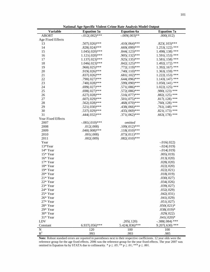
101

National Age-Specific Violent Crime Rate Analysis Model Output

Variable Equation 5a Equation 6a Equation 7a

ABORT -.012(.002)*** -.009(.003)** .000(.012)

Age Fixed Effects

13 .507(.026)*** .410(.064)*** .823(.103)***

14 .828(.024)*** .669(.099)*** 1.253(.122) ***

15 1.045(.020)*** .844(.123)*** 1.498(.138) ***

16 1.121(.020)*** .905(.132)*** 1.591(.153) ***

17 1.137(.023)*** .925(.135)*** 1.581(.158) ***

18 1.046(.023)*** .842(.125)*** 1.492(.172) ***

19 .960(.025)*** .772(.119)*** 1.392(.167) ***

20 .919(.026)*** .740(.110)*** 1.363(.159) *** 21 .837(.026)*** .681(.102)*** 1.222(.153) ***

22 .790(.027)*** .644(.096)*** 1.143(.147) ***

23 .740(.028)*** .599(.090)*** 1.050(.141) ***

24 .699(.027)*** .571(.086)*** 1.022(.125) ***

25 .698(.027)*** .572(.086)*** .980(.123) ***

26 .627(.028)*** .516(.077)*** .882(.125) ***

27 .607(.029)*** .501(.075)*** .817(.128) ***

28 .562(.028)*** .468(.070)*** .760(.128) ***

29 .521(.030)*** .438(.066)*** .761(.148) ***

30 .537(.029)*** .435(.069)*** .821(.173) ***

31 .444(.032)*** .371(.062)*** .663(.178) ***

Year Fixed Effects 2007 -.081(.010)*** omitted

2008 .012(.008) .109(.012)***

2009 .040(.008)*** .118(.010)***

2010 .001(.008) .073(.011)***

2011 .002(.009) .082(.010)***

Year -.016(.022)

13*Year -.024(.019)

14* Year -.014(.019)

15* Year .005(.019)

16* Year .013(.020)

17* Year .028(.020) 18* Year .022(.020)

19* Year .022(.021)

20* Year .018(.019)

21* Year .030(.027)

22* Year .034(.026)

23* Year .039(.027)

24* Year .032(.029)

25* Year .042(.031)

26* Year .041(.029)

27* Year .051(.027)

28* Year .050(.021)*

29* Year .038(.019)* 30* Year .029(.022)

31* Year .041(.020)*

LDV .205(.120) -.388(.084) ***

Constant 6.937(.056)*** 5.424(.836)*** 9.207(.630) ***

N 120 100 100

R2 .993 .993 .985

Note: Robust standard errors are reported in parentheses next to their respective coefficients. 12 year olds were the

reference group for the age fixed effects. 2006 was the reference group for the year fixed effects. The year 2007 was omitted in Equation 6a by STATA due to collinearity. * p ≤ .05; ** p ≤ .01; *** p ≤ .001.

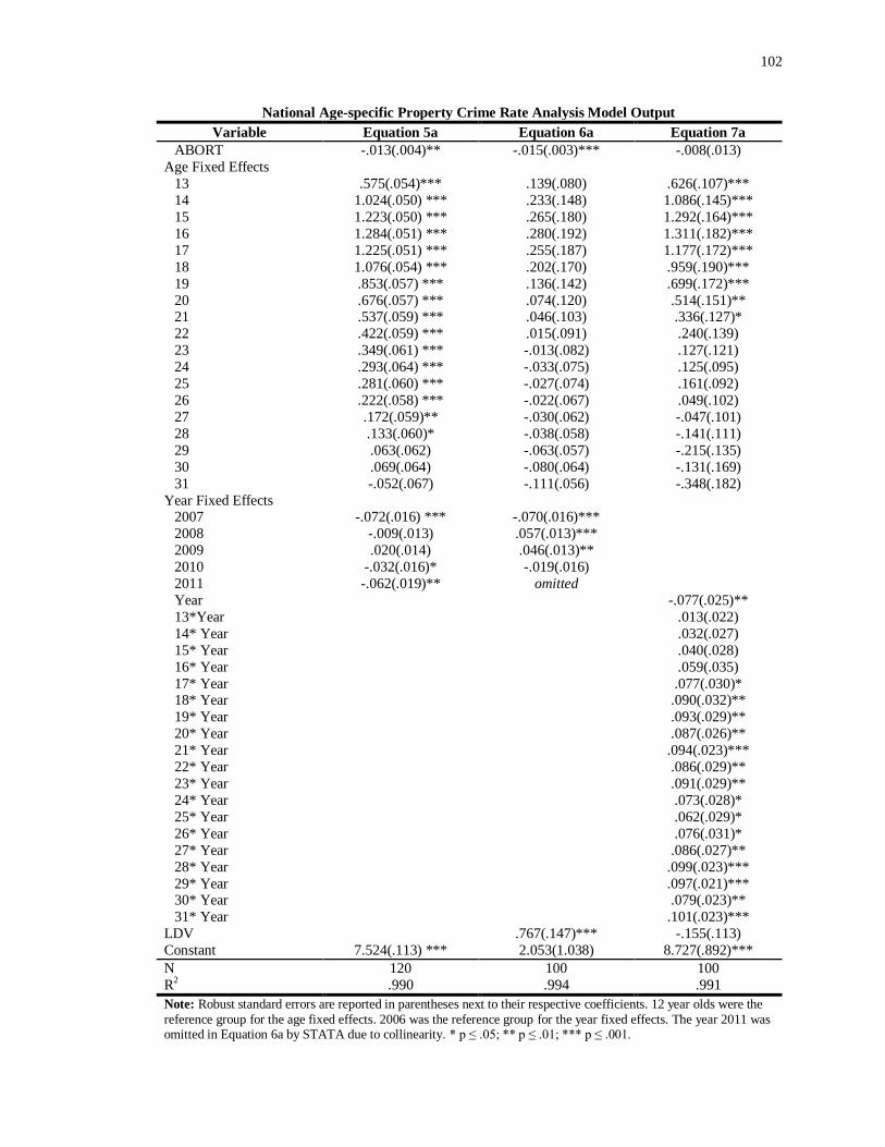
102

National Age-specific Property Crime Rate Analysis Model Output

Variable Equation 5a Equation 6a Equation 7a

ABORT -.013(.004)** -.015(.003)*** -.008(.013)

Age Fixed Effects

13 .575(.054)*** .139(.080) .626(.107)***

14 1.024(.050) *** .233(.148) 1.086(.145)***

15 1.223(.050) *** .265(.180) 1.292(.164)***

16 1.284(.051) *** .280(.192) 1.311(.182)***

17 1.225(.051) *** .255(.187) 1.177(.172)***

18 1.076(.054) *** .202(.170) .959(.190)***

19 .853(.057) *** .136(.142) .699(.172)***

20 .676(.057) *** .074(.120) .514(.151)** 21 .537(.059) *** .046(.103) .336(.127)*

22 .422(.059) *** .015(.091) .240(.139)

23 .349(.061) *** -.013(.082) .127(.121)

24 .293(.064) *** -.033(.075) .125(.095)

25 .281(.060) *** -.027(.074) .161(.092)

26 .222(.058) *** -.022(.067) .049(.102)

27 .172(.059)** -.030(.062) -.047(.101)

28 .133(.060)* -.038(.058) -.141(.111)

29 .063(.062) -.063(.057) -.215(.135)

30 .069(.064) -.080(.064) -.131(.169)

31 -.052(.067) -.111(.056) -.348(.182)

Year Fixed Effects 2007 -.072(.016) *** -.070(.016)***

2008 -.009(.013) .057(.013)***

2009 .020(.014) .046(.013)**

2010 -.032(.016)* -.019(.016)

2011 -.062(.019)** omitted

Year -.077(.025)**

13*Year .013(.022)

14* Year .032(.027)

15* Year .040(.028)

16* Year .059(.035)

17* Year .077(.030)* 18* Year .090(.032)**

19* Year .093(.029)**

20* Year .087(.026)**

21* Year .094(.023)***

22* Year .086(.029)**

23* Year .091(.029)**

24* Year .073(.028)*

25* Year .062(.029)*

26* Year .076(.031)*

27* Year .086(.027)**

28* Year .099(.023)***

29* Year .097(.021)*** 30* Year .079(.023)**

31* Year .101(.023)***

LDV .767(.147)*** -.155(.113)

Constant 7.524(.113) *** 2.053(1.038) 8.727(.892)***

N 120 100 100

R2 .990 .994 .991

Note: Robust standard errors are reported in parentheses next to their respective coefficients. 12 year olds were the

reference group for the age fixed effects. 2006 was the reference group for the year fixed effects. The year 2011 was omitted in Equation 6a by STATA due to collinearity. * p ≤ .05; ** p ≤ .01; *** p ≤ .001.

103

Provincial Age-specific Violent Crime Rate Analysis Model Output

Variable Equation 5b Equation 6b Equation 7b

ABORT .006(.005) .007(.002)** .009(.003)**

Age Fixed Effects

14-15 .776(.085)*** .328(.038)*** .296(.106)**

16-17 1.011(.087)*** .436(.045) *** .393(.127)**

18-19 .937(.097) *** .416(.046) *** .363(.129)**

20-21 .849(.101) *** .386(.048) *** .290(.126)*

22-23 .752(.106) *** .357(.047) *** .238(.124)

24-25 .687(.105) *** .330(.045) *** .192(.113)

26-27 .608(.103) *** .293(.047) *** .148(.120)

28-29 .546(.107) *** .275(.044) *** .145(.115) 30-31 .538(.110) *** .261(.047) *** .153(.138)

Year Fixed Effects

2007 .058(.073) .038(.020)

2008 .220(.067)** .162(.023) ***

2009 .269(.070)*** .111(.016) ***

2010 .237(.070)** .046(.014)**

2011 .175(.069)* omitted

Linear Year and Interaction

Year -.044(.020)*

14-15*Year .008(.024)

16-17*Year .011(.027)

18-19*Year .014(.026) 20-21*Year .026(.026)

22-23*Year .033(.026)

24-25*Year .037(.024)

26-27*Year .039(.025)

28-29*Year .035(.024)

30-31*Year .030(.027)

Province Fixed Effect

QC .003(.041) .051(.017)** .060(.018)**

AL .383(.051)*** .207(.025)*** .217(.029)***

BC -.351(.062)*** .062(.019)** .059(.021)**

LDV

.602(.030)*** .611(.044)***

Constant 6.297(.207)*** 2.308(.215)*** 2.441(.340)***

N 240 200 200

R2 .721 .953 .936

* p ≤ .05; ** p ≤ .01; *** p ≤ .001 Note: Robust standard errors are reported in parentheses next to their respective coefficients. 12-13 year olds were the reference group for the age fixed effects. 2006 was the reference group for the year fixed effects. Ontario was the reference group for the province fixed effects. The year 2011 was omitted in Equation 6b by STATA due to collinearity

104

Provincial Age-specific Property Crime Rate Analysis Model Output

Variable Equation 5b Equation 6b Equation 7b

ABORT .008(.005) .003(.002) .005(.003)*

Age Fixed Effects

14-15 .926(.087)*** .385(.050)*** .308(.140)*

16-17 1.113(.089)*** .475(.056)*** .394(.142)**

18-19 .904(.100)*** .386(.057)*** .233(.166)

20-21 .567(.104)*** .242(.050)*** .025(.136)

22-23 .357(.101)** .151(.047)** -.069(.121)

24-25 .261(.101)* .096(.049) -.136(.122)

26-27 .185(.096) .079(.046) -.115(.111)

28-29 .122(.096) .048(.045) -.173(.116) 30-31 .081(.106) .032(.050) -.166(.138)

Year Fixed Effects

2007 .058(.074) .050(.019)**

2008 .199(.066)** .156(.021)***

2009 .229(.068)** .103(.014)***

2010 .144(.070)* omitted

2011 .054(.068) -.039(.017)*

Linear Year and Interaction

Year -.078(.017)***

14-15*Year .015(.026)

16-17*Year .017(.027)

18-19*Year .037(.030) 20-21*Year .057(.025)*

22-23*Year .059(.022)**

24-25*Year .063(.021)**

26-27*Year .053(.021)*

28-29*Year .060(.020)**

30-31*Year .055(.022)*

Province Fixed Effect

QC -.156(.038)*** -.057(.020)** -.042(.024)

AL .603(.049)*** .250(.030)*** .253(.036)***

BC -.334(.064)*** .071(.021)** .071(.021)**

LDV

.595(.044)*** .619(.057)***

Constant 6.806(.202)*** 2.712(.353)*** 2.836(.478)***

N 240 200 200

R2 .836 .973 .967

* p ≤ .05; ** p ≤ .01; *** p ≤ .001 Note: Robust standard errors are reported in parentheses next to their respective coefficients. 12-13 year olds were the reference group for the age fixed effects. 2006 was the reference group for the year fixed effects. Ontario was the reference group for the province fixed effects. The year 2010 was omitted in Equation 6b by STATA due to collinearity

105

Appendix D: EAR Analysis Robustness Checks

The present study relied on two statistical strategies that have emerged from the

econometric debate to test the BMDL Hypothesis. Past research that has employed

similar strategies have included an assortment of covariates, but consistency has not been

maintained between each study (Berk et al. 2003; Moody and Marvell 2010). The present

study, therefore, did not elect to include any covariates other than the fixed effects

variables. Covariates that have been found in past research to predict crime rates at

statistically significant levels were, however, employed here to check the robustness of

the abortion coefficient estimates.

Two main sources were used to select potentially important covariates. Moody

and Marvell (2010) conducted a case study using the BMDL Hypothesis to explain their

method of selecting control variables, called the “general-to-specific (GETS) winnowing

of controls.” They found that three control variables were able to predict the US violent

crime rate at a significance level of p<0.05. These were the property crime arrest rate,

real welfare payments per capita lagged 15 years, and the three-strikes law. They found

that five control variables could predict the US property crime rate at a significance level

of p<0.05. These were the crack-cocaine index, the one-gun-per-month law, the percent

of the population that was 5-14 years old, the prison population per capita, and the

Saturday night special ban.

As Sen’s (2007) study was the sole Canadian investigation of the BMDL

Hypothesis, it was also selected to find potentially important control variables for this

robustness check. In Sen’s (2007) analysis, he found that the employment rate was able to

predict the Canadian violent crime rate at a significance level of p<0.05. He also found

that the employment rate, the average beer consumption, and the percent of low-income

families were able to predict the Canadian property crime rate at a significance level of

p<0.05.

These covariates that have been identified were added to the EAR analyses

conducted in the present study to check the robustness of the abortion coefficient

estimates because both prior studies (i.e., Moody and Marvell 2010 and Sen 2007) also

employed the EAR strategy. Canadian data that best approximated the covariates used by

Moody and Marvell (2010) were searched for and identified. For the violent crime rate,

the youth property crime rate (PROPERTY) was used instead of the property crime arrest

rate because the EAR analysis in the present study only focused on youth crime rates.

The average annual government transfers to the lowest income quintile (lagged 15 years)

(TRANSFER) was used as a proxy for real welfare payments per capita lagged 15 years.

A dummy variable capturing the Tackling Violent Crime Bill (2008) (TVCB) was used as

it was the Canadian change in law that was most similar to the American three-strike

106

laws. For the property crime rate, the percent of the population 5-14 years of age was

included. The youth incarceration rate per 10 000 young persons was used as a proxy for

the prison population per capita because, as mentioned previously, the EAR analysis in

the present study only focused on youth crime rates. A proxy for the crack-cocaine index

was not sought in the present study because such Canadian data were unavailable and, as

argued in the main text, the crack-cocaine epidemic was not a major influence in Canada

during the study time frame, between 1998-2011. No proxies for the one-gun-per-month

law or the Saturday night special ban were included because there was also no similar

legislation during the study time frame, between 1998-2011.

Data that best approximated the covariates used by Sen (2007) were also

identified. The teen employment rate (i.e., age 15-19) (EMP15-19) was used instead of

the employment rate because the EAR analysis in the present study only focused on

youth crime rates. The data for average beer consumption and the percent of low-income

families were identical to that used by Sen (2007). The results of the EAR analyses after

the aforementioned covariates were included are presented below for violent and property

crime separately.

EAR Base Model Output

Variable ln Violent Crime ln Property Crime

EAR .017 (.007)* .014 (.011)

Province Fixed Effects

NL -.155 (.058) .340 (.095)***

PE -.011 (.149) .872 (.186)***

NS -.219 (.223) 1.038 (.232)***

NB .305 (.146)* .470 (.175)**

QC .064 (.066) .140 (.165)

MB .437 (.180)* .460 (.266)

SK .226 (.123) .632 (.176)*** AB .066 (.210) .549 (.276)*

BC .134 (.141) .848 (.291)**

Year Fixed Effects

1999 .159 (.073)* omitted

2000 .267 (.061)*** .067 (.071)

2001 .298 (.054)*** .072 (.083)

2002 .299 (.058)*** .046 (.095)

2003 .268 (.068)*** .160 (.089)

2004 .204 (.058)** .130 (.105)

2005 .294 (.056)*** .114 (.125)

2006 .297 (.060)*** .148 (.150)

2007 .315 (.064)*** -.000 (.155) 2008 .001 (.063) -.069 (.169)

2009 -.049 (.049) -.066 (.168)

2010 -.023 (.045) -.164 (.196)

2011 omitted -.356 (.221)

PROPERTY .000(.000)***

TRANSFER .000(.000)

TVCB .332(.077)***

EMP15-19 -.002(.004) .005(.005)

107

POP5-14 -6.655(7.035)

INCPOP .023(.006)***

BEER -.015(.006)*

LOWINC -.025(.012)*

Constant 5.992 (.316)*** 9.390 (.994)***

N 140 125

R2 .924 .934

* p ≤ .05; ** p ≤ .01; *** p ≤ .001 Note: Robust standard errors are reported in parentheses next to their respective coefficients. Ontario was the reference group for the province fixed effects. 1998 was the reference group for the year fixed effects.

EAR with Lagged Dependant Variable Model Output

Variable ln Violent Crime ln Property Crime

EAR .017(.005)*** .012(.005) Province Fixed Effects

NL -.105(.033)** .095(.064)

PE .090(.087) .451(.102)***

NS .006(.154) .612(.131)***

NB .305(.090)*** .337(.103)**

QC .102(.035)** .099(.092)

MB .430(.116)*** .326(.145)*

SK .259(.077)*** .336(.105)**

AB .254(.133) .415(.134)**

BC .224(.102)* .449(.161)**

Year Fixed Effects

1999 omitted omitted 2000 .109(.049)* .136(.037)***

2001 .075(.050) .116(.044)*

2002 .038(.051) .067(.057)

2003 .055(.058) .186(.059)**

2004 -.051(.055) .086(.077)

2005 .056(.058) .090(.098)

2006 .065(.054) .188(.114)

2007 .043(.055) .071(.118)

2008 .058(.043) .040(.130)

2009 -.006(.037) .057(.145)

2010 .004(.028) -.019(.152) 2011 omitted -.137(.183)

LDV .410(.076)*** .648(.083)***

PROPERTY .000(000)***

TRANSFER .000(.000)

TVCB -.008(.069)

EMP15-19 -.004(.003) .000(.003)

POP5-14 -5.051(4.896)

INCPOP .006(.005)

BEER -.007(.003)*

LOWINC -.013(.010)

Constant 3.629(.506)*** 2.009(.612)**

N 130 125

R2 0.951 0.967

* p ≤ .05; ** p ≤ .01; *** p ≤ .001 Note: Robust standard errors are reported in parentheses next to their respective coefficients. Ontario was the reference group for the province fixed effects. 1998 was the reference group for the year fixed effects. The year 1999 was omitted by STATA due to collinearity

108

After the aforementioned covariates were added to the EAR models, the re-

estimated results of EAR analyses did not differ significantly from the original EAR

estimates. Only one coefficient estimate changed signs (i.e., property crime base model)

and the change was from a negative to a positive direction. The coefficient estimates did

generally increased in magnitude, but it was only in the positive direction. Considering

these results, the exclusion of these covariates may have actually suppressed the positive

association between abortion and crime. This suggests that the original EAR analyses

may represent a conservative estimate of the association between abortion and crime. The

results of this robustness check further reinforce the finding in this study and further fail

to support the BMDL Hypothesis.

109

Curriculum Vitae

Name: Timothy Kang

Post-secondary The University of Western Ontario Education and London, Ontario, Canada

Degrees: 2011-2013 M.A. (Program and Policy Evaluation Specialization)

The University of Toronto

Toronto, Ontario, Canada

2005-2011 H.B.A. (with Distinction)

Honours and Graduate Thesis Research Award

Awards: The University of Western Ontario

2012-2013

Western Graduate Research Scholarship

The University of Western Ontario 2011-2012

Related Work Graduate Student Representative, Departmental Assembly

Experience The University of Western Ontario 2012-2013

Teaching Assistant The University of Western Ontario

2011-2013

Theory and Practice of University Teaching, GS9500

Teaching Support Centre (UWO)

2012