Public and Private Provision under Asymmetric Information: Ability to Pay and Willingness to Pay Simona Grassi European University Institute Max Weber Programme Via delle Fontanelle, 10 I-50014 San Domenico [email protected] November 2008 Acknowledgement: I am very grateful to Albert Ma for his help and support. I also thank seminar participants at the Economics Department of the European University Institute for their comments.

Welcome message from author
This document is posted to help you gain knowledge. Please leave a comment to let me know what you think about it! Share it to your friends and learn new things together.
Transcript

Public and Private Provisionunder Asymmetric Information:
Ability to Pay and Willingness to Pay
Simona Grassi
European University Institute
Max Weber Programme
Via delle Fontanelle, 10
I-50014 San Domenico
November 2008
Acknowledgement: I am very grateful to Albert Ma for his help and support. I also thank seminarparticipants at the Economics Department of the European University Institute for their comments.

Abstract
I model the concept of affordability. Different consumers derive different benefits in utility unit from
the consumption of an indivisible good, such as education or health-care or housing. The benefit from
consumption is the willingness to pay for the good. Different consumers have different abilities to pay for
the good and cannot borrow money in the credit market. Consumers with high willingness to pay may not
afford the good at a given price. The market allocation is inefficient. The public sector has a budget, but
it is insufficient to supply all consumers for free. It observes consumers’ wealth and implements a policy to
maximize the sum of consumers’ utilities subject to the wealth constraints. I consider two optimal policies:
rationing and subsidization. First I study the public supplier as the sole provider of the good. Any rationing
policy that exhausts the budget is optimal. The optimal subsidy scheme requires cross subsidization: rich
consumers pay a price greater than marginal cost, and some poor consumers pay less than marginal cost.
The budget and the revenue collected from rich consumers funds the subsidies for poor consumers. I also
study the equilibrium of a simultaneous moves game where the public sector interacts with a firm in the
provision of the good. The firm chooses a price function based on consumers’ benefit, but does not observe
abilities to pay. In the highest welfare equilibrium of the game where the public supplier chooses a rationing
policy, the budget is spent on supplying the good for free to poor consumers. If the budget is very high, the
firm sets a price higher than the monopoly price. In the equilibrium of the game where the public sector
chooses subsidies, cross subsidization is impossible. The public supplier and the private firm compete a la
Bertrand. The firm sets a constant price equal to the marginal cost and prevents the public supplier to set
prices above marginal cost to wealthier consumers.
2

1 Introduction
In 2008, more than 40 millions Americans are without health insurance. According to the U.S. Department
of Housing and Urban Development, in 2007 there were more than 600,000 homeless persons in the USA.1 In
the United Kingdom, in 2007, only 28% of students enrolled in a higher education programme came from low
income families.2 Almost every government around the world is concerned with the affordability of health
care, housing and higher education. As these data suggest, many people in developed countries, and even
more in less developed countries, cannot afford to pay for goods like health care, education and housing.
This can not be an efficient outcome. This paper models the notion of affordability and applies it to the
consumption of indivisible goods such as education, health-care treatments or housing.
In this paper, I explicitly separate willingness to pay and ability to pay as different concepts. I define
willingness to pay by the benefit of consumption. I define ability to pay by the available income for con-
sumption. In the standard neoclassical approach to the consumer’s utility maximization problem, ability to
pay consists of the budget available and determines the consumer’s willingness to pay. A poor consumer is
willing to pay less than a richer consumer. This setup is inadequate to study the problem of affordability.
A consumer who derive a high benefit from the consumption of a good may be willing to pay an expensive
price even though his budget is limited. Ability to pay is a constraint that prevents the consumer to take
decisions according to his willingness to pay, when the capital market is imperfect, and does not determine
the potential benefit from the consumption of the good.
I use a setup where willingness and ability to pay are separate and independent variables to study the
design of optimal wealth-based public provision policies of goods that are sold also in a private market. I
also model the interaction between the public sector and the market. The analysis applies to the education,
health-care and housing markets. Governments in almost every countries intervene in these sectors; course of
studies, health care treatments and housing units can be modeled as indivisible goods which are consumed in
either 1 or zero quantity; they are simultaneously provided in the private markets. The rationale for public
1HUD’s July 2008 3rd Homeless Assessment Report to Congress
2See http://www.berr.gov.uk/dius/science/page40318.html
1

intervention is usually based on externalities, on the existence of market failures that make these good too
expensive to some or all consumers, or also on a merit good or ideological argument. The main problem
that underlines government’s intervention is that too many people cannot afford to pay for these goods. I
consider a government with scarce resources who tries to allocate a private indivisible good, like health care
or education or housing, to consumers who are wealth constrained. The budget available is not enough to
provide the good for free to all consumers.
Consumers are different in two dimensions: the benefit from consumption, that is also their willingness
to pay, and their ability to pay for the good. Consumers differ in the benefit from consumption of the
same good. The benefit from a course of studies depends on the student’s aptitude; different patients may
derive different utilities from illness recovery; the same house confers different benefits to families with
different compositions. Ability to pay is interpreted as consumers’ disposable wealth. This is the fraction of
consumers’ wealth set aside to pay for the good.
In the efficient allocation those who benefit most from consumption should be assigned the good. I
am concerned with the following problem: it often happens that some consumers who benefit a lot from
the consumption of a good may not have enough resources to purchase it in the market and may not be
able to borrow because of capital market imperfections. The perfectly competitive market allocation where
consumers buy the good at the market clearing price would then be inefficient. Consumers who are willing
to pay the equilibrium price but cannot afford to pay, are left unserved. Affordability calls for government
intervention.
In this paper the government can affect the allocation of the good through public provision. In many
countries we observe public schools, public hospitals, public housing. The non market allocation implemented
by the government depends on the available information. I consider wealth-based assignments (also called
need-based) where the nonmarket allocation of the good is based on consumers’ wealth. It is reasonable
to assume that the government derives wealth information from tax returns. The public supplier does not
observe or use consumers’ benefit information. The administrative body in charge of the budget allocation
may not have access to the benefit information. The government may also commit explicitly to a wealth-based
2

policy ignoring the benefit information.
There are many examples of wealth-based assignment in the education, health-care and housing markets.
Often tuition fees or scholarships in public universities depend on the household’s wealth; access to subsidized
health care is conditioned on wealth, as in the Medicaid program in the US; public housing are assigned
to poor families. Wealth-based allocation are often justified by a redistributive argument. The concern for
poor consumers in this paper is implicit in the notion of affordability and the government is not interested
in income redistribution when it deals with the design of a public provision policy. Allocating the good to
poor consumers here can only be justified by an efficiency argument and is a result of the analysis.
In the model the government, or public supplier, allocates the good in two ways. Either it rations some
consumers and provide the good for free to the others, or it sets a price and let the consumers decide if
purchasing the good or not. Both policies are based on consumers’ wealth. The subsidy scheme is a general
version of the rationing policy, given that the subsidized price can always be set to be equal to zero. I analyze
the optimal policy of the public sector when it is the sole supplier of the good. I also study the equilibrium
of the game where the public supplier interacts with a private firm.
The optimal rationing policy implemented by the public supplier when it is the sole provider of the good
is a random lottery. Any allocation that exhausts the budget is optimal. Consumers’ utility function is
linear in ability to pay, hence income redistribution is not a concern of the policy maker. I have in mind that
redistribution is implemented by general taxation and the disposable wealth is net of taxes. Lotteries are
a common mechanism to allocate scarce resources. Immigration visas, conscripts for military services, jury
duties, but also access to housing units are sometimes allocated through lotteries (see Che and Gale 2006.)
If consumers have access to a private market for the good, the equilibrium rationing policy changes. I
model the interaction between the public supplier and a monopolistic firm as a simultaneous-move game.
I let the firm observe consumers’ benefit but not consumers’ wealth. The firm has no right in asking the
consumers their wealth, but often times the firm can observe consumers’ benefits and price discriminates.
This makes the affordability problem even more important. In the game, the public supplier chooses a
rationing function based on wealth. The private firm chooses a price function based on benefit. The game
3

has multiple equilibria. The equilibrium outcome where the budget is exhausted to supply poor consumers
achieves the highest welfare . Richer consumers are rationed and decide to purchase or not from the private
firm. If the budget is very large, in the best equilibrium the firm sets a price higher than the monopoly price.
When the public supplier interacts with the firm, the wealth information is used to maximize welfare. When
deciding between a rich or poor consumer, the public sector prefers to ration the rich who is more likely to
afford the price set by the firm. Supplying the poor is efficient.
When the public supplier sets a subsidy scheme, the contrast between the optimal policy and the equi-
librium of the game is very interesting. When the public supplier is the sole provider, the optimal subsidy
scheme requires cross subsidization from the rich to the poor. If the public sector interacts with the firm,
cross subsidization is impossible. Without the private firm, the public supplier sets a constant price to richer
consumers and a price that equals ability to pay to poorer consumers. Not all consumers are supplied,
though. Poor consumers with ability to pay below the constant marginal cost and who are asked to pay a
price equal to their ability to pay, are subsidized. The cost of the subsidy increases as ability to pay decreases.
The balance between benefit from consumption and cost of the subsidy determines a lowest ability to pay
level below which no consumer is supplied. The cost of the subsidies is recovered from the budget but also
from the price paid by rich consumers, when the budget size is small. When the budget size is small, richer
consumers pay a price greater than marginal cost and cross subsidize poorer consumers. Redistribution
between rich and poor consumers is efficient.
Cross subsidization is not feasible when there is a private firm. In the game, the public supplier chooses
prices based on consumers’ available wealth and the firm selects prices according to benefit. The public
supplier and the firm compete à la Bertrand and the firm sets the price at marginal cost in equilibrium. This
prevents the public supplier to set a price above marginal cost to richer consumers. Under the assumptions
of the model, a pure private provision is welfare superior to a mixed system of provision. This result is novel
and differs from the usual conclusion in the literature on public provision of private goods, which supports
mixed3 system of provision against pure public provision.
3Mixed provision of private goods means that there exist public provision but also a market for the same good.
4

The focus of this paper is affordability of an indivisible good. The literature has already analyzed how
credit subsidies and taxes can alleviate the wealth constraint. Redistributing cash to consumers would induce
everybody to claim that they need the good, and would require a mechanism to elicit real preferences. In
kind transfers have been proved to be superior to cash transfers in the presence of asymmetric information
(see Blackorby and Donaldson, 1988). In other words, if benefits are not observed, cash transfers does not
help in achieving efficiency. This paper is related, on one hand, to the literature on wealth constraints and
inefficient allocations (among others, Che and Gale, 2006) and on the other, to the literature on the public
(and the mixed) provision of private goods. The analysis sheds light on the drawbacks of the mixed provision
of private goods. In equilibrium, the mutual best responses of the public supplier and the firm are such that
prices in the market may raise or that cross subsidization is infeasible. Compared to the case when the public
supplier is the sole provider of the good, with mixed provision the middle class consumers are penalized when
prices raise, while poor consumers are worse off when cross subsidization is impossible. These results appear
to be novel.
Section 2 and its subsections lay out the model and describe the firm’s choice of the profit maximizing
prices when there is no public sector. In Section 3, I derive the optimal policies of the public sector when
it is the sole provider of the good and I lay out the extensive-form games between consumers, the public
supplier, and the private firm. In Section 4 and 5 I describe the games and derive the equilibria respectively
when the public supplier chooses a rationing and subsidy policy. The last Section draws some conclusions.
An Appendix contains all proofs.
2 The model
I begin with the description of consumers. Next, I introduce a private sector and then a public sector. I also
derive the profit maximizing prices chosen by the firm when the public sector is inactive.
2.1 Consumers
There is a continuum of consumers, with a total mass normalized to 1. Each consumer may consume at
most one unit of an indivisible good. A consumer has disposable wealth w and obtains benefit when he
5

consumes the good. Disposable wealth w is generally different from consumer total wealth. I have in mind
that w is the amount of wealth that a consumer sets aside to pay for goods such as education or medical
treatments or housing. Each unit of the good may give different perceived benefits to different consumers.
One can think of a course of study as an indivisible good that confers different benefits to different students
depending on their aptitude. In the health markets, a medical treatment may heal an illness that causes
different disutilities to different patients. In the housing market, one can think of a house that confers
different benefits according to household compositions.
I let w and be random variables. Respectively, the variables w and have supports on the positive
intervals [w,w] and£,¤. Let F and f be the distribution and density functions of w; let G and g be the
distribution and density functions of . I assume that f(w) and g( ) are strictly positive and hence F (w) and
G( ) are strictly increasing. I will assume that these distributions are independent. I also assume that the
ratio [1−G( )] /g( ) is strictly increasing in . I introduce β to denote the average benefit in the population,
β ≡R
g( )d .
A consumer type (w, ) has utility U = w − if he does not consume the good. If the good costs p,
the utility of a consumer type (w, ) if he buys the good is U = w − p. The good confers a benefit of in
utility units but reduces disposable wealth by p. The consumer buys the good when w − ≥ w − p, that
implies > p, and the price p is affordable, w > p. In the health care setting, is like the loss of illness
in utility units. If a sick consumer goes without a course of treatment, his utility is w − ; if he pays p to
obtain treatment his utility becomes w − p. In the education setting, the variable measures his loss from
not obtaining a course of study in utility units. In the housing setting, is the loss without housing.
In this setup, disposable wealth w and benefit are easily interpreted as respectively the consumer’s
ability to pay and his willingness to pay for the good. Consumer (w, ) cannot pay more than w. His
willingness to pay to get one unit of the good is since the good can eliminate that loss. Since w and are
independently distributed, a consumer who has a high willingness to pay may be not rich enough to afford
the good. In the paper I refer to w either as ability to pay or wealth.
6

2.2 The private sector and profit-maximizing prices
I let there be a single firm in the private sector. I assume that the monopolist observes consumers’ willingness
to pay for the good but does not know their ability to pay. The consumer’s benefit and hence willingness
to pay may be evident to the specialist who provides the service. A high test score in the case of education
or the clinical history of the patient in the case of health-care treatment are good signals of the student’s
or patient’s benefit. The private firm has no right in asking the consumer about his ability to pay, though.
Consumers may misreport their w when asked, if they expect the information on w to be used to determine
the price.
The monopolist maximizes profits by setting a price to sell to consumers, given the cost c. Even though
for some services the provision cost may well depend on consumer characteristics, here I assume that the
cost level c is the same for all consumers and do not consider cost selection issues.4 I let c satisfy w< c < w
and < c < . For now, assume that the monopolist may have access to the entire mass of consumers. If
none of the consumers were wealth constrained, each would be asked to pay a price equal to his willingness
to pay. Now suppose that consumer (w, ) cannot pay more than w. For a given level of , the firm sets a
price p ≤ and all consumers with ability to pay w greater than p buy the good.
The profit function is
π(p; ) ≡Z w
p
f(w)dw (p− c) = [1− F (p)] [p− c] , (1)
given the constraint p ≤ . Let the profit-maximizing choice pm : [ , ]→ R+ be
pm( ) ≡ argmaxp
[1− F (p)] [p− c] ; ≥ p ≥ c . (2)
The profit function is differentiable in p and the first order condition for a maximum is −f(p) [p− c] +
[1− F (p)]. I assume that [1 − F (w)]/f(w) is strictly decreasing in w. Alternatively I can assume that the
profit function is quasi-concave. Hence the solution exists and is unique at any . The next Lemma describes
the profit maximizing price function.
4See Chapter 1 and 2 for the analysis of cost selection.
7

Lemma 1 The profit maximizing price function pm( ) is weakly increasing in . The monopolist sets a
constant price p∗m, with p∗m = c + 1−F (p∗m)f(p∗m) , to consumers with willingness to pay higher than p∗m:
pm( ) = p∗m, all ≥ p∗m. The profit maximizing price function is pm( ) = for consumers with willingness
to pay between marginal cost c and p∗m: pm( ) = , all c ≤ < p∗m. No consumers with below marginal
cost c are supplied by the firm.
When the monopolist observes a consumer with high willingness to pay , he would like to price discrim-
inate and obtain the highest price the consumer is willing to pay. However, the monopolist does not observe
ability to pay and by setting a high price he may lose too many consumers with insufficient ability to pay.
The monopolist prefers to set the price at a constant level p∗m to consumers with high willingness to pay.
When the monopolist observes a lower , he perfectly price discriminates because the expected demand at a
lower price is sufficiently high. The Figure (1) represents the profit maximizing price function pm( ).
)(lp
c
o45
mp*
l
Figure 1: Pure monopoly price pm( ).
2.3 The public sector
The public supplier has a fixed budget B > 0, but the budget is insufficient to supply the good to all
consumers for free. That means B < c. The cost c is the same across the public and the private sector.
The public supplier observes consumers’ ability to pay w. It is reasonable to assume that the public sector
derives the information from the tax return. Willingness to pay information is either not available or, even
if available, cannot be used. Very often the public sector commits to universal provision. Alternatively,
8

the decision to allocate the service is taken by an administrative body which is not in charge of the actual
provision and therefore cannot observe the benefit from consumption.
I consider two ways to allocate the budget for providing the good to consumers. First, the public supplier
uses a nonprice rationing rule. Consumers supplied by the public sector obtain the good for free. Second,
the public supplier chooses a subsidy policy consisting of a price schedule. The nonprice rationing rule is a
special case of the price-based policy. I sometimes refer to the price-based policy as pricing policy or subsidy
policy.
Random rationing consists of a function θ : [w,w]→ [0, 1]. Consumers with ability to pay w are assigned
the good for free with probability [1− θ(w)].56 The rationing rule θ modifies the density f so that at w,
[1− θ(w)]f(w) of consumers are supplied by the public sector at zero price.
The subsidy policy consists of a pair of functions t : [w,w] → R+ and α : [w,w] → [0, 1]. The public
supplier observes a consumer with wealth w. By setting a price t(w) such as 0 ≤ t(w) ≤ w, the public
supplier gives this consumer the option to purchase the good from the public sector at t(w) or not. In the
absence of a private market, the consumer buys at t(w) if his willingness to pay is greater than t(w). I let
t(w) be 0 ≤ t(w) ≤ w with probability7 1−α(w). By setting the price above w, the public supplier excludes
the consumer with ability to pay w from public provision. Let the probability of this event be α(w).
3 The public sector when the private market is inactive
I let the private sector be inactive and for now suppose that the public sector is the sole provider of the good.
I consider two different scenarios: the public sector chooses the optimal rationing policy and the optimal
subsidy policy. The public sector aims at maximizing the sum of consumers’ utility. First, I consider the
optimal rationing policy and second, derive the optimal subsidy policy.
5Random rationing can be interpreted as a mixed strategy of the public supplier.
6We restrict the rationing rule to leave the function θ(w)f(w), so that w
wθ(x)f(x) dx is well defined for w ∈ [w,w].
7The probability α(w) is used to make the analysis more tractable and does not have conceptual implications.
9

3.1 Optimal rationing
The public sector chooses a rationing rule θ to maximize the utilitarian social welfare index8
V (θ) ≡Z w
w
Z[w − θ(w) ] g( )f(w)d dw. (3)
The term θ(w) in (3) is the expected loss for a type (w, ) who gets the good with probability 1− θ(w).
The rationing rule must satisfy the budget constraint
Z w
w
c [1− θ(w)] f(w)dw ≤ B. (4)
Any rationing rule that exhausts the budget is optimal. The Lagrangean is
Z w
w
Z[w − θ(w) ] g( )f(w)d dw + λB −
Z w
w
c [1− θ(w)] f(w)dw.
At any given w, the first order derivative9 with respect to θf is ∂L∂θf = −β+ λc. The first order derivative is
independent on w and at the solution λ = cβ . Therefore any rationing function θ that exhausts the budget
is optimal. The rationing policy does not affect the ability-to-pay distribution which is the only information
available to the public sector. Without information on consumers’ benefits, the public sector is ex ante
indifferent about the identity of the consumer who is given the good for free. Random lotteries are common
mechanisms to allocate a good when the public sector misses information on consumers10 . Lotteries are
used, for example, to allocate immigration visas, conscripts for military services, jury duties, but also access
to housing units.
8Before semplification, the utilitarian social welfare index is: w
w[1− θ(w)]wg( )f(w)d dw +
w
wθ(w) (w − ) g( )f(w)d dw.
9β ≡ g( )d .
10See Che and Gale (2006).
10

3.2 Optimal subsidy policy
The public sector chooses the function t and α. As already explained, it sets the price t(w) at a level that
the consumer can afford with probability 1−α(w). If the price is higher than w, the consumer cannot afford
to buy the good. Let α denote the probability of the event that the good is not affordable to consumer with
wealth w. With probability 1− α(w), consumer with ability to pay w purchases the good if his willingness
to pay is greater than the price, t(w). I characterize the optimal functions t(w) and α(w) when the public
supplier is the sole provider of the good.
The public sector chooses α and t to maximize the utilitarian social welfare index
V (α, t) ≡Z w
w
Zα(w) (w − ) g( )f(w)d dw
+
Z w
w
[1− α(w)]
(Z t(w)
(w − ) g( )d +
Zt(w)
(w − t(w)) g( )d
)f(w)dw.
The first term refers to consumers who are not supplied the good. The second part of the expression
contains 1 − α(w), the probability that a consumer with ability to pay w is offered the option to buy the
good at the subsidized price t(w) ≤ w. Only if his willingness to pay is greater than the price, the consumer
decides to purchase the good and his utility is w− t(w). The utilitarian social welfare index can be simplified
to
V (α, t) ≡Z w
w
Z(w − ) g( )f(w)d dw +
Z w
w
Zt(w)
[1− α(w)] [ − t(w)] g( )f(w)d dw. (5)
The public sector faces the budget constraint
Z w
w
Zt(w)
[1− α(w)] [c− t(w)] g( )f(w)d dw ≤ B (6)
and, for each w, there exists an ability-to-pay constraint which limits the price t(w) to be smaller than
the ability to pay w
∀w, t(w) ≤ w. (7)
11

Since the public sector observes w, the problem can be solved by pointwise optimization. For a given w,
ignoring the constant termR[w − ] g( )d in (5), the Lagrangean function is:
L(α(w), t(w), λ, μ(w)) ≡Zt(w)
[1− α(w)] [ − t(w)] g( )d + (8)
λ
(B −
Zt(w)
[1− α(w)] [c− t(w)] g( )d
)+ μ(w) [w − t(w)]
where λ and μ(w) are the Lagrangean multipliers for the budget and the ability-to-pay constraints.
For each w, the first order derivative of the Lagrangean with respect to t and α are :
∂L
∂t(w)≡ [1− α(w)] λg(t(w)) [c− t(w)] + (λ− 1) [1−G(t(w))]− μ(w) (9)
and
∂L
∂α(w)≡Zt(w)
[− ( − t(w)) + λ (c− t(w))] g( )d . (10)
The expression (10) measures the tradeoff between the benefit − t(w) from consuming the good at price
t(w) and the cost of the subsidy λ (c− t(w)) adjusted by the shadow price of the budget through λ. I call
ew the ability to pay level at which the cost equals the benefit and (10) vanishes.The following Proposition 1 describes the optimal price t(w) and probability α(w) functions, t(w) and
α(w).
Proposition 1 The public sector sets t(w) = t∗ where t∗ = c − 1−G(t∗)g(t∗)
1−λλ and w≤ t∗ ≤ w to all con-
sumers with w ≥ t∗and offers them the option to buy the good. There exists an ability to pay ew such as
those consumers with w in [ ew, t∗] are offered the good at price t(w) = w. The level of ew is defined byRw[− ( − ew) + λ (c− ew)] g( )d = 0 and is such as w≤ ew ≤ t∗. Consumers with w < ew are not offered the
good.
Corollary 1 The poorest consumers who are offered the good with positive probability pay less than the
marginal cost of production. Consumers with wealth ew, are asked to pay a price t(w) = ew and ew < c.
12

The consumers’ utility function is linear in ability to pay. Hence, the price function chosen by the public
sector does not redistribute wealth from rich to poor consumers to equalize marginal utility of wealth. That
would occur with an utility function concave in w. Here, if the budget size were the only constraint, the
optimal price function would consist of a single price t∗. Not all consumers can afford to pay the price t∗
because their ability to pay is limited. These consumers may have high willingness to pay, and the public
sector has an interest in reducing prices for low w levels in order to capture high consumer surplus, − t(w).
It is optimal to set a constant price equal to t∗ to all consumers with abilities to pay above t∗. Consumers
with abilities to pay below t∗ but greater than a threshold ew, pay a price equal to their ability to pay w. Theprice reduction for low w levels generates increasing costs, measured by λ(c− w). The benefit-cost tradeoff
can be negative for very poor consumers and this explains why the public sector may want to exclude them.
Benefit and cost are equal at the ability to pay level ew. Consumers with ability to pay below ew are not
supplied the good because the cost of the subsidy more than offsets the expected benefit from provision at
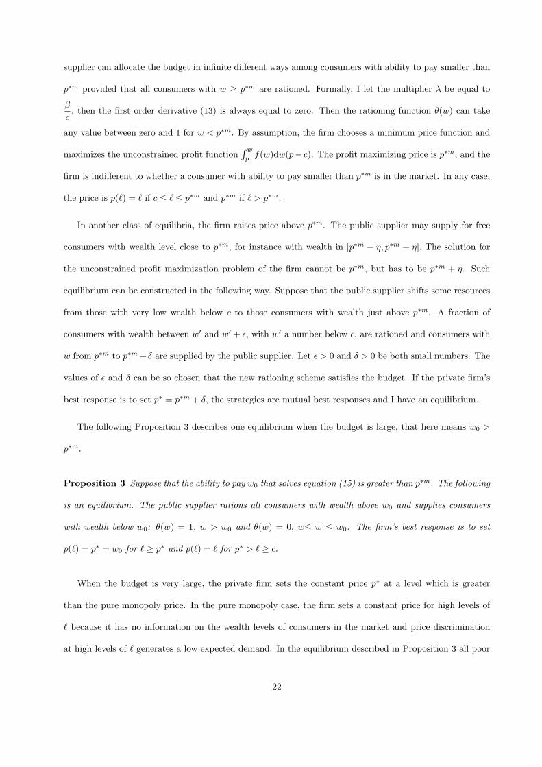
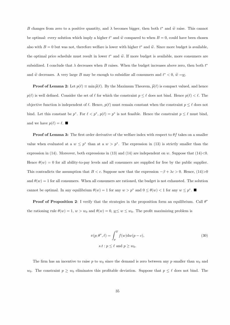
price w. All other consumers with w > ew are offered the good at price t(w) = w or t∗. An example of the
optimal price function is shown in Figure (2). The budget size B matters, as explained in this Corollary.
Corollary 2 If the budget size B is small, then t∗ > c. Since ew < c, richer consumers pay a price higher
than marginal cost and cross subsidize poorer consumers. As the budget B increases, then t∗ and ew decreaseand eventually t∗ becomes smaller than c and ew becomes w.
When the budget B is equal to zero or very small, the public supplier sets t∗ above c. Rich consumers
get a negative subsidy because they pay more than the marginal cost c. Since ew < c, there are consumers
who pay a price t(w) = w smaller than the marginal cost. The cost of these subsidies is covered by the
budget B but also by the revenue collected from consumers who pay a price greater the marginal cost.
Cross subsidization from the rich to the poor occurs and is optimal. When the budget is relatively large,
cross subsidization may not be necessary. The public supplier sets a price equal to the ability to pay to all
consumers with wealth below t∗, that is ew =w and may be able to subsidize all consumers by setting t∗
below c. The arrows in Figure (3) shows how the optimal t(w) changes as the budget B increases.
13

w
*t
w~ *t
o45)(, wtl
c
Figure 2: Pure public sector: optimal t(w).
w
*t
w~ *t
o45)(, wtl
c
Figure 3: t(w) changes with B.
14

3.3 Interaction between the public and private sector
I now consider a price reactive private market. I look for the sub-game perfect Nash equilibria of two games.
In the first, the public supplier sets a rationing rule θ. In the second, the public supplier decides a subsidy
policy t. Both games consists of the following three stages:
Stage 1: Nature draws (w, ) according to the distributions F and G. The private firm observes and the
public supplier observes w.
Stage 2: The public supplier chooses a rationing rule, θ, or a subsidy policy t and the private firm chooses
a price function bp.Stage 3: When I consider the public supplier choosing a rationing rule θ, consumers supplied by the public
sector get the good for free, and consumers not supplied by the public sector may purchase from the
private firm at prices set in Stage 2. When the public sector chooses a subsidy policy t, consumers
decide to purchase from the private firm or from the public supplier depending on the prices set in
Stage 2.
4 The private firm chooses prices and the public sector chooses arationing rule
The rationing rule assigns consumers with ability to pay w the probability of being supplied for free by
the public supplier. The density of consumers with w supplied by the public supplier is [1− θ(w)] f(w).
When there is a private market, the remaining fraction θ(w)f(w) of consumers are available to the firm. For
w ∈ [w,w], the public supplier provides consumers with wealth below w a total ofR ww(1− θ(x))f(x)dx units
of the good at zero cost, but not the remaining consumersR wwθ(x)f(x)dx who may decide to buy form the
private firm at price p( ).
Here I study the equilibrium of a game where the public sector chooses a rationing rule θ based on ability
to pay w, and the private firm selects a price rule p based on the willingness to pay . An equilibrium is
a pair of rationing and price rule (θ, p) such that θ(w) maximizes the welfare index subject to the budget
15

constraint given a price schedule p( ), and p( ) maximizes profit for every given θ. The rationing and price
schedules are mutual best responses against each other.
4.1 The firm
I start from the private firm’s best response against a given rationing rule θ. A consumer with ability to
pay w is supplied the good for free by the public supplier with probability 1 − θ(w), so this consumer is a
potential customer of the private firm with probability θ(w). The consumer (w, ) buys the good at price
p( ) only if he is willing to pay the price and can afford it, that is ≥ p( ) and w ≥ p( ).
The private firm’s profits are:
π(p; θ(w), ) =
Z w
p
θ(w)f(w)dw(p− c), (11)
s.t : p ≤ . (12)
The profit function in (11) is not in general quasi-concave so there can exist more than one price that
maximizes profits at a given . Let bp ( ) be the optimal price correspondence and bπ ( ) the maximum profit:
bp ( ) = argmaxp
π(p; θ(w), ),
bπ ( ) = π(p0; θ(w), ), p0( ) ∈ bp( ).Figure (4) and (5) depict an example of a profit function and profit maximizing correspondence. The
profit function represented in Figure (4) is maximized at two price levels, p and p. The firm is indifferent
between setting the price at p or p to consumers with greater than p, because both prices maximize profits.
Suppose that the firm faces a consumer with smaller than p but greater than p. The price p is no longer
profit maximizing, being greater than consumer’s willingness to pay, while p still belongs to the optimal
price correspondence. Lastly, when the firm observes a consumer with willingness to pay c < < p, the
constraint in (12) binds and the optimal price is p( ) = . The correspondence in Figure (5) is the optimal
price correspondence for the profit function of Figure (4).
16

)( pπ
p& p&&c l
Figure 4: An example of π(p; θ(w), ).
lc
o45
)(lp
l
p&
p&&
Figure 5: An example of bp( ).
17

The following Lemma 2 describes a useful property of one selection from the optimal price correspondence.
I call this selection the minimum price function. By the Maximum Theorem, the correspondence bp ( ) iscompact valued. Hence it has a minimum, that I call the minimum price function. The minimum price
function assigns each the lowest price which maximizes profit. Since the profit in (11) does not depend on
, it must be the case that when the constraint does not bind, the profit maximizing prices are independent
on . Let p∗ be the minimum among the profit maximizing prices when the constraint does not bind. I only
focus on those equilibria where the firm chooses the minimum price function.
Lemma 2 There exists a selection from the optimal price correspondence where the price is p( ) = for all
c < < p∗ and p( ) = p∗ for higher . This is the minimum price function.
There always exists one selection from the optimal price correspondence that is continuous and weakly
increasing in . The price is equal to for all greater than c and smaller than a threshold level p∗; the price
is constant at p∗ for all greater or equal than p∗. I argue that the firm chooses this selection because it
seems natural that the firm prefers to set the same price rather than different prices when the profits are
not going to be affected by the choice.
4.2 The public supplier
I now look for the best response rationing rule against the minimum price function. The firm is indifferent
to any rationing policy chosen by the public supplier for consumers with ability to pay smaller than the
marginal cost, that is for w < c. For example, if the public supplier has a very small budget and decides
to supply for free some of or all poorest consumers with w < c, the rationing rule has no impact on the
pricing rule of the private firm. The private firm is indifferent to consumers with ability to pay smaller than
c because it never sets a price smaller than c. Given a pricing rule, the public supplier needs to know the
probability that a consumer with ability to pay w buys the good in the market to choose his best response
rationing rule. The price p( ) is like the minimum ability to pay level at which a consumer can afford the
good.
Suppose that the public supplier observes consumers with ability to pay w ∈ [c, p∗]. Then the public
18

supplier knows that consumers with > p∗ cannot afford the price p∗ in the market and consumers with
between c and p∗ face p( ) = in the market. Among consumers with w ∈ [c, p∗], all those with willingness
to pay smaller than w, will buy at price p( ) = in the market since their ability to pay is greater than the
price . Their utility is w − though, since the firm extracts all consumer’s surplus. Also consumers with
w ∈ [w, c] have utility w − if left in the market.
Suppose now that the public supplier observes a consumer with w > p∗. If this consumer has willingness
to pay greater than p∗, that is ≥ p∗, he can buy the good in the market and earn the utility w − p∗. If
instead < p∗, the consumer is asked to pay the price p( ) = , which he can afford since w > p∗ > .
Basically only consumers with w ≥ p∗ and > p∗ earn some extra surplus by buying the good in the market.
Their utility level is infact w − p∗.
The social welfare index, given the minimum price rule, is
V (θ) =
Z w
w
[1− θ(w)]wf(w)dw +Z p∗
w
Zθ(w)(w − )g( )f(w)d dw+
Z w
p∗θ(w)
Z p∗
(w − )g( )d +
Zp∗(w − p∗)g( )d f(w)dw.
Consumers supplied for free by the public supplier earn the utility w. The budget constraint of the public
supplier is the same as in (4).
I call λ the multiplier associated to the budget constraint. The Lagrangean function for a given w is
V (θ) + λ[B − c(1 − θ)f ]. I use pointwise differentiation to determine the derivative of V (θ) + λcθf with
respect to θf. The public supplier chooses the density of consumers available to the firm in the market,
reacting to the minimum price function. The first order derivative of λcθf with respect to θf is λc, hence I
evaluate the derivative of V +λc with respect to θf for a consumer with w smaller than p∗ and greater than
p∗. For any w in [w, p∗]:
∂V
∂θf+ λc = −β + λc; (13)
and for any w in (p∗, w], the first order derivative is:
19

∂V
∂θf+ λc = −β +
Zp∗( − p∗)g( )d + λc. (14)
The expression in (13) represents the tradeoff between the cost and benefit of increasing the probability
for a consumer with wealth w ≤ w ≤ p∗ to be in the market. The consumer cannot afford the good at price
p∗ and obtains the utility w − in the market. By leaving this consumer in the market, the public supplier
saves a cost of λc (in utility units), but loses the average benefit β. The same tradeoff between the cost and
benefit takes on a different value for a consumer with ability to pay greater than p∗, because if ≥ p∗ he
obtains an extra surplus ( − p∗) from buying at a price p∗.
The public sector always prefers to leave consumers with ability to pay greater than p∗ in the market
rather than a poorer consumers. The extra surplus ( − p∗) is only generated when a consumer is able and
willing to buy the good at p∗.
Lemma 3 In any equilibrium, all consumers who can afford to pay the price p∗ are in the market, that is
θ(w) = 1 for any w > p∗. Some or all consumers with w ≤ p∗ are supplied by the public sector.
According to Lemma 3 in each equilibrium of the game, the public supplier prefers to ration consumers
who can afford to pay the price p∗. What does it happen to consumers who can not pay p∗?
4.3 Equilibrium analysis
The equilibrium of the game depends on the ratio between the budget size and the cost, B/c. Let w0 be the
ability-to-pay level that solves the following equation:
B = c
Z w0
w
f(w)dw. (15)
The public supplier can supply all consumers with w ≤ w0 for free. In the following Propositions 2 and
3, I use again the notation p∗m for the monopoly price set by the firm when all consumer are available in the
market and the constraint p ≤ does not bind. The following Proposition 2 describes one equilibrium when
20

the budget is small. Here I define the budget as small when w0 ≤ p∗m. Viceversa, the budget is large.11
Proposition 2 Suppose that the ability to pay w0 that solves equation (15) is smaller than p∗m. The
following is an equilibrium. The public supplier rations all consumers with wealth above w0 and supplies
consumers with wealth below w0: θ(w) = 1, w > w0 and θ(w) = 0, w≤ w ≤ w0. The private firm sets the
monopoly price schedule pm( ), that is p( ) = p∗m for ≥ p∗m and p( ) = for such as p∗m > ≥ c.
If all consumers were available to the private firm, the price rule would be the pure monopoly price
schedule pm( ). In this equilibrium, the private firm has no access to consumers with w ≤ w0. However
since w0 ≤ p∗m the private firm continues to set its prices like it is the monopoly. If the firm assumes that
all consumers in the market are able to pay a price set at w0, those with ≤ w0 are still willing to pay at
most . For consumers with > w0, the price w0 could have been chosen by the firm when all consumers
were available, but it was not. That implies that profits are higher with the pure monopoly price schedule.
The best response minimum price function is p( ) = , all in c < < p∗m, and p∗ = p∗m for ≥ p∗ = p∗m.
The Figure (6) represents an equilibrium when the budget is small.
0)( =wθ
c
o45
l
1)( =wθ mp*
)(, lpw
0w
Figure 6: One equilibrium when B is small.
The equilibrium described in Proposition 2 is robust to equity concerns, since the poorest consumers are
supplied by the public sector. It is not the unique equilibrium of the game, though. The game has multiple
equilibria. In one class of these equilibria, the firm sets the pure monopoly price schedule and the public
11Only in in this Section small and large are defined with respect to w0.
21
supplier can allocate the budget in infinite different ways among consumers with ability to pay smaller than
p∗m provided that all consumers with w ≥ p∗m are rationed. Formally, I let the multiplier λ be equal to
β
c, then the first order derivative (13) is always equal to zero. Then the rationing function θ(w) can take
any value between zero and 1 for w < p∗m. By assumption, the firm chooses a minimum price function and
maximizes the unconstrained profit functionR wpf(w)dw(p− c). The profit maximizing price is p∗m, and the
firm is indifferent to whether a consumer with ability to pay smaller than p∗m is in the market. In any case,
the price is p( ) = if c ≤ ≤ p∗m and p∗m if > p∗m.
In another class of equilibria, the firm raises price above p∗m. The public supplier may supply for free
consumers with wealth level close to p∗m, for instance with wealth in [p∗m − η, p∗m + η]. The solution for
the unconstrained profit maximization problem of the firm cannot be p∗m, but has to be p∗m + η. Such
equilibrium can be constructed in the following way. Suppose that the public supplier shifts some resources
from those with very low wealth below c to those consumers with wealth just above p∗m. A fraction of
consumers with wealth between w0 and w0 + , with w0 a number below c, are rationed and consumers with
w from p∗m to p∗m+ δ are supplied by the public supplier. Let > 0 and δ > 0 be both small numbers. The
values of and δ can be so chosen that the new rationing scheme satisfies the budget. If the private firm’s
best response is to set p∗ = p∗m + δ, the strategies are mutual best responses and I have an equilibrium.
The following Proposition 3 describes one equilibrium when the budget is large, that here means w0 >
p∗m.
Proposition 3 Suppose that the ability to pay w0 that solves equation (15) is greater than p∗m. The following
is an equilibrium. The public supplier rations all consumers with wealth above w0 and supplies consumers
with wealth below w0: θ(w) = 1, w > w0 and θ(w) = 0, w≤ w ≤ w0. The firm’s best response is to set
p( ) = p∗ = w0 for ≥ p∗ and p( ) = for p∗ > ≥ c.
When the budget is very large, the private firm sets the constant price p∗ at a level which is greater
than the pure monopoly price. In the pure monopoly case, the firm sets a constant price for high levels of
because it has no information on the wealth levels of consumers in the market and price discrimination
at high levels of generates a low expected demand. In the equilibrium described in Proposition 3 all poor
22

consumers are supplied for free. The firm’s best reaction is to price discriminate for a greater range of and
to increase the constant price because when poor consumers are not available, the average wealth level in
the market is higher. Figure (7) represents one equilibrium when the budget is large.
0)( =wθ
c
o45
l
1)( =wθ
)(, lpw
mppw **0 >=
mp*
Figure 7: One equilibrium when B is large.
The implication of Proposition 3 is that the interaction between the public and the private sector may
lead the private sector to increase prices. Rich consumers in the market are disadvantaged by an active
public supplier, since they are not poor enough to get the good for free, and need to pay a higher price in
the market.
There are multiple equilibria also when the budget is large. Other equilibria are constructed in following
way. The public supplier shifts resources from the consumers with wealth just above w, say w+ , to consumers
with wealth just above p∗ = w0, say w0 + δ. Again, > 0 and δ > 0 are small numbers and the budget is
satisfied. Whenever w+ ≤ c, the new equilibrium has the firm setting p∗ = w0 + δ. If w+ > c, there is
an equilibrium if the firm does not find it profitable to reduce the constant price to capture the demand of
consumers with low wealth available in the market. Corollary 3 summarizes the properties of the equilibria
of the game irrespective of the budget size.
Corollary 3 The rationing game has multiple equilibria. In all these equilibria the private firm sets p( ) = ,
all c ≤ < p∗ and p( ) = p∗, all ≥ p∗. The constant price p∗ is either p∗m, as in the pure monopoly case,
or p∗ > p∗m.
23

The equilibria with small and large budget can be ranked in terms of social welfare.
Proposition 4 Consider the equilibria of the game when the budget is small, that is w0 ≤ p∗m. All equilibria
where the firm sets the monopoly price schedule pm( ) are welfare equivalent and dominate every other
equilibria with p∗ > p∗m.
Proposition 5 Consider the equilibria of the game when the budget is large, that is w0 > p∗m. The equi-
librium where the firm sets p∗ = w0 is welfare superior to any other equilibria.
5 The private firm chooses prices and the public sector chooses asubsidy policy
What is the equilibrium outcome of the game when the public supplier has more instruments than pure
rationing? Here I let again the public supplier choose a subsidy scheme t(w) and a probability α(w). The
price t(w) is affordable to consumers with wealth w with probability 1 − α(w) and is greater than w with
probability α(w). Formally the subsidy policy consists of the price t(w). The probability α(w) is a tool that
makes the derivation of the results easier. If there exists a private market, the consumer type (w, ) decides
if and where to purchase the good, comparing t(w) to p( ). The private firm continues to choose a price
schedule p( ). An equilibrium is a pair of subsidy and price schemes (t, p) such that t maximizes the welfare
index subject to the budget constraint and ability-to-pay constraints given a price scheme p( ), and p( )
maximizes profits for every given t. That is, the subsidy and pricing schemes are mutual best responses
against each other.
The outcome of the game is similar to the equilibrium generated by Bertrand competition. In any
equilibrium the firm sets prices at marginal cost, p( ) = c and the public supplier sets some prices t(w) at
marginal cost provided the budget is small. The firm has the incentive to undercut the public supplier to
increase profits and the public supplier has the incentive to undercut the firm to increase social welfare. The
game is different from the standard Bertrand game in three respects. First, the public supplier does not
maximize profits. Second, the information available to the public supplier and the firm is different. Third,
the agents choose functions rather than single prices. The meaning of undercutting when two firms choose
24

prices is obvious. What do I mean by undercutting when the agents select functions? I show that price-
functions competition can be restricted to the competition between maximum prices. In the next Lemma,
I prove that the mutual best responses t(w) and p( ) have a maximum, but first I define the maximization
problems solved by the agents. Consider any t(w) and ignore α(w). I look for the private firm’s best response
p( ). The set Ω describes the demand faced by the firm:
Ω(p; t(w), ) = (w, ) : p ≤ , p ≤ t(w), p ≤ w.
The firm chooses p( ) to maximize profits
π(p; t(w), ) =
ZΩ(p;t(w), )
f(w)dw(p− c). (16)
The public supplier’s best response maximizes the social welfare index given any price function p( ). I
ignore α(w) and define the set Φ of consumers available to the public supplier:
Φ(t; p( ), w) = (w, ) : t ≤ , t ≤ p( ), t ≤ w.
The public supplier chooses t(w) to maximize the social welfare index:
V (t, α; p( ), w) = α
⎧⎪⎨⎪⎩Z
p( )≤w
(w − p( ))g( )d +
Zp( )>w
(w − )g( )d
⎫⎪⎬⎪⎭+ (17)
(1− α)
⎧⎪⎨⎪⎩Z
Φ(t;p( ),w)
(w − t)g( )d +
Zp( )≤w
(w − p( ))g( )dZ
p( )>w
(w − )g( )d
⎫⎪⎬⎪⎭given the budget:
B ≥Z w
w
(1− α(w))
ZΦ(t;p( ),w)
(w − t)dGdF.
The terms in (17) multiplied by α represent the utility of consumers with ability to pay w who face a
price t(w) = w. They are in the market and pay p( ) (and p( ) ≤ ) unless their ability to pay is below p( ).
25

If w < p( ), their utility is w − . Consumers with ability to pay w purchase from the public supplier at t
when they belong to the set Φ. Consumers who are not in Φ may purchase or not from the firm. Given that
p( ) ≤ , if p( ) > w, they do not buy and have utility w − ; if p( ) ≤ w, they buy from the private firm.
*******
In any equilibrium, p( ) and t(w) are mutual best responses. The price function p( ) assigns each a
real number in [c, ], given the function t. The function p( ) has a supremum, psup = supp( ), for any in
c ≤ ≤ . Given p( ), the public supplier chooses a real function t(w), which assign each w a number in
[w,w]. Hence the function t(w) has a supremum, tsup = sup t(w), for any w in w ≤ w ≤ w .
Can psup > c and tsup > c be mutual best responses? The answer is no. Suppose they are, and
tsup > psup > c. None of the consumers supplied with probability 1 − α from the public supplier and with
≥ tsup purchase the good from the public supplier. Those who can potentially buy at tsup have w ≥ tsup
and ≥ tsup, but they strictly prefer to pay psup in the market. The public supplier has two incentives to
reduce tsup just below psup and above c, say at psup− > c. First, consider those consumer types (w, ) who
purchase at psup in the market. They must have w ≥ psup and ≥ psup. The public supplier reduces tsup just
below psup and can supply consumers with w ≥ psup and ≥ psup at a lower price. Social welfare increases.
Second, by undercutting psup, the public supplier relaxes the budget constraint, because the new consumers
supplied by the public supplier pay a price tsup > c. Suppose now that psup > tsup > c. No consumers buy
at psup. The firm undercuts tsup. The following Lemma 4 states that in any equilibrium p( ) = c. The firm
never selects a price below marginal cost or above marginal cost; when the supremum of p( ) is psup = c,
then the price function is constant at c and psup is the maximum, pmax.
Lemma 4 In any equilibrium p( ) = c for any in£c,¤. The firm does not sell to consumers with < c.
With no loss of generality, p( ) = c for any < c.
I consider the best response of the public supplier given that p( ) = c. The argument outlined above
rules out that there exists an equilibrium with t(w) > c at any w. The next Lemma restricts the public
supplier best responses.
26

Lemma 5 In any equilibrium, t(w) ≤ c.
The public supplier never sets a price t(w) greater than c with positive probability because no consumers
purchase the good. Consumers would prefer to buy from firm at price p( ) = c.
5.1 Equilibrium analysis
The size of the budget B matters to determine the nature of the equilibrium. I look for the public supplier
best response given that p( ) = c. I define the social welfare index for a consumer with w below and above
c:
V |w≤c = α
Z(w − )g( )d + (1− α)
(Z t
(w − )g( )d +
Zt
(w − t)g( )d
).
and
V |w>c = α
(Z c
(w − )g( )d +
Zc
(w − c)g( )d
)+
(1− α)
(Z t
(w − )g( )d +
Zt
(w − t)g( )d
).
The budget constraint is
B ≥Z w
w
Zt(w)
[1− α(w)] [c− t(w)] g( )f(w)d dw,
and λ is the multiplier for the budget constraint. The public supplier also respects the constraints
t(w) ≤ w. I define the Lagrangean function L in the usual way. The first order derivatives of L at a given
w with respect to α, and t are
∂L
∂α|w≤c ≡
Zt
[− ( − t) + λ (c− t)]dG (18)
∂L
∂α|w>c ≡
Zc
( − c)dG+Zt
[− ( − t) + λ (c− t)]dG. (19)
27

Assuming that t(w) ≤ w does not bind, the first order derivative with respect to t is
∂L
∂t≡ [1− α] λg(t∗) (c− t∗) + (λ− 1) [1−G(t∗)] = 0. (20)
The public supplier’s best response consists of a fixed price t∗ for any w ≥ t∗ and t(w) = w, w < t∗. The
best response t(w) has the same structure as in the pure public supplier case analyzed in the Subsection 3.2.
I consider the case where the budget B is small. The budget is small when it is not enough to supply
the good at t(w) = w to all consumers with wealth w such as w≤ w < c. The following is an equilibrium
when the budget is small.
Proposition 6 Suppose that the budget B is not enough to supply the good at price w to all consumers
with w such as w≤ w < c. The following is an equilibrium. The private firm sets a constant price equal to
marginal cost, p( ) = c for all . The public supplier sets the price at t∗ = c to all consumers with ability to
pay greater or equal than c, and t(w) = w to all consumers with ability to pay below c and above a threshold
ew. The threshold is w< ew < c. For consumers with w < ew, α(w) = 1 and they do not buy the good.
Consumers with w ≥ c buy at a price set equal to marginal cost and are indifferent between purchasing from
the firm or from the public supplier.
In the equilibrium described in the Proposition 6, the firm sets a constant price schedule at marginal cost.
The Bertrand competition prevents the public supplier to implement cross subsidization across consumers
by setting some prices above c. There are no consumers willing to pay more than c to the public supplier
because the firm offers the same good at a lower price. In equilibrium the public sector sets the constant
price t∗ equal to c to consumers with ability to pay greater than c. In terms of consumers’ surplus it does
not make any difference if consumers with w and greater or equal than c buy at a price equal to c from the
firm or the public supplier. The budget is also unaffected. The analyst is free to choose a tie break rule. For
instance, one can assume that half of the consumers with w ≥ c purchase the good in the market and the
other half purchase from the public supplier. Consumers with wealth smaller than marginal cost but greater
28

than a threshold12 ew ≥w, buy from the public supplier at price t(w) = w. The budget in this equilibrium is
just enough to cover the difference between the price t(w) = w and the cost of provision (adjusted for λ) for
consumers with wealth w in [ ew, c), and ew >w. Hence consumers with w below the threshold ew go without
the good.
Given the public supplier subsidy policy, it is optimal for the firm to set the price at marginal cost.
By increasing some prices above c, the firm would lose consumers because the public supplier will try to
implement cross subsidization by setting some prices just below psup and above c. By reducing the price
below marginal cost, the firm makes negative profits.
There is a striking difference between the equilibrium of the game and the optimal subsidy policy imple-
mented by the public supplier when the firm is inactive. If there is no private firm, the public supplier can
set a price above marginal cost to rich consumers and use the extra resources to subsidize poorer consumers.
But this is impossible when there is a private firm. The budget B can not be supplemented by asking rich
consumers to pay more than c. Figure (8) represents the equilibrium described in the Proposition 6.
ww~ *t
o45)(, wtl
ct =*
Figure 8: Equilibrium t(w) when B small.
I now consider the case where the budget B is large. The budget B is large when it is more than enough
to supply the good at t(w) = w to all consumers with wealth w such as w≤ w < c. Formally ew =w and someextra budget is available. The next Proposition 7 describes the equilibrium of the game when the budget is
12The threshold w is defined in Section 3.2.
29

large.
Proposition 7 Suppose that the budget B is more than enough to supply the good at price w to all consumers
with w < c. The following is an equilibrium. The private firm sets p( ) = c but does not sell to any consumers.
The public supplier sets the price at t∗ = c − to all consumers with ability to pay greater than c − , and
t(w) = w to all consumers with ability below t∗.
Figure (9) represents the equilibrium described in the Proposition 7.
w
o45)(, wtl
ε−= ct*
w
Figure 9: Equilibrium t(w) when B is large.
In this equilibrium, the firm sets the prices at marginal cost but does not sell to any consumers. Suppose
some prices are above c, and psup is the highest price. The public supplier best response would be to
implement some cross subsidization. Hence, in equilibrium the firm set p( ) = c. Given the firm strategy,
the public supplier never set a price above marginal cost because no consumers would buy. It does not even
set any price at marginal cost, because the budget would not be exhausted.
This game has a unique equilibrium, which changes with the budget size. The more interesting equilibrium
is the equilibrium when the budget B is small. The public supplier implements cross subsidization when it
is the sole supplier of the good. It cannot cross subsidize when there is a private firm. Hence the sum of
consumers’ surplus is higher when the public supplier is the sole provider of the good. This outcome is novel
in the literature of the public provision of private goods.
30

6 Concluding remarks
I have introduced a framework for studying the concept of affordability of an indivisible good, such as a
health care treatment, a course of studies or a house. In the consumer utility function, willingness to pay
for a good is explicitly separated from ability to pay. I study the optimal policy of the public supplier when
it is the sole provider of the good. The public supplier observes consumers’ ability to pay. In the model, the
public supplier uses nonprice rationing or a subsidy policy to allocate the units of the good among consumers.
Both policies are based on ability to pay. I also study the strategic interactions between public and private
sectors. The private sector is a monopoly. The public sector and the firm have different information about
consumers. Ability to pay is observed by the public supplier and willingness to pay by the firm.
When the public supplier uses a rationing policy and strategically interacts with the firm, the highest
welfare equilibrium look like common rationing schemes: rich consumers are rationed, and the public supplier
supplies poorer consumers. It may happen that the firm set prices above the monopoly level if the budget
available to the public supplier is very large.
The optimal subsidy policy of the public supplier when it is the sole provider of the good implies cross
subsidization from rich to poor consumers. If there is a private firm, cross subsidization is impossible.
The model can be extended to look for more general mechanisms to allocate the good. For instance, the
public supplier can try to elicit some information from the private firm. It can also be used for studying
quality differences between the public and private sectors. Lastly, I have assumed a fixed budget for the
public supplier. Extending the model to determine the budget endogenously seems interesting.
31

Appendix
Proof of Lemma 1: The profit function (1) is differentiable in p. The first-order derivative of π(p; )
with respect to p is −f(p)[p− c]+ [1−F (p)]. The first order derivative does not depend on and vanishes at
a level of p that I call p∗m. Assume that the constraint > p does not bind. For any > p∗m, pm( ) = p∗m.
The profit maximizing price function is constant. At < p∗m, the solution pm( ) = p∗m is not feasible since
< pm( ) = p∗m. Hence the constraint binds and pm( ) = . The firm does not supply consumers with
< c.¥
Proof of Proposition 1. The derivative of the Lagrangean function (8) with respect to t(w) is
∂L
∂t(w)≡ [1− α(w)] λg(t(w)) [c− t(w)] + (λ− 1) [1−G(t(w))]− μ(w) (21)
and with respect to α(w) is
∂L
∂α(w)≡Zt(w)
[− ( − t(w)) + λ (c− t(w))] g( )d . (22)
The multiplier for the ability-to-pay constraint t(w) ≤ w is denoted by μ(w).
If t(w) ≤ w, then μ(w) = 0. If t(w) > w, then the ability-to-pay constraint binds and μ(w) > 0. Suppose
that 1−α(w) > 0 and t(w) ≤ w. I can set the expression (9) equal to zero and solve for the optimal t(w). I
call t∗ the value of t(w) where the first order derivative (9) vanishes:
t∗ = c− 1−G(t∗)
g(t∗)
1− λ
λ. (23)
t∗ is independent on w. At any w < t∗, the ability-to-pay constraint must bind and t(w) = w. Assume
it does not. Then t(w) = t∗, but this contradicts the assumption that t(w) ≤ w. At any w ≥ t∗, the
ability-to-pay constraint does not bind and t(w) = t∗. Notice that for λ > 1, t∗ > c, and for λ < 1, t∗ < c.
I assume that w≤ t∗ ≤ w. I now consider the first order derivative of the Lagrangean with respect to
α(w) evaluated at w < t∗and w ≥ t∗:
32

∂L
∂α(w)|w<t∗ ≡
Zw
[− ( − w) + λ (c− w)] g( )d . (24)
and
∂L
∂α(w)|w≥t∗ ≡
Zt∗[− ( − t∗) + λ (c− t∗)] g( )d . (25)
The expression in (24) is differentiable in w, and its derivative is:
∂
µ∂L
∂α(w)|w≤t∗
¶∂w
≡ − [λg(w)(c− w) + (λ− 1)(1−G(w))] . (26)
This derivative must be strictly negative in w. Consider (9).13 At any w < t∗, the ability-to-pay constraint
binds and the term [λg(w)(c− w) + (λ− 1)(1−G(w))] > 0. Hence (26) is strictly negative at any w < t∗.
The derivative in (26) is equal to zero at any w ≥ t∗. This can be proved by evaluating 26 at w = t∗
with t∗ = c− 1−G(t∗)g(t∗)
1−λλ . The first order derivative
∂L
∂α(w)as function of w is represented in Figure (10).
At w = t∗, α(t∗) < 1. Suppose not and that∂L
∂α(w)|w=t∗ > 0. Since the function
∂L
∂α(w)|w≤t∗ is
decreasing in w, it must be positive for any w < t∗. The maximization problem has a corner solution
α(w) = 1 for any w, which implies that none of the consumers is supplied the good. Since the budget is not
used, the solution cannot be optimal. I conclude that∂L
∂α(w)|w=t∗ ≤ 0.
The monotonicity of∂L
∂α(w)|w≤t∗ together with
∂L
∂α(w)|w=t∗ ≤ 0 imply that there exists a w, called ew,
such as∂L
∂α(w)|w≤t∗ = 0. By definition:
∂L
∂α(w)|w≤t∗ ≡
Zw
[− ( − ew) + λ (c− ew)]dG = 0. (27)
The budget constraint can be rewritten as:
B =
Z t∗
w
Zw
[c− w] dGdF +
Z w
t∗
Zt∗[c− t∗] dGdF. (28)
13 ∂L
∂t(w)≡ [1− α(w)] λg(t(w)) [c− t(w)] + (λ− 1) [1−G(t(w))]− μ(w)
33

)(wL
α∂∂
w
0
*t
1)(1 =− wα0)(1 =− wα
w~ ww
Figure 10: Pure Public Supplier: ∂L∂α(w) .
The solution of the optimization problem in terms of λ, ew and t∗ is defined by expressions (23), (27),
(28). ¥
Proof of Corollary 1: Consider expression (27) and rearrange it as follows:
ew = c− 1λ
Rw( − ew)dGRwg( )d
. (29)
The Lagrangean multiplier is positive and therefore ew < c. ¥
Proof of Corollary 2 Let the budget be B = 0. I prove that t∗ > c. Suppose that t∗ is t∗ = c. The
first order condition (25) is strictly negative at t∗ = c. Hence α(w) = 0 for all w ≥ c and all consumers with
ability to pay greater than marginal cost are offered the good by the public sector at marginal cost price.
The first order derivative (24) is strictly decreasing in w (see (26)), hence14 ew < c. Consumers with w in
[ ew, c] are subsidized by the public sector because they are offered the good at price t(w) = w < c. This
contradicts the assumption that B = 0. Clearly the price t∗ cannot be smaller than c. I conclude that when
B = 0, cross subsidization is optimal.
I now consider the impact of a change in B on the optimal price schedule t(w). I prove that λ > 1 if
B = 0. Since t∗ > c at B = 0, by the definition of t∗ in (23), then λ > 1 when B = 0. I claim that λ
decreases when B raises. Suppose not, and instead that λ increases with B. By (23) and (29), if the budget
14See Proof of Proposition 1 for the definition of w.
34
B changes from zero to a positive quantity, and λ becomes bigger, then both t∗ and ew raise. This cannot
be optimal: every solution which imply a higher t∗ and ew compared to when B = 0, could have been chosen
also with B = 0 but was not, therefore welfare is lower with higher t∗ and ew. Since more budget is available,the optimal price schedule must result in lower t∗ and ew. If more budget is available, more consumers aresubsidized. I conclude that λ decreases when B raises. When the budget increases above zero, then both t∗
and ew decreases. A very large B may be enough to subsidize all consumers and t∗ < 0, ew =w.Proof of Lemma 2: Let p( ) ≡ min bp( ). By the Maximum Theorem, bp( ) is compact valued, and hence
p( ) is well defined. Consider the set of for which the constraint p ≤ does not bind. Hence p( ) < . The
objective function is independent of . Hence, p( ) must remain constant when the constraint p ≤ does not
bind. Let this constant be p∗. For < p∗, p( ) = p∗ is not feasible. Hence the constraint p ≤ must bind,
and we have p( ) = . ¥
Proof of Lemma 3: The first order derivative of the welfare index with respect to θf takes on a smaller
value when evaluated at a w ≤ p∗ than at a w > p∗. The expression in (13) is strictly smaller than the
expression in (14). Moreover, both expressions in (13) and (14) are independent on w. Suppose that (14)<0.
Hence θ(w) = 0 for all ability-to-pay levels and all consumers are supplied for free by the public supplier.
This contradicts the assumption that B < c. Suppose now that the expression −β + λc > 0. Hence, (14)>0
and θ(w) = 1 for all consumers. When all consumers are rationed, the budget is not exhausted. The solution
cannot be optimal. In any equilibrium θ(w) = 1 for any w > p∗ and 0 ≤ θ(w) < 1 for any w ≤ p∗. ¥
Proof of Proposition 2: I verify that the strategies in the proposition form an equilibrium. Call θ∗
the rationing rule θ(w) = 1, w > w0 and θ(w) = 0, w≤ w ≤ w0. The profit maximizing problem is
π(p; θ∗, ) =
Z w
p
f(w)dw(p− c), (30)
s.t : p ≤ and p ≥ w0.
The firm has an incentive to raise p to w0 since the demand is zero between any p smaller than w0 and
w0. The constraint p ≥ w0 eliminates this profitable deviation. Suppose that p ≤ does not bind. The
35

solution of the restricted problem is the monopoly price p∗m if p∗m ≥ w0 and p∗ = w0 if p∗m < w0. In this
equilibrium p∗m > w0 by assumption and the constraint p ≥ w0 never binds at the optimum. When p ≤
binds, the price is p( ) = (≥ c). Hence, given the public supplier’s rationing rule, it is optimal for the firm
to set the profit maximizing pure monopoly price schedule: pm( ). The rationing rule θ(w) = 1, for w > w0,
and θ(w) = 0, for w≤ w ≤ w0 does not change the demand available at price p( ) = p∗m. By a revealed
preference argument, the unconstrained profit maximization has the same solution as in the pure monopoly
case. For levels smaller than pm, the price is determined by the constraint and is independent from the
rationing rule. Given this price schedule, I set the multiplier λ toβ
c. The first order derivative (13) is zero
for w < p∗ = p∗m and (14) strictly positive for w > p∗ = p∗m. The function θ(w) can take on any values
between zero and 1 for w < p∗ = p∗m. A rationing rule such as θ(w) = 1, w > w0 and θ(w) = 0, w≤ w ≤ w0
is consistent with (13) and (14) since w0 < p∗m, moreover the budget constraint holds as an equality. Hence
the rationing scheme defined in the Proposition is optimal. The strategies form an equilibrium. ¥
Proof of Proposition 3: I verify that the strategies in the Proposition form an equilibrium. The proof
is similar to the proof of Proposition 2. However, the constraint p ≥ w0 in the maximization problem in (30)
binds by assumption at p = p∗m. In this equilibrium p∗m < w0, hence p∗ = w0. When p ≤ binds, the price
is p( ) = (≥ c). Hence, given the public supplier’s rationing rule, the price schedule in the Proposition 3 is
optimal. Then, I set the multiplier λ toβ
c. The first order derivative (13) is zero for w < p∗ = w0 and (14)
strictly positive for w > p∗ = w0. Moreover, the budget constraint holds as an equality. Hence the rationing
scheme defined in the Proposition is optimal. The strategies form an equilibrium. ¥
Proof of Corollary 3: Let λ be λ = β/c. Given p∗, the first order derivative (13) is equal to zero at
any w ≤ p∗, hence θ(w) can take any value in the interval [0, 1]. All consumers with w > p∗, are rationed
since the first order derivative (14) is strictly positive. I call θ∗(w) any rationing rule such as the budget is
exhausted in supplying consumers with wealth below p∗:
B =
Z p∗
w
c[1− θ∗(w)]f(w)dw.
A general version of the profit maximization problem of the firm consists of (30) without the constraint
p ≥ w0. It only matters that θ∗(w = p) = 1, so that there are consumers who can pay at most p in the
36

market. The solution of the unconstrained profit maximization problem is p∗m.
Given the public supplier’s rationing rule θ∗(w), such as there are consumers with ability to pay p∗m in
the market, the firm’s best response is to select the pure monopoly price schedule. For λ = β/c, (13) equal
to zero, and (14) strictly positive, the scheme θ∗(w) that exhausts the budget is optimal. The strategies
form an equilibrium. If instead, there are no consumers with wealth w = p∗m in the market, the firm will
raise price. For instance if θ∗(w) = 0 for all w in [p∗m, p∗m + δ], then the optimal constant price set by the
firm is p∗ = p∗m + δ.¥
Proof of Proposition 4: In any equilibrium of the rationing game where the first order derivative (13)
is equal to zero and the constant price in the market is p∗ = p∗m, the sum of consumers’ surplus is the
same. Since (13) is equal to zero at any w ≤ p∗m, θ(w) can take any value in [0, 1] without affecting the
optimized value of the sum of consumers’ surplus. Whenever in equilibrium the firm sets a price p∗ > p∗m,
social welfare is reduced. Since the budget B is the same, the same quantity of goods is provided for free to
consumers who have ex ante expected benefit β. Since consumers in the market have to pay a higher price,
total welfare is reduced.
Proof of Proposition 5: The proof follows the same argument outlined in the proof of Proposition 4.¥
Proof of Lemma 4: Suppose that there exists an equilibrium where p( ) > c for some . Let pmax be
the maximum of this function. By assumption pmax > c. The public supplier increases welfare and relaxes
the budget constraint by setting tmax = pmax − > c. Then the firm does not sell. Hence pmax = c. ¥
Proof of Lemma 5 Suppose that there exists an equilibrium with p( ) = c for all and t(w) > c for
some w. The public supplier never sets a price t(w) < w with positive probability, if the demand is zero.
At all w levels such as t(w) > c, 1 − α(w) = 0. By assumption t(w) = w if and only if α(w) = 1. Hence,
t(w) ≤ c. ¥
Proof of Proposition 6: Given the public supplier subsidy policy, it is optimal for the firm to set the
price at marginal cost. By increasing the price the firm would lose all consumers and by reducing the price
it would make negative profits. Given the firm price schedule, the public supplier subsidy policy described
in the Proposition is optimal. The first order derivative in (19) equals zero when evaluated at t∗ = c. I set
37

α arbitrarily at 0.5. The public sector sets t(w) = w for those with ability to pay below c. As showed in the
Proof of Proposition 1, the first order derivative in (18) for t(w) = w is strictly decreasing in w. The budget
is used to supply consumers with w ≤ c and is exhausted at ew that solves:
B =
Z c
w
Zw
[c− w] g( )f(w)d dw.
Let λ be
λ =
Rw( − ew)dG
[1−G( ew)] (c− ew)dGand (18) is equal to zero at ew and strictly negative for any ew < w ≤ c. ¥
Proof of Proposition 7: The budget B is more than enough to supply the good at price w to all
consumers with w < c:
B >
Z c
w
Zw
[c− w] g( )f(w)d dw.
Assume p( ) = c. Since t∗ = c and t(w) = w for all w ≤ c does not exhaust the budget, the public
supplier can do better. The constant price t∗ cannot exceed c, hence it is smaller than c, say t∗ = c− . The
budget determines t∗ which solves:
B =
Z t∗
w
Zw
(c− w)g( )f(w)d dw +
Z w
t∗
Zt∗(c− t∗)g( )f(w)d dw.
The first order derivative (20) determines λ so that t∗ equals the level that exhausts the budget constraint:
t∗ = c− 1− λ
λ
1−G(t∗)
g(t∗).
The multiplier is smaller than 1. The first order derivatives with respect to α are:
∂L
∂α|w≥t ≡
Zt
[− ( − t) + λ (c− t)]dG,
38

and
∂L
∂α|w<t ≡
Zt
[− ( − w) + λ (c− w)]dG.
At t = c,∂L
∂α|w≥t < 0. Since the first order derivative is strictly monotone in the argument t, it must be
strictly negative at t = c− . By assumption the budget can be used to supply all consumers with ability to
pay w ≤ w ≤ t∗. The private sector best response to the public supplier’s strategy is to set p( ) = c. Suppose
it is not. If the supremum psup > c, then the public supplier undercuts the private firm. The private firm
never sets any price below marginal cost.¥
39

References
Besley, Timothy, and Stephen Coate, "Public Provision of Private Goods and the Redistribution of
Income", American Economic Review, 81( 4), (1991), 979-984.
Blackorby, Charles, and David Donaldson, "Cash versus Kind, Self-Selection, and Efficient Transfers",
American Economic Review, 78( 4), (1988), 691-700.
Che, Yeon-Koo and Ian Gale, "Market and Non-Market Assignment of Initial Ownership", (2006), mimeo
Epple, Dennis and Richard Romano, "Educational Vouchers and Cream Skimming," NBER Working
Paper, 2002, forthcoming International Economic Review.
Grassi, Simona, and Ching-To Albert Ma, "Rationing poor consumers to reduce prices," (2008), mimeo.
Grassi, Simona, and Ching-To Albert Ma, "Public Sector Rationing and Private Sector Selection", (2008),
Boston University Economics Department Working Papers.
Ma, Ching-To Albert, "Public rationing and private cost incentives," Journal of Public Economics, 88,
(2003), 333-352.
Weitzman, Martin, "Is the Price System or Rationing More Effective in Getting a Commodity to Those
Who Need It Most?", Bell Journal of Economics, The RAND Corporation, 8(2), (1977), 517-524.
40
Related Documents