images/logoetsf Introduction Electron Energy Loss Spectroscopy Applications: Nanotubes and Graphene Perspectives Ab Initio calculations of electronic excitations Carbon Nanotubes and Graphene layer systems Francesco Sottile Laboratoire des Solides Irradi´ es Ecole Polytechnique, Palaiseau - France European Theoretical Spectroscopy Facility (ETSF) Strasbourg, 27 August 2008 Ab Initio calculations of electronic excitations Francesco Sottile

Welcome message from author
This document is posted to help you gain knowledge. Please leave a comment to let me know what you think about it! Share it to your friends and learn new things together.
Transcript
images/logoetsf
Introduction Electron Energy Loss Spectroscopy Applications: Nanotubes and Graphene Perspectives
Ab Initio calculations of electronic excitationsCarbon Nanotubes and Graphene layer systems
Francesco Sottile
Laboratoire des Solides IrradiesEcole Polytechnique, Palaiseau - France
European Theoretical Spectroscopy Facility (ETSF)
Strasbourg, 27 August 2008
Ab Initio calculations of electronic excitations Francesco Sottile

Introduction Electron Energy Loss Spectroscopy Applications: Nanotubes and Graphene Perspectives
Outline
1 Introduction
2 Electron Energy Loss SpectroscopyLinear response within DFT
3 Applications: Nanotubes and Graphene
4 Perspectives
Ab Initio calculations of electronic excitations Francesco Sottile

Introduction Electron Energy Loss Spectroscopy Applications: Nanotubes and Graphene Perspectives
Introduction
Theoretical Spectroscopy Group (ETSF)
Results on Nanotubes and Graphene:
Coordinator: Christine GiorgettiRalf HambachXochitl LopezFederico IoriV.Olevano, A. Marinopoulos, L. Reining, F. SottileExperiments: Thomas Pichler group (Dresden)
Ab Initio calculations of electronic excitations Francesco Sottile

Introduction Electron Energy Loss Spectroscopy Applications: Nanotubes and Graphene Perspectives
Outline
1 Introduction
2 Electron Energy Loss SpectroscopyLinear response within DFT
3 Applications: Nanotubes and Graphene
4 Perspectives
Ab Initio calculations of electronic excitations Francesco Sottile

Introduction Electron Energy Loss Spectroscopy Applications: Nanotubes and Graphene Perspectives
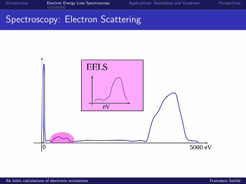
Spectroscopy: Electron Scattering
Ab Initio calculations of electronic excitations Francesco Sottile

Introduction Electron Energy Loss Spectroscopy Applications: Nanotubes and Graphene Perspectives
Spectroscopy: Electron Scattering
Energy Loss Function
d2σ
dΩdE∝ Im
ε−1
Ab Initio calculations of electronic excitations Francesco Sottile

Introduction Electron Energy Loss Spectroscopy Applications: Nanotubes and Graphene Perspectives
Spectroscopy: Electron Scattering
Ab Initio calculations of electronic excitations Francesco Sottile

Introduction Electron Energy Loss Spectroscopy Applications: Nanotubes and Graphene Perspectives
Spectroscopy: Electron Scattering
Ab Initio calculations of electronic excitations Francesco Sottile

Introduction Electron Energy Loss Spectroscopy Applications: Nanotubes and Graphene Perspectives
Spectroscopy: Electron Scattering
Ab Initio calculations of electronic excitations Francesco Sottile
Introduction Electron Energy Loss Spectroscopy Applications: Nanotubes and Graphene Perspectives
Spectroscopy: Electron Scattering
Ab Initio calculations of electronic excitations Francesco Sottile

Introduction Electron Energy Loss Spectroscopy Applications: Nanotubes and Graphene Perspectives
Spectroscopy: Electron Scattering
Ab Initio calculations of electronic excitations Francesco Sottile

Introduction Electron Energy Loss Spectroscopy Applications: Nanotubes and Graphene Perspectives
Spectroscopy: Electron Scattering
Ab Initio calculations of electronic excitations Francesco Sottile
Introduction Electron Energy Loss Spectroscopy Applications: Nanotubes and Graphene Perspectives
Outline
1 Introduction
2 Electron Energy Loss SpectroscopyLinear response within DFT
3 Applications: Nanotubes and Graphene
4 Perspectives
Ab Initio calculations of electronic excitations Francesco Sottile

Introduction Electron Energy Loss Spectroscopy Applications: Nanotubes and Graphene Perspectives
Linear Response Approach
System submitted to an external perturbation
Vtot = ε−1Vext
Vtot = Vext + Vind
E = ε−1D
Ab Initio calculations of electronic excitations Francesco Sottile

Introduction Electron Energy Loss Spectroscopy Applications: Nanotubes and Graphene Perspectives
Linear Response Approach
System submitted to an external perturbation
Vtot = ε−1Vext
Vtot = Vext + Vind
E = ε−1D
Ab Initio calculations of electronic excitations Francesco Sottile

Introduction Electron Energy Loss Spectroscopy Applications: Nanotubes and Graphene Perspectives
Linear Response Approach
System submitted to an external perturbation
Vtot = ε−1Vext
Vtot = Vext + Vind
E = ε−1D
Ab Initio calculations of electronic excitations Francesco Sottile

Introduction Electron Energy Loss Spectroscopy Applications: Nanotubes and Graphene Perspectives
Linear Response Approach
Definition of polarizability
not polarizable ⇒ Vtot = Vext ⇒ ε−1 = 1polarizable ⇒ Vtot 6= Vext ⇒ ε−1 6= 1
ε−1 = 1 + vχ
χ is the polarizability of the system
Ab Initio calculations of electronic excitations Francesco Sottile

Introduction Electron Energy Loss Spectroscopy Applications: Nanotubes and Graphene Perspectives
Linear Response Approach
Polarizability
interacting system δn = χδVext
non-interacting system δnn−i = χ0δVtot
Ab Initio calculations of electronic excitations Francesco Sottile

Introduction Electron Energy Loss Spectroscopy Applications: Nanotubes and Graphene Perspectives
Linear Response Approach
Polarizability
interacting system δn = χδVext
non-interacting system δnn−i = χ0δVtot
Single-particle polarizability
χ0 =∑ij
φi (r)φ∗j (r)φ
∗i (r
′)φj(r′)
ω − (εi − εj)
hartree, hartree-fock, dft, etc.
G.D. Mahan Many Particle Physics (Plenum, New York, 1990)
Ab Initio calculations of electronic excitations Francesco Sottile

Introduction Electron Energy Loss Spectroscopy Applications: Nanotubes and Graphene Perspectives
Linear Response Approach
Polarizability
interacting system δn = χδVext
non-interacting system δnn−i = χ0δVtot
χ0 =∑ij
φi (r)φ∗j (r)φ
∗i (r
′)φj(r′)
ω − (εi − εj)
i
unoccupied states
occupied states
j
Ab Initio calculations of electronic excitations Francesco Sottile

Introduction Electron Energy Loss Spectroscopy Applications: Nanotubes and Graphene Perspectives
Linear Response Approach
Polarizability
interacting system δn = χδVext
non-interacting system δnn−i = χ0δVtot
m
Density Functional Formalism
δn = δnn−i
δVtot = δVext + δVH + δVxc
Ab Initio calculations of electronic excitations Francesco Sottile

Introduction Electron Energy Loss Spectroscopy Applications: Nanotubes and Graphene Perspectives
Linear Response Approach
Polarizability
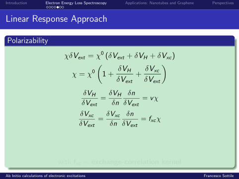
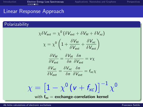
χδVext = χ0 (δVext + δVH + δVxc)
χ = χ0
(1 +
δVH
δVext+
δVxc
δVext
)δVH
δVext=
δVH
δn
δn
δVext= vχ
δVxc
δVext=
δVxc
δn
δn
δVext= fxcχ
with fxc = exchange-correlation kernel
Ab Initio calculations of electronic excitations Francesco Sottile
Introduction Electron Energy Loss Spectroscopy Applications: Nanotubes and Graphene Perspectives
Linear Response Approach
Polarizability
χδVext = χ0 (δVext + δVH + δVxc)
χ = χ0
(1 +
δVH
δVext+
δVxc
δVext
)δVH
δVext=
δVH
δn
δn
δVext= vχ
δVxc
δVext=
δVxc
δn
δn
δVext= fxcχ
with fxc = exchange-correlation kernel
Ab Initio calculations of electronic excitations Francesco Sottile

Introduction Electron Energy Loss Spectroscopy Applications: Nanotubes and Graphene Perspectives
Linear Response Approach
Polarizability
χδVext = χ0 (δVext + δVH + δVxc)
χ = χ0
(1 +
δVH
δVext+
δVxc
δVext
)δVH
δVext=
δVH
δn
δn
δVext= vχ
δVxc
δVext=
δVxc
δn
δn
δVext= fxcχ
χ = χ0 + χ0 (v + fxc) χwith fxc = exchange-correlation kernel
Ab Initio calculations of electronic excitations Francesco Sottile

Introduction Electron Energy Loss Spectroscopy Applications: Nanotubes and Graphene Perspectives
Linear Response Approach
Polarizability
χδVext = χ0 (δVext + δVH + δVxc)
χ = χ0
(1 +
δVH
δVext+
δVxc
δVext
)δVH
δVext=
δVH
δn
δn
δVext= vχ
δVxc
δVext=
δVxc
δn
δn
δVext= fxcχ
χ =[1− χ0 (v + fxc)
]−1χ0
with fxc = exchange-correlation kernel
Ab Initio calculations of electronic excitations Francesco Sottile

Introduction Electron Energy Loss Spectroscopy Applications: Nanotubes and Graphene Perspectives
Linear Response Approach
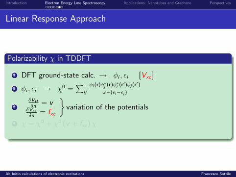
Polarizability χ in TDDFT
1 DFT ground-state calc. → φi , εi [Vxc ]
2 φi , εi → χ0 =∑
ij
φi (r)φ∗j (r)φ∗
i (r′)φj (r′)
ω−(εi−εj )
3
δVH
δn= v
δVxc
δn= fxc
variation of the potentials
4 χ = χ0 + χ0 (v + fxc) χ
Ab Initio calculations of electronic excitations Francesco Sottile

Introduction Electron Energy Loss Spectroscopy Applications: Nanotubes and Graphene Perspectives
Linear Response Approach
Polarizability χ in TDDFT
1 DFT ground-state calc. → φi , εi [Vxc ]
2 φi , εi → χ0 =∑
ij
φi (r)φ∗j (r)φ∗
i (r′)φj (r′)
ω−(εi−εj )
3
δVH
δn= v
δVxc
δn= fxc
variation of the potentials
4 χ = χ0 + χ0 (v + fxc) χ
Ab Initio calculations of electronic excitations Francesco Sottile

Introduction Electron Energy Loss Spectroscopy Applications: Nanotubes and Graphene Perspectives
Linear Response Approach
RPA and other approximations
fxc =
δVxc
δn“any” other function fxc = 0 7→ RPA
Local field effects
χ =(1− χ0v
)−1χ0 ; χ0
GG′
Ab Initio calculations of electronic excitations Francesco Sottile

Introduction Electron Energy Loss Spectroscopy Applications: Nanotubes and Graphene Perspectives
Outline
1 Introduction
2 Electron Energy Loss SpectroscopyLinear response within DFT
3 Applications: Nanotubes and Graphene
4 Perspectives
Ab Initio calculations of electronic excitations Francesco Sottile

Introduction Electron Energy Loss Spectroscopy Applications: Nanotubes and Graphene Perspectives
Actual work at the Theoretical Spectroscopy Group
EELS of semiconductors
IXS and CIXS of semiconductors and metals
EELS of nanotubes and graphene layers
EELS and IXS of strongly correlated systems (Hf, V oxydes)
RIXS spectroscopy
User projects
Ab Initio calculations of electronic excitations Francesco Sottile

Introduction Electron Energy Loss Spectroscopy Applications: Nanotubes and Graphene Perspectives
EELS of nanotubes: plasmon dispersion
Questions
theoretical understanding of electronic excitations of SWNTplasmon dispersion
SWNT and graphene. Strong connection and analysis
Ab Initio calculations of electronic excitations Francesco Sottile

Introduction Electron Energy Loss Spectroscopy Applications: Nanotubes and Graphene Perspectives
EELS of nanotubes: plasmon dispersion
VA-SWCNT
diameter: 2nm
nearly isolated
Kramberger, Hambach, Giorgetti, Rummeli, Knupfer, Fink, Buchner,
Reining, Einsarsson, Maruyama, Sottile, Hannewald, Olevano, Marinopoulos,
Pichler, Phys. Rev. Lett. 100, 196803 (2008)
Ab Initio calculations of electronic excitations Francesco Sottile

Introduction Electron Energy Loss Spectroscopy Applications: Nanotubes and Graphene Perspectives
EELS of nanotubes: plasmon dispersion
2nm is big!!
linear dispersionreminds us the Dirac
cone
Ab Initio calculations of electronic excitations Francesco Sottile

Introduction Electron Energy Loss Spectroscopy Applications: Nanotubes and Graphene Perspectives
EELS of nanotubes: plasmon dispersion
2nm is big!!
linear dispersionreminds us the Dirac
cone
Ab Initio calculations of electronic excitations Francesco Sottile
Introduction Electron Energy Loss Spectroscopy Applications: Nanotubes and Graphene Perspectives
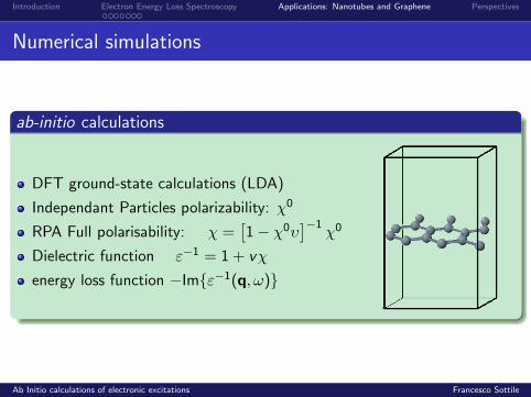
Numerical simulations
ab-initio calculations
DFT ground-state calculations (LDA)
Independant Particles polarizability: χ0
RPA Full polarisability: χ =[1− χ0υ
]−1χ0
Dielectric function ε−1 = 1 + vχ
energy loss function −Imε−1(q, ω)
Ab Initio calculations of electronic excitations Francesco Sottile

Introduction Electron Energy Loss Spectroscopy Applications: Nanotubes and Graphene Perspectives
Independent particle picture
energy loss in graphene(in-plane, q = 0.41A)
0 2 4 6 8 10energy loss (eV)
- Im
ε-1
(a
rb. u
.)
IPA =⇒ given by χ0:interpretation in terms ofband-transitions
Ab Initio calculations of electronic excitations Francesco Sottile

Introduction Electron Energy Loss Spectroscopy Applications: Nanotubes and Graphene Perspectives
Independent particle picture
energy loss in graphene(in-plane, q = 0.41A)
0 2 4 6 8 10energy loss (eV)
- Im
ε-1
(a
rb. u
.)
IPAπ−π∗ at K
bandstructure
M K Γ M-20
-15
-10
-5
0
5
Ene
rgie
(eV
)
π∗
π
σ
σ∗
Ab Initio calculations of electronic excitations Francesco Sottile

Introduction Electron Energy Loss Spectroscopy Applications: Nanotubes and Graphene Perspectives
RPA: random phase approx.
energy loss in graphene(in-plane, q = 0.41A)
0 2 4 6 8 10energy loss (eV)
- Im
ε-1
(a
rb. u
.)
IPAπ−π∗ at KRPA given by χ:
no interpretation byband-transitions
contributions from K
mixing of transitions
Ab Initio calculations of electronic excitations Francesco Sottile

Introduction Electron Energy Loss Spectroscopy Applications: Nanotubes and Graphene Perspectives
RPA: random phase approx.
energy loss in graphene(in-plane, q = 0.41A)
0 2 4 6 8 10energy loss (eV)
- Im
ε-1
(a
rb. u
.)
IPAπ−π∗ at KRPAwithout "K"
given by χ:no interpretation byband-transitions
contributions from K
mixing of transitions
Ab Initio calculations of electronic excitations Francesco Sottile
Introduction Electron Energy Loss Spectroscopy Applications: Nanotubes and Graphene Perspectives
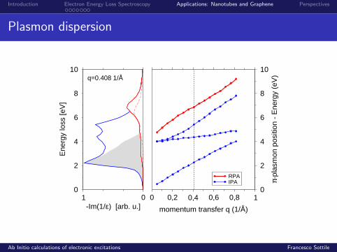
Plasmon dispersion
01-Im(1/ε) [arb. u.]
0
2
4
6
8
10E
nerg
y lo
ss [e
V]
0 0,2 0,4 0,6 0,8 1
momentum transfer q (1/Å)
0
2
4
6
8
10
π-pl
asm
on p
ositi
on -
Ene
rgy
(eV
)
RPAIPA
q=0.408 1/Å
Ab Initio calculations of electronic excitations Francesco Sottile

Introduction Electron Energy Loss Spectroscopy Applications: Nanotubes and Graphene Perspectives
SWCNT vs. Graphene
0 0.2 0.4 0.6 0.84
5
6
7
8
9
VASWCNT
(a) Experiment
0momentum transfer q (1/Å)
4
ener
gy lo
ss (
eV)
Ab Initio calculations of electronic excitations Francesco Sottile

Introduction Electron Energy Loss Spectroscopy Applications: Nanotubes and Graphene Perspectives
SWCNT vs. Graphene
0 0.2 0.4 0.6 0.84
5
6
7
8
9
VASWCNT
(a) Experiment
0 0.2 0.4 0.6 0.8 1
graphene-1L
(b) Calculation
0momentum transfer q (1/Å)
4
ener
gy lo
ss (
eV)
Ab Initio calculations of electronic excitations Francesco Sottile

Introduction Electron Energy Loss Spectroscopy Applications: Nanotubes and Graphene Perspectives
SWCNT vs. Graphene
0 0.2 0.4 0.6 0.84
5
6
7
8
9
VASWCNTbulk-SWCNT
(a) Experiment
0 0.2 0.4 0.6 0.8 1
graphene-1Lgraphene-2L
(b) Calculation
0momentum transfer q (1/Å)
4
ener
gy lo
ss (
eV)
Ab Initio calculations of electronic excitations Francesco Sottile

Introduction Electron Energy Loss Spectroscopy Applications: Nanotubes and Graphene Perspectives
SWCNT vs. Graphene: Conclusions
Graphene can be studied to get quantitative information aboutVA-SWNT
Vice-versa is also true!
Bulk (bundled) nanotubes can be studied using double layer graphene
High q measurements are applicable to probe intrinsic properties ofindividual objects within bulk arrays.
Ab Initio calculations of electronic excitations Francesco Sottile

Introduction Electron Energy Loss Spectroscopy Applications: Nanotubes and Graphene Perspectives
Outline
1 Introduction
2 Electron Energy Loss SpectroscopyLinear response within DFT
3 Applications: Nanotubes and Graphene
4 Perspectives
Ab Initio calculations of electronic excitations Francesco Sottile

Introduction Electron Energy Loss Spectroscopy Applications: Nanotubes and Graphene Perspectives
Ab initio simulation of electronic excitations
Advantages and limits√
reliable√
predictive
× cumbersome
Actual developments in the group
multiwall nanotubes - stacking of graphene layers (1 postdoc)
towards more complex systems - strongly correlated (2 postdocs)
different spectroscopies (X-ray ?) (1 postdoc)
spatial resolution EELS (PhD thesis)
Ab Initio calculations of electronic excitations Francesco Sottile

Introduction Electron Energy Loss Spectroscopy Applications: Nanotubes and Graphene Perspectives
Ab Initio calculations of electronic excitations Francesco Sottile
Introduction Electron Energy Loss Spectroscopy Applications: Nanotubes and Graphene Perspectives
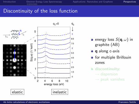
Discontinuity of the loss function
2 4 6 8 10energy loss (eV)
0
1
2
3
4
5S
(q,ω
) (1
/ keV
) 3
8/3
7/3
2
5/3
4/3
1
2/3
1/3
0
q1=0 q
3
k0
k
q
elastic inelastic
energy loss S(q, ω) ingraphite (AB)
q along c-axis
for multiple Brillouinzones
discontinuity:→ dispersion→ peak vanishes
Ab Initio calculations of electronic excitations Francesco Sottile

Introduction Electron Energy Loss Spectroscopy Applications: Nanotubes and Graphene Perspectives
Discontinuity of the loss function
2 4 6 8 10energy loss (eV)
0
1
2
3
4
5S
(q,ω
) (1
/ keV
) 3
8/3
7/3
2
5/3
4/3
1
2/3
1/3
0
q1=1/8 (~0.37 1/Å) q3
k0
k
q
elastic inelastic
energy loss S(q, ω) ingraphite (AB)
q along c-axis
for multiple Brillouinzones
discontinuity:→ dispersion→ peak vanishes
Ab Initio calculations of electronic excitations Francesco Sottile
Related Documents