Page 1 Note 1: Click CTRL+j on your keyboard before using this spreadsheet in EXCEL97. Note 2: Due to different monitor, EXCEL, and fonts capabilities on different computer sheets may be truncated. It may be necessary to unprotect the sheet a Note 3: This spreadsheet needs to be copied to the hard drive to be used. It cannot Note 4: Figures accompanying the text are scanned into the spreadsheet. For clarity useful to print these pages and use the printed figures. I. Input Sheet - General Information The general information section requests information about the agen information is not required for the analysis, but the information may be displayed on the "Results" sheet. II. Input Sheet - Design Information All design inputs are required except sensitivity analysis. No default values are used. Information can be retrieved from the "Saved Data" sheet using the button. The existing data can be replaced or saved as a new set us "Save Data" button. Clicking on the "Retrieve Data" button opens the "Saved Data" sheet appropriate row to be retrieved and click on the "Export" button. If the retrieval is successful, the data are retreived. Changes ca as a new data set using a different value for the search ID. The d be overwritten using the same search ID. The search value can be t combination of the two that uniquely identifies the data (example: This feature can also be used to save a default set of values. Using the "Clear All" ID to retrieve the "Clear All" data set clear the spreadsheet. Design information such as initial and terminal serviceability, co properties, and reliability and standard deviation can be input in Table 14 provides help for estimating base property values. Climatic properties such as wind, temperature, and precipitation, w positive temperature differential calculation, can be estimated usi properties for major cities provided in table 15. A pavement type can be selected by clicking the option buttons prov JRCP, the joint spacing needs to be entered in ft in the space prov automatically calculates the effective joint spacing to be used in Edge support can also be selected using the option buttons provided automatically calculates the edge support factor to be used in desi A first run MUST be performed using design inputs for all variables estimated effective subgrade k-value. This determines an approxima for the inputs provided. The user can then navigate to the seasona sheet (and, if necessary, the "Fill/Rigid Layer" sheet) to calculat the effects of season and presence of fill section or rigid layer b (The approximate slab thickness obtained from the first run is used during different seasons of the year.) Approximately 3 to 4 iterations will be required (i.e., after a fir a trial thickness is obtained). The "Calculate seasonal k-value" b

Welcome message from author
This document is posted to help you gain knowledge. Please leave a comment to let me know what you think about it! Share it to your friends and learn new things together.
Transcript

Page 1
Note 1: Click CTRL+j on your keyboard before using this spreadsheet in EXCEL97.Note 2: Due to different monitor, EXCEL, and fonts capabilities on different computers, the text on some of the sheets may be truncated. It may be necessary to unprotect the sheet and resize some of the columns.Note 3: This spreadsheet needs to be copied to the hard drive to be used. It cannot be run off a floppy drive.Note 4: Figures accompanying the text are scanned into the spreadsheet. For clarity of these figures it may be useful to print these pages and use the printed figures.
I. Input Sheet - General Information
The general information section requests information about the agency. This information is not required for the analysis, but the information entered here may be displayed on the "Results" sheet.
II. Input Sheet - Design Information
All design inputs are required except sensitivity analysis.No default values are used.
Information can be retrieved from the "Saved Data" sheet using the "Retrieve Data"button. The existing data can be replaced or saved as a new set using the"Save Data" button. Clicking on the "Retrieve Data" button opens the "Saved Data" sheet. Select theappropriate row to be retrieved and click on the "Export" button.If the retrieval is successful, the data are retreived. Changes can be made and savedas a new data set using a different value for the search ID. The data can alsobe overwritten using the same search ID. The search value can be text, numbers, or acombination of the two that uniquely identifies the data (example: Project Numbers).This feature can also be used to save a default set of values.Using the "Clear All" ID to retrieve the "Clear All" data set clears all the data inthe spreadsheet.
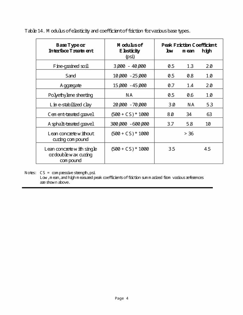
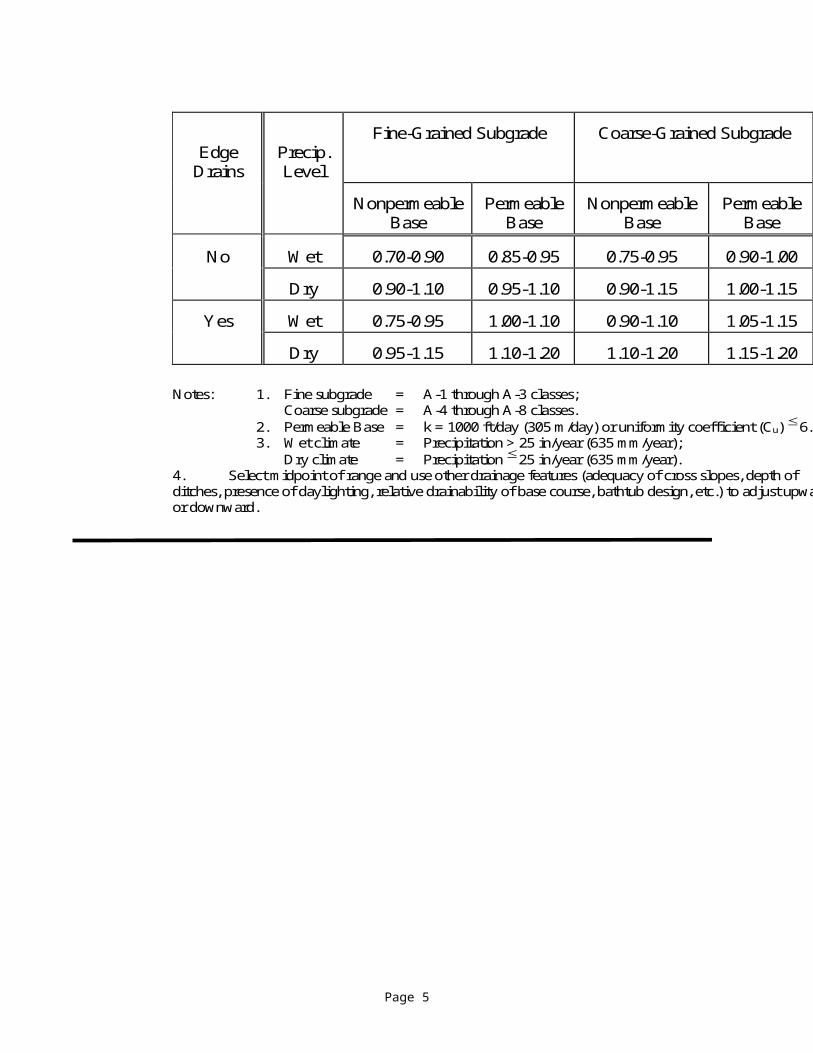
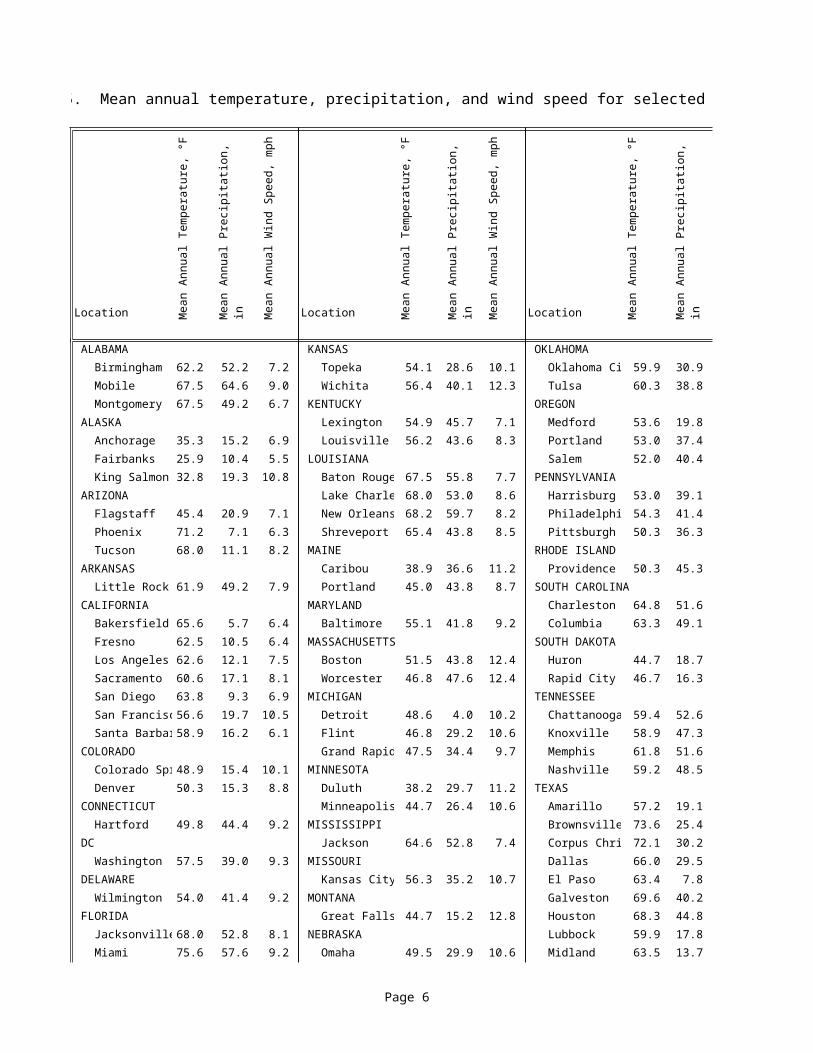
Design information such as initial and terminal serviceability, concrete properties, baseproperties, and reliability and standard deviation can be input in the appropriate cells. Table 14 provides help for estimating base property values.Climatic properties such as wind, temperature, and precipitation, which are required forpositive temperature differential calculation, can be estimated using the table of climaticproperties for major cities provided in table 15.A pavement type can be selected by clicking the option buttons provided. For JPCP and JRCP, the joint spacing needs to be entered in ft in the space provided. Thisautomatically calculates the effective joint spacing to be used in design.
Edge support can also be selected using the option buttons provided. Thisautomatically calculates the edge support factor to be used in design.
A first run MUST be performed using design inputs for all variables and using anestimated effective subgrade k-value. This determines an approximate slab thicknessfor the inputs provided. The user can then navigate to the seasonal k-value calculationsheet (and, if necessary, the "Fill/Rigid Layer" sheet) to calculate the k-value adjusted forthe effects of season and presence of fill section or rigid layer beneath the pavement. (The approximate slab thickness obtained from the first run is used in calculating the damageduring different seasons of the year.)Approximately 3 to 4 iterations will be required (i.e., after a first run with a trial k-value,a trial thickness is obtained). The "Calculate seasonal k-value" button can then be used to
Page 2
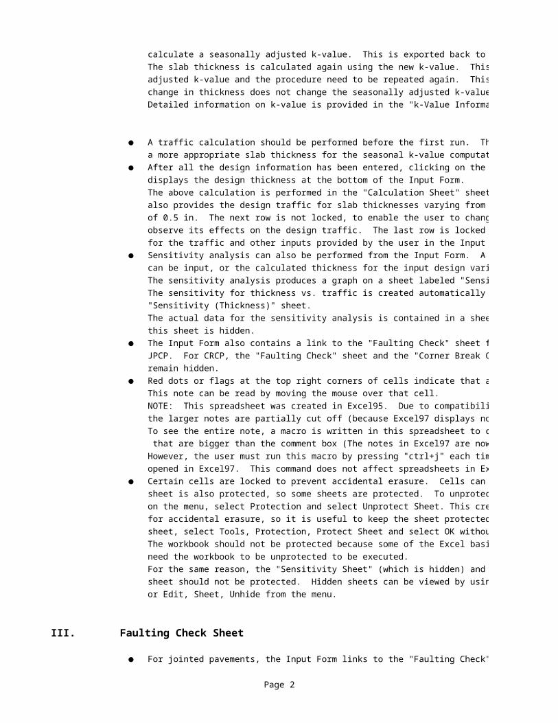
calculate a seasonally adjusted k-value. This is exported back to the "Input Form" sheet.The slab thickness is calculated again using the new k-value. This changes the seasonaladjusted k-value and the procedure need to be repeated again. This is done till thechange in thickness does not change the seasonally adjusted k-value.Detailed information on k-value is provided in the "k-Value Information" Sheet.
A traffic calculation should be performed before the first run. This will result ina more appropriate slab thickness for the seasonal k-value computation.
After all the design information has been entered, clicking on the "Calculate" buttondisplays the design thickness at the bottom of the Input Form.The above calculation is performed in the "Calculation Sheet" sheet. The "Calculation Sheet"also provides the design traffic for slab thicknesses varying from 7 in to 15 inches, in increments of 0.5 in. The next row is not locked, to enable the user to change any variable andobserve its effects on the design traffic. The last row is locked and represents the thicknessfor the traffic and other inputs provided by the user in the Input Form.
Sensitivity analysis can also be performed from the Input Form. A desired thicknesscan be input, or the calculated thickness for the input design variable can be imported.The sensitivity analysis produces a graph on a sheet labeled "Sensitivity (Other)."The sensitivity for thickness vs. traffic is created automatically on the "Sensitivity (Thickness)" sheet.The actual data for the sensitivity analysis is contained in a sheet called "Sensitivity Sheet;"this sheet is hidden.
The Input Form also contains a link to the "Faulting Check" sheet for JRCP andJPCP. For CRCP, the "Faulting Check" sheet and the "Corner Break Check" sheetremain hidden.
Red dots or flags at the top right corners of cells indicate that a note is attached to that cell.This note can be read by moving the mouse over that cell.NOTE: This spreadsheet was created in Excel95. Due to compatibility problems with Excel97,the larger notes are partially cut off (because Excel97 displays notes with fixed sizes as default).To see the entire note, a macro is written in this spreadsheet to change the size of notes that are bigger than the comment box (The notes in Excel97 are now called comments). However, the user must run this macro by pressing "ctrl+j" each time the spreadsheet is opened in Excel97. This command does not affect spreadsheets in Excel95.
Certain cells are locked to prevent accidental erasure. Cells can only be locked when thesheet is also protected, so some sheets are protected. To unprotect a sheet, go to Toolson the menu, select Protection and select Unprotect Sheet. This creates the potentialfor accidental erasure, so it is useful to keep the sheet protected. To reprotect thesheet, select Tools, Protection, Protect Sheet and select OK without entering a password.The workbook should not be protected because some of the Excel basic programs (macros)need the workbook to be unprotected to be executed.For the same reason, the "Sensitivity Sheet" (which is hidden) and the "Saved Data"sheet should not be protected. Hidden sheets can be viewed by using Format, Sheet, Unhide,or Edit, Sheet, Unhide from the menu.
III. Faulting Check Sheet
For jointed pavements, the Input Form links to the "Faulting Check" sheet. All cells
Page 3
need to be input in this sheet. The cells that do not need to be input are hidden usingthe outlining ("+") at the left of the sheet. To observe the values at this location, the sheet hasto be unprotected and the "+" clicked.Each time a cell value is changed, the "Calculate" button needs to be clicked to calculatefaulting, which is displayed at the bottom of the sheet. This is then compared with the criteria set at the bottom of the sheet to "PASS" or "FAIL" the design.The criteria can be changed by changing the values in the criteria table.
The doweled and nondoweled sheets are designed independent of each other to providethe user control over the individual design. For example, the user may decide to provide
While making a one-on-one comparison between the faulting check for the doweled andnondoweled designs, the user needs to ensure that all values are comparable.
Corner break checks need to be performed only for nondoweled pavements. This sheetcan be accessed by clicking on the "Corner Break Check" button.
edgedrains for the nondoweled design, which will change the drainage coefficient, C
Page 4
Table 14. Modulus of elasticity and coefficient of friction for various base types.
Base Type orInterface Treatment
Modulus ofElasticity
(psi)
Peak Friction Coefficientlow mean high
Fine-grained soil 3,000 - 40,000 0.5 1.3 2.0
Sand 10,000 - 25,000 0.5 0.8 1.0
Aggregate 15,000 - 45,000 0.7 1.4 2.0
Polyethylene sheeting NA 0.5 0.6 1.0
Lime-stabilized clay 20,000 - 70,000 3.0 NA 5.3
Cement-treated gravel (500 + CS) * 1000 8.0 34 63
Asphalt-treated gravel 300,000 - 600,000 3.7 5.8 10
Lean concrete withoutcuring compound
(500 + CS) * 1000 > 36
Lean concrete with singleor double wax curing
compound
(500 + CS) * 1000 3.5 4.5
Notes: CS = compressive strength, psiLow, mean, and high measured peak coefficients of friction summarized from various referencesare shown above.
Page 5
EdgeDrains
Precip.Level
Fine-Grained Subgrade Coarse-Grained Subgrade
NonpermeableBase
PermeableBase
NonpermeableBase
PermeableBase
No Wet 0.70-0.90 0.85-0.95 0.75-0.95 0.90-1.00
Dry 0.90-1.10 0.95-1.10 0.90-1.15 1.00-1.15
Yes Wet 0.75-0.95 1.00-1.10 0.90-1.10 1.05-1.15
Dry 0.95-1.15 1.10-1.20 1.10-1.20 1.15-1.20
Notes: 1. Fine subgrade = A-1 through A-3 classes;Coarse subgrade = A-4 through A-8 classes.
2. Permeable Base = k = 1000 ft/day (305 m/day) or uniformity coefficient (Cu) 6.3. Wet climate = Precipitation > 25 in/year (635 mm/year);
Dry climate = Precipitation 25 in/year (635 mm/year).4. Select midpoint of range and use other drainage features (adequacy of cross slopes, depth ofditches, presence of daylighting, relative drainability of base course, bathtub design, etc.) to adjust upwardor downward.
Page 6
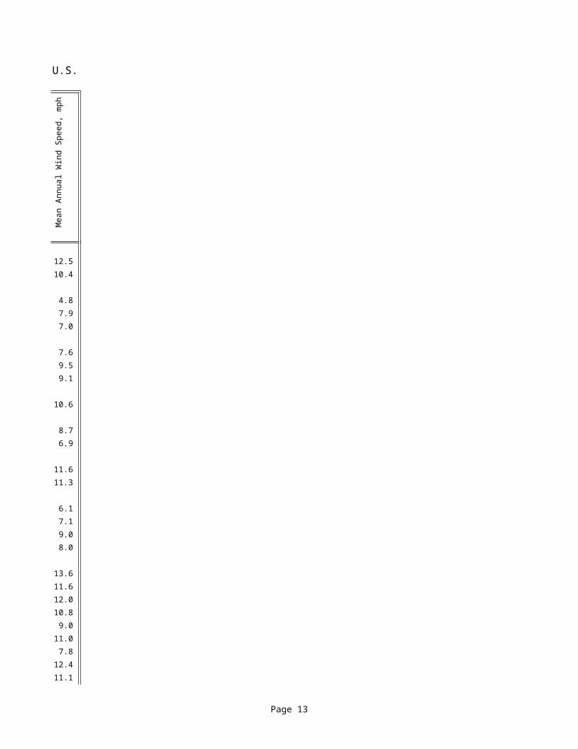
Table 15. Mean annual temperature, precipitation, and wind speed for selected U.S. cities.
Location Mea
n A
nnua
l Tem
pera
ture
, °F
Mea
n A
nnua
l Pre
cipi
tatio
n, in
Location Mea
n A
nnua
l Tem
pera
ture
, °F
Mea
n A
nnua
l Pre
cipi
tatio
n, in
Location Mea
n A
nnua
l Tem
pera
ture
, °F
ALABAMA KANSAS OKLAHOMA
Birmingham 62.2 52.2 7.2 Topeka 54.1 28.6 10.1 Oklahoma City 59.9
Mobile 67.5 64.6 9.0 Wichita 56.4 40.1 12.3 Tulsa 60.3
Montgomery 67.5 49.2 6.7 KENTUCKY OREGON
ALASKA Lexington 54.9 45.7 7.1 Medford 53.6
Anchorage 35.3 15.2 6.9 Louisville 56.2 43.6 8.3 Portland 53.0
Fairbanks 25.9 10.4 5.5 LOUISIANA Salem 52.0
King Salmon 32.8 19.3 10.8 Baton Rouge 67.5 55.8 7.7 PENNSYLVANIA
ARIZONA Lake Charles 68.0 53.0 8.6 Harrisburg 53.0
Flagstaff 45.4 20.9 7.1 New Orleans 68.2 59.7 8.2 Philadelphia 54.3
Phoenix 71.2 7.1 6.3 Shreveport 65.4 43.8 8.5 Pittsburgh 50.3
Tucson 68.0 11.1 8.2 MAINE RHODE ISLAND
ARKANSAS Caribou 38.9 36.6 11.2 Providence 50.3
Little Rock 61.9 49.2 7.9 Portland 45.0 43.8 8.7 SOUTH CAROLINA
CALIFORNIA MARYLAND Charleston 64.8
Bakersfield 65.6 5.7 6.4 Baltimore 55.1 41.8 9.2 Columbia 63.3
Fresno 62.5 10.5 6.4 MASSACHUSETTS SOUTH DAKOTA
Los Angeles 62.6 12.1 7.5 Boston 51.5 43.8 12.4 Huron 44.7
Sacramento 60.6 17.1 8.1 Worcester 46.8 47.6 12.4 Rapid City 46.7
San Diego 63.8 9.3 6.9 MICHIGAN TENNESSEE
San Francisco 56.6 19.7 10.5 Detroit 48.6 4.0 10.2 Chattanooga 59.4
Santa Barbara 58.9 16.2 6.1 Flint 46.8 29.2 10.6 Knoxville 58.9
COLORADO Grand Rapids 47.5 34.4 9.7 Memphis 61.8
Colorado Springs 48.9 15.4 10.1 MINNESOTA Nashville 59.2
Denver 50.3 15.3 8.8 Duluth 38.2 29.7 11.2 TEXAS
CONNECTICUT Minneapolis 44.7 26.4 10.6 Amarillo 57.2
Hartford 49.8 44.4 9.2 MISSISSIPPI Brownsville 73.6
DC Jackson 64.6 52.8 7.4 Corpus Christi 72.1
Washington 57.5 39.0 9.3 MISSOURI Dallas 66.0
DELAWARE Kansas City 56.3 35.2 10.7 El Paso 63.4
Wilmington 54.0 41.4 9.2 MONTANA Galveston 69.6
FLORIDA Great Falls 44.7 15.2 12.8 Houston 68.3
Jacksonville 68.0 52.8 8.1 NEBRASKA Lubbock 59.9
Miami 75.6 57.6 9.2 Omaha 49.5 29.9 10.6 Midland 63.5
Orlando 72.4 47.8 8.6 NEVADA San Antonio 68.7
Tallahassee 67.2 64.6 6.4 Las Vegas 66.3 4.2 9.2 Waco 67.0
Tampa 72.0 46.7 8.5 Reno 49.4 7.5 6.5 Wichita Falls 63.5
Mea
n A
nnua
l Win
d Sp
eed,
m
ph
Mea
n A
nnua
l Win
d Sp
eed,
m
ph

Page 7
West Palm Beach 74.6 59.7 9.4 NEW JERSEY UTAH
GEORGIA Atlantic City 53.1 41.9 10.1 Salt Lake City 51.7
Atlanta 61.2 48.6 9.1 NEW MEXICO VERMONT
Augusta 63.2 43.1 6.5 Albuquerque 56.2 8.1 9.0 Burlington 44.1
Macon 64.7 44.9 7.7 NEW YORK VIRGINIA
Savannah 65.9 49.7 7.9 Albany 47.3 35.7 8.9 Norfolk 59.5
HAWAII Buffalo 47.6 37.5 12.1 Richmond 57.7
Hilo 73.6 128.2 7.1 New York City 54.5 44.1 12.1 Roanoke 56.1
Honolulu 77.0 23.5 11.5 Rochester 47.9 31.3 9.7 WASHINGTON
IDAHO Syracuse 47.7 39.1 9.7 Olympia 49.6
Boise 51.1 11.7 8.8 NORTH CAROLINA Seattle 52.7
Pocatello 46.6 10.9 10.2 Charlotte 60.0 43.2 7.5 Spokane 47.2
ILLINOIS Greensboro 57.9 42.5 7.5 WEST VIRGINIA
Chicago 49.2 33.3 10.2 Raleigh 59.0 41.8 7.8 Charleston 54.8
Peoria 50.4 34.9 10.1 Wilmington 63.4 53.4 8.8 Huntington 55.2
Springfield 52.6 33.8 11.3 NORTH DAKOTA WISCONSIN
INDIANA Bismarck 41.3 15.4 10.3 Green Bay 43.6
Evansville 55.7 41.6 8.2 Fargo 40.5 19.6 12.4 Madison 45.2
Fort Wayne 49.7 34.4 10.1 OHIO Milwaukee 46.1
Indianapolis 52.1 39.1 9.6 Akron-Canton 49.5 35.9 9.8 WYOMING
South Bend 49.4 38.2 10.4 Cleveland 49.6 35.4 10.7 Casper 45.2
IOWA Columbus 51.7 37.0 8.7 Cheyenne 45.7
Des Moines 49.7 30.8 10.9 Dayton 51.9 34.7 10.1
Sioux City 48.4 25.4 11.0 Youngstown 48.3 37.3 10.0
Waterloo 46.1 33.1 10.7
°C =(°F - 32)/1.8, 1 in = 25.4 mm, 1 mph = 1.61 km/h Source: National Climatic Data Center, 1986
Page 8
Note 2: Due to different monitor, EXCEL, and fonts capabilities on different computers, the text on some of the sheets may be truncated. It may be necessary to unprotect the sheet and resize some of the columns.Note 3: This spreadsheet needs to be copied to the hard drive to be used. It cannot be run off a floppy drive.Note 4: Figures accompanying the text are scanned into the spreadsheet. For clarity of these figures it may be
The general information section requests information about the agency. This information is not required for the analysis, but the information entered here
Information can be retrieved from the "Saved Data" sheet using the "Retrieve Data"
Clicking on the "Retrieve Data" button opens the "Saved Data" sheet. Select the
If the retrieval is successful, the data are retreived. Changes can be made and savedas a new data set using a different value for the search ID. The data can alsobe overwritten using the same search ID. The search value can be text, numbers, or acombination of the two that uniquely identifies the data (example: Project Numbers).
Using the "Clear All" ID to retrieve the "Clear All" data set clears all the data in
Design information such as initial and terminal serviceability, concrete properties, baseproperties, and reliability and standard deviation can be input in the appropriate cells.
Climatic properties such as wind, temperature, and precipitation, which are required forpositive temperature differential calculation, can be estimated using the table of climatic
A pavement type can be selected by clicking the option buttons provided. For JPCP and JRCP, the joint spacing needs to be entered in ft in the space provided. This
A first run MUST be performed using design inputs for all variables and using anestimated effective subgrade k-value. This determines an approximate slab thicknessfor the inputs provided. The user can then navigate to the seasonal k-value calculationsheet (and, if necessary, the "Fill/Rigid Layer" sheet) to calculate the k-value adjusted forthe effects of season and presence of fill section or rigid layer beneath the pavement. (The approximate slab thickness obtained from the first run is used in calculating the damage
Approximately 3 to 4 iterations will be required (i.e., after a first run with a trial k-value,a trial thickness is obtained). The "Calculate seasonal k-value" button can then be used to
Page 9
calculate a seasonally adjusted k-value. This is exported back to the "Input Form" sheet.The slab thickness is calculated again using the new k-value. This changes the seasonaladjusted k-value and the procedure need to be repeated again. This is done till the
Detailed information on k-value is provided in the "k-Value Information" Sheet.
A traffic calculation should be performed before the first run. This will result in
After all the design information has been entered, clicking on the "Calculate" button
The above calculation is performed in the "Calculation Sheet" sheet. The "Calculation Sheet"also provides the design traffic for slab thicknesses varying from 7 in to 15 inches, in increments of 0.5 in. The next row is not locked, to enable the user to change any variable andobserve its effects on the design traffic. The last row is locked and represents the thickness
Sensitivity analysis can also be performed from the Input Form. A desired thicknesscan be input, or the calculated thickness for the input design variable can be imported.The sensitivity analysis produces a graph on a sheet labeled "Sensitivity (Other)."
The actual data for the sensitivity analysis is contained in a sheet called "Sensitivity Sheet;"
The Input Form also contains a link to the "Faulting Check" sheet for JRCP andJPCP. For CRCP, the "Faulting Check" sheet and the "Corner Break Check" sheet
Red dots or flags at the top right corners of cells indicate that a note is attached to that cell.
NOTE: This spreadsheet was created in Excel95. Due to compatibility problems with Excel97,the larger notes are partially cut off (because Excel97 displays notes with fixed sizes as default).To see the entire note, a macro is written in this spreadsheet to change the size of notes that are bigger than the comment box (The notes in Excel97 are now called comments). However, the user must run this macro by pressing "ctrl+j" each time the spreadsheet is opened in Excel97. This command does not affect spreadsheets in Excel95.Certain cells are locked to prevent accidental erasure. Cells can only be locked when thesheet is also protected, so some sheets are protected. To unprotect a sheet, go to Toolson the menu, select Protection and select Unprotect Sheet. This creates the potentialfor accidental erasure, so it is useful to keep the sheet protected. To reprotect thesheet, select Tools, Protection, Protect Sheet and select OK without entering a password.The workbook should not be protected because some of the Excel basic programs (macros)
For the same reason, the "Sensitivity Sheet" (which is hidden) and the "Saved Data"sheet should not be protected. Hidden sheets can be viewed by using Format, Sheet, Unhide,
For jointed pavements, the Input Form links to the "Faulting Check" sheet. All cells
Page 10
need to be input in this sheet. The cells that do not need to be input are hidden usingthe outlining ("+") at the left of the sheet. To observe the values at this location, the sheet has
Each time a cell value is changed, the "Calculate" button needs to be clicked to calculatefaulting, which is displayed at the bottom of the sheet. This is then compared with the criteria
The doweled and nondoweled sheets are designed independent of each other to providethe user control over the individual design. For example, the user may decide to provide
While making a one-on-one comparison between the faulting check for the doweled andnondoweled designs, the user needs to ensure that all values are comparable.Corner break checks need to be performed only for nondoweled pavements. This sheet
edgedrains for the nondoweled design, which will change the drainage coefficient, Cd.

Page 11
Table 14. Modulus of elasticity and coefficient of friction for various base types.
Base Type orInterface Treatment
Modulus ofElasticity
(psi)
Peak Friction Coefficientlow mean high
Fine-grained soil 3,000 - 40,000 0.5 1.3 2.0
Sand 10,000 - 25,000 0.5 0.8 1.0
Aggregate 15,000 - 45,000 0.7 1.4 2.0
Polyethylene sheeting NA 0.5 0.6 1.0
Lime-stabilized clay 20,000 - 70,000 3.0 NA 5.3
Cement-treated gravel (500 + CS) * 1000 8.0 34 63
Asphalt-treated gravel 300,000 - 600,000 3.7 5.8 10
Lean concrete withoutcuring compound
(500 + CS) * 1000 > 36
Lean concrete with singleor double wax curing
compound
(500 + CS) * 1000 3.5 4.5
Notes: CS = compressive strength, psiLow, mean, and high measured peak coefficients of friction summarized from various referencesare shown above.

Page 12
EdgeDrains
Precip.Level
Fine-Grained Subgrade Coarse-Grained Subgrade
NonpermeableBase
PermeableBase
NonpermeableBase
PermeableBase
No Wet 0.70-0.90 0.85-0.95 0.75-0.95 0.90-1.00
Dry 0.90-1.10 0.95-1.10 0.90-1.15 1.00-1.15
Yes Wet 0.75-0.95 1.00-1.10 0.90-1.10 1.05-1.15
Dry 0.95-1.15 1.10-1.20 1.10-1.20 1.15-1.20
Notes: 1. Fine subgrade = A-1 through A-3 classes;Coarse subgrade = A-4 through A-8 classes.
2. Permeable Base = k = 1000 ft/day (305 m/day) or uniformity coefficient (Cu) 6.3. Wet climate = Precipitation > 25 in/year (635 mm/year);
Dry climate = Precipitation 25 in/year (635 mm/year).4. Select midpoint of range and use other drainage features (adequacy of cross slopes, depth ofditches, presence of daylighting, relative drainability of base course, bathtub design, etc.) to adjust upwardor downward.
Page 13
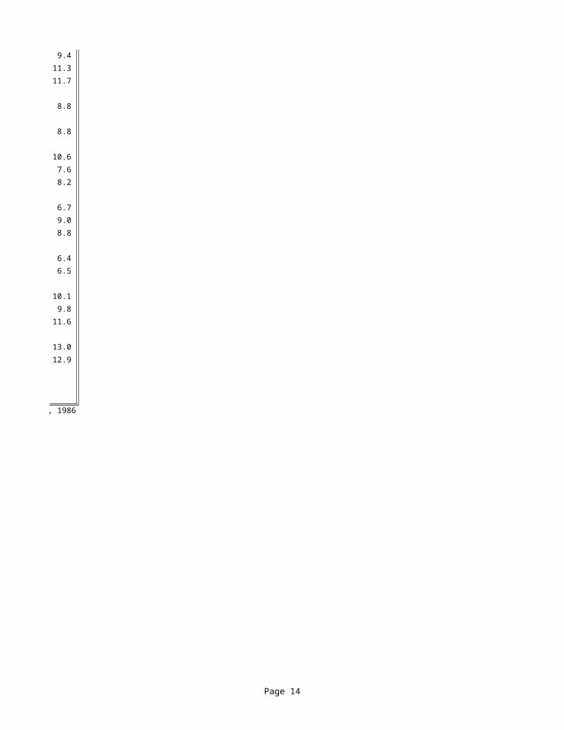
Table 15. Mean annual temperature, precipitation, and wind speed for selected U.S. cities.M
ean
Ann
ual P
reci
pita
tion,
in
30.9 12.5
38.8 10.4
19.8 4.8
37.4 7.9
40.4 7.0
39.1 7.6
41.4 9.5
36.3 9.1
45.3 10.6
51.6 8.7
49.1 6.9
18.7 11.6
16.3 11.3
52.6 6.1
47.3 7.1
51.6 9.0
48.5 8.0
19.1 13.6
25.4 11.6
30.2 12.0
29.5 10.8
7.8 9.0
40.2 11.0
44.8 7.8
17.8 12.4
13.7 11.1
29.2 9.4
31.0 11.3
26.7 11.7
Mea
n A
nnua
l Win
d Sp
eed,
m
ph
Page 14
15.3 8.8
33.7 8.8
45.2 10.6
44.1 7.6
39.2 8.2
51.0 6.7
38.8 9.0
16.7 8.8
42.4 6.4
40.7 6.5
28.0 10.1
30.8 9.8
30.9 11.6
11.4 13.0
13.3 12.9
Source: National Climatic Data Center, 1986

Rigid Pavement Design - Based on AASHTO Supplemental Guide
I. General
Agency:Street Address:
City:State:
Project Number: ID: Clear
Description:
Location:
II. Design
Serviceability
Initial Serviceability, P1: Joint Spacing:Terminal Serviceability, P2:
ftPCC Properties
psi JPCPpsi
Poisson's Ratio for Concrete, m: 0.15 Effective Joint Spacing: 0 in ###
Base Properties
psiin
Slab-Base Friction Factor, f:
Reliability and Standard Deviation
Reliability Level (R): % Edge Support Factor: 1.00
Climatic Properties Slab Thickness used forMean Annual Wind Speed, WIND: mph Sensitivity Analysis: 11.24 in
Mean Annual Air Temperature, TEMP:Mean Annual Precipitation, PRECIP: in
Subgrade k-Value
psi/in
Design ESALs
million
Calculated Slab Thickness for Above Inputs: in
Reference: LTPP DATA ANALYSIS - Phase I: Validation of Guidelines for k-Value Selection and Concrete Pavement Performance Prediction
28-day Mean Modulus of Rupture, (S'c)':Elastic Modulus of Slab, Ec:
Elastic Modulus of Base, Eb:Design Thickness of Base, Hb:
Overall Standard Deviation, S0:
oF
Pavement Type, Joint Spacing (L)
JPCP
JRCP
CRCP
Edge Support
Conventional 12-ft wide traffic lane
Conventional 12-ft wide traffic lane + tied PCC
2-ft widened slab w/conventional 12-ft traffic lane
Sensitivity Analysis
Modulus of Rupture Elastic Modulus (Slab)
Elastic Modulus (Base) Base Thickness
k-Value Joint Spacing
Reliability Standard Deviation
H31
Joint Spacing, inches: JPCP: Actual Joint Spacing JRCP: Actual Joint Spacing if less than 30 ft, 30 ft max. CRCP: 15 ft This value is automatically calculated.
D34
Refer to Table 14 in Information Sheet
D36
Refer to Table 14 in Information Sheet
H39
Edge Support Adjustment Factor =1.00 for conventional 12-ft wide lane =0.94 for conventional 12-ft wide lane + tied PCC =0.92 for 2-ft widened slab with conventional 12-ft wide lane This value is automatically calculated
D43
Refer to Table 15 in information sheet
D44
Refer to Table 15 in information sheet
D45
Refer to Table 15 in information sheet
D48
An estimated k-value is required for the seasonal adjustment calculations. Refer to "Information" sheet for more details.
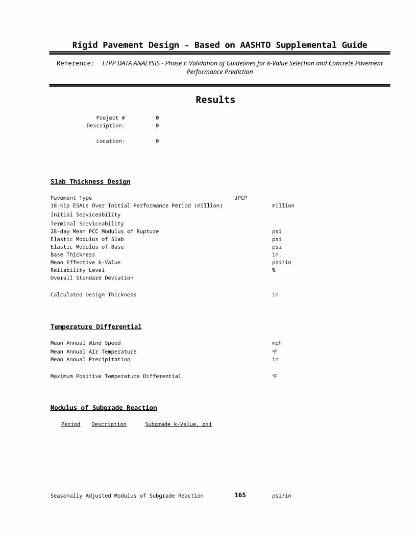
Rigid Pavement Design - Based on AASHTO Supplemental Guide
ResultsProject # 0
Description: 0
Location: 0
Slab Thickness Design
Pavement Type JPCP18-kip ESALs Over Initial Performance Period (million) millionInitial ServiceabilityTerminal Serviceability28-day Mean PCC Modulus of Rupture psiElastic Modulus of Slab psiElastic Modulus of Base psiBase Thickness in.Mean Effective k-Value psi/inReliability Level %Overall Standard Deviation
Calculated Design Thickness in
Temperature Differential
Mean Annual Wind Speed mphMean Annual Air TemperatureMean Annual Precipitation in
Maximum Positive Temperature Differential
Modulus of Subgrade Reaction
Period Description Subgrade k-Value, psi
Seasonally Adjusted Modulus of Subgrade Reaction 165 psi/in
Modulus of Subgrade Reaction Adjusted for Rigid Layerand Fill Section 0 psi/in
Reference: LTPP DATA ANALYSIS - Phase I: Validation of Guidelines for k-Value Selection and Concrete Pavement Performance Prediction
oF
oF
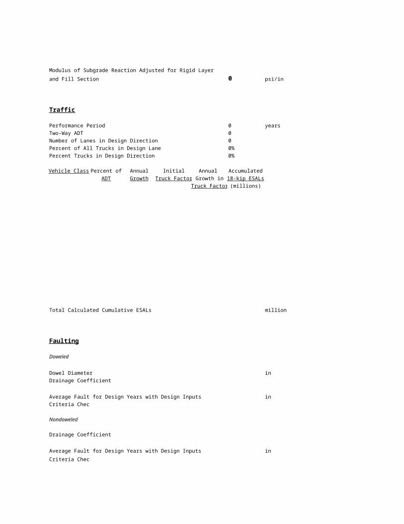
Traffic
Performance Period 0 yearsTwo-Way ADT 0Number of Lanes in Design Direction 0Percent of All Trucks in Design Lane 0%Percent Trucks in Design Direction 0%
Vehicle Class Percent of Annual Initial Annual AccumulatedADT Growth Truck Factor Growth in 18-kip ESALs
Truck Factor (millions)
Total Calculated Cumulative ESALs million
Faulting
Doweled
Dowel Diameter inDrainage Coefficient
Average Fault for Design Years with Design Inputs inCriteria Check
Nondoweled
Drainage Coefficient
Average Fault for Design Years with Design Inputs inCriteria Check
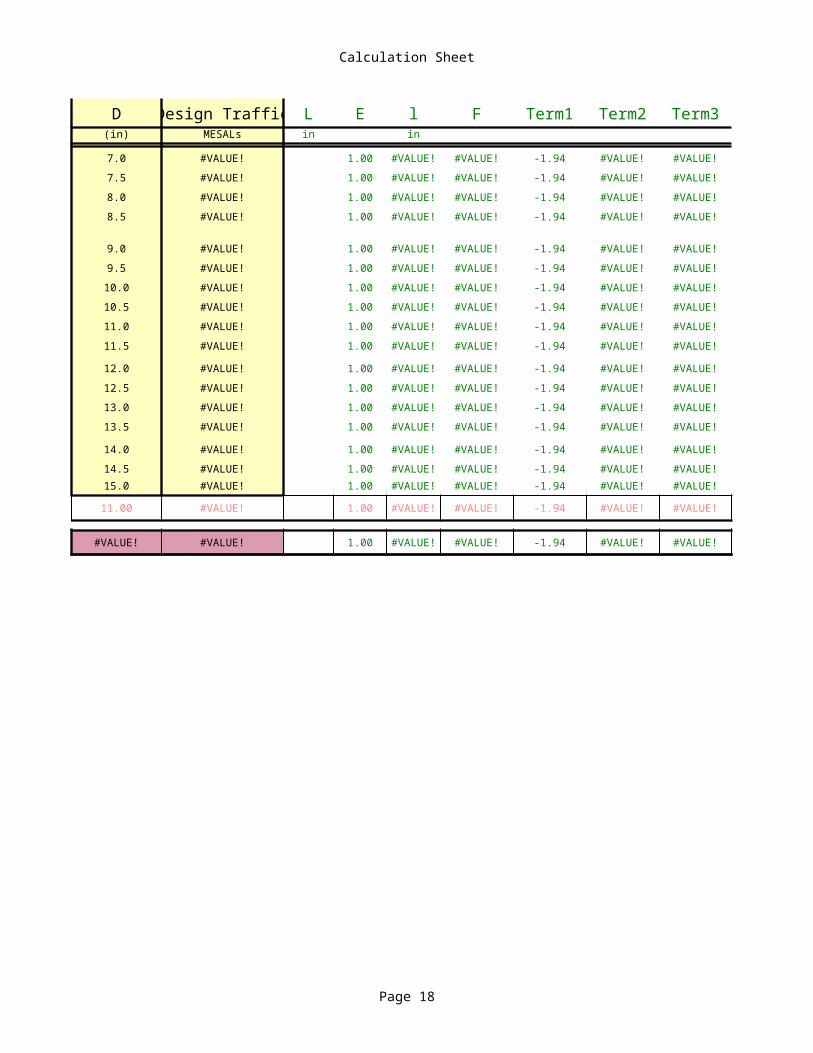
Calculation Sheet
Page 18
D Design Traffic L E l F Term1 Term2(in) MESALs in in
7.0 #VALUE! 1.00 ### #VALUE! -1.94 #VALUE!
7.5 #VALUE! 1.00 ### #VALUE! -1.94 #VALUE!
8.0 #VALUE! 1.00 ### #VALUE! -1.94 #VALUE!
8.5 #VALUE! 1.00 ### #VALUE! -1.94 #VALUE!
9.0 #VALUE! 1.00 ### #VALUE! -1.94 #VALUE!
9.5 #VALUE! 1.00 ### #VALUE! -1.94 #VALUE!
10.0 #VALUE! 1.00 ### #VALUE! -1.94 #VALUE!
10.5 #VALUE! 1.00 ### #VALUE! -1.94 #VALUE!
11.0 #VALUE! 1.00 ### #VALUE! -1.94 #VALUE!
11.5 #VALUE! 1.00 ### #VALUE! -1.94 #VALUE!
12.0 #VALUE! 1.00 ### #VALUE! -1.94 #VALUE!
12.5 #VALUE! 1.00 ### #VALUE! -1.94 #VALUE!
13.0 #VALUE! 1.00 ### #VALUE! -1.94 #VALUE!
13.5 #VALUE! 1.00 ### #VALUE! -1.94 #VALUE!
14.0 #VALUE! 1.00 ### #VALUE! -1.94 #VALUE!
14.5 #VALUE! 1.00 ### #VALUE! -1.94 #VALUE!15.0 #VALUE! 1.00 ### #VALUE! -1.94 #VALUE!
11.00 #VALUE! 1.00 ### #VALUE! -1.94 #VALUE!
#VALUE! #VALUE! 1.00 ### #VALUE! -1.94 #VALUE!
A1
Slab Thickness varied from 7 inches to 15 inches
B1
Total Number of ESALs for given reliability and slab thickness
C1
Joint Spacing, inches: JPCP: Actual Joint Spacing JRCP: Actual Joint Spacing if less than 30 ft, 30 ft max. CRCP: 15 ft
D1
Edge Support Adjustment Factor =1.00 for conventional 12-ft wide lane =0.94 for conventional 12-ft wide lane + tied PCC =0.92 for 2-ft widened slab with conventional 12-ft wide lane
E1
Radius of Relative Stiffness, in. (Equation 45)
F1
F = ratio between slab stress at given friction f between slab and base and slab stress at full friction. (Equation 46)
G1
First term (Equation 47)
H1
Second Term (Equation 47)
A21
This row is not locked to enable the user to input values in any cell of this row. To retreive the functionality user must change back to original formula in cell This can be done as follows after unprotecting the sheet a. Select any cell above (in the same column) Edit, Copy b. Select the cell that was changed Edit, Paste Special, Formula, OK
A23
This row is locked and the values in this row are representative of the traffic input (Design ESALs) by the user This is the design thickness used in other calculations
Calculation Sheet
Page 19
Term3 Term4 Term5 Term6 Term7 log b b TD
#VALUE! #VALUE! #VALUE! #VALUE! #VALUE! #VALUE! #VALUE! #VALUE!
#VALUE! #VALUE! #VALUE! #VALUE! #VALUE! #VALUE! #VALUE! #VALUE!
#VALUE! #VALUE! #VALUE! #VALUE! #VALUE! #VALUE! #VALUE! #VALUE!
#VALUE! #VALUE! #VALUE! #VALUE! #VALUE! #VALUE! #VALUE! #VALUE!
#VALUE! #VALUE! #VALUE! #VALUE! #VALUE! #VALUE! #VALUE! #VALUE!
#VALUE! #VALUE! #VALUE! #VALUE! #VALUE! #VALUE! #VALUE! #VALUE!
#VALUE! #VALUE! #VALUE! #VALUE! #VALUE! #VALUE! #VALUE! #VALUE!
#VALUE! #VALUE! #VALUE! #VALUE! #VALUE! #VALUE! #VALUE! #VALUE!
#VALUE! #VALUE! #VALUE! #VALUE! #VALUE! #VALUE! #VALUE! #VALUE!
#VALUE! #VALUE! #VALUE! #VALUE! #VALUE! #VALUE! #VALUE! #VALUE!
#VALUE! #VALUE! #VALUE! #VALUE! #VALUE! #VALUE! #VALUE! #VALUE!
#VALUE! #VALUE! #VALUE! #VALUE! #VALUE! #VALUE! #VALUE! #VALUE!
#VALUE! #VALUE! #VALUE! #VALUE! #VALUE! #VALUE! #VALUE! #VALUE!
#VALUE! #VALUE! #VALUE! #VALUE! #VALUE! #VALUE! #VALUE! #VALUE!
#VALUE! #VALUE! #VALUE! #VALUE! #VALUE! #VALUE! #VALUE! #VALUE!
#VALUE! #VALUE! #VALUE! #VALUE! #VALUE! #VALUE! #VALUE! #VALUE!#VALUE! #VALUE! #VALUE! #VALUE! #VALUE! #VALUE! #VALUE! #VALUE!
#VALUE! #VALUE! #VALUE! #VALUE! #VALUE! #VALUE! #VALUE! #VALUE!
#VALUE! #VALUE! #VALUE! #VALUE! #VALUE! #VALUE! #VALUE! #VALUE!
oF
I1
Third Term (Equation 47)
J1
Fourth Term (Equation 47)
K1
Fifth Term (Equation 47)
L1
Sixth Term (Equation 47)
M1
Seventh Term (Equation 47)
N1
(Equation 47)
O1
10^(log b)
P1
Effective positive temperature differential, top of slab minus bottom of slab. (Equation 48)

Calculation Sheet
Page 20
L E l F Term1 Term2psi psi in in
#VALUE! #VALUE! 180 1.00 32.65 1.10 -1.94 0.49
#VALUE! #VALUE! 180 1.00 34.39 1.10 -1.94 0.50
#VALUE! #VALUE! 180 1.00 36.09 1.09 -1.94 0.51
#VALUE! #VALUE! 180 1.00 37.77 1.08 -1.94 0.51
#VALUE! #VALUE! 180 1.00 39.43 1.08 -1.94 0.52
#VALUE! #VALUE! 180 1.00 41.06 1.07 -1.94 0.53
#VALUE! #VALUE! 180 1.00 42.67 1.07 -1.94 0.53
#VALUE! #VALUE! 180 1.00 44.26 1.06 -1.94 0.54
#VALUE! #VALUE! 180 1.00 45.83 1.05 -1.94 0.55
#VALUE! #VALUE! 180 1.00 47.38 1.05 -1.94 0.55
#VALUE! #VALUE! 180 1.00 48.92 1.04 -1.94 0.56
#VALUE! #VALUE! 180 1.00 50.44 1.03 -1.94 0.56
#VALUE! #VALUE! 180 1.00 51.95 1.03 -1.94 0.57
#VALUE! #VALUE! 180 1.00 53.44 1.02 -1.94 0.58
#VALUE! #VALUE! 180 1.00 54.92 1.02 -1.94 0.58
#VALUE! #VALUE! 180 1.00 56.38 1.01 -1.94 0.59#VALUE! #VALUE! 180 1.00 57.83 1.00 -1.94 0.59
#VALUE! #VALUE! 180 1.00 45.83 1.05 -1.94 0.55
#VALUE! #VALUE! 180 1.00 #VALUE! #VALUE! -1.94 #VALUE!
sl st'
Q1
Midslab tensile stress due to load only. (Equation 44)
R1
Midslab tensile stress due to laod and temperature with inputs for new pavement design. (Equation 43)
S1
Joint Spacing, inches = 180 inches at the AASHO Road Test
T1
Edge Support Adjustment Factor = 1.00 for AASHO Road Test
U1
Radius of Relative Stiffness using AASHO Road Test Values Ec = 4,200,000 psi k = 110 psi/in Poissons Ratio = 0.2
V1
F = ratio between slab stress at given friction f between slab and base and slab stress at full friction using AASHO Road Test Values Eb = 25,000 psi f = 1.5 (Equation 46)
W1
First Term using AASHO Road Test Values (Equation 47)
X1
Second Term using AASHO Road Test Values (Equation 47)

Calculation Sheet
Page 21
Term3 Term4 Term5 Term6 Term7 log b b TD
0.51 -0.17 0.09 -0.18 -0.23 -1.44 0.0362 6.16
0.48 -0.16 0.09 -0.19 -0.21 -1.44 0.0367 6.69
0.46 -0.15 0.08 -0.20 -0.19 -1.43 0.0370 7.15
0.44 -0.14 0.08 -0.20 -0.17 -1.43 0.0373 7.56
0.42 -0.13 0.08 -0.21 -0.16 -1.43 0.0374 7.92
0.40 -0.13 0.07 -0.21 -0.15 -1.43 0.0375 8.24
0.39 -0.12 0.07 -0.22 -0.14 -1.43 0.0375 8.53
0.37 -0.11 0.07 -0.22 -0.13 -1.43 0.0375 8.79
0.36 -0.11 0.07 -0.23 -0.12 -1.43 0.0375 9.03
0.35 -0.10 0.06 -0.23 -0.11 -1.43 0.0374 9.25
0.34 -0.10 0.06 -0.24 -0.10 -1.43 0.0373 9.45
0.33 -0.10 0.06 -0.24 -0.10 -1.43 0.0372 9.64
0.32 -0.09 0.06 -0.25 -0.09 -1.43 0.0371 9.81
0.31 -0.09 0.06 -0.25 -0.09 -1.43 0.0370 9.96
0.30 -0.08 0.05 -0.26 -0.08 -1.43 0.0369 10.11
0.29 -0.08 0.05 -0.26 -0.08 -1.43 0.0367 10.250.29 -0.08 0.05 -0.27 -0.07 -1.44 0.0366 10.37
0.36 -0.11 0.07 -0.23 -0.12 -1.43 0.0375 9.03
#VALUE! #VALUE! #VALUE! #VALUE! #VALUE! #VALUE! #VALUE! #VALUE!
oF
Y1
Third Term using AASHO Road Test Values (Equation 47)
Z1
Fourth Term using AASHO Road Test Values (Equation 47)
AA1
Fifth Term using AASHO Road Test Values (Equation 47)
AB1
Sixth Term using AASHO Road Test Values (Equation 47)
AC1
Seventh Term using AASHO Road Test Values (Equation 47)
AD1
log b using AASHO Road Test Values (Equation 47)
AE1
b using AASHO Road Test Values =10^logb
AF1
Effective positive temperature differential, top of slab minus bottom of slab at AASHO Road Test =14.06-55.29/D
Calculation Sheet
Page 22
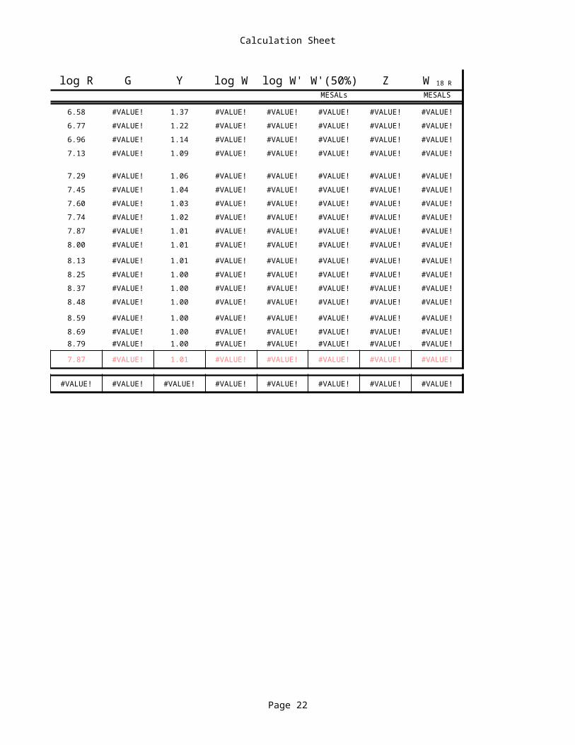
L1 L2 log R G Y log Wpsi psi kips
284.6 384.1 18 1 6.58 #VALUE! 1.37 #VALUE!
258.9 353.9 18 1 6.77 #VALUE! 1.22 #VALUE!
236.6 326.4 18 1 6.96 #VALUE! 1.14 #VALUE!
217.0 301.6 18 1 7.13 #VALUE! 1.09 #VALUE!
199.7 279.2 18 1 7.29 #VALUE! 1.06 #VALUE!
184.4 258.8 18 1 7.45 #VALUE! 1.04 #VALUE!
170.9 240.4 18 1 7.60 #VALUE! 1.03 #VALUE!
158.8 223.7 18 1 7.74 #VALUE! 1.02 #VALUE!
147.9 208.5 18 1 7.87 #VALUE! 1.01 #VALUE!
138.2 194.7 18 1 8.00 #VALUE! 1.01 #VALUE!
129.4 182.1 18 1 8.13 #VALUE! 1.01 #VALUE!
121.4 170.6 18 1 8.25 #VALUE! 1.00 #VALUE!
114.2 160.1 18 1 8.37 #VALUE! 1.00 #VALUE!
107.6 150.4 18 1 8.48 #VALUE! 1.00 #VALUE!
101.5 141.5 18 1 8.59 #VALUE! 1.00 #VALUE!
96.0 133.3 18 1 8.69 #VALUE! 1.00 #VALUE!90.9 125.8 18 1 8.79 #VALUE! 1.00 #VALUE!
147.9 208.5 18 1 7.87 #VALUE! 1.01 #VALUE!
#VALUE! #VALUE! 18 1 #VALUE! #VALUE! #VALUE! #VALUE!
sl st
AG1
Midslab tensile stress due to load only using AASHO Road Test Values (Equation 44)
AH1
Midslab tensile stress due to laod and temperature with AASHO Road Test Values (Equation 43)
AI1
Load on a single axle or tandem axle, kips
AJ1
axle code, 1 for single axle, 2 for tandem axle
AK1
log R (Equation 40)
AL1
Log ratio of change in serviceability (Equation 42)
AM1
(Equation 41)
AN1
log of Number of 18-kip ESALs computed at the AASHO Road Test (Equation 39)
Calculation Sheet
Page 23
log W' W'(50%) ZMESALs MESALS
#VALUE! #VALUE! #VALUE! #VALUE! #VALUE!
#VALUE! #VALUE! #VALUE! #VALUE! #VALUE!
#VALUE! #VALUE! #VALUE! #VALUE! #VALUE! #VALUE!
#VALUE! #VALUE! #VALUE! #VALUE! #VALUE! #VALUE!
#VALUE! #VALUE! #VALUE! #VALUE! #VALUE!
#VALUE! #VALUE! #VALUE! #VALUE! #VALUE! #VALUE!
#VALUE! #VALUE! #VALUE! #VALUE! #VALUE! #VALUE!
#VALUE! #VALUE! #VALUE! #VALUE! #VALUE!
#VALUE! #VALUE! #VALUE! #VALUE! #VALUE!
#VALUE! #VALUE! #VALUE! #VALUE! #VALUE!
#VALUE! #VALUE! #VALUE! #VALUE! #VALUE!
#VALUE! #VALUE! #VALUE! #VALUE! #VALUE!
#VALUE! #VALUE! #VALUE! #VALUE! #VALUE!
#VALUE! #VALUE! #VALUE! #VALUE! #VALUE!
#VALUE! #VALUE! #VALUE! #VALUE! #VALUE!
#VALUE! #VALUE! #VALUE! #VALUE! #VALUE!#VALUE! #VALUE! #VALUE! #VALUE! #VALUE!
#VALUE! #VALUE! #VALUE! #VALUE! #VALUE!
#VALUE! #VALUE! #VALUE! #VALUE! #VALUE! 11.239818182202
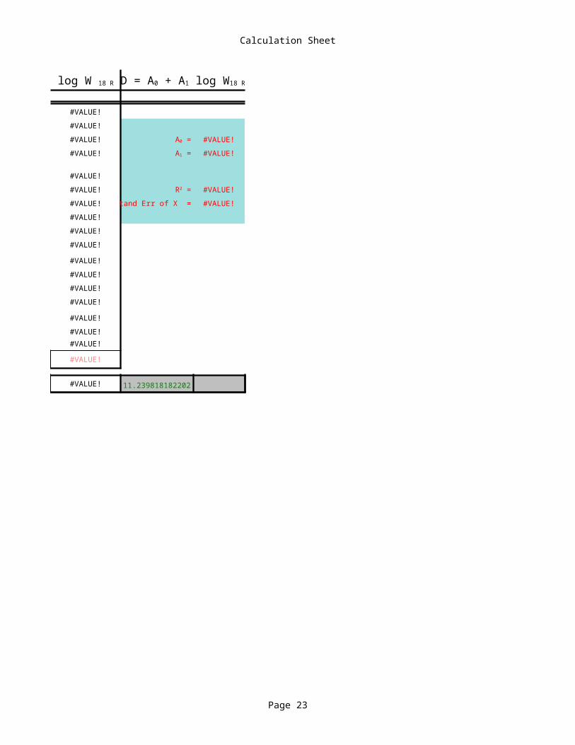
W 18 R log W 18 R D = A0 + A1 log W18 R
A0 =
A1 =
R2 =
Stand Err of X =
AO1
log of Number of 18-kip ESALs estimated for design traffic lane at 50% Reliability (Equation 38)
AP1
Number of 18-kip ESALs estimated for design traffic lane at 50% Reliability 10^logW'
AQ1
Z-value for desired Reliability
AR1
Number of 18-kip ESALs estimated for design traffic lane at desired Reliability (Equation 50)
AS1
log design 18-kip ESALs for the desired reliability R
AT5
For the given set of input variables there exists an approximate linear relationship between slab thickness D, and the log of the design 18-kip ESALs for the desired reliability R (Equation 49) The constants of this equation can be obtained by a regression between the two variables.

0 100 200 300 400 500 600 700 8000.0
2.0
4.0
6.0
8.0
10.0
12.0
Sensitivity Analysis (Effective Subgrade Support)
k-value, psi
Des
ign
Traff
ic, M
ESAL
s
Modulus of Rupture = 650 psiElastic Modulus of Concrete = 4,200,000 psi
Elastic Modulus of Base = 25,000 psi
Base Thickness = 6 in
k-Value of subgrade = 50 to 800 psiJoint Spacing = 15 ft
Reliability = 90 %
Standard Deviation = 0.34
Slab Thickness = 11.74 in

0 100 200 300 400 500 600 700 8000.0
2.0
4.0
6.0
8.0
10.0
12.0
Sensitivity Analysis (Effective Subgrade Support)
k-value, psi
Des
ign
Traff
ic, M
ESAL
s
Slab Thickness = 11.74 in

7.0 8.0 9.0 10.0 11.0 12.0 13.0 14.0 15.01
10
Sensitivity Analysis (Thickness)
Slab Thickness, in
Des
ign
Traff
ic, M
ESAL
s

7.0 8.0 9.0 10.0 11.0 12.0 13.0 14.0 15.01
10
Sensitivity Analysis (Thickness)
Slab Thickness, in
Des
ign
Traff
ic, M
ESAL
s
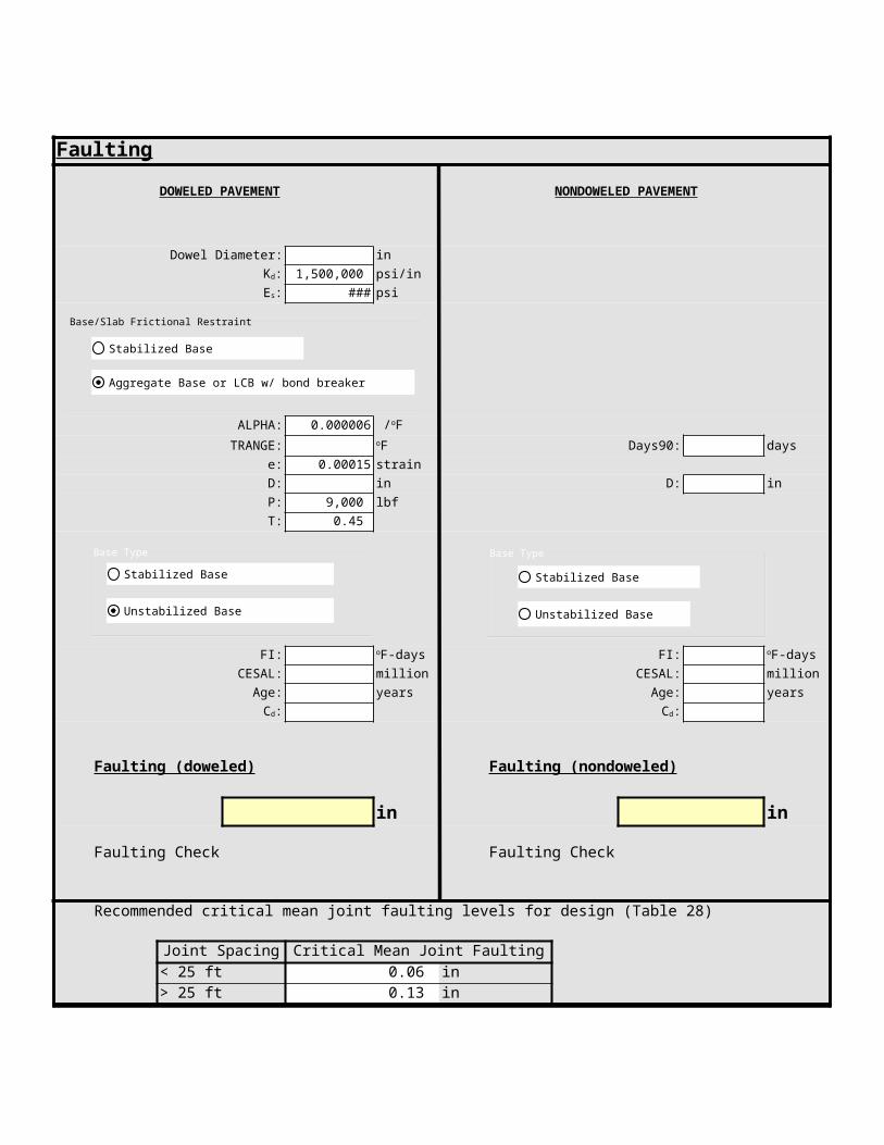
Faulting
DOWELED PAVEMENT NONDOWELED PAVEMENT
Dowel Diameter: in 1,500,000 psi/in ### 29,000,000 psi ###
ALPHA: 0.000006 ###TRANGE: Days90: days
e: 0.00015 strain ###D: in D: inP: 9,000 lbf ###T: 0.45 ###
FI: FI:CESAL: million CESAL: million
Age: years Age: years D######
Faulting (doweled) Faulting (nondoweled) ND###
in in ###
Faulting Check - Faulting Check -
Recommended critical mean joint faulting levels for design (Table 28)
Joint Spacing Critical Mean Joint Faulting< 25 ft 0.06 in> 25 ft 0.13 in
Kd:Es:
/oFoF
oF-days oF-days
Cd: Cd:
Base/Slab Frictional Restraint
Stabilized Base
Aggregate Base or LCB w/ bond breaker
Base Type
Stabilized Base
Unstabilized Base
Base Type
Stabilized Base
Unstabilized Base
D6
Modulus of Dowel Support, Default value: 1,500,000 psi/in
D7
Modulus of Elasticity of the Dowel Bar, Default value: 29,000,000 psi
D18
PCC Thermal Expansion Coefficient, Default value: 0.000006/ F
D19
Annual Temperature Range
J19
Number of days wiht maximum temperature above 90 F
K19
For quick reference, a table listing Days90 values is shown in the sheet "FI&DAYs90" for the LTPP sections.
D20
PCC Drying Shrinkage Coefficient, Default value: 0.00015 strain
D22
The slab thickness chosen as the final design slab thickness
J22
The slab thickness chosen as the final design slab thickness
D25
Applied Wheel Load, Default value: 9,000 lbf
D26
Percent Transferred Load, Default value: 0.45
D36
Mean Annual Freezing Index, Fahrenheit degree-days
E36
For quick reference, a table listing freezing index values is shown in the sheet "FI&DAYs90" for the LTPP sections.
J36
Mean Annual Freezing Index, Fahrenheit degree-days
K36
For quick reference, a table listing freezing index values is shown in the sheet "FI&DAYs90" for the LTPP sections.
D38
Cumulative equivalent 18-kip single-axle loads
J38
Cumulative equivalent 18-kip single-axle loads
D39
Pavement Age
J39
Pavement Age
D40
Modified AASHTO Drainage Coefficient Refer to Table in Information sheet
J40
Modified AASHTO Drainage Coefficient Refer to table in information sheet
F53
Default value: 0.06 in
F54
Default value: 0.13 in

Note: Joint load position stress checks need to be performed only for nondoweled pavements
Only two numbers need to be entered in this sheet:Temperature gradientTensile stress at top of slab
Step 1:
Total Negative Temperature Differential
Slab Thickness: in
Total Negative Temperature Differential:
Construction Curling and Moisture Gradient Temperature Differential
Enter temperature gradient: (enter positive value from below)
For temperature gradient use:
Wet Climate: (Annual Precipitation >= 30 in orThornthwaite Moisture Index > 0)
Dry Climate: (Annual Precipitation < 30 in orThornthwaite Moisture Index < 0)
Total Effective Negative Temp. Differential:
Step 2:
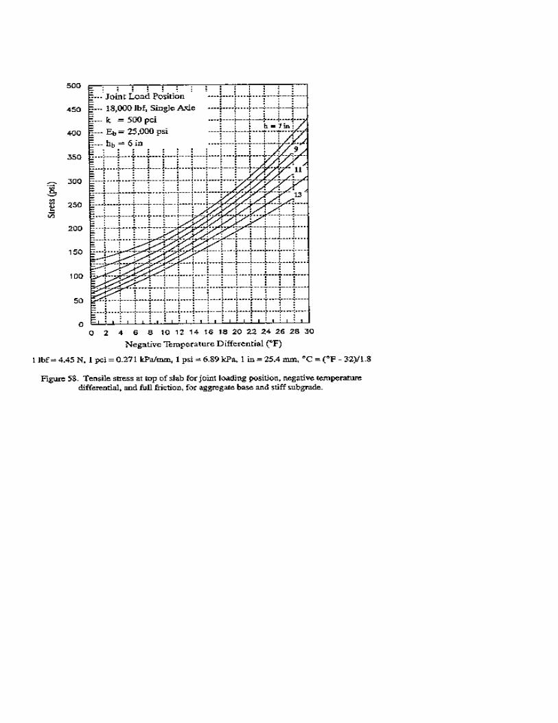
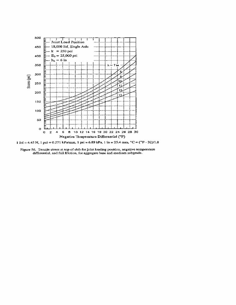
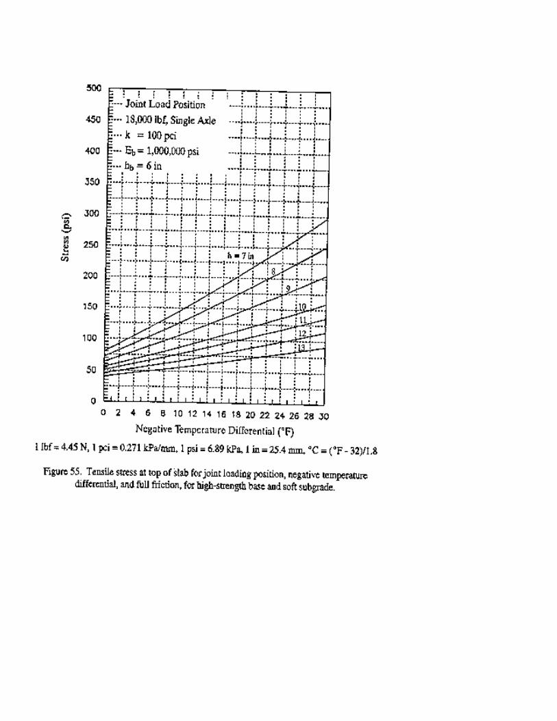
Use one or more of the following charts to estimate the tensile stress at top of slab.Note that the charts show the variation of tensile stress with negative temperature differentialfor slab thicknesses ranging from 7 to 13 in. These are plotted for a base course thickness of 6 in. The six charts represent three k-values (100, 250 and 500 psi/in) and two values for theelastic modulus of the base (25,000 psi and 1,000,000 psi). Use judgment to
oF
oF/in
0 to 2 oF/in
1 to 3 oF/in
oF
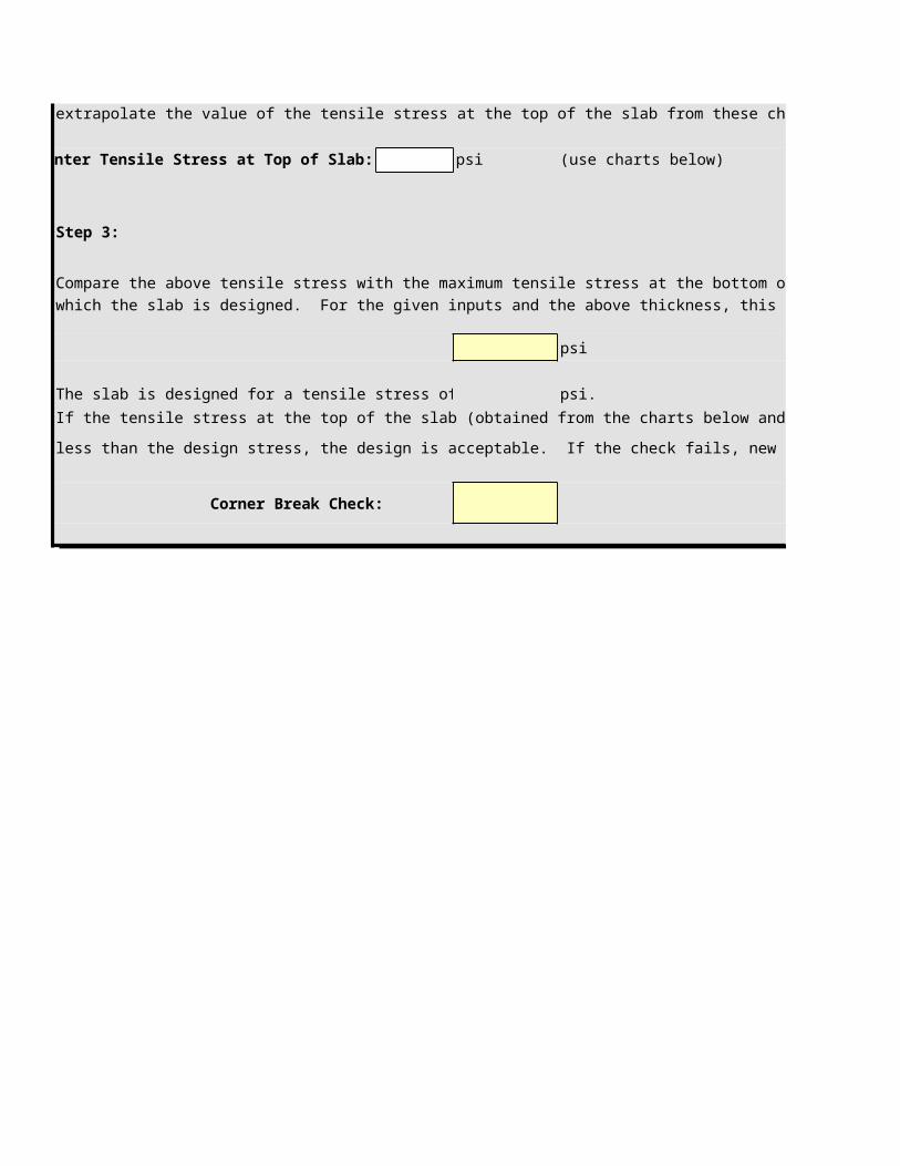
extrapolate the value of the tensile stress at the top of the slab from these charts.
Enter Tensile Stress at Top of Slab: psi (use charts below)
Step 3:
Compare the above tensile stress with the maximum tensile stress at the bottom of the slab forwhich the slab is designed. For the given inputs and the above thickness, this value is
psi
The slab is designed for a tensile stress of psi. If the tensile stress at the top of the slab (obtained from the charts below and entered above) is
less than the design stress, the design is acceptable. If the check fails, new inputs have to be provided.
Corner Break Check:


Note: Joint load position stress checks need to be performed only for nondoweled pavements
(enter positive value from below)
(Annual Precipitation >= 30 in orThornthwaite Moisture Index > 0)
(Annual Precipitation < 30 in orThornthwaite Moisture Index < 0)

less than the design stress, the design is acceptable. If the check fails, new inputs have to be provided.
NOTE: The k-value used in this design procedure is not a composite k, as in the original AASHTOdesign procedure. The k-value to be input in the "Input Form" and in the "Seasonal k-Value" sheetis the actual subgrade soil modulus of subgrade reaction.
The k-value input required for this design method is determined using the following steps:
Step 1. Select a subgrade soil k-value for each season, using any of the three following methods: (a) Correlations with soil type and other soil properties or tests. (b) Deflection testing and backcalculation (recommended). (c) Plate bearing tests.Detailed information for Step 1 is included below.
Step 2. The "Seasonal k-Value" Sheet can then be used to determine a seasonally adjusted effective k-value.
Step 3. This seasonally adjusted effective k-value can then be adjusted for the effects of a shallow rigid layer, if present, or an embankment above the natural subgrade using the"Fill/Rigid Adjustment" sheet.

Method A -- Correlations. Guidelines are presented for selecting an appropriate k-value based
on soil classification, moisture level, density, California Bearing Ratio (CBR), or Dynamic Cone
Penetrometer (DCP) data. These correlation methods are anticipated to be used routinely for
design. The k-values obtained from soil type or tests correlation methods may need to be
adjusted for embankment above the subgrade or a shallow rigid layer beneath the subgrade.
The k-values and correlations for cohesive soils (A-4 through A-7): The bearing capacity of
cohesive soils is strongly influenced by their degree of saturation (Sr, percent), which is a function
of water content (w, percent), dry density (g, lb/ft3), and specific gravity (Gs):
Recommended k-values for each fine-grained soil type as a function of degree of saturation are
shown in Figure 40. Each line represents the middle of a range of reasonable values for k. For
any given soil type and degree of saturation, the range of values is about + 40 psi/in [11 kPa/mm].
A reasonable lower limit for k at 100 percent saturation is considered to be 25 psi/in [7 kPa/mm ].
Thus, for example, an A-6 soil might be expected to exhibit k-values between about 180 and 260
psi/in [49 and 70 kPa/mm] at 50 percent saturation, and k-values between about 25 and 85 psi/in
[7 and 23 kPa/mm] at 100 percent saturation.
Two different types of materials can be classified as A-4: predominantly silty materials (at least 75
percent passing the #200 sieve, possibly organic), and mixtures of silt, sand, and gravel (up to 64
percent retained on #200 sieve). The former may have a density between about 90 and 105 lb/ft3
[1442 and 1682 kg/m3], and a CBR between about 4 and 8. The latter may have a density
between about 100 and 125 lb/ft3 [1602 and 2002 kg/m3], and a CBR between about 5 and 15.
The line labeled A-4 in Figure B-4 is more representative of the former group. If the material in
question is A-4, but possesses the properties of the stronger subset of materials in the A-4 class,
a higher k-value at any given degree of saturation (for example, along the line labeled A-7-6 in
Figure 40) is appropriate.
Recommended k-value ranges for fine-grained soils, along with typical ranges of dry density and
CBR for each soil type, are summarized in Table 11.
The k -values and correlations for cohesionless soils (A-1 and A-3): The bearing capacity of
cohesionless materials is fairly insensitive to moisture variation and is predominantly a function of
their void ratio and overall stress state. Recommended k-value ranges for cohesionless soils,
along with typical ranges of dry density and CBR for each soil type, are summarized in Table 11.
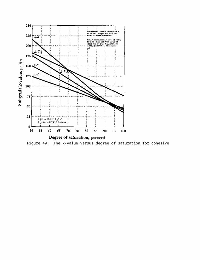
Figure 40. The k-value versus degree of saturation for cohesive soils

Table 11. Recommended k-value ranges for various soil types.
AASHTOClass
Description UnifiedClass
DryDensity(lb/ft3)
CBR(perce
nt)
k Value(psi/in)
Coarse-grained Soils:
A-1-a, well gradedgravel GW, GP
125 - 140 60 - 80 300 - 450
A-1-a, poorly graded 120 - 130 35 - 60 300 - 400
A-1-b coarse sand SW 110 - 130 20 - 40 200 - 400
A-3 fine sand SP 105 - 120 15 - 25 150 - 300
A-2 Soils (granular materials with high fines):
A-2-4, gravelly silty gravel GM 130 - 145 40 - 80 300 - 500
A-2-5, gravelly silty sandy gravel
A-2-4, sandy silty sand SM 120 - 135 20 - 40 300 - 400
A-2-5, sandy silty gravelly sand
A-2-6, gravelly clayey gravel GC 120 - 140 20 - 40 200 - 450
A-2-7, gravelly clayey sandy gravel
A-2-6, sandy clayey sandSC 105 - 130 10 - 20 150 - 350
A-2-7, sandy clayey gravellysand
Fine-grained Soils:
A-4silt
ML, OL90 - 105 4 - 8 25 - 165 *
silt/sand/gravel mixture
100 - 125 5 - 15 40 - 220 *
A-5 poorly gradedsilt
MH 80 - 100 4 - 8 25 - 190 *
A-6 plastic clay CL 100 - 125 5 - 15 25 - 255 *
A-7-5 moderately plasticelastic clay
CL, OL 90 - 125 4 - 15 25 - 215 *
A-7-6 highly plasticelastic clay
CH, OH 80 - 110 3 - 5 40 - 220 *
* k-value of fine-grained soil is highly dependent on degree of saturation. See Figure 40.
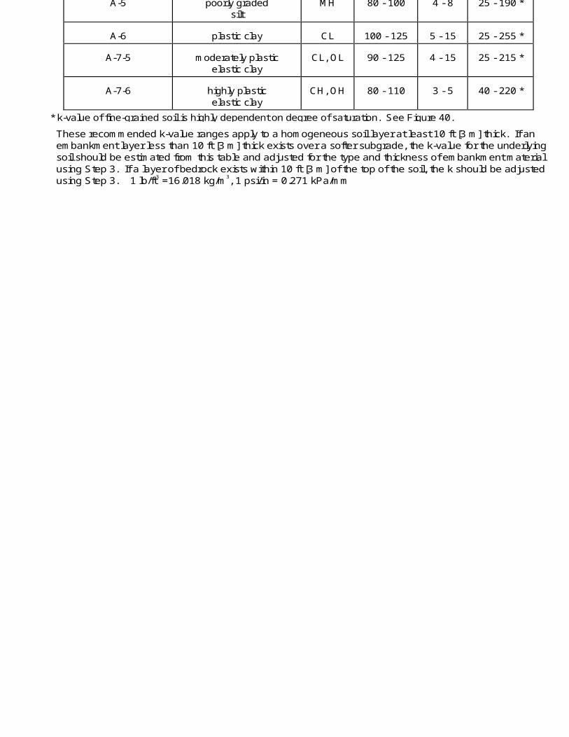
These recommended k-value ranges apply to a homogeneous soil layer at least 10 ft [3 m] thick. If anembankment layer less than 10 ft [3 m] thick exists over a softer subgrade, the k-value for the underlyingsoil should be estimated from this table and adjusted for the type and thickness of embankment materialusing Step 3. If a layer of bedrock exists within 10 ft [3 m] of the top of the soil, the k should be adjustedusing Step 3. 1 lb/ft3 =16.018 kg/m3, 1 psi/in = 0.271 kPa/mm

The k-values and correlations for A-2 soils: Soils in the A-2 class are all granular materials
falling between A-1 and A-3. Although it is difficult to predict the behavior of such a wide variety of
materials, the available data indicate that in terms of bearing capacity, A-2 materials behave
similarly to cohesionless materials of comparable density. Recommended k-value ranges for A-2
soils, along with typical ranges of dry density and CBR for each soil type, are summarized in
Table 11.
Correlation of k-value to California Bearing Ratio: Figure 41 illustrates the approximate range
of k-values that might be expected for a soil with a given CBR.
Correlation of k-values to penetration rate by Dynamic Cone Penetrometer: Figure 42
illustrates the range of k-values that might be expected for a soil with a given penetration rate
(inches per blow) measured with a Dynamic Cone Penetrometer. This is a rapid hand-held testing
device that can be used to quickly test dozens of locations along an alignment. The DCP can also
penetrate AC surfaces and surface treatments to test the foundation below.
Assignment of k-values to seasons. Among the factors that should be considered in selecting
seasonal k-values are the seasonal movement of the water table, seasonal precipitation levels,
winter frost depths, number of freeze-thaw cycles, and the extent to which the subgrade will be
protected from frost by embankment material. A "frozen" k may not be appropriate for winter,
even in a cold climate, if the frost will not reach and remain in a substantial thickness of the
subgrade throughout the winter. If it is anticipated that a substantial depth (e.g., three feet or
more) of the subgrade will be frozen, a k-value of 500 psi/in [135 kPa/mm] would be an
appropriate "frozen" k.
The seasonal variation in degree of saturation is difficult to predict, but in locations where a water
table is constantly present at a depth of less than about 10 ft [3 m], it is reasonable to expect that
fine-grained subgrades will remain at least 70 to 90 percent saturated, and may be completely
saturated for substantial periods in the spring. County soil reports can provide data on the
position of the high-water table (i.e., the typical depth to the water table at the time of the year that
it is at its highest). Unfortunately, county soil reports do not provide data on the variation in depth
to the water table throughout the year.
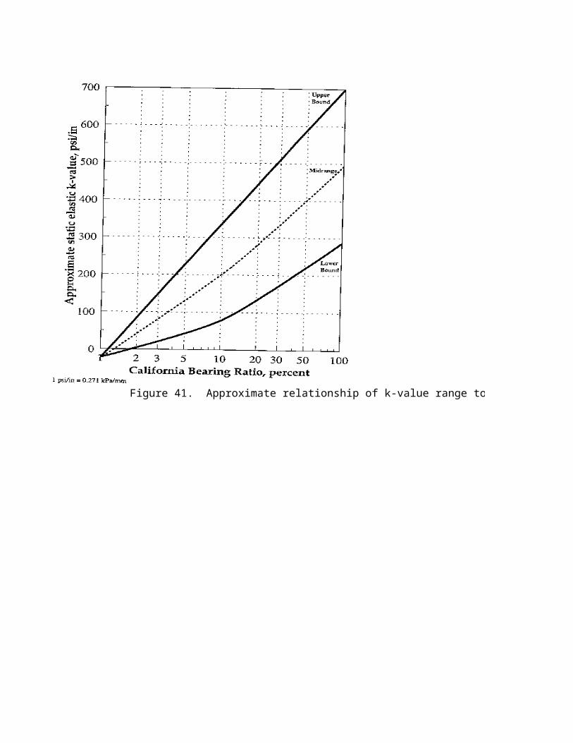
Figure 41. Approximate relationship of k-value range to CBR.

Figure 42. Approximate relationship of k-value range to DCP penetration rate.

Method B — Deflection Testing and Backcalculation Methods. These methods are suitable
for determining k-value for design of overlays of existing pavements, for design of a reconstructed
pavement on existing alignments, or for design of similar pavements in the same general location
on the same type of subgrade. An agency may also use backcalculation methods to develop
correlations between nondestructive deflection testing results and subgrade types and properties.
Cut and fill sections are likely to yield different k-values. No embankment or rigid layer adjustment
is required for backcalculated k-values if these characteristics are similar for the pavement being
tested and the pavement being designed, but backcalculated dynamic k-values do need to be
reduced by a factor of two to estimate a static elastic k-value for use in design which is required in
this catalog.
An appropriate design subgrade elastic k-value for use as an input to this design method is
determined by the following steps:
1. Measure deflections on an in-service concrete or composite (AC-overlaid PCC) pavement
with the same or similar subgrade as the pavement being designed.
2. Compute the appropriate AREA of each deflection basin.
3. Compute an initial estimate (assuming an infinite slab size) of the radius of relative stiffness, l.
4. Compute an initial estimate (assuming an infinite slab size) of the subgrade k-value.
5. Compute adjustment factors for the maximum deflection d0 and the initially estimated l to
account for the finite slab size.
6. Adjust the initially estimated k-value to account for the finite slab size.
7. Compute the mean backcalculated subgrade k-value for all of the deflection basins
considered.
8. Compute the estimated mean static k-value for use in design for the specific season during
the testing.
9. Determine the effective seasonally adjusted elastic k-value considering the factors discussed
above.
These steps are described below, with the relevant equations for bare concrete and composite
(asphalt concrete over concrete slab) pavements given for each step.
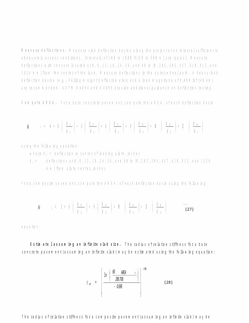
M e a s u r e d e f l e c t i o n s . M e a s u r e s l a b d e f l e c t i o n b a s i n s a l o n g t h e p r o j e c t a t a n i n t e r v a l s u f f i c i e n t t o
a d e q u a t e l y a s s e s s c o n d i t i o n s . I n t e r v a l s o f 1 0 0 t o 1 0 0 0 f t [ 3 0 t o 3 0 0 m ] a r e t y p i c a l . M e a s u r e
d e f l e c t i o n s w i t h s e n s o r s l o c a t e d a t 0 , 8 , 1 2 , 1 8 , 2 4 , 3 6 , a n d 6 0 i n [ 0 , 2 0 3 , 3 0 5 , 4 5 7 , 6 1 0 , 9 1 5 , a n d
1 5 2 4 m m ] f r o m t h e c e n t e r o f t h e l o a d . M e a s u r e d e f l e c t i o n s i n t h e o u t e r w h e e l p a t h . A h e a v y - l o a d
d e f l e c t i o n d e v i c e ( e . g . , F a l l i n g W e i g h t D e f l e c t o m e t e r ) a n d a l o a d m a g n i t u d e o f 9 , 0 0 0 l b f [ 4 0 k N ]
a r e r e c o m m e n d e d . A S T M D 4 6 9 4 a n d D 4 6 9 5 p r o v i d e a d d i t i o n a l g u i d a n c e o n d e f l e c t i o n t e s t i n g .
C o m p u t e A R E A . F o r a b a r e c o n c r e t e p a v e m e n t , c o m p u t e t h e A R E A 7 o f e a c h d e f l e c t i o n b a s i n
u s i n g t h e f o l l o w i n g e q u a t i o n :
w h e r e d 0 = d e f l e c t i o n i n c e n t e r o f l o a d i n g p l a t e , i n c h e s
d i = d e f l e c t i o n s a t 0 , 8 , 1 2 , 1 8 , 2 4 , 3 6 , a n d 6 0 i n [ 0 , 2 0 3 , 3 0 5 , 4 5 7 , 6 1 0 , 9 1 5 , a n d 1 5 2 4
m m ] f r o m p l a t e c e n t e r , i n c h e s
F o r a c o m p o s i t e p a v e m e n t , c o m p u t e t h e A R E A 5 o f e a c h d e f l e c t i o n b a s i n u s i n g t h e f o l l o w i n g
e q u a t i o n :
d
d 12 + d
d 18 + d
d 9 + d
d 6 + d
d 5 + dd 6 + 4 = AREA
0
60
0
36
0
24
0
18
0
12
0
87
dd 12 +
dd 18 +
dd 9 +
dd 6 + 3 = AREA
12
60
12
36
12
24
12
185
E s t i m a t e l a s s u m i n g a n i n f i n i t e s l a b s i z e . T h e r a d i u s o f r e l a t i v e s t i f f n e s s f o r a b a r e
c o n c r e t e p a v e m e n t ( a s s u m i n g a n i n f i n i t e s l a b ) m a y b e e s t i m a t e d u s i n g t h e f o l l o w i n g e q u a t i o n :
T h e r a d i u s o f r e l a t i v e s t i f f n e s s f o r a c o m p o s i t e p a v e m e n t ( a s s u m i n g a n i n f i n i t e s l a b ) m a y b e
e s t i m a t e d u s i n g t h e f o l l o w i n g e q u a t i o n :
E s t i m a t e k a s s u m i n g a n i n f i n i t e s l a b s i z e . F o r a b a r e c o n c r e t e p a v e m e n t , c o m p u t e a n
i n i t i a l e s t i m a t e o f t h e k - v a l u e u s i n g t h e f o l l o w i n g e q u a t i o n :
w h e r e k = b a c k c a l c u l a t e d d y n a m i c k - v a l u e , p s i / i n
P = l o a d , l b
d 0 = d e f l e c t i o n m e a s u r e d a t c e n t e r o f l o a d p l a t e , i n c h
l e s t = e s t i m a t e d r a d i u s o f r e l a t i v e s t i f f n e s s , i n c h e s , f r o m p r e v i o u s s t e p
d 0* = n o n d i m e n s i o n a l c o e f f i c i e n t o f d e f l e c t i o n a t c e n t e r o f l o a d p l a t e :
0.698-289.708
AREA 60 =
72.566
est
ln
0.476-158.40
AREA 48 =
52.220
est
ln
est2
0
*0
est dd P = k
[27]
[28]

E s t i m a t e l a s s u m i n g a n i n f i n i t e s l a b s i z e . T h e r a d i u s o f r e l a t i v e s t i f f n e s s f o r a b a r e
c o n c r e t e p a v e m e n t ( a s s u m i n g a n i n f i n i t e s l a b ) m a y b e e s t i m a t e d u s i n g t h e f o l l o w i n g e q u a t i o n :
T h e r a d i u s o f r e l a t i v e s t i f f n e s s f o r a c o m p o s i t e p a v e m e n t ( a s s u m i n g a n i n f i n i t e s l a b ) m a y b e
e s t i m a t e d u s i n g t h e f o l l o w i n g e q u a t i o n :
E s t i m a t e k a s s u m i n g a n i n f i n i t e s l a b s i z e . F o r a b a r e c o n c r e t e p a v e m e n t , c o m p u t e a n
i n i t i a l e s t i m a t e o f t h e k - v a l u e u s i n g t h e f o l l o w i n g e q u a t i o n :
w h e r e k = b a c k c a l c u l a t e d d y n a m i c k - v a l u e , p s i / i n
P = l o a d , l b
d 0 = d e f l e c t i o n m e a s u r e d a t c e n t e r o f l o a d p l a t e , i n c h
l e s t = e s t i m a t e d r a d i u s o f r e l a t i v e s t i f f n e s s , i n c h e s , f r o m p r e v i o u s s t e p
d 0* = n o n d i m e n s i o n a l c o e f f i c i e n t o f d e f l e c t i o n a t c e n t e r o f l o a d p l a t e :
0.698-289.708
AREA 60 =
72.566
est
ln
0.476-158.40
AREA 48 =
52.220
est
ln
est2
0
*0
est dd P = k
e 0.1245 = d e 0.14707- *0
est -0.07565
F o r a c o m p o s i t e p a v e m e n t , c o m p u t e a n i n i t i a l e s t i m a t e o f t h e k - v a l u e u s i n g t h e f o l l o w i n g e q u a t i o n :
d 1 2 = d e f l e c t i o n m e a s u r e d 1 2 i n [ 3 0 5 m m ] f r o m c e n t e r o f l o a d p l a t e , i n c h
l e s t = e s t i m a t e d r a d i u s o f r e l a t i v e s t i f f n e s s , i n , f r o m p r e v i o u s s t e p
d 1 2* = n o n d i m e n s i o n a l c o e f f i c i e n t o f d e f l e c t i o n 1 2 i n [ 3 0 5 m m ] f r o m c e n t e r o f l o a d p l a t e :
C o m p u t e a d j u s t m e n t f a c t o r s f o r d 0 a n d l f o r f i n i t e s l a b s i z e . F o r b o t h b a r e c o n c r e t e a n d
c o m p o s i t e p a v e m e n t s , t h e i n i t i a l e s t i m a t e o f l i s u s e d t o c o m p u t e t h e f o l l o w i n g a d j u s t m e n t f a c t o r s
t o d 0 a n d l t o a c c o u n t f o r t h e f i n i t e s i z e o f t h e s l a b s t e s t e d :
est2
1 2
*1 2
est dd P = k
e 0.12188 = d e 0 .7 9 4 3 2- *1 2
est - 0. 07074
e 1.15085 - 1 = AF L 0 .7 1 8 7 8-d est
0. 80151
0
e 0.89434 - 1 = AF L
0 .6 1 6 6 2-est
1. 04831
[30]
[32]
[31]
[29]

F o r a c o m p o s i t e p a v e m e n t , c o m p u t e a n i n i t i a l e s t i m a t e o f t h e k - v a l u e u s i n g t h e f o l l o w i n g e q u a t i o n :
d 1 2 = d e f l e c t i o n m e a s u r e d 1 2 i n [ 3 0 5 m m ] f r o m c e n t e r o f l o a d p l a t e , i n c h
l e s t = e s t i m a t e d r a d i u s o f r e l a t i v e s t i f f n e s s , i n , f r o m p r e v i o u s s t e p
d 1 2* = n o n d i m e n s i o n a l c o e f f i c i e n t o f d e f l e c t i o n 1 2 i n [ 3 0 5 m m ] f r o m c e n t e r o f l o a d p l a t e :
C o m p u t e a d j u s t m e n t f a c t o r s f o r d 0 a n d l f o r f i n i t e s l a b s i z e . F o r b o t h b a r e c o n c r e t e a n d
c o m p o s i t e p a v e m e n t s , t h e i n i t i a l e s t i m a t e o f l i s u s e d t o c o m p u t e t h e f o l l o w i n g a d j u s t m e n t f a c t o r s
t o d 0 a n d l t o a c c o u n t f o r t h e f i n i t e s i z e o f t h e s l a b s t e s t e d :
est2
1 2
*1 2
est dd P = k
e 0.12188 = d e 0 .7 9 4 3 2- *1 2
est - 0. 07074
e 1.15085 - 1 = AF L 0 .7 1 8 7 8-d est
0. 80151
0
e 0.89434 - 1 = AF L 0 .6 1 6 6 2-est
1. 04831
w h e r e , i f t h e s l a b l e n g t h i s l e s s t h a n o r e q u a l t o t w i c e t h e s l a b w i d t h , L i s t h e s q u a r e r o o t o f t h e
p r o d u c t o f t h e s l a b l e n g t h a n d w i d t h , b o t h i n i n c h e s , o r i f t h e s l a b l e n g t h i s g r e a t e r t h a n t w i c e t h e
w i d t h , L i s t h e p r o d u c t o f t h e s q u a r e r o o t o f t w o a n d t h e s l a b l e n g t h i n i n c h e s :
A d j u s t k f o r f i n i t e s l a b s i z e . F o r b o t h b a r e c o n c r e t e a n d c o m p o s i t e p a v e m e n t s , a d j u s t t h e
i n i t i a l l y e s t i m a t e d k - v a l u e u s i n g t h e f o l l o w i n g e q u a t i o n :
C o m p u t e m e a n d y n a m i c k - v a l u e . E x c l u d e f r o m t h e c a l c u l a t i o n o f t h e m e a n k - v a l u e a n y
u n r e a l i s t i c v a l u e s ( i . e . , l e s s t h a n 5 0 p s i / i n [ 1 4 k P a / m m ] o r g r e a t e r t h a n 1 5 0 0 p s i / i n [ 4 0 7 k P a / m m ] ) ,
a s w e l l a s a n y i n d i v i d u a l v a l u e s t h a t a p p e a r t o b e s i g n i f i c a n t l y o u t o f l i n e w i t h t h e r e s t o f t h e
v a l u e s .
L* 2 = L ,L* 2 > L if
L L = L ,L* 2 L if
lwl
wlwl
AF AFk = k
d2
est
0
[32]
[33]
[34]
[36]
[35]
[37]

w h e r e , i f t h e s l a b l e n g t h i s l e s s t h a n o r e q u a l t o t w i c e t h e s l a b w i d t h , L i s t h e s q u a r e r o o t o f t h e
p r o d u c t o f t h e s l a b l e n g t h a n d w i d t h , b o t h i n i n c h e s , o r i f t h e s l a b l e n g t h i s g r e a t e r t h a n t w i c e t h e
w i d t h , L i s t h e p r o d u c t o f t h e s q u a r e r o o t o f t w o a n d t h e s l a b l e n g t h i n i n c h e s :
A d j u s t k f o r f i n i t e s l a b s i z e . F o r b o t h b a r e c o n c r e t e a n d c o m p o s i t e p a v e m e n t s , a d j u s t t h e
i n i t i a l l y e s t i m a t e d k - v a l u e u s i n g t h e f o l l o w i n g e q u a t i o n :
C o m p u t e m e a n d y n a m i c k - v a l u e . E x c l u d e f r o m t h e c a l c u l a t i o n o f t h e m e a n k - v a l u e a n y
u n r e a l i s t i c v a l u e s ( i . e . , l e s s t h a n 5 0 p s i / i n [ 1 4 k P a / m m ] o r g r e a t e r t h a n 1 5 0 0 p s i / i n [ 4 0 7 k P a / m m ] ) ,
a s w e l l a s a n y i n d i v i d u a l v a l u e s t h a t a p p e a r t o b e s i g n i f i c a n t l y o u t o f l i n e w i t h t h e r e s t o f t h e
v a l u e s .
L* 2 = L ,L* 2 > L if
L L = L ,L* 2 L if
lwl
wlwl
AF AFk = k
d2
est
0
Compute the estimated mean static k-value for design. Divide the mean dynamic k-value by
two to estimate the mean static k-value for design.
A blank worksheet for computation of k from deflection data and example computations of k from
deflection basins measured on two pavements, one bare concrete and the other composite, are
given in Table 12.
Seasonal variation in backcalculated k-values. The design k-value determined from
backcalculation as described above represents the k-value for the season in which the deflection
testing was conducted. An agency may wish to conduct deflection testing on selected projects in
different seasons of the year to assess the seasonal variation in backcalculated k-values for
different types of subgrades.
Table 12.
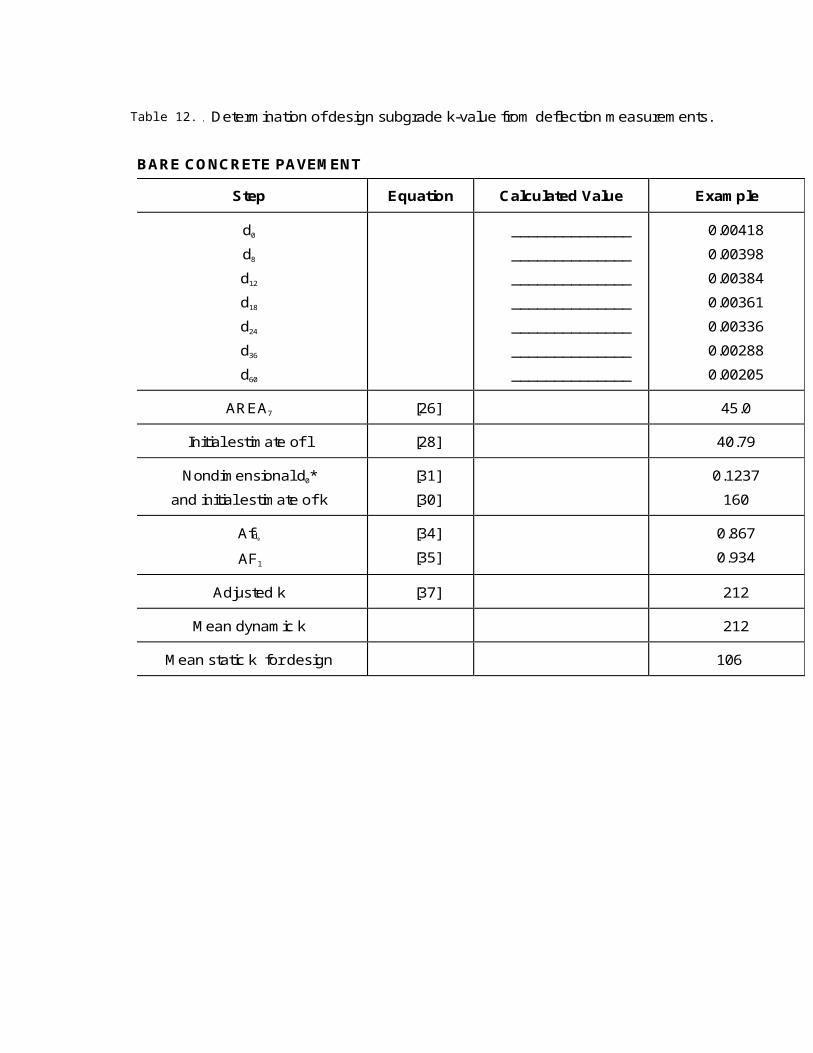
Table A2. Determination of design subgrade k-value from deflection measurements.
BARE CONCRETE PAVEMENT
Step Equation Calculated Value Example
d0
d8
d12
d18
d24
d36
d60
______________
______________
______________
______________
______________
______________
______________
0.00418
0.00398
0.00384
0.00361
0.00336
0.00288
0.00205
AREA7 [26] 45.0
Initial estimate of l [28] 40.79
Nondimensional d0*
and initial estimate of k
[31]
[30]
0.1237
160
Afd0
AFl
[34]
[35]
0.867
0.934
Adjusted k [37] 212
Mean dynamic k 212
Mean static k for design 106
Table 12.

COMPOSITE PAVEMENT
Step Equation Calculated Value Example
d12
d18
d24
d36
d60
______________
______________
______________
______________
______________
0.00349
0.00332
0.00313
0.00273
0.00202
AREA5 [27] 37.8
Initial estimate of l [29] 48.83
Nondimensional d12*
and initial estimate of k
[33]
[32]
0.1189
128
Afd0
AFl
[34]
[35]
0.823
0.896
Adjusted k [37] 195
Mean dynamic k 195
Mean static k for design 97

Method C -- Plate Bearing Test Methods. The subgrade or embankment elastic k-value may
be determined from either of two types of plate bearing tests: repetitive static plate loading
(AASHTO T221, ASTM D1195) or nonrepetitive static plate loading (AASHTO T222, ASTM
D1196). These test methods were developed for a variety of purposes, and do not provide explicit
guidance on the determination of the required k-value input to the design procedure described
here.
For the purpose of concrete pavement design, the recommended subgrade input parameter is
the static elastic k-value. This may be determined from either a repetitive or nonrepetitive test on
the prepared subgrade or on a prepared test embankment, provided that the embankment is at
least 10 ft [3 m] thick. Otherwise, the tests should be conducted on the subgrade, and the k-value
obtained should be adjusted to account for the thickness and density of the embankment, using
the nomograph provided in Step 3.
In a repetitive test, the elastic k-value is determined from the ratio of load to elastic
deformation (the recoverable portion of the total deformation measured). In a nonrepetitive test,
the load-deformation ratio at a deformation of 0.05 in [1.25 mm] is considered to represent the
elastic k-value, according to extensive research by the U.S. Army Corps of Engineers.
Note also that a 30-in-diameter [762-mm-diameter] plate should be used to determine the
elastic static k-value for use in design. Smaller diameter plates will yield substantially higher k-
values, which are not appropriate for use in this design procedure. An adequate number of tests
should be run to ensure coverage over the project length. The mean of the tests becomes the
static elastic k-value for the season of testing. This value is then used to determine the effective
seasonally adjusted elastic k-value considering the factors discussed above.

NOTE: The k-value used in this design procedure is not a composite k, as in the original AASHTOdesign procedure. The k-value to be input in the "Input Form" and in the "Seasonal k-Value" sheet
Step 1. Select a subgrade soil k-value for each season, using any of the three following methods:

Method A -- Correlations. Guidelines are presented for selecting an appropriate k-value based
on soil classification, moisture level, density, California Bearing Ratio (CBR), or Dynamic Cone
Penetrometer (DCP) data. These correlation methods are anticipated to be used routinely for
design. The k-values obtained from soil type or tests correlation methods may need to be
adjusted for embankment above the subgrade or a shallow rigid layer beneath the subgrade.
The k-values and correlations for cohesive soils (A-4 through A-7): The bearing capacity of
cohesive soils is strongly influenced by their degree of saturation (Sr, percent), which is a function
of water content (w, percent), dry density (g, lb/ft3), and specific gravity (Gs):
Recommended k-values for each fine-grained soil type as a function of degree of saturation are
shown in Figure 40. Each line represents the middle of a range of reasonable values for k. For
any given soil type and degree of saturation, the range of values is about + 40 psi/in [11 kPa/mm].
A reasonable lower limit for k at 100 percent saturation is considered to be 25 psi/in [7 kPa/mm ].
Thus, for example, an A-6 soil might be expected to exhibit k-values between about 180 and 260
psi/in [49 and 70 kPa/mm] at 50 percent saturation, and k-values between about 25 and 85 psi/in
[7 and 23 kPa/mm] at 100 percent saturation.
Two different types of materials can be classified as A-4: predominantly silty materials (at least 75
percent passing the #200 sieve, possibly organic), and mixtures of silt, sand, and gravel (up to 64
percent retained on #200 sieve). The former may have a density between about 90 and 105 lb/ft3
[1442 and 1682 kg/m3], and a CBR between about 4 and 8. The latter may have a density
between about 100 and 125 lb/ft3 [1602 and 2002 kg/m3], and a CBR between about 5 and 15.
The line labeled A-4 in Figure B-4 is more representative of the former group. If the material in
question is A-4, but possesses the properties of the stronger subset of materials in the A-4 class,
a higher k-value at any given degree of saturation (for example, along the line labeled A-7-6 in
Figure 40) is appropriate.
Recommended k-value ranges for fine-grained soils, along with typical ranges of dry density and
CBR for each soil type, are summarized in Table 11.
The k -values and correlations for cohesionless soils (A-1 and A-3): The bearing capacity of
cohesionless materials is fairly insensitive to moisture variation and is predominantly a function of
their void ratio and overall stress state. Recommended k-value ranges for cohesionless soils,
along with typical ranges of dry density and CBR for each soil type, are summarized in Table 11.

Figure 40. The k-value versus degree of saturation for cohesive soils
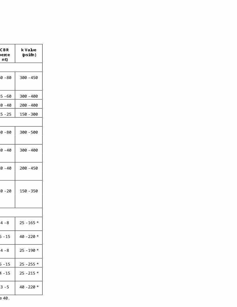
Table 11. Recommended k-value ranges for various soil types.
AASHTOClass
Description UnifiedClass
DryDensity(lb/ft3)
CBR(perce
nt)
k Value(psi/in)
Coarse-grained Soils:
A-1-a, well gradedgravel GW, GP
125 - 140 60 - 80 300 - 450
A-1-a, poorly graded 120 - 130 35 - 60 300 - 400
A-1-b coarse sand SW 110 - 130 20 - 40 200 - 400
A-3 fine sand SP 105 - 120 15 - 25 150 - 300
A-2 Soils (granular materials with high fines):
A-2-4, gravelly silty gravel GM 130 - 145 40 - 80 300 - 500
A-2-5, gravelly silty sandy gravel
A-2-4, sandy silty sand SM 120 - 135 20 - 40 300 - 400
A-2-5, sandy silty gravelly sand
A-2-6, gravelly clayey gravel GC 120 - 140 20 - 40 200 - 450
A-2-7, gravelly clayey sandy gravel
A-2-6, sandy clayey sandSC 105 - 130 10 - 20 150 - 350
A-2-7, sandy clayey gravellysand
Fine-grained Soils:
A-4silt
ML, OL90 - 105 4 - 8 25 - 165 *
silt/sand/gravel mixture
100 - 125 5 - 15 40 - 220 *
A-5 poorly gradedsilt
MH 80 - 100 4 - 8 25 - 190 *
A-6 plastic clay CL 100 - 125 5 - 15 25 - 255 *
A-7-5 moderately plasticelastic clay
CL, OL 90 - 125 4 - 15 25 - 215 *
A-7-6 highly plasticelastic clay
CH, OH 80 - 110 3 - 5 40 - 220 *
* k-value of fine-grained soil is highly dependent on degree of saturation. See Figure 40.

Table 11. Recommended k-value ranges for various soil types.
AASHTOClass
Description UnifiedClass
DryDensity(lb/ft3)
CBR(perce
nt)
k Value(psi/in)
Coarse-grained Soils:
A-1-a, well gradedgravel GW, GP
125 - 140 60 - 80 300 - 450
A-1-a, poorly graded 120 - 130 35 - 60 300 - 400
A-1-b coarse sand SW 110 - 130 20 - 40 200 - 400
A-3 fine sand SP 105 - 120 15 - 25 150 - 300
A-2 Soils (granular materials with high fines):
A-2-4, gravelly silty gravel GM 130 - 145 40 - 80 300 - 500
A-2-5, gravelly silty sandy gravel
A-2-4, sandy silty sand SM 120 - 135 20 - 40 300 - 400
A-2-5, sandy silty gravelly sand
A-2-6, gravelly clayey gravel GC 120 - 140 20 - 40 200 - 450
A-2-7, gravelly clayey sandy gravel
A-2-6, sandy clayey sandSC 105 - 130 10 - 20 150 - 350
A-2-7, sandy clayey gravellysand
Fine-grained Soils:
A-4silt
ML, OL90 - 105 4 - 8 25 - 165 *
silt/sand/gravel mixture
100 - 125 5 - 15 40 - 220 *
A-5 poorly gradedsilt
MH 80 - 100 4 - 8 25 - 190 *
A-6 plastic clay CL 100 - 125 5 - 15 25 - 255 *
A-7-5 moderately plasticelastic clay
CL, OL 90 - 125 4 - 15 25 - 215 *
A-7-6 highly plasticelastic clay
CH, OH 80 - 110 3 - 5 40 - 220 *
* k-value of fine-grained soil is highly dependent on degree of saturation. See Figure 40.
These recommended k-value ranges apply to a homogeneous soil layer at least 10 ft [3 m] thick. If anembankment layer less than 10 ft [3 m] thick exists over a softer subgrade, the k-value for the underlyingsoil should be estimated from this table and adjusted for the type and thickness of embankment materialusing Step 3. If a layer of bedrock exists within 10 ft [3 m] of the top of the soil, the k should be adjustedusing Step 3. 1 lb/ft3 =16.018 kg/m3, 1 psi/in = 0.271 kPa/mm

The k-values and correlations for A-2 soils: Soils in the A-2 class are all granular materials
falling between A-1 and A-3. Although it is difficult to predict the behavior of such a wide variety of
materials, the available data indicate that in terms of bearing capacity, A-2 materials behave
similarly to cohesionless materials of comparable density. Recommended k-value ranges for A-2
soils, along with typical ranges of dry density and CBR for each soil type, are summarized in
Table 11.
Correlation of k-value to California Bearing Ratio: Figure 41 illustrates the approximate range
of k-values that might be expected for a soil with a given CBR.
Correlation of k-values to penetration rate by Dynamic Cone Penetrometer: Figure 42
illustrates the range of k-values that might be expected for a soil with a given penetration rate
(inches per blow) measured with a Dynamic Cone Penetrometer. This is a rapid hand-held testing
device that can be used to quickly test dozens of locations along an alignment. The DCP can also
penetrate AC surfaces and surface treatments to test the foundation below.
Assignment of k-values to seasons. Among the factors that should be considered in selecting
seasonal k-values are the seasonal movement of the water table, seasonal precipitation levels,
winter frost depths, number of freeze-thaw cycles, and the extent to which the subgrade will be
protected from frost by embankment material. A "frozen" k may not be appropriate for winter,
even in a cold climate, if the frost will not reach and remain in a substantial thickness of the
subgrade throughout the winter. If it is anticipated that a substantial depth (e.g., three feet or
more) of the subgrade will be frozen, a k-value of 500 psi/in [135 kPa/mm] would be an
appropriate "frozen" k.
The seasonal variation in degree of saturation is difficult to predict, but in locations where a water
table is constantly present at a depth of less than about 10 ft [3 m], it is reasonable to expect that
fine-grained subgrades will remain at least 70 to 90 percent saturated, and may be completely
saturated for substantial periods in the spring. County soil reports can provide data on the
position of the high-water table (i.e., the typical depth to the water table at the time of the year that
it is at its highest). Unfortunately, county soil reports do not provide data on the variation in depth
to the water table throughout the year.

The k-values and correlations for A-2 soils: Soils in the A-2 class are all granular materials
falling between A-1 and A-3. Although it is difficult to predict the behavior of such a wide variety of
materials, the available data indicate that in terms of bearing capacity, A-2 materials behave
similarly to cohesionless materials of comparable density. Recommended k-value ranges for A-2
soils, along with typical ranges of dry density and CBR for each soil type, are summarized in
Table 11.
Correlation of k-value to California Bearing Ratio: Figure 41 illustrates the approximate range
of k-values that might be expected for a soil with a given CBR.
Correlation of k-values to penetration rate by Dynamic Cone Penetrometer: Figure 42
illustrates the range of k-values that might be expected for a soil with a given penetration rate
(inches per blow) measured with a Dynamic Cone Penetrometer. This is a rapid hand-held testing
device that can be used to quickly test dozens of locations along an alignment. The DCP can also
penetrate AC surfaces and surface treatments to test the foundation below.
Assignment of k-values to seasons. Among the factors that should be considered in selecting
seasonal k-values are the seasonal movement of the water table, seasonal precipitation levels,
winter frost depths, number of freeze-thaw cycles, and the extent to which the subgrade will be
protected from frost by embankment material. A "frozen" k may not be appropriate for winter,
even in a cold climate, if the frost will not reach and remain in a substantial thickness of the
subgrade throughout the winter. If it is anticipated that a substantial depth (e.g., three feet or
more) of the subgrade will be frozen, a k-value of 500 psi/in [135 kPa/mm] would be an
appropriate "frozen" k.
The seasonal variation in degree of saturation is difficult to predict, but in locations where a water
table is constantly present at a depth of less than about 10 ft [3 m], it is reasonable to expect that
fine-grained subgrades will remain at least 70 to 90 percent saturated, and may be completely
saturated for substantial periods in the spring. County soil reports can provide data on the
position of the high-water table (i.e., the typical depth to the water table at the time of the year that
it is at its highest). Unfortunately, county soil reports do not provide data on the variation in depth
to the water table throughout the year.

Figure 41. Approximate relationship of k-value range to CBR.

Figure 42. Approximate relationship of k-value range to DCP penetration rate.

Method B — Deflection Testing and Backcalculation Methods. These methods are suitable
for determining k-value for design of overlays of existing pavements, for design of a reconstructed
pavement on existing alignments, or for design of similar pavements in the same general location
on the same type of subgrade. An agency may also use backcalculation methods to develop
correlations between nondestructive deflection testing results and subgrade types and properties.
Cut and fill sections are likely to yield different k-values. No embankment or rigid layer adjustment
is required for backcalculated k-values if these characteristics are similar for the pavement being
tested and the pavement being designed, but backcalculated dynamic k-values do need to be
reduced by a factor of two to estimate a static elastic k-value for use in design which is required in
this catalog.
An appropriate design subgrade elastic k-value for use as an input to this design method is
determined by the following steps:
1. Measure deflections on an in-service concrete or composite (AC-overlaid PCC) pavement
with the same or similar subgrade as the pavement being designed.
2. Compute the appropriate AREA of each deflection basin.
3. Compute an initial estimate (assuming an infinite slab size) of the radius of relative stiffness, l.
4. Compute an initial estimate (assuming an infinite slab size) of the subgrade k-value.
5. Compute adjustment factors for the maximum deflection d0 and the initially estimated l to
account for the finite slab size.
6. Adjust the initially estimated k-value to account for the finite slab size.
7. Compute the mean backcalculated subgrade k-value for all of the deflection basins
considered.
8. Compute the estimated mean static k-value for use in design for the specific season during
the testing.
9. Determine the effective seasonally adjusted elastic k-value considering the factors discussed
above.
These steps are described below, with the relevant equations for bare concrete and composite
(asphalt concrete over concrete slab) pavements given for each step.
M e a s u r e d e f l e c t i o n s . M e a s u r e s l a b d e f l e c t i o n b a s i n s a l o n g t h e p r o j e c t a t a n i n t e r v a l s u f f i c i e n t t o
a d e q u a t e l y a s s e s s c o n d i t i o n s . I n t e r v a l s o f 1 0 0 t o 1 0 0 0 f t [ 3 0 t o 3 0 0 m ] a r e t y p i c a l . M e a s u r e
d e f l e c t i o n s w i t h s e n s o r s l o c a t e d a t 0 , 8 , 1 2 , 1 8 , 2 4 , 3 6 , a n d 6 0 i n [ 0 , 2 0 3 , 3 0 5 , 4 5 7 , 6 1 0 , 9 1 5 , a n d
1 5 2 4 m m ] f r o m t h e c e n t e r o f t h e l o a d . M e a s u r e d e f l e c t i o n s i n t h e o u t e r w h e e l p a t h . A h e a v y - l o a d
d e f l e c t i o n d e v i c e ( e . g . , F a l l i n g W e i g h t D e f l e c t o m e t e r ) a n d a l o a d m a g n i t u d e o f 9 , 0 0 0 l b f [ 4 0 k N ]
a r e r e c o m m e n d e d . A S T M D 4 6 9 4 a n d D 4 6 9 5 p r o v i d e a d d i t i o n a l g u i d a n c e o n d e f l e c t i o n t e s t i n g .
C o m p u t e A R E A . F o r a b a r e c o n c r e t e p a v e m e n t , c o m p u t e t h e A R E A 7 o f e a c h d e f l e c t i o n b a s i n
u s i n g t h e f o l l o w i n g e q u a t i o n :
w h e r e d 0 = d e f l e c t i o n i n c e n t e r o f l o a d i n g p l a t e , i n c h e s
d i = d e f l e c t i o n s a t 0 , 8 , 1 2 , 1 8 , 2 4 , 3 6 , a n d 6 0 i n [ 0 , 2 0 3 , 3 0 5 , 4 5 7 , 6 1 0 , 9 1 5 , a n d 1 5 2 4
m m ] f r o m p l a t e c e n t e r , i n c h e s
F o r a c o m p o s i t e p a v e m e n t , c o m p u t e t h e A R E A 5 o f e a c h d e f l e c t i o n b a s i n u s i n g t h e f o l l o w i n g
e q u a t i o n :
d
d 12 + d
d 18 + d
d 9 + d
d 6 + d
d 5 + dd 6 + 4 = AREA
0
60
0
36
0
24
0
18
0
12
0
87
dd 12 +
dd 18 +
dd 9 +
dd 6 + 3 = AREA
12
60
12
36
12
24
12
185
E s t i m a t e l a s s u m i n g a n i n f i n i t e s l a b s i z e . T h e r a d i u s o f r e l a t i v e s t i f f n e s s f o r a b a r e
c o n c r e t e p a v e m e n t ( a s s u m i n g a n i n f i n i t e s l a b ) m a y b e e s t i m a t e d u s i n g t h e f o l l o w i n g e q u a t i o n :
T h e r a d i u s o f r e l a t i v e s t i f f n e s s f o r a c o m p o s i t e p a v e m e n t ( a s s u m i n g a n i n f i n i t e s l a b ) m a y b e
e s t i m a t e d u s i n g t h e f o l l o w i n g e q u a t i o n :
E s t i m a t e k a s s u m i n g a n i n f i n i t e s l a b s i z e . F o r a b a r e c o n c r e t e p a v e m e n t , c o m p u t e a n
i n i t i a l e s t i m a t e o f t h e k - v a l u e u s i n g t h e f o l l o w i n g e q u a t i o n :
w h e r e k = b a c k c a l c u l a t e d d y n a m i c k - v a l u e , p s i / i n
P = l o a d , l b
d 0 = d e f l e c t i o n m e a s u r e d a t c e n t e r o f l o a d p l a t e , i n c h
l e s t = e s t i m a t e d r a d i u s o f r e l a t i v e s t i f f n e s s , i n c h e s , f r o m p r e v i o u s s t e p
d 0* = n o n d i m e n s i o n a l c o e f f i c i e n t o f d e f l e c t i o n a t c e n t e r o f l o a d p l a t e :
0.698-289.708
AREA 60 =
72.566
est
ln
0.476-158.40
AREA 48 =
52.220
est
ln
est2
0
*0
est dd P = k
[26]
[27]

E s t i m a t e l a s s u m i n g a n i n f i n i t e s l a b s i z e . T h e r a d i u s o f r e l a t i v e s t i f f n e s s f o r a b a r e
c o n c r e t e p a v e m e n t ( a s s u m i n g a n i n f i n i t e s l a b ) m a y b e e s t i m a t e d u s i n g t h e f o l l o w i n g e q u a t i o n :
T h e r a d i u s o f r e l a t i v e s t i f f n e s s f o r a c o m p o s i t e p a v e m e n t ( a s s u m i n g a n i n f i n i t e s l a b ) m a y b e
e s t i m a t e d u s i n g t h e f o l l o w i n g e q u a t i o n :
E s t i m a t e k a s s u m i n g a n i n f i n i t e s l a b s i z e . F o r a b a r e c o n c r e t e p a v e m e n t , c o m p u t e a n
i n i t i a l e s t i m a t e o f t h e k - v a l u e u s i n g t h e f o l l o w i n g e q u a t i o n :
w h e r e k = b a c k c a l c u l a t e d d y n a m i c k - v a l u e , p s i / i n
P = l o a d , l b
d 0 = d e f l e c t i o n m e a s u r e d a t c e n t e r o f l o a d p l a t e , i n c h
l e s t = e s t i m a t e d r a d i u s o f r e l a t i v e s t i f f n e s s , i n c h e s , f r o m p r e v i o u s s t e p
d 0* = n o n d i m e n s i o n a l c o e f f i c i e n t o f d e f l e c t i o n a t c e n t e r o f l o a d p l a t e :
0.698-289.708
AREA 60 =
72.566
est
ln
0.476-158.40
AREA 48 =
52.220
est
ln
est2
0
*0
est dd P = k
e 0.1245 = d e 0.14707- *0
est -0.07565
F o r a c o m p o s i t e p a v e m e n t , c o m p u t e a n i n i t i a l e s t i m a t e o f t h e k - v a l u e u s i n g t h e f o l l o w i n g e q u a t i o n :
d 1 2 = d e f l e c t i o n m e a s u r e d 1 2 i n [ 3 0 5 m m ] f r o m c e n t e r o f l o a d p l a t e , i n c h
l e s t = e s t i m a t e d r a d i u s o f r e l a t i v e s t i f f n e s s , i n , f r o m p r e v i o u s s t e p
d 1 2* = n o n d i m e n s i o n a l c o e f f i c i e n t o f d e f l e c t i o n 1 2 i n [ 3 0 5 m m ] f r o m c e n t e r o f l o a d p l a t e :
C o m p u t e a d j u s t m e n t f a c t o r s f o r d 0 a n d l f o r f i n i t e s l a b s i z e . F o r b o t h b a r e c o n c r e t e a n d
c o m p o s i t e p a v e m e n t s , t h e i n i t i a l e s t i m a t e o f l i s u s e d t o c o m p u t e t h e f o l l o w i n g a d j u s t m e n t f a c t o r s
t o d 0 a n d l t o a c c o u n t f o r t h e f i n i t e s i z e o f t h e s l a b s t e s t e d :
est2
1 2
*1 2
est dd P = k
e 0.12188 = d e 0 .7 9 4 3 2- *1 2
est - 0. 07074
e 1.15085 - 1 = AF L 0 .7 1 8 7 8-d est
0. 80151
0
e 0.89434 - 1 = AF L
0 .6 1 6 6 2-est
1. 04831

F o r a c o m p o s i t e p a v e m e n t , c o m p u t e a n i n i t i a l e s t i m a t e o f t h e k - v a l u e u s i n g t h e f o l l o w i n g e q u a t i o n :
d 1 2 = d e f l e c t i o n m e a s u r e d 1 2 i n [ 3 0 5 m m ] f r o m c e n t e r o f l o a d p l a t e , i n c h
l e s t = e s t i m a t e d r a d i u s o f r e l a t i v e s t i f f n e s s , i n , f r o m p r e v i o u s s t e p
d 1 2* = n o n d i m e n s i o n a l c o e f f i c i e n t o f d e f l e c t i o n 1 2 i n [ 3 0 5 m m ] f r o m c e n t e r o f l o a d p l a t e :
C o m p u t e a d j u s t m e n t f a c t o r s f o r d 0 a n d l f o r f i n i t e s l a b s i z e . F o r b o t h b a r e c o n c r e t e a n d
c o m p o s i t e p a v e m e n t s , t h e i n i t i a l e s t i m a t e o f l i s u s e d t o c o m p u t e t h e f o l l o w i n g a d j u s t m e n t f a c t o r s
t o d 0 a n d l t o a c c o u n t f o r t h e f i n i t e s i z e o f t h e s l a b s t e s t e d :
est2
1 2
*1 2
est dd P = k
e 0.12188 = d e 0 .7 9 4 3 2- *1 2
est - 0. 07074
e 1.15085 - 1 = AF L 0 .7 1 8 7 8-d est
0. 80151
0
e 0.89434 - 1 = AF L 0 .6 1 6 6 2-est
1. 04831
w h e r e , i f t h e s l a b l e n g t h i s l e s s t h a n o r e q u a l t o t w i c e t h e s l a b w i d t h , L i s t h e s q u a r e r o o t o f t h e
p r o d u c t o f t h e s l a b l e n g t h a n d w i d t h , b o t h i n i n c h e s , o r i f t h e s l a b l e n g t h i s g r e a t e r t h a n t w i c e t h e
w i d t h , L i s t h e p r o d u c t o f t h e s q u a r e r o o t o f t w o a n d t h e s l a b l e n g t h i n i n c h e s :
A d j u s t k f o r f i n i t e s l a b s i z e . F o r b o t h b a r e c o n c r e t e a n d c o m p o s i t e p a v e m e n t s , a d j u s t t h e
i n i t i a l l y e s t i m a t e d k - v a l u e u s i n g t h e f o l l o w i n g e q u a t i o n :
C o m p u t e m e a n d y n a m i c k - v a l u e . E x c l u d e f r o m t h e c a l c u l a t i o n o f t h e m e a n k - v a l u e a n y
u n r e a l i s t i c v a l u e s ( i . e . , l e s s t h a n 5 0 p s i / i n [ 1 4 k P a / m m ] o r g r e a t e r t h a n 1 5 0 0 p s i / i n [ 4 0 7 k P a / m m ] ) ,
a s w e l l a s a n y i n d i v i d u a l v a l u e s t h a t a p p e a r t o b e s i g n i f i c a n t l y o u t o f l i n e w i t h t h e r e s t o f t h e
v a l u e s .
L* 2 = L ,L* 2 > L if
L L = L ,L* 2 L if
lwl
wlwl
AF AFk = k
d2
est
0
Compute the estimated mean static k-value for design. Divide the mean dynamic k-value by
two to estimate the mean static k-value for design.
A blank worksheet for computation of k from deflection data and example computations of k from
deflection basins measured on two pavements, one bare concrete and the other composite, are
given in Table 12.
Seasonal variation in backcalculated k-values. The design k-value determined from
backcalculation as described above represents the k-value for the season in which the deflection
testing was conducted. An agency may wish to conduct deflection testing on selected projects in
different seasons of the year to assess the seasonal variation in backcalculated k-values for
different types of subgrades.
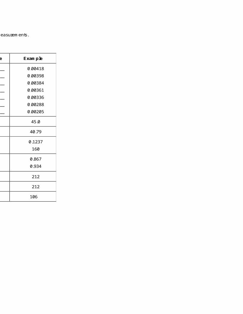
Table A2. Determination of design subgrade k-value from deflection measurements.
BARE CONCRETE PAVEMENT
Step Equation Calculated Value Example
d0
d8
d12
d18
d24
d36
d60
______________
______________
______________
______________
______________
______________
______________
0.00418
0.00398
0.00384
0.00361
0.00336
0.00288
0.00205
AREA7 [26] 45.0
Initial estimate of l [28] 40.79
Nondimensional d0*
and initial estimate of k
[31]
[30]
0.1237
160
Afd0
AFl
[34]
[35]
0.867
0.934
Adjusted k [37] 212
Mean dynamic k 212
Mean static k for design 106
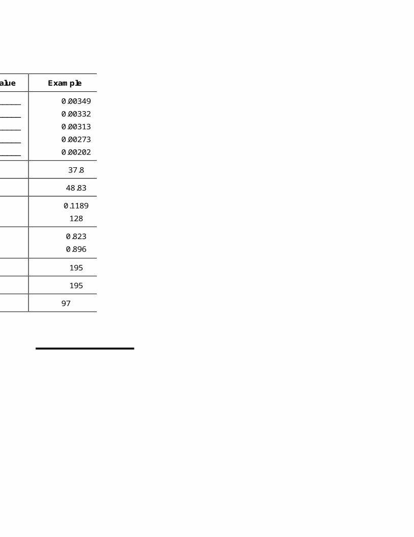
COMPOSITE PAVEMENT
Step Equation Calculated Value Example
d12
d18
d24
d36
d60
______________
______________
______________
______________
______________
0.00349
0.00332
0.00313
0.00273
0.00202
AREA5 [27] 37.8
Initial estimate of l [29] 48.83
Nondimensional d12*
and initial estimate of k
[33]
[32]
0.1189
128
Afd0
AFl
[34]
[35]
0.823
0.896
Adjusted k [37] 195
Mean dynamic k 195
Mean static k for design 97

Method C -- Plate Bearing Test Methods. The subgrade or embankment elastic k-value may
be determined from either of two types of plate bearing tests: repetitive static plate loading
(AASHTO T221, ASTM D1195) or nonrepetitive static plate loading (AASHTO T222, ASTM
D1196). These test methods were developed for a variety of purposes, and do not provide explicit
guidance on the determination of the required k-value input to the design procedure described
here.
For the purpose of concrete pavement design, the recommended subgrade input parameter is
the static elastic k-value. This may be determined from either a repetitive or nonrepetitive test on
the prepared subgrade or on a prepared test embankment, provided that the embankment is at
least 10 ft [3 m] thick. Otherwise, the tests should be conducted on the subgrade, and the k-value
obtained should be adjusted to account for the thickness and density of the embankment, using
the nomograph provided in Step 3.
In a repetitive test, the elastic k-value is determined from the ratio of load to elastic
deformation (the recoverable portion of the total deformation measured). In a nonrepetitive test,
the load-deformation ratio at a deformation of 0.05 in [1.25 mm] is considered to represent the
elastic k-value, according to extensive research by the U.S. Army Corps of Engineers.
Note also that a 30-in-diameter [762-mm-diameter] plate should be used to determine the
elastic static k-value for use in design. Smaller diameter plates will yield substantially higher k-
values, which are not appropriate for use in this design procedure. An adequate number of tests
should be run to ensure coverage over the project length. The mean of the tests becomes the
static elastic k-value for the season of testing. This value is then used to determine the effective
seasonally adjusted elastic k-value considering the factors discussed above.

Season Number of Months Subgrade k-Value, Relative Damagepsi/in millions in the Season
21.72 0.000019.19 0.000023.12 0.000022.31 0.0000
Total: 0 Mean Damage:
Seasonally Adjusted Subgrade k-Value (psi/in): 165
0 0
W18,
W18:
C1
This is the seasonal k-value of the subgrade soil for the season and not the composite k-value of the soil-base system. Formulas for calculating k from FWD data are provided in the "k-Value Information" sheet.
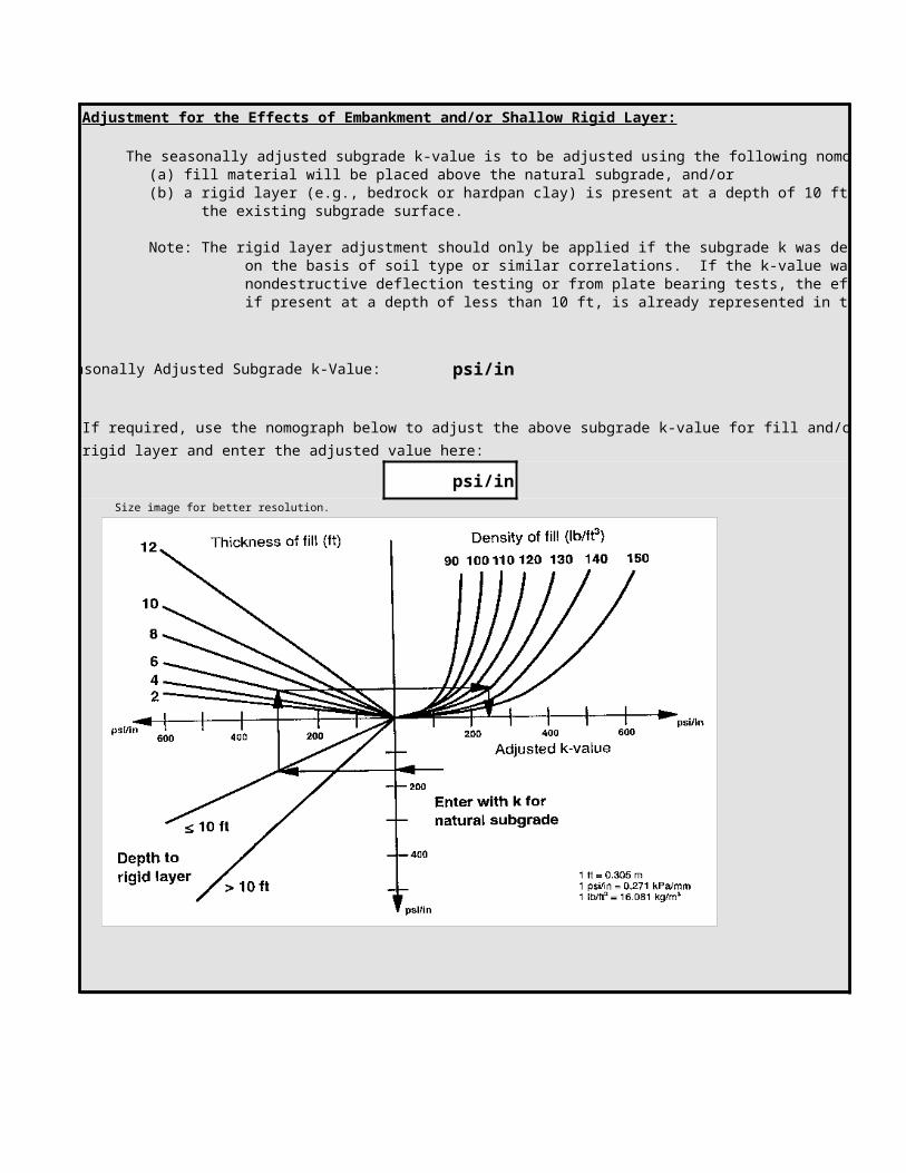
Adjustment for the Effects of Embankment and/or Shallow Rigid Layer:
The seasonally adjusted subgrade k-value is to be adjusted using the following nomograph if:(a) fill material will be placed above the natural subgrade, and/or(b) a rigid layer (e.g., bedrock or hardpan clay) is present at a depth of 10 ft or less beneath the existing subgrade surface.
Note: The rigid layer adjustment should only be applied if the subgrade k was determined on the basis of soil type or similar correlations. If the k-value was determined from nondestructive deflection testing or from plate bearing tests, the effect of a rigid layer, if present at a depth of less than 10 ft, is already represented in the k-value obtained.
Seasonally Adjusted Subgrade k-Value: psi/in
If required, use the nomograph below to adjust the above subgrade k-value for fill and/orrigid layer and enter the adjusted value here:
psi/in Size image for better resolution.
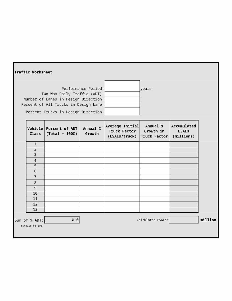
Traffic Worksheet
Performance Period: yearsTwo-Way Daily Traffic (ADT):
Number of Lanes in Design Direction: ###Percent of All Trucks in Design Lane: ###
Percent Trucks in Design Direction: ###
123456789
10111213
Sum of % ADT: 0.0 Calculated ESALs: million###(Should be 100) ###
Vehicle Class
Percent of ADT (Total = 100%)
Annual % Growth
Average Initial Truck Factor (ESALs/truck)
Annual % Growth in
Truck Factor
Accumulated ESALs
(millions)

Saved Data
Page 78
Select row to be exported and click the "Export" button.
ID Agency: Street Address: City: State: Project Number:Clear
Example ERES 505 W. University Ave. Champaign IL 1-20-98LCB

Saved Data
Page 79
Description: Location: Initial Serviceability, P1:
Lean Concrete Base, 5-in. Champaign, IL 4.5

Saved Data
Page 80
Terminal Serviceability, P2:
2.5 700
28-day Mean Modulus of Rupture, (S'c)':

Saved Data
Page 81
0.15
4500000 0.15 25000
Elastic Modulus of Slab, Ec: Poisson's Ratio for Concrete, m: Elastic Modulus of Base, Eb:

Saved Data
Page 82
Slab-Base Friction Factor, f: Reliability Level (R):
6 1.4 90
Design Thickness of Base, Hb:

Saved Data
Page 83
Mean Annual Wind Speed, WIND:
0.34 10.2
Overall Standard Deviation, S0:
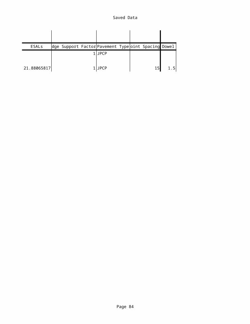
Saved Data
Page 84
Mean Annual Air Temperature, TEMP: Mean Annual Precipitation, PRECIP:
49.2 33.3
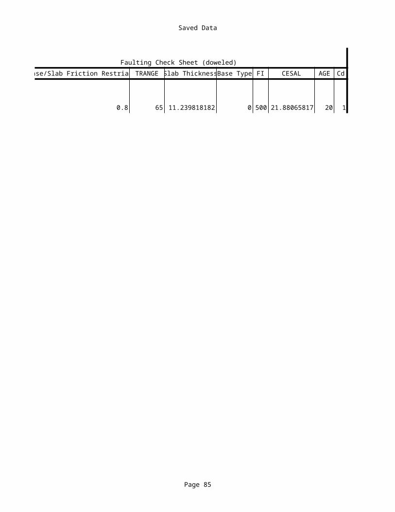
Saved Data
Page 85
Subgrade k-Value ESALs Edge Support Factor: Pavement Type Joint Spacing:1 JPCP
165 21.88065817 1 JPCP 15
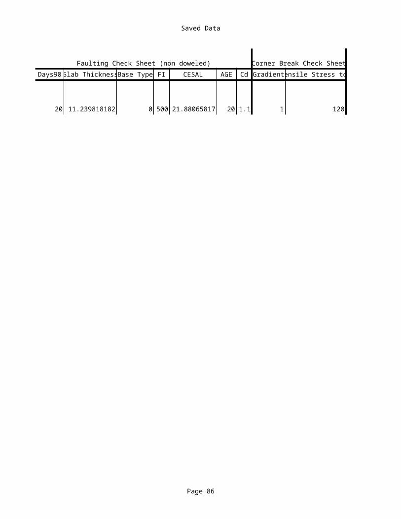
Saved Data
Page 86
Faulting Check Sheet (doweled)Dowel Base/Slab Friction Restriant TRANGE Slab Thickness Base Type FI
1.5 0.8 65 11.2398181822 0 500

Saved Data
Page 87
Faulting Check Sheet (doweled) Faulting Check Sheet (non doweled)CESAL AGE Cd Days90 Slab Thickness Base Type FI CESAL AGE Cd
21.88065817 20 1 20 11.2398181822 0 500 21.88065817 20 1.1

Saved Data
Page 88
Corner Break Check Sheet Fill/Rigid Adjustment k-Value SheetGradient Tensile Stress top Adjusted k-Value Season1 Months1 k1 Season2
1 120 175 Fall 2 150 Winter
Saved Data
Page 89
k-Value SheetMonths2 k2 Season3 Months3 k3 Season4 Months4 k4 Season5 Months5 k5
3 300 Spring 3 80 Summer 4 120
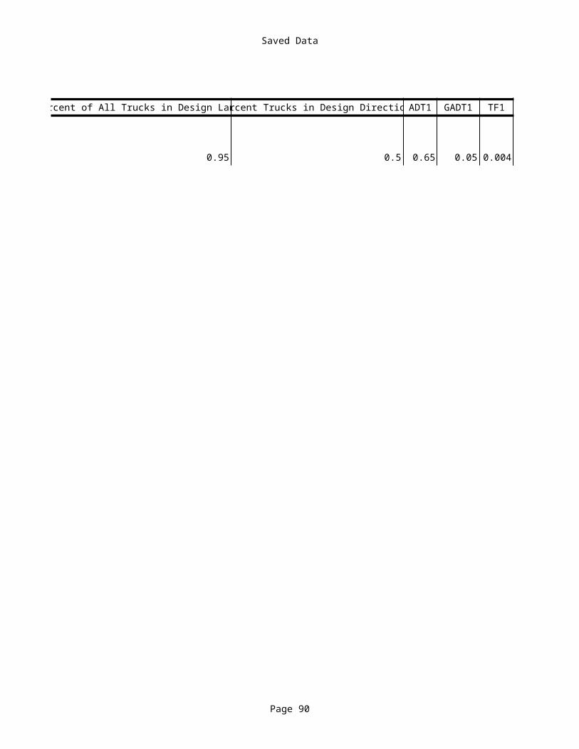
Saved Data
Page 90
k-Value Sheet Traffic SheetSeason6 Months6 Seasons6 Performance Period: Two-Way Daily Traffic (ADT):
20 8000
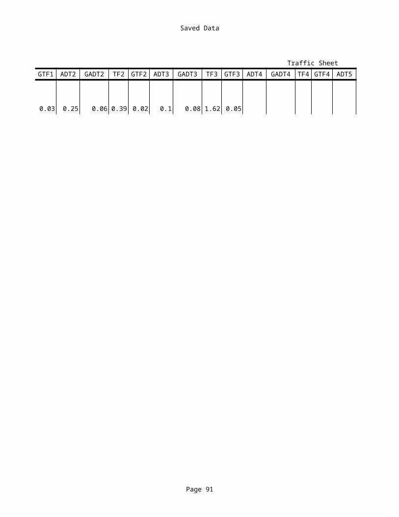
Saved Data
Page 91
Traffic SheetNumber of lanes in Design Direction: Percent of All Trucks in Design Lane:
2 0.95

Saved Data
Page 92
Traffic SheetPercent Trucks in Design Direction: ADT1 GADT1 TF1 GTF1 ADT2 GADT2 TF2
0.5 0.65 0.05 0.004 0.03 0.25 0.06 0.39

Saved Data
Page 93
Traffic SheetGTF2 ADT3 GADT3 TF3 GTF3 ADT4 GADT4 TF4 GTF4 ADT5 GADT5 TF5 GTF5
0.02 0.1 0.08 1.62 0.05
Saved Data
Page 94
Traffic SheetADT6 GADT6 TF6 GTF6 ADT7 GADT7 TF7 GTF7 ADT8 GADT8 TF8 GTF8 ADT9
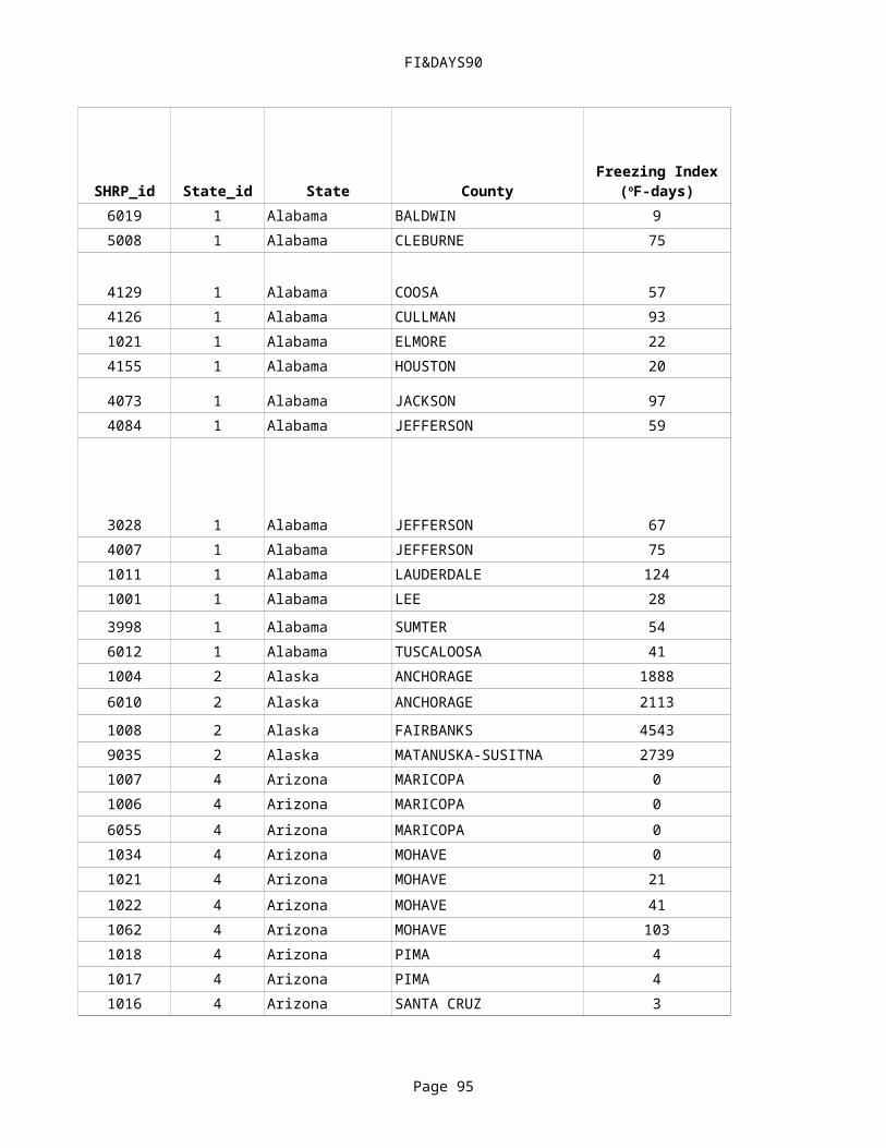
Saved Data
Page 95
Traffic SheetGADT9 TF9 GTF9 ADT10 GADT10 TF10 GTF10 ADT11 GADT11 TF11 GTF11
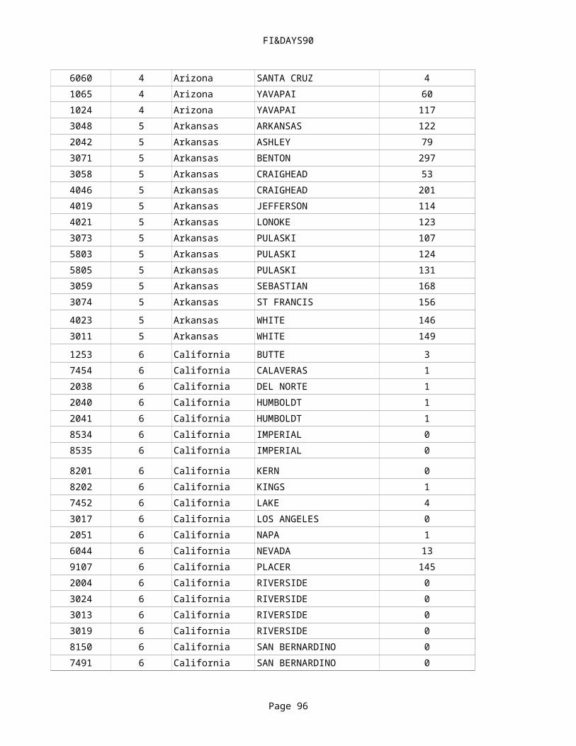
Saved Data
Page 96
Traffic SheetADT12 GADT12 TF12 GTF12 ADT13 GADT13 TF13 GTF13

FI&DAYS90
Page 97
SHRP_id State_id State County6019 1 Alabama BALDWIN 95008 1 Alabama CLEBURNE 75
4129 1 Alabama COOSA 574126 1 Alabama CULLMAN 931021 1 Alabama ELMORE 224155 1 Alabama HOUSTON 20
4073 1 Alabama JACKSON 974084 1 Alabama JEFFERSON 59
3028 1 Alabama JEFFERSON 674007 1 Alabama JEFFERSON 751011 1 Alabama LAUDERDALE 1241001 1 Alabama LEE 283998 1 Alabama SUMTER 546012 1 Alabama TUSCALOOSA 411004 2 Alaska ANCHORAGE 18886010 2 Alaska ANCHORAGE 21131008 2 Alaska FAIRBANKS 45439035 2 Alaska MATANUSKA-SUSITNA 27391007 4 Arizona MARICOPA 01006 4 Arizona MARICOPA 06055 4 Arizona MARICOPA 01034 4 Arizona MOHAVE 01021 4 Arizona MOHAVE 211022 4 Arizona MOHAVE 411062 4 Arizona MOHAVE 1031018 4 Arizona PIMA 41017 4 Arizona PIMA 41016 4 Arizona SANTA CRUZ 36060 4 Arizona SANTA CRUZ 41065 4 Arizona YAVAPAI 60
Freezing Index (oF-days)
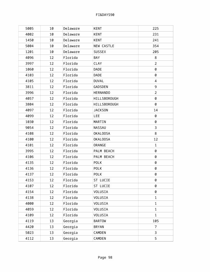
FI&DAYS90
Page 98
1024 4 Arizona YAVAPAI 1173048 5 Arkansas ARKANSAS 1222042 5 Arkansas ASHLEY 793071 5 Arkansas BENTON 2973058 5 Arkansas CRAIGHEAD 534046 5 Arkansas CRAIGHEAD 2014019 5 Arkansas JEFFERSON 1144021 5 Arkansas LONOKE 1233073 5 Arkansas PULASKI 1075803 5 Arkansas PULASKI 1245805 5 Arkansas PULASKI 1313059 5 Arkansas SEBASTIAN 1683074 5 Arkansas ST FRANCIS 1564023 5 Arkansas WHITE 1463011 5 Arkansas WHITE 1491253 6 California BUTTE 37454 6 California CALAVERAS 12038 6 California DEL NORTE 12040 6 California HUMBOLDT 12041 6 California HUMBOLDT 18534 6 California IMPERIAL 08535 6 California IMPERIAL 0
8201 6 California KERN 08202 6 California KINGS 17452 6 California LAKE 43017 6 California LOS ANGELES 02051 6 California NAPA 16044 6 California NEVADA 139107 6 California PLACER 1452004 6 California RIVERSIDE 03024 6 California RIVERSIDE 03013 6 California RIVERSIDE 03019 6 California RIVERSIDE 08150 6 California SAN BERNARDINO 07491 6 California SAN BERNARDINO 08149 6 California SAN BERNARDINO 08151 6 California SAN BERNARDINO 12
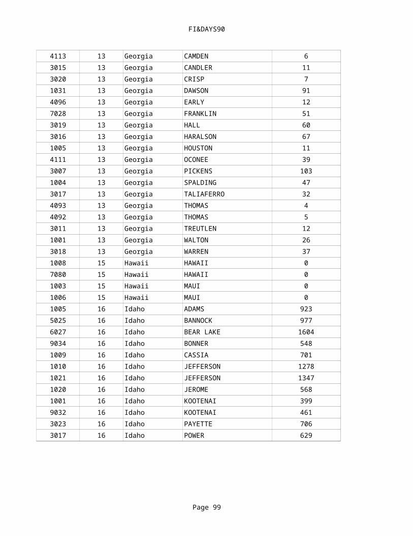
FI&DAYS90
Page 99
3010 6 California SAN DIEGO 07493 6 California SAN DIEGO 09048 6 California SAN DIEGO 03021 6 California SAN DIEGO 23042 6 California SAN JOAQUIN 17455 6 California SAN JOAQUIN 17456 6 California SAN JOAQUIN 18153 6 California SAN LUIS OBISPO 02053 6 California SAN MATEO 08156 6 California SANTA BARBARA 03030 6 California SHASTA 33005 6 California SISKIYOU 702002 6 California SISKIYOU 1432647 6 California TUOLUMNE 29049 6 California YOLO 07035 8 Colorado ADAMS 5487776 8 Colorado ADAMS 6127036 8 Colorado ARAPAHOE 6607781 8 Colorado BENT 4712008 8 Colorado BENT 4711053 8 Colorado DELTA 4647780 8 Colorado EL PASO 14533032 8 Colorado GARFIELD 6557783 8 Colorado GARFIELD 6729020 8 Colorado LARIMER 6176013 8 Colorado LOGAN 8501057 8 Colorado MESA 4591029 8 Colorado MOFFAT 13956002 8 Colorado PUEBLO 4771047 8 Colorado RIO BLANCO 12189019 8 Colorado WELD 6864008 9 Connecticut HARTFORD 5524020 9 Connecticut HARTFORD 6201803 9 Connecticut NEW LONDON 3995001 9 Connecticut TOLLAND 7155005 10 Delaware KENT 2254002 10 Delaware KENT 2311450 10 Delaware KENT 241

FI&DAYS90
Page 100
5004 10 Delaware NEW CASTLE 3541201 10 Delaware SUSSEX 2054096 12 Florida BAY 83997 12 Florida CLAY 21060 12 Florida DADE 04103 12 Florida DADE 04105 12 Florida DUVAL 43811 12 Florida GADSDEN 93996 12 Florida HERNANDO 24057 12 Florida HILLSBOROUGH 03804 12 Florida HILLSBOROUGH 04097 12 Florida JACKSON 144099 12 Florida LEE 01030 12 Florida MARTIN 09054 12 Florida NASSAU 34108 12 Florida OKALOOSA 84100 12 Florida OKALOOSA 124101 12 Florida ORANGE 13995 12 Florida PALM BEACH 04106 12 Florida PALM BEACH 04135 12 Florida POLK 04136 12 Florida POLK 04137 12 Florida POLK 04153 12 Florida ST LUCIE 04107 12 Florida ST LUCIE 04154 12 Florida VOLUSIA 04138 12 Florida VOLUSIA 14000 12 Florida VOLUSIA 14059 12 Florida VOLUSIA 14109 12 Florida VOLUSIA 14119 13 Georgia BARTOW 1054420 13 Georgia BRYAN 75023 13 Georgia CAMDEN 34112 13 Georgia CAMDEN 54113 13 Georgia CAMDEN 63015 13 Georgia CANDLER 113020 13 Georgia CRISP 71031 13 Georgia DAWSON 91

FI&DAYS90
Page 101
4096 13 Georgia EARLY 127028 13 Georgia FRANKLIN 513019 13 Georgia HALL 603016 13 Georgia HARALSON 671005 13 Georgia HOUSTON 114111 13 Georgia OCONEE 393007 13 Georgia PICKENS 1031004 13 Georgia SPALDING 473017 13 Georgia TALIAFERRO 324093 13 Georgia THOMAS 44092 13 Georgia THOMAS 53011 13 Georgia TREUTLEN 121001 13 Georgia WALTON 263018 13 Georgia WARREN 371008 15 Hawaii HAWAII 07080 15 Hawaii HAWAII 01003 15 Hawaii MAUI 01006 15 Hawaii MAUI 01005 16 Idaho ADAMS 9235025 16 Idaho BANNOCK 9776027 16 Idaho BEAR LAKE 16049034 16 Idaho BONNER 5481009 16 Idaho CASSIA 7011010 16 Idaho JEFFERSON 12781021 16 Idaho JEFFERSON 13471020 16 Idaho JEROME 5681001 16 Idaho KOOTENAI 3999032 16 Idaho KOOTENAI 4613023 16 Idaho PAYETTE 7063017 16 Idaho POWER 629
5849 17 Illinois CHAMPAIGN 8431003 17 Illinois CLINTON 336
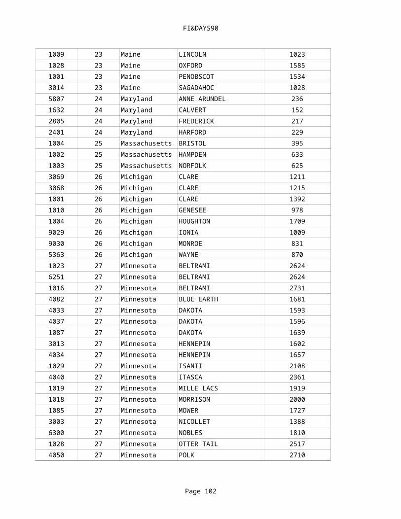
FI&DAYS90
Page 102
5020 17 Illinois CLINTON 3534082 17 Illinois CLINTON 3777937 17 Illinois HENRY 10415453 17 Illinois JEFFERSON 4865217 17 Illinois MC LEAN 7929327 17 Illinois MC LEAN 7925843 17 Illinois OGLE 10955854 17 Illinois PEORIA 8565869 17 Illinois PEORIA 8789267 17 Illinois ROCK ISLAND 10006050 17 Illinois ST CLAIR 4611002 17 Illinois STEPHENSON 10654074 17 Illinois STEPHENSON 10655908 17 Illinois WILLIAMSON 4592008 18 Indiana ALLEN 7733002 18 Indiana BENTON 8923030 18 Indiana DELAWARE 7429020 18 Indiana GRANT 8424021 18 Indiana HAMILTON 7885538 18 Indiana LA PORTE 8475528 18 Indiana LA PORTE 8475022 18 Indiana MARION 7083003 18 Indiana MARSHALL 8674042 18 Indiana POSEY 3753031 18 Indiana POSEY 4041037 18 Indiana SPENCER 3001028 18 Indiana SPENCER 4425518 18 Indiana TIPPECANOE 7965043 18 Indiana VANDERBURGH 3586049 19 Iowa CEDAR 11013006 19 Iowa CLINTON 10375046 19 Iowa FRANKLIN 14663055 19 Iowa HAMILTON 14003033 19 Iowa JOHNSON 8453028 19 Iowa JOHNSON 8493009 19 Iowa LINN 11989126 19 Iowa SCOTT 9739116 19 Iowa WORTH 1680

FI&DAYS90
Page 103
5042 19 Iowa WRIGHT 14584054 20 Kansas DICKINSON 4957073 20 Kansas DICKINSON 5773015 20 Kansas FINNEY 5541010 20 Kansas FORD 4361005 20 Kansas FRANKLIN 5303013 20 Kansas JOHNSON 4694053 20 Kansas LINCOLN 4487085 20 Kansas MARSHALL 7876026 20 Kansas RENO 4399037 20 Kansas SHAWNEE 5981009 20 Kansas STAFFORD 3784063 20 Kansas WYANDOTTE 5071034 21 Kentucky BARREN 2873016 21 Kentucky BULLITT 2546043 21 Kentucky CLAY 2794025 21 Kentucky FAYETTE 3846040 21 Kentucky FAYETTE 3941010 21 Kentucky OWSLEY 3071014 21 Kentucky PIKE 2254001 22 Louisiana LIVINGSTON 133056 22 Louisiana RAPIDES 311012 23 Maine CUMBERLAND 9813013 23 Maine CUMBERLAND 10277023 23 Maine CUMBERLAND 10371026 23 Maine FRANKLIN 15221009 23 Maine LINCOLN 10231028 23 Maine OXFORD 15851001 23 Maine PENOBSCOT 15343014 23 Maine SAGADAHOC 10285807 24 Maryland ANNE ARUNDEL 2361632 24 Maryland CALVERT 1522805 24 Maryland FREDERICK 2172401 24 Maryland HARFORD 2291004 25 Massachusetts BRISTOL 3951002 25 Massachusetts HAMPDEN 6331003 25 Massachusetts NORFOLK 6253069 26 Michigan CLARE 1211
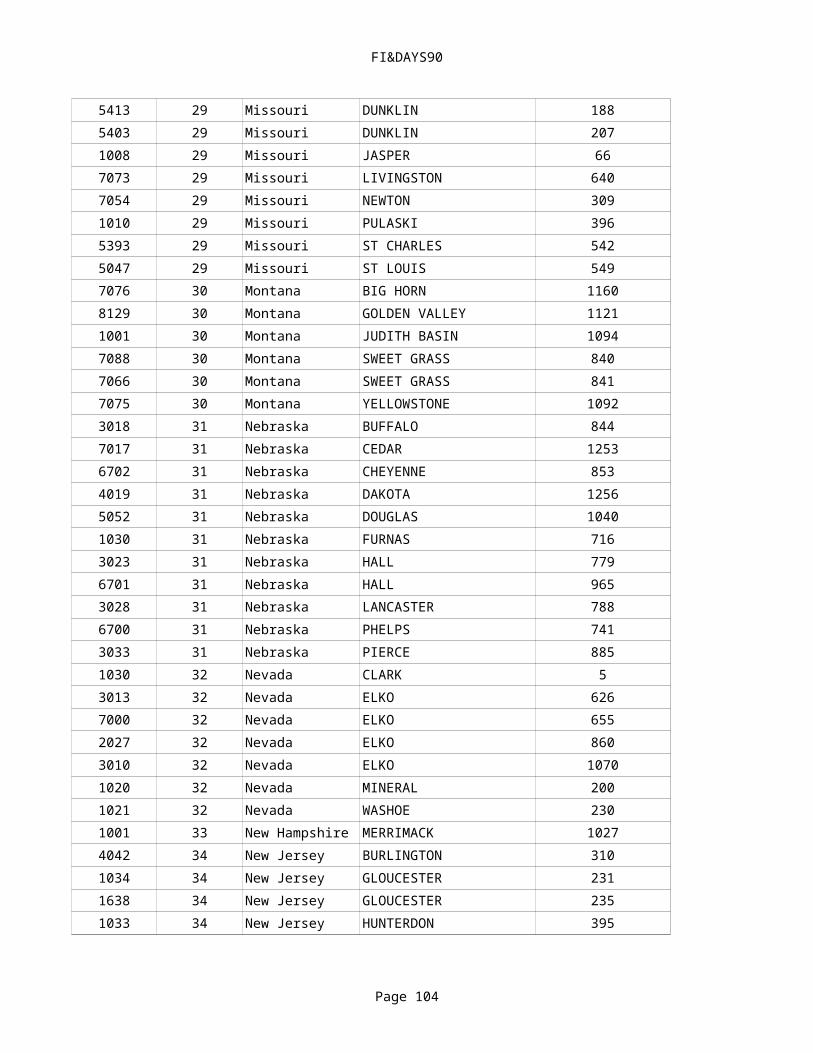
FI&DAYS90
Page 104
3068 26 Michigan CLARE 12151001 26 Michigan CLARE 13921010 26 Michigan GENESEE 9781004 26 Michigan HOUGHTON 17099029 26 Michigan IONIA 10099030 26 Michigan MONROE 8315363 26 Michigan WAYNE 8701023 27 Minnesota BELTRAMI 26246251 27 Minnesota BELTRAMI 26241016 27 Minnesota BELTRAMI 27314082 27 Minnesota BLUE EARTH 16814033 27 Minnesota DAKOTA 15934037 27 Minnesota DAKOTA 15961087 27 Minnesota DAKOTA 16393013 27 Minnesota HENNEPIN 16024034 27 Minnesota HENNEPIN 16571029 27 Minnesota ISANTI 21084040 27 Minnesota ITASCA 23611019 27 Minnesota MILLE LACS 19191018 27 Minnesota MORRISON 20001085 27 Minnesota MOWER 17273003 27 Minnesota NICOLLET 13886300 27 Minnesota NOBLES 18101028 27 Minnesota OTTER TAIL 25174050 27 Minnesota POLK 27109075 27 Minnesota RENVILLE 19187090 27 Minnesota SCOTT 18066064 27 Minnesota STEARNS 21145076 27 Minnesota WASHINGTON 16984054 27 Minnesota WINONA 15464055 27 Minnesota WRIGHT 20713097 28 Mississippi DE SOTO 1145805 28 Mississippi HARRISON 73081 28 Mississippi ITAWAMBA 793093 28 Mississippi JACKSON 113094 28 Mississippi JACKSON 133089 28 Mississippi LAFAYETTE 1293087 28 Mississippi LAFAYETTE 134

FI&DAYS90
Page 105
2807 28 Mississippi LAFAYETTE 1383091 28 Mississippi LAUDERDALE 355006 28 Mississippi LEE 1025025 28 Mississippi LINCOLN 433085 28 Mississippi MARSHALL 1483083 28 Mississippi MARSHALL 1505803 28 Mississippi MARSHALL 1743082 28 Mississippi MONTGOMERY 943090 28 Mississippi PANOLA 1263099 28 Mississippi SCOTT 323019 28 Mississippi TISHOMINGO 1483018 28 Mississippi TISHOMINGO 1509030 28 Mississippi WARREN 287012 28 Mississippi WARREN 374024 28 Mississippi WASHINGTON 626067 29 Missouri CARTER 3424036 29 Missouri CLAY 5685483 29 Missouri CLAY 5691002 29 Missouri COLE 3825473 29 Missouri COOPER 5435091 29 Missouri DAVIESS 8745081 29 Missouri DAVIESS 8745058 29 Missouri DAVIESS 8765000 29 Missouri DAVIESS 8765413 29 Missouri DUNKLIN 1885403 29 Missouri DUNKLIN 2071008 29 Missouri JASPER 667073 29 Missouri LIVINGSTON 6407054 29 Missouri NEWTON 3091010 29 Missouri PULASKI 3965393 29 Missouri ST CHARLES 5425047 29 Missouri ST LOUIS 5497076 30 Montana BIG HORN 11608129 30 Montana GOLDEN VALLEY 11211001 30 Montana JUDITH BASIN 10947088 30 Montana SWEET GRASS 8407066 30 Montana SWEET GRASS 8417075 30 Montana YELLOWSTONE 1092

FI&DAYS90
Page 106
3018 31 Nebraska BUFFALO 8447017 31 Nebraska CEDAR 12536702 31 Nebraska CHEYENNE 8534019 31 Nebraska DAKOTA 12565052 31 Nebraska DOUGLAS 10401030 31 Nebraska FURNAS 7163023 31 Nebraska HALL 7796701 31 Nebraska HALL 9653028 31 Nebraska LANCASTER 7886700 31 Nebraska PHELPS 7413033 31 Nebraska PIERCE 8851030 32 Nevada CLARK 53013 32 Nevada ELKO 6267000 32 Nevada ELKO 6552027 32 Nevada ELKO 8603010 32 Nevada ELKO 10701020 32 Nevada MINERAL 2001021 32 Nevada WASHOE 2301001 33 New Hampshire MERRIMACK 10274042 34 New Jersey BURLINGTON 3101034 34 New Jersey GLOUCESTER 2311638 34 New Jersey GLOUCESTER 2351033 34 New Jersey HUNTERDON 3956057 34 New Jersey MERCER 3481030 34 New Jersey PASSAIC 6981003 35 New Mexico CHAVES 1076401 35 New Mexico CIBOLA 2156035 35 New Mexico CIBOLA 2771112 35 New Mexico LEA 933010 35 New Mexico LEA 931002 35 New Mexico LINCOLN 1082118 35 New Mexico QUAY 1951022 35 New Mexico SAN JUAN 4651005 35 New Mexico SANTA FE 2456033 35 New Mexico SOCORRO 1134017 36 New York ALLEGANY 10281008 36 New York ONEIDA 10511011 36 New York ONONDAGA 830
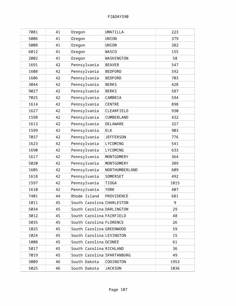
FI&DAYS90
Page 107
4018 36 New York OTSEGO 10651644 36 New York ST LAWRENCE 17575037 37 North Carolina BUNCOMBE 1501801 37 North Carolina BUNCOMBE 1641992 37 North Carolina CHATHAM 92824 37 North Carolina CHATHAM 1033008 37 North Carolina CLEVELAND 521645 37 North Carolina COLUMBUS 393807 37 North Carolina DAVIDSON 953816 37 North Carolina DURHAM 823044 37 North Carolina DURHAM 971817 37 North Carolina FORSYTH 861802 37 North Carolina GRANVILLE 852819 37 North Carolina GUILFORD 861024 37 North Carolina JACKSON 1201803 37 North Carolina JACKSON 1711814 37 North Carolina MACON 1272825 37 North Carolina MECKLENBURG 421040 37 North Carolina MITCHELL 2893011 37 North Carolina NASH 1015827 37 North Carolina ROCKINGHAM 1601352 37 North Carolina STANLY 685826 37 North Carolina SURRY 1711006 37 North Carolina WAKE 765002 38 North Dakota CASS 23392001 38 North Dakota GRAND FORKS 26233005 38 North Dakota NELSON 24813006 38 North Dakota PIERCE 26753801 39 Ohio BELMONT 4583013 39 Ohio BROWN 4789006 39 Ohio CLINTON 6214031 39 Ohio FRANKLIN 5624018 39 Ohio GREENE 6505003 39 Ohio LORAIN 6565010 39 Ohio MAHONING 7727021 39 Ohio WOOD 7354163 40 Oklahoma BLAINE 2124162 40 Oklahoma COMANCHE 163

FI&DAYS90
Page 108
4086 40 Oklahoma GRADY 1684154 40 Oklahoma GRADY 2124087 40 Oklahoma JACKSON 1504088 40 Oklahoma KAY 3216010 40 Oklahoma LE FLORE 1244164 40 Oklahoma MAJOR 2914165 40 Oklahoma MAJOR 3114157 40 Oklahoma MAYES 655021 40 Oklahoma MAYES 2533018 40 Oklahoma OKLAHOMA 1984166 40 Oklahoma PITTSBURG 994160 40 Oklahoma PONTOTOC 1574158 40 Oklahoma WASHINGTON 1444155 40 Oklahoma WASHINGTON 2527025 41 Oregon DOUGLAS 277019 41 Oregon JACKSON 455022 41 Oregon LANE 475021 41 Oregon LANE 496011 41 Oregon LINN 397018 41 Oregon LINN 495005 41 Oregon LINN 607081 41 Oregon UMATILLA 2235006 41 Oregon UNION 3795008 41 Oregon UNION 3826012 41 Oregon WASCO 1552002 41 Oregon WASHINGTON 581691 42 Pennsylvania BEAVER 5471608 42 Pennsylvania BEDFORD 5921606 42 Pennsylvania BEDFORD 7033044 42 Pennsylvania BERKS 4289027 42 Pennsylvania BERKS 5877025 42 Pennsylvania CAMBRIA 5941614 42 Pennsylvania CENTRE 8981627 42 Pennsylvania CLEARFIELD 9301598 42 Pennsylvania CUMBERLAND 4321613 42 Pennsylvania DELAWARE 3271599 42 Pennsylvania ELK 9037037 42 Pennsylvania JEFFERSON 776

FI&DAYS90
Page 109
1623 42 Pennsylvania LYCOMING 5411690 42 Pennsylvania LYCOMING 6331617 42 Pennsylvania MONTGOMERY 3645020 42 Pennsylvania MONTGOMERY 3891605 42 Pennsylvania NORTHUMBERLAND 6091618 42 Pennsylvania SOMERSET 4921597 42 Pennsylvania TIOGA 10151610 42 Pennsylvania YORK 4077401 44 Rhode Island PROVIDENCE 6811011 45 South Carolina CHARLESTON 95034 45 South Carolina DARLINGTON 293012 45 South Carolina FAIRFIELD 485035 45 South Carolina FLORENCE 261025 45 South Carolina GREENWOOD 591024 45 South Carolina LEXINGTON 151008 45 South Carolina OCONEE 615017 45 South Carolina RICHLAND 367019 45 South Carolina SPARTANBURG 493009 46 South Dakota CODINGTON 19535025 46 South Dakota JACKSON 10369197 46 South Dakota JERAULD 15273052 46 South Dakota KINGSBURY 17203013 46 South Dakota LAWRENCE 10895020 46 South Dakota LAWRENCE 11153012 46 South Dakota MEADE 10619187 46 South Dakota MEADE 16055040 46 South Dakota MINNEHAHA 16513053 46 South Dakota PENNINGTON 11359106 46 South Dakota PERKINS 17503010 46 South Dakota ROBERTS 17367049 46 South Dakota YANKTON 14003108 47 Tennessee ANDERSON 1873101 47 Tennessee CANNON 1749025 47 Tennessee CANNON 1743075 47 Tennessee DE KALB 2362001 47 Tennessee DYER 2562008 47 Tennessee GIBSON 2261028 47 Tennessee HAWKINS 194
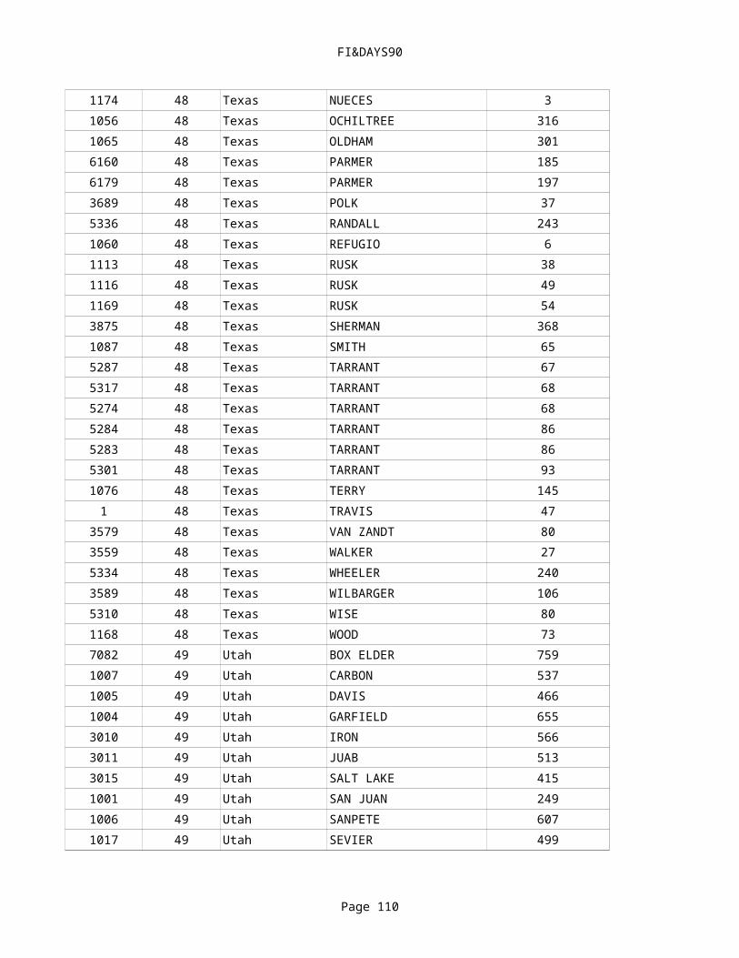
FI&DAYS90
Page 110
3109 47 Tennessee MAURY 2416015 47 Tennessee MC MINN 1763110 47 Tennessee MC MINN 1786022 47 Tennessee PUTNAM 2779024 47 Tennessee RUTHERFORD 2333104 47 Tennessee UNION 1613669 48 Texas ANGELINA 293679 48 Texas ANGELINA 411093 48 Texas ATASCOSA 112133 48 Texas BELL 449005 48 Texas BEXAR 131094 48 Texas BEXAR 165026 48 Texas BRAZORIA 161178 48 Texas BURLESON 543729 48 Texas CAMERON 45323 48 Texas CARSON 2501047 48 Texas CARSON 2531046 48 Texas CARSON 2584146 48 Texas CHAMBERS 123010 48 Texas CHAMBERS 121119 48 Texas CHEROKEE 473629 48 Texas COLORADO 145024 48 Texas COLORADO 273845 48 Texas COOKE 1105035 48 Texas DALLAS 623003 48 Texas DALLAS 636079 48 Texas DEAF SMITH 1973749 48 Texas DUVAL 103779 48 Texas EL PASO 199355 48 Texas ELLIS 481039 48 Texas ELLIS 633699 48 Texas FORT BEND 142108 48 Texas GALVESTON 61183 48 Texas GARZA 1405154 48 Texas GONZALES 155335 48 Texas GRAY 2331050 48 Texas GRIMES 271130 48 Texas GUADALUPE 14
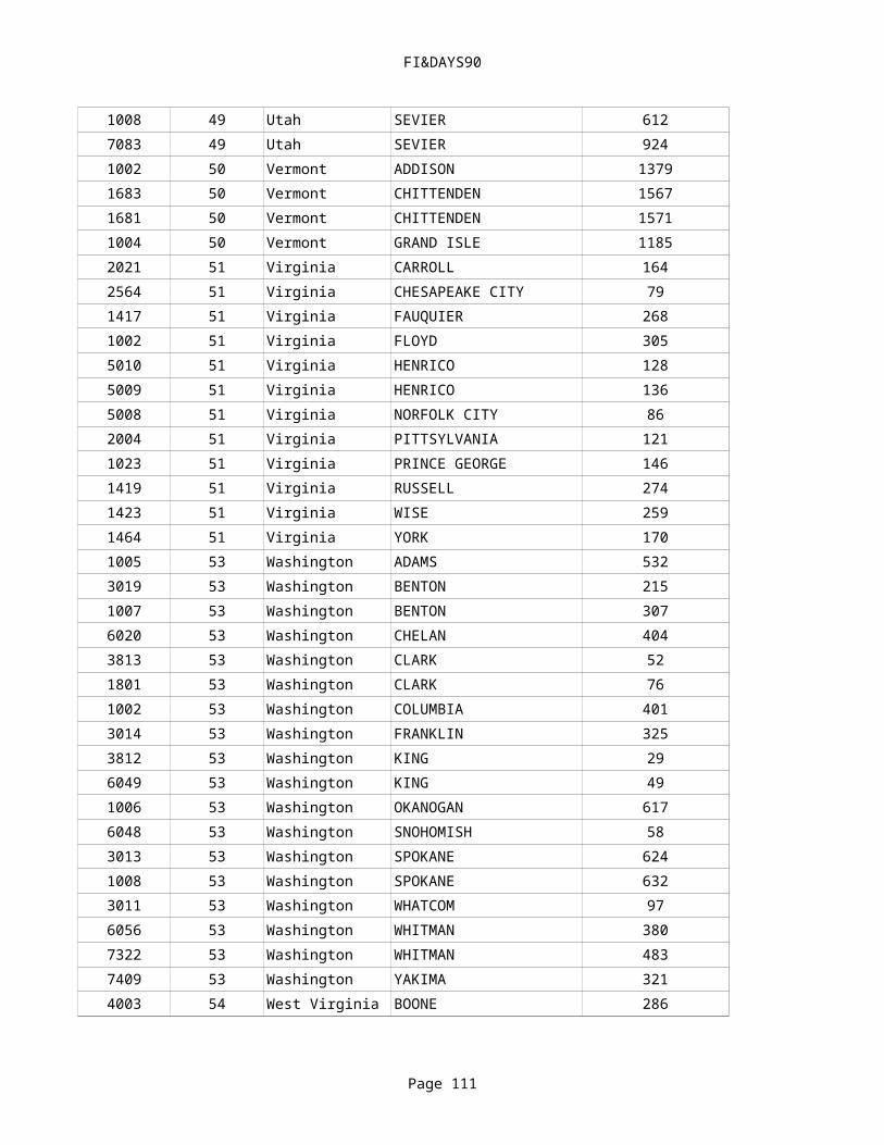
FI&DAYS90
Page 111
2176 48 Texas HALE 1901077 48 Texas HALL 1827165 48 Texas HARRIS 63569 48 Texas HOPKINS 794142 48 Texas JASPER 223719 48 Texas JEFFERSON 44143 48 Texas JEFFERSON 83739 48 Texas KENEDY 61068 48 Texas LAMAR 974152 48 Texas LIBERTY 136086 48 Texas LIVE OAK 61096 48 Texas MEDINA 121092 48 Texas MEDINA 175278 48 Texas MIDLAND 603865 48 Texas MILLS 435328 48 Texas MONTAGUE 981049 48 Texas NACOGDOCHES 379167 48 Texas NAVARRO 441174 48 Texas NUECES 31056 48 Texas OCHILTREE 3161065 48 Texas OLDHAM 3016160 48 Texas PARMER 1856179 48 Texas PARMER 1973689 48 Texas POLK 375336 48 Texas RANDALL 2431060 48 Texas REFUGIO 61113 48 Texas RUSK 381116 48 Texas RUSK 491169 48 Texas RUSK 543875 48 Texas SHERMAN 3681087 48 Texas SMITH 655287 48 Texas TARRANT 675317 48 Texas TARRANT 685274 48 Texas TARRANT 685284 48 Texas TARRANT 865283 48 Texas TARRANT 865301 48 Texas TARRANT 931076 48 Texas TERRY 145
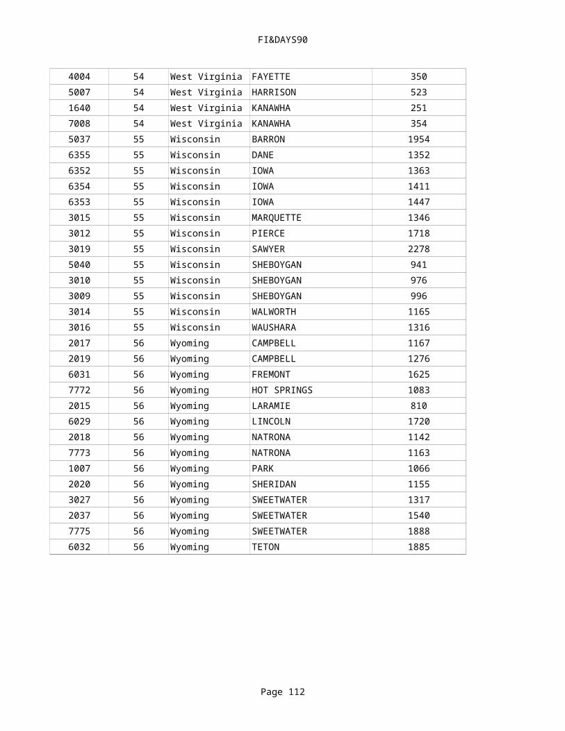
FI&DAYS90
Page 112
1 48 Texas TRAVIS 473579 48 Texas VAN ZANDT 803559 48 Texas WALKER 275334 48 Texas WHEELER 2403589 48 Texas WILBARGER 1065310 48 Texas WISE 801168 48 Texas WOOD 737082 49 Utah BOX ELDER 7591007 49 Utah CARBON 5371005 49 Utah DAVIS 4661004 49 Utah GARFIELD 6553010 49 Utah IRON 5663011 49 Utah JUAB 5133015 49 Utah SALT LAKE 4151001 49 Utah SAN JUAN 2491006 49 Utah SANPETE 6071017 49 Utah SEVIER 4991008 49 Utah SEVIER 6127083 49 Utah SEVIER 9241002 50 Vermont ADDISON 13791683 50 Vermont CHITTENDEN 15671681 50 Vermont CHITTENDEN 15711004 50 Vermont GRAND ISLE 11852021 51 Virginia CARROLL 1642564 51 Virginia CHESAPEAKE CITY 791417 51 Virginia FAUQUIER 2681002 51 Virginia FLOYD 3055010 51 Virginia HENRICO 1285009 51 Virginia HENRICO 1365008 51 Virginia NORFOLK CITY 862004 51 Virginia PITTSYLVANIA 1211023 51 Virginia PRINCE GEORGE 1461419 51 Virginia RUSSELL 2741423 51 Virginia WISE 2591464 51 Virginia YORK 1701005 53 Washington ADAMS 5323019 53 Washington BENTON 2151007 53 Washington BENTON 307

FI&DAYS90
Page 113
6020 53 Washington CHELAN 4043813 53 Washington CLARK 521801 53 Washington CLARK 761002 53 Washington COLUMBIA 4013014 53 Washington FRANKLIN 3253812 53 Washington KING 296049 53 Washington KING 491006 53 Washington OKANOGAN 6176048 53 Washington SNOHOMISH 583013 53 Washington SPOKANE 6241008 53 Washington SPOKANE 6323011 53 Washington WHATCOM 976056 53 Washington WHITMAN 3807322 53 Washington WHITMAN 4837409 53 Washington YAKIMA 3214003 54 West Virginia BOONE 2864004 54 West Virginia FAYETTE 3505007 54 West Virginia HARRISON 5231640 54 West Virginia KANAWHA 2517008 54 West Virginia KANAWHA 3545037 55 Wisconsin BARRON 19546355 55 Wisconsin DANE 13526352 55 Wisconsin IOWA 13636354 55 Wisconsin IOWA 14116353 55 Wisconsin IOWA 14473015 55 Wisconsin MARQUETTE 13463012 55 Wisconsin PIERCE 17183019 55 Wisconsin SAWYER 22785040 55 Wisconsin SHEBOYGAN 9413010 55 Wisconsin SHEBOYGAN 9763009 55 Wisconsin SHEBOYGAN 9963014 55 Wisconsin WALWORTH 11653016 55 Wisconsin WAUSHARA 13162017 56 Wyoming CAMPBELL 11672019 56 Wyoming CAMPBELL 12766031 56 Wyoming FREMONT 16257772 56 Wyoming HOT SPRINGS 10832015 56 Wyoming LARAMIE 810

FI&DAYS90
Page 114
6029 56 Wyoming LINCOLN 17202018 56 Wyoming NATRONA 11427773 56 Wyoming NATRONA 11631007 56 Wyoming PARK 10662020 56 Wyoming SHERIDAN 11553027 56 Wyoming SWEETWATER 13172037 56 Wyoming SWEETWATER 15407775 56 Wyoming SWEETWATER 18886032 56 Wyoming TETON 1885
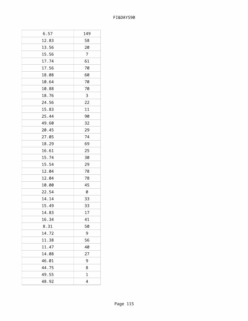
FI&DAYS90
Page 115
DAYS9065.59 5852.95 39
54.54 4763.34 4153.53 5853.68 66
66.07 3957.00 51
54.91 4253.28 5054.33 4949.83 6056.04 6557.91 5621.65 019.36 012.73 029.22 08.94 1758.41 1737.26 1735.34 170
10.90 8911.65 7914.75 3722.58 9021.95 9318.81 11117.22 11114.07 61
Average Annual Total Precipitation, PRECIP
(in)
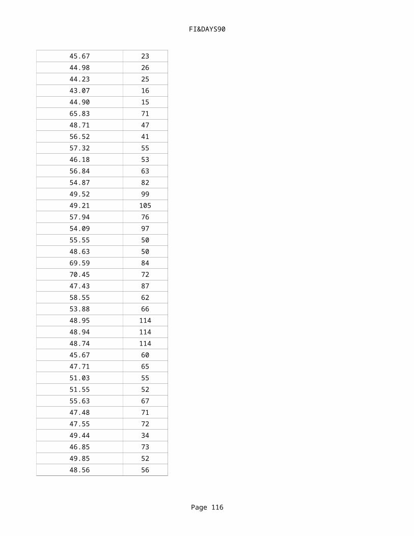
FI&DAYS90
Page 116
13.89 3754.93 6359.82 6746.83 4064.65 5647.39 5654.92 6451.05 5551.05 5752.60 5751.10 5843.82 6252.42 5853.41 7151.23 6545.94 5716.22 7371.33 048.40 148.01 02.97 1673.04 167
8.80 1137.36 95
33.03 6919.95 6026.51 2252.62 3368.72 212.48 8710.63 1059.99 106
11.23 1019.39 945.86 1596.57 149
12.83 58
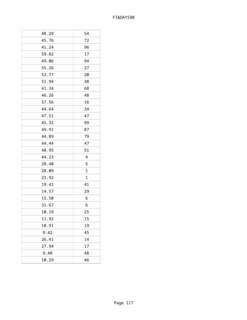
FI&DAYS90
Page 117
13.56 2015.56 717.74 6117.56 7018.08 6010.64 7010.88 7018.76 324.56 2215.83 1125.44 9049.60 3220.45 2927.05 7418.29 6916.61 2515.74 3015.54 2912.04 7812.04 7810.00 4522.54 014.14 3315.49 3314.83 1716.34 418.31 50
14.72 911.38 5611.47 4014.08 2746.01 944.75 849.55 148.92 445.67 2344.98 2644.23 25

FI&DAYS90
Page 118
43.07 1644.90 1565.83 7148.71 4756.52 4157.32 5546.18 5356.84 6354.87 8249.52 9949.21 10557.94 7654.09 9755.55 5048.63 5069.59 8470.45 7247.43 8758.55 6253.88 6648.95 11448.94 11448.74 11445.67 6047.71 6551.03 5551.55 5255.63 6747.48 7147.55 7249.44 3446.85 7349.85 5248.56 5648.29 5445.76 7241.24 9659.82 17

FI&DAYS90
Page 119
49.06 9455.26 2753.77 2051.94 3841.34 6846.26 4857.56 1644.64 3447.51 4745.32 9949.91 8744.89 7944.44 4748.95 5144.23 428.40 528.09 121.92 119.42 4114.57 2915.50 631.67 610.19 2511.92 1510.91 199.42 45
26.41 1427.94 179.48 48
10.29 46
39.39 2040.30 32
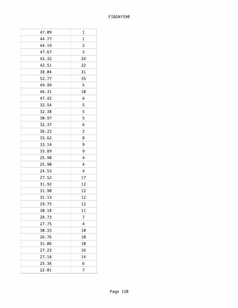
FI&DAYS90
Page 120
40.78 3041.83 3036.58 1542.42 3237.46 1637.46 1635.85 1438.11 1937.19 1835.93 1538.36 3130.19 1730.18 1745.72 2837.51 1237.01 1539.68 1137.87 941.43 1339.50 939.60 1041.42 1239.73 1445.96 3345.43 3447.60 3848.69 2336.82 1245.82 3437.08 1533.41 1432.30 1332.62 1235.53 3035.88 2632.46 1534.34 1132.32 11

FI&DAYS90
Page 121
32.10 1329.44 5030.22 5517.73 5122.70 6139.33 4641.07 2835.41 3731.04 4129.19 6235.22 3426.06 6439.92 3354.67 2848.10 4050.27 944.70 1445.18 1248.90 2845.49 3567.93 7156.16 8344.37 347.65 345.45 245.48 247.09 144.77 144.19 247.67 342.32 2442.51 2238.04 3152.77 3549.99 546.31 1047.42 632.54 5
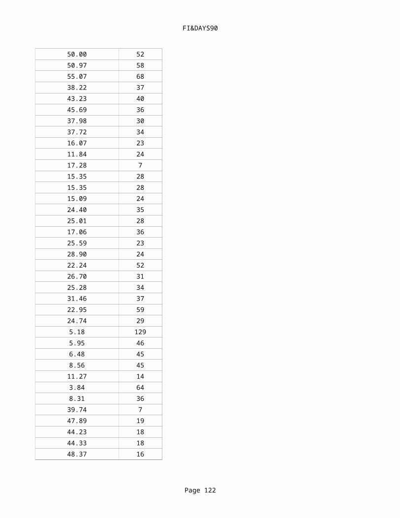
FI&DAYS90
Page 122
32.38 530.97 532.37 636.22 233.62 833.14 933.89 925.90 425.90 424.53 427.52 1731.92 1231.90 1231.13 1229.75 1230.18 1128.73 727.75 430.33 1026.76 1031.06 1027.23 1627.18 1425.36 622.01 727.45 1330.71 1027.74 831.42 933.33 928.70 1052.55 4965.16 5755.35 5763.55 3863.29 3658.88 5457.00 58

FI&DAYS90
Page 123
59.16 5457.71 5954.62 5861.47 5756.64 4956.24 4956.75 4267.88 3656.09 5361.81 6054.74 5554.84 5656.69 6755.33 6455.63 7747.17 4337.19 3737.59 3839.56 3839.54 4236.24 2536.22 2536.23 2536.22 2550.00 5250.97 5855.07 6838.22 3743.23 4045.69 3637.98 3037.72 3416.07 2311.84 2417.28 715.35 2815.35 2815.09 24

FI&DAYS90
Page 124
24.40 3525.01 2817.06 3625.59 2328.90 2422.24 5226.70 3125.28 3431.46 3722.95 5924.74 295.18 1295.95 466.48 458.56 45
11.27 143.84 648.31 36
39.74 747.89 1944.23 1844.33 1848.37 1644.87 1554.19 414.58 7212.55 3010.51 1716.79 7516.79 7516.38 3618.27 6511.07 615.83 219.46 58
36.99 143.62 438.69 5

FI&DAYS90
Page 125
42.57 243.87 046.25 541.27 648.57 3348.92 3045.18 3743.58 4744.42 3244.30 3045.88 2944.53 3043.96 4344.91 2949.46 851.58 653.88 1144.77 4156.06 044.43 3845.78 2348.56 4445.28 2045.11 2720.09 1419.35 819.05 915.71 1440.09 1144.62 1241.46 838.21 1139.36 1137.47 1238.57 534.65 2033.13 5942.92 71

FI&DAYS90
Page 126
33.60 8140.40 6331.72 9233.13 6946.67 6928.79 7631.62 7347.72 7141.93 5237.42 6466.36 6640.62 6842.20 6939.15 6948.38 1420.46 4344.40 943.98 1049.21 1045.25 1039.61 136.96 28
16.76 2216.86 2325.05 1740.28 1237.48 836.45 837.24 445.54 1247.32 1047.84 1338.91 141.79 140.66 1244.26 1543.41 344.87 1

FI&DAYS90
Page 127
40.14 1141.38 644.56 1443.95 1543.10 638.99 931.55 140.68 1645.33 549.35 4445.15 5543.45 4944.80 5544.71 4945.72 7459.91 2346.26 5452.84 3123.26 1415.75 5321.22 2721.09 2121.69 2017.74 3125.99 714.25 3623.74 2117.29 816.26 2421.58 1923.44 2854.06 1952.52 4352.50 4256.82 2153.50 4255.71 4242.53 14

FI&DAYS90
Page 128
53.89 3955.73 2754.33 2857.53 2153.36 3947.96 1744.07 8545.35 8525.49 12433.67 9129.58 10531.99 9244.20 6133.41 9926.49 11322.27 5922.25 5622.18 5554.22 7551.99 7445.74 7641.84 10239.33 11136.04 8036.77 9234.00 9418.03 6223.85 12210.39 9836.60 9436.59 9547.35 8841.24 1521.16 7537.52 10023.00 6138.01 9035.29 103

FI&DAYS90
Page 129
19.99 5822.83 8548.90 7645.26 7260.47 7758.07 6457.72 7123.89 11750.23 7859.15 8533.67 11025.80 11326.58 10315.90 9227.36 8533.83 8545.85 7939.47 8731.09 11619.83 7318.21 5017.08 5317.06 5646.23 8920.73 5233.14 9650.31 7248.58 7147.42 6919.22 5145.20 7534.02 8934.95 9333.89 8738.16 8937.98 9032.98 8518.75 78
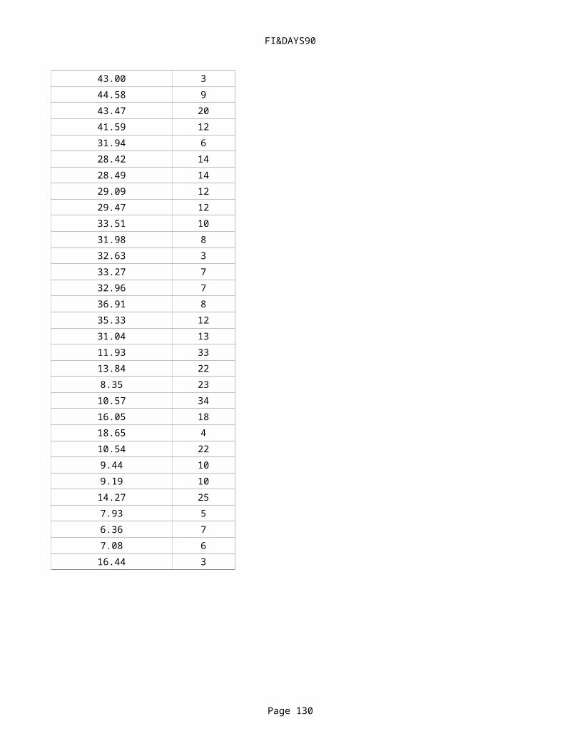
FI&DAYS90
Page 130
27.77 12043.40 7245.84 8922.63 7425.91 10137.26 8147.80 6912.47 518.73 33
22.41 409.26 14
13.45 1613.92 5717.50 448.67 75
10.22 439.45 309.90 436.31 28
41.07 139.54 139.76 130.57 451.78 2146.52 2144.27 2042.42 343.00 3542.42 3945.62 2844.70 4846.29 5344.49 845.38 643.96 3311.61 256.73 357.26 34

FI&DAYS90
Page 131
10.18 2941.29 884.16 1017.95 326.61 36
37.44 239.59 412.07 3347.94 216.59 1516.62 1435.85 019.70 2020.87 116.32 31
46.40 2343.00 344.58 943.47 2041.59 1231.94 628.42 1428.49 1429.09 1229.47 1233.51 1031.98 832.63 333.27 732.96 736.91 835.33 1231.04 1311.93 3313.84 228.35 23
10.57 3416.05 18

FI&DAYS90
Page 132
18.65 410.54 229.44 109.19 10
14.27 257.93 56.36 77.08 6
16.44 3
Related Documents