AAPM2012 MGuerrero Carlone - AMOS Onlineamos3.aapm.org/abstracts/pdf/68-19764-230349-86282.pdf · Marco Carlone, PhD Prince Margaret Hospital ... • LQ model matches other more sophisticated

7/28/12

1

Mechanistic Linear-Quadratic-Linear (LQL) Model for Large Doses Per Fraction

Mariana Guerrero, PhD Marco Carlone, PhD

Prince Margaret Hospital

Collaborator

X. Allen Li, Ph.D Associate Professor and Chief of Physics

Dept. of Radiation Oncology Medical College of Wisconsin

Background

•  Stereotactic Body Radiation Therapy (SBRT) is increasingly common for treatment of several tumor sites.

•  SBRT = single dose or small number of high dose fractions.

•  The question arises: How do we model large fraction doses? Is the Linear-Quadratic(LQ) model valid?

Is the Linear-Quadratic(LQ) model valid at large doses per fraction?

1.  ASTRO 2008: we don’t know. (Educational session, W. McBride, PhD, UCLA)

2.  Brenner (and others): Yes of course. (Seminars of Rad. Oncology, Oct 2008, etc).

3.  Other authors: no, not really. (several alternative models proposed,)

4.  Our answer: …coming soon

Answer: all over the place

7/28/12

2

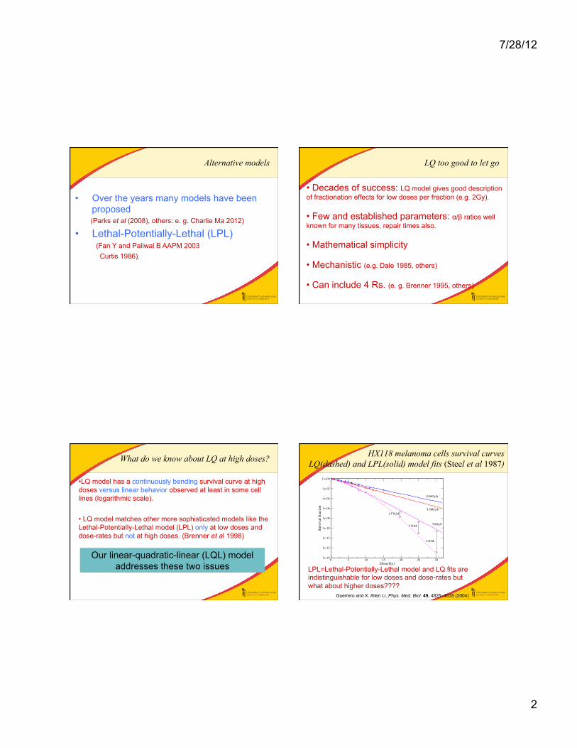
Alternative models

•  Over the years many models have been proposed

(Parks et al (2008), others: e. g. Charlie Ma 2012) •  Lethal-Potentially-Lethal (LPL)

(Fan Y and Paliwal B AAPM 2003 Curtis 1986).

LQ too good to let go

•  Decades of success: LQ model gives good description of fractionation effects for low doses per fraction (e.g. 2Gy).

•  Few and established parameters: α/β ratios well known for many tissues, repair times also.

•  Mathematical simplicity

•  Mechanistic (e.g. Dale 1985, others)

•  Can include 4 Rs. (e. g. Brenner 1995, others)

What do we know about LQ at high doses?

• LQ model has a continuously bending survival curve at high doses versus linear behavior observed at least in some cell lines (logarithmic scale).

•  LQ model matches other more sophisticated models like the Lethal-Potentially-Lethal model (LPL) only at low doses and dose-rates but not at high doses. (Brenner et al 1998)

Our linear-quadratic-linear (LQL) model addresses these two issues

HX118 melanoma cells survival curves LQ(dashed) and LPL(solid) model fits (Steel et al 1987)

LPL=Lethal-Potentially-Lethal model and LQ fits are indistinguishable for low doses and dose-rates but what about higher doses????

Extending the linear–quadratic model for large fraction doses pertinent to stereotactic radiotherapy 4827

0 5 10 15 20 25 30Dose(Gy)

1e-16

1e-14

1e-12

1e-10

1e-08

1e-06

1e-04

1e-02

1e+00

Surv

ival

frac

tion

0.96Gy/h

4.56Gy/h

90Gy/h

5 O.M.

3 O.M.

1.5 O.M.

Figure 1. Survival curves of the HX118 human melanoma cell line for three dose rates (data fromSteel et al (1987)). The LPL (solid lines) and LQ model (dashed lines) fit the data well but haveorder of magnitude (OM) differences in the predictions at high doses.

0 10 20 30Dose(Gy)

1e-10

1e-08

1e-06

1e-04

1e-02

1e+00

Surv

ival

frac

tion

0.01Gy/h0.1Gy/h1Gy/h10Gy/h100Gy/h1000Gy/h

LPL and LQ (calculated parameters)

0 10 20 30Dose(Gy)

LPL and LQM

(a) (b)

Figure 2. Comparison survival curves of (a) the LPL (symbols) and LQ (solid line) and (b) theLPL and MLQ with calculated parameters (solid line) for a wide range of dose rates. The MLQreproduces the LPL even at high acute doses, where the LQ predicts more cell kill.

!L = 0.32 Gy!1, !PL = 0.98 Gy!1, " = 6.8, T1/2 = 0.16 h for the LPL and # = 0.33 Gy!1,$ = 0.038 Gy!2, T1/2 = 0.23 h for the LQ). It is clear from this figure that both modelsdescribe the data points very well, however when extrapolating to doses of 20, 25 and 30 Gyfor high dose rate (90 Gy h!1), they yield differences of several orders of magnitude (OM) inthe survival fractions of acute exposures.

In figure 2(a) the LPL curves (with the parameters of the HX118 cells, same as figure 1)are plotted together with the LQ curves for a wide range of dose rates with parameters

Guerrero and X. Allen Li, Phys. Med. Biol. 49, 4825–4835 (2004)

7/28/12

3

Can the LQ model match the LPL at high doses?

•  LQ Survival curve:

G(µT) is the Lea-Catcheside factor èincreased survival due to repair, dose rate effect (µ=repair rate, T= treatment time)

G(x) = 2x2

x −1+ e−x( )0 <G(x)<1

SLQ=exp(-αD-βD2G(µT))

Can the LQ model match the LPL at high doses?

•  LQL Survival curve:

•  Acute dose: µT<<1 G=1 for LQ but for LQL G(δD) remains for acute doses:

SLQL=exp(-αD-βD2G(δD))

•  Introduces a new parameter δ [Gy-1].

SLQL=exp(-αD-βD2G(µT+δD))

LQL matches LPL survival for ALL doses and dose-rates


0 5 10 15 20 25 30Dose(Gy)

1e-16

1e-14

1e-12

1e-10

1e-08

1e-06

1e-04

1e-02

1e+00

Surv

ival

frac

tion

0.96Gy/h

4.56Gy/h

90Gy/h

5 O.M.

3 O.M.

1.5 O.M.

Figure 1. Survival curves of the HX118 human melanoma cell line for three dose rates (data fromSteel et al (1987)). The LPL (solid lines) and LQ model (dashed lines) fit the data well but haveorder of magnitude (OM) differences in the predictions at high doses.

0 10 20 30Dose(Gy)

1e-10

1e-08

1e-06

1e-04

1e-02

1e+00

Surv

ival

frac

tion

0.01Gy/h0.1Gy/h1Gy/h10Gy/h100Gy/h1000Gy/h

LPL and LQ (calculated parameters)

0 10 20 30Dose(Gy)

LPL and LQM

(a) (b)

Figure 2. Comparison survival curves of (a) the LPL (symbols) and LQ (solid line) and (b) theLPL and MLQ with calculated parameters (solid line) for a wide range of dose rates. The MLQreproduces the LPL even at high acute doses, where the LQ predicts more cell kill.

!L = 0.32 Gy!1, !PL = 0.98 Gy!1, " = 6.8, T1/2 = 0.16 h for the LPL and # = 0.33 Gy!1,$ = 0.038 Gy!2, T1/2 = 0.23 h for the LQ). It is clear from this figure that both modelsdescribe the data points very well, however when extrapolating to doses of 20, 25 and 30 Gyfor high dose rate (90 Gy h!1), they yield differences of several orders of magnitude (OM) inthe survival fractions of acute exposures.

In figure 2(a) the LPL curves (with the parameters of the HX118 cells, same as figure 1)are plotted together with the LQ curves for a wide range of dose rates with parameters

LPL(points) and LQ(solid) LPL(points) and LQL(solid)

The new term G(δD) with δ adjusted to match final slope, makes the LQL equivalent to LPL with advantage of familiarity and knowledge of parameters α and β. Guerrero and X. Allen Li, Phys. Med. Biol. 49, 4825–4835 (2004)

Compartmental LQL formulation (Carlone et al) (based on Dale’s 1985 LQ formulation)

LS= sub-lethal lesions LF=fatal lesions R(t)=dose-rate p=yield of LS per unit dose ε=probability of interaction

2pR(t) è LS ì

î €

dLSdt

= 2pR − µLS

€

−pRεLS

pR(t)εLS è INTERACTION

-µLS è REPAIR

í αR(t) è LF

€

dLFdt

= αR + pRεLS

M. Carlone, D. Wilkins, and P. Raaphorst Phys. Med. Biol. 50, L9–L15 (2005)

7/28/12

4

Linear-Quadratic-Linear(LQL) solution

•  New factor in solution for acute doses

S=exp(-αD-βD2G(δD)) δ=pε p=yield of LS per unit dose ε=probability of interaction

•  Interpretation of G(δD): reduction in survival due to interaction between lesions.

•  For large doses S~exp(-(α+β/2δ)D) (linear behavior).

•  LQL agrees with LPL model at all doses and dose-rates .

•  Recovers LQ at low doses and low dose-rates.

•  Mechanistic formulation

Linear-Quadratic-Linear(LQL) solution

•  For large doses S~exp(-(α+β/2δ)D) (linear behavior).

•  LQL agrees with LPL model at all doses and dose-rates

•  Mechanistic formulation

Test the models at high dose? Isoeffect equations using BED

D= total dose BED= biologically effective dose d=dose per fraction =D(1+d/(α/β)) n=number of fractions

LQ: LQL: Fe-plots: for a certain isoeffect plot 1/D vs d LQ predicts linear behavior

€

1D

=1

BED+

1BED⋅ (α /β)

d

€

1D

=1

BED+

1BED⋅ (α /β)

d⋅ G(δd)

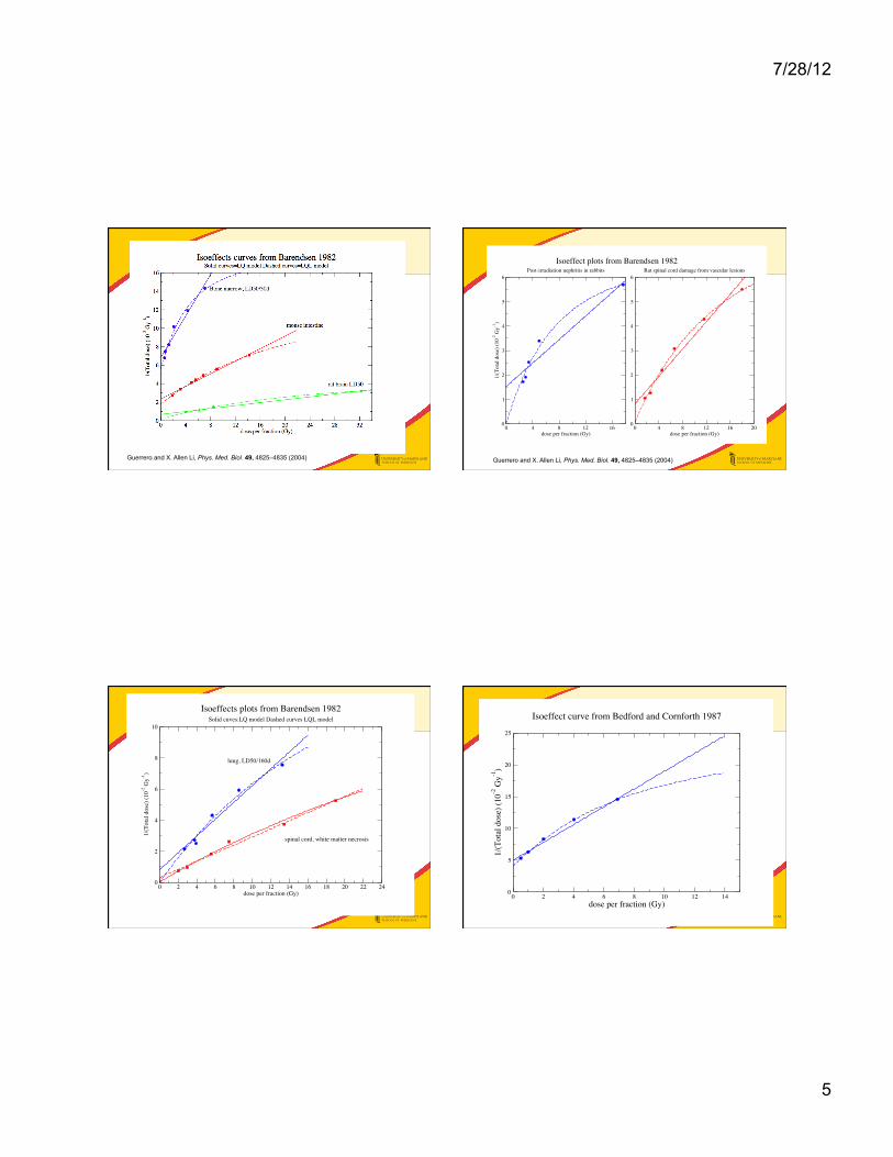
LQ vs LQL Test: Re-analyze isoeffect data

Barendsen 1982, Red Journal

“Dose fractionation, dose rate and iso-effect relationships for normal tissue responses”

Seminal work for LQ model

cited over 500 times

Fit of isoeffect curves from animal experiments with LQ formula

7/28/12

5


0 4 8 12 16dose per fraction (Gy)

0

1

2

3

4

5

6

1/(T

otal

dos

e) (1

0-2 G

y-1)

Isoeffect plots from Barendsen 1982Post-irradiation nephritis in rabbits

0 4 8 12 16 20dose per fraction (Gy)

0

1

2

3

4

5

6Rat spinal cord damage from vascular lesions


0 2 4 6 8 10 12 14 16 18 20 22 24dose per fraction (Gy)

0

2

4

6

8

10

1/(T

otal

dos

e) (1

0-2 G

y-1)

Isoeffects plots from Barendsen 1982Solid cuves:LQ model Dashed curves LQL model

lung, LD50/160d

spinal cord, white matter necrosis

0 2 4 6 8 10 12 14dose per fraction (Gy)

0

5

10

15

20

25

1/(T

otal

dos

e) (1

0-2 G

y-1)

Isoeffect curve from Bedford and Cornforth 1987

7/28/12

6

13 Isoeffect plots analysis LQ vs. LQL fits with χ2/n value


0 4 8 12 16dose per fraction (Gy)

0

1

2

3

4

5

6

7

8

9

10

1/(T

otal

dos

e) (1

0-2 G

y-1)

Post-irradiation nephritis in rabbits

0 4 8 12 16 20dose per fraction (Gy)

0

1

2

3

4

5

6Rat spinal cord damage from vascular lesions

(a) (b)

Figure 4. Fe-plots for two different end-points from Barendsen (1982) and references therein.Solid line: LQ fit. Dashed line: MLQ fit.

Table 3. LQ and MLQ model parameters for the iso-effect experiments.

LQ MLQ

Experiment !/" (Gy) #2/n !/" (Gy) $ (Gy!1) #2/n

Bone marrow LD50/30 days" 6.1 0.435 2.23 0.39 0.16Mouse jejunum crypt death" 6.9 0.034 3.25 0.09 0.0075Mouse foot skin desquamation 10.0 0.0047 9.90 <0.04 0.0052Rat brain LD50/1 year" 8.6 0.023 0.89 0.08 0.01Mouse kidney histopathologic changes 0.73 0.095 – 0.049 0.08Rabbit post-irradiation nephritis" 6.4 0.26 – 0.25 0.082Rat spinal cord (vascular lesions)" 3.0 0.094 0.14 0.13 0.01Rat spinal cord (radiculopathy) 4.5 0.019 3.86 0.01 0.02Mouse lung LD50" 1.5 0.2 – 0.096 0.13Mouse spinal cord white matter necrosis" 1.2 0.041 0.11 0.045 0.035Mouse skin contraction 5.1 0.007 4.34 <0.04 0.009Mouse spinal cord myelopathy 4.9 0.010 5.0 <0.04 0.013In vitro AG1522 cells in plateau phase" 3.6 0.29 1.7 0.23 0.0029

(1984) and de Boer (1988) have proposed better ways to estimate the !/" ratio but thesemethods cannot be easily extended for the MLQ.

The negative values of the intercept are not a shortcoming of the MLQ. For example infigures 4(a) and (b), it is clear that the LQ gives a positive value for the intercept becauseit averages out the slope for low doses per fraction with that for higher doses per fraction.However, it is evident from the figures that using a single slope is a very poor approximation.For the same reason, the MLQ !/" ratios are in general lower than the LQ !/" ratios. If onlythe low dose per fraction points were fitted with the LQ, a smaller or negative intercept wouldalso be obtained. The !/" ratios obtained by the MLQ are essentially given by the initialslope of the curves, while the LQ !/" ratios are given by the ‘average’ slope.

In the cases of mouse foot skin desquamation, mouse kidney histopathologic changes,radiculopathy of the mouse spinal cord, mouse skin contraction and myelopathy of the mousespinal cord, the MLQ and the LQ give essentially the same fit (the value of #2/n is slightlylarger for the MLQ due to the larger number of parameters). In such cases the MLQ yields a

LQ LQL


Isoeffects summary

•  Of 13 isoeffects curves studied, the LQL significantly improved the quality of the curve fit in 8 of them.

•  Values of δ ranged from 0.04 to 0.4 Gy-1

•  Dose values were the LQ loses accuracy ~ δ-1= 2.5Gy to 22Gy or larger.

Is the Linear-Quadratic(LQ) model valid at large doses per fraction?

•  Our answer: Only sometimes: depending on the end point, tissue type and the dose level the LQ model may or may not be sufficient.

Answer: all over the place

δ can be estimated from known parameters α, β and the final slope D0


Table 1. Summary of LQ and MLQ model parameters for seven tumour cell lines from Steel et al(1987).

LPL MLQ

Cell line !L (Gy!1) !PL (Gy!1) " T1/2 (h) # (Gy!1) $ (Gy!2) % (Gy!1) D" (Gy)

HX34 0.27 1.81 27 0.11 0.27 0.061 0.11 9.91HX118 0.32 0.98 6.8 0.16 0.32 0.070 0.22 4.6HX58 0.45 3.12 88 0.82 0.45 0.055 0.050 18.8HX156 0.30 2.82 156 0.54 0.30 0.026 0.027 37.7RT112 0.10 1.65 40 0.86 0.10 0.034 0.062 16.16GCT127 0.45 2.04 46 0.31 0.45 0.045 0.067 15.03HX142 0.11 1.74 1.54 0.54 0.11 0.98 1.69 0.6

For example, in the case of HX118 cells, % = 0.22 Gy!1. In this way, the four parametersof the LPL ( !L, !PL, & and ') can be mapped to the four parameters of the MLQ (#,$, %

and ') and vice versa. The survival curves of the MLQ are plotted together with the LPL infigure 2(b) for a wide range of dose rates. It is clear that the MLQ curves agree well with theLPL data for all dose rates even at the highest doses considered, while it maintains the gooddescription for low doses and dose rates similar to the standard LQ. Even though the MLQhas the same number of parameters as the LPL, it is a simpler model that does not involvedifferential equations and it is a simple extension of the LQ with the G factor.

Table 1 lists the LPL parameters from Steel et al (1987) as well as the calculated MLQparameters for seven tumour cell lines (the repair half-time is the same for both models).Except for the case of HX142 cell line, which is unusual in its large value of $, all cell lineshave % values between 0.027 and 0.22 Gy!1. (To recover the LQ model one needs % = 0).

3.2. MLQ parameter % calculated from D0,# and $

The value of % can also be calculated from # and $ and the final slope of the survival curveD0 with the formula

% = 2$D0

1 ! #D0. (3)

Table 2 reports values of % calculated using equation (3) for seven cell lines compiled byBarendsen (1982) and for the average values of #,$, and D0 for different histology. In thisway, the new parameter of the MLQ can be related to well-known parameters. The values of% obtained are pretty similar and consistent with the values from table 1 for most cell linesexcept for the oat cell carcinoma lines.

3.3. MLQ parameter % fitted from iso-effect data

Re-analysed iso-effect data from Barendsen (1982) and Bedford and Cornforth (1987) arepresented in figures 3–6. The fitted parameters are listed in table 3. Only the cases thatare better described with the MLQ are plotted (and marked with an " symbol in table 3). Infigure 3, Fe-plots for bone marrow LD50/30 days, reduction of crypt stem cells in mousejejunum and death of rat as a result of brain irradiation are presented. In figure 4 data forpost-irradiation nephritis in rabbits and rat spinal cord vascular damage are presented. Infigure 5 the tolerance dose for mice lung irradiation and rat spinal cord white matter necrosisare plotted. In figure 6 in vitro AG1522 cells iso-effect plots are presented. In all these datasets there is a systematic trend of the curves to bend downwards. The MLQ gives a better

4830 M Guerrero and X A Li

0 4 8 12 16 20 24 28 32dose per fraction (Gy)

0

2

4

6

8

10

12

14

16

1/(T

otal

dos

e) (1

0-2 G

y-1)

Bone marrow, LD50/30d

mouse intestine

rat brain LD50

Figure 3. Fe-plots for three different end-points from Barendsen (1982) and references therein.Solid line: LQ fit. Dashed line: MLQ fit.

Table 2. ! values obtained from ", # and D0 (Barendsen 1982, Malaise et al 1986).

Cell line " (Gy!1) # (Gy!2) D0 (Gy) ! (Gy!1) D" (Gy)

T-1 0.18 0.050 1.1 0.137 7.3R-1 0.18 0.037 1.3 0.126 7.9RUC-1 0.12 0.023 1.5 0.084 11.9RUC-2 0.08 0.010 2.2 0.053 18.7ROS-1 0.18 0.036 1.6 0.162 6.2RMS-1 0.22 0.054 1.1 0.157 6.4MLS-1 0.36 0.025 1.2 0.106 9.4

Gioblastomas (5) 0.241 0.029 1.44 0.128 7.8Melanomas (19) 0.255 0.053 1.04 0.150 6.7Squamous cell carcinomas (6) 0.273 0.045 1.28 0.177 5.6Adenocarcinomas (6) 0.311 0.055 1.04 0.169 5.9Lymphomas (7) 0.451 0.051 1.48 0.452 2.2Oat cell carcinomas (6) 0.650 0.081 1.51 13.2 0.076

description of all these experiments, in some cases overwhelmingly: for mouse intestine infigure 3, the per cent root-mean-square error (RMS) goes from 4% for the LQ model to 0.3%for the MLQ; for the rat spinal cord vascular lesions in figure 4(b), the RMS is 14% for theLQ versus 6% for the MLQ; in figure 6, the in vitro AG1522 cells have a RMS of 5% for theLQ versus 0.5% for the MLQ.

In some cases, (e.g. figures 4(a) and 5) the MLQ gives a negative value for the interceptand it was therefore fitted by forcing the parameters to be positive. In these cases a verylow value of the intercept is obtained, which provides a poor estimate of the "/# ratio andwe therefore do not list it in table 3. In general, Fe-plots do not provide good estimates ofthe parameters, but they are simple and useful to compare the LQ and LQM models. Tucker

Barendsen 1982, Malaise et al 1986

7/28/12

7

δ can be estimated from known parameters Extending the linear–quadratic model for large fraction doses pertinent to stereotactic radiotherapy 4829

Table 1. Summary of LQ and MLQ model parameters for seven tumour cell lines from Steel et al(1987).

LPL MLQ

Cell line !L (Gy!1) !PL (Gy!1) " T1/2 (h) # (Gy!1) $ (Gy!2) % (Gy!1) D" (Gy)

HX34 0.27 1.81 27 0.11 0.27 0.061 0.11 9.91HX118 0.32 0.98 6.8 0.16 0.32 0.070 0.22 4.6HX58 0.45 3.12 88 0.82 0.45 0.055 0.050 18.8HX156 0.30 2.82 156 0.54 0.30 0.026 0.027 37.7RT112 0.10 1.65 40 0.86 0.10 0.034 0.062 16.16GCT127 0.45 2.04 46 0.31 0.45 0.045 0.067 15.03HX142 0.11 1.74 1.54 0.54 0.11 0.98 1.69 0.6

For example, in the case of HX118 cells, % = 0.22 Gy!1. In this way, the four parametersof the LPL ( !L, !PL, & and ') can be mapped to the four parameters of the MLQ (#,$, %

and ') and vice versa. The survival curves of the MLQ are plotted together with the LPL infigure 2(b) for a wide range of dose rates. It is clear that the MLQ curves agree well with theLPL data for all dose rates even at the highest doses considered, while it maintains the gooddescription for low doses and dose rates similar to the standard LQ. Even though the MLQhas the same number of parameters as the LPL, it is a simpler model that does not involvedifferential equations and it is a simple extension of the LQ with the G factor.

Table 1 lists the LPL parameters from Steel et al (1987) as well as the calculated MLQparameters for seven tumour cell lines (the repair half-time is the same for both models).Except for the case of HX142 cell line, which is unusual in its large value of $, all cell lineshave % values between 0.027 and 0.22 Gy!1. (To recover the LQ model one needs % = 0).

3.2. MLQ parameter % calculated from D0,# and $

The value of % can also be calculated from # and $ and the final slope of the survival curveD0 with the formula

% = 2$D0

1 ! #D0. (3)

Table 2 reports values of % calculated using equation (3) for seven cell lines compiled byBarendsen (1982) and for the average values of #,$, and D0 for different histology. In thisway, the new parameter of the MLQ can be related to well-known parameters. The values of% obtained are pretty similar and consistent with the values from table 1 for most cell linesexcept for the oat cell carcinoma lines.

3.3. MLQ parameter % fitted from iso-effect data

Re-analysed iso-effect data from Barendsen (1982) and Bedford and Cornforth (1987) arepresented in figures 3–6. The fitted parameters are listed in table 3. Only the cases thatare better described with the MLQ are plotted (and marked with an " symbol in table 3). Infigure 3, Fe-plots for bone marrow LD50/30 days, reduction of crypt stem cells in mousejejunum and death of rat as a result of brain irradiation are presented. In figure 4 data forpost-irradiation nephritis in rabbits and rat spinal cord vascular damage are presented. Infigure 5 the tolerance dose for mice lung irradiation and rat spinal cord white matter necrosisare plotted. In figure 6 in vitro AG1522 cells iso-effect plots are presented. In all these datasets there is a systematic trend of the curves to bend downwards. The MLQ gives a better

LPL LQL

Average value for δ≈0.1Gy-1

Clinical application: SBRT fractionation Interplay of parameters

LQL Survival Curve: reduction in survival more pronounced for smaller α/β ratio

Prostate and lung SBRT and Hypofractionation

Prostate hypofractionation (review by Ritter et al)

-Moderate fractionation (d=2-4.3Gy) -Extreme hypofractionation(d=6.7-10.5Gy) -α/β=1.5, 3Gy or 10Gy.

Lung SBRT (review by Silva et al) -α/β=10Gy for lung -α/β=3Gy for normal tissue

Important quantities

Biologically effective dose (BED) for fractionated treatments: d=dose per fraction D=total Dose Equivalent dose in 2 Gy fractions EQD2

7/28/12

8

Prostate Cancer Equivalent Dose at 2Gy/fr Extreme hypofractionation

α/β=1.5Gy δ=0.1Gy-1

Lung cancer BED

δ=0.1Gy-1

Mechanistic formulation allows other dose-rates Ex: Split dose- recovery ratio RR

•  Two fractions of size d separated by an interval of time T.

•  Experiments look at recovery ratio RR=S(T)/S(T=0) as T goes to infinity.

  è

•  LQL predicts reduced recovery ratio.

€

RRLQ = e2βd2

€

RRLQL = e2βF (δd )d2

€

F(x) =(1− e−x )2

x 2

+

δ=0.03Gy-1

δ=0.22Gy-1

Guerrero and Carlone, Med. Phys. 37, 4173-81 (2010)

7/28/12

9

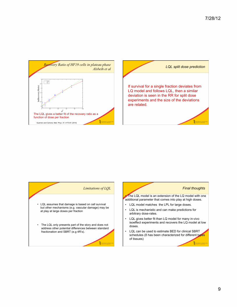
Recovery Ratio of HF19 cells in plateau phase Alsbeih et al

0 20 40 60 80 100

d2

0

0.5

1

1.5

2

2.5

3

ln(R

ecov

ery

Rat

io)

LQLLQ

The LQL gives a better fit of the recovery ratio as a function of dose per fraction

Guerrero and Carlone, Med. Phys. 37, 4173-81 (2010)

LQL split dose prediction

If survival for a single fraction deviates from LQ model and follows LQL, then a similar deviation is seen in the RR for split dose experiments and the size of the deviations are related.

Limitations of LQL

•  LQL assumes that damage is based on cell survival but other mechanisms (e.g. vascular damage) may be at play at large doses per fraction •  The LQL only presents part of the story and does not address other potential differences between standard fractionation and SBRT (e.g 4R’s).

Final thoughts

•  The LQL model is an extension of the LQ model with one additional parameter that comes into play at high doses.

•  LQL model matches the LPL for large doses.

•  LQL is mechanistic and can make predictions for arbitrary dose-rates.

•  LQL gives better fit than LQ model for many in-vivo isoeffect experiments and recovers the LQ model at low doses.

•  LQL can be used to estimate BED for clinical SBRT schedules (δ has been characterized for different types of tissues)

7/28/12

10

Thank you!

?

References

-Guerrero and Carlone, Med. Phys. 37, 4173-81 (2010) -Guerrero and X. Allen Li, Phys. Med. Biol. 49, 4825–4835 (2004). -M. Carlone, D. Wilkins, and P. Raaphorst Phys. Med. Biol. 50, L9–L15 (2005). -M. Guerrero and X. A. Li, Phys. Med. Biol. 50, L13–L15 (2005). -W. Barendsen, Int. J. Radiat. Oncol. Biol. Phys. 8,1981–1997 (1982). -R. G. Dale, Br. J. Radiol. 58, 515–528 (1985). -D. E. Lea, Actions of Radiations on Living Cells (Cambridge University Press, Cambridge, 1946). -R. K. Sachs, P. Hahnfeld, and D. J. Brenner, Int. J. Radiat. Biol. 72, 351–374 (1997). -S. B. Curtis,Radiat. Res. 106, 252–270 (1986); Erratum in: Radiat Res 119(3):584 (1989). -G. G. Steel, Radiother. Oncol. 9, 299–310 (1987). -R. G. Dale, Br. J. Radiol. 62, 241–244 (1989). -M. G. Alsbeih, B. Fertil, C. Badie, and E. P. Malaise, Int. J. Radiat. Biol. 67, 453–460 (1995).

AAPM2012 MGuerrero Carlone - AMOS Onlineamos3.aapm.org/abstracts/pdf/68-19764-230349-86282.pdf · Marco Carlone, PhD Prince Margaret Hospital ... • LQ model matches other more sophisticated

Documents