A&A 443, 451–463 (2005) DOI: 10.1051/0004-6361:20041903 c ESO 2005 Astronomy & Astrophysics AGN variability time scales and the discrete-event model P. Favre 1,2 , T. J.-L. Courvoisier 1,2 , and S. Paltani 1,3 1 INTEGRAL Science Data Center, 16 Ch. d’Ecogia, 1290 Versoix, Switzerland e-mail: [email protected] 2 Geneva Observatory, 51 Ch. des Maillettes, 1290 Sauverny, Switzerland 3 Laboratoire d’Astrophysique de Marseille, Traverse du Siphon, BP 8, 13376 Marseille Cedex 12, France Received 25 August 2004 / Accepted 3 August 2005 ABSTRACT We analyse the ultraviolet variability time scales in a sample of 15 type 1 Active Galactic Nuclei (AGN) observed by IUE. Using a structure function analysis, we demonstrate the existence in most objects of a maximum variability time scale of the order of 0.02–1.00 year. We do not find any significant dependence of these maximum variability time scales on the wavelength, but we observe a weak correlation with the average luminosity of the objects. We also observe in several objects the existence of long-term variability, which seems decoupled from the short-term one. We interpret the existence of a maximum variability time scale as a possible evidence that the light curves of type 1 AGN are the result of the superimposition of independent events. In the framework of the so-called discrete-event model, we study the event energy and event rate as a function of the object properties. We confront our results to predictions from existing models based on discrete events. We show that models based on a fixed event energy, like supernova explosions, can be ruled out. In their present form, models based on magnetic blobs are also unable to account for the observed relations. Stellar collision models, while not completely satisfactory, cannot be excluded. Key words. galaxies: active – galaxies: Seyfert – quasars: general – ultraviolet: galaxies 1. Introduction The UV excess of the spectral energy distribution of type 1 Active Galactic Nuclei (AGN), the blue bump, reflects the fact that a very large fraction of the energy is released in the wavelength domain ∼300 to 5600 Å (see e.g. Krolik 1999, Fig. 7.10). Conventional accretion disk models are able to ac- count satisfactorily for the rough shape of the blue bump (but see Koratkar & Blaes 1999), but they fail to explain the vari- ability properties (Courvoisier & Clavel 1991), a key to the un- derstanding of the AGN phenomenon. This difficulty led several authors (Cid Fernandes et al. 1996; Paltani & Courvoisier 1997 (hereafter PC97); Aretxaga et al. 1997; Cid Fernandes et al. 2000 (hereafter CSV00); see also Aretxaga & Terlevich 1994) to consider a more phe- nomenological approach based on the discrete-event model, which provides a simple explanation for the variability: The variability is the result of a superimposition of independent events occurring at random epochs at a given rate. The mo- tivations for the discrete-event model are twofold: Temporal analysis allows to constrain the event properties, while its generality leaves room for a large variety of physical events. It can be a reasonable approximation for models like star- burst (Aretxaga & Terlevich 1994; Aretxaga et al. 1997), stellar Appendix A is only available in electronic form at http://www.edpsciences.org collisions (Courvoisier et al. 1996; Torricelli-Ciamponi et al. 2000), or magnetic blobs above an accretion disk (Haardt et al. 1994). In this paper, we use data from the International Ultraviolet Explorer (IUE) covering about 17 years to determine the UV characteristic time scales in a sample of Seyfert 1 galaxies and QSOs, using a methodology similar to that used in Collier & Peterson (2001, hereafter CP01). While CP01 concentrated on the measure of time scales shorter than 100 days by selecting short portions of the light curves in which the time sampling was denser, we use here the full available light curves (on aver- age 16.5 years), highlighting a wider range of time scales, and extend the sample to 15 objects. Furthermore, using 12 wave- length windows between 1300 and 3000 Å, we investigate for the first time the existence of a wavelength dependence of the variability time scale. We interpret the variability properties of our objects in terms of discrete-event model, and we study their parameters as a function of the object properties. Our approach is similar to that of CSV00, although we use data from IUE gathered dur- ing almost 17 years, while they use optical data covering about seven years. Furthermore, the sample of CSV00 is composed of PG quasars (median z: 0.16) while ours is mainly composed of Seyfert 1 galaxies at a much smaller redshift (median z: 0.033). Their observations thus not only cover about three times less time than ours, but the observation durations are Article published by EDP Sciences and available at http://www.edpsciences.org/aa or http://dx.doi.org/10.1051/0004-6361:20041903

Welcome message from author
This document is posted to help you gain knowledge. Please leave a comment to let me know what you think about it! Share it to your friends and learn new things together.
Transcript

A&A 443, 451–463 (2005)DOI: 10.1051/0004-6361:20041903c© ESO 2005
Astronomy&
Astrophysics
AGN variability time scales and the discrete-event model�
P. Favre1,2, T. J.-L. Courvoisier1,2, and S. Paltani1,3
1 INTEGRAL Science Data Center, 16 Ch. d’Ecogia, 1290 Versoix, Switzerlande-mail: [email protected]
2 Geneva Observatory, 51 Ch. des Maillettes, 1290 Sauverny, Switzerland3 Laboratoire d’Astrophysique de Marseille, Traverse du Siphon, BP 8, 13376 Marseille Cedex 12, France
Received 25 August 2004 / Accepted 3 August 2005
ABSTRACT
We analyse the ultraviolet variability time scales in a sample of 15 type 1 Active Galactic Nuclei (AGN) observed by IUE. Using a structurefunction analysis, we demonstrate the existence in most objects of a maximum variability time scale of the order of 0.02–1.00 year. We donot find any significant dependence of these maximum variability time scales on the wavelength, but we observe a weak correlation with theaverage luminosity of the objects. We also observe in several objects the existence of long-term variability, which seems decoupled from theshort-term one. We interpret the existence of a maximum variability time scale as a possible evidence that the light curves of type 1 AGN arethe result of the superimposition of independent events. In the framework of the so-called discrete-event model, we study the event energy andevent rate as a function of the object properties. We confront our results to predictions from existing models based on discrete events. We showthat models based on a fixed event energy, like supernova explosions, can be ruled out. In their present form, models based on magnetic blobsare also unable to account for the observed relations. Stellar collision models, while not completely satisfactory, cannot be excluded.
Key words. galaxies: active – galaxies: Seyfert – quasars: general – ultraviolet: galaxies
1. Introduction
The UV excess of the spectral energy distribution of type 1Active Galactic Nuclei (AGN), the blue bump, reflects thefact that a very large fraction of the energy is released in thewavelength domain ∼300 to 5600 Å (see e.g. Krolik 1999,Fig. 7.10). Conventional accretion disk models are able to ac-count satisfactorily for the rough shape of the blue bump (butsee Koratkar & Blaes 1999), but they fail to explain the vari-ability properties (Courvoisier & Clavel 1991), a key to the un-derstanding of the AGN phenomenon.
This difficulty led several authors (Cid Fernandes et al.1996; Paltani & Courvoisier 1997 (hereafter PC97); Aretxagaet al. 1997; Cid Fernandes et al. 2000 (hereafter CSV00);see also Aretxaga & Terlevich 1994) to consider a more phe-nomenological approach based on the discrete-event model,which provides a simple explanation for the variability: Thevariability is the result of a superimposition of independentevents occurring at random epochs at a given rate. The mo-tivations for the discrete-event model are twofold: Temporalanalysis allows to constrain the event properties, while itsgenerality leaves room for a large variety of physical events.It can be a reasonable approximation for models like star-burst (Aretxaga & Terlevich 1994; Aretxaga et al. 1997), stellar
� Appendix A is only available in electronic form athttp://www.edpsciences.org
collisions (Courvoisier et al. 1996; Torricelli-Ciamponi et al.2000), or magnetic blobs above an accretion disk (Haardt et al.1994).
In this paper, we use data from the International UltravioletExplorer (IUE) covering about 17 years to determine the UVcharacteristic time scales in a sample of Seyfert 1 galaxies andQSOs, using a methodology similar to that used in Collier &Peterson (2001, hereafter CP01). While CP01 concentrated onthe measure of time scales shorter than 100 days by selectingshort portions of the light curves in which the time samplingwas denser, we use here the full available light curves (on aver-age 16.5 years), highlighting a wider range of time scales, andextend the sample to 15 objects. Furthermore, using 12 wave-length windows between 1300 and 3000 Å, we investigate forthe first time the existence of a wavelength dependence of thevariability time scale.
We interpret the variability properties of our objects interms of discrete-event model, and we study their parametersas a function of the object properties. Our approach is similarto that of CSV00, although we use data from IUE gathered dur-ing almost 17 years, while they use optical data covering aboutseven years. Furthermore, the sample of CSV00 is composedof PG quasars (median z: 0.16) while ours is mainly composedof Seyfert 1 galaxies at a much smaller redshift (median z:0.033). Their observations thus not only cover about threetimes less time than ours, but the observation durations are
Article published by EDP Sciences and available at http://www.edpsciences.org/aa or http://dx.doi.org/10.1051/0004-6361:20041903

452 P. Favre et al.: AGN variability time scales and the discrete-event model
further diminished in the observer’s frame. Finally, as variabil-ity increases towards shorter wavelengths (Kinney et al. 1991;Paltani & Courvoisier 1994; di Clemente et al. 1996; Trèvese& Vagnetti 2002), the study of the variability is more efficientin the UV than in the optical.
2. The concept of discrete-event model
The formalism of the discrete-event model was mainly devel-oped in Cid Fernandes et al. (1996), PC97, Aretxaga et al.(1997), and CSV00. In the discrete-event model, the variabilityis due to the superimposition of independent events, occurringat random epochs, on top of a possible constant source. In thesimplest form that we use here, all events are identical.
The total luminosity density at wavelength λ can be ex-pressed as:
Lλ(t) =∑
i
eλ(t − ti) + Cλ , (1)
where eλ(t − ti) is the light curve of event i, initiated at ti, andCλ reflects the possible contribution of a steady component.The distribution of ti is assumed to be Poissonian. Using N forthe event rate and Eλ =
∫eλ(t − ti)dt for the energy density
released by the ith event, the average luminosity reads:
Lλ = NEλ + Cλ . (2)
Parameterizing the event using its duration 2µλ and its ampli-tude at maximum Hλ, we have:
Lλ = NkLHλ2µλ +Cλ , (3)
where kL is a constant depending on the event shape. The vari-ance of Lλ(t) was calculated by PC97 (see their Eq. (A5)),which reduces to Var(Lλ) ∝ N. Including Hλ and 2µλ inEq. (B2) of their paper, we find:
Var(Lλ) = NkVH2λ2µλ , (4)
where kV is a constant depending on the event shape. FromEqs. (3) and (4), the event amplitude at wavelength λ reads:
Hλ =kL
kV
Var(Lλ)
Lλ −Cλ· (5)
In Sect. 4, we describe a method to estimate 2µλ. As alreadynoted by CSV00, our system will not be closed, as only threeparameters can be measured: (Lλ, Var(Lλ), 2µλ), while ourmodel requires the knowledge of six parameters (N, Eλ, 2µλ,Cλ, kL, and kV). Fixing the event shape determines kL andkV. Cλ is unknown, but constrained in the range 0 ≤ Cλ ≤mint Lλ(t), see Sect. 5.2. The system can therefore be solved forthese limiting cases. Under these assumptions, we can thereforederive the energies and rates of the events from the light curves.
3. The IUE light curves
3.1. Data selection
We selected all the type 1 AGN spectra available in earlyDecember 2001 in the INES (IUE Newly Extracted Spectra)
Fig. 1. Average IUE spectrum of the Seyfert 1 galaxy Mrk 335. Theposition of the 12 spectral windows is indicated by the gray areas.
v3.0 database at VILSPA/LAEFF, which used a new noisemodel and background determination (Rodríguez-Pascual et al.1999). We extracted the objects monitored for several years forwhich at least 20 large aperture, small dispersion observationshave been performed with the SWP instrument (1150–1950 Å).These conditions were imposed by the temporal analysis (seeSect. 4.1). Table 1 gives a list of the selected objects with theircommon names and redshifts. We finally have in our sample13 Seyfert 1 galaxies, one broad-line radio galaxy (BLRG), andone quasar.
When building the light curves, FITS headers of all spec-tra were carefully checked for anomalies. We excluded spectrawhich were affected by an objective technical problem statedin the FITS headers (e.g., no significant flux detected, objectout of aperture, no guiding, no tracking). Spectra for which thepointing direction was farther than 10′′ from the object posi-tion were also discarded. For 3C 273, the selected spectra cor-respond to the list described in Türler et al. (1999).
3.2. Light curves
For each object, we built 12 light curves in 50 Å spectralwindows starting at 1300 Å, 1450 Å, 1700 Å, 1950 Å, 2100 Å,2200 Å, 2300 Å, 2425 Å, 2550 Å, 2700 Å, 2875 Å, and 2975 Åin the rest frame of the object, avoiding contamination bystrong emission lines. Figure 1 shows the average spectrumof Mrk 335, in which the chosen continuum spectral windowshave been highlighted.
Two observations showing clearly spurious fluxes were re-moved; one in NGC 3516 (Julian day: 2 449 760.78), and onein NGC 5548 (Julian day: 2 448 993.89). No correction for red-dening was applied, as this should have no qualitative influenceon our results (See Sect. 5.3).

P. Favre et al.: AGN variability time scales and the discrete-event model 453
Table 1. The 15 objects of the sample. The redshifts are taken from NED. The columns “SWP” and “LWP/R” give the number of observationsin each wavelength range. The column “∆T ” gives the monitoring duration in the rest frame (at 1300 Å), while the average luminosity L1300 inthe band 1300–1350 Å is given in the seventh column.
Name Classification z SWP LWP/R ∆T L1300 EB−V
(year) (×1040 erg s−1)
Mrk 335 Seyfert 1 0.0257 26 28 12.66 622.58 ± 22.78 0.059Mrk 509 Seyfert 1 0.0343 39 32 15.06 1571.8 ± 67.16 0.060Mrk 926 Seyfert 1 0.0475 22 16 14.51 1182.9 ± 137.73 0.053Mrk 1095 Seyfert 1 0.0331 35 23 10.82 908.51 ± 29.44 0.170NGC 3516 Seyfert 1 0.0088 71 22 16.67 40.51 ± 2.44 0.054NGC 3783 Seyfert 1 0.0097 95 84 13.54 70.01 ± 2.13 0.141NGC 4151 Seyfert 1 0.0033 153 137 18.09 26.45 ± 2.17 0.031NGC 4593 Seyfert 1 0.0083 20 15 8.31 12.65 ± 1.22 0.034NGC 5548 Seyfert 1 0.0171 175 148 16.60 189.70 ± 5.21 0.024NGC 7469 Seyfert 1 0.0163 65 15 17.79 202.78 ± 4.59 0.0793C 120.0 Seyfert 1 0.0330 43 21 15.40 159.96 ± 9.47 0.1603C 273 Quasar 0.1583 124 114 15.36 91782 ± 1610.8 0.0273C 390.3 BLRG 0.0561 99 11 16.37 292.98 ± 16.11 0.071Fairall 9 Seyfert 1 0.0461 139 63 15.80 1981.8 ± 110.48 0.042ESO 141-55 Seyfert 1 0.0371 26 16 11.33 1785.1 ± 101.40 0.075
The light curves at 1300–1350 Å for all objects in our sam-ple are presented in Fig. 2. The monitoring durations in the restframe of the objects are between 8.31 years (NGC 4593) and18.09 years (NGC 4151), see Table 1.
4. Temporal analysis
4.1. Structure function analysis of the light curves
The first-order structure function of a light curve x(t) is afunction of the time lag τ, and is defined by:
SFx(τ) = 〈(x(t + τ) − x(t))2〉, (6)
where 〈y〉 denotes the average of y over t. The structure func-tion (hereafter SF) analysis was introduced in astronomy bySimonetti et al. (1985), and is related to power density spec-trum analysis (Paltani 1999). It measures the amount of vari-ability present at a given time scale τ. It has the advantageof working in the time domain, making the method less sen-sitive to windowing and alias problems than Fourier analysis.We shall use here the property that, if a maximum characteristictime scale τmax is present in the light curve, the SF is constantfor τ ≥ τmax, reaching a value equal to twice the variance ofx(t). Below τmax the SF rises with a logarithmic slope of two atmost. On very short time scales, the SF is dominated by the un-certainties on the light curve, and presents a plateau at a valueequal to twice the average squared measurement uncertainty.
We estimate the SFs of our light curves by averaging fluxdifferences over predefined time bins, considering only thebins containing at least six pairs. We oversample the SFs (i.e.the bin-to-bin interval is smaller than the bin width) in or-der to emphasize their characteristics. The bins are geomet-rically spaced, i.e. the bin-to-bin interval is constant on aLog scale. Finally, we do not attempt to determine error barson the SFs, as none of the prescriptions found in the liter-ature seem satisfactory. For example, in the prescriptions of
Simonetti et al. (1985) and CP01, the uncertainty on the SFvalues is proportional to n−1/2
i , where ni is the number of pairsin bin i. These prescriptions produce underestimated error barsat large τ (illustrated in Fig. 3 of CP01), because the numberof pairs is increasing roughly exponentially with τ because ofthe geometric spacing of the bins, while the total informationin the light curve is finite.
Structure functions of the 1300–1350 Å light curves for the15 objects of our sample are presented in Fig. 3. The asymp-totic values at twice the light curve variances are also shown.Narrow structures in the SF (see e.g. Fairall 9, 3C 390.3) arevery probably due to the high inter-correlation of the SF (be-cause the same measurements are used in several bins), and areprobably not physical.
In Fig. 3, we observe that, for a majority of objects, the SFsshow a plateau at about twice the variance of the light curves.However, in some cases, the SF continues to increase for τlarger than ∼5 years. Paltani et al. (1998) presented a similaranalysis on 3C 273, and concluded that a second component,varying on long time scales, was present, particularly at longwavelengths. Such a component appears in the form of a SFrising sharply at large τ. To cope with the possibility of the ex-istence of a second component, we fit the SFs using the samefunction as in Paltani et al. (1998):
SFx(τ) = 2ε2 +
{A(τ/τmax)α, τ < τmax
A, τ ≥ τmax
}+ Bτβ , (7)
where ε is the average uncertainty on the light curves, τmax themaximum variability time scale measured at the start of the up-per plateau. A and α are the parameters of a first component ofvariability. B and β are the parameters of a second component.As we assume that this second component is slowly varying,we adopt β = 2, the maximum value for the slope of an SF,which indicates very slow variability.

454 P. Favre et al.: AGN variability time scales and the discrete-event model
Fig. 2. Light curves in the range 1300–1350 Å for the 15 objects of our sample. Only one error bar is drawn on each panel for clarity (in theupper- or lower-left corner).
We first fit the 1300–1350 Å SFs; we shall discuss thelonger wavelength SFs in Sect. 4.3. The values of τmax are givenin Table 2, corrected for time dilatation. The best fits are shownin Fig. 3 by a continuous line. ε was fitted as a free parameter.The best fit values found for these parameters were compara-ble to the noise variance mesured in the light curves. In fourobjects (NGC 3516, NGC 4151, NGC 7469, Fairall 9), the fitdoes not converge unless we fix the noise parameter ε and theslope α in the fits. We have tested that reasonable choices ofε and α have little influence on the value of τmax in those fourSFs. We checked as well that the monitoring duration (∆T inTable 1) had no influence on the measure of τmax.
The SFs of NGC 3516, and NGC 4151 show strong struc-tures between 0.1 and 1 year, but their behavior at τ > 1 iscompatible with an extrapolation of their behavior at τ < 0.1.
Our fit interprets the strong structures as evidence of a τmax,but we need to check that the structures themselves do not re-sult from the sampling. To do that, we simulated light curvesusing a random walk, and projected them on the original lightcurve sampling. None of our simulations reproduced the ob-served structures in the SFs, and we consider therefore that amaximum time scale is really present in these two objects. Theshape of the SFs forces us however to make the error bars onτmax extend up to 1 year in these two objects. In Fairall 9, noplateau can be seen, but there is a clear change in the slope ofthe SF between τ = 0.1 year and τ = 3 years. We interpret thisas the presence of a τmax in this range of time scale, followedby a very strong slowly varying component. In NGC 3783, asimilar change of slope occurs, and it is impossible to locateτmax unequivocally. This is reflected in the error bar on τmax for
P. Favre et al.: AGN variability time scales and the discrete-event model 455
Fig. 3. Structure functions of the light curves at 1300–1350 Å. The horizontal dashed lines show the asymptotic value of twice the variance ofx(t). The continuous line shows the best fit, while the value of τmax is shown with its uncertainty above the SF to ease readability. The verticaldot–long dash lines indicate the location of the characteristic time scales found in CP01, while the short dash–long dash line indicates the valuefound in Paltani et al. (1998).
this object. Several other objects show the existence of a secondvariability component, but it does not affect the measurementof τmax.
We repeated the analysis of the SFs without including aslow component of variability in the model, i.e. we fitted thedata with B = 0. The values of τmax found are compared inTable 2. The values found with B = 0 are all inside the er-ror bars except for NGC 3516, NGC 3783 and NGC 4151. ForNGC 3516 and NGC 4151, the fits do not represent the data.Thus for a majority of objects, the addition of a second com-ponent has no effect while it significantly improves the fits forNGC 3516, NGC 3783 and NGC 4151.
We conclude that with these data, we cannot decide if asecond component is detected or not. This second variabilitycomponent, while interesting per se, is outside the scope of thispaper, and shall not be discussed further.
For all the objects, we estimate the effect of the binning onτmax by computing and fitting 100 SFs (at 1300–1350 Å) foreach object with different binnings, with corresponding bin-to-bin intervals between 0.002 year and 0.1 year. For all objects,the distribution of the measured τmax is mono-peaked, meaningthat a single value of τmax was always found by the algorithm.The width of this peak determines an empirical uncertainty onτmax (Table 2).

456 P. Favre et al.: AGN variability time scales and the discrete-event model
Table 2. Maximum variability time scales τmax of the 1300–1350 Ålight curves, corrected for time dilatation. The third column showsthe values of τmax obtained with B = 0, i.e. the SFs have been fit-ted without a slow variability component. The last column presentsthe corresponding range of event durations 2µ1300, deduced from thesimulations.
Object τmax τmax,B=0 2µ1300
(year) (year) (year)
Mrk 335 0.260 ± 0.120 0.222 0.238 ± 0.169Mrk 509 0.550 ± 0.100 0.550 0.489 ± 0.381Mrk 926 0.200 ± 0.120 0.227 0.180+0.239
−0.120Mrk 1095 0.400 ± 0.140 0.438 0.242+0.371
−0.140NGC 3516 0.046+1.009
−0.006 4.896 0.050+1.350−0.010
NGC 3783 0.319+0.500−0.291 1.229 0.300+1.500
−0.280NGC 4151 0.037+1.003
−0.007 2.200 0.040+1.500−0.010
NGC 4593 0.284 ± 0.230 0.262 0.686 ± 0.452NGC 5548 0.150 ± 0.030 0.154 0.196 ± 0.063NGC 7469 0.022 ± 0.005 0.023 0.035 ± 0.0143C 120.0 0.234 ± 0.070 0.287 0.321 ± 0.1193C 273 0.452 ± 0.050 0.459 0.559 ± 0.1173C 390.3 0.631 ± 0.070 0.635 0.498 ± 0.240Fairall 9 0.341+2.717
−0.227 0.760 0.350+2.800−0.250
ESO 141-55 0.997 ± 0.130 1.014 1.630 ± 0.816
We measure τmax from 0.022 to 0.997 year for the 15 ob-jects of our sample. Our time scales are of the same order ofmagnitude as the one found by previous studies in the optical-UV (Hook et al. 1994; Trevese et al. 1994; Cristiani et al. 1996;Paltani et al. 1998; Giveon et al. 1999; CSV00). The time scalesfound by CP01 and Paltani et al. (1998) are indicated in Fig. 3by a vertical line and are in reasonable agreement with what wehave found, 3C 390.3 and NGC 3783 excepted. The discrep-ancy can be explained by the fact that CP01 “detrend” their SFswith a linear component (i.e. they remove a linear fit from theirlight curves), arguing that the measured SF will deviate fromtheir theoretical shape if the light curve shows a linear trend.Our method of including a second, slowly variable componentin the structure functions is more general than the “detrend-ing”, because it makes less strict assumptions on the temporalproperties of the slowly varying component. It is neverthelessequivalent in the case where a linear trend is effectively presentin the data. Our method is also more consistent in the sensethat all components are handled in a similar way. Furthermore,a linear trend would make little sense in objects like NGC 4151.
4.2. Relation with the event duration
An easy way to explain the existence of a maximum variabil-ity time scale is provided by the discrete-event model. For aPoissonian sequence of events, the SF is proportional to the SFof a single event (Paltani 1996; Aretxaga et al. 1997; CSV00)and only has structures on time scales shorter than the eventduration. We interpret the observed SFs using discrete eventsfor which we assume a triangular, symmetric shape. The eventshape was chosen for its simplicity (Paltani et al. 1998), but ithas been shown that choosing other shapes does not affect
Fig. 4. Histogram of the event durations 2µsim,1300 input to the simu-lation that produce a measured τmax in the range 0.4–0.5 years, for3C 273. The inset shows the same diagram in linear scale, fitted witha Gaussian.
significantly the results given by the temporal analysis(CSV00). Our events are described with only two parametersat wavelength λ: the event amplitude Hλ and the event duration2µλ; µλ being defined as the time needed to reach the maxi-mum flux. It follows that kL = 1/2 and kV = 1/3 in this case(see Sect. 2).
While the SFs are in theory able to measure the event du-ration, this measure can be affected by the noise and samplingof the light curve in a complex and unpredictable way. To testif τmax measures a property of the light curves, and not of thesampling, we produce synthetic light curves by simulation, andmeasure their τmax. In the simulations, we add randomly trian-gular events with a given duration 2µsim,1300, keeping the samesampling as the original light curve. A noise with an amplitudeequal to the average of the instrumental noise is added to eachlight curve. We take 40 test values for 2µsim,1300, from 10−3 to10 years, geometrically spaced.
For each object and each 2µsim,1300, we build 1000 lightcurves, compute their SFs and, measure τmax using the methoddescribed above. The event rate N is randomly chosen between5 and 500 events per year. The result of the simulation is, foreach object and each 2µsim,1300, the distribution of the result-ing τmax. These distributions allow us to determine which in-put 2µsim,1300 can provide the observed τmax. For 3C 273 forexample, the distribution of 2µsim,1300 produced a peak around0.56 year, as represented in Fig. 4. The fit of the peak of Fig. 4with a Gaussian gives 2µsim,1300 = 0.559 ± 0.117 years.
We note that we never observe a B parameter (see Sect. 4.1)significantly larger than 0 in our simulations. This is expectedas we do not include a second component.
The simulations for all objects showed a result qualitativelyidentical to that for 3C 273, i.e. the distributions of 2µsim,1300

P. Favre et al.: AGN variability time scales and the discrete-event model 457
Fig. 5. SFs for the light curves 1300 to 3000 Å, for NGC 5548. The horizontal dashed lines show the asymptotic value of twice the variance ofthe light curve. The best fits are shown by a continuous line.
present a single peak. This means therefore that, for each ob-ject, τmax determines a unique event duration, that can be de-rived from the simulations. The values of 2µ1300 are given inTable 2. We stress that our simulations are driven by the realsampling of the light curves, and are therefore more specificthan, for example, those discussed in Welsh (1999), or CP01.
4.3. Wavelength dependence of the event duration
For each object of the sample, we apply the method describedin Sect. 4.1 to compute the event durations from the light curves1450 to 2975 Å.
Structure functions from 1300 Å to 3000 Å are presentedin Appendix A for each object, along with a description of the
particularity of each set of SFs. As an example, we show thecase of NGC 5548 in Fig. 5.
It is not possible to deduce a value of τmax for all 180 lightcurves. This is mainly due to the fact that, for some of theobjects, the number of observations in the LW range is toosmall. In addition some particular light curves are very noisy.In such cases, the SF usually does not have the canonical shape,and the fit does not succeed. We thus reject the time scalecorresponding to those particular SFs. Each individual case isdescribed in Appendix A. In some cases, the noise is such that,although τmax can be derived from the SF, its uncertainty is verylarge. In such cases, one should interpret any variation in τmax
with caution.
Figure 6 presents the variability time scale τmax as a func-tion of the wavelength for all the objects. We find that τmax is

458 P. Favre et al.: AGN variability time scales and the discrete-event model
Fig. 6. τmax as a function of wavelength for the 15 objects. The τmax are corrected for time dilatation. The two objects which present a verystrong increase in τmax at long wavelengths are shown with a dashed line.
reasonably constant over the wavelength range we use, as thesmall fluctuations can be explained by the difficulty to measurea precise value of τmax on some noisy SF. For the particularcase of NGC 5548 for example, the variations are inside theuncertainties derived in the previous section. This result was aalso found by Paltani et al. (1998) for 3C 273.
In two objects however, NGC 7469 and Fairall 9, the SFspresent a very strong increase in τmax at long wavelengths. ForNGC 7469, this is due to a lack of short term sampling of theLW light curves, which prevents the recovery of any time scalebelow 0.5 year. In Fairall 9, a similar lack of short term sam-pling affects the determination of τmax. However, the values ofτmax in the LW range are within the uncertainties on τmax deter-mined at 1300 Å.
5. Interpretation in terms of discrete-event model
5.1. 2µ1300 as a function of the luminosity
The relationship between the event duration and the luminosityhas some important consequences for the discrete-event modelthat we will discuss below (Sect. 5.4). We note, however, that
only a weak dependence between the event duration and theaverage luminosity of the object is possible as the values of theformer cover less than two orders of magnitude while the lattercovers four orders of magnitude. We thus measure a physicaltime scale which has at most a small dependence on the lumi-nosity of the objects.
The event duration 2µ1300 as a function of the average lu-minosity L1300 of the object at 1300–1350 Å is shown in Fig. 7.We use a simple cosmology with H0 = 60 km s−1 Mpc−1, andq0 = 0.5 throughout.
Using Spearman’s correlation coefficient, we find a correla-tion between the event duration and the luminosity (s = 0.38),marginally significant at the 16% level (Null hypothesis). Thedependence of 2µ1300 on L1300 can be expressed as 2µ1300 ∝L1300
δ, where the index δ = 0.21 ± 0.11 has been determined
using the BCES linear regressions (Akritas & Bershady 1996).
5.2. The steady component Cλ
The steady component Cλ (Sect. 2) can have various physicalorigins. For example, it can be associated to the non-flaring

P. Favre et al.: AGN variability time scales and the discrete-event model 459
Fig. 7. Variability time scales 2µ1300 as a function of the luminosity ofthe objects in the range 1300–1350 Å. The BCES regression is shownwith the dashed line.
part of the accretion disk, or to the host-galaxy stellar contri-bution (Cid Fernandes et al. 1996; CSV00). We shall howevercontinue our discussion in a model-independent way. We canconstrain Cλ for a particular light curve by imposing that itdoes not exceed the minimum observed luminosity Lmin
λ . On theother hand, Cλ = 0 is an obvious lower limit (although Paltani& Walter (1996) argued that Cλ > 0, at least for λ > 2000 Å).In the following, we shall use these two constraints as limitingcases.
5.3. Spectral shape of the event amplitude, eventenergy and event rate
For each object, we compute the event amplitude Hλ fromEq. (5) using both Cλ = 0 and Cλ = Lmin
λ . Figure 8 showsthe spectral shape of Hλ for NGC 5548. We integrate Eλ =2µλkLHλ interpolated over the wavelength range 1300–3000 Åto obtain the energy E released in one event, assuming isotropicemission:
E =∫ 3000 Å
1300 ÅEλdλ . (8)
We use the event duration at 1300–1350 Å, as it can be consid-ered constant over the wavelength range considered. The eventrates N are derived from Eq. (3).
Table 3 gives the event energies and rates found with theCλ = 0, and Cλ = Lmin
λ assumptions. Event energies are foundin the range 1048−1052 erg, and maximum event rates in therange 9–1133 event year−1 (Cλ = 0) while minimum event ratesare found in the range 2–270 event year−1 (upper limit of Cλ).Fig. 9 shows the event energy E as a function of the 1300–1350 Å luminosity, using the upper and lower limits on Cλ.
Fig. 8. Event amplitude spectrum Hλ as a function of wavelength forNGC 5548, with Cλ = 0 (squares), and Cλ = Lmin
λ (open triangles). Thelower curve has been slightly shifted to the right to ease readability.
Fig. 9. Event energy as a function of the object luminosity in the hy-pothesis Cλ = 0 (left panel), and using the upper limit of Cλ (rightpanel). The BCES regression is shown with the dashed line.
With Cλ = 0, E and L1300 are clearly correlated (Spearmancorrelation coefficient: s = 0.85), with a Null hypothesis prob-ability of less than 0.1%. A linear regression gives E ∝ L1300
γ,
with γ = 0.96 ± 0.09 using the BCES method (Akritas &Bershady 1996) (Fig. 9, left panel).
When using Cλ = Lminλ , the correlation is preserved
(Spearman: s = 0.89), with a Null hypothesis probability ofless than 0.1% and an index γ = 1.02±0.11 (Fig. 9, right panel).We note that E and L1300 are lower limits since no correctionsfor reddening were applied. The correlation should be pre-served by applying the corrections, as both E and L1300 wouldbe scaled by the same factor. We tested this hypothesis by cor-recting the light curves for reddening and recomputing the re-lation E = f (L1300). The correlation is preserved (Spearmancorrelation coefficient: s = 0.83) with an index γ = 0.93± 0.10for the case Cλ = 0 as well as for the case Cλ = Lmin
λ (Spearman

460 P. Favre et al.: AGN variability time scales and the discrete-event model
Table 3. Event rate N and energy E for each object, with the Cλ = 0, and Cλ = Lminλ assumptions.
Name N E N E
(year−1) (×1050 erg) (year−1) (×1050 erg)Cλ = 0 Cλ = Lmin
λ
Mrk 335 160.76 ± 123.78 0.25 ± 0.26 17.82 ± 41.22 0.72 ± 0.76Mrk 509 39.28 ± 31.89 2.03 ± 0.67 9.09 ± 15.34 5.08 ± 1.64Mrk 926 24.84 ± 17.20 3.94 ± 0.87 14.66 ± 13.22 6.12 ± 1.30Mrk 1095 149.32 ± 90.68 0.26 ± 0.08 18.45 ± 31.88 0.99 ± 0.35NGC 3516 104.90 ± 23.42 0.024 ± 0.002 75.44 ± 19.86 0.037 ± 0.004NGC 3783 50.11 ± 48.48 0.08 ± 0.02 28.21 ± 36.37 0.11 ± 0.03NGC 4151 32.12 ± 8.62 0.05 ± 0.002 31.16 ± 8.49 0.056 ± 0.002NGC 4593 10.32 ± 7.09 0.08 ± 0.02 2.32 ± 3.36 0.19 ± 0.05NGC 5548 51.59 ± 18.49 0.20 ± 0.03 29.52 ± 13.99 0.30 ± 0.05NGC 7469 1133.8 ± 543.73 0.02 ± 0.01 269.88 ± 265.39 0.04 ± 0.023C 120.0 27.53 ± 12.42 0.45 ± 0.48 13.22 ± 8.61 0.65 ± 0.673C 273 62.44 ± 14.51 71.20 ± 27.34 10.24 ± 5.88 189.62 ± 53.833C 390.3 8.94 ± 4.82 1.64 ± 0.49 5.86 ± 3.90 2.49 ± 0.78Fairall 9 8.82 ± 6.44 11.11 ± 1.49 6.50 ± 5.53 13.03 ± 1.74ESO 141-55 9.75 ± 5.11 9.38 ± 1.85 2.69 ± 2.69 20.03 ± 3.86
Fig. 10. Event rate as a function of the object luminosity in the hy-pothesis Cλ = 0 (left panel), and using the upper limit of Cλ (rightpanel).
correlation coefficient: s = 0.84) with an index γ = 0.97±0.11.These values are consistent with the non-dereddened values.
The event rates as a function of the object luminosityare given in Fig. 10, for both the upper and lower limits onCλ. A non-significant anticorrelation is found in the Cλ = 0case (Spearman’s s = −0.12, Null hypothesis probability of66.64%), while a marginally significant anticorrelation is foundfor Cλ = Lmin
λ (Spearman’s s = −0.39, Null hypothesisprobability of 15%). Using the data corrected for reddening,one finds as well a non-significant anticorrelation (Spearman’ss = −0.02, Null hypothesis probability of non-correlation of93.96%) in the case Cλ = 0, and a non-significant anticorre-lation for Cλ = Lmin
λ (Spearman’s s = −0.17, Null hypothesisprobability of 54.12%).
Table 4. Slope η of the variability-luminosity relation for the two Cλassumptions (see text).
γ δ η
Cλ = 0 0.96 ± 0.09 0.21 ± 0.11 −0.13 ± 0.06Cλ = Lmin
λ 1.02 ± 0.11 0.21 ± 0.11 −0.10 ± 0.05
5.4. Constraints on the variability-luminosity relation
Paltani & Courvoisier (1994) showed that the variability ofa similar sample was anticorrelated to the object luminosity.PC97 confirmed this result in the rest-frame of the objects andfound σrest
1250 ∼ L1250η, with η = −0.08 ± 0.16.
We showed in Sect. 5.1 that the event duration 2µ1300 isa shallow function of the luminosity and in Sect. 5.3 that themeasured event energy E ∝ L1300
γ, with γ 1. These two
results, expectedly, lead to values of η in agreement with themeasure of PC97. We thus established that the event parameterwhich drives the σ(L) dependence is the event energy, and notits duration, nor its rate.
PC97 showed that in this case one should expect avariability-luminosity relation in the form:
σ(L) ∝ L1300
γ−δ2 − 1
2 . (9)
We present in Table 4 the different values of the slope η of thevariability-luminosity relationship which are consistent withthe value of PC97.
6. Discussion
6.1. Event duration and black-hole physical timescales
We have shown that a characteristic variability time scale ex-ists, which can be measured in the light curves. It can be

P. Favre et al.: AGN variability time scales and the discrete-event model 461
Fig. 11. Time scales vs. black hole mass. The gray area shows therange of timescales found in this study.
associated with the event duration in a model-independentway. We have obtained event durations in the range 0.03 to1.6 years, which may possibly be related to the four physicaltime scales associated to black holes. They all depend on theblack hole mass MBH and Schwarzschild radius RS. We reviewthem below, from the fastest to the slowest, following Edelson& Nandra (1999) and Manmoto et al. (1996).
1. The light crossing time is given by tlc = 3.01 ×10⁻⁵ M7 (R/10RS) year;
2. the ADAF accretion time scale (comparable to free-fall ve-locity) is given by tacc ≥ 4.38×10⁻³ M7 (R/100RS)3/2 year;
3. the gas orbital time scale is given by torb = 9.03 ×10⁻⁴ M7 (R/10RS)3/2 year;
4. the accretion disk thermal time scale tth = 1.45 ×10⁻² (0.01/αvisc) M7 (R/10RS)3/2 year,
where R is the emission distance from the center of mass,M7 = M/107 M, and the Schwarzschild radius is definedRS = 2GM/c2. tth and torb can produce the range of time scalesobserved here for reasonable black hole masses (see Fig. 11).However, all these time scales depend linearly on the mass ofthe object, hence on the luminosity. The lack of strong depen-dence of the event duration on the object luminosity allows usto exclude all these mechanisms as likely candidates for theorigin of the variability.
6.2. Physical nature of the events
6.2.1. Supernovae
In the starburst model (Aretxaga et al. 1997), the variability ofAGN is produced by supernovae (SNe) explosions and compactsupernovae remnants (CSNRs). The SNe generate the CSNRin the interaction of their ejecta with the stellar wind from the
progenitor. Terlevich et al. (1992) showed that the properties ofCSNR match the properties of the broad-line region of AGN.
Aretxaga & Terlevich (1993, 1994) modeled the B bandvariability of the Seyfert galaxies NGC 4151 and NGC 5548with this model. For NGC 4151, an event rate of 0.2–0.3 events year−1 was found. However, typical predictionsof the model are more of the order of 3–200 events year−1
(Aretxaga et al. 1997), consistent with what we found. Theevent energy has to be constant (3–5× 1051 erg; e.g. Aretxagaet al. 1997), in clear contradiction with our result. The lifetimeof CSNR (0.2–3.8 years) is compatible with the event durationsfound here. But no correlation with the object luminosity is ex-pected, the more luminous objects simply having higher SNerates. Again, this is contrary to our results. Finally, Aretxagaet al. (1997) show that a −1/2 slope of the σ(L) relation shouldalways be found with this model, which again is not observed.
6.2.2. Magnetic blobs above an accretion disk
In this model, each event is associated with the discharge of anactive magnetic blob above an accretion disk. In the model pro-posed by Haardt et al. (1994), a fraction of the local accretionpower goes into magnetic field structures allowing the forma-tion of active blobs above the disk. Reconnection of the mag-netic field lines in the corona permits the transfer of the energyinto kinetic energy of fast particles. The energy is stored andreleased in the so-called charge and discharge times tc and tdwith td � tc. Using the dynamo model of Galeev et al. (1979)for the blob formation, Haardt et al. (1994) show that td scaleswith the blob size Rb which itself scales with the total luminos-ity L of the source. This trend is clearly not seen in our data(Fig. 7). Furthermore, the total number of active loops Ntot, atany time, does not depend on the luminosity nor on the mass ofthe object. The blob rate Ntot/td becomes therefore proportionalto L−1, also in clear contradiction with our results that show thatthe event rate is not correlated with the luminosity. Finally, theenergy released by a single blob can be written E = tdLblob,where Lblob is given by Eq. (7) of Haardt et al. (1994). The en-ergy E released then goes with L2, also in contradiction withthe results deduced here in which E ∝ L.
6.2.3. Stellar collisions
Courvoisier et al. (1996) proposed that the energy radiated inAGN originates in a number of collisions between stars thatorbit the supermassive black hole at very high velocities in avolume of some 100 RS. They computed the rate dn/dt of head-on stellar collisions in a spherical shell of width dr, located atdistance r from the central black hole. The stars are assumed tohave mass M and radius R of the Sun. This reads:
dndt= (ρ24πr2dr)vKπR2 , (10)
where ρ represents the stellar density and vK the Keplerianvelocity (Courvoisier et al. 1996; Torricelli-Ciamponi et al.2000). Assuming that the stars are located in a shell of inner ra-dius a and outer radius b and are distributed following a density

462 P. Favre et al.: AGN variability time scales and the discrete-event model
law ρ = N0(r/r0)−α/2, with slope α where N0 and r0 are con-stants, we find for the kinetic energy released by one event:
E =
∫12 M v2K
dndt∫
dndt
=
12 M
∫ b
adrv3K(r)r2−α
∫ b
adrvK(r)r2−α
, (11)
where α, a and b are parameters of the stellar cluster. UsingvK =
√GMtot/r leads to:
E =12 MG
∫ b
adrM
32totr
12−α
∫ b
adrM
12totr
32−α
· (12)
Neglecting the cluster’s mass with respect to the black holemass, i.e. making the assumption that Mtot(r) ∼ MBH, we fi-nally have:
E =12
MGMBH f (α, a, b) , (13)
where f is a function of the cluster parameters only, indepen-dent of MBH.
We need now to relate the average luminosity to the blackhole mass. This relation comes from L =
∫1/2 Mv2Kdn/dt =
(M R2 π2G3/2N0rα0 )M3/2BH f (α, a, b). As E ∝ MBH and L ∝
M3/2BH , we finally have:
E ∝ L23 . (14)
This relation is a relatively good approximation of the trendsseen in Fig. 9, although not completely satisfactory.
In this model, the variability time scale 2µλ is expected tobe related to the time needed to the expanding sphere to becomeoptically thin. This point is discussed in Courvoisier & Türler(2004) who found that for clumps of about one Solar mass, theexpansion time is about 2 × 10⁶ s. This enters in the range oftime scales found here. The collision rate should be going with
M1/2BH , which implies N ∝ L
1/3, which is not seen in our data.
6.2.4. Other models
For the sake of completeness, we note that gravitational micro-lensing models, in which populations of planetary mass com-pact bodies randomly cross the line of sight of an observedAGN, can be invoked to explain the long term variations overseveral years. But in the case of low-redshift Seyfert galaxies,which forms the majority of our sample, the probabilities ofmicro-lensing are not significant (Hawkins 2001).
Finally, a model of accretion disk instabilities has been sug-gested (Kawaguchi et al. 1998) to explain the optical variabilityof AGN. The SOC state model (Mineshige et al. 1994) is pro-ducing power density spectra in good agreement with the ob-servations but, since it is not an event-based model, it is difficultto use the measurements discussed here to constrain it.
7. Conclusion
We showed the existence of a maximum variability time scalein the ultraviolet light curves of 15 type 1 AGN, in the range
1300–3000 Å. We found variability time scales in the range0.02–1.00 year.
In the framework of the discrete-event model, we showedthat these time scales can be related to the event duration in asimple manner. A weak dependence of the event duration withthe object luminosity at 1300 Å is found. The event duration isnot a function of the wavelength in the range 1300 to 3000 Å.
The event energy per object varies from 1048 to 1052 ergwith a corresponding event rate comprised between 2 and270 events per year, assuming the presence of a constant com-ponent in the light curves.
Our results do not depend on the constant component Cλ.While we can only provide lower and upper bounds on Cλ, itschoice does not change the conclusions.
The event energy is strongly correlated with the object lu-minosity. We show that the combined relations of the event en-
ergy E ∝ L13001.02
, and event duration 2µ1300 ∝ L13000.21
withthe object luminosity, lead to the trend seen in the variability-luminosity relationship in the rest frame, i.e. that both variablesare correlated with a slope of about 0.08. We thus establishedthat the event parameter which drives the σ(L) dependence isthe event energy, and not its duration, nor its rate.
These results allow us to constrain the physical nature of theevents. We show that neither the starburst model nor the mag-netic blob model can satisfy these requirements. On the otherhand, stellar collision models in which the average propertiesof the collisions depend on the mass of the central black holemay be favored, although the model will need to be improvedas the result we found (for instance, the lack of correlation be-tween the event rate and the luminosity) does not match thepredictions.
Acknowledgements. S.P. acknowledges a grant from the SwissNational Science Foundation.
References
Akritas, M. G., & Bershady, M. A. 1996, ApJ, 470, 706Aretxaga, I., & Terlevich, R. J. 1993, Ap&SS, 206, 69Aretxaga, I., & Terlevich, R. 1994, MNRAS, 269, 462Aretxaga, I., Cid Fernandes, R., & Terlevich, R. J. 1997, MNRAS,
286, 271Cid Fernandes, R., Sodré, L., & Vieira da Silva, L. 2000, ApJ, 544,
123 (CSV00)Cid Fernandes, R. J., Aretxaga, I., & Terlevich, R. 1996, MNRAS,
282, 1191Collier, S., & Peterson, B. M. 2001, ApJ, 555, 775 (CP01)Courvoisier, T. J.-L., & Clavel, J. 1991, A&A, 248, 389Courvoisier, T. J.-L., Paltani, S., & Walter, R. 1996, A&A, 308, L17Courvoisier, T. J.-L., & Türler, M. 2004, submittedCristiani, S., Trentini, S., La Franca, F., et al. 1996, A&A, 306, 395di Clemente, A., Giallongo, E., Natali, G., Trevese, D., & Vagnetti, F.
1996, ApJ, 463, 466Edelson, R., & Nandra, K. 1999, ApJ, 514, 682Galeev, A. A., Rosner, R., & Vaiana, G. S. 1979, ApJ, 229, 318Giveon, U., Maoz, D., Kaspi, S., Netzer, H., & Smith, P. S. 1999,
MNRAS, 306, 637Haardt, F., Maraschi, L., & Ghisellini, G. 1994, ApJ, 432, L95Hawkins, M. R. S. 2001, ApJ, 553, L97

P. Favre et al.: AGN variability time scales and the discrete-event model 463
Hook, I. M., McMahon, R. G., Boyle, B. J., & Irwin, M. J. 1994,MNRAS, 268, 305
Kawaguchi, T., Mineshige, S., Umemura, M., & Turner, E. L. 1998,ApJ, 504, 671
Kinney, A. L., Bohlin, R. C., Blades, J. C., & York, D. G. 1991, ApJS,75, 645
Koratkar, A., & Blaes, O. 1999, PASP, 111, 1Krolik, J. H. 1999, Active galactic nuclei: from the central black hole
to the galactic environment (Princeton University Press)Manmoto, T., Takeuchi, M., Mineshige, S., Matsumoto, R., & Negoro,
H. 1996, ApJ, 464, L135Mineshige, S., Takeuchi, M., & Nishimori, H. 1994, ApJ, 435, L125Paltani, S. 1996, Ph. D. Thesis, Geneva UniversityPaltani, S. 1999, in BL Lac Phenomenon, ASP Conf. Ser., 159, 293Paltani, S., & Courvoisier, T. J.-L. 1994, A&A, 291, 74Paltani, S., & Courvoisier, T. J.-L. 1997, A&A, 323, 717 – PC97
Paltani, S., & Walter, R. 1996, A&A, 312, 55Paltani, S., Courvoisier, T. J.-L., & Walter, R. 1998, A&A, 340, 47Rodríguez-Pascual, P. M., González-Riestra, R., Schartel, N., &
Wamsteker, W. 1999, A&AS, 139, 183Simonetti, J. H., Cordes, J. M., & Heeschen, D. S. 1985, ApJ, 296, 46Türler, M., Paltani, S., Courvoisier, T. J.-L., et al. 1999, A&AS, 134,
89Terlevich, R., Tenorio-Tagle, G., Franco, J., & Melnick, J. 1992,
MNRAS, 255, 713Torricelli-Ciamponi, G., Foellmi, C., Courvoisier, T. J.-L., & Paltani,
S. 2000, A&A, 358, 57Trèvese, D., & Vagnetti, F. 2002, ApJ, 564, 624Trevese, D., Kron, R. G., Majewski, S. R., Bershady, M. A., & Koo,
D. C. 1994, ApJ, 433, 494Welsh, W. F. 1999, PASP, 111, 1347

P. Favre et al.: AGN variability time scales and the discrete-event model, Online Material p 1
Online Material

P. Favre et al.: AGN variability time scales and the discrete-event model, Online Material p 2
Appendix A: Structure functions 1300–3000 Å

P. Favre et al.: AGN variability time scales and the discrete-event model, Online Material p 3
Fig. A.1. Mrk 335, SF for the light curves 1300 to 3000 Å. The fit did not succeed for the SF (d), (f), (j), (l), because of noisy light curves (seeFigs. A.2–A.5). The time scales corresponding to the SF (d), (f), (j), (l) are thus rejected.

P. Favre et al.: AGN variability time scales and the discrete-event model, Online Material p 4
Fig. A.2. Mrk 335, comparison of the noisy light curve 1950–2000 Å(dashed line) with the 1300–1350 Å light curve.
Fig. A.3. Mrk 335, comparison of the noisy light curve 2200–2250 Å(dashed line) with the 1300–1350 Å light curve.
Fig. A.4. Mrk 335, comparison of the noisy light curve 2700–2750 Å(dashed line) with the 1300–1350 Å light curve.
Fig. A.5. Mrk 335, comparison of the noisy light curve 2975–3025 Å(dashed line) with the 1300–1350 Å light curve.

P. Favre et al.: AGN variability time scales and the discrete-event model, Online Material p 5
Fig. A.6. Mrk 509, SF for the light curves 1300 to 3000 Å.

P. Favre et al.: AGN variability time scales and the discrete-event model, Online Material p 6
Fig. A.7. Mrk 926, SF for the light curves 1300 to 3000 Å. The fit did not succeed for the all the SF built from data taken with the LW instrument(1950–3025 Å). The reason is the small number of epochs (16) taken with the LW (see Fig. A.8). We thus reject the time scales correspondingto the SF (d)–(l).

P. Favre et al.: AGN variability time scales and the discrete-event model, Online Material p 7
Fig. A.8. Mrk 926, comparison of the LW light curves (dashed lines)with the 1300–1350 Å light curve.

P. Favre et al.: AGN variability time scales and the discrete-event model, Online Material p 8
Fig. A.9. Mrk 1095, SF for the light curves 1300 to 3000 Å. The fit did not succeed for the SF (d), (e), (f), because of noisy light curves (seeFig. A.10). The time scales corresponding to the SF (d), (e), (f) are thus rejected.

P. Favre et al.: AGN variability time scales and the discrete-event model, Online Material p 9
Fig. A.10. Mrk 1095, comparison of the noisy 1950–2000, 2100–2150, 2200–2250 light curves (dashed lines) with the 1300–1350 Ålight curve.

P. Favre et al.: AGN variability time scales and the discrete-event model, Online Material p 10
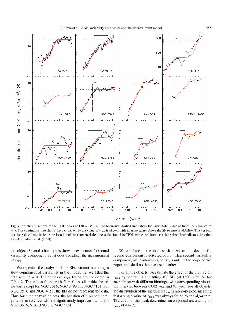
Fig. A.11. NGC 3516, SF for the light curves 1300 to 3000 Å. The fit of the SF (a)–(c) follows what was done in Sect. 4.1 (two parametersfixed). The LW was less used than the SWP during the intensive monitoring made in 1993 (see Fig. A.12). The number of LW epochs is smaller(22) than for the SWP (71). Although the fit seems to have succeeded in the LW range, one should be careful in interpreting the result asevidence for the presence of a longer timescale as the SF slope α pegged to the maximum value of 2. In addition, the fit is rather poor. We thusdecided to reject the time scales corresponding to the SF (d)–(l).
P. Favre et al.: AGN variability time scales and the discrete-event model, Online Material p 11
Fig. A.12. NGC 3516, comparison of the LW light curves (dashedlines) with the 1300–1350 Å light curve.
P. Favre et al.: AGN variability time scales and the discrete-event model, Online Material p 12
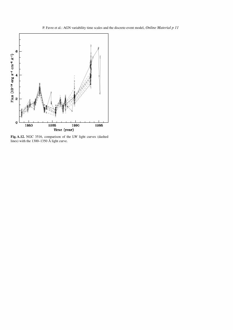
Fig. A.13. NGC 3783, SF for the light curves 1300 to 3000 Å. The time scales obtained from the LW data are more scattered because the LWdata have 12% less epochs than the SWP.

P. Favre et al.: AGN variability time scales and the discrete-event model, Online Material p 13
Fig. A.14. NGC 4151, SF for the light curves 1300 to 3000 Å. The fit of the SF follows what was done in Sect. 4.1 (two parameters fixed). Thefit did not succeed for the SF (d), the corresponding time scale was thus rejected.

P. Favre et al.: AGN variability time scales and the discrete-event model, Online Material p 14
Fig. A.15. NGC 4593, SF for the light curves 1300 to 3000 Å.
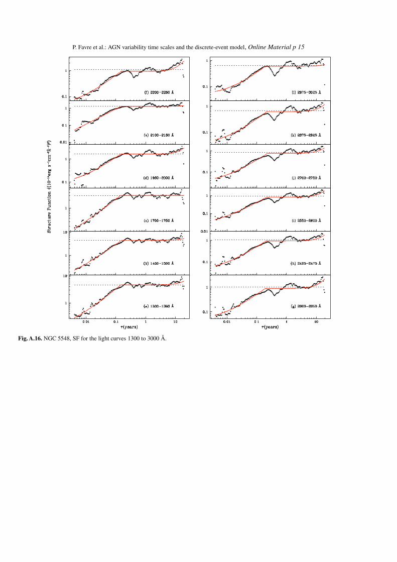
P. Favre et al.: AGN variability time scales and the discrete-event model, Online Material p 15
Fig. A.16. NGC 5548, SF for the light curves 1300 to 3000 Å.

P. Favre et al.: AGN variability time scales and the discrete-event model, Online Material p 16
Fig. A.17. NGC 7469, SF for the light curves 1300 to 3000 Å. The fit of the SF (a)–(c) follows what was done in Sect. 4.1 (two parameters fixed).Only SWP was used for the intensive monitoring made in 1996 (see Fig. A.18). As in NGC 3516, the number of LW epochs is smaller (16)than for the SWP (95). The fit did not succeed for the SF (e), (f), (h), (k), (l). The corresponding time scales were thus rejected. The SF (d), (g),(i), (j) may be interpreted as showing evidence for the presence of a longer timescale in the data, but this result should be taken with cautionbecause of the small number of epochs taken into account.

P. Favre et al.: AGN variability time scales and the discrete-event model, Online Material p 17
Fig. A.18. NGC 7469, comparison of the LW light curves (dashedlines) with the 1300–1350 Å light curve.

P. Favre et al.: AGN variability time scales and the discrete-event model, Online Material p 18
Fig. A.19. 3C 120.0, SF for the light curves 1300 to 3000 Å. The fit did not succeed for the SF (b), (d), (g)–(l) because of noisy light curves(see Fig. A.20, A.21). The time scales corresponding to these SF are thus rejected.

P. Favre et al.: AGN variability time scales and the discrete-event model, Online Material p 19
Fig. A.20. 3C 120.0, comparison of the noisy 1450–1500 Å light curve(dashed line) with the 1300–1350 Å light curve.
Fig. A.21. 3C 120.0, comparison of the noisy LW (d), (g)–(l) lightcurves (dashed lines) with the 1300–1350 Å light curve.

P. Favre et al.: AGN variability time scales and the discrete-event model, Online Material p 20
Fig. A.22. 3C 273, SF for the light curves 1300 to 3000 Å. The fit did not succeed for the SF (i)–(k) because of noisy light curves (seeFig. A.23–A.25). The time scales corresponding to these SF are thus rejected.

P. Favre et al.: AGN variability time scales and the discrete-event model, Online Material p 21
Fig. A.23. 3C 273, comparison of the noisy 2550–2600 Å light curve(dashed line) with the 1300–1350 Å light curve.
Fig. A.24. 3C 273, comparison of the noisy 2700–2750 Å light curve(dashed line) with the 1300–1350 Å light curve.
Fig. A.25. 3C 273, comparison of the noisy 2875–2925 Å light curve(dashed line) with the 1300–1350 Å light curve.

P. Favre et al.: AGN variability time scales and the discrete-event model, Online Material p 22
Fig. A.26. 3C 390.3, SF for the light curves 1300 to 3000 Å. Only SWP was used for the intensive monitoring made in 1995–1996 (seeFig. A.27). The number of LW epochs is too small to build measurable SF. The fit did not succeed and no time scales could be deduced in therange 1950 to 2975 Å for this object.

P. Favre et al.: AGN variability time scales and the discrete-event model, Online Material p 23
Fig. A.27. 3C 390.3, comparison of the LW light curves (dashed lines)with the 1300–1350 Å light curve.

P. Favre et al.: AGN variability time scales and the discrete-event model, Online Material p 24
Fig. A.28. Fairall 9, SF for the light curves 1300 to 3000 Å. The fit of the SF (a)–(c) follows what was done in Sect. 4.1 (two parameters fixed).The number of epochs between SWP and LW is very uneven (139 for the SWP and 63 for the LW). The SF (d)–(l) may be interpreted asshowing evidence for the presence of a longer timescale in the data.

P. Favre et al.: AGN variability time scales and the discrete-event model, Online Material p 25
Fig. A.29. ESO 141-55, SF for the light curves 1300 to 3000 Å. The fit did not succeed for the SF (d), (f) due to noisy light curves (seeFig. A.30); the corresponding time scales were thus rejected.

P. Favre et al.: AGN variability time scales and the discrete-event model, Online Material p 26
Fig. A.30. ESO 141-55, comparison of the noisy 1950–2000 Å and2200–2250 Å light curves (dashed lines) with the 1300–1350 Å lightcurve.
Related Documents


![Astronomy c ESO 2005 Astrophysics - delpeloso.com.br · Astrophysics The age of the Galactic thin disk from Th/Eu nucleocosmochronology I. Determination of [Th/Eu] abundance ratios,](https://static.cupdf.com/doc/110x72/5c61eb8009d3f22c068b7c4c/astronomy-c-eso-2005-astrophysics-astrophysics-the-age-of-the-galactic-thin.jpg)