Aam99-jour.pdf

S. K. Saha 1 Department of Mechanical Engineering,

I.I.T., Delhi, Hauz Khas, New Delhi 110 016, India

e-maih [email protected]

Dynamics of Serial Multibody Systems Using the Decoupled Natural Orthogonal Complement Matrices Constrained dynamic equations of motion of serial multibody systems consisting of rigid bodies in a serial kinematic chain are derived in this paper. First, the Newton-Euler equations of motion of the decoupled rigid bodies of the system at hand are written. Then, with the aid of the decoupled natural orthogonal complement (DeNOC) matrices associated with the velocity constraints of the connecting bodies, the Euler-Lagrange independent equations of motion are derived. The De NOC is essentially the decoupled form of the natural orthogonal complement (NOC) matrix, introduced elsewhere. Whereas the use of the latter provides recursive order n-n being the degrees-of-freedom of the system at hand--inverse dynamics and order n 3 forward dynamics algorithms, respectively, the former leads to recursive order n algorithms for both the cases. The order n algorithms are desirable not only for their computational efficiency but also for their numerical stability, particularly, in forward dynamics and simulation, where the system's accelerations are solved from the dynamic equations of motion and subsequently integrated numerically. The algorithms are illustrated with a three-link three-degrees-of-freedom planar manipulator and a six-degrees-of-freedom Stanford arm.

1 Introduction

The conventional approach to obtain the dynamic model, i.e., equations of motion, of a mechanical system, consisting of rigid bodies coupled by kinematic pairs or joints, is to use either Newton-Euler (NE) or Euler-Lagrange (EL) equations. While the NE equations are obtained from the free-body diagrams, the EL equations resulted from the kinetic and potential energy of the system. The former is not suitable for motion simulation, as it finds the internal forces and torques that do not affect the motion of the system. Alternatively, EL equations give independent set of equations that are good for motion simulation, however, require complex calculations for the partial derivatives. With the advent of digital computation, a series of new methods in the study of dynamic modeling of mechanical systems have been developed. Huston and Passerello (1974) introduced the first computer- oriented method to reduce the dimension of the unconstrained dynamical equations, namely, Newton-Euler equations of motion, by eliminating the constraint forces. What was basically used to reduce the dimension is an orthogonal complement of the velocity constraints of the mechanical system under study. An orthogonal complement is defined as the matrix whose columns span the null-space of the matrix of the velocity constraints, and, hence, the premultiplication of the transpose of it with the unconstrained dynamic equations of motion vanishes the constrained moments and forces. The said orthogonal complement is not unique. In some approaches, an orthogonal complement is found using numerical schemes which are of an intensive nature, requiring, for example, singular-value decomposition or eigenvalue computations (We-

Presently (May 1999-Jan. 2000) at the Institute B of Mechanics, University of Stuttgart, Stuttgart, Germany as a Humbold Fellow.

Contributed by the Applied Mechanics Division of THE AMERICAN SOCmTY OF MECHANICAL ENGINEERS for publication in the ASME JOURNAL OF APPLIED MECHANICS.

Discussion on the paper should be addressed to tile Technical Editor, Professor Lewis T. Wheeler, Department of Mechanical Engineering, University of Houston, Houston, TX 77204-4792, and will be accepted until four months after final publication of the paper itself in the ASME JOURNAL OF APPLIED MECHANICS.

Manuscript received by the ASME Applied Mechanics Division, July 14, 1998; final revision, June 17, 1999. Associate Technical Editor: N. C. Perkins.

hage and Haug, 1982; Kamman and Huston, 1984). In Angeles and Lee (1988), Angeles and Ma (1988), and Saha and Angeles (1991), however, the complement is obtained naturally from the velocity constraint expressions without any complex computation. There- fore, the complement is called natural orthogonal complement (NOC). The NOC is the matrix that relates the angular and linear velocities of the rigid bodies in the system to the associated joint rates, as in Eq. (16).

The purpose of deriving a dynamic model here is to obtain inverse and forward dynamics algorithms required in control and simulation of the mechanical systems under study, respectively. While almost all proposed inverse dynamics algorithms for serial- chain mechanical systems, as shown in Fig. 1, are recursive of order n, O(n)--n being the degrees-of-freedom of the system at hand--complexity, e.g., Hollerbach (1980), Luh, Walker and Paul (1980), Kane and Levinson (1983), Angeles et al. (1989), Scia- vicco and Siciliano (1996), most of the traditional forward dynamics algorithms are of O(n 3) (Walker and Orin, 1982; Kane and Levinson, 1983; Angeles and Ma, 1988). Note here that in inverse dynamics the explicit derivation of the equations of motion in terms of the generalized coordinates is not required, e.g., in Scia- vicco and Siciliano (1996), where the joint torques are calculated from the trajectory of the end-effector. Alternatively, explicit expressions for the matrices, particularly, the generalized inertia matrix associated with the equations of motion must be evaluated for forward dynamics, e.g., in Angeles and Ma (1988) and others, in which the joint accelerations are solved from the equations of motion. Conventionally, a numerical approach is taken to solve for the joint accelerations. For example, in Angeles and Ma (1988), (i) first, the elements of the inertia matrix are evaluated; (ii) then, the numerical decomposition of the matrix, namely, the Cholesky decomposition (Stewart, 1973), is performed; and (iii) finally, the joint accelerations are solved by backward and forward substitu- tions. Since the complexity of the Cholesky decomposition is of order n 3, the forward dynamics algorithm also requires O(n 3) computations. There is, however, an alternative approach to obtain a forward dynamics algorithm recursively, whose computational complexity is in the order n, i.e., O(n), e.g., Armstrong (1979),

986 / Vol. 66, DECEMBER 1999 Copyright © 1999 by ASME Transactions of the ASME

Downloaded 23 Nov 2007 to 203.199.213.67. Redistribution subject to ASME license or copyright; see http://www.asme.org/terms/Terms_Use.cfm

i "~'~- i+ l " ",

', n ', #2 :

2

~ ~ composite body i

Fig. 1 An n-body serial manipulator

Featherstone (1983), Rodriguez (1987), Schiehlen (1991), Rodri- guez and Kreutz-Delgado (1992), and Saha (1997). There is also a parallel O(log N) algorithm proposed in Fijany et al. (1995) which requires a special computer hardware, namely, a parallel architec- ture. Because of the special hardware requirement the parallel algorithms will not be discussed further.

The algorithm by Armstrong (1979) was the first of its kind where the recursive solution to the equations of motion of an n-link manipulator mounted on a spacecraft is obtained. Feather- stone (1983) has introduced the concept of articulated body inertia (ABI) which has been efficiently evaluated by McMillan and Orin (1995). The ABI is derived by extending the expressions for the equations of motion of a single body to a system of coupled bodies. Rodriguez (1987), on the other hand, presented a novel robot inverse and forward dynamics algorithms based on Kalman filtering and smoothing technique arising in the state estimation theory. The methodology has been used to solve several other dynamics problems as well, namely, by Rodriguez, Jain, and Kreutz-Delgado ( 1991 ), and Jain and Rodriguez (1995). Schiehlen (1991 ) and Saha (1997), however, have independently used the linear algebra approach to arrive at a recursive forward dynamics algorithm. It is interesting to note that, compared to the O(n 3) schemes, e.g., Angeles and Ma (1988), computational complexity of all the O(n) schemes, wherever known, are efficient when n ~ 12, as is evident from Table 2. The ©(n) algorithms, however, calculate the joint accelerations that are smooth functions of time (Ascher et al., 1997). As a result, numerical integration is faster and, hence, the total time in simulation may be less while comparing with the O(n 3) scheme. Besides, O(n) algorithms provide physical interpretations of the parameters they calculate and the intermediate steps they follow. Thus, the recursive forward dynamics is becom- ing more and more popular.

In this paper, the NOC (Angeles and Lee, 1988) is taken one step further to uniformly develop a set of independent dynamic equations of motion from which both recursive inverse and forward dynamics algorithms can be written. Here, the NOC is expressed as a product of two matrices, one is a block triangular and the other one is a block diagonal. Hence, the term decoupled added to it. Unlike the NOC, its modified form, i.e., the DeNOC, allows one to write expressions of the elements of the matrices and vectors associated with the dynamic equations of motion in analytical, recursive form, as shown in Section 4. These characteristics were not so obvious with the earlier form of the NOC, e.g., in Saha and Angles (1991). Moreover, many of the physical interpretations obtained in this paper have corresponding interpretations in Featherstone (1983), Rodriguez (1987), Rodriguez and Kreutz-Delgado (1992), and others, as indicated after Eqs. (14), (17), and (50). The present approach provides an alternate approach to the development of a recursive forward dynamics algorithm, compared to others, e.g., Rodriguez (1987). The present approach is built upon basic mechanics and linear algebra theory. Hence, it is easy to comprehend, even by a fresh mechanical engineer without any knowledge of control theory. Moreover, there is equivalence of many steps and interpreted variables ob-

tained from Gaussian elimination of the inertia matrix, as shown in Appendix B, and Kalman filtering (Rodriguez, 1987). As a result, it may be commented that they are equivalent under certain conditions. The real proof is, however, behind the scope of this paper.

The contributions of this paper are listed as follows.

1 A systematic uniform development of the dynamic model of a serial-chain mechanical system. Here the word, uniform, implies that no different sets of equations of motion are required to obtain inverse and forward dynamics algorithms, as in Sciavicco and Siciliano (1996) and others, where Newton-Euler equations of the motion of the uncoupled bodies are used to obtain a recursive inverse dynamics algorithm and the joint accelerations (forward dynamics) are computed from the independent set of equations.

2 Recursive expressions not only for the generalized inertia matrix (Saha, 1997), but also for the generalized matrix of convective inertia terms, and the generalized forces/torques, as shown in Section 4.

3 As a consequence of the above items, not only a forward dynamics algorithm (Saha, 1997) but also an inverse dynamics algorithm is possible from the same set of dynamics equations of motion.

4 Implementation of the above algorithms to a planar three- degrees-of-freedom manipulator and a six-degrees-of-freedom Stanford arm.

5 Physical interpretation of different terms obtained during the dynamic modeling, and correlation of those with the similar terms appeared in the literature, e.g., Featherstone (1983) and Rodriguez (1987) and Rodriguez and Kreutz-Delgado (1992).

The paper is organized as follows: Section 2 introduces some definitions required to derive the dynamic model given in Section 3. Section 4 shows how to derive the analytical expressions for the matrices and vectors associated with the equations of motion, whereas Section 5 gives the applications, namely, inverse and forward dynamics algorithms. The results of the algorithms with respect to two examples are provided in Section 6.

2 Some Definitions Referring to Fig. l, it is assumed that a serial multibody system,

namely, the serial manipulator, has a fixed "base" and n moving rigid bodies, numbered # 1 . . . . . #n, coupled by n one-degree-of- freedom kinematic pairs or joints, say, a prismatic or a revolute, which are indicated in Fig. 1 as 1 . . . . . n. The ith joint couples the ith body with that of the (i - 1)st. Now, referring to the motion of the ith body, Fig. 2, the following terms are defined:

t~ and n~: the six-dimensional vectors of twist and wrench of the ith link, i.e.,

ti-~" and wi--= fs (1) Vi

where 0~ and v~ are the three-dimensional vectors of angular velocity and the linear velocity of the mass center of the ith link, C~, as shown in Fig. 2, respectively, whereas ni and fi are the three-dimensional vectors of the moment about Ci and the force at Ci, respectively.

vi (velocity)

I m i : mass ~ - ' f ~ / Q ~ J ~ Ii : inertia T / / c i / , . . . . . .

O

Fig. 2 Free-body diagram of the fih body

Journal of Applied Mechanics DECEMBER 1999, Vol. 66 / 987


~i and M~: the 6 × 6 matrices of angular velocity and mass of the ith body, respectively, namely,

o I o 1 O toi × 1 and Mi ~ O mil (2)

where o~ × 1 is the 3 × 3 cross-product tensor associated with vector ooi, which when operates on any three-dimensional Carte- sian vector, x, results in a cross-product vector, i.e., (to~ × 1)x -~ to~ × x. Moreover, L and m~ are the 3 × 3 inertia tensor about the mass center, C~, and the mass of the ith body, respectively. Furthermore, 1 and O are the 3 × 3 identity matrix and the matrix of zeros, respectively. Henceforth, the dimensions of 1 and O should be understood as of dimensions that are compatible with the dimensions of the matrix expressions where they appear.

t and w: the 6n-dimensional vectors of generalized twist and wrench, respectively, i.e.,

t -= [t~ r . . . . . t,r] r and w ~- [w r . . . . . w,r] r (3)

where t~ and w~, for i = 1 . . . . . n, are defined in Eq. (1).

and M: the 6n x 6n matrices of generalized angular velocity and mass, respectively, namely,

-= diag [ ~ , . . . . . 1~,] and M =- diag [M~ . . . . . M,,]

(4)

where ~ i and M~, for i = 1 . . . . . n, are given in Eq. (2).

//: the n-dimensional independent vector of joint rates, i.e.,

O ~- [0 , . . . . . 0 , ] ~ (5)

where 0~ is the displacement of the ith joint, as shown in Fig. 3.

3 Dynamic Model ing Using the DeNOC

For a serial-chain mechanical system shown in Fig. l, the steps to obtain the dynamic equations of motion using the DeNOC matrices are given below:

1 Derivation of the Unconstrained Newton-Euler (NE) Equations of Motion:

(a) From the free-body diagram of the ith rigid body, Fig. 2, write the Newton-Euler equations of motion as

Iigo i -I- 0.) i X I io0 i = n i (6a)

mi~ri : f i (6b)

where ni and f~ are the resultant moment about and force applied at the mass center, C~, respectively. Using the definitions given in Eqs. (1) and (2), the above six scalar equations can be put in a compact form as

M i t i -I- [Wilt i = w i (7)

r~j ~d~

~ / / ~ ~O~--/--~:~r ~ rne

Fig. 3 A coupled system

(b)

(a)

where the six-dimensional twist-rate vector, ti, and the 6 X 6 mass-rate matrix, 19Ii, are, respectively, the time derivative of t~ and M~, which are defined as

Write Eq. (7) for i = 1 . . . . . n: This gives 6n uncoupled scalar equations for the whole system, which are put in the following form:

Mt + l~t = w (9)

where ic and 1VI are the time derivative of the generalized twist, t, and generalized mass, M, respectively, i.e.,

i ~ ITS' , . . . . [T]T and 1~ ------ diag [1VI, . . . . . l~l,]

(lO) in which t~ and IVL appear in Eq. (8).

Derivation of Kinematic Constraints:

In this step, motion constraints due to the kinematic pairs are derived. For example, velocity constraints between two links, #i and #j, coupled by the ith revolute joint, as shown in Fig. 3, can be expressed as

to i = oJj + 0iei (1 la)

vi = vj + ooj x rj + oJ~ x d i . (1 lb)

The above six scalar equations are written in a compact form as

ti = B0t j + Pi0i (12)

where the 6 X 6 matrix, B~j, and the six-dimensional vector, p~, are as follows:

Bu -= c o × 1 and Pi ~- e i N d i

% × 1 being the cross-product tensor associated with vector c u , defined similar to tos × 1 of Eq. (2), i.e., (% × 1)x ~ % × x, for any arbitrary three-dimensional Carte- sian vector x. The vector, % , as shown in Fig. 3, is given by, % --= -d~ - rj. It is interesting to note here that the matrix, B~j, and the vector, p~, have the following interpretations:

• For two rigidly connected moving bodies, #i and #j, B 0 , propagates the twist of #j to #i. Hence, matrix B u is termed here as the twist propagation matrix, which has the following properties:

BuBjk=B~k, B , = 1, and B~ 1 = Bji. (14)

Matrix B~j is nothing but the state transition matrix of Rodriguez (1987).

• Vector, pi, on the other hand, takes into account the motion of the ith joint. Hence, p~ is termed as the joint-rate propagation vector, which is dependent on the type of joint. For example, the expression of p~ in Eq. (13) is for a revolute joint shown in Fig. 3, whereas for a prismatic joint vector p~ is given by

pi--- [e0] : for a prismatic joint (15)

where e~ is the unit vector parallel to the axis of linear motion. Correspondingly, 0~ of Eq. (12) would mean the linear joint rate. Other joints are not treated here because any other joint, e.g., spherical or screw, can be treated as combination of revolute or revolute and prismatic pairs, respectively.

988 / Vol. 66, DECEMBER 1999 Transactions of the ASME


Write Eq. (12), for i = 1 . . . . . n, as

t = NO, where N---- NtNd. (16)

In Eq. (16), N is the 6n × n NOC matrix, introduced in Angeles and Lee (1988), whereas its decoupled form, N N~Nd, is termed as the decoupled NOC (DeNOC) matrices (Saha, 1997). The 6n × 6n lower block triangular matrix, N~, and the 6n × n block diagonal matrix, Nd, are given by

(b)

Nz -= 2~ 1 and

k B,I B',~2

00° ° l Nd ~ P2

0 ,,

(17)

where the first two properties of the twist propagation matrix, B~j, given in Eq. (14) are used. Moreover, O and 0 are the 6 × 6 matrix and the six-dimensional vector of zeros, respectively. Matrices N~ and Nd are the spatial operators of Rodriguez and Kreutz-Delgado (1992), which are "anticausal" and "memory-less" nonrecursive, respectively.

3 Incorporation of the Kinematic Constraints Into the NE Equations of Motion: Premultiply N T with the decoupled NE equations of motions, Eq. (9), i.e.,

N r ( M i + 1VIt) = Nr(w ~ + w') (18)

where w is substituted as w -= w L + w~--w t~ and w ~ are the generalized external and internal constraint wrenches, respectively. Since constraint moments and forces do not perform any work, trw ~ vanishes, i.e., trw I = 0rNrw~ = 0, which implies that, for independent 0, Nrw ~ = 0. Hence, Eq. (18) is rewritten as

N 7(Mi + lflt) = N rw e. (19)

Note that in order to eliminate the constraint wrench from the decoupled NE equations, Eq. (9), as done in Eq. (19), it is impor- tant to write the generalized twist, t, as a linear transformation of the independent generalized speed, as in Eq. (16).

4 Constrained Euler-Lagrange (EL) Dynamic Equations of Motion: Su.bstitute..the e.x.pression of t, Eq. (16), and its time derivative, i.e., t : NO + NO, into Eq. (19). The result is the following constrained dynamic equations of motion:

I 0 + C 0 = ' r (20)

where

I ~- N~MN --- N~'I~Nd: the n × n generalized inertia matrix

(G1M);

C --= Nr(Mlq + 1VIN) -~ N ~,l'l~I'N,l: the n × n matrix of

convective inertia terms;

~- -~ Nrw e --- N~qee: the n-dimensional vector of generalized

forces due to driving torques and those resulting from

gravity and dissipation, etc.

The expressions for 1VI, 1~I', and ~F are associated with the composite body of the system under study and derived in the next

section, Section 4. Note that Eq. (20) is essentially the Euler- Lagrange equations of motion that has been arrived from the uncoupled Newton-Euler equations, e.g., Eq. (9). Moreover, the use of the NOC, N, as introduced in Angeles and Lee (1988), does not allow further simplification of associated expressions of Eq. (20), i.e., matrices I and C, and vector ~'. Hence, a computer algorithm is required at this stage for dynamic analysis. Alterna- tively, the DeNOC matrices given in Eq. (16) allows one to write the analytical recursive expressions for each element of the matrices, I, C, and ~', as shown in the following section. These expressions lead to recursive inverse and forward dynamics algorithms, given in Sections 5. l and 5.2, respectively, whose computational complexities are of order n, i.e., ©(n), and provide many physical interpretations, e.g., after Eqs. (14), (17), (23b), and (50).

4 A n a l y t i c a l E x p r e s s i o n s for I, C, a n d 7

The analytical expressions for the GIM, I, the generalized matrix of convective inertia terms, C, and the generalized vector of joint forces/torques, as given after Eq. (20), are derived next. These expressions provide the basis for uniform development of the recursive inverse and forward dynamics algorithms. That is, unlike other approaches, e.g., Sciavicco and Siciliano (1996) and others, where free-body diagrams and NE equations are used to develop inverse dynamics algorithm and the EL equations are used for forward dynamics, here only one set of equations, namely, Eqs. (20), (24), (29), and (30), are used for both the algorithms.

4.1 Derivation of the GIM, I. Substituting the expression for the NOC in terms of the DeNOC matrices, i.e., N ~- NtNd, as in Eq. (17), into that of matrix I -~ NrMN, as given after Eq. (20), one obtains

I ~~ --= N,/MNd, where 1~1 ~ N~MNi (21)

in which the 6n × 6n symmetric matrix, 191, is given by

• T ~ 1VI, B;,NI2 • B,,M,,] • • B ,aM,, / (22) l f 4 ~ 1VI2B2, NI2 . r ~

: ~ • :

J 1VInB,I ]~I,B,~ ' • l~I

where the 6 × 6 matrix, ~L, for i = 1 . . . . . n, is defined as

t~

1Vii--= Mi + ~ B~,MkBki. (23a) k = i l l

Note the summation over k = i + l . . . . . n in Eq. (23a). An algorithm computing 1VIa, for i = 1 . . . . . n, from Eq. (23a) will certainly require order n 2 computations. However, a close look to Eq. (23a) with the first two properties of B~, Eq. (14), in mind reveals that the summation expression can be evaluated recur-

n

sively, i.e., ~ r ~ r ~ BklMkBki Bi,.l,iMi.,.iBi+l,i, f o r / = n . . . . . 1, k i ~ l

with 1~1,,+~ ~ O, because there is no (n + l )s t link in the system. Hence, Eq. (23a) has the following recursive relation:

1~I i : M i + Bf+l.il~Ii+lBi+l. i where IVI,, ~ M,,. (23b )

The 6 × 6 matrix, ~1~, is the mass matrix of composite body, i, i.e., I~lj represents the mass and inertia properties of the system com- prising of (n - i + 1) rigidly connected bodies, namely, bodies #i . . . . . #n, as indicated in Fig. 1 by dotted line. The expressions for the elements of the GIM, I of Eq. (20), which is symmetric positive definite, are then given by

iij = ij, = pfl~l,Bqpj (24)

f o r i = 1 . . . . . n ; j = 1 . . . . . i.



Table 1 Computational complexities in inverse dynamics

Algorithm M A n = 6

Hollerbach (1980) 412n - 277 320n - 201 2195M 1719A Luh et al. (1980) 150n - 48 131n + 48 852M 834A Walker and Orin

(1982) 137n - 22 101n - 11 800M 595A Proposed 120n - 44 97n - 55 676M 527A Khalil et al. (1986) 105n - 92 94n - 86 538M 478A Angeles et al. (1989) 105n - 109 90n - 105 521M 435A Balafoutis et al. (1988) 93n - 69 81n - 65 489M 421A

M: Multiplication/Division; A: Addition/Subtraction

4.2 Derivation of C Matrix. Using the NOC and its time derivative in terms of the DeNOC matrices, i.e., N =- N~N~, and lq

SlNd + NlSd, respectively., the.generalized matrix of convective inertia terms, C [ ~ N r ( M N + MN)], as defined after Eq. (20), is obtained as

C =- N~M'Nd, where lql' =- N~MN, + lq4n + 1~I ( 2 5 )

in which the following identities are used:

l~/d -~ l~Nd and l~l = NT19IN~ (26)

where the 6n × 6n matrix, 12, is defined in Eq. (4). In Eq. (25), the multiplication of two block diagonal matrices, M and fI , can be easily performed, whereas the expressions for the matrices, NfMIq, and M, are shown below:

B T11~I21

N ~Mlql ~ fI21

- In - - 1,1

7 '7 gg M M i M2

'7 ." • ~ M2 M2 M--=

7 '7 M. M,,

T ~ B.IH.,n-I T ~ B ,,2H.,.-

T " B n2Hn,n I

"

• "

i ] and

(27)

the 6 × 6 matrices, 1~I~ and ITI0, for i = 1 . . . . . n; j = 1 . . . . . i - 1, being obtained as

,7 ,"1" Mi = Mr + Mi+l and (-I 0 -~ M i U i j + BiT+l,i~Ii+l,i (28)

in which ~I,,÷ 1 = f-I,+ ~.,, = O. The individual element of the n × n matrix, C, i.e., c 0 , for i, j = 1 . . . . . n is given as

T T ~ T ~ ~ j I P i ( B j / M j f l j + Bj+I,iHj~ ,,i + ~ ) ) P j if i

CiJ = [piT(~IrBij~j + ~Iq + ~li)ps otherwise. (29)

4.3 Derivation of ~- Vector. The generalized vector of forces and torques, ~, can he obtained from its expression after Eq. (20), i.e., for, i = 1 . . . . . n,

% p(ff~, where * ~ = w ~ + r -E = Bi+l,iWi+ l (30)

in which ~ is the six-dimensional vector component of the 6n-dimensional vector, ~,F~, namely,

. . . . . (31)

Note in Eq. (30) that in the absence of any external forces and moments on the end-effector, w,,~ e, , = 0.

5 A p p l i c a t i o n s

A class of serial multibody systems are industrial manipulators. Suitable dynamic models of these manipulators are required mainly for their control and simulation purposes. Control involves inverse @namics, whereas simulation requires forward dynamics. These algorithms are presented in the following subsections.

5.1 Inverse Dynamics Algorithm. The inverse dynamics problem is defined as, given the motion of a manipulator, calculate the actuator forces~torques required to maintain the given motion. Based on the dynamic equations of motion, Eq. (20) and the expressions for the elements of the associated matrices, I, C, and ~-, Eqs. (24), (29), and (30), respectively, a recursive inverse dynamics algorithm is presented here for the following input: For i = 1 . . . . . n,

1 constant Denavit-Hartenberg (DH) parameters (Denavit and Hartenberg, 1955)--the DH parameters are also defined in Appendix A - - o f the system under study, i.e., at, br, and c~, for a revolute pair, and a~, b~, and 0r, for a prismatic pair.

2 time history of the variable DH parameter, i.e., 0r, for a revolute pair, and br, for a prismatic joint, and their first and second time derivatives, i.e., 0r, 0r, and be, ~r.

3 mass of each body, mr. 4 vector denoting the distance of the (i + l)st joint from the ith

mass center, Cr, in the (i + 1)st frame. 5 inertia tensor of the ith link about its mass center, C~, in the

(i + 1)st frame.

The inverse dynamics algorithm then calculates the joint forces/ torques, i.e., %, for i = 1 . . . . . n, in two recursive steps, as shown below:

Forward Recursion

v, = Pl01; v2 : p202 + Vl;

V~ = p,0,, + v,,-1;

~t = P101 + l l lp l01 ~2 = P20z + i"~2P202 + B21~I + I ~ 2 1 V l

~,, = p,O,, + l l ,p , ,0 , + B,,,,,_l~n_ 1 + Un,n_lv,~_ l

Backward Recursion

% = M,,~,, + M,,v,; %, = p r y , T T Y. I = M.,-i~,, I + 1VI,, iv,,-1 + B. , , , -W.; %-1 = P,,-lY.-I

Vl = Migl + M l v l + B~ly2; TI = P~TJ

where vr, ~r, and % are the six-dimensional vectors. Note from the expression for % above and that in Eq. (30), '~ff ---= %, while ~ E W,+l = 0. This implies that, without any external forces/ moments on the end-effector, only inertia forces, 3,,., contribute to w~, and, hence, the required joint forces/torques are due to system motion only.

For an all revolute-joint serial manipulator, the computational complexity of the above algorithm is compared in Table 1 with

Table 2 Computational complexities in forward dynamics

Algorithm M A n = 6 n = 12

Proposed 201n - 335 193n - 361 871M 797A 2077M 1955A Featherstone (1983) 199n - 198 174n - 173 996M 871A 2190M 1915A Walker and Orin (1982) ~nt 3 + 11 ~n2 + 38½n - 47 ~nl 3 + 7n 2 + 386n _ 46 633M480A 2357MI716A

M: Multiplication/Division; A: Addition/Subtraction



End ~ / ~ 0 ' effector ~ / , '

rl Jg~'lg ~ 02 t21 s " "

X

Fig. 4 A three-degrees-of-freedom manipulator

o

5

4

3

2

1

0

-1

-2

tau_ 1

tau 3

i

i i

2 6 time (sec)

8 10

Fig. 5 Torques for three-degrees-of-freedom manipulator

some other existing algorithms. Even though the algorithm is not the best but it is very simple, as evident from the two-step algorithm where six-dimensional vectors are treated similar to those of three dimensional vectors. That is, if one knows v~ finding out v2 is very similar to the evaluation of the linear velocity of body 2 from the known linear velocity of body 1. A computer software called RIDIM (Recursive Inverse Dynamics of Industrial Manip- ulators) is developed in C+ +, which has the following features:

• RIDIM can handle manipulators with both revolute and prismatic pairs or joints;

• gravity is taken into account by providing negative acceleration due to the gravity, denoted by g, to the first body, #l (Kane and Levinson, 1983), i.e., an additional term is added to £1 as

~ = Pt01 + l~lPl01 + P where p ~ [0 T, _griT. (32)

The rest of the algorithm remains same.

The software is illustrated with two examples, as in Section 6.

5,2 Forward Dynamics Algorithm. Forward dynamics is defined as, given the joint forces~torques, find the joint accelerations. This step is required in simulation, where the joint accelerations, 0, are solved from the dynamic equations of motion, Eq. (20), and integrated numerically to obtain the joint velocities and positions, 0 and 0, respectively, for a given set of initial conditions.

The required input for the forward dynamics algorithm are as follows: For i = 1 . . . . . n,

• inverse dynamics items, 1, and 3-5, as in Section 5.1. • initial value for the variable DH parameter, i.e., 0i, for a

revolute pair, and bl, for a prismatic pair, and their first time derivative, i.e., 0i and b,.

• .time history of the input joint forces/torques, i.e., +~. • each component of the six-dimensional vector, 4~ --- ,r - CO,

i.e., 4~, which is to be computed from any recursive inverse dynamics scheme, e.g., the one given in Section 5.1, while 0 = 0 (Walker and Orin, 1982).

The forward dynamics algorithm, as proposed in Saha (1997), is presented here for the sake of completeness of this paper. The algorithm is based on the UDU r decomposition of the generalized inertia matrix, I of Eq. (20), i.e., I -= UDU r, as outlined in Appendix B. Substituting for I, and, 4) =- ~" - CO, in Eq. (20), one obtains

UDUrO = dp. (33)

A three-step recursive scheme is then used to calculate the joint accelerations from the above equations, i.e.,

1 Solution for ÷: The solution, ÷ = U ~4~, is evaluated as

0 g o

-2

-3

-4 0 05

Fig. 6

1 1.5 2 2.5 3 3,5 time (sec)

Simulated joint angles of the planar manipulator

Journa l of App l ied M e c h a n i c s D E C E M B E R 1999, Vo l 66 / 991


End-effector ~ 0]

04

~ B a s e

Fig. 7 The six-degrees-of-freedom Stanford arm

Ti ~)i T = -- p i ' l ] i , i + l (34)

where ÷,, --= ~b,,, and the six-dimensional vector, ~b.~+~, is obtained as

- - T

~ i , i + l : Bi+l , i~ l~i+l and T~i+i ~ i~i+l~i_ 1 ..4- lf~i+1,i+2 (35)

in which ~,,.,+1 = 0. The new variable, tk~+~, is the six- dimensional vector which is defined in Appendix B.

2 Solution for ~r." The solution of the equation, Drr = ÷, involves the inverse of the diagonal matrix, D of Eq. (54), which is simple, namely, D -1 has only nonzero diagonal elements that are the reciprocal of the corresponding diagonal elements of D. Thus, vector rr is obtained as follows: For i = 1 . . . . . n,

fi = ~i/rhi.

The scalar, rh~, is defined in Eq. (47).

3 Solution for O: In this step, ~ = U rzr, is calculated, for / = 2 . . . . . n

T Oi = T i - i~i~ 'Li , i -1 (36)

where Ot --- ~-~, and the six-dimensional vector,/x~,g_~, is obtained from

~'~i,i 1 -~ B i , i - l ~ i - ! and ~ i - i ~- Pi:10i-1 -4- i . l , i_l, i 2 (37)

in which/x~0 = 0. The complexity of the proposed forward dynamics algorithm is

compared in Table 2 with some other algorithms. The complexity of the proposed algorithm is very similar to those of Featherstone (1983).

Based on the above algorithm, a simulation software, RFDSIM (Recursive Forward Dynamics and Simulation of Industrial Ma- nipulators) is also developed in C + + in which the numerical

integration scheme is based on the Runge-Kutta fifth/sixth-order method (Press et al., 1997).

6 Examples

For the illustration of the inverse and forward dynamics algorithms developed in Sections 5.1 and 5.2, respectively, two manipulators, namely, a three-degrees-of-freedom planar manipulator and a six-degrees-of-freedom Stanford arm, as shown in Figs. 4 and 7, respectively, are analyzed using RIDIM and RFDS!M software.

6.1 A Three-Degrees.of-Freedom Planar Manipulator. The manipulator under study is assumed to move in the X - Y plane, whereas the gravity is working in the negative Y direction, as indicated in Fig. 4. Let i and j be the two unit vectors parallel to the axes, X and Y, respectively, and k =-- i × j. The expressions for the three joint torques, namely, ¢1, z2, and %, are evaluated explicitly from the inverse dynamics algorithm given in Section 5.1, which exactly match with those reported in Angeles (1997). Moreover, RIDIM is used to find the joint torques for the following normal j oint angle trajectories and their corresponding 1 st and 2nd time derivatives:

0 i = ~ t

with T = 10.0 sec. The joint torques obtained from RIDIM are plotted in Fig. 5, where "tau_l .. . . tau_2" and "tau_3" denote the joint torques, T~, z2, and $3, respectively. The plots are also verified with the plots obtained from the explicit expressions.

In order to test RFDSIM, free fall simulation, i.e., motion due to gravity only, without any external joint torque, of the manipulator is carried out with the initial conditions as 0g(0) = 0r(0) = 0, for i = 1, 2, 3. The variations of the simulated joint angles are shown in Figs. 6, where "th_l," "th_2," and "th 3" represent 01,02, and 03, respectively. Note from Fig. 4 that due to gravity the first joint angle, 0~, will increase initially in the negative direction, as evident from Fig. 6. Moreover, the system under gravity behaves as a triple pendulum. These is evident from all the joint angle variations, namely, 0~, 02, and 03 of Fig. 6.

6,2 A Stanford Arm. As a second example, a more general six-axis six-degrees-of-freedom manipulator, namely, the Stanford arm, as shown in Fig. 7, is taken whose Denavit-Hartenberg (DH) parameters, along with the mass and inertia properties are given in Table 3. The normal joint trajectory for the six joints are taken from Cyril (1988) as

1 [ ~ _ ( ~ t ) ] for e (39a) 0 ~ = ~ t - s i n - - -¢3

b 3 ~ t sin

with T = 10.0 sec, 01(0) = 0, for i ¢ 2, 3, 02(0) = 90 deg, b3(0 ) -~ 0, and Oi(T) = 60 dee, for i 4= 3 and b3(T) = 0.1 m. The joint torques are calculated from RIDIM and plotted in Figs.

Table 3 DH parameters, and mass and inertia properties of Stanford arm

Link a~ b~ a~ Oi m~ rx r~ r~ 1~, 1 , Iz~ (m) (m) (deg) (deg) (kg) (m) (kg-m 2)

1 0 .2 -90 O~ (0) 9 0 -.1 0 .01 .02 .01 2 0 .1 -90 02 (90) 6 0 0 0 .05 .06 .01 3 0 b3(O) 0 0 4 0 0 0 .4 .4 .01 4 0 .6 90 04 (0) 1 0 - . 1 0 .001 .001 .0005 5 0 0 -90 05 (0) .6 0 0 0 .0005 .0005 .0002 6 0 0 0 06 (0) .5 0 0 0 .003 .00l .002

992 / Vol. 66, D E C E M B E R 1999 Transact ions of the A S M E


0.15

0.1

~" 0.05 Z

0

-0.05

-0.1

-0.15

5

0

-5

~. -10

r2 -15 o

-20

-25

-30

Z == E r 2.

1.35 1.3

1.25 1.2

1.15 1.1

1.05

1 0.95

0.9 0,85

(a)

6 8 10 time (sec)

(c)

6 8 10 time (sec)

(e)

I

2 4 6 8 10 time (sec)

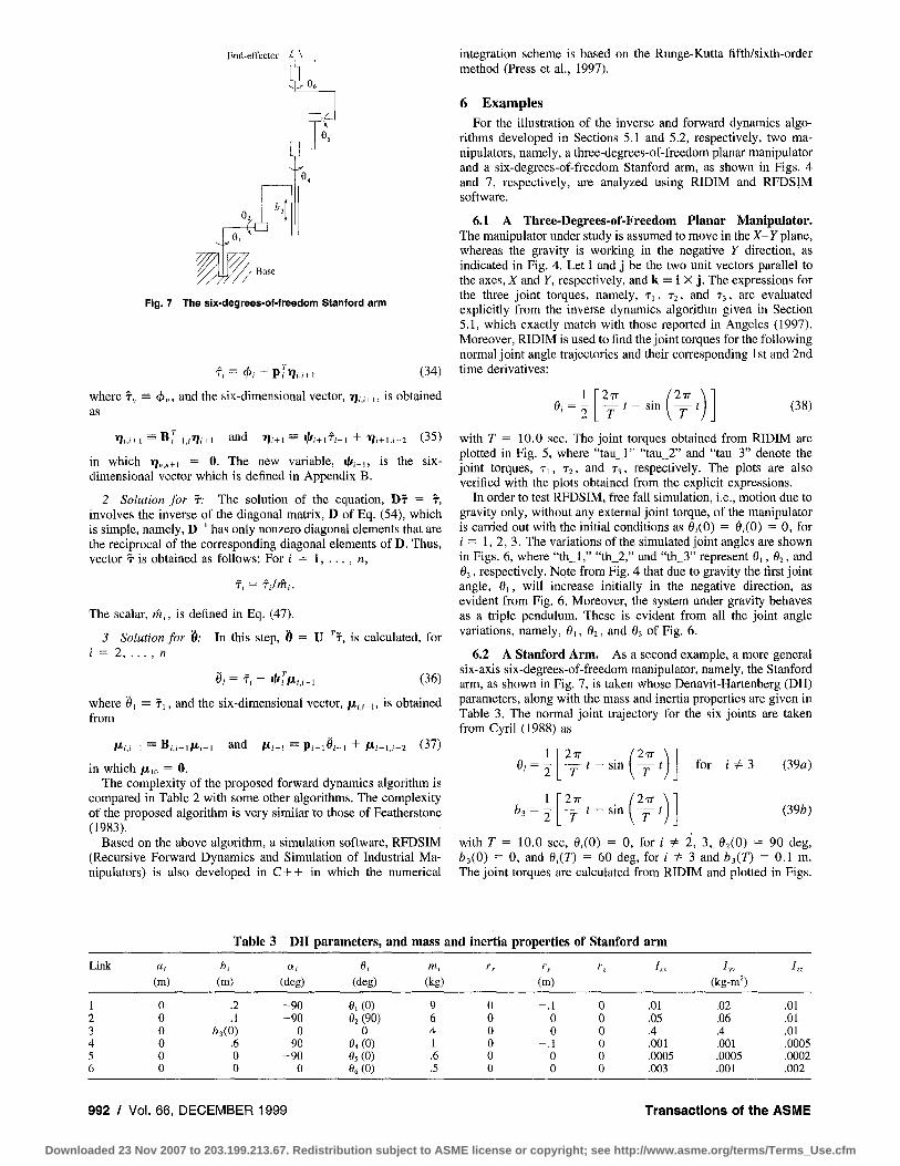
Fig. 8 4; (e) Joint 5; (0 Joint 6

8(a)-(f), which exactly match with those reported in Cyril (1988) for the same arm.

Interpretations similar to the planar manipulator, as given in Section 6.1, can be provided for the Stanford arm also. For example, the motion of joint 3 should sharply increase once the joint 2 turns more than 90 deg, which are evident from Figs. 9(c) and (b), respectively.

E Z

ET 2

E z == Cr s

18

17.5

17

16.5

16

15.5

15

14.5

0.1 0

-0.1 -0.2 -0.3 -0.4 -0.5 -0.6 -0.7 -0.8 -0.9

(b) I ' !

I t 0 2 4 10

time (sec) (d)

i! . . . . . . . . . . . . . . . . . . . . . . . . . . . . . . . . . . . . . . . . . . . . . . . . . . . . . . . . . . . . .

I

0 8 10 time (sec)

(f) 0.0003

0.0002

0.0001 Z

0

-0.0001

-0,0002

-0.0003 I i 0 2 4 6 8 10

t ime (sec)

Torques and force fOr the s ix -degrees-o f - f reedom Stanford arm at (a) Joint 1; (b) Joint 2; (c) Joint 3; (d) Joint

7 Conclusions A dynamic modeling methodology for serial multi-body

mechanical systems is presented. The modeling is based on the Newton-Euler equations of motion and the DeNOC matrices associated with the kinematic constraints, namely, Eq. (16). The dynamic modeling using the DeNOC has the following features:

• physical interpretations of many terms, e.g., the mass matrix of a composite body, as defined after Eq. (23b), and others, as given after Eqs. (14), (17), and (50).

• unlike the original definition of the NOC (Angeles and Lee, 1988), the DeNOC provides recursive analytical expressions for the elements of the associated matrices, i.e., I, C, and ¢, Eqs. (24), (29), and (30), respectively.

• due to the recursive expressions of the elements of matrices, I, C, and ~-, recursive O(n) algorithms for inverse and forward dynamics are possible for a general n-axis industrial manipulator, as presented in Section 5.1 and 5.2.

The computational complexities for both the inverse and forward dynamics algorithms are computed and compared in Tables 1 and 2, respectively. The algorithms are not the best in terms of the complexities, however, provide simple algorithms, particularly, the inverse dynamics algorithm presented in Section 5.1. They are also developed uniformly from the same set of equations, namely, Eqs. (20), (24), (29), and (30), which is simple to implement. Two software, namely, RID1M and RFDSIM are developed in C+ +, which are tested with respect to two manipulators, namely, a three-degrees-of-freedom planar manipulator and a six-degrees-of-freedom Stanford arm. The results from RIDIM are compared with those available in the literature for the same systems, namely, with Angeles (1997) for the three-degrees-of-freedom manipulator and with Cyril (1988) for the six-degrees-of-freedom Stanford arm, whereas the results of RFDSIM are interpreted intuitively.

Acknowledgment A part of the research work reported in this paper was possible

under the Department of Science and Technology, Government of India, Grant No. HR/OY/E-02/96. The author sincerely acknowl- edges the support.

References Angeles, J., 1997, Fundamentals of Robotic Mechanical Systems, Springer-Verlag,

New York.

Journa l of App l ied M e c h a n i c s D E C E M B E R 1999, Vol. 66 / 993


¢0

E o) E Q~

. g

P

0

-0.1

-0.2

-0.3

-0.4

-0.5

-0.6

-0.7

70

60

50

40

30

20

10

0

0

-0.5

-1

-1.5

-2

-2.5

-3

(a)

.......... ' .......... i ........... i .......... i! ........... ' ........... i ..........

i i

0.5 1.5 2 2.5 3 3,5 time (sec)

(c)

0.5 1 1.5 2 2,5 3 3.5 time (sec)

(e)

. . . . . . . . ' . . . . . . . . . . . ' . . . . . . . . . . . . . . . . . . . . h_

iiii! I I I

0 0.5 1.5 2.5 3 3,5 time (sec)

2

1.5

~ 0.5

-0.5

5

0

-5

~, -10

-15 ..9. -20 == <~ -25

-30

-35

-40

.9. == 03

10

8

6

4

(b)

\ . i

0 0.5 1 1.5 2 2.5 3 3.5 time (sec)

(d)

iiiiiiiiiiiii i i i ....

e i q i

0 0.5 1 1.5 2 2.5 3 3.5 time (sec)

(f)

i .i ......... :. .......... ', ......... i . . . . . .

0,5 1 1.5 2.5 3.5 time (sec)

2

0

-2 0

Fig. 9 Simulated Joint angles and displacement for the six-degrees-of-freedom Stanford arm at (a) Joint 1; (b) Joint 2; (c) Joint 3; (d) Joint 4; (e) Joint 5; (f) Joint 6

Angeles, J., and Lee, S., 1988, "The Formulation of Dynamical Equations of Holonomic Mechanical Systems Using a Natural Orthogonal Complement," ASME JOURNAL OF APPLIED MECHANICS, Vol. 55, pp. 243-244.

Angeles, J., and Ma, O., 1988, "Dynamic Simulation of n-axis Serial Robotic Manipulators Using a Natural Orthogonal Complement," Int. J. of Rob. Res., Vol. 7, No. 5, pp. 32-47.

Angeles, J., Ma, O., and Rojas, A., 1989, "An Algorithm for the Inverse Dynamics of n-Axis General Manipulator Using Kane's Formulation of Dynamical Equations," Computers and Mathematics with Applications, Vol. 17, No. 12, pp. 1545-1561.

Armstrong, W. W., 1979, "Reeursive Solution to the Equations of Motion of an n-Link Manipulator," Proc. of the 5th World Cong. on Th. of Mach. and Mech., Vol. 2, Montreal, Canada, ASME, New York, pp. 1343-1346.

Ascher, U. M., Pai, D. K., and Cloutier, B. P., 1997, "Forward Dynamics, Elimi- nation Methods, and Formulation Stiffness in Robot Simulation," Int. J. of Rob. Res., Vol. 16, No. 6, pp. 749-758.

Cyril, X., 1988, "Dynamics of Flexible-Link Manipulators," Ph.D. thesis, McGill University, Canada.

Denavit, J., and Hartenberg, R. S., 1955, "A Kinematic Notation for Lower-Pair Mechanisms Based on Matrices," ASME JOURNAL OF APPLIED MECHANICS, Vol. 77, pp. 215-221.

Featherstone, R., 1983, "The Calculation of Robot Dynamics Using Articulated- Body Inertias," Int. J. of Rob. Res., Vol. 2, No. 1, pp. 13-30.

Fijany, A., Shaft, 1., and D'Eleuterio, M. T. D., 1995, "Parallel O(log N) Algo- rithms for Computation of Manipulator Forward Dynamics," 1EEL Trans. on R&A, Vol. 11, No. 3.

Hollerbach, J. M., 1980, "A Recursive Lagrangian Formulation of Manipulator Dynamics and a Comparative Study of Dynamics Formulation Complexity," 1EEL Trans. on Sys., Man, and Cybernatics, Vol. SMC-10, pp. 730-736.

Huston, H., and Passerello, C. E., 1974, "On Constraint Eqnations--A New Approach," ASME JOURNAL OF APPLIED MECHANICS, Vol. 41, pp. 1130-1131.

Jain, A., and Rodriguez, G., 1995, "Diagonalized Lagrangian Robot Dynamics," 1EEL Trans. on R&A, Vol. 11, No. 4, pp. 571-584.

Kamman, J. W., and Huston, R. L., 1984, "Dynamics of Constrained Multibody Systems," ASME JOURNAL OF APPLIED MECHANICS, VO1. 51, pp. 899-903.

Kane, T. R., and Levinson, D. A., 1983, "The Use of Kane's Dynamical Equations for Robotics," Int. J. of Rob. Res., Vol. 2, No. 3, pp. 3-21.

Lilly, K. W., and Orin, D. E., 1990, "Efficient (9(n) Computation of the Opera- tional Space Inertia Matrix," Proc. of the IEEE Conf. on R&A, Vol. 2, Cincinnati, OH, May 13-18, pp. 1014-1019.

Luh, J. Y. S., Walker, M. W., and Paul, R. P. C., 1980, "On-Line Computational Scheme for Mechanical Manipulators," ASME Journal of Dynamic Systems, Mea- surement and Control, Vol. 102, pp. 69-76.

McMillan, S., and Odn, D. E., 1995, "Efficient Computation of Articulated-Body Inertias Using Successive Axial Screws," IEEE Trans. on R&A, Vol. 1 l, No. 4, pp. 606-611.

Press, W. H., Teukolsky, S. A., Vellerling, W. T., and Flannery, B. P., 1997, Numerical Recipes in C, 2rid Ed., Cambridge University Press, New Delhi.

Rodriguez, G, 1987, "Kalman Filtering, Smoothing, and Recursive Robot Arm Forward and Inverse Dynamics," 1EEL Trans. on R&A, VoL RA-3, No. 6, pp. 624-639.

Rodriguez, G., Jain, A., and Kreutz-Delgado, K., 1991, "A Spatial Operator Algebra for Manipulation Modeling and Control," Int. J. of Rob. Res., Vol. 10, No. 4, pp. 37t-381.

Rodriguez, G., and Krentz-Delgado, K., 1992, "Spatial Operator Factorization and Inversion of the Manipulator Mass Matrix," IEEE Trans. on R&A, Vol. 8, No. 1, pp. 65-76.

Saha, S. K., and Angeles, J., 1991, "Dynamics of Nonholonomic Mechanical Systems Using a Natural Orthogonal Complement," ASME JOURNAL OF APPLIED MECHANICS, VoI. 58, pp. 238-243.



Saha, S. K., 1997, "A Decomposition of the Manipulator Inertia Matrix," IEEE Trans. on R&A, Vol. 13, No. 2, pp. 301-304.

Schiehlen, W., 1991, "Computational Aspects in Multibody System Dynamics," Computer Methods in Applied Mechanics and Engineering, Vol. 90, No. 1-3, pp. 569-582.

Sciavicco, L., and Siciliano, B., 1996, Modeling and Conovl of Robot Manipula- tors, McGraw-Hill, New York.

Stewart, G. E., 1973, Introduction to Matrix Computation& Academic Press, San Diego, CA.

Walker, M. W., and Orin, D. E., 1982, "Efficient Dynamic Computer Simulation of Robotic Mechanisms," ASME Journal of Dynamic Systems. Measurement and Con- trol Vol. 104, pp. 205-211.

Wehage, R, A., and Haug, E. J., 1982, "Generalized Coordinate Partitioning for Dimension Reduction in Analysis of Constrained Dynamic Systems," ASME Journal of Mechanical Design, Vol. 104, pp. 247-255.

A P P E N D I X A

Denavit-Hartenberg Nomenclature In order to describe the Denavit-Hartenberg (DH) nomencla-

tures (Denavit and Hartenberg, 1955) that is followed here, note that the manipulator under study consists of n + 1 links, namely, a "base" and n links, denoted by # l . . . . . #n, coupled by n pairs numbered as l . . . . . n, respectively. As shown in Fig. 1, ith pair couples the (i - 1)st and the ith links. Moreover, a coordinate system X~, Y~, Z~ is attached to the (i - 1)st link.

Then, for the first n frames, DH parameters are defined accord- ing to the following rules: Referring to Fig. 10,

1 Zr is the axis of the ith pair. Its positive direction can be chosen arbitrarily.

2 Xr is defined as the common perpendicular to Z , and Z~, directed from the former to the latter. The origin of the ith frame, O~, is the point where Xr intersects Z, If these two axes intersect, the positive direction of Xr is chosen arbitrary. The origin, Or, is coincides with the origin of the (i - 1)st frame, O , .

3 the distance between Zi and Zr+~ is defined as ai, which is non-negative.

4 the Zr coordinate of the intersection of the X , axis with Zr is defined as br, which thus can be either positive or negative. For a prismatic joint, b~ is variable.

5 the angle between Zr and Zr+~ is defined as at , and is measured about the positive direction of Xr+l, and

6 the angle between Xr and Xr+~ is defined as 0~, and is measured about the positive direction of Z~. For a revolute joint, 0r is variable.

Since no (n + 1)st link exists the above definitions do not apply to the (n + 1)st frame and it can be chosen at will.

A P P E N D I X B

Decomposit ion of the GIM, I In order to obtain the UDU r decomposition of the GIM, I of Eq.

(20)--the elements of which are given by Eq. (24)--the rules of the Gaussian elimination (GEl (Stewart, 1973) are applied on these elements for the Reverse Gaussian Elimination (RGE), as proposed in Saha (1997). The scheme is reproduced here for the completeness of the paper.

B.1 RGE of the GIM, I. Conventionally, the GE (Stewart, 1973) begins from the first column of the matrix under interest. In the proposed elimination, it is assumed that the GE of matrix I, Eq. (20), whose elements are given by Eq. (24), starts from the nth

• Z . Zi+l

Fig. 10 Danavlt-Hartenberg nomenclature

column• This is to obtain recursive relations starting from the nth body. Thus, the RGE name is used. In RGE, after the annihilation of the first (n - 1) elements of the nth column, the modified inertia matrix, denoted by L,,, is expressed as

L,, -= .(,,/ ~ (,,I (40) l n - l , l " " " ) n - l , n - I

inl " " " in.n-I inn

• ( n ) where i,,,, is the pivot (Stewart, 1973) and trj are the modified elements of I, whereas "sym" denotes the symmetric elements of the (n - 1 ) × (n - 1) matrix, resulting from the deletion of the nth row and column of matrix L,,. Equation (40) is realized by premultiplying matrix I with the elementary upper triangular matrix (EUTM) of order, n and index n, as done in GE with elementary lower triangular matrix (ELTM) (Stewart, 1973). An EUTM of order n and index k, denoted by Ek, is defined as

E k ~ 1 - akl~" (41)

where 1 is the n × n identity matrix and the n-dimensional vectors, o~k and Ak, are defined by

Olk =-- [alk . . . . . ak-I.k, 0 . . . . . 0] r (42)

A~ ~ [0 . . . . . 0, l . . . . . 0] r. (43)

From Eqs. (42) and (43), the EUTM, Ek, Eq. (41), has the following structure:

1 0

E k 1 -ak I.k ' ' ' (44) 1 • • •

0 / ~ ' . .

where "O's" imply zeros. Moreover, in the RGE, the modified matrix after the annihilation of the first k-1 elements of the kth column is expressed as

Lk = EkLk+l (45)

Note here that, i fk = n and L,,+~ -= I, and the matrix, L,, of Eq. (40), follows from Eq. (45). Furthermore, the elements of Ek and Lk, ark and :(k) respectively, are computed from the following t o ,

scheme:

• F o r k = n . . . . . 2 ; D o i = k - 1 . . . . . 1 ; D o j = i . . . . . 1

ark = pr0i~ and i(k/ij = Prl~I~kB0Pj (46)

end do j ; end do i; end for k.

In Eq. (46), matrix B~j, and vectors p~ and p~ are defined in Eq. (13), whereas the six-dimensional vector qJrk and the terms associated to it are given as

t~ -~ 191kpk, (krk ~ B ~ k , rhk ~ P;~k, (47)

0,,k Oh -~ = - , and qJik ~ - 7 . (48)

m k m k

In Eq. (47), 1Elk --= ~Ikk+~, which is used to simplify the notation. The 6 × 6 matrix, ~Lk'of Eq. (46) and ~Ik (~k ,k+*) of Eq. (47), are evaluated from the following relation:

1VI,k ~ l~,lr- qtrk, where aItrk --= ~ i~nqt~ (49) I = k

and 1VIi is given in Eq. (23a). Note that, the 6 × 6 matrix, xI~rk, has a recursive relation, whose substitution, along with that of Mr, Eq.



(23b), into the expression of 1VI~, Eq. (49), leads to a recursive equation, i.e.,

T ^ lf, l~k = M~ + B,+~.~M~+~.~B~+i.~ and l~lkk = l~Ik -- 0tkqt~ r (50)

where k = n . . . . . 2; i = k - 1 . . . . , 1. Moreover, for i = k - 1, I~L+ i,~ -~ l~la, and 1~I,, -~ M,,.

Note that, in contrast to the definition of 1VIi associated to the composite body, i, Eq. (23a), the matrix, I~L, as in Eq. (50) for k = i, has the following interpretation: It represents the mass and inertia properties of the articulated body i, which is defined as the system consisting of bodies #i . . . . . #n that are coupled by joints i + 1 . . . . . n, i.e., replace the fixed joints of the ith composite body, as shown in Fig. 1 by the dotted line, by a kinematic pair, say, a revolute joint. Here, the matrix, I~L, incorporates the effects of joints into the rigid composite system i, resulting 1~I~ of Eq. (23a). In fact, comparison of the expressions for I~l~ and 1Vie (~1~1~,~+1), as in Eqs. (23b) and can be obtained from (49), respectively, show that the 6 × 6 matrix, ~,~+~, causes this change. This could have prompted Lilly and Ofin (1990) to name the matrix as the articulation transfotTnation matrix. Matrix, 1~I~ is also termed as the articulated-body inertia of link i (Feather- stone, 1983), and the state estimation error covariance (Rodfiguez, 1987; Rodriguez and Kreutz-Delgado, 1992) that satisfies the discrete Riccati equations. Thus, it is commented that a correlation exists between the Gaussian elimination technique and the Kalman filtering approach, which can be exploited for the deeper understanding of the dynamics characteristics of a complex mechanical system. Finally, the scalar, tfi~, is interpreted as the moment of inertia of the articulated body, i, about the axis of rotation of the ith joint.

B.2 UDU r Decomposition. The scheme to obtain the UDU r are then given in the following steps:

1 The RGE of I, whose elements are given by Eq. (24), can be expressed as

E I = L 2 , where E ~ E 2 . . . E , ~ (51)

in which the n × n matrix, Ek, for k = n . . . . . 2, is the EUTM and E and L2, respectively, are the n × n upper and lower triangular matrices.

2 An essential property of the EUTM, EK, similar to the ELTM (Stewart, 1973), is

E~ -1~ (1 - - O / k / ~ ) I _.~ I + O/k/~ ~ (52)

where eek and Ak are defined in Eqs. (42) and (43), respectively. Using Eq. (52), the GIM, I, is written from Eq. (51) as

I = U L 2 , where U ~ E J (53)

In Eq. (53), U and L2 are the n × n upper and lower triangular matrices, respectively. Moreover, from the inverse of the EUTM, Eq. (52), it is clear that the diagonal elements of U are unity and the above-diagonal elements are the compo- nents of the vector, ~ , for k = 2 . . . . . n, that are evaluated in Eq. (46).

3 Since the factorization, given by Eq. (53) is not unique (Stewart, 1973), a unique decomposition is obtained by normaliz- ing the elements of L2 as

L2 = DL, where D -= diag [thl . . . . . N,,] (54)

D being the n × n diagonal matrix, whose non zero elements are those of the matrix, Lz, as calculated in Eq. (47). Hence, the diagonal elements of matrix L are unity.

4 Since, for the SPD matrix, I, L ~ U r (Stewart, 1973), the desired decomposition of the manipulator GIM, I of Eq. (20), is given as

I = UDU r (55)

where the elements of the matrices, U and D, are evaluated using Eqs. (46)-(50).



Aam99-jour.pdf

Documents

ne equations

motion simulation

recursive order nn

recursive order n algorithms

decoupled rigid bodies

forward dynamics algorithms

newtoneuler ne

velocity constraints