Research Division Federal Reserve Bank of St. Louis Working Paper Series A Yield Spread Perspective on the Great Financial Crisis: Break-Point Test Evidence Massimo Guidolin Yu Man Tam Working Paper 2010-026A http://research.stlouisfed.org/wp/2010/2010-026.pdf August 2010 FEDERAL RESERVE BANK OF ST. LOUIS Research Division P.O. Box 442 St. Louis, MO 63166 ______________________________________________________________________________________ The views expressed are those of the individual authors and do not necessarily reflect official positions of the Federal Reserve Bank of St. Louis, the Federal Reserve System, or the Board of Governors. Federal Reserve Bank of St. Louis Working Papers are preliminary materials circulated to stimulate discussion and critical comment. References in publications to Federal Reserve Bank of St. Louis Working Papers (other than an acknowledgment that the writer has had access to unpublished material) should be cleared with the author or authors.

Welcome message from author
This document is posted to help you gain knowledge. Please leave a comment to let me know what you think about it! Share it to your friends and learn new things together.
Transcript
Research Division Federal Reserve Bank of St. Louis Working Paper Series
A Yield Spread Perspective on the Great Financial Crisis: Break-Point Test Evidence
Massimo Guidolin Yu Man Tam
Working Paper 2010-026A http://research.stlouisfed.org/wp/2010/2010-026.pdf
August 2010
FEDERAL RESERVE BANK OF ST. LOUIS Research Division
P.O. Box 442 St. Louis, MO 63166
______________________________________________________________________________________
The views expressed are those of the individual authors and do not necessarily reflect official positions of the Federal Reserve Bank of St. Louis, the Federal Reserve System, or the Board of Governors.
Federal Reserve Bank of St. Louis Working Papers are preliminary materials circulated to stimulate discussion and critical comment. References in publications to Federal Reserve Bank of St. Louis Working Papers (other than an acknowledgment that the writer has had access to unpublished material) should be cleared with the author or authors.
A Yield Spread Perspective on the Great Financial Crisis:
Break-Point Test Evidence∗
Massimo Guidolin†
Federal Reserve Bank of St. Louis and Manchester Business School
Yu Man Tam
Federal Reserve Bank of St. Louis
August 2010
Abstract
We use a simple partial adjustment econometric framework to investigate the effects of the crisis on
the dynamic properties of a number of yield spreads. We find that the crisis has caused substantial disrup-
tions revealed by changes in the persistence of the shocks to spreads as much as by in their unconditional
mean levels. Formal breakpoint tests confirm that the financial crisis has been over approximately since
the Spring of 2009. The financial crisis can be conservatively dated as a August 2007 - June 2009 phe-
nomenon, although some yield spread series seem to point out to an end of the most serious disruptions
as early as in December 2008. We uncover evidence that the LSAP program implemented by the Fed in
the US residential mortgage market has been effective, in the sense that the risk premia in this market
have been uniquely shielded from the disruptive effects of the crisis.
JEL Classification: E40, E52, C23.
Key Words: yield spreads, credit risk, liquidity risk, break-point tests, partial adjustment models.
1. Introduction
The financial crisis of 2007-2009 is viewed as the worst financial disruption since the Great Depression of
1929-33. The banking crises of the Great Depression involved runs on banks by depositors, whereas the
crisis of 2007-2009 reflected panic in wholesale funding markets that left banks unable to roll over short-term
debt. That has deteriorated to engulf most fixed income markets, both in the US and internationally. The
reaction to the crisis by central banks and governments around the world has been massive. It has involved
large-scale interventions in both short- and long-term, in private as well as public segments of international
bond markets. Because a number of such interventions have directly involved the segments of the fixed
∗The views expressed here are the author’s and do not necessarily reflect the views of the Board of Governors of the Federal
Reserve System or the Federal Reserve Bank of St. Louis. We would like to thank Bryan Noeth for valuable research assistance.†Correspondence to: Manchester Business School, MBS Crawford House, Manchester M13 9PL, United Kingdom. Tel.:
+44-(0)161-306-6406; fax: +44-(0)161-275-4023. E-mail addresse: [email protected].
income (FI) markets more severely affected by the crisis, we take a perspective that is based on yield spread
data. A yield spread is the difference between the yield to maturity of a riskier bond and the yield of a
comparatively less risky (or riskless) bond. The dimensions of risk that are measured by yield spreads may
be many, but they can be grouped as being either default or liquidity risks. We ask five questions:
• Is the financial crisis over? Here the answer (“yes”) may seem obvious in hindsight, but one question
remains: what is a financial crisis, at least in the perspective provided by bond prices and yields?
• Can we date the financial crisis? Most researchers have been referring to the crisis as a 2007-2009
phenomenon: is this dating as correct as commonly held and/or can we be more precise about the
dating as it is usually required of business cycles?
• How can we date a financial crisis, at least on the basis of the yield spread data perspective adoptedin this paper? This relates to the general question of what features and properties of yield spreads
may be affected by a financial crisis.
• Were the interventions by the Federal Reserve (more generally, by US policy-makers including theTreasury department) effective in fighting the disruptive effects of the crisis? In particular, were the
Large Scale Asset Purchases (LSAP) programs announced in late 2008 and implemented between early
2009 and mid-2010 effective and how?
• Finally, do any of these questions admit answers that may be market-specific? For instance, are thereFI markets never affected by the crisis, or for which the crisis does not seem to be over yet?
While the questions listed above are of paramount importance, it remains interesting to ask: Why a
perspective on these issues based on yield spreads, i.e., on bond market-driven estimates of measures of risk
premia? There are a number of reasons that can be invoked. A few of them are generally applicable to
all research that has focussed on FI yield spreads, and others specific to the recent financial crisis. First,
to filter a financial crisis through the lenses of spread data is implicitly a way to relate financial events to
business cycle developments. A feature of U.S. post-WWII business cycle experience that has been widely
documented (see e.g., Friedman and Kuttner, 1993; Guha and Hiris, 2002; Gilchrist, Yankov and Zakrajsek,
2009) is the tendency of a number of yield spreads (e.g., between the interest rate on commercial paper and
Treasury bills) to widen shortly before the onset of recessions and to narrow again before recoveries. One
interpretation of these results is that these credit risk spread measure the default risk on private (relatively
risky) debt. If private lenders can accurately assess increased default risks for individual firms or industries,
these changes will, after aggregation, be reflected by increases in the spread. For instance, Philippon (2009)
has proposed a model in which the predictive content of corporate bond spreads for economic activity reflects
a decline in economic fundamentals stemming from a reduction in the expected present value of corporate
cash flows prior to a downturn. Rising credit spreads may also reflect disruptions in the supply of credit
2
resulting from the worsening in the quality of corporate balance sheets or from the deterioration in the
health of financial intermediaries–the financial accelerator mechanism emphasized by Bernanke, Gertler,
and Gilchrist (1999). Therefore, the information contained in yield spreads is important because it may be
indicative of an important channel through which financial prices affect the real side of the economy. In
fact, the evidence of predictive power from yield spreads to real economic activity also holds out-of-sample.
For instance, King, Levin, and Perli (2007) have recently shown this fact by considering models of recession
risk based on 54 variables that reflect financial markets’ perceptions, including spreads on 5- and 10-year
corporate bonds with various credit ratings. These models also tend to perform well out of sample.1
More generally, a better understanding of the dynamics of credit and liquidity risk premia incorporated
in the prices of FI products (like term deposits and bonds)–specifically, the asymmetric adjustment process
that characterizes turbulent crisis periods from more normal states–has a number of practical implications
for investors. When market participants perceive an increase in default risk, they will re-allocate to safer
assets and the default risk premium will widen. Hence, investors and portfolio managers that employ such
yield spread strategies where they swap one bond for another when the yield spread is out of line with their
historical yields would benefit from an understanding the dynamic behavior of the FI risk premia.
Our key results are easy to summarize. The econometric analysis of the changing dynamic properties of
a number of commonly reported yield spread series confirms the (possibly obvious) claim that the financial
crisis is over. Although there is considerable uncertainty as to when exactly the crisis ceased producing
its disruptive effects, there is no doubt that after the Spring of 2009 most FI markets have reverted to a
normal, pre-crisis state. The financial crisis can be conservatively dated as an August 2007 - June 2009
phenomenon, although some yield spread series seem to point to an end of the most serious disruptions
as early as December 2008. The LSAP programs implemented by the Fed in the US (agency-supported)
residential mortgage market seems to have been considerably effective in the sense that risk premia in
this market have been uniquely shielded from the adverse effects of the crisis. Interestingly, this has not
occurred in the commercial mortgage market, at least insofar as the private label market for which we have
collected data. This in spite of the fact that some of the interventions under the LSAP programs have also
specifically targeted the commercial mortgage segment. This may imply that while selective portions of
LSAP have produced the desired effects, it may not have been the case across the board. Further bivariate
tests reveal that the financial crisis may be characterized as a period in which the yields defining most
of the spreads investigated stopped reacting to departures from their (common) “attractor” level in the
way they usually did under normal circumstances, always increasing even when the past spread exceeds
the long-run attractor yield. On the contrary, in the non-crisis periods and especially in the aftermath of
the Great Crisis, we observe that for most spreads, yields tend to adjust in directions–upwards for yields
on high (low) default (liquidity) risk bonds, and downward for yields on high (low) default (liquidity) risk
1See also the evidence in Mody and Taylor (2003). A number of papers have stressed that results vary across different
financial instruments underlying the credit spreads as well as across different time periods. See e.g., Stock and Watson (2003).
3
bonds–that are compatible with mean-reversion and stationarity of the spreads.
Two literatures are related to our goals in this paper. One recent literature has debated whether the
liquidity facilities and LSAP program implemented by the Federal Reserve have been as effective as the
policy-makers had hoped for. On the one hand, several papers have argued that the short-term liquidity
programs implemented by the Fed between 2007 and 2008 have been successful. For instance, Adrian,
Kimbrough, and Marchioni (2010) have concluded that the Commercial Paper Funding Facility has been
successful and that its declining volumes during 2009 were simply caused by its self-liquidating nature.
Christensen, Lopez and Rudebusch (2009) have assessed the effects of the establishment of the liquidity
facilities–in particular, of the Term Auction Facility–on the interbank lending market and, in particular,
on term LIBOR spreads over Treasury yields. Their multifactor arbitrage-free model of the term structure
of interest rates and bank credit risk reveals that the central bank liquidity facilities established in December
2007 helped lower LIBOR rates. Gagnon, Raskin, Remache and Sack (2010) have used an event study to
argue that the LSAP did reduce U.S. long-term yields. On the other hand, several papers have reached
opposite conclusions with reference to the credit facilities and the LSAP. For instance, Taylor and Williams
(2009) have reported that the TAF was ineffective in significantly influencing the spread between LIBOR
rates and overnight lending rates. Thornton (2009) has stressed that when the Fed makes a sterilized TAF
loan to a depository institution, it directly allocates credit to that institution. Until mid-September 2008,
the Fed offset the effect of its lending through the liquidity programs on the total supply of credit through
open market operations thus reducing their ability to affect financial markets.
A second literature has proposed increasingly sophisticated models of the dynamics in yield spreads.
For instance, Davies (2008) has analyzed the determinants of US credit spreads over an extensive 85 year
sample that covers several business cycles. His analysis demonstrates that econometric models are capable of
explaining up to one fifth of the movement in the various spreads considered. This explanatory power derives
from autoregressive-type models augmented by relatively small groups of lagged explanatory variables such as
changes in riskless interest rates and returns on firms’ equities or assets, as in Longstaff and Schwartz (1995).2
Morris, Neal, and Rolph (1998) have used a standard, linear cointegration approach to investigate how
monthly corporate credit spreads respond to movements in short-term riskless interest rates. Papageorgiou
and Skinner (2005) have studied corporate credit spreads and the Treasury term structure focussing on the
evidence of breakpoints in such relationships. Their results suggest that these relations are not constant but
change slowly through time. Compared to this literature, our approach is specifically geared towards our
opening questions and therefore based on the simplest available set of econometric tools adequate to develop
break tests, i.e., univariate partial adjustment time series models. These models are useful to simultaneously
estimate the persistence of the dynamic spread process (in terms of the implied half-life of a shock) and the
long-run spread, thus disregarding the connections between different segments of the FI market as well as the
2Christiansen (2002) and Manzoni (2002) have extended this early literature to incorporate GARCH specifications to ac-
commodate persistence in the conditional variance of yield spread changes.
4
relationship between credit risk spread curves and the risk-free terms structure of interest rates. Moreover,
our partial adjustment model can be interpreted as a special, restricted AR(2) process and hence it belongs
to the simple class of linear ARMA models. This has the advantage of allowing us to implement a few
well-known breakpoint test methodologies such as Chow’s (1960) and Andrews’ (1993).
The paper has the following structure. Section 2.1 reviews the unfolding of the 2007-2009 financial crisis
and proposes a short list of key episodes. Section 2.2 examines how the yield spreads in seven different
bond markets have reacted to these key events. Section 3 presents our econometric methodology. Section 4
contains our main empirical findings. It shows that yield spreads can be described as covariance stationary
series, that the parameter estimates of a simple partial adjustment model are subject to considerable insta-
bility over time, and formally tests for and finds breakpoints in correspondence to the onset and the end of
the financial crisis. In particular, Section 5.4 asks whether the failure of yield spreads to be mean-reverting
may be decomposed across the yields that enter the definition of the spread. Section 6 concludes.
2. The Financial Crisis Through the Yield Spread Lenses
In this Section we review the main events of the 2007-2009 financial crisis and proceed to familiarize with
the yield spread series that we investigate. Our objective is not to exhaustively list all the significant
developments or discuss causes and solutions to the crisis. A number of excellent analysis are available, see
e.g., Gorton (2009) and Wheelock (2010).
2.1. The Crisis and the Fed’s Reaction
The financial crisis began with a downturn in U.S. residential real estate markets as a growing number of
banks and hedge funds reported substantial losses on subprime mortgages and mortgage-backed securities
(MBS). The crisis had been slowly building up since the early months of 2007. For instance, in late February
2007 the Federal Home Loan Mortgage Corporation (Freddie Mac) had announced that it would no longer
buy the most risky subprime mortgages, which meant that a large portion of the process of origination
and securitization of subprime MBS would have to be moved to the private sector. In June 2007 Standard
and Poor’s and Moody’s Investor Services had downgraded over 100 bonds backed by second-lien subprime
mortgages. However, a major step towards a spiralling crisis was marked by Fitch Ratings’ decision in
August 2007 to downgrade one of the major firms specialized in mortgage intermediation in the subprime
segment, Countrywide Financial Co. As a result, Countrywide was forced to borrow the entire $11.5 billion
available in its credit lines with other banks, which was painful evidence that the crisis was destined to
spread from the mortgage market to the financial intermediaries backing its operators. Soon the crisis
appeared to be able to spread beyond the boundaries of the US mortgage market when it spilled over to the
interbank lending market. The London Interbank Offered Rate (LIBOR) and other funding rates spiked
after the French bank BNP Paribas announced that it was halting redemptions for three of its investment
5
funds. These two negative developments are labelled as event [1] in our list and–by wide consensus among
researchers (see e.g., Wheelock, 2010)–they mark an arbitrary but useful onset date for the crisis.
Initially, the Fed’s reaction was limited to stressing the availability of the discount window. This was done
by extending the maximum term of primary loans to 30 days and lowering the Fed fund rate target, initially
by 50 basis points. Financial strains eased in September and October 2007 but reappeared in November.
In December 2007, the Fed announced the establishment of reciprocal swap currency agreements with the
European Central Bank and the Swiss National Bank to provide a source of dollar funding to European
financial markets. Again in December, the Fed announced the creation of the Term Auction Facility (TAF)
to lend funds directly to banks for a fixed term. The Fed established the TAF in part because the volume of
discount window borrowing had remained low despite persistent stress in interbank funding markets. This
allegedly derived from a perceived stigma associated with borrowing at the discount window (see Thornton,
2009). These two initial reaction by the Fed in coordination with central banks worldwide are labelled as
event [2] in our list. Financial markets remained strained in early 2008. In March, the Federal Reserve
established the Term Securities Lending Facility (TSLF) to provide secured loans of Treasury securities to
primary dealers for 28-day terms. This is event [3] in our list. Later in March, the Fed established the
Primary Dealer Credit Facility (PDCF) to provide secured overnight loans to primary dealers under Section
13(3) of the Federal Reserve Act, which permits the Federal Reserve to lend to any individual, partnership,
or corporation “in unusual and exigent circumstances”. The PDCF essentially opened the discount window
to primary government security dealers. This is event [4] in our list.3
The financial crisis intensified during the final four months of 2008. Lehman Brothers, a major investment
bank, filed for bankruptcy on September 15. The Lehman bankruptcy immediately produced a victim. On
September 16, the Reserve Primary Money Fund announced that the net asset value of its shares had
fallen below $1 because of losses incurred on the fund’s holdings of Lehman commercial paper and notes.
The announcement triggered widespread withdrawals from other money funds, which prompted the U.S.
Treasury Department to announce a temporary program to guarantee investments in participating money
market mutual funds, the Asset-Backed Commercial Paper Money Market Mutual Fund Liquidity Facility
(AMLF), set up to extend non-recourse loans to U.S. depository institutions to finance purchases of asset-
backed commercial paper from money market mutual funds. This is event [5] in our list. Financial markets
re-plunged in a state of turmoil over the following weeks. To help alleviate financial strains in the commercial
paper market, the Fed established the Commercial Paper Funding Facility (CPFF) on October 7, 2008. This
facility provided financing for a special-purpose vehicle established to purchase 3-month unsecured and asset-
backed commercial paper. On October 21, the Fed created the Money Market Investor Funding Facility
(MMIFF). Under the MMIFF, the Fed offered to provide loans to a series of special-purpose vehicles that
purchased assets from money market mutual funds. These events are labelled as [6] in our list.
3Again in March, the Federal Reserve Board invoked Section 13(3) when it authorized the Federal Reserve Bank of New
York to lend $29 billion to a newly created limited liability corporation (Maiden Lane, LLC) to facilitate the acquisition of the
distressed investment bank Bear Stearns by JPMorgan Chase.
6
In spite of the beneficial effects produced on the short-end of the FI markets, the situation remained
difficult in most other segments. On November 25, the Federal Reserve again invoked Section 13(3) when it
announced the creation of the Term Asset-Backed Securities Lending Facility (TALF). Under this facility,
the Federal Reserve Bank of New York provided loans on a non-recourse basis to holders of Aaa-rated asset
backed securities and recently originated consumer and small business loans. At the same time, the FOMC
announced its intention to purchase large amounts of U.S. Treasury and mortgage-backed securities issued
by Fannie Mae, Freddie Mac, and Ginnie Mae.4 This is event [7]. In addition to the Fed’s programs to
stabilize specific financial markets, the FOMC reduced its target for the federal funds rate in a series of
moves that lowered the target rate from 5.25 percent in August 2007 to a range of 0 to 0.25 percent in
December 2008, event [8] in our list.
Between late 2008 and early 2009 the financial crisis remained at the forefront of policy concerns, as
witnessed by the fact that the Federal Reserve Board approved the applications of several large financial
firms to become bank holding companies (e.g., Goldman Sachs, Morgan Stanley, and GMAC). In February
2009 the Fed announced the extension of all the existing liquidity programs, listed as events [2]-[7]. In
the meantime, fears spread that the enormous market for securitized commercial mortgages would be on
the brink of collapse. The explicit admission that financial markets remained strained and the consequent
extension of the extraordinary measures enacted between December 2007 and December 2008 represents
in itself a further significant event, [9], in our list. In fact, in March 2009 the U.S. Treasury and Fed
announced the effective launch of the TALF with its first auctions, while in May 2009 the Fed announced
that commercial mortgage-backed securities (CMBS) would become eligible collateral under the TALF.
These are events [10] and [11], respectively.
The turnaround seems to have occurred after the Spring of 2009. In June 2009 (event [12] in our list) the
Fed had still announced a number of modifications to its liquidity programs, even though a novel desire to
fine-tune the programs had replaced the tension towards expanding them that had dominated policy-makers
until April 2009. The Fed announced that the amounts auctioned at the biweekly auctions of Term Auction
Facility (TAF) funds would be reduced from $150 billion to $125 billion, effective with the July 13, 2009
auction. With the situation rapidly improving, in November 2009 the Fed approved a first reduction in the
maximum maturity of credit at the discount window. Although the discount window never played a major
role in the credit easing policies of the Fed, we take this step as our event [13] because–to the best of our
knowledge–it did represent the first official acknowledgement that the financial system was healing. The
Federal Reserve completed its purchase of Treasury securities in October 2009. Our final event [14] is dated
February 2010, when a number of liquidity programs (CPFF, ABCPMLF, TSLF) expired.5
4The FOMC was later to increase the amount of its purchases in 2009. The literature has come to refer to this set of
programs with the acronym LSAP.5As of the end of the Spring 2010, the liquidity facilities in [2]-[7] have been closed. The minor exception was the TALF that
has been closed on March 31, 2010 according to schedule, but that has remained open for newly issued CMBS until June 30,
2010. As of the end of March 2010, the Federal Reserve has also concluded its LSAPs of $300 billion of Treasury securities, of
7
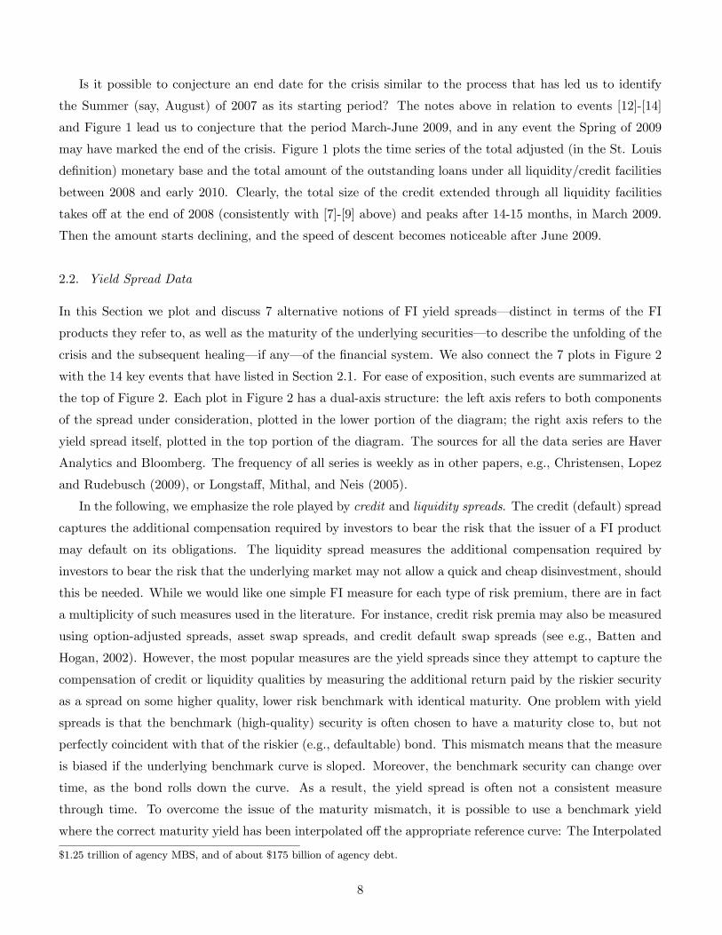
Is it possible to conjecture an end date for the crisis similar to the process that has led us to identify
the Summer (say, August) of 2007 as its starting period? The notes above in relation to events [12]-[14]
and Figure 1 lead us to conjecture that the period March-June 2009, and in any event the Spring of 2009
may have marked the end of the crisis. Figure 1 plots the time series of the total adjusted (in the St. Louis
definition) monetary base and the total amount of the outstanding loans under all liquidity/credit facilities
between 2008 and early 2010. Clearly, the total size of the credit extended through all liquidity facilities
takes off at the end of 2008 (consistently with [7]-[9] above) and peaks after 14-15 months, in March 2009.
Then the amount starts declining, and the speed of descent becomes noticeable after June 2009.
2.2. Yield Spread Data
In this Section we plot and discuss 7 alternative notions of FI yield spreads–distinct in terms of the FI
products they refer to, as well as the maturity of the underlying securities–to describe the unfolding of the
crisis and the subsequent healing–if any–of the financial system. We also connect the 7 plots in Figure 2
with the 14 key events that have listed in Section 2.1. For ease of exposition, such events are summarized at
the top of Figure 2. Each plot in Figure 2 has a dual-axis structure: the left axis refers to both components
of the spread under consideration, plotted in the lower portion of the diagram; the right axis refers to the
yield spread itself, plotted in the top portion of the diagram. The sources for all the data series are Haver
Analytics and Bloomberg. The frequency of all series is weekly as in other papers, e.g., Christensen, Lopez
and Rudebusch (2009), or Longstaff, Mithal, and Neis (2005).
In the following, we emphasize the role played by credit and liquidity spreads. The credit (default) spread
captures the additional compensation required by investors to bear the risk that the issuer of a FI product
may default on its obligations. The liquidity spread measures the additional compensation required by
investors to bear the risk that the underlying market may not allow a quick and cheap disinvestment, should
this be needed. While we would like one simple FI measure for each type of risk premium, there are in fact
a multiplicity of such measures used in the literature. For instance, credit risk premia may also be measured
using option-adjusted spreads, asset swap spreads, and credit default swap spreads (see e.g., Batten and
Hogan, 2002). However, the most popular measures are the yield spreads since they attempt to capture the
compensation of credit or liquidity qualities by measuring the additional return paid by the riskier security
as a spread on some higher quality, lower risk benchmark with identical maturity. One problem with yield
spreads is that the benchmark (high-quality) security is often chosen to have a maturity close to, but not
perfectly coincident with that of the riskier (e.g., defaultable) bond. This mismatch means that the measure
is biased if the underlying benchmark curve is sloped. Moreover, the benchmark security can change over
time, as the bond rolls down the curve. As a result, the yield spread is often not a consistent measure
through time. To overcome the issue of the maturity mismatch, it is possible to use a benchmark yield
where the correct maturity yield has been interpolated off the appropriate reference curve: The Interpolated
$1.25 trillion of agency MBS, and of about $175 billion of agency debt.
8
Spread or I-spread is the difference between the yield to maturity of the bond and the linearly interpolated
yield to the same maturity. All the yield spreads data used in this paper are interpolated spreads.
We now turn to a brief description of the 7 yield spread series in Figure 2. The Off-On the Run Treasury
spread is the difference between the yield of a Treasury with a residual maturity of 10 years but not recently
issued and the yield of highly liquid, frequently traded Treasury securities–in this case the most recently
issued security with a 10-year maturity. This spread is commonly interpreted as a measure of the market
liquidity risk premium because–given that its definition should try to minimize maturity mis-matches by
interpolation–two Treasuries with identical maturity should imply identical credit risk and differ only for
the higher “convenience yield” that a highly traded security gives over another security that is traded
infrequently. Figure 2 shows that until late 2007 the off-the-run/on-the-run spread oscillated around its
typical, long-run average of 14-18 bp. with isolated peaks of 20 bp. However, starting from October 2007,
this spread starts exhibiting a modest but noticeable upward trend that leaves it oscillating between 10 and
30 bp for most of 2008, before August. As a result of Lehman’s default in September 2008, the liquidity
premium goes through the roof, repeatedly peaking at levels in excess of 70 bp. and rarely receding below
20 bp throughout the rest of 2008 and until February 2009. During this period, the spread also appears to
be exceptionally volatile. Starting in March 2009, the off-the-run/on-the-run spread exhibits a pronounced
downward trend that stabilizes it back to 15-30 bp. by late 2009.
During the financial crisis, the LIBOR-OIS spread has been a closely watched barometer of distress in
money markets. The 3-month LIBOR is the interest rate at which banks borrow unsecured funds from other
banks in the London wholesale money market for a period of 3 months. The Overnight Indexed Swap (OIS)
rate is the fixed interest rate a bank receives in 3-month swaps between the fixed OIS rate and a (compound)
interest payment on the notional amount to be determined with reference to the effective federal funds rate.
The nature of the LIBOR-OIS spread is not completely clear. At face value, the spread measures a credit
risk premium: while the LIBOR, referencing a cash instrument, reflects both credit and liquidity risk, the
OIS is a swap rate and as such it has little exposure to default risk because swap contracts do not involve
any initial cash flows. However, the typical default risk implicit in LIBOR rates is modest.6 Figure 2
shows a pattern for the LIBOR-OIS spread that is qualitatively similar, but considerably more extreme
than the off-the-run/on-the-run spread. Until July 2007, the LIBOR-OIS spread moved in narrow corridor,
between 1 and 11 bp. At the onset of the crisis, the spread jumped to 90 bp and remained between 50
and 100 bp throughout the Summer of 2008, which is a remarkable 5-10 multiple of the historical pre-crisis
norm. However, it is after Lehman’s bankruptcy that the LIBOR-OIS spread skyrocketed to an exceptional
(but short-lived) 345 bp. In early 2009 the spread still appeared to have remained substantially alterated,
exceeding 100 bp. After March 2009, the LIBOR-OIS spread started gradually declining, oscillating between
10 and 15 bp in 2010, in line with the pre-crisis experience.
6A few researchers (e.g., Christensen et al., 2009) have argued that especially during the financial crisis the spikes in the
LIBOR rate may have reflected liquidity risks as well as credit risks.
9
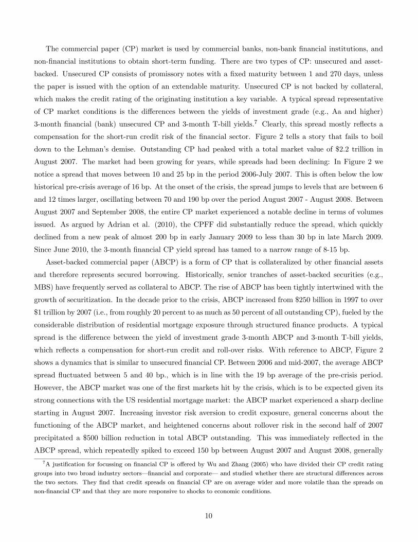
The commercial paper (CP) market is used by commercial banks, non-bank financial institutions, and
non-financial institutions to obtain short-term funding. There are two types of CP: unsecured and asset-
backed. Unsecured CP consists of promissory notes with a fixed maturity between 1 and 270 days, unless
the paper is issued with the option of an extendable maturity. Unsecured CP is not backed by collateral,
which makes the credit rating of the originating institution a key variable. A typical spread representative
of CP market conditions is the differences between the yields of investment grade (e.g., Aa and higher)
3-month financial (bank) unsecured CP and 3-month T-bill yields.7 Clearly, this spread mostly reflects a
compensation for the short-run credit risk of the financial sector. Figure 2 tells a story that fails to boil
down to the Lehman’s demise. Outstanding CP had peaked with a total market value of $2.2 trillion in
August 2007. The market had been growing for years, while spreads had been declining: In Figure 2 we
notice a spread that moves between 10 and 25 bp in the period 2006-July 2007. This is often below the low
historical pre-crisis average of 16 bp. At the onset of the crisis, the spread jumps to levels that are between 6
and 12 times larger, oscillating between 70 and 190 bp over the period August 2007 - August 2008. Between
August 2007 and September 2008, the entire CP market experienced a notable decline in terms of volumes
issued. As argued by Adrian et al. (2010), the CPFF did substantially reduce the spread, which quickly
declined from a new peak of almost 200 bp in early January 2009 to less than 30 bp in late March 2009.
Since June 2010, the 3-month financial CP yield spread has tamed to a narrow range of 8-15 bp.
Asset-backed commercial paper (ABCP) is a form of CP that is collateralized by other financial assets
and therefore represents secured borrowing. Historically, senior tranches of asset-backed securities (e.g.,
MBS) have frequently served as collateral to ABCP. The rise of ABCP has been tightly intertwined with the
growth of securitization. In the decade prior to the crisis, ABCP increased from $250 billion in 1997 to over
$1 trillion by 2007 (i.e., from roughly 20 percent to as much as 50 percent of all outstanding CP), fueled by the
considerable distribution of residential mortgage exposure through structured finance products. A typical
spread is the difference between the yield of investment grade 3-month ABCP and 3-month T-bill yields,
which reflects a compensation for short-run credit and roll-over risks. With reference to ABCP, Figure 2
shows a dynamics that is similar to unsecured financial CP. Between 2006 and mid-2007, the average ABCP
spread fluctuated between 5 and 40 bp., which is in line with the 19 bp average of the pre-crisis period.
However, the ABCP market was one of the first markets hit by the crisis, which is to be expected given its
strong connections with the US residential mortgage market: the ABCP market experienced a sharp decline
starting in August 2007. Increasing investor risk aversion to credit exposure, general concerns about the
functioning of the ABCP market, and heightened concerns about rollover risk in the second half of 2007
precipitated a $500 billion reduction in total ABCP outstanding. This was immediately reflected in the
ABCP spread, which repeatedly spiked to exceed 150 bp between August 2007 and August 2008, generally
7A justification for focussing on financial CP is offered by Wu and Zhang (2005) who have divided their CP credit rating
groups into two broad industry sectors–financial and corporate– and studied whether there are structural differences across
the two sectors. They find that credit spreads on financial CP are on average wider and more volatile than the spreads on
non-financial CP and that they are more responsive to shocks to economic conditions.
10
oscillating around a new, higher mean of 120-130 bp. Naturally, the collapse of Lehman, one of the major
players in the ABCP market, sent spreads to extraordinarily high levels, in excess of 300 bp. However, as
in the case of financial CP the creation of the CPFF and of the AMLF in September 2008 greatly helped
in bringing the situation under control and lowered the spreads back to “physiological levels” (see Adrian
et al., 2009). ABCP spreads have returned below 100 bp around the end of 2008 and after the beginning of
the Spring of 2009 they have been oscillating between 10 and 20 bp, in-line with pre-crisis levels.
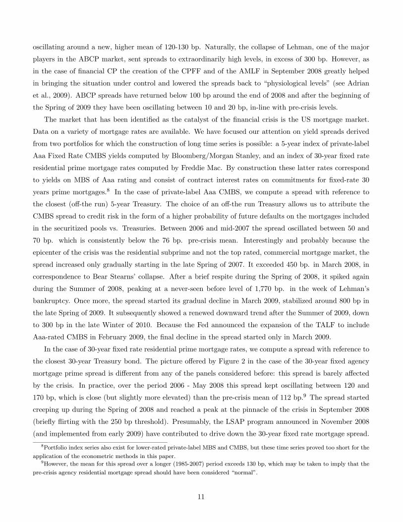
The market that has been identified as the catalyst of the financial crisis is the US mortgage market.
Data on a variety of mortgage rates are available. We have focused our attention on yield spreads derived
from two portfolios for which the construction of long time series is possible: a 5-year index of private-label
Aaa Fixed Rate CMBS yields computed by Bloomberg/Morgan Stanley, and an index of 30-year fixed rate
residential prime mortgage rates computed by Freddie Mac. By construction these latter rates correspond
to yields on MBS of Aaa rating and consist of contract interest rates on commitments for fixed-rate 30
years prime mortgages.8 In the case of private-label Aaa CMBS, we compute a spread with reference to
the closest (off-the run) 5-year Treasury. The choice of an off-the run Treasury allows us to attribute the
CMBS spread to credit risk in the form of a higher probability of future defaults on the mortgages included
in the securitized pools vs. Treasuries. Between 2006 and mid-2007 the spread oscillated between 50 and
70 bp. which is consistently below the 76 bp. pre-crisis mean. Interestingly and probably because the
epicenter of the crisis was the residential subprime and not the top rated, commercial mortgage market, the
spread increased only gradually starting in the late Spring of 2007. It exceeded 450 bp. in March 2008, in
correspondence to Bear Stearns’ collapse. After a brief respite during the Spring of 2008, it spiked again
during the Summer of 2008, peaking at a never-seen before level of 1,770 bp. in the week of Lehman’s
bankruptcy. Once more, the spread started its gradual decline in March 2009, stabilized around 800 bp in
the late Spring of 2009. It subsequently showed a renewed downward trend after the Summer of 2009, down
to 300 bp in the late Winter of 2010. Because the Fed announced the expansion of the TALF to include
Aaa-rated CMBS in February 2009, the final decline in the spread started only in March 2009.
In the case of 30-year fixed rate residential prime mortgage rates, we compute a spread with reference to
the closest 30-year Treasury bond. The picture offered by Figure 2 in the case of the 30-year fixed agency
mortgage prime spread is different from any of the panels considered before: this spread is barely affected
by the crisis. In practice, over the period 2006 - May 2008 this spread kept oscillating between 120 and
170 bp, which is close (but slightly more elevated) than the pre-crisis mean of 112 bp.9 The spread started
creeping up during the Spring of 2008 and reached a peak at the pinnacle of the crisis in September 2008
(briefly flirting with the 250 bp threshold). Presumably, the LSAP program announced in November 2008
(and implemented from early 2009) have contributed to drive down the 30-year fixed rate mortgage spread.
8Portfolio index series also exist for lower-rated private-label MBS and CMBS, but these time series proved too short for the
application of the econometric methods in this paper.9However, the mean for this spread over a longer (1985-2007) period exceeds 130 bp, which may be taken to imply that the
pre-crisis agency residential mortgage spread should have been considered “normal”.
11
In fact, this spread not only returned to its normal, pre-crisis levels (around 100 bp) by March 2009, but
subsequently it kept declining until stabilizing around 50 bp in early 2010, which are incredibly low levels
from a historical perspective.10 The fact that this spread has not reflected the crisis and it has actually been
reduced by the policy-makers’ reactions should come as no surprise if LSAP were effective.
Finally, we have also analyzed the Moody’s Baa-Aaa corporate yield spread, the difference between the
average yields of two portfolios of corporate bonds maintained and published by Moody’s: a portfolio of
Baa (i.e., the lowest investment grade rating) corporate bonds with maturities of approximately (at least)
20 years; a portfolio of similar, 20-year maturity bonds with Aaa rating issued by corporations. Given that
the spread is based on portfolios that–at least as a first approximation–differ only in their ratings, this
is an obvious credit risk premium that compensates a differential likelihood of default. Figure 2 shows the
familiar pattern. Until the end of the Summer of 2007, the default spread was oscillating in a narrow range
of variation, between 80 and 100 bp. This appears completely typical of pre-crisis experiences, when the
mean had been 98 bp. If anything, the spread appeared to gravitate towards the low-end of its typical range
of variation, which may indicate some over-pricing of lower credit ratings. The ascent of the default spread
started in early October 2007 and was initially measured, bringing it to approximately 150 bp by the end of
August 2008. Once more, Lehman’s default marked a turning point, as the spread spiked to reach 300 bp
during September 2008. It is interesting to notice that financial distress took a few months to contaminate
the long-term segments of the corporate bond market. The peak was in fact reached in early December
2008, at 347 bp. The aggressive reaction by the Fed lowered the spread below 300 bp during February 2009,
although a new local spike in excess of 300 bp occurred in April 2009. From that point on, the default
spread stabilized and quickly decreased, reaching a “close-to-normal” level slightly in excess of 100 bp.
Table 1 performs a comparison between means (medians), volatility (interquartile range) of spreads for
three periods: before the crisis (Dec. 2001-July 2007, a sample of 296 weeks), during the crisis (Aug. 2008-
June 2009, a sample of 100 weeks), and after the crisis (July 2009-Febr. 2010, a sample of 33 weeks). The
before-crisis period is easy to characterize: spreads were on average low, often lower than average spreads
over the full-sample periods (unreported). The medians are also small and not very different from means,
which is reflected by the modest and often not statistically significant skewness coefficients. The volatilities
of the spreads are tiny, always between 5 and 36 bp per week, with moderate differences when compared to
interquartile ranges. In the central crisis-related panel, all mean spreads increase, reaching levels between
2 and 9 times the pre-crisis means. The only exception concerns the 30-year fixed rate mortgage spread,
whose mean increases by a timid 44%. In this case, medians are often quite different from the means. This
is reflected by many positive and statistically significant skewness coefficients (see e.g., Manzoni, 2002).
Moreover, both the standard deviations and the interquartile ranges of the spreads increase enormously
10In a long, 1985-2010, weekly time series for this spread, we have that the minimum historical observation has occurred in
mid-December 2009 (at 37 bp). The other two periods of low agency residential mortgage spreads have been 1992 and 2003-2004,
when the 30-year spread persistently declined below 100 bp, with troughs of 40-50 bp.
12
during the crisis, ranging from 19 bp per week for the On-/Off-the run Treasury spread to 446 bp for the
5-year CMBS spread. The only exception is the 30-year mortgage rate, where all volatilities increase by a
factor of between 2 and 30. Although the sample becomes short, all means and volatilities decline when
moving from the crisis to the post-crisis period.
Figure 3 offers a visual summary. While our comments to Tables 1-2 have stressed means as a measure
of location of a series, Figure 3 presents the same information using two nonparametric statistics of location
and dispersion, the median and the interquartile range. The upper panel shows that for 5 spreads out of
7, the crisis marks a clear peak in the spread levels, with the crisis (middle, red) bars ranging between 30
and 200 percent higher than the pre-crisis (left, green) bars. In most cases, the spreads stabilize back to the
pre-crisis level in the post-crisis period (the right, yellow bars). The first exception is the 10-year Off-On-the
run Treasury spread, where the visual impression is that there is no effect of the crisis. However, this is only
due to the scale of the graph which, to accommodate the enormous variation in the 5-year CMBS spread,
largely hides the qualitative variation in the liquidity spread. The second exception is the 30-year fixed rate
residential mortgage spread. The bottom panel of Figure 3 depicts dynamics in the interquartile range. A
pattern emerges: spreads became much more variable during the crisis than they were before. In terms
of interquartile range, the increase was often between 5 and 20 times the level of the pre-crisis dispersion
measure. Once more, the only exception is the 30-year mortgage spread, which has become less variable
during the crisis. This should be expected as this outcome is likely to have been caused by the stabilizing
effects of the LSAP program that the Fed has implemented during 2008 and 2009.
3. The Empirical Model
We base our empirical tests on a simple univariate time series benchmark for the change in the yield spread
index (see e.g., Joutz and Maxwell, 2002; Manzoni, 2002),
∆ = ∆−1 + (−1 − ) + ∼ IID (0 2) (1)
where is a yield spread, ∆ ≡ − −1 is the change in the spread between week − 1 and week , ,
and are constant parameters to be estimated, and is a white noise shock. (1) has the structure of
a classical partial adjustment model, in the sense that it implies that the change in spread between time
− 1 and is also explained by the deviation of the spread at time − 1 from some “benchmark” level,
represented by the parameter . We have written “also” because the other component that explains ∆
is given by ∆−1 which is a traditional autoregressive term. For instance, when 1 0 and 0
(1) implies that a portion of the most recent change in the spread will keep propagating to time as
captured by the term ∆−1. At the same time, if in the previous period the spread has been higher than
then the spread will be reduced by (−1 − ) 0; if in the previous period the spread has been lower
than , then the spread will increase by (−1 − ) 0. This is the sense in which (1) captures mean
reversion towards when 0 and conversely mean aversion away from when 0 (1) is consistent
13
with Hendry, Pagan and Sargan’s (1984) view of error-correction models as reparameterization of dynamic
linear regression models in terms of differences and levels.11
It is easy to devise simulations to show that in the mean-reverting case of 0, the spreads tends to
converge towards and then tends to oscillate around it, while in the mean-averting case of 0 any
shock will cause the spread to permanently drift away from . In particular, when 0 and the spread
is initialized to be above it diverges to +∞. This is not economically plausible (it means that the priceof the underlying FI product must vanish). Even worse, if the spread is initialized to be below , then it
diverges to −∞ and it becomes negative in finite time. Because all the spreads we are examining in this
paper have a clear interpretation as risk premia, it is clear that to think of a permanently negative (in fact,
diverging) risk premium makes little sense. Therefore (1) is an implausible model unless 0. In the
knife-edge case of = 0, (1) simplifies to ∆ = ∆−1 + , which means that ∆ is a simple AR(1)
model. In this case, = (1 + )−1 − −2 + a (non-stationary) AR(2) model with no intercept and
with the two autoregressive coefficients restricted to be linear functions of a single parameter . In fact,
when = 0, ∆ becomes a white noise process with zero mean, = −1 + which is a classical random
walk process with no drift. This means that in finite time, is bound to become negative. and that its
first-moment is not defined. Both are unattractive properties for a yield spread. Because the spread is a
random walk, we also know that it can be written as =P
=0 which shows that any of the shocks
will affect the spread forever, i.e., the process has infinite memory. These properties explain why not only
0 but also = 0 has to be thought of as implausible.
Another useful perspective comes from noticing that (1) can be re-written as
= (1+)−1−−2+(−1−)+ = −+(1++)−1−−2+ = 0+1−1+2−2+ (2)
which is an AR(2) model with cross-coefficient restrictions as 0 = − 1 = 1 + + , and 2 = −.Interestingly, although the representation in (1) is the one with the strongest underlying economic intuition,
in the applied econometrics literature, the representation in (2) and its equivalence to (1) is what seems to
have drawn the attention to (1) itself.12 Notice that because corresponds to the unconditional mean of
the AR(2) representation, assumed to exist, i.e.,
[] =0
1− 1 − 2=
−1− (1 + + )− (−) = (3)
the error correction model may be equivalently interpreted as stating that the change in the spreads is asso-
ciated with the past movement in the spread plus a portion of the deviation from the long-run equilibrium
11This univariate error correction model (ECM) is not the same as (multivariate) ECMs employed in cointegration analysis
(e.g., see Joutz and Maxwell, 2002), where a multivariate model is internally consistent only if the variables are cointegrated.12For instance, Nickell (1985) has commented that “Since it is almost a stylized fact that aggregate quantity variables in
economics follow a second order autoregression with a root close to unity, we may expect to find the error correction mechanism
appearing in many different contexts.” (p. 124). Nickell also shows that a random walk with a moving average error also gives
rise to an error correction-type equation that shares many features with (1).
14
level, identical to the unconditional mean [] = . This is another advantage of the representation in (1):
the long-run mean of the process has become an explicit, estimable parameter.
3.1. The Meaning of 0
It is easy to show that 0 is a (part of a set of) sufficient condition(s) that guarantees the covariance
stationarity of (1). Therefore, 0 not only ensures that the process (1) is economically sensible, but
also that the process defined by (1) is “well behaved”. This is easily seen exploiting the (2) representation,
(1 − 1 − 22) = 0 + , where is the lag operator. This stochastic difference equation is stable
and the AR(2) process covariance-stationary, provided that the roots of the equation 1−1−22 = 0 lie
outside the unit circle, or
|12| =¯¯1 ±
q21 + 42
22
¯¯ =
¯¯(1 + + )±
p(1 + + )2 − 4−2
¯¯ 1 (4)
If we set = 0 (as we have done in Figure 4), then 2 = 0 and the polynomial simplifies to an AR(1)
characteristic polynomial, (1 − 1) = 0 + , which is covariance stationary provided that |11| =|1(1 + )| 1 and this requires 0. In general, when 6= 0, whether or not all the roots from (4) lie
outside the unit circle will be a complicated function of both and . However, it is easy to compute that
a min ' −05 exists such that if min 0 1 and −1 0 (simultaneously) are jointly sufficient
(but not necessary) for the roots of the AR(2) characteristic polynomial to fall outside the unit circle.
This sufficient condition has an appealing interpretation if applied to the original, partial error correction
representation (1): min 0 1 is a restriction to the standard stationarity condition within a simple
AR(1) model; −1 0 satisfies the same intuition provided above, where −1 is to be consideredinnocuous as our empirical estimates in Section 4.2 will reveal that tends to always be negative.
3.2. Testing for Instability
Because model (1)-(2) is completely described by its parameters, model stability is equivalent to parameter
stability. A large literature has emerged in econometrics that develops tests of model stability. One of the
most common tests is Chow’s (1960) simple split-sample test. This test is designed to test the null hypothesis
of constant parameters against an alternative of a one-time shift in the parameters at some known time. The
idea of the breakpoint Chow test is to fit a given model separately for each of the two (or ≥ 2) sub-samplesgenerated by a fixed break data and to see whether there are significant differences in the parameters of the
estimated equations. A significant difference indicates a structural change in the relationship. In the case
of (1)-(2), the Chow breakpoint -statistic is based on the comparison of the restricted and unrestricted
sum of squared residuals and in the simplest case involving a single breakpoint, is computed as
=[²0²− (²01²1 + ²02²2)]3(²01²1 + ²
02²2)( − 6)
(5)
15
where ² is the ×1 vector of residuals when the model is estimated on some sub-samples of observations,²0² is the restricted sum of squared residuals when no break is imposed, and ²0² is the sum of squared
residuals from the subsample = 1 2. Assuming the candidate breakpoint date is exogenous, the F-statistic
has an exact finite sample F-distribution if the errors are i.i.d. and normal. The log likelihood ratio (LR)
statistic is based on the comparison of the restricted and unrestricted maximum of the (Gaussian) log
likelihood function and has an asymptotic distribution with degrees of freedom equal to under the null
hypothesis of no structural change.
As an alternative to the classical Chow test, tests for structural change for every breakpoint can be
calculated. Although this is the test was originally proposed by Quandt (1960), a distributional theory has
been developed in Andrews (1993) and Hansen (1997). The resulting test is the Quandt-Andrews breakpoint
test for one or more unknown structural breakpoints. Call θ ≡ [ ]0 and let [ ] = 1 denote the integer
part of where 0 ≤ ≤ 1. Thus, the proportion defines sub-period 1, = 1 1. Under
the null hypothesis, (1)-(2) is stable for the entire sample period. Under the alternative hypothesis, the
model characterized by the estimator θ1() applies to observations 1 [ ] and model with θ2() applies
to the remaining − [ ] observations. This describes a nonstandard sort of hypothesis test since underthe null hypothesis, the parameter of interest, , is not part of the model. At this point, the idea is that
a single Chow test is performed at every observation between two dates, and , where ≡ [ ]and ≡ [ ]. The [(1− − ) ] test statistics from these Chow tests are summarized into one test
statistic for a test against the null hypothesis of no breakpoints between and , where + is the
percentage of observations set aside and not used to test for breaks. From each individual Chow test, two
statistics are usually reported: the Likelihood Ratio F-statistic and the Wald F-statistic. Conditioning on
being fixed, the two test statistics for testing the hypothesis of model constancy against the alternative
of structural break at are as follows. The Wald statistic is13
() = [θ1()− θ2()]0{V1() + V2()}−1[θ1()− θ2()] (6)
where V() is the (asymptotic) covariance matrix estimator for θ from the 1 [ ] sample in the case of
= 1 and from the [ ] +1 [ ]+ 2 ..., sample in the case of = 2 The likelihood ratio-like statistic is
() = [1(|θ1()) + 2(|θ2())]− [1(|θ) + 2(|θ)] (7)
where θ is based on the full sample. In both cases, the statistic has a limiting chi-squared distribution with
degrees of freedom, where is the number of parameters in the model, = 3 in the case of (1)-(2).
Since is unknown, the two tests presented above do not solve the problem posed at the outset. Andrews
(1993) has derived the behavior of these test statistics by Monte Carlo by simulating it over a range of
candidate values for . This means, for different partitionings of the sample in the interval [ ] and
13There is a small complication with this result in a time-series context. The two subsamples are generally not independent so
using V1()+V2() as an estimator for the covariance matrix of 1()− 2() may be inappropriate. However, asymptoticallythe number of observations close to the switch point, if there is one, becomes small, so this is only a finite sample problem.
16
retaining a few functions of the sequences of values obtained, for instance their maximum value for ∈[ ]. Andrews (1993) and Andrews and Ploberger (1994) have derived the non-standard asymptotic
distributions for three statistics that summarize the behavior of () and () as changes. Among
these there are the widely employed maximum (also called Sup) statistics:14
() = max≤≤
() and () = max≤≤
() (8)
Hansen (1997) has provided approximate asymptotic p-values which are used in our empirical work. The
distribution of these statistics becomes degenerate as → 0+ or → 1− i.e., when we approach the
beginning or the end of the sample. To compensate for this behavior, it is suggested that the ends of the
equation sample not be included in the testing procedure, by setting = 0 and = 1− 1 with
the trimming parameter typically between 5 and 10% of the sample. We use a 10% trimming throughout.
4. Empirical Results
4.1. Are the Spreads Stationary?
Our first step consists of verifying that it is sensible to model spreads using a covariance stationary model
with structure (1)-(2). In particular, since (2) needs to be covariance stationary, it is important to start
by asking whether the FI yield spreads under investigation may contain a unit root.15 Table 2 reports the
results of a standard Augmented Dickey-Fuller (ADF) test, when the number of lags of changes in the spread
to be included in the underlying model is selected by minimization of the BIC information criterion with a
maximum number of lags equal to 12. The table also reports the results from an alternative, nonparametric
Phillips-Perron (PP) test that controls for serial correlation when testing for a unit root induced by violation
of the classical Dickey and Fuller’s AR(1) framework.16 In the table, boldfaced p-values indicate that the
null of a unit root is rejected with a p-value of 10% or lower, an indication of covariance stationarity for the
yield spread series examined.
Table 2 shows that most (all) of the yield spread series under consideration are covariance stationary.
In the case of the ADF test, the evidence is overwhelming: in 4 cases out of 7 the ADF p-value is actually
lower than 5%, while in other 3 cases the ADF p-value is between 5 and 10%, which still represents evidence
14Two alternatives to the Sup are suggested by Andrews and Ploberger (1994) and Sowell (1996). The average statistics,
() and (), are computed by taking the sample average of the sequence of values over the [(1 − − ) ]
partitions of the sample for ∈ [ ] The exponential statistics are computed as () = ln{([(1 − − ) ])−1
∈[ ] exp[05 ()]} and likewise for the exponential LR statistics. However, Andrews and Ploberger (1994) suggest
that the Exp LR and Avg LR versions may often be less than optimal.15In economic terms, we know already the answer: because a spread containing a unit root will eventually become negative
and spend an infinite time providing negative compensation to credit and liquidity risks, this hardly makes sense.16The PP method estimates the non-augmented DF test equation and modifies the t-ratio of the key coefficient so that serial
correlation does not affect the asymptotic distribution of the test statistic. The residual spectrum at frequency zero is estimated
using a Bartlett kernel-based sum-of-covariances with a Newey-West bandwidth. In both the ADF and PP tests, the “exogenous
regressors” are simply a constant intercept as it is implausible to find time trends in risk premia.
17
against the null of a unit root. The evidence in favor of covariance stationarity of the spreads is even stronger
when the PP test is applied. Five yield spread series out of 7 lead to p-values below 5%. However, in this
case one of the two cases left (the 3-month LIBOR-OIS spread) produces a p-value of 0.078, while the other
(the 5-year CMBS-Treasury spread) actually shows evidence of containing a unit root (the p-value is 0.108
and does not allow to reject the null). However, even in this case of conflicting evidence from ADF vs. PP
tests, we have to remind ourselves that the vast majority of unit root tests have non-stationarity, i.e., a unit
root as their null hypothesis. Because the traditional classical methodology accepts the null unless there is
strong evidence against it, unit root tests usually tend to conclude that there is a unit root. The problem is
exacerbated by the fact that unit root tests generally have low power. In this sense, one may be favorable to
resolve the tension between the 0.080 ADF p-value and the 0.108 PP p-value for the 5-year CMBS-Treasury
spread in favor of stationarity. We have also repeated these tests with reference to the common pre-crisis
sample period (December 2001 - July 2007) in Table 2, finding identical results. All in all, we conclude that
a (1)-(2) representation may be consistent with stationarity of the underlying monthly spread series.17
4.2. Model Estimates
We estimate model (1) for a few alternative sub-periods.18 The results are reported in Table 3. A general
result emerges: for all sample periods, the estimated model turns out to be covariance stationary, in the
sense that the estimated coefficients θ ≡ [α ]0 map into φ ≡ [0 1 2]0 vectors that satisfy (4). This
explains why in Table 3 the estimated half-life of a shock is always a finite value, which is an implication of
covariance stationarity. This is a first important finding: even in the midst of the Great 2007-2008 Financial
Crisis, FI markets never unravelled to the point of implying non-stationary yield spread dynamics, which
would imply an infinite half-life of a shock, i.e., that whatever shock would never be re-absorbed.19
The first panel of Table 3 shows full-sample results.20 is negative for all seven spreads and only in
one case (for the 5-year CMBS spread, which is in some sense consistent with Table 2) 0 fails to be
statistically significant (but the p-value is 0.06). In fact, some yield spreads display a considerable speed of
reversion to the mean, in particular the short-term (Off-On the run Treasury, LIBOR-OIS, Financial CP-
Treasury, and ABCP-Treasury) spreads. These are all characterized by s below -0.06 and p-values of 0.00
17Using daily data, earlier papers (e.g., In et al. , 2003; Joutz and Maxwell, 2002; Manzoni, 2002) have concluded that a
range of alternative daily yield spreads are I(1) series and have therefore modelled their first-difference. However, these papers
often imply that mean spread series are hardly different from zero. In this paper, we model weekly spread series and are able
to identify positive, statistically significant and often high FI risk premia.18The model parameters are estimated by nonlinear least squares (NLS) from (1). Of course, under the assumption of
covariance stationarity, identical parameters can be recovered from MLE estimation of its AR(2) representation. However, we
use this mapping in the reverse fashion only to compute the half-life of a shock and to check for covariance stationarity.19Assuming covariance stationarity, one useful measure of persistence of a dynamic process such as (1)-(2) is how long does
it take for a shock to to be re-absorbed by the dynamic process for the yield spread. The Appendix shows that the half-life
of a shock to (i.e., a one-standard deviation shock) can be computed by solving numerically the inequality in (10)..20Results across different yield definitions are not directly comparable because the series are available for different sample
periods. The second panel of Table 4 shows pre-crisis, common sample evidence that is qualitative similar to the first panel.
18
that imply half-lives between 2 and 11 weeks, which are relatively short and tell us that in the underlying
markets shocks have transient effects on risk premia. The long-term spreads are instead characterized by
smaller estimates of 0 which imply considerably higher half-lives, around 1 year with a maximum of 68
weeks in the case of CMBS spreads. The estimates of the long-run mean are all quite plausible–ranging
from 17 bp in the case of the Off-On the run spread to 206 bp in the case of the CMBS spread–and
statistically significant. Once more the only exception occurs for the CMBS spread, in which case the p-
value of is 0.12. Most of these values, for instance the roughly 100 bp per year for the Baa-Aaa spread,
conform to the priors that are usually reported in the finance literature. A 17 bp per year for the Off-On
the run spread confirms the existence of precisely estimated, but also modest, liquidity premium. Finally,
the estimates of the autoregressive terms tend to be “all over the map” (with both positive and negative
signs) and in some cases are not statistically significant, even though this parameter plays only an indirect
role contributing to the determination of the covariance stationarity of the spread series. Interestingly, even
though (1) has a very stylized structure that obviously fails to account for a number of important influences,
Table 3 shows that the model generally offers a good fit to the data, with 2 peaks in excess of 10% for 3
spreads, consistent with Davies (2008).
The second panel of Table 3 offers similar evidence with reference to a common pre-sample period,
December 2001 - July 2007. In qualitative terms, there are no major changes from the full-sample period,
although here all but one of the estimates of are lower (more negative) and still highly statistically
significant. Together with the values for , these estimates imply half-lives of shocks that are systematically
lower than before, between 2 and 7 weeks in the case of the short-term spreads (Off-On the run Treasury,
LIBOR-OIS, Financial CP, and ABCP), and of 21 weeks for both the CMBS spread and the Baa-Aaa
spread. The only exception occurs with reference to the 30-year fixed mortgage spread, whose half-life
increases from 68 to 76 weeks, while the corresponding increases to only -0.011 and fails to be statistically
different from zero (this is the meaning of the coefficient being bold-faced in Table 3). All in all, this is
evidence that all yield spreads were strongly mean-reverting before the financial crisis, with only the fixed
rate mortgage spread close to the borderline, implying substantial persistence of shocks. A further aspect of
these estimation results is interesting: the pre-crisis period was characterized by implicit long-run spreads
that were very small, possibly surprisingly so. One is tempted to argue that they may have been “excessively”
small, although the absence of a benchmark theoretical model is an obstacle to such a conclusion. All the
estimates of are highly statistically significant.
The third panel concerns the 2007-2009 crisis period and contains some of our key results. Here, once
again, the fundamental contrast is between the fixed rate mortgage spreads and all the remaining spreads.
In general, all the estimates uniformly increase (towards 0) when going from the pre-crisis to the crisis
period. This implies a diminished speed of reversion towards the long run mean. Interestingly, most
estimates increase in absolute value and 3 of them stop being statistically significant (i.e., during the crisis
there is more autoregressive-type persistence in spread changes). Both effects contribute to a discrete jump
19
in the half-life of shocks of most spreads, from +2 weeks in the case of Off-On the run and LIBOR-OIS
spreads to +6 and 8 weeks for CMBS and corporate default spreads. In fact, in these two latter cases, the
estimates remain negative but fail to be statistically significant. The implication is that for 6 spreads out of
7, the financial crisis has implied a higher persistence of changes in the spread and a lower speed of reversion
to its long-run mean for the level of the spread itself. In the perspective of a partial adjustment model such
as (1), this is what a financial crisis is all about in the FI markets: the risk premia (for both credit and
liquidity risks) become highly persistent in the sense that any shocks–and during a crisis we can presume
that many of these shocks will carry a negative sign–take a longer time to be re-absorbed. Needless to say,
higher risk premia mean higher risk-adjusted discount rates when evaluating bonds, and lower (depressed)
market valuations for riskier bonds.
Another–possibly obvious–way in which a financial crisis manifests itself is through the implied esti-
mates of the long-run mean of the spreads, the s. These all increase by a factor between 1.8 and 9 when
we compare the estimates for the pre-crisis with the crisis sample; the smallest increase is a stunning 84%
in the case of the Off-On the run spread (from 15 to 27 bp), while the largest increase–+878% (from 11
to 92 bp) for the LIBOR-OIS spread–hardly deserves any comment and has been the focus of considerable
debate (see e.g., Christensen et al., 2009). The very levels of the s are symptomatic of the crisis, with
3 short-term spreads close to 100 bp per year, two long-term spreads in excess of 150 bp, and the CMBS
spread jumping to an unprecedented 804 bp. Yet, it is remarkable that (1) fits the data rather well during
the financial crisis, with 4 2 exceeding 10% and an impressive 46% for the corporate default spread.
The exception to the broad picture commented here deserves attention because it may have important
implications for the effectiveness of the LSAP programs. The only yield spread series for which we record
a substantial decline in both the implied half-life of a shock (persistence) and a negligible (+25%) increase
in its long-run mean is the 30-year fixed mortgage rate spread, which seems to have been left relatively
unscathed by the Great Financial Crisis. In fact, for this spread even declines when going from the pre- to
the crisis period (from -0.011 to -0.048, even though both estimates are not significant). This explains the
dramatic decline in the half-life estimate from 76 to 16 weeks.21 We attribute this singularity in the dynamics
shifts undergone by the dynamic process characterizing the prime mortgage spread to the effectiveness of
the LSAP programs implemented by the Fed. We return to this point in Section 5.3.
Obviously, it is difficult to miss the fact that a simple inspection of the second and third panels of
Table 3 reveals an enormous amount of instability in most estimated coefficients as well as in the implied
summary statistics. Some dramatic event–we now know it as the Great Financial Crisis–has enveloped
the FI markets and structurally changed their dynamic properties in ways that would have been difficult to
anticipate. This interpretation is further validated by a comparison of the third and fourth panels of the
table: after the crisis was over, the model parameters shifted once more, in this case towards the pre-crisis
levels (see below for specific comments). We formally test these hypothesis in Section 5.3.
21However, the already low 2 (2.1%) of the pre-crisis sample further declines (to 1.2%) in the crisis sample.
20
Finally, the last panel of Table 3 reports estimation results for the post-crisis period, July 2009 - February
2010. At least in a qualitative sense, all the relevant parameters revert back to values typical of the pre-crisis
period. All the estimates decline and–once more, with one exception, 30-year mortgage rate spreads for
which declines, but fails to be statistically significant–mark a renewed strength in the mean reversion
speed of spreads. In fact the estimates for 6 out of 7 stabilize to levels that are below the ones estimated
over the pre-crisis period.22 For these 6 spread series, the implied half-life of a shock is indeed below the pre-
crisis estimates with values between 1 (i.e., no persistence whatsoever) and 9 weeks. In fact, also the half-life
of shocks to mortgage rate spreads has substantially declined from 16 to 9 weeks. This means that these
declining evolution of the estimates have not been reversed by parallel breaks in the estimates reported
in Table 3, fourth panel. In fact, most estimates of the coefficients fail to be statistically significant in the
post-crisis sample. We can summarize these developments by saying that by the second half of 2009, the
financial crisis had stopped exercising its effects on the ability of (US) FI markets to self-correct towards
their long-run equilibria. This is also visible in the estimates of the long-run yield spreads implied by (1):
they all decline towards their pre-crisis levels, although in 2 cases (Off-On the run and CMBS spreads)
they have remained above the pre-crisis levels. In another case (the corporate default spread), the implied
long-run spread has simply stabilized back to the 2002-2007 levels (approximately between 95 and 100 bp).
These reversions of the estimated long-run spreads towards pre-crisis levels represents a further–in a sense,
more obvious–way in which the financial crisis seems to have been over by June 2009.
It is more ambiguous whether policy makers should develop any concerns for the fact that the estimates
for the LIBOR-OIS, the Financial CP, and the ABCP spreads appear to have traced back to long-run levels
that are inferior to their already modest pre-crisis levels.23 It should not be considered surprising that for
30-year mortgage spreads has declined between 2009 and 2010 to an exceptionally low level of 54 bp. This
low level is a likely result of the LSAP programs. However, Table 3 also stresses that any effects of the Fed
policies did not really (or not only) affect the average spreads, but also and especially their “deep” dynamic
properties as revealed by structural changes in the half-life of shocks to fixed mortgage rate spreads.24
4.3. Breakpoint Tests
Table 4 formally tests for the presence of breaks in (1) and contains the other key result of the paper. The left
portion of the table presents Andrews-Quandt break test results, when the date of the break is not assumed
22The only exception is the LIBOR-OIS spread for which the post-crisis is -0.06 vs. a pre-crisis estimate of -0.20. Oddly
enough, the LIBOR-OIS spread half-life has increased from 6 to 10 weeks. This may be related to the growing pressure on
the European fixed income markets later surfaced in the Spring of 2010 with reference to Greek bail-out and the refinancing
difficulties experienced by a few other EU countries, such as Spain and Portugal.23Some commentators (see e.g., Courtois, Gaines, and Hatchondo, 2010) have in fact written about the hazards of re-inflating
asset price bubbles by pushing bond prices (risk premia) too high (low).24However, because LSAP programs have also concerned commercial MBS through extensions of the TALF program during
2009, it is unclear why they have so far failed to produce a reparing influence on the CMBS market of a comparable extent to
the impact caused on the fixed rate residential mortgage market.
21
to be known and its assessment (“estimation”) must be based on the data.25 This a truly “ignorance prior
test” because it does not impose any structure on our search for evidence of potential breaks. The right
portion of the table resorts instead to the more traditional Chow break test, in which the researcher needs
to contribute her knowledge of the potential date of the breakpoints, with all the perils of the assumption.
Clearly, Chow tests are much more efficient in a statistical sense when the researcher is able to feed sensible
candidate break dates to the testing procedure.
The Andrews-Quandt break tests reveal evidence of only one break in the case of two series, the 3-
month ABCP and the 20-year corporate Baa-Aaa spreads; they give instead evidence of two breaks in the
case of other two series, the 3-month LIBOR-OIS and the 5-year CMBS spreads. There is no evidence of
breaks in the remaining 3 spread series, i.e., 10-year Off-On the run, 3-month Financial CP, and 30-year
fixed mortgage spreads. The two series subject to two breaks confirm the boom-bust-boom cycle that we
would expect when a serious financial crisis impacts markets and resolves later on: the first break occurs in
one case in October 2008 (the LIBOR-OIS spread), and in the other case (Baa-Aaa spread) in November
2008. Both breaks are detected at a very high level of statistical significance. In the former case, a second
break (but only using a Maximum Wald Statistic) is detected in correspondence to late 2008 after the full
deployment of the short-term liquidity facilities (e.g., CPFF and MMIFF); in the latter case, a second break
is detected in correspondence of the Spring of 2009. Based on the evidence in Table 3, it is sensible in both
cases to interpret the first breakpoint date as the date in which the corresponding FI markets (LIBOR and
CMBS) have entered the crisis, and the second date as the date in which they have emerged from the crisis.
More puzzling is the fact that two markets seemed to have entered the crisis–in October 2008 in the case
of Financial CP and in July 2007 in the case of the corporate bond market, with both breakpoint dates
detected with very low and reliable p-values–but not to have left it. This is shown by the fact that a second
Andrews-Quandt break test that conditions on a first break returns no evidence of further breakpoints for
these two series. Moreover, the fact that in Table 4 three yield series seem to have not been subject to any
breaks does not square well with the evidence in Table 3. Of course, this may due to the low power that
the Andrews-Quandt test tends to have because the breakpoint date is left unspecified.
To remedy to this drawback, the right portion of Table 4 reports the outcomes of a standard Chow break
test in which the break dates are exogenously specified to correspond to the first week of August 2007 and
the last week of June 2009. The first date is taken to represent the onset of the crisis; the second date
is a candidate date for the end of the crisis. Here the results fully conform with the evidence in Table 3:
for 6 out of 7 yield spreads series, there is evidence of a break in early August 2007. The corresponding
p-values are below 1% for 4 series, while for other 2 series they are between 1 and 5%. Not surprisingly, the
only yield spread not affected by a break in the Summer of 2007 is the 30-year mortgage spread. There are
25Both types of break tests are applied sequentially, in the sense that when the occurrence of a break is isolated (i.e, the null
of no break is rejected), tests for additional breaks are applied conditioning on the date of the first break. The Andrews-Quandt
test is applied to sample observations after cutting the first 5% and the last 5% of the available observations. The last column
of the table shows the possible ranges for break dates in the conditional mean function isolated by both sets of break tests.
22
no economically important differences between the and Log-LR versions of the Chow test. For these 6
spreads, conditioning on a first break occurring in the first week of August 2007, we further proceed to test
for another breakpoint at the end of June 2009.26 For all of the 6 spread series we find evidence of a second
break, which we interpret as evidence of the end of the financial crisis.
The last column of Table 4 provides a summary of the breakpoint test results across different method-
ologies. Clearly, this summary may provide economic intuition, but has no statistical foundation, as it is
impossible to take “averages” of breakpoint dates across methodologies. For only one spread, there is no
evidence of breaks in (1). This series is the 30-year fixed mortgage rate spread. Assuming–in the light of
the evidence for the 5-year CMBS spread–that in the absence of the LSAP programs all of the US resi-
dential mortgage market would have been significantly affected by the 2007-2008 financial crisis, the results
in Tables 3-4 show the substantial success of these policy measures. The remaining 6 series present the
typical boom-bust-boom that we would expect of financial markets when the available data span a complete
financial crisis. They all enter a crisis period–characterized by high persistence of shocks and high long-run
mean spreads (see Table 3)–between August 2007 and November 2008, which fits our summary of the main
events in Section 2.1. They all leave the crisis between December 2008 (for the 3-month LIBOR-OIS spread)
and June 2009, which is what we would have conjectured on the basis of the commentary of Section 2.1.
4.4. How Did the Crisis Affect Bond Markets?
A finding that any of the coefficients in θ ≡ [α ]0 in (1) is subject to one or more structural breaks over
the sample period, is not completely informative because it fails to give adequate information on whether the
breakpoint in the conditional mean process for ∆≡∆ −∆ –where ∆ is the series of changes
in yields for the bond with the highest (lowest) credit risk (liquidity) and ∆ is the series changes in
yields for the bond with the lowest (highest) credit risk (liquidity)–derives from the presence of breakpoints
in the dynamic process for either ∆ or ∆ . We therefore proceed to a further decomposition of our
results through the estimation of the bivariate seemingly unrelated models(∆
= ∆−1 + (−1 − ) +
∆ = ∆−1 + (−1 − ) + (9)
where is the effective federal funds rate and ²≡ [ ]0 ∼ IID (0Σ) Notice that the off-diagonal
element of Σ, [ ], represents the covariance of shocks affecting the two yield series. (9) represents
a restricted SUR bivariate regression because the coefficient loading on past changes in and the
coefficient to which the reversion yields approaches are common across the two equations in the model.
(9) is similar in spirit to the partial error correction model (1) used early on, although there are important
differences. First, current changes in yields are modeled as depending in time − 1 changes in , where
26In the case of the fixed rate mortgage spread we anyway proceed to test for the presence of a first break in 2008 or 2009
and find no evidence of a breakpoint.
23
is used to capture expected movements in interest rates that propagate from monetary policy actions
to the entire yield curve.27 Second, the correction term has in this case structure (−1 − ) ( = )
indicating that when −1 ≷ then the yield would decrease (increase) when 0 and it would increase
(decrease) when 0. However, because it models yield changes on the left-hand side as a function of
deviations of spread from some benchmark level , (9) does not represent a formal error correction model,
it does not have a (vector) autoregressive equivalent representation, and does not represent the long-run
conditional mean of any of the two yield series in (9).28 However, (9) does capture the logic that (risky)
yields adjust when the short-end of the riskfree yield curve moves (e.g., by an expectations hypothesis effect)
and when past credit and liquidity risk premia appear to have deviated from some long-run “norm”.
Although the structure of (9) does not allow us to formally connect the sign or magnitude of the
coefficients and to the covariance stationarity of the process, we have two testable formal hypotheses
concerning these adjustment coefficients:
1. If the yield spread is stationary and mean-reverting, we would expect that ≤ 0 and ≥ 0 i.e.when the spread exceeds some historical norm , both yields should contribute to the adjustment, the
yield on riskier (less liquid) bond by adjusting downwards, and the yield on the less risky (more liquid)
bond by inching up. Of course, 0 and = 0 represents a realistic possibility.
2. Unless 6= no adjustment in the yield spread is possible, although this is a rather weak necessary
condition (one may formulate a sharper condition that , although signs matter as much as
magnitudes in this case).
It may be also of interest to test 0 (or 6= 0), which is equivalent to an expectation hypothesis
effect on yield changes, if we take ffr as the rate representative of the short-end of the yield curve.
We have estimated (9) for each of the 7 yield spread series (i.e., this is total of 14 underlying yield series)
analyzed in this paper. Table 5 presents the results for the three sub-samples already used in Tables 1
and 3, distinguishing between the pre-crisis, crisis, and post-crisis periods. In the Table we have boldfaced
“rejections” of the two hypothesis (mean reversion: either = 0 and 0 or 0 and = 0; the
weaker condition 6= ).29 A glance at the table reveals that the financial crisis may be characterized
as a period in which and/or often have an incorrect sign, and in which the hypothesis that =
is often not rejected. This means that yields stop reacting to departures from the attractor in the way
they should, essentially increasing even when the past spread largely exceeds . On the contrary, in the
27We have also estimated a variety of models like (9) in which current changes in yields dependend on their most recent
change (e.g., ∆ on ∆
−1 etc.) or on the most recent change of the spread, but did not find any substantial differences.
In particular, we have noticed that in the majority of the cases, when has been allowed to differ across equations (i.e., they
become ∆ = ∆−1 + (−1 − ) + = ) Wald tests of the null that the two s were not statistically different
would lead to no rejections.28In a bivariate model one would expect a vector to possibly represent the unconditional means of the series, while is a
scalar. More importantly, notice that is compared to the past yield spread and not to the yield in the error correction term.29We are boldfacing the failure to reject the null hypothesis of = .
24
non-crisis periods and especially in the aftermath of the Great Crisis, we observe that for most spreads, the
conditions ≤ 0 and ≥ 0 hold, while 6= which is compatible with mean-reversion and stationarity
of the spreads. In particular, the pre-crisis period represents a sample in which most bond markets displayed
orderly conditions. There is only some evidence that yields on financial CP and ABCP may have failed to
move in directions opposite to (−1 − ). However, only in the case of the financial CP spread, the null of
= cannot be rejected, and even this occurs at a marginal p-value of 0.104.30 The estimates of are
never found to be statistically significant and is generally rather small, if not negative. This implies that
an expectations hypothesis-like effect on the yields investigated is small at best. Finally, the estimates of
in the pre-crisis panel of the table are generally moderate and consistent with the estimates in Table 3,
which reinforces our interpretation of as a long-run attractor value for the spread.
During the crisis, all the yield spread series are affected by a rejection of either ≤ 0 or of ≥ 0. Thisis consistent with Table 3: yield spreads simply stopped being reverting and this is also shown by the fact
that many yield series have stopped reacting to (−1 − ) at all or, worse, with a sign that is incompatible
with stationarity of the spread. Interestingly, with one exception only, this failure may actually be imputed
to the fact that 0 i.e, it is the yield on the less risky (or more liquid) bond that stops reacting to
abnormally high spreads. Additionally, for 4 out of 7 spreads, = cannot be rejected. Table 5 also
shows that during the crisis period tended to increase to an order of magnitude (between 31 and 1656
percent) higher vs. the pre-crisis period, which is consistent with our findings in Table 3. Interestingly, both
the correlations of residuals in (9) and the adjusted 2 substantially decline during the crisis, which is to be
expected in a period of highly turbulent yield spreads. The lower panel of Table 5 concludes by showing a
complete return to normal market conditions in the post-crisis period, with either ≤ 0 or ≥ 0 satisfiedfor all spreads and 6= failing in only one case (the 30-year fixed mortgage spread).
Table 6 repeats the break-point test analysis in Table 4 for the restricted bivariate SUR model in (9).
Because break-point tests for multivariate models tend to be tricky, we have resorted to testing for breaks
in each of the equations appearing in (9) separately, applying the same tests–Andrews-Quandt with no
exogenously fixed date and Chow tests with dates suggested by the anecdotal evidence in the literature as
well as by the results in Table 4–as in Section 5.3.31 Using Andrews-Quandt tests, we find evidence of two
breaks in at least one yield that is part of the definition of all the yield spreads under investigation; in the
case of the Baa-Aaa corporate default spread we actually find evidence of two breaks both in Baa and in
Aaa yields; in two other cases (3-month financial CP and 3-month ABCP yield spreads), both components
of the spread definition show at least some evidence of a breakpoint. Strikingly, in the case of 5 spreads at
least one of the components is affected by a first break in correspondence to August 2007, which confirms
our previous analysis. However, in the case of the 30-year mortgage spread and for the Baa-Aaa spread the
evidence is in favor of a break in early 2009. This latter result may be related to the tendency of corporate
30Interestingly, = seems also to hold for the CMBS spread, even though the hypothesis of 30 0 cannot be
rejected while is not statistically different from zero.31In this case we report both the Maximum LR and the Average LR statistics, as a robustness check.
25
bond markets during the crisis to reflect with a long lag the mounting stress in shorter-term FI markets.
There is considerable more uncertainty on the dating the second break, which–according to a bust-boom
logic and Table 5–ought to be interpreted as the exit date from the crisis. In four cases, markets seem to
leave the crisis as early as the Spring of 2008 (this happens for the OIS, the 3-month T-bill, and the 5-year
Treasury rates; the 3-month T-bill rate actually appears in the definition of two spreads). In the case of the
LIBOR rate, the second break is estimated to have occurred in October 2008, for the 30-year Treasury rate
in February 2009, and for Baa and Aaa corporate yields between June and August 2009.
Results are qualitatively similar in the right panel of Table 6. In four cases (Off-On the run, LIBOR-OIS,
financial CP, and ABCP spreads) a Chow test rejects the null of no break in correspondence to early August
2007; in a fifth case (CMBS spread) there is also evidence of a break, although the corresponding p-value is
between 0.05 and 0.10. The breaks affect the yields on Treasury bills and notes and the OIS rate. This is
not as counter-intuitive as this may appear because these breaks in the rate process for less risky Treasuries
(and/or more liquid, like in the case of the OIS rate) are consistent with a liquidity crisis in which there is a
massive flight to the safety of Treasuries. In the case of longer-term bonds, it is also possible that the LSAP
interventions may have weighted on the breaks we have isolated. There is instead no evidence of a mid-2007
break in fixed rate mortgage, Baa, and Aaa rates. In the case of the 10-year Off-On the run spread, there
is also evidence of an additional break in the Spring of 2009, which is consistent with Table 5.
5. Conclusions
This paper has employed simple breakpoint tests applied to univariate and bivariate partial correction models
of individual, weekly yield spread series to ask how does a financial crisis affect bond risk (both liquidity and
credit) premia and whether it is possible to “date” a financial crisis. Two insights are important and would
probably deserve further investigation. First, although most commentaries during the crisis have insisted
upon drawing our attention to level of yield spreads as indicators of market disruption, our empirical results
show that the crisis has had the power to affect the persistence structure–more precisely, the typical average
duration of shocks–of the dynamic process followed by the spreads. In a policy perspective, this means that
not only do (bond) risk premia increase during a financial crisis–as everybody would expect–but also that
any shock that may cause these premia to depart from their normal levels, is destined to produce long-lived
effects. Second, we have uncovered evidence that while one market–the prime (agency-sponsored) fixed-
rate residential mortgage market–seems to have escaped the crisis altogether, in a few other FI segments
the crisis is not only over, but the dynamics of spreads seems to have already completed reverted to the
patterns that have characterized the pre-crisis periods. We have argued that our finding of no breakpoints
in the process of residential mortgage spreads may be tentatively ascribed to the success of the portions
of the LSAP programs that led the Fed and the Treasury to intervene in the prime, agency-backed MBS
markets and to provide unlimited financial backstop to losses incurred by the government-sponsored agencies
involved in the housing market. The finding that some markets may have “under”-shot to the bubble-like
26
conditions of the pre-crisis period may instead provide reason for concern.
Of course, this paper could be extended also in ways that do not involve its methods but instead require
extensions to additional data. First, a number of papers (e.g., Gilchrist et al., 2009) have not used standard
index (portfolio) data to build yield spread series but instead carefully constructed credit and liquidity yield
spread indices for different sectors of economic activity, rating categories, and alternative maturities directly
from raw data sets that include individual (corporate) bond prices. It would be important to pursue our
question of whether and how a crisis affects the persistence structure of spread dynamics across different
risk (rating) classes and over the entire term structure of the spreads (see e.g., Ahn, Dieckmann, and Perez,
2009). Second, even if one limits herself to spreads commonly reported in the literature, a number of
additional spreads could have been examined in addition to the seven series used in this paper, such as swap
rate spreads (vs. Treasuries) or medium-term REFCO liquidity (vs. Treasuries) spreads as in In, Brown,
and Fang (2004) and Longstaff, Mithal, and Neis (2005), short-term spreads (vs. Treasuries) for adjustable
mortgage rates which are popular in the real estate finance literature (see e.g., Lehnert, Passmore, and
Sherlund, 2008), and corporate default spreads that also involve non-quality grade bonds (e.g., a Aa-Bbb
junk spread), as in Joutz and Maxwell (2002) and Mody and Taylor (2003).
Appendix A: Half-Life of a Shock in Partial Error-Correction Model
Exploiting the invertibility of a covariance-stationary process, the spread process (1)-(2) can be written as
= (1− 1− 22)−1(0 + ) =
∞X=0
0 +
∞X=0
=
01− 1 − 2
+
∞X=0
where
=1
(1 − 2)1 +
2
(2 − 1)2
and the s ( = 1 2) are the eigenvalues of the characteristic matrix
F ≡"1 + + −
1 0
#
This can be seen by defining ξ ≡ [ −1]0 and re-writing (2) as
ξ =
"0
0
#+
"1 2
1 0
#ξ−1 +
"
0
#= μ∗ +Fξ−1 + v
where μ∗ ≡ [0 0]0 and v ≡ [ 0]0. At this point, standard results (see Hamilton, 1994) give
ξ+ =
−1X=0
F−μ∗ +Fξ +
−1X=0
F−v+ =−1X=0
Fμ∗ +Fξ +
−1X=0
Fv+
where F0 = I2 and in which the first equation is:
+ = e01ξ+ =
−1X=0
e01F
μ∗ +−1X=0
e01F
v+ =
−1X=0
0 +
−1X=0
+
27
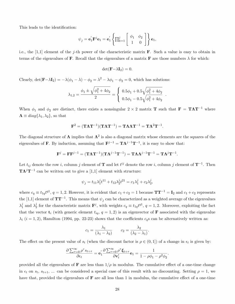
This leads to the identification:
= e01F
e1 = e01
(Q=1
"1 2
1 0
#)e1
i.e., the [1,1] element of the -th power of the characteristic matrix F. Such a value is easy to obtain in
terms of the eigenvalues of F. Recall that the eigenvalues of a matrix F are those numbers for which:
det(F−I2) = 0
Clearly, det(F−I2) = −(1 − )− 2 = 2 − 1 − 2 = 0 which has solutions:
12 =1 ±
q21 + 42
2=
⎧⎨⎩ 051 + 05
q21 + 42
051 − 05q21 + 42
When 1 and 2 are distinct, there exists a nonsingular 2 × 2 matrix T such that F = TΛT−1 where
Λ ≡ {1 2}, so that
F2 = (TΛT−1)(TΛT−1) = TΛΛT−1 = TΛ2T−1
The diagonal structure of Λ implies that Λ2 is also a diagonal matrix whose elements are the squares of the
eigenvalues of F. By induction, assuming that F−1 = TΛ−1T−1 it is easy to show that:
F = FF−1 = (TΛT−1)(TΛ−1T−1) = TΛΛ−1T−1 = TΛT−1
Let denote the row , column element of T and let denote the row , column element of T−1. Then
TΛT−1 can be written out to give a [1,1] element with structure:
= 11111 + 12
221 = 1
1 + 2
2
where ≡ 11 = 1 2 However, it is evident that 1+ 2 = 1 because TT
−1 = I2 and 1+ 2 represents
the [1,1] element of TT−1. This means that can be characterized as a weighted average of the eigenvalues
1 and
2 for the characteristic matrix F
, with weights ≡ 11 = 1 2. Moreover, exploiting the fact
that the vector t (with generic element , = 1 2) is an eigenvector of F associated with the eigenvalue
( = 1 2), Hamilton (1994, pp. 22-23) shows that the coefficients s can be alternatively written as:
1 =1
(1 − 2)2 =
2
(2 − 1)
The effect on the present value of (when the discount factor is ∈ (0 1]) of a change in is given by:
P∞
=0 +
= e
01
P∞
=0 ξ+
v0e1 =
1
1− 1 − 22
provided all the eigenvalues of F are less than 1 in modulus. The cumulative effect of a one-time change
in on +1 ... can be considered a special case of this result with no discounting. Setting = 1, we
have that, provided the eigenvalues of F are all less than 1 in modulus, the cumulative effect of a one-time
28
change in on the spread is given by 1(1− 1 − 2), which can alternatively be interpreted as giving the
eventual long-run effect on the spread of a permanent change in . Therefore the half-life of a shock
to (i.e., a one-standard deviation shock) is defined as
ÄX
=0
+
=
X=0
=
X=0
∙1
(1 − 2)1 +
2
(2 − 1)2
¸≥ 12
1
1− 1 − 2
where 1 ≡ 05(1 + + ) + 05p(1 + + )2 − 4 2 ≡ 05(1 + + ) − 05
p(1 + + )2 − 4 which
can be shown to be equivalent to:
1
(1 − 2)
1− +11
1− 1+
2
(2 − 1)
1− +12
1− 2≥ 12
1
1− 1 − 2 (10)
This equation can be solved numerically to find the minimum such that the right-hand side exceeds half
of the long-run effect of a shock.
References
[1] Ahn, S., S., Dieckmann, and M., Perez. “Exploring Common Factors in the Term Structure of Credit
Spreads: The Use of Canonical Correlations.” Working Paper, Arizona State; University University of
Pennsylvania and Wilfrid Laurier University, 2009.
[2] Adrian, T., K., Kimbrough, and D., Marchioni. “The Federal Reserve’s Commercial Paper Funding
Facility.” Staff Reports No. 423, Federal Reserve Bank of New York, January 2010.
[3] Andrews, D. “Tests for Parameter Instability and Structural Change with Unknown Change Point.”
Econometrica, 1993, 61(4), pp. 821-56.
[4] Andrews, D., and W., Ploberger. “Optimal Tests When a Nuisance Parameter is Present Only under
the Alternative.” Econometrica, 1994, 62(6), pp. 1383-414.
[5] Batten, J., and W., Hogan. “A Perspective on Credit Derivatives.” International Review of Financial
Analysis, 2002, 11(3), pp. 251-278.
[6] Bernanke, B., M., Gertler, and S., Gilchrist. “The Financial Accelerator in a Quantitative Business
Cycle Framework.” in J. B. Taylor and M. Woodford, eds., Handbook of Macroeconomics. First Edition.
Vol. 1. Chap. 21. Amsterdam: Elsevier, 1999, pp. 1341-93.
[7] Chow, G. “Tests of Equality Between Sets if Coefficients in Two Linear Regressions.” Econometrica,
1960, 28(3), pp. 591-605.
[8] Christensen, J., J., Lopez and G., Rudebusch. “Do Central Bank Liquidity Facilities Affect Interbank
Lending Rates?” Working Paper Series No. 2009-13, Federal Reserve Bank of San Francisco, 2009.
[9] Christiansen, C. “Credit Spreads and the Term Structure of Interest Rates”. International Review of
Financial Analysis, 2002, 11(3), 279-295.
29
[10] Collin-Dufresne, P. and B., Solnik. “On the Term Structure of Default Premia in the Swap and LIBOR
Markets.” Journal of Finance, 2001, 56(3), pp. 1095-115.
[11] Courtois, R., B., Gaines, and J.-C., Hatchando. “Is a New Asset Bubble Emerging in Certain Markets?”
Federal Reserve Bank of Richmond Economic Brief, 2010, 10(2).
[12] Davies, A. “Credit Spread Determinants: An 85 Year Perspective.” Journal of Financial Markets, 2008,
11(2), pp. 180-97.
[13] Davies, R. “Hypothesis Testing when a Nuisance Parameter is Present only under the Alternative.”
Biometrika, 1987, 74(1), pp. 33-43.
[14] Friedman, B., and K., Kuttner. “Why Does the Paper-Bill Spread Predict Real Economic Activity?”
in J. Stock and M. Watson, eds., Business Cycles, Indicators and Forecasting, National Bureau of
Economic Research, Inc. Chicago: University of Chicago Press, 1993, pp. 213-54.
[15] Friedman, B., and K., Kuttner. “Indicator Properties Of The Paper-Bill Spread: Lessons From Recent
Experience.” The Review of Economics and Statistics, 1998, 80(1), pp. 34-44.
[16] Gagnon, J., M., Raskin, J., Remache, and B., Sack. “Large-Scale Asset Purchases by the Federal
Reserve: Did They Work?” FRB of New York Staff Report No. 441, 2010.
[17] Gilchist, S., V., Yankov, and E., Zakrajsek. “Credit Market Shocks and Economic Fluctuations: Ev-
idence from Corporate Bond and Stock Markets.” Journal of Monetary Economics, 2009, 56(4), pp.
471-93.
[18] Gorton, G. “The Panic of 2007,” European Financial Management, 2010, Forthcoming.
[19] Guha, D., and L., Hiris. “The Aggregate Credit Spread and the Business Cycle.” International Review
of Financial Analysis, 2002, 11(2), pp. 219-27.
[20] Hamilton, J. Time Series Analysis, Princeton: Princeton University Press, 1994.
[21] Hansen, B. “Approximate Asymptotic P Values for Structural-Change Tests.” Journal of Business and
Economic Statistics, 1997, 15(1), pp. 60-67.
[22] Hendry, D., A., Pagan, and D., Sargan. “Dynamic Specification.” in Z. Griliches and M. D. Intriligator,
eds., Handbook of Econometrics, First Edition. Vol. 2. Chap. 18. Amsterdam: Elsevier, 1984, pp. 1023-
1050.
[23] Joutz, F., and W., Maxwell. “Modeling the Yields on Noninvestment Grade Bond Indices: Credit Risk
and Macroeconomic Factors.” International Review of Financial Analysis, 2002, 11(2), 345-374.
[24] King, T., A., Levin, and R., Perli, “Financial Market Perceptions of Recession Risk.” Finance and
Economics Discussion Series 2007-57, Board of Governors of the Federal Reserve System, 2007.
30
[25] Lehnert, A., W., Passmore, and S., Sherlund. “GSEs, Mortgage Rates, and Secondary Market Activi-
ties.” Journal of Real Estate Finance and Economics, 2008, 36(3), pp. 343-63.
[26] Longstaff, F., and E., Schwartz. “A Simple Approach to Valuing Risky Fixed and Floating Rate Debt”.
Journal of Finance, 1995, 50(3), pp. 789-819.
[27] Longstaff, F., S., Mithal, and E., Neis. “Corporate Yield Spreads: Default Risk or Liquidity? New
Evidence from the Credit Default Swap Market.” Journal of Finance, 2005, 60(5), pp. 2213-53.
[28] Manzoni, K. “Modelling Credit Spreads: an Application to the Sterling Eurobond Market.” Interna-
tional Review of Financial Analysis, 2002, 11(2), 183-218.
[29] Mody, A., and M., Taylor. “The High-Yield Spread as a Predictor of Real Economic Activity: Evidence
of a Financial Accelerator for the United States.” IMF Staff Papers, Third Quarter 2003, 50(3), pp.
373-402.
[30] Morris, C., R., Neal, and D., Rolph. “Credit Spreads and Interest Rates : a Cointegration Approach.”
Research Working Paper No. 98-08, Federal Reserve Bank of Kansas City, 1998.
[31] Nickell, S. “Error Correction, Partial Adjustment and All That: An Expository Note.” Oxford Bulletin
of Economics and Statistics, 1985, 47(2), pp. 119-29.
[32] Papageorgiou, N. and F., Skinner. “Credit Spreads And The Zero-Coupon Treasury Spot Curve.”
Journal of Financial Research, 2006, 29(3), pp. 421-39.
[33] Philippon, T. “The Bond Market’s Q” Quarterly Journal of Economics, 2009, 124(3), pp.1011-56.
[34] Quandt, R. “Tests of the Hypothesis that a Linear Regression System Obeys Two Separate Regimes.”
Journal of the American Statistical Association, 1960, 55(290), pp. 324-30.
[35] Sowell, F. “Optimal Tests for Parameter Instability in the Generalized Method of Moments Framework”,
Econometrica, 1996, 64(5), pp. 1085-107.
[36] Stock, J., and M., Watson. “How did leading indicator forecasts perform during the 2001 recession?”
Federal Reserve Bank of Richmond Economic Quarterly, Summer 2003, pp. 71-90.
[37] Taylor, J., and J., Williams, “A Black Swan in the Money Market.” American Economic Journal:
Macroeconomics, 2009, 1(1), pp. 58-83.
[38] Thornton, D. “The Fed, Liquidity, and Credit Allocation.” Federal Reserve Bank of St. Louis Review,
January/February 2009, 91(1), pp. 13-21.
[39] Wheelock, D. “Lessons Learned? Comparing the Federal Reserve’s Responses to the Crises of 1929-1933
and 2007-2009.” Federal Reserve Bank of St. Louis Review, March/April 2010.
[40] Wu, L., and F.-X., Zhang. “A No-Arbitrage Analysis of Macroeconomic Determinants of the Credit
Spread Term Structure.” Management Science, 2008, 54(6), pp. 1160-75.
31
32
Table 1 Summary Statistics for Yield Spreads: Common Pre-Crisis, Crisis, and Post-Crisis Sample Periods
Yield spreads are expressed in percentage, annualized basis points. The p-value for the median refers to a Wilcoxon signed rank test. Weekly Obs.
Mean Median St. Dev.Interq. Range
SkewnessExcess Kurtosis
Weekly Obs.
Mean Median St. Dev.Interq. Range
SkewnessExcess Kurtosis
Weekly Obs.
Mean Median St. Dev.Interq. Range
SkewnessExcess Kurtosis
0.148 0.129 0.892 1.444 0.265 0.230 0.791 ‐0.031 0.241 0.221 0.144 ‐0.901(0.000) (0.000) (0.026) (0.185) (0.000) (0.000) (0.031) (0.909) (0.000) (0.000) (0.729) (0.039)0.106 0.098 0.983 2.109 0.944 0.776 2.414 6.318 0.171 0.131 1.156 ‐0.106(0.000) (0.000) (0.031) (0.121) (0.000) (0.000) (0.038) (0.089) (0.000) (0.000) (0.0063) (0.826)0.157 0.130 1.285 1.838 1.020 0.985 0.994 1.397 0.132 0.130 1.288 2.118(0.000) (0.000) (0.002) (0.252) (0.000) (0.000) (0.107) (0.250) (0.000) (0.000) (0.306) (0.323)0.190 0.170 1.265 1.728 1.255 1.075 1.344 2.169 0.181 0.180 0.110 ‐0.283(0.000) (0.000) (0.002) (0.130) (0.000) (0.000) (0.060) (0.192) (0.000) (0.000) (0.852) (0.377)0.764 0.720 1.270 1.432 5.652 3.715 0.879 ‐0.635 4.507 4.370 1.604 2.363(0.000) (0.000) (0.000) (0.077) (0.000) (0.000) (0.003) (0.136) (0.000) (0.000) (0.151) (0.243)1.115 1.125 ‐0.009 ‐1.442 1.601 1.600 ‐0.328 0.754 0.674 0.710 0.032 ‐1.287(0.000) (0.000) (0.932) (0.000) (0.000) (0.000) (0.461) (0.250) (0.000) (0.000) (0.926) (0.001)
0.977 0.930 0.504 ‐0.616 1.842 1.470 0.543 ‐1.242 1.243 1.160 1.160 0.221(0.000) (0.000) (0.001) (0.010) (0.000) (0.000) (0.006) (0.000) (0.000) (0.000) (0.006) (0.000)
Post‐Crisis Period (July 2009 ‐ February 2010)
0.030
0.029 0.040
1.057 1.050
0.199 0.360100 0.401 0.405
100 0.854 1.568
10‐year Off‐On the Run Treasuries
296 0.114 0.136 100
Pre‐Crisis Period (December 2001‐ July 2007) Crisis Period (August 2007‐ June 2009)
3‐month LIBOR‐OIS 296 0.045 0.057
3‐month Fin. Comm. Paper‐Treasury
296 0.099 0.120
3‐month Asset‐Backed Comm. Paper‐Treasury
296 0.098 0.120
5‐year Comm. MBS Rate‐Treasury
296 0.153 0.170
30‐year Fixed Rate Mortgage Rate‐
296 0.360 0.673
20‐year Aaa‐Baa Moody's Default
296 0.207 0.273
0.192 0.236
100 0.589 0.310
100 0.625 0.915
100 0.846 1.040
0.087
100 4.459 6.820
0.137
0.092
33
33
33
0.118
0.026
33
33
33
33 0.246 0.200
33
Table 2 Unit Root Tests on Yield Spread Series
The table reports the results from the application of two types of unit root tests to yield spread over the full sample period Jan. 1985 – Feb. 2010. The two unit root tests are the standard Augmented Dickey-Fuller (ADF) test, when the number of lags of changes in the spread to be included is selected by minimization of the BIC information criterion with a maximum number of lags equal to 12; and the nonparametric Phillips-Perron (PP) test that controls for serial correlation when testing for a unit root induced by violation of the classical Dickey and Fuller’s AR(1) framework. In the case of the PP test, the residual spectrum at frequency zero is estimated using a Bartlett kernel-based sum-of-covariances with a Newey-West bandwidth. In both the ADF and PP tests, the “exogenous regressors” are simply represented by a constant intercept. Boldfaced p-values indicate that the null of a unit root may be rejected with a p-value of 10% or lower.
Starting date
Weekly Obs.
Diff.
ADF t‐Statistic
P‐valueBIC‐based Lag Length
PP Adj. t‐statistic
P‐valueBand‐width
Level ‐7.379 0.000 4 ‐29.389 0.000 25First‐diff. ‐20.539 0.000 6 ‐199.15 0.000 121
Level ‐2.619 0.090 4 ‐2.680 0.078 11First‐diff. ‐11.862 0.000 3 ‐11.311 0.000 25
Level ‐6.812 0.000 0 ‐6.328 0.000 13First‐diff. ‐38.087 0.000 0 ‐47.123 0.000 39
Level ‐3.596 0.006 4 ‐3.619 0.006 10First‐diff. ‐12.478 0.000 3 ‐21.163 0.000 18
Level ‐2.670 0.080 9 ‐2.533 0.108 15First‐diff. ‐7.224 0.000 8 ‐34.775 0.000 14
Level ‐2.936 0.042 0 ‐2.917 0.044 3First‐diff. ‐36.739 0.000 0 ‐36.743 0.000 3
Level ‐2.854 0.051 1 ‐3.097 0.027 20First‐diff. ‐24.566 0.000 0 ‐25.439 0.000 17
Phillips‐Perron Test
Jan. 1985 1310
Jan. 2001
Augmented Dickey‐Fuller Test
Dec. 2001 427
Jan. 1985 1310
July 1996
1310
20‐year Aaa‐Baa Moody's Default Spread
10‐year Off‐On the Run Treasuries
Jan. 1985 1310
475
3‐month LIBOR‐OIS
3‐month Fin. Comm. Paper‐Treasury3‐month Asset‐Backed Comm. Paper‐Treasury5‐year Comm. MBS Rate‐Treasury30‐year Fixed Rate Mortgage Rate‐Treasury
710
Jan. 1985
34
Table 3 Univariate Partial Correction Model Estimates: Comparing Pre- and Post-Crisis Periods
The table reports nonlinear least squares estimates for the homoskedastic error correction model for yield spread changes:
,)( 11 tttt sss εγβα +−+= −−ΔΔ where st is the yield spread and t is a white noise shock with constant variance. p-values are obtained from Newey-West HAC standard errors. The “Half-Life” column reports the point estimate of the number of weeks needed for a one-standard deviation shock to t to produce 50% of the long-run effects implied by point parameter estimates reported in the table; the experiment is performed the initial spread equals its long-run expectation (here, the estimated parameter ). In the last two panels of the table, besides the implied half-life we also report the change with respect to the previous panel, i.e., the change between the pre-crisis and crisis periods in the third panel, and the change between the post-crisis and the crisis periods in the fourth panel.
α (Persistence
coeff.)p‐value
β (Mean‐reversion coeff.)
p‐valueγ (Long‐run
mean)p‐value
Regr. SE
Adj. R2 Half‐Life (weeks)
10‐year Off‐On the Run Treasuries ‐0.2827 0.000 ‐0.3176 0.000 0.1700 0.000 0.113 0.283 23‐month LIBOR‐OIS 0.4696 0.000 ‐0.0347 0.000 0.3094 0.012 0.087 0.227 113‐month Fin. Comm. Paper‐Treasury ‐0.0197 0.477 ‐0.0662 0.000 0.2929 0.000 0.123 0.033 113‐month Asset‐Backed Comm. Paper‐Treas. 0.0956 0.038 ‐0.0591 0.000 0.4066 0.007 0.191 0.032 115‐year Comm. MBS Rate‐Treasury ‐0.2929 0.000 ‐0.0132 0.061 2.0594 0.118 0.456 0.092 6830‐year Fixed Rate Mortgage Rate‐Treas. ‐0.0081 0.770 ‐0.0141 0.004 1.2646 0.000 0.085 0.005 5020‐year Aaa‐Baa Moody's Default Spread 0.3718 0.000 ‐0.0078 0.004 0.9827 0.000 0.041 0.139 56
10‐year Off‐On the Run Treasuries ‐0.1707 0.003 ‐0.3687 0.000 0.1450 0.000 0.093 0.241 2
3‐month LIBOR‐OIS ‐0.1147 0.043 ‐0.1951 0.000 0.1047 0.000 0.027 0.116 4
3‐month Fin. Comm. Paper‐Treasury 0.1465 0.012 ‐0.0874 0.000 0.1629 0.000 0.038 0.051 7
3‐month Asset‐Backed Comm. Paper‐Treas. 0.1498 0.010 ‐0.0961 0.000 0.1950 0.000 0.039 0.056 65‐year Comm. MBS Rate‐Treasury ‐0.0592 0.308 ‐0.0346 0.008 0.7389 0.000 0.034 0.022 2130‐year Fixed Rate Mortgage Rate‐Treas. ‐0.1510 0.010 ‐0.0105 0.313 1.2013 0.001 0.064 0.021 7620‐year Aaa‐Baa Moody's Default Spread 0.2841 0.000 ‐0.0237 0.025 0.9995 0.000 0.037 0.083 21
10‐year Off‐On the Run Treasuries ‐0.4257 0.000 ‐0.2269 0.004 0.2662 0.000 0.138 0.331 4 (+2)
3‐month LIBOR‐OIS 0.5108 0.000 ‐0.0613 0.003 0.9190 0.000 0.163 0.294 6 (+2)
3‐month Fin. Comm. Paper‐Treasury 0.0058 0.954 ‐0.1041 0.012 0.9652 0.000 0.322 0.046 7 (==)
3‐month Asset‐Backed Comm. Paper‐Treas. 0.1453 0.143 ‐0.1055 0.009 1.1879 0.000 0.392 0.054 6 (==)5‐year Comm. MBS Rate‐Treasury ‐0.3097 0.001 ‐0.0316 0.221 8.0403 0.057 1.160 0.101 29 (+8)30‐year Fixed Rate Mortgage Rate‐Treas. ‐0.0878 0.388 ‐0.0476 0.185 1.5055 0.000 0.139 0.012 16 (‐60)20‐year Aaa‐Baa Moody's Default Spread 0.6105 0.000 ‐0.0104 0.131 1.9802 0.001 0.071 0.463 27 (+6)
10‐year Off‐On the Run Treasuries ‐0.1318 0.474 ‐0.5027 0.018 0.2361 0.000 0.081 0.249 1 (‐3)3‐month LIBOR‐OIS 0.1129 0.485 ‐0.0620 0.052 0.0642 0.360 0.016 0.123 10 (+4)3‐month Fin. Comm. Paper‐Treasury ‐0.3295 0.013 ‐0.3269 0.006 0.1223 0.000 0.018 0.311 3 (‐4)3‐month Asset‐Backed Comm. Paper‐Treas. ‐0.4162 0.002 ‐0.5967 0.000 0.1749 0.000 0.025 0.519 1 (‐5)5‐year Comm. MBS Rate‐Treasury 0.1600 0.336 ‐0.1291 0.019 3.7904 0.000 0.339 0.15 5 (‐24)30‐year Fixed Rate Mortgage Rate‐Treas. ‐0.0531 0.774 ‐0.0822 0.322 0.5391 0.035 0.088 ‐0.022 9 (‐7)20‐year Aaa‐Baa Moody's Default Spread 0.3248 0.054 ‐0.0542 0.083 0.9641 0.000 0.056 0.186 9 (‐18)
Post‐Crisis Period (July 2009 ‐ February 2010)
Full Sample Period (January 1985 ‐ February 2010)
Common Pre‐Crisis Period (December 2001 ‐ July 2007)
Crisis Period (July 2007 ‐ June 2009)
35
Table 4 Break Tests Applied to Univariate Partial Correction Models
The table the outcomes of two break tests applied to nonlinear least squares estimates of a homoskedastic error correction model for yield spread changes: ,)( 11 tttt sss εγβα +−+= −−ΔΔ
where st is the yield spread and t is a white noise shock with constant variance. Both types of break tests are applied sequentially, in the sense that when the occurrence of a break is isolated (or fails to be rejected), tests for additional breaks are applied conditioning on the date (assumed or endogenously determined) of the first break. The left block of the table reports the outcomes of a Andrews-Quandt test in which break dates are left unspecified. The test is applied to sample observations after cutting the first 5% and the last 5% of the available observations. In the table, we report the Maximum LR statistic. The right block of the table reports instead the outcomes of a standard Chow break test in which the break dates are exogenously specified to correspond to the first week of August 2007 and the last week of June 2009. In the case of the Chow test, both the log-likelihood and the F test statics are reported. The last column of the table shows instead the possible ranges for break dates in the conditional mean function isolated by both sets of break tests.
Maximum LR F‐Statistic
Maximum Wald F‐Statistic
Maximum LR F‐Statistic
Maximum Wald F‐Statistic Dates F Statistic
Log‐LR Stat Dates
F Statistic
Log‐LR Stat
8.256 (0.428) 7.732 (0.494) ___ ___ 5.140 15.399 8/3/2007 2.801 16.811 Aug. 2007___ ___ ___ ___ (0.002) (0.002) 6/26/2009 (0.010) (0.010) June 2009
23.006 (0.001) 25.035 (0.001) 12.263 (0.116) 19.265 (0.007) 9.628 28.331 8/3/2007 7.125 41.571 Aug. 2007 ‐ Oct. 200810/24/2008 10/24/2008 ___ 12/19/2008 (0.000) (0.000) 6/26/2009 (0.000) (0.000) Dec. 2008 ‐ June 20094.874 (0.879) 7.105 (0.578) ___ ___ 4.874 14.607 8/3/2007 5.660 33.754 Aug. 2007
___ ___ ___ ___ (0.002) (0.002) 6/26/2009 (0.000) (0.000) June 200946.299 (0.000) 46.269 (0.000) 7.122 (0.576) 9.944 (0.257) 3.512 10.553 8/3/2007 3.846 22.959 Aug. 2007 ‐ Oct. 200810/3/2008 10/3/2008 ___ ___ (0.015) (0.014) 6/26/2009 (0.001) (0.001) June 2009
30.462 (0.000) 29.493 (0.000) 7.576 (0.051) 21.003 (0.003) 2.643 7.952 8/3/2007 4.252 25.377 Aug. 2007 ‐ Nov. 200811/28/2008 11/28/2008 3/27/2009 3/27/2009 (0.048) (0.047) 6/26/2009 (0.000) (0.000) March 2009 ‐ June 2009
11.223 (0.117) 8.165 (0.439) ___ ___ 1.259 3.788 8/3/2007 1.293 7.786 ______ ___ ___ ___ (0.287) (0.285) 6/26/2009 (0.257) (0.254) ___
37.361 (0.000) 37.944 (0.000) 5.347 (0.822) 4.195 (0.945) 37.029 107.09 8/3/2007 20.293 117.19 July 2007 ‐ Aug. 2007
7/27/2007 7/27/2007 ___ ___ (0.000) (0.000) 6/26/2009 (0.000) (0.000) June 20098/3/2007
30‐year Fixed Rate Mortgage Rate‐Treasury20‐year Aaa‐Baa Moody's Default Spread
8/3/2007
Chow Break TestAndrews‐Quandt TestAndrews‐Quandt Test
Conditioning on First BreakBreak Ranges
8/3/2007
8/3/2007
10‐year Off‐On the Run Treasuries
3‐month Fin. Comm. Paper‐Treasury3‐month Asset‐Backed Comm. Paper‐Treasury
3‐month LIBOR‐OIS
5‐year Comm. MBS Rate‐Treasury
8/3/2007
8/3/2007
8/3/2007
36
Table 5 Bivariate Partial Correction Model Estimates: Comparing Pre- and Post-Crisis Periods
The table reports restricted SUR least squares estimates for the bivariate error correction model for yield changes:
⎪⎩
⎪⎨⎧
+−+=
+−+=
−−
−−
lowtt
lowt
lowt
hightt
hight
hight
sffry
sffry
εγβα
εγβα
)(
)(
11
11
ΔΔ
ΔΔ
where st ≡ yrhigh – yr
low is the yield spread between the yield yrhigh and the yield yr
low, where yrhigh is the yield of
the bond that is either riskier or less liquid (or both), ytlow is the yield of the bond that is either less risky or more
liquid (or both), thigh and t
low are white noise shocks with constant variances and constant correlation. p-values are obtained from Newey-West HAC standard errors. ffrt is the effective Federal funds rate and it proxies expectations for anticipated changes in monetary policy and fixed income market conditions. The restriction consists of imposing that the coefficients and are common across equations.
Spread Componentsα (FFR loading
coeff.)β (Mean‐
reversion coeff.)p‐value
γ (Long‐run mean)
Test H = L (p‐value)
Regr. SECorrelation of residuals
Adj. R2
Off‐the‐run 0.0811 ‐0.1549 0.003 0.1500 0.101 0.021On‐the‐run (0.165) 0.5984 0.000 (0.000) 0.071 0.472LIBOR 0.0070 ‐0.5924 0.000 0.1244 0.021 0.613OIS (0.701) 0.3890 0.000 (0.000) 0.034 0.161Fin. CP 0.0424 0.0648 0.001 0.0261 0.037 0.0053‐m T‐Bill (0.166) 0.0891 0.001 (0.057) 0.047 0.050ABCP 0.0367 0.0900 0.000 0.1103 0.040 0.0153‐m T‐Bill (0.253) 0.1373 0.000 (0.000) 0.046 0.088CMBS ‐0.0779 ‐0.0953 0.028 0.7554 0.114 0.0095y Treasury (0.388) ‐0.0599 0.140 (0.000) 0.106 0.001Fixed mtg. ‐0.0537 ‐0.0057 0.683 1.1780 0.088 ‐0.00930y Treasury (0.402) 0.0074 0.560 (0.000) 0.079 ‐0.001Baa ‐0.0567 ‐0.0267 0.235 0.9506 0.079 ‐0.006Aaa (0.397) ‐0.0085 0.718 (0.000) 0.083 ‐0.004
Off‐the‐run 0.0246 0.0779 0.311 0.2856 0.149 ‐0.017On‐the‐run (0.642) 0.4885 0.000 (0.000) 0.115 0.397LIBOR 0.0470 ‐0.0606 0.010 0.8091 0.186 0.058OIS (0.325) ‐0.0455 0.003 (0.982) 0.098 0.026Fin. CP ‐0.0510 ‐0.1007 0.019 0.4321 0.270 0.0423‐m T‐Bill (0.591) ‐0.0242 0.383 (0.023) 0.226 ‐0.060ABCP 0.0911 ‐0.0850 0.030 0.6238 0.333 0.0593‐m T‐Bill (0.358) ‐0.0095 0.674 (0.019) 0.228 ‐0.079CMBS 0.1023 ‐0.0370 0.161 6.3525 1.083 0.0055y Treasury (0.157) 0.0036 0.277 (0.006) 0.148 ‐0.006Fixed mtg. 0.0546 ‐0.1471 0.000 1.5414 0.151 0.12930y Treasury (0.366) ‐0.0926 0.003 (0.000) 0.127 0.067Baa 0.0025 ‐0.0248 0.170 2.2011 0.157 ‐0.001Aaa (0.970) ‐0.0112 0.442 (0.001) 0.132 ‐0.015
Off‐the‐run ‐0.6110 0.2191 0.213 0.2471 0.096 0.058On‐the‐run (0.313) 0.7996 0.000 (0.000) 0.069 0.474LIBOR 0.0077 ‐0.1115 0.000 0.0644 0.012 0.350OIS (0.914) ‐0.0178 0.178 (0.044) 0.011 ‐0.008Fin. CP ‐0.0012 ‐0.3666 0.002 0.1270 0.021 ‐0.0343‐m T‐Bill (0.993) 0.0922 0.401 (0.000) 0.017 ‐0.040ABCP 0.2026 ‐0.5904 0.000 0.1790 0.028 0.2793‐m T‐Bill (0.164) 0.1377 0.161 (0.000) 0.017 ‐0.014CMBS 1.2270 ‐0.1469 0.001 3.6916 0.2960 0.2515y Treasury (0.156) ‐0.0117 0.402 (0.000) 0.1082 ‐0.087Fixed mtg. ‐0.0133 ‐0.1563 0.012 0.6101 0.069 0.12230y Treasury (0.982) ‐0.0604 0.412 (0.000) 0.091 ‐0.044Baa 0.1182 ‐0.1145 0.025 0.9307 0.089 0.074Aaa (0.864) ‐0.0413 0.221 (0.000) 0.075 ‐0.023
Common Pre‐Crisis Period (December 2001 ‐ July 2007)10‐year Off‐On the Run Treas.
0.440
Crisis Period (July 2007 ‐ June 2009)
Post‐Crisis Period (July 2009 ‐ February 2010)
10‐year Off‐On the Run Treas.
0.3300.000
10‐year Off‐On the Run Treas.
0.000 0.547
0.000
3‐month LIBOR‐OIS
0.000 0.553
3‐month LIBOR‐OIS
0.403 0.120
3‐month Fin. CP ‐ Treas.
0.104 0.593
3‐month Fin. CP ‐ Treas.
0.084 0.101
0.501
3‐month Asset Bckd. CP ‐ Treas.
0.014 0.573
3‐month Asset Bckd. CP ‐ Treas.
0.080 ‐0.025
3‐month LIBOR‐OIS
0.000 0.016
0.000 0.254
5‐year CMBS ‐ Treas.
0.006 0.954
5‐year CMBS ‐ Treas.
0.135 ‐0.102
3‐month Fin. CP ‐ Treas.
0.267
5‐year CMBS ‐ Treas.
0.002 ‐0.300
30‐year mortg. ‐ Treas.
0.206 0.710
30‐year mortg. ‐ Treas.
0.117 0.485
3‐month Asset Bckd. CP ‐ Treas.
10‐year Baa ‐ Aaa Corp.
0.094 0.886
10‐year Baa ‐ Aaa Corp.
0.229 0.773
10‐year Baa ‐ Aaa Corp.
0.012 0.856
30‐year mortg. ‐ Treas.
0.182 0.413
37
Table 6 Break Tests Applied to Bivariate Partial Correction Models
The table the outcomes of two break tests applied to restricted SUR least squares estimates of the bivariate error correction model for yield changes:
⎪⎩
⎪⎨⎧
+−+=
+−+=
−−
−−
lowtt
lowt
lowt
hightt
hight
hight
sffry
sffry
εγβα
εγβα
)(
)(
11
11
ΔΔ
ΔΔ
Both types of break tests are applied sequentially to each univariate series of residuals, in the sense that when the occurrence of a break is isolated (or fails to be rejected), tests for additional breaks are applied conditioning on the date (assumed or endogenously determined) of the first break. The left block of the table reports the outcomes of a Andrews-Quandt test in which break dates are left unspecified. The test is applied to sample observations after cutting the first 5% and the last 5% of the available observations. In the table, we report the Maximum and Average LR statistic. The right block of the table reports instead the outcomes of a standard Chow break test in which the break dates are exogenously specified to correspond to the first week of August 2007 and the last week of June 2009. In the case of the Chow test, both the log-likelihood and the F test statics are reported. The last column of the table shows instead the possible ranges for break dates in the conditional mean function isolated by both sets of break tests.
Maximum LR F‐Statistic
Average LR F‐Statistic
Maximum LR F‐Statistic
Average LR F‐Statistic Dates F Statistic
Log‐LR Stat Dates F Statistic
Log‐LR Stat
65.095 (0.000) 12.685 (0.000) 34.331 (0.000) 1/11/1900 65.095 63.622 7.509 7.499 Aug. 20078/3/2007 8/3/2007 10/3/2008 10/3/2008 (0.000) (0.000) (0.006) (0.006) Oct. 2008 ‐ June 2009
1.805 (0.893) 0.421 (0.750) ___ ___ 0.010 0.010 0.001 0.001___ ___ ___ ___ (0.922) (0.922) (0.970) (0.970)
7.019 (0.124) 1.555 (0.176) ___ ___ 0.392 0.393 1.164 1.168___ ___ ___ ___ (0.532) (0.531) (0.281) (0.280)
13.933 (0.005) 3.965 (0.016) 8.170 (0.074) 2.616 (0.057) 13.933 13.775 1.463 1.477 Aug. 20078/3/2007 8/3/2007 3/28/2008 3/28/2008 (0.000) (0.000) (0.229) (0.224) March 2008
7.364 (0.096) 1.593 (0.168) 4.614 (0.342) 0.890 (0.401) 0.161 0.162 0.539 0.541 Oct. 2008?10/17/2008 ___ ___ ___ (0.688) (0.687) (0.463) (0.462)
13.933 (0.005) 3.965 (0.016) 8.170 (0.082) 2.616 (0.057) 13.933 13.775 0.064 0.064 Aug. 20078/3/2007 8/3/2007 3/28/2008 3/28/2008 (0.000) (0.000) (0.800) (0.800) March 2008
7.373 (0.096) 1.425 (0.205) 7.228 (0.113) 1.198 (0.270) 0.312 0.313 0.505 0.507 Oct. 2008?10/3/2008 ___ ___ ___ (0.577) (0.580) (0.478) (0.476)
7.428 (0.093) 2.069 (0.099) 7.524 (0.099) 1.363 (0.221) 6.889 6.866 0.460 0.467 Aug. 2007
8/3/2007 8/3/2007 3/28/2008 3/28/2008 (0.009) (0.009) (0.499) (0.500) March 20083.328 (0.558) 1.360 (0.222) ___ ___ 2.520 2.624 0.976 0.987 Aug. 2007?
___ ___ ___ ___ (0.091) (0.100) (0.325) (0.320)7.428 (0.093) 2.069 (0.099) 7.524 (0.099) 1.363 (0.221) 1.341 1.346 0.100 0.100 Aug. 20078/3/2007 8/3/2007 3/28/2008 3/28/2008 (0.247) (0.246) (0.753) (0.752) March 2008
4.883 (0.307) 1.745 (0.142) ___ ___ 0.084 0.084 2.377 2.382___ ___ ___ ___ (0.772) (0.772) (0.124) (0.123)
12.245 (0.011) 0.762 (0.475) 13.548 (0.006) 4.556 (0.009) 0.298 0.300 0.001 0.001 Jan. 2009?1/2/2009 ___ 2/13/2009 2/13/2009 (0.586) (0.585) (0.973) (0.973) Feb. 2009
21.913 (0.000) 1.769 (0.138) 22.512 (0.000) 10.483 (0.000) 0.681 0.683 6.292 6.276 Apr. ‐ June 20094/10/2009 ___ 8/21/2009 8/21/2009 (0.410) (0.409) (0.013) (0.012) Aug. 2009
17.161 (0.001) 1.433 (0.203) 9.547 (0.040) 2.839 (0.046) 0.122 0.123 1.112 1.116 Jan. 2009?1/2/2009 ___ 6/19/2009 6/19/2009 (0.727) (0.726) (0.292) (0.291) June 2009
Off‐the‐run
On‐the‐run6/26/2009
3‐month LIBOR ‐OIS
LIBOR8/3/2007 6/26/2009
3‐month Fin. Comm. Paper ‐
Treas.
3m Fin. CP8/3/2007
3‐month Asset Bcked Comm. Paper ‐ Treas.
3m ABCP
OIS
6/26/20093m T‐Bill
8/3/2007 6/26/20093m T‐Bill
Andrews‐Quandt TestAndrews‐Quandt Test
Conditioning on First BreakChow Break Test
Break Ranges
10‐year Off‐On the Run Treas.
8/3/2007
5‐year Commercial MBS ‐ Treas.
5Y CMBS8/3/2007 6/26/2009
5y Treasury
30‐year fixed rate mortgage ‐
Treas.
30Y Mortg.8/3/2007 6/26/2009
30y Treas.
10‐year Baa‐Aaa Corporate
10Y Baa8/3/2007 6/26/2009
10Y Aaa
38
Figure 1 Quantitative Evolution of Federal Reserve Credit Facilities and Adjusted Monetary Base
The figure plots the total amount (in billions of dollars) of the credit extended to the economy by the Fed through the TAF (Term Auction Facility), the bilateral currency swaps established with a number of central banks between 2007 and 2009, and the TALF (Term Asset-Backed Securities Loan Facility). As a benchmark and because it is directly affected by the securities (Treasuries and mortgage-backed securities) purchases implemented by the Fed in 2008-2010, the chart also plots the total adjusted monetary base in billions of dollars.
39
Figure 2 Plots of Yield Spreads and of Dates of Key Events in the Financial Crisis
[1] Aug. 2007 Fitch Ratings downgrades Countrywide Financial Co.; BNP Paribas halts redemptions for 3 investment funds[2] Dec. 2007 Fed announces creation of Term Auction Facility (TAF); swap lines established with foreign central banks[3] March 2008 Fed announces the creation of the Term Securities Lending Facility (TSLF); Bear Stearns rescued[4] March 2008 Fed establishes the Primary Dealer Credit Facility (PDCF)[5] Sept. 2008 Lehman files for bankruptcy; Fed announces the Asset‐Backed Commercial Paper Liquidity Facility (AMLF)[6] Oct. 2008 Fed announces the Commercial Paper Funding Facility (CPFF) and the Money Market Investor Funding Facility (MMIFF)[7] Nov. 2008 Fed announces the Term Asset‐Backed Securities Lending Facility (TALF); asset purchase program (MBS and Treasuries) announced[8] Dec. 2008 FOMC votes to establish a target range for the effective federal funds rate of 0 to 0.25 percent[9] Feb. 2009 Fed announces extension of the existing liquidity programs[10] March 2009 U.S. Treasury and Fed announce the launch of the TALF[11] May 2009 Fed announces that CMBS will be eligible collateral under the TALF[12] June 2009 Fed announces extensions of and modifications to a number of its liquidity programs[13] Nov. 2009 Fed approves a reduction in the maximum maturity of credit at the discount window[14] Feb. 2010 A number of liquidity programs (CPFF, ABCPMLF, TSLF) expire
‐0.6
‐0.4
‐0.2
0
0.2
0.4
0.6
0.8
2
3
4
5
6
7
8
9
10
2006 2007 2008 2009 2010
10‐Year Off‐On‐the Run T‐Note Yield Spread
10‐Year Off‐the‐Run Yield (left scale) 10‐Year On‐the‐Run Yield (left scale) Spread (right scale)
(1) (2) (3)(4) (5) (6)(7)(8) (9)(10)(11) (12) (13) (14)
‐2
‐1
0
1
2
3
0
2
4
6
8
10
2006 2007 2008 2009 2010
3‐Month LIBOR‐OIS Swap Spread
3‐m US Overnight Index Swap 3‐m LIBOR Rate (on USD) Spread (right scale)
(1) (2) (3)(4) (5)(6)(7)(8)(9)(10)(11)(12) (13) (14)
‐3
‐2
‐1
0
1
2
3
0
2
4
6
8
10
2006 2007 2008 2009 2010
3‐Month Fin. Commercial Paper ‐ T‐Bill Spread
3‐month T‐Bill Yield (left scale) Fin. Commercial Paper Yield (left scale) Spread (right scale)
(1) (2) (3)(4) (5)(6) (7)(8) (9)(10)(11) (12) (13) (14)
‐3
‐2
‐1
0
1
2
3
4
0
2
4
6
8
10
12
2006 2007 2008 2009 2010
3‐Month Asset‐Backed CP ‐ T‐Bill Spread
3‐month T‐Bill Yield (left scale) 3‐m Asset Backed CP Yield (left scale) Spread (right scale)
(1) (2) (3)(4) (5)(6)(7)(8) (9)(10)(11) (12) (13) (14)
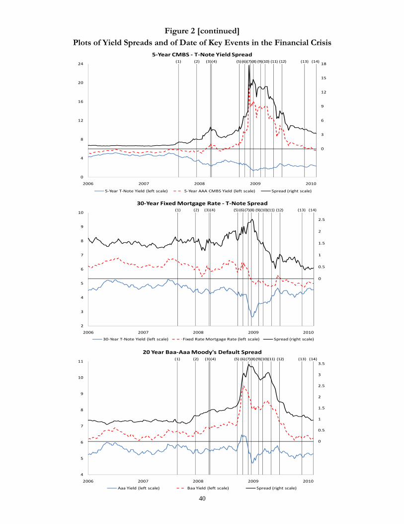
40
Figure 2 [continued] Plots of Yield Spreads and of Date of Key Events in the Financial Crisis
‐6
‐3
0
3
6
9
12
15
18
0
4
8
12
16
20
24
2006 2007 2008 2009 2010
5‐Year CMBS ‐ T‐Note Yield Spread
5‐Year T‐Note Yield (left scale) 5‐Year AAA CMBS Yield (left scale) Spread (right scale)
(1) (2) (3)(4) (5)(6)(7)(8) (9)(10) (11) (12) (13) (14)
‐2
‐1.5
‐1
‐0.5
0
0.5
1
1.5
2
2.5
2
3
4
5
6
7
8
9
10
2006 2007 2008 2009 2010
30‐Year Fixed Mortgage Rate ‐ T‐Note Spread
30‐Year T‐Note Yield (left scale) Fixed Rate Mortgage Rate (left scale) Spread (right scale)
(1) (2) (3)(4) (5) (6)(7)(8) (9)(10)(11) (12) (13) (14)
‐1.5
‐1
‐0.5
0
0.5
1
1.5
2
2.5
3
3.5
4
5
6
7
8
9
10
11
2006 2007 2008 2009 2010
20 Year Baa‐Aaa Moody's Default Spread
Aaa Yield (left scale) Baa Yield (left scale) Spread (right scale)
(1) (2) (3)(4) (5) (6)(7)(8)(9)(10)(11) (12) (13) (14)
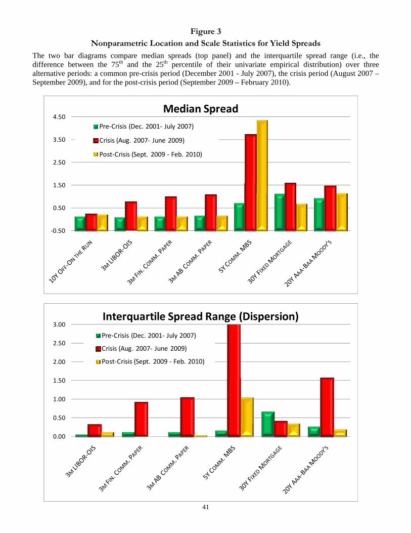
41
Figure 3 Nonparametric Location and Scale Statistics for Yield Spreads
The two bar diagrams compare median spreads (top panel) and the interquartile spread range (i.e., the difference between the 75th and the 25th percentile of their univariate empirical distribution) over three alternative periods: a common pre-crisis period (December 2001 - July 2007), the crisis period (August 2007 – September 2009), and for the post-crisis period (September 2009 – February 2010).
‐0.50
0.50
1.50
2.50
3.50
4.50Median Spread
Pre‐Crisis (Dec. 2001‐ July 2007)
Crisis (Aug. 2007‐ June 2009)
Post‐Crisis (Sept. 2009 ‐ Feb. 2010)
0.00
0.50
1.00
1.50
2.00
2.50
3.00Interquartile Spread Range (Dispersion)
Pre‐Crisis (Dec. 2001‐ July 2007)
Crisis (Aug. 2007‐ June 2009)
Post‐Crisis (Sept. 2009 ‐ Feb. 2010)
Related Documents


