A Wide-Band Dynamic Equivalent Model of Wind Power Plants for the Analysis of Electromagnetic Transients in Power Systems by Dalia Nabil Mahmoud Mohammed Hussein A thesis submitted in conformity with the requirements for the degree of Doctor of Philosophy Graduate Department of Electrical and Computer Engineering University of Toronto Copyright c ⃝ 2014 by Dalia Nabil Mahmoud Mohammed Hussein

Welcome message from author
This document is posted to help you gain knowledge. Please leave a comment to let me know what you think about it! Share it to your friends and learn new things together.
Transcript

A Wide-Band Dynamic Equivalent Model of Wind PowerPlants for the Analysis of Electromagnetic Transients in
Power Systems
by
Dalia Nabil Mahmoud Mohammed Hussein
A thesis submitted in conformity with the requirementsfor the degree of Doctor of Philosophy
Graduate Department of Electrical and Computer EngineeringUniversity of Toronto
Copyright c⃝ 2014 by Dalia Nabil Mahmoud Mohammed Hussein

Abstract
A Wide-Band Dynamic Equivalent Model of Wind Power Plants for the Analysis of
Electromagnetic Transients in Power Systems
Dalia Nabil Mahmoud Mohammed Hussein
Doctor of Philosophy
Graduate Department of Electrical and Computer Engineering
University of Toronto
2014
High depth of penetration of wind power and proliferation of wind-turbine generator
(WTG) units, clustered as wind power plants (WPPs), have invoked significant effort for
development of WPP mathematical models to reflect the WPP behavior with respect
to power system electromagnetic transients (EMTs). The detailed modeling of WPPs
is neither practical nor possible due to its significant computational burden. Therefore,
it is necessary to represent the WPP with an equivalent model that captures its EMTs
behavior.
This thesis proposes and develops a novel accurate and computationally efficient
reduced-order dynamic-equivalent of Type-41and Type-32based WPPs for the analysis
of EMTs in the power system, external to the WPP. The proposed model significantly
reduces the computational resources and the simulation run time while preserving the
WPP response fidelity in the desired frequency range, e.g., 0 to 50 kHz. The proposed
WPP equivalent model is composed of two parts: 1) a frequency-dependent equivalent
model which represents the WPP passive components in the entire frequency range and
2) a dynamic equivalent model that represents the WPP supervisory control and the
aggregated low-frequency dynamics of wind-turbine generator (WTG) units. The
proposed model is implemented in the PSCAD/EMTDC environment. Extensive case
studies, that compares the equivalent model results with those of a detailed model, are
1Type-4 refers to the WTG units with full capacity back-to-back converter interface2Type-3 refers to the WTG units with doubly-fed asynchronous generators
ii

conducted to validate the efficiency and accuracy of the proposed equivalent model. The
case studies cover different types of faults at different locations, external to the WPP,
with respect to the WPP terminal.
This thesis also presents three applications of the developed WPP equivalent model.
1. The real-time simulation of the Type-4 WPP based on the developed equivalent
model.
2. The real-time simulation of the Type-3 WPP based on the developed equivalent
model.
3. The real-time hardware-in-the-loop (HIL) testing of the WPP supervisory control
which is realized on an industrial controller platform (NI−cRIO) whereas the rest
of the WPP equivalent model is simulated on a real-time digital simulator RTDSr.
Real-time simulation case studies are performed to demonstrate (i) the accuracy of the
developed models and (ii) the computational efficiency and the saving in the hardware
resources associated with simulating the WPP equivalent model in comparison with the
the WPP detailed modeling.
iii

Dedication
To my dear mother, and my late father
To Mahmoud and Mostafa who always bring the joy to my life
iv

Acknowledgements
I would like to express my sincere gratitude to my supervisor, Professor Reza Iravani, for
his invaluable supervision, encouragement, and financial support throughout my Ph.D.
studies. Throughout the course of my Ph.D. I have learned a lot from him through our
numerous discussions and weekly meetings. I will always be grateful for his continuous
patience and support on both the academic and the personal levels and will always
remain honored that I have worked under his supervision. I would like also to thank the
Ph.D. examination committee: Professor Aleksandar Prodic, Professor Olivier Trescases,
Professor Josh Taylor, and Professor Udaya Annakkage for their review of the thesis and
their constructive comments.
Special and cordial thanks go to my dear mother who traveled overseas and acted
altruistically to help me and my family. The least I can do is to dedicate this work to
her. I would like to express my gratitude to my husband Mahmoud whom without his
support, the completion of this thesis would not be a reality. I am particularly thankful
for his continuous help, fruitful technical discussions, and personal advice. I would like
also to thank Dr. Milan Graovac and Mr. Xiaolin Wang for their valuable help and
fruitful discussions.
I would like to thank my brother, my sister, and my friends in Toronto for their
continuous support, love and encouragement throughout the course of my Ph.D.
Finally, I would like to acknowledge the financial support of the Department of Elec-
trical and Computer Engineering at the University of Toronto and the Ontario Graduate
Scholarship (OGS).
v

Contents
1 Introduction 1
1.1 Statement of the Problem and Thesis Motivations . . . . . . . . . . . . . 2
1.2 Thesis Objectives . . . . . . . . . . . . . . . . . . . . . . . . . . . . . . . 4
1.3 Proposed Wide-Band Dynamic Model of WPP . . . . . . . . . . . . . . . 5
1.4 Methodology . . . . . . . . . . . . . . . . . . . . . . . . . . . . . . . . . 5
1.5 Thesis Outlines . . . . . . . . . . . . . . . . . . . . . . . . . . . . . . . . 7
2 Frequency-Dependent Network Equivalent (FDNE) Model of WPP 9
2.1 Introduction . . . . . . . . . . . . . . . . . . . . . . . . . . . . . . . . . . 9
2.2 FDNE of WPP Passive Network . . . . . . . . . . . . . . . . . . . . . . . 10
2.2.1 WPP Driving Point Admittance Matrix . . . . . . . . . . . . . . 10
2.2.2 Vector Fitting Technique . . . . . . . . . . . . . . . . . . . . . . . 11
2.2.3 Passivity Enforcement . . . . . . . . . . . . . . . . . . . . . . . . 13
2.3 Implementation of the FDNE in a Time-Domain EMT Platform . . . . . 15
2.4 Conclusions . . . . . . . . . . . . . . . . . . . . . . . . . . . . . . . . . . 18
3 Dynamic Low-Frequency Equivalent Model of Type-4 WPP 19
3.1 Introduction . . . . . . . . . . . . . . . . . . . . . . . . . . . . . . . . . . 19
3.2 Background . . . . . . . . . . . . . . . . . . . . . . . . . . . . . . . . . . 20
3.3 Equivalent Model Assumptions . . . . . . . . . . . . . . . . . . . . . . . 21
3.4 Structure of the Dynamic Low-Frequency Equivalent (DLFE) Model of
Type-4 WPP . . . . . . . . . . . . . . . . . . . . . . . . . . . . . . . . . 22
3.5 Phase Locked Loop . . . . . . . . . . . . . . . . . . . . . . . . . . . . . . 23
3.6 Type-4 WPP Supervisory control . . . . . . . . . . . . . . . . . . . . . . 24
3.6.1 Active Power Control . . . . . . . . . . . . . . . . . . . . . . . . . 25
3.6.2 Reactive Power Control . . . . . . . . . . . . . . . . . . . . . . . 25
vi

3.6.3 WPP Current Limits . . . . . . . . . . . . . . . . . . . . . . . . . 26
3.6.4 Fault-Ride-Through (FRT) Capability . . . . . . . . . . . . . . . 27
3.7 WTGs Equivalent Model . . . . . . . . . . . . . . . . . . . . . . . . . . . 29
3.8 Wide-Band Equivalent Model of Type-4 WPP . . . . . . . . . . . . . . . 33
3.9 Test System . . . . . . . . . . . . . . . . . . . . . . . . . . . . . . . . . . 33
3.10 Case Studies . . . . . . . . . . . . . . . . . . . . . . . . . . . . . . . . . . 36
3.10.1 Case I . . . . . . . . . . . . . . . . . . . . . . . . . . . . . . . . . 37
3.10.2 Case II . . . . . . . . . . . . . . . . . . . . . . . . . . . . . . . . . 37
3.10.3 Case III . . . . . . . . . . . . . . . . . . . . . . . . . . . . . . . . 37
3.10.4 Case IV . . . . . . . . . . . . . . . . . . . . . . . . . . . . . . . . 44
3.10.5 Case V . . . . . . . . . . . . . . . . . . . . . . . . . . . . . . . . . 44
3.10.6 Case VI . . . . . . . . . . . . . . . . . . . . . . . . . . . . . . . . 52
3.10.7 Case VII . . . . . . . . . . . . . . . . . . . . . . . . . . . . . . . . 52
3.11 Discussions . . . . . . . . . . . . . . . . . . . . . . . . . . . . . . . . . . 57
3.12 Conclusions . . . . . . . . . . . . . . . . . . . . . . . . . . . . . . . . . . 58
4 Dynamic Low-Frequency Equivalent Model of Type-3 WPP 60
4.1 Introduction . . . . . . . . . . . . . . . . . . . . . . . . . . . . . . . . . . 60
4.2 Background . . . . . . . . . . . . . . . . . . . . . . . . . . . . . . . . . . 61
4.3 Equivalent Model Assumptions . . . . . . . . . . . . . . . . . . . . . . . 62
4.4 Structure of the Dynamic Low-Frequency Equivalent Model of the Type-3
WPP . . . . . . . . . . . . . . . . . . . . . . . . . . . . . . . . . . . . . . 63
4.5 Equivalent Model of Wind Turbines . . . . . . . . . . . . . . . . . . . . . 64
4.5.1 Aerodynamic Equivalent Model . . . . . . . . . . . . . . . . . . . 65
4.5.2 Parameter Estimation of Wind Turbine Equivalent Model . . . . 67
4.5.3 Drive-Train Mechanical Model . . . . . . . . . . . . . . . . . . . . 67
4.6 WPP Supervisory Control . . . . . . . . . . . . . . . . . . . . . . . . . . 68
4.7 Equivalent Model of the Generators Electrical Side and Converters . . . . 72
4.8 Wide-Band Equivalent Model of Type-3 WPP . . . . . . . . . . . . . . . 74
4.9 Test System . . . . . . . . . . . . . . . . . . . . . . . . . . . . . . . . . . 75
4.10 Case Studies . . . . . . . . . . . . . . . . . . . . . . . . . . . . . . . . . . 77
4.10.1 Case I . . . . . . . . . . . . . . . . . . . . . . . . . . . . . . . . . 78
4.10.2 Case II . . . . . . . . . . . . . . . . . . . . . . . . . . . . . . . . . 78
4.10.3 Case III . . . . . . . . . . . . . . . . . . . . . . . . . . . . . . . . 85
vii

4.10.4 Case IV . . . . . . . . . . . . . . . . . . . . . . . . . . . . . . . . 85
4.10.5 Case V . . . . . . . . . . . . . . . . . . . . . . . . . . . . . . . . . 85
4.10.6 Case VI . . . . . . . . . . . . . . . . . . . . . . . . . . . . . . . . 93
4.10.7 Case VII . . . . . . . . . . . . . . . . . . . . . . . . . . . . . . . . 93
4.11 Discussions . . . . . . . . . . . . . . . . . . . . . . . . . . . . . . . . . . 93
4.12 Conclusions . . . . . . . . . . . . . . . . . . . . . . . . . . . . . . . . . . 98
5 Real-Time Simulation and HIL Evaluation of Equivalent Models 99
5.1 Introduction . . . . . . . . . . . . . . . . . . . . . . . . . . . . . . . . . . 99
5.2 Challenges Associated With Real-Time Simulation of WPPs . . . . . . . 101
5.3 Real-Time Simulation of the WPP Equivalent Model . . . . . . . . . . . 102
5.4 Case Studies . . . . . . . . . . . . . . . . . . . . . . . . . . . . . . . . . . 103
5.4.1 Case I: Type-4 WPP . . . . . . . . . . . . . . . . . . . . . . . . . 104
5.4.2 Case II: Type-3 WPP . . . . . . . . . . . . . . . . . . . . . . . . 104
5.4.3 Discussion . . . . . . . . . . . . . . . . . . . . . . . . . . . . . . . 106
5.5 Real-Time Controller HIL Testing of a Type-4 WPP Supervisory Control 108
5.5.1 Case III . . . . . . . . . . . . . . . . . . . . . . . . . . . . . . . . 109
5.6 Conclusions . . . . . . . . . . . . . . . . . . . . . . . . . . . . . . . . . . 113
6 Conclusion and Future Work 114
6.1 Summary . . . . . . . . . . . . . . . . . . . . . . . . . . . . . . . . . . . 114
6.2 Conclusions . . . . . . . . . . . . . . . . . . . . . . . . . . . . . . . . . . 115
6.3 Contributions . . . . . . . . . . . . . . . . . . . . . . . . . . . . . . . . . 117
6.4 Future Work . . . . . . . . . . . . . . . . . . . . . . . . . . . . . . . . . . 118
A Detailed Model of the Type-4 WPP 120
A.1 WPP Supervisory Control . . . . . . . . . . . . . . . . . . . . . . . . . . 120
A.2 Type-4 GSC Control Model . . . . . . . . . . . . . . . . . . . . . . . . . 121
B DSOGI-PLL 125
C Parameters of the Test System of Chapter 3 128
D Detailed Model of the Type-3 WTG 130
D.1 Rotor-Side Converter Control . . . . . . . . . . . . . . . . . . . . . . . . 132
D.2 Grid-Side Converter Control . . . . . . . . . . . . . . . . . . . . . . . . . 134
viii

D.3 DFAG Fault-Ride-Through Capability . . . . . . . . . . . . . . . . . . . 135
E Parameters of the Test System of Chapter 4 137
ix

List of Figures
1.1 Schematic Diagram Illustrating Power System Partitioning . . . . . . . . 3
1.2 The Proposed Wind Power Plant Dynamic Equivalent . . . . . . . . . . . 6
2.1 Flowchart of the Vector Fitting Technique . . . . . . . . . . . . . . . . . 14
2.2 Passivity Enforcement . . . . . . . . . . . . . . . . . . . . . . . . . . . . 16
2.3 Discrete-Time Circuit Model of Real Partial Fractions . . . . . . . . . . . 17
2.4 Discrete-Time Circuit Model of Every Two Conjugate Partial Fractions . 17
3.1 Wind Power Plant Control Structure . . . . . . . . . . . . . . . . . . . . 20
3.2 Schematic Diagram of Type-4 WTG Unit . . . . . . . . . . . . . . . . . . 21
3.3 Dynamic Model of WPP with Type-4 WTGs . . . . . . . . . . . . . . . . 22
3.4 Block Diagram representation of the WPP Supervisory Control . . . . . 24
3.5 The Active Power Control . . . . . . . . . . . . . . . . . . . . . . . . . . 26
3.6 The Reactive Power Control . . . . . . . . . . . . . . . . . . . . . . . . . 26
3.7 The WPP Current Limits Block . . . . . . . . . . . . . . . . . . . . . . . 27
3.8 The WECC Fault-Ride-Through Standard . . . . . . . . . . . . . . . . . 28
3.9 Reactive Current Requirements for Grid Voltage Support . . . . . . . . . 29
3.10 The Fault-Ride-Through Control Block . . . . . . . . . . . . . . . . . . . 29
3.11 Active Power Reduction During Voltage Dips . . . . . . . . . . . . . . . 30
3.12 Block diagram Represents the AC-Side Dynamics . . . . . . . . . . . . . 31
3.13 Control Model of the ideal two-level VSC in the dq-frame . . . . . . . . . 31
3.14 Block Diagram of the Current Controlled GSC System . . . . . . . . . . 32
3.15 Equivalent Model of WTG Units . . . . . . . . . . . . . . . . . . . . . . 32
3.16 The Proposed Wind Power Plant Dynamic-Equivalent . . . . . . . . . . . 33
3.17 Schematic Diagram of the Modified version of Lake Erie Shores WPP . . 35
3.18 Admittance Magnitudes of the Fitted Equivalent and the Detailed Mod-
eled Passive Network - (a) self admittance, (b) mutual admittance . . . . 36
x

3.19 PCC Voltages of the Detailed and the Equivalent Models - Case I . . . . 38
3.20 WPP Output Currents of the Detailed and the Equivalent Models - Case I 39
3.21 WPP Output (a) P and Q (b) IPpcc and IQpcc (c) PCC Voltage of the
Detailed and the Equivalent Models - Case I . . . . . . . . . . . . . . . . 40
3.22 PCC Voltages of the Detailed and the Equivalent Models - Case II . . . . 41
3.23 WPP Output Currents of the Detailed and the Equivalent Models - Case II 42
3.24 The WPP Output (a) P and Q (b) IPpcc and IQpcc (c) PCC Voltage of the
Detailed Network and the Developed Equivalent of Case II . . . . . . . . 43
3.25 PCC Voltages of the Detailed and the Equivalent Models - Case III . . . 45
3.26 WPP Output Currents of the Detailed and the Equivalent Models - Case
III . . . . . . . . . . . . . . . . . . . . . . . . . . . . . . . . . . . . . . . 46
3.27 PCC Voltages of the Detailed and the Equivalent Models - Case IV . . . 47
3.28 WPP Output Currents of the Detailed and the Equivalent Models - Case IV 48
3.29 The WPP Output (a) P and Q (b) IPpcc and IQpcc (c) PCC Voltage of the
Detailed Network and the Developed Equivalent of Case IV . . . . . . . . 49
3.30 PCC Voltages of the Detailed and the Equivalent Models - Case V . . . . 50
3.31 WPP Output Currents of the Detailed and the Equivalent Models - Case V 51
3.32 PCC Voltages of the Detailed and the Equivalent Models - Case VI . . . 53
3.33 WPP Output Currents of the Detailed and the Equivalent Models - Case VI 54
3.34 PCC Voltages of the Detailed and the Equivalent Models - Case VII . . . 55
3.35 WPP Output Currents of the Detailed and the Equivalent Models - Case
VII . . . . . . . . . . . . . . . . . . . . . . . . . . . . . . . . . . . . . . . 56
3.36 PCC Voltage, phase c, of the Detailed and the FDNE Models - Case I . . 58
3.37 PCC Voltage, phase c, of the Detailed and the DLFE Models - Case I . . 58
4.1 Schematic Diagram of the Doubly-Fed Asynchronous Generator (DFAG)
Unit . . . . . . . . . . . . . . . . . . . . . . . . . . . . . . . . . . . . . . 62
4.2 The Dynamic Low-Frequency Equivalent of Type-3 WPP . . . . . . . . . 64
4.3 Wind Turbine Equivalent Model . . . . . . . . . . . . . . . . . . . . . . . 65
4.4 Power Curve of a WTG Unit . . . . . . . . . . . . . . . . . . . . . . . . . 67
4.5 Two-Mass Drive-Train Equivalent Model . . . . . . . . . . . . . . . . . . 68
4.6 Block diagram of the Two-Mass Drive-Train Model . . . . . . . . . . . . 69
4.7 Block Diagram of the Supervisory Control Module . . . . . . . . . . . . . 70
4.8 Block Diagram of DFAG Equations . . . . . . . . . . . . . . . . . . . . . 73
xi

4.9 RSC Current Control . . . . . . . . . . . . . . . . . . . . . . . . . . . . . 73
4.10 DFAG Model and RSC Control . . . . . . . . . . . . . . . . . . . . . . . 73
4.11 Equivalent Model of the Generator and Converter . . . . . . . . . . . . . 74
4.12 WPP Dynamic-Equivalent Model . . . . . . . . . . . . . . . . . . . . . . 75
4.13 Schematic Diagram of the Type-3 WPP Test System . . . . . . . . . . . 76
4.14 PCC Voltages of the Detailed and the Equivalent Models - Case I . . . . 79
4.15 PCC Output Currents of the Detailed and the Equivalent Models - Case
I. (a) Phase a (b) Phase b (c) Phase c . . . . . . . . . . . . . . . . . . . . 80
4.16 WPP Outputs (a) Active Power (b) Reactive Power (c) Active Current
(d) Reactive Current (e) PCC Voltage of the Detailed and the Equivalent
Models - Case I. . . . . . . . . . . . . . . . . . . . . . . . . . . . . . . . . 81
4.17 PCC Voltages of the Detailed and the Equivalent Models - Case II . . . . 82
4.18 PCC Output Currents of the Detailed and the Equivalent Models - Case
II. (a) Phase a (b) Phase b (c) Phase c . . . . . . . . . . . . . . . . . . . 83
4.19 WPP Outputs (a) Active Power (b) Reactive Power (c) Active Current
(d) Reactive Current (e) PCC Voltage of the Detailed and the Equivalent
Models - Case II. . . . . . . . . . . . . . . . . . . . . . . . . . . . . . . . 84
4.20 PCC Voltages of the Detailed and the Equivalent Models - Case III . . . 86
4.21 PCC Output Currents of the Detailed and the Equivalent Models - Case
III. (a) Phase a (b) Phase b (c) Phase c . . . . . . . . . . . . . . . . . . . 87
4.22 WPP Outputs (a) Active Power (b) Reactive Power (c) Active Current
(d) Reactive Current (e) PCC Voltage of the Detailed and the Equivalent
Models - Case III. . . . . . . . . . . . . . . . . . . . . . . . . . . . . . . . 88
4.23 PCC Voltages of the Detailed and the Equivalent Models - Case IV . . . 89
4.24 PCC Output Currents of the Detailed and the Equivalent Models - Case
IV. (a) Phase a (b) Phase b (c) Phase c . . . . . . . . . . . . . . . . . . . 90
4.25 PCC Voltages of the Detailed and the Equivalent Models - Case V . . . . 91
4.26 PCC Output Currents of the Detailed and the Equivalent Models - Case
V. (a) Phase a (b) Phase b (c) Phase c . . . . . . . . . . . . . . . . . . . 92
4.27 PCC Voltages of the Detailed and the Equivalent Models - Case VI . . . 94
4.28 PCC Output Currents of the Detailed and the Equivalent Models - Case
VI. (a) Phase a (b) Phase b (c) Phase c . . . . . . . . . . . . . . . . . . . 95
4.29 PCC Voltages of the Detailed and the Equivalent Models - Case VII . . . 96
xii

4.30 PCC Output Currents of the Detailed and the Equivalent Models - Case
VII. (a) Phase a (b) Phase b (c) Phase c . . . . . . . . . . . . . . . . . . 97
5.1 Real-Time HIL Closed-Loop Arrangement . . . . . . . . . . . . . . . . . 100
5.2 Structure of the Wide-band Equivalent Model of a Type-4/3 WTGs-based
WPP . . . . . . . . . . . . . . . . . . . . . . . . . . . . . . . . . . . . . . 103
5.3 Real-Time Oscilloscope trace of the WPP Terminal Voltages - Case I . . 105
5.4 Real-Time Oscilloscope trace of the WPP Output Currents - Case I . . . 105
5.5 PCC Voltages of the Equivalent Model From the RTDS and the Detailed
Model From PSCAD/EMTDC - Case I . . . . . . . . . . . . . . . . . . . 106
5.6 WPP Output Currents of the Equivalent Model From the RTDS and the
Detailed Model From PSCAD/EMTDC - Case I . . . . . . . . . . . . . . 107
5.7 Real-Time Oscilloscope trace of the WPP Terminal Voltages - Case II . . 108
5.8 Real-Time Oscilloscope trace of the WPP Output Currents - Case II . . 108
5.9 Schematic Diagram of the Real-Time HIL Test Bed . . . . . . . . . . . . 109
5.10 Real-Time HIL Test Bed . . . . . . . . . . . . . . . . . . . . . . . . . . . 110
5.11 PCC Voltages and WPP Output Currents - Case III . . . . . . . . . . . 111
5.12 WPP Output (a) Idpcc (b) IQpcc (c) P (d) Q - Case III . . . . . . . . . . . 112
A.1 Schematic Diagram of Type-4 WTG Unit . . . . . . . . . . . . . . . . . . 122
A.2 Schematic Diagram of a Typical GSC . . . . . . . . . . . . . . . . . . . . 123
A.3 Block Diagram of the GSC Control . . . . . . . . . . . . . . . . . . . . . 124
B.1 Schematic Diagram of DSOGI-PLL . . . . . . . . . . . . . . . . . . . . . 125
B.2 SOGI-QSG Schematic . . . . . . . . . . . . . . . . . . . . . . . . . . . . 126
D.1 Schematic Diagram of the Doubly-Fed Asynchronous Generator (DFAG)
Unit . . . . . . . . . . . . . . . . . . . . . . . . . . . . . . . . . . . . . . 130
D.2 Schematic Diagram of the Doubly-Fed Asynchronous Generator . . . . . 132
D.3 Block Diagram of the Rotor Side Converter Control . . . . . . . . . . . . 134
D.4 Block Diagram of the Grid Side Converter Control . . . . . . . . . . . . . 135
xiii

List of Tables
C.1 Parameters of The 34.5 kV Overhead Lines . . . . . . . . . . . . . . . . . 128
C.2 Parameters of The 115 kV Overhead Lines . . . . . . . . . . . . . . . . . 128
C.3 Grid Impedance . . . . . . . . . . . . . . . . . . . . . . . . . . . . . . . . 129
E.1 Parameters of The 13.8 kV Overhead Lines . . . . . . . . . . . . . . . . . 137
E.2 Parameters of The 115 kV Overhead Lines . . . . . . . . . . . . . . . . . 137
E.3 Parameters DFAG Unit and its interfacing Transformer . . . . . . . . . . 138
E.4 Parameters of Back-to-Back VSC and Transformer . . . . . . . . . . . . 138
xiv

List of Abbreviations
DFAG: Doubly-Fed Asynchronous Generator
DLFE: Dynamic Low-Frequency Equivalent
DSOGI-PLL: Dual Second Order Generalized Integrator-PLL
DVR: Dynamic Voltage Restorer
EMT: Electromagnetic Transient
EMTDC: Electromagnetic Transients Program for DC
FDNE: Frequency Dependent Network Equivalent
FRT: Fault-Ride Through
GSC: Grid-Side Converter
HIL: Hardware-in-the-Loop
IGBT: Insulated-Gate Bipolar Transistor
LVRT: Low-Voltage Ride Through
MSC: Machine-Side Converter
NI−cRIO: National Instrument−Compact Real-time Input and Output
PCC: Point of Common Coupling
PI: Proportional Integral
PLL : Phase Locked Loop
PSC: Positive Sequence Calculator
QSG: Quadrature Signal Generator
RTS: Real-Time Simulator
RTDS: Real-Time Digital Simulator
RSC: Rotor-Side Converter
SPWM: Sinusoidal Pulse Width Modulation
SRF-PLL : Synchronous Reference Frame-PLL
TSO: Transmission System Operator
VF: Vector Fitting
VSC: Voltage-Sourced Converter
WECC: Western Electricity Coordinated Council
WPP: Wind Power Plants
WTG: Wind Turbine Generator
xv

Chapter 1
Introduction
During the last two decades, generation of electricity from wind energy has increased
drastically. The amount of energy generated from wind doubles almost every three years
and the rate is expected to go even higher [1], [2].
Traditionally, a wind power plant (WPP) was designed to disconnect from the system
during grid disturbances [3]. However, with the continuous increase in the depth of
penetration of wind power into the power system and as the generating capacity of each
individual WPP can reach hundreds of megawatts, disconnection during transients may
cause system instability, frequency drop, and disruption of service. Thus, recent grid
codes [4], [5] require that WPPs ride through faults, remain connected to the grid, and
even actively contribute to grid operation during dynamic conditions. Therefore, the
impact of a WPP on the power system, during both steady state and power system
dynamics, needs to be analyzed and quantified. This necessitates the developments of
appropriate WPP models that reflect the behavior of WPPs with respect to different
types of power system phenomena and a wide range of studies, i.e., from planning to fast
electromagnetic transients (EMTs). EMTs studies are conducted either within a WPP
or in the power system external to the WPP. The latter is the focus of this thesis. EMTs
occur frequently in the power system due to faults and switching events and include
frequencies from DC to multi-MHz. Although the EMTs last only for short periods of
time, i.e., up to tens of cycles, it is necessary to conduct EMTs studies to obtain detailed
information about the study system behavior during EMTs. In addition, EMTs studies
have a vital role in the design/verification of control/protection platforms.
1

Chapter 1. Introduction 2
1.1 Statement of the Problem and Thesis Motiva-
tions
Analysis of EMTs in a power system inherently necessitates the system model to ac-
curately represent the overall system, including WPPs, within the required frequency
range. Thus, the brute force approach to model a WPP for EMTs studies is to repre-
sent all components of each WPP based on their detailed models. However, a typical
WPP consists of tens or even hundreds of wind turbine generator (WTG) units, their
power electronic interfaces, local controllers, the collector network, and the WPP super-
visory controller. As such, with the significant size and complexity of a WPP combined
with the required high resolution (small time-step for numerical integrations), associated
with EMT-type time-domain simulation programs, the detailed modeling of a WPP ne-
cessitates (i) significant hardware computational resources, and (ii) imposes formidable
run-time for each case study. The former is practically a major limitation for EMTs
studies in a real-time simulation environment where the WPP detailed modeling imposes
a drastic computational burden on the real-time simulator (RTS) and hence will require
extensive increase in the size and cost of the expensive RTS hardware. Therefore, there is
a need to adopt a more computationally efficient modeling approach to represent WPPs
for EMTs studies. The system under study, Figure 1.1, can be virtually divided into two
zones. The first (study) zone, Figure 1.1, encompasses that part of the system where the
EMTs are investigated and consequently all the corresponding components need to be
modeled in detail. The second (external) zone, Figure 1.1, covers the rest of the system
which has secondary impact on the study zone transients; yet, it cannot be discarded
or represented by an approximated, simplified, fundamental-frequency model. Thus, the
external zone can be represented by an equivalent model that reflects its impact on the
EMTs of the study zone in the frequency range of interest. This strategy is adopted
in this thesis and the WPP forms (for transients initiated outside the WPP) the exter-
nal zone that needs to be represented by a reduced-order, wide frequency-band WPP
equivalent model, connected to the point of common coupling (PCC).
WPP reduced-order models have been developed in the technical literature, e.g., the
WPP generic, non-proprietary models [6]–[10] and the WPP aggregated models that
lump all WTG units within the WPP into single or multiple units with re-scaled power
capacity [11]–[13]. However, these models are neither tailored for EMTs studies nor

Chapter 1. Introduction 3
Figure 1.1: Schematic Diagram Illustrating Power System Partitioning
adequately represent the EMTs behavior of the WPP of interest. The main reasons are:
• These models are designed for power flow and transient stability studies, and valid
only for a very narrow frequency range of 0-2 Hz [10].
• These models do not represent the EMTs behavior of the WPP collector network
in response to external EMTs. This shortcoming results from either omitting the
collector system from the equivalent or only considering its fundamental-frequency
short-circuit equivalent [14], [15].
• These models are not suitable for the hardware-in-the-loop testing of control/protection
platforms since they do not represent the EMTs behavior of the WPP, and due to
the computational burden associated with the multiple WTG representation.
EMT-type WPP equivalent models do not exist; previously there was no real need for
them since the WPPs were designed to disconnect from the system during transients.
However, such models are now crucial since the current grid codes require WPPs to
remain connected to the grid during disturbances.
The aforementioned limitations and the fact that EMT-type WPP equivalent models
do not exist, are the main motivations behind the development of a new computationally-
efficient dynamic equivalent model of WPPs proposed in this thesis.

Chapter 1. Introduction 4
1.2 Thesis Objectives
Based on the aforementioned discussion, the objectives of this thesis are:
1. Develop a wide-band reduced-order dynamic equivalent model of a Type-41and a
Type-32based WPPs for the analysis of EMTs in the power system external to the
WPP. The salient features of the proposed equivalent model are:
• It represents the dynamic behavior of the WPP components including: (i) the
WPP collector network and passive components, (ii) the WPP supervisory
control, and (iii) WTGs and their local controls.
• It is computationally efficient, i.e., significantly reduces the hardware/software
computational burden as compared to the WPP detailed models.
• It accurately mimics the terminal response of the WPP with respect to the
power system EMTs over a wide-band of the frequency spectrum, e.g., ranging
from DC to 50 kHz.
• It represents the fault-ride through behavior of the WPP which is a mandatory
requirement of the grid codes.
• It is suitable for real-time simulation based on practically available computa-
tional resources.
2. Implement the proposed equivalent model in a time-domain simulation platform
(PSCAD/EMTDC) for the off-line analysis.
3. Develop a benchmark system for Type-3 and Type-4 based WPPs.
4. Validate the accuracy of the proposed equivalent models with respect to detailed
WPP models.
5. Implement the proposed equivalent model in a real-time simulation platform.
6. Utilize the real-time simulatedWPP equivalent model in the testing of control/protection
platforms in a hardware-in-the-loop (HIL) environment.
1Type-4 refers to the WTG units with full capacity back-to-back converter interface2Type-3 refers to the WTG units with doubly-fed asynchronous generators

Chapter 1. Introduction 5
1.3 Proposed Wide-Band Dynamic Model of WPP
Figure 1.2(a) shows a schematic diagram of a power system which also includes a WPP.
The WPP is composed of: 1) multiple WTG units and their local controls, 2) a collector
system, and 3) the WPP supervisory control. The main objective of this work is to
represent the WPP, with respect to the PCC, by an equivalent model that can accurately
represent the impact of the WPP on EMT phenomena that occur in the power system,
external to the WPP, e.g., EMTs due to the faulted line, Figure 1.2(a). To achieve this
objective, the WPP model is mathematically represented by the following two segments
as symbolically shown in Figure 1.2(b).
• Passive (static) Frequency Dependent Network Equivalent (FDNE) Model: This
represents the response of all passive components of the WPP, i.e., WPP substation
transformer(s), overhead lines and underground cables of the collector system, filter
and capacitor banks, passive loads, and any other passive component within the
WPP. The frequency bandwidth of the passive equivalent model is determined
based on the type and the characteristics of the EMTs to be investigated external
to the WPP, e.g., 0 to 50 kHz.
• Dynamic Low-Frequency Equivalent (DLFE) Model: This represents the dynamic
behavior of the WTG units (and their local controls) within the WPP and the
WPP supervisory controller with respect to the WPP external power system. The
DLFE model represents the WPP low-frequency dynamics about the nominal power
frequency.
The combined FDNE model and the DLFE model constitutes the net model of the WPP
with respect to its host power system at the PCC, Figure 1.2(b), in the desired wide
frequency range.
1.4 Methodology
In order to achieve the aforementioned thesis objectives, the following methodology is
employed:

Chapter 1. Introduction 6
Figure 1.2: The Proposed Wind Power Plant Dynamic Equivalent
Benchmark Test System Development
Two test systems, one includes a Type-4 based WPP and the other includes a Type-3
based WPP connected to a power system are used. Each test system is simulated in the
PSCAD/EMTDC time-domain simulation platform based on the detailed modeling of
all components of the WPP that include WTG units (17 and 8 WTGs for the Type-4
and Type-3 WPPs respectively), their local controls, a collector network, and a WPP
supervisory control. The detailed model of each WPP is used in the development of the
WPP equivalent model and the simulation results of that detailed model are considered
as benchmark results. The detailed models of the Type-4 WPP and the Type-3 WPP
are in Appendices A and D respectively.
Equivalent Model Development
The PSCAD/EMTDC detailed model is used to develop the FDNE model of the WPP,
with respect to the PCC. The FDNE development approach is detailed in Chapter 2
of this thesis. The DLFE model of each WPP is then developed as described in chap-
ters 3 and 4. The proposed dynamic WPP equivalent model is the combination of the
FDNE and the DLFE as symbolically depicted in Figure 1.2(b). The equivalent model
is constructed and implemented in the PSCAD/EMTDC.

Chapter 1. Introduction 7
Equivalent-Model Accuracy Validation
The numerical accuracy and computational efficiency of the developed dynamic equiva-
lent model are validated by comparing the time-domain simulation test case results when
the WPP is represented once by its detailed model and once by the proposed equivalent
model.
Real-Time Simulation/HIL Testing
To demonstrate the effectiveness and the computational efficiency of the proposed equiv-
alent model for real-time applications, the equivalent models of both Type-3 and Type-4
based WPPs are embedded in a real-time digital simulator (RTDS) and investigated.
The equivalent model of a Type-4 based WPP is also used for the HIL testing of the
WPP supervisory control.
1.5 Thesis Outlines
The rest of this thesis is organized as follows:
Chapter 2 presents the development of the WPP passive network equivalent model.
It describes the mathematical model and procedures to generate the frequency dependent
network equivalent; this includes the formation of the WPP driving point admittance
matrix and fitting the frequency dependent response to a rational function representation
based on the vector fitting technique. This chapter also describes the discretization of the
frequency-domain model of the FDNE for the implementation in the PSCAD/EMTDC
and the RTS environments.
Chapter 3 presents the development of the dynamic low-frequency equivalent model
of the Type-4 WPP and its integration with the FDNE to form the wide-band dynamic
equivalent model of Type-4 WPPs. It also provides the validation and performance
evaluation of the proposed Type-4 WPP equivalent model in the PSCAD/EMTDC en-
vironment.
Chapter 4 presents the development and validation of the dynamic low-frequency
equivalent (DLFE) model of WPPs based on doubly-fed asynchronous generator (DFAG)
WTG, Type-3, units. The integration of the DLFE with the equivalent model of the WPP
collector network model to form a wide-band equivalent model of Type-3 WPP is also
presented in this chapter. The accuracy of the developed model is demonstrated through

Chapter 1. Introduction 8
several case studies, using the PSCAD/EMTDC.
Chapter 5 is devoted to the implementation of the proposed WPP dynamic equiva-
lent models, developed in chapters 2 to 4, in the RTDSr real-time simulation platform.
This chapter also presents the real-time HIL testing of the WPP supervisory control of
the Type-4 WPP, realized in an industrial controller platform (NI-cRIO).
Chapter 6 summarizes the conclusions, main contributions, and suggestions for fu-
ture work.

Chapter 2
Frequency-Dependent Network
Equivalent (FDNE) Model of WPP
2.1 Introduction
To provide accurate and computationally efficient simulation of EMTs external to a WPP,
the computationally expensive detailed modeling of the WPP passive network needs to be
replaced by a frequency-dependent equivalent model to (i) provide the required accuracy,
and (ii) alleviate the computational burden associated with detailed modeling.
This chapter presents the development of the frequency dependent network equivalent
(FDNE) model as an accurate and computationally efficient representation of the WPP
passive network. The FDNE reflects the behavior of the WPP passive network at the
WPP terminals (PCC) which is critical for assessing the impact of the WPP on its host
power system EMTs transients. The FDNE reproduces the frequency response of the
WPP passive components over the required wide-band of the frequency spectrum. This
frequency range is usually determined based on the type of the EMTs to be investigated.
In this work it is considered to be from DC to about 50 kHz.
This chapter describes, in section 2.2, the mathematical model and procedures to
generate the FDNE; this includes determining the frequency response of the original WPP
passive network and fitting that frequency-dependent response to a rational function
representation based on the vector fitting technique [16]. This chapter also describes,
in section 2.3, the discretization of the frequency-domain model of the FDNE for the
realization of the WPP passive network equivalent model in both PSCAD/EMTDC and
RTDSr simulation environments. However, the validation of the accuracy of the FDNE
9

Chapter 2. FDNE Model of WPP 10
in modeling the passive components of the WPP is presented in Chapter 3 where the
WPP benchmark system is first described.
2.2 FDNE of WPP Passive Network
The development of the FDNE model [17] consists of two main steps:
1. Determining the frequency response of the original WPP passive network with
respect to the PCC.
2. Representing the frequency response based on a rational function approximation
[16], [18].
2.2.1 WPP Driving Point Admittance Matrix
The first step in developing the FDNE is to construct the frequency-dependent admit-
tance matrix of the WPP passive network over the frequency range of interest. This
can be done based on an analytical approach or by conducting a frequency scan at the
terminals of the WPP. The construction of the frequency dependent admittance matrix
can be summarized in the following steps:
1. At PCC, disconnect the WPP power circuit from the power system and open-circuit
all WTG units at their connection point with their local step-up transformers.
2. Inject a current signal into the WPP from the PCC. The current signal is the
summation of a set of sinusoidal current components at unity amplitudes, zero phase
angles, and discrete frequencies that cover a prespecified frequency bandwidth and
prespecified frequency steps. The frequencies of these currents are logarithmically
distributed over the desired frequency bandwidth.
3. Measure the WPP voltage at the PCC. This voltage represents the WPP equivalent
impedances at the frequencies of the injected currents.
4. Decompose the voltage, based on the Fourier analysis, into its components at the
frequencies of the injected current components.
The above procedure results in a matrix of the form of (2.1) where a, b, and c are
the three phases of the WPP terminal bus (PCC); the diagonal elements are the self

Chapter 2. FDNE Model of WPP 11
admittances while the off-diagonal elements are the mutual admittances, each element is
a function of the frequency,
Y (fi) =
Yaa Yab Yac
Yba Ybb Ybc
Yca Ycb Ycc
. (2.1)
2.2.2 Vector Fitting Technique
The second step in developing the FDNE is to fit the obtained frequency response into
a rational function representation of the form (2.2) which can be efficiently implemented
in the time-domain simulation programs
f(s) =n∑
i=1
cis− ai
+ d+ sh. (2.2)
In (2.2), residues ci’s and poles ai’s can be either real numbers or complex conjugate
pairs, d and h are real numbers, and n is the number of poles. The goal of the fitting
process is to estimate the parameters of (2.2) such that a least square approximation of
f(s) is obtained over the frequency range of interest. It is to be noted that in (2.2) the
unknown poles ai’s appear in the denominator which make the above problem a nonlinear
one [18].
The vector fitting technique is a well established, accurate, and stable method to
obtain the parameters of (2.2) [16], [18]–[21]. The concept of this technique is based on
solving the nonlinear problem, (2.2), sequentially in two stages of linear problems based
on the known initial poles. The rational function form of (2.2) can be written as
f(s) ≈ ffit(s) =n∑
i=1
cis− ai
+ d+ sh = h
∏n+1i=1 (s− yi)∏ni=1(s− ai)
. (2.3)
Function σ(s) with known poles ai, (2.4), is introduced such that the product of σ(s)f(s)
takes the form of (2.5) where σ(s)f(s) has the same poles as σ(s)
σ(s) = 1 +n∑
i=1
ci(s− ai)
=
∏ni=1(s− zi)∏ni=1(s− ai)
, (2.4)
σ(s)f(s) =n∑
i=1
eis− ai
+ l + sm. (2.5)

Chapter 2. FDNE Model of WPP 12
From (2.3) and (2.4), σ(s)f(s) is expressed as
σ(s) ffit(s) = h
∏ni=1(s− zi)
∏n+1i=1 (s− yi)∏n
i=1(s− ai)∏n
i=1(s− ai). (2.6)
To force the poles of σ(s) to be the same as poles of σ(s)ffit(s), the condition is∏n
i=1(s−zi) =
∏ni=1(s−ai). This indicates poles of ffit(s) become equal to the zeros of σ(s). Thus,
the steps to perform the vector fitting technique are
1. Select a set of starting initial poles ai. These poles can be chosen as complex
conjugate pairs with their imaginary parts distributed over the frequency range of
fitting [16].
2. Substitute σ(s) from (2.4) in (2.5) as
n∑i=1
eis− ai
+ l + sm = (1 +n∑
i=1
ci(s− ai)
)f(s), (2.7)
orn∑
i=1
eis− ai
+ l + sm − (n∑
i=1
ci(s− ai)
)f(s) = f(s). (2.8)
Equation (2.8) is linear in terms of its unknowns ci, ei, l,m. For a given frequency
point sk, (2.8) can be written in the form of Akx = bk where
Ak =
[1
sk − a1...
1
sk − an1 sk
−f(sk)sk − a1
...−f(sk)sk − an
],
x = [e1 ..en l m c1 ... cn]T ,
and bk = f(sk) which is an element of the admittance matrix, obtained from the
frequency scan, at frequency sk. Expressing (2.8) at a series of frequency points
gives an overdetermined linear problem of Ax = b, since the number of frequency
points is much larger than the number of unknowns.
3. Solve the overdetermined linear problem with a standard least square technique
and obtain residues ci of the function σ(s).
4. Calculate zeros zi of the function σ(s), (2.4). Based on the poles and residues of
σ(s), the zeros zi are calculated as the eigenvalues of matrix [16]
H = A− b cT , (2.9)

Chapter 2. FDNE Model of WPP 13
where A is a diagonal matrix containing the initial poles, b is a unity column, and
cT is a row vector containing the residues of σ(s). The zeros zi are then the new
poles of ffit(s).
5. Check the stability of the new poles. For any unstable pole, invert the sign of its
real part [16].
6. Theoretically, residues ci are calculable as the follow up of the above steps. However,
a more accurate fitting can be obtained by using the new poles obtained in Step
4 as the starting poles in Step 2, in an iterative manner [16], [18]. The iterative
process stops when the change in the pole values between two consecutive iterations
is below a selected threshold.
7. Calculate residues ci, d and h by solving the linear least square problem (2.2).
The aforementioned steps are summarized in the flowchart of Figure 2.1
2.2.3 Passivity Enforcement
The WPP collector network is physically a passive network, i.e., the network components
absorb active power for any applied voltage at any frequency. However, this may not be
the case when fitting the elements of the network admittance matrix [Y ] with rational
functions [22]. The fitting process may result in an admittance with negative real part.
This may result in unstable simulation results although the elements of [Yfit] are fitted
with stable poles [22], [23]. To prevent this problem, the passivity of the approximated
network need to be enforced, i.e., the components must absorb active power for any
applied voltage at any frequency.
The active power absorbed by network components is given by:
P = Reυ∗Y υ = Reυ∗(G+ jB)υ = Reυ∗Gυ (2.10)
where υ is the voltage and the asterisk denotes transpose and conjugate. The power
P will always be positive only if all eigenvalues of G = ReYfit are positive definite
(PD) [22]. Therefore, the criterion for passivity is to enforce all eigenvalues of G to be
positive. It is to be noted that since G is a symmetric, real matrix, all of its eigenvalues
are real.

Chapter 2. FDNE Model of WPP 14
!"!#$"%
""&&'
() *"
!"+ "!$"
,-./0""
01'
"""
" ""
!
2
3
4"
#%"
* *
"
""0 5 50
Figure 2.1: Flowchart of the Vector Fitting Technique
The real-part of the rational approximation of element m,n of the Yfit matrix can be
expressed as
Gfitm,n(s) = d+Re
n∑
i=1
cis− ai
= dm,n + pm,n(s). (2.11)

Chapter 2. FDNE Model of WPP 15
For the full matrix (2.11) becomes
Gfit(s) = D + P (s). (2.12)
At each frequency s, matrix Gfit is diagonalized as
TΛT−1 = D + P (s), (2.13)
where Λ is a diagonal matrix that contain the eigenvalues of Gfit and T contains the
corresponding eigenvectors. Λ is then separated into Λ+ and Λ− which contain the
positive and negative eigenvalues respectively.
T (Λ+ + Λ−)T−1 = D + P (s). (2.14)
The reorganization of (2.14) produces the modified positive definite Gfit
GfitPD= TΛ+T
−1 = D − TΛ−T−1 + P (s). (2.15)
The matrix Gfit is modified such that its negative eigenvalues are replaced by zeros by
adding a correction to D. The above procedure is repeated for all frequencies for which
passivity enforcement is required, Figure 2.2 [22].
2.3 Implementation of the FDNE in a Time-Domain
EMT Platform
In a time-domain EMT simulation programs where a numerical integration is used, power
system components such as R, L, and C are converted to Norton equivalent circuits
(known as companion circuits). A companion circuit consists of a conductance and a
current source whose value depends on the circuit solution from the previous time step
(called a history current source) [24]. To implement the FDNE in the PSCAD/EMTDC
and the RTDS environments, each rational function is represented with a companion
circuit [25]–[27]. The discrete time-domain of a rational functions is obtained based on
the bilinear transformation
s =2
∆t
[1− z−1
1 + z−1
], (2.16)
where z−1 represents a one time-step delay in the time-domain, and ∆t is the integration
time-step. The poles and residues of the rational functions (2.2) are either real or complex

Chapter 2. FDNE Model of WPP 16
7/
4
## "7
8$#' "7
$,
$,#
3
918:
8/8*;*
7/7<
3
47/7.
"
Figure 2.2: Passivity Enforcement
conjugate pairs. For every partial fraction of the rational function that has a real pole
and a residue, i.e.,c
s+ a, the discrete time-domain representation is shown in Figure 2.3
where the value of the history current source Ih, Figure 2.3, is updated every simulation
time-step based on (2.17) [26]
Ih(t) = v(t).G.
[1− (a− α)
(a+ α)
]− a− α
a+ αIh(t−∆t), (2.17)
where the conductance G is
G =c
α + a, (2.18)

Chapter 2. FDNE Model of WPP 17
and
α =2
∆t. (2.19)
Figure 2.3: Discrete-Time Circuit Model of Real Partial Fractions
For every two partial fractions of the rational function that have complex conjugate
poles (ar± jai) and residues (cr± jci) , the discrete time-domain representation is shown
in Figure 2.4. The values of the history current sources I1h and I2h, Figure 2.4, are
updated using
I1h(t) =
[4A− 2(B − α2)G
C
]v(t)−
[2(B − α2)
C
][I1h(t−∆t) + I2h(t− 2∆t)] , (2.20)
I2h(t) =
[(2A− 2crα)− (α2 − 2α +B)G
C
]v(t)−
[α2 − 2α +B
C
][I1h(t−∆t) + I2h(t− 2∆t)] ,
(2.21)
where A = arcr + aici, B = a2r + a2i , C = α2 + 2arα + B, and the conductance G is
G =2crα + 2A
C.
Figure 2.4: Discrete-Time Circuit Model of Every Two Conjugate Partial Fractions

Chapter 2. FDNE Model of WPP 18
2.4 Conclusions
This chapter presented the development of the FDNE model that reflects the frequency
response of the WPP passive network. The FDNE is developed by: 1) conducting a fre-
quency scan of the WPP passive system at the PCC based on the WPP PSCAD/EMTDC
model, and 2) representing the frequency scan results by a rational function using the
vector fitting technique. The rational function is then represented based on the compan-
ion circuit approach, in the time-domain simulation package used to conduct the EMT
studies of the power system external to the WPP. Development and the results associated
with the FDNE of the passive networks of the test systems are presented in the following
chapters.

Chapter 3
Dynamic Low-Frequency Equivalent
Model of Type-4 WPP
3.1 Introduction
This chapter presents the development and evaluation of the dynamic low-frequency
equivalent (DLFE) model of the Type-4 WPP which represents the aggregated dynamic
behavior of the active components within a Type-4 based WPP. The proposed equivalent
model includes (i) the WPP supervisory control model, and (ii) the equivalent model of
the Type-4 WTGs and their local controls. The integration of the aforementioned DLFE
model and the FDNE of the WPP collector network (presented in chapter 2) forms the
reduced-order, wide-band, dynamic-equivalent model of Type-4 WPPs. The proposed
equivalent model represents the transient behavior of the WPP in response to EMTs in
the power system external to the WPP.
The structure of this chapter is as follows: Section 3.2 is a brief overview of the
Type-4 WTG and the hierarchical control of the WPP. Section 3.3 states the equivalent
model assumptions. The structure of the dynamic-equivalent model is demonstrated
in Section 3.4. Sections 3.5 - 3.7 describe the model of the phase-locked loop (PLL),
the WPP supervisory control model, and the equivalent model of WTG units and their
local controls respectively. The integration of the DLFE model in conjunction with the
FDNE to form the complete WPP equivalent model is presented in Section 3.8. Sections
3.9 - 3.11 demonstrate the validation process of the proposed equivalent model and the
discussion of the study results respectively. The conclusions of this chapter are in Section
3.12. The detailed model of the Type-4 WPP that is used as the benchmark system to
19

Chapter 3. DLFE Model of the Type-4 WPP 20
& / $ '
0 $
1+ /'
(
*+ 2 ' 0
' '
3 -(
-( -
(&43 -
(&
2//,'5
! -
Figure 3.1: Wind Power Plant Control Structure
verify the accuracy of the equivalent model is presented in Appendix A.
3.2 Background
The hierarchical control of a WPP is composed of three-levels of controls, Figure 3.1,
[28], [29]. At the highest level, the control center of the transmission system operator
(TSO) communicates with the WPP supervisory control and provides reference values of
the required active and reactive power components based on the WPP state of generation
and the power system requirements. This level of control is not discussed here as it does
not impact the dynamics of interest.
The second level of control is the WPP supervisory control that coordinates the
operation of all WTG units within the WPP such that the collective WPP power injection
at the PCC satisfies the active and reactive power requirements of the TSO. The reference
signals from the supervisory control are then sent to the next control level, i.e., the WTG
local control. The WTG operation is controlled through the control of the corresponding
rotor-side converter (RSC) and grid-side converter (GSC) whose functions are to adjust
the WTG injections to satisfy the WPP supervisory control requirements. Figure 3.2
depicts a Type-4 WTG unit with its collector network interface of a full rated back-

Chapter 3. DLFE Model of the Type-4 WPP 21
Figure 3.2: Schematic Diagram of Type-4 WTG Unit
to-back converter and a step-up transformer. The back-to-back converters decouple the
turbine-generator from the collector network such that disturbances that take place on
the collector network side have insignificant effects on the machine side of the converter
[6], [30]–[32].
The second and third levels of control, i.e., the WPP supervisory control and the local
WTG unit control respectively, are discussed in Appendix A.
3.3 Equivalent Model Assumptions
To develop the Type-4 WPP equivalent model, the following assumptions are made:
1. The WTG units within the WPP of interest are assumed to be of the same type
(Type-4 in this chapter).
2. The proposed equivalent model represents the WPP dynamic response with respect
to transients in the host power system, i.e., external to the WPP.
3. The low-frequency dynamics of the WTG units are represented by those of the
grid-side converters (GSCs) and their local controls. This assumptions is justified
since the turbine-generators and the rotor-side converters (RSCs) have secondary
impact on the collective WPP dynamic behavior at the PCC. This is due to the
decoupling effect of the WTG back-to-back converter system [6], [30]–[32].

Chapter 3. DLFE Model of the Type-4 WPP 22
3.4 Structure of the Dynamic Low-Frequency Equiv-
alent (DLFE) Model of Type-4 WPP
The DLFE model of the Type-4 WPP, Figure 3.3, proposed in this chapter represents the
low-frequency dynamics of the WPP active components, e.g., in a range of 0 up to 20 Hz
and intends to represent low-frequency dynamics of the WPP and the natural modes of
controls. In order to represent the dynamics of the WPP, the DLFE model of the WPP
active components, Figure 3.3, consists of four components:
!"
!#
!#
$ %$# " &
'
'("
)%
!$
Figure 3.3: Dynamic Model of WPP with Type-4 WTGs
(i) The measurements module represents the sensors and measurement devices within
the WPP. It monitors the instantaneous WPP terminal voltages and output cur-
rents at the high-voltage side of the WPP substation transformer and provides the
measured signals to the other blocks.
(ii) The supervisory control represents the functions and dynamics of the WPP super-
visory control. For this purpose, this module includes control loops that process the
input reference values of the active and reactive power components, P and Q, de-
termines the corresponding active and reactive current commands IPcmd and IQcmd,
and sends them to the WTGs equivalent model. More details of this block are given
in Section 3.6.

Chapter 3. DLFE Model of the Type-4 WPP 23
(iii) The WTGs equivalent model represents the equivalent aggregated dynamics of the
WTGs within the WPP which are dominated by the dynamics of the GSCs and their
local controls. This module generates the active and reactive current components to
be injected at the PCC in response to IPcmd and IQcmd received from the supervisory
control module.
(iv) The phase-locked loop (PLL) synchronizes the modules of the equivalent model
with the positive sequence voltage at the PCC.
The aforementioned modules form the proposed reduced order model which represents the
WPP EMTs behavior without modeling the components of the WPP in detail. Sections
3.5 - 3.7 elaborate on the details of the above modules.
3.5 Phase Locked Loop
The phase-locked loop (PLL) block, Figure 3.3, represents the function of the PLL in a
WPP. It synchronizes the equivalent model blocks with the PCC voltage, i.e., aligns the
d-axis of the dq-reference frame with the WPP terminal voltage, at both steady state
and transient conditions. The advantages gained from developing the controllers in the
dq-frame are:
• The control signals are DC values which simplifies the control design and allows
the use of PI controllers.
• Active and reactive power components can be independently controlled by control-
ling id and iq respectively.
In this work, the dual second order generalized integrator-PLL (DSOGI-PLL) [33] is
used as a generic PLL in the proposed WPP equivalent model. The performance of
the DSOGI-PLL surpasses that of the basic synchronous reference frame PLL (SRF-
PLL) [34] whose performance degrades under unbalanced and distorted grid conditions
[35], [36]. The DSOGI-PLL is accurate in detecting the fundamental frequency positive-
sequence component of the voltage and its phase angle even under extreme unbalanced
and distorted grid operation [33]. In addition, the DSOGI-PLL has a relatively simple
structure. The structure of the DSOGI-PLL and its mathematical representation are
given in Appendix B.

Chapter 3. DLFE Model of the Type-4 WPP 24
3.6 Type-4 WPP Supervisory control
The WPP supervisory control, Figure 3.3, represents the control functions to coordinate
WTGs such that their collective operation satisfies the grid requirements at the PCC
(the high voltage side of the substation transformer). The model proposed in this thesis
includes the WPP active and reactive power control and a fault-ride through (FRT)
control according to [29].
!"#$%&!'
()*!+'
,)-$+).
',/++!-$'0%1%$2
3+!4
5#$%&!'
()*!+'
,)-$+).
6)7!.
3(,,
(+!4
(1/.$%8.%!+
9:1";
9:1%-
9(1";
<
9(#17
9:#17
:+!4
:(,,
9:1"; 9(1";9:1%-
((,,
:1";
:1%-
= >
,)-$+).
6)7!.
9:?= >
9:
9(
= >?=."@
3(,,
Figure 3.4: Block Diagram representation of the WPP Supervisory Control
Figure 3.4 depicts the main building blocks of the WPP Supervisory Control. The
active and reactive power (P and Q) control receives the reference values of Vref , Pref and
Qref and measured feedback signals VPCC , IPCC , PPCC , and QPCC ; and then determines
the active and reactive reference current values of IPcmd and IQcmd to be sent to the WTGs
equivalent model [37]. The supervisory control model also includes a FRT control, Figure
3.4, which is activated during transient conditions that are accompanied with voltage
fluctuations at the PCC. The objective of the FRT control is to comply with grid codes
that require WPP to remain in service and ride through the fault to support the grid
voltage through the exchange of reactive current with the grid [4], [38].

Chapter 3. DLFE Model of the Type-4 WPP 25
Both the P and Q controls apply limits over IPcmd and IQcmd. These limits are de-
termined in the WPP current limits block to meet the operational priority and require-
ments [31], [39]. The following subsections elaborate on the details of the components of
the supervisory control model.
3.6.1 Active Power Control
The active power control block, Figure 3.4, represents the WPP supervisory active power
control function. In this block, Figure 3.5, the active current command IPcmd, which is
the overall active current required from all WTGs, is calculated and sent to the WTGs
equivalent model. IPcmd, Figure 3.5, is calculated based on the active power reference
Pref and the WPP terminal voltage VPCC [37]. However, during transients that result in
voltage fluctuations, IPcmd has to be reduced to allow the WTG converters to generate
more reactive current to support the grid voltage and to avoid over charging the converters
DC link. This reduction in IPcmd is represented in the active control block by multiplying
Pref by a factor (Pmultiplier) which becomes less than unity when the PCC voltage drops
below certain threshold. Pmultiplier is determined in the FRT control block as explained
in Section 3.6.4. It is to be noted that the active power control block applies limits on
both its input and output signals to satisfy the operational requirements; the input signal
Pref is limited by the WPP available power from the wind, Pmax wind, Figure 3.5, and
the output active current is limited by the maximum active current limit, IPmax, which
is calculated in the current limits block, section 3.6.3. It is to be noted also that all
values used in this control block are normalized quantities; this is advantageous as the
base values can be re-scaled to the size and voltage level of the WPP of interest, i.e., the
structure of this control is scalable and independent of the size of the WPP.
3.6.2 Reactive Power Control
The reactive power control block, Figure 3.6, represents the Q-control function of the
WPP supervisory control, Figure 3.4. In this block, the reactive current command IQcmd
of all WTGs is determined based on the control option that may include: PCC voltage
control, power factor control, and PCC reactive power control [6], [37]. Based on the
control option, Qref is determined and limited to the WPP rated reactive power. The
output reactive current IQ is limited by the reactive current limits calculated in the
current limits block and this results in the reactive current command IQcmd that is sent

Chapter 3. DLFE Model of the Type-4 WPP 26
!"
#
Figure 3.5: The Active Power Control
!
"#$$
%&'
(
() )*+,"
-#"
() )*+"
(() ).+#
!"#$%&'(!)#*!"
+!,&*'
-$.#!*'
(!)#*!"
/012
"1&3
"14'
/1&3
/14'
!5678 9/
"678
!!
#:678
##$$
$;.!(/1&3
/14'
/&$.#01&'+!,&*'
(!)#*!"
/678
/678
/678
/#$$
"#$$
9/<:,+:6;1)%=7)
:,+)$;'%6;>
(
?
@
(
?
9/1&3
9/14'
+;)A+B.)CDE45&>7'%)F;27>
9/012
G
H
#9 #9
Figure 3.6: The Reactive Power Control
to the WTGs equivalent model. However, during intervals where the voltage is beyond
certain threshold, IQcmd is determined by the FRT control as discussed in section 3.6.4.
3.6.3 WPP Current Limits
The function of the WPP current limits block, Figure 3.4, is to calculate the limits
that have to be imposed on the dq-current commands to prevent their net component
from exceeding the rated current of converters within the WPP. The dq-current limits
are calculated based on the capability of the aggregated WPP converters and the WPP
terminal voltage that determines the priority of generation. During the steady state
operation, the active current priority mode is typically enabled to supply the maximum
available active power to the grid while during transients under voltage fluctuations, the

Chapter 3. DLFE Model of the Type-4 WPP 27
reactive current priority is enabled such that the WPP can supply extra reactive current
to support the grid voltage as required by the grid code. During P-priority, Figure 3.7,
the upper limit of the active current IPmax is set to the aggregated rating of the converters
Imax while the maximum reactive current limit IQmax is determined based on both the
aggregated converter rating Imax and the active current command
IPmax = Imax , IQmax =√I2max − I2Pcmd. (3.1)
For Q-priority, the upper limit for the reactive current is set to be Imax while the
active current limit is calculated based on both the aggregated converter rating Imax and
the reactive current command IQcmd as in (3.2). The minimum reactive current IQmin is
the negative of the maximum limit IQmax.
IQmax = Imax , IPmax =√I2max − I2Qcmd. (3.2)
*
*
'F*1,'1
*
*
'F*1,'1
#
!"
!"
Figure 3.7: The WPP Current Limits Block
3.6.4 Fault-Ride-Through (FRT) Capability
During system transients that are accompanied with severe voltage fluctuations, the
tripping of WPPs may result in a significant loss of generation which could be disruptive
to the grid especially if the tripped WPP is considered large in the context of its host
grid [40]. Thus, it is necessary to include the FRT control in the proposedWPP equivalent
model to enable simulations of realistic scenarios.
Chapter 3. DLFE Model of the Type-4 WPP 28
.
*/0
*/2
*/1
*/3
. 0 4*
./0
2
5 6
7 5//6
8
9'%
9
Figure 3.8: The WECC Fault-Ride-Through Standard
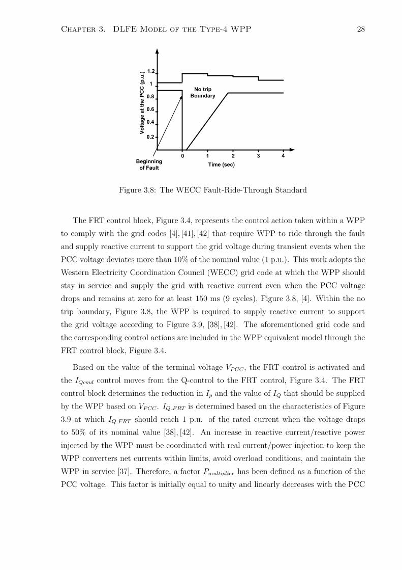
The FRT control block, Figure 3.4, represents the control action taken within a WPP
to comply with the grid codes [4], [41], [42] that require WPP to ride through the fault
and supply reactive current to support the grid voltage during transient events when the
PCC voltage deviates more than 10% of the nominal value (1 p.u.). This work adopts the
Western Electricity Coordination Council (WECC) grid code at which the WPP should
stay in service and supply the grid with reactive current even when the PCC voltage
drops and remains at zero for at least 150 ms (9 cycles), Figure 3.8, [4]. Within the no
trip boundary, Figure 3.8, the WPP is required to supply reactive current to support
the grid voltage according to Figure 3.9, [38], [42]. The aforementioned grid code and
the corresponding control actions are included in the WPP equivalent model through the
FRT control block, Figure 3.4.
Based on the value of the terminal voltage VPCC , the FRT control is activated and
the IQcmd control moves from the Q-control to the FRT control, Figure 3.4. The FRT
control block determines the reduction in Ip and the value of IQ that should be supplied
by the WPP based on VPCC . IQ FRT is determined based on the characteristics of Figure
3.9 at which IQ FRT should reach 1 p.u. of the rated current when the voltage drops
to 50% of its nominal value [38], [42]. An increase in reactive current/reactive power
injected by the WPP must be coordinated with real current/power injection to keep the
WPP converters net currents within limits, avoid overload conditions, and maintain the
WPP in service [37]. Therefore, a factor Pmultiplier has been defined as a function of the
PCC voltage. This factor is initially equal to unity and linearly decreases with the PCC

Chapter 3. DLFE Model of the Type-4 WPP 29
-50%
-100%
IQ/In
V/Vn
Voltage
Support
Voltage
Limitation
-10% 10%
Dead band
around nominal
voltage
Figure 3.9: Reactive Current Requirements for Grid Voltage Support
Figure 3.10: The Fault-Ride-Through Control Block
voltage dip, Figure 3.11. This factor is sent to the active power control block to reduce
the value of Pref .
3.7 WTGs Equivalent Model
The WTGs equivalent model, Figure 3.3, represents the aggregated dynamics of the
WTGs within a WPP. Due to the design of Type-4 WTGs and the decoupling effect
of the back-to-back converter interface, the dynamics of the turbine-generator and the
rotor-side converter have secondary impact on the net WPP dynamic behavior at the

Chapter 3. DLFE Model of the Type-4 WPP 30
*01 *02*03 .
.
*04
*04
*02
*03
*01
Figure 3.11: Active Power Reduction During Voltage Dips
PCC [6],[30]–[32]. Consequently, the dynamic model of the WTG units can be adequately
represented by those of the corresponding GSCs and their local controls.
The equivalent representation of the GSC and its local control is deduced from the
detailed model of Type-4 GSC, Figure A.2 of Appendix A, with the assumption that the
WTG interfacing converter is three-phase, two-level, current-controlled voltage-sourced
converter. The equivalent model of one WTG is first developed in per unit at the WTG
unit base values. By scaling the base values, the equivalent will represent the aggregated
dynamics of all WTGs within the WPP. The dynamics of the AC side can be described
in the dq-frame by [43]:
Ldiddt
= Lωoiq −Rid + Vtd − VSd, (3.3)
Ldiqdt
= −Lωoid −Riq + Vtq − VSq. (3.4)
Representing (3.3) and (3.4) in the S-domain results in
id(Ls+R) = Lωoiq + Vtd − VSd, (3.5)
iq(Ls+R) = −Lωoid + Vtq − VSq. (3.6)
The above two equations represent the dynamics of the GSC AC-side, Figure 3.12, in
which id and iq are the state variables; Vtd and Vtq are the control inputs; and VSd and
VSq are the disturbance inputs. In (3.5) and (3.6) Vtdq are the GSC terminal voltages
and are given by [43]:
Vtd(t) =VDC
2md(t), (3.7)
Vtq(t) =VDC
2mq(t). (3.8)

Chapter 3. DLFE Model of the Type-4 WPP 31
.
"
;
%
"%
%
.
"
;
&
"&
&
Figure 3.12: Block diagram Represents the AC-Side Dynamics
&
%
/1
%
&#
#
Figure 3.13: Control Model of the ideal two-level VSC in the dq-frame
The above two equations represent the model for the two-level GSC in the dq-frame,
Figure 3.13, where md and mq are the dq-component of the modulation signal sent to the
GSC switches. The modulation signals are determined by the GSC closed loop control
that regulates the GSC output currents (idq). The GSC local control is discussed in
Section A.2 and employed in this section. The integration of the models of the GSC,
the dynamics of the AC side, and the current control, i.e., Figures 3.13, 3.12, and A.3
respectively forms the model of the current controlled GSC, Figure 3.14 [43]. The model
of Figure 3.14 can be simplified into the equivalent block diagram of Figure 3.15 where
the d- and q-compensators are PI-controllers that track the reference values (idref and
iqref ).
The block diagram of Figure 3.15, re-scaled to the base values of the WPP, represents

Chapter 3. DLFE Model of the Type-4 WPP 32
!"
#$
%&$
%'$
(
)
)
!"
#*%&*
%'*
)
(#*(+,-
#$(+,- .$/&0
.*/&0
(
))
)
1$
1*
)
#$
#*
%2345
4
46*
6$
%2345
7
&8)89
!"
#$
%&$
%'$
(
)
)
7
&8)89
!"
#*
%&*
%'*
(
)
(
:38;#$,82<=>6#?&
%;3831++,='83"='+"@@,+
%;3
Figure 3.14: Block Diagram of the Current Controlled GSC System
%
&
&
% =%6"7
=&6"7
%
&
.
"
%
.
"
&
&+)"
%+)"
Figure 3.15: Equivalent Model of WTG Units
the equivalent model of the aggregated GSCs and their local controls. The input reference
currents idref and iqref are the command currents from the supervisory control (IPcmd
and IQcmd) while the output currents id and iq represent the WPP output currents that
are injected to the grid at the PCC.

Chapter 3. DLFE Model of the Type-4 WPP 33
3.8 Wide-Band Equivalent Model of Type-4 WPP
The proposed reduced-order dynamic-equivalent model of Type-4 WPP is based on the
integration of the FDNE, Chapter 2, and the DLFE, Figure 3.3. These two parts are
represented by two circuit blocks that are in parallel with respect to the PCC, Figure
3.16. The FDNE is implemented in the PSCAD/EMTDC, based on the companion
circuit approach [25], [26]. The trapezoidal numerical integration method is utilized to
convert the rational function, obtained from the vector fitting, to a resistive network in
conjunction with a set of history current sources as explained in Chapter 2. The DLFE
model is represented in the PSCAD/EMTDC based on the transfer function method and
is interfaced to the electrical network through a three-phase controlled current source,
Figure 3.16.
#$%&'
($
'
$'
# " &
!"
$%
'("
)%
!$
Figure 3.16: The Proposed Wind Power Plant Dynamic-Equivalent
3.9 Test System
The system of Figure 3.17 which is a modified form of the Lake Erie [44], [45] WPP and
connected to the Hydro One system is used to evaluate and verify performance of the
proposed WPP equivalent model.
The WPP is composed of (i) one 34.5/115-kV transformer, (ii) a 34.5-kV collector
system, (iii) 0.6-kV Type-4 WTG units and their local controllers that are connected to
the collector system through 0.6/34.5-kV delta/wye-grounded transformers, and (iv) the

Chapter 3. DLFE Model of the Type-4 WPP 34
WPP supervisory control. For the reported studies, WTG units in the collector branches
are represented by 17 Type-4 units where power rating of each unit is given on Figure
3.17. The original Lake Erie WPP includes 66, 1.5-MW WTG units. The collector
system includes four main branches and 17 sub-branches. Each sub-branch is connected
to 3, 4, 5, or 6 WTG units. Due to the computational burden to run a simulation with
such a high number of units, the units in each sub-branch are represented by one unit as
shown in Figure 3.17. Appendix C provides the line parameters.
Each WTG unit of Figure 3.17 is equipped with a dq-current controller that deter-
mines its id and iq current injection into the collector system. The WPP supervisory
control provides reference values for each WTG unit to meet the grid power require-
ments and FRT requirements during transients. The adopted FRT characteristics are
described in [4], [42].
The power system external to the WPP is composed of two parallel 115-kV overhead
lines that connect the WPP to the load bus, Figure 3.17. The load bus is also connected
by a short overhead line to the grid which is represented by a three-phase source behind
a three-phase impedance.
To evaluate performance of the proposed equivalent model and verify its accuracy,
the following procedures were followed.
A. The study system of Figure 3.17 is modeled in detail in the PSCAD/EMTDC
platform as described in Appendix A. The WPP is represented by 17 WTG units,
Figure 3.17. The VSC of each WTG unit is represented by a three-phase two-level
VSC and constructed with six IGBT valves. The converter operates based on a
3060-Hz SPWM. The local controller of each VSC is based on a decoupled d- and q-
current approach that utilizes PI-controllers to enable each WTG output current
to track the reference dq-current components provided by the WPP supervisory
control [43]. The dq-current reference values for each WTG are determined by
the WPP supervisory control based on the P and Q components to be delivered
by the WPP. The AC-side terminal of each VSC is connected to the collector
system through a three-phase LC filter and a three-phase transformer. Each 3-
km section of the collector system is represented by a π-equivalent. The WPP
interface transformer is represented as a three-phase transformer, including the
magnetization branch. The overhead lines in the AC power system are represented
by π-equivalent models.

Chapter 3. DLFE Model of the Type-4 WPP 35
!"#$%!&'(
)$
#'*
+&,-.%!&,-.%!&,-+&,-
/&,-/&,-/&,- /&,-/&,-
#'* #'* #'* #'*
#'* #'* #'*
#'*
0123
!!
-)0&4526
"#!$!
$!#!
78 789
)
)9
)#
:;<3&
8=>9+%?&'*
9&'*
%!&'*
#'* #'* #'* #'*
$%!&,-$%!&,-$%!&,-$%!&,-
#'* #'* #'* #'*
$%!&,-$%!&,-$%!&,-$%!&,-
-@@
7;561;A
);&-)0>
-@@
:B2A6C1
7B2A6C1
DB2A6C1
EF6C15<A&7;**<53>
Figure 3.17: Schematic Diagram of the Modified version of Lake Erie Shores WPP
B. The PSCAD/EMTDC detailed model of part A above is used to develop the FDNE
model of the WPP, with respect to the PCC, Chapter 2. The PSCAD/EMTDC
model is used to obtain the frequency scan of the WPP using 5000 logarithmically-
distributed frequency points in the range of 0 to 50 kHz. Then fitted to a 56th-order
rational function given by (2.2), using the vector fitting technique, Chapter 2.
C. The DLFE model of the WPP is developed as described in the previous sections of
this chapter.
D. Based on the models of parts B and C, the overall equivalent model of the WPP is
constructed and implemented in the PSCAD/EMTDC.
Figure 3.18 compares the input admittance of the WPP passive network obtained
from the detailed model and the FDNE. In this Figure, the two solid waveforms represent
the self and mutual admittances of the passive network of the detailed model while the
two dashed waveforms represent the same admittances, but of the FDNE. The close
agreement between the two groups of waveforms demonstrates the accuracy of the FDNE
in modeling the WPP passive network.

Chapter 3. DLFE Model of the Type-4 WPP 36
!"
#
!"
Figure 3.18: Admittance Magnitudes of the Fitted Equivalent and the Detailed Modeled
Passive Network - (a) self admittance, (b) mutual admittance
3.10 Case Studies
A set of case studies is performed on the system of Figure 3.17 to quantitatively demon-
strate and verify the accuracy of the WPP equivalent model when line T2 is subjected to
different faults and switching events. For each fault study, the power system (right-side
of the PCC of Figure 3.17) is represented in the PSCAD/EMTDC environment and the
WPP (left-side of the PCC of Figure 3.17) is represented once by its detailed model
(Section 3.9-A), and once by its equivalent model (Section 3.9-D) and the corresponding
study results are identified by the “Detailed Model” and the “Equivalent Model”, respec-
tively. Each reported case study is simulated for up to 6-second of real-time to allow the
supervisory control, units control, and the system reach a steady state condition before

Chapter 3. DLFE Model of the Type-4 WPP 37
imposing a fault on line T2.
3.10.1 Case I
The system is subjected to a 150-ms temporary L-L-L-G fault, 15-km from the PCC on
line T2 at t= 4.5s. Prior to the fault, the system is under steady-state conditions and the
WPP delivers 99-MW to the system at PCC. Figures 3.19-3.21 show the system response
to the fault based on the detailed model and the equivalent model of the WPP.
Figure 3.19 shows the instantaneous PCC voltages prior, during, and immediately
after the fault and illustrates close agreement between the results of the equivalent model
and the detailed model. Figure 3.20 shows the injected current by the WPP into the
system (at the WPP transformer HV-side) during and after the fault clearance and also
indicates close agreement between the results of the two models. Figure 3.21 shows real
and reactive power and current components and the PCC rms voltage. Figure 3.21 also
illustrates the PCC voltage FRT characteristic [4]. Figure 3.21 indicates that during the
fault, the WPP remains in service even when the PCC voltage, Figure 3.21(e), drops
to 15% of its nominal value and the WPP output reactive current increases to 1.0 p.u.
while the active current drops to zero, Figures 3.21(c) and 3.21(d).
3.10.2 Case II
This case is to investigate the accuracy of the developed equivalent model as the location
of the fault changes along the line T2. The worst case scenario is considered here when
the fault takes place at the PCC. The fault type, application time, and the prefault
steady-state conditions are the same as those of Case I. The protecting circuit breakers
on the terminals of the line T2 will react to clear the fault after five cycles.
Figures 3.22 to 3.24 show and compare the time-domain simulation results of both the
detailed system and the corresponding results obtained from the developed equivalent.
The close agreement between the results verifies the accuracy of the developed equivalent.
3.10.3 Case III
The system of Figure 3.17 is subjected to a 150-ms temporary L-G fault at t= 4.5s at the
same location where the L-L-L-G fault of Case I was imposed. The prefault steady-state
conditions are the same as those of Case I. Figures 3.25 and 3.26 show the PCC voltages

Chapter 3. DLFE Model of the Type-4 WPP 38
) $ ) $ )
&'(
.
./
12'
! "
$ ) $
!11
$ ) $
&'(
.
./%
12'
! "
$ ) $
./(
.
&'(
12'
! "
$ ) #
$
)
$
$
!11
!11
&
)- 0
)- 0
$
Figure 3.19: PCC Voltages of the Detailed and the Equivalent Models - Case I
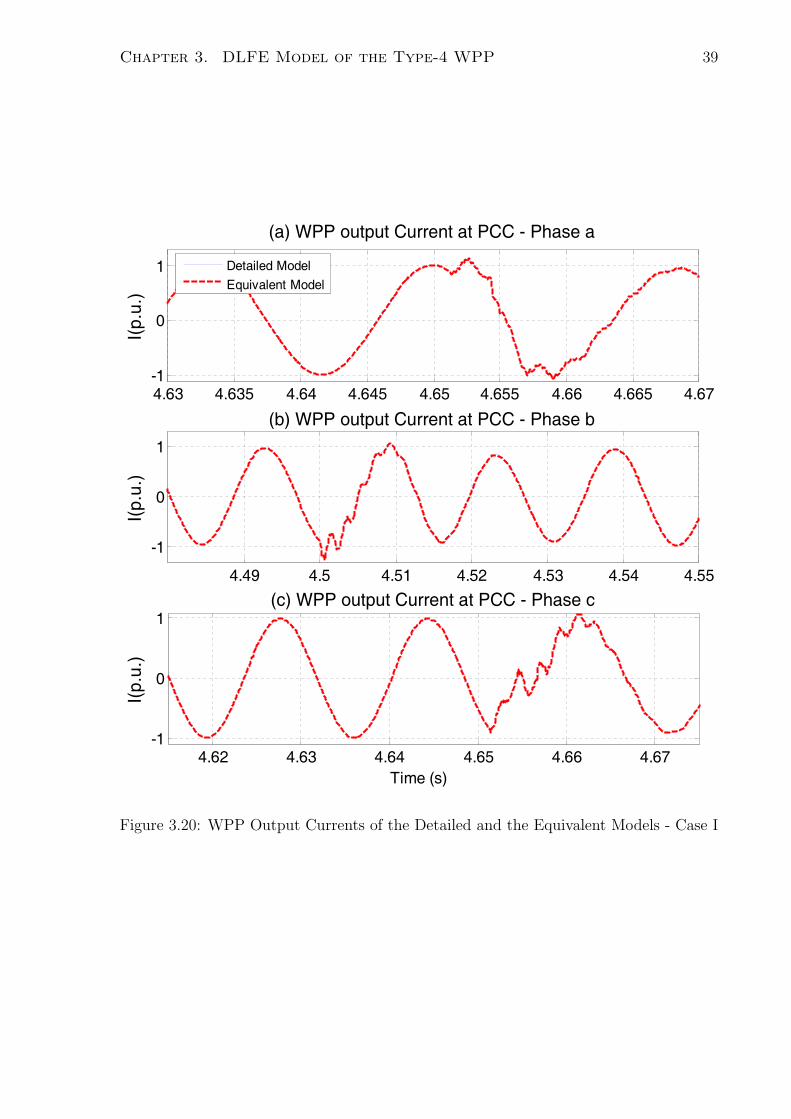
Chapter 3. DLFE Model of the Type-4 WPP 39
!"
# $
% %
$
&'
( (
Figure 3.20: WPP Output Currents of the Detailed and the Equivalent Models - Case I
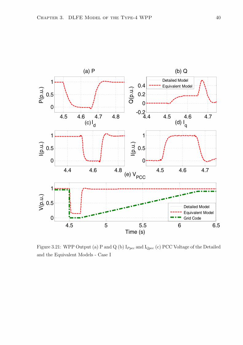
Chapter 3. DLFE Model of the Type-4 WPP 40
# $ 0
'
'
# $
1
-1
"+
# 0
%
-%
# $
%
%
# #
2'((
./ *
2
"+
3(
)*
Figure 3.21: WPP Output (a) P and Q (b) IPpcc and IQpcc (c) PCC Voltage of the Detailed
and the Equivalent Models - Case I

Chapter 3. DLFE Model of the Type-4 WPP 41
) $ ) $
&'
+
+-
) $ ) $
&'
+
+-%
!"
) $ ) $
&'
+
+-(
)) # #$ # # #)
) )) # #$ # #
Figure 3.22: PCC Voltages of the Detailed and the Equivalent Models - Case II

Chapter 3. DLFE Model of the Type-4 WPP 42
) $ ) $$
$
&'
!"
) $ ) $$
$
&'
%
) $ ) $$
$
&'
(
Figure 3.23: WPP Output Currents of the Detailed and the Equivalent Models - Case II

Chapter 3. DLFE Model of the Type-4 WPP 43
)
&'
$
&'
*
%*
!"
)
&'
(
)
&'
!
&'
+
+
!"
,
Figure 3.24: The WPP Output (a) P and Q (b) IPpcc and IQpcc (c) PCC Voltage of the
Detailed Network and the Developed Equivalent of Case II

Chapter 3. DLFE Model of the Type-4 WPP 44
and the WPP output currents; they demonstrate close agreement between the results
of the detailed and the equivalent models which verifies the accuracy of the developed
equivalent even under unbalanced conditions.
3.10.4 Case IV
This case is to investigate the effect of a sequence of multiple transients on the accuracy
of the developed model. The system of Figure 3.17, is subjected to the L-L-L-G fault of
Case I at t=4.5s, after 5 cycles the circuit breakers CB1 and CB2 react and disconnect
the faulted transmission line. The circuit breakers remain open for 15 cycles, during
which the fault clears, and then the circuit breakers successfully reclose. Figure 3.27
shows the WPP terminal voltages over the aforementioned sequence of operation and
demonstrate the close agrement between the simulation results of both the detailed and
the equivalent models. Figures 3.28 and 3.29 depict the WPP output currents, power
components, and the PCC rms voltage of both the detailed and the equivalent models.
The close agreement between the results of the two models verifies the accuracy of the
developed equivalent model.
3.10.5 Case V
The system of Figure 3.17 is subjected to the L-L-L-G fault of Case I at t=4.5s. The fault
is cleared after 5 cycles by circuit breakers CB1 and CB2. After another 15 cycles CB1 and
CB2 automatically reclose and since the fault is permanent, the reclosure is unsuccessful
and subjects the system to another L-L-L-G fault. The second fault is cleared by CB1 and
CB2 which permanently remain open after the second fault clearing. Figure 3.30 shows
transients of the PCC voltages corresponding to the fault and its subsequent switching
events. Figure 3.30 also illustrates close agreement between the corresponding results
of the two models. Figure 3.31 depict the time-domain simulation results of the WPP
output currents of both the detailed system and the corresponding results obtained from
the developed equivalent. Close agreement between the corresponding results of Figures
3.30 and 3.31 also verifies accuracy of the results obtained from the equivalent model.

Chapter 3. DLFE Model of the Type-4 WPP 45
) $ ) $ )
+
+-(
$ ) $
$
)
$
) $ ) $ )
+
+-
!"
) #
) $ ) $ )
&'
+
+-%
Figure 3.25: PCC Voltages of the Detailed and the Equivalent Models - Case III

Chapter 3. DLFE Model of the Type-4 WPP 46
$
$
!"
$
$
%
$
$
&'
(
Figure 3.26: WPP Output Currents of the Detailed and the Equivalent Models - Case
III

Chapter 3. DLFE Model of the Type-4 WPP 47
) $ ) $
&'
+
+-(
) $ ) $
&'
+
+-%
) $ ) $
&'
+
+-
!"
) ) )) # #$ # #
## $
)$ ) ) )) # #$ #
Figure 3.27: PCC Voltages of the Detailed and the Equivalent Models - Case IV

Chapter 3. DLFE Model of the Type-4 WPP 48
) $ ) $
&'
!"
) $ ) $
&'
%
) $ ) $
&'
(
Figure 3.28: WPP Output Currents of the Detailed and the Equivalent Models - Case
IV

Chapter 3. DLFE Model of the Type-4 WPP 49
)
&'
$
)
&'
*
%*
!"
)
&'
(
&'
!
) $ ) $
&'
+
+
!"
,
Figure 3.29: The WPP Output (a) P and Q (b) IPpcc and IQpcc (c) PCC Voltage of the
Detailed Network and the Developed Equivalent of Case IV

Chapter 3. DLFE Model of the Type-4 WPP 50
) ) # #
&'
+
+-
) ) # #
&'
+
+-%
!"
) ) # #
&'
+
+-(
) ) )) # #$ #
)$ ) ) )) ) )$ )
# #$ #$ #
Figure 3.30: PCC Voltages of the Detailed and the Equivalent Models - Case V

Chapter 3. DLFE Model of the Type-4 WPP 51
) ) # #
&'
) ) # #
&'
%
) ) # #
&'
(
Figure 3.31: WPP Output Currents of the Detailed and the Equivalent Models - Case V

Chapter 3. DLFE Model of the Type-4 WPP 52
3.10.6 Case VI
This case introduces more complex transients which combines multiple transients, un-
balanced fault, and unbalanced fault clearance. The system of Figure 3.17, is subjected
to the L-G fault at t=4.5s, after 5 cycles the circuit breakers CB1 and CB2 disconnect
the faulted transmission line through only one pole operation. The circuit breakers will
remain open for 15 cycles, during which the fault clears, and then the circuit breakers
successfully reclose. The transient scenario includes an unbalanced fault transient that
is followed by an unbalanced circuit breaker operation at which only one phase of the
transmission line is disconnected to clear the fault; then, the faulted phase successfully
recloses after 15 cycles.
The time-domain simulation results of both the detailed and the equivalent models
are shown in Figures 3.32 and 3.33. The close agreement between the corresponding
results of Figures 3.32 and 3.33 verifies the accuracy of the developed equivalent model
for EMT-type studies.
3.10.7 Case VII
This case is similar to Case VI, but with double line to ground fault and in consequence
double pole circuit breaker operation. The time-domain simulation results of both the de-
tailed and the equivalent models are shown in Figures 3.34 and 3.35. The close agreement
of the corresponding results verifies the accuracy of the developed equivalent model.
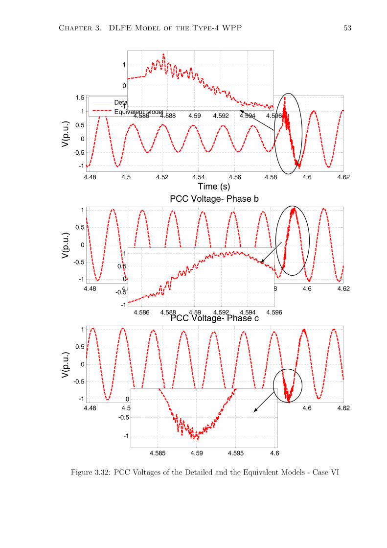
Chapter 3. DLFE Model of the Type-4 WPP 53
) $ ) $
&'
+
+-
!"
) $ ) $
&'
+
+-%
) $ ) $
&'
+
+-(
) )) # #$ # #
) )) # #$ # #
) # #
Figure 3.32: PCC Voltages of the Detailed and the Equivalent Models - Case VI

Chapter 3. DLFE Model of the Type-4 WPP 54
) $ ) $$
$
&'
!"
) $ ) $
$
$
&'
%
) $ ) $$
$
&'
(
Figure 3.33: WPP Output Currents of the Detailed and the Equivalent Models - Case
VI

Chapter 3. DLFE Model of the Type-4 WPP 55
) $ ) $
&'
+
+-
!"
) $ ) $
&'
+
+-%
) $ ) $
&'
+
+-(
$ )
)$ ) ) )) # #$ # #
)$ ) ) )) # #$ # #
Figure 3.34: PCC Voltages of the Detailed and the Equivalent Models - Case VII

Chapter 3. DLFE Model of the Type-4 WPP 56
) $ ) $
&'
!"
) $ ) $
$
&'
%
) $ ) $$
$
&'
(
Figure 3.35: WPP Output Currents of the Detailed and the Equivalent Models - Case
VII

Chapter 3. DLFE Model of the Type-4 WPP 57
3.11 Discussions
The case studies have been conducted to investigate the accuracy of the proposed equiv-
alent model. These case studies cover different types of faults that occur at different
locations. In addition, case studies were conducted where a sequence of multiple and
unbalanced transients occurred in the power system external to the WPP. The close
agreement between the time-domain simulation results obtained from the detailed model
and the corresponding results obtained from the developed equivalent model, Figures 3.19
to 3.35, verifies the accuracy of the developed equivalent model for EMT-type studies. In
addition, the errors between the maximum overvoltages and overcurrents obtained from
the detailed and the equivalent models are 1.6% and 1.3% respectively.
The developed equivalent model drastically reduces the computational burden and
hence the computation time required to conduct EMT-type studies. For instance, the
time required to conduct a 6-second real-time simulation run with a 5 µs time-step, using
the detailed model is approximately 5 hours and 8 minutes on a quad cores Intel 3.07
GHz i7 machine with 6 GB of memory. On the other hand the proposed equivalent
only requires approximately 110 seconds to solve the same case study and with the same
simulation time-step, i.e., the equivalent model reduces the computation time by a factor
of 218 as compared to the detailed model.
Figures 3.36 and 3.37 compare the PCC voltage of phase c, Case I, obtained from
the detailed and the equivalent models when the WPP equivalent model only consists of
(i) the FDNE model, Figure 3.36, and (ii) the DLFE model, Figure 3.37. Figures 3.36
and 3.37 demonstrate that neither the FDNE model nor the DLFE model individually
can accurately represent the WPP for EMT type studies. In Figure 3.36 the equivalent
model is represented by the DLFE which represents only the low frequency dynamics
of the WPP active components. This representation misses the high frequency response
resulted from the exchange of energy between the inductances and capacitances of the
WPP passive network, due to system transients. Comparing Figures 3.19, 3.36, and 3.37
clearly demonstrates that the FDNE model and the DLFE model jointly can provide an
accurate model of the WPP. This justifies the need for a wide-band equivalent model of
WPP for EMT studies.

Chapter 3. DLFE Model of the Type-4 WPP 58
$ ) $ )
&'
.
./(
45
$ )
$
)
$
$
Figure 3.36: PCC Voltage, phase c, of the Detailed and the FDNE Models - Case I
$ ) $ )
&'
.
./(
34
$ )
Figure 3.37: PCC Voltage, phase c, of the Detailed and the DLFE Models - Case I
3.12 Conclusions
This chapter developed and validated a reduced-order, dynamic-equivalent model of
Type-4 based WPPs, for the analysis of EMTs external to the WPP, within a frequency

Chapter 3. DLFE Model of the Type-4 WPP 59
range of 0-50 kHz. The proposed equivalent model captures (i) the frequency response
of the WPP passive components, and (ii) the dynamics of the WPP active components.
The accuracy and computational efficiency of the proposed equivalent model have been
validated through multiple case studies that compare the simulation results of the equiva-
lent model and those of the detailed model of a modified version of the Lake Erie WPP in
the PSCAD/EMTDC. The case studies covered different types of transients due to faults
at different locations with respect to the WPP terminal. The study results concluded
that:
• The developed equivalent model simulation results and the corresponding detailed
model results closely agree and confirm accuracy of the proposed equivalent model.
• Compared to the detailed model, the equivalent model adopts a simpler structure
and does not explicitly model the VSCs.
• The developed equivalent model is computationally efficient. Compared to the
detailed model, the equivalent model reduces the computational time for the test
system by factor of about 218.
• The developed equivalent model is a scalable model, i.e., its per unit signals can
be scaled to the base values of the WPP of interest. In other words, the size
and number of WTGs units within the WPP do not affect the structure of the
equivalent.
• The developed equivalent model is a wide band model that represents the WPP re-
sponse in a frequency range of about 0-50 kHz. This frequency range is determined
based on the phenomenon of interest. The equivalent model can be adapted to a
new frequency range based on modification to the FDNE.

Chapter 4
Dynamic Low-Frequency Equivalent
Model of Type-3 WPP
4.1 Introduction
This chapter presents the development and validation of the dynamic low-frequency
equivalent (DLFE) model of WPPs with doubly-fed asynchronous generator (DFAG)
WTG units known as Type-3 units. The DLFE of Type-3 WPP represents the aggre-
gated dynamic model of the DFAG-WTGs, their local controls, and the WPP supervisory
control and it includes (i) the equivalent model of the wind turbines, (ii) the equivalent
model of the Type-3 generation units and their converters local controls, and (iii) the
WPP supervisory control. The above mentioned DLFE is integrated with the equivalent
model of the WPP collector network model to form a wide-band equivalent model of
Type-3 WPP. The Type-3 WPP equivalent model reproduces the dynamic behavior of
the WPP in response to an electromagnetic transient in the host power system.
The structure of this chapter is as follows: section 4.2 is a brief overview of the DFAG
unit, its advantages, and the motivation behind developing the equivalent model of this
chapter. Section 4.3 states the equivalent model assumptions. Section 4.4 presents the
structure of the DLFE. The modules of the DLFE, i.e., the equivalent model of the
wind turbines, the WPP supervisory control, and the equivalent model of the generators
with their converters are presented in Sections 4.5, 4.6, and 4.7 respectively. Section
4.8 integrates the DLFE with the WPP collector network equivalent model. The ac-
curacy of the developed model is demonstrated through several case studies, using the
PSCAD/EMTDC in sections 4.9 and 4.10. Discussion of the study results and the con-
60

Chapter 4. Dynamic-Equivalent Model of the Type-3 WPP 61
clusions of this chapter are in Sections 4.11 and 4.12 respectively. The detailed model
of Type-3 WPP, including the local and central controls, which is used to guide the
development and validation of the equivalent model is presented in Appendix D.
4.2 Background
The DFAG-based WTG is widely used in existing WPPs [46] where each DFAG unit is
connected to the collector network directly through its stator while its rotor is interfaced
to the network through a back-to-back converter system, Figure 4.1. The back-to-back
converter allows the independent control of the active power delivery and the reactive
power exchange with the grid. Typically the RSC controls the stator power flow through
a smaller percentage of power injected into the rotor circuit; therefore, the back-to-back
converter is typically rated to 30-40 % of the machine rated power [47]. The reduced
size of the converter translates to a reduced cost of both the converter and its filter. In
addition, it results in a reduced converter losses, compared to the full rated converters,
and potentially higher efficiency [32], [48].
With the wide use and increased capacity of the Type-3 WPP, it is vital to develop
an appropriate model to analyze its response to different transients in the power system.
For EMTs studies, the full order models that include differential equations of the whole
WPP are used to simulate the WPP in time-domain simulation programs which in turn
use a small integration time-step to solve the model equations. The small integration
time-step along with the significant number of differential equations corresponding to
the complex configuration of the DFAG and the typical large number of units within the
WPP result in a significant computational burden and therefore prolonged simulation
time. The computationally efficient equivalent model developed in this chapter overcomes
the aforementioned limitations. The developed equivalent model is simple yet accurate
in modeling the response of the active components of Type-3 WPPs to EMTs, external
to the WPP in the power system, within the frequency range of 0 up to 20 Hz.
There are various control schemes for a DFAG-based WTG in a WPP [49]. In order
to develop the equivalent model of this thesis, the DFAG detailed model of Appendix D
is considered. In this detailed model, the local control of the RSC controls the generator
torque and the stator reactive power flow while the local control of the GSC controls the
DC-link voltage and the reactive current at the machine terminal. The local controls are
decoupled current controllers with inner dq current control loops. This detailed model

Chapter 4. Dynamic-Equivalent Model of the Type-3 WPP 62
is also used as a benchmark system to validate the accuracy of the developed equivalent
model. Multiple control strategies and hardware apparatus have been introduced in the
literature to enable the DFAG-based WPPs to satisfy the fault-ride-through requirements
[46],[50]–[53]. Each of these techniques has its own merits and limitations; however, many
of them fail to achieve their objective during transients which impose severe voltage
dips [52]. In this thesis, a dynamic voltage restorer (DVR) [51], [52] at the unit terminal
is assumed to assist in boosting the unit terminal voltage during transients and thus
enable the DFAG unit and the WPP to provide ride-through capability subsequent to a
fault, Figure D.2, Section D.3.
,*
'-'
./' 0
1
Figure 4.1: Schematic Diagram of the Doubly-Fed Asynchronous Generator (DFAG) Unit
4.3 Equivalent Model Assumptions
The equivalent model of Type-3 based WPP is developed based on the following assump-
tions:
• The proposed equivalent model represents the collective terminal behavior of the
WPP and not the individual behavior of each WTG unit.
• The disturbance is considered to take place in the power system external to the
WPP.
• The WTG units within the WPP are considered to be of the same type (Type-3 in
this chapter) and their local controls adopt the same control objectives.

Chapter 4. Dynamic-Equivalent Model of the Type-3 WPP 63
• The dynamics of the pitch control is not represented in this equivalent model since
the time constant of the pitch control and the mechanical inertia are assumed to
be very large relative to the time frame of the EMTs of interest.
4.4 Structure of the Dynamic Low-Frequency Equiv-
alent Model of the Type-3 WPP
The DLFE model of the Type-3 based WPP, Figure 4.2, represents the dynamics of
the aggregated WTG units and the natural modes of controls, typically, in a frequency
range of 0 up to 20 Hz. Based on the DFAG structure and its components, described in
Appendix D, the DLFE of Figure 4.2 is proposed. The DLFE, Figure 4.2, constitutes a
complete equivalent of the DFAG-based WPP low-frequency dynamics.
The measurement block represents the function of the measuring devices of the WPP.
It acquires instantaneous three-phase PCC voltage and the WPP net current (at the HV-
side of WPP substation transformer) and generates the required signals for control and
PLL blocks. The PLL provides synchronization to the positive-sequence PCC voltages.
The wind turbines equivalent block represents the dynamics of the aggregated wind
turbines. It determines the WPP equivalent mechanical power that corresponds to the
wind speed, taking into consideration the wind turbine characteristics. This block also
includes an equivalent drive-train model that computes the equivalent angular frequency
ωreq, Figure 4.2. The supervisory control block represents the conceptual functions of
the WPP supervisory control which includes the control of active and reactive power
components injected by the WPP into the system [31], [37], [39]. This block determines
the d- and q-current references corresponding to the WPP P and Q reference values. The
FRT control function is also represented in this block. The FRT control provides the
reference currents to enable the WPP fault ride-through subsequent to transients [4],[38].
The generators and converters equivalent block represents the dynamics of the aggregated
machines, converters, and their local controllers. This block injects currents into the
system at the PCC, in response to the current references from the supervisory control.
The following sections elaborate on the details of each block. The PLL block in Figure
4.2 is identical to the PLL described in Section 3.5 and not discussed in this chapter.

Chapter 4. Dynamic-Equivalent Model of the Type-3 WPP 64
!
"
#
#
$
"
#
%
Figure 4.2: The Dynamic Low-Frequency Equivalent of Type-3 WPP
4.5 Equivalent Model of Wind Turbines
This model is an equivalent of the WPP wind turbines mechanical rotating systems.
This model provides transformation of the wind energy into mechanical power and the
aggregated dynamic behavior of the drive-trains. This equivalent model is composed of
two main parts, Figure 4.3:
(i) The aerodynamic-equivalent model that determines the mechanical power harnessed
from the wind based on the wind speed and the power coefficient (Cp).
(ii) The drive-train model that determines the equivalent generator and turbine angular
speeds ωreq and ωteq respectively.
It is to be noted that the parameters of the Cp equation, (4.3) and (4.5), required
by the aerodynamic model are not necessarily available from the turbine manufacturer;
therefore, to set a systematic method to obtain those parameters, an optimization al-
gorithm is introduced to estimate the parameters, using either field measurements or
simulation of the turbine detailed model, Figure 4.3. The next three subsections elabo-
rate on the components of the wind turbines equivalent model.

Chapter 4. Dynamic-Equivalent Model of the Type-3 WPP 65
!"#$%%&'()(*
+",-./01!2#%3-."4
!"#$%&'()*+&,&-.(/#'(#
514#)416"%72'%
8'"".%9162-
01+2
1'34/
:,2;"<7,120%
3-."4
567+18"/.19&-.(#1.*&:.36*+
='62!2>162-0%
+4?-,26$!
;"+*34<='$#&
:.3+*&>'#'
!'1'?+#+1/&.@&
-7&<26'#".(
@20.%7),A20"B%CD)2;14"06%3-."4
3"#$102#14%
-E",%
514#)4162-0
0A'/+01+2
7B6B
!+ C7B6BD01+2
C7B6BD
EF"(3
Figure 4.3: Wind Turbine Equivalent Model
4.5.1 Aerodynamic Equivalent Model
This equivalent model computes the mechanical power Pmech extracted from the wind
energy as a function of the wind speed and the turbine power coefficient Cp. Equation
(4.1), [54], [55], calculates Pmech of one WTG unit which then has to be scaled to all the
units within the WPP.
Pmech =1
2ρAυ3windCp(λ, β) /SWTG
base , (4.1)
where ρ, A, υwind, λ, β and SWTGbase are the air density in kg/m3, the area of the rotor
blades in m2, the wind speed in m/s, the blade tip speed ratio, the blade pitch angle,
and the base power of one WTG respectively; the output Pmech is in per unit. λ is the
ratio between the speed at the blade tip and the wind speed.
λ =υtipυwind
=(ωreq/G).r
υwind
, (4.2)
where r is the blade radius and G is the gearbox ratio. The turbine power coefficient
Cp(λ, β) is usually represented by a set of curves; each curve relates Cp and λ for a certain
pitch angle β. Typically these curves are mathematically represented by [55], [56]:
Cp(λ, β) = c1
(c2λi
− c3β − c4βc5 − c6
)exp
(−c7λi
), (4.3)

Chapter 4. Dynamic-Equivalent Model of the Type-3 WPP 66
λi =
[(1
λ+ c8β
)−(
c9β3 + 1
)]−1
, (4.4)
where constants c1 to c9 are determined such that the resulting equation/curves repre-
sent the performance of the actual turbine [54], [56], [57]. The optimization algorithm,
described in subsection 4.5.2 is used to determine these constants based on the simulation
results or field measurements.
Typically, all units within the WPP are of the same size and type; therefore, the per
unit mechanical power calculated from (4.1), based on the WTG unit MVA, represents
also the total power of the WPP when multiplied by the WPP base MVA. If the units
within the WPP are of different sizes or have different turbine characteristics, units can
be grouped into groups of identical units. For each group, the total mechanical power is
calculated as described and then the WPP total power is the summation of the groups
mechanical powers. If the units experience different wind speeds with small deviations,
then
υeq =1
n
n∑i=1
υi, (4.5)
where υeq is the WPP equivalent wind speed, n is the number of WTG units, and υi is
the wind speed at unit i. If wind units are exposed to noticeably different wind speeds,
then the WPP equivalent speed is calculated using the WPP power curve [13] as follows.
(i) For each unit, based on its wind speed, the WTG output power Pi is obtained
using the WTG power curve, Figure 4.4, and the total WPP output power is the
summation of power components of all units PWPP =∑n
i=1 Pi.
(ii) An equivalent WPP power curve is obtained by summing the individual WTG units
power curves. This is done by summing the powers of the individual WTG units
for each incoming wind speed.
(iii) From the curve of (ii), the WPP equivalent wind speed, corresponding to the WPP
power of (i) is obtained.

Chapter 4. Dynamic-Equivalent Model of the Type-3 WPP 67
Figure 4.4: Power Curve of a WTG Unit
4.5.2 Parameter Estimation of Wind Turbine Equivalent Model
If the wind turbine manufacturers data is not available, an optimization algorithm is
used to identify the parameters for the wind turbine model. This is based on results
from simulation of detailed model or field measurements.
The constants c1 to c9 of (4.3) need to be determined to minimize deviation between
Pmech of the equivalent model (4.1), calculated with the optimized constants, and that of
the original WTG unit (Pm org). This requires measurements results or detailed simula-
tion results of Pm org, υwind, β, and ωr. Based on this data and a least square minimization
process, an optimization with the objective function
F =∥Pmech − Pm org∥
∥Pm org∥, (4.6)
is constructed. The MATLAB optimization toolbox is used for minimizing (4.6) [58].
4.5.3 Drive-Train Mechanical Model
The wind turbine drive-train is modeled as a set of two lumped rigid masses that are
connected to each other through the corresponding shafts [17],[59]. This thesis adopts the
widely accepted approach of representing the wind turbine drive-train with two masses
[60]–[63]. One mass represents the turbine inertia and the other mass represents the
generator inertia, (4.7), Figure 4.5, and represented by
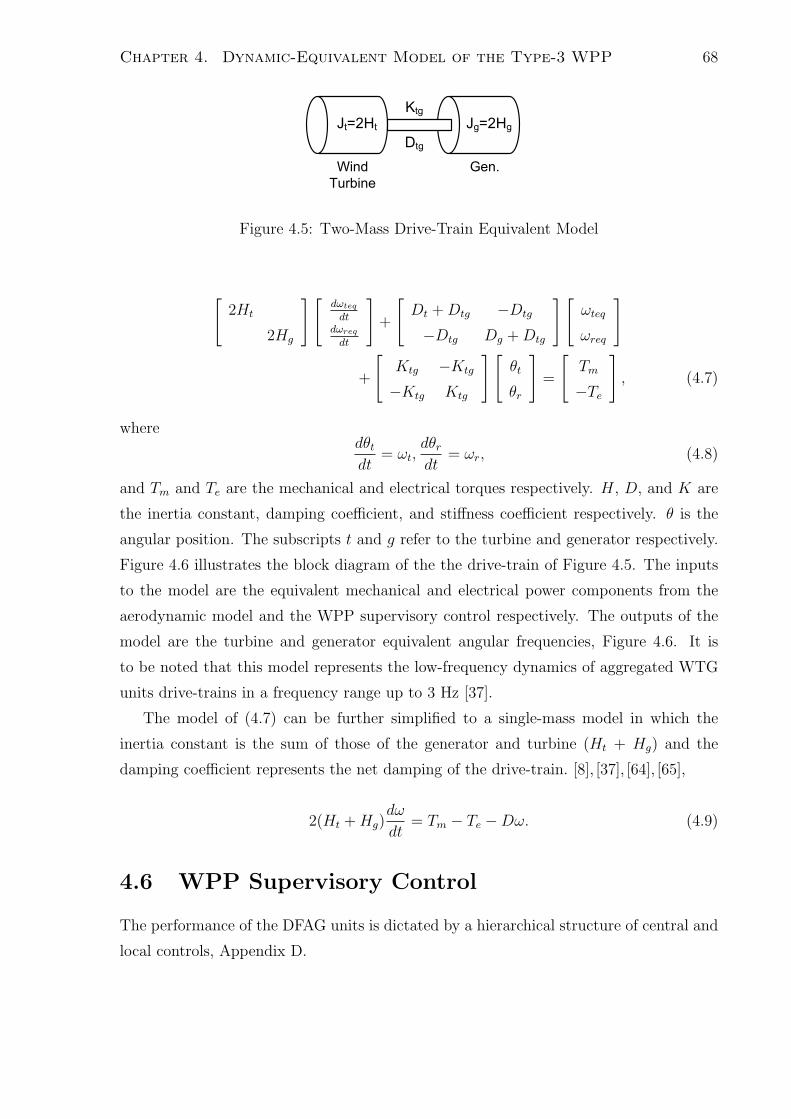
Chapter 4. Dynamic-Equivalent Model of the Type-3 WPP 68
Figure 4.5: Two-Mass Drive-Train Equivalent Model
[2Ht
2Hg
][dωteq
dtdωreq
dt
]+
[Dt +Dtg −Dtg
−Dtg Dg +Dtg
][ωteq
ωreq
]
+
[Ktg −Ktg
−Ktg Ktg
][θt
θr
]=
[Tm
−Te
], (4.7)
wheredθtdt
= ωt,dθrdt
= ωr, (4.8)
and Tm and Te are the mechanical and electrical torques respectively. H, D, and K are
the inertia constant, damping coefficient, and stiffness coefficient respectively. θ is the
angular position. The subscripts t and g refer to the turbine and generator respectively.
Figure 4.6 illustrates the block diagram of the the drive-train of Figure 4.5. The inputs
to the model are the equivalent mechanical and electrical power components from the
aerodynamic model and the WPP supervisory control respectively. The outputs of the
model are the turbine and generator equivalent angular frequencies, Figure 4.6. It is
to be noted that this model represents the low-frequency dynamics of aggregated WTG
units drive-trains in a frequency range up to 3 Hz [37].
The model of (4.7) can be further simplified to a single-mass model in which the
inertia constant is the sum of those of the generator and turbine (Ht + Hg) and the
damping coefficient represents the net damping of the drive-train. [8], [37], [64], [65],
2(Ht +Hg)dω
dt= Tm − Te −Dω. (4.9)
4.6 WPP Supervisory Control
The performance of the DFAG units is dictated by a hierarchical structure of central and
local controls, Appendix D.

Chapter 4. Dynamic-Equivalent Model of the Type-3 WPP 69
4
4
4
4
23(
4
23
,( 0(
5
5
5
5
5
5
%6
6
6
6
6%
%
%
5
5
,
,(
0
0
'
%
%
Figure 4.6: Block diagram of the Two-Mass Drive-Train Model
The supervisory control module is the part of the WPP DLFE equivalent model,
Figure 4.2, that represents the operation of the WPP central control. It includes (i)
P control (ii) Q control (iii) fault-ride through (FRT) control and (iv) current limits
calculations. The collective operation of these parts reflects the performance of the WPP
supervisory control and the outer control level of the WTG units controls before, during,
and after the grid transients. The functions of this equivalent module include:
• Generation of the dq-current references to satisfy the grid requirements correspond-
ing to P and Q and/or to satisfy certain control objectives, e.g., PCC voltage
control, taking into consideration feedback signals from the PCC.
• Representing the active and reactive power generation availability of WTG units,
taking into consideration the available wind and the units generation limits.
• Enabling the FRT control based on the grid requirements.
• Enabling the limits that should be imposed on the WTG units reference cur-
rents/power based on the operation requirements.
The above functions are implemented through the control structure of Figure 4.7.
The P control block, Figure 4.7, can be switched between two modes:
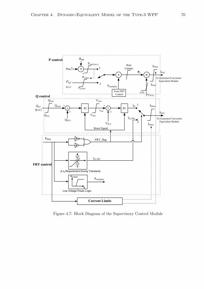
Chapter 4. Dynamic-Equivalent Model of the Type-3 WPP 70
$! !
%&'
(
(
%
)
*&
&
&
& )+,!-
&(
*&
*&
*& )
* *
"./
00(
* )
)
+,!- !,
1 1"
$! !
2,,
#3
:;
; <
"
#
+,!-
0
1"4)/
*&41"
!,
2(2 (
= - ($
(
*&41"
$
*
*
!%
Figure 4.7: Block Diagram of the Supervisory Control Module

Chapter 4. Dynamic-Equivalent Model of the Type-3 WPP 71
1. Maximum Power Tracking Mode: The maximum power that can be extracted from
the wind is calculated from Pref = Koptω3req, more details regarding this expression
is in Appendix D. This power set point is limited to the rated power of the WPP
to avoid over loading.
2. Operator Requirement Mode: The active power set point Pref is received from the
operator. Pref is limited to the power value at point 1, Figure 4.7, to guarantee
that the control set point does not exceed either the WPP rating or the power
available from the wind.
The ramp rate applied on P set point, Figure 4.7, serves to limit the power rate of
increase during the post-fault recovery; this limit can be set to a very large value if there
is no requirement for it in the design of the actual WPP.
The Q control, Figure 4.7, is a coordinated Q/V controller that determines the reactive
current command IQref to satisfy the requirements of both Qref and voltage control at
the PCC. Qref is determined based on the PCC voltage control, power factor control, or
PCC reactive power control as explained in chapter 3.
During transients, e.g., faults, that are accompanied with voltage fluctuations at the
PCC, the FRT should retain the WPP in service and enable ride through the fault
[4], [38]. Based on the voltage at the WPP terminals, the FRT control determines the
value of the supplied IQref during the ride-through process [42]. It also coordinates
the increase in reactive current/reactive power injected by the WPP with a decrease in
real current/power injection through the less than unity Pmultiplier, Figure 4.7, to avoid
overload conditions.
The limits applied on Qref represent the WTG limits with respect to the reactive
power generation/absorption. The limits on IPref and IQref are applied such that their
net effect does not exceed the total current limit of the aggregated WTG units. The
priority of generation may be given to the active or the reactive current based on the
steady state/transient operation. The detail of the current limits block is similar to that
of section 3.6.3. The outputs of the supervisory control module are: (i) the dq-current
references to the module of the generators and converters equivalent model, and (ii) the
electrical power Pe, Figure 4.7, to the wind turbines equivalent module.

Chapter 4. Dynamic-Equivalent Model of the Type-3 WPP 72
4.7 Equivalent Model of the Generators Electrical
Side and Converters
This section presents the dynamic equivalent model of the DFAG units, their converters,
and local controls. This equivalent model represents the response of the WTG units
to commands from the WPP supervisory control, Figure 4.2. The equivalent model of
one WTG unit is developed in per unit on the unit base values. By scaling the base
values, the equivalent model is used to approximate the response of all units within the
WPP. The equivalent model is deduced based on the detailed model of the DFAG unit,
(D.1)-(D.4), Appendix D as follows
By substituting is in (D.4) from (D.3)
ψr =Lm
Ls
ψs +
(Lr −
L2m
Ls
)ir. (4.10)
Defining σ = 1− (L2
m
LsLr
), σs =Ls
Lm
− 1, and σr =Lr
Lm
− 1, (4.10) becomes,
ψr =
(1
1 + σs
)ψs + σ (1 + σr)Lmir. (4.11)
By differentiating (4.11) and substituting fordψr
dtfrom (D.2),
σ (1 + σr)Lmdirdt
= Vr −Rrir − j∆ωψr. (4.12)
Note that the stator flux derivative is neglected, i.e.,dψs
dt= 0 [31], [43], [49], [66]. This
assumption is valid because of the adopted approach of installing a voltage controller in
series with the WTG unit that limits the stator voltage variations.
Substituting ψr from (4.11) in (4.12)and dividing the equation by Rr
στrdirdt
=VrRr
− ir − j∆ω
(ψs
(1 + σs)Rr
+ στrir
), (4.13)
where τr =(1 + σr)Lm
Rr
.
Re-arranging (4.13) results in (4.14), and represented by the block diagram of Figure
4.8.
στrdirdt
+ ir =VrRr
− j(1− σ)τrLm
∆ωψs − j∆ωστrir. (4.14)

Chapter 4. Dynamic-Equivalent Model of the Type-3 WPP 73
The inputs to the block diagram of Figure 4.8 are the rotor voltages Vr and the outputs
are the rotor currents. Vr is controlled by the RSC control as described in Section D.1.
Based on Figure D.3, the RSC inner control can be represented as shown in Figure 4.9.
Figure 4.9 and Figure 4.8 conclude the DFAG model depicted in Figure 4.10. To further
.
<
=>
4
-
.
>
"#
Figure 4.8: Block Diagram of DFAG Equations
.
>"#
= > <
Figure 4.9: RSC Current Control
.
<
=>
4
-
.
>
"#
.
>"#
= > <
Figure 4.10: DFAG Model and RSC Control
simplify the model and present it in a form that relates the inputs and outputs of the
WTG unit, independent of the internal parameters, the following can be considered [31]:
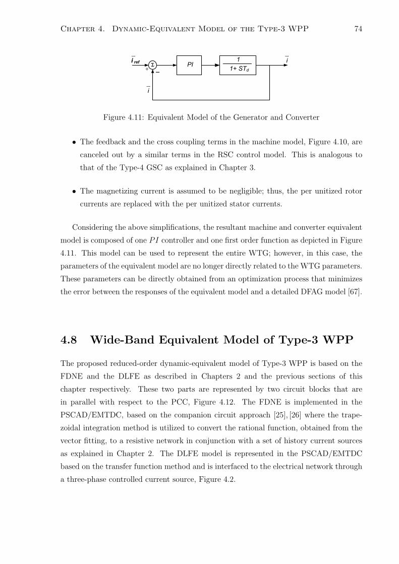
Chapter 4. Dynamic-Equivalent Model of the Type-3 WPP 74
<%$ .
Figure 4.11: Equivalent Model of the Generator and Converter
• The feedback and the cross coupling terms in the machine model, Figure 4.10, are
canceled out by a similar terms in the RSC control model. This is analogous to
that of the Type-4 GSC as explained in Chapter 3.
• The magnetizing current is assumed to be negligible; thus, the per unitized rotor
currents are replaced with the per unitized stator currents.
Considering the above simplifications, the resultant machine and converter equivalent
model is composed of one PI controller and one first order function as depicted in Figure
4.11. This model can be used to represent the entire WTG; however, in this case, the
parameters of the equivalent model are no longer directly related to the WTG parameters.
These parameters can be directly obtained from an optimization process that minimizes
the error between the responses of the equivalent model and a detailed DFAG model [67].
4.8 Wide-Band Equivalent Model of Type-3 WPP
The proposed reduced-order dynamic-equivalent model of Type-3 WPP is based on the
FDNE and the DLFE as described in Chapters 2 and the previous sections of this
chapter respectively. These two parts are represented by two circuit blocks that are
in parallel with respect to the PCC, Figure 4.12. The FDNE is implemented in the
PSCAD/EMTDC, based on the companion circuit approach [25], [26] where the trape-
zoidal integration method is utilized to convert the rational function, obtained from the
vector fitting, to a resistive network in conjunction with a set of history current sources
as explained in Chapter 2. The DLFE model is represented in the PSCAD/EMTDC
based on the transfer function method and is interfaced to the electrical network through
a three-phase controlled current source, Figure 4.2.

Chapter 4. Dynamic-Equivalent Model of the Type-3 WPP 75
+-="
-+"
Figure 4.12: WPP Dynamic-Equivalent Model
4.9 Test System
The system of Figure 4.13 is used to validate the accuracy of the proposed WPP equiv-
alent model in representing the dynamic response of Type-3 based WPPs. The WPP
(left side of the PCC) is composed of (i) one 13.8/115-kV transformer, (ii) a 13.8-kV
collector system, (iii) 2.3-kV DFAG WTG units and their local controllers that are con-
nected to the collector system through voltage controllers (DVRs) and 2.3/13.8-kV wye-
grounded/delta transformers, and (iv) the WPP supervisory control. The WPP includes
eight Type-3 units and power rating of each unit is 1.7 MW. The collector system, con-
necting the WTGs, includes two main branches and eight sub-branches. Appendix E
provides the transmission lines and WTG unit parameters [43], [68]. The test system of
Chapter 3 with 17 WTG units could not be used in this validation because of the pro-
hibitive computational requirements to simulate the detailed model of 17 DFAG-based
WTGs.
Each WTG unit of Figure 4.13 is composed of a turbine and a DFAG unit equipped
with AC/DC/AC voltage sourced-converter. The AC-side terminal of each grid-side
converter is connected to a three-phase RL filter and a three-phase 0.6/2.3-kV wye/delta
transformer. Each converter is equipped with a dq-current controller that regulate its ip
and iq current injection. The WPP supervisory control provides reference values for each
WTG unit to meet the grid power requirements and FRT requirements during transients.
The design of the supervisory and local controls and the control objectives are similar to
what has been described in Appendix D of the DFAG detailed modeling. The adopted
FRT characteristics are described in [4], [42].
The power system external to the WPP is composed of two parallel 115-kV overhead
lines that connect the WPP to the grid which is represented by a three-phase source

Chapter 4. Dynamic-Equivalent Model of the Type-3 WPP 76
!"#$ %&'(
!)*
!)* !)* !)* !)*
!)* !)* !)*
+,-.
!!
!"#$%&'
/0 /01
2
21
13"#&)*
455
/678,69
26&42+:455
;<8=,7>9&/6**>7.:
!"#
$%&#%&
(
'$
!()*+,
Figure 4.13: Schematic Diagram of the Type-3 WPP Test System
behind a three-phase impedance, Figure 4.13.
The procedures to verify the accuracy of the proposed equivalent model are similar
to what introduced in Chapter 3, Section 3.9. It is adapted to this test system as follows:
A. The system of Figure 4.13 is modeled in detail in the PSCAD/EMTDC platform
based on the DFAG detailed model of Appendix D. This include the detailed
representation of:
(a) The WPP supervisory control which determine the dq-current references for
each WTG such that the collective operation of all WTGs satisfies the gener-
ation objectives.
(b) Eight WTG units, Figure 4.13. Each unit is represented by a turbine model,
DFAG unit detailed model with RSC and GSC connected back-to-back. Each
converter is represented by a three-phase two-level converter and constructed
with six IGBT valves. Each converter operates based on a 2340-Hz SPWM.
The local controllers of RSC and GSC are based on a decoupled d- and q- cur-
rent approach that utilizes PI controllers to enable each WTG output current
to track the references provided by the WPP supervisory control as explained
in Appendix D. The WTG units operate in the maximum power tracking
mode. With wind speed of 12 m/s, the WPP generates a total power of 12.08

Chapter 4. Dynamic-Equivalent Model of the Type-3 WPP 77
MW.
(c) The WPP collector network which consists of 3-km sections. Each section is
represented by a π-equivalent.
(d) The WPP interface transformer is represented as a three-phase transformer,
including the magnetization branch.
(e) The overhead lines in the AC power system are represented by π-equivalent
models.
B. The detailed model of part A above is used to develop the FDNE model of the
WPP as discussed in Chapter 2. The admittance frequency response is generated
for the frequency range of 0-50 kHz with 5000 logarithmically-distributed frequency
points, then fitted to a 12th-order rational function given by the expression (2.2),
using the vector fitting technique, Chapter 2.
C. The DLFE model of the WPP is developed as described in sections 4.4, 4.5, 4.6,
and 4.7.
D. Based on the models of parts B and C, the overall equivalent model of the WPP is
constructed and implemented in the PSCAD/EMTDC.
4.10 Case Studies
A set of case studies, similar to the ones performed in Chapter 3, are performed on
the system of Figure 4.13 to demonstrate the performance and verify the accuracy of
the WPP equivalent model when line T2 is subjected to different faults and switching
events. For each fault study, the power system (right-side of the PCC of Figure 4.13)
is modeled in the PSCAD/EMTDC environment and the WPP (left-side of the PCC
of Figure 4.13) is represented once by its detailed model (Section 4.9-A), and once by
its equivalent model (Section 4.9-D) and the corresponding study results are identified
by the “Detailed Model” and the “Equivalent Model”, respectively. Each reported case
study is simulated for up to 5-second of real-time to allow the supervisory control, units
control, and the system reach a steady state condition before imposing a fault on line
T2.

Chapter 4. Dynamic-Equivalent Model of the Type-3 WPP 78
4.10.1 Case I
The system is subjected to a 150-ms temporary L-L-L-G fault, 15-km from the PCC on
line T2 at t= 3.8s. Prior to the fault, the system is under steady-state conditions and
the WPP delivers 12.08-MW to the system at PCC. Figures 4.14-4.16 show the system
response to the fault based on the detailed model and the equivalent model of the WPP.
Figure 4.14 shows the instantaneous PCC voltages prior, during, and immediately
after the fault and illustrates close agreement between the results of the equivalent model
and the detailed model. Figure 4.15 shows the injected currents by the WPP into the
system (at the WPP transformer HV-side) during and after the fault clearance and also
indicates close agreement between the results of the two models. Figure 4.16 shows real
and reactive power and current components and the PCC rms voltage. Figure 4.16 also
illustrates the PCC voltage FRT characteristic [4]. Figure 4.16 indicates that during the
fault, the WPP remains in service even when the PCC voltage, Figure 4.16(e), drops to
35% of its nominal value. Figures 4.16(c) and 4.16(d) show the WPP output reactive
current increases to 1.0 p.u. while the active current drops to zero when the voltage drop.
4.10.2 Case II
The system of Figure 4.13 is subjected to a 150-ms temporary L-G fault at t= 3.8s at the
same location where the L-L-L-G fault of Case I was imposed. The prefault steady-state
conditions are the same as those of Case I. Figure 4.17-4.19 show the PCC voltages,
the WPP output currents, and the real and reactive power and current components
respectively. Figure 4.17-4.19 demonstrate close agreement between the results of the
detailed and the equivalent models under unbalanced conditions.

Chapter 4. Dynamic-Equivalent Model of the Type-3 WPP 79
!"!
#$%&"!
'
(
Figure 4.14: PCC Voltages of the Detailed and the Equivalent Models - Case I

Chapter 4. Dynamic-Equivalent Model of the Type-3 WPP 80
)
)
'
)
(
!"!
#$%&"!
Figure 4.15: PCC Output Currents of the Detailed and the Equivalent Models - Case I.
(a) Phase a (b) Phase b (c) Phase c

Chapter 4. Dynamic-Equivalent Model of the Type-3 WPP 81
*
'*
)
()!
)
!)$
!"!
#$%&"!
+,!!
Figure 4.16: WPP Outputs (a) Active Power (b) Reactive Power (c) Active Current (d)
Reactive Current (e) PCC Voltage of the Detailed and the Equivalent Models - Case I.

Chapter 4. Dynamic-Equivalent Model of the Type-3 WPP 82
!"!
#$%&"!
'
(
!"!
#$%&"!
Figure 4.17: PCC Voltages of the Detailed and the Equivalent Models - Case II

Chapter 4. Dynamic-Equivalent Model of the Type-3 WPP 83
)
)
'
!"!
#$%&"!
)
(
!"!
#$%&"!
Figure 4.18: PCC Output Currents of the Detailed and the Equivalent Models - Case II.
(a) Phase a (b) Phase b (c) Phase c

Chapter 4. Dynamic-Equivalent Model of the Type-3 WPP 84
*
'*
)
()!
)
!)$
!"!
#$%&"!
Figure 4.19: WPP Outputs (a) Active Power (b) Reactive Power (c) Active Current (d)
Reactive Current (e) PCC Voltage of the Detailed and the Equivalent Models - Case II.

Chapter 4. Dynamic-Equivalent Model of the Type-3 WPP 85
4.10.3 Case III
This case is conducted to investigate the accuracy of the developed equivalent model as
the location of the fault on line T2 changes along the line. The scenario of Case I is
introduced in this case with the fault location at the PCC. This scenario represents the
worst fault scenario and the extreme case in evaluating the accuracy of the equivalent
model since the fault is applied at the interface point between the WPP (external zone)
and the grid system (study zone). Figures 4.20 to 4.22 show and compare the time-domain
simulation results of both the detailed model and the corresponding results obtained
from the developed equivalent model. The close agreement between the results of the
two models verifies the accuracy of the developed equivalent model.
4.10.4 Case IV
The system of Figure 4.13 is subjected to the L-L-L-G fault of Case I at t=3.8s. The fault
is cleared after 5 cycles by circuit breakers CB1 and CB2. After another 15 cycles CB1
and CB2 automatically reclose and since the fault is cleared, the reclosure is successful.
Figures 4.23 and 4.24 illustrate close agreement between the corresponding results of the
two models.
4.10.5 Case V
The system of Figure 4.13 is subjected to the L-L-L-G fault of Case I at t=3.8s. The
fault is cleared after 5 cycles by circuit breakers CB1 and CB2. After another 15 cycles
CB1 and CB2 automatically reclose and since the fault is permanent, the reclosure is
unsuccessful and subjects the system to another L-L-L-G fault. The second fault is
cleared by CB1 and CB2 which permanently remain open after the second fault clearing.
Figure 4.25 shows transients of the PCC voltages corresponding to the fault and its
subsequent switching events. Figures 4.25- 4.26 also illustrate close agreement between
the corresponding results of the two models.

Chapter 4. Dynamic-Equivalent Model of the Type-3 WPP 86
!"!
#$%&"!
(
'
Figure 4.20: PCC Voltages of the Detailed and the Equivalent Models - Case III

Chapter 4. Dynamic-Equivalent Model of the Type-3 WPP 87
)
)
'
!"!
#$%&"!
)
(
Figure 4.21: PCC Output Currents of the Detailed and the Equivalent Models - Case
III. (a) Phase a (b) Phase b (c) Phase c

Chapter 4. Dynamic-Equivalent Model of the Type-3 WPP 88
*
'*
)
()!
)
!)$
!"!
#$%&"!
+,!!
Figure 4.22: WPP Outputs (a) Active Power (b) Reactive Power (c) Active Current (d)
Reactive Current (e) PCC Voltage of the Detailed and the Equivalent Models - Case III.

Chapter 4. Dynamic-Equivalent Model of the Type-3 WPP 89
!"!
#$%&"!
'
(
Figure 4.23: PCC Voltages of the Detailed and the Equivalent Models - Case IV

Chapter 4. Dynamic-Equivalent Model of the Type-3 WPP 90
)
)
'
!"!
#$%&"!
)
(
Figure 4.24: PCC Output Currents of the Detailed and the Equivalent Models - Case
IV. (a) Phase a (b) Phase b (c) Phase c

Chapter 4. Dynamic-Equivalent Model of the Type-3 WPP 91
!"!
#$%&"!
'
(
Figure 4.25: PCC Voltages of the Detailed and the Equivalent Models - Case V
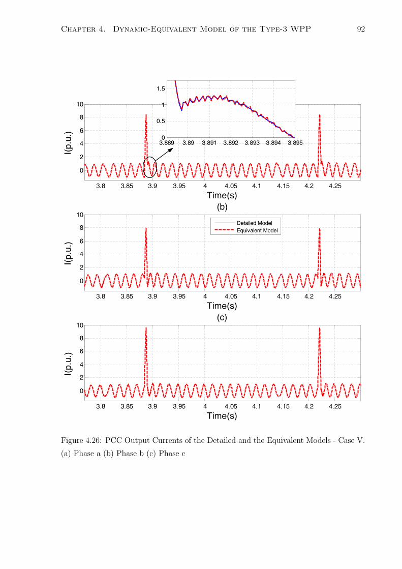
Chapter 4. Dynamic-Equivalent Model of the Type-3 WPP 92
)
)
'
!"!
#$%&"!
)
(
Figure 4.26: PCC Output Currents of the Detailed and the Equivalent Models - Case V.
(a) Phase a (b) Phase b (c) Phase c

Chapter 4. Dynamic-Equivalent Model of the Type-3 WPP 93
4.10.6 Case VI
In order to test the accuracy of the equivalent model for more complex transients, this
case combines multiple transients, unbalanced fault, and unbalanced fault clearance.
The transient scenario is similar to Case IV, but with single line to ground fault. The
circuit breaker reaction to clear the fault is through only one pole operation. Thus, the
unbalanced fault transient will be followed by an unbalanced circuit breaker operation
at which only one phase of the transmission line is disconnected to clear the fault; then,
this phase will be a successfully reconnected after 15 cycles.
The time-domain simulation results of both the detailed system and the correspond-
ing results obtained from the developed equivalent are shown in Figures 4.27 and 4.28.
The close agreement between the results of the two models verifies the accuracy of the
developed equivalent model.
4.10.7 Case VII
This case is similar to Case VI, but with double line to ground fault and in consequence
double pole circuit breaker operation. The time-domain simulation results of both the
detailed system and the corresponding results obtained from the developed equivalent
are shown in Figures 4.29 and 4.30. The close agreement between the results of the two
models verifies the accuracy of the developed equivalent model.
4.11 Discussions
The close agreement between the time-domain simulation results obtained from the de-
tailed and the equivalent models of the WPP, Figures 4.14-4.30, verifies the accuracy of
the proposed equivalent model for EMT-type studies external to the WPP. Case studies
of Section 4.10 are conducted to investigate the accuracy of the developed equivalent
model as the type of the fault and the location of the fault on line T2 change. Even in
the worst fault scenario when the fault is imposed at the PCC, the results obtained from
the detailed model and the equivalent model show close agreement verifies the accuracy
of the equivalent model. In addition, the errors between the maximum overvoltages and
overcurrents obtained from the detailed and the equivalent models are 1.42% and 1.3%
respectively. Figures 4.15, 4.21, 4.24, and 4.26 show the WPP output current measured
at the high voltage side of the WPP substation transformer. The aforementioned Fig-

Chapter 4. Dynamic-Equivalent Model of the Type-3 WPP 94
'
!"!
#$%&"!
(
!"!
#$%&"!
Figure 4.27: PCC Voltages of the Detailed and the Equivalent Models - Case VI

Chapter 4. Dynamic-Equivalent Model of the Type-3 WPP 95
)
!"!
#$%&"!
)
'
)
(
!"!
#$%&"!
Figure 4.28: PCC Output Currents of the Detailed and the Equivalent Models - Case
VI. (a) Phase a (b) Phase b (c) Phase c
ures are for case studies that include three phase-to-ground faults; such fault is cleared
one phase at a time at the zero crossing of the fault current at each phase. Therefore,
when the fault at the first phase is cleared while the currents in the other two phases
did not reach their zero crossing, an unbalance takes place and a zero sequence current

Chapter 4. Dynamic-Equivalent Model of the Type-3 WPP 96
!"!
#$%&"!
Figure 4.29: PCC Voltages of the Detailed and the Equivalent Models - Case VII

Chapter 4. Dynamic-Equivalent Model of the Type-3 WPP 97
)
)
'
)
(
!"!
#$%&"!
Figure 4.30: PCC Output Currents of the Detailed and the Equivalent Models - Case
VII. (a) Phase a (b) Phase b (c) Phase c
contribution from the system side appears with a high value. This explains the spikes
that appear in the transient currents at the clearance of the three phase-to-ground faults.
The proposed equivalent model significantly reduces the computational time and re-
sources and hence enables comprehensive time-domain simulation studies of the system
transients, e.g., statistical EMT-type studies to identify and evaluate worst case fault
scenarios, e.g., fault instant on the voltage waveform. The time required to conduct a 5-
second real-time simulation run, with a 5 µs time-step, using the detailed system model,
corresponding to case I, requires approximately 31 hours and 34 minutes using a quad-
Chapter 4. Dynamic-Equivalent Model of the Type-3 WPP 98
core Intel 3.07 GHz i7 computer with 6 GB of memory. The proposed equivalent model
reduces the computational time for the same case study (and with the same simulation
time-step) to about 45.12 seconds, i.e., a reduction in computation time by a factor of
2480.
It has to be noted that the equivalent model can be tuned based on field measure-
ments, if available. However, those measurements are not necessarily available especially
at the design stage prior to the actual installation of the WPP; therefore, detailed models
supplied by the vendors are typically used to accurately represent the WPP for system
impact studies as well as in developing the WPP equivalent model.
4.12 Conclusions
This chapter introduced, developed, evaluated, and verified an equivalent model that rep-
resent the Type-3-based WPP for the analysis of EMTs external to the WPP within the
desired frequency bandwidth, e.g., 0 to 50 kHz. The numerical accuracy and computa-
tional efficiency of the proposed equivalent model were verified by comparing time-domain
simulation test case results when a wind power plant is represented once by its detailed
model and once by the proposed equivalent model. The test cases cover different types of
faults at different locations outside the WPP. The studies show that the proposed method
can reduce computational time and resources by a factor of 2480 and for example enables
statistical studies that require a large number of simulation runs.

Chapter 5
Real-Time Simulation and HIL
Evaluation of Equivalent Models
5.1 Introduction
A real-time simulator (RTS) plays a vital role in the verification of the control/protection
platform functions/performances as they enable the testing of the physical controller in a
hardware-in-the-loop (HIL) configuration. In the HIL arrangement, a RTS, simulates the
power system under consideration in real-time and the physical controller is interfaced
to the RTS in a closed-loop fashion, Figure 5.1. In this arrangement, the device under
test is interfaced to the simulator in the same manner as it is integrated in the actual
power system [69]. The HIL testing has the following advantages:
• The physical control/protection is tested instead of its off-line simulated model
which may neither reflect all the functions nor preserve its fidelity.
• The control platform can be tested even before its installation and commissioning
which allows for modifications and improvements in the design.
• The control/protection can be tested under extreme scenarios that are not allowed
in a real system.
For a credible HIL testing results, the power system has to be accurately modeled on
the RTS. Due to the high penetration and the increased capacity of WPPs integrated with
the power system, it has become inevitable to include the WPPs model in the simulated
power system in the real-time simulator to study their effect on the overall performance
99

Chapter 5. RTS and HIL Evaluation of Equivalent Models 100
of the power system. The detailed modeling of WPPs in the RTS is neither practical nor
possible due to its drastic computational burden. Therefore, in order to practically use
the RTS to simulate the power system including the WPPs, it is required to represent the
WPP with an equivalent model that accurately captures the electromagnetic transients
behavior.
The accuracy and computational efficiency of the WPP equivalent model developed
in this thesis make it a prime choice for real-time simulation. This chapter presents the
real-time simulation of the developed Type-3 WPP and Type-4 WPP equivalent models.
Case studies are carried out to evaluate the performances of the developed models in the
RTDSr and to compare the hardware resources required for simulating both the detailed
and the equivalent WPP models. This chapter also presents hardware-in-the-loop (HIL)
testing of the WPP supervisory control. This is possible since the WPP equivalent model
is developed from self-contained blocks and the supervisory control can be excluded from
the equivalent model and realized on a reconfigurable control and acquisition system
(NI−cRIO).
The structure of this chapter is as follows. Section 5.2 highlights the challenges asso-
ciated with the real-time simulation of WPPs. Section 5.3 describes the real-time simu-
lation of the developed WPP equivalent model. Section 5.4 presents real-time Simulation
case studies of the Type-4 and Type-3 WPPs based on the developed WPP equivalent
models of Chapters 3 and 4. The real-time HIL testing of a Type-4 WPP supervisory
control is discussed in section 5.5. The conclusions are stated in section 5.6.
Figure 5.1: Real-Time HIL Closed-Loop Arrangement

Chapter 5. RTS and HIL Evaluation of Equivalent Models 101
5.2 Challenges Associated With Real-Time Simula-
tion of WPPs
The RTS hardware typically includes a number of digital processors, either digital signal
processors or general purpose processors, that share the computational burden. To simu-
late a large system, the system has to be divided into parts (subsystems) such that each of
them is simulated in a separate processor. Since the solution algorithm applied in a RTS
is based on the nodal admittance matrix technique, the system division is then based on
traveling wave transmission line models to break up the large nodal admittance matrix
into smaller matrices. These matrices can be solved in parallel, each on a processor, if
the solution time-step is smaller than the traveling wave of the transmission lines, e.g.,
for a simulation time-step of 50 µs, the transmission line separating any two subsystems
should be at least 15 km in length [70]. The parallel operation of these processors enables
the simulator to simulate power systems without violating the real-time constraints, i.e.,
the computation time to solve the system mathematical model is less than the simulation
time-step.
Meeting the real-time constraints when simulating WPPs, based on their detailed
model, is a challenging task not only because of the significant number of components
within a WPP which translates to a large number of equations, but also because of the
nature of these components and their simulation requirements. These can be summarized
as follows.
• The simulation of power electronic devices, which form the main part of WTG unit,
adds an additional computational burden on the RTS hardware due to the need to
invert/refactorize the admittance matrix due to switchings.
• The presence of power electronic converters necessitates the use of small simulation
time-step, i.e., few microseconds.
• The significant number of components within a WPP makes it inevitable to divide
the WPP model into smaller subsystems connected together with long fictitious
transmission line. The presence of these lines alters, to some extent, the behavior
of the collector network.
• The high cost of the associated hardware required for simulating practical WPP
with hundreds of components could be prohibitive.

Chapter 5. RTS and HIL Evaluation of Equivalent Models 102
In the light of the above challenges, it is necessary to use an equivalent WPP model
that can accurately represent its EMTs behavior without imposing prohibitive computa-
tional burden on the RTS and without the need to divide the WPP model into multiple
subsystems.
5.3 Real-Time Simulation of the WPP Equivalent
Model
The WPP equivalent models developed in Chapters 2 to 4, also provide substantial
advantages for real-time simulation and hardware-in-the-loop real-time simulation, i.e.,
• There is no explicit modeling of the WTGs power electronic interface. There-
fore, there is no need to use a very small simulation time-step or corrective algo-
rithms, e.g., interpolations/extrapolations, that accounts for the converters switch-
ing events [71].
• The FDNE submodule replaces the detailed WPP passive network that utilizes
significant number of nodes with an equivalent that utilizes far less hardware re-
sources, e.g., for a single port equivalent, the WPP collector network, irrespective
of its size, is replaced with an equivalent that adds only 3 extra nodes to the system
admittance matrix without compromising the accuracy of the simulation results,
• The developed equivalent model is scalable as the DLFE is represented on the RTS
using the per unit system. Hence, increasing/decreasing the size and capacity of
the WPP is accommodated through changing the base MVA. If there is a change
in the passive elements, the FDNE has to be reconstructed.
• The developed equivalent model makes use of the standard blocks and transfer
functions already available in the RTS components library. Therefore, there is no
need to develop user-defined models or custom submodules.
To imbed the developed equivalent model in a digital real-time simulator, it needs to
be represented with its discrete time-domain model. As depicted in Figure 5.2, the WPP
equivalent model is composed of the FDNE and the DLFE. To incorporate the FDNE into
the nodal solution of the system equations (the solution technique utilized by RTS) the
rational functions, representing the FDNE, are represented with the companion circuits

Chapter 5. RTS and HIL Evaluation of Equivalent Models 103
Figure 5.2: Structure of the Wide-band Equivalent Model of a Type-4/3 WTGs-based
WPP
based on the trapezoidal numerical integration technique and the bilinear transform,
i.e., each of the rational functions is represented by a conductance and a current source
whose value depends on the circuit solution from the previous time step (a history current
source) [26], [72], [73] as described in Chapter 2.
Unlike the FDNE, the DLFE consists of a set of transfer functions that are interfaced
to the electric circuit through a controlled current source, Figure 5.2. Hence, the DLFE
is constructed in the RTS interfacing time-domain simulation software with the available
standard control blocks. The instantaneous voltages and currents at the PCC are mea-
sured and converted to phasor values to be used by the DLFE. The outputs of the DLFE
are in the dq-reference frame which are converted back to instantaneous values in the
abc-frame to be injected to the system through controlled current sources.
5.4 Case Studies
The main objective of this section is to demonstrate the suitability of the proposed
WPP equivalent model for real-time applications. Two case studies are carried out on
the systems of Figures 3.9 and 4.13 to demonstrate the feasibility and accuracy of the
real-time simulation of large WPPs based on the proposed equivalent models for the
analysis of EMTs in the power system. In this work a real-time simulator from RTDSr
Technologies [74] is used as the implementation platform. The software interface of the
RTDSr is the RSCAD time-domain simulation program. The RTDSr platform used in
this work is a single rack device with five PB5 and GPC processing cards. For this rack,

Chapter 5. RTS and HIL Evaluation of Equivalent Models 104
the maximum number of nodes in a single network solution is 72 single-phase nodes.
Two network solutions can be included in one rack, i.e., two 72 nodes subsystems can be
included in one rack.
For each case study, the test system including the WPP is simulated in the RTDSr
environment. The WPP is represented based on its equivalent model proposed in this
thesis and simulated in the RTDSr based on its discrete time-domain model as described
in Section 5.3. The test systems, system prefault steady state conditions, and the fault
scenarios of Case I and Case II are identical to that of the offline case studies in Sections
3.10.1 and 4.10.1 respectively. In response to a fault in the power system external to
the WPP, the real-time simulation results of each case study are compared to that of
the offline PSCAD/EMTDC simulation presented in the corresponding case study in
Chapters 3 and 4.
5.4.1 Case I: Type-4 WPP
The test system of Figure 3.17 that includes a Type-4 WPP is simulated in the RTDSr
environment with an integration time-step of 50 µs. The Type-4 WPP is represented
by its equivalent model developed in Chapters 2 and 3 and simulated in real-time in the
RTDSr. The system is subjected to a 150-ms temporary L-L-L-G fault, 15-km from the
PCC on line T2. Prior to the fault, the system is under steady-state conditions and the
WPP delivers 99 MW to the system at PCC. Figure 5.3 shows an oscilloscope snap shot
of the instantaneous PCC voltages prior, during, and immediately after the fault. Figure
5.4 shows the injected current by the WPP into the system (at the WPP transformer
HV-side) during the fault and after the fault clearance. Figures 5.5 and 5.6 compare
the real-time simulation results, Figures 5.3 and 5.4, to those obtained from simulating
the system detailed model in the offline PSCAD/EMTDC, Section 3.10.1. The close
agreement between the real-time and the off-line results, Figures 5.5 and 5.6, verifies the
accuracy of the developed equivalent model in a real-time platform.
5.4.2 Case II: Type-3 WPP
The test system with Type-3 based WPP of Figure 4.13 is simulated in the RTDSr
environment. The Type-3 WPP is represented by its equivalent model developed in
chapters 2 and 4 and simulated with the host power system in the RTDSr environment
with a time-step of 50 µs. The system is subjected to a temporary fault that takes place

Chapter 5. RTS and HIL Evaluation of Equivalent Models 105
Figure 5.3: Real-Time Oscilloscope trace of the WPP Terminal Voltages - Case I
Figure 5.4: Real-Time Oscilloscope trace of the WPP Output Currents - Case I
in the power system external to the WPP. The system prefault steady state condition and
the fault scenario are identical to that of Section 4.10.1. Figure 5.7 shows an oscilloscope
snap shot of the instantaneous PCC voltages prior, during, and immediately after the
fault. Figure 5.8 shows the injected current by the WPP into the system (at the WPP
transformer HV-side) before, during, and after the fault clearance. Figures 5.7 and 5.8
demonstrate the expected behavior of the Type-3 WPP as compared to the off-line results
presented in Section 4.10.1 which verifies the feasibility and accuracy of the real-time
simulation of WPPs based on the proposed equivalent model.

Chapter 5. RTS and HIL Evaluation of Equivalent Models 106
Figure 5.5: PCC Voltages of the Equivalent Model From the RTDS and the Detailed
Model From PSCAD/EMTDC - Case I
5.4.3 Discussion
The simulation of the test systems of chapters 3 and 4 with their WPPs represented by
the proposed equivalent models has been completed in the RTDSr with 50 µs solution
time-step and the terminal behavior of the WPP in response to an EMT in the power
system has been investigated. In order to evaluate the reduction in the computational
hardware resources associated with simulating the WPP based on its equivalent model,
an attempt was made to compare the hardware resources required to simulate the test
system of Figure 3.17 with its WPP represented once by its detailed model and once
with its equivalent model. The test system with its WPP represented by its equivalent
model has utilized only 27 nodes in the RTDSr. On the other hand, the WPP host
power system and the detailed model of only the WPP passive network formed a system
of 146 nodes which is beyond the capability of the single rack RTDSr. Even with the

Chapter 5. RTS and HIL Evaluation of Equivalent Models 107
Figure 5.6: WPP Output Currents of the Equivalent Model From the RTDS and the
Detailed Model From PSCAD/EMTDC - Case I
assumption that additional RTDSr rack(s) are available, in order to divide the network
solution of the test system between racks, the simulated system has to be broken down
into a number of subsystems, each with maximum of 72 nodes. These subsystems are
interfaced to each other with long fictitious transmission lines to decouple the solution of
each subsystem from the others. The presence of these transmission lines alters, to some
extent, the behavior of the collector network.
As can be concluded from the aforementioned discussion, the WPP equivalent model
enables the real-time simulation of large WPPs at a fraction of the required hardware
resources as compared to the detailed WPP. This reduction of the required hardware is
due to the computationally efficient design of the WPP equivalent model that accurately
represent the dynamic behavior of the WPP.
It has to be noted that the time-step of 50 µs is a limitation of the RTDSr that
results in reducing the frequency range of the simulation results.

Chapter 5. RTS and HIL Evaluation of Equivalent Models 108
Figure 5.7: Real-Time Oscilloscope trace of the WPP Terminal Voltages - Case II
Figure 5.8: Real-Time Oscilloscope trace of the WPP Output Currents - Case II
5.5 Real-Time Controller HIL Testing of a Type-4
WPP Supervisory Control
Another potential application of the proposed equivalent model is the HIL testing of
the WPP supervisory control. This is possible due to the modular structure of the

Chapter 5. RTS and HIL Evaluation of Equivalent Models 109
!"!
#$
$
Figure 5.9: Schematic Diagram of the Real-Time HIL Test Bed
developed WPP equivalent model. The WPP supervisory control is excluded from the
model simulated in the RTS platform and its physical hardware counterpart is interfaced
to the real-time simulator for the purpose of HIL testing.
For the purpose of validating this concept, a WPP supervisory control has been
realized in a reconfigurable industrial control platform (NI−cRIO) comprised of an 800
MHz real-time powerPC processor and a Virtex-5 LX110 FPGA. LabVIEW software is
used to program the NI−cRIO and to develop the user interface for the WPP supervisory
control. On the other hand, the WPP, excluding the WPP supervisory control module,
and the WPP host power system are simulated in the RTDSr simulator. Figure 5.9
shows a schematic diagram of the HIL test bed. In this arrangement, the supervisory
control on the NI−cRIO platform receives feedback signals of the instantaneous PCC
voltages and currents through the I/O analog interface and sends back the d- and q-
reference current components to the RTDSr in order to satisfy the control objectives.
Figure 5.10 shows a picture of the real-time HIL testing environment.
5.5.1 Case III
This case demonstrates the capability of the equivalent model to be used in the HIL
testing of the WPP supervisory control. Instead of simulating the full equivalent model in
the RTDSr, the WPP supervisory controller module is omitted from the WPP equivalent

Chapter 5. RTS and HIL Evaluation of Equivalent Models 110
Figure 5.10: Real-Time HIL Test Bed
model and a physical WPP supervisory controller is interfaced to the RTDSr instead. In
this work, the WPP supervisory controller is realized on the NI−cRIO platform. The test
system and the fault condition of this case are similar to those of Case - I. Figures 5.11
and 5.12 depict the measurements of the voltages, currents, active and reactive power
components at the PCC that correspond to the control signals sent by the NI−cRIO
platform to the RTDSr. The results match those of Case I which verifies the effectiveness
of using the WPP equivalent model in validating the performance of parts of the WPP
through real-time HIL testing configuration.

Chapter 5. RTS and HIL Evaluation of Equivalent Models 111
!"#$
%&##'' (#
Figure 5.11: PCC Voltages and WPP Output Currents - Case III
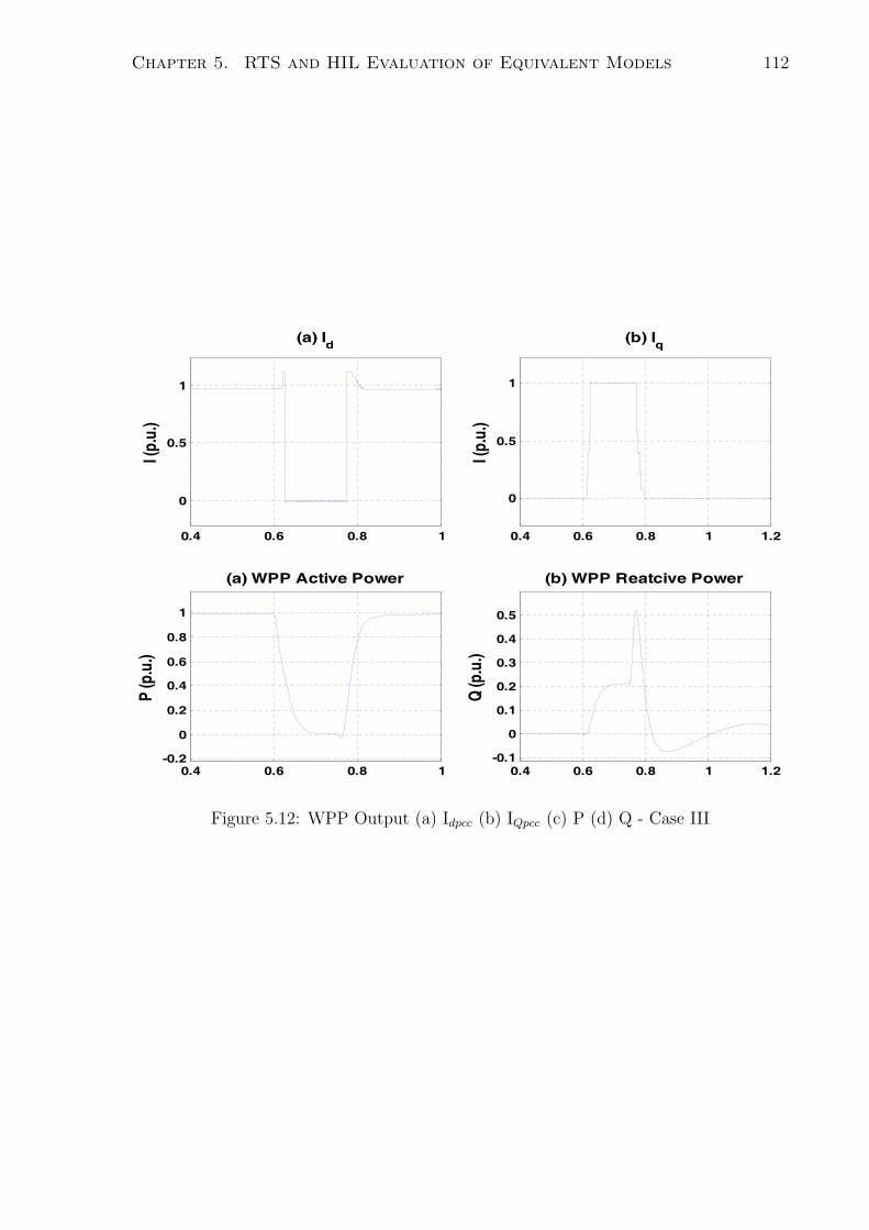
Chapter 5. RTS and HIL Evaluation of Equivalent Models 112
*
+
%#, !- '
)
.
% #, !- '
Figure 5.12: WPP Output (a) Idpcc (b) IQpcc (c) P (d) Q - Case III

Chapter 5. RTS and HIL Evaluation of Equivalent Models 113
5.6 Conclusions
This chapter presented the real-time simulation of WPPs based on the developed WPP
equivalent model of both Type-3 and Type-4 WPPs. The study results conclude that:
• The use of the developed WPP equivalent model enhances the capability of RTS
to simulate large power systems with multiple WPPs. The size of the simulated
system is not affected by the number of units and the MW size of the simulated
WPPs.
• The drastic reduction in the computational time and burden associated with the
equivalent model highly reduces the size and consequently the cost of the required
real time simulator hardware as compared to the hardware required to implement
detailed models.
This chapter also presents the real-time HIL testing of the WPP supervisory control
which is realized on an industrial controller platform (NI−cRIO) whereas the rest of the
WPP equivalent model is simulated in a RTDS simulator. This arrangement allows for
the testing of the physical supervisory control prior to its actual installation in the WPP
site and the testing of the control functions and the resultant system interaction.

Chapter 6
Conclusion and Future Work
6.1 Summary
This thesis proposed, developed, evaluated, and verified an accurate and computationally
efficient reduced-order dynamic-equivalent model that represents a wind power plant
(WPP) for the analysis of EMTs in the power system, external to the WPP. The proposed
models have been developed to represent Type-3 based WPPs and Type-4 based WPPs
within the desired frequency bandwidth, e.g., 0 to 50 kHz. The WPP equivalent model
consists of two distinct sub-models,
1. a static wide frequency-band FDNE which captures the frequency response of all
the passive WPP components within the desired frequency range,
2. a dynamic low-frequency equivalent (DLFE) model which represents dynamics of
WPP supervisory control and dynamics of the WTG units and local controls, within
the range of several Hz about the system nominal frequency.
This thesis presents a systematic approach to develop the wide-band WPP equivalent
models. The numerical accuracy and computational efficiency of the proposed equivalent
models were tested by comparing time-domain simulation test case results when a WPP
is represented once by its detailed model and once by the proposed equivalent model,
in the PSCAD/EMTDC environment. The test cases cover different types of faults at
different locations with respect to the WPP point of common coupling (PCC).
This thesis also presents three applications of the developed WPP equivalent models.
114

Chapter 6. Conclusion and Future Work 115
1. The real-time simulation of the Type-4 WPP based on the developed equivalent
model.
2. The real-time simulation of the Type-3 WPP based on the developed equivalent
model.
3. The real-time HIL testing of the WPP supervisory control which is realized on an
industrial controller platform (NI−cRIO) whereas the rest of the WPP equivalent
model and the host power system is simulated in a RTDSr simulator.
6.2 Conclusions
The study results reported in this thesis conclude that:
• The developed WPP equivalent model significantly reduces the computational time
and burden as compared to the WPP detailed model since the equivalent model
represents all WTG units, local controls, and the WPP supervisory control with a
single DLFE model and represents the collector network with the FDNE model.
• The developed WPP equivalent model accurately mimics the terminal behavior of
WPPs in response to power system transients external to the WPP. The accuracy
of the developed models has been validated through the performed case studies.
• The equivalent model represents the dynamic behavior of (i) the WPP collector
network and passive components, (ii) the WPP supervisory control, and (iii) the
WTG units and their local controls. In addition, it represents specific performance
requirements, e.g., the fault-ride through behavior of the WPP which is a manda-
tory requirement by the grid codes.
• The developed equivalent is tailored for EMTs studies since it represents the WPP
terminal behavior over a wide range of the frequency spectrum, e.g., from 0 up to
50 kHz.
• Various simulation scenarios that cover different types of faults at different locations
outside the WPP and multiple switching transients demonstrate that the accuracy
of the proposed model is neither affected by the type nor the location of the fault,
even when the fault occurs at the WPP point of connection to the grid.
Chapter 6. Conclusion and Future Work 116
• The equivalent model is a scalable model, since the DLFE is developed in per unit
and can be scaled to the base values of any WPP of interest. Therefore, the size
and number of WTGs units within the WPP do not affect the structure of the
equivalent.
• The equivalent model provides a platform portability in the sense that it is suitable
to be implemented in different time-domain simulation platforms since it can be
constructed using the standard power components and transfer functions available
in the library of the production-grade time-domain simulation software tools; hence,
it does not necessitates development of user-defined models or custom submodules.
• The equivalent model has a flexible design such that for changes in the WPP of
interest, the equivalent model can be adapted to these changes as follows.
1. Changes in the passive collector network are accommodated by updating only
the FDNE.
2. Addition/disconnetion of WTG units is represented by changing the equivalent
model normalization base values.
3. Changes/Modifications in the functions of the WPP supervisory control is
represented by updating the corresponding module at the equivalent model.
The computational efficiency of the equivalent model makes it a prime choice to
represent a WPP in a real-time simulation environment. Based on the reported real-time
simulation case studies, the following conclusions were drawn.
• The use of the equivalent model enhances the capability of the real-time simulator
(RTS) to simulate large power systems with multiple WPPs. The size of the sim-
ulated equivalent WPP on the RTS, measured by the number of system nodes, is
not affected by the number of units and the MW size of the simulated WPP.
• The drastic reduction in the computational time and burden associated with the
equivalent model highly reduces the size and consequently the cost of the required
RTS hardware platform as compared to the hardware required to simulate the
detailed model of a WPP.
• The equivalent model alleviates the additional computational burden, on the RTS
hardware, associated with simulating power electronic converters. Therefore, it

Chapter 6. Conclusion and Future Work 117
obviates the need for very small simulation time-steps or corrective algorithms,
e.g., interpolations/extrapolations to account for the converters switching events.
• The WPP equivalent model is developed from self-contained blocks. Therefore, it
is possible to test the physical WPP supervisory control in a HIL environment. In
this test the WPP equivalent model (excluding the supervisory control) is simulated
in the RTS whereas the WPP supervisory control is realized on a reconfigurable
control and acquisition system (NI−cRIO). This arrangement allows for the testing
of the physical supervisory control prior to its actual installation in the WPP site
and the testing of the control functions and the resultant system interaction.
Based on the studies reported in this work, the following quantitative conclusions are
deduced:
• As indicated in Chapter 3, compared to the detailed model of the test system with
Type-4 based WPP, the developed equivalent model reduces the off-line simulation
time from more than 5 hours to 110 seconds, i.e., a reduction in computation time
by a factor of 218, without compromising the accuracy.
• As indicated in Chapter 4, compared to the detailed model of the test system with
Type-3 based WPP, the developed equivalent model reduces the off-line simulation
time from 31.5 hours to 45 seconds, i.e., a reduction in computation time by a
factor of 2480, without compromising the accuracy.
• As indicated in Chapter 5, The real-time simulation of the test system of chapter
3 has utilized only 27 nodes and was carried out in a single RTDS rack, whereas
the simulation of detailed model of only the test system passive network (not con-
sidering the WTG units) include 146 nodes which requires more than one RTDSr
rack.
6.3 Contributions
The main contributions of this thesis are
1. Proposal and development of a novel reduced-order, wide-band frequency depen-
dent dynamic-equivalent model of WPPs which to the best of the author’s knowl-
edge has not been previously introduced in the technical literature. The developed

Chapter 6. Conclusion and Future Work 118
model significantly reduces the required computational resources and the simula-
tion run time while preserving the WPP response fidelity in a desired frequency
range.
2. Application of the developed model to represent realistic size Type-4 and Type-3
WPPs, that include (i) WTG units, (ii) collector network, and (iii) WPP supervi-
sory control, with reasonable resources and computation time.
3. Development of a systematic approach to construct the proposed WPP equivalent
model, incorporating the WTG controls and the WPP supervisory control.
4. Validation and evaluation of the practical feasibility of the real-time simulation
of power systems with WPPs using limited hardware resources without sacrificing
the simulation accuracy. This is possible due to the reduced hardware resource
requirements for representing the proposed equivalent model.
5. Proposal of a framework for HIL testing of WPP supervisory control based on the
developed WPP equivalent model.
6.4 Future Work
1. Validate the accuracy of the developed equivalent model against field measured
data for an actual WPP installed in the field. Since it is not possible to apply
a fault condition in the power system hosting the WPP only for the purpose of
collecting data, the field measured data of interest is expected to be historically
collected during previous fault incidents.
2. Utilize the model to investigate mutual interactions of electrically-close WPPs.
3. Utilize the WPP equivalent model simulated in RTDS to test protection devices
connected to the high voltage side of the substation transformer in a HIL environ-
ment.
4. Develop an equivalent model to represent the EMT response of grid-connected pho-
tovoltaic (PV) power plants. The equivalent model of inverter-based PV generation
is expected to be similar to that of Type-4 WTG units; hence, an equivalent model
of PV system is an intuitive extension of the WPP equivalent model.

Chapter 6. Conclusion and Future Work 119
5. Based on the proposed equivalent model, develop equivalent models that represent
Types-1 and -2 based WPPs.
Appendix A
Detailed Model of the Type-4 WPP
This appendix presents the detailed EMT model of the Type-4 WPP. Section A.1 presents
the supervisory control of the WPP whose function is to control the exchange of power
components between the WPP and the grid according to the power system requirements
and grid code. Section A.2 presents the detailed model of the Type-4 WTG unit.
A.1 WPP Supervisory Control
This control coordinates the operation of all WTG units within the WPP such that
the collective WPP power injection at the PCC satisfies the active and reactive power
requirements of the TSO. For this purpose, there should be a two-way communication
between the supervisory control and the WTG units such that each unit provides its
generation availability and receives reference values from the WPP supervisory control.
The inputs to the WPP control are:
1. Reference values of the voltage, and the active and reactive power components from
the TSO
2. Feedback measurements of the voltages and currents from the PCC
3. The available power at each WTG unit
Based on the above inputs, the WPP supervisory control specifies the WPP power in-
jection as follows [49]. For the active power:
1. Set the operating mode: either to supply certain active power reference or generate
the maximum available power based on the available wind.
120

Appendix A. Detailed Model of the Type-4 WPP 121
2. Calculate and send the power reference of each unit (PWTGref ). This is done by
sending the WPP reference power (PWPPref ), calculated as a percentage of the WPP
total capacity, to all WTG units such that each unit generates active power equal
to the same percentage of its capacity. Another option is to calculate PWTGref of each
unit based on the power availability of the unit.
3. Reduce PWTGref in case of grid transients accompanied with voltage fluctuations.
This reduction is calculated based on the WPP terminal voltage and according to
the grid code.
For the reactive power:
1. Set the operating mode either to supply certain reactive power reference or generate
reactive power/current to regulate the voltage/power factor at the WPP terminal.
2. Calculate and send the reference QWTGref or its corresponding IWTG
Qref to each WTG
unit.
3. Change the value of IWTGQref in case of voltage fluctuations resulting from grid tran-
sients. This change is calculated based on the the WPP terminal voltage and
according to the grid requirements.
The reference signals from the supervisory control are then sent to the next control
level, i.e., the WTG local control. Figure A.1 depicts a Type-4 WTG unit. The full-rated
back-to-back converters decouple the turbine-generator from the collector network such
that disturbances that take place on the collector network side have insignificant effects
on the machine side of the converter [6], [30]–[32]. Consequently, the dynamic model of
each WTG unit can be adequately represented by those of the corresponding GSC and
its local control.
A.2 Type-4 GSC Control Model
The GSC is modeled as a three-phase two-level current-controlled voltage-sourced con-
verter with six IGBT valves as shown in Figure A.2 where the GSC is interfaced to the
AC collector network through a series RL filter. GSCs within the WPP are synchronized
with the positive sequence voltage at the WPP terminals through a phase-locked loop.
This enables the derivation of the GSC control in the dq-frame of reference where the

Appendix A. Detailed Model of the Type-4 WPP 122
Figure A.1: Schematic Diagram of Type-4 WTG Unit
d-axis is aligned with the PCC voltage and hence the voltage q-component Vsq is zero.
Therefore, the control of the GSC output power components (P and Q) can be achieved
through the independent control of the dq-output current components Id and Iq.
The AC-side power components are
Ps(t) =3
2[Vsd(t)id(t) + Vsq(t)iq(t)] , (A.1)
Qs(t) =3
2[−Vsd(t)iq(t) + Vsq(t)id(t)] . (A.2)
Imposing Vsq = 0, (A.1) and (A.2) become,
Ps(t) =3
2Vsd(t)id(t), (A.3)
Qs(t) = −3
2Vsd(t)iq(t). (A.4)
Hence
idref (t) =2
3VsdPsref (t), (A.5)
iqref (t) = − 2
3VsdQsref (t). (A.6)
The current control of the GSC is deduced based on Figure A.2 from
Ldiddt
= Lωoiq −Rid + Vtd − VSd, (A.7)
Ldiqdt
= −Lωoid −Riq + Vtq − VSq, (A.8)
where Vtdq are the VSC terminal voltages and given by [43]:
Vtd(t) =VDC
2md(t), (A.9)

Appendix A. Detailed Model of the Type-4 WPP 123
Figure A.2: Schematic Diagram of a Typical GSC
Vtq(t) =VDC
2mq(t), (A.10)
where md and mq are the dq-component of the modulation signal sent to the GSC
switches. The modulation signals are determined by the GSC closed loop control that
regulates the GSC output currents (idq). Equations (A.7) and (A.8) indicate that the
presence of the terms Lωoid and Lωoiq couple the dynamics of id and iq. Therefore, to
decouple these dynamics, feed-forward Lωo is introduced [43]. For this purpose, md(t)
and mq(t) are introduced as
md(t) =2
VDC
(ud − Lωoiq + VSd), (A.11)
mq(t) =2
VDC
(uq + Lωoid + VSq), (A.12)
where ud and uq are new control inputs [75],[76]. Substituting for md and mq from (A.11)
and (A.12) into (A.9) and (A.10) and then substituting Vtd and Vtq from (A.9) and (A.10)
into (A.7) and (A.8) result in:
Ldiddt
= −Rid + ud, (A.13)
Ldiqdt
= −Riq + uq. (A.14)
Based on (A.11) to (A.14), Figure A.3 shows a block representation of the dq-frame
current controllers of the GSC where the d- and q-compensators process the reference
and the feedback currents to provide ud and uq respectively.

Appendix A. Detailed Model of the Type-4 WPP 124
!"
Figure A.3: Block Diagram of the GSC Control

Appendix B
DSOGI-PLL
The structure of the DSOGI-PLL, Figure B.1, consists of three main components:
1. abc/ αβ Clarke transformation block.
2. Dual SOGI with quadrature signal generator (QSG): it filters the input αβ volt-
ages into (Vα,filtered, Vβ,filtered) and extracts their 90o shifted version (qVα,filtered,
qVβ,filtered)
3. A Positive sequence calculator (PSC): processes its inputs from the dual SOGI and
calculates the positive sequence fundamental frequency component of the voltage
V +α , V +
β [33].
4. Basic SRF-PLL: estimates the phase angle θ and use it to transform V +α , and V +
β ,
from the PSC, to the dq-reference frame.
!"
#$
%&
'(
'(
)*+$,-)+
)*+$,-)+
!"#$%&'
( !"#$%&'
.
.
.
.
/01
)"#$%&'
( )"#$%&'
2
2
2
32
3
4'2
4(2
4&2
4%2
567
8
8
67
!
"
)9:,#;;#)<=)*+$,-)+
674&>?@
!
)
Figure B.1: Schematic Diagram of DSOGI-PLL
125

Appendix B. DSOGI-PLL 126
Mathematically, each SOGI-QSG is expressed by its characteristic transfer functions
as follows [33]:
D(s) =vFilter
v(s) =
kw′s
s2 + kw′s+ w′2(B.1)
Q(s) =qvFilter
v(s) =
kw′2
s2 + kw′s+ w′2(B.2)
Equations B.1 and B.2 can be realized with the block diagram of Figure B.2 where q is
the 90o phase shift operator, ω′ and k are the resonance frequency and the damping factor
of the SOGI-QSG respectively. Both the components of vFilter and its 90o lag qvFilter
are then used by the PSC to determine V +αβ. In order to have an accurate results under
grid frequency variations, the grid frequency detected at the SRF-PLL is fed-back to the
DSOGI-QSG to dynamically adapt its resonance frequency ω′ to match the estimated
grid frequency as shown in Figure B.1.
= ;B ,
;B ,
Figure B.2: SOGI-QSG Schematic
The PSC calculates the positive-sequence component of the input Vαβas follows:
According to clarke transformation [77]:
Vαβ = [Tαβ]Vabc (B.3)
Where
[Tαβ] =2
3
[1 −1
2−1
2
0√32
−√32
]. (B.4)
Therefore, the positive-sequence component V +αβ can be calculated as:
V +αβ = [Tαβ]V
+abc (B.5)
According to the symmetrical components method [78]:
V +abc = [ v+a v+b v+c ]
T = [T+]Vabc (B.6)

Appendix B. DSOGI-PLL 127
where
[T+]=
1
3
1 a a2
a2 1 a
a a2 1
, a = ej2π3 . (B.7)
Hence, substituting from (B.6) in (B.5) and then from (B.3) in (B.5) result in,
V +αβ = [Tαβ][T
+]Vabc,
= [Tαβ][T+][T−1
αβ ]Vαβ,
=1
2
[1 −qq 1
]Vαβ , q = e−j π
2 . (B.8)
q is the same phase shift operator used before which obtains the quadrature waveform
form the original in-phase waveform [33]. The previous equation can be written as follows:
V +α =
1
2(Vα − qVβ) (B.9)
V +β =
1
2(qVα + Vβ) (B.10)
Figure B.1 depicts the PSC as described in (B.9) and (B.10), its inputs are the filtered
values of Vαβ and qVαβ supplied by the DSOGI-QSG and its output are V +αβ. V +
αβ are
then fed to the basic SRF-PLL to estimate the grid frequency and the phase angle θ
of the fundamental frequency positive sequence component of the voltage. The angle
θ is estimated through a feedback control loop that regulates the q-component to zero,
Figure B.1, [33], [34].

Appendix C
Parameters of the Test System of
Chapter 3
Parameters of the 34.5-kV and 115-kV transmission lines and the grid impedance of the
test system are given in Tables C.1, C.2, and C.3. Z1, Z2, and Z0 are the positive,
negative, and zero sequence series impedances respectively where Z= R+jXL . Xc is the
capacitive shunt reactance.
Table C.1: Parameters of The 34.5 kV Overhead LinesZ1 = Z2 0.128 + j 0.391 Ω/km
Z0 0.306 + j 1.791 Ω/km
Xc1 = Xc2 0.239 MΩ*km
Xc0 0.578 MΩ*km
Table C.2: Parameters of The 115 kV Overhead LinesOverhead Line 1,2 Overhead Line 3
Z1 = Z2 0.081 + j 0.462 Ω/km 0.162 + j 0.923 Ω/km
Z0 0.240 + j 1.385 Ω/km 0.481 + j 2.770 Ω/km
Xc1 = Xc2 0.148 MΩ*km 0.295 MΩ*km
Xc0 0.369 MΩ*km 0.738 MΩ*km
128

Appendix C. Parameters of the Test System of Chapter 3 129
Table C.3: Grid Impedance
Z1 = Z2 0.1448 + j 2.8971 Ω
Z0 0.16068 + j 1.60699 Ω

Appendix D
Detailed Model of the Type-3 WTG
This appendix presents the detailed dynamic model of the DFAG units for EMTs studies
and the units local controls which control the operation of the DFAG units in order
to satisfy the WPP generation requirements. Unlike Type-4 WTGs, the stator of each
DFAG unit is directly connected to the grid; hence, the dynamics of the machine will
reflect in the grid side.
The DFAG stator is connected to the WPP collector network through a step-up
transformer, Figure D.1, whereas the rotor is interfaced to the collector network with
back-to-back voltage-sourced converter, referred to as rotor-side converter (RSC) and
grid-side converter (GSC). The converters control the active and reactive power exchange
between the DFAG and the collector network. The differential equations that describe
,*
'-'
./' 0
1
Figure D.1: Schematic Diagram of the Doubly-Fed Asynchronous Generator (DFAG)
Unit
130
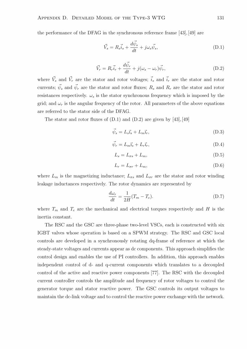
Appendix D. Detailed Model of the Type-3 WTG 131
the performance of the DFAG in the synchronous reference frame [43], [49] are
Vs = Rsis +dψs
dt+ jωsψs, (D.1)
Vr = Rrir +dψr
dt+ j(ωs − ωr)ψr, (D.2)
where Vs and Vr are the stator and rotor voltages; is and ir are the stator and rotor
currents; ψs and ψr are the stator and rotor fluxes; Rs and Rr are the stator and rotor
resistances respectively. ωs is the stator synchronous frequency which is imposed by the
grid; and ωr is the angular frequency of the rotor. All parameters of the above equations
are referred to the stator side of the DFAG.
The stator and rotor fluxes of (D.1) and (D.2) are given by [43], [49]
ψs = Lsıs + Lmır, (D.3)
ψr = Lmıs + Lrır, (D.4)
Ls = Lσs + Lm, (D.5)
Lr = Lσr + Lm, (D.6)
where Lm is the magnetizing inductance; Lσs and Lσr are the stator and rotor winding
leakage inductances respectively. The rotor dynamics are represented by
dωr
dt=
1
2H(Tm − Te). (D.7)
where Tm and Te are the mechanical and electrical torques respectively and H is the
inertia constant.
The RSC and the GSC are three-phase two-level VSCs, each is constructed with six
IGBT valves whose operation is based on a SPWM strategy. The RSC and GSC local
controls are developed in a synchronously rotating dq-frame of reference at which the
steady-state voltages and currents appear as dc components. This approach simplifies the
control design and enables the use of PI controllers. In addition, this approach enables
independent control of d- and q-current components which translates to a decoupled
control of the active and reactive power components [77]. The RSC with the decoupled
current controller controls the amplitude and frequency of rotor voltages to control the
generator torque and stator reactive power. The GSC controls its output voltages to
maintain the dc-link voltage and to control the reactive power exchange with the network.

Appendix D. Detailed Model of the Type-3 WTG 132
Multiple software control methods and/or hardware methods have been introduced in
the literature to enable the DFAG-based WPPs to satisfy the fault-ride-through require-
ments [46],[50]–[53]. Each of these techniques has its own merits and limitations; however,
many of them fail to achieve the objective during transients which impose severe voltage
dips [52]. In this thesis, a dynamic voltage restorer (DVR) has been considered [51], [52]
to be connected at the unit terminal to restore the terminal voltage during transients
and thus enable the DFAG unit to provide ride-through capability subsequent to a fault,
Figure D.2.
,*
'-'
./' 0
.
1
Figure D.2: Schematic Diagram of the Doubly-Fed Asynchronous Generator
The control of the WPP is composed of a three-level hierarchical control as discussed
in Appendix A, Figure 3.1 [28]. Sections D.1 and D.2 discuss the WTG local control
level which is divided into RSC and GSC controls.
D.1 Rotor-Side Converter Control
The local control of the RSC controls the generator torque and the stator reactive power
flow through an inner and outer control loops. In the outer control loop, the torque and
reactive power references are translated to a corresponding q- and d-current references,
respectively. The current references are then sent to the RSC inner decoupled current
control loop [43], [49]. The control of the RSC is derived in a synchronously rotating
dq-reference frame synchronized with the stator flux, i.e., its d-axis is aligned with the
stator flux. In such case, a flux observer is used to estimate the flux and its angle [43],[49];
then, the rotor voltages and currents are transformed from the abc-stationary frame to
the dq-frame using the angle between the d-axis and the rotor phases θr. Alignment of

Appendix D. Detailed Model of the Type-3 WTG 133
the d-axis with the stator flux space vector is equivalent to alignment of the q-axis with
the stator voltage space vector and delaying the d-axis by 90o since the flux is shifted 90o
with respect to the stator voltage. Therefore, a PLL [33] is used to obtain the angle of
stator voltage space vector. In this thesis, the voltage orientation is considered and the
PLL of Appendix B is adopted.
Based on (D.1)-(D.7), the stator reactive power and the electromagnetic torque are
[43]
Qs =
(3
2
)V 2s
(1 + σs)Lmωs
−(3
2
)1
(1 + σs)Vsird, (D.8)
Te =Pe
ωr
= −(3
2
)Vs
(1 + σs)ωs
irq, (D.9)
where
Vs =√V 2d + V 2
q , and σs =Ls
Lm
− 1. (D.10)
The first component of (D.8) corresponds to the machine magnetizing current while
the second component is a function of the d-component of the rotor current ird. irdref
is determined from (D.8) based on the reactive power reference value. To operate the
machine at unity power factor, irdref takes the value of Vs/(Lmωs) to compensate for
the magnetizing reactive power [43]. During transients in which PCC voltage drops,
irdref is increased to boost the WTG output reactive current/power to meet the voltage
requirements.
As mentioned before, the WTG may receive a value of Pref or set to the maximum
power tracking mode. In the former case, irqref is calculated directly from (D.9) based
on the Pref obtained from the WPP supervisory control. In the latter case, Teref corre-
sponding to the maximum power has to be calculated first and then the corresponding
irqref is determined.
To operate in the maximum power tracking mode, the electromagnetic torque Te is
expressed as [43], [79], [80]:
Teref = Toptpu = −Kopt ω2rpu, (D.11)
where
Kopt =0.5ρAr3ω3
bCpmax
G3Pbλ3opt. (D.12)
In (D.12) ρ, r, A, ωb, G, Pb, λopt, and Cpmax are the air density, turbine blade radius,
turbine blade area, base value of the machine rotor speed, gear box ratio, base power,
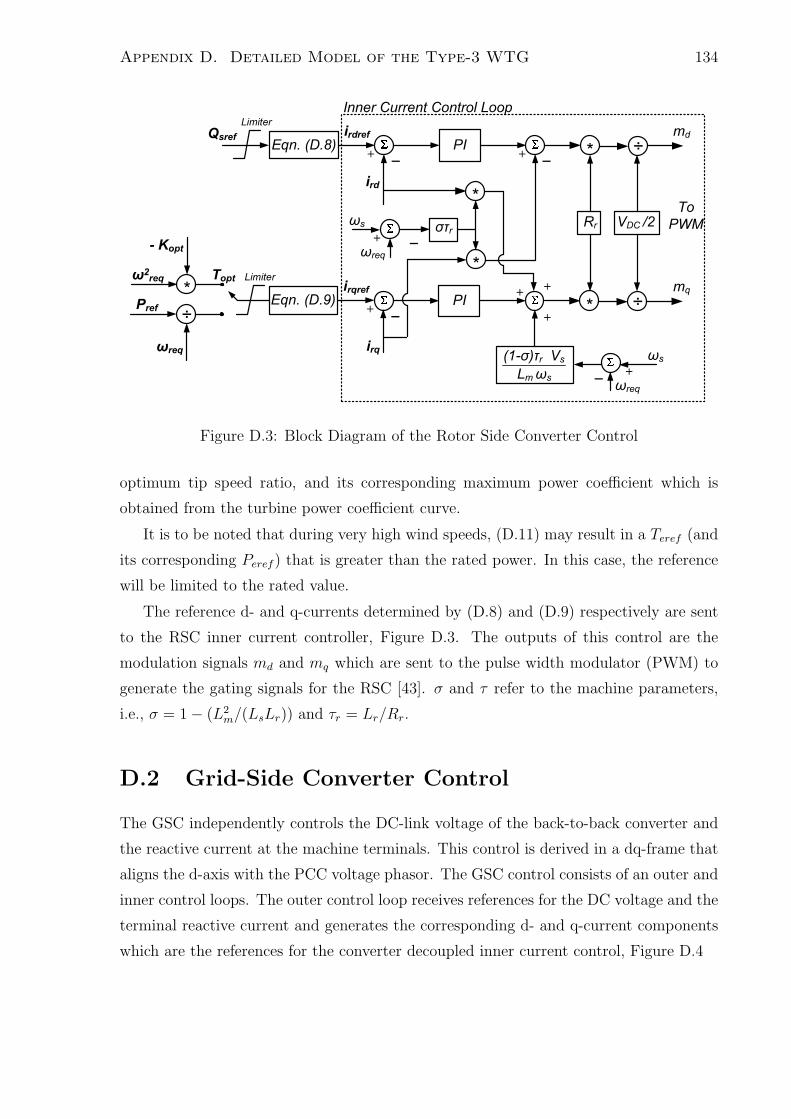
Appendix D. Detailed Model of the Type-3 WTG 134
8
7
. .
8
8 7
.
8 7
!
.
8
"#
#$
#
%&
'(
"#
"#
) & &"&&*
.
Figure D.3: Block Diagram of the Rotor Side Converter Control
optimum tip speed ratio, and its corresponding maximum power coefficient which is
obtained from the turbine power coefficient curve.
It is to be noted that during very high wind speeds, (D.11) may result in a Teref (and
its corresponding Peref ) that is greater than the rated power. In this case, the reference
will be limited to the rated value.
The reference d- and q-currents determined by (D.8) and (D.9) respectively are sent
to the RSC inner current controller, Figure D.3. The outputs of this control are the
modulation signals md and mq which are sent to the pulse width modulator (PWM) to
generate the gating signals for the RSC [43]. σ and τ refer to the machine parameters,
i.e., σ = 1− (L2m/(LsLr)) and τr = Lr/Rr.
D.2 Grid-Side Converter Control
The GSC independently controls the DC-link voltage of the back-to-back converter and
the reactive current at the machine terminals. This control is derived in a dq-frame that
aligns the d-axis with the PCC voltage phasor. The GSC control consists of an outer and
inner control loops. The outer control loop receives references for the DC voltage and the
terminal reactive current and generates the corresponding d- and q-current components
which are the references for the converter decoupled inner current control, Figure D.4

Appendix D. Detailed Model of the Type-3 WTG 135
9
9
!
#$
#
%&
'("
.
.
.
:
:
!
! 0
. 01
) & &"&&*
0
.
Figure D.4: Block Diagram of the Grid Side Converter Control
To regulate the dc voltage (VDC), the active power flow through the GSC is controlled
to keep the power balance over the dc-link, Figure D.2 [43]
d
dt
(1
2CdcV
2DC
)= PR − PG. (D.13)
The left hand side of (D.13) represents the energy stored in the DC-capacitor, PR is the
DC-side power of the RSC, and PG is the power flow into the GSC, Figure D.2. Assuming
lossless converters, PR is the same as the AC-side rotor power Pr and PG is the same as
the AC power leaving the GSC Pf ; therefore, (D.13) can be expressed as
d
dt
(1
2CdcV
2DC
)= −Pr − Pf . (D.14)
The compensator (K(v)), Figure D.4, determines the GSC reference power that reg-
ulates VDC to its reference value. The rotor power Pr is included in the control loop as a
feedforward term such that any change in PR is rapidly reflected in the output reference
current [43], [81].
D.3 DFAG Fault-Ride-Through Capability
The DFAG unit is sensitive to the grid transients at which the rotor windings experience
overvoltages and overcurrents that can destroy the converter if no protection measures are

Appendix D. Detailed Model of the Type-3 WTG 136
considered [46]. The traditional solution to protect the converter is to activate a crowbar
that short-circuits the rotor through a resistance and deactivate the rotor converter.
Nevertheless, the crowbar operation causes the DFAG to act as a squirrel cage machine
that absorb reactive power from the grid which aggravates the voltage dip [46]. In an
effort to comply with the grid codes and allow DFAG to supply reactive current during
faults, a number of techniques have been introduced in the technical literature to improve
the DFAG fault-ride-through, e.g., injecting a demagnetizing current into the rotor to
reduce its voltage [49], [82]. Other approaches suggested using additional hardware like
a series dynamic resistance in the rotor [83], a stator damping resistance [84], a series
grid side converter [85], or the use of a parallel grid-side rectifier and a series-grid side
converter [86]. Each of those approaches has its merits and limitations; however, during
severe voltage dips the activation of the crowbar is inevitable in most of the cases and
hence the continuous control of reactive current is not guaranteed [52].
In this thesis, a dynamic voltage restorer (DVR) [51],[52],[87]–[89] has been considered
to allow DFAG to ride through the fault even during severe voltage dips. The DVR is a
voltage sourced-converter connected in series between the machine stator and the step-up
transformer and compensates for the voltage during the fault. With this approach, the
stator voltage is kept constant even under severe balanced/unbalanced faults and hence
the transients have limited effect on the machine operation. The use of this external
device is useful in the already installed wind turbines that do not comply with the
fault ride-through regulations. Since the detailed design and control of the DVR is not
within the scope of this thesis, the DVR is simulated using a voltage source, connected
between the stator and the step-up transformer, Figure D.2. During disturbances the
DVR monitors the stator voltage and maintains it at its nominal value.

Appendix E
Parameters of the Test System of
Chapter 4
Parameters of the 34.5-kV and 115-kV transmission lines of the test system of Figure
4.13 are given in Tables E.1, and E.2. Z1, Z2, and Z0 are the positive, negative, and zero
sequence series impedances respectively where Z= R+jXL . Xc is the capacitive shunt
reactance.
Table E.1: Parameters of The 13.8 kV Overhead LinesZ1 = Z2 0.128 + j 0.391 Ω/km
Z0 0.306 + j 1.791 Ω/km
Xc1 = Xc2 0.239 MΩ*km
Xc0 0.578 MΩ*km
Table E.2: Parameters of The 115 kV Overhead LinesOverhead Line 1,2
Z1 = Z2 0.081 + j 0.462 Ω/km
Z0 0.240 + j 1.385 Ω/km
Xc1 = Xc2 0.148 MΩ*km
Xc0 0.369 MΩ*km
Parameters of the DFAG machine and the its interfacing transformer are given in
Table E.3 where the subscripts of s, r, and M refer to the stator, rotor, and magnetization
137

Appendix E. Parameters of the Test System of Chapter 4 138
parameter respectively. H and D are the inertia constant and the damping coefficient
respectively.
Table E.3: Parameters DFAG Unit and its interfacing Transformer
Parameter Value Unit
Base Power 1.7 Mw
Base Voltage 2.3 Kv
Base Frequency 377 rad/s
Rs 0.00779 p.u.
Rr 0.025 p.u.
Ls 0.07937 p.u.
Lr 0.4 p.u.
LM 4.1039 p.u.
H 1 s
D 0.0001 p.u.
Transformer Nominal Power 2 MVA
Transformer Voltage Ratio 2.3/13.8 Kv
Transformer Leakage Reactance 0.0575 p.u.
Parameters of the back-to-back converters and the RSC interfacing transformer are
given in Table E.4
Table E.4: Parameters of Back-to-Back VSC and TransformerParameter Value Unit
Switching Frequency 2340 Hz
DC Capacitor 10000 µF
RSC Interface Inductance 525 µH
Transformer Nominal Power 0.4 MVA
Transformer Voltage Ratio 0.6/2.3 Kv
Transformer Leakage Reactance 0.1 p.u.

Bibliography
[1] B. Fox, D. Flynn, L. Bryans, N. Jenkins, D. Milborrow, M. O’Malley, R. Watson,
and O. Anaya-Lara, “Wind power integration: Connection and system operational
aspects,” The Institution of Engineering and Technology (IET) Power and Energy
Series 50, 2007.
[2] “World wind energy report 2010, available online: http://www.wwindea.org.”
[3] I. Martinez de Alegria, J. Andreu, J.and Martin, P. Ibanez, J. Villate,
and H. Camblong, “Connection requirements for wind farms: A survey on
technical requierements and regulation,” Renewable and Sustainable Energy
Reviews, vol. 11, no. 8, pp. 1858 – 1872, 2007. [Online]. Available:
http://www.sciencedirect.com/science/article/pii/S1364032106000463
[4] The Wind Generation Task Force (WGTF), “The technical basis for
the new wecc voltage ride-through (VRT) standard a white paper
developed by the wind generation task force1 (WGTF),” available:
www.wecc.biz/Standards/Development/WECC, Tech. Rep., 2007.
[5] I. Erlich, W. Winter, and A. Dittrich, “Advanced grid requirements for the integra-
tion of wind turbines into the german transmission system,” in Power Engineering
Society General Meeting, 2006. IEEE, 0-0 2006, p. 7 pp.
[6] M. Asmine, J. Brochu, J. Fortmann, R. Gagnon, Y. Kazachkov, C. E. Langlois,
C. Larose, E. Muljadi, J. MacDowell, P. Pourbeik, S. A. Seman, and K. Wiens,
“Model validation for wind turbine generator models,” Power Systems, IEEE Trans-
actions on, vol. 26, no. 3, pp. 1769 –1782, Aug. 2011.
[7] ”WECC Wind Power Plant Dynamic Modeling Guide”, WECC Wind Generator
modeling Group, November 2010.
139

Bibliography 140
[8] A. Ellis, Y. Kazachkov, E. Muljadi, P. Pourbeik, and J. Sanchez-Gasca, “Description
and technical specifications for generic wtg models - a status report,” in Power
Systems Conference and Exposition (PSCE), 2011 IEEE/PES, march 2011.
[9] Y. kazachkov, P. Keung, and J. Senthil, “Generic wind models for PSSE stability
simulation,” Siemens PTI Power Technology eNewsletter Issue 103, Jan. 2009.
[10] A. Ellis, E. Muljadi, Y. Kazachkov, and J. Sanchez-Gasca, “Generic models for
simulation of wind power plants in bulk system planning studies,” in IEEE PES
General Meeting, 2011.
[11] V. Akhmatov, “Analysis of dynamic behavior of electric power systems with large
amount of wind power,” Ph.D. dissertation, Electrical Power Engineering, Technical
University of Denmark, Lyngby, Denmark,, April 2003.
[12] L. M. Fernandez, F. Jurado, and J. R. Saenz, “Aggregated dynamic model for
wind farms with doubly fed induction generator wind turbines,” Renewable Energy,
vol. 33, no. 1, pp. 129–140, 2008.
[13] L. Fernndeza, C. Garcaa, J. Saenza, and F. Juradob, “Equivalent models of wind
farms by using aggregated wind turbines and equivalent winds,” Energy Conversion
and Management, Elsevier, vol. 50, pp. 691–704, 2009.
[14] E. Muljadi, C. Butterfield, A. Ellis, J. Mechenbier, J. Hochheimer, R. Young,
N. Miller, R. Delmerico, R. Zavadil, and J. Smith, “Equivalencing the collector sys-
tem of a large wind power plant,” in Power Engineering Society General Meeting,
2006. IEEE, 0-0 2006, p. 9 pp.
[15] E. Muljadi, S. Pasupulati, A. Ellis, and D. Kosterov, “Method of equivalencing for a
large wind power plant with multiple turbine representation,” in Power and Energy
Society General Meeting - Conversion and Delivery of Electrical Energy in the 21st
Century, 2008 IEEE, July 2008.
[16] B. Gustavsen and A. Semlyen, “Rational approximation of frequency domain re-
sponses by vector fitting,” IEEE Trans. Power Delivery, vol. 14, no. 3, pp. pp.
1052–1061, July 1999.

Bibliography 141
[17] N. R. Watson and J. Arrillaga, Power Systems Electromagnetic Transients Simu-
lation (IEE Power & Energy Series). Institution of Engineering and Technology,
2003.
[18] B. Porkar, M. Vakilian, R. Feuillet, M. Ghassemi, and A. Akhavan, “Multi-port
frequency-dependent network equivalent for electromagnetic transient studies,” Pro-
ceedings of the 37th Annual North American Power Symposium, pp. 287–295, Octo-
ber 2005.
[19] B. Gustavsen, “Improving the pole relocating properties of vector fitting,” IEEE
Trans. Power Delivery, vol. 21, no. 3, pp. 1587–1592, July 2006.
[20] D. Deschrijver, M. Mrozowski, T. Dhaene, and D. De Zutter, “Macromodeling of
multiport systems using a fast implementation of the vector fitting method,” IEEE
Microwave and Wireless Components Letters, vol. 18, no. 6, pp. 383–385, June 2008.
[21] X. Lin, A. M. Gole, and M. Yu, “A wide-band multi-port system equivalent for
real-time digital power system simulators,” IEEE Trans. Power Systems, vol. 24,
no. 1, pp. 237–249, Feb. 2009.
[22] B. Gustavsen and A. Semlyen, “Enforcing passivity for admittance matrices approx-
imated by rational functions,” IEEE Transactions on Power Systems, vol. 16, no. 1,
pp. 97–104, 2001.
[23] X. Lin, “System equivalent for real time digital simulator,” Ph.D. dissertation, Uni-
versity of Manitoba, Manitoba, Canada., 2010.
[24] H. Dommel, “Digital computer solution of electromagnetic transients in single-and
multiphase networks,” IEEE Transactions on Power Apparatus and Systems, vol.
PAS-88, no. 4, pp. 388–399, 1969.
[25] B. Gustavsen and O. Mo, “Interfacing convolution based linear models to an elec-
tromagnetic transients program,” International Conference on Power Systems Tran-
sients (IPST’07), pp. 1–6, June 2007.
[26] M. Matar, M. Abd-El-Rahman, and A. Soliman, “Developing an FPGA coprocessor
for real time simulation of power systems,” in ICEEC04, Egypt, August 2004.

Bibliography 142
[27] B. Gustavsen, “Computer code for rational approximation of frequency dependent
admittance matrices,” IEEE Transactions on Power Delivery, vol. 17, no. 4, pp.
1093–1098, 2002.
[28] A. D. Hansen, P. Sorensen, F. Iov, and F. Blaabjerg, “Centralised power
control of wind farm with doubly fed induction generators,” Renew-
able Energy, vol. 31, no. 7, pp. 935 – 951, 2006. [Online]. Available:
http://www.sciencedirect.com/science/article/pii/S0960148105001205
[29] M. Altin, R. Teodorescu, B. Bak-Jensen, P. Rodriguez, F. Iov, and P. C. Kjar,
“Wind power plant control – an overview,” in Proceedings of the 9th International
Workshop on Large-Scale Integration of Wind Power into Power Systems., 2010.
[30] P.-K. Keung, Y. Kazachkov, and J. Senthil, “Generic models of wind turbines for
power system stability studies,” in 8th International Conference on Advances in
Power System Control, Operation and Management (APSCOM 2009)., Nov. 2009.
[31] J. Fortmann, S. Engelhardt, J. Kretschmann, C. Feltes, M. JanBen, T. Neumann,
and I. Erlich, “Generic simulation model for DFIG and full size converter based
wind turbines,” in IEEE PES General Meeting, 2011.
[32] IEEE PES Wind Plant Collector System Design Working Group, “Characteristics
of wind turbine generators for wind power plants,” IEEE Power & Energy Society
General Meeting, PES ’09., 2009.
[33] P. Rodriguez, R. Teodorescu, I. Candela, A. V. Timbus, M. Liserre, and F. Blaabjerg,
“New positive-sequence voltage detector for grid synchronization of power converters
under faulty grid conditions,” 37th IEEE Power Electronics Specialists Conference,
PESC ’06., pp. 1–7, June 2006.
[34] V. Kaura and V. Blasko, “Operation of a phase locked loop system under distorted
utility conditions,” IEEE Transactions on Industry Applications, vol. 33, no. 1, pp.
58–63, 1997.
[35] L. Limongi, R. Bojoi, C. Pica, F. Profumo, and A. Tenconi, “Analysis and compar-
ison of phase locked loop techniques for grid utility applications,” in Power Conver-
sion Conference - Nagoya, 2007. PCC ’07, april 2007, pp. 674 –681.

Bibliography 143
[36] A. Nicastri and A. Nagliero, “Comparison and evaluation of the pll techniques for
the design of the grid-connected inverter systems,” in Industrial Electronics (ISIE),
2010 IEEE International Symposium on, july 2010, pp. 3865 –3870.
[37] K. Clark, N. W. Miller, and J. J. Sanchez-Gasca, “Modeling of GE wind turbine-
generators for grid studies,” version 4.5, April 2010.
[38] I. Erlich, W. Winter, and A. Dittrich, “Advanced grid requirements for the integra-
tion of wind turbines into the german transmission system,” in Proc. IEEE Power
Engineering Society General Meeting, 2006.
[39] CIGRE Technical Brochure on Modeling and Dynamic Behavior of wind genera-
tion as it relates to power system control and dynamic performance, working group
C4.601, August 2007.
[40] R. Zavadil, N. Miller, A. Ellis, E. Muljadi, E. Camm, and B. Kirby, “Queuing up,”
IEEE Power and Energy Magazine, vol. 5, no. 6, pp. 47 –58, nov.-dec. 2007.
[41] “United states of america, federal energy regulatory commission ; order no. 661-a,
available online: http://http://www.ferc.gov/eventcalendar/files/20051212171744-
rm05-4-001.pdf.”
[42] “E.on netz grid code, april 2006, available online:
http://www.pvupscale.org/img/pdf.”
[43] A. Yazdani and R. Iravani, Voltage-Sourced Converter in Power systems. IEEE -
Wiley, 2010.
[44] “Erie shores wind farm system impact study july 2004 final report,” IESO, Tech.
Rep., July 2004.
[45] [Online]. Available: http : //www.erieshores.ca
[46] J. Lopez, E. Gubia, E. Olea, J. Ruiz, and L. Marroyo, “Ride through of wind
turbines with doubly fed induction generator under symmetrical voltage dips,” IEEE
Transactions on Industrial Electronics, vol. 56, no. 10, pp. 4246–4254, 2009.
[47] E. Tremblay, A. Chandra, and P. J. Lagace, “Grid-side converter control of DFIG
wind turbines to enhance power quality of distribution network,” in IEEE Power
Engineering Society General Meeting, 2006, pp. 6 pp.–.

Bibliography 144
[48] S. Muller, M. Deicke, and R. De Doncker, “Doubly fed induction generator systems
for wind turbines,” Industry Applications Magazine, IEEE, vol. 8, no. 3, pp. 26–33,
2002.
[49] G. Abad, J. Lopez, M. A. Rodriguez, P.guez, L. Marroyo, and G. Iwanski, Dynamic
Modeling of the Doubly Fed Induction Machine. John Wiley & Sons, Inc., 2011.
[50] D. Xiang, L. Ran, P. Tavner, and S. Yang, “Control of a doubly fed induction
generator in a wind turbine during grid fault ride-through,” IEEE Transactions on
Energy Conversion, vol. 21, no. 3, pp. 652–662, 2006.
[51] A. Ibrahim, T. Nguyen, L. D., and S. Kim, “A fault ride-through technique of
DFIG wind turbine systems using dynamic voltage restorers,” IEEE Transactions
on Energy Conversion, vol. 26, no. 3, pp. 871–882, 2011.
[52] C. Wessels, F. Gebhardt, and F. Fuchs, “Fault ride-through of a dfig wind turbine
using a dynamic voltage restorer during symmetrical and asymmetrical grid faults,”
IEEE Transactions on Power Electronics, vol. 26, no. 3, pp. 807–815, 2011.
[53] P. Flannery and G. Venkataramanan, “A fault tolerant doubly fed induction gener-
ator wind turbine using a parallel grid side rectifier and series grid side converter,”
IEEE Transactions on Power Electronics, vol. 23, no. 3, pp. 1126–1135, 2008.
[54] P. Anderson and A. Bose, “Stability simulation of wind turbine systems,” IEEE
Transactions on Power Apparatus and Systems, vol. PAS-102, no. 12, pp. 3791–
3795, 1983.
[55] S. Heier, Grid Integration of Wind Energy Conversion Systems. Chicester, U.K.,
Wiley, 1998.
[56] O. Wasynczuk, D. T. Man, and J. P. Sullivan, “Dynamic behavior of a class of wind
turbine generators during random wind fluctuations,” IEEE Transactions on Power
Apparatus and Systems, vol. PAS-100, no. 6, pp. 2837–2845, 1981.
[57] J. Slootweg, S. W. H. De Haan, H. Polinder, and W. Kling, “General model for
representing variable speed wind turbines in power system dynamics simulations,”
IEEE Transactions on Power Systems, vol. 18, no. 1, pp. 144–151, 2003.
[58] The Math Works Inc., ”Matlab Optimization Toolbox - User’s Guide”.

Bibliography 145
[59] H. W. Dommel, EMTP Theory Book. Microtran Power System Analysis Corpora-
tion, 1996.
[60] V. Akhmatov, “Variable-speed wind turbines with doubly-fed induction generators.
part i: Power system stability,” Journal of Wind Engineering, vol. 26, pp. 85–108,
2002.
[61] P. Novak, I. Jovik, and B. Schmidtbauer, “Modeling and identification of drive-
system dynamics in a variable-speed wind turbine,” in Proceedings of the Third
IEEE Conference on Control Applications., 1994, pp. 233–238 vol.1.
[62] T. Ackermann, Ed., Wind Power in Power Systems. Wiley, 2005.
[63] M. Singh and S. Santoso, “Dynamic model for full-converter wind turbines employ-
ing permanent magnet alternators,” in IEEE Power and Energy Society General
Meeting, 2011, pp. 1–7.
[64] A. Perdana, “Dynamic models of wind turbines,” Ph.D. dissertation, Chalmers Uni-
versity of Technology, 2008.
[65] I. Hiskens, “Dynamics of type-3 wind turbine generator models,” Power Systems,
IEEE Transactions on, vol. 27, no. 1, pp. 465–474, 2012.
[66] I. Erlich, J. Kretschmann, J. Fortmann, S. Mueller-Engelhardt, and H. Wrede,
“Modeling of wind turbines based on doubly-fed induction generators for power
system stability studies,” IEEE Transactions on Power Systems, vol. 22, no. 3, pp.
909–919, 2007.
[67] A. Gole, S. Filizadeh, R. Menzies, and P. Wilson, “Electromagnetic transients sim-
ulation as an objective function evaluator for optimization of power system perfor-
mance,” IPST’03, 2003.
[68] Y. Lei, A. Mullane, G. Lightbody, and R. Yacamini, “Modeling of the wind turbine
with a doubly fed induction generator for grid integration studies,” IEEE Transac-
tions on Energy Conversion, vol. 21, no. 1, pp. 257–264, 2006.
[69] W. Ren, M. Sloderbeck, M. Steurer, V. Dinavahi, T. Noda, S. Filizadeh, A. R.
Chevrefils, M. Matar, R. Iravani, C. Dufour, J. Belanger, M. Faruque, K. Strunz,

Bibliography 146
and J. Martinez, “Interfacing issues in real-time digital simulators,” Power Delivery,
IEEE Transactions on, vol. 26, no. 2, pp. 1221–1230, 2011.
[70] R. Kuffel, J. Giesbrecht, T. Maguire, R. Wierckx, and P. McLaren, “Rtds-a fully
digital power system simulator operating in real time,” in IEEE WESCANEX 95.
Communications, Power, and Computing Conference Proceedings., vol. 2, 1995, pp.
300–305 vol.2.
[71] M. Matar and R. Iravani, “FPGA implementation of the power electronic converter
model for real-time simulation of electromagnetic transients,” Power Delivery, IEEE
Transactions on, vol. 25, no. 2, pp. 852 –860, april 2010.
[72] ——, “FPGA implementation of a modified two-layer network equivalent for real-
time simulation of electromagnetic transients,” International Conference on Power
Systems Transients (IPST’09), 2009.
[73] T. Noda, “Identification of a multiple network equivalent for electromagnetic tran-
sient calculations using partitioned frequency response,” IEEE Trans. Power Deliv-
ery, vol. 20, no. 2, pp. 1134–1142, April 2005.
[74] RTDS/RSCAD Tutorial Manual, RTDS Technologies Inc., 2008.
[75] C. D. Schauder and R. Caddy, “Current control of voltage-source inverters for fast
four-quadrant drive performance,” Industry Applications, IEEE Transactions on,
vol. IA-18, no. 2, pp. 163 –171, march 1982.
[76] C. Schauder and H. Mehta, “Vector analysis and control of advanced static var
compensators,” Generation, Transmission and Distribution, IEE Proceedings C, vol.
140, no. 4, pp. 299 –306, jul 1993.
[77] P. Krause, S. Sudhoff, and O. Wasynczuk, Analysis of Electric Machinery and Drive
Systems. Wiley - IEEE Press, 2002.
[78] W. Stevenson, Elements of Power System Analysis. McGraw - Hill, 1982.
[79] R. Datta and V. T. Ranganathan, “Variable-speed wind power generation using
doubly fed wound rotor induction machine-a comparison with alternative schemes,”
IEEE Transactions on Energy Conversion, vol. 17, no. 3, pp. 414–421, 2002.

Bibliography 147
[80] R. Pena, J. Clare, and G. Asher, “Doubly fed induction generator using back-to-
back pwm converters and its application to variable-speed wind-energy generation,”
IEE Proceedings - Electric Power Applications, vol. 143, no. 3, pp. 231–241, 1996.
[81] M. Bongiorno and T. Thiringer, “A generic dfig model for voltage dip ride-through
analysis,” IEEE Transactions on Energy Conversion, vol. 28, no. 1, pp. 76–85, 2013.
[82] D. Xiang, L. Ran, P. Tavner, and S. Yang, “Control of a doubly fed induction
generator in a wind turbine during grid fault ride-through,” IEEE Transactions on
Energy Conversion, vol. 21, no. 3, pp. 652–662, 2006.
[83] J. Yang, J. Fletcher, and J. O’Reilly, “A series-dynamic-resistor-based converter pro-
tection scheme for doubly-fed induction generator during various fault conditions,”
IEEE Transactions on Energy Conversion, vol. 25, no. 2, pp. 422–432, 2010.
[84] M. Rahimi and M. Parniani, “Coordinated control approaches for low-voltage ride-
through enhancement in wind turbines with doubly fed induction generators,” IEEE
Transactions on Energy Conversion, vol. 25, no. 3, pp. 873–883, 2010.
[85] P. Flannery and G. Venkataramanan, “Unbalanced voltage sag ride-through of a
doubly fed induction generator wind turbine with series grid-side converter,” IEEE
Transactions on Industry Applications, vol. 45, no. 5, pp. 1879–1887, 2009.
[86] ——, “A fault tolerant doubly fed induction generator wind turbine using a paral-
lel grid side rectifier and series grid side converter,” IEEE Transactions on Power
Electronics, vol. 23, no. 3, pp. 1126–1135, 2008.
[87] A. Ibrahim, T. Nguyen, L. D., and S. Kim, “Ride-through strategy for DFIG
wind turbine systems using dynamic voltage restorers,” in IEEE Energy Conver-
sion Congress and Exposition, ECCE., 2009, pp. 1611–1618.
[88] C. Wessels, F. Gebhardt, and F. Fuchs, “Dynamic voltage restorer to allow lvrt for
a dfig wind turbine,” in IEEE International Symposium on Industrial Electronics
(ISIE), 2010, pp. 803–808.
[89] P. Zhang, F. Zhang, and B. Teng, “Study of application of dynamic voltage restorer
on low voltage ride-through capability of doubly fed induction generator,” in Power
and Energy Engineering Conference (APPEEC), 2012, pp. 1–4.
Related Documents


