Diss. ETH No. 20039 A wave packet approach to interacting fermions Abhandlung zur Erlangung des Doktor der Wissenschaften der ETH Z¨ urich vorgelegt von Matthias Ossadnik Dipl. Phys., Julius-Maximilians-Universit¨ at W¨ urzburg (Germany) geboren am 20.03.1981 Staatsangeh¨ origkeit: Deutsch Angenommen auf Antrag von Prof. Dr. M. Sigrist, examiner Prof. Dr. T. M. Rice, co-examiner Prof. Dr. C. Honerkamp, co-examiner 2012 arXiv:1603.04041v1 [cond-mat.str-el] 13 Mar 2016

Welcome message from author
This document is posted to help you gain knowledge. Please leave a comment to let me know what you think about it! Share it to your friends and learn new things together.
Transcript

Diss. ETH No. 20039
A wave packet approach to interacting fermions
Abhandlung zur Erlangung des Doktor der Wissenschaften
der
ETH Zurich
vorgelegt von
Matthias Ossadnik
Dipl. Phys., Julius-Maximilians-Universitat Wurzburg (Germany)
geboren am 20.03.1981
Staatsangehorigkeit: Deutsch
Angenommen auf Antrag von
Prof. Dr. M. Sigrist, examiner
Prof. Dr. T. M. Rice, co-examiner
Prof. Dr. C. Honerkamp, co-examiner
2012
arX
iv:1
603.
0404
1v1
[co
nd-m
at.s
tr-e
l] 1
3 M
ar 2
016


Abstract
The complexity of the cuprate superconductors continues to challenge physicists
even 25 years after their discovery. At half-filling they are antiferromagnetic Mott
insulators. Upon doping the antiferromagnetism vanishes, and at some finite doping
superconductivity sets in. In between these two phases lies the so-called pseudogap
phase, which features a gap for electronic excitations in the anti-nodal directions
around the saddle points (0, π) and (π, 0)as well as a partial spin gap [18]. At the
same time, electronic excitations around the nodal points (±π/2,±π/2) are gapless
even for relatively small doping. For large doping, the superconductivity vanishes,
and the cuprates behave like ordinary Fermi liquids.
The Mott insulator and the Fermi liquid phase are understood very well, yet the
intermediate pseudogap phase remains controversial. In order to tackle this problem
theoretically, one may base the description either on the Mott insulator and consider
the effect of doping, or on the Fermi liquid, and consider the partial truncation of
the Fermi surface.
In this thesis, we use the latter approach, and study the breakdown of the Fermi
liquid state using the renormalization group (RG) [10]. The advantage of the method
is that it is well suited for studying anisotropies in momentum space. Moreover, it
treats d-wave pairing- and antiferromagnetic spin-fluctuations on an equal footing.
In the first part of this thesis, we use the RG approach in order to study anisotropic
quasi-particle scattering rates. This undertaking is motivated by transport exper-
iments on overdoped cuprates [1], which point towards a breakdown of the Fermi
liquid phenomenology due to strong scattering at the saddle points, leading to a
linear temperature dependence of the transport scattering rates. We show that a
similar linear dependence arises from the renormalization group treatment down to
low temperatures, thus providing an additional piece of evidence that the breakdown
of the Fermi liquid phase is dominated by the saddle points.
In the remainder of the thesis, we seek to extend the work on the crossover from the
Fermi liquid state to the pseudogap phase [20]. In earlier works it has been argued
that the RG flows in the so-called saddle point regime, where the Fermi surface
lies close to the saddle points, are indicative of a transition to an insulating spin
liquid state, which truncates the Fermi surface in the vicinity of the saddle points
iii

[12, 58, 66]. Progress in the derivation of effective models for the conjectured spin
liquid state has been hindered, however, by the difficulties involved in solving the
strong coupling low energy Hamiltonian. We approach the problem by observing that
the pseudogap phase is intermediate between a phase where electrons are localized
in real space (Mott insulator) and a phase where they are localized in momentum
space (Fermi liquid). We introduce an orthogonal wave packet basis, the so-called
Wilson-Wannier (WW) basis [41, 42], that can be used to interpolate between the
momentum space and the real space descriptions. Its main feature is that the basis
functions are localized in phase space, which allows for a coarse grained description
of the physics in both momentum space and real space at the same time. The price
that is paid for this convenience is that the translational invariance of the lattice is
explicitly broken from the onset.
Nevertheless, the positive features of the WW basis appear to be very attractive
for studying the pseudogap regime because it is experimentally well established
that nodal and anti-nodal states behave very differently in this regime, so that the
anisotropy in momentum space is important. At the same time, scanning tunnel-
ing microscope measurements suggest that the physics of the anti-nodal states takes
place in real space, rather than momentum space [24].
In order to prepare the stage for the study of the saddle point regime, we develop
the necessary ideas step by step, starting with the construction of the basis and the
derivation simple approximate formulas for the transformation of the Hamiltonian.
Since the approach is novel, these steps are performed in considerable detail.
We then discuss the relation of the WW basis to the phenomenon of fermion pairing
in both particle-particle and particle-hole channels in one and two dimensions. We
use the example of simple mean-field Hamiltonians to show that when the size of
the wave packets is chosen properly, the description of states with fermion pairing
simplifies considerably. Moreover, we relate the geometry of the Brillouin zone in two
dimensions to a separation of length scales between nodal and anti-nodal directions,
which suggests that the anti-nodal states are locally decoupled from the nodal states.
The phase space localization allows to include both of these aspects.
In the remainder we show how to combine the WW basis with the RG, such that the
RG is used to eliminate high-energy degrees of freedom, and the remaining strongly
correlated system is solved approximately in the WW basis.
We exemplify the approach for different one-dimensional model systems, and find
good qualitative agreement with exact solutions even for very simple approximations.
Finally, we reinvestigate the saddle point regime of the two-dimensional Hubbard
model. We show that the anti-nodal states are driven to an insulating spin-liquid
state with strong singlet pairing correlations, thus corroborating earlier conjectures
[20, 66].
Throughout, we limit ourselves to the simplest treatment of each model, so that
all results are rather qualitative in nature. On the other hand, we hope that this
iv

Abstract
allows to understand the workings of the method and the physical arguments that
are derived from the phase space analysis of the interacting fermion system.
v
vi

Contents
Abstract iii
Contents vii
1 Introduction 1
2 Renormalization group calculation of angle-dependent scattering
rates in the two-dimensional Hubbard model 5
2.1 Introduction . . . . . . . . . . . . . . . . . . . . . . . . . . . . . . . . 5
2.2 Renormalization group setup . . . . . . . . . . . . . . . . . . . . . . 6
2.3 Results . . . . . . . . . . . . . . . . . . . . . . . . . . . . . . . . . . . 9
2.4 Conclusions . . . . . . . . . . . . . . . . . . . . . . . . . . . . . . . . 12
3 Introduction to the wave packet approach to interacting fermions 13
3.1 Introduction . . . . . . . . . . . . . . . . . . . . . . . . . . . . . . . . 13
3.2 The pseudogap phase of the cuprates and the saddle point regime of
the Hubbard model . . . . . . . . . . . . . . . . . . . . . . . . . . . . 14
3.3 Phase space localized basis functions . . . . . . . . . . . . . . . . . . 16
3.4 Outline of the remaining chapters . . . . . . . . . . . . . . . . . . . . 21
4 Wilson-Wannier basis for a finite lattice 25
4.1 Wilson-Wannier basis in one dimension . . . . . . . . . . . . . . . . 25
4.1.1 Construction of the basis functions . . . . . . . . . . . . . . . 25
4.1.2 Relation to real space and momentum states . . . . . . . . . 29
4.1.3 Analytical window functions . . . . . . . . . . . . . . . . . . 30
4.2 Wilson-Wannier basis for the square lattice . . . . . . . . . . . . . . 31
5 Wilson-Wannier representation of operators 35
5.1 General transformation formula in one dimension . . . . . . . . . . . 35
5.2 Wilson-Wannier basis and wave packet transformation . . . . . . . . 37
5.3 Transformation of hopping and interaction operators . . . . . . . . . 40
5.3.1 Hopping . . . . . . . . . . . . . . . . . . . . . . . . . . . . . . 40
vii

CONTENTS
5.3.2 Interaction . . . . . . . . . . . . . . . . . . . . . . . . . . . . 42
5.4 Two-dimensional square lattice . . . . . . . . . . . . . . . . . . . . . 44
5.4.1 General transformation formula, wave packet transform, and
local approximation . . . . . . . . . . . . . . . . . . . . . . . 44
5.4.2 Hopping . . . . . . . . . . . . . . . . . . . . . . . . . . . . . . 45
5.4.3 Interaction . . . . . . . . . . . . . . . . . . . . . . . . . . . . 46
6 Wave packets and fermion pairing 49
6.1 One dimension . . . . . . . . . . . . . . . . . . . . . . . . . . . . . . 50
6.1.1 Superconductivity . . . . . . . . . . . . . . . . . . . . . . . . 50
6.1.2 Antiferromagnetism . . . . . . . . . . . . . . . . . . . . . . . 55
6.2 Two dimensions: Effect of anisotropy . . . . . . . . . . . . . . . . . . 56
6.2.1 Antiferromagnetism . . . . . . . . . . . . . . . . . . . . . . . 58
6.2.2 d-wave superconductivity . . . . . . . . . . . . . . . . . . . . 59
6.3 Conclusions . . . . . . . . . . . . . . . . . . . . . . . . . . . . . . . . 61
7 Wave packets and the renormalization group 63
7.1 Scaling dimensions . . . . . . . . . . . . . . . . . . . . . . . . . . . . 64
7.2 One-loop RG via continuous unitary transformations . . . . . . . . . 67
7.3 The geometry of the low-energy states in the Brillouin zone . . . . . 68
8 Wave packets and effective Hamiltonians in one dimension 73
8.1 Introduction . . . . . . . . . . . . . . . . . . . . . . . . . . . . . . . . 73
8.2 Renormalization group and wave packets for chains . . . . . . . . . . 74
8.3 Chain with repulsive interactions at half-filling . . . . . . . . . . . . 78
8.4 Chain with attractive interactions . . . . . . . . . . . . . . . . . . . 81
8.5 Two-leg ladder at half-filling . . . . . . . . . . . . . . . . . . . . . . . 83
8.6 Conclusions . . . . . . . . . . . . . . . . . . . . . . . . . . . . . . . . 88
9 Saddle point regime of the two-dimensional Hubbard model 91
9.1 Introduction . . . . . . . . . . . . . . . . . . . . . . . . . . . . . . . . 91
9.2 The microscopic model and its renormalization group treatment . . . 92
9.3 Effective Hamiltonian for the saddle points . . . . . . . . . . . . . . 94
9.4 The local problem . . . . . . . . . . . . . . . . . . . . . . . . . . . . 96
9.5 Diagonalization of small clusters . . . . . . . . . . . . . . . . . . . . 99
9.6 Effective quantum rotor model . . . . . . . . . . . . . . . . . . . . . 101
9.7 Conclusions . . . . . . . . . . . . . . . . . . . . . . . . . . . . . . . . 105
10 Conclusions and outlook 107
10.1 Summary . . . . . . . . . . . . . . . . . . . . . . . . . . . . . . . . . 107
10.2 Outlook . . . . . . . . . . . . . . . . . . . . . . . . . . . . . . . . . . 109
viii
CONTENTS
A Construction of the window function 111
A.1 Conditions on the window function . . . . . . . . . . . . . . . . . . . 111
A.2 Zak transformation . . . . . . . . . . . . . . . . . . . . . . . . . . . . 114
A.3 Conditions for band limited window functions . . . . . . . . . . . . . 115
B Window function gymnastics 119
C One loop RG equations from Wegner’s flow equation 121
D Contractor renormalization 127
Bibliography 129
ix
CONTENTS
x

Chapter 1
Introduction
Despite many efforts, the phenomenology of the cuprate superconductors still offers
challenging problems [18, 24]. Their schematic phase diagram is shown in Fig. 1.1.
At half-filling, they are antiferromagnetic Mott insulators. Upon doping, the anti-
ferromagnetic order is destroyed rapidly, and the materials enter a phase known as
the pseudogap phase that has a variety of exotic properties [18]. Among them is a
gap for electronic excitations around the so-called anti-nodal directions (0, π) and
(π, 0) that coexists with a truncated Fermi surface around the nodal directions. At
even larger doping, they eventually become superconducting with a d-wave order
parameter. The pseudogap gradually decreases with doping, until it merges with
the superconducting gap around the optimal doping, where Tc is maximal. As the
doping is increased even more (overdoped region in Fig. 1.1), Tc decreases, and the
system behaves like a conventional Fermi liquid.
There are different routes that can be followed in order to increase our understanding
of these complex materials theoretically. Either one starts from the Mott insulator
CONTENTS 5
Figure 1. (Color online) The boundary between the antiferromagnetically ordered
state (denoted by AFM) and the d -wave superconductor (denoted by d-sc.) is
uncertain. The overdoped Fermi liquid has a full Fermi surface while the stoichiometric
Mott insulator has a charge gap.
T 2-behavior, peaks in the antinodal directions and implies the presence of an anomalous
and anisotropic strong scattering vertex for low energy quasiparticles connecting these
antinodal regions in k-space. As will be discussed later such anomalous behavior was
foreshadowed by functional renormalization group (FRG) calculations on a single band
Hubbard model a decade earlier [10, 11]
Starting from the undoped side a t − J model describes the doped Mott insulator
as a dilute density of holes moving in a background of an AF coupled square lattice
of S =1/2 spins. The motion of a hole rearranges the spin configuration leading to
strong coupling between the two degrees of freedom. In the past two decades many
methods, both numerical and analytical, have been employed to analyze this t−J model,
e.g. renormalized mean field theories (RMFT) and numerical Monte Carlo sampling of
variational wavefunctions (VMC) for Gutzwiller projected fermionic wavefunctions [12].
Another set of theories implements the Gutzwiller constraint in terms of a gauge theory
and slave boson formulation or a slave fermion and Schwinger boson formulation. These
methods have been extensively reviewed in a series of recent articles by Lee, Nagaosa
and Wen [13], Edegger, Muthukumar and Gros [14], Lee [15], and Ogata and Fukuyama
[16]. An earlier review by Dagotto covered numerical approaches [17] and a survey of
the current status of various theories has recently been published by Abrahams [18].
In this review we will not cover these approaches again and refer the reader instead to
these comprehensive reviews.
These approaches successfully explain the suppression of long range AF order as
holes are introduced. One issue, which remains open, concerns the possible coexistence
of d -wave superconductivity and long range AF order. Earlier experiments found an
intermediate region with a disordered spin glass separating the two ordered phases but
recently NMR experiments on multilayer Hg-cuprates have been interpreted as evidence
for coexistence of both broken symmetries [19, 20]. The multilayered Hg-cuprates are
undoubtedly cleaner especially in the inner layers, than the acceptor doped single layer
cuprates but suffer from the complications of interlayer coupling between adjacent CuO2
Figure 1.1: Schematic phase diagram of the cuprates. (Figure reproduced from [13])
1
and investigates the effect of doping, or one starts at the overdoped side and tries to
understand the transition from a Fermi liquid to the unconventional pseudogap state
around optimal doping. We follow the latter path and focus on the transition from
a normal Fermi liquid phase to the pseudogap phase. Since the cuprates are Fermi
liquids in the overdoped regime, we base our investigation on a weak to moderate
coupling approach, the functional renormalization group [10].
This method has been successfully used in the past in order to arrive at a phase
diagram of the Hubbard model at moderate coupling [2–4, 7, 58]. Similar to the
phase diagram of the cuprates, antiferromagnetic and superconducting phases are
obtained at half-filling and moderate doping, respectively. In between, one finds
the so-called saddle point regime, which is characterized by a crossover between the
two phases, with a strongly anisotropic scattering vertex and dominant correlations
around the saddle points.
It has been conjectured that the latter regime is the weak coupling analogue of
the Fermi surface truncation that is observed in cuprates [12, 20, 66]. This con-
jecture is based on similarities of the flow to strong coupling in the saddle point
regime and quasi-one dimensional ladder systems [33, 53]. The latter systems can be
solved exactly, and exhibit the so-called d-Mott phase at half-filling, with gaps for
all excitations and strong singlet correlations, similar to the RVB states proposed
by Anderson [17, 20]. This analogy has been fruitfully used as a starting point for a
phenomenological theory of the underdoped cuprates recently [13].
In this thesis, we try to add some new aspects to these earlier works. It consists
of two parts: The first part is very short, consisting only of Ch. 2. In this part,
we apply the renormalization group to study recent transport measurements on
overdoped cuprates [1]. In the experiment, superconductivity was suppressed using
a magnetic field, and the transport scattering rate was determined from interlayer
angle-dependent magnetoresistance (ADMR) measurements. Interestingly, it was
found that the onset of superconductivity is accompanied by a strong anisotropic
scattering rate with maxima in the anti-nodal directions. Moreover, the anisotropic
part of the scattering rate shows a linear temperature dependence, whereas the
isotropic part retained the usual quadratic temperature dependence. From the point
of view of the saddle point regime found within the RG, the pronounced anisotropy is
very natural since the scattering vertex itself is highly anisotropic, with the strongest
scattering occurring at the saddle points. Hence we investigate the quasi-particle
scattering rates using a band structure from [1] in order to see whether the anisotropy
and temperature dependence of the renormalized vertex can explain the observed
phenomena. We find good qualitative agreement with the experimental results,
including the approximately linear temperature dependence of the scattering rate.
The bulk of this work is contained in the second part, where we seek to establish a
new approach for the approximate solution of the strong coupling fixed point found
in the RG. Since the two parts are independent of each other, we present a separate
2
Introduction
introduction to this part in Ch. 3.
3
4
Chapter 2
Renormalization group
calculation of
angle-dependent scattering
rates in the two-dimensional
Hubbard model
2.1 Introduction
In this chapter we apply the functional renormalization group (RG) in order to
compute quasi-particle life-times in the two-dimensional Hubbard model. The mo-
tivation for this study is provided by transport experiments by Abdel-Jawad et al.
[1]. In their experiment they found that the close to onset of superconductivity in
overdoped cuprate superconductors, the quasi-particle scattering rate can be decom-
posed into two term: The first term is isotropic, does not depend strongly on doping
and shows the usual T 2 dependence on temperature characteristic of Fermi liquids.
The second term is anisotropic, with the maxima at the anti-nodal points (π, 0) and
(0, π). This term increases strongly at the onset of superconductivity as the super-
conducting dome is approached from the overdoped side. Strikingly, it shows linear
temperature dependence. Since the cuprates appear to be ordinary Fermi liquids in
the highly overdoped regime, the linear temperature dependence is a puzzling result.
In the following, we use the functional renormalization group (FRG) investigate the
problem. Since we are dealing with the overdoped regime, effects due to strong on-
site interactions are not expected to be very important, so that it makes sense to
5
2.2 Renormalization group setup
employ the (weak coupling) renormalization group in the following.
We note that within the RG framework, it is natural to expect anisotropy along
the Fermi surface due to an interplay of anisotropy of the Fermi velocity and the
imperfect nesting of the Fermi surface in the regime under study. In fact, earlier
investigations of the two-dimensional Hubbard model on a square lattice using the
renormalization group found that d-wave pairing in the overdoped region of the phase
diagram was driven by the appearance of a strongly anisotropic scattering vertex in
the particle-particle and particle-hole channels at low energies and temperatures
[2–5]. Relatedly, it was shown that the self-energy is also anisotropic [6–9].
In the following section, we describe the RG setup used, in particular the calculation
of the self-energy, and the introduction of an (artificial) decoherence rate for the
fermions, that we use to suppress the superconducting instability in our calculation.
We then show how the anisotropic scattering vertex leads to the anisotropy of the
quasi-particle scattering rate. Surprisingly, the renormalization of the vertex gives
rise to a linear temperature dependence of the scattering rate due to the scale depen-
dence of the vertex when the pairing divergence is suppressed, in good qualitative
agreement with the experiments.
2.2 Renormalization group setup
Our approach relies on the functional RG equation for the one-particle irreducible
(1PI) generating functional Γ[Φ], which is derived in [4, 10], and which leads to a
hierarchy of coupled flow equations for the 1PI vertices after a suitable expansion
of the functional. We use a Wilsonian flow scheme with a sharp momentum cutoff.
This cutoff underestimates effects of small wavelength scattering [25], but these
processes are important only if the FS is very close to a van Hove singularity. This
is not the case in the doping regime studied here. To solve the flow equations,
the hierarchy has to be truncated, and in the following we will use the standard
truncation of neglecting all vertices with more than four legs. In this approximation,
the only quantities appearing in the calculation are the self-energy ΣΛ(k) and the
four-point vertices VΛ(k1, k2, k3). The ki also contain the frequency, ki = (ωi,ki).
All propagators contain a sharp infrared cutoff χΛ(k) = θ(|ε(k)| −Λ) in momentum
space, where the flow parameter Λ flows from Λ = ∞ to Λ = 0 with the initial
condition V∞(k1, k2, k3) = U . We neglect the frequency dependence of all vertices
and discretize their momentum dependence. The latter is done by dividing the
Brillouin zone into elongated patches, cf. Fig. 2.1. The vertices are taken to be
constant in each patch. Their values are calculated at a reference point in each
patch, which we choose to lie where the FS crosses the center of the patch.
Typically, the truncated flows diverge at some energy scale Λ > 0. The leading
divergence can be interpreted as the dominant instability. The scale at which the
divergence occurs gives an estimate of the corresponding Tc [4]. In the regime of
6
Renormalization group calculation of angle-dependent scattering rates in thetwo-dimensional Hubbard model
1
40
1011
20
21
30 31
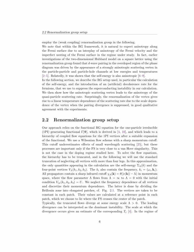
Figure 2.1: Left: Fermi surface (solid line) and discretization of the BZ for p = 0.22.
The boundaries of the patches (labelled by 1, 2, . . . , 40) are indicated by the dashed
lines. All vertices are evaluated at the points marked by the red dots, and are
taken constant within each patch. Right: Two-loop diagrams contributing to the
self-energy. Only diagrams a) and b) contribute to the scattering rate.
interest here, d-wave pairing is the leading instability, and in our approximation Tctakes the values Tc = 0.26t1 for p = 0.15, Tc = 0.22t1 for p = 0.22, and Tc =
0.16t1 for p = 0.30. These Tcs are way too high, mainly because we neglect self-
energy corrections in the flow of the scattering vertex. Nevertheless, Tc grows with
decreasing hole doping reproducing qualitatively the experimental results [1].
The experiments by Abdel-Jawad et al. [1] were carried out on well character-
ized Tl2Ba2CuO6+x samples. The interlayer angle-dependent magnetoresistance
(ADMR) provided detailed Fermi surface (FS) information which we use to fix the
band parameters as follows:
ε(kx, ky) = −2t1 (cos kx + cos ky) + 4t2 (cos kx cos ky)
+2t3 (cos 2kx + cos 2ky) + 4t4(cos 2kx cos ky
+ cos 2ky cos kx) + 4t5 (cos 2kx cos 2ky) , (2.1)
with t1 = 0.181, t2 = 0.075, t3 = 0.004, t4 = −0.010, and t5 = 0.0013(eV).
We use a moderate starting value of the onsite repulsion, U . Our goal is a qualitative
rather than a quantitative description which would require a larger value of U and
multi-loop corrections to the RG flow equations. The experiments were carried out
in a high magnetic field to suppress superconductivity and allow to access the normal
state down to low T . However, including a magnetic field into our RG calculation is
difficult, so that we choose to suppress superconductivity by introducing an isotropic
7
2.2 Renormalization group setup
1 10 20 30 401
10
20
30
40
k1
k 2
24
20
16
12
8
4
0
-4
-8
-12
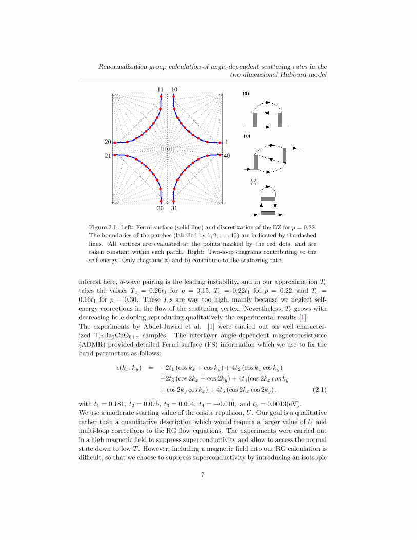
Figure 2.2: Characteristic momentum dependence of the renormalized vertex
VΛ(k1,k2,k3)/t1 for p = 0.22, T = 0.02t1, 1/τ0 = 0.2t1 at Λ = 0. In the fig-
ure, the dependence on the two ingoing wave vectors (k1,k2) is shown, where the
outgoing wave vector k3 is taken to lie in patch 1 close to (π, 0) (cf. Fig. 2.1) and
k4 is fixed by momentum conservation.
scattering rate 1/τ0 into the action. This smears out the Fermi distribution at the
FS, which in turn regularizes the loop integrals and subsequently the flow of the
four-point vertices. This scattering rate is included in the flow equation of the four-
point vertex only, whereas the flow equation for the self-energy is left unaltered. We
found that for our choice of U = 4t1 and the range of temperatures (T ≥ 0.004t1)
and dopings (p ≥ 0.15), a scattering rate of 1/τ0 = 0.2t1 is sufficient to suppress the
divergences associated with superconductivity, while leaving the one-loop integrals
corresponding to other channels, e.g. the π − π-particle-hole diagram, basically
unchanged. On average the vertices remain comparable to the bandwidth and the
largest vertices do not grow larger than≈ 3×bandwidth (Fig. 2.2). The renormalized
vertex is used as an input into a standard lowest order calculation of the quasi-
particle decay rate.
In Fig. 2.2 we display a typical result of our calculations for the four-point vertex
VΛ(k1,k2,k3) at energy scale Λ for fixed outgoing wavevector k3 close to (π, 0) as a
function of the two incoming wavevectors (k1,k2). The remaining outgoing wavevec-
tor is determined by momentum conservation allowing for umklapp processes. The
strongest scattering processes occur for a momentum change of (π, π) and the kinear (π, 0) and (0, π).
As we are only interested in the scattering rates at the FS, which are given by
Im Σ(k ∈ FS, ω → 0 + iδ), we will restrict the calculation of the self-energy to this
quantity in the following. Obviously, the frequency-dependence of Σ cannot be ne-
glected in the calculation. On the other hand, if we neglect the frequency-dependence
8

Renormalization group calculation of angle-dependent scattering rates in thetwo-dimensional Hubbard model
of the four-point vertices, it is clear from the structure of the flow equations that
Σ will also be frequency-independent, as only Hartree and Fock diagrams are in-
cluded. This difficulty can be overcome by replacing the four-point vertex appearing
in the self-energy flow equation by the integrated flow equation of the vertex [7],
schematically,
ΣΛ=0 =
∫dΛ
(∫dΛVΛSΛGΛVΛ
)SΛ, (2.2)
where in our approximation the single-scale propagator SΛ [4, 10] and the full prop-
agator GΛ are related to the free propagator G0 by SΛ = χΛG0 and GΛ = χΛG0,
respectively. The RHS of eq. (2.2) depends on Λ only through the cutoff χΛ. After
a partial integration with respect to Λ and after explicitly inserting a sharp cutoff
χΛ(k) = Θ(|ε(k)| − Λ) we have
ΣΛ=0 =
∫dΛθ(|ε(k1)| − Λ)δ(|ε(k2)| − Λ)θ(Λ− |ε(k3)|)
×V 2ΛG0(k1)G0(k2)G0(k3), (2.3)
where summation and integration over internal momenta and Matsubara frequencies
is implied. Inspection of (2.3) shows that it amounts to evaluting the two-loop
contribution to the self-energy, but with the flowing vertex VΛ instead of the initial
interaction U .
The diagrams corresponding to (2.3) are shown in Fig. 2.1. As we are inter-
ested in the scattering rates at the FS, we need only consider diagrams a) and
b), because the contribution of diagram c) is real for external frequencies ω + iδ.
For a) and b), for external frequency limω→0 ω + iδ, we obtain an imaginary part
∝ δ (ε(k3)− ε(k2)− ε(k1)), reflecting energy conservation.
Neglecting the flow of the four-point vertices, i.e. setting VΛ = U in eq. (2.2), is
equivalent to a second order perturbative calculation of the scattering rate, which
gives a T 2 behavior away from van Hove singularities. All deviations from the
Landau theory scaling form may be attributed to the renormalization of the four-
point vertices.
2.3 Results
Based on eq. (2.3) we calculate both the temperature and the doping dependence of
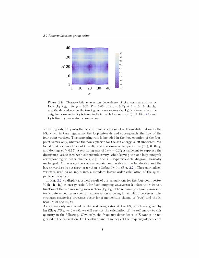
the angle-resolved quasi-particle scattering rates at the Fermi surface. We find that
the scattering rates are anisotropic for all choices of parameters. The precise shape
of the angular dependence changes with doping, but does not change very much with
temperature, as shown in Fig. 2.3. In general, we find that in the nodal direction
(φ = π/4) the scattering rates have a minimum, and increase towards the anti-nodal
direction (φ = 0). The size of the anisotropy grows as doping is decreased. This
parallels the increase of Tc with lower doping in a calculation without the regularizing
9
2.3 Results
0.05 0.10 0.15 0.200.0
0.2
0.4
0.6
0.8
1.0
ΦΠ
ΤaH0LΤ
aHΦL
Figure 2.3: Angle-dependence of the anisotropic component of the quasi-particle
scattering rate on a Fermi surface segment for p = 0.15 (dashed line) and p = 0.30
(solid line). The scattering rates are normalized to unity in the antinodal direction.
The dots are the values at different temperatures, the lines connect the temperature
averages.
scattering rate. This is in accord with the results of Ref. [1], where with decreasing
doping both Tc and the anisotropic part of the scattering rates increase, whereas the
uniform component remains constant.
Separating the scattering rates into an isotropic and an anisotropic part, we write
1
τ(φ, T ) =
1
τi(T ) +
1
τa(φ, T ), (2.4)
where 1/τi ≡ minφ 1/τ(Φ) so that 1/τa(φ) ≥ 0. We characterize the T -dependence
of the anisotropic part by its average over the angle, 〈1/τa〉(T ). This makes sense as
the angular dependence of 1/τa is approximately T -independent (Fig. 2.3). Using
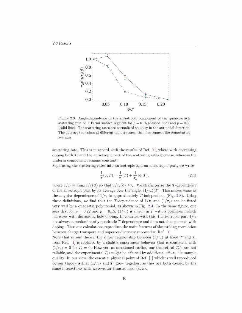
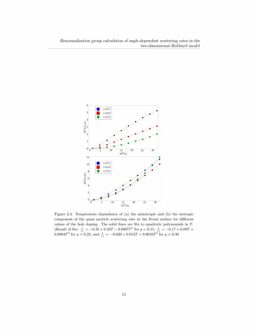
these definitions, we find that the T -dependence of 1/τi and 〈1/τa〉 can be fitted
very well by a quadratic polynomial, as shown in Fig. 2.4. In the same figure, one
sees that for p = 0.22 and p = 0.15, 〈1/τa〉 is linear in T with a coefficient which
increases with decreasing hole doping. In contrast with this, the isotropic part 1/τihas always a predominantly quadratic T -dependence and does not change much with
doping. Thus our calculations reproduce the main features of the striking correlation
between charge transport and superconductivity reported in Ref. [1].
Note that in our theory, the linear relationship between 〈1/τa〉 at fixed T and Tcfrom Ref. [1] is replaced by a slightly superlinear behavior that is consistent with
〈1/τa〉 = 0 for Tc = 0. However, as mentioned earlier, our theoretical Tc’s are not
reliable, and the experimental Tcs might be affected by additional effects like sample
quality. In our view, the essential physical point of Ref. [1] which is well reproduced
by our theory is that 〈1/τa〉 and Tc grow together, as they are both caused by the
same interactions with wavevector transfer near (π, π).
10
Renormalization group calculation of angle-dependent scattering rates in thetwo-dimensional Hubbard model
0 5 10 15 20 25 300
1
2
3
4
5
6
103Tt1
103 X
1Τ
a\t
1
Τ=12.5
Τ=25.0
Τ=37.5
0 5 10 15 20 25 300
2
4
6
8
10
12
103 Tt1
103 H
1Τ
iLt
1
Τ=12.5
Τ=25.0
Τ=37.5
Figure 2.4: Temperature dependence of (a) the anisotropic and (b) the isotropic
component of the quasi particle scattering rate at the Fermi surface for different
values of the hole doping. The solid lines are fits to quadratic polynomials in T .
(Result of fits: 1τa
= −0.35 + 0.20T − 0.0007T 2 for p = 0.15, 1τa
= −0.17 + 0.09T +
0.0004T 2 for p = 0.22, and 1τa
= −0.020 + 0.012T + 0.0016T 2 for p = 0.30
11

2.4 Conclusions
2.4 Conclusions
The results signal presented above point towards a clear breakdown of Landau-
Fermi liquid behavior. The linear temperature dependence is not due to a proximity
to the van Hove singularity at the saddle points of the band structure, as these
points lie well below the Fermi surface at energies T . Further, the increase
in the linear term in T with decreasing hole dopings occurs as the energy of the
van Hove singularity moves further away from the Fermi energy. Recalling Eq.
(2.3), it is clear that deviations from the ordinary Fermi liquid behavior result from
the scale-dependence of the scattering vertex, since this is the only quantity that
differs from the perturbative calculation that leads to Fermi liquid behavior. Hence
anomalous T -dependence of 〈1/τa〉 arises from the increase in the four-point vertex
with decreasing temperature or energy scale. This increase is not restricted to the
d-wave pairing Cooper channel since the divergence in this channel is suppressed
in our calculations. Examination of the RG flows shows that several channels in
the four-point vertex grow simultaneously, e.g. particle-hole and particle-particle
umklapp processes, both with wavevector transfer near (π, π) and with initial and
final states in the anti-nodal regions. This phenomenon is not simply a precursor
of d-wave superconductivity but rather signals that a crossover to strong coupling
in several channels of the four-point vertex is responsible for the breakdown of the
Landau-Fermi liquid. It will be challenging to find out more about the relation
of this breakdown to the opening of the pseudogap at smaller doping levels. The
simultaneous enhancement of several channels through mutual reinforcement was
earlier identified as a key feature of the anomalous Fermi liquid in the cuprates and
associated with the onset of resonant valence bond (RVB) behavior [4, 12].
In conclusion, our RG calculations suggest that the anomalous behavior of the in-
plane quasi-particle scattering rate revealed by the ADMR experiments [1] on over-
doped cuprates can be understood as an intrinsic feature of the doped Hubbard
model that is already present at weaker interaction strengths. The positive correla-
tion between Tc and the anisotropic scattering rate shows up in the calculation as a
general increase of correlations in the anti-nodal direction that is not restricted to the
d-wave pairing channel. Our calculations are in agreement with earlier RG studies
using different hopping parameters [2–4, 7] as far as the structure of the scattering
vertex is concerned, so that we expect that our results hold in more general settings
as well.
12
Chapter 3
Introduction to the wave
packet approach to
interacting fermions
3.1 Introduction
In this chapter we give a general overview of the wave packet approach to interacting
fermions that has been newly developed in this work. It is based on a description
of electrons in terms of a complete orthogonal basis of phase space localized states -
the wave packets. These states are intermediate between real and momentum space
states in the sense that they have a finite extension in both spaces, similar to a
Gaussian. As a consequence, a length scale M is introduced into the problem from
the beginning. Intuitively, this makes sense only when a physical length scale is
present in the system under investigation. The typical example of the introduction
of such a length scale is provided by systems with a gap for single particle excita-
tions. Because of the gap, single particle correlations decay exponentially in space,⟨c†(r) c (0)
⟩∼ e−|r|/ξ, and in this case ξ yields a natural length scale.
The two limiting case ξ → ∞ and ξ → a (where a is the lattice constant) are
relatively well understood: The most celebrated example of the former is given by
conventional, weakly coupled superconductors. These systems are known to be very
well described by a mean-field approach, the BCS theory of superconductivity [14].
In a superconductor, electrons are bound into pairs, and ξ may be thought of as
the pair size. The success of the BCS theory relies on the fact that the pairs are so
large that many of them overlap, effectively eliminating quantum fluctuations [23].
Corresponding to the large pair size in real space, the pairs are very localized in
momentum space, and only a thin shell around the Fermi surface is correlated. The
13
3.2 The pseudogap phase of the cuprates and the saddle point regime of theHubbard model
opposite limit of ξ → 0 is exemplified by the strong coupling limit of a Mott insulator,
where each lattice site is occupied by one electron and only local spin degrees of
freedom remain, which are well separated from the charge sector. Alternatively, one
may think of this state as a paired state as well, where each electron is bound to a
hole. Since the pairs are localized, the pair size vanishes. Conversely, the pairs are
very delocalized in momentum space and spread out over the whole Brillouin zone
in this limit.
Clearly, these two extreme cases are best described in the space where the fermion
pairs are as local as possible, which allows to map the fermion problem to a tractable
effective model. Our motivation is to obtain a similar description for the intermediate
regime, where ξ is neither small nor large, and hence momentum space concepts such
as the Fermi sea and real space phenomena like the suppression of double occupancy
both play a role. From this point of view it is quite natural to employ phase space
localized basis functions: Due to their localization in real space some effects of local
correlations can be taken into account, and their localization in momentum space
allows to resolve certain features of the Brillouin zone, such as the approximate
position of the Fermi surface.
The remainder of this chapter is organized as follows: First, we introduce the specific
context of our study, the pseudogap phase of the cuprate superconductors. After a
brief review of the part of the phenomenology that is relevant in the following, we
discuss some theoretical studies that try to elucidate the opening of the pseudogap
from a weak coupling point of view [20], and the problems faced there related to
the difficulties of treating renormalization flows that flow to strong coupling. Then
we explain the wave packet approach and how it relates to the experimental and
theoretical situation. Finally, we give an outline of the remaining chapters.
3.2 The pseudogap phase of the cuprates and the
saddle point regime of the Hubbard model
The pseudogap phase of the cuprates
The pseudogap phase of cuprate superconductors is arguably one of the more puz-
zling aspects of their phenomenology. Here we highlight some aspects of this phase
which are important for what follows, and refer to the review [18] for a more detailed
account. The phase lies between the Mott insulating state at zero doping, and the
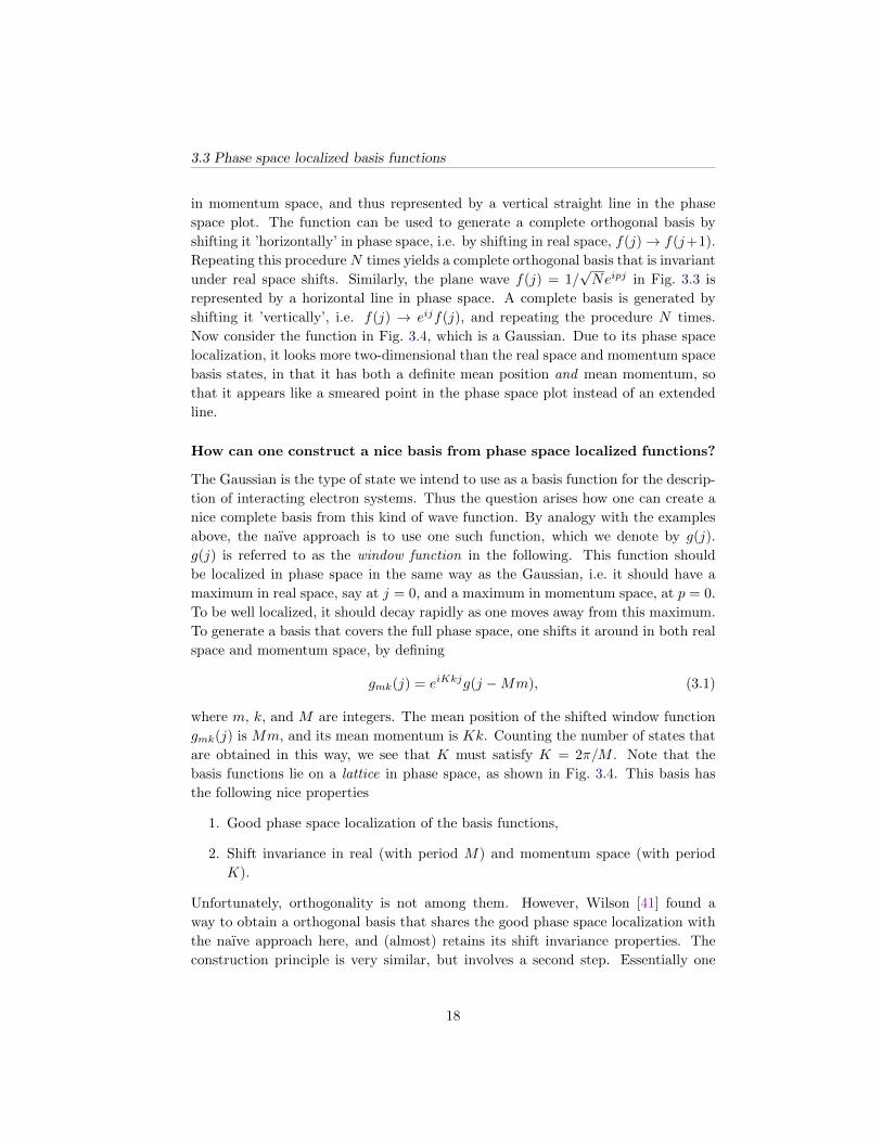
superconducting state at doping p ≈ 16% as displayed schematically in Fig. 3.1 a).
Spectroscopic experiments, in particular ARPES measurements have shown that it
is characterized by highly anisotropic electronic excitations, shown in Fig. 3.1 b): In
the nodal regions, close to (π/2, π/2) a Fermi surface exists and electronic excita-
tions are gapless. For large enough doping, a superconducting gap opens on these
Fermi surface arcs. The corresponding gap for electronic excitations tracks the Tc of
14

Introduction to the wave packet approach to interacting fermions
4
0.05 0.10 0.15 0.20 0.250
40
80
120
160
E (m
eV)
p
Optimal
Doping1
0
bT
( K )
p
AFI
PG
dSC
Tc
T!
T*a
Figure 1. (a) Schematic copper oxide phase diagram. Here, Tc is the criticaltemperature circumscribing a ‘dome’ of superconductivity, Tφ is the maximumtemperature at which superconducting phase fluctuations are detectable withinthe PG phase, and T ∗ is the approximate temperature at which the PGphenomenology first appears. (b) The two classes of electronic excitations incuprates. The separation between the energy scales associated with excitationsof the superconducting state (dSC, denoted by 0) and those of the PG state (PG,denoted by 1) increases as p decreases (reproduced from [7]). The differentsymbols correspond to the use of different experimental techniques.
The energies 0 and 1 diverge from one another with diminishing p, as shown in figure 1(b)(reproduced from [7]). Angle-resolved photoemission (ARPES) reveals that, in the PG phase,excitations with E ∼ 1 occur in the regions of momentum space near k ∼= (π/a0, 0); (0, π/a0)and that 1(p) increases rapidly as p → 0 [6–9]. In contrast, the ‘nodal’ region of k-spaceexhibits an ungapped ‘Fermi Arc’ [41] in the PG phase, and a momentum- and temperature-dependent energy gap opens upon this arc in the dSC phase [41–47]. Results from many otherspectroscopies appear to be in agreement with this picture. For example, optical transient gratingspectroscopy finds that the excitations near 1 propagate very slowly without recombination toform Cooper pairs, whereas lower-energy excitations near the d-wave nodes propagate easilyand reform delocalized Cooper pairs as expected [37]. Andreev tunneling exhibits two distinctexcitation energy scales that diverge as p → 0: the first is identified with the PG energy 1
and the second lower scale 0 with the maximum pairing gap energy of delocalized Cooper-pairs [38]. Raman spectroscopy finds that scattering near the node is consistent with delocalizedCooper pairing, whereas scattering at the antinodes is not [39]. Finally, muon spin rotationstudies of the superfluid density show its evolution to be inconsistent with states on the wholeFermi surface being available for condensation, as if anti-nodal regions cannot contribute todelocalized Cooper pairs [40].
Tunneling density-of-states measurements have reported an energetically particle–holesymmetric excitation energy E = ±1, which is indistinguishable in magnitude in the PG anddSC phases [48, 49]. In figure 2(b), we show the evolution of spatially averaged differentialtunneling conductance [50–52] g(E) for Bi2Sr2CaCu2O8+δ. The p dependence of this PG energyE = ±1 is indicated by a blue dashed curve (see sections 3, 5 and 7), whereas the approximate
New Journal of Physics 13 (2011) 065014 (http://www.njp.org/)
Figure 3.1: Electronic excitations in the pseudogap phase. a) Schematic phase di-
agram of the cuprates. Tc is the critical of d-wave superconductivity, Tφ is the
maximal temperature at which superconducting phase fluctuations are detectable,
and T ∗ is the pseudogap temperature. b) Electronic excitations in the cuprates
fall into two classes: The dome shaped curve (∆0) corresponds to excitations above
the superconducting state. The gap tracks Tc and decreases for small doping. The
curve labelled ∆1 separates from the superconducting gap in the underdoped regime,
increasing towards half-filling. The different symbols correspond to different exper-
imental techniques (Figure reproduced from [16])
the superconducting phase. At the same time, the gap for excitations at the saddle
points stays large and increases as the doping is decreased [24]. The gap for exci-
tations at the saddle points persists up to the pseudogap temperature T ∗, which is
much larger than Tc at low doping. NMR Knight shift measurements [19] indicate
that a (partial) spin gap opens below T ∗, which is generally taken as evidence for
spin-singlet pairing.
The saddle point regime of the Hubbard model
Despite the fact that the cuprates are often modeled as lightly doped Mott insulators,
we have seen in Ch. 2 that the opposite approach using weak coupling renormaliza-
tion group equations can yield valuable insights. The analysis of the RG equations
for the full Hubbard model is still very complicated. Since the correlations are
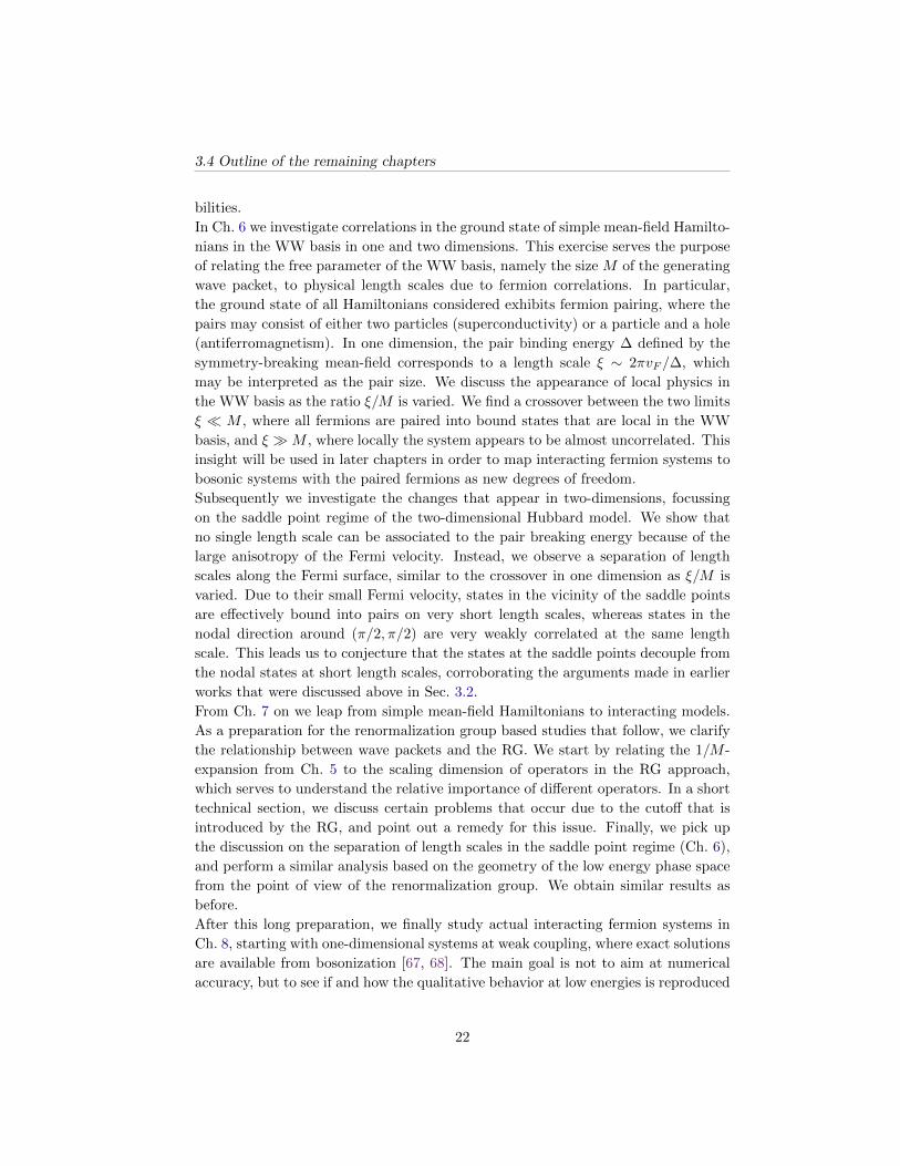
strongest in the vicinity of the saddle points, various researchers were led to study a
reduced saddle point model instead of the full Hubbard model [59–62, 66]. Within
the one-loop RG approach it has been established that the model has strong corre-
lations at low energies, with the leading instablities occuring in the d-wave pairing
and antiferromagnetic channels. However, it was found that at the same time, the
uniform spin and charge susceptibilities are suppressed. Since the latter behavior is
consistent with gaps for spin and charge excitations, Furukawa et al. [66] were lead
to conjecture that the ground state for this model is an insulating spin liquid. The
conjecture is based on an analogy to the physics of ladder systems [33, 53], where
15
3.3 Phase space localized basis functions
VOLUME 81, NUMBER 15 P HY S I CA L REV I EW LE T T ER S 12 OCTOBER 1998
Truncation of a Two-Dimensional Fermi Surface due to Quasiparticle Gap Formationat the Saddle Points
Nobuo Furukawa* and T.M. RiceInstitute for Theoretical Physics, ETH-Hönggerberg, CH-8093 Zurich, Switzerland
Manfred SalmhoferMathematik, ETH Zentrum, CH-8092 Zürich, Switzerland
(Received 12 June 1998)We study a two-dimensional Fermi liquid with a Fermi surface containing the saddle points p , 0
and 0, p. Including Cooper and Peierls channel contributions leads to a one-loop renormalizationgroup flow to strong coupling for short range repulsive interactions. In a certain parameter range thecharacteristics of the fixed point, opening of a spin and charge gap, and dominant pairing correlationsare similar to those of a two-leg ladder at half-filling. We argue that an increase of the electron densityleads to a truncation of the Fermi surface to only four disconnected arcs. [S0031-9007(98)07323-2]
PACS numbers: 71.10.Hf, 71.27.+a, 74.72.–h
The origin of the instability of the Landau-Fermi liquidstate as the electron density is increased in overdopedcuprates is one of the most interesting open questionsin the field. Recently, we proposed that the origin liesin a flow of umklapp scattering to strong coupling [1].The simpler case with the Fermi surface (FS) extrema at6p2, 6p2 was considered and not the realistic casefor hole-doped cuprates where the leading contributionfrom umklapp processes comes from scattering at thesaddle points p, 0 and 0, p. In this Letter we reporta one-loop renormalization group (RG) calculation for therealistic case including contributions from both Cooperand Peierls channels. Reasonable conditions can lead toa strong coupling fixed point whose characteristics aresimilar to those of half-filled two-leg ladders. There,strong coupling umklapp processes lead to spin and chargegaps but only short range spin correlations. A particularlyinteresting and novel feature is that, although the strongestdivergence is in the d-wave pairing channel, the chargegap causes insulating not superconducting behavior.There have been a number of previous RG investigations
for a FS with saddle points. Schulz [2] and Dzyaloshinskii[3] considered the special case with only nearest neigh-bor (nn) hopping so that the saddle points coincide with asquare FS and perfect nesting exactly at half-filling, lead-ing to a fixed point with long range antiferromagnetic (AF)order. Lederer et al. [4] and Dzyaloshinskii [5] also con-sidered the same model as we do. There are two fixedpoints, one at a strong coupling fixed point with d-wavepairing found by Lederer et al. [4], and a weak couplingexamined by Dzyaloshinskii [5]. A Hubbard parametriza-tion of the repulsive interactions U and moderate interac-tion strength suffices to stabilize the strong coupling fixedpoint. The new feature we wish to stress is that there canbe both spin and charge gaps. The FS is then truncatedthrough the formation of an insulating spin liquid (ISL)with resonance valence bond (RVB) character. We pro-
pose that as the hole doping decreases these gaps spreadout from the saddle points so the FS consists of a set of arcs,which progressively shrink as the hole doping decreases.We start with a two-dimensional FS touching the saddle
points p, 0 and 0, p. Such a FS is realized in the caseof the dispersion relation ´k 22tcos kx 1 cos ky 24t0 cos kx cos ky with t . 0 t0 , 0 as nn [next-nearestneighbor (nnn)] hoppings. Throughout this Letter, weassume t0t small but nonzero so that we are close to half-filling. Because of the van Hove singularity, the leadingsingularity arises from electron states in the vicinity of thesaddle points. We consider two FS patches at the saddlepoints and examine the coupling between them using one-loop RG equations, as illustrated in Fig. 1a. kc is the radiusof the patches.The susceptibility for the Cooper channel at q 0 has
a log-square behavior of the form
xpp0 v 2h lnvE0 lnv2tk2
c . (1)
Here, the sum over k is restricted to the patches. E0 isthe cutoff energy and h 8p2t21 for jt0tj ø 1. The
FIG. 1. Fermi surface (FS). (a) Two patches of the FS atthe saddle points. (b) Truncated FS as electron density isincreased.
0031-90079881(15)3195(4)$15.00 © 1998 The American Physical Society 3195
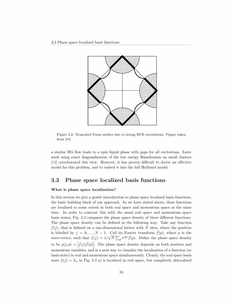
Figure 3.2: Truncated Fermi surface due to strong RVB correlations. Figure taken
from [66]
a similar RG flow leads to a spin liquid phase with gaps for all excitations. Later
work using exact diagonalization of the low energy Hamiltonian on small clusters
[12] corroborated this view. However, it has proven difficult to derive an effective
model for this problem, and to embed it into the full Hubbard model.
3.3 Phase space localized basis functions
What is phase space localization?
In this section we give a gentle introduction to phase space localized basis functions,
the basic building block of out approach. As we have stated above, these functions
are localized to some extent in both real space and momentum space at the same
time. In order to contrast this with the usual real space and momentum space
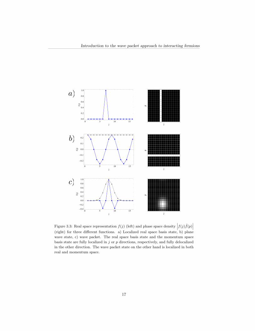
basis states, Fig. 3.3 compares the phase space density of three different functions.
The phase space density can be defined in the following way: Take any function
f(j), that is defined on a one-dimensional lattice with N sites, where the position
is labelled by j = 0, . . . , N − 1. Call its Fourier transform f(p), where p is the
wave-vector, such that f(j) = 1/√N∑p e
ipj f(p). Define the phase space density
to be ρ(j, p) =∣∣∣f(j)f(p)
∣∣∣. The phase space density depends on both position and
momentum variables, and is a neat way to visualize the localization of a function (or
basis state) in real and momentum space simultaneously. Clearly, the real space basis
state f(j) = δij in Fig. 3.3 a) is localized in real space, but completely delocalized
16
Introduction to the wave packet approach to interacting fermions
j
p
0 5 10 150.0
0.2
0.4
0.6
0.8
1.0
j
fj
0 5 10 150.4
0.2
0.0
0.2
0.4
0.6
0.8
1.0
j
fj
j
p
0 5 10 15
0.2
0.1
0.0
0.1
0.2
j
fj
j
p
a)
b)
c)
Wednesday, October 26, 2011
Figure 3.3: Real space representation f(j) (left) and phase space density∣∣∣f(j)f(p)
∣∣∣(right) for three different functions. a) Localized real space basis state, b) plane
wave state, c) wave packet. The real space basis state and the momentum space
basis state are fully localized in j or p directions, respectively, and fully delocalized
in the other direction. The wave packet state on the other hand is localized in both
real and momentum space.
17
3.3 Phase space localized basis functions
in momentum space, and thus represented by a vertical straight line in the phase
space plot. The function can be used to generate a complete orthogonal basis by
shifting it ’horizontally’ in phase space, i.e. by shifting in real space, f(j)→ f(j+1).
Repeating this procedure N times yields a complete orthogonal basis that is invariant
under real space shifts. Similarly, the plane wave f(j) = 1/√Neipj in Fig. 3.3 is
represented by a horizontal line in phase space. A complete basis is generated by
shifting it ’vertically’, i.e. f(j) → eijf(j), and repeating the procedure N times.
Now consider the function in Fig. 3.4, which is a Gaussian. Due to its phase space
localization, it looks more two-dimensional than the real space and momentum space
basis states, in that it has both a definite mean position and mean momentum, so
that it appears like a smeared point in the phase space plot instead of an extended
line.
How can one construct a nice basis from phase space localized functions?
The Gaussian is the type of state we intend to use as a basis function for the descrip-
tion of interacting electron systems. Thus the question arises how one can create a
nice complete basis from this kind of wave function. By analogy with the examples
above, the naıve approach is to use one such function, which we denote by g(j).
g(j) is referred to as the window function in the following. This function should
be localized in phase space in the same way as the Gaussian, i.e. it should have a
maximum in real space, say at j = 0, and a maximum in momentum space, at p = 0.
To be well localized, it should decay rapidly as one moves away from this maximum.
To generate a basis that covers the full phase space, one shifts it around in both real
space and momentum space, by defining
gmk(j) = eiKkjg(j −Mm), (3.1)
where m, k, and M are integers. The mean position of the shifted window function
gmk(j) is Mm, and its mean momentum is Kk. Counting the number of states that
are obtained in this way, we see that K must satisfy K = 2π/M . Note that the
basis functions lie on a lattice in phase space, as shown in Fig. 3.4. This basis has
the following nice properties
1. Good phase space localization of the basis functions,
2. Shift invariance in real (with period M) and momentum space (with period
K).
Unfortunately, orthogonality is not among them. However, Wilson [41] found a
way to obtain a orthogonal basis that shares the good phase space localization with
the naıve approach here, and (almost) retains its shift invariance properties. The
construction principle is very similar, but involves a second step. Essentially one
18

Introduction to the wave packet approach to interacting fermions
Example: Gaussian Frame
1 5 10 16
1
5
10
16
1 5 10 16
1
5
10
16
j
gmk(j)gmk(j)
Matrix of scalar products
Not orthogonal!
Generate basis by shifting Gaussian wave packet in real- and momentum-space
g(j) = e−j2
M2
• Complete basis for N = M K
• Basis states form lattice in phase-space
•
Real space shift: M m
Momentum space shift: K k
gmk = e2πiN Kkjg(j − Mm)
0 < m < K
0 < k < M
j
p
Monday, October 3, 2011
Figure 3.4: Phase space positions of the basis states of a complete shift-invariant
wave packet basis. The basis is created by applying real and momentum shifts to
a single wave packet For a complete basis, the states generated lie on a lattice in
phase-space. In order to have the correct number of states, the area of a unit cell
must be N for a lattice with N sites.
first generates a basis with 2N states by setting K = π/M (instead of K = 2π/M).
One then forms linear combinations such as
ψmk(j) =1√2
[gm,k(j)± gm,−k(j)] , (3.2)
which are either even or odd under reflections (i.e. parity ±1). Finally, one discards
half of the states, such that neighboring states in phase space have the opposite
parity. In Ch. 4 we present more details on the construction of this so-called Wilson-
Wannier basis.
How can phase space localization help to understand correlated electrons?
Most microscopic approaches to correlated electron systems can be loosely catego-
rized into two classes: First, there are methods that are more naturally situated in
momentum space such as the renormalization group [10]. These methods are very
effective in capturing longer range correlations, and relatedly are good at resolving
features in the Brillouin zone, such as the anisotropy of quasi-particle life times on
the Fermi surface in Ch. 2. In addition, they often lead to simple physical pic-
tures, that allow an intuitive understanding of complex physical problems, a feature
that has merits on its own. On the other hand, it is rather difficult to treat strong
short-range correlations, and more often than not uncontrolled approximations are
necessary. The second class is usually defined in real space, and contains methods
19

3.3 Phase space localized basis functions
Microscopic Model H
E!ective momentum space model H!
at scale "
Lattice model HW
with short range interactions
Low-energy degrees of freedom
E!ective Hamiltonian He"
for low-energy degrees of freedom
Renormalizationgroup
Truncated Wilsonbasis expansion
Local part ofHamiltonian
Real spacerenormalization
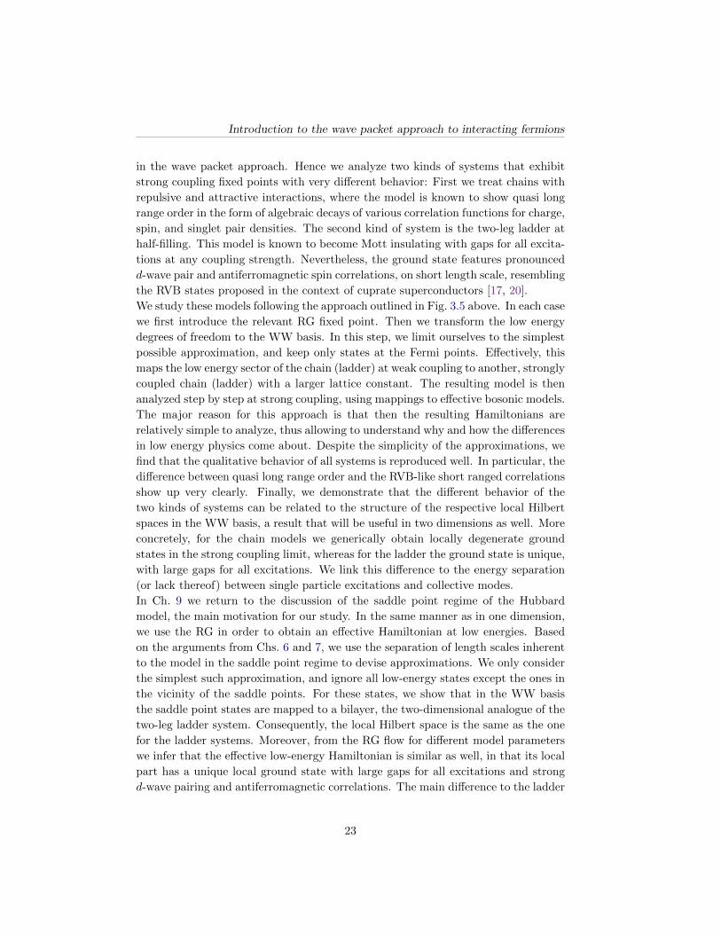
Figure 3.5: The different steps in the wave packet approximation
like exact diagonalization of small clusters [21], strong coupling expansions [22], or
the dynamical mean-field theory [35]. These methods are usually very effective when
it comes to dealing with strong correlations on small length scales, but it is difficult
to incorporate the build-up of correlations on longer length scales. Moreover, they
often involve a high computational cost, and the sheer complexity of the calculations
can make it hard to develop a physical understanding of the solution.
We try to find a middle ground between these two approaches, by combining features
of both: We split the Brillouin zone into a low-energy part in the vicinity of the Fermi
surface, and the remaining states which are at higher energies. It stands to reason
that the states at the Fermi surface are more strongly correlated than states that
are very far away from the Fermi surface. Hence we use the renormalization group
to treat the high-energy problem perturbatively and obtain an effective Hamiltonian
for the low energy degrees of freedom. Note that this only makes sense when the
onsite interactions are not too strong. The remaining low-energy problem is then
transformed to the Wilson-Wannier (WW) basis, and solved using real space meth-
ods, namely strong coupling approximations and real space RG [36]. The different
steps are summarized in Fig. 3.5.
The usefulness of the momentum space localization lies in the fact that one can
isolate the low-energy degrees of freedom simply by truncating the basis, retaining
only those states whose mean moment lies close to the Fermi surface, or a part
of the Fermi surface, such as the saddle points. At the same time, the real space
20

Introduction to the wave packet approach to interacting fermions
localization is helpful because the effective Hamiltonian in the WW basis remains
short-ranged, which makes it possible to analyze the strong coupling problem.
In closing, we would like to remark that the wave packet approach is not really a
method to solve Hamiltonians, but rather a different way to view many-electron
problems. Thus it is in principle compatible with many different methods that can
be used to solve these problems.
3.4 Outline of the remaining chapters
In the remainder of this thesis, we develop the above heuristic ideas in more detail,
and discuss applications to one- and two-dimensional interacting fermion systems.
Since our approach is novel, the exposition starts from scratch, gradually moving
towards the saddle point regime that is the motivation for our work. We begin
with two rather technical chapters where the basic formalism for dealing with the
Wilson-Wannier basis is established.
In Ch. 4 we introduce the Wilson-Wannier (WW) basis states for one-dimensional
lattices, following the exposition given in [43, 44]. In particular, we show how the
basis can be generated from a single window function (or wave packet) by applying
shifts in real space and momentum space. We reformulate the construction by relat-
ing the construction principle to the point group of the lattice, which leads to a more
compact and physically transparent form. Some elementary, yet lengthy mathemati-
cal derivations are involved in the construction. These are relegated App. A to avoid
interrupting the logical flow. In order to generate the basis, one must have a suitable
window function first. We introduce a family of such window functions which allows
to obtain many approximate analytical results. Finally, we extend the WW basis to
the square lattice by taking the tensor product of one-dimensional basis functions.
Ch. 5 deals with the transformation of operators from real or momentum space to
the WW basis in one and two dimensions, respectively. For each case, we derive the
general basis transformation formula first. Then we decompose it into two steps:
First the operator is expanded into an overcomplete wave packet basis, which has
the advantage that matrix elements are much simpler to understand than in the
WW basis itself. This step naturally leads to a systematic and intuitively appealing
approximation method for local operators (referred to as 1/M -expansion, where M
is the size of a wave packet), similar to the gradient expansion in field theory. In the
second step, the orthogonalization procedure for the WW basis is applied to the wave
packet transform in order to arrive at the final form. We find our group theoretical
formulation form Ch. 4 very helpful in developing intuition and (relatively) simple
formulas for this step.
In Chs. 6 and 7 we use the results from the preceding sections to explore the physics
of interacting fermions from the point of view of phase space localization, focussing
on superconductivity and antiferromagnetism and the resulting Fermi surface insta-
21
3.4 Outline of the remaining chapters
bilities.
In Ch. 6 we investigate correlations in the ground state of simple mean-field Hamilto-
nians in the WW basis in one and two dimensions. This exercise serves the purpose
of relating the free parameter of the WW basis, namely the size M of the generating
wave packet, to physical length scales due to fermion correlations. In particular,
the ground state of all Hamiltonians considered exhibits fermion pairing, where the
pairs may consist of either two particles (superconductivity) or a particle and a hole
(antiferromagnetism). In one dimension, the pair binding energy ∆ defined by the
symmetry-breaking mean-field corresponds to a length scale ξ ∼ 2πvF /∆, which
may be interpreted as the pair size. We discuss the appearance of local physics in
the WW basis as the ratio ξ/M is varied. We find a crossover between the two limits
ξ M , where all fermions are paired into bound states that are local in the WW
basis, and ξ M , where locally the system appears to be almost uncorrelated. This
insight will be used in later chapters in order to map interacting fermion systems to
bosonic systems with the paired fermions as new degrees of freedom.
Subsequently we investigate the changes that appear in two-dimensions, focussing
on the saddle point regime of the two-dimensional Hubbard model. We show that
no single length scale can be associated to the pair breaking energy because of the
large anisotropy of the Fermi velocity. Instead, we observe a separation of length
scales along the Fermi surface, similar to the crossover in one dimension as ξ/M is
varied. Due to their small Fermi velocity, states in the vicinity of the saddle points
are effectively bound into pairs on very short length scales, whereas states in the
nodal direction around (π/2, π/2) are very weakly correlated at the same length
scale. This leads us to conjecture that the states at the saddle points decouple from
the nodal states at short length scales, corroborating the arguments made in earlier
works that were discussed above in Sec. 3.2.
From Ch. 7 on we leap from simple mean-field Hamiltonians to interacting models.
As a preparation for the renormalization group based studies that follow, we clarify
the relationship between wave packets and the RG. We start by relating the 1/M -
expansion from Ch. 5 to the scaling dimension of operators in the RG approach,
which serves to understand the relative importance of different operators. In a short
technical section, we discuss certain problems that occur due to the cutoff that is
introduced by the RG, and point out a remedy for this issue. Finally, we pick up
the discussion on the separation of length scales in the saddle point regime (Ch. 6),
and perform a similar analysis based on the geometry of the low energy phase space
from the point of view of the renormalization group. We obtain similar results as
before.
After this long preparation, we finally study actual interacting fermion systems in
Ch. 8, starting with one-dimensional systems at weak coupling, where exact solutions
are available from bosonization [67, 68]. The main goal is not to aim at numerical
accuracy, but to see if and how the qualitative behavior at low energies is reproduced
22
Introduction to the wave packet approach to interacting fermions
in the wave packet approach. Hence we analyze two kinds of systems that exhibit
strong coupling fixed points with very different behavior: First we treat chains with
repulsive and attractive interactions, where the model is known to show quasi long
range order in the form of algebraic decays of various correlation functions for charge,
spin, and singlet pair densities. The second kind of system is the two-leg ladder at
half-filling. This model is known to become Mott insulating with gaps for all excita-
tions at any coupling strength. Nevertheless, the ground state features pronounced
d-wave pair and antiferromagnetic spin correlations, on short length scale, resembling
the RVB states proposed in the context of cuprate superconductors [17, 20].
We study these models following the approach outlined in Fig. 3.5 above. In each case
we first introduce the relevant RG fixed point. Then we transform the low energy
degrees of freedom to the WW basis. In this step, we limit ourselves to the simplest
possible approximation, and keep only states at the Fermi points. Effectively, this
maps the low energy sector of the chain (ladder) at weak coupling to another, strongly
coupled chain (ladder) with a larger lattice constant. The resulting model is then
analyzed step by step at strong coupling, using mappings to effective bosonic models.
The major reason for this approach is that then the resulting Hamiltonians are
relatively simple to analyze, thus allowing to understand why and how the differences
in low energy physics come about. Despite the simplicity of the approximations, we
find that the qualitative behavior of all systems is reproduced well. In particular, the
difference between quasi long range order and the RVB-like short ranged correlations
show up very clearly. Finally, we demonstrate that the different behavior of the
two kinds of systems can be related to the structure of the respective local Hilbert
spaces in the WW basis, a result that will be useful in two dimensions as well. More
concretely, for the chain models we generically obtain locally degenerate ground
states in the strong coupling limit, whereas for the ladder the ground state is unique,
with large gaps for all excitations. We link this difference to the energy separation
(or lack thereof) between single particle excitations and collective modes.
In Ch. 9 we return to the discussion of the saddle point regime of the Hubbard
model, the main motivation for our study. In the same manner as in one dimension,
we use the RG in order to obtain an effective Hamiltonian at low energies. Based
on the arguments from Chs. 6 and 7, we use the separation of length scales inherent
to the model in the saddle point regime to devise approximations. We only consider
the simplest such approximation, and ignore all low-energy states except the ones in
the vicinity of the saddle points. For these states, we show that in the WW basis
the saddle point states are mapped to a bilayer, the two-dimensional analogue of the
two-leg ladder system. Consequently, the local Hilbert space is the same as the one
for the ladder systems. Moreover, from the RG flow for different model parameters
we infer that the effective low-energy Hamiltonian is similar as well, in that its local
part has a unique local ground state with large gaps for all excitations and strong
d-wave pairing and antiferromagnetic correlations. The main difference to the ladder
23
3.4 Outline of the remaining chapters
model is that there is no universal fixed-point of the RG, and that in particular we
observe a crossover between AF and dSC dominated regimes as a function of doping.
In order to assess the effect of the higher dimensionality on the stability of the local
ground state, we diagonalize the effective model on small clusters, and map it to an
effective bosonic model that is analyzed by means of variational coherent states. We
find that the RVB-like ground state appears to be robust over a sizable parameter
range, indicating spin-liquid behavior.
Even though the results are robust within our approximations, we are reluctant to
draw definite conclusions from the calculations at this point, since the approxima-
tions involved are quite drastic. However, since the wave packet approach is still in
its early stages of development, there is a lot of space for improvements in different
directions, some of which we point out in the conclusions. Moreover, the approxima-
tion is based on physical arguments that are fairly elementary, namely the separation
of length scales due to the vicinity of the saddle points and the possibility to localize
states due to umklapp scattering (manifested by the commensurability of the AF
spin correlations), both of which are independent of the details of the calculation.
Finally, we summarize our thesis in Ch. 10, and give an outlook on possible future
work.
24
Chapter 4
Wilson-Wannier basis for a
finite lattice
In this technical chapter we introduce the Wilson-Wannier (WW) basis [41, 43, 44],
an orthogonal basis whose basis states are wave packets that are localized in real
space and bimodal in momentum space. The reason for using this type of basis is that
even though there are no-go theorems on the localization in both momentum- and
real space of orthonormal wave packet bases[47, 48], these can be circumvented if one
allows wave packets to be localized around two points in momentum space. Moreover,
the packets can be chosen such that in momentum space each wave packet is localized
around the two momenta ±p, so that for systems with inversion symmetry, they can
still be used to resolve states that are close to the Fermi points.
4.1 Wilson-Wannier basis in one dimension
4.1.1 Construction of the basis functions
Definition
In the following we consider a finite one-dimensional lattice of size N with periodic
boundary conditions. In order to introduce the Wilson basis, we assume that N can
be written as N = ML, where both M and L are even. The basis is generated from
a single window function (or wave packet) g(j), 0 ≤ j < N . We demand that it is
exponentially localized in both real and momentum space with widths of order M
and K ≡ πM , respectively. In order to generate the basis, we will need the shifted
window function
gmk(j) = eiKkj︸ ︷︷ ︸momentum shift
g (j −mM)︸ ︷︷ ︸position shift
. (4.1)
25
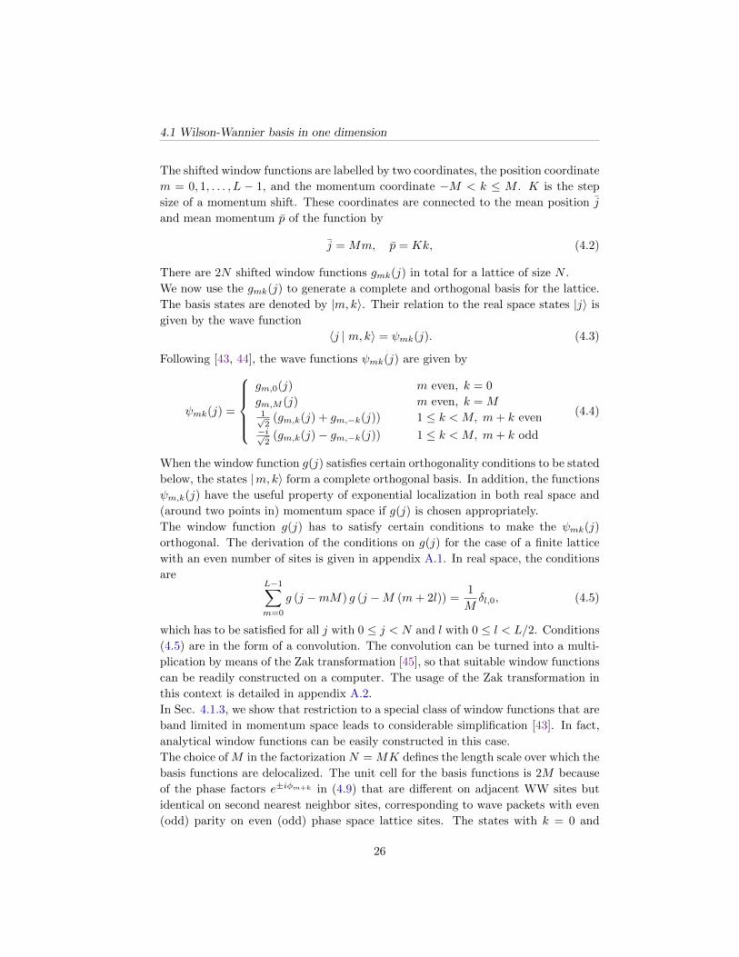
4.1 Wilson-Wannier basis in one dimension
The shifted window functions are labelled by two coordinates, the position coordinate
m = 0, 1, . . . , L − 1, and the momentum coordinate −M < k ≤ M . K is the step
size of a momentum shift. These coordinates are connected to the mean position j
and mean momentum p of the function by
j = Mm, p = Kk, (4.2)
There are 2N shifted window functions gmk(j) in total for a lattice of size N .
We now use the gmk(j) to generate a complete and orthogonal basis for the lattice.
The basis states are denoted by |m, k〉. Their relation to the real space states |j〉 is
given by the wave function
〈j | m, k〉 = ψmk(j). (4.3)
Following [43, 44], the wave functions ψmk(j) are given by
ψmk(j) =
gm,0(j) m even, k = 0
gm,M (j) m even, k = M1√2
(gm,k(j) + gm,−k(j)) 1 ≤ k < M, m+ k even−i√
2(gm,k(j)− gm,−k(j)) 1 ≤ k < M, m+ k odd
(4.4)
When the window function g(j) satisfies certain orthogonality conditions to be stated
below, the states |m, k〉 form a complete orthogonal basis. In addition, the functions
ψm,k(j) have the useful property of exponential localization in both real space and
(around two points in) momentum space if g(j) is chosen appropriately.
The window function g(j) has to satisfy certain conditions to make the ψmk(j)
orthogonal. The derivation of the conditions on g(j) for the case of a finite lattice
with an even number of sites is given in appendix A.1. In real space, the conditions
areL−1∑
m=0
g (j −mM) g (j −M (m+ 2l)) =1
Mδl,0, (4.5)
which has to be satisfied for all j with 0 ≤ j < N and l with 0 ≤ l < L/2. Conditions
(4.5) are in the form of a convolution. The convolution can be turned into a multi-
plication by means of the Zak transformation [45], so that suitable window functions
can be readily constructed on a computer. The usage of the Zak transformation in
this context is detailed in appendix A.2.
In Sec. 4.1.3, we show that restriction to a special class of window functions that are
band limited in momentum space leads to considerable simplification [43]. In fact,
analytical window functions can be easily constructed in this case.
The choice of M in the factorization N = MK defines the length scale over which the
basis functions are delocalized. The unit cell for the basis functions is 2M because
of the phase factors e±iφm+k in (4.9) that are different on adjacent WW sites but
identical on second nearest neighbor sites, corresponding to wave packets with even
(odd) parity on even (odd) phase space lattice sites. The states with k = 0 and
26
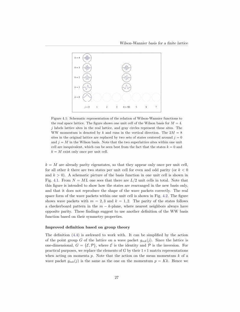
Wilson-Wannier basis for a finite lattice
k 4
k 3
k 2
k 1
k 0
j 0 1 2 3 4 H= ML 5 6 7
Figure 4.1: Schematic representation of the relation of Wilson-Wannier functions to
the real space lattice. The figure shows one unit cell of the Wilson basis for M = 4.
j labels lattice sites in the real lattice, and gray circles represent these sites. The
WW momentum is denoted by k and runs in the vertical direction. The 2M = 8
sites in the original lattice are replaced by two sets of states centered around j = 0
and j = M in the Wilson basis. Note that the two superlattice sites within one unit
cell are inequivalent, which can be seen best from the fact that the states k = 0 and
k = M exist only once per unit cell.
k = M are already parity eigenstates, so that they appear only once per unit cell,
for all other k there are two states per unit cell for even and odd parity (or k < 0
and k > 0). A schematic picture of the basis function in one unit cell is shown in
Fig. 4.1. From N = ML one sees that there are L/2 unit cells in total. Note that
this figure is intended to show how the states are rearranged in the new basis only,
and that it does not reproduce the shape of the wave packets correctly. The real
space form of the wave packets within one unit cell is shown in Fig. 4.2. The figure
shows wave packets with m = 2, 3 and k = 1, 2. The parity of the states follows
a checkerboard pattern in the m − k-plane, where nearest neighbors always have
opposite parity. These findings suggest to use another definition of the WW basis
function based on their symmetry properties.
Improved definition based on group theory
The definition (4.4) is awkward to work with. It can be simplified by the action
of the point group G of the lattice on a wave packet gmk(j). Since the lattice is
one-dimensional, G = E ,P, where E is the identity and P is the inversion. For
practical purposes, we replace the elements of G by their 1×1 matrix representations
when acting on momenta p. Note that the action on the mean momentum k of a
wave packet gmk(j) is the same as the one on the momentum p = Kk. Hence we
27
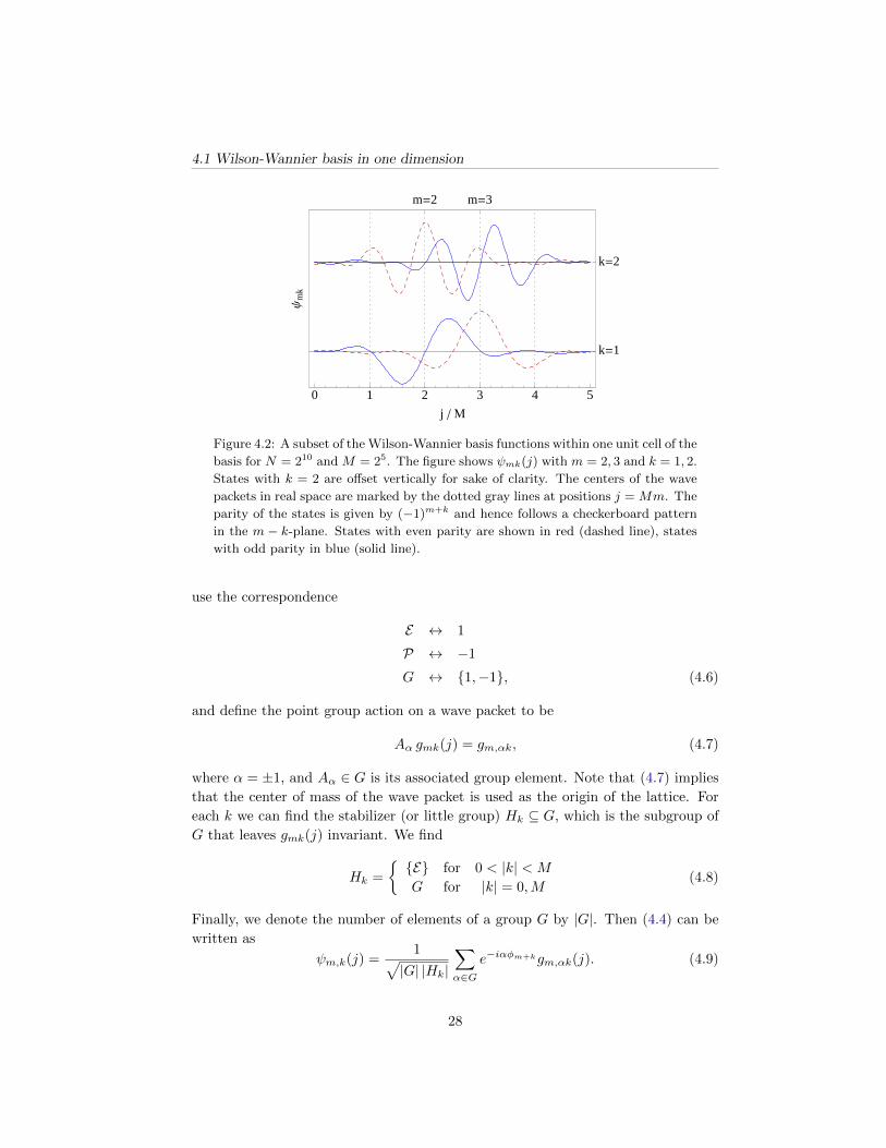
4.1 Wilson-Wannier basis in one dimension
0 1 2 3 4 5
m=2 m=3
k=1
k=2
j M
Ψm
k
Figure 4.2: A subset of the Wilson-Wannier basis functions within one unit cell of the
basis for N = 210 and M = 25. The figure shows ψmk(j) with m = 2, 3 and k = 1, 2.
States with k = 2 are offset vertically for sake of clarity. The centers of the wave
packets in real space are marked by the dotted gray lines at positions j = Mm. The
parity of the states is given by (−1)m+k and hence follows a checkerboard pattern
in the m − k-plane. States with even parity are shown in red (dashed line), states
with odd parity in blue (solid line).
use the correspondence
E ↔ 1
P ↔ −1
G ↔ 1,−1, (4.6)
and define the point group action on a wave packet to be
Aα gmk(j) = gm,αk, (4.7)
where α = ±1, and Aα ∈ G is its associated group element. Note that (4.7) implies
that the center of mass of the wave packet is used as the origin of the lattice. For
each k we can find the stabilizer (or little group) Hk ⊆ G, which is the subgroup of
G that leaves gmk(j) invariant. We find
Hk =
E for 0 < |k| < M
G for |k| = 0,M(4.8)
Finally, we denote the number of elements of a group G by |G|. Then (4.4) can be
written as
ψm,k(j) =1√|G| |Hk|
∑
α∈Ge−iαφm+kgm,αk(j). (4.9)
28
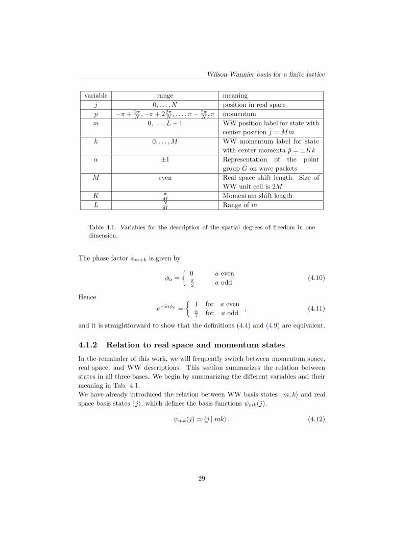
Wilson-Wannier basis for a finite lattice
variable range meaning
j 0, . . . , N position in real space
p −π + 2πN ,−π + 2 2π
N , . . . , π − 2πN , π momentum
m 0, . . . , L− 1 WW position label for state with
center position j = Mm
k 0, . . . ,M WW momentum label for state
with center momenta p = ±Kkα ±1 Representation of the point
group G on wave packets
M even Real space shift length. Size of
WW unit cell is 2M
K πM Momentum shift length
L NM Range of m
Table 4.1: Variables for the description of the spatial degrees of freedom in one
dimension.
The phase factor φm+k is given by
φa =
0 a evenπ2 a odd
(4.10)
Hence
e−iαφa =
1 for a evenαi for a odd
, (4.11)
and it is straightforward to show that the definitions (4.4) and (4.9) are equivalent.
4.1.2 Relation to real space and momentum states
In the remainder of this work, we will frequently switch between momentum space,
real space, and WW descriptions. This section summarizes the relation between
states in all three bases. We begin by summarizing the different variables and their
meaning in Tab. 4.1.
We have already introduced the relation between WW basis states |m, k〉 and real
space basis states | j〉, which defines the basis functions ψmk(j),
ψmk(j) = 〈j | mk〉 . (4.12)
29
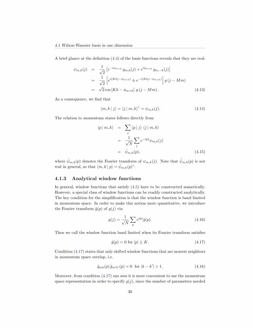
4.1 Wilson-Wannier basis in one dimension
A brief glance at the definition (4.4) of the basis functions reveals that they are real:
ψm,k(j) =1√2
[e−iφm+k gm,k(j) + eiφm+k gm,−k(j)
]
=1√2
[ei(Kkj−φm+k) ± e−i(Kkj−φm+k)
]g (j −Mm)
=√
2 cos [Kk − φm+k] g (j −Mm) . (4.13)
As a consequence, we find that
〈m, k | j〉 = 〈j | m, k〉∗ = ψm,k(j). (4.14)
The relation to momentum states follows directly from
〈p | m, k〉 =∑
j
〈p | j〉 〈j | m, k〉
=1√N
∑
j
e−ipjψm,k(j)
= ψm,k(p), (4.15)
where ψm,k(p) denotes the Fourier transform of ψm,k(j). Note that ψm,k(p) is not
real in general, so that 〈m, k | p〉 = ψm,k(p)∗.
4.1.3 Analytical window functions
In general, window functions that satisfy (4.5) have to be constructed numerically.
However, a special class of window functions can be readily constructed analytically.
The key condition for the simplification is that the window function is band limited
in momentum space. In order to make this notion more quantitative, we introduce
the Fourier transform g(p) of g(j) via
g(j) =1√N
∑
p
eipj g(p). (4.16)
Then we call the window function band limited when its Fourier transform satisfies
g(p) = 0 for |p| ≥ K. (4.17)
Condition (4.17) states that only shifted window functions that are nearest neighbors
in momentum space overlap, i.e.
gmk(p) gm′k′(p) = 0 for |k − k′| > 1. (4.18)
Moreover, from condition (4.17) one sees it is more convenient to use the momentum
space representation in order to specify g(j), since the number of parameters needed
30
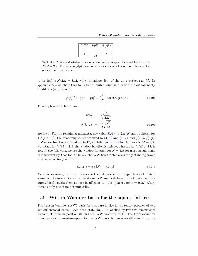
Wilson-Wannier basis for a finite lattice
N/M g (0) g(
2πN
)
2 1 0
4 1√2
12
Table 4.2: Analytical window functions in momentum space for small lattices with
N/M = 2, 4. The value of g(p) for all other momenta is either zero or related to the
ones given by symmetry.
to fix g(p) is N/2M = L/2, which is independent of the wave packet size M . In
appendix A.3 we show that for a band limited window function the orthogonality
conditions (4.5) become
|g (p)|2 + |g (K − p)|2 =2M
Nfor 0 ≤ p ≤ K. (4.19)
This implies that the values
g(0) =
√N
2M,
g (K/2) =1
2
√N
M(4.20)
are fixed. For the remaining momenta, any value g(p) ≤√
2M/N can be chosen for
0 < p < K/2, the remaining values are fixed by (4.19) and (4.17), and g(p) = g(−p).Window functions that satisfy (4.17) are listed in Tab. ?? for the casesN/M = 2, 4.
Note that for N/M = 2, 4, the window function is unique, whereas for N/M > 4 it is
not. In the following, we use the window function for N = 4M for most calculations.
It is noteworthy that for N/M = 2 the WW basis states are simply standing waves
with wave vector p = K, i.e.
ψmk(j) = cos [Kj − φm+k] . (4.21)
As a consequence, in order to resolve the full momentum dependence of matrix
elements, the interactions in at least one WW unit cell have to be known, and the
purely local matrix elements are insufficient to do so (except for k = 0,M , where
there is only one state per unit cell).
4.2 Wilson-Wannier basis for the square lattice
The Wilson-Wannier (WW) basis for a square lattice is the tensor product of two
one-dimensional bases. Each basis state |m,k〉 is labelled by two two-dimensional
vectors: The mean position m and the WW momentum k. The transformation
from real- or momentum-space to the WW basis is hence no different from the
31
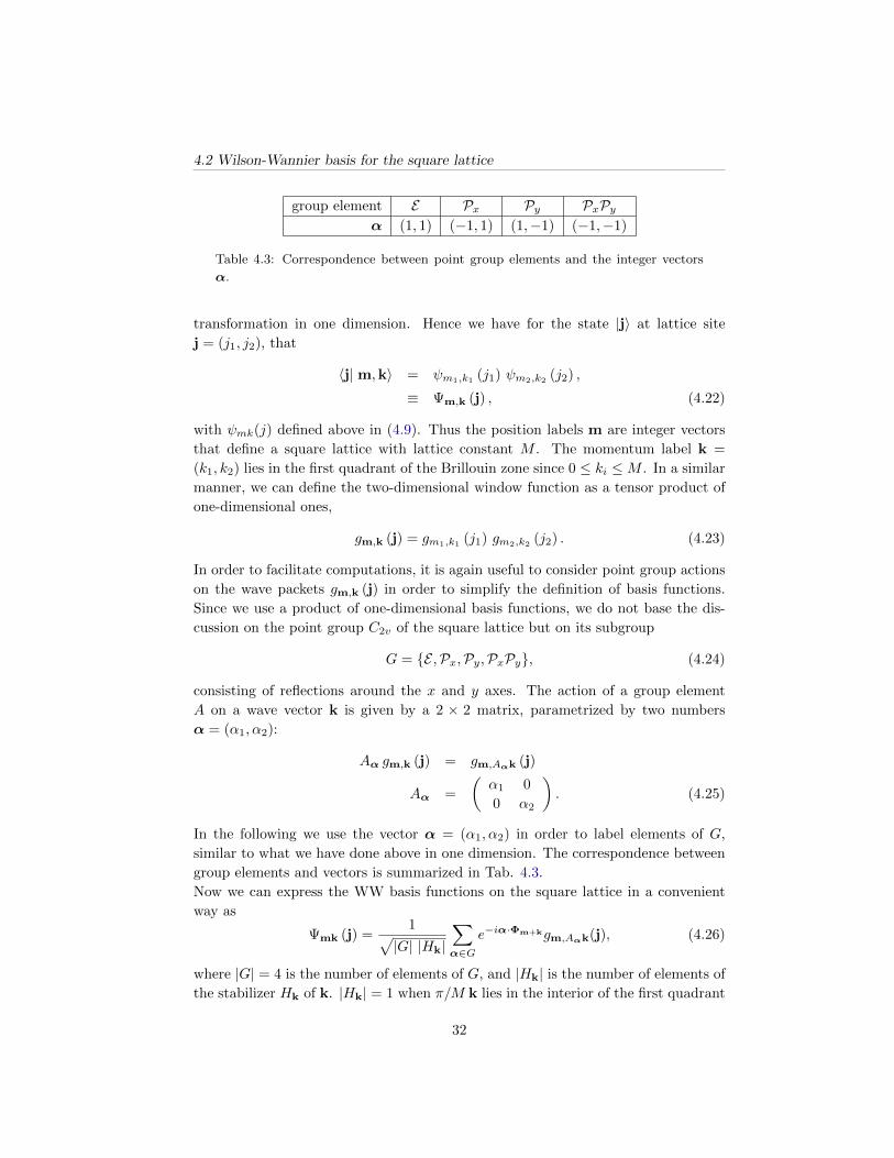
4.2 Wilson-Wannier basis for the square lattice
group element E Px Py PxPyα (1, 1) (−1, 1) (1,−1) (−1,−1)
Table 4.3: Correspondence between point group elements and the integer vectors
α.
transformation in one dimension. Hence we have for the state |j〉 at lattice site
j = (j1, j2), that
〈j|m,k〉 = ψm1,k1 (j1) ψm2,k2 (j2) ,
≡ Ψm,k (j) , (4.22)
with ψmk(j) defined above in (4.9). Thus the position labels m are integer vectors
that define a square lattice with lattice constant M . The momentum label k =
(k1, k2) lies in the first quadrant of the Brillouin zone since 0 ≤ ki ≤M . In a similar
manner, we can define the two-dimensional window function as a tensor product of
one-dimensional ones,
gm,k (j) = gm1,k1 (j1) gm2,k2 (j2) . (4.23)
In order to facilitate computations, it is again useful to consider point group actions
on the wave packets gm,k (j) in order to simplify the definition of basis functions.
Since we use a product of one-dimensional basis functions, we do not base the dis-
cussion on the point group C2v of the square lattice but on its subgroup
G = E ,Px,Py,PxPy, (4.24)
consisting of reflections around the x and y axes. The action of a group element
A on a wave vector k is given by a 2 × 2 matrix, parametrized by two numbers
α = (α1, α2):
Aα gm,k (j) = gm,Aαk (j)
Aα =
(α1 0
0 α2
). (4.25)
In the following we use the vector α = (α1, α2) in order to label elements of G,
similar to what we have done above in one dimension. The correspondence between
group elements and vectors is summarized in Tab. 4.3.
Now we can express the WW basis functions on the square lattice in a convenient
way as
Ψmk (j) =1√
|G| |Hk|∑
α∈Ge−iα·Φm+kgm,Aαk(j), (4.26)
where |G| = 4 is the number of elements of G, and |Hk| is the number of elements of
the stabilizer Hk of k. |Hk| = 1 when π/M k lies in the interior of the first quadrant
32
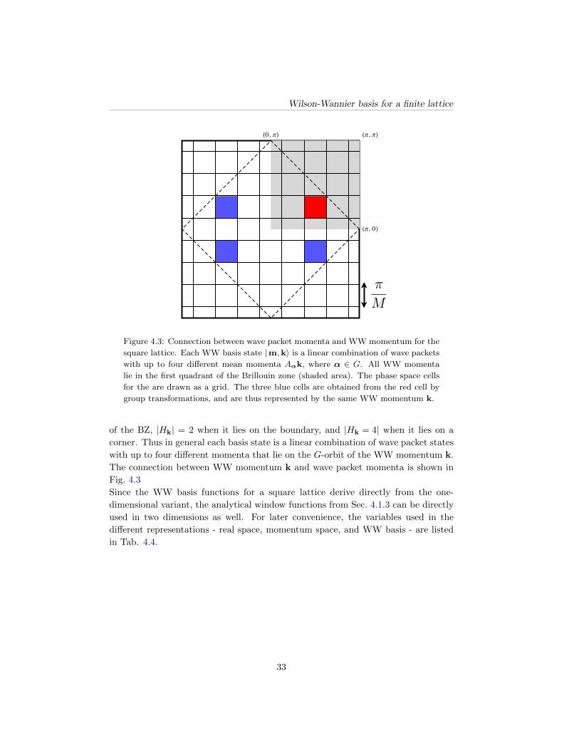
Wilson-Wannier basis for a finite latticeWilson-Wannier Basis
Gmk (j) = gm1k1(j1) gm2k2
(j2)
Ψmk (j) = ψm1k1(j1) ψm2k2
(j2)
Tensor product basis
• Tensor-product window function localized in square of area M!
• k lies in first quadrant because of symmetrization
• WW unit cell contains four sites
• Everything else unchanged
Π, 0
Π, Π0, Π
π
M
Sunday, October 2, 2011
Figure 4.3: Connection between wave packet momenta and WW momentum for the
square lattice. Each WW basis state |m,k〉 is a linear combination of wave packets
with up to four different mean momenta Aαk, where α ∈ G. All WW momenta
lie in the first quadrant of the Brillouin zone (shaded area). The phase space cells
for the are drawn as a grid. The three blue cells are obtained from the red cell by
group transformations, and are thus represented by the same WW momentum k.
of the BZ, |Hk| = 2 when it lies on the boundary, and |Hk = 4| when it lies on a
corner. Thus in general each basis state is a linear combination of wave packet states
with up to four different momenta that lie on the G-orbit of the WW momentum k.
The connection between WW momentum k and wave packet momenta is shown in
Fig. 4.3
Since the WW basis functions for a square lattice derive directly from the one-
dimensional variant, the analytical window functions from Sec. 4.1.3 can be directly
used in two dimensions as well. For later convenience, the variables used in the
different representations - real space, momentum space, and WW basis - are listed
in Tab. 4.4.
33
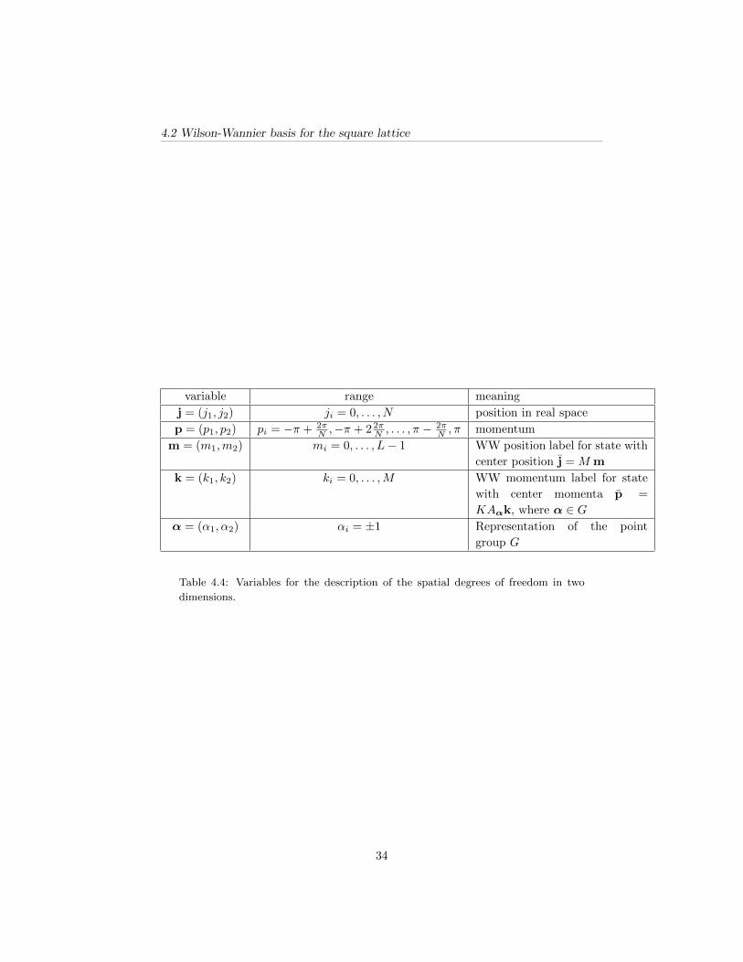
4.2 Wilson-Wannier basis for the square lattice
variable range meaning
j = (j1, j2) ji = 0, . . . , N position in real space
p = (p1, p2) pi = −π + 2πN ,−π + 2 2π
N , . . . , π − 2πN , π momentum
m = (m1,m2) mi = 0, . . . , L− 1 WW position label for state with
center position j = M m
k = (k1, k2) ki = 0, . . . ,M WW momentum label for state
with center momenta p =
KAαk, where α ∈ Gα = (α1, α2) αi = ±1 Representation of the point
group G
Table 4.4: Variables for the description of the spatial degrees of freedom in two
dimensions.
34
Chapter 5
Wilson-Wannier
representation of operators
This chapter discusses the transformation of operators to the WW basis. We consider
the one-dimensional case first, beginning with the general transformation formula
for many-body operators in Sec. 5.1. In Sec. 5.2 we introduce a useful splitting of
the general formula into two steps: A transformation into an overcomplete wave
packet basis, and a second step to orthogonalize these basis states, similar to the
construction in Ch. 4. We focus in particular on the transformation of local and
almost local operators, leading to an expansion in 1/M for those operators that
is analogous to gradient expansions in field theory. The subsequent sections apply
these results to the most relevant cases, namely hopping and interaction operators.
Finally we generalize all results to two dimensions in Sec. 5.4.
5.1 General transformation formula in one dimen-
sion
Transformation of annihilation and creation operators
We consider transformation properties of the fermion creators and annihilators first.
We denote the state with no fermions by | 0〉, and states with one fermion in state
j by | j〉 etc. For sake of clarity, we omit spin indices in this section. The fermion
annihilator (creator) for a fermion in state |m, k〉 is denoted by γm,k (γ†m,k). Using
35

5.1 General transformation formula in one dimension
the resolution of the identity∑j | j〉 〈j |, we the find
γ†m,k | 0〉 = |m, k〉=
∑
j
| j〉 〈j | m, k〉
=∑
j
ψm,k(j) c†j | 0〉 . (5.1)
Taking the Hermitian conjugate of (5.1) yields a similar relation for 〈0 | γm,k. Hence
the transformation from real space to WW basis takes the form
γ†m,k =∑
j
ψm,k(j)c†j ,
γm,k =∑
j
ψm,k(j) cj . (5.2)
Using the resolution of the identity∑p | p〉 〈p | instead of
∑j | j〉 〈j |, the analogous
transformation from momentum space to WW basis is obtained:
γ†m,k =∑
p
ψm,k(p) c†p
γm,k =∑
p
ψm,k(p)∗ cp. (5.3)
Transformation of arbitrary operators
Eqns. (5.2, 5.3) can be used to transform all many-body operators from real (mo-
mentum) space to the WW basis. This is done by applying the transformation rule
for the fermion operators to each operator separately. Consider a general operator
O. It can be expanded in any of the three bases. The transformation rule for the
expansion coefficients follows from the fact that the operator is independent of the
particular representation chosen. We assume that the real space expansion is given
by
O =∑
j1···j2nO (j1, . . . , j2n) c†j1 · · · c
†jncjn+1
· · · cj2n . (5.4)
The same operator in the WW representation can be written as
O =∑
m1k1···m2nk2n
O (m1k1, . . . ,m2nk2n) γ†m1k1· · · γ†mnkn γmn+1kn+1
· · · γm2nk2n.
(5.5)
Using (5.2), the relation between the two expansions is given by
O (m1k1, . . . ,m2nk2n) =∑
j1···j2nO (j1, . . . , j2n)
[2n∏
l=1
ψml,kl (jl)
]. (5.6)
36

Wilson-Wannier representation of operators
In a similar manner, the momentum space representation can be written as
O =1
Nn−1
∑
p1···p2nO (p1, . . . , p2n) c†p1 · · · c†pn cpn+1
· · · cp2n . (5.7)
It is related to the real space representation (5.4) by Fourier transformation in each
index. From the WW representation (5.5) and the transformation rule (5.3) it follows
that
O (m1k1, . . . ,m2nk2n) =1
Nn−1
∑
p1···p2nO (p1, . . . , p2n)
×[
n∏
l=1
ψml,kl (pl)
][2n∏
l=n+1
ψml,kl (pl)∗].
(5.8)
Eqns. (5.6, 5.8) can be used directly in order to obtain the WW representation of any
operator. On the other hand, it is not very intuitive due to the rather complicated
definition of the ψmk(p). In the next section, we bring (5.8) into a more easily
understandable (if less compact) form.
5.2 Wilson-Wannier basis and wave packet trans-
formation
The goal of this section is to split the transformation (5.8) into two steps, where the
first step involves sums over products of window functions. This step yields matrix
elements between different wave packet states with wave function gmk(j), and hence
we refer to it as wave packet transformation. The second step involves the sum over
the point group G that takes the overcomplete wave packet states to the WW basis
states. Simplifications occur because the wave packet states are shift invariant under
general phase space shifts, so that only a few matrix elements have to be evaluated.
Moreover, the wave packet matrix elements are easier to understand, since each wave
packet is localized around one point in phase space (instead of two points for the
WW basis states). In the following we focus on the wave packet part of the WW
transformation, since this part contains most of the physical information. The effect
of the symmetrization is discussed in Secs. 5.3.1-5.3.2 below.
We restrict ourselves to the transformation from momentum space to the WW basis,
since this transformation will be used most of the time in the remainder of this work.
The corresponding formulas in real space are completely analogous.
First, we use the definition (4.9) of ψmk(j) (and hence ψmk(p)) in terms of the wave
packets, and split each sum over p in two parts as follows:
∑
p
(· · ·)ψmk(p) =
1√|G| |Hk|
∑
α∈Ge−iαφm+k
︸ ︷︷ ︸orthogonalization
×[∑
p
(· · ·)gm,αk(p)
]
︸ ︷︷ ︸wave packet transformation
(5.9)
37
5.2 Wilson-Wannier basis and wave packet transformation
Now we exploit the shift invariance of the window function in order to replace all
gmk(p) by g(p), using Eq. (B.7) that is derived in App. B. It states that for an
arbitrary function f(p) the identity∑
p
f(p)gmk(p) =∑
p
f (p+Kk) e−iMmpg (p) (5.10)
holds. Applying (5.9) and (5.10) to (5.8), we find
O (m1k1, . . . ,m2nk2n) =1
|G|n1√∏2n
l=1 |Hkl |(5.11)
×∑
α1···α2n
exp
−i
n∑
l=1
(αl φml+kl − αn+lφmn+l+kn+l
)
×O (m1α1k1, . . . ,m2nα2nk2n) , (5.12)
where the wave packet transform O (m1α1k1, . . . ,m2nα2nk2n) is given by
O (m1α1k1, . . . ,m2nα2nk2n) =1
Nn−1
∑
p1...p2n
O (p1 + α1Kk1, . . . , p2n + α2nKk2n)
× exp
−iM
n∑
l=1
(mlpl −mn+lpn+l)
[2n∏
l=1
g (pl)
].
(5.13)
Wave packet transformation for local operators
Eqns. (5.12-5.13) appear to be rather formidable, and it is indeed tedious to dis-
cuss their properties in full generality. Hence we will consider only a special case
here, which is nevertheless instructive. To be specific, we consider the wave packet
transform of a local operator,
O (p1, . . . , p2n) = Oloc δ
(n∑
i=1
[pi − pi+n]
), (5.14)
where δ (· · · ) is the delta function modulo 2π that enforces momentum conservation.
We also define the wave packet momentum mismatch
Q = K
2n∑
i=1
[αiki − αi+nki+n] , (5.15)
which specifies the amount of violation of conservation of k, where Q = 0 when k is
conserved modulo 2M . Inspection of (5.13) shows that the delta function in (5.14)
now enforces the conditionn∑
i=1
[pi − pi+n] = −Q mod 2π. (5.16)
38
Wilson-Wannier representation of operators
Since this is the only dependence on the variables αi and ki, these variables influence
the matrix element only through Q. Thus we may set k1 = Q/K, ki = 0 for i > 1,
and αi = 1 without loss of generality. In order to keep the notation readable, we use
p1 ≡ −Q− pn+1 +∑ni=2 [pi − pn+i] as a short hand. Then (5.13) becomes
O (m1, 1, Q; . . . ;m2n, 1, 0) = Oloc1
Nn−1
∑
p2···p2n
2n∏
i=1
g (pi) (5.17)
× exp−iMn∑
i=1
[mipi −mn+ipn+i],
which depends only on g, on Q, and on the mi. By virtue of translational invariance
of the wave packet states, the expression is shift invariant in real space with period
2M when Q 6= 0, and with period M when Q = 0.
It is important to realize that the assumption that O is local is not as restrictive as
it might seem. Since the presence of the window functions restrict all sums over p
to −K < p < K, in fact the local case is a valid approximation whenever
O (p1 +Kα1k1, . . . , p2m +Kα2mk2m) ≈ C δ(
2n∑
i=1
[pi +Kαiki − pn+i −Kαn+ikn+i]
)
(5.18)
for some constant C and −K < pi < K. This translates into the statement that
the spatial range of O should be small compared to M . This short range spatial de-
pendence is then contained in the dependence on αiki in the wave packet transform,
and ki in the WW basis. As a consequence, only few matrix elements need to be
evaluated, and the evaluation is very fast because (5.18) can be computed once and
tabulated for later use.
When greater precision is necessary (for instance for longer ranged interactions), or
when matrix elements vanish in the local approximation (which we will see to be the
case for the hopping operator), it is straightforward to improve the approximation
by Taylor expanding O (p1, . . . , p2m) around the maximum of the product of wave
packets. Since the window functions restrict the summation over the momenta to
|p| . π/M , the Taylor expansion leads effectively to an expansion in 1/M . This
1/M -expansion leads to expansion coefficients that are universal in the sense that
they depend on the window function and a few parameters only. We will pursue this
procedure for the hopping matrix elements below in Sec. 5.3.1, but stick to the local
approximation for interaction terms. We discuss the relation of the wave packet
transform of an operator to the notion of scaling dimension of operators that is used
in the renormalization group below in Ch. 7.
39
5.3 Transformation of hopping and interaction operators
5.3 Transformation of hopping and interaction op-
erators
5.3.1 Hopping
In this section we discuss the WW representation of the kinetic energy operator
Hkin =∑
p
ε(p)c†p cp, (5.19)
where we assume εp = −2t cos p in the following, but the treatment below applies to
any dispersion. t is the hopping rate for nearest neighbor hopping, the bandwidth
is W = 4t. We denote the WW transform of ε(p) by T (mk,m′k′). From the
transformation formula (5.8) we obtain
T (mk,m′k′) =∑
p
ε(p)ψmk(p) ψm′k′ (p′)∗. (5.20)
Since g(p) is band limited (cf. Sec. 4.1.3), T (mk,m′k′) = 0 if |k − k′| > 1 because of
vanishing overlap of the WW basis functions in momentum space. In the following
we focus on the case k′ = k, which, again by virtue of momentum space localization,
is the dominant term in the expansion. We express ψmk(p) in terms of g(p) using
(5.12) as discussed above:
T (mk,m′k) =1
|G| |Hk|∑
α,α′
e−i(αφm+k−α′φm′+k) δαk,α′k (5.21)
×∑
p
ε (p+ αK) e−iMp(m−m′) |g (p)|2
=1
2
∑
α
e−iα(φm+k−φm′+k)∑
p
ε (p+ αK) e−iMp(m−m′) |g (p)|2 ,
where we have used |G| = 2. Note that the factor 1/Hk cancels against one of the
sums over α for the case k = 0, where the Kronecker delta does not restrict the
summation over α.
Wave packet transformation and 1/M-expansion around the local limit
We note that the factor |g (p)|2 restricts the sum over p to −π/M < p < π/M , so
that it makes sense to expand ε (p+ αq) around p = 0:
ε (p+ αK) ≈ ε (Kk)︸ ︷︷ ︸mean kinetic energy
+ αε′ (Kk)︸ ︷︷ ︸group velocity
p+ ε′′ (Kk)︸ ︷︷ ︸dispersion
1
2p2 + . . . , (5.22)
where ε′ (Kk) = ∂pε (Kk + p)∣∣p=0
etc.
40
Wilson-Wannier representation of operators
We treat the kinetic energy contribution term by term, starting with the first term.
Since this term is a constant, the corresponding contribution in the WW basis is
diagonal by virtue of the orthogonality of the basis states. Hence the contribution
is∑mk ε (Kk) γ†mk γmk
For the remaining contributions, we focus on the leading terms only. These are the
terms that are diagonal in k and act over the shortest distance. We use the wave
packet transformation first in order to estimate the magnitude of the different terms,
and apply the orthogonalization afterwards. Moreover, we use the analytical window
function for N/M = 4 from Tab. ?? in order to obtain analytical estimates. For the
group velocity term the leading contribution arises from nearest neighbor hopping
with m′ −m = ±1, with magnitude
ε′ (Kk)∑
p
pe±iMp g2(p) = ±i π4M
ε′ (Kk) , (5.23)
which is O(1/M) as announced above. The term proportional to p2 is dominated by
hopping to second nearest neighbors, m′ −m = ±2, and its contribution is
1
2ε′′ (Kk)
∑
p
p2e±i2Mp g2(p) = − π2
16M2ε′′ (Kk) . (5.24)
Orthogonalization
In order to arrive at the WW representation of the hopping operator, its wave packet
transform has to be orthogonalized. This eliminates some term that are finite in the
wave packet transform. For example, consider the first term of the expansion of
ε (Kk + p) ≈ ε (Kk). In the wave packet transform, matrix elements between wave
packets that are adjacent in phase space are finite, since they involve the scalar
product of two wave packets,
ε (Kk)∑
p
gmk (p) gm′k′ (p)∗ 6= 0, (5.25)
and the wave packet states are not orthogonal. The WW basis states, on the other
hand, are orthogonal, so that their scalar product is 〈mk | m′k′〉 = δmm′δkk′ . As a
consequence, the constant term in the expansion of ε(p) leads to a diagonal contri-
bution to the WW transform.
In a similar manner, other matrix elements that are finite in the wave packet trans-
form vanish in the WW basis due to the symmetry of the basis states (recall that
the orthogonalization amounts to linear combining wave packet states such that they
fall into irreducible representations of the point group).
Hopping Hamiltonian in WW-representation
In summary, the hopping Hamiltonian in the WW basis is dominated by the k-
diagonal part, however, in principle the other hopping matrix elements are not
41
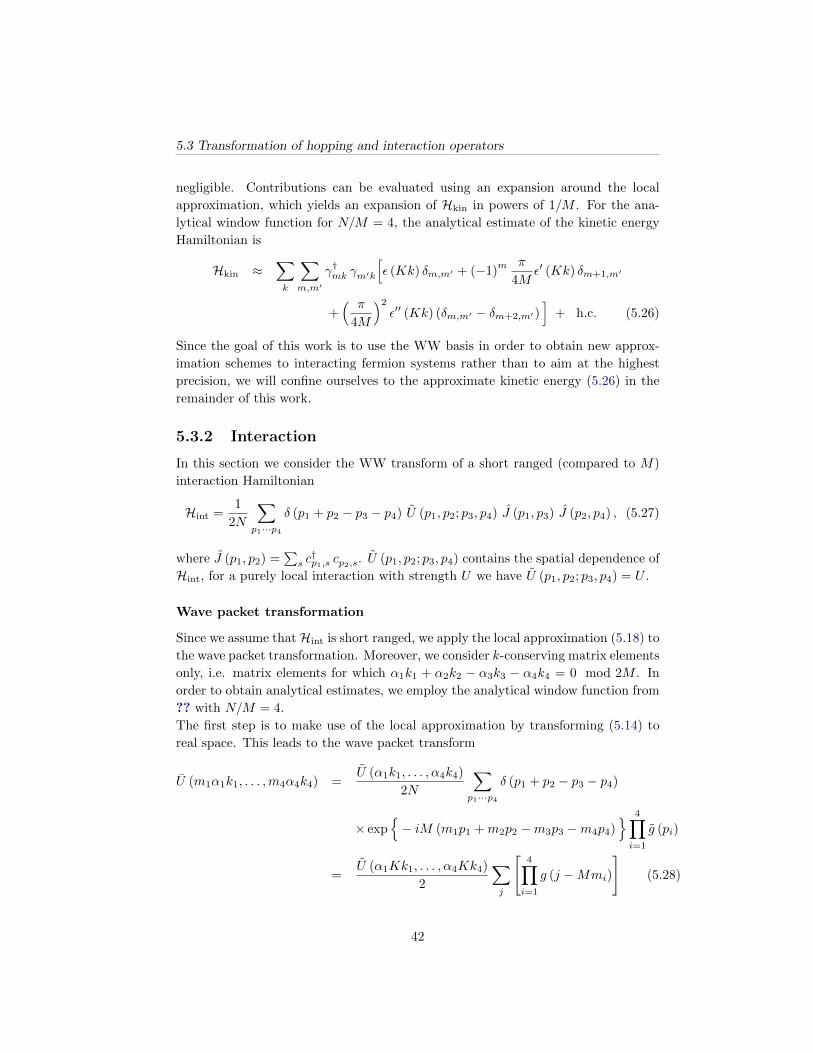
5.3 Transformation of hopping and interaction operators
negligible. Contributions can be evaluated using an expansion around the local
approximation, which yields an expansion of Hkin in powers of 1/M . For the ana-
lytical window function for N/M = 4, the analytical estimate of the kinetic energy
Hamiltonian is
Hkin ≈∑
k
∑
m,m′
γ†mk γm′k
[ε (Kk) δm,m′ + (−1)
m π
4Mε′ (Kk) δm+1,m′
+( π
4M
)2
ε′′ (Kk) (δm,m′ − δm+2,m′)]
+ h.c. (5.26)
Since the goal of this work is to use the WW basis in order to obtain new approx-
imation schemes to interacting fermion systems rather than to aim at the highest
precision, we will confine ourselves to the approximate kinetic energy (5.26) in the
remainder of this work.
5.3.2 Interaction
In this section we consider the WW transform of a short ranged (compared to M)
interaction Hamiltonian
Hint =1
2N
∑
p1···p4δ (p1 + p2 − p3 − p4) U (p1, p2; p3, p4) J (p1, p3) J (p2, p4) , (5.27)
where J (p1, p2) =∑s c†p1,s cp2,s. U (p1, p2; p3, p4) contains the spatial dependence of
Hint, for a purely local interaction with strength U we have U (p1, p2; p3, p4) = U .
Wave packet transformation
Since we assume thatHint is short ranged, we apply the local approximation (5.18) to
the wave packet transformation. Moreover, we consider k-conserving matrix elements
only, i.e. matrix elements for which α1k1 + α2k2 − α3k3 − α4k4 = 0 mod 2M . In
order to obtain analytical estimates, we employ the analytical window function from
?? with N/M = 4.
The first step is to make use of the local approximation by transforming (5.14) to
real space. This leads to the wave packet transform
U (m1α1k1, . . . ,m4α4k4) =U (α1k1, . . . , α4k4)
2N
∑
p1···p4δ (p1 + p2 − p3 − p4)
× exp− iM (m1p1 +m2p2 −m3p3 −m4p4)
4∏
i=1
g (pi)
=U (α1Kk1, . . . , α4Kk4)
2
∑
j
[4∏
i=1
g (j −Mmi)
](5.28)
42

Wilson-Wannier representation of operators
N/M m 0 1 2
4 V (0, 0, 0,m) 1732M
832M − 1
64M
4 V (0, 0,m,m) 1732M
732M
164M
2 V (0, 0, 0,m) 12M
14M 0
2 V (0, 0,m,m) 12M
14M 0
Table 5.1: Approximate analytical values of V (m1, . . . ,m4) (see Eq. (5.29)) for the
dominant matrix elements in the wave packet transform of a local interaction. In
the following, we us the matrix elements for N/M = 2.
It follows that the spatial dependence of the wave packet matrix elements is deter-
mined by
V (m1, · · · ,m4) ≡∑
j
[4∏
i=1
g (j −Mmi)
]. (5.29)
The dominant matrix elements arise for m1 = m2 = m3 6= m4, where three operators
reside on one site, and m1 = m2 6= m3 = m4, where two operators are located at
the same site. Note that only the relative positions matter due to the residual
translational invariance of the wave packet states. Approximate analytical values of
V (m1, . . . ,m4) for these cases are tabulated in Tab. 5.1. Interactions decay rapidly,
with spatial separation, so that V (0, 0, 0, 2)/V (0, 0, 0, 0) ≈ 1/32. Consequently, we
will take only nearest neighbor interactions into account. The table also shows the
corresponding value for the case that the window function for N/M = 2 is used.
Since these are very similar, we will use the latter in the following for analytical
calculations, and the former for numerical ones.
Orthogonalization
In order to obtain the WW representation of the interaction, the wave packet states
have to be orthogonalized (see Sec. 5.2). The orthogonalization leads to cancellations
between some non-local terms. We focus on weakly coupled systems, so that the
states at k = 0,M can be ignored, which implies |Hk| = 1 in the following. Plugging
the wave packet transform (5.28) into the orthogonalization formula (5.12), we obtain
U (m1k1, . . . ,m4k4) =V (m1, . . . ,m4)
2
1
2
∑
α1···α4
U (α1Kk1, . . . , α4Kk4)
× e−i(α1φ1+α2φ2−α3φ3−α4φ4), (5.30)
where we have introduced the short hand φi = φmi+ki .
At low energies, the interaction Hamiltonian that couples states at the Fermi points
can be reduced to a small set of coupling constants. This will be considered in Ch. 8.
43

5.4 Two-dimensional square lattice
5.4 Two-dimensional square lattice
Having discussed the transformation of operators to the WW basis for the one-
dimensional case, we now turn to the two-dimensional square lattice. All the steps
from the one-dimensional calculation can be essentially repeated in the same man-
ner. Therefore the discussion in this section is somewhat shorter, highlighting the
differences to the one-dimensional case. Only the transformation from momentum
space to WW basis will be treated. All the WW basis related quantities can be
found in Tab. 4.4.
5.4.1 General transformation formula, wave packet transform,
and local approximation
Transformation of annihilation and creation operators
The transformation formula follows directly from the definition (4.26) of the basis
functions Ψmk(j and their Fourier transform Ψmk (p), where now all position related
coordinates are vectors, e.g. j = (j1, j2). Thus we have
γ†mk =∑
p
Ψmk (p) c†p,
γmk =∑
p
Ψmk (p)∗cp. (5.31)
Transformation of arbitrary operators
In the same way as in one dimension, an arbitrary many-body operator O can be
expanded in any single-particle basis. The transformation rules for the coefficients in
the expansion follow from the fact that the operator is independent of the basis. For
sake of readability, we continue to suppress spin indices in this section. We assume
that O contains n creators and n annihilators. Hence its momentum representation
can be written as
O =1
N2n−2
∑
p1···p2n
O (p1, . . . ,p2n) c†p1· · · cp2n
. (5.32)
The WW representation can be similarly written as
O =∑
m1k1···m2nk2n
O (m1k1, · · · ,m2nk2n) γ†m1k1· · · γm2nk2n
. (5.33)
44

Wilson-Wannier representation of operators
Equating the right hand sides of (5.32) and (5.33), we obtain the general transfor-
mation rule for the square lattice:
O (m1k1, . . . ,m2nk2n) =1
N2n−2
∑
p1···p2n
O (p1, . . . ,p2n)
×[n∏
l=1
Ψmlkl (pl)
][2n∏
l=n+1
Ψmlkl (pl)∗] (5.34)
WW basis and wave packet transformation
In order to arrive at a more manageable form of (5.34), we use the two-dimensional
version of the wave packet transformation (cf. Sec. 5.2) and write
∑
p
(· · ·)
Ψmk(p) =1√|G| |Hk|
∑
α∈Ge−iα·Φm+k
︸ ︷︷ ︸orthogonalization
×[∑
p
(· · ·)gm,Aαk(p)
]
︸ ︷︷ ︸wave packet transformation
(5.35)
We only treat k-conserving matrix elements in the following. In the local approxi-
mation, the wave packet transform of O (p1, . . . ,p2n) is given by
O (m1α1k1, . . . ,m2nα2nk2n) ≈ O (KAα1k1, . . . ,KAα2n
k2n)
×∑
j
[2n∏
i=1
g (j−Mmi)
](5.36)
The WW representation of O is then obtained from the wave packet transform using
the orthogonalization part of the WW transformation. This yields
O (m1k1, . . . ,m2nk2n) =1
|G|n√∏2n
i=1 |Hki |
∑
α1···α2n
e−i∑nl=1[αl·Φl−αn+l·Φn+l]
× O (m1α1k1, . . . ,m2nα2nk2n)
(5.37)
where we have used the short hand Φi ≡ Φm+k. In analogy to the one-dimensional
case, the local approximation can be improved by expandingO (p1, . . . ,p2n) around
pi = KAαiki, leading to an expansion in 1/M .
5.4.2 Hopping
Wo consider the hopping operator
Hkin =∑
p
c†p cp [−2t (cos px + cos py) + 4t′ cos px cos py − µ]︸ ︷︷ ︸=: ε(p)
(5.38)
45
5.4 Two-dimensional square lattice
which includes nearest and next-to-nearest neighbor hopping. First note that when
t′ = 0, the hopping Hamiltonian consists of two one-dimensional hopping terms, so
that in this case the results from one dimension can be reused without any changes for
each direction. In order to take the t′ term into account, we abbreviate Q = KAαk
and expand ε (Q + p) to leading order around p = 0. To the first order we obtain
ε (Q + p) ≈ ε (Q) + vg (Q) · p + . . . , (5.39)
where the group velocity vg (Q) is given by
vg (Q) =
2t sinQx
[1− 2t′
t cosQy
]
2t sinQy
[1− 2t′
t cosQx
] . (5.40)
Thus we can still use the one-dimensional result without changes up to O(1/M), and
the t′ term merely leads to a Q-dependent multiplicative correction to the nearest
neighbor hopping term. At order O(1/M2), a mixed term ∝ pxpy appears, which
leads to diagonal hopping in the WW basis. However, taking into account the leading
order only, this term can be neglected unless the first order term vanishes. This is
the case whenever vg (Q) = 0, i.e. at the band edges Q = (0, 0) and Q = (π, π),
and at the saddle points Q = (π, 0) and Q = (0, π). In both cases, the group
velocity vanishes because of the higher symmetry around these points which demands
ε (Q + p) = ε (Q− p). However, the same symmetry forbids the mixed term pxpy in
the expansion of the kinetic energy, so that the second order contribution is a sum
of two one-dimensional terms as well in this case.
Summarizing the above, to the leading order in the 1/M -expansion the hopping
operator for the square lattice is the sum of two one-dimensional hopping operators
with a k and direction dependent hopping rate
tx → t
(1− 2t′
tcosKky
)
ty → t
(1− 2t′
tcosKkx
)(5.41)
5.4.3 Interaction
We consider the WW representation of the interaction operator
Hint =1
2N2
∑
p1···p4
δ (p1 + p2 − p3 − p4) U (p1, . . . ,p4) J (p1,p3) J (p2,p4) ,
(5.42)
where J (p,p′) =∑s c†p,s cp′,s. Similarly, in the WW basis we write
Hint =1
2
∑
m1k1···m4k4
U (m1k1, . . . ,m4k4) J (m1k1,m3k3) J (m2k2,m4k4) , (5.43)
46

Wilson-Wannier representation of operators
where J (mk,m′k′) =∑s γ†mk,s γm′k′,s.
We follow the argumentation of Sec. 5.3.2 and focus on matrix elements that are
k-conserving, i.e. Aα1k1 + Aα2
k2 = Aα3k3 + Aα4
k4 in the wave packet transform
U (m1α1k1, . . . ,m4α4k4) of Hint. Moreover, we use the local approximation for
the interaction matrix elements in momentum space. The general transformation
formula (5.37) then reduces to
U (m1k1, . . . ,m4k4) =1
|G|n√∏4
i=1 |Hki |
∑
α1···α4
U (m1α1k1, . . . ,m4α4k4)
× e−i(αl·Φl+α2·Φ2−α3·Φ3−α4·Φ4).
(5.44)
Similarly to Sec. 5.3.2, the wave packet transform U (m1α1k1, . . . ,m4α4k4) is given
by
U (m1α1k1, . . . ,m4α4k4) =1
2U (KAα1k1, . . . ,KAα4k4)
× δAα1k1+Aα2
k2,Aα3k3+Aα4
k4
× V (m1,x, . . . ,m4,x)V (m2,y, . . . ,m4,y)
(5.45)
with the same function V (m1, · · · ,m4) =∑j
∏4i=1 g (j −Mmi) as in the one-
dimensional case. Thus the decay properties are the same as in one dimension,
and we restrict ourselves to nearest neighbor interactions only, neglecting all but the
leading matrix elements. It is noteworthy that individual interaction matrix elements
U (m1k1, . . . ,m4k4) are proportional to 1/M2 because V (m1, . . . ,m4) ∝ 1/M (cf.
Tab. 5.1), whereas they are ∝ 1/M in one dimension. The scaling of operators and
its connection to their relevance in the RG sence is considered in Ch. 7. We conclude
this chapter with the remark that since the low-energy region of the Brillouin zone
in two dimensions extends over the whole Fermi surface, there is no universal low-
energy parametrization of interactions as it was the case in one dimension. Instead,
the full momentum dependence of the interaction along the Fermi surface has to
be taken into account in general. Whether approximations are admissible has to
be decided based on the shape of the Fermi surface and the length scale M under
consideration. This is discussed in Ch. 9.
47
5.4 Two-dimensional square lattice
48
Chapter 6
Wave packets and fermion
pairing
Symmetry breaking in fermion systems can often be understood as a transition
from free to paired fermions. The best known example is superconductivity [23],
where electrons bind into pairs which form the condensate that characterizes the
superconducting state. However, spin and charge density waves may also be viewed
as pairing of electrons and holes, so that a wide variety of states falls into the class
of paired fermion states. Such a paired state introduces an energy scale ∆, given by
the fermion gap, and a length scale, the pair size ξ. In the weak coupling limit, we
can estimate
ξ ≈ 2πvF∆
(6.1)
on dimensional grounds.
In this section we discuss fermion pairing in the context of the WW basis. Since the
WW basis states are localized on the length scale M , one expects that for M > ξ
pairs are (predominantly) local in the WW basis, whereas for M < ξ they are non-
local. On the other hand, the pair correlations in the BCS state decay as one moves
away from the Fermi surface, and the corresponding width in momentum space is
2π/ξ ∼ ∆/vF . Hence, we expect states within a distance less than ∆/vF to the
Fermi surface to be strongly correlated, whereas they should be weakly correlated
when they are far away from the Fermi surface.
These estimates suggest that it is possible to replace fermionic degrees of freedom by
pairs that are local (in real space) in the WW basis when M/ξ is chosen large enough.
In this way the low energy problem may be bosonized. They also suggest that only
about ξ/M states in the direction perpendicular to the Fermi surface are strongly
correlated, whereas the remainder may be treated perturbatively. Thus pairs may
be considered to be local in momentum space (in the direction perpendicular to the
Fermi surface) when M/ξ is made small enough. It is natural to expect that for
49

6.1 One dimension
M ∼ ξ, pairs are reasonably localized in both momentum and real space, hence
allowing for a simplified description of the low energy physics in terms of relatively
few (by momentum space localization) bosonic degrees of freedom that are local in
real space (by virtue of real space localization) in the WW basis.
The remainder of this chapter elaborates on these heuristic considerations. To this
end, we compute the WW transform of several mean-field Hamiltonians, discussing
the relevance of different terms and their dependence on ξ/M . Moreover, we com-
pute single-particle correlations of the respective ground states in the WW basis.
Motivated by applications in later chapters, we focus on superconductivity and anti-
ferromagnetism. In Sec. 6.1 we treat one-dimensional systems, the extension to the
square lattice follows in Sec. 6.2.
6.1 One dimension
6.1.1 Superconductivity
We consider the BCS mean-field Hamiltonian in one dimension, which is given by
HBCS = −t∑
j
∑
s
[c†j,s cj+1,s + c†j+1,s cj,s − µc†j,s cj,s
]+ ∆
∑
j
[c†j,↑ c
†j,↓ + cj,↓ cj,↑
].
(6.2)
HBCS can be easily diagonalized by applying a Bogoliubov transformation to the
fermion operators [23], so that in particular its ground state and correlation functions
can be computed exactly. We first transform HBCS to the WW basis and investigate
the relative importance of the hopping and the pairing term as a function of ξ/M .
Afterwards we compute single-particle correlations of the exact ground state in the
WW basis. Both results illustrate that unpaired fermions become less and less
important as ξ/M goes to zero.
WW representation of the BCS mean-field Hamiltonian
We consider the WW representation of HBCS. The hopping term has already been
discussed above in Sec. 5.3.1, so we will turn directly to the anomalous term
∆∑j
(c†j,↑ c
†j,↓ + h.c.
). Its WW representation can be obtained using Eq. (5.2):
∆∑
j
(c†j,↑ c
†j,↓ + h.c.
)= ∆
∑
mk,m′k′
(γ†mk,↑ γ
†m′k′,↓ + h.c.
) ∑
j
ψmk(j)ψm′k′(j)
= ∆∑
mk
(γ†mk,↑ γ
†mk,↓ + h.c.
). (6.3)
The pairing mean-field term is local in the WW basis, hence it acts independently
on each WW orbital. All non-vanishing matrix elements are O(1). In conjunction
50
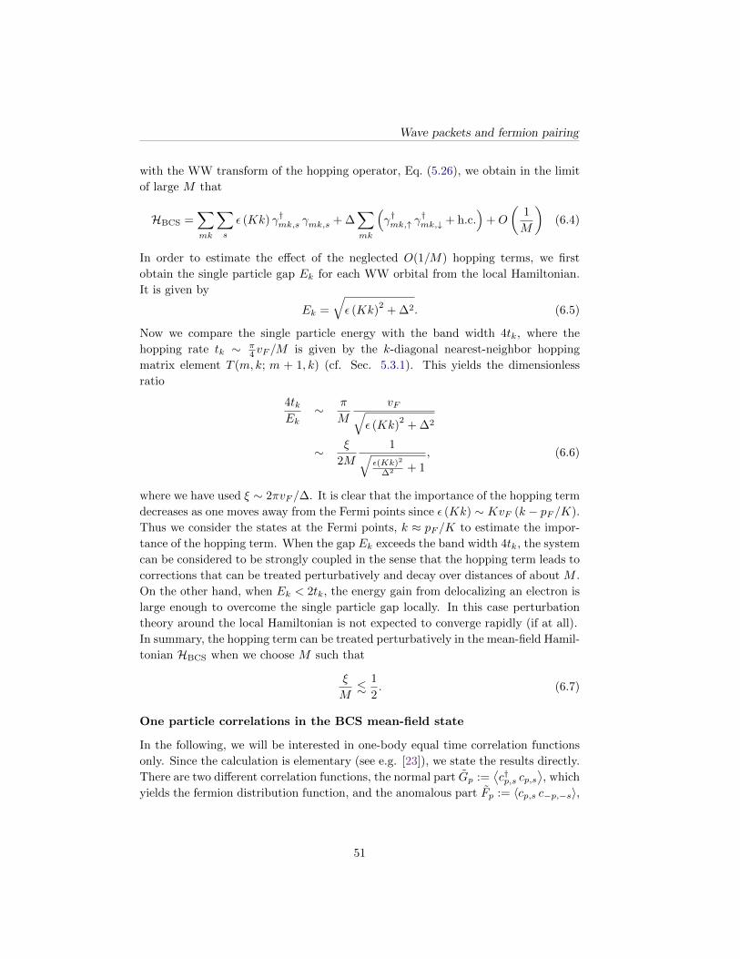
Wave packets and fermion pairing
with the WW transform of the hopping operator, Eq. (5.26), we obtain in the limit
of large M that
HBCS =∑
mk
∑
s
ε (Kk) γ†mk,s γmk,s + ∆∑
mk
(γ†mk,↑ γ
†mk,↓ + h.c.
)+O
(1
M
)(6.4)
In order to estimate the effect of the neglected O(1/M) hopping terms, we first
obtain the single particle gap Ek for each WW orbital from the local Hamiltonian.
It is given by
Ek =
√ε (Kk)
2+ ∆2. (6.5)
Now we compare the single particle energy with the band width 4tk, where the
hopping rate tk ∼ π4 vF /M is given by the k-diagonal nearest-neighbor hopping
matrix element T (m, k; m + 1, k) (cf. Sec. 5.3.1). This yields the dimensionless
ratio
4tkEk
∼ π
M
vF√ε (Kk)
2+ ∆2
∼ ξ
2M
1√ε(Kk)2
∆2 + 1, (6.6)
where we have used ξ ∼ 2πvF /∆. It is clear that the importance of the hopping term
decreases as one moves away from the Fermi points since ε (Kk) ∼ KvF (k − pF /K).
Thus we consider the states at the Fermi points, k ≈ pF /K to estimate the impor-
tance of the hopping term. When the gap Ek exceeds the band width 4tk, the system
can be considered to be strongly coupled in the sense that the hopping term leads to
corrections that can be treated perturbatively and decay over distances of about M .
On the other hand, when Ek < 2tk, the energy gain from delocalizing an electron is
large enough to overcome the single particle gap locally. In this case perturbation
theory around the local Hamiltonian is not expected to converge rapidly (if at all).
In summary, the hopping term can be treated perturbatively in the mean-field Hamil-
tonian HBCS when we choose M such that
ξ
M.
1
2. (6.7)
One particle correlations in the BCS mean-field state
In the following, we will be interested in one-body equal time correlation functions
only. Since the calculation is elementary (see e.g. [23]), we state the results directly.
There are two different correlation functions, the normal part Gp :=⟨c†p,s cp,s
⟩, which
yields the fermion distribution function, and the anomalous part Fp := 〈cp,s c−p,−s〉,
51

6.1 One dimension
that contains pair correlations. They are given by
Gp =Ep − εp
2Ep(6.8)
Fp =∆
Ep, (6.9)
where εp = −2t cos p − µ is the kinetic energy, and Ep =√ε2p + ∆2 is the energy
of a Bogoliubov quasi-particle. The corresponding correlation function in the WW
representation is obtained using Eq. (5.3). For the normal part Gmk,m′k′ this yields
Gmk,m′k′ =⟨γ†mks γm′k′s
⟩
=∑
p
ψmk(p) ψm′k′(p)∗ ⟨c†p,s cp,s
⟩
=∑
p
ψmk(p) ψm′k′(p)∗ Gp. (6.10)
Similarly, for the anomalous part we obtain
Fmk,m′k′ =⟨γmk,s γm′k′,−s
⟩
=∑
p
ψmk(p)∗ ψm′k′(−p)∗ Fp. (6.11)
In the following, we focus on two key quantities. First, we evaluate Gmk,m+1,k,
which non-local fermion correlations, and Fmk,m+1,k/Fmk,mk, which measures the
decay of pair correlations with distance from the Fermi surface. Since correlations
are strongest at the Fermi surface, we set k = kF = pF /K. A plot of these ratios as
a function of ξ/M is shown in Fig. 6.1. It can be seen that the non-local correlators
vanish when the pair size ξ is much smaller than M .
Next we consider the decay of correlations with distance from the Fermi surface. To
this end, we evaluate the ratios 2Gmk,mk for k = 1 + kF . This is a measure of the
occupation of WW orbitals next to the Fermi surface. Analogously, we evaluate the
anomalous correlator Fmk,mk/FmkF ,m kF at k = 1 + kF , which measures the decay
of pair correlations as one moves away from the Fermi surface. This is shown in
Fig. 6.2.
We are interested in the case that the states at the Fermi points are strongly coupled,
i.e. ξ/M ≈ 1/2 (cf. Eq. 6.7), the non-local correlations are strongly suppressed. At
the same time, from Fig. 6.2 we see that the WW orbitals next to the Fermi surface
have a mean occupancy of about 1/6 above the Fermi surface (5/6 below the Fermi
surface). For larger |k − kF |, the occupation number approaches its non-interacting
value apart from small deviations, as shown in Fig. 6.3. This suggests that most
of the WW orbitals can be treated perturbatively, since they deviate only slightly
from their non-interacting ground state, where all orbitals below (above) the Fermi
surface are filled (empty).
52
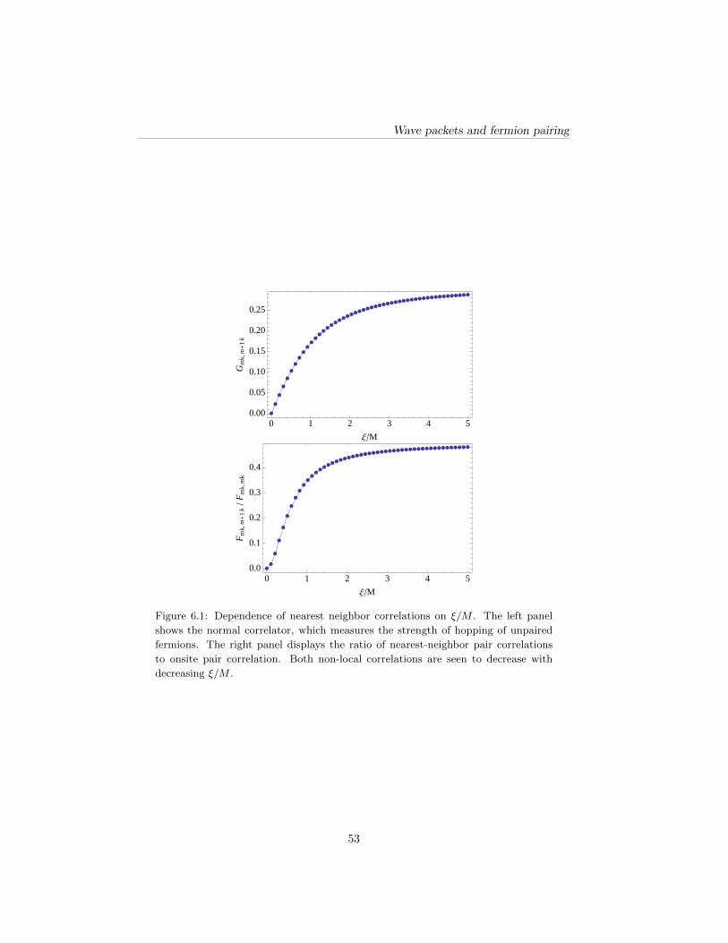
Wave packets and fermion pairing
æ
æ
æ
æ
æ
æ
æ
æ
æ
æ
æ
æ
ææ
ææ
ææ
ææ
ææææææææææææææææææææææææææææææ
0 1 2 3 4 50.00
0.05
0.10
0.15
0.20
0.25
ΞM
Gm
k,m
+1
k
æ
æ
æ
æ
æ
æ
æ
æ
æ
æ
æ
ææ
ææ
ææ
æææææææææææææææææææææææææææææææææ
0 1 2 3 4 50.0
0.1
0.2
0.3
0.4
ΞM
Fm
k,m
+1
k
Fm
k,m
k
Figure 6.1: Dependence of nearest neighbor correlations on ξ/M . The left panel
shows the normal correlator, which measures the strength of hopping of unpaired
fermions. The right panel displays the ratio of nearest-neighbor pair correlations
to onsite pair correlation. Both non-local correlations are seen to decrease with
decreasing ξ/M .
53

6.1 One dimension
æ
æ
æ
æ
æ
æ
æ
æ
ææ
ææ
ææææææææææææææææææææææææææææææææææææææ
0 1 2 3 4 50.0
0.2
0.4
0.6
0.8
1.0
ΞM
2Gm
k,m
k
æ
æ
æ
æ
æ
æ
æ
æ
æ
æ
ææ
ææ
ææ
ææææææææææææææææææææææææææææææææææ
0 1 2 3 4 5
0.2
0.4
0.6
0.8
1.0
ΞM
Fm
k,m
k
Fm
k F,m
k F
Figure 6.2: Decay of correlation with separation from the Fermi surface as a function
of ξ/M . Left panel: Decay of the occupation number at k = kF + 1. Note that
the plot shows two times the occupation number. Right panel: Ratio of local pair
correlations at k = kF + 1 and k = kF . Both quantities decrease with increasing
ξ/M .
æ æ æ æ æ ææ
æ
æ
æ
ææ æ æ æ æ æ
-5 0 50.0
0.2
0.4
0.6
0.8
1.0
k-kF
Gm
k,m
k
Figure 6.3: WW orbital occupation number as a function of k− kF for ξ/M = 1/2.
All orbitals except the ones at the Fermi surface and their nearest neighbors deviate
only weakly from their non-interacting occupation number.
54

Wave packets and fermion pairing
6.1.2 Antiferromagnetism
The antiferromagnetic case is relevant when the system half-filled, which implies
that pF = π/2 = KM/2 and µ = 0. The mean-field Hamiltonian is given by
HAF = −t∑
j
∑
s
[c†j,s cj+1,s + c†j+1,s cj,s
]+ ∆
∑
j
(−1)jc†j,s σ
zss′ cj,s′ , (6.12)
where ∆ is the mean-field for the staggered magnetization, which we take to point
into the z-direction. In many respects, HAF leads to results similar to the BCS case
above, so that the discussion will be focussed on obtaining the WW transform of the
AF mean-field operator.
WW representation of the AF mean-field Hamiltonian
The WW transform of the mean-field term is given by
∆∑
j
(−1)jc†j,s σ
zss′ cj,s′ = ∆
∑
mk,m′k′
γ†mk,s σzss′ γm′k′,s′
∑
j
(−1)jψmk(j)ψm′k′(j)
(6.13)
Now we use that (−1)j
= eiπj to obtain
(−1)jψmk(j) =
1√|G| |Hk|
∑
α
e−iαφm+k eiπjgm,αk (j)
=1√|G| |Hk|
∑
α
e−iαφm+k gm,−M+αk(j)
=1√|G| |Hk|
∑
α
e−iαφm+k (−1)m+k
gm,M−αk(j)
= (−1)m+k
ψm,M−k(j), (6.14)
where we have used that e−iφm+k = (−1)m+k
e+iφm+k and 0 ≤ M − k = −M + k
mod 2M in the third line. Plugging the result into (6.13) we obtain
∆∑
j
(−1)jσzss′ c
†j,s cj,s′ = ∆
∑
mk
(−1)m+k
γ†mk,s σzss′ γm,M−k,s′ . (6.15)
In general, the staggered magnetization couples the two WW orbitals |m, k〉 and
|m,M − k〉. However, at the Fermi points we have k = M/2 = M − k, so that only
one orbital is involved.
The AF mean-field Hamiltonian in the WW representation is thus given by
HAF =∑
mk
[δss′ε (Kk) γ†mk,s γmk,s′ + ∆σzss′ γ
†mk,s γm,M−k,s′
]+O
(1
M
)(6.16)
Note that the single particle gap is exactly the same as for the BCS case above, Eq.
(6.5). Thus the ratio tk/Ek and the single particle correlations show exactly the
same behavior as a function of ξ/M and k.
55

6.2 Two dimensions: Effect of anisotropy
6.2 Two dimensions: Effect of anisotropy
In this section we apply a similar analysis to the case of the two-dimensional square
lattice. Since we will be interested mainly in the case that the Fermi surface lies
close to the saddle points (0, π) and (π, 0), we use the kinetic energy
Hkin = −2t∑
p
∑
s
(cos px + cos py) c†p,s cp,s (6.17)
and set the chemical potential µ = 0. We consider two types of mean-fields, d-wave
superconductivity (dSC) and antiferromagnetism (AF). The major novelty compared
to the one-dimensional case is that now several WW orbitals lie close to the Fermi
surface. Moreover, the number of orbitals at the Fermi surface depends on the wave
packet scale M , with M orbitals at the Fermi surface for the model considered here.
In addition, the Fermi velocity along the Fermi surface is strongly anisotropic. As one
moves from (π, 0) to (0, π) along the Fermi surface, i.e. py = π−px, its x-component
(the y-component is the same) varies as
vF,x (p) = 2t sin px. (6.18)
As a consequence, no simple relation between the gap magnitude ∆ and the pair
size ξ exists that holds for the whole Fermi surface even in the case of an angle-
independent mean-field.
Since correlations are expected to be strongest where vF is smallest, we use estimates
of the pair size at the saddle points in the following, and adjust M accordingly. In
the vicinity of the saddle point (π, 0), the kinetic energy (6.17) can be approximated
as
ε (p− (π, 0)) ≈ t(p2y − p2
x
), (6.19)
and similarly for the other saddle point (0, π). The natural length scale ξ for a pair
gap of size ∆ is then given by
ξ = π
√t
∆. (6.20)
We are mainly interested in cases where pairing occurs at relatively small scales. We
hence fix M = 4 for the remainder of this chapter. The phase space cells and the
states at the Fermi surface for this case are shown in Fig. 6.4.
Since at the saddle points the distance between two WW states in real space is 2M
(cf. Ch. 4), ξ should be compared to 2M . For ξ = 2M we obtain
∆ ∼ π2
4M2t =
π2
64t, (6.21)
which evaluates to ∆ ≈ 0.15 t.
In the following two sections we discuss pairing in the AF and dSC channels. We
will show that even when the order parameter is constant along the Fermi surface,
56
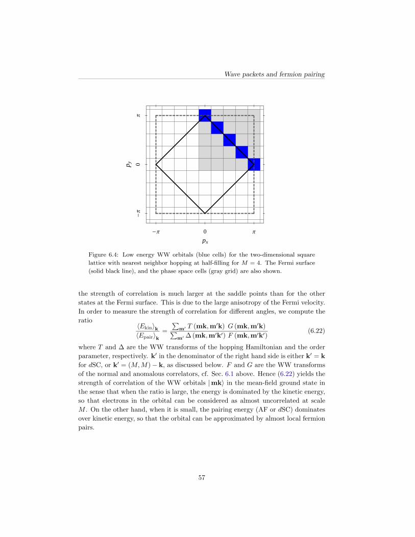
Wave packets and fermion pairing
px
p y
-Π 0 Π
-Π
0Π
Figure 6.4: Low energy WW orbitals (blue cells) for the two-dimensional square
lattice with nearest neighbor hopping at half-filling for M = 4. The Fermi surface
(solid black line), and the phase space cells (gray grid) are also shown.
the strength of correlation is much larger at the saddle points than for the other
states at the Fermi surface. This is due to the large anisotropy of the Fermi velocity.
In order to measure the strength of correlation for different angles, we compute the
ratio〈Ekin〉k〈Epair〉k
=
∑m′ T (mk,m′k) G (mk,m′k)∑
m′ ∆ (mk,m′k′) F (mk,m′k′)(6.22)
where T and ∆ are the WW transforms of the hopping Hamiltonian and the order
parameter, respectively. k′ in the denominator of the right hand side is either k′ = k
for dSC, or k′ = (M,M)− k, as discussed below. F and G are the WW transforms
of the normal and anomalous correlators, cf. Sec. 6.1 above. Hence (6.22) yields the
strength of correlation of the WW orbitals |mk〉 in the mean-field ground state in
the sense that when the ratio is large, the energy is dominated by the kinetic energy,
so that electrons in the orbital can be considered as almost uncorrelated at scale
M . On the other hand, when it is small, the pairing energy (AF or dSC) dominates
over kinetic energy, so that the orbital can be approximated by almost local fermion
pairs.
57
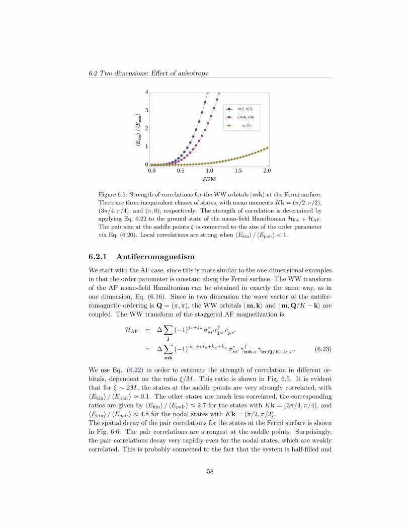
6.2 Two dimensions: Effect of anisotropy
ææææææææ
ææ
æ
æ
æ
æ
æ
æ
æ
æ
æ
æ æ
à à à à à à à à àà
àà
à
à
à
à
à
à
à
à
à
à
à
ììììììììììììììììììììììììììììììììììììììì
ì
0.0 0.5 1.0 1.5 2.00
1
2
3
4
Ξ2M
XEki
n\X
Epa
ir\
ì HΠ, 0L
à H3Π4, Π4L
æ HΠ2, Π2L
Figure 6.5: Strength of correlations for the WW orbitals |mk〉 at the Fermi surface.
There are three inequivalent classes of states, with mean momenta Kk = (π/2, π/2),
(3π/4, π/4), and (π, 0), respectively. The strength of correlation is determined by
applying Eq. 6.22 to the ground state of the mean-field Hamiltonian Hkin +HAF.
The pair size at the saddle points ξ is connected to the size of the order parameter
via Eq. (6.20). Local correlations are strong when 〈Ekin〉 / 〈Epair〉 < 1.
6.2.1 Antiferromagnetism
We start with the AF case, since this is more similar to the one-dimensional examples
in that the order parameter is constant along the Fermi surface. The WW transform
of the AF mean-field Hamiltonian can be obtained in exactly the same way, as in
one dimension, Eq. (6.16). Since in two dimension the wave vector of the antifer-
romagnetic ordering is Q = (π, π), the WW orbitals |m,k〉 and |m,Q/K − k〉 are
coupled. The WW transform of the staggered AF magnetization is
HAF = ∆∑
j
(−1)jx+jy σzss′c
†j,s cj,s′
= ∆∑
mk
(−1)mx+my+kx+ky σzss′ γ
†mk,s γm,Q/K−k,s′ . (6.23)
We use Eq. (6.22) in order to estimate the strength of correlation in different or-
bitals, dependent on the ratio ξ/M . This ratio is shown in Fig. 6.5. It is evident
that for ξ ∼ 2M , the states at the saddle points are very strongly correlated, with
〈Ekin〉 / 〈Epair〉 ≈ 0.1. The other states are much less correlated, the corresponding
ratios are given by 〈Ekin〉 / 〈Epair〉 ≈ 2.7 for the states with Kk = (3π/4, π/4), and
〈Ekin〉 / 〈Epair〉 ≈ 4.8 for the nodal states with Kk = (π/2, π/2).
The spatial decay of the pair correlations for the states at the Fermi surface is shown
in Fig. 6.6. The pair correlations are strongest at the saddle points. Surprisingly,
the pair correlations decay very rapidly even for the nodal states, which are weakly
correlated. This is probably connected to the fact that the system is half-filled and
58
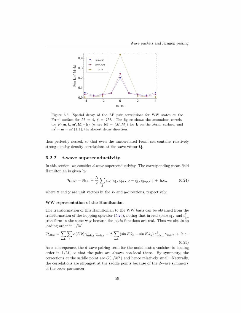
Wave packets and fermion pairing
æ
ææ
æ
æ
ææ
æ
æ
à
àà
à
à
à
àà
à
ìì
ì
ìì
-4 -2 0 2 40.0
0.1
0.2
0.3
0.4
m-m'
FHm
k,m
'M-
kLì HΠ, 0L
à H3Π4, Π4L
æ HΠ2, Π2L
Figure 6.6: Spatial decay of the AF pair correlations for WW states at the
Fermi surface for M = 4, ξ = 2M . The figure shows the anomalous correla-
tor F (m,k,m′,M− k) (where M = (M,M)) for k on the Fermi surface, and
m′ = m = m′ (1, 1), the slowest decay direction.
thus perfectly nested, so that even the uncorrelated Fermi sea contains relatively
strong density-density correlations at the wave vector Q.
6.2.2 d-wave superconductivity
In this section, we consider d-wave superconductivity. The corresponding mean-field
Hamiltonian is given by
HdSC = Hkin +∆
2
∑
j
εss′ [cj,s cj+x,s′ − cj,s cj+y,s′ ] + h.c., (6.24)
where x and y are unit vectors in the x- and y-directions, respectively.
WW representation of the Hamiltonian
The transformation of this Hamiltonian to the WW basis can be obtained from the
transformation of the hopping operator (5.26), noting that in real space cj,s and c†j,stransform in the same way because the basis functions are real. Thus we obtain to
leading order in 1/M
HdSC =∑
mk
∑
s
ε (Kk) γ†mk,s γmk,s + ∆∑
mk
(sinKkx − sinKky) γ†mk,↓ γmk,↑ + h.c..
(6.25)
As a consequence, the d-wave pairing term for the nodal states vanishes to leading
order in 1/M , so that the pairs are always non-local there. By symmetry, the
corrections at the saddle point are O(1/M2) and hence relatively small. Naturally,
the correlations are strongest at the saddle points because of the d-wave symmetry
of the order parameter.
59
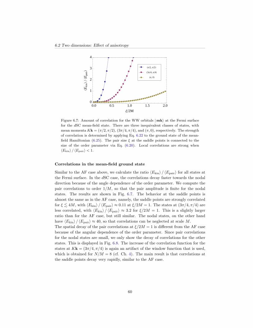
6.2 Two dimensions: Effect of anisotropy
æææ
æ
æ
æ
æ
æ
ææ æ
à à à à à à à àà
àà
à
à
à
à
à
à
à
à
à
à
à
ììììììììììììììììììììììììììììììììììììììì
ì
0.0 0.5 1.0 1.5 2.00
1
2
3
4
Ξ2M
XEki
n\X
Epa
ir\
ì HΠ, 0L
à H3Π4, Π4L
æ HΠ2, Π2L
Figure 6.7: Amount of correlation for the WW orbitals |mk〉 at the Fermi surface
for the dSC mean-field state. There are three inequivalent classes of states, with
mean momenta Kk = (π/2, π/2), (3π/4, π/4), and (π, 0), respectively. The strength
of correlation is determined by applying Eq. 6.22 to the ground state of the mean-
field Hamiltonian (6.25). The pair size ξ at the saddle points is connected to the
size of the order parameter via Eq. (6.20). Local correlations are strong when
〈Ekin〉 / 〈Epair〉 < 1.
Correlations in the mean-field ground state
Similar to the AF case above, we calculate the ratio 〈Ekin〉 / 〈Epair〉 for all states at
the Fermi surface. In the dSC case, the correlations decay faster towards the nodal
direction because of the angle dependence of the order parameter. We compute the
pair correlations to order 1/M , so that the pair amplitude is finite for the nodal
states. The results are shown in Fig. 6.7. The behavior at the saddle points is
almost the same as in the AF case, namely, the saddle points are strongly correlated
for ξ . 4M , with 〈Ekin〉 / 〈Epair〉 ≈ 0.11 at ξ/2M = 1. The states at (3π/4, π/4) are
less correlated, with 〈Ekin〉 / 〈Epair〉 ≈ 3.2 for ξ/2M = 1. This is a slightly larger
ratio than for the AF case, but still similar. The nodal states, on the other hand
have 〈Ekin〉 / 〈Epair〉 ≈ 40, so that correlations can be neglected at scale M .
The spatial decay of the pair correlations at ξ/2M = 1 is different from the AF case
because of the angular dependence of the order parameter. Since pair correlations
for the nodal states are small, we only show the decay of correlations for the other
states. This is displayed in Fig. 6.8. The increase of the correlation function for the
states at Kk = (3π/4, π/4) is again an artifact of the window function that is used,
which is obtained for N/M = 8 (cf. Ch. 4). The main result is that correlations at
the saddle points decay very rapidly, similar to the AF case.
60

Wave packets and fermion pairing
æ
ææ
æ
æ
ææ
æ
æ
àà
à
àà
-2 -1 0 1 20.0
0.1
0.2
0.3
0.4
m-m'
FHm
k,m
'kL à HΠ, 0L
æ H3Π4, Π4L
Figure 6.8: Spatial decay of the dSC pair correlations for WW states at the
Fermi surface for M = 4, ξ = 2M . The figure shows the anomalous correlator
F (m,k,m′Q/K − k) for k on the Fermi surface, and m′ = m = m′ (1, 1), the
slowest decay direction.
6.3 Conclusions
In this chapter we have used the WW basis states in order to analyze the correlations
of AF and dSC mean-field states in one and two dimensions. We found that the ratio
ξ/M of the (particle-hole or particle-particle) pair size to the size of the wave packets
that define the WW basis controls a crossover between locally almost uncorrelated
fermions for ξ M and tightly bound fermions for ξ M . Even though this result
is based on simple mean-field Hamiltonians, it is reasonable to expect that locally
the physics is similar at scale M independently of the behavior at larger scales. This
insight will be used in the following sections to analyze strong coupling fixed points of
the renormalization group in one and two dimensions. The key idea from this section
is that if the wave packet size M is chosen appropriately, the fermions can be replaced
by effective bosonic degrees of freedom corresponding to the paired fermions. The
interactions between the new degrees of freedom determine the physical behavior at
larger distances and low energies.
In two dimensions, we have seen that even in simple mean-field states the physics
involves multiple length scales when the Fermi velocity is strongly anisotropic. In
particular, when the Fermi surface lies in the vicinity of the saddle points, the wave
packets there are easily localized and bound into pairs. On the other hand, states in
the nodal direction remain essentially uncorrelated at the same length scale. This
separation of length scales forms the basis of the treatment of the saddle point regime
of the two-dimensional Hubbard model in Ch. 9.
61

6.3 Conclusions
62

Chapter 7
Wave packets and the
renormalization group
In the last chapter we have discussed the manifestation of fermion pairing in the WW
basis for simple mean-field Hamiltonians. The type of pairing and its associated
length scale ξ have been put in by hand. It is clear, however, that microscopic
Hamiltonians rarely are of the mean-field variety, instead it is a complex task by itself
to obtain an effective Hamiltonian that eventually leads to pair formation (or more
complicated orderings) from the microscopic interactions. For weak to moderate
initial interactions, the renormalization group is one of the standard methods for
obtaining effective Hamiltonians for the low-energy degrees of freedom of a many-
fermion system from the microscopic interactions [26].
In this chapter we seek to establish the connection between the renormalization
group for interacting fermions and the WW basis. We begin in Sec. 7.1 by relating
the M -dependence of the wave packet transform of an operator to its naıve scaling
dimension. This serves to discuss the relevance of different operators for large M .
In Sec. 7.2 we introduce very briefly the method of continuous unitary transforma-
tions [54–56], a Hamiltonian formulation of the renormalization group, which avoids
certain problems connected with the cutoff in the renormalization group. Since this
topic is rather technical, we relegate the bulk of the material to App. C. Finally, in
Sec. 7.3 we discuss the implications of the geometry of the Brillouin zone and the
Fermi surface for the treatment of low-energy problems. In particular, we show that
in the proximity of the van Hove singularity, the problem can be simplified due to
a separation of scales. This is an ingredient to the treatment of the saddle point
regime of the Hubbard model in Ch. 9.
63
7.1 Scaling dimensions
7.1 Scaling dimensions
In the following we elaborate on the relation between the so-called naıve scaling di-
mension of operators in the RG approach [26] and the dependence of matrix elements
on the wave packet scale M in the wave packet transform of operators. In particular,
we will see that the latter is given by the scaling dimension of the operator under
consideration.
Scaling dimensions in the RG approach
The scaling dimension within the renormalization group arises as follows: In its orig-
inal formulation [26], each renormalization step consists in integrating out degrees of
freedom with energy Λ/s < E < Λ, where s is close to one. Afterwards, the cutoff Λ
is lowered to Λ/s, and all length scales are rescaled, such that in the new units the
cutoff is again Λ. All field operators are rescaled such that the kinetic energy part
remains unchanged, which allows to compare the relative growth of the interaction
part compared to the kinetic energy. In addition to the rescaling, perturbative cor-
rections arise from integrating out degrees of freedom, which completes the RG step.
The naıve scaling dimension of an operator is related to the rescaling of lengths,
and is thus obtained by omitting the perturbative renormalization. It measures the
importance of operators at low energies. An operator that becomes asymptotically
more important than the kinetic energy is called relevant, it is called marginal if it
scales in the same way as the kinetic energy, and irrelevant if it decreases at low
energies. We follow the discussion in [26] for the RG part.
For interacting fermion systems, the programme is implemented by imposing an
upper cutoff on all momentum space integrals as follows∫ddp→
∫ Λ/vF
−Λ/vF
dp⊥
∫dd−1p‖, (7.1)
where p⊥ measures the distance to the Fermi surface, p⊥ = |p| − pF with the Fermi
momentum pF . vF is the Fermi velocity which is assumed to be constant. The
remaining integral∫dd−1p‖ runs over fixed energy shells, with energy vF p⊥. The
action of spinless free fermions in the vicinity of the Fermi surface (i.e. with cutoff
Λ vF pF ) is then given by
S =
∫dω
∫ Λ/vF
−Λ/vF
dp⊥
∫dd−1p‖ψ (ω,p)
[− iω + vF p⊥
]ψ (ω,p) . (7.2)
This action is a fixed point of the RG transformation Λ → Λ/s when ω, p⊥, and
ψ (ω,p) are rescaled as
ω → ω/s
p⊥ → p⊥/s
ψ (ω,p) → s3/2ψ (ω,p) . (7.3)
64

Wave packets and the renormalization group
ψ (ω,p) is rescaled in the same way as ψ (ω,p). This definition of the rescaling
ensures that the kinetic energy part of the action remains invariant, so that the effect
of rescaling on other operators measures the change in their importance when the
cutoff is lowered. Relevant (irrelevant) operators are proportional to some positive
(negative) power of s after rescaling, whereas marginal ones are unchanged. On the
other hand, other types of operators are affected by the rescaling, for example one
may add a quadratic term ∝ p2⊥ to the kinetic energy. Under rescaling (omitting the
angular integrals over p‖ which do not play a role), this term changes as
∫dω
∫p⊥ ψ (ω,p) p2
⊥ψ (ω,p) →∫dω
s
∫dp⊥ss3/2ψ (ω,p)
(p⊥s
)2
s3/2ψ (ω,p)
=1
s
∫dω
∫dp⊥ ψ (ω,p) p2
⊥ψ (ω,p) , (7.4)
so that it decreases as the cutoff is lowered. It is clear that additional powers of p⊥make the decrease even faster. In a similar manner, one finds that interactions that
involve the full Fermi surface when evaluated at p⊥ = 0 are marginal, whereas all
others are irrelevant. Since it is quite lengthy to show this, we refer the reader to
[26]. Instead, we show how the scaling dimensions of operators follow directly from
their wave packet transform.
Scaling dimensions from wave packets
The dependence of the wave packet transform of an operator on M can be found
using the transformation rules from Ch. 5. Instead of reiterating them, we give
intuitive arguments why they are true in this section. We first consider the kinetic
energy, and consider its wave packet transform. We focus on k-conserving matrix
elements that involve wave packets with m′ = m + 1. Since the states are wave
packets with a mean momentum Kk, they move at the group velocity vg = ε′ (Kk).
The distance between two adjacent sites is M , hence we find for the wave packet
hopping rate
hopping rate ∼ group velocity
distance
∼ M−1. (7.5)
Rescaling the Hamiltonian by M , the leading part of the kinetic energy is hence
independent of M . Consequently, operators that decrease faster (slower) than 1/M
as M →∞ are irrelevant (relevant), and operators that scale like 1/M are marginal.
Expanding the kinetic energy to higher order around Kk leads to higher powers of p
that are integrated against the wave packets. Since the wave packets are narrow in
p-space, with a width ∼ 1/M , each additional power of p contributes an additional
power of 1/M , so that corrections to the leading term are less and less important as
M →∞.
65

7.1 Scaling dimensions
Scaling Dimensions
Π, 0
Π, Π0, Π
hopping rate =group velocity
distance
interaction strength ∝ density2 × volume
Recall from d = 1:
independent of dimension: t ∼ 1
M
BUT:
depends on dimension: u ∼ 1
Md
Need to sum over O(M) states to have marginal interactions
Interactions that involve full Fermi surface marginal, all
others irrelevant
O(M)
Saturday, October 1, 2011
Figure 7.1: WW basis states at the Fermi surface in two dimensions. There are
O(M) states at the Fermi surface in total.
For states at points of high symmetry in the Brillouin zone, the behavior is different.
Because of the symmetry, ε′ (Kk) vanishes, and the kinetic energy is O(1/M2).
Consequently, the kinetic energy at these points can be neglected compared to generic
points on the Fermi surface for large M .
The scaling of local (at scale M) interactions can be understood as follows: The
matrix element of a local interactions between two pairs of wave packet states is of
the form
interaction strength ∼ (density of wave packet)2
︸ ︷︷ ︸∼M−2d
× volume of wave packet︸ ︷︷ ︸∼Md
∼ M−d. (7.6)
Note that the interaction need only be local compared to the wave packet scale M
for the argument to hold, since all k-conserving matrix elements transform in the
same way, regardless of the momenta involved.
In order to link this result to the scaling dimensions from the RG approach, we
implement the cutoff by restricting the WW basis states to states that lie at the Fermi
surface. There is one such state per WW lattice site in one dimension, regardless of
M . Since the interaction matrix elements for this state scale like 1/M , the interaction
is marginal in one dimension. The matrix elements in two dimensions scale like
M−2 and may thus appear to be irrelevant. However, the number of states at the
Fermi surface scales linearly with M , since the Fermi surface has a fixed length in
66
Wave packets and the renormalization group
momentum space, cf. Fig. 7.1. Thus each state can couple to M other states, and
interaction terms that involve a finite fraction of the states at the Fermi surface
(i.e. with all four momenta at the Fermi surface) scale like 1/M instead. In the
same manner as for the kinetic energy, when the interaction is not local but contains
additional powers of p, each power of p contributes an additional power of 1/M in
the wave packet transform, so that for large enough M interactions can be assumed
to be local to high accuracy.
The argument that interactions have to couple many states at the Fermi surface
is not new, and has been used by various investigators to facilitate the analysis
of weakly coupled fermion systems by means of a 1/N -expansion, where N is the
number of states at the Fermi surface with discretized angles [26–30].
It should be noted, that for the states at the saddle points (or other points of high
symmetry) the interaction in two dimensions always scales in the same way as the
hopping terms. This suggests that when the Fermi surface touches the saddle points,
the states there may become strongly coupled even when they are not coupled to
the rest of the Fermi surface.
7.2 One-loop RG via continuous unitary transfor-
mations
In this section we introduce the continuous unitary transformations (CUT) [54–
56], which are the Hamiltonian equivalent of the action-based RG flow equations
[10, 26]. Whereas the RG is based on integrating out degrees of freedom, and thus
decreases the number of the degrees of freedom in the system, the CUT method
merely decouples states with different kinetic energies, so that the number of degrees
of freedom stays the same. The decoupling is achieved by a sequence of infinitesimal
canonical transformations that is applied to the Hamiltonian of the system. We
denote the generator of the infinitesimal transformation by η (B), where B is the
flow parameter related to the renormalization scale. The flowing Hamiltonian H (B)
obeys the equationd
dBH (B) = [η (B) ,H (B)] , (7.7)
which is just the first order expansion of the unitary transformation e−η(B)Heη(B).
In principle, the flow equation is exact, but in practice one has to resort to approx-
imations. In App. C we show that for a suitable generator η(B), the flow equation
(7.7) leads to a set of coupled flow equations for a set of auxiliary coupling constants
F (p1, · · · ,p4). These flow equations are structurally very similar to the usual RG
equations when the frequency dependence is neglected. The major difference to the
RG equations is that there is no cutoff. Instead, the physical coupling constants
67

7.3 The geometry of the low-energy states in the Brillouin zone
U (p1, · · · ,p4) are obtained from the auxiliary ones via
U (p1, · · · ,p4) = e−[ε(p1)+ε(p2)−ε(p3)−ε(p4)]2/16Λ2
F (p1, · · · ,p4) , (7.8)
where Λ is the RG energy scale. The exponential on the right hand side contains
the kinetic energy differences of the initial and final states of an interaction matrix
elements. As a consequence, states with kinetic energy larger than Λ decouple from
the low energy states and can be neglected when |ε| Λ. The advantage of this
scheme within the wave packet approach is that the wave packet states may lie
partially below and partially above the cutoff. In the RG scheme it is difficult
to obtain an effective Hamiltonian in this situation, whereas in the CUT method,
Eq. 7.8 gives a simple rule for all cases. Since the CUT flow equations in the one-
loop approximations are essentially equivalent to the RG one-loop equations, we do
not discuss them any further. The only CUT related equation that is needed in the
remainder of this work is Eq. 7.8.
More details can be found in App. C and many more in the book by Kehrein [57].
7.3 The geometry of the low-energy states in the
Brillouin zone
In this section we discuss the influence of the shape of the low-energy phase space
on the low-energy physics of the Hubbard model in two dimensions. In particular,
we look at the influence of strong anisotropy in the Fermi velocities along the Fermi
surface. The most extreme case of anisotropy is realized when the Fermi surface
touches the saddle points, where the van Hove singularity in the density of states
manifests itself through a vanishing Fermi velocity at the saddle points. We will
show that in this case, slow and fast parts of the Fermi system at a fixed energy
scale Λ live on different length scales, which leads to an approximate decoupling of
these two kinds of states.
van Hove singularities
The influence of the latter can be seen in Fig. 7.2, which shows the tube of states
with energy |ε| < Λ for Λ = 0.1t. In the case of a generic Fermi surface, the Fermi
velocity is approximately constant along the Fermi surface. Since the energy close to
the Fermi surface is ε ∼ vF p⊥, the tube has width ∆p ∼ 2ε/vF everywhere. On the
other hand, when the Fermi surface is in the vicinity of the saddle points, the Fermi
velocity becomes strongly anisotropic (and vanishes at the saddle points). In the
vicinity of the saddle points the width of the tube is asymptotically ∆p ∼ 2√
Λ/t.
We will be mainly interested in the latter case in the following. Due to the large
anisotropy of the Fermi velocity, there is no unique length scale associated to the
problem, so that there exists no single wave packet size M that fits for all angles.
68
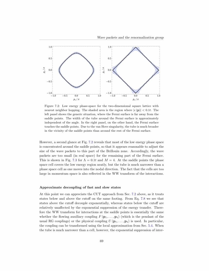
Wave packets and the renormalization group
-1.0 -0.5 0.0 0.5 1.0-1.0
-0.5
0.0
0.5
1.0
px Π
p y
Π
-1.0 -0.5 0.0 0.5 1.0-1.0
-0.5
0.0
0.5
1.0
px Π
p y
Π
Figure 7.2: Low energy phase-space for the two-dimensional square lattice with
nearest neighbor hopping. The shaded area is the region where |ε (p)| < 0.1t. The
left panel shows the generic situation, where the Fermi surface is far away from the
saddle points. The width of the tube around the Fermi surface is approximately
independent of the angle. In the right panel, on the other hand, the Fermi surface
touches the saddle points. Due to the van Hove singularity, the tube is much broader
in the vicinity of the saddle points than around the rest of the Fermi surface.
However, a second glance at Fig. 7.2 reveals that most of the low energy phase space
is concentrated around the saddle points, so that it appears reasonable to adjust the
size of the wave packets to this part of the Brillouin zone. Accordingly, the wave
packets are too small (in real space) for the remaining part of the Fermi surface.
This is shown in Fig. 7.3 for Λ = 0.1t and M = 4. At the saddle points the phase
space cell covers the low energy region neatly, but the tube is much narrower than a
phase space cell as one moves into the nodal direction. The fact that the cells are too
large in momentum space is also reflected in the WW transform of the interactions.
Approximate decoupling of fast and slow states
At this point we can appreciate the CUT approach from Sec. 7.2 above, as it treats
states below and above the cutoff on the same footing. From Eq. 7.8 we see that
states above the cutoff decouple exponentially, whereas states below the cutoff are
relatively unaffected by the exponential suppression of the energy transfer. There-
fore the WW transform for interactions at the saddle points is essentially the same
whether the flowing auxiliary coupling F (p1, . . . ,p4) (which is the pendant of the
usual RG couplings) or the physical coupling U (p1, . . . ,p4) is used. In particular,
the coupling can be transformed using the local approximation from Sec. 5.4. When
the tube is much narrower than a cell, however, the exponential suppression of inter-
69

7.3 The geometry of the low-energy states in the Brillouin zone
px
p y
-Π 0 Π
-Π
0Π
Figure 7.3: Low energy phase space for the two-dimensional square lattice with
nearest neighbor hopping at half-filling. Λ = 0.1t, the region with |ε| < Λ is shaded.
The phase space cells of the WW basis with M = 4 are also shown. At the saddle
points, the size π/4 of the cells matches the width of the low energy tube, but the
cells are too large for the remaining part of the Fermi surface.
70
Wave packets and the renormalization group
actions effectively restricts all the momentum space summations in the wave packet
transform to the area of the tube. As a rule of thumb, we have
interaction strength ∝ area in momentum space
area of BZ. (7.9)
Thus we expect the interactions in the nodal directions to decrease in the WW basis
representation when the tube is chosen too small. This expectation is born out, and
the decrease of the local interaction as a function of 2MπvF
Λ, which measures the size
mismatch between the tube and the cells, is shown in Fig. 7.4. The decrease of the
local effective interactions leads to a partial decoupling of the slow parts of the Fermi
surface from the fast parts, where slow and fast refer to the Fermi velocity compared
to Λ, i.e. a region is fast when vF > 2M/(πΛ) and slow otherwise. This effect is
increased because of the kinetic energy in the WW basis. The key observation is
that the RG flow does not enter the strong coupling regime for all parts of the Fermi
surface simultaneously. In particular, for the states at the saddle points the band
width in the WW basis is Wsp ≈ 8t/M2 ∼ Λ, where 8t is the full band width of the
model. The flow goes to strong coupling at the saddle points when the interaction
strength U ≈ Wsp ∼ Λ. In the nodal region, on the other hand, the band width is
Wnod ∼ 16t/M = 2MWsp. Thus, even for the relatively small value M = 4 we have
Wnod ≈ 8Wsp. As a consequence, the fast regions behave almost like non-interacting
fermions at scale M , and correlations involve very delocalized states only.
This separation of scales justifies to treat the region around the saddle point in
isolation when it becomes strongly coupled. The strong correlations imply that at
larger length scales this region should be modeled in terms of the low energy degrees
of freedom that emerge from the strongly correlated problem at scale M . The
coupling to the remaining states at larger length scales involves these new degrees of
freedom only. This route is pursued in Ch. 9 for the saddle point regime of the two-
dimensional Hubbard model. It should be emphasized that the decoupling of scales
does not rely on the fact that the Fermi surface touches the saddle points exactly.
Indeed, it is clear that for strong coupling problems at finite Λ, the width of the tube
with |ε| < Λ limits the sensitivity to the precise position of the Fermi surface. For
Λ = 0.1t, the width at the saddle points is π/4, so that the same reasoning should
hold when the Fermi surface is dislocated from the saddle points by less than about
half this distance.
Finally, it is noteworthy that the idea of a decoupling of fast and slow fermions
is not new. In fact, it is a well established effect for multi-band systems, where
the most celebrated example is probably the Kondo-lattice model of heavy fermion
systems [31, 32], where slow f -electrons are modeled as localized spins (i.e. effective
low-energy degrees of freedom), whereas the fast s-electrons are treated as non-
interacting. Another example that is more closely related to the problem here is
given by N -leg ladders at weak coupling, where a similar decoupling of slow and fast
bands has been observed within the renormalization group [33].
71

7.3 The geometry of the low-energy states in the Brillouin zone
0.0 0.5 1.0 1.5 2.00.0
0.2
0.4
0.6
0.8
1.0
2 M
ΠvF
L
U
Figure 7.4: Reduction of the local interaction due to size mismatch between low
energy tube and phase space cells. The local part of the wave packet transform is
shown as a function of 2MπvF
Λ. For 2MπvF
Λ < 1, the tube is narrower than the phase
space cell, and the exponential cutoff (7.8) reduces the interaction in the WW basis.
A window function with N/M = 8 is used. For very narrow tubes (Λ → 0), the
momentum resolution of this function is not sufficient to resolve the decreasing
width of the tube.
72

Chapter 8
Wave packets and effective
Hamiltonians in one
dimension
8.1 Introduction
In this chapter we apply the WW basis states to three strongly coupled fixed points
of RG flows for one dimensional systems: Chains with attractive interactions away
from half-filling (Sec. 8.4), chains with repulsive interactions at half-filling (Sec. 8.3),
and the two-leg ladder with repulsive interactions at half-filling (Sec. 8.5). The low-
energy phenomenology of these systems is very well understood (see e.g. [67, 68]),
so that we can compare the results obtained from the wave packet approach with
exact solutions that are obtained from bosonization and Bethe ansatz [67, 68]. We
do not aim at quantitative results, and merely seek to obtain qualitative features of
the low-energy physics. The main concern in this respect is the distinction between
algebraic decays and exponential decays of correlation functions. Since the WW basis
breaks the translational invariance of the system, it is not obvious that power-law
correlations can be obtained at all.
The qualitative nature of the study is reflected in the approximations used: Through-
out, we discard all basis states except the ones at the Fermi points, with k = pF /K,
where pF is the Fermi momentum. We use the fixed point Hamiltonians obtained
from one-loop RG for the interaction, and expand around the strong coupling limit.
Somewhat surprisingly, we recover the nature of the dominant correlations in the
ground state in all three cases, despite the simplicity of the approximations.
More explicitly, we will see that within the WW approach, the long range physics at
the strong coupling fixed points is to a large extent determined by the structure of
73

8.2 Renormalization group and wave packets for chains
Figure 8.1: Scattering processes corresponding to the four coupling constants
u1, . . . , u4.
the local (at scale M) Hilbert space and its ground state degeneracy. This motive is
picked up in the study of the two-dimensional Hubbard model in the next chapter.
8.2 Renormalization group and wave packets for
chains
In this section we briefly review the one-loop renormalization group equations for the
one-dimensional Hubbard model at weak coupling (see e.g. [67]). Based on the weak
coupling assumption we take into account only interaction terms that are allowed
in the vicinity of the Fermi points. Momentum conservation can then be used to
parametrize the interaction in terms of four coupling constants u1, . . . , u4 following
the so-called g-ology scheme [67].
Low energy Hamiltonian in momentum space
We begin with the interaction part of the Hamiltonian, and introduce the current
operators
Jα,α′ (p′, p′) =
∑
s
c†αpF+p,s cα′pF+p′ . (8.1)
The indices α, α′ label right- and left-movers and take the values α = ±1. Note that
this use of α coincides with the one in the definition of the WW basis functions,
Ch. 4.
In the spirit of the renormalization group we assume that the interaction does not
depend on the momenta relative to the Fermi points, i.e. we set
Hint =∑
α1···α4
U (α1pF , . . . , α4pF ) δα1pF+α2pF ,α3pF+α4pF ,
× 1
N
∑
p1···p4δp1+p2,p3+p4 Jα1α2
(p1, p2) Jα3α4(p3, p4) , (8.2)
where U (p1, . . . , p4) is the interaction in momentum representation. Note that this
approximation is analogous to the local approximation in the wave packet transfor-
mation introduced in Ch. 5. Momentum conservation restricts the values of the αi,
74
Wave packets and effective Hamiltonians in one dimension
so that one can parametrize
U (α1pF , . . . , α4pF ) = u1 δα1,−α3δα2,−α4
δα1,−α2
+ u2 δα1,α3δα2,α4δα1,−α2
+u3
2δα1,−α3
δα2,−α4δα1,α2
+u4
2δα1,−α3δα2,−α4δα1,α2 . (8.3)
Note that u3 is present at half-filling only, when umklapp scattering is allowed at low
energies because of pF = π/2. The coupling u4 will be neglected in the following,
since it does not influence the flow to strong coupling.
The prefactors in (8.3) are chosen such that for the case of an onsite interaction U
the coupling constants have the value
ui = U, (8.4)
which is used as initial condition for the renormalization group.
The kinetic energy can be linearized around the Fermi points at weak coupling and
is given by
Hkin =2πvFN
∑
p
∑
α
αp Jαα (p, p) . (8.5)
Renormalization group equations and their fixed points
The one-loop RG equations for the coupling constants ui are given by [49, 50]:
u1 = − 1
πvFu2
1
u2 = − 1
2πvF
(u2
1 − u23
)
u3 = − 1
2πvF(u1 − 2u2)u3, (8.6)
where the dot is shorthand for the logarithmic scale derivative dds = − 1
ΛddΛ , so that
s = e−Λ/W . Λ is the renormalization scale, and W is the initial bandwidth. We will
be interested in two cases, both involving finite scale singularities. The first one is
the half-filled repulsive Hubbard model, for which the strong coupling fixed-point of
(8.6) is given by
2u2 = u3 = uAF > 0
u1 = 0. (8.7)
This fixed point is characterized by a diverging staggered spin-susceptibility.
75

8.2 Renormalization group and wave packets for chainsSimplest approximation
1.0 0.5 0.0 0.5 1.01.0
0.5
0.0
0.5
1.0
p Π
Ε p
coupling regime, which makes it impossible to continue the flow because it is basedon the perturbative expansion around the non-interacting groundstate. In orderto arrive at an effective description of the low-energy behavior, we switch to theWilson basis. Because of the exponential localization of the basis functions in realspace, the interactions are short-ranged in this basis. Hence we aim to find newlocal degrees of freedom that are not strongly interacting by solving a local (inreal space) problem. Subsequently, we derive an effective Hamiltonian for the newdegrees of freedom by means of contractor renormalization [2, 3].
Because of the high-energy cutoff in the renormalized couplings, the expansioninto the Wilson basis can be restricted to contain only states that are close to theFermi level. Clearly, the introduction of the new length scale M - the size of half aunit cell of the Wilson basis - may lead to artifacts, so care has to be taken how totruncate the expansion in momentum space. In the next section we will show howto perform truncations that conserve salient features of the original Hamiltonianfor the simplest truncation where only one value of k is kept. The extension tomore values of k is straightforward and will be the subject of future work.
5.1 Simplest truncation scheme: Single k-point
We stop the RG flow at the scale Λ where the renormalized interaction exceeds thebandwidth, because this is the transition line between weak coupling and strongcoupling regimes, and one expects a transition from free to confined fermions at thisscale. We choose M such that the reduced bandwidth πvF
Mequals the bandwidth
below the cutoff, πvF
M= 2Λ.
We restrict our attention to the case that the Fermi momentum is given by pF =πM
kF for some kF , and truncate the expansion for left- and right-movers in thefollowing way:
Rp ≈ 1√2
m
γm,kFe−iφm gm,0(p) (50)
Lp ≈ 1√2
m
γm,kFeiφm gm,0(p), (51)
where we have used pF = πM
kF to remove the Fermi momentum from the windowfunction gm,±kF
, and have eliminated a global phase in the phase factors iφm+kF
that occurs when kF is odd by replacing φm+kF→ φm. In this truncated expansion,
there are two states per WW unit cell, corresponding to the two Fermi points.These states are centered around the momenta ±π
2. When the system is half filled,
there are two fermions per WW unit cell in the states at the Fermi points.
25
Truncated WW expansion
The transformation for c†j is identical because the ψmk(j) are real. Now we turn
to momentum space, where the transformation is given by the Fourier transformψmk(p) of ψmk(j):
cp =
mk
ψmk(p)γmk
c†p =
mk
ψmk(p)∗ γ†mk. (8)
However, it will turn out to be convenient to use (3) and express the transformationin terms of the fourier transform of the shifted window function gmk(p). Thetransformation then becomes
cp =1√2
mk
e−iφm+k gmk(p) + eiφm+k gm,−k(p)
γmk
=
mk
γmk1√2
µ=±1
e−iµφm+k gm,µk(p). (9)
In the formula for c†p, one obtains the complex conjugate of (9). One reason why
the shifted window functions (and their fourier transform) are useful is that theylead to universal expressions for the transformation of operators, in the sense thattransformation formulas are independent of the values of the labels m and k, anddepend on differences of mean position label m and mean momentum label k only.In order to expose this simplicity, we will frequently express the shifted windowfunction gm,k(p) in terms of the unshifted function g0,0(p). The relation betweenthe two is
gm,k(p) = gm,0
p − π
Mk
= e−iMm(p− πM
k)g0,0
p − π
Mk
. (10)
Since we always use window functions such that g0,0(p) is real and symmetricaround p = 0, we obtain the further relation
g∗m,k(p) = eiMm(p− π
Mk)g0,0
p − π
Mk
= e−iMm(−p+ πM
k)g0,0
−p +
π
Mk
= gm,−k(−p) (11)
for the complex conjugate g∗m,k(p) of gm,k(p).
10
Whereas the gmk(j) are by themselves not a good basis for the lattice, we show -following refs. [8, 9] - that the functions
ψmk(j) =
gm,0(j) m even, k = 0gm,M(j) m even, k = M1√2(gm,k(j) + gm,−k(j)) 1 ≤ k < M, m + k even
−i√2(gm,k(j) − gm,−k(j)) 1 ≤ k < M, m + k odd
(3)
form an orthonormal basis for the single particle states when g(j) satisfies certainconditions to be derived below. First, we introduce a new notation which is moreconvenient for practical calculations:
ψm,k(j) =
gm,0(j) m even, k = 0gm,M(j) m even, k = M1√2
e−iφm+kgm,k(j) + eiφm+kgm,−k(j)
0 < k < M
, (4)
where
φa =
0 a evenπ2
a odd(5)
Apart from being orthonormalized, the functions ψm,k(j) have the useful propertyof exponential localization in both real space and (around two points in) momen-tum space when g(j) is chosen appropriately as detailed below.
Before we embark into the explicit construction of the Wilson-Wannier (WW)functions, we will investigate some general properties of the basis. The choice ofM in the factorization N = 2MK defines the length scale over which the basisfunctions are delocalized. The unit cell for the basis functions is 2M because ofthe phase factors e±iφm+k in (4) that are different on adjacent sites but identicalon second nearest neighbor sites. In fact, the principle of the construction is notto use the shifted window functions gmk(j) as basis functions, but to decomposethem into parity eigenstates, where the parity of a state is (−1)m+k (Note thatby the parity operation we mean reflection about the center of the wave packet,not about the origin). The states with k = 0 and k = M are already parityeigenstates, so that they appear only once per unit cell, for all other k there aretwo states per unit cell for even and odd parity (or k < 0 and k > 0). A schematicpicture of the basis function in one unit cell is shown in fig. 2. From N = 2MKone sees that there are K unit cells in total. Note that this figure is intended toshow how the states are rearranged in the new basis only, and that it does notreproduce the shape of the wave packets correctly. The real space form of the wavepackets within one unit cell is shown in fig. 3. The figure shows wave packets withm = 2, 3 and k = 1, 2. The parity of the states follows a checkerboard pattern inthe m − k-plane, where nearest neighbors always have opposite parity.
7
Low energy part mapped to chain
with Interactions from RG
fixed point
Sunday, October 2, 2011
Figure 8.2: The simplest wave packet approximation for chains: Only one WW
momentum k = pF /K is kept, the remainder is discarded. It is assumed that M is
chosen such that only this state lies below the cutoff (shaded region). WW basis
states are marked by red dots at momentum Kk, and drawn on top of the dispersion
of the chain.
The second one is the attractive Hubbard model away from half-filling (i.e. g3 = 0),
for which the fixed point couplings are
u1 = 2u2 = uSC < 0. (8.8)
This fixed point is characterized by diverging singlet pairing correlations.
The couplings uAF and uSC diverge at a critical scale Λc, that depends on the initial
interaction strength U and the full band width W . Here we are not interested in
the magnitude of this scale. It is sufficient to know that at some scale the couplings
exceed the band width below the cutoff, at which point the perturbative approach
breaks down.
In order to obtain a qualitative picture of the fixed point behavior, we assume in
the following that the couplings define the largest energy scale in the problem, and
investigate the strong coupling limit. This approach is similar to the semi-classical
approximation to the sine-Gordon problem that describes the low-energy physics of
one-dimensional chains in the bosonization method [67, 68]. In order to study the
fixed points, we need the WW representation of the fixed point Hamiltonian first.
The kinetic energy part has been discussed in Sec. 5.1, and will not be important in
what follows.
WW representation of Hint
Moreover, we will restrict the WW basis to states |mk〉 with k = pF /K ≡ kF ,
and assume that M is chosen such that only this state lies below the cutoff, as
indicated in Fig. 8.2. In order to investigate the properties of the fixed points, we
76
Wave packets and effective Hamiltonians in one dimension
first transform the fixed point interactions to the WW basis using the methods from
Sec. 5.3.2, in particular Eq. (5.30), which we restate here for convenience. Since we
set all the ki to pF /K, we suppress the WW momentum index k in the following.
Then Eq. (5.30) becomes
U (m1, . . . ,m4) =V (m1, . . . ,m4)
2
1
2
∑
α1···α4
U (α1pF , . . . , α4pF )
× e−i(α1φ1+α2φ2−α3φ3−α4φ4), (8.9)
where φi = φmi , and φa = π/2 (φa = 0) for a even (odd). The values of V (m1, . . . ,m4)
depend on the window function, the values we use are tabulated in Tab. 5.1.
Plugging the g-ology couplings (8.3) into the right hand side of (8.9), we observe
that the Kronecker deltas can be used to perform three of the four sums over the αi.
We evaluate the remaining sum for the u1 term (the other terms being similar) only,
and state the results for the other terms. We note that α1 = −α2 = −α3 = α4 = α,
and find1
2
∑
α
e−iα(φ1−φ2+φ3−φ4) = cos [φ1 + φ3 − φ2 − φ4] (8.10)
Now recall from Eq. (4.10) that φi can take on the values 0 (for m+k even) and π/2
(for m+ k odd) only. Then the cos vanishes when an odd number of operators acts
on an odd (i.e. m+k odd) WW orbital, since its argument is either π/2 or 3π/2. In
particular, terms of the form m1 = m2 = m3 = m4 ± 1 vanish, since there is always
an even number of odd ki (for k-conserving matrix elements). Since the interactions
decay rapidly with distance, the contribution from this type of interaction is thus
strongly suppressed in one dimension, and we neglect it in the following. Now we
turn to the type m1 = m2 6= m3 = m4. Focussing on nearest neighbor interactions
and setting all k = pF /K, we find that the cosine contributes ±1, depending on
which of the mi are even (odd). Thus there are no terms that vanish exactly in this
case. Finally, when all sites involved are even (odd), the cosine always evaluates to
1.
The general form of the Hamiltonian for the states at the Fermi points, ki = pF /K
can now be written down using similar considerations for the other parts of the
interaction. In order to simplify the notation, we define
J (m1,m2) ≡∑
s
γ†m1,pF /K,sγm2,pF /K,s
. (8.11)
77
8.3 Chain with repulsive interactions at half-filling
Then the WW Hamiltonian for the states at the Fermi points is given by
Hint
∣∣∣ki=pF /K
≈ 1
4M
∑
m
(u1 + u2 + u3/2 + u4/2) J (m,m) J (m,m) (8.12)
+1
8M
∑
〈m,m′〉
[(−u1 + u2 − u3/2 + u4/2) J (m,m) J (m′,m′)
+ (u1 − u2 − u3/2 + u4/2) J (m,m′) J (m′,m)
+ (u1 + u2 − u3/2− u4/2) J (m,m′) J (m,m′)]
(8.13)
where we have used the values of V (0, 0,m,m) from Tab. 5.1. The WW transforms
of the fixed point couplings can be obtained in a straightforward manner from (8.13).
This is used in the following two sections to analyze the two fixed points above.
8.3 Chain with repulsive interactions at half-filling
In this section we discuss the fixed point 2u2 = u3 = uAF > 0 for the half-filled
chain with repulsive interactions. We use Eq. (8.13) in order to obtain the WW
representation of the interaction. We proceed by diagonalizing the local part of the
Hamiltonian, and find that charge degrees of freedom are gapped, so that locally
only the spin degree of freedom survives. As a consequence, the ground state of the
local interaction Hamiltonian has two-fold degeneracy per site, corresponding to the
two possible spin states. In the next step, we show that the non-local part of the
interaction is of the Heisenberg form, so that it leaves the local low-energy subspace
invariant. The Heisenberg model can be solved using the Bethe ansatz [67], so that
the asymptotic form of the spin-spin correlation functions can be obtained. The
correlation functions of the effective model in the WW basis are then transformed
back to momentum space, revealing a power-law form of the spin-spin correlation
function for momenta close to p = 0 and p = π. This result is in qualitative
agreement with the bosonization solution of the chain problem [67, 68].
Fixed point interaction in WW representation
The fixed point interaction can be transformed to the WW basis by plugging 2u2 =
u3 = uAF into (8.9). The result is
HAF =1
4MuAF
∑
m
J (m,m) J (m,m)
︸ ︷︷ ︸local interaction
− 1
4MuAF
∑
m
J (m,m+ 1) J (m+ 1,m)
︸ ︷︷ ︸nearest neighbor interaction
.
(8.14)
Using the identity3∑
i=1
σiab σicd =
1
2δad δbc −
1
4δab δcd (8.15)
78

Wave packets and effective Hamiltonians in one dimension
the non-local part of the interaction can be rewritten as
−∑
m
J (m,m+ 1) J (m+ 1,m) = 2∑
m
S (m) · S (m+ 1) +1
2n (m) n (m+ 1) ,
(8.16)
where the Si (m) and n (m) are spin and charge operators at site m, respectively.
Similarly, the local part can be rewritten as
Hloc =1
4MuAF
∑
m
J (m,m) J (m,m) =1
4MuAF
∑
m
n (m) n (m) . (8.17)
Local Hilbert space and effective spin model
In order to arrive at suitable low-energy degrees of freedom, we investigate the local
part (8.17) of the interaction first. The local Hilbert space consists of the four states
| 0〉, | ↑〉, | ↓〉, and | ↑↓〉. Since the wave packets lie at the Fermi surface, there is one
fermion per site, and after adjusting the chemical potential accordingly, the energies
of the four states are
Hloc | ↑〉 = 0
Hloc | ↓〉 = 0
Hloc | 0〉 =1
4MuAF | 0〉
Hloc | ↑↓〉 =1
4MuAF | ↑↓〉 . (8.18)
Hence the low energy sector of the local Hamiltonian consists of the two states
| ↑〉 , | ↓〉. Since these states are degenerate, the effective Hamiltonian to leading
order is found by simply projecting each WW site down to the spin sector.
The action of the non-local interactions in the spin sector can be inferred from (8.16).
The charge operators n (m) have no effect on the spin sector. Therefore we are left
with the nearest-neighbor spin-spin interactions. Hence we arrive at the effective
Hamiltonian
Heff = J∑
m
S (m) · S (m+ 1) , (8.19)
where J = 12M uAF > 0. The effective model is simply an antiferromagnetic S − 1/2
Heisenberg model.
Asymptotic spin-spin correlation function
The properties of the Heisenberg model in one dimension are well known, and the
spin-spin correlation function has been derived using the Bethe ansatz [51, 67]:
⟨S (m) · S (m′)
⟩= C1
1
(m−m′)2 + C2 (−1)m−m′ 1
|m−m′| , (8.20)
79

8.3 Chain with repulsive interactions at half-filling
0.0 0.2 0.4 0.6 0.8 1.0
q
Π
Ω
Figure 8.3: Schematic spectral weight of spin-density excitations of the repulsive
Hubbard model at half-filling. Low energy excitations exist at q ≈ 0 and q ≈ π.
The spin-density excitations in the truncated WW basis are confined to the encircled
regions when transformed back into momentum space. At the points q = 0, π the
correspondence is exact (cf. (8.21)), but for general momenta excitations around
q = 0 and q = π are mixed because translational invariance is broken.
where the Ci are constants. It follows that there are soft excitations at the points 0
and π of the Brillouin zone of the superlattice defined by the WW basis states.
Now we transform this correlator back to momentum space in order to see what
these results mean. We denote the momentum representation of the spin density by
s (q), where q is the momentum transfer. Since the WW basis states are localized in
momentum space around ±π/2, the momentum transfer q of two-fermion operators
such as the Si (m) is restricted to the vicinity of the two points q = 0 and q = π,
as indicated in Fig. 8.3. In Ch. 6 we have found that the staggered magnetization
si (q = π) is given by
si (q = π) =∑
j
(−1)jσiss′c
†j,s cj,s′
=∑
mk
(−1)m+k
σiss′γ†mk,s γm,M−k,s′
≈∑
m
(−1)mσiss′γ
†m,M/2,s, γm,M/2,s′
=∑
m
(−1)mSi (m) , (8.21)
in the WW basis. Therefore the power law in the staggered magnetization in the WW
basis corresponds to the same power law in the staggered magnetization in real space.
A similar line of reasoning for the uniform spin-density, si (q = 0) shows that in the
same manner the uniform spin density in the WW basis corresponds to the uniform
spin density in the original lattice. The momenta that lie far away from the center
80
Wave packets and effective Hamiltonians in one dimension
and boundary of the Brillouin zone of the WW basis are in general superpositions
of momenta close to 0 and π, reflecting the broken translational invariance.
In summary, the asymptotic behavior of the spin-spin correlation function in the real
space lattice inferred from the effective model is the same as in eq. (8.20), withm−m′replaced by j−j′. The wave velocity of excitations has to be rescaled because the unit
cell is larger in the WW basis by a factor of M . We conclude that our approximation
produces algebraically spin-density correlations round q = 0 and q = π, and gaps
for all charged excitations in agreement with bosonization treatments. However, the
exponents of the power law decays, which are influenced by the Luttinger liquid
physics are not recovered. This is not surprising given that the Luttinger liquid
physics has its origins in the asymptotically linear fermion dispersion [52], a feature
that is hard to conserve in a cluster approximation (not to mention that the Fermi
velocity appears nowhere in the present treatment). Nevertheless, we emphasize
that the qualitative features of the model including algebraic decays are recovered,
which is in our view a non-trivial result, in particular when taking into account the
simplicity of the approximation.
8.4 Chain with attractive interactions
Now we consider the fixed point for attractive interactions at arbitrary filling, char-
acterized by u1 = 2u2 = −uSC < 0. We follow the same step as in Sec. 8.3 above.
First we obtain the WW representation of the interaction Hamiltonian. We analyze
the local part of the interaction and find that the low energy sector contains only
singlet pairs of fermions. Then we map the projected Hamiltonian to a spin problem
and deduce the asymptotic correlation function from the Bethe ansatz solution.
Fixed point interaction in WW representation
The WW transform of the interaction Hamiltonian is again obtained using (8.13).
The local part is given by
Hloc = − 3
4MuSC
∑
m
J (m,m) J (m,m)
= − 3
4MuSC
∑
m
n (m) n (m) . (8.22)
For the non-local part, we introduce the additional pair annihilation operators
∆ (m) = γm,pF /K,↓ γm,pF /K,↑ (8.23)
and their hermitian conjugates Ơ (m). In terms of the spin-, charge- and pair-
81
8.4 Chain with attractive interactions
operators the non-local interactions are given by
Hn.n. =3
4MuSC
∑
m
[− ∆† (m) ∆ (m+ 1)− ∆ (m) ∆† (m+ 1)
+1
2n (m) n (m+ 1) + S (m) · S (m+ 1)
](8.24)
Local Hilbert space and effective spin model
The analysis of the local Hilbert space and Hamiltonian is the same as in Sec. 8.3,
except that now the interactions are attractive, so that the low-energy states are | 0〉and | ↑↓〉. Again, the ground state is two-fold degenerate per site so that we obtain
the effective Hamiltonian by projection onto the degenerate subspace. The spin
operators in the second line of (8.24) do not contribute since in the low energy sector
all spins are bound into singlet pairs. In order to treat the remaining interactions
we note that the local low energy subspace can be mapped onto a spin system with
S = 1/2, similar to the repulsive chain above.
The mapping is accomplished by identifying
Sz (m) ≡ 1
2(n (m)− 1) (8.25)
S− (m) ≡ ∆ (m) . (8.26)
In terms of the spin operators, the projection of the interaction Hamiltonian to the
low energy subspace becomes
Heff =∑
m
[− J
2
(S+ (m) S− (m+ 1) + S− (m) S+ (m+ 1)
)
+ JSz(m) Sz (m+ 1)],
(8.27)
where J = 38M uSC. The effective Hamiltonian is hence an XXZ spin chain model.
Note that the sign of the first term can be reversed by a gauge transformation on
the spin states, e.g. | ↑〉 → − | ↑〉 on every second site without changing the model.
Consequently, we find that the effective model is again an antiferromagnetic S−1/2
Heisenberg model. Note however, that the emergent SU(2)-symmetry is due to the
approximation, and that in general the symmetry is U(1).
Asymptotic correlation functions
Since the effective Hamiltonian (8.27) is again of the Heisenberg type, we do not
need to discuss the asymptotic correlations in the WW basis, for the results we
refer to Eq. (8.20). Instead we discuss the meaning of the different correlators in
real space. In the same way as before, the uniform spin-densities in the WW basis
correspond to uniform spin-densities in real space. The staggered spin-density in the
82
Wave packets and effective Hamiltonians in one dimension
WW basis corresponds to spin-density in real space that oscillates with wave vector
pF (instead of π/2). Translating the spin operators back to the fermion operators
(using Eq. 8.26), we obtain that the charge density (corresponding to Sz) becomes
soft at the momenta q = 0 and q = 2pF . The pair correlations (corresponding to
S±) show algebraic decay for the same momenta.
Comparison with the solution from bosonization [67] shows that the slow decay of
pair correlations with momentum 2pF is an artifact of our approximation. The other
power laws are in qualitative agreement, however. For the same reasons as for the
repulsive chain, it is clear that the precise power laws connected to Luttinger liquid
physics can not be recovered.
8.5 Two-leg ladder at half-filling
In this section we discuss the low energy behavior of the SO(5) symmetric two-leg
ladder at half-filling. Since the Hubbard ladder has two legs, the diagonalization
of the hopping term leads to two bands. The bands will be labelled by indices like
a, b, c, . . . = 1, 2 in the following. There are four Fermi points in total which are
all equivalent in the sense that the Fermi velocity is the same (because of particle-
hole symmetry). Compared to the single chains considered so far, this opens up
the possibility of competition between different order parameters. Indeed, it is well
established that the Hubbard ladder has a Mott insulating ground state at half-
filling, regardless of the interaction strength. In this so-called d-Mott phase [53],
dSC and AF correlations are strong, but decay exponentially, and all excitations are
gapped. Remarkably, the single particle excitations at weak coupling are of the same
order of magnitude as the bosonic spin- and pair-excitations.
The renormalization group flow for the Hubbard ladder at half-filling has been de-
rived by Lin and Balents [53]. There it was also shown that the system generically
flows to strong coupling, and that the fixed point displays an enhanced SO(8) sym-
metry. The resulting low-energy Hamiltonian turns out to be exactly solvable, with
a so-called d-Mott ground state, which has gaps for all excitations. When the high-
energy Hamiltonian is SO(5) symmetric, the system retains this symmetry, which
shows up as a degeneracy of d-wave pair excitations and AF spin-excitations. Since
the interplay between superconductivity and antiferromagnetism is our main inter-
est, we focus on the SO(5) case.
The existence of more than one band poses no problems for the transformation to
the WW basis. Since the problem is weakly coupled, we transform each band to
the WW basis separately, and label all WW quantities by an additional band index.
The position of the WW states in the Brillouin zone is illustrated in Fig. 8.4. In the
following, we use the same approximations as before, namely, we truncate the WW
basis and keep only the states at the Fermi points. We use the fixed point couplings
of the RG to define the interaction Hamiltonian, and solve it in the strong coupling
83

8.5 Two-leg ladder at half-filling
-1.0 -0.5 0.0 0.5 1.0
-2
-1
0
1
2
p Π
ΕHp
L
Figure 8.4: The simplest wave packet approximation for the two-leg ladder. The
blue lines show the kinetic energy of the two bands as a function of p. The red
dots indicate the mean momenta and mean kinetic energy of the WW basis states.
Since there are two bands, there are two families of WW basis states as well. In the
simplest approximation to the low energy problem, we truncate the basis and keep
only states at the Fermi points.
limit.
We will see that within the WW basis, the presence of two bands leads to a local
problem with a non-degenerate ground state. This is to be contrasted with the
generic case of degenerate ground states for chains above. The ground state features
pronounced d-wave SC and AF correlations. The lowest excited states fall into two
classes: There are eight degenerate fermionic excitations, and five degenerate bosonic
excitations that correspond to the vector bosons above. Both types of excitations
have comparable gaps. We find that this situation is robust against the perturbation
by non-local interactions and fermion hopping, hence reproducing the exact solution
of this problem qualitatively.
Effective Hamiltonian
The SO(5) symmetry at low energies is realized in terms of local fermion bilinears
in the continuum limit. The Lie algebra is generated by 10 operators: The particle
number, the three spin operators and six so-called π-generators which create and
annihilate triplet pairs with total momentum (π, π). Because of the high symmetry
of the kinetic energy part of the Hamiltonian, all these operators commute with the
kinetic energy. The Lie algebra generators will not be important in the following,
so that we refer the interested reader to the review by Zhang [64]. In addition to
the generators, there are five bilinears that transform in the vector representation
of SO(5). In order to avoid amassing more indices than necessary, we omit position
labels, and write Ras and Las instead of cp±αpF ,a,s. With this notation, the vector
84
Wave packets and effective Hamiltonians in one dimension
operators are given by
∆x =1
2σzab εss′
(Ras Lbs′ +R†as′ L
†bs
)
∆y =i
2σzab εss′
(Ras Lbs′ −R
†as′ L
†bs
)
Ai = σxab σiss′
(R†as Lbs′ + L†asRbs′
). (8.28)
The effective interaction can be written in terms of these operators. Due to the
symmetry, it is convenient to introduce the vector B =(
∆x, ∆y, Ax, Ay, Az
).The
fixed-point interaction is given by [53]
Hint = −u∫dr B(r) · B(r) (8.29)
in the continuum limit, where u > 0. The operators Ai create AF spin-fluctuations
with momentum (π, π). Note that this involves a transition from one band to the
other. The operators ∆i create d-wave pair excitations with both fermions of a pair
in the same band, and a relative minus sign of the phase between the bands.
WW representation of the effective Hamiltonian
We now turn to the transformation of the interaction (8.29) to the WW basis. Sur-
prisingly, the transformation is simpler for the ladder than for the chain systems.
The reason is that the interaction is written as a scalar product of operators with
definite parity. In fact, all components of the vector B(r) are even under parity.
Since the parity of a bilinear is the product of the parity of its constituting fermions,
the fact that the parity of the WW basis states is opposite on neighboring sites can
be expected to lead to cancellations of terms in the WW transformation.
We show the highlights of the transformation for the dSC operators only, since the
AF operators behave essentially in the same way. We use the local approximation
as before, so that we only need the matrix elements U∆ (a1, α1, s1; . . . ; a4, α4 s4) at
the Fermi points:
U∆ (a1, α1, s1; . . . ; a4, α4, s4) = −u 1
4εTs1,s2εs3,s4︸ ︷︷ ︸spin singlet
δa1a2 δa3a4︸ ︷︷ ︸pair within one band
δα1,−α2 δα3,−α4︸ ︷︷ ︸pair momentum =0
,
(8.30)
where we have omitted the pF ’s on the left hand side. The important point is
that there are only two Kronecker deltas involving the αi, and that the first pair
of coordinates is indpendent of the second pair of coordinates, because the of the
factorization into bilinears. In the orthogonalization formula (8.9) the summation
85

8.5 Two-leg ladder at half-filling
over αi then leads to
U (m1, . . . ,m4) ∝ 1
4
∑
α1···α4
e−i(α1φ1+α2φ2−α3φ3−α4φ4)δα1,−α2δα3,−α4
=
[1
2
∑
α1
e−iα1(φ1−φ2)
]×[
1
2
∑
α2
e−iα2(φ3−φ4)
]
= cos [φ1 − φ2] cos [φ3 − φ4] . (8.31)
Recalling that φi = φmi at the Fermi points, we see that the contribution is finite for
m1 = m2 mod 2 and m3 = m4 mod 2. Since we keep nearest neighbor interactions
only, this leads to m1 = m2, m3 = m4. In the SC case this implies that interactions
involve local pairs only, which may interact locally or hop to the neighboring site.
The same conclusion holds for the operators Ai, which involve local particle-hole
pairs only.
In summary, the local Hamiltonian can be expressed conveniently in terms of the
operators
∆− (m) =1√2σzab γa,↓ γb↑
∆+ (m) =1√2σzab γ
†a,↑ γ
†b↓
Ai (m) = σxab σiss′ γ
†as γbs′ (8.32)
and the corresponding local SO(5) vector operator
B (m) =(
(∆−(m) + ∆+(m))/2, i(∆−(m)− ∆+(m))/2, Ax(m), Ay(m), Az(m)).
(8.33)
The interaction is given by
Hint = − 1
4Mu∑
m
(B(m) ·B(m) +
1
2B(m) ·B(m+ 1)
). (8.34)
As usually, the numerical prefactors depend on the choice of the window function.
Local Hilbert space and effective quantum rotor model
Following the same routine as before, we start by investigating the local Hilbert
space of the problem, focussing on the bosonic states. The ground state | 0〉 is
non-degenerate, and consists of one d-wave pair per site,
| 0〉 ≡∣∣∣∣↑↓0
⟩−∣∣∣∣
0
↑↓
⟩. (8.35)
86

Wave packets and effective Hamiltonians in one dimension
4 5 6 7 8 9 100.0
0.5
1.0
1.5
2.0
2.5
3.0
L
pair
gap
Figure 8.5: Finite size scaling of the gap for SO(5) vector excitations in the two-leg
ladder. The gap quickly converges due to its infinite system value.
In addition, there are five degenerate bosonic excited states that are obtained by
applying the components of the vector operator B to the ground state,
∣∣A+⟩
=
∣∣∣∣↑↑
⟩× 3,
∣∣∆+⟩
=
∣∣∣∣↑↓↑↓
⟩, and (8.36)
∣∣∆−⟩
=
∣∣∣∣0
0
⟩, (8.37)
where∣∣Ai⟩
= Ai | 0〉 etc. Finally, there are eight equivalent single fermion excita-
tions. The energies of these two types of excitations are are very close to each other.
In units of the WW basis coupling, they are given by
Efermion =15
4Eboson = 4. (8.38)
This situation is quite different from the behavior of the single chains, where the
bosonic (spin or pair) excitations are in the degenerate ground state manifold of the
local Hamiltonian, and thus far below the single particle spectrum. In the ladder
case, the bosonic and fermionic excitations are almost degenerate locally, and in fact
the bosonic excitations lie slightly above the fermionic ones.
Results
Since the ground state is non-degenerate, we may expect it to be of the RVB form
[17, 20], with strong but short ranged d-wave pairing and AF correlations. In order to
check the robustness of these findings with respect to non-local perturbations, we use
87
8.6 Conclusions
the CORE algorithm [36] to integrate out the fermionic degrees of freedom. A short
description of this algorithm can be found in App. D. The resulting bosonic model is
then diagonalized on a cluster. Results of finite size scaling of the bosonic gap and
the inferred value at infinite size are shown in Fig. 8.5. The gap remains practically
unchanged, and we conclude that the system is in a RVB state, in agreement with
the exact solution [53].
In addition to the results at half-filling, we can infer the behavior when the system is
doped away from half-filling. From the spectrum of the local Hamiltonian it follows
directly that doped holes (or electrons) are bound into pairs, since the pair binding
energy is of the same order as the single particle gap. As soon as hole pairs are
introduced, the ground state of the system is degenerate, and a low-energy model
is obtained by projecting the Hamiltonian onto the degenerate ground state. This
leads to a hardcore boson problem at small filling, with the number of bosons (i.e.
hole pairs) equal to δ/2, where δ denotes the doping level. We conclude that the
system turns into a superfluid with superfluid density ∝ δ.
8.6 Conclusions
In this section we have applied the simplest possible wave packet approximation to
a variety of one-dimensional systems. The approach consists of first applying the
renormalization group to the microscopic model to find possible fixed points of the
flow. The fixed point Hamiltonians are then solved in the strong coupling limit for
the set of WW basis states that lie at the Fermi surface. Due to the fact that the
WW basis states always involve at least nearest neighbor interactions, the resulting
effective Hamiltonians are non-trivial even when the kinetic energy is neglected.
A surprising amount of information about the nature of the ground state has been
shown to be present in the local interaction and the excitation spectrum of the local
problem in the WW basis. We have seen two radically different cases: For the chain
problems, the ’order parameter’ decouples from the fermionic degrees of freedom lo-
cally, in the sense that the corresponding bosonic excitations are ungapped, whereas
fermions have a gap. This kind of behavior is very much in line with the assumptions
made in deriving effective field theories for slow order parameter fields that separate
from the gapped fermions. For the ladder case, on the other hand, we have seen
that fermions and ’order parameter’ excitations exist on the same energy scale, due
to strong short ranged singlet correlations, leading to an RVB state that has very
little in common with the paradigm of effective theories for slow variables.
In the next chapter, we will apply a similar methodology to the two-dimensional
Hubbard model, where we will find a similar behavior at the saddle points.
In closing this chapter, we would like to explain briefly how the admittedly oversim-
plified approach presented here can be extended. Based on our findings of correla-
tions in mean-field states in Ch. 6, it is clear that it is inconsistent to use the strong
88

Wave packets and effective Hamiltonians in one dimension
coupling limit for states at the Fermi surface while neglecting states away from the
Fermi surface. The reason is that correlations of the neglected states are significant
when the coupling at the Fermi points is strong. A straightforward extension of the
approach considered here is two include more WW momenta, so that the transition
from weak-coupling RG to strong-coupling wave packet approach becomes smoother.
However, in the presentation here we have chosen simplicity over numerical accuracy,
and leave this exploration for future work.
89
8.6 Conclusions
90

Chapter 9
Saddle point regime of the
two-dimensional Hubbard
model
9.1 Introduction
In this chapter we apply the methodology developed in the previous chapter to the
two-dimensional Hubbard model at moderate coupling. We focus on the so-called
saddle point regime, where the Fermi surface lies in the vicinity of the saddle points
(π, 0) and (0, π). As discussed in Ch. 3, earlier RG studies [58, 66] in this regime have
shown that both d-wave pairing (dSC) and antiferromagnetic (AF) correlations are
strong in this region of the phase diagram, and especially the exact diagonalization
study by Lauchli et al. [12] points to the possibility that an insulating RVB is realized
in the vicinity of the saddle points, which would lead to a natural explanation for
the truncated Fermi surface of the cuprate superconductors [18, 20] that does not
rely on symmetry breaking. This type of scenario requires a ’phase separation in
the Brillouin zone’, in that electrons at the saddle points are localized on relatively
short length scales, whereas the electrons in the nodal directions are delocalized over
large distances.
In Ch. 6 we have seen that the corresponding separation of length scales naturally
appears even at the mean-field level in the saddle point regime due to the vastly
different Fermi velocities in the nodal and anti-nodal directions. Relatedly, we have
shown in Ch. 7 that in this situation RG flows to strong coupling lead to a strongly
correlated problem at the saddle points, whereas the faster states in the nodal di-
rections behave almost like free particles at the same length scale (at moderate
coupling). As a consequence, the slow states decouple from the fast states, and may
91

9.2 The microscopic model and its renormalization group treatment
be bound into pairs at relatively small length scales more or less independently of
the what the fast states in the nodal direction do.
These findings in conjunction with the experimental phenomenology discussed in
Ch. 3 motivate us to apply the wave packet method to states in the vicinity of the
saddle points. Following the procedure we have already used for one-dimensional
systems, we first compute an effective Hamiltonian using the one-loop renormal-
ization group. Details of the implementation can be found in Sec. 9.2. In order to
monitor the flow of correlations at the saddle points, we compute the WW transform
of the flowing interaction vertex at each step, as discussed in Sec. 9.3. In partic-
ular, we compute the single particle gap from the local interactions, and stop the
flow when the gap exceeds the bandwidth of the wave packet states at the saddle
points. The analysis of this local problem is dealt with in Sec. 9.4. We find a striking
similarity between the local (in the WW basis) behavior of the saddle point states
and the low-energy problem for the two-leg ladder from Sec. 8.5. In particular, the
system has the same local ground state, and large gaps for all excitations when the
flow approaches the strong coupling region. In order to assess the stability of the
local ground state to the non-local couplings, we diagonalize the effective saddle
point Hamiltonian on a plaquette in Sec. 9.5. Depending on the parameters, we find
cooperon- and spin triplet-modes emerging below the single particle continuum. In
order to overcome the limitations of small clusters, we compute an effect model for
the d-wave pairs at the saddle points using the CORE algorithm [36] (see App. D),
and estimate the stability of the insulating RVB state against pair fluctuations with
a variational ansatz in Sec. 9.6. In this section we also discuss the general structure
of the low energy states and relate it to the phenomenological SO(5) theory proposed
by Zhang [64].
9.2 The microscopic model and its renormalization
group treatment
Model
We investigate the two-dimensional Hubbard model on a square lattice with nearest
and next-to-nearest neighbor hopping. The Hamiltonian is given by
H =∑
p
∑
s
ε (p) c†p,s cp +U
2N
∑
p1···p4
δ (p1 + p2 − p3 − p4) J (p1,p3) J (p2,p4) ,
(9.1)
where J (p,p′) =∑s c†p,s cp′,s. The kinetic energy part is given by
ε (p) = −2t (cos px + cos py) + 4t′ cos px cos py − µ. (9.2)
92

Saddle point regime of the two-dimensional Hubbard model
px
p y
-Π 0 Π
-Π
0Π
Figure 9.1: Discretization of the flowing vertex. The vertex is computed on a discrete
set of points that lie on a lattice with lattice constant 2π/16 in the Brillouin zone
(green dots). The shaded area contains all states with energy |ε (p) | < 0.1t for
t′ = 0.2t. WW phase space cells for M = 4 are also shown. The size of the π/M
of the cells is adjusted to the saddle point regions such that the cells around each
saddle point (marked in red) contain approximately all low energy states there. The
states that are kept in the saddle point truncation are marked red.
We focus on the case that the Fermi surface touches the saddle points, which fixes
µ = −4t′. The interaction part describes onsite repulsion of strength U .
Renormalization group
The setup of the RG in this chapter is different from the one in Ch. 2. Based on the
findings of Ch. 7, we prefer to use the Hamiltonian flow equations (or continuous
unitary transformations [54–56]) that are derived in App. C. The main reason is
that it is unclear in the usual RG approach [10] how the transformation to the WW
basis is to be performed when the cutoff cuts through a phase space cell. We recall,
however, that the Hamiltonian flow equations are essentially the same as the RG
equations when both are performed in the leading one-loop approximation as shown
in App. C.
Moreover, we use a different discretization of the flowing vertex. This is connected
to our aim to use the WW basis states in order to treat the low-energy problem.
As discussed in Sec. 5.4, this is facilitated when the interaction vertex is known on
93
9.3 Effective Hamiltonian for the saddle points
a discrete set of p-points that lie on a square lattice. The lattice spacing (in the
Brillouin zone) should be ∆p = π/(nM) = K/n for some integer n in order to be
able to transform the interaction to the WW basis using the formulas from Sec. 5.4.
Since such a discretized Brillouin zone corresponds to a lattice of linear extension
N = 2nM , the analytical window function for N/M = 2n (cf. Sec. 4.1.3) can be
used in order to transform the discretized interaction numerically. In practice, we
use M = 4 and N = 4M = 16 throughout, so that the vertex is computed for 256
different momenta in total. The discretization is shown in Fig. 9.1.
The restriction to M = 4 has different reasons. First, this value corresponds to
a strong coupling scale Λ ≈ 0.1t, which is in the range where the unconventional
RG flows have been observed in earlier studies [58]. In addition, we think it is
advantageous to use a relatively large value for the minimum energy scale Λ at which
the RG flow is stopped, since for small values the results depend very strongly on
the precise shape of the Fermi surface, whereas we are more interested in the effect
of short-ranged correlations which build up at higher energies and are therefore
relatively insensitive to the detailed geometry of the Fermi surface.
Fixing M implies that we do not use a fixed value for U . Instead, we adjust the value
of U such that the flow goes to strong coupling at Λ ≈ 0.1t. We estimate the onset of
the strong coupling regime by computing the local fermion gap at the saddle points
in the WW basis (see Sec. 9.4), and stop the flow when the gap exceeds the band
width of the states there. All calculations are done at zero temperature. Since U is
fixed, the only parameter that is varied is t′. We consider the cases t′/t = 0.1, 0.2
and 0.3 in the following. The corresponding values of U are U = 2.5, 3, and 3.7
respectively.
The flows are very similar to the ones reported in earlier works [58], with the dom-
inant correlations in the dSC and AF channels. The AF channel is dominant for
small t′, but the dSC channel becomes increasingly important for larger t′. Since
the general behavior of the RG flows in this regime has been dealt with extensively
in the literature [2–4, 7], we focus on the analysis of the saddle point states in the
following.
9.3 Effective Hamiltonian for the saddle points
In the following we restrict the WW basis to the states right at the saddle points
(0, π) and (π, 0). Accordingly, we restrict the WW momentum coordinates k to the
two vectors k(1) = (M, 0) and k(2) = (0,M).
Interaction Hamiltonian in momentum space
Since we focus on the region around the saddle points in the following, only a fraction
of the renormalized couplings is needed. It is useful to parametrize the couplings
that act on states in the vicinity of the saddle point such that short- and long-range
94
Saddle point regime of the two-dimensional Hubbard model
behavior are separated. This is achieved by shifting p → Kk(a), where a = 1, 2
labels the saddle points. Since all momentum space sums are effectively restricted to
a square with side length 2π/M around the saddle points, there is no risk of double
counting.
We introduce the operators
Jab (p1,p2) ≡∑
s
c†Kk(a)+p1,s
cKk(b)+p2,s
= J(Kk(a) + p1,Kk(b) + p2
). (9.3)
In terms of the Jab (p,p′), the part of the flowing interaction U (p1,p2,p3) that acts
on states in the vicinity of the saddle points can be expanded as
Hint =1
N
∑
p1···p4
δ (p1 + p2 − p3 − p4)
×u1 (p1,p2,p3) J12 (p1,p3) J21 (p2,p4)
+ u2 (p1,p2,p3) J11 (p1,p3) J22 (p2,p4)
+u3
2(p1,p2,p3) [J21 (p1,p3) J21 (p2,p4) + J12 (p1,p3) J12 (p2,p4)]
+u4
2(p1,p2,p3) [J11 (p1,p3) J11 (p2,p4) + J22 (p1,p3) J22 (p2,p4)]
,
(9.4)
where all momentum sums are restricted to −π/M < pi < π/M for some M that
depends on the renormalization scale as discussed above. The spatial dependence
of the interaction for scales less than M is contained in the average values of the
ui (p1,p2,p3), whereas the dependence on scales greater than M is given by the p
dependence of each ui. In accordance with the usual RG scaling arguments [26], we
find numerically that the p-dependence of the interactions is always small compared
to the a-dependence, so that the effective interactions are short ranged for length
scales larger than the renormalization scale.
Effective Hamiltonian in the Wilson-Wannier basis
Summarizing the results established above, we arrive at a model on a square lattice
with lattice constant 2M . There are two orbitals per site, labelled by the orbital
index a = 1, 2. The hopping Hamiltonian connects nearest neighbors only, and is de-
termined by the two hopping terms t and t′ of the original Hamiltonian. Interactions
are local, and there are four coupling constants u1, . . . , u4 that are related directly
to the corresponding coupling constants in the two-patch model from Sec. 8.2. All
couplings scale like M−2, so that it makes sense pull this factor out to arrive at an
95
9.4 The local problem
M -independent Hamiltonian. The Hamiltonian is given by
(M)2Heff = Hhop +Hint
= −∑
m,m′
∑
σ
T abm,m′ γ†maσ γm′aσ (9.5)
+∑
m
[u1 J
12m J21
m + u2 J11m J22
m
+u3
2
(J12
m J12m + J21
m J21m
)+u4
2
(J11
m J11m + J22
m J22m
) ],
where Jabm =∑σ γ†maσ γmbσ.
9.4 The local problem
Local Hilbert space
The unperturbed Hamiltonian Hint is local, so that we begin the investigation with
the local physics. The local Hamiltonian has a non-degenerate ground state for all
values of the couplings ui considered here. The local ground state is given by
| 0〉loc =1√2
(∣∣∣∣↑↓0
⟩−∣∣∣∣
0
↑↓
⟩), (9.6)
with energy
E0 = u1 − u3 + 2u4. (9.7)
There are eight degenerate single particle excitations with energy Ep per site, corre-
sponding to all combinations of the three quantum numbers orbital, spin, and charge
(particle or hole). Furthermore, there are six bosonic excitations with relatively low
energy, corresponding to the three order parameters for antiferromagnetism (three
states, labelled by∣∣Ai⟩), d-wave superconductivity (two states |∆±〉) and dCDW
(one state |φ〉). The states are
∣∣Ai⟩
=
∣∣∣∣↑↑
⟩,
1√2
(∣∣∣∣↑↓
⟩+
∣∣∣∣↓↑
⟩),
∣∣∣∣↓↓
⟩
∣∣∆±⟩
=
∣∣∣∣↑↓↑↓
⟩,
∣∣∣∣0
0
⟩,
|φ〉 =1√2
(∣∣∣∣↑↓
⟩−∣∣∣∣↓↑
⟩). (9.8)
The remaining state is given by an s-wave pair on a WW site, and is always highest
in energy. The energies of the fermionic and bosonic excited states (relative to the
96
Saddle point regime of the two-dimensional Hubbard model
groundstate) are
Ef = −u1 + u4
2+ u2 + u3
EA = −u1 + u2 + u3 − u4
E∆ = −u1 + 2u2 + u3
Eφ = u1 + u2 + u3 − u4. (9.9)
At the beginning of the flow we have ui ∝ U , so that the excitation energy of the
triplet states∣∣Ai⟩
vanishes exactly. This can be understood by performing a linear
transformation on the two states | 1〉 =∣∣k(1)
⟩and | 2〉 =
∣∣k(2)⟩
(at fixed m), such
that
| a〉 =1√2
(| 1〉+ | 2〉)
| b〉 =1√2
(| 1〉 − | 2〉) . (9.10)
In terms of the new states, the Hubbard interaction is a local repulsive interaction
for a two-orbital model, so that locally the two orbitals are decoupled, and the
ground state degeneracy is two per orbital. All other excitations have gaps of order
U (corresponding to about U/4M2 in the original units). The following section
discusses how this picture changes when renormalization is taken into account.
Influence of renormalization on the local problem
In this section, we use the RG method discussed in Sec. 9.2 together with the anal-
ysis of the local spectrum above to investigate the influence of the renormalization
group flow on the saddle point states. Instead of monitoring the flowing couplings
u1, . . . , u4, we use (9.9) and follow the flowing local energy gaps. Results for U = 3.7t,
t′ = 0.3t are shown in fig. 9.2. Initially, the excitation energies for charge and (AF)
spin excitations are separated: The spin excitation energy vanishes for the initial in-
teraction, whereas the pair and dCDW energies are exactly twice the single particle
energy U . However, in the course of the RG flow a spin gap starts to build up. At
the end of the flow at Λ ≈ 0.1t, the spin gap is comparable to the single particle gap.
The energy of the dCDW excitations remains comparable to the energy to excite a
d-wave pair, but the pair excitations are slightly lowered when t′ is increased. For
t′ = 0.3t, the spin excitations are pushed up in energy, so that they lie above the
single particle excitations and their energy is comparable to that of a pair excitation.
The local behavior for t′ = 0.3t is similar to the strong coupling fixed point of the
RG for the two-patch model [65] with particle-hole symmetry, which displays an
emergent O(6) symmetry. In this case, all three bosonic excitations are degenerate.
However, the symmetry is realized only locally in the case at hand. Particle-hole
symmetry violating terms show up in the non-local part of the Hamiltonian, in par-
ticular in the hopping term. In order to obtain a more complete picture of the local
97
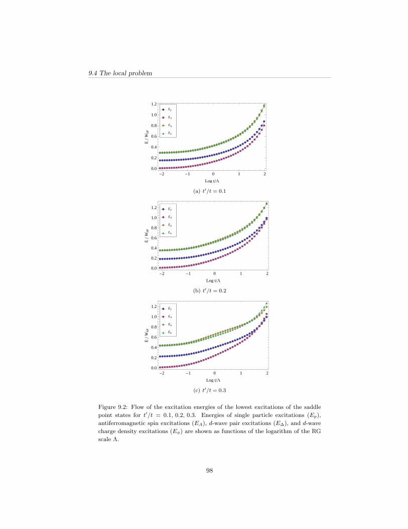
9.4 The local problem
æææææææææææææææææææææææææææææææ
ææ
ææ
ææ
ææ
æ
æ
æ
æ
æ
æ
ààààààààààààààààààààààààààààà
àà
àà
àà
àà
àà
à
à
à
à
à
à
ììììììììììììììììììììììììììììììì
ìì
ìì
ìì
ìì
ì
ì
ì
ì
ì
ì
òòòòòòòòòòòòòòòòòòòòòòòòòòòòòò
òò
òò
òò
òò
òò
ò
ò
ò
ò
ò
-2 -1 0 1 20.0
0.2
0.4
0.6
0.8
1.0
1.2
Log tL
E
WSP ò EΦ
ì ED
à EA
æ Ep
(a) t′/t = 0.1
æææææææææææææææææææææææææææææ
ææ
ææ
ææ
ææ
ææ
æ
æ
æ
æ
æ
æ
ààààààààààààààààààààààààà
àà
àà
àà
àà
àà
àà
à
à
à
à
à
à
à
à
ìììììììììììììììììììììììììììììì
ìì
ìì
ìì
ìì
ìì
ì
ì
ì
ì
ì
òòòòòòòòòòòòòòòòòòòòòòòòòòòòòò
òò
òò
òò
òò
òò
ò
ò
ò
ò
ò
-2 -1 0 1 20.0
0.2
0.4
0.6
0.8
1.0
1.2
Log tL
E
WSP
ò EΦ
ì ED
à EA
æ Ep
(b) t′/t = 0.2
æææææææææææææææææææææææææææææææ
ææ
ææ
ææ
ææ
ææ
æ
æ
æ
æ
ààààààààààààààààààà
àà
àà
àà
àà
àà
àà
àà
àà
àà
àà
à
à
à
à
à
à
ììììììììììììììììììììììììììììììììììììì
ìì
ìì
ìì
ì
ì
òòòòòòòòòòòòòòòòòòòòòòòòòòòòòòòòò
òò
òò
òò
òò
ò
ò
ò
ò
-2 -1 0 1 20.0
0.2
0.4
0.6
0.8
1.0
1.2
Log tL
E
WSP
ò EΦ
ì ED
à EA
æ Ep
(c) t′/t = 0.3
Figure 9.2: Flow of the excitation energies of the lowest excitations of the saddle
point states for t′/t = 0.1, 0.2, 0.3. Energies of single particle excitations (Ep),
antiferromagnetic spin excitations (EA), d-wave pair excitations (E∆), and d-wave
charge density excitations (Eφ) are shown as functions of the logarithm of the RG
scale Λ.
98

Saddle point regime of the two-dimensional Hubbard model
physics of the effective saddle point Hamiltonian we turn to the diagonalization of a
plaquette in the next section.
9.5 Diagonalization of small clusters
In order to better estimate the interplay between kinetic energy and interaction at
low energy scales, we diagonalize the effective Hamiltonian on a 2× 2 plaquette. We
also take into account the non-local part of the interaction. The non-local interac-
tions are generally an order of magnitude smaller than their local counterparts, so
that their overall effect is not large, but still noticeable. The main effect is to push
pair- and spin-excitations down in energy with respect to single particle and dCDW
excitations. We use periodic boundary conditions, so that bandwidth of the hopping
operator is the same as for an infinite size system. The effect of renormalization
on the saddle point degrees of freedom is discussed in the same way as before, by
evaluating all quantities at different stages of the flow, characterized by the flow
parameter Λ.
We compute three different kinds of observables: First, the excitation energies for
the four types of interactions discussed above in Sec. 9.4. The flow of the excitation
energies is shown in Fig. 9.3. Compared to the local Hamiltonian above, we note
that the dCDW excitations are raised in energy compared to the other excitations
in the later stages of the flow. For the other bosonic excitations, we find that there
is a crossover controlled by t′. For t′ = 0.1t, the AF spin excitations are lowest in
energy, and are lowered in energy compared to the local Hamiltonian, so that they lie
significantly below the single particle excitations. For t′ = 0.3t, on the other hand,
the pair excitations have the lowest energy. At t′ = 0.2t, pair and spin excitations
are approximately degenerate, and are both comparable to the single particle energy.
Note that for all parameter values the bosonic excitations retain a large gap that is
of the order of the fermion gap on the plaquette. However, it is clear that the system
is very small, so that finite size effects are expected to be large. In order to gain a
better understanding of the model, we now turn to the ground state properties of
the plaquette Hamiltonian.
The saddle point Hamiltonian consists of a local part, with a non-degenerate local
ground state, and the non-local terms, which are dominated by the kinetic energy.
The ground state of the kinetic energy is the half-filled Fermi sea. In order to
characterize the behavior of the saddle point system, we compute the weight of two
trial ground states in the plaquette ground state. The first state is the uncorrelated
Fermi sea state
|FS〉 =
Ep<0∏
|p
∏
σ
γ†pσ | vac〉 , (9.11)
where here the momenta p refer to the Fourier transform with respect to m, and
Ep is the single particle energy associated to the WW hopping operator T abmm′ . The
99
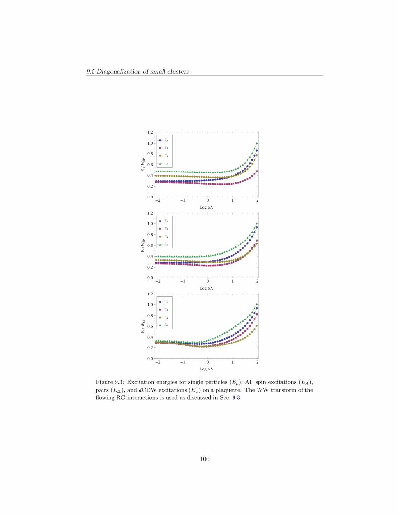
9.5 Diagonalization of small clusters
ææææææææææææææææææææææææææææææææææææ
ææ
ææ
æ
æ
æ
æ
æ
àààààààààààààààààààààààààààààààààààààààà
àà
à
à
à
ììììììììììììììììììììììììììììììììììììììì
ìì
ì
ì
ì
ì
òòòòòòòòòòòòòòòòòòòòòòòòòòòòòòòòòòòòò
òò
ò
ò
ò
ò
ò
ò
-2 -1 0 1 20.0
0.2
0.4
0.6
0.8
1.0
1.2
Log tL
E
WSP
ò EΦ
ì ED
à EA
æ Ep
æææææææææææææææææææææææææææææææææ
ææ
ææ
ææ
æ
æ
æ
æ
æ
æ
àààààààààààààààààààààààààààààààààààà
àà
àà
à
à
à
à
à
ììììììììììììììììììììììììììììììììììììììì
ìì
ìì
ì
ì
òòòòòòòòòòòòòòòòòòòòòòòòòòòòòòòòòò
òò
òò
òò
ò
ò
ò
ò
ò
-2 -1 0 1 20.0
0.2
0.4
0.6
0.8
1.0
1.2
Log tL
E
WSP
ò EΦ
ì ED
à EA
æ Ep
ææææææææææææææææææææææææææææææææ
ææ
ææ
ææ
æ
æ
æ
æ
æ
æ
æ
ààààààààààààààààààààààààààààààààà
àà
àà
àà
à
à
à
à
à
à
ììììììììììììììììììììììììììììììììììììììì
ìì
ìì
ì
ì
òòòòòòòòòòòòòòòòòòòòòòòòòòòò
òò
òò
òò
òò
òò
òò
òò
ò
ò
ò
-2 -1 0 1 20.0
0.2
0.4
0.6
0.8
1.0
1.2
Log tL
E
WSP
ò EΦ
ì ED
à EA
æ Ep
Figure 9.3: Excitation energies for single particles (Ep), AF spin excitations (EA),
pairs (E∆), and dCDW excitations (Eφ) on a plaquette. The WW transform of the
flowing RG interactions is used as discussed in Sec. 9.3.
100
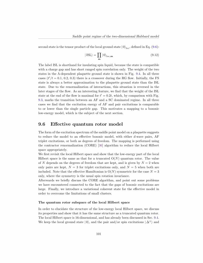
Saddle point regime of the two-dimensional Hubbard model
second state is the tensor product of the local ground state | 0〉loc, defined in Eq. (9.6):
| ISL〉 =∏
m
| 0〉loc,m (9.12)
The label ISL is shorthand for insulating spin liquid, because the state is compatible
with a charge gap and has short ranged spin correlation only. The weight of the two
states in the Λ-dependent plaquette ground state is shown in Fig. 9.4. In all three
cases (t′/t = 0.1, 0.2, 0.3) there is a crossover during the RG flow. Initially, the FS
state is always a better approximation to the plaquette ground state than the ISL
state. Due to the renormalization of interactions, this situation is reversed in the
later stages of the flow. As an interesting feature, we find that the weight of the ISL
state at the end of the flow is maximal for t′ = 0.2t, which, by comparison with Fig.
9.3, marks the transition between an AF and a SC dominated regime. In all three
cases we find that the excitation energy of AF and pair excitations is comparable
to or lower than the single particle gap. This motivates a mapping to a bosonic
low-energy model, which is the subject of the next section.
9.6 Effective quantum rotor model
The form of the excitation spectrum of the saddle point model on a plaquette suggests
to reduce the model to an effective bosonic model, with either d-wave pairs, AF
triplet excitations, or both as degrees of freedom. The mapping is performed using
the contractor renormalization (CORE) [36] algorithm to reduce the local Hilbert
space appropriately.
We first revisit the local Hilbert space and show that the low-energy part of the local
Hilbert space is the same as that for a truncated O(N) quantum rotor. The value
of N depends on the degrees of freedom that are kept, and is given by N = 2 when
only pairs are kept, N = 3 for triplet excitations only, and N = 5 when both are
included. Note that the effective Hamiltonian is O(N) symmetric for the case N = 3
only, where the symmetry is the usual spin rotation invariance.
Afterwards we briefly discuss the CORE algorithm, and point out some problems
we have encountered connected to the fact that the gaps of bosonic excitations are
large. Finally, we introduce a variational coherent state for the effective model in
order to overcome the limitations of small clusters.
The quantum rotor subspace of the local Hilbert space
In order to elucidate the structure of the low-energy local Hilbert space, we discuss
its properties and show that it has the same structure as a truncated quantum rotor.
The local Hilbert space is 16-dimensional, and has already been discussed in Sec. 9.4.
We keep the local ground state | 0〉, and the pair and/or spin excitations |∆±〉 and
101
9.6 Effective quantum rotor model
ææææææææææææææææææææææææææææææææ
ææ
ææ
æ
æ
æ
æ
æ
æ
æ
æ
æ
ààààààààààààààààààààààààà
àà
àà
àà
à
à
à
à
à
à
à
à
à
à
à
à
àà
-2 -1 0 1 20.0
0.2
0.4
0.6
0.8
1.0
Log tL
ÈXG
SÈX
\2
à ÈX\ = ÈFS\
æ ÈX\ = ÈISL\
æææææææææææææææææææææææææææ
ææ
ææ
ææ
æ
æ
æ
æ
æ
æ
æ
æ
æ
æ
æ
æ
ààààààààààààààààààààà
àà
àà
àà
à
à
à
à
à
à
à
à
à
à
àà
àà
àà
àà
-2 -1 0 1 20.0
0.2
0.4
0.6
0.8
1.0
Log tL
ÈXG
SÈX
\2
à ÈX\ = ÈFS\
æ ÈX\ = ÈISL\
ææææææææææææææææææææ
ææ
ææ
ææ
ææ
ææ
ææ
ææ
ææ
ææ
æ
æ
æ
æ
æ
æ
æ
ààààààààààààààààààà
àà
à
à
à
à
à
àà
àà
àà
àà
àà
àà
àà
àà
ààà
-2 -1 0 1 20.0
0.2
0.4
0.6
0.8
1.0
Log tL
ÈXG
SÈX
\2
à ÈX\ = ÈFS\
æ ÈX\ = ÈISL\
Figure 9.4: Weight of the two trial ground states |FS〉 and | ISL〉 in the ground
state of the saddle point model on a plaquette for different values of Λ, and t′/t =
0.1, 0.2, 0.3.
102
Saddle point regime of the two-dimensional Hubbard model
∣∣Ai⟩, respectively. The excited states are obtained from the ground state by applying
pair- and AF-spin-operators:
∆± | 0〉 =∣∣∆±
⟩
Ai | 0〉 =∣∣Ai⟩, (9.13)
where
∆+ =1√2
(γ†1↑ γ
†1↓ − γ
†2↑ γ
†2↓
)
∆− =[∆+]†
Ai =1
2σiσσ′
(γ†2σγ1σ′ + γ†1σγ2σ′
). (9.14)
We also introduce the total charge and spin operators for a WW site, that locally
generate the corresponding O(2) (equivalently U(1)) and O(3) symmetries:
n =1
2
(∑
a
∑
σ
γ†aσ γaσ
)− 2
Si =∑
a
∑
σ,σ′
γ†aσ σiσσ′ γaσ′ . (9.15)
Note that the charge operator has zero eigenvalue at half-filling, and that the charge
of a fermion is ±1/2 in this convention. Then it is straightforward to verify the
commutation relations
[n,∆±
]= ±∆±
[∆+,∆−
]= n
[Si, Aj
]= iεijkA
k
[Ai, Aj
]= iεijkS
k. (9.16)
The first and third line are identical to the defining commutation relations of the O(2)
and O(3) quantum rotors, respectively [46]. The second and fourth line originate
in the fact that the Hilbert space is finite, as opposed to the infinite Hilbert space
of the quantum rotor. When both pairs and AF triplets are kept, the symmetry
generators (9.15) can be augmented by the so-called π-generators
πi =i
2
(σyσi
)σσ′
γ1σ γ2σ, (9.17)
and their hermitian conjugates. These operators transform ∆± into Ai and vice
versa. In conjunction with the spin and charge operators, they generate the O(5)
algebra [64].
The local ground state | 0〉 is annihilated by all the generators, and is thus a singlet
under O(5) and its O(2) and O(3) subgroups, the five states |∆±〉 and∣∣Ai⟩
transform
103

9.6 Effective quantum rotor model
under the vector representation of O(5). Hence the bosonic state may be viewed as
the first two levels of a quantum rotor system with the appropriate dimensionality
(2,3, or 5). We stress, however, that the Hamiltonian is not O(5) symmetric, and
that the rotor model is only a convenient way to organize the low-energy sector of the
local Hilbert space. The Hamiltonian is always O(3) symmetric. The O(2) charge
symmetry holds when it is particle-hole symmetric, which can only be the case when
t′ = 0.
Contractor Renormalization
The CORE method is a real space renormalization scheme for lattice systems. It
consists of two steps: First, one truncates the local Hilbert space to a subset of states
that are the most relevant for the low energy behavior. The effective Hamiltonian for
these local degrees of freedom is then found by diagonalization of small clusters using
the linked cluster theorem, essentially by projecting low energy cluster states to the
reduced Hilbert space followed by orthogonalization. Contributions from clusters
with n sites lead to n-site interactions in the effective model. n is called the range of
an interaction. When the reduction is good, the importance of interactions decays
with their range. For a detailed discussion, we refer to [36] and to App. D. In the
following, we keep interactions up to range 3.
Since the CORE algorithm is based on an application of the linked cluster theorem
and it is controlled only when the renormalization due to high energy states is short
ranged. For this reason, we apply it only to the Hamiltonian obtained at the end
of the flow, where the weight of the RVB state in the ground state of the plaquette
system is large, cf. Fig. 9.4.
We have encountered problems when applying the method to the spin excitations.
The main reason is that the bosonic excitations are not well separated from the
fermionic excitations, due to the insulating spin liquid nature of the local ground
state. In a nutshell, the algorithm works by diagonalizing a small cluster, and
projecting low-lying eigenstates to the tensor product of local bosonic states. When
there are κ states in the local projected Hilbert space, then κ2 eigenstates have to
be projected for the simplest case of a two-site cluster. However, even when these
bosonic states are lower in energy locally than the fermions, the tensor product
state contains high-energy states as well. For example, there are nine possible states
with two spin excitations, with S = 0, 1, 2. The state with S = 0 has the same
quantum numbers as the ground state, a state with two fermion excitations that
form a singlet, or a state with two pair excitations of opposite charge. Hence there
are many possibilities which Eigenstate should be chosen, and the algorithm tends
to become unstable with respect to level crossings.
As a consequence, we limit ourselves to the case t′/t = 0.3, and obtain an effective
Hamiltonian for the pair states.
104

Saddle point regime of the two-dimensional Hubbard model
Variational ground state for d-wave pair excitations
The effective quantum rotor Hamiltonian obtained from the CORE method is very
complicated, since it contains interactions involving up to three sites in the present
setup. Since our main interest here is to distinguish regimes with long range order
from quantum disordered states, we use a family of coherent states in order to
estimate the behavior of the effective model on longer length scales.
For t′ = 0.3t, we reduce the model to the pair excitations (or O(2) rotor model). We
estimate the charge gap using the variational wave function
| θ〉 =∏
m
| θ〉m (9.18)
| θ〉m = cos θ | 0〉m + sin θ∣∣∆±
⟩m, (9.19)
where the sign of the charge carriers is selected according to the charge carrier type
with the lower gap. The wave function | θ〉 is a coherent state wave function, the
local charge fluctuations depend on θ. For θ = 0, there are no charge fluctuations
at the mean-field level, and the system is insulating. For finite θ, the system is
doped away from half-filling, and charges move freely. The charge gap is estimated
by introducing a chemical potential term into the Hamiltonian. Results are shown
in Fig. 9.5. For small values of µ, the system remains insulating. For large negative
(positive) values, hole (particle) pairs are doped into the system, and it becomes
superconducting, with a superfluid density that depends on the doping level. The
size of the insulating region yields an estimate of the charge gap. We find that the
charge gap remains large within this approach. It is clear, however, that the nature
of the approximations made does not allow to make firm conclusions at present.
9.7 Conclusions
In summary, we have applied the wave packet approach to the saddle point regime of
the two-dimensional Hubbard model. Based on arguments developed in earlier chap-
ters, we have argued that a separation of length and energy scales takes place in this
regime, allowing the states at the saddle points to become localized independently
of the behavior of the nodal states, which extend over much larger length scales. We
have then used the WW basis states to isolate the region around the saddle points,
and have analyzed the flow of the effective saddle point Hamiltonian using exact
diagonalization and a mapping to an effective bosonic model. We observed that the
local Hilbert space at the saddle points is identical to the two-leg ladder, Ch. 8.
Similarly, the local ground state is the same, even though the excitation spectrum
depends on the doping, displaying a crossover between AF dominated and dSC dom-
inated regimes as t′ (and therefore the doping) is increased. Correspondingly, the
non-degeneracy of the local ground state and the fact that it is compatible with AF
105
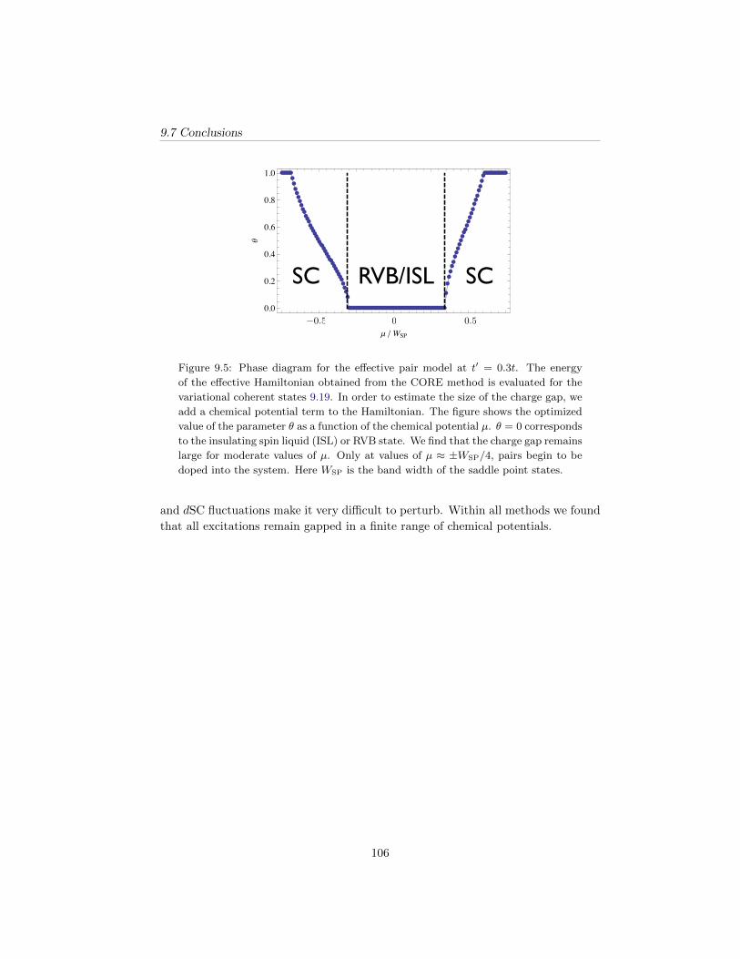
9.7 Conclusions
Effective hardcore boson modelfor pair excitations
Reduce local Hilbert space to U(1)-rotor subspaceCORE algorithm, Morningstar & Weinstein 96
↑↓0
−
0↑↓
00
↑↓↑↓
n = −1
n = 0
n = 1
n =1
2
−2 +
aσ
γ†aσ γaσ
∆− =1√2
(γ1↑γ1↓ − γ2↑γ2↓)
∆+ =∆−†
n, ∆±
= ±∆±
H =
m
n2m − λ
m,m
∆+
m∆−m + h.c.
+ . . .
ISL SCSC
1.5 1.0 0.5 0.0 0.5 1.0 1.50.0
0.2
0.4
0.6
0.8
1.0
Μ WSP
Θ
−0.5 0.50
SC SCRVB/ISL
The local ground state | 0 is annihilated by all the generators, and is thus asinglet under O(5) and its O(2) and O(3) subgroups, the five states |∆± and |Aitransform under the vector representation of O(5). Hence the bosonic state maybe viewed as the first two levels of a quantum rotor system with the appropriatedimensionality (2,3, or 5). We stress, however, that the Hamiltonian is not O(5)symmetric, and that the rotor model is only a convenient way to organize thelow-energy sector of the local Hilbert space. The Hamiltonian is always O(3)symmetric. The O(2) charge symmetry holds when it is particle-hole symmetric,which can only be the case when t = 0.
Comment: write something about core
5.3.2 Variational ground state
The effective quantum rotor Hamiltonian obtained from the CORE method is verycomplicated, since it contains interactions involving up to four sites in the presentsetup. Since our main interest here is to distinguish regimes with long range orderfrom quantum disordered states, we use a family of coherent states in order toestimate the behavior of the effective model on longer length scales.
For t = 0.3t, we reduce the model to the pair excitations (or O(2) rotor model).We estimate the charge gap using the variational wave function
| θ =
m
| θm (46)
| θm = cos θ | 0m + sin θ∆±
m, (47)
where the sign of the charge carriers is selected according to the charge carrier typewith the lower gap. The wave function | θ is a coherent state wave function, thelocal charge fluctuations depend on θ. For θ = 0, there are no charge fluctuationsat the mean-field level, and the system is insulating. For finite θ, the system isdoped away from half-filling, and charges move freely. The charge gap is estimatedby introducing a chemical potential term into the Hamiltonian. Results are shownin Fig. 7. For small values of µ, the system remains insulating. For large negative(positive) values, hole (particle) pairs are doped into the system, and it becomessuperconducting, with a superfluid density that depends on the doping level. Thesize of the insulating region yields an estimate of the charge gap.
23
U(1) rotor operators
Local Hilbert space
Renormalized Hamiltonian
Variational coherent state
t = 0.3t
U = 3.5t
Tuesday, October 4, 2011 Figure 9.5: Phase diagram for the effective pair model at t′ = 0.3t. The energy
of the effective Hamiltonian obtained from the CORE method is evaluated for the
variational coherent states 9.19. In order to estimate the size of the charge gap, we
add a chemical potential term to the Hamiltonian. The figure shows the optimized
value of the parameter θ as a function of the chemical potential µ. θ = 0 corresponds
to the insulating spin liquid (ISL) or RVB state. We find that the charge gap remains
large for moderate values of µ. Only at values of µ ≈ ±WSP/4, pairs begin to be
doped into the system. Here WSP is the band width of the saddle point states.
and dSC fluctuations make it very difficult to perturb. Within all methods we found
that all excitations remain gapped in a finite range of chemical potentials.
106
Chapter 10
Conclusions and outlook
10.1 Summary
The unifying theme of this work is the investigation of the competition and mu-
tual reinforcement of antiferromagnetism and superconductivity in one- and two-
dimensional interacting electron systems, motivated by the phenomenology of cuprate
superconductors. We have pursued a weak coupling approach, sacrificing the pos-
sibility to treat strong coupling effects, while gaining momentum space resolution.
Throughout, we have employed the renormalization group which treats all particle-
particle and particle-hole channels on an equal footing - a prerequisite for the study
of the mutual influence of different possible instabilities.
Anisotropic scattering rates in the Hubbard model
We began our investigation with an experimentally motivated study of anisotropic
quasi-particle scattering rates in the two-dimensional Hubbard model with parame-
ters corresponding to the overdoped regime of Tl2Ba2CuO6+x. We found that the
strongly renormalized interactions lead to enhanced scattering for electrons in the
anti-nodal direction. In conjunction with the scale-dependence of the renormalized
vertex this was found to give rise to a highly anisotropic quasi-particle scattering
rate at the Fermi surface. Moreover, the anisotropic part, which was shown to be
peaked in the anti-nodal direction, was seen to have an almost linear temperature
dependence down to very low temperatures, in qualitative agreement with experi-
ment [1]. We traced this behavior back to the simultaneous growth of correlations
in the antiferromagnetic and d-wave superconducting channels in the vicinity of the
saddle points.
In fact, it has been known for a long time that the Hubbard model exhibits other
peculiar features in the so-called saddle point regime [58], where the Fermi surface
lies in the vicinity of the saddle points (but not necessarily at these points). In
107
10.1 Summary
particular, the overlap between the antiferromagnetic and d-wave pairing channels
is large there, especially when the couplings are not too weak. The strong coupling
phase does not appear to lead to a simple ordered phase, but to an insulating spin
liquid phase with RVB correlations [12, 20].
The wave packet approach to the saddle point regime
In order to investigate this phase we set out to try to obtain a better grasp of
the low-energy physics in this regime in the remaining chapters. To this end, we
introduced a novel tool, the use of the Wilson-Wannier basis functions [41–44], for
the study of the strongly correlated low energy problem. The basis is generated from
wave packet states with a fixed length scale M . It involves two coordinates, a coarse
grained momentum coordinate that describes the physics on scales less than M , and
a coarse grained real space coordinate, that describes scale larger than M .
The basic idea was based on the fact that a gap in the single particle spectrum
introduces a length scale into the problem that is given by the exponential decay of
spatial correlations. This led us to expect that the description simplifies if a basis
is chosen that reflects this length scale, the fermions should ’disappear’ from the
physics at larger length scales, leaving only effective degrees of freedom that can be
determined from an analysis of the Hamiltonian. At the same time, the dependence
on the wave packet momentum can be used to single out the low energy states close
to the Fermi surface, and to incorporate effects of Fermi surface anisotropy.
Since the approach is new, we spent some time developing the necessary formal-
ism and useful approximation methods. These were used in order to highlight the
influence of the (coarse grained) geometry of the Brillouin zone on Fermi surface
instabilities. In particular, we have seen in Ch. 6 that a separation of length scales
between nodal and anti-nodal states occurs whenever the Fermi surface lies in the
vicinity of the saddle points. While it is well known that because of the van Hove
singularity the low energy phase space tends to concentrate around the saddle points
[59, 60], our approach allowed us to estimate the anisotropy of the strength of cor-
relations at a fixed length scale. We found that generically the states at the saddle
points are much more correlated than the nodal states at the same length scale, so
that they effectively decouple.
We proceeded by studying one-dimensional chains with quasi-long range order, and
the two-leg ladder at half-filling, which is known to exhibit a RVB-like insulating
spin liquid phase [53]. The main aim was to compare the results from the wave
packet approach to exact solutions, and we found good qualitative agreement in all
three cases despite of very simplistic approximations. We explained the agreement
in terms of the separation of scales between fermionic and bosonic excitations at the
length scale where the pairing occurs.
We used this separation of scales and computed and effective Hamiltonian for the
anti-nodal states in isolation. We analyzed this Hamiltonian, and compared it to
108
Conclusions and outlook
the two-leg ladder system that was treated in a similar approximation. We found
that locally, the two models are very similar. Consequently, the states at the saddle
point appear to be prone to localize in a state with strong (but short ranged) singlet
correlations, resembling the RVB state of the ladder system with large gaps for all
excitations at the pairing scale, in agreement with earlier calculations based on exact
diagonalization [12].
We emphasize that all the results are only qualitative, and that the approxima-
tions made are quite drastic. Nevertheless, we think that the underlying physical
arguments based on the separation of length scales on the one hand and the non-
degeneracy of local ground states are sound. Clearly the WW basis breaks the
underlying translational invariance so that one might think that it overestimates
gap formation. While this is certainly true to some extent, the states involved can
localize because they are coupled by umklapp scattering. Moreover we have seen
that our approach does lead to quasi-long range order for one-dimensional chains,
where the order parameter modes separate from the fermionic degrees of freedom. It
is worth pointing out that it is not necessary for the Fermi surface to lie exactly at
the van Hove points, since we consider singlet-pair formation on rather short scales
(about 8 lattice constants), so that the pairs are too delocalized in momentum space
to resolve the exact position of the Fermi surface.
Finally, our results are compatible with other studies that start from the strong
correlation limit. In particular, exact diagonalization studies for the t − J-model
[21] find a cooperon mode with weight at the saddle point at finite energy for a
lightly doped system. This is consistent with our results which naturally lead to
such a mode. Similarly, recent cluster DMFT calculations indicate that strong short-
ranged singlet correlations can lead to the formation of a pseudogap in the anti-nodal
direction without long range ordering [63]. The authors attributed the opening of
the single fermion gap to strong single correlations, similar to our observation.
In summary, the wave packet approach to interacting fermions provides surprising
insights to complicated problems already in its simplest implementation. Its main
strength in our view is that it provides a relatively straightforward bridge between
effective interactions and the geometry of the Brillouin zone on the one hand to
effective models low energy physics on the other hand. However, the approach is
still in its infancy, and much more work is needed in order to assess its merits and
shortcomings.
10.2 Outlook
We see several possible extensions to this work. First and foremost, we think it would
be highly useful to improve on the approximations made in this thesis by using more
WW orbitals (recall that we have truncated the basis to only one or two states per
WW site). There is no problem of principle, and only the finite time horizon of this
109
10.2 Outlook
project has prevented us from pursuing this route so far.
From the point of view of flexibility it would be interesting to see whether similar
constructions can be worked out for other lattice geometries, such as the honeycomb
lattice. Note that the WW basis is in essence a one-dimensional construct, so that
it can be used for all rectangular lattices directly, but not for lattices that are not
tensor products of the one-dimensional chain. We hope that our group theoretical
reformulation from Ch. 4 may be helpful for this problem.
The WW basis incorporates a single length scale, but many problems, such as the
pseudogap problem, exhibit multiple length scales. In this work we invoked the sep-
aration of length scales in order to treat the anti-nodal states in isolation. However,
it is clear that for a full account of the phenomenology the nodal states have to be
dealt with. We see two possible approaches: First, in the sprit of two-length-scale
expansions, one could use the effective Hamiltonian for the d-wave pairs at anti-
nodal states and couple them to the nodal states. This is feasible since all couplings
are known. Since the translational invariance breaking strongly distorts the Fermi
surface, one might then take the continuum limit, effectively setting the length scale
for the nodal states to infinity. This leads to a model of mobile fermions coupled to
immobile pairs, similar to some phenomenological models [69].
On the other hand, one might try to develop a true multiscale approach, that can deal
with several length scales at once, for example by applying the WW transformation
for a second time to some of the WW orbitals of the first transformation. However,
we can not judge at present the feasibility or usefulness of this idea.
Finally, the model developed so far exhibits several features which should be elabo-
rated from a phenomenological point of view: First, as the doping level is increased,
a transition in the charge sector arises at the nodal points (cf. Fig. 9.5, and the
hole pairs become mobile. Intuitively, this transition may be linked to the rapid
rise of the superconducting dome at this point. Second, our model includes spin
excitations with wave vector around (π, π), which are expected to be coherent since
they lie below the particle-hole continuum at the saddle points. These might offer
a natural explanation of the so-called hourglass that is observed at optimal doping
[70].
We are confident that more such extensions can be found, and that many routes are
open to extend the very modest first steps presented in this work.
110
Appendix A
Construction of the window
function
A.1 Conditions on the window function
We derive the conditions that the window function g(j) has to satisfy to make the
Wilson basis orthonormal. The derivation closely follows the ones given in [43, 44].
The conditions on g(j) that make the ψmk(j) an orthogonal basis can be derived
from the conditions ∑
mk
ψmk(j1)ψmk(j2) = δj1,j2 . (A.1)
We consider only the case of a real window function g(j), so that the ψmk(j) are
real, too. Condition (A.1) then amounts to demanding that the matrix ψmk,j with
rows given by ψmk(j) is an orthogonal matrix. This implies that the condition
of orthonormality,∑j ψm1k1(j)ψm2k2(j) = δm1m2
δk1k2 , is automatically fulfilled
whenever (A.1) is satisfied.
We use the definition (4.9), and write ψmk(j) in terms of the window function g(j).
111
A.1 Conditions on the window function
Moreover, we split the sum over m into sums over even and odd m,
∑
mk
ψmk(j1)ψmk(j2) =
L/2−1∑
l=0
g(j1 − 2Ml)g(j2 − 2Ml)
1 + (−1)j1+j2
+ 2
M−1∑
k=1
cos[ πMkj1 − φk
]cos[ πMkj2 − φk
]
+
M/2−1∑
l=0
g(j −M(2l + 1)) g(j −M(2l + 1))
× 2
M−1∑
k=1
cos[ πMkj1 − φk+1
]cos[ πMkj2 − φk+1
]
(A.2)
Now we use
2 cos[ πMkj1 − φ
]cos[ πMkj2 − φ
]= cos
[ πMk (j1 − j2)
]+ cos
[ πMk (j1 + j2)− 2φ
],
and notice that
2φk = πk mod 2π.
Then
cos[ πMk(j1 + j2)− 2φk+m
]= (−1)m cos
[ πMk (j1 + j2 −M)
].
Hence we have
∑
mk
ψmk(j1)ψmk(j2) =
L/2−1∑
l=0
g(j1 − 2Ml)g(j2 − 2Ml)
(1 + (−1)j1+j2
)(A.3)
+
M−1∑
k=1
cos[ πMk(j1 − j2)
]+ cos
[ πMk(j1 + j2 −M)
]
+
L/2−1∑
l=0
g(j1 −M(2l + 1))g(j2 −M(2l + 1))
×M−1∑
k=1
(cos[ πMk(j1 − j2)
]− cos
[ πMk(j1 + j2 −M)
])
Because of the symmetry cosx = cos (−x) we can transform the domain of the sums
over k from 1, . . . ,M − 1 to −M + 1, . . . ,M as follows:
(1 + (−1)j1+j2
)+
M−1∑
k=1
(cos[ πMk(j1 − j2)
]+ cos
[ πMk(j1 + j2 −M)
] )
=1
2
M∑
k=−M+1
cos[ πMk(j1 − j2)
]+
1
2
M∑
k=−M+1
cos[ πMk(j1 + j2 −M)
](A.4)
112
Construction of the window function
for terms even in m and
M−1∑
k=1
(cos[ πMk(j1 − j2)
]− cos
[ πMk(j1 + j2 −M)
] )
=1
2
M∑
k=−M+1
cos[ πMk(j1 − j2)
]− 1
2
M∑
k=−M+1
cos[ πMk(j1 + j2 −M)
](A.5)
for the odd terms. Now the summation over k can be performed using the orthogo-
nality of exponential functions, yielding
1
2
M∑
k=−M+1
cos
[2π
2Mka
]= M δ
(2M)a,0 , (A.6)
where a is any integer and δ(2M)ij is the Kronecker delta modulo 2M . The final
expression is then
∑
mk
ψmk(j1)ψmk(j2) = M
L−1∑
m=0
g(j1 −Mm)g(j2 −Mm) δ(2M)j1,j2
+M
L−1∑
m=0
(−1)mg(j1 −Mm)g(j2 −Mm) δ(2M)j1+j2,M
.
(A.7)
Now we show that whenever g(j) = g(−j), the second line vanishes identically. We
set j2 = −j1 + M(2l + 1) (with 0 ≤ l < L/2) to satisfy the Kronecker delta. The
resulting expression is
L−1∑
m=0
(−1)mg(j−Mm)g(−j−M(m−2l−1)) =
L−1∑
m=0
(−1)mg(j−Mm)g(j−(2l+1−m)),
where we have used g(j) = g(−j). To see that this sum vanishes we introduce the
new summation variable m = 2l+ 1−m. Under this transformation the product of
the window functions is invariant, but (−1)m = −(−1)m, and hence the sum has to
vanish.
From (A.7) we then conclude that the conditions
L−1∑
m=0
g(j −Mm)g(j −M(m+ 2l)) =1
Mδl,0 0 ≤ l < L/2 (A.8)
guarantee orthonormality of the Wilson basis. These are the conditions stated above
in eq. (4.5). Since (A.8) depends on j mod M only, the number of independent
conditions is N/2.
113

A.2 Zak transformation
æææææææææææææææææææææææææææææææææææææææææææææææææææææææææææææææææææææææææææææææææææææææææææææææææææææææææææææææææææææææææææææææææææææææææææææææææææææææææææææææææææææææææææææææææææææææææææææææææææææææææææææææææææææææææææææææææææææææææææææææææææææææææææææææææææææææææææææææææææææææææææææææææææææææææææææææææææææææææææææææææææææææææææææææææææææææææææææææææææææææææææææææææææææææææææææææææææææææææææææææææææææææææææææææææææææææææææææææææææææææææææææææææææææææææææææææææææææææææææææææææææææææææææææææ
æ
æ
æ
æ
æ
æ
æ
æ
æ
æ
æ
æ
æ
æ
æ
æ
æææ
æ
æ
æ
æ
æ
æ
æ
æ
æ
æ
æ
æ
æ
æ
æ
æ
ææææææææææææææææææææææææææææææææææææææææææææææææææææææææææææææææææææææææææææææææææææææææææææææææææææææææææææææææææææææææææææææææææææææææææææææææææææææææææææææææææææææææææææææææææææææææææææææææææææææææææææææææææææææææææææææææææææææææææææææææææææææææææææææææææææææææææææææææææææææææææææææææææææææææææææææææææææææææææææææææææææææææææææææææææææææææææææææææææææææææææææææææææææææææææææææææææææææææææææææææææææææææææææææææææææææææææææææææææææææææææææææææææææææææææææææææææææææææææææææææææææææææææææææ
aL
-400 -200 0 200 4000.00
0.05
0.10
0.15
0.20
0.25
jgH
jL
æææææææææææææææææææææææææææææææææææææææææææææææææææææææææææææææææææææææææææææææææææææææææææææææææææææææææææææææææææææææææææææææææææææææææææææææææææææææææææææææææææææææææææææææææææææææææææææææææææææææææææææææææææææææææææææææææææææææææææææææææææææææææææææææææææææææææææææææææææææææææææææææææææææææææææææææææææææææææææææææææææææææææææææææææææææææææææææææææææææææææææææææææææææææææææææææææææææææææææææææææææææææææææææææææææææææææææææææææææææææææææææææææææææææææææææææææææææææææææææææææææææææææææææææ
æ
æ
æ
æ
æ
æ
æ
æ
æ
æ
æ
æ
æ
æææææææææ
æ
æ
æ
æ
æ
æ
æ
æ
æ
æ
æ
æ
æ
ææææææææææææææææææææææææææææææææææææææææææææææææææææææææææææææææææææææææææææææææææææææææææææææææææææææææææææææææææææææææææææææææææææææææææææææææææææææææææææææææææææææææææææææææææææææææææææææææææææææææææææææææææææææææææææææææææææææææææææææææææææææææææææææææææææææææææææææææææææææææææææææææææææææææææææææææææææææææææææææææææææææææææææææææææææææææææææææææææææææææææææææææææææææææææææææææææææææææææææææææææææææææææææææææææææææææææææææææææææææææææææææææææææææææææææææææææææææææææææææææææææææææææææææ
bL
-400 -200 0 200 4000.00
0.05
0.10
0.15
0.20
0.25
j
gHjL
Figure A.1: Window functions in real space. a) shows the function g0(j) before the
application of the transformation (A.12), in b) the function g(j) that results from
the transformation is shown.
A.2 Zak transformation
To simplify these conditions it is convenient to introduce the so-called finite Zak
transform Zg(j, p) of g(j) [45]. From the definition
Zg(j, p) =1
L
L−1∑
m=0
g(j +mM)e−2πiL pm
g(j +mM) =1
L
L−1∑
p=0
Zg(j, p)e2πiL pm, (A.9)
where 0 ≤ j < L and 0 ≤ p < M , one can see that the Zak transform of a function
is very similar to the Bloch representation of wave functions in a periodic potential.
The lattice is split into unit cells of size M , and the degrees of freedom within
one unit cell are represented in real space, but the change from unit cell to unit
cell is Fourier transformed leading to the pseudo-momentum p. The Zak transform
simplifies conditions (4.5) because they are in the form of a convolution with the sum
running over unit cells of size M . The convolution is turned into a multiplication,
and the conditions on Zg are
|Zg(j, p)|2 + |Zg(j, p+ L/2)|2 = C(j), (A.10)
114
Construction of the window function
where C(j) is independent of p. C(j) is fixed by the condition
L−1∑
p=0
|Z(j, p)|2 =1
M. (A.11)
As a practical consequence of this simple condition, one can use (almost) any initial
window function g0(j) as long as Zg0(j, p) and Zg0(j, p+ L/2) do not vanish simul-
taneously for some j. A window function g(j) that satisfies conditions (A.10) up to
a constant prefactor can then be obtained via
Zg(j, p) ∝Zg0(j, p)√
|Zg0(j, p)|2 + |Zg0(j, p+ L/2)|2. (A.12)
The normalization is fixed by demanding
∑
j
g2(j) = 1 (A.13)
for the modified window function. For finite lattices this procedure is easily imple-
mented on a computer. A convenient choice of g(j) is a Gaussian centered around
j = 0 with width M , but the qualitative results do not depend on the exact choice
of g(j). In particular, one one can show that salient features like the exponential
decay are preserved [43]. To illustrate the preservation of rapid decay, we display
the effect of the transformation (A.12) on a Gaussian initial window function in fig.
A.1.
A.3 Conditions for band limited window functions
The orthogonality conditions (A.8) on the window function simplify when it is band
limited in the sense that the Fourier transform g(p) = 1√N
∑j g(j)e−ipj satisfies
g(p) = 0 for |p| ≥ π
M. (A.14)
In this case it is more useful to express (A.8) in momentum space. We first express
g(j) in (A.8) in terms of g(p), which leads to
1
N
∑
p,p′
g (p) g (p′) eij(p+p′)e−i2Mlp
L−1∑
m=0
e−iMm(p+p′) =1
Mδl,0. (A.15)
Now we take the Fourier transform of (A.8) with respect to j. The right hand side
becomes1
N
∑
j
e−iqj1
Mδl,0 =
1
Mδq,0 δl,0. (A.16)
115

A.3 Conditions for band limited window functions
The left hand side becomes
1
N
∑
p,p′
g (p) g (p′) e−i2Mlp ×
1
N
∑
j
eij(p+p′−q)
︸ ︷︷ ︸=δp+p′,q
×[L−1∑
m=0
e−iMm(p+p′)
]
︸ ︷︷ ︸=L
∑a δp+p′, 2π
Ma
. (A.17)
The first Kronecker delta can be used to eliminate via p′ = q−p, and using L = N/M
we arrive at1
M
∑
p
g (p) g
(2π
Ma− p
)e−i2Mlp =
1
Mδa,0 δl,0, (A.18)
where we have used the Kronecker deltas to replace q by the integer a. From the
condition (A.14) that g(p) is band limited it follows that
g (p) g
(2π
Ma− p
)= 0 for a 6= 0, (A.19)
so that all conditions with a 6= 0 are identically satisfied, so that only the case a = 0
has to be taken into account. Hence the orthogonality conditions become
δl,0 =∑
p
g (p) g (−p) e−i2Mlp
=∑
p
|g(p)|2 e−i2Mlp, (A.20)
since g(p) = g(−p) by assumption. The exponential on the right hand side is periodic
in p with period πM , so that we can write
∑
p
|g(p)|2 e−i2Mlp =∑
p∈rBZ
e−i2Mlp∑
a
∣∣∣g(p+
π
Ma)∣∣∣
2
, (A.21)
where we have introduced the reduced Brillouin zone (rBZ) −πM ≤ p < πM . Hence
(A.20) states that ∑
a
∣∣∣g(p+
π
Ma)∣∣∣
2
=2M
N∀ p ∈ rBZ. (A.22)
The value of the constant on the right hand side is determined by the number of
points in the reduced Brillouin zone, which is N2M . This can be further simplified
using the fact that g(p) is band limited and symmetric. The band limitation implies
that only a = −1, 0,+1 contribute to the sum. Moreover, we must have ap < 0,
otherwise the term vanishes. By virtue of the symmetry of g(p), it is clear that
g(p− π
M
)= g
(−p+ π
M
), so that it is sufficient to consider the case p ≥ 0. Hence
we obtain the final form of the orthogonality conditions:
|g (p)|2 +∣∣∣g( πM− p)∣∣∣
2
=2M
Nfor 0 ≤ p ≤ π
M. (A.23)
116

Construction of the window function
Note that these conditions can be trivially satisfied by fixing g(p) to arbitrary values
less than√
2M/N for 0 < p < π/2M , and to use (A.23) to infer the absolute value of
g(p) for π/2M < p < π/M . Note that g(0) =√
2M/N and g (π/2M) =√M/N are
fixed. When we choose g(p) ≥ 0 everywhere, the window function is fully determined.
117

A.3 Conditions for band limited window functions
118

Appendix B
Window function gymnastics
This appendix summarizes some useful relations between window functions. In par-
ticular, it is shown how to replace the shifted window functions gmk(j) by their
unshifted counterparts. All relations follow from the fact that g(j) is symmetric
around the origin and real for all j, i.e.
g(j) ∈ R (B.1)
g(j) = g(−j) (B.2)
We recall the definition (cf. Eq. (4.1)) of the phase space shift of g(j):
gm,k(j) = eiπM kj g (j −Mm) (B.3)
It follows directly that
gm,k(j)∗ = gm,−k(j), (B.4)
where gm,k(j)∗ is the complex conjugate of gm,k(j).
For the Fourier transform gm,k(p) we find
gm,k(p) =1√N
∑
j
e−ipjgm,k(j)
=1√N
∑
j
e−i(p−πM k)g (j −Mm)
= (−1)mk
e−iMmp 1√N
∑
j
e−i(p−πM k)jg(j)
= (−1)mk
e−iMmpg(p− π
Mk), (B.5)
where we have used (B.3) in the second line, and shifted the summation variable
j → j +Mm in the third line.
119

Now we note that the properties (B.1) and (B.2) imply that g(p) is real, and that
g(p) = g(−p). For the complex conjugate gm,k(p)∗ of gm,k(p) this leads to
gm,k(p)∗ = (−1)mk
e+iMmpg(p− π
Mk)
= (−1)mk
e+iMmpg(−p+
π
Mk)
= gm,−k(−p), (B.6)
where we have used (B.5) in the first line and g(p) = g(−p) in the second line.
The replacement of gmk(p) by g(p), Eq. (B.5) can be used in order to simplify sums
involving the shifted window function. Let f(p) be an arbitrary function of the
momentum, then
∑
p
f(p)gmk(p) = (−1)mk∑
p
f(p)e−iMmpg(p− π
Mk)
= (−1)mk
eiπMmk∑
p
f(p+
π
Mk)e−iMmpg (p)
=∑
p
f(p+
π
Mk)e−iMmpg (p) , (B.7)
where we have used (B.5) in the first line, and shifted p → p + πM k in the second
line.
Finally, it is worth mentioning that the phase space shift (B.3) could also be defined
as
gm,k(j) = eiπM k(j−Mm) g (j −Mm) . (B.8)
Both definitions can be used, since the difference amounts to a gauge transformation
|m, k〉 → (−1)mk |m, k〉 . (B.9)
With the alternative definition (B.8), the factor (−1)mk shows up in the real space
representation of the shifted window function instead of the momentum space form,
i.e.
gm,k(j) = (−1)mk
eiπM kjg (j −Mm) ,
gm,k(p) = e−iMmpg(p− π
Mk). (B.10)
In this work, we will stick to the definition (B.3), however, since it is more convenient
for practial calculations.
120
Appendix C
One loop RG equations from
Wegner’s flow equation
We derive equations that are structurally similar to the one loop RG equations from
Wegner’s flow equation [54], also known as continuous unitary transformation (CUT,
[55, 56]). In this method, a sequence of infinitesimal canonical transformations
is applied to partially diagonalize the Hamiltonian. Since each transformation is
infinitesimal, it can be approximated by linearizing in its generator η:
eηHe−η = [η,H] + . . . (C.1)
Introducing a parameter flow parameter B, the flow equation for the Hamiltonian is
given byd
dBH(B) = [η(B),H(B)] . (C.2)
One can show [54] that the so-called canonical generator
η(B) = [Hkin(B),Hint(B)] (C.3)
leads to a Hamiltonian that commutes with the kinetic energy in the limit B →∞.
In general, single particle states with a kinetic energy difference ∆Ekin start to
decouple at B ∼ (∆Ekin)−2
. In particular, states with a kinetic energy greater than
B−1/2 decouple from the states at the Fermi surface. From the low energy point
of view, the method is thus similar to the usual renormalization group approach of
integrating out states [26] that are far away from the Fermi surface, with the RG
scale Λ ∼ B−1/2. However, it should be noted that no modes are integrated out,
and thus the full information about the Hamiltonian and its spectrum is conserved
in the flow equation approach. Moreover, whereas in the renormalization group an
effective action is obtained, the flow equation yields an effective Hamiltonian, which
is more suitable for our purposes.
121

In order to solve eq. (C.2), approximations are necessary, since infinitely many opera-
tors are generated during the flow. We follow the usual practice of making an ansatz
for the flowing Hamiltonian H(B), and thus truncating the number of operators.
More specifically, we use the ansatz
H(B) =∑
p
εp : J(p, p) :
+1
2N
∑
p1···p4Up1p2p3(B) δp1+p2,p3+p4 : J (p1, p3) J (p2, p4) :,
J (p1, p2) =∑
σ
c†p1σ cp2σ, (C.4)
where : O : denotes normal ordering of the operator O with respect to the Fermi sea.
We omit the flow of the kinetic energy in the following, so that only the couplings
Up1p2p3 (B) depend on B. From (C.3), the canonical generator is then given by
η (B) =1
2N
∑
p1···p4Up1p2p3 (B)Dp1p2p3δp1+p2,p3+p4 : J (p1, p3) J (p2, p4) :,
Dp1p2p3 = εp3 + εp4 − εp2 − εp1 . (C.5)
Plugging this into the flow equation (C.2), we see that there are two different con-
tributions:d
dBH(B) = [η(B),Hkin]︸ ︷︷ ︸
O(U)
+ [η(B),Hint(B)]︸ ︷︷ ︸O(U2)
. (C.6)
The first term gives rise to a set of linear differential equations for the couplings
Up1p2p3(B), whereas the second term incorporates perturbative renormalization ef-
fects. We will first investigate the flow equation to O(U). With the generator given
by (C.5) we obtain
d
dBH(B) = [η(B),Hkin] +O
(U2)
(C.7)
= − 1
2N
∑
p1···p4δp1+p2,p3+p4 D
2p1p2p3Up1p2p3 (B) : J (p1, p3) J (p2, p4) :
Comparing the coefficients of the operators :J (p1, p3) J (p2, p4): on both sides, we
obtain an equation for the couplings Up1p2p3(B):
d
dBUp1p2p3(B) = −D2
p1p2p3Up1p2p3(B) +O(U2), (C.8)
which is solved by
Up1p2p3(B) = Up1p2p3(0) e−D2p1p2p3
B . (C.9)
From the solution one sees that interaction matrix elements that couple states with
energy difference larger than B−1/2 are suppressed exponentially, as announced
122
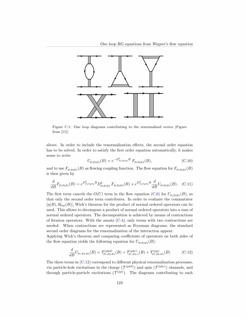
One loop RG equations from Wegner’s flow equation
FIG. 2. The particle-particle and particle-hole diagrams contributing to the one-loop RG equation.
T dPH,!(p1, p2; p3, p4) =
!!
dp
"!2V!(p1, p, p3)L(p, p + p1 ! p3)V!(p + p1 ! p3, p2, p)
+V!(p1, p, p + p1 ! p3)L(p, p + p1 ! p3)V!(p + p1 ! p3, p2, p)
+V!(p1, p, p3)L(p, p + p1 ! p3)V!(p2, p + p1 ! p3, p)
#(16)
T crPH,!(p1, p2; p3, p4) =
!!
dp V!(p1, p + p2 ! p3, p)L(p, p + p2 ! p3)V!(p, p2, p3) (17)
In these equations,
L(p, p!) = S!(p)W(2)! (p!) + W
(2)! (p)S!(p!) (18)
with the so-called single-scale propagator
S!(p) = !W(2)! (p)
"d
d!Q!(p)
#W (2)
s (p) . (19)
The one-loop diagrams corresponding to the terms (15), (16) and (17) are shown in Fig. 2.In the typical momentum-shell RG, the varying parameter ! is an energy scale which separates high and low
energy modes. The strategy is to integrate out the high energy modes first. In this case the scale parameter onlya"ects the quadratic part Q!(p), which is multiplied with an appropriate cuto" function. Here, for the reasonsdiscussed in the introduction, we want to treat the temperature as varying parameter. Our reasoning is as follows:at high temperatures, where !T is larger than the bandwidth and the interaction energies, perturbation theoryconverges, and moreover the corrections to the selfenergy and four–point function are of order 1/T , hence small.Thus at high temperature, the vertex functions are essentially identical to the terms in the action. Then we trackthe renormalization of the vertex functions when the temperature is lowered. Of course this idea is implicit in mostof the well-known scaling approaches4. On a technical level however this strategy has usually been cast into somecuto"-variation procedure with similar results as the more elaborate modern Wilsonian schemes.
In order to apply the RG scheme for the 1PI vertex functions with T as a flow parameter we first have to performa transformation which shifts all temperature dependence to the quadratic part of the action.
A. New fields
The T 3-factor in the interaction part can be removed by transforming the action to the new fermionic fields givenby
5
Figure C.1: One loop diagrams contributing to the renormalized vertex (Figure
from [25])
above. In order to include the renormalization effects, the second order equation
has to be solved. In order to satisfy the first order equation automatically, it makes
sense to write
Up1p2p3(B) = e−D2p1p2p3
B Fp1p2p3(B), (C.10)
and to use Fp1p2p3(B) as flowing coupling function. The flow equation for Fp1p2p3(B)
is then given by
d
dBFp1p2p3(B) = eD
2p1p2p3
BD2p1p2p3 Fp1p2p3(B) + eD
2p1p2p3
B d
dBUp1p2p3(B). (C.11)
The first term cancels the O(U) term in the flow equation (C.6) for Up1p2p3(B), so
that only the second order term contributes. In order to evaluate the commutator
[η(B),Hint(B)], Wick’s theorem for the product of normal ordered operators can be
used. This allows to decompose a product of normal ordered operators into a sum of
normal ordered operators. The decomposition is achieved by means of contractions
of fermion operators. With the ansatz (C.4), only terms with two contractions are
needed. When contractions are represented as Feynman diagrams, the standard
second order diagrams for the renormalization of the interaction appear.
Applying Wick’s theorem and comparing coefficients of operators on both sides of
the flow equation yields the following equation for Up1p2p3(B):
d
dBUp1,p2,p3(B) = T (phd)
p1,p2,p3(B) + T (phc)p1,p2,3(B) + T (pp)
p1,p2,p3(B) (C.12)
The three terms in (C.12) correspond to different physical renormalization processes,
via particle-hole excitations in the charge (T (phd)) and spin (T (phc)) channels, and
through particle-particle excitations (T (pp)). The diagrams contributing to each
123
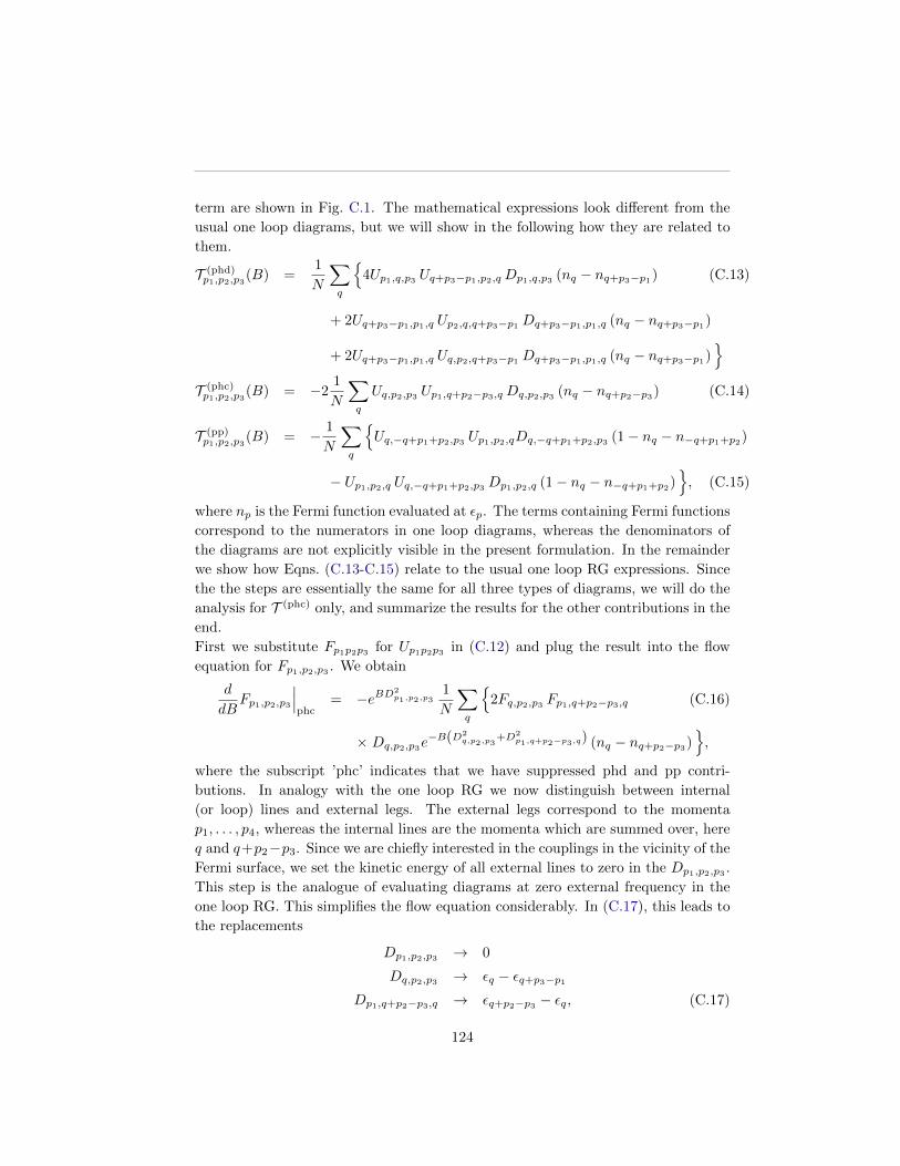
term are shown in Fig. C.1. The mathematical expressions look different from the
usual one loop diagrams, but we will show in the following how they are related to
them.
T (phd)p1,p2,p3(B) =
1
N
∑
q
4Up1,q,p3 Uq+p3−p1,p2,qDp1,q,p3 (nq − nq+p3−p1) (C.13)
+ 2Uq+p3−p1,p1,q Up2,q,q+p3−p1 Dq+p3−p1,p1,q (nq − nq+p3−p1)
+ 2Uq+p3−p1,p1,q Uq,p2,q+p3−p1 Dq+p3−p1,p1,q (nq − nq+p3−p1)
T (phc)p1,p2,p3(B) = −2
1
N
∑
q
Uq,p2,p3 Up1,q+p2−p3,qDq,p2,p3 (nq − nq+p2−p3) (C.14)
T (pp)p1,p2,p3(B) = − 1
N
∑
q
Uq,−q+p1+p2,p3 Up1,p2,qDq,−q+p1+p2,p3 (1− nq − n−q+p1+p2)
− Up1,p2,q Uq,−q+p1+p2,p3 Dp1,p2,q (1− nq − n−q+p1+p2), (C.15)
where np is the Fermi function evaluated at εp. The terms containing Fermi functions
correspond to the numerators in one loop diagrams, whereas the denominators of
the diagrams are not explicitly visible in the present formulation. In the remainder
we show how Eqns. (C.13-C.15) relate to the usual one loop RG expressions. Since
the the steps are essentially the same for all three types of diagrams, we will do the
analysis for T (phc) only, and summarize the results for the other contributions in the
end.
First we substitute Fp1p2p3 for Up1p2p3 in (C.12) and plug the result into the flow
equation for Fp1,p2,p3 . We obtain
d
dBFp1,p2,p3
∣∣∣phc
= −eBD2p1,p2,p3
1
N
∑
q
2Fq,p2,p3 Fp1,q+p2−p3,q (C.16)
× Dq,p2,p3e−B(D2
q,p2,p3+D2
p1,q+p2−p3,q) (nq − nq+p2−p3),
where the subscript ’phc’ indicates that we have suppressed phd and pp contri-
butions. In analogy with the one loop RG we now distinguish between internal
(or loop) lines and external legs. The external legs correspond to the momenta
p1, . . . , p4, whereas the internal lines are the momenta which are summed over, here
q and q+p2−p3. Since we are chiefly interested in the couplings in the vicinity of the
Fermi surface, we set the kinetic energy of all external lines to zero in the Dp1,p2,p3 .
This step is the analogue of evaluating diagrams at zero external frequency in the
one loop RG. This simplifies the flow equation considerably. In (C.17), this leads to
the replacements
Dp1,p2,p3 → 0
Dq,p2,p3 → εq − εq+p3−p1Dp1,q+p2−p3,q → εq+p2−p3 − εq, (C.17)
124
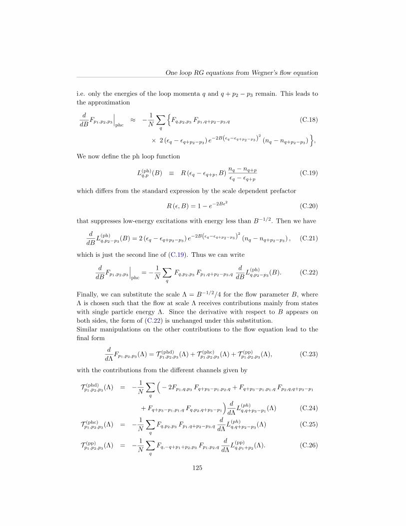
One loop RG equations from Wegner’s flow equation
i.e. only the energies of the loop momenta q and q + p2 − p3 remain. This leads to
the approximation
d
dBFp1,p2,p3
∣∣∣phc
≈ − 1
N
∑
q
Fq,p2,p3 Fp1,q+p2−p3,q (C.18)
× 2 (εq − εq+p2−p3) e−2B(εq−εq+p2−p3)2
(nq − nq+p2−p3),
We now define the ph loop function
L(ph)q,p (B) ≡ R (εq − εq+p, B)
nq − nq+pεq − εq+p
(C.19)
which differs from the standard expression by the scale dependent prefactor
R (ε, B) = 1− e−2Bε2 (C.20)
that suppresses low-energy excitations with energy less than B−1/2. Then we have
d
dBL
(ph)q,p2−p3(B) = 2 (εq − εq+p2−p3) e−2B(εq−εq+p2−p3)
2
(nq − nq+p2−p3) , (C.21)
which is just the second line of (C.19). Thus we can write
d
dBFp1,p2,p3
∣∣∣phc
= − 1
N
∑
q
Fq,p2,p3 Fp1,q+p2−p3,qd
dBL
(ph)q,p2−p3(B). (C.22)
Finally, we can substitute the scale Λ = B−1/2/4 for the flow parameter B, where
Λ is chosen such that the flow at scale Λ receives contributions mainly from states
with single particle energy Λ. Since the derivative with respect to B appears on
both sides, the form of (C.22) is unchanged under this substitution.
Similar manipulations on the other contributions to the flow equation lead to the
final form
d
dΛFp1,p2,p3(Λ) = T (phd)
p1,p2,p3(Λ) + T (phc)p1,p2,p3(Λ) + T (pp)
p1,p2,p3(Λ), (C.23)
with the contributions from the different channels given by
T (phd)p1,p2,p3(Λ) = − 1
N
∑
q
(− 2Fp1,q,p3 Fq+p3−p1,p2,q + Fq+p3−p1,p1,q Fp2,q,q+p3−p1
+ Fq+p3−p1,p1,q Fq,p2,q+p3−p1) d
dΛL
(ph)q,q+p3−p1(Λ) (C.24)
T (phc)p1,p2,p3(Λ) = − 1
N
∑
q
Fq,p2,p3 Fp1,q+p2−p3,qd
dΛL
(ph)q,q+p2−p3(Λ) (C.25)
T (pp)p1,p2,p3(Λ) = − 1
N
∑
q
Fq,−q+p1+p2,p3 Fp1,p2,qd
dΛL
(pp)q,p1+p2(Λ). (C.26)
125

0 1 2 3 40.0
0.2
0.4
0.6
0.8
1.0
Ε L
RL
H2Ε
L
0 1 2 3 40.0
0.1
0.2
0.3
0.4
0.5
0.6
0.7
Ε L
-L
2¶
LR
LH2
ΕL
Figure C.2: Dependence of the cutoff function R(n)Λ (2ε) and its scale derivative on
the average single-particle energy ε.
The loop functions with Λ as a flow variable are
L(ph)q,p (Λ) = RΛ (εq − εq+p)
nq − nq+pεq − εq+p
(C.27)
L(pp)q,p (Λ) = RΛ (εq + ε−q+p)
1− nq − n−q+pεq + ε−q+p
(C.28)
RΛ(ε) = 1− e−ε2/8Λ2
(C.29)
Once the flow equation is solved up to some scale Λ, the renormalized interaction
Hamiltonian is obtained by transforming from Fp1,p2,p3(Λ) back to Up1,p2,p3(Λ). Re-
calling (C.10), we have
Up1,p2,p3(Λ) = e−D2p1,p2,p3
/16Λ2
Fp1,p2,p3(Λ), (C.30)
the physical interaction decouples states at the Fermi surface from states with single
particle energy |ε| > Λ. As a consequence, states above the cutoff may be neglected
or treated perturbatively, so that only states below the cutoff remain.
Comparison of (C.23) with the flow equation derived from functional RG [25] shows
that the structure of the two equations is identical when the FRG equation is eval-
uated in the one-loop approximation, i.e. omitting the frequency dependence and
using bare propagators in all diagrams. In both equations, the flow is generated by
second order perturbation theory. The bubble diagrams are scale dependent due to
the presence of an infrared cutoff, and their contribution to the flowing couplings is
given by the scale derivative of the bubble. However, in the present approach, the
cutoff function acts on the energy of two-particle excitations (pp or ph), whereas
in the functional RG the cutoff acts on single particle energies. From a practical
point of view, however, this difference should be small in most situations, since the
two types of cutoff only differ when the single particle energies of the two particles
taking part in the excitation are very different. Due to kinematic restrictions in the
presence of a Fermi surface this is not expected to matter in most situations.
126

Appendix D
Contractor renormalization
In the following we review briefly the contractor renormalization (CORE) method
[36] for correlated lattice systems. The method is based on first choosing a truncated
set of κ states for the local Hilbert space of a lattice system. There is no general rule
how to choose these states, so that the choice has to be based on physical insight.
These κ states are used as effective degrees of freedom per site. The dimension of
the local Hilbert space is denoted by ν. The couplings between sites are evaluated
by diagonalizing connected clusters of lattice sites and projecting lowest states onto
the tensor product of the truncated local basis. For an N -site cluster, one has to
diagonalize an νN -dimensional matrix and find its lowest κN states.
We denote the κ2 tensor products of projected single-site states by |αi〉. We need
the κ2 lowest eigenstates of the two-site cluster for the projection, and will denote
the n-th such state by |n〉. The CORE algorithm consists of three steps:
First the low-lying states of the cluster are projected onto the |αi〉,
|ψn〉 =∑
i
|αi〉〈αi|n〉. (D.1)
Second, the projected states |ψn〉 are orthonormalized, using the Gram-Schmidt
method starting with the groundstate:
|ψn〉 =1
Zn
(|ψn〉 −
∑
i<n
|ψi〉〈ψi|ψn〉). (D.2)
The effective Hamiltonian for the N -site cluster is then given by
H(N) =∑
n
En|ψn〉〈ψn|, (D.3)
where En is the energy of state |n〉. Finally, one can write the total effective Hamil-
tonian as a sum over irreducible N -site operators, where the irreducible part of the
127

N -site Hamiltonian for the cluster CN is defined by
Hirred.(CN ) = H(N) −∑
N ′<N
∑
CN′∈CNH(CN ′) (D.4)
where∑CN′ ∈CN denotes summation over all connected subclusters of CN of size
N ′. One can show [36] that the expansion
Heff =
Nmax∑
N=1
∑
CN
H(CN ) (D.5)
reproduces the lowest κ energies of the original Hamiltonian in the limit Nmax →∞.
In practice, however, the expansion has to be truncated at some point, and here
we will consider the simplest approximation only, and restrict ourselves to two-site
interactions.
128

Bibliography
[1] M. Abdel-Jawad et al., Nature Physics 2, 821 (2006). M. Abdel-Jawad et al.,
Phys. Rev. Lett. 99, 107002 (2007).
[2] D. Zanchi, H. J. Schulz, Europhys. Lett. 44, 235 (1998).
[3] C. J. Halboth, W. Metzner, Phys. Rev. B 61, 7364 (2000); Phys. Rev. Lett.
85, 5162 (2000).
[4] C. Honerkamp et al., Phys. Rev. B 63, 035109 (2001).
[5] A. A. Katanin, arXiv:0806.0300.
[6] D. Zanchi, Europhys. Lett. 55, 376 (2001).
[7] C. Honerkamp, Eur. Phys. J. B 21, 81 (2001).
[8] A. A. Katanin, A. P. Kampf, Phys. Rev. Lett. 93, 106406 (2004).
[9] D. Rohe, W. Metzner, Phys. Rev. B 71, 115116 (2005).
[10] C. Honerkamp, M. Salmhofer, Prog. Theor. Phys. 105, 1 (2001).
[11] C. Honerkamp, M. Salmhofer, Phys. Rev. B 64, 184516 (2001).
[12] A. Lauchli et al., Phys. Rev. Lett. 92, 037006 (2004).
[13] T. M. Rice et al., cond-mat:1109.0632.
[14] J. Bardeen et al., Phys. Rev. 108, 1175 (1957).
[15] J. G. Bednorz and K. A. Muller, Z. Phys. B 64, 189 (1986).
[16] S. Huefner et al., Rep. Prog. Phys. 71, 062501 (2008).
[17] P. W. Anderson, Science 235, 1196 (1987).
[18] T. Timusk and B. Statt, Rep. Prog. Phys. 62, 61 (1999).
[19] H. Alloul et al., Phys. Rev. Lett 63, 1700 (1989).
129
BIBLIOGRAPHY
[20] T. M. Rice, Prog. Theor. Phys. Supp. 160, 39 (2005).
[21] T. A. Maier et al., Phys. Rev. Lett. 100, 237001.
[22] J. Oitmaa et al., Series expansion methods for strongly correlated lattice models,
Cambridge University Press (2006).
[23] M. Tinkham, Introduction to Supeconductivity, Dover Publications (2004).
[24] A. R. Schmidt et al., New J. Phys. 13, 065014 (2011).
[25] C. Honerkamp and M. Salmhofer, Phys. Rev. B 64, 184516 (2001).
[26] R. Shankar, Rev. Mod. Phys. 66, 129 (1994).
[27] A. H. Castro Neto and E. Fradkin, Phys. Rev. B 49, 10877 (1994).
[28] T. Chen et al., Fluctuating geometries in statistical mechanics and field theory,
Les Houches session LXII (1994).
[29] W. Metzner et al., Adv. Phys. 47, 317 (1998).
[30] C. Honerkamp and M. Salmhofer, Prog. Theor. Phys. 113 (6), 1145 (2005).
[31] A. C. Hewson, The Kondo Problem to Heavy Fermions, Cambridge University
Press (1993).
[32] H. Tsunetsugu et al., Rev. Mod. Phys. 69, 809 (1997).
[33] U. Ledermann et al., Phys. Rev. B 62, 16383 (2000).
[34] S. R. White, Phys. Rev. B 48, 10345 (1993).
[35] A. Georges and G. Kotliar, Phys. Rev. B 45, 6479 (1992).
[36] C. Morningstar and M. Weinstein, Phys. Rev. D 54, 4131 (1996).
[37] J. Reiss, D. Rohe, and W. Metzner, Phys. Rev. B 75, 075110 (2007).
[38] E. Altman and A. Auerbach, Phys. Rev. B 65, 104508 (2002)
[39] A. Auerbach, cond-mat/0510738 (2005).
[40] E. Hernandez and G. Weiss, A first course on wavelets, CRC Press (1996).
[41] K. G. Wilson, Generalized Wannier functions, Cornell preprint (1987).
[42] D. J. Sullivan et al., cond-mat:1007.3522.
[43] I. Daubechies et al., SIAM J. Math. Anal. 22 (2), 554 (1991).
130

BIBLIOGRAPHY
[44] H. Bolcskei et al., Proc. of the IEEE-SP symposium on time-frequency and
time-scale analysis, 525 (1996).
[45] J. Zak, Phys. Rev. Lett. 19, 1385 (1967).
[46] S. Sachdev, Quantum phase transitions (1999).
[47] R. A. Balian, C.R. Acad. Sci. Paris 292 (20), 13571362, (1981).
[48] F. Low, Complete sets of wave packets, in A Passion for Physics - Essays in
Honor of Geoffrey Chew, C. DeTar et al., Eds., World Scientific, Singapore,
1722, (1985).
[49] J. Solyom, Adv. Phys. 28 (2), 201 (1979).
[50] P. Kopietz et al., Introduction to the Functional Renormalization Group,
Springer (2010).
[51] J. Timonen and A. Luther, J. Phys. C 18, 1439 (1985).
[52] J. M. Luttinger, J. Math. Phys. 4, 1154 (1963).
[53] H.-H. Lin, L. Balents, and M. P. A. Fisher, Phys. Rev. B 58, 1794 (1998).
[54] F. Wegner, Ann. Phys. 3, 77 (1994).
[55] S. D. Glazek and K. G. Wilson, Phys. Rev. D 48, 5863 (1993).
[56] S. D. Glazek and K. G. Wilson, Phys. Rev. D 49, 4214 (1994).
[57] S. Kehrein, The Flow Equation Approach to Many-Particle Systems, Springer
(2006).
[58] C. Honerkamp et al., Phys. Rev. B 63, 035109 (2001).
[59] H. J. Schulz, Europhys. Lett. 4, 609 (1987).
[60] I. Dzyaloshinskii, Sov. Phys. JETP 66, 848 (1987).
[61] P. Lederer et al., J. Phys. (France) 48, 1613 (1987).
[62] I. Dzyaloshinskii, J. Phys. I (France) 6, 119 (1996).
[63] M. Ferrero et al., Phys. Rev. B 80, 064501 (2009).
[64] E. Demler, W. Hanke, and S.-C. Zhang, Rev. Mod. Phys. 76, 909 (2004).
[65] Chubukov et al., Phys. Rev. B 78, 134512 (2008).
[66] M. Furukawa, T. M. Rice, and M. Salmhofer, Phys. Rev. Lett. 81, 3195 (1998).
131

BIBLIOGRAPHY
[67] T. Giamarchi, Quantum Physics in One Dimension.
[68] A. O. Gogolin et al., Bosonization and Strongly Correlated Systems, Cambridge
University Press (1999).
[69] V. B. Geshkenbein et al., Phys. Rev. B 55, 3173 (1996).
[70] M. Arai et al., Phys. Rev. Lett. 83, 608 (1999).
132
Acknowledgements
During the time I spent working on this thesis, I had the pleasure of interacting
with many people that contributed directly or indirectly. I would like to thank
my supervisors Manfred Sigrist and T. Maurice Rice for giving me the opportunity
to work on a project which for a long time resembled Schrodingers cat, oscillating
between success and failure.
The time I spent at my office was made much more fun by the people that shared
it with me, Andreas Ruegg, Hiroto Adachi, Kaiyu Yang, Sebastian Pilgrim, Yoshiki
Imai, and Daniel Muller. I thank all of them for discussions, creating a friendly at-
mosphere, and in particular for enduring my frequent and lengthy rants, digressions,
and ’brief’ sketches of ideas.
I would also like to thank the other members of the solid state theory groups,
Jonathan Buhmann, Adrien Bouhon, Mark Fischer, Sarah Thaler, Ludwig Klam,
Jun Goryo, Sebastian Huber, Fabian Hassler, Barbara Theiler, Alexander Thomann,
Roland Willa, and David Oehri. I have learnt many things through fruitful discus-
sions with them, and benefitted greatly from their kindness in many ways.
Finally, I am very grateful to Lena Hartmann for spending the last few years
with me emotionally, and for her tolerance in spending them mainly without me
physically.
133

BIBLIOGRAPHY
134
Related Documents