A VLSI architecture for simplified arithmetic Fourier transform algorithm

1122 JEEE TRANSACTJONS ON SIGNAL PROCESSING. VOL. 40. NO. 5, MAY 1992

A VLSI Architecture for Simplified Arithmetic Fourier Transform Algorithm

Irving S. Reed, Fellow, IEEE, Ming-Tang Shih, Member, IEEE, T. K . Truong, Senior Member, IEEE, E , Hendon, and D. W. Tufts, Fellow, IEEE

Abstract-The arithmetic Fourier transform (AFT) is a number-theoretic approach to Fourier analysis which has been shown to perform competitively with the classical FFT in terms of accuracy, complexity, and speed. Theorems developed in a previous paper for the AFT algorithm are used here to derive the original AFT algorithm which Bruns found in 1903. This is shown then to yield an algorithm of less complexity and of im- proved performance over certain recent AFT algorithms. A VLSI architecture is suggested for this simplified AFT algorithm. This architecture uses a butterfly structure which re- duces the number of additions by 25% of that used in the direct method.

I. INTRODUCTION HE Fourier representation of a periodic signal is im- T portant to Fourier analysis and the discrete Fourier

transform. The Fourier series of a periodic sequence cor- responds to the discrete Fourier transform (DFT) of a finite-length numerical sequence. The most efficient method for computing the DFT is the fast Fourier transform (FFT) [I]. However, computation of the FFT is still complicated and time consuming, especially in terms of the number of needed complex multiplications.

At the beginning of this century, in 1903, a mathema- tician named H. Bruns [2] developed a method for computing the coefficients of a Fourier series of a periodic function using the Mobius inversion formula for series. This technique of Fourier analysis was considered again by Wintner [3] in a 1945 monograph.

A similar algorithm was rediscovered recently [4] by Tufts and Sadasiv and called the arithmetic Fourier transform (AFT). This AFT is based on the Mobius inversion of series and can be used to compute finite Fourier coefficients of even periodic function. The advantages of the AFT over the FFT is that this method of Fourier analysis needs only addition operations with one exception, namely, multiplications by an inverse-integer scale factor at one stage of the computation.

The AFT developed in [4] was extended very recently in [5] to compute the Fourier coefficients of both the even and odd components of a periodic function. This latter algorithm can be used to find the Fourier coefficients of any complexed-valued periodic function. The main draw- back of this AFT algorithm is the oversampling problem, i.e., the higher the required accuracy is, the greater the number of samples needs to be. However, the AFT algorithm can be used with sampling rates close to the Nyquist rate (see [ 5 ] ) . Another disadvantage in this latter algorithm is that the amount of computation needed for the odd components of a periodic function is apparently greater than for the even components. As a consequence, the number of real additions needed to realize the N-point Fourier coefficients of real-valued waveform in this latter algorithm is N2/2 , see [9], [lo].

This paper consists of three parts. First, the AFT algorithm in the form developed in [5] is outlined. This algorithm is used then to derive Bruns’ original method in [2] for finding Fourier coefficients. It is shown here that Bruns’ AFT algorithm is more balanced than the algorithm in [5] in the amount of computation needed for computing the even and odd coefficients of a Fourier series. In fact, the matrix needed to compute the odd coefficients is identical in Complexity to the matrix needed for the even coefficients. Also, this new version of Bruns’ AFT technique is compared with the previous AFT algorithms in [5] on the basis of accuracy, complexity, and speed. Fi- nally, an architecture of this simplified AFT is suggested in order to reduce the number of additions. This reduction in the addition operations is accomplished primarily by decomposing the Bruns alternating average into two ordinary averages. Then a systolic array structure is developed to propagate the required k-point averages into 2k- point averages, etc. As a result, a parallel Fourier transform is developed which is suitable for VLSI implementation.

Manuscript received July 31, 1989; revised February 12, 1991. This work was supported in part by SRC 88-DP-075 and in part by NASA 7-100.

I . S. Reed, M.-T. Shih, and E. Hendon are with the Department of Elec- trical Engineering, University of Southern California. LOS Aneeles. CA

11. THE FOURIER ANALYSIS BY USING THE MOBIUS INVERSION FORMULA

Reed et al. [51 introduced the arithmetic Fourier trans- - 90089-0272.

pulsion Laboratory, Pasadena, CA 91 109.

sity of Rhode Island, Kingston, RI 02881.

form as fol1ows:Let a real function A( t ) be a finite Fourier series of period T. The Fourier series of A(t) has the form

bn sin 2nnfot (1)

T. K. Truong is with Communication System Research Section, Jet Pro-

D. W. Tufts is with the Department of Electrical Engineering, Univer-

IEEE Log Number 9106572. n = I n = 1

N N

A( t ) = a. + c an cos 2nnfot +

1053-587X/92$03.00 0 1992 IEEE

REED er al.: VLSI ARCHITECTURE

A(0.2)

A (0.3)

A(0.4)

A(0.5)

A(0.6)

A(0.7)

1123

'

where f, = 1 / T . ao. the zeroth harmonic. is the mean of A( t ) , and a, and b, are nonvanishing coefficients in the interval 1 I n I Nand vanishing elsewhere. The zeroth harmonic a,, in (1) is given by

a0 = T o j T A ( t ) dt. (2)

If the mean in (1) is removed, one obtains N

A(t) = A(t ) - a. = C a, cos 2anht n = l

N

+ b, sin 2nnfot. (3) n = l

Now shift the periodic function A(t) in (3) in time by an amount aT, where - 1 < a < 1, as follows:

A(t + a ~ ) = C a, cos 2 a n ( h t + a) N

n = I

N

+ c b, sin 27rn(fot + a) n = I

N

= C c,(a) cos 2anfot , = I

N

+ d,(a) sin 2anfot (4a) n = l

wherefor -1 < a < 1

c,(a) = a, cos 2ana + 6, sin 2ana (4b) and

&(a) = -a, sin 2ana + b, cos 2ana. (4c) Dejinition 1: Let S(n, a ) be the nth average

1 ,-' S(n, a ) = - C A ( m T / n + a T ) (5) n m = O

of the n values A ( m T / n + a T ) for ( m = 0, 1, 2 , , n - 1) of A ( t ) shifted by the amount a T where - 1 < a < 1.

The following two theorems proved in [5] contain the mathematics needed to describe the recent versions of the AFT algorithm as exposed in [3]-[5].

*

meorem 1 (5, theorem 41: The coefficients c,,(a) in (4b) are given by the Mobius inversion formula for a finite series as follows:

W l n l

/ = 1 c,(a) = c p ( O S ( l n , a ) (6)

where S(n, a) is the nth average defined in ( 5 ) of Defini- tion 1 and ~ ( ( 1 ) is the Mobius function defined by

p(Z) = 1 if 1 = I

= (- 1)' if 1 = pIp2 . . p r ,

where the p , are distinct primes

= o i f p 2 1 1 for any prime p .

meorem 2 (5, theorem 51: The Fourier coefficients a, and b, of the Fourier series in (3) for n = 2'! (2m + I ) are computed by

a,, = C,(O) ( 7 4

b, = (- 1) '"~,( 1 / 2 h + 2 ) (7b) and

where m and k are determined by the factorization, n = 2k(2m + 1).

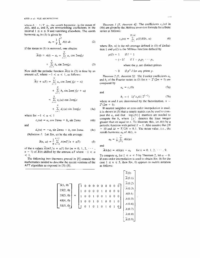
If nearest neighbor or zero-order interpolation is used, it is shown in [5] that a simple matrix can be used to compute the a, and that rlog2(N)1 matrices are needed to compute the b, where rx1 denotes the least integer greater than or equal to x. To illustrate this, let A ( f ) be a periodic function with period T = 1. Also assume that 2N = 10 and At = T / 2 N = 0.1. The mean value, i.e., the zeroth harmonic a. of A ( t ) , is

9

a0 = kzo 4 k A t )

and A(kAt) = A(kAf) - a. fork = 0, 1, 2 , * * . , 9.

To compute a, for 1 I n I 5 by Theorem 2 , let a = 0. If zero-order interpolation is used to obtain S(n, 0) for the case 1 I n 5 5 , then S(n, 0) appears in matrix notation as follows:

0 0

0 0

0 1

0 1

1 0

0 0

0 1

0 0

0 1

1 0

0 0

0 0

1 0

0 0

1 0

I] I O

1 0

IEEE TRANSACTIONS ON SIGNAL PROCESSING, VOL. 40, NO. 5, MAY 1992 1124

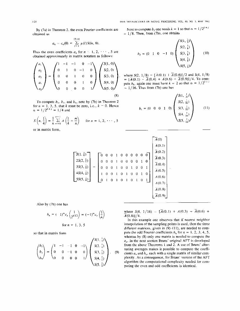
By (7a) in Theorem 2, the even Fourier coefficients are

[ 5 /,I

Next to compute b2 one needs k = 1 so that CY = 1 /2”‘ obtained as = 1/8. Then, from (7b), one obtains

a, = C,(O) = c p ( l ) S ( l n , 0). I = I

Thus the even coefficients a, for n = 1, 2, . . obtained approximately in matrix notation as follows:

, 5 are

where S(2, 1/8) = [A(Od) + A(0.5)]/2 and S(4, 1/8) = [A(0.1) + A(0.4) + A(0.6) + A(0.9)]/4. To compute b4, again one must have k = 2 so that CY = 1/2”’ = 1 / 16. Thus from (7b) one has

(8)

To compute b l , b3, and b5, note by (7b) in Theorem 2 for n = 1, 3 , 5 , that k must be zero, i.e., k = 0. Hence (y = 1/2k+2 = 1 / 4 and (1 1) b4 = (0 0 0 1 0)

fern= 1 , 2 ; * * , 5

or in matrix form,

0 0

0 0

0 0

0 0

1 0

0 0

0 0

0 1

1 0

1 0

0 0

0 1

0 0

0 1

1 0

1 0

1

A(0.2)

A(0.3)

A(0.4)

A(0.5)

A(0.6)

A(0.7)

Also by (7b) one has

where S(4, 1/16) = [A(0.1) + A(0.3) + A(0.6) + A (0. S)] /4 .

In this example one observes that if nearest neighbor interpolation of the sampling points is used, then the three different matrices, given in (9)-(ll), are needed to compute the odd Fourier coefficients b, for n = 1, 2, 3 , 4, 5 , whereas by (8) only one matrix is needed to compute the a,. In the next section Bruns’ original AFT is developed from the above Theorems 1 and 2. A use of Bruns’ alternating averages makes it possible to compute the coeffi- i) . (9) cients a, and b,, each with a single matrix of similar complexity. As a consequence, for Bruns’ version of the AFT algorithm the computational complexity needed for computing the even and odd coefficients is identical.

forn = 1, 3, 5

so that in matrix form

S(1, $)

f:) = (% -% -:) ( f: S(5,

REED er al.: VLSl ARCHITECTURE I I25

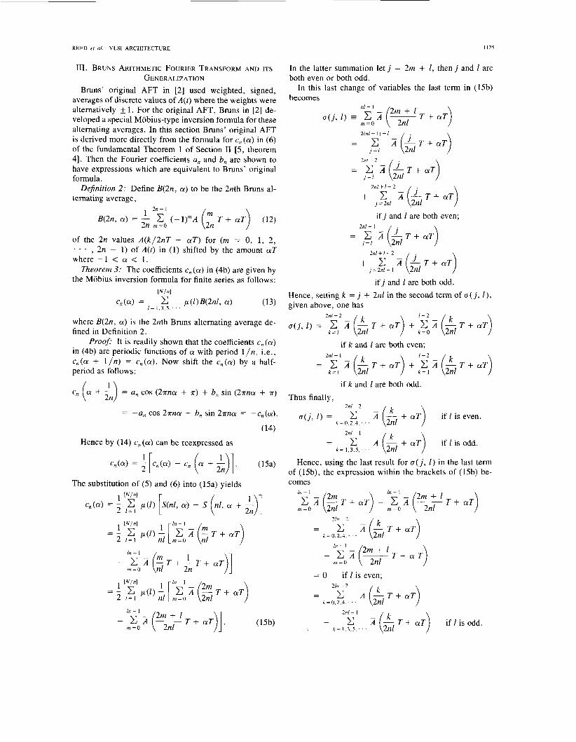
111. BRUNS ARITHMETIC FOURIER TRANSFORM AND ITS

GENERALIZATION Bruns' original AFT in [2] used weighted, signed,

averages of discrete values of A(t) where the weights were alternatively + 1. For the original AFT, Bruns in [2] developed a special Mobius-type inversion formula for these alternating averages. In this section Bruns' original AFT is derived more directly from the formula for c, (a) in (6) of the fundamental Theorem 1 of Section I1 [ 5 , theorem 41. Then the Fourier coefficients a, and b, are shown to have expressions which are equivalent to Bruns' original formula.

Dejinition 2: Define B(2n, a) to be the 2nth Bruns alternating average,

of the 2n values A(k/2nT + CYT) for (m = 0, 1, 2, . . . , 2n - 1) of A(t) in (1) shifted by the amount a T where -1 < CY < 1.

Theorem 3: The coefficients c, (a) in (4b) are given by the Mobius inversion formula for finite series as follows:

W / n I

c,(a) = C p((1)~(2n1, CY) (13) 1 = 1 , 3 , 5 ; . .

where B(2n, a) is the 2nth Bruns alternating average defined in Definition 2.

Proof? It is readily shown that the coefficients c,(a) in (4b) are periodic functions of a with period l / n , i.e., c,(a + l / n ) = c,(a). Now shift the C,(CY) by a half- period as follows:

c, a + - = a, cos (2ana + n) + b, sin (2nna + a) ( 2 3 = -a, cos 27rna - b, sin 27rna = -c,(a).

Hence by (14) c,(a) can be reexpressed as

The substitution of (5) and (6) into (15a) yields

m = O (nl 2n l )

In - I

- C A ~ T + - T + ~ T

In - 1 - C A (7 2m + 1 T + a T ) ] . m = O

In the latter summation l e t j = 2m + I, t h e n j and 1 are both even or both odd.

In this last change of variables the last term in (15b) becomes

nl-1 - 2 m + l

m = O a ( j , 1 ) = C A (7 T + a T )

2(nl - I ) + I

; = 1

2nl - 2

= 2 / T + j = l (2n1

2nl+ / - 2

+ ; = C 2nl A ( - & T + c Y T )

if j and 1 are both even; 2nl- I

;=/

2 n l f 1 - 2

+ j = 2 n / + I c A ( - & T + ~ T )

i f j and 1 are both odd. Hence, setting k = j + 2nE in the second term of o ( j , l ) , given above, one has

2 n l - 2

if k and 1 are both even; 2nl - 1 1-2

= c A L T + ~ T + C A - T + ~ T k = l ( 2 d ) k = l ( l 1 )

if k and 1 are both odd. Thus finally,

2111 - 2

a ( j , 1 ) = c A (& + a T ) i f 1 is even. k = 0 , 2 . 4 ; ' .

Hence, using the last result for a ( j , I ) in the last term of (15b), the expression within the brackets of (15b) becomes

2m + 1 In - 1 In- 1

m = O c A & T + ~ T ) - m = O c A ( ~ T + ~ T )

21n - 2

k = 0 , 2 , 4 ; ' . In - I 2m + 1

- m = O C A ( T T + C Y T )

= 0 if 1 is even;

2n/ - I

- A (& T + C Y T ) if l i s odd. k = 1.3.5 ' . '

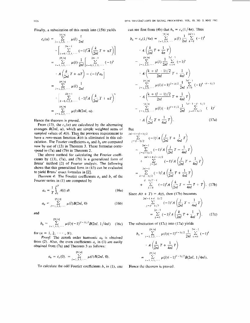
I I26 IEEE TRANSACTIONS ON SIGNAL PROCESSING, VOL. 40. NO. 5 , MAY 1992

Finally, a substitution of this result into (15b) yields

I IN/,]

I = 1,3,5; ' .

2 h - I

* [ k = O , 2 3 , . . . P"n1

= C p(1)~(2n1, a>. I = 1.3 .5 , ' ' '

Hence the theorem is proved. From (13), the c,(a) are calculated by the alternating

averages B(2n1, a), which are simple weighted sums of sampled values of A( t ) . Thus the previous requirement to have a zero-mean function A(t) is eliminated in this calculation. The Fourier coefficients a, and b, are computed now by use of (13) in Theorem 3. These formulas corre- spond to (7a) and (7b) in Theorem 2.

The above method for calculating the Fourier coefficients by (13), (7a), and (7b) is a generalized form of Bruns' method [2] of Fourier analysis. The following shows that this generalized form in (13) can be evaluated to yield Bruns' exact formulas in [2].

Theorem 4: The Fourier coefficients a, and b, of the Fourier series in (1) are computed by

a0 = - A(t ) dt ( 1 6 4 T o s' IN/,]

a, = c p(l)B(2nf, 0) ( 16b) /=1,3,5; . .

and

INlnl

b, = p(1)(-1)('-1'/2B(2nl, 1/4nl) (16c) I = 1.3.5: ' .

for (n = 1, 2, Proof: The zeroth order harmonic a. is obtained

from (2). Also, the even coefficients a, in (1) are easily obtained from (7a) and Theorem 3 as follows:

W / n l

a, = c,(o). = C p((1)~(2nl , 01.

* 9 , N ) .

I = 1,3,5, ' . .

can see first from (4b) that b, = c,(l/4n). Thus

I = 1.3.5. ' ' '

. A - T + - T ( k i 4n

1 2"1 - P " n l

= C p(1) - c ( -1y 1=1,3,5:.. 2nl 1 ; = 0

- A (in1 - T + I T ) . 4nl (17a)

But 2nI- 1 + ( I - I ) / 2

2 n l - I

4nl

1 2nI - I + ( I - 1) /2

+ J = 2n/ (-1)IA ("..-T) 2nl 4nl

( k l 4nl

2nI- 1

k = ( I - 1)/2 = C (-l)kA - T + - T

Since A(t + T ) = A ( t ) , then (17b) becomes

j = ( / - 1)/2 2,- I

The substitution of (17c) into (17a) yields

1 2 n / - 1 IN/nl

I = 1.3.5.. ' '

b, = C p(f)(- l )o-1) '2- 2nl k = o C (-l)k

* A - T + - T ( l l 4nl

To calculate the odd Fourier coefficients b, in ( I ) , one Hence the theorem is proved.

I I27 REED et al.: VLSI ARCHITECTURE

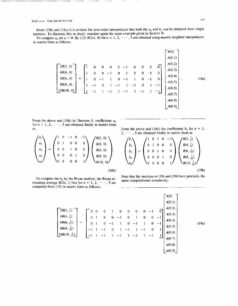
From (16b) and (16c) it is evident for zero-order interpolation that both the a, and b, can be obtained from single

To compute a, set (Y = 0. By (12) B(2nl, 0) for n = 1, 2, - , 5 are obtained using nearest neighbor interpolation matrices. To illustrate this in detail, consider again the same example given in Section 11.

in matrix form as follows:

1 0 0 0 0 - 1

0 0 - 1 0 1

1 0 -1 1 -: -: 1 - 1 1 -

-1 1 -1 1 - 1

0

0

0

0

-1

0

-1

-1

1

1

A(0.2)

A(0.3)

A(0.4)

A(0.5)

A(0.6)

A(0.7)

- 1

- 1

From the above and (16b) in Theorem 4, coefficients a, for n = 1, 2, * , 5 are obtained finally in matrix form as From the above and (16c) the coefficients b, for n = 1,

2, * , 5 are obtained finally in matrix form as

Note that the matrices in (1 8) and (19) have precisely the Same computational complexity. To compute the b, by the Bruns method, the Bruns al-

, 5 are ternating average B(2n, 1/4n) for n = 1, 2, computed from (15) in matrix form as follows:

*

A(0 .2 )

A(0 .3 )

A(0.4)

A(0.5)

A(0.6)

A(0.7)

0 0 0 1 0 0 0

0 1 0 0 - 1 0 1

0 1 0 - 1 1 0 - 1 (194 1 - 1 0 1 - 1 1 -1 0

1 - 1 1 -1 1 - 1 1 -1

I128 IEEE TRANSACTIONS ON SIGNAL PROCESSING, VOL. 40, NO. 5, MAY 1992

TABLE I COMPARISON OF THE DIFFERENT METHODS FOR CALCULATING A N M-POINT

IV. COMPARISON OF DIFFERENT METHODS FOR

COMPUTING THE AFT AFT

Bruns Original Method AFT Method in 151 In order to calculate 6, the shift a needed in the alter-

nating average B(2n, a) of Bruns' method is equal to 1/4n. Note also that the row of the matrix used to Cal- Additions (1 /2)M2 (3/8)M2

M (3/2)M Larger

culate B(2n, 1 /4n) in (19a) is a cyclic shift of the corresponding row for calculating B(2n, 0) in (18a). The shifted Er&lexity Low Higher structure of these two matrices may be useful when the entries of the matrix are shifted serially into a signal processor.

Multiplications Small

The Bruns alternating average B(2nZ, a) in (12) differs from S(n, a) in (5) in that it uses only an even number of samples. This fact overcomes the requirement in (5) for using a zero-mean function.

From (5) and (12) the number of operations needed to calculate B(2nl, a) is twice that needed for S(nZ, a). How- ever, the calculation of a, and b, in (16b) and (16c) needs only the terms B(2n1, a) for odd 1, only half of the terms of type S(n1, a) used for the AFT algorithm in [5].

Hence the total number of additions needed for a direct computation of the Bruns method is approximately the same as for the previous method in [5]. This fact is supported by the results shown in Table I: In the Bruns method the number of additions is greater than the method in [5]. However, the number of multiplications by scale factors are less in the Bruns technique. As a result, the total number of operations required in Bruns method is approximately the same as the method in [5]. Finally the calculation of the zero-mean function A(t) in [5] is a time- consuming process not needed in the Bruns AFT. As a consequence Bruns method should have a better through- put than the method in [5]. This is an important factor for designing a real-time parallel signal processor.

An approximate error analysis of Bruns' method is given in Appendix A. It appears to show a 1.25-dB reduction in noise level compared with the method given in [5]. However, a computer simulation for calculating the coefficients of a Gaussian periodic function with zero-order interpolation shows that in actuality there is only about a 0.92-dB gain in signal-to-noise ratio by Bruns' method compared with the method in [5]. This is illustrated in

TABLE I1 COMPARISON OF THE RELATIVE ROOT-MEAN-SQUARE ERROR WITH

DIFFERENT AFT'S IN THE COMPUTATION OF A GAUSSIAN WAVEFORM WITH 1024 SAMPLES

AFT Method in [ 5 ] Bruns Method

1.41 X 1.27 x 1 0 - ~

Definition 3: Let W(n, a) be the n-point average

(20) 1 n - l

W(n, a) = - c A(mT/n + a T ) n m = O

of the n values A ( m T / n + a T ) for (m = 0, 1, 2, . * , n - 1) of A ( t ) shifted by the amount a T where - 1 < a < 1.

Note by (3) that average W(n, a) in (20) is related to average S(n, a) in (5) by the relation, W(n, a) = S(n, a) + a. where a. is the zeroth harmonic of the periodic function A( t ) .

Theorem 4: The Bruns 2n-point alternating average B(2n, a) decomposes into

B(2n, a) = - W(n, a) - w n, a + - 2 lL ( 2 3 1 (21)

and the 2n-point average W(2n, a) decomposes into

W(2n, a) = - W(n, a) + w n a + - 2 l [ ( ' 2 3 1 (22) Table I1 where the error is the root-mean-square error be-

form using an inverse FFT of the coefficients. tween the original waveform and the reconstructed wave- where w(n, a) is the n-point average Of A ( t ) given in Def-

inition 3 . Proof: First, by the definition of B(2n, a) in (12), it

V. A VLSI ARCHITECTURE FOR ARITHMETIC FOURIER is not difficult to show that

TRANSFORM 1 2 n - l B(2n, a) = - C (-l)*A In this section one shows that Bruns alternating average 2n m = O -

B(2n, a) can be decomposed into two n-point averages. Then a systolic array structure is developed which uses n-point averages to obtain 2n-point averages and so forth. Both of the Bruns alternating averages B(2n, 0) and B(2n, 1/4n) for calculating the even and odd components of a signal can be generated by the same such architecture. As a result, a VLSI architecture is suggested here to reduce the number of computations of the arithmetic Fourier transform.

n - I

=I[ ' - 2 nm=o c (-1)2mA

+ - 1 n - l C (-1)2m+lA f* T + a T ) ] n m = O

REED er a / . : VLSI ARCHITECTURE

2n 1 n - l

- - c A - T + a T + - T nm=o

Also, by the definition in (20),

+ - C A - T + a T + - T n m = O 2n

and the theorem is proved. From (21) and (22) it is evident that both the B(2k, a)

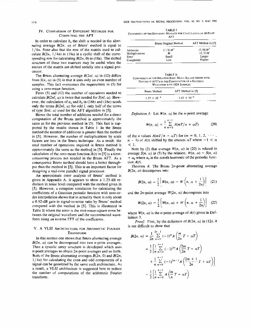
and W(2n, a) can be obtained from the n-point averages W(n, a) and W(n, a + 1 /2n). The basic operations given in (21) and (22) constitute what might be called the AFT butterfly as shown in Fig. 1. A systolic array based on the AFT butterfly is constructed such that the averages W(2n, a) are propagated by the corresponding previous averages W(n, a). The Bruns alternating averages B(2n, a) needed for calculating the Fourier coefficients are obtained at the same butterfly level but with possibly different signs. The structure of this method is shown in Fig. 2. In Fig. 2, both B(2n, 0) and B(2n, 1/4n) are obtained in the same structure. Thus a substantial reduction of the number of additions is accomplished by this method.

To illustrate this in detail, again consider the example developed in Section 111. To compute B(2, 0), B(4, 0), andB(8,O)in(17a)andB(2, 1/4)andB(4, 1/8)in(18a), one needs to calculate W(2, 0), W(2, 1/4), W(2, l / 8 ) , and W(2, 3/8) first. As it is shown in Fig. 3,

W(2, 0) = k[W(l, 0) + W(1, 1/2)]

= i[A(O) + A(0.5)]

/4) = i W ( 1 , 1/41 + W(1, 3/4)1

= i[A(0.3) + A(0.8)]

/8) = i[W(1, 1/8) + W(1, 5/81]

= ;[A(O.l) + A(0.7)]

W(2, 3 /8 ) = ;[W(l, 3/8) + W(1, 7/8)]

= ;[A(0.4) + A(0.9)].

As a consequence one has

W(4, 0) = i [ W ( 2 , 0) + W(2, 1/4)]

1 I29

B(2j,a ) = 1/2 [ W(j,a ) - W(j,a +1/2j) 1

W(2j, a ) = 112 [ W(j. a ) + WO, a +1/2j) I Fig. 1. Butterfly structure of the AFT.

W ( k . l l 4 k ) B ( 2 k , 1 / 4 k ) '>(

Fig. 2. General tree of butterfly structure for calculating Bruns' altei averages.

mating

and

W(4, 1/8) = i [ W ( 2 , l /8 ) + W(2, 3/8)].

Finally the required alternating averages are obtained as outputs from the butterfly tree as follows:

B(2, 0) = k[W(l, 0) - W(1, 1/2)]

= i[A(O) + A(0.5)]

B(4, 0) = i[W(2, 0) - W(2, 1/4)]

B(8, 0) = 5[W(4, 0) - W(4, l/8)]

B(2, 1/4) = i[W(l, 1/4) - W(1, 3/4)]

= ;[A(0.3) - A(0.8)]

and

B(4, 1/8) = i[W(2, 1/8) - W(2, 3/8)].

1130 IEEE TRANSACTIONS ON SIGNAL PROCESSING, VOL. 40, NO. 5, MAY 1992

W ( 2 , 3 / 8 ) W ( 4 , 1 / 8 )

Fig. 3 . Example of butterfly tree for calculating Bruns' alternating averages B(2, 0), B(4, 0 ) , B(8, 0 ) , B(2, 1/4), and B(4, 1/8).

4(2 A

4(3 A

I I I I I I I I

I I

I I I

I I

I I B(6.0), B(6.1112)

8 (12 ,0 ) ,8 (12 .1 /24 )

I 1 I I

~ ( K A t)

Fig. 4 . VLSI architecture for the arithmetic Fourier transform.

Note that the averages B(2 , a), B(4, a) and B(8 , a) are calculated in the same group. Also, the computations of W(2, a) and "(4, a) are inherent in those computations needed for B(8, a). The division-by-two operations in (21) or (22) are achieved by one bit shifts when the data is represented in binary form. The number of additions

needed to calculate the alternating averages is O ( N 2 ) (see Table I and [ 5 ] ) . As a result, an approximate 25% reduction in the number of additions is accomplished by this new method when the number of coefficients is large.

A VLSI architecture for the arithmetic Fourier transform, using zero-order interpolation, is shown in Fig. 4.

1131 REED er a/. : VLSI ARCHITECTURE

If the real function A ( t ) is sampled at points t = m T / k where 0 I m < k and T is the period, then the zeroth order harmonic is the sample average. That is, aO = (1 / k )

= O A ( m T / k ) . Also, the different required terms of form B(2n, a) can be computed by a use of the method shown in Fig. 2 and zero-order interpolation. Finally, the even and odd harmonics, i.e., a, and b,,, are computed by means of ( 16b) and ( 16c).

z k - I

VI. CONCLUSION A computationally balanced AFT algorithm for Fourier

analysis and signal processing is developed in this paper. This algorithm does not require complex multiplications, which is one of the obstacles needed for developing faster Fourier transform algorithms. Finally, this new, efficient AFT algorithm is shown to be identical to Bruns' original AFT algorithm.

The simple weight values { - 1 , 0 , l } required by the Mobius function reduce substantially the number of multiplications required by a conventional forward FFT. The error analysis in Appendix A shows a better upper bound for this algorithm than the result previously obtained in [ 5 ] . Also, this generalized algorithm is suited ideally to parallel processing and data-flow methods. Finally, a newly found VLSI architecture is shown to reduce the number of additions. As a consequence, this simplified AFT algorithm is well suited to a VLSI implementation.

APPENDIX A Fourier analysis of a random signal is used to develop

on error analysis of Bruns' original method. This error analysis is derived by the method used in [ 5 ] . First consider the error in computing the Fourier series of A(t) due to zero-order interpolation. The mean-square error over a period is given by

E[e21 = E /f 1' [A@) - AO(t) l2 dr]

N 1 = - E C (U, - + C (b, - b!o')2 2 n = ~ n = 1

('41) where U(:' and b!" are obtained by using zero-order interpolation.

/ N

One has

F,(CX) = b, - bLo' [Nln l 21n- I

21n [ A (2 + a) - A0 (2 + a)]

where AO ( (m/21n) + a) is the nearest neighbor sample to A ( ( m / 2 l n ) + a).

Assume the sampling errors c , (m, 1, a) act like independent, identically distributed, zero-mean, random variables for different values of m , I, n, and a. That is, the sampling errors behave like

E[cn(m, 1, a) en, ( m I , 1 ', a11

0 i f m # m ' or

1 # I ' o r n # n ' o r a # a'

a: if m = m' and

I = 1' and n = n' and a = a'.

(A31

= r Then one obtains the following bound on the error dispersion of the Fourier coefficients as follows:

[N/nl 2In- 1

a:" = c C - ' p ( 1 ) ' 2 E[c , (m, I , a)I2 I = 1.3.5:. . m=O (21n)' a 2 W/nI 1

<' C -

a2

2n I = 1.3 .5; ' 1

(A4) I L [ l n N - I n n + I n 2 + y ] 2n

where y = 0.534 is Euler's constant. The variance a:,, of error F,(a) = c,(a) - ~ ~ ~ ' ( a ) is

functionally independent of the value a, hence one finds the E [ e 2 ] is given by

N

~ [ e ~ ] = C a:,,. ('45) n = I

By this result, one gets the error bound

(In N +y)(ln N + y + In 2 - 1 ) + (A61

In order to find a: one defines cJ = A ( t ) - A ( t J ) , where tJ - ( A / 2 ) < t < tJ + + (A/2) and tJ is the sampling time and A = 1 / M O is the sampling interval. Then by the first mean value theorem of calculus, one has

a: = E[A(t) - A(t,)I2 = E[A(t,) + & t j ) ( t - t J )

where tJ E ( t ] , t ) f o r t > tJ or 4; E ( r , t J ) f o r t < tJ. Let A = 1 / M O . Then if A ( t ) is a section of a Gaussian

process, the random variable &E,), 4, E ( t ] , t ) , is independent of the random variable, r = t - tJ where - A / 2 < r I A / 2 . Next if r is subjected to the uniform distribu- tion, then

- A(5)12 = E [ A 2 ( t j > ( f - t J ) 2 1 (A71

I I32 IEEE TRANSACTIONS ON SIGNAL PROCESSING, VOL. 40, NO. 5, MAY 1992

is the dispersion 7 . Also it is proved in [8] that

E[;1(4j)]2 = -&4(0) (A91 where RAA ( 7 ) is the autocorrelation function of A( t ) . Thus a substitution of (A8) and (A9) into (A7) yields

A 2 .. .f = -- 12 RAA(0).

Now consider a random signal with a Gaussian power spectrum density,

where W is the m.s. bandwidth. Then, one obtains

R M ( 0 ) = -PA(2nW)2. (A 12) Thus for zero-order interpolation this yields finally the relative error bound

+ In 2 - 1) + - ( ~ T W ) ~ (A13)

for Fourier analysis. For a Gaussian waveform with N = 512, A = 1/1024, T = 1 and interval, the bandwidth is approximately W 2: 1.0. Hence

”‘1 6

By an argument similar to that used above for zero- order interpolation, one can obtain an error bound for lin- ear interpolation which is given by

+ In 2 - 1) + - R$(O) (A15) “‘1 6

where R$ is the fourth-order derivative of RAA. From (A14), the upper error bound appears to be better

than that found in [ 5 ] . This result shows the signal-to- noise ratio in Bruns method is better by a factor of 4 over the previous method in [ 5 ] .

REFERENCES J. W . Cooky and J. W . Tukey, “An algorithm for the machine calculation of complex Fourier series,” Math. Computation, vol. 19,

H. Bmns, Grundlinien des Wissenschajilichnen Rechnens. Leipzig, 1903. A. Wintner, An Arithmerical Approach to Ordinary Fourier Series, Baltimore, MD, privately published monograph, 1947. D. W . Tufts and G . Sadasiv, “The arithmetic Fourier transform,” IEEEASSP M a g . , pp. 13-17, Jan. 1988. I. S . Reed, D. W. Tufts, Xiaoli Yu, T. K . Truong, M. T. Shih, and X. Yin, “Fourier analysis and signal processing by use of the Mobius inversion formula,” IEEE Trans. Acoust., Speech, Signal Process- ing, vol. 38, no. 3 , Mar. 1990.

pp. 297-301, 1965.

[6] E. 0. Brigram, The Fast Fourier Transform. Englewood Cliffs, NJ: Prentice-Hall, 1974.

[7] L. K. Hua, Introduction to Number Theory. Berlin, Heidelberg, New York: Springer, 1982.

[8] A. Papoulis, Probability, Random Variable, and Stochastic Pro- cesses. New York: McGraw-Hill, 1984.

[9] N. Tepedelenliglu, “A note on the computational complexity of the arithmetic Fourier transform,” IEEE Trans. Acoust. , Speech, Signal Processing, vol. 37, no. 7, pp. 1146-1 147, July 1989.

[ lo] D. W . Tufts, “Comments on ‘A note on the computational complexity of the arithmetic Fourier transform’,” IEEE Trans. Acoust., Speech, Signal Processing, vol. 37, no. 7 , pp. 1147-1 148, July 1989.

Irving S. Reed (SM’69-F’73) was born in Seat- tle, WA, on November 12, 1923. He received the B.S. and Ph.D. degrees in mathematics from the California Institute of Technology, Pasadena, in 1944 and 1949, respectively.

From 1951 to 1960 he was associated with Lin- coln Laboratory, Massachusetts Institute of Tech- nology, Lexington. From 1960 to 1968 he was a Senior Staff Member with the Rand Corporation, Santa Monica, CA. Since 1963 he has been a Pro- fessor of Electrical Engineering and Computer

Science at the University of Southern California, Los Angeles. He holds the Charles Lee Power Professorship in Computer Engineering at USC. He is also a Consultant to the Rand Corporation, the MITRE Corporation, and a Director of Adaptive Sensors, Inc. His interests include mathematics, VLSI computer design, coding theory, stochastic process, and information theory.

Dr. Reed is a member of the National Academy of Engineering and received the 1989 IEEE Richard W. Hamming Medal.

Ming-Tang Shih (M’90) was born in Kaohsiung, Taiwan, on December 19, 1953. He received the B.S. and M.S. degrees in electrical engineering from the National Cheng-Kung University, Tainan, Taiwan, in 1976 and 1978, respectively, and the Ph.D. degree from the University of Southern California, Los Angeles, in 1990.

From 1980 to 1990 he was with the Electronic Research and Service Organization, Hsin-Chu, Taiwan. He served as the Design Engineer and the Section Manager involved in data conversion and

telecommunication integrated circuit design. Since 1990 he has been with the Computer and Communication Research Laboratories, Hsin-Chu, Tai- wan. He is currently a project leader of ISDN design. His research interests include communication system, signal processing, coding theory, and VLSI design.

T. K. Truong (M’82-SM’83) was born in Cho- lon, Vietnam, on December 4 , 1944 He received the B S degree in electrical engineering from the National Cheng Kung University, Taiwan, China, in 1966, the M.S. degree in electrical engineering from Washington University, St. Louis, MO, in 1971, and the Ph.D. degree from the University of Southern California, Los Angeles, in 1976

Since 1976 he has been with the Communica- tion System Research Section, System Engineer- ing Technical Staff of the Jet Propulsion Labora-

tory, California Institute of Technology, Pasadena Also he is currently an Adjunct Associate Professor with the Department of Electrical Engineer- ing, University of Southern California, Los Angeles, and a Consultant to the Department of Radiology, Memorial Hospital, Long Beach, CA His research interests are in the areas of mathematics, VLSI architecture, coding theory, X-ray reconstruction, and digital signal processing

REED er al. : VLSI ARCHITECTURE I I33

E. Hendon was born in Birmingham, AL, on March 1, 1958. She received the B.A. degree in physics and the M.S. degree in electrical engineering from Vanderbilt University, Nashville, TN, in 1980 and 1982, respectively, and the Ph.D. degree from the University of Southern Califor- nia, Los Angeles, in 1990.

She has been working with TRW, Inc., in Re- dondo Beach, CA, since 1982. Presently, she is with Southern Research Technology, Inc., Bir- mingham, AL. Her areas of interest are radar, de-

tection theory, and signal processing.

D. W. Tufts (S’SS-M’6l-SM’78-F’82) received the B.A. degree in mathematics from Williams College, Williamstown, MA, in 1955, and the S.B., S.M., and Sc.D. degrees in electrical engineering from the Massachusetts Institute of Technology, Cambridge, in 1957, 1958, and 1960, respectively.

From 1960 to 1967 he was at Harvard Univer- sity, Cambridge, MA, first as a Research Fellow and Lecturer and later as an Assistant Professor of ADDlied Mathematics. Since 1967 he has been a ..

Professor of Electrical Engineering at the University of Rhode Island, Kingston, RI. He has been a consultant to Bell Telephone Laboratories, Sanders Associates, Inc., and other companies.

A VLSI architecture for simplified arithmetic Fourier transform algorithm

Documents