OT REPORT 75-76 A VERSATILE THREE·DIMENSIONAL RAY TRACING COMPUTER PROGRAM FOR RADIO WAVES IN THE IONOSPHERE R. MICHAEL JONES JUDITH J. STEPHENSON u.s. DEPARTMENT OF COMMERCE Rogers C. B. Morton, Secretary Betsy Ancker-Johnson, Ph. D. Assistant Secretary for Science and Technology OFFICE OF TELECOMMUNICATIONS John M. Richardson. Acting Oirector October 1975 For sa le by the Superintendent of Documents, U.S. Government Printing Office, Washington, D.C. 20402

Welcome message from author
This document is posted to help you gain knowledge. Please leave a comment to let me know what you think about it! Share it to your friends and learn new things together.
Transcript
OT REPORT 75-76
A VERSATILE THREE·DIMENSIONAL RAY TRACING COMPUTER
PROGRAM FOR RADIO WAVES IN THE IONOSPHERE
R. MICHAEL JONES JUDITH J. STEPHENSON
u.s. DEPARTMENT OF COMMERCE Rogers C. B. Morton, Secretary
Betsy Ancker-Johnson, Ph. D. Assistant Secretary for Science and Technology
OFFICE OF TELECOMMUNICATIONS John M. Richardson. Acting Oirector
October 1975 For sa le by the Superintendent of Documents, U.S. Government Printing Office, Washington, D.C. 20402

UNITED STATES DEPARTMENT OF COMMERCE OFFICE OF TELECOMMUNICA liONS
STATEMENT OF MISSION
The mission of the Office of Telecommunications in the Department of Commerce is to assist the Department in fostering, serving, and promoting the nation 's economic development and technological advancement by improving man 's comprehension of telecommunication science and by assuring effective use and growth of the nation's telecommunication resources.
In carrying out this mission, the Office
o Conducts research needed in the evaluation and development of policy as required by the Department of Commerce
o Assists other government agencies in the use of telecommunications
o Conducts research, engineering, and analysis in the general field of telecommunication science to meet government needs
o Acquires, analyzes, synthesizes, and disseminates information for the efficient use of the nation's telecommunication resources.
o Performs analysis, engineering, and related administrative functions responsive to the needs of the Director of the Office of Telecommunications Policy, Executive Office of the President, in the performance of his responsibilities for the management of the radio spectrum
o Conducts research needed in the evaluation and development of telecommunication policy as required by the Office of Telecommunications Policy, pursuant to Executive Order 11556
USCOMIII .. E.I.L
ii
PREFACE
This report documents the latest version of the three -dimensional
ray tracing program originally described in "A Three-Dimensional Ray
Tracing Computer Program," by R. M. Jones, ESSA Technical Report
IER 17 -IT SA 17, and later modified in "Modifications to the Three
Dimensional Ray Tracing Program Described in IER 17 -ITSA 17, " by
R. M. Jones, ESSA Technical Memorandum ERLTM-ITS 134. This
report replaces all of the material contained in the above two reports.
iii

PREFACE
LIST OF TABLES
LIST OF FIGURES
TABLE OF CONTENTS
LIST OF INPUT PARAMETER FORMS
ABSTRACT
1. INTRODUCTION
2 . GENERAL DESCRIPTION
3. RAY TRACING EQUATIONS
4. CHOOSING AND CALCULATING THE HAMILTONIAN
5. REFRACTIVE INDEX EQUATIONS
5. 1 Appleton-Hartree Formula with Field, with
Page
iii
ix
x
xi
1
2
2
2
8
14
Collis ions 16 5.2 Appleton-Hartree Formula with Field, no Collisions 19 5.3 Appleton-Hartree Formula no Field, with Collisions 20 5 . 4 Appleton-Hartree Formula no Field, no Collisions 21 5.5 Booker Quartic with Field, w ith Collisions 21 5.6 Booker Quartic with Field, no Collisions 25 5.7 Sen-Wyller Formula with Field 25 5.8 Sen-Wyller Formula no Field 32
6. IONOSPHERIC MODELS 34
7. FINDING THE RAY PATHS THAT CONNECT A TRANS-MITTER AND RECEIVER
8. OUTPUT
8. 1 Printout 8.2 Punched Cards 8.3 Plots of the Ray Path
9. DECK SET UP
10. INPUT
11. ACCURACY
12. COORDINATE SYSTEMS
13. HOW THE PROGRAM WORKS
v
35
36
36 37 37
37
41
43
45
46
14.
15.
ACKNOWLEDGMENTS
REFERENCES
APPENDIX 1. l.JSTINGS OF THE MAIN PROGRAM AND SUBROUTINES IN THE MAIN DECK
a. Input parameter form for three-dimensional ray paths
b. Program NITIAL c. Subroutine READW d. Subroutine TRACE e. Subroutine BACK UP f. Subroutine REACH g . Subroutine POL CAR h. Subroutine PRINTR i. Input parameter forms for plotting j. Subroutine RAYPLT k. Subroutine PLOT l. Subroutine LABPLT m. Subroutine RKAM n. Subroutine HAMLTN
APPENDIX 2. VERSIONS OF THE REFRACTIVE INDEX SUBROUTINE (RINDEX)
a.
b.
c .
d.
e.
f.
g. h.
Subroutine AHWFWC (Appleton-Hartree formula with field, with collisions) Subroutine AHWFNC (Appleton-Hartree formula with field, no collisions) Subroutine AHNFWC (Appleton - Hartree formula no field, with collisions) Subroutine AHNFNC (Appleton-Hartree formula no field, no collisions) Subroutine BQWFWC (Booker Quartic with field, with collisions) Subroutine BQWFNC (Booker Quartic with field no collisions) Subroutine SWWF (Sen- Wyller formula with field) Subroutine SWNF (Sen- Wyller no field) Subroutine FGSW Subroutine FSW Fresnel integral function C Fresnel integral function S
vi
Page
49
64
67
68 69 72 72 74 76 77 78 82 84 86 87 88 90
91
93
94
96
97
98
100 102 105 106 106 108 108
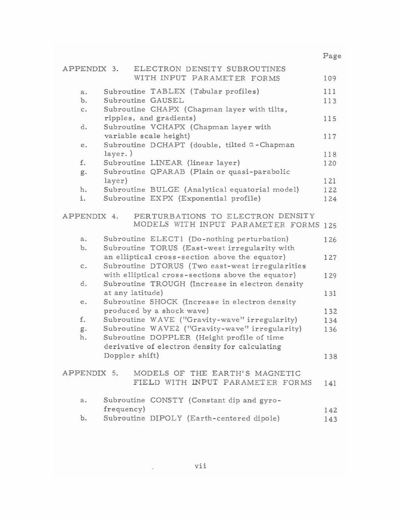
APPENDIX 3. ELECTRON DENSITY SUBROUTINES WITH INPUT PARAMETER FORMS
a. b. c.
d.
e.
f. g.
h. i.
Subroutine T ABLEX {Tabular profiles} Subroutine GAUSEL Subroutine CHAPX {Chapman layer with tilts, ripple s, and gradients} Subroutine VCHAPX {Chapman layer with variable scale height} Subroutine DCHAPT {double, tilted a -Chapman layer. } Subroutine LINEAR {linear layer} Subroutine QPARAB {Plain or quasi - parabolic layer} Subroutine BULGE {Analytical equatorial model} Subroutine EXPX {Exponential profile}
Page
109
111 113
115
117
118 120
121 122 124
APPENDIX 4. PERTURBATIONS TO ELECTRON DENSITY MODELS WITH INPUT PARAMETER FORMS 125
a. b.
c.
d.
e.
f. g. h.
Subroutine ELECTl {Do - nothing perturbation} Subroutine TORUS {East-west irregularity with an elliptical cross-section above the equator} Subroutine DTORUS {Two east-west irregularities with elliptical cross-sections above the equator} Subroutine TROUGH {Increase in electron density at any latitude} Subroutine SHOCK {Increase in electron density produced by a shock wave} Subroutine WAVE {"Gravity-wave" irregularity} Subroutine W A VE2 {"Gravity - wave" irregularity} Subroutine DOPPLER {Height profile of time derivative of electron density for calculating Doppler shift}
APPENDIX 5. MODELS OF THE EARTH'S MAGNETIC FIELD WITH INPUT PARAMETER FORMS
a.
b.
Subroutine CONSTY {Constant dip and gyrofrequency} Subroutine DIPOLY {Earth - centered dipole}
vii
126
127
129
131
132 134 136
138
141
142 143
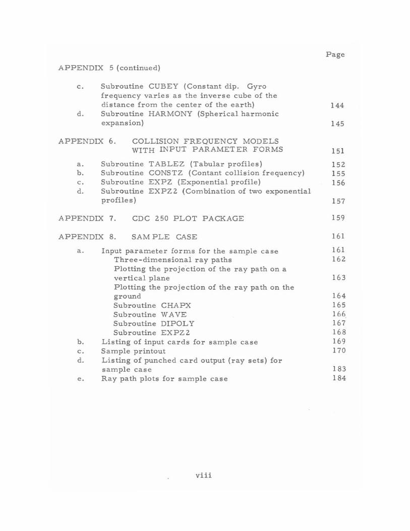
APPENDIX 5 (continued)
c. Subroutine CUBEY (Constant dip. Gyro frequency varies as the inverse cube of the distance from the center of the earth) Subroutine HARMONY (Spherical harmonic d. expansion)
APPENDIX 6. COLLISION FREQUENCY MODELS WITH INPUT PARAMETER FORMS
a. b. c . d.
Subroutine T ABLEZ (Tabular profiles) Subroutine CONSTZ (Contant collision frequency) Subroutine EXPZ (Exponential profile) Subroutine EXPZ2 (Combination of two exponential profile s)
APPENDIX 7. CDC 250 PLOT PACKAGE
APPENDIX 8. SAMPLE CASE
a.
b. c. d.
e.
Input parameter forms for the sample case Three-dimensional ray paths Plotting the projection of the ray path on a vertical plane Plotting the projection of the ray path on the ground Subroutine CHAPX Subroutine WAVE Subroutine DIPOL Y Subroutine EXPZ2
Listing of input cards for sample case Sample printout Listing of punched card output (ray sets) for sample case Ray path plots for sample case
viii
Page
144
145
151
152 155 156
157
159
161
161 162
163
164 165 166 167 168 169 170
183 184
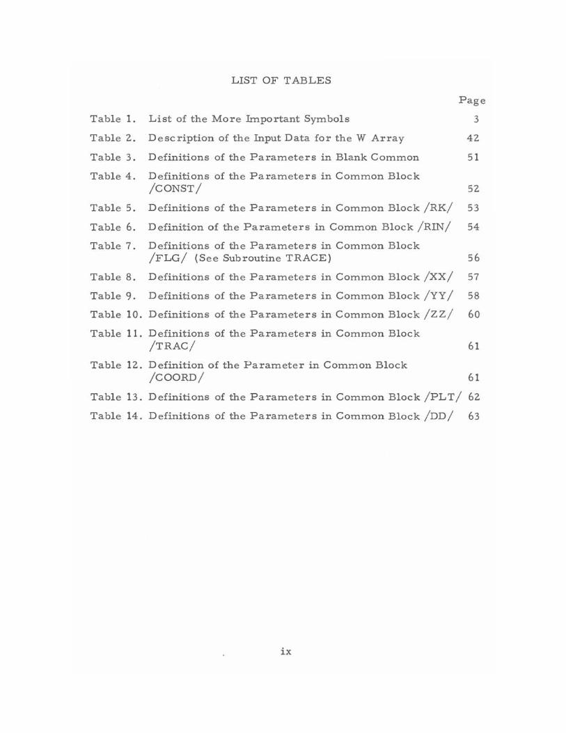
LIST OF TABLES
Pag e
Table 1. List of the More Important Symbols 3
Table 2. Description of the Input Data for the W Array 42
Table 3. Definitions of the Paramet e rs in Blank Common 51
Table 4. Definitions of the Paramet er s in Common Block /CONST/ 52
Table 5. Definitions of the Paramete rs in Common Block /RK / 53
Table 6. Definition of the Paramet e rs in Common Block /RIN/ 54
Table 7. Definitions of the Paramete rs in Common Block /FLG/ (S ee Subroutine TRACE) 56
Table 8. Defihitions of the Paramete rs in Common Block /XX/ 57
Table 9 . Definitions of the Parameters in Common Block /YY / 58
Table 10. Definitions of the Parameters in Common Block / ZZ / 60
Table 11. Definitions of the Parameters in Common Block /TRAC/ 61
Table 12. Definition of the Parameter in Common Block /COORD/ 61
Table 13. Definitions of the Paramete rs in Common Block / PLT / 62
Table 14. Definitions of the Paramete rs in Common Block /DD/ 63
ix
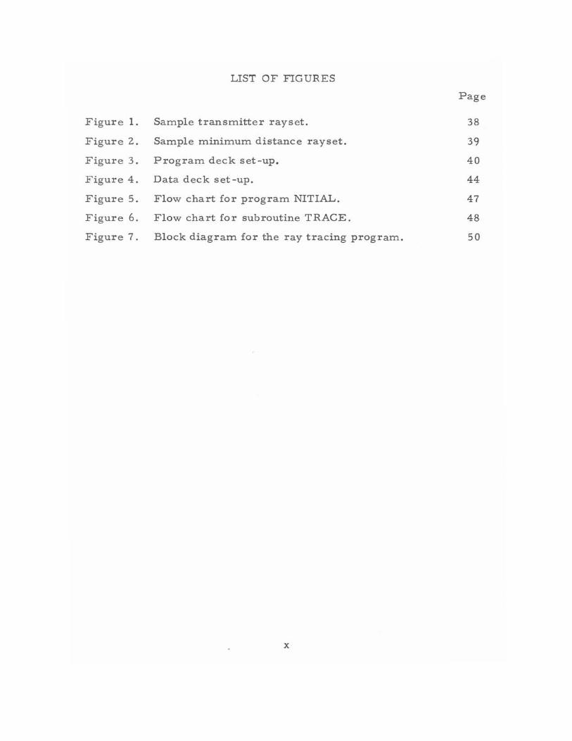
LIST OF FIGURES
Figure 1. Sample transmitter rayset.
Figure 2. Sample minimum distance rayset.
Figure 3. Program deck set-up.
Figure 4. Data deck set-up.
Figure 5. Flow chart for program NITIAL.
Figure 6. Flow chart for subroutine TRACE.
Figure 7. Block diagram for the ray tracing program.
x
Page
38
39
40
44
47
48
50
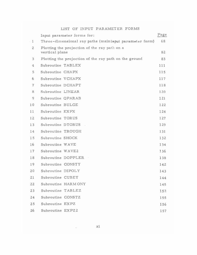
LIST OF INPUT PARAMETER FORMS
Input parameter forms for: Page
1 Three - dimensional ray paths (main i"put parameter form) 68
2 Plotting the projection of the ray path on a
vertical plane 82
3 Plotting the projection of the ray path on the ground 83
4 Subroutine TABLEX 111
5 Subroutine CHAPX 115
6 Subroutine VCHAPX 117
7 Subroutine DCHAPT 118
8 Subroutine LINEAR 120
9 Subroutine QPARAB 121
10 Subroutine BULGE 122
11 Subroutine EXPX 124
12 Subroutine TORUS 127
13 Subroutine DTORUS 129
14 Subroutine TROUGH 131
15 Subroutine SHOCK 132
16 Subroutine WAVE 134
17 Subroutine WAVE2 136
18 Subroutine DOPPLER 138
19 Subroutine CONSTY 142
20 Subroutine DIPOLY 143
21 Subroutine CUBEY 144
22 Subroutine HARMONY 145
23 Subroutine TABLEZ 152
24 Subroutine CONSTZ 155
25 Subroutine EXPZ 156
26 Subroutine EXPZ2 157
xi

"
A VERSATILE THREE-DIMENSIONAL RAY TRACING COMPUTER PROGRAM FOR RADIO WAVES
IN THE IONOSPHERE
* ::;,* R. Michael Jones and Judith J. Stephenson
This report describes an accurate, versatile FORTRAN computer program for tracing rays through an anisotropic medium whose index of refraction varies continuously in three dimensions. Although developed to calculate the propagation of radio waves in the ionosphere, the program can be easily modified to do other types of ray tracing because of its organi zation into subroutines.
The program can represent the refractive index by either the Appleton-Hartree or the Sen-Wyller formula, and has several ionospheric models for electron density, perturbations to the electron density (irregularities), the earth's magnetic field, and electron collision frequency.
For each path, the program can calculate group path length, phase path length, absorption, Doppler shift due to a time-varying ionosphere, and geometrical path length. In addition to printing the3e parameters and the direction of the wave normal at various points along the ray path, the program can plot the projection of the ray path on any vertical plane or on the ground and punch the main characteristics of each ray path on cards.
The documentation includes equations, flow charts, program listings with comments, definitions of program variables, deck set-ups, descriptions of input and output, and a sample case.
Key words: Ray tracing, computer program, radio waves, ionosphere, three-dimensional, AppletonHartree formula, Sen-Wyller formula.
The author is with the National Oceanic and Atmospheric Administra -tion, U. S. Department of Commerce, Boulder, Colorado 80302.
** The author is with the Institute for Telecommunication Sciences, Office of Telecommunications, U. S. Department of Commerce, Boulder, Colorado 80302.
1. INTRODUCTION
This report describes a three-dimensional ray tracing program
written in FORTRAN language for the CDC - 3800 computer. Copies of
the program deck are available from the Institute for Telecommunication
Sciences.
Earlier versions of this program have been in use now for over nine
years, both by us and by people scattered all over the world. During that
time we have improved and modified the program to the extent that we now
need to document these changes so that the present program will be easier
to use. We have included the input parameter forms that we use to request
ray path calculations because they give nearly all the neces sary input data
and describe the electron density, collision frequency, and magnetic field
models.
2. GENERAL DESCRIPTION
This computer program traces the path of radio wave through a
user-specified model of the ionosphere when given the transmitter location
(longitude, latitude, and height above the ground), the frequency of the
wave, the direction of transmission (both elevation and azimuth), the
receiver height, and the maximum number of hops wanted.
3. RAY TRACING EQUATIONS
T he program calculate s ray paths by numeri cally integrating
Hamilton's equations. Lighthill (1965) gives Hamilton's equations in
four dimensions (three spatial and one time) for Cartesian coordinates.
Haselgrove (1954) give s Hamilton's equations in three dimensions for
spherical polar coordinates. Combining the two gives Hamilton's
equations in four dimensions in which the three spatial coordinates are
spherical polar (see Table 1 for a definition of the symbols):
dr = oH d,. 0 k
r
2
(1 )
A
B a
c
C
e
F( w )
f
M
m
N
n
n'
P
P'
r,
s
S
e, cp
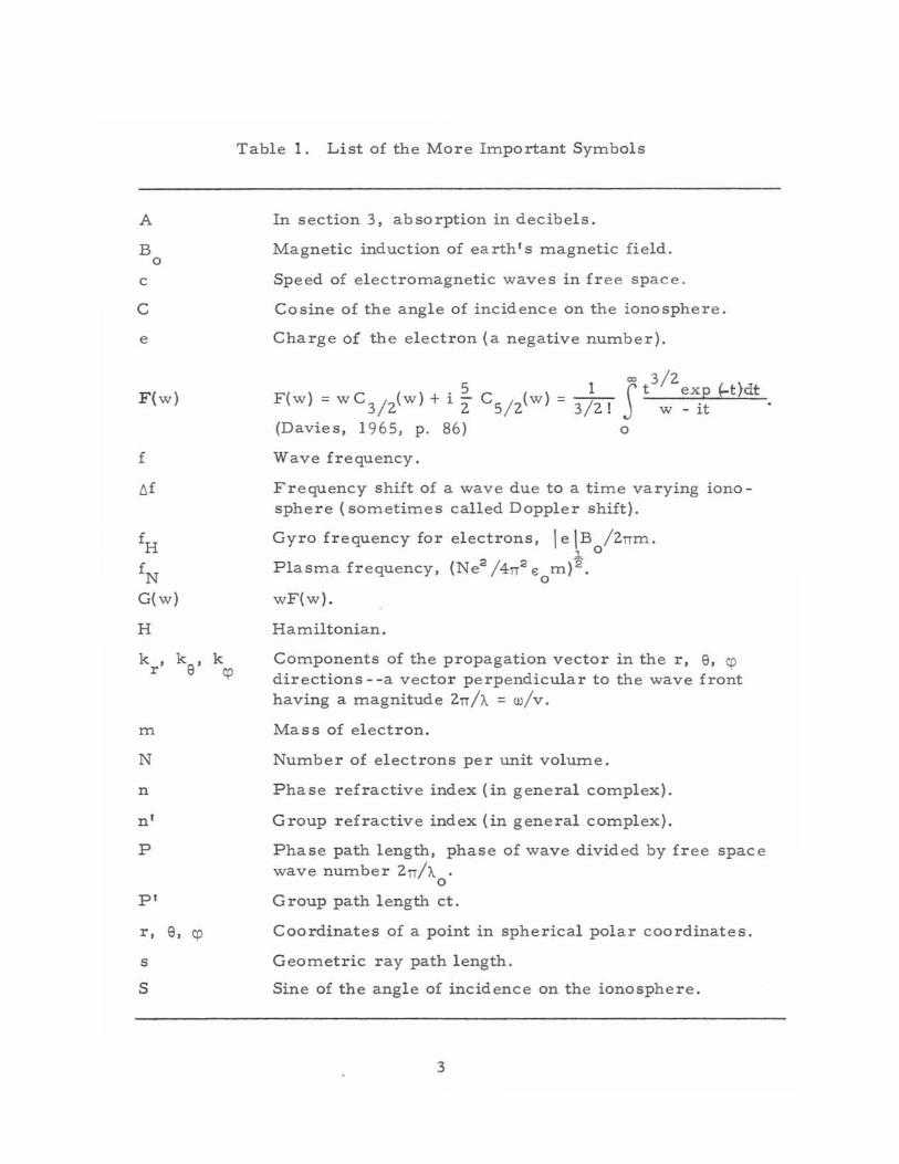
Table 1. List of the More Important Symbols
In section 3, absorption in decibels.
Magnetic induction of earth's magnetic field.
Speed of electromagnetic waves in free space.
Cosine of the angle of incidence on the ionosphere.
Charge of the e l ectron (a negative number) .
'" 3 /Z - . ~ __ 1 _ S t exp ~t}dt
F(w) - wC 3 / Z(w) + 1 Z C 5/ Z(w) - 3/Z! w _ it
(Davies, 1965, p. 86) a
Wave frequency.
Frequency shift of a wave due to a time varying ionosphere (sometimes called Doppler shift).
Gyro frequency for electrons, Ie IB / Znm. ~ a
Plasma frequency, (NeE /4n2 e mfE. a
wF(w).
Hamiltonian.
Components of the propagation vector in the r, e, cp directions - - a vector perpendicular to the wave front having a magnitude Zn/'A = w/v.
Mass of electron.
Number of electrons per unit volume.
Phase refractive index (in general complex).
Group refractive index (in general complex).
Phase path length, phase of wave divided by fr ee space wave number Zn/'A .
a Group path length ct.
Coordinates of a point in spherical polar coordinates.
Geometric ray path length.
Sine of the angle of incidence on the ionosphere.
3
t
u
v
1.)
1.) m
co
w
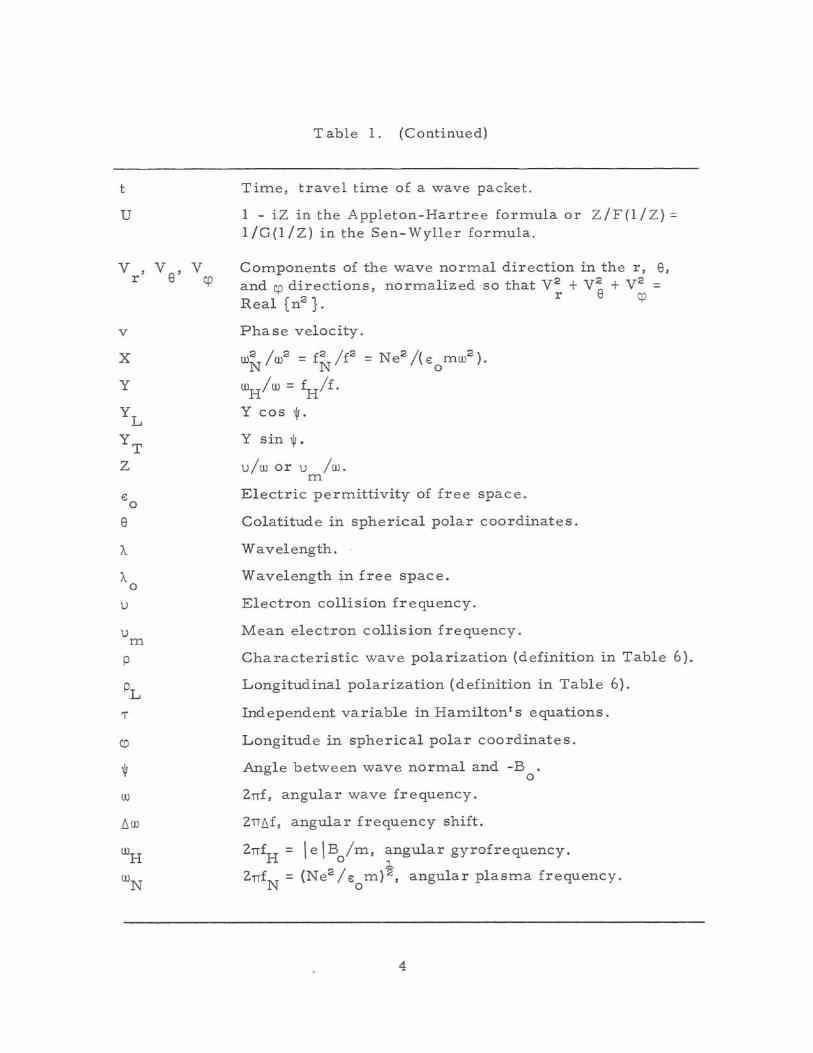
Table 1. (Continued)
Time, travel time of a wave packet.
I - iZ in the Appleton - Hartree formula or Z/F(l / Z) = l/G(l/Z) in the Sen - Wyller formula.
Components of the wave normal direction in the r, e, and cp directions, normalized so that y2 + y~ + y2 = Real [n2}. r cp
Phase velocity.
w2 Iw2 = f2 /f2 = Ne 2 /(e mw2 ). N N 0
wH/w = fH/£.
Y cos 1jI .
Y sin 1jI .
1.)/w or 1.) Iw . m
Electric permittivity of free space.
Colatitude in spherical polar coordinates.
Wavelength.
Wavelength in free space.
Electron collision frequency.
Mean electron collision frequency.
Characteristic wave polarization (definition in Table 6).
Longitudinal polarization (definition in Table 6).
Independent variable in Hamilton's equations.
Longitude in spherical polar coordinates.
Angle between wave normal and -B . o
2TTf, angular wave frequency.
2TTllf, angular frequency shift.
Ie IB 1m, angular gyrofrequency. o ~
(Ne2 /e m)2, angular plasma frequency. o
4
dk r
dk 1 ----.Sf! - ----''-dT - r sine
=
de =.!. oH dT r oke
,
~= 1 oH dT r sine ok
cp
dt _ oH -
dT oW
oH de ~ or tke dT t kcp sine dT
( oH . dr de ) - - - k SIne - - k r cose - , ocp cp dT CD dT
dw oH dT - ot
(2)
(3)
(4 )
(5)
( 6)
(7)
( 8)
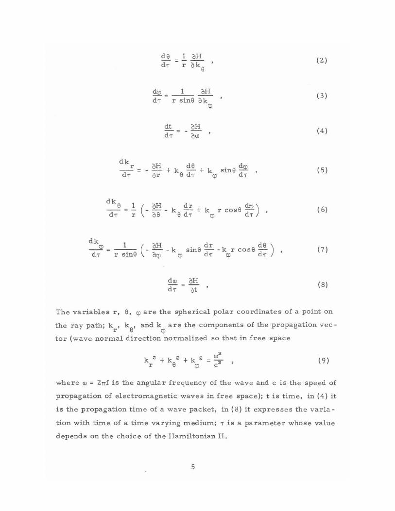
The variables r, e, cp are the spherical polar coordinates of a point on
the rav path; k , k , and k are the components of the propagation vec-, r e cp
tor (wave normal direction normalized so that in free space
WE k 2 tk E tk 2 =""2
r e cp c (9)
where w = 2TTf is the angular frequency of the wave and c is the speed of
propagation of electromagnetic waves in free space); t is time, in (4) it
is the propagation time of a wave packet, in (8) it expresses the varia-
tion with time of a time varying medium; T is a parameter whose value
d epends on the choice of the Hamiltonian H.
5
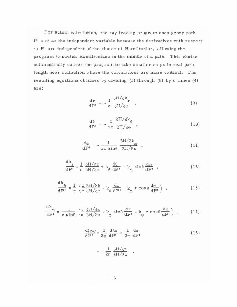
For actual calculation, the ray tracing program uses group path
F' = c t as the independent variable because the derivatives with respect
to F' are independent of the c hoice of Hamiltonian, allowing the
program to switch Hamiltonians in the middle of a path. T hi s choice
automatically causes the program to take smaller steps in real path
length near reflection where the calculations are more critical. The
resulting equations obtained by dividing (1) through (8) by c times (4)
are:
dk e dF'
dr dF' =
de dF'
~=
=
1 dF' rc sine
dk __ r = 1.. oH/or + k ~ + k sine dd
FCQ ,
dF' cOR/oW e dF' cp
1 (1.. oH/oe dr d co ) r c oH/ow - ke dF' + kcp r cose dF' '
dk 1 ----.CO. = _:::..-.,. dF' r s i ne (~ oH/oco
oH/ow
dIM) 1 dllw 1 dw -- = --- = ---dF' 2n dF' 2n dF'
= _ ~ oH/ot 2n oH/ow
6
(9)
( 10)
( 11)
(12)
(13 )
( 14)
(15 )
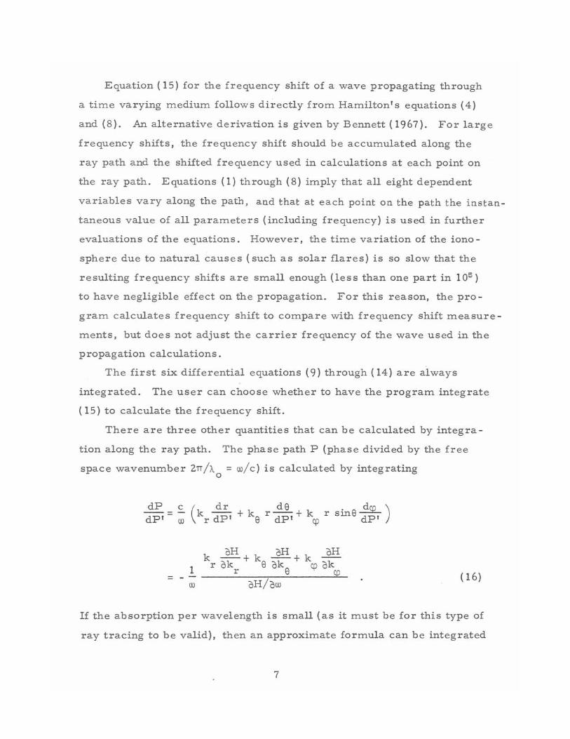
Equation ( 15) for the frequency shift of a wave propagating through
a time varying medium follows directly from Hamilton's equations (4)
and (8). An alternative derivation is given by Bennett (1967). For large
frequency shifts, the frequency shift should be accumulated along the
ray path and the shifted frequency used in calculations at each point on
the ray path. Equations (1) through (8) imply that all eight dependent
variables vary along the path, and that at each point on the path the instan
taneous value of all parameters (including frequency) is used in further
evaluations of the equations. However, the time variation of the iono
sphere due to natural causes (such as solar flares) is so slow that the
resulting frequency shifts are small enough (less than one part in 105 )
to have negligible effect on the propagation. For this reason, the pro
gram calculates frequency shift to compare with frequency shift measure
ments, but does not adjust the carrier frequency of the wave used in the
propagation calculations.
The first six differential equations (9) through (14) are always
integrated. The user can choose whether to have the program integrate
(15) to calculate the frequency shift.
There are three other quantities that can be calculated by integra
tion along the ray path. The phase path P (phase divided by the free
space wavenumber 2TC/A = w/c) is calculated by integrating o
dP -
dP'
oH oH oH kr ok + ke ok + k ok
1 r e cP CO
w oH/ow ( 16) =
If the absorption per wavelength is small (as it must be for this type of
ray tracing to be valid), then an approximate formula can be integrated
7
to give the absorption in decibels
dA dP' =
ul lOw imag (~ n')
log 10 c k 2 + k' + k 2 ere cp
w' 10 imag (~n2)
= ,..-'::"":':-:- ----,.-----iC---,,log 10 k' +k' +k' ere cp
dP dP'
c oH/ow ( 17)
whe re n is the (complex) phase refractive index. The geometrical path
length of the ray can be calculated by integrating
ds (~)' + de 2
2 . 2 (deo )' = r2 (dP') + r Sln e dP' dP' dP'
j (::)2 OHt (:: )' + ( oke
+ r co (18) = oH/ow c
The user can choose to have frequency shift, phase path, absorption,
or p ath length calculated using equations (15), (16), (17), or (18) and
printed by setting the appropriate value in the input W array. (W59,
W57, W58, w60 in Table 2.)
If the user wants to add differential equations to the program, he
can do so by modifying subroutine HAMLTN, which evaluates Hamil
ton's equations.
The Hamiltonian and its derivatives are calculated by one of the
versions of subroutine RINDEX, which also calculates the phase refrac
tive index and its derivatives.
4. CHOOSING AND CALCULATING THE HAMILTONIAN
Because Hamilton's equations guarantee that the Hamiltonian is con-
stant along the ray path and because it is desirable to have the dispersion
8
relation satisfied at each point on the ray path, it is usual to write the
dispersion relation in the form H = constant and choose that H as the
Hamiltonian. Two problems arise. First, in a lossy medium the dis
persion relation is complex, so that the resulting complex Hamiltonian
gives ray paths having complex coordinates when used in Hamilton's
equations. Second, in some cases some forms of the dispersion rela
tion have computational advantages over others when used as a Hamil
tonian.
Allowing the coordinates of the ray path to assume complex values
is called ray tracing in complex space (Budden and Jull, 1964; Jones,
1970; Budden and Terry, 1971) which is the extension to three dimen
sions of the phase integral method (Budden, 1961). Ray tracing in
complex space is necessary to calculate the propagation of LF radio
waves in the D region of the ionosphere (Jones, 1970), and it may also
be needed for some medium frequencies.
However, the effect of losses on the ray path of HF radio waves in
the ionosphere is probably small, so that the only effect of losses
is to attenuate the signal. For this case, then, it is desirable to find a
prescription for calculating ray paths having real coordinates. Several
methods exist for doing this, and except for computational difficulties,
one is probably as good as another. One should recognize that along
the ray path:
(1) the dispersion cannot be exactly satisfied, or
(2) Hamilton's equations cannot be satisfied, or
(3) both of the above.
In our program, we have chosen to keep Hamilton's equations and re
quire only the real part of the dispersion relation to be satisfied,
neglecting the imaginary part. Another approach (Suchy, 1972) is to
alter Hamilton's equations so that the full complex dispersion relation
is still satisfied along a ray path having real coordinates. Weare
9
reasonably certain that for any situation in which Suchy's method gives
significantly different answers from ours, neither method is valid;
ray tracing in complex space or an equivalent method would then be
r equired.
Thre e choices for the Hamiltonian illustrate the computational dif
ficulties involved. Haselgrove (1954) used the following Hamiltonian
c H=
Ul real (n) - 1 (19)
which, except for the effects of errors in the numerical integration and
the value of the independent variable, is equivalent to
H 1 - Ul r eal (n) = ~ c (k 2 + k 2 + k 2 )"
r e Cjl
real {I - ~ n
+ k 2)~ } ( ZO) =
(k 2 + k 2 r e Cjl
There are eight versions of the subroutine RIND EX which calculate
the Hamiltonian and its partial derivatives. (Eight versions allow the
US er to choose the Appleton-Hartree formula or the Sen-Wyller formula,
and to include or ignore the earth's magnetic field and collisions. ) Six of
thes e versions (subroutines AHWFWC, AHWFNC, AHNFWC, AHNFNC,
SWWF, and SWNF) use the following Hamiltonian:
real (n2»)
1 { I (c 2 (k 2 + ke2 + kr~ ) _ n2)} . = r ea 2' ;;(' r 't'
(Z 1)
The other two versions (subroutines BQWFWC and BQWFNC) USe as a
Hamiltonian the r eal part of the quadratic equation whose solution is
the Appleton -Hartree formula (Budden, 1961)
10
H = real {[(U -X) U 2 _y 2 U] c 4 k4 +X(k. y)2 c 4 k" +
+ [-2U(U -X)" + y2(2U -X)] c"k2 w" -X(k· Y)" c"w2 +
( 22)
except in or near free space (defined by X < o. 1) where they also use
(21) as the Hamiltonian. In (22), U = 1 - iZ, and X, Y, and Z are the
,usual magnetoionic parameters.
In a lossy medium, the Hamiltonians in (20), (21), and (22) determine
slightly different ray paths, but the differences are significant only when
it is no longer valid to represent ray paths with coordinates that are
real rather than complex. In fact, this is a weak criterion. The ray
paths determined by these three Hamiltonians will become invalid be
fore there are noticeable differences between the three ray paths. In
a lossless medium, the above three Hamiltonians determine identical
ray paths (except for integration errors).
For either a lossy or lossless medium, some of the above three
Hamiltonians have computational difficulties. Special care must be
taken in using (19) or (20) in an evanescent region (which is frequently
necessary at or near vertical incidence because the numerical integra
tion subroutine usually requires the evaluation of the differential equa
tions not only on the ray path, but also at points near the ray path). For
instance, in a lossless medium, real (n) is zero in an evanescent
region, which leads to problems in (19) and (20). This problem will
not arise in (21) because real (n") is well behaved in or at the boundary
of an evanescent region, nor will it occur in using (22).
Neither (20) nor (21) (nor any other Hamiltonian based on the refrac
tive index) will work for a ray passing through,a spitze (Davies, 1965,
p. 202) because the refractive index is indeterminate at a spitze, and
11
some of the derivatives of n diverge. So far, we have had no problems
using (22) to calculate ray paths through a spitze with or without
collisions.
However, the Hamiltonian in (22) will not work in or near free space
because all of its derivatives are zero in free space. This problem is
related to (22) not being able to distinguish between ordinary and extra
ordinary waves. To get started, the program uses (21) until the elec
tron density is large enough that X is equal or greater than 1/l0.
As far as we can tell, the AHWFWC (Appleton-Hartree, with field,
with collisions) version of subroutine RINDEX has been made obsolete
by the BQWFWC (Booker quartic, with field, with collisions) version .
The latter will do everything the AHWFWC version will do and in addi
tion it will calculate rays through spitzes . A few trial runs, however,
indicate that AHWFWC runs about 30 percent faster than BQWFWC.
Similarly, the AHWFP#C (Appleton-Hartree, with field, no c~lli sions) version has been made obsolete by the BQWFNC ve rsion, which
apparently runs just as fast as the AHWFNC version. We are continu
ing to include the AHWFNC version just in case there are undiscovered
problems with the BQWFNC version.
In addition to the Appleton-Hartree formula, which is based on a
constant co llision frequency, the program also includes the generalized
formula of Sen and Wyller (1960), which assumes a Maxwell - Boltzman
distribution of electron energy and a collision frequency proportional to
energy. Two versions of subroutine RINDEX use the Sen-Wyller formula
for calculating the refractive index and the resulting Hamiltonian with
its derivatives. These are SWWF, which includes the effects of the
earth's magnetic field, and SWNF, which neglects the Earth's magnetic
field. The SWWF version will probably not work for calculating rays
through a spitze . It would be possible to make a version which used as
12
its Hamiltonian the quadratic equation whose solution is the Sen-Wyller
formula for calculating rays through a spitze, but it is unlikely that we
will ever do that .
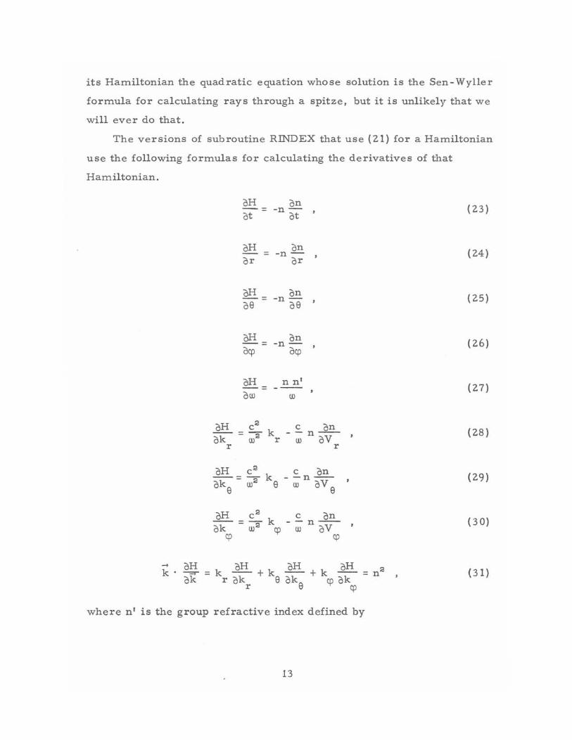
The versions of subroutine RINDEX that use (21) for a Hamiltonian
use the fo llowing formulas for calculating the derivatives of that
Hamiltonian .
k·
oH at
oH
on -n-
ot
on = -n-
oH ok
r
o r
oH = 09
oH -= ocp
oH -= oW
or
on -n-09
on -n-ocp
n n ' W
c on -- n--
W oV r
c on - -n--
W oV 9
c on k --n--
cp W oV cp
~ = k oH ok r ok
r
k oH koH + -- + --9 ok9 cp ok cp
where n ' is the group refractive index defined by
13
(23)
(24)
(25 )
(26 )
(27)
(28)
(29)
(30)
(31 )
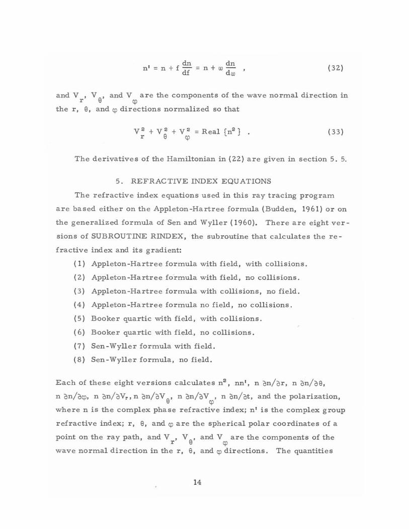
dn n' = n + f - =
df dn n+ wdw
(32)
and V , V , and V are the components of the wave normal direction in r e cp
the r, e, and cp directions normalized so that
(33)
The derivatives of the Hamiltonian in (22) are given in section 5. 5.
5. REFRACTIVE INDEX EQUATIONS
The refractive index equations used in this ray tracing program
are based either on the Appleton -Hartree formula (Budden, 1961) or on
the generalized formula of Sen and Wyller (1960). There are eight ver
sions of SUBROUTINE RINDEX, the subroutine that calculates the re
fractive index and its gradi ent:
(1) Appleton-Hartree formula with field, with collisions.
(2) Appleton-Hartree formula w ith field, no collisions.
(3) Appleton-Hartree formula with collisions, no field.
(4) Appleton -Hartree formula no field, no collisions.
(5) Booker quartic with field, with collisions.
(6) Booker quartic with field, no collisions.
(7) Sen -Wyller formula with field.
(8) Sen-Wyller formula, no field.
Each of these e ight versions calculates n 2, nn', non/or, n on/oe,
n on/ocp, n on/oVr , n on/oV , n on/oV , n on/at, and the polarization, e cp where n is the complex phase refractive index; n' is the complex group
refractive index; r, e, and cp are the spherical polar coordinates of a
point on the ray path, and V , V , and V are the components of the r e cp
wave normal direction in the r, e, and cp directions. The quantities
14
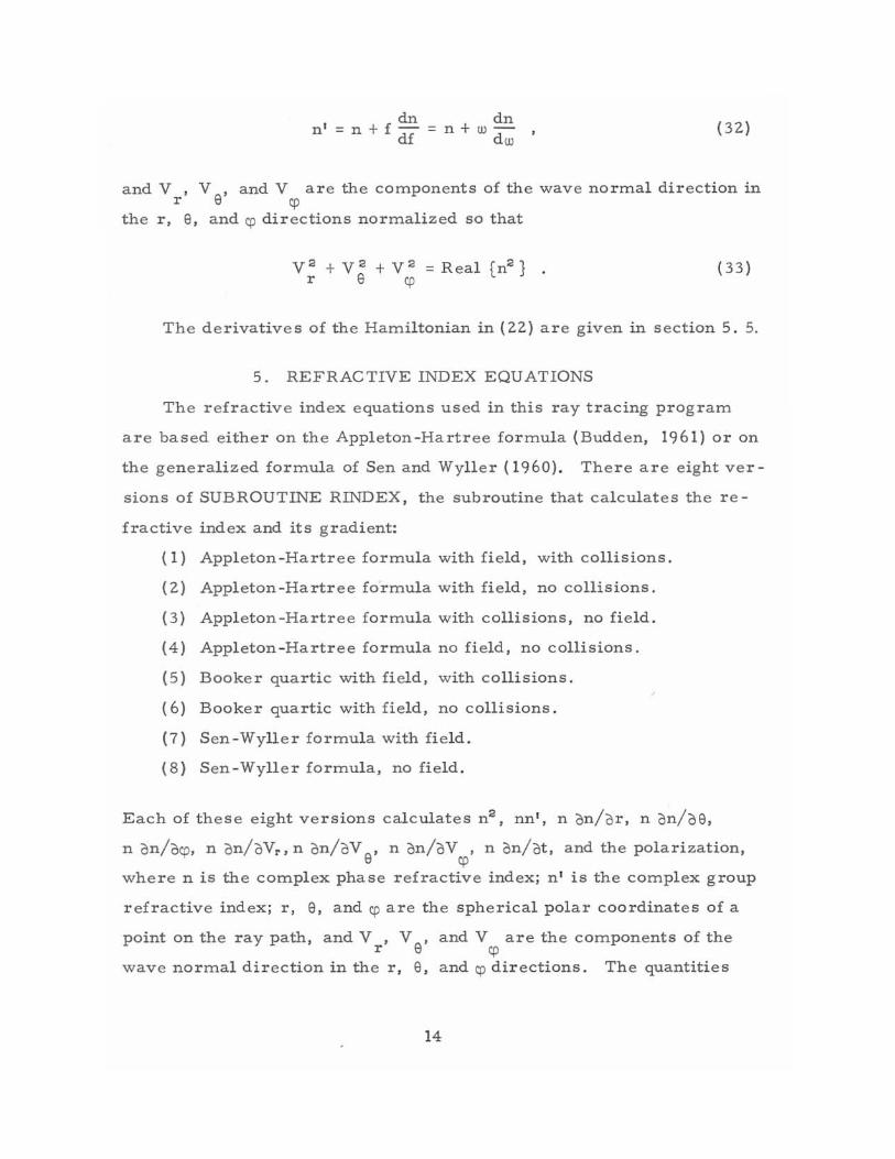
dn n' = n t f - =
df dn
ntwdw
( 32)
and V , V , and V are the components of the wave normal direction in r e cp
the r, e, and cp directions normalized so that
(33)
The derivatives of the Hamiltonian in (22) are given in section 5. 5.
5. REFRACTIVE INDEX EQUATIONS
The refractive index equations used in this ray tracing program
are based either on the Appleton-Hartree formula (Budden, 1961) or on
the generalized formula of Sen and Wyller (1960). There are eight ver
sions of SUBROUTINE RINDEX, the subroutine that calculates the re-
fractive index and its gradient:
(1) Appleton-Hartree formula with field, with collisions.
(2) Appleton-Hartree formula with field, no collisions.
(3) Appleton-Hartree formula with collisions, no field.
(4) Appleton -Hartree formula no field, no collisions.
(5) Booker quartic with field, with collisions.
(6) Booker quartic with field, no collisions.
(7) Sen-Wyller formula with field.
(8) Sen-Wyller formula, no field.
Each of these eight versions calculates n 2, nn', non/or, n on/oe,
n on/ocp, n on/oVr. n on/oV , n on/oV , n on/ot, and the polarization, e cp where n is the complex phase refractive index; n' is the complex group
refractive index; r, e, and cp are the spherical polar coordinates of a
point on the ray path, and V , V , r e
wave normal direction in the r, e, and V are the components of the
cp and cp directions. The quantities
14
x, oX/or, oX/09, oX/oep, and oX/ot are supplied by one of the versions
of subroutine ELECTX which defines the electron density model. The
quantities Y, oY/or, oY!o9, oY/acp, Y , oY /o r, oY /09, oY /oep, r r r r
Y9
' oY /or, oY /09, oy /oep, Y , oY /o r, oYep/09, and oY /oep are 9 9 ep ep ep ep
supplied by one of the versions of subroutine MAGY which defines the
magnetic field model. The quantities Z, oZ/or, oZ/09, and oZ/oep are
supplied by one of the versions of subroutine COLFRZ which defines
the collision frequenc y model.
In our formulation, we have tried to avoid using multivalued -1
functions, such as the square root or cos ,wherever possible. Only
twice do we use the square root. One instance is the square root in the
Appleton-Hartree formula, unavoidable without adding more differential
equations to the system. The second instance is a square root used to
calculate polarization. T his latter use is unimportant becaus e the
polarization is not used in the ray tracing equations .
It is desirable to avoid multivalued functions because, unless
extreme care is us ed, the value of such a function can c hange discon-
tinuously from one point on the ray path to the next. A particularly
troublesome case occurs at reflection for vertical incidence. At that 2
point, the real part of n goes through zero, and n c hanges from
approximately purely real to approximately purely imaginary. Since
the numerical integration subroutine usually requires the evaluation of
the differential equations not only on the ray path, but also at points
near the ray path, it is necessary to be able to evaluate the differential
equations above the reflection height, that is, in an evanescent region.
We have found that it is possible to regroup the variables in the
equations to avoid this problem: we calculate the real part of n 2 and
its derivatives instead of the real part of n and its derivatives. And
we calculate nn I instead of I
n .
15
It was not easy to avoid using lllultivalued functions, however. Many
of the usual parallleters used to cOlllpute the refractive index require the
use of lllultivalued functions in their calculation. Thus, we couldn't
calculate
v = ~ V~ + V~ + V~ nor cos 1\1, nor sin 1\1, where 1\1 i s the angle between the wave norlllal
direction and the earth's lllagnetic field. Thus, we also could not
calculate
nor
Y L = Y cos 1\1
Y = Y sin 1\1 T
The lllOSt difficult part of avoiding the use of lllultivalued functions was
in calculating the derivatives.
The following is a list of the equations calculated by the e ight versions
of subroutine RINDEX.
5 . 1 Appleton -Hartree Forlllula with Field, with Collisions
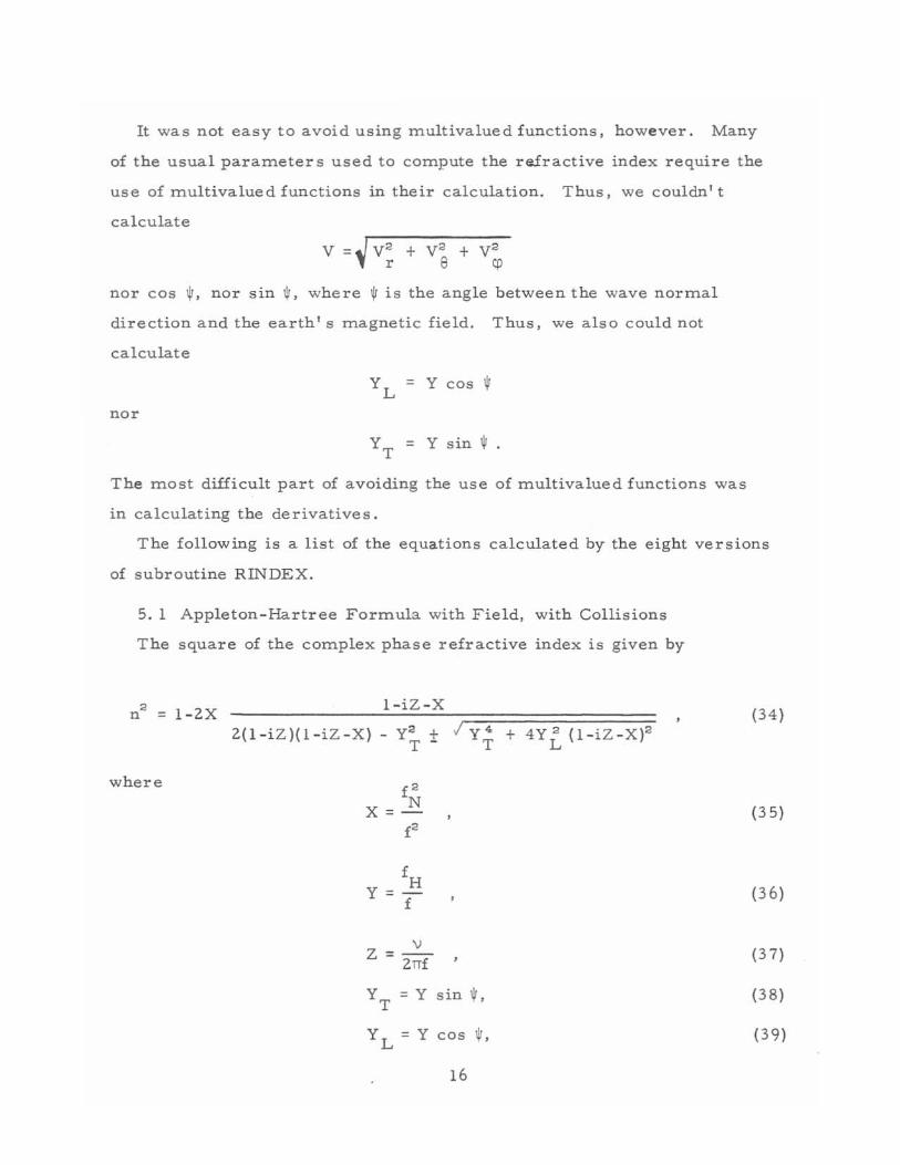
The square of the cOlllplex phase refractive index is given by
n2 = 1-2X l-iZ - X
2(l-iZ)(1-iZ -X) - Y~ ± j Y~ + 4Yt, (l-iZ-X)2
where
Y=
Z v
=--2n f
YT
= Y s in 1\1 ,
YL
= Y cos 1\1 ,
16
(34)
(35)
(36)
(37)
(38)
(39)
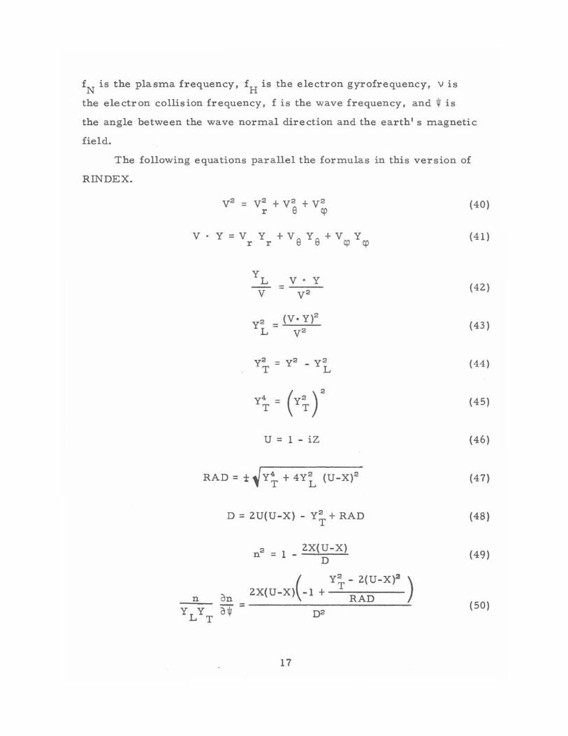
fN is the plasma frequency, fH is the electron gyrofrequency, v is
the electron collision frequency, f is the wave frequen cy, and $ is
the angle between the wave normal direction and the earth's magnetic
field.
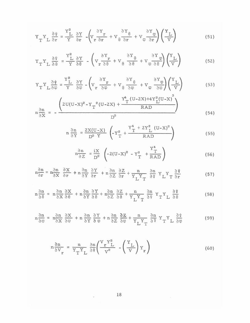
The following equations par a llel the formulas in thi s version of
RINDEX.
= y 2 + y2 + y2 r 8 cp
y . Y = Y Y r r
YL Y
y 2 L
=
y . Y = y2
(y. y)2
y 2
y2 = y2 _ y2 T L
U = 1 - iZ
RAD = ± ~/y4 + 4y2 (U_X)2 , T L
D = 2U(U-X) - y~ + RAD
n 2 = 1 _ 2X(U-X) D
( y2 2(U-X)2)
n an 2X(U-X) -1 + T RAD =------------~~--~
YLYT ~ D2
17
(40)
(41 )
(42 )
(43)
(44 )
(45 )
(46)
(47)
(48)
(49)
(50)
Y Y ~ = Y~ OY T Lor Y or
_ V _r_ + V __ + v.-5£. --.!::.. (
oY oY 8 oY ) (Y ) r or 8 or cp or V
Y Y 2! T L 08
y2
Y Y ~=~ T L oCP Y
oY (OYr oY 8 OYcp) (Y L) -- V --+ V --+V -- --ocp r ocp 8 ocp cp ocp V
3
2U(U-X)2_Y 2(U_2X) + T L T RAD ·
on naX
( Y' (U-2X)+4y2 (U-X) )
- - ~----------------'
on = 2X(U -X) n oY 02 Y
_y2 + T L (
y4 + 2y2 (U_X)2)
T RAD
on n
oZ i X ( = - 2(U _X)2 - y2T D2
+ T y4 )
RAD
on on AX on oY n-=n- -+n-- on Y Y II
01\1 L T o r or AX or oY o r
on n- =
08
on n- =
oCP
on AX on oY on oZ n n a X as + n a Y a 8 + no Z 0 8 + Y L Y T
on Y Y ~ 01\1 T L 08
on Y Y .z.1 o'l' T L ocp
on n-- = oV
r
on r L L (V y2 (Y) ) aT V 2 - V Yr
18
(51 )
(52)
(53)
(54)
(55)
(56)
(57)
(58)
(59)
(60)
2
-CvL~ Ye ) on n on Ce
:2L n oV = ~ Y Y
e L T
on n on ~ L =
(V y2 -(Yv
L ) Y~) nay-
YLY T oW V2
~
, 2 ( o n nn = n - 2Xn oX +Yn -+ Zn -on on) o y o Z
(-Y~ + RAD) J V2
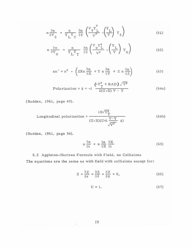
Polarization = p = -i 2(U-X) V . Y
(Budden, 1961, page 49).
iX,JYT Longitudinal polarization = ----....;.:,,:----
(U-X)(U+i V· Y p) Jv2
(Budden, 1961, page 54) .
on n
ot on oX
=n--oX ot
5.2 Appleton-Hartree Formula with Field, no Collisions
The equations are the same as with field with collisions except for:
Z = o Z = o Z = oZ = 0, or oe o~
U=l.
19
(61 )
(62)
(63)
(64a)
(64b)
(65 )
(66 )
(67)
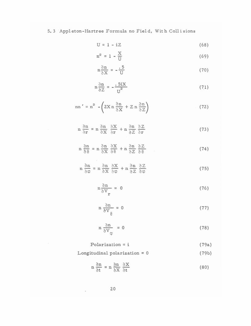
5. 3 Appl eton-Hartree Formula no Fiel d, Wit h Coll i sions
u = 1 - i2
n 2 1 X
= U
21 n . 5 n- =
21 X U
21 n . 5iX n 2l2 = -7
, 2 nn = n
( 21 n o n) - 2Xn- + 2n -21X 212
21 n 21 n 21 X 21 n 21 2 n-=n- +n--
21 r 21X 21 r 212 21 r
21n 21 n 21 X + n 21 n 21 2 naB =n 2lX 08 21 2 218
n 21n = n 21n 21 X + n on 21 2 ocp aX 21CP 02 21cp
21 n nav- = 0 r
21 n n~=O
e
21 n n-- = 0
21 V cp
Polar ization = i
Longitudinal polarization = 0
on 21 n 21X n- =n--
21 t 21 X 21 t
20
(68 )
(69 )
( 70)
(71 )
(72)
(73)
(74 )
(75)
(76)
(77)
(78)
(79a)
(79b)
( 80)
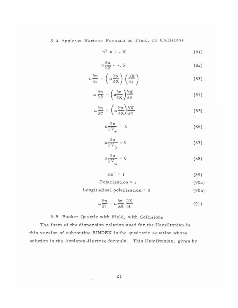
5.4 Appletotl-Hartree Formula no Field, no Collisiotls
on n - = - . 5
oX
n on = (n on) ox oCP oX oCP
on 0 n o V =
r
on n--=
a Ve 0
on 0 noV =
cP
nn' = 1
Polarization = i
Longitudinal polarization = 0
on on a x n- =n--
a t oX a t
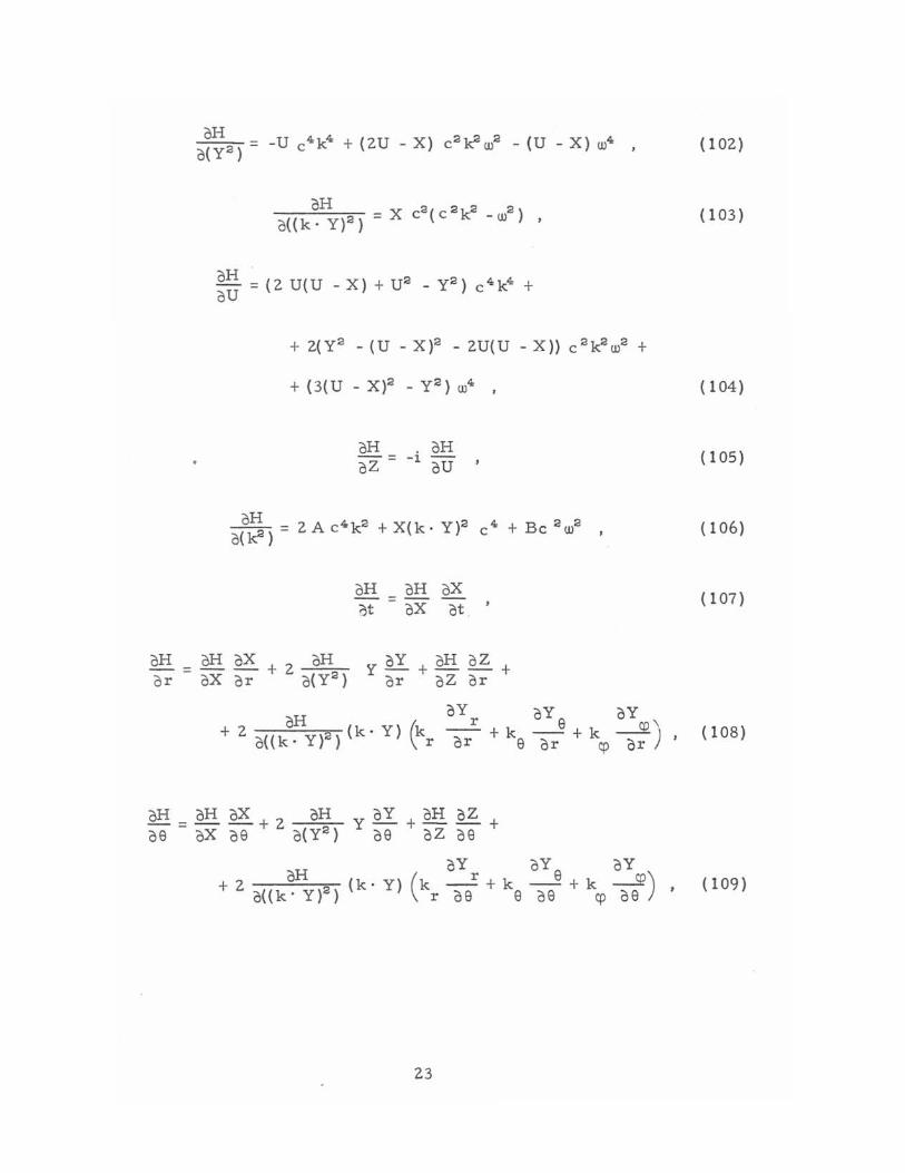
5.5 Booker Quartic with Field, with Collisions
(81 )
(82)
(83)
(84)
(85 )
(86 )
(87)
(88)
(89 )
(90a)
(90b)
(91 )
The form of the dispersion rela tion used for the Hamiltonian in
this version of subroutine RINDEX is the quadratic equation whose
solution is the Appleton -Hartree formula. This Hamiltonian, given by
21
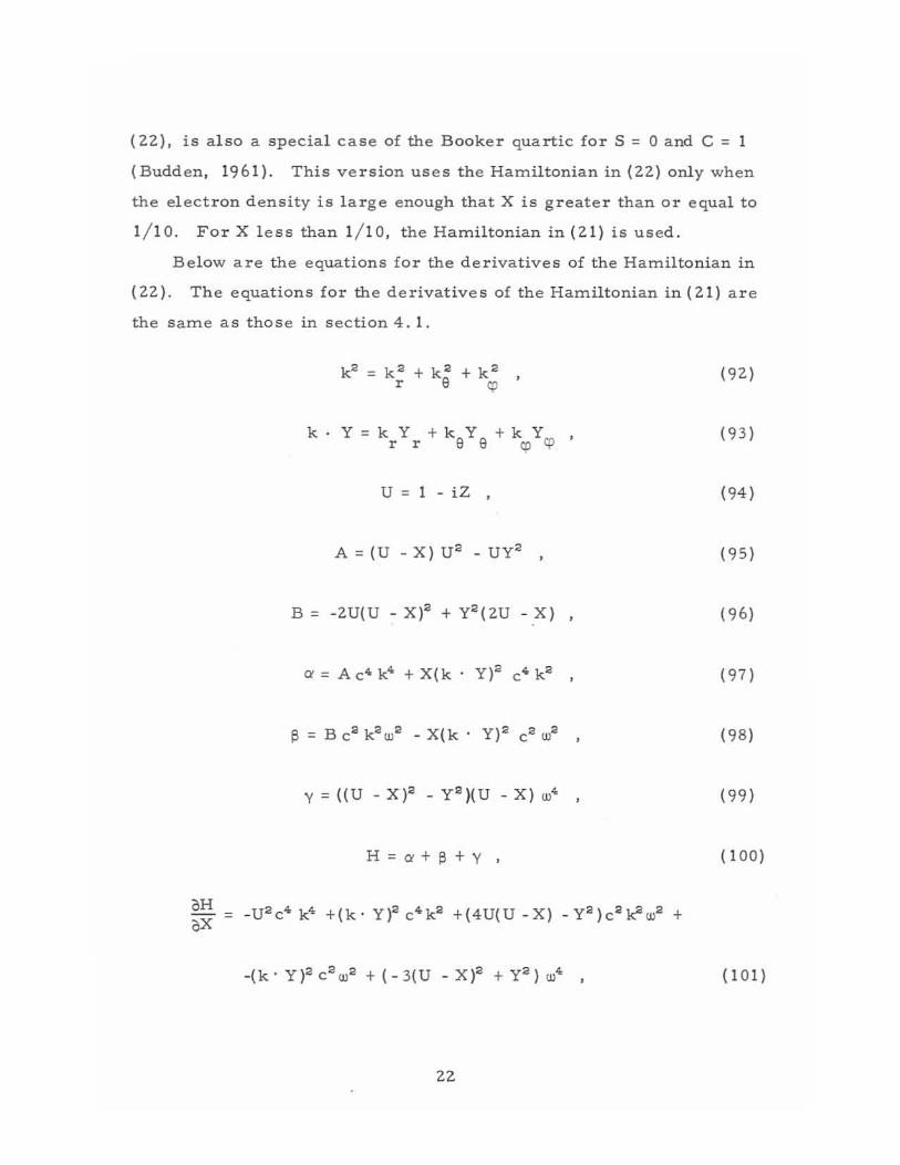
(22). is also a special case of the Booker quartic for S = 0 and C = 1
(Budden, 1961). This version us e s the Hamiltonian in (22) only when
the electron density is large enough that X is greater than or equal to
1/ 10. For X less than 1/ 10, the Hamiltonian in (21) is used.
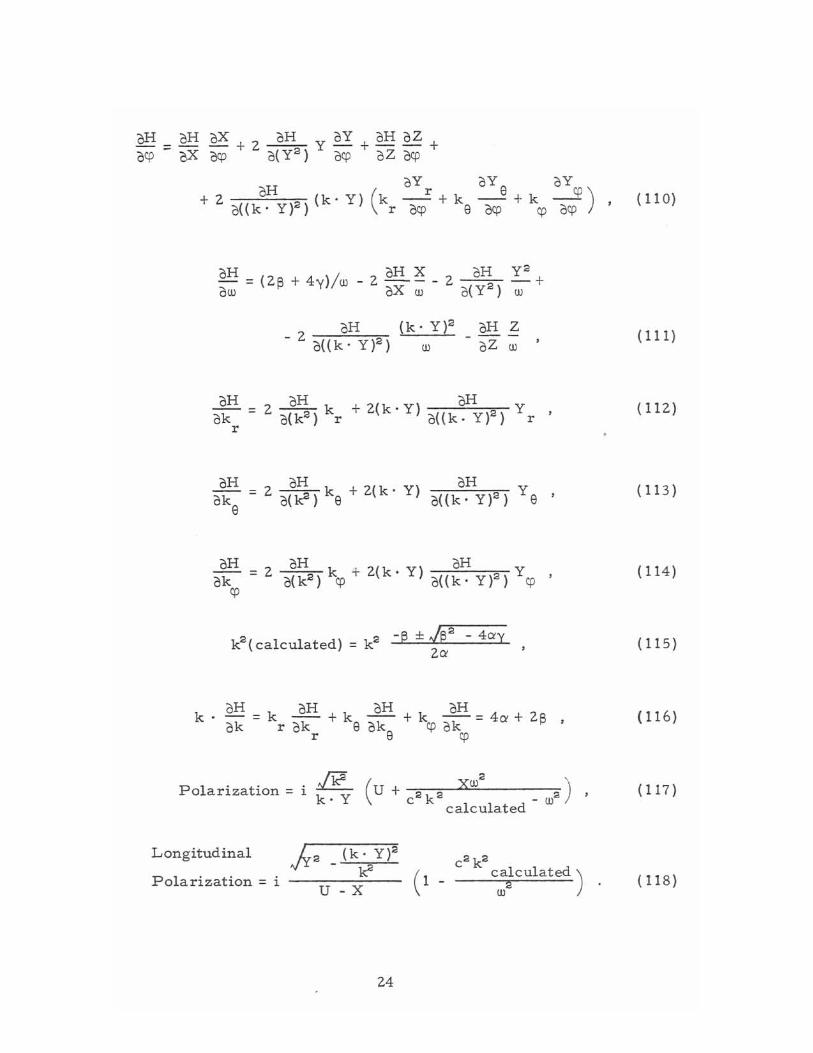
Below are the equations for the derivatives of the Hamiltonian in
(22). The equations for the derivatives of the Hamiltonian in(21) are
the same as those in section 4. 1.
(92)
k . Y = k Y + k Y + krpYro r r e e .,.. (93)
u = 1 - iZ , (94)
(95)
B = -2U(U - X)2 + y2(2U - X) , (96)
(97)
(98)
(99)
H=O!+~+y , (100)
(101)
22
oH __ oH oZ - -1 oU
oH oH oX ~t = oX ot
oH = oH oX + 2 oH '[ oY + oH oZ + or oX or 0(y2) or oZ or
( 104)
( 105)
( 106)
( 107)
oH _ oY r oY 9 ~\ + 2 o((k- y)2) (k Y) ~r or + k9 ar + kcp or)' (108)
oH = oH oX + 2 oH Y oY + oH oZ + 09 oX 09 0(y2) 09 oZ 09
oY oY oY + 2 oH (k Y) (k r + k 9 + k ---.SQ) (l 09)
o((k- y)2) - r as 9 as cp 09 '
23
oH oH X oH y2 - = (2(3 + 4y)/UJ - 2 - - - 2 - + oUJ oX UJ o( y2) UJ
oH (k·y)2 oH Z - 2 o( (k· y)2) UJ ---
oH = 2 ok
cp
oZ UJ
2 2 -13 ± Jf,2 - 4",y k (calculated) = k -- -2",
k· oH oH oH oH - = k -- + k -- + k "k = 4", + 213 , ok r ok r e oke cP 0 cP
Polarization = i ~ k·Y
Longitudinal (k. y)2
o Polarization = i -----.:::.--u-x
24
(111 )
( 112)
( 113)
( 114)
( 115)
( 116)
( 117)
(118)
5.6 Booker Quartic with Field, no Collisions
All the equations here are the same as for the Booker quartic version
with collisions (section 5.5) except for:
oZ oZ oZ Z= -=-=-= or 09 ocp o , (119)
U = 1. ( 120)
All the variable s exce pt polarization are real; polarization is pure
imaginary.
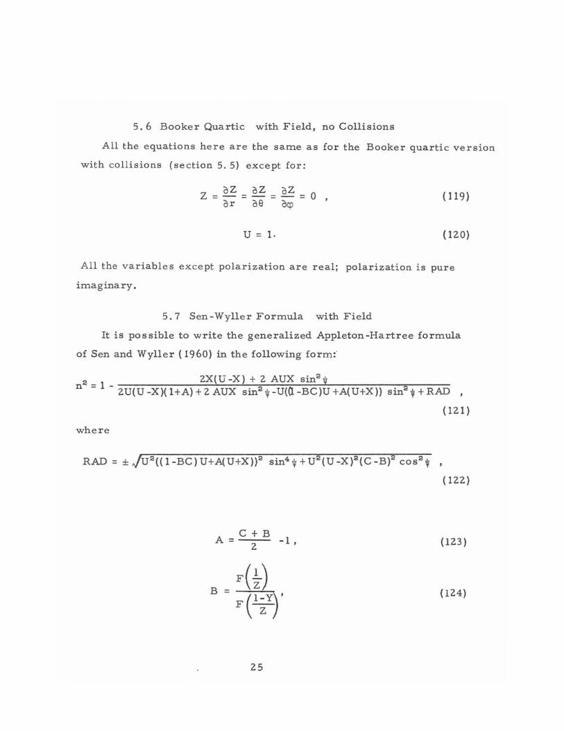
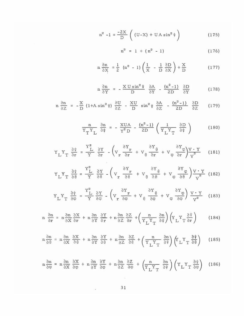
5.7 Sen-Wyller Formula with Field
It is possible to w rite the generalized App1eton-Hartree formula
of Sen and Wyller (1960) in the following form:
2_ 2X(u-X)+2AUXsin2 $ n - 1 - 2U(U -XlI 1+A) + 2 AUX sin2 ~ - U(n -BC)U +A(U+X» sin2 ~ + RAD ,
(121 )
where
(122)
-1 , (123 )
(124)
25
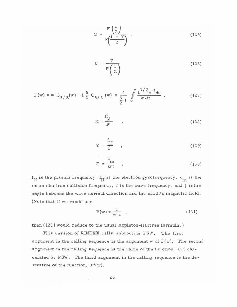
C =
U = z
F(w) = w C 3t 2(w) + i t Cst 2 (w) = 31
2
y fH
= f
v Z
m =
2nf
(12S)
(126 )
'" 3 t 2 -t
f t e dt W-lt
(127) o
(128)
(129)
( 130)
fN is the plasma frequency, fH is the electron gyrofrequency, vm is the
mean electron collision frequency, f is the wave frequency, and 1jI is the
angle between the wave norma l direction and the earth's magnetic field.
(Note that if we would use
1 F(w) = - . ,
W-l
then (121) would r educe to the usual Appleton-Hartree formula.)
This version of RINDEX calls subroutine FSW. The first
( 131)
argument in the calling sequence is the argument w of F(w). The second
argument in the calling sequence is the value of the function F(w) cal
culated by FSW. The third argument in the calling sequence is the de
rivative of the function, F'(w).
26
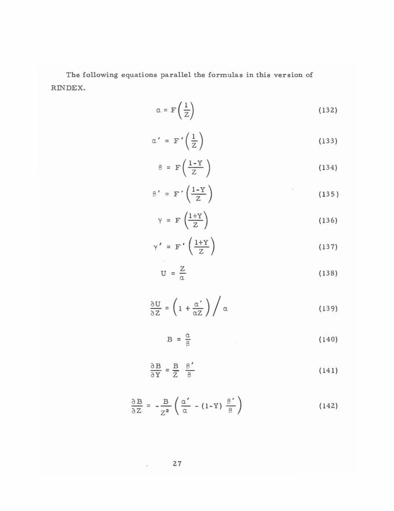
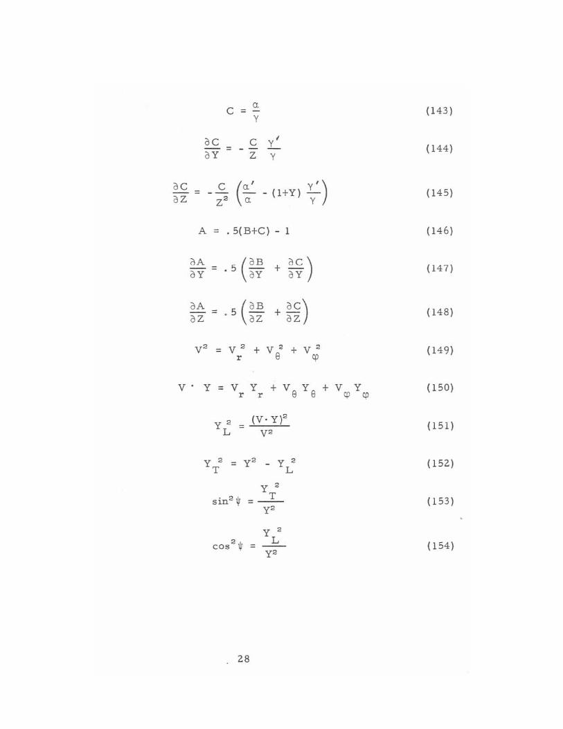
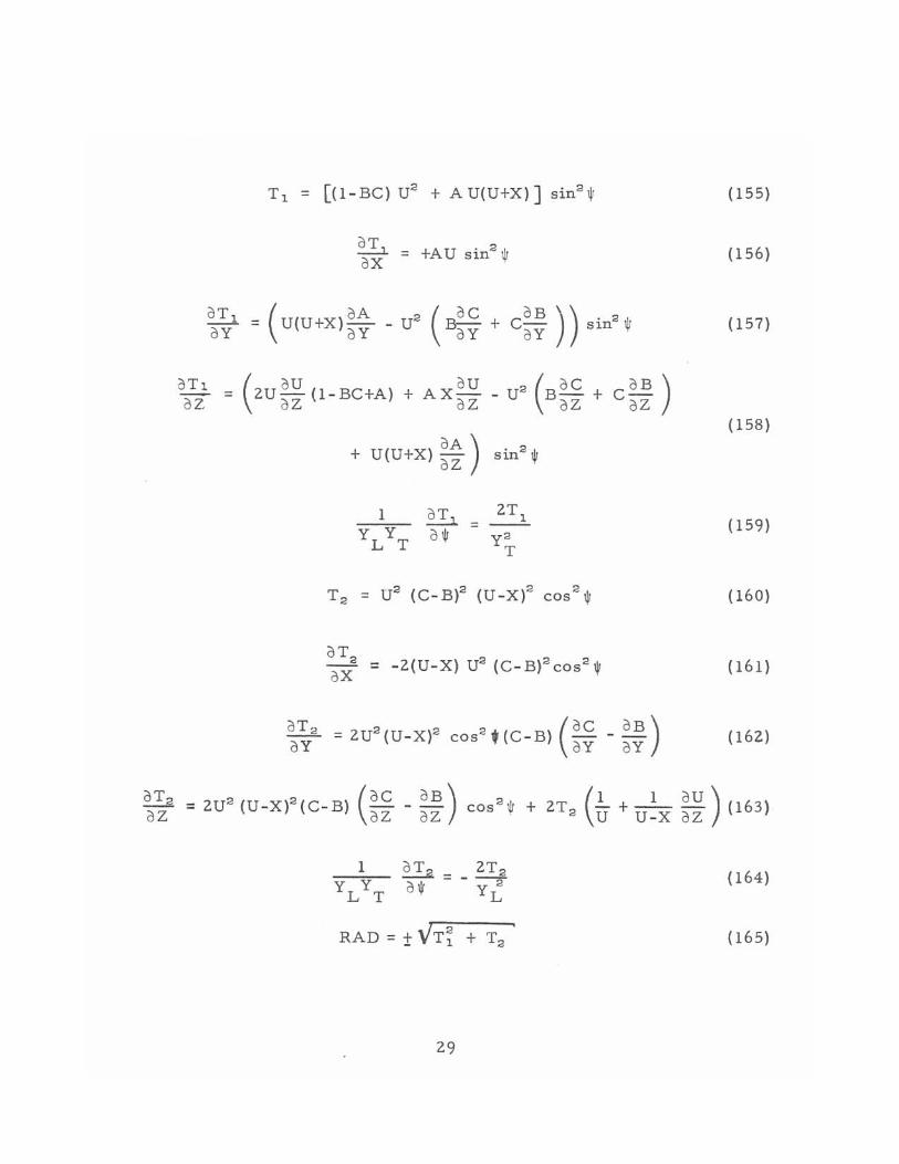
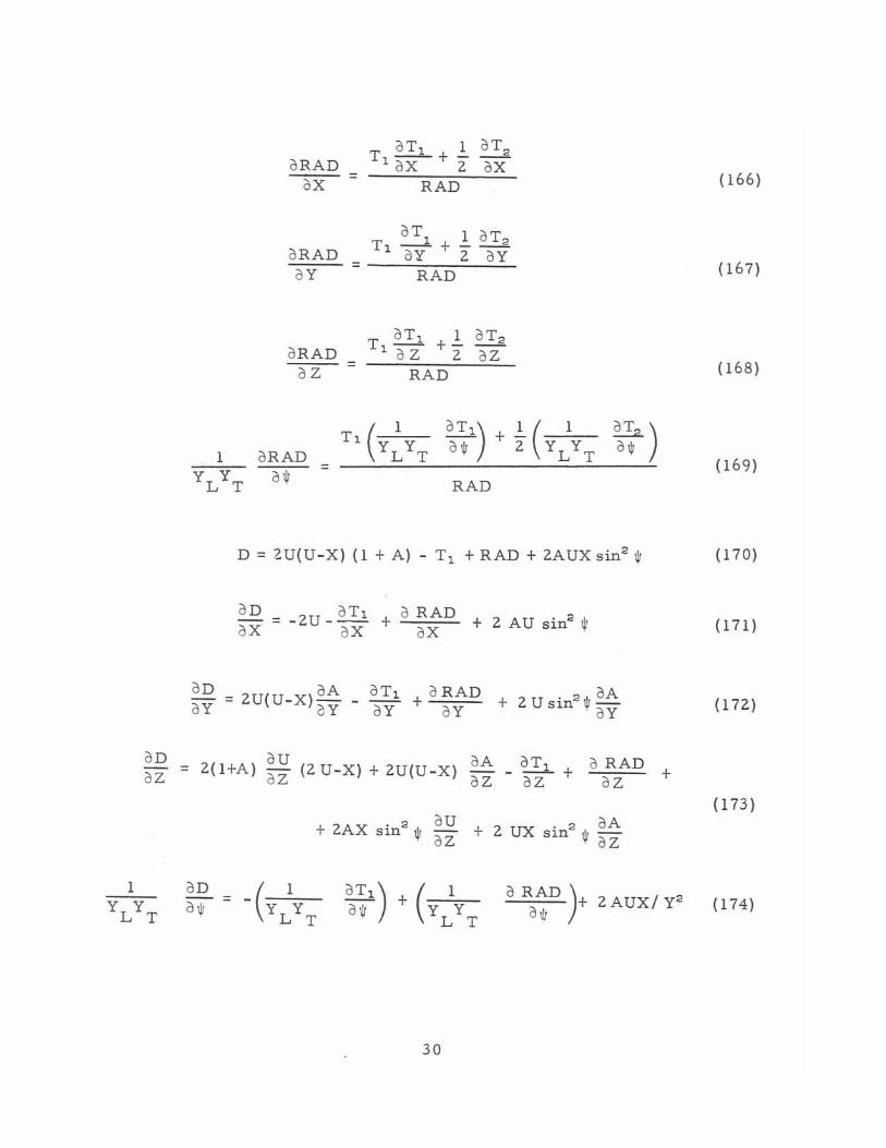
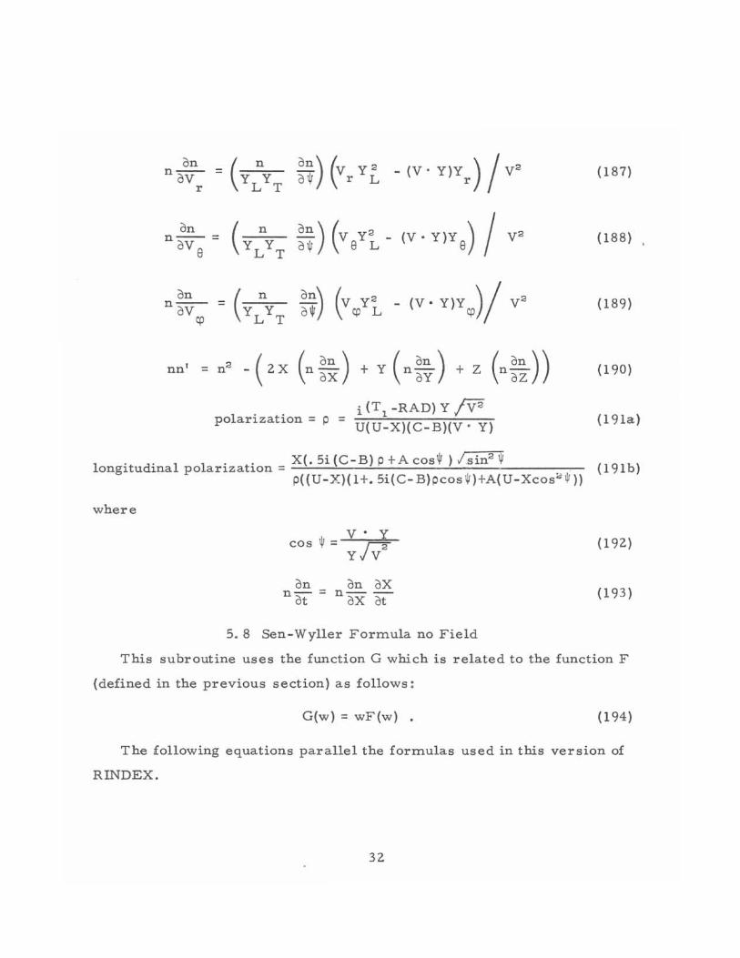
The following equations parallel the formulas in this version of
RINDEX.
a B -= az
Ct'=F'(~)
8 = Fe~Y ) 8 '=F'e~Y)
Y = F e;y) Y'=F,( l;Y)
u =
au
z Ct
-= az
Ct B =
S
aB B £ ay = Z !3
-- ~ -(l-Y)-B ( , S') Z2 Ct S
27
(132)
(133)
(134)
(135)
(136)
(13 7)
( 138)
(139)
(140)
(141 )
( 142)
C a
= -y
oC C L - = o Y Z y
o C C -- (:' Y') - (1+Y) y o Z Z2
A = • 5( B+C) - 1
d A .5( ~~ +~~) -= oY
oA = 5 (OB + Oc) oZ • o Z o Z
V 2 = V 2 + V 2 + V 2 r e qJ
V· Y = V Y + Ve Ye
+ V Y r r qJ qJ
Y 2 = L
Y 2 = y2 T
sin2 ~ =
cos2 ~ =
28
- Y 2 L
Y 2 T
y2
Y 2
L y2
(143 )
( 144)
(145)
(146 )
(147)
(148)
( 149)
(150)
(151 )
(152)
(153 )
(154)
OTl oZ
oT, = oX
OTl = (U(U+X)OA _ U? oY oY
+AU sin?1jr
(~ + COB)) sin?1jI OY oY
= (2U~~ (l-BC+A) + AX~~ - U? (B~~ + C~~ )
+ U(U+X) ~~) sin?1jI
1 oT J 2Tl = Y
L Y oljl y? T T
T? U? (C-B)? (U -X)? ? = cos 1jr
__ 2 = 2U? (U-X)? COS? (C-B) - - -oT. (OC OB) oY oY oY
(155)
(156 )
(157)
(158)
(159)
(160)
( 161)
(162)
oT? _? ? (OC OB)? (1 1 Ou) 6 oZ - 2U (U-X) (C-B) OZ - oZ cos 1jr + 2T? U + U-X OZ (1 3)
loT2=_2T? YLYT oljl Y/!,
(164)
RAD = ±VTi + T? (165)
29
1
T 21 T, + .!. 21T 8 21 RAD ' 2l X 2 21 X
(166 ) = 21 X RAD
T 21 T, + .!. 21 T8 21 RAD 1 Cl Y 2 21 Y
( 167) = 21 Y RAD
T 21 T, +.!. 21 T 8 21 RAD 1 21 Z 2 21 Z
(168) = 21 Z RAD
Tl(y1y 21 T ') 1 ( 1 ZIa) 21W + 2" YLY
T 21W
1 21 RAD L T (169) =
YLYT 21W RAD
D = 2U(U-X) (1 + A) - T, + RAD + 2AUX sin8 W (170)
21 D = -2U _ 21 T, + 21 RAD + 2 AU sin8 W 21 X o X o X
a D 21A - = W(U-X)-21 Y CY
21T, 21 RAD . 21A 21Y + 21 Y + 2 U sm8 w2l y
~~ = 2(l+A) ~ ~ (2 U-X) + W(U-X) ~~ _ ~~' + 21 :ZAD +
+ 2AX sin8 lit ~ ~ + 2 UX sin8
lit ~~
30
21 RAD )+ 2 AUX/ y8 21 ~
(171 )
(172)
(173 )
(174)
2 -2X ( 2 ) n -1 = n- (U-X) + UAsin $
n2 = 1 + (n2 - 1)
on 1 (n2
- 1) (~ 1 aD) x n~ = D oX + D oX 2
on XUsin2 $ oA (n2 -1) oD n oY - - OY 2D oY D
on X au xu oD (l+A sin2 $) . 2 oA (n2 -1) n- = - - sm $ oZ -
OZ oZ 2D oZ D
y2 L
Y
y2 L Y
oY 08
Y~ oY = ----
Y ocp
= XUA y2D
D
(
oY _V __ r+
r 08
(
oY _ V _r_+v
r ocp 8
oycp)v. Y v --~ cp or V~
+V_CP_V'Y oY )
cp 08 v 2
OYcp) V. Y +v -- ---
cp ocp. v 2
on n
or = on aX on oY on oZ ( non) (Y Y 0$)
noX or + nay a;.- + noZ or + YLYT ~ L Tar-
on on ax on oY nae = n ax ~ + n OY 08 + on
noZ
on n- =
ocp non aX + n onoY + n on oZ
oX ocp oY ocp oZ ocp
31
(175)
(176 )
(177)
(178)
(179)
( 180)
(181 )
(182)
(183 )
(184)
( 185)
(186)
on
(Y:YT ~~) (Vr Y~ - (V' Y)Yr) / V2 n oV =
r ( 187)
on
( Y:YT
on) (V y2_ (v.Y)Y e)!V2 n-- = oVe 0'1' e L
(188) ,
on
(Y:YT ~~) (Vcl~ - (V, Y)Y~)/ V
2 n~ =
~
( 189)
( 190)
" i (T , -RAD) Y fV2 polarlZatlOn = p = U(U-X)(C-B)(V' Y) (191a)
1 'd' 1 1 ' ,X(.5i(C-B)P+AcosW)lsinQ (191b) ongltu Ina po arlZatlOn = p( (U -X)( 1+. 5i( C- B)pcos $ )+A(U - Xcos" 1jJ ))
where
V· Y cos IjJ = r--2
YJV2 (192)
on on oX nat = noX at (193)
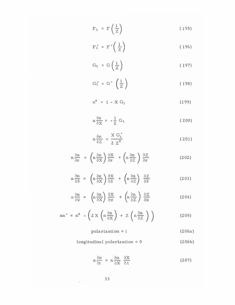
5. 8 Sen-Wyller Formula no Field
This subroutine uses the function G which is related to the function F
(defined in the previous section) as follows:
G(w) = wF{w) . (194)
The following equations parallel the formulas used in this version of
RINDEX.
32
Fl = F (~) ( 195)
F{ = F '( ~) ( 196)
G 1 = G (~) ( 197)
G{ = G' (~) ( 198)
n 2 = 1 - X G 1 ( 199)
on 1 ( 200) n oX = -- G 1 2
on X G' 1
( 201) n- = oZ 2 Z2
on (n~) ax + (n ~~ ) oZ (202) n- =
or a X or or
on ( ~) aX (n~~) OZ
(203 ) na-e = n ax 08 + 08
on (n~) ax + (n ~~ ) oZ
(204) n - ~
oqJ ax oqJ oqJ
nn = n 2 - ( 2 X (n ~~) + Z ( n ~~ ) ) (205)
polarization = i (206a)
longitudinal polarization = 0 (206b)
on on ax (207) n- = n oX at at
33
6. IONOSPHERI C MODELS
When using the prograUl, one UlUSt specify ionospheric Ulodels
which define electron density, collision frequency (if the effect of
collisions is being considered), and the earth's Ulagnetic field (if its
effects are being taken into account) as a function of position in space.
Each of these three characteristics of the ionosphere is defined by a
separate subroutine.
Appendices 3, 4, 5, and 6 contain descriptions, input parameter
forUls and listings of ionospheric Ulodels that now exist. These iorlO
spheric Ulodels are not likely to cover the needs of everyone who wants to
use the prograUl. Anticipating this when we wrote the prograUl, we Ulade
it possible to add Ulodels easily . The user Ulay Ulake up his own iono
spheric Ulodels by siUlply writing subroutines to define electron density,
collision frequency, and the earth's Ulagnetic field (and their gradi -
ents) as a function of position in space in spherical polar coordinates,
following the forUl of the subroutines in appendices 3, 4, 5, and 6.
Appendix 3 contains electron density Ulodels; appendix 4 con
tains Ulodels of irregularities which Ulay be applied as perturbations
to any of the electron density Ulodels; appendix 5 contains Ulodels of
the earth's Ulagnetic field; and appendix 6 contains collision frequency
Ulodels.
Having several versions of the subroutines for refractive index,
electron density, collision frequency, and the earth's Ulagnetic field
gives the user not only a wide choice among ionospheric Ulodels,
but also a variety of cOUlproUlises between cost and an accurate
description of the ionosphere, while still keeping the program siUlple.
34
7. FINDING THE RAY PATHS THAT CONNECT A TRANSMITTER AND RECEIVER
The reason for using a ray tracing program is to find all impor
tant ray paths that co nnect a g iven t ransmitter and re ce i ve r (either or
both of which may be on a satellite) on a particular frequency and such
properties of these ray paths as group time delay, phase time delay,
and absorption of the wave. "All important" ray paths include those
that reflect from the various ionospheric layers (including multiple
refle c tions) and that propagate off the g r eat circle path.
Since basically all that a ray tracing program can do is to cal cul
ate the path of a ray when given the transmitter location, frequency, and
direction of transmission, it cannot directly calculate those ray paths that
arrive at a specified receiver. The problem is to know, before tracing
the ray, in which directions to transmit the ray so that it will arrive
at the receiver . Since there are no general solutions to this problem,
the user of a ray tracing program must rely on some sort of trial and
error technique to find those ray paths that connect the transmitter and
receiver. This involves va r ying the dire c tion of transmission until a
ray is found that rea c hes the receiver. If a ray tracing program does
this automatically, we say that it has a homing feature. This program
does not have such a feature. To find all the paths connecting the trans
mitter with the receiver requires a very e laborate homing routine be-
cause "homing in" on a r eceiver takes more judgment and common
sense than speed in performing massive calculations. Therefore, the
person using the program is more fitted to this task than is the computer
program itself.
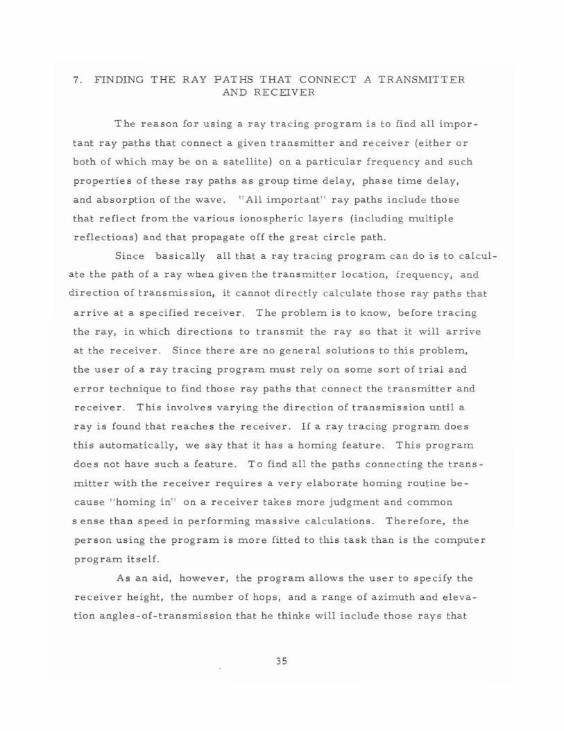
As an aid, however, the program allows the user to specify the
receiver height, the number of hops, and a range of azimuth and eleva
tion angles-of-transmission that h e thinks will include those rays that
35
will arrive at the receiver. The program then calculates a ray path for
each of the azimuth and elevation angles - of- transmission specified in
the range. Usually only in the case of ionospheres with large horizon
tal gradients will the azimuth angle -of-transmis sion have to be varied.
T he program will calculate each ray path far enough to intersect or
make a closest approach to the receiver height for the requested
number of hops. The user can then interpolate between those rays
which surround the receiver.
We define the point of "closest approach" as the point on the ray
path where the wave normal direction is horizontal. It approximates an
apogee if the receiver is above the apogee height and it approximates a
perigee if the receiver is below the perigee height. The approximation
is good for oblique propagation. When the earth's magnetic field is
neglected, a point of" closest approach" is exactly an apogee or perigee.
We count one hop every time the ray crosses the receiver height.
If the receiver is on the ground, a ground reflection counts as one hop
for the downcoming ray before the ground reflection, and another hop
for the upgoing ray after the ground reflection. We count two hops
every time the ray passes through a point of "closest approach" to the
receiver height. T his procedure helps make rays that have the same
hop number have a ground range that is a continuous function of the
direction of transmission.
8. OUTPUT
8. 1 Printout
Periodically and at selected points during a ray trace, the
program will print information giving the position of the current ray
path point, the direction of the wave normal, and the cumulative values
of quantities being integrated along the ray path such as group path,
phase path, absorption, and Doppler shift. Appendix 8c contains a
sample of the printout.
36
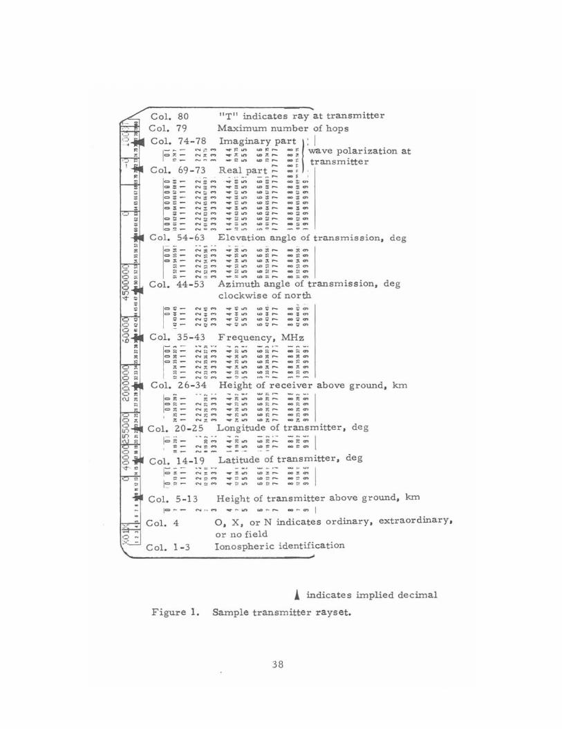
8. 2 Punched Cards
T he program will punch a card at the beginning of each ray, a
card at each ground reflection, a card at each crossing of the receiver
height, two cards for each closest approach to the receiver height, and
a card at the end of each ray to summarize the main results of the ray
path calculations. These cards are explained in figures 1 and 2.
These cards are very useful as input data to other computer
programs and for plotting the results of the ray tracing. In fact, these
cards represent the most useful form of output for production ray path
calculations. This method, called the rayset information - storage
technique, was developed by Dr . T. A. Croft (Croft and Gregory, 1963)
of Stanford University.
8. 3 Plots of the Ray Path
A plot of the actual ray path, especially for very irregular iono
spheres, can be helpful in understanding what sometimes seems like
strange results in light of the lnput data . Thus, the program has an
option for plotting, providing, of course, that the user has a plotter and
plotting subroutine s such as tho se de scribed in appendix 7. T he program
can plot the projection of the ray path on any vertical plane or on the
ground. T he input parameter forms for plots of the ray path (appendix Ii)
give more details. Appendix 8e contains sample plots of the raypath.
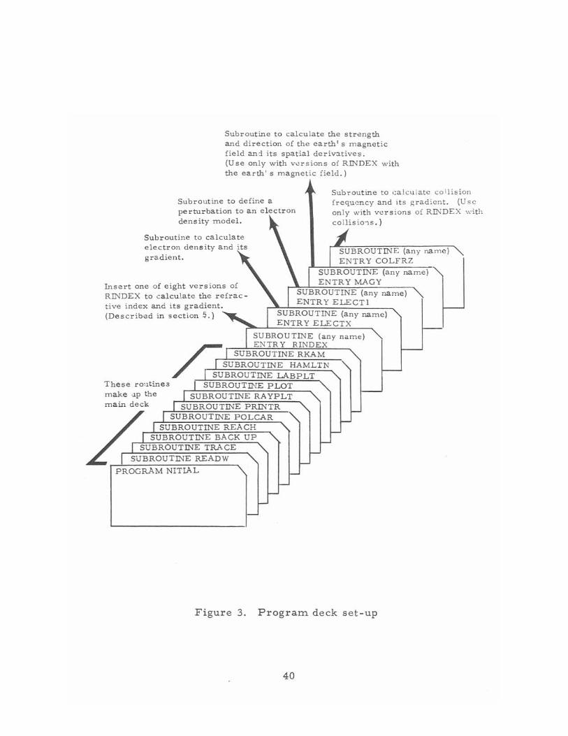
9. DECK SET UP
The versatility gained by having several versions of some of the
subroutines is somewhat offset because the user must learn the deck
set up in order to make necessary substitutions. Figure 3 shows the
deck setup, including the subroutines that make up the main deck and
those which are frequently exchanged with alternate versions. The
order of the subroutines is unimportant.
37
Col. 80 11TH indicates ray at transmitter Col. 79 Maximum number of hops
Col. 74-78 Imaginary part I: I I ~... roo )." ..,..,. ~ .,., ..,. IC ..... - ~ wave polarization at ~~_ N~'" _~.,., ..,.~ ..... _~
!:'.- ...... ~- -~ .... U)I:: ..... _ r: transmitter Col. 69-73 Real part;:: :: :
c:::>:_ N::: at: ......... :: -=-:;- ..... :; -::- ..... :: c:::>~_ ...... ~ c:::>;:_ ...... ;:
:::- ..... ; c:::>:;;: .... ""'::;: c:::>::;;_ ..... ::;;
Col. 54-63 = • - ~ • = • - ~ • = • - ~ • • - ~ • ~ • - ~ , ~
~ - ~ , ~ Col. 44-53
1=' - ~. ~
=:;:- ~. .- ~. .- ~.
Col. 35-43 , ... 1'1 , • •
c:::>::;_ ...... ::; .., =>J:!:- 1N )jt <"> e> ~ _ IN~""
~- ..... ;; .... ::; _ N ::; '" !::_ ..... !>O ...
Col. 26-34
I:~= ~ ~ c:::> ~ _ ..... ~
l!:: - ...... t;: ~- ..... ::::;
Col. 20-25 1;;;;;- .~
=- ...... = ..,
Col. 5-13 1= - ....
· .. _. - ~ ..... -~
• • ~ ~ • ~ ~ • ~ • = ~ ~ ~ ~ = ~ • , ~ ~ , ~ ~
• • ~ ~ • ~ ~ • ~ • ~ ~ • ~ -• ~ • • ~ ~ • ~ -• ~ • • ~ ~ • ~ -= ~ • = ~ ~ • ~ -•. ~ • , ~ ~ , ~ --~ - • - m · -
Elevation angle of transmission, deg
• • ~ ~ • ~ -• ~ • • ~ ~ • ~ -• ~ • • ~ ~ • ~ -• ~ • • ~ ~ • ~ -• ~ ~
, ~ ~ , ~ -,
~ -~ - ~ ~ ~ -~ ~
Azimuth angle of transmission, deg clockwise of north
-• ~ ~ • ~ - ~
• • ~ ~ • ~ -• ~ · ~ • ~ -= ~ · • ~ • ~ -• ~ Frequency, MHz
• • ~ ~ • ~ -• • • ~ ~ • ~ -• ~ • ~ ~ • ~ -• • • ~ ~ • ~ -• · • ~ ~ • ~ -• -0 .~
Height of receiver above ground, km
~ ~ :.: : ~ ;: =::;: I .... ::; ..n u:o ;:; ..... _ ::;; cn ...... le .,., u:o ~ ..... .... le o. ...... t; .,., c.o t: .... _ ~ O'>
_::::;.,., u:o::::; .... _::::;cn
Longitude of transmitter, deg
:;;:;; I .... ~ en
Latitude of transmitter, deg - · 0'
I · , ~ ~ , ~ -• ~ · • ~ ~ • ~ -• ~ · • ~ ~ • ~ -• ~ Height of transmitter above ground, km
ocr - .... .... .... .... I
Col. 4 0, X, or N indicates ordinary, extraordinary. or no field
Col. 1-3
Figure 1.
Ionospheric identification
! indicates implied decimal
Sample transmitter rayset.
38
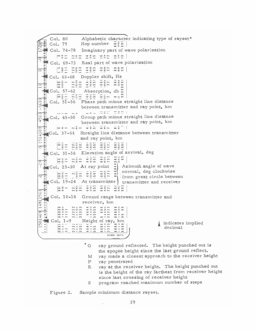
Col. 80 - Col. 79
Alphabetic character indicating type of rayset' Hop number ;;; ;: ;;; 1 -. ~
Col. 74-78 Imaginary part of wave polarization
Col. 69-73 Real part of wave polarization
1- --.-
Col. 63-68 Doppler shift, Hz
[==-=. c:::> :;;
Col. 57 - 62 Absorption, db :
1
- ... - ' .... ;n •••
~:= ~ : ~ ~ ~ ~ ~~~ - ~ ~
Col. 51-56 Phase path minus straight line distance between transmitter and ray point, km
=;;:..- =::: :: I
Col. 45-50 Group path minus straight line distance between transmitter and ray point, km
...... :::..... .....:; on <D:;..... ;;.:: - - I Straight line distance between transm itter and ray point, km
Col. 31-36 Elevation angle of arrival, deg
1=-- --- --~ --- ::: I ~~- ...... g ..... ..... g on ~~~ ao g
Col. 25-30 At ray point :1 Azimuth angle of wave
I -. . ..... . - - .... -- ..... ,. .- : normal deg clockwise
c:::> ~ _ ...... ~ .......... ~ o.n <D ~ _ _ J
c:::> • - ........... -.... <D'" r- -) ft· 1 b t _ ~ _ . 0 .. 0 . . . 0 . rom grea Clrc e e ween Col. 19-24 At transmitter transmitter and receiver
I~~ - ~;~ ; ; ~ :;~ ;;;;: I c:::>~ ...... ~~ ..... ~ .... _~ _ _ ~~
Col. 10-18 Grou..,.,d range between transmitter and receiver, km
r , -= - -= - -
Col. 1-9
[ -= " =" -= --
Figure 2.
- = -...... 2...., ------c-.o , • ..,
-" -----.--
-= = .. 2 .... - - = - - =
Height
-" = - - = -• =
_ = CI">
<D~ .... _ ~ CI">
--~ of ray, km
--- -- ~ .. lI 9<X 3eOl~
! indicate s implied decimal
• G ray ground reflected. The height punched out is the apogee height since the last ground reflect.
M ray made a closest approa=h to the receiver height P ray penetrated R ray at the receiver height. The height punched out
is the height of the ray farthe st from receiver height since last cros sing of receiver height
S program reached maximum number of steps
Sample minimum distance ray set.
39
Subroutine to calcu late the strength and direction of the earth I s magnetic field an:! its spatial deriv3.tives. (Use only with v~rsions of RIN"DEX with the earth ' s magnetic field . )
Subroutine to define a perturbation to an electron density m odel.
Subroutine to calculate electron dens ity and gradient.
Subroutine to ,:a lcul atc co llision fr equ(!ncy and i t s gradient. (U sc only with versions of RINDEX with collisio,s. )
SUBROUTINE (any na m e ) E NT RY COLFRZ
SUBROUTINE (any name) ENTRY MAGY
SUBROUTINE (any name) ENTRY ELECTl
Insert one of eight versions of RINDEX to calculate the refrac tive index and its gradient. (Described in secti.on ~ . ) SUBROUTINE (any name)
ENTRY ELECTX
These rO:ltine5 make .~p the
SUBROUTINE (any name)
~ ENTRY RINDEX
SUBROUTINE RKAM
SUBROUTINE HAMLTN SUBROUTINE LABPLT
SUBROUTINE PLOT SUBROUTINE RAYPLT
main deck SUBROUTINE PRINTR
A SUBROUTINE POLCAR
SUBROUTINE REACH SUBROUTINE BACK UP
SUBROUTINE TRACE
SUBROUTINE READW
PROGRAM NITIAL
Figure 3. Program deck set - up
40
10. INPUT
T he input data for a ray tracing program divide themselves
naturally into two groups:
First, data that control the type of ray trace requested, such as
the transmitter location and frequency, plus parameters describing
analytic models of the ionosphere . Since there are few of these,
efficiency in packing such data can be exchanged for versatility and
ease of data handling. Therefore, by putting only one piece of data on
each card, we gain the convenience s of reading in the se data in any order
and of having the program read in only those data that are different
from those of the previous case. A number in the first three columns
of each card identifies the data being read in. Table 2 defines the
identifying numbers that are subscripts for a linear array, W The
last 56 columns of the card are available for comments.
We have also provided a method for conversion of units for input.
The computer program needs allgles in radians, whereas people usually
like to use angles in degrees. The program is set up f()r angles in radians,
but putting a "1" in column 18 allows the user to enter the angle in degree s
and have the program make the conversion. A" 1" in column 19 allows
the user to enter central earth angles as the great circle distance along
the ground in kilometers. (The program will calculate the latitude of a
transmitter which is 500 km north of the equator, for instance.) The
program expects d i stances in kilometers . A" 1" in column 20 indicates
a distance in nautical miles, and a "1" in column 21 indicates a distance
in fe et.
Appendix 8b contains a sample of how the cards are to be punched.
If two or more cards have the same identifying number, the last one
dominates. A card with the first three columns blank indicates the end
of this type of data cards.
41
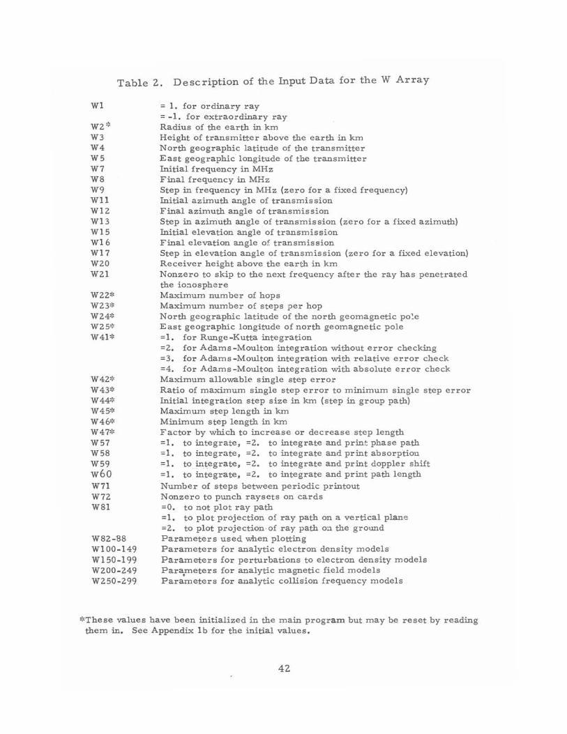
Table 2. Description of the Input Data for the W Array
WI
W2':' W3 W4 W5 W? W8 W9 Wll WI2 WI3 WI5 WI6 WI? W20 W2I
W22'~
W23* W24'~
W2S* W4I *
W42i,(
W43" W44i~
W45" W46'; W47~f.
W5? W58 W59 w60 W71 W72 W8I
W82-S8 WIOO-I49 W ISO-I99 W200-249 W2S0-299
= 1. for ordinary ray = -1. for extraordinary ray Radius of the earth in km Height of transmitter above the earth in km North geographic latitude of the transmitter East geographic longitude of the transmitter Initial frequency in MHz Final frequency in MHz Step in frequency in MHz (zero for a fixed frequency) Initial azimuth angle of transmis sion Final azimuth angle of transmission Step in azimuth angle of transmis sion (zero for a fixed azimuth) Initial elevation angle of transmission Final elevation angle of transmission Step in elevation angle of transmission (zero for a fixed elevation) Receiver height above the earth in km Nonzero to skip to the next frequency after the ray has penetrated the iO:l.Osphe.re Maximum number of hops Maximum number of steps per hop North geographic latitude of the north geomagnetic po~e East geographic longitude of north geomagnetic pole =1. for Runge-Kutta integration =2. for Adams-Moulton integration without error checking =3. for Adams -Moulton integration with relative error check =4. for Adams - Moulton integration with absolute error check Maximum allowable- single step error Ratio of maximum singl e step error to minimum single step error Initial integration step size in km (step in group path) Maximum step length in kIn Minimum step length in km Factor by which to increase or decrease step length =1. to integrate, =2. to integrate and print phase path =1. to integrate, =2. to integrate and print absorption =1. to irl:~~grate, =2. to integrate and print doppler shift =1. to integrate, =2. to integrate and print ·path length Number of steps between periodic printout Nonzero to pWlch raysets on cards =0. to not plot ray path =1. to plot projection of ray path on a vertical plane =2. to plot projection· of ray path on the ground Parameters used "When plotting Parameters for analytic electron density models Parameters for perturbations to electron density models Para.meters for analytic magnetic field models Parameters for analytic collision frequency models
*These values have been initialized in the main program but may be reset by reading them in. See Appendix lb for the initial values.
42
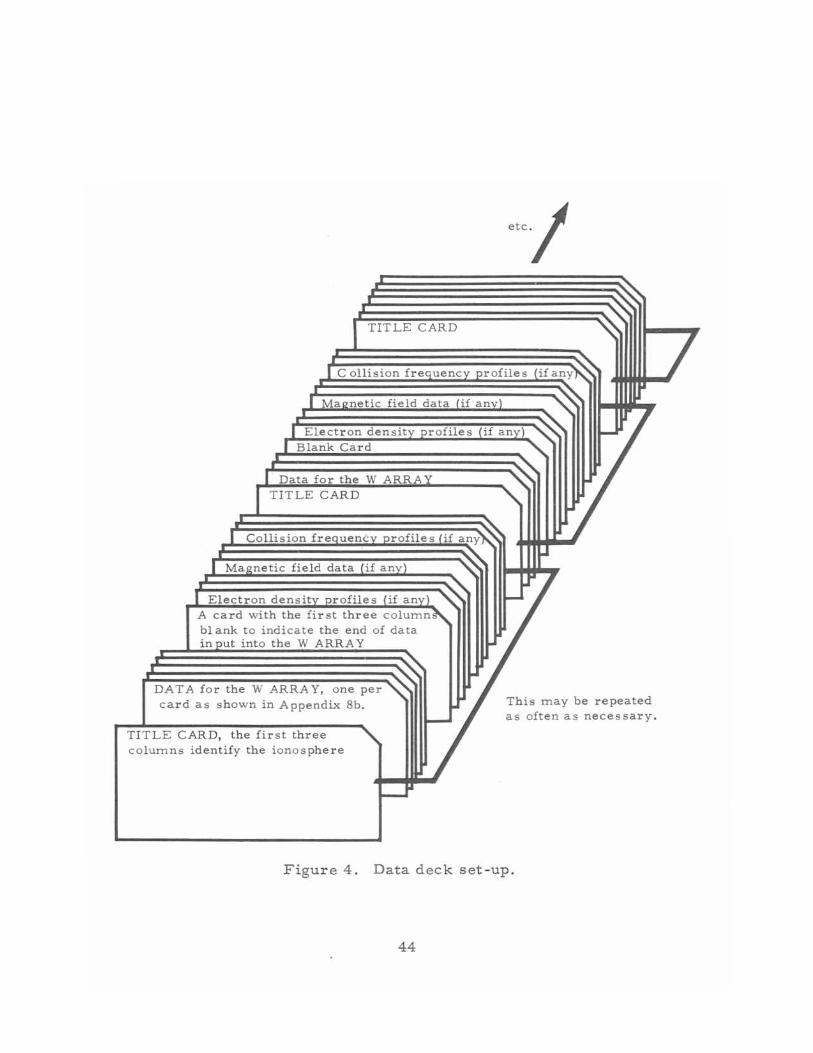
A second group of input data cards are necessary if nonanalytic iono
spheric models such as the electron density profile defined by subroutine
T ABLEX or the collision frequency profile defined by subroutine T ABLEZ
are used. Each subroutine defining a nonanalytic ionospheric model reads
in data cards according to a format defined in that subroutine. An ele
ment in the W ar r ay controls the reading of these cards. (See table 2. )
Figure 4 shows the order in which these data cards should be arranged.
11 . ACCURACY
The numerical integration subroutine has a built-in mechanism to
check errors and adjust the integration step length accordingly. If
the errors get larger than a maximum specified by the user, the routine
will decrease the step length in order to maintain the accuracy. On the
other hand, if the accuracy is greater than that required by the user,
the routine will increase the step length in order to reduce the comput
ing cost. The user specifies the desired accuracy in W42 (see
table 2). W 42 is the maximam allowable relative error in any single
step for any of the equations being integrated. To get a very accurate _5 _ 6
(but expensive) ray trace, one can use a small W 42 (about 10 or 10 ).
For a cheap, approximate ray trace, one should use a large W 42
(10-3
or even 10 - 2). For cases in which all of the variables being inte
grated increase monotonically, the total relative error can be guaranteed
to be less than W42. Otherwise, the total relative error cannot be
easily estimated.
T he far left column of the printout from the ray path calculation
gives an indication of the integration error in the magnitude of the vector
which points in the wave normal direction. Although the calculation of
this error is made independently of the error calculation in the numeri
cal integration routine, we have found that except near reflection for ver
tical or near vertical incidence this error is usually of the same order
43
CARD
TITLE CARD
A card with the first three CO,lU<nlnS',,"
bl ank to indicate th e end of data
DAT A the W ARRA y, one per car d as shown in Appendix 8b .
TITLE CARD,
etc./
This may be repeated as often as necessary.
Figure 4 . Data deck set -up.
44
of magnitude as that specified in W42. We have found that whenever
this error has exceeded W42 by several orders of magnitude, the elec
tron density subroutine we had written was calculating a gradient of
electron density inconsistent with the spatial variation of electron
density being calculated. See the general description of electron
density models in Appendix 3a for more information.
12. COORDINATE SYSTEMS
The program uses two different spherical polar coordinate
systems, namely, a geographic and a computational coordinate system.
Input data for the coordinates of the transmitter (W4 and W 5) and input
data for the coor din ate s of the north pole of the computational coordi_
nate system (W24 and W2 5) are entered in geographic coordinates.
(Putting W25 equal to O' and W24 equal to 90· would superimpose the
two north poles and equate the two coordinate systems. )
When the two coordinate systems do not coincide, the three types
of ionospheric models calculate electron density, the earth's magnetic
field, and collision frequency in terms of the computational coordinate
systerrl. In particular, the dipole model of the earth's magnetic field
uses the axis of the COrrlputational coordinate systerrl as the axis for the
dipole field. Thus, when using this dipole model, the COrrlputational
coordinate systerrl is a georrlagnetic coordinate system, and both elec
tron density and collision frequency must be defined in georrlagnetic
coordinates. Dudziak (1961) describes the transformations between
these coordinate systerrls.
45
13. HOW THE PROGRAM WORKS
This ray tracing program consists of various subroutines that per
form specific tasks in calculating ray paths. This division of labor
facilitates modifying the program to solve specific problems. Often it
may be necessary to change only one or two subroutines to convert the
program to a different uSe.
The main program (NITIAL) sets up the initial conditions (trans
mitter location, wave frequency, and direction of transmission) for
each ray trace. In setting up the initial conditions for each ray trace,
the main program (NITIAL) steps frequency, azimuth angl e of trans
mission, and elevation angle of transmission. The details of the workings
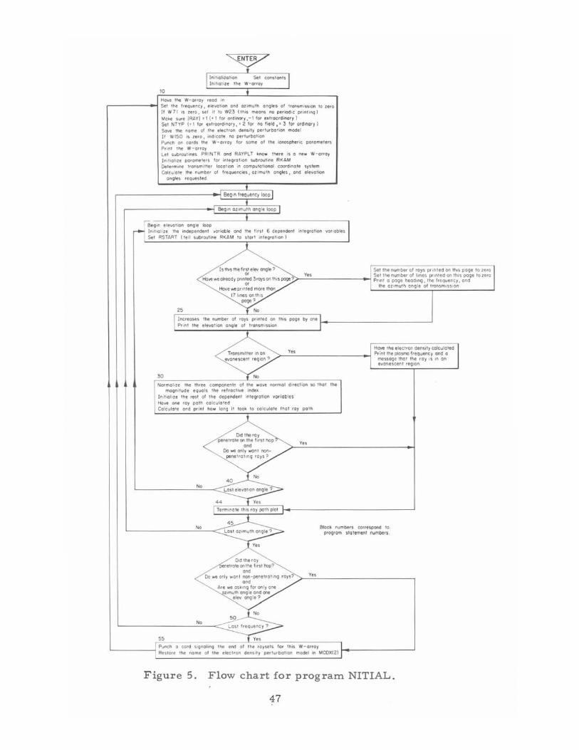
of NITIAL can be found in the flow chart in figure 5. Then subroutine
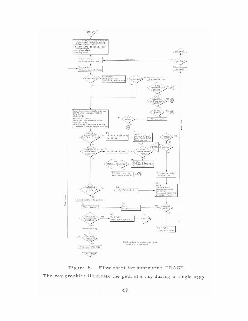
TRACE calculates one ray path for the requested number of crossings
of the specified receiver height. Subroutine TRACE is the heart of the
ray tracing program. It is the most complicated subroutine included,
but also the most important to understand. The flow chart in figure 6
should help to expl ain TRACE.
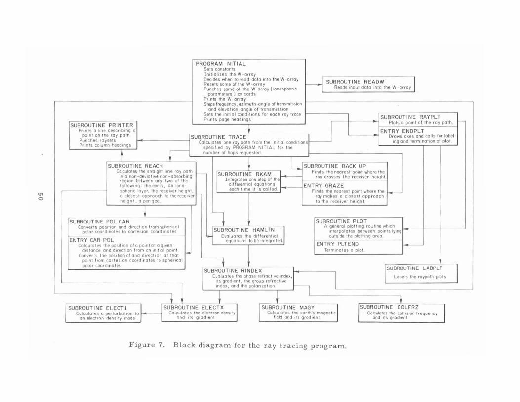
Subroutine RKAM integrates the differential equations numerically
using an Adams -Moulton predictor -corrector method with a Runge-
Kutta starter. Subroutine HAMLTN evaluates the differential equa-
tions to be integrated. Sub routine RIND E X calculates the phase refrac
tive index and its gradients, the group refractive index, and the polariza
tion. (Eight versions of subroutine RINDEX are included.) Subroutines
ELECTX, ELECT!, MAGY, and COLFRZ calculate the ionospheric
electron density, perturbations to the electron d ensity (irregularities),
the earth's magnetic field, and the electron collision frequency, respec
tively. Several versions of these four subroutines are included and it
is easy to add more. Subroutine REACH calculates a straight-
line segment of a ray path in free space between the earth and the
46
I I ~nil'OI;lO"On In,holile The
SeT conslanTs I W-or<oy
'0
Ho~e , .. W-o"oy ,ead '" SeT the f,equency, Ilel/aloOf! ond azimuTh onoles of I.ansm,nion 10 zero II W71 '5 lero. fe T iT 10 W23 (Ih" meons n<) per iOdic prinlinql Mo"e sure IRAYI . , (+, 1o. ordinary, · 1 10' Ulroordino.y 1 Set NT YP (.1 10< e~l,oQ'dino'Y, • 2 IQf no fi eld . ' :3 for ordingry I $olle the nome of . he electron densiTy pe.lu.baljor, model
" W150 is ze .o, Ind,eoTe no pertu,botion PunCh on COtCS The W-orroy 10' some at The IOnosptumc PG.omele., P"nl , .. W-orroy LeI sub'oulmes PRINTR ond RAYPLT ~nQ" The.e ,$ 0 new W-O HOy
In",ohze ~"'omelers 10' Integrotion subrOUTine RKAM DetermIne T,o nsm, I'e ' locaTion In com~ulo T lOnol coordinote sySTem Calculate The numbe. of fr eQuencies . azimuth onqles, and ele llOll(ln
onQles . eQues ted
SeQln Irequeney loop
Begon Ol,muth angle loop
rrse9,n elevolion on91e loop va. iab le s I !"'t,a lia Ihe 'ndependent variable ond Ihe li ',~1 6 dependent in le9 'otion
Sel RSTART ( Ie ll subrou line RKA M 10 slarl ,nle""ot,on )
Is ' !'ws thelN'St elev 0t'I91e? I , .. oh, "om' .. 0' "" ~'"'" 00 ,., 00" """j ~ , .. Sel the number of I,nes pr,nted on til,s page 10lero How ",e olreQdy pronle<l3royson Ih<s page? I Pront a page head 'nQ. lhe frequency. and
" the aZlmulh ang le o f Ircnsm,ss,an Hove 'M! prlnled more thon
17 lines an n'l 's po,"'
25 No
\ Inc.eases lhe number 01 .oys p",nted on Ih,s page by one Pr,nt the elevation Qnqle 01 "on,m"s_
,,, I H~, '" , .. ,,"" doe,'"~ ,,''"''''' I ~ P.int the plO$lTlO f.eQuency ond 0 evonescenl r:oon? I meSSQge lhal Ihe .oy 's ,n Qn
evenescen' .eglon
'0
Normolile the Ih.ee comPQnenl!, QI Ihe wove no.mol di.ection so Ihat oh, magnilude equals Ihe .ef.act,ve indu
Inilia li ze lhe .esl of Ihe dependenl inleg.o l ic n varicbln
",,' one roy PClh COlculQ led Calculale ond pr int M oo long it taa~ to colcuto le Ihat .ay pa th
Dod 'he.oy penel.o'e 00 Ihe h,s' hop , ..
'"' Do we only won' r'(ln-penelrot,ng rays?
No '0
No LoS! elevoloen on",l. ?
" -r Yes
\ Termlnote III'S .oy polh pial
" ...L No 91oc~ numbers correspond " Losl cZ,muth cnQle? p"OQrcl'l'l sia lemen' numDers
", I)d 'he roy
Irate on!he hrs! 1'Op" 0",
Do we only wo n I non-pen" r o l' n~ rays? , .. '"' A. e we os~on", lor only one
mnulll onQI. and one ele\' angl.?
No '0
No Los! freQuency"
" Tyes Punch 0 cc.d ,i9nclin", , .. , .. of Ihe roysels 10. Ih ,s W-orray I RestOfe the nome 01 the elect.on den" Iy ~e. tu.bal"m modoe l in MOOX\2)
Figure 5. Flow chart for program NITIAL.
47
In,Mh,. NHOP. tl.A.X ,N SI<.I p. RSTART \HOP. HTM fIo X. NEWRAY. THERE
Call H:.M LTON lca lc"'o'e o"""a'''H) (al'"lOIe HOME (~' '''' a ... ay I,om
'O"Ce,ye' he'9"') p"n'. p.mc~ )M TR Pici a ,ey po, n' RETURN
", I _____________ C"~O"~,.OO"'~ ____________________ C"~O~C;~
-'==-'F",-,-,-~r ~ .. I>o~
So.., "" "",a"on "'"obl .. e. wIVal,.." 5., WAS 1'0 '."'.mbe, THERE I Call RKA M Co1c" 'a,. H 5 .. THERE '0101 •• S., WASNT 1'0 , • ......."b., HOME I Calcu lo,o HOME Calcu la,. SMT ( .. "ma'. of "",toca l
d .. 'cnce to nee,." apogee 0< ".,*"
f;c. 'he ,oy """""o,.~ 'he ,,,"o<p.hc,. ?
...
A"h'~ ' ..:. ".' heo;M"
(THERE)
" Y I ~'HOME I
I I
I I
Y'~t8\ -0
On 'h. Y.'~60 9'0""0 1 ~
", 79
. '$;. P(N[T '" ~ R(TUR I P"nl. P""C~ P EN ETRAT ~
alo<~ numb. " ce,,"POnd 'o<lO"mOn' O\JmOe., 'n the "'~',,""n.
Figure 6. Flow chart for subroutine TRACE .
T he ray graphics illustrate the path of a ray during a single step.
48
ionosphere or between ionospheric laye rs. Subroutine BACK UP finds
an intersection of the ray with the receiver height or with the ground.
Subroutine PRINTR prints information describing the ray path and
punch e s the r esults on cards (raysets ). Subroutine RAYPLT plots the
ray path. The block diagram in figure 7 shows the relationship among
these (and other) subroutines.
Th e listing s of most of the subroutines have comments that should
help in understanding how they work. In addition, Tables 3 through 14
define the variables in the common blocks.
14. ACKNOWLEDGMENTS
Part of the organization of this program into subroutines follows
that of the program of Dudziak (1961), in particular for subroutines
RKAM, HAMLTN ,RINDEX, ELECTX, MAGY, and COLFRZ. Also,
the coordinate transformation in subroutine PRINTR and the method for
data input via the W array are taken from the program of Dudziak (1961).
The term "rayset, II the idea of punching results of each hop for each
ray trac e onto cards, and the idea of automatically plotting r ay paths
come from the program of Croft and Gregory (1963). The quasi-parabolic
lay e r electron density model QPARAB is taken from the pape r by Croft
and Hoogasian (1968). Notice that the quasi-parabolic laye r that is
now in the program is slightly different from the one in the program of
Jones (1966). Subroutine RKAM is a modification of subroutine RKAMSUB,
which was written by G. J. Lastman and is available through the CDC
CO -OP library (the CO-OP identification is D2 UTEX RKAMSUB). Sub
routine GAUSEL was written by L. David L ewis, Spac e Environment
Laboratory, National Oceanic and Atmospheric Administration. Sub
routine FSW was written in conjunction with Helmut Kopka of the Max
Planck-Institut fUr Aeronomie, Lindau/Ha rz, Germa ny.
49
U> o
L
PROGRAM NITIA L Sets conston ts Initlollzes the W-orroy Decides when to read dolo In lO the W-o rroy Resets some of the W-orroy Punches some of the W-o rroy (ionospheric
parameters) on cords Prints the W- orroy Sleps frequency, azimuth angle of transmission
and elevation angle of transmiSSion
H SUBROUT IN E REAOW l Reads Input dolo mto the W -array I
Sets the miliol condi tions for eoch roy Iroce SUBROUTINE RAYPLT Prints page headings Plots a pomt of the roy poth.
SUBROUTINE PRINTER ! Pnnts a line describing a , ENTRY ENDPLT
pOlO! on the ray path SUBROUTINE TRACE Punches roy se ' s Calculates one ray path from the Initial condl'lons ~I-----.J Prints column headings specified by PRCXJRAM NITIAL for the
L---__ >-jl Draws axes and calls for label-Ing and termination of plot.
t t number of hops requested.
SU BR OUTINE REACH Calcula tes the straight Ime roy path l---
m a non-devlatlve non - absorbmg region between any two of the follOWing ; the ear th, on iono-spheriC loyer, the receiver heigh t , l-e closest approach to the receiver height, a perigee.
1 I SUBROUTINE POL CAR
Converts pOSllion and direction from spherical polar coordinates to corte slon coordinates
ENTRY CAR t-'UL Calcula tes the poSiti on of a POint a t a given
dis tance and direction from on 11'111101 pOint Convert s the pos I lIOn of and direction at that
paint from car tesian coordinate s to spherical polar coordinates
I--
L~
SUBROUTINE BACK UP Fmds the nearest pOint where the
SUBROUTINE RKAM ray crosses the rece ive r height In teg rates one step of the
differential equa tions ENTRY GRAZE each lime It IS calle d. Finds the nearest POint where the
~ SUBROUTINE HAMLTN
Evaluates the differential equa tions to be mtegra ted
,
ray makes a closest approach to the receiver height
SUBROUTINE PLOT A general plaiting routine which
In ter pola tes between pomts Iymg outside the plolling area
ENTRY PLTEND Terminates a plot.
SUBROUTINE RINDEX SUBROUTINE LABPL T
Evaluates the phase refrac tive mdex, ItS gradient, the group re f ractive Index, and the potorrzallan
Labels the raypath pla l s
SUBROUTINE ELECTl I SUBROUTINE MAGY SUBROUTINE COLFRZ Calculates a perturbation 10 Calcula tes the elec tron denSity Calculates the ear th:s magnetic Calculates the ColliSion f requency
on p.le<.trnn denSit y model and li s gradlenl field and lIs grad,cn1. and lis gradien t
Figur e 7 . B lock diagram for t h e r ay tracing program.
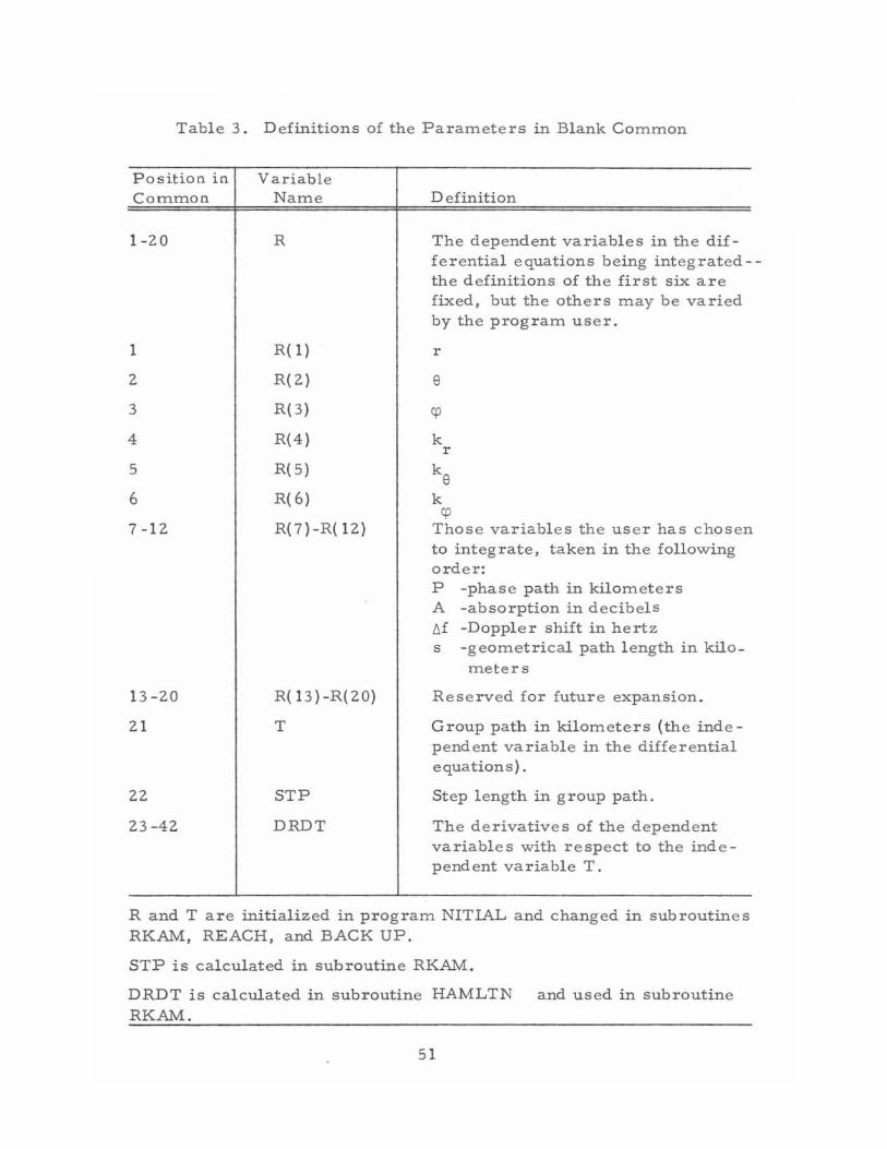
Table 3. Definitions of the Para meters in Blank Common
Position in Variable C o mmon
1-20
1
2
3
4
5
6
7 -12
13 -20
21
22
2 3 -42
Name
R
R( 1)
R(2)
R( 3)
R(4)
R(5)
R( 6)
R(7)-R( 12)
R( 13)-R(20)
T
STP
DRDT
Definition
The d ep endent varia bles in the differ ential e quations being integ rated-the d efinitions of the first six ar e fix ed, but the othe rs m ay be v a ried by the program us e r.
r
e cp
k r
ke k
cp Thos e variable s the us e r has c hos e n to integrate, t a k e n in the following orde r: P -phas e path in kilomet e rs A -absorption in d e cibel s M -Dopple r shift in hertz s -geo metrica l p a th l en g th in kilo
met e rs
Res e rved for futur e expa nsion.
Group p a th in kilometers (the inde pend ent va riabl e in the diffe r ential e qua tion s ) .
Step l ength in group path.
The d e rivative s of the d e p ende nt variabl e s with r e spe ct to the independ ent variable T.
Rand T a r e initialized in prog r a m NITIAL a nd cha n ged in subroutine s RKAM, REACH, and BACK UP.
STP is c a lculated in subroutine RKAM.
DRDT is calculated in subroutine HAMLTN RKAM.
51
and us ed in subro utine
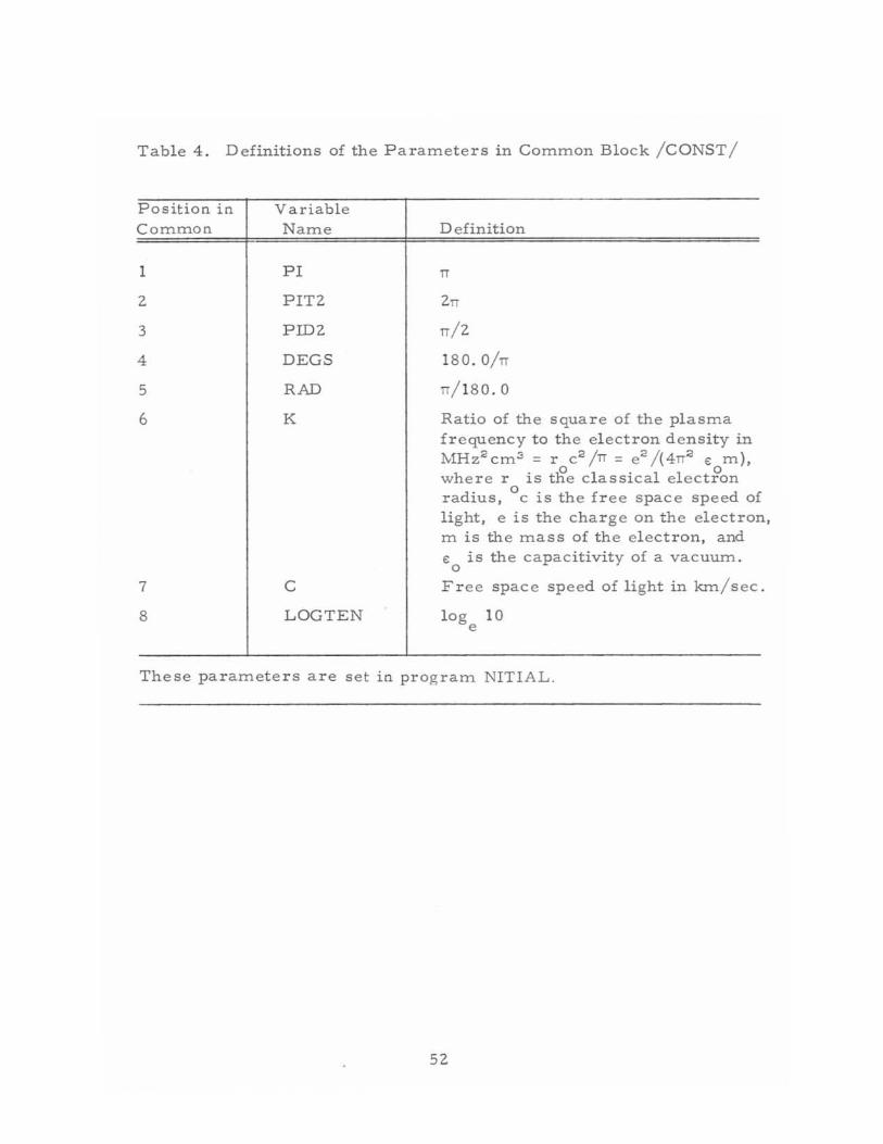
Table 4. Definitions of the Parameters in Common Block / CONST /
Positiotl itl Commotl
1
2
3
4
5
6
7
8
Variable Name
PI
PIT2
PID2
DEGS
RAD
K
C
LOGTEN
Definition
TT
2TT
TT/2
180.0/TT
TT/ 180.0
Ratio of the square of the plasma frequency to the electron density in MHz2 cm3 = r c2/TT = e 2 / (4TT2 € m). where r is tfi'e classical elect:?'on radius, a c is the fre e space speed of light, e is the charge on the electron, m is the mass of the electron, and € is the capacitivity of a vacuum.
a Free space speed of light in km / s ec .
log 10 e
These parameters are set itl program NITIAL .
52
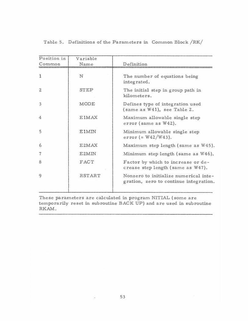
Table 5. Definitions of the Parameters ill Common Block /RK/
Position in Variable Common Name
1 N
2 STEP
3 MODE
4 EIMAX
5 EIMIN
6 E2MAX
7 E2MIN
8 FACT
9 RSTART
Definition
The number of equations being integrated.
The initial step in group path in kilometers.
Defines type of integration used (same as W41), see Tabl e 2.
Maximum allowable single step error (same as W42).
Minimum allowable single step error (= W42/W43).
Maximum step l ength (same as W45).
Minimum step·length (same as W46).
Factor by which to increase or de creaSe step length (same as W47).
Nonzero to initialize numerical integration, zero to continue integration.
These parameters are calculated in program NITIAL (some are temporarily reset in subroutine BACK UP) and are used in subroutine RKAM.
53
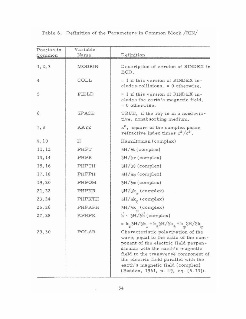
Table 6. Definition of the Parameters in Common Block IRINI
Postion in Variable Common
1,2,3
4
5
6
7,8
9,10
11, 12
13 , 14
15, 16
17, 18
19,20
21,22
23,24
25,26
27,28
29,30
Name
MODRIN
COLL
FIELD
SPACE
KAY2
H
PHPT
PHPR
PHPTH
PHPPH
PHPOM
PHPKR
PHPKTH
PHPKPH
KPHPK
POLAR
Definition
Description of ve rsion of RIND EX in BCD.
= 1 if this version of RINDEX includes collisions, = 0 otherwise.
= 1 if this version of RINDEX includes the earth's magnetic field, = 0 otherwise.
TRUE, if the ray is in a nondeviative, nonabsorbing medium.
k 2, square of the complex phase
refractive index times w2 Ic2•
Hamiltonian (complex)
oH/ot (complex)
oH/or (complex)
oH/oe (complex)
oH/oc:p (complex)
oH/ow (complex)
oH/ok (complex) r
oH/oke (complex)
oH/ok (complex) ~ c:p ~ k . oH/ok (complex)
= k oH/ok + k oH/ok + k oH/ok r r e e c:p c:p
Characteristic polarization of the wave; equal to the ratio of the component of the electric field perpendicular with the earth's magnetic field to the transverse component of the electric field parallel with the earth's magnetic field (complex) (Budden, 1961, p. 49, eq. (5. 13)}.
54
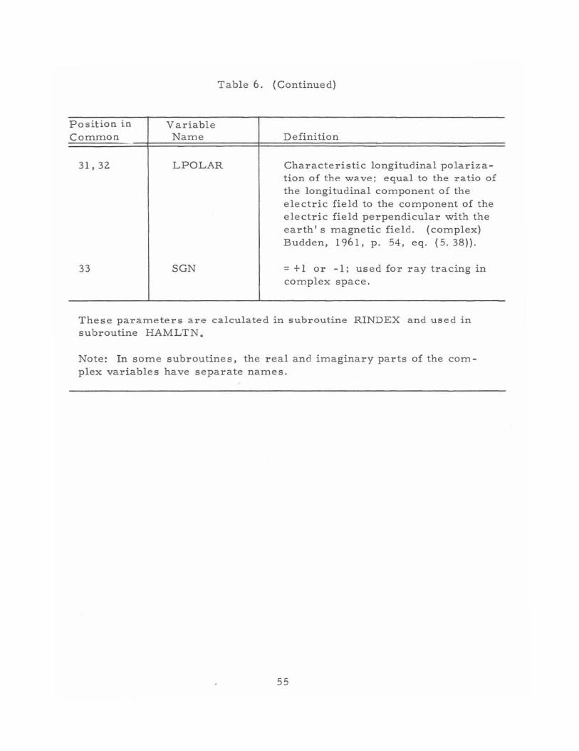
position in Common
31,32
33
Table 6. (Continued)
Variable Name
LPOLAR
SGN
Definition
Characteristic longitudinal polariza tion of the wave; equal to the ratio of the longitudinal component of the electric field to the component of the electric field perpendicular with the earth's magnetic field. (complex) Budden, 1961, p. 54, eq. (5.38}).
= + 1 or -1; used for ray tracing in complex space.
These parameters are calculated in subroutine RINDEX and used in subroutine HAMLTN.
Note: In some subroutines, the real and imaginary parts of the com plex variables have separate names.
55
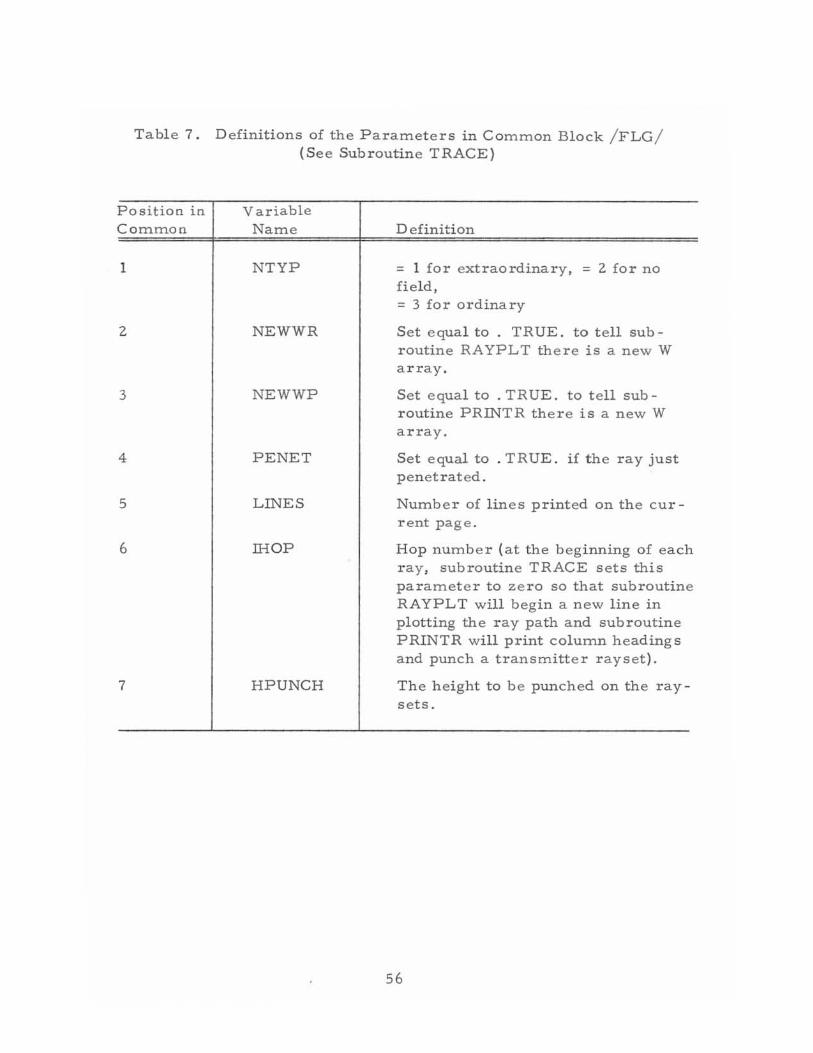
Table 7. Definitions of the Parameters in Common Block /FLG / (Se e Subroutine TRACE)
Position in Variable Common Name
1 NTYP
2 NEWWR
3 NEWWP
4 PENET
5 LINES
6 IHOP
7 HPUNCH
Definition
= 1 for extraordinary, = 2 for no field, = 3 for ordinary
Set equal to . TRUE. to t e ll subroutine RAYPLT the r e is a new W a rray .
S et equ a l to . TRUE. to t e ll subroutine PRINTR there is a new W array.
Set equ a l to . TRUE . if the ray just penetrated .
Numbe r of lines printed on the current page .
Hop number (at the beginning of each r ay, subroutine TRACE sets this paramet e r to ze ro so that subroutine RAYPLT w ill begin a n ew line in plotting th e r ay path a nd subroutine PRINTR w ill print column h eadings a nd punc h a transmitte r r ay set).
The height to be punch e d on the raysets.
56
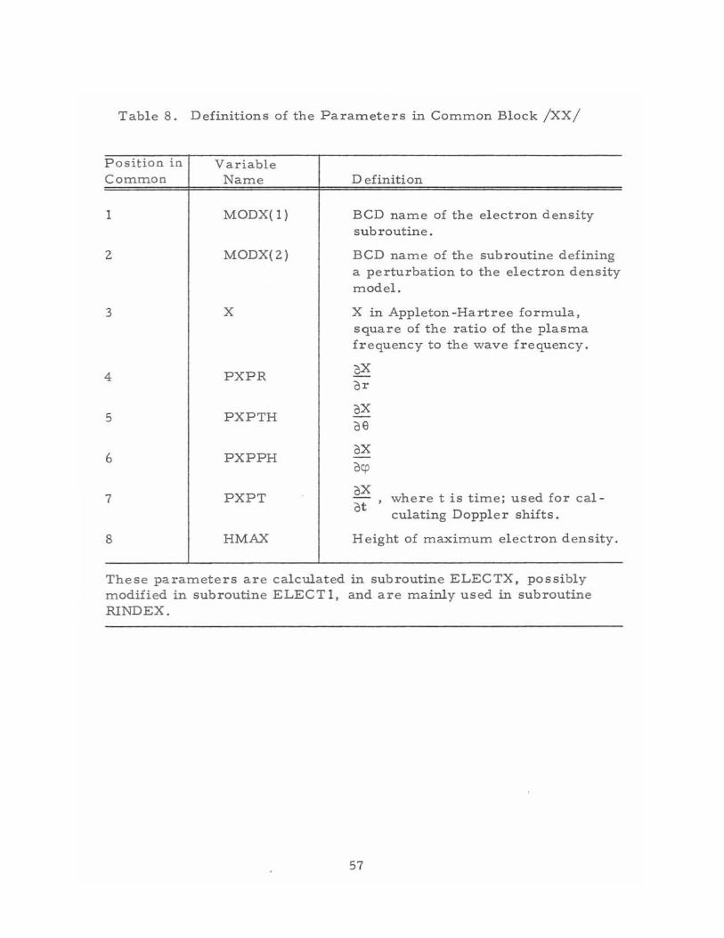
Table 8. Definitions of the Parameters in Common Block /XX/
Position in Variable Common Name
1 MODX( 1)
2 MODX(2)
3 x
4 PXPR
5 PXPTH
6 PXPPH
7 PXPT
8 HMAX
D efinition
BCD name of the electron density sub routine.
BCD name of the subroutine defining a p e rturbation to the e lectron density model.
X in Appleton -Hartree formula, squar e of the ratio of the plasma frequency to the wave frequency.
0X or oX oG oX ocp oX ot wh e r e t is time; used for cal
culating Dopple r shifts .
H e ight of maximum e l ectron d ensity.
These parameters are calculated in subroutine ELECTX, possibl y modified in subroutine ELECTl, and are mainly used in subroutine RlNDEX.
57
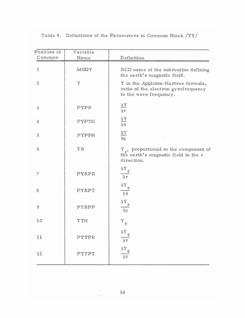
Table 9. Definitions of the Parameters in Common Block /YY /
Position in Variable .Common Name Definition
1 MODY BCD name of the subroutine defining the earth's magnetic field.
2 Y Y in the Appleton-Hartree formula, ratio of the e l ectron gyrofrequency to the wave frequency.
3 PYPR oY or
4 PYPTH oY
08
5 PYPPH oY
oql
6 YR Y , proportional to the component of th';, earth's magnetic field in the r direction.
I • oY 7 PYRPR
r or
oY 8 PYRPT
r
08
oY
9 PYRPP r
Oql
10 YTH Y 8
11 PYTPR oY 8
or
12 PYTPT oY
8 08
58
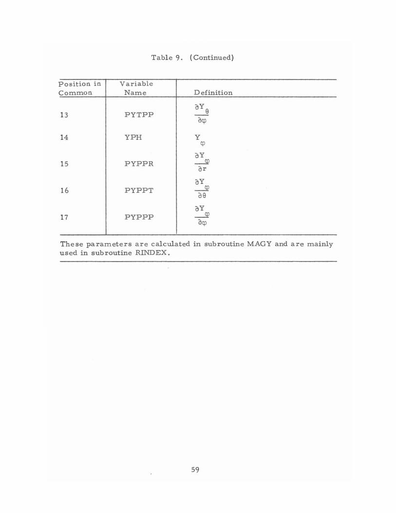
position in Common
13
14
15
16
17
Table 9. (Continued)
Variable Name
PYTPP
YPH
PYPPR
PYPPT
PYPPP
Definition
Y cp
oY ~ or
oY ~ 09
oY ---'E
ocp
These parameters are calculated in subroutine MAGY and are mainly us ed in subroutine RIND EX .
59
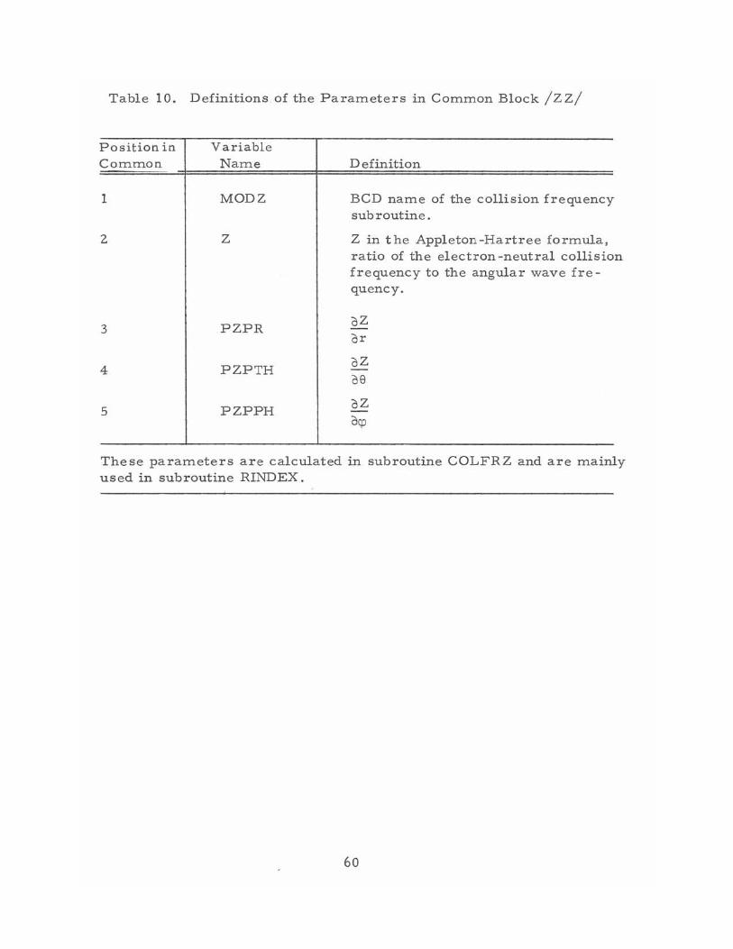
Table 10. Definitions of the Parameters in Common Block /ZZ/
Position in Variable Comtnon Name
1 MODZ
2 Z
3 PZPR
4 PZPTH
5 PZPPH
Definition
BCD name of the collision frequency sub routine.
Z in the Appleton-Hartree formula, ratio of the electron -neutral collision frequency to the angular wave frequency.
oZ or oZ 09
oZ o<;p
These parameters are calculated in subroutine COLFRZ and are mainly used in subroutine RIND EX.
60
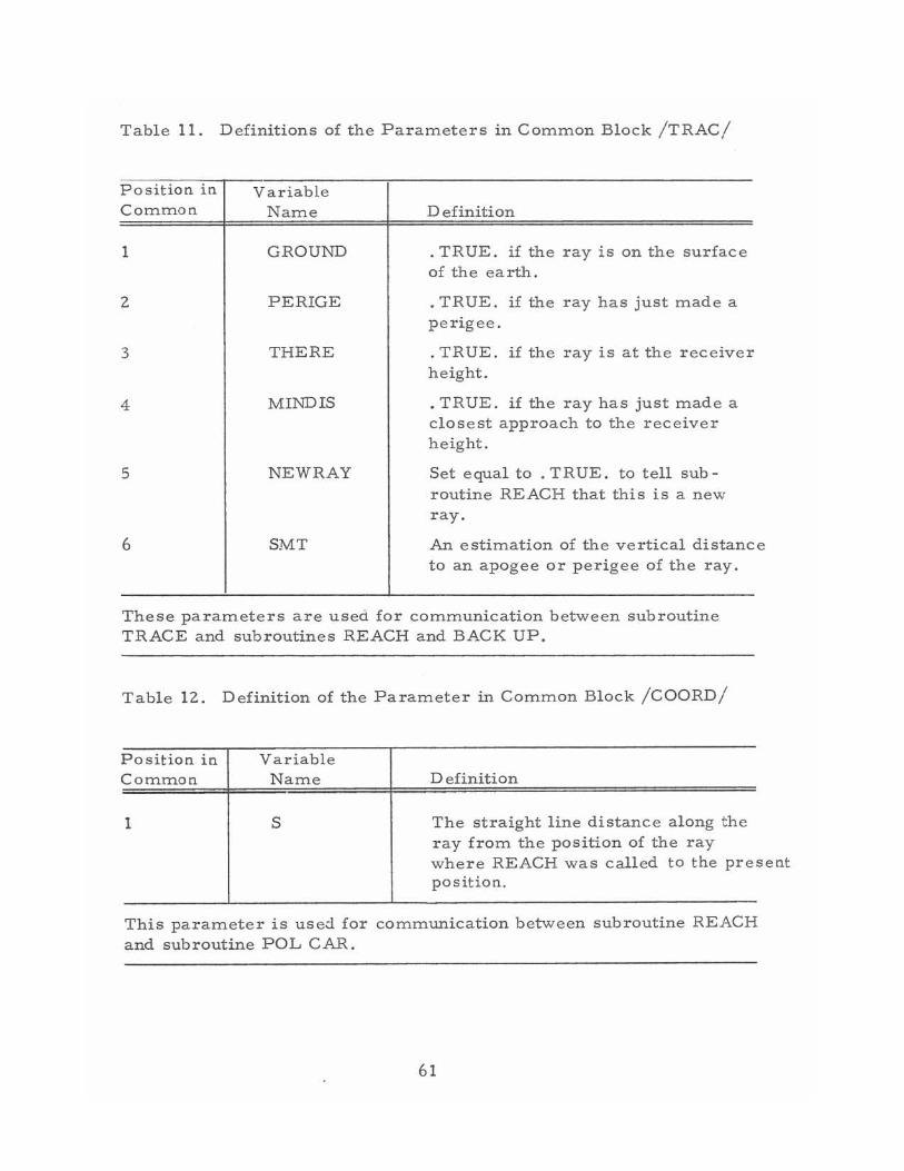
Table 11. Definitions of the Parameters in Common Block /TRAC/
Position in Variable Common Name
1 GROUND
2 PERIGE
3 THERE
4 MIND IS
5 NEWRAY
6 SMT
Definition
· TRUE. if the ray is on the surface of the earth.
· TRUE. if the ray has just made a perigee.
· TRUE. if the ray is at the receiver height.
· TRUE. if the ray has just made a closest approach to the receiver height.
Set equal to . TRUE. to tell subroutine REACH that this is a new ray.
An estimation of the vertical distance to an apogee or perigee of the ray.
These parameters are used for communication between subroutine TRACE and subroutines REACH and BACK UP.
Table 12. Definition of the Parameter in Common Block /COORD/
Position in Variable ComITIon Name
1 S
Definition
The straight line distance along the ray from the position of the ray where REACH was called to the present position.
This parameter is used for communication between subroutine REACH and subroutine POL CAR.
61
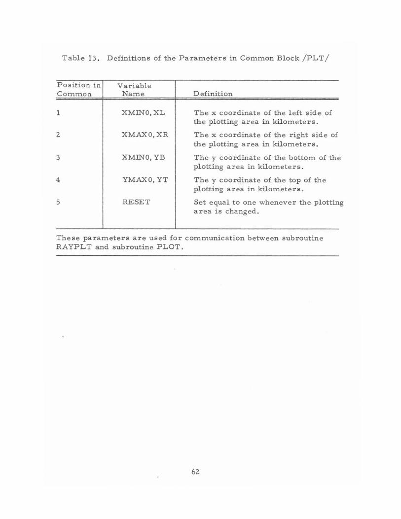
Table 13. Definitions of the Parameters in Common Block /PLT/
Position in Common
1
2
3
4
5
Variable Name
XMINO,XL
XMAXO,XR
XMINO, YB
YMAXO, YT
RESET
Definition
The x coordinate of the left side of the plotting area in kilometers.
The x coordinate of the right side of the plotting area in kilometers.
The y coordinate of the bottom of the plotting area in kilometers.
The y coordinate of the top of the plotting area in kilometers.
Set equal to one whenever the plotting area is changed.
These parameters are used for communication between subroutine RAYPLT and subroutine PLOT.
62
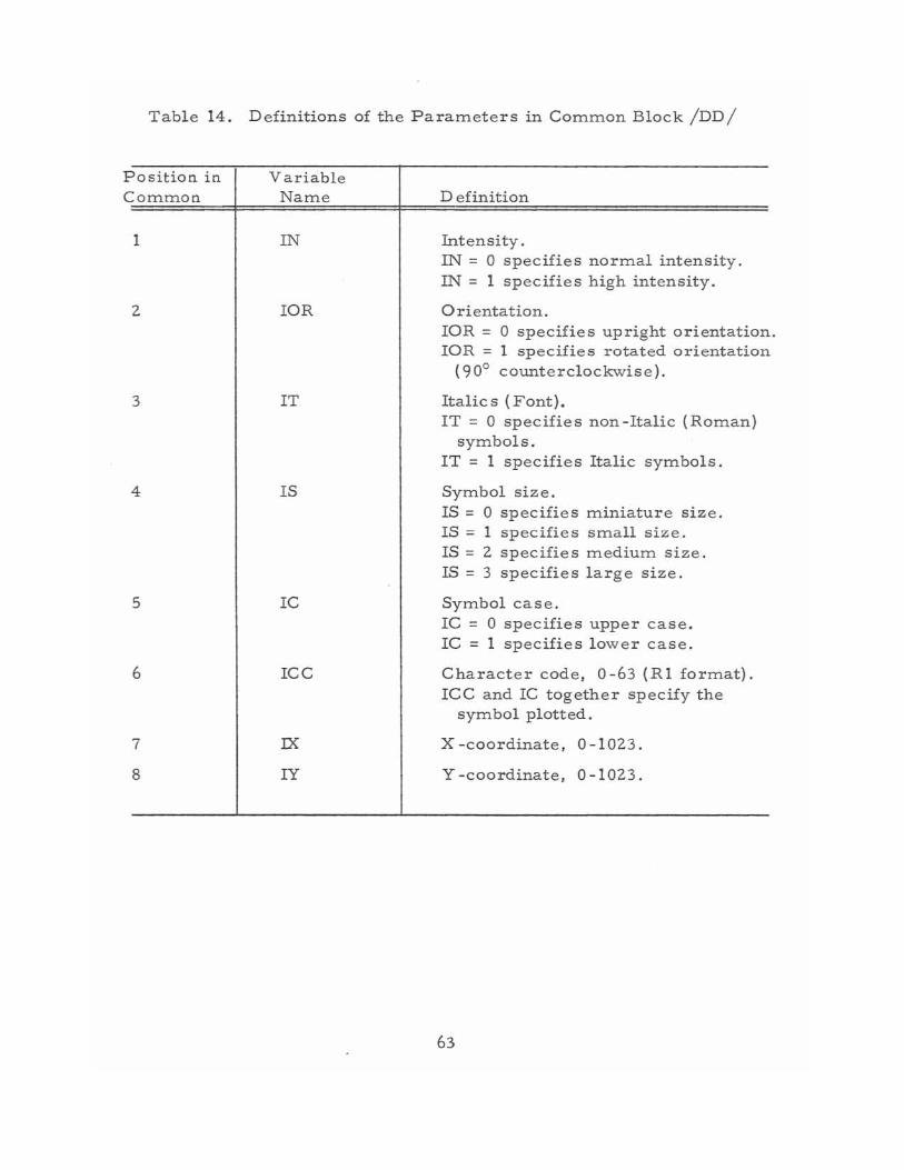
Table 14. Definitions of the Parameters in Common Block /DD/
Position in Variable Common
1
2
3
4
5
6
7
8
Name
IN
IOR
IT
IS
IC
ICC
IX
IY
Definition
Intensity. IN = 0 specifies normal intensity. IN = 1 specifies high intensity.
Orientation. lOR = 0 specifies upright orientation. lOR = 1 specifies rotated orientation
(900 counterclockwise).
Italic s (Font). IT = 0 specifies non-Italic (Roman)
symbols. IT = 1 specifies Italic symbols.
Symbol size. IS = 0 specifies miniature size. IS = 1 specifies small size. IS = 2 specifies medium size. IS = 3 specifies large size.
Symbol case. IC = 0 specifies upper case. IC = 1 specifies lowe r case.
Character code, 0 - 63 (R1 format). ICC and IC together specify the
symbol plotted.
X -coordinate, 0 -1023.
Y -coordinate, 0 -1023.
63
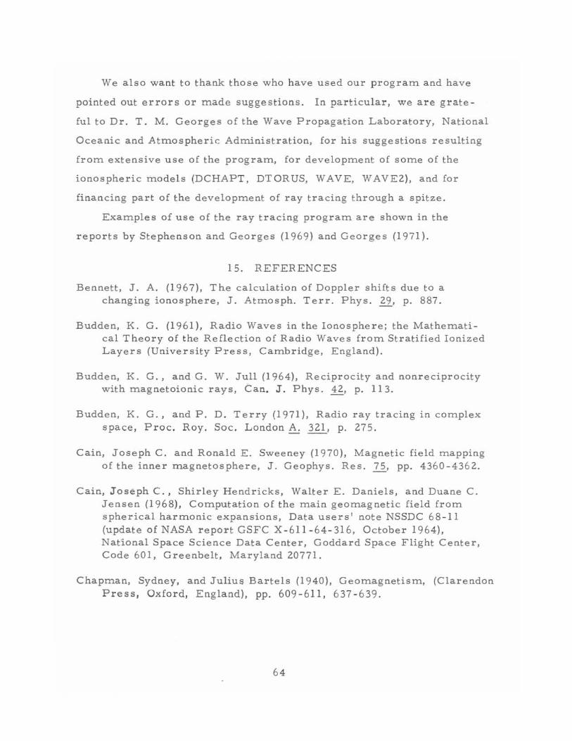
We also want to thank those who have used our program and have
pointed out errors or made suggestions. In particular, we are grate
ful to Dr. T. M. Georges of the Wave Propagation Laboratory, National
Oceanic and Atmospheric: Administ ration, for his suggestions resulting
from extensive use of the program, for development of some of the
ionospheric models (DCHAPT, DTORUS, WAVE, WAVE 2). and for
financing part of the development of ray tracing through a spitze.
Examples of us e of the ray tracing program are shown in the
reports by Stephenson and Georges (1969) and Georges (1971).
15. REFERENCES
Bennett, J. A. (1967), The calculation of Doppler shifts due to a changing ionosphere, J. Atmosph. Terr. Phys. ~, p. 887.
Budden, K. G. (19 6 1), Radio Waves in the Ionosphere; the Mathematical Theory of the Reflection of Radio Waves from Stratified Ionized Layers (University Press, Cambridge, England).
Budden, K. G., and G. W. Jull (1964). Reciprocity and nonreciprocity with magnetoionic rays, Can. J. Phys. 42, p. 113.
Budden, K. G ., and P. D. Terry (1971), Radio ray tracing in complex space, Proc. Roy. Soc. London A. 321, p. 275.
Cain, Joseph C. and Ronald E. Sweeney (1970). Magnetic field mapping of the inner magnetosphere, J. Geophys. Res. li, pp. 4360 -43 6 2.
Cain, Joseph C., Shirley Hendricks, Walter E. Daniels, and Duane C. J ensen (1968), Computation of the main geomagnetic field from sphe rical harmonic expansions, Data users' note NSSDC 68-11 (update of NASA report GSFC X - 61 1-64 -31 6, October 1964). National Space Science Data Center, Goddard Space Flight Center, Code 60 1, Greenbelt. Maryland 20771.
Chapman, Sydney, and Julius Bartels (1940), Geomagnetism, (Clarendon Press, Oxford, England). pp. 609-611. 637-639.
64
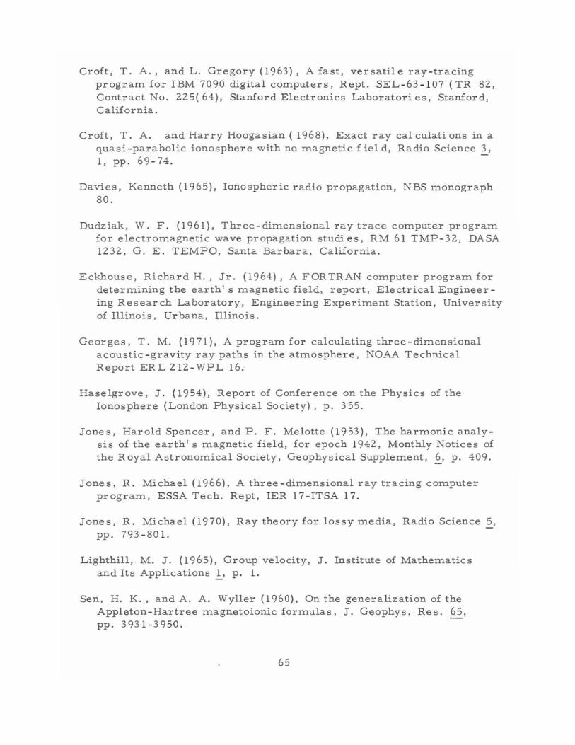
Croft, T. A., and L. Gregory (1963) , A fast, versatil e ray - tracing program for IBM 7090 digital compute r s, Rept. SEL - 63 -1 07 (TR 82, Contract No. 225( 64), Stanford Electronics Laboratori es, Stanford, California.
Croft, T. A. and Harry Hoogasian (1968), Exact ray calculations in a quasi - parabolic ionosphere with no magnetic f iel d, Radio Science ~, 1, pp. 69 - 74.
Davies, Kenneth (1965), Ionospheric radio propagation, NBS monograph 80.
Dudziak , W. F. (1961), Three - dimensional ray trace computer program for electromagnetic wave propagation studi es, RM 61 TMP - 32, DASA 1232 , G. E. TEMPO, Santa Barbara, California.
Eckhouse, Richard H., Jr. (1964), A FOR TRAN computer program for determining the earth's magnetic field, report , Electrical Engineer ing Re search Laboratory, Engineering Experiment Station, University of Illino is, Ur bana, Illinois.
Georges, T . M. (1971), A program for calculating three-dimensional acoustic - gravity ray paths in the atmosphere, NOAA Technical Report ERL 212 - WPL 16.
Haselgrove, J. (1954), Report of Conference on the Physics of the Ionosphere (London Physical Society), p. 355.
Jones, Harold Spencer, and P . F. Melotte (1953), The harmonic analysis of the ear th's magnetic field, for epoch 1942, Monthly Notices of the Royal Astronomical Society, Geophysical Supplement, ~, p. 409.
Jones, R. Michael (1966), A three-dimensional ray tracing computer program, ESSA Tech. Rept, IER 17 - ITSA 17.
Jones, R. Michael ( 1970), Ray theory for lossy media, Radio Science .?' pp. 793-801.
Lighthill, M. J. (1965), Group velocity, J. Institute of Mathematics and Its Applications .!.' p. 1.
Sen, H. K., and A. A. Wyller (1960), On the generalization of the Appleton - Hartree magnetoionic formulas, J. Geophys. Re s. 65, pp. 3931-3950.
65
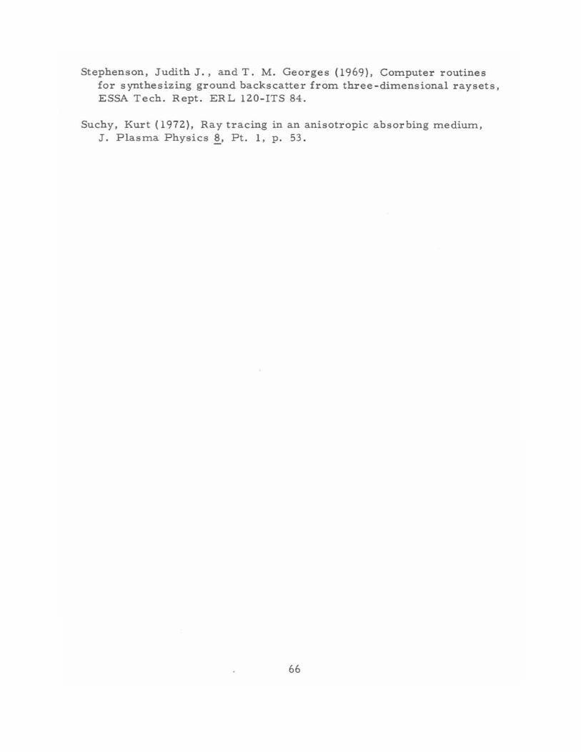
Stephenson, Judith J., and T. M. Georges (1969), Computer routines for synthesizing ground backscatter from three -dimensional raysets, ESSA Tech. Rept. ERL 120-ITS 84 .
Suchy, Kurt (1972), Ray tracing in an anisotropic absorbing medium, J . Plasma Physics ~, Pt. 1, p. 53.
66
APPENDIX 1. LISTINGS OF THE MAIN PROGRAM AND SUBROUTINES IN THE MAIN DECK
T his appendix contains listings of the m.ain program. and those sub-
routine s that have only one version (with the exception of subroutine
RAYPLT, which has a do - nothing version for users lacking a plotter to
plot ray paths). Thus, the routines which form. the contents of this appen
dix will be used in all ray path calculations.
Additionally, this appendix contains the m.ain input param.eter form.
for ray tracing and the input param.eter form.s for plotting. These form.s
are very useful when using the program. because they indicate the input
parameters needed for ray path calculations
The contents of this appendix are arranged as follows:
a. Main input param.eter form. 68
b. Program. NITIAL 69
c. Subroutine READ W 72
d Subroutine TRACE 72
e. Subroutine BACKUP 74
f. Subroutine REACH 76
g. Subroutine POLCAR 77
h. Subroutine PRINTR 78
i. Input param.eter form.s for plotting 82
j. Subroutine RAYPLT 84
k. Subroutine PLOT 86
1. Subroutine LABPLT 87
m.. Subroutine RKAM 88
n . Subroutine HAMLTN 90
67
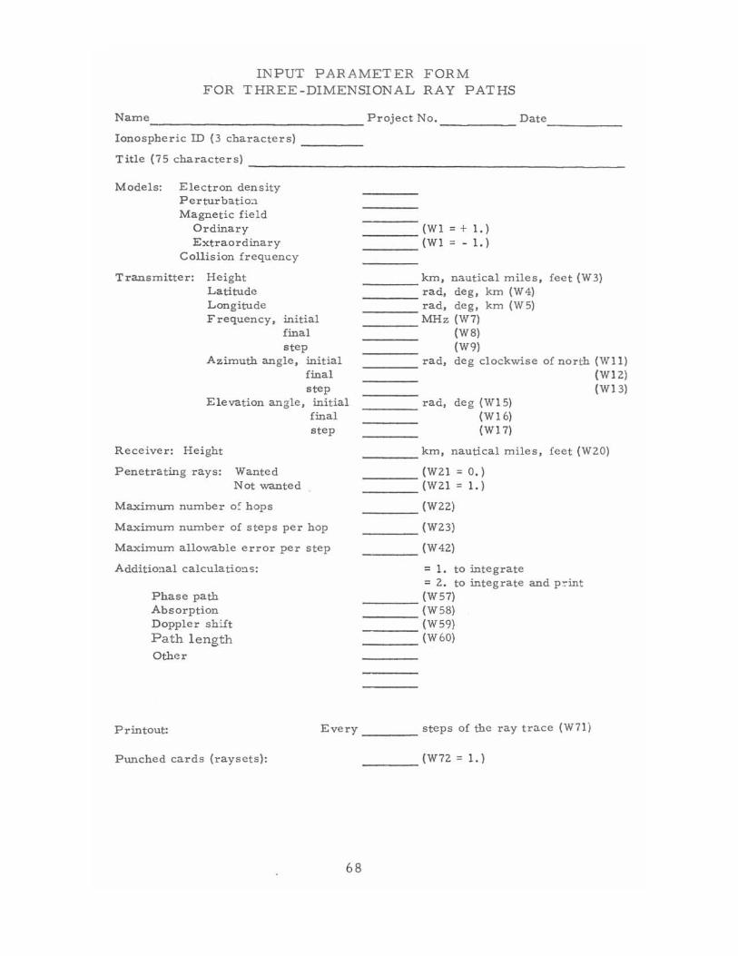
INPUT PARAMETER FORM FOR THREE-DIMENSIONAL RAY PATHS
Name Project No. Date ------------ ----- -----Ionospheric ID (3 characters) ____ _
Title (75 characters) ------------------------------------Models: Electron density
Perturbatio:l Magnetic field
Ordinary Extraordinary
Collision frequency
Transmitter: Height Latitude Longitude Frequency, initial
final step
Azimuth angle , initial final step
Elevation angle, initial
Receiver: Height
Penetrating rays: Wanted Not wanted
Maximum number 0: hops
final step
Maximum number of steps per bop
Maximum allowable error per step
Addition.al calculations:
Phase path Absorption Doppler shift
Path length Other
(Wl= + 1.) ---___ (WI - - 1.)
____ krn, nautical miles, feet (W3) ____ rad, deg, km (W4) ____ rad, deg, km (W5) ____ MHz (W7)
(W8) (W9)
____ rad, deg clockwise of north (W 11) (WI2) (WI3)
____ rad, deg (WI5) (WI6) (WI7)
____ km, nautical miles, feet (W20)
___ (W21 = 0,) ___ (W21 = 1.)
___ (W22)
___ (W23)
___ (W42)
::: 1. to integrate ::: 2. to integrate and p:-:int
___ (W 57) ___ (W58) ___ (W59) ___ (W 60)
Printout: Every ____ steps of the ray trace (W71)
Punched cards (raysets): ___ (W72 = 1.)
68
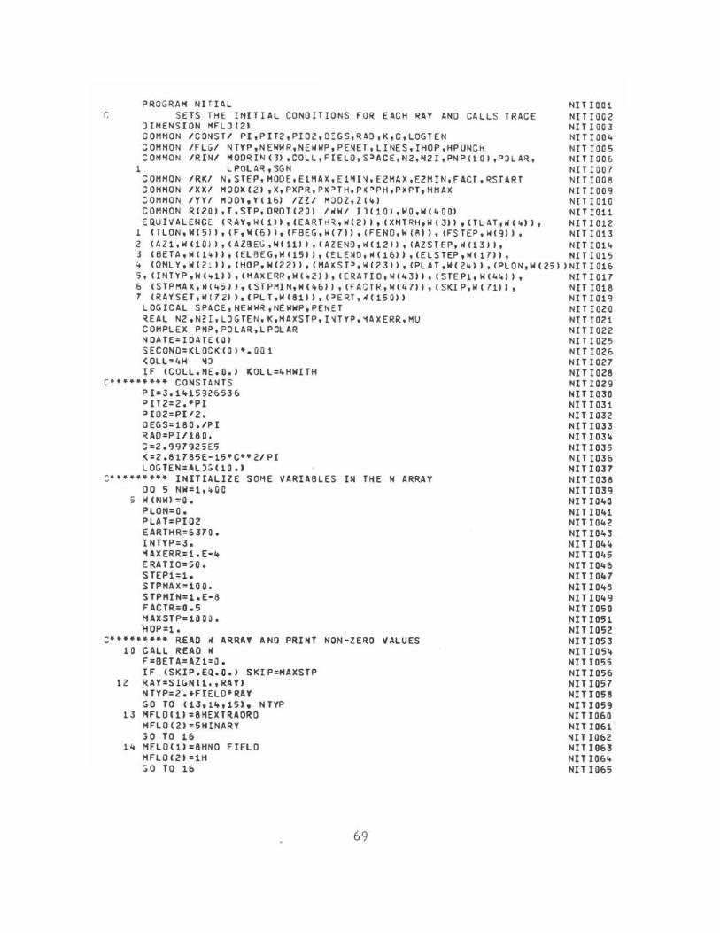
PROGRAM NlII~L NIT 1001 r. SE TS THE INITIAL CONOITIONS FOR EACH RAY ANO CALLS TRACE NITIOC2
JINENSION MFLO(2' NITI003 COMMON tCDNSTI PI.PIT2,PI02.0~GS,RAO,K,C,LOGTEN NITI004 :OMHON IFLGI NTYP,NEWHR,NEWWP,PENET,LINES,IHOP,HPUNCH NIlIOOS :OMHON IRINI P100~IN('3) .COLL,F[ELO.S=-ACE,N2,N2I.PNP(tO},?JlAR. NITI006
1 LPOUR.SGN NITI007 :OHHON IRKI N,STEP,HOOE,EIMAX,El~I~.E2HAX,EZMIN,FACT,~START NITtOOS :;OHMON IX'1..I "'001(2) ,X,PXPR,P)( :tTH,P I( :lPH,P XP T,HMAX NITI009 CONNON IVYI "00Y.Y(16' IlU NJOl.Z{f.' NITI010 COMMON R(ZQ},T,STP,O~OT(20) /JiW/ 1)(10),HQ,W(ItOOI NITrOl1 EQUIVALENCE (R.AY .. W(U),(EARTH~,W(2),(XMTRH,W{3)},(TLAT,"(It», NITI012
1 <TLON,W(SlJ,(F,W(6»,(FBEG,\oI(71),(FENO,WUH),(FSTEP,IH9», NITIOl3 2 (AZ1,WUOJ) ,(AZ3EG,W(111) ,(AZEND.WClZ», (AlSTE"P,W(13J), NITI014 3 (BETA,W(11t)',(ELBEG,HUS)J,CELENO,WC1&)),(ELSTEP,W(17l', NITI01S :. (ONLY,W(2lt), (HOP,W(2Z», 01AKST',W(Z3», (PLAT,W(Z4») ,(PLON,W(Z5' 'NITIOt& S. (lNTYP,WC't1), (HAXERR,W(!.tZ»), (ERATlO,WC43", (SlEP1,W(Lt4»), NITI017 & (STPHAX,W(45J ',(STPMIN,W(4&1', (FA :::TR,W(47)I, (SI(IP,W(71)), NITr018 7 (RAYSET,W(72).(PLT,W(81)',C'ERl,,..(150') NITI019
LOGICAL SPACE,NEWWq,NEWWP,PENET NITIOZO ~EAL NZ.N2I,LJGlEN,K,MAXSTP,I~TYP,1AXERR,MU NIlIOZ1 COM PLEX PNP,POlAR,LPOlAR NITIOZZ NQATE=IDATECQJ NITIOZ5 SECONO=KLOCK(O)".OOl NIT 1026 <OLL'4H ~J NITI027 IF (C OLL.NE.O.' (OLL=4HWITH NITI028
C'" .......... CONSTANTS NIT IOZ9 PI=3.1415n6536 NIT 1030 PIT2=2."PI NITI031 'I02=PI/2. NIT 1032 OEGS=180.IPI NITIOH RAO=PI/18D. NITI034 ;=2.997925E5 NITI035 K=2.81785E-15"C"21PI NITI036 LOGTEN=AL):;11D.1 NIT 1037
C .. •••••••• INITIALIZE SOME VARIABLES IN THE H ARRAY NITI038 00 5 NW=1 •• 00 NITI039
5 W(NH'=Q. NITIG40 PLON=O. NITI041 PLAT=P102 NITI042 EARTHR=6370. NITI043 INTYP=3. NIT 1044 ~AXERR=1.E·4 NITI045 ERATIO=50. NIT 1046 STEP1=1. NIT 1047 HPMAX=100. NIT 1048 STPMIN=1.E·8 NITI049 FACTR=0.5 NITI050 HAXSTP=l~OO. NIT1051 "HOP=l. NIT 1052
C· .. ••••••• REAO W ARRAY AND PRINT NON-ZE~O VALUES NIlI053 10 CALL REAO W NITI054
F=BETA=AZ1=O. NIT 1055 IF (SKIP.EQ.O.' SKIP=HAXSTP NITI056
12 RAY :SIGNll .. RAYI NITI057 ~TYP:Z.+FIELO·RAY NITI05S GO TO (13.14,15). NTYP NITI059
13 HFLOI1l:8HEXTRAORO NITI060 NFLO(2':5HINARY NIT 1061 ;0 TO 16 NIT 1062
14 NFLOI1l:8HNO FIELO NIT 1063 MFLOIZ.:1N NITI064 :;0 TO 16 NIT 1065
69
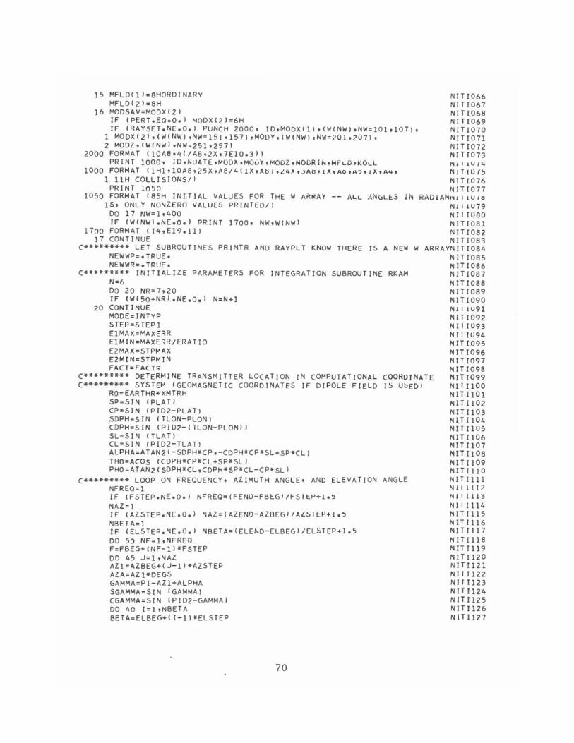
15 MFLDIII=8HORDINARY MFLDI21=8H
16 MODSAV=MODXI21 IF (PERT.Ea.o.1 MODX(21=6H IF (RAYSET.NE.O.I PUNCH 2000, ID,MODXI!I,(WINW),NW=101,101),
1 MOOX(2I,(W(NWI ,NW=151.157) ,MODY,I'WINWI ,NW=201,Z071, 2 MODl,(WINW I ,NW=251,2571
2000 FORMAT (lOA8,4(/A8.2X.1EIO.31) PR I NT 1000. 10 ,NUA TE ,MOD"- • MOul' • MOOZ ,MOCR 1 N .MfLu .KOLL
1000 FORMAT (lHl,lOA8,25X,1\8/4(lX'A/jJ'L4X'~A!j'lX'AO'A:>'L};'A4' I IlH COLLISIONS/i
PRINT In 50 1050 FORMAT 185H INITIAL VALUES FOR THE W AR~AY -- ALL ANGLtS IN
IS. ONLY NONZERO VALUES PRINTED/I DO 17 NW=1,400 IF (WCNWI.NE.o.1 PRINT 1700. NW,WINWI
1700 FORMAT (14,EI9.111 ]7 CONTINUE
c********* LET SUBROUTINES PRtNTR AND RAYPLT KNOW THERE IS A NEW W NEWWP=.TRUE. NEWWR=.TRUE.
c********* INITIALIZE PARAMETERS FOR INTEGRATION SUBROUTINE RKAM N=6 DO 20 NR=7,20 IF (W(50+NRI.NE.O.1 N=N+l
20 CONTINUE MOOE=INTYP STEP=STEPI ElMAX=MAXERR EIMIN=MAXERR/ERATIO E2MAX=STPMAX E2MIN=STPMIN FACT·FACTR
NITI066 NITI061 NITI068 NITI069 NITI07Q NITI011 N I Tl012 NITI013 '''0 I aU 14
NJTIU'~ NITI016 NITIOl1
RADIAN"u I JU 10
NJ I lU79 NIII080 NITl081 NITI082 NITI083
ARRAYNITIOB4 N IT 1085 NITI086 NITI081 NITI088 NITI089 NIT 1090 NJ I lu91 NITIOn N I I 1093 NIIIU94 NlTI095 NlTI096 NITI091
C********* DETERMINE TRANSMITTER LOCATI ON IN COMPUTATIONAL COO~OINATE c********* SYSTEM (GEOMAGNETIC COOROINATES IF DIPOLE FIELD IS U~EDI
RO<EARTHR+XMTRH
NITl098 NIT 1099 N(lllOO NlTIIOl NlTII02 NITl103 N 1.T1104 N 111105 NlTll06 NITII01 NITll08 NIT 1109 NITIIIO NITllll Nl111l2 Ni l 111 ~ NI II114 NITIl15 NlTIl16 NITll11 NITI1l8 NlTI1l9 NITl120 NIT1121 N 111122 N1I1123 NITI124 NITI125 NITll26 NlTI121
SP=SIN IPLATI CP-SIN IPID2-PLATI SDPH=SIN I TLON-PLON I CDPH=SIN IPID2-ITLON-PLONII SL=SIN fTLATI · CL=SIN IPI02-TLATI ALPHA=ATAN2(-SDPH*CP,-CDPH*CP*SL+SP*CLI THO=ACOs (CDPH*CP*CL+SP* SLJ PHO=ATAN2(SDPH*CL,CDPH*SP*CL-CP*SLI
C********* LOOP ON FREQUENCY, AZIMUTH ANGLE' AND ELEVATION ANGLE NFREQ=1 IF (FSTEP.NE.O.I NFREQ.{fENO-F~~GI/~Slt~+l.~ NAZ=1 IF (AZSTEP.NE.O.1 NAZ=(AZEND-AZBEGIIAL~ltP+l.~
NBETA=1 IF IELSTEP.NE.O.I NBETA=IELEND-ELBEGI/ELSTEP+I.5 DO 50 NF=l.NFREQ F=FBEG+INF-ll*FSTEP DO 45 J=l,NAZ AZl=AZBEG+IJ-ll*AZSTEP AZA=AZl*OEGS GAMMA=PI-AZ1+ALPHA SGAMMA<SIN IGAMMAI CGAMMA=SIN (PID2-GAMMAI 00 40 I=l,NBETA BETA=ELBEG+II-ll*ELSTEP
70
~L=AETA*nFr,s NITII2e CBETA=SIN (PID?-BETAl NITI12q R(l}=RO NITI13 0 R(2)=THO NITI131 RI11=PHn NITI132 R(4)=SIN (BETAl NITII31 R(Sl=CBETA*CGAM~A NITI134 R(6)=CAET~4SGAM~A Nlr113~
T=r1. NITIl3£, RSTART=I. NITIl37
C SGN=l. (NEt:D FOR RAY TRACINCl IN COr.1PLEx SPACE.) NITI138 c********* ALLOW 10NO~PHERIC MOD~L SU~ROUTINES TO READ AND PRIN1 DATA NITt139
CALL RINOfX NITIl4U IF (I.NE.l.AND.NPAGE.LT.3.AND.LINES.L~.l7) GO 1025 NIl I141 ~PAGE~LINFS=n NITJ142 PRINT lnoo, JD,NDATE,rv.O()X,t··, U()Y,~Of)L,."1V[)1-<11\j,MI-L[)'''ULL NT r 1143 PRINT 2400, F,AZA NITf144
2400 FORMAT (18X,11HFREQUENCY =,FI2.6,37H MHZ, AZIMlJTH ANGLE OF TRANSMINITI145 lSSION = ,F12.6,4H DEG) NITI146
25 NPAGE=NPAGE+l NITI147 PRINT 2500, EL NITr148
250n FORMAT U31X,33HELfVATION ANGLI: 01- TRANSMl~.slUN =,l-l£.6,4H [)EG/I NIlr149 IF (N2.GT.n.l GO Tn 30 NIT1150 CALL ELECTX NITI15l FN=SIGN (SORT (ABS (Xll*F,XI NIT"Il5? PR I NT 7Qon, FN NITr151
2900 FORMAT (58HOTRANSMITTER IN EVANfSCENT REGION, TRANSMISSION IMPOSSINITI154 lBLE/20HoPLASMA FRECUENCY = ,El7.]01 NITI155
GO TO 44 NITI156 30 MU =SQRT (N2/(R(41**2+R{5 1**2+R(61**21) NITI157
DO 34 NN =4,6 NITIl~8 34 R ( NN1=R ( NN1*~U NITI159
DO 35 NN=7,N NITI160 35 R(NN1 =O. NITI161
CALL TRACE NITI162 OSEC =SECOND NITll63 SECOND=KLnCKlol*.OOl NITI166 DIFF=SECONO-OSEC NITIl65 PRINT 3500, DIFF NITI166
3500 FORMAT (36X,26HTHIS RAY CALCULATION TOOK ,FB.3,4H SEC) NTTI167 IF ( PENET.AND.ON LY.NE.n •• ANO.IHOP.fO.ll GO TO 44 NITI168
40 CONTINUE NITIl69 44 IF (PLT.NE.O.) CALL ENDPLT NITI170 45 CONT I NUE NITIl71
IF( PENET.AND.ONLY.NE.O •• AND.IHOP.EO.l.AND.NAZ.EQ.l,AND.NBETA.EQ.llNITI172 1 GO TO 5S NITI173
50 CONT I NUE NITI174 5C; IF ( RAYSET.NE~O.1 PUNCH 5000 NITI175
soon FOR~AT (78X,lH- l NITI176 MODXI21=MODSAV NIT1177 GO TO 10 NITIl78
END NITIl79 -
71
C C
SUBROUTINE REAO W REAOS W ARRAY
READOOI READ002
MAKE THE DESCRIBED CONVERSIONSREAD003 COL IS COL 19 COL 20 COL 21 (
A 1 IN THE FOLLOWING COLUMNS WILL DEGREES TO RADIANS GREAT CIRCLE DISTANCE IN KM TO RADIANS NAUTICAL MILE S TO KM FEET TO KM
READ004 READ005 READ006 READOO 7 READOOS READ009 READOlO
(OMMON ICONSTI PI,P[T2,PID2,DEG S ,RAD.DUMf3 1 (OMMON /WW/ IDflOl,W Q,Wf4001 EQUIVALENCE fEARTHR,W(21) INTEGER DEG,FEET READ 10nO, ID
1000 FORMAT (IOAS) IF fEOF,60J 3,4
3 CALL EX IT 4 READ 1100, NW,W{NW1,DEG,KM,NM,FEET
11no FORMAT (13,E14.7.511 ) IF fNW.E0.0 1 GO Tn 10 IF INW.GT.O.ANO.NW.L E.400) GO TO 5 PRINT 4noo. NW
4000 FORMAT(15HITHE SUBSCRIPT ,r3,77H ON THE W-ARRAY lUNDS. ALLOWABLE VALUES ARE 1 THR OUGH 400. )
CALL EX IT 5 IF IDEG.NE.O.) WINW ) =WINW1*RAD
IF (KM.NE.O' WINW)=WINW)/EARTHR IF (NM.NE.OJ W(NWJ=W{NWI*].852 IF (FEET.NE.Ol W(NW)=W(NW1*3.048 006096E-4 GO TO 4
10 RETURN END
READOll READ012 READO 13 READ014 READ015 READ016 READO 17 READO IS READ019 READ020 READ02l
INPUT IS UUT OF BOREAD 0 22 READ023 REA0024 READ025 READ026 READ02 7 READ02S READ029 RE ADO 3 0 READ03l-
SUBROUTINE T~~CE TRAC001 C CAlCJL~ES THE RAY PATH TRAC002
DIHENSION ROLO(20) ,OROLJ(20) TRAC003 COMMON IRKI N,STEP,HOOE,E1HAX,E1HIN,E2HAX,EZHIN,FACT,RSTART TRACOO~
COHMON IFLGI NTYP,NfHHR,NEWWP,PENET,LINES,IHOP,HPUNCH TRACOOS COHHON ITRA:I GROUNO,PE~IGE,THERE,HINOIS,NEWRAy,SHT TRAC006 CJHHON IRINI HOORIN(3),COLL,FIElO.SPACE,N2,PNP(lO),POlAR.LPOlAR TRAC007 COHHON IXXI HOOX(ZI,X,PXPR,PXPTH,PXPPH,PXPT,HHAX TRAC008 COHMON R(20) ,T,STF.OROT{ZO) IWWI IO(1 0 ),HQ,W(ltOOI TRAC009 LOGICAL SPA:E,HOHE,WASNT,UNDRGD,GROUNO,PERIGE,THERE,MINDIS,NEMHR, TRAC010
1 NEWj.lP,PENET,NEWRAY,WAS TRACOl1 REAL MAXSTP TRAC012 COHPLEX N2,PNP,POLAR,LPOLAR TRAC013 E lU I V Al ENe E (E A RT HR. W (211 , (RCV RH, j.I {2 0 » " ( HOP, H ( 22) ) , OUXS T P, W ( 2 3 ) ) TRA C 0 lit
1, (SKIP,M<7U), (RAYSET,W<7Z)), (PlT,W(8U) TRACD15 N~OP=HOP TRA C01& MAX =HAXST? TRAC017 NSKIP=SKIP TRAC018 RSTART =1. TRAC019 CALL HAHLTN TRAC020 HOHE'=ORO T( 1) • (R (11 -EART~ ~ - RC VRH) • GE. o. TRAC 021
C ••• • ••••• IHOP =O TELLS PRINTR TO PRINT HEADING AND PUNCH A TRANSMITTER TRAC022 C •••• • •• •• RAys::r AND TELLS RAY'PLT TO ST·ART A NEW RAY TRAC023
IHOP=O TRAC024 CALL PRINTR (8HXHTR ,0.) TRAC025 IF (PLT.NE.O.) CALL RAYPLT TRAC026 HTHAX=O. TRAC027 NE"RAY=.TRUE. TRAC028 T~ERE=R(l)-EARTHR.EO.RCVR~ TRAC029
72
c········· lOOP ON ~UMBER OF HOPS lD IHOP=IHOP+1
IF (IHOP •• T.NHOP) RETURN PENET=.FALSE. APHT=RC ~RH
C········· LOOP ON MAXIMUM NUMBER OF STEPS PER HOP 00 79 J=l. HAX H=R (ll-EARTHR IF (ABS(H-RC~~H) .GT.ABS(A'HT-RCYRH)) APHT=H HTHAX=AHAX1(H.HTHAX) IF (.NOT.SPACE) GO TO lZ CALL REACH RSTART: 1. H:R (ll-EARTHR IF (ABS (H-RC~RH) • G T • ABS (A PHT -RCYRH)) A PHT =H HTHAX=AHAX1(H.HTHAX) IF (.NOT.SPACE) GO TO lZ IF (PERIGE) CALL PRINTR (8HPERIGEE .D.) IF !THERE) :;0 TO 51 IF (MINOIS) GO TO .0 IF (GROUND) :;0 TO oD IF (PU.NE.D.) CALL RAYPU IF (PERI.E) GO TO 79
lZ ~O 13 L=l.N ROLO(L) 'R(Ll
13 OROLO(L)=DROT(L) TOLD=T WAS=THERE CALL RKA" H=R (lI-EARTHR TriERE=.FALSE. 4ASNT=.~OT.HOHE HOHE=OROT(l)·(H-RCVRH).GE.D. UP= (OROHlI-OR a.. 0 (1) ) +!T-TQ LO) SHT=D. IF (THP.NE.D.) SHT=D.S'(R(1) -ROLO(ll+D.S'THP)"ZlABS!THP) IF « (rl-R;H,j) +(ROLO(lI-EARTHR-RCVRH) .LT.D .. ANO •• NOr.WAS) .00..
1 (WAS.ANO.ORaT(U+OROLO(ll.LT.D .. ANO.HOHE)) GO TO SO IF (HOHE.ANO.4ASNT) GO TO 30 IF (H.LT.O •• OR.DROT(U.:;T.O •• ANO.DROlO(U.LT.O •• ANO.SHT.GT.H)
1 GO TO ZU IF (OROLO(l) .LT.D .. ANO.ORDT(lI.GT.O.) CALL PRINTR(8HPERIGEE .0.) IF (oROLO(ll.'T.D •• ANO.ORJT(ll.LT.O.) CALL PRINTR(SHAPOGEE .0.) IF (OROLO(Z)·JROT(Z).LT.D.) CALL PRINTR(8HHAX LAT .0.) IF (OROLO(3)+OROT(3).LT.0.) CALL PRINTR(8HMAX LONG.o.) )0 14 1=4,6 IF (ROLO(I)'R(Il.LT.O') ;ALL PRINTR(8HHAVE REV.o')
H CONTINUE GO TO 75
c········· RAY WENT UNOERGROUNJ ZO CALL BACK UP(D.)
GO TO 00 c····· .. ·. RAY MAY ~AVE HADE A CLOSEST APPROACH 30 CALL GRAZE(RC~RH)
IF (THERE) GO TO 51 .0 DROHll :0.
HPUNCH=R(l)-EARTHR CALL PRINTR(8HHIN OIST.RAYSET) IF (PLT.NE.o.) CALL RAYPLT IF IIHO>.GE.~~OP) RETURN. IHOP:IHOP+1 CALL PRINTR (8HlUN OIST.RAYSETl GO TO 89
73
TRACD30 TRACD31 TRAC03Z TRACD33 TRACD3. TRACD35 TRACD30 TRACD37 TRACD38 TRAC039 TRACo .. o TRACD.1 TRACo .. Z TRACo .. 3 TRACo .... TRACo .. 5 Tuca.o TRACo .. ? TRACo .. 8 TRACo.9 TRAC05D TRAC051 TRACoSZ TUCoS3 TRACoS .. TRAC055 TRAC050 TRACoS7 TRACoS8 TRAC059 TRACDoa TRACool TRACDoZ TRACo03 TRACoo" TRACDoS TRACOoo TRACo07 TRA C 008 TRACo09 TRA CD7D TRAC071 TRAC07Z TRAcon TRACOH TRAC075 TRAC070 TRAcon TRAC078 TRAC079 TRACoSO TRACDSI TRAC08Z TRAC083 TRAC08" TRAC08S TRAC080 TRAC087 TRAC088 TRAC089 TRA C 09 0 TRAC091 TRAC09Z
c········· RAY CROSSED RECEr~ER HEIGHT 50 CALL BACK UP(~C~RHI
THERE=. TRUE. 51 R(l'=EARTHR+RCtRH
HTHA X=AHAX1(RCVRH,HTHAXI HPUN CH= APH T ;ALL PRINTR(8~RCYR ,RAYSETI IF (PLT.NE.O.I CALL RAYPLT IF (RCYRH.NE.O.I GC TO 89 IF (IHOP.GE.NHOPI RETURN IHOP=IHOP+l APHT=RCVRH
C········· GROUND REFLE CT &0 R(1)=EARTHR
IF (ABS(RCYHI.GT.ABS(APHT-RCYRHII APHT=O. R(41=ABS (R(41 I OROT(ll=AaS (OROT(111 RSTART=1. HPUNCH=HTHAX CALL PRINTR(8HGRNO REF,RAYSETI HTHAX=O. IF (RCYRH.NE.O.I GO TO &; THERE=. TRUE. HPUNCH=APHT CALL PRINTR (8HRCYR ,~AYSETI
GO TO 89 :'5 H=O.
THERE=.FALSE.
C···· ····· 75 IF (PLT.NE.O.I CALL RAYPLT
IF (H.GT.HHH.ANO.H.GT.RCYRH.ANO.OROTlll.GT.O.I GO TO 90 IF (HOO(J,NSKIPI.EQ.OI CALL PRINTR(8H ,0.1
79 ;ONTINUE C········· EXCEEDED MA XIMUM NUMBER OF STEPS
HPUNCH=H CALL PRINTR(8HSTEP HAX,RAYSETI RETURN
C········· S9 HOHE=.TRUE.
GO TO 10 C. · . ... ••••• RAY PE~ETRATfO
90 PENEr=. TRU E. HPUNCH=H CAll P R I N T R(6~PEN E TRAT,RAfSET)
RET URN END
SUBROUT INE BA CK UPIHSI CO MMON IRKI N, STEP,MOO E, EI MAX,E IM IN, E2MAX . E2MIN,FAC T. RS TA RT COMMON I TRACI GROUNO ,P ERI GE,T HER E, MINDIS , NE WR AY,SMT COMMON R(20),T , STP'DRO TI20 } IWWI IDIIO} , WO .W( 400) EQUIVA LENCE IE ARTHR, W( 211 , IINTYP,W{4111 , {ST EPl , W(4411 RE AL I NTYP LOG ICAL G ROUN D . PER I GE .THER F' ~ I NO I S . NE W RAY 'HOME
c ******** * DIAG NOSTI C PRINTOUT C CALL PRI NTR (BHBACK UPO . O. 1 C**.***·** GO ING AWAY FROM THE HE IGH T HS
HOME=ORD T( 1 1* ( R( 1 1- EARTHR- HS1 . GE.O . IF IHS . GT. O •• ANO •• NOT .HOME . OR . HS . EO . O •• ANO . OROT{ ll. GT. O.1 GO TO
74
TRAC093 TRAC09" TRAC095 TRAC09& TRAC097 TRAC098 TRACQ99 TRAC100 TRAC101 TRAC102 TRAC103 TRAC10" TRAC105 TRAC10& TRAC107 TRAC108 TRAC109 TRAC110 TRAC111 TRAC112 TRAC113 TRAC114 TRAC115 TRAC11& TRAC117 TRAC118 TRAC119 TRAC120 TRAC121 TRAC122 TRAC123 TRAC124 TRAC125 TRAC12& TRAC127 TRAC128 TRAC129 TRAC130 TRAC131 TRA C132 TRAC133 TRAC134 TRAC13S TRA C13& TRA Cl37 TRAC13 8
BACKOOI BAC K002 BACK003 BACK00 4 BACK005 BACK006 BACK 007 BAC KOOa BACK009 BACKO I O BACK OI I
30 BACKOl2
C********* FIND NEAREST INTERSECTION OF RAY WITH THE HEIGHT HS no 10 1=1,10 STEP=-IRI11-EARTHR-HS'/DRDTI!. STEP=SIGNCAMINl(ABSCSTP).ABSCSTEPI).STEPJ IF IABSIRII'-EARTHR-HS •• LT •• 5E-4.AND.ABSISTEP •• LT.!.' GO TO 60
c* •• ·.**** DIAGNOSTIC PRINTOUT C CALL PRINTRC8HBACK UP1.Q.)
MODE=I RSTART=I. CALL RKAM
10 RSTART=I. C c********* FIND NEAREST CLOSEST APPROACH OF RAY TO THE HEIGHT HS
ENTRY GRAZE THERE=.FALSE.
c******·** DIAGNOSTIC PRTNTOUT C CALL PRINTR 18HGRAZE 0 .0.'
IF ISMT.GT.ABSIRII'-EARTHR-HS" GO TO 30 DO 20 1=1,10 STEP=-R(41/DRDT(4) STEP=S JGN (AM INI (ASS (STP) .ABS( STEP) ) .STEP I IF (ABSCR(4 1).LE.l.E-6.AND.ABSCSTEP).LT.l.) GO TO 60
C.·.*··.** DIAGNOSTIC PRINTOUT C CALL PRINTR 18HGRAlE ! .0.'
MODE=I RSTARTzl. CALL RKAM RSTART=l. IF IDRDTI4'*IRII'-EARTHR-HS'.LT.D.1 GO TO 30 IFCR(5).EO.0 •• AND.R(61.EO.0.) GO TO 60
20 CONTINUE C**····*** IF A CLOSEST APPROACH COULD NOT 8E FOUND TN 10 STEPS. IT c****·**** PROBABLY MEANS THAT THE RAY INTERSECTS THE HEIGHT HS
30 CONTINUE c******·** DIAGNOSTIC PRINTOUT C CALL PRINTR (BHBACK UP2,0.1
MODE=! c*·******· ESTIMATE DISTANCE TO NEAREST INTERSEcTION OF ~AY WITH HEIGHT c******* •• HS BEHIND THE PRESENT RAY POINT
STEP=(-RC4)-SORT(R(41**2-2.*(RCI1-EARTHR-HSJ*DRDTC4))1IDRDT(4) RSTART=I. CALL RKAM RSTART=!.
c*·******* FINO NEAREST INTERSECTION OF RAY WITH HEIGHT HS DO 40 1=1,10 S TEP=-(R(lJ-EARTH~-HSJ/DRDT(l)
STEP=SIGN(AMINICABSfSTPI.ABSCSTEPI).STEP) IF IABSIRII 1-EARTHR-HS •• LT •• 5E-4. AND.ABSISTEP1.LT.I.' GO To 60
c**.**·*** DIAGNOSTIC PRINTOUT C CALL PRINTR (BHBACK UP3.0.1
MODE=! RSTART=!. CALL RKAM
40 RSTART=I. 50 THERE =- TRUE.
c********* RESET STANDARD MODE AND INTEGRATION TYPE 60 MOOE=INTYP
STEP=STEPI RETURN
END
75
BACKO!3 BACKO!4 BACKO!5 BACKO!6 BACKO!7 BACKOl8 BACKOl9 BACK020 BACK021 BACK022 BACKOZ3 BACKOZ4 BACKOZ5 BACKOZ6 BACKOZ7 BACK028 BACK029 BACK030 BACK03! BACK032 BACK033 BACK034 BACK035 BACK036 BACK037 BACK038 BACK039 BACK040 BACK041 BACK042 BACK043 BACK044 BACK045 BACK046 BACK047 BACK048 BACK049 BACK050 BACK05! BACK052 BACK053 BACK054 BACK055 BACK056 BACK0 57 BACK058 BACK059 BACK060 BACK06! BACK062 BACK063 BACK064 BACK065 BACK066 BACK067 BACK068 BACK069 BACK070 BACK07! BACK072-
SUBROUTINE REACH C CALCULATES THE STRAIGHT LINE RAY PATH I!"ETWEEN THE EARTH C AND THE IONOSPHERE OR BETWEEN IONOSPHERIC LAYERS
COMMON I~KI N,STEP,HOOE,El~AX,~lMrN,E2MAX,E2HIN,FACT,RSTART Cor-a'1ON ITRACI GROUND, PE~IGE, THERE ,MINOIS, NEWRAY .SMT COMMON /C08RD/ S CO~MON I~INI HOORINe31,COLL,FIELO,SPACE,N2,NZI,PNPC10I,POlAk,
1 LPOLAR COPMON IXXI MODXC2J,X,PXPR,PXPTH,PXPPH,PXPT,HMAX COt-'MON ~C2:J),T,STP,DROT(20) IHHI IDC10I,WQ,W(4QO) f.QUIVALENe=. (fARTHR,W(2JI,eXHTRH,W(3»),(RCVRH,H(20) LOGICAL CPOSS,CROSSG,CROSSR,SPACE,GROUND,P£RIGE,THERE,MINors,
1 N::-WRAY,RSPACE R.f:A L N2,N2I CO~PLEX PNP,POlAR,LPOLAR DATA (NST"P=SOOI CALL HHUN H=R (ll-lA"lHR IF (.NOT.NEWRAY.ANO .. NOT.RSPACEI CALL PRINTR(8HEXIT ION.O.I N£WRAY=-.FALSE. V;SQRT(RC4)·~2~R(5)··Z+R(o'··2)
C········· NORMALIZE TH~ WAVE NORMAL DIR£CTION TO ONE R(41 ='<1 4l/V ;U5, =R(5'/ij' R("I=R( "I/V
C········· NEGATIVE OF DISTANC~ ALONG RAY TO CLOSEST APPROACH TO CENTER C········· OF EA~TH
UP;R(lJ ·R(.J RADG;EAKTH~··2-R(1)··Z·(~(5'··2+R(0'··ZI DISTG=SORT (AMAX1(O .. RADGII C········· DISTANCE ALONG ~AY TO FIRST INTERSECTION WITH OR CLOS~ST C········· APPROACH TO TH~ EARTH SG= -UP- 01 ST G
C········· CROSSG IS TRUE IF THE RAY WILL INTERSECT OR TOUCH THt iARTH CROSSG=-UP.LT.O •• ANO.RAOG.GE.O. ~AO R= (E AR. THR. RC VRH, •• Z-Q (1) ··2'" (R (5' ··Z ~R (0' ··2) DISTR=SORT IAHAX1(0 •• RADRII C········· DISTANCE ALONG RAY TO THE FIRST INTERSECTION WITH O~ CLOSEST C········· APPROACH TO THE R_ECEIVER HEIGHT SR=DISTR-UP IF (UP.LT.O •• AND.DISTR.LT.-UP.AND.R(ll.NE.EARTHR+RCVRHI SR=-OISTR
1 -UP c········· CROSSR IS T~UE IF THE RAY WILL INTERSECT C········· ClOSfST APPROACH TO THE RECEIVE~ HEIGHT
CROSSR=RI 41 .L T. O •• OR. R( 11 • LT. IE ARTHR+RCVRHI eRO SS=C PO SSG. OR.C ROSSR
WITH OR MAKo A
C········· !'IAXIMUH DISTANCE IN Sl=AHINlISR.SGI IFf.NOT.CROSSGI S1=SR
WHICH TO LOOK FOR THE IONOSPHERE
IF (UP.GE.O.1 GO TO 15 CROSS=.TRUE.
REACO!)l REAC002 REACO 03 REACCO~
REACt 'J3 R€ACC06 PEACJ07 RC:ACCGS R':ACC c q P,EAC(:10 ~:::ACOll
R~AC( 12 REAC,13 REAC 1 ... RtAC 15 ROC 16 ~f.AC 17 R.EAC 1~ REAC 1') REAC 2J 'I.E A C 21 '<E AC 22 REAC 23 iF AC 2 .. Rc.AC 23 R.EAC 26 REAC 27 Rf.AC 21t R.~AC 21 ~£AC 30 R::AC 31 R':A( 32 RcAC 33 REAC 3 ... REAC 35 REAC 3& REAC 37 ,<"AC 38 R~AC REAC
3q 4~
.1 REAC REAC 42 REAC 43 REAC 4. ROC 45 REAC 46 RE AC 47 REAC 46 REAC 4q REAC 50 REAC 51
c········· IF RAY IS GOING DOWN, Sl=AHINlIS1.-UPI
C······.·· CONVERT THE c~········ COORDINATES
Sl IS AT MOST THE DISTANCE TO A PERIGEEREAC 52 REAC 53
POSITION AND OIRECTION JF THE RAY TO CARTESIAN REAC 5. REAC 55 REAC 5& REAC 57 REAC 56 RfAC sq
15 CALL POL CAR SSTEP=l 00. S=S!STEP DO 20 I=l.NSTEP IF IIS-SSToPI.GT.S1.AND.CROSSI GO TO 25
C········· CONVERT POSITION AND DIRECTION TO SPHERICAL POLAR C········· AT A DISTANCE S ALONG THE RAY
CALL CA R POL CALL ELEClX
C········· FREE SPACE
76
REAC 60 COORDINATESREAC 61
REAC 62 REAC 63 REAC 6. REAC 65
IF IX.EO.C. I GO TO 20 CAL L RI NOO
C········· eFFECTIVELY FREE SPAC~ IF (SPACE) GO TO 2D IF ISSTEP.LT.O.5E-4) GO TO 25 c·.···.··· RAY IN THE IONOSPHERE. STEP S=S-SSTfP
c········· DECREASE STEP SSTEP=SST"P/10.
20 S=S"SSTt.P PRINT 2COQ, NSTEP
SIZE
BACK O~T
2000 FORMAT (gH EXCEEOEO.I5.25H STEPS IN SUBROUTINE REACHI CALL ::X IT
25 IF(CQOSS) S=HIN1 (S.S1) c··.· ... ·. CONVE~T POSITION AND DIRECTION TO SPHERICAL POLA~ c·······.· AT A DISTANCf S ALONG TH~ RAY CALL CAP POL
c· •••• •••• .o.VOIO THE. ~AY BEING SLIGHTLY UNO:=:R:G~OlJNO Q(1)=AMAXitP(t) ,EARTH~'
c········ .. ONE STEP INTEGRATION IF IN.LT.71 GO TO 31 00 30 NN=7,N
30 R(NN' =p INN' +S·OROT(NN' 31 T=l+S
CALL qINOEX c··.···.·· AT A P~RIG[E PEFIGE=S.~Q.(-UP'
c········· COR~~CT HINOR ERRORS IF (PERIGfl Q(4)=D. c······.·· KEEP CONSISTENCY AFTER CORRECTING MINOR ERRORS QROTllI=Ql")
c······· •• ON TH~ GROUND GROUNO=S.EQ.SG.ANO.CROSSG c·.···.··. AT THE RECEIVER HEIGHT THERE=S.EO.SR.ANO.CROSSR.ANO •• NOT.PERIGE c········· AT A CLOSEST APPROACH TO THE REC£IV~R MINOI S= PERIGE. A NO. S. EQ. S~.ANO. C ROSSR RSPACE=SPACE V=SQRT(N2/(R(4'··2+R(5'··2+RC6)··21J
HE IG HT
REAC 66 REAC 67 REAC 66 REAC 69 R€AC REAC
70 71
RfAC 72 Rt::AC 73 RfAC "'i+
75 R:=:AC R:_AC 76 R, AC 77
7\ 79
R[AC R~AC
COuRJINAT~SR t.AG ~J
R':AC 61
c •••• ••••• R~NORHAlIZE THE WAVE NORMAL DIRECTION TO = R(I+)=~(4'·1J
SaRT(REAL(N"·2')
R7:AC ~2
R':AC 8 3 Rt.AC 84 REAC BS R':AC .6 RfAC 87 REAC 6~
REAC R9 R~AC gO R~AC 91 RtAC g2 REAC q3 REA C g .. RE AC 95 REAC 96 REAC 97 R[AC g~
R"AC 99 RfAC10J REAC10i REAC102 REAC103 R£AClG .. REAC105 REAC1J6 REACH7 REAC106 REAC10q REACl1D REAC111 REAC112-
C C
R(5)=R( 5)'W R(6)=R(61'W RST AR T= 1. IF (.NOT.SPACE) CALL PRINTR 16HENTR ION.D.I RETURN
END
SUBROUTINE POL CAR DIMENSION XOl61 ,X(61 ,RO{41 COMMON R(6) /CQQRDI S COMMON /CONSTI Pt,PtT2,PID2,DUMI5J
CONVERTS SPHERICAL COORDINATES TO CARTESIAN IF (R(51.EQ.O •• ANO.R(6'.EQ.O.l GO TO 1 VERT=O. SINA=SINIR(21 1 COSA=SINIPI02-R(21 1 SINP=SINIR(31 I COSP=SIN(PID2-R(3' I XQ(l)=R(ll*SINA*COSP XQ(ZI=RIIJ*SINA*SINP XO(31=R(ll*COSA
77
POLCOOl POLC002 POL C003 POLc004 POLC005 POLc006 POLC007 POLC008 POLC009 POLCOlO POLCO 11 POLC012 POLC013 POLC014 POLCOl5
C
C C C
C
C
X(4)cR(41*SINA*COSP+RI51*CO SA*C OS P-RCbl*SINP X(5)=R(4)*SINA*SINP+R(5'*COSA*SINP+R(61·CQSP X(6)=RI4J*COSA-RI51*SINA RETURN
VERTICAL INCIDENCE 1 VERT=1.
RO(ll=R(lI RO(2 l =R(2l RO(3l=R("ll RQ(4)=SIGN (1.,RC4)) RETURN
STEPS THE RAY A DISTANCE S. AND THEN CONVERTS CARTESIAN COORDINATES TO SPHERICAL COORDINATfS
ENTRY CAR POL IF (VERT.NE.O.) GO TO 2 XIll=XOllJ+S*X(4) X(21=XO(2J+S*X(S' X(31=XOI31+S.XI6' TEMP=SQRT(Xlll**Z+XCZ'**2) RIIJ=SORT(X(ll**Z+X(2J**Z+X{31**2' R(2)=ATAN2ITEMP,X{3)1 R(3J=ATAN2IX(2 1 ,XIlll R(4)={X{11*X(41+X(ZI*X(S)+X{31*X(6)J/RIll R (5 I = (X ( 3 1*( X (1) *X (4) +X ( 2 J * X (5 J )- (X ( II **2+X ( 2) **2) *x (6 I ) I
1 (R<llHEMPl R(61=(XIll*X(SI-XI21*X(411/T EMP RETURN
VERTICAL INCIDENCE 2 R ( 1 ) =RO (11 +RQ (41 *S
R(2l=RO(2l R(3l=RO( 3 l R(4l-RO(4l RI51:z0. R{61=O. RETURN
END
SUBROUTINE PRINTRINWHY.CAROI PRINTS OUTPUT AND PUNCHES RAYSETS WHEN REQUESTED
DIHENSION GI3,31.G113.31.TYPEI31.HEADR1IZ01.HEADRZIZOI.UNITSIZOI. 1 HEA 0 1( Z D I • HEAOZ 1 Z 0 I • UNIT 1 Z D I • RP RINT< Z D I • NPR ( Z 0 I
COHHON ICONSTI PI.PITZ.PIOZ. OEGS.RAO.OUHI31 COHMON IFLGI -. TY p, NEWWR, ~ EWMP, PENE T, LINES, IHOP, HPUNCH COHHON IRINI NOORIN(3).COLL.FIELO,SPACE.NZ.NZI.PNPll01.POLARIZI,
1 LPOLARIZI COHHON RIZDI,T IW~I IOltal.WO.W(400) ElU IVAL ENCE <THET A .R 1 Z)) • IPH I. R (311 EQU I V AL EN CE 1 E A RT ~R. W 1 ZII • 1 XHT RH. W ( 31 I • 1 TLAT • W 1411 • 1 TL ON. WI 51 I •
1 ( F , W (&) ) , (4 Z 1 , W ( 1 0 ) ) , (BE T A, W ( 14) ) , (RC VRH , \of ( 20 ) ) , (H OP, W ( 22) ) , ~ (PLAT,W(Z4»,(PLON,W(Z5»,(RAYSEf,W(7Z)
LOGICAL SPACE,NEWWR,NEWWP,PENET ~EAL NZ,NZI,LPOlAR COMPLEX PHP OA fA IT YPE=lHX .1HN ,1HO)
~,(HEAOR1(71 = €d Pt-IAS)'(H::AORZ(7)=&HE PATH) ,(UNlfS(7J=&H 1(f'1) t
3 IHEAOR1I81=6H ABSOI. (HEAORZI81 =6HRPTION). (UNITSI81=6H OB I. "IHEAOR1I91 =6H OOPI.(HEAORZI91=6HPLER I,(UNITSI91=6H CIS I. , IHEAOR1Il01=5H PATH 1.IHEAORZI101=6HLENGTHI.IUNITS(101 =6H XH
CALL RINOEX IF (.NOT.NEWW'I GO TO 10
78
POLCO 16 POLc017 POLC018 POLC019 POLC OZO POLC 021 POLC022 POLCOZ3 POLCOZ4 POLCOZ5 POLC026 PDLCOZ7 POLC028 POLc029 POLC030 POLC031 POLC032 POLC033 POLC034 POLC035 POLC036 POLC037 POLC038 POLC039 POLc040 POLC041 POLc04Z POLC043 POLC044 POLC045 POLc046 POLC047 POLC048 POLC049 POLC050 POLC051 POLC 52-
PRINODl PRINDDZ PRI NOO 3 PRIN004 PRINODS PRIN006 PRIN007 PRINOO! PRIN009 PRIN010 PRINOl1 PRIN01Z PRI N013 PRI N014 PRIN015 PRIND16 PRIN017 PRIND18 PRI ND19 PRINDZD PRINOZ3 PRINOZ4 PRINDZS
c .. • .. •••••• NEW W ARRAY -- REINITIAlIZE PRIN026 NEWWP=. fALSE. PRIN027 SPL=SIN (PLON-TLONI PRINOZ6 GPL=SIN (PIOZ- (FLON-TLONI I PRINOZ9 SP=SIN IPLATI PRIN030 ~P=SIN (PIOZ-?LATI PRIN031 SL=SIN (fLAT! PRIN03Z CL=SIN IPIOZ-TLATI PRIN033
C ...... •• ... •• MATRIX TO ROTATE COORDINATES PIUN03'4 G (1,1) =CPl·Sp· CL -C P·SL PRIN035 GI1.ZI=SPL·SP PRIN036 G(1.31=-SL·SP·e fL-eL'ep PIUN037 GIZ.11=-SPL·GL PRIN036 GIZ.ZI=CPL PRIN039 GIZ.31=SL·SPL PRIN040 G(3,1)=Cl·CP·~PL+SP·SL PRIN041 GI3.21=CP·SPL PRIN042 GI3.31=-SL·CP·eFL+SP·CL PRIN043 OENH=G(1,1)"'G(Z,Z)"'G(3.3)+G(1,Z)"'G(3,1)"'G(Z,3)+G(Z,1)'"G(3,Z)·G(1,3PRIN044
lJ-G(Z,Z)·G(3,1)"'G(1,3)-G(1.Z)·G(Z,1)·G(3,J)-G(l.1)·G(3,2)·G(2,3) PRIN045 C········· THE "ATRIX G1 IS THE INVERSE OF THE HATRIX G PRIN046 G111.11=(GI2.ZI·GI3.31-GI3.ZI'GIZ.311/0ENH PRIN047 G111.21=IGI3.ZI·GI1.31-GI1.ZI·GI3.311/0ENH PRIN048 Gl(1,3)~(G(1,2)·G(2,3)-G(2,2)"'G(lt3»)/OENH PRIN049 G1IZ.11'IGI3.11·GI2.31"GIZ.11'GI3.311/0ENH PRINOSO G1 12.Z1 = (G 11.U·G 13.31 -GI 3 .il·G (1,31 I/OENH PRINOS1 G1IZ.31=IGIZ.11·GI1.31-GI1.11·GIZ.311/0ENH PRIN052 G113.11=IG(Z.11·GI3.21-GI3.11·GI2.211/0ENH PRIN053 G113.ZI=IGI3.11·G(1.21-GI1.11'GI3.211/0ENH PRINOS4 G113.31=IGI1.11'GI2.ZI-GI2.11·GI1.211/0ENH PRINOS5 RO=EARTHR+XHTRH PRIN05&
e .. • .... •• CARTESIAN COORDINATES OF TRANSHITTER PRINOS7 XR=RO·GI1.11 PRIN058 YR=RO·GI2.11 PRIN059 ZR=RO·GI3.11 PRIN060 eTHR=GI3.11 PRIN061 STHR=SIN lAeos leTHRI I PRIN062 PHIR=ATANZ IYR. XRI PRIN063 ALPH=ATlN2(GI3.ZI.GI3.311 PRIN064 e···· ........ · PRINO&5 NR=6 PRIN066 NP=O PRIN067 00 7 NN=7.20 PRIN068 IF IWINN+SOI .EIl.. O. I GO TO 7 PRIN069 C········· DEPENDENT VARIABLE N~HBER NN IS BEING INTEGRATED PRIN070 C········· NR IS THE NUMBER OF DEPENDENT VARIABLES BEING INTEGRATED PRIN071 NR=NR+1 PRIN072 IF IW INN+SOI .NE.2. I GO TO 7 PRINOT3 C········· DEPENDENT VARIABLE NJHBER NN IS BEING INTEGRATED AND PRINTED.PRINOT4 C········· NP IS THE NUMBER OF DEPENDENT VARIABLES BEING INTEGRATED AND PRIN075
c .. ••••• .. •• PRINTE) PRIN07& NP=NP+1 PRIN07T
c········· SAVE THE INDEX OF THE DEPENDENT VARIABLE TO PRINT PRINOT8 NP RINPI =NR ~EA01 INPI =HEADR1 INNI HEADZ IN?I =HEADR ZINNI UNITINPI=UNITSINNI
7 CONTINUE W1=HINO INP. 31 PDEV=ABSOR8=DOPP=O.
79
PRI N079 PRIN080 PRIN081 PRI N08Z PRIN083 PRIN084 PRI N085
c·.·· ... ·· PRINT COLUMN HEADINGS AT THE BEGINNING OF EACH RAY PRIN08& til IF <IHOP.NE.O) GO TO 12 PRIN087
PRINT 1100. (HEA01(NN) .HEA02(NN).NN=1.NP1) PRIN088 1100 FORMAT (I.4X.7,jAZIMUTH/43(.9HOEVIATION.6X.9HELEVATIONI PRIN089
1 19X.16HHEIGHT RANGE.1X.2(SX.12HXMTR LOCAL).SX.26HPOLARIZATIPRIN090 20N GROUP PATH. SA6.AS) PRIN091
PRINT l1S0. (JNIT(NN) .NN=I.NPll PRINOn 115.:1 FORMAT C13X,2C8X,2HKM',ZJ(,Z{&X,3HOEG,5X,3HDEG1,&X,12HREAL IHAG.PRtN093
1 7X,ZHKH,4X,3(4X,A&,2X» PRIN094 IF (RAYSET .EQ. 0.) GO TO 12 PRIN09S
C·· ...... •• .. • PUNC"f A TRANSMITTER RA~SET PRIN09& TLONO=TLON'OEGS PRIN097 IF <TLONO.LT.O.) TLONO=TLONO.360. PRIN096 TLATO=TLAT'OEGS PRIN099 IF <TLATO.LT.O.) TLATQ=TLATO'360. PRIN100 AZ=AZ1'OE,S PRIN101 EL=BETA'OEGS PRIN102 NHOP=HOP PRIN103 PUNCH 1200, 10(i) ,TYPE(NTYP) ,XMTRH,TLATD, TLONO,RC'lfRH,F,AZ,EL,POLARPRIN104
1,NHOP,lHT PRIN10S 1200 FORHAT (A3,A1,4PF9.0,3PlFEJ.O,4PZF9.0,5PZF10.0,5X,2P2F5.0. Il,AU PRIN10&
C·· .. · .. ·· .. · PRIN107 12 V=O. PRIN106
IF (Nl.NE.O.l 'If=(R(4)··2+~(5)"·2+R(o)··Z)/N2-1. PRIN109 H=R(1)-EARTHR PRIN110 STH=SIN (THETA) PRIN111 CTH=SIN (Pro2-THETA) PRIN112 C········· CARTESIAN COOROINATES OF RAY POINT. ORIGIN AT TRANSMITTER PRIN113 XP=R(1) 'STH'SIN (PI02-PHI) -XR PRIN114 YP=R(1)'STH'SIN (PHI)-YR PRIN115 ZP=R(1)'CTH-ZR PRIN116 C········. CARTESIAN COORDINATES OF RAY POINT. ORIGIN AT TRANSMITTER ANOPRIN117 C········· ROTATED PRIN116 EP5=Xp· G1 (1,1) +yp. G1< 1,2) + Zp·G 1 (1, 3) ~I N1l 9 ETA=Xp·Gl(Z,1) +VP·Gl(l,Z)+ZP·G1(Z,3) PRIN1Z0 ZE T A%:XP.Gl (3,1) +yp. Gl (3,2) +ZP.G 1( 3,3) PRt N121 ~CE2=ETA··2+ZETA··2 PRIN12Z <CE=SQRT (R"EZ) PRIN1Z3
C········· GROUND ~ANGE PRIN124 RANGE=EART HR' A TAN2 (RCE. EA RTHR'EPS) PRI N1Z5
C········· ANGLE OF WAVE NORMAL WITH LOCAL HORIZONTAL PRIN1Z6 ELL=ATANZ(R(') .SQRT (R(5)"ZtR(6)"Z))'OEGS PRIN1Z7
C········· STRAIGHT LINE OISTAN~E FROM TRANSMITTER TO RAY POINT PRIN128 S~=SQRT (RCEZ'EPS"Z) PRIN1Z9 IF (NP.LT.ll GO TO 16 PRIN130 DO 1S I=1.N? PRIN131 NN;NPR(I) PRIN13Z
15 RPRINT(I)=R[NN) PRIN133 16 IF (SR •• E.1.E-6) GO TO ZO PRIN134 C.· .•.• ··• TOO CLOSE TO TRANSMITTER TO CALCULATE OIRECTION FRO" PRIN13S
C.· •• • •• •• TRANSMITTER PRIN13& PRINT 1500, V,NWHt,H,RANGE,ELL,POLAR,T,(RPRINT (NN' ,NN=l,NPU PRIN137
1500 FORHAT (lX,E&.O,lX,A8,Fl0.4,F11.4,Z6X,F6.3,F9.3,F6.3,4F1Z.4) PRIN138 .0 TO 40 PRIN139
C········· ELEVATION ANGLE OF RAY POINT FROM TRANSMITTER PRIN140 ZO EL=ATANZ(EPS.RCE)·OEGS PRIN1.1
IF (RCE.GE.1.E-6) GO TO 30 PRIN1.Z C •• •• ••• •• NEARLY DIRECTLY ABOVE OR BELOW TRANSMITTER. CAN NOT CALCULATEPRIN143 C ............ AZIH~T~ DIRECTION FROM TRANSMITTER ACCURATELY PRIN144
PRINT 2500, ~INWH",H,RANGE,EL,ELL,POLAR,TI(RPRINT(NN),NN%:l,NP1) PRIN145 2500 FORHAT (lXIEo.0,lX,A6,Fl0.~,Fl1.4,17X,F9.3,F8.3,~q.3,F8.3, PRIN146
1 .F1Z.,) PRIN147 GO TO .0 PRIN148
80
C···~····· AZIMUTH ANGLE OF RAY POINT FROM TRANSMITTER PRIN1~q 30 ANGA=ATAN2(ETA,ZETAI PRIN150
AZOEV=180. -AHOO (54 0.- (AZ1-ANGAl 'OEGS, 360.1 PRI N151 IF (R(51.NE.0 .. OR.R(61.NE.0.l GO TO 34 PRIN152
C········· HA~E NORMAL IS VERTICAL. SO AZIMUTH OIRECTION CANNOT BE PRIN153 C········· CALCULATED PRIN15~
PRINT 3000. ~.NWH"H,RAN;~.AZOEV,EL,ELl,~OLAR,T,(RPRINT(NN).NN=l, PRIN155 1 NPll PRIN156
3000 FORHAT (lX,E&.0,lX,A8,Fl0.~.Fl1.~.Fq.Jt8X,Fq.J,FS.3,Fq.3.F8.3, ~RIN151
1 4F12.41 PRIN158 GO TO 40 PRIN159
34 ANA=AN,A-ALPH PRIN160 SANA=SIN (ANAl PRIN161 SPHI=SANA'STHRISTH PRIN162 CPHI=-SIN (PIOZ-ANAl'SIN (PIOZ-(PHI-PHIRll +SANA'SIN (PHI-PHIRI PRIN163
1 .CTHR PRIN16~
A Z A = 18 0 • - A HO 0 (540. - ( A TA ,~ 2 ( S PH I ,CP HI I - A T A NZ (R ( 61 ,R (51 I I • 0 EGS , 360 • I PR IN 165 PRINT 3500, V.NWHY.H,RAN~E,AZOEV.AZA,EL,ELLtPOLARtTt(RPRINT(NN),NNPRIN16&
1 =l,NPll PRIN167 3500 FORHAT (1(,E&.0,lX,A8.Fl0.4,Fl1.~,Z(Fq.3.F8.3},F9.3,F8.3, PRIN1&8
1 4F1Z.41 PRIN169 C········· PRIN170
40 LINE5=LINES+l PRIN171 IF (NP.LE.31 GO TO 45 PRIN172 C········· ADDITIONAL LINE TO PRINT REHAINING OEPENOENT INTEGRATION PRIN173
C········· VARIABLES PRIN174 F'RINT 4000, (RPRINT(NNl,NN=4,NPl PRIN175
4000 FORHAT (99X,3F1Z,41 PRIN176 LINES=LINES+l PRIN177
45 IF (CARO.EQ.O.l RETURN PRIM178 c c········· PUNCH A RAVSET
IF (AlOEV.LT.-90.1 AlOEV=AlOE~+360.
IF (AlA.LT.-90.1 AlA=AZA+360. TOEV=T-SR NR=6 IF (W(571.EQ.0.l GO TO 47
C········· PHASE PATH NR=NR+l POEV=R(NRl-S~
.7 IF (W(581.EQ.0.l GO TO 48 c ••• •••• •• ABSO~PTION
NR=NR+1 ABSORB=R(NRI
C········· OO~PlER SHIFT 48 IF (W(591.NE.O,1 OOPP=R(NR+ll
~UNCH ~5QO, H~UNCH,RANGE,AZOEV.AZA,ELL,SR,TOEV,POEV.ABSORB,OOPP. 1 POLAR,IHOP,NWHY
4500 FORHAT (4P2F9.0,3P3F6.0,3PF8.0,3P4F6.0,2P2F5.0,Il.Al1 RETURN
ENO
81
PRIN179 PRI N180 PRI N181 PRIN182 PRIN183 PRIN184 PRIN185 PRIN186 PUN187 PRI N188 PRI N189 PRIN190 PRIN191 PRI N192 PRIN193 PRIN194 F'RIN195 PRIN196 PRI N197 PRIN198 PIUN199-
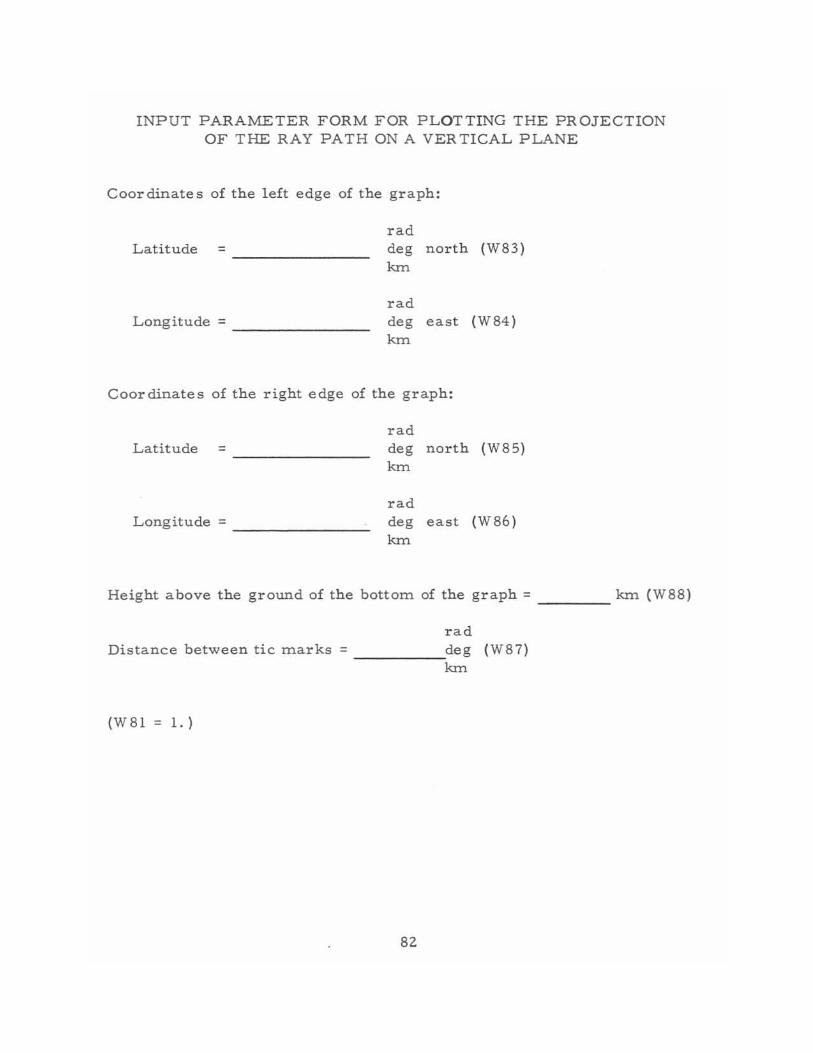
INPUT PARAMETER FORM FOR PLOTTING THE PROJECTION OF THE RAY PATH ON A VERTICAL PLANE
Coor dinate s of the left edge of the graph:
Latitude = -------
Longitude = _______ _
rad deg north (W83) krn
rad deg east (W84) krn
Coordinates of the right edge of the graph:
Latitude = -------
Longitude = _______ _
rad deg north (W85) krn
rad deg east (W 86) krn
Height above the ground of the bottom of the graph = ____ krn (W88)
rad Distance between tic marks = _ _ _ _ _ _ de g (W87)
krn
(W81 = 1.)
82
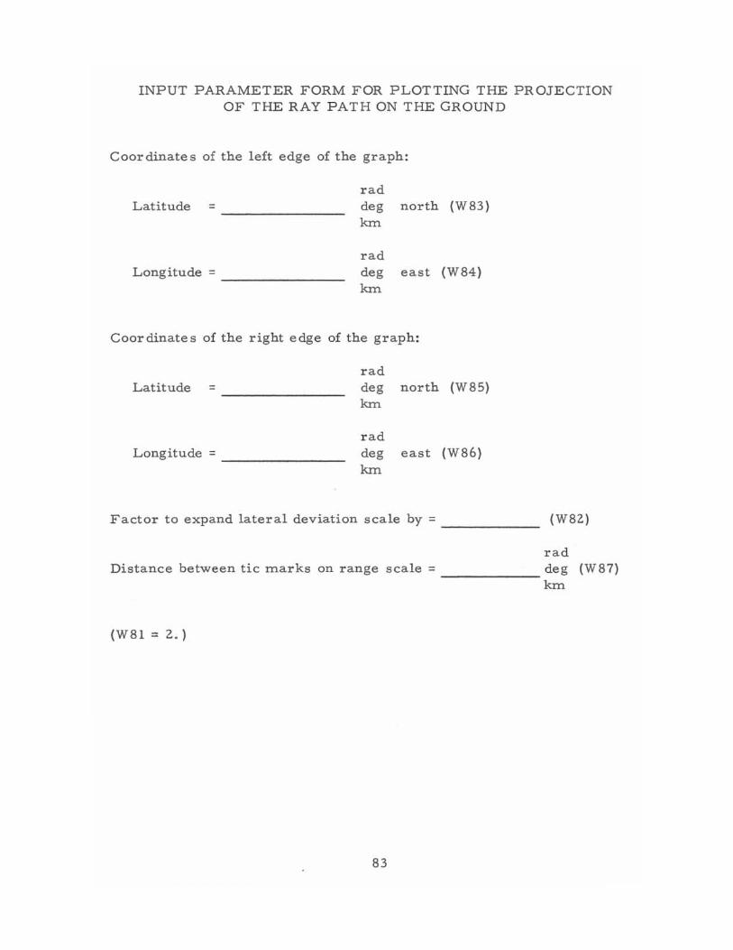
INPUT PARAMETER FORM FOR PLOTTING THE PROJECTION OF THE RAY P ATH ON THE GROUND
Coordinates of the left edge of the graph:
Latitude = - - --- -
Longitude = _______ _
rad deg north (W83) krn
rad deg east (W84) krn
Coordinates of the right edge of the graph:
Latitude = ------
Longitude = _______ _
rad deg north (W85) krn
rad deg east (W86) krn
Factor to expand lateral deviation scale by = _____ _ (W82)
rad Distance between tic Inarks on range scale = ______ deg (W87)
kIn
(W8l = 2. )
83
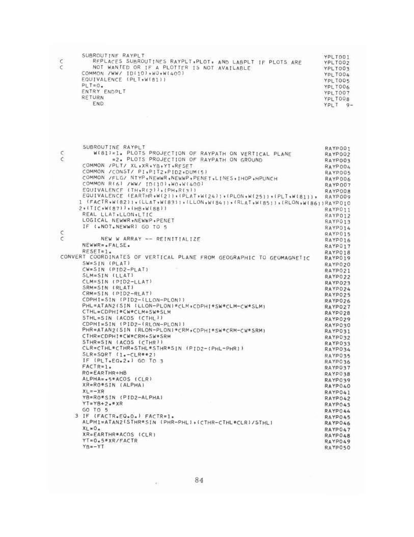
C C
C C
C C
SU BROUTINf RAYPLT REPLACES SUBROUTINES RAYPLT,PLOT, AND LABPLT IF PLOTS ARE NOT WAN fED OR IF A PLOTT fR IS NOT AVA I LABL E
COMMON I WW I IDIIO),WQ,W(4001 EQU IV ALENCE (PL T,WI8 11J PLT=O. EN TRY ENDPLT RETURN
END
YPLTODl YPL T002 YPL T003 YPL T004 YPL T005 YPL T006 YPL T007 YPL T008 YPLT 9 -
SUBROUTINE RAYPLT RAYPOOI WIBl)=l. PLOTS PROJE CTI ON OF RAYPATH ON VERTICAL PLANE RAYP002
=2. PLOTS PROJE CTI ON OF RA YPATH ON GROUND RAYP003 COM MON IPLT I XL,XR.YB,YT,RESET RAYP004 COMMON ICONS TI PI,PIT2,PID2,DUM(5) RA YP005 COMMON I FLGI NTYP,NEWWR,N EW WP,P ENET ,LI NES ,IH OP,HPUNCH RAYP006 CO~MON RI61 IW'WI IDfl OI,Wo ,W(4 00 1 RAYP007 EQUIVALENCE (TH,Rf2)),(PH,R(?,11 RAYPOOB EQU IVA LENCE (EA RTHR ,WI2 1 ), (P LAT,WI 24JI ,(PLON ,W(25) I ,(PLT,W(B l ll, RAYP009
1 IF ACTR ,W I 82 J I , (LLA T, W (8 3 I J , f LL ON , W {84 I J , (RLA T ,W ( 85 I I , (RLON ,w (86 J IRA YPO 1 0 2 .(TI C,W I B7J}' (H8,W(881 J RA.YPOll
REAL LLA T,LLON,LTIC RAYP012 LOGICAL NEWWR,NEWWP,PENET RAYP013 IF (.NOT.NEWW R) GO TO 5 RAYP014
NEW W ARRAY - - REINITIALIlE NEWWR=.FALSE. RESET=I.
VERTICAL PLANE FROM GEOGRAPHIC TO GEOMAGNETIC CONVERT COORDI NA TES OF SW" S IN (PLAT) CW=SIN (PID2-PLAT)
RA YP DI5 RAYP016 RAYPOl1 RAYP018 RAYP019 RA YPD 20 RAYP021 RAYP022 RAYP023 RA YP024 RAYP025 RAYP026 RAYP021 RAYP028 RAYP029 RAYP030 RA YP031 RAYP032 RAYP033 RAYP034 RAYP035 RA YPO 36 RAYP031 RA YPO 38 RAYP039 RAYP040 RAYP041 RAYP042 RAYP043 RAYP044 RAYP045 RAYP046 RAYP041 RAYP048 RAYP049 RAYP050
S LM= SIN (LLATI CLM=SIN (PI02-LLAT) SRM=SIN (RLAT) CRM=SIN (PID2 - RLAT) CDPHI=SIN (PI02-(LLON-PLONJ) PHL=ATAN2(SIN ILLON-PLONI*ClM,CDPHr*SW*CLM- CW*SLMI CTHL=CDPHI*CW*C LM+SW*SLM STHL=SIN (ACOS (CTHL)) CDPHI=SIN (PID2-(RLON-PL ON) ) PHR=ATAN2ISIN IRLON - PL ON I*CRM .CDPHI*SW*CRM- CW*SRM) CTHR~CDPHI*CW*CRM+SW*SRM STHR=SIN (ACOS (CTHR)) CLR=CTHl*CTHR+S THL*STHR*SIN (PJ02-(PHL-PHRI I SLR~SORT Il.-CLR**2 J IF (PLT.EQ.2.) GO TO 3 FACTR=l. RO =EARTHR+HB ALPHA:.S*ACOS ( CLRI XR=RO*SIN (ALPHA) XL=-XR YB=RO*SIN (PID2-ALPHA) YT=YB+2.*XR GO TO 5
3 IF (FACTR.EO.O.1 FACTRcl. ALPHl:ATAN2(STHR*SIN (PHR-PHL),ICTHR- CTHL*ClRI/STHLI XL"'O. XR,EARTHR*ACOS (CLR) YT=O.S*XR/FACTR YB =-YT
84
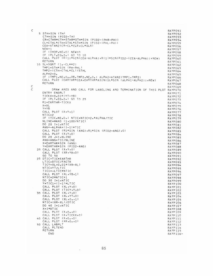
C
C C
5 STH=SIN ITHI CTH=SIN IPID2-THI CR%CTHR*CTH+STHR*STH*SIN IPIOZ-IPHR-PHI' CL=CTHL*CTH+ST~L*STH*SIN (PID2-IPHL-PHll CEA=ATAN2(CR-CL*CLR,CL*SLRI NEW=1 IF (IHOP.NE.O) NE'Io/=n IF (PLT.Eo.2. 1 GO TO 10 CA LL PLOT (R1l)*SINICEA - ALPHA),RI11*SINIPrD2 -lcEA-ALPHA1 ).NEW) RETURN
10 SL=SQRT (1.-CL**21 TMPl=STH*SIN (PH-PHLI TMP2=(CTH-(THL*CL)/STHL ALPH2=O . IF (TMPl.NE.O •• OR.TMP2.NE.O.J ALPH2=ATAN2(TMPl,TMP21 CALL PLOT (EARTHR*CEA,EARTHR*ASJNISL*SIN (ALPHl-A LPH 21) , NEWI RETURN
DRAW AXES AND CALL FOR LABELING AND TERMINATION OF THIS PLOT EN TR Y ENDPL T TICKX=Q.Ol*IYT-YBl IF (PL T.EO.2.) GO TO 25 Rl=EARTHR-TICKX X""XL Y=yB CALL PLOT (X,Y,11 NTIC =2 IF ITIC.NE.D.) NTIC=NTIC+2.*AlPHA/TIC NLINE=MAXO 11.100/NTICl DO 20 I=bNTIC ANG =-ALPHA+ ( I-I).TIC CALL PLOT (Rl*SIN (ANG),Rl*5IN (PID2-ANG ),Q) CALL PLOT (X,y,aJ DO 20 J=bNLINE ANG=ANG+TIC/NLINE X-EARTHR-SIN IANGl Y=EARTHR*SIN (PJ02-ANG)
20 CALL PLOT (X,y,o) CALL PLOT (XR,YB.OI GO TO 50
25 DTIC=TIC_EARTHR L TIC=DTICIFACTR TICY=XL+O.Ol*IXR-XL ) NTIC=YT ILT IC T IC1=-L TIC-NT IC CALL PLOT (XL,YB,ll NTIC'2*NTIC+l 00 30 1=1 ,NT Ie Y.TICl+( I-I)*LTIC CALL PLOT (XL,Y,O) CALL PLOT (TIC Y,Y,O)
30 CALL PLOT (Xl,Y,OJ CALL PLOT (XL,YT,O) CALL PLOT (XL,O.,11 NTIC·IXR-XLl/DTIC 00 40 I=I,NTJC X-I-DTIC CALL PLOT (X,O.,OI CALL PLOT (X,TICKX,OI
40 CALL PLOT (X,O.,OI CALL PLOT IXR,O.,OI
50 CALL LABPL T CALL PLTEND RETURN
END
85
RAYP051 RAYP052 RAYP053 RAYP054 RAYP055 RAYP056 RAYP 0 57 RAYP058 RAYP059 RAYP060 RAYP061 RAYP062 RAYP063 RAYP064 RAYP065 RAYP066 RAYP067 RAYP068 RAYP069 RAYP070 RAYP071 RA ypon RAYP073 RAYP074 RAYP075 RAYP076 RAYP077 RAYP078 RAYP079 RAYP080 RAYPO 81 RAYP082 RAYP083 RAYP084 RAYP085 RAYP086 RAYP087 RAYP088 RAYP089 RAYP090 RAYP091 RAYP092 RAYP093 RAYP094 RAYP095 RAYP096 RAYP097 RAYP098 RAYP099 RA YP 100 RAYPI0l RAYPI02 RAYPI03 RAYPI04 RAYPI05 RAYPI06 RAYPI07 RAYPI08 RAYPI09 RAYPllO RAYPlll RAYPI12 RAYP113 RAYP1l4 RAYP115 RAYPl16-
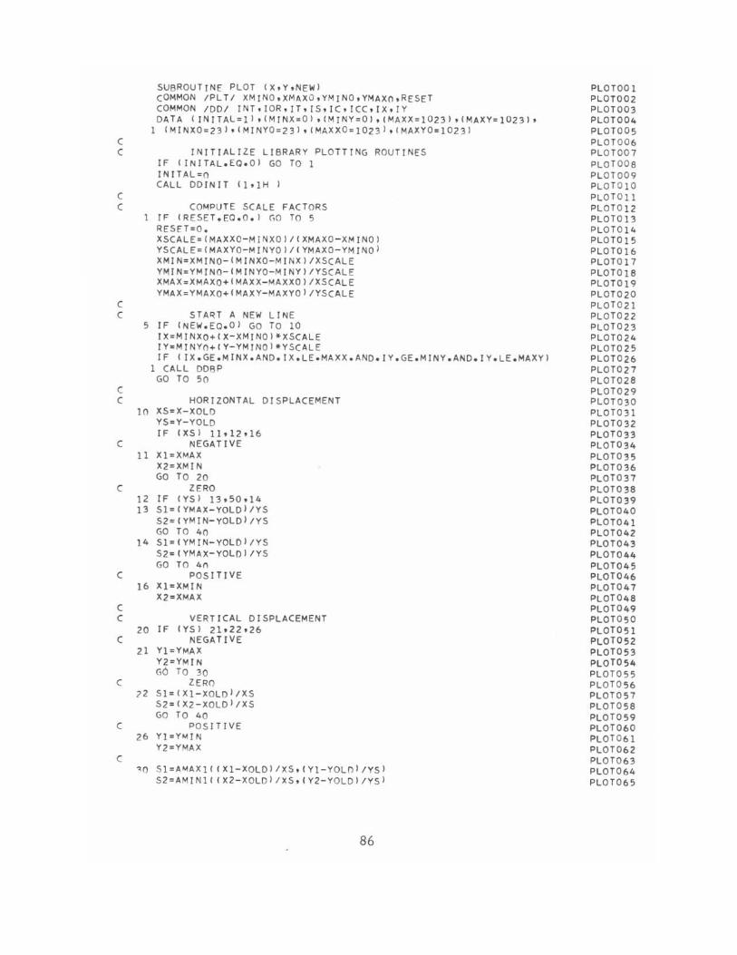
C
SUBROUTINE PLOT (X.Y.NEWI COMMON IPLTI XMINO.XMAXO .YMrN O.YMAXn .RESET (OMMON 1001 INT,IORdTdSdCdC(,IXdY DATA (INITAL=11 ,IMINX= OI ,IMINY=OI ,(MAXX= 10231 .(MAXY=10231.
1 IMINXO=231,IMINYO=23J,(MAXXO=1023),IMAXYO=1023J
C INITIALIZE LIBRARY PLOTTING ROUTINES IF (INITAL.EO.OI GO TO I INITAL=n CALL DDINIT (l,lH I
C C COMPUTE SCALE FACTORS
C
IF (RESET.EO.O.I (,0 TO 5 RESET=O. XSCALE=(MAXXC-MINXQI/(XMAXO-XMINOJ YSCALE={MAXYO-MINYOI/CYMAXO-YMINO' XMIN =XMINO-IMINXQ-MJNXJ/XSCALE YMIN=YMINO-IMINYO-MINYI/YSCALE XMAX=XMAXo+IMAXX-MAXXOI/XSCALE YMAX=YMAXQ+IMAXY-MAXYOJ/YSCALE
C STA~T A NEW LINE 5 IF (NEW.EO.OI GO TO 10
IX=MINXQ+IX-XMIN OI*XSCA LE IYzMINYO+(Y- YMINOJ*VSCALE IF CIX .GE.MINX.ANO.IX.LE.MAXX .ANO.I Y. GE.MINY.AND.IY.LE .MAXYI
I CALL DDBP GO TO 50
C C HORIZONTAL DISPLACEMENT
10 XS=X-XOLD YS=Y-YOLD IF (XSI llt12,16
C NEGATIVE II XI=XMAX
X2=XMIN GO TO 20
C ZERO 12 IF CYSI 13,50,14 13 SI=(YMAX -YOLDI /ys
S2=(YMIN-YOLDI/yS GO TO 40
14 SI=(YMIN-YOLOI/yS S2=IYMAX-YOLDI/YS GO TO 4"
C POSITIVE 16 XI=XMIN
X2=XMAX C C VERTICAL DISPLACEMENT
20 IF IYS) 21-22,26 C NEGATIVE
21 Y!=YMAX Y2=YMIN G6 TO 30
C ZERO 72 S I=( XI - XOLOI/ XS
S2 =I X2-XOLOJ/XS GO TO 40
( POSITIVE
C
26 Y1=YM;!N Y2 =YMAX
':10 Sl=AM;AXli {X1-XOLDI/XS,IYI-YOLD)/YSI S2=AMI N1 ( I X2-XOLD I IXS, (V2- YOLD) IYS J
86
PLOTOO I PLOT002 PLOT003 PLOT004 PLOT005 PLOT006 PLOT007 PLOT008 PLOT009 PLOTOIO PLOTO II PLOTOl2 PLOT Ol3 PLOTOl4 PLOTOl5 PLOTOl6 PLOTOl7 PLOTOl8 PLOTOl9 PLOT020 PLOT021 PLOTO 2 2 PLOT023 PLOT024 PLOT025 PLOT026 PLOT027 PLOT028 PLOT029 PLOT030 PLOT031 PLOT032 PLOT033 PL OT034 PLOT035 PLOT036 PLOT037 PLOT038 PLOT039 PLOT 040 PLOT041 PLOT042 PLOT043 PLOT044 PLOT045 PLOT046 PLOT047 PLOT048 PLOT049 PLOT050 PLOT051 PLOT052 PLOT053 PLOT054 PLOT055 PLOTO 56 PLOT057 PLOT058 PLOT059 PLOT06 0 PLOT061 PLOT062 PLOT063 PLOT064 PLOT065
C C PLOT LINE -- CHECKING FOR BORDER CROSSINGS
40 S=SQRTIX5**2+YS**21 IF {S2.LT.O •• OR.S*Sl-S.GT.O.1 GO TO 50 IF (S1_lT.a.1 Gf') TO 42
C PREVIOUS POINT OFF GRAPH IX=MINXO+(XOLD+XS*Sl-XMINO'*XSCALE+O.S IY=MI NYO+IYOLD+YS*Sl-YMI N01*YSCALE+n.5 CALL DDBP
42 IF (S*S2-S.GT.O.1 GO TO 44 C CIJRREN T POINT OFF GRAPH
IX =MINXQ+(XOLD+XS* S2 -X MIN01*XSCAlE+O.S IY=MINYO+(YOLD+YS*S2-YMINo1*YSCAlE+O.5 CALL DOVC GO Tn 50
C CURRENT POINT ON GRAPH
C
44 IX=MINXQ+{X-XMINOI*XSCALf+O.5 IY=MINYO+(Y-YMINOI*YSCALE+O.5 CALL DOVC
C EXIT ROUTINE SO XOLD =X
YOLO=Y RETURN
C C TERMINATE THE CURRENT PLOT
ENTRY PL TEND CALL ODFR RETURN
END
SUdRouTINE LA3PLT C LABEL THE CURRENT PLOT
JIMENSIDN lABEL(9) ,TYPE(3) COMMON IJOI INT,IOR,IT,IS,IC,ICC,IX,IY CO~MON ICO~STI PI,PIT2,PI02,OEGS,QUM(4) COHMON /FLG/ NTYP,NlWWP,NEWWP,PENET,LINES,IHOP,HPUNCH CJMHON IWW/ ID(lO)tWO,W(~OJ)
EQUIVALENCE tEART"'R,W(2», (F,W(6») ,(AZ1,W (10», (PLT,W(8U), 1 (FACTR,W(8Z)),(TIC,W(87))
LJGICA L NEWWR,NEW,,"P,PENET ~EAL LTre JATA (TYPE::;8H::XTR.AORO,8H~O FIELO,8t-iORDINARYl IOR=IT=O IS=2 IX::;O $ IY::;1023 $ CALL DOTAB $ CALL OOTEXT (7.IO) NOATE =IOAT E( 0) CALL DOTEKT (I.NOAT.) AZA::;AZ1"OEGS OT IC=TI C'EARTHR ENCODE (72,100Q,LABEL) ~,AZA,TYPE(NTYP),DTIC
1000 FORMAT (3HF =,F7.3,6H, Al =,F7 .2,2H, ,A8,2H, ,F7.2,24H K~ BETWEEN ITICK MARKS'.)
IX=O $ 1.=991 $ CALL OOTAS $ CALL OOTEXT (9.LABEL) IF (PLT.EQ.1.) RETURN LTIC=DHC/FACTR ENCODE (32.2000.LAB[L) LTIC
200n FORHAT (F7.2.2 .. H KM BETWEEN TICK HARKS'.) IOR=I IX=O $ H =O $ CALL OOTAB $ CALL OOTEXT ( ... LABEll IOR=O RETURN
END
87
PLOT066 PLOT067 PLOT068 PLOT069 PLOT070 PLOT07! PLOT072 PLOT073 PLOT074 PLOT075 PLOT076 PLOT077 PLOT07B PLOT079 PLOTOBO PLOTOB! PLOTOB2 PLOT083 PLOT084 PLOTOB5 PLOT086 PLoTOB7 PLOTOBB PLOTOB9 PLOT090 PLOT09! PLOT092 PLOT093 PLOT094 PLOT 95-
LABPao 1 LABPOG2 LABPJ03 LARPJ04 LABP005 LABPJ06 LABPl)07 LABPJOB LABPilOg LABPQ10 LABPill1 LABP012 LABPJ13 LABP014 LA8POl5 LABPOl6 LAB P017 LABPOl8 LABP019 LABP020 LABP021 LABP022 LABP023 LABP02 .. LABP025 LABP026 LABP027 LABP028 LABP029 LABP030 LABP031 LABP 32-
C
320
1000 C C lUJl
13S0
103 ..
1039
ISO
C C
2000
20S1
SUBROUTINE RKAH NUMERICAL INTEGRATION OF DIFFERENTIAL EQUATIONS
COHMON IR(I NN,SPACE,HOOE.E1HAX.E1HIN,EZHAX,EZHIN,FACT,RSTART COHHON H20) .T.STEP.OYOT(ZO) OIHENSION OELY(".20).BET(').XV(S).FV( ... 20).YU(S.20) TYPE OOJBLE YU IF (RSTART.E~.O.) GO TO 1000 LL=HH=1 IF (HOOE.Eo..lI HH=" ALPHA=T E~t1:;O.O
BET(lI=BET(Z)=O.S BET(3)=I.J BET (")=0.0 STEP=SPACE ~=19.01270 .0 X;<HH)=T IF (EU4IN.LE.O.l E1HIN=EUAX/SS. IF (FACT.LE.O.) FACT=O.S CALL HAHLTN OJ 320 I=I.NN FV(HM,I)=DYOT<I) Y U ( tiM , I ) :; '( (I) ~S TART= O. GO TO 1001 IF (HOOE.NE.lI GO TO 2000
RUNGE-KUTTA 00 103 .. K=I, .. 00 13S0 I=1.NN OELY(K,I)=STEP·F~(HH,I)
Z=YU(HH,I) Y(I)=Z+BET(K)·OELY(K.I) T=BET(K)·STEP.XV(HH) CALL HAHLrN 00 1034 I=l.NN FV(MH.I)=OYOT(I) 00 1039 I=I.NN OEL=(OELY(1.I)+2.0·0ELY(2,I'+Z.O·DELY(3.t)+OELY(4,I»1&.0 YU(HH+l.I'=YU(HH,I,tOEL MM=HM+l XV(HH)=XV(HH-ll+STEP 00 1 .. 00 I=I.NN y(I)=YU(HH.I) T=XV(MH) CALL HAHL TN IF (HOOE.EQ.l) GO TO .. 2 00 ISO I=I.NN FV (HH, I I =OYOT< Il IF (HM.LE.3) .0 TO 1001
AOAH;-~OJLTON
00 20 .. 6 1=1. NN OEL=STEP'(55.·FV(~.1)-59.'FV(3.1).37.·FV(2.I)-q.·FV(1.1))/2 ... Y(I)bYU(4.I)+OEL OELY(1.Il=Y<Il T=XV( .. )+STEP CALL HAHLrN XV(S)=T DO 20S1 1=1. NN OEL=STEP·(9.·OYOT(I)+19.·FV( ... 1r-5.·FV(3.1)+FV(Z.I))/Z ... YU (5, I) =YU (4, I' +0 El HI) =YU (S,!) CALL HAHLrN IF (HOOE.LE.2) GO TO .. 2
88
RKAHOOI RKAH002 RKAHOOJ RKA HOO .. RKAH005 RKAHOO& RKAH007 RKAH006 RKA H009 RKAH010 RKA HOll RKA H012 RKAH013 RKAH01" RKAM01S RKAM01& RKA MOl7 RKAH016 RKA H019 RKA H020 RKAH021 RKA H022 RKAH023 RKA M02 .. RKA M025 RKAH02& RKAH027 RKAH026 RKAH029 RKAM030 ROH031 RKAM032 RKAHOJ3 RKAHOJ .. RKAH035 RKA M03& RKA H037 RKAH036 RKAHOJ9 RKA HO .. O RKA H041 RKAHO .. 2 RKA HO .. 3 RKAHO .... RKAMO .. S RKA H O~& RKAHO .. 7 RKA H046 RKAHO .. 9 RKAH050 RKAH051 RKAH052 RKAMOS3 RKAH054 RKAH055 RKAH05& RKAH057 RKAH058 RKAH059 RKAHO&O RKAH061 RKAH062 RKAH063 RKlH06 .. RKAH065
c C ERROR ANALYSIS
C
SSE=O.O DO 3033 1=1. NN EPSIL=R·ABS(Y(I)-oELY(l.I)) IF (HOoE.EQ.3.ANo.Y(!) .NE.O.) EPSIL=EPSIL/ABS(y(I)) IF (SSE.LT.EPSILl SSE=EPSIL
3033 CONTINUE IF (E1MAX.GT .SSE) GO TO 3035 IF (ABS(STEP).LE.E2MIN) ;;0 TO ~2
LL=HH=l STEP=STEP·FI\::;r GO TO 1001
3035 IF (LL.LE.l.0~.SSE.GE.El~IN.OR.E2MAX.LE.ABS(STEP)) GO TO ~2
LL= 2 ~M=3
X~(2)=XV(3)
X~(3)=X~(5)
DO 5363 I:::l t N" F'J(Z,I'=FV'(3,I) F~(3.Il=OYOT(!)
YU(Z,I) =YJ<3,I) 531)3 YU(3,lJ =,('.)(5,1)
5TEP=2.0·STEf) GO TO 1001
C EXIT ROUTINE 42 LL=2
MM=4 )0 12 K=1.3 X~(K)=X~(K+1)
00 12 l=l.NN F'J(K,I.:FV(K+1,I)
12 YU(K,U=YU(I(+1 , D XV(4)=XV(S) 00 52 l=l . NN n(4.Il=oYoT(!)
52 YU(4,I)=YU(S,I) IF (HOOE.LE.2) RETURN E=ABS(XV(4)-ALPHA) IF (E.LE . EPM) GO TO 2000 EPH=E RETURN
END
89
RKAH066 RKAH067 RKAH068 RKAH069 RKAH070 RKAH071 RKAH072 RKAH073 RKAH074 RKA H075 RKAM07c RKA H077 RKAM078 RKAH079 RKAH080 RKAH081 RKAH082 RKAH083 RKAM084 RKA M085 RKAH08c RKAH087 RKAH086 RKAH089 RKA H090 RKAM091 RKAH092 RKA H093 RKAH094 RKA H095 RKAH096 RKAH097 RKAH098 RKAH099 RKA H10 0 RKA H 10 1 RKAH102 RKAH103 RKA Hl04 RKAH105 RKAH10c RKAH107 RKAH108 RKA Hl09-
SUBROUTINE HAMLTN HAML001 C········· CALCULATES HAMILTONS EQUATIONS FOR RAY TRACING HAML002 COHMON ICONSTI PI,PIT2,PI02,DEGS,RAO,K,C,LOGTEN HAML003 COHMON IRINI MOORIN(3) ,COLL,FIELO,SPACE,KAY2,KAYZI, HAML004
1 H,HI,PHPT,PHPTI,PHPR,PHPRI,PHPTH,PHPTHI,?HPPH,PHP?HIHAHl005 ~, PHPOH,PHPO"I.PHPKRtPHP(~ItPHPKTH.PHPKTI, PHPKPH,PHPKPI HAML006 3 ,KPHPK, KPHPKI, POLAR, POLARI, LPOLAR,LPOLRI HAML007
COMMON RIZO),T,STP,OROTIZO) IWW/IO(10),WO,WI400) HAML008 EQUIVALENCE UH,R{Z)),(PH,R.(3)),CKR,R(4)),(KTH,R(S)),CKPH.R(6)', HAHL009
1 IOTHOT ,OROHZ», I OPHOT ,DROT (3», IDKROT,ORDT(4», (OKTHOT, OROTlS» ,HAML010 Z CDKPHOT,ORDTlG»,(F,WIG» HAML011
REAL KR.KTH,KPH,KPHPK,KPrlPKltlPOLA~tLPOLRItlOGTEN.KtKAY2tKAY2I HAHL012 DH;PITZ·l.Eo"c HAHL013 STH:SIN(TH) HAHL014 CTH=SIN(PIO?-TH) HAML01S RSTH=R( U'STH HAML01& RCTH:R(1)'CTH HAML017 CALL RINOEX HAML018 ORO T:-PHPKRI (PHPOH'C) HAHL019 OTHOT:-PH'KTH/(PHPOM'R(1)'C) HAHL020 OPHOT=-PHPKPH/(PHPOH'RSTH'C) HAML021 DKROT=PHPR/(?HPOM'C)+KTH'DTHOT+KPH'STH'OPHOT HAHL022 DKTHDT=(PHPTHI (PHPOM'C)-(TH'OROT+KPH'RCTH'DPHDT) IR(1) HAHL023 OKPHOT: (PHPPHI (PHPOM'C)-KPH'STH'OROT-KPH'RCTH'OTHOT)/R STH HAHL024 NR=G HAML02S
C········· PHASE PATH HAHL026 IF (W(S7l.EQ.O.) GO TO 10 HAHL027 NR:NR+1 HAML028 OROTlNR) =- KPHPK/PHPJM/OH HAML029
C········· ABSORPTION HAHL030 10 IF (W(SS) .D.O') GO TO 15 HAML031
~R=NR+l HAHL032 ORDT(NR); 10./LOGTEN"KPHPK"KAY21/(KR"KRtKTH"KTHtKPH"KPH)/PHPOH/C HAHl033
C········· DOPPLER SHIFT HAI'1LD34 15 IF (WI59) .EQ.Ool GO TO 20 HAHL035
NR=NR+l HAHL03G D~DT (NR) :::-PH~T IPHPOM/C/PI T2 HAML037
C·· .. • .. •••• GEOt.fET~I::AL PATH LEN:;rH HAI'1L038 20 IF (W(GO) .EQ.O,) GO TO 25 HAHL039
~R~NR+l HAML040 ORDT(NR):::-SQRr(PHP~R··2+PHP~TH··Z+PHPKPH··2)/PHPOH Ie HAML041 c···· .. ···· OTHER CALCULATIONS HAI'1L042
2S CONTINUE HAML043 RETURN HAHL044
END HAHL04S-
90
APPENDIX 2. VERSIONS OF THE REFRACTIVE INDEX
SUBROUTINE (RINDEX)
This ray tracing program gains versatility without sacrificing speed
by having several versions of some of the subroutines. For example,
the 8 versions of the refractive index subroutine allow the user to decide
for each ra y path calculation whether to include or ignore various as pects
of the propagation medium such as the earth's magneti c field or collisions
between electrons and neutral air molecules.
If collisions are included, the user has the option of using the Apple
ton_Hartree form.ula (which assumes a constant collision frequency) or the
Sen- Wyller formula (which assumes a Maxwell distribution of electron
energies and a collision frequency proportional to energy). The Sen
Wyller formula is generally assumed to be more accurate, especially
in the lower ionosphere, but the Appleton-Hartree formula can often be
used with an effective collision frequency profile to save computer time.
When the effect of the earth's magnetic field is included and ray
paths are calculated near vertical incidence, a spitze (Davies, 1965, p.
202) often occurs in the ray path. (At a spitze, the usual formulas for
refractive index become indeterminate because the wave normal is paral-
lei with the earth's magnetic field and the wave frequenc y equals the
local plasma frequency.) Two versions of the refr active index subrou
tine have been developed to calculate ray paths through a spitze . These
two versions will also work in the absence of a spitze, but the standard
versions are much faster.
The input to the refractive index subroutines is through blank com
mon and common blocks /XX / , / yy /, and / ZZ/. Output is through com
mon block /RIN /. The refractive index subroutine is called through the
entry RINDEX. The subroutine names are used only for user identifica
tion. The following 8 versions of the refractive index subroutine are
9 1
listed in this appendix:
a. Subroutine AHWFWC (Appleton-Hartree formula with field, with collisions)
b. Subroutine AHWFNC (Appleton-Hartree formula with field, no collisions)
c. Subroutine AHNFWC (Appleton-Hartree formula no field, with collisions)
d. Subroutine AHNFNC (Appleton-Hartree formula no field, no collisions)
e. Subroutine BQWFWC (Booker Quartic with field, with collisions)
f. Subroutine BQWFNC (Booker Quartic with field, no collisions)
93
94
96
97
98
100
g. Subroutine SWWF (Sen- Wyller formula with field) 102
h. Subroutine SWNF (Sen-Wyller no field) 105 Subroutine FGSW Subroutine FSW Fresnel integral function C Fresnel integral function S
92
106
106 108
108
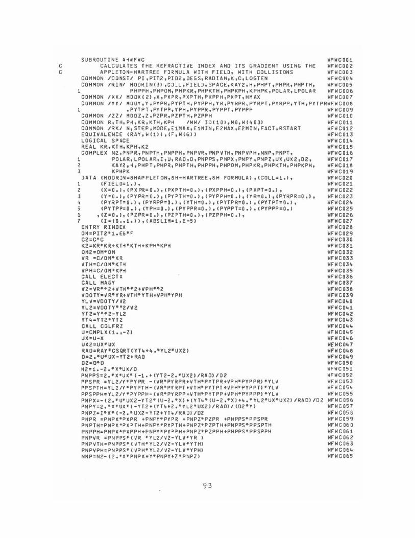
SUBROUTINE Ai~fWC WfWC001 C CALCULATES THE REfRACTIVE INDEX AND ITS GRADIENT USING THE WfWC002 C APPLETON-HARTREE FJ~~ULA WITH FIELO, WITH COLLISIONS WFWC003
COHMON ICONSTI PI,PIT2,PI02,OEGS,RADIAN,K,C,lOGTEN WFWCD04 COHHON /RINI MOORIN(3) ,CJ_L,FIELJ,SPACE,KAY2,H,PHPT,PHPR,PHPTH, WFWC005
1 PHPPH,PHPOH,PHPKR,PHPKTH,PHPKPH,I(PHPK,POLAR,LPOLAR HfWC006 COMMON IXXI 1'1:10)((2) ,X,PX?R,PXPTH,PXPPH,PXPT,HMAX WFWCOQ7 COHHON IYYI "OOY,Y,PYPR,PYPTH,PYPPH,YR,PYRPR\PYRPT,PXRPP,YTH,PYTPRWFWC008
1 ,PYTPT,PYTPP,YPH,PYPPR,PYPPT,PYPPP WFHCOOq COMMON IZZI MOOZ,Z,PZPR,PZPTH,PZPPH WFWC010 COHMON R,TH,Pri,KR,KTH,KPH IWWI IO(10J,HO.W(400) WFWC011 COMMON IRKI N,STEP,MOOE,£1MAX,E1MIN,E2MAX,E2MIN,FACT,RSTART WFWC012 EQUIVALENCE (RAy,~(ll) ,(F,W(6)) WFWC013 LOGICAL SPACE WFWC014 REAL KR,KTH,KPH,K2 WFWC01S COMPLEX N2,PNPR,PNPTH,PNPPH,PNPVR,PNPVTH,PNPVPH,NNP,PNPT , WFWC016
1 PO LA R. l POL ARt I, U, RAO ,0, PNPPS, P NPX, PNPY t PNPZ, UX ,UX 2 ,[)2, WFW C017 ? KAY2.~,PHPT,PHPR,PHPTH,PHPPH,PHPOH,PHPK~tPHPKTH,PHPKPH, WFHC016 3 KPHPK Wf'W C01. 9
lATA (MOORIN=8HAPPLETON,8H-HARTREE,8H FORMULA) ,(COLL=1.), WfWC020 1 (fIELO=1.), WfWC021 2 (X=O . I,(PXPR=O.),(PXPTH=O.),(PXPPH=O.),(PXPT=O.), WfWC022 3 (Y = 0 • ) , (P Y PR= O. ) , (pr? T H =0 .) , ( PY PP H=O • ) , (Y R= O. ) • (PYRP R =0 • ) , WF W C 02 3 " (PYRPT=O.) , (PYRPP=O.) , (YTH=Q.), (PYTPR=O.) , (PYTPT=O.) , WFWC024 :; (PYTPP=O.), (YPH=O.), (PVPPR=O.), (PYPPT=O.),(PYPPP::cO.) WFWC025 :; ,(Z=O.J,(PZPR=O.),(PZ?TH=O.),(PZPPH=O.), WFWC02& 7 tI=(0 .. 1.)),(ABSLlH=1.E-S) WFWC027
ENTRY RINOEX WFliC028 OH=PITZ'1.E6" WFWC029 C2=C'C WFWC030 K2=KR'KR+KT~' KTH+KPH'KPH WFWC031 OH2=OM'OH WfWC032 VR =C/OH'KR WfNC033 ~TH=C/OH'KTH WfWC034 ~PH=C/OH·KP.1 WFWC03S CALL ELECTX WFWC036 CALL MAGY WfWC037 ~2;VR""2+~TH·.2+VPH··2 WFWCQJ8 VOO TY=~ R' r R+VTH'Y T H+VPH'rPH WfN C039 YLV=VOOTY/V2 WFWCO~O
YL2=VOOTY"21V2 NFIIC041 YT2=Y"2-YL2 NfNCO~2 YT~=YTZ'YT2 WFNCO~3 CALL COLfRZ WfWC044 U=CHPLX(1.,-Z) WFNCO~S UX=U-X WfWC046 UX2=UX'UX WfWCO~7 RAO=RAY 'CSQRT (Yh+4 .·YL2·UX2) WFWC 0~8 0=2 •• U·UX-YT2+RAO WFWC049 02=0-0 WfNCOSD N2=1.-2.-X'UX/O WFWCOS1 PNPPS=2 •• X'UX'(-1.+(YT2-2.'UXZ)/RAO)/02 WFWCOS2 PPSPR =YL2/Y"?YPR -(VR"PYRPR+VTH.PYTPR+VPH"PVPPR).YlV WFWC053 PPSPTH=YLZ/Y.PYPTH-(VR.PYRPT+VTH"pYrpT+VPH·PYPPT).YL~ WFWC054 PPSPPH=VL2/Y.~YPPH-(VR"PYRPP+VTH.PYTPP+VPH.PYPPP).YlV WFHC05S PNPX=-(Z."U"UX2-YTZ.(U-Z •• X)+(YT4.(U-Z •• X)+4 •• VL2.UX·UXZ)/RAO)/OZ WFWC05& ?NPY=2 •• X.UX. (-YTZ+ ('1T4+2 ."YL2"UXZ) IRAO) I (OZ·V) HFWC057 PNP Z= I- X. (-2.' U XZ- YTZ +YTIt IRA 0) 102 WfW COS 8 PNPR =PNPX·PXPR +PNP'1.PYPR +PNPZ·PZPR +PNPPS.PPSPR WFWC059 ?NPTH=PN?X+PX~TH+PNP'1.P.YPTH+PNPZ.PZPTH+PNPPS·PPSPTH WFWCO&O PNPPH=PNPX.PXPPH+PNPY.PY~PH+PNPZ.PZPPH+PNPPS.PPSPPH WFWCO&1 PNPVR =PNPPS"(VR ·YL2/V2-YU'·YR ) WFWCO&Z PNP VTH= PNPPS. (VTH" Yl21 V2-YLV. Y TH) WFW C 063 PNPVPH=PNPPS' (VPH.YL21 V2-YLV.YPH) WFWC064 NNP=N2-(Z.4X.PNPX+Y4PNPY+Z4PNPZ) WFWCO&5
93
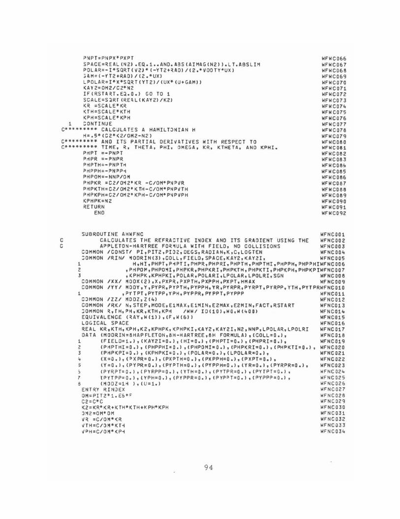
P,\lPT=PN PX" PXPT SPACE;RE AL (N ZI • Ell.. 1.. AND. ABS (A I HAG (NZ I I. LT. ABSLIH POLAR;-I·SQRT(VZI·(-YTZ.~AOI/(Z.·VOOTY·UXI ;4M=(-YT2+RAO'/(2.·UX, LPOLAR=I"X"SQRT(YT2)/(UX"(U+GAM)) KAYZ;OHZlCZ'NZ IF(RSTA~T.EQ.O.I GO TO 1 SCALE=SlRT(REALIKAYZ'/KZI KR =SCALE'KR KTH=SCALE"KTH KPH=SCALE"KPH
1 CONTINUE C .... ~·~·· .. • CAlCULAT£S A HAHllTJNIAN H
H=.S·(CZ·KZ/OHZ-NZI C· .. ••••••• AND ITS PARTIAL DERIvATIVES WITH RESPECT TO C········· TIME, R.. THETA, PHI, OMEGA, KR, KTHETA. AND KPHI ..
PHPT =-PNPT PMPR =-PNPR PHPTH=-PNPTH eHPPH=-PNPP; PHPOH=-NNP/OH PHPKR =CZ/OHZ'KR -C/OH"PN?VR PHPKTH= CZI OHZ' K TH -C/OH' PN PHH PHPKPH=CZ/OHZ'KPH-C/OH"P~PVPH KPHPK=NZ RETURN
ENO
HFHC066 HFHC067 HFHC066 HFHC069 HFHC070 HFHC 071 WFHC07Z HFHC073 HFHC07~
HFH C07S HFHC076 HFHC077 HFWC078 WFHC079 WFHC080 WFWC081 WFHC08Z HFHC083 HFHC08~
HFWC08S HFHC086 WFWC087 HFHC088 WFWC089 WFWC090 WFWC091 WFWC09Z
SUBROUTINE AHWFNC WFNC001 C CALCULATES THE REFRACTIVE INOEX ANO ITS GRAOIENT USING THE WFNCOOZ C APPLETON-HARTREE FOR~ULA wITH FIELO, NO COLLISIONS WFNC003
COHNON ICONSTI PI,PITZ,PI02;OEGS,RAOIAN,K,C,LOGTEN WFNCOO~ ~ONHON IRINI ~OOR!N(3I,COLL,FIELO,SPACE,KAY2,KAYZI, WFNCOOS
1 H,HI,PHPT,P~PTI,PHPR,PHPRI,PHPTH,PHPTHI,PHPPH,PHPPHIWF NCaD6 2 ,PH POM, PHPOMI, PH~K.R, PHPKR I ,PHPI<TH, PHPKT I, PHPICPH, PHPKPIWFHCaa 7 3 ,K PHPK ,KPHPKI, PO LA R,POLARI,LPOLAR, LPOLRI, SGN WFNC 00 6
COHMON IXXI ~OOX(2),X,PXPRtPXPTH,PXPPH,PXPT,HHAX WFNC009 COHMON IYYI HOOY,Y,PYPR,PYPTH,PYPPH,YR,PYRPR,PYRPT.PVRPP,YTH,PYTPRHFNC010
1 ,PYTPT,PYTPP,VPH,PYPPR,PYPPT,PYPPP WFHe011 CJNHON Illl HOOl,l(~1 WFNC012 COHHON IRKI N,STEP,HOOE,E1HAX,E1NIN,EZHAX,EZHIN,FACT,RSTART WFNC013 ~OHHON ~,TH,~H,KR,KTH,KPti IWH/IO(lD},WO,W(4DO' WFNe01,. EQUIVALENCE (UY,H(1II,(F,W(611 WFNC01S LOGICAL SPACE WFNC016 REAL KR.KTH,KPH,K2,KPHPK,KPHPKI,ICAY2,KAY2I,N2,N~P,LPOlAR,LPOLRI WFNCD17 DATA (HOORIN=6HAPFLETON,8H-HARTREE,8H FORMULAI,(COLL=O.I, WFNC016
1 (FI EL 0= 1. I , ( KAYZ I =0. I , ( HI = O. I , ( PH PTI = O. I , ( PHPR 1= 0 .) , WFN COL 9 2 (PHPTHI=O.I,(PHPPHI=O') ,IPHPOHI=O.I, (PHPKRI=O.I,(PHPKTI=O .1, WFNCOZO 3 (PHPKPI=D.I,(KPHPKI=O.I,(POLAR=O.I,(LPOLAR=O.I, WFNCOZ1 It (X=O . ), (DXPR=O.), (PXPTH=O.),(P)(PPH=O.),(PXPT=O.). WFNCD22 :;; (Y = 0 • , t (P Y PR= 0 • ) , (PY P T H =0 • ) , ( PY PP H=D • ) , (Y R= 0 • ) , ( PYR?R=O • ) , WFN C 02 3 51 (PYRPT=O.) ,(P'YRPP=O.) t (YTH=O.), (PYTPR=O.) ,(PYTPT=O.) t WFNC024 7 t P Y T PP= o. } • ( Y PH= 0 • ) t (P Y PP R = 0 • ) , (P YP;:) T= 0 • ) , ( py ppp = 0 .) , HF NCO 2 5 6 (MOOl=lM I, (U=1.1 "FNCOZ6
ENTRY RINJE X WFNCOZ7 OH=prT2.1.Eo·~ WFNC026 CZ=C"C WFNCOZ9 K2=KR.KR+KTH.KTH+KPH.KPH WFNC030 J .~2=OH'OH WFNC031 V~ =C/OH"~R WFNCOJZ VTH=C/OM"KT1 WFNCOJ3 ~PH=C/O~.(P~ WFNC034
94
CALL ELECTX :ALL MAGY ~2=~R··Z+~TH··2+~PH··Z
~OOTY=~R·YR+~TH·YTH+~PH·YPH
YLV=VOOTYIV2 YL2=vDOTY··ZI1/2 YT2=Y··Z-YL2 YTI+=YT2".,T2 UX=U-X UX2=UX·UX RAO=RAY·SlRTIYT4+4.·YL2·UX21 O=Z."UK-YTZ+RAO 02 = O' 0 N2=1.-2.·x·UX/O PNPPS=2.·X·UX"(-1.+(YT2-Z."UXZ)/RAOl/02 ??SPR= YL2/Y.'YPR -(VR·PYRPR+"TH.PYTPR+VPH.PYPPR).YL~ PPSPTH=YLZ/Y·PYPTH-{VR·PYRPT+VTH"PYTPT+V'PH·PYPPT)·Ylv PPSPPH=YLZ/Y·PYPPH-(VR"PYRPPtVTHiJPVTPP+V'PH"PYPPP)·YLV PNPX=-(2.·UX2-YT2·(U-2.·X)+(YT~·(U-2.·X)+4.·YL2·UX·UXZ J/RAOJ/OZ
PNPY=2."X·UX·(-YT2+(YT4+2.·YLZ·UXZ'/RAO)/(OZ"Y) NNP=N2-(2.·X·~NPX+Y·PNPY)
PNPR =PNPX"PXPR tPNPY·PYPR tPNPPS.PPSPR PNPTH=PNPK·PXPTH+PNPY·PY~TH+PNPPS·PPSPTH PNPPH=PNPX·PXPPHtPNPY·PYPPH+PNPPS·PPSPPH PNPVR =PNPPS'IVR 'YL2-VOOTY'YR I/V2 PNPVTH=PNPPS'IVTH'YL2-VOOTY'YTH)IV2 PNPVPH=PNPPS'IVPH'YL2-VOOTY'YPH)/V2 PNPT=PNPX< PX PT SP'ACE=NZ.EQ.1. POLARI=SQRTIVZ)·IYT2-RAOIIIZ.·VOOTY·UXI GAH=(-YT2+RAO)/ (Z •• UX) LPOLRI=X'SQRTIYT21/IUX'IU+GAMI) ~AY2=OMZI:2'N2 IFIRSTART.EQ.O.) GO TO 1 SCALE=SQRTIKAr2I(2) KR :SCALE'KR KTH=SCALE'KTH K~H=SCALE'K?~
1 CONTINUE C········· CALCULATES A HA"ILTO~IAN H
H=.5·IC2·K210~2-N2) C······ ••• AND ITS PARTIAL DERIVATIVES WITH RESPECT TO C········· TIME, R, THETA, PHI, OMEGA, KR, KTHETA, AND KPHI.
PHPT =-PNPT P~PR =-PNPR PHPTH=- PNPT~ PHPPH=-PNPPH ?HPOM=-NNP/O~ PHPKR =C2/0~Z'KR -C/OM'P~PVR PHPKTH=CZ/OMZ'KTH-C/OH'PNPVTH PHPKPH=C210M2'KPH-CIOM'PNPVPH KPHPK=N2 RETURN
ENO
95
WFNC035 WFNC036 WFNC037 WFNC038 WFNC039 WFNCO.O WFNC041 WFNC042 WFNC043 WFNCO.4 WFNC045 WFNCQ46 WFNC047 WFNC048 WFNCO.9 WFNCOSO WFNC051 WFNCOS2 WFNCOS3 WFNCOS4 WFNCOSS WFNC056 WFNC057 WFNCOS8 WFNCOS9 WFNC060 WFNC061 WFNC062 WFNC063 WFNC064 WFNC06S WFNC066 WFNCOf>7 WFNC068 WFNC069 WFNC070 WFNC071 WFNC072 WFNC073 WFNC074 WFHC075 WFHC076 WFHC077 WFHC078 WFHC079 WFHC080 WFNC081 WFNC082 WFNC083 WFNC084 WFNC08S WFNC086 WFNC087 WFNC088-
SUBROUTINE ~~NFWC NFWC010 C CALCULAToS THE REFRACTIVE INOEX ANO ITS GRAOIENT USING THE NFWC011 C APPLETON-HARTREE FO~.ULA -- NO FIELO, WITH COLLISIONS NFWC01Z
~OMHON ICONSTI PI,PIT2,PIJ2,OEGS.R4DIAN,K,C,LOGTEN NFW C0 13 :OHH ON IRINI MODRIN(3),CJLltFIELO,SPACEtKAY2,H,PHPT.PHP~,PHPTH, NFWC014
1 f»HPPH, PHPOI1, 'HPKR, PHPKTH, PH? J(PH, I(PHPK, POLAR, lPOLAR, NF W COl5 2 SGN NFWC01&
COMMON IXKI HOOX(Z),X,PXPR,PXPTH,PXPPH,PXPT,HHAX NFHC 017 COMHON IHI MOOy,~ ' (1&) NFWC018 COMMON IZlt 110DZ,Z,PZPR,PZPTH,PZPPH NFW C019 COHMON IR(I N,STEP.HODE,E1H~X,E1MIN,E2HAXtE2HINtFACT,RSTART NFWC020 COHMON K,TH,P"I,KR,KTH,KPti 110110/1 10(10',1010,'''<400) NFWC021 EQUIvALENCE (RAY,W(1}), (F,W(6») NFWC022 LOGICAL SPACE NFWC023 REAL KR,KTH,KPH,K2 NFWCOZ4 COMPLEX KAYZ,H,PHPT,PHPR,PHPTH,PHPPH,PHPOH,PHPKR,PHPKTH,PHPKPH. NFWCOZ5
1 KPHPK,POLAR,LPOLAR,U,I,PNPX,PNPZ. NFWC026 2 N2,PNPR,PNPTH,PNPPH,PNPVR.PNPVTH,PNPVPH,NNP,PNPT NFWCOZ7
DHA (~OORIN:8HAPPLETON,8H-HARTREE.8H FORMULA), (COLL:1.), NFWC028 1 (FIELO= O.), (POlAR=(O.,l.» ,(LPOLAR=(O •• O.», NFWCOZ9 2 (X = O.),(PXPR=O.), (PXPTH=O.), (PXPPH=O.), (PXPT=O.), NFWC030 3 (HJOY:1H ), NFWCQ31 ~ (Z=O.},(PZPR=O.),(PZPTH=O.),(PZPPH::rO.), NFWC032 , ({:(O •• l.)), (ABSLIM:l.E-5) ,(PNPVR:O,),(PNPVTH:O,) ,(PNPVPH:O,)NFWC033
ENTRY RINOEX NFWC034 OH:PITZ'l.Eo'< NFWC035 C2 : C'C NFWC03& (Z=KR·KR+KTH"KTH+KPH·KPH NFWC037 OM2:0M'OM NFWC038 VR :C/OH'XR NFWC039 VTH:C/O.·XTH NFWC040 VPH : C/OH'KPH NFWC041 CALL ELECTX NFHC042 CA LL COLFRZ NFHCQ43 U:1.-I'Z NFWC044 N2=1.-X/U NFWCO~5 PNPX=-1./(2.'U) NFWCQ40 PNPZ:-I'X/(2,'U"2) NFHC047 NNP=N2-(2,'X'PNPX+Z'PNPZ) NFWC048 PNPR =PNPX'PX?R +PNPZ'PZ?R NFWC049 PNPTH=PNPX'PXPTH+PNPZ'PZ'TH NFWC050 PNPPH=PNPX·PXPPH+PNPZ"PZP~H NFWC051 PNPT =PNPX'PXPt NFWC052 SPACE=REAL (NZ) ,EQ.1., ANO, ABS (AIMAG (N2)).LT .ABSLIM NFWC053 (AY2 : 0MZIC2'NZ NFHC054 IF(RSTART.EQ.O,) GO TO 1 NFWCQ55 SCALE=SQRT(REAL(KJY2)/K2) NFHC050 KR =SCALE'KR NFWC057 XTH=SCALE'KTH NFWC058 KPH=SCALE'KPH ~FWC059
1 CONTINUE NFWCOoQ C·· .. • .. • .. •• CALCULATES A HAMILTJNIAN H NFWC061
~:.5·(C2·KZ/0~2-N2) NFWCQo2 C········· ANO ITS PARTIAL DERIVATIVES WITH RESPECT TO NFWC063 C ...... •• ..... • TIME. ~, THETA. PHI, OMEGA, !CR, KTHETA, AND KPHI. NFWC064
PHPT =-PNPT NFHC065 P~PR :-PNPR NFWC066 PHPTH=-PNPTH NFWC067 PHPPH:-PNPPH NFHC068 PHPOH=-NNP/OH NFHCQ69 PHPKR =C2/OH2'KR NFWC070 PHPKTH=C2/0H2'KTH NFWCQ71 PHPKPH=C210H2'KPH NFWC072 KPHPK=NZ NFWC073 RETURN NFWC074
ENO NFWC 075-
96
SUBROUTINE AHNFNC NFNCDD1 C CALCULATES THE REFRACTIVE INOEX AND ITS GRAOIENT USING THE NFNCQDZ C APPLETO~-HARTREE FO~~ULA -- NO FIELD, NO COLLISIONS NFNCDD3
COHMON ICDNSTI PI,PIT2,PI02,OEGS,RAOIAN,K,C.LOGTEN NFNC004 :~HMON IRINI ~ODRIN(3),CJLL,FIELO,SPACE,KAY2,KAY2It NFNC005
1 H t HI, PHPT, PH?T I t ?HPR, PHPR.I. PHPTH, PHPTHI, PHPPH, PHP'P"'l r, NFNC006 2 PHPO~,PHPOHI,PHPKR.PHP~RltPHPKTH,PHPKTI,PHP~PHtPHPKPINFNC007
3 ,(PHPK ,KPHPKI, PO LAR, POLAR! .LPOLAR, lPCLRI, SGN NFNC008 COHMON IX't-/ 110QX(Z) ,X,PXPR,PXPTH,PXPPH,PXPT,HHAX NFNC009 COHHON IYYI ~ODy,Y(lbl Illl HDDl,l(41 NFNCD10 COHMON IRK/ N,STEP,HOOE,~lMAX,E1HIN,E2I1AXtE2I1rN.FACT,RSTART NFNC011 COMMON R,TH,PH,KR,KTH,KPH 1\0/101/ IO(10),HOdH400) NFNC012 EJuIVALENCE (RAY,W(II1'(F,W(bU NFNC013 LOGICAL SPACE NFNCD14 REAL NZ.NNP,KR.KTH,KPH.K2,KPHPK,I(PHPKI.KAYZ,KAYZI,lPOLAR,LPOLRI NFNC015 DATA (HODHN=eHAppLETON,6~-"ARTREE,8H FORHULAI, (COLL=O.I, NFNCDlb
1 (FIELO=D.I,(KAYZI=D.I,(HI = D.I ,(PHPTI=O.I, (PHPRI=D.I, NFNCD17 2 (PHPTHI=D.I,(PHPPHI=D.I,(PHPOMI=D.I,(PHPKRI=D.I,(PHPKTI=0.1, NFNCD16 1 (PHPKPI=D.I, (KPHPKI=D.I,(POLAR=D.I'(POLARI=I.I,(LPOLAR=D.I, NFNCD1Q !.t (LPOLRI:::l.) t NFNCQ20 !.t U=O.),(PXPR=O.),(PXPTH=O.),(PXPPH=O.J,(PXPT =O.', NFNC021 5 (MODY=IH I, (HODl=IH I, NFNCDZZ :. (NNP = 1. I , ( PI( P X =-0 .51 , ( PH P V R= 0 .1 , (PNP VTH= 0 • I , (PNPV PH= 0 .1 NF N CD Z 3
ENTRY UNOEX NFNCDZ4 JH=PITZ·I.Eo·F NFNCDZS CZ=C'C NFNCDZb K2=KR'KR+KTH'KTH+KPH'KPH NFNCD21 DH2=OH+DM NFNCD2e VR =C/OH+CR NFNCD2Q V TH=C/OH+UH NFNC03D VPH=C/O~'KPH NFNC031 CALL ELECTX NFNCD32 PNPR =PNPX'PXoR NFNCD33 PNPTH=PNPX'PXPTH NFNC034 PNPPH=PNPX+PXPPH NFNC03S PNPT=PNPX'PXPT NFNC03b N2=1.-X NFNCD37 SPACE=NZ.EQ.1. NFNCD3e KAYZ=OHZ/CZ'NZ NFNCD3Q IF(RSTART.EQ.O.I GO TO 1 NFNC04D SCALE=SlRT(KAYZ/KZI NFNCD41 KR =SCALE'KR NFNCD4Z KTH=SCALE'KTH NFNCD~3 KPH=SCALE'KP" NFNC044
1 CONTINUE NFNCD4S C········. CALCULATES A HAHILT~NIAN H NFNCO~&
H=.S·(CZ·KZ/OHZ-NZI NFNCD47 C·· .. · .... AND ITS PARTIAL DERI·VATIVES WITH RESPECT TO NFNCD~8
C···· .. •••• TIME, R, THETA, PHI, OMEGA. !CR, KTHETA, AND KPHI. NFNCO~9 PHPT =-PNPT NFNCDSD PHPR =-PNPR NFNCD51 PHPTH=-PNPTH NFHCD52 PHPPH=-PNPPH NFNCD53 PHPOH=-NNP/OH NFNCD54 ?~PKR =CZIOHZ'KR NFNCD55 PHPKTH=CZIOHZ'KTH NFNCD5b PHPKPH=CZIOHZ'KPH NFNC057 KPHPK=NZ NFNC058 RETURN NFNCD5Q
END NFNCD60
97
SUBROUTINE BQWFWC C········· CALCULATES A HAMILTONIAN H C········· (= BOOKER QUARTIC FOR VERTICAL INCIDENCE, 5=0, C=U C········· ANO ITS PARTIAL OERIVATIVES WITH RESPECT TO
BQWC001 8QWCOOZ BQWC003 8QWCOO~
c .. • .. •••••• TIME, ~. THETA, PHI. OMEGA, KR., KTHETA, AND KPHI. BQWC005 C········· WITH FIELD, ~ITH COLLISIONS BQWC006
COHMON ICONSTI PI,PIT2,PI02,OEGS,RAOIAN,K,C,LOGTEN BQWC007 ~JHHON IRINI HOORIN(3),CJLL,FIELO,SPACE,KAY2,H,PHPT,PHPR,PHPTH, BQWC008
1 ~HPPH,PHPOM,PHPKR,PHPKTH,PHPKPH,KPHPK,POLAR.,LPOLAR, BQWC009 2 SGN BQWC010
CJHHON IXXI HODX(Z),X,PXPR,PXPTH,PXPPH,PXPT,HHAX 8QWC011 :OHHON IVY/ HOOY,Y,PYPR,PYPTH,PYPPH,YR,PYRPR,PYRPT,PYRPP,YTH,PYTPRB~WC01Z
1 ,?YTPT,PVTPP,YPH,PYPPR,PVPPT,PYPPP eQWC013 COHMON IZZI HJDZ,Z,PZPR,PZPTH,PZPPH 8QWC014 COMMON R,TH,PH,KR,KTH,KPI't IWW/IO(10),WQ,W(400J BQWC015 ;OMMON IRKI N,STEP,HOO(,E1MAX.E1MIN,E2MAX,E2MIN,FACT,RSTART 8QWC01& ;OMMOH IFlGI NTYP,NEWWR,NEWWP,PENET,LINES,IHOP,HPUNCH BlWC017 EQUIVALENCE (RAY,W(U), (F,W(o)) SQWC018 LOGICAL SPACE B~WCOlq REAL KR,KTH,KPH,K2,KOOTY,(4,KOOTYZ SQWCOZO COMPLEX KAY2.i,PHPT,PHPR,PHPTH,PHPPH.PHPOM,PHPKR,PHPKTH,PHPKPH, 8QWC021
1 POLAR,LPOLAR,I,U,RAO,O,PNPPS,PNPX,PNPY,PNPZ,UX,UX2,02, SQWC022 ~ KPHP(,U2,A,B,ALPI'tA,BETA,GAMHA,PHPX,PHPYl,PHPKl,PHPU,PHPZ. SQWCOl3 3 N2,PNPR,PNPTH,P~P~H,PNPVR.PNPVTHtPNPVPH.NNPtPNPT SQWCOl4
OA TA (MOORIN=8HBOO KER Q,8HUARTIC, ,8HS=O, C=ll, (COLL=l.), BQWC025 1 (FIELD=1.), BQWCOZo 2 (X=O.), (PXPR=O.), (PXPTH=O.) ,(.PXPPH=O.), (PXPT=O.), BQWCOZ7 3 (Y ;;; 0 • ) , (? Y PR = 0 • ) , (py ~ T H;;; 0 • ) , (PY PP H= 0 • ) , (y R;;; 0 • ) , (P YRP R=Q • ) , BQW C02 8 It ( P Y RP T;;; a • ) t (PY RPP;;; Q • ) , (Y T H=O • ) , (PYTP R=O .) , {PY T PT = 0 • J , BQW C 0 Z 9 5 {P '( T PP= 0 • ) t ( Y PH= 0 • ) , (P Y PP R= o. ) , (fi' ypp T =0 .) , (py PPP = a • ) 8QW C 0 30 o ,(Z=O.},{PZPR=O.J,(PZPTH=O.J,CPZPPH=O.', 8QWC031 7 <I=(O.,l.)), (ABSLlM=1.E-S) ,eSGN=l.) BQWC03Z
ENTRY RINOEX BQWC033 JM=PITZ·1.Eo·F BQWC034 C2=C'C BQWC035 K2;;;KR·KR+KT~·KTH+KPH·KPH SQWC036 OMZ=OH'OH BQWC037 CALL ELECTX BQWCQ38 IFeX.Lr •• ll GJ TO Z BQWC03Q ~4=K2'KZ BQWCO~O OM4=OHZ'OMZ BQWC041 C~=CZ'CZ BQWC04Z CALL HAGY BQWCO~3
Y2=Y'Y BQWCO~~ ~OO TV =KRoy R+KTH'Y TH+KPH'Y PH BQWCO~5
<OOTYZ=KOOTY"KOOTY BQWCO~o CALL COLFRZ BQWC047 U=CHPLX(1.,-Z) BQWC048 U2=U'U BQWCO~Q UX=U-X BQWC050 UXz=ux'UX BQWC051 A=UX'UZ-U'YZ BQWC05Z 8:·Z.·U·UXZ+YZ·(Z.·U·X) BQWC053 ALPHA=A·C4·K4+X·KOOTYZ-C4·K2 BQWC054 3ETA=B'CZ'012'KZ-X'KOOTrZ'CZ'OHZ BQWC055 GAHHA=(UXZ-YZ) 'UX'OH4 BQWC056 H=A~PHA.BETA.:;AHHA BQWC057 PHPX=·UZ·C4.K4+KOOTYZ·C~·KZ+(4.·U·UX-Y2)·CZ·OMZ.KZ·KOO TYZ·CZ.OHZ+ SQWC058
1 e-3.·UXZ.Y2)·OH~ BQNC05Q PH?Y Z=-U. C4·1(4 + (Z. ·U-X)·C Z· OMZ·KZ-UX·O H4 BQW C060 PHPKYZ =x'GZ'eCZ'KZ-OMZ) BQWC061 PHPU;;;(Z.·U·UX+U2-YZ'·C4·K4+Z.·(YZ-UXZ-Z.·U·UX)·CZ·KZ·O~Z+(J •• UX2 BQWC06Z
1 -YZ)'OH4 BQWC063 PHPZ=-I'PHPU BQWC06~ PHPKZ;;;Z •• A.:~.K2+X.KOOTYZ.C4+B.C2·0H2 BQWC065
98
C
PHPT=PHPXOPXPT PHPR ~PHPK·PXPR +PHPYZ·Z.·Y·PYPR +PHP~YZ .Z.4KDOTY.
1 (KR·PYRPR+KTH·PYTPR+KPH*PYPPR) +PHPZ.PZPR PHPTH=PHPK·PKPTH+PHPYZ*Z.*Y·PYPTH+PHPKYZ .Z •• KOOTY.
1 (KR·PYRPT+(T",4PYTPT+KPH"PYPPT) +PHPZ.PZPTH PHPPH=PHPX·~XPPH+PHPY2·Z.·Y·PYPPi+PHPKY2 "2."KOOTY.
1 (KR·PYRPP+KTH.PYTPP.KPH~PYPPP) +PHPZ·PZPPH ~HPOM=(2.·BET~+~.·GAHHA)/OH
1 -2.·P~PX·X/O~-Z.·PHPY2·Y2/0H-2.·PHPKY2 "KDOTYZ/OH -PHPZ.Z/OH PHPKR= 2."PHPKZ"KR +2."KJOTY·PHPKY2 .YR PHPKTH=2."PHPKZ"KTH+2."KDOTY·PHPKY2 .YTH PHPKPH=2."PHPKZ·KPH+Z."KJJTY·PHPKY2 .YPH <AY2=K2·(-BETA+SGN·RAY·CSQRT(aETA··2-~.·ALPHA·GAM"A)1 CZ."ALPHA)
IF(RSTART.E •• O.) GO TO 1 5CALE=SQRT((-REAL(BETA)+5~N"RAY"SQRT(REAL(BETA)""Z
1 -'."REAL(ALP~A)"REAL(GAHHAI)) I (Z."REALlALPHA)) I <R =SCALE"KR (TH=SCALE"KTH KPH=SCALE'KP~
1 :ONTIN:JE C········· THE FOLLJWING 3 CARDS USED FOR RAY TRACING IN COHPLEX SPACE C IF(CABS((-BETA-SGN"RAY"CSQRT(BETA""Z-'."ALPHAoGAHHAIIIALPHA-Z.I. C lLT.CABS((-BET'+SGN"RAY'CS.RT(BETA"'Z-'."ALPHA'GAHMA))IAL?HA-Z.) C Z .AND.RSTART.EQ..O.I SGN=-SGN
KPHPK=~.·.L?rlA+2.·BETA
5PACE=CABS (CZ"KAY2IOHZ-l. I .L T .ABSLIH POLAR =SQRT(KZ)"(U+X"OMZ/(CZ"KAYZ-OHZ))/KDOTY'I LPOLR = S~RT (rZ -KDOTYZlKZ I lUX" (1. -CZ"KAY2IOHZ)" I RETURN
C CALCULATES THE REFRACTI~E INDEX AND ITS GRADIENT USING THE C APPLETON-HARTREE FO .~HULA WITH FIELD. WITH COLLISIONS
2 ;ONTINUE ~R =C/OH"KR ~TH=C/OH"HH
~PH=C/OH"KPH ~UL MAGY V2=VR"'·Z+VTH"'·Z+VPH"'·Z VOQTY=VR"'YR+VTH"'YTH+VPH"'YPH YLV=VOOTY/VZ YL2=VOOTY·"'ZI'II2 YT2=Y··Z-YLZ YH=YTZ'YTZ CALL COLFRZ U=CHPLX (1 •• -Zl UX=U-X UXZ=UX"UX ~AD=SGN"RAY" C SQ.RT(YT'+'.·YLZ"UXZ) O=Z."U·UX-YTZ+RAO OZ=O"O NZ=1.-2."')("'UX/O PNPPS~Z.·X"UX·(-1.+(YTZ-Z."UX21/RAOI/DZ PPSPR= YLZ/yoPYPR -(VR"PYRPR+VTHoPYTPR+VPH"PYPPR)"YLV PPSPTH= YL2IY 'PYPT H- (VR"pr RPJ + VTHoPYTPT+VP H"PYPPTl"YLV PPSPPH=YLZ/Y"PYPPH-(VR"PYRPP+VTH"PYtPP+VPH"PYPPP)"YL~ PNPX=-(Z.·U·UX2-YT2·(U-Z.·X).(YT~·(U-2.·X'+4.·YL2·UX·UXZI/RAO)/DZ PNPY=Z.·X·UX-(-YTZ+(YT4+Z."'YLZ"'UXZI/RAO)/(OZ"'Y) PNPZ=I"X"(-Z."UXZ-YTZ+YT~/RAO)/OZ
NNP=N2- (2. ·X"'NPX+ Y·PNPY+Z"'PNPZ) PNPR =PNPX"PXPR +PNPY"PYP~ +PNPZ'PZPR +PNPPS"PPSPR PNPTH=PNPX"PXPTH+PNPY"PYPTH+PNPZ"PZPTH+PNPPS"PPSPTH PNPPH=PNPX"PXPPH+PNPY"PYPPH+PNPZ'PZPPH+PNPPS"PPSPPH PNPVR =PNPPS"(VR "YLZ-VDDTY"YR I/VZ PNPVTH=PNPPS'(~TH'YLZ-VDOTY"YTH)/VZ
PNPVPH=PNPPS"(VPH"YLZ-VDOTY"YPH)/VZ
99
BQWC066 BQWC067 BQWC068 BQWC069 BQWC070 BQWC071 BQWC072 BQWC073 BQWCOH BQWC075 BQWC076 BQWC077 BlWC07S BQWC079 BQWC080 BQ.WC081 BQWC08Z BQWC083 BQ.WCOa. BQWC085 BQ.WC086 BQ.W C 08 7 BQWC088 BQ.WC089 BQWC090 BQWC091 BQWC09Z BQWC093 BQWC094 BQ.WC095 BQWC096 BQ.WC097 BQ.WC09S BQWC099 BQWC100 BQWC10l BQWC10Z BQWC103 BQWC10. BQ.WC105 BQWC106 BQWC107 BQWC108 BQ.WC109 BQ.WC110 BQ.WC111 BQ.WC11Z BQ.WC113 BQ.WC11. BQWC115 BQWC116 BQWC117 BQWC118 BQWC119 BQWC1Z0 BQWC1Zl 8QWC1Zl BQ.WCll3 BQWCll~
8QWC125 8QWC1Z6 8Q.WCll7 BlWC1ZS 8Q.WC129 8QWC130
3
PNPT=PNPX'PXPT SPACE=REA LIN Z) • Ell.. 1 •• AND. ABS (AI HAG (NZ ) ). LT. AB SLIM POLAR=-I'SQRTI~Z)·(-YTZ.RAD)/IZ.·VDOTY·UX) GAH=(-YT2+RAO)/(Z.·UX) LPOLAR=I·X·SQ~T(YT2)/(UX·(U+GAH» KAY2 = 0P12/:;2H~2
IF(RSTART.EQ.D.) GO TO 3 SCALE=S~RTIREAL(KAYZ)/KZ)
KR =SCALE'KR <TH=SCALE'KTH KPH =S CALE·KPrl CONTINUE ~=.5·(C2·K2/0~2-N2) PHPT =-~ NPT
PHPR =-PNPR PHPTH=-PNPTH PHPPH=-PNPPH PHPOH=-NNP/OH PHPKR =C2/0HZ.KR -C/OH·PNPVR PHPKTH=CZIOHZ'KTH-C/OH'PNPVTH PHPKPH=CZIOHZ'KPH-C/OH'PNPVPH KPHPK =NZ RETURN
ENO
8QWC131 8QWC13Z BQWC133 BQWC134 BQH C135 BQHC 136 BQHC137 BQWC138 BQHC139 BQHC14D BQHCl41 BQHC1 .. Z BQHC1 .. 3 BJHC1 .... BQWC1 .. 5 BQHC1 .. 6 BQWC1 .. 7 BQH C 1" 8 BQHC1 .. 9 BQWC150 BQHC151 BQWC15Z BQW C 15 3 BQWCI5 ..
SUBROUTINE BQ~FNC BQNCOOI C········· CALCJL~T~S A HAHIlTO~IAN H BQNC002 C········· (= BOOKER QUARTIC FOR VERTICAL INCIDENCE, $=0. C=1) 8QNC003 C········· AND ITS ~ARTIAL DERIVATIVES WITH RESPECT TO BQNCOa~ C········· TIME, ~, THETA, PHI, OMEGA, KR, KTHETA, ANO KPHI. BQNC005 C········· wITH FIELD, NO COLLISIONS BQNC006
CJHHON ICON5TI PI,PITZ,PIDZ,DEGS,RADIAN,K,C,LDGTEN BQNC007 COHMON IRINI HOORIN(3),CJLl,FIELD,SPACE.KAY2,KAY2I, BQNCD08
1 ~,HltPHPT,PHPTI,PHPR,PHPRI,PHPTH,PHPTHI,PHPPH,PHPPHI,BQNC009 2 ~HPO~,PHPO~I,PHPKR,PHPKRI,PHPKTH,PHPKTltPHPKPH,PHPKPIBQNC010 3 ,KPHPK, KPHPKI, POLA R, PO LA R I, lP OlAR. LPoufI, SGN 8C,NC011
COMMON IXXI MOaX(ZJ,X,PXPR,PXPTH,?XPPH,PXPT,HHAX BQNC01Z COHHON IYYI "OOY,Y,PYPR,PYPTH,PYPPH,YR,PYRPR,PYRPT,PYRPP,YTH,PYTPRBQNC013
1 ,PfTPT,PYTPP,,(:JH,PYPPR,PYPPT,PYPPP BQNC014 COHHON Illl ~DDl,ll") BQNC015 COHHON IR~I N,STEP,MDDE,E1HAX,E1HIN,EZHAX,EZHIN,FACT,RSTART BQNCD16 COMMON R,TH,P-t,KR,KTH,KP-t 11011011 IO(10),WO,lU400) BC,NC011 EQUIVALENCE (RAY,Wll)) ,1F,W(6)) BQNC018 LOGICAL S'ACE SQNC019 REA L NZ, NNP, LPOLA R, L POLARI, KR, KTH, KPH, KZ, KOOTY t Kit, KOOTYZ, BQNC Q2Q
1 KPHPK,KPHPKI,KAY2,KAY21 BQNCOZI DATA (~ODRIN=8HBOOKER Q,8.HUARTIC, ,8HS =O, G=I), ICOll=O.), BQNCOZZ
1 (F I E L 0= 1. ) , ( K Av Z I =0. ) , I HI = 0.) , I PH PTI = 0 .) , I PHPRI=.O • ) , BIl.NC 02 3 2 IPHPTHI=D.),IPHPPHI=O.),(PHPOHI=O.),(PHPKRI=O.),(PHPKTI=0.), BQNC024 3 IPHPKPI=D'), (KPHPKI=D.) ,(POlAR=O.),(LPOlAR=O.), BIl.NCDZ5 .. (X=O.),(PXPR=O.),(PKPTH=O.),IPKPPH=O.),IPKPT=D.), BQNCOZ6 5 n=o.}, (PVPR=O.', {PYPTH=Q." (PYPPH=O.l, (YR=Q.), (PYRPR=O.', BQNC027 5 (PYRPT=O.), (PYRPP=Q.) ,(yTH=O.', (PYTPR=O.) ,(PYTPT=O.) t 8QNC026 7 I P YT PP= 0 • ) , ( Y PH= 0 • ) , (py PPR= 0 • ) , (P YPP T=O .) , I PYPPP= 0,) , BIl.N C DZ9 8 (HODZ=IH ), (U=I.) ,WZ=1.) BIl.NC030
ENTRY RINDEX BQNCOJI O~=PITZ·I.E&·< BQNCD3Z C2=C'C BQNCDJ3 (Z =KR·KR. KTH'KTH.KPH·KPH BQNCOJ .. OH2=OH'OH BIl.NCD35
100
C C
1
2
CALL ELECTX IF(X.LT •• ll GO TO 2 <~=K2'K2
0"4=0t12"0"2 V4::CZ·CZ CALL HAGY 12=Y"Y KOOTY=KR·YR+~T~·YTH+KPH·rpH KDOTY2=KDOTY'KDOTY ux=u-x UX2=Ux"UX t!,=UX·U2 "'U· Y'2 B=-2. 4 U·UX2+'(2" (2 .·U-X) tl,LPHA=A·C~·K4+X·KOOTY2·C4·K2
aETA=S"CZ"OHZ"K2-X·KOOTYZ"CZ·0t12 ~AMHA=(UX2-r2)·UX·0t14 H=ALPHA+SETA+GAHHA PrlPX=-UZ"C4"<4+KOOTYZ·C .. "(2+(4."U·UX-YZ)·CZ"OHZ4K2-KOOTYZ.CZ.OH2+
1 (-3."U)(2+Y2).0"4 PHPY2=-U·C .. "K4+(Z.·U-X)·CZ"OHZ·K2-UX·OH4 ~HPKY2 =X·CZ·(CZ"K2-0MZ) PrlPKZ=Z."A·C .. ·K2+X·KOOTYZ·C4+B·CZ·OM2 PHPT=PHPX·PXPT PHPR =PHPX·PXPR +PHPYZ"Z.·Y·PY?R +PHPKYZ ·Z •• KDOTY.
1 (KR·PY RPR +(TIi"PYT PR+KPH"PYPPR) PHPTH=PHPX·PX?TH+PHPYZ"Z.·Y·PYPTH+PHPKYZ "2."KOOTY.
1 (KR.pYRpr+(T~.pYTPT+KPH.PYPPT)
PHPPH=PHP~·?X~PH+PHPY2·2.·Y·PYPP~+PHPKY2 .Z.-KOOTY-1 (KR*PYRPP+I<Ht.PYTPP+KPH"PYPPPJ PHPOH=CZ.·BETA+~.·GAHHA)/OH
1 -2.·PHPX·X/~~-2.·PHPYZ.Y2/0H-2 •• PHPKYZ .KOOTY2/0M PHPKR= Z.·PHPKZ·KR +2.-KOOTY-PHPKYZ .YR PHPKTH=Z.'P~PKZ'KTH+2.'KDOTY'PHPKYZ 'YTH PHPI<PH=Z.·PHPI<Z·KPH+Z.·KOOTY·PHPKYZ -YPH KAYZ = (2 '(-SETA+RAY'S~RT(SETA'·2-4.'ALPHA'GAHHA'l/(2.'ALPHA' IF(RSTART.EQ..O.l GO TO 1 SCALE=SQ.RT«AYZ/K2l KR =SCALE'KR UH=SCALE'KTH KPH=SCALE'KPH CONTINUE KPHPK=~.·AL~HA+2.·BETA SPACE=KAYZ.E~.OHZIC2 PDLARI=SQ.RT(K2'"(U+X'OH2/(CZ'KAY2-0H2ll/KDOTY LPOLRI= S~RT(Y2-KOOTY2/KZl/UX"(1.-C2'KAY2/0H2l RETURN
CALCULATES THE REFRACTIVE I~OEX AND ITS GRADIENT USING THE APPLETON-HARTREE FORMULA WITH FIELD. NO :OLLISIONS
~ONTINUE WR =C/DH'KR IJTH=C/OP1*)(TH VPH=C/DH'KPH CALL HAGY V2=VR··Z+VTH**Z+V?H··Z VOOTY=YR·YR+VTH*YTH+VPH·YPH YLW=VDOTV/W2 YL 2=VOO TV" '21W 2 YT2=Y*·Z-YLZ VTIt:zYTZ·YTZ JX=U-X UX2=UX'UX RAO=RAY"S~RT(YT4+4.'YL2"JX2' O=Z.*UX-YTZ+RAO 02=0·0 N2=1.-2.·X·UX/0
101
BQ.NC036 SQ.NCOJ7 BQ.NC03S BQ.NC039 SQ.NCO~O BQ.NCO.l SQ.NCO.2 SQ.NCO~3 SQ.NCO •• SQ.NCO.5 SQ.NC046 SQ.NCO.7 SQ.NC048 SQNCO.9 SQ.NC050 SQ.NC051 SQ.NC052 SQ.NC053 BQ.NC05~ SQ.NC055 SQ.NC056 SQ.NCOS7 SQ.NC058 SQ.NCOS9 SQ.NC060 SQ.NC06l SQ.NC062 SQ.NC063 SQ.NC06. SQ.NCOGS SQ.NC066 SQ.NCOG7 BQ.NCOG8 SQ.NC069 SQ.NC070 S~NC07l BQ.NC072 SQ.NCOn SQ.NC07~ S~NC07S SQ.NC076 BQ.NC077 SQNC078 SQ.NC079 SQ.NC080 SQ.NC081 BQ.NC082 SQNCOB3 SQ.NCOB. SQ.NCOB5 SQNC08G BQ.NCOB7 SQNC088 BQ.NC089 SQNC090 SQ.NC09l BQNC092 SQ.NC093 SQ.NC09. SQ.NC09S SQ.NC096 BQ.NC097 SQ.NC09S SQ.NC099 SQNC100
3
~N~~S=Z.·X·U(·(-1.+(YT2-2.·UX2)/RAO)/02
~~S~R= YL2/Y'~Y~R -(VR'~YR~R+VTH'PYTPR+VPH'PYPPR)'YLV ~PSPTH=YL2/f'?YPTH-(VR'PYRPT+VTH'PYTPT+VPH'PYPPT)'YLV ~~SPPH=YL2/Y'~Y~~H-(VR'PYR~P+VTH'~YTP~+VPH'~Y~P~)'YLV
PNPX=-(Z.-UX2-YTZ·(U-2.-X)+(YT4·(U-2.·X)+4.·YLZ·UX·UX2)/RAO)/02 PNPY=Z.·X·UX·(-YT2+(YT4+2.·YlZ·UXZ'/RAO)/(OZ·Y) NNP=N2-(2.·X·~NPX+Y·PNPY) ~NPR =PNPX'PX'R +PNPY'~Y~R +PNPPS'PPSPR ~NPTH=PNPX'~XPTH+PNPY'PY~TH+~NP~S'PPSPTH
PNPPH=PNPX·PXPPH+PNPY·PYPPH+PNPPS·PPSPPH ?NPVR =PN?PS4(VR ·YL2-VOJTY.YR )/VZ PNPVTH=PNPPS·(VTH·Yl2-VOOTY·YTH)/V2 PNPVPH=~NP~S'(VPH'YL2-VOOTY'Y~H)/V2 PNPT:PNPX·PXPT SPACE=N2.EQ.1. ~OLARI=SQRT(V2)·(YT2-RAO)/(2.·VOOTY·UX) GAH=(-YT2+RAO)/(2.·UX) LPOLRI=X'SQRT(YT2)/(UX'(J+GAH)) KAYZ=OH2ICZ'NZ IF(RSTART.EQ.O.) GO TO 3 ,:ALE=SQRT(KAY2/K2) KR =SCALE'KR KTH=SCALE"KTH KPH=SCALE'K~H CONTINUE "=.5·(CZ·K2/0~2-N2)
~HPT =-~NPT
~HPR =-PN~R PHPTH=-PNPTH PHPPH=-PNPPH PHPOH=-NN~/O~
PHPKR =CZIOHZ.KR -C/OH.P~PVR
~HPKTH=C2/0H2'KTH-C/OH'P~~VTH PHPKPH=CZIOHzoKPH-C/OHoPNPVPH K~HPK=N2 RETURN
END
BQNC10l BQNC102 BQNC10J BQNC104 BQNC105 BQNC106 BQNC107 BQNC108 BQNC109 BQNC110 B~NC111
BQNC112 BQNC 113 B~NC1H BQNC115 BQNC116 BQNC117 BQNC118 BQNC 119 BQNC120 BQNC 121 BQNC122 BQNC123 BQNC124 BQNC125 BQNC126 BQNC127 BQNC128 BQNC129 BQNC1JO BQNC131 BQNC1J2 BQNC1J3 BQNC1J4 BQNC135 BQNC136 BQNC137-
SUBROUTINE SWWF SWWFOOl C CALCULATES THE REFRA:TIVE INOEX AND ITS GRADIENT USING THE SWWF002 C SEN-WYLLER FORHULA -- WITH FIELD SWWF003 C NEEDS SUBROUTINE FSW AND FUNCTIONS C AN~ S. SWWF004
COHHON ICONSTI PI,PIT2,PI02,OEGS,RAOIAN,K,SEA,LOGTEN SWWf005 :OHHON IRI NI HOOR IN (3) ,CaLL, FI ELO, SPACE, KAY2, H, PHPT ,PHPR, PHPTH, SWW F006
1 PH PP H, PHPOH, PH PKR t PHPKTH, PHPKPH. K PHPK. POLAR, LPOLAR, SWWFOO 7 2 SGN SWWF008
COHMON IXXI HOOX(Z),X,PXPR,PXPTH,PXPPH,PXPT,HHAX SHWFQ09 COMHON IYYI HOOY,Y,PYPR,PYPTH,PYPPH,YR,PYRPR,PYRPT,PYRPP,YTH,PYTPRSWWFD1D
1 ,PYTPT,PYTPP,YPH,PYPPR,PYPPT,PYPPP SWWF011 COHHO~ IZZI HOOZ,Z,PZPR,PZPTH,PZPPH SWWF012 COHHON IRKI N,STEP,HOOE,E1HAX,E1HIN,E2HAX,E2HIN,FACT,RSTART SWWF01J ::;OHHON R,TH,Pi,KR,KTH,KP"I IWW/IO(10),ND,W(c.IlIJ) swwrD14 EQUIVALENCE (RAY,W(1)),(F,W(6)) SWWF015 LOGICAL S~ACE SWWF016 REAL KR,KTH,KPH,K2 SWWF017 CONPLEX KAY2,H,PHPT,PHPR,PHPTH,PHPPH,PHPOH,PHPKR,PHPKTH,PHPKPH, SWWF018
1 KPHPK,POLAR~LPOLAR,I,UtRAO,O,pNpps,PNPX,PNPy,PNPZ,UX.uxz, SWNF019 2 AlPHA,BETA,GAHHA,A,B,C,TEHP1,TEMP2,TEHPJ.AlPOAL,BEPOBE, SWWFD20 l GAPOGA.CB2,N2H1,J2.02GA,QAL,OBET.OGAH,OAOy,OADl.OBOy,DBDl,SWWFOZ1 4 OCOY,OCOZ,OUOZ,OT10X,OT10Y,OT10Z,OT10PS,OT20X,OT20Y,DT20Z,SWWFOZ2 :; 0 fZOPS, ORA OOX, OR4 DOY, ORAOOl, DROOPS, 000 x, OOOY, OilDZ. OOOPX. SWW FOZ3
102
o U~X,N2,PNPR,PNPTi,PNPPH,PNPYR,PNPVTH,PNPVPH,NNP,PNPT SWWF024 OATA (HOORIN-SH S£,6iN-WYLL£R,6H FORHULAI, ICOLL=1.I, SWWFOZ5
1 IFI£LO=1.I,(LPOLAR=(0.,O.II, SWWFOZ& ~ OC =0 • ) , (P XPR= a • ) , (PI( PT H=O • ) • ( PX PP H=Q • ) , ( P XPT= O. ) , Siol N F 027 3 I Y = 0 • I , I PY PR= 0 • I , (PY PTH=O • I , I PY PP H= 0 • I , ( Y R= O. I , I PYRPR=O .I , SWW F OZ 6 <0 (PYRPT=O. I, (PYRPP=O. I , (YTH=O. I, (PYTPR=O. I, (PHPT=O. I, SWWFOZ9 5 IPHPP= O. I , IYPH=O.l , I PYPPR=O. I , I PYPP T=O. I ,I PYPPP=O. I , SWWF030 • (Z=O.I, IPZPR=O.l, (PlPTH=O.l,IPZPPH=O.I, SWWF031 7 II=(O.,l.II,(ABSLIH=1.£-51 SWWF03Z
£NTRY RINO£X SWWF033 OH=PITZ·1.E6"F SWWF03<O CZ=SEA'S£A SWWF035 KZ=KRoKR+KTH"KTH+KPHoKPH SWWF036 ~HZ=OH·OH SWWF037 vR =SEA/OH"KR SWHF036 ~TH=SEA/O"·(T~ $WWF039 ~PH=SEA/O"+~P~ SWWF040 ~ALL ELECTX SWHFO<01 CALL HAGY SHWFO<oZ OPV=l.+Y SWWF043 OHY=1.-Y SWWFO<O<O CALL COLFRZ SWWFO<o5 ZZ=Z'Z SWWFO<O& :ALL FSW(1./Z,ALP~A,OAL) SWWF047 ALPOAL=OAL/ALPHA SWWFO<o6 CALL FSW(OMY/Z,BETA,OBETl SWWFO<09 B£POB£=OB£T/BETA SWWF050 CALL FSW(OPY/Z,GAMHA,OGA~I SWWF051 GAPOGA=~GAHlGAHHA SHWF05Z U=Z/ALPHA SHWF053 DUOZ=I1.+ALPJ~L/Z I/ALPHA SWWF05<o UZ=U'U SHWF055 UX=U-X SWWF05& UPX=U+X SWWF057 B=ALPHA/BETA SHWF056 D30Y=B"BEP03E1 Z SWWF059 OBOZ=-B'(ALPOAL-OHY'BEPOBEI/ZZ SWWF060 C=ALPHA/GAHHA SWWFO&1 OCOY=-C"GAPOGA/Z SWWF06Z O:OZ=-C" (ALPOlL-OPY'GAPa:;uIZZ SHWF063 A=.5·(B+CI-l. SWWFO&<O OAOY=.5·IOBOroOCOYI SWWF065 OAOZ=.5·(OBOZ+OCOZI SHWF066 TEHP3=11.-B"CloUZ+A"U·UPX SWWF067 IIZ= VR··Z+VTH··Z+VPH··Z SwWF068 'JOOTY=I/ R.·Y R+ \I T H+ Y T H+VPH·Y' PH SWW F 069 YLZ=VOOTY'"Z/VZ SWWF070 YTZ=Y"Z-rLZ SHWFon YZ=Y.Y SWWF07Z SZPSI=YTZ/YZ SHWF073 CZPSI=YLZ/Y2 SWWF07<O UXZ=UX'UX SWWF075 CBZ=(C-BI"'Z SWWF076 TEHP1=TEHP3'SZPSI SWWF077 0T10X= A"U"SZPSI SWWF078 OT10Y=IU'UPX'OAOY-UZ'IB"OCOY+C'OBOYII'SZPSI SWWF079 OT10Z=(Z.·U·DUOZ·(1.-S·C+A)+A·X·OUOZ-UZ·(S·OCDZ+C·080Z)+U.UPX.OADZSWWFoeo
L I"SZPSI SWWF061 C 11/lLYT! O/OPSIITEHPll SWWF06Z
OTLOPS=2.·T£HP1/YTZ SWWF063 TEHPZ=UZ'CBZOJX ZOCZPSI SWWF064 OT ZOX=- z.· UX'UZ"CBZ'CZPSI SWWF065 OTZOY=Z.·UZ·UXZ·CZPSI·(C-BI·lOCOY-OBOYI SHWF066 OTZOZ=2.·UZ"UXZ·C2PSI·IC-BI·IOCOZ-OBOZI+Z."T£HPZ·11./U+1./UXI'OUOZSHWF067
C 11IYLYTl O/OPSl(T£HPZI SHWF066 OTZOPS=-Z.·TEHPZ/YLZ SHWFoe9
103
C
C
C
c
C
C
C
c
C
RAO=RAY"CSQRT(TEHP1""2+TE~P2) ORAOOX'(TEN?1"OT10X +.5 "OT20X )/RAO ORAOOY=(TEHP1"OT1DY + .5"OT20Y)/RAO ORAOOZ=(TEH~1'OT10Z + .;"DT20Z )/RAO
I1/YLY Tl O/DPSIlRAO) OROOPSz(TEHP1'OT10PS+ .;"OT20PS)/RAO O=2.·U·UX"Cl.+A)-TEMP1+RAD+2."A"U·X·SZPSI 000 X=-Z." U-OT 10 X+OR.AOOX+2.·A ".U·S2PSI OODY= 2."U·UX.OAOY-DT10Y+DRAODY+2."U·S2PSr"OAOY ODDI=2."Cl.+A)·OUDZ"CU+UX)+l."U·UX·OAOI-OT1Dl+DRAODI+2."X·SZPSI"
1 (A"OUOZtJ"ilAOn (1/YLYT) O/OPSI(O)
OODPS;-OT1DPS+ORODPS+2."A"U·X/Y2 N2Ml=-2 .·X·(UX+U·~·S2PSII/O
N2=1.+N2"1 N OtOX{N)
PNPX =-(J X+U"A"S2PSI)" Cl .-X"DDOX/OI/O+X/O N O/OYlN)
PNPY=-X·U·S2PSI/O·OAOY-.S"N2Ml/0·000Y N O/OZ(N)
PNPZ= -X·(1.+A'S2P SI)/O·O~DZ - X·U·S2PSI /O·OADZ-.S· N2Hl/0 "0001 (N/YLYT) D/OPSII~)
PNPPS=-X·U"AI(O"YZ) -.5"N2Ml/0·00DPS YLV=VOOTY/V2
IYLYT) O/OR(PSI) PPsPR=YL2/Y'PYPR-(VR'PYRP~+vrH,pYTPR+VPH'PYPPR)'YLV
(YLYT) J/OTHETA(PSIl PPSPTH=YL2/Y·PYPTH-(~R·PYRPT+VTH·PYTPT+~PH·PYPPT)·YLV
(YLYT) O/OPHIIPSll ~PSPPH=YL2/Y"~YPPH-(VR"PYRPP+VTH"PYTPP+VPH"PYPP~)"YL~ PNPR=PNPX"P~PR+PNPY"PYPR+PNPZ"PZPR+PN~PS"PPSPR PNPTH=PNPX"~xpiH+PNPY·PYPTH+PNPZ·PZPTH+PNPPS·PPSPTH PNPPH=~NPX·~XPPH+PNPY"PYP'H+PNPZ·PZPPH+PNPPS"PPSPPH PNPVR=PNPPS"(VR'YLZ/VZ-YLV"YR) PNPvT H= PNPPS. (V TH" YL2/ '12 - YLV'Y TH) ?N?VPH=PNPPS·(V?H"YLZ/VZ-YLV"YPH' NNP=NZ-(Z.'X"PNPX+Y"PNPY+Z·PNPZ) PNPT=PNPX"PXPT POLAR=I'ITENP1-RAO)"Y'SQRT(V2)/(U'UX"IC-B)'VOOTY) COSPSI=VOOTY/(Y'SQRT(V2)) LPOLAR=(.S"I·IC-B)·POLAR+A"COSPSI)·SQRTIS2PSI)1
1 (POLAR"(JX·(l.+.S·I·(C-B)·COSPSI"POLAR)+A"(U-X'CZPSI)) SPACE=REALlN2) • EQ. 1 .. ANO. ABS I A IHAG (N2) ). L T .ABS LIN (AYZ =OH2/:;Z'N2 IF(RSTART.EQ.D.) GO TO 1 SCALE=SQRT(REAL(KAY2)/K2) KR =SCALEoKR KTH:SCAL EoKTH <PH = SCALE'K~H
1 CONTINUE C',······· CALCULATES A HAMILTONIAN H
H=.5"IC2"K2/0H2-N2) C······,·· AND ITS PARTIAL DERIVATIVES WITH RESPECT TO C········· TIHE, R, THETA, PHI, OMEGA, KR, I(THETA, AND KPHI.
~HPT =-PNPT PHPR =-PHPR PHPTH=- PHP TH PHPPH=-PNPPH ~HPOH=-NN~/OM PHPKR =C2/0HZ'KR -SEA/OH'PHPVR PHPKTH=C2/OH2'KTH-SEA/OH'?HPVTH ~~PKPH=C2/0H2'KPH-SEA/OH'PNPVPH KPHPK=N2 RETURN
ENO
104
SWW F090 SWWF091 SWWF092 SWWFD93 SWWF09" SWWFD9S SWW F D96 SWW FD97 SWWF098 SWWF D99 SWWF10D SWWFiD1 SWWF102 SWWF103 swwn04 SWWF10S SWWF106 SWWF107 SWWF108 SWWF109 sww F 110 SwWF 111 SWWF112 SWWF113 SWWFJt" SWWF11S SWWF116 SWWF117 SWWF118 SWWF 11 9 SWHF120 SWWF121 sww F 122 SWW F123 SWW F124 SWWF125 SWWF126 SWWF127 SWWFi28 S,WWFi29 sww F 13 0 SWWFi31 SW W F 132 SWWF133 SWWF13" SWWF135 SWWFi36 SWWF137 SWW F138 SWWF139 SWWFi"O SWWFi"1 SW W F 1"2 SWWF 1"3 SWWF 1"4 SWWF145 SWWF146 SWW F147 SWWF1"8 SWWF149 SWWF1S0 SWWF151 SWWF152 SWWF153 SWWF154-
SUBROUTINE SHNF C CALCULATES THE REFRACTIVE INOEX ANO ITS GRAOIENT USING THE C SEN-HYLL£R FORMULA -- NO FIELO C NEEOS SUBROUTINES FGSW ANO FSW ANO FUNCTIONS C ANO S.
;OMMON ICONSTI PI,PITZ,PIJ2,OEGS,RADIAN,K,C,LOGTEN COMMON IRINI MOORIN(3',COLL,FIElO,SPACE,KAY2,H,PHPT,PHPR,PHPTH,
1 PHPPH,PHPOH,PHPKR,PHPKTH,PHPKPH,KPHPK,POlAR.LPOLAR. 2 5GN
COHMON IXXI HOOX(Z),X,PXPR,PXPTH,PXPPH,PXPT,HHAX COMHON Iyrl MOOY.Y(101 :OHHON 1111 HOOZ.Z,PZPR,~ZPTH.PZPPH COHMON IRK! N,STEP,MODE,E1HAX,E1HIN,EZHAX,EZHIN,FACT,RSTART COHMON R.TH,PH,KR,KTH,KPH INWI IO(10),WO,w(~oa) ElUIVALENCE (~AY.W(lll.(F.W(oll LOGICAL SPACE REAL KR,KTH,KPH,K2 :)HPLEX KAY2,~,PHPT,PHPR,~HPTH.PHPPH,PHPOH,PHPKR,PHPKTH,PHPKPH,
1 KPHP<,POLARtLPOLA~,PNPX,PNPZ,Fl,OFtGltOG1, 2 NZ,PNPR,PNPTH,PNPPH,PNPVR,PNPVTH,PNPVPH,NNP,PNPT
OATA (~OORIN=6H SE.6~N-WYLLER.SH FORMULAI. (COLL=1.1. 1 (F I EL 0= 0 • ) , ( POLAR.: (0. , 1.) ) , (L POL A R= ( 0 • , 0 • ) ) , 2 (x=o.), (PXPRz:O.', (PXPTH=O.),(PXPPH=O.), {PXPT=O.J , 3 (HOOV=lH I. 4 (Z <0 • I. (P Z PR= 0 .J • (PZ P T H= 0 • ) • ( PZ PP H= 0 • I • ~ (A8SLIM=1.E-5),(PHP~~=O.),(PHPVTH=O.),(PNPVPH%O.)
ENTRY RINJEX OM=PITZ·l.Eo·F CZ=Coc K2=KR·K~+KTH·(TH+KPH·KPH
OH2=0"'''OH VR =C/OKoKR vtH=C/O~oKTH VPH=C/O~oKPH
CALL ELECTX CALL COLFRZ CALL FGSW(1./Z,Fl,OF1,Gl,OG1) NZ =l.-xoGl PNPX=-.soGl PNPZ=.S·X·.OG1/Z··2 P~PR=PNPX·PX?R+PNPZ·PZPR
PNPTH=PHPX·PXPTH+PNPZ·PZPTH PNPPH=PNPX·PXPPH+PNPZ·PZPPH NNP=N2-(Z.·X·PNPX+Z·PNPZ} PNPT=PNPX·PXPT S PACE=RE AL (NZI • EO. .1 •• ANO. ABS (A IHAG (NZ) I. LT. ABS LIH KAYZ=OH2ICzoNZ IF(RSTART.El.D . I GO TO 1 SCALE=So.RT(REAL(KAYZI/KZI KR =SCAlPKR KTH=SCALEoKT ~
<PH=SCAlE·KPH 1 ~ONTINUE
C •••• • ••• • CALCULATES A H~HILTONIAN H H=.S"(:?·K2/0M2-N2'
C ••• •• ... •• AND ITS PARTIAL DERIVATIVES WITH RESPECT TO c ....... • .. •• TIHE, R, THETA, PHI, OHEGA, KR, KTHETA, AND KPHI.
PtiPT =-PNPT PHPR = -PNPR PHPTH=-PNPTH PHPPH=-PNPPH PHPOH=-NNP/O~
PMPKR =C2/0~Z'KR PHPKTH=CZIOHZ'KTH PHPKPH=CZIOHZ'KPH KPHPK=NZ RETURN
ENO
105
SWNFOOl SWNF002 SWNF003 SWNF004 SWNF005 SWNFOOo SWNF087 SWNF008 SWNFOD9 SWNF010 SWNFDl1 SWNFD1Z SHNFD13 SWNFD14 SWNF015 SWNFD10 SWNFD17 SWNFD18 SWNFD19 SWNFOZO SWNF021 SWNFD22 SWNFDZ3 SWN FD24 SHNFDZ5 SHNFD20 SWNF027 SWNFOZ6 SWHF029 SWNFOJO SWHFOJl SWNF032 SWNF03J SWNFOJ4 SWNF035 SNNFOJ6 SNNFOJ7 SWNFOJS SHNF039 SHNF040 SWNF041 SHNF04Z SHNFD43 SWNF044 SWNF045 SWNF040 SWNF047 SWNF048 SWNF049 SWNFOSO SWNFOSI SHNFOSZ SWNFOS3 SHNF054 SHNFOSS SWNF05& SWH F 05 7 SWN F 05 8 SWNFOS9 SWNFOoO SNNFOol SWN F OOZ SWNFOoJ SWN F 004 SWNFOoS SWNF 000 SWNF067-
C C C
C
C
100
300
SUBROUTINE FGSW ( X,F ,DF,G,or.l FGSWOOI COMPLEX F,DF, G, DG FGSWO OZ CALL FSW (X,F, DFI FGSW0 03 IF(ABS(Xl.GT.S O. ) GO TO 1 FGSW 00 4 G=X*F FGSW OO S DG =F+X*DF FGSW 00 6 RETURN FGSW007 XZ=X * X FGSWOOS X3 =XZ*X FGSW009 TZ=Z.*XZ FGS WOIO T3=3.*XZ FGSWOll T4=4.*X? FGSWOI Z T8=8.*XZ FGSW0 13 TIZ=lZ.*X2 FGSW014 T16=16.*X 2 FGSWOlS G=CMPLX(1.-3S.IT4*<1.-99.IT4*{1. -1 95.IT4*{1. - 323.IT4)) )IT4, FGSW016
lZ.5*{1.-6 3 ./T4* (1 .-143./T4* ( 1.-255. I T4* (1 .-399./T4) I ))/X) FGSWOl1 DG=.5*CMPLX(3S.*(1.-99./TZ*<1.-585.ITS*(1.-323./T 3* ( 1. -241S./T1611FGSW018
1 J )/X3, FGSW019 2-5.*(1. -189 ./T4*{l.-11S./T12*(1.-357.IT4*(1. - 513.IT41 )II/XZ) FGSW0 2 0
RETURN F GS W021 END FGSW 22-
SUBROUTINE FSW IZ,F,OF) FSW FIZ) = Z'C312IZ) + 2.S'I'CS/2IZ) AND DFlll = DF/DZ FSW WHERE THE INPUT Z IS REAL AND THE OUTPUT F AND OF ARE COMPLEX. FSW
NEEDS TiE SUBPROGRAMS <OR THE FRESNEL INTEGRAL FUNCTIONS SAND CFSW DIMENSION All0),Bll0),OI10) FSW COMPLEX F,O!=',Cl,C2,C3,C8, If,TEHP,I FSW DATA 11=10.,1.)), IPI=3.1lt15926536), IA3=1.333333333) FSW DATA IC2=ll.,l.)), IC3=<1.,-1.)) ,ICIt=.79788456 ),IC6=1.333333333) FSW
C4=SQRTI2./PI) FSW JATAIA=.36230545E-02,.29579186E+00 •• 23193588E+Ol,.91J55870E+Ol, FSW
1.25856287E+02,.60488560E+02,.12562218E+03,.24214980E+OJ, FSW 2.44918106E+03 •• 84244774E+03), FSW 3 I B= doH 7It 79€- 02, .8479626 OE- 01 •• 252650 OLE +00, .2266585 TE+O 0, FSW 4.83871933 E -01, • 138118 75E- 01, .98017 4HE -0 3,.202 991"8E-0 4, FSW i.19761GO&E-OEl, • 187811t7&E-tJ 'H , FSW 5(O:.100IJOo53E-03, .461179ItlE-Ol, .38507&1t3E+OO, .&8507885E+OQ, FSW 7.426481 05E +0 0, • 10742102E+00, .10 985920E -0 1,. "0924533E-0 3, FSW 6.41881263E-05, ."'513142E-08) ,IG=1.5045055) FSW Cl:Z./3. 4 r FSW ~8=C2'A3'SQRTIPI/Z.) FSW X=Z FSW .(Z=X"X FSW )(3=XZ·X FSW IFIABSIO.GT.;O.) GO TO 500 FSW IFIABSIX).GT.6.) GO TO 1 FSW IFIABSIX).LT •• 05)GO TO ZOO FSW
IFIX.GT.O.) GO TO 300 Y,C4'SQRT I-X)
)(2=X·X
FRESNEL
!of= (COS( X) +r.SIN (X) 4( 1.-C3 4 (C(Y) +14S (Y»)) F =Cl+:&.(X+:3.X.X/Y.W) OF:A3·CMPLX( 1., Xl +CHPLXU. 5, Xl 4A3·C3·X/Y·W
;o.ETURN Y=C4'SQRT I X) XZ=X·X W= ICOS( X) +1' SIN IX) )' I 1.-CZ' IC I V) -I 'S Iv))) F =CltCo'(X-:Z'X'X/Y'W) OF=A3·CMPLX(1.,X)-CMPLX(1.5,X)·A3·CZ·X/Y·W RETURN
106
FSW FSW FSW FSW FSW FSW FSW FSW FSW FSW FSW FSW FSW FSW
001 002 003 004 005 006 007 008 009 010 011 012 013 014 015 010 017 Die 019 020 021 022 023 OZ4 025 026 027 OZ6 OZ9 030 031 032 033 03<0 035 03& 037 038 039 040
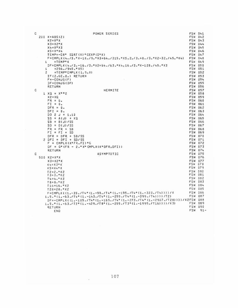
C POWER SERIES FSW 0~1 ZOO ~=ABS(ZI FSW 0~2
~2=X"X FSW 0~3
X3=~2"X FSW O~~ X,=X"X3 FSW 0~5 ~5=X"X' FSW 0~6
TEMP=-C6' SQRTlXI'CEXP(I'XI FSW 0~7 F=CHPLX(4./J.*X-16./9 •• X3+64./315 •• X5.2./3.+6./3 •• X2-3 2./45 •• X4) FSW 046
1 +TEptP·1( FSW 049 OF=CHPLX(,./3.-16./3."X2+&~./63.'X •• 16./3."X-126.1'5." X3 FSW 050
1 +256./9~5.'X51 FSW 051 2 +TEHP"GHPLX (1. 5.XI FSW 052
IF(Z.GE .O.I RETURN FSW 053 F=-CONJG(FI FSW 05~ JF=CONJG(OFI FSW 055 RETURN FSW 056
C HERHITE FSW 057 1 X~ = X··2 FSW 058
X2=XQ FSW 059 FR = O. FSW 060 FI = O. FSW 061 OFR = O. FSW 062 OFI = O. FSW 063 00 2 J = 1.10 FSW 06~ SS = A(J) + XQ FSW 065 SB = S(JI/SS FSW 066 SO = O(JI/SS FSW 067 FR = FR + sa FSW 068 FI = FI + SO FSW 069 OFR = OFR + S3/SS FSW 070
2 OFI = OFI • SO/SS FSW 071 F = CHPLX(X'F~.FII"G FSW 072 OF = G'(FR - 2.'~'CHPLX(X'OFR.OFIll FSW 073 RETURN FSW 07.
C ASYMPTOTIC FSW 075 500 ~2=X"X FSW 076
X3=X2'X FSW 077 X~=X3.( · FSW 078 X5 =X4-X FSW 079 TZ=2.'X2 FSW 080 T3=3.'X2 FSW 061 T~=4 •• (2 FSW 082 T6=6.'X2 FSW 083 T16=16.'X2 FSW 08. T26=26.'X2 FSW 065 F=CHPLX«l.-35./T"(1.-99./T"(1.-195./T"(l.-323./T41II)/X FSW 066 1.5.'(1.-63./T"(1.-143./T"(1.-255./T"(l.-399./T~111 I/T21 FSW 067 OF=-CHPLX«1. -105./T"(l.-165./T" (l.-273./T~'(l.-2907./T281111/X2FSW 088
1,5 •• (1.-63.IT2.U.-429./TS.(1.-255.IT3.U.-1995./T1&") )/X3) FSWaeq RETURN FSW 090
END FSW 91-
107
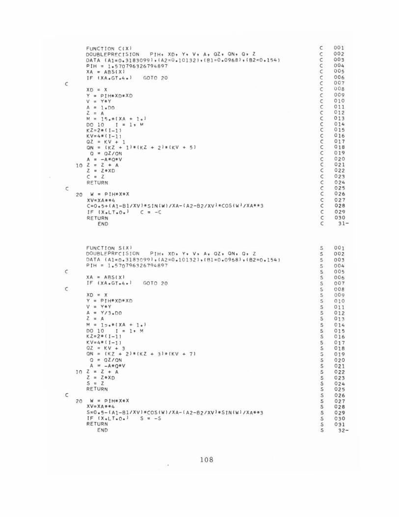
c
c
c
c
c
FUNCTION C(XI DOUB LEPRECISION PIH, XD .. Y .. V. A, OZ, ON, 0, Z DATA (Al=O.31830991,(A2= O. 10132),{Bl=O.0968),{B2=0.154) PIH = 1.570796326794897 XA = ASS!Xi IF (XA.GT.4.1 GOTa 20
XD = X Y PIH*XD*XD V y*y A = 1. DO 2 A M 15.*CXA + 1.1 DO 10 I = 1, ~
KZ=2*( I-I) KV=4*( I-I) QZ KV + 1 ON = IKl + 1)*{KZ + ZI*IKV + 51
Q = OZION A - A*O*V
10 Z Z + A Z l*XD C Z RETURN
20 W = PIH*X*X XV~XA**4 C=O.5+(AI - BI/XV)*SINCW1/XA-(A2-B2/XV1*COSIW 1/XA**3 IF (X.LT.O.) C = -C RETURN
END
FUNC TI ON SeX) DOUBLfPR~ctSION PIH, XD, y, V, A. OZ. ON, O. Z DATA CAl=0. 3 183 099 ),(A 2=0.lOI321,(Bl=O. 0968),(B2=0.1541 PIH = 1.5707963Z679~897
XA = AAS(XI IF (XA.GT.4.1 GO TQ 20
XD = X Y PIH*XO*XI) V Y*Y A Y/3.DO Z A M 1~.*(XA + 1.) 00 10 J = 1. M KZ=2*(I-l) KV=4*(I-IJ OZ K V + 3 ON CKZ + 2)4CKl + 3 1*CKV + 71
Q OZION A :::r -A*Q*V
10 Z = Z + A l = l*XD S = Z RETURN
20 W = PIH*X*X XV=XA**4 S=0.S -(AI-BI/XVJ*CO S(WI/XA-IA2-B2/XVI4 SIN (W 1/ XA**3 IF IX.LT.O.1 S = - S RETURN
END
108
c c c c c c c c c c c c c c c c c c c c c c c c c c c c c c c
S S S S S S S S S S S S S S S S S S s S S S S S S S S S S S S S
001 002 003 004 005 006 007 008 009 010 0 11 0 12 013 0 14 015 016 017 018 019 020 021 022 023 024 025 026 027 028 029 030 31-
001 002 003 00 4 005 006 007 008 009 010 011 012 013 014 0 15 0 16 017 018 019 020 021 022 023 024 025 026 027 028 029 030 031
32-
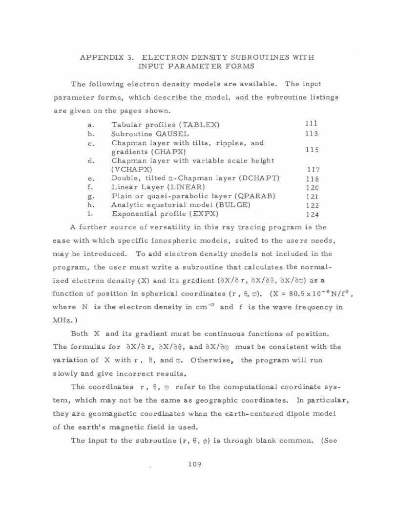
APPENDIX 3 . ELECTRON DENSITY SUBROUTINES WITH INPUT PARAMETER FORMS
The following electron density models are available. The input
parameter forms, which describe the model, and the subroutine listings
are given on the pages shown.
a. b. c.
d.
e. f. g. h. i.
Tabular profiles (TABLEX) Subroutine GA USEL Chapman layer with tilts, ripples, and gradients (CHAPX) Chapman layer with variable scale height (VCHAPX) Double, tilted a -Chapman layer (DCHAPT) Linear Layer (LINEAR) Plain or quasi-parabolic layer (QPARAB) Analyti c equatorial model (BULGE) Exponential profile (EXPX)
lli 113
115
117 118 120 121 122 124
A further sourc e of versatility in this ray tracing program is the
ease with which specific ionospheric models, suited to the users needs,
may be introduced. To add electron density models not included in the
program, the user must write a subroutine that calculates . the normal-
ized electron density (X) and its gradient (oX/a r, aX/a8, oX/acp) as a
function of position in spherical coordinates (r, 8, cp ). (X = 80.5xIO- 6 N/f 2,
where N is the electron density in cm --3 and f is the wave frequency in
MHz. )
Both X and its gradient must be continuous functions of position.
The formulas for oX /a r, oX/ae, and aX/ocp must be consistent with the
variation of X with r, 8, and cp . Otherwise, the program will run
slowly and give inco rrect results.
The coordinates r, 8 , cp refer to the computational coordinate sys
tem, which may not be the same as geographic coordinates. In particular,
they are geomagnetic coordinates when the earth- centered dipole model
of the earth's magnetic field is us ed.
The input to the subroutine (r, 8, ¢) is through blank common. (See
109
Table 3.) The output is through common block IXX/. (See Table 8 . ) It
is useful if the name of the subroutine suggests the model to which it cor
responds. The subroutine should have an entry point ELECTX so that
other subroutines in the program can call it. Any parameters needed by
the subroutine should be input into WIOI through W149 of the Warray.
(See Table 2.) If the model needs massive amounts of data,' these should
be read in by the subroutine following the example of TABLEX. As in
the already existing electron density subroutines, provision should be
made for perturbations to the electron density model (irregularities) by
having the statement
IF(PERT.NE.O.) CALL ELECTl
before the RET URN statement at the end of the subroutine.
110
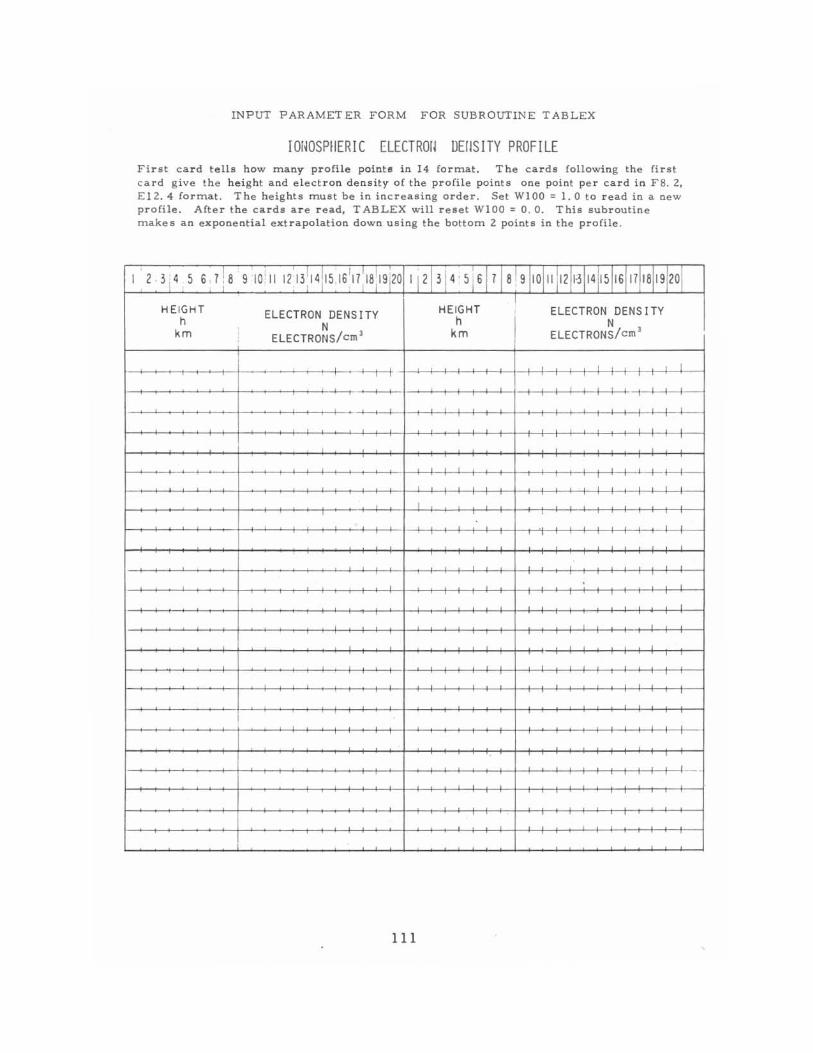
INPUT PARAMET ER FORM FOR SUBROUTINE TABLE X
IOiWSPIiERIC ELECTROIl DEIISITY PROFILE Fir s t card tells how many profile pointe in 14 format. The cards following the first c ard give the height and electron density of the profile points one point per card in F8. 2, E Il.4 forITlat. The h e ights must be in inc reasing order. Set WIOO = 1. 0 to read in a new pr o file. After the cards are read, T ABLEX will reset WIOO = O. O. This subroutine m akes an exponential extrapolation down using the bot tom 2 points in the profile .
I ' 1.3i4,5 6,7la 9 10! II 111 3 : 14 1 15 , 16 ~ 17 : la : 19 i10 I 111314 ' 5 i 6171ai911OH 1111'31141151161171 1al191101 I
HEIGHT HEIGHT ELECTRON DENSITY ELECTRON DENSITY h N h N km ELECTRONs/em' km ELECTRor~s/em '
-+-t-+ I I I I I I I I
, I I I I I I f-I--+--t-f-l-I-
I I , I
,
,
,
111
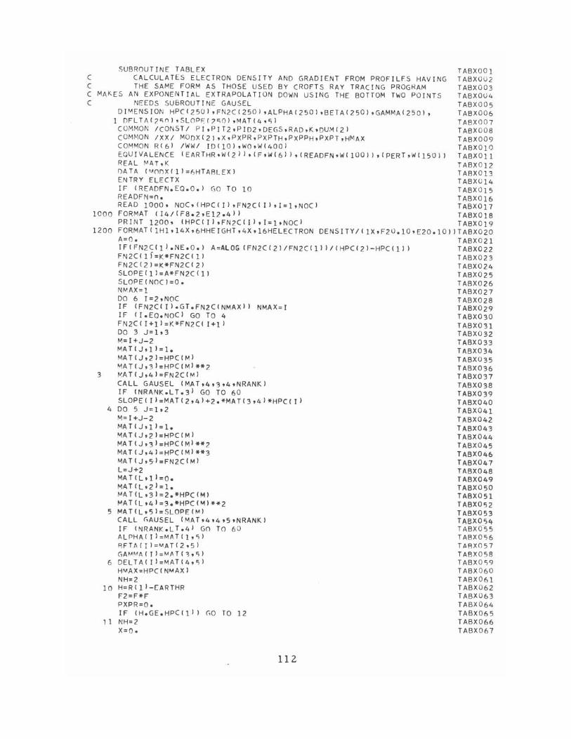
SUBROUTINE TABLEX C CALCULATES ELECTRON OENSITY C THE SAME FORM AS THOSE USED C MAKES AN EXPONENTIAL EXTRAPOLATION C NEEDS SUBROUTINE GAuSEL
ANO GRADIENT FROM PROFILFS HAVING BY CROFTS RAY TRACING PROGRAM DOWN USING THE BOTTOM TWO POINTS
DIMENSION HP(C250),FN2C(250)'ALPHA(250),BETA(2S0),GAMMAC250), 1 DFLTAf?tinl , SLOPF:f?liOI,MATI4,'i)
(OMMON ICONST/ PI,PIT2,PID2,DEGS,RAD.K.DUMI21 cOMMON IXX; MOOX(2).X,PXPR,PXPTH,PXPPH,PXPT,HMAX COMMON R(61 /'WW/ lOtIO) ,WO,WI40QI E.QUIVALENCE (EARTHR.W(2») ,(F,W{6)) ,(READFN.WI 100) ) ,(PERT,W( 150) I REAL MAT,K DATA {MOnXflJ=6HTAALEXI ENTRY ELECTX IF fREADFN.EQ.O.l GO TO 10 READFN=n. READ 1000, NOC,(HPCCJ),FN2CCII,I=1,NOCI
1000 FORMAT (I4/(F8.2,E12.411
TABXOOI TABX002 TABX003 TABXOU4 TABX005 TABX006 TA8X007 TABX008 TABX009 TABX OIO TABXOII TABXOl2 TAAX013 TABX014 TABX015 TABX016 TABX017 TABXOl8 TABX019 PRINT 1200, (HPCIIl,FN2C(Ild=1,NOCI
1200 FORMATIIHl,14X,6HHEIGHT,4X,16HELECTRON DENSITY/IIX,F20.IO,E20.101ITABX020
3
A=O. IFIFN2CCII.NE.0.1 FN2CCli=K*FN2CCll FN2C(21=K*FN2C(Z) SLOPECII=A*FN2CCII SLOPECNOCI=O. NMAX=1 DO 6 I=2,NOC
A=ALOG C FN2C C 21/FN2C C 11 II C HPC C 2 I-HPC C II I
IF CFN2CCII.GT.FN2CCNMAXII NMAX=I IF C I. EO. NOC I GO TO 4 FNZC(I+l'=K*FN2C( 1+1' DO 3 J=1,3 M=I+J-2 MATIJ,ll=l. MATIJ,21=HPC{MI ~AT(J,31=HPC(M)**2 ~AT(J,4)=FN2C(MJ
CALL GA USEL (MAT,4,~,4,NRANKI IF CNRANK.LT03 1 GO TO 60 SLOPEII)=MAT(2,4'+Z.*MATI3,4 J *HPClt)
400 5 J=1.2 M=I+J-2 MA T(J ,l) =l. MATIJ,Z' =HPC{MI MATIJ'3'=HPCCM)**Z MATIJ,4J=HPCCM'**3 MAT IJ,SI=FN2C(MI L=J+2 MATIL,l'=O. MATIL,ZI=l. MA TIL,31=2.*HPCIMI ~A T{l'41=3.*HPC{MI**2
5 MAT(L.SI=SLOPE(MI CALL ~AUSEL (MAT,4,4.5,NRANKI IF (NRANK.LT.4) Go TO 60 ALPHA ( I I =MAT (I, "i I AFTA(j)=MAT(2,5J GAM¥A(TI=MAT(~,"i1
6 DELTA(IJ =MAT(4,1j) HMAX=HPC(NMAX) NH=2
10 H=RCII-[ARTHR F2=F*F PXPR=O. IF CH.GE.HPCIIII
11 NH=2 X=O.
0,0 TO 12
112
TABX021 TABX022 TABX023 TABX024 TABX025 TABX026 TABX027 TABX028 T ABX029 TABX030 TABX031 TABX032 TABX033 TABX034 TABX035 TABX036 TABX037 TABX03B TABX039 TABX040 TABX041 TABX042 TABX043 TABX044 TABX045 TABX046 TABX047 TABX048 TAB X049 TABX050 TABX051 TABX 052 TABX053 TA8X054 TABXd-55 TABXO,6 TAAX057 TABX058 TA8XOlj9 TABX060 T ABX061 TABX062 TABX063 TA8X064 TABX065 TABX066 TABX067
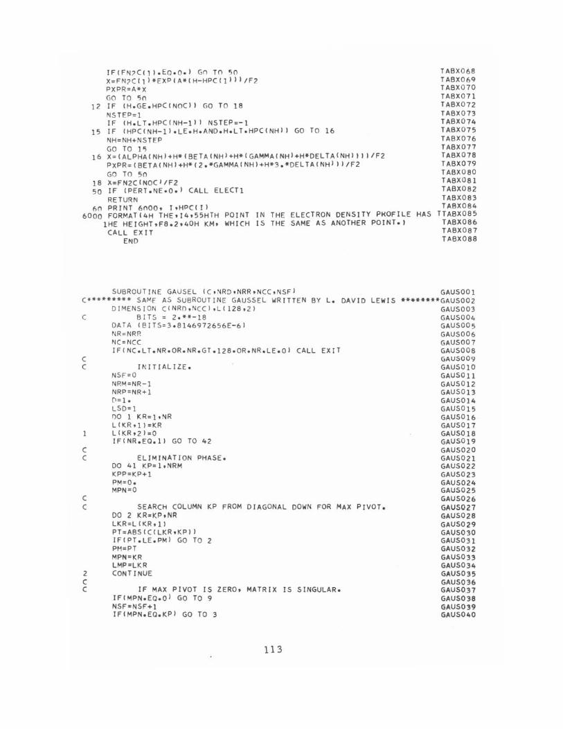
IFIFN?Clll.EQ.O.1 Gn Tn 50 X=FN?C{l l *EXPIA*(H-HPCll lll tF/. PXPR=A*X GO TO 50
12 IF IH.GE.HPCINOCII GO TO 18 NSTEP=1 IF IH.lT.HPCINH-11 I NSTEP=-1
15 IF IHPCINH-II.lE.H.AND.H.lT.HPCINHII GO TO 16 NH=NH+NSTEP GO TO 1~
16 X=(ALPHAINH'+H*'BETAINHI+H*IGAMMA(NHI+H*OELTA{NHIIII/F 2 PXPR= (SETA( NH) +H* (2 •• GAMMA (NH I+H* 3 .-DEL TA (NH) II IF2 GO TO 50
18 X=FN2CINOC'/F2 50 IF IPERT.NE.O.I CAll ELECT}
RETURN 60 PRINT 6000. I .HPC( J)
TABX068 T ABX06Q TABX070 TABX071 TABX072 TABX073 TABX074 TABX 0 75 TABX076 TABX071 TABX078 TABX079 TABX080 TABX081 TABX082 TABX083 T ABX084
6000 FORMATI4H THE.I4.55HTH POINT IN THE ELECTRON DENSITY PHOFIlE HAS lHE HEIGHT,F8.2.40H KM. WHICH IS THE SAME AS ANOTHER POINT.)
TTABX085 TABX086 TABX087 TABX088
CAll EXIT END
SUBROUTINE GAUSEL {(,NRD,NRR,NCC.NSFI C·*·*···· * SAMf AS SUBROUTINE GAUSSEL WRITTEN BY L. DAVID LEWiS
DIMENSION C(NRO,~CC1,L(128,21 C SITS = 2.*.-18
C
DATA IBIT S=3.8146972656E-61 NR=NRR NC=NCC
C INITIALIZE.
C
NSF=O NRM=NR-l NRP=NR+l D=l. lSD=1 1)0 1 KR=l.NR LIKR.!'=KR LIKR.2)=O IFINR.EO.ll GO TO 42
C ELIMINATION PHASE.
C
DO 41 KP= l.NRM KPP=KP+l PM=O. MPN=O
C SEARCH COLUMN KP FROM DIAGONAL DOWN FOR MAX PIVOT. DO 2 KR·KP.NR LKR=LIKRd) PT=ABSICILKR,KPJ 1 IFIPT.lE.PMI GO TO 2 PH=PT MPN=KR lMP=lKR
2 cONT INUE C C IF MAX PIVOT IS ZERO. MATRIX IS SINGULAR.
IFIMPN.EO.O' GO TO 9 NSF=NSF+l IFIMPN.EO.KPI GO TO 3
113
GAUSOOI ...... **· ...... ·GAUS002
GAUS003 GAUS004 GAUS005 GAUS006 GAUS007 GAUS008 GAUSQ09 GAUS010 GAUSOll GAUS012 GAUS013 GAUS014 GAUS015 GAUS016 GAUS017 GAUS018 GAUS019 GAUS020 GAUS021 GAUS022 GAUS023 GAUS024 GAUS025 GAUS026 GAUS027 GAUS028 GAUS029 GAUS030 GAUS031 GAUS032 GAUS033 GAUS034 GAUS035 GAUS036 GAUSO.37 GAUS038 GAUS039 GAUS040
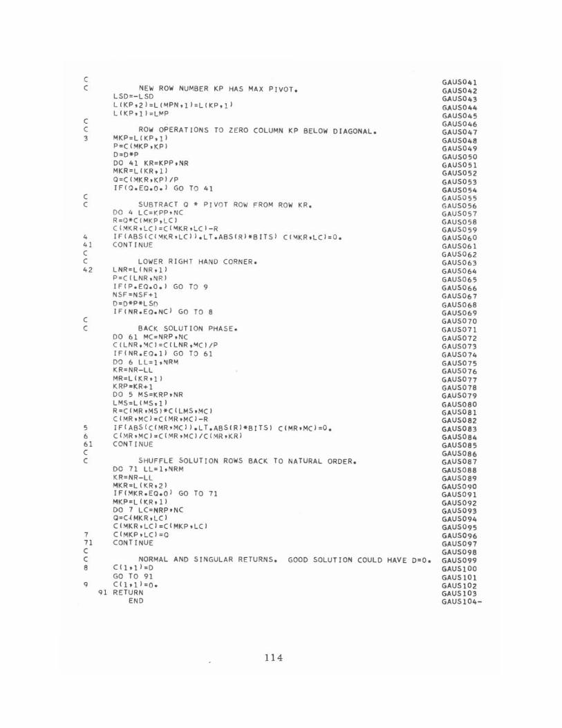
(
( NEW ROW NUMBER KP HAS MAX PIVOT.
(
LSD=-LSD L{KP,2)=L(~PN,1)=L(KP,11
L(KP'I1=L~P
( ROW OPERATIONS TO ZERO (OLUMN KP BELOW DIAGONAL. 3 MKP=LCKP,11
(
P=CI!o1KP,KPI D:::ID*P DO 41 KR=KPP,NR MKR=L (KR, II Q=CI~KR,KP)/P
IFCQ.EO.O.) GO TO 41
C SUBTRAC T 0 * PIVOT ROW FROM ROW KR. DO 4 LC=KPP,N C R=O*CIMKP,LCI C(~KR ,LC1=C{~KR'LCI-R
4 IF(ABS(C{~KR'LCll.LT.ABSIRI*BrTSI C(~KR'LCI = O. 41 (O NTINUE (
( LOWER RIGHT HAND (ORNER. 42 LNR=lINR,ll
(
P=CCLNR,NRI IFCP.EQ.O.I GO TO 9 NSF=NSF+l D=O*P*LSo IF'NR.Eo.N(1 GO TD 8
( BACK SOLUTION PHASE. DO 61 MC=NRP,NC C (LNR.~CI=C{LNR,MCI/P
IF'NR.EO.II GO TO 61 DO 6 LL=l ,NR~ KR=NR -LL MR=L(KR,ll KRP"'KR+l DO 5 M$=KRP,NR LMS=LIMSdl R=C(MR,MSI*C{LMS,MCl CIMR,MCI=CCMR.MCI -R
5 IFIABS(CCMR,MCII.LT.ABSIRI*BITSI CIMR,MCI=O. 6 CIMR.MC1=CIMR,MCI/(IMR,KRI 61 (ONTINUE (
( SHUFFLE SOLUTION ROWS BACK TO NATURAL ORDER. DO 71 lL=l,NRM KR=NR-LL MKRzL{KR,2) IF'~KR.EO.OI GO TO 71 MKP=LiKR,ll DO 7 LC=NRP,NC Q=«MKR.LCI C(MKR,LCI=CIMKP,LCI
7 C{MKP,LCi=O 71 CONTINUE (
( NORMAL AND SINGULAR RETURNS. GOOD SOLUTION (OULD HAVE D=O. B C{1,1i=D
GO TO 91 q (<1,11=0.
91 RETURN END
114
GAUSO.l GAUS042 GAUSO.3 GAUS044 GAUS045 GAUS046 GAUS047 GAUS048 GAUS049 GAUS050 GAUS051 GAUS052 GAUS053 GAUS054 GAUS055 GAUS056 GAUS057 GAUS058 GAUS059 GAUS060 GAUS061 GAUS062 GAUS063 GAUS064 GAUS065 GAUS066 GAUS067 GAUS068 GAUS069 GAUS070 GAUS071 GAUS072 GAUS073 GAUS074 GAUS075 GAUS076 GAUS077 GAUS078 GAUS079 GAUS080 GAUS081 GAUS082 GAUS083 GAUS08. GAUS085 GAUS086 GAUS087 GAUS088 GAUS089 GAUS090 GAUS091 GAUSD92 GAUS093 GAUS094 GAUS095 GAUS096 GAUS097 GAUS098 GAUS099 GAUSI00 GAUSI0l GAUSI02 GAUSI03 GAUSI04-
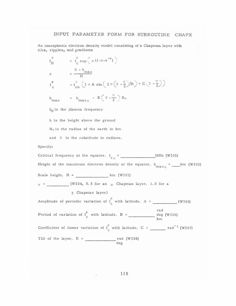
INPUT PARAMETER FORM FOR SUBROUTINE CHAPX
An ionospheric electron density model cons isting of a Chapman layer with tilts, ripple 5, and gradients
z =
:2 r - z " fC exp ,,- Ci (l-z-e ) /
h - h max
H
2 f
c =<0 ( I +ASin ( 2T1 (e - D/B)+C "e -%) )
h max
h ~ E (e - ~ 'I R o rnax o 2 ",,'
IN is the plasma frequency
h is the height above the ground
Ro is the radius of the earth in km
and e is the colatitude in radians.
Specify:
Critical frequency at the equator, f = _________ MHz (WIDI) Co
H e ight of the maximum electron density at the equator, h = max o
Scale height, H = _______ km (WI03)
'" = _____ (WI04, 0.5 for an Ci Chapman layer, 1. 0 for a
8 Chapman layer)
2
km (WI02)
Amplitude of periodic variation of Ie with latitude, A = ______ (WIOS)
rad Period of variation of £2 with latitude, B = deg (WI06)
c ------ km
Coefficient of linear variation of l with latitude, C = C
Tilt of the layer, E = _______ rad (WIOS) deg
115
___ rad- 1 (WIO?)
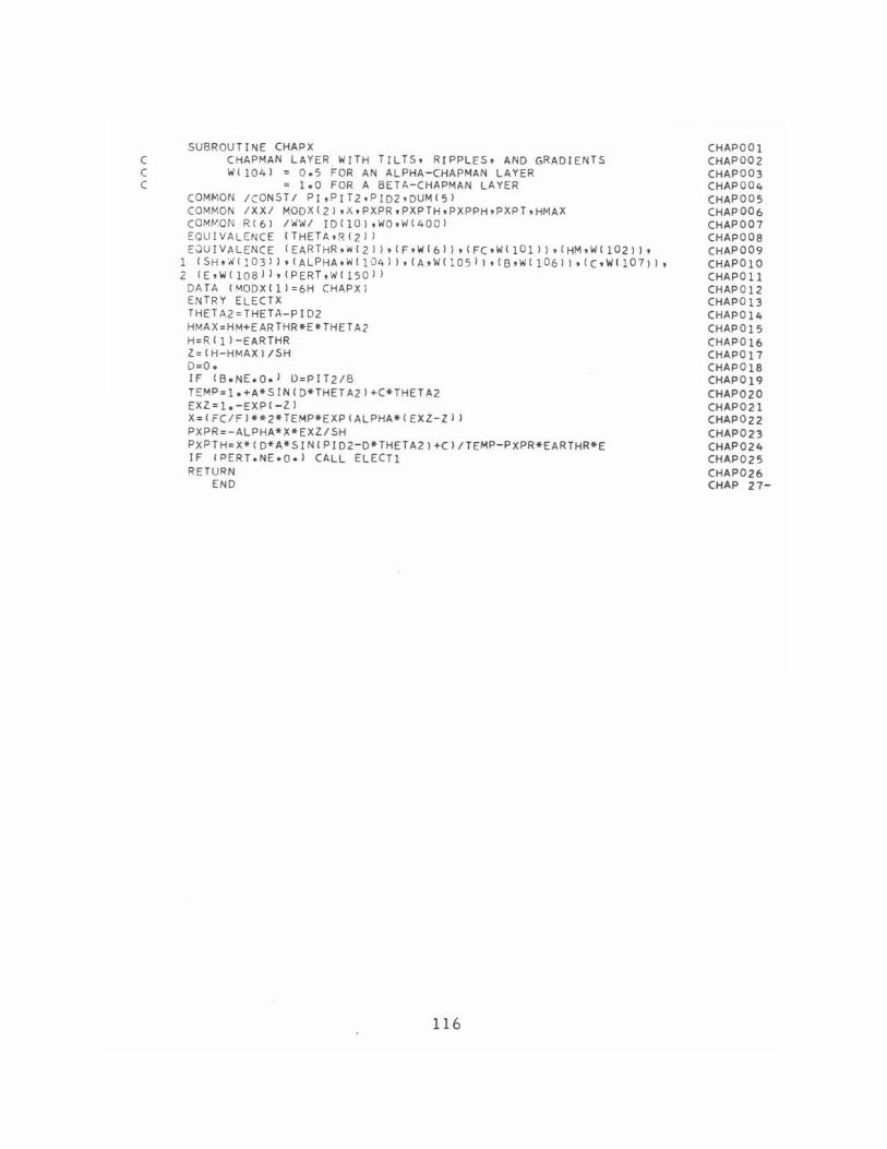
C C C
SU8ROUTINE CHAPX CHAPMAN LA YER WITH TILTS~ RIPPLES. ANO GRAOlENTS W{1041 = 0 . 5 FOR AN ALPHA - CHAPMAN LAYER
= 1.0 FOR A 8ETA - CHA PMAN LAYER COMMON ICONST! Pr , P tT2,PI02' DUM(51 COMMON /XX/ MODX(21, X,P XPR,PXPTH ,P XPPH,PXPT ,HMAX COMVON R(6) /~W/ ID ( l O ),WQ,W(40 0 1 EQUrVAlE:N CE (THET A.RIzJ 1 EJU IVALENCE iEARTHR.W(2 J) .tF.W(6)),(FC.WIIOll),(HM,WllOZ)).
1 ISH,WII03)),(ALPHA,WII 04) ),(A.W(lOSJ),(S.Wtl06) ),(C.W(107)1. 2 (E.W(lOa) ),(PERT,W(1 50 1 )
DA TA (MOOXIll=6H CHAPX I ENTRY ELECTX THETAl=THETA-PIDl HMAX =HM+EARTHR*E*TH ETA2 H=R'll -EARTHR l=IH-HMAXI/SH 0 =0. IF CB.NE.O.l D=PIT2/8 TEMP =1.+A*SINI D* THET A21+C*THETA2 EXl =I.-E XP' - Zl X=IFC/FI**Z*TEMP*EXPIALPHA*(EXl -ZI I PXPR =-AL PHA*X*E XZ/SH PxPTH=X*ID*A*SINIPJD2 - D*THETA21+CI/TEMP-P XPR*EARTHR*E IF ,PERT.NE.O.l CALL ELECTI RETURN
END
116
CHAPOOI CHAPOOl CHAP003 CHAP004 CHAP005 CHAP006 CHAP007 CHAP008 CHAP009 CHAPOIO CHAPOII CHAPOll CHAPOl3 CHAPOl4 CHAPOl5 CHAPOl6 CHAPOl7 CHAPOIS CHAPOl9 CHAPOlO CHAPOll CHAPOll CHAPOZ3 CHAPOl4 CHAPOl5 CHAPOl6 CHAP l7-
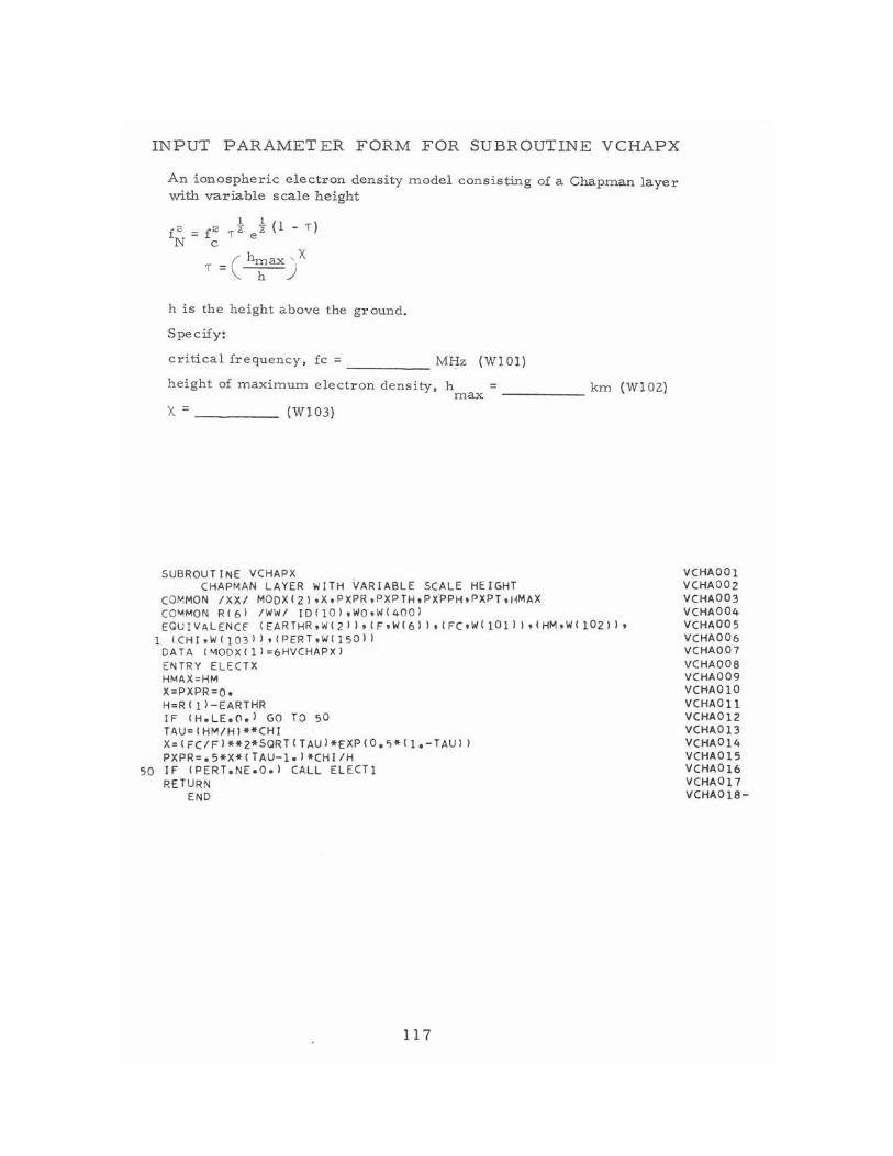
INPUT PARAMETER FORM FOR SUBROUTINE VCHAPX
An ionospheric electron density model consisting of a Chapman layer with variable scale height
h is the height above the ground.
Specify:
critical frequency, fc = _____ M~z (WlGl)
height of maximum electron density, h = ______ km (WI02) max
)( ~----- (WI03)
SUBROUTINE VCHAPX CHAP~AN LAYER WITH VARIABLE SCALE HEIGHT
cOMMON IXX/ MODX(21,X,PXPR,PXPTH,PX'PPH,PXPT,HMAX COMMON R(6i /WW/ IO{lOI.WQ.W(40Ql EQUIVALENCf (EARTHR,W(211 ,(F,W{611 ,(Fe.WI 101)) ,(HM,W( 102)1,
1 (CHI,WQ031 J ,(PERT.WIl501 I DATA (~ODX(lJ=6HVCHAPX)
EN TRY ELECTX HMAX=HM X=PXPR=O. H=R(jl-EARTHR IF (H.LE.n.1 GO TO 50 TAU=IHM/H1**CHI X=(FC/FI**2*SQRT(TAU1*EXP{O.S*<1. -TAUJ I PXPR=.S*X*/TAU-l.I*CHI/H
SO IF (PERT.NE.O.l CALL ELECTl RETURN
END
117
VCHAOOI VCHA002 VCHA003 VCHA004 VCHA005 VCHA006 VCHA007 VCHA008 VCHA009 VCHAOjO VCHAOll VCHAOl2 VCHA013 VCHAOl4 VCHA015 VCHAOl6 VCHA017 VCHAOl8-
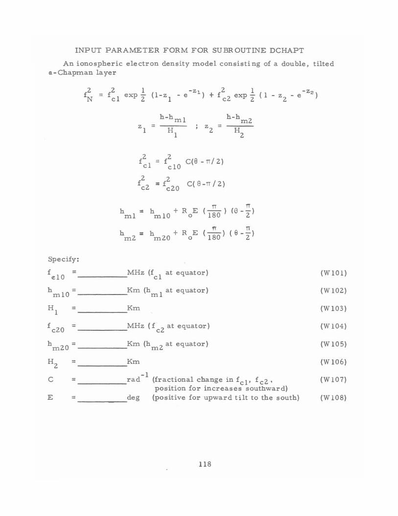
INPUT PARAMETER FORM FOR SUBROUTINE DCHAPT
An ionospheric electron density m.odel consisting of a double, tilted (1- Chapm.an layer
l fZ 1 (l-z
-Zl Z 1 -Z2 = exp - - e ) + f cZ exp 2 (l-z -e ) N cl Z 1 Z
h-hm.l h-h m.Z
zl = Zz = HI HZ
fZ = fZ C(8 -n/Z) cl clO
l Z C(S-n/Z) cZ = f
czo
n n h = h + R E ( 180 ) (8 --)
m.l m.lO 0 Z
fT n h = hm.ZO + R E ( 180 ) ( e - -)
m.Z 0 Z
Specify:
f dO
= MHz (fcl
at equator) (W 101)
h = Km. (hm.l at equator) (W 10Z) m.lO
HI = Km. (W 103)
f = MHz (f cZ at equator) (W 104) cZO
h = Km. (hm.Z at equator) (W 105) m.ZO
HZ = Km. (W 106)
-1 (fractional change in fCl' fcZ. (WI07) C = rad position for increases southward)
E = deg (positive for upward tilt to the south) (WI08)
118
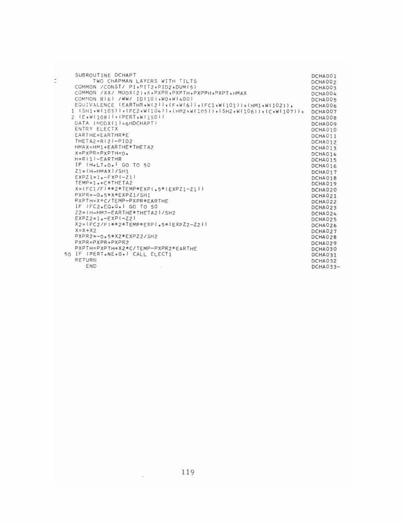
SUBROUTINE DCHAPT TWO CHAPMAN LAYERS WITH TILTS
COMMON ICONS T/ PI,PIT2,PID2,OUM(5) COMMON /XX/ MODX(2),X,PXPR,PXPTH,PXPPH,PXPT,HMAX COM ~·10N R(6) /WWI IOIIOI,WQ,WI4001 EQUiVALENCE (EARTHR,W(2J1,(F,W(6)),{FCl,WllOll),(HMl.Wl102)).
1 (SHbW( 103) I ,(FC2,W(104) ) , (Hf-12,W( 1(1511 ,(SH2,WCI 0611, ((,WIID7)), 2 (E,WII08),(PERT,w(150))
DATA (~ODX(lJ=6HDCHAPTl ENTRY ELECTX EARTHE =EARTHR*E THElAZ=R(Zl -PID2 HMAX=HMl+EARTHE*THETA2 X=PXPR=PXPTH=a. H=RCIJ-EARTHR IF (H .ll.O.) GO TO 50 ll=(H-HMAX1/SHl EXPZl=l.-FXP(-Zll TEMP=1.+C*THETA2 X=(FCI/F1**2*TEMP*EXP(.S*(EXPZI-Zl'l PXPR=-O.5*X*EXPll/SHl PXPTH=X*C/TEMP-PXPR*EARTHE IF (Fe2.EO.o.) GO TO 50 l2=(H-HM?-EARTHE*THETA21/$H2 EXPZ2=1.-EXP(-Z2) X2=(FC2 / FI**2*TEMP*EXPI.S*IEXPZ2-Z2)' X=X+X2 PXPR2=-O.S*X2*EXPZ2/SH2 PXPR=PXPR+PXPR2 PXPTH=PXPTH+X2*C/TEMP-PXPR2*EARTHE
50 IF (PERT.NE.D.l CALL ELECTl RETURN
END
119
OCHAOOl DCHAODZ DCHA003 DCHAOD4 DCHAD05 DCHAD06 DCHA007 DCHAOD8 DCHAOD9 DCHAOIO DCHADll DCHA012 DCHADl3 DCHA014 DCHA015 DCHADl6 DCHAOl7 DCHA018 DCHA019 DCHADZO DCHAOZI DCHADZZ DCHAOZ3 DCHAOZ4 DCHADZ5 DCHAOZ6 DCHAOZ7 DCHADZ8 DCHAD29 DCHA030 DCHA031 DCHA032 DCHA033-
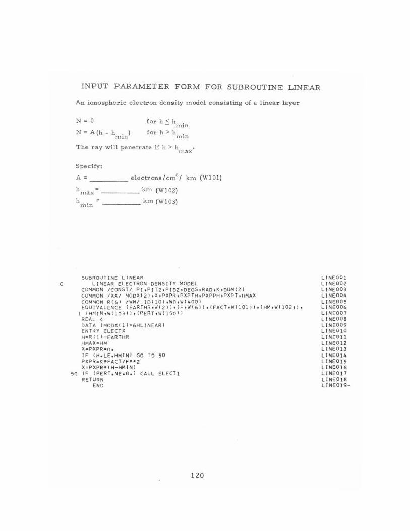
INPUT PARAMETER FORM FOR SUBROUTINE LINEAR
An ionospheric electron density :model consisting of a linear layer
N=O
N = A(h - h . ) rnm
for h < h . - mln
for h> h . rnm
The ray will penetrate if h> h . max
Specify:
A = _____ electrons/crn3/ krn (WIOI)
hrnax= _____ krn (WI02)
h = _____ krn (WI03) min
SUBROUTINE LINEAR C LINE AR ELECTRON DENS ITY MODEL
CO MMON ICONST! PI .pr T2,P ID2,OEGS,RAD,K,DUM{21 CO MMON /XX/ MODX(ZI,X,PXPR,PXPTH,PXPPH,PXPT,HMAX COMMON R(6) /WW/ I D(lO).,W(),WI4001 EQU 1 VA LENCE (EAR THR, W { 2 I I , ( F, W (6 I J , (F ACT, w ( 101 ) I , (HM, W ( 102 I I ,
1 (Hr-t IN,WII 03)},(PERT,W(lSOI) REAL K DATA (MODX(11=6HLINEAR) EN T~Y ELECT X H=R(1) - EAR THR HMAX=H~
X",PXPR =O. IF (H.LE.HMINI GO TO 50 PXPR=K*FACT/F**2 X=PXPR*(H-HMIN)
50 IF (PERT.NE.D.I CALL ELECTI RETURN
END
120
L1NE ODI LI NEOOZ LI NE003 LI NED04 L1NE005 LINEOD6 LINE007 UNE ODa LINE 009 LI NED 10 LINEDl! LINEOIZ L1NEOI3 L1NEOI4 LINE015 L1NEDI6 LINE017 L1NEOla Ll NEOI9-
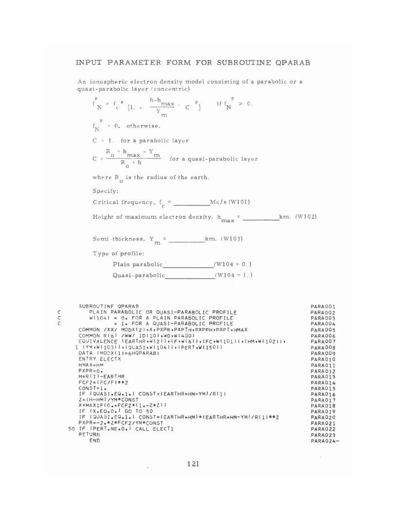
INPUT PARAMETER FORM FOR SUBROUTINE QPARAB
An ionospheric electron density model consisting of a parabolic or a quasi-parabolic layer ( concentric)
, f N ~ f " c [1.
h-h max
y m
fN O. otherwise.
. C
C 1. for a parabolic layer
R + h Y
, 1
,. f f N
> O.
c o max m R + h
o for a quasi-paraboli c layer
whE>re R is the radius of the ea rth . o
Specify :
Critical f r equency .. fc = ______ Mc/s (W I Dl)
Height of maximum electron density, h max
_____ km. (WI02)
S e mi -thickness, Y m
____ ---'km. (W I03)
Type of profile:
Plain parabolic _______ (W I 04 = O.
Quasi-parabolic (WI04 = 1.
SUBROUTINE QPARAB C PLAIN PARABOLIC OR QUASI-PARABOLIC PROFILE C W(lO~) = O. FOR A PLAIN PARABOLIC PROFILE C 1. FOR A QUASI-PARABOLIC PROFILE
COMMON IXX/ MOOX(2),X,PXPR,PXPTH,PXPPH,PXPT,HMAX CO~MON R(6) /WIN/ IDIIO),WQ,W(4001 EQUIVALENCE IEARTHR ,W(2)),(F,W(61),(FC,W1I Ol)) ,(HM,W(102)),
1 (Y."1,W(103)),CQUASI,\!,' (!04)J,CPERT,WI150)) DATA IMOJXIll=6HOPARABI ENTRY ELECTX HMAX=HM PXPR=O. H=RIII-EARTHR FCF2=(FC/FI**2 CONST=!. IF (QUASI.EQ.I.) CONST=(EARTHR+HM-YM)/R(I) Z=CH-HM1/YM*CONST X=MAXIFfO.,FCF2*(1.-Z*ZII IF (X.EO.O.) GO TO 50 IF (QUASr.EO.I.) CONST=(EARTHR+HMI*IEARTHR+HM-YM )/ R(1)**2 PXPR=-2.*Z*FCF2/YM*CONST
50 IF (PERT.NE.O.) CALL ELEcT 1 RETURN
END
121
PARA OO l PARA002 PARA003 PARA004 PARA005 PARA006 PARA001 PARAOOB PARA009 PARAOIO PARAOII PARAO!2 PARA013 PARAO!4 PARAOI5 PARAOI6 PARAOI7 PARAOIB PARAOI9 PARA020 PARA02I PARA022 PARA023 PARA024-
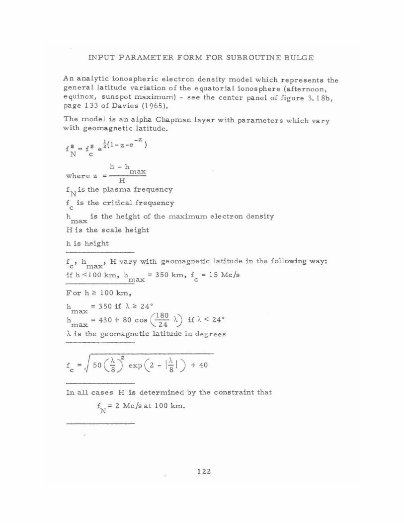
INPUT PARAMETER FORM FOR SUBROUTINE BULGE
An analytic ionospheric electron density model which represents the general latitude variation of the equatorial ionosphere (afternoon, equinox, sunspot maximum) - see the center panel of figure 3.18b, page 133 of Davies (1965) .
The model is an alpha Chapman layer with parameters which vary with geomagnetic latitude.
1 _z z(l-z-e )
e
h - h max
where z = --::-:..::::=:.: H
fN is the plasma frequency
f is the critical frequency c
h is the height of the maximum electron density max
H is the scale height
h is height
f , h , H vary with geomagnetic latitude in the following way: c max
if h<lOO krn, h = 350 km, f = 15 Mc/s max c -------=
For h;;, 100 km,
h = 350 if A;;' 24 0
max (180 ) hmax
= 430 + 80 cos 24 A if A < 24 0
A is the geomagnetic latitude in degrees
In all cases H is determined by the constraint that
f = 2 Mc/s at 100 km. N
122
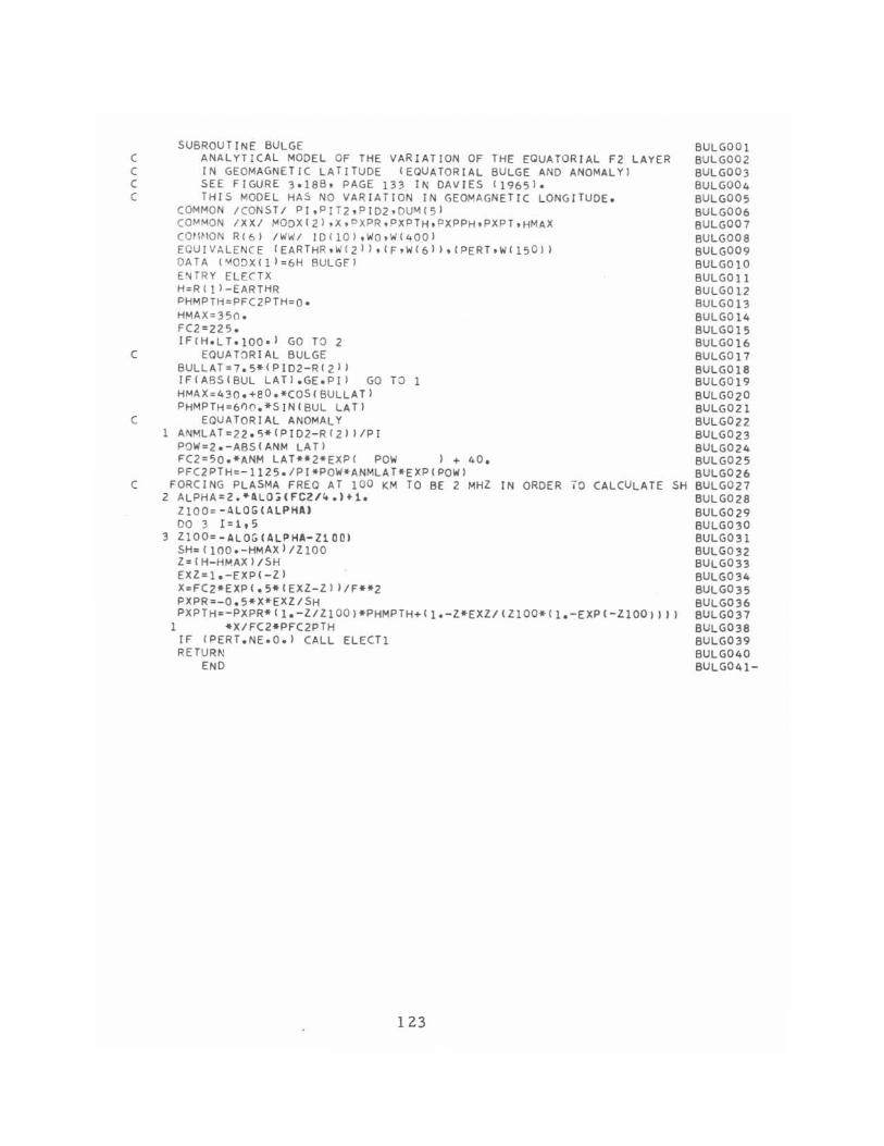
C C C C
C
C
C
SUBROUTINE BULGE ANALYTICAL MODEL OF THE VARIATION OF THE EQUATORIAL F2 LAYER IN GEOMAGNETIC LATITUDE (EQUATORIAL BULGE AND ANOMALY) SEE FIGURE 3.18B, PAGE 133 IN DAVIES 11965J. THIS MODEL HA S NO VARIA TION IN GEOMAGNETIC LONGITUDE.
COMM ON I CQNSTI PI,PI T 2,PID2t DU~(5) COM MON I XX! ~ODX{2 J , X , cXPR tPXPTH.PXPPH,PXPT'HMAX
(OW·ION RIb) tWWI I D tl O ),WQ ,W(4QQI EQU I VAL ENCE (EARTH R .W ( 2 1) ,(F.W(6J),(PERT,W(15 0 1J DATA (~ODX(lJ=6H 8ULGFJ EN TR Y ELECTX H=RIl)-EARTHR PHMPTH=PFC2PTH=Q. HMA X=35 0 . FC2;225. IFIH.LT.IOO') GO TO 2
EQUA TOR I AL BULGE BULLAT=7.5*IPID2 - R(2)) IFIABSIBUL LAT).GE.PI) GO n 1 HMAX=43Q.+SO.*CQSISULlATI PHMPTH=600.*SIN(BUL lAT)
EQUATORIAL ANOMALY ANMLAT;22.5*IPID2- R(2))/PI POW=2.-ABSIANM LAT) FC2=50.*ANM LAT**2*EXP { POW ) + 40. PF C2PTH=- 1125./PI*PQW*ANMLAT*EXPIPOWl
FORCING PLASMA FREQ AT 100 KM TO BE 2 MHl IN ORDER ,0 CALCULATE SH 2 ALPHA =2.·ALO;(FC2/~.).1.
l100; -ALOG (ALPHA) DO 3 1=1,5
3 l100; -ALD GI ALPHA-ZlOO) SH=II00.-HMAX)/ZIOO Z=IH-HMAXI/SH EXZ=l.-EXPI -Zl X~FC2*EXP (.5* (EXZ-Z ) I/F**Z PXPR=-O.5*X*EXZ/SH PXPTH=-PXPR*(l.-lIZlOO)*PHMPTH+(I. -Z*E XZ/(ZlOO*(I.-EXP( -lI OO}}l)
I *X/FCZ*PFCZPTH IF IPERT.NE.O.) CALL ELECT I RETURN
END
123
BULGOOI BULG002 BULG003 BULG004 BULG005 BULG006 BULG007 BULG008 BULG009 BULGOIO BULGOII BULGOI2 BULGOI3 BULGOI4 BULGOI5 BULGOI6 BULGOI7 BULGOI8 BULGOI9 BULG020 BULG02I BULG022 BULG023 BULG024 BULG025 BULG026 BULG027 BULG028 BULG029 BULG030 BULG03I BULG032 BULG033 BULG034 BULG035 BULG036 BULG037 BULG038 BULG039 BULG040 BULG041-
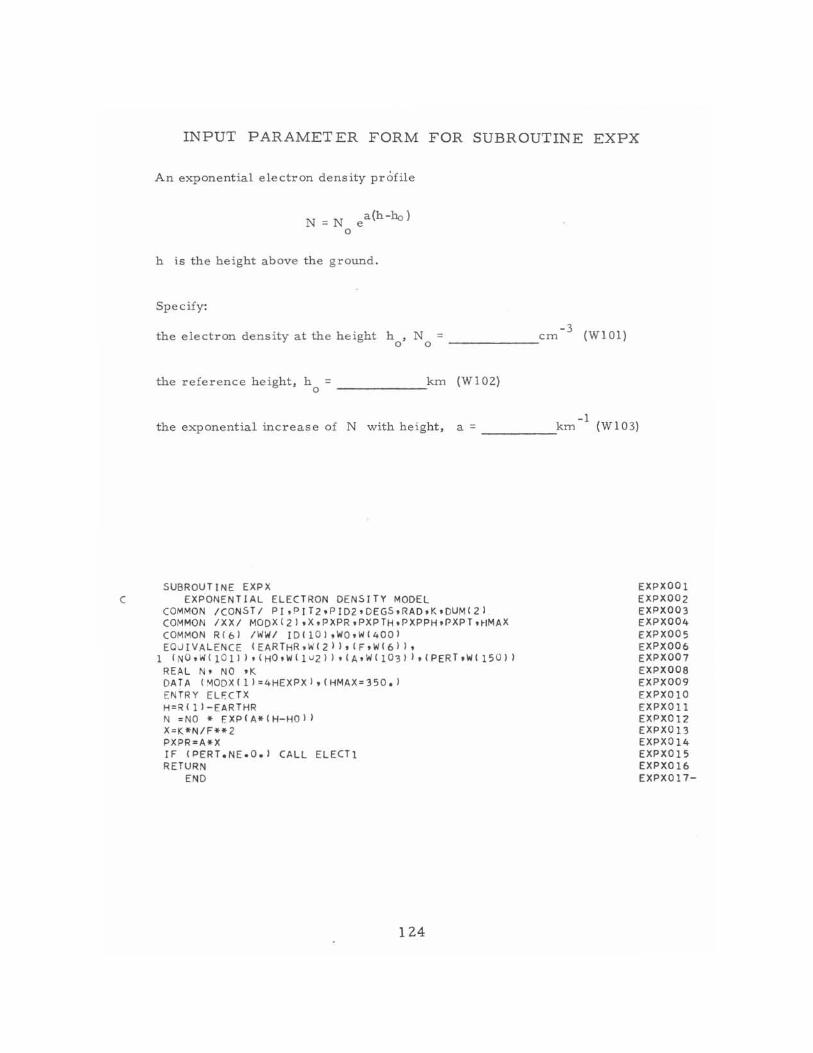
C
INPUT PARAMETER FORM FOR SUBROUTINE EXPX
An exponential electron density profile
a(h-bo ) N = N e
o
h is the height above the ground .
Specify:
the electron density at the h eight h ,N = _______ ,cm - 3 (WIDI) o 0
the reference h eight, ho = ______ km (WID2)
- I the exponential increase of N with height, a = ____ ---'km (WI0 3)
SUBROUT INE EXPX EXPONENTIAL ELECTRON DENSITY MODEL
COMMON teONSTI PI,PIT2,PID2,DEGS,RAD,K'DUM(21 COMMON IXX/ MODX(2),X,PXPR,PXPTH,PXPPH,PXPT'~IMAX (OMMON RIb! /WWI ID(l O ),WQ,W(400J EQJ IVALENCE (EARTHR,W(2),IF,W(6 1 1,
1 q"O,W(lOlJ) '(HQ,WII IJ2) I '(A,WfI03) I,{PERT,WI 15 0)) REAL Nt NO 'K DA TA (MODX(lJ=4HEXPX1,{HMAX=350 . ) EN TRY ELf'cTX H=RIII-EARTHR N =NO * EXP(A*fH-HOll X=K*N/F**2 PXPR=A*X IF (PERT.NE.O.l CALL ELECT 1 RETURN
END
124
EXPXOOI EXPXOOz EXPX003 EXPX004 EXPXOOS EXPX006 EXPX007 EXPX008 EXPX009 EXPXOI0 EXPXOll EXPXOIZ EXPX013 EXPXO 14 EXPX015 EXPX016 EXPXO 17-
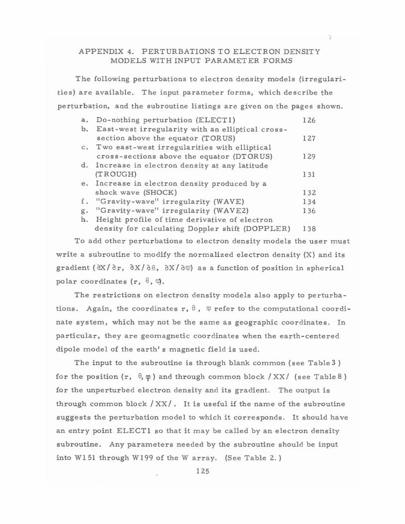
APPENDIX 4. PERTURBATIONS TO ELECTRON DENSITY MODELS WITH INPUT PARAMETER FORMS
The following perturbations to electron density models (irregulari
ties) are available. The input parameter forms, which describe the
perturbation, and the subroutine listings are given on the pages shown.
a. Do-nothing perturbation (ELECT1) 126 b. East - we st irregularity with an elliptical cro s s-
section above the equator (TORUS) 127 c. Two east-west irregularities with elliptical
cross -s ections above the equator (DTORUS) 129 d . Increase in electron density at any latitude
(TROUGH) 131 e. Increase in electron density produced by a
shock wave (SHOCK) 132 f. "Gravity - wave" irregularity (WAVE) 134 g. "Gravity-wave" irregularity (WAVE2) 136 h. Height profile of time derivative of ele.ctron
density for calculating Doppler shift (DOPPLER) 138
To add other perturbations to electron density models the user must
write a subroutine to modify the normalized electron density (X) and its
gradient (aX I or, aX / a e, aX / aqJ) as a function of position in spherical
polar coordinates {r, e, CIl.
The restrictions on electron density models also apply to perturba
tions. Again, the coordinates r, e, qJ refer to the computational coordi
nate system, which may not be the same as geographic coordinates. In
particular, they are geomagnetic coordinates when the earth-centered
dipole model of the earth's magnetic field is used.
The input to the subroutine is through blank common (see Table 3 )
for the position (r, e, cp ) and through common block / XX / (see Table 8 )
for the unperturbed electron density and its gradient. The output is
through common block / XX /. It is useful if the name of the subroutine
suggests the perturbation model to which it corresponds. It should have
an entry point ELECTI so that it may be called by an electron density
subroutine. Any parameters needed by the subroutine should be input
into WI 51 through W 199 of the W array. (See Table 2. )
125
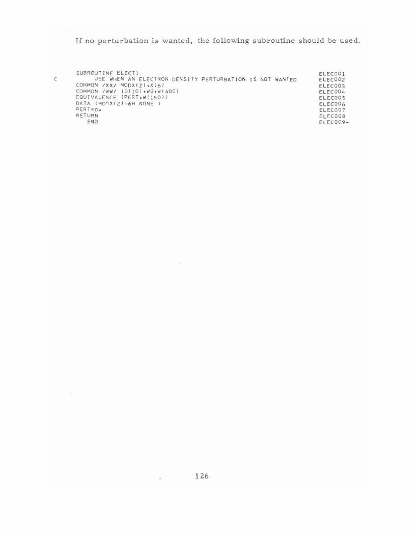
C
If no perturbation is wanted, the following subroutine should be used.
SUBROUTINE ELECTl USE WHEN AN ELE CTRON DENSITY PERTURBAT I ON IS NOT WANTED
(OMMON /XXI MODX(2),X(6) COMMON /WW/ IDIIO),WQ,W(4QO) EQUIVALENCE (PERT,WC1501 I DATA (~O~X(21=6H NONE) PERT=O. RETURN
END
126
ELEC OOl ELEC002 ELEC003 ELEC004 ELEC005 ELEC006 ELEC007 ELECOOB ELEC009 -
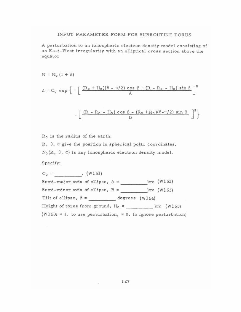
INPUT PARAMETER FORM FOR SUBROUTINE TORUS
A perturbation to an ionospheric electron density model consisting of an East-West irregularity with an elliptical cross section above the equator
N = No (1 + ll)
{ [ (Ro + Ho){ 8 - n /2) cos S + (R - Ro - Ho) sin B ] 2
ll= Co exp - A
_ [ (R - Ro - Ha) cos SB- (Ro +Ho}{8-n/2) sin S T}
Ro is the radius of the earth.
R, 8, cp give the position in spherical polar coordinates.
No (R, 8, cp) is any ionospheric electron density model.
Specify:
Co = ____ • (W15I)
Semi-major axis of ellipse, A = ______ km (W152)
Semi-minor axis of ellipse, B = km (WI 53)
Tilt of ellipse, S = _____ degrees (W154)
Height of torus from ground, Ho = km (W155) ----(W150: = 1. to use perturbation, -= O. to ignore perturbation)
127
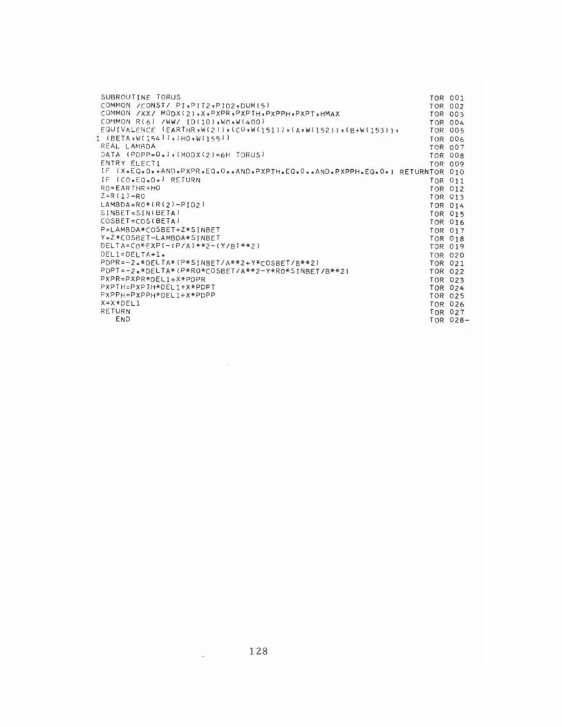
SUBROUTINE TORUS COMMON ICONST/ PI,PrT2,PJD2,DUM(51 (OMMON IXXI MODX(2),X,P XPR ,PXPTH,PXPPH,PXPT,HMAX (OHMQN R(61 /WW/ IDflO),WO,W(4QQI Eau ! VA LENC E (EAR T HR ,W ( 2 I ) , ( C () ,w ( 151 I I , ( A' W ( 152 I ) , ( B' W ( 153 I I ,
1 (BETA,ItJ( ~C:;4J 1,(HQ.W(15S1 ) REA L LA~\RDA DATA (PDPP=O.J,(~ODX(21=6H TORUS) EN TRY ELECTI IF (X.Eo.O •• AND.PXPR.EQ.O •• AND.PXPTH.EQ.O •• AND.PXPPH.EQ.O.) IF (C o . EO ,O.1 RETURN RO =EARTHR+HO Z;R(IJ-RO LAMBDA=R O*tR( 2)-PJD2) SINBET ; SIN(eETAJ (OSBET;(OS(BETAJ P=LAMBDA*CQSBET+Z*SINBET Y=Z*COSBET-LAMBDA*SINBET DEL TA=CO* EXP{ -fP/A1**2-(Y/SJ·*ZI DELl;DELTA+I . PDPR=-2.*OElTA*IP*SINBET/A**z+v*caSBET/S**21 POPT=-2.*OELTA*fP*RO*COSBET/A**2-Y*RO*SINBET/S**21 PXPR =PXPR*OELl+X*PDPR PXPTH=PXPTH*OELl+X*PDPT PXPPH =PXPPH*DEL1+X*PDPP X=X*DELl RETURN
END
128
TOR 001 TOR 002 TOR 003 TOR 004 TOR 005 TOR 006 TOR 007 TOR 008 TOR 009
RETURNTOR 010 TOR 011 TOR 012 TOR 013 TOR 014 TOR 015 TOR 016 TOR 017 TOR 018 TOR 019 TOR 020 TOR 021 TOR 022 TOR 023 TOR 024 TOR 025 TOR 026 TOR 027 TOR 028-
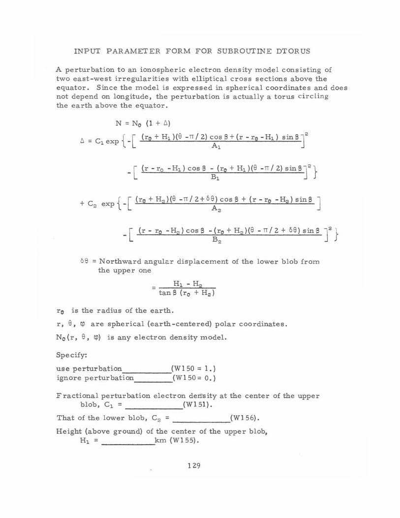
INPUT PARAMETER FORM FOR SUBROUTINE DTORUS
A perturbation to an ionospheric electron density model consisting of two east -west irregularities with elliptical cross sections above the equator. Since the model is expressed in spherical coordinates and does not depend on longitude, the perturbation is actually a torus circling the earth above the equator.
N = No (l + 6 )
6 = C 1 exp { -[ {re + Hl)(8 - n IZ) cos S + (r - rQ -H1 ) SinS]?
Al
+ C? exp {-[ {rQ+H? )(8 - n /z+ 08 )cosS + {r-ro -~)sinS ]
A?
_ [ (r - rQ - H?) cos S -~:" + H? )(8 - n Iz + 08 ) sin S r} 08 = Northward angul<:.r displacement of the lower blob from
the uppe r one
= Hl - Ha tanS (ro + Ha)
rQ is the radius of the earth.
r, 8 , (!) are spherical (earth-centered) pOlar coordinates.
No (r, 8 , (!)) is any electron density model.
Specify:
use perturbation,-:-_____ {,W150 = 1.) ignore perturbation (W150 = 0.)
Fractional perturbation ele ctron dell'sity at the center of the upper blob, C 1 = (W15l).
That of the lower blob, C? = _______ {W15 6) .
Height (above ground) of the center of the upper blob, Hl = km (W155) .
lZ9
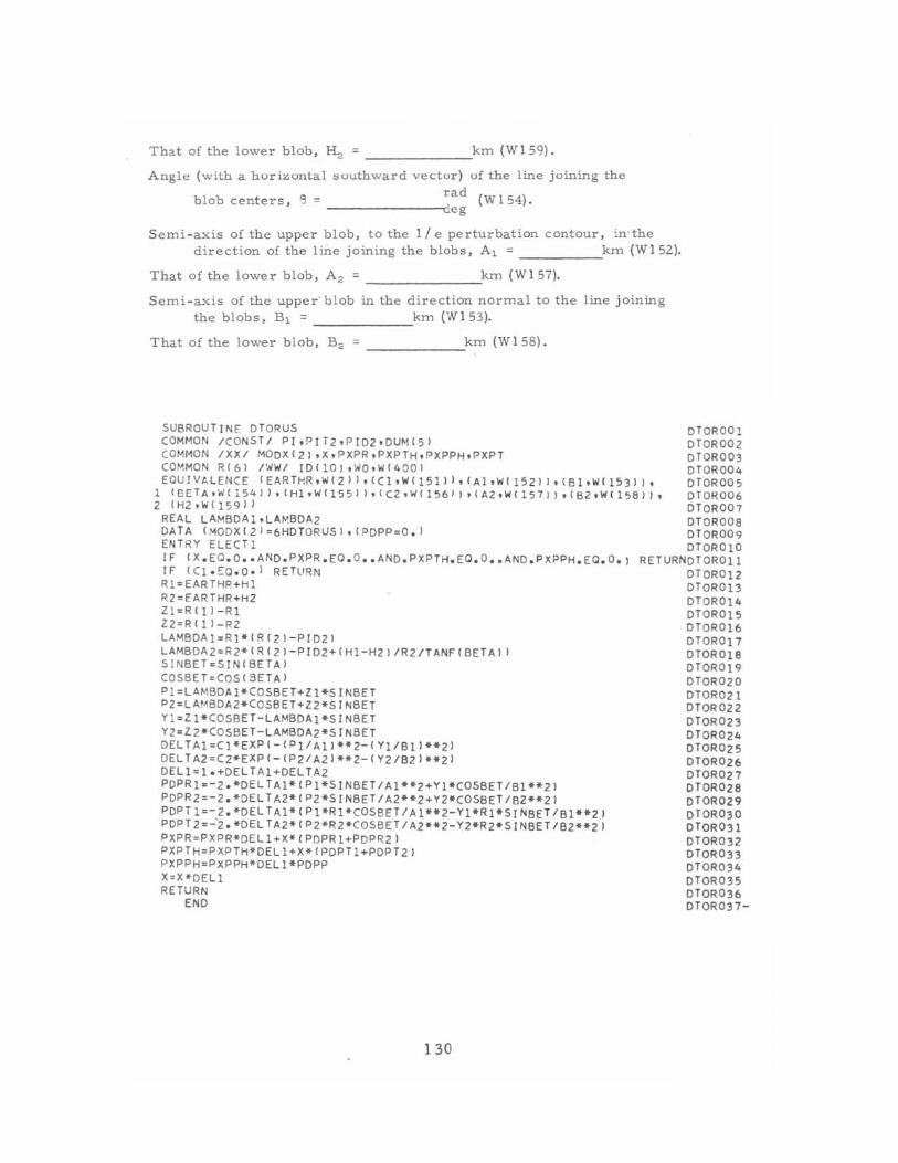
That of the lowe r blob, H . = _______ km (WI 59) .
Angle (with a ho r izontal suuthward vectur) of the line juining the
blob centers , 9 = rad (W 1 54) . --------<!deg
S emi - axis of the upper blob, to the 1/ e perturbation contour , in'the direction of the Ime joining the blobs, Al = km (W 1 52).
That of the lowe r blob, A . = _______ km (WI 57).
Semi-ax is of the upper' blob in the direction normal to the l ine joining the blobs , B, = ______ km (WI 53).
That of the lower blob, B. = km (WI 58) .
SUB ROU TINE DTORUS COMMON ICONS T I PI,PIT2,PI02,DUM(5) CO MMON IXXI MOQX(2),X,PXPR,PXPTH,PXPPH,PXPT COMMON R(6) /WW/ IOI IO),WQ ,W (400 1
DTORDOI DTOROOZ DTORO D3
EQUIVA LENCE IEARTHR,W(21),(Cl.W11511l,(Al,W(15211.(Bl.W(1531), DTOR004 DTOROD5 OTOR00 6 DTOR007
1 IBE TA."" ( 1541 ),CHl.,WI1551 ),(C2, .... C1561) ,(A2,W(157 )) , (B2 .WII S811. 2 (H2 ,W I159 1)
REAL LA MBDA l,LAMBDA2 DATA (MODX(ZJ =6HDTORUSI,IPDPP=O.1 ENTRY ELECT! IF IX.EQ.O •• AND.PXPR.EQ. O •• AND.PXPTH.EO.O •• ANO.PXPPH.EO.O.J [F 1(1 . £0 . 0 .J RETURN R1=EARTHR+H1 R2=EAR THR+H2 Zl =Rlll - Rl Z2 =Rfll - R2 LAMBOAl =Rl *(R(2 1-PI02J LAMB DA2 =R2*(R(2J -PI0 2+(HI-HZ1/RZ/TANF(BETAJ) S INBET:SINfB ETA l COSBET =COS(SE TAl Pl =L AMBDAl*COSBET+Zl*SINBE T P2=LAMBDA2*COSBET+ZZ*SINBET Yl=Zl*COSB ET-LAMBDA1*SINBET Y2 =Z Z*COSBET-LAMBDAZ*SINBET DEL TAl=(1* EXP(-(Pl/AlJ**Z- (Y l / B11**Z) DELTA2=C2*EXP( -( PZ/A2 1**2-(Y2/BZ1**Z) DEL1=1.+DE LT A1+DELTA2 PDPRl~-Z.*DELTAl*(Pl*SINBET /A l**2+Yl*COSBET/Bl**Z) POPR2= - Z. *OELTA2*(P2*SINBET/AZ**Z+YZ*(OSBET/BZ**Z) POPT l =- Z.*OELTAl*(Pl*Rl* COSBE T/Al**Z- Yl*Rl*SINBET/Sl**2) P OPT 2= ~Z .*DELTA2*(P2*R2*COSBET/A2**2 - Y2*R2*SINBET /B2** 21 PXPR=PXPR*OEL l+X*(P DP Rl+ PD PRZ J PXPTH=P XP TH*OELl+X*(PDPTl+PDPTZ) PXPPH =PXPPH*DELl*POPP X=X*OELI RETURN
END
130
DTDR008 DTOR009 DTOROIO
RETURNDTOROIl DTOR012 DTOR013 DTORD14 DTORD15 DTOR016 DTOR017 DTOR018 DTOR019 DTOR020 DT OR021 DTOR02Z DTOR DZ3 DTORDZ4 DTOROZ5 DTORDZ6 DTORD27 DTORDZ8 DTORD29 DTOR030 DTOR031 DTORD3Z DTOR033 DTDR034 DTOR035 DTORD36 DTOR037-
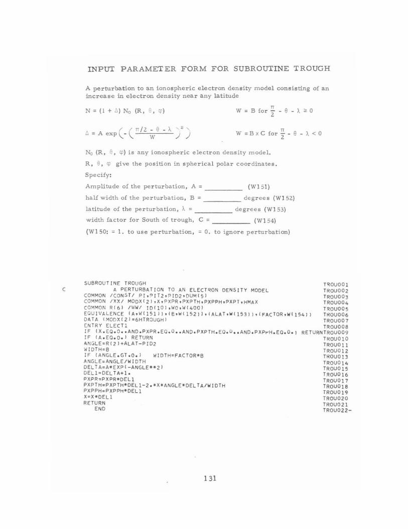
INPUT PARAMETER FORM FOR SUBROUTINE TROUGH
A perturbation to an ionospheric electron density model consisting of an increase in electron density near any latitude
N = ( I + 6 ) No (R. 6 . cp )
(,rr /Z- 6 - A , 2 ,.
6 = A exp - \. W ) )
W = B for ~ - 6 - A ;, 0 Z
rr W = B X C for "2 - 6 - A < 0
No (R, e. cp ) is any ionosphe ric electron density mode l.
R, e, cp give the position in spherical polar coordinates.
Specify:
Amplitude of the perturbation , A ;;; ____ _ (WI 51)
half width of the pertur bation , B ;:: ____ _ deg rees (WI5Z)
degr ees (WI 53)
(WI 54)
latitude of the perturbation, A ;;; ____ _
w idth facto r for South of trough, C ;;; ____ _
(WI 50: ;;; 1. to use perturbation, ;;; O. to ignore perturba t ion)
SUBROU TINE TROUGH T~OUOOI C A PERTURBATI ON TO AN ELECTRON DENSITY MODEL TROU002
COMMON ICONS TI PI,PIT2, P ID2,DUM(SI TROU003 COM MON lX X/ MODX(21,X,PXPR ,PXPTH,PXPPH,PXPT,HMA X TROU004 COM MON R(61 /WWI ID{lOJ,WQ,W{40Q) T~OU00 5
EQU IVALENCE (A,WI151)),IE,WII5211,IALATt'wI1531),IFACTOR,WI1541) THOU006 DA TA (MODX IZ)=6HTROUGHI TRO U007 ENTRY ELECTl TROU008 IF IX . EQ.O •• AND.PXPR.EO.O •• AND . PXPTH . EO. O •• ANO.PXP~H.EQ.O.1 RET URNTROU009 IF IA.EO.a . 1 RETURN TROUOIO ANG LE=RI2J+ALAT - PID2 TROUOll WIOTH=B TROUalZ IF IANGLE .GT.O.J WIDTH=FACTOR*B TROU 0 13 ANG LE=ANGLE/WIDTH TRO U0 14 OELTA=A*EXP I-ANGLE**Z) TROU015 DEL1= DEL TA+l. TROU016 PXPR =PXPR*DELI TROU017 PXPTH=PXP TH *OELI - Z.*X*ANGLE*OELTA/WIDTH TROUOlS PXPP H=PXPPH*OELI TROUOI9 X=X*DEL I TROU020 RETURN TROU021
END TROU022 -
1 31
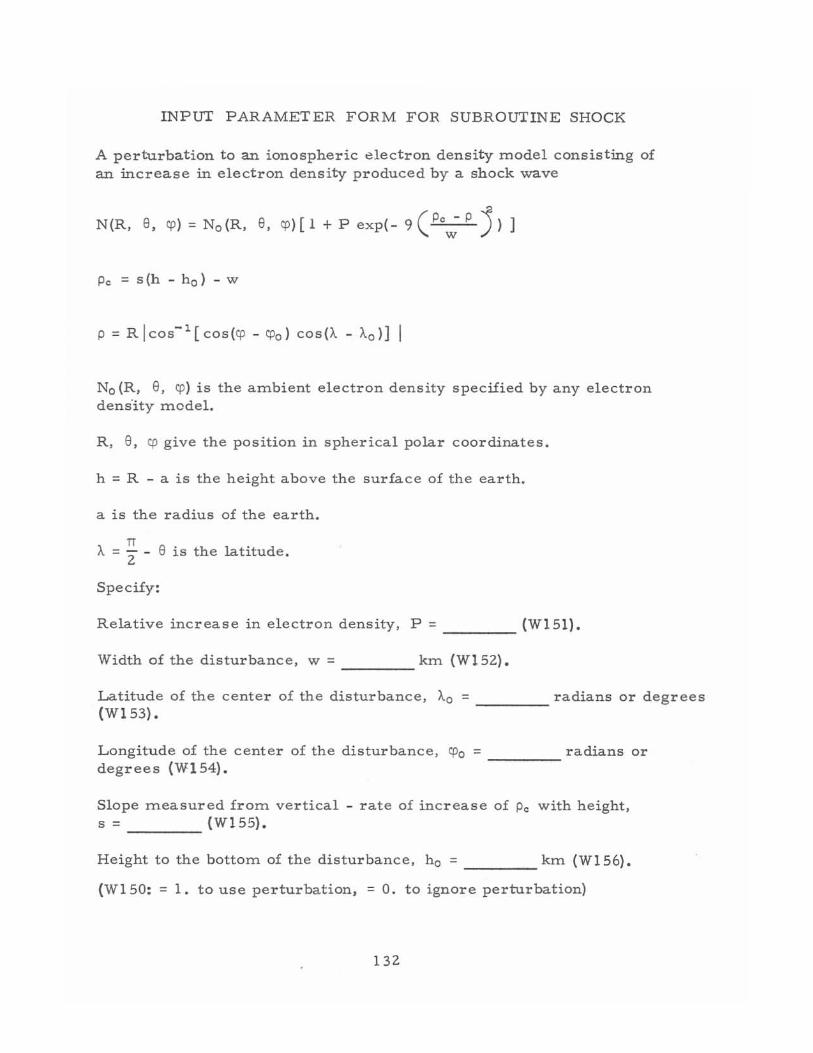
INPUT PARAMETER FORM FOR SUBROUTINE SHOCK
A perturbation to an ionospheric electron density model consisting of an increase in electron density produced by a shock wave
N(R, 8, cp ) = No(R, 8, cp )[l + P exp(- 9(Pc; P:)]
Pc = s (h - h o) - w
P = R[cos- 1 [cos(cp - CPo ) cos (A - 1,.0)] [
No (R, 8, cp ) is the ambient electron density specified by any electron dens·ity model.
R, 8, cp give the position in spherical polar coordinates.
h = R - a is the height above the surface of the earth.
a is the radius of the earth.
TT A = 2" - e is the latitude.
Specify:
Relative increase in electron density, P = _____ (WI 51).
Width of the disturbance, w = km (WI 52) • ----Latitude of the center of the disturbance, 1,.0 = radians or degrees (WI53). ---
Longitude of the center of the disturbance, CPo = radians or degrees (W154). ----
Slope measured from vertical - rate of increase of Pc with height, s = (W155).
Height to the bottom of the disturbance, ho = ____ km (WI 56).
(W150: = 1. to use perturbation, = O. to ignore perturbation)
132
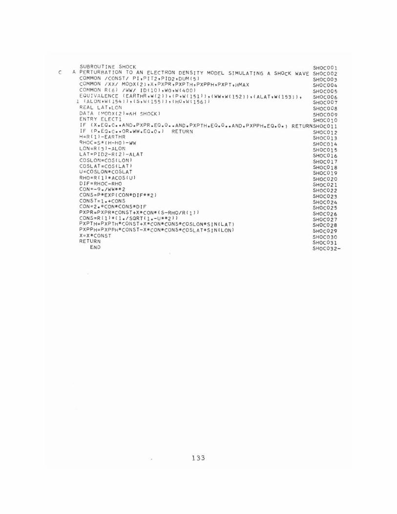
SUBROUTINE SHOCK SHOCOOl C A PERTURBATION TO AN ELECTRON DENSITY MODEL SIMULATING A SHOCK WAVE SHOC002
COMMON ICONST/ PI,PIT2,PI02,QUM(5 1 5HO(003 COMMON IXX/ MODX(2I,X,PXPR,PXPTH,PXPPH,PXPT,liMAX SHOC004 (OHMQN R(61 /'NW/ IO(lOI,WQ,W(40QI SHOC005 EOUIVALENCE {EAR THR ,W (21 J , (P,W( 1511) ,(WW,W( 152» ,(ALAT,W(153 1), SHOC006
1 (ALON,W(1541),(S,\;I(155 1 )dHQ,\-J1l561 J 5HOC007 RE:AL LAT ,LON SHOC008 DATA (~ODX(2) =~H SHOCK) SHOCQ09 ENTRY ELECTl SHOCOlO IF (X.EQ.O •• AND.PXPR.EQ.O •• AND.PXPTH.EQ.O •• ANO.PXPPH.EQ.O.) RETURNSHOCOll IF (P.EQ. Q •• OR.WW.E O.O.1 RETURN SHOC012 H=RIll -EARTHR SHOCOl3 QHQC=5*(H-H01-WW 5HOC014 LON=RI3
'- ALON SHOCOl5
LAT=PID2-RI21-ALAT SHOCOl6 COSLON=COSILONI SHOCOl7 COSLAT=COSILATI SHOC018 U=CaSLON*CQSLAT 5HOC019 RHO=RIll*ACOSIUI SHOC020 DIF=RHOC - RHO SHOC021 CON =-9 ./WIA'** 2 SHOC022 CONS=P*EXP(CON*DIF**21 SHOC023 CONST=l.+CONS SHOC024 CON=Z.*CON*CONS*OIF SHOc025 PXPR=PXPR*CONST+X*CON*IS-RHO/R(l») SHOC026 CONS=R(1)*ll./SQRTll.-U**2) SHOC027 PXPTH=PXPTH*CONST+X*CON*CONS*COSLON*SINILAT) SHOC028 PXPPH=PXPPH*CONST-X*CON*CONS*COSLAT*SrNILON) SHOC029 X=X*CONS T SHOC030 RETURN SHOC031
EN D SHOC032-
133
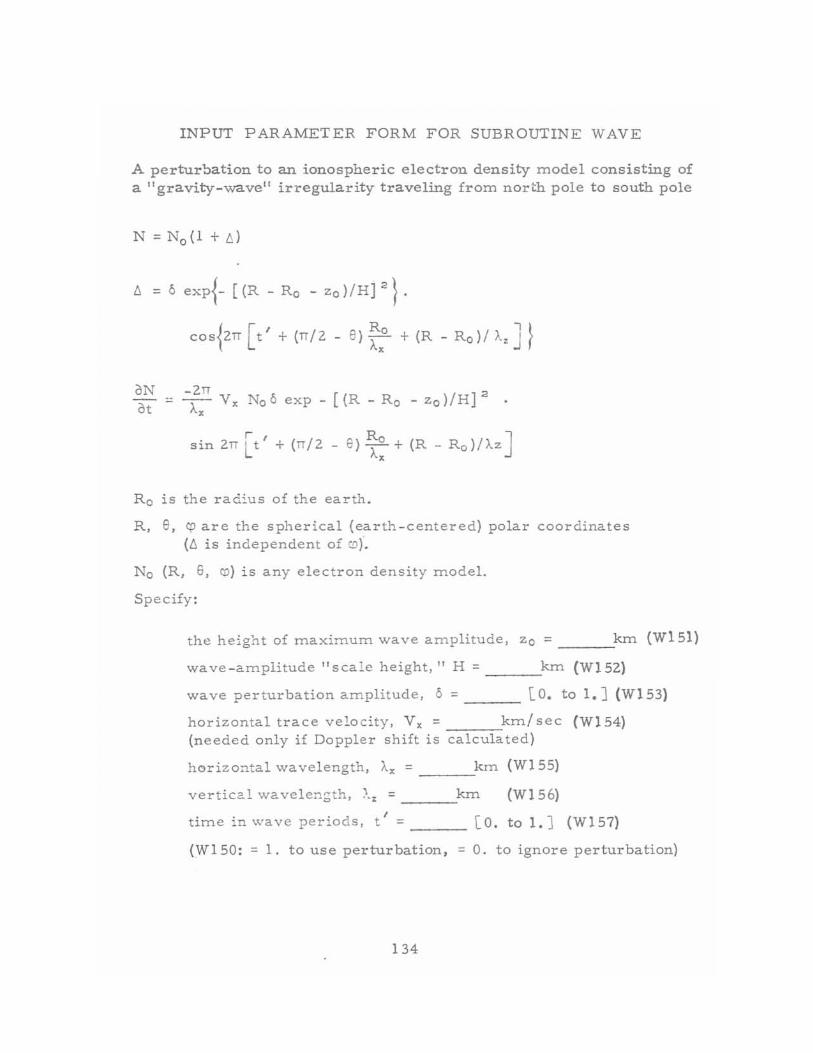
INPUT PARAMETER FORM FOR SUBROUTINE WAVE
A perturbation to an ionospheric electron density model consisting of a "gravity-wave" irregularity traveling from north pole to south pole
I'> = 0 exp{- [(R - Ro - Zo )!HP} •
oN at
COS{ZTT [t' + (TT!Z - 8) ~o + (R - Ro)! Az J}
-ZTT 2 - - 1.- Vx NoO exp - [(R - Ro - zo)!H]
x
sin 2TT [t' + (TT!Z - 9) ~: + (R - Ro)!AzJ
Ro is the radius of the earth.
R, 8, CD are the spherical (earth - centered) polar coordinates (I'> is independent of CD ).
No (R, 6, CD) is any electron density model.
Specify:
the height of maximum wave amplitude, Zo = ___ -.:km (WI51)
wa ve -amplitude "scale height, " H = ____ km (W15Z)
wave perturbation amplitude, 0 = [0. to 1. J (WI 53)
horizontal trace velocity, Vx = km/sec (W154) (needed only if Doppler shift is calculated)
horizoCltal wavelength, Ax = ___ .-:krn (W155)
vertical we. velenf;th 1 ~.z = ____ km (W156)
time in wave periods, t' = ____ [0. to 1. J (W157)
(W150: = 1. to use perturbation, = O. to ignore perturbation)
134
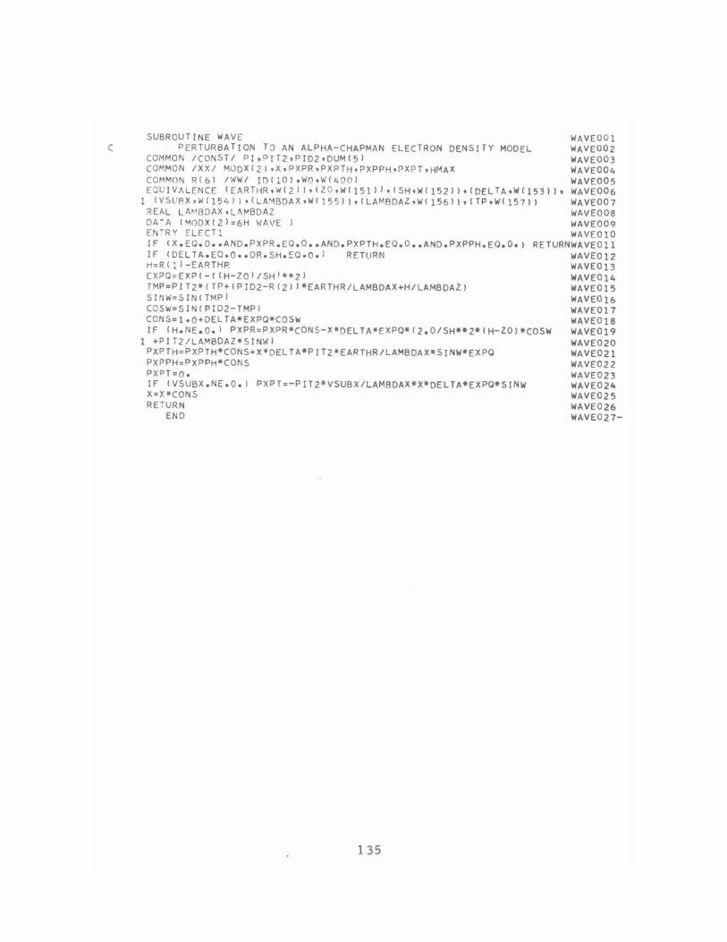
SUBROUTINE WAVE WAVE001 C PERTURBATION TO AN ALPHA-CHAPMAN ELEcTRON DENSITY MODEL WAVE002
COMMON ICONSTI PI,prT2,PI02.DUM(51 WAVE003 COMMON IXXI MOOX(21,X,PXPR,PXPTH,PXPPH,PXPT,HMAX WAVE004 COMMON R(6) IWWI IDIIO),WO,Wf4 00 1 WAVE005 EQUIVI\LENCE (EARTHR,WI211,(l O,WI15111,(SH,WI152)),(DELTA,W(lS31). WAVE006
1 (VSURX,W(154)1,ILA~BOAX,W{15511'(LAMBDAl'W{15611,(TP,W(157)) WAVE007 REAL LAMBDAX,LAMBDAl WAVE008 OA-A IMODXf2J=6H WAVE) WAVE009 ENTRY ELECT, WAVEOIO IF fX.EQ.O •• AND.PXPR.EO.O •• AND.PXPTH.EO.O •• AND.PXPPH.EQ.O.) RETURNWAVE011 IF fDElTA.EO.O •• OR.SH.~Q.O.) RETURN WAVE012 H~RI1J-EARTHR WAVE013 EXPO=EXPI-{(H-lOJ/SH )·*2' WAVE014 TMP=PIT2*ITP+(PID2-R(ZI'*EARTHR/LAMBDAX+H/LAMBDAZI WAVEOlS SINW=SINITMP) WAVE016 COSW=SIN(PID2-TMP) WAVE017 CONS=l.O+DELTA*EXPO*COSW WAVE018 IF (H.NE.O. 1 PXPR=PXPR*CONS-X*DELTA*EXPO*'2.0/SH**Z*IH-ZO)*COSW WAVE019
1 +PITZ/LAMSDAZ*SINW) WAVE020 PXPTH=PXPTH*CONS+X* OElTA*PIT2*EARTHR/LAMBDAX*SINW*EXPQ WAVE021 PXPPH=PXPPH*CONS WAVE022 PXPT=O. WAVE023 IF IVSUBX.NE.O.) PXPT=-PITZ*VSUBX/LAMBDAX*X*DELTA*EXPQ*SINW WAVEOZ4 X=X*CONS WAVE025 RE TURN WAVE026
END WAVE027-
135
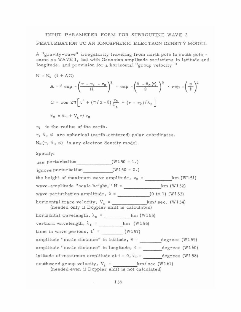
INPUT PARAMETER FORM FOR SUBROUTINE WAVE Z
PERTURBATION TO AN IONOSPHERIC ELECTRON DENSITY MODEL
A "gravity-wave" irregularity traveling from north pole to south pole -same as WAVE 1, but with Gaus s ian amplitude variations in latitude and longitude, and provision for a horizontal "group velocity"
N = No (I + AC)
A = 6 exp - (r - ;; - zQ r . exp - C -@8 9 (t) r . exp -( : r C = cos ZTI[t' + (TI/Z-8) ~ + (r - r@)/),.zJ
x
rg is the radius of the earth.
r, 8, ~ are spherical (earth-centered) polar coordinates.
No (r, 8, (iI) is any electron density model.
Specify:
use perturbation _______ (WISO = 1.)
ignore perturbation (WI SO = 0.)
the height of maximum wave amplitude, z~ = ______ km (WISI)
wave -amplitude" scale height," H = km (WI SZ)
wave perturbation amplitude, 6 = (0 to I) (WIS3)
horizontal trace velocity, Vx = kml sec. (WlS4) (needed only if Doppler shift is calculated)
horizontal wavelength, Ax = km (WISS) -----vertical wavelength, Az = km (WlS6)
time in wave periods, tf = (WlS7)
amplitude" scale distance" in latitude, @ = degree s (WlS9) ---" amplitude "scale distance" in longitude, ~ = degrees (WI60)
latitude of maximum amplitude at t = 0, 8", = degrees (WIS8)
southward group velocity, V, = kml sec (WI61) (needed even if Doppler shift is not calculated)
136
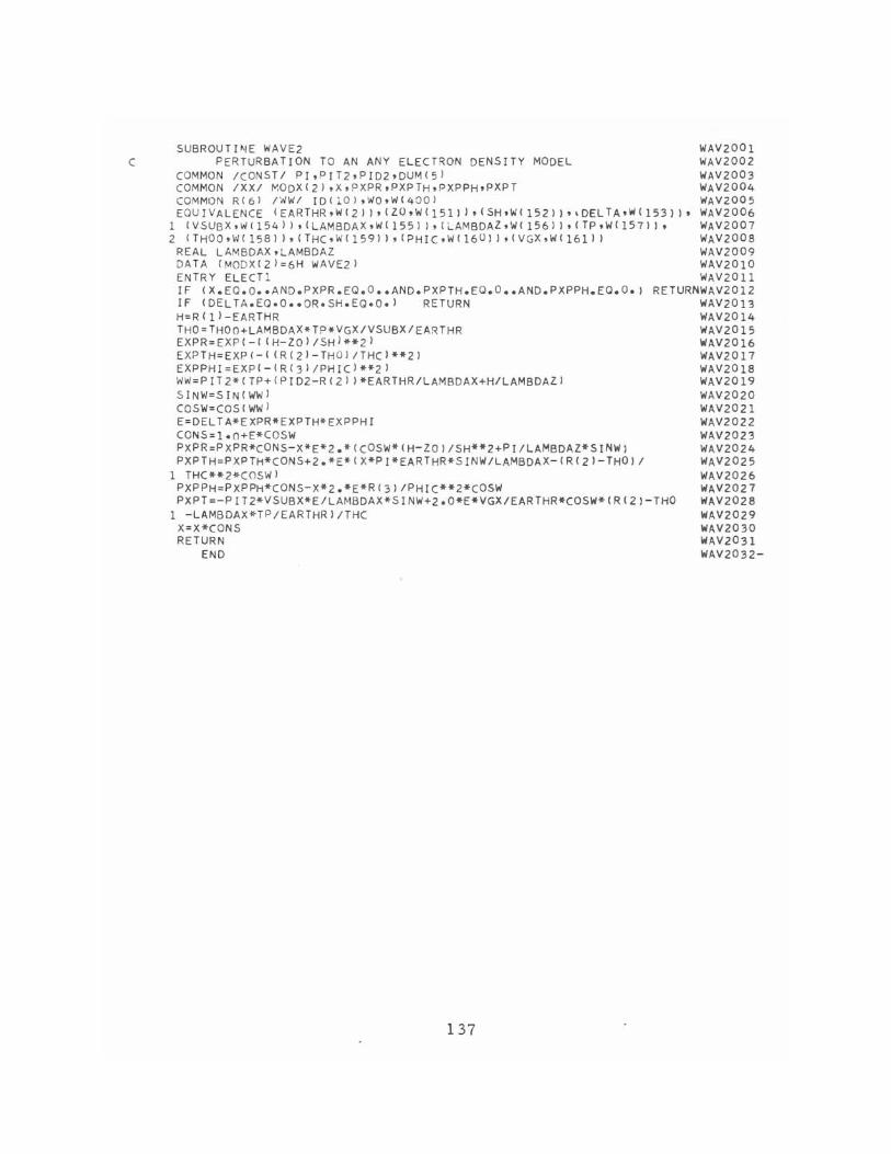
SUBROUTI~E WAVE2 WAV2001 C PERTURBATION TO AN ANY ELECrqON DENSITY MODEL WAV2002
COMMON ICONSTI PI,PIT2,PID2,DUM(SJ WAV2003 COMMON IXXI MODX(2),X,PXPR,PXPTH,PXPPH,PXPT WAV2004 COMMON R(6J l'tlWI IOC1 0J , ...... O'W(400J WAV2005 EQUIVALENCE (EARTHR,W(2J),{ZO,W(151)),(SH,W(152 )1'~DELTA"ff'(1531)' WAV2006
1 (VSUBX,WIl54)),(LAMBDAX,W{l55)),(i....AMBDAZ,'NIl56JI,( TP,W( 157)), WAV2007 2 (THOO,V" 158) ),(THC,W(15911 ,(PHIC,W(l6011 ,(VGX,WI161) I WAV200a
REA L LAMBDAX,LAMBDAZ WAV2009 DATA IMODX(2)=6H WAVE2) WAV2010 ENTRY ELECTl WAV20ll IF (X.EO.O •• AND.PXPR.EO.O •• AND.PXPTH.EO.O •• AND.PXPPH.EO.O.J RETURNWAV2012 IF (DELTA.EO.O •• OR.SH.EO.O.) RETURN WAV20l3 H=RIl)-EARTHR WAV2014 THO =THO O+LAMBDAX*T?*VGX/VSUBX/EARTHR WAV2015 EXPR=EXP(-( (H-Z01/ SH1**2) WAV2016 EXP TH=E XP( - (R(21 -TH 01/ THC)**2) WAV2017 EXPPHI=EXP(-IR{3)/PHIC)**2) WAV2018 WW=PIT2*(TP + IPID2 -R (2J J*EARTHR/LAMBDAX+H/LAMBDAZI WAV2019 SINW =S INIWW) WAV2020 COSW=COSIWW) WAV2021 E=DEL T A*E XPR*EXPTH*EXPPH I WAV2022 CONS=I.0+E*COSW WAV2023 PXPR=PxPR*cONS-X*E*2.*(COSW*IH-ZO)/SH**2+PJ/LAMBDAZ*SINW) WAV2024 PXPTH=PXPTH*CONS+2.*E*(X*PI*EARTHR*SINW/LAMBDAX-{R(21 - THO) I WAV2025
1 THC**2*C OS W) WAV2026 PXPPH=PXPPH*CONS-X*2.*E*RI31/PHIC**2*COSW WAV2027 PXPT=-PIT2*VSUBX*E/LAMBDAX*SINW+Z.O*E*VGX/EARTHR*COSW*(RIZI-THO WA,V2028
1 -LAMBDAX*TP/EARTHR)/THC WAV2029 X=X*C ONS WAVZ030 RETURN WAV2031
END WAV2032-
137
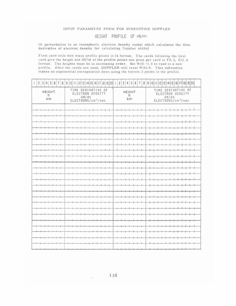
INPUT PARAMETER FORM FOR SUBROUTINE DOPPLER
HEIGHT PROFILE OF dN/dt
(A perturbation to an ionospheric electron density model which calculates the time derivative of electron density for c alculating Doppler shifts)
First card te lls how many profile po i nt s in 14 format. The c ard s following the first c ard g ive the he ight and dN/dt of the profile points one point per card in FS . 2, E l2. 4 format. The heights must be in increasing order. Set WISt ::.1. 0 to read in a new profile. After the c ards are read, DOPPLER will reset W151 .: 0. This subroutine makes an exponential extrapolation down using the bottom 2 points in the profile.
112T3FTsT6171a 91~II I I~ijl~~1 6 1 17 : la I 19 120 112T3141 sl6171a 9110111 11211311411511611711all *01 HEIGHT
TIME DERIVATIVE OF HEIGHT
TIME DERIVATIVE OF ELECTRON DENSITY ELECTRON DENSITY h dN/dt h dN/d t km ELECTRONS/em ' /see km ELECTRONS/em ' /see
, I
,
I
, ,
,. , , ,
,
,
138
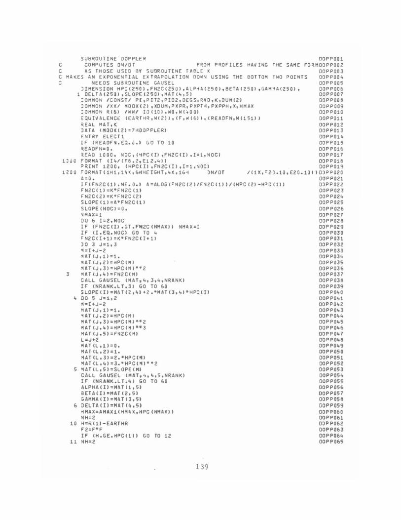
SUB~OUTINE OOPPLER OOPPOOl C COMPUTES ON/OT FR)M PROFILES HAV ING THE SAME C AS THOSE USED 9r SUBROUTINE TABLE X
FHMOOPP002 00PP003 OOPPOO' 00PP005
C MAKES AN EXPONENTIAL ExTRAPOLATION OO~" USING THE BOTTOH TWO POINTS NEEDS SUaROUT[NE GAUSEL
IJuO
JIM£NSION HP::(ZSQ) .FN2C(Z5Q} .Cl.LP·U(250),BETA(25(JI ,GAH'fA(Z50). 1 DElTA(ZSfU ,SlOPE(Z50) ,MArett,S)
:OHHON ICONSTI P(,PIT2,PI02,OEGS,R"'O,K.OU~(2) ::OHMON IXXI 1100)(2) ,XOUH,PXPR..PXPT-t,PXPPH,X,HHAX :OMMON R(E,) nn", Itl(10),WO,WC:o.oo) EQUIVALENCE (EA~THRtW(21),(F,jIf(&)lt{REAOFNtW(1511)
REAL HATtK 'JATA (HOOl(21=7HOOPPLER) ENTRY ELECTl IF (REAOF".EQ.'.I GO TO 10 REAOFN=O. ,~EAO 1000, NJC,(liPC(I) ,FN2C(l) .1=l,NOC) FORHAT HIt/CFe.Z.ElZ.Ct') PRINT 1200, (HPC(IJ ,FNZC(!) ,I=l.NOCl
OOPPOOb 00PP007 OOPPOO 6 00PP009 00PP010 OOPP011 00PP012 00PP013 00PP01lo 00PP015 OOPPOlb 00PP017 00PP016 00PP019
1200 ~ORHAT(lHl,1~(,&KH£IGHTt4(,161 JN/OT II 1 X. 02 .J .10. E2 O. 1J1 I 0) P P 020
3
A=Q. IF(FN2CLlI.NE.0.1 A=ALO:;(ON2C(2I1F'2C(1I)/(HPC(21-H'C(1I1 FN2C(1)=K'FN2C(1) FN2C(21=K'FN2C(21 SLOPE(1)=A>FN2CLL) SLOPE(NOC)=O. .... ,.,AX=1 00 6 I=2.NOC IF (FN2C(lI.GT.FM2C(NMAX)) IF (I.E(;I.NOC) GO TO • FN2C(I+11=K-FN2CCI+l) )0 3 Jzl,3 '1=I+J-Z ,'1AT(J,l)::l. MAT(J.2)=rlPC(H) MAT(J,3)::HPC(M)··2 HAT(J.Iol=FN2C(M)
NM4X=I
CALL GAUSEL OUT .tt .. 3 .. ,+,NRANK) IF (NRANK.LT.31 GO TO 60 SlOPE(I)::HAT(2.tt'+2. 4HAT(3,'+)·HPC(I)
'+ 00 5 J::l,Z .1=I+J-2 HAT<J.lI =1. '1AT(J,Z)::HPC(H) HAT(J.3J=HPC(H,4·Z MAT(J.4)=HPC(H'··3 MAT (J.51=FN2CLHI L=J+2 HAT (L .1>=0. HAT(l.ZJ=l. HAT(L.31=2.·HPC(N' MAT(L.4'=3.·HPC(K,·4Z
5 ~AT(L.5)=SLOPE(H' CALL GAUSEL (HAT.,+,4,5 .. NRANK) IF (NRANK.LT.41 GO TO 60 ALPHA(I)=KAT(1.51 6ETA(I)=HAT<2.5) GAMKA(I)=NAT(3.51
6 DELTA(I)=KAT(4.51 HHAX=AHlX1(HHlX,HPC(NHAX)1 NH =2
10 H=R(1)-EARTHR FZ=F·F IF (H.GE.HPC<111
11 NH=2 GO TO 12
139
00PP021 0)PP022 00PP023 00PP02. 00PP025 OOP P 026 00PP027 00PP026 00PP029 00PP030 OOPP031 00PP032 00PP033 00PP03. 00PP035 00PP036 00PP037 00PP036 00PP039 OOPPO.O OOPPO.l 00PP042 00PP043 00PP044 00PP045 00PP046 00PP047 00PP046 00PP049 00PP050 00PP051 OOPP052 00PP053 00PP054 00PP055 00PP056 OOP P05 7 00PP056 00PP059 OOPPObO 00PP061 00PP062 00PP063 00PP06. 00PP065
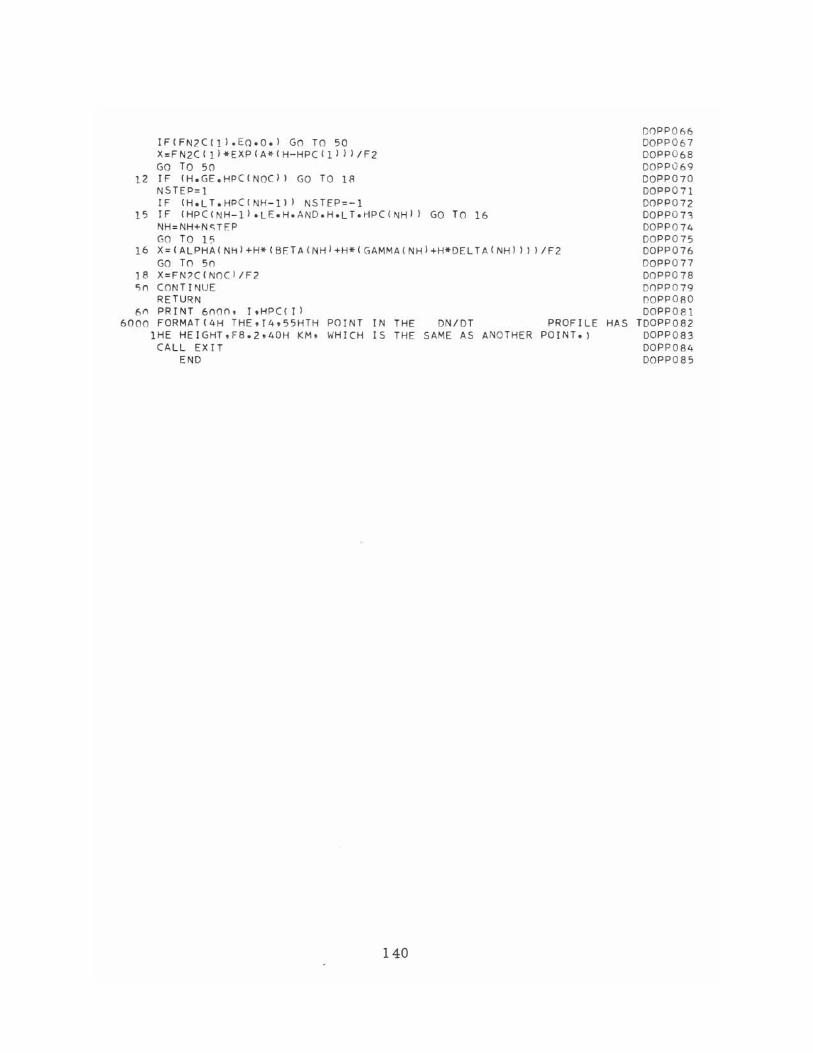
IF(FN2C(II.EO.0.I GO TO 50 X=FN2C(11*EXPIA*(H-HPC(1)) I/F2 GO TO 50
12 IF (H.GE.HPC(NOCI I GO TO 18 NSTEP=1 IF (H.lT.HPCINH-ll) NSTEP=-l
15 IF (HP((NH-!I.LE.H.AND.H.LT.HPCINHI) GO TO 16 NH =NH+N C;TEP GO TO l~
16 X =(ALPH AINHI+H*(BF.TA{NHJ+H*(GAMMAINH)+H*OELTA(NHJ II )/F2 GO TO 50
J8 X =F N~C(NOCI/F2
<;n CONTINUE RETURN
f,f"I PRINT 6()l1n, I .HPC( r I 6000 FORMAT(4H THE,T4,55HTH POINT IN THE DN/DT PROFILE HAS
lHE HEIGHT,F8.2,40H KM, WHICH IS THE SAME AS ANOTHER POINT.) CALL EXIT
END
140
DOPP066 DOPP067 DOPP068 DOPP069 DOPP070 DOPPO 71 DOPP072 DOPPO 73 DOPPO 74 DOPP075 DOPP076 DOPP077 DOPPO 78 DOPP079 OOPPORO DOPPORI
TDOPP082 DOPP083 DOPP084 DOPP085
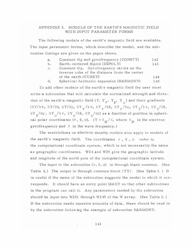
APPENDIX 5. MODELS OF THE EARTH'S MAGNETIC FIELD WITH INPUT PARAMETER FORMS
The following models of the earth's magnetic field are available .
The input parameter forms, which describe the model, and the sub
routine listings are given on the pages shown.
a. b. c .
d .
Constant dip and gyrofrequency (CONSTY) Earth- centered dipole (DIPOL Y) Constant dip . Gyrofrequency varies as the inverse cube of the distance from the center of the ea rth (CUBEY) Spherical harmonic expansion (HARMONY)
142 143
144 145
To add o ther models of the earth's magnetic field the user must
write a subroutine that will calculate the normalized strength and direc
tion of the earth's magnetic field (Y, Y , Y , Y ) and their gradients r 9 cp
(oY/o r, oY/09, oY/oco, oY 10 r, oY 109. oY 10qJ. oY Slo r, oY S/0 9, . r r r
oY 9/0cp, oY qJ/o r, oY col09 , oY cp/0qJ ) as a function of position in spheri-
cal polar coordinates (r, 9, cp l. (Y = fHI f, where fH is the electron
gyrofrequencyand f is the wave frequency. )
The restrictions on electron density models also apply to lTIodels of
the earth's magnetic field. The coordinates r, e , cp refp.r to
the computational coordinate system, which is not necessarily the same
as geographic coordinates. W24 and W25 give the geographic latitude
and longitude of the north pole of the computational coordinate sys tem.
The input to the subroutine (r, 9 , 'II ) is through blank com.m.on. (See
Table 3.) The output is through common block IYY/. (See Table 9.) It
is useful if the name of the subroutine suggests the model to which it cor
responds. It should have an entry point MAGY so that other subroutines
in the program can call it. Any parameters needed by the subroutine
should be input into W201 through W249 of the Warray. (See Table 2. )
1£ the subroutine needs massive amounts of data, these should be read in
by the subroutine follow ing the example of subroutine HARMONY.
141
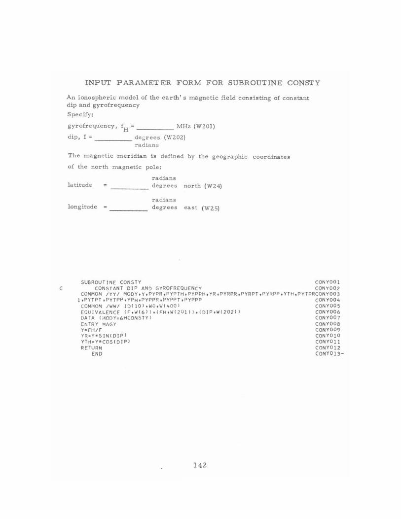
INPUT PARAMETER FORM FOR SUBROUTINE CONSTY
An ionospheric ITlodel of the earth's magnetic fie ld consisting of constant dip and gyrofrequency
Specify:
gyrofr equency , fH ~ MHz (W201)
dip, I ~ _____ deg rees (W202)
radians
The magnetic meridian is defined by the geographic coordinates
of the north rnagnetic pole :
radians latitude degrees north (W 24)
radians longitude ~ degrees east (W25)
SUBROU TINE CONSTY CONYOOI C CONSTANT DIP AND GYROFREOUENCY CONY002
COMMON IYY/ MODy,y,PVPR,PYPTH,PYDPH,YR,PYRPR,PYRPT,PYRPP,YTH,PYTPRCONV003 1,PYTPT,PYTPP,YPH,PYPPR,PYPPT,PYPPP CONV004
COMMON /WW/ IDI I O),WO ,W(40 01 CONV005 EOUIVALENCE (F,W I6) ) ,(FH,W (ZOll} ,(DIP,W {Z02 )) CONY006 DATA (i.,ODY=6HCONSTYl CONYOD7 ENTRY MAGY CONYOOB Y~FH/F CONY009 YR=Y*SIN {DIPI CONYOIO YTH:Y*COSCDIPI CONYOll RETURN CONY0 12
END CONY013 -
142
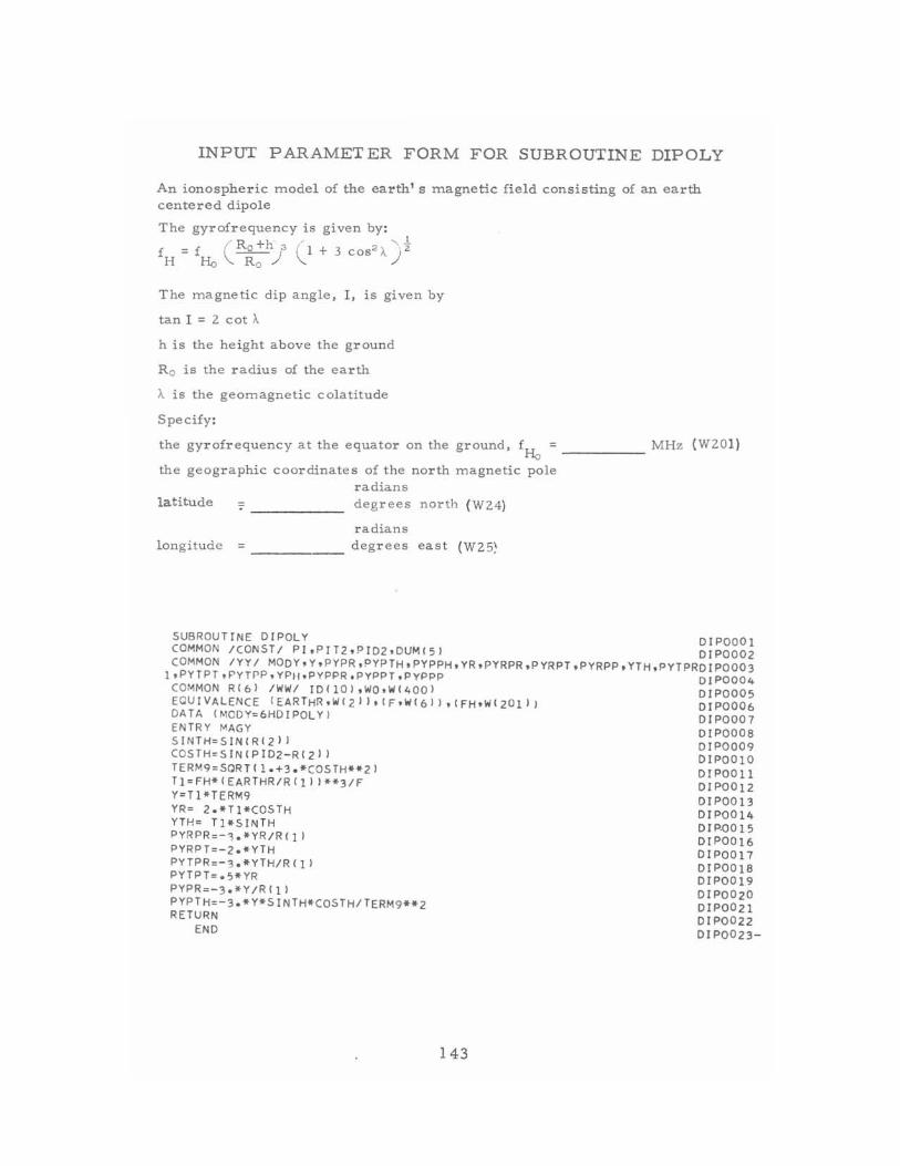
INPUT PARAMETER FORM FOR SUBROUTINE DIPOLY
An ionospheric model of the earth 1 s magnetic field consisting of an earth centered dipole
The gyrofrequency is given by:
(R +h' (F "" .1
f = f _0_)3 ( I + 3 COS 2 A)" HHoRo '-
The magnetic dip angle 1 I, is given by
tan I ;:: 2 cot A
h is the height above the ground
Ro is the radius of the earth
A is the geomagnetic colatitude
Specify:
the gyrofrequency at the e quator on the ground, fHo ::; ______ MHz (W201)
the geographic coordinates of the north magnetic pole radians
latitude degrees north (W24)
radians longitude ;:: _____ _ degrees east (W25:\
SUBROUTINE OIPOLY DIPOOOI COMMON ICONST/ PJ,PJT2,PID2,OUM(SI DIP0002 COMMON IYY! MOOY,Y,PYPR,PYPTH,PYPPH,YR,PYRPR,PYRP T,PYRPP,YTH,PYTPRDIP0003
1,PYTPT,PYTPP,YPH.PYPPR,PYPPT ,PYPPP COMMON Rlbl IWWI IDIIOI,WQ,WI4QQI EQUIVALENCE (E ARTHR,W1Z) I, (F,W (6 11,I FH,W1ZOllj OATA (MOOV=6HOIPOLVJ ENTRY MAGY SIN TH=SIN(R(211 COSTH=SIN (PID2-R(2 11 TERM9 =SQRTI1 . +3.*COSTH**2) Tl=FH*IEARTHR/R{111**3/F Y=Tl*TERM9 VR= 2.*Tl*COSTH YTH= Tl*SINTH PYRPR=-~.*YR/R(ll PYRPT=-2.*YTH PYTPR=-3.*YTH/RIl) PYTPT=.S*VR PYPR=-3.*Y/RIll PVPTH=-3.*V*SINTH*CQSTH/TERM9**2 RETURN
END
143
DIP0004 DIP0005 DIP0006 DIP0007 DIPOOOS DIP0009 DIPOOIO DIPOOII DIPOOl2 DIPOOl3 DIPOOl4 DIP.oOl5 DIPOOl6 DIP0017 DIPOOIS DIPOOl9 DIP0020 DIP0021 DIP0022 DIPOO23-
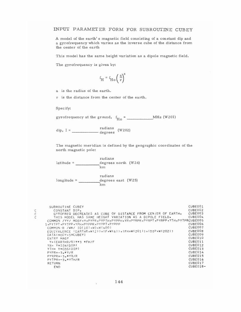
INPUT PARAMETER FORM FOR SUBROUTINE CUBEY
A model of the earth' 5 magnetic field consisting of a constant dip and a gyrofrequency which varies as the inverse cube of the distance from the center of the earth
This model has the same height variation as a dipole magnetic field.
The gyrofrequency is given by:
a is the radius of the earth.
r is the distance from the center of the earth.
Specify:
gyrofrequency at the ground, ~o = _____ -----'MHz (W201)
radians dip, I = (W202)
------- degrees
The magnetic meridian is defined by the geographic coordinates of the north magnetic pole:
radians latitude = ______ degrees north (W24)
km
radians longitude = _____ :degrees east (W25)
km
SUBROUTINE CUBEY CUBEOOI C CONSTANT DIP. CUBE002 C GYROFREO DECREASES AS CUBE OF DISTANCE FROM CENiER OF EARTH. CUBE003 C THIS MODEL HAS SAME HEIGHT VARIATION AS A DIPOLE FIELD. CUBE004
(OMMON IYY/ MODy,y,PYPR,PYPTH,PYPPH,YR,PYRPR,PYRPT,PYRPP,YTH,PYTPRCUBE005 1,PYTPT,PYTPP,VPH,PVPPR,PVPPT,PVPPP CUBE006
COMMON 'R IWWI ID(lOI,WO,W(4001 CUBE007 EQUIVALENCE (EARTHR,W(211,(F,W(611,(FH,W(2011),(DIP,W(202J 1 CUBEOoa DATA(MODY =5HCUBEYI CUBE009 ENTRY MAGY CUBEOIO
V=(EARTHR/RJ**3 *FH/F CUBED11 YR= Y*SINfDIP) CUBE012 VTH = V*COS(DIPI CUBE013 PYPR=-3.*Y/R CUBE014 PYRPR=-3.*YR/R CUBE015 PYTPR=-3.*VTH/R CUBE016 RETURN CUBE017
END CUBED18-
144
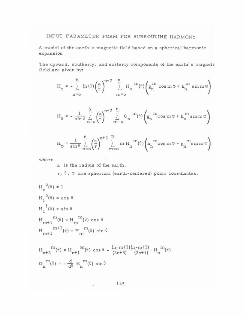
INPUT PAR AMETER FORM FOR SUBROUTINE HARMONY
A model of the earth's magnetic field based on a spherical harmonic expansion
The upward, soutberly, and easterly components of tbe earth's magneti field are given by:
6 n +2
Hr = - I (n+1)(~) n=o
where a is the radius of tbe eartb.
m cos m cp + h
n sinm cp)
m. ) - gn Slnrn ~
r, 8 , ~ are spherical (eartb-centered) polar coordinates.
H o(8} = 1 a
Hl
o(8} = cos 8
HII (8) = sin 8
H rn(8} = H rn(8} cos 8 rn+ 1 rn
Hm+1 rn+l(8} = Hm rn(8} sin 8
m 8 m(8 ) 8 (n+rn+l)(n-rn+l) H rn(8} Hn+2 () = H n + 1 cos - (2n+3) (2n+ 1) n
Gn
rn(8} = - : 8 Hn rn(8} sin8
145
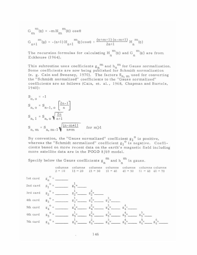
m G (e)
m
m = -mH (e) cose
m
m G
n+1 (e)
m + (n+m+l) (n-m+l) H m(e) = -(n+l) Hn+l (e)cose 2n+l n
T he recursion formulas Eckhouse (1964).
m m for calculating H (e) and G (e) are from
n n
This subroutine uses coefficients gn m and h n m for Gauss normalization. Some coefficients are now being published for Schmidt normalization (e. g. Cain and Sweeney, 1970). The factors Sn, m used for converting the "Schmidt normalized" coefficie nts to the "Gauss normalized" coefficients are as follows (Cain, et. al., 1968, Chapman and Bartels, 1940) :
S· = -1 0,0
S = S [2:-1J n, 0 n-l,o
S = s{!K n, 1 n,o n+l
S = S _!(n-m+l) n, rn. n, rn.-I " n+rn.
for m)1
By convention, the "Gauss normalized" coefficient gl° is positive, whe reas the "Schmidt normalized" coefficient gl° is negative. Coefficients based on more recent data on the earth's magnetic field including nlOre satellite data are in the POGO 8/69 model.
Specify below the Gaus s coefficients m
and h m.
gn ln gaus s . n
columns columns columns columns columns columns columns 2- 10 11 - 20 21 - 30 31 - 40 41 - SO 51 - 60 61 - 70
1st card 0
go =
0 1 2nd card gl gl=--
0 1 2 3rd card g2 = g = g =
2-- 2--0 1 2 3
4th card g3 = g3=-- g3=-- g3=--
0 1 2 3 4 5th card g4 = g = g4=-- g = g4=--4-- 4 --
6th card 0 1 2 3 4 S
gs = g = gS=-- gS=-- gS=-- gS=--S--0 1 2 3 4 S 6
7th card g6 = g = g = g = . g = g6=-- g6=--6 -- 6 -- 6 -- 6 --
146
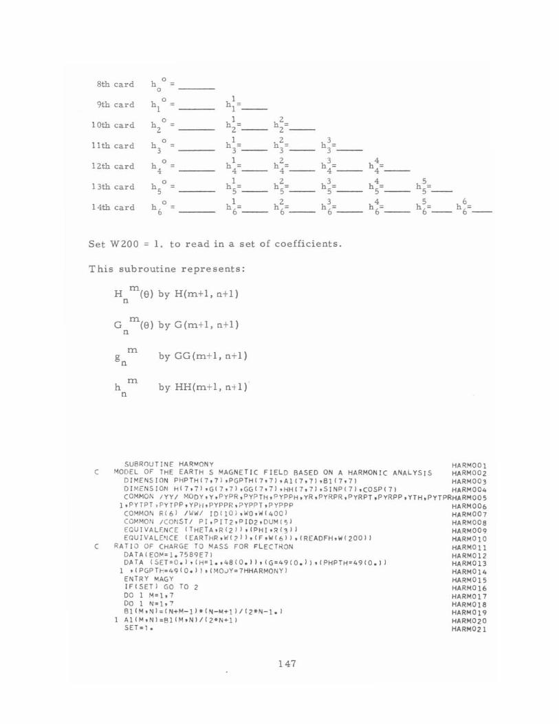
8th card h 0
= 0
9th card h[ 0
h1
= = 1
10th card h2 0
h1
= h2
= = 2 - - 2 --
11 th card h3 0
h1
= h2
= h3
= = 3 -- 3 3 --
12th card h 0 = 4
h1
= 4 --
h2
= 4
h3
= 4 --
h 4= 4
0 1 h
2= h
3= h 4= h
5= 13th card h5 = h =
5 -- 5 -- 5 5 -- 5 --
h6 0
h1
= h2
= h3
= h 4= h5
= h 6= 14th card = 6 - - 6 - - 6 -- 6 -- 6 -- 6
Set W200 = 1. to read in a set of coefficients .
This subroutine represents:
rn H (e) by H(rn+l, n+l)
n
rn G (e)byG(rn+l,n+l)
tl
by GG(rn+l, n+l)
h n
rn by HH(rn+l, n+l)
SUBROUTINE HARMON y HARMODl C MODEL OF THE EARTH S MAGNETIC FIELD BASED ON A HARMONIC ANALYSIS HARM002
DIMENSION PHPTH(7,7J ,PGPTH(7,7) ,A1(7,7) ,81(7,7) HARMOD) DIMENSJON H17,7) ,G17,71 ,GG(7.71 .HH(7,7),SINP(7),caSP(7) HARM004 COMMO~ IYY/ MODy,y,PYPR,PYPTH,PYPPH,yR,PYRPR,PYRPT,PYRPP,YTH,PYTPRHARM005
1,PYTPT ,PYTPP ,YPH,PYPPR,PYPPT,PYPPP HARM006 Cm·1MON R(6) /~"WI IDCIO),WQ,WI400 1 HARMOD7 COMMON ICONSTI PI,PIT2,PID2.DUM(SI HARMOOe EOUIVA LENCE (THETA,RI21) ,(PHI,RI3' ) HARM009 EQUIVALENCE IEARTHR,WI2J ),IF,W(6)) ,IREADFH.WI200IJ HARMOIO
C RAT IQ OF CHARGE 10 MASS FOR FLECT~ON HARMOll DATAIEOM = 1.7589E7) HARM012 DATA (5E1=0.) ,iH=1.,48(O.», (G =49(O.» ,(PHPTH=49(O.» HARM013
1 ,(P GPTh=49(O.» tCMOJY=7HHARMONY) HARM014 ENTRY MAGY HARM015 IFISET) GO TO 2 HARM016 DO 1 M=1,7 HARM017 DO 1 N=1,7 HARM018 BICM,NI=(N+M- ll·(N - M+11/C2*N-1.1 HARM019 AICM,Nl=81CM,N1/C2*N+11 HARM020 SET=,. HARM021
147
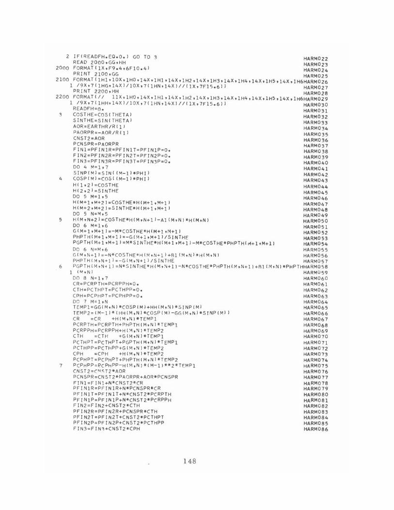
2 IF(READFH.EQ.O.) GO TO 3 HARM022 READ 20QQ,GG.HH KARM023
2000 FORMAT(lX,F9.4,6FIO.4) HARM024 PRINT 210Q,GG HARM025
2100 FORMAT(lHl,lOX,lHQ,14X,lHl,14X,lH2,14X,lH3,14X.lH4.14X,lH5.14X,lH6HARM026 1/9X,7(lHG,14XI/IOX,7 11HN'14XI//(lX,7F15.6)) HARM027
PRINT 220Q,HH HARM028 2200 FeRMAT(// llX,lHQ,14X,lHl,14X,lH2.14X,lH3,14X,lH4,14X.IHS.14X.IH6HARM029
1 19X,7(IHH,14X)/lOX,7(lHN,14XII/(lX,7F15.6)) HARM030 READFH=O. HARM031
3 COSTHE=COS(THETA) HARM032 SINTHE=SIN(THETA) HARM033 AOR=EARTHR/R(lJ HARM034 PAORPR= - AOR/R(I) HARM035 CNST2=AOR HARM036 PCNSPR=PAORPR HARM037 FINI=PFINIR=PFINIT=PFINIP=O. HARMD38 FIN2=PFIN2R=PFIN2T=PFIN2P=O. HARM039 FIN3=PFIN3R=PFIN3T=PFIN3P=O. HARM040 DO 4 M=1,7 HARM041 SINP{MI=SIN{(M-!I*PHII HARM042
4 COSP(M)=CQS((M-!I*PHIJ HARM043 HIl.2i=COSTHE HARM044 H(2,2)=SINTHE HARM045 DO 5 M=1,5 HARM046 H(M+l'~+2J=COSTHE*H(M+l,M+ll HARM047 H(M+2,M+21=SINTHE*H(M+l,M+ll HARM048 DO 5 N=~,5 HARM049
5 H(M,N+2 1=COSTHE*H(M,N+II-Al(M,NI*H(M,NI HARM050 DO 6 M=1,6 HARM05l G(,101+1 ,M+l J =-M*COSTHE*H(M+l ,r~+l I HARM052 PHPT H (M+ 1,,"'1+ 1 I =-G U-1+ 1 ,M+ 1) IS r NTHE HARMO 53 PGPTH (M+ 1 ,M+ 1) =M*S I NTHE*H (M+ 1 ,M+ 1) -M*COSTHE*PHPTH (tof+ 1 ,M+l) HARM054 DO 6 N=M,6 HARM055 G(M,N+ll=-N*C05THE*H(M,N+ll+81(M,N'*H(M,NJ HARM056 PHPTHIM,N+IJ:-G(M,N+11/5INTHE HARM057
6 PGPTH(M,N~lJ=N*5INTHE*H(~,N+l)-N*COSTHE*PHPTH(M,N+l)+Rl(M,Nl*PHPTHHARM058 1 (M,NI HARM()59
DO 8 N=1,7 HARM060 CR=PCRPTH =PCRPPH= O. HARM061 CTH=PCTHPT=PCTHPP=O. HARM062 CPH=PCPtiPT=PCPHPP=O. HARM063 DO 7 M=l,N HARM064 TEMPl=GG(M,Nl*COSP(M'+HH(M,NI*5INP(MI HARM065 TEMP2= (M-l) * (HH (M ,N I *casp (MI -GG (M ,N) *5 TNP (HI) HARM066 CR =CR +H(~,Nl*TEMPl HARM067 PCRPTH=PCRPTH+PHPTH(M,Nl*TEMPl HARM068 PCRPPH=PCRPPH+H(~,~I*TEHP2 HARM069 CTH =CTH +G(M,NJ*TEMPI HARM070 PCTHPT=PCTHPT+PGPTH(M,Nl*TEMPl HARM07l PCTHPP=PCTHPP+G(M,NI*TEMP2 HARM072 CPH =CPH +H(M,NI*TEMP2 HARM073 PCPHPT=PCPHPT+PHPTHIM,N'*TEMP2 HARM074
7 PCPHPP=P,CPHPP-H(M,N)*(M-IJ**2*T~MPl HARM075 CNST2=(~IST2*AOR HARM076 PCNSPR=CNST2*PAORPR+AOR*PCNSPR HARM077 FINl=FTNl+N*CNST2*CR HARM078 PFINIR=PFINIR+N*PCNSPR*CR HARM079 PFINlT=PFINIT+N*CNST2*PCRPTH HARM080 PF r N IP=PF I·N lP+N*CNS T 2*PCRPPH HARM081 FIN2=FIN2+CNST2*CTH HARM082 PFIN2R=PFIN2R+PCNSPR*CTH HARM083 PFIN2T=PFIN2T+CNST2*PCTHPT HARM084 PFIN2P=PFIN2P+CNST2*PCTHPP HARM085 FIN3=FIN3+CNST2*CPH HARM086
148
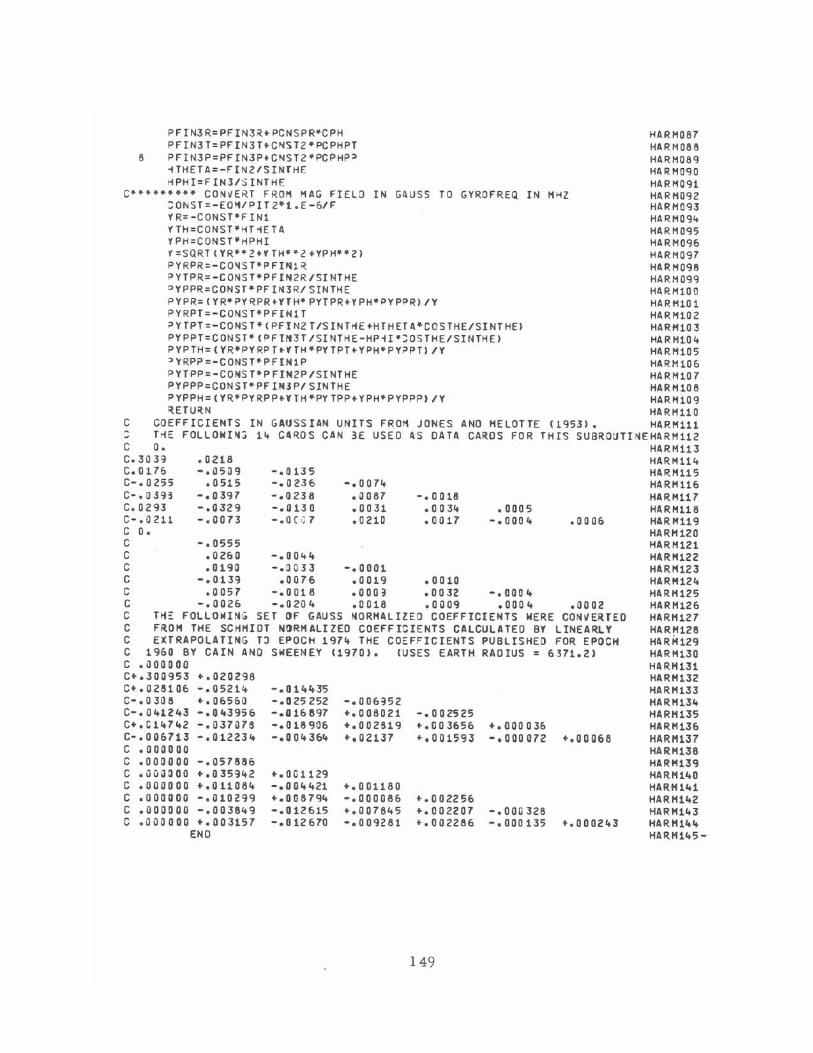
P FI N3 R=PF IN3 iH PCNSPR"'CPH HARM087 P FINH= PF INH +CNST2 "PCPHPT HAR M066
a PFIN3P=PFIN3P"CNSTZ·PCPHP::> HARt10a9 ~THETA=-FIN2/SINTHE HARHOgO HPHI=FIN3/SINTHF. HARMOg1
C~·~·····'" CONvERT FROM MAG FIELQ IN G4USS TO GYROFREQ IN H~Z HARH09Z :ONST=-EOH/PIT2"t . E-6/F HARHOg3 YR=-CONST"FINt HARMOg~
YTH=CONST'HT~ETA HARMOg5 YPH=CONsr·H?HI HARM096 Y=SQRT(YR··2"YTH··2+YPH··Z) HARM097 PYRPR=-COHST+PFIN1~ HARHOg6 P YTPR=-CONS T'PF IN2R/51 NT HE HARM Ogg cYPPR=CONST' PF I "3RI SIN THE HA RM10 0 PYPR= (YR"'PY ~PR"YTH· PYTPR+YPH·PYPPRJ IV HARt110i PYRPT=-CONST+PFINl T HARHt02 >YlPT =-CONS T' (PFI N2 TIS INT"E +H T H ET A 'COS THE/SI NT HE) HARIHO J PY PPT=C ONST' (PF I.3T lSI NTH E -HPH ":05 THE/SINTHE) HAR HtO ~ PYPTH= ('t'R,.PY RP T .... TH "'PY TPT "YPH. PY??T) IY HARHi05 ~YRPP=-CONST·PF[N1P HARMi0G P YT PP=-CONS Tt-? FIN2P lSI NT HE HAR M 10 7 PYPPP=CON ST" PF IN] PI SIN THE HARM to 6 PYPPH=' 't'R·Py RPP+'f TH "'PY TPP+ YPH· PYPPP) IY HARH109 RETURN HARHttO
C COEFFICIENTS IN GAUSSIAN UNITS FROM JONES AND HELOTTE (195]). HARM11t : THE FOLLOWI., 1. CARDS CAN 3E USED AS DATA CARDS FOR THIS SUBRDUTINEHARMl12 C O. HARHl13 C.3039 .Ol16 HARMll~ C.0t76 -.Q5Qg -.0135 HARH115 C-.0255 .0515 -.02J6 -.00" HARH116 C-.OH~ -.OJ97 -.0236 .a067 -.0016 HARH117 C.029] -.0329 -.0130 .00Jl .OOJ~ .0005 HARM118 C-.0211 -.0073 -.0( ,:7 .0210 .0017 -.OOO~ .000. HARH119 C O. HARH120 C -.0555 HARM121 C .02.0 -.00" HARH122 C .0190 -.0033 -.0001 HARH1ZJ C -.0139 .0076 .0019 .0010 HARH124 C .0057 -.0016 .OOO~ .0032 -.OOO~ HARM1Z5 C -.0026 -.0204 .0016 .0009 .0004 .0002 HARH126 C THo FOLLOWING SET OF GAUSS NORMALIZED COEFFICIENTS WERE CONVERTED HARN127 C FROM THE SCHMIDT NORMALIZED COEFFICIENTS CALCULATED BY LINEARLY HARH128 C EXTRAPOLATING TO EPOCH 197. THE COoFFICIENTS PUBLISHED FOR EPOCH H4RH129 C 19.0 BY CAIN AND SWEENEY (1970). (USES EARTH RADIUS = 6J71.2) HARH1JO C .000000 HARH131 C+.30095J +.020296 HARH132 C+.028106 -.052" -.014435 HARH1JJ C-.0306 +.0.5;;0 -.025252 -.00'~52 HARH134 C-.041Z43 -.04395. -.01.897 +.006021 -.002525 HARH135 C+.C1'7~2 -.037076 -.016g06 +.00Z519 +.00365. +.00003. HARH13. C-.006713 -.01223~ -.00.3.4 +.02137 +.001593 -.000072 +.00066 HARM137 C .000000 HARH138 C .000000 -.05788. HARH139 C .0UOOOO +.OJ59.2 +.001129 HARH140 C .000000 +.01106~ -.004421 +.001180 HARH141 C .000000 -.010299 +.0087g4 -.000086 +.002256 HARH14Z C .000000 -.0036~9 -.012615 +.0076~5 +.002207 -.000326 HARH143 C .000000 +.003157 -.012670 -.009261 +.002266 -.000135 +.0002~3 HARH14~
END HARH145-
149

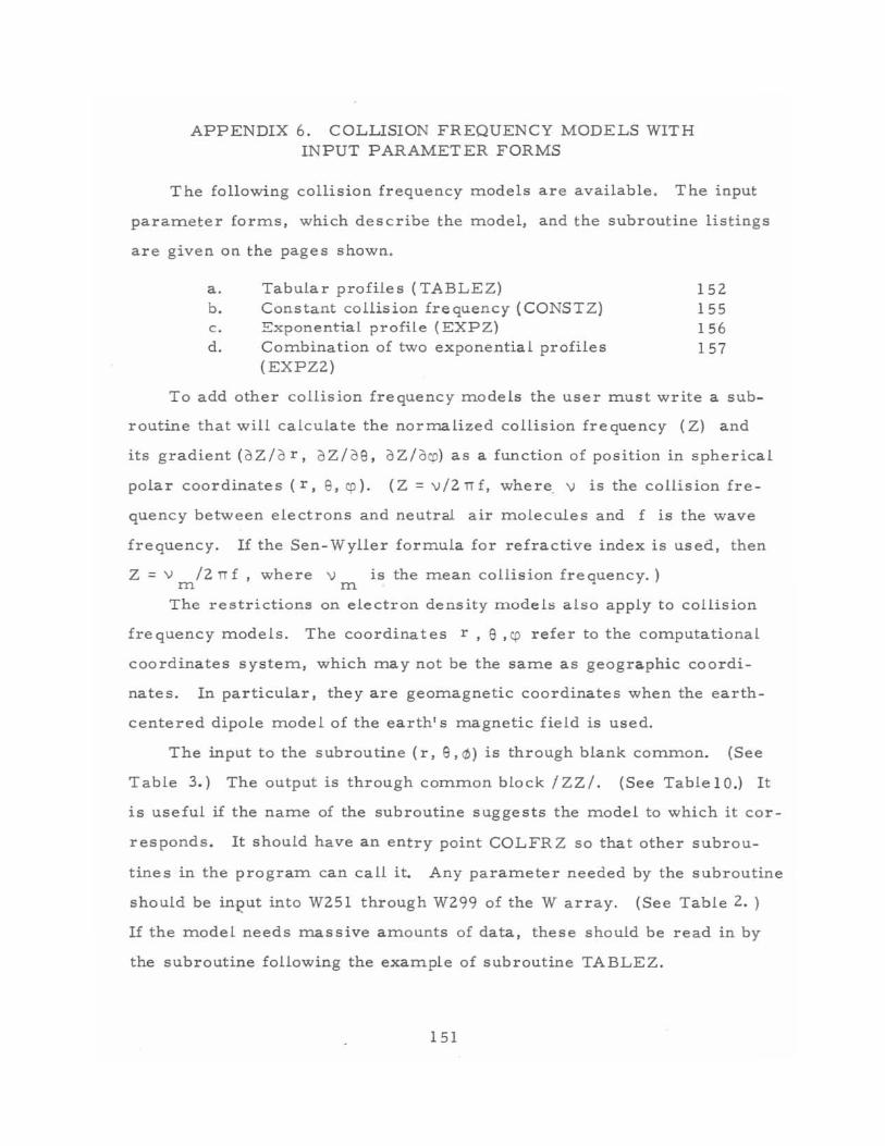
APPENDIX 6. COLLISION FREQUENCY MODELS WITH INPUT PARAMETER FORMS
The following collision frequency m.odels are available . The input
param.eter form.s, which describe the m.odel, and the subroutine listings
are given on the pages shown.
a . Tabular profiles ( TABLEZ) 152 b. Constant collision frequency (CONSTZ) 155 c. Exponential profile (EXPZ) 156 d. Com.bination of two exponential profiles 157
(EXPZ2)
To add other collision frequency m.odels the user m.ust write a sub
routine that will calculate the norm.alized collision frequency (Z) and
its gradient (OZ/O r, oZ/09, oZ/ocp) as a function of position in spherical
polar coord inates (r, 9, cp ). (Z = v/2 n f, where V is the collision fre
quency between electrons and neutral air m.olecules and f is the wave
frequency. If the Sen- Wyller form.ula for refractive index is used, then
Z = v /2 n f , where V is the m.ean collision frequency. ) m. m.
The restrictions on electron density m.odel. also apply to collision
frequency m.odels. The coordinates r, e ,cp refer to the com.putational
coordinates system., which m.ay not be the sam.e as geographic coordi
nates. In particular, they are geom.agnetic coordinates when the earth
centered dipole m.odel of the earth's m.agnetic field is used.
The input to the subroutine (r, e,<tl) is through blank com.m.on. (See
Table 3.) The output is through com.m.on block /ZZ/ . (See Tablel0 .) It
is useful if the nam.e of the subroutine suggests the m.odel to which it cor
responds. It should have an entry point COLFRZ so that other subrou
tines in the prograIn can call it. Any param.eter needed by the subroutine
should be inl'ut into W251 through W299 of the W array. (See Table 2. )
If the Inodel needs Inassive am.ounts of data, these should be read in by
the subroutine following the exam.ple of subroutine TABLEZ.
151
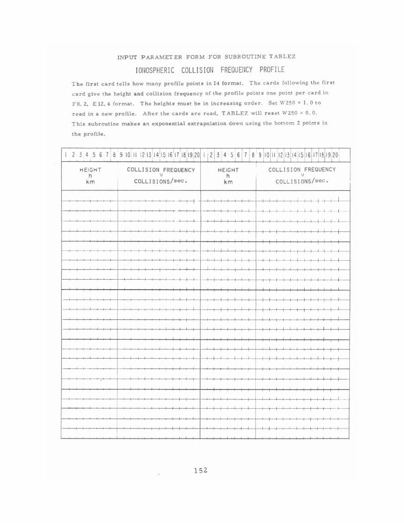
I
INPUT PARAMETER FORM FOR SUBROUTINE T ABL EZ
IOIWSPHERIC COLLlSIOIl FREQUEIKY PROFILE
T h e first card t ells how many profile points in 14 farrnaL The c ards follow ing the fi rs t
c ard giv e the he ight and collision frequency of the profile po int s one po int per c ard i n
F 8 . 2, E 12. 4 format. T he heights must be in increasing order . Set W 250 = 1. 0 t o
r e ad in a new profile. After the cards are read, TABLE Z will res et W 2 50 = O. o.
T his subroutine makes an exponential extrapolation down using the bottom 2 points in
t he profile.
2 3,456 7; S 9 loi ll 1 1 1 3 ~ 1 4 i I5 1 6 ~ 17 : IS : 19 1 2 0 112i 3i45 ;6i 7i S' 9 iIOi ll :12iI3hI 5iI 6i I7 iISI19120i
HE IGHT COLLISION FREQUENC Y HEIGHT COLLISION FREQUENC Y h v h v
km COLLI S I ONs/sec. km COLLI S IONs/sec.
I --'-t-t 1+-1-1-
-"--T -+--+-+-- I I 1 ~--i~t·-t--I·---
, , , I , , -'- 1 I I I I I I-I-j-+--
t--I- +- I -+-,-+--L
I
I I I
,
, , ,
I I I I I I I 1 1 I
-1-1--1-+ I I I 1 I-+-t--I- --
152
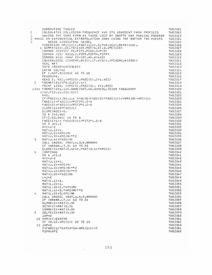
SUBROUTINE TABLEI C :ALCULATES COLLISION FREQUENCY A~O ITS GRADIENT FROM PROFILSS C HAVING THo SAME FORM AS THOSE USED BY CROFTS RAY TRACING PROGRAM C ~AKES AN EXPONENTIAL EXTRAPOLATION ~OWN USING THE BOTTO~ TWO POINTS C NEEDS SJOR~UTINE GAUSEL
DIMENSION HP:(100),FN2C(100),~LPHA(100),BETA(lCOJ. 1 GAHI'1A(1001 ,DELTA(100) ,I'1AT(~,5) ,5LOPE(100)
:OHMON tCONSTI P(,PIT2,PI02,OJM(5) :OHHON IlZI HOOl.l,PZPR,PZPTH,PZ~P~
COMMON FUo' IWHI IO(10I,HO,ltHItOO) EQ.UIVALENCE (::AR.fHR,W(Z)). (F"H&I) t<PEAONU,WC25011 UAL MA T ~ATA (MOOZ.6HTA~LEI)
ENTRY COLF~1 [F (.NOT.~EADNU) GO TO 10 REAONU'O. ~EAO 2, NO::,(HPCCII ,FN2C(I) ,I::::l,~O::)
l FORMAT([4/(F8.l.E1l.4)) PRINT 1200, (HPC( II .FN2C(II, l;I,NDe)
1200 FORHAT(lHlfl~X,bHHEIGHT,~X,20HCOLLISION FREQUENCY 1(lX,F20.10,E2J.10I)
A·O. [F(FNlCU) .N£.O.I A'ALOG(FNlC(l)/FNlC(ll )/(HPCIZ) -HPC(lll >NlC(1)'FN2C(11/PITl'1.E-6 FNlC(Z)'FNlC('I/PITZ'1.E-6 SLOPE(11;A·FN2C(11 SLOPE(NOCI'O. )0 5 I'Z.NOC IF(I.EQ.NOCI GO TO 6 FNZC(I+l)' FNZCII+11/PITZ'1.E-6 JO 3 J::l,3 M=I+J-Z MAT (Jtl)=1. HAT(J.Z)'HPC(HI ~AT(J,3'=H~C(H)··2
3 MAT(J,~)=FNZC(H)
CALL GAUSEL PlAf.It,3,It,NRANK) IF INRANK.LT.3) GO TO ZO SLOPE (Xl =I1AT (2 ,It)"2 .·Jr1AT (3, It) .HPC(I)
; :ONTINUE iJO It ..J::1,2 Jr1=I"J-Z MAT(J.l)=l. UT(J.ZI=HPC(HI I1AT(J,3J;HPC(H)··Z MAT(J,It)::HPC(")··3 HAT(J.51=FNZCIHI L =J"Z HAHL.U',. HAT(L,Z)::1. ~ATIL.31'Z.·HPCIMI I1AT(L,It)::3.·HPC(H)··Z
4 ~ATIL.51=SLOPE(MI
CALL GAUSEL (HAT.It,4,5,NRANK) IF (NRANK.LT.41 GO TO ZO ALPHA(II'HAT(1.51 3ETA(I1=HAT(Z.51 ~AHHA(I'=MAT(3,5)
S DELTA(II=HAT('.51 JUP=Z
10 H=Rlll-EARTHR IF (H.GE.HPC(UI GO TO 1Z
1l JUP=Z Z=FNZC(ll'EXP(A"H-HPC(lIII/F PZPR=A'Z
153
TAB lOO 1 TABZOOZ TABZ003 TABl004 TAB lOOS TAB Z006 TABl007 TABl008 TABl009 TABlOl0 TAB lOll TABl01Z TAB lOll TABl014 TABl01S TABl016 TABl017 TAB l018 TABl019 TABzoza TABlOZl TAB lOZZ TAB ZOZ3 TABIOZ4 TAB lOZS TABlOZ6 TABZOZ7 TABZOZ8 TAB lOZ9 TABl030 TABl031 TABl03Z TABl033 TABZ034 TAB Z035 TAB l036 TABZ037 TABl038 TAB Z039 TABZO,O TABZ041 TAB l04Z TAB Z043 TABZO .. TABl045 TABZO,6 TAB ZO.r TAB Z048 TAB l049 TAB l 050 TABZ051 TABZ05Z TAB Z053 TAB Z054 TABZ055 TABZ056 TABl057 TABZ058 TABZ059 TABZ060 TAB Z061 TABl06Z TAB la63 TABl064 TABl065
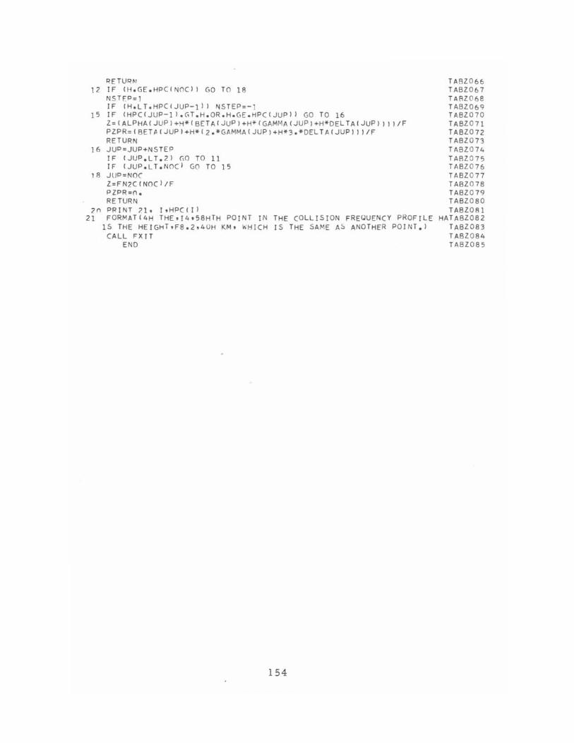
RETUR"I 12 IF IH.GE.HPC(NOCI I GO TO 18
NS rEP= I IF fH.LT.HPCfJUP-I)) NSTEP=- I
15 IF fHPCfJUP-]l.GT.H.OR.H.GE.HPCfJUP)) GO TO 16 Z=IALPHA(JUPI+H*IBETAIJUP)+H*!GAMMA(JUP1+H*DELTA(JUPJ IIIIF PlPR=IBET~(JUPI+H*12.*GAMMA{JUPI+H*3.*OELTA(JUP)))/F
RETURN }6 JUo=JUP+NSTEP
IF CJUP.LT.21 GO TO 11 IF fJUP.LT.NOC) G(l TO 15
18 JlJP=NO( l=FN2CfNOCl/F PZPR=n. RETURN
20 PRINT 7.1. J,HPcctl 21 FORMAT'4H THE.I4.5BHTH POINT IN THE COLLISION FREQUENCY PROFILE
1S THE HEIGHT.F8.2,40H KM, WHICH IS THE SAME A~ ANOTHER POINT.' CALL FXIT
END
154
TABl 0 66 TABl 06 7 TABl068 TABl069 TABl070 TABl 07 1 TABl072 TABl073 TABl 074 TAAl 0 75 TABl 076 T ABlO 77 TABl078 TABl 079 TABl OBO TABl ORl
HATABl082 TABl083 TABl OB4 TABlOB5
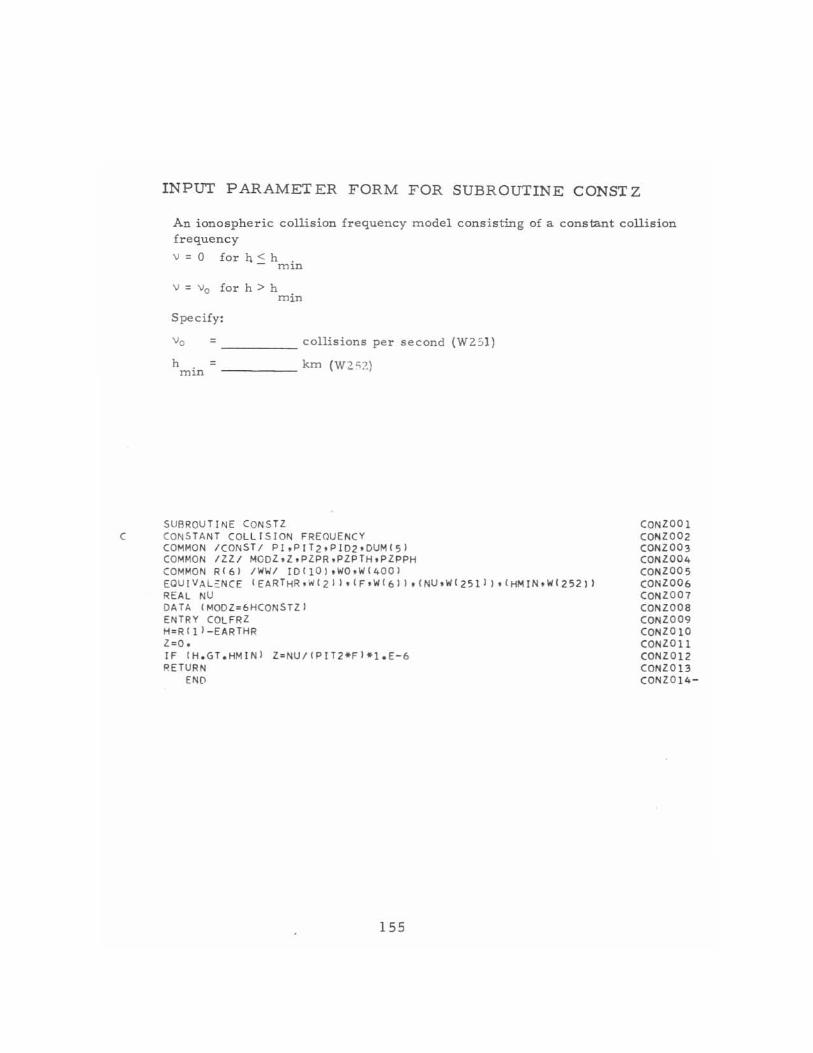
(
INPUT PARAMETER FORM FOR SUBROUTINE CONSTZ
An ionospheric collision frequency model consisting of a constant collision frequency
" = 0 for I) < h . - m iD
for h> h min
Specify:
"0 = _____ collisions pe r second (W251)
h = krn (W 2 <;2) min -----
SUBROU TINE (ONSTl CONSTAN T COLLISION FREQUENCY COMMON ICONST/ PI,PIT2,PI02,DUM(51 COMMON IlZI MOOl,Z,PZPR,PZPTH,PZPPH (OMMON R(6) /WWI IDIIO),WQ,W(400J EQUrVAL::NCE (EARTHR,W(2) J, (F,W{61I,{NU,WI251) I ,(HMIN,W(2521) REAL NU DATA (MOD l=6HCQNSTlJ ENTRY (OLFRl H=R '11 -EARTHR l=O. IF ( H.GT.HMINI Z=NU/ (PIT2*Fl*1.E-6 RETURN
END
155
(ONlOOl (ONl002 (ONl003 (ON2004 (ON2005 (ON2006 (ON2007 (ON2008 (ON2009 (ON2010 (ON20 11 (ON2012 (ON2013 (ON2014-
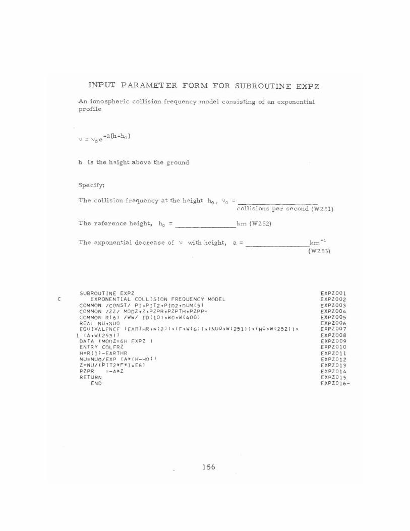
c
I NPUT PARAMET ER FORM F OR S UBR OUT INE E XP Z
An ionospheri c collis i on frequency model consisting of an exponential profile
h is the h ~ight above the groWld
Specify:
The collis.lon frequency at the h.:;ight he, Vo
collisions per second (W251)
The reference height, 110 = ___ ______ km (W252)
The ~xpo:''len:ial decrease 0: \) with tv'!ight, a = _ ________ -ckrn - 1 (W253)
SUBROU TI NE ExPZ EXPONENTIAL COLL ISION FREQUENCY MODEL
(OMMON ICONSTI PI,prT2,p r02 , DUM(51 (OMMON Ill/ MOQZ,Z,PlPR,PZPTH,PZPPH COMMON RCb) /WWI rO(l OJ,WQ,W(4001 REA L NU , ,"lUG EQU I VALENCE (EAR THR, w (2 ) ) , (F, ',4 (6) ) , (NUD, W ( 25 1 ) I • (HO , W (252 I I ,
1 (A,W ( 253J J
DATA ( MOnl=6H EXPZ I ENTRY COLFRZ H=R( j l - EAPTHR NU=NUQ/EXP (A*CH- HOI I Z=NU/ f P I T2* F*1 . E6) PZPR =-A*l RETURN
END
156
EXPZOOt EXPZOOz EXPZ003 EXPl004 EXPZ005 EXPZ006 EXPZ007 EXPlOOa EXPZ009 EXPZOIO EXPZOll EXPZOIZ EXPZOl3 EXPZ014 EXPZOl5 EXPZOI6 -
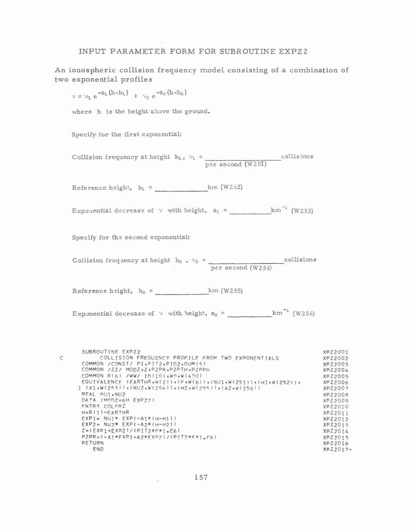
INPUT PARAMETER FORM FOR SUBROUTINE EXPZ2
An ionospheric co lli sion frequency tnodel consisting of a cotnbination of two exponential profiles
c
- a,(h-h1 ) - "-<; (h - h. ) V = \he + v2 e
where h is the height ab:Jve the ground.
Specify for the first exponential:
Collision frequency at height hl J \11 = ---, ___ ---,-;-;=",-;,,-; __ collis ion s per second (W 251)
Reference he igh~, h 1 ; _______ km (W2 52)
Expo·~1.e-ntial decrease of \I with height, al = _____ ----'km - 1 (W2 53)
Specify for th·~ second exponential:
Collision frcq'~ency at height h2 . \12 = _____ -:--,--__ .,-_collisions p'or second (W254)
Reference h.ight, h.; _______ km (W255)
Expvnential decrease of \) with beight, ~ _____ km - 1 (W2S6)
SUBROUTrNE EXPl2 COLLISION FREQUENCY PROFILE FRO~ TWO EXPONENTIALS
CO MM ON ICONST! PI,PIT2,PI02,DUMISI COMMON IlZ/ MODZ,Z,PZPR,PZPTH,PlPPH COMMON RI61 /WW/ tD(lO),WQ,W(4COJ EOU t V 1\ L ENe E 'f AR THR , W ( 2 ) I , ( F ,W { 6 J I , ( NU 1 'W ( 251 ) J , I HI, W ( 252 I I ,
1 (Al,W(2~1) J ,INU2,W(2541),{H2,W(25,)J,(A2,WI25&1' RFA.L NUl.NU2 DA TA (Mn~Z=6H EXPZ?I I="NTRY COLFRZ H=Rfll-EARTHR EXPl = NUl* EXPf - Al*IH - Hll I EXP2 = NU2. EXP(-A2*(H - H21 I Z=(EXP1+EXP2)/(PIT2*F*1.E6) PZPR = (-Al*FXPl -A2*EXP?I/(PIT?*~*1.F61 RETURN
ENO
157
XPl2001 XPl2002 XPl2003 XPl2004 XPl2005 XPl2006 XPl2007 XPl2008 XPl2009 XPl2 010 XPl2 0 11 XPl2012 XPl2013 XPZ20j4 XPl2015 XPl2016 xpl2017-

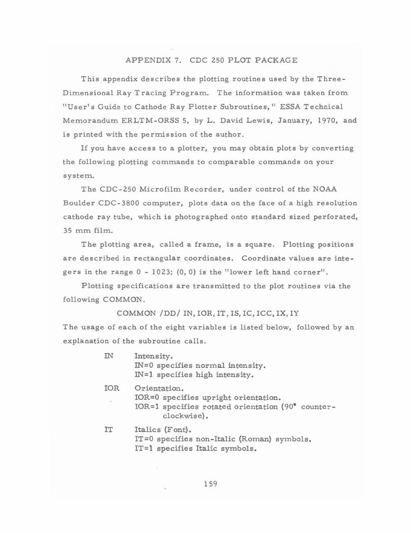
APPENDIX 7. CDC 250 PLOT PACKAGE
This appendix describes the plotting routines used by the Three-
Dimensional Ray T racing Program. T he information was taken from
"User's Guide to Cathode Ray Plotter Subroutines," ESSA Technical
Memorandum ERLTM-ORSS 5, by L. David Lewis, January, 1970, and
is printed with the permission of the author.
If you have access to a plotter, you may obtain plots by converting
the following plotting commands to comparable commands on your
system.
The CDC-250 Microfilm Recorder, under control of the NOAA
Boulder CDC - 3800 computer, plots data on the face of a high resolution
cathode ray tube, which is photographed onto standard sized perforated,
35 mm film.
T he plotting area, called a frame, is a square . Plotting positions
are described in rectangular coordinates. Coordinate values are inte
gers in the range 0 - 1023; (0,0) is the "lower left hand corner".
Plotting specifications are transmitted to the plot routines via the
following COMMON.
COMMON /DD/ IN, IOR, IT, IS, IC, ICC, IX, IY
T he usage of each of the eight variables is listed below, followed by an
explanation of the subroutine calls .
IN Intensity. IN=O specifies normal intensity. IN=1 specifies high intensity.
lOR Orientation. IOR=O specifies upright orientation. IOR= 1 specifies rotated orientation (90· counter
clockwise) •
IT Italics (Font). IT=O specifies non-Italic (Roman) symbols. IT=1 specifies Italic symbols.
159
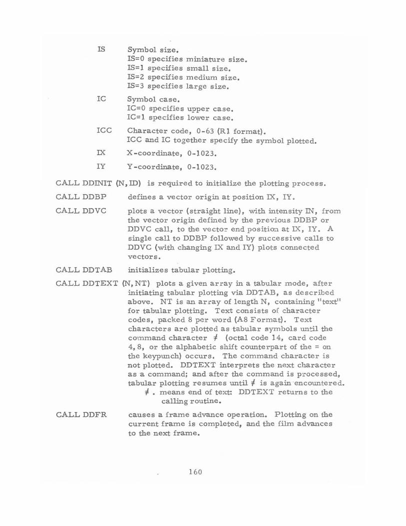
IS Symbol size. IS=O specifies miniature size. IS= 1 specifies small size. IS=2 specifies medium size. IS=3 specifies large size.
IC Symbol case. IC=O specifies upper case. IC= 1 specifies lower case.
ICC Character code, 0-63 (R1 format). ICC and IC together specify the symbol plotted.
IX X-coordinate, 0-1023.
IY Y -coordinate, 0-1023.
CALL DDINIT (N,ID) is required to initialize the plotting process.
CALL DDBP
CALL DDVC
defines a vector origin at position IX, IY.
plots a vector (straight line), with intensity IN, from the vector origin defined by the previous DDBP or DDVC call, to the vecto:: end position at IX, IY. A single call to DDBP followed by successive calls to DDVC (with changing IX and IY) plots connected vectors.
CALL DDTAB initializes tabular plotting.
CALL DDTEXT (N, NT) plots a given array in a tabular mode, after initiating tabular plotting via DDTAB, as described above. NT is an ar ray of length N, containing "text" for tabular plotting. Text consists oC character codes, packed 8 per word (A8 Format). Text characters are plotted as tabular symbols until the cO'.11mand character I (octal code 14, card code
CALLDDFR
4,8, or the alphabetic shift counterpart of the = on the keypunch) occurs. The command character is not plotted. DDTEXT interprets the next character asa command; and after the command is processed, tabular plotting resumes until I is again -encountered.
I . means end of text: DDTEXT returns to the calling routine.
causes a frame advance operation. Plot1:ing on the current frame is completed, and the film advances to the next frame.
160
APPENDIX 8. SAMPLE CASE
A sam.ple case is included with the description of the program. for
three reasons. First, it dem.onstrates the use of the program.. Second,
it illustrates the three types of output available (printout, punched cards,
and ray path plots). Finally, it serves as a test case to verify that the
user's copy of the program. is running correctly. This last point is es
pecially im.portant if the user has had to m.ake m.any m.odifications in
converting the program. to run on a com.puter other than a CDC 3800 .
Although the ionospheric m.odels in the sam.ple case dem.onstrate
the use of the program., they don't give realistic absorption for the radio
waves. The absorption in the sam.ple case is too low for two reasons.
First, although the Chapm.an layer has a realistic electron density for
the F region, it has In.uch too low an electron nensity for the D region,
where m.ost of the absorption occurs. Second, the collision frequency
profile in the sam.ple case is designed for use with the Sen-Wyller for
m.ula for refractive index rather than the Appleton-Hartree form.ula used
in the sam.ple case. Multiplying the collision frequency profile in the
sam.ple case by 2.5 gives an effective collision frequency profile for use
with the Appleton-Hartree form.ula that will give nearly the correct
absorption for HF radio waves (Davies, 1965, p. 89).
Appendix 8a. Input Param.eter Form.s for the Sam.ple Case
Filled-out input param.eter form.s are included to describe the
sam.ple case (i. e., show what ray paths are requested for which iono
spheric m.odels and what type of output is wanted). Furtherm.ore,
com.paring them. with Appendix 8b illustrates the relationship between
the form.s and the input data cards.
161
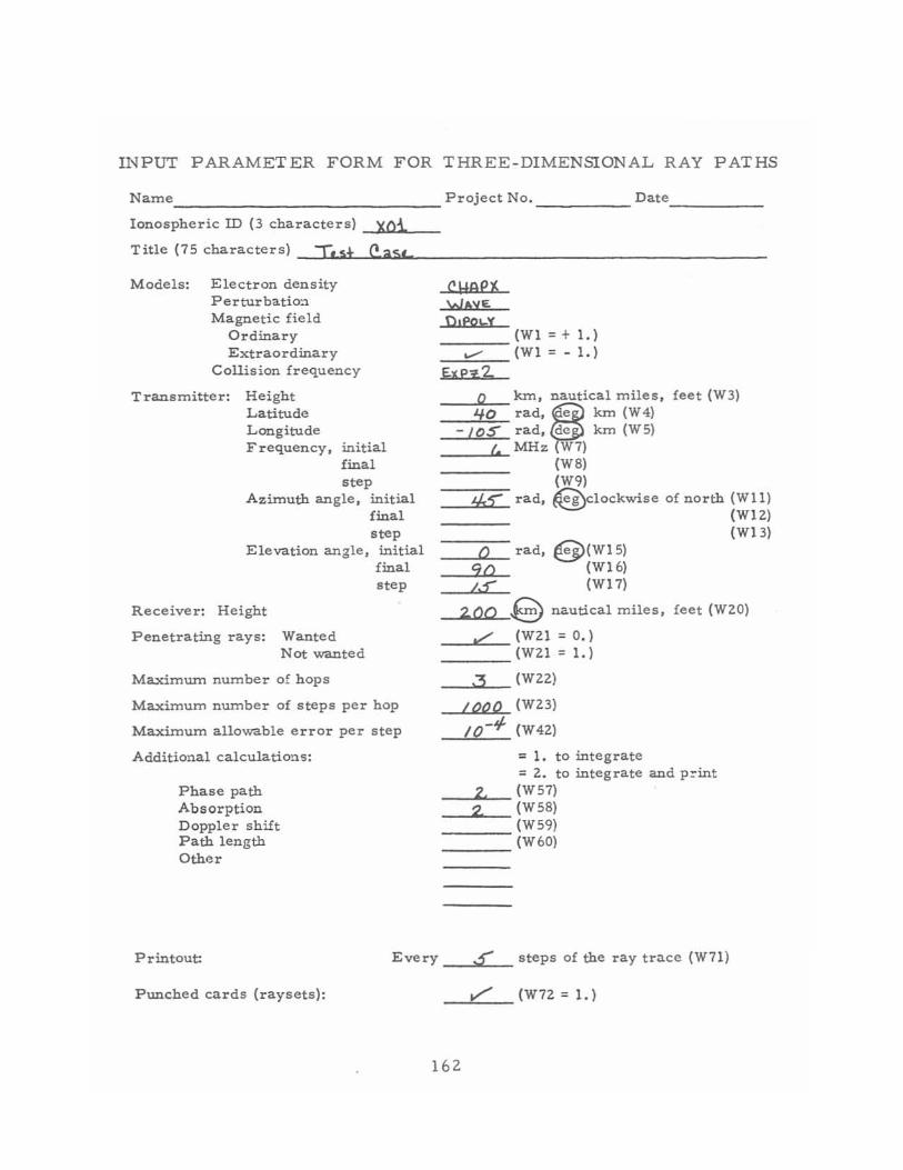
INPUT PARAMETER FORM FOR THREE-DIMENSIONAL RAY PATHS
Name ________________ Project No. ______ Date _____ _
Ionospheric ill (3 character s) xoi Title (75 characters) __ To ...... ,.s+L..JC, ..... a"'s .. L ____________________ _
Models: Electron density Perturbation Magnetic field
Ordinary Extraordinary
Collision frequency
Transmitter: Height Latitude Longitude Frequency, initial
final step
Azimuth angle, initial final step
Elevation angle, initial final step
Receiver: Height
Penetrating rays: Wanted Not wanted
Maximum number of hops
Maximum number of steps per hop
Maximum allowable error per step
Additional calculations:
Phase path Absorption Doppler shift Path length Other
CI+QPJI WAvE D,foLV ___ (WI = + 1.)
_.!::......-~_ (WI = - 1.)
Ex p'f 2. __ "'0'-_ km, nautical miles, feet (W3)
40 rad, ~ km (W 4) -lOS rad, de km (W5)
__ ...... r .... MHz W7) (W8) (W9)
_-,*"",,5""e-rad, ~clockwise of north (WII) (WI2)
_-::!O'-L_ rad, e(W15) 90 (W16)
(W13)
/,5" (W17)
200 .@ nautical miles, feet (W20)
..r (W21 = 0.) ___ (W21 = 1.)
_ ... .3.L-_ (W22)
/000 (W23)
to-if (W42)
= 1. to integrate = 2. to integrate and p~int
_ .... Z .... _(W57) _ .... :2. ____ (W 58)
___ (W59) ___ (W60)
Printout:
Punched cards (raysets):
Every _-"S,,-_ steps of the ray trace (W71)
_1::.,/" __ (W72 = 1.)
162
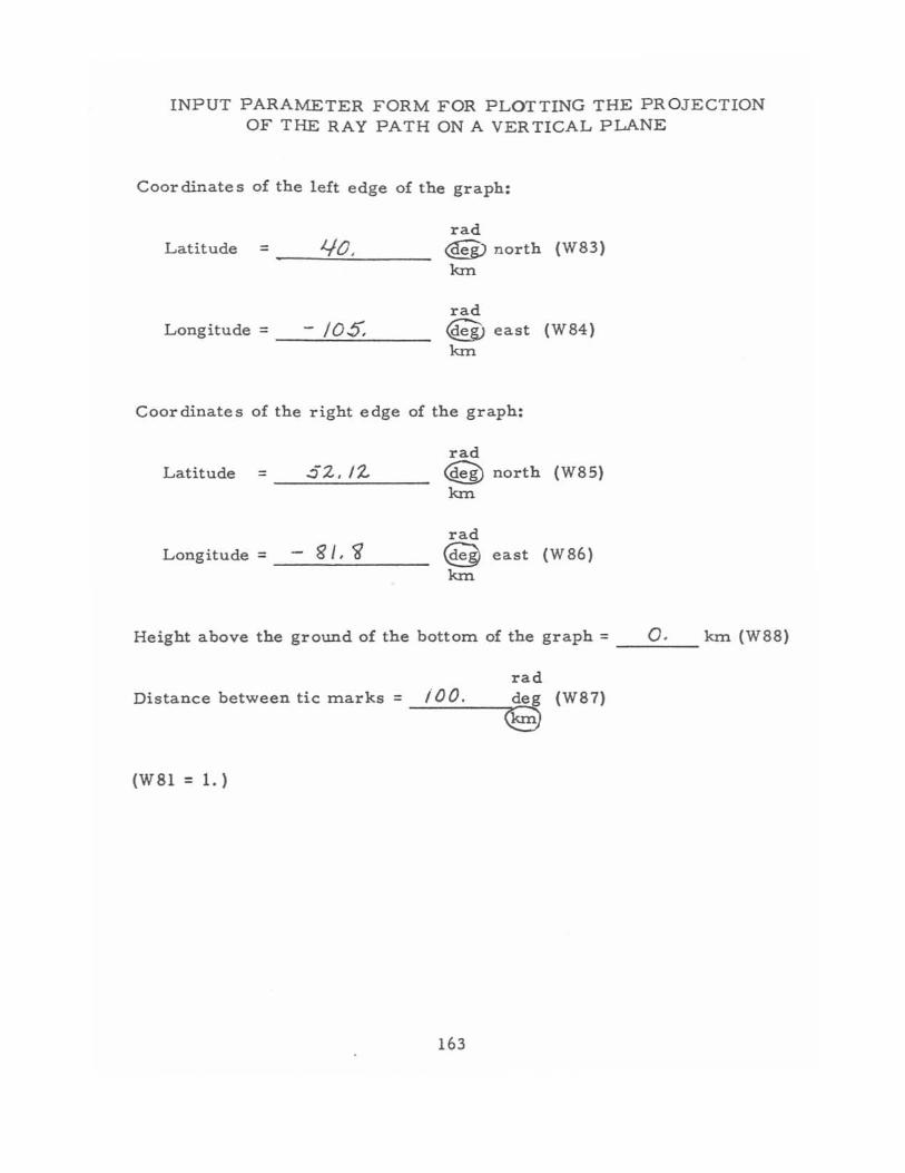
INPUT PARAMETER FORM FOR PLOTTING THE PROJECTION OF THE RAY PATH ON A VERTICAL PLANE
Coor dinate s of the left edge of the graph:
Latitude = 1../0, ----'-"'-'----
Longitude = __ --'-/~O....:.$.:....:, __ _
rad ~ north (W83) knt
rad ~ east (W84) knt
Coordinates of the right edge of the graph:
Latitude = 52, 1'2---"---'--'----
Longitude = - g I, 'if
rad ~ north (W85) knt
rad ~ east (W86) kIn
Height above the ground of the bottom of the graph = _-=0_, __ kIn (W88)
rad Distance between tic marks = --.:.i_O_O_' __ .,;d",e"l;g (W87)
<§9
(W81 = 1.)
163
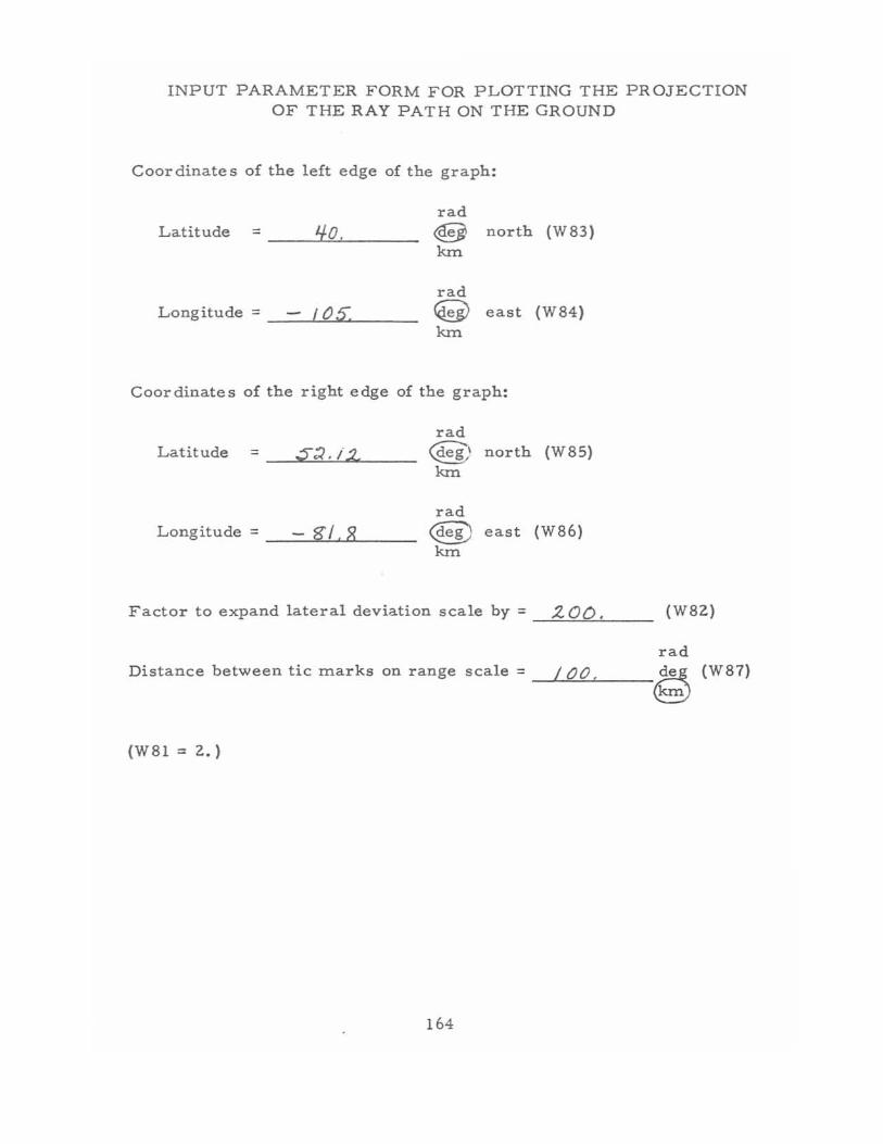
INPUT PARAMETER FORM FOR PLOTTING THE PROJECTION OF THE RAY PATH ON THE GROUND
Coor dinate s of the left edge of the gr a ph:
L a titude = ___ 4-'-"'0-'-, ___ _
Longitude = - lOS:
rad ~ north (W 83) kIn
r a d ~ east (W84) kIn
Coordinates of the right edge of the graph:
Latitude = __ 3",,-,:<,,-,-, !-i .. .:2..~ __
Longitude = _---"-_8'2..!/~,.L8L_ __
rad Qiei,1 north (W8S) kIn
rad Qieg) east (W86) kIn
Factor to expand lateral deviation scale by = 2. 00 , (W82)
rad Distance between tic marks on range scale = _-'I--'O=O-",'--_ _ ~
<e::J
(W8l = 2.)
164
(W87)
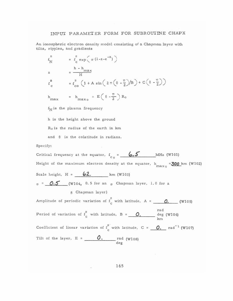
INPUT PARAMETER FORM FOR SUBROUTINE CHAPX
An ionospheric electron density model consisting of a Chapman layer w i th tilts, ripples, and gradients
2 r -z '\ = fC exp\.. Ci (l - z - e ).J
h - h max
z H
2 f
c = <0 (1+ A SID ( 2 T1 (e -D/B) + C (8 - D)
h max
h maxo
+ E( 8 -~ 'I Ro 2 "
iN is the plasma frequency
h is the height above the ground
Ro is the radius of the earth in km
and e is the colatitude in radians.
Specify:
Critical frequency at the equator, f = __ ~""-• ...,,S'=--___ ...:MHz (W I OI) Co
Height of the rnaximwn electron density at the equator, h =300 km (WI02) maxo
Scale height. H = _-',,"'2.=-. ___ km (W I 03)
Ci = _ -"O='S'>L __ (W I 04, 0.5 for an Ci Chapman layer, 1. 0 for a
8 Chapman layer)
2 Amplitude of. periodic variation of f w ith latitude, A =
c __ ",Q,,-, __ (W I 0 5)
rad Period of variation of l with latitude, B = __ -'0::0.... ____ deg (WIO 6)
c km
2· Coefficient of linear variation of f with latitude, C =
c
Tilt of the layer, E = __ ---'0::...:.. ___ rad (WI08) deg
165
0. r ad - 1 (W I O?)
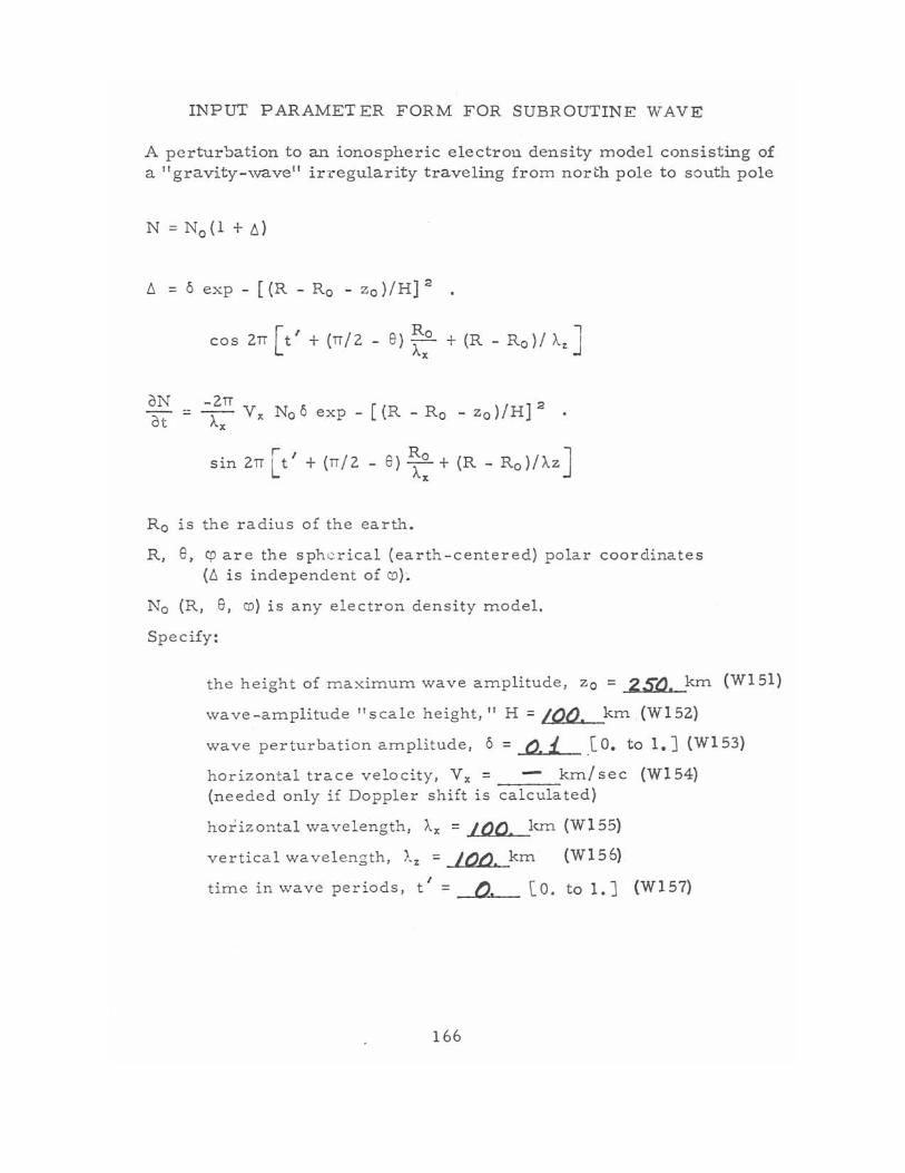
INPUT PARAMETER FORM FOR SUBROUTINE WAVE
A pertur"!:>ation to an ionospheric electron density model consisting of a "gravity-wave" ir 'regularity traveling from north pole to south pole
6. = 6 exp - [(R - Ro - zo)/H]2
aN at
cos 2rr [t' + (rr/2 - 8) ~xo + (R - Ro)1 A, ]
__ ~rr Vx No 6 exp _ [(R - Ro _ zo)/H]2 x
sin 2rr [t' + (n/2 - 6) ~: + (R - Ro)/Az ]
Ro is the radius of the earth.
R, e, cp are the spherical (earth-centered) polar coordinates (6. is independent of co ).
No (R, 6, co) is any electron density model.
Specify:
the height of maximum wa ve amplitude, Zo = 250. km (Wl5l)
wave-amplitude "scale height," H = /00. km (W152)
wave perturbation amplitude, 6 = 0.1. [0. to 1.J (W153)
horizontal trace velocity, Vx = - km/sec (W154) (needed only if Doppler shift is calculated)
horizontal wa velength, Ax
vertical wa velength, }~% =
.. . d t' tlme In \vave perlO 5, =
= 100. km (W155)
100. km (W156)
0. [0. to 1. J (W157)
166
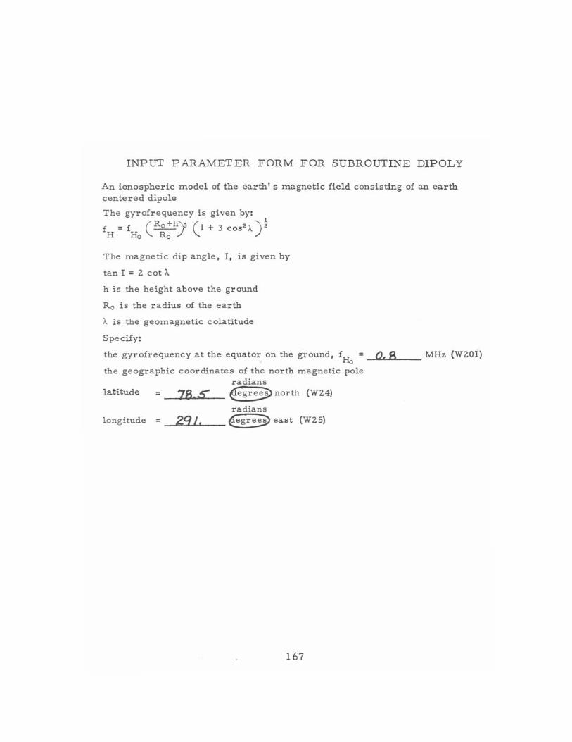
INPUf PARAMETER FORM FOR SUBROUfINE DIPOLY
An ionospheric lTIodel of the earth I S magnetic field consisting of an earth centered dipole
The gyrofrequency is given by: 1
fH = fHo ( R;:h) (1 + 3 cos2 >-)'
The magnetic dip angle, I, is given by
tan I = 2 cot >-h is the height above the ground
Ro is the radius of the earth
A is the geomagnetic colatitude
Specify:
the gyrofrequency at the equator on the ground, fHo = ---,0"",-,-,8,,-__ MHz (W20i)
the geographic coordinates of the north magnetic pole radians
latitude = _ ... 7",8","",5'",-_ (!egr e!]> north (W24)
radians long itude = _2b...QL' ... ,,--_ ([egre§> east (W25)
167
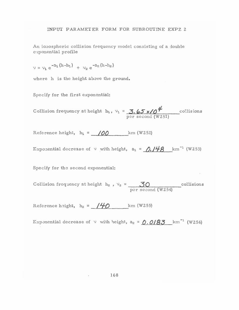
INPUT PARAMETER FOR M FOR SUBROUTINE EXPZ 2
An io'"1ospheric collision frequcncy model con,sisting of a double c'<po!1cntial profile
where h is thc height above the ground.
Specify for the first exponential:
Collision frequency at he i ght h1' \11 = 3. "5 x/O ¢ p,~r second (W251)
Reference height, h1 = _ .... I'-'O"'-"O<-___ km (W252)
Expoc,ential dec r ease of \I with height, a1 = (J.IJf8
Specify for th-~ second exponential:
collis ions
km - 1 (W253)
Collision freq'~ency at height h2 , \12 = __ .... ,_3'-O'""----:---:-:-=-::-c:--_collisions p'~r second (W254)
Reference h 'oight, h2 = _LI_If'-"'O"-___ km (W255)
Exponential decrease of \I with he ight, a2 = D.o/83 km -1 (W256)
168
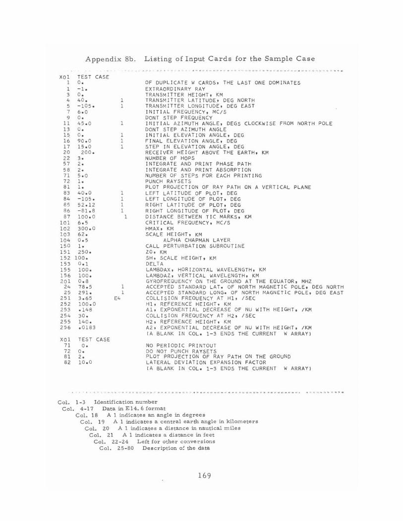
XOI 1 1 3 4 5 7 9
11 13 15, 16 17 20 22 57 58 71 72 81 83 84 85 86 87
101 102 103 104 150 151 152 153 155 156 201
24 25
251 252 253 254 255 256
Appendix Sb . Listing of I nput Cards for t h e Sample Case
TEST CASE O. - 1. O. 40. - 105. 6.0 o. 45.0 o. O. 90.0 15.0 200.
3. 2. 2. 5.0 1. 1. 40.0 -105. 52.12 -81.8 100.0 6.5 300.0 62. 0.5 1. 250.
100. 0 .1 100. 100. 0.8 78.5 291. 3.65 100.0 .148 30. 140. .0183
1 1
1
1 1 1
1 1 I 1
1 1
E4
1
OF DUPLICATE W CARDS, THE LAST ONE DOMINATES EXTRAORDINARY RAY TRANSMITTER HEIGHT. KM TRANSMITTER LATITUDE. DEG NORTH TRANSMITTER LONGITUDE. DEG EAST INITIAL FREQUENCY, MC/S DONT STEP FREQUENCY INITIAL AZIMUTH ANGLE, DEGS CLOCKWISE FROM NORTH POLE DONT STEP AZIMUTH ANGLE INITIAL ELEVATION ANGLE, DEG FINAL ELEVATION ANGLE, DEG STEP IN ELEVATION ANGLE. DEG RECEIVER HEIGHT ABOVE THE EARTH, KM NUMBER OF HOPS INTEGRATE AND PRINT PHASE PATH INTEGRATE AND PRINT ABSORPTION NUMBER OF STEPS FOR EACH PRINTING PUNCH RAYSETS PLOT PROJECTION OF RAY PATH ON A VERTICAL PLANE LEFT LATITUDE OF PLOT, OEG LEFT LONGITUDE OF PLOT. DEG RIGHT LATITuDE OF PLOT. DEG RIGHT LONGITUDE OF PLOT, DEG DISTANCE BETWEEN TIC MARKS. KM CRITICAL FREQUENCY, MC/S HMAX, KM SCALE HEIGHT, KM
ALPHA CHAPMAN LAyER CALL PERTURBATION SUBROUTINE zo, KM SH, SCALE HEIGHT, KM DELTA LAMBDAX, HORIZONTAL WAVELENGTH, KM LAMBDAZ, VERTICAL WAVELENGTH, KM GYROFREQUENCY ON THE GROUND AT THE EQUATOR. MHZ ACCEPTED STANDARD LAT. OF NORTH MAGNETIC PO LE. DEG NORTH ACCEPTED STANDARD LONG. OF NORTH MAGNETIC POLE, OEG EAST COLLISION FREQUENCY AT HI. ISEC HI, REFERENCE HEIGHT, KM AI, EXPONENTIAL DECREASE OF NU WITH HEIGHT, /KM COLLIsION FREQUENCY AT H2. ISEC HZ, REFERENCE HEIGHT, KM A2, EXPONENTIAL DECREASE OF NU WITH HEIGHT. IKM (A BLANK IN COL. 1- 3 ENDS THE CURRENT W ARRAY)
XOI TEST CASE 71 o. NO PERIODIC PRINTOUT
DO NOT PUNCH RAYSETS 72 o. 81 2. 82 10.0
PLOT PROJECTION OF RAY PATH ON THE GROUND LATERAL DEVIATION EXPANSION FACTOR (A BLANK IN COL . 1- 3 ENDS THE CURRENT W ARRAY)
Col. 1 - 3 Identification number Col. 4-17 Data in E14. 6 format
Col. 18 A 1 indicates an angle in degrees Col. 19 A 1 indicates a central earth angle in kilometers
Col. 20 A 1 indicates a distance in nautical miles Col. 21 A 1 indicates a distance in feet
Col. 22-24 Left for other cO!lve-rsions Col. 25-80 Description 0: the data
169
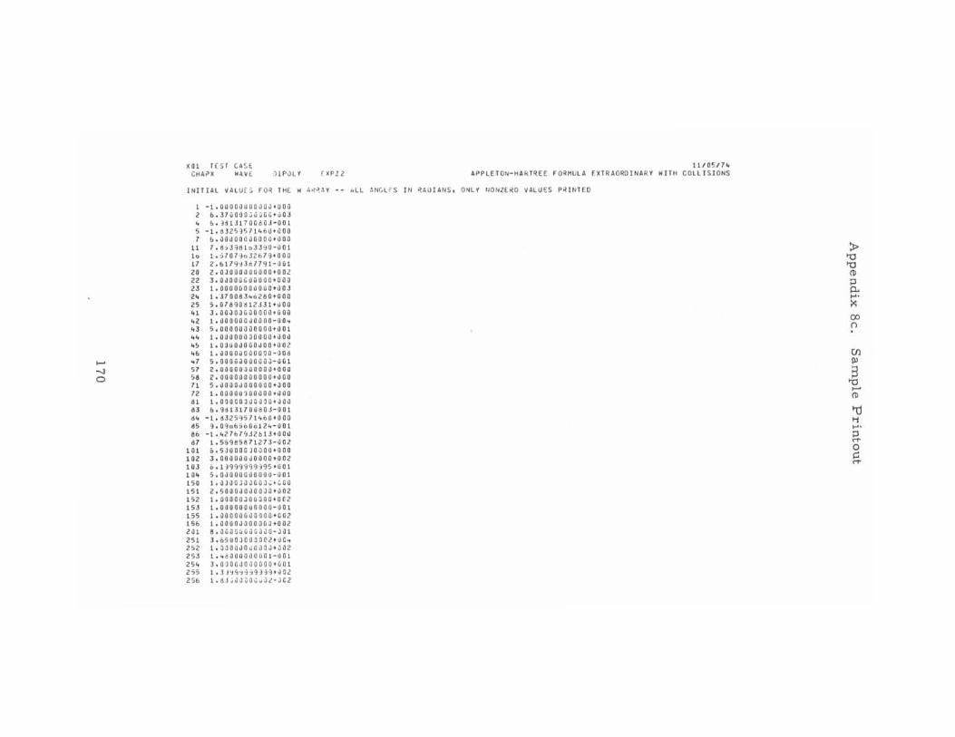
>-'
"" o
)(01 I[SI CA~f.
CHAn: WAH ,HP.JL'f 11/ 05/71.
r )(Pl Z APPLETON - HAkTREE FO~HULA rlCTRAOROlNAR'f WITll COLLISIONS
INITIAL VALU ES ro~ THE w ~~~~'f -- kLL ~NGL ~S IN ~AUIA~S . ONL'f ~ONZERO VALUES P~ I NTEO
1 -1 .00000UOO~OJ*UOO , b.J7~O~O~~~GG~ti0 3
• Eo . ~<HJ 1 700o0 J-OOl
5 -1. 6jZ5357 14 &u9~OO
7 b.OOuOOO~OOOO ' OOO
11 7.8,3~o l oJ3~0 - ~0 1
10 1. :j 7 OHI) 32679*0 00 17 2.6 17 q~3077ql - u& 1
" 2.0JOOOOOOOOOt002 zz 3.00 00~COOOOO+COO
" 1.0000&000000 +003
" I .J 10083kQZ80+000
" 5 . 0189061ZJ31 9uOO .. 3.DDJOJ&uOOOO 9&OO
" 1 • .JOOOOOJOOOO - OOk ., 5.00000000000900 1
" 1.000000 00000 *000 ., 1.0U OOuOOO~00 t D02 .. I.J OOOJOOOOOO - uOo .7 5.0DODJOOOaOJ-O OI
" 2.o0Dooaooooo ~ ooo
" 2.00000000000 90 00 71 5.0000~OOOOOO + OOO
7Z 1 .00000100000 t O~0
" t. O~OCo~uOO~Ot~OO
8l b . 9613 1 70080 J- 001 ~ .. -1 .~32 59S 71 .. 60 t OOO
" :;t.0'l007000 1 2/o - 001 86 -1 ... Z7b7'1JZb lJtOOO
" 1.55'16 5~ 71 Z 73-u02
101 o . 5JOOOCJOOOO t OOO 10' 3.00000000000+002 103 D.l~999999~9S + 00 1
10. :; . 00000 0 00000-001 150 1 .i)Ji)CJJJGOJ~.COij
151 Z. 5000JOOOOJO +002 1" 1 .00000JOO300.0~Z
1" 1.00000 000000 - 00 1 IS' 1.i)0 00000OOOO t C02 1" 1 .0000JOOOOOJ +ODZ '01 ! . o~~a~OJCi)i)O - JOl
'51 l.D5UOJOODQ02 +ilC~
'52 1. 0300JOOOJOJ+JJ2 "3 1 . .. d OOOOilOOOl - llOl
'" J . OaOO.JOilOOOa t OO l
'" 1. lJ~ o;~HqH~ . OO2
256 1. 6J.uJJOJ~J~ - JCZ
~ '0 '0 (l)
P P. .... :><:
00 ()
(J) \11
S '0 >-' (l)
'1:l " .... g. o g.
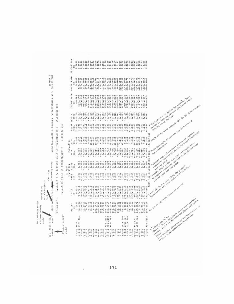
0 w 0
0
0 0
, "
~ 0
~ > ~
C
0
, 0
" > , •
• o :;:;:;:;:; ~:! ~ ~ ~.: ~ ~ ~ 6:e :: ; !: ~ ~ ~ ~ ~ ~ ~ ~:;::;: :;: ~ oooooQg O O O Oo ______ NNNNNNNNNMMM ~=c c cococoOoooo ooOoOcOcoccooOooc <1<0 ' • •• •• •• • ••• • • • • • • • •• ••• •• • • • • ~ oooOcOoOOCOOgoocoOCOOOOOOOCO -Q
~ ~~~~~* ~~~~ !: : ~~~:~ ~~ ~~~~ ~ ~~ ~~~: ~ O~~~~~~~M _ ~~ ~~ ~~~ ~~~~~jjjj_jOO
EO NNNNNNN _ ~~ O~~ ~~O~~~N~~~~~~ j ~C .... '" .. .. . ..... . .... , ... . . . . . . .... . ~ OMNNNCCCC~~~~N~~ j MM~MCN~ __ ~C~~ 4 N ~_~jN oC~ M' ___ OCjONjC~jjjOj N ~
r CC~~O_NNMjj ~~~~~ CON~~~~OO_NMM ~ ______ _ ______ NNNMMM jjjjjj
r ~MMMMMMMMMMM NNNNNNNN~ ~~~~~~~~_
~ O~~~~~~~~~~~NNNNNNNNNOOOOOOOOM
~ O~~~~~~~~~~~OOOOOOOO~~~~~~~~~j ~NNNNNNNNNNN~~~~~ ~~ ~ j~~ ______ O
0..:1: • • • • •••• •• •••• • • •• • • • • ••••• " • ~"'oMNNNCCCC COO CCN~~ ~~~~Oj_MM ___ C o N __ ~ ~ ~g~~ ~ ~ __ ~ ~ ~~~~~gg~~~ _~~ ~
~ ~~~~O _ ~~~~~~~~~~~ON~~ ~ ~OO _ N~~ ~ ~~ __________ ~N NN~ ~~~~~~~#
~ ::O$~
:l:O U .... ... _ O?
i:-'
L 0
>. " ",,,,
- - > .. ~ -- . no w
Z. > . r< .
171
Z .... ::: > e ;;~ _ w . .. ~ 0 o. '" _Z_ .> Z
"'..,,~ .. . o w .. z
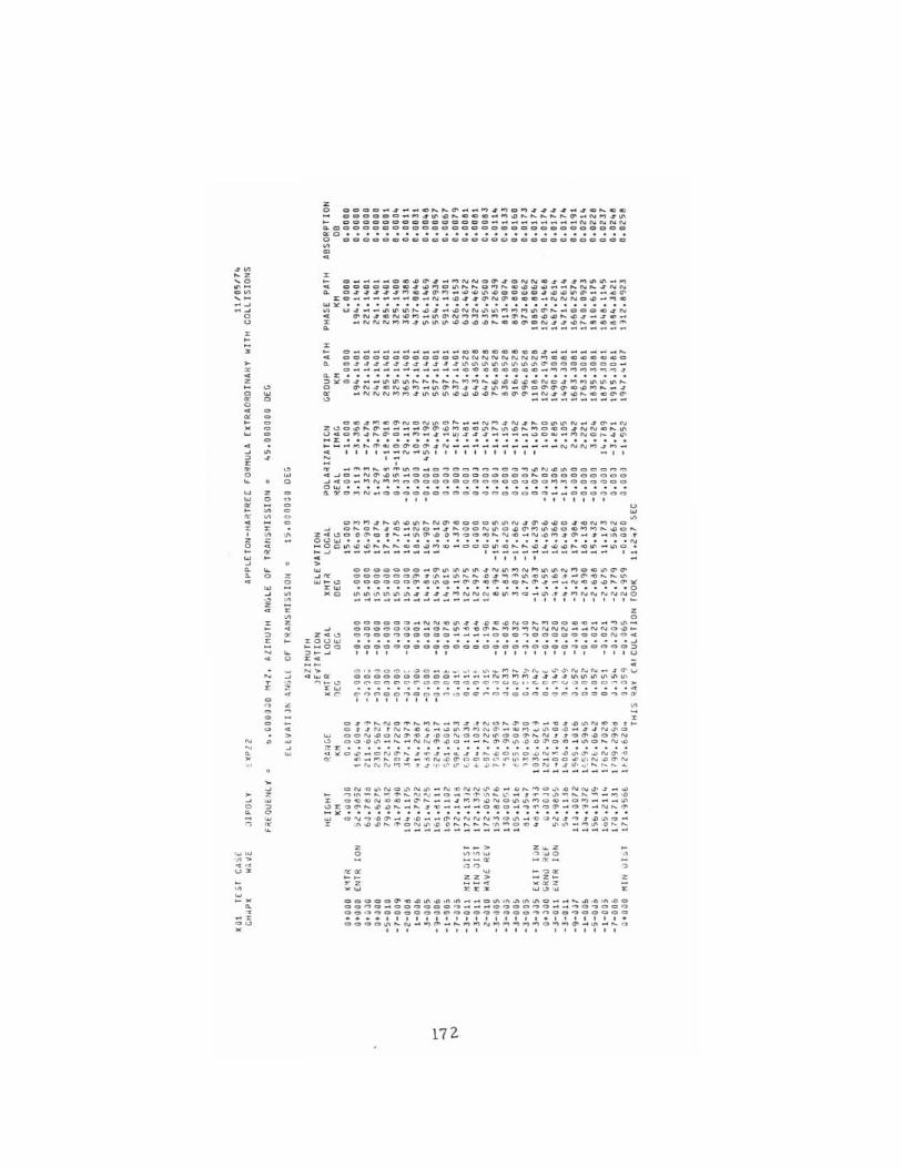
,~
.z ,0
~-o ~ , --~ -~ 0
u
z · ; > ~
• z 0 ~ 0
• ~ · w
· ~ 0 z • 0
" w w ~ • • z , z e ~ • ;
u w 0
0
0
~ ,
z 0
~
~
z ~
" • . " 0
w ~
u :; z 0 z
u w o o ., o e o o
z o goaO~~~~~~~~~~~~~O~~~4~~4~~~ ~
oooooo_~~~~~ ~~~ _~~~~~~~~_N~4 ~ ~ coooooocOO===== _________ NNNNN ~mo==o=oo=ooooooooooooooooooooo
a: c •• • •••••••• ••••••••••• • • ••••• o 0000 000 000000000 0000000 0 000 0 0 ~
~
z ~ O ____ O~~~4_~ NNO~40NN~ 444~~~_M ~ OOOOO=~4~M O~ ~~O M~O~~~ __ ~ N ~4N N
~ 044444M04~M_~~~~00004~~~~ __ ~~ ~O ___ ~ __ O_N_~~4~N~OOO_NNNO~_Me
ILl:.: •••••• • ••• •••••••• ••••• •• • • •• ~ U~ __ ~~~~~4 _ ~NN~~ M MM~~ ~_ 0000 4 N
~ ~N40N~M_~~NMMMM _~~O~~~~3_4~_
X _N NN MM4~~~~~~~~OO~ON44~~~Oo~
~ ----------0 ___________ 00000000 4 _______ ~
OOOOOOOOOOOONNNNN NNNMO OOOOOOO o44444444J34~~~~~~~~~ooooooo_ = ___________ OOOCOOOO _ MMMMMMM4
Q.. J: • ••••••••• ••••• •••••••••••••• ~~Q~~_~~~~~~~~MM~~~~~~"'Q~MM~ ~ ~~ o ~"'~~"'~M ~ ~~M~ ~~ ~M ~ ~O~~~~~M~ ~ ~ ~ ~ NN"'MM ~ ~~~~~~~~~~~ ~ N ~~~ ~~~~~
~ ~~~~~-~--~
O~~M~~NO N~O ~~_NM~N~~Q~~N_~~_N Z~O~~~"_""~~~M~~~~ ~ ~~MQ~a~NN~~~ 0 40 M.~~Q"M _ ... ~~ . ~ ___ "O O~ _M N O ~ • • ... l: • • • • • • • • • • • • • • • • • • • • • • • • • • • • • ~~"M ~~~ O ~O~~N ___ ~" ______ NNNM ~M_
'" ",' _ - "' .... '" , , , , , , , , , , , .. , , N ''';' ~
~ ~~M ~~ ~~~~=~= o ~ o~=~ ~~ N~~===o ~ ~
4~=_N ~~~ .... OQ==OOOOQOCC~cc==COOOO ~~O_MNMM~COC OCO OOOC=OCOMMOOOOOO
f~~~~ ;~~~~~~ ~~~~~ ~~~~~~ ~~ ~~~~~~ , , , , , , , , , ,
OMM~~"'~"'~N~~OOO"' ~N .~ ~~O ~ ~NMNO
u w •
~ O~C~~~ ~ NO _ ~~OON"'O~~M"'~O~MM~~O~ Z4~OD~O ~~" ~~~DMO~~~~~"N~M~~_. " I~O ~ 0<..1 ............... .. . . . .... . ....... N ... OO~~~~~~~~~M~_OOO"' ~ ~~~.~~~~"'_"'O •
~ ~ -- .... ----~-- ,-- -- -- --- --- ,-.. , , , , , >
~
OOOOOOO_~~~~~ . N"'MNM"''''NMO~~~~ oooooO~.~_~~ ~ ~ ~~~ ~~~~I_~~ ~~ ~ OO OO OO~G~C _ ~~~~GO~~. _ _ NG~~~~~ •••••••••••••••••••••• • •• • • · 0 ~~"'~~~ .~ •• M NNN~~Mo _ ~~~MNNNNNO __ ___ _________ """",,~
z o
OC OOOO_NN~"'II ~~.NO ~MO OG~ __ M"'_ OOOOOO O_O~ "'~ ~ ~~ MMMNNN N _" NNO~ ~
ze u :Z:OU ... ...... 00 O .~
Z.
oooonooooo ____ ooo~cooococoNo .. • ••••••••••••••• • ••••••• • ••• J OOOOOOOOOOOOoooooooooonooooo~
, • ' " , , , , , , , , , , " '" U
<:> ., ." <:> '=' L. c:> 0 ...... _ '. ... , ~ "' ... M ~ J' "- ... oJ' J ' N '" N .... J (t' .., oooooooOOo ____ NMMM~~~~~~~~~'"
~~~~~~~~~~~~~~~~~~ ~~ ~~~~~~~~: ~?~~~?~~~~~oer n ~c~~o~e~nOQ~~~
Z OI~~NC~~ M~_M' .tNO~.C~ ~ ~'~~N~n~~ <:> ;~N ' N~oQ" ~"' '''M'''''' <:1' _ q>M'''~O ,D _I..zN ''''Q
w OCN~ON<:1'~. ·DC~OON~OO~~N .t~ ~~O~N ~ oO~~ _~~N N~~O _~~<:1' ~~.~<:1'CC _ ~O~N~ ~ r ••••••••••••••••••••••••••••• d~O~ _ ON~~,~..z ~ ~~ Z~ ~O~O~N~~"'~~N~·O ~ ~ _ ~~~ ..z~ ~N 'D~QOO~~WMM_oe~ ~ N~~N
... "''''''' '''..., :y, ." .. ' '" -..> ,L .., ... . .... ~ :: ::: ~~ ~::::::::~:
ONQ"'NO~N~ _ N~NN~~ ~~ ~MO~4NN""~ ~ ~ ~,~ _ ~_~~~ ~ _ o ~_ ~ ,~~ ~ _t~ ~~""~~ ~_ "' · D
X o~~N~e _ <:1'~ __ ~M "'~NO"'~Moe_o"' ___ ~ ~ r o ~~ ~~ ~_~I ~ ____ o~o ~~ m~<:1'_O~ _ N~~ ... ~ ............................ . w O~~·~<:1'_I. __ ~NNNN"'O~ _~~~..z ~:Y~~o ~
X .~~~~~ON~~D~ ~~ ~·~~o~ ..z ~"'_ ~ ~ ·D~~
------~----- ----- -z -. > '". ~ VI '" ILl ':>:...00
--~ - <>: -an 0 .~ '" · o~ .- ~~~
_z. z r z , .z 'W r:z:,. W<.!)I .oJ z =oooo~ ~ ~~~.n~ __ o~'~~ln~o __ ~~ .nl~.o
oo~c _ oooooo~ __ " oooo ~o_~~ O~oon OoQ o OOoOOo o ~oooo~oo ~ noo~ooooo ....... , , , • , , , , , , , , , , , , • , , I , , , ...
OOOO~ ~ N _"' ~_~"'MN"'M~MMOMM<:1'_~_~O • ,. " " ,.," " I , , , , ,
172
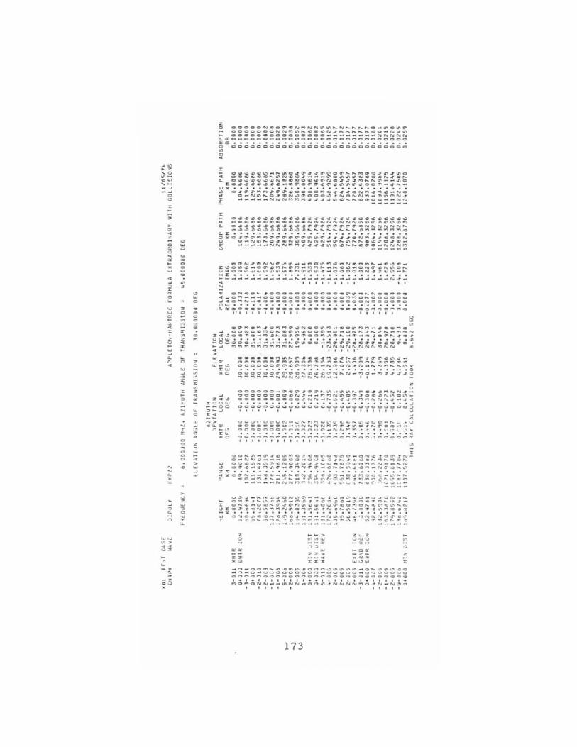
> ~
• z
o o ~
N <
" W o
, o
, 8 ~~~~~~~~~~~~~~~~~~~~~~~~~~~~ ~ QOCCOCCOCQOOOOO~_~_~ ___ NNNNN ~~oooooooooococccoccocoococooc
a: 0 •••••••••••••••••••••••••••• o occoocooocooccccccooooaooooc ~
~
• ~ =~~~~~_~~o~~~~~~c~~~~~~~ ~~~o 4 O~~~~~~~N~~~ ___ ~O~~~~~~~N~C~ ~ C~~~~~~N~==C~~~N=~~~~~~~ __ ~O ~O~~~~~~~_=~O~~~~~~~~~OO~_4~_ ,,,\0< ......••••...... •..•••..•..•
~ O ~ ~~MM~~~~OOCOM~8~ ~ONM.M ~_Na • C_N~~O.~N~~OOC~.NONNM_~~~N. Z _____ NNNMMM •••• ~~~~=~OC __ N N
~ ------• c~~~~~~~~~~~ •••••••• o~~~~~~~ • OOOOOOOOOOOONNNN~NNN~~~~~~~M ~ a~~~~~~~~~~~~~~~~~~~ONNNNNN~
O~~~~~~~~~~~~~~~~~~~DM~~MMMO Q. Z; • • • • • • • • • • • • • • • • • • • • • • • • • • • • ~~O.~~MM~~~~~~~~~ •••• ONM •• OOO N o O_N~~C.ON~ONNN_~~~~~O~.O.O_
~ ~~_~~ NNN~~4444~~~~~~~O_NNN~
~ ~~----
C~N4~NN~~~ __ OO~~~CN~o~~_~~e_ Z~O~~~O~~~~~~_~~~_~~~_ON~~N~O~
04cN~~~~~~~~~~~~. ~_O UOOON~~~~_~ ..... z: ••••••• • ••••• • •••••• • •• • •••• ~~ __________ ~ ____ ~ ___ ~ __ ~~_N~_ .. , , , , , , , , , , , ~ ~ ON~o~~oco~ccoeceC~~~~~Neo~ce "~e~~ __ ccooooooooeOO~~O~OOOOOo ~"O~N_ooooooeooooUOCCOONOOOOOO 0'-' ••••••••••• •• ••••••••••••••• ~~OOooo~OOOOOOOOOoo~oooon~o~~o
' " , , • " , , , , , I , , , ,
~ ~
O~~O~~O~~~~NOO~~_~o~~~_~~~~o ~ OCNo~~o~~~~~oO~_~ _ O~~~~~~_~cN
Z,,~o=~o_~~~o~~~oO~~~~~~_n '~o~~~o, 00..1 .... ........................ • • •• '" _ OOooo ~ ____ ~~~~oo_~~~~~~~~o",o~o. ~~ M~M~~M~~~N_ 'NNNNNNNN~NN = ~ , , 1 , ' "
.... oooooo~~~~~~e~~~ ~~~~~ ~~~~~ _ ~~ OO~COO~~~CO~~ ~ ~~~~O~O~'~~~~ .... ~ ~ oocooO~~~~~MM_~~ON'N_~~M~~~~
z: W ••• • •••••••••••••••••••• • •• 0 ~o ouooOO~~~~~~~~~N~N_~O_~~~~~O
" ,.~
z:o u w ~_oo ,-" ..
~M~M~~NN NNNNNN ~_ , , ~
a oooooO _ ~~~~~~~~_~~~~=4~~NN' _ ~oOOOOOO~N' __ ~~N~O~'O~~N~O ~ _
~~~~~~~~~~~~~ ~~ ~ ~~;;;~~~~~~~ oooo~OOOOOOOOOOOOOOOOUOOOOO~ 1 , , " ., , I , , , , , , , " <.)
" C O V <' U CU~_~~ M MO~U~~~~~ U O _ ~ ~ .• U OOOOOCOU __ NNNN~~~ ~ ~O~~~OO __
~~~~~~~~~~~~~~~~~~;~~~~~ ~ \ ~ = "'" 0 0"'" c 0 C' c> "" 0 ....,..,"'" 0 c> 0 e C Q 0 Q . , Q 0 "" "" c '"" , , I • , , , I , , , , , ,
O O~~ _ ~'~~Me~ee ~ O~ ~ O_ON"'TO~~N! O _ N~~ ___ Ouo_ uu ",e~~'~~~~~~M O ~
W oo", ~ ~~~eNo~O"O~ _ N~"'oM~N __ ~N ~ U~ ·O_'M~~_~MN~~_"'~~ ~ ~"'M_N~O~~ z't • •••••• • •••••••••••••••••••• "~ O~ N __ ~ ~ _~~O N ,~ e"' M_O'MO Q~ _ ~ ~~
Q ~O_M~~_'~_T ~ ~ ~N ~ "' M~MMn~ N~C O _____ N N~ M~N. M~44 ~~ .~~ r· ~ ~~ ~ :
O~ ~_~~~~ON~~ __ ~~O_~~O_~~O~ N ~
O~~'~~ ~ \~~_~"'~T ~ ~ ~ ·O _ ~",,~~o~ ·ft ~_ X o~~_O~~~~~M~~",o~~~c~o~~~ ~ ~~N ~z:C~ft~~~MMN~OM ~~ ' N O~~~O~O~~OO~ -~ . . .... . . ... .. .. . . .......... . .... O N C~ ~~~~~~' ____ N~ln ~~~NNN~ ~ ~~
z: ~ .~~~~:~~~!:==~~~~~~ ~ ~ ~!~~!
, -- > ", ~ 0 ~_ W o w ·.::t -- ~ -.-, , 0
W _ O ~ ;!! ==;; _z ... , ~~ x"(""!"
~ r.r:>: W~W
_ ~ _ OO~~~~I~~~DOO"'~~~ I~_O~ ~ ~ ~ ~O _~_O_oOOOOOOD~_OOOOO_o~OOOOO
OOOoOooooOOOO~OOOOOOoo~OoOOO
,.,. ," "", .. ,"""., ",,. ~OMCNN __ ~NN _ OO~'NNNN~O~N _ N~O
, '" I , , ","
173
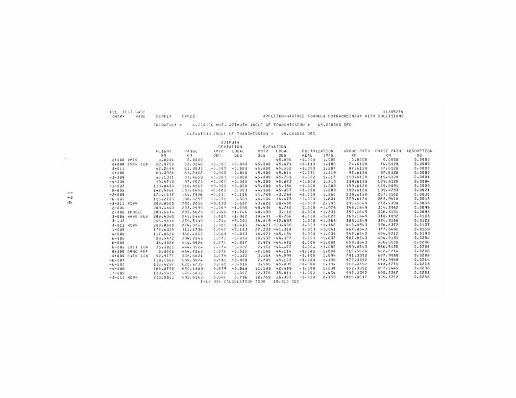
'" TEST CASE 11/0517'0 CHIl.~)( w~"E OIPOlY fXPlZ APfLETml-HART~EE FO :~HlJlA EXTR:AORDINA iH WITH COLLISIONS
FI<EaU[ ,'j(.Y b.COQJ~G MHZ . tZIMUTH ANGLE OF T~ANSHI SSION 4s.000nOD DEG
ELEVATr~~ ANGL~ OF TRANSHISSION = 1t5.DOOOOO DEG
AlPW T>i !lEVIA TI ON ELEYATION
HE r;:;H1 °A .~GE XHT P. LOCAL XH T ~ LOCAL POLARIZATION GROUP PATH PHASE PA TH ABSORPT ION
'" !<M OEf, OEG DE;'; OEG REAL tMAG '" '" DB 0"000 XHTR O.OOH: Q.OO OO 45 . 000 -0,000 1.000 0.0000 0.0000 0.0000 0.000 OUR 101\' 52 . '315'1 52 . 32"0 -0. ; 0 ~ - 0.000 45 . 000 1+5 ... 71 -0.113 1.1 00 74.&126 74.6128 0.0000 ]-011 oZ . 24·}Q &1 . 3530 - J.~on - 0.0 aD ,*5.000 45.552 -O.O5~ 1 .207 87.6128 87.b 126 0.0000 0+ I) oa 69 , J"2(: &~ . 2802 O. ~ 0 0 0.000 .. 5.000 .. 5.bI4 -0.021 1.219 ':IT.blza ':17.6 126 o.aooo
-j-JOq i6.1331 d3.it&S'1 - O . 1(j~ -0. 000 "5.000 .. 5 .751 -0.002 1.217 11':I.b128 119. &126 0.0001 -lo-\I J8 "9.47 .. 3 'l7 . 2010 - O. JCC -,). J a oj .. 5.000 45.d73 -0.000 1.213 139.&126 UCJ.6125 0.00010 -1- 0Jl 113.d433 110. II8£; ~ -I). 'l 0 C - 0.000 45.000 45. H6 - 0 .000 1. 209 159.&128 1 59.60 cl1 0.0009 5-0J~ 142.55of: 1311.045" - 0.002 0.003 .. lo.'J80 .. 5.d57 -') . 000 1.20'l 1 'l'J.&126 1 'l'J .10 233 0.0021 - -2-005 I1J.I0H 1&,,0762& -~. il g - 0.10& .. 4.789 .. 3.266 -0.001 1.2&0 239.0128 231 . 3102 0 .0 030
-J &-Jil5 133 . 2703 130.6257 - J .'~71 0 . 369 .. lo.1i1 .. J4.o7J -J.OOJ 1.€:H 279.b126 2&8.91018 0.00106
"'" -3-iI11 RCVR 200 .i1000 700.2014 -Jo1]2 II. &07 .. 3.622 26 ... 80 - iJ . OO~ 2.2'l3 295.1649 278.4396 0.0056 2 - 00" 209.011 .. 3 233 .25<;9 -0 . J 6 Q -1. 590 40.lo 3& 4.180 0.000 -1. <;76 3 10 601&109 JO Io. 3962 0.0095 2-il06 AP OGEE 20'1.68J .. 23~ . 8629 - 0 . J .. c -1.7 .. & .. 0.109 3.110 O. OOJ -1.631 35201649 30603131 0.00CJ8 3 - 00:' IojAVE REV 20~.4300 24 1. 0~b9 (I . ~21 -1. 9i12 J9'''3 1 -0.26& i). 0 Oil -1. 623 360.1649 3 1 0 .1 892 0.0103 _3- ~,)7 2u5 d&lS 259.5H9 ,.; . 24" -2. 00 1 36.11 19 -12.692 0 . 000 -1.266 366.1649 32 ... 3tH 0.0122 J-011 RCVR 2G~.OliOO 774.371:18 J. HS -1 .4 15 34.427 -23."56 J . oo~ -1 .142 4 1 0.6543 336 . 837Z O. 0 137 1-005 172 . 6329 111.8136 'J . S 47 -0.183 21.233 -41.316 0.00 ] -1.041 4&7.d543 317. &491 o.01&CJ 4-00& 117.8':> 20 3&'; .;' 6liO J. '> &~ -0.033 1&.021 - .. 50154 ~.OOJ -1.031 547.8543 454 . 521 2 0.0 193 &- ilO" 119 . 5472 394 . 264'3 J. <; 7 ~ -0. OH 10.932 - 44"'127 J. 00] -1.G32 587 . 6543 .. 94 . 513 1 ~. 0204 6-0iH. 3d . "02!) 444.9524 'J . " 74 - 0 . 027 2 . 976 -4 .. ... 72 il.004 -1. 000 659.8543 566.5130 0.0206 6-~0" EXIT 10,", 30.3021: _ .. 4 . 952<0 0 . :; 7 ~ -0.027 2 . '178 - .. 4 ... 72 il . OO .. -1. GOO &59 . 65 .. 3 566.5130 0.020& O+JOO GR.NO REf 0 . 0000 <'81, .7 ilbO J.57& - 0.025 - 2.t ~ 0 4 4.11 .. -o.o~] 1. 000 715 . 5&2& &22.2214 0.0206 0 +000 E~ T K ION 52.'3177 3311 .6621 O . ~ltl - 0.J22 3.168 44.599 -'J. 105 1. C '34 791.33CJ2 &97.9960 0.Ol06
-&-007 l1(1. 1 (i6~ <;,15 .3 574 O, "!H -0.020 7.7as 1,5 .1 03 -~.oo~ 1.1"6 672.3392 77e.9960 0.02 14 -6-007 13 d .4~ 'JI t:Z2 . ':IrJ<; ~ .5111 - 0.01& 9.566 .. 5 . 0':15 -0.000 1.19 .. '31203]':12 616 . 81 7 .. O. liZ26 - .. -006 165.6750 tSn .166'l 0.5 7~ - 0.0001 11.1 '39 "2.~69 -J.OOO 1.230 952.3392 857.2445 0.02 36
7-005 I dOl . 5Qj':i (,7& . 0632 0 . '.>72 0.057 12.376 35 . 811 -0.001 1. 434 99203392 690.3307 0 . 02 5 2 -3- Hl RCV~ 2~O.OOJ': ';H .5163 'J . '-''of 0 . 796 12.71',9 2&.'153 - O.OOil 20159 1015.6617 905.3752 0.02&6
Trl IS ~Af CALCULATION TOOK 10.310 SEC
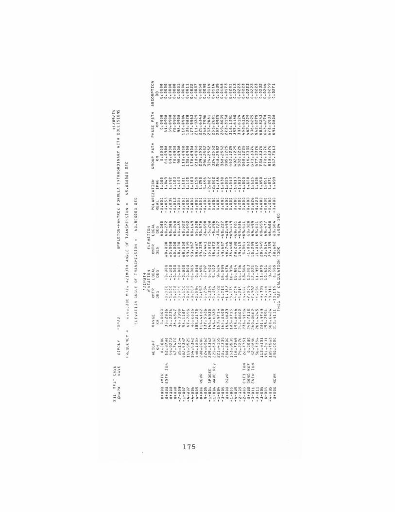
.~ . z ,0 .~ g~ ,~
~~
"~ 0 u z >
z > ~ · z 0 ~ 0 • ~ >
· -0 z ~ 0
" ~ U
~ ! z · z ~ w -• • ·
N
~
> -C
t
.. .> ., ~ Z
> • ~ X • < .Z ~U
>
u w 0
0 0 0 u
• •
z 0
~ • ~ • ; ~ >
" 0
w ~
0
~ z 0
= N <
Z
u g
~ · 0
> U
" W 0 0 · • "
o •
> w -. '
z ~ ~~~~:~:~~~~!!~:~~:~~~~~~;~~ ~ QoOOOOOOOOO~""_"NNNNNNNNNNN
~moCoOOCCOoCOOCOOCOOOOOOCOOOo ~ <:I ••••••••••••••••••••••••••• o OOOOOOOooQOOOOOOOOOO OOOOOOO ~
~
z ~ O~~~C40~~M~_"~~~"04~~~~~~MC ~ OOOOOON~N~~~~N~~Q'~NNN~~4~MO ~ o~~ ~~~C~MM~~~~O "M ___ NN NNN OC rOOOOoOO~~~~NNOCM"~~~NCCC4NO
W >l •••• •••••••••• ••• • • •••••••• ~ O"~cccC~~~cMM~~MO~hMNcNMMC" ~ ~~h~"Mh_N4~~~~h "~~ ~OM404h~ ~ _"_N NNNNNNNMMM44~~~~~~ • z ~ OOOOOOOOONNNNNN~~~~~O~~~~~M C OOOOOOOOO~~~~~~NNNNNMhhhhh_
~ O~~~~~~~~~~~~~~NNNNNMMMMMMO OOOOOOOOONNNNNN __ ~ __ 'MMMMM~ 0.. z: •• • •• • • • ••••••••••••••••••• ~>lO _ ~OOOOOO~~4 40 0~NNN~~~~~~~~ C ~~~~~~~~~~NN~~~~~~~~~~~~~~ = ~~~NNN~~~ ~~33~~~~~~ ~ ~~ o
C~N~~~c~ec~NN~c~~~~cc~ec __ ~ Z~O~~CCOD D~ ~~CC~~N_ ~~ CON~~~~~ U4~Ou~ __ ~ __ N~Oc_ooOOOC~~COOC~ ... :a:: ••••••••••••••••••••••••••• ~ ... __________ ~NN _____________ ~
~ I I •• I •• , ,
~ ~~I~N _~c cc~Ooco~o~~~oo.~ ~oo o
~~O~~_oooOOOOccOOOCCCCONNOCOO
~4 00QODOOOOCOOOODOOOCOCOOOCOO
C 1,01 •••• • •••••• •• •• •• •••••••• •• ~=OO~OOOOOOOOOOOOOOOOOOOOOOO~
••• I I I I I I I I I I t I I I I
~ ~
cN~e~NN~O~G~~~~~~_~_O~_~~C~
~ O~C~~N~~~~~~~NN~ _ Oe_N~ _~~ O~~ ~~~ON~~~~~_~~~~~~N~r~~~~~~~~~~O
0<..)1,01 • ••••• ••••••••••••••• ' , ' • • •• 0 "'CQOOOOCOOO~O~~~~ON~~~~~~~~~~M. ~~ .O~~~QD~~~~N I 'M ~Q.~~~~.~~.'O.G ;! , , , , I I ,
~ ~4~
~o uw ~~ oo 0 >" z<
COOOO~~~~_NNe~~OO~_~~~~~~N ~COOO~~~N~~~N~~~ __ ~~~ _~_ Me
oCCOC~~ ·OM~GGO.~~N~~CNo~~ ~~V •••• • ••••••••••• •• • •• •• ••• a OOOOc~~~~~~~~~ee~~~ _ o_o~~oo ·oo. ,O'O~~~'~'~I~'~~r~MN _ I __ NNNM~
z o
OOOOOO~G _~NN~ ~~~~~~M_~~ __ ~'" OOOOOOO~~~OON~~~O~~ON~ ~ OM~~ OOOOOOOOG~~~.O~~G~~OC.O.N~4 ....... .... ............ . .. ~ OOCOOOOOQ~~~~ ••• ~~MMN __ c~e~ I , , , , .,' ___________ <..)
~ . QOO~WQ~~~~I~NO~M\~~·,_~h~~~a~U ~ ooooCO~~~~~N_G~o _l o~~MI __
~~~ ~':~~ ~ ~ ~~~'~~~~~~~~~~~!~~= oooonooOO"~OO __ M~~C~~~~_~O~ , • , , • , • , , , , , , , , , I • I , • , , •• ._ ..
z O~~~O~~.~N.oorO~~.NO~N~~ _~ __ ~M~~~O~M~O~~M_OM _I O~_~~~~N_
!,oj O~N~~_~~ __ ~~~~~~~~~~_~N~~~_ ~ CNN~~_~UN~~.~~O_~~O~~O~~NO~
7'1: ••••• ••••••••••••••••• •• • •• ~yc,~~~~~~,O~.~ •• ~~~~~N~gQ_ ~ ~~M
~ Mn~~~~~c_~ •• ~~.~~ _ M~~.~~C_ ._ __ _______ NNNNNNNn~
~~NOt~~NU~NNN~~~~~~_g~~ __ M~ O~~~.~~N~'~o~.~~no~~~~~~~~~oo
X O~N~MM~~40Q~~_~O~NN~CG~ __ ~O ~rn~~~ _ ~~~ _ O.G~~NO~~N'O~~~N~C - y •• •• ••••••••• •• • • •••• •• • ••• ~ ~N~~~~~I~O~~~_.O~~~OCN~~_~C ~ ~~~~c_~~~NNNNOC~ _~ N ~~ _ ~~~ ____ NNNNNNN __ _ __ N
< Z" Z 0 ~ CU~
U" ~ ~ ~
w ~. ~ ~ > 0. Ow ~ > 0> > z >
~~ u .. ., ~~% U • .z ~ "ow ~
O~OQ~~ ~ ~~~~314~o~~~,~c __ ,n.n~g Oooooo~ooaoooaOOO~"OO __ CC~o o~~Oaa~aOoOOcOOOoO~~OooOoOO .............. , • I .... , I • , .... I , .... , , , , , ... aoaO~ _1140~ ___ M O _4 NNO~~M.t~
I. , , , , " " , I '" ,
175
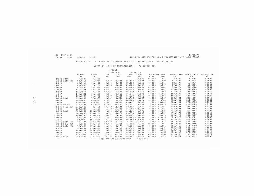
<0, TES T C ~ SE 1110517r. CHAP)( WAvE il iF OLY E: ){PZZ APP LET ON-HAr..TREE FORHULA rxTRAOROINARY wITH COLLISIONS
n~OU ('lt y 6 . COO~OO ~ .... z, AZIMUTH ANGLE OF TRANSMI SS ION IoS.CDooaD OEG
F LEV~TIJN ~NGL f OF TRAN SMISSION = H.ODOODD OEG
t Z 1 t'u T H il [VUTJON ELEVATION
tiE I GH r f\ llrl(,E nlHI l OC Al l(MTR LOCAL PO LA RIZ ATION GRO UP PATH PHASE PHH 48S(lRP T ION
'" '" ;:lEG OEG DEO OEG REA L IHt>G K" K" 08 Oi 000 )(HT R O. Of.iJO O. ':,)0 Il 75.000 -0. DOl 1.GOO 0.0000 0 . 0000 D.OOO O uiODa [NTR l Ot- 52 .9blt b 1 ... 0 7 5 9 - 0 . 00 0 -0.000 75.0,)0 75. 1l7 -a.allt i.IlZ] SIo.0371o 510 .837" 0.0000
- J - 0 11 oO.71b~ 10 .11 tO - il . O DC -0.000 75.000 75 .110 5 - 0.0110 1.0410 62./lJ71o 62./13710 0.0000 -3-011 65 .5~"' '' 17.3H8 - 0 . CO 0 iJ -0.000 75.000 75.156 - 0.00 II 1 '(l107 67 .11 3710 67.63710 0.0000 -2-0011 87 . 785~ 23 .1901 -O.DOL -0. 000 75 .0 00 75.209 -01 . oo~ 1. Glt6 90.83710 90.6374 0.0001 -1-~07 IJ7.1 217 Z e . 2 1 Zit -,J . u DC -0.000 75.0')0 75.253 - 0.000 loIl47 110.il371o 110.6365 0.0005 -9-007 1 2€l . 455tJ J3 .20 25 - 0 . 00 1 O. 000 71t.9'}9 75.279 -O. OO~ I.C4£> 13006374 130.8161 0.0013
'+-007 1 .. 5.£>921 3e .l'+ 96 - 0.007 - 0 .012 74. 9~" 75.166 - o. a Dol l.tllo7 150.637" 150.£>143 0.00 19 3-00:' 17d.77 37 .. (; .6 08 1 - 0 . !1 £>2 - 0.32 1 7 ... nO 73 . 849 - 0 . 000 1.057 166.a37" 183 . 5011 0.0030 .... O+OilO RCIIR 2)O . J O)( 52 . &IP5 - 0 . Ho2 1.3310 '''.7d3 71.357 - 0 . 000 1.067 213dl81 202 .12e" 0.00"6 ...., 6 -00 5 2210 . ~1o .. C 00 . 6£>'15 -1 • ., 77 1.370 74.379 52 .074 -0.00 0 1.5&8 2&& . 9181 2 17.2922 0.0091
a- I- DO .. 230. 7 "if> 1;)(;, 1025 -1. 7 11 -7.3':10 73 ... 32 15.5&9 :1.000 -9. 825 306.9161 220.0213 0.0127 1-004 APOGEE 230 dl S3 o ?55G .. -1. 511 -8. 853 73 .111 8 . 2l1 J. 000 -J. e 7& 314dl81 220.4&73 O.Olllo 9 - 0H lIol II:; RE II 2loJ .259;; '0. 76"1 - ')'~22 -11.181 72.J07 -10.10 74 iI. 001 -1 . 95i1 330 . 9161 221.5762 0.01" 7 5-:10$ 222.0226 ~ .. . 262:1 1. ; 1,3 -110. 20& 68 .50e -29.337 !j, 0 0(1 -1.143 376.9181 228.5 798 0 .01 81 0+000 RCIIR 200 . 000(0 100.62<;7 S . 5 ll -13. 5 43 01.084 - :'&.1075 0.000 -1.0210 10310. 96 73 2109.21"7 0.0232 2":"10 5 161.ob'll 13/0 .6131 3 • .,,.2 -11.276 ,,9 . 25& -55.293 0.000 -1.007 491.9£>13 291.7604 0.02&3
- 2-0015 129.0135 1 'j5 .6~6" 10 . J 9 2 -9.7510 J8.6&1 -56 ... 07 J. a a 0 -1. (j0& 53 1 .9013 330.5977 0.0275 - l- a O£> ')S.7312 In. Ide s 11. ~I! ~ - 8 . 5&2 27 .405 - 5& .2 82 0.0001 -1 . co£> 571 . 9673 370.5601 0.0289 -1-00 & n2 ... 97/o 19G . 950d 12.?2~ -7. &20 tb.'t63 -56.0810 ~ .001 -1.00& 1'>11.9673 410.5600 0.0292 -1- 006 ExIT r ON 23. J;, 2 C1 ~20 . 990S 12 .192 - 6 . ~56 1'>.551 - 55'8f5 ~. 00 J -1.000 &51 . 9673 1050.5600 0.0292
OtOOO GR N" REf 0 . 0000 ? .. C.75b9 13. <;':>7 - o.ZcU -1.0 83 55.706 - 'J. 00 a 1. 000 £>67.41059 1066.0386 0 . 0292 0 +000 EN T~ I ON 52 . 96.1b 2 7 b . JIo 1; J 1" . ]7 ~ - 5 , "1 ~ 9 .5 65 56 . ~27 -3. 069 1.0b4 7~1,"563 550 .04e9 0.0292
-8-00' '17 . 0257 ?qb . e Io 6 ~ I/o. 7 6~ - 5.'165 1/o.7 d5 56.231 -11. 00 1 1.134 792.10563 591.01069 0.0293 -6- 00& lZIl . J0 97 l2e . Sllt .. 1'.; . 121' -,. .72 1 16 . 9 .. 6 56 . .. 0b -!l.000 1.1-JO IIJ£' '' ~ bJ bJt.OJ.,b O.O JOJ
2-005 153 .37 H 310 " . 0&24 1'> ." 2. -4./0 25 22 .35 3 55. ~O .. - J.ooa 1 .13'> 872 ... 563 &70.52(,0 0.031", 4- 0J5 la].o}'1l~ 3E-Z . 9 J72 15 . " 7 '; -". 2 14 2 ,..q15 51 . H4 - 0 . 0 00 1.19, HZ./oS63 705 .8795 0 . 0327
-3·011 ~CIIR 200 .0 0~L J7 .... . 35{:7 1 5 .7')" -l. 6"" l5 .9H 45.37& -0.000 1. l710 937.9,1' 7 2 2.6911 0 .03 103 THI S ~A' C Al CU L4TI ON TOOK ').&24 SE::
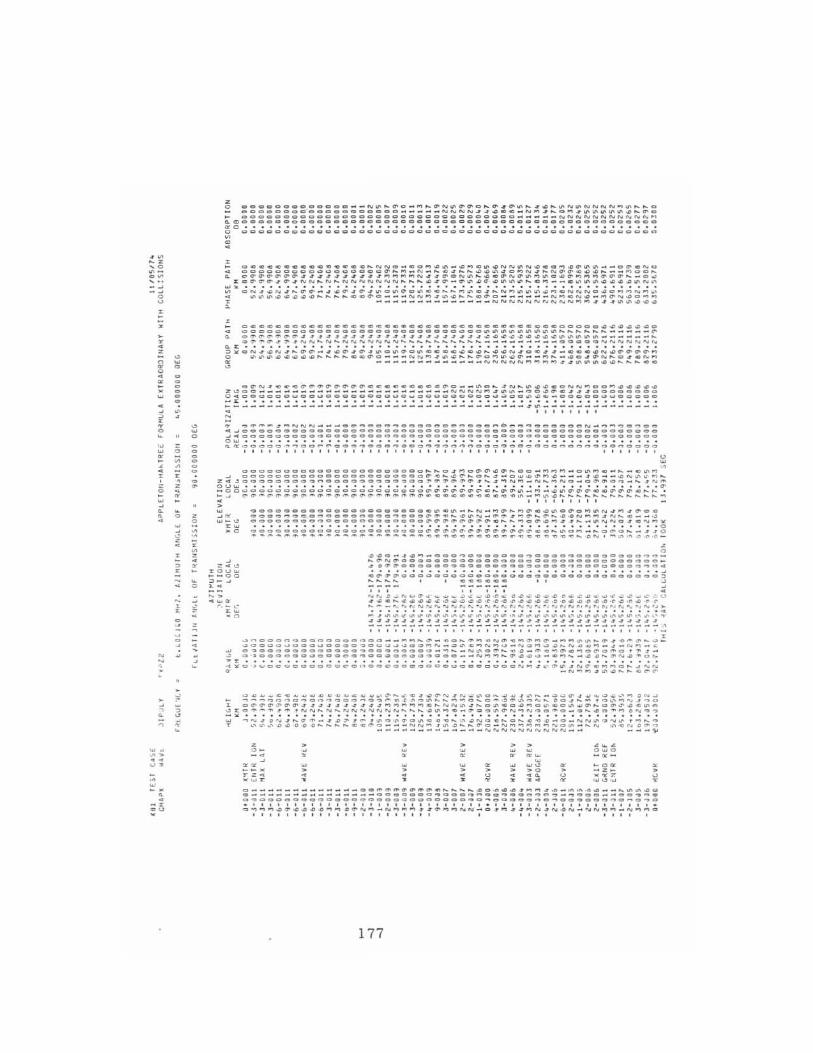
, " .z ,. .-
~~ - " - " • 0
~
! z
" ~ ~
~ ; w 0
~ , ;
~ • " 0
'" <; w 0
~ " 0
" " ~ r , ;; ~
~
w
~ " 0 z 0
w
" " " " ;0
" ~ z 0 z r
" c
i 0 z
~ -~
.; -, , .:. ..
" " ~ , • 0
;; ~
w " ~
>
>
." w
" r
00
z 8 ~~~~~~~~~~~~~::~~=~=::~~:~:=:~:::=~~~=~=~~::::::~~ ~ COOOOOogcoCaoOO=o=OOOO=O=O==== O= O~~ _~_ NNNNNNNNNNN" ~m==O=O=OO==ODOO=CCOC=CCCOC c =cc= ==Occ =cccccoccOccccc or c •••••••••••••••• ••••• • •••••••• •• •••••••••••••• •• •• ~ ccocccccccoocccccccoccccocccccocccooccooooccOcoocn
o . r o~ee~e~eee~~~ee~NNo~ec~~~ _ ~Me~~NN~N~eOM~~~~ ~_ o~cNu
4 COOCOOCCO~OCOOOOO~~~_N~~~j~~~~~ ~ OMN ~ ~N~~~~~ ~ __ MOO~ ~ c ~~~~~~ ~~~~~~~4~~MM~MN~~~O N~ ~~C~N~~M~o ~~M nn~ ~~~ _ o~
~:~~~~~~~~~~~~~~~~~~~~ ~ ~~~~ ~ ~~~~~~~~~~~::~~~~~~~~~~~ W ON6~N.~~~_.~~.~.~o~~o~eC~~M~C.hNM~~~~nCNNNo~onnNM~ ~ ~~~~~~~~~~~~~~~O ___ NN ~~~~~~~~C __ " __ _ N~~N~ _~~ N~C~~ r ______________ NNNNNNNNNN~~~~~~~~~~
" o~~~~~~~~e~~~e~~~~~.e~e~e~e~~e~~~eee~ecocac~~~~~~c OOOOOooooocoooccccaCCCOaOaOcO~~~~~~~~~~~~ ~~~ _ ____ ~
~ o~~~~~~ 4 3~~~~3~~~~~333~~3~ ~~~~~~ ~~~~~~~~~~~ _ _ _ ___ ~ ~~~~~~~NN~N~NNNNNNN~~~~~~~~h~ _____ __ __ OOCCONNNNNNN
Q. :II: • • • • • • • • • • • • • • • • • • • • • • • • • • • • • • • • • • • • • • • • • • • • • • • • • • ~¥ON~~N~~~~_~~~~~~~o~~o~~ce~~e~h~~N~ce3~_~e.~N~~~~~~ o ~~~~~~~~~~~~.~~O ___ NN~~~~~h~a~~~~ __ ~~ _ ~C ~ ~N~o~eNM ~ _________ ____ NNNNN~~~~~~~~~~~~~~.~
O~N~~~~~~~~~~~~ecee.~.~~~c __ ~ C~~N~~~~mON N~Oc~~~~~~ Z~oo _ _ _______ _____ ____ _ ____ NNNN~ ~ ~~_~C~~C33~ocooaoca
OqCo~coc~ao~aaccaOac~c~coooocoocu~ca~~~ _o oooc~~oaaoo .... ,. ...................... " . ........... . .. .... ...... . ~ _____________ _______ _ ____ ___ _______ 3 ~ _____________ _
;! I , , , I , , ,
; ~~~~~~NNN ___ O~~oo~~ooaoeoe~ooo~6oe~ooaOOON_~~OO~OO ~;~~~~~~~~~~~~~~~~~g~~ggggg~ggg~~ggg6ggg~gggg~6ggg~g ~~~~~~;~~~~~~~~;~~~~~~~~~~~~~~~ ~~~~~~ ~~~~~~~;~~~~~~~
, , , , , • , , , 1 , , I , I , I I , , , , • , , , , , I I , I I , 1 , , , I I , ,
~ ~
oooccooocccoooooaaaaCO~~a 3 MO~~~~~OO_MMM _ C~~~ _ h_~~M ~ coooeoococoaCCCOOOOCOO~~~~~hOh~ _ O~~~M~ _ _ _ 3~ __ ~N~VMh zq~ooaaoooo~~OCOOOO~OO~OO~~~~~~~~~~N~_Nh~NO_O~~C~~~~N~ OU,,-, •••••• • ••• •• •••• •• •• • ••••• •••• ••••••••••• •• •••• • • • ~ ~O Ocoocccooooaoc=cocococa~~~~~~~~ ~~~~_M_~~~~ ~~~~~~~h~ • ~ ~ ~~-~~~~~~~~~~~~~~~~~~~~~~~~~~~~~~~_M~~~~h~h~~hhhhh~ ;! I I , , , I , , ,
" Z<tl!l I:OUW ~~ OO
i.':;;~
N> <w'
r. ~ L'
~ :;;
~oaoooooococcc=coaoooe~~~~~N ~~ ~~~~~~~O~C~~N~M~~C~ QOOO~o~o~oaoancoa ~ oaO~~~h~~N _~ ~~~~~~~~·ON~~~N~~ __ .~ =oooaooo~ooaccaoocooo~~~~~~~~~~~~C~~~~~h_~NNC~~NM¥
. .. ... . ............ - . .... ....... ....... . ....... . ' 0 0===oooo=ooc==oca=coc~~~~~~~~~~~~~C~h~0~.~=~ah_~40
?-~-~~~~-----~-~--·--~~~~~~~~O~_~~~~~~~~ON '~ ~~O"·"_
" o ~~a_~~~_occ~aooo=oo~oaac~cooocaoc~~_
~~N~oc=a=coooQo=c=ooooeocccccaaooco_ ~o~~o=acoooooo=ocoo=cooc~COCoa==o~ o~ .. . . . .... . ........... . ...... ...... . ~ c~~~aOOOOOOo==ooocc=aooao=aaaaaaoao~
777h I ' 77:777 ' I ~ NN~~~U~~~~_~~~~~~O~~.~~~~~~~~~~~~~~U
3~~h~~~~~ ~~~.~·~~~~~~~ ~,~·o~~~~~·~~.~"r
~~ ~ ~~~~~~~~~~~~~~~~~~~~~~~~~~~~~~~~: ~~~~~~w~~~~~w~~~~ 'n ~~~~~~~~~~~~~~~ ~~ ~
!!!!!!!!!!!!!!!!!~!!!!!!!!!!!!!!!!! , , , , • , , , , , , , , I I I , , , , , , , • , , • , , • , , , , .....
y ~~oo=~~oaoaooc~oC __ ~~~~_~=~~~~N~~~~~~ _ ~M~~~~~o~~~u _
~~Og~voo=uao=c~OQU~UOOMN_~~Q~N~U_N=MU~hNU~M_4_NM_~
O?oooo=caoooaco=0=oa~OU_~~ _ N~O~~~D _ ~~~~~~a~a~O'~3_
~:II:~~~~~~~~~~~~~~~~~~~~~~~~~~ ~~ ~ ~~~~~ ~~ ~ ~~~:~~~~~~~~~ .~ '« '" ~ We':' 0,,", gQO 00<:"'0 0>00 QOO coo 00"'", 00 '" <> OoN~ ~ or ~~ ~ N<1'.,.., ~O'" j "'N ~ _N~"'~~~~"' ~~~
O~~_C~~~~~~~~~~~~~~~~~~~N~N~~O~~~4~~_OU~4~~~~~~ON~ ~-_~O~Q~on~~OC"O~_~~·~~~h"''''~O_O~~~~~'''~DO~hM'~~~'''j~C
~ =~~~~~~ ~~~4~4334~"' M~M~~~NN~~~O~~O~~=~~O~~~~Q~~~"~~
~~~~:~!~!~~~~~~~~~~~~~~~~~~~~~~~~~~~~~~~~~~~~~:~~~~~ w _"'IO",~~q~_~~~~~~~a~.a~~O~h~~No~ ~=~~ ~~_o_NN~~"'~''''h~ ~ ~~~~~ ·OOO~"'~h~~~~ " •• NN~~~~ ~~ <t'O _ "'M"'M"'~ NO~ _~'" ~~ND~~ _-_~ ___ - •• ___ "'N"''''N'''NNNN__ _ __ ~
y > > > > > .. " 0_ " w w " owo > • • • .. -.-.
.~ w " w . ~ .0 ~ _0' ~ > > > >0 -z_ T;:", . ; . 0 ; ;e. ~ .. .y7. 0 < w r , > • • .,<,!I • ., • o _ ___ __ • ___ __ _ aO~~~.<t' ~~.,~ ...... h~O~~~I~~~. _ 'n~·n~ __ ... ~~~~
~~~~~~~~~~~~~~~~~:~~~~~~g~:~~~~~~~~~~~~~~~:~~:~~~~ .. , • , , , I , I , , , I • , , I I I , I , , , I I I , ... , I , , I , , , , , I • , , I I I , , .. O.., ..,M ~<t'~~~~M~O~NM _ N~~ ~~3~MMNN_O~..,3~~N~N ~N _ NN..,~ _ N~~O
, , I I , I , , , I , , , "" , , I I , , , I " I I " " ,
177
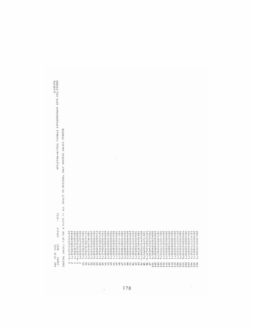
, ~
~z '0 ~. o~ ,. - " 0
u
= • > ~ · z 0 « ~ ~ -· ~ 0
" ~ ~
~ , · z , z 0
~ • ~
N
" · · " 0
" 0
W W
~~ U .
-W -. ~ _z
oU .
u ~ -Z
« • ~
" " · > 0 • ~ z 0 z >
" z 0
~ , 0 · « z
~
~ " " " " · ~ · • • ~ z
• U
M W
; · >
" · Z
OM _ ~C_O_N~MQ~03 _ QN~ _ OO~O __ O _ ~NON __ oNN _ NN _~N __ NN O OOcOO UOOOOO~OoOoOo O OOOOOOOOO~OO O~ C = OOOOCOO ~~OO
~OOO~O~OO~~~OoOOOO~OO~~OOOOO~OO O ~~OO"OO ~ OO~o~oo .. . , .... ,. , ........... , ..... " ........ , .. , .. , ..... , .. .. .. , .. , .... , .. , ~O MO OO~ _ OOOO _O OOOOU~OOO~OMO~MMOO~~OOooooONo _ grN
~OO~O~~~oooe~ooooo~OOOOOO O ~N _ ~ O O~OOOOOO~OOOOO~O
O~O~~M~~OOONMOOOOO~OOOOOOO~ _ ~NOO~~OOOOOOOOOOQ~O OOU _ ~~N~OOo ·ONOoooooooooooo _ ~N _ oo~oooooOooooou~o UOO~OOMOUOOI _ OOOOO~OOOOOOO~ ·~~~OO~ ·~OO~OO,OO~O ·~ ~ ~
~O~~O _ ~ ~OOOM~OOOOOUOOOO " O~ 'A~~D~O~·~OOOOO .,OOOO~~ O
~O _ ~OO_~~OO~OOOOOOOOO~OOO _ .~~~~~.~OOOOOoo~oooro
OOM~o~~~caao~aaaoocaccC~CM~~~~oC~coccaa~aaQOO~O
~O_NaMa~aaoo~oaoo~ooOOOO~ _ ND~~ oo ~~aooooo~~ooo~~
~~~Mo '~~ _ ~ao_~ooooo~oooOOOeM~~~ ?O ~~O~OOO~O~O~O _M
OM~~O~~~OO?~~Oooooooaoo~o~~o.~~o _o~ ~ooooo~o~o ~~ .... ...... .. ..................... . .. . ..... . .... 7'n .o 7 ~~ - NNM -- ~M - ~ --- ~NN - N - ~ 7 ~ 7_ ~M~~ _ N ___ _ ~ M __ M __
_N~~~ _ ~~CN M.~_NM.~~~_e __ NM.~~ __ NM~O_NM~~ __ NM~~~ ___ NNNNN ~~~~~ •• ~~~ee~eee~aooo~ '~~~~~o~~~~~~ __________ NNNNNN N
178
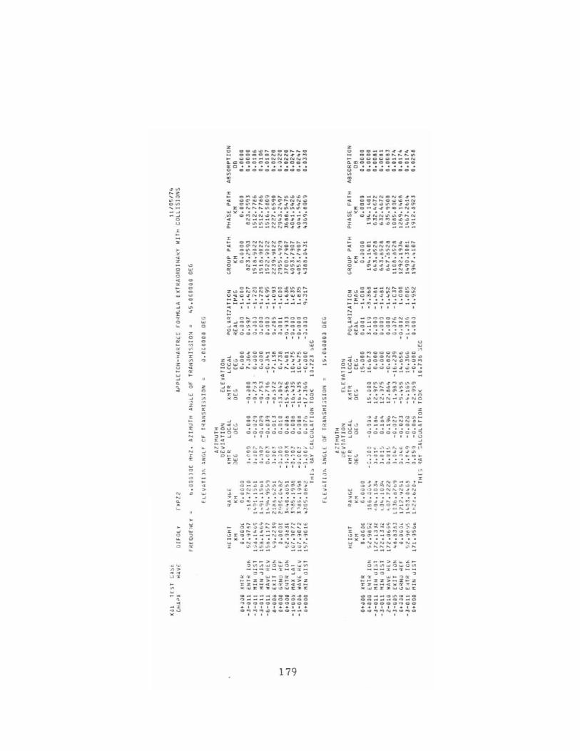
.~ ~z
~;: o~
- " - " 0 U
L ~
• > • • " 0 ~ 0 < ~
~
< " " ~ 0
" "' ," ~ ~
< L , Z 0
W
" " ~
N N
~ ~
~ 0 · 0
" '" "> • ur
," , < _z
~U .
~
"' 0
0 0 0 0
~
•
Z 0
:;; ~ r ~
~ ~
" 0
" , ;; z
" = N <
N C Z
u 0
~
•
>
~ " " 0 W ~
"
~ W o
o o o U o
z o
" u
z o OO'O..D ...... c:>O ......... ."
OC>CC>C>NNN~-4 ... ... c::>O ........... N"'NNt\j", o..<l:)ooc>C>oOO<;>OCC> 0<'0' •••••••••• o ..,<;;><:>000:;><:>c:>000 ~
~
z .... 0 ... .0.00"0 .... "''''.''', .. "" 00"...,.000"0''''(\1",.0 Q. O"' ........ CI"' .... ., ........ O
:z::e>"' .......... oD"''''''''''CI .... '" .......... . . ~ O~~~~~~::;:;~ J: _"I''''''' '" "'.0<:::1 C>.., 0.. __ ..oN"'", ............
z ... O..,"'NNN"' ....... ,.._ <C oO'NNNNN ... OO'" 0.. O"'CQClC"""'C7'C7' ....
ONO'C7'O""' ............... O 0..:1: ••••••••••• ::>"'c;> ... C>C>Naolt\O ...... ., o (\I ...... "' ... "'C>\I'I"'CI ~ ., ..... "'''',...''' ... 00,.., <.!I ...... _NN"' ............
..... o c", ... C .. .o","' .... Z"-'ONNNC7'C7'O ... ...., ...... O ... .., .... , ..... oI.IQQ>iJ .... ClM .... :l; ••••••••••• ...... __ .. __ .............. _13'
"" "" I I ,
'" 0 ......... .,"' .... .... 00<::1 .. ...JoC7'OOOc:;lc:>..,OOC> ...... ""0"' .... 0<:1"'0(0'0<:>0 OW· •••••••••• O:YogOOoC'>,=,Oco,""
" , , c:> .... OO .... e)CI .... "''''c
...J o,Doo .... ...,,..,<:> ....... <:> ... Z"'..,O..,,, .......................... ON 0<.)\01 ........... .... .... OClo ... gOa ... o .... coo. o-...J " .... _, "" < > W "~ , ... .... ..,
ZW XO
" Z< 0 rou ..... ~ .... o-:. " ~" z< N> 41"'~
0 " 0 zw xc.
0 ... ",.0 """' .0"''''''' C> ' /'I "' ........... .0'" ... '" "" ......... '" 0 '" 4 4 .... '>t ••••••••• ·0
~,;,~~,:,::~~~:::e , I' I ,
Z o
0~C"~""0"'''''''.n_ 0 ........ .......... 000 ...... 0000000000"" . . . . . . . . . . -, oo oooo oooo~ , , , ~
C'>t\.t\. ... , .. , '" "" .. ,.., .-..u OClOOOOOOcCl
'::C:O:;':; ':':~":!; C'>~,:>o",o""O'Olo'" , , , , ,
< 0<:> __ (7' .... "" .... ..,"" "' ...
% o
<:> .... .n ;:) .......... .., ..... (7' oJ' ~ ... c"" 'I' .............. 4'O~ ... :ICI ">
~ '01",_ """,,"'''''' __ 0
". 1: • • • • • • • • • •• -' ~'>t<:>", __ ~~~c>~,I"~ ~
Q' _ 17 · "' ... ..;<:>4"""".;0 • , ~ • .3_ ':·r ... r...,
.... --""""...,..,..,~ '~"" <1'oJ'""",o "''''NoD "" .... ·0"' .... ..,0.., ..........
J: c .... 44'_Nc~<;lClo;:l <.!):r",(J''''' __ NO(J'''''''''7' ... :roo: ••••••••• •• W o .... 'C""-eC"""N ...... 1'-
: ..... . ,;":::~4' -l':=;:~
"" __ >.tlo.;;!: > ... ::0 ..... ..., ... 0 ... 0_ ........ _ ... _Q::_,._~O!: ...
:::.., ...0 ':) <1::11: WI-:::Ieo. W ...... zz> _z ... ><>z rz .... ""><'Y~""""_ >< ' ... II: x: ~ .... <!O .... II::S-:I:
:;:::::::;g~:;~~g -.0000000=>00 . , , , , , .... . 0"""'"" <D ""c <:> .... 0 , , , , , ,
179
Z o CO ..... .... 4'4'."fOO
00.,.,., .......... '" .... 00000 .......... "" CL-a)oooooo<:>oo co: 0 ••••••••• o COOOOOOo;:lO ~
~
z ~ O ... N"'ONC>,z .... ... oO ....... O"""' _ N ~ 04''o£)<D '"0 4'''''''
:1:0"' 4'4' "'C>_ .... ." Wlo( ••••••••• ..... 0./'''' ......... '''0' ........ "" ~ .......... ..,"''''-r .. 'o£)<D"'<:> .... 4(7' <l. _ ... _ ...
z ... C ... ..,OO..,..,4' ....... ... <:>"' .... NN"'..,..,C;O a. 04''''''' ..... '''''' 0 ... 0_00..,.., ......... .,. a. J: • • • . " . • • • • ::o:ro:O~ ......... ..,NO ... o a-.,../'.,.0<1'f1'4' (J£ .... "'oD<D_N4'f1' <!I ...... _ ...
0.., ...... .... 1'-0"' .... Z <!IO"''''''",,,,,,,,,,,,,, OqOM4.l..tOOI(>Q"\ ....:1: ••••••••• ~ ...... ,., ...... -............. .0; """ , ~
co: "" a-O"O"'''',,"''' 4...00_0<:>01'-000 ..... 4.0 ... 000'""0..,0 OW , •••••••• a.~o..,ooooo .... c:> , ,
o .... oo"'""''''oDQ
:.l " -' O ... OON ......... "'OoD
Z4.<.!)o oDOO"'''''''''' 0"" o u ............. ... .... 00 ..... "'000"'4''''0. ~...o _ ... '--'_'0 < ,-> w "~ W ~ ~
0 ..... "',z.., ..... ~0' 0 ........ "'""",<D", oa- ... .,O'4' .... a-:roo:
<w _0
" Z<~ 'I: 0 u .... ....... 00
"~ " Z<
••••••• _0
"' .... N .... - ..... ./' .... O ............. , , , , ... Z o
·~./'J ,O ....... o ..... ... C., ... "' .... N...,O ... co ........ OOC04
" • " • " •• "...0 00000<:>00::::J , , , , ' U
" < <,,~ ~",~,,,,,,o,€O'a-<' c ...... _ 4' 4' ~ '" "'oOOc,""coc," •••• " •• '4
•..• "'<:oo~n"='OfY , z
C4'4'./''''a- ... .., ~I-o ./'.., .~ .... .D ..... ~Q
.... '='OCO"' ........... .... <!I cO __ I'-'I),J'ooD ?':I: • " ••••••• <>.lo(~ "'~~""",,,,,,,,,,,,,, It' ..,CQo .... _ c ....
... . , .. ~~ C'> ........ z:-
Q "" .... ,.." "' .... ..> w' 0 o"''"'-t/'....,O~ ... <D
r ~.., ... ..,oD .... O~'" <!Iro "' __ 0'"'0 '7'''' .... lo( •••••• • _ •
..... c"""" .... N'CO"'"N _ 1: "' ~~~~ \.. .. ~
OI: __ >;;!: .... "" ...
0 '1'1 ........ 00.;0<11 ..._ ... 3:_"' .... _ 00 ,
fICO!: W I-":lOC ...... 2:Z>_OI: ... z 1:Z __ ""><tr:>:_ >< ... r.::r:J< .... <!I .... :I:;
~C ....... o"'Q ... O 00_"'''''''0'0''''0 "00000"'<:>0 + • , •• , • , • 00 ...... "1 ... 0"'0
" , ,
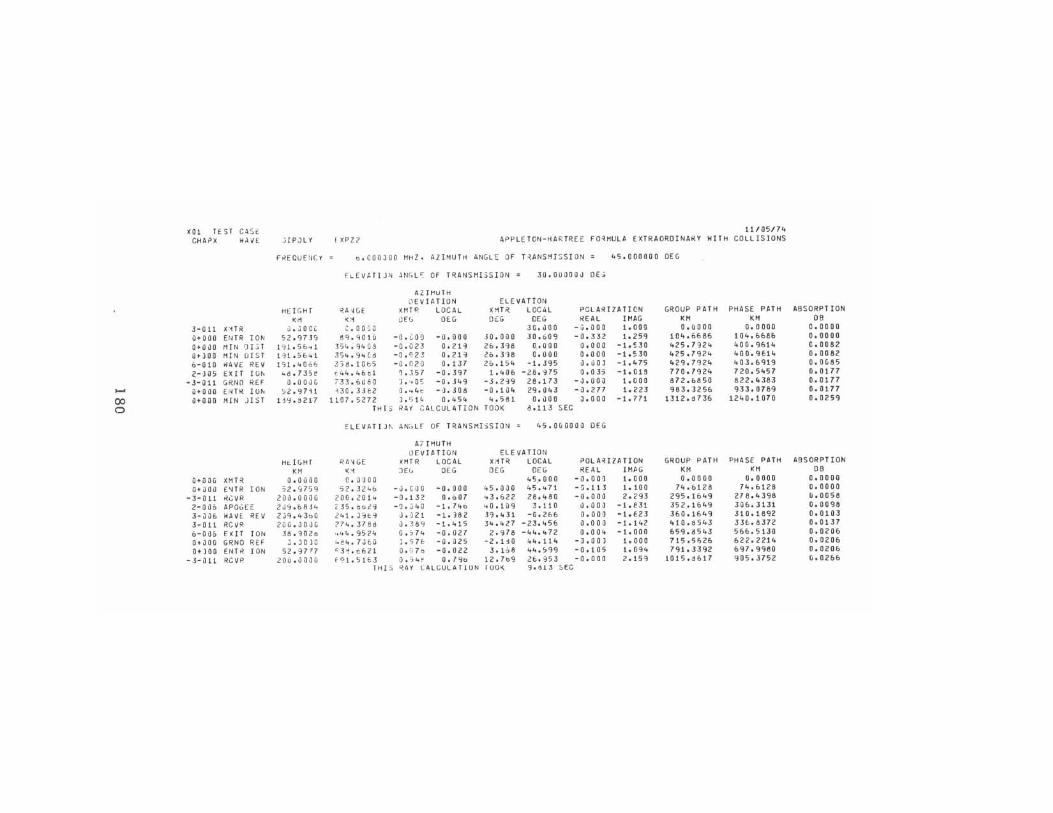
'"' TEST C",S<: 11105/71+
CHAi'X W.l.~[ JIPJL'f f XPZ 2 APPL[TOtl-HA RTREE FO~I1ULA ExTRAORDINARY HITH COLLISIONS
FI'IECuEllCr 0.006JOO MHZ. AZIMUTH ANGLE Of T~ANS~I SS I ON "5.000000 DEC,
fLEV~r I JN ~Nr,l~ OF TRANSMI5SION = 30.000011~ DEa
il.21~uTH
DEvIATION [l[V ATIOtl
ttEIGHT ~A ~ GE ~HTP. LOCAL xrHit LOCAL PGLAiHZATICN GROUP P A' H PHASE PATM ABSORPTION
" " ,," OEO DEG OEG RElIl IHAG KH KH DB 3- 011 ~ 'nR :l . } 0 C~ ~. 0 orie 30.ol00 - ,:; .0 aD 1.000 D.ooon 0.0000 0.0000
0+000 ENTR ION 52.'373<;' 1\9.<JOtu - C. COO -0.000 30.000 30.6(1'3 - O. HZ 1.25<) 10 ... 6686 104.6686 0.0000
0+0,)0 NIN 'JI'; I l'H.Sb .. l 354. '14 (HI - 0 . 023 0.21'3 lo .HS 0.000 0 . 000 -1.0;30 1025.79210 ItO O. 'H>14 c..ooel O+JOO MIN (JIST 191.5b41 3S4 . 94(d - 0 . ~ Z 3' O.2B 26.3'18 0.000 0 .000 -1.530 425.7924 40D,qUlo 0.0062
0-010 \oI",VE REV Fll.40':';o, 3~8.1Gb5 - O. OZO 0 .137 26 .154 -1. J95 ~. u 0) -1. 4 75 r.2'3.7nr. 1003.6'31'3 0.oti65
Z-'liI5 E~ IT '" "d. 7 3:;~ t;41o.46e1 ~ .357 -0.3'37 1.406 -26.'H5 0.03, -1.013 770.7n4 720.51057 0.0177
-3-011 GRrlO REF O.OOUO i3l.Quao "). '. O~ -0 • .14'3 -3. 29'3 28.17 3 -J.OOil 1.coa 872.6850 822.10383 0.0177 ..... 1i*IlOO UH~ 101\ :'2.Q711 ~3Q .l H2 ~ . ,.Iot: -;).308 -0.1 0 10 2Q.0103 -Q.271 1.223 963.3256 933.0789 O. 0177
00 1i*000 l'1IN JIST UY.:\217 1107.5272 J . r; 1~ 0.454 10.581 O. liD 0 0.000 -1.771 1312.1:1736 1240.1070 0.OZ59
0 THI::; R41 C4lCUL4TION TOOK iI.113 SEC
ELEVATl)!\. AN;;Lf OF TR:4NSMISSION = 45.0GQOOO OEG
4,IMUTH lJEVU TI ON ELEVATION
HI:. IGHT R: 0\, 'I GE ~MrR: LOC Al ~ ,'1TR: LOCAL POLA~IZA TION GROUP PATH PH4SE PATH ABSORPT ION
'" K< JEt. DEO DEO DEl; ~EAL IM.IIG '" '" 08
o*aOG ~MH 0.0000 c.oaoo 105,.000 - (I.OO·J 1.000 0.0000 0.0000 0.0000
0+000 E'I TR ION :;;2. "I75Q 52 .3246 - U.C~O -0.000 45.0JO 45.471 - ~ .113 1.100 74.6126 74.6128 0.0000
-3-011 ~';VR 2iJ~ . OOOO 200.2014 -0.132 O. '" 07 .. 3.622 28.480 -0.000 2.293 295016109 276.~398 ~.OC58
2-00:' APOGEE 2J~ . c8j4 ,,35. bol~ -'J. :iltC -1. 740 .. 0.lQ9 3 .110 \1.00 ,) -1. e3 l 352.1649 306. J131 0.0098
3·JJ., .u .... E. REV 2~q .43 "O 241. J"Ie~ J. -)21 -1. 'H2 39.1031 -0.2"6 O.OO'} -1.t23 360.1"49 310.18'92 0.0103
3- 0 11 RCVR 2ilO.JO\l1i ?74.3781:1 J .. ~8<j -1.415 34.427 -23.45£> \I.OOil -1.1102 410.8543 H€;. 8372 0.0137
a-DO" EUT 10'" 36.3020 .• 4~.9524 0 . :; 74 -0.027 2.\178 -'+4 ... 72 0.004 -1.000 659.dS103 566.5130 0.020"
0*\100 GR."'O REf J.JO)O 4e4.7J6il JoSH - 0 . \125 -2.1 :10 44.114 -J. OO ) 1.000 715.51'>26 622.2214 0.0206
0*)00 ErHR ION 52.9717 I:. J~.c621 O. '.i 71> -0. 022 3. b8 104.5099 -0.105 1.091, 7Ql.3392 697.9980 0.0206
- j-HI RCVP. 20U .,) 0\10 t<> 1.51cj 0 . 5 .. • O. '90 12.709 26.953 - 0 . 000 2.159 t015.j617 905.3752 (). 0266 TH[S R~1 CALCULATiUN roo~ ".013 SoEC
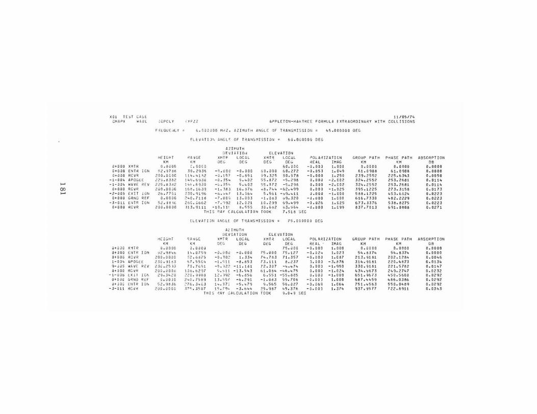
<01 TEjT C~~f 11/05/7'. C~APX W 4~E 0 I PCl Y , 'IF l2 APPLETON - HARTREE FORMULA EXTRA ORDINARY WITH COLLISIONS
FRi:..OlJE,ilY 6.0QQ,JOO Hill. AZIMUTH ANGLE OF TRAN $ MI SS IO II 1,5.00 0000 DEC.
ELl ~ A TIJ ~ ~NGL ~ OF rRAN~HISSION : DO .O COOa~ OEC.
AztHuTH rJl:VIATlO,1 ELE'IATION
liE I GH T ~4 ~ GE XHTF LOC4 l XHTR LOC~L ;>OLA~IZATIGN GR.OUP PATH PHASE PATH ABSORPTION K" K" OEG OEG OEG DEb REAL IM.IIG K" <. 0'
0+ 0 00 XMTR a .D OOG C. GOQO 6C.OOC - a.OOJ 1.000 0 .0 000 0.0000 0.0000 o+oao HHR 10N 52 . 9He 30 . l Si]&, -1). 0 0 e -0. 000 ;, o. 00 0 60.272 -0.053 1.01t9 61.0908 61.0906 0.0000 O+ (j 00 RCVR 200 . 0(;oe 111, . 41.<,2 -0.15 7 -0 .&51 3'3 .325 50.576 -D.DIlO 1.250 239.25'52 225.&3 '+3 0.0050
-1-004 AP OGt:E £25 .83 32 14f>.6930 - il .354 5 ... 02 55 .672 -5.296 0 . 00 () -2.C02 324.2552 253.2661 0.0114 - -1- ~(l 1t WAVE i?EV 225 . 83.i2 1 <t~ . ~»30 - li .35" 5 .4 02 55 . 872 - 5 .2 98 0 . 300 - 2 .C02 3210.2552 253.2661 0.0114 00 OtOOO RCvR 2uO.OOJIi 168 .1Ii3» -1. Ja J 1':'.370 .. 1'1 .7104 -62.1099 O. a 0 (I -1. 025 J95.1225 273 .. H58 C. 0 1 73 - -2-~0 7 EXIT lON 26 . 77 :; 1 230 .91 96 - 6 . ;' 107 13. ;; 6" 5 .561 - ~9 .'+11 ;).000 -1.000 588.1225 1053.61210 0.0223
OtOOO GRNU REF a.OODO 2"0 .711rl -7. I) 0" 13.003 -1.01:13 1>9.320 - ~.~oo 1.DOO 616.7330 "82.2229 0.0223 -3-011 EN I R I ON 52 d8 Ie 20G . G662 - 7 . '1 92 12. 02 1 1 0 . 2'019 69.1t')'J -0.026 1.(;25 673.3376 538.8275 0.0223
Ot-OOO ~CVR 200 . 0 00 0 3 13.'3111 -10. t 1 ~ 8.555 30 .632 6 3.,6" - 0.000 1.e9,) 837.7013 691.0808 0.0271 THI S RAY CALCULATION r OOK 7.518 ~EC
ELEVATIJtl ANGLE. OF T~ANSHISSION 75.000000 DEG
AZIHUTH l)EVIATION ELE VA lION
HEIGHT q /l~ C.E ~MT R LOC AL XHT~ LOCAL POLAR IZATI ON GROUP PATH PHASE PA TH ABSORPTION <" K.' OEG OEG OEG O£O RE AL IMA G K" K" 0'
utQJO X'1T R O .~ OOO il . 0 ~ OU 75. UOO -0.000 1.000 0.0000 0.0000 0.0000 OtJOD ErHR I ON ";2 .9 Slob lit. a 7S9 - v. OOoJ - O.OOV 75.000 750127 - 0.02,+ 1.023 54.H7 .. 54.8371t 0.0000 OtOOO RCVR 200 . 0000 52 . 6 d 75 - 0 . 3 02 1.331t 74.783 71.357 - 0.0 OJ 1.087 213.9181 202.1281t 0.001t6 1- 00 4 APOGEE 230 091<:13 :' 7. 5SG,+ -i. '> 11 -a.853 73 .111 8.237 J. 0 a J - 3.8 76 314.9181 220.4673 0.0134 9- B5 WAV" REV 2J~.l513 70.7691 -~. 12Z -11.101 72.3Q7 -4.47" a. a O'J -1.'3S0 330.9181 221.5782 0.011t7 OtDOO RCvR 200 .<l OOU l J6 . bZ')7 5 . '> 11 -13. 543 6 1.084 -46.,+7S 0.000 -1 .021t 434.Y673 2109.27"7 0 . 0232
-1- DOb EXIT 10' 2903420 220. 'B08 12. J9Z -6.85& 6 . 55 1 - 55.685 1.1. a 0 J -1.000 651.9673 1050.5600 0.02'32 Ot-OUO G~NO Rt: F () . 00 JD 240 .75119 13. 5 S7 - 6 .291 -ldld3 55.706 -0.00) 1.000 687.'+459 1t86.o386 0.02')2 <l * Jij G EtH R lOt. 52.9636 'N6 . 3 4 G3 1 ... 3n -5 . .. 7') '1.565 56. <127 -(1. 0 69 1.061t 751.IoS63 550.0 f!89 0.0292
-3-011 RCVi( 2~0.1l00G 37<;.3507 15.794 - 3 . 61t4 25. 91H 45 .376 - O.OD~ 1 . 374 937 . 9577 722.8911 0.0343 THI S ~AY CA L CULA TI ON TOOK 9.0 .. 9 SEC
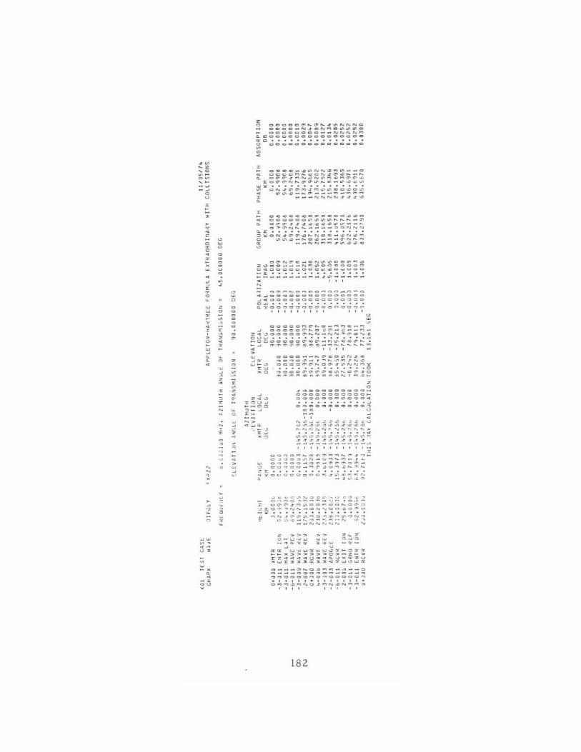
.~ ~ z , 0
~::;:; ,~
~" ~ "
0 0
~
> • · z ~
0 ~ • 0
0 · • , 0 ~
" ~
0 • r " 0 0 ~
0
" z ~ 0
~ ~ ~ , _0 ~ • ~ I , ~
~ Z " ~ • ~
" " " ~ 0 Z
'" 2 " ~ , ~
;; r ~
r z ; .
~ • ~ " 0
" " ;: c' Z -. z "
~ ~ " " ,
u
" '" 0 0 • c ~ •
.~ ~ ,
"" UI
'0 ~ ,
• · ~I
00
z o d dOOC ~ ~~~~~NNNC C>""c:> O .... N~<CN..., "' '''''''''C>
~ ooccco O "' _ _ "'''''''''''''' ~mooo o c>oococ:>ooc>oc> 0< C • • • •• • • •• • •• ••• o 000000000000000 ~
~
I ~ O<C<C<C .... ~"'NN~...,"' _ .... C 4 CCCC"" ~ ~ON ~ ~~~_~ ~ C~~~""N~N"'M~""~~~
~C~~N~~~"'~~"""'~~'" w ~ ••• • • • • • ••• • • • • ~ CNj~~""~M"''''<CC~O''' ~ "''''~_~~ _ _ ''''M_~~'''' r _ ........ NNNN4jj~
• o <c<c>""..,..,<C., OO"'C O>&loDO
~ OCCCOC"''''''''''~~~_~ ~ O~~jj j ~oDoDoD"'''' __ ~
C,...a'N ........ .... __ .... ~ONNN o..:r • • • • • • • • • • • • • • • ~~ONj~a'oD .... NC<C .... oDNoD..., '" "''''oD ........ OoD_ .... _ ~N .... M ~ .... .... NN""MjlnoDoD<C o
O<1'N<1'.., .... CNU"IoDOOc->..,'" Z~OO ___ NM"'Oc..,OOOO
O~OOOOOOOOU,"'O~UOO ..... ::1: • • ••••• •• • • ••••
~- .... --- ----j"' --- --""' I , , ~
~ O~~ NO ~~O~~~ .... ~-~ ""'~oO~oooCOOoooooo
~""'~OOOOOOOOOOOOOO
'" UJ ••• ••••••• • •••• o..~OO~OO~OOOO~OO~~
I I I I , I I I I I I I
000001")(1' .... "' ... ..,"''''_1'') " ~
~ oooco(1' .... OC(1'~~ __ "' ... Z~~ooooo~ .... N~NN~(1'O~O OU W • •••• •• • •• • •• ~ ..... ~OOOOOOO(1''''(1' .... '''~~~(1' .... • ~~ ~(1'~(1'~~~~ .... ~ ........ ~ ........ .., ;;: I I I I
"
OC>OO ....... .... (1''"'O~N~.., ~0"'0,ro .... .......... (>"' ... N>O ooOo~(1''''O(1' .... tf\NN''''lI!
• • ••• • ••• •• ••• 0 oOOO(1'(1'(1'(1'~~""",(1'",O
'" '"'''',....., ... "'..,...,.,., N , "'.0 ~
""""'<.!l 1:0U .... ....... 00 :::> .... ~
z o
.... 0000000""'00 ... 00000000,,"00 ... 0:>0000000"'00"'" . ... .... ... ~ 00<:>0000000"':;:>
..,,,,, I <.1
'" " , , " '" '" w .... .:J .f' ," _" C '" ., V o!J .f' ..c oJ;> .!) ~ >0 ..c ..c ..c .0
";"; "~":";". ~ ~ ~": '::; '" or' '" '" '" ... " ... " '" '" '" '" 'Y ~ .... ~ ..................... ... _ ........ _...;- - ----"" I , I , , , I • • , , ....
r O""oo.., .... ~m(1'..,M ... (1' ... ~~ O.:>·~c:>;:>tf\N ... <:'O.., .... "'_ ... '" 0"""'00 .... 0"'_(1'(1'(1'0(1' _
<.!l Oq~o<:> _ ..,(1'DcMD ... ~ .... ;>-:>: •• •• ••••• • •• • • • ~KCL'OOOOOOM3~"'MMN Q _ ... ~ .C'"
~ ....... ..., ~" N <.:> ., .,-. ,~ ,J ., C J.J ;>
= ~;~;~~~~~~~~~~~ ~ ~C~~ N .... _ ON~OO~O:>"'O .... lI! ••• ••• ••••••••• ~ ~N~~(1'~~~n..,~~ON~ = "'~ .O_ .... O~~M~N 'n ~ __ NNNN~ '"
Z ,>, Z .... Z 0 ....... ' .. '" WuJ 0, .. 0 ~""Il.''''Q: "l: 'r'" _10:_
" '" 0::0:: l.UW "'~l.U l.U<.!l'r ... :=oa::o:: ......... "'"",'O, ... Z ... , ::c 7""'4'" ""U""'C(n.U"'trZu "'lL.I'1:S"~~O::~'X""'trl.U<.!IWO::
<:> .... _ ... 0' .... 0 .0,..,.., ..... n ........ <:> 0 .......... 000000 .... 0 ........ 0 ~"'OOoO"'o~o<:>o<:>"" ..... .. , , , , I • , , I , , I , ..
0,..,""'" "'NO"'''''N.tIN''''''0 , , , , , ., "
18 2
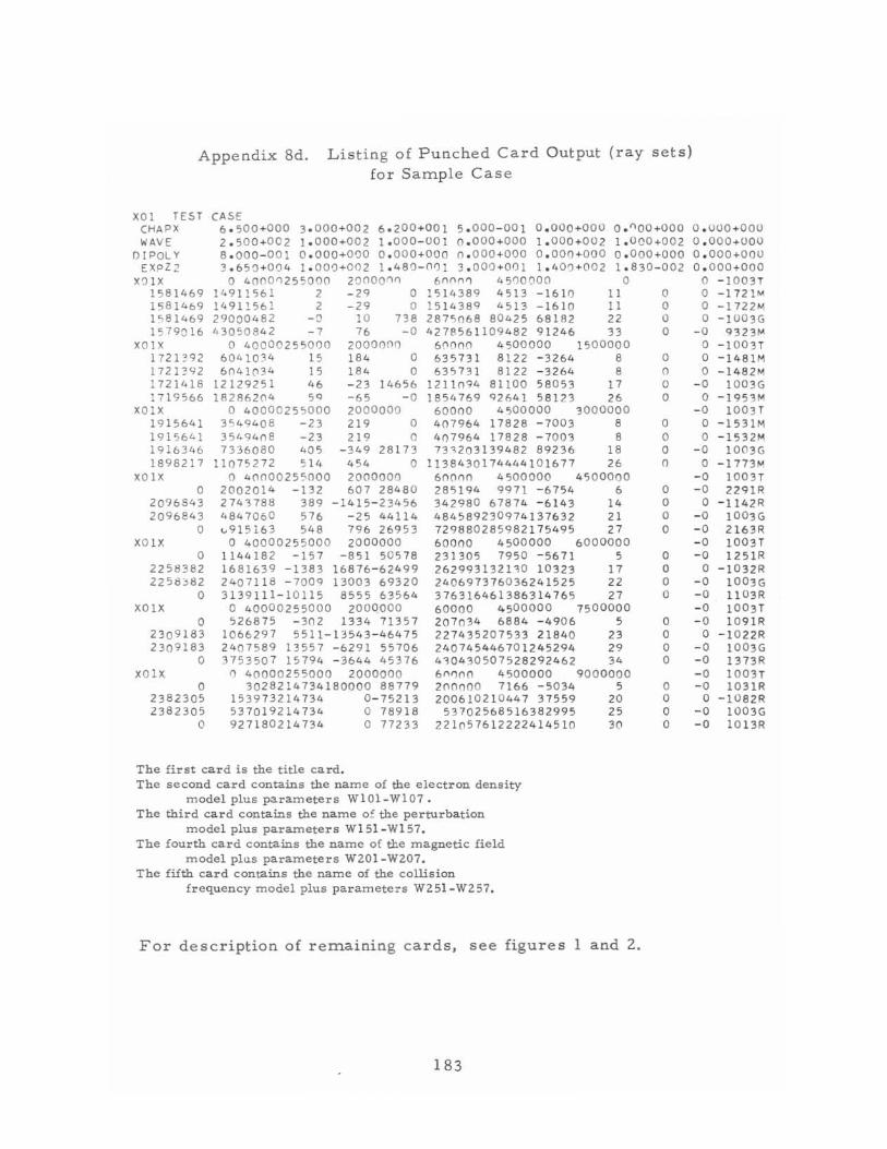
Appendix 8d. Listing of Punched Card Output (ray sets) for Sample Case
XOI TEST CASE CHAPX 6 . 500+000 3.000+002 6.200+001 5.000-001 0.000+000 0. 1100+000 WAVE 2.500+002 1.000+002 1.000-001 0.000+000 1.000+002 1 .O CO +002
DIPQLY 8.000- 001 0 .0 00+0')0 0 . 000+000 n . OOO+OOO 0 .0 00+000 0 . 000+000 EXPZ2 3 .6 5() +OO4 1.000+002 1.480-(11)1 3.000 +01)1 1.40')+002 1.830-002
x'Jlx o 4000'1255000 2000 001"1 6f'l(l ('I '1 450QOOO 1581469 1' .. 911561 2 - 29 0 1514 389 4513 -161 0 1581469 14912561 2 - 29 0 1514389 4513 -161 0 1~81469 29000482 - 0 10 738 2875068 80425 68182 1579016 £..3050842 - 7 76 - 0 '12785611 09 482 91246
XOl:< o 40000255000 2000 000 600(10 4500000 1721392 6041034 15 184 0 635731 8122 - 3264 1721392 6<141('13 4 1 5 184 0 635731 8122 - 3264 1721416 12129251 46 -23 14656 1211ng4 81100 58053 1719566 18286204 59 -65 - 0 1854769 92641 58123
XOIX o 40 000255000 2000000 60000 4500000 19 15641 3549 4 08 - 23 219 0 407964 17828 - 7003 1915641 35494(18 -23 219 0 407964 17828 - 7003 1916346 7336080 405 -349 28173 731203139482 89236 1898217 11075272 514 454 0 11384 30174444 101677
XOlx o 4()OOO255000 20000 00 60000 4500000 0 2002014 -132 607 28480 285194 9971 -6754
2096543 274,788 389 -1415-23456 342980 67874 -6143 2096843 4847060 576 - 25 44114 484589230974137632
0 (..1915163 548 796 26953 729880 285982175495 XOIX o 40000255000 2000000 60000 4500000
0 1144182 -1 57 -851 505 78 231305 7950 - 5671 22 58382 1681639 -1383 16876- 62499 2629931321'0 10323 2258>82 2407118 -7009 13003 69320 240697376036241525
0 3139111-1 01 15 8555 63564 376316461386314765 XOlx 0 40000255000 2000000 60000 450 0000
0 526875 -302 1334 71357 207034 6884 -4906 2309183 1066297 5511-1>543 -46475 227435207533 21840 230,183 24 07589 13557 -6291 55706 240745446701245294
0 3753507 15794 - 3644 45376 4,0 4 30507528292462 X01X o 40000255000 2000000 6n'1no 4500000
0 3028214734180000 88779 200000 7166 -5034 2382305 153973214734 0 - 75213 200610210447 37559 2382305 537019214734 0 78918 53702568516382995
0 927180214734 0 77233 221057612222414510
The first card is the title card. The second card contains the name of the electron density
model plus parameters W101 - WI0? The third card contains the name of the perturbation
model plus parameters WlSl - WlS7 . The fourth card contains the name of the magnetic field
model plus parameters WZOI - WZ07. The fifth card contains the name of the collision
frequency model plus parameters WZ51-WZ57.
0 11 11 22 33
1500000 8 8
17 26
3000000 8 8
18 26
45 00000 6
14 21 27
6000000 5
17 22 27
7500000 5
23 29 34
9000000 5
20 25 30
For description of remaining cards, see figures 1 and 2.
183
0 0 0 0
0 0 0 0
0 0 0 0
0 0 0 0
0 0 0 0
0 0 0 0
0 0 0 0
o . uoo +ooo 0 . 000+000 0.000+000 0 . 000+000
o - 1003T 0 -17Z1 M o - 1722M o -1 00%
-0 9323"" 0 - lOOn 0 -1481M 0 - 1482M
- 0 1003G 0 -1953M
- 0 1003T 0 - 1531M 0 -1532M
-0 1003G 0 -1773f.A
- 0 1003T - 0 2291R
0 -1142R - 0 100% - 0 2163R - 0 1003T - 0 1251R
0 -1 032R - 0 1003G -0 11 0 3R - 0 1003T -0 1091R
0 -1022R - 0 1003G - 0 1373R -0 1003T - 0 1031R
0 - 1082R -0 1003G -0 1013R
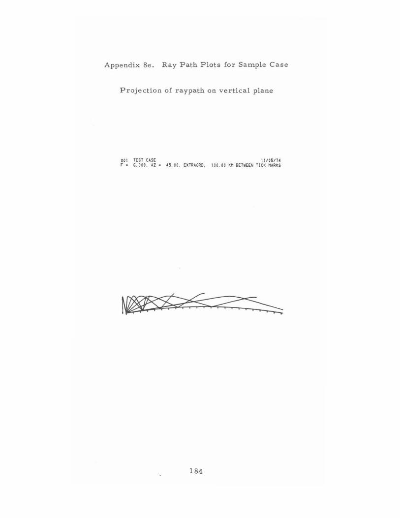
Appendix 8e. Ray Path Plots for Sample Case
Projection of raypath on vertical plane
XOI TEST CA.SE 11/05174 r: = S.OOO, AZ = A5.00, EXTRAORD. 100.00 KM BETWEEN TICK HARKS
184
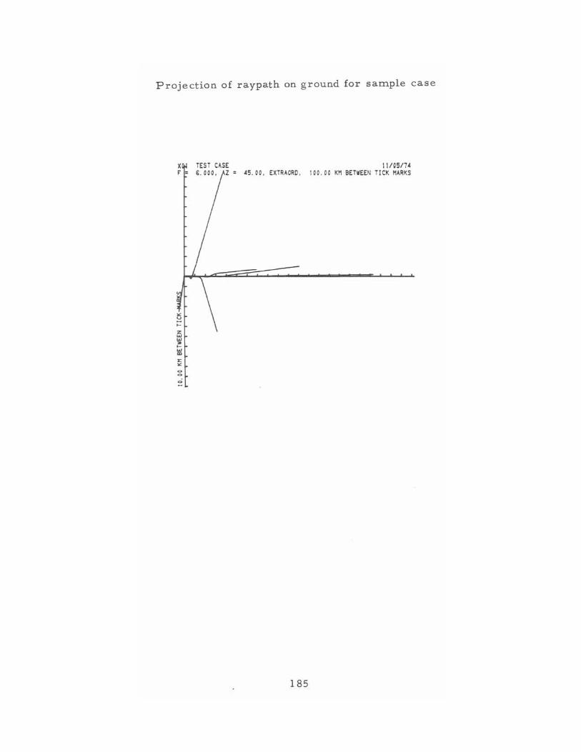
Projection of raypath on ground for sample case
X TEST C~SE II/O~I7' F' = 6.000 , Z = 45.00 , EXTRMRD, 100.00 KH BETWEEN TICI( MARKS
185

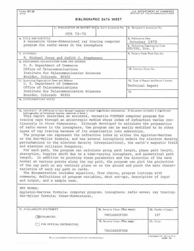
FORM OT·29 U.S . DEPAR T MENT OF COMMERCE 13·73 1 O F FICE OF TELECOMMUNICATIONS
BIBLIOGRAPHIC DATA SHEET
I. PUBLICATION OR REPORT NO 2. Gov't Accession No. 3. Recip ient's Acce ss ion No.
OTR 75 - 76 4. TITLE AND SUB TITLE S. Publ icat ion Date
A versatile three- dimensional ray tracing computer October 1975 program for radio waves i n the ionosphere 6. Perf orm in g Organization Code
OT/ITS, Div. 1
7. AUTHOR(S) 9. Pr oj e ct / Task / Work Unit No.
R. Michael Jones and J ud i th J. Stephenson 8. PERFORMING ORGANIZATION NAME AND ADDRESS
U. S. Department of Conunerce Office of Telecommunications 10. Contract / Grant No.
Insti tute for Telecommunicati on Sciences Boulder, Colorado 80302
11. Sponsoring Organ izat ion Name and Address 12. Ty~ of Rep ort and Period Covered U. S. Department of Conunerce
Technical Office of Telecommunications Report
Institute for Telecommunication Sc i ences 13.
Boulder, Col orado 80302 14. SU PPLEMENTARY NOTES
IS. ABSTRACT (A 20()-'woro or les s factual summary of most sifP1ificant information. It document includes a siQniticant bjbljo~raphy ot literature survey, ment;oo it here . ) Thi s report describes an accurate, versat i le FORTRAN computer program f or
tracing rays through an anisotropic medium whose index of r efracti on varies con-tinuously in three dimensions. Although developed to calculate the propagation of radio waves in the i onosphere , the program can be easi l y modifi ed to do other types of ray tracing because of its organizat i on into subroutine.
The program can represent the refracti ve index by e i ther the Appleton- Hartree or the Sen- \,yller formul a, and has several ionospheric models for electron density perturbations to the e l ectron density (irregularities), the earth's magnetic fie l d and e l ectron co l l i s i on f requency.
For each path, the program can calculate group path length, phase path length, absorption, Doppler shift due to a t i me - varying ionosphere , and geometrical path l ength . In addition to pr i nting these' parameters and the direct i on of the wave normal a t various point s along the ray path, the program c an p l ot the projecti on of the ray path on any verti cal plane or on the ground and punch the main charac-teristics of each ray path on cards .
The documentation incl udes equations, flow charts , program listings with corrunents, definitions of program variables, deck set- ups, description of input and output, and a sample case.
KEY WORDS: Appleton- Hartree formul a; computer progr am; ionosphere; radio Sen-Wyller formula; three- dimensional.
17. AV AILA BILITY STATEMENT 18. ~cwi ty Class (This report)
CZlXUNLlM1TED. UNCLASSIFIED
19. ~curity Class (This pa~)
0 FOR OFFICIAL DISTRIBUTION.
UNCLASSIFIED
~ u. S. GOVERNMENT PRINTING OFFICE 1117~· 662·16t1111C1 R .... e
waves; ray tracing;
20. Number of pages
197
21. Price:
l'SCOMM- 'J C 2Sl716-P73 16(X)1Ot • fJJ.
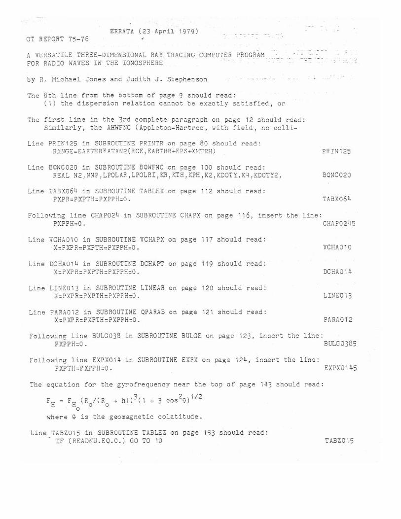
ERRATA (21 April 1979) OT REPORT 75-76
A VERSATILE THREE-DIMENSIONAL RAY rOR RADIO WAVES IN THE IONOSPHERE
TRACING COMPUTER PROGRAM .... _ _ ' .
by R. Michael Jones and Judith J . Stephenson
The 8th line from the bottom of page 9 should read : (1) the dispersion relat i on cannot be exactly satisfied, or
The first line in the 3rd complete paragraph on page 12 should read : Similarly, the AHWrNC (Appleton- Hartree , ',; ith field , no colli -
Line P~IN'25 in SUBROUTINE PRI1'1TR on pa~e 80 should read : RANG"C:=EJl.R THR '" .~.7 AN2 (RCE, EARTHR+EPS+Xt1'i'RH)
Line 8C1'1C020 in SUBROUTINE BQI-1F"NC on page 100 should read : REJl.L N2, NNP, L?OLAR , LPOLRI, KR, KtH! [(PH, K2 , KDOTY, K4, KDOTY2,
Line 7.o.8X064 in SUBROUTINE TABLEX on page 112 s"r.ould read : PXPR=PXPTH=PXPPH=O .
Follo'.{ing line PXPPH=O .
CHAP024 in SUBROUTINE CH.Il. PX on page 116, insert the line :
Line VeHA010 in SUBROUTINE VCHAPX on page 111 should read : X=PXPR=PXPTH=PxPFH=O .
Line DCHA014 in SUBROUTINE DCHAPT on page 119 should read : X=PXPR=PXPTH=?XPPH=O.
Line LINE013 in SUBROUTINE LINEAR on page 120 should read : X=PXPR=PXPTH=PXPPH=O .
Line PARA012 in ~UBROUTINE QPARAB on page 121 should re?d : X =P XP R=P XPTH = PXPPH =0 .
PRIN12S
BONC020
TABX064
CHAP0245
VCHA010
DCHA014
LINEO 13
PARA012
Following line PXPPH=O .
BULG038 in SUBROUTINE BULGE on page 123, insert the line : BULG0385
Following line EXPX014 in SUBROUTINE EXPX on page 124, insert the line : PXPTH=PXPPH=O. EXPX014S
The equation for the gyro frequency near the top of page 143 should r ead :
F .. = FH (R I(R + h»3(1 + 3 cos2g)1/2
n . 0 0 o
where 9 is the geomagnetic colatitude .
Line TABZ01S in SUBROUTINE TABLEZ on page 153 should r ead : IF (READNU . EO.O . ) GO TO 10 TABZ01S
Related Documents