A variational deduction of second gradient poroelasticity I: general theory

JOURNAL OF MECHANICS OF MATERIALS AND STRUCTURESVol. 3, No. 3, 2008

A VARIATIONAL DEDUCTION OF SECOND GRADIENT POROELASTICITYPART I: GENERAL THEORY

GIULIO SCIARRA, FRANCESCO DELL’ISOLA, NICOLETTA IANIRO AND ANGELA MADEO

Second gradient theories have to be used to capture how local micro heterogeneities macroscopically

affect the behavior of a continuum. In this paper a configurational space for a solid matrix filled by an

unknown amount of fluid is introduced. The Euler–Lagrange equations valid for second gradient porome-

chanics, generalizing those due to Biot, are deduced by means of a Lagrangian variational formulation.

Starting from a generalized Clausius–Duhem inequality, valid in the framework of second gradient the-

ories, the existence of a macroscopic solid skeleton Lagrangian deformation energy, depending on the

solid strain and the Lagrangian fluid mass density as well as on their Lagrangian gradients, is proven.

1. Introduction

Poroelasticity stems from Biot’s pioneering contributions on consolidating fluid saturated porous mate-

rials [Biot 1941] and now spans a lot of different interrelated topics, from geo- to biomechanics, wave

propagation, transport, unsaturated media, etc. Many of these topics are related to modeling coupled

phenomena (for example, chemomechanical swelling of shales [Dormieux et al. 2003; Coussy 2004], orbiomechanical models of cartilaginous tissues), and nonstandard constitutive features (for instance, in

freezing materials [Coussy 2005]). In all these cases, complexity generally remains in rendering how

heterogeneities affect the macroscopic mechanical behavior of the overall material.It is well known from the literature how microscopically heterogeneous materials can be described in

the framework of statistically homogeneous media [Torquato 2002] considering suitable generalizationsof the dilute approximation due to Eshelby [Nemat-Nasser and Hori 1993; Dormieux et al. 2006]; how-ever, some lack in the general description of the homogenization procedure arises when dealing with

heterogeneous materials, the characteristic length of which can be compared with the thickness of the

region where high deformation gradients occur. This could be due, for example, to external periodic

loading, the wavelength of which is comparable with the characteristic length of the material, or to phasetransition, etc.

From the macroscopic point of view the quoted modeling difficulties, arising when high gradients

occur, are discussed in the framework of so called high gradient theories [Germain 1973], where the

assumption of locality in the characterization of the material response is relaxed. In these theories,

the momentum balance equation reads in a more complex way than the classical one used for Cauchy

continua. As a matter of fact, it is the divergence of the difference between the stress tensor and the

divergence of so-called hyperstresses that balance the external bulk forces. Stress and hyperstress are

introduced by a straightforward application of the principle of virtual power, as those quantities working

on the gradient of velocity and the second gradient of velocity, respectively [Casal 1972; Casal and

Keywords: poromechanics, second gradient materials, lagrangian variational principle.

507

508 GIULIO SCIARRA, FRANCESCO DELL’ISOLA, NICOLETTA IANIRO AND ANGELA MADEO

Gouin 1988]. Even the classical Cauchy theorem is, in this context, revised by introducing dependenceof tractions not only on the outward normal unit vector but also on the local curvature of the boundary

[dell’Isola and Seppecher 1997]; moreover symmetric and skew-symmetric couples (the actions called

“double-forces” by Germain) must be prescribed on the boundary in terms of the hyperstress tensor

together with contact edge forces along the lines where discontinuities of the normal vector occur.Following the early papers on fluid capillarity [Casal 1972; Casal and Gouin 1988], the second gradient

model can indeed be introduced by means of a variational formulation where the considered Helmholtzfree energy depends both on the strain and the strain gradient tensors.

In the case of fluids, second gradient theories are typically applied for modeling phase transition

phenomena [de Gennes 1985] or for modeling wetting phenomena [de Gennes 1985], when a character-istic length, say the thickness of a liquid film on a wall, becomes comparable with the thickness of the

liquid/vapor interface [Seppecher 1993], annihilation (nucleation) of spherical droplets, when the radiusof curvature is of the same order of the thickness of the interface [dell’Isola et al. 1996], or topological

transition [Lowengrub and Truskinovsky 1998].In the case of solids, second gradient theories are applied, for instance, when modeling the failure

process associated with strain localization [Elhers 1992; Vardoulakis and Aifantis 1995; Chambon et al.2004]. To the best of our knowledge, second gradient theories are very seldom applied in the mechanicsof porous materials [dell’Isola et al. 2003] and no second gradient poromechanical model, consistent

with the classical Biot theory, is available except the one presented in [Sciarra et al. 2007]. As gradientfluid models, second gradient poromechanics will be capable of providing significant corrections to

the classical Biot model when considering porous media with characteristic length comparable to the

thickness of the region where high fluid density (deformation) gradients occur. We refer, for instance, tocrack/pore opening phenomena triggered by strain gradients or fluid percolation, the characteristic length

being in this case the average length of the space between grains (pores).Several authors have focused their attention on the development of homogenization procedures capable

of rendering the heterogeneous response of the material at the microlevel by means of a second gradi-

ent macroscopic constitutive relation [Pideri and Seppecher 1997; Camar-Eddine and Seppecher 2003];however, very few contributions seem to address this problem in the framework of averaging techniques[Drugan and Willis 1996; Gologanu and Leblond 1997; Koutzetzova et al. 2002]. The present work does

not investigate the microscopic interpretation of second gradient poromechanics, but directly discusses

its macroscopic formulation. It is divided into two papers: in the first paper the basics of kinematics,

Section 2; the physical principles, Section 3; the thermodynamical restrictions, Section 4; and in Section

5 the variational deduction of the governing equations for a second gradient fluid filled porous materialare presented.

In particular, in Section 2 a purely macroscopic Lagrangian description of motion is addressed by

introducing two placement maps in χs and φ f (Equation (1)). We do not explicitly distinguish which

part of the current configuration of the fluid filled porous material is occupied at any time t by the solidand fluid constituents, this information being partially included by the solid and fluid apparent density

fields, which provide the density of solid/fluid mass with respect to the volume of the porous system

(Equation (5)).

A VARIATIONAL DEDUCTION OF SECOND GRADIENT POROELASTICITY I 509

The deformation power, or stress working (Equation (12)), following Truesdell [1977] is deduced in

Section 3 starting from the second gradient expression of power of external forces (Equation (9)) Cauchytheorem (Equation (10)) and balance of global momentum (see (11)).

In the spirit of Coussy et al. [1998] and Coussy [2004] thermodynamical restrictions on admissible

constitutive relations are stated in Section 4, finding out a suitable overall potential, defined on the

reference configuration of the solid skeleton. This last depends on the skeleton strain tensor and the

fluid mass content, measured in the reference configuration of the solid, as well as on their Lagrangian

gradients, in Equation (18).Finally a deduction of the governing equations is presented in Section 5, based on the principle of

virtual works, by requiring the variation of the internal energy to be equal to the virtual work of external

and dissipative forces (see (19)). A second gradient extension of the two classical Biot equations of

motion [Coussy 2004; Sciarra et al. 2007], endowed with the corresponding transversality conditions onthe boundary, is therefore formulated (see Equations (30)–(33)). Generalizing the treatment developed,

for example, by Baek and Srinivasa [2004] for first gradient theories, one of the equations of motion

found by means of a variational principle is interpreted as the balance law for total momentum, when

suitable definitions of the global stress and hyperstress tensors are introduced (see (34)).In a subsequent paper (Part II, to be published in a forthcoming issue of this journal), an application of

the second gradient model to the classical consolidation problem will be discussed. Our aim is to showhow the present model enriches the description of a well-known phenomenon, typical of geomechanics,curing some of the weaknesses of the classical Terzaghi equation [von Terzaghi 1943]. In particular

we will figure out the behavior of the fluid pressure during the consolidation process when varying the

initial pressures of the solid skeleton and/or the saturating fluid. From the mathematical point of view,

the initial boundary value problem will be discussed according with the theory of linear pencils.

2. Kinematics of fluid filled porous media and mass balances

The behavior of a fluid filled porous material is described, in the framework of a macroscopic model,

adopting a Lagrangian description of motion with respect to the reference configuration of the solid

skeleton. At any current time t the configuration of the system is determined by the maps χs and φ f ,

defined as

χs : �s × � → �, φ f : �s × � → � f , (1)

where �α (α = s, f ) is the reference configuration of the α-th constituent, while � is the Euclidean placemanifold, and � indicates a time interval. The map χs ( · , t) prescribes the current (time t) placement

x of the skeleton material particle Xs in �s . The map φ f ( · , t), on the other hand, identifies the fluid

material particle X f in � f which, at time t , occupies the same current place x as the solid particle Xs .

Therefore the set of fluid material particles filling the solid skeleton is unknown, to be determined by

means of evolution equations. Both these maps are assumed to be at least diffeomorphisms on �. The

current configuration �t of the porous material is the image of �s under χs ( · , t). In accordance with

the properties of χs and φ f it is straightforward to introduce the fluid placement map as

χ f : � f × � → �, such that χ f ( · , t) = χs ( · , t) ◦ φ f ( · , t)−1 ,

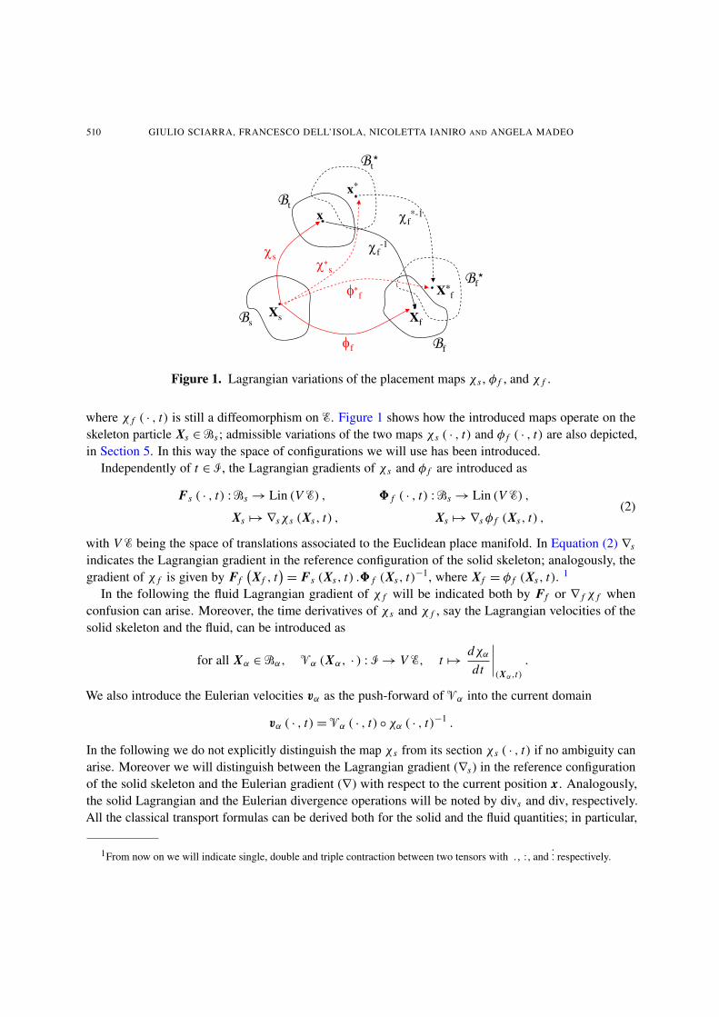
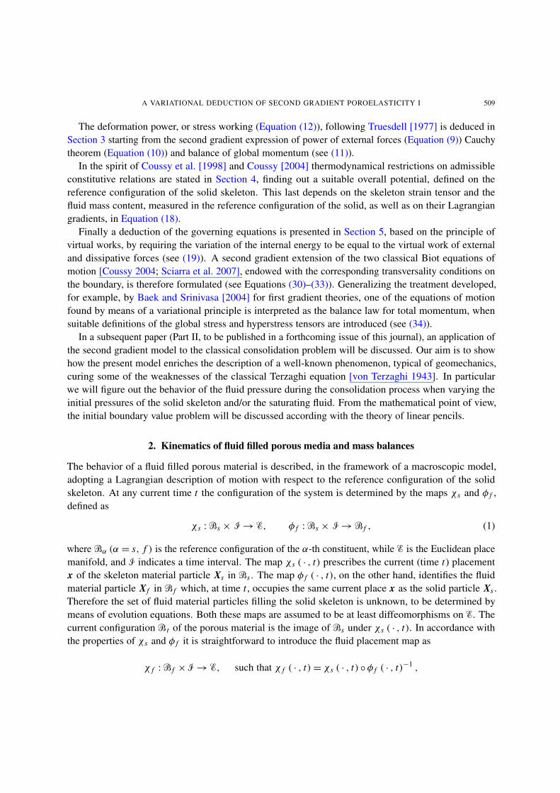
510 GIULIO SCIARRA, FRANCESCO DELL’ISOLA, NICOLETTA IANIRO AND ANGELA MADEO

tx

s

s

f

t*

Xs

x*

s

f

f

Xf

X*ff*

f-1

f*-1

Figure 1. Lagrangian variations of the placement maps χs , φ f , and χ f .

where χ f ( · , t) is still a diffeomorphism on �. Figure 1 shows how the introduced maps operate on theskeleton particle Xs ∈ �s ; admissible variations of the two maps χs ( · , t) and φ f ( · , t) are also depicted,in Section 5. In this way the space of configurations we will use has been introduced.

Independently of t ∈ �, the Lagrangian gradients of χs and φ f are introduced as

Fs ( · , t) : �s → Lin (V �) , � f ( · , t) : �s → Lin (V �) ,

Xs �→ ∇sχs (Xs, t) , Xs �→ ∇s φ f (Xs, t) ,(2)

with V � being the space of translations associated to the Euclidean place manifold. In Equation (2) ∇sindicates the Lagrangian gradient in the reference configuration of the solid skeleton; analogously, the

gradient of χ f is given by Ff�X f , t

�= Fs (Xs, t) .� f (Xs, t)−1, where X f = φ f (Xs, t). 1

In the following the fluid Lagrangian gradient of χ f will be indicated both by Ff or ∇ f χ f when

confusion can arise. Moreover, the time derivatives of χs and χ f , say the Lagrangian velocities of the

solid skeleton and the fluid, can be introduced as

for all Xα ∈ �α, �α (Xα, · ) : � → V �, t �→ dχα

dt

����(Xα,t)

.

We also introduce the Eulerian velocities vα as the push-forward of �α into the current domain

vα ( · , t) = �α ( · , t) ◦ χα ( · , t)−1 .

In the following we do not explicitly distinguish the map χs from its section χs ( · , t) if no ambiguity canarise. Moreover we will distinguish between the Lagrangian gradient (∇s) in the reference configurationof the solid skeleton and the Eulerian gradient (∇) with respect to the current position x. Analogously,

the solid Lagrangian and the Eulerian divergence operations will be noted by divs and div, respectively.All the classical transport formulas can be derived both for the solid and the fluid quantities; in particular,

1From now on we will indicate single, double and triple contraction between two tensors with . , : , and... respectively.

A VARIATIONAL DEDUCTION OF SECOND GRADIENT POROELASTICITY I 511

those ones for an image volume and oriented surface element turn to be

d�t = Jαd�α, nd St = Jα F−Tα .nαd Sα,

where d�t and d St represent the current elementary volume and elementary oriented surface corre-

sponding to d�α and d Sα, respectively, where Jα = det Fα, and where n and nα are the outward unit

normal vectors to d St and d Sα . As far as only the solid constituent is concerned, we can understand that

deformation induces changes in both the lengths of the material vectors and the angles between them.

As it is well known, the Green–Lagrange strain tensor ε measures these changes, and is defined as

ε := 12

�FT

s .Fs − I�, (3)

where I clearly represents the second order identity tensor.The balance of mass both for the solid and the fluid constituent are introduced as

�α =�

�t

ρα d�t = const =�

�α

ρ0α d�α, (α = s, f ) , (4)

where �α is the total mass of the α-th constituent, ρα is the current apparent density of mass of the α-th

constituent per unit volume of the porous material, while ρ0α is the corresponding density in the reference

configuration of the α-th constituent. When localizing, Equation (4) reads

ρα Jα = ρ0α, (α = s, f ) ,

or, in differential form,dαρα

dt+ ρα div (vα) = 0, (α = s, f ) , (5)

where dαρα/dt represents the material time derivative relative to the motion of the α-th constituent. In

other words,dα

dt:= d

dt

����Xα=const

.

The macroscopic conservation laws could also be deduced in the framework of micromechanics

[Dormieux and Ulm 2005; Dormieux et al. 2006] starting from a refined model, where the solid and

the fluid material particles occupy two disjoint subsets of the current configuration, and considering an

average of the solid and fluid microscopic mass balances. The macroscopic laws do involve the so called

apparent density of the constituents and suitable macroscopic velocity fields. For a detailed descriptionof the procedure which leads to averaged conservation laws we refer to the literature [Coussy 2004].

2.1. Pull back of continuity equations. It is clear that Equation (5) consists of Eulerian equations, mean-ing that they are defined on the current configuration of the porous medium. Following Wilmanski [1996]and Coussy [2004] we want to write both these equations in the reference configuration of the solid

skeleton. With this purpose in mind let us define the relative fluid mass flow w as w := ρ f�v f − vs

�.

The use of this definition allows us to rearrange the fluid continuity (5) in the form

dsρ f

dt+ ρ f div vs + div w = 0. (6)

512 GIULIO SCIARRA, FRANCESCO DELL’ISOLA, NICOLETTA IANIRO AND ANGELA MADEO

We want now to rewrite the continuity equation for the fluid constituent in the reference configuration of

the solid skeleton. The Lagrangian approach to the fluid mass balance can be carried out by introducingthe current Lagrangian fluid mass content m f , defined as

m f := Js�ρ f ◦ χs

�. (7)

Furthermore, let M be the Lagrangian vector referred to the reference configuration of the solid and

related to the flow w through the relations

M := Js F−1s . (w ◦ χs) , Js (div w ◦ χs) = (divs M) . (8)

By using the definitions from Equations (7) and (8) in (6) the fluid Lagrangian mass balance takes the

formdm f

dt+ divs M = 0.

3. Power of external forces

In this section, starting from the statement of the power of external forces for a second gradient solid-

fluid mixture, we deduce its corresponding reduced form, accounting for the extended Cauchy theoremvalid for second gradient continua [Casal 1972; Germain 1973; dell’Isola and Seppecher 1997], and thebalance of global momentum. The external power �ext �vs, v f

�for a second gradient porous medium

can be defined as a continuous linear functional of the velocity fields vα; in particular

�ext �vs, v f�:=

�

�t

�bs .vs + b f .v f

�d�t +

�

∂�t

�ts .vs + t f .v f

�d�t

+�

∂�t

�τ s .

∂vs

∂n+ τ f .

∂v f

∂n

�d�t +

m�

k=1

�

�k

�f k

s .vs + f kf .v f

�dl, (9)

where �t is the current volume occupied by the porous medium, ∂�t its boundary, and m is the numberof edges �k (if any) of the boundary. In addition, bα, tα, τα, and f k

α represent the body force density,

the generalized traction force (Cauchy stress vector), the double force vector, and the force per unit lineacting on the k-th edge of the boundary, respectively.

The physical meaning of the double force τα can be described in a way similar to that used in differentcontexts in [Germain 1973] and [dell’Isola and Seppecher 1997]. It can be regarded as the sum of two

different contributions, the first of which works on the rate of dilatancy along the outward unit normal n(∇vα : (n ⊗ n)), and the second being a tangential couple working on the vorticity; this nomenclature isdue to Germain [1973].

Let σ α and �α be the apparent Cauchy stress and hyperstress tensors per unit volume of the porous

material relative to the α-th constituent [Germain 1973; dell’Isola and Seppecher 1997]. The Cauchy

theorem can be extended for a second gradient continuum, and in particular for a second gradient porous

continuum, in order to specify how the generalized external tractions appearing in (9) can be balanced

A VARIATIONAL DEDUCTION OF SECOND GRADIENT POROELASTICITY I 513

by the internal forces when considering any subdomain of the current volume. In particular we have2

tα = (σ α − div �α).n − divS (�α.n) , τα = (�α.n).n, f kα = [] (�α.n).ν[]k, (10)

where ν is the binormal unit vector which form a left-handed frame with the unit normal n and the

unit vector being tangent to the k-th edge. We note that, since n is not continuous through the edge k,

the vector ν is also discontinuous when passing from one side of the edge k to the other. It is for this

reason that the edge force f kα is balanced by the jump of the internal force (�α.n).ν through the edge

k. Extending classical poromechanics [Biot 1941; Coussy 2004] we now define the overall stress and

hyperstress tensors as σ := σ f + σ s and � := � f + �s, so that the momentum balance for the porous

medium as a whole readsdiv (σ − div �) + b = 0, (11)

where b = bs +b f is the overall body force. Bearing in mind both the extended Cauchy theorem, Equation(10), and the overall balance of momentum, (11), together with the principle of virtual powers (�ext =�def.), (9) leads to the expression for the deformation power

�def.(v, ω) =�

�t

�σ : ∇v + div

�σ T

f .ω�

+ �... ∇∇v + � f

... ∇∇ω − div�div � f

�.ω

�d�t . (12)

Here and later on v := vs and ω := v f − vs . Moreover, it must be remarked that (12) is obtained underthe hypothesis of absence of volume forces (bα = 0) so that no inertia is taken into account in our model.

We refer to [Coussy 2004] for the complete form of the deformation power in the case of first gradient

porous continua. From now on, we also assume that the structure of the hyperstress tensors �α (α = f, s)takes the particular form

�α = I ⊗ cα, α = f, s, (13)

where I is the second order identity tensor and cα is a kind of hyperstress vector related to the α-th

constituent. The use of this assumption restricts second gradient external forces just to vector fields

τα, which only work on the stretching velocity of the α-th constituent; in other words, no contribution

to the vorticity on the boundary of �t comes from τα. The aforementioned hypotheses indeed restrict

the second gradient model; however, solid microdilatancies and capillarity effects can be still describedby this second gradient model. According to (13) the external power due to second gradient effects,

Equations (9) and (10), reduces to

τα.∂vα

∂n= {[(I ⊗ cα) .n] .n} .

∂vα

∂n= (cα.n) n.

∂vα

∂n= (cα.n) [∇vα : (n ⊗ n)] .

3.1. Pull-back operations. Let us now consider the solid reference configuration pull-back of the defor-

mation power; in order to do so, we will introduce the Piola–Kirchhoff like stress and hyperstress tensorsfor the overall body and for the fluid constituent. Thus, Piola–Kirchhoff stress (S) and hyperstress (γ )

are defined so that

Jsσ : ∇v =: S : dε

dt�⇒ S = Js F−1

s .σ .F−Ts , (14)

2Fixed a basis (e1, e2, e3), where e1 and e2 span the plane tangent to the surface ∂�t at x, and the surface divergence of a

second order tensor field A is defined as divS A := �2α=1 (∂ A/∂xα) eα .

514 GIULIO SCIARRA, FRANCESCO DELL’ISOLA, NICOLETTA IANIRO AND ANGELA MADEO

Js�... ∇∇v =: γ .

��∇s

dε

dt

�T

: C−1 − (∇s C)T :�

C−1.dε

dt.C−1

��

�⇒ γ = Js F−1s .c,

where C = FTs .Fs is the Cauchy–Green strain tensor and c is the total hyperstress vector defined by

c = cs + c f . Moreover, the fluid ones are Sf =: Js F−1s .σ f .F−T

s , and γ f =: Js F−1s .c f . The deformation

power �def. can be finally written in the Lagrangian form

��def. =

�

�s

�̂�def. d�s,

where

�̂�def. =

��S − C−1. ((∇s C).γ ) .C−1� : dε

dt+

�C−1 ⊗ γ

� ...

�∇s

dε

dt

�+ divs

�1

m fST

f .M�

+ ∇s

�divs

�Mm f

��.γ f − M

m f.∇s

�divs γ f

�+ divs

��J−1

sMm f

.∇s Js

�γ f

��.

4. Thermodynamics: deduction of a macroscopic second gradient strain energy potential

In this section, starting from the first and second principles of thermodynamics, we will prove that a

suitable macroscopic strain potential can be identified depending both on the solid strain and on the fluid

mass density as well as on their Lagrangian gradients. Let eα be the Eulerian density of internal energyrelative to the α-th constituent, and the corresponding energy density of the porous medium is defined

as e := ρses + ρ f e f . The first principle of thermodynamics can be written as [Coussy 2004]

ds

dt

�

�t

ρses d�t + d f

dt

�

�t

ρ f e f d�t = �ext + Q̊,

where Q̊ := −�

�tq.nd�t is the rate of heat externally supplied, and where q is the heat flow vector. In

the Lagrangian form the first principle reads

ddt

�

�sE d�s = ��

def. −�

�s

divs�e f M + Q

�d�s . (15)

where we recall that d/dt is the material time derivative associated with the motion of the solid, E := Jserepresents the Lagrangian density of internal energy, and Q is the Lagrangian heat flux defined by

Q := Js F−1s .q. Starting from Equation (15), the local Lagrangian form of the first principle is naturally

given byd Edt

= �̂�def. − divs

�e f M + Q

�.

Let us now consider the second principle of thermodynamics and introduce the overall Eulerian densityof entropy s as s := ρsss + ρ f s f . The corresponding Lagrangian entropy is S := Jss, and the Lagrangian

form of the second principle can be written as [Coussy 2004]

ddt

�

�s

S d�s ≥ −�

�s

divs

�s f M + Q

T

�d�s . (16)

A VARIATIONAL DEDUCTION OF SECOND GRADIENT POROELASTICITY I 515

If we now introduce the Helmholtz free energy � as � := E − T S, Equation (16) can be rewritten in

the local form asd Edt

− SdTdt

− d�

dt≥ −T divs

�s f M + Q

T

�.

Merging the local form of the first and the second principles, the extended Clausius–Duhem inequality(dissipation inequality) can be deduced. In particular, following Sciarra et al. [2007], we will distinguish

different contributions to the dissipation function due to the solid and fluid motion and to thermal effects,

respectively (�s , � f , and �th).We now constitutively restrict [Coleman and Noll 1963] the admissible processes only to those ones

which guarantee the dissipation inequality to be satisfied, because �s , � f and �th are separately non-

negative. In particular, the solid dissipation �s reads

�s =�

S − C−1. [(∇s C).γ ] .C−1 −�Js C−1.∇s

�J−1

s m f��

⊗γ f

m f

�: dε

dt+

�C−1 ⊗ γ

� ...ddt

(∇sε)

+�

g f −�

1 + 1tr I

�γ f .∇s

�1

m f

�− J−1

str I

γ f

m f.∇s Js

�.dm f

dt−

γ f

m f.

ddt

�∇sm f

�− S

dTdt

− d�

dt. (17)

Assuming nondissipative processes occurring in the solid skeleton (�s = 0), Equation (17) allows for

regarding the internal energy � as a state function

� = ��ε, m f , ∇sε, ∇sm f , T

�. (18)

From now on we will treat an isothermal problem and therefore assume the energy � does not depend

on the temperature field T .

5. Variational deduction of second gradient poroelastic equations

5.1. Basic concepts and first variation of the internal energy. In this section we deduce the governingequations for a second gradient poroelastic continuum by means of a variational procedure. Variationalapproaches to first gradient mixture models are available in the literature [Bedford and Drumheller 1978;

Gavrilyuk et al. 1998; Gouin and Ruggeri 2003].In our case, we introduce the varied placement maps χ∗

s and φ∗f for all Xs ∈ �s as

χ∗s (Xs, t) = χs (Xs, t) + δχs (Xs, t) , φ∗

f (Xs, t) = φ f (Xs, t) + δφ f (Xs, t) ,

where δχs and δφ f represent arbitrary variations of the functions χs and φ f , respectively. The physicalmeaning of the variation δχs is well known in continuum mechanics, and stands for the virtual displace-ment (deformation) of the solid skeleton. The variation δφ f , instead, accounts for the virtual relative

displacement of a fluid material particle with respect to a solid one (see Figure 1). Since these variations

keep fixed Xs ∈ �s we label them Lagrangian variations and we note that the symbol δ commutes withthe integral over �s and with the Lagrangian gradient operator ∇s .

Following the statements of classical mechanics [Gantmacher 1970; Arnold 1989], the principle of

virtual works readsδ� = δ�ext + δ�diss, (19)

516 GIULIO SCIARRA, FRANCESCO DELL’ISOLA, NICOLETTA IANIRO AND ANGELA MADEO

where δ� represents the Lagrangian variation of the internal energy of the porous material, defined as

� :=�

�s

� d�s,

while δ�extand δ�diss

are the virtual works due to the external and dissipative forces acting on the

porous system. Because of the aforementioned properties of the Lagrangian variations we can write

δ� = δ

�

�s

� d�s =�

�s

δ� d�s . (20)

Recalling now Equation (18), (20) implies

δ� =�

�s

�∂�

∂ε: δε + ∂�

∂m fδm f + ∂�

∂ (∇sε)

... δ (∇sε) + ∂�

∂�∇sm f

� .δ�∇sm f

��

d�s . (21)

The variations δε, δm f , δ (∇sε), and δ�∇sm f

�must now be rewritten in terms of the variations of the

primitive kinematical fields χs and φ f , bearing in mind that the Lagrangian variation commutes with the

operator ∇s . We show here directly the results obtained in Appendix A, to which we refer for detailed

calculations,δε = 1

2

�(∇s (δχs))

T .Fs + FTs .∇s (δχs)

�, (22)

andδm f = m f

�∇s φ f

�−T : ∇s�δφ f

�. (23)

Substituting (22) and (23) into (21), integration by parts (see Appendix B for details), allows us to

write the variation of the second gradient potential � as

δ� =�

�s

Ad�s +�

∂�s

a d�s +m�

k=1

�

Ek

αdl, (24)

where m is the number of edges Ek of the body in the reference configuration of the solid and

A := − divs

�Fs .

�∂�

∂ε− divs

�∂�

∂(∇sε)

���.δχs+

��∇s φ f

�−T.

�

−m f ∇s

�∂�

∂m f− divs

�∂�

∂�∇sm f

�����

.δφ f ,

a :=��

Fs .

�∂�

∂ε− divs

�∂�

∂(∇sε)

���.ns − divS

s

�Fs .

�∂�

∂(∇sε).ns

���.δχs

+��

Fs .

�∂�

∂(∇sε).ns

��.ns

�.∂(δχs)

∂ns

+�

�∇s φ f

�−T.

�

m f

�∂�

∂m f− divs

�∂�

∂�∇sm f

���

ns − m f ∇Ss

�∂�

∂�∇sm f

� .ns

���

.δφ f

+��∇s φ f

�−T.

�

m f∂�

∂�∇sm f

� .ns

�

ns

�

.∂

�δφ f

�

∂ns,

α :=��

Fs .

�∂�

∂ (∇sε).ns

��.ν

�.δχs, +

��∇s φ f

�−T.

�

m f∂�

∂�∇sm f

� .ns

�

ν

�

.δφ f .

A VARIATIONAL DEDUCTION OF SECOND GRADIENT POROELASTICITY I 517

5.2. Dissipative governing equations. In order to obtain the equations of motion for a second gradientporoelastic continuum, the form of the external and dissipation virtual works, δ�ext

and δ�diss, formally

introduced in Equation (19), must be stated. The virtual dissipation δ�disswill account for the classi-

cal Darcy effects and for the so called Brinkman-like contributions [Brinkman 1947]. We define the

dissipation δ�diss in the Eulerian configuration as

δ�diss := −�

�t

��

�v f − vs

�.��

δχ f ◦ φ f − δχs�◦ χ−1

s��

d�t

−�

�t

���.∇

�v f − vs

��: ∇

��δχ f ◦ φ f − δχs

�◦ χ−1

s��

d�t , (25)

where � is the symmetric, definite positive Darcy tensor and � is a suitably defined symmetric, definitepositive second gradient Darcy-like tensor.

Moreover, from now on, we assume the following Eulerian expression for the external work δ�ext,

δ�ext := −�

∂�t

�t .

�δχs ◦ χ−1

s�+ t f .

��δχ f ◦ φ f − δχs

�◦ χ−1

s��

d�t . (26)

We restrict our attention to t and t f , defined as

t := pext n, t f := ρ f µext n, (27)

where pext is the overall external pressure applied on ∂�t , and µext is the chemical potential of the fluidoutside the porous system. By comparison of Equation (26) with (9), we are assuming vanishing doubleforces and edge forces on the external boundary, as well as vanishing bulk actions. Equation (26), the

expression for the external work, states that the external force t works only on the displacement of the

solid skeleton (δχs), while µextworks on the fluid mass virtual relative displacement ρ f

�δχ f − δχs

�.

We note that if µext is spatially constant then�

∂�t

ρ f µext ��δχ f ◦ φ f − δχs

�◦ χ−1

s�

d�t =�

∂�s

�µext ◦ χs

�δm f d�s,

that is, µextworks on the fluid mass which leaves (or enters) the solid skeleton (see Appendix C for

details). Equation (26) for δ�extcan be rewritten (see Appendix C) on the reference configuration of the

solid as

δ�ext =�

∂�s

�−

�pext Js F−T

s .ns�.δχs +

�µextm f

�∇s φ f

�−T.ns

�.δφ f

�d�s . (28)

Finally, (25) for δ�diss (see Appendix C) assumes the Lagrangian form

δ�diss =�

�s

���∇s φ f

�−T.�Js D FT

s .�� f ◦ φ f − �s

���.δφ f

�d�s

−�

�s

��∇s φ f

�−T.�FT

s . divs�Js�.∇s

�� f ◦ φ f − �s

�.(FT

s .Fs)−1��

�.δφ f d�s

+�

∂�s

���∇s φ f

�−T.�Js FT

s .�.∇s�� f ◦ φ f − �s

�.(FT

s .Fs)−1�

�.ns

�.δφ f d�s . (29)

518 GIULIO SCIARRA, FRANCESCO DELL’ISOLA, NICOLETTA IANIRO AND ANGELA MADEO

Starting from the principle of virtual works, (19), and using (24), (29), and (28) for δ�, δ�diss, and

δ�ext, respectively, we can write the local equations of motion on �s as

− divs

�Fs .

�∂�

∂ε− divs

�∂�

∂ (∇sε)

���= 0, (30)

and

�∇s φ f

�−T.

�

−m f ∇s

�∂�

∂m f− divs

�∂�

∂�∇sm f

���

− Js D FTs .

�� f ◦ φ f − �s

��

+�∇s φ f

�−T.�FT

s . divs�Js�.∇s

�� f ◦ φ f − �s

�.(FT

s .Fs)−1�� = 0. (31)

Analogously the boundary conditions on ∂�s read�

Fs .

�∂�

∂ε− divs

�∂�

∂ (∇sε)

���.ns − divS

s

�Fs .

�∂�

∂ (∇sε).ns

��= − Js pext F−T

s .ns

�∇sφ f

�−T.

�

m f

�∂�

∂m f− divs

�∂�

∂�∇sm f

���

ns − m f ∇Ss

�∂�

∂�∇sm f

� .ns

��

+

−�∇sφ f

�−T.��

JsFTs .�.∇s

�� f ◦ φ f − �s

�.(FT

s .Fs)−1� .ns

�=

�∇sφ f

�−T.�m f µ

ext ns�, (32)

�Fs .

�∂�

∂ (∇sε).ns

��.ns = 0,

�∇sφ f

�−T.

��

m f∂�

∂�∇sm f

� .ns

�

ns

�

= 0.

Finally, on the edges Ek of the boundary (if any) the following conditions hold true:�

Fs .

�∂�

∂ (∇sε).ns

��.ν = 0,

�∇s φ f

�−T.

��

m f∂�

∂�∇sm f

� .ns

�

ν

�

= 0. (33)

The Darcy and Brinkman dissipations appearing in Equations (31) and (32) can be rewritten in termsof the Lagrangian vector M, previously defined as M = m f F−1

s .�v f − vs

�. In fact, after some straight-

forward calculations, it can be proven that

∇�v f − vs

�= 1

m f

��(∇s Fs)

T . M�T + Fs .∇s M

�+ Fs .

�M ⊗ ∇s

�1

m f

��.

We now show that (30) is in agreement with the classical second gradient balance law for the total

momentum [Germain 1973; dell’Isola and Seppecher 1997]. In order to do so, considering assumption

(13), it can be proven that the constitutive relations for S and γ (see Equations (14))

∂�

∂ε= S − C−1. ((∇s C).γ ).C−1,

∂�

∂ (∇sε)= C−1 ⊗ γ , (34)

A VARIATIONAL DEDUCTION OF SECOND GRADIENT POROELASTICITY I 519

imply that (30) can be regarded as the solid-Lagrangian pull-back of (11). In other words,

Js div (σ − div �) = divs�

Fs .�S − C−1. ((∇s C).γ ).C−1 − Fs . divs

�C−1 ⊗ γ

���= 0.

6. Concluding remarks

In this paper a purely macroscopic second gradient theory of poromechanics is presented, extending

classical Biot poromechanics [Biot 1941; Coussy 2004]. Following a standard procedure, sketched in

[Coussy et al. 1998], we determine a suitable representation formula of the deformation power, (12), fora second gradient porous medium, assuming the forces acting on solid skeleton to be balanced (using

the generalized second gradient balance of momentum in the current domain and the generalized second

gradient Cauchy theorem on its boundary) and the power of external forces to be that of two super-

posed second gradient continua [Germain 1973]. The principles of thermodynamics, together with the

aforementioned representation of the deformation power, allow for deducing the existence of a suitableoverall strain energy potential � depending on the solid strain tensor ε and the solid Lagrangian fluid

mass density m f , as well as on their Lagrangian gradients.The Euler–Lagrange equations associated with the energy density � are the governing equations of

the problem. In particular, Lagrangian variations of the placement maps χs and φ f are considered. It

is worth noting that the governing equations associated with the solid Lagrangian displacement δχs(when δφ f = 0) represents the balance of total momentum and therefore allows for the constitutive char-

acterization of the overall stress and hyperstress tensors. This is a characteristic feature of the classical

Biot model [Baek and Srinivasa 2004], which is completely recovered in this more general framework.

On the other hand, the governing equation associated with the fluid placement map δφ f represents the

balance of momentum relative to the pure fluid, which, in this case, is a generalization of the classical

Darcy law.In part II, an application to the classical consolidation problem will show how the present model

improve the classical ones. It is well known that second gradient theories are capable to detect boundary

layer effects in the vicinity of interfaces; this is indeed what we will observe in the case of consolidation.

In particular, a kind of fluid mass density increment in the neighborhood of the impermeable wall will

be observed for the first time in a one dimensional problem [Mandel 1953; Cryer 1963].

Appendix A: Basic variations

We show here how to derive the variations δε and δm f in terms of the kinematical variations δχs and

δφ f . Equation (3) for the Green–Lagrange strain tensor implies

δε = 12

��δs FT

s�.Fs + FT

s .δs Fs�,

where by definition Fs := ∇sχs ; the expression (22) for δε is easily derived. As far as the variation δm fis concerned, recalling definition (7) for m f we can write

m f = Js J−1f ρ0

f , (A.1)

where ρ0f is the fluid density in the reference configuration of the fluid. Since by definition

J f := det(∇ f χ f ) and φ f := χ−1f ◦ χs,

520 GIULIO SCIARRA, FRANCESCO DELL’ISOLA, NICOLETTA IANIRO AND ANGELA MADEO

we haveJ f = det

�∇ f

�χs ◦ φ−1

f

��= det

�∇sχs .∇ f φ

−1f

�= Js det

�∇s φ f

�−1,

where for the sake of simplicity we neglect the dependence of the considered fields on the reference

places. Equation (A.1) thus readsm f = ρ0

f det�∇s φ f

�. (A.2)

By derivation rule of the determinant and assuming ρ0f = constant, we get

δm f = ρ0f δ

�det

�∇s φ f

��= ρ0

f det�∇s φ f

�tr

��∇s φ f

�−1.δ

�∇s φ f

��= m f

��∇s φ f

�−T : ∇s�δφ f

��.

Appendix B: Variation of the internal energy

The procedure to calculate the variation δ� of the internal energy will be here shown in detail.According to Equations (21)–(23) and recalling that ∂�/∂ε is a symmetric second order tensor, while

∂�/∂(∇sε) is a third order tensor symmetric with respect to its first two indices, we can write

δ� =�

�s

�A1 + A2

s + A2f

�d�s, (B.1)

where

A1 := ∂�

∂ε:�FT

s .∇s (δχs)�+ m f

∂�

∂m f

�∇s φ f

�−T : ∇s�δφ f

�,

A2s := ∂�

∂ (∇sε)

... ∇s�FT

s .∇s (δχs)�,

A2f := ∂�

∂�∇sm f

� .∇s

�m f

�∇s φ f

�−T : ∇s�δφ f

��,

account for the first gradient contribution to δ� and for the solid and fluid second gradient contributions

respectively.The following identities are recalled in order to perform integrations by parts in (B.1); let λ, a, A,

and � be scalar, first, second, and third order tensor fields respectively. (Here ∇S a indicates the surfacegradient operator of a vector field a defined — analogously to divS

s — as ∇S a = ∂a/∂xα ⊗ eα, α = 1, 2,where eα belong to the tangent plane.) Then,

div�

AT .a�= A :∇a + a. div A, div (λA) = A.∇λ + λ div A, div (λa) = a.∇λ + λ div a,

div��T : A

�= A : div �+ (∇ A)

... �, ∇a = ∇S a + ∂a∂n

⊗ n,

where transposition for third order tensors is defined so as �T := ai jk ek ⊗ ei ⊗ e j if � = ai jk ei ⊗ e j ⊗ ek .Moreover, given second order tensors A, B, C, third and first order tensors � and a the following

identities are satisfied:

A : (B.C) =�BT.A

�: C =

�A.CT �

: B,��T : A

�.a = A : (�.a) .

A VARIATIONAL DEDUCTION OF SECOND GRADIENT POROELASTICITY I 521

Finally, if ϕ = χs or ϕ = φ f , the identity holds true that

0 = divs�det (∇sϕ) (∇sϕ)−T �

= det (∇sϕ) divs�(∇sϕ)−T �

+ (∇sϕ)−T .∇s [det (∇sϕ)] . (B.2)

We underline that this equality holds unchanged for the surface divergence operator divSs . For the sake

of simplicity, we will perform integration by parts for the first and second gradient terms appearing in

(B.1) separately. Integration by parts of the first gradient term, recalling Equation (A.2) for m f and usingEquation (B.2) for φ f , leads to

� 1

�sA1 d�s = −

�

�sdivs

�Fs .

∂�

∂ε

�. δχs d�s +

�

∂�s

��Fs .

∂�

∂ε

�.ns

�. δχs d�s

−�

�s

��∇s φ f

�−T.

�m f ∇s

�∂�

∂m f

���. δφ f d�s +

�

∂�s

��∇s φ f

�−T.

�m f

∂�

∂m fns

��. δφ f d�s . (B.3)

Integrating by parts the solid second gradient term we get

� 2

�sA2

s d�s = −�

�s∇s (δχs) :

�Fs . divs

�∂�

∂ (∇sε)

��d�s +

�

∂�s

∇s (δχs) :�

Fs .

�∂�

∂ (∇sε).ns

��d�s

= −�

∂�s

��Fs . divs

�∂�

∂ (∇sε)

��.ns

�. δχs d�s +

�

�sdivs

�Fs . divs

�∂�

∂ (∇sε)

��. δχs d�s

+�

∂�s

�∇S

s (δχs) + ∂ (δχs)

∂ns⊗ ns

�:�

Fs .

�∂�

∂ (∇sε).ns

��d�s .

Performing a further surface integration by parts we finally get

�

�sA2

s d�s = −�

∂�s

��Fs . divs

�∂�

∂ (∇sε)

��.ns

�.δχs d�s +

�

�sdivs

�Fs . divs

�∂�

∂ (∇sε)

��.δχs d�s

−�

∂�s

divSs

�Fs .

�∂�

∂ (∇sε).ns

��.δχs d�s +

�

∂�s

��Fs .

�∂�

∂ (∇sε).ns

��.ns

�.∂ (δχs)

∂nsd�s

+n�

k=1

�

Ek

��Fs .

�∂�

∂ (∇sε).ns

��.ν

�. δχs dl. (B.4)

We finally rewrite the fluid second gradient term as

� 2

�sA2

f d�s =�

�s

∂�

∂�∇sm f

� .∇s

�m f divs

��∇s φ f

�−1.δφ f

��d�s

−�

�s

∂�

∂�∇sm f

� .∇s

�m f divs

��∇sφ f

�−T�

.δφ f

�d�s;

522 GIULIO SCIARRA, FRANCESCO DELL’ISOLA, NICOLETTA IANIRO AND ANGELA MADEO

recalling Equation (A.2) for m f , using Equation (B.2) for φ f and rearranging, we have

�

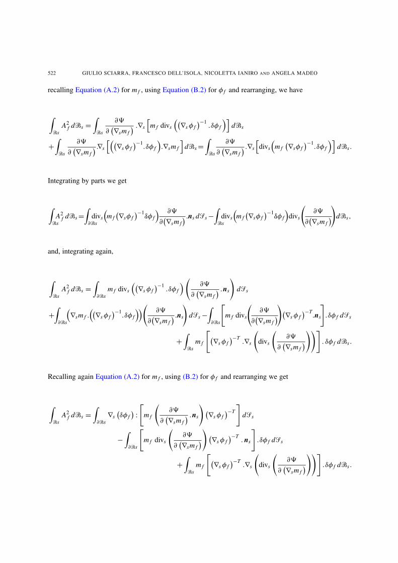
�sA2

f d�s =�

�s

∂�

∂�∇sm f

� .∇s

�m f divs

��∇s φ f

�−1.δφ f

��d�s

+�

�s

∂�

∂�∇sm f

� .∇s

���∇s φ f

�−1.δφ f

�.∇sm f

�d�s =

�

�s

∂�

∂�∇sm f

� .∇s

�divs

�m f

�∇sφ f

�−1.δφ f

��d�s .

Integrating by parts we get

�

�sA2

f d�s =�

∂�sdivs

�m f

�∇sφ f

�−1.δφ f

� ∂�

∂�∇sm f

� .ns d�s −�

�sdivs

�m f

�∇sφ f

�−1.δφ f

�divs

�∂�

∂�∇sm f

��

d�s,

and, integrating again,

�

�sA2

f d�s =�

∂�sm f divs

��∇s φ f

�−1.δφ f

� �∂�

∂�∇sm f

� .ns

�

d�s

+�

∂�s

�∇sm f .

��∇s φ f

�−1.δφ f

���∂�

∂�∇sm f

� .ns

�

d�s −�

∂�s

�

m f divs

�∂�

∂�∇sm f

��

�∇s φ f

�−T.ns

�

.δφ f d�s

+�

�sm f

��∇s φ f

�−T.∇s

�

divs

�∂�

∂�∇sm f

����

. δφ f d�s .

Recalling again Equation (A.2) for m f , using (B.2) for φ f and rearranging we get

�

�sA2

f d�s =�

∂�s∇s

�δφ f

�:�

m f

�∂�

∂�∇sm f

� .ns

��∇s φ f

�−T�

d�s

−�

∂�s

�

m f divs

�∂�

∂�∇sm f

��

�∇s φ f

�−T. ns

�

.δφ f d�s

+�

�sm f

��∇s φ f

�−T.∇s

�

divs

�∂�

∂�∇sm f

����

.δφ f d�s .

A VARIATIONAL DEDUCTION OF SECOND GRADIENT POROELASTICITY I 523

Decomposing ∇s�δφ f

�as ∇s

�δφ f

�= ∇S

s�δφ f

�+

�∂

�δφ f

�/∂ns

�⊗ ns , performing a last surface inte-

gration by parts and using (B.2) for the surface divergence operator we finally get

�

�sA2

f d�s =�

∂�s

��∇s φ f

�−T.

�

m f

�∂�

∂�∇sm f

� .ns

�

ns

��

.∂

�δφ f

�

∂nsd�s+

−�

∂�s

��∇sφ f

�−T.

�

m f ∇Ss

�∂�

∂�∇sm f

� .ns

���

.δφ f d�s+n�

k=1

�

Ek

��∇sφ f

�−T.

�

m f

�∂�

∂�∇sm f

� .ns

�

ν

��

.δφ f dl

−�

∂�s

��∇s φ f

�−T.

�

m f divs

�∂�

∂�∇sm f

��

ns

��

. δφ f d�s

+�

�s

��∇s φ f

�−T.

�

m f ∇s

�

divs

�∂�

∂�∇sm f

�����

. δφ f d�s . (B.5)

Substituting (B.3), (B.4), and (B.5) into (B.1), the variation of the internal energy given in (24) has beenrecovered.

Appendix C: External and dissipation works

The dissipation and external works have been defined in (25) and (26) on the Eulerian configuration of

the system in terms of δχs and δχ f ◦φ f . These works must then be rewritten in terms of the independentvariations δχs and δφ f . In order to do so, the relationship between (δχ f ◦ φ f − δχs) and δφ f must

be established. We know by definition that χ f ◦ φ f = χs, so that δ�χ f ◦ φ f

�= δχs . Moreover, by

differentiation rule for composite functions we have δχs = δ�χ f ◦ φ f

�= δχ f ◦φ f +

��∇ f χ f

�◦ φ f

�.δφ f .

But since χ f = χs ◦ φ−1f , we get

∇ f χ f ◦ φ f = ∇sχs .�∇ f

�φ−1

f

�◦ φ f

�= ∇sχs .

�∇sφ f

�−1,

so that δχs = δχ f ◦ φ f + ∇sχs .�∇s φ f

�−1. δφ f , or,

δχ f ◦ φ f − δχs = − Fs .�∇sφ f

�−1. δφ f . (C.1)

We now prove that the external work due to the force t f appearing in Equation (26) and prescribed

by (27) represents the external work � fext done to change the fluid mass inside the porous system when

the external chemical potential µext is assumed to be constant. We define this work as

� fext =

�

�s

�µext ◦ χs

�δm f d�s;

according to (23) and neglecting composition operations we can write

� fext =

�

�s

µextm f�∇sφ f

�−T : ∇s�δφ f

�d�s,

524 GIULIO SCIARRA, FRANCESCO DELL’ISOLA, NICOLETTA IANIRO AND ANGELA MADEO

which, integrating by parts, recalling (A.2) for m f , and assuming µext constant, gives

� fext =

�

∂�s

��µextm f

�∇s φ f

�−T. ns

�.δφ f

�d�s −

�

�s

µextρ0f divs

�det

�∇s φ f

� �∇s φ f

�−T�

d�s .

It is known from (B.2) that the divergence appearing in the second integral is vanishing, so that � fext

can be rewritten on the Eulerian configuration as

� fext =

�

∂�t

��µextρ f

��∇s φ f

�−T. FT

s

�.n

�.δφ f

�◦ χ−1

s d�t ,

or, using (C.1),

� fext = −

�

∂�t

�ρ f µ

extn .�δχ f ◦ φ f − δχs

��◦ χ−1

s d�t ,

which is the expression of the fluid external work used in (26).The final expressions for δ�diss and δ�ext can now be determined. We first consider the solid

Lagrangian pull-back of (25), which, recalling that ∇vα = ∇s�α.F−1s , reads

δ�diss := −�

�s

�Js D

�� f ◦ φ f − �s

�.��

δχ f ◦ φ f − δχs���

d�s

−�

�s

�Js

�� .∇s

�� f ◦ φ f − �s

�. F−1

s�: ∇

��δχ f ◦ φ f − δχs

���d�s .

Recalling Equation (C.1), the dissipation work can be rewritten as

δ�diss =�

�s

��∇sφ f

�−T.�Js D FT

s .�� f ◦ φ f − �s

���. δφ f d�s

+�

�s

�Js

�� .∇s

�� f ◦ φ f − �s

�. F−1

s .F−Ts

�: ∇s

�Fs .

�∇s φ f

�−1. δφ f

��d�s;

integrating the second term by parts, Equation (29) for the dissipation work is easily recovered.

References

[Arnold 1989] V. I. Arnold, Mathematical methods of classical mechanics, Springer Verlag, New York, 1989.

[Baek and Srinivasa 2004] S. Baek and A. R. Srinivasa, “Diffusion of a fluid through an elastic solid undergoing large defor-

mation”, Int. J. Non-Linear Mech. 39 (2004), 201–218.

[Bedford and Drumheller 1978] A. Bedford and D. S. Drumheller, “A variational theory of immiscible mixtures”, Arch. Ratio-nal Mech. Anal. 68 (1978), 37–51.

[Biot 1941] M. A. Biot, “General theory of three-dimensional consolidation”, J. Appl. Phys. 12 (1941), 155–164.

[Brinkman 1947] H. C. Brinkman, “A calculation of the viscous force exerted by a flowing fluid on a dense swarm of particles”,

Appl. Sci. Res. A 1 (1947), 27–34.

[Camar-Eddine and Seppecher 2003] M. Camar-Eddine and P. Seppecher, “Determination of the closure of the set of elasticityfunctionals”, Arch. Rational Mech. Anal. 170 (2003), 211–245.

[Casal 1972] P. Casal, “La théorie du second gradient et la capillarité”, C. R. Acad. Sc. Paris Série A 274 (1972), 1571–1574.

A VARIATIONAL DEDUCTION OF SECOND GRADIENT POROELASTICITY I 525

[Casal and Gouin 1988] P. Casal and H. Gouin, “Equations du mouvement des fluides thermocapillaires”, C. R. Acad. Sci. ParisSérie II 306 (1988), 99–104.

[Chambon et al. 2004] R. Chambon, D. Cailleire, and C. Tamagnini, “A strain space gradient plasticity theory for finite strain”,Comput. Methods Appl. Mech. Eng. 193 (2004), 2797–2826.

[Coleman and Noll 1963] B. D. Coleman and W. Noll, “The thermodynamics of elastic material with heat conduction and

viscosity”, Arch. Rational Mech. Anal. 13 (1963), 167–178.

[Coussy 2004] O. Coussy, Poromechanics, J. Wiley & Sons, Chichester, 2004.

[Coussy 2005] O. Coussy, “Poromechanics of freezing materials”, J. Mech. Phys. Solids 53 (2005), 1689–1718.

[Coussy et al. 1998] O. Coussy, L. Dormieux, and E. Detournay, “From mixture theory to Biot’s approach for porous media”,

Int. J. Solids Struct. 35:34–35 (1998), 4619–4635.

[Cryer 1963] C. W. Cryer, “A comparison of the three-dimensional consolidation theories of Biot and Terzaghi”, Q. J. Mech.Appl. Math. 16:4 (1963), 401–412.

[dell’Isola and Seppecher 1997] F. dell’Isola and P. Seppecher, “Edge contact forces and quasi balanced power”, Meccanica32 (1997), 33–52.

[dell’Isola et al. 1996] F. dell’Isola, H. Gouin, and G. Rotoli, “Nucleation of spherical shell-like interfaces by second gradienttheory: numerical simulation”, Eur. J. Mech. B: Fluids 15 (1996), 545–568.

[dell’Isola et al. 2003] F. dell’Isola, G. Sciarra, and R. C. Batra, “Static deformations of a linear elastic porous body filled withan inviscid fluid”, J. Elasticity 72 (2003), 99–120.

[Dormieux and Ulm 2005] L. Dormieux and F. J. Ulm, Applied micromechanics of porous materials series CISM n. 480,

Springer-Verlag, Wien New York, 2005.

[Dormieux et al. 2003] L. Dormieux, E. Lemarchand, and O. Coussy, “Macroscopic and micromechanical approaches to the

modeling of the osmotic swelling in clays”, Transp. Porous Media 50 (2003), 75–91.

[Dormieux et al. 2006] L. Dormieux, D. Kondo, and F. J. Ulm, Microporomechanics, Wiley, Chichester, 2006.

[Drugan and Willis 1996] W. J. Drugan and J. R. Willis, “A micromechanics-based nonlocal constitutive equation and estimates

of representative volume element size for elastic component”, J. Mech. Phys. Solids 44:4 (1996), 497–524.

[Elhers 1992] W. Elhers, “An elastoplasticity model in porous media theories”, Transp. Porous Media 9:1–2 (1992), 49–59.

[Gantmacher 1970] F. R. Gantmacher, Lectures in analytical mechanics, MIR, Moscow, 1970.

[Gavrilyuk et al. 1998] S. Gavrilyuk, H. Gouin, and Y. V. Perepechko, “Hyperbolic models of homogeneous two-fluid mix-

tures”, Meccanica 33 (1998), 161–175.

[de Gennes 1985] P. G. de Gennes, “Wetting: statics and dynamics”, Rev. Mod. Phys. 57:3 (1985), 827–863.

[Germain 1973] P. Germain, “La méthode des puissances virtuelles en mécanique des milieux continus”, J. Mecanique 12:2

(1973), 235–274.

[Gologanu and Leblond 1997] M. Gologanu and J. B. Leblond, Recent extensions of Gurson’s model for porous ductile mate-rials in continuum micromechanics, vol. 377, CISM Courses and Lectures, Springer, New York, 1997.

[Gouin and Ruggeri 2003] H. Gouin and T. Ruggeri, “Hamiltonian principle in the binary mixtures of Euler fluids with appli-

cations to second sound phenomena”, Rend. Mat. Acc. Lincei 14:9 (2003), 69–83.

[Koutzetzova et al. 2002] V. Koutzetzova, M. G. D. Geers, and W. A. M. Brekelmans, “Multi-scale constitutive modelling of

heterogeneous materials with a gradient-enhanced computational homogenization scheme”, Int. J. Numer. Methods Eng. 54(2002), 1235–1260.

[Lowengrub and Truskinovsky 1998] J. Lowengrub and L. Truskinovsky, “Quasi-incompressible Cahn-Hilliard fluids and topo-logical transitions”, Proc. R. Soc. Lond. A 454 (1998), 2617–2654.

[Mandel 1953] J. Mandel, “Consolidation des sols (étude mathématique)”, Géothecnique 3 (1953), 287–299.

526 GIULIO SCIARRA, FRANCESCO DELL’ISOLA, NICOLETTA IANIRO AND ANGELA MADEO

[Nemat-Nasser and Hori 1993] S. Nemat-Nasser and M. Hori, Micromechanics: Overall properties of heterogeneous materials,

North-Holland, Amsterdam, 1993.

[Pideri and Seppecher 1997] C. Pideri and P. Seppecher, “A second gradient material resulting from the homogenization of a

heterogeneous linear elastic medium”, Continuum. Mech. Therm. 9 (1997), 241–257.

[Sciarra et al. 2007] G. Sciarra, F. dell’Isola, and O. Coussy, “Second gradient poromechanics”, International Journal of Solidsand Structures 44 (2007), 6607–6629.

[Seppecher 1993] P. Seppecher, “Equilibrium of a Cahn-Hilliard fluid on a wall: influence of the wetting properties of the fluidupon the stability of a thin liquid film”, Eur. J. Mech. B:Fluids 12 (1993), 169–184.

[von Terzaghi 1943] K. von Terzaghi, Theoretical soil mechanics, John Wiley & Sons, Chichester, 1943.

[Torquato 2002] S. Torquato, Random heterogeneous materials, Springer, New York, 2002.

[Truesdell 1977] C. A. Truesdell, A first course in rational continuum mechanics, Academic Press, New York, 1977.

[Vardoulakis and Aifantis 1995] I. Vardoulakis and E. C. Aifantis, “Heterogeneities and size effects in geo materials”, AMD -Am. Soc. Mech. Eng., Appl. Mech. Div. Newsl. 201 (1995), 27–30.

[Wilmanski 1996] K. Wilmanski, “Porous media at finite strains. The new model with the balance equilibrium for porosity”,

Arch. Mech. 48:4 (1996), 591–628.

Received 8 Mar 2007. Revised 27 Jul 2007. Accepted 25 Nov 2007.

GIULIO SCIARRA: [email protected] di Ingegneria Chimica Materiali Ambiente, Università di Roma “La Sapienza”, Via Eudossiana 18, 00184 Rome,Italy

FRANCESCO DELL’ISOLA: [email protected] di Ingegneria Strutturale e Geotecnica, Università di Roma “La Sapienza”, Via Eudossiana 18, 00184 Rome,Italy

and

Laboratorio di Strutture e Materiali Intelligenti, Palazzo Caetani (Ala Nord), 04012 Cisterna di Latina (Lt),Italy

NICOLETTA IANIRO: [email protected] di Metodi e Modelli Matematici per le Scienze Applicate, Università di Roma “La Sapienza”, Via Scarpa 16,00161 Rome, Italy

ANGELA MADEO: [email protected] di Metodi e Modelli Matematici per le Scienze Applicate, Università di Roma “La Sapienza”, Via Scarpa 16,00161 Rome, Italy