A universal model for mobility and migration ... - UC Berkeley

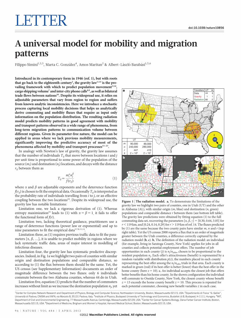
LETTERdoi:10.1038/nature10856

A universal model for mobility and migrationpatternsFilippo Simini1,2,3, Marta C. Gonzalez4, Amos Maritan2 & Albert-Laszlo Barabasi1,5,6

Introduced in its contemporary form in 1946 (ref. 1), but with rootsthat go back to the eighteenth century2, the gravity law1,3,4 is the pre-vailing framework with which to predict population movement3,5,6,cargo shipping volume7 and inter-city phone calls8,9, as well as bilateraltrade flows between nations10. Despite its widespread use, it relies onadjustable parameters that vary from region to region and suffersfrom known analytic inconsistencies. Here we introduce a stochasticprocess capturing local mobility decisions that helps us analyticallyderive commuting and mobility fluxes that require as input onlyinformation on the population distribution. The resulting radiationmodel predicts mobility patterns in good agreement with mobilityand transport patterns observed in a wide range of phenomena, fromlong-term migration patterns to communication volume betweendifferent regions. Given its parameter-free nature, the model can beapplied in areas where we lack previous mobility measurements,significantly improving the predictive accuracy of most of thephenomena affected by mobility and transport processes11–23.

In analogy with Newton’s law of gravity, the gravity law assumesthat the number of individuals Tij that move between locations i and jper unit time is proportional to some power of the population of thesource (mi) and destination (nj) locations, and decays with the distancerij between them as

Tij~ma

i nbj

f (rij)ð1Þ

where a and b are adjustable exponents and the deterrence functionf(rij) is chosen to fit the empirical data. Occasionally Tij is interpreted asthe probability rate of individuals travelling from i to j, or an effectivecoupling between the two locations24. Despite its widespread use, thegravity law has notable limitations:

Limitation one, we lack a rigorous derivation of (1). Whereasentropy maximization25 leads to (1) with a 5 b 5 1, it fails to offerthe functional form of f(r).

Limitation two, lacking theoretical guidance, practitioners use arange of deterrence functions (power law or exponential) and up tonine parameters to fit the empirical data5,7,8,11,14.

Limitation three, as (1) requires previous traffic data to fit the para-meters [a, b, …], it is unable to predict mobility in regions where welack systematic traffic data, areas of major interest in modelling ofinfectious diseases.

Limitation four, the gravity law has systematic predictive discrep-ancies. Indeed, in Fig. 1a we highlight two pairs of counties with similarorigin and destination populations and comparable distance, soaccording to (1) the flux between them should be the same. Yet, theUS census (see Supplementary Information) documents an order ofmagnitude difference between the two fluxes: only 6 individualscommute between the two Alabama counties, whereas 44 do in Utah.

Limitation five, equation (1) predicts that the number of commutersincreases without limit as we increase the destination population nj, yet

1Center for Complex Network Research and Department of Physics, Biology and Computer Science, Northeastern University, Boston, Massachusetts 02115, USA. 2Dipartimento di Fisica ‘‘G. Galilei’’,Universita di Padova, CNISM and INFN, via Marzolo 8, 35131 Padova, Italy. 3Institute of Physics, Budapest University of Technology and Economics, Budafoki ut 8, Budapest, H-1111, Hungary. 4MIT,Department of Civil and Environmental Engineering, 77 Massachusetts Avenue, Cambridge, Massachusetts 02139, USA. 5Center for Cancer Systems Biology, Dana-Farber Cancer Institute, Boston,Massachusetts 02115, USA. 6Department of Medicine, Brigham and Women’s Hospital, Harvard Medical School, Boston, Massachusetts 02115, USA.

Data

Radiation

Gravity

UT AL

44

66

1

6

2

1

Travellers

mnrs

UT AL

240,000

90,000 89,000

2 × 106

280,000

447 410

s

m

n

a

Washington County,UT

Houston County,AL

Madison County,AL

Davis County,UT

1

1

4

13

251313

22

235

3

3

44

44

4

4

4

4

5

2

9

8

9

8

9

8

9

8

98

9

8

7

67

6

6 7

6

6

5

5

5

10

5

11

12

12

1115

17

32

10

11

12

11 1715173

3

3

4

4

2

10

2 2

1

1

1

1

2

2

28

6

9

8

6

8

7

8 6

7

8

9

7 8

9

7

8

6

9

8

69

7

6

9

7

18

16 20

16

16

2

121511 12

11

11

4

2

5

3 5

3

510

10

22

9

1112

?

22224

888888888888888888888888

5

2

7

1310

1

1

4

13

251313

2

2

25

3

3

44

44

4

4

4

5

2

9

8

9

8

99

8

98

9

8

67

6

6 7

6

6

5

5

5

10

12

12

1115

17 10

11

12

11 1715173

3

4

4

2

2 2

1

11

2

2

86

9

6

8

8 6

7

9

7 8

9

7

6

96

9

7

9

7

18

20

16

16

2

1511

11

5 10

3210

1

8

7

88

8616 12

12

11

4

2

5

3

3

510

11

11111111111111111111111333333333333333333

48

4

87

533

5543

543

5543

10

!

13

b c2 × 107

Figure 1 | The radiation model. a, To demonstrate the limitations of thegravity law we highlight two pairs of counties, one in Utah (UT) and the otherin Alabama (AL), with similar origin (m, blue) and destination (n, green)populations and comparable distance r between them (see bottom left table).The gravity law predictions were obtained by fitting equation (1) to the fullcommuting data set, recovering the parameters [a, b, c] 5 [0.30, 0.64, 3.05] forr , 119 km, and [0.24, 0.14, 0.29] for r . 119 km of ref. 14. The fluxes predictedby (1) are the same because the two county pairs have similar m, n and r (topright table). Yet the US census 2000 reports a flux that is an order of magnitudegreater between the Utah counties, a difference correctly captured by theradiation model (b, c). b, The definition of the radiation model: an individual(for example, living in Saratoga County, New York) applies for jobs in allcounties and collects potential employment offers. The number of jobopportunities in each county (j) is nj/njobs, chosen to be proportional to theresident population nj. Each offer’s attractiveness (benefit) is represented by arandom variable with distribution p(z), the numbers placed in each countyrepresenting the best offer among the nj/njobs trials in that area. Each county ismarked in green (red) if its best offer is better (lower) than the best offer in thehome county (here z 5 10). c, An individual accepts the closest job that offersbetter benefits than his home county. In the shown configuration the individualwill commute to Oneida County, New York, the closest county whose benefitz 5 13 exceeds the home county benefit z 5 10. This process is repeated foreach potential commuter, choosing new benefit variables z in each case.

9 6 | N A T U R E | V O L 4 8 4 | 5 A P R I L 2 0 1 2

Macmillan Publishers Limited. All rights reserved©2012

the number of commuters cannot exceed the source population mi,highlighting the gravity law’s analytical inconsistency (see Supplemen-tary Information, Section 4).

Limitation six, being deterministic, the gravity law cannot accountfor fluctuations in the number of travellers between two locations.

Motivated by these known limitations, alternative approaches likethe intervening opportunity model26 or the random utility model27 (Sup-plementary Information, Section 7) have been proposed. Althoughderived from first principles, these models continue to containcontext-specific tunable parameters, and their predictive power is atbest comparable to the gravity law28.

Here we introduce a modelling framework that relies on firstprinciples and overcomes the problems of limitations one to six ofthe gravity law. Whereas commuting is a daily process, its source anddestination is determined by job selection, a decision made over longertimescales. Using the natural partition of a country into counties (forwhich commuting data are collected), we assume that job selectionconsists of two steps (Fig. 1 b, c).

Step one, an individual seeks job offers from all counties, includinghis/her home county. The number of employment opportunities ineach county is proportional to the resident population, n, assumingthat there is one job opening for every njobs individuals. We capture thebenefits of a potential employment opportunity with a single number,z, randomly chosen from distribution p(z) where z represents a com-bination of income, working hours, conditions, etc. Thus, each countywith population n is assigned n/njobs random numbers, z1, z2, …,z½n=njobs�, accounting for the fact that the larger a county’s population,the more employment opportunities it offers.

Step two, the individual chooses the closest job to his/her home,whose benefits z are higher than the best offer available in his/her homecounty. Thus lack of commuting has priority over the benefits, that is,individuals are willing to accept lesser jobs closer to their home.

This process, applied in proportion to the resident population ineach county, assigns work locations to each potential commuter, whichin turn determines the daily commuting fluxes across the country. Themodel has three unknown parameters: the benefit distribution p(z), thejob density njobs, and the total number of commuters, Nc. We show,however, that the commuting fluxes Tij are independent of p(z) andnjobs, and the remaining free parameter, Nc, does not affect the fluxdistribution, making the model parameter-free. As the model can beformulated in terms of radiation and absorption processes (seeSupplementary Information, Section 2), we will refer to it as the radi-ation model. To analytically predict the commuting fluxes we considerlocations i and j with population mi and nj respectively, at distance rij

from each other, and we denote with sij the total population in thecircle of radius rij centred at i (excluding the source and destinationpopulation). The average flux Tij from i to j, as predicted by the radi-ation model (see Supplementary Information, Section 2), is

Tij� �

~Timinj

(mizsij)(miznjzsij)ð2Þ

which is independent of both p(z) and njobs. Hence (2) represents thefundamental equation of the radiation model, the proposed alternativeto the gravity law (1). Here Ti:

Pj=i

Tij is the total number of commuters

that start their journey from location i, which is proportional to thepopulation of the source location, hence Ti 5 mi(Nc/N), where Nc is thetotal number of commuters and N is the total population in the country(Fig. 2g).

Equation (2) resolves limitations one to six of the gravity law: it has arigorous derivation (resolving limitation one) and has no free para-meters (bypassing limitations two and three). To understand the originof limitation four, we note that a key difference between the radiationmodel (2) and the gravity law (1) is that the variable of (2) is not thedistance rij, but sij. Thus the commuting flux depends not only on mi

and nj but also on the population sij of the region surrounding the

source location. For uniform population density sij<mir2ij and n 5 m,

(2) reduces to the gravity law (1) with f(r) 5 rc, c 5 4 and a 1 b 5 1.The non-uniform population density, however, is key to resolving theproblem of limitation four: equation (2) predicts an order of magnitudedifference in Alabama and Utah, in line with the census data (seeFig. 1a). Indeed the population density around Utah is significantlylower than the United States average, thus work opportunities withinthe same radius are ten times smaller in Utah than in Alabama, imply-ing that commuters in Utah have to travel farther to find comparableemployment opportunities. Note also that equation (2) predicts thatthe number of travellers leaving from a location with population m toone with n?? saturates at Tn??~ m2

(mzs) zO 1n

� �ƒm, resolving the

unphysical divergence highlighted in limitation five. Finally, Tij in theradiation model is a stochastic variable, predicting not only the averageflux between two locations (2), but also its variance (see SupplementaryInformation, Section 2), resolving the problem of limitation six.

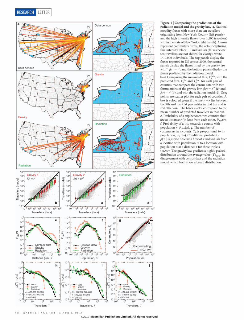
To explore the radiation model’s ability to predict the correctcommuting patterns, in Fig. 2a we show the commuting fluxes withmore than ten travellers originating from New York County. Thedestinations predicted by the gravity law14 are all within 400 km fromthe origin, missing all long distance and many medium distance trips.The gravity law’s local performance is equally poor: within the State ofNew York it grossly overestimates fluxes in the vicinity of New YorkCity and underestimates the fluxes in the rest of the state (Fig. 2a, rightcolumn). The radiation model offers a more realistic approximation tothe observed commuting patterns, both nationally and state-wide(Fig. 2a, bottom panels). To quantify the observed differences, wecompare the measured and the predicted non-zero commuting fluxesfor all pairs of counties in the United States. We find that both standardimplementations of the gravity law11,14 (f(r) 5 rc and f(r) 5 edr, where dis a fitting parameter with the unit of an inverse length needed to ensurea dimensionless argument to the exponential function) significantlyunderestimate the high flux commuting patterns, often by an order ofmagnitude or more (Fig. 2b, c). In contrast, the average fluxes predictedby the radiation model are within the error bars despite the observedsix orders of magnitude span in commuting fluxes (Fig. 2d).

The systematic failure of the gravity law is particularly evident if wemeasure the probability Pdist(r) of a trip between locations at distance r(Fig. 2e), and the probability of trips towards a destination with popu-lation n, Pdest(n) (Fig. 2f). For Pdist(r) the radiation model clearlyfollows the peak around 40 km in the census data. The predictionbased on the gravity law lacks this peak and thus it overestimates bythree orders of magnitude the number of short distance trips.Similarly, the gravity law overestimates the low n values of Pdest(n)by nearly an order of magnitude.

Another important mobility measure is the conditional probabilityp(T jm,n,r) to observe a flux of T individuals from a location withpopulation m to a location with population n at a distance r. Thegravity law predicts a highly peaked p(T jm,n,r) distribution aroundthe average Th imnr~

XT

p(Tjm,n,r)T (Fig. 2h–j), because, accord-ing to (1) pairs of locations with the same (m, n, r) have the same flux.In contrast the radiation model predicts a broad p(T jm,n,r) distri-bution, in reasonable agreement with the data.

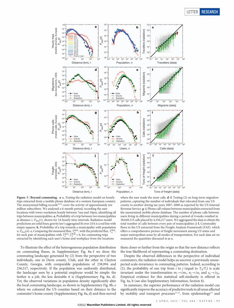
To show the generality of the model in Fig. 3 we test its performancefor four socio-economic phenomena: hourly travel patterns, migra-tions, communication patterns and commodity flows. We find that theradiation model offers an accurate quantitative description of mobilityand transport spanning a wide range of time scales (hourly mobility,daily commuting, yearly migrations), capturing diverse processes(commuting, intra-day mobility, call patterns, trade), collected via awide range of tools (census, mobile phones, tax documents) on differ-ent continents (America, Europe). The agreement with data of suchdiverse nature is somewhat surprising, suggesting that the hypothesesbehind the model capture fundamental decision mechanisms that,directly or indirectly, are relevant to a wide span of mobility andtransport-driven processes.

LETTER RESEARCH

5 A P R I L 2 0 1 2 | V O L 4 8 4 | N A T U R E | 9 7

Macmillan Publishers Limited. All rights reserved©2012

Data census

Radiation

Gravity

Data census

Radiation

Gravity

a

10–1

100

101

102

103

104

105

106

10–1 100 101 102 103 104 105 106

Tra

velle

rs (m

od

el)

Travellers (data)

Gravity 1

f(r) = rγ

b

Tra

velle

rs (m

od

el)

Travellers (data)

Gravity 2

c

Tra

velle

rs (m

od

el)

Travellers (data)

Radiation

d

Population, n

f

Census dataGravityRadiation

Pd

ist(r)

Distance (km), r

e

Census dataGravityRadiation

Co

mm

ute

rs, T i

Population, mi

US commutingTi = 0.11mi

g

p(T

| m

,n,r

)

Travellers, T

m = (10,000–50,000)

n = (10,000–50,000)

r = (40–60)

DataGravityRadiation

Travellers, T

m = (80,000–150,000)

n = (10,000–50,000)

r = (40–60)

Travellers, T

m = (10,000–50,000)

n = (10,000–50,000)

r = (80–100)

DataGravity

Radiation

h i j

DataGravity

Radiation

10–1

100

101

102

103

104

105

106

10–1 100 101 102 103 104 105 106

f(r) = erd

10–1

100

101

102

103

104

105

106

10–1 100 101 102 103 104 105 106

10–7

10–6

10–5

10–4

10–3

10–2

10–1

100

10–8

100 101 102 103 104

Pd

ist(n)

10–11

10–10

10–9

10–8

10–7

10–6

10–5

10–4

101 102 103 104 105 106 107 108100

101

102

103

104

105

106

101 102 103 104 105 106 107

100 101 102 103 10410–7

10–6

10–5

10–4

10–3

10–2

10–1

100

10–6

10–5

10–4

10–3

10–2

10–1

p(T

| m

,n,r

)

100 101 102 103 104 100 101 102 103 104

10–6

10–5

10–4

10–3

10–2

10–1

100

101

10–7

p(T

| m

,n,r

)

Figure 2 | Comparing the predictions of theradiation model and the gravity law. a, Nationalmobility fluxes with more than ten travellersoriginating from New York County (left panels)and the high intensity fluxes (over 1,100 travellers)within the state of New York (right panels). Arrowsrepresent commuters fluxes, the colour capturingflux intensity: black, 10 individuals (fluxes belowten travellers are not shown for clarity), white,.10,000 individuals. The top panels display thefluxes reported in US census 2000, the centralpanels display the fluxes fitted by the gravity lawwith14 f(r) 5 rc, and the bottom panels display thefluxes predicted by the radiation model.b–d, Comparing the measured flux, Tdata

ij , with thepredicted flux, TGM

ij and TRadij , for each pair of

counties. We compare the census data with twoformulations of the gravity law, f(r) 5 edr (c) andf(r) 5 rc (b), and with the radiation model (d). Greypoints are scatter plot for each pair of counties. Abox is coloured green if the line y 5 x lies betweenthe 9th and the 91st percentiles in that bin and isred otherwise. The black circles correspond to themean number of predicted travellers in that bin.e, Probability of a trip between two counties thatare at distance r (in km) from each other, Pdist(r).f, Probability of a trip towards a county withpopulation n, Pdest(n). g, The number ofcommuters in a county, Ti, is proportional to itspopulation, mi. h–j, Conditional probabilityp(T | m,n,r) to observe a flow of T individuals froma location with population m to a location withpopulation n at a distance r for three triplets(m,n,r). The gravity law predicts a highly peakeddistribution around the average value Th imnr , indisagreement with census data and the radiationmodel, which both show a broad distribution.

RESEARCH LETTER

9 8 | N A T U R E | V O L 4 8 4 | 5 A P R I L 2 0 1 2

Macmillan Publishers Limited. All rights reserved©2012

To illustrate the effect of the heterogeneous population distributionon commuting fluxes, in Supplementary Fig. 8a–f we show thecommuting landscape generated by (2) from the perspective of twoindividuals, one in Davis county, Utah, and the other in ClaytonCounty, Georgia, with comparable populations of 238,994 and236,517, respectively. If the population was uniformly distributed,the landscape seen by a potential employee would be simple: thefarther is a job, the less desirable it is (Supplementary Fig. 8a, d).Yet, the observed variations in population density significantly alterthe local commuting landscape, as shown in Supplementary Fig. 8b, ewhere we coloured the US counties based on their distance to thecommuter’s home county (Supplementary Fig. 8a, d) and then moved

them closer or further from the origin so that the new distance reflectsthe true likelihood of representing a commuting destination.

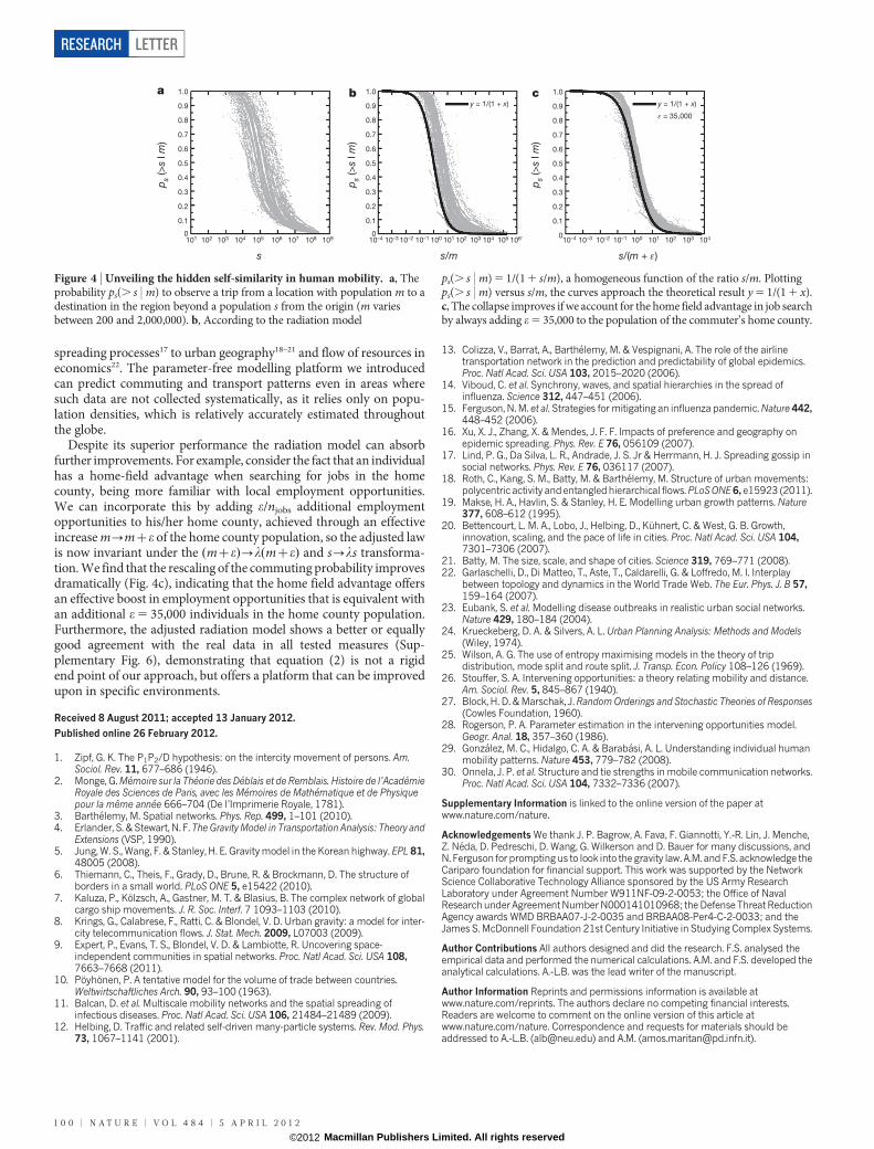
Despite the observed differences in the perspective of individualcommuters, the radiation model helps us uncover a previously unsus-pected scale-invariance in commuting patterns. Indeed, according to(2), the probability of one trip from i to j (equal to Tij/Ti) is scaleinvariant under the transformation mi?lmi, nj?lnj and sij?lsij.Empirical evidence for this statistical self-similarity is offered inFig. 4a, b (see also Supplementary Information, Section 8).

In summary, the superior performance of the radiation model cansignificantly improve the accuracy of predictive tools in all areas affectedby mobility and transport processes11,12, from epidemiology13 and

100 101 102 103 104 105 106 107

Population, n

b

10–8

10–7

10–6

10–5

10–4

10–3

10–2

10–1

100

100 101 102 103 104P

dis

t(r)

Distance (km), r

a

7-88-99-1010-1111-1212-1313-1414-1515-1616-1717-1818-1919-2020-2121-22Gravity model

10–1

100

101

102

103

104

105

10–1 100 101 102 103 104 105

Tra

velle

rs (ra

dia

tio

n)

Travellers (data)

c

Population, n

e

DataGravityRadiation

Distance (km), r

d

DataGravityRadiation

100

101

102

103

104

105

100 101 102 103 104 105

Mig

ran

ts (ra

dia

tio

n)

Migrants (data)

f

10–7

10–6

10–5

10–4

10–3

10–2

100 101 102 103 104 105 106

Users, n

h

DataGravityRadiation

Distance (km), r

g

DataGravityRadiation

10–1

100

101

102

103

104

105

106

10–1 100 101 102 103 104 105 106C

alls

(ra

dia

tio

n)

Calls (data)

i

10–9

10–8

10–7

10–6

105 106 107 108

Population, n

k

DataGravityRadiation

Distance (km), r

j

DataGravityRadiation T

on

s o

f fr

eig

ht

(rad

iatio

n)

Tons of freight (data)

l

Ho

urly t

rip

s(m

ob

ile p

ho

nes, E

uro

pe)

Mig

ratio

ns

(tax d

ocum

ents

, U

SA

)

Pho

ne c

alls

(mo

bile

calls

, E

uro

pe)

Fre

ight

(inte

rsta

te, U

SA

)

Pd

est(n)

10–8

10–7

10–6

10–5

10–4

10–3

10–9

Pd

ist(r)

10–8

10–7

10–6

10–5

10–4

10–3

10–2

10–1

100

100 101 102 103 104 101 102 103 104 105 106 107 108

10–9

10–8

10–7

10–6

10–5

10–4

10–10P

dest(n)

10–8

10–7

10–6

10–5

10–4

10–3

10–2

10–1

100

100 101 102 103 104

Pd

ist(r)

Pd

est(n)

Pd

ist(r)

10–8

10–7

10–6

10–5

10–4

10–3

10–2

10–1

100

100 101 102 103 104

Pd

est(n)

10–1

100

101

102

103

104

105

106

10–1 100 101 102 103 104 105 106

Figure 3 | Beyond commuting. a–c, Testing the radiation model on hourlytrips extracted from a mobile phone database of a western European country.The anonymized billing records29,30 cover the activity of approximately tenmillion subscribers. We analysed a 6-month period, recording the userlocations with tower resolution hourly between 7am and 10pm, identifying alltrips between municipalities. a, Probability of a trip between two municipalitiesat distance r, Pdist(r), shown for 14-hourly time intervals. Radiation modelpredictions are solid lines; gravity law’s aggregated fit over 24 h is a red line withempty squares. b, Probability of a trip towards a municipality with populationn, Pdest(n). c, Comparing the measured flux, Tdata

ij , with the predicted flux, TRadij ,

for each pair of municipalities with Tdataij ,TRad

ij w0, for commuting tripsextracted by identifying each user’s home and workplace from the locations

where the user made the most calls. d–f, Testing (2) on long-term migrationpatterns, capturing the number of individuals that relocated from one UScounty to another during tax years 2007–2008 as reported by the US InternalRevenue Service. g–i, Phone call volume between municipalities extracted fromthe anonymized mobile phone database. The number of phone calls betweenusers living in different municipalities during a period of 4 weeks resulted in38,649,153 calls placed by 4,336,217 users. We aggregated the data to obtain thetotal number of calls between every pair of municipalities. j–l, Commodityflows in the US extracted from the Freight Analysis Framework (FAF), whichoffers a comprehensive picture of freight movement among US states andmajor metropolitan areas by all modes of transportation. For each data set wemeasured the quantities discussed in a–c.

LETTER RESEARCH

5 A P R I L 2 0 1 2 | V O L 4 8 4 | N A T U R E | 9 9

Macmillan Publishers Limited. All rights reserved©2012

spreading processes17 to urban geography18–21 and flow of resources ineconomics22. The parameter-free modelling platform we introducedcan predict commuting and transport patterns even in areas wheresuch data are not collected systematically, as it relies only on popu-lation densities, which is relatively accurately estimated throughoutthe globe.

Despite its superior performance the radiation model can absorbfurther improvements. For example, consider the fact that an individualhas a home-field advantage when searching for jobs in the homecounty, being more familiar with local employment opportunities.We can incorporate this by adding e/njobs additional employmentopportunities to his/her home county, achieved through an effectiveincrease m?mze of the home county population, so the adjusted lawis now invariant under the (mze)?l(mze) and s?ls transforma-tion. We find that the rescaling of the commuting probability improvesdramatically (Fig. 4c), indicating that the home field advantage offersan effective boost in employment opportunities that is equivalent withan additional e 5 35,000 individuals in the home county population.Furthermore, the adjusted radiation model shows a better or equallygood agreement with the real data in all tested measures (Sup-plementary Fig. 6), demonstrating that equation (2) is not a rigidend point of our approach, but offers a platform that can be improvedupon in specific environments.

Received 8 August 2011; accepted 13 January 2012.

Published online 26 February 2012.

1. Zipf, G. K. The P1P2/D hypothesis: on the intercity movement of persons. Am.Sociol. Rev. 11, 677–686 (1946).

2. Monge, G. Memoire sur la Theorie des Deblais et de Remblais. Histoire de l’AcademieRoyale des Sciences de Paris, avec les Memoires de Mathematique et de Physiquepour la meme annee 666–704 (De l’Imprimerie Royale, 1781).

3. Barthelemy, M. Spatial networks. Phys. Rep. 499, 1–101 (2010).4. Erlander, S. & Stewart, N. F. The Gravity Model in Transportation Analysis: Theory and

Extensions (VSP, 1990).5. Jung, W. S., Wang, F. & Stanley, H. E. Gravity model in the Korean highway. EPL 81,

48005 (2008).6. Thiemann, C., Theis, F., Grady, D., Brune, R. & Brockmann, D. The structure of

borders in a small world. PLoS ONE 5, e15422 (2010).7. Kaluza, P., Kolzsch, A., Gastner, M. T. & Blasius, B. The complex network of global

cargo ship movements. J. R. Soc. Interf. 7 1093–1103 (2010).8. Krings, G., Calabrese, F., Ratti, C. & Blondel, V. D. Urban gravity: a model for inter-

city telecommunication flows. J. Stat. Mech. 2009, L07003 (2009).9. Expert, P., Evans, T. S., Blondel, V. D. & Lambiotte, R. Uncovering space-

independent communities in spatial networks. Proc. Natl Acad. Sci. USA 108,7663–7668 (2011).

10. Poyhonen, P. A tentative model for the volume of trade between countries.Weltwirtschaftliches Arch. 90, 93–100 (1963).

11. Balcan, D. et al. Multiscale mobility networks and the spatial spreading ofinfectious diseases. Proc. Natl Acad. Sci. USA 106, 21484–21489 (2009).

12. Helbing, D. Traffic and related self-driven many-particle systems. Rev. Mod. Phys.73, 1067–1141 (2001).

13. Colizza, V., Barrat, A., Barthelemy, M. & Vespignani, A. The role of the airlinetransportation network in the prediction and predictability of global epidemics.Proc. Natl Acad. Sci. USA 103, 2015–2020 (2006).

14. Viboud, C. et al. Synchrony, waves, and spatial hierarchies in the spread ofinfluenza. Science 312, 447–451 (2006).

15. Ferguson, N. M. et al. Strategies for mitigating an influenza pandemic. Nature 442,448–452 (2006).

16. Xu, X. J., Zhang, X. & Mendes, J. F. F. Impacts of preference and geography onepidemic spreading. Phys. Rev. E 76, 056109 (2007).

17. Lind, P. G., Da Silva, L. R., Andrade, J. S. Jr & Herrmann, H. J. Spreading gossip insocial networks. Phys. Rev. E 76, 036117 (2007).

18. Roth, C., Kang, S. M., Batty, M. & Barthelemy, M. Structure of urban movements:polycentric activity andentangledhierarchical flows. PLoS ONE 6, e15923 (2011).

19. Makse, H. A., Havlin, S. & Stanley, H. E. Modelling urban growth patterns. Nature377, 608–612 (1995).

20. Bettencourt, L. M. A., Lobo, J., Helbing, D., Kuhnert, C. & West, G. B. Growth,innovation, scaling, and the pace of life in cities. Proc. Natl Acad. Sci. USA 104,7301–7306 (2007).

21. Batty, M. The size, scale, and shape of cities. Science 319, 769–771 (2008).22. Garlaschelli, D., Di Matteo, T., Aste, T., Caldarelli, G. & Loffredo, M. I. Interplay

between topology and dynamics in the World Trade Web. The Eur. Phys. J. B 57,159–164 (2007).

23. Eubank, S. et al. Modelling disease outbreaks in realistic urban social networks.Nature 429, 180–184 (2004).

24. Krueckeberg, D. A. & Silvers, A. L. Urban Planning Analysis: Methods and Models(Wiley, 1974).

25. Wilson, A. G. The use of entropy maximising models in the theory of tripdistribution, mode split and route split. J. Transp. Econ. Policy 108–126 (1969).

26. Stouffer, S. A. Intervening opportunities: a theory relating mobility and distance.Am. Sociol. Rev. 5, 845–867 (1940).

27. Block, H. D. & Marschak, J. Random Orderings and Stochastic Theories of Responses(Cowles Foundation, 1960).

28. Rogerson, P. A. Parameter estimation in the intervening opportunities model.Geogr. Anal. 18, 357–360 (1986).

29. Gonzalez, M. C., Hidalgo, C. A. & Barabasi, A. L. Understanding individual humanmobility patterns. Nature 453, 779–782 (2008).

30. Onnela, J. P. et al. Structure and tie strengths in mobile communication networks.Proc. Natl Acad. Sci. USA 104, 7332–7336 (2007).

Supplementary Information is linked to the online version of the paper atwww.nature.com/nature.

Acknowledgements We thank J. P. Bagrow, A. Fava, F. Giannotti, Y.-R. Lin, J. Menche,Z. Neda, D. Pedreschi, D. Wang, G. Wilkerson and D. Bauer for many discussions, andN. Ferguson for prompting us to look into the gravity law. A.M. and F.S. acknowledge theCariparo foundation for financial support. This work was supported by the NetworkScience Collaborative Technology Alliance sponsored by the US Army ResearchLaboratory under Agreement Number W911NF-09-2-0053; the Office of NavalResearch underAgreement Number N000141010968; the Defense Threat ReductionAgency awards WMD BRBAA07-J-2-0035 and BRBAA08-Per4-C-2-0033; and theJames S. McDonnell Foundation 21st Century Initiative in Studying Complex Systems.

Author Contributions All authors designed and did the research. F.S. analysed theempirical data and performed the numerical calculations. A.M. and F.S. developed theanalytical calculations. A.-L.B. was the lead writer of the manuscript.

Author Information Reprints and permissions information is available atwww.nature.com/reprints. The authors declare no competing financial interests.Readers are welcome to comment on the online version of this article atwww.nature.com/nature. Correspondence and requests for materials should beaddressed to A.-L.B. ([email protected]) and A.M. ([email protected]).

1.0

0.9

0.8

0.7

0.6

0.5

0.4

0.3

0.2

0.1

0

1.0

0.9

0.8

0.7

0.6

0.5

0.4

0.3

0.2

0.1

0

1.0

0.9

0.8

0.7

0.6

0.5

0.4

0.3

0.2

0.1

0101 102 103 104 105 106 107 108 109 10–4 10–3 10–2 10–1 100 101 102 103 104 105 106 10–4 10–3 10–2 10–1 100 101 102 103 104

ps

(>s

l m

)

y = 1/(1 + x) y = 1/(1 + x)

ε = 35,000

s s/m s/(m + ε)

ps

(>s

l m

)

ps

(>s

l m

)

a b c

Figure 4 | Unveiling the hidden self-similarity in human mobility. a, Theprobability ps(. s | m) to observe a trip from a location with population m to adestination in the region beyond a population s from the origin (m variesbetween 200 and 2,000,000). b, According to the radiation model

ps(. s | m) 5 1/(1 1 s/m), a homogeneous function of the ratio s/m. Plottingps(. s | m) versus s/m, the curves approach the theoretical result y 5 1/(1 1 x).c, The collapse improves if we account for the home field advantage in job searchby always adding e 5 35,000 to the population of the commuter’s home county.

RESEARCH LETTER

1 0 0 | N A T U R E | V O L 4 8 4 | 5 A P R I L 2 0 1 2

Macmillan Publishers Limited. All rights reserved©2012