A Univariate Time Series Analysis of Philippine Inflation … · 2014-05-23 · This study relies on a univariate time series analysis of Philippine m-o-m ... the model is completed

42

AUThORS

Felipe M. Medalla Dr. Felipe Medalla is a member of the Monetary Board of the Bangko Sentral ng Pilipinas (the Philippines’ central bank, since July 2011). Before he joined the Monetary Board, he was a professor at the University of the Philippines School of Economics, where he served as dean for four years prior to his appointment as a member of the cabinet under President Joseph Estrada (as Secretary of Socio-Economic Planning and Director-General of the national Economic and Development Authority in 1998–2001). he was a member of the Presidential Task Force on Tax and Tariff Reform under the administration of President Fidel Ramos and was President of the Philippine Economic Society in 1996. he was Chairman of the Foundation for Economic Freedom, a non-govermental organization that is primarily engaged in public advocacy for fiscal reforms and market-friendly government policies. he has written on the effects of economic policies on poverty and problems in the measurement of Philippine economic growth, among other topics. Dr. Medalla got his Ph.D. in Economics from northwestern University in Evanston, Illinois and has an M.A. in Economics from the University of the Philippines. he graduated cum laude from De La Salle University with a Bachelor of Arts and Bachelor of Science in Commerce (Economics-Accounting) degree.

Laura B. Fermo Ms. Laura B. Fermo is Bank Officer V at the Department of Economic Research and presently assigned to the Office of Monetary Board (MB) Member Felipe M. Medalla, providing inputs and technical research assistance on macroeconomic issues and monetary policy, including but not limited to preparing research papers and conducting statistical and econometric analyses. Ms. Fermo is a PhD candidate in Economics from the University of the Philippines School of Economics (UPSE) where she also obtained her MA and undergraduate degree (cum laude) in Economics. Before joining the BSP, Ms. Fermo worked at the Asian Development Bank and the University of Asia and the Pacific. She has also served as lecturer at the University of the Philippines School of Economics.

A Univariate Time Series Analysis of Philippine Inflation During the Inflation Targeting Period

Introduction

This paper examines the behavior of month-on-month (m-o-m) inflation

and finds empirical evidence that the BSP’s inflation targeting (IT) policy

regime over the past ten years was indeed successful in anchoring infla-

tion expectations compared to the decade before, during its early years

as an independent monetary authority, prior to its adoption of IT. Inflation

expectations are said to be well anchored if the public expects the infla-

tion rate to converge back to the central bank’s inflation target, in spite

of the occurrence of a short spell when the inflation rate is outside the

central banks’ officially announced target range.1 One indicator of this is

when the m-o-m inflation rate becomes an autoregressive mean-station-

ary process, where the variations (i.e., the change in the m-o-m inflation

rate) are generally white noise.

Consequently, if only unanticipated shocks move m-o-m inflation, it is important to ask which movements in the inflation rate monetary authorities should react to and which it should not react to. Our recommendation is that monetary authorities need not respond to short-run, and likely to be temporary, deviations in the m-o-m inflation rate from the mean.2 This holds true unless the changes, whether for a single month or a string of months, are large enough to dislodge inflation expectations, which could possibly lead to permanent changes in the long-run inflation trend. Such would be the case, for example, if there is a large random shock (or a string of smaller shocks, which taken together is large) and administered (or politically-set) wages are adjusted as a reaction to the large shock. If this happens, a wage-price spiral could be triggered which could, in turn, result in inflation that would be persistently higher than the central bank’s target band.

This study relies on a univariate time series analysis of Philippine m-o-m inflation before and during IT to show that inflation expectations were better anchored during the IT period than before IT. This is consistent with the fact that m-o-m inflation was not stationary during the pre-IT period but became stationary during the IT period. The study also looks at the behavior of m-o-m inflation before the BSP became an independent monetary authority and finds that it was also mean stationary, but with a much higher mean and variance. We proceed as well with several empirical tests on the characteristics of the change in the m-o-m inflation rate series to check if it is a white noise process, and proceed with the development of an applicable autoregressive-moving average (ARMA) model for the series.

1 Ball and Cecchetti (1990, p.215) noted than inflation “[…] would not be particularly costly if it were constant and dully anticipated but that a rise in the level of inflation raises uncertainty about future inflation.”

2 As Ball and Cecchetti (1990, p. 216) pointed out, “Permanent shocks are shifts in trend inflation, and temporary shocks are fluctuations around the trend. Uncertainty about [short-term or] next quarter’s inflation depends mainly on the variance of temporary shocks […].” Inflation uncertainty, they add, refers to the variance of unanticipated changes.

Bang

ko S

entra

l Rev

iew

201

3

18

Theoretical Framework and Literature ReviewIn order to guide the framework of analysis for this study, it is relevant to look into the basic concepts on the optimal conduct of monetary policy that have been widely developed in the literature. We use what is now the usual textbook model as in Froyen and Guender (2007). The model starts with a Lucas-type aggregate supply function, wherein output deviates from potential output only to the extent that inflation is higher or lower than expected or because of supply shocks. The aggregate demand function is derived from standard IS and LM equations. Lastly, as is now almost standard in most advanced macroeconomic textbooks, the model is completed by specifying objectives and constraints faced by policymakers and their effects on the formation of inflation expectations.

Thus, we have:

a Lucas-type aggregate supply equation:

y = y* + c (p – pe) + u, (1.1)

an IS curve:

y = f(r – πe, zIS) + v, (1.2)

an LM curve:

m/p = f(y, r , zLM, ) + η (1.3)

and inflation expectations are formed as:

πe = f(π*, π-k , ze). (1.4)

The rest of the variables are defined as:

y = real output,

y* = potential output

πe = ((pe-p-1 )/ p-1) = expected inflation

π* and π-k = long-run inflation target, vector of past inflation rates that are relevant for expectations formation, respectively,

p = aggregate price level,

r = nominal interest rate,

zIS and zLM = vector of exogenous variables affecting the IS and LM curves, respectively

ze = are other variables that economic agents use to forecast inflation

g = central bank instruments other than the interest rate and fiscal policies by the national government that could affect expectations

m = nominal money supply,

pe = expectation of the aggregate price level for the current period, formed on the basis of information at period (t – 1),

u,v,η = white noise disturbances with variances, σ2u, σ2

v, σ2η and zero

covariances.

From equation 1.1, it follows that supply or output is equal to potential output but deviates from it depending on the current period price forecast error and random supply shocks represented by the stochastic term ut. Equation 1.2, the IS equation, states that demand is a decreasing function of the real interest rate—defined as the nominal interest rate (r) minus the expected inflation rate from period t-1, a vector of other variables zIS (which the monetary authorities cannot directly influence but can either observe or predict with some level of confidence), and a stochastic term vt to measure shocks which affect demand in the goods market. Equation 1.3 is the LM curve which describes portfolio balance (e.g., between

Bangko Sentral Review 2013

19

bonds and money in the simplest textbook model). The left-hand side of the LM equation is real money supply and the right-hand side is demand for money which is assumed to be positively related to real income (y), and negatively related to nominal interest rate on bonds (r). The demand for money is also affected by a vector of variables zLM which the central bank cannot control but can either measure or predict with some level of confidence and the stochastic term η which represents shocks to money demand.

There are several permutations of policymaker behavior and expectations formation behavior that can be used to close the model. The simplest case is when expectations are well-anchored and there is an independent central bank which minimizes a generalized loss function such as equation 1.5 below.3

L(i,h) = Ei [ Σhi=1 βi{ μ1 [πi – π*]2 + µ2 [yi – y*]2} ] (1.5)

where:

πi = the actual inflation rate at period i,

yi = the growth rate of actual output at period i,

π* and y* = the desired levels for π and y,

β = the discount factor for period i

h = the horizon

µ1 and μ2 = the relative weight given to squared price and output deviations from their desired paths

Ei = expectation conditional on information available at period i

If we define expectations as being well anchored at π*, such that the public is expecting inflation to be π* except for random forecast errors, all terms except π* drop out from the right-hand side of equation 1.4, which becomes simply πe = π*. It follows from the loss function 1.5 and from the supply function equation 1.1 that it is optimal for the central bank to calibrate its policy variables such that Ey = y* (except when monetary policy is at a “zero-bound”, which means that the values of zIS and the parameters in the IS curve are such that output would be less than y* even when the nominal interest rate is zero). In other words, the central bank will disregard the stochastic terms of equations 1.1 and 1.2 and solve for the optimal values of y and r.4 Then given that y = y* and π = π*, r can be solved for in equation 1.2. note that given y and r, and setting p = p-1(1+ π*), m can be solved for using the expected value of equation 1.3, but the money supply that will result is a conditional mean value, not an actual realized value.5 In other words, to the extent that demand for money is volatile, monetary policy will be operationalized through interest rate setting, not through the direct determination of money supply.6

Equation 1.5 is clearly minimized if actual π equals π* plus a random error term and actual y equals y* plus a random error term, since the random errors are themselves just a linear combination of the error terms u, v, η in equations 1.1, 1.2 and 1.3. note that in this scenario, it is useful to distinguish between changes in y and p that are due to random shocks u, v, and η and those that emanate from changes in zIS and zLM. The first set of changes is essentially

3 Borrowing from papers such as Turnovsky (1980, 1983) and Benavie & Froyen (1983) as cited in Froyen & Guender (2007).

4 The assumption that the interest rate that the monetary policymaker controls is the same rate that is relevant for the IS schedule. In practice, it is a short-term rate, such as the Reverse Repurchase overnight rate in the case of the BSP, which is the monetary policy instrument. But the interest rate that has the most significant impact on aggregate demand and the IS schedule is, in fact, a long-term rate (Froyen and Guender, 2007, p. 45).

5 The same results are arrived at by the algebraic solution from Froyen and Guender (2007).6 In the absence of uncertainty, the policymaker can achieve its goals for output and the price level equally

well with either the money supply or the interest rate as its instrument. Policy is expressed here in terms of an interest rate setting, but within the information variable approach, the choice of which instrument is used to represent the policy setting is arbitrary. The optimal policy can therefore be expressed as a deterministic relationship between the money supply and the interest rate, similar to Poole’s (1970) (Froyen and Guender, 2007, p. 36). In practice, the BSP actually sets the policy interest rate, but closely monitors what happens to monetary aggregates.Ba

ngko

Sen

tral R

evie

w 2

013

20

unpredictable and it is therefore unwise for forward-looking policies to react to them. On the other hand, to the extent that the z variables can be predicted (e.g., that there are leading indicators that help predict whether the economy will be either weaker or stronger, or in the case of an open economy, that global economic conditions will reduce or increase net exports), then changes in monetary policy (e.g., the main policy interest rate in the case of the BSP) could be called for. The discussion of optimal policy under a target rule such as the inflation targeting framework of the BSP emphasizes the point that the policymaker can observe p and y in setting policy. In the real world, policymakers can observe some prices contemporaneously such as spot and futures commodity prices, but an index such as the GDP deflator is available only with considerable lag (Froyen and Guender, 2007). At any rate, it is clear in this case that the inflation rate can be described as a mean-stationary series, with a variance that would be difficult to reduce further because the changes in the inflation rate emanate from unpredictable random shocks in equations 1.1., 1.2 and 1.3.

If the central bank is not independent from the government but the latter cares as well about keeping the inflation rate stable and output as close as possible to potential output, equation 1.5 would need to also include the policy objectives of the national government and reflect its budget constraints. In effect, the non-independent inflation target π** will be higher than the independent central bank inflation target π* and non-independent preferences µ** will be higher than µ because politicians will have seignorage objectives since an inflation tax may be more palatable than additional explicit taxes. In general, the desired inflation targets of independent central bankers would be much lower than what maximizes seignorage since the independent central bank will not take into account the political benefits that arise from replacing explicit taxes by implicit ones (which, in this case, is in the form of higher inflation).7

If the political and macroeconomic governance scenario as described above has been the normal state for quite some time, people will be able to predict inflation, albeit with bigger prediction errors. The reason being is that as seen from equation 1.3, there would be shocks coming not just from the right-hand side of the equation but also from the left-hand side.8 Thus the LM curve will have an additional error term ζ that would be an additional source of variation for p and y, in addition to the error terms u,v,η. If πNI (actual inflation during the non-independent central bank period) is stable, inflation will still be mean-stationary but with a bigger mean and variance. On the other hand, if the tolerance for inflation varies with the electoral cycle, stationarity may or may not be ruled out depending on the stability of the tolerance for inflation as the economy goes through the political or election-related cycle. At any rate, neither stationarity nor non-stationarity can be ruled out but it is expected that inflation will be more volatile under non-independence than in the scenario where the central bank is independent and has had enough time to gain its credibility.

The transition between the two scenarios just described is bound to result in inflationary expectations that may become well anchored at the lower level only after a considerable period of time. It is probably worthwhile to attempt to explain why this transition period will not be very short or why a newly independent central bank may take some time before it can achieve its goal of significantly lower and well-anchored inflation expectations. Initially, the public will give little or no weight to the newly independent central bank’s long-run inflation target. Thus, equation 1.4 becomes:

πe = k(π-k , ze) (1.4’)

Where ze are indicators other than past inflation rates which are used to forecast inflation (e.g., the size of budget deficits).

7 Politicians may have a higher tolerance for inflation but they would not want to maximize seignorage either because the politically tolerable inflation rate is likely to be lower than what maximizes seignorage income because excessively higher inflation (i.e., beyond a certain threshold) may be more undesirable than new taxes.

8 This would be the case, for instance, in an open economy if the ability to finance the maturing portion of the public debt is disrupted by surprises in global capital markets, which would force the government to rely more on seigniorage than initially intended.


21

Given 1.1, 1.2, 1.3, 1.4’ and 1.5, policymakers must find the optimal values of r, m, and g. Unless expected inflation is already firmly set at π* (in which case, as previously discussed, r, m and g will be chosen to set Ey = y* and Eπ = π*) equations 1.1 to 1.5 are not sufficient to determine optimal r, m, and g. This optimal policy can be viewed as a solution to a problem in which the policymaker uses an instrument or instruments to stabilize the variability of output and prices to achieve a certain target or move toward a certain direction.

As the policymaker operates under uncertainty, his objective is to minimize the expected value of the loss function specified by equation 1.6. This loss function may be termed as an ‘intertemporal’ loss function. The time horizon for policy objectives extends from the current period to a finite period h which is the period relevant for the impact of monetary policy on the real economy. The size of β indicates to what extent losses in the future are discounted. A value of β=1 means that future losses are just as important as the losses in the current period. If equation 1.6 is determined solely by the central bank, then it has goal independence. If equation 1.6 comes from the central bank’s assessment of what the government wants but the latter does not interfere in the former’s choice of the policy variables that are under its control, the former is said to have instrument independence.9

Given the presence of stochastic terms, uncertainty is central to the question of the optimal conduct of monetary policy. The central bank will choose the instrument, whether m or r or a combination of the two which will result in the lowest expected value for the loss function. This optimization problem facing the policymaker has two characteristics: the objective function (1.4) is quadratic and the stochastic terms enter (1.1) to (1.3) additively. Problems of this form have a property called certainty equivalence.10 Certainty equivalence means that the solution to the stochastic optimization problem is the same as the solution to the problem ignoring uncertainty. This implies that the optimal setting for whichever instrument will be chosen is the same with what will be found under perfect certainty (Froyen and Guender, 2007, p.13). In other words, the central bank will use the expected values of equations 1.1 to 1.3. note that when inflation expectations are firmly set equal to π*, setting Ey = y* minimizes equation 1.5, which makes it very straightforward to find the optimal m and r.

As already stated, expected inflation could initially be much higher than π*, the long-run inflation target that a newly independent central bank would prefer. A new independent central bank would need to time to gain credibility, especially if economic agents have not, for a very long time, had any first-hand experience with an inflation-targeting central bank. Indeed, fiscal dominance was observed for a long time before the independent BSP was established in 1993. For instance, the only reason that the losses of the old Central Bank of the Philippines (CBP) did not result in loss of control over money aggregates was that the government was borrowing more than what was needed to finance its deficit and was depositing the excess borrowing with the old CBP to help control liquidity. (In turn, the large accumulated losses of the CBP were incurred because it was performing fiscal functions.) If, due to historical reasons, expected inflation is adaptive and is much higher than π*, it is not feasible to achieve Eπ = π* and Ey = y* immediately and at the same time. If Eπ = π*, then Ey < y*, or if Ey = y* then Eπ > π*. This means that there is a trade-off between achieving output and inflation targets during the period of disinflation. Given the quadratic

9 The BSP has instrument independence but not full goal independence. Although the BSP participates in the formulation of macroeconomic targets including inflation rates in the medium term, the national Economic and Development Authority (nEDA) is the lead agency in formulating the Medium-Term Philippine Development Plan. As the Plan is prepared only once during an administration’s term, the Development Budget Coordination Committee (DBCC) is the interagency body which periodically reviews the inflation targets and, if new conditions arise, the BSP may recommend any revision to the target, subject to DBCC approval. The DBCC is composed of the Department of Budget and Management (DBM), the Department of Finance (DOF), nEDA, the Office of the President, and the BSP. In practice, however, the BSP’s proposed inflation targets have always been approved by the DBCC (Lamberte, 2002).

10 The model solution has a certainty equivalence property if the optimization problem can be separated into two stages: first, getting the minimum mean squared error forecasts of the exogenous variables, which are the conditional expectations; second, at time t, solving the non-stochastic optimization problem, using the mean in place of the random variable. This separation of forecasting from optimization is computationally very convenient and explains why quadratic objective functions are assumed in much applied work. For general functions, however, the certainty equivalence principle does not hold, so that the forecasting and optimization problems cannot be separated (Sargent, 1979). Retrieved from http://economics.about.com/library/glossary/bldef-certainty-equivalence-principle.htm

Bang

ko S

entra

l Rev

iew

201

3

22

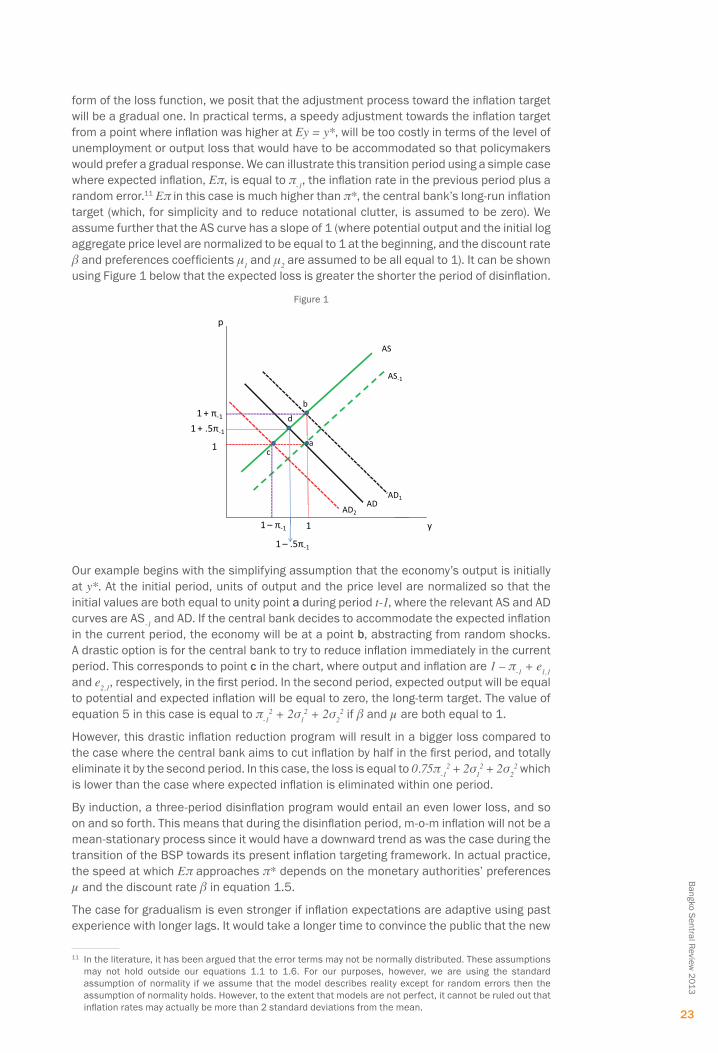
form of the loss function, we posit that the adjustment process toward the inflation target will be a gradual one. In practical terms, a speedy adjustment towards the inflation target from a point where inflation was higher at Ey = y*, will be too costly in terms of the level of unemployment or output loss that would have to be accommodated so that policymakers would prefer a gradual response. We can illustrate this transition period using a simple case where expected inflation, Eπ, is equal to π-1, the inflation rate in the previous period plus a random error.11 Eπ in this case is much higher than π*, the central bank’s long-run inflation target (which, for simplicity and to reduce notational clutter, is assumed to be zero). We assume further that the AS curve has a slope of 1 (where potential output and the initial log aggregate price level are normalized to be equal to 1 at the beginning, and the discount rate β and preferences coefficients μ1 and μ2 are assumed to be all equal to 1). It can be shown using Figure 1 below that the expected loss is greater the shorter the period of disinflation.

Figure 1

y

1

1 + π-1

1

AD

AS-1

AS

1 – π-1

AD1

1 – .5π-1

1 + .5π-1

p

a

b

AD2

c

d

Our example begins with the simplifying assumption that the economy’s output is initially at y*. At the initial period, units of output and the price level are normalized so that the initial values are both equal to unity point a during period t-1, where the relevant AS and AD curves are AS-1 and AD. If the central bank decides to accommodate the expected inflation in the current period, the economy will be at a point b, abstracting from random shocks. A drastic option is for the central bank to try to reduce inflation immediately in the current period. This corresponds to point c in the chart, where output and inflation are 1 – π-1 + e1,1 and e2,1, respectively, in the first period. In the second period, expected output will be equal to potential and expected inflation will be equal to zero, the long-term target. The value of equation 5 in this case is equal to π-1

2 + 2σ12 + 2σ2

2 if β and µ are both equal to 1.

however, this drastic inflation reduction program will result in a bigger loss compared to the case where the central bank aims to cut inflation by half in the first period, and totally eliminate it by the second period. In this case, the loss is equal to 0.75π-1

2 + 2σ12 + 2σ2

2 which is lower than the case where expected inflation is eliminated within one period.

By induction, a three-period disinflation program would entail an even lower loss, and so on and so forth. This means that during the disinflation period, m-o-m inflation will not be a mean-stationary process since it would have a downward trend as was the case during the transition of the BSP towards its present inflation targeting framework. In actual practice, the speed at which Eπ approaches π* depends on the monetary authorities’ preferences µ and the discount rate β in equation 1.5.

The case for gradualism is even stronger if inflation expectations are adaptive using past experience with longer lags. It would take a longer time to convince the public that the new

11 In the literature, it has been argued that the error terms may not be normally distributed. These assumptions may not hold outside our equations 1.1 to 1.6. For our purposes, however, we are using the standard assumption of normality if we assume that the model describes reality except for random errors then the assumption of normality holds. however, to the extent that models are not perfect, it cannot be ruled out that inflation rates may actually be more than 2 standard deviations from the mean.


23

central bank will do its best to break away from the past. This is the case when the newly created independent central bank has yet to establish its credibility in achieving the inflation target it has set, so that the public uses information from past inflation as a basis for expected inflation. The most recent literature has turned to the concept of persistence in the inflation rate and the output gap12, which denotes backward-looking behavior. however, the focus of this study is on the forward-looking case, consistent with the framework implemented by the BSP. Another characteristic common to recent literature worth noting is the interest in the properties of monetary policy rules. Efforts have been made across a wide variety of specifications and empirical studies to examine the properties and applicability of simple, tractable rules such as the Taylor Rule (Taylor, 1999). nonetheless, we believe that at the heart of these policy evaluations is still the policymakers’ objective function or loss function. This involves an optimization problem which requires the minimization of the present value of losses, where any given period’s loss is a quadratic sum of deviations of output from potential output and inflation from the inflation target.

We have seen from the discussion above that, even under uncertainty, as long as monetary authorities are credible and inflation expectations are well anchored, and inasmuch as there are enough instruments at the central bank’s arsenal—e.g., the policy interest rate, the gap between the Special Deposit Account interest rate and the policy rate, the reserve requirement (RR) and open market operations (OMO) that expand or contract money supply—monetary authorities will seek to minimize the central bank’s intertemporal loss function and hence achieve E[yt] = y* and E[πt] = π*. The simple AS-AD closed economy model as discussed in this section is far from exhaustive and is not in any way being presented as a comprehensive representation of how the BSP conducts monetary policy in the Philippines. In actual practice, it is clearly more complex. The Philippine economy is an open economy, and the BSP utilizes more policy tools in the conduct of its monetary policy.13 The basic framework hence would be expected to have a number of shortcomings; nonetheless, this is a workhorse model in the literature where other more complex models have been built upon. In addition, we limit the framework utilized for this study to one that is simple enough to be able to focus on how an inflation targeting policy framework within an environment of well-anchored expectations will impact short-run inflation dynamics and the long-run inflation trend. The approach utilized in this paper is to emphasize simplicity over complexity (Froyen and Guender, 2007, p.135) given that more complicated models building on from the simple one generally do not change and remain consistent with the main results.14 The theoretical framework presented herewith serves as a guide to the empirical analysis that follows.

In summary, given the model considered in this section, we therefore expect the empirical analysis to show that the behavior of m-o-m inflation would fit the following pattern: Phase (1), prior to central bank independence, m-o-m inflation will be stationary but with a higher mean and a higher variance than during the inflation targeting period; Phase (2), the early years of the BSP’s central bank independence prior to IT, m-o-m inflation would show nonstationarity and a declining trend converging toward the long-term inflation target as inflation expectations are still “maturing” while the BSP is still establishing its credibili ty and undergoing a disinflation process; and Phase (3), during the IT period of the independent central bank, we expect the m-o-m inflation series to be a mean-stationary process where the error terms are white noise. By this time, the BSP has already established its credibility with the public; the public now believes that it is a central bank with a clear long-term inflation target in mind so that inflation expectations have become well-entrenched to that target.

12 The output gap is defined as the deviation of actual real output from potential real output.13 Most inflation targeting central banks in Asia, including the Philippines, are currently equipped with

a moderately rich policy tool kit including the policy interest rate, the monetary aggregate using its open monetary operations, the reserve requirement ratio, and, even perhaps a certain degree of de facto exchange rate management. Micro- and Macroprudential regulations and various creative forms of capital controls have also become more important given the environment that central banks are faced with in the aftermath of the global economic and financial crisis (Eichengreen, Barry et al., 2011).

14 Froyen and Guender (2007) provide a survey of the more complex models used in the analysis of optimal monetary policy under uncertainty, and found that relaxing the restrictive assumptions of the basic IS - LM approach do not digress in any large way from the main findings of the simple model. Chapter 5 extends the basic closed model to the open economy, Chapters 9-11 consider optimal monetary policy with a “forward-looking” Phillips curve specification of the Aggregate Supply curve, and Chapter 12 discusses the backward-looking specification considered by Ball (1999) and others.

Bang

ko S

entra

l Rev

iew

201

3

24

Empirical AnalysisThe Data: Key features of Philippine inflation before and during IT

Using CPI 2000=100 data, Philippine inflation from the 1970s to the 1980s was generally characterized as high and volatile, wrought with sharp peaks and troughs. The specter of the Philippines’ monthly year-on-year (y-o-y) headline inflation rate was predominantly associated with either supply-side shocks, such as world oil crises, commodity price hikes, or weather disturbances; regime-changing political events or civil unrest, such as the First Quarter Storm, the assassination of Benigno Aquino, Jr., the snap elections, and the People Power declaring Corazon Aquino as the President; or domestic macroeconomic crises often rooted in either balance of payments, foreign exchange, or fiscal crises, or a combination of these occurring simultaneously.

The economic literature in the 1990s brought forward theoretical and empirical evidence supporting the notion that in order to ensure the success of an independent monetary authority both in managing inflation and in establishing its credibility in being able to do so, the BSP needed to adopt a nominal anchor. The nominal anchor adopted by central banks usually took the form of a monetary policy rule. The BSP at this time began with a monetary targeting approach up to May 1995, and in June of the same year, monetary authorities decided on a “modified” monetary targeting framework, where monetary aggregate targeting was combined with some form of inflation targeting. It is apparent from descriptive statistics on the data that beginning 1993, there was a marked improvement in year-on-year headline inflation rate compared to the period 1970 to 1992, both in terms of its long-term average (from 14.8 percent in 1970 to 1992 to 6.0 percent in 1993 to 2011) and in terms of volatility (with standard deviation from 11.1 to 2.6 in the same subperiods, respectively).

By 2002, the BSP decided to shift fully to a forward-looking inflation targeting framework for monetary policy. Based on the last column in Table 1, the average monthly year-on-year rate of inflation particularly for the IT period January 2002 to October 2011 declined further to about 5.0 percent, and the standard deviation, the measure for the variability in the inflation rates or how spread out the inflation outturns were, has been reduced further to 2.5.

A Closer Look at M-O-M Inflation (Using CPI 2000=100)

While y-o-y headline inflation tends to get the most attention in the general public and media, the trend in m-o-m inflation may be considered the more valuable metric to analyze the variability in headline inflation rate over a year. Large amounts of volatility m-o-m is not captured by, or reflected in, the y-o-y headline inflation rate data. We need a measure that extracts the signal from the noise, getting at the core of the inflation story.

Trend and CyclesChart 1

-6

-4

-2

0

2

4

6

8

10

1970

:01M

1970

:07M

1971

:01M

1971

:07M

1972

:01M

1972

:07M

1973

:01M

1973

:07M

1974

:01M

1974

:07M

1975

:01M

1975

:07M

1976

:01M

1976

:07M

1977

:01M

1977

:07M

1978

:01M

1978

:07M

1979

:01M

1979

:07M

1980

:01M

1980

:07M

1981

:01M

1981

:07M

1982

:01M

1982

:07M

1983

:01M

1983

:07M

1984

:01M

1984

:07M

1985

:01M

1985

:07M

1986

:01M

1986

:07M

1987

:01M

1987

:07M

1988

:01M

1988

:07M

1989

:01M

1989

:07M

1990

:01M

1990

:07M

1991

:01M

1991

:07M

1992

:01M

1992

:07M

1993

:01M

1993

:07M

1994

:01M

1994

:07M

1995

:01M

1995

:07M

1996

:01M

1996

:07M

1997

:01M

1997

:07M

1998

:01M

1998

:07M

1999

:01M

1999

:07M

2000

:01M

2000

:07M

2001

:01M

2001

:07M

2002

:01M

2002

:07M

2003

:01M

2003

:07M

2004

:01M

2004

:07M

2005

:01M

2005

:07M

2006

:01M

2006

:07M

2007

:01M

2007

:07M

2008

:01M

2008

:07M

2009

:01M

2009

:07M

2010

:01M

2010

:07M

2011

:01M

2011

:07M

Headline Inflation (CPI 2000=100)Month-on-Month Inflation (%)

Inflation TargetingBSP as an independent

central bank: The New Central

Bank Act

Linear Trend Lines

Phase 3: Stationary m-o-m inflation, with average inflation close to the target

Phase 2: nonstationary m-o-m inflation, and downward inflation trend

Phase 1: Stationary m-o-m inflation, with high average inflation


25

Stationarity

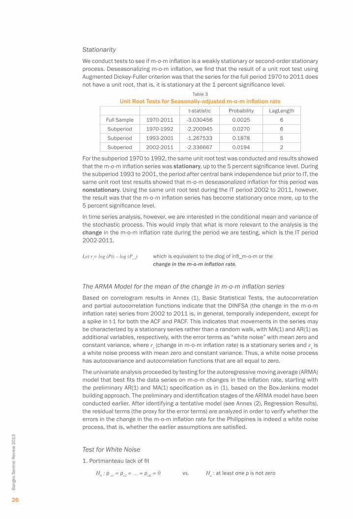
We conduct tests to see if m-o-m inflation is a weakly stationary or second-order stationary process. Deseasonalizing m-o-m inflation, we find that the result of a unit root test using Augmented Dickey-Fuller criterion was that the series for the full period 1970 to 2011 does not have a unit root, that is, it is stationary at the 1 percent significance level.

Table 3Unit Root Tests for Seasonally-adjusted m-o-m inflation rate

t-statistic Probability LagLength

Full Sample 1970-2011 -3.030456 0.0025 6

Subperiod 1970-1992 -2.200945 0.0270 6

Subperiod 1993-2001 -1.267533 0.1878 5

Subperiod 2002-2011 -2.336667 0.0194 2

For the subperiod 1970 to 1992, the same unit root test was conducted and results showed that the m-o-m inflation series was stationary, up to the 5 percent significance level. During the subperiod 1993 to 2001, the period after central bank independence but prior to IT, the same unit root test results showed that m-o-m deseasonalized inflation for this period was nonstationary. Using the same unit root test during the IT period 2002 to 2011, however, the result was that the m-o-m inflation series has become stationary once more, up to the 5 percent significance level.

In time series analysis, however, we are interested in the conditional mean and variance of the stochastic process. This would imply that what is more relevant to the analysis is the change in the m-o-m inflation rate during the period we are testing, which is the IT period 2002-2011.

Let rt= log (Pt) – log (Pt-1) which is equivalent to the dlog of infl_m-o-m or the change in the m-o-m inflation rate.

The ARMA Model for the mean of the change in m-o-m inflation series

Based on correlogram results in Annex (1), Basic Statistical Tests, the autocorrelation and partial autocorrelation functions indicate that the DInFSA (the change in the m-o-m inflation rate) series from 2002 to 2011 is, in general, temporally independent, except for a spike in t-1 for both the ACF and PACF. This indicates that movements in the series may be characterized by a stationary series rather than a random walk, with MA(1) and AR(1) as additional variables, respectively, with the error terms as “white noise” with mean zero and constant variance, where rt (change in m-o-m inflation rate) is a stationary series and εt is a white noise process with mean zero and constant variance. Thus, a white noise process has autocovariance and autocorrelation functions that are all equal to zero.

The univariate analysis proceeded by testing for the autoregressive moving average (ARMA) model that best fits the data series on m-o-m changes in the inflation rate, starting with the preliminary AR(1) and MA(1) specification as in (1), based on the Box-Jenkins model building approach. The preliminary and identification stages of the ARIMA model have been conducted earlier. After identifying a tentative model (see Annex (2), Regression Results), the residual terms (the proxy for the error terms) are analyzed in order to verify whether the errors in the change in the m-o-m inflation rate for the Philippines is indeed a white noise process, that is, whether the earlier assumptions are satisfied.

Test for White Noise

1. Portmanteau lack of fit

H0 : ρ e1 = ρe2 = … = ρeK = 0 vs. Ha : at least one ρ is not zero

Bang

ko S

entra

l Rev

iew

201

3

26

Based on this test, the error terms appear to be a white noise process. Other alternative approaches also indicate that the residuals of the ARMA model for m-o-m inflation exhibit white noise properties (see Annex [1]).

2. Alternative approach by Bollerslev

Another test can be performed by looking at the correlogram of squared residuals. A Portmanteau type of test is conducted (similar to the Ljung-Box statistic) is applied to the square of the residuals and test results in Annex (1) show that the residuals remain within the band and do exhibit white noise properties.

3. normality of the error terms

The null hypothesis is that the error terms, as measured by the residuals, are normally distributed. histogram statistics indicate that skewness of the residuals is relatively small, indicating that the distribution of the errors has a slightly longer right tail. In terms of kurtosis, the kurtosis of a normal distribution is 3, but results indicate a value higher than 3 indicating that the distribution is leptokurtic. Based on the Jarque-Bera test for normality, we see that we need to reject the null hypothesis of a normal distribution. however, looking at the histogram, the error terms appear to behave relatively close to a normal distribution.15

Test for Serial Correlation

Using the Breusch-Godfrey Serial Correlation LM Test on the residuals, no serial correlation was exhibited (see Annex [1]).

Test for Non-Constancy of the Variance

The test used for the constancy of variance is the AutoRegressive Conditional heteroskedasticity (ARCh) test (see Annex [2]). The null hypothesis in this test is constant variance, against the alternative of non-constant variance. The conditional variance, ht, to differentiate it from the unconditional variance σ2, depends nontrivially on the past innovations or error term, εt, and perhaps together with some other latent variables. Based on this test, the null hypothesis of constant variance is rejected. Based on the lagged residuals from the preliminary ARMA model, we have seen that the squared residuals from two periods back are significant, that is, the square of the residual two periods in the past affects the change in the m-o-m inflation rate in the current period. This also indicates that the variance in the change in m-o-m inflation is not constant over time, even during the IT period. It is probable that m-o-m inflation exhibits volatility clustering, that is, large changes tend to be followed by large changes, of either sign, and small changes tend to be followed by small changes. In other words, volatility shocks today could influence the expectation of volatility several periods in the future: A high value of εt

2 increases ht+1, which, in turn, increases the expectation of εt+1

2. The GARCh (1,1) process, ht = α0 + α1εt-12 + β1ht-1, was

found sufficient enough to explain the characteristics of the time series. The conditional variance is a linear function of the square of the error terms (εt+1

2), or the ARCh term (also referred to as the “news from the past”), and the lag of the past values of the conditional variance ht-1, or the GARCh term, and a constant α0.

15 The standard assumption in linear regression is that the theoretical residuals are independent and normally distributed. The histogram and the normal probability plot are used to check whether or not it is reasonable to assume that the random errors inherent in the process have been drawn from a normal distribution. The normality assumption is needed for the error rates we are willing to accept when making decisions about the process. If the random errors are not from a normal distribution, incorrect decisions will be made more or less frequently than the stated confidence levels for our inferences indicate. The observed residuals are an estimate of the theoretical residuals, but are not independent. If the theoretical residuals are not exactly normally distributed, but the sample size is large enough then the Central Limit Theorem says that the usual inference (tests and confidence intervals, but not necessarily prediction intervals) based on the assumption of normality will still be approximately correct. Retrieved from http://stats.stackexchange.com/questions/12053/what-should-i-check-for-normality-raw-data-or-residuals and http://www.itl.nist.gov/div898/handbook/pmd/section4/pmd445.htm.


27

Results of the GARCH Model for the variance – ARMA (1,1)-Garch (2,1)

A natural extension of our empirical findings above is to develop an appropriate ARMA or ARMA-Garch model for the change in the m-o-m inflation series (see Annex, [2]) that would best represent or approximate the evolution of the m-o-m inflation rate series, with a view to developing a simple but effective and efficient short-term forecasting model for the series in the future. This exercise would be a good precursor to such an extension paper.

In consideration of nonconstancy in the variance and a GARCh term up to the second month, the out-of-sample (for 2011) static forecast for the change in m-o-m inflation fluctuate very closely to the zero value during the inflation targeting period. Looking at the conditional variance forecasts, it can be seen that the most volatile values were evident during the global financial and economic crises of 2008-2009, followed by another bout of volatility at the end of 2010. There was also some sharp swings in the variance during 2004 and then early 2006. nonetheless, the variance terms fluctuate very close to the 0.1 value over the entire period.

For forecasting purposes, however, there is a need to improve on the model’s goodness-of-fit or R2 of 17 percent (see Annex [2]). We do this by including dummy variables to represent those periods marked with spikes in variability as noted earlier. The extreme values were particularly evident for november 2010, January 2009, April 2008, March 2002, and June 2004 (positive spikes) as well as for March 2006, March 2011, and August 2008 (negative spikes). Understandably, these periods were characterized by extremely volatile oil and other commodity prices, such as that in 2008, 2006 and 2004, as well as the significant increase in the level of uncertainty during the global financial crisis in 2008 and 2009, and the renewed bout of pessimism over Europe and the stability of the global economic recovery in late 2010 and early 2011. We included these dummy variables as additional regressors in the mean equation. As a result of the various iterations of the estimation including the dummy variables, the R-squared has improved to 49 percent in the final model below, with the AR(1) term becoming insignificant and replaced with the MA(12) term.

Results of the ARMA(0,12)-GARCH (2,1) Model with Dummy Variables

In consideration of the various dummy variables representing periods characterized by sharp volatilities in oil and other commodity prices, the global financial crisis and the ensuing global economic uncertainties thereafter, the change in the m-o-m inflation rate for the Philippines may be estimated using a univariate model with an MA term for the first month and the 12th month, and GARCh terms up to the second month of each year during the inflation targeting period 2002 to 2011. It can also be observed that the out-of-sample (for 2011) static forecast for the change in m-o-m inflation rate continued to fluctuate very closely toward the zero value during the inflation targeting period. Residual tests on the error terms from the ARMA(0,12) - GARCh(2,1) model showed that the remaining residuals in the rightmost figure above is stationary, and does not show any spikes in the ACF and PACF under both the correlogram-Q statistics and the correlogram squared residuals tests.16 This would mean that while about 50 percent of the variability in the change in the m-o-m inflation series for the Philippines during the IT period may be represented or modeled using an ARMA(0,12) (for the mean) and GARCh (2,1) (for the variance) univariate model, the rest of the movements, or about 50 percent, are purely random shocks, as can be deemed from the residual series above.

16 The ARMA-GARCh model results indicated that 50 percent of the movements in the change in the month-on-month inflation rate series may be represented by a univariate autoregressive moving average model (of order 1 and 12) including dummy variables associated with months of either unanticipated developments in the global economy, or volatile global commodity prices and the minimum wage adjustments that were implemented in response to them. These ARMA terms denote that the shocks or innovations to month-on-month inflation for the first and the twelfth month of the year affect the current month-on month inflation rate. In addition, the GARCh terms for the first and the second month were also seen as relevant for the variance equation, denoting that “news from the past” first and second months affect current movements. Meanwhile, the rest of the changes in the series (the residual terms) are random shocks or white noise. These results may be interpreted to mean that unanticipated shocks move inflation month-on-month 50 percent of the time, whereas 50 percent of the movements in the change in month-on-month inflation are affected by the error terms or shocks during the first and the twelfth month of the year, as well as inflation “news” from 1 to 2 months back.

Bang

ko S

entra

l Rev

iew

201

3

28

Conclusion and Policy ImplicationsIn Section B of the paper, we presented a simple intertemporal loss function and an AS-AD framework from existing literature and illustrated a stylized representation of an inflation targeting central bank’s optimal decision-making when inflation expectations are well anchored and, conversely, when the monetary authority is credible. This model provided an intuitive explanation on why changes in the short-run inflation rate, as measured by the first difference of deseasonalized m-o-m inflation, is a mean-stationary process whose variations, save for some degree of autoregressive features, are white noise when an inflation targeting central bank is indeed operating within this environment.

Our univariate time series analysis on Philippine inflation (using CPI 2000=100) before and during the IT period confirmed this hypothesis. Indeed, changes in Philippine m-o-m inflation rate was characterized as a mean-stationary process during the IT period 2002-2011, but nonstationary during the period 1993-2001 before the implementation of the IT framework. It became an interesting result as well that m-o-m inflation changes were stationary during the period 1970 to 1992.

We were able to offer an intuitive explanation on the existence of these three phases in the evolution of the BSP’s IT monetary policy framework: Phase (1) – Prior to central bank independence, m-o-m inflation was stationary but had a higher mean inflation rate and higher variance than during the inflation targeting period. Prior to being an independent monetary authority, the central bank’s monetary policies were subservient to political or fiscal objectives. If firms and households can easily anticipate the actions of fiscal authorities, and the objectives and constraints faced by fiscal authorities are fairly stable, then the resulting m-o-m inflation series would be stationary, albeit at a higher average inflation rate level since a great weight is assigned to seignorage objectives. When money creation is used to finance the deficit, it is likely to result in inflation much higher and more volatile than what is preferred by the central bank. Phase (2) – In the early years of the BSP’s central bank independence, prior to IT, m-o-m inflation showed nonstationarity as the BSP is still establishing its credibility and undergoing a disinflation process while at the same time inflation expectations were still “maturing”—the m-o-m inflation series showed a declining trend, converging toward the long-term inflation target. here the public uses information from past inflation as a basis for expected inflation. Lastly, Phase (3) – During the IT period of the independent BSP, the m-o-m inflation rate series was indeed found to follow a mean-stationary process where the error terms are white noise. As proposed earlier, the BSP has already established its credibility with the public by this time so that inflation expectations have become well entrenched.

Another intuitive finding we have established in the study is that a more gradual, longer disinflation process will incur the central bank a lower loss compared to an abrupt movement toward the inflation target. That non-stationarity occurred only during the transition from the old central bank to the independent and inflation targeting central bank is consistent with the view that disinflation programs under adaptive expectations will result in considerable output losses if the inflation reduction is carried out too drastically. This is because the public still has a wait-and-see attitude regarding the newly created central bank’s ability to resist pressures upon it to pursue fiscal objectives. In other words, if the public would have a strong tendency to under-forecast the decline in inflation (and therefore over-forecast inflation) during the transition from a government-controlled to an independent central bank, more drastic inflation reduction programs will result in greater output losses than a more gradual one. To the extent that the central bank’s optimization problem is minimizing a quadratic loss function that is the sum of the squared deviations of inflation from the long-run target and of output from potential, a longer transition period towards inflation targeting may be preferred to a very short one.

Meanwhile, based on the ARMA(0,12)-GARCh(2,1) model we developed in the Empirical Analysis section of the paper, the change in the m-o-m inflation for one period ahead is affected by the moving average term denoting the errors or shocks in the current month and twelve months back, as well as the “news” or volatility in the change in the m-o-m inflation


29

in the current month and one month ago—at most 50 percent of the time—whereas at least 50 percent of the time the change in m-o-m inflation is driven purely by random shocks. The implication of the results is that indeed, monetary policy need not respond to the short-run temporary deviations or small shocks in m-o-m changes in inflation but only to large enough factors which may dislodge inflation expectations, and hence possibly lead to permanent changes in the long-run inflation trend. however, we should be aware of the fact that these results are based on the assumption that inflationary expectations once well entrenched will not be disanchored. If the central bank decides, however, to react in the face of small enough shocks or not to react even in the face of large shocks, the BSP then needs to put particular emphasis on its effective communication to the public particularly in its monetary policy statements to explain effectively why it has decided to do so.17

So what are these large enough factors? Looking back at the significant dummy variables representing specific periods that showed sharp spikes or extreme movements in the m-o-m inflation, what stood out were the months during 2008 and 2009 which were the height of the global financial crisis, and most recently, the surge in risk aversion during late 2010 when the global economic recovery began to falter given the weaknesses in the US and several debt-ridden countries in Europe, and more importantly the months during 2008 as well as the months in 2004 and 2006, when there were sharp movements in global commodity prices, particularly for oil and rice. While the former were driven by factors which are external in nature, and hence outside of the influence of the domestic economy and its agents and players, the latter periods were associated with periods when administered or “politically-sensitive” prices, particularly minimum wages and transport fares, were raised by government authorities in response to the clamor of laborers and public transport workers for such increases as a knee-jerk reaction to the commodity price hikes at that time.

The uncertainties and implications of global financial and economic crises are demand-side factors which definitely warrant extreme caution on the part of monetary authorities. Their forward-looking framework requires that the direct implications or the ensuing outlook on these factors need to be taken into account early in the policy decision-making process. however, save for a few economists who claim to have foreseen the recent crisis way before August 2008, forecasting the occurrence of global financial or economic crises with accuracy remains a daunting task.

In contrast, the volatility in global oil and commodity prices, although equally difficult to forecast, is a supply-side phenomenon, and so debate arises on whether such movements warrant policy response from monetary authorities such as the BSP. It is interesting to note that the political dimension associated with the setting of administered prices such as minimum wages and transport fares usually lead to adjustments in response to oil price and rice price hikes without regard for the possibility that the associated commodity price increases may or may not be permanent. In other words, the adjustments in the prices may not necessarily be based on a well-informed view on the nature and persistence of the commodity price shocks. But as these items affect production costs and disposable income directly, when large enough they could almost always be expected to dislodge inflation expectations.

It is therefore important to distinguish when significant movements in m-o-m inflation are driven by permanent changes, or driven by purely temporary shocks which will correct themselves later on, or whether they are in fact temporary shocks which could translate into permanent changes because they are affecting politically-sensitive administrative prices such as wages and fares and hence can potentially dislodge inflation expectations in the future. The best example during the inflation targeting period to illustrate this point was the m-o-m inflation outturns and the resulting monetary policy response in 2008. It may be recalled that prices jumped during the second and third quarter of 2008, largely due

17 As discussed in Fermo (2012), the BSP provides guidance to the markets so that expectations are anchored as they can be formed more efficiently and accurately. This guidance helps the markets understand how monetary policy responds to economic developments and shocks and thus helps them anticipate the broad direction of monetary policy over the longer term. Blinder, et al. (2008, p. 1) more importantly noted that based on their survey, “…evidence suggests that communication can be an important and powerful part of the central bank’s toolkit since it has the ability to move financial markets, to enhance the predictability of monetary policy decisions, and potentially to help achieve central banks’ macroeconomic objectives.”

Bang

ko S

entra

l Rev

iew

201

3

30

to the big surge in the international prices of oil and food, particularly rice. A confluence of global and supply-side factors resulted in the unprecedented movements in the domestic prices of rice and fuel that year.

Apart from the rise in global commodity prices during the period, adverse weather conditions and speculative activities in global commodity markets aggravated the situation. Then, toward the end of the year, international commodity price pressures receded, so that domestic inflation fell quickly as well. We can see this clearly in Chart 2 below, which shows that the top five highest m-o-m inflation rates from 2002-2011 occurred in 2008, but at the same time, the lowest four m-o-m inflation rates were also registered in 2008. This illustrates not only that large shocks come in sequence in Philippine m-o-m inflation, but also that large positive shocks in the m-o-m inflation rate can be followed by large negative m-o-m inflation later on. This correction is very much consistent with the temporary nature of commodity shocks. At first glance, therefore, the 2008 experience was an argument why monetary policy should not react to price increases which are caused mainly by supply-side factors.

Abstracting from the weaknesses in Philippine institutions, textbook macroeconomics would dictate that because the abrupt and significant changes in the inflation rate in 2008 were driven mainly by factors which no amount or form of monetary policy can influence, then the BSP should have accommodated the sharp price increases at that time and maintained the policy rate. A further examination, however, would reveal that institutions like the wage and fare board have contributed in making these temporary, supply-side driven shocks transform into permanent disturbances in the inflation path via their impact on inflation expectations, justifying the need for monetary policy response.

The BSP was aware that the initial rise in prices was primarily supply side in origin and that commodity shocks are generally transitory in nature, so that the BSP accommodated the initial price increases during the first four to five months. however, as rising food and energy prices continued over a longer period, these contributed to second-round effects, affecting inflation expectations by the end of the second quarter.

Chart 2.Number of Months Belonging to Top 10 to Lowest 10

Month-on-Month Inflation Rates in a Year from 2002-2011

0

1

2

3

4

5

6

1 2 3 4 5 6 7 8 9 10 11 12

Number of Months Belonging to Top 10 to Lowest 10 Month-on-Month Inflation Rates in a Year from 2002-2011

2002

2004

2007

2008

Rank of 10's from largest to smallest month -on-month inflation

Num

ber o

fMon

ths

Increases in rice and fuel prices are particularly virulent as these figure prominently in Filipino consumers’ expectations and could lead to clamor for upward adjustments in wage and transport fares.18 True enough, a rise in inflation expectations became evident from surveys and financial market data at that time, so that the BSP decided to raise key policy rates by a total of 100 basis points from June to August 2008. The inflation outturn, however, started to improve in September with the sharp decline in international commodity prices. Given the significant fall in november inflation and the significant slowdown in global economic growth with the effects of the Lehman collapse reverberating across all economies around the world, the BSP reduced key policy rates by 50 basis points during its last policy meeting for the year in December 2008.

18 BSP Open Letter to the President (2009).


31

The BSP’s policy reaction in 2008 was hence justifiable given the present weaknesses in Philippine institutions governing administered prices. The first-best solution is to change the way institutions for wage-setting and fare adjustments are handling political pressures from lobby groups such as labor groups and the transport sector and even the media and how they make an assessment if and when wage increases or fare hikes are indeed warranted—what is defined by the government as valid “supervening events”19. In the meantime, while these weaknesses still persist, the second-best alternative for the BSP is monetary policy action. It appears to be beneficial, therefore, to develop institutional arrangements that would foster even closer and more direct coordination between the nWPC and the Land Transportation Franchising and Regulatory Board (LTFRB) and the BSP in order to ensure that any wage and transport fare increases are indeed warranted by developments in the domestic economy and not just a result of political pressures or lobbying forces. In fact, what would be most ideal is perhaps for the BSP to help “educate” labor unions and the members governing the RTWPB and the nWPC that any justifiable wage adjustments at any particular point in time be set within the medium-term inflation target of the BSP. It is, of course, maybe impractical to expect full rationality on the part of all labor unions. holden (2000, p. 22) said that …“It is true that in the real world, unions that compete for members, or union leaders that are pushed by a militant membership, may have limited scope for wage moderation.” nonetheless, it will prove beneficial for the BSP to help unions develop a certain level of understanding of the central bank’s objectives and policy framework and take this into account in nominal wage setting. The impact of the minimum wage and transport fare changes in Philippine m-o-m inflation may be examined empirically using the ARMA model estimated earlier. The significant dummy variables representing the spikes or the extremely volatile episodes for the change in m-o-m inflation, which are also reflected in the forecasts for the conditional variance, more or less coincide with the minimum wage adjustments.20 Only minimum wage adjustments became a significant factor in the ARMA model.

Based on these estimation results, in the case of the Philippines, it is not the unanticipated supply-side shocks coming from global commodity prices which had moved the changes in m-o-m inflation permanently away from the long-term trend, and hence are not the factors which monetary authorities should respond to. It was, in fact, the higher increases in administered prices, particularly minimum wages, which were implemented in response to the higher commodity prices that appeared to consistently affect inflation expectations significantly, and hence should signal the need for future monetary policy action. For a country with a specific inflation target such as the BSP, the central bank will, to some extent, discipline wage-setters even when they do not coordinate their wage-setting, as higher wages will be met with a rise in the policy rate.21 however, international comparisons show that countries with coordinated wage setting generally have lower unemployment than countries with less-coordinated wage setting. Going forward, closer coordination of the central bank with the wage board and the education of the labor unions could help anchor inflation expectations even more firmly with the BSP’s long-run inflation target.

19 Section 3, Rule IV of national Wages and Productivity Commission (nWPC) Guidelines no. 01 Series of 2007, Amended Rules of Procedures on Minimum Wage Fixing, provide: “Any Wage Order issued by the Regional Tripartite Wages and Productivity Board (RTWPB) may not be disturbed for a period of twelve (12) months from its effectivity, and no petition for wage increase shall be entertained within the said period. In the event, however, that supervening conditions, such as extraordinary increase in prices of petroleum products and basic goods/services, demand a review of the minimum wage rates as determined by the RTWPB and confirmed by the nWPC, the RTWPB shall proceed to exercise its wage-fixing function even before the expiration of the said period. Retrieved from http://www.nwpc.dole.gov.ph/legal.html#guide1_2007.html.

20 See the nWPC and LTFRB websites for minimum wage adjustments and the transport fare hikes implemented from 1989 to 2011.

21 For example, Germany restricted growth in its public wage bill much more successfully than all the other countries, in the dimension of both employment and wages per employee. As cited in holden (2000), Soskice & Iversen (1998) use Germany as their leading example how a strict central bank may induce coordinated wage restraint. holden (2000, p. 25) added that: “A strict monetary regime disciplines wage setters by increasing the wage elasticity of employment, thus dampening the negative consequences of uncoordinated wage setting.”

Bang

ko S

entra

l Rev

iew

201

3

32

Annex A1. Statistical Results

Correlogram of DINFSA Correlogram of ResidualsCorrelogram of ResidualsSample: 2002M1 to 2011M10Included Observation: 118Q-statistic probabilities adjusted for 2 ARMA termsDate: 11/17/11

AC PAC Q-Stat Prob.1 -0.048 -0.048 0.27772 -0.007 -0.01 0.28413 0.165 0.164 3.6203 0.0574 -0.091 -0.078 4.6539 0.0985 -0.025 -0.031 4.7317 0.1936 -0.089 -0.123 5.7387 0.227 -0.02 0 5.7873 0.3278 -0.095 -0.099 6.949 0.3269 0.038 0.065 7.139 0.415

10 0.061 0.05 7.6225 0.47111 -0.176 -0.154 11.708 0.2312 -0.081 -0.151 12.592 0.24713 -0.038 -0.076 12.79 0.30714 -0.004 0.042 12.793 0.38415 0.029 0.06 12.905 0.45516 -0.089 -0.098 13.999 0.4517 0.111 0.057 15.723 0.40118 -0.007 -0.048 15.73 0.47219 -0.011 -0.03 15.749 0.54220 0.041 -0.009 15.99 0.59321 -0.085 -0.037 17.036 0.58722 0.173 0.176 21.447 0.37123 -0.075 -0.103 22.289 0.38324 -0.145 -0.218 25.443 0.276

Correlogram of Residuals Squared Breusch-Godfrey Serial Correlation LM Test

Correlogram of Residuals SquaredSample: 2002M01 to 2011M10Included Observations: 118Q-Statistic probabilities adjusted to 2 ARMA termsDate: 11/17/11

AC PAC Q-Stat Prob.1 0.117 0.117 1.65562 0.269 0.259 10.5063 0.069 0.017 11.095 0.0014 0.19 0.123 15.575 05 0.062 0.016 16.053 0.0016 0.024 -0.065 16.124 0.0037 0.008 -0.018 16.133 0.0068 0.074 0.066 16.846 0.019 0.089 0.081 17.875 0.013

10 -0.016 -0.058 17.909 0.02211 -0.057 -0.099 18.34 0.03112 -0.104 -0.112 19.783 0.03113 -0.061 -0.043 20.289 0.04214 -0.074 -0.002 21.044 0.0515 -0.129 -0.066 23.323 0.03816 -0.101 -0.038 24.742 0.03717 -0.049 0.011 25.084 0.04918 -0.055 -0.017 25.506 0.06119 -0.093 -0.045 26.739 0.06220 -0.07 0 27.455 0.07121 -0.04 0.023 27.691 0.0922 0.029 0.066 27.811 0.11423 0.086 0.127 28.903 0.11624 0.029 0.021 29.026 0.144

F-statistic 1.135912 Prob. F(12,104) 0.3398

Obs*R-squared 13.63391 Prob. Chi Square(12) 0.3247

Test Equation:Dependent Variable: RESIDMethod: Least SquaresDate: 11/17/11 Time: 11:42Sample: 2002M01 2011M10Included observations: 118Presample missing value lagged residuals set to zero.

Coefficient Std. Error t-Statistic Prob.AR(1) 0.761869 1.786212 0.426528 0.6706

MA(1) 0.003496 0.011392 0.306852 0.7596

RESID(-1) -0.820046 1.799202 -0.455783 0.6495

RESID(-2) -0.478661 1.136826 -0.421051 0.6746

RESID(-3) -0.121467 0.722541 -0.168110 0.8668

RESID(-4) -0.289183 0.464717 -0.622276 0.5351

RESID(-5) -0.157473 0.304052 -0.517913 0.6056

RESID(-6) -0.231897 0.207792 -1.116003 0.2670

RESID(-7) -0.078706 0.152132 -0.517355 0.6060

RESID(-8) -0.111652 0.123686 -0.902703 0.3688

RESID(-9) 0.069613 0.109949 0.633145 0.5280

RESID(-10) 0.037167 0.103858 0.357865 0.7212

RESID(-11) -0.174575 0.101364 -1.722266 0.0880

RESID(-12) -0.170559 0.105727 -1.613201 0.1097

R-squared 0.115542 Mean dependent var -0.006151Adjusted R-squared 0.004984 S.D. dependent var 0.316250S.E. of regression 0.315461 Akaike info criterion 0.641433Sum squared resid 10.34965 Schwarz criterion 0.970159Log likelihood -23.84456 hannan-Quinn criter. 0.774905Durbin-Watson stat 2.012189


33

1. Basic Statistical TestsCorrelogram of DInFSASample: 2002M01 to 2011 M12Included Observations: 118Date: 11/15/11 AC PAC Q-Stat Prob.1 -0.233 -0.233 6.582 0.0102 -0.121 -0.185 8.367 0.0153 0.128 0.056 10.379 0.0164 -0.140 -0.125 12.813 0.0125 -0.027 -0.073 12.904 0.0246 -0.085 -0.172 13.807 0.0327 0.008 -0.060 13.816 0.0558 -0.085 -0.169 14.741 0.0649 0.077 0.005 15.516 0.07810 0.112 0.067 17.158 0.07111 -0.162 -0.123 20.627 0.03712 -0.044 -0.178 20.884 0.05213 -0.005 -0.162 20.888 0.07514 0.021 -0.052 20.947 0.10315 0.051 0.012 21.308 0.12716 -0.101 -0.144 22.710 0.12217 0.132 0.011 25.156 0.09118 -0.014 -0.073 25.185 0.12019 -0.016 -0.068 25.221 0.15320 0.050 -0.049 25.575 0.18021 -0.101 -0.085 27.061 0.16922 0.217 0.208 33.986 0.04923 -0.067 0.015 34.647 0.05624 -0.134 -0.164 37.349 0.04025 -0.001 -0.178 37.349 0.05326 -0.013 -0.048 37.376 0.06927 -0.049 -0.118 37.743 0.08228 0.031 -0.006 37.892 0.10029 0.074 0.021 38.769 0.10630 -0.123 -0.149 41.209 0.08331 0.142 -0.033 44.492 0.05532 0.157 0.061 48.562 0.03133 -0.119 0.095 50.916 0.02434 -0.039 0.031 51.178 0.03035 -0.013 -0.082 51.209 0.03836 0.028 -0.026 51.343 0.047

2. Regression Results

Dependent Variable: DInFSASample (adjusted): 2002M01 2011M10Included observations: 118 after adjustmentsConvergence achieved after 16 iterations; MA Backcast: 2001M12

Coefficient Std. Error t-Statistic Prob.

AR(1) 0.630234 0.081360 7.746270 0.0000

MA(1) -0.996933 0.034040 -29.28690 0.0000

R-squared 0.189534 Mean dependent var 0.001654

Adjusted R-squared 0.182547 S.D. dependent var 0.351355

Durbin-Watson stat 2.086762

Inverted AR Roots .63Inverted MA Roots 1.00

Heteroskedasticity Test: ARCHF-statistic 1.331737 Prob. F(12,93) 0.2142

Obs*R-squared 15.54374 Prob. Chi-Square(12) 0.2130

Test Equation:Dependent Variable: RESID^2, Method: Least SquaresDate: 11/17/11 Time: 10:53Sample (adjusted): 2003M01 2011M10Included observations: 106 after adjustments


C 0.066334 0.028933 2.292665 0.0241

RESID^2(-1) 0.076146 0.102836 0.740465 0.4609

RESID^2(-2) 0.250942 0.103202 2.431553 0.0170

RESID^2(-3) 0.004650 0.106542 0.043643 0.9653

RESID^2(-4) 0.145233 0.105975 1.370440 0.1738

RESID^2(-5) 0.008805 0.105966 0.083091 0.9340

RESID^2(-6) -0.091096 0.105764 -0.861312 0.3913

RESID^2(-7) -0.013542 0.105578 -0.128262 0.8982

RESID^2(-8) 0.087760 0.105362 0.832932 0.4070

RESID^2(-9) 0.105959 0.105515 1.004209 0.3179

RESID^2(-10) -0.011037 0.107374 -0.102787 0.9184

RESID^2(-11) -0.089071 0.101956 -0.873624 0.3846

RESID^2(-12) -0.148534 0.120040 -1.237376 0.2191



S.E. of regression 0.186565 Akaike info criterion -0.405632

Sum squared resid 3.237001 Schwarz criterion -0.078984

Log likelihood 34.49848 hannan-Quinn criter. -0.273239

F-statistic 1.331737 Durbin-Watson stat 2.013680

Prob. (F-statistic) 0.214213

Dependent Variable: DInFSAMethod: ML - ARCh (Marquardt) - normal distribution, Sample: 2002M01 2010M12;GARCh = 0.125606121047*(1 - C(3) - C(4) - C(5)) + C(3)*RESID(-1)^2 + C(4)*GARCh(-1) + C(5)*GARCh(-2)

Coefficient Std. Error z-Statistic Prob.

AR(1) 0.633218 0.059967 10.55937 0.0000

MA(1) -0.981662 0.008665 -113.2967 0.0000

Variance Equation

C 0.028829 -- -- --

RESID(-1)^2 0.257980 0.057120 4.516455 0.0000

GARCh(-1) 1.093077 0.132242 8.265725 0.0000

GARCh(-2) -0.580575 0.111536 -5.205255 0.0000




Bang

ko S

entra

l Rev

iew

201

3

34

Heteroskedasticity Test: ARCHDependent Variable: DInFSASample: 2001M01 2010M12, Included observations: 120Presample variance: backcast (parameter = 0.7)GARCh = C(8) + C(9)*RESID(-1)^2 + C(10)*GARCh(-1) + C(11)*GARCh(-2)

Coefficient Std. Error z-Statistic Prob.

DUM10 0.886009 0.150745 5.877528 0.0000

7DUM08 0.724596 0.223411 3.243334 0.0012

DUM04 0.392604 0.158256 2.480811 0.0131

DUM08n -1.240735 0.239180 -5.187449 0.0000

DUM09 0.402802 0.244376 1.648291 0.0993

MA(1) -0.611621 0.062321 -9.814055 0.0000

MA(12) -0.332792 0.057358 -5.802026 0.0000

Variance Equation

C 0.051707 0.018649 2.772660 0.0056

RESID(-1)^2 0.277746 0.166755 1.665595 0.0958

GARCh(-1) 0.484362 0.202234 2.395055 0.0166

GARCh(-2) -0.404905 0.163852 -2.471159 0.0135

R-squared 0.490435 Mean dependent var -0.002467



Dependent Variable: InFLSA_MOM, Method: Least SquaresSample (adjusted): 2002M01 2011M10, Included observations: 118 after adjustmentsWhite heteroskedasticity-Consistent Standard Errors & CovarianceMA Backcast: 2001M01 2001M12


DUM10 0.850339 0.111067 7.656093 0.0000

DUM09 0.407798 0.278135 1.466188 0.1456

DUM08 0.727027 0.315409 2.305030 0.0231

DUM04 0.516247 0.124487 4.147006 0.0001

DUM08n -0.537672 0.299575 -1.794781 0.0755

DUM06 0.493553 0.116638 4.231488 0.0000

DUMWAG 0.140635 0.070488 1.995151 0.0486

AR(1) 0.849784 0.080366 10.57390 0.0000

AR(11) 0.143190 0.077906 1.837983 0.0689

MA(11) -0.291149 0.077641 -3.749955 0.0003

MA(1) -0.212415 0.094525 -2.247178 0.0267

MA(12) -0.472595 0.105740 -4.469403 0.0000




2. Unit Root Tests

null hypothesis: InFLSA_MOM has a unit rootExogenous: noneLag Length: 6 (Automatic based on Modified hQ, MAxLAG=17)

t-Statistic Prob.*

Augmented Dickey-Fuller test statistic -3.030456 0.0025

Test critical values: 1% level -2.569652

5% level -1.941466

10% level -1.616269

*MacKinnon (1996) one-sided p-values.

Augmented Dickey-Fuller Test EquationDependent Variable: D(InFLSA_MOM)Method: Least SquaresDate: 11/14/11 Time: 11:32Sample (adjusted): 1970M09 2011M10


t-Statistic Prob.*



5% level -1.942013

10% level -1.615909


Augmented Dickey-Fuller Test EquationDependent Variable: D(InFLSA_MOM)Method: Least SquaresDate: 11/24/11 Time: 10:24Sample (adjusted): 1970M09 1992M12Included observations: 268 after adjustments


t-Statistic Prob.*



5% level -1.943824

10% level -1.614767


Augmented Dickey-Fuller Test EquationDependent Variable: D(InFLSA_MOM)Method: Least SquaresDate: 11/14/11 Time: 11:37Sample: 1993M01 2001M12Included observations: 108


t-Statistic Prob.*



5% level -1.943563

10% level -1.614927


Augmented Dickey-Fuller Test EquationDependent Variable: D(InFLSA_MOM)Method: Least SquaresDate: 11/14/11 Time: 11:40Sample (adjusted): 2002M01 2011M10Included observations: 118 after adjustments


35

ReferencesBall, L. (1999). Efficient Rules for Monetary Policy. International Finance, 2(1), 63-83. Retrieved from http://

onlinelibrary.wiley.com/doi/10.1111/1468-2362.00019/pdf

Ball, L. & Cecchetti, S. G. (1990). Inflation and Uncertainty at Short and Long horizons. Brookings Paper on Economic Activity, 1:1990, 215-254. Retrieved from http://www.brookings.edu/~/media/Projects/BPEA/1990%201/1990a_bpea_ball_cecchetti_gordon.PDF

Blinder, A., Ehrmann, M., Fratzscher, M., de haan, J., & Jansen, D. (2008, December). Central Bank Communication and Monetary Policy: A Survey of Theory and Evidence (nBER Working Paper Series 13932). Journal of Economic Literature, 46(4), 910-945. American Economic Association.

Bangko Sentral ng Pilipinas (2009, January). BSP Open Letter to the President. Retrieved from http://www.bsp.gov.ph/monetary/ open_2008.asp.

Cecchetti, S. G. (1998, June). Policy Rules and Targets: Framing the Central Banker’s Problem. FRBnY Economic Policy Review.

Clive, B. & Roman, F. (1983). The Derivation and Interpretation of the Lucas Supply Function. Journal of Money, Credit, and Banking, 15(1), Ohio State University Press.

Edge, R. M. & Gurkaynak, R. S. (2011). how Useful Are Estimated DSGE Model Forecasts. Finance and Economics Discussion Series, 209-223. Federal Reserve Board, Washington D.C.

Eichengreen, B., El-Erian, M., Fraga, A., Ito, T., Pisani-Ferry, J., Prasad, E., Rajan, R….& Yu, Y. (2011, September). Rethinking Central Banking, Committee on International Policy and Reform.

Fermo, L. (2012). Central Bank Communication and the BSP’s Monetary Policy Statements, BSP newsletter Series (September - October 2012).

Franses, P. h. (1991). Seasonality, non-Stationarity and the Forecasting of Monthly Time Series. International Journal of Forecasting 7, 199-208. north holland: Elsevier Science Publishers.

Froyen, R. & Guender, A. (2007). Optimal Monetary Policy Under Uncertainty. Cheltenham: Edward Elgar.

hassel, A. (2006). Wage Setting, Social Pacts and the Euro: A new Role for the State. Amsterdam University Press.

holden, S. (2000). Monetary Regime and the Coordination of Wage Setting. Department of Economics University of Oslo and norges Bank.

International Monetary Fund (IMF) (2009). A Model of Full-fledged Inflation Targeting and Application to Ghana (IMF Working Paper, WP/10/25).

Lamberte, M. (2002). Central Banking in the Philippines: Then, now and the Future. Philippine Institute of Development Studies (PIDS).

national Wages and Productivity Commission (nWPC) (2007). Section 3, Rule IV of Guidelines no. 01 Series of 2007, Amended Rules of Procedures on Minimum Wage Fixing. Retrieved from http://www.nwpc.dole.gov.ph/legal.html#guide1_2007.html.

Reis, R., (2010). Brookings Papers on Economic Activity, Fall 2010, 245-259.

Sargent, T. (1979). Macroeconomic Theory. Academic Press, new York. Retrieved from http://economics.about.com/library/glossary/bldef-certainty-equivalence-principle.htm.

Taylor, J. (1999). Monetary Policy Rules. Chicago, IL: University of Chicago Press.

Bang

ko S

entra

l Rev

iew

201

3

36

A Univariate Time Series Analysis of Philippine Inflation … · 2014-05-23 · This study relies on a univariate time series analysis of Philippine m-o-m ... the model is completed

Documents