A Unifying Framework for Modelling and Analysing - CiteSeer

A Unifying Frameworkfor Modelling and Analysing

Biochemical Pathways Using Petri Nets

David Gilbert1, Monika Heiner2, and Sebastian Lehrack3

1 Bioinformatics Research Centre, University of GlasgowGlasgow G12 8QQ, Scotland, UK

[email protected], on sabbatical leave from 3

2 INRIA Rocquencourt, Projet ContraintesBP 105, 78153 Le Chesnay CEDEX - France

[email protected], on sabbatical leave from 3

3 Department of Computer Science, Brandenburg University of TechnologyPostbox 10 13 44, 03013 Cottbus, Germany

[email protected]

Abstract. We give a description of a Petri net-based framework formodelling and analysing biochemical pathways, which unifies the qualita-tive, stochastic and continuous paradigms. Each perspective adds its con-tribution to the understanding of the system, thus the three approachesdo not compete, but complement each other. We illustrate our approachby applying it to an extended model of the three stage cascade, whichforms the core of the ERK signal transduction pathway. Consequentlyour focus is on transient behaviour analysis. We demonstrate how quali-tative descriptions are abstractions over stochastic or continuous descrip-tions, and show that the stochastic and continuous models approximateeach other. A key contribution of the paper consists in a precise defi-nition of biochemically interpreted stochastic Petri nets. Although ourframework is based on Petri nets, it can be applied more widely to otherformalisms which are used to model and analyse biochemical networks.

1 Motivation

Biochemical systems are inherently governed by stochastic laws. However, dueto the computational efforts required to analyse stochastic models, two abstrac-tions are more popular: qualitative models, abstracting away from any timedependencies, and continuous models, commonly used to approximate stochas-tic behaviour by a deterministic one. The interrelationships between these threemodels are not always properly understood; for example, how the kinetics of abiochemical reaction, when described by a continuous model, is related to thestochastic nature of the underlying molecular mechanism.

In a previous paper [GH06] we developed an approach for modelling andanalysing biochemical networks using discrete and continuous Petri nets. Ourcurrent work has taken this forward by considering stochastic Petri nets and

M. Calder and S. Gilmore (Eds.): CMSB 2007, LNBI 4695, pp. 200–216, 2007.c© Springer-Verlag Berlin Heidelberg 2007

A Unifying Framework for Modelling and Analysing 201

developing an overall framework to unify these three approaches, providing afamily of related models with high analytical power.

A key contribution of this paper is the precise definition of biochemically in-terpreted stochastic Petri nets in a generic manner, and we demonstrate thebenefit of their incorporation into the model development process. We showhow the general definition can be tailored to very specific kinetic assumptionsby appropriate adjustments of the general hazard function. Also we discuss therelation of the stochastic Petri net to its time-free, purely qualitative abstrac-tion - the standard Petri net, as well as to its continuous approximation - thecontinuous Petri net (i.e., an ordinary differential equation system).

This paper is organised as follows. The following section provides an overviewof the biochemical context and introduces our running example. Next we outlineour framework, discussing the special contributions of the three individual anal-ysis approaches with special emphasis on the transient behaviour analysis, andexamining their interrelations. We then present the individual approaches anddiscuss mutually related properties in all three paradigms in the following order:we start off with the qualitative approach, which is conceptually the easiest, anddoes not rely on knowledge of kinetic information, but describes the networktopology and presence of the species. The qualitative modelling and analysisbasically adheres to the steps proposed in [GH06]. In addition, we show how tosystematically derive and interpret the partial order run of the signal responsebehaviour. We then demonstrate how the validated qualitative model can betransformed into the stochastic representation by addition of stochastic firingrate information. Next, the continuous model is derived from the qualitative orstochastic model by considering only deterministic firing rates. Suitable sets ofinitial conditions for all three models are constructed by qualitative analysis. Weconclude with a summary and outlook regarding further research directions.

2 Biochemical Context

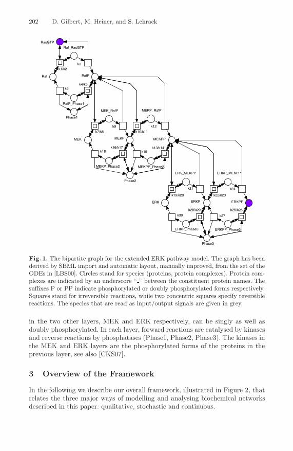
We have chosen a model of the mitogen-activated protein kinase (MAPK) cas-cade published in [LBS00] as a running case study. This is the core of the ubiq-uitous ERK/MAPK pathway that can, for example, convey cell division anddifferentiation signals from the cell membrane to the nucleus. The model doesnot describe the receptor and the biochemical entities and actions immediatelydownstream from the receptor. Instead the description starts at the RasGTPcomplex which acts as a kinase to phosphorylate Raf, which phosphorylatesMAPK/ERK Kinase (MEK), which in turn phosphorylates Extracellular signalRegulated Kinase (ERK). This cascade (RasGTP → Raf → MEK → ERK) ofprotein interactions controls cell differentiation, the effect being dependent uponthe activity of ERK. We consider RasGTP as the input signal and ERKPP (ac-tivated ERK) as the output signal.

The bipartite graph in Figure 1 describes the typical modular structure forsuch a signalling cascade. Each layer corresponds to a distinct protein species.The protein Raf in the first layer is only singly phosphorylated. The proteins

202 D. Gilbert, M. Heiner, and S. Lehrack

Raf

RasGTP

Raf_RasGTP

RafP

RafP_Phase1

MEK_RafP MEKP_RafP

MEKP_Phase2 MEKPP_Phase2

ERK

ERK_MEKPP ERKP_MEKPP

ERKP

MEKPP

ERKPP_Phase3ERKP_Phase3

MEKP

ERKPP

Phase2

Phase3

MEK

Phase1

k3

k6

k21

k18

k9 k12

k15

k24

k27k30

k7/k8

k1/k2

k4/k5

k10/k11

k16/k17

k22/k23k19/k20

k13/k14

k28/k29 k25/k26

Fig. 1. The bipartite graph for the extended ERK pathway model. The graph has beenderived by SBML import and automatic layout, manually improved, from the set of theODEs in [LBS00]. Circles stand for species (proteins, protein complexes). Protein com-plexes are indicated by an underscore “ ” between the constituent protein names. Thesuffixes P or PP indicate phosphorylated or doubly phosphorylated forms respectively.Squares stand for irreversible reactions, while two concentric squares specify reversiblereactions. The species that are read as input/output signals are given in grey.

in the two other layers, MEK and ERK respectively, can be singly as well asdoubly phosphorylated. In each layer, forward reactions are catalysed by kinasesand reverse reactions by phosphatases (Phase1, Phase2, Phase3). The kinases inthe MEK and ERK layers are the phosphorylated forms of the proteins in theprevious layer, see also [CKS07].

3 Overview of the Framework

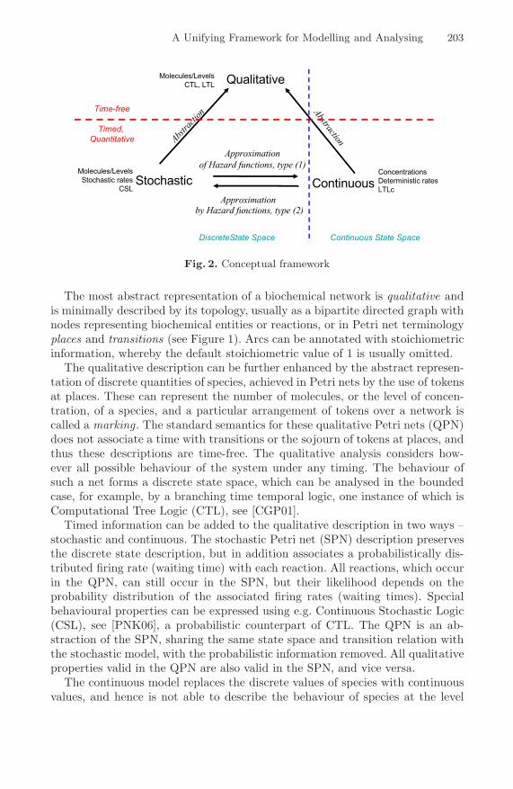
In the following we describe our overall framework, illustrated in Figure 2, thatrelates the three major ways of modelling and analysing biochemical networksdescribed in this paper: qualitative, stochastic and continuous.


Fig. 2. Conceptual framework

The most abstract representation of a biochemical network is qualitative andis minimally described by its topology, usually as a bipartite directed graph withnodes representing biochemical entities or reactions, or in Petri net terminologyplaces and transitions (see Figure 1). Arcs can be annotated with stoichiometricinformation, whereby the default stoichiometric value of 1 is usually omitted.

The qualitative description can be further enhanced by the abstract represen-tation of discrete quantities of species, achieved in Petri nets by the use of tokensat places. These can represent the number of molecules, or the level of concen-tration, of a species, and a particular arrangement of tokens over a network iscalled a marking. The standard semantics for these qualitative Petri nets (QPN)does not associate a time with transitions or the sojourn of tokens at places, andthus these descriptions are time-free. The qualitative analysis considers how-ever all possible behaviour of the system under any timing. The behaviour ofsuch a net forms a discrete state space, which can be analysed in the boundedcase, for example, by a branching time temporal logic, one instance of which isComputational Tree Logic (CTL), see [CGP01].

Timed information can be added to the qualitative description in two ways –stochastic and continuous. The stochastic Petri net (SPN) description preservesthe discrete state description, but in addition associates a probabilistically dis-tributed firing rate (waiting time) with each reaction. All reactions, which occurin the QPN, can still occur in the SPN, but their likelihood depends on theprobability distribution of the associated firing rates (waiting times). Specialbehavioural properties can be expressed using e.g. Continuous Stochastic Logic(CSL), see [PNK06], a probabilistic counterpart of CTL. The QPN is an ab-straction of the SPN, sharing the same state space and transition relation withthe stochastic model, with the probabilistic information removed. All qualitativeproperties valid in the QPN are also valid in the SPN, and vice versa.

The continuous model replaces the discrete values of species with continuousvalues, and hence is not able to describe the behaviour of species at the level


of individual molecules, but only the overall behaviour via concentrations. Wecan regard the discrete description of concentration levels as abstracting over thecontinuous description of concentrations. Timed information is introduced by theassociation of a particular deterministic rate information with each transition,permitting the continuous model to be represented as a set of ordinary differentialequations (ODEs). The concentration of a particular species in such a model willhave the same value at each point of time for repeated experiments. The statespace of such models is continuous and linear. It can be analysed by, for example,Linear Temporal Logic with constraints (LTLc) in the manner of [CCRFS06].

The stochastic and continuous models are mutually related by approxima-tion. The stochastic description can be used as the basis for deriving a continu-ous Petri net (CPN) model by approximating rate information. Specifically, theprobabilistically distributed reaction firing in the SPN is replaced by a particularaverage firing rate over the continuous token flow of the CPN. This is achievedby approximation over hazard functions of type (1), described in more detail insection 5.1. In turn, the stochastic model can be derived from the continuousmodel by approximation, reading the tokens as concentration levels, as intro-duced in [CVGO06]. Formally, this is achieved by a hazard function of type (2),see again section 5.1.

It is well-known that time assumptions generally impose constraints on be-haviour. The qualitative and stochastic models consider all possible behavioursunder any timing, whereas the continuous model is constrained by its inherentdeterminism to consider a subset. This may be too restrictive when modellingbiochemical systems, which by their very nature exhibit variability in their be-haviour.

In the following the reader is assumed to be familiar with the standard Petrinet terminology as well as foundations of temporal logics, for an introductionsee, e.g., [Mur89] and [CGP01].

4 The Qualitative Approach

4.1 Qualitative Modelling

We interpret the graph given in Figure 1 as a place/transition Petri net, and callthe circles places , and the rectangles transitions . Reversible reactions have to bemodelled explicitly by two opposite transitions in the basic Petri net notation.However in order to retain the elegant graph structure of Figure 1, we use macrotransitions, each of which stands here for a reversible reaction. The entire (flat-tened) place/transition Petri net consists of 22 places and 30 transitions, wherek1, k2, . . . stand for reaction (transition) labels.

We associate a discrete concentration with each of the 22 species. In thesimplest way, these concentrations can be thought of as being “high” or “low”(above or below a certain threshold), resulting in a two-level model where eachspecies can be read as a Boolean variable. More generally, we could apply amulti-level approach by differentiating between a finite number of discrete levels,


each standing for an equivalence class of possibly infinitely many concentrations.Then species can be read as integer variables.

4.2 Qualitative Analysis

Analysis of general behavioural properties. The Petri net enjoys the threeorthogonal general properties of a discrete Petri net: boundedness, liveness andreversibility. The decision about the first two can be made for our running exam-ple in a static way, while the last property requires dynamic analysis techniques.The necessary steps of the systematic analysis procedure follow basically thosegiven in [GH06]. We restrict ourselves here to the most essential points.

The net is strongly connected and thus self-contained, i.e. a closed system. Inorder to bring the net to life, we construct an initial marking using P-invariants.These are non-trivial non-negative integer solutions of the homogeneous linearequation system x · C = 0, where C stands for the incidence matrix of the net.There are seven minimal P-invariants covering the net, and consequently the netis bounded for any initial marking. All these P-invariants xi contain only entriesof 0 and 1, permitting a short-hand specification by just giving the names of theplaces involved.

x1 = (RasGTP, Raf RasGTP)x2 = (Raf, Raf RasGTP, RafP, RafP Phase1, MEK RafP, MEKP RafP)x3 = (MEK, MEK RafP, MEKP RafP, MEKP Phase2, MEKPP Phase2,

ERK MEKPP, ERKP MEKPP, MEKPP, MEKP)x4 = (ERK, ERK MEKPP, ERKP MEKPP, ERKP, ERKPP Phase3,

ERKP Phase3, ERK PP)x5 = (Phase1, RafP Phase1)x6 = (Phase2, MEKP Phase2, MEKPP Phase2)x7 = (Phase3, ERKP Phase3, ERKPP Phase3)

Each P-invariant stands for a reasonable conservation rule, the species preservedbeing given by the first name in the invariant. In signal transduction networksa P-invariant typically comprises all the different states of one species. In aBoolean approach, each species can be only in one state at any time, thus eachP-invariant gets exactly one token. Within a P-invariant, the species with themost inactive (i.e. non-phosphorylated) or the monomeric (non-complexed) stateis chosen. Following these criteria, the initial marking is: one token on each of Raf,RasGTP, MEK, ERK, Phase1, Phase2 and Phase3, while all remaining placesare empty. With this marking, the net is covered by 1-P-invariants (exactly onetoken in each P-invariant), and is therefore 1-bounded.

Generalising this reasoning to a multi-level concept, we could assign n tokensto each place, representing the most inactive state, in order to indicate thehighest concentration level for them in the initial state. The “abstract” massconservation within each P-invariant would then be n tokens, which could bedistributed fairly freely over the P-invariant’s places during the behaviour of themodel. This results in a dramatic increase of the state space, cf. the discussionin Section 5.2, while not improving the qualitative reasoning.


Model validation should include a check of all T-invariants for their biologicalplausibility. T-invariants are non-trivial non-negative integer solutions of thehomogeneous linear equation system C · y = 0. The entries of a T-invariantcan be read as the specification of a multiset of transitions, which reproduce agiven marking by their firing. If there are non-trivial solutions, then there areinfinitely many ones. Therefore, the plausibility check is usually restricted tothe consideration of all minimal solutions. The net representations of minimalT-invariants (their transitions plus their pre- and post-places and all arcs inbetween) characterise minimal self-contained subnetworks with an identifiablebiological meaning.

The net under consideration is covered by T-invariants, a necessary condi-tion for bounded nets to be live. Besides the expected ten trivial T-invariantsfor the ten reversible reactions, there are five non-trivial, but obvious minimalT-invariants, each corresponding to one of the five phosphorylation / dephos-phorylation cycles in the network structure:

y1 = (k1, k3, k4, k6), y2 = (k7, k9, k16, k18), y3 = (k10, k12, k13, k15),y4 = (k19, k21, k28, k30), y5 = (k22, k24, k25, k27).

The interesting net behaviour, demonstrating how input signals cause finallyoutput signals, is contained in a non-negative linear combination of all five non-trivial T-invariants, y1−5 = y1 + y2 + y3 + y4 + y5, which is called an I/OT-invariant in the following. The I/O T-invariant is systematically constructedby starting with the two minimal T-invariants, involving the input and outputsignal, which define disconnected subnetworks. Then we add minimal sets ofminimal T-invariants to get a connected subnet. For our running example, thesolution is unique, which is not generally the case.

We check the I/O T-invariant for feasibility in the constructed initial mark-ing, which then involves the feasibility of all trivial T-invariants. We obtain aninfinite partial order run, the beginning of which can be characterised in a short-hand notation by the following partially ordered word out of the alphabet of alltransition labels (“;” stands for “sequentiality”, “‖” for “concurrency”):

( k1; k3; k7; k9; k10; k12;( (k4; k6) ‖ ( (k19; k21; k22; k24); ( (k13; k15; k16; k18) ‖ (k25; k27; k28; k30) ) ) ) ),

see [GHL07] for a graphical representation. This partial order run gives furtherinsight into the dynamic behaviour of the network, which may not be apparentfrom the standard net representation, e.g. we are able to follow the (minimal)producing process of the proteins RafP, MEKP, MEKPP, ERKP and ERKPP,compare [GHL07], and we notice the clear independence of the dephosphoryla-tion in all three levels.

The reachability graph of the net is finite because the net is bounded, and hasin the Boolean token interpretation 118 states out of 222 theoretically possibleones, forming one strongly connected component. Therefore, the Petri net isreversible, i.e. the initial system state is always reachable again, or in otherwords the system has the capability of self-reinitialization. Moreover, from the


viewpoint of the discrete model, all of these 118 states are equivalent, and eachcould be taken as an initial state resulting in exactly the same total (discrete)system behaviour. This prediction will be confirmed by the observations gainedduring quantitative analyses, see Sections 5.2 and 6.2.

Model checking of special behavioural properties. Temporal logic is par-ticularly helpful in expressing special behavioural properties of the expectedtransient behaviour, whose truth can be determined via model checking. Weconfine ourselves here to two CTL properties, checking the generalizability ofthe insights gained by the partial order run of the I/O T-invariant. In the fol-lowing, places are interpreted as Boolean variables, in order to simplify notation.

Property Q1: The signal sequence predicted by the partial order run of theI/O T-invariant is the only possible one. In other words, starting at the initialstate, it is necessary to pass through states RafP, MEKP, MEKPP and ERKPin order to reach ERKPP.

¬ [ E ( ¬ RafP U MEKP ) ∨ E ( ¬ MEKP U MEKPP ) ∨E ( ¬ MEKPP U ERKP ) ∨ E ( ¬ ERKP U ERKPP ) ]

Property Q2: Dephosphorylation takes place independently. E.g., the dura-tion of the phosphorylated state of ERK is independent of the duration of thephosphorylated states of MEK and Raf.

( EF [ Raf ∧ ( ERKP ∨ ERKPP ) ] ∧ EF [ RafP ∧ ( ERKP ∨ ERKPP ) ] ∧EF [ MEK ∧ ( ERKP ∨ ERKPP ) ] ∧EF [ ( MEKP ∨ MEKPP ) ∧ ( ERKP ∨ ERKPP ) ] )

In subsequent sections we will use Q1 as a basis to illustrate how the stochastic andcontinuous approaches provide complementary views of the system behaviour.

5 The Stochastic Approach

5.1 Stochastic Modelling

As with a qualitative Petri net, a stochastic Petri net maintains a discrete num-ber of tokens on its places. But contrary to the time-free case, a firing rate(waiting time) is associated with each transition t, which are random variablesXt ∈ [0, ∞), defined by probability distributions. Therefore, all reaction timescan theoretically still occur, but the likelihood depends on the probability dis-tribution. Consequently, the system behaviour is described by the same discretestate space, and all the different execution runs of the underlying qualitativePetri net can still take place. This allows the use of the same powerful analysistechniques for stochastic Petri nets as already applied for qualitative Petri nets.

For a better understanding we describe the general procedure of a particularsimulation run for a stochastic Petri net. Each transition gets its own localtimer. When a particular transition becomes enabled, meaning that sufficienttokens arrive on its pre-places, then the local timer is set to an initial value,


which is computed at this time point by means of the corresponding probabilitydistribution. In general, this value will be different for each simulation run. Thelocal timer is then decremented at a constant speed, and the transition will firewhen the timer reaches zero. If there is more than one enabled transition, a racefor the next firing will take place.

Technically, various probability distributions can be chosen to determine therandom values for the local timers. Biochemical systems are the prototype forexponentially distributed reactions. Thus, for our purposes, the firing rates ofall transitions follow an exponential distribution, which can be described bya single parameter λ, and each transition needs only its particular, generallymarking-dependent parameter λ to specify its local time behaviour.

Definition 1 (Stochastic Petri net, Syntax). A biochemically interpretedstochastic Petri net is a quintuple SPN Bio = (P, T, f, v, m0), where

– P and T are finite, non empty, and disjoint sets. P is the set of places, andT is the set of transitions.

– f : ((P × T ) ∪ (T × P )) → IN0 defines the set of directed arcs, weighted bynon-negative integer values.

– v : T → H is a function, which assigns a stochastic hazard function ht toeach transition t, wherebyH :=

⋃t∈T

{ht | ht : IN|•t|

0 → IR+}

is the set of all stochastic hazard func-tions, and v(t) = ht for all transitions t ∈ T .

– m0 : P → IN0 gives the initial marking.

The stochastic hazard function ht defines the marking-dependent transition rateλt(m) for the transition t. The domain of ht is restricted to the set of pre-placesof t, i.e. •t := {p ∈ P |f (p, t) �= 0}, to enforce a close relation between networkstructure and hazard functions. Therefore λt(m) actually depends only on asub-marking.

Stochastic Petri net, Semantics. Transitions become enabled as usual, i.e.if all pre-places are sufficiently marked. However there is a time, which has toelapse, before an enabled transition t ∈ T fires. The transition’s waiting timeis an exponentially distributed random variable Xt with the probability densityfunction:

fXt(τ) = λt(m) · e(−λt(m)·τ), τ ≥ 0.

The firing itself does not consume time and again follows the standard firingrule of qualitative Petri nets. The semantics of a stochastic Petri net (withexponentially distributed reaction times for all transitions) is described by acontinuous time Markov chain (CTMC). The CTMC of a stochastic Petri netis isomorphic to the reachability graph of the underlying qualitative Petri net,while the arcs between the states are now labelled by the transition rates. Formore details see [Mur89], [BK02].

Based on this general SPN Bio definition, specialised biochemically inter-preted stochastic Petri nets can be defined by specifying the required kind of


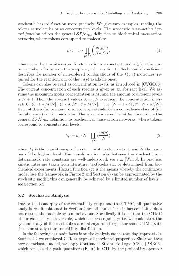
stochastic hazard function more precisely. We give two examples, reading thetokens as molecules or as concentration levels. The stochastic mass-action haz-ard function tailors the general SPN Bio definition to biochemical mass-actionnetworks, where tokens correspond to molecules:

ht := ct ·∏

p∈•t

(m(p)f(p, t)

)

, (1)

where ct is the transition-specific stochastic rate constant, and m(p) is the cur-rent number of tokens on the pre-place p of transition t. The binomial coefficientdescribes the number of non-ordered combinations of the f(p, t) molecules, re-quired for the reaction, out of the m(p) available ones.

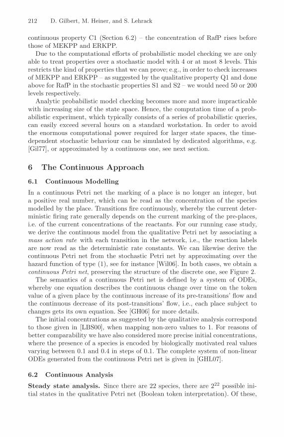
Tokens can also be read as concentration levels, as introduced in [CVGO06].The current concentration of each species is given as an abstract level. We as-sume the maximum molar concentration is M , and the amount of different levelsis N + 1. Then the abstract values 0, . . . , N represent the concentration inter-vals 0, (0, 1 ∗ M/N ], (1 ∗ M/N, 2 ∗ M/N ], . . . , (N − 1 ∗ M/N, N ∗ M/N ].Each of these (finite many) discrete levels stands for an equivalence class of (in-finitely many) continuous states. The stochastic level hazard function tailors thegeneral SPN Bio definition to biochemical mass-action networks, where tokenscorrespond to concentration levels:

ht := kt · N ·∏

p∈•t

(m(p)N

), (2)

where kt is the transition-specific deterministic rate constant, and N the num-ber of the highest level. The transformation rules between the stochastic anddeterministic rate constants are well-understood, see e.g. [Wil06]. In practice,kinetic rates are taken from literature, textbooks etc. or determined from bio-chemical experiments. Hazard function (2) is the means whereby the continuousmodel (see the framework in Figure 2 and Section 6) can be approximated by thestochastic model; this can generally be achieved by a limited number of levels –see Section 5.2.

5.2 Stochastic Analysis

Due to the isomorphy of the reachability graph and the CTMC, all qualitativeanalysis results obtained in Section 4 are still valid. The influence of time doesnot restrict the possible system behaviour. Specifically it holds that the CTMCof our case study is reversible, which ensures ergodicity; i.e. we could start thesystem in any of the reachable states, always resulting in the same CTMC withthe same steady state probability distribution.

In the following our main focus is on the analytic model checking approach. InSection 4.2 we employed CTL to express behavioural properties. Since we havenow a stochastic model, we apply Continuous Stochastic Logic (CSL) [PNK06],which replaces the path quantifiers (E, A) in CTL by the probability operator


P��p, whereby �� p specifies the probability of the given formula. For example,introducing in CSL the abbreviation Fφ for trueUφ, the CTL formula EFφbecomes the CSL formula P≥0[Fφ ], and AFφ becomes P≥1[Fφ ].

In order to use the probabilistic model checker PRISM [PNK06], we encodethe extended ERK pathway in its modelling language, as proposed in [DDS04].This translation requires knowledge of the boundedness degree of all speciesinvolved, which we acquire by the structural analysis technique of P-invariants.

We only consider here the level semantics. Since the continuous concentrationsof proteins in the ERK pathway are all in the same range (0.1. . . 0.4 mMol in0.1 steps), we employ a model with only 4, and a second version with 8 levels.The corresponding CTMCs (and reachability graphs) comprise 24,065 states forthe 4 level version and 6,110,643 states for the 8 level version.

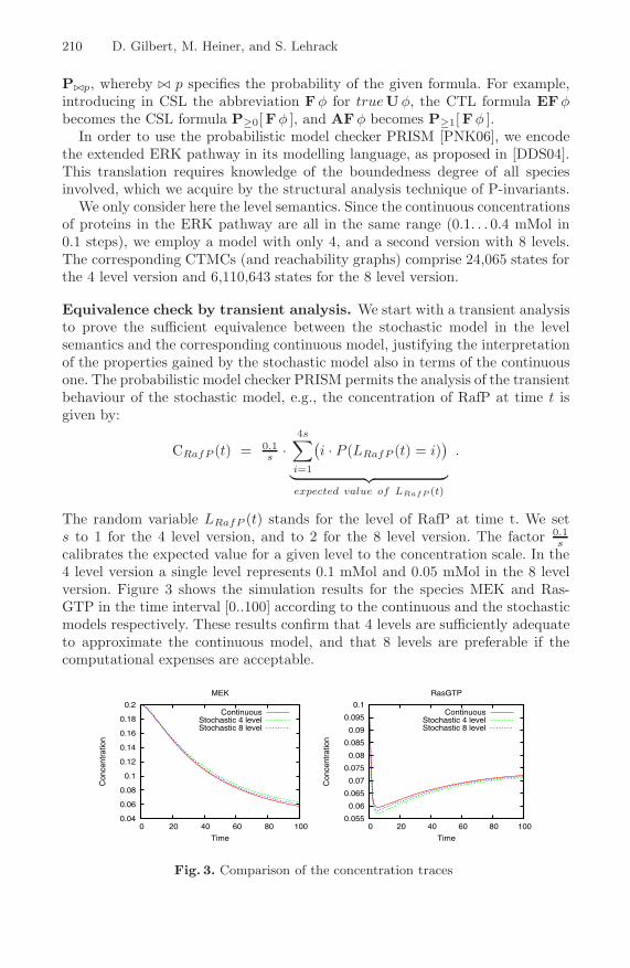
Equivalence check by transient analysis. We start with a transient analysisto prove the sufficient equivalence between the stochastic model in the levelsemantics and the corresponding continuous model, justifying the interpretationof the properties gained by the stochastic model also in terms of the continuousone. The probabilistic model checker PRISM permits the analysis of the transientbehaviour of the stochastic model, e.g., the concentration of RafP at time t isgiven by:

CRafP (t) = 0.1s ·

4s∑

i=1

(i · P (LRafP (t) = i)

)

︸︷︷︸expected value of LRafP (t)

.

The random variable LRafP (t) stands for the level of RafP at time t. We sets to 1 for the 4 level version, and to 2 for the 8 level version. The factor 0.1

scalibrates the expected value for a given level to the concentration scale. In the4 level version a single level represents 0.1 mMol and 0.05 mMol in the 8 levelversion. Figure 3 shows the simulation results for the species MEK and Ras-GTP in the time interval [0..100] according to the continuous and the stochasticmodels respectively. These results confirm that 4 levels are sufficiently adequateto approximate the continuous model, and that 8 levels are preferable if thecomputational expenses are acceptable.

0.04

0.06

0.08

0.1

0.12

0.14

0.16

0.18

0.2

0 20 40 60 80 100

Con

cent

ratio

n

Time

MEK

ContinuousStochastic 4 levelStochastic 8 level

0.055

0.06

0.065

0.07

0.075

0.08

0.085

0.09

0.095

0.1

0 20 40 60 80 100

Con

cent

ratio

n

Time

RasGTP

ContinuousStochastic 4 levelStochastic 8 level

Fig. 3. Comparison of the concentration traces


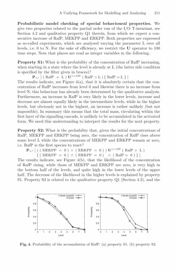
Probabilistic model checking of special behavioural properties. Wegive two properties related to the partial order run of the I/O T-invariant, seeSection 4.2 and qualitative property Q1 therein, from which we expect a con-secutive increase of RafP, MEKPP and ERKPP. Both properties are expressedas so-called experiments, which are analysed varying the parameter L over alllevels, i.e. 0 to N. For the sake of efficiency, we restrict the U operator to 100time steps. Note that places are read as integer variables in the following.

Property S1: What is the probability of the concentration of RafP increasing,when starting in a state where the level is already at L (the latter side conditionis specified by the filter given in braces)?

P=? [ ( RafP = L ) U<=100 ( RafP > L ) { RafP = L } ]The results indicate, see Figure 4(a), that it is absolutely certain that the con-centration of RafP increases from level 0 and likewise there is no increase fromlevel N; this behaviour has already been determined by the qualitative analysis.Furthermore, an increase in RafP is very likely in the lower levels, increase anddecrease are almost equally likely in the intermediate levels, while in the higherlevels, but obviously not in the highest, an increase is rather unlikely (but notimpossible). In summary this means that the total mass, circulating within thefirst layer of the signalling cascade, is unlikely to be accumulated in the activatedform. We need this understanding to interpret the results for the next property.

Property S2: What is the probability that, given the initial concentrations ofRafP, MEKPP and ERKPP being zero, the concentration of RafP rises abovesome level L while the concentrations of MEKPP and ERKPP remain at zero,i.e. RafP is the first species to react?

P=? [ ( ( MEKPP = 0 ) ∧ ( ERKPP = 0 ) ) U<=100 ( RafP > L ){ ( MEKPP = 0 ) ∧ ( ERKPP = 0 ) ∧ ( RafP = 0 ) } ]

The results indicate, see Figure 4(b), that the likelihood of the concentrationof RafP rising, while those of MEKPP and ERKPP are zero, is very high inthe bottom half of the levels, and quite high in the lower levels of the upperhalf. The decrease of the likelihood in the higher levels is explained by propertyS1. Property S2 is related to the qualitative property Q1 (Section 4.2), and the

0

0.2

0.4

0.6

0.8

1

0 1 2 3 4 5 6 7 8

Pro

babili

ty

Level

4 levels (scaled)8 levels

0

0.2

0.4

0.6

0.8

1

0 1 2 3 4 5 6 7 8

Pro

babili

ty

Level

4 levels (scaled)8 levels

Fig. 4. Probability of the accumulation of RafP. (a) property S1. (b) property S2.


continuous property C1 (Section 6.2) – the concentration of RafP rises beforethose of MEKPP and ERKPP.

Due to the computational efforts of probabilistic model checking we are onlyable to treat properties over a stochastic model with 4 or at most 8 levels. Thisrestricts the kind of properties that we can prove; e.g., in order to check increasesof MEKPP and ERKPP – as suggested by the qualitative property Q1 and doneabove for RafP in the stochastic properties S1 and S2 – we would need 50 or 200levels respectively.

Analytic probabilistic model checking becomes more and more impracticablewith increasing size of the state space. Hence, the computation time of a prob-abilistic experiment, which typically consists of a series of probabilistic queries,can easily exceed several hours on a standard workstation. In order to avoidthe enormous computational power required for larger state spaces, the time-dependent stochastic behaviour can be simulated by dedicated algorithms, e.g.[Gil77], or approximated by a continuous one, see next section.

6 The Continuous Approach

6.1 Continuous Modelling

In a continuous Petri net the marking of a place is no longer an integer, buta positive real number, which can be read as the concentration of the speciesmodelled by the place. Transitions fire continuously, whereby the current deter-ministic firing rate generally depends on the current marking of the pre-places,i.e. of the current concentrations of the reactants. For our running case study,we derive the continuous model from the qualitative Petri net by associating amass action rate with each transition in the network, i.e., the reaction labelsare now read as the deterministic rate constants. We can likewise derive thecontinuous Petri net from the stochastic Petri net by approximating over thehazard function of type (1), see for instance [Wil06]. In both cases, we obtain acontinuous Petri net, preserving the structure of the discrete one, see Figure 2.

The semantics of a continuous Petri net is defined by a system of ODEs,whereby one equation describes the continuous change over time on the tokenvalue of a given place by the continuous increase of its pre-transitions’ flow andthe continuous decrease of its post-transitions’ flow, i.e., each place subject tochanges gets its own equation. See [GH06] for more details.

The initial concentrations as suggested by the qualitative analysis correspondto those given in [LBS00], when mapping non-zero values to 1. For reasons ofbetter comparability we have also considered more precise initial concentrations,where the presence of a species is encoded by biologically motivated real valuesvarying between 0.1 and 0.4 in steps of 0.1. The complete system of non-linearODEs generated from the continuous Petri net is given in [GHL07].

6.2 Continuous Analysis

Steady state analysis. Since there are 22 species, there are 222 possible ini-tial states in the qualitative Petri net (Boolean token interpretation). Of these,


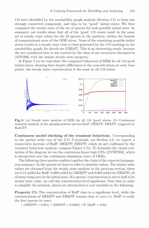
118 were identified by the reachability graph analysis (Section 4.2) to form onestrongly connected component, and thus to be “good” initial states. We thencomputed the steady state of the set of species for each possible initial state. Insummary, our results show that all of the ’good’ 118 states result in the sameset of steady state values for the 22 species in the pathway, within the boundsof computational error of the ODE solver. None of the remaining possible initialstates results in a steady state close to that generated by the 118 markings in thereachability graph; for details see [GHL07]. This is an interesting result, becausethe net considered here is not covered by the class of net structures discussed in[ADLS06] with the unique steady state property.

In Figure 5 (a) we reproduce the computed behaviour of MEK for all 118 goodinitial states, showing that despite differences in the concentrations at early timepoints, the steady state concentration is the same in all 118 states.

0 50 100 150 200 250 300 3500

0.1

0.2

0.3

0.4

0.5

0.6

0.7

0.8

0.9

1

Time (sec)

Con

cent

ratio

n (r

elat

ive

units

)

MEK

MEK

0

0.02

0.04

0.06

0.08

0.1

0.12

0 50 100 150 200 250 300 350

RasGTPRafP

MEKPPERKPP

Fig. 5. (a) Steady state analysis of MEK for all 118 ‘good’ states. (b) Continuoustransient analysis of the phosphorylated species RasP, MEKPP, ERKPP, triggered byRasGTP.

Continuous model checking of the transient behaviour. Correspondingto the partial order run of the I/O T-invariant, see Section 4.2, we expect aconsecutive increase of RafP, MEKPP, ERKPP, which we get confirmed by thetransient behaviour analysis, compare Figure 5 (b). To formalise the visual eval-uation of the diagram we use the continuous linear logic LTLc [CCRFS06], whichis interpreted over the continuous simulation trace of ODEs.

The following three queries confirm together the claim of the expected propaga-tion sequence. In the queries we have to refer to absolute values. The steady statevalues are obtained from the steady state analysis in the previous section; theseare 0.12 mMol for RafP, 0.008 mMol for MEKPP and 0.002 mMol for ERKPP, allof them being zero in the initial state. If a species’ concentration is above half of itssteady state value, we call this concentration level significant. Note that in orderto simplify the notation, places are interpreted as real variables in the following.

Property C1: The concentration of RafP rises to a significant level, while theconcentrations of MEKPP and ERKPP remain close to zero; i.e. RafP is reallythe first species to react.

( (MEKPP < 0.001) ∧ (ERKPP < 0.0002) ) U (RafP > 0.06)


Property C2: if the concentration of RafP is at a significant concentrationlevel and that of ERKPP is close to zero, then both species remain in thesestates until the concentration of MEKPP becomes significant; i.e. MEKPP isthe second species to react.

( (RafP > 0.06) ∧ (ERKPP < 0.0002) ) ⇒( (RafP > 0.06) ∧ (ERKPP < 0.0002) ) U (MEKPP > 0.004)

Property C3: if the concentrations of RafP and MEKPP are significant, theyremain so, until the concentration of ERKPP becomes significant; i.e. ERKPPis the third species to react.

( (RafP > 0.06) ∧ (MEKPP > 0.004) ) ⇒( (RafP > 0.06) ∧ (MEKPP > 0.004) ) U (ERKPP > 0.0005)

Note that properties C1, C2 and C3 correspond to the qualitative propertyQ1, and that S2 is the stochastic counterpart of C1.

7 Tools

The bipartite graph in Figure 1 and its interpretation as the three Petri net mod-els have been done using Snoopy [Sno], a tool to design and animate hierarchicalgraphs, including SBML import.

The qualitative analyses have been made using the Integrated Net AnalyserINA [SR99] and the Model Checking Kit [SSE04]. We employed PRISM [PNK06]for probabilistic model checking, and Biocham [CCRFS06] for LTLc-based con-tinuous model checking.

MATLAB [SR97] was used to produce the steady state analysis of all ini-tial states in the continuous model, and the transient analysis was done usingBioNessie [Bio], an SBML-based simulation and analysis tool for biochemicalnetworks.

8 Summary and Outlook

In this paper we have described an overall framework that relates the three majorways of modelling biochemical networks – qualitative, stochastic and continuous– and illustrated this in the context of Petri nets. In doing so we have given a pre-cise definition of biochemically interpreted stochastic Petri nets. We have shownthat the qualitative time-free description is the most basic, with discrete valuesrepresenting numbers of molecules or levels of concentrations. The qualitativedescription abstracts over two timed, quantitative models. In the stochastic de-scription, discrete values for the amounts of species are retained, but a stochasticrate is associated with each reaction. The continuous model describes amountsof species using continuous values and associates a deterministic rate with eachreaction. These two time-dependent models can be mutually approximated byhazard functions belonging to the stochastic world.

We have illustrated our framework by considering qualitative, stochastic andcontinuous Petri net descriptions of the ERK signalling pathway, based on the


model from Levchenko et al [LBS00]. We have focussed on analysis techniquesavailable in each of these three paradigms, in order to illustrate their complemen-tarity. Our special emphasis has been on model checking, which is especially use-ful for transient behaviour analysis, and we have demonstrated this by discussingrelated properties in the qualitative, stochastic and continuous paradigms. Al-though our framework is based on Petri nets, it can be applied more widely toother formalisms which are used to model and analyse biochemical networks.

We are now working on the incorporation of deterministic time into stochasticmodels, as well as the integration of continuous and stochastic aspects into onemodel.

Acknowledgements. The running case study has been partly carried out bySebastian Lehrack during his study stay at the Bioinformatic Research Centreof the University of Glasgow. This stay was supported by the Max GruenebaumFoundation [MGF] and the UK Department of Trade and Industry Beacon Bio-science Programme.

We would like to thank Richard Orton and Xu Gu for the constructive dis-cussions as well as Vladislav Vyshermirsky for his support in the computationalexperiments.

References

[ADLS06] Angeli, D., De Leenheer, P., Sontag, E.D.: On the structural monotonic-ity of chemical reaction networks. In: ICATPN 2003, pp. 7–12. IEEEComputer Society Press, Los Alamitos (2006)

[Bio] BioNessie. A biochemical pathway simulation and analysis tool. Univer-sity of Glasgow, http://www.bionessie.org

[BK02] Bause, F., Kritzinger, P.S.: Stochastic Petri Nets. Vieweg (2002)[CCRFS06] Calzone, L., Chabrier-Rivier, N., Fages, F., Soliman, S.: Machine learn-

ing biochemical networks from temporal logic properties. In: Priami, C.,Plotkin, G. (eds.) Transactions on Computational Systems Biology VI.LNCS (LNBI), vol. 4220, pp. 68–94. Springer, Heidelberg (2006)

[CGP01] Clarke, E.M., Grumberg, O., Peled, D.A.: Model checking. MIT Press,Cambridge (2001)

[CKS07] Chickarmane, V., Kholodenko, B.N., Sauro, H.M.: Oscillatory dynamicsarising from competitive inhibition and multisite phosphorylation. Jour-nal of Theoretical Biology 244(1), 68–76 (2007)

[CVGO06] Calder, M., Vyshemirsky, V., Gilbert, D., Orton, R.: Analysis of sig-nalling pathways using continuous time Markov chains. In: Priami, C.,Plotkin, G. (eds.) Transactions on Computational Systems Biology VI.LNCS (LNBI), vol. 4220, pp. 44–67. Springer, Heidelberg (2006)

[DDS04] D’Aprile, D., Donatelli, S., Sproston, J.: CSL model checking for theGreatSPN tool. In: Aykanat, C., Dayar, T., Korpeoglu, I. (eds.) ISCIS2004. LNCS, vol. 3280, pp. 543–552. Springer, Heidelberg (2004)

[GH06] Gilbert, D., Heiner, M.: From Petri nets to differential equations - anintegrative approach for biochemical network analysis. In: Donatelli, S.,Thiagarajan, P.S. (eds.) ICATPN 2006. LNCS, vol. 4024, pp. 181–200.Springer, Heidelberg (2006)

http://www.bionessie.org


[GHL07] Gilbert, D., Heiner, M., Lehrack, S.: A unifying framework for modellingand analysing biochemical pathways using Petri nets. TR I-02, CS Dep.,BTU Cottbus (2007)

[Gil77] Gillespie, D.T.: Exact stochastic simulation of coupled chemical reactions.The Journal of Physical Chemistry 81(25), 2340–2361 (1977)

[LBS00] Levchenko, A., Bruck, J., Sternberg, P.W.: Scaffold proteins may bipha-sically affect the levels of mitogen-activated protein kinase signaling andreduce its threshold properties. Proc. Natl. Acad. Sci. USA 97(11), 5818–5823 (2000)

[MGF] Max-Gruenebaum-Foundation,http://www.max-gruenebaum-stiftung.de

[Mur89] Murata, T.: Petri nets: Properties, analysis and applications. Proc.of theIEEE 77 4, 541–580 (1989)

[PNK06] Parker, D., Norman, G., Kwiatkowska, M.: PRISM 3.0.beta1 Users’ Guide(2006)

[Sno] Snoopy. A tool to design and animate hierarchical graphs. BTU Cottbus,CS Dep., http://www-dssz.informatik.tu-cottbus.de

[SR97] Shampine, L.F., Reichelt, M.W.: The MATLAB ODE Suite. SIAM Jour-nal on Scientific Computing 18, 1–22 (1997)

[SR99] Starke, P.H., Roch, S.: INA - The Intergrated Net Analyzer. HumboldtUniversity, Berlin (1999),www.informatik.hu-berlin.de/∼starke/ina.html

[SSE04] Schroter, C., Schwoon, S., Esparza, J.: The Model Checking Kit. In: vander Aalst, W.M.P., Best, E. (eds.) ICATPN 2003. LNCS, vol. 2679, pp.463–472. Springer, Heidelberg (2003)

[Wil06] Wilkinson, D.J.: Stochastic Modelling for System Biology, 1st edn. CRCPress, New York (2006)

Appendix

The data files of the model in its three versions and the analysis results are avail-able at www-dssz.informatik.tu-cottbus.de/examples/levchenko. A self-contai-ned documentation of the case study as well as related work is given in [GHL07].

http://www.max-gruenebaum-stiftung.de

http://www-dssz.informatik.tu-cottbus.de

www.informatik.hu-berlin.de/~starke/ina.html

A Unifying Framework for Modelling and Analysing - CiteSeer

Documents