A Unified Statistical Approach for Simulation, Modeling, Analysis and Mapping of Environmental Data

A Unified Statistical Approach for Simulation,Modeling, Analysis and Mapping ofEnvironmental DataAlessandro FassòMichela CamelettiUniversity of BergamoViale Marconi n. 524044 Dalmine (BG)[email protected]

In this paper, hierarchical models are proposed as a general approach for spatio-temporal problems,including dynamical mapping, and the analysis of the outputs from complex environmental modelingchains. In this frame, it is easy to define various model components concerning both model outputsand empirical data and to cover with both spatial and temporal correlation. Moreover, special sensi-tivity analysis techniques are developed for understanding both model components and mapping ca-pability. The motivating application is the dynamical mapping of airborne particulate matters for riskmonitoring using data from both a monitoring network and a computer model chain, which includesan emission, a meteorological and a chemical-transport module. Model estimation is determinedby the Expectation-Maximization (EM) algorithm associated with simulation-based spatio-temporalparametric bootstrap. Applying sensitivity analysis techniques to the same hierarchical model pro-vides interesting insights into the computer model chain.

Keywords: Hierarchical modeling, spatio-temporal process, EM algorithm, sensitivity analysis, par-ticulate matters

1. Introduction

Thanks to the increase in development and use of sim-ulation models for environmental studies, computationaland statistical models have become increasingly coupledtogether.

1.1 General Remarks

On the one hand, statistical methods can be successfullyused for the analysis of environmental computer models[1], in particular for planning computer simulations bymeans of Monte Carlo or more general computer experi-ments [2] and for modeling and analysis of the uncertaintyof model outputs and sensitivity analysis [3].

Moreover, statistical modeling has been proved usefulfor constructing model emulators [4]. These are simplified

SIMULATION, Vol. 86, Issue 3, March 2010 139–154c� 2010 The Society for Modeling and Simulation InternationalDOI: 10.1177/0037549709102150Figure 1 appears in color online: http://sim.sagepub.com

versions of more complex environmental computer mod-els and can be used for model interpretation [5, 6] andapproximated code runs. The latter are especially usefulfor expensive and time-consuming code runs, which in-clude meteorology, transport, etc. Statistical modeling isalso being increasingly used to integrate simulated andobserved data in the so-called ‘data assimilation’ prob-lem which may be tackled by statisticians using the order-reduced Kalman filtering approach [7]. In some othercases, the Bayesian approach is useful to model the un-certainty of mechanistic models [8].

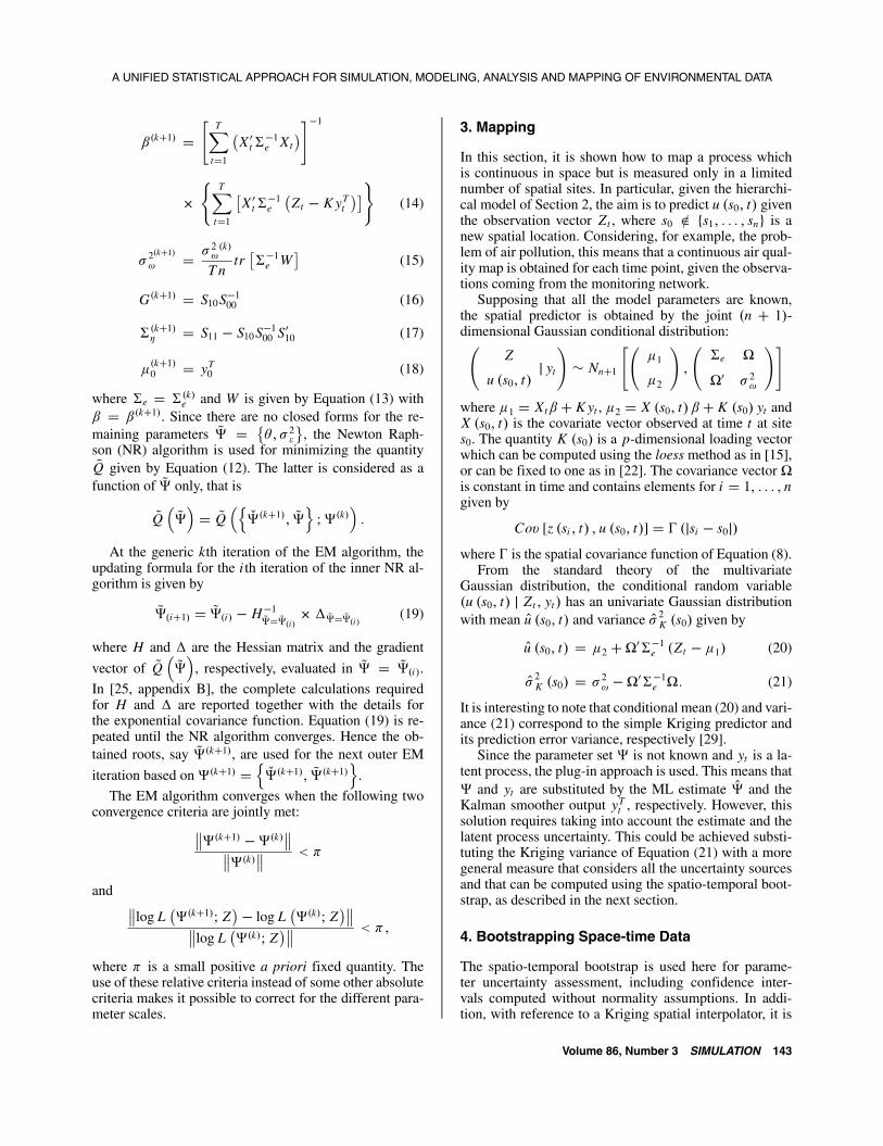
On the other hand, simulation is becoming an impor-tant part of statistical estimation of environmental models.When these simulations involve a large number of replica-tions of complex spatio-temporal model runs, a distributedcomputing environment is called for.

1.2 Case Study

We show how the general approach of hierarchical spatio-temporal models may be used in mapping and understand-ing airborne particulate matter concentrations, when dataare available on a daily frequency from different sources.

Volume 86, Number 3 SIMULATION 139

Fassò and Cameletti

These sources include land description, a monitoring net-work and a computer model chain (EMCT) which in-cludes modules for emissions, meteorology, chemistryand transport. Moreover, we show how to assess the simu-lation model outputs and obtain a surrogate model whichmay be useful for further simulations as the full modelchain is computationally expensive. Hence, following theapproach of [9] and [10], we demonstrate how the above-mentioned problems can be unified to some extent and theresulting uncertainty assessed.

1.3 Hierarchical Models

As described in [11–13], the hierarchical approach is use-ful for complex environmental processes. These vary intime and space and depend on several variables that inter-act on a wide variety of scales. As a matter of fact, thisapproach makes it possible to take a conditional view-point for which the joint probability distribution of thespatio-temporal process can be expressed as the productof some simpler conditional distributions defined at eachhierarchical stage. Hierarchical models can be tackled us-ing a Bayesian or a classical point of view, the latter beingthe main focus of this paper. In particular, both cases relyheavily on simulations and this may result in huge com-putational challenges.

This modeling approach has already been used invarious environmental applications. For example, spatio-temporal modeling for calibration of radar rainfall data bymeans of a ground-truth monitoring network have beenconsidered [14]. Similarly, the calibration of particulatematters measurements from heterogeneous networks hasbeen investigated [15]� daily sulphur dioxide data havebeen analyzed [16] and near-surface wind modeling hasbeen developed [7]. Moreover, in hydrology, the concur-rent estimation of model parameters and missing data inriver runoff series has been considered [17]. [18] demon-strate that, for hourly air quality data, non-linear mod-els seem more appropriate� however, on the daily scale itis common practice to use linear models on transformeddata.

Using the Bayesian paradigm, Markov Chain MonteCarlo (MCMC) algorithms are required for sampling fromthe posterior distributions of the parameters while, in theclassical framework, optimization and resampling meth-ods are used for estimation and uncertainty assessment.For example, the EM algorithm [19, 20] is a sequential es-timation algorithm, while bootstrap resampling is an em-barrassingly parallel problem with coarse grains.

1.4 Sensitivity Analysis

The statistical approach to sensitivity analysis (SA) is es-sentially based on some appropriate variance decomposi-tions. According to this, the sensitivity of a model output

to certain model inputs is assessed in terms of output un-certainty which can be apportioned to each input.

The classical approach to statistical SA is based onmodel repeated simulation [2], which may be based onMonte Carlo or other sampling plans. Application of SAranges from meteorology to econometrics, see e.g. [2]. Inwaste water treatment, SA has been considered [5] for siz-ing the treatment plant and understanding filter life span.Moreover, SA in recreational water quality monitoring hasbeen considered [1]. In this paper, a model-based SA forcorrelated inputs is proposed. This extends the classicalSA for independent inputs and also extends the results of[10], as a new concept of conditional SA is introduced.

1.5 Structure of Article

This article is organized as follows: the next four sectionsare on methods and one large section is on the case study.In particular, Section 2 discusses a rather general spatio-temporal model, which encompasses various model com-ponents and covers both spatial and temporal correlation.The model under consideration has three levels of hierar-chy and takes into account a measurement error as wellas a spatio-temporal dynamical field with both stochasticand systematic components. Temporal and spatial randomeffects are introduced in the second level and, in the laststage, a Markovian process is used for modeling the tem-poral dynamics of the latent process.

Section 2.3 defines the details of a new version of theEM algorithm for model coefficient estimation, which ex-tends [21] to deterministic trends with covariates.

Section 3 considers the spatial interpolation problemfor mapping and shows that this can be solved by theKriging method implemented using the plug-in approach.The methodological part ends with Section 4, where thespatio-temporal parametric bootstrap is used for obtainingthe parameter standard errors and for evaluating map un-certainty.

After briefly reviewing the basic concepts of SA, Sec-tion 5 introduces the concept of conditional SA, which isespecially useful for hierarchical models in order to adjustfor the latent components.

Section 6 discusses the application of daily data to air-borne particulate matters for the Piemonte Region, Italy,where data from a monitoring network and an EMCTmodel chain are integrated. After model identification, themapping capabilities are discussed and the model is inter-preted in terms of various uncertainty decompositions. AConclusion closes the paper.

2. Statistical Modeling

In this section, after introducing the structure of the hi-erarchical spatio-temporal model, the iterative estimationalgorithm based on the Gaussian maximum likelihood isdefined in detail.

140 SIMULATION Volume 86, Number 3

A UNIFIED STATISTICAL APPROACH FOR SIMULATION, MODELING, ANALYSIS AND MAPPING OF ENVIRONMENTAL DATA

2.1 Model Setup

In this work a three-stage hierarchical model takes intoaccount measurement errors as well as deterministic andstochastic spatio-temporal dynamical fields. In particular,after using the first level for measurement error, temporaland spatial random effects are introduced at the secondlevel. At the third level, a Markovian process models thetemporal dynamics.

Suppose that a certain phenomenon, e.g. particulatematters concentration, is observed at location s � D andday t � 1� 2� � � � � T by the following measurement equa-tion:

z �s� t� � u �s� t�� s� t� (1)

where u �s� t� is the underlying ‘true’ local pollution levelwith the structure:

u �s� t� � X �s� t� � � K �s� yt � � �s� t� � (2)

In Equation (2), X �s� t� is a d-dimensional spatio-temporal field of known covariates observed at time t atlocation s including, for example, land features (which arepurely spatial) and spatio-temporal fields that can be ob-served or simulated. The p-dimensional vector yt , whichis constant in space, is related to the ‘global true’ pollutionlevel� the matrix K �s� defines a p�dimensional field ofknown coefficients able to ‘localize’ the global level� forexample, it may be based on the observed data throughan EOF decomposition [7] or, in other cases, it may beconstant over the geographical space D [22].

The process ��s� t� is a typical Gaussian instrumentalerror which is white noise in space and time with variance 2� . The Gaussian process ��s� t� is the spatial small-scale

component and is a white noise in time, but is correlatedover space with a covariance function depending on theparameter , namely

E�� s� t�� s�� t�� 2

�C �h�

where h � ��s � s �� is the Euclidean distance between

sites s and s�. As the covariance function depends onlyon h, the spatial process � �s� t� is second-order station-ary and isotropic. Various examples of spatial covariancefunctions are discussed in [23, chapter 1] and a typicalcase is given by the following exponential function

C �h� � exp ��h� � (3)

Moreover, yt has stable Markovian temporal dynamicsgiven by

yt � Gyt�1 � �t (4)

where �t is a p-dimensional Gaussian white noise processwith variance-covariance matrix ��. The process startsfrom y0 which is given by a p-dimensional Gaussian vec-tor with mean 0 and variance-covariance matrix �0.

Note that the three error components, namely ��s� t�,��s� t� and �t , are zero-mean and independent over time

as well as mutually independent. Hence, the parameter setwhich identifies Equations (1–4) and is estimated usingobserved data is given by

� � �� 2��

2��G�� 0

�� (5)

2.2 Matrix Representation

In this section, the matrix notation to be used for the esti-mation and mapping procedures described in Sections 2.3and 3, respectively, is introduced. Suppose there is a net-work of n stations and observations for T consecutivedays. Denoting the network information at time t by the n-dimensional column vector Zt � �z�s1� t�� z�sn� t��and the full data set by Z � �Z1� � � � � ZT �� similarly y isused for the full latent information. Moreover, let Xt de-note the corresponding n � d matrix of known regressorsat time t and K be the n � p loading matrix.

Equations (1), (2) and (4) can be rewritten compactlyusing the two-stage hierarchical model:

Zt � Xt� � K yt � et (6)

yt � Gyt�1 � �t (7)

which can be considered as a classical state-space model[24], where Equation (6) is the measurement equation andEquation (7) is the state equation.

If all the parameters are known, the unobserved tempo-ral process yt is estimated for each time point t using theKalman filter and Kalman smoother techniques with ini-tial conditions given by y0. In the following, the Kalmansmoother outputs are denoted by yT

t , PTt and PT

t�t�1 whichare the mean, variance and lag-one covariance of the ytconditional on the complete observation matrix Z , respec-tively, as defined in detail in [25, appendix A].

In Equation (6), the error et � �t � �t has a zero-mean Gaussian distribution with variance-covariance ma-trix �e � 2

��si � s j

��i� j�1��n , where � is the scaled

spatial covariance function:

� �h� �� 1� 2

�2�

h � 0

C �h� h � 0�(8)

It is interesting to note that the measurement error vari-ance 2

� can be interpreted in geostatistical terms as theso-called ‘nugget effect’ of the spatial process e �s� t� forfixed t .

2.3 Estimation using the EM Algorithm

The maximum likelihood (ML) estimation of the un-known parameter set � defined by Equation (5) is per-formed by optimizing the log-likelihood function which,as shown in [26], is given by



log L �� Z� � �nT

2log �2�� 1

2

Tt�1

�log �t

� �Zt � t

��1

t

�Zt � t

��(9)

where

t ��

Xt� � K yt�1t

��

�t ��

K Pt�1t K � ��e

��

y01 � 0, P0

1 � �0 and the symbol � is used for matrixdeterminant. Since direct maximization of log-likelihoodEquation (9) is complex, the Expectation-Maximization(EM) algorithm is used [27, 28]. This method, which isbased on the complete log-likelihood Equation (10), isparticularly suitable for missing data problems, includingthe models defined by Equations (6) and (7), where themissing data component is given by the latent process yt .

Moreover, the EM algorithm is useful for spatio-temporal separable models because the maximization stepdoes not require numerical optimization for the model pa-rameters, except those related to the spatial covariance.Hence, it avoids large Hessian matrix inversions and therelated instability and non-positive definiteness which of-ten arise in performing numerical maximization of thelikelihood. Missing data are also handled in a natural way.

Apart from an additive constant, the complete log-likelihood is given by

log Lc�� Z� � �T

2log �e

� 1

2

Tt�1

�Zt � Xt� � K yt��1

e �Zt � Xt� � K yt�

� 1

2log �0 � 1

2

�y0 � 0

��1

0

�y0 � 0

�

� T

2log�� 1

2

Tt�1

�yt � Gyt�1��1

�

� �yt � Gyt�1� (10)

where �Z � �y0� � � � � yT � Z1� � � � � ZT � is the completedataset. At each iteration k � 1� 2� � � � the EM algorithmconsists of an expectation step (E) and a maximizationstep (M) which are described extensively in the followingsections. Given the current values of the parameters ��k�,the E-step computes the expected value of the completelog-likelihood function log Lc

�� Z� conditional on the

observation matrix Z and ��k�, that is

Q�� k�� E��k�

�log Lc

�� Z� Z

��

At the M-step, a value ��k�1� is chosen so thatQ��k�1� ��k�� Q

��k� ��k��.

2.3.1 E-step

With reference to the complete log-likelihood Equa-tion (10), it is easy to implement the E-step and to com-pute the function Q

�� k�� which is reported in the

equation as follows:

� 2Q�� k�� 2E��k�

�log Lc

�� Z� Z

�� Q � log �0 � T log

�� tr

��1

0

��yT

0 � 0

� �yT

0 � 0

�� PT0

�� tr

��1�

�S11 � S10G � � GS�10 � GS00G�� (11)

where

�Q � �Q �� k�� T log �e � tr��1

e W�

(12)

and

W �T

t�1

��Zt � Xt� � K yT

t

� �Zt � Xt� � K yT

t

��

�T

t�1

K PTt K �� (13)

Note also that

S00 � S�k�00 ��T

t�1

�yT

t�1 yT �t�1 � PT

t�1

�T

�

S10 � S�k�10 ��T

t�1

� �yt �y�t�1 � PTt�t�1

�T

and

S11 � S�k�11 ��T

t�1

�yT

t yT �t � PT

t

�T

�

with the Kalman smoother outputs yTt , PT

t and PTt�t�1

computed using ��k� as the ‘true’ value.

2.3.2 M-step

Using the so-called conditional maximization steps [28,chapter 5], the solution of �Q

�� 0 is approximated by

partitioning � � �� The first result is a closed

form solution for the first component:

�� 2��G�� 0

�holding the second component fixed at its current value��

� 2�

�and �0 constant. In particular, the closed

forms are given by



��k�1� ��

Tt�1

�X �t�

�1e Xt

��1

��

Tt�1

�X �t�

�1e

�Zt � K yT

t

��(14)

2�k�1�

� � 2��k�

T ntr��1

e W�

(15)

G�k�1� � S10S�100 (16)

��k�1�� S11 � S10S�1

00 S�10 (17)

�k�1�0 � yT

0 (18)

where �e � ��k�e and W is given by Equation (13) with� � ��k�1�. Since there are no closed forms for the re-maining parameters ��

� 2�

�, the Newton Raph-

son (NR) algorithm is used for minimizing the quantity�Q given by Equation (12). The latter is considered as a

function of �� only, that is

�Q� �� Q

� ��k�1�� k�

��

At the generic kth iteration of the EM algorithm, theupdating formula for the i th iteration of the inner NR al-gorithm is given by

��i�1� � ��i� � H�1�� i� �� i� (19)

where H and � are the Hessian matrix and the gradient

vector of �Q� ��, respectively, evaluated in �� i�.

In [25, appendix B], the complete calculations requiredfor H and � are reported together with the details forthe exponential covariance function. Equation (19) is re-peated until the NR algorithm converges. Hence the ob-tained roots, say ��k�1�, are used for the next outer EM

iteration based on ��k�1� � ��k�1�� k�1�

�.

The EM algorithm converges when the following twoconvergence criteria are jointly met:��k�1� ��k��k��

and ��log L��k�1� Z

�� log L��k� Z

��log L��k� Z

��

where � is a small positive a priori fixed quantity. Theuse of these relative criteria instead of some other absolutecriteria makes it possible to correct for the different para-meter scales.

3. Mapping

In this section, it is shown how to map a process whichis continuous in space but is measured only in a limitednumber of spatial sites. In particular, given the hierarchi-cal model of Section 2, the aim is to predict u �s0� t� giventhe observation vector Zt , where s0 �� s1� � � � � sn� is anew spatial location. Considering, for example, the prob-lem of air pollution, this means that a continuous air qual-ity map is obtained for each time point, given the observa-tions coming from the monitoring network.

Supposing that all the model parameters are known,the spatial predictor is obtained by the joint �n � 1�-dimensional Gaussian conditional distribution:�

Z

u �s0� t� yt

�� Nn�1

�� 1

2

��

��e �

�� 2�

��

where 1 � Xt� � K yt , 2 � X �s0� t� � � K �s0� yt andX �s0� t� is the covariate vector observed at time t at sites0. The quantity K �s0� is a p-dimensional loading vectorwhich can be computed using the loess method as in [15],or can be fixed to one as in [22]. The covariance vector �is constant in time and contains elements for i � 1� � � � � ngiven by

Co� [z �si � t� � u �s0� t�] � � �si � s0�where � is the spatial covariance function of Equation (8).

From the standard theory of the multivariateGaussian distribution, the conditional random variable�u �s0� t� Zt � yt� has an univariate Gaussian distributionwith mean �u �s0� t� and variance � 2

K �s0� given by

�u �s0� t� � 2 ��1e �Zt � 1� (20)

� 2K �s0� � 2

� ��1e �� (21)

It is interesting to note that conditional mean (20) and vari-ance (21) correspond to the simple Kriging predictor andits prediction error variance, respectively [29].

Since the parameter set � is not known and yt is a la-tent process, the plug-in approach is used. This means that� and yt are substituted by the ML estimate �� and theKalman smoother output yT

t , respectively. However, thissolution requires taking into account the estimate and thelatent process uncertainty. This could be achieved substi-tuting the Kriging variance of Equation (21) with a moregeneral measure that considers all the uncertainty sourcesand that can be computed using the spatio-temporal boot-strap, as described in the next section.

4. Bootstrapping Space-time Data

The spatio-temporal bootstrap is used here for parame-ter uncertainty assessment, including confidence inter-vals computed without normality assumptions. In addi-tion, with reference to a Kriging spatial interpolator, it is



applied for computing map uncertainty and data rough-ness assessment.

In this section, a sampling scheme for bootstrappingdata which are dependent in space and time is proposed.In the literature, only purely spatial or temporal bootstraptechniques have been discussed [e.g. 30, 31].

The resampling spatio-temporal strategy introducedhere is very simple and is based on the estimated paramet-ric model of Section 2. In particular, samples are drawndirectly from the Gaussian distributions involved and areused in Equations (6) and (7), with � replaced by itsML estimate �� for obtaining the bootstrap samples Z�b,b � 1� � � � � B. The procedure starts from a p-dimensionalvector y�0 simulated from N

� � 0��0�.

In this way, B bootstrap samples are simulated and, foreach of them, the ML estimate ��b and the spatial pre-diction �u�b �s0� t� are computed using the EM algorithmand the spatial prediction technique described in Sec-tions 2.3 and 3, respectively. The bootstrap replications��1� � � � � ��B and �u�1 �s0� t� � � � � � �u�B �s0� t� are then used

for computing the standard error of each parameter andspatial prediction. Moreover, percentile confidence inter-vals and full empirical distributions can be easily calcu-lated.

5. Conditional Sensitivity Analysis

The modern approach to statistical SA is based on anappropriate variance decomposition [e.g. 2, 5, 6]. If re-peated code runs are possible, sensitivity analysis designmakes it possible to define an appropriate input samplingplane, e.g. Latin hypercubes. This in turn implies orthogo-nal inputs and the variance decomposition is easier. If thecode runs are expensive and/or the model requires obser-vational data, repeated inputs are not allowed and one hasto adapt the variance decomposition to the input structureat hand.

In our case, the hierarchical model of Section 2 can beused for simulation but the ECMT outputs are difficult torepeat since ECMT is not a cheap code.

Generally speaking, using the notation in [10], a lin-ear model with three correlated input sets is considered,namely:

z � u � � � � �1x1 � � �2x2 � � �3x3 � �� (22)

This model is similar to Equation (1) with known latentvariables y and �.

If the three input sets are independent, then

V ar �z� �3

j�1

� �j V�x j�� j � V ��

and sensitivity of z to the input sets x j , j � 1� 2� 3, issimply given by

Sj �� j V

�x j�� j

V ar �z�

where V ar �z� is the variance of scalar random variable zand V �x� is the variance-covariance matrix of the stochas-tic vector x � From a more general point of view, this prob-lem could also be attached by regression elements [32] orby additive elements of the likelihood function [33].

When x3 is not present in Equation (22), giving u �� 1x1 � � �2x2, and the input sets x1 and x2 are not inde-pendent, [10] suggests starting from the general variancedecomposition

V ar �u� � V ar �E �ux1�� E �V ar �ux1��

which also holds for correlated x’s. This gives two sensi-tivity indexes for assessing the effect of, say, x1. The firstis the total effect of x1:

S1 � V ar �E �ux1��

V ar �z�

which also incorporates the effect of x2 due to correlationbetween x1 and x2. The second index is the net effect ofx1 adjusted for x2, namely

S12 � E �V ar �ux2��

V ar �z��

If the input sets x1 and x2 are linearly related, i.e.E �x2x1� � b�21x1, the above sensitivity indexes are sim-ply given by

S1 � b�1V �x1� b1

V ar �z�and

S12 � � �1V �x1x2� �1

V ar �z��

The coefficients involved in these definitions are thestandard conditional Gaussian quantities or least squarequantities, namely

b21 � V �x1��1 Co�

�x1� x �2

��

b1 � �1 � b21�2

and

V �x1x2� � V �x1��Co��x1� x �2

�V �x2�

�1 Co��x2� x �1

��

the latter being the standard residual variance-covariancematrix.

The comparison between the two input sets thereforemay be determined by comparing

�S1� S12

�to�

S2� S21�.

In the case of Equation (22) with three input sets,the sensitivity analysis of the first two sets (as above) isinfluenced by x3. In other words, if x3 is correlated withthe other inputs, then spurious sensitivity conclusions mayoccur.

To avoid this, the conditional SA is proposed by apply-ing the above SA indexes for correlated inputs to adjustedvariables x13 � x1� E �x1x3�, x23 � x2� E �x2x3� andz3 � z� E �zx3�, which are easily estimated under linearassumptions using least square residuals and are uncorre-lated with x3.



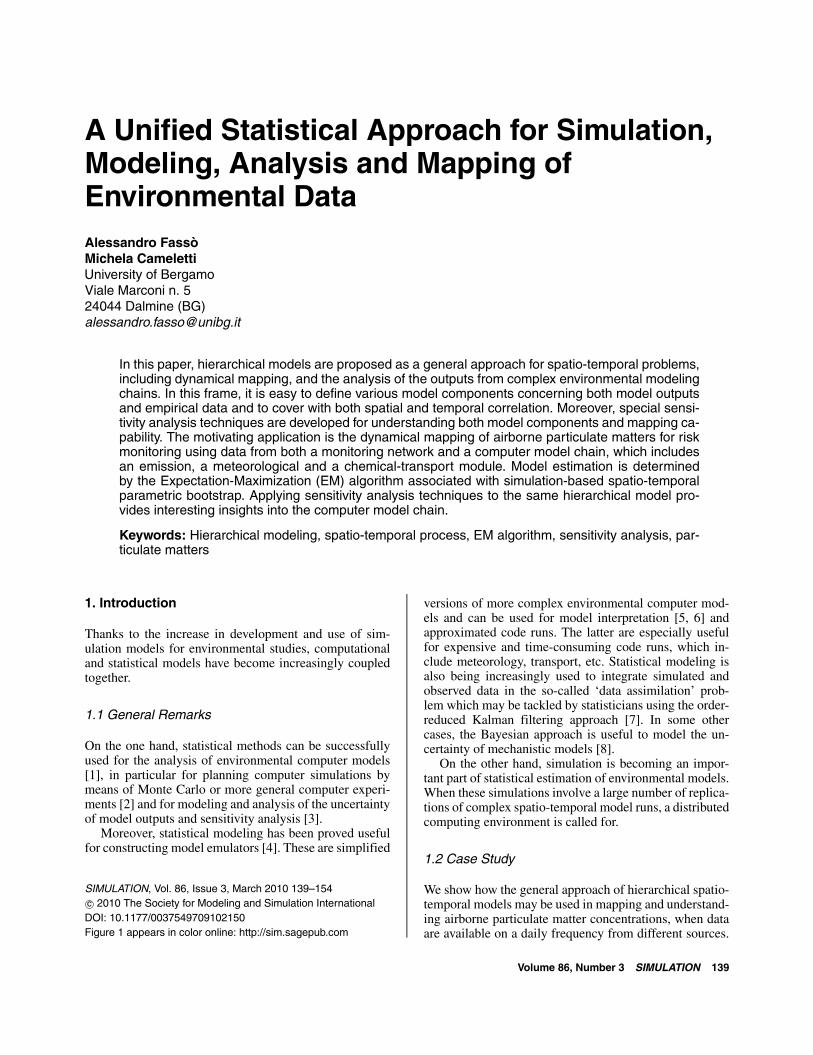
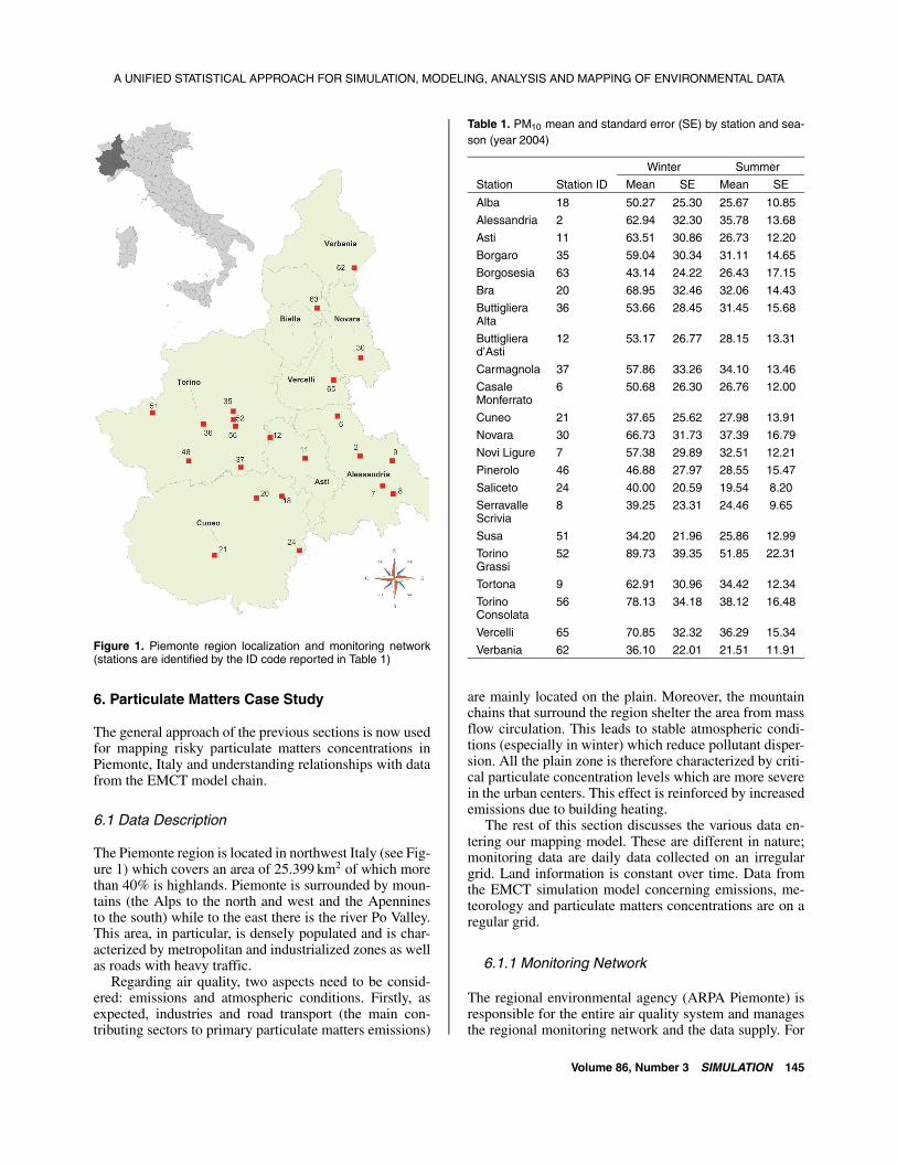
Figure 1. Piemonte region localization and monitoring network(stations are identified by the ID code reported in Table 1)

6. Particulate Matters Case Study

The general approach of the previous sections is now usedfor mapping risky particulate matters concentrations inPiemonte, Italy and understanding relationships with datafrom the EMCT model chain.

6.1 Data Description

The Piemonte region is located in northwest Italy (see Fig-ure 1) which covers an area of 25.399 km2 of which morethan 40% is highlands. Piemonte is surrounded by moun-tains (the Alps to the north and west and the Apenninesto the south) while to the east there is the river Po Valley.This area, in particular, is densely populated and is char-acterized by metropolitan and industrialized zones as wellas roads with heavy traffic.

Regarding air quality, two aspects need to be consid-ered: emissions and atmospheric conditions. Firstly, asexpected, industries and road transport (the main con-tributing sectors to primary particulate matters emissions)

Table 1. PM10 mean and standard error (SE) by station and sea-son (year 2004)

Winter Summer

Station Station ID Mean SE Mean SE

Alba 18 50.27 25.30 25.67 10.85

Alessandria 2 62.94 32.30 35.78 13.68

Asti 11 63.51 30.86 26.73 12.20

Borgaro 35 59.04 30.34 31.11 14.65

Borgosesia 63 43.14 24.22 26.43 17.15

Bra 20 68.95 32.46 32.06 14.43

ButtiglieraAlta

36 53.66 28.45 31.45 15.68

Buttiglierad’Asti

12 53.17 26.77 28.15 13.31

Carmagnola 37 57.86 33.26 34.10 13.46

CasaleMonferrato

6 50.68 26.30 26.76 12.00

Cuneo 21 37.65 25.62 27.98 13.91

Novara 30 66.73 31.73 37.39 16.79

Novi Ligure 7 57.38 29.89 32.51 12.21

Pinerolo 46 46.88 27.97 28.55 15.47

Saliceto 24 40.00 20.59 19.54 8.20

SerravalleScrivia

8 39.25 23.31 24.46 9.65

Susa 51 34.20 21.96 25.86 12.99

TorinoGrassi

52 89.73 39.35 51.85 22.31

Tortona 9 62.91 30.96 34.42 12.34

TorinoConsolata

56 78.13 34.18 38.12 16.48

Vercelli 65 70.85 32.32 36.29 15.34

Verbania 62 36.10 22.01 21.51 11.91

are mainly located on the plain. Moreover, the mountainchains that surround the region shelter the area from massflow circulation. This leads to stable atmospheric condi-tions (especially in winter) which reduce pollutant disper-sion. All the plain zone is therefore characterized by criti-cal particulate concentration levels which are more severein the urban centers. This effect is reinforced by increasedemissions due to building heating.

The rest of this section discusses the various data en-tering our mapping model. These are different in nature�monitoring data are daily data collected on an irregulargrid. Land information is constant over time. Data fromthe EMCT simulation model concerning emissions, me-teorology and particulate matters concentrations are on aregular grid.

6.1.1 Monitoring Network

The regional environmental agency (ARPA Piemonte) isresponsible for the entire air quality system and managesthe regional monitoring network and the data supply. For



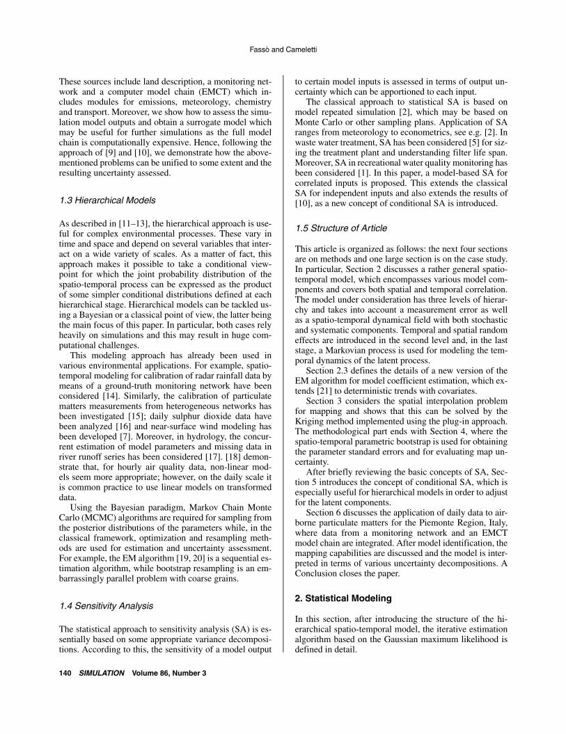
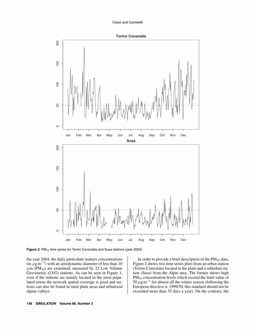
Figure 2. PM10 time series for Torino Consolata and Susa stations (year 2004)

the year 2004, the daily particulate matters concentrations(in g m�3) with an aerodynamic diameter of less than 10 m (PM10) are examined, measured by 22 Low VolumeGravimetric (LVG) stations. As can be seen in Figure 1,even if the stations are mainly located in the most popu-lated towns the network spatial coverage is good and sta-tions can also be found in rural plain areas and urbanizedalpine valleys.

In order to provide a brief description of the PM10 data,Figure 2 shows two time series plots from an urban station(Torino Consolata) located in the plain and a suburban sta-tion (Susa) from the Alpin area. The former shows highPM10 concentration levels which exceed the limit value of50 g m�3 for almost all the winter season (following theEuropean directive n. 1999/30, this standard should not beexceeded more than 35 days a year). On the contrary, the



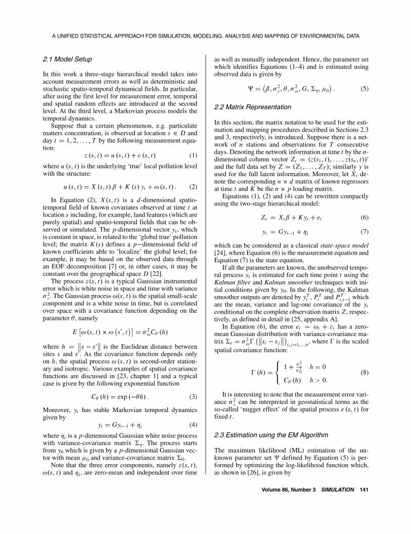
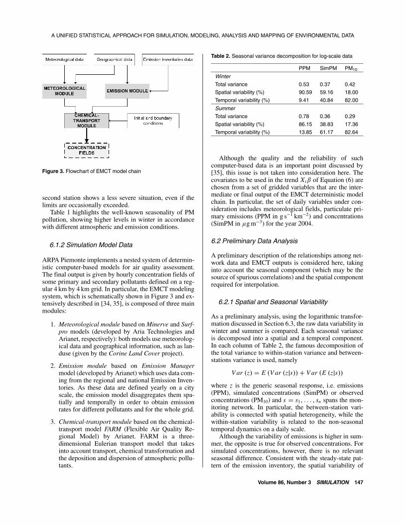
Figure 3. Flowchart of EMCT model chain

second station shows a less severe situation, even if thelimits are occasionally exceeded.

Table 1 highlights the well-known seasonality of PMpollution, showing higher levels in winter in accordancewith different atmospheric and emission conditions.

6.1.2 Simulation Model Data

ARPA Piemonte implements a nested system of determin-istic computer-based models for air quality assessment.The final output is given by hourly concentration fields ofsome primary and secondary pollutants defined on a reg-ular 4 km by 4 km grid. In particular, the EMCT modelingsystem, which is schematically shown in Figure 3 and ex-tensively described in [34, 35], is composed of three mainmodules:

1. Meteorological module based on Minerve and Surf-pro models (developed by Aria Technologies andArianet, respectively): both models use meteorolog-ical data and geographical information, such as lan-duse (given by the Corine Land Cover project).

2. Emission module based on Emission Managermodel (developed by Arianet) which uses data com-ing from the regional and national Emission Inven-tories. As these data are defined yearly on a cityscale, the emission model disaggregates them spa-tially and temporally in order to obtain emissionrates for different pollutants and for the whole grid.

3. Chemical-transport module based on the chemical-transport model FARM (Flexible Air Quality Re-gional Model) by Arianet. FARM is a three-dimensional Eulerian transport model that takesinto account transport, chemical transformation andthe deposition and dispersion of atmospheric pollu-tants.

Table 2. Seasonal variance decomposition for log-scale data

PPM SimPM PM10

Winter

Total variance 0.53 0.37 0.42

Spatial variability (%) 90.59 59.16 18.00

Temporal variability (%) 9.41 40.84 82.00

Summer

Total variance 0.78 0.36 0.29

Spatial variability (%) 86.15 38.83 17.36

Temporal variability (%) 13.85 61.17 82.64

Although the quality and the reliability of suchcomputer-based data is an important point discussed by[35], this issue is not taken into consideration here. Thecovariates to be used in the trend Xt� of Equation (6) arechosen from a set of gridded variables that are the inter-mediate or final output of the EMCT deterministic modelchain. In particular, the set of daily variables under con-sideration includes meteorological fields, particulate pri-mary emissions (PPM in g s�1 km�2) and concentrations(SimPM in g m�3) for the year 2004.

6.2 Preliminary Data Analysis

A preliminary description of the relationships among net-work data and EMCT outputs is considered here, takinginto account the seasonal component (which may be thesource of spurious correlations) and the spatial componentrequired for interpolation.

6.2.1 Spatial and Seasonal Variability

As a preliminary analysis, using the logarithmic transfor-mation discussed in Section 6.3, the raw data variability inwinter and summer is compared. Each seasonal varianceis decomposed into a spatial and a temporal component.In each column of Table 2, the famous decomposition ofthe total variance to within-station variance and between-stations variance is used, namely

V ar �z� � E �V ar �zs�� V ar �E �zs��where z is the generic seasonal response, i.e. emissions(PPM), simulated concentrations (SimPM) or observedconcentrations (PM10) and s � s1� � � � � sn spans the mon-itoring network. In particular, the between-station vari-ability is connected with spatial heterogeneity, while thewithin-station variability is related to the non-seasonaltemporal dynamics on a daily scale.

Although the variability of emissions is higher in sum-mer, the opposite is true for observed concentrations. Forsimulated concentrations, however, there is no relevantseasonal difference. Consistent with the steady-state pat-tern of the emission inventory, the spatial variability of



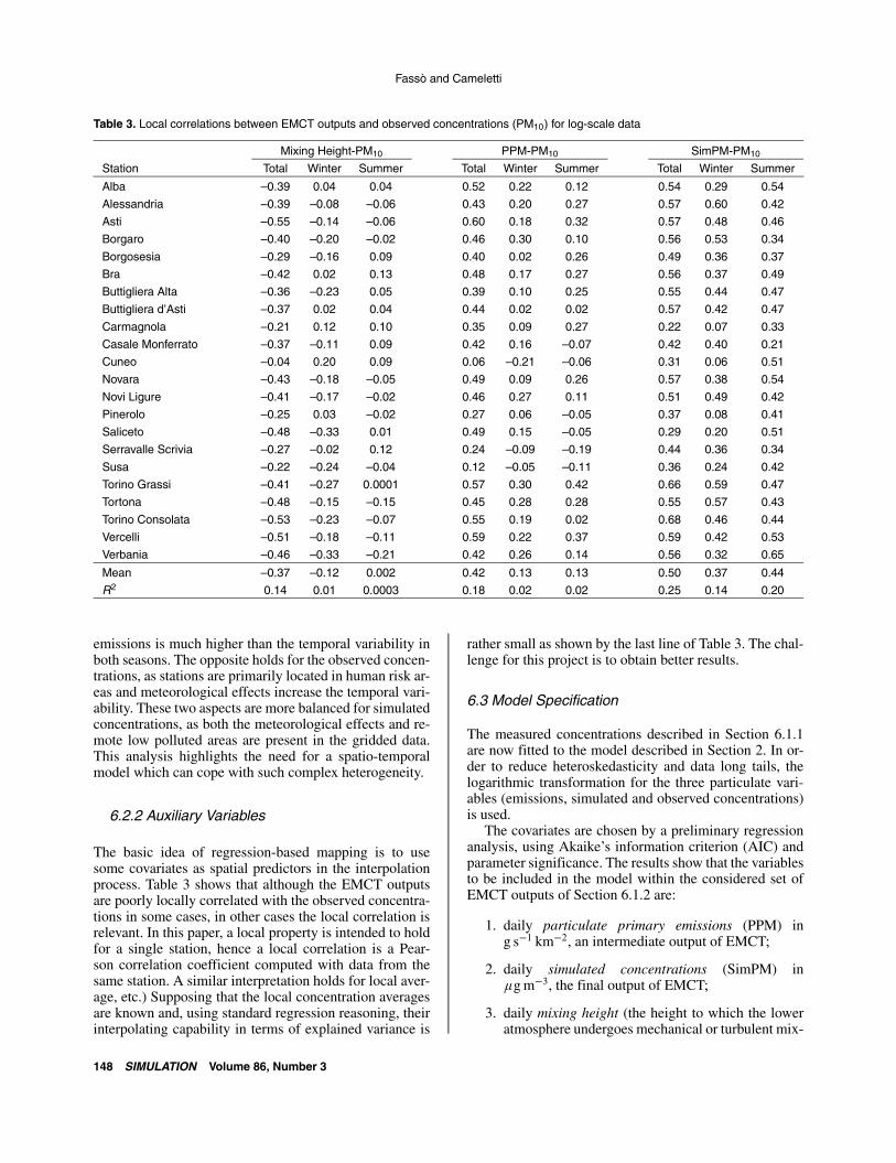
Table 3. Local correlations between EMCT outputs and observed concentrations (PM10) for log-scale data

Mixing Height-PM10 PPM-PM10 SimPM-PM10

Station Total Winter Summer Total Winter Summer Total Winter Summer

Alba –0.39 0.04 0.04 0.52 0.22 0.12 0.54 0.29 0.54

Alessandria –0.39 –0.08 –0.06 0.43 0.20 0.27 0.57 0.60 0.42

Asti –0.55 –0.14 –0.06 0.60 0.18 0.32 0.57 0.48 0.46

Borgaro –0.40 –0.20 –0.02 0.46 0.30 0.10 0.56 0.53 0.34

Borgosesia –0.29 –0.16 0.09 0.40 0.02 0.26 0.49 0.36 0.37

Bra –0.42 0.02 0.13 0.48 0.17 0.27 0.56 0.37 0.49

Buttigliera Alta –0.36 –0.23 0.05 0.39 0.10 0.25 0.55 0.44 0.47

Buttigliera d’Asti –0.37 0.02 0.04 0.44 0.02 0.02 0.57 0.42 0.47

Carmagnola –0.21 0.12 0.10 0.35 0.09 0.27 0.22 0.07 0.33

Casale Monferrato –0.37 –0.11 0.09 0.42 0.16 –0.07 0.42 0.40 0.21

Cuneo –0.04 0.20 0.09 0.06 –0.21 –0.06 0.31 0.06 0.51

Novara –0.43 –0.18 –0.05 0.49 0.09 0.26 0.57 0.38 0.54

Novi Ligure –0.41 –0.17 –0.02 0.46 0.27 0.11 0.51 0.49 0.42

Pinerolo –0.25 0.03 –0.02 0.27 0.06 –0.05 0.37 0.08 0.41

Saliceto –0.48 –0.33 0.01 0.49 0.15 –0.05 0.29 0.20 0.51

Serravalle Scrivia –0.27 –0.02 0.12 0.24 –0.09 –0.19 0.44 0.36 0.34

Susa –0.22 –0.24 –0.04 0.12 –0.05 –0.11 0.36 0.24 0.42

Torino Grassi –0.41 –0.27 0.0001 0.57 0.30 0.42 0.66 0.59 0.47

Tortona –0.48 –0.15 –0.15 0.45 0.28 0.28 0.55 0.57 0.43

Torino Consolata –0.53 –0.23 –0.07 0.55 0.19 0.02 0.68 0.46 0.44

Vercelli –0.51 –0.18 –0.11 0.59 0.22 0.37 0.59 0.42 0.53

Verbania –0.46 –0.33 –0.21 0.42 0.26 0.14 0.56 0.32 0.65

Mean –0.37 –0.12 0.002 0.42 0.13 0.13 0.50 0.37 0.44

R2 0.14 0.01 0.0003 0.18 0.02 0.02 0.25 0.14 0.20

emissions is much higher than the temporal variability inboth seasons. The opposite holds for the observed concen-trations, as stations are primarily located in human risk ar-eas and meteorological effects increase the temporal vari-ability. These two aspects are more balanced for simulatedconcentrations, as both the meteorological effects and re-mote low polluted areas are present in the gridded data.This analysis highlights the need for a spatio-temporalmodel which can cope with such complex heterogeneity.

6.2.2 Auxiliary Variables

The basic idea of regression-based mapping is to usesome covariates as spatial predictors in the interpolationprocess. Table 3 shows that although the EMCT outputsare poorly locally correlated with the observed concentra-tions in some cases, in other cases the local correlation isrelevant. In this paper, a local property is intended to holdfor a single station, hence a local correlation is a Pear-son correlation coefficient computed with data from thesame station. A similar interpretation holds for local aver-age, etc.) Supposing that the local concentration averagesare known and, using standard regression reasoning, theirinterpolating capability in terms of explained variance is

rather small as shown by the last line of Table 3. The chal-lenge for this project is to obtain better results.

6.3 Model Specification

The measured concentrations described in Section 6.1.1are now fitted to the model described in Section 2. In or-der to reduce heteroskedasticity and data long tails, thelogarithmic transformation for the three particulate vari-ables (emissions, simulated and observed concentrations)is used.

The covariates are chosen by a preliminary regressionanalysis, using Akaike’s information criterion (AIC) andparameter significance. The results show that the variablesto be included in the model within the considered set ofEMCT outputs of Section 6.1.2 are:

1. daily particulate primary emissions (PPM) ing s�1 km�2, an intermediate output of EMCT�

2. daily simulated concentrations (SimPM) in g m�3, the final output of EMCT�

3. daily mixing height (the height to which the loweratmosphere undergoes mechanical or turbulent mix-



Table 4. Seasonal parameter estimates, standard errors (SE) and95% bootstrap confidence interval bounds

Estimate SE 95% CI bounds

Winter

Intercept 3.237 0.046 3.147 3.325

PPM 0.040 0.012 0.017 0.062

SimPM 0.239 0.019 0.203 0.275

Mixing height –0.133 0.108 –0.364 0.072

Altitude –0.822 0.060 –0.948 –0.701

Summer

Intercept 2.417 0.071 2.185 2.649

PPM 0.093 0.008 0.080 0.109

SimPM 0.233 0.016 0.204 0.268

Mixing height 0.191 0.076 0.047 0.335

Altitude –0.252 0.052 –0.348 –0.146

Table 5. Non-seasonal parameter estimates, standard errors (SE)and 95% bootstrap confidence interval bounds

Estimate SE 95% CI bounds

2� 0.078 0.001 0.075 0.080

0.023 0.002 0.019 0.026

2� 0.078 0.002 0.074 0.082

G 0.747 0.038 0.651 0.806

�� 0.054 0.004 0.045 0.062

0 –0.434 1.074 –2.544 1.551

ing producing a nearly homogeneous air mass, re-lated to the height where relatively vigorous mixingand pollutant dispersion occurs) in km�

4. altitude in km, which is not a simulated variable.

To cope with the strong seasonality of air quality data,a seasonal model with different � coefficients for win-ter and summer is used. Moreover, according to an unre-ported performance analysis which is similar to the cross-validation described in Section 6.6, one dimensional un-derlying process yt with p � 1 was chosen. Finally, thespatial covariance function is the exponential term givenby Equation (3).

6.4 Model Estimation and Description

Tables 4 and 5 report the estimates computed using theEM algorithm described in Section 2.3. The estimates,which are also used as a basis of B � 500 bootstrapreplications, are given together with the correspondingbootstrap standard errors and the bounds of the 95%confidence intervals.

Examining the size of confidence intervals, apart fromthe initial value 0 which is a nuisance parameter for the

model with no substantial interest, it can be observed thatall but one of the parameters are characterized by a highlevel of accuracy.

The coefficients for altitude are both negative, consis-tently with less anthropized highlands and ceteris paribus,this effect is stronger in winter.

Generally speaking, mixing height is expected to benegatively correlated with pollutant concentrations. Forexample, using the Piemonte data, the correlation for thewhole year between mixing height and log�P M10� is –0.32. Things change after deseasonalizing as the wintercorrelation is reduced to –0.16 while the summer correla-tion is +0.06 which is non-significantly positive. A similarresult holds for our model, where the conditioning on mix-ing height induced by the other variables is stronger thansimply splitting winter and summer as above. The result istherefore further modified so that in winter the coefficientis non-significantly negative and in summer is moderatelypositive.

The values of the intercept give information about theaverage regional pollution level. In particular, returningto the original scale, the hypothetical difference betweenwinter and summer (with all the other variables at zero)would be 14 g m�3.

As expected, the coefficient for emissions (PPM) is sig-nificantly positive and doubles in summer. The concentra-tions are more sensitive to variations of emissions in sum-mer than in winter, when pollution is more persistent.

Similarly to the emissions, the coefficient for simulatedconcentrations (SimPM) is significantly positive but, con-trary to the emissions, it is more stable over the year withalmost the same value in winter and summer. This is con-sistent with the point that both SimPM and the networkPM10 measure the same quantity but the spatial resolutionis different. A deeper comparison of the roles of emissionsand simulated concentrations is given in Section 6.6.

Considering the non-seasonal part of the estimatedmodel, note that the variances 2

� and 2� are quite close.

Moreover, from the spatial correlation parameter wenote that at 50 km the spatial correlation is about 0.3 andat 90 km is about 0.1. Finally, the temporal coefficient G,being less than one, is in the stationarity range and its pos-itive value confirms the well-known temporal persistenceof particulate matters even after adjusting for all the co-variates. In this sense, the spatial and temporal persistencecoefficients, and G, complement and clarify the prelim-inary analysis of Section 6.2.1.

6.5 Mapping

In this section, the mapping of the P M10 field measuredby the monitoring network is taken into consideration. Theproblem of network design is not examined at this point.However, it is worth mentioning that the stations are oftenlocalized for assessing risk and, in this sense, risky con-centrations are being mapped here.



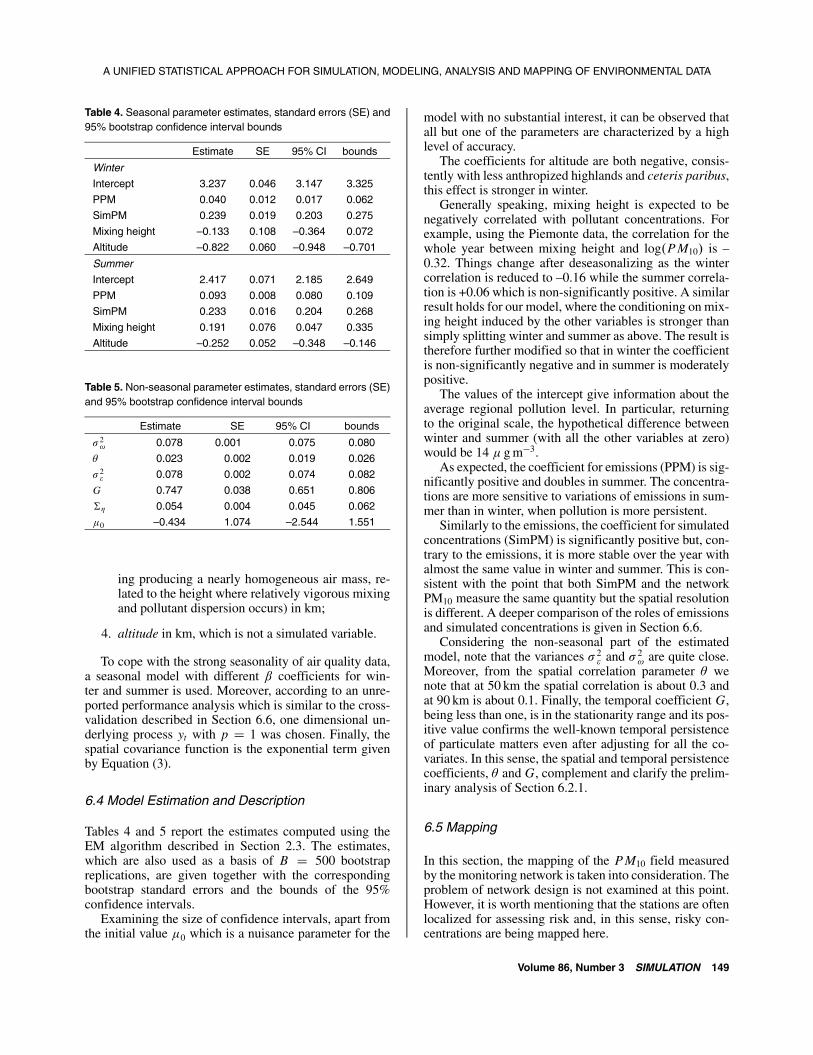
Figure 4. Concentration map for 30 January 2004 for log-scaledata

Figure 4 is the regional log-concentration map for 30January 2004 obtained using Equation (20) and the grid-ded data X �s0� t� of Section 6.1.2. The concentration mapshows that the more heavily polluted areas are locatedin the plain around Torino and near the urban centers ofthe southern part of the region, while the lowest concen-trations are in the boundary mountain areas. In the cen-tral plain part of the region, a homogeneous concentrationlevel can be seen. This is in accordance with the value ofthe spatial parameter discussed previously.

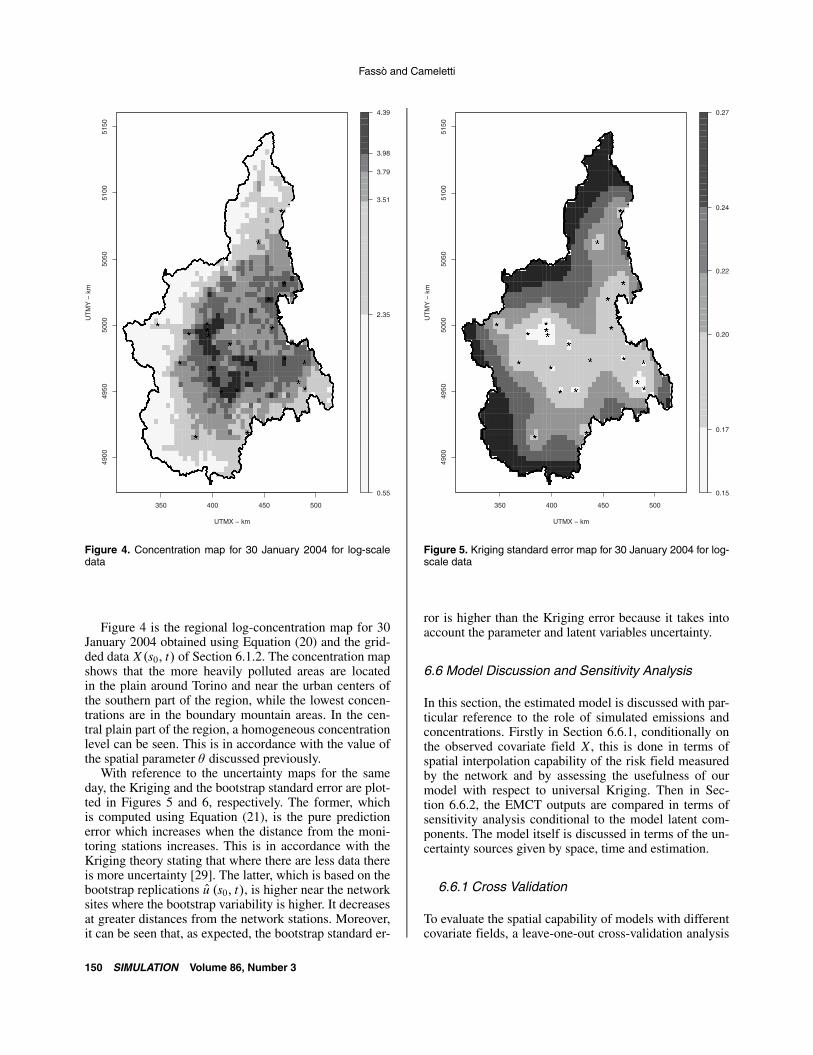
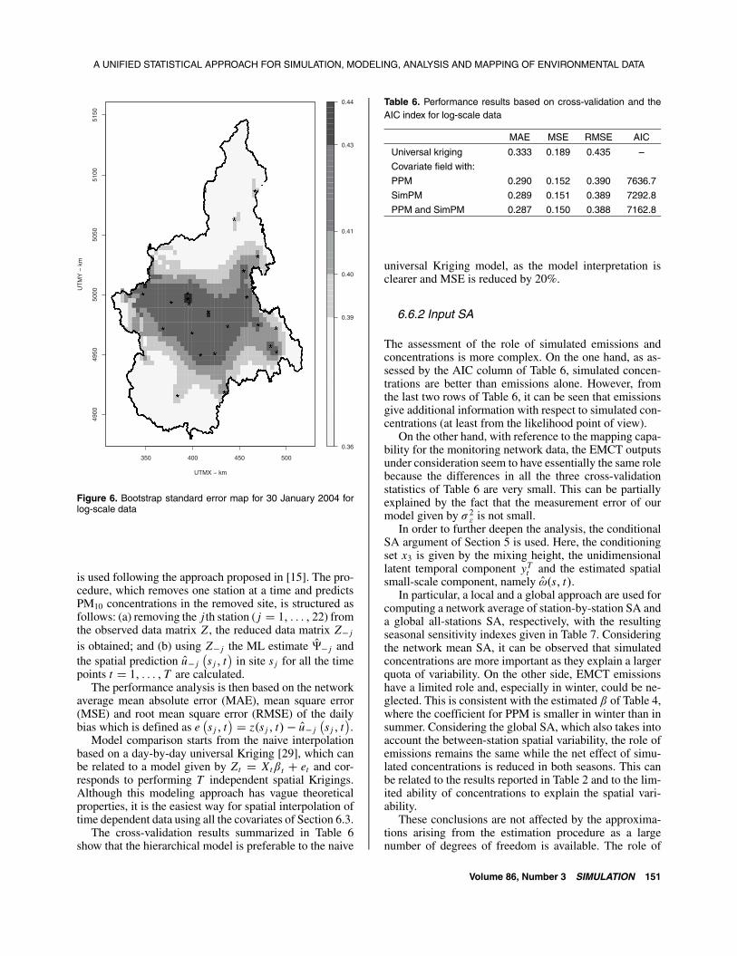
With reference to the uncertainty maps for the sameday, the Kriging and the bootstrap standard error are plot-ted in Figures 5 and 6, respectively. The former, whichis computed using Equation (21), is the pure predictionerror which increases when the distance from the moni-toring stations increases. This is in accordance with theKriging theory stating that where there are less data thereis more uncertainty [29]. The latter, which is based on thebootstrap replications �u �s0� t�, is higher near the networksites where the bootstrap variability is higher. It decreasesat greater distances from the network stations. Moreover,it can be seen that, as expected, the bootstrap standard er-

Figure 5. Kriging standard error map for 30 January 2004 for log-scale data

ror is higher than the Kriging error because it takes intoaccount the parameter and latent variables uncertainty.

6.6 Model Discussion and Sensitivity Analysis

In this section, the estimated model is discussed with par-ticular reference to the role of simulated emissions andconcentrations. Firstly in Section 6.6.1, conditionally onthe observed covariate field X , this is done in terms ofspatial interpolation capability of the risk field measuredby the network and by assessing the usefulness of ourmodel with respect to universal Kriging. Then in Sec-tion 6.6.2, the EMCT outputs are compared in terms ofsensitivity analysis conditional to the model latent com-ponents. The model itself is discussed in terms of the un-certainty sources given by space, time and estimation.

6.6.1 Cross Validation

To evaluate the spatial capability of models with differentcovariate fields, a leave-one-out cross-validation analysis



Figure 6. Bootstrap standard error map for 30 January 2004 forlog-scale data

is used following the approach proposed in [15]. The pro-cedure, which removes one station at a time and predictsPM10 concentrations in the removed site, is structured asfollows: (a) removing the j th station ( j � 1� � � � � 22) fromthe observed data matrix Z , the reduced data matrix Z� j

is obtained� and (b) using Z� j the ML estimate �� j andthe spatial prediction �u� j

�s j � t

�in site s j for all the time

points t � 1� � � � � T are calculated.The performance analysis is then based on the network

average mean absolute error (MAE), mean square error(MSE) and root mean square error (RMSE) of the dailybias which is defined as e

�s j � t

� � z�s j � t�� u� j�s j � t

�.

Model comparison starts from the naive interpolationbased on a day-by-day universal Kriging [29], which canbe related to a model given by Zt � Xt� t � et and cor-responds to performing T independent spatial Krigings.Although this modeling approach has vague theoreticalproperties, it is the easiest way for spatial interpolation oftime dependent data using all the covariates of Section 6.3.

The cross-validation results summarized in Table 6show that the hierarchical model is preferable to the naive

Table 6. Performance results based on cross-validation and theAIC index for log-scale data

MAE MSE RMSE AIC

Universal kriging 0.333 0.189 0.435 –

Covariate field with:

PPM 0.290 0.152 0.390 7636.7

SimPM 0.289 0.151 0.389 7292.8

PPM and SimPM 0.287 0.150 0.388 7162.8

universal Kriging model, as the model interpretation isclearer and MSE is reduced by 20%.

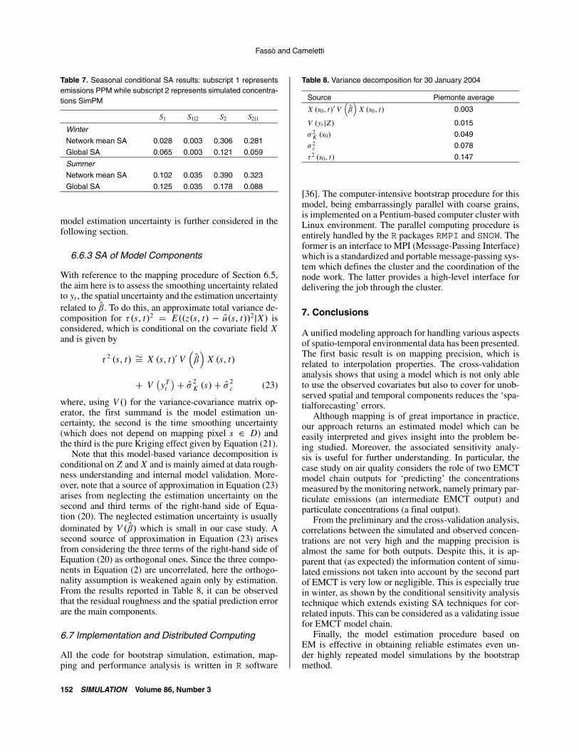
6.6.2 Input SA

The assessment of the role of simulated emissions andconcentrations is more complex. On the one hand, as as-sessed by the AIC column of Table 6, simulated concen-trations are better than emissions alone. However, fromthe last two rows of Table 6, it can be seen that emissionsgive additional information with respect to simulated con-centrations (at least from the likelihood point of view).

On the other hand, with reference to the mapping capa-bility for the monitoring network data, the EMCT outputsunder consideration seem to have essentially the same rolebecause the differences in all the three cross-validationstatistics of Table 6 are very small. This can be partiallyexplained by the fact that the measurement error of ourmodel given by 2

� is not small.In order to further deepen the analysis, the conditional

SA argument of Section 5 is used. Here, the conditioningset x3 is given by the mixing height, the unidimensionallatent temporal component yT

t and the estimated spatialsmall-scale component, namely ��s� t�.

In particular, a local and a global approach are used forcomputing a network average of station-by-station SA anda global all-stations SA, respectively, with the resultingseasonal sensitivity indexes given in Table 7. Consideringthe network mean SA, it can be observed that simulatedconcentrations are more important as they explain a largerquota of variability. On the other side, EMCT emissionshave a limited role and, especially in winter, could be ne-glected. This is consistent with the estimated � of Table 4,where the coefficient for PPM is smaller in winter than insummer. Considering the global SA, which also takes intoaccount the between-station spatial variability, the role ofemissions remains the same while the net effect of simu-lated concentrations is reduced in both seasons. This canbe related to the results reported in Table 2 and to the lim-ited ability of concentrations to explain the spatial vari-ability.

These conclusions are not affected by the approxima-tions arising from the estimation procedure as a largenumber of degrees of freedom is available. The role of



Table 7. Seasonal conditional SA results: subscript 1 representsemissions PPM while subscript 2 represents simulated concentra-tions SimPM

S1 S12 S2 S21Winter

Network mean SA 0.028 0.003 0.306 0.281

Global SA 0.065 0.003 0.121 0.059

Summer

Network mean SA 0.102 0.035 0.390 0.323

Global SA 0.125 0.035 0.178 0.088

model estimation uncertainty is further considered in thefollowing section.

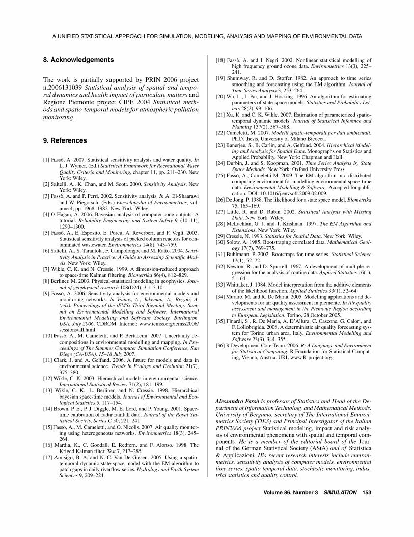
6.6.3 SA of Model Components

With reference to the mapping procedure of Section 6.5,the aim here is to assess the smoothing uncertainty relatedto yt , the spatial uncertainty and the estimation uncertaintyrelated to ��. To do this, an approximate total variance de-composition for ��s� t�2 � E��z�s� t� � �u�s� t��2X� isconsidered, which is conditional on the covariate field Xand is given by

� 2 �s� t� �� X �s� t�� V� �� X �s� t�

� V�

yTt

�� 2K �s�� 2

� (23)

where, using V �� for the variance-covariance matrix op-erator, the first summand is the model estimation un-certainty, the second is the time smoothing uncertainty(which does not depend on mapping pixel s � D) andthe third is the pure Kriging effect given by Equation (21).

Note that this model-based variance decomposition isconditional on Z and X and is mainly aimed at data rough-ness understanding and internal model validation. More-over, note that a source of approximation in Equation (23)arises from neglecting the estimation uncertainty on thesecond and third terms of the right-hand side of Equa-tion (20). The neglected estimation uncertainty is usuallydominated by V � �� which is small in our case study. Asecond source of approximation in Equation (23) arisesfrom considering the three terms of the right-hand side ofEquation (20) as orthogonal ones. Since the three compo-nents in Equation (2) are uncorrelated, here the orthogo-nality assumption is weakened again only by estimation.From the results reported in Table 8, it can be observedthat the residual roughness and the spatial prediction errorare the main components.

6.7 Implementation and Distributed Computing

All the code for bootstrap simulation, estimation, map-ping and performance analysis is written in R software

Table 8. Variance decomposition for 30 January 2004

Source Piemonte average

X �s0� t�� V� �� X �s0� t� 0.003

V �yt Z� 0.015

2K �s0� 0.049

2� 0.078

� 2 �s0� t� 0.147

[36]. The computer-intensive bootstrap procedure for thismodel, being embarrassingly parallel with coarse grains,is implemented on a Pentium-based computer cluster withLinux environment. The parallel computing procedure isentirely handled by the R packages RMPI and SNOW. Theformer is an interface to MPI (Message-Passing Interface)which is a standardized and portable message-passing sys-tem which defines the cluster and the coordination of thenode work. The latter provides a high-level interface fordelivering the job through the cluster.

7. Conclusions

A unified modeling approach for handling various aspectsof spatio-temporal environmental data has been presented.The first basic result is on mapping precision, which isrelated to interpolation properties. The cross-validationanalysis shows that using a model which is not only ableto use the observed covariates but also to cover for unob-served spatial and temporal components reduces the ‘spa-tialforecasting’ errors.

Although mapping is of great importance in practice,our approach returns an estimated model which can beeasily interpreted and gives insight into the problem be-ing studied. Moreover, the associated sensitivity analy-sis is useful for further understanding. In particular, thecase study on air quality considers the role of two EMCTmodel chain outputs for ‘predicting’ the concentrationsmeasured by the monitoring network, namely primary par-ticulate emissions (an intermediate EMCT output) andparticulate concentrations (a final output).

From the preliminary and the cross-validation analysis,correlations between the simulated and observed concen-trations are not very high and the mapping precision isalmost the same for both outputs. Despite this, it is ap-parent that (as expected) the information content of simu-lated emissions not taken into account by the second partof EMCT is very low or negligible. This is especially truein winter, as shown by the conditional sensitivity analysistechnique which extends existing SA techniques for cor-related inputs. This can be considered as a validating issuefor EMCT model chain.

Finally, the model estimation procedure based onEM is effective in obtaining reliable estimates even un-der highly repeated model simulations by the bootstrapmethod.



8. Acknowledgements

The work is partially supported by PRIN 2006 projectn.2006131039 Statistical analysis of spatial and tempo-ral dynamics and health impact of particulate matters andRegione Piemonte project CIPE 2004 Statistical meth-ods and spatio-temporal models for atmospheric pollutionmonitoring.

9. References

[1] Fassò, A. 2007. Statistical sensitivity analysis and water quality. InL. J. Wymer, (Ed.) Statistical Framework for Recreational WaterQuality Criteria and Monitoring, chapter 11, pp. 211–230. NewYork: Wiley.

[2] Saltelli, A., K. Chan, and M. Scott. 2000. Sensitivity Analysis. NewYork: Wiley.

[3] Fassò, A. and P. Perri. 2002. Sensitivity analysis. In A. El-Shaarawiand W. Piegorsch, (Eds.) Encyclopedia of Environmetrics, vol-ume 4, pp. 1968–1982. New York: Wiley.

[4] O’Hagan, A. 2006. Bayesian analysis of computer code outputs: Atutorial. Reliability Engineering and System Safety 91(10–11),1290–1300.

[5] Fassò, A., E. Esposito, E. Porcu, A. Reverberi, and F. Vegli. 2003.Statistical sensitivity analysis of packed column reactors for con-taminated wastewater. Environmetrics 14(8), 743–759.

[6] Saltelli, A., S. Tarantola, F. Campolongo, and M. Ratto. 2004. Sensi-tivity Analysis in Practice: A Guide to Assessing Scientific Mod-els. New York: Wiley.

[7] Wikle, C. K. and N. Cressie. 1999. A dimension-reduced approachto space-time Kalman filtering. Biometrika 86(4), 812–829.

[8] Berliner, M. 2003. Physical-statistical modeling in geophysics. Jour-nal of geophysical research 108(D24), 3.1–3.10.

[9] Fassò, A. 2006. Sensitivity analysis for environmental models andmonitoring networks. In Voinov, A., Jakeman, A., Rizzoli, A.(eds). Proceedings of the iEMSs Third Biennial Meeting: Sum-mit on Environmental Modelling and Software. InternationalEnvironmental Modelling and Software Society, Burlington,USA, July 2006. CDROM. Internet: www.iemss.org/iemss2006/sessions/all.html.

[10] Fassò, A., M. Cameletti, and P. Bertaccini. 2007. Uncertainty de-compositions in environmental modelling and mapping. In Pro-ceedings of The Summer Computer Simulation Conference, SanDiego (CA-USA), 15–18 July 2007.

[11] Clark, J. and A. Gelfand. 2006. A future for models and data inenvironmental science. Trends in Ecology and Evolution 21(7),375–380.

[12] Wikle, C. K. 2003. Hierarchical models in environmental science.International Statistical Review 71(2), 181–199.

[13] Wikle, C. K., L. Berliner, and N. Cressie. 1998. Hierarchicalbayesian space-time models. Journal of Environmental and Eco-logical Statistics 5, 117–154.

[14] Brown, P. E., P. J. Diggle, M. E. Lord, and P. Young. 2001. Space-time calibration of radar rainfall data. Journal of the Royal Sta-tistical Society, Series C 50, 221–241.

[15] Fassò, A., M. Cameletti, and O. Nicolis. 2007. Air quality monitor-ing using heterogeneous networks. Environmetrics 18(3), 245–264.

[16] Mardia, K., C. Goodall, E. Redfern, and F. Alonso. 1998. TheKriged Kalman filter. Test 7, 217–285.

[17] Amisigo, B. A. and N. C. Van De Giesen. 2005. Using a spatio-temporal dynamic state-space model with the EM algorithm topatch gaps in daily riverflow series. Hydrology and Earth SystemSciences 9, 209–224.

[18] Fassò, A. and I. Negri. 2002. Nonlinear statistical modelling ofhigh frequency ground ozone data. Environmetrics 13(3), 225–241.

[19] Shumway, R. and D. Stoffer. 1982. An approach to time seriessmoothing and forecasting using the EM algorithm. Journal ofTime Series Analysis 3, 253–264.

[20] Wu, L., J. Pai, and J. Hosking. 1996. An algorithm for estimatingparameters of state-space models. Statistics and Probability Let-ters 28(2), 99–106.

[21] Xu, K. and C. K. Wikle. 2007. Estimation of parameterized spatio-temporal dynamic models. Journal of Statistical Inference andPlanning 137(2), 567–588.

[22] Cameletti, M. 2007. Modelli spazio-temporali per dati ambientali.Ph.D. thesis, University of Milano Bicocca.

[23] Banerjee, S., B. Carlin, and A. Gelfand. 2004. Hierarchical Model-ing and Analysis for Spatial Data. Monographs on Statistics andApplied Probability. New York: Chapman and Hall.

[24] Durbin, J. and S. Koopman. 2001. Time Series Analysis by StateSpace Methods. New York: Oxford University Press.

[25] Fassò, A., Cameletti M. 2009. The EM algorithm in a distributedcomputing environment for modelling environmental space-timedata. Environmental Modelling & Software. Accepted for publi-cation. DOI: 10.1016/j.envsoft.2009.02.009.

[26] De Jong, P. 1988. The likelihood for a state space model. Biometrika75, 165–169.

[27] Little, R. and D. Rubin. 2002. Statistical Analysis with MissingData. New York: Wiley.

[28] McLachlan, G. J. and T. Krishnan. 1997. The EM Algorithm andExtensions. New York: Wiley.

[29] Cressie, N. 1993. Statistics for Spatial Data. New York: Wiley.[30] Solow, A. 1985. Bootstraping correlated data. Mathematical Geol-

ogy 17(7), 769–775.[31] Buhlmann, P. 2002. Bootstraps for time-series. Statistical Science

17(1), 52–72.[32] Newton, R. and D. Spurrell. 1967. A development of multiple re-

gression for the analysis of routine data. Applied Statistics 16(1),51–64.

[33] Whittaker, J. 1984. Model interpretation from the additive elementsof the likelihood function. Applied Statistics 33(1), 52–64.

[34] Muraro, M. and R. De Maria. 2005. Modelling applications and de-velopments for air quality assessment in piemonte. In Air qualityassessment and management in the Piemonte Region accordingto European Legislation. Torino, 28 October 2005.

[35] Finardi, S., R. De Maria, A. D’Allura, C. Cascone, G. Calori, andF. Lollobrigida. 2008. A deterministic air quality forecasting sys-tem for Torino urban area, Italy. Environmental Modelling andSoftware 23(3), 344–355.

[36] R Development Core Team. 2006. R: A Language and Environmentfor Statistical Computing. R Foundation for Statistical Comput-ing, Vienna, Austria. URL www.R-project.org.

Alessandro Fassò is professor of Statistics and Head of the De-partment of Information Technology and Mathematical Methods,University of Bergamo, secretary of The International Environ-metrics Society (TIES) and Principal Investigator of the ItalianPRIN2006 project Statistical modeling, impact and risk analy-sis of environmental phenomena with spatial and temporal com-ponents. He is a member of the editorial board of the Jour-nal of the German Statistical Society (AStA) and of Statistica& Applicazioni. His recent research interests include environ-metrics, sensitivity analysis of computer models, environmentaltime-series, spatio-temporal data, stochastic monitoring, indus-trial statistics and quality control.



Michela Cameletti is a postdoctoral researcher in Environ-mental Statistics at the Department of Information Technologyand Mathematical Methods, University of Bergamo. Her PHD(2007) was on Spatio-temporal models for environmental data at

this department. She is a member of the Italian research groupon environmental statistics named GRASPA (www.graspa.org).Her research interests include statistical modeling of particulatematters in space and time.


A Unified Statistical Approach for Simulation, Modeling, Analysis and Mapping of Environmental Data

Documents