A unified approach to pca, pls, mlr and cca

A Uni�ed Approach to PCA, PLS, MLR and CCA

Magnus Borga Tomas Landelius Hans [email protected] [email protected] [email protected]

Computer Vision Laboratory

Department of Electrical Engineering

Link�oping University, S-581 83 Link�oping, Sweden

Abstract

This paper presents a novel algorithm for analysis of stochastic processes. The algorithmcan be used to �nd the required solutions in the cases of principal component analysis (PCA),partial least squares (PLS), canonical correlation analysis (CCA) or multiple linear regression(MLR). The algorithm is iterative and sequential in its structure and uses on-line stochasticapproximation to reach an equilibrium point. A quotient between two quadratic forms is usedas an energy function and it is shown that the equilibrium points constitute solutions to thegeneralized eigenproblem.

Keywords: Generalized eigenproblem, stochastic approximation, on-line algorithm, systemlearning, self-adaptation, principal components, partial least squares, canonical correlation,linear regression, reduced rank, mutual information, independent components.

1 Introduction

The ability to perform dimensionality reduction is crucial to systems exposed to high dimensionaldata e.g. images, image sequences [10], and even scalar signals where relations between a highnumber of di�erent time instances need to be considered [6]. This can for example be done byprojecting the data onto new basis vectors that span a subspace of lower dimensionality. Withoutdetailed prior knowledge, a suitable basis can only be found using an adaptive approach [17, 18].For signals with high dimensionality, d, an iterative algorithm for �nding this basis must not exhibita memory requirement nor a computational cost signi�cantly exceeding O(d) per iteration. Theemployment of traditional techniques, involving matrix multiplications (having memory require-ments of order O(d2) and computational costs of order O(d3)), quickly become infeasible whensignal space dimensionality increases.

The criteria for an appropriate the new basis is, of course, dependent on the application. Oneway of approaching this problem is to project the data on the subspace of maximum data variation,i.e. the subspace spanned by the largest principal components. There are a number of applicationsin signal processing where the largest eigenvalue and the corresponding eigenvector of input datacorrelation- or covariance matrices play an important role, e.g. image coding.

In applications where relations between two sets of data, e.g. process input and output, areconsidered an analysis can be done by �nding the subspaces in the input and the output spaces forwhich the data covariation is maximized. These subspaces turn out to be the ones accompanyingthe largest singular values of the between sets covariance matrix [19].

In general, however, the input to a system comes from a set of di�erent sensors and it is evidentthat the range (or variance) of the signal values from a given sensor is unrelated to the importanceof the received information. The same line of reasoning holds for the output which may consistof signals to a set of di�erent e�ectuators. In these cases the covariances between signals arenot relevant. Here, correlation between input and output signals is a more appropriate target foranalysis since this measure of input-output relations is invariant to the signal magnitudes.

Finally, when the goal is to predict a signal as well as possible in a least square error sense,the directions must be chosen so that this error measure is minimized. This corresponds to a

1

low-rank approximation of multiple linear regression also known as reduced rank regression [14] oras redundancy analysis [23].

An important problem with direct relation to the situations discussed above is the generalizedeigenproblem or two-matrix eigenproblem [3, 9, 22]:

Ae = �Be or B�1Ae = �e: (1)

The next section will describe the generalized eigenproblem in some detail and show its rela-tion to an energy function called the Rayleigh quotient. It is shown that four important problemsemerges as special cases of the generalized eigenproblem: principal component analysis (PCA),partial least squares (PLS), canonical correlation analysis (CCA) and multiple linear regression(MLR). These analysis methods corresponds to �nding the subspaces of maximum variance, max-imum covariance, maximum correlation and minimum square error respectively.

In section 3 we present an iterative, O(d) algorithm that solves the generalized eigenproblem bya gradient search on the Rayleigh quotient. The solutions are found in a successive order beginningwith the largest eigenvalue and corresponding eigenvector. It is shown how to apply this algorithmto obtain the required solutions in the special cases of PCA, PLS, CCA and MLR.

2 The generalized eigenproblem

When dealing with many scienti�c and engineering problems, some version of the generalizedeigenproblem needs to be solved along the way.

In mechanics, the eigenvalues often corresponds to modes of vibration. In this paper, however,we will consider the case where the matrices A and B consist of components which are expectationvalues from stochastic processes. Furthermore, both matrices will be hermitian and, in addition,B will be positive de�nite.

The generalized eigenproblem is closely related to the the problem of �nding the extremumpoints of a ratio of quadratic forms

r =wTAw

wTBw(2)

where both A and B are hermitian and B is positive de�nite, i.e. a metric matrix. This ratiois known as the Rayleigh quotient and its critical points, i.e. the points of zero derivatives, willcorrespond to the eigensystem of the generalized eigenproblem. To see this, let us look at thegradient of r:

@r

@w=

2

wTBw(Aw � rBw) = �(Aw � rBw); (3)

where � = �(w) is a positive scalar and \^" denotes a vector of unit length. Setting the gradientto 0 gives

Aw = rBw or B�1Aw = rw (4)

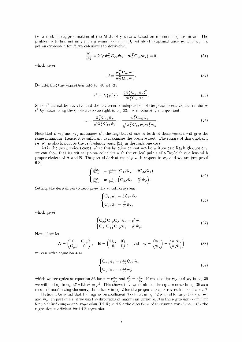
which is recognized as the generalized eigenproblem, eq. 1. The solutions ri and wi are the eigenval-ues and eigenvectors respectively of the matrix B�1A. This means that the extremum points (i.e.points of zero derivative) of the Rayleigh quotient r(w) are solutions to the corresponding general-ized eigenproblem so that the eigenvalue is the extremum value of the quotient and the eigenvectoris the corresponding parameter vector w of the quotient. As an ilustration, the Rayleigh quotientis plotted to the left in in �gure 1 for two matrices A and B. The quotient is plotted as the radiusin di�erent directions w. Note that the quotient is invariant to the norm of w. The two eigenval-ues are shown as circles with their radii corresponding to the eigenvalues. It can be seen that theeigenvectors e1 and e2 of the generalized eigenproblem coincides with the maximum and minimumvalues of the Rayleigh quotient. To the right in the same �gure, the gradient of the Rayleighquotient is illustrated as a function of the direction of w. Note that the gradient is orthogonalto w (see equation 3). This means that a small change of w in the direction of the gradient canbe seen as a rotation of w. The arrows indicate the direction of this orientation and the radii ofthe 'blobs' correspons to the magnitude of the gradient. The �gure shows that the directions of

2

−1 0 1

−1

0

1

w1

w2

e1

e2

r( w)

The Rayleigh quotient

−1 0 1

−1

0

1

e1

e2

→

→

→

←

w1

w2

The gradient ( A w − r B w)

Figure 1: Left:The Rayleigh quotient r(w) between two matrices A and B. The curve is plottedas rw. The eigenvectors of B�1A are marked as reference. The corresponding eigenvalues aremarked as the radii of the two circles. Note that the quotient is invariant to the norm of w.Right: The gradient of r. The arrows indicate he direction of this orientation and the radii of the'blobs' correspons to the magnitude of the gradient.

zero gradient coincides with the eigenvectors and that the gradient points towards the eigenvectorcoresponding to the largest eigenvalue.

If the eigenvalues ri are distinct (i.e. ri 6= rj for i 6= j), the di�erent eigenvectors are orthogonalin the metrics A and B which means that

wTi Bwj =

(0 for i 6= j

�i > 0 for i = jand wT

i Awj =

(0 for i 6= j

ri�i for i = j(5)

(see proof 6.1). This means that the wis are linearly independent (see proof 6.2). Since ann-dimensional space gives n eigenvectors which are linearly independent, hence, fw1; : : : ;wngconstitutes a base and any w can be expressed as a linear combination of the eigenvectors. Now, itcan be proved (see proof 6.3) that the function r is bounded by the largest and smallest eigenvalue,i.e.

rn � r � r1 (6)

which means that there exists a global maximum and that this maximum is r1.To investigate if there are any other local maxima, we look at the second derivative, or the

Hessian H, of r for the solutions of the eigenproblem,

Hi =@2r

@w2

����w=wi

=2

wTi Bwi

(A� riB) (7)

(see proof 6.4). It can be shown (see proof 6.5) that the Hessian Hi have got positive eigenvaluesfor i > 1, i.e. there exits vectors w such that

wTHiw > 0 8 i > 1 (8)

This means that for all solutions to the eigenproblem except for the largest root, there exists adirection in which r increases. In other words, all extremum points of the function r are saddlepoints except for the global minimum and maximum points. Since the two-dimensional examplein �gure 1 only has two eigenvalues, as illustrated in the �gure, they correspond to the maximumand minimum values of r.

We will now show that �nding the directions of maximum variance, maximum covariance,maximum correlation and minimum square error can be seen as special cases of the generalizedeigenproblem.

3

2.1 Direction of maximum data variation

For a set of random numbers fxkg with zero mean, the variance is de�ned as Efxxg. Now let usturn to a set of random vectors, with zero mean. In this case we consider the covariance matrix,de�ned by:

Cxx = EfxxT g (9)

By the direction of maximum data variation we mean the direction w with the property that thelinear combination x = wTx posses maximum variance. Hence, �nding this direction is henceequivalent to �nding the maximum of

� = Efxxg = EfwTxwTxg = wTEfxxT gw =wTCxxw

wTw: (10)

This problem is a special case of that presented in eq. 2 with

A = Cxx and B = I: (11)

Since the covariance matrix is symmetric, it is possible to expand it in its eigenvalues andorthogonal eigenvectors as:

Cxx = EfxxT g =X

�i eieTi (12)

where �i and ei are the eigenvalues and orthogonal eigenvectors respectively. This is known asprincipal component analysis (PCA). Hence, the problem of maximizing the variance, �, can beseen as the problem of �nding the largest eigenvalue, �1, and its corresponding eigenvector since:

�1 = eT1Cxxe1 = max

wTCxxw

wTw= max �: (13)

It is also worth noting that it is possible to �nd the direction and magnitude of maximum datavariation to the inverse of the covariance matrix. In this case we simply identify the matrices ineq. 2 as A = I and B = Cxx.

2.2 Directions of maximum data covariation

Given two sets of random numbers with zero mean, fxkg and fykg, their covariance is de�ned asEfxyg = Efyxg. If we consider the multivariate case, we can de�ne the between sets covariancematrix according to:

Cxy = EfxyT g (14)

This time we look at the two directions of maximal data covariation, by which we mean thedirections, wx and wy, such that the linear combinations x = wT

x x and y = wTy y gives maximum

covariance. This means that we want to maximize the following function:

� = Efxyg = EfwTxxw

Ty yg = wT

xEfxyT gwy =

wTxCxywyq

wTxwxwT

ywy

: (15)

Note that, for each �, a corresponding value �� is obtained by rotating wx or wy 180�. For thisreason, we obtain the maximum magnitude of � by �nding the largest positive value.

This function cannot be written as a Rayleigh quotient. However, the critical points of thisfunction coincides with the critical points of a Rayleigh quotient with proper choices of A and B.To see this, we calculate the derivatives of this function with respect to the vectors wx and wy

(see proof 6.6): (@�@wx

= 1

kwxk(Cxywy � �wx)

@�@wy

= 1

kwyk(Cyxwx � �wy):

(16)

4

Setting these expressions to zero and solving for wx and wy results in(CxyCyxwx = �2wx

CyxCxywy = �2wy:(17)

This is exactly the same result as that obtained after a gradient search on r in eq. 2 if the matricesA and B and the vector w are chosen according to:

A =

�0 Cxy

Cyx 0

�, B =

�I 0

0 I

�, and w =

��xwx

�ywy

�: (18)

This is easily veri�ed by insertion of the expressions above into eq. 4 which results in8<:Cxywy = r�x�y wx

Cyxwx = r�y�xwy

(19)

and then solving for wx and wy which gives equation 17 with r2 = �2. Hence, the problem of�nding the direction and magnitude of the largest data covariation can be seen as maximizing aspecial case of eq. 2 with the appropriate choice of matrices.

The between sets covariance matrix can be expanded by means of singular value decomposition(SVD) where the two sets of vectors fexig and feyig are mutually orthogonal:

Cxy = ExyfxyT g =

X�i exie

Tyi (20)

where the positive numbers, �i, are referred to as the singular values. Since the basis vectors areorthogonal, we see that the problem of maximizing the quotient in eq. 15 is equivalent to �ndingthe largest singular value:

�1 = eTx1Cxyey1 = maxwTxCxywyq

wTxwxwT

ywy

= max �: (21)

The SVD of a between-sets covariance matrix has a direct relation to the method of partialleast squares (PLS) [13, 25].

2.3 Directions of maximum data correlation

Again, consider two random variables x and y with zero mean and stemming from a multi-normaldistribution with

C =

�Cxx Cxy

Cyx Cyy

�= E

(�x

y

��x

y

�T)

(22)

as the covariance matrix. Consider the linear combinations x = wTx x and y = wT

y y of the two

variables respectively. The correlation1 between x and y is de�ned as Efxyg=pEfxxgEfyyg. This

means that the function we want to maximize can be written as

� =Efxygp

EfxxgEfyyg=

EfwTxxy

T wygqEfwT

xxxT wxgEfwT

y yyT wyg

=wTxCxywyq

wTxCxxwxwT

yCyywy

: (23)

Also in this case, as � changes sign if wx or wy is rotated 180�, it is su�cient to �nd the positivevalues.

Just like equation 15, this function cannot be written as a Rayleigh quotient. But also in thiscase, we can show that the critical points of this function coincides with the critical points of a

1The term correlation is some times inappropriately used to denote the second order origin moment (�x2) asopposed to variance which is the second order central moment (�[x�x0]2). The de�nition used here can be found intextbooks in mathematical statistics. It can loosely be described as the covariance between two variables normalizedwith the geometric mean of the variables' variances.

5

Rayleigh quotient with proper choices of A and B. The partial derivatives of � with respect to wx

and wy are (see proof 6.7)8>><>>:

@�@wx

= akwxk

�Cxywy �

wTxCxywy

wTxCxxwx

Cxxwx

�@�@wy

= akwyk

�Cyxwx �

wTy Cyxwx

wTy Cyywy

Cyywy

� (24)

where a is a positive scalar. Setting the derivatives to zero gives the equation system8<:Cxywy = ��xCxxwx

Cyxwx = ��yCyywy

(25)

where

�x = ��1y =

swTyCyywy

wTxCxxwx

: (26)

�x is the ratio between the standard deviation of y and the standard deviation of x and vice versa.The �'s can be interpreted as a scaling factor between the linear combinations. Rewriting equationsystem 25 gives (see proof 6.9) (

C�1xxCxyC

�1yyCyxwx = �2wx

C�1yyCyxC

�1xxCxywy = �2wy:

(27)

Hence, wx and wy are found as the eigenvectors to C�1xxCxyC

�1yyCyx and C�1

yyCyxC�1xxCxy respec-

tively. The corresponding eigenvalues �2 are the squared canonical correlations [4, 5, 24, 12, 16].The eigenvectors corresponding to the largest eigenvalue �2

1are the vectors wx1 and wy1 that

maximizes the correlation between the canonical variates x1 = wTx1x and y1 = wT

y1y.Now, if we let

A =

�0 Cxy

Cyx 0

�; B =

�Cxx 0

0 Cyy

�; and w =

�wx

wy

�=

��xwx

�ywy

�(28)

we can write equation 4 as 8<:Cxywy = r�x�yCxxwx

Cyxwx = r�y�xCyywy

(29)

which we recognize as equation 25 for ��x = r�x�y and ��y = r�y�x. If we solve for wx and wy in

eq. 29, we will end up in eq. 27 with r2 = �2. This shows that we obtain the equations for thecanonical correlations as the result of a maximizing the energy function r.

An important property of canonical correlations is that they are invariant with respect to a�netransformations of x and y. An a�ne transformation is given by a translation of the origin followedby a linear transformation. The translation of the origin of x or y has no e�ect on � since it leavesthe covariance matrix C una�ected. Invariance with respect to scalings of x and y follows directlyfrom equation 23. For invariance with respect to other linear transformations see proof 6.10.

2.4 Directions for minimum square error

Again, consider two random variables x and y with zero mean and stemming from a multi-normaldistribution with covariance as in equation 22. In this case, we want to minimize the square error

�2 = Efky� �wywTx xk

2g

= EfyTy � 2�yT wywTx x+ �2wT

x xxT wxw

Ty g

= EfyTyg � 2�wTyCyxwx + �2wT

xCxxwx;

(30)

6

i.e. a rank-one approximation of the MLR of y onto x based on minimum square error. Theproblem is to �nd not only the regression coe�cient �, but also the optimal basis wx and wy. Toget an expression for �, we calculate the derivative

@�2

@�= 2

��wT

xCxxwx � wTyCyxwx

�= 0; (31)

which gives

� =wTyCyxwx

wTxCxxwx

: (32)

By inserting this expression into eq. 30 we get

�2 = EfyTyg �(wT

yCyxwx)2

wTxCxxwx

: (33)

Since �2 cannot be negative and the left term is independent of the parameters, we can minimize�2 by maximizing the quotient to the right in eq. 33, i.e. maximizing the quotient

� =wTxCxywypwTxCxxwx

=wTxCxywyq

wTxCxxwxwT

ywy

: (34)

Note that if wx and wy minimizes �2, the negation of one or both of these vectors will give thesame minimum. Hence, it is su�cient to maximize the positive root. The square of this quotient,i.e. �2, is also known as the redundancy index [21] in the rank one case.

As in the two previous cases, while this function cannot not be written as a Rayleigh quotient,we can show that its critical points coincides with the critical points of a Rayleigh quotient withproper choices of A and B. The partial derivatives of � with respect to wx and wy are (see proof6.8) 8<

:@�@wx

= akwxk

(Cxywy � �Cxxwx)

@�@wy

= akwxk

�Cyxwx �

�2

� wy

�:

(35)

Setting the derivatives to zero gives the equation system8<:Cxywy = �Cxxwx

Cyxwx =�2

� wy;(36)

which gives (C�1xxCxyCyxwx = �2wx

CyxC�1xxCxywy = �2wy:

(37)

Now, if we let

A =

�0 Cxy

Cyx 0

�; B =

�Cxx 0

0 I

�; and w =

�wx

wy

�=

��xwx

�ywy

�(38)

we can write equation 4 as 8<:Cxywy = r�x�yCxxwx

Cyxwx = r�y�xwy

(39)

which we recognize as equation 36 for � = r�x�y and �2

� = r�y�x. If we solve for wx and wy in eq. 39

we will end up in eq. 37 with r2 = �2. This shows that we minimize the square error in eq. 30 as aresult of maximizing the energy function r in eq. 2 for the proper choice of regression coe�cient �.

It should be noted that the regression coe�cient � de�ned in eq. 32 is valid for any choice of wx

and wy. In particular, if we use the directions of maximum variance, � is the regression coe�cientfor principal components regression (PCR) and for the directions of maximum covariance, � is theregression coe�cient for PLS regression.

7

2.5 Examples

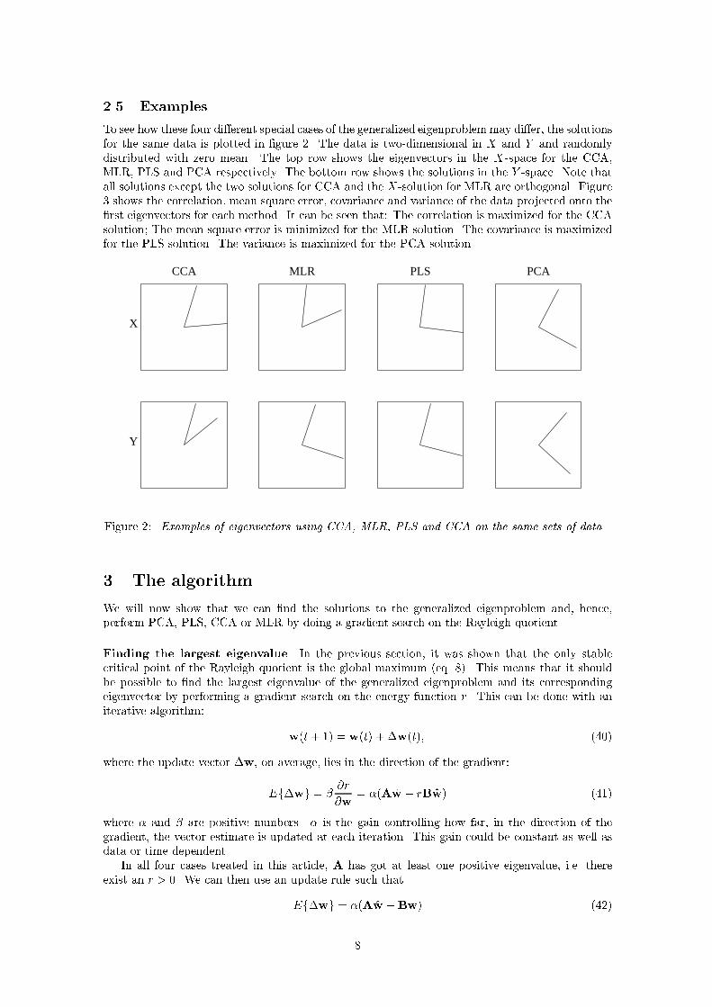
To see how these four di�erent special cases of the generalized eigenproblemmay di�er, the solutionsfor the same data is plotted in �gure 2. The data is two-dimensional in X and Y and randomlydistributed with zero mean. The top row shows the eigenvectors in the X-space for the CCA,MLR, PLS and PCA respectively. The bottom row shows the solutions in the Y -space. Note thatall solutions except the two solutions for CCA and the X-solution for MLR are orthogonal. Figure3 shows the correlation, mean square error, covariance and variance of the data projected onto the�rst eigenvectors for each method. It can be seen that: The correlation is maximized for the CCAsolution; The mean square error is minimized for the MLR solution. The covariance is maximizedfor the PLS solution. The variance is maximized for the PCA solution.

CCA

X

Y

MLR PLS PCA

Figure 2: Examples of eigenvectors using CCA, MLR, PLS and CCA on the same sets of data.

3 The algorithm

We will now show that we can �nd the solutions to the generalized eigenproblem and, hence,perform PCA, PLS, CCA or MLR by doing a gradient search on the Rayleigh quotient.

Finding the largest eigenvalue In the previous section, it was shown that the only stablecritical point of the Rayleigh quotient is the global maximum (eq. 8). This means that it shouldbe possible to �nd the largest eigenvalue of the generalized eigenproblem and its correspondingeigenvector by performing a gradient search on the energy function r. This can be done with aniterative algorithm:

w(t+ 1) = w(t) + �w(t); (40)

where the update vector �w, on average, lies in the direction of the gradient:

Ef�wg = �@r

@w= �(Aw � rBw) (41)

where � and � are positive numbers. � is the gain controlling how far, in the direction of thegradient, the vector estimate is updated at each iteration. This gain could be constant as well asdata or time dependent.

In all four cases treated in this article, A has got at least one positive eigenvalue, i.e. thereexist an r > 0. We can then use an update rule such that

Ef�wg = �(Aw �Bw) (42)

8

0

0.05

0.1

0.15

0.2

0.25

0.3

0.35

0.4

0.45

0.5corr

CC

A

MLR

PLS

PC

A

0

1

2

3

4

5

6

7

8

9

10mse

CC

A

MLR

PLS

PC

A

0

0.2

0.4

0.6

0.8

1

1.2

1.4cov

CC

A

MLR

PLS

PC

A

0

0.5

1

1.5

2

2.5

3var

CC

A

MLR

PLS

PC

A

Figure 3: The correlation, mean square error, covariance and variance when using the �rst pairof vectors for each method. The correlation is maximized for the CCA solution; The mean squareerror is minimized for the MLR solution. The covariance is maximized for the PLS solution. Thevariance is maximized for the PCA solution. (See section 2.5)

to �nd the positive eigenvalues. Here, the length of the vector will represent the correspondingeigenvalue, i.e. kwk = r. To see this, consider a choise of w that gives r < 0. Then we havewT�w < 0 since wTAw < 0. This means that kwk will decrease until r becomes positive.

The function Aw �Bw is illustrated in �gure 4 together with the Rayleigh quotient plottedto the left in �gure 1.

Finding successive eigenvalues Since the learning rule de�ned in eq. 41 maximizes the Rayleighquotient in eq. 2, it will �nd the largest eigenvalue �1 and a corresponding eigenvector w1 = �e1of eq. 1. The question naturally arises if, and how, the algorithm can be modi�ed to �nd thesuccessive eigenvalues and vectors, i.e. the successive solutions to the eigenvalue equation 1.

Let G denote the n� n matrix B�1A. Then the n equations for the n eigenvalues solving theeigenproblem in eq. 1 can be written as

GE = ED ) G = EDE�1 =X

�ieifTi ; (43)

where the eigenvalues and vectors constitute the matrices D and E respectively:

D =

0B@�1 0

. . .

0 �n

1CA ; E =

0@ j je1 � � � enj j

1A ; E�1 =

0B@� fT

1�

...� fTn �

1CA : (44)

The vectors, fi, appearing in the rows of the inverse of the matrix containing the eigenvectors arethe dual vectors to the eigenvectors ei, which means that

fTi ej = �ij : (45)

9

−1 0 1

−1

0

1

w1

w2

r( w)

The gradient ( A w − B w) ^

Figure 4: The function Aw � Bw, for the same matrices A and B as in �gure 1, plotted fordi�erent w. The Rayleigh quotient is plotted as reference.

ffig are also called the left eigenvectors of G and feig , ffig are said to be biorthogonal. From eq.5 we know that the eigenvectors ei are both A and B orthogonal, i.e. that

eTi Aej = 0 and eTi Bej = 0 for i 6= j: (46)

Hence we can use this result to �nd the dual vectors fi possessing the property in eq. 45, e.g. bychoosing them according to:

fi =Bei

eTi Bei: (47)

Now, if e1 is the eigenvector corresponding to the largest eigenvalue of G, the new matrix

H = G� �1e1fT1

(48)

will have the same eigenvectors and eigenvalues as G except for the eigenvalue corresponding toe1, which now becomes 0 (see proof 6.11). This means that the eigenvector corresponding to thelargest eigenvalue of H is the same as the one corresponding to the second largest eigenvalue of G.

Since the algorithm will �rst �nd the vector w1 = e1, we only need to estimate the dual vectorf1 in order to subtract the correct outer product from G and remove its largest eigenvalue. In ourcase this is a little bit tricky since we do not generate G directly. Instead we must modify its twocomponents A and B in order to produce the desired subtraction. Hence we want two modi�edcomponents, A

0

and B0

, with the following property:

B0�1A

0

= B�1A� �1e1fT1: (49)

A simple solution is obtained if we only modify one of the matrices and keep the other matrix�xed:

B0

= B and A0

= A� �1Be1fT1: (50)

This modi�cation can be accomplished if we estimate a vector u1 = �1Be1 = Bw1 iteratively as:

u1(t+ 1) = u1(t) + �u1(t) (51)

where

Ef�u1g = � [rBw1 � u1] : (52)

Once this estimate has converged, we can use u1 = �1Be1 to express the outer product in eq. 50:

�1Be1fT1=

�1Be1eT1BT

eT1BeT

1

=u1u

T1

eT1u1

: (53)

10

We can now estimate A0 and, hence, get a modi�ed version of the learning algorithm in eq. 41which �nds the second eigenvalue and the corresponding eigenvector to the generalized eigenprob-lem:

Ef�wg = �hA

0

w � rBwi= �

��A�

u1uT1

wT1u1

�w � rBw

�: (54)

The vector w1 is the solution �rst produced by the algorithm, i.e. the largest eigenvalue and thecorresponding eigenvector.

This scheme can of course be repeated to �nd the third eigenvalue by subtracting the secondsolution in the same way and so on. Note that this method does not put any demands on therange of B in contrast to exact solutions involving matrix inversion.

It is, of course, possible to enhance the proposed update rules and also take second orderderivatives into account. This would include estimating the inverse of the Hessian and usingthis matrix to modify the update direction. Such procedures are, for the batch or o�-line case,known as Gauss-Newton methods [7]. In this paper, however, we will not emphasize on speed andconvergence rates. Instead we are interested in the structure of the algorithm and how di�erentspecial cases of the generalized eigenproblem is re ected in the structure of the update rule.

In the following four sub-sections it will be shown how this iterative algorithm can be appliedto the four important problems described in the previous section.

3.1 PCA

Finding the largest principal component We can �nd the direction of maximum data vari-ation by a stochastic gradient search according to eq. 42 with A and B de�ned according to eq.11:

Ef�wg = @�

@w= � [Cxxw � �w] = � EfxxT w� �wg (55)

This leads to a novel unsupervised Hebbian learning algorithm that �nds both the direction ofmaximum data variation and the variance of the data in that direction. The update rule for thisalgorithm is given by

�w = � (xxT w �w); (56)

where the length of the vector represents the estimated variance, i.e. kwk = �. (Note that � inthis case is allways positive.)

Note that this algorithm �nds both the direction of maximal data variation as well as how muchthe data varies along that direction. Often algorithms for PCA only �nds the direction of maximaldata variation. If one is also interested in the variation along this direction, another algorithmneed to be employed. This is the case for the well known PCA algorithm presented by Oja [20].

Finding successive principal components In order to �nd successive principal components,we we recall that A = Cxx and B = I. Hence we have the matrix G = B�1A = Cxx which issymmetric and has orthogonal eigenvectors. This means that the dual vectors and the eigenvectorsbecome indistinguishable and that we need not estimate any other vector than w itself. The outerproduct in eq. 50 then becomes:

�1Be1fT1= �1Ie1e

T1= w1w

T1: (57)

From this we see that the modi�ed learning rule for �nding the second eigenvalue can be writtenas

Ef�wg = �hA

0

w �Bwi= �

�(Cxx �w1w

T1)w �w

�; (58)

A stochastic approximation of this rule is achieved if we at each time step update the vector w by

�w = ��(xxT �w1w

T1)w �w

�: (59)

11

As mentioned in section 2.1, it is possible to perform a PCA on the inverse of the covariancematrix by choosing A = I and B = Cxx. The learning rule associated with this behavior thenbecomes:

�w = � (w � xxTw): (60)

3.2 PLS

Finding the largest singular value If we want to �nd the directions of maximum data covari-ance, we de�ne the matrices A and B according to eq. 18. Since we want to update w, on average,in direction of the gradient, the update rule in eq. 42 gives:

Ef�wg = @r

@w= �

��0 Cxy

Cyx 0

�w � r

�I 0

0 I

�w

�: (61)

This behavior is accomplished if we at each time step update the vector w with

�w = �

��0 xyT

yxT 0

�w �w

�(62)

where the length of the vector at convergence represents the covariance, i.e. kwk = r = �. Thiscan be done since we know that it is su�cient to search for positive values of �.

Finding successive singular values Also in this case, the special structure of the A and B

matrices will simplify the procedure for �nding the subsequent directions with maximum datacovariance. We have

A =

�0 Cxy

Cyx 0

�and B =

�I 0

0 I

�; (63)

which again means that the compound matrix G = B�1A = A will be symmetric and have or-thogonal eigenvectors, which are identical to their dual vectors. The outer product for modi�cationof the matrix A in eq. 50 becomes identical to the one presented in the previous section:

�1Be1fT1= �1

�I 0

0 I

�e1e

T1= w1w

T1: (64)

A modi�ed learning rule for �nding the second eigenvalue can thus be written as

Ef�wg = �hA

0

w �Bwi= �

���0 Cxy

Cyx 0

��w1w

T1

�w�

�I 0

0 I

�w

�: (65)

A stochastic approximation of this rule is achieved if we at each time step update the vector w by

�w = �

���0 xyT

yxT 0

��w1w

T1

�w �w

�: (66)

3.3 CCA

Finding the largest canonical correlation Again, the algorithm in eq. 42 for solving thegeneralized eigenproblem can be used for the stochastic gradient search. With the matrices A andB and the vector w as in eq. 28, we obtain the update direction as:

Ef�wg = @r

w= �

��0 Cxy

Cyx 0

�w � r

�Cxx 0

0 Cyy

�w

�: (67)

This behavior is accomplished if we at each time step update the vector w with

�w = �

��0 xyT

yxT 0

�w �

�xxT 0

0 yyT

�w

�: (68)

Since we will have kwk = r = � when the algorithm converges, the length of the vector representsthe correlation between the variates.

12

Finding successive canonical correlations In the two previous cases it was easy to cancel outan eigenvalue because the matrix G was symmetric. This is not the case for canonical correlation.Here, we have

A =

�0 Cxy

Cyx 0

�and B =

�Cxx 0

0 Cyy

�; (69)

which gives us the non-symmetric matrix

G = B�1A =

�C�1xx 0

0 C�1yy

��0 Cxy

Cyx 0

�=

�0 C�1

xxCxy

C�1yyCyx 0

�: (70)

Because of this, we need to estimate the dual vector f1 corresponding to the eigenvector e1, orrather the vector u1 = �1Be1 as described in eq. 52:

Ef�u1g = � [Bw1 � u1] = �

��Cxx 0

0 Cyy

�w1 � u1

�: (71)

A stochastic approximation for this rule is given by

�u1 = �

��xxT 0

0 yyT

�w1 � u1

�: (72)

With this estimate, the outer product in eq. 50 can be used to modify the matrix A:

A0

= A� �1Be1fT1= A�

u1uT1

wT1u1

: (73)

A modi�ed version of the learning algorithm in eq. 42 which �nds the second largest canonicalcorrelations and its corresponding directions can be written on the following form:

Ef�wg = �hA

0

w �Bwi= �

���0 Cxy

Cyx 0

��u1u

T1

wT1u1

�w �

�Cxx 0

0 Cyy

�w

�: (74)

Again to get a stochastic approximation of this rule, we perform the update at each time stepaccording to:

�w = �

���0 xyT

yxT 0

��u1u

T1

wT1u1

�w �

�xxT 0

0 yyT

�w

�: (75)

Note that this algorithm simultaneously �nds both the directions of canonical correlations andthe canonical correlations �i in contrast to the algorithm proposed by Kay [15], which only �ndsthe directions.

3.4 MLR

Finding the directions for minimum square error Also here, the algorithm in eq. 42 canbe used for a stochastic gradient search. With the A, B and w according to eq. 38, we get theupdate direction as:

Ef�wg = @r

@w= �

��0 Cxy

Cyx 0

�w � r

�Cxx 0

0 I

�w

�: (76)

This behavior is accomplished if we at each time step update the vector w with

�w = �

��0 xyT

yxT 0

�w �

�xxT 0

0 I

�w

�: (77)

Since we have kwk = r = � when the algorithm converges, we get the regression coe�cient as� = kwk�x�y

13

Finding successive directions for minimum square error Also in this case we must usethe dual vectors to cancel out the detected eigenvalues. Here, we have

A =

�0 Cxy

Cyx 0

�and B =

�Cxx 0

0 I

�; (78)

which gives us the non-symmetric matrix G as

G = B�1A =

�C�1xx 0

0 I

��0 Cxy

Cyx 0

�=

�0 C�1

xxCxy

Cyx 0

�: (79)

Because of this, we need to estimate the dual vector f1 corresponding to the eigenvector e1, orrather the vector u1 = �1Be1 as described in eq. 52:

Ef�u1g = � [Bw1 � u1] = �

��Cxx 0

0 I

�w1 � u1

�: (80)

A stochastic approximation for this rule is given by

�u1 = �

��xxT 0

0 I

�w1 � u1

�: (81)

With this estimate, the outer product in eq. 50 can be used to modify the matrix A:

A0

= A� �1Be1fT1= A�

u1uT1

wT1u1

: (82)

A modi�ed version of the learning algorithm in eq. 42 which �nds the successive directions ofminimum square error and their corresponding regression coe�cient can be written on the followingform:

Ef�wg = �hA

0

w �Bwi= �

���0 Cxy

Cyx 0

��u1u

T1

wT1u1

�w �

�Cxx 0

0 I

�w

�: (83)

Again to get a stochastic approximation of this rule, we perform the update at each time stepaccording to:

�w = �

���0 xyT

yxT 0

��u1u

T1

wT1u1

�w �

�xxT 0

0 I

�w

�: (84)

We can see that, in this case, the wys are orthogonal but not necessarily the wxs. The or-thogonality of the wys is easily explained by the Cartesian separability of the square error; whenthe error in one direction is minimized, no more can be done in that direction to reduce the error.This shows that we can use this method for successively building up a low-rank approximation ofMLR by adding a su�cient number of solutions, i.e.

~y =

kXi=1

�iwyiwTxix (85)

where ~y is the estimated y and k is the rank. It may be pointed out that if all solutions are used,we obtain the well known Wiener �lter.

4 Experiments

The memory requirement as well as the computational cost per iteration for the presented algo-rithm is of order O(md). This enables experiments in signal spaces having dimensionalities whichwould be impossible to handle using traditional techniques involving matrix multiplications (havingmemory requirements of order O(d2) and computational costs of order O(d3)).

This section presents some experiments with the algorithm for analysis of stochastic processes.First, the algorithm is employed to perform PCA, PLS, CCA, and MLR. Here the dimensionality

14

of the signal space is kept reasonably low in order to make a comparison with the performance ofan optimal, in the sense of maximum likelihood (ML), deterministic solution which is calculatedfor each iteration, based on the data accumulated so far.

Second, the algorithm is applied to a process in a high-dimensional (1000-dim.) signal space.In this case, the gain sequence is made data dependent and the output from the algorithm ispost-�ltered in order meet requirements for quick convergence together with algorithm robustness.

In all experiments the error in magnitude and angle were calculated relative the correct answerwc. The same error measures were used for the output from the algorithm as well as for theoptimal ML estimate:

�m(w) = kwok � kwk (86)

�a(w) = arccos(wT wo): (87)

4.1 Comparisons to optimal solutions

The test data for these four experiments was generated from a 30-dimensional Gaussian distributionsuch that the eigenvalues of the generalized eigenproblem decreased exponentially, from 0.9:

�i = 0:9

�2

3

�i�1

:

The two largest eigenvalues (0.9 and 0.6) and the corresponding eigenvectors were simultane-ously searched for. In the PLS, CCA and MLR experiments, the dimensionalities of signal vectorbelonging to the x and y part of the signal were 20 and 10 respectively.

The average angular and magnitude errors were calculated based on 10 di�erent runs. Thiscomputation was made for each iteration, both for the algorithm and for the ML solution. Theresults are plotted in �gures 5, 6, 7 and 8 for PCA, PLS, CCA and MLR respectively. The errors ofthe algorithm are drawn with solid lines and the errors of the ML solution are drawn with dottedlines. The vertical bars show the standard deviations. Note that the angular error is always positiveand, hence, does not have have a symmetrical distribution. However, for simplicity, the standarddeviation indicators have been placed symmetrically around the mean. The �rst 30 iterations wereomitted to avoid singular matrices when calculating matrix inverses for the ML solutions.

No attempt was made to �nd an optimal set of parameters for the algorithm. Instead theexperiments and comparisons were carried out only to display the behavior of the algorithm andshow that it is robust and converges to the correct solutions. Initially, the estimate was assigned asmall random vector. A constant gain factor of � = 0:001 was used throughout all four experiments.

4.2 Performance in high dimensional signal spaces

The purpose of the methods presented in this paper is dimensionality reduction in high-dimensionalsignal spaces. We have previously shown that the proposed algorithm have the computationalcapacity to handle such signals. This experiment illustrates that the algorithm also behaves wellin practice for high-dimensional signals. The dimensionality of x is 800 and the dimensionality ofy is 200, so the total dimensionality of the signal space is 1000. The object in this experiment isCCA.

In the previous experiment, the algorithm was used in its basic form with constant updaterates set by hand. In this experiment, however, a more sophisticated version of the algorithm isused where the update rate is adaptive and the vectors are averaged over time. The details of thisextension to the algorithm are numerous and beyond the scope of this paper. Here, we will onlygive a brief explanation of the basic structure of the extended algorithm.

Adaptability is necessary for a system without a pre-speci�ed (time dependent) update rate �.Here, the adaptive update rate is dependent on the energy of the signal projected onto the vectoras well as the consistency of the change of the vector.

The averaged vectors wa are calculated as

wa ( wa + (w �wa) (88)

15

2000 4000 6000 8000 100000

π/4

π/2

PCA: Mean angular error for w1

2000 4000 6000 8000 100000

π/4

π/2

PCA: Mean angular error for w2

2000 4000 6000 8000 10000

0

0.2

0.4

0.6

0.8

1

PCA: Mean norm error for w1

2000 4000 6000 8000 10000

0

0.2

0.4

0.6

0.8

1

PCA: Mean norm error for w2

Figure 5: Results for the PCA case

2000 4000 6000 8000 100000

π/4

π/2

PLS: Mean angular error for w1

2000 4000 6000 8000 100000

π/4

π/2

PLS: Mean angular error for w2

2000 4000 6000 8000 10000

0

0.2

0.4

0.6

0.8

1

PLS: Mean norm error for w1

2000 4000 6000 8000 10000

0

0.2

0.4

0.6

0.8

1

PLS: Mean norm error for w2

Figure 6: Results for the PLS case

16

2000 4000 6000 8000 100000

π/4

π/2

CCA: Mean angular error for w1

2000 4000 6000 8000 100000

π/4

π/2

CCA: Mean angular error for w2

2000 4000 6000 8000 10000

0

0.2

0.4

0.6

0.8

1

CCA: Mean norm error for w1

2000 4000 6000 8000 10000

0

0.2

0.4

0.6

0.8

1

CCA: Mean norm error for w2

Figure 7: Results for the CCA case

2000 4000 6000 8000 100000

π/4

π/2

MLR: Mean angular error for w1

2000 4000 6000 8000 100000

π/4

π/2

MLR: Mean angular error for w2

2000 4000 6000 8000 10000

0

0.2

0.4

0.6

0.8

1

MLR: Mean norm error for w1

2000 4000 6000 8000 10000

0

0.2

0.4

0.6

0.8

1

MLR: Mean norm error for w2

Figure 8: Results for the MLR case

17

where depends on the consistency of the changes in w. When there is a consistent change inw, is small and the averaging window is short and wa follows w quickly. When the changes inw are less consistent, the window gets longer and wa is the average of an increasing number ofinstances of w. This means, for example, that if w is moving symmetrically around the correctsolution with a constant variance, the error of wa will still tend towards zero (see �gure 9).

0 0.2 0.4 0.6 0.8 1 1.2 1.4 1.6 1.8 2

x 105

0

0.5

1

1.5

iterations

corr

elat

ion

0 0.2 0.4 0.6 0.8 1 1.2 1.4 1.6 1.8 2

x 105

−5

−4

−3

−2

−1

0

1

iterationsA

ngle

err

or

[ log

(rad

) ]

Figure 9: Left: Figure showing the estimated �rst canonical correlation as a function of numberof actual events (solid line) and the true correlation in the current directions found by the algo-rithm (dotted line). The dimensionality of one set of variables is 800 and of the second set 200.Right:Figure showing the log of the angular error as a function of number of actual events.

The experiment was carried out using a randomly chosen distribution of a 800-dimensional xvariable and a 200-dimensional y variable. Two x and two y dimensions were correlated. Theother 798 dimensions of x and 198 dimensions of y were uncorrelated. The variances in the 1000dimensions were of the same order of magnitude.

The left plot in �gure 9 shows the estimated �rst canonical correlation as a function of numberof actual events (solid line) and the true correlation in the current directions found by the algorithm(dotted line).

The right plot in �gure 9 shows the e�ect of the adaptive averaging. The two upper noisycurves show the angular errors of the `raw' estimates in the x and y spaces and the two lowercurves shows the angular errors for x (dashed) and y (solid). The angle errors of the smoothedestimates are much more stable and decrease more rapidly than the `raw' estimates. The errorsafter 2 � 105 samples is below one degree. (It should be noted that this is an extreme precisionas, with a resolution of 1 degree, a low estimate of the number of di�erent orientations in a 1000-dimensional space is 102000.) The angular errors were calculated as the angle between the vectorsand the exact solutions, e (known from the x y sample distribution), i.e.

Err[w] = arccos(wTa e):

5 Summary and conclusions

We have presented an iterative algorithm for analysis of stochastic processes in terms of PCA,PLS, CCA, and MLR. The directions of maximal variance, covariance, correlation, and least squareerror are found by a novel algorithm performing a stochastic gradient search on suitable Rayleighquotients. The algorithm operates on-line which allows non-stationary data to be analyzed. Whensearching for an m-rank approximation, the computational complexity is O(md) for each iteration.Finding a full rank solution have a computational complexity of order O(d3) using traditionaltechniques.

The equilibrium points of the algorithm were shown to correspond to solutions of the generalizedeigenproblem. Hence, PCA, PLS, CCA and MLR were presented as special cases of this moregeneral problem. In PCA, PLS and CCA, the eigenvalues corresponds to variance, covariance andcorrelation respectively of the projection of the data onto the eigenvectors. In MLR, the eigenvalues,

18

together with a function of the corresponding eigenvector, provide the regression coe�cients. Theeigenvalues are given by the lengths of the basis vectors found by the proposed algorithm. A lowrank approximation is obtained when only the solutions with the largest eigenvalues and theircorresponding vectors are used.

Reduced rank MLR can, for example, be used to increase the stability of the predictors whenthere are more parameters than observations, when the relation is known to be of low rank or,maybe most importantly, when a full rank solution is unobtainable due to computational costs.The regression coe�cients can of course also be used for regression in the �rst three cases. In thecase of PCA, the idea is to separately reduce the dimensionality of the X and Y spaces and doa regression of the �rst principal components of Y on the �rst principal components of X . Thismethod is known as principal components regression. The obvious disadvantage here is that thereis no reason that the principal components of X are related to the principal components of Y .To avoid this problem, PLS regression is some times used. Clearly, this choice of basis is betterthan PCA for regression purposes since directions of high covariance are selected, which meansthat a linear relation is easier to �nd. However, neither of these solutions results in minimum leastsquares error. This is only obtained using the directions corresponding to the MLR problem.

PCA di�ers from the other three methods in that it concerns only one set of variables while theother three concerns relations between two sets of variables. The di�erence between PLS, CCAand MLR can be seen by comparing the matrices in the corresponding eigenproblems. In CCA,the between sets covariance matrices are normalized with respect to the within set covariancesin both the x and the y spaces. In MLR, the normalization is done only with respect to the xspace covariance while the y space, where the square error is de�ned, is left unchanged. In PLS,no normalization is done. Hence, these three cases can be seen as the same problem, covariancemaximization, where the variables have been subjected to di�erent, data dependent, scaling.

In some PLS applications, the variances of the variables are scaled to unity [25, 8, 13]. Thismay indicate that the aim is really to maximize correlation and that CCA would be the propermethod to use.

Recently, the neural network community has taken an increased interest in information theo-retcal approaches[11]. In particular, the concepts independant components and mutual informationhas been the basis for a number of successful applications, e.g. blind separation and blind decon-volution [2]. It is appropriate to point out that there is a strong relation between these conceptsand canonical correlation [1, 15]. The relevance of the present paper in this context is apparent.

6 Proofs

6.1 Orthogonality in the metrics A and B (eq. 5)

wTi Bwj =

(0 for i 6= j

�i > 0 for i = jand wT

i Awj =

(0 for i 6= j

ri�i for i = j(5)

Proof: For solution i we haveAwi = riBwi

The scalar product with another eigenvector gives

wTj Awi = riw

Tj Bwi

and of course alsowTi Awj = rjw

Ti Bwj

Since A and B are Hermitian we can change positions of wi and wj which gives

rjwTi Bwj = riw

Ti Bwj

and hence(ri � rj)w

Ti Bwj = 0:

19

For this expression to be true when i 6= j, we have that wTi Bwj = 0 if ri 6= rj . For i = j we now

have that wTi Bwi = �i > 0 since B is positive de�nite. In the same way we have�

1

ri�

1

rj

�wTi Awj = 0

which means that wTi Awj = 0 for i 6= j. For i = j we know that wT

i Awi = riwTi Bwi = ri�i.

2

6.2 Linear independence

fwig are linearly independent.

Proof: Suppose fwig are not linearly independent. This would mean that we could write aneigenvector wk as

wk =Xj 6=k

jwj :

This means that for j 6= k,wTj Bwk = jwjBwj 6= 0

which violates equation 5. Hence, fwig are linear independent.2

6.3 The range of r (eq. 6)

rn � r � r1 (6)

Proof: If we express a vector w in the base of the eigenvectors wi, i.e.

w =Xi

iwi

we can write

r =

P iw

Ti A

P iwiP

iwTi B

P iwi

=

P 2i �iP 2i �i

;

where �i = wTi Awi. Now, since �i = �iri (see equation 5), we get

r =

P 2i �iriP 2i �i

:

Obviously this function has the maximum value r1 when 1 6= 0 and i = 0 8 i > 1 if r1 is thelargest eigenvalue. The minimum value, rn, is obtained when n 6= 0 and i = 0 8 i < n if rn isthe smallest eigenvalue.

2

6.4 The second derivative of r (eq. 7)

Hi =@2r

@w2

����w=wi

=2

wTi Bwi

(A� riB) (7)

Proof: From the gradient in equation 3 we get the second derivative as

@2r

@w2=

2

(wTBw)2

��A�

@r

@wwTB� rB

�wTBw � (Aw � rBw)2wTB

�:

20

If we insert one of the solutions wi, we have

@r

@w

����w=wi

=2

wTi Bwi

(Awi � rBwi) = 0

and hence@2r

@w2

����w=wi

=2

wTi Bwi

(A� riB) :

2

6.5 Positive eigenvalues of the Hessian (eq. 8)

wTHiw > 0 8 i > 1 (8)

Proof: If we express a vector w as a linear combination of the eigenvectors we get

�i2wTHiw = wT (A� riB)w

= wTB(B�1A� riI)w

=X

jwTj B(B

�1A� riI)X

jwj

=X

jwTj B

�Xrj jwj �

Xri jwj

�=X

jwTj B

X(rj � ri) jwj

=X

2j �j(rj � ri)

where �i = wTi Bwi > 0. Now, (rj � ri) > 0 for j < i so if i > 1 there is at least one choice of w

that makes this sum positive.2

6.6 The partial derivatives of the covariance (eq. 16)

(@�@wx

= 1

kwxk(Cxywy � �wx)

@�@wy

= 1

kwyk(Cyxwx � �wy):

(16)

Proof: The partial derivative of � with respect to wx is

@�

@wx=Cxywykwxkkwyk �wT

xCxywykwxk�1wxkwyk

kwxk2kwyk2

=Cxywy

kwxk�

�wx

kwxk2

=1

kwxk(Cxywy � �wx)

The same calculations can be made for @�@wy

by exchanging x and y .2

6.7 The partial derivatives of the correlation (eq. 24)

8>><>>:

@�@wx

= akwxk

�Cxywy �

wTxCxywy

wTxCxxwx

Cxxwx

�@�@wy

= akwyk

�Cyxwx �

wTy Cyxwx

wTy Cyywy

Cyywy

� (24)

21

Proof: The partial derivative of � with respect to wx is

@�

@wx=

(wTxCxxwxw

TyCyywy)

1=2Cxywy

wTxCxxwxwT

yCyywy

�wTxCxywy(w

TxCxxwxw

TyCyywy)

�1=2CxxwxwTyCyywy

wTxCxxwxwT

yCyywy

= (wTxCxxwxw

TyCyywy)

�1=2

�Cxywy �

wTxCxywy

wTxCxxwx

Cxxwx

�

= kwxk�1(wT

xCxxwxwTyCyywy| {z }

�0

)�1=2�Cxywy �

wTxCxywy

wTxCxxwx

Cxxwx

�

=a

kwxk

�Cxywy �

wTxCxywy

wTxCxxwx

Cxxwx

�; a � 0:

The same calculations can be made for @�@wy

by exchanging x and y .2

6.8 The partial derivatives of the MLR-quotient (eq. 35)

8<:

@�@wx

= akwxk

(Cxywy � �Cxxwx)

@�@wy

= akwxk

�Cyxwx �

�2

� wy

�:

(35)

Proof: The partial derivative of � with respect to wx is

@�

@wx=

(wTxCxxwxw

Tywy)

1=2Cxywy

wTxCxxwxwT

ywy

�wTxCxywy(w

TxCxxwxw

Tywy)

�1=2CxxwxwTywy

wTxCxxwxwT

ywy

= (wTxCxxwxw

Tywy)

�1=2

�Cxywy �

wTxCxywy

wTxCxxwx

Cxxwx

�

= kwxk�1(wT

xCxxwxwTy wy| {z }

�0

)�1=2�Cxywy �

wTxCxywy

wTxCxxwx

Cxxwx

�

=a

kwxk(Cxywy � �Cxxwx) ; a � 0:

22

The partial derivative of � with respect to wy is

@�

@wy=

(wTxCxxwxw

Tywy)

1=2Cyxwx

wTxCxxwxwT

ywy

�wTxCxywy(w

TxCxxwxw

Tywy)

�1=2wTxCxxwxwy

wTxCxxwxwT

ywy

= (wTxCxxwxw

Tywy)

�1=2

�Cyxwx �

wTxCxywyw

TxCxxwx

wTxCxxwxwT

ywywy

�

= kwyk�1(wT

xCxxwx| {z })�1=2 �Cyxwx � wTxCxywywy

�

=a

kwxk

�Cyxwx �

�2

�wy

�; a � 0:

2

6.9 Combining eigenvalue equations (eqs. 27)

(C�1xxCxyC

�1yyCyxwx = �2wx

C�1yyCyxC

�1xxCxywy = �2wy:

(27)

Proof: Since Cxx and Cyy are nonsingular, equation system 25 can be written as8<:C

�1xxCxywy = ��xwx

C�1yyCyxwx = ��ywy

Inserting wy from the second line into the �rst line gives

C�1xxCxyC

�1yyCyxwx = �2�x�ywx = �2wx;

since �x = ��1y . This proves the �rst line in eq. 27. In the same way, solving for wx proves thesecond line in eq. 27.

2

6.10 Invariance with respect to linear transformations

Canonical correlations are invariant with respect to linear transformations.

Proof: Letx = Axx

0 and y = Ayy0:

where Ax and Ay are non-singular matrices. If we denote

C0xx = Efx0x0

Tg;

then the covariance matrix for x can be written as

Cxx = EfxxT g = EfAxx0x0

TAT

x g = AxC0xxA

Tx :

In the same way we have

Cxy = AxC0xyA

Ty and Cyy = AyC

0yyA

Ty :

Now, the equation system 27 can be written as((AT

x )�1C0�1

xx (Ax)�1AxC

0xyA

Ty (A

Ty )

�1C0�1yy (Ay)

�1AyC0yxA

Tx wx = �2wx

(ATy )

�1C0�1yy (Ay)

�1AyC0yxA

Tx (A

Tx )

�1C0�1xx (Ax)

�1AxC0xyA

Ty wy = �2wy;

23

or (C0�1

xxC0xyC

0�1yyC

0yxw

0x = �2w0

x

C0�1yyC

0yxC

0�1xxC

0xyw

0y = �2w0

y;

where w0x = AT

x wx and w0y = AT

y wy. Obviously this transformation leaves the roots � unchanged.If we look at the canonical variates,(

x0 = w0Txx

0 = wTxAA

�1x = x

y0 = w0Ty y

0 = wTyAA

�1y = y;

we see that these too are una�ected by the linear transformation.2

6.11 The successive eigenvalues (eq. 48)

H = G� �1e1fT1

(48)

Proof: Consider a vector u which we express as the sum of one vector parallel to the eigenvector e1,and another vector uo that is a linear combination of the other eigenvectors and, hence, orthogonalto the dual vector f1.

u = ae1 + uo

wherefT1e1 = 1 and fT

1uo = 0:

Multiplying H with u gives

Hu =�G� �1e1f

T1

�(ae1 + uo)

= a (Ge1 � �1e1) + (Guo � 0)

= Guo:

This shows that G and H have the same eigenvectors and eigenvalues except for the largesteigenvalue and eigenvector of G. Obviously the eigenvector corresponding to the largest eigenvalueof H is e2.

2

24

References

[1] S. Becker. Mutual information maximization: models of cortical self-organization. Network:Computation in Neural Systems, 7:7{31, 1996.

[2] A. J. Bell and T. J. Sejnowski. An information-maximization approach to blind separationand blind deconvolution. Neural Computation, 7:1129{59, 1995.

[3] R. D. Bock. Multivariate Statistical Methods in Behavioral Research. McGraw-Hill series inpsychology. McGraw-Hill, 1975.

[4] M. Borga. Reinforcement Learning Using Local Adaptive Models, August 1995. Thesis No.507, ISBN 91{7871{590{3.

[5] M. Borga, H. Knutsson, and T. Landelius. Learning Canonical Correlations. In Proceedingsof the 10th Scandinavian Conference on Image Analysis, Lappeenranta, Finland, June 1997.SCIA.

[6] R. Bracewell. The Fourier Transform and its Applications. McGraw-Hill, 2nd edition, 1986.

[7] J. Dennis and R. Schnabel. Numerical Methods for Unconstrained Optimization and NonlinearEquations. Prentice Hall, Englewood Cli�s, New Jersey, 1983.

[8] P. Geladi and B. R. Kowalski. Parial least-squares regression: a tutorial. Analytica ChimicaActa, 185:1{17, 1986.

[9] G. H. Golub and C. F. Van Loan. Matrix Computations. The Johns Hopkins University Press,second edition, 1989.

[10] G. H. Granlund and H. Knutsson. Signal Processing for Computer Vision. Kluwer AcademicPublishers, 1995. ISBN 0-7923-9530-1.

[11] S. Haykin. Neural networks expand sp's horizons. IEEE Signal Processing Magazine, pages24{49, March 1996.

[12] H. Hotelling. Relations between two sets of variates. Biometrika, 28:321{377, 1936.

[13] A. H�oskuldsson. PLS regression methods. Journal of Chemometrics, 2:211{228, 1988.

[14] A. J. Izenman. Reduced-rank regression for the multivariate linear model. Journal of Multi-variate Analysis, 5:248{264, 1975.

[15] J. Kay. Feature discovery under contextual supervision using mutual information. In Inter-national Joint Conference on Neural Networks, volume 4, pages 79{84. IEEE, 1992.

[16] H. Knutsson, M. Borga, and T. Landelius. Learning Canonical Correlations. Report LiTH-ISY-R-1761, Computer Vision Laboratory, S{581 83 Link�oping, Sweden, June 1995.

[17] T. Landelius. Behavior Representation by Growing a Learning Tree, September 1993. ThesisNo. 397, ISBN 91{7871{166{5.

[18] T. Landelius. Reinforcement Learning and Distributed Local Model Synthesis. PhD thesis,Link�oping University, Sweden, S{581 83 Link�oping, Sweden, 1997. Dissertation No 469, ISBN91{7871{892{9.

[19] T. Landelius, H. Knutsson, and M. Borga. On-Line Singular Value Decomposition of Stochas-tic Process Covariances. Report LiTH-ISY-R-1762, Computer Vision Laboratory, S{581 83Link�oping, Sweden, June 1995.

[20] E. Oja and J. Karhunen. On stochastic approximation of the eigenvectors and eigenvaluesof the expectation of a random matrix. Journal of Mathematical Analysis and Applications,106:69{84, 1985.

25

[21] D. K. Stewart and W. A. Love. A general canonical correlation index. Psychological Bulletin,70:160{163, 1968.

[22] G. W. Stewart. A bibliographical tour of the large, sparse generalized eigenvalue problem. InJ. R. Bunch and D. J. Rose, editors, Sparse Matrix Computations, pages 113{130, 1976.

[23] A. L. van den Wollenberg. Redundancy analysis: An alternative for canonical correlationanalysis. Psychometrika, 36:207{209, 1977.

[24] E. van der Burg. Nonlinear Canonical Correlation and Some Related Techniques. DSWOPress, 1988.

[25] S. Wold, A. Ruhe, H. Wold, and W. J. Dunn. The collinearity problem in linear regression.the partial least squares (pls) approach to generalized inverses. SIAM J. Sci. Stat. Comput.,5(3):735{743, 1984.

26